applied sciences

Article

Experimental Comparison of Heating Emitters inMediterranean Climate

Rosa Francesca De Masi 1,*, Silvia Ruggiero 1 and Giuseppe Peter Vanoli 2

�����������������

Citation: Masi, R.F.D.; Ruggiero, S.;

Vanoli, G.P. Experimental

Comparison of Heating Emitters in

Mediterranean Climate. Appl. Sci.

2021, 11, 5462. https://doi.org/

10.3390/app11125462

Academic Editor: Demis Pandelidis

Received: 20 May 2021

Accepted: 10 June 2021

Published: 12 June 2021

Publisher’s Note: MDPI stays neutral

with regard to jurisdictional claims in

published maps and institutional affil-

iations.

Copyright: © 2021 by the authors.

Licensee MDPI, Basel, Switzerland.

This article is an open access article

distributed under the terms and

conditions of the Creative Commons

Attribution (CC BY) license (https://

creativecommons.org/licenses/by/

4.0/).

1 DING-Department of Engineering, University of Sannio, 82100 Benevento, Italy; sruggiero@unisannio.it2 Department of Medicine and Health Sciences—Vincenzo Tiberio, University of Molise,

86100 Campobasso, Italy; giuseppe.vanoli@unimol.it* Correspondence: rfdemasi@unisannio.it; Tel.: +39-(0)824-3055577

Abstract: The need to increase the level of quality of indoor environments requires an extremelyaccurate definition of the microclimatic requisites to guarantee, in the spaces where people live andwork, global and local conditions of comfort, considering, at the same time, the aspects related toenergy savings and environmental sustainability. In this framework, the paper proposes a comparisonof indoor parameters for three different types of heating emitters: fan-coils, baseboards heaters, andradiant floor systems. The comparison is based on seasonal monitoring performed in a test-roomlocated in a Mediterranean climate; it can simulate an insulated room with office usage. The proposedindices demonstrate that the floor radiant system is characterized by lower horizontal and verticaldifferences in air temperature distribution that can guarantee more comfortable conditions and lowerheat losses. The operative temperature is often higher than the neutral point; thus, management witha lower set-point temperature should be experimented with in further studies. More generally, theintroduced method could help designers to choose the proper system and management strategy withthe dual purpose to select a comfortable but energy savings-oriented operating temperature.

Keywords: thermal comfort; emitters; experimental measures; temperature distribution

1. Thermal Comfort: Indoor Plant Emitters and Control Strategies

According to the definition by ASHRAE [1,2], thermal comfort is the condition ofmind that expresses satisfaction with the thermal environment. It has a wide connotation,also including physiological and psychological aspects in addition to ambient characteris-tics [3,4]. The overall thermal sensation and the degree of discomfort of people exposed tomoderate thermal environments can be determined according to international standardEN ISO 7730 [5]. This standard allows the analytical determination and interpretationof thermal comfort conditions through the calculation of the predicted mean vote (PMV)and predicted percentage of dissatisfied (PPD), as well as the analysis of local thermaldiscomfort phenomena (vertical air temperature differences, warm and cool floors, drafts,radiant temperature asymmetries).

The PMV index, based on an analysis of the heat balance equation for the humanbody, takes into account the influence of thermal comfort factors (air temperature, airvelocity, mean radiant temperature, humidity, clothing, and activity) by means of a valueon a 7-point scale (0 is neutral, +1 is slightly warm, and −1 is slightly cool). The PPD iscorrelated to the PMV value by means of a mathematical equation that reveals a smallpercentage of dissatisfied (5%) under thermal neutrality conditions (i.e., PMV = 0).

According to the criteria of [5], three categories can be identified for classifying thethermal environment. These are shown in Table 1, where DR is the draught rate; Tf indicatesthe value of an acceptable floor temperature; ∆Tpr,wc is the radiant asymmetry for a warmceiling; ∆Tpr,cc is the radiant asymmetry for a cool ceiling; ∆tpr,ww is the radiant asymmetryfor a warm wall; ∆Tpr,cw is the radiant asymmetry for a cold wall; and finally in the last

Appl. Sci. 2021, 11, 5462. https://doi.org/10.3390/app11125462 https://www.mdpi.com/journal/applsci

Appl. Sci. 2021, 11, 5462 2 of 25

column there is the vertical difference between the value of air temperature measured at1.1 m (Ta_1.1) and at 0.1 m (Ta_0.1).

Table 1. Categories of thermal comfort and local discomfort according to ISO 7730.

Global Comfort Local Discomfort

PMV PPD (%) Tf (◦C) DR (%) ∆Tpr,wc(◦C)

∆Tpr,cc(◦C)

∆Tpr,ww(◦C)

∆Tpr,cw(◦C)

Ta,1.1 − Ta,0.1(◦C)

A −0.20 to 0.20 <6 19–29 <10 <5 <14 <23 <10 <2B −0.50 to 0.50 <10 19–29 <20 <5 <14 <23 <10 <3C −0.70 to 0.70 <15 17–31 <30 <7 <18 <35 <13 <4

Designers must take into account these criteria, not only for assuring occupant well-being but also for optimizing the whole building’s HVAC system’s energy efficiency, asdiscussed by D’ambrosio Alfano et al. [6]. In this regard, researchers usually investigatethe relationship between comfort and plant design focusing on two aspects: differencebetween HVAC types [7], and selection of the optimized control strategy [8].

Regarding the first item, Gendelis et al. [9], comparing three different systems, foundthat only the electric heater satisfies the requirements of the A category of the thermalenvironment, with 20 ◦C indoor temperature and a normal ventilation regime. The experi-mental data collected in the building of Tsinghua University [10] suggest that in continuousheating, there is no significant difference between radiant and convective systems in termsof mean radiant temperature, indoor humidity, and noise issues. Despite split-type systemsfor cooling being popular in many countries, da Silva Junior et al. [11] underlined thatthese systems commonly promote high gradients of both temperature and air velocity inrooms and these can cause thermal discomfort. Han et al. [12] showed that when imple-mented in industrial factory buildings, radiant heating can save over 10% energy comparedto convection heating. However, Karman et al. [13], elaborating data of a survey from3892 respondents in 60 office buildings located in North America, showed that radiant andall-air buildings have equal indoor environmental quality, including acoustic aspects. Simi-larly, by means of measurements and questionnaires in Dutch primary schools, Zeiler andBoxem [14] found that there is no significant difference in the perceived comfort betweenheated by radiant floor heating systems and by convection heating systems. Inard et al. [15],with a simplified model of dwelling-cells, concluded that the hot-water heated-floor systemprovides a good compromise between energy consumption and thermal comfort. Theelectrical heated ceiling has an equivalent consumption with a low level of thermal comfort,and the localized heat sources give very satisfactory comfort conditions, but the energyconsumption is slightly higher. Petráš and Kalús [16] showed with experimental resultsthat infrared gas heaters in a workplace provide an immediate effect on thermal comfortwhen compared with other heating systems. However, Ghaddar et al. [17] explored aradiant stove space-heating unit, underlining that it is possible to save 14% of the heatingenergy by changing the stove position in the room with the same level of comfort. Threeelectric heaters were compared by Léger et al. [18] in a bi-climatic chamber. The resultsshowed that the convector does not consume less energy, since it heated the adjacentwindows and wall less than the radiant heater and baseboard heater. Simulating a radi-ant heating system at different locations, with different surface areas and correspondingtemperatures, Tye-Gingras and Gosselin [19] showed that all three parameters could affectenergy consumption and thermal comfort. Instead, Sevilgen and Kilic [20] found thatenergy consumption can be significantly reduced while increasing the thermal comfort byusing better-insulated outer wall materials and windows.

Despite these results, according to Halawa et al. [21], study of radiant systems shouldcontinue in terms of system design, configuration, and control. For instance, air movementseems to be a critical issue since some studies, such as [22], affirm that radiant heatingsystems led to more thermal comfortable votes due to less air movement, and others [23]report that occupants might doubt the freshness of the air since they cannot feel the air

Appl. Sci. 2021, 11, 5462 3 of 25

movement. In this field, Corgnati et al. [24] proposed the coupling of primary air systems,and Causone et al. [25] verified the effectiveness of displacement ventilation for improvingthe indoor air quality.

Few studies are available on baseboard heaters such as the one proposed byBagheri et al. [26]. They found that a baseboard heater with a convector fin can increasethe performance by up to 42% and 94%, respectively, compared to the conventional fins.Similarly, Shobi et al. [27] revealed that the total thermal power of the modified radiantbaseboard with higher free convection is 34% higher than that of the conventional one.

Finally, the review analysis of Karmann et al. [28] pointed out that five studies es-tablished a thermal comfort preference between all-air and radiant systems, and threestudies showed a preference for radiant systems. However, more recently, by means ofexperiments in a test chamber, Sun et al. [29] found that there was no significant thermalcomfort difference during the steady stage of convective and radiative heaters.

On the other hand, in recent years, several studies focused on approaches and strate-gies to control building HVAC systems for reducing energy consumption and pollutingemissions without compromising thermal comfort. Lin et al. [30] experimentally verifiedan optimized control strategy for fan-coil units achieving 39.71% energy conservation.Sánchez-García et al. [31] found that the adaptive approach in Mediterranean cities canguarantee reductions in cooling consumption (around 50–60%) in contrast with discretesavings for heating (around 20%). Considering the temperature set point strategies, Dateet al. [32] obtained peak demand reductions of up to 10% and 25% when the conventionalnight time setback temperature profile was respectively changed with a one hour or twohours ramp with baseboards. For the ‘hot summer–cold winter’ climatic region of China,Wang et al. [33] hypothesized a heating temperature set point of 17–18 ◦C based on alumped-parameter four-node steady-state model. By means of simulations for typicalUSA single-family homes, Moon and Han [34] found a linear increase of 5.4%/◦C forheating consumption in a cold climate passing from 15.6 to 26.7 ◦C. According to Ghahra-mani et al. [35], the potential savings from selecting daily optimal set-points in the rangeof 22.5 ± 3 ◦C for small, medium, and large office buildings would lead to 10.09–37.03%,11.43–21.01%, and 6.78–11.34% savings, respectively, depending on the climate. Bienvenido-Huertas et al. [36] demonstrated that the set-point values prefixed by EN 16798-1:2019 fornew buildings can bring significant savings with respect to the static model.

In field measurements of indoor environments and occupant satisfaction, surveys wereused in [37] to evaluate optimized strategies to manage the HVAC system in an existingoffice building—the Town Hall of Viborg, Denmark. Proposed optimization scenarios(lower set point temperature, adoption of CO2 sensors for the openings) brought a 21–37%reduction of heating consumption and thermal comfort improvement by 7–12%. Hangand Kim [38] introduced an enhanced model-based predictive control practical systemconsidering both the PMV index and the outdoor environment conditions. Tushar et al. [39]proposed a control system in which each occupant can input their preferences on theset-point temperature. It was shown that the policy can benefit occupants by increasingthe aggregated thermal comfort and also building management in terms of reducing thecost for maintaining a set-point temperature. Wang et al. [40] showed with two test-bedsat Guangzhou and Lanzhou in China that the satisfaction-based control can achieve amore comfortable and stable indoor thermal environment than set-point-based control.Moreover, the satisfaction-based control reduced consumption by about 15.3% and 11.9% inthese test-beds. In a small office building, for five climate zones representative of the UnitedStates, Nikdel et al. [41] found that occupancy-based strategies could bring 22–50% and47–87% reduction in electricity and natural gas use, respectively, compared to no thermostatcontrol. Considering the response of 1400 thermal comfort surveys in a naturally ventilatedbuilding, Yongchao et al. [42] found that with adaptive control behaviors, occupants werethermally neutral and satisfied from 18 to 27 ◦C. Their satisfaction exceeded that predictedby ASHRAE Standard 55 or PMV-based ISO standards.

Appl. Sci. 2021, 11, 5462 4 of 25

Finally, Aftab et al. [43] presented an automatic HVAC control system, featuring real-time occupancy recognition, dynamic occupancy prediction, and simulation-guided modelpredictive control, implemented in a low-cost embedded system. This system was able toachieve more than 30% energy saving but also the comfort level.

Despite several studies being available on comparisons of heating emitters, the anal-ysis of the literature underlines the lack of data for Mediterranean regions but also thepoorness in the monitoring investigations. Indeed, the experimental analysis are basedon short periods, and the indoor parameters are monitored in a few points used for thedescription of the whole ambient area. Moreover, comparison of radiant and convectiveheating terminals has not found a general preference according to experimental and numer-ical results. Another critical point is that the analysis of thermal comfort with baseboardheaters is not supported by data, since the available papers are focused mainly on designsfor increasing the energy efficiency.

The available researchers have not investigated the behaviors of the different systemsby highlighting the effects of the heat gains that instead give an important contribution,mainly in the Mediterranean climate. Indeed, during the winter, the solar radiation, theoccupants, and the equipment can contribute to create the comfort conditions also withlower set-points, and thus it is possible to implement cheap energy measures according tothe type of emitters installed in the building.

Considering these issues, this paper proposes an experimental comparison during theheating period of three emitters supplied by a gas boiler in a Mediterranean climate to helpdesigners to choose the proper system and management strategy with the dual purpose ofselecting a comfortable but energy saving-oriented operating temperature. To give moredetail, it is proposed to elaborate measured data for some reference days and weeks byanalyzing the differences in thermal comfort conditions and local discomfort factors underthe real operating conditions of a typical Mediterranean climate. The complete monitoringof the heated room is proposed thanks to several types of sensors that allow a discrete butdetailed distribution of temperature to be discussed. The analysis of these data allows alsoa discussion of the operating regimes in term of set-point temperature control. Additionally,if long-term monitoring should be considered for complete characterization, this workcan be considered the starting point for developing a deeper study on the optimizationof a heating control strategy to avoid overheating, and local discomfort conditions forclimates with mild winters. Indeed, with these data, a simulation model will be validatedfor exploring the energy saving potential on a seasonal basis.

2. Study Proposal and Methodological Approach

This paper focuses on the evaluation of the incidence of local heating emitters onthermal comfort on seasonal and diurnal scales.

The adopted methodological approach is based on in-field monitoring of indoorand outdoor parameters by using an experimental test-facility in a Mediterranean city.Three indoor heating emitters (fan-coil unit, radiant floor panels, radian baseboards) werecompared. These systems were tested in the experimental station of the Department ofEngineering of University of Sannio, located in Benevento [44].

The monitoring started in November 2017, and many data were acquired; in the follow-ing analysis, a 15-day period for continuous monitoring of the three systems was considered.

More in detail, with reference to the external environment, all main thermodynamicparameters were measured, including air temperature, relative humidity, solar radiation,IR radiation, rainfall, wind speed, and direction.

The indoor experimental set-up included a number of sensors for air temperature,relative humidity, average radiant temperature, and air speed (by including a black globethermometer). The monitoring was done by dividing the room into four quadrants (namely,S1 is sector 1, S2 is sector 2, S3 is sector 3, S4 is sector 4); for each of them, the temperatureand humidity sensors were positioned at 4 different heights; moreover, these sensors, thatfor air speed and the globe thermometer, were positioned in the center of the room.

Appl. Sci. 2021, 11, 5462 5 of 25

Data elaboration allowed us to obtain two main lines of analysis. First of all, acomparison between the three systems was proposed by analyzing the trend per minuteof air temperature, mean radiant temperature, and relative humidity measured in thecenter of the room in two typical days. Then, the operative temperature was calculatedand compared in order to verify the achievement of thermal comfort conditions in thesedays. Considering some hours, with monitored data of air speed, using 1 clo as winterclothing resistance and 1.1 m for the activity (corresponding to work office), the PMV andPPD indexes were calculated.

Moreover, considered all acquired data, the tTO% index was calculated. It consistsof percentage of time (minutes) in which the operative temperature (TO) is maintainedwithin the comfort range, subdivided into some intermediate bands in order to discretizethe description of the monitored values.

Furthermore, for each sector, the temperature distribution was studied with the aimof underlining if and how the chosen emission systems can to reach uniform conditions orif these are characterized by thermal stratification and local discomfort phenomena, suchas the large temperature difference between ankles and head. More in detail, temperaturetrends at different heights were compared, and the temperature difference was calculatedbetween the air temperature at 3.1 m (Ta_3.1) and 0.1 m (Ta_0.1) for evaluating the verticalthermal uniformity: the measured air temperature in the middle of the room (Ta_c) andthat at all heights. Finally, the difference between the 1.1 m and the 0.1 m positions wascalculated, since it should always be less than 3.0 ◦C, as previously explained with referenceto local discomfort phenomena.

The last analysis concerns the value of the air temperature. In detail, for each sector, thepercentage of time (tTa%) in which the air temperature falls within intervals derived fromthe comfort zone for the operative temperature was evaluated (in a moderate environment,air and operative temperatures have very close values). Through the analysis of themonitored values, some preliminary considerations were presented regarding the optimalvalue for set-point temperature to reach the comfort conditions. This aspect is particularlyinteresting considering that, mainly for very insulated building and for systems withhigh inertia, the comfort conditions can be reached with lower values of the set-pointtemperature, achieving energy saving targets through the optimal management of thebuilding-plant system.

3. Experimental Activity: Set-Up

The experimental analysis was conducted by means of the MATRIX-Multi ActivityTest-Room for InnovatingX (Figure 1a), a building integrated laboratory for testing energyperformance of components and systems under real weather conditions, as described byauthors in [44].

Figure 1. Experimental equipment: (a) matrix; (b) fan-coil unit; (c) radiant floor system; (d) heating baseboard.

Appl. Sci. 2021, 11, 5462 6 of 25

3.1. Brief Description for Test-Room

The MATRIX structure is composed of a wooden basement and roof and vertical steelframe. Three vertical walls are changeable (thicknesses between 10 and 40 cm). Duringthe monitoring, the wall package is composed by aerated cellular concrete and vacuuminsulation panels, with an overall thermal transmittance of 0.40 W/(m2 K). The fourth wallis mainly formed by 42 cm of insulation, and the overall thermal transmittance is around0.05 W/(m2 K). The window has a wood frame, with a double layer of electro-tropic glassand an air gap of 16 mm. The overall transmittance is around 2.5 W/m2K. The test cell isequipped with a condensing boiler and electric heat pump with a rated cooling capacity of10.37 kW (EER = 4.34 WTH/WEL). The hot and cold heat transfer fluids suffer an additionalthermal exchange in hot and cold storage tanks, designed to allow maximum versatility ofthe test-cell for future developments. With reference to the heat emitters, the MATRIX isequipped with three devices in order to study different thermo-hygrometer configurations.Thus, there are two fan-coils (FCXI ACT) provided with inverter of the tangential fan andelectronic thermostat. The three-speed ventilation can be controlled either manually orautomatically. Figure 1b shows the thermal power, the water rate, and the losses of eachfan speed.

Above the intrados of the floor (with 42 cm of polyurethane foam from the ground),an insulating panel with preformed design and the presence of joints and knuckles wasused to simplify distribution of the pipes. Four separated circuits were installed (Figure 1c),powered by two coplanar collectors; each circuit has length of 65 m for an overall size of7 m2. The pipes are made of polyethylene with a diameter of 17 mm, with an anti-oxygenbarrier and these are distributed with a constant pitch of 50–1000 mm.

Finally, two radiative baseboards are installed (Figure 1d), one for each wall withoutdoor and window. The baseboard has made with aluminum alloy (EN AW 6060) certifiedaccording to reference standard. It was characterized experimentally by varying the flowrate and the supply temperature during the last winter. The experimental tests carried outshow that the heating capacity (W/m) is a linear function of the temperature differencebetween the supply and return water. Considering the actual operating regime (water flowof 3 L/m), the average heating capacity was 170 W/m.

Additionally, the flow of primary air could be modified from 0.30 to 1.00 ACH, throughthe use of variable centrifugal air flow fans, provided with an inverter (Ariett Habitat LL12008), in order to test different inner conditions.

The artificial lighting was achieved by means of LED light sources, fully dimmable.The recording of climatic data was carried out by means of the central weather station

placed on the roof of the laboratory, at a height of about 7.20 m from the ground level.Technical specifications are summarized in Table 2.

Table 2. Technical specifications of the external climatic station.

Sensor Type Model Range Accuracy

Rain Gauge Cylindrical body of 400 cm3 NESA-ANS-PL400-N 0 ÷ 300 mm/h ±2%

Wind speed Ultrasonic anemometer

DELTA OHMHD52.3D

0 ÷ 60 m/s ±2%Wind direction Ultrasonic anemometer 0 ÷ 359.9◦ ±2◦ RMSE 1.0 m/sAir temperature Pt100 −40 ÷ 60 ◦C ±0.1%

Relative humidity Capacitive transducer 0 ÷ 100% ±1.5% RH at 15 ÷ 35 ◦CAtmospheric pressure Piezoresistive transducer 600 ÷ 1100 hPa ±0.5 hPa at 20 ◦CGlobal solar radiation Class II thermopile pyranometer 0 ÷ 2000 W/m2 <10% day−1

3.2. Set-Up of Experimental Equipment

Baseboards were installed during the spring 2017; thus, the compared measurementsrefer to the winter 2017–2018. During the monitoring period, the operation of heatingemitters was alternated with continuous monitoring as in the following schedule:

• 21 December 2017–03 January 2018 with baseboard heating;• 20 January 2018–02 February 2018 with fan-coil units;

Appl. Sci. 2021, 11, 5462 7 of 25

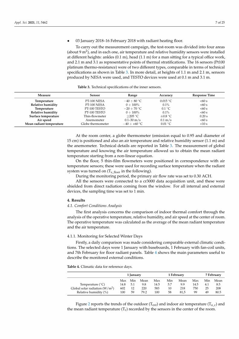
• 03 January 2018–16 February 2018 with radiant heating floor.

To carry out the measurement campaign, the test-room was divided into four areas(about 9 m2), and in each one, air temperature and relative humidity sensors were installedat different heights: ankles (0.1 m), head (1.1 m) for a man sitting for a typical office work,and 2.1 m and 3.1 as representative points of thermal stratifications. The 16 sensors (Pt100platinum thermo-resistance) were of two different types, comparable in terms of technicalspecifications as shown in Table 3. In more detail, at heights of 1.1 m and 2.1 m, sensorsproduced by NESA were used, and TESTO devices were used at 0.1 m and 3.1 m.

Table 3. Technical specifications of the inner sensors.

Measure Sensor Range Accuracy Response Time

Temperature PT-100 NESA −40 ÷ 80 ◦C 0.015 ◦C <60 sRelative humidity PT-100 NESA 0 ÷ 100% 0.1% <60 s

Temperature PT-100 TESTO −20 ÷ 70 ◦C 0.1 ◦C <60 sRelative humidity PT-100 TESTO 0 ÷ 100% 0.1% <60 s

Surface temperature Thin-flowmeter ≥205 ◦C ±0.8 ◦C 0.20 sAir speed Anemometer 0.1–30 m/s 0.1 m/s <60 s

Mean radiant temperature Globe thermometer −40 ÷ +60 ◦C 0.01 ◦C <10 s

At the room center, a globe thermometer (emission equal to 0.95 and diameter of15 cm) is positioned and also an air temperature and relative humidity sensor (1.1 m) andthe anemometer. Technical details are reported in Table 3. The measurement of globaltemperature and knowing the air temperature allowed us to obtain the mean radianttemperature starting from a non-linear equation.

On the floor, 5 thin-film flowmeters were positioned in correspondence with airtemperature sensors; these were used for recording surface temperature when the radiantsystem was turned on (Ts_floor in the following).

During the monitoring period, the primary air flow rate was set to 0.30 ACH.All the sensors were connected to a cr3000 data acquisition unit, and these were

shielded from direct radiation coming from the window. For all internal and externaldevices, the sampling time was set to 1 min.

4. Results4.1. Comfort Conditions Analysis

The first analysis concerns the comparison of indoor thermal comfort through theanalysis of the operative temperature, relative humidity, and air speed at the center of room.The operative temperature was calculated as the average of the mean radiant temperatureand the air temperature.

4.1.1. Monitoring for Selected Winter Days

Firstly, a daily comparison was made considering comparable external climatic condi-tions. The selected days were 1 January with baseboards, 1 February with fan-coil units,and 7th February for floor radiant panels. Table 4 shows the main parameters useful todescribe the monitored external conditions.

Table 4. Climatic data for reference days.

1 January 1 February 7 February

Max Min Mean Max Min Mean Max Min MeanTemperature (◦C) 14.8 5.1 9.8 14.5 5.7 9.9 14.5 4.1 8.5

Global solar radiation (W/m2) 602 12 220 583 10 218 750 25 208Relative humidity (%) 100 59 79.2 100 58 81,5 99 49 80.5

Figure 2 reports the trends of the outdoor (Text) and indoor air temperature (Ta_c) andthe mean radiant temperature (Tr) recorded by the sensors in the center of the room.

Appl. Sci. 2021, 11, 5462 8 of 25

Figure 2. Recorded temperatures in the center of room: (a) baseboards; (b) fan-coil units; (c) radiantheating floor.

With the radiant floor and the baseboard system, the two profiles were almost stack-able. In case of baseboards, since these were mounted near the walls, the radiative heatexchange increased and thus Tr was close to the indoor air with an average daily dif-ference of 0.01 ◦C and a maximum difference of 0.25 ◦C at 7:10. When the radiant floorwas considered, an average daily difference of 0.31 ◦C was recorded, while the maximumdifference was 0.82 ◦C; it occurred during the late afternoon. On the other hand, the radianttemperature was higher (maximum deviation of 0.67 ◦C) than Ta_c during the early after-noon when the combined effect of the solar radiation and floor temperature contributed toheat the building envelope. Additionally, in this case the monitored trend allowed us tohighlight the different operating principle of the compared systems. The values of surfacetemperatures recorded on the floor also suggested uniform conditions when the radiative

Appl. Sci. 2021, 11, 5462 9 of 25

floor was operating. More in detail, considering the five available sensors, the averagedaily Ts_floor varied between 20 ◦C and 21 ◦C. The highest value was 22.8 ◦C and it wasrecorded at 12:20 when there was thus an important contribution of solar radiation. Thiswas in agreement with the trend of Ta_c and Tr proposed in Figure 2c.

Considering the calculated value of operative temperature, starting from the measure-ments of the black globe in the room center, it ranged between 18.6 ◦C and 20.1 ◦C whenthe baseboards were active, with an average daily value of 19.6 ◦C, which did not matchwith the comfort requirements. The relative humidity varied between 43% and 53%. Asshown in Figure 3, the calculated values of PMV and PPD for typical working hours in apublic office were outside the comfort range with a percentage of dissatisfied people from12% to 24%. The calculation was done considering the measurements of air speed duringthe selected day.

Figure 3. PMV and PPD calculation: baseboards.

With fan-coils turned on, the operative temperature varied between 19.3 ◦C and21.7 ◦C with an average daily value of 20.7 ◦C; thus, it was included in the comfort zone.The relative humidity varied between 36% and 40%, with an average daily value of 40%.According to Figure 4, the value of the predicted mean vote was always near the lower limit,but the percentage of dissatisfied people was under 10% starting from the early afternoon.

Figure 4. PMV and PPD calculation: fan coil units.

Figure 5 indicates the major attitude of the radiant system to maintain more stationaryconditions. The neutral point was very close during the late morning and afternoon;instead, starting from 20:00, the PMV values tended to −0.5 also if the temperature wasnear 21 ◦C with a low level of relative humidity (35–37%). In this case, the operativetemperature was varied between 20.4 ◦C and 22.5 ◦C, and the average daily value was21.1 ◦C, while the average daily relative humidity was 39%.

It has to be underlined that the floor heating usually has different comfort effects onthe human body when compared to convective systems, because it has stronger effectson lower body parts, while the fan coil unit creates a layer of conditioned air around thebody. Therefore, it would be not accurate to compare the two systems and their effect on

Appl. Sci. 2021, 11, 5462 10 of 25

the comfort level based on the operative temperature. However, the measured value offloor surface temperature suggests that for the available test-room, the radiant asymmetryis always under the threshold value. For example, the widely used ∆tpr represents theasymmetry of a radiant field by referring to the difference between the plane radianttemperature of the two opposite sides of a small plane element [45], typically 0.6 m abovethe floor. Additionally, if this measure is not available, the measures at 0.1 m and 1.1 m thatare shown in the next section indicate that there is not vertical and horizontal asymmetryfor the designed system. Moreover, the current floor surface temperature requirement (Tf inTable 2) based on the comfortable contacting temperature is always respected. Indeed, it isbelieved that an excessively hot floor will lead to local thermal discomfort complaints [46].

Figure 5. PMV and PPD calculation: radiant floor system.

However, further investigations will be done for evaluating different time exposures,the asymmetric-satisfaction requirement.

Finally, it can be concluded that only the fan-coil units and the radiant floor system areable to assure comfort conditions if the air temperature is also frequently higher than 20 ◦C,which corresponds to the set point value. The low value of relative humidity influences, inall analyzed cases, the calculated comfort indexes.

4.1.2. Operative Temperature and Relative Humidity Analysis

The comfort range for operative temperature (19–23.5 ◦C) was divided into severalintermediate bands in order to discretize the analysis of monitored data in the room center.The Figure 6 shows the percentage of time in which the calculated value (starting frommonitored air temperature and radiant temperature) falls within these ranges, consideringthe whole monitoring period for the three systems.

Figure 6. Percentage of time in comfort range for all systems—operative temperatures.

Appl. Sci. 2021, 11, 5462 11 of 25

Furthermore, from these data, it is clear that operative temperature was within thecomfort range almost entirely throughout the considered period; it was lower than 19.5 ◦Conly for 1.0% of the acquisition period in the case of the radiant floor, and 11% when thefan-coils were switched on. The opposite situation occurred in the case of baseboards, sincethe operative temperature was lower than 19.5 ◦C for around 48% of the monitored values.This indicates that the baseboards needed more time to reach the set-point values and weremore prone to a temperature decay during the day.

In addition, it is evident that while with the fan-coils the operative temperature waspositioned for 78% of the time between 20 ◦C and 21 ◦C, with the radiant floor, around 64%of the measures were characterized by values higher than 21 ◦C. This analysis allowed us toconclude that for this system, a lower set-point temperature could be used with consequentenergy savings, assuring, at the same time, the comfort zone.

With reference to relative humidity values, with fan-coils, it was found that it was lessthan 40% (generally between 37% and 39%) 88% of the time, and, globally, it was alwayslower than 50%. In the case of the radiant system, the relative humidity was lower than40% for 58% of the monitoring period, and during the remaining period, it was still lowerthan 50% of the period. When the baseboards were active, the relative humidity variedbetween 40% and 50% only for 38% of the time, and it was lower than 40% for 58% of themonitored values.

In all cases, it is clear that the emitters were not able, for their characteristics, to controlthe latent load.

4.2. Air Temperature Distribution

The second part of the proposed elaboration concerns the analysis of air temperaturedistribution in the four sectors individuated in the test-room, taking into consideration thatfan-coils were located in the 2nd sector (right window side) and in the 4th sector (left doorside). Instead, the baseboards were located on the walls without the door and the window.The same monitoring periods presented in the previous section were considered.

4.2.1. Air Temperature Field

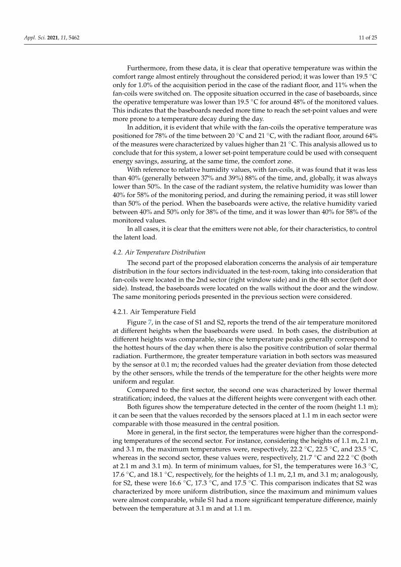
Figure 7, in the case of S1 and S2, reports the trend of the air temperature monitoredat different heights when the baseboards were used. In both cases, the distribution atdifferent heights was comparable, since the temperature peaks generally correspond tothe hottest hours of the day when there is also the positive contribution of solar thermalradiation. Furthermore, the greater temperature variation in both sectors was measuredby the sensor at 0.1 m; the recorded values had the greater deviation from those detectedby the other sensors, while the trends of the temperature for the other heights were moreuniform and regular.

Compared to the first sector, the second one was characterized by lower thermalstratification; indeed, the values at the different heights were convergent with each other.

Both figures show the temperature detected in the center of the room (height 1.1 m);it can be seen that the values recorded by the sensors placed at 1.1 m in each sector werecomparable with those measured in the central position.

More in general, in the first sector, the temperatures were higher than the correspond-ing temperatures of the second sector. For instance, considering the heights of 1.1 m, 2.1 m,and 3.1 m, the maximum temperatures were, respectively, 22.2 ◦C, 22.5 ◦C, and 23.5 ◦C,whereas in the second sector, these values were, respectively, 21.7 ◦C and 22.2 ◦C (bothat 2.1 m and 3.1 m). In term of minimum values, for S1, the temperatures were 16.3 ◦C,17.6 ◦C, and 18.1 ◦C, respectively, for the heights of 1.1 m, 2,1 m, and 3.1 m; analogously,for S2, these were 16.6 ◦C, 17.3 ◦C, and 17.5 ◦C. This comparison indicates that S2 wascharacterized by more uniform distribution, since the maximum and minimum valueswere almost comparable, while S1 had a more significant temperature difference, mainlybetween the temperature at 3.1 m and at 1.1 m.

Appl. Sci. 2021, 11, 5462 12 of 25

Figure 7. Air temperature at different heights with baseboards: (a) 1st sector, (b) 2nd sectors.

The sensor at 0.1 m was characterized by 12.9 ◦C as the minimum value in both sectors,and this value was significantly lower than that monitored by the other sensors, a sign ofunevenness in the distribution of the temperature at the level of occupants’ ankles.

Figure 8a,b refers to 3rd and 4th sectors. Additionally, in this case the trends werecomparable to the great variation for Ta_0.1, for which the minimum value, recorded inthe early morning of 31 December, was around 12 ◦C in both sectors. The temperaturemonitored by the central sensor (Ta_c) had a comparable trend with the monitored valuesat 1.1 m and 2.1 m. The S3 was characterized by a more uniform distribution comparedwith S4, but the values monitored at 1.1 m were comparable; indeed, Ta_1.0 varied between15.8 ◦C and 22.5 ◦C for S3 and between 15.9 ◦C and 22 ◦C for S4. When Ta_3.1 wasconsidered, the higher values were recorded for S4, since it varied between 18.1 ◦C and22.8 ◦C.

The comparison between all sectors indicates that the higher temperatures wererecorded in the first sector, probably due to the positive contribute of the solar gains duringthe late morning and late afternoon.

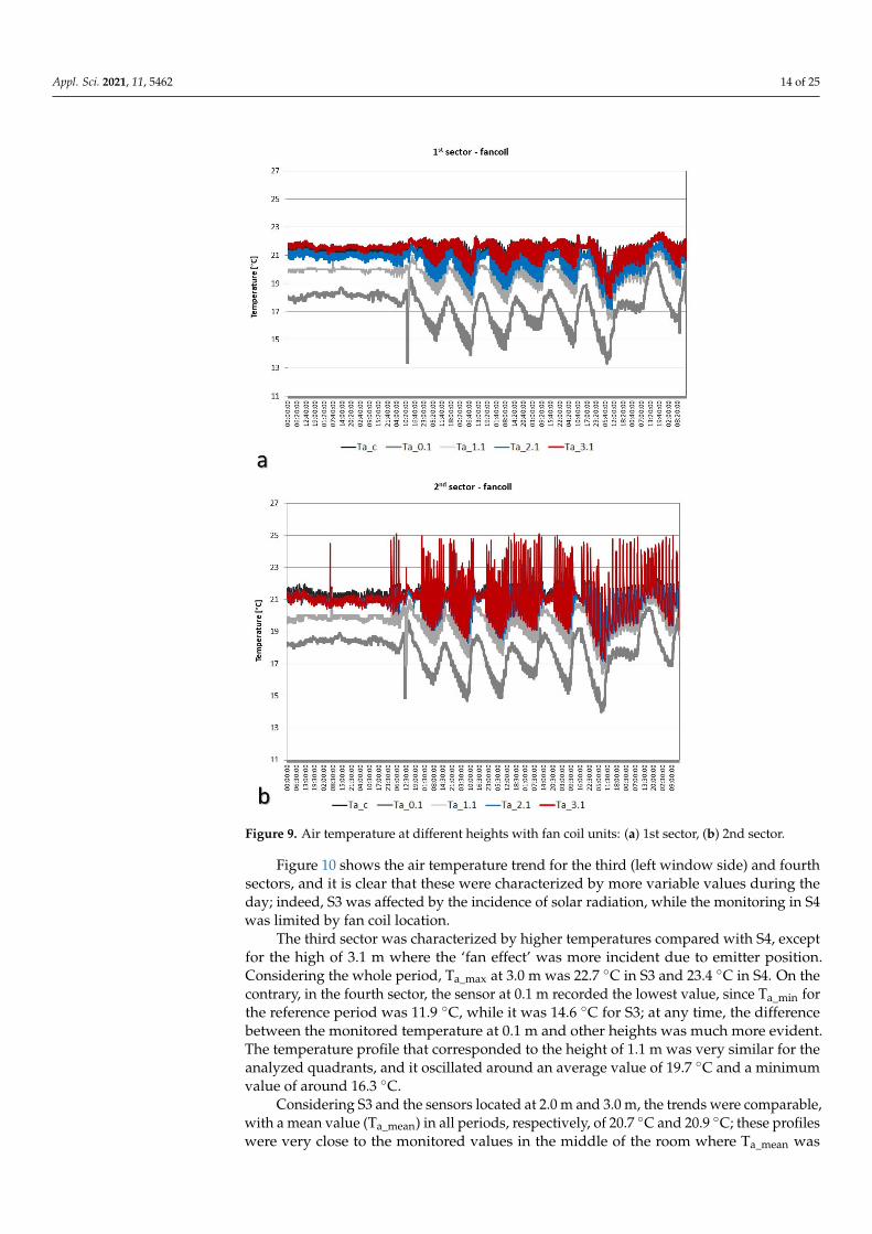
Figure 9, in the case of S1 and S2, reports the trend of the air temperature monitored atdifferent heights when fan coil units were switched on. Data showed that, in most cases, thesecond sector was characterized by higher temperatures, which was due to the combinedeffect of solar radiation, more incident in the sector facing the window, and of the emitterposition. The sensor at 3.0 m showed a more irregular trend, and indeed the temperature

Appl. Sci. 2021, 11, 5462 13 of 25

also reached the value of 25.1 ◦C, while for S1, the maximum value was about 22.6 ◦C, andit was around 20 ◦C at 1.1 m. This trend provided evidence of the phenomenon of thermalstratification caused by the heat exchange method, which was essentially convective, dueto fan-coils. The temperature peaks usually correspond to the hottest hours of the daywhen there is also a positive contribution from solar gains.

Figure 8. Air temperature at different heights with baseboards: (a) 3rd sector, (b) 4th sectors.

Figure 9 also shows the temperature monitored in the center of the room; the valuesrecorded by sensors placed at 3.1 m approximated, better than the others, data recorded inthe room’s center for S1, since the sensor at a height of 2.1 m was characterized by biggeroscillations, mainly with reference to the minimum values. For the second sector, data at2.1 m and 3.1 m were comparable with Ta_c; however, the sensor at 3.1 m was characterizedby stronger oscillations, mainly with reference to the peak values.

Considering the extreme values for all considering periods, in both sectors, the maxi-mum value (Ta_max) recorded at 0.1 m was 20.5 ◦C, while the minimum (Ta_min) was 13.3 ◦Cfor S1 and 14.0 ◦C for S2. These were significantly different from data at other heights. Forinstance, at 3.1 m and 1.1 m, Ta_min was, respectively, 16.4 and 18.0 ◦C in S1 and 16.4 ◦Cand 17.2 ◦C in the second sector; these measurements evidence the risk of unevennessbetween different heights in the same sector.

Appl. Sci. 2021, 11, 5462 14 of 25

Figure 9. Air temperature at different heights with fan coil units: (a) 1st sector, (b) 2nd sector.

Figure 10 shows the air temperature trend for the third (left window side) and fourthsectors, and it is clear that these were characterized by more variable values during theday; indeed, S3 was affected by the incidence of solar radiation, while the monitoring in S4was limited by fan coil location.

The third sector was characterized by higher temperatures compared with S4, exceptfor the high of 3.1 m where the ‘fan effect’ was more incident due to emitter position.Considering the whole period, Ta_max at 3.0 m was 22.7 ◦C in S3 and 23.4 ◦C in S4. On thecontrary, in the fourth sector, the sensor at 0.1 m recorded the lowest value, since Ta_min forthe reference period was 11.9 ◦C, while it was 14.6 ◦C for S3; at any time, the differencebetween the monitored temperature at 0.1 m and other heights was much more evident.The temperature profile that corresponded to the height of 1.1 m was very similar for theanalyzed quadrants, and it oscillated around an average value of 19.7 ◦C and a minimumvalue of around 16.3 ◦C.

Considering S3 and the sensors located at 2.0 m and 3.0 m, the trends were comparable,with a mean value (Ta_mean) in all periods, respectively, of 20.7 ◦C and 20.9 ◦C; these profileswere very close to the monitored values in the middle of the room where Ta_mean was

Appl. Sci. 2021, 11, 5462 15 of 25

21 ◦C. In the fourth sector, from the data recorded at 2.0 m and 3.0 m, rounding up anddown, for the trend monitored at the room’s center, the Ta_mean was 19.7 ◦C at 2.0 m and20.7 ◦C at 3.1 m, respectively. However, there was a temperature difference at each timeof around 2–3 ◦C with values recorded at 1.1 m, and a greater difference of 4–5 ◦C withvalues corresponding at 0.1 m.

Figure 10. Air temperature at different heights with fan coil units: (a) 3rd sector, (b) 4th sector.

Comparing the four sectors, it is evident that S2 was characterized by the highestvalues. The temperature profiles relating to the same height but on different sectors werequite comparable; there was not evident horizontal asymmetry, especially at a height of1.1 m and 2.1 m. Instead, considering the position at 3.1 m, the difference between airtemperatures recorded at the same time in S1 and S2 varied between −4.0 ◦C and +2.0 ◦C,and it varied from –2.6 ◦C and 3.7 ◦C considering sectors S2 and S4. At the height of

Appl. Sci. 2021, 11, 5462 16 of 25

0.1 m, the greatest variation happened between S1 and S3 (−3.6 ◦C ÷ 0.3 ◦C) while thetemperature difference varied between 0.2 ◦C and 2.9 ◦C considering sectors S2 and S4.

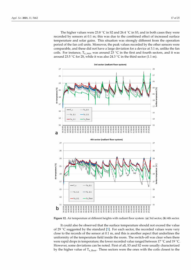
The same analysis was proposed for the radiant floor system for which also the surfacetemperature was shown. The monitored data for the first and second sectors are proposed,respectively, in Figure 11a,b; the profiles for the other sectors are reported in Figure 12.

Figure 11. Air temperature at different heights with radiant floor system: (a) 1st sector, (b) 2nd sector.

In all cases, it is evident that the long start-up period of the system allowed 20 ◦Cto be reached in more than three hours, starting from air temperature of around 17 ◦C.After this transient period, the air temperature trend at 0.1 m was close enough to valuesat other heights; this phenomenon did not happen with the fan coil system, due to thedifferent heat exchange mechanism. For each other height, air temperature values werecomparable, and these were very close to data recorded by the sensor in the room center;for instance, considering the whole monitoring period in S1, Ta_mean was 21.0 ◦C at 1.1 m,21.4 ◦C at 2.1 m, and at room center it was 21.7 ◦C at 3.1 m. In the second and third sectors,the mean values were around 21.2 ◦C at each height, and Ta_mean was 21.5 ◦C in the lastconsidered sector.

Appl. Sci. 2021, 11, 5462 17 of 25

The higher values were 23.8 ◦C in S2 and 26.4 ◦C in S3, and in both cases they wererecorded by sensors at 0.1 m; this was due to the combined effect of increased surfacetemperature and solar gains. This situation was strongly different from the operationperiod of the fan coil units. Moreover, the peak values recorded by the other sensors werecomparable, and these did not have a large deviation for a device at 3.1 m, unlike the fancoils. For instance, Ta_max was around 23 ◦C in the first and fourth sectors, and it wasaround 23.5 ◦C for 2S, while it was also 24.3 ◦C in the third sector (1.1 m).

Figure 12. Air temperature at different heights with radiant floor system: (a) 3rd sector, (b) 4th sector.

It could also be observed that the surface temperature should not exceed the valueof 29 ◦C suggested by the standard [5]. For each sector, the recorded values were veryclose to the records of the sensor at 0.1 m, and this is another aspect that underlines theuniformity of the temperature field inside the room. The switch-off was clear when therewere rapid drops in temperature; the lower recorded value ranged between 17 ◦C and 19 ◦C.However, some deviations can be noted. First of all, S3 and S2 were usually characterizedby the higher value of Ts_floor. These sectors were the ones with the coils closest to the

Appl. Sci. 2021, 11, 5462 18 of 25

flow manifold, and therefore the hottest water circulates; for this reason, the temperatureat ignition increased faster and to a higher value (24.5 ◦C) in S3. Moreover, during thesunniest hours, the temperature increased; for instance, in the last day of monitoring at13:30, with an outdoor temperature of 15 ◦C, Ts_floor was 27.4 ◦C for S2 and 27.6 ◦C for S3.

The calculation of horizontal temperature difference between sensors correspondingto the same height but in different sectors showed that only the sensors located lowerhad greater deviations due mainly to the effect of solar irradiation from the window.This phenomenon was particularly evident between sectors 1 and 3 during the afternoon(13:00–14:00) of 15 February, with external solar radiation between 539 and 567 W/m2.Indeed, in this case, the air temperature difference was −5.5 ◦C. For all other heights, thisdifference was much limited and lower compared with the operation period of fan coils.For instance, at 1.1 m, between S1and S2 and between S1 and S3, this difference variedfrom −1.9 ◦C to 0.7 ◦C; at 2.0 m considering the first and fourth sectors, it varied between−0.4 ◦C and 0.3 ◦C; at 3.0 m for S2 and S4 it varied during the monitoring period between−1.8 ◦C and 1.1 ◦C.

4.2.2. Asymmetry of Air Temperature

Another analysis concerns the comparison between vertical temperature differencewith data of sensors in the same sectors and air temperature difference with data recordedin the room center. The temperature difference between data at 1.1 m and 0.1 m wascalculated; it should be always lower than 3.0 ◦C, as previously explained with reference tolocal discomfort phenomena.

Figure 13, in the case of baseboards, shows the maximum, minimum, and mean valuesof the calculated temperature differences.

The discrete evaluation of ∆Tpr,wc, assumed as the difference Ta_3.1–Ta_0.1, highlightsthat in all sectors, the threshold value was exceeded; for instance, in the first sector, duringthe 30th of December, from 10:00 to 11:30 this values was higher than 6 ◦C, while in theother sectors it varied from 1.0 ◦C to 4.5 ◦C on the same day. However, for S4, the maximumdifference (7.4 ◦C) was recorded at 13:30 during the same day. Considering the averagevalue for all monitoring periods, it seems that a sensible thermal stratification occurredmainly in S1 and S4.

The temperature difference between the room center and the other sensor allowed usto estimate horizontal non-uniformity inside the room. Considering the difference withthe values monitored at 1.1 m and 2.1 m, both the average and extreme values were verylimited. More in detail, Ta_c–Ta_1.1 was always lower than 3 ◦C with a maximum value of1.1 ◦C, which usually occurred after midday, and thus it was also influenced by the externalconditions. Instead, the maximum difference Ta_c–Ta_3.1 varied between −3.2 ◦C (S3) and−4.1 ◦C (S1). The negative values confirmed the phenomenon of thermal stratificationalso when the reference was the central sensor. Finally, according to the average value, thedifference Ta_1.1–Ta_0.1 was lower than 3 ◦C, and thus the discomfort phenomenon wasusually avoided. However, the extreme value of 4.9 ◦C could be reached in the first andfourth sectors in both cases on 30 December, which was a sunny day.

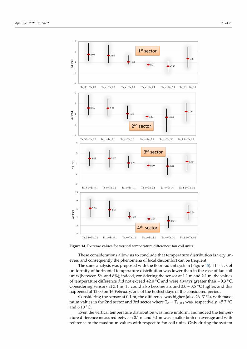
In the case of fan-coils, Figure 14 shows that in the fourth sector, where the fan-coil was located, the vertical temperature difference was very considerable; indeed, forthe calculation of Ta_3.1 − Ta_0.1, the maximum recorded value could reach 10 ◦C, andthe maximum value was 8.3 ◦C for S1 and S2. These values indicate a possible thermalstratification phenomenon in the ceiling. Indeed, the average values, mainly in the sectorswhere the units were located, were also high, and this indicates that usually in the roomthere was a vertical temperature difference that was on the verge of overcoming theprescribed threshold.

Analyzing temperature differences between the sensor in the room center and sensorsat other heights (horizontal asymmetry), it can be seen that lower values were obtained,for each sector, with the sensor at 2.1 m. The mean values, considering data for the entiremonitoring period, suggested good results also for sensors at 3.1 and 1.1 m, also if, with

Appl. Sci. 2021, 11, 5462 19 of 25

several external conditions, very extreme temperature differences could be recorded; forinstance, Tc could be also 17.1% (S4) or 19.9% (S2) higher than values recorded at 1.1 m.Moreover, Ta_c–Ta_3.1 could reach −5.6 ◦C around 15:00 on 21 January or −5.0 ◦C at 6:30 on1 February. This means that non-uniformity was due both to external conditions (e.g., effectof solar radiation) and position or operating mode of the fan coil units. The greatestdifference could be noted between Tc and Ta_0.1, since the mean values recorded for thewhole period in the center could be higher, from 14.6% (S3) to 22.3% (S4). More in detail, inS2, during the early morning (7:30–8:30) when the fan coils started working, this differencewas around 8.8 ÷ 9.0 ◦C; in the same hours, it was around 6.0 ◦C in the other sectors.

Figure 13. Extreme values for vertical temperature difference: baseboards.

Appl. Sci. 2021, 11, 5462 20 of 25

Figure 14. Extreme values for vertical temperature difference: fan coil units.

These considerations allow us to conclude that temperature distribution is very un-even, and consequently the phenomena of local discomfort can be frequent.

The same analysis was proposed with the floor radiant system (Figure 15). The lack ofuniformity of horizontal temperature distribution was lower than in the case of fan coilunits (between 5% and 8%); indeed, considering the sensor at 1.1 m and 2.1 m, the valuesof temperature difference did not exceed +2.0 ◦C and were always greater than −0.3 ◦C.Considering sensors at 3.1 m, Tc could also become around 3.0 – 3.5 ◦C higher, and thishappened at 12:00 on 16 February, one of the hottest days of the considered period.

Considering the sensor at 0.1 m, the difference was higher (also 26–31%), with maxi-mum values in the 2nd sector and 3rd sector where Tc − Ta_0.1 was, respectively, +5.7 ◦Cand 6.10 ◦C.

Even the vertical temperature distribution was more uniform, and indeed the temper-ature difference measured between 0.1 m and 3.1 m was smaller both on average and withreference to the maximum values with respect to fan coil units. Only during the system

Appl. Sci. 2021, 11, 5462 21 of 25

start-up some bigger differences were recorded, for instance in sector 3 and 1 it was −4.6 ◦Csince when radiant floor is turned off temperature reaches 16–17 ◦C at 0.1 m.

Figure 15. Extreme values for vertical temperature difference: radiant floor system.

The temperature difference for heights 1.1 m and 0.1 m was usually lower than in theprevious case, and only in a few cases did it exceed the limit value (3 ◦C). More in detail, ithappened only on 16 February around 12:00 when the effect of solar gains tended to locallyheat the place where the sensor was placed; extreme values were recorded in the 3rd sector(+6.40) and in the 1st sector (+4.30 ◦C). For all other days, this difference varied between0.2 ◦C and 1.5 ◦C.

Appl. Sci. 2021, 11, 5462 22 of 25

5. Discussion

Monitoring results suggest that for the heating season, the radiant floor system allowsbetter performance in term of thermal comfort and temperature distribution. All availabledata indicate another interesting consideration regarding air temperature value, takinginto account that set point temperature, during the experiment, was fixed to 20 ◦C, as thenormative for public buildings imposed in many countries.

More in detail, assuming that for moderate environments the air temperature is agood approximation of the operative temperature, the percentage of time (tTa%) in whichthe air temperature falls within intervals derived from the comfort zone for the operativetemperature was evaluated. Figure 16 shows the proposed index considering the value ofair temperature recorded in the center of room, in each period, and for all systems.

Figure 16. Percentage of time in comfort range for all systems—air temperature.

The baseboards are the more critical system, since for around 50% of monitoredvalues, the set point is not met, and for the other hours, the air temperature is near 20 ◦C.Two reasons can be argued: the set-point is not adequate, or the surface covered by thebaseboards is not enough and they should be installed on all four walls.

During the period with fan-coils, air temperature was for much more time in the rangeof 22–23.5 ◦C (≈63%) than in the range of 19–21 ◦C (≈17%). In the case of the radiant floor,for the previous monitoring period, the Ta_c tended to be higher than 21 ◦C for 75% of timebut it never exceeded 23.5 ◦C. With both systems, a lower set point could reduce the energyconsumption by avoiding air temperature higher than the assumed set-point. This is due tothe inertial properties of the radiant floor system that continues to heat the room until thewater inside the pipes cools down. For the fan-coil, the effect of ventilation increases theair temperature but, as shown in the previous section, also the non-uniformity of verticaland horizontal distribution.

The statement that temperature exceeds the set point values for most of the monitoredtime seems to suggest that in a well-insulated structure and with good inertial properties,a management with lower set-point temperature could determine free-cost energy savingby guaranteeing at same time the respect of comfort limits.

The analysis of the proposed result must be contextualized to the quality of thebuilding envelope that influences the uniform condition and the comfort indices. Indeed,the test-room is a particular volume with a very insulated roof and basement as well as atechnical wall that can be considered quasi-adiabatic. Assuming a real application, this canbe considered an office room in the middle floor of a building (upper and lower heatedrooms) with three exposed walls and a room at the same temperature on the north side(technical wall). Thus, the heat losses of the opaque envelope are quite limited, and this canbe considered a typical condition of the new designed highly efficient building. More indetail, the insulation level of the basement helps to favor the direction of the heat exchangewhen the radiative floor system is activated. Indeed, the heat losses on the ground can

Appl. Sci. 2021, 11, 5462 23 of 25

be considered null, and this is the main causes of the comparable values of Ts_floor andTa_0.1 and Ta_1.1. Instead, the extreme insulation of the roof negatively affects the thermalstratification with the fan-coils. Indeed, the heat exchange through the roof is also nullified,and the hot air stratifies. As regard the baseboards, these are installed on two exposedwalls and also if these are well insulated (the thermal transmittance is comparable withthe threshold value for Mediterranean cities), part of the radiated flow heats the walls andis exchanged with the outside. This could be one of the reasons why this system showedthe least effectiveness. Probably, the location on the boundary walls with other rooms (orof the technical wall in the proposed case study) would have increased the heat exchangewith the indoor air temperature.

6. Conclusions

The paper proposed an experimental comparison of three different heating emittersin Mediterranean climates. Thermo-hygrometric comfort was evaluated, as well as theasymmetry of vertical and horizontal distribution, considering an insulated heated volume.

The monitoring results indicate that only the baseboard system is not always able toassure comfort conditions with an operative temperature lower than 19.5 ◦C for around 48%of the monitored values. However, with fan-coil units and a floor radiative system, the airtemperature often rises up 20 ◦C (set point value). More in particular, with a radiant floor,for 64% of the time the operative temperature is characterized by values higher than 21 ◦C.The low value of relative humidity influences, in all analyzed cases, the calculated comfortindexes. More in general, it can be underlined that for insulated rooms in Mediterraneanclimates with important solar gains, the management of floor radiative systems requires alower set-point temperature of about 1–2 ◦C with respect to the desired value of the airtemperature, and this could bring important energy savings, without compromising thethermal comfort. Instead, when baseboards are installed, it has to be taken into account thatthe system requires more time to reach the set-point temperature, and thus managementshould consider switching on the system some hours before occupation. At the same time,the temperature values decrease more rapidly.

When the fan-coils are used, the ventilation increases the air temperature but also thenon-uniformity of vertical and horizontal distribution compared with the other analyzedsystems. In this case, the location of the units should be appropriately evaluated foravoiding local discomfort and for favoring the mixing of indoor air. The reduction ofstratification with an appropriate design would increase the time with a high operativetemperature, and this could reduce the set point temperature for obtaining a reduction ofthe heating consumption.

Author Contributions: Conceptualization and methodology G.P.V.; experimental monitoring andelaboration, S.R.; elaboration, writing, and editing, R.F.D.M. All authors have read and agreed to thepublished version of the manuscript.

Funding: This research received no external funding.

Institutional Review Board Statement: Not applicable.

Informed Consent Statement: Not applicable.

Data Availability Statement: The data presented in this study are available on request from thecorresponding author. The data are not publicly available because there is not yet an easily share-able database.

Conflicts of Interest: The authors declare no conflict of interest.

References1. ASHRAE Fundamentals. Thermal comfort. In ASHRAE Handbook; American Society of Heating, Refrigerating and Air Condition-

ing Engineers: Atlanta, GA, USA, 2017.2. ASHRAE Thermal Environmental Conditions for Human Occupancy Standard 55; American Society of Heating, Refrigerating and Air

Conditioning Engineers: Atlanta, GA, USA, 2013.

Appl. Sci. 2021, 11, 5462 24 of 25

3. Parsons, K.C. Environmental ergonomics: A review of principles, methods and models. Appl. Ergon. 2000, 31, 581–594. [CrossRef]4. Liu, J.; Yao, R.; McCloy, R. A method to weight three categories of adaptive thermal comfort. Energy Build. 2012, 47, 312–320.

[CrossRef]5. International Standardization Organization. ISO 7730—Ergonomics of the Thermal Environment—Analytical Determination and

Interpretation of Thermal Comfort Using Calculation of the PMV and PPD Indices and Local Thermal Comfort; ISO: Geneva, Switzer-land, 2005.

6. Alfano, F.R.A.; Olesen, B.W.; Palella, B.I.; Riccio, G. Thermal comfort: Design and assessment for energy saving. Energy Build.2014, 81, 326–336. [CrossRef]

7. Ferrantelli, A.; Võsa, K.; Kurnitski, J. Optimization of radiators, underfloor and ceiling heater towards the definition of a referenceideal heater for energy efficient buildings. Appl. Sci. 2018, 8, 2477. [CrossRef]

8. Gorni, D.; Visioli, A. Genetic algorithms based reference signal determination for temperature control of residential buildings.Appl. Sci. 2018, 8, 2129. [CrossRef]

9. Gendelis, S.; Jakovics, A.; Ratnieks, J. Thermal comfort condition assessment in test buildings with different heating/coolingsystems and wall envelopes. Energy Proced. 2017, 132, 153–158. [CrossRef]

10. Lin, B.; Wang, Z.; Sun, H.; Zhu, Y.; Ouyang, Q. Evaluation and comparison of thermal comfort of convective and radiant heatingterminals in office buildings. Build. Environ. 2016, 106, 91–102. [CrossRef]

11. Da Silva Júnior, A.; Mendonça, K.C.; Vilain, R.; Pereira, M.L.; Mendes, N. On the development of a simplified model for thermalcomfort control of split systems. Build. Environ. 2020, 179, 106931. [CrossRef]

12. Han, Y.; Li, Z.; Xu, P. Comparative study on energy consumption of gas-fired infrared radiant and convection heating. Adv. Mater.Res. 2014, 953, 849–853. [CrossRef]

13. Karmann, C.; Schiavon, S.; Graham, L.T.; Raftery, P.; Bauman, F. Comparing temperature and acoustic satisfaction in 60 radiantand all-air buildings. Build. Environ. 2017, 126, 431–441. [CrossRef]

14. Zeiler, W.; Boxem, G. Effects of thermal activated building systems in schools on thermal comfort in winter. Build. Environ. 2009,44, 2308–2317. [CrossRef]

15. Inard, C.; Meslem, A.; Depecker, P. Energy consumption and thermal comfort in dwelling-cells: A zonal-model approach. Build.Environ. 1998, 33, 279–291. [CrossRef]

16. Petráš, D.; Kalús, S. Effect of thermal comfort/discomfort due to infrared heaters installed at workplaces in industrial buildings.Indoor Built Environ. 2000, 9, 148–156. [CrossRef]

17. Ghaddar, N.; Salam, M.; Ghali, K. Steady thermal comfort by radiant heat transfer: The impact of the heater position. Heat Transf.Eng. 2006, 27, 29–40. [CrossRef]

18. Léger, J.; Rousse, D.R.; Le Borgne, K.; Lassue, S. Comparing electric heating systems at equal thermal comfort: An experimentalinvestigation. Build. Environ. 2018, 128, 161–169. [CrossRef]

19. Tye-Gingras, M.; Gosselin, L. Comfort and energy consumption of hydronic heating radiant ceilings and walls based on cfdanalysis. Build. Environ. 2012, 54, 1–13. [CrossRef]

20. Sevilgen, G.; Kilic, M. Numerical analysis of air flow, heat transfer, moisture transport and thermal comfort in a room heated bytwo-panel radiators. Energy Build. 2011, 43, 137–146. [CrossRef]

21. Halawa, E.; van Hoof, J.; Soebarto, V. The impacts of the thermal radiation field on thermal comfort, energy consumption andcontrol A critical overview. Renew. Sustain. Energy Rev. 2014, 37, 907–918. [CrossRef]

22. Catalina, T.; Virgone, J.; Kuznik, F. Evaluation of thermal comfort using combined CFD and experimentation study in a test roomequipped with a cooling ceiling. Build. Environ. 2009, 44, 1740–1750. [CrossRef]

23. Kitagawa, K.; Komoda, N.; Hayano, H.; Tanabe, S. Effect of humidity and small air movement on thermal comfort under a radiantcooling ceiling by subjective experiments. Energy Build. 1999, 30, 185–193. [CrossRef]

24. Corgnati, S.P.; Perino, M.; Fracastoro, G.V.; Nielsen, P.V. Experimental and numerical analysis of air and radiant cooling systemsin offices. Build. Environ. 2009, 44, 801–806. [CrossRef]

25. Causone, F.; Baldin, F.; Olesen, B.W.; Corgnati, S.P. Floor heating and cooling combined with displacement ventilation: Possibilitiesand limitations. Energy Build. 2010, 42, 2338–2352. [CrossRef]

26. Bagheri, N.; Moosavi, A.; Safii, M.B. Thermal enhancement of baseboard heaters using novel fin-tube arrays: Experiment andsimulation. Int. J. Therm. Sc. 2020, 151, 106285. [CrossRef]

27. Shobi, M.O.; Salarian, H.; Nichkoohi, A.L.; Nimvari, M.E. Experimental and numerical investigations of a modified designedbaseboard radiator using an air gap enhancing free convection heat transfer. J. Build. Eng. 2020, 32, 101535. [CrossRef]

28. Karmann, C.; Stefano, S.; Bauman, F. Thermal comfort in buildings using radiant vs. all-air systems: A critical literature review.Build. Environ. 2017, 111, 123–131. [CrossRef]

29. Sun, H.; Yang, Z.; Lin, B.; Shi, W.; Zhu, Y.; Zhao, H. Comparison of thermal comfort between convective heating and radiantheating terminals in a winter thermal environment: A field and experimental study. Energy Build. 2020, 224, 110239. [CrossRef]

30. Lin, C.; Liu, H.; Tseng, K.; Lin, S. Heating, Ventilation, and air conditioning system optimization control strategy involving fancoil unit temperature control. Appl. Sci. 2019, 9, 2391. [CrossRef]

31. Sánchez-García, D.; Bienvenido-Huertas, D.; Pulido-Arcas, J.A.; Rubio-Bellido, C. Analysis of energy consumption in differentEuropean cities: The Adaptive Comfort Control Implemented Model (ACCIM) considering Representative ConcentrationPathways (RCP) scenarios. Appl. Sci. 2020, 10, 1513. [CrossRef]

Appl. Sci. 2021, 11, 5462 25 of 25

32. Date, J.; Athienitis, A.K.; Fournier, M. A study of temperature set point strategies for peak power reduction in residentialbuildings. Energy Proced. 2015, 78, 2130–2135. [CrossRef]

33. Wang, Z.; de Dear, R.; Lin, B.; Zhu, Y.; Ouyang, Q. Rational selection of heating temperature set points for China’s hot summer eCold winter climatic region. Build. Environ. 2015, 93, 63–70. [CrossRef]

34. Moon, J.W.; Han, S.H. Thermostat strategies impact on energy consumption in residential buildings. Energy Build. 2011, 43,338–346. [CrossRef]

35. Ghahramani, A.; Zhang, K.; Dutta, K.; Yang, Z.; Becerik-Gerber, B. Energy savings from temperature set-points and deadband:Quantifying the influence of building and system properties on savings. Appl. Energy 2016, 165, 930–942. [CrossRef]

36. Bienvenido-Huertas, D.; Sánchez-García, D.; Rubio-Bellido, C.; Pulido-Arcas, J.A. Influence of the improvement in thermalexpectation levels with adaptive set-point temperatures on energy consumption. Appl. Sci. 2020, 10, 5282. [CrossRef]

37. Christensen, J.E.; Chasapis, K.; Gazovic, L.; Kolarik, J. Indoor environment and energy consumption optimization using fieldmeasurements and building energy simulation. Energy Proced. 2015, 78, 2118–2123. [CrossRef]

38. Hang, L.; Kim, D. Enhanced model-based predictive control system based on fuzzy logic for maintaining thermal Comfort in IoTSmart Space. Appl. Sci. 2018, 8, 1031. [CrossRef]

39. Tushar, W.; Wang, T.; Lan, L.; Xu, Y.; Withanage, C.; Yuen, C.; Wood, K.L. Policy design for controlling set-point temperature ofACs in shared spaces of buildings. Energy Build. 2017, 134, 105–114. [CrossRef]

40. Wang, F.; Chen, Z.; Feng, Q.; Zhao, Q.; Cheng, Z.; Guo, Z.; Zhong, Z. Experimental comparison between set-point based andsatisfaction based indoor thermal environment control. Energy Build. 2016, 128, 686–696. [CrossRef]

41. Nikdel, L.; Janoyan, K.; Bird, S.D.; Powers, S.E. Multiple perspectives of the value of occupancy-based HVAC control systems.Build. Environ. 2018, 129, 15–25. [CrossRef]

42. Yongchao, Z.; Honnekeri, A.; Pigman, M.; Fountain, M.; Zhang, H.; Xiang, Z.; Arens, E. Use of adaptive control and its effects onhuman comfort in a naturally ventilated office in Alameda, California. Energy Build. 2019, 203, 109435.

43. Aftab, M.; Chen, C.; Chau, C.; Rahwan, T. Automatic HVAC control with real-time occupancy recognition and simulation-guidedmodel predictive control in low-cost embedded system. Energy Build. 2017, 154, 141–156. [CrossRef]

44. Ascione, F.; De Masi, R.F.; de Rossi, F.; Ruggiero, S.; Vanoli, G.P. MATRIX, a multi activity test-room for evaluating the energyperformances of ‘building/HVAC’ systems in Mediterranean climate: Experimental set-up and CFD/BPS numerical modelling.Energ. Buildings 2016, 126, 424–446. [CrossRef]

45. Zhou, X.; Liu, Y.; Luo, M.; Zhang, L.; Zhang, Q.; Zhang, X. Thermal comfort under radiant asymmetries of floor cooling system in2 h and 8 h exposure durations. Energ. Build. 2019, 188–189, 98–100. [CrossRef]

46. Fanger, P.O.; Banhidi, L.; Olesen, B.W.; Langkilde, G.L. Comfort limits for heated ceilings. ASHRAE Trans. 1980, 86, 141–156.