Experimental and Numerical Analysis of Sidewall Curl in ...
174
University of Windsor University of Windsor Scholarship at UWindsor Scholarship at UWindsor Electronic Theses and Dissertations Theses, Dissertations, and Major Papers 2011 Experimental and Numerical Analysis of Sidewall Curl in Experimental and Numerical Analysis of Sidewall Curl in Advanced High Strength Steels Advanced High Strength Steels ALI ARYANPOUR University of Windsor Follow this and additional works at: https://scholar.uwindsor.ca/etd Recommended Citation Recommended Citation ARYANPOUR, ALI, "Experimental and Numerical Analysis of Sidewall Curl in Advanced High Strength Steels" (2011). Electronic Theses and Dissertations. 171. https://scholar.uwindsor.ca/etd/171 This online database contains the full-text of PhD dissertations and Masters’ theses of University of Windsor students from 1954 forward. These documents are made available for personal study and research purposes only, in accordance with the Canadian Copyright Act and the Creative Commons license—CC BY-NC-ND (Attribution, Non-Commercial, No Derivative Works). Under this license, works must always be attributed to the copyright holder (original author), cannot be used for any commercial purposes, and may not be altered. Any other use would require the permission of the copyright holder. Students may inquire about withdrawing their dissertation and/or thesis from this database. For additional inquiries, please contact the repository administrator via email ([email protected]) or by telephone at 519-253-3000ext. 3208.
-
Upload
khangminh22 -
Category
Documents
-
view
2 -
download
0
Transcript of Experimental and Numerical Analysis of Sidewall Curl in ...
University of Windsor University of Windsor
Scholarship at UWindsor Scholarship at UWindsor
Electronic Theses and Dissertations Theses, Dissertations, and Major Papers
2011
Experimental and Numerical Analysis of Sidewall Curl in Experimental and Numerical Analysis of Sidewall Curl in
Advanced High Strength Steels Advanced High Strength Steels
ALI ARYANPOUR University of Windsor
Follow this and additional works at: https://scholar.uwindsor.ca/etd
Recommended Citation Recommended Citation ARYANPOUR, ALI, "Experimental and Numerical Analysis of Sidewall Curl in Advanced High Strength Steels" (2011). Electronic Theses and Dissertations. 171. https://scholar.uwindsor.ca/etd/171
This online database contains the full-text of PhD dissertations and Masters’ theses of University of Windsor students from 1954 forward. These documents are made available for personal study and research purposes only, in accordance with the Canadian Copyright Act and the Creative Commons license—CC BY-NC-ND (Attribution, Non-Commercial, No Derivative Works). Under this license, works must always be attributed to the copyright holder (original author), cannot be used for any commercial purposes, and may not be altered. Any other use would require the permission of the copyright holder. Students may inquire about withdrawing their dissertation and/or thesis from this database. For additional inquiries, please contact the repository administrator via email ([email protected]) or by telephone at 519-253-3000ext. 3208.

EXPERIMENTAL & NUMERICAL STUDY
OF SIDEWALL CURL IN
ADVANCED HIGH STRENGTH STEELS
By
Ali Aryanpour
A Thesis
Submitted to the Faculty of Graduate Studies
through Mechanical, Automotive and Materials Engineering
in Partial Ful�llment of the Requirements for
the Degree of Master of Applied Science at the
University of Windsor
Windsor, Ontario, Canada
2011
c©2011 Ali Aryanpour
Experimental & Numerical Analysis of Sidewall Curl
in Advanced High Strength Steels
ByAli Aryanpour
APPROVED BY:
Dr. V. Stoilov, Outside ReaderDepartment of Mechanical, Automotive and Materials Engineering
Dr. W. Altenhof, Program ReaderDepartment of Mechanical, Automotive and Materials Engineering
Mr. M. Rodzik, Industrial AdvisorThe NARMCO Group
Dr. D. E. Green, AdvisorDepartment of Mechanical, Automotive and Materials Engineering
Dr. B. Zhou, Chair of DefenseDepartment of Mechanical, Automotive and Materials Engineering
October 18, 2011

iii
Author's Declaration of Originality
I hereby certify that I am the sole author of this thesis and that no part of this
thesis has been published or submitted for publication.
I certify that, to the best of my knowledge, my thesis does not infringe upon any-
one's copyright nor violate any proprietary rights and that any ideas, techniques,
quotations, or any other material from the work of other people included in my the-
sis, published or otherwise, are fully acknowledged in accordance with the standard
referencing practices. Furthermore, to the extent that I have included copyrighted
material that surpasses the bounds of fair dealing within the meaning of the Canada
Copyright Act, I certify that I have obtained a written permission from the copy-
right owner(s) to include such material(s) in my thesis and have included copies of
such copyright clearances to my appendix.
I declare that this is a true copy of my thesis, including any �nal revisions, as
approved by my dissertation committee and the Graduate Studies o�ce, and that
this dissertation has not been submitted for a higher degree to any other University
or Institution.

iv
ABSTRACT
Sidewall curl is a type of springback deformation resulting from successive bending-
unbending when a sheet metal is drawn over a die radius or through a drawbead.
In this study, the sidewall curl in stamped AHSS parts (TRIP780 and DP980) was
predicted using four models from LS-DYNA material library: 24, 36, 37, 125 and a
UMAT in ABAQUS based on the Yoshida-Uemori model. Various material charac-
terization tests were analyzed to identify the input parameters. Plane-strain channel
sections were drawn in a specialized die with adjustable drawbeads and various die
entry radii and compared with simulation results. By increasing drawbead penetra-
tion, the springback angle decreased but the sidewall curl increased in the channel
sections. For simulations in LS-DYNA, MAT37 with increased integration points
predicted the most accurate results. The YU model in ABAQUS showed less than
8% error compared to the predicted sidewall curl for channel sections with shallow
drawbeads.

v
Dedicated to my wife, for her loving support

vi
ACKNOWLEDGEMENTS
I wish to express my greatest gratitude for my advisor, Dr. Daniel E. Green in
providing continuous support and helpful ideas in the course of my graduate studies
and di�erent stages of my research. I consider myself to be very fortunate to work
under his supervision and learn from him in discipline, knowledge and character.
I would like to thank my thesis committee members, Dr. William Altenhof, Dr.
Vesselin Stoilov and Matthew Rodzik for their valuable comments and recommenda-
tions. I should also express my great appreciation for the discussions and exchange
of ideas with my colleague, Amir Hassannejad-asl.
During the course of my studies and throughout the di�culties experienced
during this time, I received full support from my beloved wife and helpful advice
from my brothers. I wish to thank them and all my family for their belief in me and
the strength I gained from their encouragement.
Finally, I want to express my sincere gratitude to the following individuals and
organizations:
• Professor Chester Van Tyne and Lee Rothleutner from Colorado School of
Mines, for carrying out the Unloading modulus experiments.
• Dr. Ming Shi from USSteel, for carrying out the cyclic tension-compression
tests.
• Patrick Seguin, for his help in performing the uniaxial tensile tests and up-
grading the data acquisition system.
• Brian Vensk, Kapco Tool& Die Co. plant manager, for his numerous supports
and advices during the experimental phase of the project.
• The Narmco group for sponsoring the channel draw experiments and in-kind
provision of the study materials.
vii
Table of Contents
Author's Declaration of Originality iii
Abstract iv
Dedication v
Acknowledgements vi
List of Tables ix
List of Figures x
List of Abbreviations and Symbols xv
1 Introduction 1
1.1 Overview . . . . . . . . . . . . . . . . . . . . . . . . . . . . . . . . . 1
1.2 Sidewall curl and springback . . . . . . . . . . . . . . . . . . . . . . . 2
1.3 Springback of Advanced High Strength Steels . . . . . . . . . . . . . 5
1.4 Prediction and Compensation . . . . . . . . . . . . . . . . . . . . . . 9
1.5 Objective and outline of thesis . . . . . . . . . . . . . . . . . . . . . 11
2 Material Models 13
2.1 Introduction . . . . . . . . . . . . . . . . . . . . . . . . . . . . . . . . 13
2.2 Literature review . . . . . . . . . . . . . . . . . . . . . . . . . . . . . 14
2.2.1 Early studies . . . . . . . . . . . . . . . . . . . . . . . . . . . 14
2.2.2 Analytical solutions . . . . . . . . . . . . . . . . . . . . . . . 16
2.2.3 Numerical studies . . . . . . . . . . . . . . . . . . . . . . . . . 19
2.2.4 Constitutive material models . . . . . . . . . . . . . . . . . . 22
2.2.5 Identi�cation of material parameters . . . . . . . . . . . . . . 30
2.3 Yoshida-Uemori two-surface plasticity model . . . . . . . . . . . . . . 33
2.3.1 Degradation of elastic sti�ness during unloading . . . . . . . 39
2.3.2 Identify the YU Hardening parameters from cyclic tests . . . 42
2.4 LS-DYNA material models for sheet metal forming . . . . . . . . . . 45
3 Experimental study 50
3.1 Introduction . . . . . . . . . . . . . . . . . . . . . . . . . . . . . . . . 50
3.2 Description of the channel draw process . . . . . . . . . . . . . . . . 50

viii
3.2.1 Data acquistion system . . . . . . . . . . . . . . . . . . . . . 59
3.3 Experimental results of channel draw for DP980 and TRIP780 . . . . 62
3.3.1 Punch force vs. displacement curves . . . . . . . . . . . . . . 62
3.3.2 Channel sidewall pro�les . . . . . . . . . . . . . . . . . . . . . 68
3.3.3 Thickness reduction and strain distribution . . . . . . . . . . 75
3.4 Material characterization and mechanical properties . . . . . . . . . 77
3.4.1 Uniaxial tension tests . . . . . . . . . . . . . . . . . . . . . . 78
3.4.2 Unloading elastic modulus . . . . . . . . . . . . . . . . . . . . 84
3.4.3 Cyclic Tension and Compression tests . . . . . . . . . . . . . 91
3.4.4 Friction coe�cient . . . . . . . . . . . . . . . . . . . . . . . . 94
4 Numerical Analysis 95
4.1 Introduction . . . . . . . . . . . . . . . . . . . . . . . . . . . . . . . . 95
4.2 Determination of Constitutive Material Parameters . . . . . . . . . 96
4.3 Finite element model of channel draw . . . . . . . . . . . . . . . . . 105
4.4 Results of channel forming simulations . . . . . . . . . . . . . . . . . 114
4.4.1 Punch Force vs. Displacement curves . . . . . . . . . . . . . . 114
4.4.2 Channel sidewall pro�les . . . . . . . . . . . . . . . . . . . . . 126
4.4.3 Thickness reduction and strain distribution . . . . . . . . . . 135
5 Final Discussions and Conclusions 140
A Simulation of B-pillar 148
Bibliography 150
Vita Auctoris 158

ix
List of Tables
3.1 Geometrical dimensions for channel draw process . . . . . . . . . 57
3.2 Adjustable parameters of drawbeads and kiss blocks for each
con�guration . . . . . . . . . . . . . . . . . . . . . . . . . . . . . . . 57
3.3 Speci�cations of channel draw conditions with di�erent die entry
radius and no drawbeads . . . . . . . . . . . . . . . . . . . . . . . 66
3.4 Geometrical measures of channel draw experiments for various
drawbead penetrations . . . . . . . . . . . . . . . . . . . . . . . . . 73
3.5 Principal strains and thickness of blanks measured in channel
sidewalls . . . . . . . . . . . . . . . . . . . . . . . . . . . . . . . . . 77
3.6 Summary of mechanical properties measured by tensile tests at
USSteel . . . . . . . . . . . . . . . . . . . . . . . . . . . . . . . . . . 82
3.7 Average experimental results for Unloading Elastic Modulus . . 87
3.8 Identi�ed parameters for decay formula of unloading elastic mod-
ulus for prestrains up to 4.5% . . . . . . . . . . . . . . . . . . . . . 87
3.9 Identi�ed parameters for decay formula of unloading elastic mod-
ulus with prestrain 12% for TRIP780 and 9% for DP980 . . . . 90
4.1 Intermediate YU model parameters from systematic analysis of
tension compression test . . . . . . . . . . . . . . . . . . . . . . . . 96
4.2 Optimized YU model parameters for LS-DYNA with Mat125 . . 102
4.3 Original YU parameters reported in another study . . . . . . . . 105
4.4 Coe�cients for Hill's 1948 yield function . . . . . . . . . . . . . . 112
4.5 Stress anisotropic ratios for channel model in ABAQUS . . . . . 113
4.6 Transverse shear sti�ness for channel model in ABAQUS . . . . 113
4.7 Geometrical measures for channel sidewall pro�les with shallow
beads, predicted with LS-DYNA . . . . . . . . . . . . . . . . . . . 132
4.8 Geometrical measures for channel sidewall pro�les without beads
and DER=12 mm, predicted with LS-DYNA . . . . . . . . . . . 133
4.9 Summary of maximum values of thickness reduction and plastic
strains predicted in the channel sidewalls . . . . . . . . . . . . . . 136
x
List of Figures
1.1 Di�erent types of sidewall springback . . . . . . . . . . . . . . . . 4
1.2 Origin and Mechanism of Sidewall curl . . . . . . . . . . . . . . . 4
1.3 Elastic recovery comparison between AHSS and MS during un-
loading . . . . . . . . . . . . . . . . . . . . . . . . . . . . . . . . . . 5
1.4 Schematic of AHSS steels compared to conventional HSS and
mild steels . . . . . . . . . . . . . . . . . . . . . . . . . . . . . . . . 6
1.5 TRIP350/600 with a greater elongation than DP350/600 and
HSLA350/450 . . . . . . . . . . . . . . . . . . . . . . . . . . . . . . 7
1.6 Two channels made sequential in the same die . . . . . . . . . . . 8
1.7 Elastic recovery comparison between AHSS and MS during un-
loading . . . . . . . . . . . . . . . . . . . . . . . . . . . . . . . . . . 8
1.8 The AHSS have greater sidewall curl for equal tensile strength
steels . . . . . . . . . . . . . . . . . . . . . . . . . . . . . . . . . . . 9
1.9 Design process schematic . . . . . . . . . . . . . . . . . . . . . . . 11
2.1 E�ect of stretching in SHAPESET process . . . . . . . . . . . . . 15
2.2 A schematic diagram of the 2-D draw bending operation . . . . 16
2.3 Schematic of straight �anging process . . . . . . . . . . . . . . . . 17
2.4 Geometry of the draw bend test with deformed shape before and
after springback . . . . . . . . . . . . . . . . . . . . . . . . . . . . . 18
2.5 Schematics of cylindrical and 2-D draw bending tests and a
double-S rail . . . . . . . . . . . . . . . . . . . . . . . . . . . . . . . 21
2.6 Description of isotropic hardening model with the uniaxial stress-
strain curve . . . . . . . . . . . . . . . . . . . . . . . . . . . . . . . 23
2.7 Description of kinematic hardening model showing the transla-
tion and the resulting stress-strain curve with shifted yield stress
in compression . . . . . . . . . . . . . . . . . . . . . . . . . . . . . . 25
2.8 Schematics of the isotropic hardening in the deviatoric plane and
the stress vs. plastic strain response . . . . . . . . . . . . . . . . . 27
2.9 Schematics of the linear kinematic hardening in the deviatoric
plane and the stress vs. plastic strain response . . . . . . . . . . 27
2.10 Schematic showing the stress-strain response with and without
Bauschinger e�ect during forward and reverse loading paths . . 28
2.11 Stress-strain response of a mild steel in a forward and reverse
loading and the cyclic phenomena . . . . . . . . . . . . . . . . . . 34

List of Figures xi
2.12 Schematic illustration of the YU two-surface model . . . . . . . . 35
2.13 De�nition of the parameters in the Yoshida-Uemori hardening
model . . . . . . . . . . . . . . . . . . . . . . . . . . . . . . . . . . . 37
2.14 Schematic illustration of stagnation surface . . . . . . . . . . . . 38
2.15 An example of unloading stress-strain response for the high strength
steel sheet . . . . . . . . . . . . . . . . . . . . . . . . . . . . . . . . 41
2.16 A schematic illustration of the stress-strain relationship of an
unloading/reloading cycle . . . . . . . . . . . . . . . . . . . . . . . 41
2.17 Schematic illustration of stress-strain response during forward
and reverse deformation for identi�cation of YU hardening pa-
rameters . . . . . . . . . . . . . . . . . . . . . . . . . . . . . . . . . 42
2.18 Schematic illustrations of the motion of the yield and bounding
surfaces under a uniaxial forward-reverse deformation . . . . . . 43
3.1 A/SP die installed in a hydraulic press . . . . . . . . . . . . . . . 52
3.2 sideview of the A/SP die components and general dimension
parameters . . . . . . . . . . . . . . . . . . . . . . . . . . . . . . . . 53
3.3 Draw die schematic view . . . . . . . . . . . . . . . . . . . . . . . . 53
3.4 Illustration of symmetry in the channel draw process . . . . . . . 54
3.5 Drawbead at 0% penetration . . . . . . . . . . . . . . . . . . . . . 55
3.6 Drawbead at 100% penetration . . . . . . . . . . . . . . . . . . . . 56
3.7 Electroetching a grid of circles of 0.1(in) diameter onto one side
of a blank . . . . . . . . . . . . . . . . . . . . . . . . . . . . . . . . . 58
3.8 Sample of channels produced for various drawbead con�gurations 59
3.9 Front panel of the data acquisition software . . . . . . . . . . . . 60
3.10 Sensors used for the data acquisition system . . . . . . . . . . . . 61
3.11 Experimental punch force-displacement curves for TRIP780 chan-
nels drawn with various drawbead penetrations . . . . . . . . . . 63
3.12 Experimental punch force-displacement curves for DP980 chan-
nels drawn with various drawbead penetrations . . . . . . . . . . 64
3.13 Experimental punch force-displacement curve for DP980 chan-
nels drawn with a shallow bead penetration (20%) . . . . . . . . 65
3.14 Channels drawn with various die entry radii and without draw-
beads . . . . . . . . . . . . . . . . . . . . . . . . . . . . . . . . . . . 65
3.15 omparison of punch force-displacement curves for TRIP780 chan-
nels drawn with shallow bead penetration (20%) when blanks are
cut parallel to the rolling and the transverse directions . . . . . . 66

List of Figures xii
3.16 Experimental punch force-displacement curves for TRIP780 chan-
nels drawn without beads and with various die entry radii, and
for blanks cut in either the rolling or transverse directions . . . . 67
3.17 Experimental punch force-displacement curves for DP980 chan-
nels drawn with various die entry radii . . . . . . . . . . . . . . . 68
3.18 Geometrical measures of sidewall curl for channel pro�le . . . . . 69
3.19 Sidewall pro�les of TRIP780 channels drawn with various draw-
bead penetrations . . . . . . . . . . . . . . . . . . . . . . . . . . . . 70
3.20 Sidewall pro�les of DP980 channels drawn with various draw-
bead penetrations . . . . . . . . . . . . . . . . . . . . . . . . . . . . 71
3.21 Comparison of sidewall pro�les for channels drawn with and
without drawbeads . . . . . . . . . . . . . . . . . . . . . . . . . . . 72
3.22 Sidewall pro�les of channels made from TRIP780 blanks sheared
in the rolling and transverse directions, with shallow bead pen-
etration (20%) and no drawbeads (DER=12mm) . . . . . . . . . 74
3.23 Comparison of sidewall pro�les for channels drawn with various
die entry radii and without drawbeads . . . . . . . . . . . . . . . 75
3.24 Location of surface strain measurements on the channel sidewalls 76
3.25 Thickness measurment of channel sections using an ultrasonic
thickness device . . . . . . . . . . . . . . . . . . . . . . . . . . . . . 76
3.26 Specimen for uniaxial tension test designed according to ASTM-E8 78
3.27 Uniaxial tension test data obtained at the University of Windsor
for TRIP780 and DP980 . . . . . . . . . . . . . . . . . . . . . . . . 81
3.28 Plasticity curves for TRIP780 from uniaxial tests performed at
University of Windsor, USSteel and a power law curve . . . . . . 83
3.29 Plasticity curves for DP980 from uniaxial tests performed at
University of Windsor, USSteel and a power law curve . . . . . . 84
3.30 Engineering stress-strain curves for unloading elastic modulus of
TRIP780 and DP980, performed at the Colorado School of Mines 85
3.31 Sample of estimating initial and unloading elastic modulus of
TRIP780 and DP980 from stress-strain curves . . . . . . . . . . . 86
3.32 Multiple loading and unloading cycles to estimate saturated un-
loading elastic modulus of TRIP780 and DP980 . . . . . . . . . . 89
3.33 Fitting analytical decay function to unloading elastic modulus
of TRIP780 and DP980 . . . . . . . . . . . . . . . . . . . . . . . . 90
3.34 Cyclic tension - compression tests of TRIP780 . . . . . . . . . . . 92
3.35 Cyclic tension - compression tests of DP980 . . . . . . . . . . . . 93

List of Figures xiii
4.1 Fitting bounding surfaces to experimental tension and compres-
sion data of DP980 . . . . . . . . . . . . . . . . . . . . . . . . . . . 97
4.2 Fitting bounding surfaces to experimental tension and compres-
sion data of TRIP780 . . . . . . . . . . . . . . . . . . . . . . . . . . 98
4.3 Schematic representation of the �nite element model for tension
compression test . . . . . . . . . . . . . . . . . . . . . . . . . . . . . 99
4.4 Comparison of experimental tension and compression test results
with isotropic hardening and YU models (Mat 125) for TRIP780
and DP980 . . . . . . . . . . . . . . . . . . . . . . . . . . . . . . . . 100
4.5 Optimized simulations with Material type 125 for tension com-
pression tests of TRIP780 and DP980 . . . . . . . . . . . . . . . . 103
4.6 Correlation matrices between Mat125 parameters and curve map-
ping error response for TRIP780 and DP980 . . . . . . . . . . . . 104
4.7 Finite element model of the channel draw forming in LS-DYNA 107
4.8 Comparison of predicted and experimental punch force results
for DP980 with various material models . . . . . . . . . . . . . . 114
4.9 Comparison of predicted and experimental punch force results
for TRIP780 with various material models . . . . . . . . . . . . . 115
4.10 Comparison of experimental and predicted punch force results
for TRIP780 with shallow beads using the YUmodel in ABAQUS
and LS-DYNA . . . . . . . . . . . . . . . . . . . . . . . . . . . . . . 116
4.11 Energy balance for TPSB case with various material models . . 118
4.12 Energy balance for TPSB case with various material models . . 119
4.13 Energy balance for TPSB case in ABAQUS - YU model . . . . . 120
4.14 Energy balance for DPSB case with various material models . . 121
4.15 Energy ratio for DPSB case with various material models . . . . 123
4.16 Comparison of predicted and experimental punch forces for TRIP780
and DP980 without draw beads and with DER=12 mm . . . . . 124
4.17 Comparison of predicted and experimental punch forces for cases
without beads, DER=12mm and Mat 24 for various coe�cients
of friction . . . . . . . . . . . . . . . . . . . . . . . . . . . . . . . . . 125
4.18 Schematic illustration of sidewall comparison between simulated
and experimental curves . . . . . . . . . . . . . . . . . . . . . . . . 126
4.19 Comparison of simulated and experimental sidewall pro�les for
TRIP780 channels with shallow beads . . . . . . . . . . . . . . . . 128
4.20 Comparison of simulated and experimental sidewall pro�les for
DP980 channels with shallow beads . . . . . . . . . . . . . . . . . 129
List of Figures xiv
4.21 Comparison of simulated and experimental sidewall pro�les for
TRIP780 channels without beads and DER=12mm . . . . . . . . 130
4.22 Comparison of simulated and experimental sidewall pro�les for
DP980 channels without beads and DER=12mm . . . . . . . . . 131
4.23 Simulated sidewall pro�les for TPNB12 condition with various
friction coe�cients . . . . . . . . . . . . . . . . . . . . . . . . . . . 134
4.24 Maximum principal strain histories for an element on the side-
wall of TPSB channel forming simulation . . . . . . . . . . . . . . 137
4.25 Minimum principal strain histories for an element on the sidewall
of TPSB channel forming simulation . . . . . . . . . . . . . . . . . 137
4.26 Shell thickness reduction (%) for TPSB and DPSB conditions . 138
4.27 E�ective plastic strain distributions for TPSB and DPSB con-
ditions . . . . . . . . . . . . . . . . . . . . . . . . . . . . . . . . . . . 139
5.1 Modi�ed prediction of cyclic behaviour of TRIP780 sheet metal
by the isotropic hardening law . . . . . . . . . . . . . . . . . . . . 141
5.2 Prediction of the cyclic behaviour of TRIP780 and DP980 steels
with the combined isotropic-linear kinematic hardening law . . . 142
5.3 Channel sidewall pro�les for the TPSB and DPSB cases pre-
dicted with the YU model in ABAQUS and LS-DYNA and com-
pared with the experimental results . . . . . . . . . . . . . . . . . 144
5.4 Prediction of the thickness along the channel section predicted
with the YU model in ABAQUS for TRIP780 and DP980 . . . . 145
A.1 FE model of crash forming a B pillar part from DP980 . . . . . 149
A.2 Plastic strain distribution of forming simulation of a B-pillar,
using Mat37 . . . . . . . . . . . . . . . . . . . . . . . . . . . . . . . 149
A.3 Predicted sprungback B-pillar, using Mat37 model . . . . . . . . 149

xv
List of Abbreviations and Symbols
AHSS Advanced High Strength Steels
AKDQ Aluminum-Killed Draw Quality steel
DP Dual phase steel
NIP Number of Integration Points
TRIP TRansformation Induced Plasticity
YU Yoshida - Uemori plasticity model
IH Isotropic hardening
LK Linear Kinematic mardening
NKH Nonlinear Kinematic hardening
Mat 18 Power law isotropic hardening model
Mat 24 Piecewise linear plasticity model
Mat 36 3-Parameter Barlat plasticity model
Mat 37 Transversely anisotropic elastic plastic model
Mat 125 Kinematic hardening transversely anisotropic model
E Elastic Modulus
σ E�ective stress
σy0 Initial yield stress
α Back-stress tensor

1
Chapter 1
Introduction
1.1 Overview
The ongoing need for vehicle weight reduction and safety improvement has re-
sulted in the use of advanced high strength steels (AHSS) such as Dual Phase
(DP) and TRansformation Induced Plasticity (TRIP) sheet metals (along with alu-
minum). The advanced performance of these steels in ductility and strain hardening
characteristics provides an opportunity to stamp complex geometries and improve
performance of automotive body in crash, ductility and strength while reducing the
overall weight. This increased formability of AHSS materials is their main advantage
over conventional HSS. However, speci�c material characteristics have increased the
challenges encountered when forming parts made from such steels.
One of the main challenges in industrial sheet metal forming processes is to
satisfy design speci�cations without causing defects such as splits, wrinkling, skid
lines, surface distortion and springback. From these, the springback deformation
is unavoidable for all sheet metals because this type of elastic recovery appears
naturally as a result of the unbalanced stresses that develop in the part as well as
through-thickness just after its removal from the die. Along with the increase in
strength and formability of sheet metals, the occurrence of severe distortions like
springback and side-wall curl also increases. These complex deformations are the
most signi�cant factors that change the shape of parts after forming and make it
di�cult to achieve the required dimensional accuracy for the �nal product. This
can lead to a product in which loss of dimensional accuracy causes di�culties to
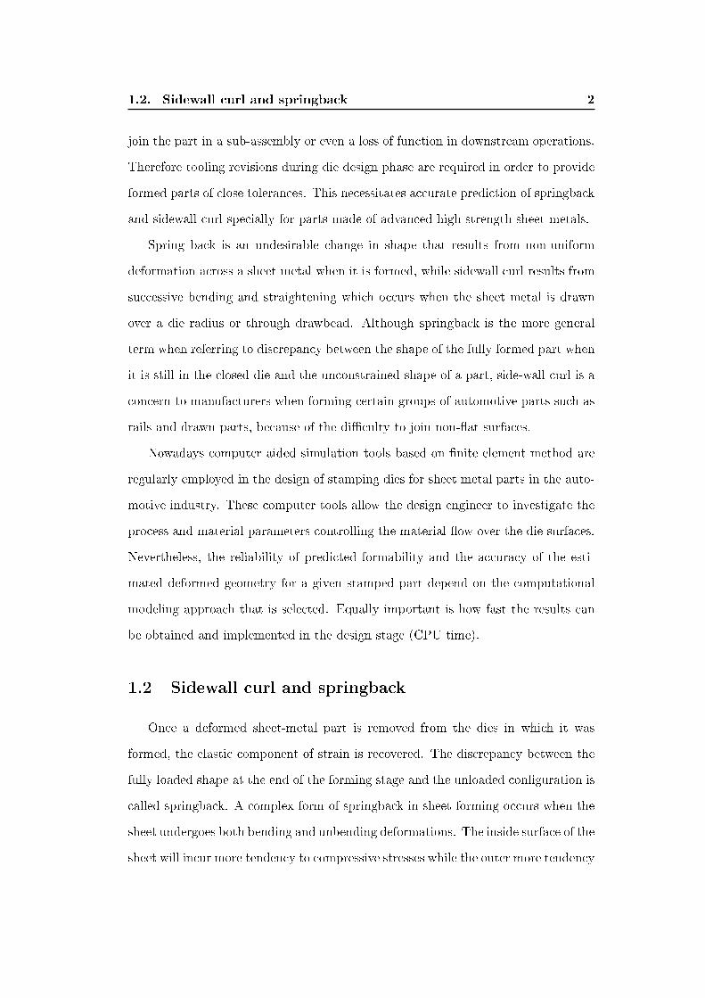
1.2. Sidewall curl and springback 2
join the part in a sub-assembly or even a loss of function in downstream operations.
Therefore tooling revisions during die design phase are required in order to provide
formed parts of close tolerances. This necessitates accurate prediction of springback
and sidewall curl specially for parts made of advanced high strength sheet metals.
Spring back is an undesirable change in shape that results from non-uniform
deformation across a sheet metal when it is formed, while sidewall curl results from
successive bending and straightening which occurs when the sheet metal is drawn
over a die radius or through drawbead. Although springback is the more general
term when referring to discrepancy between the shape of the fully formed part when
it is still in the closed die and the unconstrained shape of a part, side-wall curl is a
concern to manufacturers when forming certain groups of automotive parts such as
rails and drawn parts, because of the di�culty to join non-�at surfaces.
Nowadays computer aided simulation tools based on �nite element method are
regularly employed in the design of stamping dies for sheet metal parts in the auto-
motive industry. These computer tools allow the design engineer to investigate the
process and material parameters controlling the material �ow over the die surfaces.
Nevertheless, the reliability of predicted formability and the accuracy of the esti-
mated deformed geometry for a given stamped part depend on the computational
modeling approach that is selected. Equally important is how fast the results can
be obtained and implemented in the design stage (CPU time).
1.2 Sidewall curl and springback
Once a deformed sheet-metal part is removed from the dies in which it was
formed, the elastic component of strain is recovered. The discrepancy between the
fully loaded shape at the end of the forming stage and the unloaded con�guration is
called springback. A complex form of springback in sheet forming occurs when the
sheet undergoes both bending and unbending deformations. The inside surface of the
sheet will incur more tendency to compressive stresses while the outer more tendency
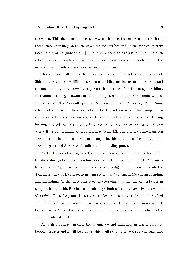
1.2. Sidewall curl and springback 3
to tension. This phenomenon takes place when the sheet �rst makes contact with the
tool surface (bending) and then leaves the tool surface and partially or completely
loses its curvature (unbending) [43], and is referred to as �sidewall curl�. In such
a bending and unbending situation, the deformation histories for both sides of the
material are unlikely to be the same, resulting in curling.
Therefore sidewall curl is the curvature created in the sidewalls of a channel.
Sidewall curl can cause di�culties when assembling mating parts such as rails and
channel sections, since assembly requires tight tolerances for e�cient spot welding.
In channel forming, sidewall curl is superimposed on the more common type of
springback which is sidewall opening. As shown in Fig.1.1.a, b & c, wall opening
refers to the change in the angle between the two sides of a bend line compared to
the as-formed angle whereas in wall curl a straight sidewall becomes curved. During
forming, the sidewall is subjected to plastic bending under tension as it is drawn
over a die or punch radius or through a draw bead [22]. The primary cause is uneven
stress distribution or stress gradient through the thickness of the sheet metal. This
stress is generated during the bending and unbending process.
Fig.1.2 describes the origins of this phenomenon when sheet metal is drawn over
the die radius (a bending-unbending process). The deformation in side A changes
from tension (A1) during bending to compression (A2) during unbending while the
deformation in side B changes from compression (B1) to tension (B2) during bending
and unbending. As the sheet pulls over the die radius into the sidewall, side A is in
compression and side B is in tension although both sides may have similar amount
of strains. Once the punch is retracted (unloading), side A tends to be stretched
and side B to be compressed due to elastic recovery. This di�erence in springback
between sides A and B would lead to a non-uniform stress distribution which is the
source of sidewall curl.
For higher strength metals, the magnitude and di�erence in elastic recovery
between sides A and B will be greater which will result in greater sidewall curl. The

1.2. Sidewall curl and springback 4
Figure 1.1: Di�erent types of sidewall springback: a)wall opening, b)wall curl, [1]
Figure 1.2: Origin and Mechanism of Sidewall curl, [1]
strength of the deformed metal depends not only on the as-received yield strength,
but also on the work hardening capacity, which is one of the key di�erences between
1.3. Springback of Advanced High Strength Steels 5
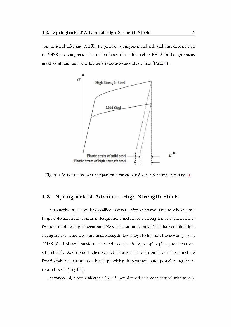
conventional HSS and AHSS. In general, springback and sidewall curl experienced
in AHSS parts is greater than what is seen in mild steel or HSLA (although not as
great as aluminum) with higher strength-to-modulus ratios (Fig.1.3).
Figure 1.3: Elastic recovery comparison between AHSS and MS during unloading, [1]
1.3 Springback of Advanced High Strength Steels
Automotive steels can be classi�ed in several di�erent ways. One way is a metal-
lurgical designation. Common designations include low-strength steels (interstitial-
free and mild steels); conventional HSS (carbon-manganese, bake hardenable, high-
strength interstitial-free, and high-strength, low-alloy steels); and the newer types of
AHSS (dual phase, transformation-induced plasticity, complex phase, and marten-
sitic steels). Additional higher strength steels for the automotive market include
ferritic-bainitic, twinning-induced plasticity, hot-formed, and post-forming heat-
treated steels (Fig.1.4).
Advanced high strength steels (AHSS) are de�ned as grades of steel with tensile

1.3. Springback of Advanced High Strength Steels 6
Figure 1.4: Schematic of AHSS steels compared to conventional HSS and mild steels, [1]
strength higher than 500 MPa and complex microstructures such as bainite, marten-
site, retained austenite, etc. and exclude the classical HSLA steels. The principal
di�erence between conventional HSS and AHSS is their microstructure. Conven-
tional HSS are single phase ferritic steels. AHSS are primarily multi-phase steels,
which contain ferrite, martensite, bainite, and/or retained austenite in quantities
su�cient to produce unique mechanical properties. Some types of AHSS have a
higher strain hardening capacity resulting in a strength-ductility balance superior
to conventional steels. Other types have ultra-high yield and tensile strengths and
show a bake hardening behaviour.
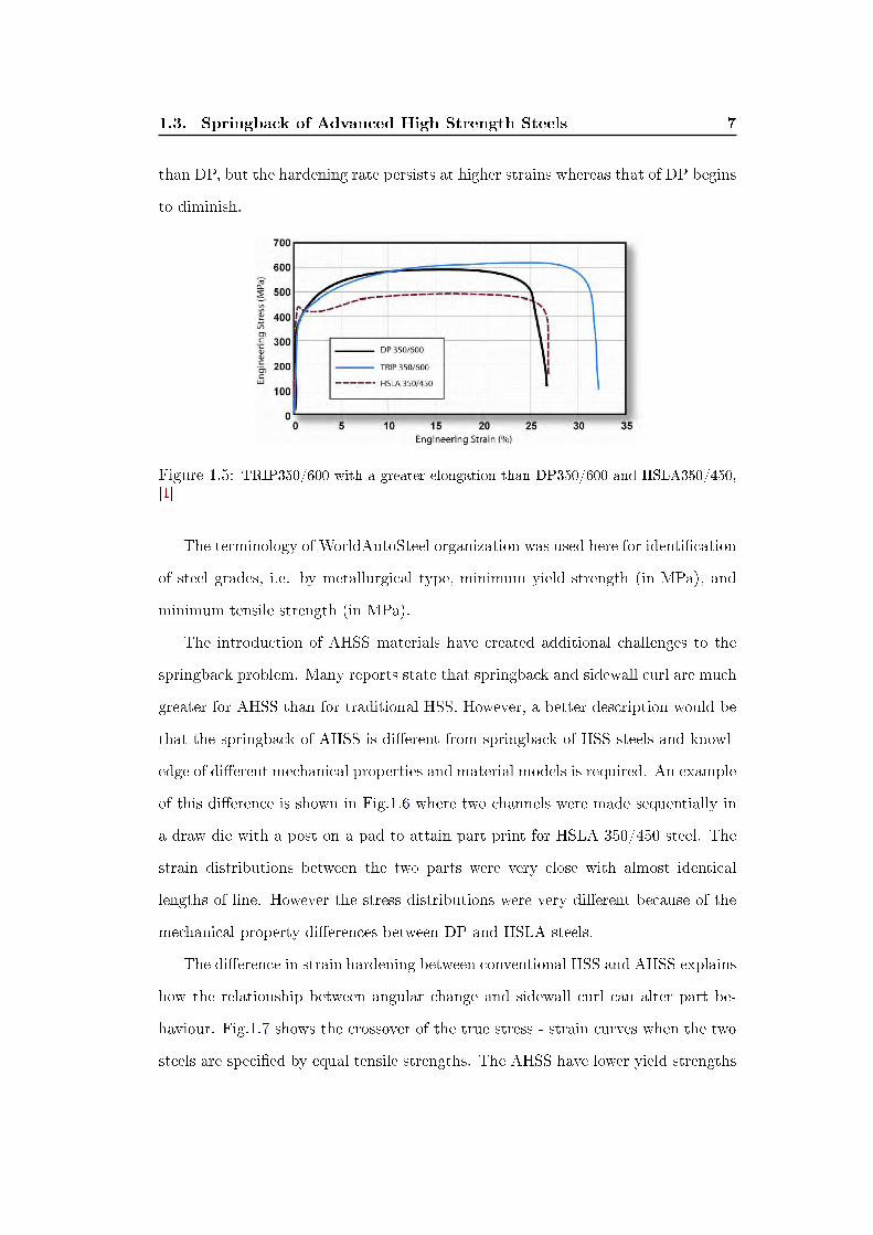
The microstructure of DP steels is composed of ferrite and martensite, while the
microstructure of TRIP steels is a matrix of ferrite, in which martensite and/or bai-
nite and more than 5% retained austenite exist. DP steel has good formability due to
high volume fraction of ferrite with high ductility and has good spot weldability due
to the small amount of alloying elements. TRIP steel has extremely high elongation
and n-values relative to DP grades providing opportunities for accommodating com-
plex part geometries at strength levels not possible with the equivalent DP strength,
but present greater challenges in weldability due to higher alloying content than DP
grades. A comparison between three types of steels with approximately similar yield
strength can be seen in Fig.1.5, where TRIP has a lower initial work hardening rate
1.3. Springback of Advanced High Strength Steels 7
than DP, but the hardening rate persists at higher strains whereas that of DP begins
to diminish.
Figure 1.5: TRIP350/600 with a greater elongation than DP350/600 and HSLA350/450,[1]
The terminology of WorldAutoSteel organization was used here for identi�cation
of steel grades, i.e. by metallurgical type, minimum yield strength (in MPa), and
minimum tensile strength (in MPa).
The introduction of AHSS materials have created additional challenges to the
springback problem. Many reports state that springback and sidewall curl are much
greater for AHSS than for traditional HSS. However, a better description would be
that the springback of AHSS is di�erent from springback of HSS steels and knowl-
edge of di�erent mechanical properties and material models is required. An example
of this di�erence is shown in Fig.1.6 where two channels were made sequentially in
a draw die with a post on a pad to attain part print for HSLA 350/450 steel. The
strain distributions between the two parts were very close with almost identical
lengths of line. However the stress distributions were very di�erent because of the
mechanical property di�erences between DP and HSLA steels.
The di�erence in strain hardening between conventional HSS and AHSS explains
how the relationship between angular change and sidewall curl can alter part be-
haviour. Fig.1.7 shows the crossover of the true stress - strain curves when the two
steels are speci�ed by equal tensile strengths. The AHSS have lower yield strengths

1.3. Springback of Advanced High Strength Steels 8
Figure 1.6: Two channels made sequential in the same die, [1]
than traditional HSS for equal tensile strengths. At lower strain levels usually en-
countered in angular change at the punch radius, AHSS have a lower level of stress
and therefore less springback.
Figure 1.7: Elastic recovery comparison between AHSS and MS during unloading, [1]
Sidewall curl is a higher strain event because of the bending and unbending of
the steel going over the die radius and possible drawbeads. For the two stress-strain
curves shown in Fig.1.7, the AHSS reaches a higher stress level with increased elastic
stresses. Therefore the sidewall curl is greater for AHSS as also compared in Fig.1.8.

1.4. Prediction and Compensation 9
Figure 1.8: The AHSS have greater sidewall curl for equal tensile strength steels, [1]
These phenomena are dependent on many factors, such as part geometry, tool-
ing design, process parameters and material properties. However, the high work-
hardening rate of DP and TRIP steels causes higher increase in the strength of the
deformed steel for the same amount of strain. Therefore any di�erences in tool
build, die and press de�ection, location of pressure pins and other inputs to the part
can cause varying amounts of springback - even for completely symmetrical parts.
1.4 Prediction and Compensation
As stated, forming of a part creates elastic stresses unless the forming is per-
formed at a higher temperature range where stresses are relieved before the part
leaves the die. Therefore some form of springback correction is required to bring
the part back to design intent. Several approaches have been proposed to control
springback.
The �rst approach is to apply an additional process that changes undesirable

1.4. Prediction and Compensation 10
elastic stresses to less damaging elastic stresses. One example is a post-stretch
operation that reduces sidewall curl by changing the tensile-to-compressive elastic
stress gradient through the thickness of the sidewall to all tensile elastic stresses
through the thickness. Another example is over-forming panels and channels so that
the release of elastic stresses brings the part dimension back to design speci�cations
instead of becoming undersized. However, the maximum tension in the sheet is
limited by the fracture strength of the sheet material. Moreover this stretch-forming
technique is generally not su�cient to eliminate springback. Some studies also
suggest using a variable blank holder force during the punch trajectory. In this
method, the blank holder force is low from the beginning until almost the end of
the forming process and then it is increased at the end of the process such that a
large tensile stress is applied to the sheet material.
A second approach is to modify the process and/or tooling to reduce the level
of elastic stresses actually imparted to the part during the forming operation. An
example would be to reduce sidewall curl by replacing sheet metal �owing through
draw beads and over a die radius with a simple 90 degree bending operation.
A third approach for correcting springback problems is to modify the product
design to resist the release of elastic stresses. Mechanical sti�eners are added to the
part design to lock in the elastic stresses to maintain desired part shape.
Most of these approaches are applicable to all higher strength steels, however
the very high �ow stresses encountered with AHSS make springback correction high
on the priority list [1]. In order to successfully manufacture a sheet metal part from
AHSS material with the desired shape and performance, an extensive knowledge
about the in�uence of various parameters is needed. Nowadays, to establish this
knowledge base, experimental try-outs and numerical simulations are used. Com-
puter simulation, based on the �nite element (FE) method, is a powerful tool that
gives the possibility to observe e�ects of changing process parameters prior to the
1.5. Objective and outline of thesis 11
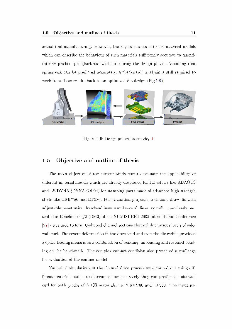
actual tool manufacturing. However, the key to success is to use material models
which can describe the behaviour of such materials su�ciently accurate to quanti-
tatively predict springback/sidewall curl during the design phase. Assuming that
springback can be predicted accurately, a �backward� analysis is still required to
work from these results back to an optimized die design (Fig.1.9).
Figure 1.9: Design process schematic, [4]
1.5 Objective and outline of thesis
The main objective of the current study was to evaluate the applicability of
di�erent material models which are already developed for FE solvers like ABAQUS
and LS-DYNA (DYNAFORM) for stamping parts made of advanced high strength
steels like TRIP780 and DP980. For evaluation purposes, a channel draw die with
adjustable penetration drawbead inserts and several die entry radii - previously pre-
sented as Benchmark #3 (BM3) at the NUMISHEET 2005 International Conference
[27] - was used to form U-shaped channel sections that exhibit various levels of side-
wall curl. The severe deformation in the drawbead and over the die radius provided
a cyclic loading scenario as a combination of bending, unbending and reversed bend-
ing on the benchmark. The complex contact condition also presented a challenge
for evaluation of the contact model.
Numerical simulations of the channel draw process were carried out using dif-
ferent material models to determine how accurately they can predict the sidewall
curl for both grades of AHSS materials, i.e. TRIP780 and DP980. The input pa-
1.5. Objective and outline of thesis 12
rameters for these constitutive models were separately determined for both grades
of steel through a series of laboratory experiments and subsequent analysis.
The present thesis is composed of �ve chapters. The �rst chapter provides a
brief introduction to the general terms used in this study as well as its organization.
A review of the literature related to the prediction of springback phenomena in gen-
eral and sidewall curl in particular are presented in the second chapter along with
detailed explanations about the candidate material models for the AHSS panels,
i.e. TRIP780 and DP980. Chapter three covers the experimental studies performed
for the material characterization tests as well as channel draw forming experiments.
Numerical analysis of these experiments are explained in chapter four. Final discus-
sions and conclusions of this study are given in chapter �ve.

13
Chapter 2
Material Models
2.1 Introduction
Metal forming researchers have investigated the prediction and compensation of
springback and sidewall curl since the early 1980's. Di�erent approaches such as
analytical, semi-analytical and �nite element methods have been extensively em-
ployed in these studies to quantitatively analyze the problem. FEM is a relatively
time-consuming method whereas analytical solutions can instantaneously provide
a description of the deformation mechanism based on a theoretical model. How-
ever, analytical solutions are limited to simple applications and often only provide
qualitative estimation of springback.
It has been shown that many process variables such as friction, temperature,
variations in the thickness and mechanical properties of the incoming sheet metals
along with numerical parameters such as material model, element type and size,
integration algorithms, contact de�nition and convergence criteria, etc. a�ect the
accuracy and validity of the solution. Moreover, complex strain histories and highly
nonlinear deformation of the material during the forming process add to the di�culty
of predicting springback/sidewall curl. Therefore, it is important to critically review
related studies before selecting the appropriate solution method for the problem.
Results of the most recent studies on analytical and numerical solutions for
springback and sidewall curl problem are summarized in the rest of this chapter.
Special attention is given to the constitutive material models used to describe the
deformation behaviour of sheet metals, and in particular to models for cyclic loading

2.2. Literature review 14
and unloading of AHSS material which are necessary to accurately predict sidewall
curl. The most widely used approach is to carry out computer simulations that rely
on advanced material models to compute the stress distribution in the part and the
�nal geometry of the part after unloading.
2.2 Literature review
2.2.1 Early studies
Davies (1984, [15]) proposed a simple experimental apparatus to examine the
sidewall curl that occurred in low-carbon, HSLA 50 and 80 (with ultimate strengths
of 450 and 620 MPa), and DP-80 (850 MPa ultimate strength) steels. He found
that by imposing a plastic deformation, the curl can be eliminated as a result of
the removal of the nonuniform distribution of residual stresses. Hayashi and Tagagi
(1984, [29]) performed a series of experiments to investigate the e�ects of process
parameters on the formation of sidewall curl for high-strength steels. They also tried
to explain the deformation behaviour by stress/strain paths of di�erent areas of the
blank. Liu (1988, [37]) obtained quantitative relationships between restraining force
and shape deviations, such as springback and side wall curl, in �anged channels
made of AKDQ and high strength streets. It was observed that shape deviation is
greatly reduced if the applied restraining force is beyond the yield strength of the
material. However, due to the restriction of die entrance and punch corners, this
condition cannot be readily achieved in the conventional bead system as sidewall
fracture intervenes. Therefore an intermediate restraining process was proposed to
form high quality �anged channels in one single operation through displacement
control, once the properties of the material are known.
In another study, Ayres (1984, [2]) investigated a process developed by GM re-
search fellows, known as `SHAPESET', to reduce curl springback for a variety of
high-strength steel. In the SHAPESET process, the steel is �rst bent to shape
without drawbeads and without tension, which creates severe sidewall curl. This
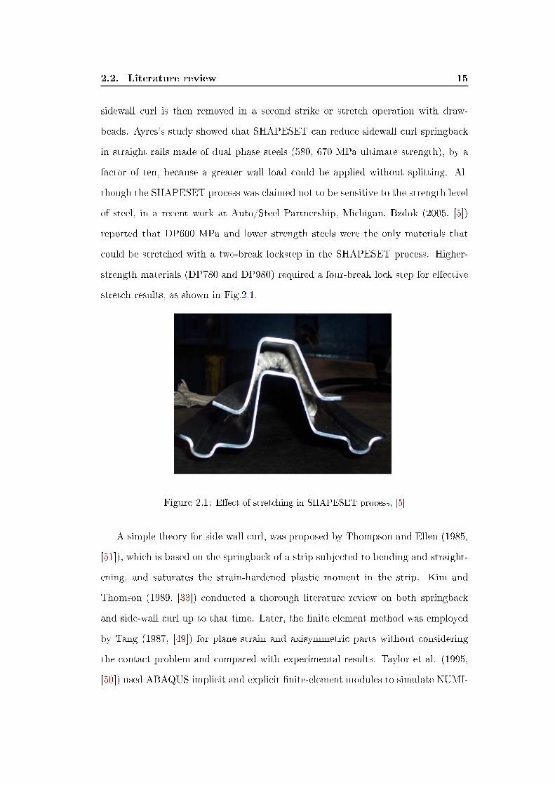
2.2. Literature review 15
sidewall curl is then removed in a second strike or stretch operation with draw-
beads. Ayres's study showed that SHAPESET can reduce sidewall curl springback
in straight rails made of dual phase steels (580, 670 MPa ultimate strength), by a
factor of ten, because a greater wall load could be applied without splitting. Al-
though the SHAPESET process was claimed not to be sensitive to the strength level
of steel, in a recent work at Auto/Steel Partnership, Michigan, Bzdok (2005, [5])
reported that DP600 MPa and lower strength steels were the only materials that
could be stretched with a two-break lockstep in the SHAPESET process. Higher-
strength materials (DP780 and DP980) required a four-break lock step for e�ective
stretch results, as shown in Fig.2.1.
Figure 2.1: E�ect of stretching in SHAPESET process, [5]
A simple theory for side-wall curl, was proposed by Thompson and Ellen (1985,
[51]), which is based on the springback of a strip subjected to bending and straight-
ening, and saturates the strain-hardened plastic moment in the strip. Kim and
Thomson (1989, [33]) conducted a thorough literature review on both springback
and side-wall curl up to that time. Later, the �nite element method was employed
by Tang (1987, [49]) for plane strain and axisymmetric parts without considering
the contact problem and compared with experimental results. Taylor et al. (1995,
[50]) used ABAQUS implicit and explicit �nite-element modules to simulate NUMI-

2.2. Literature review 16
FORM'93 benchmark problems and compared the results.
Chu (1991, [12]) analyzed the e�ects of restraining force on the springback and
side-wall curl using an isotropic-kinematic hardening rule, and the signi�cance of in-
dividual parameters on general springback phenomena was clearly identi�ed. Pour-
boghrat and Chu (1995, [43]) made use of moment-curvature relationships derived
for sheets undergoing plane-strain stretching, bending and unbending deformations,
and employed the membrane �nite element solutions to calculate the springback and
side-wall curl in 2-D draw bending operations (Fig.2.2).
Figure 2.2: A schematic diagram of the 2-D draw bending operation, [43]
2.2.2 Analytical solutions
Cao and Buranathiti (2004, [6]) developed an analytical model for springback
prediction of a straight �anging process (Fig.2.3), by calculating the bending mo-
ment under plane-strain conditions. They used the model to predict springback for a
few HSS materials and compared the predicted results reported by other researchers.

2.2. Literature review 17
Figure 2.3: Schematic of straight �anging process, [6]
Chen and Tseng (2005, [10]) proposed a theoretical model for prediction of side-
wall curl occurring in the forming of a �anged channel subjected to bending, slid-
ing, and unbending. By numerically solving the governing equations, the amount of
sidewall curl was calculated from the stress distribution through the sheet thickness
and validated by experimental and �nite element simulations. Lee et. al. (2007,
[35]) developed a semi-analytic hybrid method to predict springback in a 2D draw
bend test under plane strain conditions which superposed bending e�ects onto a
membrane element formulation (Fig.2.4). This method was also shown to be use-
ful for analyzing the e�ects of various process parameters such as the amount of
bending curvature, normalized back force and friction, as well as material prop-
erty e�ects such as hardening behaviour including the Bauschinger e�ect and yield
surface shapes. Good agreement was reported for a dual phase steel compared to
sprungback shapes. Springback was found to decrease by increasingR
t, restraining
force and friction between sheet and tools.

2.2. Literature review 18
Figure 2.4: (a) Geometry of the draw bend test with, (b) deformed shape before and afterspringback, [35]
An analytical model of elasto-plastic bending under tension followed by elastic
springback was proposed by Wagoner and Li (2007, [52]) to address the controver-
sial problem of the number of through-thickness integration points (NIP) for shell
elements. Using this model, guidelines for choosing NIP to assure a speci�ed spring-
back accuracy, varying withR
t, sheet tension and the required con�dence limit, were
presented. The relative springback error was shown to oscillate and in some cases
even more than 51 integration points were required. Zhang et al. (2007, [62]) de-
veloped an analytical model to predict springback and sidewall curl in sheets bent
in a U-die under plane-strain conditions (NUMISHEET'93 benchmark). They used
Hill's 1948 yield function and took into account the e�ects of deformation history
(by using three hardening rules: kinematic, isotropic and combined hardening), the
evolution of sheet thickness and the shifting of the neutral surface.
In another study, Yi et al. (2008, [55]) developed an analytical model based on
di�erential strains after relief from the maximum bending stress for six di�erent de-
formation patterns. They used each deformation pattern to estimate springback by

2.2. Literature review 19
the residual di�erential strains between outer and inner surfaces after elastic recov-
ery, while other analytical models were based on elastic unloading from a bending
moment. Such residual di�erential strain model only required the stress state on
the outer and inner surfaces rather than through the whole thickness of the sheet
metal. Moon and others (2008, [41]) developed a model based on the moment-
curvature relationship during stretch-bend sheet forming operations and veri�ed it
with the sidewall curl experimentally measured after deformation of a strip subject
to bending-under-tension.
A review of the aforementioned studies showed that although the use of analytical
models is advantageous because of their simplicity, the application of these models
is limited to simple geometries.
2.2.3 Numerical studies
Many researchers have used �nite element analysis to numerically simulate side-
wall curl during sheet metal forming operations. Such FE analyses consist of two
main steps. Firstly, an explicit incremental or implicit incremental-iterative FE
method is applied in order to simulate the forming process that includes the blank
and the tooling. Secondly, the springback deformation is simulated with the static
implicit FE approach based on the formed geometry along with the forming stress
distribution as the baseline input. The accuracy of such simulations depends not
only on the forming conditions (friction, tool and binder geometry), but also on the
numerical parameters such as element type, in-plane mesh size and the number of
through-thickness integration-points, as well as the constitutive model that governs
the behaviour of the deformable sheet [25].
Yang and Lee (1998, [54]) used the Taguchi method to study numerical factors
a�ecting springback of a mild steel after the U-bending draw test in which drawbeads
were not used (Numisheet'93). Through an ANOVA study, the mesh size was found
to have the strongest e�ect on the accuracy of springback prediction with respect to
2.2. Literature review 20
damping and penalty parameters and punch velocity. Samuel (2000, [45]) proposed
a numerical model based on the �updated Lagrangian� formulation to calculate
springback and sidewall curl in a plane-strain stretch/draw sheet forming using the
MARC FE package. Both the experimental data and the theoretical 2D model
suggested that in draw bending, sidewall curl decreases with the die radius but also
depends greatly on blank-holder force.
Al Azraq (2006, [3]) studied a simple channel pro�le after springback using the
AUTOFORM incremental code for DP600 and TRIP800 materials. The springback
was shown to increase with angular variation of the channels but for pro�les with the
same angle, TRIP 800 showed more vertical displacement than DP 600. Chung et.
al. (2005, [13]) formulated a modi�ed Chaboche-type combined Isotropic-Kinematic
hardening law which accounted for the Bauschinger e�ect and transient behaviour,
using Yld2000-2d under plane stress condition. Comparisons of simulations and
experiments were in good agreement for the unconstrained cylindrical bending, 2-D
draw bending and the modi�ed industrial part (the double-S rail) for two Aluminum
sheets and DP steel (Fig.2.5a, b, c).

2.2. Literature review 21
Figure 2.5: Schematics of (a)cylindrical bending test, (b)2-D draw bending test, (c)double-S rail, [13]
The in�uence of low-strain deformation behaviour on curl and springback in
advanced high strength steels was assessed by Matlock et. al. (2007, [39]) using a
bending-under-tension test apparatus. A non-linear relationship was found between
curl height and back tension, though it might be approximated as linear for industrial
purposes. The curl also depended on the low-strain deformation characteristics of
the material. The TRIP590 material had less curl compared to a dual-phase steel
of similar initial thickness and tensile strength at back tensions ranging from 15 to
45% of the sheet tensile strength.
Later, Aydin (2008, [31]) implemented the Yoshida-Uemori (YU) material model
in LS-DYNA user material interface and used it for analysis of channel draw tests
with various die radii for several grades of high strength steels. In order to detect
the springback accuracy of this model, the results were evaluated with LS-DYNA

2.2. Literature review 22
standard material models like Mat36 and Mat103. This study showed that the
YU model is the most reliable and also the most expensive model to detect the
springback of high strength steels. Also it was not possible to obtain a unique
set of parameters from di�erent characterization tests (for example from tension-
compression or bending-unbending).
Firat (2008, [21]) presented a rate dependent anisotropic plasticity model ac-
counting for the Bauschinger e�ect that was used in a FE analysis of the Nu-
misheet'93 U-channel benchmark as well as an automotive part made of HSLA 350.
Comparison of FE results using both an isotropic hardening model and his proposed
model showed similar strain and thickness predictions but signi�cant di�erences in
residual stresses and �nal part geometry.
Recently, Taherizadeh et. al. (2009, [48]) predicted the springback of Numisheet
2005 Benchmark#3 with di�erent material models using the commercial �nite ele-
ment code ABAQUS and four di�erent drawbead penetrations for AKDQ-DP600-
HSLA50-AA6022/T43. Later Ghaei and Green (2010, [26]) used the return mapping
procedure to implement the YU two surface model in ABAQUS for arbitrary yield
functions. As an example, Yld2000-2d and Hill48 yield functions were developed
in the subroutines and were used to simulate springback of the Numisheet BM3
U-channel for the same material types studied by Taherizadeh. A comparison of
the experimental and predicted channel sidewall pro�les showed that the YU model
improves the springback prediction compared to the isotropic hardening model or
the combined isotropic-nonlinear kinematic hardening model.
2.2.4 Constitutive material models
It has often been observed that the FE springback/sidewall curl predictions are
not be always accurate and the shape distortions estimated for some industrial ap-
plications have been notably erroneous. The inaccuracy of springback prediction
becomes even more signi�cant when it comes to high strength steels. An inves-

2.2. Literature review 23
tigation of the FE springback predictions for the representative conditions in the
previous studies indicated that the discrepancies cannot be explained on the basis
of variability of the input parameters or numerical factors alone and the plasticity
models employed in the FE analyses signi�cantly in�uence the predicted deforma-
tion [24] & [21].
It is well known that a phenomenological plasticity model is composed of : a
yield condition, a plastic work hardening law and a model of degradation of elastic
sti�ness due to plastic straining. In classical plasticity, the yield function represents
a convex yield surface in stress space, which limits the elastic range of materials.
The proper measurements and descriptions of the initial yield stress surface and its
evolution are essential for the constitutive law in plasticity. Since the yield surface
and, especially, its evolution are di�cult to measure experimentally, the isotropic
hardening of the initial yield surface is often assumed in the classical plasticity.
Under this assumption, the initial yield surface expands radially (or proportionally)
in stress space during plastic deformation. This assumption is reasonably e�ective to
predict plastic deformations, especially when the deformation of material elements
is approximately monotonous and proportional (Fig.2.6).
Figure 2.6: Isotropic hardening: the yield surface expands with plastic deformation, ac-cording to the work hardening described by the uniaxial stress-strain curve, [16]
2.2. Literature review 24
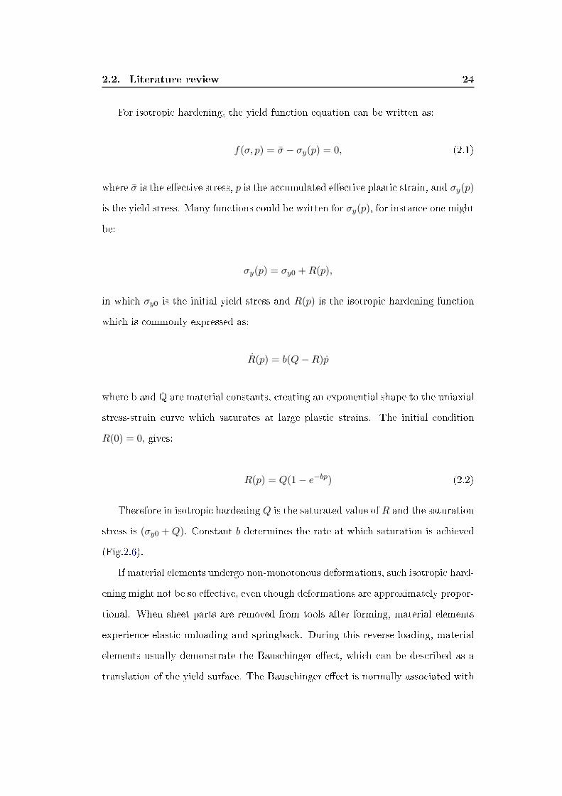
For isotropic hardening, the yield function equation can be written as:
f(σ, p) = σ − σy(p) = 0, (2.1)
where σ is the e�ective stress, p is the accumulated e�ective plastic strain, and σy(p)
is the yield stress. Many functions could be written for σy(p), for instance one might
be:
σy(p) = σy0 +R(p),
in which σy0 is the initial yield stress and R(p) is the isotropic hardening function
which is commonly expressed as:
R(p) = b(Q−R)p
where b and Q are material constants, creating an exponential shape to the uniaxial
stress-strain curve which saturates at large plastic strains. The initial condition
R(0) = 0, gives:
R(p) = Q(1− e−bp) (2.2)
Therefore in isotropic hardening Q is the saturated value of R and the saturation
stress is (σy0 +Q). Constant b determines the rate at which saturation is achieved
(Fig.2.6).
If material elements undergo non-monotonous deformations, such isotropic hard-
ening might not be so e�ective, even though deformations are approximately propor-
tional. When sheet parts are removed from tools after forming, material elements
experience elastic unloading and springback. During this reverse loading, material
elements usually demonstrate the Bauschinger e�ect, which can be described as a
translation of the yield surface. The Bauschinger e�ect is normally associated with

2.2. Literature review 25
conditions where the yield strength of a metal decreases when the direction of strain
is changed. It is a general phenomenon found in many polycrystalline metals. When
the yield surface is assumed to expand uniformly in isotropic hardening, the yield
stress in the reverse loading is predicted to be equal to that in forward loading, but
this is not often the case. Therefore, isotropic hardening is not able to describe the
Bauschinger e�ect in reverse loading.
Figure 2.7: Kinematic hardening showing (a) the translation, and (b) the resulting stress-strain curve with shifted yield stress in compression, [16]
Assuming the initial yield surface to translates in stress space without changing
its shape and size during plastic deformation is another way to model the evolution
of the yield surface; this is called kinematic hardening. In order to reproduce the
Bauschinger e�ect, a linear kinematic hardening model was �rst proposed by Prager
(1956) and later modi�ed by Ziegler (1959). Assuming kinematic hardening, the
yield surface equation can be written as:
f(σ − α)− σy = 0, (2.3)
where α, called the backstress tensor, is a variable in the stress space and determines
the location of the centre of the yield surface. As shown in Fig.2.7, the elastic
region predicted by kinematic hardening, when unloading starts at point (1) and
the material deforms elastically until point (2), is smaller than what is predicted

2.2. Literature review 26
by isotropic hardening. The evolution of the backstress tensor can be de�ned by
various functions. Prager proposed a linear kinematic hardening rule:
dα =2
3cdε
where c is a material constant. Ziegler modi�ed Prager's rule according to the
following equation:
dα = dµ(σ − α), where dµ > 0.
and dµ also depends on the material. Classical isotropic hardening and Prager's or
Ziegler's linear kinematic hardening models provide a reasonable description of the
hardening properties of materials, for the case of proportional loading where the
load is increasing monotonically and no unloading occurs.
In order to describe the expansion and translation of the yield surface during
plastic deformation, the combination of isotropic (Fig.2.8) and kinematic harden-
ing (Fig.2.9) is also commonly used. The combined isotropic-kinematic hardening
constitutive law based on the modi�ed Chaboche model [13] is given by:
f(σ − α)− σiso = 0, (2.4)
where α is the back stress for the kinematic hardening and σiso is the e�ective
stress related to the isotropic hardening. In the Chaboche model, the back stress
increment is composed of two terms, dα = dα1 − dα2 to di�erentiate the transient
hardening behaviour during loading and reverse loading.
Recent experiments in cyclic loading have revealed that the material responses
under this loading condition are much more complex than under monotonic loading
and cannot be described by the aforementioned isotropic, kinematic or combined
hardening rules. The following phenomena have been observed during cyclic plastic
deformation of sheet metals (mild steels and dual phase steels) [25]:

2.2. Literature review 27
Figure 2.8: Schematics of the isotropic hardening. Left: in the deviatoric plane; right: thestress vs. plastic strain response, [8]
Figure 2.9: Schematics of the linear kinematic hardening. Left: in the deviatoric plane;right: the stress vs plastic strain response, [8]
• Transient Bauschinger behaviour characterized by early re-yielding and a
smooth elastic-plastic transition
• Abnormal shapes of reverse stress-strain curves due to work-hardening stag-
nation caused by dissolution of dislocation cell walls during reverse loading.

2.2. Literature review 28
• Decrease of elastic modulus during unloading as the plastic strain increases
and �nally saturates to a particular value after large plastic strains
• Permanent softening appears after rapid changes of work-hardening rate in
reverse plastic deformation.
Therefore in order to perform an accurate simulation of such a sheet metal forming
process, it is necessary to have an appropriate constitutive model, which can consider
the phenomena that occur during cyclic loading and unloading of such sheet metals
(Fig.2.10).
Figure 2.10: Schematic showing the stress-strain response with and without Bauschingere�ect during forward and reverse loading paths, [21]
Within the last half-century some models have been proposed to meet the chal-
lenge. The most important ones are the multisurface model proposed by Mroz
(1967), the two-surface model by Dafalias and Popov (1976), the nonlinear kine-
matic hardening model initiated by Armstrong and Fredrick (1966) and then devel-
oped further by Chaboche (1977) and the Endochronic theory proposed by Valant
(1971) and developed further by Watanabe and Atluir (1986) [32].

2.2. Literature review 29
Armstrong and Frederick [23] proposed the nonlinear kinematic hardening model
in order to capture the transient behaviour curve during reverse loading:
dα =2
3cdεp − γαdp, (2.5)
where c and γ are two material constants, and p is the accumulated e�ective plas-
tic strain. Later, Chaboche (1986, [9]) modi�ed the Armstrong-Frederick nonlinear
kinematic model to better reproduce the transient behaviour and ratcheting in fa-
tigue. Ratcheting is a very important factor in the design of components subject to
cyclic loading in the inelastic domain. The amount of plastic strain can accumulate
continuously with an increasing number of cycles and may eventually cause mate-
rial failure. For better modeling of cyclic deformations, Yoshida et al. (2002, [60])
developed two constitutive models called IH+NKH and IH+NLK+LK. The �rst
model used a combined isotropic-nonlinear kinematic hardening and in the second
model, a linear term was added to the Armstrong-Frederick model for evolution of
backstress in LK. However they concluded that neither the IH+NLK model nor the
IH+NLK+LK model could accurately describe all the phenomena observed in cyclic
experiments [57].
In parallel to modifying the nonlinear kinematic hardening models, two-surface
plasticity models also attracted a lot of attention because both the transient and
long-term behaviour of the material could be fairly well described by these models.
In two-surface models, the evolution of the inner surface is usually de�ned such
that it describes the transient response of the material and the evolution of the
bounding surface is usually responsible for describing the long-term response of the
material. Among these models, the two-surface model developed by Yoshida and
Uemori (2002) is of more interest in the current study and will be used for the
analysis of sidewall curl for the channel draw operation in AHSS materials.
An assessment of recent plasticity models indicates that various methods exist
to quantitatively describe the deformation of sheet metals. But as the capabilities
2.2. Literature review 30
of material model improve, the number of material parameters necessary to describe
the deformation also increases, and this inevitably leads to more complex material
characterization tests and more sophisticated mathematical techniques to determine
these parameters [21]. This may be an undesirable situation from an industrial per-
spective, since the simple tension test is usually the only available material data
during the tooling design phase and is also the industry standard for the identi�-
cation of sheet metal properties. However once the parameters are identi�ed, more
accurate results can be expected from improved material models.
2.2.5 Identi�cation of material parameters
As discussed, many purely phenomenological hardening laws have been proposed
in the literature with the purpose of describing the cyclic behaviour of metal sheets.
The complexity of these models can vary considerably with respect to the number of
material parameters and strain history variables. The material parameters involved
have to be determined from some kind of cyclic loading experiment.
In theory, the most simple and straightforward test is a tension/compression test
of a sheet strip. In practice, however, such a test is very di�cult to perform, due
to the tendency of the strip to buckle in compression. In spite of these di�culties,
some successful attempts to perform cyclic tension/compression tests have been re-
ported in the literature. Bulk compression tests (Abel and Ham, 1966; Bate and
Wilson, 1986) and in-plane compression tests (Ramberg and Miller, 1946; Tan et
al.,1994; Yoshida et al., 2002) provided more uniform strain distribution with appro-
priate length-to-thickness ratio. But large strain was not easy to obtain due to the
specimen's tendency to buckle under compression. Yoshida et al. [60] successfully
bonded a few thin sheets of metal to provide support for the sheet during uniaxial
compression.
Kuwabara (1995, [34]) used fork-shaped dies to reduce the unsupported area dur-
ing uniaxial tension-compression tests. Normal forces were provided by the weight
2.2. Literature review 31
of the die itself. However there were unavoidable uncovered areas of the sample
between each pair of `�ngers' of the die which were prone to buckling. Wagoner
et al. (2005, [53]) used solid �at plates as buckling constraints and applied normal
pressure through a hydraulic clamping system. But the problem remained with gaps
between the die and clamps of the tensile machine.
Recently, Cao et al. (2009, [7]) developed a �xture to perform uniaxial tension-
compression tests on modi�ed �dog-bone� specimens with single or double sided
�ns. Experiments were done for DP600 and AA6111-T4 sheet samples and material
parameters were determined for a combined isotropic-kinematic hardening law based
on the Chaboche model as well as for a modi�ed two surface model based on Dafalias-
Popov and Krieg models.
Cyclic simple shear tests have also attracted the attention of some researchers as
the specimen is not compressed during these tests. Miyauchi (1984, [30]), Genevois
(1992, [42]), Rauch (1998, [44]) and Barlat et al. (2003, [20]) have successfully used
the simple shear test for reverse loading at large strains.
Another kind of test that frequently has been used for the determination of
material hardening parameters is some kind of bending test [63], [40], [56]. The
advantage of this kind of test is that it is simple to perform, and standard test
equipments can be used. However, a bending test will involve inhomogeneous stress
and strain distributions in the sheet specimen, and the stress-strain response cannot
be directly determined from the experiment. This means that the material param-
eters have to be determined by an inverse approach. Usually, the experiments are
simulated by FEA, and the material parameters are identi�ed by means of some
optimization technique.
The optimization methods for determining the parameters in a material model
are usually based on an inverse approach in which an appropriate algorithm allows
the minimization between experimental observable variables and simulated ones.
Here, the optimization variables x are the material parameters and the purpose is

2.2. Literature review 32
to �nd a vector x that minimizes the objective function:
F (x) =L∑i=1
siF i(x), Aj ≤ xj ≤ Bj , (j = 1, 2, ..., N) (2.6)
where L is the total number of deformation cycles, Aj and Bj are the lower and
upper limits of the searching area for a material parameter xi, and F i(x) is the
dimensionless function de�ned as the square of the di�erence in stress between the
experimental data, and the corresponding calculated results for an assumed set of
material parameters x. For the minimization of the objective function di�erent
techniques are used by researchers. Yoshida (1998, [56]) used an iterative multi-
point approximation concept by minimizing the di�erence between the test results
and the results obtained by numerical simulation of the same test. This approach
was veri�ed by comparing simulated stress-strain curves using constitutive model
incorporating identi�ed parameters with experimental cyclic bending curves. The
same method was later used for identi�cation of Chaboche model parameters for an
aluminum clad stainless steel sheet (2003, [61]) and also for determining parameters
in the YU model from cyclic tension-compression tests for mild and high strength
steels (2002, [57]).
Collin et. al. (2009, [14]) used an inverse approach coded in a software called
`SidoLo' which allows the minimization between experiments and simulations with
a decrease direction algorithm to determine the Chaboche model parameters from
monotonic and cyclic tensile tests. The parameters were then used in a FE code to
simulate cyclic indentation experiments.
In a recent study, Eggertsen and Mattiasson (2010, [17]) used an inverse ap-
proach for determining di�erent hardening parameters, using simulations of three-
point cyclic bending tests by means of the explicit FE-code LS-DYNA [38]. The
identi�cation of the hardening parameters was performed by means of the optimiza-
tion code LS-OPT [47] and a Response Surface Methodology (RSM). The RSM
is especially advantageous for problems in which gradients to the objective func-
2.3. Yoshida-Uemori two-surface plasticity model 33
tion are di�cult to calculate, such as in highly nonlinear problems of parameter
identi�cation.
Although using optimization tools like LS-OPT or SiDoLo facilitates the deter-
mination of material parameters, it should be pointed out that di�erent experiments
as well as the same experiment performed with varying conditions can result in dif-
ferent parameter sets which may a�ect the predictability of the material model
specially for springback/sidewall curl in AHSS [31].
The methods for identi�cation of the YU model parameters from cyclic tension-
compression experiments are discussed after a brief explanation of the model itself.
Later, several other material models that are implemented in commercial �nite
element codes are described and compared with YU model.
2.3 Yoshida-Uemori two-surface plasticity model
As mentioned before, advanced models of material equations are required for
more accurate simulation of sheet metal forming and subsequent springback. Cyclic
loading is a very common type of loading in sheet metal forming processes as the ma-
terial �ows over the punch radius, die radius or through a drawbead. The Yoshida-
Uemori (YU) model [57] is one of the most sophisticated and comprehensive phe-
nomenological models and is capable of reproducing the transient Bauschinger e�ect,
permanent softening and work-hardening stagnation in large elasto-plastic deforma-
tions, as shown in Fig.2.11.

2.3. Yoshida-Uemori two-surface plasticity model 34
Figure 2.11: Stress-strain response of a mild steel in a forward and reverse loading andthe cyclic phenomena, [58]
The YU model assumes kinematic hardening of the yield surface within the
bounding surface and mixed isotropic-kinematic hardening of the bounding surface
itself. The evolution of the yield surface is de�ned by superposition of two kinematic
hardening laws and therefore it is possible to assume that a total of three surfaces
are de�ned in the plane stress space. The additional surface controls the permanent
softening and the work hardening stagnation.
The inner surface, or yield surface, determines the elastic domain of the material
in stress space. It is assumed that this surface can only translate in stress space,
i.e. it undergoes a pure kinematic hardening. This is a valid assumption since
experimental stress-strain responses under reverse deformation show that the re-
yielding starts at a very early stage of stress reversal. Therefore, kinematic hardening
of the yield surface describes the transient Bauschinger deformation characterized
by early re-yielding and subsequent rapid change of work-hardening rate, which is
mainly due to the motion of less stable dislocations, such as piled-up dislocations.
The bounding surface, on the other hand, can translate as well as expand, i.e. mixed
hardening prevails (Fig.2.12).
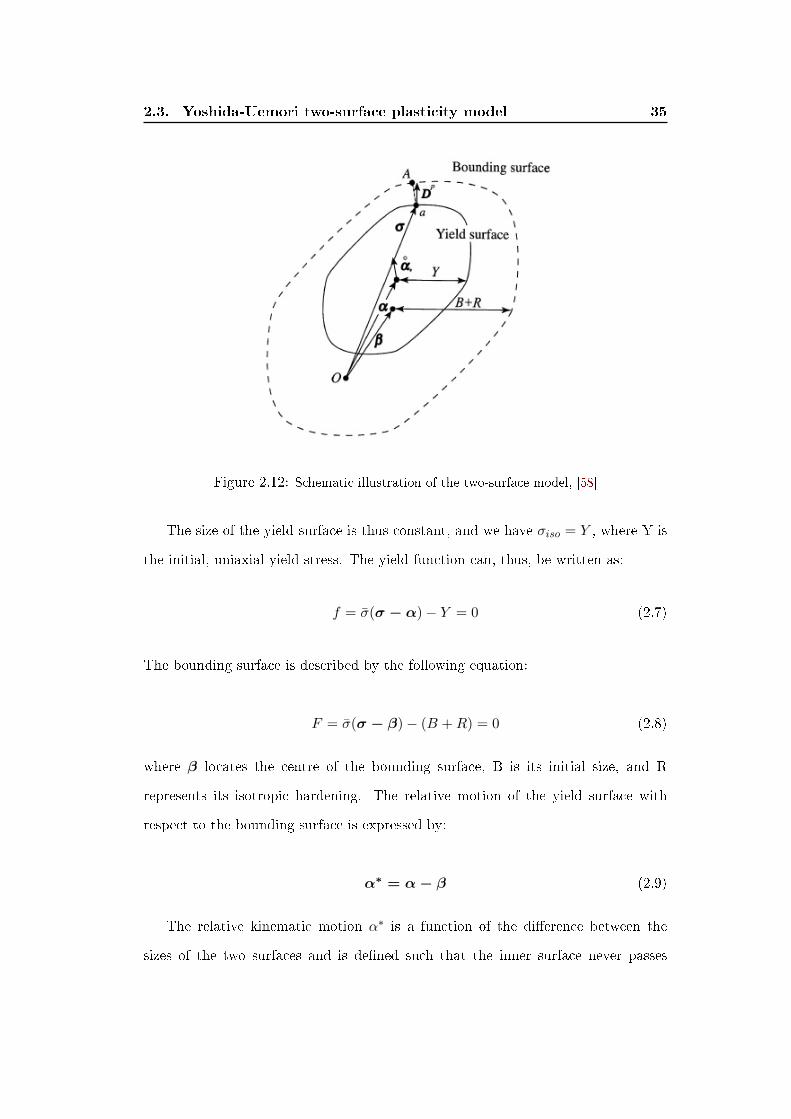
2.3. Yoshida-Uemori two-surface plasticity model 35
Figure 2.12: Schematic illustration of the two-surface model, [58]
The size of the yield surface is thus constant, and we have σiso = Y , where Y is
the initial, uniaxial yield stress. The yield function can, thus, be written as:
f = σ(σ − α)− Y = 0 (2.7)
The bounding surface is described by the following equation:
F = σ(σ − β)− (B +R) = 0 (2.8)
where β locates the centre of the bounding surface, B is its initial size, and R
represents its isotropic hardening. The relative motion of the yield surface with
respect to the bounding surface is expressed by:
α∗ = α− β (2.9)
The relative kinematic motion α∗ is a function of the di�erence between the
sizes of the two surfaces and is de�ned such that the inner surface never passes
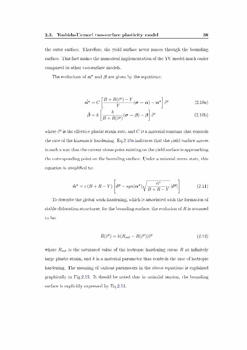
2.3. Yoshida-Uemori two-surface plasticity model 36
the outer surface. Therefore, the yield surface never passes through the bounding
surface. This fact makes the numerical implementation of the YU model much easier
compared to other two-surface models.
The evolutions of α∗ and β are given by the equations:
α∗ = C
[B +R(εp)− Y
Y(σ − α)−α∗
]˙εp (2.10a)
β = k
[b
B +R(εp)(σ − β)− β
]˙εp (2.10b)
where ˙εp is the e�ective plastic strain rate, and C is a material constant that controls
the rate of the kinematic hardening. Eq.2.10a indicates that the yield surface moves
in such a way that the current stress point existing on the yield surface is approaching
the corresponding point on the bounding surface. Under a uniaxial stress state, this
equation is simpli�ed to:
α∗ = c (B +R− Y )
[εp − sgn(α∗)
√α∗
B +R− Y|εp|
](2.11)
To describe the global work-hardening, which is associated with the formation of
stable dislocation structures, for the bounding surface, the evolution of R is assumed
to be:
R(εp) = k(Rsat −R(εp)) ˙εp (2.12)
where Rsat is the saturated value of the isotropic hardening stress R at in�nitely
large plastic strain, and k is a material parameter that controls the rate of isotropic
hardening. The meaning of various parameters in the above equations is explained
graphically in Fig.2.13. It should be noted that in uniaxial tension, the bounding
surface is explicitly expressed by Eq.2.13.

2.3. Yoshida-Uemori two-surface plasticity model 37
Figure 2.13: De�nition of the parameters in the Yoshida-Uemori hardening model - For-ward Bounding, [18]
σforwardbound = B +R+ β = B + (Rsat + b)(
1− e−kεp)
(2.13)
It should be emphasized that the mentioned formulas are the original form of
the Yoshida-Uemori model. Further modi�cations were later made to this model in
order to be able to reproduce more exactly the experimental hardening curves from
a uniaxial tensile test, in which:
B = Y (2.14)
Y +R(εp) + β(εp) = H(εp) (2.15)
where H(εp) is the experimental plastic hardening curve [18].
The experimentally obtained stress-strain curves on a mild steel exhibit apparent
work-hardening stagnation in a certain period of reverse deformation starting from
the reverse re-yielding. This phenomenon is also related to the cyclic strain-range,
as well as the mean-strain. It is mainly caused by the dissolution of dislocation cell
walls performed during forward deformation and the formation of new dislocation
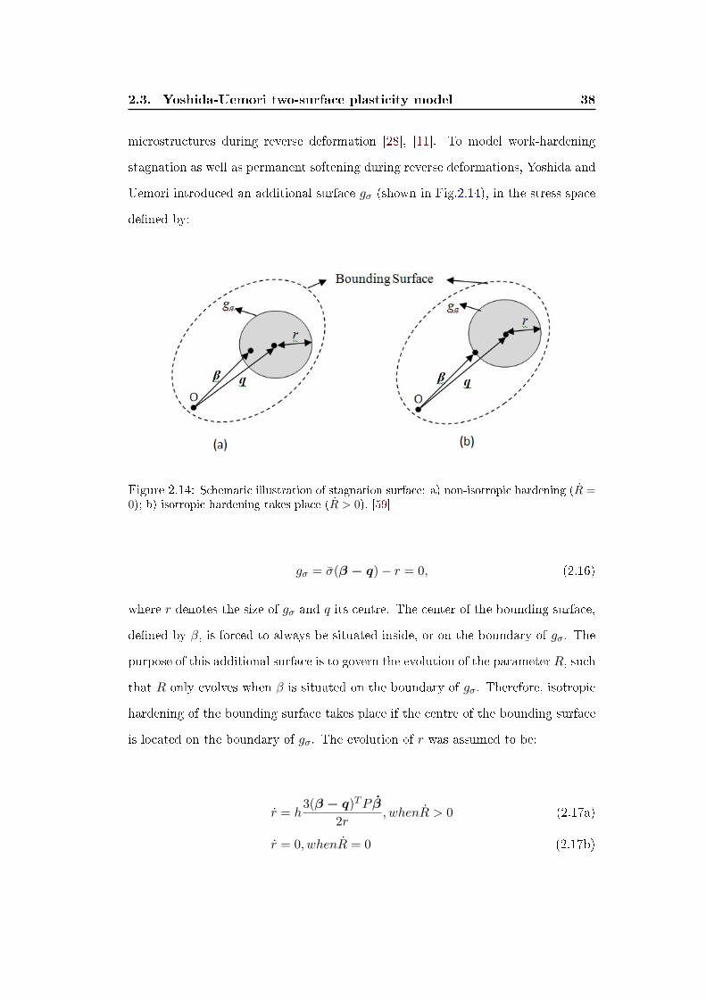
2.3. Yoshida-Uemori two-surface plasticity model 38
microstructures during reverse deformation [28], [11]. To model work-hardening
stagnation as well as permanent softening during reverse deformations, Yoshida and
Uemori introduced an additional surface gσ (shown in Fig.2.14), in the stress space
de�ned by:
Figure 2.14: Schematic illustration of stagnation surface: a) non-isotropic hardening (R =0); b) isotropic hardening takes place (R > 0), [59]
gσ = σ(β − q)− r = 0, (2.16)
where r denotes the size of gσ and q its centre. The center of the bounding surface,
de�ned by β, is forced to always be situated inside, or on the boundary of gσ. The
purpose of this additional surface is to govern the evolution of the parameter R, such
that R only evolves when β is situated on the boundary of gσ. Therefore, isotropic
hardening of the bounding surface takes place if the centre of the bounding surface
is located on the boundary of gσ. The evolution of r was assumed to be:
r = h3(β − q)TP β
2r, whenR > 0 (2.17a)
r = 0, whenR = 0 (2.17b)
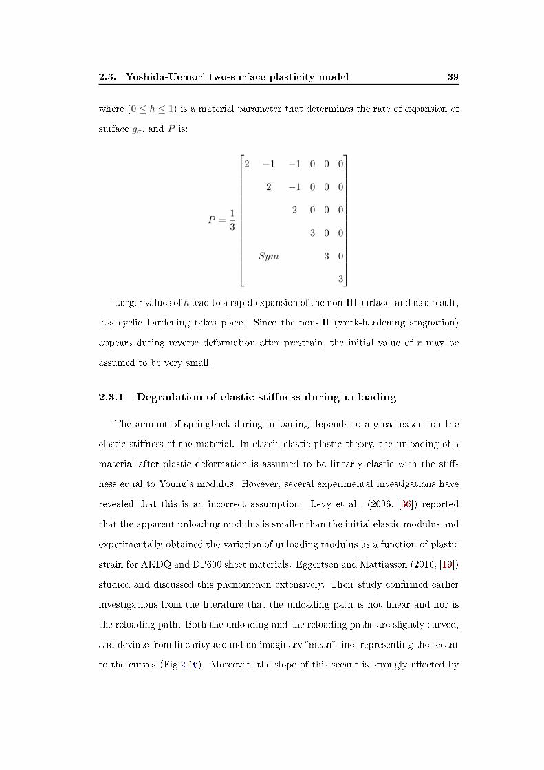
2.3. Yoshida-Uemori two-surface plasticity model 39
where (0 ≤ h ≤ 1) is a material parameter that determines the rate of expansion of
surface gσ, and P is:
P =1
3
2 −1 −1 0 0 0
2 −1 0 0 0
2 0 0 0
3 0 0
Sym 3 0
3
Larger values of h lead to a rapid expansion of the non-IH surface, and as a result,
less cyclic hardening takes place. Since the non-IH (work-hardening stagnation)
appears during reverse deformation after prestrain, the initial value of r may be
assumed to be very small.
2.3.1 Degradation of elastic sti�ness during unloading
The amount of springback during unloading depends to a great extent on the
elastic sti�ness of the material. In classic elastic-plastic theory, the unloading of a
material after plastic deformation is assumed to be linearly elastic with the sti�-
ness equal to Young's modulus. However, several experimental investigations have
revealed that this is an incorrect assumption. Levy et al. (2006, [36]) reported
that the apparent unloading modulus is smaller than the initial elastic modulus and
experimentally obtained the variation of unloading modulus as a function of plastic
strain for AKDQ and DP600 sheet materials. Eggertsen and Mattiasson (2010, [19])
studied and discussed this phenomenon extensively. Their study con�rmed earlier
investigations from the literature that the unloading path is not linear and nor is
the reloading path. Both the unloading and the reloading paths are slightly curved,
and deviate from linearity around an imaginary �mean� line, representing the secant
to the curves (Fig.2.16). Moreover, the slope of this secant is strongly a�ected by

2.3. Yoshida-Uemori two-surface plasticity model 40
the amount of plastic strain.This is mainly due to very early re-yielding and the
Bauschinger e�ect and strongly a�ected by the amount of plastic strain. More pre-
cisely, the magnitude of the unloading modulus is decreasing with increasing plastic
strain.
Such a prestrain dependency of Young's modulus would much in�uence the
springback behaviour especially when sheets are subjected to a large deformation
during press forming. However, for practical modeling, instead of instantaneous
Young's modulus, Yoshida introduced a term called `average Young's modulus',
Eav, as an average slope of the unloading stress-strain curve calculated from each
of following stress ranges (Fig.2.15) :
1. 0.75σ0 ≤ σ ≤ 0.95σ0,
2. 0.50σ0 ≤ σ ≤ 0.95σ0,
3. 0.25σ0 ≤ σ ≤ 0.95σ0,
4. 0 ≤ σ ≤ 0.95σ0.
Since the stress-strain response just after the beginning of unloading was highly
nonlinear, which would be due to the viscosity of the steels, 0.95σ0 was chosen as
the starting point for determination of the average Young's modulus, rather than
the stress reversal point, σ0.
The variation of the unloading modulus with plastic strain was expressed with
an analytical function by Yoshida et al. [58] :
Eu = E0 − (E0 − Esat).(
1− e−ξ.εp)
(2.18)
where E0 is the initial Young modulus, Esat is a value that the unloading modulus
saturates towards, and ξ is a material parameter. The notation Eu represents the
slope of the secant to the non-linear unloading path and the variable Et in Fig.2.16
is the slope just at the beginning of the unloading or reloading path. Instead of Eu,
it would be more practical to use Eav as explained before. The parameters Esat

2.3. Yoshida-Uemori two-surface plasticity model 41
Figure 2.15: An example of unloading stress-strain response for the high strength steelsheet. The average Young's modulus Eav is de�ned as an average slope of the unloadingstress-strain curve in a certain stress range, as shown by broken lines, [60]
Figure 2.16: A schematic illustration of the stress-strain relationship of an unload-ing/reloading cycle, [19]
and ξ are determined from experimental uniaxial tension data at various pre-strain
levels until the saturated values can be observed at su�ciently large prestrain levels.

2.3. Yoshida-Uemori two-surface plasticity model 42
2.3.2 Identify the YU Hardening parameters from cyclic tests
The original YU hardening model contains seven material parameters (Y, C, B,
Rsat, b, k, h). In order to obtain these unknown parameters from experimental
cyclic tests, tension-compression in particular, one of two methods can be used: the
systematic method and the optimization method. In the systematic method, the
cyclic stress-strain curve is used to calculate the parameters as follows (Fig.2.17):
Figure 2.17: Schematic illustration of stress-strain response during forward and reversedeformation, [60]
• The radius of the yield surface Y is determined as the elastic limit.
• From a forward-reverse stress-strain curve, the lines of forward and reverse
bounds can be drawn as schematically illustrated in Fig.2.18.b (lines (b)-(c)
for forward deformation and (j)-(f)-(g) for reverse deformation). The forward
bounding stress curve is used in the �rst cycle to �t the experimental curve
to Eq.2.13. Therefore, parameters B, (Rsat + b) and k will be found.
It should be mentioned that the stress o�set σB, de�ned as the di�erence in
the �ow stress between forward and reverse deformations, is a measure of the
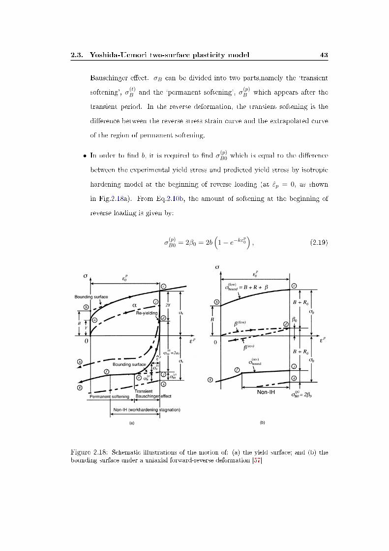
2.3. Yoshida-Uemori two-surface plasticity model 43
Bauschinger e�ect. σB can be divided into two parts,namely the `transient
softening', σ(t)B and the `permanent softening', σ
(p)B which appears after the
transient period. In the reverse deformation, the transient softening is the
di�erence between the reverse stress-strain curve and the extrapolated curve
of the region of permanent softening.
• In order to �nd b, it is required to �nd σ(p)B0 which is equal to the di�erence
between the experimental yield stress and predicted yield stress by isotropic
hardening model at the beginning of reverse loading (at εp = 0, as shown
in Fig.2.18a). From Eq.2.10b, the amount of softening at the beginning of
reverse loading is given by:
σ(p)B0 = 2β0 = 2b
(1− e−kε
p0
), (2.19)
Figure 2.18: Schematic illustrations of the motion of: (a) the yield surface; and (b) thebounding surface under a uniaxial forward-reverse deformation [57]

2.3. Yoshida-Uemori two-surface plasticity model 44
where β0 denotes the kinematic hardening of the bounding surface at the
stress reversal point, and εp0 is the plastic prestrain at the beginning of reverse
loading. From Eq.2.19, the parameter b is obtained. Since (Rsat+b) is already
known from the previous step, Rsat is also determined.
Refering to the de�nition of σ(t)B and σ
(p)B , the determination of the dividing
point `e', Fig.2.18a includes a certain ambiguity, however it should not a�ect
the relationship between the transient and permanent softening vs. εp, as the
rate of work-hardening at this point is so small with respect to the transient
softening. The initial value of transient softening when reverse re-yielding
just starts (at εp = 0 which is indicated as σ(t)B0 = 2a in Fig.2.18a, increases
with the plastic prestrain.
Alternatively, it is possible to �nd parameter b from the reverse bounding
surface in the region of work-hardening stagnation:
σ(rev)bound = −(B +R0) + β(rev), (2.20a)
R0 = Rsat
(1− e−kε
p0
), (2.20b)
β(rev) = b[−1 + 2e−kε
p − e−k(εp0+εp)]. (2.20c)
• Parameter C is identi�ed from the stress-strain curve of the transient Bauschinger
deformation. From Eq.2.10a, for reverse deformation after large forward pre-
strain:
C ≈ 2
εp
[(1 + ln2)−
√|α∗|a
+ ln (1 + sgn(α∗)
√|α∗|a
](2.21)
Since σ(t)B = a+α∗,
α∗a
is given as a function of the transient stress o�set σ(t)B
as:
2.4. LS-DYNA material models for sheet metal forming 45
α∗a≈σ
(t)B
a0− 1 = 2
(σ
(t)B
σ(t)B0
)− 1, a0 =
1
2σ
(t)B0 = σ0 − Y −
1
2σ
(p)B0 (2.22)
It is then possible to plot εp vs.σ
(t)B
σ(t)B0
for various values of C and compare
them with experimental data to �nd the best value for C.
• Parameter h should be identi�ed either from the experimental magnitude of
the plastic strain in which work-hardening stagnation takes place and cyclic
hardening characteristics, or from numerical simulation so as to obtain the
best-�t curves to the corresponding experimental data.
Instead of the above scheme which has certain amount of ambiguity, it is possible
to identify the YU set of parameters simultaneously by using an optimization method
introduced in the previous section (Eq.2.6). More details for implementing this
methodology will be explained in the next chapters.
2.4 LS-DYNA material models for sheet metal forming
The numerical simulations in this investigation were performed with the commer-
cial software LS-DYNA for explicit simulations of forming and implicit simulations
of springback. LS-DYNA accepts a wide range of material models and equations of
state, each with its unique number of stress-strain history variables. Approximately
150 material models are implemented, and space has been allotted for up to 10
user-speci�ed models [38]. From these models, more attention is placed on several
material types that are conventionally used in DYNAFORM, a pre/post processor
with LS-DYNA solver engine, which is extensively used for simulation of industrial
sheet metal forming processes. An analogy will be presented between these models
and the constitutive models explained in the beginning of this chapter.
• Mat 18: Power Law Isotropic Plasticity This model provides elasto-
plastic behaviour with isotropic hardening. The yield stress, σy, is a function

2.4. LS-DYNA material models for sheet metal forming 46
of plastic strain and obeys the equation:
σy = Kεn = K (εyp + εp)n
where εyp is the elastic strain to yield and εp is the e�ective plastic logarithmic
strain.
• Mat 24: Piecewise Linear Plasticity de�nes elasto-plastic material with
a user-de�ned stress vs. strain curve and strain rate dependency. It can also
model failure.
• Mat 36: 3_Parameter Barlat was developed by Barlat and Lian [1989]
for modeling the forming of anisotropic sheet materials under plane stress
conditions. This model allows the use of the Lankford parameters to de�ne
the material anisotropy. The yield condition can be written as:
f(σ, εp) = σeff (σ11, σ22, σ12)− σY (εp) ≤ 0
where
σeff (σ11, σ22, σ12) =(a
2|K1 +K2|m +
a
2|K1 −K2|m +
c
2|2K2|m
)1/m
(2.23a)
K1 =σ11 + hσ22
2(2.23b)
K2 =
√σ11 − hσ22
2
2
+ p2σ122 (2.23c)
and the hardening of the yield surface is either linear, exponential or deter-
mined by a load curve. In the above, the stress components σ11, σ22 and σ12
are with respect to the material coordinate system and εp denotes the e�ective
plastic strain. The material parameters a, c, h and p can be determined from

2.4. LS-DYNA material models for sheet metal forming 47
the Lankford parameters R0, R45 and R90 (the ratios of instantaneous width
to thickness change for each of the directions 0◦, 45◦ and 90◦ with respect to
the sheet rolling direction R =dWdε /WdTdε /T
with W and T as functions of width
and thickness strain):
a =2
(1−
√R0
1 +R0
R90
1 +R90
)(2.24a)
c =2− a (2.24b)
h =
√R0
1 +R0
1 +R90
R90(2.24c)
The anisotropy parameter p can be calculated implicitly by an iterative search
for the root of the following function:
g(p) =2mσmY(
∂f(σ)∂σx
+ ∂f(σ)∂σy
)σ45
− 1−R45
For FCC materials m=8 is recommended and for BCC materials m=6 may be
used.
• Mat 37: Transversely Anisotropic Elastic Plastic is a fully iterative
plasticity model for simulation of anisotropic sheet metal forming only with
shell elements. Hill 1948 yield function with isotropic hardening and trans-
verse anisotropy can be considered as well as optional de�nition of stress
vs. plastic strain curve. The decrease in Young's modulus w.r.t. e�ec-
tive plastic strain can be accommodated with a curve of scale factors or by
de�ning the parameters in the empirical function proposed by Yoshida, Eq.
refeq:unloadingelasticmodulus. Considering Cartesian reference axes parallel
to the planes of anisotropic symmetry, the Hill [1948] yield function of can be
2.4. LS-DYNA material models for sheet metal forming 48
written as:
F (σ22−σ33)2+G(σ33−σ11)2+H(σ11−σ22)2+2Lσ223+2Mσ2
31+2Nσ212−1 = 0,
(2.25)
where σ11, σ22 and σ33 are the tensile normal stresses and σ12, σ23 and σ31 are
the shear stresses. The anisotropy constants F, G, H, L, M and N are related
to the yield stress as in Eq.2.26.
F =(σ0)2
2
(1
σ222
+1
σ233
− 1
σ211
),
G =(σ0)2
2
(1
σ233
+1
σ211
− 1
σ222
),
H =(σ0)2
2
(1
σ211
+1
σ222
− 1
σ233
),
L =3
2
(τ0
σ23
)2
,
M =3
2
(τ0
σ13
)2
,
N =3
2
(τ0
σ12
)2
.
(2.26)
where each σij is the measured yield stress value when σij is applied as the
only nonzero stress component; σ0 is the user-de�ned reference yield stress
speci�ed for the metal plasticity de�nition; and τ0 =σ0
√3.
For the special case of plane stress, where σ33 = 0, the anisotropy input
parameter R is de�ned as the ratio of the in-plane plastic strain rate to the
out-of-plane plastic strain rate:
R =˙εp22
˙εp33
Using the plane stress assumption and the de�nition of R, the yield function
can be written as:
2.4. LS-DYNA material models for sheet metal forming 49
f(σ) =
√σ2
11 + σ222 −
2R
1 +Rσ11σ22 + 2
2R+ 1
1 +Rσ2
12, (2.27)
• Mat 125: Kinematic Hardening Transversely Anisotropic combines
Yoshida non-linear kinematic hardening rule with Mat37. This theory needs
two surfaces to describe the hardening behaviour: the yield surface and the
bounding surface. In the forming process, the yield surface does not change in
size but its center translates with deformation; the bounding surface changes
both in size and location. This model also allows for a change of Young's
modulus as explained in Mat 37.
It should be mentioned here that Mat 125 was implemented in LS-DYNA
based on the general publications of YU model. However it has been observed
that springback results using this model are not consistent with predictions
using other software. Therefore, it appears that the YU model was incorrectly
implemented in the current version of LS-DYNA (version 971, edition R5.1.1)
Material models 24, 36, 37 and 125 will be used for the numerical analysis
of the channel draw process in order to identify how accurately they can predict
the springback and sidewall curl of the channel sections made of AHSS materials.
Further details of implementation and modeling will be explained in subsequent
chapters.

50
Chapter 3
Experimental study
3.1 Introduction
A channel forming process - previously presented as Benchmark #3 in Numisheet
2005 conference - was used in the current research in order to assess the capability
of various material models to predict sidewall curl, as well as the e�ect of several
geometrical parameters such as die entry radius and drawbead penetration for high
strength steels. Two grades of steel, DP980 and TRIP780, were used to draw channel
sections in the presence of drawbeads and with various die entry radii in a draw die
specially designed for this type of research. The experimental work to produce
these channels is described hereafter. This will provide the necessary information
for numerical simulating the channel drawing process.
As DP980 and TRIP780 materials have variable properties with respect to the
rolling direction, a series of characterization tests were also performed to identify
their respective mechanical properties. Furthermore, the procedure for identifying
speci�c material parameters for the constitutive models introduced in the second
chapter, will be explained in this chapter. Results of various characterization tests
for each of the study materials will also be presented.
3.2 Description of the channel draw process
Numisheet channel draw benchmark was provided by General Motors Corpo-
ration, Research & Development Institute IRDI and the US National Institute of

3.2. Description of the channel draw process 51
Standards and Technology (NIST) along with the US Steel Corporation for the Nu-
misheet 2005 conference in Detroit, MI. The draw die was made by the Auto/Steel
Partnership (A/SP) to form straight channel sections. The draw die was installed
at a local stamping plant (NARMCO) in a Williams/White hydraulic 600-ton press
with a stroke of 1310 mm, for the analysis of di�erent grades of advanced high
strength steel sheets and in order to understand the e�ects of di�erent forming pa-
rameters on the springback and sidewall curl of the channels (Fig. 3.1 ). The draw
die was constructed in such a way that the material in the channel sidewalls was
formed over a drawbead and a die entry radius, thus work hardening the sheet by
cyclic bending and unbending in the drawbead and over the die radius. Blanks were
sheared to a width of 254 mm so that the channel sidewalls would be stretched in
plane strain.

3.2. Description of the channel draw process 52
Figure 3.1: A/SP die installed in a hydraulic press
A schematic of the draw die in its open position is shown in Fig. 3.2 . This tool
consists of an upper moving die section, a �oating binder mounted on six cylinders
pressurized by Nitrogen and a �xed lower punch. The upper die is equipped with
changeable inserts on each side that provide di�erent die entry radii as well as
di�erent inboard and outboard penetrations for the drawbeads. In this project no
outboard drawbeads were used and �at blocks were inserted in their locations. Lower
female drawbead inserts were mounted on the binder such that they would mate
with the upper B and C male drawbead inserts. The female inserts could provide
space for single or double beads to deform the sheet metal as well (Fig.3.3).

3.2. Description of the channel draw process 53
Figure 3.2: sideview of the A/SP die components and general dimension parameters
Figure 3.3: (a) schematic view of the die with changeable inserts with various die entry
radius and inboard drawbeads (B, C) and outboard beads (A,D); (b)dimensional parameters
of die drawbead block and kiss block on the binder shown in open position
Motion of the upper die and binder was restricted by four rigid blocks positioned
under the binder for about 20 mm of the whole stroke. Also for safety considerations
and ensuring repeatable total stroke, blocks with a total height of 1074 mm were set
on two sides of the tool to restrict the movement of the press ram during the stroke.
There were also four shimmable kiss blocks located on the top surface of the binder

3.2. Description of the channel draw process 54
which were used to maintain a constant gap between the binder and the upper die.
This kiss gap was adjusted for each material thickness to maintain a clearance of
approximately 30% more than the stock thickness. The symmetry of the tool was
checked by multiple measurements of the drawbead height, kiss blocks heights with
respect to the binder surface and dimensions with respect to the center of symmetry
as shown in Fig.3.4.
Figure 3.4: Illustration of symmetry in the channel draw process
From the set of available drawbeads, round beads with a 4mm radius were se-
lected for the single bead trials. These drawbeads and the die entry blocks were
polished with very �ne sandpaper (180 - 320 grit). They were then heat-treated
to a hardness of 50 HRC. Shims were added to their back plates to increase the
drawbead penetration and to produce channels with a variety of adjustable param-
eters. A brief description of these parameters is provided here before identifying the
selected cases for each material type:
• Clearance: The binder clearance is the distance measured vertically between
the binder surface and the upper die surface when the upper die is in contact
with the kiss blocks.

3.2. Description of the channel draw process 55
This vertical clearance between the binder and the upper die was equivalent
to the sheet thickness plus the kiss gap. This parameter could be measured
with solder imprints by closing the die without a sheet metal blank. The same
clearance was applied to all sides.
• Kiss gap: Vertical distance (air gap) between the binder and the upper die
NOT including the thickness of the sheet material. �Kiss� blocks that were
located on each corner of the �oating binder maintained the kiss gap.
Kiss gap = Clearance - Material Thickness
• Male bead height: The height of a male bead is the vertical distance that
the bead protrudes from the surface of the upper insert that is �ush with the
upper die face. The penetration of the drawbead is then calculated from the
measured male bead height as:
(average) Penetration = (average) Height - Kiss gap
• Penetration: The penetration of a drawbead was de�ned according to the
following:
• 0% penetration: when the male bead is in contact with the sheet material
but the sheet is not subject to any bending (Fig.3.5).
Figure 3.5: Drawbead at 0% penetration

3.2. Description of the channel draw process 56
• 100% penetration: when the centres of curvature for the radii of both
male and female beads lie on the same horizontal line (Fig.3.6).
Figure 3.6: Drawbead at 100% penetration
Penetration%=Ave.Penetration ∗ 100
Upper Bead Radius + Female Insert Radius + Material Thk
Based on these de�nitions, a set of geometrical and process parameters for the
study materials were selected and tested during a set of pre-trial experiments. The
general dimensional parameters of the tools and blanks were as summarized in Table
3.1 and selected drawbead con�gurations are presented in Table 3.2.
The pre-trial tests showed that with the high strength materials, deeper draw-
beads would require much more force input from the press and also resulted in
scoring of the channel sidewalls. Therefore only the speci�c cases which are de-
scribed in Table 3.2 were selected for the actual experiments. Another set of tests
were also performed for each material type using inserts with a die entry radius of
12, 6 and 3 mm but without any male drawbeads. Other parameters of the latter
experiments were similar to the conditions with beads.

3.2. Description of the channel draw process 57
Table 3.1: Geometrical dimensions for channel draw processComponent Description Symbol value(mm)
Upper DieWidth of Die Cavity Wd 257.8Die Entry Radius DER 12.0
PunchWidth of Punch Wp 224.0Radius of Punch Pro�le Rp 12.0
BinderWidth of Binder 1074.0Kiss block gap Bg See Table 3.2
Drawbead
Bead position w.r.t. cavity center line Bp 31.05Male bead height Db See Table 3.2Radius of bead Rb 4.0Width of female bead Wc 10.8Radius of female bead Rc 4.0
BlankWidth BW 254
Length BL996 (DP980)
965 (TRIP780)
Table 3.2: Adjustable parameters of drawbeads and kiss blocks for each con�guration
Material Thickness Clearance Adjusted kiss Actual bead Db Symbol(mm) (mm) gap (mm) penetration% (mm)
DP980 1.5 1.85 0.36
20 2.2 DPSB25 2.7 DPMB37 4.0 DPDB100 9.5 -
TRIP780 1.2 1.5 0.30
20 2.2 TPSB25 2.7 TPMB40 4.0 TPDB100 9.2 -
After setting up each con�guration, sample tryouts were carried out using ordi-
nary draw quality steel sheet before the actual tests were done. A total of 5 channel
sections were produced for each case of the experiments, while recording the punch
force, binder displacement and cylinder pressures using a data acquisition system.
A brief explanation of the data acquisition hardware and setup of the measurement
sensors is given in next section. Before the actual experiments for each material
type, the blanks cut to the required dimensions were clean, marked in the middle of
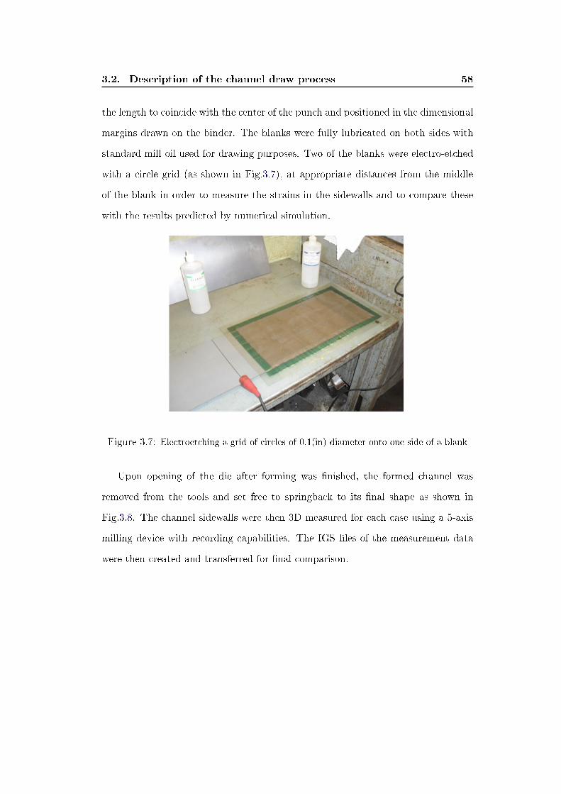
3.2. Description of the channel draw process 58
the length to coincide with the center of the punch and positioned in the dimensional
margins drawn on the binder. The blanks were fully lubricated on both sides with
standard mill oil used for drawing purposes. Two of the blanks were electro-etched
with a circle grid (as shown in Fig.3.7), at appropriate distances from the middle
of the blank in order to measure the strains in the sidewalls and to compare these
with the results predicted by numerical simulation.
Figure 3.7: Electroetching a grid of circles of 0.1(in) diameter onto one side of a blank
Upon opening of the die after forming was �nished, the formed channel was
removed from the tools and set free to springback to its �nal shape as shown in
Fig.3.8. The channel sidewalls were then 3D measured for each case using a 5-axis
milling device with recording capabilities. The IGS �les of the measurement data
were then created and transferred for �nal comparison.

3.2. Description of the channel draw process 59
Figure 3.8: Sample of channels produced for various drawbead con�gurations
3.2.1 Data acquistion system
In order to measure the force exerted on the punch during the forming stage
as well as the displacement of the binder (which is equivalent to the relative punch
displacement), several sensors were installed in the A/SP die and connected to
a desktop computer with a data acquistion card. The acquisition software was
developed in LabView 7.1 and was calibrated for the current project (Fig.3.9).
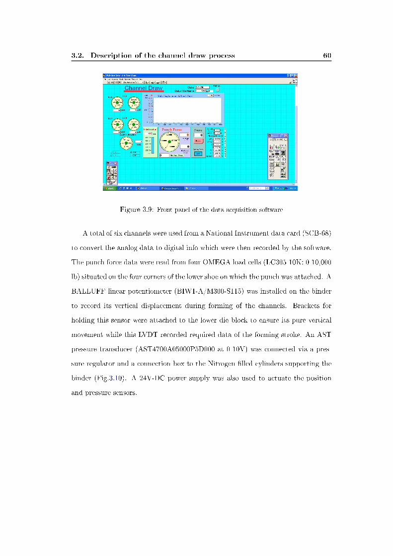
3.2. Description of the channel draw process 60
Figure 3.9: Front panel of the data acquisition software
A total of six channels were used from a National Instrument data card (SCB-68)
to convert the analog data to digital info which were then recorded by the software.
The punch force data were read from four OMEGA load cells (LC305-10K: 0-10,000
lb) situated on the four corners of the lower shoe on which the punch was attached. A
BALLUFF linear potentiometer (BIW1-A/M300-S115) was installed on the binder
to record its vertical displacement during forming of the channels. Brackets for
holding this sensor were attached to the lower die block to ensure its pure vertical
movement while this LVDT recorded required data of the forming stroke. An AST
pressure transducer (AST4700A05000P5D000 at 0-10V) was connected via a pres-
sure regulator and a connection box to the Nitrogen �lled cylinders supporting the
binder (Fig.3.10). A 24V-DC power supply was also used to actuate the position
and pressure sensors.
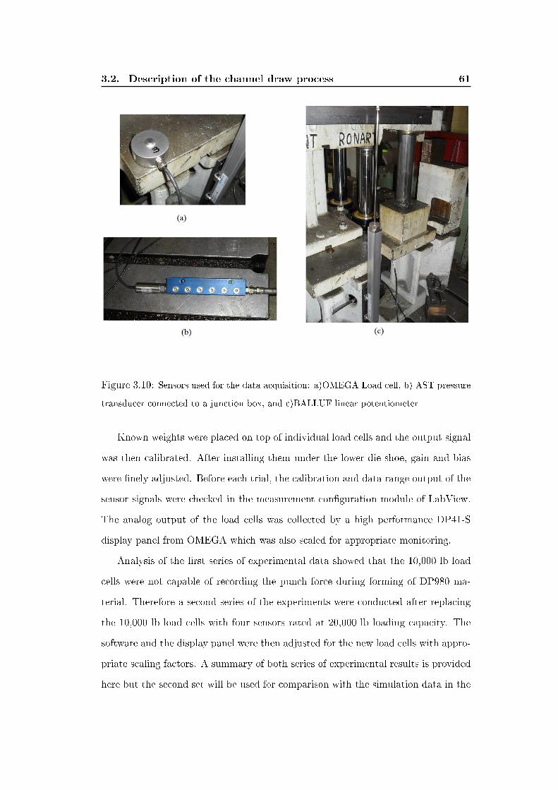
3.2. Description of the channel draw process 61
Figure 3.10: Sensors used for the data acquisition: a)OMEGA Load cell, b) AST pressure
transducer connected to a junction box, and c)BALLUF linear potentiometer
Known weights were placed on top of individual load cells and the output signal
was then calibrated. After installing them under the lower die shoe, gain and bias
were �nely adjusted. Before each trial, the calibration and data range output of the
sensor signals were checked in the measurement con�guration module of LabView.
The analog output of the load cells was collected by a high performance DP41-S
display panel from OMEGA which was also scaled for appropriate monitoring.
Analysis of the �rst series of experimental data showed that the 10,000 lb load
cells were not capable of recording the punch force during forming of DP980 ma-
terial. Therefore a second series of the experiments were conducted after replacing
the 10,000 lb load cells with four sensors rated at 20,000 lb loading capacity. The
software and the display panel were then adjusted for the new load cells with appro-
priate scaling factors. A summary of both series of experimental results is provided
here but the second set will be used for comparison with the simulation data in the

3.3. Experimental results of channel draw for DP980 and TRIP780 62
next chapter.
3.3 Experimental results of channel draw for DP980 and
TRIP780
The experimental results from the channel draw trials for each of the con�gu-
rations mentioned in Table 3.2 are explained in this section. These results include:
punch force vs. displacement curves recorded by the data acquisition system; ge-
ometrical parameters derived from the sidewall pro�le as well as measurements of
wall thickness and residual strain distributions. A set of user de�ned Matlab codes
were developed for data interpretation and to produce appropriate results.
3.3.1 Punch force vs. displacement curves
The total punch force exerted on a blank was the sum of the force data recorded
by the four load cells at each corner of the punch. The vertical displacement of the
punch with respect to the blank was also identical to the displacement recorded by
the LVDT as the blank remained in contact with the binder throughout the forming
stage. Graphs for channels made from TRIP780 with shallow(20%), medium (25%)
and deep (40%) bead penetrations are shown in Fig.3.11. Results for DP980 with
approximately similar bead con�gurations are shown in Fig.3.12. It should be noted
that a constant kiss gap was maintained for each condition as mentioned in Table
3.2 . As shown, the signals from the load cells saturated during the forming of
DP980 channel sections. Also a drop in the punch force for deeper penetrations
of drawbeads for DP980 is observed which showed non-uniform forming process
of these cases. Therefore a subsequent series of experiments were performed for
channels with shallow beads for DP980, and the average punch force results that
were obtained with load cells with a greater capacity (20,000 lbf each), are shown
in Fig.3.13.

3.3. Experimental results of channel draw for DP980 and TRIP780 63
Figure 3.11: Experimental punch force-displacement curves for TRIP780 channels drawnwith various drawbead penetrations: a)TPSB (20%), b)TPMB (25%), c)TPDB (40%)

3.3. Experimental results of channel draw for DP980 and TRIP780 64
Figure 3.12: Experimental punch force-displacement curves for DP980 channels drawnwith various drawbead penetrations: a)DPSB (20%), b)DPMB (25%), c)DPDB (37%)

3.3. Experimental results of channel draw for DP980 and TRIP780 65
Figure 3.13: Experimental punch force-displacement curve for DP980 channels drawn witha shallow bead penetration (20%)
Figure 3.14: Channels drawn with various die entry radii and without drawbeads
For studying the e�ect of the die entry radius, a series of tests were performed
such that the upper die inserts without drawbeads but with varying die entry radii
were used (Fig.3.14). A summary of the speci�cations for these conditions are given
in Table 3.3 and the resultant punch force curves are shown in Figs.3.16 and 3.17.
Results of TRIP780 were also compared for channels made of blanks cut both par-
allel as well as perpendicular to the rolling direction (i.e. Rolling and Transverse

3.3. Experimental results of channel draw for DP980 and TRIP780 66
directions). Further comparison of rolling induced anisotropy on the required form-
ing force was also performed with shallow bead penetrations of TRIP780 material
and results were compared in Fig.3.15.
Table 3.3: Speci�cations of channel draw conditions with di�erent die entry radius and no
drawbeads
Material Type adjusted kiss Die Entry Radius Symbol
gap (mm) [DER] - (mm)
DP980 1.85
12 DPNB12
6 DPNB6
3 DPNB3
TRIP780 1.5
12 TPNB12
6 TPNB6
3 TPNB3
Figure 3.15: Comparison of punch force-displacement curves for TRIP780 channels drawnwith shallow bead penetration (20%) when blanks are cut parallel to the rolling and thetransverse directions

3.3. Experimental results of channel draw for DP980 and TRIP780 67
Figure 3.16: Experimental punch force-displacement curves for TRIP780 channels drawnwith various die entry radii, and for blanks cut in either the rolling or transverse directions:a)TPNB12, b)TPNB6, c)TPNB3
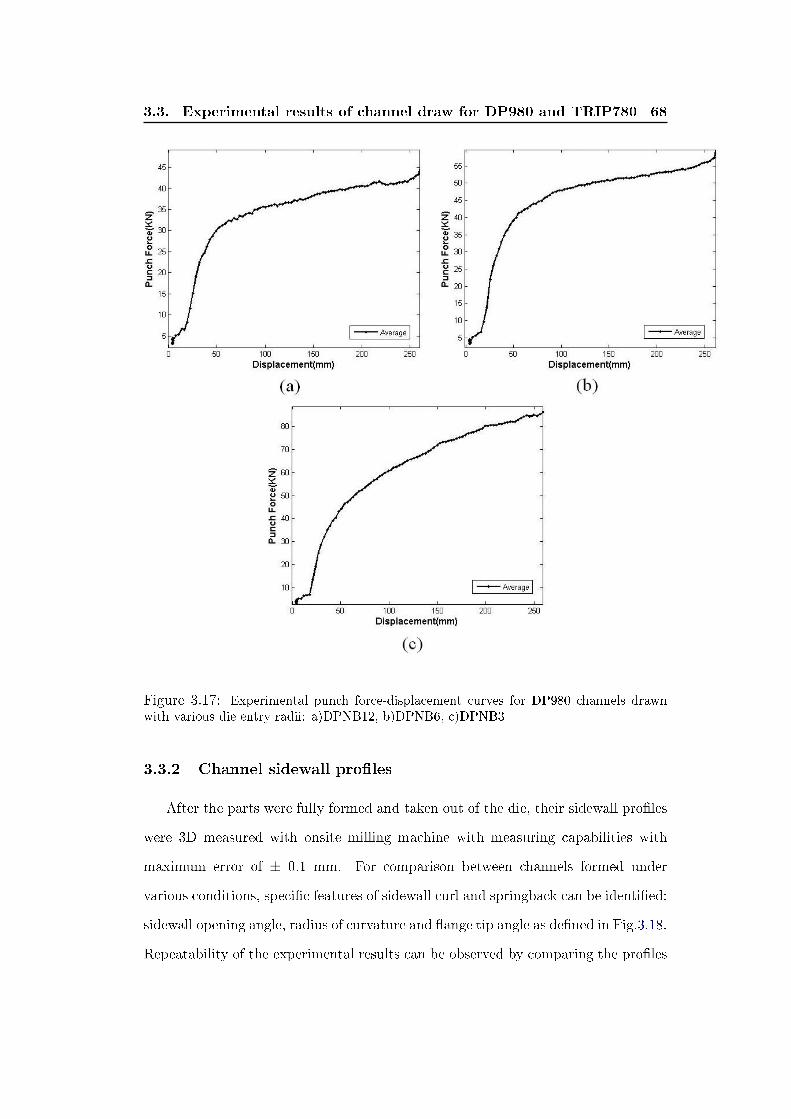
3.3. Experimental results of channel draw for DP980 and TRIP780 68
Figure 3.17: Experimental punch force-displacement curves for DP980 channels drawnwith various die entry radii: a)DPNB12, b)DPNB6, c)DPNB3
3.3.2 Channel sidewall pro�les
After the parts were fully formed and taken out of the die, their sidewall pro�les
were 3D measured with onsite milling machine with measuring capabilities with
maximum error of ± 0.1 mm. For comparison between channels formed under
various conditions, speci�c features of sidewall curl and springback can be identi�ed:
sidewall opening angle, radius of curvature and �ange tip angle as de�ned in Fig.3.18.
Repeatability of the experimental results can be observed by comparing the pro�les
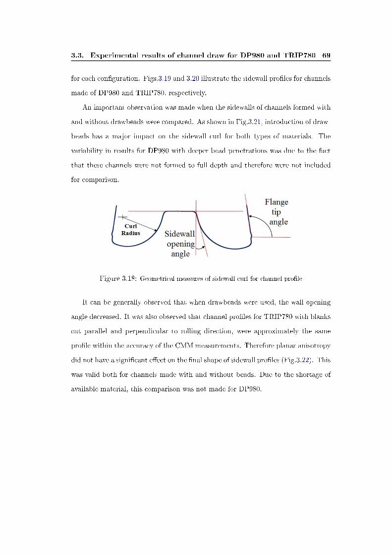
3.3. Experimental results of channel draw for DP980 and TRIP780 69
for each con�guration. Figs.3.19 and 3.20 illustrate the sidewall pro�les for channels
made of DP980 and TRIP780, respectively.
An important observation was made when the sidewalls of channels formed with
and without drawbeads were compared. As shown in Fig.3.21, introduction of draw-
beads has a major impact on the sidewall curl for both types of materials. The
variability in results for DP980 with deeper bead penetrations was due to the fact
that these channels were not formed to full depth and therefore were not included
for comparison.
Figure 3.18: Geometrical measures of sidewall curl for channel pro�le
It can be generally observed that when drawbeads were used, the wall opening
angle decreased. It was also observed that channel pro�les for TRIP780 with blanks
cut parallel and perpendicular to rolling direction, were approximately the same
pro�le within the accuracy of the CMM measurements. Therefore planar anisotropy
did not have a signi�cant e�ect on the �nal shape of sidewall pro�les (Fig.3.22). This
was valid both for channels made with and without beads. Due to the shortage of
available material, this comparison was not made for DP980.
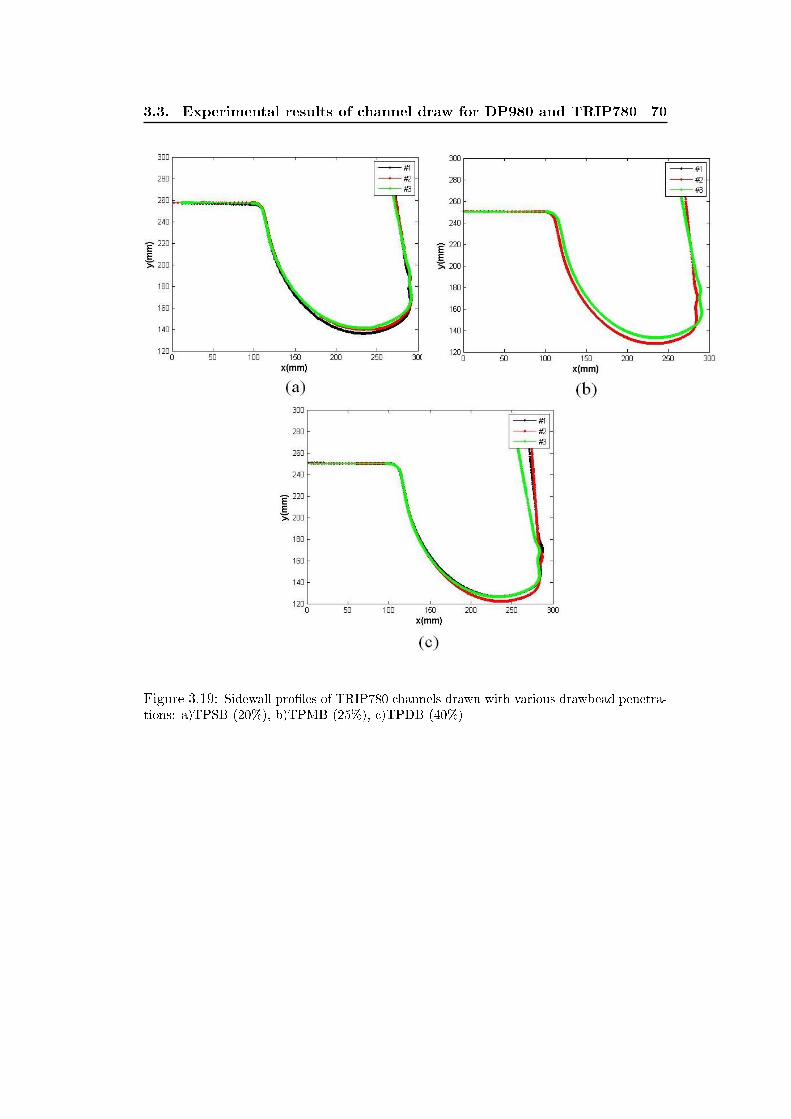
3.3. Experimental results of channel draw for DP980 and TRIP780 70
Figure 3.19: Sidewall pro�les of TRIP780 channels drawn with various drawbead penetra-tions: a)TPSB (20%), b)TPMB (25%), c)TPDB (40%)
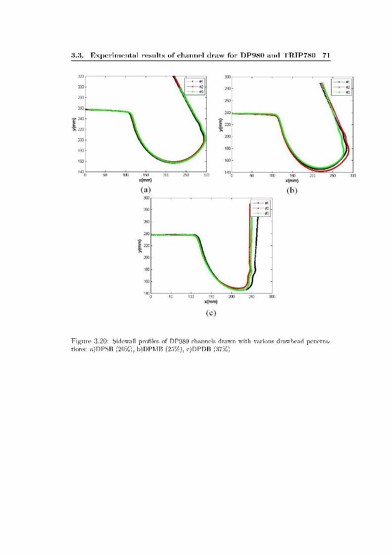
3.3. Experimental results of channel draw for DP980 and TRIP780 71
Figure 3.20: Sidewall pro�les of DP980 channels drawn with various drawbead penetra-tions: a)DPSB (20%), b)DPMB (25%), c)DPDB (37%)
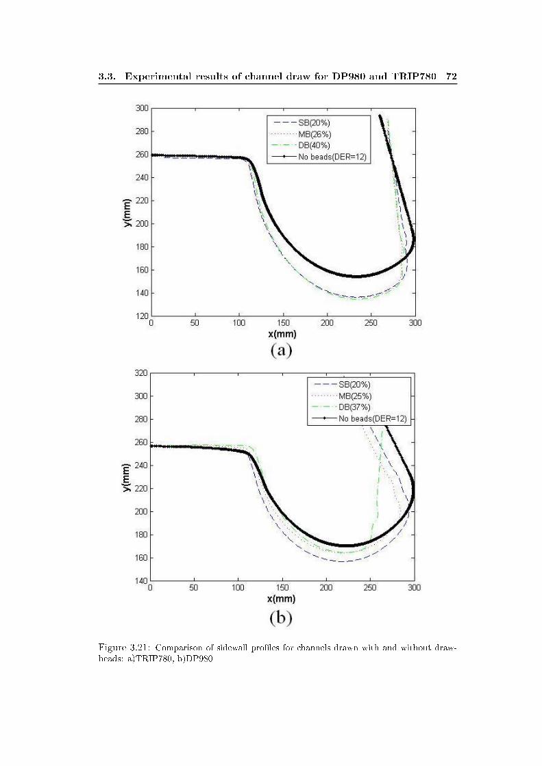
3.3. Experimental results of channel draw for DP980 and TRIP780 72
Figure 3.21: Comparison of sidewall pro�les for channels drawn with and without draw-beads: a)TRIP780, b)DP980
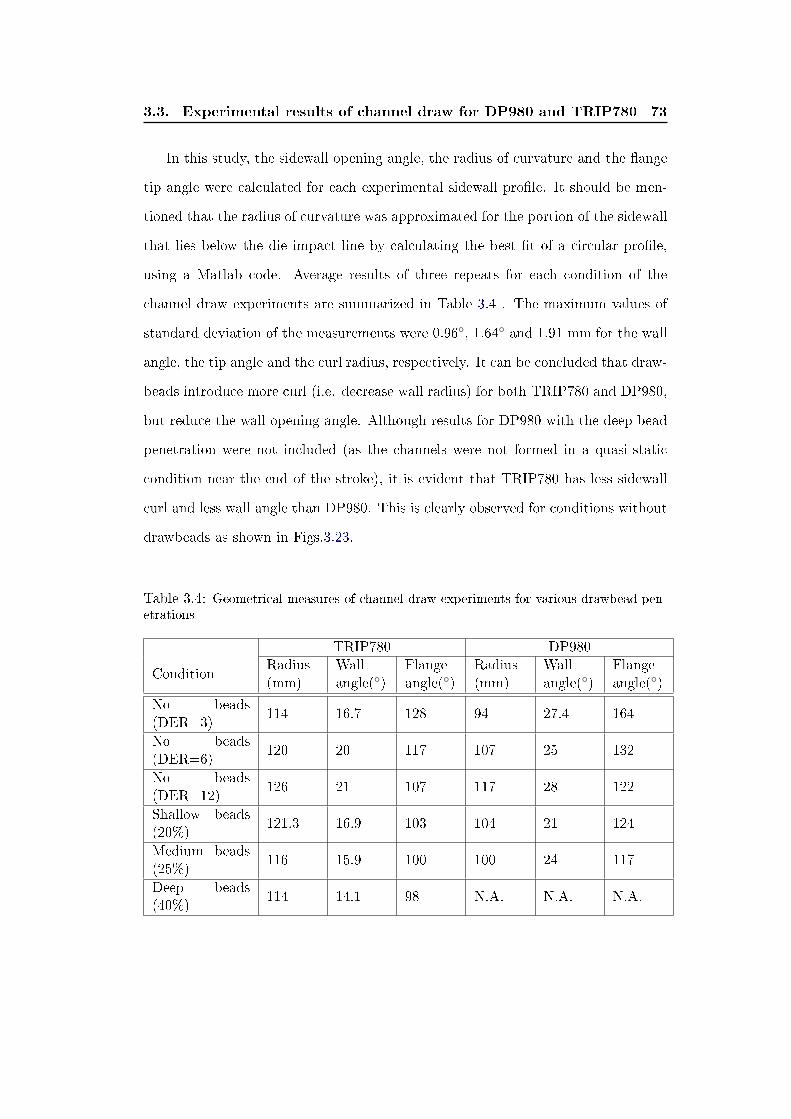
3.3. Experimental results of channel draw for DP980 and TRIP780 73
In this study, the sidewall opening angle, the radius of curvature and the �ange
tip angle were calculated for each experimental sidewall pro�le. It should be men-
tioned that the radius of curvature was approximated for the portion of the sidewall
that lies below the die impact line by calculating the best �t of a circular pro�le,
using a Matlab code. Average results of three repeats for each condition of the
channel draw experiments are summarized in Table 3.4 . The maximum values of
standard deviation of the measurements were 0.96◦, 1.64◦ and 1.91 mm for the wall
angle, the tip angle and the curl radius, respectively. It can be concluded that draw-
beads introduce more curl (i.e. decrease wall radius) for both TRIP780 and DP980,
but reduce the wall opening angle. Although results for DP980 with the deep bead
penetration were not included (as the channels were not formed in a quasi-static
condition near the end of the stroke), it is evident that TRIP780 has less sidewall
curl and less wall angle than DP980. This is clearly observed for conditions without
drawbeads as shown in Figs.3.23.
Table 3.4: Geometrical measures of channel draw experiments for various drawbead pen-etrations
TRIP780 DP980
ConditionRadius(mm)
Wallangle(◦)
Flangeangle(◦)
Radius(mm)
Wallangle(◦)
Flangeangle(◦)
No beads(DER=3)
114 16.7 128 94 27.4 164
No beads(DER=6)
120 20 117 107 25 132
No beads(DER=12)
126 21 107 117 28 122
Shallow beads(20%)
121.3 16.9 103 104 21 124
Medium beads(25%)
116 15.9 100 100 24 117
Deep beads(40%)
114 14.1 98 N.A. N.A. N.A.

3.3. Experimental results of channel draw for DP980 and TRIP780 74
Figure 3.22: Sidewall pro�les of channels made from TRIP780 blanks sheared in the rollingand transverse directions: a) with shallow bead penetration (20%) and b) no drawbeadsand DER=12mm
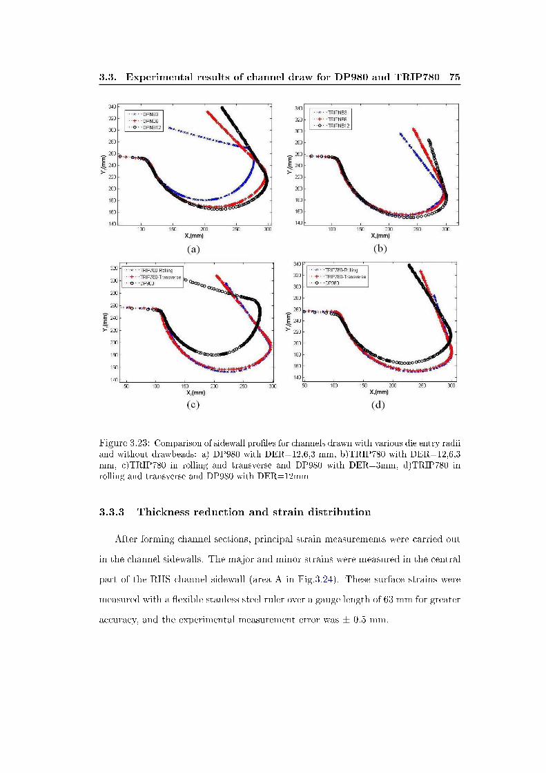
3.3. Experimental results of channel draw for DP980 and TRIP780 75
Figure 3.23: Comparison of sidewall pro�les for channels drawn with various die entry radiiand without drawbeads: a) DP980 with DER=12,6,3 mm, b)TRIP780 with DER=12,6,3mm, c)TRIP780 in rolling and transverse and DP980 with DER=3mm, d)TRIP780 inrolling and transverse and DP980 with DER=12mm
3.3.3 Thickness reduction and strain distribution
After forming channel sections, principal strain measurements were carried out
in the channel sidewalls. The major and minor strains were measured in the central
part of the RHS channel sidewall (area A in Fig.3.24). These surface strains were
measured with a �exible stanless steel ruler over a gauge length of 63 mm for greater
accuracy, and the experimental measurement error was ± 0.5 mm.
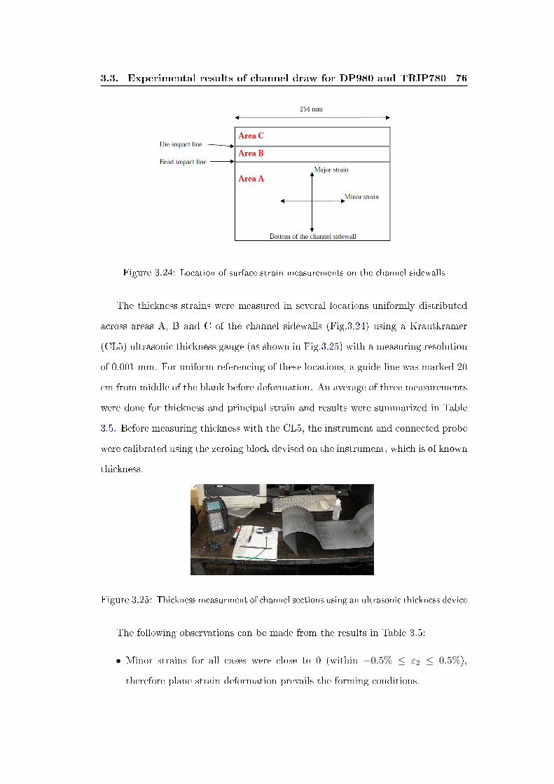
3.3. Experimental results of channel draw for DP980 and TRIP780 76
Figure 3.24: Location of surface strain measurements on the channel sidewalls
The thickness strains were measured in several locations uniformly distributed
across areas A, B and C of the channel sidewalls (Fig.3.24) using a Krautkramer
(CL5) ultrasonic thickness gauge (as shown in Fig.3.25) with a measuring resolution
of 0.001 mm. For uniform referencing of these locations, a guide line was marked 20
cm from middle of the blank before deformation. An average of three measurements
were done for thickness and principal strain and results were summarized in Table
3.5. Before measuring thickness with the CL5, the instrument and connected probe
were calibrated using the zeroing block devised on the instrument, which is of known
thickness.
Figure 3.25: Thickness measurment of channel sections using an ultrasonic thickness device
The following observations can be made from the results in Table 3.5:
• Minor strains for all cases were close to 0 (within −0.5% ≤ ε2 ≤ 0.5%),
therefore plane strain deformation prevails the forming conditions.

3.4. Material characterization and mechanical properties 77
• Major strains were almost zero (≤ 0.8%)when no drawbeads were used. This
con�rms that drawbeads increase the major strain in the channel draw.
• When drawbeads were used, di�erences in thickness strains between areas A
& C were observed and maximum sidewall thickness reduction of 8.8% was
measured for deep bead penetration for channels made of TRIP780. For chan-
nels without drawbeads maximum thickness reduction was 1.25% of nominal
stock (for TRIP780 with thickness of 1.2 mm).
Table 3.5: Principal strains and thickness of blanks measured in channel sidewalls. Accu-racy of measurement was ±0.01% strain.
TRIP780-RollingMajorstrain
Minorstrain
Thickness strain (%)
% % area C area A
NB12 0.8 0 -0.85 -1.25
NB6 0.8 0 -0.7 -1.0
NB3 0.8 0 -0.75 -1.1
SB(20%) 4 -1.6 -1.0 -5.8
MB(25%) 6.5 -0.4 -0.8 -7.3
DB(40%) 9.8 -0.4 -0.5 -8.8
TRIP780-Transverse
NB12 0.5 0 -0.6 -1.0
NB6 0.4 0 -0.7 -0.8
NB3 0.5 0 -1.1 -0.8
SB(20%) 4 -1.5 -1.7 -3.9
DP980
NB12 0.8 0. -0.1 -0.6
NB6 0.81 0 -0.4 -0.6
NB3 0.81 0 -0.5 -0.5
SB(20%) 2.4 -0.4 -0.8 -3.4
3.4 Material characterization and mechanical properties
The experimental procedures and tests used to determine the mechanical prop-
erties of the materials included in this study are discussed in this section. As men-

3.4. Material characterization and mechanical properties 78
tioned before, TRIP780 with 1.2mm thickness and DP980 with 1.5mm were used to
produce channel sections. In order to characterize the mechanical and anisotropy
properties of as-received sheets, specimens were cut at di�erent angles to the rolling
direction (0◦, 45◦ and 90◦) and sets of uniaxial tension and tension compression
tests were conducted.
3.4.1 Uniaxial tension tests
The tensile specimens were designed according to ASTM-E8 standard as shown
in Fig.3.26 and machined by wire EDM. The tests were conducted to determine
the stress-strain curves as well as anisotropy parameters with respect to the rolling
direction.
Figure 3.26: Specimen for uniaxial tension test designed according to ASTM-E8: G=50,W=12.5, R=12.5 (mm)
Two sets of uniaxial tension experiments were performed at separate facilities
and results were compared. A group of tests were conducted in an INSTRON 8562
machine at the University of Windsor on samples cut in rolling, transverse and
diagonal directions. Extensions were measured by means of a 25.4 mm gauge exten-
someter along with the applied force at a constant cross-head velocity to maintain
quasi-static conditions for the experiments. Recorded data were manipulated in

3.4. Material characterization and mechanical properties 79
order to calculate the engineering stress-strain data using:
σeng =FiA0, εeng =
Li − L0
L0
where Fi was the instantaneous tensile load, A0 the initial gauge cross-sectional area
and L0, Li were the initial and instantaneous gauge length, respectively. True values
of stresses and strains were then calculated considering constant volume assumption
during plastic deformation, as:
σ = σeng(1 + εeng), ε = ln(1 + εeng)
Results of tensile tests for TRIP780 and DP980 are shown in Fig.3.27. It was
observed that the stress-strain curves obtained from di�erent orientations of the
specimens are almost identical. Specimens showed consistency in their response
for each orientation with respect to the rolling direction. It can be observed that
the 45◦ specimens experience lower stresses than the 0◦ and 90◦ test specimens.
Moreover, there was no signi�cant di�erence between the behaviours of the latter
two directions. These results were observed for DP980 as well as TRIP780.
The yield stress of the specimens were obtained from the stress - strain curves
at a strain o�set of 0.002. It was then used to determine the true stress - plastic
strain curve required for simulation models using:
εP = ε− σYE,
where σY is the yield stress and E is the initial elastic modulus, assumed to be 207
GPa for both types of steels. The elastic modulus was also estimated by a linear
�t to the beginning portions of the uniaxial test results between stresses of 0 and
200 MPa. The tangential modulus that was measured by this method ranged from
195 to 208 GPa for DP980 and 192 to 210 for TRIP780. The uniaxial curves were
then averaged to a �nal �ow curve up to the maximum strength for each material
3.4. Material characterization and mechanical properties 80
type and compared with results from other sources. The second series of tensile
tests were performed at US Steel, Automotive Center Laboratory, MI, in which
anisotropy ratios were also measured. As mentioned in Chapter 2, at a given angle
φ to the rolling direction, the anisotropy of the sheet is characterized by the plastic
strain ratio, r-value, and is de�ned as:
rφ =−εW
εL + εW=
−ln( WW0)
ln( LL0) + ln( WW0
)
It is common to describe an average r-value, R, (Hertzberg, 1995) obtained
from three directions 0◦ (parallel), 45◦ (diagonal) and 90◦ (transverse) to the rolling
direction that describes the normal anisotropy and is de�ned as:
R =r0 + 2r45 + r90
4(3.1)
Also ∆R, de�ned as a measure of the tendency of the sheet to draw in nonuniformly
and form ears in the �ange of deep-drawn cylindrical parts in the direction of the
higher r-value was calculated by:
∆R =r0 + r90 − 2r45
2(3.2)
Results from uniaxial tensile tests performed at USS are summarized in Table
3.6 . It can be seen that the e�ect of orientation on the yield stress is relatively small.
Therefore an average value of the yield stress can be used to characterize these two
sheet steels. Also the plasticity curves obtained from tensile tests on samples in the
rolling direction were compared with those performed at University of Windsor, as
well as the power law σ = K ∗ εn, as shown in Figs.3.28 and 3.29. The consistency
between the results was reasonably good, therefore an average curve from the uni-
axial test results was used to obtain a best �t of the power law function for each
grade of steel, and these were used as input data in the numerical simulations.
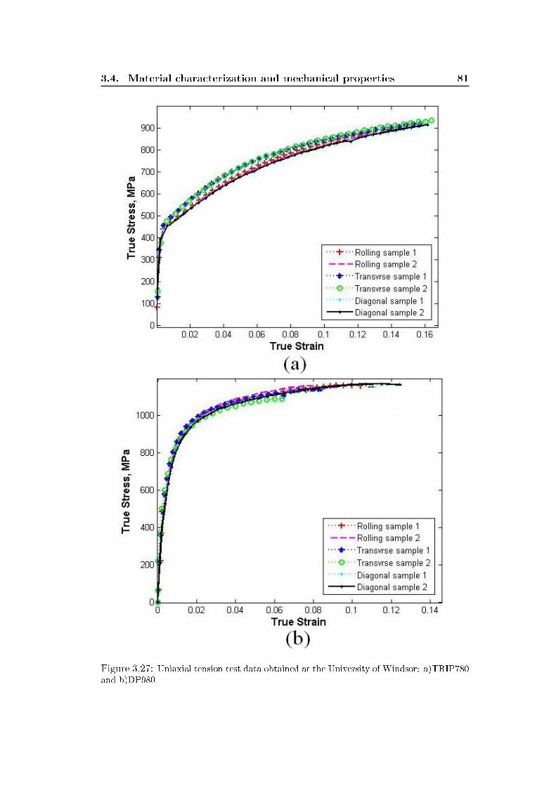
3.4. Material characterization and mechanical properties 81
Figure 3.27: Uniaxial tension test data obtained at the University of Windsor: a)TRIP780and b)DP980
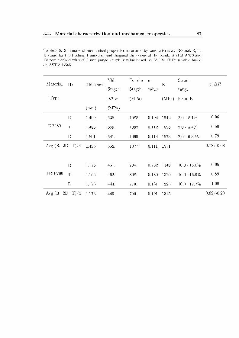
3.4. Material characterization and mechanical properties 82
Table 3.6: Summary of mechanical properties measured by tensile tests at USSteel, R, T,D stand for the Rolling, transverse and diagonal directions of the blank, ASTM A370 andE8 test method with 50.8 mm gauge length; r-value based on ASTM E517; n-value basedon ASTM E646
Material ID ThicknessYld
Strgth
Tensile
Strgth
n-
valueK
Strain
ranger, ∆R
Type 0.2 % (MPa) (MPa) for n, K
(mm) (MPa)
DP980
R 1.499 638. 1088. 0.104 1542 2.0 - 8.1% 0.96
T 1.483 689. 1082. 0.112 1595 2.0 - 5.4% 0.56
D 1.501 641. 1069. 0.114 1573 2.0 - 6.3 % 0.79
Avg (R+2D+T)/4 1.496 652. 1077. 0.111 1571 0.78/-0.03
TRIP780
R 1.176 451. 794. 0.202 1348 10.0 - 18.0% 0.65
T 1.166 462. 808. 0.180 1320 10.0 - 16.9% 0.89
D 1.176 443. 779. 0.191 1295 10.0 - 17.7% 1.00
Avg (R+2D+T)/4 1.173 449. 790. 0.191 1315 0.89/-0.23
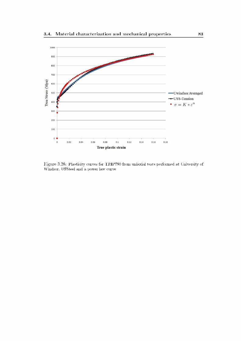
3.4. Material characterization and mechanical properties 83
Figure 3.28: Plasticity curves for TRIP780 from uniaxial tests performed at University ofWindsor, USSteel and a power law curve

3.4. Material characterization and mechanical properties 84
Figure 3.29: Plasticity curves for DP980 from uniaxial tests performed at University ofWindsor, USSteel and a power law curve
3.4.2 Unloading elastic modulus
A series of uniaxial tests were performed on samples taken parallel to the rolling
direction in order to study the evolution of the unloading elastic modulus of TRIP780
and DP980 sheet metals. Specimens were prepared according to the ASTM E8
standard, and tests were performed at the Colorado School of Mines. A series of
specimens were strained to 1.5%, 2.5%, 3.5% and 4.5 % before they were unloaded,
as it was expected from previous studies [36] that the unloading modulus follow an
exponential decay function with saturation between 3 to 4% initial strain for high
strength steels (such as DP600). For each material, tests were repeated three times
for each of the prestrain levels. Representative engineering stress-strain curves of
one set of the tests are shown in Figs.3.31.
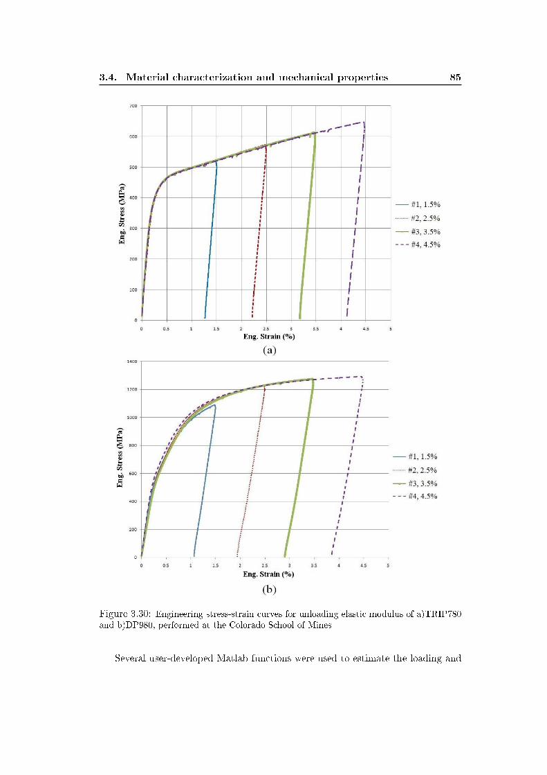
3.4. Material characterization and mechanical properties 85
Figure 3.30: Engineering stress-strain curves for unloading elastic modulus of a)TRIP780and b)DP980, performed at the Colorado School of Mines
Several user-developed Matlab functions were used to estimate the loading and
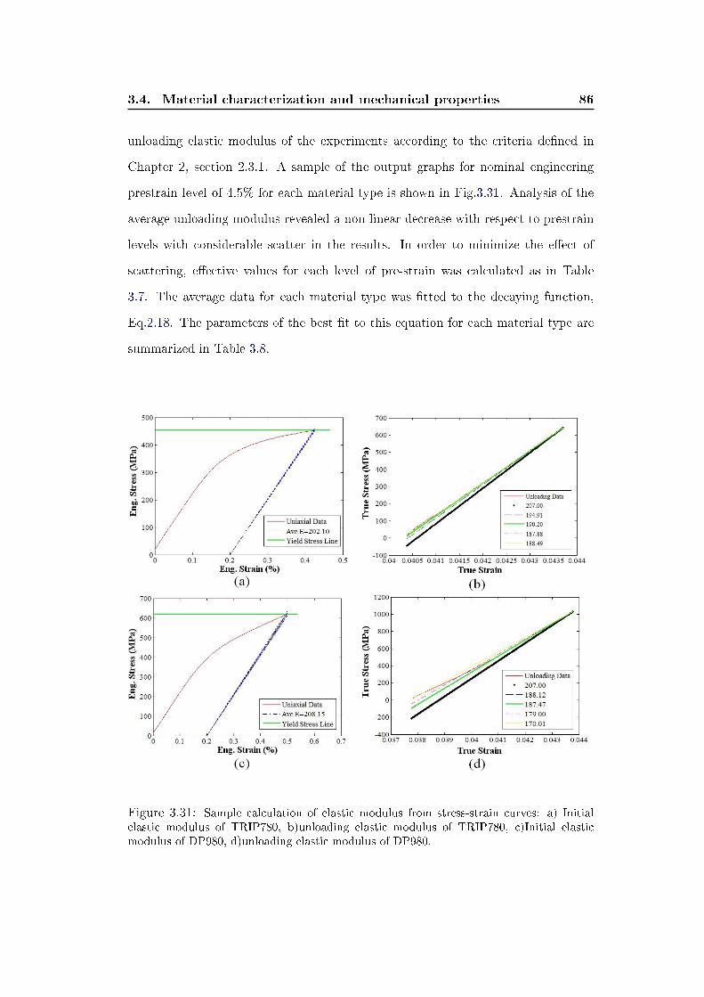
3.4. Material characterization and mechanical properties 86
unloading elastic modulus of the experiments according to the criteria de�ned in
Chapter 2, section 2.3.1. A sample of the output graphs for nominal engineering
prestrain level of 4.5% for each material type is shown in Fig.3.31. Analysis of the
average unloading modulus revealed a non-linear decrease with respect to prestrain
levels with considerable scatter in the results. In order to minimize the e�ect of
scattering, e�ective values for each level of pre-strain was calculated as in Table
3.7. The average data for each material type was �tted to the decaying function,
Eq.2.18. The parameters of the best �t to this equation for each material type are
summarized in Table 3.8.
Figure 3.31: Sample calculation of elastic modulus from stress-strain curves: a) Initialelastic modulus of TRIP780, b)unloading elastic modulus of TRIP780, c)Initial elasticmodulus of DP980, d)unloading elastic modulus of DP980.
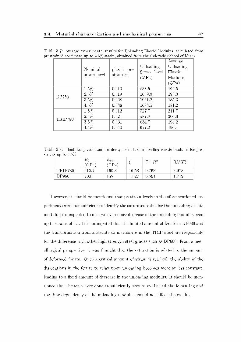
3.4. Material characterization and mechanical properties 87
Table 3.7: Average experimental results for Unloading Elastic Modulus, calculated fromprestrained specimens up to 4.5% strain, obtained from the Colorado School of Mines
Nominalstrain level
plastic pre-strain ε0
UnloadingStress level(MPa)
AverageUnloadingElasticModulus(GPa)
DP980
1.5% 0.010 888.5 199.52.5% 0.019 1009.9 193.33.5% 0.028 1061.2 185.34.5% 0.038 1083.5 181.2
TRIP780
1.5% 0.012 527.7 211.72.5% 0.021 587.8 200.03.5% 0.031 634.7 198.24.5% 0.040 677.2 190.4
Table 3.8: Identi�ed parameters for decay formula of unloading elastic modulus for pre-strains up to 4.5%
E0
(GPa)Esat(GPa)
ξ Fit R2 RMSE
TRIP780 210.7 160.3 16.58 0.768 3.978
DP980 200 158 11.27 0.894 1.712
However, it should be mentioned that prestrain levels in the aforementioned ex-
periments were not su�cient to identify the saturated value for the unloading elastic
moduli. It is expected to observe even more decrease in the unloading modulus even
up to strains of 0.1. It is anticipated that the limited amount of ferrite in DP980 and
the transformation from austenite to martensite in the TRIP steel are responsible
for the di�erence with other high strength steel grades such as DP600. From a met-
allurgical perspective, it was thought that the saturation is related to the amount
of deformed ferrite. Once a critical amount of strain is reached, the ability of the
dislocations in the ferrite to relax upon unloading becomes more or less constant,
leading to a �xed amount of decrease in the unloading modulus. It should be men-
tioned that the tests were done at su�ciently slow rates that adiabatic heating and
the time dependency of the unloading modulus should not a�ect the results.
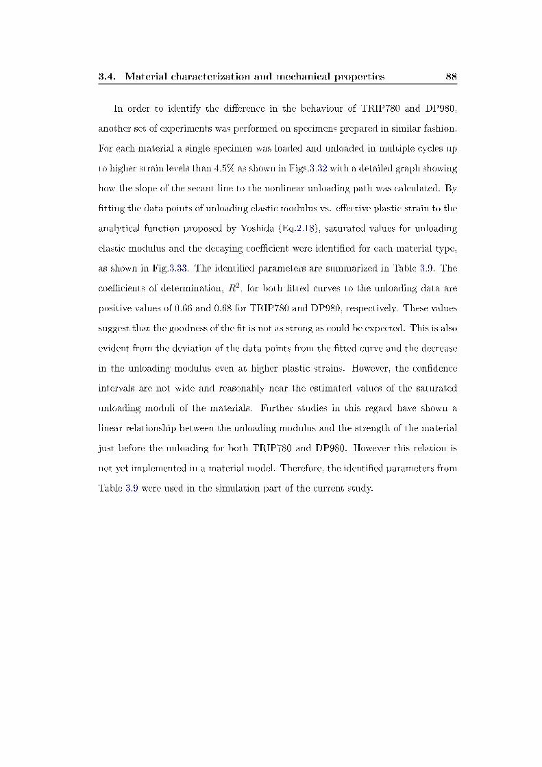
3.4. Material characterization and mechanical properties 88
In order to identify the di�erence in the behaviour of TRIP780 and DP980,
another set of experiments was performed on specimens prepared in similar fashion.
For each material a single specimen was loaded and unloaded in multiple cycles up
to higher strain levels than 4.5% as shown in Figs.3.32 with a detailed graph showing
how the slope of the secant line to the nonlinear unloading path was calculated. By
�tting the data points of unloading elastic modulus vs. e�ective plastic strain to the
analytical function proposed by Yoshida (Eq.2.18), saturated values for unloading
elastic modulus and the decaying coe�cient were identi�ed for each material type,
as shown in Fig.3.33. The identi�ed parameters are summarized in Table 3.9. The
coe�cients of determination, R2, for both �tted curves to the unloading data are
positive values of 0.66 and 0.68 for TRIP780 and DP980, respectively. These values
suggest that the goodness of the �t is not as strong as could be expected. This is also
evident from the deviation of the data points from the �tted curve and the decrease
in the unloading modulus even at higher plastic strains. However, the con�dence
intervals are not wide and reasonably near the estimated values of the saturated
unloading moduli of the materials. Further studies in this regard have shown a
linear relationship between the unloading modulus and the strength of the material
just before the unloading for both TRIP780 and DP980. However this relation is
not yet implemented in a material model. Therefore, the identi�ed parameters from
Table 3.9 were used in the simulation part of the current study.

3.4. Material characterization and mechanical properties 89
Figure 3.32: Multiple loading and unloading cycles performed at the Colorado School ofMines to estimate saturated unloading elastic modulus: a)TRIP780, b)DP980

3.4. Material characterization and mechanical properties 90
Figure 3.33: Fitting analytical decay function to unloading elastic modulus of TRIP780and DP980
Table 3.9: Identi�ed parameters for decay formula of unloading elastic modulus withprestrain 12% for TRIP780 and 9% for DP980
E0
(GPa)Esat(GPa)
ξ Fit R295% Con�denceinterval Esat(GPa)
TRIP780 207 132.7 46.1 0.665 (124.8, 140.6)
DP980 207 157.8 57.5 0.682 (151.6, 163.9)
In a recent study presented by Kuwabara at the ESAFORM conference in
Belfast, 2011, the unloading modulus data for DP980 saturated at an e�ective strain
around 0.1. The equation provided was :
E(MPa) = 153.934 + 53.918 ∗ e(−57.4∗εp) (3.3)
The values reported in Eq.3.3 are in good agreement with the parameters found

3.4. Material characterization and mechanical properties 91
in the current study. The identi�ed unloading parameters from Table 3.9 are used
for the parameters optimization study in the subsequent chapter.
3.4.3 Cyclic Tension and Compression tests
Di�erent tension and compression tests were performed at USSteel on tensile
samples of DP980 and TRIP780 in order to identify material hardening parameters.
These tests included :
• a single cycle tension and compression test starting in tension and then, at a
certain strain level, reversing to compression until the strain reaches zero;
• a single full cycle tension and compression test starting at tension and then,
at a certain strain level, reversing to compression until the compression strain
reaches the same amount of positive strain in tension and at this compression
strain level, re-loading in tension until the net strain reaches zero
• a multiple cycle tension and compression test repeating a single cycle tension
and compression test several times.
For each material type, all of the tests were repeated twice. Results of the single
and multiple cycles until zero strains (type 1 and 3) were identical. Therefore
results of complete single cycle as well as multiple cycles are shown in Figs.3.34 and
3.35. Strain memory as well as prestrained tension and compression tests were not
performed.

3.4. Material characterization and mechanical properties 92
Figure 3.34: Cyclic tension - compression tests of TRIP780: a) Single cycle, b) Multiplecycles
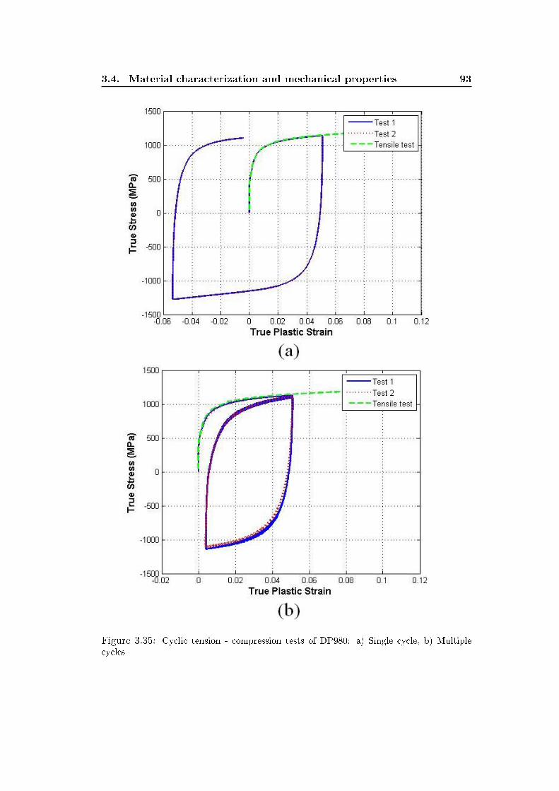
3.4. Material characterization and mechanical properties 93
Figure 3.35: Cyclic tension - compression tests of DP980: a) Single cycle, b) Multiplecycles
3.4. Material characterization and mechanical properties 94
The graphs clearly show the repeatability of the tests results. Di�erent regions
of cyclic loading can be distinguished as discussed in Chapter 2. For DP980, the
region of permanent softening is evident after the transient stage, but for TRIP780
the transient region extends well into the compressive zone. An average of the cyclic
stress-strain data was used to determine the parameters required in the constitutive
models which is explained in Chapter 4.
3.4.4 Friction coe�cient
Specimens of each material type in form of square plates (760 mm by 760 mm)
were used for friction tests at Arcelor Mittal Dofasco R&D centre in Hamilton, ON.
Tests were conducted perpendicular to the sheet rolling direction (i.e. transverse)
using a drawbead simulator.
All of the test specimens exhibited good surface quality (free of mechanical
interference - scratches, gouges, heavy dirt, etc.). The drawbeads were cleaned with
mineral oil, wiped dry with a lint free tissue, and lubricated with the wealth oil
prior to testing. The depth of penetration for the male Roller and Fixed bead was
reduced by around 50%. Five repeat tests were done for each material type to
permit conditioning of the beads which were not used to characterize the frictional
performance of the material. The next �ve tests were used as the �steady state�
components of the test matrix. An average value of 0.097 and 0.102 were determined
for TRIP780 and DP980, respectively.
95
Chapter 4
Numerical Analysis
4.1 Introduction
LS-DYNA explicit/implicit solver (version 971) was used in this study to simu-
late the forming and springback stages of a channel draw process. Three-dimensional
shell models for each drawbead con�guration of TRIP780 and DP980 were created
using a phyton script in ABAQUS 6.9. Geometrical parameters for channels with
and without drawbeads as well as the explicit simulation variables required to setup
the forming step in ABAQUS, were de�ned as the input parameters in this script.
Therefore, a variety of models can be created in a short time. Di�erent constitutive
models from LS-DYNA library - explained in chapter 2- were used in the simu-
lations. Modeling parameters such as the number of integration points, element
formulations, contact types and properties were also analyzed. For selective cases,
simulations in LS-DYNA were compared with results from ABAQUS and a user-
de�ned subroutine of the YU material model. Input parameters for the material
models were determined using the experimental results from tensile tests and cyclic
tension-compression tests. The optimization method used to identify the hardening
parameters from tension-compression tests, is explained and compared with results
reported by other studies for TRIP780 and DP980. Various results from both the
forming and subsequent springback stages of the simulations were obtained and com-
pared with the experimental values in order to identify the ability of each modeling
technique to predict sidewall curl results of the channels.

4.2. Determination of Constitutive Material Parameters 96
4.2 Determination of Constitutive Material Parameters
For material models with isotropic hardening, plasticity curves of TRIP780 and
DP980 (Fig.3.27) were used as the stress-strain curves. Other numerical parameters
such as the yield strength, r-value and elastic modulus were assigned from Table 3.6
and the initial elastic modulus of steel is 207 GPa.
The systematic approach that was explained in Chapter 2, was used in order
to determine the preliminary hardening parameters for the YU material model in
LS-DYNA. A user-developed Matlab code helped to estimate these parameters from
the tension-compression graphs of TRIP780 and DP980 as shown in Figs.4.1 and
4.2. The estimated parameters are summarized in Table 4.1.
Table 4.1: Intermediate YU model parameters from systematic analysis of tension com-pression test
Material B Rsat + b kRe-yield stress(MPa)
σpB0 b Rsat
DP980 909.3 272.5 36 -203.4 155.1 92.3 180.2
TRIP780 429.8 862.7 8 -151.9 49.2 71.6 791.1
Tension-compression tests were then simulated in LS-DYNA by a single plane
stress shell element model. This model consisted of a square element with a 1-mm
side. The bottom side was �xed in the Y-direction and the left bottom corner �xed
both in X- and Y directions, while the top side was extended and then compressed
0.1 mm in each stage in the Y-direction. Element formulation 2 (Belytschko-Tsay)
with one integration point through the thickness was used to mesh the part. The
schematic of this model is shown in Fig.4.3.
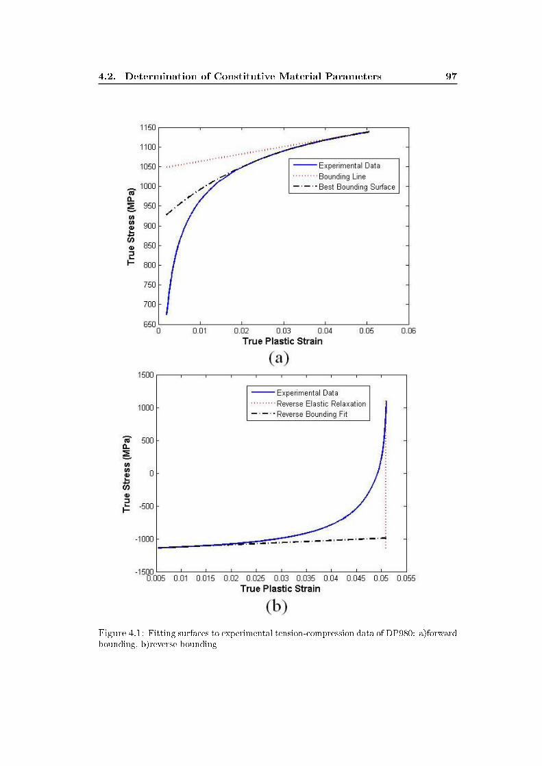
4.2. Determination of Constitutive Material Parameters 97
Figure 4.1: Fitting surfaces to experimental tension-compression data of DP980: a)forwardbounding, b)reverse bounding

4.2. Determination of Constitutive Material Parameters 98
Figure 4.2: Fitting surfaces to experimental tension-compression data of TRIP780:a)forward bounding, b)reverse bounding

4.2. Determination of Constitutive Material Parameters 99
Figure 4.3: Schematic representation of the �nite element model for tension compressiontest
The base simulations with the preliminary set of material parameters from Tables
3.6, 3.8 and 4.1 were assigned to material type 125 (YU model) for TRIP780 and
DP980 as well as an isotropic hardening model (Mat 24). The predicted stress vs.
strain outputs were then compared with the experimental test results in Fig.4.4. It
was observed that the simulation results for an isotropic hardening model could not
capture the response of the materials during cyclic loading particularly during the
compression cycle. The YU simulations did not correlate well with the experimental
values and therefore an optimization of the parameters was required to obtain a more
accurate description of the cyclic behaviour.
In order to optimize the YU model parameters, the developed models in LS-
DYNA with Mat125 were used in a Metamodel-based optimization project with LS-
OPT 4.2 software. A sequential strategy with domain reduction (SRSM) method
was used assuming normal distribution of the model variables. Linear order polyno-
mial meta-model with D-Optimal selection of simulation points and default number
of 11 iterations per case along with radial basis function for approximation of his-
tories were incorporated to compare the cross-plot of Y-stress vs. Y-strain of the
middle surface of the element with the experimental values of a single cycle tension-
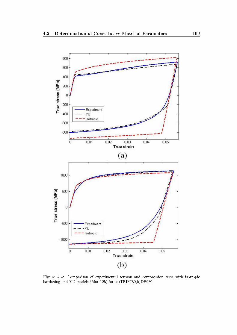
4.2. Determination of Constitutive Material Parameters 100
Figure 4.4: Comparison of experimental tension and compression tests with isotropichardening and YU models (Mat 125) for: a)TRIP780,b)DP980
4.2. Determination of Constitutive Material Parameters 101
compression test for TRIP780 and DP980. For comparison of the experimental and
simulation curves a special function `MeanSqErr' has been frequently used to com-
pute the mean square error for the discrepancy between the output curve and the
target curve:
ε =1
P
P∑p=1
Wp
[fp(x)−Gp
sp
]2
=1
P
P∑p=1
Wp
[εp(x)
sp
]2
, (4.1)
It is constructed so thatGp, p = 1...P are the values on the target curveG and
fp(x) the corresponding components of the computed curve f . fp(x) are represented
internally by the response surface values. x is the design vector. Recently, it has
been argued that the mean square error function is suitable for ordinate-based curve
matching. However a major di�culty is that steep parts of the target curve are
di�cult to incorporate in the matching.These kinds of problems present a strong
case for incorporating the abscissa into the curve-matching metric. In our case,
cyclic material models (hysteric curves) with more than one possible y-value for
some of the x-values present more di�culty as they can not be quanti�ed because
of the non-uniqueness of the ordinate values of the computed curve with respect
to the target curve. A logical approach to comparison of the two curves is to map
one of the curves onto the other using Frechet distance. The analogy is that of a
dog walking along one curve and the dog's owner walking along the other connected
by a leash. Both walk continuously and monotonically along the curve from the
start point to the end point and can vary their velocities. The Frechet distance
is the length of the shortest leash that is su�cient for transversing both curves in
this manner. In version 4.2 of LS-OPT software, this method is implemented by
mapping the points of one curve onto the second curve and computing the volume
(area) between the two curves. When both curves are normalized, this typically
yields a mismatch error with values much less than 1 for two reasonably matching
curves [47].
Therefore, the curve mapping method was used as the weighted objective for

4.2. Determination of Constitutive Material Parameters 102
optimizing YU parameters in material type 125 for cyclic tension-compression tests
of TRIP780 and DP980. Results of the optimization are shown in Fig. 4.5 and the
identi�ed parameters are summarized in Table 4.2. However, it should be taken into
consideration that the prediction errors not only come from the variance error due
to the intrinsic noise and unreliabilities in the measurement of the dependent vari-
ables but also from the systematic (bias) error due to model mis-speci�cation. To be
genuinely useful, a �tting procedure should provide the means to assess whether or
not the model is appropriate and to test the goodness-of-�t against some statistical
standard.
Table 4.2: Optimized YU model parameters for LS-DYNA with material type 125
Material Y c B Rsat b k h E0 Ea ξ(MPa) (MPa) (MPa) (MPa) (GPa) (GPa)
DP980 670.7 156.3 909.3 161.7 121.2 36.5 0.05 207 157.8 57.5
TRIP780 452.2 205.5 489.8 587.6 178.7 10.05 0.03 207 132.7 46.1
The correlation matrices between Mat 125 parameters and the mapping error of
the network response for each of the sheet metals are shown in Fig.4.6. A strong
positive correlation was found between the response error and Rsat, b and k parame-
ters while a negative correlation was observed with h, for both material types. Mean
square error was also compared against the curve mapping error. The correlation
coe�cient is a measure of how well the variation in the output is explained by the
targets. Outliers can greatly a�ect the magnitudes of correlation coe�cients. Of
course, the larger the sample size, the smaller is the impact of several outliers.

4.2. Determination of Constitutive Material Parameters 103
Figure 4.5: Optimized simulations with Material type 125 for tension compression testsof: a)TRIP780, b)DP980

4.2. Determination of Constitutive Material Parameters 104
Figure 4.6: Correlation matrices between Mat125 parameters and curve mapping errorresponse for: a)TRIP780, b)DP980
It should be mentioned that the optimized parameters found for DP980 sheets,
were somewhat di�erent from the values reported in another study. Shi et al. [46]
identi�ed parameters for both the original and modi�ed YU models for a group of
AHSS materials through similar tension-compression tests . The parameters for the
original YU model for two grades of steel sheets similar to those used in our study
are summarized in Table 4.3 . It was reported that the DP980 material exhibited
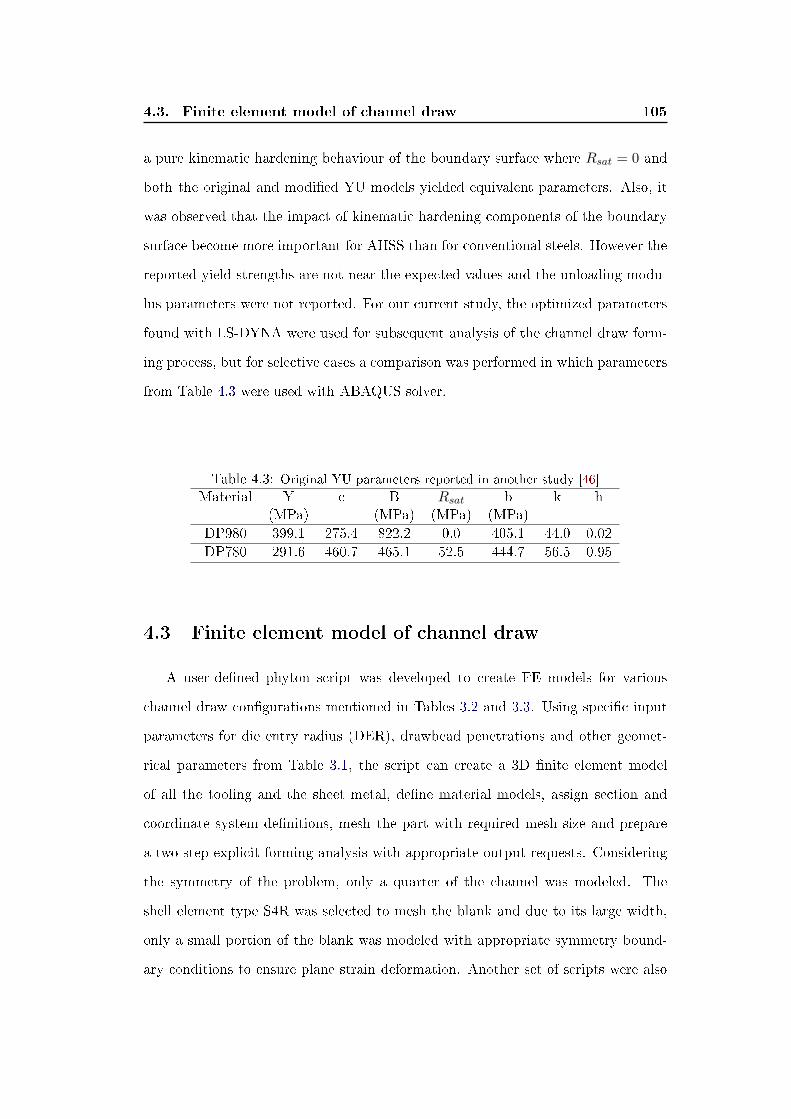
4.3. Finite element model of channel draw 105
a pure kinematic hardening behaviour of the boundary surface where Rsat = 0 and
both the original and modi�ed YU models yielded equivalent parameters. Also, it
was observed that the impact of kinematic hardening components of the boundary
surface become more important for AHSS than for conventional steels. However the
reported yield strengths are not near the expected values and the unloading modu-
lus parameters were not reported. For our current study, the optimized parameters
found with LS-DYNA were used for subsequent analysis of the channel draw form-
ing process, but for selective cases a comparison was performed in which parameters
from Table 4.3 were used with ABAQUS solver.
Table 4.3: Original YU parameters reported in another study [46]
Material Y c B Rsat b k h(MPa) (MPa) (MPa) (MPa)
DP980 399.1 275.4 822.2 0.0 405.1 44.0 0.02
DP780 291.6 460.7 465.1 52.5 444.7 56.5 0.95
4.3 Finite element model of channel draw
A user-de�ned phyton script was developed to create FE models for various
channel draw con�gurations mentioned in Tables 3.2 and 3.3. Using speci�c input
parameters for die entry radius (DER), drawbead penetrations and other geomet-
rical parameters from Table 3.1, the script can create a 3D �nite element model
of all the tooling and the sheet metal, de�ne material models, assign section and
coordinate system de�nitions, mesh the part with required mesh size and prepare
a two-step explicit forming analysis with appropriate output requests. Considering
the symmetry of the problem, only a quarter of the channel was modeled. The
shell element type S4R was selected to mesh the blank and due to its large width,
only a small portion of the blank was modeled with appropriate symmetry bound-
ary conditions to ensure plane strain deformation. Another set of scripts were also

4.3. Finite element model of channel draw 106
developed to create 2D and 3D solid models, but are not reported in this study.
Previous studies have indicated that both solid and shell elements with su�ciently
�ne mesh would produce the same springback pro�le for the channel draw process
[25].
In these FE models, all the tools, die, punch and binder were modeled as rigid
bodies. The forming simulation was de�ned in two steps; �rst, the drawbeads and
the die part were moved on to the panel up to a constant clearance and then draw-
ing was simulated by movement of the punch while the die and binder remain �xed
relative to the punch. Once the forming stage was completed, the part with its
stress-strain state was transferred to an implicit springback analysis in which spe-
ci�c nodes of the part were constrained in order to eliminate the rigid body motion
of the part and allow it to naturally springback to its �nal shape, just as when the
part is removed from the tools.
The parts created by the script �le in ABAQUS were then exported in IGES
format to prepare the required surfaces for the models in LS-DYNA. An initial mesh
size of 2.5 mm was used for tools and a mesh size of 3 mm for the blank, as shown
in Fig.4.7. Mesh adaptivity was used for all the models up to 4 levels with 5 degrees
of adaptive error tolerance relative to the surrounding elements for each element
of the blank to be re�ned. The recommended one-pass with look-forward active
parameters were also considered for the adaptive re-meshing.

4.3. Finite element model of channel draw 107
Figure 4.7: Finite element model of the channel draw forming in LS-DYNA
Shell elements were used to model the blank with element formulation 2 (Belytschko-
Tsay) and 9 integration points through the thickness. Quadrilateral element type
2 was used due to its e�ciency, although it requires one-point integration, does
not pass the patch test and performs poorly on warped geometries. Therefore a
comparison was also made when full integration elements were used. The problem
with reduced integration and kinematic modes were resolved partially by hourglass
control, which leads to satisfactory results in most situations. The shear correction
factor was set equal to5
6which is valid for isotropic materials but not for sandwich
and laminated shells. The shell formulations in LS-DYNA, with the exception of
BCIZ triangular shells and DK fully integrated linear quadrilateral/triangular shell
elements (formulations 3 and 18, respectively), are based on a �rst order shear de-
formation theory that yields constant transverse shear strains which violates the
condition of zero traction on the top and bottom surfaces of the shell. The shear
correction factor is an attempt to compensate for this error.
For treating the interaction between tools and the blank, three contact interfaces
with algorithm type �FORMING_ONE_WAY_SURFACE_TO_SURFACE� were
de�ned in which the blank was the slave part set and tools were the master, using
the standard formulation of the penalty method. Viscous damping coe�cient was
set as 20% of the critical in order to avoid undesirable oscillations in contact dur-
4.3. Finite element model of channel draw 108
ing forming simulations and was applied perpendicular to the contacting surfaces.
Suitable velocity curves in the Y-direction were de�ned for the forming steps with
prescribed rigid body motions as well as a load curve for the binder force. One way
contact types allow for compensation loads to be transferred between the slave nodes
and the master segments. Tangential loads are also transmitted if relative sliding
occurs when contact friction is active. The one-way term in one-way contact is used
to indicate that only the user-speci�ed slave nodes are checked for penetration of
the master segments. One-way contacts may be appropriate when the master side is
a rigid body, e.g., a punch or die in a metal stamping simulation. A situation where
one-way contact may be appropriate for deformable bodies is where a relatively �ne
mesh (slave) encounters a relatively smooth, coarse mesh (master). Orientation is
automatic with forming contacts. The rigid tooling surface can be constructed from
disjoint element patches where contiguous nodal points are sometimes merged out,
but not always. These patches are not assumed to be consistently oriented; conse-
quently, during initialization, the reorientation of these disjoint element patches is
performed. Forming contact tracks the nodal points of the blank as they move be-
tween the disjoint element patches of the tooling surface. Penalty forces are used to
limit penetrations. Generally the ONE_WAY_SURFACE_TO_SURFACE option
is recommended since the penetration of master nodes through the slave surface is
considered in adaptive re-meshing. Without this feature, adaptive re-meshing may
fail to adequately re�ne the mesh of the blank to capture sharp details in the master
surface, and the master surface will protrude through the blank.
The friction between the blank and the tools was modeled as a constant coe�-
cient of static friction identi�ed from the friction test results. It should be mentioned
that there are still major uncertainties in the description of friction-contact phenom-
ena in simulation of sheet metal forming processes. Simulation calculations show
that a small change in the friction-contact situation can have a signi�cant e�ect

4.3. Finite element model of channel draw 109
on the springback. However, the coe�cient of friction is an experimental factor
over which relatively minimal control is available in FE simulations. Researchers
often use a coe�cient value that best simulates the blank-tool interaction. For the
channel draw process, a constant kiss gap of around 30% of the sheet thickness was
maintained throughout the forming stage (Table 3.2), therefore the e�ect of friction
was expected to have a minor e�ect on springback in this problem. Besides, punch
velocity and binder pressure were kept constant during the forming and no depen-
dency could be assumed between friction and relative velocity and pressure. Since
only a limited area of the blank was in contact with the die radius and draw beads
when present, and the contact area did not change signi�cantly during the drawing
stage, it was reasonable to assume a steady state kind of problem for the forming
phase. The experimental punch force results shown in chapter 3, also con�rm that
the forming stage was nearly a quasi-static process. This suggests that a constant
friction coe�cient is valid for this problem. However, di�erent values were used in
the simulations to investigate the sensitivity of the predicted pro�les to the coe�-
cient of friction. This analysis showed that a higher value of the friction coe�cient
than the experimental results, best simulates the channel forming and springback
stages when no drawbeads are used. For channels formed with drawbeads, friction
coe�cient had minimal e�ect on the results.
After the forming stage was completed, all the contact pairs de�ned between
the blank and tools were removed allowing the channel to deform freely to its �nal
sprungback shape.
As mentioned before, the models in ABAQUS were created using a user-de�ned
script. Material models with isotropic hardening as well as the YU model accom-
panied by a user subroutine (UMAT) from a previous study [25] were compared
for selected cases. For the user subroutine of the YU model, two sets of parameters
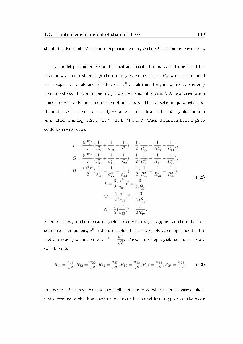
4.3. Finite element model of channel draw 110
should be identi�ed: a) the anisotropic coe�cients, b) the YU hardening parameters.
YU model parameters were identi�ed as described here. Anisotropic yield be-
haviour was modeled through the use of yield stress ratios, Rij which are de�ned
with respect to a reference yield stress, σ0 , such that if σij is applied as the only
non-zero stress, the corresponding yield stress is equal to Rijσ0. A local orientation
must be used to de�ne the direction of anisotropy. The Anisotropic parameters for
the materials in the current study were determined from Hill's 1948 yield function
as mentioned in Eq. 2.25 as F, G, H, L, M and N. Their de�nition from Eq.2.26
could be rewritten as:
F =(σ0)2
2(
1
σ222
+1
σ233
− 1
σ211
) =1
2(
1
R222
+1
R233
− 1
R211
),
G =(σ0)2
2(
1
σ233
+1
σ211
− 1
σ222
) =1
2(
1
R233
+1
R211
− 1
R222
),
H =(σ0)2
2(
1
σ211
+1
σ222
− 1
σ233
) =1
2(
1
R211
+1
R222
− 1
R233
),
L =3
2(τ0
σ23)2 =
3
2R223
,
M =3
2(τ0
σ13)2 =
3
2R213
,
N =3
2(τ0
σ12)2 =
3
2R212
.
(4.2)
where each σij is the measured yield stress when σij is applied as the only non-
zero stress component; σ0 is the user-de�ned reference yield stress speci�ed for the
metal plasticity de�nition; and τ0 =σ0
√3. These anisotropic yield stress ratios are
calculated as :
R11 =σ11
σ0, R22 =
σ22
σ0, R33 =
σ33
σ0, R12 =
σ12
τ0, R13 =
σ13
τ0, R23 =
σ23
τ0. (4.3)
In a general 3D stress space, all six coe�cients are used whereas in the case of sheet
metal forming applications, as in the current U-channel forming process, the plane
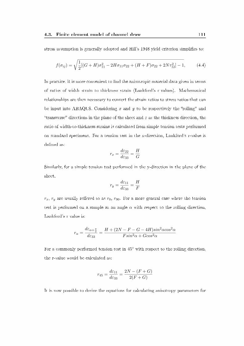
4.3. Finite element model of channel draw 111
stress assumption is generally adopted and Hill's 1948 yield criterion simpli�es to:
f(σij) =
√1
2[(G+H)σ2
11 − 2Hσ11σ22 + (H + F )σ22 + 2Nτ212]− 1, (4.4)
In practice, it is more convenient to �nd the anisotropic material data given in terms
of ratios of width strain to thickness strain (Lankford's r-values). Mathematical
relationships are then necessary to convert the strain ratios to stress ratios that can
be input into ABAQUS. Considering x and y to be respectively the �rolling� and
�transverse� directions in the plane of the sheet and z as the thickness direction, the
ratio of width-to-thickness strains is calculated from simple tension tests performed
on standard specimens. For a tension test in the x-direction, Lankford's r-value is
de�ned as:
rx =dε22
dε33=H
G
Similarly, for a simple tension test performed in the y-direction in the plane of the
sheet,
ry =dε11
dε33=H
F
rx, ry are usually re�ered to as r0, r90. For a more general case where the tension
test is performed on a sample at an angle α with respect to the rolling direction,
Lankford's r-value is:
rα =dεα+π
2
dε33=H + (2N − F −G− 4H)sin2αcos2α
Fsin2α+Gcos2α
For a commonly performed tension test in 45◦ with respect to the rolling direction,
the r-value would be calculated as:
r45 =dε11
dε33=
2N − (F +G)
2(F +G)
It is now possible to derive the equations for calculating anisotropy parameters for
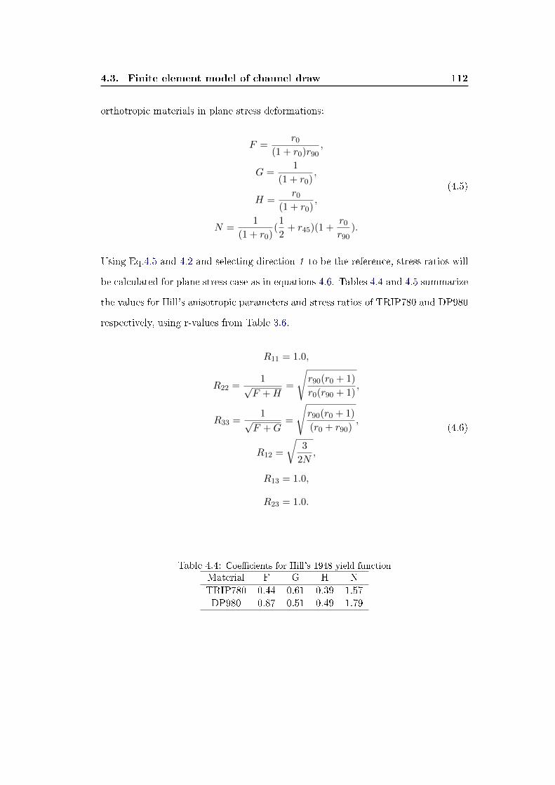
4.3. Finite element model of channel draw 112
orthotropic materials in plane stress deformations:
F =r0
(1 + r0)r90,
G =1
(1 + r0),
H =r0
(1 + r0),
N =1
(1 + r0)(1
2+ r45)(1 +
r0
r90).
(4.5)
Using Eq.4.5 and 4.2 and selecting direction 1 to be the reference, stress ratios will
be calculated for plane stress case as in equations 4.6. Tables 4.4 and 4.5 summarize
the values for Hill's anisotropic parameters and stress ratios of TRIP780 and DP980
respectively, using r-values from Table 3.6.
R11 = 1.0,
R22 =1√
F +H=
√r90(r0 + 1)
r0(r90 + 1),
R33 =1√
F +G=
√r90(r0 + 1)
(r0 + r90),
R12 =
√3
2N,
R13 = 1.0,
R23 = 1.0.
(4.6)
Table 4.4: Coe�cients for Hill's 1948 yield function
Material F G H N
TRIP780 0.44 0.61 0.39 1.57DP980 0.87 0.51 0.49 1.79

4.3. Finite element model of channel draw 113
Table 4.5: Stress anisotropic ratios for channel model in ABAQUS
Material R11 R12 R22 R33
TRIP780 1.00 0.98 1.09 0.98DP980 1.00 0.92 0.86 0.85
When using shell elements in ABAQUS (and LS-DYNA), which are based on
�rst-order transverse shear �exible theory with constant through thickness shear
strains, transverse shear, correction factors should be used to compensate for this
assumption. For a homogeneous shell made of a linear, orthotropic elastic material,
where the strong material direction aligns with the element's local 1-direction, the
transverse shear sti�ness should be:
Kts11 =
5
6GE13t,K
ts22 =
5
6GE23t, andK
ts12 = Kts
21 = 0.
where GE13 and GE23 are the material's shear modulus in the out-of-plane direction.
The correction factor 56 results from matching the transverse shear energy to that
for a three-dimensional structure in pure bending. For our study, the shear modulus
was de�ned as:
G =E
2(1 + ν)
and the values of the transverse shear sti�ness were calculated as in Table 4.6.
Table 4.6: Transverse shear sti�ness for channel model in ABAQUS, (N
mm)
Material thickness K11 K12 K22
TRIP780 1.2 79000 0 79000DP980 1.5 101000 0 101000

4.4. Results of channel forming simulations 114
4.4 Results of channel forming simulations
Simulation results from FE models developed in LS-DYNA for each con�gura-
tion of the channel draw are presented in this section. Comparison with related
experimental results are also made.
4.4.1 Punch Force vs. Displacement curves
Punch force results were calculated from the contact forces of forming simulations
of channels. For the cases with drawbeads, su�cient stretch was available to form the
sidewalls. As shown in Figs.4.8 and 4.9, the punch force is overestimated by material
models 24, 36 and 37 (with isotropic hardening [IH]) and underestimated by Mat
125 model for both TRIP780 and DP980 when drawbeads are used. Overestimation
of IH models could be attributed to the failure of such hardening to capture the
Bauschinger e�ect, and therefore the material response is over-predicted during
cyclic loading.
Figure 4.8: Comparison of predicted and experimental punch force results for DP980 withvarious material models
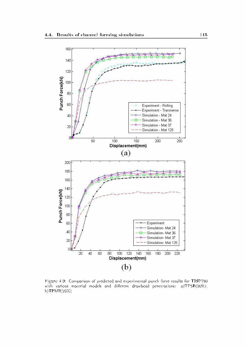
4.4. Results of channel forming simulations 115
Figure 4.9: Comparison of predicted and experimental punch force results for TRIP780with various material models and di�erent drawbead penetrations: a)TPSB(20%),b)TPMB(25%)

4.4. Results of channel forming simulations 116
However, more accurate results were expected for the YU model (Mat 125). Re-
sults of YU model in ABAQUS were compared against LS-DYNA results in Fig.4.10
which demonstrate better conformity of the converged punch force. Data set from
ABAQUS was smoothed using curve �tting tool of Matlab. The smoothing was
performed by using a piecewise polynomial computed from parameter p which was
set to 0.8 and the resulting R2 of the �t was 0.997.
Figure 4.10: Comparison of experimental and predicted punch force results for TRIP780with shallow beads using the YU model in ABAQUS and LS-DYNA
In order to identify the problem with simulations of Mat 125, energy balance of
the simulations were checked and compared with those from other material models.
As shown in Fig.4.11, energy levels of the simulations with Mat 125 demonstrate a
mismatch between the total energy and the external work delivered to the system.
For every correct simulation in LS-DYNA the energy levels should balance according
to Eq.4.7:

4.4. Results of channel forming simulations 117
Ekin + Eint + Esi + Erw + Edamp + Ehg︸ ︷︷ ︸Total Energy: Etotal
= E0kin + E0
int +Wext (4.7)
where su�xes on the left hand side represent Kinetic, Internal, Sliding interface
(including Friction), rigid wall, damping and hourglass energies which should bal-
ance with the sum of initial values plus the external work on the right hand side.
No rigid wall, damping and hourglass energies were present in the aforementioned
simulations. The energy ratio is thus de�ned as:
eratio =Etotal
E0total +Wext

4.4. Results of channel forming simulations 118
Figure 4.11: Energy balance for TPSB case with various material models: a)Mat24,b)Mat36, c)Mat37, d)Mat125
As can be seen in Fig.4.12, energy ratio for simulation with material type 125 fell
well below unit and leveled o� near 0.8 which con�rmed the mismatch between total
energy and the external work. In other words, part of the external work transferred
to the system was not converted to increase in internal energy nor dissipated by the
sliding. Such a situation is referred to as `arti�cial absorption' of the energy. It could
result from many sources, however in this case the only di�erence between multiple
simulations was the material model. The energy balance equation was validated
for other material types with the same mesh, contact de�nition and other model
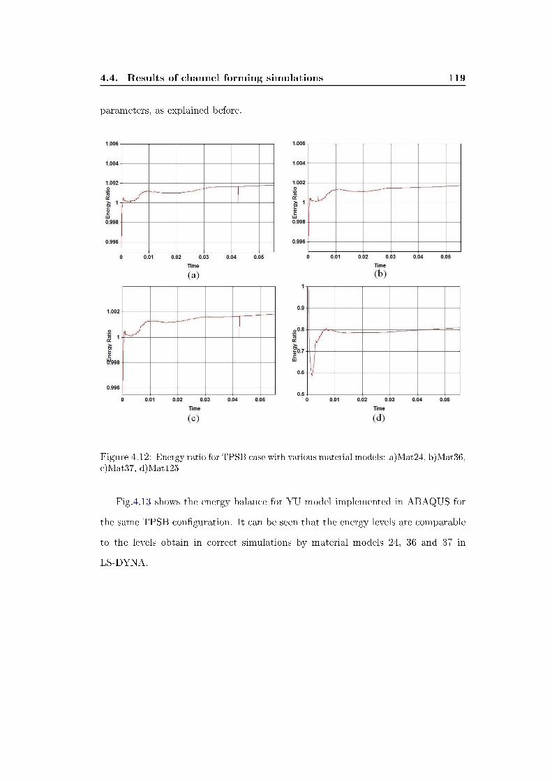
4.4. Results of channel forming simulations 119
parameters, as explained before.
Figure 4.12: Energy ratio for TPSB case with various material models: a)Mat24, b)Mat36,c)Mat37, d)Mat125
Fig.4.13 shows the energy balance for YU model implemented in ABAQUS for
the same TPSB con�guration. It can be seen that the energy levels are comparable
to the levels obtain in correct simulations by material models 24, 36 and 37 in
LS-DYNA.

4.4. Results of channel forming simulations 120
Figure 4.13: Energy balance for TPSB case in ABAQUS - YU model
Also results for energy balance and ratio for DPSB case were checked with various
material types, shown in Figs.4.14 and 4.15 which con�rm that the problem with Mat
125 is not related to numerical parameters. To further investigate this problem, sim-
ulations for DPSB and Mat125 were altered by changing element formulation from
2 to 16 (Fully integrated shell elements), increasing the number of integration points
from 9 to 19, 29 and 49, eliminating mass scaling and mesh adaptivity while re�ning
meshes of blank and tools to an approximate size of 0.5, using other contact types
`FORMING_SURFACE_TO_SURFACE', `SURFACE_TO_SURFACE' and sev-
eral values of friction coe�cient (0.0, 0.07, 0.125, 0.15, 0.2, 0.25). Simulation results
for the both shell and solid elements of the single element model were also checked.
However the energy balance problem persisted for all of these simulation with mate-
rial type 125. This problem was reported to LSTC representative and was con�rmed
to be an issue that should be recti�ed. This problem leads to erroneous stress-strain
results in the �nal stage of the forming which would be transferred to the implicit
scheme for springback calculation. It is evident that the absorbed internal plastic
energy is not at the same level as predicted by other material types.
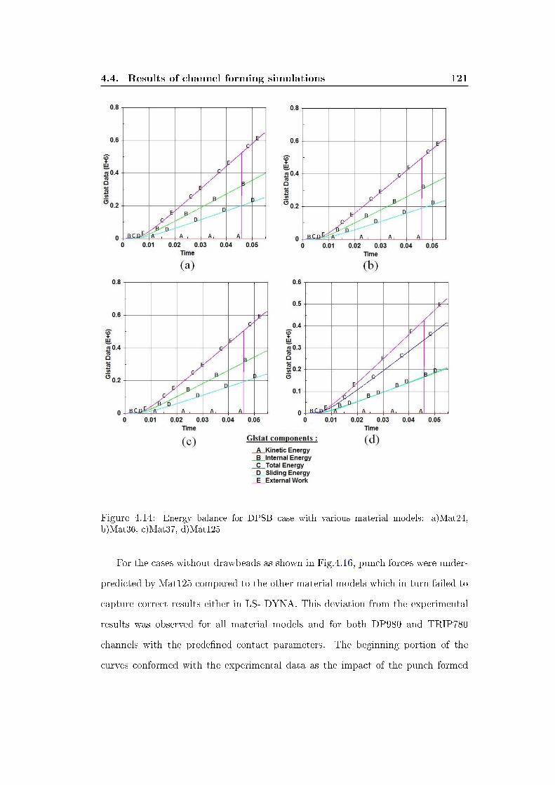
4.4. Results of channel forming simulations 121
Figure 4.14: Energy balance for DPSB case with various material models: a)Mat24,b)Mat36, c)Mat37, d)Mat125
For the cases without drawbeads as shown in Fig.4.16, punch forces were under-
predicted by Mat125 compared to the other material models which in turn failed to
capture correct results either in LS- DYNA. This deviation from the experimental
results was observed for all material models and for both DP980 and TRIP780
channels with the prede�ned contact parameters. The beginning portion of the
curves conformed with the experimental data as the impact of the punch formed
4.4. Results of channel forming simulations 122
the blank. After this initial step, the normal force that was exerted on the blank
by the die was limited to a small contact area of the die radius region. With the
default values of static coe�cient of friction, the stretching force was not su�cient
to maintain the required tension in the blank during the forming stage. When
the movement of the blank was observed during the forming simulation, it became
evident that the blank was under-constrained along its length. In this case, it
was possible to calibrate the friction coe�cient of the contact algorithms so that
the predicted punch force correlated with the experimental results. A study with
various friction coe�cients was performed with material model 24, as shown in
Fig.4.17. This suggests that friction forces at the contact interface between the
blank and die radius would be more prominent in cases where no draw beads were
present. A friction coe�cient equal to 0.19 best conformed with the experimental
data.
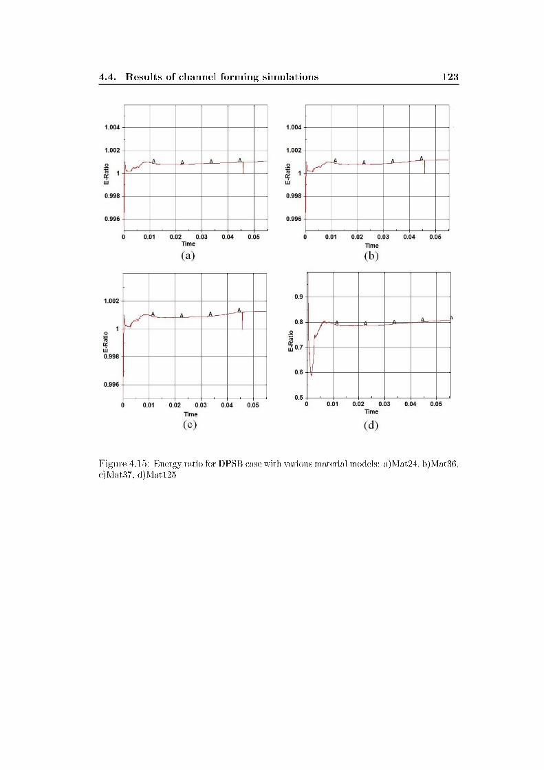
4.4. Results of channel forming simulations 123
Figure 4.15: Energy ratio for DPSB case with various material models: a)Mat24, b)Mat36,c)Mat37, d)Mat125

4.4. Results of channel forming simulations 124
Figure 4.16: Comparison of predicted and experimental punch forces for channels withoutdraw beads and with DER=12mm: a) TRIP780, b)DP980
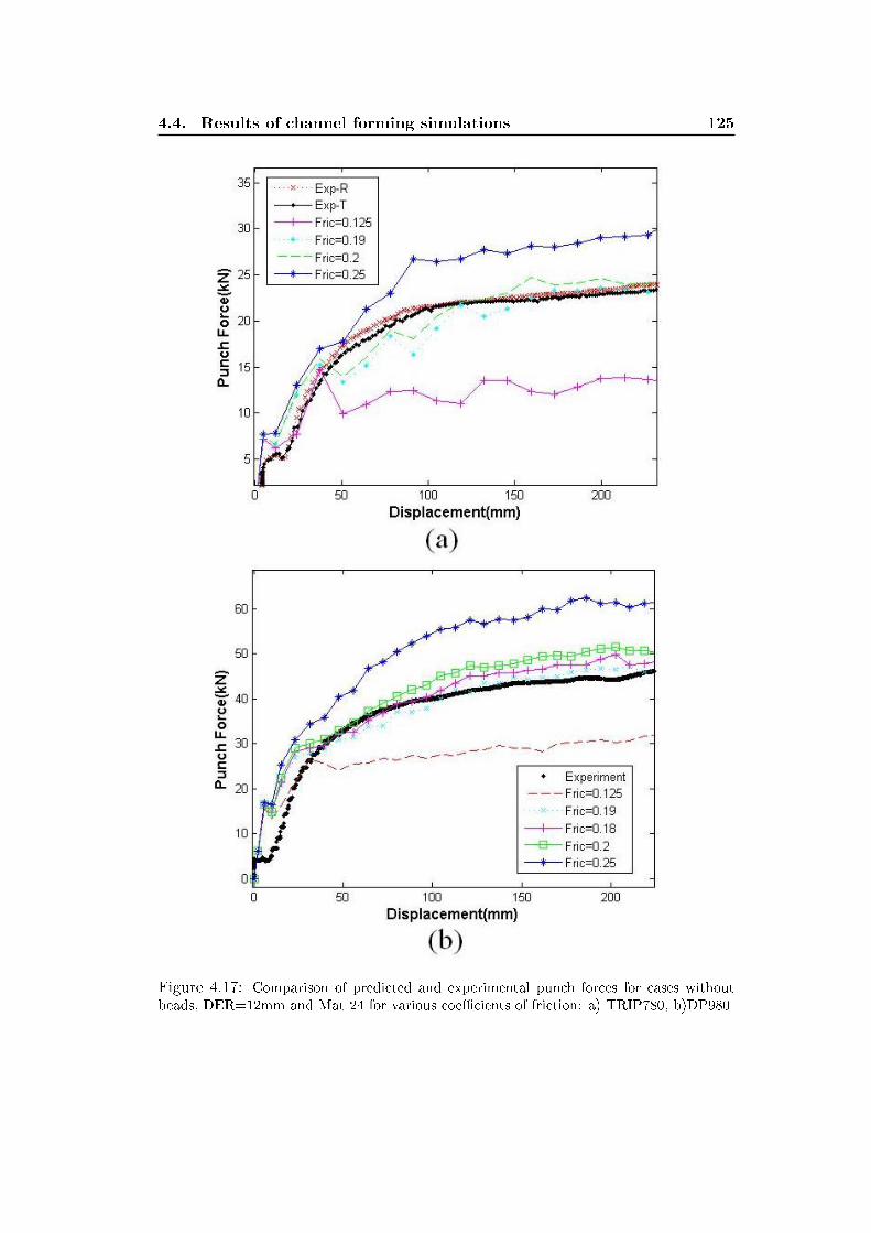
4.4. Results of channel forming simulations 125
Figure 4.17: Comparison of predicted and experimental punch forces for cases withoutbeads, DER=12mm and Mat 24 for various coe�cients of friction: a) TRIP780, b)DP980

4.4. Results of channel forming simulations 126
4.4.2 Channel sidewall pro�les
The �nal geometry of the parts after springback is an important measure for
comparison between di�erent models. Sidewall opening angle, �ange tip angle and
curl radius as de�ned in Fig.3.18 provide appropriate measures for comparing U-
channels parts. However it should be noted that for such open channel geometries a
fairly small angular di�erence coupled with di�erent sidewall curvatures may bring
about a relatively large change in the overall dimensions of the channel. Moreover
they do not provide a single criteria for comparison. For this sake, an area inte-
gration method, used in previous studies, was also further developed as a measure
to estimate the error between simulated and experimental sidewall curl results. For
more elaborate parts or surfaces a cross correlation method might be more appro-
priate.
Figure 4.18: Schematic illustration of sidewall comparison between simulated and experi-mental curves
The error between simulated and experimental channel pro�les was quanti�ed
by computing the area under the curves of both pro�les drawn on a 2D diagram, as
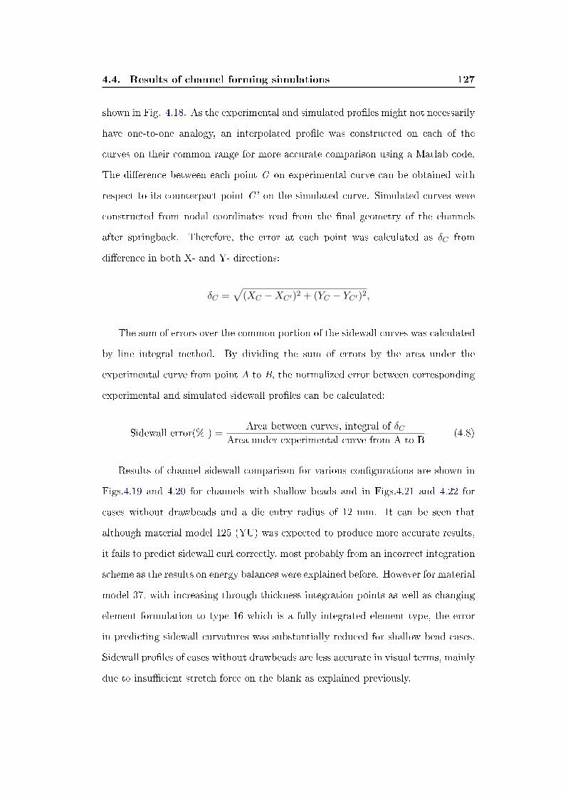
4.4. Results of channel forming simulations 127
shown in Fig. 4.18. As the experimental and simulated pro�les might not necessarily
have one-to-one analogy, an interpolated pro�le was constructed on each of the
curves on their common range for more accurate comparison using a Matlab code.
The di�erence between each point C on experimental curve can be obtained with
respect to its counterpart point C' on the simulated curve. Simulated curves were
constructed from nodal coordinates read from the �nal geometry of the channels
after springback. Therefore, the error at each point was calculated as δC from
di�erence in both X- and Y- directions:
δC =√
(XC −XC′)2 + (YC − YC′)2,
The sum of errors over the common portion of the sidewall curves was calculated
by line integral method. By dividing the sum of errors by the area under the
experimental curve from point A to B, the normalized error between corresponding
experimental and simulated sidewall pro�les can be calculated:
Sidewall error(% ) =Area between curves, integral of δC
Area under experimental curve from A to B(4.8)
Results of channel sidewall comparison for various con�gurations are shown in
Figs.4.19 and 4.20 for channels with shallow beads and in Figs.4.21 and 4.22 for
cases without drawbeads and a die entry radius of 12 mm. It can be seen that
although material model 125 (YU) was expected to produce more accurate results,
it fails to predict sidewall curl correctly, most probably from an incorrect integration
scheme as the results on energy balances were explained before. However for material
model 37, with increasing through-thickness integration points as well as changing
element formulation to type 16 which is a fully integrated element type, the error
in predicting sidewall curvatures was substantially reduced for shallow bead cases.
Sidewall pro�les of cases without drawbeads are less accurate in visual terms, mainly
due to insu�cient stretch force on the blank as explained previously.
4.4. Results of channel forming simulations 128
Figure 4.19: Comparison of simulated and experimental sidewall pro�les for TRIP780channels with shallow beads: a)di�erent material models, b)sidewall error(Eq.4.8)
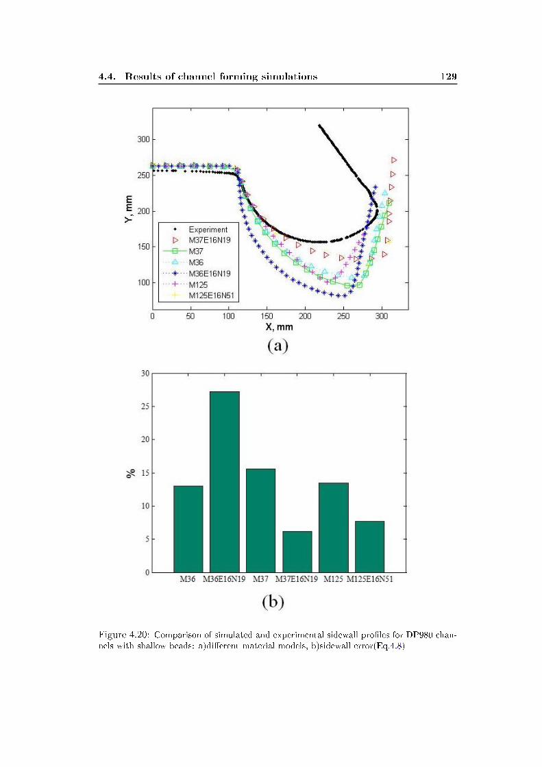
4.4. Results of channel forming simulations 129
Figure 4.20: Comparison of simulated and experimental sidewall pro�les for DP980 chan-nels with shallow beads: a)di�erent material models, b)sidewall error(Eq.4.8)

4.4. Results of channel forming simulations 130
Figure 4.21: Comparison of simulated and experimental sidewall pro�les for TRIP780channels without beads and DER=12mm: a)di�erent material models, b)sidewall er-ror(Eq.4.8)

4.4. Results of channel forming simulations 131
Figure 4.22: Comparison of simulated and experimental sidewall pro�les for DP980 chan-nels without beads and DER=12mm: a)di�erent material models, b)sidewall error(Eq.4.8)
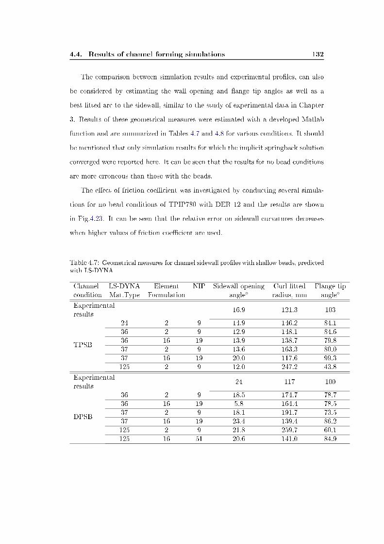
4.4. Results of channel forming simulations 132
The comparison between simulation results and experimental pro�les, can also
be considered by estimating the wall opening and �ange tip angles as well as a
best �tted arc to the sidewall, similar to the study of experimental data in Chapter
3. Results of these geometrical measures were estimated with a developed Matlab
function and are summarized in Tables 4.7 and 4.8 for various conditions. It should
be mentioned that only simulation results for which the implicit springback solution
converged were reported here. It can be seen that the results for no bead conditions
are more erroneous than those with the beads.
The e�ect of friction coe�cient was investigated by conducting several simula-
tions for no bead conditions of TPIP780 with DER 12 and the results are shown
in Fig.4.23. It can be seen that the relative error on sidewall curvatures decreases
when higher values of friction coe�cient are used.
Table 4.7: Geometrical measures for channel sidewall pro�les with shallow beads, predictedwith LS-DYNA
Channel LS-DYNA Element NIP Sidewall opening Curl �tted Flange tipcondition Mat.Type Formulation angle◦ radius, mm angle◦
Experimentalresults
16.9 121.3 103
TPSB
24 2 9 14.9 146.2 84.136 2 9 12.9 148.1 84.636 16 19 13.9 138.7 79.837 2 9 13.6 163.3 80.037 16 19 20.0 117.6 99.3125 2 9 12.0 247.2 43.8
Experimentalresults
24 117 100
DPSB
36 2 9 18.5 174.7 78.736 16 19 5.8 164.4 78.537 2 9 18.1 191.7 73.537 16 19 23.4 139.4 86.2125 2 9 21.8 259.7 60.1125 16 51 20.6 141.0 84.9

4.4. Results of channel forming simulations 133
Table 4.8: Geometrical measures for channel sidewall pro�les without beads and DER=12mm, predicted with LS-DYNA
Channel LS-DYNA Element NIP Sidewall opening Curl �tted Flange tipcondition Mat.Type Formulation angle◦ radius, mm angle◦
Experimentalresults
21 107 126
TPNB12
24 2 9 23.1 131.3 88.236 16 19 24.4 150.2 81.437 2 9 16.0 157.9 78.637 16 19 26.8 147.6 81.637 16 25 23.6 138.4 87.6125 16 9 24.7 198.1 67.3
Experimentalresults
28 122 117
DPNB1224 2 9 22.6 153.6 89.537 2 9 29.9 208.9 92.7125 2 9 28.1 314.4 50.6

4.4. Results of channel forming simulations 134
Figure 4.23: Simulated sidewall pro�les for TPNB12 condition: a)with various frictioncoe�cients, b)sidewall error(Eq.4.8)
4.4. Results of channel forming simulations 135
4.4.3 Thickness reduction and strain distribution
Shell thickness reduction and e�ective plastic and total strain values were ob-
tained for each simulation in LS-DYNA. For TPSB and DPSB conditions, results
of thickness reduction with material type 37, element formulation 16 and 19 inte-
gration points are shown in Fig.4.26, as a representative demonstration. Plastic
strain distributions for the same simulations are displayed in Fig.4.27. It is notable
that maximum values of thickness reduction and plastic strains for conditions with
drawbeads, happened on sidewall of the channels after the impact of drawbeads.
Strains along the width of channels were checked to ensure they are smaller than
strains along width and through the thickness of the blank, con�rming the plane
stress condition of the simulations.
Thickness reduction and strain outputs of simulations for channels with and
without beads and various models were summarized in Table 4.9. It should be
noted that in order to compare simulation results with experimental values, maxi-
mum and minimum strains should be used instead of the plastic strains. As shown
for a representative case of the forming simulations in Fig.4.24, maximum principal
strains on lower, upper and mid surfaces of a shell element - which passes through
the drawbead, over the die radius and ends up in the sidewall - converges to an
average strain value, while the e�ective plastic strain is the accumulated result of
the entire strain history. Minimum principal strains for the same element are also
shown in Fig.4.25 and these converge to a value which is approximately the negative
value of the maximum strain. The abrupt change that is obsevered in the strain
history on the lower surface of this element (curve C), is due to the element pass-
ing through the drawbead region. But it can be seen that the strain levels on the
upper and lower surfaces converged to the strain at the mid-plane. The simulation
results that were reported in Table 4.9 showed an acceptable conformity with the
experimental data summarized in Table 3.5.

4.4. Results of channel forming simulations 136
Table 4.9: Summary of maximum values of thickness reduction and plastic strains predictedin the channel sidewallsChannel LS-DYNA Element NIP Max. Thickness Major sidewallcondition Mat.Type Formulation reduction (%) strain (%)
Experimentalresults
5.8 4.0
TPSB
24 2 9 4.6 4.036 2 9 4.5 4.136 16 19 4.4 4.137 2 9 4.3 3.937 16 19 4.7 4.2125 2 9 4.5 2.5
Experimentalresults
3.4 2.4
DPSB
24 2 9 5.4 4.836 16 19 5.8 4.237 2 9 5.1 4.937 16 19 4.8 3.6125 2 9 2.1 3.4125 16 51 3.2 3.4
Experimentalresults
1.25 0.8
TPNB12
24 2 9 1 0.0836 2 9 0.6 0.0637 2 9 0.5 0.06125 2 9 0.4 0.04
Experimentalresults
0.6 0.8
DPNB1224 2 9 0.9 0.0937 2 9 0.5 0.8125 2 9 1 0.01

4.4. Results of channel forming simulations 137
Figure 4.24: Maximum principal strain histories for an element on the sidewall of TPSBchannel forming simulation
Figure 4.25: Minimum principal strain histories for an element on the sidewall of TPSBchannel forming simulation
Finally, the shell thickness reduction and e�ective plastic strain distributions for
TPSB and DPSB cases simulated with Mat37 model are shown in Figs.4.26 and
4.27, respectively.

4.4. Results of channel forming simulations 138
Figure 4.26: Shell thickness reduction (%) for TPSB and DPSB conditions

4.4. Results of channel forming simulations 139
Figure 4.27: E�ective plastic strain distributions for TPSB and DPSB conditions
140
Chapter 5
Final Discussions and Conclusions
In the previous chapters, various experimental results of the channel draw form-
ing were presented and then compared with predicted results in LS-DYNA. Di�erent
material models were used to simulate the forming and springback of the U-channel
sections made from advanced high strength materials TRIP780 and DP980. Also
speci�c material characterization tests were performed on these two grades of AHSS.
Neither the TRIP780 nor the DP980 material showed any work-hardening stag-
nation during cyclic tension-compression tests, however, both sheet materials ex-
hibited signi�cant transient work-hardening during reverse loading. Both materials
also showed signi�cant Bauschinger e�ect although it was less signi�cant for DP980
material, as the yield stress during reverse loading was closer to that in forward
loading than TRIP780. The isotropic hardening model (IH) which is implemented
in material types 24, 36 and 37 of LS-DYNA, is not able to accurately describe
the cyclic behaviour of either materials. Although this prediction can be improved
when numerical parameters are �nely tuned with Nelder-Mead simplex optimization
method, as shown in Fig.5.1, but it still cannot predict the reverse loading or the
re-loading behaviours.

141
Figure 5.1: Modi�ed prediction of cyclic behaviour of TRIP780 sheet metal by the isotropichardening law
The combined isotropic-linear kinematic hardening model (which is also available
in LS-DYNA as material model 3, MAT_PLASTIC_KINEMATIC ) is also not able
to accurately predict the cyclic behaviour of the two sheet steels as it can be seen in
Fig.5.2. However, the cyclic behaviour of TRIP780 and DP980 is very well predicted
with the YU model (Mat125), as shown in Fig.4.5.

142
Figure 5.2: Prediction of the cyclic behaviour of a)TRIP780 and b)DP980 with the com-bined isotropic-linear kinematic hardening law
Since the YU model is able to predict the actual cyclic behaviour of these sheet

143
material, it was expected that it would also accurately predict the actual forming and
springback of the channel section. However, the miscalculation of energy balances
and probably the stress state with the YU model (Mat 125) limits its applicability.
This is because of the incorrect implementation of the YU model in LS-DYNA
solver (version 971 edition R5.1.1). To show this, the energy balance and punch
force results predicted with the YU model in ABAQUS were examined in Chapter 4
and did not exhibit such error for a similar representative case (TPSB), in Figs.4.10
and 4.11.
Further comparison can be made from the results of simulations in ABAQUS
with those from LS-DYNA. Fig.5.3 compares the predicted channel sidewall pro�les
for the TPSB case carried out with both ABAQUS and LS-DYNA. The YU material
model, with the parameters in Table 4.3, was used to obtain these results. As can
be seen, more accurate prediction of the channel pro�le is achieved by YU model in
ABAQUS than LS-DYNA. A similar result is also observed for the DPSB case. In
terms of the sidewall curvature, less than 8% error was calculated for the simulation
results with ABAQUS compared to the experimental results. Another interesting
result is the over-prediction of the channel pro�les with the YU model with respect
to the experimental values in ABAQUS. This is most probably due to the fact that
the material parameters reported by Shi et. al [46] were not optimized for the
DP980 material used in the current study. It is intended to continue this aspect
of the research using an optimization code for ABAQUS, and also when the bug is
�xed for Mat125 in LS-DYNA.
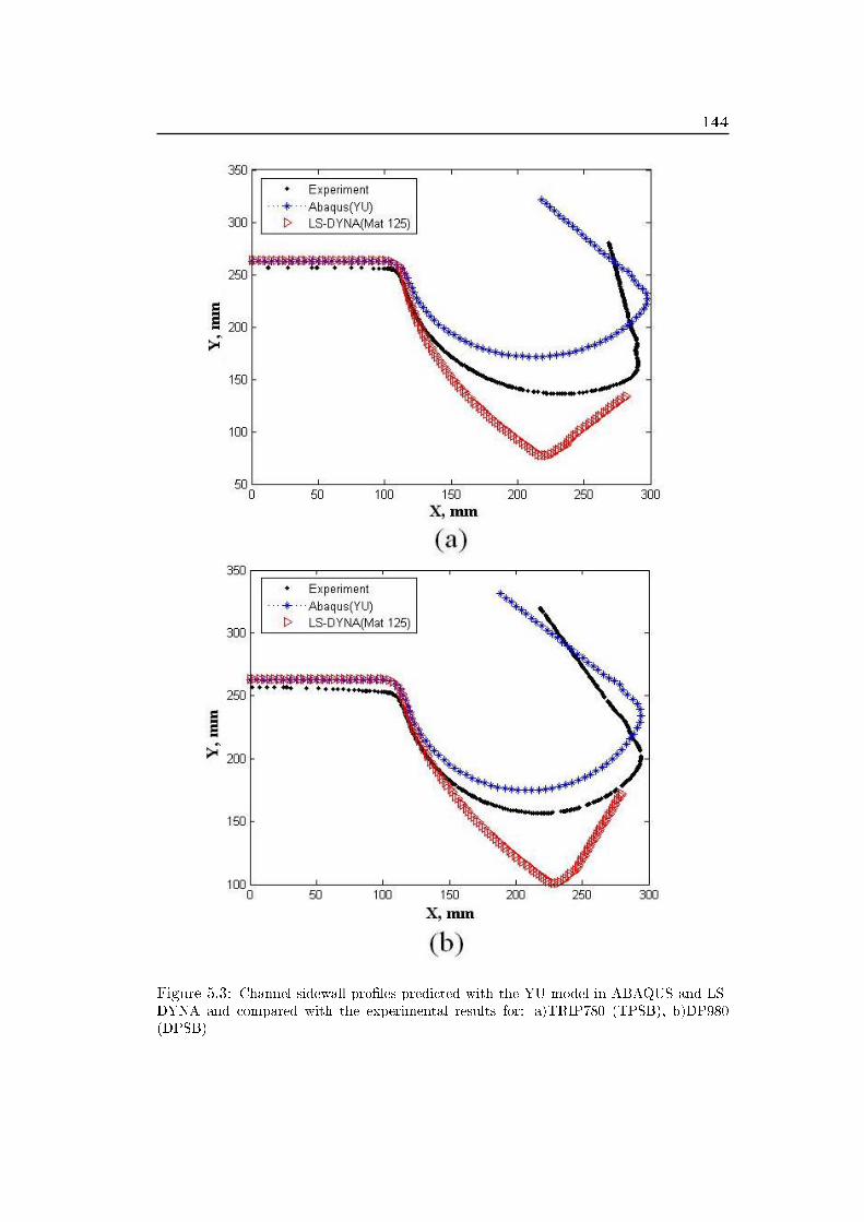
144
Figure 5.3: Channel sidewall pro�les predicted with the YU model in ABAQUS and LS-DYNA and compared with the experimental results for: a)TRIP780 (TPSB), b)DP980(DPSB)
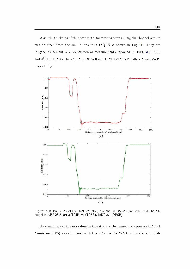
145
Also, the thickness of the sheet metal for various points along the channel section
was obtained from the simulations in ABAQUS as shown in Fig.5.4. They are
in good agreement with experimental measurements reported in Table 3.5, by 2
and 3% thickness reduction for TRIP780 and DP980 channels with shallow beads,
respectively.
Figure 5.4: Prediction of the thickness along the channel section predicted with the YUmodel in ABAQUS for: a)TRIP780 (TPSB), b)DP980 (DPSB)
As a summary of the work done in this study, a U-channel draw process (BM3 of
Numisheet 2005) was simulated with the FE code LS-DYNA and material models

146
24, 36, 37 and 125 for TRIP780 and DP980 sheet materials. Experimental channel
sections were drawn with various drawbead penetrations and without drawbeads
but with di�erent die entry radii. Based on the numerical studies of Chapter 4 and
comparisons with the experimental results in Chapter 3, the following conclusions
can be drawn for this study:
1. For advanced high strength steels such as TRIP780 and DP980, parameters of
the constitutive model have a great impact on the convergence of the spring-
back simulations. Without appropriate parameters, it is likely that the implicit
springback simulation will not converge to an appropriate solution.
2. From the material models in the LS-DYNA library, Mat 125 (YU) failed to
predict accurate sprungback and sidewall curl results. The stress and strain
distributions and various energy levels predicted with this material model
show signi�cant deviation from what is predicted by other material models.
These results were also di�erent from results predicted with the YU model
implemented in ABAQUS used-de�ned model.
3. Mat 37 (transverse anisotropy constitutive model) with increased number of
integration points (up to 19) yielded more accurate results than other material
models in the LS-DYNA library which were used to predict the sidewall curl
of channels made of TRIP780 and DP980.
4. The severity of sidewall curl increased when no drawbeads were used and also
when a tighter die entry radius was used for both TRIP780 and DP980.
5. When drawbeads were used in the channel draw process, springback (wall
opening angle) decreased but sidewall curl increased in the channel sections
for both TRIP780 and DP980.
6. By comparison of the sprungback channel sidewall pro�les of TRIP780 when
the blanks were taken parallel and perpendicular to the sheet rolling direction,

147
it was concluded that in-plane anisotropy did not have a signi�cant e�ect on
the �nal sidewall curl. Tensile test results for samples cut at di�erent angles
with respect to the rolling direction also did not show signi�cant variations.
7. Channels made of TRIP780 show less sidewall curl and less springback angle
than those made of DP980.
8. The unloading elastic modulus of TRIP780 and DP980 was determined for a
range of strain up to 0.1. Although the results were �tted to the empirical
decaying function of plastic strains, the decreasing trend is expected to con-
tinue even beyond this strain level. Further investigations are in progress in
this regard.
9. The YU model implemented in ABAQUS with a user de�ned subroutine pro-
duced less than 8% error in predicting sidewall curl for channels made of
TRIP780 and DP980 with the shallow drawbead con�guration. Similar re-
sults are expected with LS-DYNA once the implementation of this constitutive
model is corrected in the solver or a user-de�ned material model is developed
for Yoshida in LS-DYNA.
10. The coe�cient of friction had an important e�ect in predicting punch force
results of the forming stage when no drawbeads were present in the model.
When drawbeads were used, the tension force on the blank was mainly pro-
duced in the drawbead region and the friction coe�cient had a minor e�ect.
11. The amount of predicted sidewall curl and springback depended on the mate-
rial constants which were obtained by �tting the simulated stress-strain curves
to the experimental data. Therefore an optimization method was required to
minimize the �tting error and globally determine the best set of parameters. It
is worth noting various sets of material parameters are expected from di�erent
types of cyclic tests, and this may a�ect the accuracy of the results. Further
investigation is required in this regard.

148
Appendix A
Simulation of B-pillar
The forming and springback of an industrial auto body part known as B-pillar
made of DP980 sheet steel with a thickness of 1.5 mm was simulated with LS-
DYNA. The FE model of the forming process was created and analyzed here, using
the �ndings from the current study. Material model 37 with 19 integration points
through the thickness and fully integrated element formulation (type 16) was used.
The upper and lower tools were created with zero o�set as shown in Fig.A.1. Two
�FORMING_ONE_WAY_SURFACE_TO_SURFACE� contact algorithms with a
friction coe�cient of 0.1 were de�ned between the blank and the upper and lower
tools. A prescribed rigid motion boundary condition in the form of a velocity curve
was assigned to the upper tool to form the part in one step until the complete closure
of the die. Adaptive meshing and other control parameters were assigned similar
to the channel forming simulations. The deformed part after the forming stage was
submitted to an implicit springback solution by �xing three points to eliminate the
rigid body motion of the part. The result of the forming stage is shown Fig.A.2
and the result of the springback stage is shown in Fig.A.3 which showed very little
springback or twist in the part. More investigation for the improvement of the
analysis is in progress.
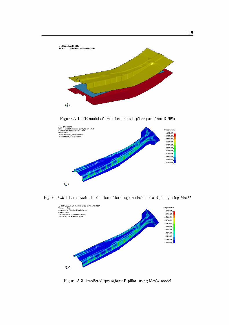
149
Figure A.1: FE model of crash forming a B pillar part from DP980
Figure A.2: Plastic strain distribution of forming simulation of a B-pillar, using Mat37
Figure A.3: Predicted sprungback B-pillar, using Mat37 model
150
Bibliography
[1] AHSS application guidelines. Technical report, World Auto Steel, June, 2009.
(Cited on pages 4, 5, 6, 7, 8, 9 and 10.)
[2] R. A. Ayres. Shapeset: A process to reduce sidewall curl springback in high
strength rails. Applied Metalworking, 2(3):127�134, 1984. (Cited on page 14.)
[3] S. Al. Azraq, R. Teti, and J. Costa. Springback prediction with FEM analysis of
advanced high strength steel stamping process. Intelligent Production Machines
and Systems, pages 264�269, 2006. (Cited on page 20.)
[4] I. A. Burchitz. Improvement of Springback Prediction in Sheet Metal Forming.
PhD thesis, Twente University, 2008. (Cited on page 11.)
[5] M.S. Bzdok, J. Fekete, and C Du. High strength steel stamping projects.
Technical report, Auto/Steel Partnership, 2005. (Cited on page 15.)
[6] J. Cao and Th. Buranathiti. An e�ective analytical model for springback pre-
diction in straight �anging processes. International Journal of Manufacturing
and Product Technology, 21:137�153, 2004. (Cited on pages 16 and 17.)
[7] J. Cao, W. Lee, H. S. Cheng, M. Seniw, H.P. Wang, and K. Chung. Experi-
mental and numerical investigation of combined isotropic-kinematic hardening
behavior of sheet metals. International Journal of Plasticity, 25(5):942�972,
2009. (Cited on page 31.)
[8] J. Chaboche. A review of some plasticity and viscoplasticity constitutive the-
ories. International Journal of Plasticity, 24(10):1642�1693, 2008. (Cited on
page 27.)
[9] J.L. Chaboche. Time-independent constitutive theories for cyclic plasticity.
International Journal of Plasticity, 2(2):149�188, 1986. (Cited on page 29.)

Bibliography 151
[10] F.K. Chen and P.C. Tseng. Deformation analysis of side-wall curl in the sheet
metal forming of �anged channels. Journal of Manufacturing Science and En-
gineering, 127(2):369�375, 2005. (Cited on page 17.)
[11] N. Christodoulou, O.T. Woo, and S.R. MacEwen. E�ect of stress reversals
on the work hardening behaviour of polycrystalline copper. Acta Metallurgica,
34(8):1553�1562, 1986. (Cited on page 38.)
[12] C. C. Chu. The e�ect of restraining force on springback. International Journal
of Solids Structures, 8(27):1035�1046, 1991. (Cited on page 16.)
[13] K. Chung, M. Lee, D. Kim, C. Kim, M. L. Wenner, and F. Barlat. Spring-back
evaluation of automotive sheets based on isotropic-kinematic hardening laws
and non-quadratic anisotropic yield functions Part I : theory and formulation.
International Journal of Plasticity, 21:861�882, 2005. (Cited on pages 20, 21
and 26.)
[14] J.M. Collin, T. Parenteau, G. Mauvoisin, and P. Pilvin. Material parame-
ters identi�cation using experimental continuous spherical indentation for cyclic
hardening. Computational Materials Science, 46(2):333�338, 2009. (Cited on
page 32.)
[15] R. G. Davies. Side-wall curl in high-strength steels. Applied Metalworking,
2(3):120�126, 1984. (Cited on page 14.)
[16] F. Dunne and N. Petrinic. Introduction to Computational Plasticity. Oxford
University press, 2005. (Cited on pages 23 and 25.)
[17] P. Eggertsen and K. Mattiasson. On constitutive modeling for springback anal-
ysis. International Journal of Mechanical Sciences, 52(6):804�818, 2010. (Cited
on page 32.)
[18] P. Eggertsen and K. Mattiasson. On the identi�cation of kinematic hardening

Bibliography 152
material parameters for accurate springback predictions. International Journal
of Material Forming, 4(2):103�120, 2010. (Cited on page 37.)
[19] P. Eggertsen and K. Mattiasson. On the modeling of the unloading modulus
for metal sheets. International Journal of Material Forming, 3(S1):127�130,
2010. (Cited on pages 39 and 41.)
[20] Barlat F., J.M. Ferreira, J.J. Gracio, Lopes A.B., and Rauch E.F. Plastic
�ow for non-monotonic loading conditions of an aluminum alloy sheet sample.
International Journal of Plasticity, 19:1215�1244, 2003. (Cited on page 31.)
[21] M. Firat, B. Kaftanoglu, and O. Eser. Sheet metal forming analyses with
an emphasis on the springback deformation. Journal of Materials Processing
Technology, 196(1-3):135�148, 2008. (Cited on pages 22, 23, 28 and 30.)
[22] Chen F.K. and Tseng P.C. Deformation analysis of sidewall curl in sheet metal
forming of �anged channels. Manufacturing Science and Engineering, 127:369�
375, 2005. (Cited on page 3.)
[23] C.O. Frederick and P.J. Armstrong. A Mathematical representation of the
multiaxial Bauschinger e�ect. Technical report, G.E.G.B Report RD/B/N731,
1966. (Cited on page 29.)
[24] L. Geng and R.H. Wagoner. Role of plastic anisotropy and its evaluation in
springback. International Journal of Mechanical Sciences, 44(1):123�148, 2002.
(Cited on page 23.)
[25] A. Ghaei. Modeling springback in stamped automotive structures. PhD thesis,
University of Windsor, 2009. (Cited on pages 19, 26, 106 and 109.)
[26] A. Ghaei and D.E. Green. Numerical implementation of Yoshida-Uemori two-
surface plasticity model using a fully implicit integration scheme. Computa-
tional Materials Science, 48(1):195�205, 2010. (Cited on page 22.)
Bibliography 153
[27] D. E. Green. Description of Numisheet 2005 Benchmark #3 stage-1: Chan-
nel Draw with 75% drawbead penetration. Proceedings of Numisheet 2005,
B(1):894�904, 2005. (Cited on page 11.)
[28] T. Hasegawa, T. Yakou, and S. Karashima. Deformation behaviour and dislo-
cation structures upon stress reversal in polycrystalline aluminum. Materials
Science and Engineering, 20:267�276, 1975. (Cited on page 38.)
[29] Y. Hayashi and M. Tagagi. Control of side-wall curl in draw-bending of high
strength steel sheets. Advanced Technology of Plasticity, 1:735�740, 1984.
(Cited on page 14.)
[30] Miyauchi K. A proposal of a planar simple shear test in sheet metals. Scienti�c
Papers of the Institute of Physical and Chemical Research, 78(3):27�40, 1984.
(Cited on page 31.)
[31] L. Kessler, M. S. Aydin, and J. Gerlach. Springback simulation with complex
hardening material models. In 7th LS-DYNA Conference, pages 1�10, 2008.
(Cited on pages 21 and 33.)
[32] A. S. Khan and S. Huang. Continuum Theory of Plasticity. John Wiley &
Sons. Inc., 1996. (Cited on page 28.)
[33] J. K. Kim and P. F. Thomson. Springback and side-wall curl of galvanized
and galvalume steel sheets. Mechanical Working Technology, 19:223�238, 1989.
(Cited on page 15.)
[34] T. Kuwabara, Y. Morita, Y. Miyashita, and S. Takahashi. Elastic-plastic behav-
ior of sheet metal subjected to in-plane reverse loading. In 5-th International
Symposium on Plasticity and its current applications, pages 841�844, 1995.
(Cited on page 30.)
[35] M.G. Lee, D. Kim, R. H. Wagoner, and K. Chung. Semi-Analytic hybrid
Bibliography 154
method to predict springback in the 2D draw bend test. Journal of Applied
Mechanics, 74(6):1264�1275, 2007. (Cited on pages 17 and 18.)
[36] B.S. Levy, C.J. Van Tyne, Y.H. Moon, and C. Mikalsen. The e�ective unloading
modulus for automotive sheet steels. In Proceeding of SAE 2006 World Congress
& Exhibition, Detroit, MI, USA, pages 264�269, 2006. (Cited on pages 39
and 84.)
[37] Y. C. Liu. The e�ect of restraining force on shape deviations in �anged channels.
ASME Journal of Engineering Materials Technology, 110:389�394, 1988. (Cited
on page 14.)
[38] Livermore Software Technology Corporation (LSTC). LS-DYNA keyword user's
manual. Vol. I. version 971, 2007. (Cited on pages 32 and 45.)
[39] D. Matlock, T.B. Hilditch, and J. Speer. In�uence of low-strain deformation
characteristics of high strength sheet steel on curl and springback in bend-
under-tension tests. Journal of Materials Processing Technology, 182(1-3):84�
94, 2007. (Cited on page 21.)
[40] O. E. Mattiasson and Enqvist B. K. Identi�cation of material hardening pa-
rameters by the three-point bending of metal sheets. International Journal of
Mechanical Sciences, 48:1525�1532, 2006. (Cited on page 31.)
[41] Y. Moon, D Kim, and C Vantyne. Analytical model for prediction of side-
wall curl during stretch-bend sheet metal forming. International Journal of
Mechanical Sciences, 50(4):666�675, 2008. (Cited on page 19.)
[42] Genevois P. Etude expérimentale et modélisation du comportement plastique
anisotrope de tôles d'acier en grandes déformations. PhD thesis, Institute Na-
tional Polytechnique de Grenoble, 1992. (Cited on page 31.)
[43] F. Pourboghrat and E.Chu. Prediction of spring-back and side-wall curl in 2-d
Bibliography 155
draw bending. Materials Processing Technology, 50:361�374, 1995. (Cited on
pages 3 and 16.)
[44] E.F. Rauch. Plastic anisotropy of sheet metals determined by simple shear
tests. Journal of Material Science and Engineering, 241:179�183, 1998. (Cited
on page 31.)
[45] M. Samuel. Experimental and numerical prediction of springback and side wall
curl in U-bendings of anisotropic sheet metals. Journal of Materials Processing
Technology, 105(3):382�393, 2000. (Cited on page 20.)
[46] M. F. Shi, X Zhu, C. Xia, and T. Stoughton. Determination of nonlinear
isotropic/kinematic hardening constitutive parameters for AHSS using tension
and compression tests. In Proceedings of Numisheet 2008, pages 264�270, 2008.
(Cited on pages 104, 105 and 143.)
[47] N. Stander, W. Roux, T. Eggleston, and K. Craig. LS-OPT User's Manual,
version 4.2. (Cited on pages 32 and 101.)
[48] A. Taherizadeh, A. Ghaei, D. E. Green, and W. J. Altenhof. Finite element sim-
ulation of springback for a channel draw process with drawbead using di�erent
hardening models. International Journal of Mechanical Sciences, 51(4):314�
325, 2009. (Cited on page 22.)
[49] S. C. Tang. Analysis of springback in sheet forming operation. Advanced
Technology of Plasticity, I:193�197, 1987. (Cited on page 15.)
[50] L. Taylor, J. Cao, M. C. Kara�llis, and M. C. Boyce. Numerical simulations
of sheet-metal forming. Materials Processing Technology, 50:168�179, 1995.
(Cited on page 15.)
[51] N. E. Thompson and C. H. Ellen. A simple theory for side-wall curl. Applied
Metalworking, 1(4):39�42, 1985. (Cited on page 15.)

Bibliography 156
[52] R. Wagoner and M. Li. Simulation of springback: Through-thickness inte-
gration. International Journal of Plasticity, 23(3):345�360, 2007. (Cited on
page 18.)
[53] R.H. Wagoner, R.K. Boger, F. Barlat, M.G. Lee, and K. Chung. Continu-
ous, large strain, tension/compression testing of sheet material. International
Journal of Plasticity, 21(12):2319�2343, 2005. (Cited on page 31.)
[54] D.Y. Yang and S.W Lee. An assessment of numerical parameters in�uenc-
ing springback in explicit �nite element analysis of sheet metal forming pro-
cess. Journal of Materials Processing Technology, 80-81:60�67, 1998. (Cited on
page 19.)
[55] H. K. Yi, D. W. Kim, C. J. Van Tyne, and Y. H. Moon. Analytical prediction
of springback based on residual di�erential strain during sheet metal bending.
Journal of Mechanical Engineering Science, 222(2):117�129, 2008. (Cited on
page 18.)
[56] F. Yoshida, Urabe M., and V.V. Toropov. Identi�cation of material parameters
in constitutive model for sheet metals from cyclic bending tests. International
Journal of Mechanical Sciences, 40:237�249, 1998. (Cited on pages 31 and 32.)
[57] F. Yoshida and T. Uemori. A model of large-strain cyclic plasticity describing
the Bauschinger e�ect and work-hardening stagnation. International Journal
of Plasticity, 18(5-6):661�686, 2002. (Cited on pages 29, 32, 33 and 43.)
[58] F. Yoshida and T. Uemori. A model of large-strain cyclic plasticity and its
application to springback simulation. International Journal of Mechanical Sci-
ences, 45:1687 � 1702, 2003. (Cited on pages 34, 35 and 40.)
[59] F. Yoshida, T. Uemori, and S. Abe. Modeling of large-strain cyclic plasticity for
accurate springback simulation. Key Engineering Materials, 340-341:811�816,
2007. (Cited on page 38.)
Bibliography 157
[60] F. Yoshida, T. Uemori, and K. Fujiwara. Elastic-plastic behavior of steel sheets
under in-plane cyclic tension-compression at large strain. International Journal
of Plasticity, 18(5-6):633�659, 2002. (Cited on pages 29, 30, 41 and 42.)
[61] F. Yoshida, M. Urabe, R. Hino, and V.V. Toropov. Inverse approach to identi�-
cation of material parameters of cyclic elasto-plasticity for component layers of
a bimetallic sheet. International Journal of Plasticity, 19(12):2149�2170, 2003.
(Cited on page 32.)
[62] D. Zhang, Z. Cui, X. Ruan, and Y. Li. An analytical model for predicting
springback and side wall curl of sheet after U-bending. Computational Materials
Science, 38(4):707�715, 2007. (Cited on page 18.)
[63] K. M. Zhao and J. K. Lee. Generation of cyclic stress-strain curves for sheet
metals. Journal of Engineering Materials and Technology, 123(4):391�395,
2001. (Cited on page 31.)

158
VITA AUCTORIS
NAME Ali Aryanpour
PLACE OF BIRTH DEZFOOL, IRAN
YEAR OF BIRTH 1977
EDUCATION KAMAL HIGH SCHOOL, TEHRAN, IRAN
1991 - 1995
Sharif University, Tehran, IRAN
1995 - 1999, B.A.Sc.
University of Windsor, Windsor, Ontario
2009 - 2011, M.A.Sc.