PHYSICAL REVIEW E 85, 066119 (2012)

Existence and significance of communities in the World Trade Web

Carlo Piccardi*

Department of Electronics and Information, Politecnico di Milano, Piazza Leonardo da Vinci 32, I-20133 Milano, Italy

Lucia TajoliDepartment of Management, Economics and Industrial Engineering, Politecnico di Milano, I-20133 Milano, Italy

(Received 28 February 2011; revised manuscript received 22 May 2012; published 18 June 2012)

The World Trade Web (WTW), which models the international transactions among countries, is a fundamentaltool for studying the economics of trade flows, their evolution over time, and their implications for a number ofphenomena, including the propagation of economic shocks among countries. In this respect, the possible existenceof communities is a key point, because it would imply that countries are organized in groups of preferentialpartners. In this paper, we use four approaches to analyze communities in the WTW between 1962 and 2008,based, respectively, on modularity optimization, cluster analysis, stability functions, and persistence probabilities.Overall, the four methods agree in finding no evidence of significant partitions. A few weak communities emergefrom the analysis, but they do not represent secluded groups of countries, as intercommunity linkages are alsostrong, supporting the view of a truly globalized trading system.

DOI: 10.1103/PhysRevE.85.066119 PACS number(s): 89.75.Hc, 89.65.Gh

I. INTRODUCTION

Among the many real-world networks studied in theliterature, the World Trade Web (WTW) has recently receivedincreasing attention because of a number of interesting fea-tures. It is quite natural to represent international transactionsamong countries as a network, where countries are the nodesand the connecting edges are the international trade flowsbetween them, giving rise to an intricate system of exchangesaffecting all the countries. The specific economic motivationsdriving international trade flows shape this network, whichconsequently displays characteristics that are relevant for theireconomic implications, as well as for the network analysis initself.

The main topological properties observed in the WTWindicate that this network is disassortative, with a highclustering coefficient and a number of small-world properties[1–4]. Its evolution over time is slow, showing an increasingconnectivity among nodes [5].

In what follows, we use the term “globalization” accordingto the definition given by Deardorff [6], “The increasing world-wide integration of markets for goods, services and capital,”or by Robertson [7], “Globalization refers to the compressionof the world and the intensification of consciousness of theworld as a whole.” (We note that many other definitions ofglobalization exist, not always in full agreement: also, in hisglossary, Deardorff [6] quotes alternative definitions.) Bothdefinitions stress the idea that globalization is affecting theworld as a whole, and here we stress the economic aspectsof globalization as economic integration between countries.A number of indicators show its rapid increase over time(see, e.g., Williamson [8] or Baldwin and Martin [9]), but thepatterns of this integration can be quite different: for example,economic integration can increase at the regional level ratherthan “globally,” and this has important consequences for

*Corresponding author: carlo.piccardi@polimi.it

many issues, such as the way in which economic shocks aretransmitted among countries and the extent of competitionbetween countries in the international market. This is also trueusing network analysis to measure the economic integrationin the WTW, as the overall high degree of connectivity in thenetwork might, nonetheless, imply quite different underlyingnetwork structures.

The aim of this paper is to study the possible existenceof communities within the WTW to better understand thecharacteristics of economic integration. In general terms,a significant network community is a set of nodes withstrong internal connections, much stronger than those withthe remaining nodes of the network. Applying communityanalysis to the WTW should reveal groups of countries withprivileged relationships, originating by geographical vicinity,trade agreements, common language or religion, traditionalpartnerships, etc. What defines a community, therefore, isstrong commercial ties (compared to the rest of the world)rather than common individual characteristics of the nodes,such as economic size, level of development, and even thenumber or strength of their links.

So far, very few studies have analyzed communities, orclustering, within the WTW [10–13], possibly because ofthe many open issues still existing in the methodologies forcommunity analysis [14]. It is indeed problematic to interpretthe results of these studies. Reyes et al. [11], looking forcommunities in the WTW, use as a benchmark the groupsof countries that signed regional trade agreements, and theyfind that, over time, the formation of communities followsan irregular pattern. Instead, He and Deem [13] move froma peculiar definition of distance and clusters within thenetwork to find that clustering declined over time, making theworld increasingly “global.” Barigozzi et al. [12] examine theWTW considering sectoral trade flows, finding no clear timetrend in community formation. They observe heterogeneouscommunity structures in different sectors, even though itis impossible to compare the significance of the differentcommunities. The above-mentioned studies define and detect

066119-11539-3755/2012/85(6)/066119(12) ©2012 American Physical Society

CARLO PICCARDI AND LUCIA TAJOLI PHYSICAL REVIEW E 85, 066119 (2012)

communities in the WTW in distinct ways, but in all cases itis quite difficult to assess the significance of the partitions thatemerge.

In this paper, we look for communities in the WTW inthe period between 1962 and 2008, and we compare differentmethodologies to search for communities in networks, in orderto verify the robustness of the results that we obtain. All themethods applied here base the search for a community on theidentification of a group of countries sharing a disproportionateamount of trade among them compared with the trade they havewith the rest of the world. From the economic point of view,the existence of communities would imply that countries tradeespecially with a group of preferential partners and trade tendsto be “regionalized,” especially if communities coincide withgroups of geographically close countries [15]. Instead, in aglobalized world defined as a whole, as we recalled above, wedo not expect communities to be significant, as countries canbe connected through trade to nearly any country in the worldwith similar ease.

Our analyses shed many doubts on the existence ofcommunities in the WTW, as the results show that the networkis not significantly split between different groups. Some“weak” communities emerge, but these groups of countriesare not more connected with each other than with the restof the world to the extent of forming truly privileged orexclusive relationships, supporting the view of a globalizedtrading system.

II. THE WORLD TRADE WEB

Data for our analysis come from the Direction of TradeStatistics published by the International Monetary Fund (IMF)and from the NBER-UN Trade Data data set made availableby the Center for International Data at the University ofCalifornia, Davis, which is an elaboration from United Nationstrade data by Feenstra et al. [18]. We use annual bilateralimports for the years 1962, 1965, 1970, 1975, 1980, 1985,1990, 1995, 2000, 2005, and 2008. More precisely, we useIMF data for the 1985–2008 period and NBER-UN data forthe previous years, which are not covered in the IMF database.We note that the two sources are strongly consistent in theyears for which they are both available (1985–2000) [19].

A number of important events affected the patterns ofworld trade in the period considered: the end of coloniallinks, changes in the exchange rate regime, the removal ofmany barriers to trade, and the increasing role of emergingcountries in the international markets. Our observation periodstops before the outbreak of the financial crisis began to affectinternational trade, which was still growing, by 15% in valuein 2008, before the dramatic drop recorded in 2009.

We use directed flows received by an importing countryfrom any given exporting country, measuring the value in USdollars at current prices of all merchandise imported by acountry from each partner country (import data are generallymore reliable and complete than export data). We preferdirected data because the direction of trade is economicallyimportant and there is no a priori reason to expect symmetry inbilateral trade flows. However, in order to thoroughly validateour community analysis, we also consider a symmetrizedversion of the trade network (see Sec. III). Finally, we note

that here we are not concerned with the change in prices overtime, as we do not carry out any time series analysis, but weconsider the existence of communities in each year separately(for other analyses of the WTW as a directed network, see [5]and [12]).

The WTW is then modeled as a directed, weighted networkcomposed of N nodes corresponding to countries (N ={1,2, . . . ,N} is the set of nodes) and L edges representingthe trade flows among countries. We denote by W = [wij ] theN × N weight matrix, where wij � 0 is the trade flow fromcountry i to country j . The connectivity matrix A = [aij ] is theN × N matrix, where aij = 1 if wij > 0, i.e., if there existsthe edge i → j , and aij = 0 otherwise.

The network being directed, for each node i we distinguishbetween the in-degree kin

i = ∑j aji , the out-degree kout

i =∑j aij , and the total degree ki = kin

i + kouti , and we denote

the average degree 〈k〉 = ∑i ki/N . Analogously, we define

the in-, out-, and total strength of node i as s ini = ∑

j wji ,souti = ∑

j wij , and si = s ini + sout

i , respectively, and the totalweight of the network edges as w = ∑

ij wij .The network is strongly connected if, for every pair (i,j )

of distinct nodes, there exists an oriented path from i to j

(e.g., [23]). If the network is not connected, the set N of nodescan be partitioned in components K1,K2, . . . ,Km having,without loss of generality, N1 � N2 � · · · � Nm > 0 nodes,respectively (

∑i Ni = N ). Each component is a maximally

strongly connected subnetwork (i.e., it is strongly connectedand it is not part of a larger connected subnetwork). In ourstudy, we find that the largest component K1 is actually a giantcomponent, i.e., it has a dimension N1 which has the sameorder of magnitude as N , and on the other hand, it is muchlarger than all the other components. Network componentscan be identified by means of standard algorithms of graphanalysis [24].

Not all the countries in our sample are connected in everyperiod. In fact, even if the cases in which a country does nottrade at all are really exceptional, in our database a countrycan appear not connected in a given year for a number ofreasons. For example, some countries, such as the USSR andEast Germany, simply did not formally exist throughout theentire period, whereas other countries did not report their datain a given year. In 1962, the strongly connected componentincludes 145 countries, and it keeps slowly increasing, toreach 180–182 countries from 1995 on, including the newcountries born from the dismantling of the former Soviet bloc.In the analysis in the following section we consider the giantcomponents only.

In our sample, the total value of world imports w = ∑ij wij

increases from about 126 billion in 1962 to 15 760 billion in2008 (all amounts in US dollars). The value of imports inour data set represents approximately 95% of the total worldimports in 2008 and slightly lower amounts in the previousyears [25]. Not only the trade value but also the number ofedges L registers a remarkable increase, increasing from 7870in 1962 to 21 123 in 2008. The average in-strength of eachnode also increases significantly, but average values in thisnetwork are not especially relevant, as nodes and edges (inour case, countries and trade flows) are very heterogeneous.For example, import flows in 2008 range from 160 million for

066119-2

EXISTENCE AND SIGNIFICANCE OF COMMUNITIES IN . . . PHYSICAL REVIEW E 85, 066119 (2012)

Tonga to more than 2000 billion for the United States. Thesehuge differences reflect the large diversity in the economicweight of countries across the world.

III. COMMUNITIES IN THE WTW

Consider now a directed, weighted, strongly connectednetwork (or, if not connected, its giant component). Roughlyspeaking, a subset Ch ⊂ N is called a community if thetotal weight of the edges internal to Ch is much largerthan that of the edges connecting Ch to the rest of thenetwork. The community analysis of a given network withnodes N therefore consists in finding the “best” partitionC1,C2, . . . ,Cq (i.e.,

⋃h Ch = N and Ch ∩ Ck = � for all

h,k), according to some criteria (for simplicity, we do notconsider possibly overlapping communities). Despite the hugenumber of contributions [14], there is not a consensus onformal criteria for defining communities and for testing theirsignificance. We use four approaches to analyze communitiesin the WTW.

A. Modularity optimization

Finding the partition that maximizes a quality index calledmodularity is by far the most popular method for findingcommunities in a given network. Originally proposed byNewman and coworkers [26,27], this approach has foundplenty of applications in diverse areas and has been extendedin many directions [14].

In the case of a directed and weighted network, themodularity Q associated with the partition C1,C2, . . . ,Cq isgiven by

Q = 1

w

q∑h=1

∑i,j∈Ch

[wij − sout

i s inj

w

], (1)

which is the fraction of the network weight internal tocommunities minus the expected value of this fraction in arandom network that has in common the in- and out-strengthswith the original one [28].

Although the best partition (i.e., the one with Q = Qmax)cannot be found by exhaustive search even in rather small net-works, for computational reasons, many efficient algorithmsare available for obtaining a presumably “close-to-optimal”solution [14]. We use the aggregative, hierarchical methoddevised by Blondel et al. [29], which is considered veryeffective both in terms of Qmax (i.e., in the capability of findinga partition with a high modularity) and in computationalrequirements [30,31].

Throughout this paper, the results of the application ofcommunity analysis methods to the WTW are compared withthose obtained for two synthetically generated benchmarknetworks, purposely built with a well-defined cluster structure.We denote them Girvan-Newman (GN) and Lancichinetti-Fortunato-Radicchi (LFR) networks, respectively. The formeris an undirected, unweighed network with N = 128 nodes,often used in the last few years for testing community analysisalgorithms [14,33]. It is built by defining four blocks of 32nodes each and by purposely (and randomly) inserting a largenumber of intrablock edges but only a few interblock edges.One of the possible parametrizations prescribes the average

degree 〈k〉 and the average internal degree 〈k〉int, i.e., thenumber of neighbors each node has in its same block. We let〈k〉 = 16 and 〈k〉int = 14, which yields a strongly clusterizednetwork. In fact, modularity optimization easily recognizes thefour-community planted partition, with Qmax = 0.604. LFRnetworks are instead a more complex class of benchmarksrecently proposed by Lancichinetti et al. [34,35]. This classexplicitly takes into account two properties often found inreal networks, namely, the heterogeneity in the distributionsof node degrees and community sizes, which are both takenas power laws. Furthermore, once the number and sizeof communities are defined, a tunable “mixing parameter”prescribes the fraction of edges that each node shares withthe nodes of the other communities. We built a directed,weighted network with (we refer to [35] for the detailedparameter definition) N = 171, 〈k〉 = 20, τ1 = −2, and τ2 =−1 (exponents of the power-law degree and community sizedistributions, respectively), β = 1.5 (coefficient of the degree-weight relationship), and mixing parameter μ = 0.1. Theresult is a strongly clusterized network with 10 communities.Modularity optimization perfectly recognizes the plantedpartition, with Qmax as large as 0.820.

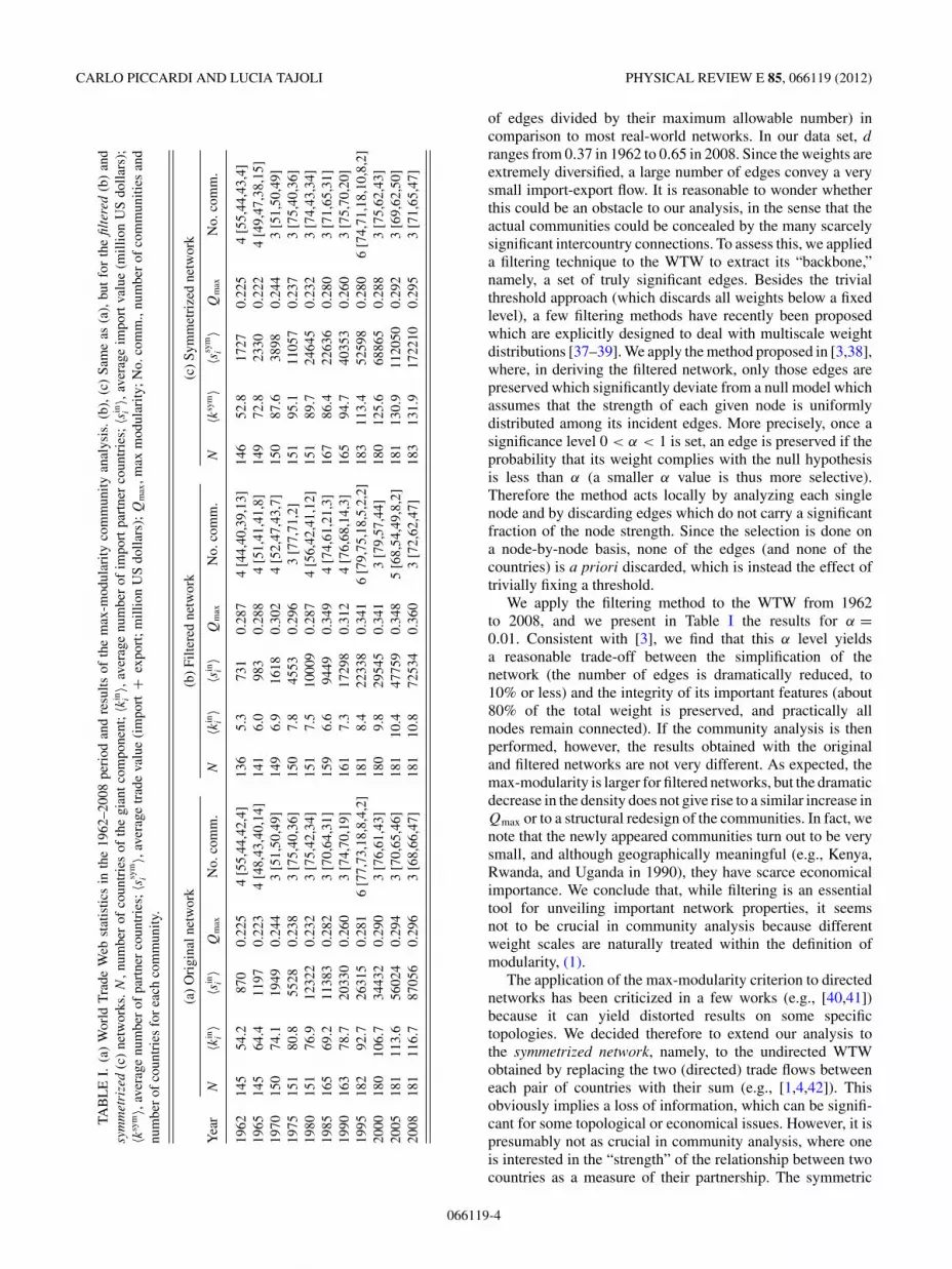
The results of modularity optimization for all the yearsof our WTW data set are reported in Table I [36]. In1962 we obtain q = 4 communities with Qmax = 0.225. Thecommunities count 55, 44, and 22 countries, plus a verysmall community formed by only 4 countries. The largestcommunities essentially coincide with most of Europe andAfrica, America, and Asia plus Oceania, respectively. Thelatter community also includes the United Kingdom andIreland, still strongly linked to Commonwealth countries.From 1970 onward the results show q = 3, with a similargrouping of countries (possibly with the exception of Africancountries, that tend to become more scattered across commu-nities) and with the United Kingdom and Ireland shifting tothe European community, following their membership in theEuropean Economic Community in 1973. The only exceptionis in 1995, when data for the new countries formed by thedismantling of the Soviet bloc start to be recorded, and indeedone of the communities is formed essentially by this group.Over time, the strong ties between these countries loosen up,as they appear no longer as a separate group, but mostly inthe large Europe-based community. In 2008 the communitiescontain 68, 66, and 47 countries, but the largest cluster isnow associated with Asia plus Oceania, confirming the rapidlyincreasing role of Asia in international trade. This clusteringby continents is very much in line with the large body ofliterature showing that geographical proximity still matters forinternational trade (e.g., [5]). We also note that, in terms ofthe number q of communities, our results are qualitativelyconsistent with [12], where a value of q ranging from 2to 4 is reported for the period 1992–2003 (no modularityvalue is reported, however, in that paper). Finally, note thatslightly larger modularity values appear over time, reachingQmax = 0.296 in 2008. This increase can hardly be consideredsignificant, however, especially because it is known that themaximum modularity (max-modularity) tends to grow withthe size of the graph (e.g., [14], p. 90).

A well-known peculiarity of the WTW is the large valueof the density d = L/(N (N − 1)) (i.e., the actual number

066119-3

CARLO PICCARDI AND LUCIA TAJOLI PHYSICAL REVIEW E 85, 066119 (2012)

TAB

LE

I.(a

)W

orld

Tra

deW

ebst

atis

tics

inth

e19

62–2

008

peri

odan

dre

sults

ofth

em

ax-m

odul

arity

com

mun

ityan

alys

is.

(b),

(c)

Sam

eas

(a),

but

for

the

filte

red

(b)

and

sym

met

rize

d(c

)ne

twor

ks.N

,num

ber

ofco

untr

ies

ofth

egi

ant

com

pone

nt;〈kin i

〉,av

erag

enu

mbe

rof

impo

rtpa

rtne

rco

untr

ies;

〈sin i〉,

aver

age

impo

rtva

lue

(mill

ion

US

dolla

rs);

〈ksym〉,

aver

age

num

ber

ofpa

rtne

rco

untr

ies;

〈ssym

i〉,

aver

age

trad

eva

lue

(im

port

+ex

port

;mill

ion

US

dolla

rs);

Qm

ax,m

axm

odul

arity

;No.

com

m.,

num

ber

ofco

mm

uniti

esan

dnu

mbe

rof

coun

trie

sfo

rea

chco

mm

unity

.

(a)

Ori

gina

lnet

wor

k(b

)Fi

ltere

dne

twor

k(c

)Sy

mm

etri

zed

netw

ork

Yea

rN

〈kin i〉

〈sin i〉

Qm

axN

o.co

mm

.N

〈kin i〉

〈sin i〉

Qm

axN

o.co

mm

.N

〈ksym〉

〈ssym

i〉

Qm

axN

o.co

mm

.

1962

145

54.2

870

0.22

54

[55,

44,4

2,4]

136

5.3

731

0.28

74

[44,

40,3

9,13

]14

652

.817

270.

225

4[5

5,44

,43,

4]19

6514

564

.411

970.

223

4[4

8,43

,40,

14]

141

6.0

983

0.28

84

[51,

41,4

1,8]

149

72.8

2330

0.22

24

[49,

47,3

8,15

]19

7015

074

.119

490.

244

3[5

1,50

,49]

149

6.9

1618

0.30

24

[52,

47,4

3,7]

150

87.6

3898

0.24

43

[51,

50,4

9]19

7515

180

.855

280.

238

3[7

5,40

,36]

150

7.8

4553

0.29

63

[77,

71,2

]15

195

.111

057

0.23

73

[75,

40,3

6]19

8015

176

.912

322

0.23

23

[75,

42,3

4]15

17.

510

009

0.28

74

[56,

42,4

1,12

]15

189

.724

645

0.23

23

[74,

43,3

4]19

8516

569

.211

383

0.28

23

[70,

64,3

1]15

96.

694

490.

349

4[7

4,61

,21,

3]16

786

.422

636

0.28

03

[71,

65,3

1]19

9016

378

.720

330

0.26

03

[74,

70,1

9]16

17.

317

298

0.31

24

[76,

68,1

4,3]

165

94.7

4035

30.

260

3[7

5,70

,20]

1995

182

92.7

2631

50.

281

6[7

7,73

,18,

8,4,

2]18

18.

422

338

0.34

16

[79,

75,1

8,5,

2,2]

183

113.

452

598

0.28

06

[74,

71,1

8,10

,8,2

]20

0018

010

6.7

3443

20.

290

3[7

6,61

,43]

180

9.8

2954

50.

341

3[7

9,57

,44]

180

125.

668

865

0.28

83

[75,

62,4

3]20

0518

111

3.6

5602

40.

294

3[7

0,65

,46]

181

10.4

4775

90.

348

5[6

8,54

,49,

8,2]

181

130.

911

2050

0.29

23

[69,

62,5

0]20

0818

111

6.7

8705

60.

296

3[6

8,66

,47]

181

10.8

7253

40.

360

3[7

2,62

,47]

183

131.

917

2210

0.29

53

[71,

65,4

7]

of edges divided by their maximum allowable number) incomparison to most real-world networks. In our data set, d

ranges from 0.37 in 1962 to 0.65 in 2008. Since the weights areextremely diversified, a large number of edges convey a verysmall import-export flow. It is reasonable to wonder whetherthis could be an obstacle to our analysis, in the sense that theactual communities could be concealed by the many scarcelysignificant intercountry connections. To assess this, we applieda filtering technique to the WTW to extract its “backbone,”namely, a set of truly significant edges. Besides the trivialthreshold approach (which discards all weights below a fixedlevel), a few filtering methods have recently been proposedwhich are explicitly designed to deal with multiscale weightdistributions [37–39]. We apply the method proposed in [3,38],where, in deriving the filtered network, only those edges arepreserved which significantly deviate from a null model whichassumes that the strength of each given node is uniformlydistributed among its incident edges. More precisely, once asignificance level 0 < α < 1 is set, an edge is preserved if theprobability that its weight complies with the null hypothesisis less than α (a smaller α value is thus more selective).Therefore the method acts locally by analyzing each singlenode and by discarding edges which do not carry a significantfraction of the node strength. Since the selection is done ona node-by-node basis, none of the edges (and none of thecountries) is a priori discarded, which is instead the effect oftrivially fixing a threshold.

We apply the filtering method to the WTW from 1962to 2008, and we present in Table I the results for α =0.01. Consistent with [3], we find that this α level yieldsa reasonable trade-off between the simplification of thenetwork (the number of edges is dramatically reduced, to10% or less) and the integrity of its important features (about80% of the total weight is preserved, and practically allnodes remain connected). If the community analysis is thenperformed, however, the results obtained with the originaland filtered networks are not very different. As expected, themax-modularity is larger for filtered networks, but the dramaticdecrease in the density does not give rise to a similar increase inQmax or to a structural redesign of the communities. In fact, wenote that the newly appeared communities turn out to be verysmall, and although geographically meaningful (e.g., Kenya,Rwanda, and Uganda in 1990), they have scarce economicalimportance. We conclude that, while filtering is an essentialtool for unveiling important network properties, it seemsnot to be crucial in community analysis because differentweight scales are naturally treated within the definition ofmodularity, (1).

The application of the max-modularity criterion to directednetworks has been criticized in a few works (e.g., [40,41])because it can yield distorted results on some specifictopologies. We decided therefore to extend our analysis tothe symmetrized network, namely, to the undirected WTWobtained by replacing the two (directed) trade flows betweeneach pair of countries with their sum (e.g., [1,4,42]). Thisobviously implies a loss of information, which can be signifi-cant for some topological or economical issues. However, it ispresumably not as crucial in community analysis, where oneis interested in the “strength” of the relationship between twocountries as a measure of their partnership. The symmetric

066119-4

EXISTENCE AND SIGNIFICANCE OF COMMUNITIES IN . . . PHYSICAL REVIEW E 85, 066119 (2012)

WTW is described by the weight matrix W sym = [wsymij ], with

wsymij = w

symji = wij + wji , and the expression of modularity

becomes [14]

Q = 1

2wsym

q∑h=1

∑i,j∈Ch

[w

symij − s

symi s

symj

2wsym

], (2)

where ssymi = ∑

j wsymij = ∑

i wsymji and wsym = ∑

ij wsymij /2.

The results are reported in Table I, and they are very similarto the results obtained for the original directed network. Weconclude, therefore, that the network directionality is not anobstacle to community analysis.

The problem we face now is the significance of the obtainednetwork partitions. Maximizing the modularity obviouslyyields some “best” partition, but this does not imply that thenetwork is actually structured in significant clusters. Althougha large value of Qmax per se should reveal that the network hasa modular organization (as it measures a kind of “dissimilarity”between the network and its randomizations), it is well knownthat a large value of Qmax can even be obtained in random(i.e., Erdos-Renyi) networks, which instead are expected tohave no community structure by construction [43]. In addition,the values of Qmax we obtain can hardly be considered tobe large (remember that the GN and LFR benchmarks haveQmax = 0.604 and 0.820, respectively).

In other words, finding the partition that maximizes Q byno means concludes the community analysis of the network[14]. For undirected, unweighted networks, some methodshave been proposed for complementing the max-modularityapproach with a test of statistical significance. In the simplestapproach, one can consider the ensemble of networks havingthe same degree sequence k1,k2, . . . ,kN as the original one,extract a large number of random networks from this ensemble,and compute the max-modularity Qi for each one of them.Then a large value of the z score, z = (Qmax − μ(Qi))/σ (Qi),indicates that the max-modularity obtained for the originalnetwork is likely to be significantly high. Karrer et al. [44],however, showed, by analyzing a pool of real networks, thatthe z score can fail in some cases. They proposed a robustnessanalysis based on perturbing the original network by randomlyrewiring a given fraction of edges, recomputing the bestpartition by max-modularity, and measuring to what extentthe partitions of the original and perturbed networks overlap.The rationale is that, if communities are not significant, evena small perturbation of the network topology should induce alarge reorganization of the clusters. Hu et al. [45] generalizedthis perturbational approach by defining a suitable “universalindex” R for measuring the significance of communities,which they proved to be fairly effective by a series of testson both artificial and real networks.

All the above methods, however, have some features thatmake their use problematic in our case. First, the significanceanalysis is based on the modularity optimization of manyinstances of a random model or of a perturbed network, thuspotentially it suffers from the same criticalities that affectthe computation of Qmax (and of the associated partition) inthe original network. Second, no straightforward extensionsexist in the case of weighted, directed networks, for which thedefinition of randomized models and of suitable perturbation

schemes is absolutely not trivial. The situation is especiallyproblematic in our case, since the link weights of theWTW span many orders of magnitude and make whateverdiscretization scheme (such as those proposed in [46,47])absolutely critical, as well as any technique based on fixedpercentage perturbations [48] or on weight extraction fromsome postulated probability distribution [49].

Instead of randomizing the network, we can assess whetherour results are robust by randomizing the assignment of nodesto communities. Starting from the optimal partition (i.e.,the one with Q = Qmax), imagine selecting and relabelinga fraction 0 < α < 1 of nodes, namely, assigning them to a(randomly selected) different community. As α increases, weobtain partitions more and more distant from the optimal one,and we can quantify this distance by the (normalized) variationof information V [50], a measure which is 0 if and only if thetwo partitions are identical and 1 when they are “maximallydifferent” (i.e., one partition has N clusters and the other hasonly one). It is natural to expect that, as V increases whiledeparting from the optimal partition, the modularity Q(V ) ofthe associated partition decreases accordingly. And indeed thisis the case, but the form of the function Q(V )—which a prioridepends on which nodes are relabeled—can disclose importantproperties.

The function Q(V ) is displayed in Fig. 1 for the WTWin 3 years and for the GN and LFR benchmark networksintroduced above. In all cases, two functions are depicted:one is the result of the random selection of the fraction α ofnodes to be relabeled, and the other is obtained by relabelingthe least connected nodes (i.e., the nodes with the smallest total

FIG. 1. (Color online) The (normalized) modularity Q(V ) of theperturbed partitions obtained, from the optimal one [Q(0) = Qmax],by relabeling 10% to 50% of the nodes, i.e., by assigning themto a different community. V is the variation of information of theperturbed partitions. The (blue) curve with filled circles was obtainedby relabeling randomly selected nodes (each point is the average of100 realizations); the (red) curve with filled triangles is obtained byrelabeling the least connected nodes (lowest strength or degree).

066119-5

CARLO PICCARDI AND LUCIA TAJOLI PHYSICAL REVIEW E 85, 066119 (2012)

strength or degree). If the communities are significant, movingeven the least connected nodes should in any case producean important effect on the modularity values, because thosenodes also crucially affect the community structure. Indeed,this is what happens in the GN and LFR cases, where thetwo curves are qualitatively similar and quantitatively close.On the contrary, the three WTW panels strikingly put intoevidence the scarce significance of the optimal partition. As amatter of fact, we can randomly relabel as many as 50% of thenodes (inducing a large variation of information), yielding justa slight decrease in the modularity Q(V ). This means that thepositioning of a large number of countries, actually the leastimportant ones from an economic point of view, is more or lessirrelevant and that modularity is only determined by the linkswith the largest weights. In other words, the landscape of themodularity Q is extremely insensitive, since a large numberof partitions (even very distant one from the other) have veryclose modularity values. Overall, this suggests that the resultsof the modularity analysis should be taken with great caution,as they denote an extremely scarce robustness of the obtainedcommunities: indeed, a large number of very distant partitionsare qualified as nearly equally “optimal.”

Given the low robustness of the partitions found viamodularity optimization, in order to have a complete view ofthe cluster structure of the WTW, in the next sections we moveto completely different approaches for testing the existenceand significance of communities in the WTW.

In general terms, the weak evidence of a clusterizedstructure of the WTW, indicated both by the rather smallmodularity values and by the above sensitivity test, shouldnot be surprising. Notice that interactions among countriesare measured by their absolute trade values. As such, astrongly clusterized network would possibly be formed byclearly distinct groups of countries with large intra- but smallintercommunity trades. But the largest edges (in terms of theirweight) basically involve the largest world economies (e.g.,in 2008, on at least one side of the top 20 edges, we find theUnited States, China, Canada, Mexico, Japan, Germany, theNetherlands, France, Korea, the United Kingdom, Belgium,and Italy). We can hardly expect these countries (or a subset ofthem) to form a community as defined here, because the tradeflows among them are not strongly differentiated from theirtrade with the remaining countries. At the same time, it canalso hardly be expected that the remaining countries form oneor more communities. In the next sections, in order to clearlyunderstand the possible clusterized structure of the WTW, wenot only consider different community analysis techniques,but also move to analyzing relative trade values.

B. Cluster analysis

Standard data clustering is aimed at organizing objects into“homogeneous groups,” trying to maximize, at the same time,the intragroup similarity and the intergroup dissimilarity. Thisrequires defining a suitable distance among data. When wemove to graph clustering, i.e., grouping the nodes of a network,which distance should be used is by no means obvious.

We adopt a notion of distance among nodes which isbased on random walks. An N -state Markov chain canstraightforwardly be associated with the N -node network by

row-normalizing the weight matrix W , i.e., by letting thetransition probability from i to j equal

pij = wij∑j wij

= wij

souti

. (3)

The resulting transition matrix P = [pij ] is a stochastic (orMarkov) matrix, i.e., 0 � pij � 1 for all i,j , and

∑j pij = 1

for all i. The study of many problems in network sciencebenefits from some sort of Markov chain approach (e.g.,epidemic spreading, navigation, etc. [23,51]). Communityanalysis is one of them, and several contributions in this veinhave been published; we recall [40] and [52–55] among others(see, again, [14] for a comparative survey).

It is important to note that modeling the WTW by Eq. (3)corresponds to moving from absolute to relative trade values,since the flow from i to j is now normalized by thetotal export flow from country i. The consequence is thatcommunities, if any, will not necessarily be composed ofgroups of countries related by large trading but, instead, ofcountries with privileged partnership, namely, whose tradingis important in relative terms. This can originate from, e.g.,geographical vicinity, trade agreements, common languageor religion, and traditional partnerships. Since we naturallyexpect such communities to be composed of a mixture of largeand small economies, the use of relative trade values appearsto be more appropriate, as absolute measures would a prioriobscure the position of medium-small countries.

In defining a distance among nodes, we essentially adopt theapproach of [54], where a T -step random walk is performed,in a Monte Carlo fashion, from each of the N network nodes.If the two nodes (i,j ) are visited along the same walk, thesimilarity counter σij is increased by 1. At the end, a similaritymatrix � = [σij ] is obtained which is used as a basis foragglomerative, hierarchical clustering. The rationale for themethod is the following: if the number T of steps is limited,the random walker starting from i will more likely visit nodesstrongly connected to i, i.e., within the same community.The choice of T is thus quite critical: if T is too large, theprobability of visiting a given state becomes independent ofthe starting state (as it tends to the stationary Markov chainstate probability distribution π = πP ), whereas if T is toosmall, the information gathered is possibly insufficient. Wereturn to this point later.

We partially modify the above method in that we donot explicitly perform random walks. In fact, consider M

repetitions of a random walk started from i. For each repetition,the probability that the walker is in j after t steps is [P t ]ij .Thus, if M random walks of length T are performed fromi, the expected number of visits of j in any time instant in1 � t � T is M

∑Tt=1[P t ]ij . Note that this is conceptually

equivalent to the above explicit random walk approach [54],but with an arbitrarily large number M of repetitions fromeach starting node instead of only one. By averaging withrespect to M and T , and recalling that we are dealingwith directed networks (thus [P t ]ij = [P t ]ji), we propose asimilarity matrix � = [σij ] defined by

σij = σji = 1

T

T∑t=1

([P t ]ij + [P t ]ji). (4)

066119-6

EXISTENCE AND SIGNIFICANCE OF COMMUNITIES IN . . . PHYSICAL REVIEW E 85, 066119 (2012)

Finally, the distance dij = dji between nodes (i,j ) is definedby complementing the similarity and normalizing the resultsbetween 0 and 1:

dij = dji = 1 − σij − min σij

max σij − min σij

. (5)

At this point, a standard hierarchical, aggregative cluster anal-ysis is used to explore the possible existence of communities[56]. More precisely, a binary cluster tree (dendrogram) iscomputed initially by defining N groups each containing asingle node and then by iteratively linking the two groups withminimal distance [57].

Cluster analysis yields a different dendrogram for eachtime horizon T , whose choice is thus nontrivial. At the twoextremes, setting T = 1 restricts the pairs of nodes whichare candidate to nonzero similarity to neighboring pairs only,whereas larger and larger values of T tend to make any nodeequally similar to any other. We solve this indeterminacy by asort of optimization. For each network under scrutiny, we builda dendrogram for each T from 1 to a sufficiently large valueTmax (of the order of N ), and we take the one that maximizes thecophenetic correlation coefficient C, which is defined as thelinear correlation between the distances dij and the copheneticdistances cij [56]. The latter are a product of the hierarchicalcluster analysis: for any node pair (i,j ), the cophenetic distancecij is the height of the link joining (directly or indirectly)nodes (i,j ) in the dendrogram. Recall that, when nodes areincreasingly grouped together building the dendrogram, theirdistances to the other nodes (or groups) is replaced by theiraverage. The effect is small if the nodes that are groupedtogether are very close each other, namely, if they form acluster. If so, we expect similar values for the dij and the cij

values and, thus, a large value of C. Although this approach canreveal criticalities in some specific applications [58], the valueof C is generally used to assess whether the adopted distancedij induces an effective clusterization: by maximizing C, wethus select the best possible clusterization with respect to T .

The dendrograms obtained for the WTW in 1962, 1980,and 2008 (i.e., the two extremes of the time window of ourdata set, plus an intermediate year) are displayed in the upperthree plots in Fig. 2 [36]. Each vertical line corresponds to anode (country). Horizontal lines (“links”) connect two groupsof nodes, and the height of the link (as read on the y axis) isthe distance between the two groups. In the two lower plots inFig. 2, dendrograms of the GN and LFR benchmark networksare displayed.

A clear, visual indication of a clusterized network structureis, in the benchmark’s dendrograms, the existence of longvertical segments or, equivalently, of links (i.e., horizontalsegments) whose height is largely different from the heightsof the links below them. In fact, this situation arises whenthe distance between the two groups joined by the link ismuch larger than the distance among the nodes forming thetwo groups; this exactly means that there are clusters in thenetwork. This phenomenon is strikingly evident in the GNdendrogram: whereas there is a “continuum” of distanceswithin a single community, the intergroup distance is largeand sharply divides the four planted communities. The samehappens in the LFR dendrogram.

0

0.2

0.4

0.6

0.8

1

dist

ance

WTW 1962

0

0.2

0.4

0.6

0.8

1

dist

ance

WTW 1980

0

0.2

0.4

0.6

0.8

1

dist

ance

WTW 2008

0

0.2

0.4

0.6

0.8

1

dist

ance

LFR

0

0.2

0.4

0.6

0.8

dist

ance

GN

FIG. 2. (Color online) Dendrograms obtained by hierarchicalcluster analysis. From top to bottom: WTW in 1962, 1980, and 2008;GN benchmark network; and LFR benchmark network. Colors (otherthan black) denote groups of nodes whose distances are all not largerthan 0.7.

The situation appears to be markedly different for the WTWdendrograms. Only a few distinct groups appear, and they aremostly composed of few countries. Moreover, there seem to beno significant structural differences through the years, possiblywith a diminishing visual distance between groups over time.As specified above, we take the dendrogram for which thecophenetic correlation coefficient C is the maximum valueattained by varying the time horizon T of the random walker[see Eq. (4)]. Notably, such a value is attained for T = 12 andT = 6 for the GN and LFR benchmarks, respectively, whilethe maximum C is obtained at T = 1 for all the WTW cases.This means that, in the latter case, the best clusterization (as

066119-7

CARLO PICCARDI AND LUCIA TAJOLI PHYSICAL REVIEW E 85, 066119 (2012)

measured by C) is obtained by assessing the node similarityonly among direct neighboring countries. This is an effectof the anomalously high network density, for which directconnections carry over most of the information to the randomwalker.

In all years, some expected patterns can be observed.The United States and Canada form one of the strongestpartnerships: their distance in the dendrogram stays constantlyvery small from 1970 [in seven cases of nine, their distance isactually 0, meaning that they are the closest pair consistentwith (5)]. France is strongly connected to some of itsformer colonies, whereas Germany is close to other Europeancountries. Some of these links are very large both in absoluteand in relative terms (e.g., between the United States andCanada); others are important in relative terms (e.g., about 80%of the Guadeloupe export in 1995 is directed to France). Oftenvery small countries are connected to much larger ones, aneffect of the disassortativity already observed in the WTW [4].These links tend to be small in absolute terms, given the smalleconomic size of the countries, but they are very important inrelative terms, as they show a strong preference for a givenpartner.

The scenario is not modified if we analyze the filteredand the symmetrized networks defined in Sec. III A [36]:qualitatively, they display no difference with respect to thoseof the original WTW.

As pointed out above, visual analysis of the dendrogramsleads us to claim that the WTW, through the years, does notdisplay a significant community structure. It is important topoint out that this result is specific neither to our particularchoice of node distance nor to the choice of considering relativetrade values. As a matter of fact, we repeated the hierarchicalcluster analysis by using the distance proposed by He andDeem [13], both on the WTW and on the benchmark networks.In [13] the node distance is defined as dij = wmax − wij ,with wmax = maxij wij . Note that dij relates country i toits direct neighbors through the absolute trade value wij .Inspection of the corresponding dendrograms [36] leads toexactly the same conclusion as above: the qualitative structureof the dendrograms is markedly different passing from thebenchmarks to the WTW, denoting clusterization levels verystrong for the former but extremely mild for the latter.

In summary, the results of the cluster analysis, althoughbased on visual evidence only, seem to denote the absence ofthe existence of a significant community structure in the WTW.This emerges both from the use of relative trade measures, ametric that appears to be more suited to a multiscale networksuch as the WTW (it is actually consistent with the filteringtechnique described in Sec. III A), and from the adoption ofa node distance based on absolute trade values. Together withthe small modularity level (Sec. III A), this is a further clue ofa mild community structure of the WTW.

C. Stability of partitions

A different approach for exploiting random walks in study-ing network communities has been devised by Delvenne et al.[59], who introduced the concept of stability of a partition. Asabove, the rationale is that, in a strongly clusterized network,a random walker starting in a community is likely to remain

for quite a long time within that community, before leavingit to enter another community. Imagine that the walker emitsa signal at each step, which has the same value as long asit remains within a community and changes upon movingto another community. Then studying the persistence of thissignal provides important information on the communitystructure of the network.

The probability πit that the random walker is in state i at

time t evolves according to the Markov chain equation πt+1 =πtP , and the vector πt = (π1

t π2t . . . πN

t ), assuming ergodicity,tends to the stationary state π = πP as t → ∞. Considernow a network partition C1,C2, . . . ,Cq and assume that thewalker, at each step t , emits a signal st which takes valuec as long as it moves within Cc. Delvenne et al. [59] showthat the autocovariance of st can be usefully expressed as cov[st ,st+τ ] = (1,2, . . . ,q)′Rτ (1,2, . . . ,q), where Rτ is the q × q

clustered autocovariance matrix,

Rt = H ′(diag(π )P t − π ′π )H, (6)

where H is a N × q binary matrix coding the partition, i.e.,its entry hic is 1 if and only if node i belongs to communityc. Note that Rt depends on the network and on the partitiononly. Equation (6) provides an interpretation of each entry[Rt ]cd as the probability of starting in community c at time0 and being in community d at time t , minus the probability,evaluated at stationarity, that two independent walkers are in c

and d. If the partition coded by H is significant, one expects adominance of the diagonal terms [Rt ]cc over time. The stabilityof the partition H is thus defined as the following functionof time:

rHt = min

0�s�ttrace[Rs]. (7)

A good, significant partition will have stability rHt which

remains large over a long time span, since the random walkerhas a high likelihood of remaining within the same communityfor long time. On the contrary, a rapidly decaying rH

t denotesa scarcely significant partition, because the walker rapidlyabandons the starting community [60].

We compute the stability function rHt for all the WTW cases

in our data set 1962–2008 and, for comparison, for the GN andLFR benchmark networks. In all instances, we consider thepartition H obtained via modularity optimization (Sec. III A).The results are depicted in the upper panel in Fig. 3 (forreadability, only the WTW curves for 1962, 1980, and 2008 areplotted). These functions are, however, not easily compared,essentially for two reasons. First, the curves start from differentvalues rH

1 [61]. Second, the decay velocities are hardlycomparable because of the different dimensions N of thenetworks (recall that time t is the number of steps of the randomwalker). For these reasons, we normalize the curves along bothaxes and plot, in the lower part of Fig. 3, the normalizedstability rH

t /rH1 with respect to the normalized time t/N .

In this way the curves are directly comparable and clearlydemonstrate the exponential behavior rH

t /rH1 ∼ exp(−γ t/N).

Visual examination of Fig. 3 is probably sufficient to grasp themuch more rapid decay of the WTWs with respect to thetwo benchmarks, but the computation (via linear fitting) ofthe decay rate γ reinforces this impression: while the GNand LFR networks have γ = 23.3 and 5.73, respectively, the

066119-8

EXISTENCE AND SIGNIFICANCE OF COMMUNITIES IN . . . PHYSICAL REVIEW E 85, 066119 (2012)

FIG. 3. (Color online) Top: Stability functions rHt of the GN and

LFR benchmark networks and those of the World Trade Web (WTW)in 1962, 1980, and 2008. For each network, we consider the partitionH obtained via modularity optimization. Bottom: Same as above, butthe stability is normalized by the initial value rH

1 and the time axis isnormalized, separately for each curve, by the number N of networknodes.

WTWs in 1962, 1980, and 2008 are characterized by the muchhigher values 106.8, 100.3, and 97.6, respectively. Similarfigures (92.4 < γ < 109.4) are obtained for the other yearsin the data set, with no clear trend with respect to time, aswell as for the symmetrized network (90.4 < γ < 107.4). Aslightly slower decay, although still significantly faster thanthe benchmark networks, instead characterizes the filterednetworks (59.8 < γ < 72.5).

D. Persistence probabilities

We can complement the above analysis by extractingother quantitative indicators, which we call the persistenceprobabilities of the communities. Starting from the N -statenetwork, a given partition C1,C2, . . . ,Cq induces a q-statemetanetwork, where communities becomes metanodes. Atthis scale, the random walker can be described by the q-statelumped Markov chain [62] with the stochastic matrix

U = [diag(πH )]−1H ′diag(π )PH, (8)

which is actually obtained by row-normalizing the termH ′diag(π )PH appearing in the first term in (6). In rigor-ous terms, the q-state lumped Markov chain t+1 = tU

provides, in general, only an approximate description of thedynamics of the random walker at the metanetwork level.

Nonetheless, it becomes exact under the assumption thatthe Markov chain πt+1 = πtP is at stationarity, i.e., πt = π

[63,64]. Under this assumption, the entry ucd of U is theprobability that the random walker is at time (t + 1) inany of the nodes of community Cd , provided it is at timet in any of the nodes of community Cc. We define thepersistence probability of the community Cc as the diagonalterm ucc in U . Large values of ucc are expected for significantcommunities. In fact, the expected escape time from Cc isτc = (1 − ucc)−1: the walker will spend a long time withinthe same community if the weights of the internal edges arecomparatively large with respect to those pointing outside.The analysis of the persistence probabilities induced in anetwork by a given partition has recently been proven to bean effective tool for testing the existence and significance ofcommunities [55].

From (8) one can derive the explicit expression for ucc [55],

ucc =∑i∈Cc

π i

c

∑j∈Cc

wij

souti

, (9)

where πi is the stationary probability of node i, and c =∑i∈Cc

π i . For the WTW, this means that ucc is a weightedaverage (a convex combination) of the fractions of the exportflows that the countries of community Cc direct within thecommunity itself. For example, ucc = 0.5 denotes that, on(weighted) average, the countries of Cc direct half of theirexport flow to the countries in the same community and halfto the rest of the world: a very mild requirement for a baselinelevel of significance. With this in mind, we compute thepersistence probabilities ucc, c = 1,2, . . . ,q, of the WTWs inthe 1962–2008 period and of the two benchmark networks, forthe partition corresponding to the max-modularity (Sec. III A).The results are shown in Fig. 4, for the original, filtered, andsymmetrized WTWs. It is evident from Fig. 4 that, on average,the ucc values of all the WTWs under scrutiny are much smallerthan those of the benchmarks (which, we recall, are purposelybuilt with a significant cluster structure). Actually, in almostall instances the entire range of the ucc values of the WTWs isbelow the corresponding range of the benchmarks. If we thenindividually analyze each single community, we discover thatmost of them turn out to be scarcely significant, as revealed bythe small persistence probability (note, for comparison, thatall the ucc values of the 10-community partition of the LFRnetwork are larger than 0.84, although the communities havediversified sizes, ranging from 11 to 25 nodes). Specifically,only in recent years (since 2005) are the ucc values of theWTW all larger than 0.5, but two of three still remain below0.6, meaning that, on average, these countries direct more than40% of their export outside their community. In all years in thesample, therefore, the communities dictated by the analyzedpartitions are by no means secluded from the rest of the world,as their in- and out-community trade volumes have comparablemagnitude.

In this respect, the results are even worse for the filterednetworks. On one hand, removing several low-weight edgesslightly increases the highest persistence probabilities. Buton the other hand, the finer partition detected by the max-modularity approach pops up some small, scarcely significant

066119-9

CARLO PICCARDI AND LUCIA TAJOLI PHYSICAL REVIEW E 85, 066119 (2012)

FIG. 4. Persistence probabilities of the World Trade Web (WTW;1962–2008) and of the GN and LFR benchmark networks. The threepanels refer, respectively, to the original, filtered, and symmetrizedWTW, as defined in Sec. III A. For each network, we consider theq-community partition obtained via modularity optimization: the q

horizontal dashes denote the values of the diagonal terms ucc of thelumped Markov matrix U (vertical straight lines are for visual aidonly).

communities, as clearly highlighted by the larger number ofsmall ucc values in the middle panel in Fig. 4.

Nonetheless, some important information is revealed byanalysis of Fig. 4. Even if, in most instances, the partition ofthe WTW is scarcely significant as a whole, we notice that,since 1975, there is in each case (at least) one communitywith a rather high persistence probability, both in absoluteterms and comparatively with respect to most of the other ucc

values. It turns out that it is a large community which alwaysincludes the entire set of European countries, plus a numberof minor non-European partners (partially varying from yearto year), mainly from North Africa, the Near East, and the

Asian republics of the former USSR. Up to 1995, there is alsoanother large community with a high persistence probability,which includes the entire North America and most of Centraland South America, plus China, Australia, and many others.Since 2000, however, the community partition dictated bythe max-modularity suggests a different arrangement, withNorth and South America in one community and China andAustralia in another. Notably, both these new communitieshave definitely lower persistence probabilities than before,denoting less exclusive intracommunity partnerships. Theevidence emerging from this analysis is very much in linewith what can be expected looking at the existence oftrade agreements between countries. European countries formthe oldest and deeper custom union in the world, and thepersistence of their ties is confirmed by the data, which alsosuggest, though, that this is not a group of countries separatedfrom to the rest of the world (in 2008, over one-third ofEuropean Union imports came from non–European Unioncountries). The reported evidence also captures the new activerole of China, which became a major player in many areas ofthe world, less dependent on the US market.

Overall, we can conclude that, as well as the othermethods above presented, the use of stability functions andthe evaluation of the persistence probabilities seem to confirmthe absence of a strong clusterized structure in the WTW,when considered as a whole. However, the capability of thepersistence probabilities to assess the quality of each singlecommunity, differently from the other tools of analysis, putsforward the existence of some significant clusters of countrieswith privileged intracommunity partnerships.

IV. CONCLUDING REMARKS

In this paper we have used four approaches to analyzecommunities in the WTW. In the literature of communityanalysis, these methods have been extensively tested on avariety of networks having features such as directed edges,multiscale weights, and heterogeneity in the distributions ofnode degrees and/or community sizes. In the case of the WTW,however, all four approaches led to similar conclusions: there isno significant evidence of the existence of a strong communitystructure in the WTW. The eligible communities found in thedata are reasonable, but, with very few exceptions, they are notvery significant according to any of the criteria adopted. Evenif there is not a single robust measure to identify communitiesin the WTW, the convergence of results from all the approachesstrengthens the robustness of this conclusion.

The configuration of the WTW therefore supports theview that the growth of international trade linkages did notoccur only involving specific groups of countries. Even ifthe phenomenon of rapidly increasing economic integrationamong countries clearly appears in a number of measurescomputed for the WTW over time (such as the increase indensity or the sharp change in the nodes’ average strength), thenew links that have been forming have not changed the (weak)cluster structure of the network, as they have not followed astrong or exclusive preferential pattern. Countries do selecttheir trading partners—given that countries are on averageconnected to “only” approximately half of the other existingcountries—but this selection is quite open. In this respect,

066119-10

EXISTENCE AND SIGNIFICANCE OF COMMUNITIES IN . . . PHYSICAL REVIEW E 85, 066119 (2012)

economic integration involves the world as a whole, and inthis sense it indeed appears to be a “global” phenomenon.

While a nonpreferential structure in terms of aggregateflows is quite plausible, much stronger community ties can

emerge considering trade in specific sectors [12]. Futuredevelopments of this work could focus on trade flows betweencountries in particular commodities, using these aggregateresults as a benchmark.

[1] M. A. Serrano and M. Boguna, Phys. Rev. E 68, 015101(2003).

[2] D. Garlaschelli and M. I. Loffredo, Physica A 335, 138 (2005).[3] M. A. Serrano, M. Boguna, and A. Vespignani, J. Econ. Interac.

Coord. 2, 111 (2007).[4] G. Fagiolo, J. Reyez, and S. Schiavo, Physica A 387, 3868

(2008).[5] L. De Benedictis and L. Tajoli, World Econ. 34, 1417 (2011).[6] A. Deardorff, Terms of Trade. Glossary of International Eco-

nomics (World Scientific, Singapore, 2006).[7] R. Robertson, Globalization (Sage, Thousand Oaks, CA,

1992).[8] J. G. Williamson, J. Econ. Hist. 56, 277 (1996).[9] R. E. Baldwin and P. Martin, NBER Working Papers Series no.

6904 (1999).[10] I. Tzekina, K. Danthi, and D. N. Rockmore, Eur. Phys. J. B 63,

541 (2008).[11] J. A. Reyes, R. B. Wooster, and S. Shirrell, Regional trade

agreements and the pattern of trade: A networks approach (2009)[http://ssrn.com/abstract=1408784].

[12] M. Barigozzi, G. Fagiolo, and G. Mangioni, Physica A 390,2051 (2011).

[13] J. He and M. W. Deem, Phys. Rev. Lett. 105, 198701 (2010).[14] S. Fortunato, Phys. Rep. 486, 75 (2010).[15] Many works in the international trade literature show the

increasing tendency for countries to sign preferential tradeagreements, but there is a debate on the actual effects of thesetreaties. See, for example, [16,17].

[16] R. Pomfret, World Econ. 30, 923 (2007).[17] S. Baier and J. Bergstrand, J. Int. Econ. 71, 72 (2007).[18] R. Feenstra, R. Lipsey, H. Deng, A. C. Ma, and H. Mo, NBER

Working Papers Series no. 11040 (2005).[19] We validated our analysis on an alternative data set

[20] [data available at http://privatewww.essex.ac.uk/∼ksg/exptradegdp.html]: we found very similar results, with somenon-negligible difference only in the 1962–1970 period, wherethe data coverage of whatever source is well known to be rathermodest and all existing databases went through some sort ofmanipulation (as widely discussed in the economic literature,e.g., [18], [20–22]). These different figures, however, are notsuch as to modify our overall conclusions.

[20] K. S. Gleditsch, J. Conflict Resolut. 46, 712 (2002).[21] G. Parniczky, Int. Stat. Rev. 48, 43 (1980).[22] G. J. Felbermayr and W. Kohler, Rev. World Econ. 142, 642

(2006).[23] A. Barrat, M. Barthelemy, and A. Vespignani, Dynamical

Processes on Complex Networks (Cambridge University Press,2008).

[24] T. H. Cormen, C. E. Leiserson, R. L. Rivest, and C. Stein,Introduction to Algorithms, 2nd ed. (MIT Press and McGraw–Hill, New York, 2001).

[25] Our data set does not cover all trade flows registered in agiven year because some exchanges are covered by secrecy forsecurity or similar reasons (e.g., arms trade) and the origin and/ordestination of the flow is not recorded.

[26] M. E. J. Newman and M. Girvan, Phys. Rev. E 69, 026113(2004).

[27] M. E. J. Newman, Proc. Natl. Acad. Sci. USA 103, 8577 (2006).[28] A. Arenas, J. Duch, A. Fernandez, and S. Gomez, New J. Phys.

9, 176 (2007).[29] V. D. Blondel, J.-L. Guillaume, R. Lambiotte, and E. Lefebvre,

J. Stat. Mech.: Theory Exp. (2008) P10008.[30] A. Lancichinetti and S. Fortunato, Phys. Rev. E 80, 056117

(2009).[31] We validated our modularity results by using a different

method, namely, extremal optimization [32] [code available athttp://deim.urv.cat/∼sgomez/radatools.php], obtaining the sameresults up to the third significant digit.

[32] J. Duch and A. Arenas, Phys. Rev. E 72, 027104 (2005).[33] M. Girvan and M. Newman, Proc. Natl. Acad. Sci. USA 99,

7821 (2002).[34] A. Lancichinetti, S. Fortunato, and F. Radicchi, Phys. Rev. E 78,

046110 (2008).[35] A. Lancichinetti and S. Fortunato, Phys. Rev. E 80, 016118

(2009).[36] See Supplemental Material at http://link.aps.org/supplemental/

10.1103/PhysRevE.85.066119 for the composition of eachcommunity; the full set of dendrograms with the indication ofthe countries; the complete set of dendrograms for the filteredand symmetrized networks; the dendrograms with the He-Deemdistance.

[37] J. B. Glattfelder and S. Battiston, Phys. Rev. E 80, 036104(2009).

[38] M. A. Serrano, M. Boguna, and A. Vespignani, Proc. Natl. Acad.Sci. USA 106, 6483 (2009).

[39] F. Radicchi, J. J. Ramasco, and S. Fortunato, Phys. Rev. E 83,046101 (2011).

[40] M. Rosvall and C. T. Bergstrom, Proc. Natl. Acad. Sci. USA105, 1118 (2008).

[41] Y. Kim, S.-W. Son, and H. Jeong, Phys. Rev. E 81, 016103(2010).

[42] D. Garlaschelli and M. I. Loffredo, Phys. Rev. Lett. 93, 188701(2004).

[43] J. Reichardt and S. Bornholdt, Physica D 224, 20 (2006).[44] B. Karrer, E. Levina, and M. E. J. Newman, Phys. Rev. E 77,

046119 (2008).[45] Y. Hu, Y. Nie, H. Yang, J. Cheng, Y. Fan, and Z. Di, Phys. Rev.

E 82, 066106 (2010).[46] V. Zlatic, G. Bianconi, A. Diaz-Guilera, D. Garlaschelli, F. Rao,

and G. Caldarelli, Eur. Phys. J. B 67, 271 (2009).[47] C. Piccardi, L. Calatroni, and F. Bertoni, Physica A 389, 5247

(2010).

066119-11

CARLO PICCARDI AND LUCIA TAJOLI PHYSICAL REVIEW E 85, 066119 (2012)

[48] R. Lambiotte, in Proceedings, 8th International Symposium onModeling and Optimization in Mobile, Ad Hoc and WirelessNetworks (WiOpt), Avignon, France (2010), pp. 546–553.

[49] M. Rosvall and C. T. Bergstrom, PLoS One 5, e8694 (2010).[50] M. Meila, J. Multivar. Anal. 98, 873 (2007).[51] M. E. J. Newman, Networks: An Introduction (Oxford University

Press, New York, 2010).[52] P. Pons and M. Latapy, in Computer and Information Sciences—

ISCIS 2005, Proceedings. Vol. 3733 of Lecture Notes inComputer Science, edited by P. Yolum, T. Gungor, F. Gurgen,and C. Ozturan (Springer-Verlag Berlin, 2005), pp. 284–293.

[53] S. Van Dongen, SIAM J. Matrix Anal. Appl. 30, 121 (2008).[54] K. Steinhaeuser and N. V. Chawla, Pattern Recognit. Lett. 31,

413 (2010).[55] C. Piccardi, PLoS One 6, e27028 (2011).[56] B. S. Everitt, S. Landau, M. Leese, and D. Stahl, Cluster

Analysis, 5th ed. (John Wiley & Sons, Chichester, UK, 2011).[57] When a new group G of nodes is created by linking two existing

groups Ga , and Gb, the distance between G and another groupG′ is the average of the distances (Ga ,G′) and (Gb,G′) (averagelinking).

[58] M. Holgersson, Pattern Recognit. 10, 287 (1978).[59] J. C. Delvenne, S. N. Yaliraki, and M. Barahona, Proc. Natl.

Acad. Sci. USA 107, 12755 (2010).[60] In [59], rH

t is actually proposed not only for testing thesignificance of a given partition but mainly as a tool for findingthe “best” partition. If a pretty large number of “good” candidatepartitions H are derived (this can be done by using a varietyof algorithms; see [14,59]), then the graph stability functionrt = maxH rH

t puts into evidence, for each instant in time,t , which is the “optimal” partition according to the stabilitycriterion. It is suggested in [59] that the most relevant partitionsare those which are optimal over long time windows.

[61] For undirected networks, [59] proved that rH1 = Q, i.e., the mod-

ularity associated with the partition H . For directed networks,it can easily be checked that rH

1 = Qlr, which is the so-calledLinkRank modularity proposed in [41].

[62] J. G. Kemeny and J. L. Snell, Finite Markov Chains (Springer-Verlag, New York, 1976).

[63] P. Buchholz, J. Appl. Prob. 31, 59 (1994).[64] K. H. Hoffmann and P. Salamon, Appl. Math. Lett. 22, 1471

(2009).

066119-12