arX

iv:1

004.

4439

v1 [

astr

o-ph

.CO

] 2

6 A

pr 2

010

Mon. Not. R. Astron. Soc. 000, 1–32 (2009) Printed 27 April 2010 (MN LATEX style file v2.2)

Evolutionary Stellar Population Synthesis with MILES.

Part I: The Base Models and a New Line Index System

A. Vazdekis1,2⋆, P. Sanchez-Blazquez1,2, J. Falcon-Barroso1,2, A. J. Cenarro1,2,3,

M. A. Beasley1 N. Cardiel4, J. Gorgas4, R. F. Peletier51Instituto de Astrofısica de Canarias, La Laguna, E-38200 Tenerife, Spain2Departamento de Astrofısica, Universidad de La Laguna, E-38205 La Laguna, Tenerife, Spain3Centro de Estudios de Fısica del Cosmos de Aragon, C/ General Pizarro 1, E-44001, Teruel, Spain4Dept. de Astrofısica, Fac. de Ciencias Fısicas, Universidad Complutense de Madrid, E-28040 Madrid, Spain5Kapteyn Astronomical Institute, University of Groningen, Postbus 800, 9700 AV, Groningen, Netherlands

ABSTRACT

We present synthetic spectral energy distributions (SEDs) for single-age, single-metallicity stellar populations (SSPs) covering the full optical spectral range at mod-erately high resolution (FWHM=2.3A). These SEDs constitute our base models, asthey combine scaled-solar isochrones with a empirical stellar spectral library (MILES),which follows the chemical evolution pattern of the solar neighbourhood. The modelsrely as much as possible on empirical ingredients, not just on the stellar spectra, butalso on extensive photometric libraries, which are used to determine the transforma-tions from the theoretical parameters of the isochrones to observational quantities.The unprecedent stellar parameter coverage of the MILES stellar library allowed usto safely extend our optical SSP SEDs predictions from intermediate- to very-old ageregimes, and the metallicity coverage of the SSPs from super-solar to [M/H] = −2.3.SSPs with such low metallicities are particularly useful for globular cluster studies. Wehave computed SSP SEDs for a suite of IMF shapes and slopes. We provide a quan-titative analysis of the dependence of the synthesized SSP SEDs on the (in)completecoverage of the stellar parameter space in the input library that not only shows thatour models are of higher quality than other works, but also in which range of SSPparameters our models are reliable. The SSP SEDs are a useful tool to perform thestellar populations analysis in a very flexible manner. Observed spectra can be studiedby means of full spectrum fitting or by using line indices. For the latter we proposea new Line Index System (named LIS) to avoid the intrinsic uncertainties associatedwith the popular Lick/IDS system and provide more appropriate, uniform, spectralresolution. Apart from constant resolution as function of wavelength the system is alsobased on flux-calibrated spectra. Data can be analyzed at three different resolutions:5 A, 8.4 A and 14 A (FWHM), which are appropriate for studying globular cluster,low and intermediate-mass galaxies, and massive galaxies, respectively. Furthermorewe provide polynomials to transform current Lick/IDS line index measurements tothe new system. We provide line-index tables in the new system for various popularsamples of Galactic globular clusters and galaxies. We apply the models to variousstellar clusters and galaxies with high-quality spectra, for which independent studiesare available, obtaining excellent results. Finally we designed a web page from whichnot only these models and stellar libraries can be downloaded but which also providesa suite of on-line tools to facilitate the handling and transformation of the spectra.

Key words: galaxies: abundances – galaxies: elliptical and lenticular,cD – galaxies:stellar content – globular clusters: general

⋆ E-mail: vazdekis@iac.es

1 INTRODUCTION

To obtain information about unresolved stellar populationsin galaxies, one can look at colours, ranging from the UV

c© 2009 RAS

to the infrared. Such a method is popular especially whenstudying faint objects. Since colours are strongly affectedby dust extinction, one prefers to use spectra when study-ing brighter objects. These have the additional advantagethat abundances of various elements can be studied, fromthe strength of absorption lines (e.g. Rose 1985; Sanchez-Bl’azquez et al. 2003; Carretero et al. 2004). Although theUV and the near IR are promising wavelength regions tostudy, the large majority of spectral studies is done in theoptical, mainly because of our better understanding of theregion. To obtain information, one generally compares modelpredictions with measurements of strong absorption linestrengths. This method, which is insensitive to the effects ofdust extinction (e.g., MacArthur 2005) very often uses theLick/IDS system of indices, which comprises definitions of 25absorption line strengths in the optical spectral range, origi-nally defined on a low resolution stellar library (FWHM>8-11 A) (Gorgas et al. 1993, Worthey et al. 1994, Worthey &Ottaviani 1997). There is an extensive list of publications inwhich this method has been applied, mainly for early-typegalaxies (see for example the compilation provided in Trageret al. 1998).

Predictions for the line-strength indices of the integratedlight of stellar clusters and galaxies are obtained with stellarpopulation synthesis models. These models calculate galaxyindices by adding the contributions of all possible stars, inproportions prescribed by stellar evolution models. The re-quired indices of all such stars are obtained from observedstellar libraries, but since the spectra in these libraries wereoften noisy, and did not contain all types of stars present ingalaxies, people used the so-called fitting functions, whichrelate measured line-strength indices to the atmosphericparameters (Teff, log g, [Fe/H]) of library stars. The mostwidely used fitting functions are those computed on the basisof the Lick/IDS stellar library (Burstein et al. 1984; Gorgaset al. 1993; Worthey et al. 1994) There are, however, alterna-tive fitting functions in the optical range (e.g., Buzzoni 1995;Gorgas et al. 1999; Tantalo, Chiosi & Piovan 2007; Schiavon2007) and in other spectral ranges (e.g., Cenarro et al. 2002;Marmol-Queralto et al. 2008).

The most important parameters that can be obtainedusing stellar population synthesis are age (as a proxy for thestar formation history) and metallicity (the average metalcontent). There are several methods to perform stellar pop-ulation analysis based on these indices. By far the most pop-ular method is to build key diagnostic model grids by plot-ting an age-sensitive indicator (e.g. Hβ) versus a metallicity-sensitive indicator (e.g., Mgb, 〈Fe〉), to estimate the age andmetallicity (e.g. Trager et al. 2000; Kuntschner et al. 2006).There are other methods that, e.g., employ as many Lickindices as possible and simultaneous fit them in a χ2 sense(e.g., Vazdekis et al. 1997; Proctor et al. 2004). An alter-native method is the use of Principal Component Analysis(e.g. Covino et al. 1995; Wild et al. 2009).

In the last decade the appearance of a generation ofstellar population models that predict full spectral energydistributions (SEDs) at moderately high spectral resolutionhas provided new means for improving the stellar popula-tion analysis (e.g., Vazdekis 1999, hereafter V99; Bruzual& Charlot 2003; Le Borgne et al. 2004). These models em-ploy newly developed extensive empirical stellar spectral li-braries with flux-calibrated spectral response and good at-

mospheric parameter coverage. Among the most popularstellar libraries are those of Jones (1999), CaT (Cenarro etal. 2001a), ELODIE (Prugniel & Soubiran 2001), STELIB(Le Borgne et al. 2003), INDO-US (Valdes et al. 2004), andMILES (Sanchez-Blazquez et al. 2006d, hereafter Paper I).Models that employ such libraries are, e.g., Vazdekis (1999),Vazdekis et al. (2003) (hereafter V03), Bruzual & Charlot(2003), Le Borgne et al. (2004). Alternatively, theoreticalstellar libraries at high spectral resolutions have also beendeveloped for this purpose (e.g., Murphy & Meiksin 2004;Zwitter et al. 2004; Rodrıguez-Merino et al. 2005; Munari etal. 2005; Coelho et al. 2005; Martins & Coelho 2007). Mod-els that use such libraries are, e.g., Schiavon et al. (2000),Gonzalez-Delgado et al. (2005), Coelho et al. (2007).

There are important limitations inherent to the methodthat prevent us from easily disentangling relevant stel-lar population parameters. The most important one isthe well known age/metallicity degeneracy, which not onlyaffects colours but also absorption line-strength indices(e.g. Worthey 1994). This degeneracy is partly due to theisochrones and partly due to the fact that line-strength in-dices change with both age and metallicity. The effects ofthis degeneracy are stronger when low resolution indices areused, as the metallicity lines appear blended. Alternativeindices that were thought to work at higher spectral resolu-tions, such as those of Rose (1985, 1994), have been proposedto alleviate the problem.

New indices with greater abilities to lift theage/metallicity degeneracy have been proposed with the aidof the new full-SED models (e.g., Vazdekis & Arimoto 1999;Bruzual & Charlot 2003; Cervantes & Vazdekis 2009). Thesemodels allow us to analyze the whole information containedin the observed spectrum at once. In fact, there is a grow-ing body of full spectrum fitting algorithms that are beingdeveloped for constraining and recovering in part the StarFormation History (e.g., Panter et al. 2003; Cid Fernandes etal. 2005; Ocvirk et al. 2006ab; Koleva et al. 2008). Further-more the use of these SSP SEDs, which have sufficiently highspectral resolution, has been shown to significantly improvethe analysis of galaxy kinematics both in the optical (e.g.,Sarzi et al. 2006) and in the near-IR (e.g., Falcon-Barroso etal. 2003), for both absorption and emission lines.

Here we present single-age, single-metallicity stellarpopulation (SSP) SEDs based on the empirical stellar spec-tral library MILES that we presented in Paper I) and Ce-narro et al. (2007, hereafter Paper II). These models repre-sent an extension of the V99 SEDs to the full optical spec-tral range. These MILES-models are meant to provide betterpredictions in the optical range for intermediate- and old-stellar populations. In Paper I we provided all relevant de-tails for MILES, which has been obtained at the 2.5 m IssacNewton Telescope (INT) at the Observatorio del Roque deLos Muchachos, La Palma. The library is composed of 985stars covering the spectral range λλ 3540-7410 A at 2.3 A(FWHM). MILES stars were specifically selected for pop-ulation synthesis modeling. In Paper II we present a ho-mogenized compilation of the stellar parameters (Teff, log g,[Fe/H]) for the stars of this library. In fact the parameter cov-erage of MILES constitutes a significant improvement overprevious stellar libraries and allows the models to safely ex-tend the predictions to intermediate-aged stellar populationsand to lower and higher metallicities.

The models that we present here are based on an em-pirical library, i.e. observed stellar spectra, and therefore thesynthesized SEDs are imprinted with the chemical compo-sition of the solar neighbourhood, which is the result of thestar formation history experienced by our Galaxy. As thestellar isochrones (Girardi et al. 2000) – i.e. the other mainingredient feeding the population synthesis code – are solar-scaled, our models are self-consistent, and scaled-solar forsolar metallicity. In the low metallicity regime, however, ourmodels combine scaled-solar isochrones with stellar spec-tra that do not show this abundance ratio pattern (e.g.,Edvardsson et al. 1993; Schiavon 2007). In a second pa-per we will present self-consistent models, both scaled-solarand α-enhanced, for a range in metallicities. For this pur-pose we have used MILES, together with theoretical modelatmospheres, which are coupled to the appropriate stellarisochrones.

We note, however, that the use of our (base) models,which are not truly scaled-solar for low metallicities, doesnot affect in a significant manner the metallicity and ageestimates obtained from galaxy spectra in this metallicityregime (e.g., Michielsen et al. 2008). For the high metallic-ity regime, where massive galaxies reside and show enhanced[Mg/Fe] ratios, the observed line-strengths for various pop-ular indices (e.g., Mgb, Fe5270) are significantly differentfrom the scaled-solar predictions. It has been shown that bychanging the relative element-abundances, and making themα-enhanced, both the stellar models (e.g., Salaris, Groenewe-gen & Weiss 2000) and the stellar atmospheres (e.g. Tripicco& Bell 1995; Korn, Maraston & Thomas 2005; Cohelo et al.2007) are affected. However it has also been shown that basemodels, such as the ones we are presenting here, can be usedto obtain a good proxy for the [Mg/Fe] abundance ratio, ifappropriate indices are employed for the analysis (e.g. Ya-mada et al. 2006). In fact we confirm the results of, e.g.,Sanchez-Blazquez et al. (2006b), de la Rosa et al. (2007)and Michielsen et al. (2008), who obtain a linear relationbetween the proxy for [Mg/Fe], obtained with scaled-solarmodels, and the abundance ratio estimated with the aid ofmodels that specifically take into account non-solar elementmixtures (e.g., Tantalo et al. 1998; Thomas et al. 2003; Lee& Worthey 2005; Graves & Schiavon 2008).

In Section 2 we describe the main model ingredients,the details of the stellar spectral library MILES and thesteps that have been followed for its implementation in thestellar population models. In Section 3 we present the newsingle-age, single-metallicity spectral energy distributions,SSP SEDs, and provide a quantitative analysis for assessingtheir quality. In Section 4 we show line-strengths indices asmeasured on the newly synthesized SSP spectra and proposea new reference system, as an alternative to the Lick/IDSsystem, to work with these indices. In Section 5 we providea discussion about the colours measured on the new SSPSEDs. In Section 6 we apply these models to a set of repre-sentative stellar clusters and galaxies to illustrate the capa-bility of the new models. In Section 7 we present a webpageto facilitate the use and handling of our models. Finally inSection 8 we provide a summary.

2 MODELS

The SSP SEDs presented here represent an extension to thefull optical spectral range of the V99 models, as updated inV03. We briefly summarize here the main ingredients andthe relevant aspects of this code.

2.1 Main ingredients

We use the solar-scaled theoretical isochrones of Girardi etal. (2000). A wide range of ages and metallicities are cov-ered, including the latest stages of stellar evolution. A syn-thetic prescription is used to include the thermally puls-ing AGB regime to the point of complete envelope ejection.The isochrones are computed for six metallicities Z =0.0004,0.001, 0.004, 0.008, 0.019 and 0.03, where 0.019 representsthe solar value. In addition we include an updated version ofthe models published in (Girardi et al. 1996) for Z =0.0001.The latter calculations are now compatible with Girardi etal. (2000). The range of initial stellar masses extends from0.15 to 7M⊙. The input physics of these models has been up-dated with respect to Bertelli et al. (1994) with an improvedversion of the equation of state, the opacities of Alexander& Ferguson (1994) (which results in a RGB that is slightlyhotter than in Bertelli et al.) and a milder convective over-shoot scheme. A helium fraction was adopted according tothe relation: Y ≈ 0.23 + 2.25Z. For the TP-AGB phase Gi-rardi et al. (2000) adopt a simple synthetic prescription that,for example, does not take into account the third dredge-up.An improved treatment for this difficult stellar evolutionaryphase has been recently included by Marigo et al. (2008).The effects of such improvements become relevant for thenear-IR spectral range (see e.g., Marigo et al. 2008; Maras-ton 2005).

The theoretical parameters of the isochrones Teff, log g,[Fe/H] are transformed to the observational plane by meansof empirical relations between colours and stellar parame-ters (temperature, metallicity and gravity), instead of us-ing theoretical stellar atmospheres. We mostly use themetallicity-dependent empirical relations of Alonso, Arribas& Martınez-Roger (1996, 1999; respectively, for dwarfs andgiants). Each of these libraries are composed of ∼ 500 starsand the obtained temperature scales are based on the IR-Flux method, i.e. only marginally dependent on model at-mospheres. We use the empirical compilation of Lejeune,Cuisinier & Buser (1997, 1998) (and references therein) forthe coolest dwarfs ( Teff 6 4000K and giants (Teff 6 3500K)for solar metallicity. For these low temperatures we use asemi-empirical approach to other metallicities on the ba-sis of these relations and the model atmospheres of Bessellet al. (1989, 1991) and the library of Fluks et al. (1994).The empirical compilation of Lejeune et al. (1997,1998) wasalso used for stars with temperatures above ∼8000K. Weapply the metal-dependent bolometric corrections given byAlonso, Arribas & Martınez-Roger (1995, 1999; respectively,for dwarfs and giants). For the Sun we adopt BC⊙ = −0.12and a bolometric magnitude of 4.70.

We have computed our predictions for several IMFs: thetwo power-law IMFs described in Vazdekis et al. (1996) (i.eunimodal and bimodal), which are characterized by its slopeµ as a free parameter, and the multi-part power-law IMFs ofKroupa (2001) (i.e. universal and revised). In our notation

the Salpeter (1955) IMF corresponds to a unimodal IMFwith µ = 1.3. Further details of the IMF definitions aregiven in Appendix A of V03. We set the lower and uppermass-cutoff of the IMF to 0.1 and 100M⊙, respectively.

2.2 MILES stellar library

To compute the SSP SEDs in the full optical spectral rangewe use the MILES library, for which the main character-istics are given in Paper I. The stars of the library wereselected to optimize the stellar parameter coverage requiredfor population synthesis modelling. This is, in fact, one of themajor advantages of this library. Another important featureof the library is that the stellar spectra were carefully flux-calibrated. To reach this goal, all the stars were observedthrough a wide (6′′) slit to avoid selective flux losses dueto the differential refraction effect, in addition to the higherresolution setups used to achieve the blue and red parts ofthe stellar spectra. Telluric absorptions that were present inthe redder part of the spectra were properly removed. We re-fer to Paper I for the technical details on how these aspectswere tackled.

To prepare this library for its implementation in themodels we identified those stars whose spectra might not beproperly representative of a given set of atmospheric param-eters. We used the SIMBAD database for identifying thespectroscopic binaries in the MILES sample. A number ofthese stars were removed from the original sample as theywere found non essential as MILES contains sufficient starswith similar atmospheric parameters. We also checked forthose stars with high signal of variability (∆V > 0.10 mag),according to the Combined General Catalogue of VariableStars of Kholopov et al. (1998) (the electronically-readableversion provided at CDS). Some stars with signs of vari-ability were removed, when no such high variability was ex-pected according to their spectral types and atmosphericparameters and, at the same time, we were able to iden-tify alternative stars in the library with similar parametersand no such sign of variability. Various stars were discardedbecause emission lines were detected in their spectra. Forvarious technical reasons we also discarded from the orig-inal MILES list an additional number of stars: those withvery low signal-to-noise in the blue part of the spectrum orfor which the atmospheric parameters were lacking or hadproblems in the continuum.

Each stellar spectrum of this selected subsample of starswas compared to a synthetic spectrum of similar atmosphericparameters computed with the algorithm described in V03(Appendix B) (see also 2.3) employing the MILES stellar li-brary. To perform this test we first excluded from the list thetarget star for which we wished to synthesize a similar spec-trum. We then compared the synthesized stellar spectrumwith the observed one. This comparison was found to bevery useful for identifying stellar spectra with possible prob-lems and, eventually, discard them. In case of doubt, par-ticularly for those regions of parameter space with poorercoverage, we compared the observed spectrum of our starwith the spectra of those stars, with the closest atmosphericparameters, which were selected by the algorithm to synthe-size our target star. As an example of this method, Fig. 1shows the results for stars of varying temperature, gravityand metallicity.

According to these careful inspections and tests wemarked 135 stars of the MILES database. While 60 of thesestars were removed from the original sample, we kept 75stars, which were found to be useful for improving the cov-erage of certain regions of parameter space. For the latter,however, we decreased the weight with which they contributewhen we synthesize a stellar spectrum for a given set of at-mospheric parameters. In practise this is performed by arti-ficially decreasing their signal-to-noise, according to the pre-scription adopted in 2.3. For the interested reader we provideexplanatory notes for these stars in an updated table of theMILES sample that can be found in http://miles.iac.es.

2.2.1 Stellar atmospheric parameter coverage

Figure 2 shows the parameter coverage of the selected sub-sample of MILES stars for dwarfs and giants (separated atlog g = 3.0) compared with the original MILES sample. The75 stars with decreased weights are also indicated. The pa-rameters of MILES plotted here are the result of an exten-sive compilation from the literature, homogenized by takingas a reference the stars in common with Soubiran, Katz &Cayrel (1998), which have very well determined atmosphericparameters. We refer the reader to Paper II for an extensivedescription of the method and the adopted parameters. Forcomparison we show the parameter coverage of some popularstellar libraries (STELIB: LeBorgne et al. 2003; Lick/IDS:Gorgas et al. 1993, Worthey et al. 1994; INDO-US: Valdes etal 2004; and ELODIE 3.1: Prugniel et al. 2007). For ELODIE3.1 we use the parameters determined with the TGMET soft-ware (see Prugniel & Soubiran 2004 for details) to maximizethe number of plotted stars. We adopt the mean value forthose stars with repeated observations.

Fig. 2 shows that, at solar metallicity, all types of starsare well represented in all libraries. At lower metallicities,however, MILES shows a much better coverage of the param-eter space for both, dwarfs and giants, than other libraries.Particularly relevant is the presence of dwarfs with temper-atures above Teff > 6000K and metallicities [M/H] < −0.5.With these stars we are in position to overcome a major lim-itation of current population synthesis models based on em-pirical stellar libraries providing with predictions for metal-poor stellar populations in the age range 0.1 – 5Gyr. Fur-thermore, there are sufficient stars to compute models formetallicities as low as [M/H] = −2.3, particularly for veryold stellar populations where the temperature of the turnoffis lower.

Another advantage with respect to the other libraries isthe coverage of metal-rich dwarf and giant stars that allowus to safely compute SSP SEDs for [M/H] = +0.2. Also foreven higher metallicities MILES shows a good stellar param-eter coverage and, therefore, it is possible to compute SEDsfor [M/H] ∼ +0.4. These predictions will be presented –andwe will make them available in our website – in a future pa-per, where we feed the models with the Teramo isochrones(Pietrinferni et al. 2004), that reach these high metallicityvalues.

These supersolar metallicity predictions are particularlyrelevant for studying massive galaxies and it is the firsttime they can be safely computed, without extrapolatingthe behaviour of the spectral characteristics of the stars athigher metallicities as it is done, e.g., in models based on

Figure 1. MILES stars for various representative spectral types are plotted in the different panels in black. In each panel we overplotthe spectrum corresponding to a star with identical atmospheric parameters that we have computed on the basis of the MILES database(except for the star itself) following the algorithm described in Section 2.3. The residuals are given in the bottom of each panel. (see thetext for details).

the Lick/IDS empirical fitting functions (e.g. Worthey 1994;Thomas et al. 2003). Finally, it is worth noting that thesenew model predictions also extend the range of SSP metal-licities and ages of our previous model SEDs based on theJones (1999) (V99) and Cenarro et al. (2001a) (V03) stel-lar libraries. A quantitative analysis of the quality of themodels based on the atmospheric parameter coverage of theemployed libraries is provided in Section 3.2.

2.3 SSP spectral synthesis

We use the method described in V99 and V03 for comput-ing the SSP SEDs on the basis of the selected subsample ofMILES stars. In short, we integrate the spectra of the starsalong the isochrone taking into account their number permass bin according to the adopted IMF. For this purpose,

each requested stellar spectrum is normalized to the cor-responding flux in the V band, following the prescriptionsadopted in our code, which are based on the photometriclibraries described in § 2.1. We refer the interested reader tothe papers previously mentioned for a full description of themethod.

The SSP SED, Sλ(t, [M/H]), is calculated as follows:

Sλ(t, [M/H]) =

∫ mt

ml

Sλ(m, t, [M/H])N(m, t)×

FV (m, t, [M/H])dm, (1)

where Sλ(m, t, [M/H]) is the empirical spectrum, normalizedin the V band, corresponding to a star of mass m and metal-licity [M/H], which is alive at the age assumed for the stel-lar population t. N(m, t) is the number of this type of star,

Figure 2. The fundamental parameter coverage of the subsample of selected MILES stars is shown in the left panels for dwarfs (top) andgiants (bottom). Stars with decreased weights are plotted with open circles. The parameters of the original MILES sample are plottedin the second column of the panels. We show, for comparison, the parameter coverage of various popular stellar libraries (STELIB, Lick,INDO-US and ELODIE). For reference we indicate in each panel the solar metallicity (thin dashed vertical line).

which depends on the adopted IMF. ml and mt are the starswith the smallest and largest stellar masses, respectively,which are alive in the SSP. The upper mass limit dependson the age of the stellar population. Finally, FV (m, t, [M/H])is its flux in the V band, which comes from transforming thetheoretical parameters of the isochrones. It is worth notingthat the latter is performed on the basis of empirical pho-tometric stellar libraries, as described in Section 2.1, ratherthan relying on theoretical stellar atmospheres, as it is usu-ally done in other stellar population synthesis codes. Thisavoid errors coming from theoretical uncertainties as the in-correct treatment of convection, turbulence, non-LTE effects,incorrect or imcomplete line list, etc (see Worthey & Lee2006).

We obtain the spectrum for each requested star witha given atmospheric parameters interporlating the spectraof adjacent stars using the algorithm described in V03. Thecode identifies the MILES stars whose parameters are en-closed within a given box around the point in parameterspace (θ0, log g0, [M/H]0). When needed, the box is enlargedin the appropriate directions until suitable stars are found

(for example, less and more metal-rich). This is done by di-viding the original box in 8 cubes, all with one corner at thatpoint. This reduces the errors in case of gaps and asymme-tries in the distribution of stars around the point. The largerthe density of stars around the requested point, the smallerthe box is. The sizes of the smallest boxes are determined bythe typical uncertainties in the determination of the param-eters (Cenarro et al. 2001b). In each of the boxes, the starsare combined taking into account their parameters and thesignal-to-noise of their spectra. Finally, the combined spec-tra in the different boxes are used to obtain a spectra withthe required atmospheric parameters by weighting for theappropiate quantity. For a full description of the algorithmwe refer the reader to V03 (Appendix B).

It is worth noting that, within this scheme, a stellarspectrum is computed according to the requested atmo-spheric parameters, irrespective of the evolutionary stage.We are aware that this approach is not fully appropriate forthe TP-AGB phase, where O-rich, C-rich and stars in thesuperwind phase are present. In fact, in Marmol-Queraltoet al. (2008) we have found non negligible differences in the

Figure 3. Comparison of MILES temperatures with those of Gonzalez-Hernandez & Bonifacio (2009) as a function of temperature (leftpanel) and metallicity (right panel). Giants are represented by red solid circles (81 stars) whereas dwarfs are represented by open bluecircles (134 stars). The error weighted linear fit to all the stars is plotted in the two panels with a solid line. The dashed line in each panelshows the mean error weighted offset obtained from all the stars ∆Teff = 51(±10) K, whereas the dotted lines represent the standarddeviation (140K) from this offset.

CO bandhead at 2.3µm between 19 AGB stars, all from theMILES library, and RGB stars of similar parameters. This,in principle, could introduce an error in our predictions asvery few C-rich, O-rich or superwind phase TP-AGB starscan be found in MILES. However, the contribution of suchstars to the total flux budget in the V-band is just a fewpercent, mainly for stellar populations of intermediate-ages(0.1 – 1.5Gyr; see e.g., Bruzual 2007).

2.3.1 Effects of systematic variations in the adoptedstellar parameters

Percival & Salaris (2009) have recently shown that system-atic uncertainties associated with the three fundamental stel-lar atmospheric parameters might have a non negligible im-pact on the resulting SSP line-strength indices. The inter-ested reader is refered to that paper for details and for asuite of tests showing the effects of varying these parame-ters.

In particular, a relatively small offset in the effectivetemperature of 50-100 K, which is of the order of the sys-tematic errors in the conversion from temperature to coloursused here (Alonso et al. 1996) may change the age of a 14Gyrstellar population by 2-3 Gyr and alliviate the so-called zero-point problem for which the ages of the globular clusters(GCs) are older than the most recent estimations of the ageof the Universe. Furthermore, they show that, in many cases,there is a mistmatch in scales between the underlying models(the isochrones) and the adopted stellar library in the stellarpopulation models. We showed already in Paper II that theAlonso et al. (1996, 1999) photometric library did not showany offset with the MILES atmospheric parameters. There-fore, there is not a missmatch in scales between the modelsand the stellar library in the models presented here.

However, inspired by this work we decided to compareour stellar parameters with those from several recently pub-lished works, e.g., Gonzalez-Hernandez & Bonifacio (2009),Casagrande et al. (2006), Ramırez & Melendez (2005), to

see if our parameters should be corrected. We show here,for ilustrative purposes, the comparison of our parameterswith those using the new temperature scale of Gonzalez-Hernandez & Bonifacio (2009), whom derived Teff using theinfrared flux method (Blackwell et al. 1990), as it is the workwith a larger number of stars in common with MILES (215)and because it is the one showing larger differences.

In Fig. 3 we plot the difference in temperature forthe dwarf and giant stars in common between Gonzalez-Hernandez & Bonifacio (2009) and MILES as a functionof temperature and metallicity. We performed linear fitsweighted with the errors obtaining the following relations:

∆Teff = −116(±80) + 0.0312(±0.0148)TeffMILES (2)

and metallicity

∆Teff = 7(±17) − 36.56(±11.79)[Fe/H] (3)

obtaining an rms of 138K in the two cases. The mean tem-perature offset of 59K and 54K for dwarfs and giants, re-spectively. This is in good agreement with the offsets ob-tained by Gonzalez-Hernandez & Bonifacio (2009) whencomparing their temperature scale with that of Alonso etal. (1996) and Alonso et al. (1999). Finally we did not findany significant offset in metallicity or gravity among thesesamples.

We computed an alternative SSP model SED library bytransforming the MILES temperatures to match this scale.These models can be used to better assess the uncertaintiesinvolved in the method. We comment on these models inSections 5 and 6.1.1. However, we do not find any strong rea-son for adopting the Gonzalez-Hernandez & Bonifacio (2009)since the accuracy at high metallicities is worse than in theAlonso et al. (1996,1999) (the temperature scale of Gonzalez-Hernandez & Bonifacio (2009) has been optimized for lowmetallicities while the errors in the temperature determina-tion for metal rich giant stars are very large). Furthermore,

as we already mentioned above, the temperature scale of theisochrones and stellar libraries in our models do not showany offset.

3 MILES SSP SEDS

Table 1 summarizes the spectral properties of the newly syn-thesized SSP SEDs. The nominal resolution of the models isFWHM=2.3 A, which is almost constant along the spectralrange. For applications requiring to know the resolution withmuch greater accuracy, we refer the reader to Fig. 4 of Pa-per I. This resolution is poorer than that of the models wepresented in V99 (FWHM=1.8 A), but this is compensatedby the large spectral range λλ 3540.5-7409.6 A, with flux-calibrated response and no telluric residuals. For computingthe SEDs we have adopted a total initial mass of 1M⊙. Ta-ble 1 also summarizes the SSP parameters for which ourpredictions can be safely used. We discuss this issue in Sec-tion 3.2.

3.1 Behaviour of the SSP SEDs

In Fig. 4 we show the new spectral library of SSP models fordifferent ages and metallicities. All the spectra are plotted atthe nominal resolution of the models (FWHM=2.3A). TheSSP age-sequence shows weaker 4000 A break and strongerBalmer line strengths as the age decreases. The largestBalmer line strengths, however, are reached for ages of ∼0.4Gyr. On the other hand the metallic absorption lines be-come more prominent with increasing age. It can be seenthat the continuum of the models with larger ages is heav-ily lowered by the strengthening of the metallic features(line blanketing). This is the reason why the Lick/IDS in-dices were defined using psedocontinua instead of real con-tinua (Worthey et al. 1994). In the SSP SED metallicity-sequence it can be seen that Balmer line-strengths decrease,and metallicity-sensitive features get stronger for increasingmetallicity. These two SSP SED sequences clearly illustratethe effects of the age/metallicity degeneracy.

In Fig. 5 we illustrate the effects of varying the IMFslope (µ) and the IMF shape. The left panel shows a se-quence of SSP spectra of solar metallicity and 10Gyr, wherethe slope is varied for the Unimodal IMF. For old stellarpopulations this IMF type shows the largest variations asthe fraction of low mass stars vary dramatically when vary-ing the IMF slope. We see that the reddest part of the spec-trum shows the largest sensitivity to this parameter. Thesevariations do no evolve linearly as a function of µ. In factthe SSP SEDs corresponding to the flatter IMFs look rathersimilar. On the other hand, the effects caused by varyingµ quickly become stronger for the steepest IMFs, notablyredward of ∼5500 A, including the Na line at ∼5800 A andthe TiO molecular band around ∼6200 A and ∼6800 A. Theright panel shows that the effects of varying the IMF slopeare much less significant for the Bimodal IMF. This is be-cause for this IMF type the contribution from stars withmasses lower than 0.6M⊙ is decreased. Since this IMF moreclosely resembles the Kroupa IMFs, it is probably more real-istic. Finally, we note that the SSP SEDs for the two Kroupa(2001) IMFs and the Bimodal IMF with slope 1.3 (as wellas the Salpeter IMF) do not show significant differences.

3.2 Reliability of the SSP SEDs

In this section we try to provide some quantitative way ofestimating the reliability and the quality of the synthesizedSSP SEDs, and to estimate the size of the errors due to anincomplete coverage of the stellar parameter space of theinput library. We perform this evaluation as a function ofSSP age, metallicity and IMF. To do this, we have takenadvantage of our algorithm for synthesizing a representativestellar spectrum for a given set of atmospheric parameters(see Section 2.3) to compute for each SSP a parameter, Q,as follows

Q =

∑nmti=1

xs∑8

j=1 Nji

∑8j=1

√

√

√

√

(

φθji

σθm

)2

+

(

φlog gji

σlog gm

)2

+

(

φ[M/H]ji

σ[M/H]m

)2

NiFV i

∑nmti=1 NiFV i

(4)

We integrate the term enclosed within the square-bracketsalong the isochrone, from the smallest stellar mass, ml, to themost massive star, mt, which is alive at the age of the stellarpopulation t, weigthing by the flux in the V band, FV i, andthe number of stars, Ni, according to the adopted IMF. N j

i

is the number of stars that have been found within cube j inparameter space (where j = 1, . . . , 8, see Section 2.3). For astar with given θ, log g and [M/H], the size of these cubes isgiven by φθ

ji ,φlog g

ji and φ[M/H]

ji. σθm , σlog gm and σ[M/H]m

isthe minimum uncertainty in the determination of θ, log g and[M/H], respectively. Following V03 we adopt σθm = 0.009,σlog gm = 0.18 and σ[M/H]m

= 0.09. The size of the smallestcube is obtained by multiplying the minimum uncertainty bythe factor xs. Therefore, according to the square-bracketedterm, for each star along the isochrone, the larger the totalnumber of stars found in these 8 cubes and the smaller thetotal volume, the larger the quality of the synthesized stellarspectrum is.

We also compute, for each SSP, the minimum accept-able value for this parameter, Qm. Our algorithm ensuresthat at least we find stars in 3 (out of 8) cubes to synthe-size a stellar spectrum (see Appendix B of V03 for details).Furthermore the maximum enlargement that is allowed foreach cube is assumed to be 1/10 of the total range coveredby the stellar parameters in our library. Therefore the sizesfor the largest cubes are σθM = 0.17, σlog gM = 0.51 andσ[M/H]M

= 0.41. Note that for σθ we also assume the con-dition that 60 6 Teff 6 3350K, which corresponds to theadopted σθ limiting values when transforming to the Teff

scale. Therefore to compute Qm we will assume for eachstellar spectrum along the isochrone the following three con-ditions that must be satisfied: i) we find stars in three cubes,ii) there is a single star for each of these three cubes, whichimplies that Nm =

∑8j=1 N

ji =3, and iii) it is necessary to

open the size of these cubes, generically, fp×σpM, fp =0.34,i.e. the star is found to be located within 1σ of σpM, con-sidering the two directions at either side of the requestedparametric point. By substituting these values in Eq.4 weobtain

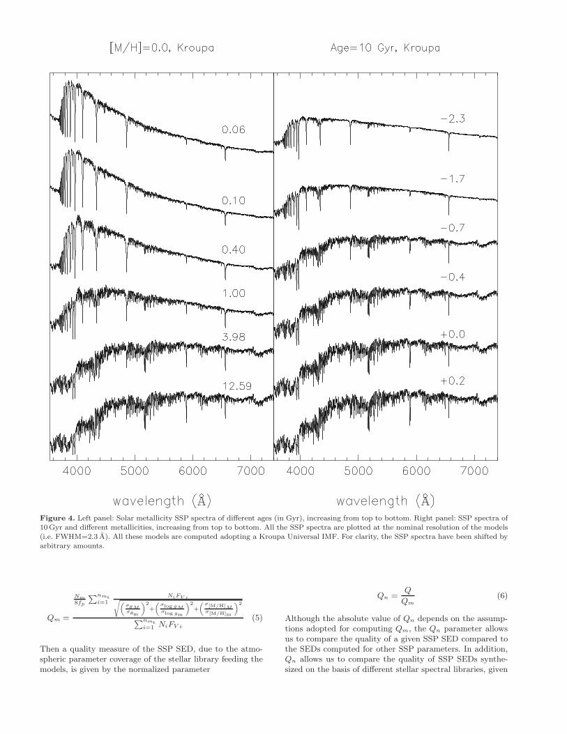
Figure 4. Left panel: Solar metallicity SSP spectra of different ages (in Gyr), increasing from top to bottom. Right panel: SSP spectra of10Gyr and different metallicities, increasing from top to bottom. All the SSP spectra are plotted at the nominal resolution of the models(i.e. FWHM=2.3 A). All these models are computed adopting a Kroupa Universal IMF. For clarity, the SSP spectra have been shifted byarbitrary amounts.

Qm =

Nm8fp

∑nmti=1

NiFV i√

(

σθMσθm

)2

+

(

σlog gMσlog gm

)2

+

(

σ[M/H]Mσ[M/H]m

)2

∑nmti=1 NiFV i

(5)

Then a quality measure of the SSP SED, due to the atmo-spheric parameter coverage of the stellar library feeding themodels, is given by the normalized parameter

Qn =Q

Qm(6)

Although the absolute value of Qn depends on the assump-tions adopted for computing Qm, the Qn parameter allowsus to compare the quality of a given SSP SED compared tothe SEDs computed for other SSP parameters. In addition,Qn allows us to compare the quality of SSP SEDs synthe-sized on the basis of different stellar spectral libraries, given

Figure 5. Left panel: solar metallicity SSP spectra of 10Gyr, computed using a Unimodal IMF of increasing slope from top to bottom.The Salpeter case, i.e. µ =1.3, has been plotted in the right panel of Fig. 4. The SSP spectra are plotted at the nominal resolution of themodels (i.e. FWHM=2.3 A). Right panel: solar metallicity SSP spectra of 10Gyr for different IMF shapes. From top to bottom: KroupaUniversal, Kroupa Revised and Bimodal with increasing slopes, as indicated in the panel. All the spectra have been shifted by arbitraryamounts for clarity.

Table 1. Spectral properties and parameter coverage of the synthesized MILES SSP SEDs

Spectral properties

Spectral range λλ 3540.5-7409.6 ASpectral resolution FWHM = 2.3 A, σ = 54 km s−1

Linear dispersion 0.9 A/pix (51.5 km s−1)Continuum shape Flux-scaledTelluric absorption residuals Fully cleaned

Units Fλ/L⊙A−1M−1⊙

, L⊙ = 3.826 × 1033erg.s−1

SSPs parameter coverage

IMF type Unimodal, Bimodal, Kroupa universal, Kroupa revisedIMF slope (for unimodal and bimodal) 0.3 – 3.3Stellar mass range 0.1 – 100M⊙

Metallicity −2.32, −1.71, −1.31, −0.71, −0.41, 0.0, +0.22Age ([M/H] = −2.32) 10.0 < t < 18Gyr (only for IMF slopes 6 1.8)Age ([M/H] = −1.71) 0.07 < t < 18GyrAge (−1.31 6 [M/H] 6 +0.22) 0.06 < t < 18Gyr

Figure 6. The quality parameter, Qn, as a function of the SSP age (in Gyr) for different metallicities, indicated by the line types asquoted in the inset. For computing the SEDs we use a Unimodal IMF with the slope indicated on the top of each panel. SSPs with Qn

values larger than 1 can be safely used (see the text for details).

the fact that the stellar spectra of these libraries are of suffi-ciently high quality. Furthermore these prescriptions are thesame that we use for computing a stellar spectrum of givenatmospheric parameters, which have been extensively testedin V03.

Figure 6 shows the value of Qn as a function of theSSP age (in Gyr) for different metallicities (different linetypes) and adopting a Unimodal IMF, with its slope increas-ing from the left to the right panel. SSP SEDs with Qn valuesabove 1 can be considered of sufficient quality, and thereforethey can be safely used. The panels show that, as expected,the higher quality is achieved for solar metallicity. For theSalpeter IMF, i.e. the second panel, Qn reaches a value of∼5 for stellar populations in the range 1 – 10Gyr. Outsidethis age range the quality starts to decrease as low-mass andhotter MS stars are less numerous in the MILES database.

A similar behaviour is found in Fig. 6 for the SSPsof metallicities [M/H] = +0.22, −0.41 and −0.71, all withQn values in the range 3 – 4. Despite the fact that forall these metallicities the value of Qn sharply decreases to-ward younger stellar populations, the computed SSP SEDscan be considered safe. For lower metallicities we obtainsignificantly lower Qn values, which gradually decrease to-ward younger ages. For old stellar populations we obtainQn values around 2 and around 1.5 for [M/H] = −1.31and [M/H] = −1.71, respectively. Interestingly, according to

our quantitative analysis, the SSP SEDs synthesized for[M/H] = −2.32 and ages above 10Gyr are barely acceptablefor IMFs with slopes µ = 0.3 and µ = 1.3. These SEDsare particularly useful for globular cluster studies. Note thesharp increase of Qn observed for ages around 1Gyr. Thisshould be mostly attributed to the fact that for stars of tem-peratures larger than 9000K we do not take into accountthe metallicity of the available stars for computing a stellarspectrum of given atmospheric parameters (see V03 for de-tails). Therefore, the quality of the SEDs synthesized for theyounger stellar populations is lower than stated by Qn.

Fig. 6 also shows that Qn decreases slightly with in-creasing IMF slope. In fact, the largest values are obtainedfor the flatter IMF (µ =0.3), as a result of the smaller contri-bution of low mass stars, which are less abundant in MILES.This explains why Qn drops significantly for the steepestIMF. It is worth noting that the SSP SEDs that are synthe-sized for the lowest metallicity cannot be considered safe forIMFs steeper than Salpeter.

For comparison we show in Fig. 7 the Qn values ob-tained for two of the most popular libraries that are used instellar population synthesis, i.e. Lick and STELIB. The firstlibrary is mainly used to predict Lick/IDS line indices viathe empirical fitting functions of Worthey et al. (1994) (e.g.,Worthey 1994; Vazdekis et al. 1996; Thomas et al. 2003).STELIB is the library feeding the models of Bruzual & Char-

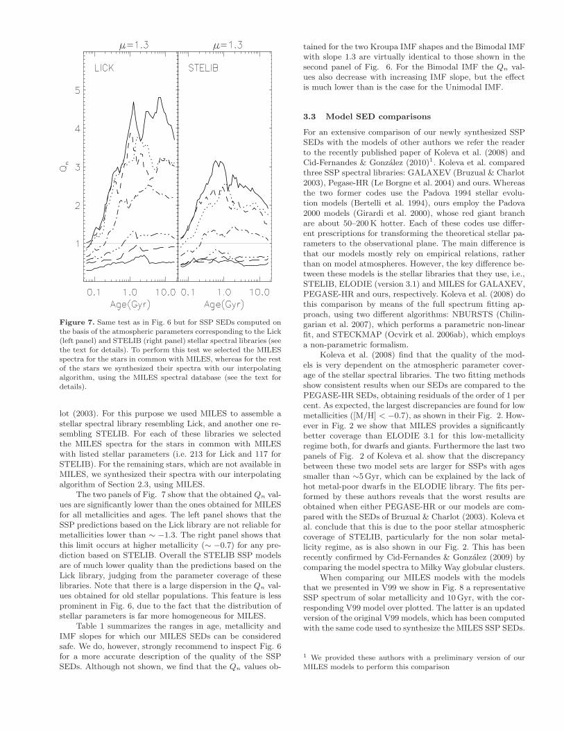
Figure 7. Same test as in Fig. 6 but for SSP SEDs computed onthe basis of the atmospheric parameters corresponding to the Lick(left panel) and STELIB (right panel) stellar spectral libraries (seethe text for details). To perform this test we selected the MILESspectra for the stars in common with MILES, whereas for the restof the stars we synthesized their spectra with our interpolatingalgorithm, using the MILES spectral database (see the text fordetails).

lot (2003). For this purpose we used MILES to assemble astellar spectral library resembling Lick, and another one re-sembling STELIB. For each of these libraries we selectedthe MILES spectra for the stars in common with MILESwith listed stellar parameters (i.e. 213 for Lick and 117 forSTELIB). For the remaining stars, which are not available inMILES, we synthesized their spectra with our interpolatingalgorithm of Section 2.3, using MILES.

The two panels of Fig. 7 show that the obtained Qn val-ues are significantly lower than the ones obtained for MILESfor all metallicities and ages. The left panel shows that theSSP predictions based on the Lick library are not reliable formetallicities lower than ∼ −1.3. The right panel shows thatthis limit occurs at higher metallicity (∼ −0.7) for any pre-diction based on STELIB. Overall the STELIB SSP modelsare of much lower quality than the predictions based on theLick library, judging from the parameter coverage of theselibraries. Note that there is a large dispersion in the Qn val-ues obtained for old stellar populations. This feature is lessprominent in Fig. 6, due to the fact that the distribution ofstellar parameters is far more homogeneous for MILES.

Table 1 summarizes the ranges in age, metallicity andIMF slopes for which our MILES SEDs can be consideredsafe. We do, however, strongly recommend to inspect Fig. 6for a more accurate description of the quality of the SSPSEDs. Although not shown, we find that the Qn values ob-

tained for the two Kroupa IMF shapes and the Bimodal IMFwith slope 1.3 are virtually identical to those shown in thesecond panel of Fig. 6. For the Bimodal IMF the Qn val-ues also decrease with increasing IMF slope, but the effectis much lower than is the case for the Unimodal IMF.

3.3 Model SED comparisons

For an extensive comparison of our newly synthesized SSPSEDs with the models of other authors we refer the readerto the recently published paper of Koleva et al. (2008) andCid-Fernandes & Gonzalez (2010)1. Koleva et al. comparedthree SSP spectral libraries: GALAXEV (Bruzual & Charlot2003), Pegase-HR (Le Borgne et al. 2004) and ours. Whereasthe two former codes use the Padova 1994 stellar evolu-tion models (Bertelli et al. 1994), ours employ the Padova2000 models (Girardi et al. 2000), whose red giant branchare about 50–200K hotter. Each of these codes use differ-ent prescriptions for transforming the theoretical stellar pa-rameters to the observational plane. The main difference isthat our models mostly rely on empirical relations, ratherthan on model atmospheres. However, the key difference be-tween these models is the stellar libraries that they use, i.e.,STELIB, ELODIE (version 3.1) and MILES for GALAXEV,PEGASE-HR and ours, respectively. Koleva et al. (2008) dothis comparison by means of the full spectrum fitting ap-proach, using two different algorithms: NBURSTS (Chilin-garian et al. 2007), which performs a parametric non-linearfit, and STECKMAP (Ocvirk et al. 2006ab), which employsa non-parametric formalism.

Koleva et al. (2008) find that the quality of the mod-els is very dependent on the atmospheric parameter cover-age of the stellar spectral libraries. The two fitting methodsshow consistent results when our SEDs are compared to thePEGASE-HR SEDs, obtaining residuals of the order of 1 percent. As expected, the largest discrepancies are found for lowmetallicities ([M/H] < −0.7), as shown in their Fig. 2. How-ever in Fig. 2 we show that MILES provides a significantlybetter coverage than ELODIE 3.1 for this low-metallicityregime both, for dwarfs and giants. Furthermore the last twopanels of Fig. 2 of Koleva et al. show that the discrepancybetween these two model sets are larger for SSPs with agessmaller than ∼5Gyr, which can be explained by the lack ofhot metal-poor dwarfs in the ELODIE library. The fits per-formed by these authors reveals that the worst results areobtained when either PEGASE-HR or our models are com-pared with the SEDs of Bruzual & Charlot (2003). Koleva etal. conclude that this is due to the poor stellar atmosphericcoverage of STELIB, particularly for the non solar metal-licity regime, as is also shown in our Fig. 2. This has beenrecently confirmed by Cid-Fernandes & Gonzalez (2009) bycomparing the model spectra to Milky Way globular clusters.

When comparing our MILES models with the modelsthat we presented in V99 we show in Fig. 8 a representativeSSP spectrum of solar metallicity and 10Gyr, with the cor-responding V99 model over plotted. The latter is an updatedversion of the original V99 models, which has been computedwith the same code used to synthesize the MILES SSP SEDs.

1 We provided these authors with a preliminary version of ourMILES models to perform this comparison

Figure 8. SSP SEDs of solar metallicity and 10Gyr computedwith the MILES (thin solid line) and Jones (1999) stellar libraries,i.e. the V99 model (thick dotted line). We adopted a Unimodal

IMF of slope 1.3. The V99 model, which has a higher resolution(FWHM=1.8 A) than MILES, was smoothed to match the res-olution of the MILES model (FWHM=2.3 A). The residuals areplotted in the lower panel with the same scale.

The V99 SSP spectrum, with a resolution of 1.8 A (FWHM),was smoothed to match the resolution of the MILES model,i.e., 2.3 A (FWHM). The residuals are plotted on a similarscale. The residuals show a systematic trend in the two nar-row spectral ranges covered by the V99 models. This mustbe attributed to errors in the flux-calibration quality of thelatter, as was reported in V99. The same pattern is seen inthe residuals of Fig. 9, which shows a similar comparison atmetallicity [M/H] = −1.7. Contrary to Fig. 8, the residualsof Fig. 9 show much larger variations at shorter wavelengthscales. This translates into larger index strength variationsin this low metallicity regime, showing that the Jones (1999)library feeding the V99 models lacks important stars. Thiscomparison illustrates how relevant it is to synthesize SSPSEDs with stellar libraries with good atmospheric parame-ters coverage, such as MILES.

4 DEFINING A NEW STANDARD SYSTEMFOR INDEX MEASUREMENTS

A major application of the SSP SEDs is to produce key line-strength indices that can be compared to the observed val-ues. In practise this has been the most popular approachfor studying in detail the stellar content of galaxies. So farthe most widely used indices are those of the Lick/IDS sys-tem (e.g., Gonzalez 1993; Trager et al. 1998, 2000; Vazdekiset al. 1997; Jørgensen 1999; Sanchez-Blazquez et al. 2003,2006a,b,c, 2009). The standard Lick/IDS system of indiceswas defined on the basis of a stellar spectral library (Gor-gas et al. 1993; Worthey et al. 1994), which contains about430 stars in the spectral range λλ4000-6200 A. The Lick/IDSsystem has been very popular because the stellar library con-tains stars with a fair range of stellar parameters and, there-fore, is appropriate to build stellar population models. The

Figure 9. Similar comparison as in Fig. 8 but for metallicity[M/H] = −1.7.

most popular application of this library has been the use ofempirical fitting functions, which relate the index strengths,measured at the Lick/IDS resolution, to the stellar atmo-sphere parameters. Because the value of the Lick/IDS indicesdepend on the broadening of the lines, authors with spectraldata who wish to use the population models based on theLick/IDS fitting functions (e.g., Worthey 1994; Vazdekis etal. 1996; Thomas et al. 2003), or compare them with previ-ously published data, need to transform their measurementsinto the Lick/IDS system. As the resolution of the Lick/IDSlibrary (FWHM∼8-11A) is much lower than what is avail-able with modern spectrographs, the science spectra are usu-ally broadened to the lower Lick/IDS resolution. This is per-formed by convolving with a Gaussian function, whose widthvaries as a function of wavelength, as the resolution of theLick/IDS system, apart from being low, also suffers from anill-defined wavelength dependence (see Worthey & Ottaviani1997). This effect is particularly significant for systems withsmall intrinsic velocity dispersions, such as globular clustersand dwarf galaxies, for which part of the valuable informa-tion contained in the higher resolution galaxy spectra is lost.

After that, it is still necessary to correct the measure-ments for the line broadening due to the velocity dispersionof the stars in the integrated spectra of galaxies. The cor-rection should be calculated by finding a good stellar tem-plate of the galaxy by combining an appropriate set of stel-lar or synthetic spectra which matches the observed spec-trum. This is because this correction is highly sensitive tothe strength of the index. Despite of this, many studies stilluse single polynomial obtained with a single star as a tem-plate, that may have very different index-values than thoseon the observed spectra (see Kelson et al. 2006 for a discus-sion of the systematic effects associated to this procedure).

Due to the fact that the shape of the continuum in theLick/IDS stars is not properly calibrated, the use of the Licksystem requires a conversion of the observational data tothe instrumental response curve of Lick/IDS dataset (seethe analysis by Worthey & Ottaviani 1997) that will affect,predominantly, the broad indices. This is usually done by ob-

serving a number of Lick stars with the same instrumentalconfiguration as for the science objects. Then, by comparingwith the tabulated Lick index measurements, the authorsfind empirical correction factors for each index. This experi-ment shows that even for the narrow indices, differences existbetween the Lick/IDS stars and other libraries (see Worthey& Ottavianni 1997; Paper I). The origin of these differencesis not clear, but they need to be corrected.

Furthermore, the spectra of this library have a low ef-fective signal-to-noise ratio due to the significant flat-fieldnoise (Dalle Ore et al. 1991; Worthey et al. 1994; Trager etal. 1998). This translates into larger random errors in theindices, much larger than in present-day galaxy data. It isworth noting that the accuracy of the measurements basedon the Lick system is often limited by these transformations,rather than by the quality of the galaxy data.

4.1 A new Line Index System: LIS

With the advent of new stellar libraries, such as MILES,with better resolution, better signal-to-noise, larger numberof stars and a very complete coverage of the atmosphericparameter space, it is about time to revisit the standardspectrophotometric system at which the indices are mea-sured. It is not our objective to tell the authors at whichresolution the indices need to be measured. In fact, we rec-ommend to use the flexibility provided by the model SSPSEDs and compare the measurements performed on each ob-ject with models with the same total broadening. However,this might not be a valid option in many cases, e.g., whena group of measurements is to be represented together inthe same index-index diagram. It is also convenient to agreeon a standard resolution at which to measure line-strengths,so that measurements can be compared easily with previousstudies, with colleagues, and to avoid systematic errors thatmight affect the conclusions. One of the reasons why theLick/IDS system is still popular nowadays is because mostprevious studies have calculated their indices in this sys-tem. Although it is a good standard procedure to comparenew measurements with previous works, the fact that thoseare transformed into the Lick/IDS systems perpetuates theproblem. For this reason, we propose in this section a newLine Index System, hereafter LIS, with three new spectralresolutions at which to measure the Lick indices. Note thatthis new system should not be restricted to the Lick set of in-dices in a flux calibrated system. In fact, LIS can be used forany index in the literature (e.g., for the Rose (1994) indices),including newly defined indices (e.g., Cervantes & Vazdekis2009).

We provide conversions to transform the data from theLick/IDS system to LIS as well as tables with index measure-ments in the new system for popular samples of Milky Wayglobular clusters, nearby elliptical galaxies and bulges. Forthis purpose we use index tables already published by otherauthors, and transform them into the new system. To cal-culate the conversion, we have broadened the MILES starsin common with the Lick/IDS library (218 stars in total) tothe new standard resolutions defined for both, globular clus-ters and galaxies, and compare the indices measured in bothdatasets. Third-order polynomials were fitted in all cases.These transformations are given in Appendix A. In a forth-coming paper, we will present empirical fitting functions for

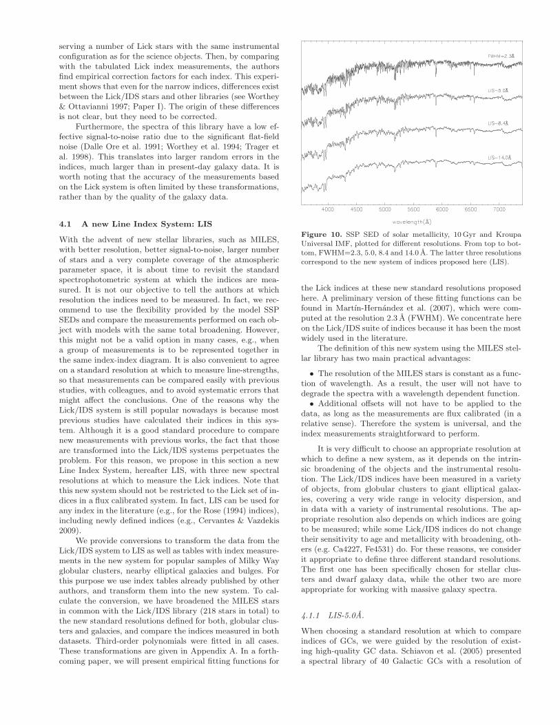
Figure 10. SSP SED of solar metallicity, 10Gyr and KroupaUniversal IMF, plotted for different resolutions. From top to bot-tom, FWHM=2.3, 5.0, 8.4 and 14.0 A. The latter three resolutionscorrespond to the new system of indices proposed here (LIS).

the Lick indices at these new standard resolutions proposedhere. A preliminary version of these fitting functions can befound in Martın-Hernandez et al. (2007), which were com-puted at the resolution 2.3 A (FWHM). We concentrate hereon the Lick/IDS suite of indices because it has been the mostwidely used in the literature.

The definition of this new system using the MILES stel-lar library has two main practical advantages:

• The resolution of the MILES stars is constant as a func-tion of wavelength. As a result, the user will not have todegrade the spectra with a wavelength dependent function.

• Additional offsets will not have to be applied to thedata, as long as the measurements are flux calibrated (in arelative sense). Therefore the system is universal, and theindex measurements straightforward to perform.

It is very difficult to choose an appropriate resolution atwhich to define a new system, as it depends on the intrin-sic broadening of the objects and the instrumental resolu-tion. The Lick/IDS indices have been measured in a varietyof objects, from globular clusters to giant elliptical galax-ies, covering a very wide range in velocity dispersion, andin data with a variety of instrumental resolutions. The ap-propriate resolution also depends on which indices are goingto be measured; while some Lick/IDS indices do not changetheir sensitivity to age and metallicity with broadening, oth-ers (e.g. Ca4227, Fe4531) do. For these reasons, we considerit appropriate to define three different standard resolutions.The first one has been specifically chosen for stellar clus-ters and dwarf galaxy data, while the other two are moreappropriate for working with massive galaxy spectra.

4.1.1 LIS-5.0A.

When choosing a standard resolution at which to compareindices of GCs, we were guided by the resolution of exist-ing high-quality GC data. Schiavon et al. (2005) presenteda spectral library of 40 Galactic GCs with a resolution of

∼ 3.1 A(FWHM). This represents an important comparisondatabase for extragalactic GC systems, and a logical upperlimit for our choice of resolution. However, the majority ofextragalactic spectral data for GCs have lower resolution.Data from the Gemini/GMOS collaboration (e.g., Norris etal. 2008; Pierce et al. 2006ab) exhibits a typical FWHMof ∼5 A. Very similar to that are the VLT/FORS spectrapresented by Puzia et al. (2004). Keck/LRIS data from theSAGES2 group has been generally taken at slightly higherresolutions ∼2.8–4 A (e.g. Strader et al. 2005; Beasley et al.2006; Cenarro et al. 2007; Chomiuk et al. 2008; Beasley etal. 2009). Since it is considerably more straightforward todegrade higher resolution data to lower resolution than itis the attempt to correct lower resolution indices to higherresolution, we suggest using a resolution (FWHM) of 5 A inGC index comparisons, a choice which encompasses all of theabove data. This choice reflects a factor of 2 improvement inresolution over the Lick/IDS system.

Authors willing to compare their data with the modelspresented here will only have to broad their spectra to a res-olution of 5 A (FWHM) (this corresponds to σ = 127 kms−1

at 5000 A) and measure the indices in there. If they wishto compare with previous published data in the Lick/IDSsystem, they can use the conversion provided in Table A.

4.1.2 LIS-8.4A.

For galaxies we have decided to define two different stan-dard resolutions. The first one, discussed in this subsection,is fixed at resolution FWHM=8.4 A (this corresponds toσ = 214 kms−1 at 5000 A). The reasons for this choice aretwofold:

• It matches, roughly, the resolution of the Lick/IDSsystem in the Hβ – Mg triplet region. The indices in thisregions (e.g., Hβ, Mgb, Fe5270) are the most widely used inthe literature and, therefore, the measurements in the newsystem will not differ considerably from previous measure-ments.

• 200 kms−1 is roughly the mean velocity dispersionfor the early-type galaxies in the Sloan Digital Sky Survey(Bernardi et al. 2003a,b,c).

This system is particularly appropriate for studiesof dwarf and intermediate-mass galaxies, where the totalbroadening of the spectra (σ2

inst + σ2gal) is not higher than

σ = 214 kms−1 at 5000 A. In this case, the author will onlyhave to broad their spectra to the proposed total σ using aGaussian broadening function and measure the indices.

If, on the contrary, the total broadening of the objectis higher than this value, the author has the option of usingthe system LIS-14.0A, or to correct his/her measurements toa total broadening of 8.4 A(FWHM) using polynomials (see,e.g., Kuntschner 2000; Sanchez-Blazquez et al. 2006a).

In a similar way as for LIS-5 A, previous data in theLick system can be converted into this new system using thepolynomials given in Table A2.

2 http://www.ucolick.org/∼brodie/sages/SAGES Welcome.html

4.1.3 LIS-14.0A.

The third system is defined at a resolution of FWHM=14 A(this corresponds to σ =357 kms−1 at 5000 A). LIS-14.0Ahas been designed especially for the study of massive galax-ies. In the spectra obtained for these galaxies the broadeningis dominated by the velocity dispersion of the stars. The totalbroadening is higher than the standard Lick/IDS resolutionfor which, in order to compare with the models, usually onehad to perform a correction due to velocity dispersion of thegalaxy. As mentioned above, this correction is one of thelargest sources of systematic errors in the measurement ofthe indices (e.g. Kelson et al. 2006).

For studies that only analyse the stronger Lick in-dices in a sample of galaxies with velocity dispersionsσ > 200 kms−1, we suggest to broaden all the spectraby an amount such that the total resolution (σtotal =√

σ2inst + σ2

gal + σ2broad) matches FWHM=14 A, before mea-

suring the indices, where σinst represents the instrumentalresolution and σgal the velocity dispersion of the galaxy. Thiswill help us to avoid to have to perform any further correc-tion to the indices due to broadening.

Fig 10 shows the synthetic spectra of an SSP with10Gyr and solar metallicity broadened to the resolutionof the different LIS- systems. The polynomials required totransform the indices on the Lick/IDS system to this reso-lution are provided in Table A3.

4.2 Brief notes about system transformation

Most spectrographs keep the resolution constant in units ofwavelength, rather than velocity. Therefore, the broadeningof the spectra, if done in linear wavelength scale, should bealways performed using gaussians of a fixed number of pixels.If the broadening of the data has to be made with a Gaus-sian with a constant width in kms−1. then the broadeningin the spectra should be performed on a spectrum with alogarithmic wavelength scale.

It is common practise in studies of stellar populationsto observe stars in common with the Lick/IDS library. Thisis done to derive offsets to transform the data onto the spec-trophotometric system of the Lick library3. We stress herethat this is necessary, only because the Lick/IDS spectra suf-fer from a number of calibration problems. However, theseoffsets will not correct properly any uncertainty in the cal-ibration of the science spectra, as the position of the line-index on the detector changes for extragalactic objects dueto their redshift.

3 For most indices, the corrections are better described by linearrelations instead of offsets, see appendix in Sanchez-Blazquez etal. (2009)

Table 2. Lick indices measured in the Line Index System for globular clusters and galaxies from selected references.

Puzia et al. (2002) [LIS-5.0A]

Name HδA HδF CN1 CN2 Ca4227 G4300 HγA HγF Fe4383 Ca4455 Fe4531 C4668 Hβ

NGC5927 −2.2576 0.1134 0.0975 0.1362 0.8685 4.9847 −4.1324 −1.2751 2.9922 0.6743 2.6763 3.0431 1.75020.0388 0.0269 0.0009 0.0012 0.0176 0.0282 0.0408 0.0277 0.0493 0.0247 0.0424 0.0629 0.0335

NGC6218 3.1849 2.8266 −0.0543 −0.0298 0.2969 3.3555 1.4944 1.9157 0.1026 0.0319 1.3028 0.1446 2.83340.0186 0.0123 0.0007 0.0007 0.0098 0.0251 0.0248 0.0161 0.0358 0.0127 0.0344 0.0535 0.0278

NGC6284 2.0326 2.6239 −0.0210 0.0056 0.3717 3.8327 0.2104 1.3103 0.8237 0.1649 1.8133 0.5586 2.54390.0250 0.0187 0.0007 0.0008 0.0128 0.0248 0.0288 0.0207 0.0442 0.0161 0.0363 0.0575 0.0272

NGC6356 −1.0805 0.6216 0.0606 0.0891 0.6710 5.4774 −3.8769 −0.9782 2.3657 0.4230 2.6000 1.7702 1.74840.0186 0.0117 0.0006 0.0007 0.0100 0.0142 0.0214 0.0139 0.0272 0.0122 0.0253 0.0440 0.0189

NGC6388 −0.2366 1.0513 0.0602 0.0917 0.5320 4.8704 −2.6754 −0.1589 2.4337 0.3673 2.5714 1.7768 2.12590.0100 0.0062 0.0003 0.0004 0.0049 0.0092 0.0128 0.0078 0.0158 0.0066 0.0120 0.0196 0.0098

NGC6441 −0.2459 1.1013 0.0682 0.0997 0.6307 4.8525 −2.8379 −0.1968 2.7413 0.3912 2.6228 1.7832 2.05520.0260 0.0176 0.0007 0.0009 0.0150 0.0237 0.0271 0.0200 0.0333 0.0157 0.0320 0.0501 0.0240

NGC6528 −2.0478 0.3512 0.1078 0.1389 1.0559 5.6030 −5.6367 −1.6013 4.6496 0.7368 2.9746 4.4146 1.88890.0439 0.0294 0.0011 0.0013 0.0194 0.0303 0.0452 0.0302 0.0509 0.0276 0.0447 0.0796 0.0351

NGC6553 −2.2176 0.8167 0.1465 0.1810 1.2451 5.7732 −5.8327 −1.6070 3.9143 0.6909 3.3030 3.7248 2.00260.0705 0.0432 0.0017 0.0022 0.0328 0.0476 0.0639 0.0425 0.0777 0.0460 0.0672 0.1140 0.0521

NGC6624 −0.9553 0.6427 0.0650 0.0977 0.6539 5.3411 −3.7187 −0.8093 2.4164 0.4004 2.5801 1.8939 1.76450.0184 0.0136 0.0005 0.0006 0.0092 0.0144 0.0209 0.0161 0.0252 0.0128 0.0218 0.0366 0.0199

NGC6626 2.3537 2.4215 −0.0247 0.0026 0.3655 3.7828 0.1746 1.2743 0.7371 0.0931 1.6467 0.6247 2.39040.0222 0.0178 0.0006 0.0009 0.0113 0.0260 0.0278 0.0171 0.0381 0.0124 0.0351 0.0571 0.0278

NGC6637 −1.1022 0.3993 0.0417 0.0691 0.5761 5.5794 −3.9200 −1.0808 2.1029 0.3539 2.4863 1.7632 1.73670.0155 0.0107 0.0004 0.0005 0.0071 0.0105 0.0175 0.0127 0.0214 0.0096 0.0200 0.0303 0.0141

NGC6626 2.3537 2.4215 −0.0247 0.0026 0.3655 3.7828 0.1746 1.2743 0.7371 0.0931 1.6467 0.6247 2.39040.0222 0.0178 0.0006 0.0009 0.0113 0.0260 0.0278 0.0171 0.0381 0.0124 0.0351 0.0571 0.0278

NGC6637 −1.1022 0.3993 0.0417 0.0691 0.5761 5.5794 −3.9200 −1.0808 2.1029 0.3539 2.4863 1.7632 1.73670.0155 0.0107 0.0004 0.0005 0.0071 0.0105 0.0175 0.0127 0.0214 0.0096 0.0200 0.0303 0.0141

NGC6981 1.5589 1.7715 −0.0262 −0.0091 0.3862 3.5881 0.4667 1.2872 0.1925 0.0895 1.3977 0.3620 2.50910.0179 0.0127 0.0006 0.0007 0.0091 0.0208 0.0220 0.0164 0.0360 0.0126 0.0333 0.0475 0.0255

Name Fe5015 Mg1 Mg2 Mgb Fe5270 Fe5335 Fe5406 Fe5709 Fe5782 Na5895 TiO1 TiO2

NGC5927 4.9167 0.0756 0.1999 3.5827 2.2866 2.0628 1.3108 0.5205 0.8942 4.4516 0.0377 0.08950.0715 0.0007 0.0009 0.0358 0.0442 0.0524 0.0381 0.0340 0.0317 0.0396 0.0008 0.0008

NGC6218 2.8312 0.0232 0.0582 1.1352 0.8644 1.0777 0.4432 −0.1952 0.2400 1.1520 0.0101 0.00450.0691 0.0006 0.0008 0.0343 0.0311 0.0490 0.0289 0.0345 0.0275 0.0387 0.0009 0.0010

NGC6284 3.2827 0.0375 0.0854 1.5008 0.9413 1.2086 0.6797 0.1218 0.3272 2.2529 0.0083 0.00440.0752 0.0007 0.0009 0.0323 0.0364 0.0454 0.0328 0.0350 0.0227 0.0420 0.0008 0.0008

NGC6356 4.1852 0.0647 0.1602 2.8145 1.7640 1.8961 1.0925 0.4241 0.5489 3.1437 0.0224 0.05020.0446 0.0005 0.0006 0.0214 0.0231 0.0326 0.0210 0.0217 0.0191 0.0262 0.0005 0.0006

NGC6388 4.2186 0.0502 0.1310 2.1997 1.9315 1.9042 1.1532 0.5123 0.6698 3.6860 0.0219 0.04470.0244 0.0002 0.0003 0.0107 0.0158 0.0146 0.0125 0.0106 0.0096 0.0143 0.0003 0.0003

NGC6441 4.3328 0.0640 0.1586 2.7556 2.0015 1.9567 1.1619 0.5665 0.8016 3.9727 0.0128 0.05130.0591 0.0006 0.0007 0.0269 0.0379 0.0432 0.0253 0.0258 0.0239 0.0265 0.0006 0.0006

NGC6528 5.2490 0.1033 0.2382 3.7516 2.4408 2.5976 1.7286 0.8399 0.8249 5.1220 0.0575 0.11960.0807 0.0009 0.0009 0.0395 0.0457 0.0479 0.0476 0.0311 0.0364 0.0402 0.0010 0.0009

NGC6553 5.7870 0.0897 0.2324 3.9036 2.7011 2.5835 1.3858 0.7923 1.1831 3.7845 0.0523 0.13400.0971 0.0011 0.0013 0.0514 0.0702 0.0753 0.0521 0.0424 0.0454 0.0563 0.0010 0.0009

NGC6624 4.3141 0.0628 0.1554 2.7574 1.8628 1.8745 1.1159 0.5191 0.6466 2.5670 0.0337 0.05930.0422 0.0004 0.0005 0.0166 0.0243 0.0342 0.0256 0.0173 0.0214 0.0219 0.0005 0.0005

NGC6626 3.3106 0.0364 0.0811 1.4305 1.1532 1.1603 0.7001 0.1977 0.4725 1.9530 0.0187 0.03630.0669 0.0005 0.0006 0.0299 0.0322 0.0365 0.0272 0.0304 0.0269 0.0322 0.0007 0.0006

NGC6637 4.0857 0.0501 0.1388 2.5752 1.6781 1.6068 0.9602 0.3732 0.4894 2.4638 0.0263 0.04180.0365 0.0004 0.0005 0.0164 0.0212 0.0237 0.0170 0.0143 0.0144 0.0225 0.0004 0.0005

NGC6626 3.3106 0.0364 0.0811 1.4305 1.1532 1.1603 0.7001 0.1977 0.4725 1.9530 0.0187 0.03630.0669 0.0005 0.0006 0.0299 0.0322 0.0365 0.0272 0.0304 0.0269 0.0322 0.0007 0.0006

NGC6637 4.0857 0.0501 0.1388 2.5752 1.6781 1.6068 0.9602 0.3732 0.4894 2.4638 0.0263 0.04180.0365 0.0004 0.0005 0.0164 0.0212 0.0237 0.0170 0.0143 0.0144 0.0225 0.0004 0.0005

NGC6981 2.7705 0.0265 0.0532 1.1555 0.9544 0.7882 0.3914 −0.1326 0.1239 1.2737 0.0070 −0.00340.0619 0.0006 0.0007 0.0304 0.0323 0.0394 0.0218 0.0333 0.0151 0.0367 0.0006 0.0008

The complete version of this table can be found in the electronic version of the journal.

.

Figure 11. Hβ vs. [MgFe] diagnostic diagram in the LIS-5.0Asystem. Asterisks represent the globular cluster sample of Schi-avon et al. (2005), whereas the solid circles represent the clustersof Puzia et al. (2002). We used the indices listed in Table 2 (theelectronic version). For the models we used a Kroupa Universal

IMF.

4.3 Reference tables

One of the reasons many authors keep using the Lick/IDSsystem is to compare with previous studies, which are usu-ally presented in this system. We provide here with a set ofindices, obtained from several references already transformedto the new systems. The data are available at the CDS andin the electronic version of the paper.

We have selected several samples of early-type galaxiesand globular clusters from the literature and transformedthe line-strength indices to the new systems defined here.This is intended to provide a benchmark of indices properlytransformed into LIS and measured on high quality data thatother authors can use to compare with. The selected samplesare the following:

• Puzia et al. (2002). This sample comprises 12 Galacticglobular clusters. Lick indices were measured from long-slitspectra obtained with the Boller & Chivens Spectrographmounted on the 1.5m telescope in La Silla. The wavelengthcoverage of the spectra ranges from 3400 to 7300 A with afinal resolution of ∼6.7 A. All the spectra were observed witha slit with of 3.′′0. We transformed the Lick indices into thenew system using the transformations provided in this paper(Table A1).

• Schiavon et al. (2005). The sample consists of 40 galac-tic globular clusters, obtained with the Blanco 4-m telescopeat the Cerro Tololo observatory. The spectra cover the range∼3350-6430A with 3.1 A (FHWM) resolution. The signal-to-noise ratio of the flux calibrated spectra ranges from 50 to240 A−1 at 4000 A and from 125 to 500 A−1 at 5000 A. Thesample has been carefully selected to contain globular clus-ters with a range of ages and metallicities. The indices pro-vided in Table 2 have been measured directly in the spectradegraded to the LIS-5.0A resolution.

• Trager et al. (2000). This sample consist of 40 galax-ies drawn from that of Gonzalez (1993) intended to cover,relatively uniformly, the full range of velocity dispersion,

line-strength and color displayed by local elliptical galax-ies. The line-strength indices (i.e. Hβ, Mgb, Fe5270, Fe5335)were measured from long-slit data obtained with the CCDCassegrain Spectrograph on the 3m Shane Telescope of LickObservatory. The spectral features were measured withinre/8 aperture. The indices were transformed into the newsystem applying the transformations from Tables A2 andA3.

• Sanchez-Blazquez et al. (2006a). This sample consistsof 98 early-type galaxies including ellipticals and lenticulars,spanning a wide range in central velocity dispersion (σ). Thesample contains galaxies in different environments: isolatedgalaxies, galaxies in groups, and in several clusters. Thecentral spectra were extracted within an aperture 0.6 kpc(assuming H0=70 kms−1). The spectra were corrected fromthe presence of nebular emission using GANDALF (Sarzi etal. 2006), instead of using the [OIII]λ-based correcion pub-lished in the original paper. We use the models providedin this paper as templates. The spectral range covers from∼3500/3700 (depending on the run) to ∼5200/5700 A, withspectral resolution ranging from 3.6 to 6.56 A (FWHM) (seeoriginal paper for more details). The indices provided in Ta-ble 2 have been measured in the emission-free spectra previ-ously degraded at the different LIS resolutions. For thosegalaxies with a σ larger than the LIS resolution an ad-ditive correction was made using the kinematic templates(the combination of SSP-models that better reproduced thegalaxy spectra obtained in the measurement of σ using ppxf

(Cappellari & Emsellem 2004)), following the prescriptionsin Kelson et al. (2006). The correction was obtained as thedifference in the indices measured in these templates de-

graded at the LIS-resolution and at the√

σ2gal + σ2

ins, where

σgal is the velocity dispersion of the galaxy and σinst the in-strumental resolution.

• Yamada et al. (2006). The sample consists of 14 galax-ies, morphologically classified as E in the Virgo cluster. Thegalaxies where selected with three criteria: (1) they had tobe classified as elliptical galaxy in the RC3 catalogue (deVaucouleurs et al. 1991); (2) they had to be free from strongemission lines; (3) they have to cover a wide range of lumi-nosity evenly distributed along the color-magnitude of theVirgo cluster. These extremely high quality spectra, whichhave been extracted within an aperture of re/10, have signal-to-noise ratio well above >100 A−1 for all the galaxies, andabout ∼500 A−1 for some of them. The spectra cover a wave-length range from 3800 to 5800 A, and the resolution rangesfrom 2.0 A to 3.1 A, depending on the observational runs,which have been performed at the William Herschel Tele-scope (WHT; 4.2m) and Subaru (8.2m) telescopes. For fulldetails of the sample we refer the reader to the original pa-per. Three galaxies have a velocity dispersion larger thanthe resolution of the LIS-8.4A and the indices in this systemwere corrected in the same way as in the SB06b sample

• Kuntschner et al. (2006). This sample consists of 48E/S0 galaxies in the SAURON survey of early-type galaxies(de Zeeuw et al. 2002) at the William Herschel 4.2m tele-scope in La Palma. We use here the line strength measure-ments (i.e. Hβ, Fe5015, Mgb) averaged within re/8 aperture.The spectral coverage of the observed SAURON integral-field observations ranges from 4800 to 5380 A at resolution∼4.2 A (FWHM). The indices of Table 2 were obtained ap-

.

Figure 12. Hβ vs. [MgFe] and Hβ vs. [MgFe50] diagnostics diagrams in LIS-8.4A. In the left panel we plot the galaxy samples of Trageret al. (2000) (solid circles), Yamada et al. (2006) (stars) and Sanchez-Blazquez et al. (2006a) (open triangles). In the right panel weplot the galaxy sample of Kuntschner et al. (2006) (asterisks) and 36 galaxies from the sample of Sanchez-Blazquez et al. (2006a) (opentriangles), as for all these galaxies the two iron lines required to calculate the [MgFe] index fall outside the covered spectral range (i.e.Fe5270 and Fe5335).

.

Figure 13. Same as in Fig. 12 but for LIS-14.0A.

plying the transformations of Table A2 and A3 to the indicestransformed into the Lick systems provided in the originalpaper.

Table 2 shows a portion of the tables to illustrate its for-mat and content. The table contains the Lick/IDS indicesmeasured at the different LIS resolutions with the index def-initions provided in Trager et al. (1998). The full tables areavailable in the electronic version of the paper.

Fig. 11 shows the commonly used index-index diagnosticdiagram Hβ vs. [MgFe] in the new LIS-5.0A system for thePuzia et al. (2002) and Schiavon et al. (2005) globular clustersamples. We use the indices in Table 2. Note that we do

not plot the model indices for SSPs younger than 10Gyrfor [M/H] = −2.3, according to our Qn parameter analysis.In Fig. 12 and Fig. 13 we show the Hβ vs. [MgFe] and Hβvs. [MgFe50] diagrams for the four galaxy samples both inLIS-8.4A and LIS-14.0A. Note that for all the galaxies ofKuntschner et al. (2006) and for 36 galaxies in the Sanchez-Blazquez et al. (2006a) sample it was not possible to plot the[MgFe] index, as either one or the two iron indices (Fe5270,Fe5335) required to calculate this index were outside thecovered spectral range. Note that we used GANDALF (Sarzi etal. 2006) to remove nebular emission from the galaxy spectraof Sanchez-Blazquez et al. (2006a) and Yamada et al. (2006).

Figure 15. Time evolution of various Balmer line-strength in-dices measured on the SSP SEDs of solar metallicity and KroupaUniversal IMF smoothed at different resolutions as in Fig. 14.

We refer the reader to all these original works for a detaileddiscussion of the obtained results.

4.4 MILES SSP SED index measurements

Figure 14 shows the predicted time evolution of our solarmetallicity and Salpeter IMF models for a selection of line-strength indices measured at four different spectral resolu-tions: the nominal resolution of the models, i.e. FWHM =2.3 A, and the resolutions of LIS-5.0A, LIS-8.4A, and LIS-14.0A (i.e., FWHM=5, 8.4 and 14 A, respectively). It canbe seen that the sensitivity of some indices to variationsin resolution is barely noticeable. This is the case for thewide molecular index definitions, i.e., CN, Mg and TiO. Forsome lines, however, broadening the spectra means loosingpart of the information contained in them (e.g. Ca4227). Themost critical situation when analyzing data by means of di-agnostic diagrams based on these indices happens when therelative variation of the index with age depends on resolu-tion. Authors should keep this in mind in order to choosethe right system and diagnostics to work with the data. Ourrecommendation is to use the most straightforward approachpossible, which is to work with the model SEDs smoothedto match the total resolution of the data. This approach al-lows the user to take full advantage of the whole informationcontained in the data (see V99 for an extensive discussion).Interestingly we note that the time evolution for most Lickindices shows a minimum for intermediate-age stellar pop-

Figure 17. Variation of Balmer line-strength indices with metal-licity predicted by our single stellar population models of 10Gyrand Kroupa Universal IMF. Different line-styles show predictionsfor indices measured at different spectral resolution, as in Fig. 14.

ulations in the range 0.1–1.0 Gyr, as already mentioned inSec. 3.1. This is particularly evident for the CN indices.

Fig. 15 is similar to Fig. 14 but here several Balmerindex definitions are shown. We plot the standard Lick Hβindex and the four higher-order Balmer indices of Worthey &Ottaviani (1997). We also include two of the age indicators ofVazdekis & Arimoto (1999), the recently defined Hβo indexof Cervantes & Vazdekis (2009) and the D4000 break (e.g.,Gorgas et al. 1999). We see that for all the Balmer indexdefinitions the dependence on resolution is marginal or vir-tually nil (e.g. the 4000 A break). The two Hγσ of Vazdekis& Arimoto (1999) are specifically defined to be insensitive toresolution. For this reason we only plot, for Hγ125, the valuescorresponding to the resolution of LIS-5.0A and for Hγ200the ones for LIS-8.4A as these two resolutions fall within thestability range of these indices, respectively. We did not in-clude the third index defined in Vazdekis & Arimoto (1999),Hγ275, as the resolution of LIS-14.0A is larger than is al-lowed for this index. Interestingly, being almost negligible,we see that, whereas the sensitivity to resolution for the newHβo index is slightly larger than that for the standard HβLick index for old stellar populations, the situation is reversefor ages smaller than ∼1Gyr. The higher-order Balmer lineindex definitions of Worthey & Ottaviani (1997) also showlarger resolution sensitivity for younger stellar populations.Note that all Balmer indices, except the D4000 break, peakat ∼0.3Gyr and, therefore, the fits obtained on the basis ofthese indices can have two solutions. Kauffmann et al. (2003)

Figure 14. Time evolution of several Lick line-strength indices measured on our new SSP SEDs for solar metallicity and Kroupa UniversalIMF, smoothed to different resolutions. Solid line: resolution of LIS-5.0 A (FWHM = 5 A); dashed line: resolution of LIS-8.4 A (FHWM= 8.4 A); dashed-dotted line: resolution of LIS-14.0A (FWHM = 14 A).

take advantage of the behaviour of these indices to define di-agnostics for constraining the Star Formation History.

Figure 16 and Fig. 17 shows the variation of the line-strength indices as a function of metallicity predicted by ournew models for stellar populations of 10Gyr and SalpeterIMF. As in the previous figures the predictions are shownfor three different resolutions; FWHM= 5.0, 8.4 and 14 A.We see a resolution-dependent differential behaviour as func-tion of metallicity for several indices, such as for exampleCa4227, Fe5335, Fe5782. This shows that a lot of care has tobe taken to match the resolution of data and models whencomparing both as, otherwise, artificial trends can be de-rived (see Kelson et al. 2006). Fig. 17 shows the somewhatopposite dependence on the resolution of two Hβ index defi-nitions: Hβo shows larger resolution dependence than Hβ forhigher metallicities. Note however the insensitivity to metal-licity achieved by this Hβo definition for [M/H] > −1, whichis not seen for the commonly used Hβ Lick index. Such in-sensitivity is also shown by the two Hγ indices of Vazdekis& Arimoto (1999) plotted here. We are not describing herein detail the index bahaviour as function of metallicity andage, but the metallicity insensitivity of the two TiO molec-ular indices for [M/H] > −0.5 is particularly noteworthy.

4.5 Hβ: comparison with the fitting functionpredictions

In Fig. 18 we focus specifically on the behaviour of the mostpopular age indicator, the Lick Hβ index, as a function ofage (plotted in linear scale, for ages >1Gyr) and metallicity.In this figure we compare the index computed on the basisof the empirical fitting functions of Worthey et al. (1994),using the Vazdekis et al. (1996) code, as updated in thiswork and transformed to the LIS-8.4A system following Ta-ble A2, with the Hβ index measured on the SSP SEDs, oncesmoothed to the LIS-8.4A resolution. We see that the modelsbased on MILES provide larger values for solar and super-solar metallicities and for [M/H] < −1 than those based onthe Lick/IDS fitting functions. This implies that when usingMILES models the obtained ages are older by about ∼2Gyrfor SSPs around ∼10Gyr.

Another interesting effect at metallicities [M/H] < −1is that, for ages above ∼12Gyr, Hβ starts increasing insteadof decreasing as expected. This effect, not seen at highermetallicities, is attributed to the contributions of the Hori-zontal Branch (HB) stars (e.g. Maraston & Thomas 2000).Therefore the Hβ index, rather than indicating the age of thestellar population due to their sensitivity to the Teff of theturnoff stars, become sensitive to the HB morphology. Thisresult is in agreement with Maraston & Thomas (2000). Wesee, however, that this sudden increase in the strength of theHβ index is less visible for the new predictions for the threelowest metallicities plotted in this figure. In fact, the effect

Figure 16. Variation of line-strength indices with metallicity predicted by our single stellar population models of 10Gyr and KroupaUniversal IMF. Different line-styles show predictions for indices measured at different spectral resolution, as in Fig. 14.

virtually disappears for [M/H] < −2. This result would haveimportant implications for the interpretation of integratedspectra of composite stellar systems, for which the Balmerlines, such as the Hβ index, are the primary age diagnostics.In fact, Maraston & Thomas (2000) have suggested that aan spread in metallicity of an old stellar populations can ac-count for most of the dispersion of Hβ values observed in theellipticals family – due to the higher Hβ index of the metalpoor stars– without the need of a young population as hadbeen previously suggested in other studies (e.g. Gonzalez1993). As we obtain with MILES higher Hβ strengths, therequired fraction for the metal-poor component should besmaller than is suggested by Maraston & Thomas (2000).

It is very important to note that in Fig. 18 we are com-paring the same synthesis code, with identical HB prescrip-tions. The different behaviour at low metallicities betweenthe two sets of predictions should be fully attributed, there-fore, to the limitations of the Lick stellar library, as it be-comes evident when comparing the Qn values obtained forthese two sets of predictions in this low metallicity regime(see the second panel of Fig. 6 and first panel of Fig. 7)4.

4 In fact, guided by the obtained Qn parameter, we only plottedthe Hβ values for ages larger than 10Gyr for the MILES models

of [M/H] = −2.3. However we plotted the Hβ values obtained forthe Lick/IDS fitting functions for [M/H] = −1.7, despite the factthat their corresponding Qn values are lower than 1 (see the firstpanel of Fig. 7)

.

Figure 18. Comparison of the Hβ index computed on the basisof the empirical fitting functions of Worthey et al. (1994), usingthe models of Vazdekis et al. (1996), as updated in this workand transformed to the LIS-8.4A system following Table A2, withthe index measured on the SSP SEDs, once smoothed to the LIS-8.4A resolution. For the lowest metallicity we only plot the resultsfor SSPs older than 10Gyr according to our qualitative analysisshown in the second panel of Fig. 6. However, for the sake of thediscussion we also show the predictions based on the Lick/IDSfitting functions for [M/H] = −1.7 despite we consider they donot have enough quality due to the low number of stars at thosemetallicities (see the text for details).

5 MILES SSP COLOURS

One of the main advantages of MILES is that the stellarspectra were carefully flux-calibrated. In fact we obtainedfor each star of the library a wide-slit spectrum to avoidselective flux losses due to the differential refraction effect(see Paper I for details). This allows us to measure accuratecolours from the synthesized SSP SEDs. This is performed byconvolving the SED with the corresponding filter responses.To obtain the Johnson B − V broad band colour we use thefilters of Buser & Kurucz (1978), with the zero points setwith Vega. To obtain the zero point for the B and V filters,we used two different Vega SEDs from Hayes (1985) andfrom Bohlin & Gilliland (2004), the latter based on highsignal to noise Space Telescope Imaging Spectroph (STIS)observations and extrapolated to higher wavelengths usingKurucz model atmospheres. After normalising the syntheticspectra to the SED of Vega we measured the B − V coloursby applying the selected filter transmission curves.

The results are shown in Fig. 19. We also plot, forcomparison, the photometric version of this colour followingVazdekis et al. (1996) which is computed with the Alonso etal. (1996, 1999) calibrations. The figure shows a good agree-ment for nearly all ages and metallicities, within the typi-cal photometric uncertainties derived from the zero point ofthe B and V filters, as shown by the colours differences us-ing two different normalizations of the Vega spectrum. Weobtain rather similar time evolution colour curves for allthe metallicities, with an offset of ∼0.02mag. For the SSPswith [M/H] = −2.32 the offset can be as large as ∼0.05mag(MILES SEDs colours slightly bluer), which is well belowthe photometric errors of the colours. Note, however, thatfor this metallicity the MILES models are barely acceptable,as shown by the Q parameter (see Fig. 6). This is becauseof the stellar parameter coverage of the MILES library andthe fact that colour transformation are not accurate at suchlow metallicity.

A rather similar offset (∼0.015mag.) has been quotedin Paper I (see their Fig. 8) by comparing the B−V coloursderived from MILES stellar spectra to the values tabulatedin the Lausanne photometric database (Mermilliod et al.1997) for the same stars. As discussed in Paper I this off-set sets an upper limit to the systematic uncertainties ofour photometry. For the sake of clarity we do not show inFig. 19 the colours obtained from the model SEDs computedwith the temperature scale of Gonzalez-Hernandez & Boni-facio (2009). These models provide redder B − V colour by∼0.02mag, i.e. similar to the zero point uncertainties. Thisis because for a given temperature the stellar populationmodel selects cooler spectra as the Gonzalez-Hernandez &Bonifacio (2009) temperatures are hotter than MILES by51K.

The results presented here show that the colours derivedfrom our models, either those predicted via photometric li-braries or the ones measured from our MILES SSP SEDs,are consistent. Such agreement shows the reliability of thetemperatures adopted in Paper II, which are consistent withthe temperature scales of Alonso et al. (1996,1999), i.e. thephotometric libraries that feed our models. We also provide,in electronic form and on the web (see Section 7), coloursmeasured directly in the MILES spectra using combinations

..

Figure 19. We plot the broad band B − V colour derived fromthe SSP SEDs for different ages and metallicities (as indicatedwithin the panel) and the Kroupa Universal IMF with the zeropoint set with two different Vega spectra in black (very thin)and red (thicker) (see the text for details). The thickest greenline represents the photometric colour computed by Vazdekis etal. (1996), as updated in this work, which is based on extensiveempirical photometric stellar libraries.

of various filter systems that are commonly used in the lit-erature (e.g., SDSS, HST).

6 APPLICATIONS TO STELLAR CLUSTERAND GALAXY DATA

We compare, in this section, our new model SEDs with a setof representative stellar clusters of varying age and metallic-ity. We also illustrate the use and capabilities of these modelsfor the study of galaxies with varying age, metallicity, abun-dance ratio and mass, by giving a few examples for somewell-studied galaxies.

6.1 Stellar Clusters

Galactic globular clusters allow us to uniquely test our evolu-tionary synthesis models, since independent age and metal-licity estimates are available through deep CMD analyses.These studies have concluded that, in most cases, globularclusters can be considered as formed in a single burst, whichis characterized by a single age and a single metallicity, i.e.an SSP. Note, however, that there are clusters for which two

.

Figure 20. Spectra of various representative Galactic globularclusters with varying metallicity, from Schiavon et al. (2005), plot-ted in black. For each cluster we overplot in green the best fittingSSP SED. We adopt for the models a Kroupa Universal IMF. Theage and metallicity of the SSP are indicated within each panel.The SSP SEDs were smoothed to match the instrumental reso-lution of the observations (i.e. σ = 120 km s−1). The obtainedresiduals are plotted at the same scale. Note that no continuumremoval was applied when performing the fit.

stellar components have been identified (e.g., Meylan 2003)and that stochastic effects (e.g., Cervino et al. 2002) mayaffect significantly their integrated spectra.

We have selected three representative Galactic globu-lar clusters, with varying metallicity, from the sample ofSchiavon et al. (2005), which is composed of 40 clusters.These authors obtained integrated spectra of high signal-to-noise (S/N∼250) covering the range λλ3350–6430 A with3.1 A (FHWM) resolution. Fig. 20 shows the spectra and thebest SSP SED fits overplotted. We used, for this purpose,our SSP SED library with Kroupa Universal IMF. The SSPSEDs were conveniently smoothed to match the instrumen-tal resolution of the observations (i.e. σ ∼ 120 km s−1). Wenormalized the stellar cluster spectra and the model SEDsat 5000 A, but we did not modify the spectral shape of thedata (and the models) to perform the fits. The best fit isunderstood as the one that minimizes the residuals, whichare also plotted in the figure at the same scale. The obtainedages and metallicities fully agree with the CMD-derived es-

timates of the Harris (1996) catalog. For 47Tuc we obtainedthe same fit as in V99. For NGC5904 we derived a youngerage, in agreement with the very deep CMD study of Marin-Franch et al. (2009) who have estimated for this cluster arelative age of 0.83, i.e. the cluster is located within theiryoung GC branch. We also found a younger age for this clus-ter, by means of a line-strength analysis that included thenewly defined Hβo age indicator of Cervantes & Vazdekis(2009). The higher Hβ value obtained for this cluster is at-tributed in part to the presence of an increased fraction ofBlue Stragglers (see Cenarro et al. 2008).

The residuals of Fig. 20 do not show any significantcolour difference in the covered spectral range, but somevery low frequency variations that can be fully attributedto differences in the flux calibration. In fact, note that theselow frequency residuals are qualitatively identical among thethree clusters. However the residuals show differences in var-ious molecular bands, mainly in the blue part of the spectrafor all the clusters. In particular, CN features at ∼3860 A and∼4150 A, are much stronger in the clusters than in the mod-els. We also see a residual in the G band at ∼4300 A, beingthis absorption weaker in the data. The CN-strong absorp-tion, and its anticorrelation with CH, is a well known featurein the Galactic globular cluster family, which has been shownin both their individual stars (e.g., Norris & Freeman 1979)and its integrated spectra (e.g. Rose & Tripicco 1986). A sim-ilar result is obtained in V99 for 47Tuc, but using a differentinput stellar spectral library and also a different spectrum forthe cluster. Such CN-strong absorption feature has also beenreported for extragalactic globular clusters, like NGC1407(Cenarro et al. 2007b). Their Lick/IDS C24668 vs. CN2 di-agram shows the same anticorrelation with respect to thescaled-solar abundance ratios. Overall, we find that the resid-uals blueward of ∼4300A are significantly larger than for theredder part of the spectra for all the clusters. We do notdiscard possible effects due to the fact that the Milky Wayglobular clusters show oxygen-enhanced abundance ratios forlow metallicities. In fact Cassisi et al. (2004) have shown thatsuch effects become relevant for the spectral ranges coveredby the B, and mostly U , broadband filters. Therefore an ap-propriate modelling for these clusters requires working withsuch α-enhanced stellar evolutionary isochrones as well asthe use of stellar spectra with similar abundance pattern. Inaddition we also require to use specific stellar spectra withCN-strong absorption features and CN-enhanced isochrones.

In Fig. 21 we show our SED fit to the integrated spec-trum of the standard open cluster M67 (Schiavon, Caldwell& Rose 2004). Unlike for the globular clusters of Fig. 20these authors obtained the integrated spectrum for M67 byco-adding individual spectra of cluster members, weightedaccording to their luminosities and relative numbers. Theobtained age and metallicity is in good agreement with theseauthors (see also Schiavon 2007) and with our isochrone fit-ting results (Vazdekis et al. 1996) within the uncertainties.The residuals only show a low frequency pattern, which isrelated to differences in the flux calibration. However thehigher frequency residuals are negligible. It is particularlyinteresting that, unlike in Fig. 20, we do not see the residu-als blueward of 4300 A. This shows that all relevant spectraltypes are present in the MILES library. Therefore the residu-als obtained for Galactic globular clusters can be attributedto the non-solar abundance ratios present in these clusters.

.

Figure 21. The spectrum of the Milky Way open cluster M67(Schiavon et al. 2004) plotted in black. We overplot the best fittingSSP SED in green, with its age and metallicity indicated withinthe panel. We adopt a Kroupa Universal IMF. The model has beensmoothed to match the instrumental resolution of the observedspectrum (also quoted). The residuals are plotted in the bottompanel with the same scale. Note that no continuum removal wasapplied for performing the fit.

.

Figure 22. The spectrum a bright globular cluster of the galaxyNGC1407, from Cenarro et al. (2007b), plotted in black. We over-plot the best fitting SSP SED in green, with its age and metallicityindicated within the panel. We adopt a Kroupa Universal IMF.The model has been smoothed to match the instrumental reso-lution of the observed spectrum (also quoted). The residuals areplotted in the bottom panel with the same scale. Note that nocontinuum removal was applied for performing the fit.

However we propose to use our base models in the same waythat we describe in Section 6.2.1 to deal with such abundancepatterns.

We illustrate in Fig. 22 the potential use of thesemodels for the study of extragalactic globular cluster sys-tems. We plot a Keck/LRIS spectrum of a globular clusterof the massive elliptical galaxy NGC1407 (Cenarro et al.2007b), with mean S/N∼40. The model SEDs were properlysmoothed to match the resolution of the observed spectrum(σ ∼ 100 km s−1). We obtain an age of 17.78 Gyr and ametallicity of [M/H]= −0.71 in agreement, within the er-rors, with the values derived from the detailed line-strengthanalysis performed by these authors.

6.1.1 Using line-strength indices to estimate GC ages andmetallicities

The line-strengths derived from our base models have al-ready been compared to the line-strengths of the integrated

spectra of Galactic globular clusters (e.g., Mendel et al. 2007;Cenarro et al. 2008; Cervantes & Vazdekis 2009). These com-parisons confirm the well known model zero-point problemaffecting the age estimates obtained from the Balmer lines,i.e. the derived ages are larger than the CMD-derived ages.Note that the same problem appears when using other mod-els. For an extensive description and discussion of this prob-lem we refer the reader to the above papers and to, e.g.,Gibson et al. (1999), Vazdekis et al. (2001a), and Schiavonet al (2002).

In Fig. 23 we plot several line-strength diagnostic dia-grams to obtain the ages and metallicities of the Galacticglobular cluster sample of Schiavon et al. (2005). We use, forthis purpose, our reference models and the alternative set ofmodels described in Section 2.3.1, which adopt the recentlypublished temperature scale of Gonzalez-Hernandez & Boni-facio (2009). We see that the data fall outside the model gridtowards ages larger than the oldest predicted SSP (see alsoFig. 12). This is older than the ages derived from CMDs. Ifwe use the model grid that adopt the Gonzalez-Hernandez& Bonifacio (2009) temperature scale we obtain, however,lower Hβo values, i.e., we alleviate in part the model zero-point problem obtaining slighly younger ages for the globu-lar clusters than with the reference models, using the MILEstemperatures. This is because when synthesizing a SSP SEDthe code assigns a cooler spectrum (i.e. with lower Balmerindex values) to a requested star of given parameters, as theGonzalez-Hernandez & Bonifacio (2009) temperatures are∼51K hotter than in MILES. Note also that these modelsprovide slightly larger values for the metallicity indices. How-ever, as pointed out in Section 2.3.1, we do not find a strongphysical reason to use the Gonzalez-Hernandez & Bonifacio(2009) temperature scale, particularly for metal-rich objects.Note that Fig. 23 also shows that a significantly larger tem-perature offset (∼150K), i.e., much larger than the currentuncertainties in the temperature scale, is required to be ableto overcome the model zero-point. Therefore other aspects,such as those discussed in Vazdekis et al. (2001a) and Schi-avon et al. (2002) should be considered.

It is remarkable the large age sensitivity of the Hβo

index, which allows us to obtain nearly orthogonal modelgrids, particulalry for [M/H]> −0.71. We see that our ageestimates for the most metal-rich globular clusters do notdepend on the metallicity indicator in use. However the ob-tained metallicities might differ among the plotted diagnos-tic diagrams, indicating a departure from the scaled-solarabundance pattern. In fact, based on the Hβo vs. CN2 dia-gram we obtain for many globular clusters metallicities thatare significantly larger than the ones inferred from the Hβo

vs. [MgFe] plot. Therefore these clusters show CN2 valuesthat are larger than expected according to their total metal-licities, as traced by the [MgFe] index (e.g. Thomas et al.2003). Note that characteristic CN-strong pattern emergedin the residuals obtained from the full-spectrum fits shownin Fig. 20.

Finally, note that these index-index diagrams show thatthere are a group of clusters with apparently younger ages.Cenarro et al. (2008) found a clear correspondence betweenthe Hβ values and the specific frequency of Blue Stragglers(BSS), such that the higher the BSS ratio the younger theapparent spectroscopic age. We refer the reader to that paperfor further details.

.

Figure 23. The Hβo age indicator of Cervantes & Vazdekis (2009) is plotted versus various metallicity indices, all measured at LIS-5.0Aresolution, for the Galactic globular cluster sample of Schiavon et al. (2005). Overplotted are our reference models (solid lines), whichadopt the MILES temperatures, and another set of models that adopt the recently published temperature scale of Gonzalez-Hernandez& Bonifacio (2009) (dotted lines). SSP metallicities are quoted on the top of the model grid, just above the line corresponding to theyoungest stellar populations (i.e. 3.16Gyr). We indicate the age of the SSPs (in Gyr) for the most metal-rich models (i.e.[M/H]= +0.22).

.

Figure 24. Various Virgo elliptical galaxies from the sample of Yamada et al. (2006), with S/N >100 A−1 at the Hγ feature, are plottedin black. For each galaxy we overplot in green the SSP SED, with Kroupa Universal IMF, corresponding to the age and metallicity(indicated within each panel), which have bee derived by these authors via the Hγσ vs. [MgFe] diagnostic diagram. The model spectrawere smoothed to match the total resolution of the spectra (also indicated within the panels). Note that no continuum correction wasapplied. The residuals are plotted within the panels with the same scale.

6.2 Galaxies

In this section we show the use of our models for studyinggalaxy spectra. With this aim we have chosen four galaxies(out of 14) of the Virgo early-type galaxy sample of Yamadaet al. (2006), with spectra of extraordinarily high S/N (S/N>100 A−1 at the Hγ feature), extracted within an apertureof re/10. Our subsample of galaxies (NGC4387, NGC4473,NGC4489 and NGC4621) cover a range in age, metallicity,abundance ratio and mass, as these galaxies were selectedalongside the Colour-Magnitue Relation of the Virgo clus-

ter. The resolution of the Subaru spectrum for NGC4489is FWHM=3.1 A, whereas for the other three galaxies, ob-served at the William Herschel Telescope (Vazdekis et al.2001b), the resolution is FWHM=2.4 A. Such high qualityspectra were obtained to be able to measure the Hγσ age in-dicator of Vazdekis & Arimoto (1999), which is virtually in-sensitive to metallicity. Mean luminosity weighted ages andmetallicities were obtained by plotting Hγσ versus the to-tal metallicity indicator [MgFe] (Gonzalez 1993; Vazdekis etal. 2001b; Thomas et al. 2003). The derived values are tabu-lated in Table 5 of Yamada et al. (2006). We did not attempt

here to fit the spectra of these galaxies, but in Fig. 24 weoverplot for each galaxy the SSP SED with the closest ageand metallicity, as listed in their Table 5. The model SEDswere smoothed to match the total resolution of the galaxyspectra (i.e. taking into account the instrumental resolutionand galaxy velocity dispersion), which are indicated in thepanels.

The residuals of the comparison for the low-velocity dis-persion (σ), old galaxy, NGC4387, are very small. For theother galaxy with low σ but young age, NGC 4489, theresiduals in the blue part are as small as those obtainedfor NGC4387. However, we see a pattern in the residu-als at longer wavelengths. If the stars of this galaxy wouldhave formed in two bursts then a characteristic residual pat-tern would be seen, namely a surplus of light in the blueand a deficit in the red, which is not the case. The goodflux-calibration of the models presented here allows thistype of analysis. Unlike the other galaxies, the spectrum ofNGC4489 was taken in one of the Subaru observing runs,for which the correction of the continuum shape to a fluxscale is less accurate than is achieved for the observing runsat the WHT. The same applies to the feature seen in theresiduals at ∼4225 A.

6.2.1 Dealing with abundance ratios using the base models

For the most massive galaxies, NGC4473 and NGC4621 wesee in Fig. 24 positive residuals for the Fe features, e.g.,Fe4383, Fe5270, Fe5335, and negative residuals for the Mgfeature at ∼5170 A. This shows the well known [Mg/Fe] en-hancement, which is characteristic of massive galaxies (e.g.,Peletier 1989; Worthey, Faber & Gonzalez 1992; Gonzalez1993).

We show here how our base models can be safely used forstudying galaxies with non-solar element mixtures. A goodexample of such use is shown in the line-strength analysisof Yamada et al. (2006). A proxy for the [Mg/Fe] abun-dance ratio is obtained with the aid of the base model gridsand an age indicator that is almost insensitive to metallic-ity. If a galaxy spectrum is enhanced in Mg/Fe, we obtain ahigher metallicity when this age indicator is plotted vs. a Mg-dominated index than when the index is Fe-dominated. Ya-mada et al. use the Hγσ index of Vazdekis & Arimoto (1999),which requires spectra with extremely high S/N, and themetallicity indicators Mgb and Fe3 (≡ Fe4383+Fe5270+Fe5335

3

defined in Kuntschner, 2000). Irrespective of the metallic-ity indicator in use, such optimized age indicators provideorthogonal model grids, and the lines of constant age are es-sentially horizontal, which means that a given measurementfor the age indicator corresponds to a unique age (see Cer-vantes & Vazdekis 2009). The metallicity difference obtainedin this way, [ZMg/ZFe], is a good proxy for the abundanceratio [Mg/Fe], as was shown in, e.g., Sanchez-Blazquez etal. (2006b), de la Rosa et al. (2007) and Michielsen et al.(2008). In Fig. 25 we plot the values obtained by Yamada etal. (2006, Table 5) for this proxy vs. the [Mg/Fe] estimatesderived with the aid of the models of Thomas et al. (2003),which specifically account for non scaled-solar element par-titions. To apply these models we use the Lick/IDS versionof the Hβ, Mgb and Fe3 indices of Yamada et al. (2006). Asan example, Table 5 of Yamada et al. lists [ZMg/ZFe]∼0.6 forNGC4473 and NGC4621. Following Fig. 25 this translates

.

Figure 25. [ZMg/ZFe] vs. [Mg/Fe] abundance ratio estimates forthe Virgo elliptical galaxies of Yamada et al. (2006). The proxyfor the abundance ratio is the metallicity difference derived fromplotting the Hγσ age indicator of Vazdekis & Arimoto (1999)vs. the magnesium-dominated index, Mgb, and Hγσ vs. the iron-dominated index, Fe3. We plot the [ZMg/ZFe] values listed inTable 5 of Yamada et al. To estimate the [Mg/Fe] abundance ra-tio we use the Lick/IDS indices and the models of Thomas et al.(2003).

to [Mg/Fe]∼ +0.25 on the abundance ratio scale of Thomaset al. (2003). Note that this [Mg/Fe] abundance scale is alsoa considerable approximation because i) the use of scaled-solar isochrones, ii) it is based on three synthetic spectrato model the SSPs and iii) a fixed element ratio pattern isadopted. Note also that in Fig. 25 we combine the resultsfrom two different model predictions, and that our methodrequires extrapolating to higher metallicities to obtain ZMg

(see the corresponding plots in Yamada et al. 2006). Thisexplains in part the larger dispersion obtained for the higherabundance ratios.

It is worth noting that the newly defined Hβo indexof Cervantes & Vazdekis (2009) provides similar age disen-tangling power as the Hγσ index, but with the advantagethat Hβo requires spectra of similar qualities as usually em-ployed for measuring the standard Hβ index (see Cervantes& Vazdekis 2009). Hβ can also be used for this purpose, butthe resulting model grids are significantly less orthogonal,increasing the error bars of the [ZMg/ZFe] determinations.

Finally, to obtain the total metallicity, these optimizedage indicators can be plotted versus the combined indices[MgFe] (Gonzalez 1993) or [MgFe]’ (Thomas et al. 2003),which have been shown to be virtually insensitive to the[Mg/Fe] abundance ratio.

In the second paper of this series we will present anupdated version of Fig. 25, where we use both the scaled-solar and the α-enhanced version of our MILES models, inorder to be fully consistent. In addition, these models reachhigher metallicities, avoiding in this way the extrapolationthat might be required to obtain [ZMg/ZFe]. However, wehave shown here that our base models, which combine scaled-solar isochrones with an empirical stellar library, can be usedfor studying galaxies with α-enhanced element partitions viathe line-strength analyses.

6.2.2 Cautionary remark on the Hβ model predictions

Figure 26 shows the very popular diagnostic diagram Hβ vs.[MgFe], which is obtained from our MILES SSP SEDs oncesmoothed to match the LIS-14.0A resolution. For compari-son we show the equivalent model grid from the V99 models,as updated in this work, which use the Jones (1999) stellarspectral library. Fig. 26 shows that the V99 model grid issignificantly more orthogonal than the grid obtained withthe MILES SSP SEDs, mainly due to the lower sensitivityof Hβ index to metallicity variations. The MILES SSP gridlooks, in fact, more similar to the equivalent standard gridobtained on the basis of the empirical fitting functions ofWorthey et al. (1994) on the Lick/IDS system.

We plot the radial line-strength profile for the Virgogalaxy NGC4387, which has been obtained from low resolu-tion Keck/LRIS spectra by Sanchez-Blazquez et al. (2007).We deliberately do not plot the observational errors, as weare only interested in illustrating the net effect on the trend.Note that we also plotted in Fig. 24 the higher resolutionspectrum obtained at the William Herschel Telescope forthe central aperture re/10, i.e., 1.6 arcsec (Yamada et al.2006). According to the V99 model grid, the observed gra-dient can be attributed to a decreasing metallicity with in-creasing galactocentric distance. Using the MILES SSP grid,the gradient can be explained by a combination of increasingage and decreasing metallicity.

We have investigated the possible cause for the differ-ences between the two model grids. As we use here an up-dated version for the V99 models, which is now based onthe same isochrones and transformations to the observa-tional plane that we employ for the MILES models, thesetwo ingredients cannot be the the ones we are looking for.We identified three other possible sources: i) intrinsic differ-ences in the spectra of MILES and Jones (1999) stellar li-braries, mostly around the Hβ feature (such differences havebeen quoted before by Worthey & Ottaviani (1997); ii) dif-ferences in the stellar parameters adopted here (i.e. Paper II)and in V99 and iii) differences in the algorithms employed forcomputing/assigning a stellar spectrum to a given set of at-mospheric parameters. In order to understand this issue, wesynthetized SEDs using the 245 stars, both in the Jones andMILES libraries, with the following characteristics: (a) Mod-els using both stellar libraries. MILES and Jones.(b) Modelsusing MILES spectra assigning them the two set of stellarparameters, those used in V99 and in MILES (c) Models us-ing MILES stellar spectra and with both algorthims, the oneused in V99 and the new algortihm described in V03.

For the sake of brevity we do not show here this detailedstudy but we summarize the main results. We found thatthese model differences are mostly originated by the stellarspectrum assignation scheme employed in V99, which worksat a significantly more coarse stellar parameter resolution.The other aspects described above also have a significantimpact, but to a lesser degree. Furthermore the Hβ indexmeasurements on the SSP SEDs synthesized with the samealgorithm but exchanging the stellar spectral libraries areconsistent with the Hβ index measurements obtained on astar by star basis. Unfortunately, this problem might havesome impact on certain studies that make use of the Hβindex derived from V99 models.

Given the improvement on the stellar spectrum assig-

.

Figure 26. Hβ vs. [MgFe] diagnostic diagram obtained fromour MILES base model SEDs (solid line) and V99 (dotted line),which uses the Jones (1999) stellar library. The indices were mea-sured on the SSP spectra once smoothed to match the LIS-14.0Aresolution. We plot the radial line-strength profile for the Virgogalaxy NGC4387, which has been obtained from low resolutionKeck/LRIS spectra by Sanchez-Blazquez et al. (2007). The size ofthe filled circles decrease with increasing galactocentric distance:1.25, 2.5, 5, 10, 20 arcsec.

nation scheme used for the MILES SSPs, we will provide anupdated version of the V99 predictions in our website usingthe new algorithms.

7 THE WEB TOOL

The exploitation of stellar population synthesis models hasdepended in part on the development of tools by users. Someauthors offer software to either help to interpret or aid theuser to handle the provided predictions. A few examplesinclude LECTOR (V99), GALAXEV (Bruzual & Charlot2003), PEGASE (Fioc & Rocca-Volmerange 1997,1999), orEZ Ages (Graves & Schiavon 2008). In an effort to continueand extend these initiatives, we have created a new website(http://miles.iac.es) to provide support for using the spec-tra of both the MILES stellar library and the model predic-tions described in this paper, but also in V99 at 1.8 A resolu-tion. The webpage also handles the near-IR stellar spectrallibrary CaT and models that we published in Cenarro etal. (2001a), Cenarro et al. (2001b), Cenarro et al. (2002)and V03. Line-strength predictions based on empirical fit-ting functions (including the ones of the Lick/IDS system)are also included. Furthermore the webpage includes photo-metric quantities such as fluxes, colours, mass-to-light ratiosand surface brightness fluctuations, which have been pub-lished in Vazdekis et al. (1996) and Blakeslee, Vazdekis &Ajhar (2001). It is very important to note that all thesepredictions will be continuously updated with the latest de-

velopments and with the feedback from users. These complywith the standards of the Virtual Observatory.

This webpage is intended for users not only to retrieveboth the stellar spectra and the synthetic SSP SED predic-tions in this project, but also to provide webtools to facilitatethe handling and transformation of the spectra. Beyond thebasic tools for the exploration and visualization of the wholedataset, at a first stage, we also provide advanced webtoolsto:

• Generate synthetic stellar spectra for a given set of stel-lar atmosphere parameters. These spectra are computed onthe basis of our stellar libraries according to the mathemati-cal algorithm described in Appendix B of V03 (see also Sec-tion 2.3).

• Transform the stellar spectra or the SSP spectra to theinstrumental setup of the data observed by the user. Thistool will allow the user to input the details of the instrumen-tal configuration of the observed data (spectral resolutionand sampling) and generate a set of spectra matching thatsetup. The model/library spectra will be convolved with theobservational PSF (typically Gaussian) to match the spec-tral resolution of the observed data. During this step, partic-ular attention will be paid as to whether the user requires theFWHM to be constant as a function of wavelength (in whichcase convolution will be performed in linear space), or con-stant in velocity (in which case convolution will be performedin logarithmic space). Finally, the data will be rebinned (i.e.spectrally sampled, and if desired, in log scale).

• Measure a variety of line-strength indices and colors onthe spectra. We make use of LECTOR (V99) and INDEXF(Cardiel 2007) for this purpose. This tool allows to inputnewly defined indices by the user.

• Convert Lick/IDS line-strength indices to the new LineIndex System proposed here. We use for this purpose thetransformations described in Appendix A.

• Estimate the best luminosity weighted age and metal-licity, and alpha-enhancement for a given set of line indicesusing RMODEL (Cardiel et al. 2003). This program deter-mines stellar population parameters (e.g. age, metallicity,IMF type and slope), using as input line-strength indices byinterpolating SSP model predictions. Both linear and bivari-ate fits are computed to perform the interpolation.

• Provide spectra for a given star formation history.

These tools are intended to be the first of many moresophisticated tools, that we will incorporate in the websiteover time, to facilitate the comparison between the observeddata and our stellar library and models, and in this waymake the analysis easier.

8 SUMMARY AND CONCLUSIONS

Here we present stellar population model SEDs based on theempirical stellar spectral library MILES . In Paper I we havepresented and described this library, whereas in Paper II wehave published the stellar parameter determinations. Herewe present synthetic SEDs for single-age, single-metallicitystellar populations (SSPs) covering the full optical spec-tral range, 3540.5–7409.6 A, at moderately high resolution,FWHM=2.3 A, which is virtually constant as a function ofwavelength (see Fig. 4 of Paper I). The SSP SEDs have a

reliable, accurate flux calibration, which is one of the ma-jor advantages of the MILES library. Furthermore the red-der part of the SSP spectra do not show telluric residuals,as these were carefully cleaned from the stellar spectra asshown in Paper I.

We consider the SEDs presented here as our base mod-els, as they combine an empirical library, which is im-printed with the chemical composition of the solar neigh-bourhood, with scaled-solar stellar isochrones (Girardi etal. 2000). Therefore, whereas our models are self-consistent,and scaled-solar for solar metallicity, this is not the case forthe low metallicity regime, as the observed stars there donot show this abundance pattern (see Schiavon 2007). Ina second paper we will present self-consistent models, bothscaled-solar and α-enhanced, for a range in metallicities. Forthis purpose we have used MILES, together with theoreticalmodel atmospheres, which are coupled to the appropriatestellar isochrones.

An interesting feature of our base models is that theyrely, as much as possible, on empirical ingredients. Apartfrom using MILES stellar spectra, we also use transforma-tions of the theoretical parameters of the isochrones to obser-vational, measurable, quantities that are based on extensiveempirical, photometric libraries, with marginal dependenceon model atmospheres. The implementation of MILES inthe population synthesis code has been done very carefully:each star of the library has been compared with other MILESstars with similar atmospheric parameters, using the sameinterpolation algorithm used in the synthesis code. As a re-sult of these tests and other considerations, we have removedor decreased the weight with which a given star contributesto the synthesis of a stellar spectrum for 135 (out of 985)stars of MILES.

The unprecedented stellar parameter coverage of theMILES library has allowed us to safely extend our opticalSSP SEDs from intermediate to very old age regimes (0.06–18Gyr) and the metallicity coverage of the SSPs from su-persolar ([M/H] = +0.22) to [M/H] = −2.32. The very lowmetallicity SSPs should be of particular interest for globularcluster studies. In addition, we have computed SSP SEDsfor a suite of IMF shapes and slopes: unimodal and bimodalIMF shapes as defined in Vazdekis et al. (1996) with slopesvarying in the range 0.3-3.3 (Salpeter: unimodal with slope1.3), and the segmented IMFs of Kroupa (2001) (Univer-sal and Revised cases). In addition to our reference models,which adopt the MILES temperatures published in Paper II,we provide an alternative set of models that adopt the re-cently published temperature scale of Gonzalez-Hernandez& Bonifacio (2009) (i.e., about ∼51K hotter). The most rel-evant feature of these models is that the well known modelzero-point problem affecting the age estimates obtained fromthe Balmer lines, i.e. the obtained ages are larger than theCMD-derived ages, is partially alleviated.

To constrain the range of ages, metallicities and IMFswhere the use of these SEDs are safe, we provide a quan-titative analysis. This analysis, which basically takes intoaccount the parameter coverage of the stellar library feed-ing the models, clearly shows that our SSP SEDs can besafely used in the age range 0.06–18 Gyr, and for all themetallicities, except for [M/H] = −2.32, for which only stel-lar populations with ages above ∼10Gyr can be consideredsafe. This applies to the standard IMF shapes. However our

quantitative analysis has shown that the quality of the SSPSEDs decreases as we increase the IMF slope, especially forthe Unimodal IMF. For example, for slopes above 1.8, thesynthesized SSP SEDs for [M/H] = −2.32 are no longer safefor a Unimodal IMF. According to this analysis our pre-dictions are of significantly higher quality than any previ-ous model predictions in the literature for all the ages andmetallicities that have been computed in this work. For ex-ample, any predictions based on the standard fitting func-tions of the Lick/IDS system (Worthey et al. 1994), e.g. line-strength indices, with which most stellar population studieshave been performed so far, should not be considered safe for[M/H] < −1.3 (for standard IMF shapes). This limit is setat higher metallicity, [M/H] ∼ −0.7, for predictions basedon STELIB (e.g., Bruzual & Charlot 2003). The comparisonof our new models, based on MILES, with the SSP SEDspublished in V99, reveals systematic differences due to limi-tations in the flux calibration of the Jones (1999) stellar li-brary that feeds the latter models. As for the line-strengthsthe most important difference between these two models isfound for the Hβ index, which shows a lower metallicity sen-sitivity in the V99 models. We show an example where thiseffect has a non-negligible impact on our interpretation ofgalaxy age/metallicity gradients.

The SSP SEDs increase our ability to perform the stel-lar populations analysis, which can be done in a very flexi-ble manner. Observed spectra can be studied by fitting thefull spectrum or by focussing on selected line indices, ei-ther standard or newly defined. An example of the previousmethod can be found in Koleva et al. (2008), where variousstellar populations models were compared following this ap-proach. Our favourite approach is to analyze the spectrumof a galaxy at the resolution imposed by its velocity disper-sion (and its instrumental resolution), which require us tosmooth the SSP SEDs to match the observed total resolu-tion. Therefore, the line index analysis to obtain relevantstellar population parameters is performed in the system ofthe galaxy, either through full spectrum fitting or line indexapproaches.

As many authors prefer to plot the line-strength mea-surements of their whole galaxy sample in a single index-index diagnostic diagram, or to compare their data to tab-ulated indices in the literature, we propose a new Line In-dex System (LIS), which makes this method straightforwardto apply. With LIS we avoid the well known uncertaintiesinherent to the widely employed Lick/IDS system. Unlikethe latter, LIS has two main advantages, i.e., a constantresolution as function of wavelength and a universal flux-calibrated spectral response. Data can be analyzed in thissystem at three different resolutions: 5 A, 8.4 A and 14 A(FWHM), i.e. σ =127, 214 and 357 km s−1 at 5000 A, re-spectively. These resolutions are appropriate for studyingglobular cluster, low and intermediate-mass galaxies, andmassive galaxies, respectively. Line-strength measurementsgiven at a higher LIS resolution can be smoothed to matcha lower LIS resolution. Furthermore we provide polynomialsto transform current Lick/IDS line-index measurements inthe literature to the new system. We provide LIS line-indextables for various popular samples of Galactic globular clus-ters and galaxies. We also show various popular index-indexdiagnostic diagrams for these samples in the LIS system.

As an application, we have fitted a number of represen-

tative stellar clusters of varying ages and metallicities withour models, obtaining good agreement with CMD determi-nations. Unlike for the open cluster M67, our SED fits fora sample of Galactic globular clusters show non negligibleresiduals blueward of 4300 A, which mostly reflect the char-acteristic CN-strong features of these clusters among otherdeviations from the scaled-solar pattern. We also applied ourmodels to representative galaxies with high quality spec-tra, for which independent studies are available, obtaininggood results. We show that our base models can be used forstudying line-strength indices of galaxies with α-enhancedelement partitions. Examples of such a use can be foundin, e.g., Vazdekis et al. (2001b), Kuntschner et al. (2002),Carretero et al. (2004), Yamada et al. (2006). The methodconsists in plotting a highly sensitive age indicator, such asthose of Vazdekis & Arimoto (1999), or the recently definedHβo index of Cervantes & Vazdekis (2009) versus Mg (e.g.,Mgb) and versus Fe (e.g., Fe4383, 〈Fe〉), obtaining a virtu-ally orthogonal model grid where the estimated age does notdepend on the metallicity indicator in use. Unlike the age,for a [Mg/Fe] enhanced galaxy the obtained metallicities dif-fer when plotted against, for example, Mgb and 〈Fe〉 indices.This metallicity difference, [ZMgb/Z<Fe>], can be used as agood proxy for the abundance ratio determined with theaid of stellar population models that specifically take intoaccount non-solar element partitions. Although this proxyyields larger [Mg/Fe] values, there is a linear relation be-tween these two ways of estimating the abundance ratios(e.g., Sanchez-Blazquez et al. 2006b; de la Rosa et al. 2007;Michielsen et al. 2008). In the second paper of this serieswe will present both α-enhanced and scaled-solar self con-sistent SSP SEDs, all based on MILES, but modified withthe aid of model atmospheres. By applying these models togalaxies with varying abundance ratios, for which high S/Nspectra are available, we confirm the linear relation men-tioned above. There is one advantage in using this proxy:the abundance ratios determined in this way do not dependon the specific details of modeling of α-enhanced stellar pop-ulations such as those that are implicit to the computationsof the atmosphere, or the adopted element mixtures.

Our fits to the stellar cluster and galaxy spectra of highquality have confirmed the high precision of the flux calibra-tion of our SSP SEDs. Furthermore the colours that we ob-tained from our SSP SEDs are consistent with the ones thatwe derived via the employed photometric stellar libraries,within typical zero point uncertaintes. Such agreement showsthe reliability of the temperatures adopted for the MILESstars (Paper II), which are consistent with the temperaturescales of Alonso et al. (1996,1999). Such accuracy opens newapplications for these models. For example, the model SEDscan be used as templates for codes aiming at determiningspectrophotometric redshifts, particularly for those based onnarrow-band filters (e.g. ALHAMBRA, PAU).

Finally we present a webpage from which not only thesemodels and stellar libraries can be downloaded, but wherewe also provide a suite of user-friendly webtools to facil-itate the handling and transformation of the spectra. Forexample, once the user enters the details of the instrumentalsetup employed in the observations (e.g., PSF, sampling),the users can obtain their favourite line strength indicesand diagnostic diagrams, ready to plot their observationalmeasurements. Apart of the model SEDs shown here, the

webpage also provides predictions for a suite of observablequantities.

ACKNOWLEDGMENTS

We are indebted to the Padova group for making availabletheir isochrone calculations. We are grateful to P. Coelho,J. L. Cervantes, I. G. de la Rosa, M. Koleva, E. Riccia-rdelli and J. Gonzalez-Hernandez for very useful discussions.We also would like to thank J. A. Perez Prieto for help-ing us in the construction of the web page for the mod-els. We thank the referee for pointing out relevant aspectsthat were useful for improving the original manuscript. TheMILES library was observed at the INT on the island ofLa Palma, operated by the Isaac Newton Group at the Ob-servatorio del Roque de los Muchachos of the Instituto deAstrofısica de Canarias. This research has made an exten-sive use of the SIMBAD data base (operated at CDS, Stras-bourg, France), the NASA’s Astrophysics Data System Ar-ticle Service, and the Hipparcos Input Catalogue. PSB ac-knowledges the support of a Marie Curie Intra-EuropeanFellowship within the 6th European Community FrameworkProgramme. JFB acknowledges support from the Ramony Cajal Program financed by the Spanish Ministry of Sci-ence and Innovation. AJC is a Ramon y Cajal Fellow of theSpanish Ministry of Science and Innovation. This work hasbeen supported by the Programa Nacional de Astronomıa yAstrofısica of the Spanish Ministry of Science and Innova-tion under grants AYA2007-67752-C03-01, AYA2007-67752-C03-02 and AYA2006-15698-C02-02.

REFERENCES

Alexander D. R., Ferguson J. W., 1994, ApJ, 437, 879Alonso A., Arribas S., Martınez-Roger C., 1995, A&A, 297,197

Alonso A., Arribas S., Martınez-Roger C., 1996, A&A, 313,873

Alonso A., Arribas S., Martınez-Roger C., 1999, A&AS,140, 261

Beasley M. A., Cenarro J., Strader J., Brodie J., , 2009,AJ, 137, 5146

Beasley M. A., Strader J., Brodie J., Cenarro J., Geha M.,2006, AJ, 131, 814

Bernardi M., et al. 2003a, AJ, 125, 1817Bernardi M., et al. 2003b, AJ, 125, 1849Bernardi M., et al. 2003c, AJ, 125, 1866Bertelli G., Bressan A., Chiosi C., Fagotto F., Nasi E., 1994,A&AS, 106, 275

Bessell M.S., Brett J.M., Wood P.R., Scholz M., 1989,A&AS, 77, 1

Bessell M.S., Brett J.M., Scholz M., Wood P.R., 1991,A&AS, 89, 335

Blakeslee J. P., Vazdekis A., Ajhar E. A., 2001, MNRAS,320, 193

Blackwell, D. E., Petford, A. D, Arribas, S., Haddock, D. J.,Selby, M. J., 1990, A&A, 232, 396

Bohlin R. C., Gilliland R. L., 2004, AJ, 127, 3508Bruzual G., Charlot S., 2003, MNRAS, 344, 1000

Bruzual G., 2007, in Vazdekis A. & Peletier R. eds. Proc.IAU Symposium 241, Stellar populations as BuildingBlocks of Galaxies. Cambridge Univ. Press, p. 125.

Burstein D., Faber S. M., Gaskell C. M., Krumm N., 1984,ApJ, 287, 586

Buser R., Kurucz R. L. 1978, A&A, 70, 555Buzzoni, A. 1995, ApJS, 98, 69Cappellari M., Emsellem E. 2004, PASP, 116, 138Cardiel N., 2007, Highlights of Spanish Astrophysics IV,proceedings of the 7th Scientific Meeting of the SpanishAstronomical Society, F. Figueras et al. Eds., Springer,CD-ROM.

Cardiel N., Gorgas J., Sanchez-Blazquez P., Cenarro A. J.,Pedraz S., Bruzual G., Klement J. 2003, A&A, 409, 511

Carretero, C., Vazdekis, A., Beckman, J., Sanchez-Blazquez, P., Gorgas, J. 2004, ApJ, 609, L45

Casagrande, L., Portinari, L., Flynn, C. 2006, MNRAS,373, 13

Cassisi S., Salaris M., Castelli F., Pietrinferni A., 2004,ApJ, 616, 498

Cenarro A. J., Cervantes J. L., Beasley M. A, Marin-FranchA., Vazdekis A., 2008, ApJ, 689, L29

Cenarro A. J., et al., 2007, MNRAS, 374,664 (PAPER II)Cenarro A. J., Beasley M. A., Strader J., Brodie J., ForbesD., 2007b, AJ, 134, 391

Cenarro A. J., Gorgas J., Cardiel N., Vazdekis A., PeletierR. F., 2002, MNRAS, 329, 863

Cenarro A. J., Cardiel N., Gorgas J., Peletier R. F.,Vazdekis A., Prada F., 2001, MNRAS, 326, 959

Cenarro A.J., Gorgas J., Cardiel N., Pedraz S., PeletierR.F., Vazdekis A., 2001b, MNRAS, 326, 981

Cervantes, J. L., Vazdekis A., 2009, MNRAS, 392, 691Cervino M., Valls-Gabaud D., Luridiana V., Mas-HesseJ. M., 2002, A&A, 381, 51

Chilingarian I. V., Prugniel, P., Sil’Chenko O. K., KolevaM., 2007, in Vazdekis A. & Peletier R. eds. Proc. IAUSymposium 241, Stellar populations as Building Blocks ofGalaxies. Cambridge Univ. Press, p. 175.

Chomiuk L., Strader J., Brodie J., 2008, AJ, 136, 234Cid Fernandes, R., Mateus, A., Sodre, L., Stasinska, G.,Gomes, J. M., 2005, MNRAS, 358, 363

Cid Fernandes, R., Gonzalez-Delgado, R., 2010, MNRAS,403, 780

Coelho P., Bruzual G., Charlot S., Weiss A., Barbuy B.,Ferguson J., 2007, MNRAS, 382, 498

Coelho P., Barbuy B., Melendez J., Schiavon R. P., CastilhoB. V., 2005, A&A, 443, 735

Covino, S., Galletti, S., Pasinetti, L. E., 1995, A&A, 443,735

Dalle Ore C., Faber S. M., Gonzalez J. J., Stoughton R.,Burstein D., 1991, ApJ 375, 427

de la Rosa, I. G., de Carvalho, R. R., Vazdekis, A., Barbuy,B., 2007, AJ, 133, 330

de Vaucouleurs, G.; de Vaucouleurs, A.; Corwin, H. G., Jr.;Buta, R. J.; Paturel, G.; Fouque, P. 1991, Third ReferenceCatalogue of Bright Galaxies, Springer, New York.

de Zeeuw P. T., et al., 2002, MNRAS, 329, 513Edvardsson, B., Andersen, J., Gustafsson, B., Lambert, D.L., Nissen, P. E., Tomkin, J., 1993, A&AS, 102, 603

Falcon-Barroso J., Balcells M., Peletier R., Vazdekis A.,2003, A&A, 405, 455

Fioc M., Rocca-Volmerange B., 1997, A&A, 326, 950

Fioc M., Rocca-Volmerange B., 1999, preprint(astro-ph/9912179)

Fluks M.A., Plez B., The P.S., de Winter D., WesterlundB.E., Steenman H.C., 1994, A&AS, 105, 311

Gibson B. K., Madgwick D. S., Jones L. A., Da Costa G. S.,Norris J. E., 1999, AJ, 118, 1268

Girardi L., Bressan A., Bertelli G., Chiosi C., 2000, A&AS,141, 371

Girardi L., Bressan A., Chiosi C., Bertelli G., Nasi E., 1996,A&AS, 117, 113

Gonzalez J. J., 1993, Ph.D. Thesis, Univ. Santa CruzGonzalez-Delgado, R. Cervino, M., Martins, L. P., Lei-therer, C., Hauschildt, P. H., 2005, MNRAS, 357, 945

Gonzalez-Hernandez, J., Bonifacio, 2009, A&A, 497, 497Gorgas J., Cardiel N., Pedraz S., Gonzalez J. J. 1999,A&AS, 139, 29

Gorgas J., Faber S. M., Burstein D., Gonzalez J. J.,Courteau S., Prosser C., 1993, ApJS, 86, 153

Graves, G. J., Schiavon, R. P., 2008, ApJS, 177, 446Harris W., 1996, AJ, 112, 1487Hayes, D. S., 1985, in D. S. Hayes, L. E. Pasinetti, &A. G. D. Philip, eds. Proc. IAU Symposium 111, Calibra-tion of fundamental stellar quantities. Dordrecht, Reidel,p. 225.

Jones L. A., 1999, Ph.D. thesis, Univ. of North Carolina,Chapel Hill

J orgensen I., 1999, MNRAS, 306, 607Kauffmann G. et al., 2003, MNRAS, 341, 33Kholopov P.N. et al., 1998, The Combined General Cat-alogue of Variable Stars 4th Edition.; Moscow: SternbergAstronomical Institute; http://vizier.u-strasbg.fr/II/214A

Kelson D., Illingworth G., Franx M., van Dokkum P. G.,2006, ApJ, 653, 159

Koleva, M., Prugniel, Ph., Ocvirk, P., Le Borgne, D., Soubi-ran, C., 2008, MNRAS, 385, 1998

Korn A. J., Maraston C., Thomas D., 2005, A&A, 438, 685Kroupa P., 2001, MNRAS, 322, 231Kuntschner H. 2000, MNRAS, 315, 184Kuntschner H., Smith, R. J., Colless, M., Davies, R. L.;Kaldare, R., Vazdekis, A. 2002, MNRAS, 337, 172

Kuntschner H. et al. 2006, MNRAS, 369, 497Le Borgne, J.-F., Rocca-Volmerange, B., Prugniel, P., Lan-con, A., Fioc, M., Soubiran, C., 2004, A&A, 425, 881

Le Borgne, J.-F., Bruzual, G., Pello, R., Lancon, A., Rocca-Volmerange, B., Sanahuja, B., Schaerer, D., Soubiran, C.,Vılchez-Gomez, R., 2003, A&A, 402, 433

Lee H.-C., Worthey G., 2005, ApJS, 160, 176Lejeune T., Cuisinier, F., Buser R., 1997, A&AS, 125, 229Lejeune T., Cuisinier, F., Buser R., 1998, A&AS, 130, 65MacArthur L. A., 2005, ApJ, 623, 795Maraston C., 2005, MNRAS, 362, 799Maraston C., Thomas D., 2000, ApJ, 541, 126Marigo, P., Girardi, L., Bressan, A., Groenewegen, M. A.T.; Silva, L.; Granato, G. L. 2008, A&A, 482, 883

Marin-Franch A. et al., 2009, ApJ, 694, 1498Marmol-Queralto E., Cardiel N., Cenarro A. J., VazdekisA., Gorgas J., Pedraz S., Peletier R. F., Sanchez-BlazquezP., 2008, A&A, 489, 885

Martın-Hernandez J. M., Marmol-Queralto E., Gorgas J.,Cardiel N., Sanchez-Blazquez P., Cenarro A. J., PeletierR. F., Vazdekis A., Falcon-Barroso J., 2007, in VazdekisA. & Peletier R. eds. Proc. IAU Symposium 241, Stellar

populations as Building Blocks of Galaxies. CambridgeUniv. Press, p. 99.

Martins, L. P., Coelho, P., 2007, MNRAS, 381, 1329Mendel J. T., Proctor R. N., Forbes D. A., 2007, MNRAS,379, 1618

Mermilliod J.-C., Mermilliod M., Hauck B., 1997, A&AS,124, 349

Meylan G., 2003, in ”New Horizons in Globular ClusterAstronomy”, ASP Conference Proceedings, eds. G. Piotto,G. Meylan, S. G. Djorgovski, M. Riello. Vol. 296, p.17

Michielsen D., et al. 2008, MNRAS, 385, 1374Munari U., Sordo R., Castelli F., Zwitter T., 2005, A&A,442, 1127

Murphy, T., Meiksin, A., 2004, MNRAS, 351, 1430Norris J., Freeman K. C., 1979, ApJ, 230, L19Norris M. A. et al., 2008, MNRAS, 385, 40Ocvirk, P., Pichon, C., Lancon, A., Thiebaut, E., 2006a,MNRAS, 365, 74

Ocvirk, P., Pichon, C., Lancon, A., Thiebaut, E., 2006b,MNRAS, 365, 46

Panter, B., Heavens, A. F., Jimenez, R., 2003, MNRAS,343, 1145

Peletier R. J., 1989, Ph.D. Thesis, Univ. GroningenPercival, S. M., Salaris, M., 2009, ApJ, 703, 1123Pierce M., et al., 2006a, MNRAS, 366, 1253Pierce M., et al., 2006b, MNRAS, 368, 325Pietrinferni, A., Cassisi, S., Salaris, M., Castelli, F. 2004,ApJ, 612, 168

Proctor, R., Forbes, D., Beasley, M. A., 2004, MNRAS, 355,1327

Prugniel Ph., Soubiran C., 2004, preprint(astro-ph/0409214)

Prugniel Ph., Soubiran C., 2001, A&A, 369, 1048Prugniel, P., Soubiran, C., Koleva, M., & Le Borgne, D.2007, preprint (astro-ph/0703658)

Puzia T., et al., 2004, A&A, 415, 123Puzia T. H., Saglia R. P., Kissler-Patig M., Maraston C.,Greggio L., Renzini A., Ortolani S., 2002, A&A, 395, 45

Ramırez, I., Melendez, J., 2005, ApJ, 626, 446Rodrıguez-Merino, L. H., Chavez, M., Bertone, E., Buzzoni,A., 2005, ApJ, 626, 411

Rose J. A., 1994, AJ, 107, 206Rose J. A., 1985, AJ, 90, 1927Rose J. A., Tripicco M. J., 1986, AJ, 92, 610Salaris M., Groenewegen M., Weiss A., 2000, A&A, 355,299

Salpeter E. E., 1955, ApJ, 121, 161Sanchez-Blazquez P., Gorgas J., Cardiel N., Cenarro J.,Gonzalez J. J., 2003, ApJ, 590, L91

Sanchez-Blazquez P., Forbes D. A. Strader J., Brodie J.,Proctor R., 2007, MNRAS, 377, 759

Sanchez-Blazquez P., et al., 2006d, MNRAS, 371, 703 (PA-PER I)

Sanchez-Blazquez P., Gorgas, J., Cardiel, N., Gonzalez,J. J., 2006a, A&A, 457, 787

Sanchez-Blazquez P.,Gorgas, J., Cardiel, N., Gonzalez,J. J., 2006b, A&A, 457, 809

Sanchez-Blazquez P.,Gorgas, J., Cardiel, 2006c, A&A, 457,823

Sanchez-Blazquez P. et al., 2009, A&A, 499, 47Sarzi M., et al., 2006, MNRAS, 366, 1151Schiavon R. P., 2007, ApJS, 171, 146

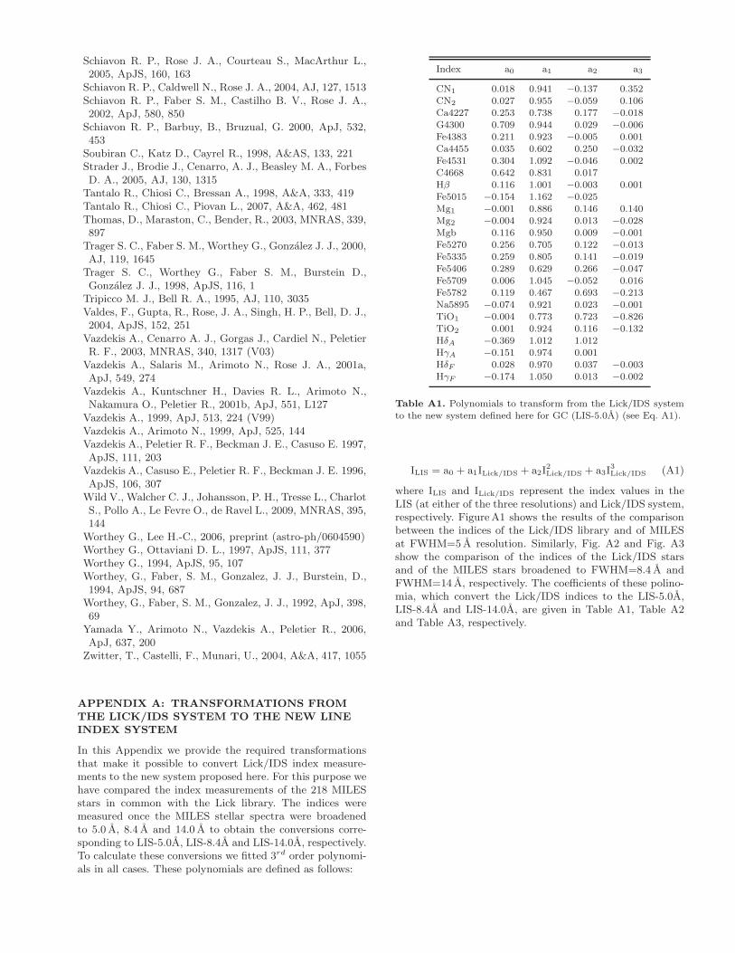
Schiavon R. P., Rose J. A., Courteau S., MacArthur L.,2005, ApJS, 160, 163

Schiavon R. P., Caldwell N., Rose J. A., 2004, AJ, 127, 1513Schiavon R. P., Faber S. M., Castilho B. V., Rose J. A.,2002, ApJ, 580, 850

Schiavon R. P., Barbuy, B., Bruzual, G. 2000, ApJ, 532,453

Soubiran C., Katz D., Cayrel R., 1998, A&AS, 133, 221Strader J., Brodie J., Cenarro, A. J., Beasley M. A., ForbesD. A., 2005, AJ, 130, 1315

Tantalo R., Chiosi C., Bressan A., 1998, A&A, 333, 419Tantalo R., Chiosi C., Piovan L., 2007, A&A, 462, 481Thomas, D., Maraston, C., Bender, R., 2003, MNRAS, 339,897

Trager S. C., Faber S. M., Worthey G., Gonzalez J. J., 2000,AJ, 119, 1645

Trager S. C., Worthey G., Faber S. M., Burstein D.,Gonzalez J. J., 1998, ApJS, 116, 1

Tripicco M. J., Bell R. A., 1995, AJ, 110, 3035Valdes, F., Gupta, R., Rose, J. A., Singh, H. P., Bell, D. J.,2004, ApJS, 152, 251

Vazdekis A., Cenarro A. J., Gorgas J., Cardiel N., PeletierR. F., 2003, MNRAS, 340, 1317 (V03)

Vazdekis A., Salaris M., Arimoto N., Rose J. A., 2001a,ApJ, 549, 274

Vazdekis A., Kuntschner H., Davies R. L., Arimoto N.,Nakamura O., Peletier R., 2001b, ApJ, 551, L127

Vazdekis A., 1999, ApJ, 513, 224 (V99)Vazdekis A., Arimoto N., 1999, ApJ, 525, 144Vazdekis A., Peletier R. F., Beckman J. E., Casuso E. 1997,ApJS, 111, 203

Vazdekis A., Casuso E., Peletier R. F., Beckman J. E. 1996,ApJS, 106, 307

Wild V., Walcher C. J., Johansson, P. H., Tresse L., CharlotS., Pollo A., Le Fevre O., de Ravel L., 2009, MNRAS, 395,144

Worthey G., Lee H.-C., 2006, preprint (astro-ph/0604590)Worthey G., Ottaviani D. L., 1997, ApJS, 111, 377Worthey G., 1994, ApJS, 95, 107Worthey, G., Faber, S. M., Gonzalez, J. J., Burstein, D.,1994, ApJS, 94, 687

Worthey, G., Faber, S. M., Gonzalez, J. J., 1992, ApJ, 398,69

Yamada Y., Arimoto N., Vazdekis A., Peletier R., 2006,ApJ, 637, 200

Zwitter, T., Castelli, F., Munari, U., 2004, A&A, 417, 1055

APPENDIX A: TRANSFORMATIONS FROMTHE LICK/IDS SYSTEM TO THE NEW LINEINDEX SYSTEM

In this Appendix we provide the required transformationsthat make it possible to convert Lick/IDS index measure-ments to the new system proposed here. For this purpose wehave compared the index measurements of the 218 MILESstars in common with the Lick library. The indices weremeasured once the MILES stellar spectra were broadenedto 5.0 A, 8.4 A and 14.0 A to obtain the conversions corre-sponding to LIS-5.0A, LIS-8.4A and LIS-14.0A, respectively.To calculate these conversions we fitted 3rd order polynomi-als in all cases. These polynomials are defined as follows:

Index a0 a1 a2 a3

CN1 0.018 0.941 −0.137 0.352CN2 0.027 0.955 −0.059 0.106Ca4227 0.253 0.738 0.177 −0.018G4300 0.709 0.944 0.029 −0.006Fe4383 0.211 0.923 −0.005 0.001Ca4455 0.035 0.602 0.250 −0.032Fe4531 0.304 1.092 −0.046 0.002C4668 0.642 0.831 0.017Hβ 0.116 1.001 −0.003 0.001Fe5015 −0.154 1.162 −0.025Mg1 −0.001 0.886 0.146 0.140Mg2 −0.004 0.924 0.013 −0.028Mgb 0.116 0.950 0.009 −0.001Fe5270 0.256 0.705 0.122 −0.013Fe5335 0.259 0.805 0.141 −0.019Fe5406 0.289 0.629 0.266 −0.047Fe5709 0.006 1.045 −0.052 0.016Fe5782 0.119 0.467 0.693 −0.213Na5895 −0.074 0.921 0.023 −0.001TiO1 −0.004 0.773 0.723 −0.826TiO2 0.001 0.924 0.116 −0.132HδA −0.369 1.012 1.012HγA −0.151 0.974 0.001HδF 0.028 0.970 0.037 −0.003HγF −0.174 1.050 0.013 −0.002

Table A1. Polynomials to transform from the Lick/IDS systemto the new system defined here for GC (LIS-5.0A) (see Eq. A1).

ILIS = a0 + a1ILick/IDS + a2I2Lick/IDS + a3I

3Lick/IDS (A1)

where ILIS and ILick/IDS represent the index values in theLIS (at either of the three resolutions) and Lick/IDS system,respectively. FigureA1 shows the results of the comparisonbetween the indices of the Lick/IDS library and of MILESat FWHM=5 A resolution. Similarly, Fig. A2 and Fig. A3show the comparison of the indices of the Lick/IDS starsand of the MILES stars broadened to FWHM=8.4 A andFWHM=14 A, respectively. The coefficients of these polino-mia, which convert the Lick/IDS indices to the LIS-5.0A,LIS-8.4A and LIS-14.0A, are given in Table A1, Table A2and Table A3, respectively.

Figure A1. Comparison of the Lick/IDS indices of the Lick/IDS library and those in MILES broadened to a constant resolutionFWHM=5 A. Solid lines show the transformation from one system to the other.

Figure A2. Comparison between the Lick/IDS indices of the Lick library and those measured on the stars in common with the MILESlibrary broadened to FWHM=8.4 A. Solid lines represent the transformation from one system to the other (see Table A2)

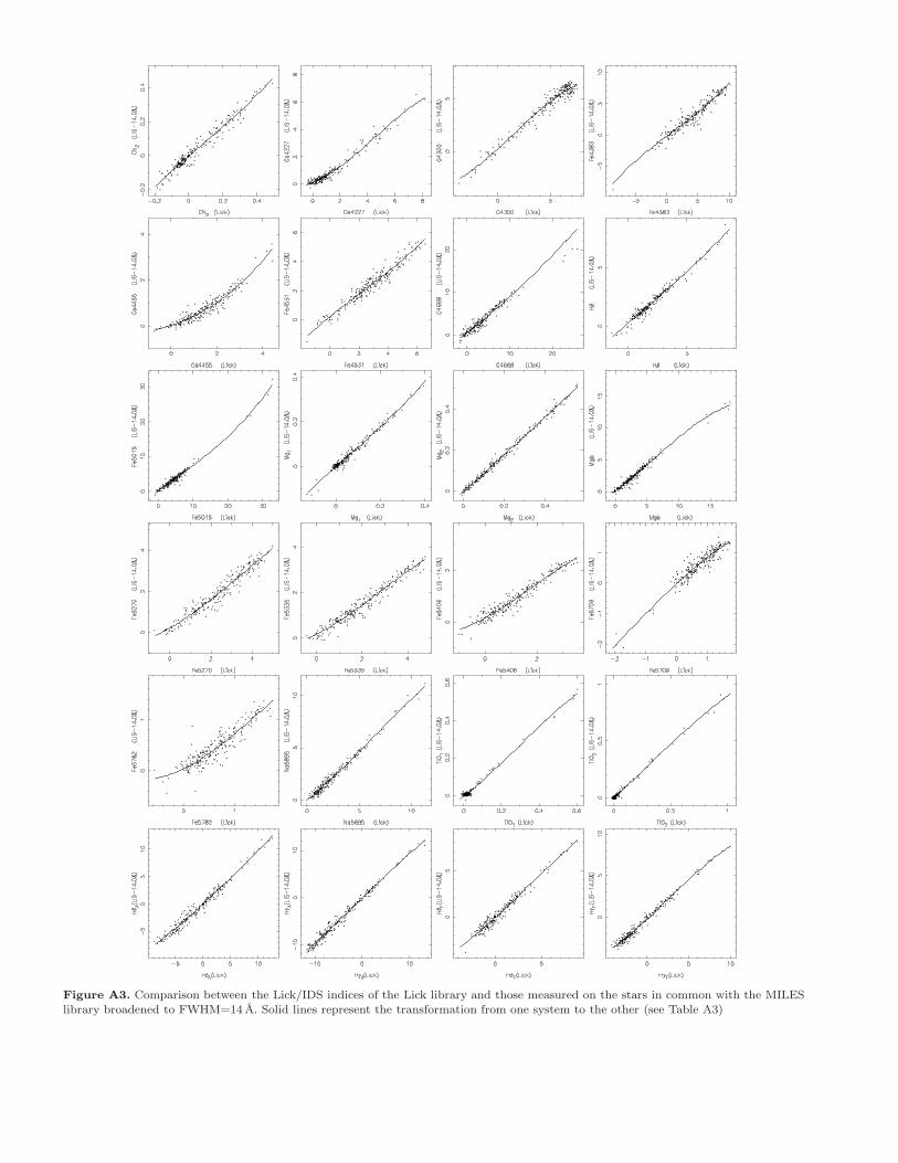
Figure A3. Comparison between the Lick/IDS indices of the Lick library and those measured on the stars in common with the MILESlibrary broadened to FWHM=14 A. Solid lines represent the transformation from one system to the other (see Table A3)

a0 a1 a2 a3

CN1 0.011 0.913 −0.119 0.400CN2 0.016 0.911 0.025 0.076Ca4227 0.217 0.668 0.140 −0.014G4300 0.541 0.540 0.015 −0.004Fe4383 0.106 0.796 0.015Ca4455 0.021 0.466 0.187 −0.016Fe4531 0.267 0.972 −0.032 0.003C4668 0.616 0.819 0.017Hβ 0.159 0.953 −0.002 0.001Fe5015 −0.037 0.994 −0.018Mg1 −0.001 0.884 0.056 0.358Mg2 −0.004 0.906 0.054 −0.051Mgb 0.116 0.912 0.009 −0.001Fe5270 0.253 0.649 0.104 −0.010Fe5335 0.214 0.708 0.120 −0.015Fe5406 0.257 0.587 0.225 −0.040Fe5709 −0.005 1.024 −0.108 0.030Fe5782 0.055 0.707 0.182Na5895 −0.057 0.887 0.025 −0.001TiO1 −0.004 0.766 0.736 −0.841TiO2 0.001 0.919 0.128 −0.142HδA −0.246 0.977 0.006HγA −0.175 0.986HδF 0.027 0.973 0.016 −0.001HγF −0.149 1.010 0.015 −0.002

Table A2. Polynomials to transform from the Lick/IDS systemto the new system defined here for dwarf and intermediate-massgalaxies (LIS-8.4A).

a0 a1 a2 a3

CN1 0.005 0.875 −0.091 0.402CN2 −0.002 0.863 −0.110 0.477Ca4227 0.134 0.380 0.113 −0.008G4300 0.251 0.910 0.019 −0.004Fe4383 −0.203 0.749 −0.004 0.001Ca4455 0.031 0.331 0.073 0.005Fe4531 0.211 0.814 −0.025 0.004C4668 0.500 0.779 0.006Hβ 0.257 0.861 −0.003 0.001Fe5015 0.123 0.738 −0.004Mg1 −0.003 0.885 −0.164 0.856Mg2 −0.003 0.874 0.154 −0.134Mgb 0.112 0.738 0.022 −0.001Fe5270 0.224 0.565 0.076 −0.007Fe5335 0.178 0.496 0.090 −0.010Fe5406 0.160 0.547 0.084 −0.015Fe5709 −0.018 0.929 −0.064 −0.013Fe5782 0.038 0.490 0.254 −0.056Na5895 −0.022 0.801 0.034 −0.002TiO1 −0.004 0.749 0.798 −0.902TiO2 0.000 0.909 0.144 −0.155

HδA −0.017 0.914 0.008HγA −0.126 0.971HδF −0.074 0.909 0.013 −0.001HγF −0.199 0.925 0.014 −0.002

Table A3. Polynomials to transform from the Lick/IDS systemto the new system defined here for massive galaxies (LIS-14.0A).