
Evolutionary Dynamics - Institute for Theoretical Chemistry
390
Evolutionary Dynamics A Special Course on Dynamical Systems and Evolutionary Processes for Physicists, Chemists, and Biologists Summer Term 2014 Version of February 24, 2014 Peter Schuster Institut f¨ ur Theoretische Chemie der Universit¨atWien W¨ ahringerstraße 17, A-1090 Wien, Austria Phone: +43 1 4277 52736 , eFax: +43 1 4277 852736 E-Mail: pks @ tbi.univie.ac.at Internet: http://www.tbi.univie.ac.at/~pks
-
Upload
khangminh22 -
Category
Documents
-
view
3 -
download
0
Transcript of Evolutionary Dynamics - Institute for Theoretical Chemistry

Evolutionary Dynamics
A Special Course on Dynamical Systems and
Evolutionary Processes for Physicists,
Chemists, and Biologists
Summer Term 2014
Version of February 24, 2014
Peter Schuster
Institut fur Theoretische Chemie der Universitat Wien
Wahringerstraße 17, A-1090 Wien, Austria
Phone: +43 1 4277 52736 , eFax: +43 1 4277 852736
E-Mail: pks @ tbi.univie.ac.at
Internet: http://www.tbi.univie.ac.at/~pks

2 Peter Schuster

Preface
The current text contains notes that were prepared first for a course on ‘Evo-lutionary Dynamics’ held at Vienna University in the summer term 2014.No claim is made that the text is free of errors. The course is addressedto students of physics, chemistry, biology, biochemistry, molecular biology,mathematical and theoretical biology, bioinformatics, and systems biologywith particular interests in evolutionary phenomena. Evolution although inthe heart of biology as expressed in Theodosius Dobzhansky famous quote,
”nothing in biology makes sense except in the light of evolution”,is a truly interdisciplinary subject and hence the course will contain ele-ments from various disciplines, mainly from mathematics, in particular dy-namical systems theory and stochastic processes, computer science, chemicalkinetics, molecular biology, and evolutionary biology. Considerable usage ofmathematical language and analytical tools is indispensable, but we haveconsciously avoided to dwell upon deeper and more formal mathematicaltopics.
Evolution has been shifted into the center of biological thinking throughCharles Darwin’s centennial book ’On the Origin of Species’ [45]. GregorMendel’s discovery of genetics [206] was the second milestone of evolutionarybiology but it remained largely ignored for almost forty years before it be-came first an alternative concept to selection. Biologists were split into twocamps, the selectionists believing in continuity in evolution and the geneti-cists, who insisted in the discreteness of change in the form of mutation (Anaccount of the historic development of mutation as an ides is found in therecent publication [34]. The unification of two concepts was first achievedon the level of a mathematical theory through population genetics [92, 318]developed by the three great scholars Ronald Fisher, J.B.S. Haldane, andSewall Wright. Still it took twenty more years before the synthetic theoryof evolution had been completed [202]. Almost all attempts of biologiststo understand evolution were and most of them still are completely freeof quantitative or mathematical thinking. The two famous exceptions areMendelian genetics and populations genetics. It is impossible, however, tomodel or understand dynamics without quantitative description. Only re-cently and mainly because of the true flood of hitherto unaccessible data thedesire for a new and quantitative theoretical biology has been articulated[26, 27]. We shall focus in this course on dynamical models of evolutionary
3

4 Peter Schuster
processes, which are rooted in physics, chemistry, and molecular biology. Onthe other hand, any useful theory in biology has to be grounded on a solidexperimental basis. Most experimental data on evolution at the molecularlevel are currently focussing on genomes and accordingly, sequence compar-isons and reconstruction of phylogenetic trees are a topic of primary interest[232]. The fast, almost explosive development of molecular life sciences hasreshaped the theory of evolution [276]. RNA has been considered as a ratheruninteresting molecule until the discovery of RNA catalysis by Thomas Cechand Sidney Altman in the nineteen eighties, nowadays RNA is understood asan important regulator of gene activity [9], and we have definitely not comenear to the end of the exciting RNA story.
This series of lectures will concentrate on principles rather than techni-cal details. At the same time it will be necessary to elaborate tools thatallow to treat real problems. The tools required for the analysis of dynam-ical systems are described, for example, in the two monographs [143, 144].For stochastic processes we shall follow the approach taken in the book [107]and presented in the course of the Summer term 2011 [36, 251]. Some of thestochastic models in evolution presented here are described in the excellentreview [22]. Analytical results on evolutionary processes are rare and thus itwill be unavoidable to deal also with approximation methods and numericaltechniques that are able to produce results through computer calculations(see, for example, the article [112, 113, 115, 117]). The applicability of sim-ulations to real problems depends critically on population sizes that can byhandled. Present day computers can readily deal with 106 to 107 particles,which is commonly not enough for chemical reactions but sufficient for mostbiological problems and accordingly the sections dealing with practical ex-amples will contain more biological than chemical problems. A number oftext books have been used in the preparation of this text in addition to theweb encyclopedia Wikipedia. In molecular biology, molecular genetics, andpopulation genetics these texts were [5, 125, 130, 136]
The major goal of this text is to avoid distraction of the audience by takingnotes and to facilitate understanding of subjects that are quite sophisticatedat least in parts. At the same time the text allows for a repetition of themajor issues of the course. Accordingly, an attempt was made in preparing auseful and comprehensive list of references. To study the literature in detailis recommended to every serious scholar who wants to progress towards adeeper understanding of this rather demanding discipline.
Peter Schuster Wien, February 2014.
1. Darwin’s principle in mathematical language
Charles Darwin’s principle of natural selection is a powerful abstraction
from observations, which provides insight into the basic mechanism giving
rise to changing species. Species or populations don’t multiply but individu-
als do, either directly in asexual species, like viruses, bacteria or protists, or
in sexual species through pairings of individuals with opposite sex. Variabil-
ity of individuals in populations is an empirical fact that can be seen easily
in everyday life. Within populations the variants are subjected to natural
selection and those having more progeny prevail in future generations. The
power of Darwin’s abstraction lies in the fact that neither the shape and
the structure of individuals nor the mechanism of inheritance are relevant
for selection unless they have an impact on the number of offspring. Oth-
erwise Darwin’s approach had been doomed to fail since his imagination of
inheritance was incorrect. Indeed Darwin’s principle holds simultaneously for
highly developed organisms, for primitive unicellular species like bacteria, for
viruses and even for reproducing molecules in cell-free assays.
Molecular biology provided a powerful possibility to study evolution in its
simplest form outside biology: Replicating ribonucleic acid molecules (RNA)
in cell-free assays [268] play natural selection in its purest form: In the test
tube, evolution, selection, and optimization are liberated from all unneces-
sary complex features, from obscuring details, and from unimportant acces-
sories. Hence, in vitro evolution can be studied by the methods of chemical
kinetics. The parameters determining the “fitness of molecules” are repli-
cation rate parameters, binding constants, and other measurable quantities,
which can be determined independently of in vitro evolution experiments,
and constitute an alternative access to the determination of the outcome of
selection. Thereby “survival of the fittest” is unambiguously freed from the
reproach of being the mere tautology of “survival of the survivor”. In ad-
dition, in vitro selection turned out to be extremely useful for the synthesis
5

6 Peter Schuster
of molecules that are tailored for predefined purposes. A new area of appli-
cations called evolutionary biotechnology branched off evolution in the test
tube. Examples for evolutionary design of molecules are [166, 176] for nucleic
acids, [25, 161] for proteins, and [316] for small organic molecules.
The chapter starts by mentioning a few examples of biological applica-
tions of mathematics before Darwin (section 1.1), then we derive and analyze
an ODE describing simple selection with asexual species (section 1.2), and
consider the effects of variable population size (section 1.3). The next sub-
section 1.4 analyzes optimization in the Darwinian sense, and eventually we
consider generic properties of typical growth functions (section 1.5).
1.1 Counting and modeling before Darwin
The first mathematical model that seems to be relevant for evolution was
conceived by the medieval mathematician Leonardo Pisano also known as
Fibonacci. His famous book Liber abaci has been finished and published in
the year 1202 and was translated into modern English eight years ago [264].
Among several other important contributions to mathematics in Europe Fi-
bonacci discusses a model of rabbit multiplication in Liber abaci. Couples
of rabbits reproduce and produce young couples of rabbits according to the
following rules:
(i) Every adult couple has a progeny of one young couple per month,
(ii) a young couple grows to adulthood within the first month and accord-
ingly begins producing offspring in the second months,
(iii) rabbits live forever, and
(iv) the number of rabbit couples is updated every month.
The model starts with one young couple (1), nothing happens during mat-
uration of couple 1 in the first month and we have still one couple in the
second month. In the third month, eventually, a young couple (2) is born
and the number of couples increases to two. In the fourth month couple 1
produces a new couple (3) whereas couple 2 is growing to adulthood, and
Evolutionary Dynamics 7
we have three couples now. Further rabbit counting yields the Fibonacci
sequence:1
month 0 1 2 3 4 5 6 7 8 9 . . .
#couples 0 1 1 2 3 5 8 13 21 34 . . .
It is straightforward to derive a recursion for the rabbit count. The number
of couples in month (n + 1), fn+1, is the sum of two terms: The number
of couples in month n, because rabbits don’t die, plus the number of young
couples that is identical to the number of couples in month (n− 1):
fn+1 = fn−1 + fn with f0 = 0 and f1 = 1 . (1.1)
With increasing n the ratio of two subsequent Fibonacci numbers converges
to the golden ratio, fk+1/fk = (1+√5)/2 (For a comprehensive discussion of
the Fibonacci sequence and its properties see [124, pp.290-301] or, e.g., [61]).
In order to proof this convergence we make use of a matrix representation
of the Fibonacci model:
Fn
(
f0
f1
)
=
(
fn
fn+1
)
with F =
(
f0 f1
f1 f2
)
and Fn =
(
fn−1 fn
fn fn+1
)
.
The matrix representation transforms the recursion into an expression that
allows for direct computation of the elements of the Fibonacci sequence.
fn =(
1 0)
Fn
(
f0
f1
)
=(
1 0)
(
fn−1 fn
fn fn+1
)(
f0
f1
)
. (1.2)
Theorem 1.1 (Fibonacci convergence). With increasing n the Fibonacci
sequence converges to a geometric progression with the golden ratio as factor,
q = (1 +√5)/2.
Proof. The matrix F is diagonalized by the transformation T−1 · F · T = D
with D =
(
λ1 0
0 λ2
)
. The two eigenvalues of F are: λ1,2 = (1±√5)/2. Since
1According to Parmanand Singh [265] the Fibonacci numbers were invented earlier in
India and used for the solution of various problems (See also Donald Knuth [178]).
8 Peter Schuster
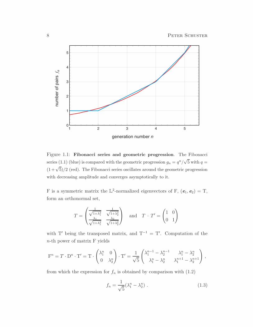
Figure 1.1: Fibonacci series and geometric progression. The Fibonacci
series (1.1) (blue) is compared with the geometric progression gn = qn/√5 with q =
(1+√5)/2 (red). The Fibonacci series oscillates around the geometric progression
with decreasing amplitude and converges asymptotically to it.
F is a symmetric matrix the L2-normalized eigenvectors of F, (e1, e2) = T,
form an orthonormal set,
T =
1√1+λ2
1
1√1+λ2
2
λ1√1+λ2
1
λ2√1+λ2
2
and T · T ′ =(
1 0
0 1
)
with T′ being the transposed matrix, and T−1 = T′. Computation of the
n-th power of matrix F yields
Fn = T · Dn · T′ = T ·(
λn1 0
0 λn2
)
· T′ = 1√5
(
λn−11 − λn−12 λn1 − λn2λn1 − λn2 λn+1
1 − λn+12
)
,
from which the expression for fn is obtained by comparison with (1.2)
fn =1√5(λn1 − λn2 ) . (1.3)
Evolutionary Dynamics 9
Because λ1 > λ2 the ratio converges to zero: limn→∞ λn2/λ
n1 = 0, and the
Fibonacci sequence is approximated well by a geometric progression fn ≈gn = 1√
5qn with q = (1 +
√5)/2.
Since λ2 is negative the Fibonacci sequence alternates around the geometric
progression. Expression (1.3) is commonly attributed to the French mathe-
matician Jacques Binet [21] and named after him. As outlined in ref. [124,
p.299] the formula has been derived already hundred years before by the
great Swiss mathematician Leonhard Euler [80] but was forgotten and redis-
covered.
Thomas Robert Malthus was the first who articulated the ecological and
economic problem of population growth following a geometric progression
[193]: Animal or human populations like every system capable of repro-
duction grow like a geometric progression provided unlimited resources are
available. The resources, however, are either constant or grow – as Malthus
assumes – according to an arithmetic progression if human endeavor is in-
volved. The production of nutrition, says Malthus, is proportional to the land
that is exploitable for agriculture and the gain in the area of fields will be a
constant in time – the increase will be the same every year. An inevitable
result of Malthus’ vision of the world is the pessimistic view that populations
will grow until the majority of individuals will die premature of malnutrition
and hunger. Malthus could not foresee the green revolutions but he was also
unaware that population growth can be faster than exponential – sufficient
nutrition for the entire human population is still a problem. Charles Darwin
and his younger contemporary Alfred Russel Wallace were strongly influ-
enced by Robert Malthus and took form population theory that in the wild,
where birth control does not exist and individuals fight for food, the major
fraction of of progeny will die before they reach the age of reproduction and
only the strongest will have a chance to multiply.
Leonhard Euler introduced the notions of the exponential function in the
middle of the eighteenth century [81] and set the stage for modeling growing
populations by means of ordinary differential equations (ODEs). The growth
10 Peter Schuster
rate is proportional to the number of individuals or the population size N
dN
dt= r N , (1.4)
where the parameter r is commonly called Malthus or growth parameter.
Straightforward integration yields:
∫ N(t)
N(0)
dN
N=
∫ t
0
dt and N(t) = N0 exp(rt) with N0 = N(0) . (1.5)
Simple reproduction results in exponential growth of a population with N(t)
individuals.
Presumably not known to Darwin, the mathematician Jean Francois Ver-
hulst complemented the concept of exponential growth by the introduction
of finite resources [292–294]. The Verhulst equation is of the form2
dN
dt= rN
(
1− N
K
)
, (1.6)
where N(t) again denotes the number of individuals of a species X, and K
is the carrying capacity of the ecological niche or the ecosystem. Equ. (1.6)
can be integrated by means of partial fractions (γ = 1/K):
∫ N(t)
N0
dN
N(1 − γN)=
∫ N(t)
N0
dN
N+
∫ N(t)
N0
γ dN
1− γN ,
and the following solution is obtained
N(t) = N0K
N0 +(
K −N0
)
exp(−rt) . (1.7)
Apart from the initial condition N0, the number of individuals X at time
t = 0, the logistic equation has two parameters: (i) the Malthusian parameter
or the growth rate r and (ii) the carrying capacity K of the ecological niche
or the ecosystem. A population of size N0 grows exponentially at short
times: N(t) ≈ N0 exp(rt) for K ≫ N0 and t sufficiently small. For long
2The Verhulst equation is also called logistic equation and its discrete analogue is the
logistic map, a standard model to demonstrate the occurrence of deterministic chaos in a
simple system. The name logistic equation was coined by Verhulst himself in 1845.
Evolutionary Dynamics 11
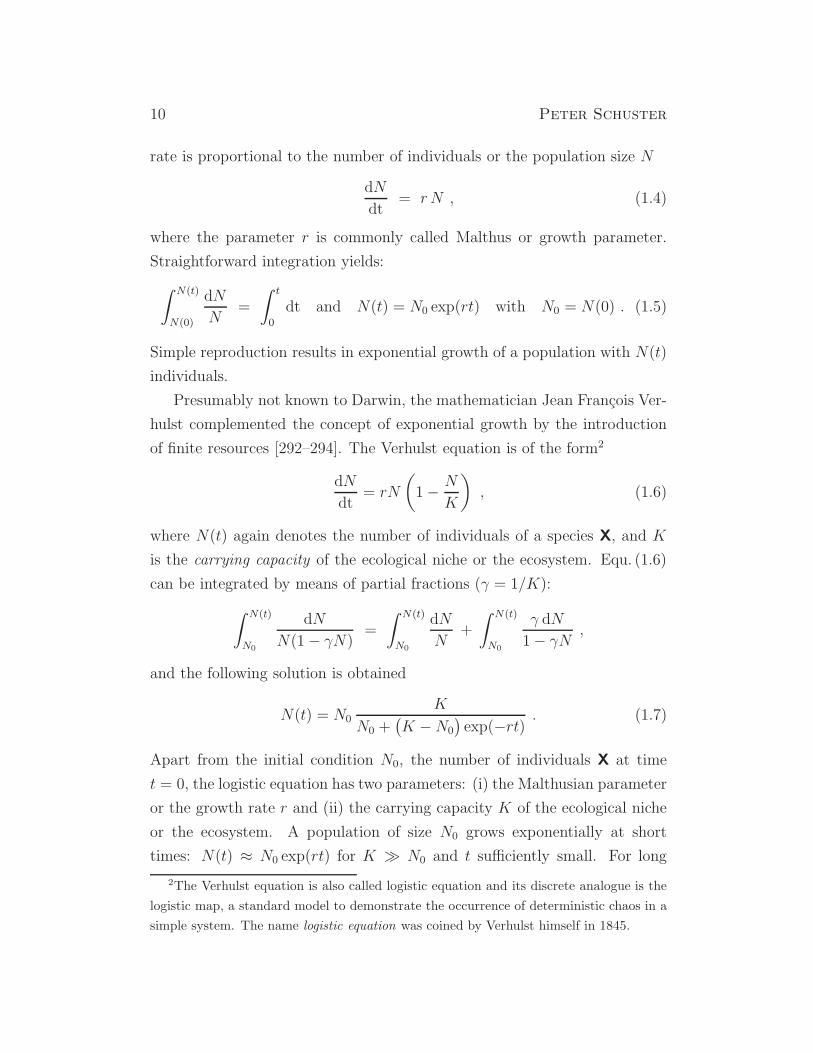
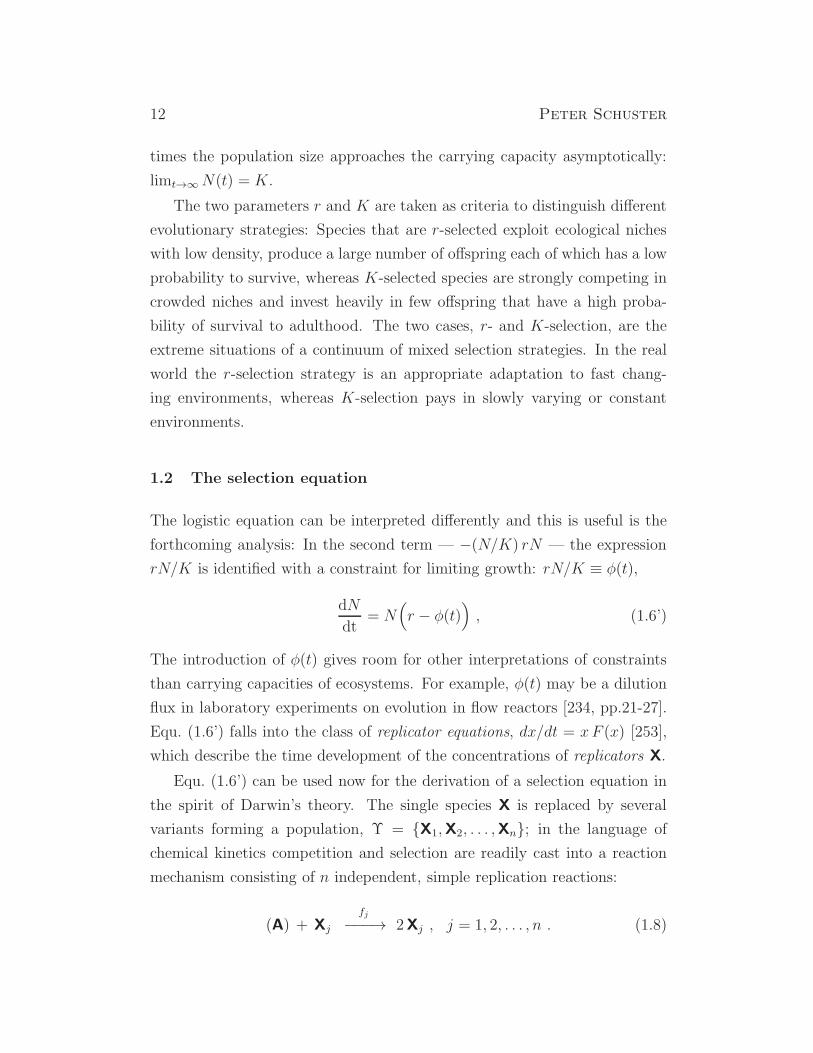
Figure 1.2: Solution curves of the logistic equations (1.7,1.13). Upper plot:
The black curve illustrates growth in population size from a single individual to
a population at the carrying capacity of the ecosystem. The red curve represents
the results for unlimited exponential growth, N(t) = N(0) exp(rt). Parameters:
r = 2, N(0) = 1, and K = 10000. Lower plot: Growth and internal selection is
illustrated in a population with four variants. Color code: C black, N1 yellow,
N2 green, N3 red, N4 blue. Parameters: fitness values fj = (1.75, 2.25, 2.35, 2.80),
Nj(0) = (0.8888, 0.0888, 0.0020, 0.0004), K = 10000. The parameters were ad-
justed such that the curves for the total populations size N(t) coincide (almost)
in both plots.
12 Peter Schuster
times the population size approaches the carrying capacity asymptotically:
limt→∞N(t) = K.
The two parameters r and K are taken as criteria to distinguish different
evolutionary strategies: Species that are r-selected exploit ecological niches
with low density, produce a large number of offspring each of which has a low
probability to survive, whereas K-selected species are strongly competing in
crowded niches and invest heavily in few offspring that have a high proba-
bility of survival to adulthood. The two cases, r- and K-selection, are the
extreme situations of a continuum of mixed selection strategies. In the real
world the r-selection strategy is an appropriate adaptation to fast chang-
ing environments, whereas K-selection pays in slowly varying or constant
environments.
1.2 The selection equation
The logistic equation can be interpreted differently and this is useful is the
forthcoming analysis: In the second term — −(N/K) rN — the expression
rN/K is identified with a constraint for limiting growth: rN/K ≡ φ(t),
dN
dt= N
(
r − φ(t))
, (1.6’)
The introduction of φ(t) gives room for other interpretations of constraints
than carrying capacities of ecosystems. For example, φ(t) may be a dilution
flux in laboratory experiments on evolution in flow reactors [234, pp.21-27].
Equ. (1.6’) falls into the class of replicator equations, dx/dt = xF (x) [253],
which describe the time development of the concentrations of replicators X.
Equ. (1.6’) can be used now for the derivation of a selection equation in
the spirit of Darwin’s theory. The single species X is replaced by several
variants forming a population, Υ = X1,X2, . . . ,Xn; in the language of
chemical kinetics competition and selection are readily cast into a reaction
mechanism consisting of n independent, simple replication reactions:
(A) + Xj
fj−−−→ 2Xj , j = 1, 2, . . . , n . (1.8)
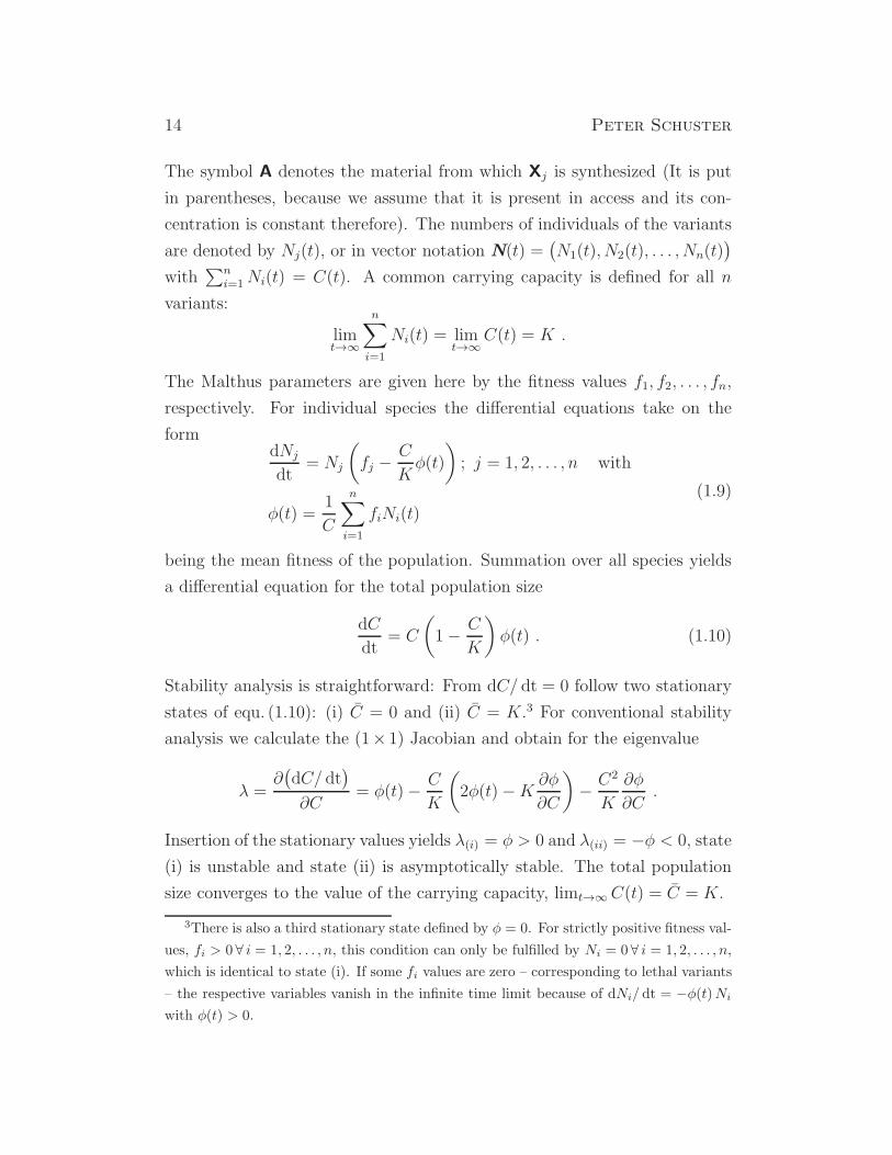
Evolutionary Dynamics 13
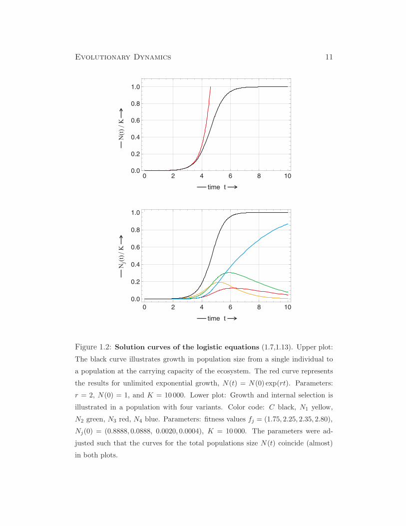
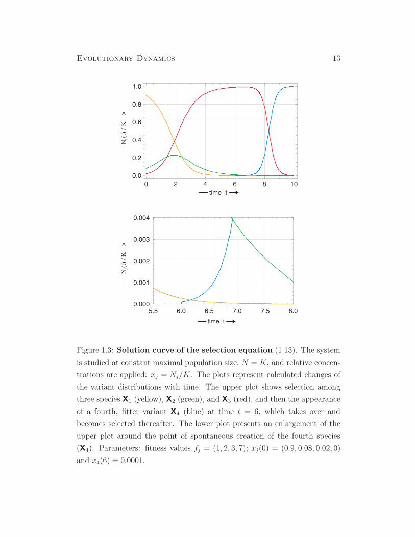
Figure 1.3: Solution curve of the selection equation (1.13). The system
is studied at constant maximal population size, N = K, and relative concen-
trations are applied: xj = Nj/K. The plots represent calculated changes of
the variant distributions with time. The upper plot shows selection among
three species X1 (yellow), X2 (green), and X3 (red), and then the appearance
of a fourth, fitter variant X4 (blue) at time t = 6, which takes over and
becomes selected thereafter. The lower plot presents an enlargement of the
upper plot around the point of spontaneous creation of the fourth species
(X4). Parameters: fitness values fj = (1, 2, 3, 7); xj(0) = (0.9, 0.08, 0.02, 0)
and x4(6) = 0.0001.
14 Peter Schuster
The symbol A denotes the material from which Xj is synthesized (It is put
in parentheses, because we assume that it is present in access and its con-
centration is constant therefore). The numbers of individuals of the variants
are denoted by Nj(t), or in vector notation N(t) =(
N1(t), N2(t), . . . , Nn(t))
with∑n
i=1Ni(t) = C(t). A common carrying capacity is defined for all n
variants:
limt→∞
n∑
i=1
Ni(t) = limt→∞
C(t) = K .
The Malthus parameters are given here by the fitness values f1, f2, . . . , fn,
respectively. For individual species the differential equations take on the
formdNj
dt= Nj
(
fj −C
Kφ(t)
)
; j = 1, 2, . . . , n with
φ(t) =1
C
n∑
i=1
fiNi(t)
(1.9)
being the mean fitness of the population. Summation over all species yields
a differential equation for the total population size
dC
dt= C
(
1− C
K
)
φ(t) . (1.10)
Stability analysis is straightforward: From dC/ dt = 0 follow two stationary
states of equ. (1.10): (i) C = 0 and (ii) C = K.3 For conventional stability
analysis we calculate the (1× 1) Jacobian and obtain for the eigenvalue
λ =∂(
dC/ dt)
∂C= φ(t)− C
K
(
2φ(t)−K ∂φ
∂C
)
− C2
K
∂φ
∂C.
Insertion of the stationary values yields λ(i) = φ > 0 and λ(ii) = −φ < 0, state
(i) is unstable and state (ii) is asymptotically stable. The total population
size converges to the value of the carrying capacity, limt→∞C(t) = C = K.
3There is also a third stationary state defined by φ = 0. For strictly positive fitness val-
ues, fi > 0 ∀ i = 1, 2, . . . , n, this condition can only be fulfilled by Ni = 0 ∀ i = 1, 2, . . . , n,
which is identical to state (i). If some fi values are zero – corresponding to lethal variants
– the respective variables vanish in the infinite time limit because of dNi/ dt = −φ(t)Ni
with φ(t) > 0.
Evolutionary Dynamics 15
Equ. (1.10) can be solved exactly yielding thereby an expression that con-
tains integration of the constraint φ(t):
C(t) = C(0)K
C(0) +(
K − C(0))
exp(−Φ) with Φ =
∫ t
0
φ(τ)dτ ,
where C(0) is the population size at time t = 0. The function Φ(t) depends
on the distribution of fitness values within the population and its time course.
For f1 = f2 = . . . = fn = r the integral yields Φ = rt and we retain equ. (1.7).
In the long time limit Φ grows to infinity and C(t) converges to the carrying
capacity K.
At constant population size C = C = K equ. (1.9) becomes simpler
dNj
dt= Nj
(
fj − φ(t))
; j = 1, 2, . . . , n . (1.9’)
and can be solved exactly by means of the integrating factor transformation
[329, p. 322ff.]:
Zj(t) = Nj(t) exp
(∫ t
0
φ(τ) dτ
)
. (1.11)
Insertion into equ. (1.9’) yields
dNj
dt=
dZj
dtexp
(∫ t
0
−φ(τ) dτ)
− Zj exp
(∫ t
0
−φ(τ) dτ)
φ(t) =
= Zj exp
(∫ t
0
−φ(τ), dτ)
(
fj − φ(t))
,
dZj
dt= Zj , j = 1, 2, . . . , n or dZ/ dt = F · Z , (1.12)
where F is a diagonal matrix containing the fitness values fj (j = 1, 2, . . . , n)
as elements. Using the trivial equality Zj(0) = Nj(0) we obtain for the
individual genotypes:
Nj(t) = Nj(0) exp(fjt)C
∑ni=1Ni(0) exp(fit)
; j = 1, 2, . . . , n . (1.13)
Equ. (1.13) encapsulates Darwinian selection and optimization of fitness in
populations that will be discussed in detail in section 1.4.
16 Peter Schuster
The use of normalized or internal variables xj = Nj/C provides certain
advantages and we shall use them whenever we are dealing with constant
population size. The ODE is of the form
dxjdt
= fjxj − xjφ(t) = xj
(
fj − φ(t))
; j = 1, 2, . . . , n with
φ(t) =
n∑
i=1
fixi ,(1.14)
the solution is trivially the same as in case of equ.(1.9):
xj(t) =xj(0) exp(fjt)
∑ni=1 xi(0) exp(fit)
; j = 1, 2, . . . , n . (1.15)
The use of normalized variables,∑n
i=1 xi = 1, defines the unit simplex, S(1)n =
0 ≤ xi ≤ 1 ∀ i = 1, . . . , n ∧ ∑ni=1 xi = 1, as the physically accessible
domain that fulfils the conservation relation. All boundaries of the simplex —
corners, edges, faces, etc. — are invariant sets, since xj = 0 ⇒ dxj/ dt = 0
by equ. (1.14).
Asymptotic stability of the simplex follows from the stability analysis
of equ. (1.10) and implies that all solution curves converge to the unit sim-
plex from every initial condition, limt→∞
(
∑ni=1 xi(t)
)
= 1. In other words,
starting with any initial value C(0) 6= 1 the population approaches the unit
simplex. When it starts on Sn it stays there and in presence of fluctuations
it will return to the invariant manifold. As long as the population is finite,
0 < C < +∞, and since Nj(t) = xj(t) · C(t), we can restrict population
dynamics to the unit simplex without loosing generality and characterize the
state of a population at time t by the vector x(t) which fulfils the L(1) norm∑n
i=1 xi(t) = 1 (as an example see fig. 1.4). In the next section 1.3 we shall
consider variable C(t) explicitly.
1.3 Variable population size
Now we shall show that the solution of equ. (1.9) describes the internal equi-
libration for constant and variable population sizes as long as the popu-
lation does neither explode nor die out, 0 < C(t) < +∞ [71]. The va-
lidity of theorem 1.2 as will be shown below is not restricted to constant
Evolutionary Dynamics 17
fitness values fj and hence we can replace them by general growth functions
Gj(N1, . . . , Nn) = Gj(N) or fitness functions Fj(N) with Gj(N) = Fj(N)Nj
in the special case of replicator equations [253]: dNj/ dt = Nj
(
Fj(N)−Ψ(t))
where Ψ(t) comprises both, variable total concentration and constraint.
Time dependence of the conditions in the ecosystem can be introduced in
two ways: (i) variable carrying capacity, K(t) = C(t), and (ii) a constraint or
flux ϕ(t),4 where flux refers to some specific physical device, for example to a
flow reactor. The first case is given, for example, by changes in the environ-
ment as there are periodic changes like day and night or seasons. In addition
there are slow non-periodic changes or changes with very long periods like
climatic change. Constraints and fluxes may correspond to unspecific or spe-
cific migration.5 Considering time dependent carrying capacity and variable
constraints simultaneously, we obtain
dNj
dt= Gj(N)− Nj
K(t)ϕ(t); j = 1, 2, . . . , n . (1.16)
Summation over the concentrations of all variants Xj and restricting the
analysis to slowly changing environments – K(t) varies on a time scale that
is much longer than the time scale of population growth C(t) – we can assume
that the total concentration is quasi equilibrated, C ≈ C = K, and obtain a
relation between the time dependencies of flux and total concentration:
ϕ(t) =
n∑
i=1
Gj(N) − dC
dtor
C(t) = C(0) +
∫ t
0
(
n∑
i=1
Gj(N)− ϕ(τ))
dτ .
(1.17)
The proof for internal equilibration in growing populations is straightforward.
4There is a difference in the definitions of the fluxes φ and ϕ: φ(t) = ϕ(t)/C(t).5Unspecific migration means that the numbers Nj of individuals for each variant Xj
decrease (or increase) proportional to the numbers of individuals currently present in the
population, dNj = kNj dt. Specific migration is anything else. In a flow reactor, for
example, we have a dilution flux corresponding to unspecific emigration and an influx of
one or a few molecular species corresponding to specific immigration into the reactor.

18 Peter Schuster
Theorem 1.2 (Equilibration in populations of variable size). Evolution in
populations of changing size approaches the same internal equilibrium as evo-
lution in populations of constant size provided the growth functions are homo-
geneous functions of degree γ in the variables Nj. Up to a transformation of
the time axis, stationary and variable populations have identical trajectories
provided the population size stays finite and does not vanish.
Proof. Normalized variables, xi = Ni/C with∑n
i=1 xi = 1, are introduced
in order to separate of population growth, C(t), and population internal
changes in the distribution of variants Xi. From equations (1.16) and (1.17)
with C = C = K and Nj = Cxj follows:
dxjdt
=1
C
(
Gj
(
Cx)
− xjn∑
i=1
Gi
(
Cx)
)
; j = 1, 2, . . . , n . (1.18)
The growth functions are assumed to be homogeneous of degree γ in the
variables6 Nj : Gj(N) = Gj(Cx) = Cγ Gj(x). and we find
1
Cγ−1dxjdt
= Gj(x) − xj
n∑
i=1
Gi(x); j = 1, 2, . . . , n ,
which is identical to the selection equation in normalized variables for C = 1.
For γ = 1 the concentration term vanishes and the dynamics in populations
of constant and variable size are described by the same ODE. In case γ 6= 1
the two systems still have identical trajectories and equilibrium points up to
a transformation of the time axis (for an example see section 4.2):
dt = Cγ−1 dt and t = t0 +
∫ t
t0
Cγ−1(t) dt ,
where t0 is the time corresponding to t = 0 – commonly t0 = 0. From
equ. (1.18) we expect instabilities at C = 0 and C =∞.
6A homogenous function of degree γ is defined by G(Cx) = CγG(x). The degree
γ is determined by the mechanism of reproduction. For sexual reproduction according
to Ronald Fisher’s selection equation (2.9) we have γ = 2 [92]. Asexual reproduction
discussed here fulfils γ = 1.
Evolutionary Dynamics 19
The instability at vanishing population size, limC → 0, is, for example, also
of practical importance for modeling drug action on viral replication. In
the case of lethal mutagenesis [30, 31, 283] medication aims at eradication
of the virus population, C → 0, in order to terminate the infection of the
host. At the instant of virus extinction equ. (1.9) is no longer applicable (see
chapter 6.2).
1.4 Optimization
For the discussion of the interplay of selection and optimization we shall
assume here that all fitness values fj are different. The case of neutrality will
be analyzed in chapter 10.3 and without loosing generality we rank them:
f1 > f2 > . . . > fn−1 > fn . (1.19)
The variables xj(t) fulfil two time limits:
limt→0
xj(t) = xj(0) ∀ j = 1, 2, . . . , n by definition, and
limt→∞
xj(t) =
1 iff j = 1
0 ∀ j = 2, . . . , n .
In the long time limit the population becomes homogeneous and contains only
the fittest genotype X1. The process of selection is illustrated best by differ-
ential fitness, fj − φ(t), the second factor in the ODE (1.14): The constraint
φ(t) =∑n
i=1 fixi = f represents the mean fitness of the population. The
population variables xl of all variants with a fitness below average, fl < φ(t),
decrease whereas the variables xh with fh > φ(t) increase. As a consequence
the average fitness φ(t) is increasing too and more genotypes fall below the
threshold for survival. The process continues until the fittest variant is se-
lected. Since another view of optimization will be needed in chapter 2, we
present another proof for the optimization of mean fitness without referring
to differential fitness.
Theorem 1.3 (Optimization of mean fitness). The mean fitness φ(t) = f =∑n
i=1 fixi with∑n
i=1 xi = 1 in a population as described by equ. (1.14) is
non-decreasing.

20 Peter Schuster
Proof. The time dependence of the mean fitness or flux φ is given by
dφ
dt=
n∑
i=1
fidxidt
=n∑
i=1
fi
(
fixi − xin∑
j=1
fjxj
)
=
=
n∑
i=1
f 2i xi −
n∑
i=1
fixi
n∑
j=1
fjxj =
= f 2 −(
f)2
= varf ≥ 0 .
(1.20)
Since a variance is always nonnegative, equ. (1.20) implies that φ(t) is a non-
decreasing function of time.
The condition varf = 0 is met only by homogeneous populations. The
one containing only the fittest variant X1 has the largest possible mean fit-
ness: f = φmax = f1 = maxfj ; j = 1, 2, . . . , n. φ cannot increase any
further and hence, it was been optimized by the selection process. The state
of maximal fitness of population Υ = X1, . . . ,Xn,x|maxφ(Υ) = x1 = 1, xi = 0 ∀ i = 2, . . . , n = P1, is the unique stable
stationary state, and all trajectories starting from initial conditions with
nonzero amounts of X1, x1 > 0, have P1 as ω-limit. An illustration of the
selection process with three variants and the trajectories are plotted on the
unit simplex S(1)3 is shown in figure 1.4.
Gradient systems [143, p.199] facilitate the analysis of the dynamics, they
obey the equation
dx
dt= −gradV (x) = −∇V (x) (1.21)
and fulfil criteria that are relevant for optimization:
(i) The eigenvalues of the linearization of (1.21) evaluated at the equilib-
rium point are real.
(ii) If x0 is an isolated minimum of V then x0 is an asymptotically stable
solution of (1.21).
(iii) If x(t) is a solution of (1.21) that is not an equilibrium point, then
V(
x(t))
is a strictly decreasing function and the trajectories are per-
pendicular to the constant level sets of V .
Evolutionary Dynamics 21
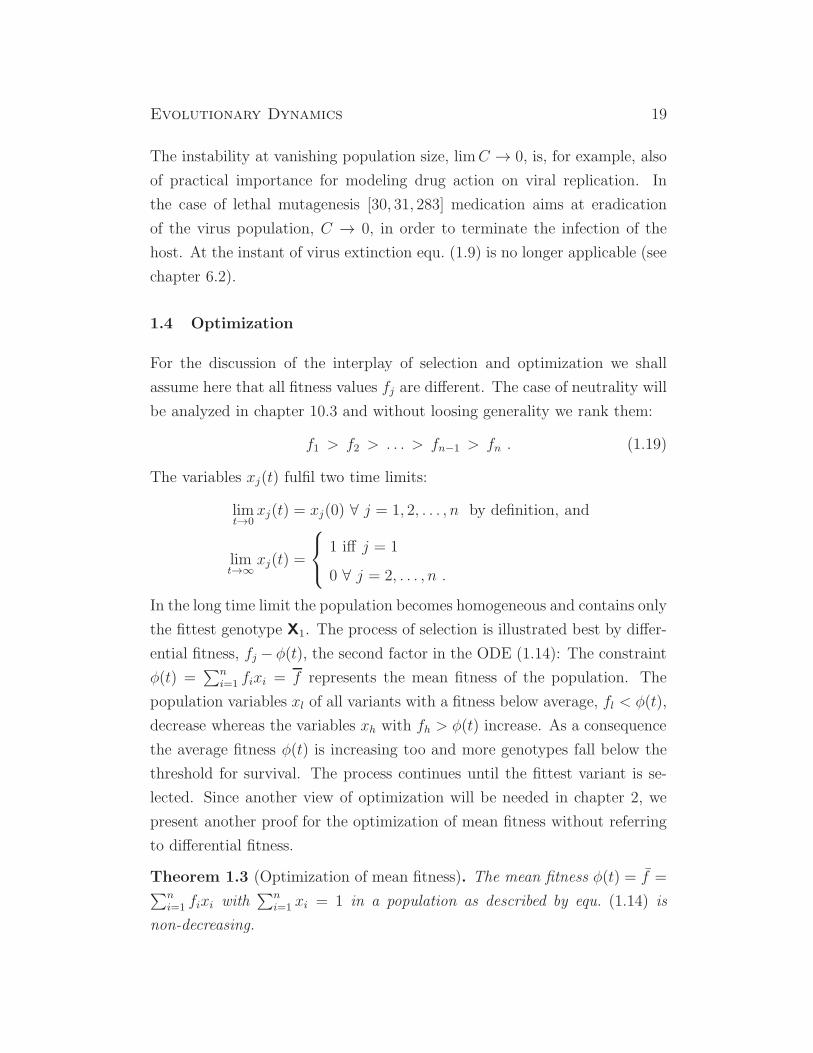
Figure 1.4: Selection on the unit simplex. In the upper part of the figure we
show solution curves x(t) of equ. (1.15) with n = 3. The parameter values are:
f1 = 3 [t−1], f2 = 2 [t−1], and f3 = 1 [t−1], where [t−1] is an arbitrary reciprocal
time unit. The two sets of curves differ with respect to the initial conditions:
(i) x(0) = (0.02, 0.08, 0.90), dotted curves, and (ii) x(0) = (0.0001, 0.0999, 0.9000),
full curves. Color code: x1(t) black, x2(t) red, and x3(t) green. The lower part of
the figure shows parametric plots x(t) on the unit simplex S(1)3 . Constant level sets
of φ(x) = f are shown in grey. The trajectories refer to different initial conditions.
22 Peter Schuster
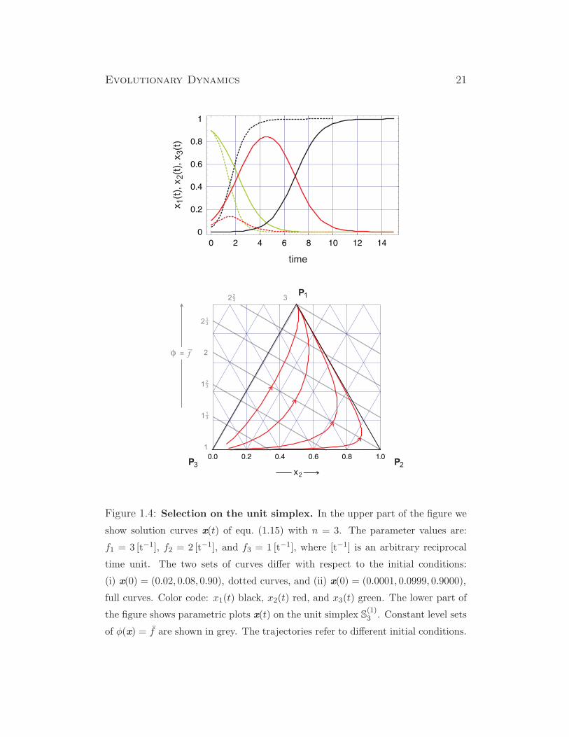
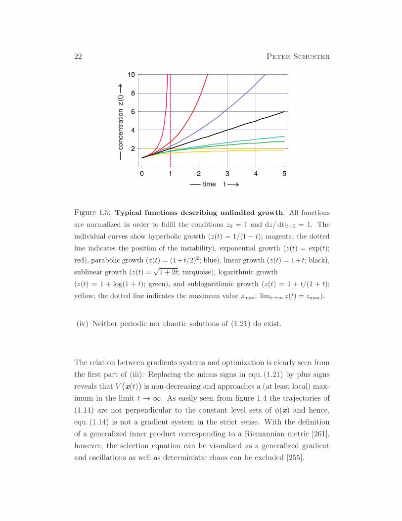
Figure 1.5: Typical functions describing unlimited growth. All functions
are normalized in order to fulfil the conditions z0 = 1 and dz/dt|t=0 = 1. The
individual curves show hyperbolic growth (z(t) = 1/(1 − t); magenta; the dotted
line indicates the position of the instability), exponential growth (z(t) = exp(t);
red), parabolic growth (z(t) = (1+ t/2)2; blue), linear growth (z(t) = 1+ t; black),
sublinear growth (z(t) =√1 + 2t; turquoise), logarithmic growth
(z(t) = 1 + log(1 + t); green), and sublogarithmic growth (z(t) = 1 + t/(1 + t);
yellow; the dotted line indicates the maximum value zmax: limt→∞ z(t) = zmax).
(iv) Neither periodic nor chaotic solutions of (1.21) do exist.
The relation between gradients systems and optimization is clearly seen from
the first part of (iii): Replacing the minus signs in equ. (1.21) by plus signs
reveals that V(
x(t))
is non-decreasing and approaches a (at least local) max-
imum in the limit t → ∞. As easily seen from figure 1.4 the trajectories of
(1.14) are not perpendicular to the constant level sets of φ(x) and hence,
equ. (1.14) is not a gradient system in the strict sense. With the definition
of a generalized inner product corresponding to a Riemannian metric [261],
however, the selection equation can be visualized as a generalized gradient
and oscillations as well as deterministic chaos can be excluded [255].
Evolutionary Dynamics 23
1.5 Growth functions and selection
It is worth considering different classes of growth functions z(t) and the be-
havior of long time solutions of the corresponding ODEs. An intimately
related problem concerns population dynamics: What is the long time or
equilibrium distribution of genotypes in a normalized population, limt→∞ x(t)
provided the initial distribution has been x0? Is there a universal long time
behavior, for example selection, coexistence or cooperation, that is charac-
teristic for certain classes of growth functions?
Differential equations describing unlimited growth of the class
dz
dt= f · zn (1.22)
will be compared here. Integration yields two types of general solutions for
the initial value z(0) = z0
z(t) =(
z1−n0 + (1− n)ft)1/(1−n)
for n 6= 1 and (1.22a)
z(t) = z0 · eft for n = 1 . (1.22b)
In order to make growth functions comparable we normalize them such that
they fulfil the two conditions z0 = 1 and dz/ dt|t=0 = 1. For both equs. (1.22)
this yields z0 = 1 and f = 1. The different classes of growth functions, which
are drawn in different colors in figure 1.5, are characterized by the following
behavior:
(i) Hyperbolic growth requires n > 1; for n = 2 it yields a solution curve
of the form z(t) = 1/(1 − t). Characteristic is the existence of an
instability in the sense that z(t) approaches infinity at some critical
time, limt→tcr z(t) = ∞ with tcr = 1. The selection behavior of hy-
perbolic growth is illustrated by the Schlogl model:7 dzj/ dt = fjz2j ;
j = 1, 2, . . . , n. Depending on the initial conditions each of the repli-
cators Xj can be selected. Xm the species with the highest replication
7The Schlogl model is tantamount to Fisher’s selection equation with diagonal terms
only: fj = ajj ; j = 1, 2, . . . , n [242].

24 Peter Schuster
parameter, fm = maxfi; i = 1, 2, . . . , n has the largest basin of at-
traction and the highest probability to be selected. After selection has
occurred a new species Xk is extremely unlikely to replace the cur-
rent species Xm even if its replication parameter is substantially higher,
fk ≫ fm. This phenomenon is called once-for-ever selection.
(ii) Exponential growth is observed for n = 1 and described by the so-
lution z(t) = et. It represents the most common growth function in
biology. The species Xm having the highest replication parameter,
fm = maxfi; i = 1, 2, . . . , N, is always selected, limt→∞ zm = 1. In-
jection of a new species Xk with a still higher replication parameter,
fk > fm, leads to selection of the fitter variant Xk (fig.1.3).
(iii) Parabolic growth occurs for 0 < n < 1 and for n = 1/2 has the solution
curve z(t) = (1 − t/2)2. It is observed, for example, in enzyme free
replication of oligonucleotides that form a stable duplex, i.e. a complex
of one plus and one minus strand [295]. Depending on parameters and
concentrations coexistence or selection may occur [311].
(iv) Linear growth follows from n = 0 and takes on the form z(t) = 1 + t.
Linear growth is observed, for example, in replicase catalyzed replica-
tion of RNA at enzyme saturation [17].
(v) Sublinear growth occurs for n < 0. In particular, for n = −1 gives rise
to the solution z(t) = (1 + 2t)1/2 =√1 + 2t.
In addition we mention also two additional forms of weak growth that do not
follow from equ. (1.22):
(vi) Logarithmic growth that can be expressed by the function z(t) = z0 +
ln(1 + ft) or z(1) = 1 + ln(1 + t) after normalization, and
(vii) sublogarithmic growth modeled by the function z(t) = z0+ ft/(1+ ft)
or z(t) = 1 + t/(1 + t) in normalized form.
Hyperbolic growth, parabolic growth, and sublinear growth constitute fam-
ilies of solution curves that are defined by a certain parameter range (see
Evolutionary Dynamics 25
figure 1.5), for example a range of exponents, nlow < n < nhigh, whereas expo-
nential growth, linear growth and logarithmic growth are critical curves sepa-
rating zones of characteristic growth behavior: Logarithmic growth separates
growth functions approaching infinity in the limit t → ∞, limt→∞ z(t) = ∞from those that remain finite, limt→∞ z(t) = z∞ < ∞, linear growth sepa-
rates concave from convex growth functions, and exponential growth eventu-
ally separates growth functions that reach infinity at finite times from those
that don’t.

26 Peter Schuster
2. Mendel’s genetics and recombination
Darwin’s principle of natural selection was derived from a wealth of ob-
served adaptations that he had made during all his life and in particular
on a journey all around the world, which he made as the naturalist on
H.M.S.Beagle. Although adaptations are readily recognizable in nature with
educated eyes, very little was evident about the mechanisms of inheritance
except perhaps the general principle that children resemble their parents to
some degree. Similarity in habitus manifests itself nowhere so clearly as with
identical twins, and this was, of course, already noticed long time before ge-
netics has been discovered and analyzed. Although twins were of interest to
scholars since the beginnings of civilization, for example in the fifth century
B.C. the Greek physician Hippocrates had been studying similarity in the
course of diseases in twins, the modern history of twin research was initiated
only since the nineteenth century by the polymath Sir Francis Galton, who
was a cousin of Charles Darwin. The lack of insight into the mechanisms of
inheritance, however, caused him and many other scientists and physicians
afterwards – among them also the population geneticist Ronald Fisher [91] –
to miss the difference between monozygotic (MZ) or identical and dizygotic
(DZ) or fraternal twins. Before Fisher’s failure, however, this difference had
been recognized already by the German physician and pioneer of population
genetics Wilhelm Weinberg [303] and later rediscovered and documented by
the German physician Hermann Werner Siemens [263].
Darwin’s ideas on inheritance focussed on the concept of pangenesis,
which assumed that tiny particles from cells, so called gemmules, are trans-
mitted from parents to offspring and maternal and paternal features are
blended in the progeny. Pangenesis, however, was wrong in two important
aspects: (i) Not all cells contribute to inheritance only the germ cells [304]
and (ii) inheritance occurs in discrete packages nowadays called genes, many
features, for example the colors or leaves, flowers or fruits, are discrete rather
27
28 Peter Schuster
than continuously varying. Here we shall start with a discussion of Gre-
gor Mendel’s experiments on Pisum sativum, the garden pea [206], and Hi-
eracium, the hawkweed [207], and after that introduce elementary population
genetics and, in particular, we derive the Hardy-Weinberg equilibrium, and
analyze Fisher’s selection equation and the fundamental theorem. Finally we
shall discuss Fisher’s criticism on Mendel’s work.
2.1 Mendel’s experiments
The Augustinian friar Gregor Mendel performed a series of experiments with
plants under controlled fertilization (For a detailed outline of Mendel’s ex-
periments and patterns of inheritance in general see [125, pp.27-66]. Luckily
Mendel was choosing the garden pea, Pisum sativum as the object of his
studies. His works are remarkable for at least two reasons: (i) Mendel im-
proved the experimental pollination technique in such a way that unintended
fertilization could be excluded (Among more than 10 000 plants, which were
carefully examined, only in a very few cases an indubitable false impregna-
tion by foreign pollen had occurred), and (ii) he discovered a statistical law
and therefore he had to carry out a sufficiently large number of individual
experiments before the regularities became evident.
Mendel’s contributions to evolutionary biology were twofold:
(i) He discovered two laws of inheritance, Mendel’s first law called the law of
segregation – the hereditary material is cut into pieces that represent individ-
ual characters in the offspring, and Mendel’s second law called independent
assortment – the hereditary characters from father and mother come into a
pool are combined anew without reference to their parental combinations.
(ii) By careful planning and recording of experiments he found two modes
of hereditary transmission: Dominance – one of the two parental features is
reproducibly transmitted to the offspring whereas the second one disappears
completely in the first generation (F1) – and recessiveness – a feature that has
disappeared in the first generation will show up again if hybrid individuals
of the first generation are crossed among each other (F2).
Gregor Mendel was choosing seven characters for experimental recording:
Evolutionary Dynamics 29
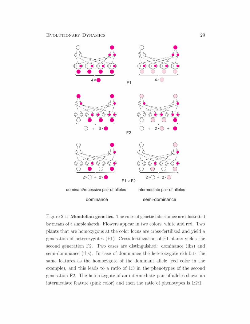
Figure 2.1: Mendelian genetics. The rules of genetic inheritance are illustrated
by means of a simple sketch. Flowers appear in two colors, white and red. Two
plants that are homozygous at the color locus are cross-fertilized and yield a
generation of heterozygotes (F1). Cross-fertilization of F1 plants yields the
second generation F2. Two cases are distinguished: dominance (lhs) and
semi-dominance (rhs). In case of dominance the heterozygote exhibits the
same features as the homozygote of the dominant allele (red color in the
example), and this leads to a ratio of 1:3 in the phenotypes of the second
generation F2. The heterozygote of an intermediate pair of alleles shows an
intermediate feature (pink color) and then the ratio of phenotypes is 1:2:1.
30 Peter Schuster
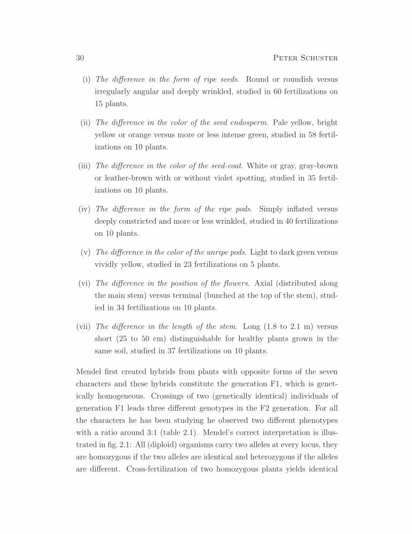
(i) The difference in the form of ripe seeds. Round or roundish versus
irregularly angular and deeply wrinkled, studied in 60 fertilizations on
15 plants.
(ii) The difference in the color of the seed endosperm. Pale yellow, bright
yellow or orange versus more or less intense green, studied in 58 fertil-
izations on 10 plants.
(iii) The difference in the color of the seed-coat. White or gray, gray-brown
or leather-brown with or without violet spotting, studied in 35 fertil-
izations on 10 plants.
(iv) The difference in the form of the ripe pods. Simply inflated versus
deeply constricted and more or less wrinkled, studied in 40 fertilizations
on 10 plants.
(v) The difference in the color of the unripe pods. Light to dark green versus
vividly yellow, studied in 23 fertilizations on 5 plants.
(vi) The difference in the position of the flowers. Axial (distributed along
the main stem) versus terminal (bunched at the top of the stem), stud-
ied in 34 fertilizations on 10 plants.
(vii) The difference in the length of the stem. Long (1.8 to 2.1 m) versus
short (25 to 50 cm) distinguishable for healthy plants grown in the
same soil, studied in 37 fertilizations on 10 plants.
Mendel first created hybrids from plants with opposite forms of the seven
characters and these hybrids constitute the generation F1, which is genet-
ically homogeneous. Crossings of two (genetically identical) individuals of
generation F1 leads three different genotypes in the F2 generation. For all
the characters he has been studying he observed two different phenotypes
with a ratio around 3:1 (table 2.1). Mendel’s correct interpretation is illus-
trated in fig. 2.1: All (diploid) organisms carry two alleles at every locus, they
are homozygous if the two alleles are identical and heterozygous if the alleles
are different. Cross-fertilization of two homozygous plants yields identical
Evolutionary Dynamics 31
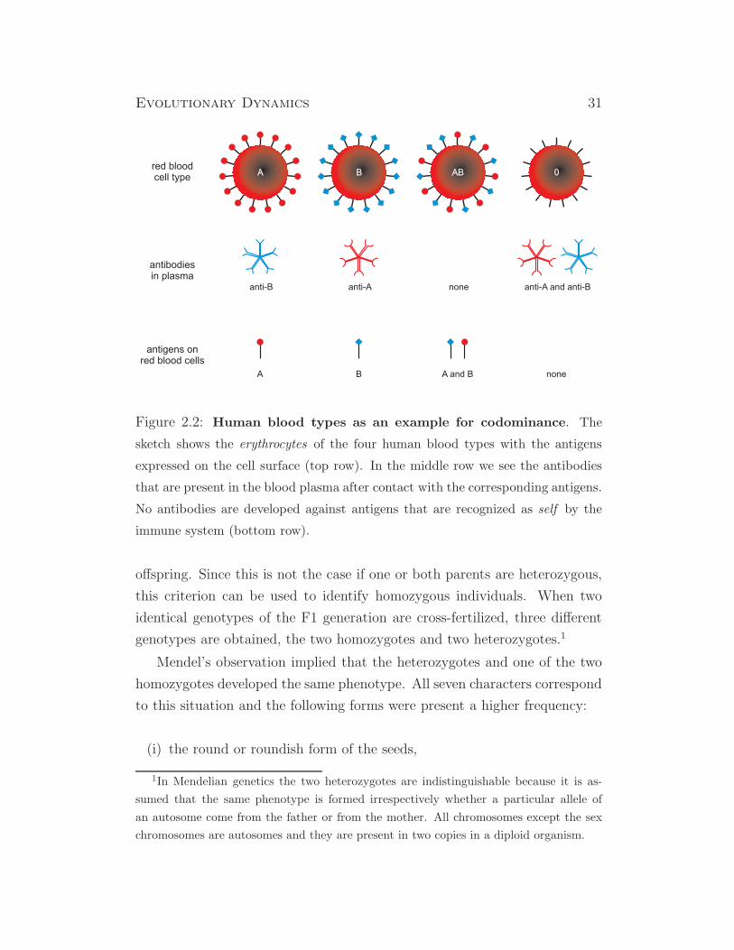
Figure 2.2: Human blood types as an example for codominance. The
sketch shows the erythrocytes of the four human blood types with the antigens
expressed on the cell surface (top row). In the middle row we see the antibodies
that are present in the blood plasma after contact with the corresponding antigens.
No antibodies are developed against antigens that are recognized as self by the
immune system (bottom row).
offspring. Since this is not the case if one or both parents are heterozygous,
this criterion can be used to identify homozygous individuals. When two
identical genotypes of the F1 generation are cross-fertilized, three different
genotypes are obtained, the two homozygotes and two heterozygotes.1
Mendel’s observation implied that the heterozygotes and one of the two
homozygotes developed the same phenotype. All seven characters correspond
to this situation and the following forms were present a higher frequency:
(i) the round or roundish form of the seeds,
1In Mendelian genetics the two heterozygotes are indistinguishable because it is as-
sumed that the same phenotype is formed irrespectively whether a particular allele of
an autosome come from the father or from the mother. All chromosomes except the sex
chromosomes are autosomes and they are present in two copies in a diploid organism.
32 Peter Schuster
(ii) the yellow color of the endosperm,
(iii) the gray, gray-brown or leather-brown color of the seed coat,
(iv) the simply inflated form of the ripe pods,
(v) the green coloring of the unripe pod,
(vi) the axial distribution of the flowers along the stem, and
(vii) the long stems.
The figure shows in addition the ratios of phenotypes when one individual
of the F1 generation is cross fertilized with a homozygous plant of the F2
generation. Later such an allele pair has been denoted as dominant-recessive.
In table 2.1 we show the detailed results of Mendel’s experiments and point
a two features that a typical for a statistical law: (i) the large number of
repetitions, which are necessary to be able to recognize the regularities and
(ii) the rather small deviations from the ideal ratio three. In section 2.6 we
shall analyze Mendel’s data by means of the χ2-test, a statistical reliability
test that has been introduced around nineteen hundred by the Karl Pearson.
From Mendel’s experiment we conclude that every diploid organism car-
ries two copies of each (autosomal) gene. The copies are separated during
sexual reproduction and combined anew. Alleles shall be denoted by sans-
serif letters, in a dominant-recessive allele pair we shall denote the dominant
allele by an upper-case letter and the recessive allele by a lower-case letter,
A and a, respectively. The four zygote are then AA, Aa, aA, and aa where
the first three genotypes express the same phenotype. Although dominance
is by far the more common feature in nature, other form exist and they are
also familiar to careful observers and naturalists.
Incomplete dominance or semi-dominance is a form of intermediate in-
heritance in which one allele for a specific trait is not completely dominant
over the other allele, and a combined phenotype is the results (fig. 2.1, rhs):
The phenotype expressed by the heterozygous genotype is an intermediate of
the phenotypes of the homozygous genotypes. For example, the color of the
Evolutionary Dynamics 33
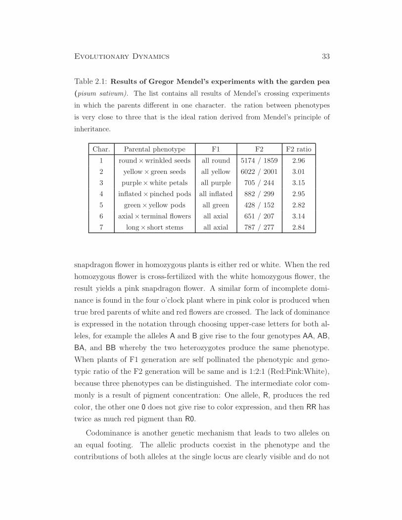
Table 2.1: Results of Gregor Mendel’s experiments with the garden pea
(pisum sativum). The list contains all results of Mendel’s crossing experiments
in which the parents different in one character. the ration between phenotypes
is very close to three that is the ideal ration derived from Mendel’s principle of
inheritance.
Char. Parental phenotype F1 F2 F2 ratio
1 round×wrinkled seeds all round 5174 / 1859 2.96
2 yellow× green seeds all yellow 6022 / 2001 3.01
3 purple×white petals all purple 705 / 244 3.15
4 inflated×pinched pods all inflated 882 / 299 2.95
5 green× yellow pods all green 428 / 152 2.82
6 axial× terminal flowers all axial 651 / 207 3.14
7 long× short stems all axial 787 / 277 2.84
snapdragon flower in homozygous plants is either red or white. When the red
homozygous flower is cross-fertilized with the white homozygous flower, the
result yields a pink snapdragon flower. A similar form of incomplete domi-
nance is found in the four o’clock plant where in pink color is produced when
true bred parents of white and red flowers are crossed. The lack of dominance
is expressed in the notation through choosing upper-case letters for both al-
leles, for example the alleles A and B give rise to the four genotypes AA, AB,
BA, and BB whereby the two heterozygotes produce the same phenotype.
When plants of F1 generation are self pollinated the phenotypic and geno-
typic ratio of the F2 generation will be same and is 1:2:1 (Red:Pink:White),
because three phenotypes can be distinguished. The intermediate color com-
monly is a result of pigment concentration: One allele, R, produces the red
color, the other one 0 does not give rise to color expression, and then RR has
twice as much red pigment than R0.
Codominance is another genetic mechanism that leads to two alleles on
an equal footing. The allelic products coexist in the phenotype and the
contributions of both alleles at the single locus are clearly visible and do not
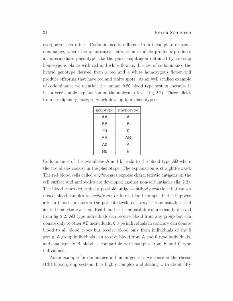
34 Peter Schuster
overpower each other. Codominance is different from incomplete or semi-
dominance, where the quantitative interaction of allele products produces
an intermediate phenotype like the pink snapdragon obtained by crossing
homozygous plants with red and white flowers. In case of codominance the
hybrid genotype derived from a red and a white homozygous flower will
produce offspring that have red and white spots. As an well studied example
of codominance we mention the human AB0 blood type system, because it
has a very simple explanation on the molecular level (fig. 2.2). Three alleles
from six diploid genotypes which develop four phenotypes:
genotype phenotype
AA A
BB B
00 0
AB AB
A0 A
B0 B
Codominance of the two alleles A and B leads to the blood type AB where
the two alleles coexist in the phenotype. The explanation is straightforward:
The red blood cells called erythrocytes express characteristic antigens on the
cell surface and antibodies are developed against non-self antigens (fig. 2.2).
The blood types determine a possible antigen-antibody reaction that causes
mixed blood samples to agglutinate or forms blood clumps. If this happens
after a blood transfusion the patient develops a very serious usually lethal
acute hemolytic reaction. Red blood cell compatibilities are readily derived
from fig. 2.2: AB type individuals can receive blood from any group but can
donate only to other AB individuals, 0 type individuals in contrary can donate
blood to all blood types but receive blood only from individuals of the 0
group, A group individuals can receive blood from A and 0 type individuals,
and analogously B blood is compatible with samples from B and 0 type
individuals.
As an example for dominance in human genetics we consider the rhesus
(Rh) blood group system. It is highly complex and dealing with about fifty
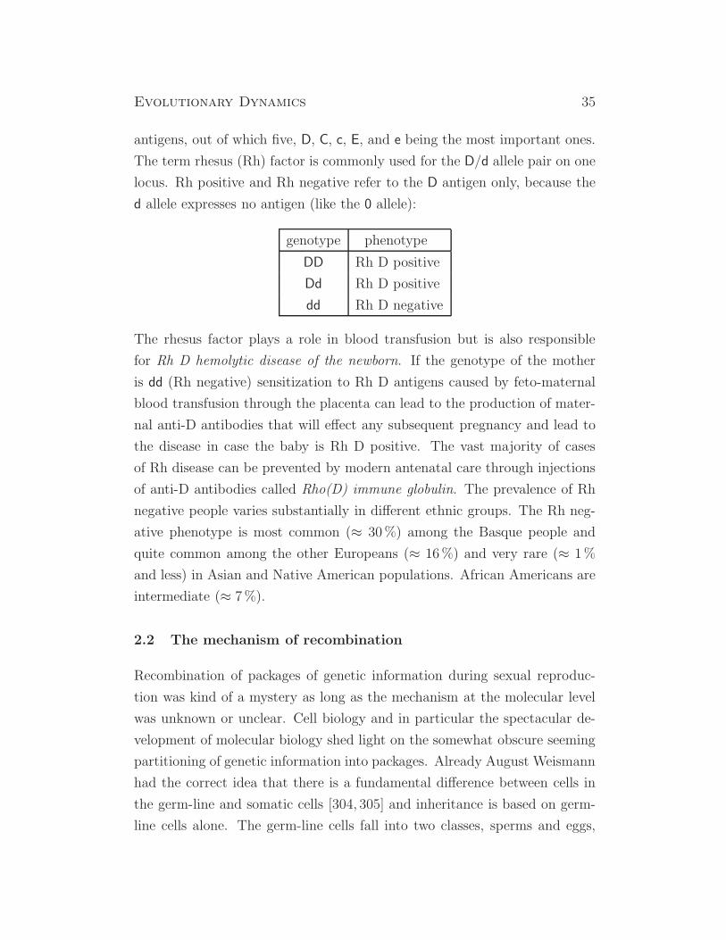
Evolutionary Dynamics 35
antigens, out of which five, D, C, c, E, and e being the most important ones.
The term rhesus (Rh) factor is commonly used for the D/d allele pair on one
locus. Rh positive and Rh negative refer to the D antigen only, because the
d allele expresses no antigen (like the 0 allele):
genotype phenotype
DD Rh D positive
Dd Rh D positive
dd Rh D negative
The rhesus factor plays a role in blood transfusion but is also responsible
for Rh D hemolytic disease of the newborn. If the genotype of the mother
is dd (Rh negative) sensitization to Rh D antigens caused by feto-maternal
blood transfusion through the placenta can lead to the production of mater-
nal anti-D antibodies that will effect any subsequent pregnancy and lead to
the disease in case the baby is Rh D positive. The vast majority of cases
of Rh disease can be prevented by modern antenatal care through injections
of anti-D antibodies called Rho(D) immune globulin. The prevalence of Rh
negative people varies substantially in different ethnic groups. The Rh neg-
ative phenotype is most common (≈ 30%) among the Basque people and
quite common among the other Europeans (≈ 16%) and very rare (≈ 1%
and less) in Asian and Native American populations. African Americans are
intermediate (≈ 7%).
2.2 The mechanism of recombination
Recombination of packages of genetic information during sexual reproduc-
tion was kind of a mystery as long as the mechanism at the molecular level
was unknown or unclear. Cell biology and in particular the spectacular de-
velopment of molecular biology shed light on the somewhat obscure seeming
partitioning of genetic information into packages. Already August Weismann
had the correct idea that there is a fundamental difference between cells in
the germ-line and somatic cells [304, 305] and inheritance is based on germ-
line cells alone. The germ-line cells fall into two classes, sperms and eggs,

36 Peter Schuster
Figure 2.3: The life cycle of a diploid organism. The life cycle of a typical
diploid eukaryote consists of a haploid phase with γ = n chromosomes (blue) that
is initiated by meiosis and ends with the fusion of a sperm and an egg cell in
order to form a diploid zygote. During the rest of the life cycle each somatic cell
of the organism has γ = 2n chromosomes in n − 1 autosomal pairs and the sex
chromosomes (red). Special cell lines differentiate into meiocytes, which undergo
meiosis and form the gametes.
which differ largely in the amount of cytoplasm that they contain: In the
sexual union of sperm and egg forming a zygote the egg contributes almost
the entire cytoplasm. The nuclei of egg and sperm cells are of approximately
the same size and therefore the nuclei were considered as candidates for har-
boring the structures that are responsible for inheritance. A sketch of the
typical diploid life cycle with a long diploid phase and a short haploid stage
providing the frame for sexual reproduction is shown in Fig. 2.3. In the eigh-
teen eighties the German biologist Theodor Boveri demonstrated that within
the nucleus the chromosomes were the vectors of heredity. It was also Boveri
who pointed out that Mendel’s rules of inheritance are consistent with the
observed behavior of chromosomes and developed independently from Walter
Sutton in 1902 the chromosome theory of inheritance. The ultimate proof
of the role of chromosome was provided by the American geneticist Thomas

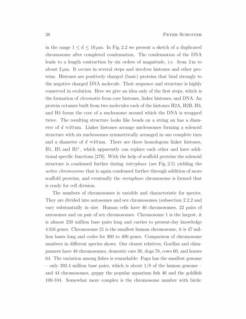
Evolutionary Dynamics 37
Figure 2.4: Sketch of a
replicated and condensed
eukaryotic chromosome.
Shown are the two sister
chromatids in the meta
phase after the synthetic
phase. The centromere (red)
is the point where the two
chromatids touch and where
the microtubules attach.
The ends of the chromatids
(green) are called telomeres
and carry repetitive sequences
that protect the chromosomes
against damage.
Hunt Morgan who started with systematic crossing experiments with the
fruit fly drosophila around 1910.
2.2.1 Chromosomes
Chromosomes are complex structures consisting of DNA molecules and pro-
teins. The necessity to organize DNA structure becomes evident from con-
sidering its size: The DNA molecule of a human consists of 2×3×109 base
pairs and in fully stretched state the double-helical DNA molecule would
be 6×109 · 0.34 nm≈ 2m long. Clearly, such a long molecule can only be
processed successfully in an compartment with the diameter of a eucaryotic
cell when properly condensed to smaller size. Mammalian cells vary consid-
erably in size: Among the smallest are the red blood cells with a diameter of
about 0.76µm and among the largest cells are are the nerve cells that span a
giraffe’s neck and which can be longer than 3m. Analogously human nerve
cells may be as long as 1m. The size of the average human cell, however, lies
38 Peter Schuster
in the range 1 ≤ d ≤ 10µm. In Fig. 2.2 we present a sketch of a duplicated
chromosome after completed condensation. The condensation of the DNA
leads to a length contraction by six orders of magnitude, i.e. from 2m to
about 2µm. It occurs in several steps and involves histones and other pro-
teins. Histones are positively charged (basic) proteins that bind strongly to
the negative charged DNA molecule. Their sequence and structure is highly
conserved in evolution. Here we give an idea only of the first steps, which is
the formation of chromatin from core histones, linker histones, and DNA. An
protein octamer built from two molecules each of the histones H2A, H2B, H3,
and H4 forms the core of a nucleosome around which the DNA is wrapped
twice. The resulting structure looks like beads on a string an has a diam-
eter of d ≈10 nm. Linker histones arrange nucleosomes forming a solenoid
structure with six nucleosomes symmetrically arranged in one complete turn
and a diameter of d ≈10 nm. There are three homologous linker histones,
H1, H5 and H1 , which apparently can replace each other and have addi-
tional specific functions [278]. With the help of scaffold proteins the solenoid
structure is condensed further during interphase (see Fig. 2.5) yielding the
active chromosome that is again condensed further through addition of more
scaffold proteins, and eventually the metaphase chromosome is formed that
is ready for cell division.
The numbers of chromosomes is variable and characteristic for species.
They are divided into autosomes and sex chromosomes (subsection 2.2.2 and
vary substantially in size. Human cells have 46 chromosomes, 22 pairs of
autosomes and on pair of sex chromosomes. Chromosome 1 is the largest, it
is almost 250 million base pairs long and carries to present-day knowledge
4 316 genes. Chromosome 21 is the smallest human chromosome, it is 47 mil-
lion bases long and codes for 300 to 400 genes. Comparison of chromosome
numbers in different species shows. Our closest relatives, Gorillas and chim-
panzees have 48 chromosomes, domestic cats 38, dogs 78, cows 60, and horses
64. The variation among fishes is remarkable: Fugu has the smallest genome
– only 392.4 million base pairs, which is about 1/8 of the human genome –
and 44 chromosomes, guppy the popular aquarium fish 46 and the goldfish
100-104. Somewhat more complex is the chromosome number with birds:

Evolutionary Dynamics 39
The domestic pigeon has 18 large chromosomes and 60 microchromosomes
and similarly chicken with 10 chromosomes and 60 microchromosomes, and
eventually the pretty bird kingfisher 132 total. The chromosome numbers
in plants are highly variable as well: the thale cress, arabidopsis thaliana,
has 10 chromosomes and the pea, pisum sativum, 24, and the pineapple 50.
The well-studied yeast, saccharomyces cerevisiae, has 32 chromosomes. Fi-
nally, we make a glance on prokaryotes. The eubacterium Escherichia coli
has a single circular chromosome, which when fully stretched is many orders
of magnitude larger than the cell itself, but no histones like other eubacte-
ria. DNA is condensed mainly by supercoiling and the process is assisted
by specific enzymes called topoisomerases [162]. Topoisomerases, in general,
resolve the topological problems associated with DNA replication, transcrip-
tion, recombination, and chromatin remodeling in a trivial but highly efficient
way: They introduce temporary single- or double-strand breaks into DNA,
unwind, and ligate again.
After DNA replication and condensation into chromosomes the two sis-
ter chromatids have a long and a short arm (Fig. 2.2) and they are joined
at the centromere that is also the point of attachment of the microtubules,
which organize chromosome transport during cell division. In order to pre-
vent loss of DNA ends during cell division at the tips, the chromosomes carry
telomeres, which are stretches of short repeats of oligonucleotides that can
be understood as disposable buffers blocking the ends of the chromosomes.
In case of vertebrates the repeat in the telomeres is TTAGGG. Part of the
telomeres are consumed during cell division and replenished by an enzyme
called telomerase reverse transcriptase. Cells, which have completely con-
sumed their telomeres, are destroyed by apoptosis and in rare cases they
find ways of evading programmed destruction and become immortal cancer
cells. In 2009 Elizabeth Blackburn, Carol Greider, and Jack Szostak were
awarded the Nobel Prize in Physiology and Medicine for the discovery of
how chromosomes are protected by telomeres and the enzyme telomerase.
The telomeres are tightly bound to the inner surface of the nuclear enve-
lope during prophase 1 (see Fig. 2.6) and play an important role in pairing
homologous chromosomes during meiosis.
40 Peter Schuster
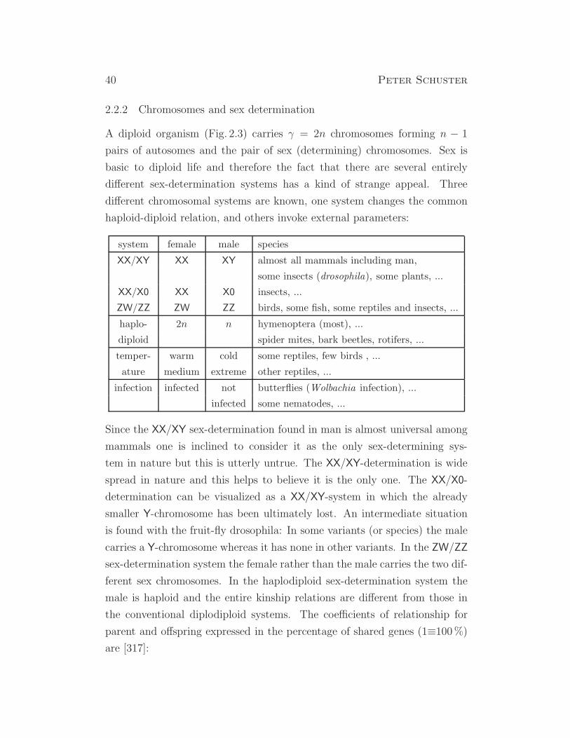
2.2.2 Chromosomes and sex determination
A diploid organism (Fig. 2.3) carries γ = 2n chromosomes forming n − 1
pairs of autosomes and the pair of sex (determining) chromosomes. Sex is
basic to diploid life and therefore the fact that there are several entirely
different sex-determination systems has a kind of strange appeal. Three
different chromosomal systems are known, one system changes the common
haploid-diploid relation, and others invoke external parameters:
system female male species
XX/XY XX XY almost all mammals including man,
some insects (drosophila), some plants, ...
XX/X0 XX X0 insects, ...
ZW/ZZ ZW ZZ birds, some fish, some reptiles and insects, ...
haplo- 2n n hymenoptera (most), ...
diploid spider mites, bark beetles, rotifers, ...
temper- warm cold some reptiles, few birds , ...
ature medium extreme other reptiles, ...
infection infected not butterflies (Wolbachia infection), ...
infected some nematodes, ...
Since the XX/XY sex-determination found in man is almost universal among
mammals one is inclined to consider it as the only sex-determining sys-
tem in nature but this is utterly untrue. The XX/XY-determination is wide
spread in nature and this helps to believe it is the only one. The XX/X0-
determination can be visualized as a XX/XY-system in which the already
smaller Y-chromosome has been ultimately lost. An intermediate situation
is found with the fruit-fly drosophila: In some variants (or species) the male
carries a Y-chromosome whereas it has none in other variants. In the ZW/ZZ
sex-determination system the female rather than the male carries the two dif-
ferent sex chromosomes. In the haplodiploid sex-determination system the
male is haploid and the entire kinship relations are different from those in
the conventional diplodiploid systems. The coefficients of relationship for
parent and offspring expressed in the percentage of shared genes (1≡100%)
are [317]:
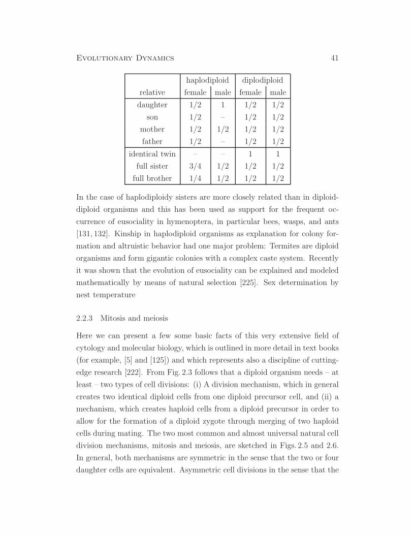
Evolutionary Dynamics 41
haplodiploid diplodiploid
relative female male female male
daughter 1/2 1 1/2 1/2
son 1/2 – 1/2 1/2
mother 1/2 1/2 1/2 1/2
father 1/2 – 1/2 1/2
identical twin – – 1 1
full sister 3/4 1/2 1/2 1/2
full brother 1/4 1/2 1/2 1/2
In the case of haplodiploidy sisters are more closely related than in diploid-
diploid organisms and this has been used as support for the frequent oc-
currence of eusociality in hymenoptera, in particular bees, wasps, and ants
[131, 132]. Kinship in haplodiploid organisms as explanation for colony for-
mation and altruistic behavior had one major problem: Termites are diploid
organisms and form gigantic colonies with a complex caste system. Recently
it was shown that the evolution of eusociality can be explained and modeled
mathematically by means of natural selection [225]. Sex determination by
nest temperature
2.2.3 Mitosis and meiosis
Here we can present a few some basic facts of this very extensive field of
cytology and molecular biology, which is outlined in more detail in text books
(for example, [5] and [125]) and which represents also a discipline of cutting-
edge research [222]. From Fig. 2.3 follows that a diploid organism needs – at
least – two types of cell divisions: (i) A division mechanism, which in general
creates two identical diploid cells from one diploid precursor cell, and (ii) a
mechanism, which creates haploid cells from a diploid precursor in order to
allow for the formation of a diploid zygote through merging of two haploid
cells during mating. The two most common and almost universal natural cell
division mechanisms, mitosis and meiosis, are sketched in Figs. 2.5 and 2.6.
In general, both mechanisms are symmetric in the sense that the two or four
daughter cells are equivalent. Asymmetric cell divisions in the sense that the
42 Peter Schuster
offspring cells are intrinsically different play a role in embryonic development
[139], in particular with stem cells [177]. As an example we mention the
nematode Caenorhabditis elegans where several successive asymmetric cell
divisions in the early embryo are critical for setting up the anterior/posterior,
dorsal ventral, and left/right axes of the body plan [119].
In mitosis one diploid cell divides into two diploid cells that – provided no
accident has happened – carry the same genetic information as the parental
cell and the over-all process is simple duplication (Fig. 2.5). Homologous
chromosomes behave independently during mitosis – and this distinguishes
it from meiosis. The problem that has to be solved, nevertheless, is of
formidable complexity: A molecule of about 2m length has to be copied
in a cell of about 10µm diameter and than divided equally during cell di-
vision. Long before the advent of molecular biology cell division has been
studied extensively by means of light microscopy and the different stages
shown in Fig. 2.5 were distinguished. DNA replication takes place in the
interphase nucleus and each chromosome is transformed into two identical
sister chromatids, in prophase we have the sister chromatids in perfect align-
ment and ready for cell division then the nuclear membrane dissolves and in
metaphase the chromosomes migrate to the equator of the cell. Microtubules
form and attach to the centromeres (Fig. 2.2) in anaphase and telophase the
sister chromatids are pulled apart and to the two opposite poles of the cell.
At the end of telophase the cell splits into two daughter cells and nuclear
membrane are formed in both cells.
Meiosis is initiated like mitosis by DNA replication but instead of cell
division two organized cell divisions follow with no second replication phase
in between. Accordingly one diploid cell is split into four haploid gametes
during meiosis. The major difference between the two cell division scenar-
ios occurs in prophase 1 and metaphase 1: The two duplicated homologous
chromosomes are pairing and crossover between the four chromatids is disen-
tangled by homologous recombination.2 During prophase 1 the tight binding
2Homologous recombination is the precise notion of recombination during meiosis since
there are also other forms of recombination in the sense of exchange of genetic material,
for example, with bacterial conjugation or multiple virus infection of a single cell.

Evolutionary Dynamics 43
2n
2n
2n
interphase prophase metaphase anaphase
telophase
daughter cells
replication segregation
Figure 2.5: Mitosis. Mitosis is the mechanism for the division of nuclei associated
with the division of somatic cells in eukaryotes. During interphase that comprises
of three stages of the cell cycle – gap 1 (G1), synthesis (S), and gap2 (G2) –
the DNA of each chromosome replicates and each chromosome is transformed
into two sister chromatids, which lie side by side. The mitosis stage of the cell
cycle (M) starts with prophase when the sister chromatids become visible in the
light microscope. During metaphase the sister chromatid pairs are moving to the
equatorial plane of the cell. In anaphase microtubules being part of the nuclear
spindle attach to the centromeres (small orange balls in the sketch), separate the
sister chromatids, and pull them in opposite direction towards the cellular poles.
In telophase the separation is completed and a nuclear membrane forms around
each nucleus and cell division completes mitosis. The sketch shows the fate of
a single chromosome, which is present in two differently marked copies (red and
bright violet) that appear in identical form in the two daughter cells. Mitosis
produces two (in essence) genetically identical diploid (2n) daughter cells from one
diploid cell (2n). Here and in Fig. 2.6 we do not show the nuclear membrane in
order to avoid confusion. During interphase, the first part of prophase, and in the
daughter cells the compartment shown is the nucleus whereas the circles mean the
entire cell during the stages of segregation.
between the sister chromatids is weakened and eventually resolved through
the formation of a large complex in which all four chromatids of the two dupli-
cated homologous chromosomes are aligned by means of an extensive protein
machinery. This process is slow as prophase 1 may occupy 90% or more
44 Peter Schuster
2n
2n
n
n
n
n
2n
interphase prophase 1
prophase 2
metaphase 1
metaphase 2
anaphase 1
anaphase 2
telophase 1
telophase 2
prophase 2
gametes
replication pairing segregation
segregation
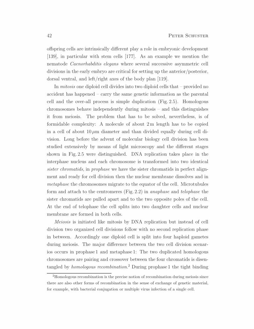
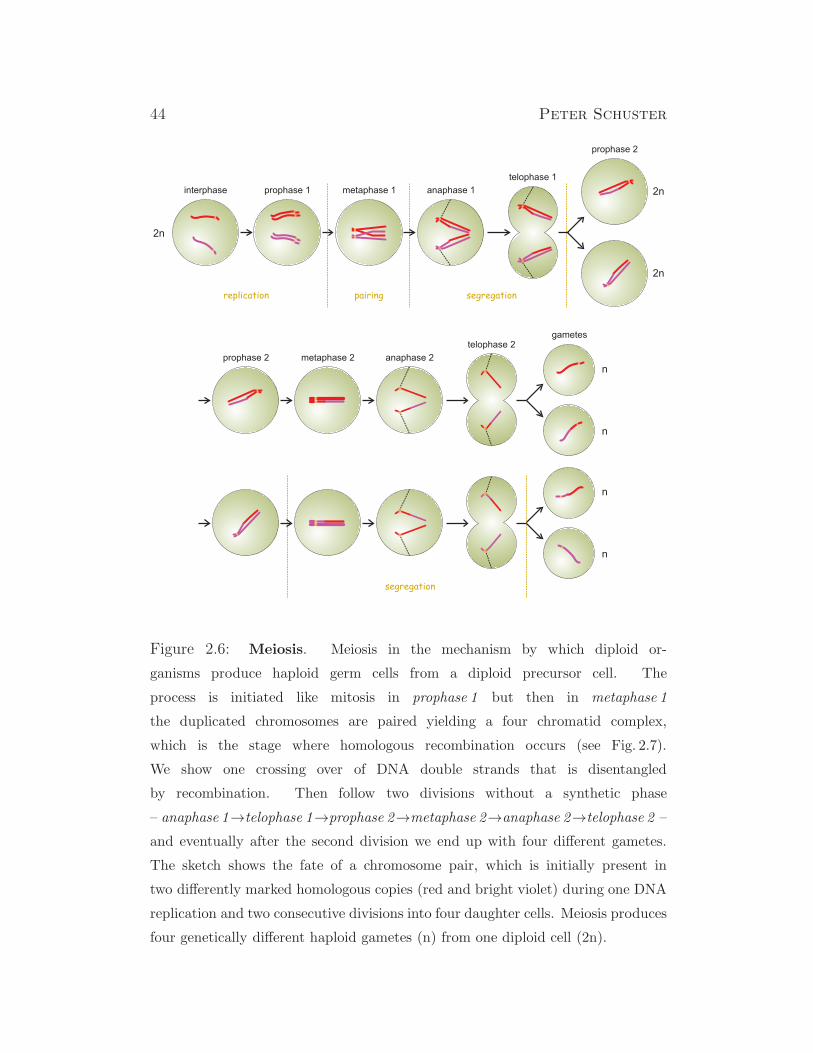
Figure 2.6: Meiosis. Meiosis in the mechanism by which diploid or-
ganisms produce haploid germ cells from a diploid precursor cell. The
process is initiated like mitosis in prophase 1 but then in metaphase 1
the duplicated chromosomes are paired yielding a four chromatid complex,
which is the stage where homologous recombination occurs (see Fig. 2.7).
We show one crossing over of DNA double strands that is disentangled
by recombination. Then follow two divisions without a synthetic phase
– anaphase 1→telophase 1→prophase 2→metaphase 2→anaphase 2→telophase 2 –
and eventually after the second division we end up with four different gametes.
The sketch shows the fate of a chromosome pair, which is initially present in
two differently marked homologous copies (red and bright violet) during one DNA
replication and two consecutive divisions into four daughter cells. Meiosis produces
four genetically different haploid gametes (n) from one diploid cell (2n).
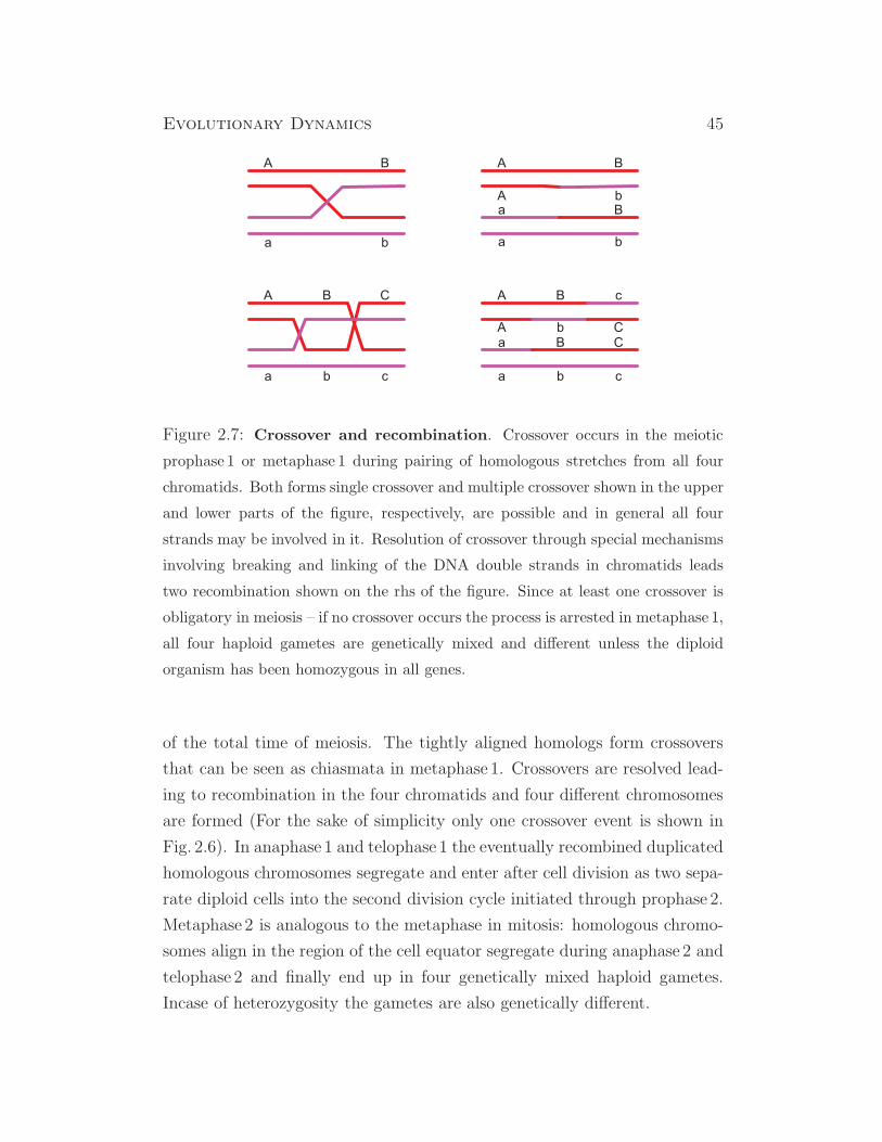
Evolutionary Dynamics 45
Figure 2.7: Crossover and recombination. Crossover occurs in the meiotic
prophase 1 or metaphase 1 during pairing of homologous stretches from all four
chromatids. Both forms single crossover and multiple crossover shown in the upper
and lower parts of the figure, respectively, are possible and in general all four
strands may be involved in it. Resolution of crossover through special mechanisms
involving breaking and linking of the DNA double strands in chromatids leads
two recombination shown on the rhs of the figure. Since at least one crossover is
obligatory in meiosis – if no crossover occurs the process is arrested in metaphase 1,
all four haploid gametes are genetically mixed and different unless the diploid
organism has been homozygous in all genes.
of the total time of meiosis. The tightly aligned homologs form crossovers
that can be seen as chiasmata in metaphase 1. Crossovers are resolved lead-
ing to recombination in the four chromatids and four different chromosomes
are formed (For the sake of simplicity only one crossover event is shown in
Fig. 2.6). In anaphase 1 and telophase 1 the eventually recombined duplicated
homologous chromosomes segregate and enter after cell division as two sepa-
rate diploid cells into the second division cycle initiated through prophase 2.
Metaphase 2 is analogous to the metaphase in mitosis: homologous chromo-
somes align in the region of the cell equator segregate during anaphase 2 and
telophase 2 and finally end up in four genetically mixed haploid gametes.
Incase of heterozygosity the gametes are also genetically different.
46 Peter Schuster
In prophase 1 and metaphase 1 of meiosis individual chromatids pair with
the other homologous chromosome with the help of a large protein machin-
ery called the recombination complex (see [5, chapter 21]). Tight packing
of the four chromatids of the duplicated homologous chromosomes together
with the protein machinery and produces a very large synaptonemal complex.
The processes in the synaptonemal complex may last for days and longer
and eventually, prophase 1 ends through disassembling of the synaptonemal
complex and initiating metaphase 1. Chiasmata being the visual point of
crossing-over of chromatid strands that might have occurred already before
and during the formation of the complex appear during the phase of disas-
sembly. Resolution of crossover in consequence leads to recombination. The
chromosomes determining the sex of the carrier may behave differently from
autosomes. In mammals female sex chromosomes XX behave like autosomes
during meiosis. Male sex chromosomes – XY in mammals – however, require
special features during meiosis. Although the X and the Y chromosome in a
male are not homologous they too must pair and undergo crossover during
prophase 1 in order to allow for normal segregation in anaphase 1. Pair-
ing, crossing-over, and segregation are made possible because there are small
regions of homology between X and Y at one end or both ends of the chro-
mosomes. The two chromosomes pair and crossover in these regions during
prophase 1 and ensure thereby that each sperm cell receives either one X or
one Y chromosome – and neither both nor none – and the sperm cells deter-
mine whether the zygote develops into a female or male embryo, respectively.
Meiosis is regulated differently in female and male mammals. In males meio-
sis begins begins in sperm precursor cells called spermatocytes in the testes at
puberty and then goes on continuously. It takes about 24 days for a human
spermatocyte to complete meiosis. In females the egg precursor cells, the
oocytes begin meiosis in the fetal ovary but arrest after the synaptonemal
complex has disassembled in metaphase 1. Oocytes complete meiosis only
after the female has become sexually mature and the oocyte is released from
the ovary during ovulation and the released oocyte completes meiosis only
if it is fertilized. In humans some oocytes my be arrested in netaphase 1 for
40 years or more. There are specific stop and start mechanisms in female
Evolutionary Dynamics 47
meiosis that are lacking in the male. Finally, we remark that according to
the current state of knowledge meiosis goes wrong frequently and this leads
to early abortion or serious damage of the embryo.
Crossover occurs before the first cell division in meiosis and can be seen in
the microscope in the form of a chiasma where a chromatid strands switches
from one chromosome to the other. Chiasmata or crossovers are resolved by
splitting and ligating DNA and eventually genes from homologous but differ-
ent chromatids find itself recombined on the same chromosome. As shown in
Fig. 2.7 a single crossover is sufficient to produce four different chromosomes.
Double and multiple crossovers may occur as well and they give rise to a
great variety of gene patterns. How are crossover and recombination related
to Gregor Mendel’s laws of inheritance? Linkage equilibrium in population
genetics is achieved when the association of alleles at two or more loci is
random. In other words, Mendel made the assumption of random assort-
ment of alleles, which is at the same time the basis for linkage equilibrium
and accordingly, every deviation from it is called linkage disequilibrium. This
deviation can be cast into a quantitative relation. For the sake of simplicity
we consider a haplotype3 for two loci A and B with two alleles each, and the
following frequencies for all possible combinations:
[A1B1] = x11, [A1B2] = x12, [A2B1] = x21, and [A2B2] = x22.
These frequencies are assumed to be normalized,∑
i,j xij = 1, and this leads
to the following frequencies of the alleles:
[A1] = p1 = x11 + x12 , [A2] = p2 = x21 + x22 , and p1 + p2 = 1 ,
[B1] = q1 = x11 + x21 , [B2] = q2 = x12 + x22 , and q1 + q2 = 1 .
At linkage equilibrium we obtain from trivial statistics xij = piqj and de-
fine the linkage disequilibrium by the deviation of the real value from the
equilibrium value:
D = x11 − p1q1 = x11x22 − x12x21 . (2.1)
3A haplotype in genetics is a combination of alleles at adjacent locations on the chro-
mosome that are transmitted together. A haplotype may be one locus, several loci, or an
entire chromosome depending on the number of recombination events that have occurred.
48 Peter Schuster
Expressing the state of a population with respect to haplotypes on finds
the phrases ”two alleles are in linkage disequilibrium” for D 6= 0, and al-
ternatively linkage equilibrium stands for D = 0. Because of the various
conservation relations linkage disequilibrium is a one-parameter manifold as
follows from the table relating haplotype and allele frequencies:
A1 A2 total
B1 x11 = p1q1 +D x21 = p2q1 −D q1
B2 x12 = p1q2 −D x22 = p2q2 +D q2
total p1 p2 1
Sometimes the parameter D is normalized
ϑ =D
Dmax
with Dmax =
minp1q1, p2q2 if D < 0
minp1q2, p2q1 if D > 0.
As an alternative to ϑ the correlation coefficient between pairs of loci is used
(For a comparison of various linkage disequilibrium measures see, e.g., [50]):
r =D√
p1p2q1q2. (2.2)
The frequency of recombination between two loci c can be used to demon-
strate that linkage disequilibrium converges to zero in absence of other evo-
lutionary factors than Mendelian segregation and random mating. The fre-
quency of the haplotype A1B1 is given by the difference equation
x(n+1)11 = (1− c) x(n)11 + c p1q1 . (2.3)
This equation is readily interpreted: A fraction (1−c) of the haplotypes havenot recombined and hence are present in the next generation, multiplication
by x(n)11 yields the fraction of the not-recombined haplotypes that are A1B1,
and a fraction c did recombine the two loci. Random mating presupposed we
compute the fraction of the haplotype under consideration: The probability
that A1 is at locus A is p1 and the probability that the copy has B1 at locus
B. Since the alleles are initially on different loci the events are independent
and the probabilities can be simply multiplied. Rewriting of Equ. (2.3) yields
x(n+1)11 − p1q1 = (1− c)
(
x(n)11 − p1q1
)
or Dn+1 = (1− c)Dn ,
Evolutionary Dynamics 49
which for an initial linkage disequilibrium of D0 takes on the form
Dn = (1− c)nD0 . (2.4)
As time progresses and the number of generations approaches infinity we find
limn→∞
Dn = 0 ,
since limn→∞(1 − c)n = 0 because of 0 < 1 − c < 1. After a sufficiently
number of generations linkage disequilibrium will disappear due to recombi-
nation. The smaller the distance between the two loci, however, the smaller
will be the frequency of recombination c, and the slower will be the rate of
convergence of D towards zero.
2.2.4 Molecular mechanisms of recombination
The first molecular mechanism of crossover and recombination has been pro-
posed by Robin Holliday in 1964 [150] (For a more recent account see [273]).
It centers around the notion of a Holliday junction (Fig. 2.8), which is a cova-
lently linked crossing of two double-helical DNA strands.4 Holliday junctions
combining largely homologous stretches of DNA – as, for example, in case
of paired chromatids – can migrate by means of a simple base pair opening
and base pair closing mechanism. As shown in the lower part of Fig. 2.8 two
DNA double helices become longer and the other two are shortened during
migration. According to current knowledge, which is far from satisfactory
understanding, homologous crossing-over of chromatid strands is highly reg-
ulated with respect to (i) number and (ii) location. There is at least one
crossover event between the members of each homolog pairs because this
is necessary for normal segregation in metaphase 1, and there is crossover
interference inhibiting crossover points to be closer than some critical dis-
tance. Although the required two strand breaks occurring during meiosis can
be located almost everywhere on the chromosome, they are not distributed
uniformly: They cluster at hot spots where the chromatin is accessible, and
4In order to distinguish DNA single strands and double strands as used, for example,
in Fig. 2.7 we indicate 5’- and 3’ends of the single strands.
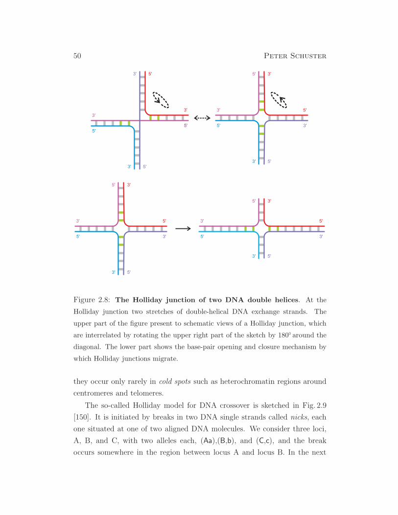
50 Peter Schuster
5' 5'3' 3'
5'
5'
3'
3'
5' 5'3' 3'
5'
5'
3'
3'
5'3'
5'3'
5' 3'
5' 3'
3'3'
5'3'
5'5'
3' 5'
Figure 2.8: The Holliday junction of two DNA double helices. At the
Holliday junction two stretches of double-helical DNA exchange strands. The
upper part of the figure present to schematic views of a Holliday junction, which
are interrelated by rotating the upper right part of the sketch by 180 around the
diagonal. The lower part shows the base-pair opening and closure mechanism by
which Holliday junctions migrate.
they occur only rarely in cold spots such as heterochromatin regions around
centromeres and telomeres.
The so-called Holliday model for DNA crossover is sketched in Fig. 2.9
[150]. It is initiated by breaks in two DNA single strands called nicks, each
one situated at one of two aligned DNA molecules. We consider three loci,
A, B, and C, with two alleles each, (Aa),(B,b), and (C,c), and the break
occurs somewhere in the region between locus A and locus B. In the next
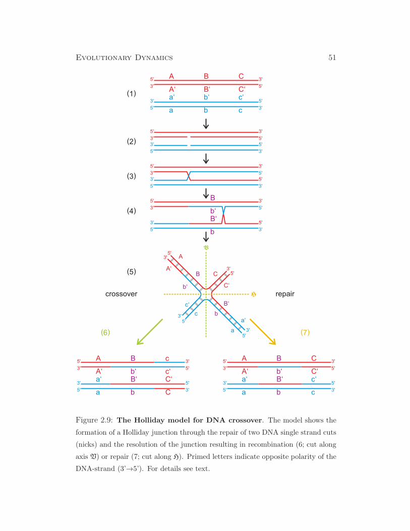
Evolutionary Dynamics 51
Figure 2.9: The Holliday model for DNA crossover. The model shows the
formation of a Holliday junction through the repair of two DNA single strand cuts
(nicks) and the resolution of the junction resulting in recombination (6; cut along
axis V) or repair (7; cut along H). Primed letters indicate opposite polarity of the
DNA-strand (3’→5’). For details see text.

52 Peter Schuster
Figure 2.10: The double strand break repair (DSBR) model for DNA
crossover. The double strand repair model starts from a double strand break
and a 5’-exonuclease produces sequence gaps. Strand invasion, DNA-synthesis
and second end capture leads to a structure with two Holliday junctions that can
be resolved to yield either double strand break repair (resolution at a & b or α & β)
or crossover and recombination (resolution at a & β or α & b). Newly synthesized
DNA stretches are shown as dashed lines. For details see text.
Evolutionary Dynamics 53
step the open ends are linked to the other DNA molecules resulting in a
Holliday junction. The junction migrates and finds an appropriate site for
resolving the crossover somewhere between locus B and locus C. The result-
ing Holliday junction can be cleaved in two ways, one yielding a recombined
DNA with a heteroduplex at locus B and one repaired molecules without
recombination but still showing the heteroduplex at B. One of the most im-
portant results of the Holiday model was to demonstrate the relation between
crossover and DNA damage repair. As outlined in Fig.2.9 (2) the process is
initiated by two single strand breaks (nicks), which are closed through the
formation of a strand switch from one double helix to the other forming
thereby a Holliday junction (3). The Holliday junction migrates along locus
B until it reached a point appropriate for resolution (4) and then an enzyme
called Holliday junction resolvase cuts and ligates the DNA strands elimi-
nating the entanglement of the two DNA double helices (5). The resolution
is possible in two different ways: (i) a vertical cut (V) and (ii) a horizontal
cut (H). The vertical cut resolves the Holliday junction into a structure in
which the two chromatid strands show crossover leading to recombination
(6) whereas the horizontal cleavage is leading to a structure in which the two
nicks have been repaired (7). In both cases the structures differ from the
original double helical strands at locus B where they have now heteroduplex
pairings Bb. The Holliday-model was complemented ten years after its inven-
tion by the more general Meselson-Radding model [208], which starts from
a single-strand break in one DNA molecule that becomes the site of strand
displacement by a DNA-polymerase. The displaced single-strand pairs with
the complementary sequence of a second homologous DNA-molecule and it
induces thereby a single strand break in the latter. Migration of the Holliday
junction and its resolution is similar to the Holliday-model. One difference
between the two models is that the heteroduplex region is confined to one
DNA molecule at the beginning in the Meselson-Radding model but is always
found in both DNA molecules in the Holliday model.
Work on plasmids in yeast [231] has shown that double strand gap repair
can lead to crossing-over but does not always do so. The corresponding
double-strand-break repair (DSBR) model is sketched in Fig. 2.10. It starts

54PeterSchuster
Figure 2.11: Enzymatic resolution of chiasmata. Three enzymatic resolution pathways of a double strand break
(For stage (1) and (2) see Fig. 2.10). The enzyme complexes are denoted by α, β, and γ, respectively. Newly synthesized
DNA stretches are shown as dashed lines. For details see text.

Evolutionary Dynamics 55
from a double-strand-break (1) and action of 5’-exonucleases as well as some
(or no) double strand degradation lead to a structure with free 3’-ends (2).
These ends are the active agents in the forthcoming steps: One strand with
an active 3’-end invades the double helix of the homologous chromatid and
initiates DNA double strand synthesis (3) until the free 3’-end is captured
(4). Completion and gap closure on both double helices leads to a structure
with two Holliday junctions (5). The resolution of the two junctions leads
either to break repair (6) or crossover and recombination (7) depending on
the direction of the cuts in the Holliday junctions: Both cuts horizontal or
both cuts vertical yields break repair whereas one cut horizontal and one
cut vertical produces crossover. Four years after the proposal of the DSBR-
model it was tested for recombination of phage λ and plasmid λdv [274, 284].
The most relevant new feature of this paper for the DSBR-model was that
a topoisomerase has been suggested to resolve the Holliday junctions. Later
topoisomerases were indeed identified that did precisely this job [257, 258].
Research on Holliday junctions and their resolution led to a rather confus-
ing multiplicity of possible pathways and a variety of endonuclease enzymes
called resolvases were identified in prokaryotes [60], in yeast [23, 230] and
eventually also in human cells [37]. In essence, three different pathways for
DSBR where found to be most prominent [307]. New light has been shed
on the problem when three enzymes from different organisms where shown
to promote Holliday junction resolution in analogous manner: the resolvases
RuvC from Escherichia coli, Yen1 from yeast and GEN1 from human cells
[157]. In Fig. 2.11 we show a sketch of the three pathways taken from [281].
The first two steps are identical with the corresponding steps in the DSBR
model in Fig. 2.10, one Holliday junction results from DNA strand invasion
(3), and then both single strand are completed to full double helices (4). Here
we have the first branching point: Either the two open ends are ligated and
the second Holliday junction is formed (5) (as in the simple DSBR model) or
structure (4) is directly resolved by the protein complex χ=Mus81-Eme1,
which cleaves the asymmetrically [23, 151] and produces a crossover product
(11). Two pathways branch out from the double Holliday junction structure
(5): One pathway makes use of the protein complex α=BLM-TopoIIIα-
56 Peter Schuster
RMI1 and disentangles the structure by two concerted topoisomerase dou-
ble strand openings and closures (7) [32, 320]. The resulting final product
is a double strand repair structure with a heteroduplex region in one dou-
ble strand (9). The third pathway engages the above mentioned resolvase,
β=GEN1 or β=Yen1, respectively, and resolves the double Holliday junc-
tion structure symmetrically by one vertical and one horizontal cut (8) as
also shown in Fig. 2.10) leading thereby to crossover (10). Although the 2008
paper [281] had the promising title Resolving Resolvases: The Final Act?,
research on Holliday junction resolution remained an exciting story until now
[217, 279].
After having had a glance on the enormously complicated processes of
meiosis and the state of the art in understanding its molecular mechanisms
we shall now return to the formal aspects and repeat the basic facts. re-
combination pure. Homologous chromatid strands do not pair in full length
during meiotic prophase 1 but show deviations in the sense that different
stretches are aligned to different chromatids, and this leads to chiasmata,
crossover and recombination. At least one crossover and recombination event
per chromosome is required for successful meiosis, since cells without chi-
asmata get arrested in metaphase 1 and are eliminated through apoptosis.
In essence recombination serves three purposes: (i) repair of double strand
breaks that have occurred during replication or pairing, (ii) enabling segre-
gation in metaphase 1 of meiosis, and (iii) creating genetic diversity through
recombination.
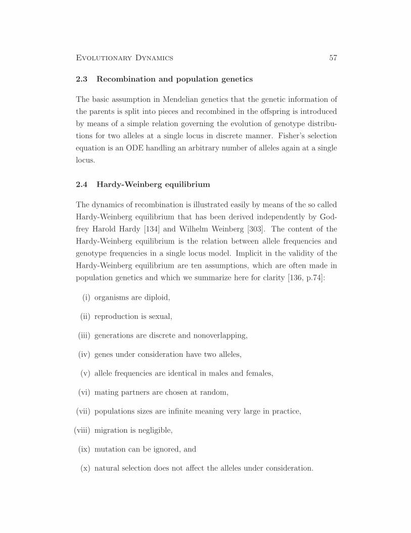
Evolutionary Dynamics 57
2.3 Recombination and population genetics
The basic assumption in Mendelian genetics that the genetic information of
the parents is split into pieces and recombined in the offspring is introduced
by means of a simple relation governing the evolution of genotype distribu-
tions for two alleles at a single locus in discrete manner. Fisher’s selection
equation is an ODE handling an arbitrary number of alleles again at a single
locus.
2.4 Hardy-Weinberg equilibrium
The dynamics of recombination is illustrated easily by means of the so called
Hardy-Weinberg equilibrium that has been derived independently by God-
frey Harold Hardy [134] and Wilhelm Weinberg [303]. The content of the
Hardy-Weinberg equilibrium is the relation between allele frequencies and
genotype frequencies in a single locus model. Implicit in the validity of the
Hardy-Weinberg equilibrium are ten assumptions, which are often made in
population genetics and which we summarize here for clarity [136, p.74]:
(i) organisms are diploid,
(ii) reproduction is sexual,
(iii) generations are discrete and nonoverlapping,
(iv) genes under consideration have two alleles,
(v) allele frequencies are identical in males and females,
(vi) mating partners are chosen at random,
(vii) populations sizes are infinite meaning very large in practice,
(viii) migration is negligible,
(ix) mutation can be ignored, and
(x) natural selection does not affect the alleles under consideration.
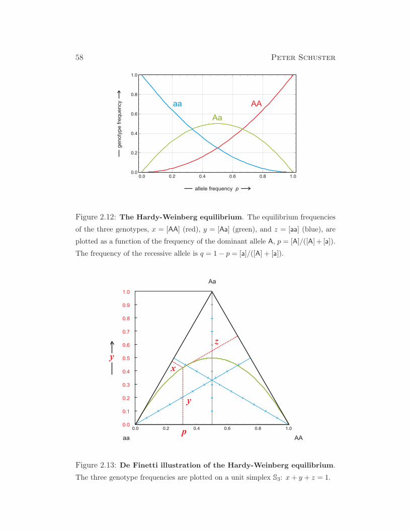
58 Peter Schuster
Figure 2.12: The Hardy-Weinberg equilibrium. The equilibrium frequencies
of the three genotypes, x = [AA] (red), y = [Aa] (green), and z = [aa] (blue), are
plotted as a function of the frequency of the dominant allele A, p = [A]/([A] + [a]).
The frequency of the recessive allele is q = 1− p = [a]/([A] + [a]).
Figure 2.13: De Finetti illustration of the Hardy-Weinberg equilibrium.
The three genotype frequencies are plotted on a unit simplex S3: x+ y + z = 1.
Evolutionary Dynamics 59
These ten assumptions are often addressed as the Hardy-Weinberg model. In
order to derive the relations we assume a diploid population with two alleles
A and a where A is dominant and with p and q, p + q = 1, being the allele
frequencies of A and a in the population. At Hardy-Weinberg equilibrium we
obtain the three genotype frequencies
x = [AA] = p2 , y = [Aa] = 2 pq , z = [aa] = q2 . (2.5)
In order to show the one-step convergence towards the equilibrium rela-
tions we start from an initial population Υ0 with a distribution of genotypes
(AA),(Aa), and (aa) being x : y : z = p0 : 2q0 : r0, respectively, fulfilling the
condition p0 + 2q0 + r0 = 1. The sum is now written as (p0 + q0) + (q0 + r0),
we build the square of both sides and find:
p1 + 2q1 + r1 = (p0 + q0)2 + 2 (p0 + q0)(q0 + r0) + (q0 + r0)
2 = 1 .
The individual frequencies are p1 = (p0 + q0)2, q1 = (p0 + q0)(q0 + r0) and
r1 = (q0+r0)2, which is already Hardy’s result for random mating (2.5). The
equivalence condition is readily verified:
E1 = q21 − p1 r1 =(
(p0+ q0)(q0+ r0))2
− (p0+ q0)2(q0+ r0)
2 = 0 . (2.6)
It is straightforward to show now that for all generations after the first one
the Hardy-Weinberg equilibrium is fulfilled:
p2 = (p1 + q1)2 = p21 + 2p1q1 + q21 =
= (p0 + q0)2(
(p0 + q0)2 + 2(p0 + q0)(q0 + r0) + (q0 + r0)
2)
= (p0 + q0)2 .
Accordingly p2 = p1 and this remains so in all succeeding generations. The
same holds for the other two genotypes.
The generalization of the Hardy-Weinberg equilibrium to n alleles is
straightforward: Assume a distribution (p1, p2, . . . , pn) for n alleles A1,A2 . . .An
with∑n
i=1 pi = 1 and then the Hardy-Weinberg equilibrium is achieved when
the genotype frequencies fulfil
xi = [AiAi] = p2i and yij = [AiAj] = 2 pipj ; i, j = 1, 2, . . . , n . (2.7)
60 Peter Schuster
This equation will be the basis for Fisher’s selection equation, which will
be discussed in the next section 2.5. Another straightforward generalization
the case of polyploidy that leads to a genotype distribution according to
the binomial distribution for tetraploidy and two alleles, A and a, with the
frequencies (p, q) we find
[AAAA] = p4 , [AAAa] = 4p3q , [AAaa] = 6p2q2 , [Aaaa] = 4pq3 , [aaaa] = q4 .
The derivation of the completely general form, n alleles and m-ploidy, is left
to the reader as an exercise.
As an example of Hardy Weinberg equilibrium in case of dominance we
consider the human Rh blood groups (see section 2.1). The dominant allele
D codes for the Rhesus antigen, which is presented on the surface of red
blood cells, whereas the d allele fails to code for the antigen. Accordingly,
the two genotypes DD and Dd unfold the Rhesus positive phenotype (Rh+),
whereas dd has the Rhesus negative phenotype (Rh−). The frequency of Rh+
phenotypes among American Caucasians is about 0.858, leaving 14.2% for
Rh− people [216]. Left with this information only the data are insufficient
to calculate the genotype frequencies, because there is no way to distinguish
between DD and Dd since both give rise to the Rh+ phenotype. Under
the assumption of random mating, however, the relative proportions of DD
and Dd genotypes are given by the Hardy-Weinberg principle: The genotype
frequencies at equilibrium are given by p2, 2pq, and q2, respectively. An
estimate of q from the known frequency of the homozygote [dd] = q2 is
straightforward:5 From q2 = 0.142 we obtain q ≈√0.142 = 0.3768. The
result is easily generalized: If R is the frequency of homozygous recessive
genotypes in a population of N individuals, then q and its standard deviation
σ6 are obtained from
q =√
R and σ(q) =
√
1− R4N
. (2.8)
5The remark estimate refers to the uncertainty, how well the assumption of random
mating is fulfilled. Accordingly, we denote the estimated values for the allele frequencies
by p and q in order to distinguish them from the exact values p and q, respectively.6The standard deviation is calculated under the assumption of a binomial distribution
in the limit of the normal distribution: σ =√
p q/N =√
(1− q) q/n.
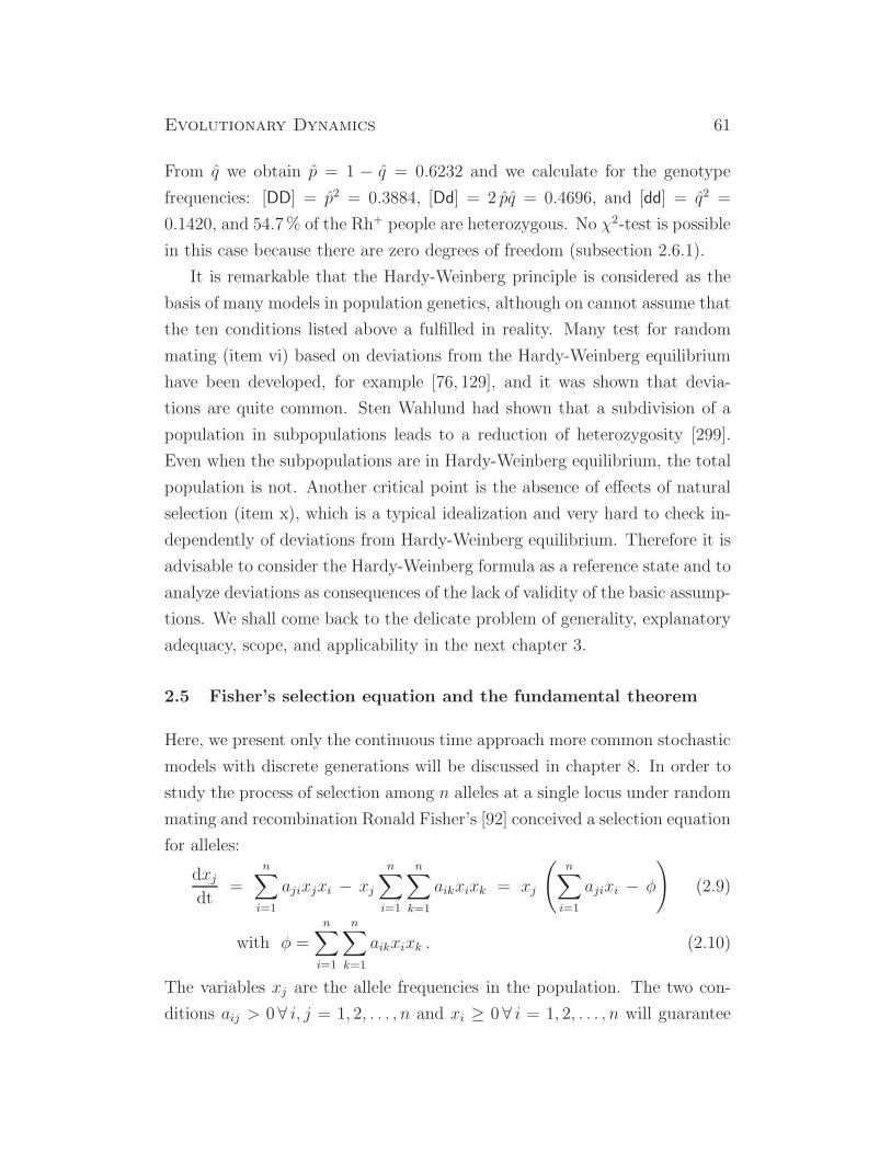
Evolutionary Dynamics 61
From q we obtain p = 1 − q = 0.6232 and we calculate for the genotype
frequencies: [DD] = p2 = 0.3884, [Dd] = 2 pq = 0.4696, and [dd] = q2 =
0.1420, and 54.7% of the Rh+ people are heterozygous. No χ2-test is possible
in this case because there are zero degrees of freedom (subsection 2.6.1).
It is remarkable that the Hardy-Weinberg principle is considered as the
basis of many models in population genetics, although on cannot assume that
the ten conditions listed above a fulfilled in reality. Many test for random
mating (item vi) based on deviations from the Hardy-Weinberg equilibrium
have been developed, for example [76, 129], and it was shown that devia-
tions are quite common. Sten Wahlund had shown that a subdivision of a
population in subpopulations leads to a reduction of heterozygosity [299].
Even when the subpopulations are in Hardy-Weinberg equilibrium, the total
population is not. Another critical point is the absence of effects of natural
selection (item x), which is a typical idealization and very hard to check in-
dependently of deviations from Hardy-Weinberg equilibrium. Therefore it is
advisable to consider the Hardy-Weinberg formula as a reference state and to
analyze deviations as consequences of the lack of validity of the basic assump-
tions. We shall come back to the delicate problem of generality, explanatory
adequacy, scope, and applicability in the next chapter 3.
2.5 Fisher’s selection equation and the fundamental theorem
Here, we present only the continuous time approach more common stochastic
models with discrete generations will be discussed in chapter 8. In order to
study the process of selection among n alleles at a single locus under random
mating and recombination Ronald Fisher’s [92] conceived a selection equation
for alleles:
dxjdt
=
n∑
i=1
ajixjxi − xj
n∑
i=1
n∑
k=1
aikxixk = xj
(
n∑
i=1
ajixi − φ
)
(2.9)
with φ =
n∑
i=1
n∑
k=1
aikxixk . (2.10)
The variables xj are the allele frequencies in the population. The two con-
ditions aij > 0 ∀ i, j = 1, 2, . . . , n and xi ≥ 0 ∀ i = 1, 2, . . . , n will guarantee
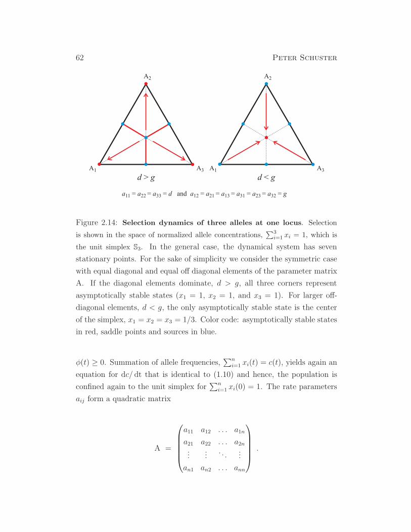
62 Peter Schuster
Figure 2.14: Selection dynamics of three alleles at one locus. Selection
is shown in the space of normalized allele concentrations,∑3
i=1 xi = 1, which is
the unit simplex S3. In the general case, the dynamical system has seven
stationary points. For the sake of simplicity we consider the symmetric case
with equal diagonal and equal off diagonal elements of the parameter matrix
A. If the diagonal elements dominate, d > g, all three corners represent
asymptotically stable states (x1 = 1, x2 = 1, and x3 = 1). For larger off-
diagonal elements, d < g, the only asymptotically stable state is the center
of the simplex, x1 = x2 = x3 = 1/3. Color code: asymptotically stable states
in red, saddle points and sources in blue.
φ(t) ≥ 0. Summation of allele frequencies,∑n
i=1 xi(t) = c(t), yields again an
equation for dc/ dt that is identical to (1.10) and hence, the population is
confined again to the unit simplex for∑n
i=1 xi(0) = 1. The rate parameters
aij form a quadratic matrix
A =
a11 a12 . . . a1n
a21 a22 . . . a2n...
.... . .
...
an1 an2 . . . ann
.
Evolutionary Dynamics 63
The dynamics of equ. (2.9) may be very complicated for general matrices A
and involve oscillations as well as deterministic chaos [243, 253]. In case of
Fisher’s selection equation, however, we are dealing with a symmetric matrix
for biological reasons,7 and then the differential equation can be subjected
to straightforward qualitative analysis.
Qualitative analysis of equ. (2.9) yields 2n − 1 stationary points, which
depending on the elements of matrix A may lie in the interior, on the
boundary or outside the unit simplex S(1)n . In particular, we find at max-
imum one equilibrium point on the simplex and one on each subsimplex
of the boundary. For example, each corner, represented by the unit vector
ek = xk = 1, xi = 0 ∀ i 6= k, is a stable or unstable stationary point. In
case there is an equilibrium in the interior of S(1)n it may be stable or unstable
depending on the elements of A. In summary, this leads to a rich collection
of different dynamical scenarios, which share the absence of oscillations or
chaotic dynamics.
The coordinates of the stationary points are derived through solution of
the equations derived from (2.9) by putting dxi/dt = 0 for i = j, k, l with
xj + xk + xl = 1 and xi = 0 ∀ i /∈ (j, k, l):
corner j : xj = 1
edge jk : xj =akk − ajk
ajj − 2ajk + akk, xk =
ajj − ajkajj − 2ajk + akk
face jkl : xj =Zj
D, xk =
Zk
D, xl =
Zl
Dwith
Zj = ajlakk + ajkall + a2kl − ajkakl − ajlakl − akkall ,Zk = ajjakl + a2jl + akjall − ajlajk − aklajl − ajjall ,Zl = a2jk + ajlakk + ajjakl − ajkajl − ajkakl − ajjakk ,D = Zj + Zk + Zl .
7Fisher’s equation is based on the assumption that phenotypes are insensitive to the
origin of the parental alleles on chromosomes. Phenotypes derived from genotype AiAj
are assumed to develop the same properties, no matter which allele, , on the chromosomal
locus comes from the mother and which comes from the father. New results on human
genetic diseases have shown, however, that this assumption can be questioned.

64 Peter Schuster
Local stability analysis on the simplex S3 through diagonalization of the
(2× 2) Jacobian yields for the corners
corner j : λ1 = ajk − ajj , λ2 = ajl − ajj ,
and for the edges
edge jk : λ1 =(ajk − ajj)(ajk − akk)ajj − 2ajk + akk
,
λ2 = −ajjakk − ajjakl − ajlakk − a2jk + ajkajl + ajkakl
ajj − 2ajk + akk.
The corner j is asymptotically stable for (ajk, ajl) < ajj or in other words,
if the homozygote AjAj has higher fitness than the two heterozygotes AjAk
and AjAl. The stationary point on the edge jk is unstable for (ajj, akk) > ajk
because λ1 is positive. We dispense here for a more detailed discussion of
the eventually quite sophisticated situation and refer to the simplified model
discussed below.
The calculation of the eigenvalues of the Jacobian at the stationary point
in the interior of the face jkl is even more involved but, nevertheless, can
be computed analytically. We present the results for the stationary point on
the face jkl in order to demonstrate the strength and the limits of machine
based symbolic computation. For the two eigenvalues of the Jacobian we
find:
λ1,2 = (Q1 ±√
Q2)/(2D2) with
Q1 = (akl − akk)P1 + (ajl − ajj)P2 and
Q2 =(
(ajl − ajj)(akl − akk)− (ajk − ajl)(ajk − akl))
P1P2 ,
P1 = ajkajl − ajkall − ajjakl + ajlakl + ajjall − a2jl ,
P2 = ajkakl − ajkall − ajlakk + ajlakl + akkall − a2kl ,
D = a2jk + a2jl + a2kl − ajjakk − ajjall − akkall+
+ 2(ajjakl + ajlakk + ajkall − ajkajl − ajkakl − ajlakl)Q2 when completely expanded becomes a sixth order polynomial in ajk with
more than 120 terms. Although fully analytical the expressions are pro-
Evolutionary Dynamics 65
hibitive for further calculations and will be studied numerically in practical
calculations.
A simple example of a three-allele one-locus model is shown on Fig. 2.14:
The matrix of rate parameters is simplified to
A =
a11 a12 a13
a21 a22 a23
a31 a32 a33
=
d g g
g d g
g g d
,
which has only two parameters the diagonal terms d representing the fitness
of the homozygotes, and g the off-diagonal elements for the heterozygotes.
From a11 = a22 = a33 = d and a12 = a13 = a23 = g we have Q2 = 0. In this
fully symmetric case the coordinates of stationary points and the eigenvalues
of the Jacobian fulfil very simple expressions:
corner (1, 0, 0) : λ1 = λ2 = d− f
edge (1
2,1
2, 0) : λ1 = −λ2 = −
1
2(g − d)
face (1
3,1
3,1
3) : λ1 = λ2 = −
1
3(g − d) .
The critical quantity here is the difference between the off-diagonal and the
diagonal term of matrix A, g−d. As long as d > g is fulfilled – corresponding
to higher fitness of homozygotes, AjAj and AiAi, than heterozygotes, AjAi
and AiAj – the corners are stable stationary points and depending on initial
conditions one allele, Aj or Ai, is selected. For overdominance of heterozy-
gotes, g > d, the stable points are on the edges or in the interior of the face
(Fig. 2.14). Multiple stationary states do occur and more than one may be
stable and the outcome of population dynamics need not be uniquely de-
fined. Instead depending on initial conditions the distribution of alleles may
approach one of the local optima [4, 86, 147, 245].
In order to analyze the behavior of the mean fitness φ(t) we introduce
mean rate parameters ai =∑n
j=1 aijxj , which facilitate the forthcoming anal-
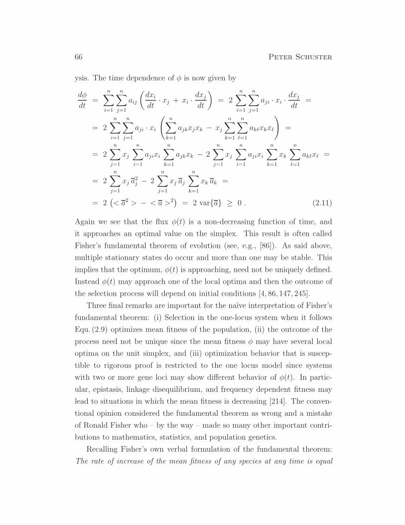
66 Peter Schuster
ysis. The time dependence of φ is now given by
dφ
dt=
n∑
i=1
n∑
j=1
aij
(
dxidt· xj + xi ·
dxjdt
)
= 2n∑
i=1
n∑
j=1
aji · xi ·dxjdt
=
= 2n∑
i=1
n∑
j=1
aji · xi(
n∑
k=1
ajkxjxk − xj
n∑
k=1
n∑
ℓ=1
akℓxkxℓ
)
=
= 2
n∑
j=1
xj
n∑
i=1
ajixi
n∑
k=1
ajkxk − 2
n∑
j=1
xj
n∑
i=1
ajixi
n∑
k=1
xk
n∑
ℓ=1
akℓxℓ =
= 2n∑
j=1
xj a2j − 2
n∑
j=1
xj aj
n∑
k=1
xk ak =
= 2(
< a2 > − < a >2)
= 2 vara ≥ 0 . (2.11)
Again we see that the flux φ(t) is a non-decreasing function of time, and
it approaches an optimal value on the simplex. This result is often called
Fisher’s fundamental theorem of evolution (see, e.g., [86]). As said above,
multiple stationary states do occur and more than one may be stable. This
implies that the optimum, φ(t) is approaching, need not be uniquely defined.
Instead φ(t) may approach one of the local optima and then the outcome of
the selection process will depend on initial conditions [4, 86, 147, 245].
Three final remarks are important for the naıve interpretation of Fisher’s
fundamental theorem: (i) Selection in the one-locus system when it follows
Equ. (2.9) optimizes mean fitness of the population, (ii) the outcome of the
process need not be unique since the mean fitness φ may have several local
optima on the unit simplex, and (iii) optimization behavior that is suscep-
tible to rigorous proof is restricted to the one locus model since systems
with two or more gene loci may show different behavior of φ(t). In partic-
ular, epistasis, linkage disequilibrium, and frequency dependent fitness may
lead to situations in which the mean fitness is decreasing [214]. The conven-
tional opinion considered the fundamental theorem as wrong and a mistake
of Ronald Fisher who – by the way – made so many other important contri-
butions to mathematics, statistics, and population genetics.
Recalling Fisher’s own verbal formulation of the fundamental theorem:
The rate of increase of the mean fitness of any species at any time is equal
Evolutionary Dynamics 67
to its genetic variation at that time, allow for many different interpretations.
A more recent reinterpretation the theorem [103, 228] tries to rehabilitate
Fisher’s claim for universality. These interpretations are based on partition-
ing genetic variation in additive and nonadditive, in other words epistatic,
effects and intrinsic and environment caused contributions. The misunder-
standing of Fisher’s original intensions is mainly attributed to the thirty
years controversy about the meaning of natural selection between Fisher and
Wright. We shall come back to these differences in view when we discuss
Fisher’s theorem and Wright’s concept of adaptive landscapes in the light of
a general theory of evolution (chapter 3).
2.6 Evaluation of data and the Fisher-Mendel controversy
Derivation and experimental verification of statistical laws requires a firm
mathematical theory of testing whether or not the observed regularity fol-
lows significantly from the harvested data. Ronald Fisher criticized Mendel’s
work [93] and brought up the argument that Mendel’s data are too good and,
presumably, were slightly manipulated by the author. Fisher’s paper was the
beginning of a seventy years long debate and eventually led to a monograph
stating that it is high-time to end the controversy [104]. It is fair to say
that Mendel work in essence has been rehabilitated but Fisher’s statistical
perfection in data analysis created a new standard in th e validation of sta-
tistical laws. We dispense from here from all historical details but use the
Mendel-Fisher discussion to digress on statistical methods that allow for an
evaluation of the statistical significance of harvested data.
2.6.1 The χ2-distribution
The conventional statistical test for data from random sampling is called
Pearson’s χ2-test, because it has been introduced by the statistician Karl
Pearson [233] and assesses two kinds of comparisons: (i) a quality test that
establishes whether or not an observed value distribution differs from a the-
oretical distribution, and (ii) a test of independence that assesses whether
paired observations on two variables are independent of each other.
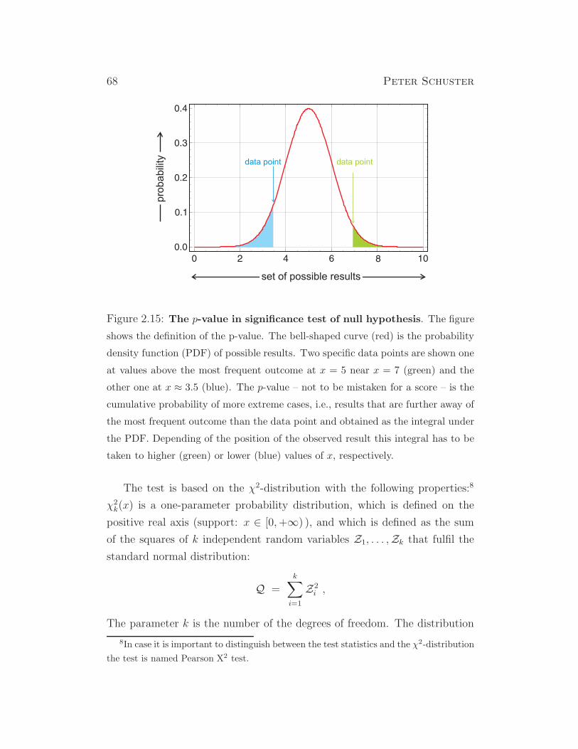
68 Peter Schuster
set of possible results
pro
babili
ty data point data point
Figure 2.15: The p-value in significance test of null hypothesis. The figure
shows the definition of the p-value. The bell-shaped curve (red) is the probability
density function (PDF) of possible results. Two specific data points are shown one
at values above the most frequent outcome at x = 5 near x = 7 (green) and the
other one at x ≈ 3.5 (blue). The p-value – not to be mistaken for a score – is the
cumulative probability of more extreme cases, i.e., results that are further away of
the most frequent outcome than the data point and obtained as the integral under
the PDF. Depending of the position of the observed result this integral has to be
taken to higher (green) or lower (blue) values of x, respectively.
The test is based on the χ2-distribution with the following properties:8
χ2k(x) is a one-parameter probability distribution, which is defined on the
positive real axis (support: x ∈ [0,+∞) ), and which is defined as the sum
of the squares of k independent random variables Z1, . . . ,Zk that fulfil the
standard normal distribution:
Q =
k∑
i=1
Z2i ,
The parameter k is the number of the degrees of freedom. The distribution
8In case it is important to distinguish between the test statistics and the χ2-distribution
the test is named Pearson X2 test.
Evolutionary Dynamics 69
of Q is given by
probability density function: f(x; k) =1
2k2 Γ(
k2
)x
k2−1 e−
x2 ,
cumulative distribution function: F (x; k) =1
Γ(
k2
) γ
(
k
2,x
2
)
,
(2.12)
whereby χ2k(x) = f(x; k). The functions Γ(z), γ(s, z) and Γ(s, z) are the
Gamma function and the lower and the upper incomplete Gamma function,
respectively:
Γ(z) =
∫ ∞
0
e−t tz−1 dt and Γ(n) = (n− 1)!; , n ∈ N0 ,
γ(s, z) =
∫ z
0
e−t tz−1 dt , and
Γ(s, z) =
∫ ∞
z
e−t tz−1 dt .
The χ2 density and distribution functions are available in tables that were
used before the ubiquitous availability of computers, which allow for straight-
forward calculation of numerical values from the functions available in all
statistics packages. Since Γ(1) = 1 the case k = 2 is particularly simple and
serves as an example:
f(x; 2) =1
2e−
x2 and F (x; 2) =
∫ x
0
f(x; 2) dx = 1− e−x2 .
The integration starts here at x = 0 rather than at x = −∞ because the
support of the distribution is restricted to the positive real axis.
In order to perform a specific test the start is to define the null hypothesis
that is the assumption of a theoretical distribution of the measured values
commonly in form of an expected partitioning of N observations in n cells.
In case of a discrete uniform distribution as null hypothesis – as it is very
often the case – the theoretical frequency is given by
εi =N
n, i = 1, 2, . . . , n .
Other common null hypotheses are the assumption of a normal, a Poisson
or a binomial distribution. Next the test statistic is calculated according to
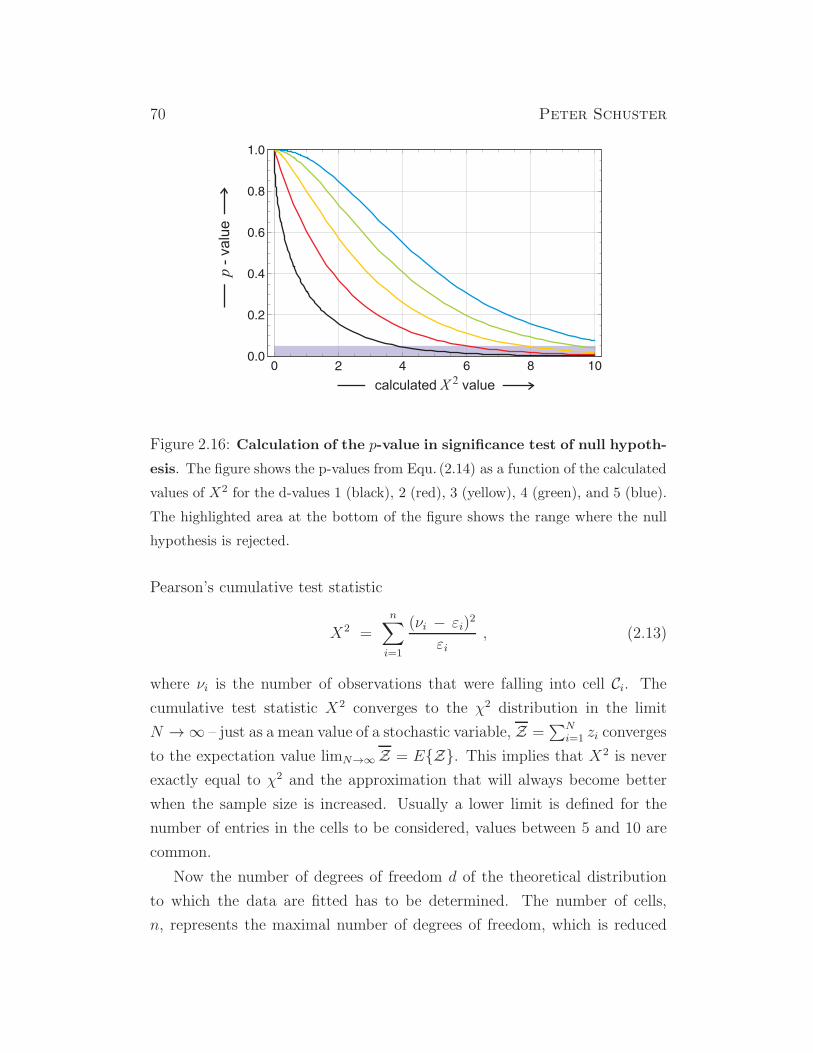
70 Peter Schuster
Figure 2.16: Calculation of the p-value in significance test of null hypoth-
esis. The figure shows the p-values from Equ. (2.14) as a function of the calculated
values of X2 for the d-values 1 (black), 2 (red), 3 (yellow), 4 (green), and 5 (blue).
The highlighted area at the bottom of the figure shows the range where the null
hypothesis is rejected.
Pearson’s cumulative test statistic
X2 =n∑
i=1
(νi − εi)2
εi, (2.13)
where νi is the number of observations that were falling into cell Ci. The
cumulative test statistic X2 converges to the χ2 distribution in the limit
N →∞ – just as a mean value of a stochastic variable, Z =∑N
i=1 zi converges
to the expectation value limN→∞Z = EZ. This implies that X2 is never
exactly equal to χ2 and the approximation that will always become better
when the sample size is increased. Usually a lower limit is defined for the
number of entries in the cells to be considered, values between 5 and 10 are
common.
Now the number of degrees of freedom d of the theoretical distribution
to which the data are fitted has to be determined. The number of cells,
n, represents the maximal number of degrees of freedom, which is reduced

Evolutionary Dynamics 71
by π = s + 1 where s is the number of parameters used in fitting of the
distribution of the distribution of the null hypothesis and accordingly we have
d = n−π. Considering the uniform distribution that is parameter free we find
d = n−1 and this is readily interpreted: Because the data fulfil∑n
i=1 πi = N
only n − 1 cells can be filled independently. Eventually, we determine the
p-value of the data sample as a measure of statistical significance. Precisely,
the p-value is the probability of obtaining a test statistic that is at least as
extreme as the actually observed one under the assumption that the null
hypothesis is true. We call a value a more extreme than b if a is less likely to
occur under the null hypothesis as b. As shown in Fig. 2.15 this probability
is obtained as the integral below the PDF from the calculated X2-value to
+∞. In case of the χ2 distribution we have
p =
∫ +∞
X2
χ2d(x) dx = 1 −
∫ X2
0
χ2d(x) dx = 1 − F (X2; d) , (2.14)
which involves the cumulative distribution function F (x; d) defined in
Equ. (2.12). Commonly, the null hypothesis is rejected when p is smaller
than the significance level: p < α with 0.001 ≤ α ≤ 0.05. If the condition
p < α is fulfilled one says the null hypothesis is statistically significantly
rejected.
A simple example is used for the purpose of illustration: Two random
samples of N animals was drawn from a population, ν1 were males and ν2
were females with ν1 + ν2 = N . The first sample,
N = 322, ν1 = 170, ν2 = 152 : X2 =(170 − 161)2 + (152 − 161)2
322= 0.503 ,
p = 1− F (0.503; 1) = 0.478 ,
clearly supports the null hypothesis that that males and females are equally
frequent since p > α ≈ 0.05. The second sample,
N = 467, ν1 = 207, ν2 = 260 : X2 =(207 − 233.5)2 + (260 − 233.5)2
233.5= 6.015 ,
p = 1− F (6.015; 1) = 0.0142 ,
leads to a p-value, which definitely is at the lower limit or below the critical
limit and the rejection of the null hypothesis is statistically significant.
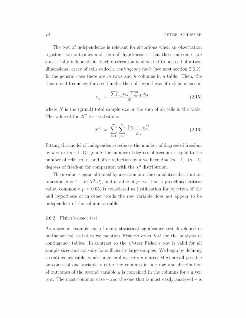
72 Peter Schuster
The test of independence is relevant for situations when an observation
registers two outcomes and the null hypothesis is that these outcomes are
statistically independent. Each observation is allocated to one cell of a two-
dimensional array of cells called a contingency table (see next section 2.6.2).
In the general case there are m rows and n columns in a table. Then, the
theoretical frequency for a cell under the null hypothesis of independence is
εij =
∑nk=1 νik
∑mk=1 νkj
N, (2.15)
where N is the (grand) total sample size or the sum of all cells in the table.
The value of the X2 test-statistic is
X2 =m∑
i=1
n∑
j=1
(νij − εij)2εij
. (2.16)
Fitting the model of independence reduces the number of degrees of freedom
by π = m+n−1. Originally the number of degrees of freedom is equal to the
number of cells, m ·n, and after reduction by π we have d = (m− 1) · (n− 1)
degrees of freedom for comparison with the χ2 distribution.
The p-value is again obtained by insertion into the cumulative distribution
function, p = 1 − F (X2; d), and a value of p less than a predefined critical
value, commonly p < 0.05, is considered as justification for rejection of the
null hypothesis or in other words the row variable does not appear to be
independent of the column variable.
2.6.2 Fisher’s exact test
As a second example out of many statistical significance test developed in
mathematical statistics we mention Fisher’s exact test for the analysis of
contingency tables. In contrast to the χ2-test Fisher’s test is valid for all
sample sizes and not only for sufficiently large samples. We begin by defining
a contingency table, which in general is a m×n matrix M where all possible
outcomes of one variable x enter the columns in one row and distribution
of outcomes of the second variable y is contained in the columns for a given
row. The most common case – and the one that is most easily analyzed – is

Evolutionary Dynamics 73
2× 2, two variables with two values each. The the contingency table has the
form
x1 x2 total
y1 a b a+ b
y2 c d c+ d
total a+ c b+ d N
where every variable, x and y, has two outcomes and N = a+ b+ c+d is the
grand total. Fisher’s contribution was to prove that the probability to obtain
the set of values (x1, x2, y1, y2) is given by the hypergeometric distribution
probability mass function fµ,ν(k) =
(
µk
)(
N−µν−k)
(
Nν
) ,
cumulative density function Fµ,ν(k) =
k∑
i=0
(
µk
)(
N−µν−k)
(
Nν
) ,
(2.17)
where N ∈ N = 1, 2, . . ., µ ∈ 0, 1, . . . , N, ν ∈ 1, 2, . . . , N, and the
support k ∈ max(0, ν+µ−N), . . . ,min(µ, ν). Translating the contingency
table into the notation of probability functions we have: a ≡ k, b ≡ µ − k,c ≡ ν−k, and d ≡ N+k−(µ+ν) and hence Fisher’s result for the probability
of the general 2× 2 contingency table is
p =
(
a+ba
)(
c+dc
)
(
Na+c
) =(a+ b)! (c+ d)! (a+ c)! (b+ d)!
a! b! c! d!N !, (2.18)
where the expression on the rhs shows beautifully the equivalence between
rows and columns. We present the right- or left-handedness of human males
or females as an example for the illustration of Fisher’s test: A sample con-
sisting of 52 males and 48 females yields 9 left-handed males and 4 left-handed
females. Is the difference statistically significant and allows for the conclu-
sion that left-handedness is more common among males than females? The
calculation yields p ≈ 0.10 which is above the critical value 0.001 ≤ α ≤ 0.05
and p > α confirms the rejection of the assumption that men are more likely
to be left-handed for these data.

74 Peter Schuster
3. Fisher-Wright debate and fitness landscapes
Although Ronald Fisher, J.B.S. Haldane, and Sewall Wright were united
in their search for compatibility of Mendelian genetics and Darwinian se-
lection, they differed strongly in their view on the existence and nature of
a universal mechanism of evolution. In particular Fisher and Wright were
engaged for more than thirty years in a heavy debate and each of both was
more or less convinced that he had the solution to the problem [266]. No
end of the debate occurred and no end was insight until Fisher’s death in
1962. Interestingly the debate got a revival in 1997 when Jerry Coyne, Nick
Barton and Michael Turelli [41] claimed that Fisher had the right theory and
Wright’s model is of minor importance if not dispensable at all. Inspired by
this one-sided point of view Michael Wade and Charles Goodnight gave an
answer in the same journal [297] wherein they argued that Fisher’s theory
cannot be applied to a variety of relevant phenomena in population genet-
ics and is far away from being fully general. Accordingly, there is plenty of
room for other theoretical approaches Wright’s model being the most promi-
nent one at the current state of knowledge [297]. In two follow-up papers
[42, 120] the Fisher-Wright debate has been reignited and began to interest
philosophers: Robert Skipper classified this scientific contest as a relative
significance controversy and presented a proposal for a solution in the future
that will be discussed in section 3.2. First, however, we shall present a new
interpretation of Fisher’s fundamental theorem that tries to rescue generality
and relevance of this evolutionary optimization principle.
3.1 Fisher’s fundamental theorem revisited
In section 2.5 Fisher’s differential equation combining recombination and se-
lection has been presented and analyzed. It describes the evolution of the
allele distribution at a single locus. The variables are the normalized allele
75
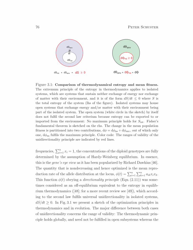
76 Peter Schuster
dS int
dSenv dfenv
dS int dSdSenv =+ ³ 0
dfns ³ 0
dfenv dfns df+ =
Figure 3.1: Comparison of thermodynamical entropy and mean fitness.
The extremum principle of the entropy in thermodynamics applies to isolated
systems, which are systems that sustain neither exchange of energy nor exchange
of matter with their environment, and it is of the form dS/dt ≤ 0 where S is
the total entropy of the system (lhs of the figure). Isolated systems may house
open systems that exchange energy and/or matter with their environment being
part of the isolated system. The open system (white circle in the sketch) by itself
does not fulfil the second law criterium because entropy can be exported to or
imported from the environment: No maximum principle holds for Sint. Fisher’s
fundamental theorem is sketched on the rhs. The change in the mean population
fitness is partitioned into two contributions, dφ = dφns + dφenv, out of which only
one, dφns fulfils the maximum principle. Color code: The ranges of validity of the
unidirectionality principle are indicated by red lines.
frequencies,∑n
i=1 xi = 1, the concentrations of the diploid genotypes are fully
determined by the assumption of Hardy-Weinberg equilibrium. In essence,
this is the gene’s eye view as it has been popularized by Richard Dawkins [46].
The quantity that is nondecreasing and hence optimized is the mean repro-
duction rate of the allele distribution at the locus, φ(t) =∑n
i=1
∑nk=1 aikxixk.
This function φ(t) obeying a directionality principle (Equ. (2.11)) was some-
times considered as an off-equilibrium equivalent to the entropy in equilib-
rium thermodynamics ([48]; for a more recent review see [49]), which accord-
ing to the second law fulfils universal unidirectionality in isolated systems,
dS/dt ≥ 0. In Fig. 3.1 we present a sketch of the optimization principles in
thermodynamics and in evolution. The major difference between both cases
of unidirectionality concerns the range of validity: The thermodynamic prin-
ciple holds globally, and need not be fulfilled in open subsystems whereas the

Evolutionary Dynamics 77
fundamental theorem is valid only for a subset of factors influencing mean
fitness φ. This subset can be identified with natural selection. For reasons
the will become clear within the next paragraphs the more recent and more
elaborate interpretations of the fundamental theorem suggest that such an
correspondence is not justified. It is, however, fair to say that Fisher himself
stressed the limitation of the analogy [228, pp.346,347].
At first it is important to emphasize that Fisher’s theorem as expressed
by Equ. (2.11) is neither wrong not inexact. The (justified) critique concerns
the very limited applicability. As said before the theorem does not apply
in the two locus case when the two genes interact – a phenomenon that is
called epistasis, there must be no linkage disequilibrium implying the neces-
sity of random mating, and all other nonadditive genetic interactions must be
zero. As we shall see later on, Fisher’s large population size theory (L[P]ST)1
several of the jeopardizing deviations become small and unimportant in the
limit Fisher is considering [62, 87, 228, 236]. Secondly, as Ronald Fisher him-
self stressed several times, the (total) mean fitness of a population in nature
can only fluctuate around zero because otherwise the population would either
explode or collapse and die out.2 How can this undeniable fact be reconciled
with the Darwinian principle of optimizing fitness? The explanation of the
contradiction The variation in the mean fitness is split into two different con-
tributions: (i) the increase in mean fitness caused by natural selection, and
(ii) the change in mean fitness caused by the environment where we define the
environment as everything contributing to changes except natural selection:
dφ = dφns + dφenv , (3.1)
and φns =∑n
k=1
∑ni=1 aikxixk is obeying the directionality principle. The no-
tation of dφenv being the change in mean fitness caused by the environment
1Fisher’s theory is often abbreviated as LPST, sometimes as LST. We shall adopt here
the shorter three letter version.2Cases of such explosions are known but very rare. If, for example, a species is trans-
ferred into a new environment where other species predating on them are missing extremely
rapid population growth occurs, which corresponds to a (temporarily) large positive mean
fitness. Examples are the rabbits in Australia and several cases of insect proliferations
causing major damage.

78 Peter Schuster
sounds weird, and makes sense only in the gene’s eye view. Then, epistatic
effects coming from other genes through interaction may look as environmen-
tal influence for the gene under consideration. The interpretation of other
contributions to dφenv is even more difficult. However, with this definition
Fisher’s fundamental theorem can be rescued also its range of applicability
has shrunk to the small white area in Fig. 3.1 and definitely FTNS cannot
be applied to the total dφ as it is done in the conventional interpretation.
There are still a number of problems with the subtler recent interpretation
but most of them can be straightened out by careful argumentation [228].
A straightforward interpretation of the two views on Fisher’s fundamental
theorem concerns the nature of the time derivative:
conventional view:dφ
dt≥ 0 , new view:
∂φns
∂t
∣
∣
∣
∣
env
≥ 0 ,
The conventional view was dealing with the total differential whereas the
new view considers the partial differential at constant environment.
The important issue touched upon above can now find an answer. The
gain in mean fitness of the allele population resulting from natural selection
is compensated by the changes in the environment. Accordingly, we have
dφenv < 0 or in other words for the gene the environment deteriorates to
such an extent that the stationarity of the (eco)system is maintained. This
compensation effect reminds of Leigh van Valen’s red queen hypothesis :3 ...
and the Red Queen said to Alice: ”In this place it takes all the running you
can do, to keep in the same place. ...”. This sentence is commonly used as a
metaphor for the requirement of continuing development of an evolutionary
system in order to maintain its (total) fitness relative to the (environmental)
system it is coevolving with. Transferring the metaphor to Fisher’s (peculiar)
definition of environment this means for the allele population at a given
locus: As its mean fitness increases by natural selection the environment
deteriorates to about the same amount.
3The Red Queen is a fictional character in Lewis Carroll’s fantasy novella, Through the
Looking-Glass, which is often mistaken with the Queen of the Heart in Carroll’s previous
book Alice’s Adventures in Wonderland.
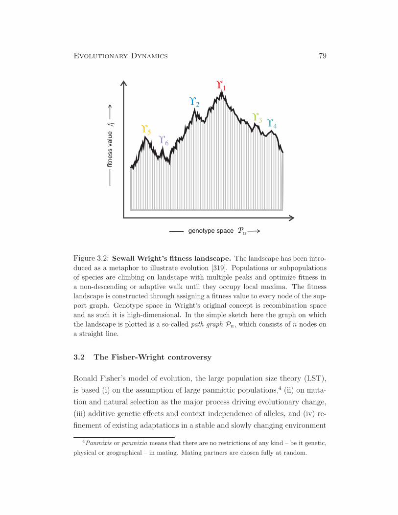
Evolutionary Dynamics 79
¡1
¡2
¡3 ¡4
¡6
¡5
genotype space Pn
fitn
ess v
alu
ef j
Figure 3.2: Sewall Wright’s fitness landscape. The landscape has been intro-
duced as a metaphor to illustrate evolution [319]. Populations or subpopulations
of species are climbing on landscape with multiple peaks and optimize fitness in
a non-descending or adaptive walk until they occupy local maxima. The fitness
landscape is constructed through assigning a fitness value to every node of the sup-
port graph. Genotype space in Wright’s original concept is recombination space
and as such it is high-dimensional. In the simple sketch here the graph on which
the landscape is plotted is a so-called path graph Pn, which consists of n nodes on
a straight line.
3.2 The Fisher-Wright controversy
Ronald Fisher’s model of evolution, the large population size theory (LST),
is based (i) on the assumption of large panmictic populations,4 (ii) on muta-
tion and natural selection as the major process driving evolutionary change,
(iii) additive genetic effects and context independence of alleles, and (iv) re-
finement of existing adaptations in a stable and slowly changing environment
4Panmixis or panmixia means that there are no restrictions of any kind – be it genetic,
physical or geographical – in mating. Mating partners are chosen fully at random.

80 Peter Schuster
as the ultimate driving force for evolution. Seen from this point of view the
factors giving rise to deviations from the fundamental theorem are minor cor-
rections of the global picture. For example, random drift plays a dominant
role in small population, when genetic effects are predominantly additive and
context independent, epistasis and pleiotropy are negligible.
Sewall Wright’s model contrasts Fisher’s view in many aspects. His model
consists of three logical phases: (i) Random drift leads to semi-isolated sub-
populations or demes within the global population, which are losing fitness
because of accidental loss of fittest genotypes by the mechanisms of Mullers
ratchet,5 (ii) natural selection acts on complex genetic reaction networks and
raises the mean fitness of subpopulations, (iii) interdemic selection raises
the mean fitness of the global population. Eventually, environmental change
shifts the adaptive peaks of mean fitness and drives the dynamics of evolution
[228].
Depending on the species under consideration both evolutionary scenar-
ios, the Fisher scenario and the Wright scenario, can be realized. None of the
two models of evolution has internal inconsistencies that would allow for re-
jection. Thus the dispute between the two scholars is – what the philosophers
call – a relative significance controversy. Both concepts are valid approaches
that apply only to a limited subset of evolutionary scenarios and multiplic-
ity of theoretical approaches is unavoidable at least at the current state of
knowledge. In contrast to the view of most biologists and some philosophers
(see, e.g., [266]) I think there is no need to believe that there will never be
a uniform theory of evolution [249]. The unification, however, will not come
on the phenomenological level of biology, it will be the result of a compre-
hensive theoretical biology that has its basis at the molecular level. The
basis of this optimistic view comes from examples from physics: Electricity
and magnetism were seen as largely unrelated phenomena unless the unifying
theory of electromagnetism was born that found its elegant completion by
James Clerk Maxwell who conceived the famous Maxwell equations.
5Hermann Joseph Muller considered a random drift process in a finite population.
Stochasticity (see chapter 8) will cause a loss of the fittest genotype at some instant, then
the fittest genotype of the rump population will be lost, and so on [90, 220, 221].
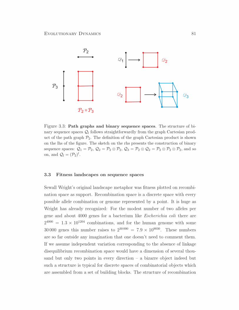
Evolutionary Dynamics 81
P3
P2
P2 P3Ä
Q 3Q 2
Q 2Q 1
Figure 3.3: Path graphs and binary sequence spaces. The structure of bi-
nary sequence spaces Ql follows straightforwardly from the graph Cartesian prod-
uct of the path graph P2. The definition of the graph Cartesian product is shown
on the lhs of the figure. The sketch on the rhs presents the construction of binary
sequence spaces: Q1 = P2, Q2 = P2 ⊗ P2, Q3 = P2 ⊗Q2 = P2 ⊗ P2 ⊗ P2, and so
on, and Ql = (P2)l.
3.3 Fitness landscapes on sequence spaces
Sewall Wright’s original landscape metaphor was fitness plotted on recombi-
nation space as support. Recombination space is a discrete space with every
possible allele combination or genome represented by a point. It is huge as
Wright has already recognized: For the modest number of two alleles per
gene and about 4000 genes for a bacterium like Escherichia coli there are
24000 = 1.3 × 101204 combinations, and for the human genome with some
30 000 genes this number raises to 230 000 = 7.9 × 109030. These numbers
are so far outside any imagination that one doesn’t need to comment them.
If we assume independent variation corresponding to the absence of linkage
disequilibrium recombination space would have a dimension of several thou-
sand but only two points in every direction – a bizarre object indeed but
such a structure is typical for discrete spaces of combinatorial objects which
are assembled from a set of building blocks. The structure of recombination

82 Peter Schuster
H (1,4) H (2,4)
Figure 3.4: Four letter sequence spaces. The sequence space derived from
the four letter alphabet (AT(U)GC; κ = 4) are the Hamming graphs H(l, 4).The Hamming graph for a single nucleotide is the complete graph H(1, 4) = K4
(lhs) and for the 16 two letter sequences the space is H(2, 4) = K4 ⊗ K4 (rhs).
The general case, the space of sequences of chain length l, H(l, 4) is the graph
Cartesian product with l factors K4.
space has been studied in some detail [269, 272] but we dispense here from
reviewing it, because we shall be mainly concerned with another discrete
formal space, the sequence space here and in the forthcoming chapters.
Despite enormous progress in synthetic biology [137, 196] the possibilities
to construct gene combinations at will are still very limited. For example,
oscillatory gene networks [75] and genetic toggle switches [108] were engi-
neered in bacteria, and various synthetic genetic regulatory elements were
introduced into eukaryotic cells [11, 13], but engineered recombination is still
not achievable at present. Engineering sequences with mutations at arbi-
trary positions has become routine thirty years ago already [96, 155, 184] and
searching a space of sequences is much easier than searching recombination
space therefore.
The idea of sequence space without the explicit notion has been used to
order strings in informatics for quite some time (see, e.g., [133]) before the
word has been coined for proteins [201] and nucleic acids [65]. Like recombi-

Evolutionary Dynamics 83
nation space sequence space is a discrete formal space where each sequence
is represented by a point (see, for example, Fig. 4.7 where the sequence space
of binary sequences of length l is used for illustration). The sequence space
for binary sequences is a hypercube Ql of dimension l where l is the sequence
length of the string. The building principle of sequence spaces by means of
the graph Cartesian product is illustrative and can be used for sequences over
arbitrary alphabets and, in particular, also for the natural AT(U)GC alpha-
bet. The Cartesian product of two graphs is illustrated in Fig. 3.3 by means
of two path graphs:6 The product graph, P(1) ⊗P(1) is two-dimensional and
has P(1) on its horizontal and P(2) on its vertical margin, respectively. There
are many ways to visualize binary sequence spaces as hypercubes – one, the
consecutive product of P2 graphs is illustrated in Fig. 3.3:
Ql = P2 ⊗ P2 ⊗ . . . ⊗ P2 =(
P2
)l. (3.2)
The advantage of the construction of sequence spaces a graph Cartesian
products has the advantage of being generalizable. If we choose a complete
graph Kκ as unit the consecutive Cartesian product yields the corresponding
sequence space for sequences of chain length l:
Q(κ)l = K(l, κ) = Kκ ⊗ Kκ ⊗ . . . ⊗ Kκ =
(
Kκ
)l. (3.3)
The most important case is the natural alphabet with κ = 4 (Fig. 3.4).
Both recombination and sequence spaces are characterized by high di-
mensionality and this makes it difficult to visualize distances. Considering,
for example, the binary sequence space for strings of chain length l = 10 that
contains 210 = 1024 sequences. Were sequence space a (one dimensional)
path graph, the longest distance would be 1023. In two dimensions is would
be 62 and on the hypercube Q(2)10 it is shrunk to only 10. Both recombination
and sequence space are metric spaces. The most natural metric for sequence
spaces is the Hamming distance dH (see section 4.3.1), for recombination
spaces the construction an appropriate metric is somewhat more involved
and can be done by using graph theory [272].
6A path graph Pn is a one-dimensional graph with n nodes. Two nodes at the ends
have vertex degree one and all other n− 2 nodes have vertex degree two.

84 Peter Schuster
A landscape is obtained through plotting some property on a graph as
support (see Fig. 3.2). On a fitness landscape fitness values are assigned to
the nodes of sequence space. The mathematical analysis of typical landscape
properties, for example correlation functions, on discrete spaces require spe-
cial techniques that are based on the use of Laplace operators on graphs [271].
Landscapes on supports that are combinatorial manifolds like the genomes
obtained by recombination and/or mutation have been studied [238, 239] in
some detail. Since the size of even the smallest sequence spaces is pro-
hibitive for the empirical determination of a fitness landscape, simple models
were used in particular in population genetics. The three most popular are
(i) the additive fitness landscape, (ii) the multiplicative fitness landscape, and
(iii) the single peak fitness landscape. Sequences are grouped around the
fittest genotype. It is assumed that all sequences of a given mutant class
have the same fitness. In the first case all mutations reduce the fitness of the
fittest genotype by a constant increment θ, in the second case by a constant
factor ϕ, and
additive landscape : fj = fm − k θ ∀ Xj ∈ Γk , (3.4a)
multiplicative landscape : fj = fm ϕk ∀ Xj ∈ Γk , and (3.4b)
single peak landscape : fj =
f0 if j = m
fn if j 6= m, (3.4c)
where Γk is the k-th mutant class of the fittest sequence Xm:
Γ(m)k : Xi ∈ Γ
(m)k iff dH(Xi,Xm) = k . (3.5)
Instead of the increment θ and the factor φ one might also use the lowest
fitness value fn for calibration and obtains θ = (f0−fn)/l and φ = (fn/f0)1/l,
respectively. As we shall later in a detailed discussion of the the properties
of these different types of simple fitness landscapes (section 4.3.3) they are
convenient for mathematical analysis but completely unrealistic.
Empirical knowledge and computer models of biopolymer – protein and
nucleic acid – structures confirm to properties of realistic landscapes: (i) they
are rugged and (ii) they are rich in neutral sequences. Rugged means that
Evolutionary Dynamics 85
nearby lying sequences – these are sequences of short Hamming distance –
may have very different fitness values. This is easy to visualize since a single
nucleotide exchange leading to an exchange of an amino acid that is essential
for protein activity may render an enzyme functionless and in consequence
the mutation might be lethal for its carrier. On the other hand, a single nu-
cleotide exchange may have no effect at all and give rise to a neutral variant.
What is true for a single nucleotide exchange already holds as well for mul-
tiple point mutations and other sequence changes Neutrality has been found
early and predicted theoretically when the traces of evolution were discovered
on the molecular level [173, 175]. The existence of a molecular clock of evolu-
tion is one important consequence of neutrality in evolution (for a review see
[183]). One consequence of neutrality is random drift of populations through
sequence space as described by Motoo Kimura’s theory of neutral evolution
[174] (see also section 10.3). Not all sequences are neutral, of course, but
the neutral sequences form neutral networks in sequence space [238, 252] and
these subsets of sequences set the stage for evolutionary dynamics.
The new techniques in molecular genetics provided access to empirical
data of fitness landscapes for protein and nucleic acid evolution. Both basic
features, ruggedness and neutrality were confirmed. Examples are protein fit-
ness landscapes [140], landscapes derived from in vitro evolution of molecules
[3], and a recent extensive study on the HIV-I fitness landscape in presence
and absence of medication [181].

86 Peter Schuster

4. Mutation and selection
Gregor Mendel’s concepts of segregation and independent assortment of
genes during reproduction provides an excellent example of an approximate
statistical law that has been modified by molecular insight but remained cor-
rect as the proper reference for the limit of infinitely frequent recombination.
In case of mutation such an ideal reference does not exist and indeed this
idea of change in the hereditary material has a fascinating history [34].
In this chapter we shall consider the consequences of mutation for evo-
lutionary dynamics. We start by giving a brief historical account on the
sharpening of the originally diffuse notion of mutation and then introduce
chemical kinetics by means of a flow reactor that is useful for both, modeling
and experimental studies. The kinetic model of a chemical reaction network
based on ODEs introduced by Manfred Eigen in which correct replication
and mutation are parallel reaction channels [65, 68, 70–72] replaces the deus
ex machina appearance of mutants by. The formulation of the kinetic equa-
tions for overall replication,1 that is without dwelling into molecular details
is straightforward. Two major results of the mathematical analysis of these
reaction networks are: (i) The formation of well defined stationary states
called quasispecies and (ii) the existence of a maximal mutation rate char-
acterized as error threshold above which no stationary states exist. This
chemical reaction model of evolution has been directly applied to evolution
of RNA molecules in the test-tube (see e.g. [14]), viroids and viruses, and
bacteria as long as recombination plays very little or no role.
Reaction kinetics of RNA replication, for example, is a multi-step pro-
cess that has been investigated at molecular resolution by Christof Biebricher
[17–19] and the established mechanism can be incorporated into the model of
1Here we use replication when we have the molecular mechanism or some over-all
kinetics of it in mind, and characterize the process of multiplication as reproduction when
we don’t refer to the molecular level or when the mechanisms is completely unknown.
87
88 Peter Schuster
evolution at any level of detail. In this case the extension of the overall kinetic
description of evolution to a comprehensive model that treats replication and
mutation at full molecular detail is possible and will be presented. Quasis-
pecies theory has been applied to virus populations by Esteban Domingo
and turned out to be the proper concept for a description of virus infection
and virus evolution [51, 54, 191]. The error threshold phenomenon provides
a proper frame for the development new antiviral strategies [56]. A dispute
arose whether or not viral quasispecies pass the error threshold before the
die out [30, 31, 283] and we shall present a brief overview of models for lethal
mutagenesis.
For bacteria or higher organism the kinetic model of evolution can be ap-
plied in the same spirit as the ODE models in population genetics but the full
details of reproduction are still in the dark. Nevertheless much progress has
been made within the last ten years The organisms that come closest to full
understanding in the spirit of systems biology are small parasitic bacteria of
the species Mycoplasma. Examples are the works of the Spanish group of Luis
Serrano’s [128, 182, 322] who have almost completed the full biochemistry of
an entire small bacterial cell. About 75% of the approximately 6 000 genes
of a small eukaryote, the yeast Saccharomyces cerevisiae, where studied with
respect to their function and a quantitative genetic interaction profile has
been established [38]. Functional cross-connections between all bioprocesses
were derived from the global network and mapped onto a cellular wiring dia-
gram of pleiotropy. These investigations in essence tell us two things: (i) The
complexity of cellular biology at the molecular level is enormous, and (ii) the
modern techniques of genomics, proteomics, transcriptomics, metabolomics,
and so on, together with conventional biochemistry and biochemical kinet-
ics can be successfully applied to decipher all processes in an entire cell at
molecular resolution, and the data are usable for mathematical modeling and
computer simulation at all levels of complexity.
Evolutionary Dynamics 89
4.1 The historical route to mutation
Systematic mutation studies were initiated in Thomas Hunt Morgan’s labo-
ratory. He began his seminal work with the fruit fly Drosophila melanogaster
as animal model around 1910 and was awarded the Nobel Prize 1933 for Phys-
iology for his extensive and path-breaking genetic studies. Later Drosophila
melanogaster 2 became the standard animal for genetic studies mainly be-
cause of its enormous fertility and short (mean) generation time of only 7 to
60 days depending on subspecies on nutrition condition. Morgan’s contribu-
tions were frequently dealing with genes on sexual chromosomes where the
mechanism of gene action can be inferred and discussed more easily because
every species provides two different chromosomal types, male and female.
In the early days of genetics the term mutation was used for all inheritable
changes of phenotypes, no matter whether the cause was a change in the
gene or a rearrangement of the chromosomal structure of the cell. Known,
of course, was the distinction between mutation along the germ line and so-
matic mutation that was not inheritable. The American biologist Hermann
Muller argued that the term mutation should be restricted to variation due
to change in the individual gene [218] and chromosomal changes should be
considered separately since they have a different origin. Examples are poly-
ploidy, gains or losses of entire sets of chromosomes, aneuploidy, gains or
losses of single chromosome in otherwise diploid organisms, and structural
rearrangements of chromosomes. The notion of point mutation had been
created for spontaneous changes in phenotypic properties determined by a
single locus, was not clearly distinguished from the mutation, and got his
meaning only with the discovery of DNA as genetic material.
The idea to increase the natural mutation rate by radiation, mainly X-
rays, in order to produce a diversity of variants was already pursued by the
Morgan group and others but little progress was made. The early attempts
to use radiation failed for several reasons, one of them was the lack of reli-
able dosimeters and the application of wrong doses – low dose for long times.
2Due to a more recent classification of the Drosophilidae the famous model animal
belongs now to the subgenus Sophophora and the official name is Sophophora melanogaster.
90 Peter Schuster
Muller and others found that the occurrence of point mutations increases
linearly with time whereas chromosomal rearrangements showed an expo-
nential time law. By applying high doses Muller was able to increase the
mutation rate by a factor of 150. The technique and the results of Muller’s
systematic studies on X-ray induced mutation [219] were also of great im-
portance for agriculture where human selection of desired variants initiated
a green revolution. Useful mutants were nevertheless rare as the majority
of radiation induced variants that showed a phenotype were lethal. Muller
was awarded the Nobel Prize for Physiology in 1946 for the discovery of the
production of mutations by means of X-ray irradiation. Muller also tried to
distinguish effects from primary radiation impacts, which are mainly identi-
fied with double strand breaks or point mutations originating from damage
repair, and secondary effects that result from chemical mutagenesis caused
by the products of radiation impact on water. Muller’s view was that the
secondary effects dominate and candidates for chemical mutagenesis were
among others hydrogen peroxide – already close to the most potent agent
produced by irradiation of water: the hydroxy radical. Many other chemi-
cals were found to produce or promote mutation, but time was not yet ripe
for chemical models of mutation because the molecular nature of the ge-
netic material was still (at least to a large extent) in the dark. In particular
the clear separation of variants producing processes into mutation, recom-
bination, and major chromosomal rearrangements was impossible without a
knowledge of the molecular structure and function of DNA.
The next major breakthrough in understanding mutation came from bio-
chemistry. George Wells Beadle and Edward Lawrie Tatum found that mu-
tations (can) change the metabolism of the affected mutation carrier [12].
Mutations change genes and the changes genes give rise to modification in
an enzyme that is active in cellular metabolism: The one gene - one enzyme
hypothesis of biology was born. Together with Joshua Lederberg Beadle
and Tatum received the Nobel Prize 1958 in Physiology. Although time was
already overripe for a major step forward in the understanding of the mech-
anisms of reproduction and inheritance, progress in the knowledge about
nucleic acids was relatively slow [167]. It was Watson and Crick’s model of

Evolutionary Dynamics 91
Figure 4.1: Point mutation in DNA replication. A misincorporation of a
nucleotide during DNA replication leads to unpaired nucleotides at one position
of the DNA double helix (second line, rhs: highlighted). The next replication step
results in one correct copy and one mutant (third line, rhs: highlighted). The
nucleotides are sketched as beads. Watson-Crick base pairs (A=T and G≡C) areshown a thick gray lines connecting two beads on opposite strands. Color code: A
green, T magenta, G blue, and C yellow.
DNA structure that changed the situation completely, and the reason for
this new insight is hidden in the famous sentence at the end of the letter
to Nature: ”It has not escaped our notice that the specific pairing we have
postulated immediately suggests a possible copying mechanism for the genetic
material”. As a matter of fact the DNA structure suggested at the same time
a mechanism for the origin and inheritance of point mutations (Fig. 4.1). On
the other hand the consequences of mutations for fitness and evolution were
completely in the dark and still are unknown in many aspects at present.
Many different classes of mutations and major DNA rearrangements were
observed so far. The three most important classes are sketched in Fig. 4.2.
Apart from point mutations deletions and insertions occur rather often. Dele-
tions represent losses of a wide range of sizes, from individual nucleotides to
whole genes or chromosomes. Insertions commonly are duplication of DNA
stretches and they comprise an even wider range of seizes from single nu-

92 Peter Schuster
Figure 4.2: Classes of mutations. The sketch shows the three most common
classes of DNA mutations: (i) point mutations (top, see Fig. 4.1), (ii) deletions
(middle), and (iii) insertions (bottom). Deletion and insertions can be of any size.
Examples for large scale events are gene loss and gene duplication. Eventually,
whole genome duplication events have occurred in evolution. Color code: A green,
U magenta, G blue, and C yellow.
cleotide duplications to gene duplication and duplications of entire genomes.
Gene duplication has been postulated as a major driving force for evolution
by the Japanese Biologist Susumo Ohno [226]. Over the years many instances
of genome duplications that have occurred in the past were found [289]. In
particular, the role of genome duplications in developmental were studied
in detail and the evolution of the Hox genes was found to present excellent
examples for such events [59, 106, 185]. An ancient genome duplication event
in the yeast Saccharomyces cerevisiae is especially well documented [168].

Evolutionary Dynamics 93
Figure 4.3: The continuously stirred tank reactor (CSTR). The CSTR is
a device for simulating deterministic and stochastic kinetics in an open system. A
stock solution containing all materials for RNA replication ([A] = a0) including
an RNA polymerase flows continuously at a flow rate r into a well stirred tank
reactor (CSTR) and an equal volume containing a fraction of the reaction mixture
([⋆] = a, b, ci) leaves the reactor. A population of RNA molecules in the reactor
(X1,X2, . . . ,Xn present in the numbers N1, N2, . . . , Nn with N =∑n
i=1Ni) fluc-
tuates around a mean value, N ±√N . RNA molecules replicate and mutate in
the reactor, and the fastest replicators are selected. The RNA flow reactor has
been used also as an appropriate model for computer simulations [99, 100, 156, 234],
which allow for the application of other criteria for selection than fast replication.
For example, fitness functions are defined that measure the distance to a prede-
fined target structure and then the mean fitness of the population increases during
the approach towards the target [101].
94 Peter Schuster
4.2 The flow reactor
The theoretical and experimental device of a flow reactor shown in Fig. 4.3
represents an open system that is perfectly suited for studies on evolution-
ary dynamics. The setup explains its name continuously stirred tank reactor
(CSTR). A basic assumption of the theoretical model is instantaneous and
complete mixture of the reactor content at any moment, and spatial homo-
geneity of the solution in the reaction volume allows for the usage of ordinary
rather than partial differential equations for modeling reaction kinetics. Here
we consider replication of RNA molecules as an example of an ensemble of
competitive autocatalytic reactions in the spirit of the selection Equ. (1.9).
The reaction mechanism is of the form
∗a0 r
−−−→ A , (4.1a)
A + Xj
kj−−−→ 2Xj ; j = 1, . . . , n , (4.1b)
Xj
kj−−−→ B ; j = 1, . . . , n , (4.1c)
Ar
−−−→ ∅ , (4.1d)
B
r
−−−→ ∅ , and (4.1e)
Xj
r
−−−→ ∅ ; j = 1, . . . , n . (4.1f)
The symbol A stands for the material required in RNA synthesis and B are
the degradation products of the RNA molecules.3 The flow rate parameter
r is the reciprocal mean residence time of a volume element in the reactor,
r = τ−1R . If the reactor has a volume V then a mean volume V has flown
through it in the time interval ∆t = τ−1R . The influx of A into the reactor
is a so-called zeroth order reaction, because the rate dA = a0r dt does not
depend on concentrations in reaction step (4.1a). The autocatalytic second
order reaction step (4.1b) is identical to the reproduction step in Equ. (1.8)
only here the concentration of A is a variable [A] = a(t). The degradation
reaction of Xj (4.1c) can be united with the outflux of Xj (4.1f) yielding a
3For the sake of simplicity we lump all building blocks Ai and all degradation products
Bi (i = 1, 2, . . .) together in a single symbol.
Evolutionary Dynamics 95
rate parameter of kj + r unless B enters the system again via a chemical or
photochemical recycling reaction B+D→ A or B+ hν → A. The reaction
steps (4.1d-4.1f) eventually describe the outflux of the reactor content that
compensates the increase in volume through influx of stock solution.
The mechanism (4.1) can be casted into a chemical master equation or
modeled by stochastic processes. Here we shall assume large population
sizes and use ODEs for modeling. The kinetic equations, with [A] = a and
[Xj ] = cj , are of the form
da
dt= − a
n∑
j=1
kjcj + r (a0 − a) ,
dcjdt
= cj(
a kj − r)
; j = 1, . . . , n ,
(4.2)
and can be readily analyzed with respect to long time behavior. For this goal
we introduce a total concentration of replicators, c =∑n
i=1 ci, that fulfils
dc
dt= c (a φ − r) with φ(t) =
1
c
n∑
i=1
ki ci (4.3)
being the mean replication rate parameter. The total concentration of ma-
terial in the flow reactor, C = a+ c, fulfils the kinetic equation
dC
dt=
da
dt+
dc
dt= r (a0 − C) .
From dC/dt = 0 follows the stationarity condition C = a + c = a0, and two
more conditions derived from da/dt = 0 and dc/dt = 0 yield:
(i) P (1) : c(1) = 0 and a(1) = a0,
(ii) P (2) : c(2) = a0 − r/φ and a(2) = r/φ .
Thus, we have a state of extinction, P (1), with c = 0 ⇒ cj = 0 (j = 1, . . . , n),
and n active states Pj belonging to P (2)), with different combinations of the
individual concentrations cj . For these states the conditions dcj/dt = 0 are
fulfilled by n different solutions
ci = 0 for all i 6= j ; i = 1, . . . , n , cj = a0 −r
kjand
a =r
kjfor j = 1, . . . , n and r < kj a0
(4.4)
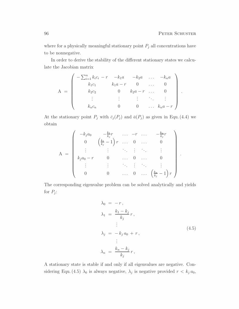
96 Peter Schuster
where for a physically meaningful stationary point Pj all concentrations have
to be nonnegative.
In order to derive the stability of the different stationary states we calcu-
late the Jacobian matrix
A =
−∑ni=1 kici − r −k1a −k2a . . . −knak1c1 k1a− r 0 . . . 0
k2c2 0 k2a− r . . . 0...
......
. . ....
kncn 0 0 . . . kna− r
.
At the stationary point Pj with cj(Pj) and a(Pj) as given in Equ. (4.4) we
obtain
A =
−kja0 −k1kjr . . . −r . . . −kn
kjr
0(
k1kj− 1)
r . . . 0 . . . 0...
.... . .
.... . .
...
kja0 − r 0 . . . 0 . . . 0...
.... . .
.... . .
...
0 0 . . . 0 . . .(
knkj− 1)
r
.
The corresponding eigenvalue problem can be solved analytically and yields
for Pj :
λ0 = − r ,
λ1 =k1 − kjkj
r ,
...
λj = − kj a0 + r ,...
λn =kn − kjkj
r ,
(4.5)
A stationary state is stable if and only if all eigenvalues are negative. Con-
sidering Equ. (4.5) λ0 is always negative, λj is negative provided r < kj a0,
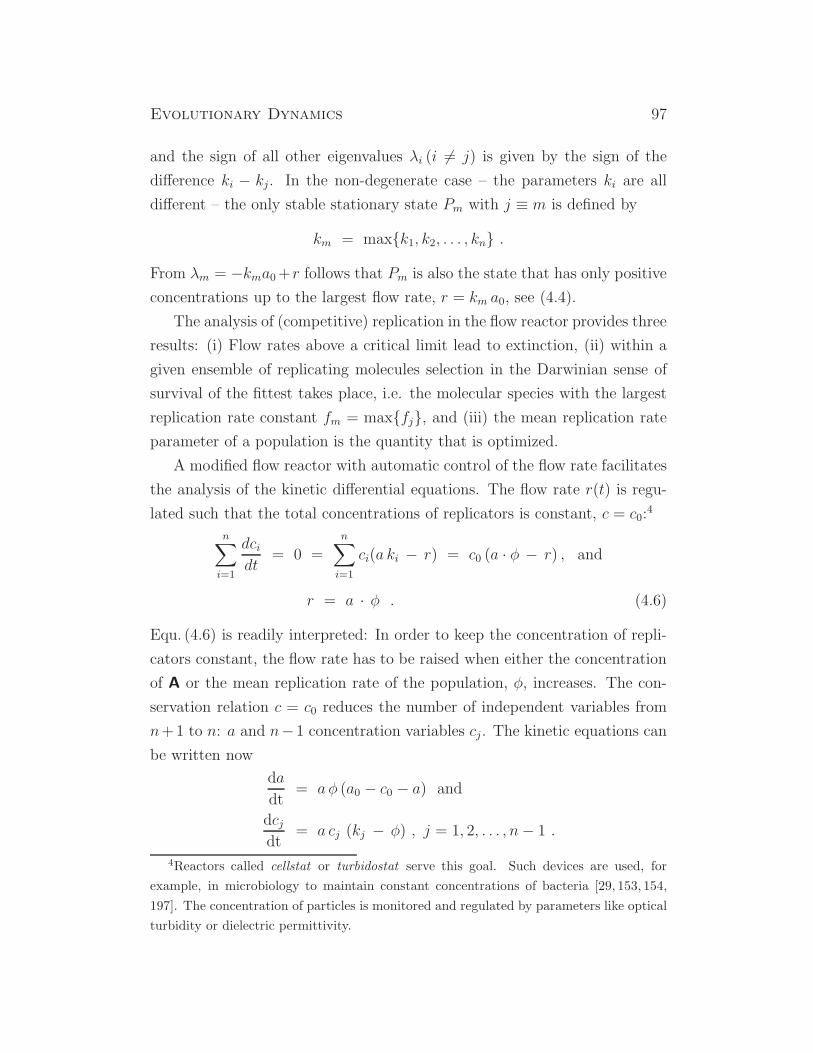
Evolutionary Dynamics 97
and the sign of all other eigenvalues λi (i 6= j) is given by the sign of the
difference ki − kj. In the non-degenerate case – the parameters ki are all
different – the only stable stationary state Pm with j ≡ m is defined by
km = maxk1, k2, . . . , kn .
From λm = −kma0+r follows that Pm is also the state that has only positive
concentrations up to the largest flow rate, r = km a0, see (4.4).
The analysis of (competitive) replication in the flow reactor provides three
results: (i) Flow rates above a critical limit lead to extinction, (ii) within a
given ensemble of replicating molecules selection in the Darwinian sense of
survival of the fittest takes place, i.e. the molecular species with the largest
replication rate constant fm = maxfj, and (iii) the mean replication rate
parameter of a population is the quantity that is optimized.
A modified flow reactor with automatic control of the flow rate facilitates
the analysis of the kinetic differential equations. The flow rate r(t) is regu-
lated such that the total concentrations of replicators is constant, c = c0:4
n∑
i=1
dcidt
= 0 =
n∑
i=1
ci(a ki − r) = c0 (a · φ − r) , and
r = a · φ . (4.6)
Equ. (4.6) is readily interpreted: In order to keep the concentration of repli-
cators constant, the flow rate has to be raised when either the concentration
of A or the mean replication rate of the population, φ, increases. The con-
servation relation c = c0 reduces the number of independent variables from
n+1 to n: a and n−1 concentration variables cj. The kinetic equations can
be written now
da
dt= a φ (a0 − c0 − a) and
dcjdt
= a cj (kj − φ) , j = 1, 2, . . . , n− 1 .
4Reactors called cellstat or turbidostat serve this goal. Such devices are used, for
example, in microbiology to maintain constant concentrations of bacteria [29, 153, 154,
197]. The concentration of particles is monitored and regulated by parameters like optical
turbidity or dielectric permittivity.
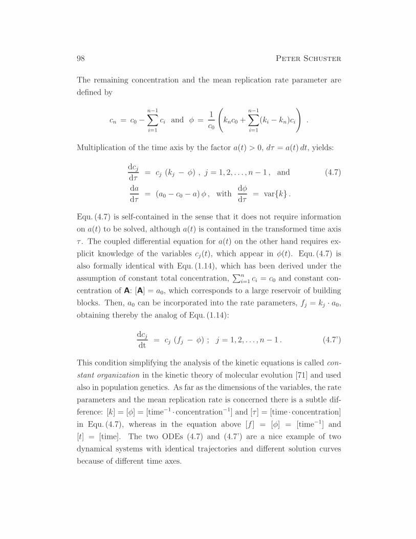
98 Peter Schuster
The remaining concentration and the mean replication rate parameter are
defined by
cn = c0 −n−1∑
i=1
ci and φ =1
c0
(
knc0 +n−1∑
i=1
(ki − kn)ci)
.
Multiplication of the time axis by the factor a(t) > 0, dτ = a(t) dt, yields:
dcjdτ
= cj (kj − φ) , j = 1, 2, . . . , n− 1 , and (4.7)
da
dτ= (a0 − c0 − a)φ , with
dφ
dτ= vark .
Equ. (4.7) is self-contained in the sense that it does not require information
on a(t) to be solved, although a(t) is contained in the transformed time axis
τ . The coupled differential equation for a(t) on the other hand requires ex-
plicit knowledge of the variables cj(t), which appear in φ(t). Equ. (4.7) is
also formally identical with Equ. (1.14), which has been derived under the
assumption of constant total concentration,∑n
i=1 ci = c0 and constant con-
centration of A: [A] = a0, which corresponds to a large reservoir of building
blocks. Then, a0 can be incorporated into the rate parameters, fj = kj · a0,obtaining thereby the analog of Equ. (1.14):
dcjdt
= cj (fj − φ) ; j = 1, 2, . . . , n− 1 . (4.7’)
This condition simplifying the analysis of the kinetic equations is called con-
stant organization in the kinetic theory of molecular evolution [71] and used
also in population genetics. As far as the dimensions of the variables, the rate
parameters and the mean replication rate is concerned there is a subtle dif-
ference: [k] = [φ] = [time−1 · concentration−1] and [τ ] = [time · concentration]in Equ. (4.7), whereas in the equation above [f ] = [φ] = [time−1] and
[t] = [time]. The two ODEs (4.7) and (4.7’) are a nice example of two
dynamical systems with identical trajectories and different solution curves
because of different time axes.

Evolutionary Dynamics 99
mutant class
0
1
2
3
number of sequences
1 1
3 9
3 27
1 27
number of sequences
Figure 4.4: Consecutive mutations. Consecutive point mutations propagate
into sequence space and are properly group in mutant classes Γk where k is the
Hamming distance from the reference sequence in Γ0. For binary sequences (κ = 2)
the numbers of sequences in mutant class k follows the binomial distribution:
|Γk| =( lk
)
, and in the general case we have |Γk| = (κ− 1)k( lk
)
. The figure sketches
the sequence spaces of binary (lhs) and natural (AUGC) sequences (rhs) of chain
length l = 3.
4.3 Replication and mutation
The interplay of replication, mutation, and selection is a core issue of Dar-
winian evolution, which could not be properly approach before knowledge
on structures and functions of the molecules involved in the process became
available. In particular, the accessibility of mutants requires knowledge on
the mechanism of mutation and the internal structure of a mutation space.
In section 3.3 we discussed the sequence space as the mutation compatible
ordering principle of sequences and considered it as the appropriate support
for fitness landscapes. Mathematically the internal structure of sequence
space is given by the properties of the Hamming graph H(l, κ) where l is thechain length of the sequence and κ the size of the nucleobase alphabet. Evo-
lution proceeding via consecutive mutations is confined by the properties of
sequence space as sketched in Fig. 4.4 for the paths determined by point mu-
tations. The size of the nucleobase alphabet clearly determines the diversity
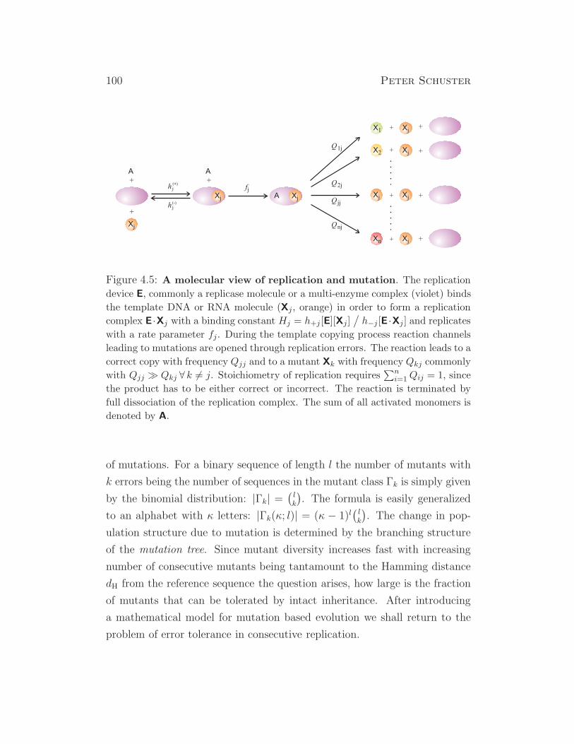
100 Peter Schuster
+
+
+
+
A
+
+ +
+
+
+
+
A A
XjXj
Xj
X2
X1
Xj
Xn
Xj
Xj
Xj
Xj
Q1j
Q2j
Q jj
Qnj
fjh j
h j(-)
( )+
Figure 4.5: A molecular view of replication and mutation. The replication
device E, commonly a replicase molecule or a multi-enzyme complex (violet) binds
the template DNA or RNA molecule (Xj, orange) in order to form a replication
complex E ·Xj with a binding constant Hj = h+j [E][Xj]/
h−j [E ·Xj ] and replicates
with a rate parameter fj. During the template copying process reaction channels
leading to mutations are opened through replication errors. The reaction leads to a
correct copy with frequency Qjj and to a mutant Xk with frequency Qkj commonly
with Qjj ≫ Qkj ∀ k 6= j. Stoichiometry of replication requires∑n
i=1 Qij = 1, since
the product has to be either correct or incorrect. The reaction is terminated by
full dissociation of the replication complex. The sum of all activated monomers is
denoted by A.
of mutations. For a binary sequence of length l the number of mutants with
k errors being the number of sequences in the mutant class Γk is simply given
by the binomial distribution: |Γk| =(
lk
)
. The formula is easily generalized
to an alphabet with κ letters: |Γk(κ; l)| = (κ − 1)l(
lk
)
. The change in pop-
ulation structure due to mutation is determined by the branching structure
of the mutation tree. Since mutant diversity increases fast with increasing
number of consecutive mutants being tantamount to the Hamming distance
dH from the reference sequence the question arises, how large is the fraction
of mutants that can be tolerated by intact inheritance. After introducing
a mathematical model for mutation based evolution we shall return to the
problem of error tolerance in consecutive replication.
Evolutionary Dynamics 101
4.3.1 Mutation-selection equation
As follows from the logic of mutation shown in Fig. 4.1 correct replication
and mutation are parallel chemical reactions, which are initiated in the same
way. A sketch of such a mechanism is shown in Fig. 4.5: A replication device
– a single single-strand DNA replicating enzyme in the polymerase chain re-
action (PCR), an RNA-specific RNA polymerase in most cases of viral RNA
replication or a large multi-enzyme complex in DNA double-strand repli-
cation – binds the template, replication is initiated and correct replication
and mutations represent different replication channels, since replication er-
rors occur on the fly. When replication is completed the complex between
template, product, and replication device dissociates. We distinguish direct
replication, X → 2X, and complementary replication, X(+) → X(−) + X
(+)
and X(−) → X
(+) + X(−), where the former is typical for DNA replication
of all organisms and the latter occurs commonly with RNA single-strand
viruses. Here, we start by considering direct application first and shall show
later that complementary replication under almost all reasonable conditions
can be well approximated by a single overall direct replication step.
In order to introduce mutations into selection dynamics Manfred Eigen
[65] conceived a kinetic model based on overall stoichiometric equations,
which handle correct replication and mutation of an asexually reproducing
species as parallel reactions (Fig. 4.5)
(A) + Xi
Qjifi−−−→ Xj + Xi ; i, j = 1, . . . , n . (4.8)
Since A is assumed to be present in excess it is a constant and contained as
a factor in the rate parameter fj = a0 kj
In normalized coordinates (4.8) corresponds to a differential equation of
the form
dxjdt
=n∑
i=1
Qjifi xi − xj φ(t) ; j = 1, . . . , n ;n∑
i=1
xi = 1 . (4.9)
The finite size constraint φ(t) =∑n
i=1 fixi is precisely the same as in the
mutation-free case (1.14), and the integrating factor transformation [329,
102 Peter Schuster
p. 322ff.] can be used to solve the differential equation [165, 285]:
zj(t) = xj(t) exp
(∫ t
0
φ(τ)dτ
)
with exp
(∫ t
0
φ(τ)dτ
)
=
n∑
i=1
zi(t) ,
Insertion into Equ. (4.9) yields
d
dt
(
zj(t) e−
t∫
0
φ(τ)dτ
)
=dzjdt
e−
t∫
0
φ(τ)dτ+ zj(t)
d
dte−
t∫
0
φ(τ)dτ=
=dzjdt
e−
t∫
0
φ(τ)dτ− zj(t) e
−t∫
0
φ(τ)dτφ(t) =
=
(
n∑
i=1
Qjifi zi(t) − zj(t)φ(t)
)
e−
t∫
0
φ(τ)dτ,
dzjdt
= Qjifi zi(t) ordz
dt= Q · F · z = W · z . (4.10)
The transformation turns the mildly nonlinear ODE (4.9) into a linear equa-
tion, which can be solved by standard mathematical techniques. All pa-
rameters are contained in the two n × n matrices, the mutation matrix Q,
the fitness matrix F: The mutation frequencies are subsumed in the ma-
trix Q = Qji with Qji being the probability that Xj is obtained as an
error copy of Xi. The fitness values are the elements of a diagonal matrix
F = Fij = fi δi,j and the value matrix W finally, is the product of the two
matrices: W = Q · F = Wji = Qjifi.Provided matrix W is diagonalizable, which will always be the case if
the mutation matrix Q and the fitness matrix F are based on real chemical
reaction mechanisms, we can transform variables by means of the two n× nmatrices B = bij and B−1 = H = hij (i, j = 1, . . . , n),
z(t) = B · ζ(t) and ζ(t) = B−1 · z(t) = H · z(t) ,
such that B−1 ·W ·B = Λ is diagonal and its elements, λk, are the eigenvalues
of the matrix W. The right-hand eigenvectors of W are given by the columns
of B, bj = (bi,j; i = 1, . . . , n), and the left-hand eigenvectors by the rows of
B−1 = H, hk = (hk,i; i = 1, . . . , n), respectively. These eigenvectors are the
normal modes of mutation-selection kinetics.
Evolutionary Dynamics 103
For strictly positive off-diagonal elements of W, implying the same for
Q, which implies nothing more than every mutation Xi → Xj has to be
possible although the probability of occurrence might be extremely small,
Perron-Frobenius theorem holds (see, for example, [259] and below) and we
are dealing with a non-degenerate largest eigenvalue λ0,
λ0 > |λ1| ≥ |λ2| ≥ |λ3| ≥ . . . ≥ |λn| , (4.11)
and a corresponding dominant eigenvector b0 with strictly positive compo-
nents, bi0 > 0 ∀ i = 1, . . . , n.5 In terms of components the differential equation
in ζ has the solutions
ζk(t) = ζk(0) exp(λk t) . (4.12)
Transformation back into the variables z yields
zj(t) =
n−1∑
k=0
bjk βk(0) exp(λk t) , (4.13)
with the initial conditions encapsulated in the equation
βk(0) =n∑
i=1
hki zi(0) =n∑
i=1
hki xi(0) . (4.14)
From here we obtain the solutions in the original variables xj through inverse
transformation and normalization
xj(t) =
∑n−1k=0 bjk βk(0) exp(λk t)
∑ni=1
∑n−1k=0 bik βk(0) exp(λk t)
. (4.15)
For sufficiently long times the contribution of the largest eigenvalue domi-
nates the summations and we find for the long time solutions
xj(t) ≈bj0 β0(0) exp(λ0 t)
∑ni=1 bi0 β0(0) exp(λ0 t)
and
limt→∞
xj(t) = xj =bj0 β0(0)
∑ni=1 bi0 β0(0)
,
(4.16)
5We introduce here an asymmetry in numbering rows and columns in order to point at
the special properties of the largest eigenvalue λ0 and the dominant eigenvector b0.
104 Peter Schuster
which represent the components of the stationary population vector denoted
by Υ = (x1, . . . , xn). Solution curves Υ(t) =(
x1(t), . . . , xn(t))
and station-
ary mutant distributions Υ were derived here in terms of the eigenvectors of
the matrix W and can be obtained by numerical computation. Highly flexible
and accurate computer codes for matrix diagonalization are available and the
only problem that the numerical approach visualizes is high-dimensionality
since n is commonly very large.
Perron-Frobenius theorem comes in two versions [259], which we shallnow apply to the selection-mutation problem. The stronger version providesa proof for six properties of the largest eigenvector of non-negative primitivematrices6 T:
(i) The largest eigenvalue is real and positive, λ0 > 0,
(ii) a strictly positive right eigenvector ℓ0 and a strictly positive left eigen-vector h0 are associated with λ0,
(iii) λ0 > |λk| holds for all eigenvalues λk 6= λ0,
(iv) the eigenvectors associated with λ0 are unique up to constant factors,
(v) if 0 ≤ B ≤ T is fulfilled and β is an eigenvalue of B, then |β| ≤ λ0,and, moreover, |β| = λ0 implies B = T,
(vi) λ0 is a simple root of the characteristic equation of T.
The weaker version of the theorem holds for irreducible matrices7 T. Allthe above given assertions hold except (iii) has to be replaced by the weakerstatement
(iii) λ0 ≥ |λk| holds for all eigenvalues λk 6= λ0.
Irreducible cyclic matrices can be used straightforwardly as examples in or-der to demonstrate the existence of conjugate complex eigenvalues. Perron-Frobenius theorem, in its strict or weaker form, holds not only for strictly
6A square non-negative matrix T = tij ; i, j = 1, . . . , n; tij ≥ 0 is called primitive ifthere exists a positive integer m such that Tm is strictly positive: Tm > 0 which implies
Tm = t(m)ij ; i, j = 1, . . . , n; t
(m)ij > 0.
7A square non-negative matrix T = tij ; i, j = 1, . . . , n; tij ≥ 0 is called irreducible iffor every pair (i, j) of its index set there exists a positive integer mij ≡ m(i, j) such thattmij
ij > 0. An irreducible matrix is called cyclic with period d, if the period of (all) itsindices satisfies d > 1, and it is said to be acyclic if d = 1.
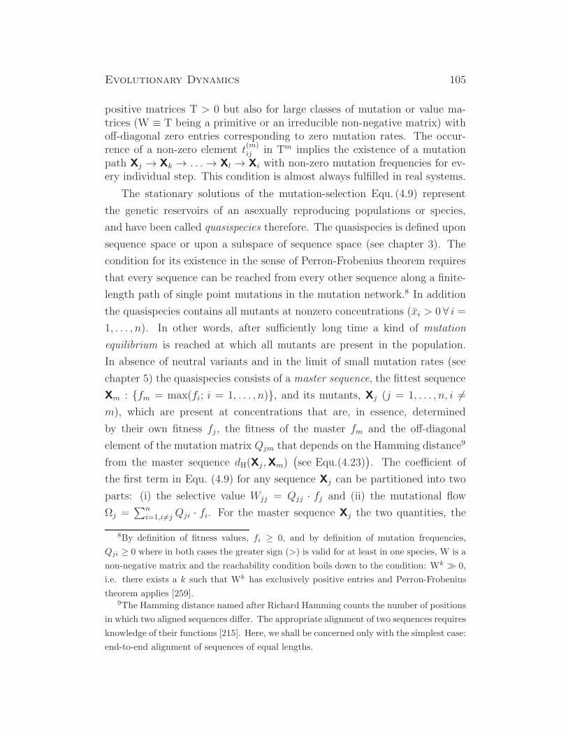
Evolutionary Dynamics 105
positive matrices T > 0 but also for large classes of mutation or value ma-trices (W ≡ T being a primitive or an irreducible non-negative matrix) withoff-diagonal zero entries corresponding to zero mutation rates. The occur-rence of a non-zero element t
(m)ij in Tm implies the existence of a mutation
path Xj → Xk → . . .→ Xl → Xi with non-zero mutation frequencies for ev-ery individual step. This condition is almost always fulfilled in real systems.
The stationary solutions of the mutation-selection Equ. (4.9) represent
the genetic reservoirs of an asexually reproducing populations or species,
and have been called quasispecies therefore. The quasispecies is defined upon
sequence space or upon a subspace of sequence space (see chapter 3). The
condition for its existence in the sense of Perron-Frobenius theorem requires
that every sequence can be reached from every other sequence along a finite-
length path of single point mutations in the mutation network.8 In addition
the quasispecies contains all mutants at nonzero concentrations (xi > 0 ∀ i =1, . . . , n). In other words, after sufficiently long time a kind of mutation
equilibrium is reached at which all mutants are present in the population.
In absence of neutral variants and in the limit of small mutation rates (see
chapter 5) the quasispecies consists of a master sequence, the fittest sequence
Xm : fm = max(fi; i = 1, . . . , n), and its mutants, Xj (j = 1, . . . , n, i 6=m), which are present at concentrations that are, in essence, determined
by their own fitness fj , the fitness of the master fm and the off-diagonal
element of the mutation matrix Qjm that depends on the Hamming distance9
from the master sequence dH(Xj ,Xm)(
see Equ.(4.23))
. The coefficient of
the first term in Equ. (4.9) for any sequence Xj can be partitioned into two
parts: (i) the selective value Wjj = Qjj · fj and (ii) the mutational flow
Ωj =∑n
i=1,i 6=j Qji · fi. For the master sequence Xj the two quantities, the
8By definition of fitness values, fi ≥ 0, and by definition of mutation frequencies,
Qji ≥ 0 where in both cases the greater sign (>) is valid for at least in one species, W is a
non-negative matrix and the reachability condition boils down to the condition: Wk ≫ 0,
i.e. there exists a k such that Wk has exclusively positive entries and Perron-Frobenius
theorem applies [259].9The Hamming distance named after Richard Hamming counts the number of positions
in which two aligned sequences differ. The appropriate alignment of two sequences requires
knowledge of their functions [215]. Here, we shall be concerned only with the simplest case:
end-to-end alignment of sequences of equal lengths.
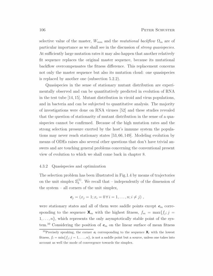
106 Peter Schuster
selective value of the master, Wmm and the mutational backflow Ωm are of
particular importance as we shall see in the discussion of strong quasispecies.
At sufficiently large mutation rates it may also happen that another relatively
fit sequence replaces the original master sequence, because its mutational
backflow overcompensates the fitness difference. This replacement concerns
not only the master sequence but also its mutation cloud: one quasispecies
is replaced by another one (subsection 5.2.2).
Quasispecies in the sense of stationary mutant distribution are experi-
mentally observed and can be quantitatively predicted in evolution of RNA
in the test tube [14, 15]. Mutant distribution in viroid and virus populations,
and in bacteria and can be subjected to quantitative analysis. The majority
of investigations were done on RNA viruses [52] and these studies revealed
that the question of stationarity of mutant distribution in the sense of a qua-
sispecies cannot be confirmed. Because of the high mutation rates and the
strong selection pressure exerted by the host’s immune system the popula-
tions may never reach stationary states [53, 66, 149]. Modeling evolution by
means of ODEs raises also several other questions that don’t have trivial an-
swers and are touching general problems concerning the conventional present
view of evolution to which we shall come back in chapter 8.
4.3.2 Quasispecies and optimization
The selection problem has been illustrated in Fig.1.4 by means of trajectories
on the unit simplex S(1)3 . We recall that – independently of the dimension of
the system – all corners of the unit simplex,
ej = (xj = 1; xi = 0 ∀ i = 1, . . . , n; i 6= j) ,
were stationary states and all of them were saddle points except em corre-
sponding to the sequence Xm with the highest fitness, fm = maxfj; j =
1, . . . , n, which represents the only asymptotically stable point of the sys-
tem.10 Considering the position of em on the linear surface of mean fitness
10Precisely speaking, the corner el corresponding to the sequence Xl with the lowest
fitness, fl = minfj; j = 1, . . . , n, is not a saddle point but a source, unless one takes into
account as well the mode of convergence towards the simplex.
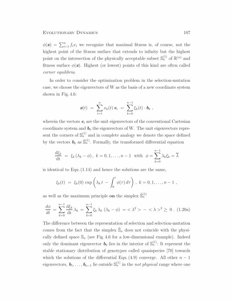
Evolutionary Dynamics 107
φ(x) =∑n
i=1 fixi we recognize that maximal fitness is, of course, not the
highest point of the fitness surface that extends to infinity but the highest
point on the intersection of the physically acceptable subset S(1)n of R(n) and
fitness surface φ(x). Highest (or lowest) points of this kind are often called
corner equilibria.
In order to consider the optimization problem in the selection-mutation
case, we choose the eigenvectors of W as the basis of a new coordinate system
shown in Fig. 4.6:
x(t) =
n∑
i=1
xk(t) ei =
n−1∑
k=0
ξk(t) · bk ,
wherein the vectors ei are the unit eigenvectors of the conventional Cartesian
coordinate system and bk the eigenvectors of W. The unit eigenvectors repre-
sent the corners of S(1)n and in complete analogy we denote the space defined
by the vectors bk as S(1)n . Formally, the transformed differential equation
dξkdt
= ξk (λk − φ) , k = 0, 1, . . . , n− 1 with φ =n−1∑
k=0
λkξk = λ
is identical to Equ. (1.14) and hence the solutions are the same,
ξk(t) = ξk(0) exp
(
λk t −∫ t
0
φ(τ) dτ
)
, k = 0, 1, . . . , n− 1 ,
as well as the maximum principle on the simplex S(1)n
dφ
dt=
n−1∑
k=0
dξkdt
λk =n−1∑
k=0
ξk λk (λk − φ) = < λ2 > − < λ >2 ≥ 0 . (1.20a)
The difference between the representation of selection and selection-mutation
comes from the fact that the simplex Sn does not coincide with the physi-
cally defined space Sn (see Fig. 4.6 for a low-dimensional example). Indeed
only the dominant eigenvector b0 lies in the interior of S(1)n : It represent the
stable stationary distribution of genotypes called quasispecies [70] towards
which the solutions of the differential Equ. (4.9) converge. All other n − 1
eigenvectors, b1, . . . , bn−1 lie outside S(1)n in the not physical range where one
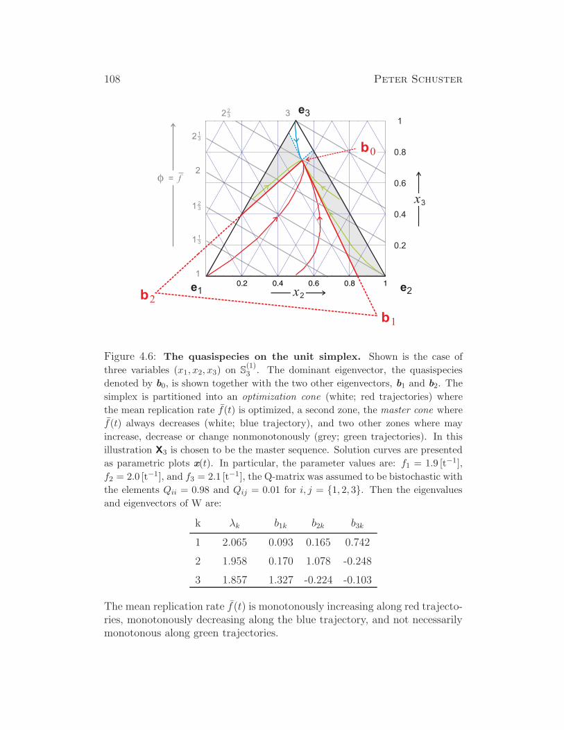
108 Peter Schuster
e3
e2e1 x2
x3
3
1 23
2 13
2 23
1 13
1
2f = f
b0
b1
b2
0.8
1
0.6
0.4
0.2
Figure 4.6: The quasispecies on the unit simplex. Shown is the case of
three variables (x1, x2, x3) on S(1)3 . The dominant eigenvector, the quasispecies
denoted by b0, is shown together with the two other eigenvectors, b1 and b2. The
simplex is partitioned into an optimization cone (white; red trajectories) where
the mean replication rate f(t) is optimized, a second zone, the master cone where
f(t) always decreases (white; blue trajectory), and two other zones where may
increase, decrease or change nonmonotonously (grey; green trajectories). In this
illustration X3 is chosen to be the master sequence. Solution curves are presented
as parametric plots x(t). In particular, the parameter values are: f1 = 1.9 [t−1],f2 = 2.0 [t−1], and f3 = 2.1 [t−1], the Q-matrix was assumed to be bistochastic with
the elements Qii = 0.98 and Qij = 0.01 for i, j = 1, 2, 3. Then the eigenvalues
and eigenvectors of W are:
k λk b1k b2k b3k
1 2.065 0.093 0.165 0.742
2 1.958 0.170 1.078 -0.248
3 1.857 1.327 -0.224 -0.103
The mean replication rate f(t) is monotonously increasing along red trajecto-ries, monotonously decreasing along the blue trajectory, and not necessarilymonotonous along green trajectories.

Evolutionary Dynamics 109
or more variables xi are negative. The quasispecies b0 is commonly dom-
inated by a single genotype, the master sequence Xm, having the largest
stationary relative concentration: xm ≫ xi ∀ i 6= m, reflecting, for not too
large mutation rates, the same sequence in the elements of the matrix W:
Wmm ≫Wii ∀ i 6= m. As sketched in Fig. 4.6 the quasispecies is then situated
close to the unit vector em in the interior of S(1)n .
For the discussion of the optimization behavior the simplex is partitioned
into three zones: (i) The zone of maximization of φ(t), the (large) lower
white area in Fig. 4.6 where Equ. (1.20a) holds and which we shall denote
as optimization cone,11 (ii) the zone that includes the unit vector of the
master sequence, em, and the quasispecies, b0, as corners, and that we shall
characterize as master cone,11 and (iii) the remaining part of the simplex
S(1)n (two zones colored grey in Fig. 4.6). It is straightforward to proof that
increase of φ(t) and monotonous convergence towards the quasispecies is
restricted to the optimization cone [256]. From the properties of the selection
Equ. (1.14) we recall and conclude that the boundaries of the simplex S(1)n
are invariant sets. This implies that no orbit of the differential Equ. (4.9) can
cross these boundaries. The boundaries of S(1)n , on the other hand, are not
invariant but have the restriction that they can be crossed exclusively in one
direction: from outside to inside.12 Therefore, a solution curve starting in
the optimization cone or in the master cone will stay inside the cone where
it started and eventually converge towards the quasispecies, b0.
In zone (ii), the master cone, all variables ξk except ξ0 are negative and ξ0
is larger than one in order to fulfill the L(1)-norm condition∑n−1
k=0 ξk = 1. In
order to analyze the behavior of φ(t) we split the variables into two groups,
ξ0 the frequency of the quasispecies and the rest [256], ξk; k = 1, . . . , n− 111The exact geometry of the optimization cone or the master cone is a polyhedron that
can be approximated by a pyramid rather than a cone. Nevertheless we prefer the inexact
notion cone because it is easier to memorize and to imagine in high-dimensional space.12This is shown easily by analyzing the differential equation, but follows also from the
physical background: No acceptable process can lead to negative particle numbers or
concentrations. It can, however, start at zero concentrations and this means the orbit
begins at the boundary and goes into the interior of the physical concentration space, here
the simplex S(1)n .
110 Peter Schuster
with∑n−1
k=1 ξk = 1− ξ0:
dφ
dt= λ20ξ0 +
n−1∑
k=1
λ2kξk −(
λ0ξ0 +
n−1∑
k=1
λkξk
)2
.
Next we replace the distribution of λk values in the second group by a single
λ-value, λ and find:
dφ
dt= λ20ξ0 + λ2(1− ξ0) −
(
λ0ξ0 + λ(1− ξ0))2
.
After a view simple algebraic operations we find eventually
dφ
dt= ξ0 (1− ξ0) (λ0 − λ)2 . (4.17)
For the master cone with ξ0 ≥ 1, this implies dφ(t)/dt ≤ 0, the flux is a
non-increasing function of time. Since we are only interested in the sign of
dφ/dt, the result is exact, because we could use the mean value λ = λ =
(∑n−1
k=1 λkξk)/(1 − ξ0), the largest possible value λ1 or the smallest possi-
ble value λn−1 without changing the conclusion. Clearly, the distribution
of λk-values matters for quantitative results. As it has to be, Equ. (4.17)
applies also to the optimization cone and gives the correct result that φ(t)
is non-decreasing. Decrease of mean fitness or flux φ(t) in the master cone
is readily illustrated: Consider, for example, a homogeneous population of
the master sequence as initial condition: xm(0) = 1 and φ(0) = fm. The
population becomes inhomogeneous because mutants are formed. Since all
mutants have lower replication constants by definition, (fi < fm ∀ i 6= m),
φ becomes smaller. Finally, the distribution approaches the quasispecies b0
and limt→∞ φ(t) = λ0 < fm.
An extension of the analysis from the master cone to the grey zones, where
not all ξk values with k 6= 0 are negative, is not possible. It has been shown
by means of numerical examples that dφ(t)/dt may show nonmonotonous
behavior and can go through a maximum or a minimum at finite time [256].
4.3.3 Error thresholds
How many mutations per generation can be tolerated without jeopardizing
inheritance? This is a proper question that is very hard to analyze without
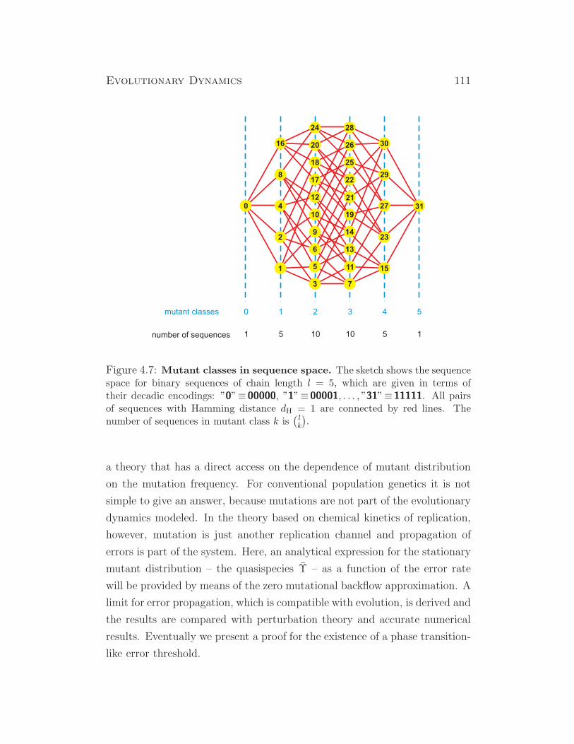
Evolutionary Dynamics 111
Figure 4.7: Mutant classes in sequence space. The sketch shows the sequencespace for binary sequences of chain length l = 5, which are given in terms oftheir decadic encodings: ”0”≡ 00000, ”1”≡ 00001, . . . , ”31”≡ 11111. All pairsof sequences with Hamming distance dH = 1 are connected by red lines. Thenumber of sequences in mutant class k is
(
lk
)
.
a theory that has a direct access on the dependence of mutant distribution
on the mutation frequency. For conventional population genetics it is not
simple to give an answer, because mutations are not part of the evolutionary
dynamics modeled. In the theory based on chemical kinetics of replication,
however, mutation is just another replication channel and propagation of
errors is part of the system. Here, an analytical expression for the stationary
mutant distribution – the quasispecies Υ – as a function of the error rate
will be provided by means of the zero mutational backflow approximation. A
limit for error propagation, which is compatible with evolution, is derived and
the results are compared with perturbation theory and accurate numerical
results. Eventually we present a proof for the existence of a phase transition-
like error threshold.
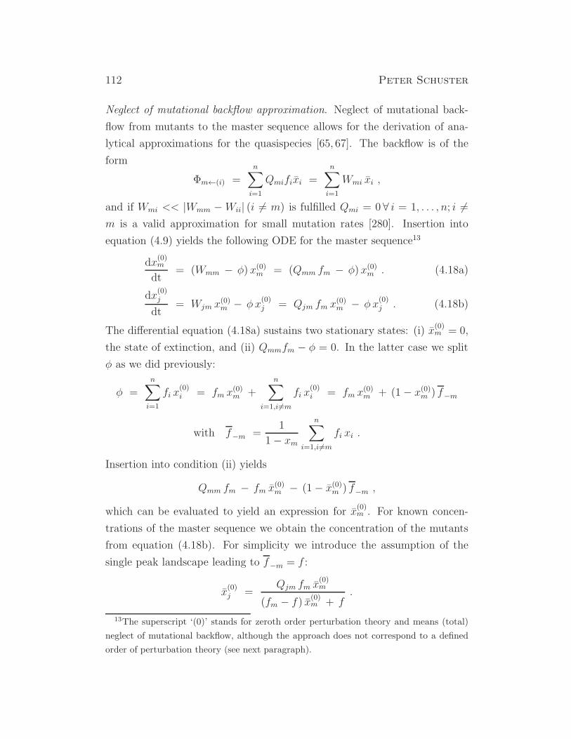
112 Peter Schuster
Neglect of mutational backflow approximation. Neglect of mutational back-
flow from mutants to the master sequence allows for the derivation of ana-
lytical approximations for the quasispecies [65, 67]. The backflow is of the
form
Φm←(i) =
n∑
i=1
Qmifixi =
n∑
i=1
Wmi xi ,
and if Wmi << |Wmm −Wii| (i 6= m) is fulfilled Qmi = 0 ∀ i = 1, . . . , n; i 6=m is a valid approximation for small mutation rates [280]. Insertion into
equation (4.9) yields the following ODE for the master sequence13
dx(0)m
dt= (Wmm − φ) x(0)m = (Qmm fm − φ) x(0)m . (4.18a)
dx(0)j
dt= Wjm x
(0)m − φ x
(0)j = Qjm fm x
(0)m − φ x
(0)j . (4.18b)
The differential equation (4.18a) sustains two stationary states: (i) x(0)m = 0,
the state of extinction, and (ii) Qmmfm − φ = 0. In the latter case we split
φ as we did previously:
φ =
n∑
i=1
fi x(0)i = fm x
(0)m +
n∑
i=1,i 6=m
fi x(0)i = fm x
(0)m + (1− x(0)m ) f−m
with f−m =1
1− xm
n∑
i=1,i 6=m
fi xi .
Insertion into condition (ii) yields
Qmm fm − fm x(0)m − (1− x(0)m ) f−m ,
which can be evaluated to yield an expression for x(0)m . For known concen-
trations of the master sequence we obtain the concentration of the mutants
from equation (4.18b). For simplicity we introduce the assumption of the
single peak landscape leading to f−m = f :
x(0)j =
Qjm fm x(0)m
(fm − f) x(0)m + f.
13The superscript ‘(0)’ stands for zeroth order perturbation theory and means (total)
neglect of mutational backflow, although the approach does not correspond to a defined
order of perturbation theory (see next paragraph).
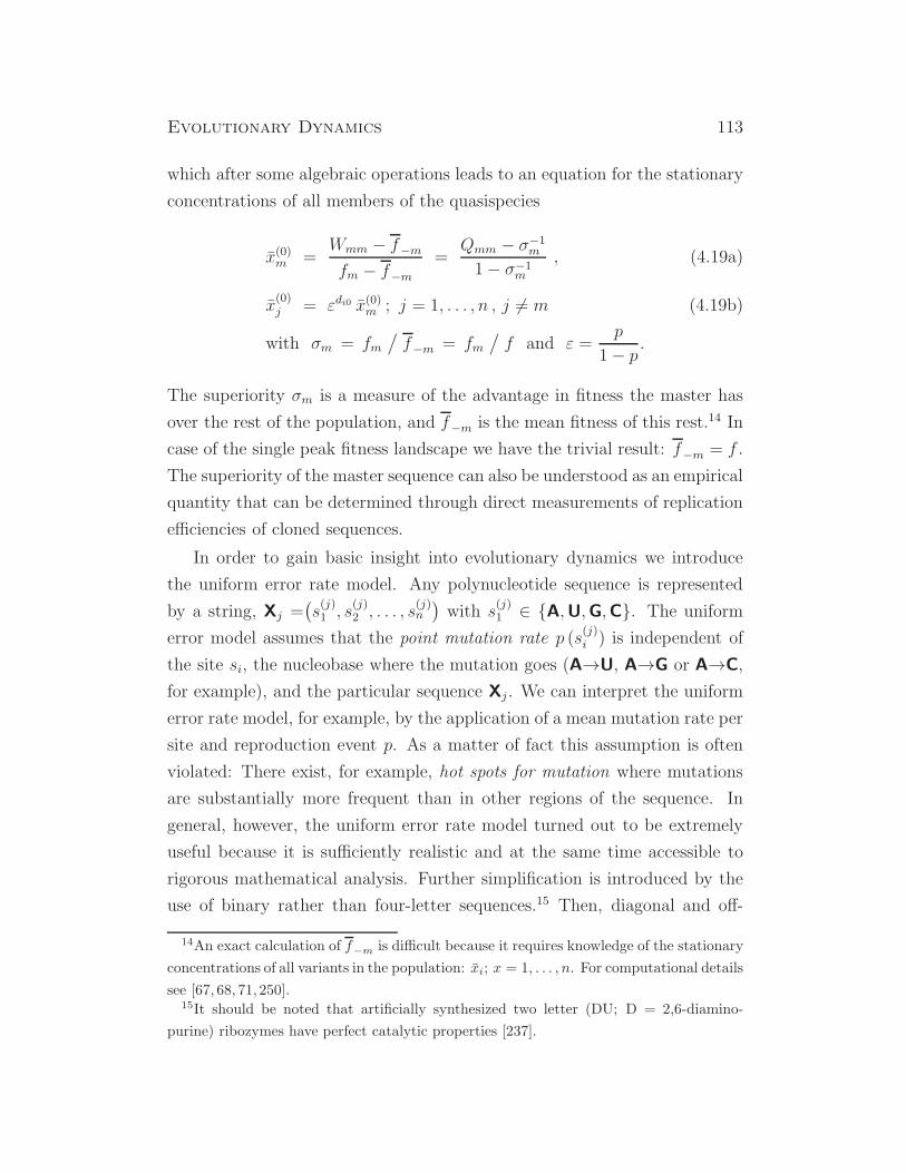
Evolutionary Dynamics 113
which after some algebraic operations leads to an equation for the stationary
concentrations of all members of the quasispecies
x(0)m =Wmm − f−mfm − f−m
=Qmm − σ−1m
1− σ−1m
, (4.19a)
x(0)j = εdi0 x(0)m ; j = 1, . . . , n , j 6= m (4.19b)
with σm = fm/
f−m = fm/
f and ε =p
1− p.
The superiority σm is a measure of the advantage in fitness the master has
over the rest of the population, and f−m is the mean fitness of this rest.14 In
case of the single peak fitness landscape we have the trivial result: f−m = f .
The superiority of the master sequence can also be understood as an empirical
quantity that can be determined through direct measurements of replication
efficiencies of cloned sequences.
In order to gain basic insight into evolutionary dynamics we introduce
the uniform error rate model. Any polynucleotide sequence is represented
by a string, Xj =(
s(j)1 , s
(j)2 , . . . , s
(j)n
)
with s(j)1 ∈ A,U,G,C. The uniform
error model assumes that the point mutation rate p (s(j)i ) is independent of
the site si, the nucleobase where the mutation goes (A→U, A→G or A→C,
for example), and the particular sequence Xj . We can interpret the uniform
error rate model, for example, by the application of a mean mutation rate per
site and reproduction event p. As a matter of fact this assumption is often
violated: There exist, for example, hot spots for mutation where mutations
are substantially more frequent than in other regions of the sequence. In
general, however, the uniform error rate model turned out to be extremely
useful because it is sufficiently realistic and at the same time accessible to
rigorous mathematical analysis. Further simplification is introduced by the
use of binary rather than four-letter sequences.15 Then, diagonal and off-
14An exact calculation of f−m is difficult because it requires knowledge of the stationary
concentrations of all variants in the population: xi; x = 1, . . . , n. For computational details
see [67, 68, 71, 250].15It should be noted that artificially synthesized two letter (DU; D = 2,6-diamino-
purine) ribozymes have perfect catalytic properties [237].
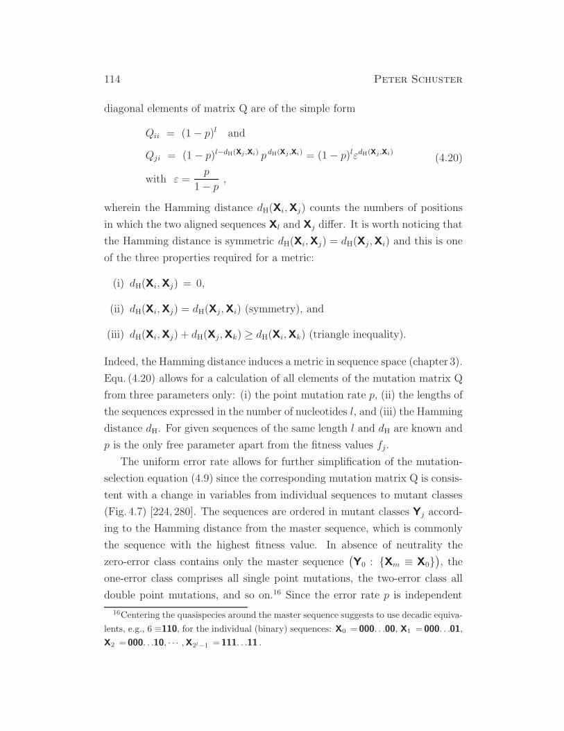
114 Peter Schuster
diagonal elements of matrix Q are of the simple form
Qii = (1− p)l and
Qji = (1− p)l−dH(Xj ,Xi) p dH(Xj ,Xi) = (1− p)lεdH(Xj ,Xi)
with ε =p
1− p ,(4.20)
wherein the Hamming distance dH(Xi,Xj) counts the numbers of positions
in which the two aligned sequences Xl and Xj differ. It is worth noticing that
the Hamming distance is symmetric dH(Xi,Xj) = dH(Xj ,Xi) and this is one
of the three properties required for a metric:
(i) dH(Xi,Xj) = 0,
(ii) dH(Xi,Xj) = dH(Xj,Xi) (symmetry), and
(iii) dH(Xi,Xj) + dH(Xj,Xk) ≥ dH(Xi,Xk) (triangle inequality).
Indeed, the Hamming distance induces a metric in sequence space (chapter 3).
Equ. (4.20) allows for a calculation of all elements of the mutation matrix Q
from three parameters only: (i) the point mutation rate p, (ii) the lengths of
the sequences expressed in the number of nucleotides l, and (iii) the Hamming
distance dH. For given sequences of the same length l and dH are known and
p is the only free parameter apart from the fitness values fj .
The uniform error rate allows for further simplification of the mutation-
selection equation (4.9) since the corresponding mutation matrix Q is consis-
tent with a change in variables from individual sequences to mutant classes
(Fig. 4.7) [224, 280]. The sequences are ordered in mutant classes Yj accord-
ing to the Hamming distance from the master sequence, which is commonly
the sequence with the highest fitness value. In absence of neutrality the
zero-error class contains only the master sequence(
Y0 : Xm ≡ X0)
, the
one-error class comprises all single point mutations, the two-error class all
double point mutations, and so on.16 Since the error rate p is independent
16Centering the quasispecies around the master sequence suggests to use decadic equiva-
lents, e.g., 6 ≡110, for the individual (binary) sequences: X0 = 000. . .00, X1 = 000. . .01,
X2 = 000. . .10, · · · ,X2l−1 = 111. . .11 .
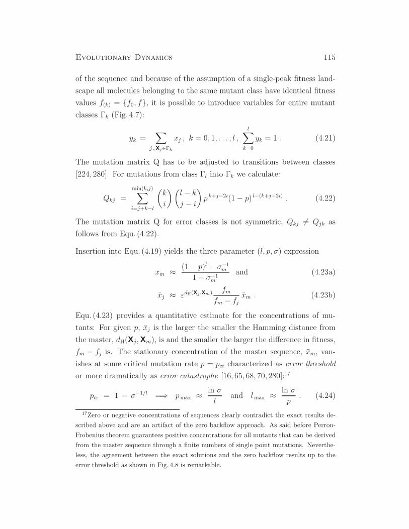
Evolutionary Dynamics 115
of the sequence and because of the assumption of a single-peak fitness land-
scape all molecules belonging to the same mutant class have identical fitness
values f(k) = f0, f, it is possible to introduce variables for entire mutant
classes Γk (Fig. 4.7):
yk =∑
j ,Xj∈Γk
xj , k = 0, 1, . . . , l ,
l∑
k=0
yk = 1 . (4.21)
The mutation matrix Q has to be adjusted to transitions between classes
[224, 280]. For mutations from class Γl into Γk we calculate:
Qkj =
min(k,j)∑
i=j+k−l
(
k
i
)(
l − kj − i
)
p k+j−2i(1− p) l−(k+j−2i) . (4.22)
The mutation matrix Q for error classes is not symmetric, Qkj 6= Qjk as
follows from Equ. (4.22).
Insertion into Equ. (4.19) yields the three parameter (l, p, σ) expression
xm ≈(1− p)l − σ−1m
1− σ−1m
and (4.23a)
xj ≈ εdH(Xj ,Xm) fmfm − fj
xm . (4.23b)
Equ. (4.23) provides a quantitative estimate for the concentrations of mu-
tants: For given p, xj is the larger the smaller the Hamming distance from
the master, dH(Xj,Xm), is and the smaller the larger the difference in fitness,
fm − fj is. The stationary concentration of the master sequence, xm, van-
ishes at some critical mutation rate p = pcr characterized as error threshold
or more dramatically as error catastrophe [16, 65, 68, 70, 280]:17
pcr = 1 − σ−1/l =⇒ pmax ≈ln σ
land lmax ≈
ln σ
p. (4.24)
17Zero or negative concentrations of sequences clearly contradict the exact results de-
scribed above and are an artifact of the zero backflow approach. As said before Perron-
Frobenius theorem guarantees positive concentrations for all mutants that can be derived
from the master sequence through a finite numbers of single point mutations. Neverthe-
less, the agreement between the exact solutions and the zero backflow results up to the
error threshold as shown in Fig. 4.8 is remarkable.
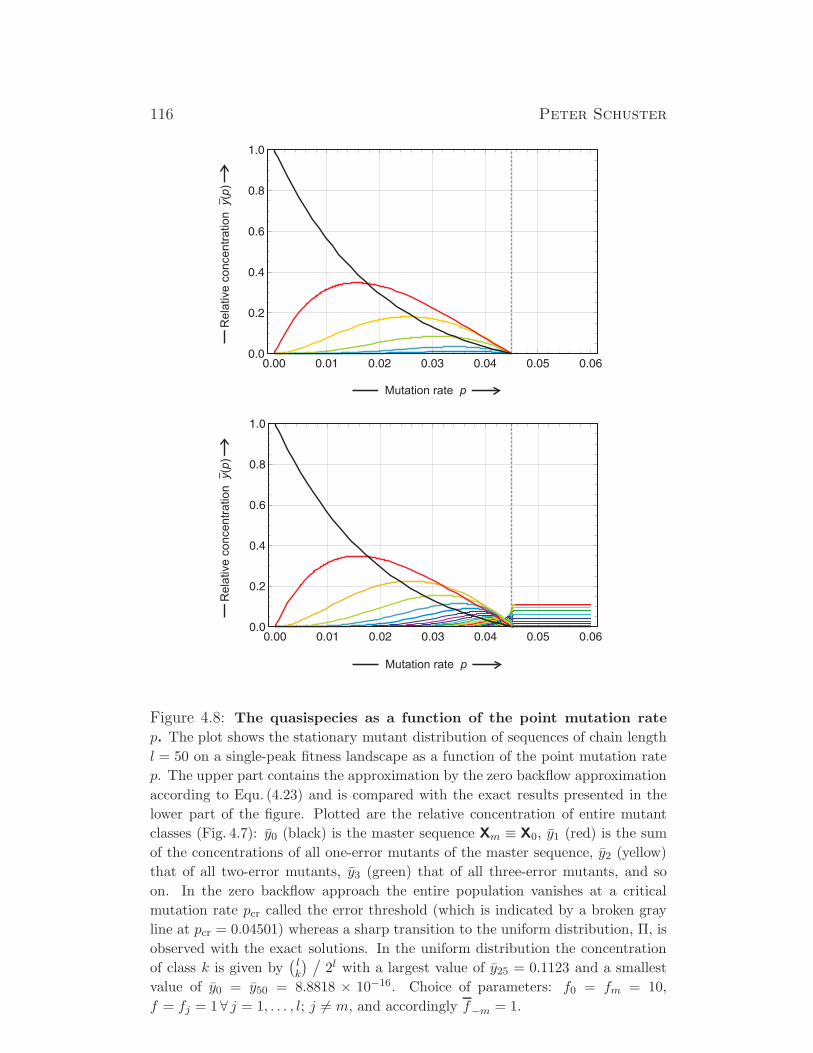
116 Peter Schuster
Figure 4.8: The quasispecies as a function of the point mutation rate
p. The plot shows the stationary mutant distribution of sequences of chain length
l = 50 on a single-peak fitness landscape as a function of the point mutation rate
p. The upper part contains the approximation by the zero backflow approximation
according to Equ. (4.23) and is compared with the exact results presented in the
lower part of the figure. Plotted are the relative concentration of entire mutant
classes (Fig. 4.7): y0 (black) is the master sequence Xm ≡ X0, y1 (red) is the sum
of the concentrations of all one-error mutants of the master sequence, y2 (yellow)
that of all two-error mutants, y3 (green) that of all three-error mutants, and so
on. In the zero backflow approach the entire population vanishes at a critical
mutation rate pcr called the error threshold (which is indicated by a broken gray
line at pcr = 0.04501) whereas a sharp transition to the uniform distribution, Π, is
observed with the exact solutions. In the uniform distribution the concentration
of class k is given by(
lk
) /
2l with a largest value of y25 = 0.1123 and a smallest
value of y0 = y50 = 8.8818 × 10⁻¹⁶. Choice of parameters: f0 = fm = 10,
f = fj = 1∀ j = 1, . . . , l; j 6= m, and accordingly f−m = 1.
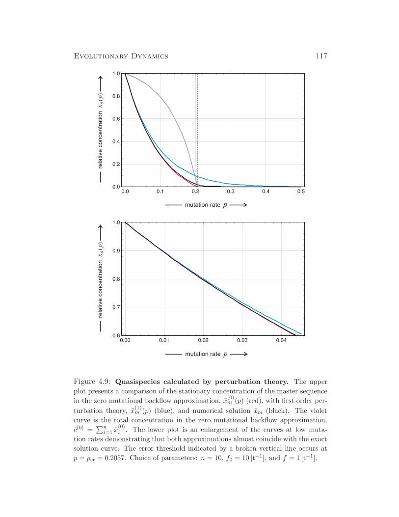
Evolutionary Dynamics 117
mutation rate p
rela
tive c
oncentr
ation
()
x0
p
mutation rate p
rela
tive
co
nce
ntr
atio
n(
)x
0p
Figure 4.9: Quasispecies calculated by perturbation theory. The upper
plot presents a comparison of the stationary concentration of the master sequence
in the zero mutational backflow approximation, x(0)m (p) (red), with first order per-
turbation theory, x(1)m (p) (blue), and numerical solution xm (black). The violet
curve is the total concentration in the zero mutational backflow approximation,
c(0) =∑n
i=1 x(0)i . The lower plot is an enlargement of the curves at low muta-
tion rates demonstrating that both approximations almost coincide with the exact
solution curve. The error threshold indicated by a broken vertical line occurs at
p = pcr = 0.2057. Choice of parameters: n = 10, f0 = 10 [t−1], and f = 1 [t−1].
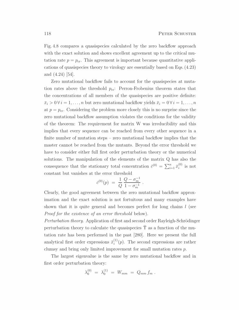
118 Peter Schuster
Fig. 4.8 compares a quasispecies calculated by the zero backflow approach
with the exact solution and shows excellent agreement up to the critical mu-
tation rate p = pcr. This agreement is important because quantitative appli-
cations of quasispecies theory to virology are essentially based on Eqs. (4.23)
and (4.24) [54].
Zero mutational backflow fails to account for the quasispecies at muta-
tion rates above the threshold pcr: Perron-Frobenius theorem states that
the concentrations of all members of the quasispecies are positive definite:
xi > 0 ∀ i = 1, . . . , n but zero mutational backflow yields xi = 0 ∀ i = 1, . . . , n
at p = pcr. Considering the problem more closely this is no surprise since the
zero mutational backflow assumption violates the conditions for the validity
of the theorem: The requirement for matrix W was irreducibility and this
implies that every sequence can be reached from every other sequence in a
finite number of mutation steps – zero mutational backflow implies that the
master cannot be reached from the mutants. Beyond the error threshold we
have to consider either full first order perturbation theory or the numerical
solutions. The manipulation of the elements of the matrix Q has also the
consequence that the stationary total concentration c(0) =∑n
i=1 x(0)i is not
constant but vanishes at the error threshold
c(0)(p) =1
Q
Q− σ−1m
1− σ−1m
.
Clearly, the good agreement between the zero mutational backflow approx-
imation and the exact solution is not fortuitous and many examples have
shown that it is quite general and becomes perfect for long chains l (see
Proof for the existence of an error threshold below).
Perturbation theory. Application of first and second order Rayleigh-Schrodinger
perturbation theory to calculate the quasispecies Υ as a function of the mu-
tation rate has been performed in the past [280]. Here we present the full
analytical first order expressions x(1)i (p). The second expressions are rather
clumsy and bring only limited improvement for small mutation rates p.
The largest eigenvalue is the same by zero mutational backflow and in
first order perturbation theory:
λ(0)0 = λ
(1)0 = Wmm = Qmm fm .
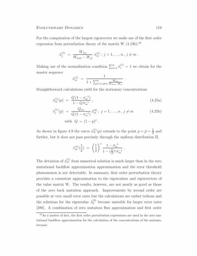
Evolutionary Dynamics 119
For the computation of the largest eigenvector we make use of the first order
expression from perturbation theory of the matrix W (4.19b):18
x(1)j =
Wjm
Wmm −Wjjx(1)m ; j = 1, . . . , n , j 6= m .
Making use of the normalization condition∑n
i=1 x(1)i = 1 we obtain for the
master sequence
x(1)m =1
1 +∑n
i=1,i 6=mWim
Wmm−Wii
.
Straightforward calculations yield for the stationary concentrations
x(1)m (p) =Q (1− σ−1m )
1−Qσ−1m
, (4.25a)
x(1)j (p) =
Qim
Q (1− σ−1m )x(0)m ; j = 1, . . . , n , j 6= m (4.25b)
with Q = (1− p)ν .
As shown in figure 4.9 the curve x(1)m (p) extends to the point p = p = 1
2 and
further, but it does not pass precisely through the uniform distribution Π,
x(1)m (1
2) =
(
1
2
)ν1− σ−1m
1− (12)νσ−1m
.
The deviation of x(1)m from numerical solution is much larger than in the zero
mutational backflow approximation approximation and the error threshold
phenomenon is not detectable. In summary, first order perturbation theory
provides a consistent approximation to the eigenvalues and eigenvectors of
the value matrix W. The results, however, are not nearly as good as those
of the zero back mutation approach. Improvements by second order are
possible at very small error rates but the calculations are rather tedious and
the solutions for the eigenvalue λ(2)0 become unstable for larger error rates
[280]. A combination of zero mutation flux approximation and first order
18As a matter of fact, the first order perturbation expressions are used in the zero mu-
tational backflow approximation for the calculation of the concentrations of the mutants,
because
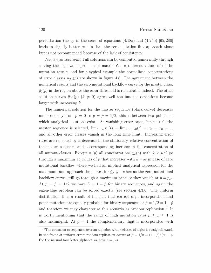
120 Peter Schuster
perturbation theory in the sense of equations (4.18a) and (4.25b) [65, 280]
leads to slightly better results than the zero mutation flux approach alone
but is not recommended because of the lack of consistency.
Numerical solutions. Full solutions can be computed numerically through
solving the eigenvalue problem of matrix W for different values of of the
mutation rate p, and for a typical example the normalized concentrations
of error classes y(k)(p) are shown in figure 4.8. The agreement between the
numerical results and the zero mutational backflow curve for the master class,
y0(p) in the region above the error threshold is remarkable indeed. The other
solution curves y(k)(p) (k 6= 0) agree well too but the deviations become
larger with increasing k.
The numerical solution for the master sequence (black curve) decreases
monotonously from p = 0 to p = p = 1/2, this is between two points for
which analytical solutions exist. At vanishing error rates, lim p → 0, the
master sequence is selected, limt→∞ x0(t) = limt→∞ y0(t) = y0 = x0 = 1,
and all other error classes vanish in the long time limit. Increasing error
rates are reflected by a decrease in the stationary relative concentration of
the master sequence and a corresponding increase in the concentration of
all mutant classes. Except y0(p) all concentrations yk(p) with k < ν/2 go
through a maximum at values of p that increases with k – as in case of zero
mutational backflow where we had an implicit analytical expression for the
maximum, and approach the curves for yν−k – whereas the zero mutational
backflow curves still go through a maximum because they vanish at p = pcr.
At p = p = 1/2 we have p = 1 − p for binary sequences, and again the
eigenvalue problem can be solved exactly (see section 4.3.6. The uniform
distribution Π is a result of the fact that correct digit incorporation and
point mutation are equally probable for binary sequences at p = 1/2 = 1− pand therefore we may characterize this scenario as random replication.19 It
is worth mentioning that the range of high mutation rates p ≤ p ≤ 1 is
also meaningful: At p = 1 the complementary digit is incorporated with
19The extension to sequences over an alphabet with κ classes of digits is straightforward.
In the frame of uniform errors random replication occurs at p = 1/κ = (1 − p)/(κ − 1).
For the natural four letter alphabet we have p = 1/4.
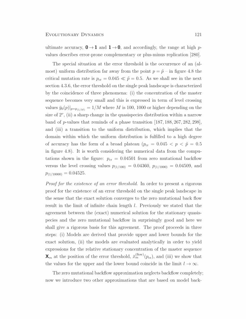
Evolutionary Dynamics 121
ultimate accuracy, 0→ 1 and 1→ 0, and accordingly, the range at high p-
values describes error-prone complementary or plus-minus replication [280].
The special situation at the error threshold is the occurrence of an (al-
most) uniform distribution far away from the point p = p – in figure 4.8 the
critical mutation rate is pcr = 0.045 ≪ p = 0.5. As we shall see in the next
section 4.3.6, the error threshold on the single peak landscape is characterized
by the coincidence of three phenomena: (i) the concentration of the master
sequence becomes very small and this is expressed in term of level crossing
values y0(p)|p=p(1/M)= 1/M whereM is 100, 1000 or higher depending on the
size of 2ν , (ii) a sharp change in the quasispecies distribution within a narrow
band of p-values that reminds of a phase transition [187, 188, 267, 282, 298],
and (iii) a transition to the uniform distribution, which implies that the
domain within which the uniform distribution is fulfilled to a high degree
of accuracy has the form of a broad plateau (pcr = 0.045 < p < p = 0.5
in figure 4.8). It is worth considering the numerical data from the compu-
tations shown in the figure: pcr = 0.04501 from zero mutational backflow
versus the level crossing values p(1/100) = 0.04360, p(1/1000) = 0.04509, and
p(1/10000) = 0.04525.
Proof for the existence of an error threshold. In order to present a rigorous
proof for the existence of an error threshold on the single peak landscape in
the sense that the exact solution converges to the zero mutational back flow
result in the limit of infinite chain length l. Previously we stated that the
agreement between the (exact) numerical solution for the stationary quasis-
pecies and the zero mutational backflow in surprisingly good and here we
shall give a rigorous basis for this agreement. The proof proceeds in three
steps: (i) Models are derived that provide upper and lower bounds for the
exact solution, (ii) the models are evaluated analytically in order to yield
expressions for the relative stationary concentration of the master sequence
Xm at the position of the error threshold, x(flow)m (pcr), and (iii) we show that
the values for the upper and the lower bound coincide in the limit l →∞.
The zero mutational backflow approximation neglects backflow completely;
now we introduce two other approximations that are based on model back-
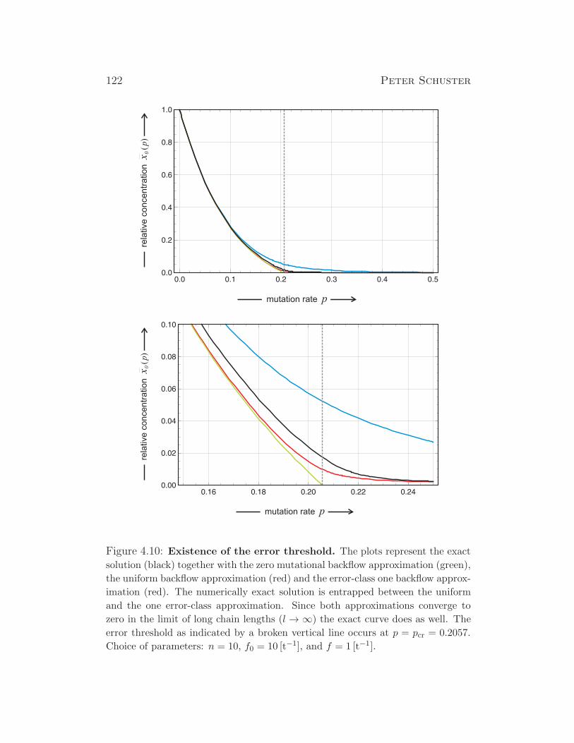
122 Peter Schuster
Figure 4.10: Existence of the error threshold. The plots represent the exact
solution (black) together with the zero mutational backflow approximation (green),
the uniform backflow approximation (red) and the error-class one backflow approx-
imation (red). The numerically exact solution is entrapped between the uniform
and the one error-class approximation. Since both approximations converge to
zero in the limit of long chain lengths (l →∞) the exact curve does as well. The
error threshold as indicated by a broken vertical line occurs at p = pcr = 0.2057.
Choice of parameters: n = 10, f0 = 10 [t−1], and f = 1 [t−1].
Evolutionary Dynamics 123
flows that represent lower and upper bounds for the exact backflow. Com-
putation of the mutational backflow requires either knowledge of the distri-
bution of concentrations of all sequence of an assumption about it. In order
to be able to handle the problem analytically the backflow must lead to an
autonomous equation for the master concentration x0. The minimal back-
flow can be estimated by the assumption of a uniform distribution (Π) for
all sequences except the master. In this case all sequences contribute equally
no matter whether a particular sequence is close to the master sequences or
far apart. For the concentrations xi = (1 − x(Π)0 )/(n− 1) ∀ i = 1, . . . , n with
n = κl we obtain under the further assumption of a single peak landscape
and the uniform error rate model the ODE for x(Π)0 :
dx(Π)0
dt= x
(Π)0 (Q00f0 − φ) + f
1− x(Π)0
n− 1(4.26)
with φ = f + (f0 − f) x(Π)0
The stationary concentration is obtained as the solution of a quadratic equa-
tion
x(Π)0 =
Qf0 − f − fγ(1−Q) +
√
(
Qf0 − f − fγ(1−Q))2
+ 4(f0 − f)(1−Q)fγ
2(f0 − f)
with Q = Q00 = (1− p)l and γ =1
n− 1
Insertion of the value of the mutation rate parameter at the error threshold, p =
pcr = 1− σ−1/l or Q = (1− pcr)l = σ−1 leads to the result
x(Π)0 (pcr) =
1
2
√
1 + 4σ(n − 1) − 1
σ(n− 1), (4.27)
which yields in the limit of long chains or large l-values
x(Π)0 (pcr) ≈
1√σ n
=1√σ κl
. (4.27’)
Ultimately the value of the stationary concentration of the master sequence decays
exponentially with one halt of the chain lengths as exponent: x(Π)0 (pcr) ∝ κ−l/2.
It is straightforward to show that the uniform mutational backflow approximation
becomes exact at the point p = p and insertion in the quadratic equation yields:
124 Peter Schuster
x(Π)0 (12) =
(12)l. Generalization, of course, is straightforward and yields p = p and
insertion in the quadratic equation yields: x(Π)0 (1/κ) =
(
1/κ)l
In order to find an upper bound for the stationary solution of the master se-
quence we assume that mutational backflow comes only form the sequences in the
one error class, Γ(0)1 , which can be assumed to be present at equal concentrations,
xi = (1 − x(I)0 )/l, and
∑li=1 xi = 1 − x0. All other sequences except the master
sequence and the one error class are absent. Pointing at the fact that Γ(0)1 rep-
resents the entire mutant cloud we shall denote this distribution by I. For the
corresponding elements of the mutation matrix Q we use the usual expressions,
which are all equal: Q0i = Q0(1) = Q01 ∀ i = 1, . . . , l. The ODE for the master
sequence is then again autonomous and can be readily solved for the stationary
state:
dx(I)0
dt= x
(I)0 (Q00f0 − φ) + Q01 f (1− x
(I)0 ) (4.28)
with φ = f + (f0 − f)x(I)0 .
The stationary concentration is again obtained from a quadratic equation of similar
structure as before
x(I)0 =
Q00f0 −Q01f − f +
√
(
Q00f0 −Q01f − f)2
+ 4(f0 − f)Q01f
2(f0 − f)
with Q00 = (1− p)l and Q01 = (1− p)l−1 p .
It is shown straightforwardly that the curve for the class one backflow passes
through the point p = p = κ−l. For the stationary concentration of the master
sequence at the error threshold we find
x(I)0 (pcr) = − Q01 f
2 (f0 − f)+
√
Q01 f
f0 − f·√
1 +Q01 f
4 (f0 − f), (4.29)
with three components. Before we can discuss the individual terms we have to
examine the asymptotic dependence of the mutation rate p on the chain length l,
which is encapsulated in the series expansion
Q01 = (1− p)l−1 p = p − (l − 1) p2 +(l − 1)(l − 2)
2p3 − · · ·
with the first term being p. The critical mutation rate can be approximated by
pcr ≈ lnσ/l and we can consider Equ. (4.29). The negative term in equation shows
Evolutionary Dynamics 125
Table 4.1: Proof of the error threshold. Two auxiliary model assumptions
concerning mutational backflow are applied: (i) uniform distribution for all one
error mutants, called class one uniform, and (ii) the uniform distribution Π for all
sequences except the master sequence denoted as all uniform. All solution curves
x0(p) – exact and approximate – begin at the value x0(0) = 1 and all except the
zero backflow approximation end at the point x(p) = x(κ−1) = 1/κl
x0-value at the mutation rate
mutational backflow notation p = 0 p = pcr p = 1κ
class one uniform x(I)0 (p) 1
√
ln σ/(σ − 1) · 1/√
l κ−l
exact x0(p) 1 computed κ−l
all uniform x(Π)0 (p) 1 1/
√
σκl κ−l
zero x(0)0 (p) 1 0 negative
an asymptotic dependence on the chain length of l−1, the first factor behaves
asymptotically like 1/√l whereas the second factor converges to unity. What
remains in the limit of long chains or large l-values is
x(I)0 (pcr) ≈
√
f lnσ
f0 − f· 1√
l=
√
lnσ
σ − 1· 1√
l. (4.29’)
The value of the stationary concentration of the master sequence decays with the
reciprocal square root of the chain length: x(I)0 (pcr) ∝ 1/
√l. Although the class
one uniform distribution is not an impressively good upper bound for the exact
solution curve, it is sufficient for our purpose here because x(I)0 (pcr) vanishes in the
limit l→∞.
In summary the solution curve of the mutation-selection equation (4.9) for
the master sequence and the three approximations at the critical mutation
rate pcr appear in the order shown in Tab. 4.1 and there is no reason to
doubt that the same order prevails for the entire domain 0 < p < p = κ−l:
The exact solution is indeed entrapped between the two approximations for
the mutational backflow and, since both converge asymptotically to zero the
exact curve approaches the zero mutational backflow approximation in the
limit of long chains. All four curves (Fig. 4.10) start at the point xm(0) and
all except the zero backflow approximation end at the correct value p = κ−l.
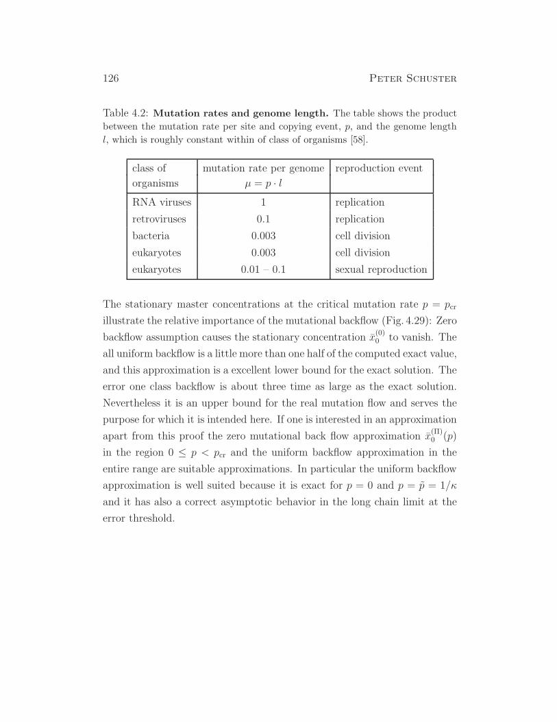
126 Peter Schuster
Table 4.2: Mutation rates and genome length. The table shows the product
between the mutation rate per site and copying event, p, and the genome length
l, which is roughly constant within of class of organisms [58].
class of mutation rate per genome reproduction event
organisms µ = p · lRNA viruses 1 replication
retroviruses 0.1 replication
bacteria 0.003 cell division
eukaryotes 0.003 cell division
eukaryotes 0.01 – 0.1 sexual reproduction
The stationary master concentrations at the critical mutation rate p = pcr
illustrate the relative importance of the mutational backflow (Fig. 4.29): Zero
backflow assumption causes the stationary concentration x(0)0 to vanish. The
all uniform backflow is a little more than one half of the computed exact value,
and this approximation is a excellent lower bound for the exact solution. The
error one class backflow is about three time as large as the exact solution.
Nevertheless it is an upper bound for the real mutation flow and serves the
purpose for which it is intended here. If one is interested in an approximation
apart from this proof the zero mutational back flow approximation x(Π)0 (p)
in the region 0 ≤ p < pcr and the uniform backflow approximation in the
entire range are suitable approximations. In particular the uniform backflow
approximation is well suited because it is exact for p = 0 and p = p = 1/κ
and it has also a correct asymptotic behavior in the long chain limit at the
error threshold.
Evolutionary Dynamics 127
Error thresholds and applications. The error threshold has been put in rela-
tion to phase transitions [187, 188, 282]. Here, we are in a position to prove
the behavior of the exact solution curve x0(p) in the limit l →∞. The critical
mutation rate converges to the value zero: liml→∞ pcr = liml→∞ ln σ/l = 0.
At the same time we have liml→∞ x0 = 0 for p > 0 and thus the quasispecies
degenerates to an “L”-shaped distribution, x0(0) = 1 and x0(p) = 0 ∀ p > 0,
and we are left with a pathological phase transition at pcr = 0.
According to Equ. (4.24) the error threshold defines a maximal error rate
for evolution, p ≤ pmax, at constant chain length l, and at constant reproduc-
tion accuracy p the length of faithfully copied polynucleotides is confined to
l ≤ lmax [70, 72]. The first limit of a maximal error rate pmax has been used
in pharmacology for the development of new antiviral strategies [56], and
the second limit entered hypothetical modeling of early biological evolution
where the accuracy limits of enzyme-free replication confine the lengths of
polynucleotides that can be replicated faithfully [73].
The error threshold relation (4.24) can be written in a different form that
allows for straightforward testing with empirical data:
µ = l p ≈ ln σ , (4.24’)
the product of the genome length and the mutation per site and replication,
µ, which represents the mean number of mutations per full genome repro-
duction, corresponds to the logarithm of the superiority. In a publication by
John Drake et al. the mutation rates µ were found to be remarkably con-
stant for organisms of the same class (table 4.2 and [58]). In other words, for
organisms within one class – viruses, retroviruses, bacteria, and eukaryotes
– the replication is more accurate if the genome is longer. A comparison
between the bacteriophage Qβand the vesicular stomatitis virus (SVS) may
serve as an example [57]: The genome lengths are 4 200 and 11 200 and the
mutation rates per site and replication are 1.5×10⁻³ and 3.8×10⁻⁴, respec-
tively. The large difference in reproduction accuracy between mitosis and
meiosis is remarkable.
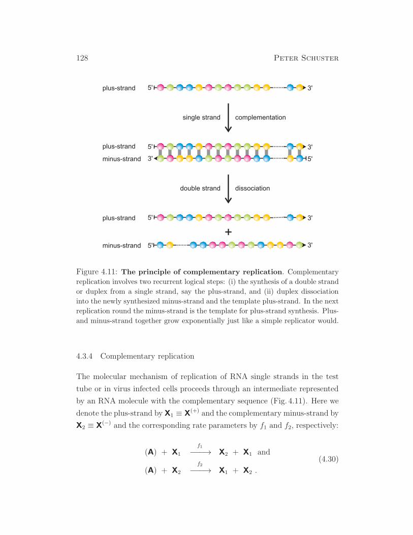
128 Peter Schuster
5' 3'plus-strand
5'
3'
3'
5'
plus-strand
minus-strand
5'
3'
3'
5'
+
plus-strand
minus-strand
single strand complementation
double strand dissociation
Figure 4.11: The principle of complementary replication. Complementary
replication involves two recurrent logical steps: (i) the synthesis of a double strand
or duplex from a single strand, say the plus-strand, and (ii) duplex dissociation
into the newly synthesized minus-strand and the template plus-strand. In the next
replication round the minus-strand is the template for plus-strand synthesis. Plus-
and minus-strand together grow exponentially just like a simple replicator would.
4.3.4 Complementary replication
The molecular mechanism of replication of RNA single strands in the test
tube or in virus infected cells proceeds through an intermediate represented
by an RNA molecule with the complementary sequence (Fig. 4.11). Here we
denote the plus-strand by X1 ≡ X(+) and the complementary minus-strand by
X2 ≡ X(−) and the corresponding rate parameters by f1 and f2, respectively:
(A) + X1
f1−−−→ X2 + X1 and
(A) + X2
f2−−−→ X1 + X2 .
(4.30)
Evolutionary Dynamics 129
In analogy to Equ. (4.8), with f1 = k1 [A], f2 = k2 [A], x1 = [X1], x2 = [X2],
and x1 + x2 = 1 we obtain the following differential equation [65, 70, 71]:
dx1dt
= f2x2 − x1 φ and
dx2dt
= f1x1 − x2 φ with φ = f1x1 + f2x2 .
(4.31)
Applying again the integrating factor transformation [329, p. 322ff.] yields
the linear equation
dz1dt
= f2z2 anddz2dt
= f1z1 ordz
dt= W ·z ; z =
(
z1
z2
)
, W =
(
0 f2
f1 0
)
.
The eigenvalues and (right hand) eigenvectors of the matrix W are
λ1,2 = ±√
f1f2 = ±f with f =√
f1f2 ,
b1 =
(√f2√f1
)
and b2 =
(
−√f2√f1
)
.(4.32)
Straightforward calculation yields analytical expressions for the two variables
(see paragraph mutation) with the initial concentrations x1(0) and x2(0),
and γ1(0) =√f1x1(0) +
√f2x2(0) and γ2(0) =
√f1x1(0) −
√f2x2(0) as
abbreviations:
x1(t) =
√f2(
γ1(0) · eft + γ2(0) · e−ft)
(√f1 +
√f2)γ1(0) · eft − (
√f1 −
√f2)γ2(0) · e−ft
x2(t) =
√f1(
γ1(0) · eft − γ2(0) · e−ft)
(√f1 +
√f2)γ1(0) · eft − (
√f1 −
√f2)γ2(0) · e−ft
.
(4.33)
After sufficiently long time the negative exponential has vanished and we
obtain the simple result
x1(t)→√
f2/(√
f1+√
f2) , x2(t)→√
f1/(√
f1+√
f2) as exp(−ft)→ 0 .
After an initial period, the plus-minus pair, the ensemble X1,2 ≡ X(±), grows
like a single replicator with a fitness value f =√f1f2 and a stationary ratio
of the concentrations of complementary stands x1/x2 ≈√f2/√f1. It is worth
noticing that the faster replicating strand is present at a lower equilibrium
concentration: x1√f2 = x2
√f1. By mass action it is guaranteed that the
ensemble grows at an optimal rate.

130 Peter Schuster
4.3.5 Quasispecies on ”simple” model landscapes
First we consider the general properties of a quasispecies distribution of bi-
nary sequences as a function of the mutation rate Υ(p). There are two
p-values for which we have exact analytical solutions: (i) error-free repli-
cation at p = 0, and (ii) random replication at p = 12 . The first case
is the selection scenario that we have discussed already in section 1.2: All
sequences except the master sequence vanish after sufficiently long time,
Υ(0) = (xm = 1, xj = 0 ∀ j 6= m).
For p = 12 the incorporation of the incorrect digits into the growing binary
string has exactly the same probability as the incorporation of the correct
digit, 1 − p = 12 , wrong and right digits are chosen at random and every
sequence has the same probability to be outcome of a replication event –
as easily visualized, the template plays no role. Accordingly, the mutation
matrix Q and the value matrix W are of the form:
Q =
(
1
2
)l
1 1 . . . 1
1 1 . . . 1...
.... . .
...
1 1 . . . 1
, W =
(
1
2
)l
f1 f2 . . . fn
f1 f2 . . . fn...
.... . .
...
f1 f2 . . . fn
.
Matrix W has only one nonzero eigenvalue λ0 = (12)l∑n
i=1 fi the number
of sequences n = 2l, and the corresponding eigenvector is the uniform dis-
tribution: Υ(12) = 2−l(1, 1, . . . , 1). Between these two limiting cases the
quasispecies fulfills∑n
i=1 xi = 1 and xi > 0 ∀ i by Perron-Frobenius theorem.
The influence of the landscape on the solution curves Υ(p) is thus restricted
to the way the transition from the homogeneous (p = 0) to the uniform
distribution occurs. We shall call the transition smooth when there is no
recognizable abrupt change in at some critical value of the mutation rate
parameter p = pcr (for an example see Fig. 4.12). A typical sharp transition
in Υ(p) from a structured distribution to the uniform distribution is shown
in Fig. 4.8: It occurs in a very narrow range of p around pcr, and pcr = 0.045
is far away from the random replication point (p = 12). Thus we have a wide
range of p-values where Υ(p) (almost) coincides with the uniform distribu-
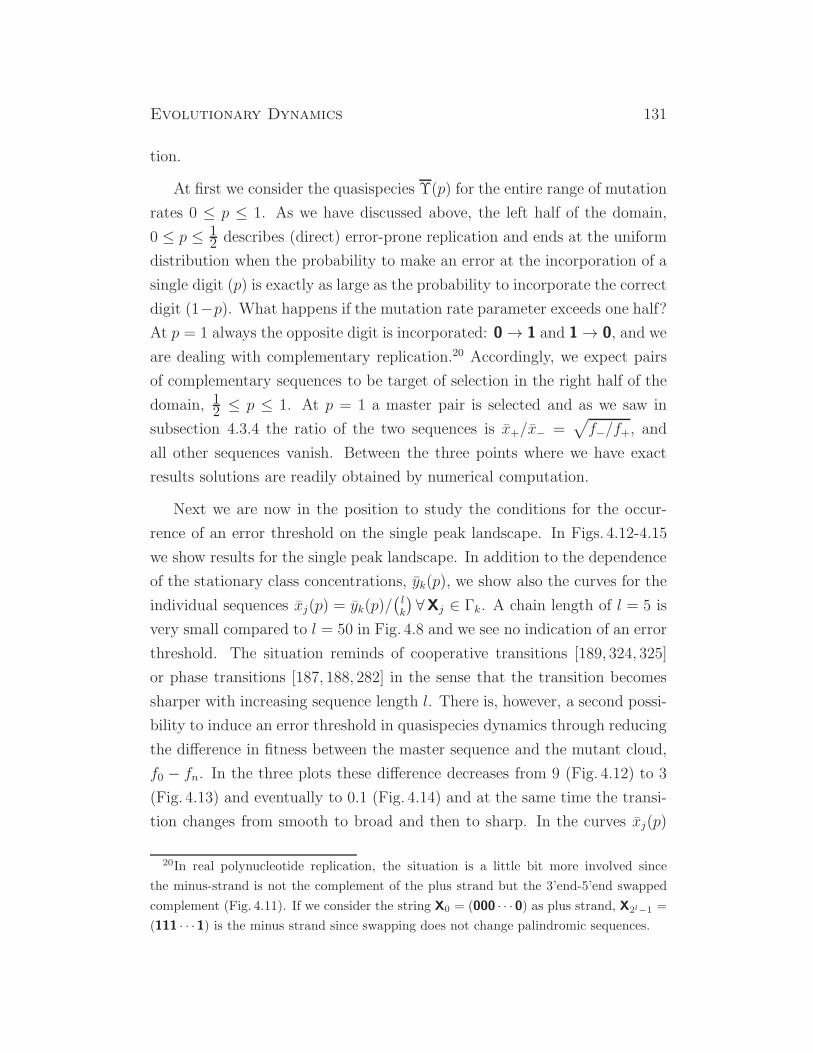
Evolutionary Dynamics 131
tion.
At first we consider the quasispecies Υ(p) for the entire range of mutation
rates 0 ≤ p ≤ 1. As we have discussed above, the left half of the domain,
0 ≤ p ≤ 12 describes (direct) error-prone replication and ends at the uniform
distribution when the probability to make an error at the incorporation of a
single digit (p) is exactly as large as the probability to incorporate the correct
digit (1−p). What happens if the mutation rate parameter exceeds one half?
At p = 1 always the opposite digit is incorporated: 0→ 1 and 1→ 0, and we
are dealing with complementary replication.20 Accordingly, we expect pairs
of complementary sequences to be target of selection in the right half of the
domain, 12 ≤ p ≤ 1. At p = 1 a master pair is selected and as we saw in
subsection 4.3.4 the ratio of the two sequences is x+/x− =√
f−/f+, and
all other sequences vanish. Between the three points where we have exact
results solutions are readily obtained by numerical computation.
Next we are now in the position to study the conditions for the occur-
rence of an error threshold on the single peak landscape. In Figs. 4.12-4.15
we show results for the single peak landscape. In addition to the dependence
of the stationary class concentrations, yk(p), we show also the curves for the
individual sequences xj(p) = yk(p)/(
lk
)
∀Xj ∈ Γk. A chain length of l = 5 is
very small compared to l = 50 in Fig. 4.8 and we see no indication of an error
threshold. The situation reminds of cooperative transitions [189, 324, 325]
or phase transitions [187, 188, 282] in the sense that the transition becomes
sharper with increasing sequence length l. There is, however, a second possi-
bility to induce an error threshold in quasispecies dynamics through reducing
the difference in fitness between the master sequence and the mutant cloud,
f0 − fn. In the three plots these difference decreases from 9 (Fig. 4.12) to 3
(Fig. 4.13) and eventually to 0.1 (Fig. 4.14) and at the same time the transi-
tion changes from smooth to broad and then to sharp. In the curves xj(p)
20In real polynucleotide replication, the situation is a little bit more involved since
the minus-strand is not the complement of the plus strand but the 3’end-5’end swapped
complement (Fig. 4.11). If we consider the string X0 = (000 · · · 0) as plus strand, X2l−1 =
(111 · · ·1) is the minus strand since swapping does not change palindromic sequences.
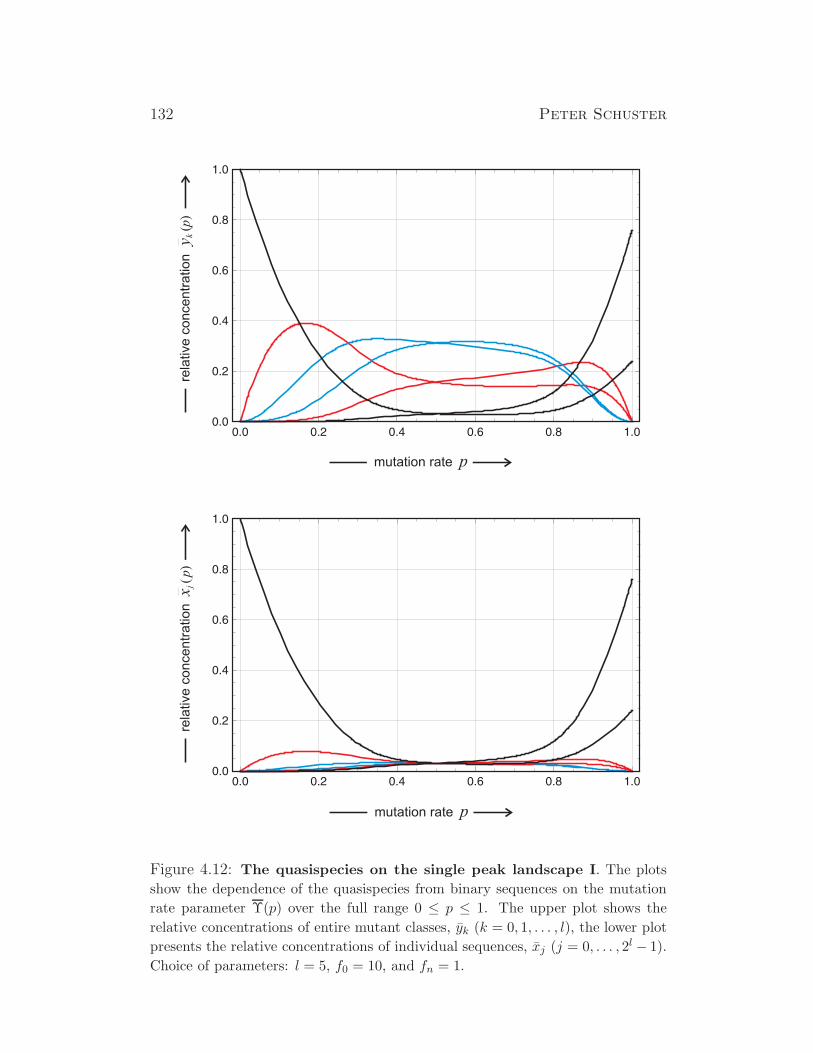
132 Peter Schuster
mutation rate p
rela
tive
co
nce
ntr
atio
n(
)y
kp
mutation rate p
rela
tive c
oncentr
ation
()
xj
p
Figure 4.12: The quasispecies on the single peak landscape I. The plots
show the dependence of the quasispecies from binary sequences on the mutation
rate parameter Υ(p) over the full range 0 ≤ p ≤ 1. The upper plot shows the
relative concentrations of entire mutant classes, yk (k = 0, 1, . . . , l), the lower plot
presents the relative concentrations of individual sequences, xj (j = 0, . . . , 2l − 1).
Choice of parameters: l = 5, f0 = 10, and fn = 1.
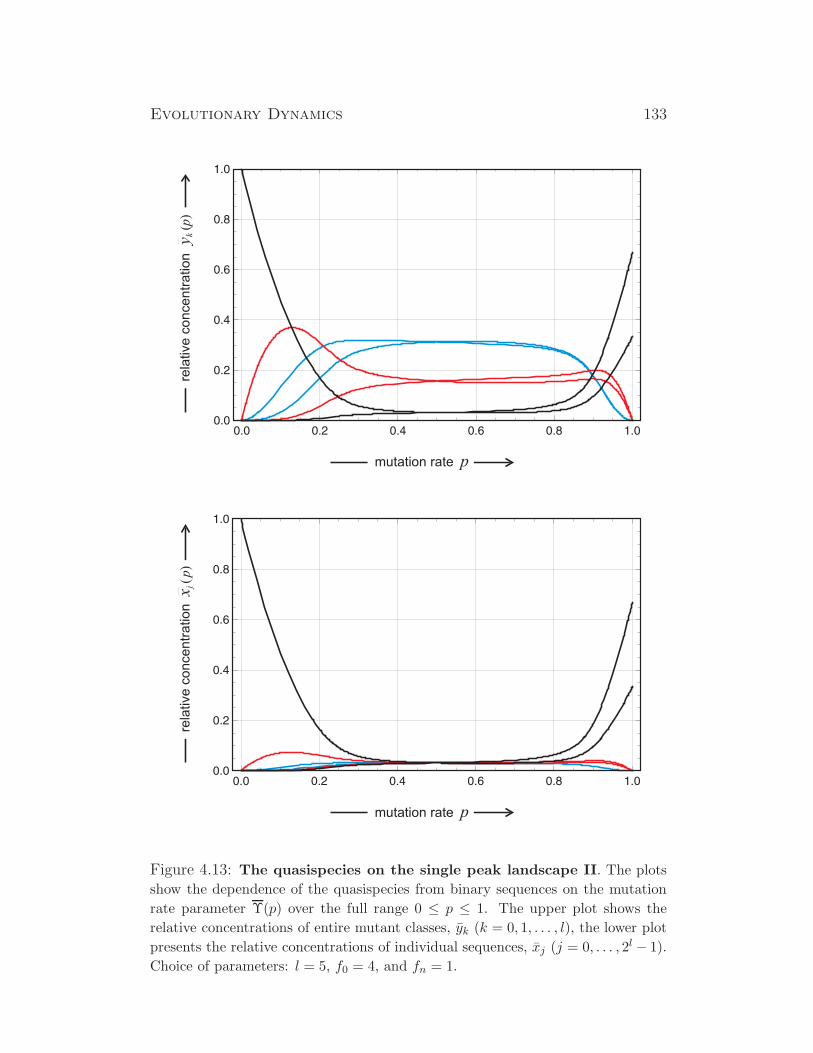
Evolutionary Dynamics 133
mutation rate p
rela
tive c
oncentr
ation
()
yk
p
mutation rate p
rela
tive c
oncentr
ation
()
xj
p
Figure 4.13: The quasispecies on the single peak landscape II. The plots
show the dependence of the quasispecies from binary sequences on the mutation
rate parameter Υ(p) over the full range 0 ≤ p ≤ 1. The upper plot shows the
relative concentrations of entire mutant classes, yk (k = 0, 1, . . . , l), the lower plot
presents the relative concentrations of individual sequences, xj (j = 0, . . . , 2l − 1).
Choice of parameters: l = 5, f0 = 4, and fn = 1.
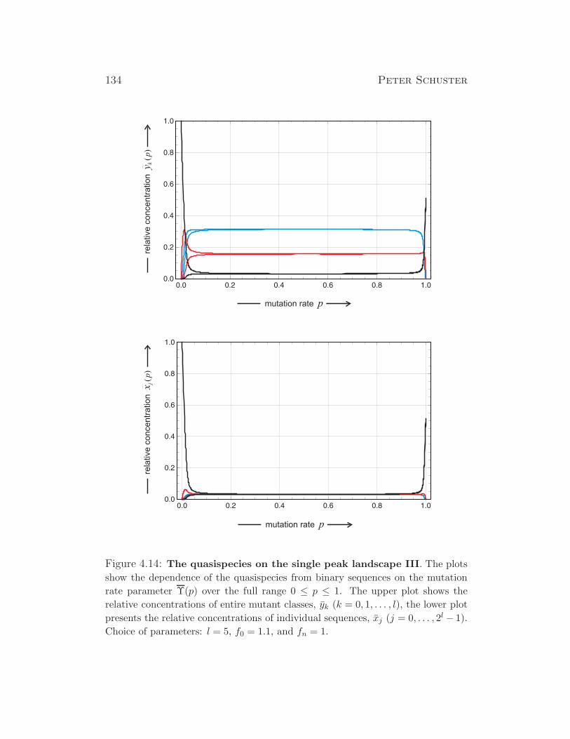
134 Peter Schuster
mutation rate p
rela
tive c
oncentr
ation
()
y kp
mutation rate p
rela
tive c
oncentr
ation
()
xj
p
Figure 4.14: The quasispecies on the single peak landscape III. The plots
show the dependence of the quasispecies from binary sequences on the mutation
rate parameter Υ(p) over the full range 0 ≤ p ≤ 1. The upper plot shows the
relative concentrations of entire mutant classes, yk (k = 0, 1, . . . , l), the lower plot
presents the relative concentrations of individual sequences, xj (j = 0, . . . , 2l − 1).
Choice of parameters: l = 5, f0 = 1.1, and fn = 1.
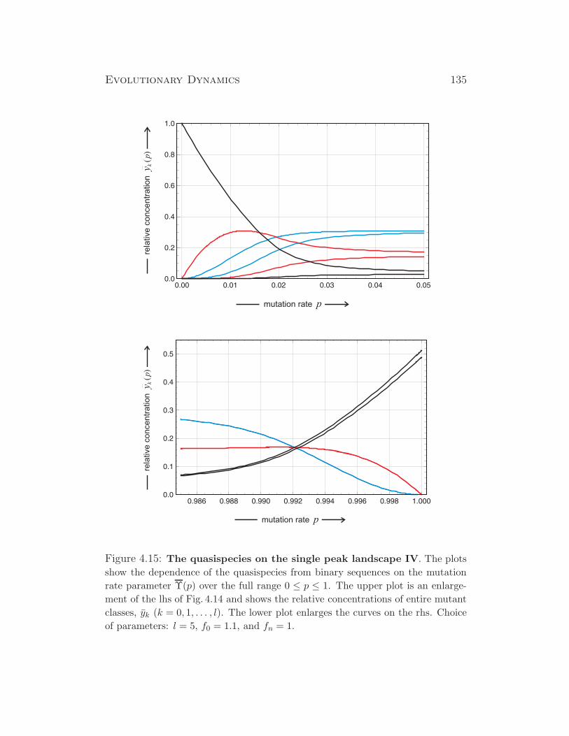
Evolutionary Dynamics 135
mutation rate p
rela
tive c
oncentr
ation
()
y kp
mutation rate p
rela
tive c
oncentr
ation
()
y kp
Figure 4.15: The quasispecies on the single peak landscape IV. The plots
show the dependence of the quasispecies from binary sequences on the mutation
rate parameter Υ(p) over the full range 0 ≤ p ≤ 1. The upper plot is an enlarge-
ment of the lhs of Fig. 4.14 and shows the relative concentrations of entire mutant
classes, yk (k = 0, 1, . . . , l). The lower plot enlarges the curves on the rhs. Choice
of parameters: l = 5, f0 = 1.1, and fn = 1.

136 Peter Schuster
mutation rate p
rela
tive
co
nce
ntr
atio
n(
)y
kp
mutation rate p
rela
tive c
oncentr
ation
()
xj
p
Figure 4.16: The quasispecies on the multiplicative landscape. The plots
show the dependence of the quasispecies from binary sequences on the muta-
tion rate parameter Υ(p) on the multiplicative landscape (3.4b). The upper plot
shows the relative concentrations of entire mutant classes, yk(p) (k = 0, 1, . . . , l),
the lower plot presents the relative concentrations of individual sequences, xj(p)
(j = 0, 1, 2, . . . , 2l − 1). Choice of parameters: l = 50, f0 = 10, fn = 1, and
ϕ = 1/(101/50).
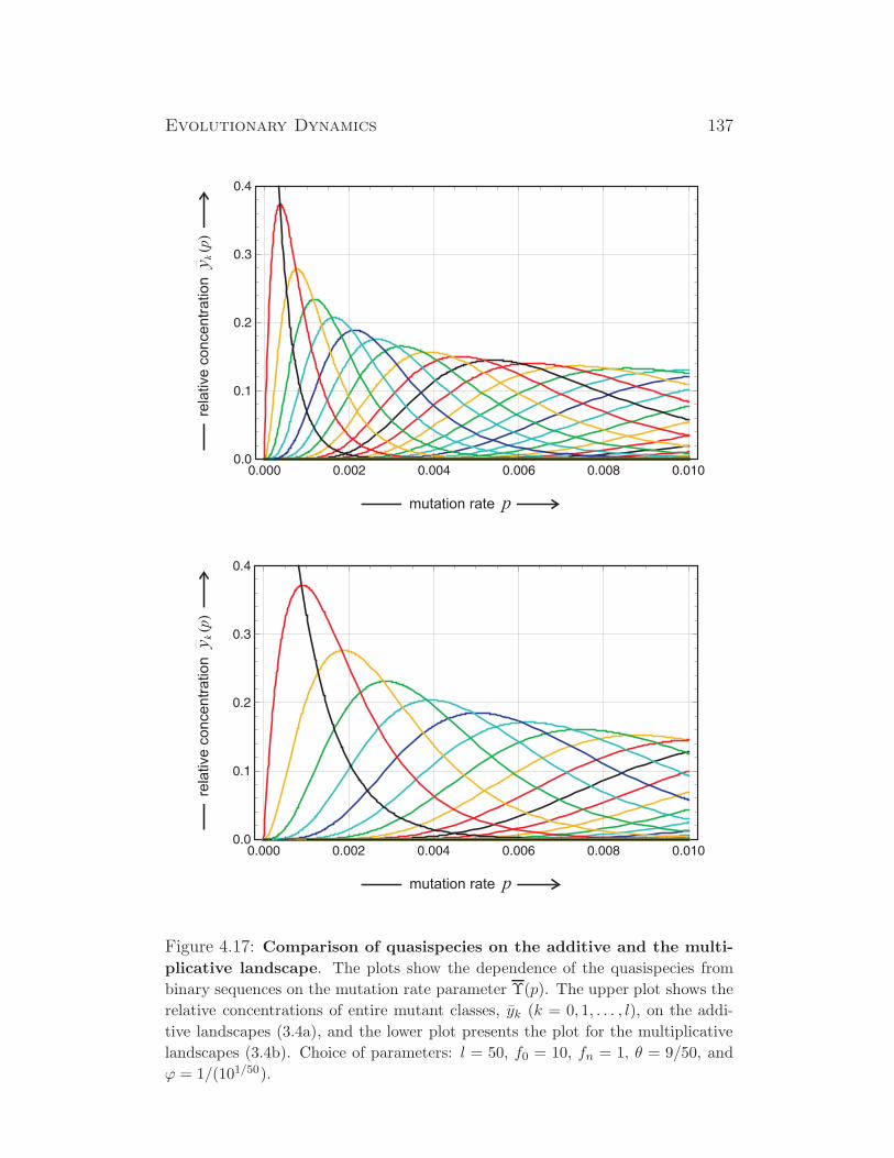
Evolutionary Dynamics 137
mutation rate p
rela
tive
co
nce
ntr
atio
n(
)y
kp
mutation rate p
rela
tive
co
nce
ntr
atio
n(
)y
kp
Figure 4.17: Comparison of quasispecies on the additive and the multi-
plicative landscape. The plots show the dependence of the quasispecies from
binary sequences on the mutation rate parameter Υ(p). The upper plot shows the
relative concentrations of entire mutant classes, yk (k = 0, 1, . . . , l), on the addi-
tive landscapes (3.4a), and the lower plot presents the plot for the multiplicative
landscapes (3.4b). Choice of parameters: l = 50, f0 = 10, fn = 1, θ = 9/50, and
ϕ = 1/(101/50).
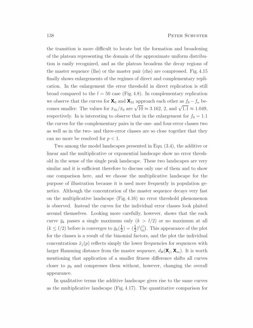
138 Peter Schuster
the transition is more difficult to locate but the formation and broadening
of the plateau representing the domain of the approximate uniform distribu-
tion is easily recognized, and as the plateau broadens the decay regions of
the master sequence (lhs) or the master pair (rhs) are compressed. Fig. 4.15
finally shows enlargements of the regimes of direct and complementary repli-
cation. In the enlargement the error threshold in direct replication is still
broad compared to the l = 50 case (Fig. 4.8). In complementary replication
we observe that the curves for X0 and X31 approach each other as f0−fn be-
comes smaller: The values for x31/x0 are√10 ≈ 3.162, 2, and
√1.1 ≈ 1.049,
respectively. In is interesting to observe that in the enlargement for f0 = 1.1
the curves for the complementary pairs in the one- and four-error classes two
as well as in the two- and three-error classes are so close together that they
can no more be resolved for p < 1.
Two among the model landscapes presented in Equ. (3.4), the additive or
linear and the multiplicative or exponential landscape show no error thresh-
old in the sense of the single peak landscape. These two landscapes are very
similar and it is sufficient therefore to discuss only one of them and to show
one comparison here, and we choose the multiplicative landscape for the
purpose of illustration because it is used more frequently in population ge-
netics. Although the concentration of the master sequence decays very fast
on the multiplicative landscape (Fig. 4.16) no error threshold phenomenon
is observed. Instead the curves for the individual error classes look plaited
around themselves. Looking more carefully, however, shows that the each
curve yk passes a single maximum only (k > l/2) or no maximum at all
(k ≤ l/2) before is converges to yk(12) = (12)
l(
lk
)
. This appearance of the plot
for the classes is a result of the binomial factors, and the plot the individual
concentrations xj(p) reflects simply the lower frequencies for sequences with
larger Hamming distance from the master sequence, dH(Xj,Xm). It is worth
mentioning that application of a smaller fitness difference shifts all curves
closer to p0 and compresses them without, however, changing the overall
appearance.
In qualitative terms the additive landscape gives rise to the same curves
as the multiplicative landscape (Fig. 4.17). The quantitative comparison for
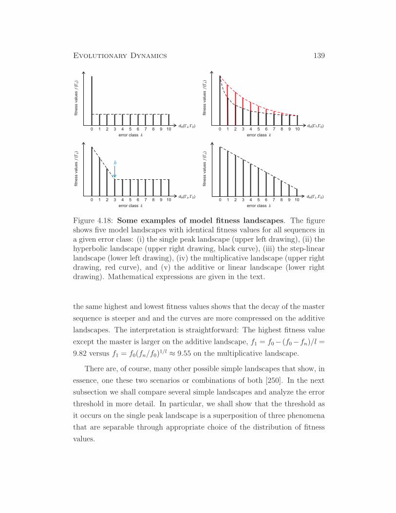
Evolutionary Dynamics 139
fitn
ess v
alu
es
()
fG
k
error class k
dH 0( , )G Gk0 1 2 3 4 5 6 7 8 9 10 0 1 2 3 4 5 6 7 8 9 10
fitn
ess v
alu
es
()
fG
k
error class k
dH 0( , )G Gk
0 1 2 3 4 5 6 7 8 9 10
fitn
ess v
alu
es
()
fG
k
error class k
dH 0( , )G Gk
h
0 1 2 3 4 5 6 7 8 9 10fitn
ess v
alu
es
()
fG
kerror class k
dH 0( , )G Gk
Figure 4.18: Some examples of model fitness landscapes. The figureshows five model landscapes with identical fitness values for all sequences ina given error class: (i) the single peak landscape (upper left drawing), (ii) thehyperbolic landscape (upper right drawing, black curve), (iii) the step-linearlandscape (lower left drawing), (iv) the multiplicative landscape (upper rightdrawing, red curve), and (v) the additive or linear landscape (lower rightdrawing). Mathematical expressions are given in the text.
the same highest and lowest fitness values shows that the decay of the master
sequence is steeper and and the curves are more compressed on the additive
landscapes. The interpretation is straightforward: The highest fitness value
except the master is larger on the additive landscape, f1 = f0− (f0−fn)/l =9.82 versus f1 = f0(fn/f0)
1/l ≈ 9.55 on the multiplicative landscape.
There are, of course, many other possible simple landscapes that show, in
essence, one these two scenarios or combinations of both [250]. In the next
subsection we shall compare several simple landscapes and analyze the error
threshold in more detail. In particular, we shall show that the threshold as
it occurs on the single peak landscape is a superposition of three phenomena
that are separable through appropriate choice of the distribution of fitness
values.
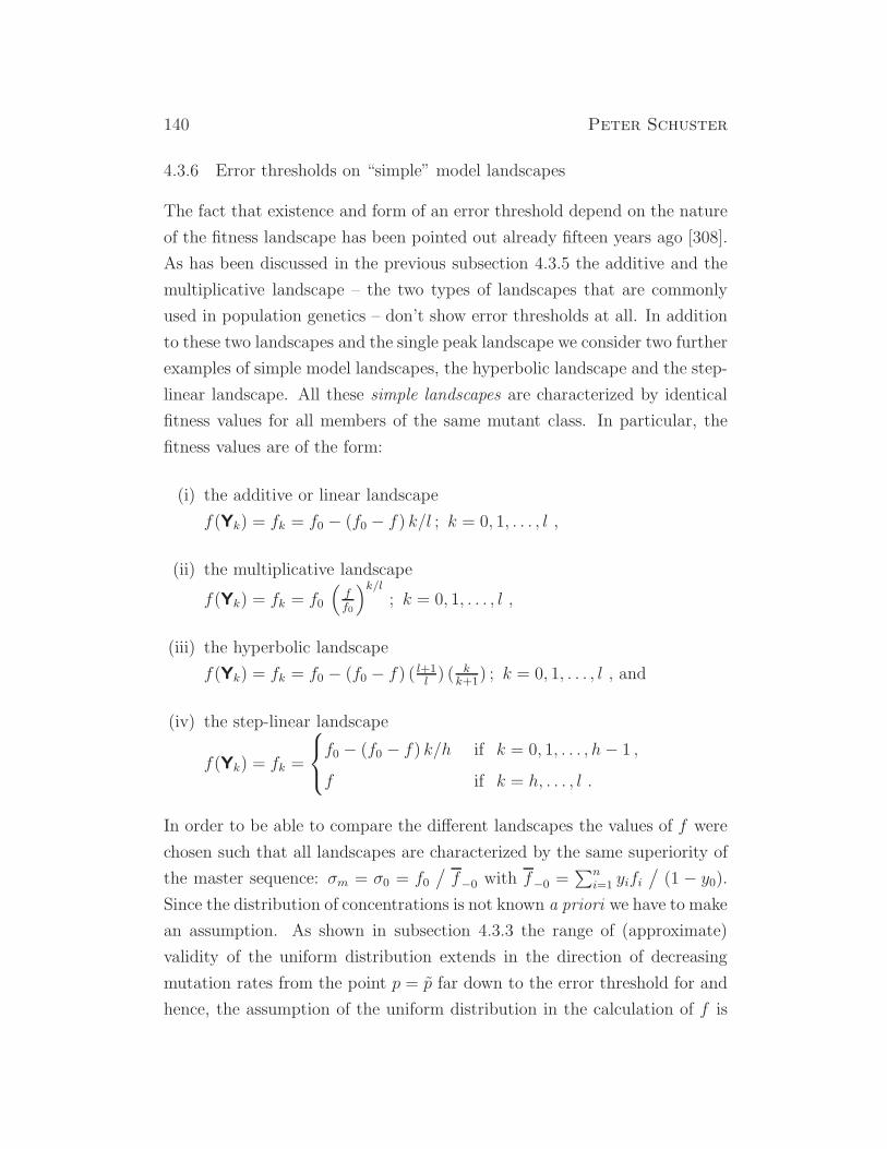
140 Peter Schuster
4.3.6 Error thresholds on “simple” model landscapes
The fact that existence and form of an error threshold depend on the nature
of the fitness landscape has been pointed out already fifteen years ago [308].
As has been discussed in the previous subsection 4.3.5 the additive and the
multiplicative landscape – the two types of landscapes that are commonly
used in population genetics – don’t show error thresholds at all. In addition
to these two landscapes and the single peak landscape we consider two further
examples of simple model landscapes, the hyperbolic landscape and the step-
linear landscape. All these simple landscapes are characterized by identical
fitness values for all members of the same mutant class. In particular, the
fitness values are of the form:
(i) the additive or linear landscape
f(Yk) = fk = f0 − (f0 − f) k/l ; k = 0, 1, . . . , l ,
(ii) the multiplicative landscape
f(Yk) = fk = f0
(
ff0
)k/l
; k = 0, 1, . . . , l ,
(iii) the hyperbolic landscape
f(Yk) = fk = f0 − (f0 − f) ( l+1l) ( k
k+1) ; k = 0, 1, . . . , l , and
(iv) the step-linear landscape
f(Yk) = fk =
f0 − (f0 − f) k/h if k = 0, 1, . . . , h− 1 ,
f if k = h, . . . , l .
In order to be able to compare the different landscapes the values of f were
chosen such that all landscapes are characterized by the same superiority of
the master sequence: σm = σ0 = f0/
f−0 with f−0 =∑n
i=1 yifi/
(1 − y0).Since the distribution of concentrations is not known a priori we have to make
an assumption. As shown in subsection 4.3.3 the range of (approximate)
validity of the uniform distribution extends in the direction of decreasing
mutation rates from the point p = p far down to the error threshold for and
hence, the assumption of the uniform distribution in the calculation of f is
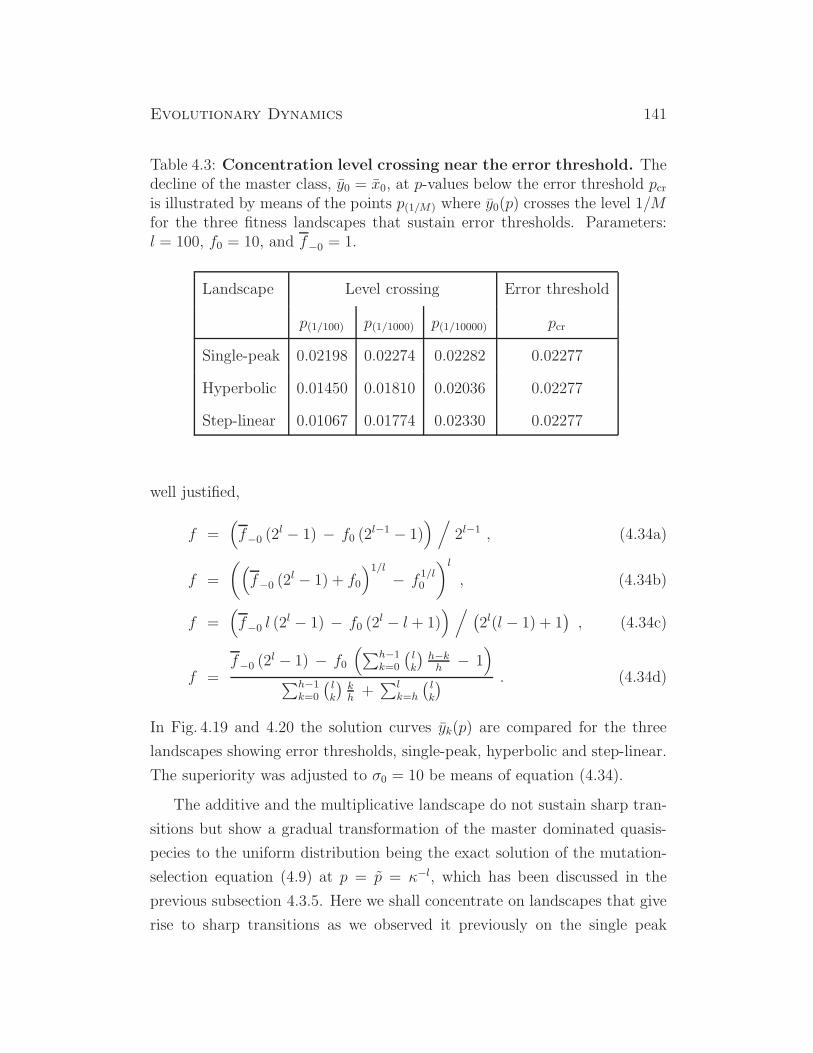
Evolutionary Dynamics 141
Table 4.3: Concentration level crossing near the error threshold. Thedecline of the master class, y0 = x0, at p-values below the error threshold pcris illustrated by means of the points p(1/M) where y0(p) crosses the level 1/Mfor the three fitness landscapes that sustain error thresholds. Parameters:l = 100, f0 = 10, and f−0 = 1.
Landscape Level crossing Error threshold
p(1/100) p(1/1000) p(1/10000) pcr
Single-peak 0.02198 0.02274 0.02282 0.02277
Hyperbolic 0.01450 0.01810 0.02036 0.02277
Step-linear 0.01067 0.01774 0.02330 0.02277
well justified,
f =(
f−0 (2l − 1) − f0 (2
l−1 − 1)) /
2l−1 , (4.34a)
f =
(
(
f−0 (2l − 1) + f0
)1/l
− f1/l0
)l
, (4.34b)
f =(
f−0 l (2l − 1) − f0 (2
l − l + 1)) /
(
2l(l − 1) + 1)
, (4.34c)
f =f−0 (2
l − 1) − f0
(
∑h−1k=0
(
lk
)
h−kh− 1
)
∑h−1k=0
(
lk
)
kh+∑l
k=h
(
lk
) . (4.34d)
In Fig. 4.19 and 4.20 the solution curves yk(p) are compared for the three
landscapes showing error thresholds, single-peak, hyperbolic and step-linear.
The superiority was adjusted to σ0 = 10 be means of equation (4.34).
The additive and the multiplicative landscape do not sustain sharp tran-
sitions but show a gradual transformation of the master dominated quasis-
pecies to the uniform distribution being the exact solution of the mutation-
selection equation (4.9) at p = p = κ−l, which has been discussed in the
previous subsection 4.3.5. Here we shall concentrate on landscapes that give
rise to sharp transitions as we observed it previously on the single peak
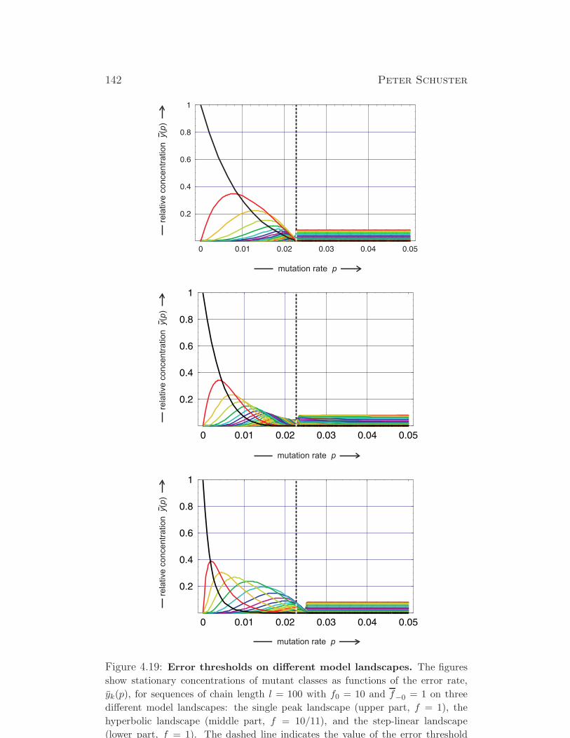
142 Peter Schuster
Figure 4.19: Error thresholds on different model landscapes. The figures
show stationary concentrations of mutant classes as functions of the error rate,
yk(p), for sequences of chain length l = 100 with f0 = 10 and f−0 = 1 on three
different model landscapes: the single peak landscape (upper part, f = 1), the
hyperbolic landscape (middle part, f = 10/11), and the step-linear landscape
(lower part, f = 1). The dashed line indicates the value of the error threshold
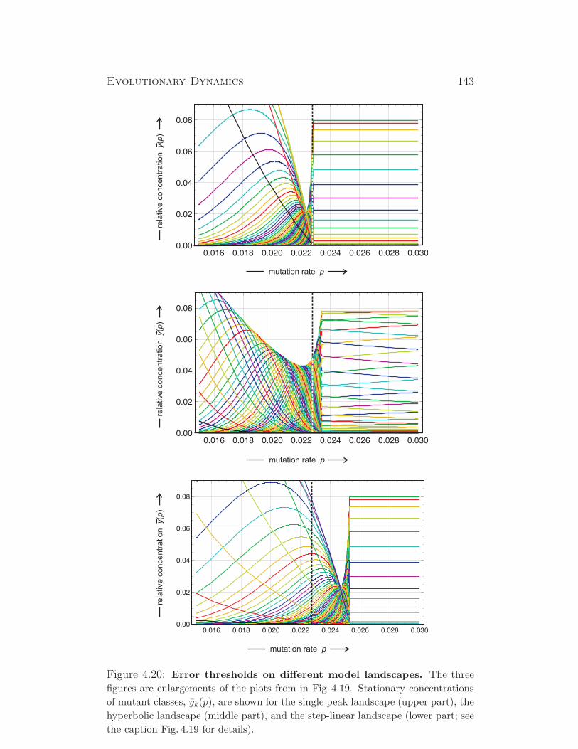
Evolutionary Dynamics 143
Figure 4.20: Error thresholds on different model landscapes. The three
figures are enlargements of the plots from in Fig. 4.19. Stationary concentrations
of mutant classes, yk(p), are shown for the single peak landscape (upper part), the
hyperbolic landscape (middle part), and the step-linear landscape (lower part; see
the caption Fig. 4.19 for details).
144 Peter Schuster
landscape. The three examples chosen differ in the way the fitness function
changes with k the index of the mutant class (Γk): (i) the “L” shaped single
peak landscape, (ii) the hyperbolic landscape that shows fast steep but at the
same gradual decay of the fitness with k, and (iii) the step-linear landscape
that combines features of the linear and the single peak landscape – linear
decay of fitness values and completely flat part.
As already shown in Fig. 4.8 and analyzed in the proof for the occurrence
of the threshold (Tab. 4.1) the calculated value for pcr coincides perfectly
with the position of the transition on the single-peak landscape, and the
p-values for concentration level crossing lie close together and near pcr (see
table 4.3) indicating a rather steep decrease of y0 in the range on the left-
hand side of the transition to the uniform distribution. Comparison with
the other two landscapes shows that the error threshold phenomenon can be
separated into three different features, which happen to coincide on the single
peak landscape: (i) fast decay of the concentration of the master sequence
x0(p) in the range 0 ≤ p ≤ pcr, (ii) a sharp transition to another sequence
distribution and (iii) an extension of the solution at point p = p towards
smaller mutation rates that gives rise to a broad domain pcr < p < p within
which the quasispecies is very close to the uniform distribution.
On the hyperbolic landscape, the actual transition occurs slightly above
the error threshold of the single-peak landscape, the decrease of y0 is flatter,
and the transition also sharp does not result in the uniform distribution.
Instead we observe a mutant distribution above the error threshold, which
changes slightly with p.The interpretation is straightforward: A flat part of
the landscape in required for the expansion of the unform distribution and
such a flat part does not exist on the hyperbolic landscape, and therefore we
observe a gradually changing flat distribution. On the step-linear landscape,
eventually, the curve of y0 is even flatter, the transition is shifted further
to higher p-values, but the transition leads to the uniform distribution as
in the single-peak case. Knowing the behavior of the quasispecies on the
single-peak and the linear landscape an interpretation of the observed plots
for the step-linear landscape is straightforward: In the range of small Ham-
ming distances from the master sequence the fitness landscape has the same
Evolutionary Dynamics 145
shape as the linear landscape and for small mutation rates the quasispecies
is dominated by sequences, which are near the master in sequence space,
at higher mutation rates p sequences that are further away from the mas-
ter gain importance, and indeed we observe a similarity of the quasispecies
with that on the linear landscape at small p-values whereas an error thresh-
old and the uniform distribution beyond it are observed at higher mutation
rates p. In the step-linear landscape the position of the step, h can be varied
as well. For the parameters f0 = 10 and f = 1 we observe error thresholds
in the range 0 ≤ h ≤ 35, at higher h-values it becomes softer and eventually
around h = 45 it has completely disappeared.21 A useful indicator for the
existence of an error threshold is the upper envelope of all individual curves
yk(p): The absence of a threshold leads to a monotonous decrease off the
envelope (Figs. 4.16 and 4.17) whereas an error threshold manifests itself in
a pronounced minimum of the envelope just below pcr (Fig. 4.20).
The fact that the behavior of quasispecies depends strongly on the na-
ture of the fitness landscape is not surprising. Fitness values after all play
the same role as rate parameters in chemical kinetics and the behavior of
a system can be changed completely by a different choice of rate parame-
ters. The most relevant but also most difficult question concerns the relation
between rate parameters and observed stationary distributions: Can we pre-
dict the quasispecies from a knowledge of the fitness landscape? Or the even
more difficult inverse problem [77]: Does the observed behavior of the qua-
sispecies allow for conclusions about the distribution of fitness values? A few
regularities were recognized already from observations on the simple model
landscapes: (i) steep decay of the master concentration, y0(p) may occur
without the appearance of a sharp transition, (ii) a sharp transition may
occur on fitness landscapes with gradually changing fitness values provided
the decay of f(Yk) with k is sufficiently steep, (iii) a sharp transition may
occur without leading to the uniform distribution, and (iv) the appearance
of the uniform distribution at pcr-values lower than p requires a flat part of
21Like in physics we distinguish hard and soft transitions. A hard transition is confined
to a very narrow range of the order parameter – here the error rate p – and becomes
steeper and steeper as the system grows to infinity.

146 Peter Schuster
the fitness landscapes in the sense that fitness values of neighboring classes
are the same.
5. Fitness landscapes and evolutionary dynamics
Sewall Wright’s metaphor of a fitness landscape has been considered
far off reality for more than forty years. Growing knowledge on biopoly-
mer structure and function, in particular structural data from proteins and
RNA molecules, led to first speculations on the nature of sequence struc-
ture mappings. The notion of sequence space was suggested [65, 201] for
the support in mappings and landscapes based on combinatorial diversity.
Relatedness in sequence space was derived from the mutational distance
that is commonly identified with the Hamming distance between sequences,
dH(Xj ,Xi) = dji = dij, which induces a metric and hence is symmetric
with respect to the aligned sequences. Still the tools for systematic searches
in sequence space were not yet available and it needed the new sequenc-
ing methods as well as high-throughput techniques before progress in the
empirical determination of fitness landscapes became possible. Much later,
mainly based on experimentally as well as theoretically derived properties of
biomolecules the notion of a structure space or shape space1 has been created
[98, 238, 252] that corresponds to a phenotype space in evolution research.
In this chapter we present at first the landscape concept from the point
of view of a structural biologist. Fitness and other properties can be derived
from molecular functions, which are thought to be essentially determined
by molecular structures. RNA secondary structures are used as a model
system, which is sufficiently simple to be analyzed by rigorous mathemat-
ics but encapsulates at the same time the essential features of more complex
sequence-structures mappings. Two features are characteristic for landscapes
derived from biopolymers, in particular RNA molecules, are: (i) ruggedness
– pairs of sequences situated nearby in sequence space, i.e., having Hamming
distance dH = 1, may give rise to very similar or entirely different structures
1The notion of shape space is commonly used also in mechanical engineering for the
complete set of shapes that can be assembled from a few elementary objects.
147
148 Peter Schuster
and properties – and (ii) neutrality – two or more sequences may have iden-
tical structures and properties,2 and these neutral sequences form neutral
networks in sequence space, which are the preimages of the structures (see
Fig. 5.2).
In the second part we introduce model fitness landscapes that reproduce
the basic characteristics of functions derived from biopolymer structures and
study evolutionary dynamics on them. The dynamics on these “realistic” fit-
ness landscapes reflects several features that were observed on simple fitness
landscapes already (subsection 4.3.5) like the existence of error thresholds but
reveals also new phenomena like phase-transition like conversions between
different quasispecies. The third part is dealing with neutrality and deter-
ministic evolutionary dynamics in presence of two or more neutral sequences.
This section is complementary to the chapter on stochasticity (chapter 8).
5.1 RNA landscapes
The majority of data on the relation between sequences and molecular prop-
erties comes from structural biology of biopolymers, in particular RNA and
protein. As said RNA secondary structures are chosen here because they
provide a simple and mathematically accessible example of a realistic map-
ping of biopolymer sequences onto structures [248, 252]. The RNA model is
commonly restricted to the assignment of a single structure to every sequence
but the explicit consideration of suboptimal conformations is possible as well
[248] (see Fig. 5.7) and will be used here to illustrate more complex functions
of RNA molecules, for example switches controlling metabolism. Neutrality
with respect to structure formation implies that several sequences fold into
the same structure or, in other words, the RNA sequence-structure mapping
is not invertible.
Originating from the application of quantum mechanics to molecular mo-
tions the Born-Oppenheimer approximation gave rise to molecular hyper-
surfaces upon which nuclear motion takes place. Meanwhile the landscape
2Identical in the context of neutrality does not mean identical in strict mathematical
sense but indistinguishable for the experimental setup or for natural selection [174, 227].
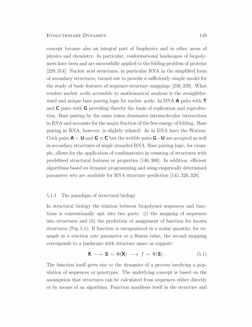
Evolutionary Dynamics 149
concept became also an integral part of biophysics and in other areas of
physics and chemistry. In particular, conformational landscapes of biopoly-
mers have been and are successfully applied to the folding problem of proteins
[229, 314]. Nucleic acid structures, in particular RNA in the simplified form
of secondary structures, turned out to provide a sufficiently simple model for
the study of basic features of sequence-structure mappings [238, 239]. What
renders nucleic acids accessible to mathematical analysis is the straightfor-
ward and unique base pairing logic for nucleic acids: In DNA A pairs with T
and C pairs with G providing thereby the basis of replication and reproduc-
tion. Base pairing by the same token dominates intramolecular interactions
in RNA and accounts for the major fraction of the free energy of folding. Base
pairing in RNA, however, is slightly relaxed: As in DNA have the Watson-
Crick pairs A = U and G ≡ C but the wobble pairs G−U are accepted as well
in secondary structures of single stranded RNA. Base pairing logic, for exam-
ple, allows for the application of combinatorics in counting of structures with
predefined structural features or properties [146, 300]. In addition, efficient
algorithms based on dynamic programming and using empirically determined
parameter sets are available for RNA structure prediction [145, 326, 328].
5.1.1 The paradigm of structural biology
In structural biology the relation between biopolymer sequences and func-
tions is conventionally spit into two parts: (i) the mapping of sequences
into structures and (ii) the prediction or assignment of function for known
structures (Fig. 5.1). If function is encapsulated in a scalar quantity, for ex-
ample in a reaction rate parameter or a fitness value, the second mapping
corresponds to a landscape with structure space as support:
X −→ S = Φ(X) −→ f = Ψ(S) . (5.1)
The function itself gives rise to the dynamics of a process involving a pop-
ulation of sequences or genotypes. The underlying concept is based on the
assumption that structures can be calculated from sequences either directly
or by means of an algorithm. Function manifests itself in the structure and
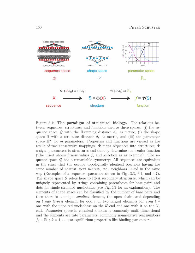
150 Peter Schuster
Figure 5.1: The paradigm of structural biology. The relations be-tween sequences, structures, and functions involve three spaces: (i) the se-quence space Q with the Hamming distance dH as metric, (i) the shapespace S with a structure distance dS as metric, and (iii) the parameterspace Rm
+ for m parameters. Properties and functions are viewed as theresult of two consecutive mappings: Φ maps sequences into structures, Ψassigns parameters to structures and thereby determines molecular function(The insert shows fitness values fk and selection as as example). The se-quence space Q has a remarkable symmetry: All sequences are equivalentin the sense that the occupy topologically identical positions having thesame number of nearest, next nearest, etc., neighbors linked in the sameway (Examples of a sequence spaces are shown in Figs. 3.3, 3.4, and 4.7).The shape space S refers here to RNA secondary structures, which can beuniquely represented by strings containing parentheses for base pairs anddots for single stranded nucleotides (see Fig. 5.3 for an explanation). Theelements of shape space can be classified by the number of base pairs andthen there is a unique smallest element, the open chain, and dependingon l one largest element for odd l or two largest elements for even l –one with the unpaired nucleobase on the 5’-end and one with it on the 3’-end. Parameter space in chemical kinetics is commonly multi-dimensionaland the elements are rate parameters, commonly nonnegative real numbersfk ∈ R+; k = 1, . . . , or equilibrium properties like binding parameters.

Evolutionary Dynamics 151
Figure 5.2: A sketch of the mapping of RNA sequences onto secondarystructures. The points of sequence space (here 183 on a planar hexagonal lattice)are mapped onto points in shape space (here 25 on a square lattice) and, inevitably,the mapping is many to one. All sequences X. folding the same mfe structure forma neutral set, which in mathematical terms is the preimage of Sk in sequencespace. Connecting nearest neighbors of this set – these are pairs of sequences withHamming distance dH = 1 – yields the neutral network of the structure, Gk. Thenetwork in sequence space consists of a giant component (red) and several othersmall components (pink). On the network the stability against point mutationsvaries from λ = 1/6 (white points) to λ = 6/6 = 1 (black point). We remark thatthe two-dimensional representations of sequence are used here only for the purposeof illustration. In reality, both spaces are high-dimensional – the sequence space
of binary sequences Q(2)l , for example, is a hypercube of dimension n and that of
natural four-letter sequences Q(4)l an object in 3n dimensional space.
should be predictable therefore. As it turned out after some spectacular
successes in the early days (see, e.g., [302]) both steps are feasible but the
mappings are highly complex and not fully understood yet. The alternative
way to determine parameters consists of an inversion of conventional kinetics:
The measured time dependence of concentrations is the input and parame-
ters are fit to the data either by trial and error or systematically by means
of inverse methods involving regularization techniques [77].
Counting sequences and structures reveals the ultimate basis for neu-
trality. In the natural AUGC alphabet we are dealing with κl = 4l RNA
152 Peter Schuster
sequences whereas the number of acceptable secondary structures3 that has
been determined by combinatorics [146, 300]:
∣
∣
∣S(3,2)lim
∣
∣
∣(l) = 1.4848× l−3/2(1.84892)l . (5.2)
The formula is asymptotically correct for long sequences as indicated by the
limit. Insertion of moderately long or even small chain lengths l into Equ. 5.2
shows that we are always dealing with orders of magnitude more sequences
that structures and therefore neutrality with respect to structure and the
formation of neutral network for common structures is inevitable [247].
The conventional problem in structural biology is to find the structures
into which a sequences folds under predefined conditions [327, 328]. Solutions
to the inverse problem, finding a sequence that folds into a given structure
are important for the design of molecules in synthetic biology. An inverse
folding algorithm has been developed for RNA secondary structures [145]
(for a recent variant see [2]) and turned out to be a very useful tool for
studying sequence-structure mappings. In particular, these mappings are
not invertible: Many sequences fold into the same structure, and the notion
of neutral network has been created for the graph representing the preimage
of a given structure in sequence space [252]:
Φ(Xj) = Sk =⇒ Gk = Φ−1(Sk) ≡ Xj|Φ(Xj = Sk , (5.3)
The neutral set Gk in converted into the neutral network Gk through con-
necting all pairs of sequences with Hamming distance dH = 1. The definition
of the neutral networks in a way restores uniqueness of the mapping: Every
structure Sk has a uniquely defined neutral network Gk in sequence space.
Every sequence Xj belongs to one and only one neutral network. Neutral
networks are characterized by a (mean) degree of neutrality
λk =
∑
j|Xj∈Gkλ(k)j
|Gk|, (5.4)
3Acceptable means here that hairpin loops of lengths nhp = 1 or 2 are excluded for
stereochemical reasons and stacks of length nst = 1, i.e. isolated base pairs, are not
considered for poor energetics (see Fig. 5.4).
Evolutionary Dynamics 153
wherein λ(k)j is the local fraction of neutral nearest neighbors of sequence Xj
in sequence space (An example is sketched in Fig.5.2). Without knowing
special features of neutral networks derived from RNA secondary structures
the application of random graph theory [78, 79] to neutral networks is obvious.
One (statistical) result of the theory dealing with the connectedness of the
graph applies straightforwardly and relates it with the degree of neutrality
λk: Neutral networks Gk with a degree of neutrality above a critical value,
λk > λcr, are connected whereas networks with lower degree of neutrality,
λk < λcr, are partitioned into components with one particularly large and
several small components. The large component is commonly characterized
as giant component. The critical degree of neutrality depends only on the size
of the nucleobase alphabet: λcr = 1−κ−1/(κ−1) leading to λcr = 0.5 for κ = 2
and to λcr = 0.370 for κ = 4. Because of the non-invertibility of the mapping
distance relations in structure space are different from those in sequence space
and they are more complex. The notion of distance is replaced by a concept
on nearness [102] of neutral networks. Nearness, however, does not fulfill the
properties of a metric as careful mathematical analysis reveals but leads to
a pretopology in phenotype space [270]. Fig.5.2 shows a sketch of a typical
neutral network in a ’two-dimensional’ sequence space. The network consists
of several components with one giant component being much larger than the
others. Random graph theory was found to represent a proper reference also
for the neutral networks based on RNA secondary structures in the sense
that deviations from the idealized node distribution can be interpreted by
structure based nonhomogeneous distributions of sequences in sequence space
[127]. Some structures with special features like, for example, stack with free
ends on both sides may show two or four giant components of equal size or
three giant components with a size distribution 1:2:1.
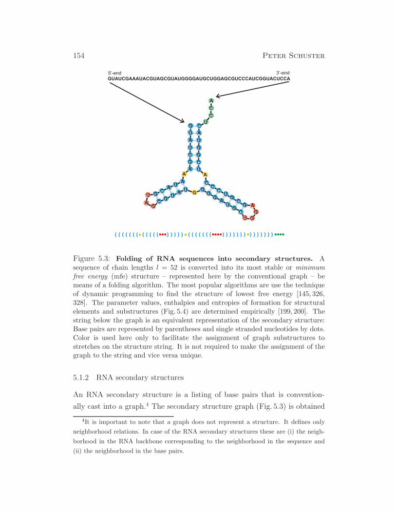
154 Peter Schuster
Figure 5.3: Folding of RNA sequences into secondary structures. Asequence of chain lengths l = 52 is converted into its most stable or minimumfree energy (mfe) structure – represented here by the conventional graph – bemeans of a folding algorithm. The most popular algorithms are use the techniqueof dynamic programming to find the structure of lowest free energy [145, 326,328]. The parameter values, enthalpies and entropies of formation for structuralelements and substructures (Fig. 5.4) are determined empirically [199, 200]. Thestring below the graph is an equivalent representation of the secondary structure:Base pairs are represented by parentheses and single stranded nucleotides by dots.Color is used here only to facilitate the assignment of graph substructures tostretches on the structure string. It is not required to make the assignment of thegraph to the string and vice versa unique.
5.1.2 RNA secondary structures
An RNA secondary structure is a listing of base pairs that is convention-
ally cast into a graph.4 The secondary structure graph (Fig. 5.3) is obtained
4It is important to note that a graph does not represent a structure. It defines only
neighborhood relations. In case of the RNA secondary structures these are (i) the neigh-
borhood in the RNA backbone corresponding to the neighborhood in the sequence and
(ii) the neighborhood in the base pairs.
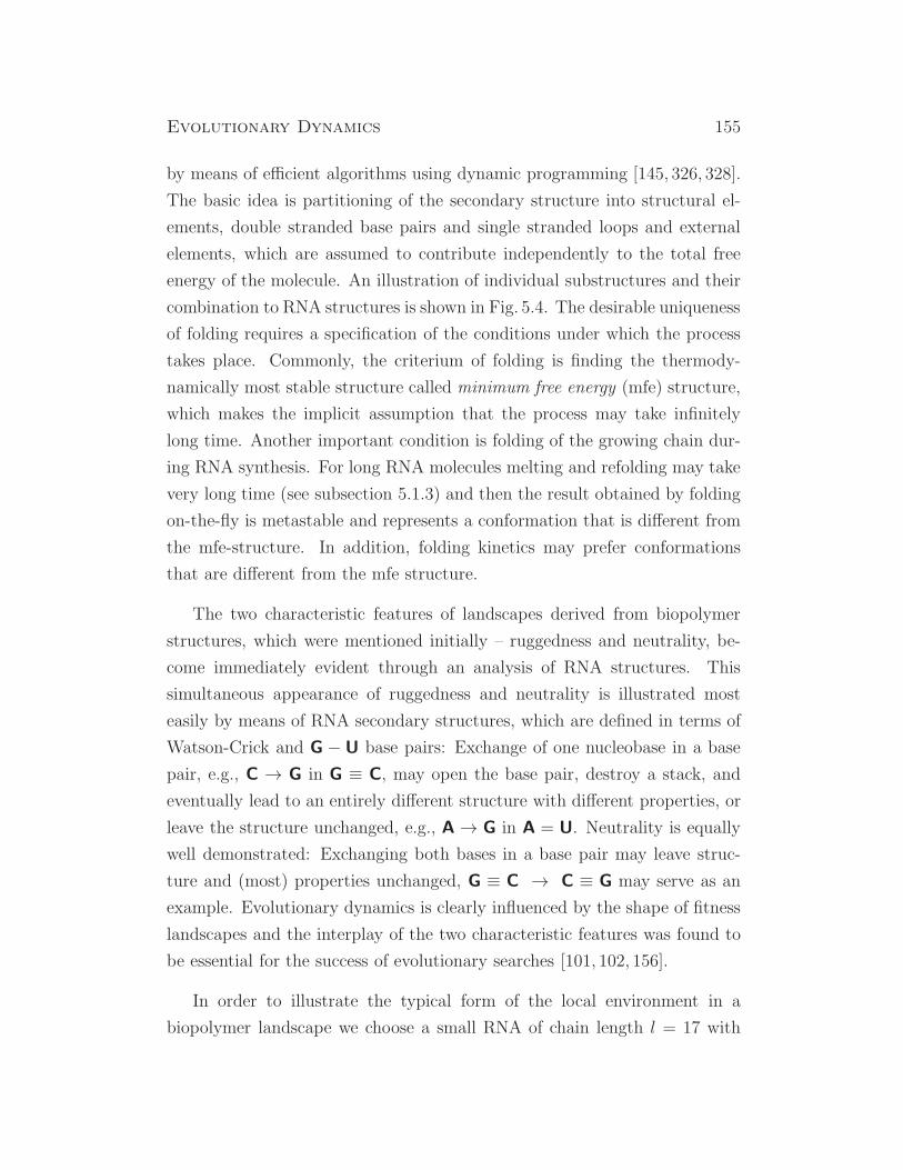
Evolutionary Dynamics 155
by means of efficient algorithms using dynamic programming [145, 326, 328].
The basic idea is partitioning of the secondary structure into structural el-
ements, double stranded base pairs and single stranded loops and external
elements, which are assumed to contribute independently to the total free
energy of the molecule. An illustration of individual substructures and their
combination to RNA structures is shown in Fig. 5.4. The desirable uniqueness
of folding requires a specification of the conditions under which the process
takes place. Commonly, the criterium of folding is finding the thermody-
namically most stable structure called minimum free energy (mfe) structure,
which makes the implicit assumption that the process may take infinitely
long time. Another important condition is folding of the growing chain dur-
ing RNA synthesis. For long RNA molecules melting and refolding may take
very long time (see subsection 5.1.3) and then the result obtained by folding
on-the-fly is metastable and represents a conformation that is different from
the mfe-structure. In addition, folding kinetics may prefer conformations
that are different from the mfe structure.
The two characteristic features of landscapes derived from biopolymer
structures, which were mentioned initially – ruggedness and neutrality, be-
come immediately evident through an analysis of RNA structures. This
simultaneous appearance of ruggedness and neutrality is illustrated most
easily by means of RNA secondary structures, which are defined in terms of
Watson-Crick and G − U base pairs: Exchange of one nucleobase in a base
pair, e.g., C → G in G ≡ C, may open the base pair, destroy a stack, and
eventually lead to an entirely different structure with different properties, or
leave the structure unchanged, e.g., A → G in A = U. Neutrality is equally
well demonstrated: Exchanging both bases in a base pair may leave struc-
ture and (most) properties unchanged, G ≡ C → C ≡ G may serve as an
example. Evolutionary dynamics is clearly influenced by the shape of fitness
landscapes and the interplay of the two characteristic features was found to
be essential for the success of evolutionary searches [101, 102, 156].
In order to illustrate the typical form of the local environment in a
biopolymer landscape we choose a small RNA of chain length l = 17 with

156 Peter Schuster
hairpin loop
hairpin loop
hairpin loop
hairpinloop
hairpinloop
hairpinloop
stack
stack
stack
stackstack
stack
stack
stack
stack
free endfree end
freeend
freeend
freeend
joint
internal loop
bulge
multilo
op
Figure 5.4: Elements of RNA secondary structures. Three classes ofstructural elements are distinguished: (i) stacks (indicated by nucleotides in bluecolor), (ii) loops, and (iii) external elements being joints (chartreuse) and free ends(green). Loops fall into several subclasses: Hairpin loops (red) have one base pair,called the closing pair, in the loop. Bulges (violet) and internal loops (orange)have two closing pairs, and loops with three or more closing pairs (yellow) arecalled multiloops. The number of closing pairs is the degree of the loop.
the sequence X0 ≡AGCUUACUUAGUGCGCU as example.5 At 0 C the se-
quence forms the minimum free energy structure S0 = Φ(X0), which consists
of an hairpin with six base pairs and an internal loop that separates two
5All polynucleotide sequences are written from the 5’-end at the lhs to the 3’-end on
the rhs.
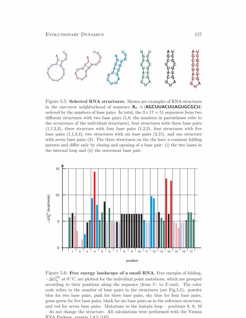
Evolutionary Dynamics 157
Figure 5.5: Selected RNA structures. Shown are examples of RNA structuresin the one-error neighborhood of sequence X0 ≡ (AGCUUACUUAGUGCGCU)ordered by the numbers of base pairs. In total, the 3×17 = 51 sequences form twodifferent structures with two base pairs (1,8; the numbers in parentheses refer tothe occurrence of the individual structures), four structures with three base pairs(1,1,2,3), three structure with four base pairs (1,2,3), four structures with fivebase pairs (1,1,3,4), two structures with six base pairs (2,15), and one structurewith seven base pairs (3). The three structures on the rhs have a common foldingpattern and differ only by closing and opening of a base pair: (i) the two bases inthe internal loop and (ii) the outermost base pair.
Figure 5.6: Free energy landscape of a small RNA. Free energies of folding,
−∆G(0)0 at 0 C, are plotted for the individual point mutations, which are grouped
according to their positions along the sequence (from 5’- to 3’-end). The colorcode refers to the number of base pairs in the structures (see Fig.5.5): powderblue for two base pairs, pink for three base pairs, sky blue for four base pairs,grass green for five base pairs, black for six base pairs as in the reference structure,and red for seven base pairs. Mutations in the hairpin loop – positions 8, 9, 10– do not change the structure. All calculations were performed with the ViennaRNA Package, version 1.8.5 [145].
158 Peter Schuster
stacks with three base pairs each (Fig.5.5; black structure), and the free en-
ergy of structure formation is: ∆G(0)0 = −6.39 kcal/mole. The molecule is
relatively stable and has three low lying suboptimal conformations with free
energies at 0.29, 0.38, and 0.67 kcal/mole above the minimum free energy
structure. These three states differ from the ground state through opening
of one or both external base pairs (see e.g. Fig.5.7), all three suboptimal
configurations are lying within reach of thermal energy and therefore con-
tribute to the partition function of the molecule. The Hamming distance
one neighborhood of X0 consists of 17 × 3 = 51 sequences, which form 16
different structures. Out of the 51 sequences 15 form the same minimum
free energy structure as X0 and 10 have also the same minimum free energy
energy implying a local degree of neutrality of λ(0)0 = 0.29 for structures and
λ(∆G)0 = 0.19 for the free energies, respectively. The plot of the free energies
of folding ∆G(0)0 for all 51 mutants in Fig.5.6 is a perfect illustration of the
ruggedness of the free energy landscape: The stability range of the one-error
mutants goes from marginal stability at position 2, G → U, to more than
twice the absolute free energy of the reference at position 4, U→ G.
Recently, methods were developed that allow for efficient construction of
fitness landscapes for catalytically active RNA molecules [235]. Ruggedness
and neutrality are not restricted to RNA-molecules, similar results provid-
ing direct evidence were found with proteins [140]. Protein space, however,
is more complex than RNA space since a large fraction of amino acid se-
quences does not lead to stable protein structures. Strongly hydrophobic
molecular surfaces, for example, lead to protein aggregation and accordingly
the landscapes have holes where no sequences are situated that cane give
rise to useful structures. The landscape then reminds of a holey landscape as
introduced in a different context by Sergey Gavrilets [109]. Holey landscapes
provide a challenge for adaptive evolution because certain areas of sequence
are not accessible. Attempts were made to reconstruct fitness landscapes
for simple parasitic organisms like viruses. A recent example is large scale
fitness modeling for HIV I [181]. Apart from a few exceptions experimen-
tal comprehensive information on fitness landscapes or conformational free
energy surfaces is still rare but the amount of reliable data is rapidly grow-
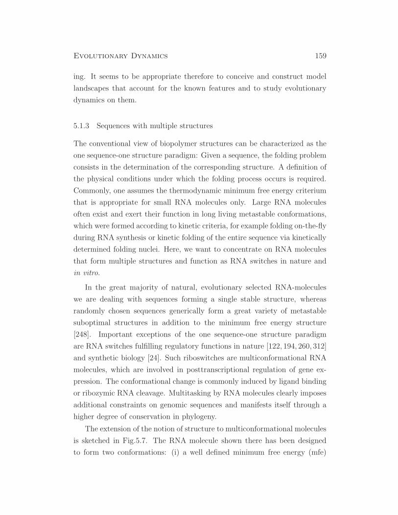
Evolutionary Dynamics 159
ing. It seems to be appropriate therefore to conceive and construct model
landscapes that account for the known features and to study evolutionary
dynamics on them.
5.1.3 Sequences with multiple structures
The conventional view of biopolymer structures can be characterized as the
one sequence-one structure paradigm: Given a sequence, the folding problem
consists in the determination of the corresponding structure. A definition of
the physical conditions under which the folding process occurs is required.
Commonly, one assumes the thermodynamic minimum free energy criterium
that is appropriate for small RNA molecules only. Large RNA molecules
often exist and exert their function in long living metastable conformations,
which were formed according to kinetic criteria, for example folding on-the-fly
during RNA synthesis or kinetic folding of the entire sequence via kinetically
determined folding nuclei. Here, we want to concentrate on RNA molecules
that form multiple structures and function as RNA switches in nature and
in vitro.
In the great majority of natural, evolutionary selected RNA-molecules
we are dealing with sequences forming a single stable structure, whereas
randomly chosen sequences generically form a great variety of metastable
suboptimal structures in addition to the minimum free energy structure
[248]. Important exceptions of the one sequence-one structure paradigm
are RNA switches fulfilling regulatory functions in nature [122, 194, 260, 312]
and synthetic biology [24]. Such riboswitches are multiconformational RNA
molecules, which are involved in posttranscriptional regulation of gene ex-
pression. The conformational change is commonly induced by ligand binding
or ribozymic RNA cleavage. Multitasking by RNA molecules clearly imposes
additional constraints on genomic sequences and manifests itself through a
higher degree of conservation in phylogeny.
The extension of the notion of structure to multiconformational molecules
is sketched in Fig.5.7. The RNA molecule shown there has been designed
to form two conformations: (i) a well defined minimum free energy (mfe)
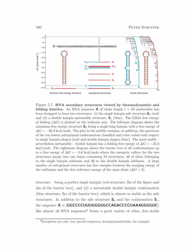
160 Peter Schuster
-26.0
-24.0
-22.0
-20.0
-18.0
-16.0
-14.0
-12.0
-10.0
- 8.0
- 6.0D
G
[kca
l.m
ole
]-1
S0
S2
S3
S7,8
S9
2
3
87
9S10
S6S4,5
456
10
kinetic structuressuboptimal structuresminimum free energy structure
S0
S1
S0S1
X = (GGCCCCUUUGGGGGCCAGACCCCUAAAGGGGUC)
Figure 5.7: RNA secondary structures viewed by thermodynamics andfolding kinetics. An RNA sequence X of chain length l = 33 nucleotides hasbeen designed to form two structures: (i) the single hairpin mfe structure,S0 (red)and (ii) a double hairpin metastable structure, S1 (blue). The Gibbs free energyof folding (∆G) is plotted on the ordinate axis. The leftmost diagram shows theminimum free energy structure S0 being a single long hairpin with a free energy of∆G = −26.3 kcal/mole. The plot in the middle contains, in addition, the spectrumof the ten lowest suboptimal conformations classified and color coded with respectto single hairpin shapes (red) and double hairpin shapes (blue). The most stable –nevertheless metastable – double hairpin has a folding free energy of ∆G = −25.3kacl/mole. The rightmost diagram shows the barrier tree of all conformations upto a free energy of ∆G = −5.6 kcal/mole where the energetic valleys for the twostructures merge into one basin containing 84 structures, 48 of them belongingto the single hairpin subbasin and 36 to the double hairpin subbasin. A largenumber of suboptimal structures has free energies between the merging energy ofthe subbasins and the free reference energy of the open chain (∆G = 0).
structure – being a perfect single hairpin (red structure; lhs of the figure and
rhs of the barrier tree), and (ii) a metastable double hairpin conformation
(blue structure; lhs of the barrier tree), which is almost as stable as the mfe
structures. In addition to the mfe structure S0 and the conformation S1,
the sequence X ≡ (GGCCCCUUUGGGGGCCAGACCCCUAAAGGGGUC)
like almost all RNA sequences6 forms a great variety of other, less stable
6Exceptions are only very special sequences, homopolynucleotides, for example.
Evolutionary Dynamics 161
conformations called suboptimal structures (S2 to S10 are shown by numbers
in the middle of the figure and in the barrier tree). The numbers of all
suboptimal structures are huge but most suboptimal conformations have free
energies way above the mfe structure and don’t appreciably contribute to
the low-lying conformations. Structures, mfe and suboptimal structures,
are related through transitions, directly or via intermediates, which in a
simplified version can be represented by means of a barrier tree [95, 313]
shown on the rhs of the figure. Kinetic folding introduces a second time
scale into the scenario of molecular evolution.7 Based on Arrhenius theory of
chemical reaction rates,
k = A · e−Ea/RT , (5.5)
the height of the barrier, Ea determines the reaction rate parameter k and
thereby the half life of the conformation t1/2 = ln 2/k. In equation (5.5),
A is the pre-exponential factor of the reaction, R is the gas constant and T
the absolute temperature in Kelvin. The two structures shown in Fig.5.7
are connected by a lowest barrier of 20.7 kcal/mole that depending on the
pre-exponential factors implies half lives of days or even weeks for the two
conformations. In a conventional experiment with a time scale of hours the
two conformations would appear as two separate entities. Barriers, neverthe-
less, can be engineered to be much lower and then an equilibrium mixture of
rapidly interconverting conformations may be observed. Several constraints
are required for the conservation of an RNA switch, and the restrictions of
variability in sequence space are substantial.
The comparison of the two dominant structures S0 and S1 in Fig. 5.7
provides a straightforward example for the illustration of different notions of
stability: (i) thermodynamic stability, which considers only the free energies
of the mfe structures – S0 in Fig.5.7 is more stable than S1 since it has a lower
free energy, ∆G(S0) < ∆G(S1), (ii) conformational stability, which can be
expressed in terms of suboptimal structures or partition functions within a
7Timescale number one is the evolutionary process – mutation and selection – itself. In
order to be relevant for evolutionary dynamics the second timescale has to be substantially
faster than the first one, or in other words, the conformational changes has to occur almost
instantaneously on the timescale of evolution.
162 Peter Schuster
basin or a subbasin of an RNA sequence – a conformationally stable molecule
has no low lying suboptimal conformations that can be interconverted with
the mfe structure or another metastable structure at the temperature of the
experiment; for kinetic structures separated by high barriers the partition
functions are properly restricted to individual subbasins [195], and (iii) mu-
tational stability that is measured in terms of the probability with which a
mutation changes the structure of a molecule (see Fig.5.2). All three forms of
stability are relevant for evolution, but mutational stability and the spectrum
of mutational effects – adaptive, neutral or deleterious – are most important.
RNA suboptimal structures were also used for explaining characteristic
feature of the evolution of organisms like plasticity, evolvability, and modu-
larity [6, 7, 97]. Among these very complex features modularity is the most
intriguing one, because it plays a crucial role from the early beginnings of
evolution to the most complex relations in societies. Modularity is indis-
pensable for understanding complex systems in biology and anywhere else.
Modular structure in cases where it is not congruent with other forces shap-
ing subunits is hard to interpret still and as it seems will remain a hot topic
for many years in the future.
5.2 Dynamics on realistic rugged landscapes
The majority of data on the relation between sequences and molecular prop-
erties comes from structural biology of biopolymers, in particular RNA and
protein. RNA secondary structures as shown in the previous section 5.1 pro-
vide a simple and mathematically accessible example of a realistic mapping
of biopolymer sequences onto structures [252]. The RNA model is commonly
restricted to the assignment of a single structure to every sequence but the
explicit consideration of suboptimal conformations is possible as well (see
subsection 5.1.3 and [248]). Two features are characteristic for landscapes
derived from RNA molecules: (i) ruggedness – pairs of sequences situated
nearby in sequence space, i.e., having Hamming distance dH = 1, may give
rise to very similar or entirely different structures and properties – and (ii)

Evolutionary Dynamics 163
neutrality – two or more sequences may have identical structures and prop-
erties.
Rugged fitness landscapes, which are more elaborate than the simple ones
discussed in section 4.3.6, have been proposed. The most popular example
is the Nk-model conceived by Stuart Kauffman [169, 170, 306] that is based
on individual loci on a genome and interactions between them: N is the
number of loci and k is the number of interactions. A random element,
which is drawn from a predefined probability distribution – commonly the
normal distribution – and which defines the interaction network, is added
to the otherwise deterministic model: N and k are fixed and not subjected
to variation. Here a different approach is proposed that starts out from
the nucleotide sequence of a genome rather than from genes and alleles,
and consequently it is based on the notion of sequence space. Ruggedness
(this section 5.2) and neutrality (see section 5.3) are introduced by means
of tunable parameters, d and λ, and pseudorandom numbers are used to
introduce random scatter, which reflects the current ignorance with respect
to detailed fitness values and which is thought to be replaced by real data
when they become available in the near future. We begin with an overview
of the current knowledge on biopolymer landscapes and discuss afterwards
model landscapes that come close to real landscapes at the current state of
knowledge and investigate then evolutionary dynamics on such “realistic”
landscapes.
A new type of landscapes, the realistic rugged landscape (RRL), is in-
troduced and analyzed here. Ruggedness is modeled by assigning fitness
differences at random within a predefined band of fitness values with ad-
justable width d. The highest fitness value is attributed to the master se-
quence Xm.= X0, fm = f0, and the fitness values of all other sequences are
obtained by means of the equation
f(Xj) = fj =
f0 if j = 0 ,
f + 2d(f0 − f)(
η(s)j − 0.5
)
if j = 1, . . . , κ l ,(5.6)
where η(s)j is the j-th output random number from a pseudorandom number
164 Peter Schuster
generator with a uniform distribution of numbers in the range 0 ≤ η(s)j ≤ 1.
The random number generator is assumed to have been started with the
seed s,8 which will be used to characterize a particular distribution of fitness
values (Fig. 5.8). The parameter d determines the amount of scatter around
the mean value f−0 = f , which is independent of d: d = 0 yields the single
peak landscape, and d = 1 leads to fully developed or maximal scatter where
individual fitness values fj can reach the value f0. A given landscape can be
characterized by
L = L(λ, d, s; l, f0, f) , (5.7)
where λ is the degree of neutrality (see section 5.3; here we have λ = 0).
The parameters l, f0 and f have the same meaning as for the single peak
landscape (3.4c).
Two properties of realistic rugged landscapes fulfilled by fitness values
relative to the mean except the master, ϕj = fj − f ∀ j = 0, . . . , κ l − 1,
are important: (i) the ratio of two relative fitness values of sequences within
the mutant cloud is independent of the scatter d and (ii) the ratio of the
relative fitness values of a sequence from the cloud and the master sequence
is proportional to the scatter d:
ϕj
ϕk=
η(s)j − 0.5
η(s)k − 0.5
; j, k = 1, . . . , κ l − 1 and (5.8a)
ϕj
ϕ0= 2 d
(
η(s)j − 0.5
)
; j = 1, . . . , κ l − 1 . (5.8b)
The second equation immediately shows that∑κl−1
j=1 ϕj = 0.
5.2.1 Single master quasispecies
We are now in a position to explore whether or not the results derived from
simple model landscapes are representative for mutation-selection dynamics
in real populations. At first the influence of random scatter on quasispecies
8The seed s indeed determines all details of the landscape, which is completely defined
by s and the particular type of the pseudorandom number generator as well as by f0, f ,
and d.
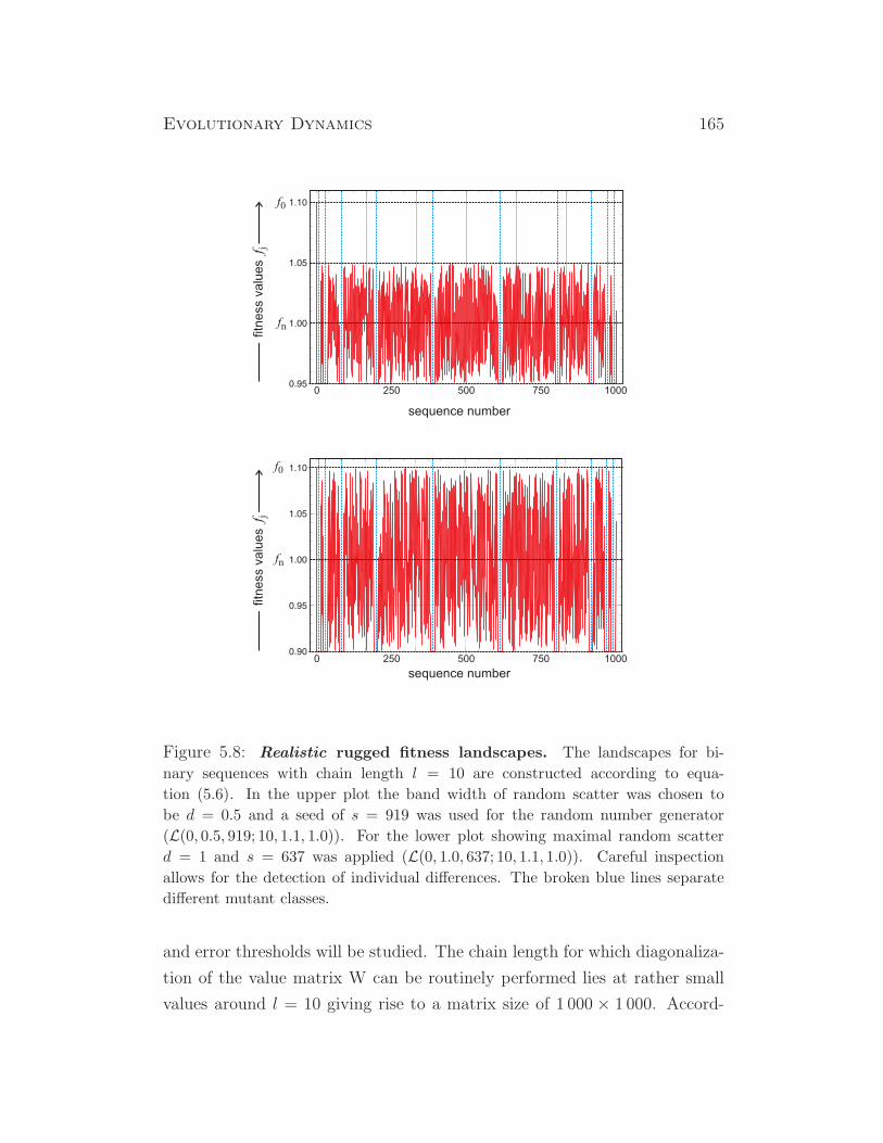
Evolutionary Dynamics 165
fitn
ess v
alu
es
f j
sequence number
f0
fn
0 250 500 750 1000
f0
fn
fitn
ess v
alu
es
f j
sequence number
0 250 500 750 1000
Figure 5.8: Realistic rugged fitness landscapes. The landscapes for bi-
nary sequences with chain length l = 10 are constructed according to equa-
tion (5.6). In the upper plot the band width of random scatter was chosen to
be d = 0.5 and a seed of s = 919 was used for the random number generator
(L(0, 0.5, 919; 10, 1.1, 1.0)). For the lower plot showing maximal random scatter
d = 1 and s = 637 was applied (L(0, 1.0, 637; 10, 1.1, 1.0)). Careful inspection
allows for the detection of individual differences. The broken blue lines separate
different mutant classes.
and error thresholds will be studied. The chain length for which diagonaliza-
tion of the value matrix W can be routinely performed lies at rather small
values around l = 10 giving rise to a matrix size of 1 000 × 1 000. Accord-
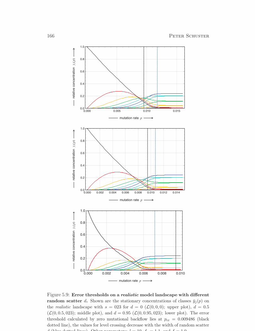
166 Peter Schuster
Figure 5.9: Error thresholds on a realistic model landscape with different
random scatter d. Shown are the stationary concentrations of classes yj(p) on
the realistic landscape with s = 023 for d = 0 (L(0, 0, 0); upper plot), d = 0.5
(L(0, 0.5, 023); middle plot), and d = 0.95 (L(0, 0.95, 023); lower plot). The error
threshold calculated by zero mutational backflow lies at pcr = 0.009486 (black
dotted line), the values for level crossing decrease with the width of random scatter
d (blue dotted lines). Other parameters: l = 10, f0 = 1.1, and f = 1.0.
Evolutionary Dynamics 167
ingly, it has to be confirmed first whether or not such a short chain length
is sufficient to yield representative results. In Fig. 5.9 the stationary con-
centrations of mutant classes, yk (k = 0, 1, . . . , 10) are shown for different
band widths d of random scatter: The purely deterministic case d = 0 rep-
resenting the single-peak landscape, d = 0.5, and d = 0.95, the maximal
scatter that sustains a single quasispecies over the entire range, 0 ≤ p < pcr.9
Despite the short chain length of l = 10 the plots reflect the threshold phe-
nomena rather well, the width of the transition to the uniform distribution
is hardly changing, and values for level crossing (section 4.3.6 and table 4.3)
are shifted towards smaller p(1/M)-values with increasing d. Answering the
initial question, computer studies with l = 10 are suitable for investigations
on quasispecies behavior.
For d > 0 the fitness values for individual sequences within one class
are no longer the same and hence the curves xj(p) differ from each other
and form a band for each class that increases in width with the amplitude
d of the random component (Fig. 5.11). The separation of the bands formed
by curves belonging to different error classes is always recognizable at suf-
ficiently small mutation rates p but the bands overlap and merge at higher
p-values. As expected the zone where the bands begin to mix moves in the
direction p = 0 with increasing scatter d. Interestingly, the error threshold
phenomenon is fully retained thereby, only the level-crossing value p(1/100)
is shifted towards lower error rates (figs. 5.10, 5.11, and 5.12). Indeed, the
approaches towards the uniform distribution on the landscape without a ran-
dom component (d = 0) and on the landscape with d = 0.5 are very similar
apart from the relatively small shift towards lower p-values, whereas the shift
for d = 0.95 is substantially larger and the solution curve x0(p) is curved up-
wards more strongly. Closer inspection of the shift of the level-crossing value
shows nonmonotonous behavior for some landscapes: The level crossing value
is shifted towards larger p-values at first, passes a maximum value and then
9As shown below in detail (Fig. 5.14) individual quasispecies may be replaced by others
at certain critical p-values, ptr. For a given scatter s the number of such transitions
becomes larger with increasing values of d.
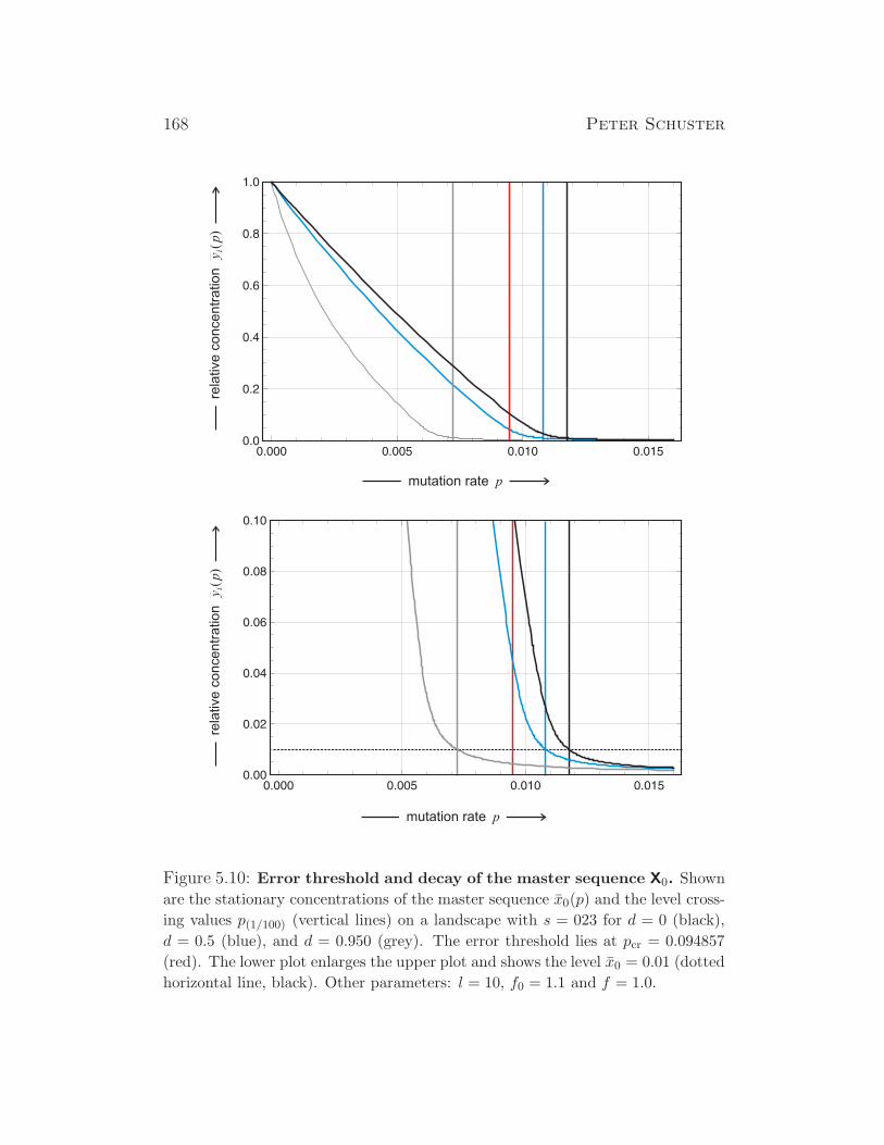
168 Peter Schuster
Figure 5.10: Error threshold and decay of the master sequence X0. Shown
are the stationary concentrations of the master sequence x0(p) and the level cross-
ing values p(1/100) (vertical lines) on a landscape with s = 023 for d = 0 (black),
d = 0.5 (blue), and d = 0.950 (grey). The error threshold lies at pcr = 0.094857
(red). The lower plot enlarges the upper plot and shows the level x0 = 0.01 (dotted
horizontal line, black). Other parameters: l = 10, f0 = 1.1 and f = 1.0.
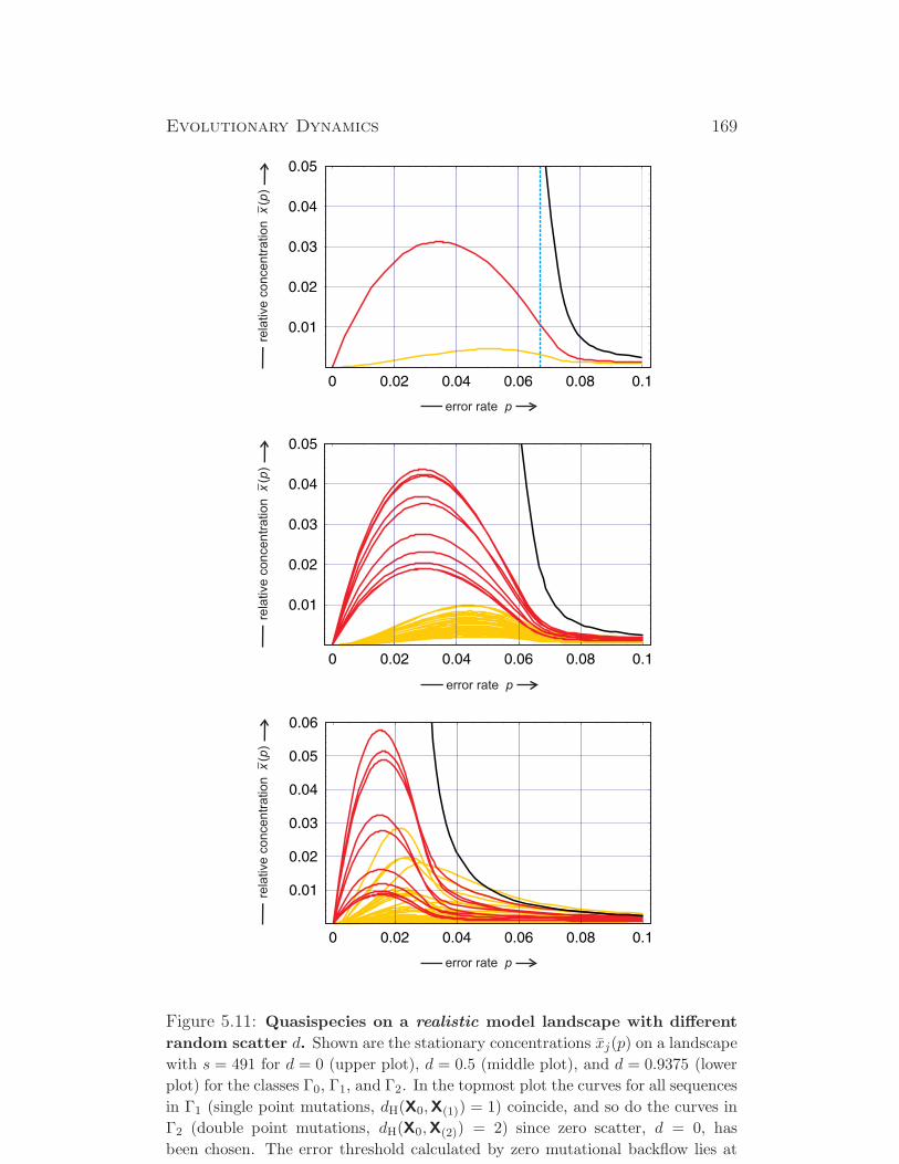
Evolutionary Dynamics 169
error rate p
rela
tive
co
nce
ntr
atio
n(
)x
p
error rate p
rela
tive c
oncentr
ation
()
xp
error rate p
rela
tive
co
nce
ntr
atio
n(
)x
p
Figure 5.11: Quasispecies on a realistic model landscape with different
random scatter d. Shown are the stationary concentrations xj(p) on a landscape
with s = 491 for d = 0 (upper plot), d = 0.5 (middle plot), and d = 0.9375 (lower
plot) for the classes Γ0, Γ1, and Γ2. In the topmost plot the curves for all sequences
in Γ1 (single point mutations, dH(X0,X(1)) = 1) coincide, and so do the curves in
Γ2 (double point mutations, dH(X0,X(2)) = 2) since zero scatter, d = 0, has
been chosen. The error threshold calculated by zero mutational backflow lies at
p = 0.066967. Other parameters: l = 10, f = 2.0, and f = 1.0.

170 Peter Schuster
Figure 5.12: Level-crossing values for the master sequence of dif-
ferent model landscape with different random scatter d. Shown are
the level crossing values for M = 100 as functions of the random scat-
ter p(1/100)(d). The error threshold calculated by zero mutational backflow
lies at pcr = 0.0117481. Color code for different seeds s: 023= orange,
229= red, 367=green, 491=black, 577= chartreuse, 637=blue, 673=yellow,
877=magenta, 887= turquoise, 919=blue violet, and 953=hot pink. Other pa-
rameters: l = 10, f0 = 1.1, and f = 1.0.
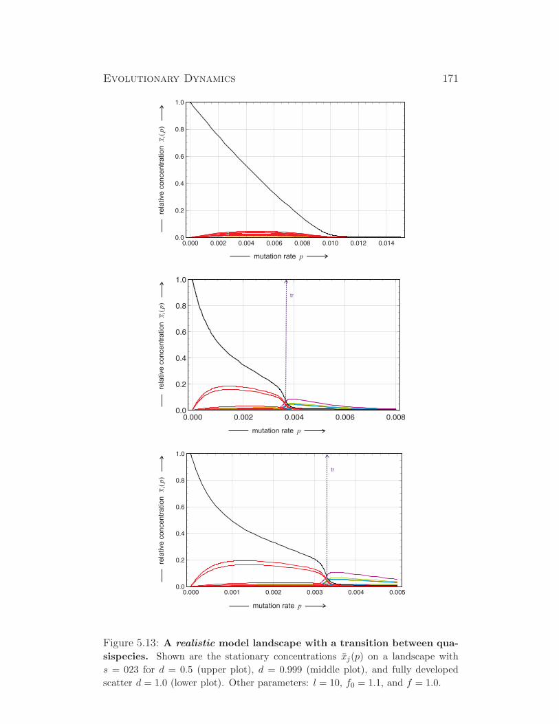
Evolutionary Dynamics 171
mutation rate p
rela
tive
co
nce
ntr
atio
n(
)x
pi
mutation rate p
rela
tive
co
nce
ntr
atio
n(
)x
pi
tr
mutation rate p
rela
tive
co
nce
ntr
atio
n(
)x
pi
tr
Figure 5.13: A realistic model landscape with a transition between qua-
sispecies. Shown are the stationary concentrations xj(p) on a landscape with
s = 023 for d = 0.5 (upper plot), d = 0.999 (middle plot), and fully developed
scatter d = 1.0 (lower plot). Other parameters: l = 10, f0 = 1.1, and f = 1.0.
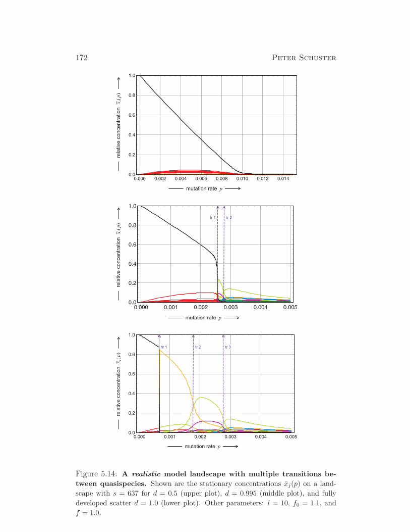
172 Peter Schuster
mutation rate p
rela
tive
co
nce
ntr
atio
n(
)x
pi
mutation rate p
tr 2tr 1
rela
tive
co
nce
ntr
atio
n(
)x
pi
mutation rate p
tr 1 tr 2 tr 3tr 1
rela
tive
co
nce
ntr
atio
n(
)x
pi
Figure 5.14: A realistic model landscape with multiple transitions be-
tween quasispecies. Shown are the stationary concentrations xj(p) on a land-
scape with s = 637 for d = 0.5 (upper plot), d = 0.995 (middle plot), and fully
developed scatter d = 1.0 (lower plot). Other parameters: l = 10, f0 = 1.1, and
f = 1.0.
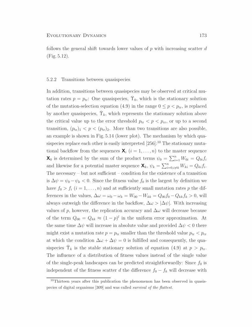
Evolutionary Dynamics 173
follows the general shift towards lower values of p with increasing scatter d
(Fig. 5.12).
5.2.2 Transitions between quasispecies
In addition, transitions between quasispecies may be observed at critical mu-
tation rates p = ptr: One quasispecies, Υ0, which is the stationary solution
of the mutation-selection equation (4.9) in the range 0 ≤ p < ptr, is replaced
by another quasispecies, Υk, which represents the stationary solution above
the critical value up to the error threshold ptr < p < pcr, or up to a second
transition, (ptr)1 < p < (ptr)2. More than two transitions are also possible,
an example is shown in Fig. 5.14 (lower plot). The mechanism by which qua-
sispecies replace each other is easily interpreted [256]:10 The stationary muta-
tional backflow from the sequences Xi (i = 1, . . . , n) to the master sequence
X0 is determined by the sum of the product terms ψ0 =∑n
i=1W0i = Q0ifi
and likewise for a potential master sequence Xk, ψk =∑n
i=0,i 6=kWki = Qkifi.
The necessary – but not sufficient – condition for the existence of a transition
is ∆ψ = ψ0−ψk < 0. Since the fitness value f0 is the largest by definition we
have f0 > fi (i = 1, . . . , n) and at sufficiently small mutation rates p the dif-
ferences in the values, ∆ω = ω0−ωk =W00−Wkk = Q00f0−Qkkfk > 0, will
always outweigh the difference in the backflow, ∆ω > |∆ψ|. With increasing
values of p, however, the replication accuracy and ∆ω will decrease because
of the term Q00 = Qkk ≈ (1 − p)l in the uniform error approximation. At
the same time ∆ψ will increase in absolute value and provided ∆ψ < 0 there
might exist a mutation rate p = ptr smaller than the threshold value ptr < pcr
at which the condition ∆ω + ∆ψ = 0 is fulfilled and consequently, the qua-
sispecies Υk is the stable stationary solution of equation (4.9) at p > ptr.
The influence of a distribution of fitness values instead of the single value
of the single-peak landscapes can be predicted straightforwardly: Since f0 is
independent of the fitness scatter d the difference f0 − fk will decrease with
10Thirteen years after this publication the phenomenon has been observed in quasis-
pecies of digital organisms [309] and was called survival of the flattest.
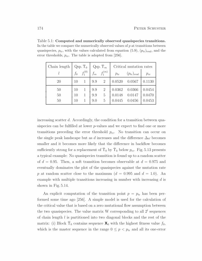
174 Peter Schuster
Table 5.1: Computed and numerically observed quasispecies transitions.
In the table we compare the numerically observed values of p at transitions between
quasispecies, ptr, with the values calculated from equation (5.9), (ptr)eval, and the
error thresholds, pcr. The table is adopted from [256].
Chain length Qsp. Υ0 Qsp. Υm Critical mutation rates
l f0 f(0)1 fm f
(m)1 ptr (ptr)eval pcr
20 10 1 9.9 2 0.0520 0.0567 0.1130
50 10 1 9.9 2 0.0362 0.0366 0.0454
50 10 1 9.9 5 0.0148 0.0147 0.0470
50 10 1 9.0 5 0.0445 0.0456 0.0453
increasing scatter d. Accordingly, the condition for a transition between qua-
sispecies can be fulfilled at lower p-values and we expect to find one or more
transitions preceding the error threshold pcr. No transition can occur on
the single peak landscape but as d increases and the difference ∆ω becomes
smaller and it becomes more likely that the difference in backflow becomes
sufficiently strong for a replacement of Υ0 by Υk below pcr. Fig. 5.13 presents
a typical example: No quasispecies transition is found up to a random scatter
of d = 0.95. Then, a soft transition becomes observable at d = 0.975 and
eventually dominates the plot of the quasispecies against the mutation rate
p at random scatter close to the maximum (d = 0.995 and d = 1.0). An
example with multiple transitions increasing in number with increasing d is
shown in Fig. 5.14.
An explicit computation of the transition point p = ptr has been per-
formed some time ago [256]. A simple model is used for the calculation of
the critical value that is based on a zero mutational flow assumption between
the two quasispecies. The value matrix W corresponding to all 2l sequences
of chain length l is partitioned into two diagonal blocks and the rest of the
matrix: (i) Block Υ0 contains sequence X0 with the highest fitness value f0,
which is the master sequence in the range 0 ≤ p < ptr and all its one-error
Evolutionary Dynamics 175
mutants X(0)(1) = Xj ∈ Γ
(0)1 with a fitness value f
(0)1 , (ii) block Υm contains
sequence Xm with the fitness value fm, which is the master sequence in the
range ptr ≤ p < pcr, and all its one-error mutants X(m)(1) = Xj ∈ Γ
(m)1 with a
fitness value f(m)1 , and (iii) the rest of the matrix W is neglected completely
as all entries are set equal zero:
W = ql
f0 f(0)1 ε · · · f
(0)1 ε · · · 0 0 · · · 0
f0ε f(0)1 · · · f
(0)1 ε2 · · · 0 0 · · · 0
......
. . ....
. . ....
.... . .
...
f0ε f(0)1 ε2 · · · f
(0)1 · · · 0 0 · · · 0
0 0 · · · 0 · · · fm f(m)1 ε · · · f
(m)1 ε
0 0 · · · 0 · · · fmε f(m)1 · · · f
(m)1 ε2
......
. . ....
. . ....
.... . .
...
0 0 · · · 0 · · · fmε f(m)1 ε2 · · · f
(m)1
.
Each block is now represented by a 2 × 2 matrix
W0 = ql
(
f0 l f(0)1 ε
f0ε f(0)1
(
1 + (l − 1)ε2)
)
and
Wm = ql
(
fm l f(m)1 ε
fmε f(m)1
(
1 + (l − 1)ε2)
)
.
Calculation of the two largest eigenvalues λ0 and λm yields the condition for
the occurrence of the transitions: λ0 = λm. The result is
ptr = 1 −√
1− ϑ tr
l − 1, (5.9)
with ϑ tr being the result of the equation
ϑ tr =1
2
(
α + β − γ +√
(α + β − γ)2 − 4αβ)
with (5.9’)
α = l − f0 − fmf(m)1 − f (0)
1
,
β = l − f0fm(f(m)1 − f (0)
1 )
f(0)1 f
(m)1 (f0 − fm)
, and
γ =(f0f
(0)1 − fmf (m)
1 )2
(l − 1)f(0)1 f
(m)1 (f0 − fm)(f (m)
1 − f (0)1 )
.
176 Peter Schuster
Although the complexity of these equations is prohibitive for further manip-
ulations, the accuracy of the zero mutational flow approximations is relevant
for the next subsection 5.2.3 were we shall apply a similar approximation.
The corresponding table 5.1 is reproduced from [256]. The agreement is very
good indeed but is cases where ptr and pcr are very close it can nevertheless
happen that the calculated value lies above the error threshold.
5.2.3 Clusters of coupled sequences
A certain fraction of landscapes gives rise to characteristic quasispecies dis-
tributions as a function of the mutation rate p that is substantially different
from the one shown in Fig. 5.14 and discussed above. No transitions are
observed, not even at fully developed scatter d = 1 (Fig. 5.15). Another fea-
ture concerns the classes to which the most frequent sequences belong. On
the landscape defined by s = 919 these sequences are the master sequence
(X0; black curve), one one-error mutant (X4; red curve), and one two-error
mutant (X516; yellow curve).11 The three sequences are situated close-by in
sequence space – Hamming distances dH(X1,X4) = dH(X4,X516) = 1 and
dH(X1,X516) = 2)– form a cluster, which is dynamically coupled by means
of strong mutational flow (Fig. 5.16). Apparently, such a quasispecies is not
likely to be replaced in a transition by another one that is centered around
a single master sequence and accordingly, we call such clusters strong qua-
sispecies. The problem that ought to be solved now is the prediction of the
occurrence of strong quasispecies from know fitness values.
First, a heuristic is mentioned that serves as an (almost perfect) diagnostictool for detecting whether or not a given fitness landscape gives rise to astrong quasispecies: (i) For every mutant class we identify the sequence withthe highest fitness value, f0, (f(1))max = f(Xm(1)), (f(2))max = f(Xm(2)), . . . ,and call them class-fittest sequences. Next we determine the fittest sequencesin the one-error neighborhood of the class-fittest sequences. Clearly, for theclass k-fittest sequence Xm(k) this sequence lies either in class k − 1 or inclass k+1.12 Simple combinatorics is favoring classes closer to the middle of
11Naıvely we would expect a band of one-error sequences at higher concentration than
the two-error sequence.12For class k = 1 we omit the master sequence X0, which trivially is the fittest sequence
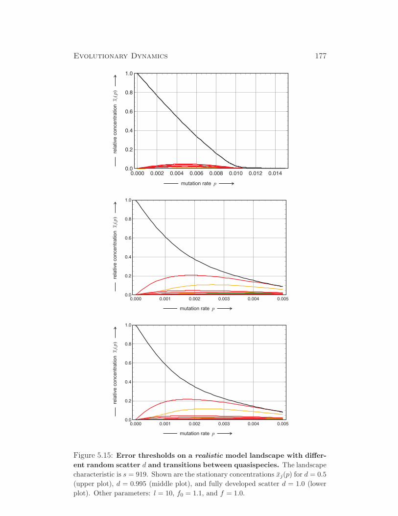
Evolutionary Dynamics 177
mutation rate p
rela
tive c
oncentr
ation
()
xp
i
mutation rate p
rela
tive c
oncentr
ation
()
xp
i
mutation rate p
rela
tive c
oncentr
ation
()
xp
i
Figure 5.15: Error thresholds on a realistic model landscape with differ-
ent random scatter d and transitions between quasispecies. The landscape
characteristic is s = 919. Shown are the stationary concentrations xj(p) for d = 0.5
(upper plot), d = 0.995 (middle plot), and fully developed scatter d = 1.0 (lower
plot). Other parameters: l = 10, f0 = 1.1, and f = 1.0.

178 Peter Schuster
0
1 6432164 82 512256128
3
65
260
17
129
513
34
160
544
12
96
384
33
144
528
10
80
320
6
68
272
9
72
288
5
66
264
24
136
520
48
258
768
20
132
516
40
257
640
18
130
514
36
192
576
769
0
1 6432164 82 512256128
3
65
260
17
129
513
34
160
544
12
96
384
33
144
528
10
80
320
6
68
272
9
72
288
5
66
264
24
136
520
48
258
768
20
132
516
40
257
640
18
130
514
36
192
576
Figure 5.16: Mutation flow in quasispecies. The sketch shows two typicalsituations in the distribution of fitness values in sequence space. In the upper dia-gram (s = 637) the fittest two-error mutant, X768, has its fittest nearest neighbor,X769, in the three-error class Γ3, and the fittest sequence in the one-error neigh-borhood of X4 (being the fittest sequence in the one-error class), X68, is differentfrom X768, the mutational flow is not sufficiently strong to couple X0, X4, and X68,and transitions between different quasispecies are observed (Fig. 5.14). The lowerdiagram (s = 919) shows the typical fitness distribution for a strong quasispecies:The fittest two-error mutant, X516, has its fittest nearest neighbor, X4, in the one-error class Γ1 and it coincides with the fittest one-error mutant. Accordingly, thethree sequences (X0, X4, and X516) are strongly coupled by mutational flow and astrong quasispecies is observed (Fig. 5.15).
Evolutionary Dynamics 179
sequence space. Any sequence in the two-error class, for example, has twonearest neighbors in the one-error class but n − 2 nearest neighbors in thethree-error class. To be a candidate for a strong quasispecies requires that– against probabilities – the fittest sequence in the one-error neighborhoodof Xm(2) lies in the one-error class: (f(Xm(2))m(1)
)max with (Xm(2))m(1) ∈ Γ1
and preferentially, this is the fittest one-error sequence, (Xm(2))m(1) ≡ Xm(1).Since all mutation rates between nearest neighbor sequences in neighboringclasses are the same – (1 − p)n−1p within the uniform error model – thestrength of mutational flow is dependent only on the fitness values, and theway in which the three sequences were determined guarantees optimalityof the flow: If such a three-membered cluster was found it is the one withthe highest internal mutational flow for a given landscape. Fig. 5.16 (lowerpicture, s = 919) shows an example where such three sequences form astrongly coupled cluster. There is always a fourth sequence – here X512 –belonging to the cluster but it may play no major role because of low fitness.The heuristic presented was applied to 21 fitness landscapes with differentrandom scatter and three strong quasispecies (s =401, 577, and 919) wereobserved. How many would be expected by combinatorial arguments? Theprobability for a sequence in Γ2 to have a neighbor in Γ1 is 2/10 = 0.2and, since the sequence Xm(1) is fittest in Γ1 and hence also in the one-error neighborhood of Xm(2), this is also the probability for finding a strongquasispecies. The sample that has been investigated in this study comprised21 landscapes an hence we expect to encounter 21/5 = 4.2 cases, which is– with respect to the small sample size – in agreement with the three casesthat we found.
The suggestion put forward in the heuristic mentioned above – a clusterof sequences coupled by mutational flow that is stronger within the groupthan to the rest of sequence space because of frequent mutations and high fit-ness values – will now be analyzed and tested through the application of zerobackflow approximation. Instead of a single master sequence we considera master cluster of sequences and then proceed in full analogy to subsec-tion 4.3.3 by applying zero mutational backflow from the rest of sequencespace to the cluster. In order to be able to deal with a cluster of sequences
in the one-error neighborhood, and search only in class k = 2.
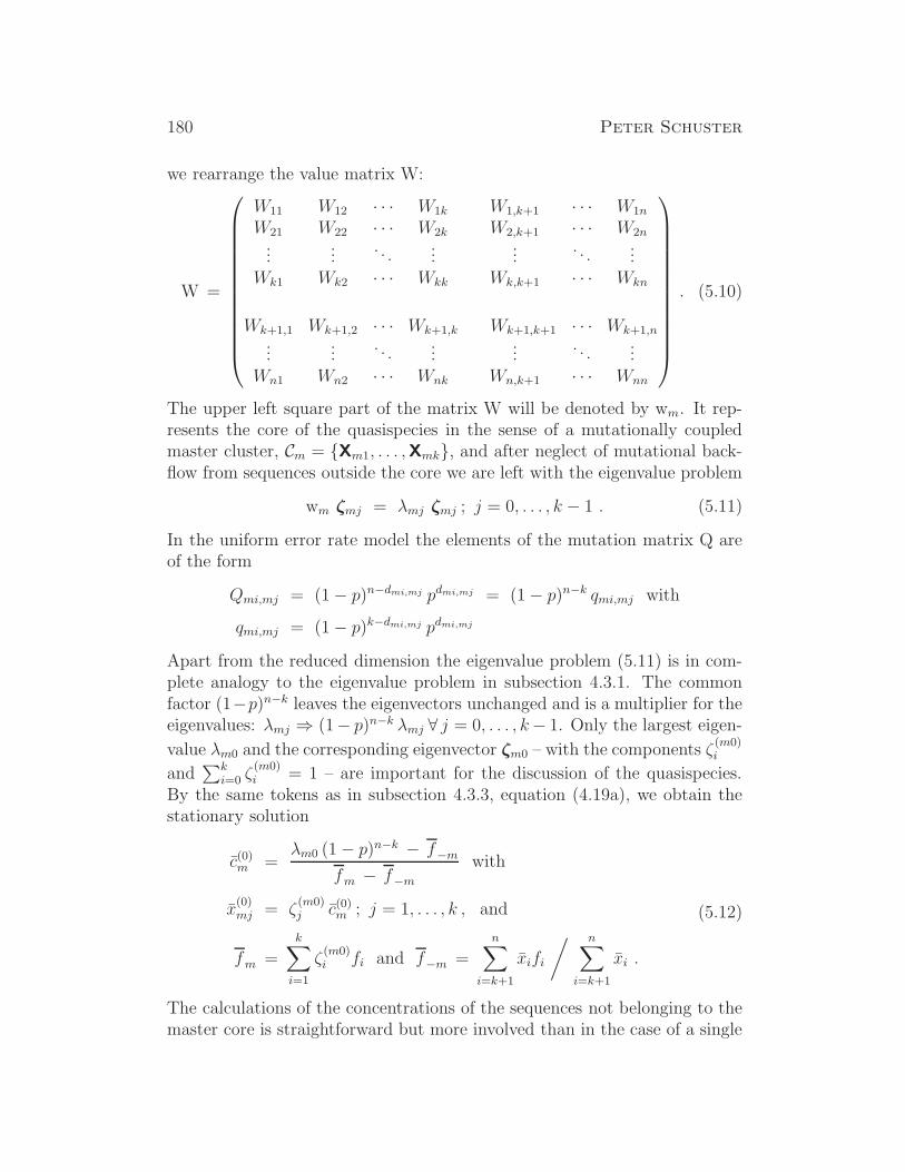
180 Peter Schuster
we rearrange the value matrix W:
W =
W11 W12 · · · W1k W1,k+1 · · · W1n
W21 W22 · · · W2k W2,k+1 · · · W2n...
.... . .
......
. . ....
Wk1 Wk2 · · · Wkk Wk,k+1 · · · Wkn
Wk+1,1 Wk+1,2 · · · Wk+1,k Wk+1,k+1 · · · Wk+1,n...
.... . .
......
. . ....
Wn1 Wn2 · · · Wnk Wn,k+1 · · · Wnn
. (5.10)
The upper left square part of the matrix W will be denoted by wm. It rep-resents the core of the quasispecies in the sense of a mutationally coupledmaster cluster, Cm = Xm1, . . . ,Xmk, and after neglect of mutational back-flow from sequences outside the core we are left with the eigenvalue problem
wm ζmj = λmj ζmj ; j = 0, . . . , k − 1 . (5.11)
In the uniform error rate model the elements of the mutation matrix Q areof the form
Qmi,mj = (1− p)n−dmi,mj pdmi,mj = (1− p)n−k qmi,mj with
qmi,mj = (1− p)k−dmi,mj pdmi,mj
Apart from the reduced dimension the eigenvalue problem (5.11) is in com-plete analogy to the eigenvalue problem in subsection 4.3.1. The commonfactor (1−p)n−k leaves the eigenvectors unchanged and is a multiplier for theeigenvalues: λmj ⇒ (1− p)n−k λmj ∀ j = 0, . . . , k− 1. Only the largest eigen-
value λm0 and the corresponding eigenvector ζm0 – with the components ζ(m0)i
and∑k
i=0 ζ(m0)i = 1 – are important for the discussion of the quasispecies.
By the same tokens as in subsection 4.3.3, equation (4.19a), we obtain thestationary solution
c(0)m =λm0 (1− p)n−k − f−m
fm − f−mwith
x(0)mj = ζ
(m0)j c(0)m ; j = 1, . . . , k , and
fm =
k∑
i=1
ζ(m0)i fi and f−m =
n∑
i=k+1
xifi
/ n∑
i=k+1
xi .
(5.12)
The calculations of the concentrations of the sequences not belonging to themaster core is straightforward but more involved than in the case of a single

Evolutionary Dynamics 181
Table 5.2: Strong quasispecies. Shown are error thresholds and level crossing
values for three cases of strong quasispecies.
Random seeds s = 401 s = 577 s = 919
j fitness j fitness j fitness
Core sequences 0 1.1000 0 1.1000 0 1.1000
64 1.0981 64 1.0951 4 1.0966
16 1.0772 256 1.0894 512 0.9296
80 1.0987 320 1.0999 516 1.0970
j p(1/100) j p(1/100) j p(1/100)
Level crossing, d = 0 0 0.01396 0 0.01410 0 0.01320
64 0.01406 64 0.01402 4 0.01348
16 0.01318 256 0.01377 512 0.00828
80 0.01389 320 0.01410 516 0.01304
Level crossing, d = 1 0 0.008443 0 0.006921 a 0 0.007876
64 0.008359 64 0.006481 4 0.008385
16 0.007003 256 0.006440 512 - - - b
80 0.007876 320 0.006733 516 0.007476
Error threshold (pcr) 0.01134 0.01145 0.01087
a The quasispecies with s = 577 shows a small smooth transition just above
the error threshold. The following three sequences have the same or higher
level crossing values: p(1/100)(X899) = 0.008026, p(1/100)(X931) = 0.007186, and
p(1/100)(X962) = 0.006842.b The stationary concentration x512(p) never exceeds nor reaches the value 0.01.
master sequence. We dispense here from details because we shall not makeuse of the corresponding expressions. In the forthcoming examples we shallapply a modified single peak landscape where all sequences except those inthe master core have the same fitness values f and then the equation f−m = fis trivially fulfilled.
182 Peter Schuster
For the purpose of illustration of the analysis of sequence clustering in
strong quasispecies full numerical computations are compared with the zero
mutational backflow approximation for the four membered cluster on the fit-
ness landscape L(λ = 0, s = 919, d = 1.00) in Fig. 5.17. Although differences
are readily recognized and the agreement between the full calculation and
the approximation is not as good as in the case of a single master sequence,
the appearance of the cluster is very well reproduced by the zero mutational
backflow approximation. In particular, the relative frequencies of the four
sequences forming the cluster are reproduced well. In comparison to the
full calculation, the critical mutation rate at the error threshold, the point
p = pcr at which the entire quasispecies Υ(0) vanishes, appears at a higher
p-value than the level crossings of the full calculation. The difference in the
critical mutation rates is readily interpreted: The full calculation is based
on a landscape with fully developed random scatter whereas the zero muta-
tional backflow calculation compares best with a four peak landscape where
the four peaks correspond to the members of the cluster (X0, X4, X516, X512)
and all other sequences have identical fitness values. In order to show that
this interpretation is correct the cluster has been implemented on a single
peak landscape (d = 0) with the same fitness values (f0 = 1.1 and f = 1.0)
and the error threshold on this landscape is shifted slightly to higher values
of the mutation rate parameter p. The agreement with the zero mutational
backflow approximation is remarkably good. This agreement can be taken
as a strong indication that the interpretation of strong quasispecies being a
result of the formation of mutationally linked clusters of sequences within
the population.
Three strong quasispecies with the values s = 401, 577, and 919 were
found among the 21 landscapes studied here. The most important computed
data are summarized in table 5.2. Like in the single master case on the single
peak landscape the level crossing values p(1/100) occur at higher mutation rates
than the error threshold (see Fig. 5.10). The shift in the strong quasispecies
is about ∆p = 0.0265 somewhat larger than that for the single master lying
at ∆p = 0.00226. In the single master case the error threshold was calculated
to be pcr = 0.094875 whereas here it is shifted to higher p-values by about
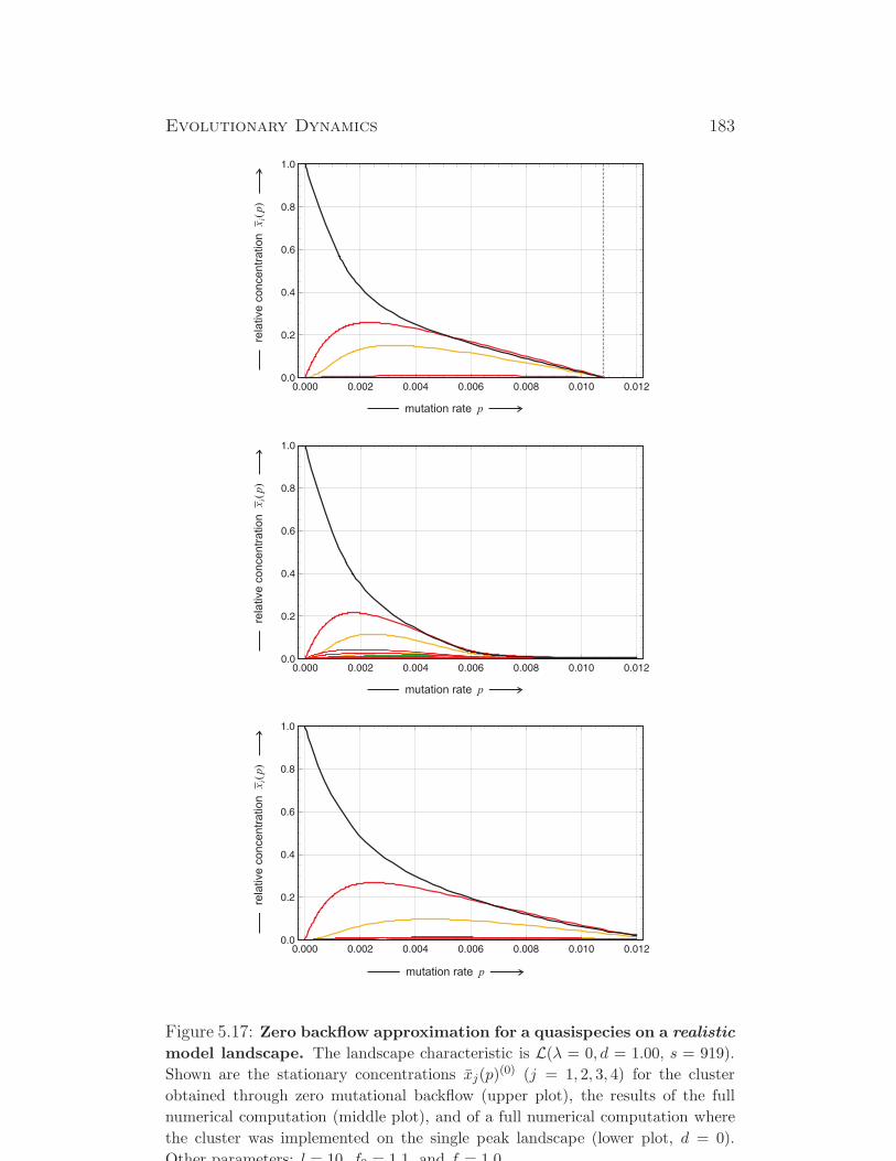
Evolutionary Dynamics 183
mutation rate p
rela
tive c
oncentr
ation
()
xp
i
Figure 5.17: Zero backflow approximation for a quasispecies on a realistic
model landscape. The landscape characteristic is L(λ = 0, d = 1.00, s = 919).
Shown are the stationary concentrations xj(p)(0) (j = 1, 2, 3, 4) for the cluster
obtained through zero mutational backflow (upper plot), the results of the full
numerical computation (middle plot), and of a full numerical computation where
the cluster was implemented on the single peak landscape (lower plot, d = 0).
Other parameters: l = 10, f0 = 1.1, and f = 1.0.
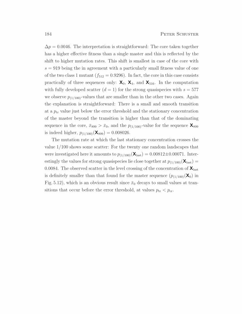
184 Peter Schuster
∆p = 0.0046. The interpretation is straightforward: The core taken together
has a higher effective fitness than a single master and this is reflected by the
shift to higher mutation rates. This shift is smallest in case of the core with
s = 919 being the in agreement with a particularly small fitness value of one
of the two class 1 mutant (f512 = 0.9296). In fact, the core in this case consists
practically of three sequences only: X0, X4, and X516. In the computation
with fully developed scatter (d = 1) for the strong quasispecies with s = 577
we observe p(1/100)-values that are smaller than in the other two cases. Again
the explanation is straightforward: There is a small and smooth transition
at a ptr value just below the error threshold and the stationary concentration
of the master beyond the transition is higher than that of the dominating
sequence in the core, x899 > x0, and the p(1/100)-value for the sequence X899
is indeed higher, p(1/100)(X899) = 0.008026.
The mutation rate at which the last stationary concentration crosses the
value 1/100 shows some scatter: For the twenty one random landscapes that
were investigated here it amounts to p(1/100)(Xlast) = 0.00812±0.00071. Inter-estingly the values for strong quasispecies lie close together at p(1/100)(Xlast) =
0.0084. The observed scatter in the level crossing of the concentration of Xlast
is definitely smaller than that found for the master sequence (p(1/100)(X0) in
Fig. 5.12), which is an obvious result since x0 decays to small values at tran-
sitions that occur before the error threshold, at values ptr < pcr.
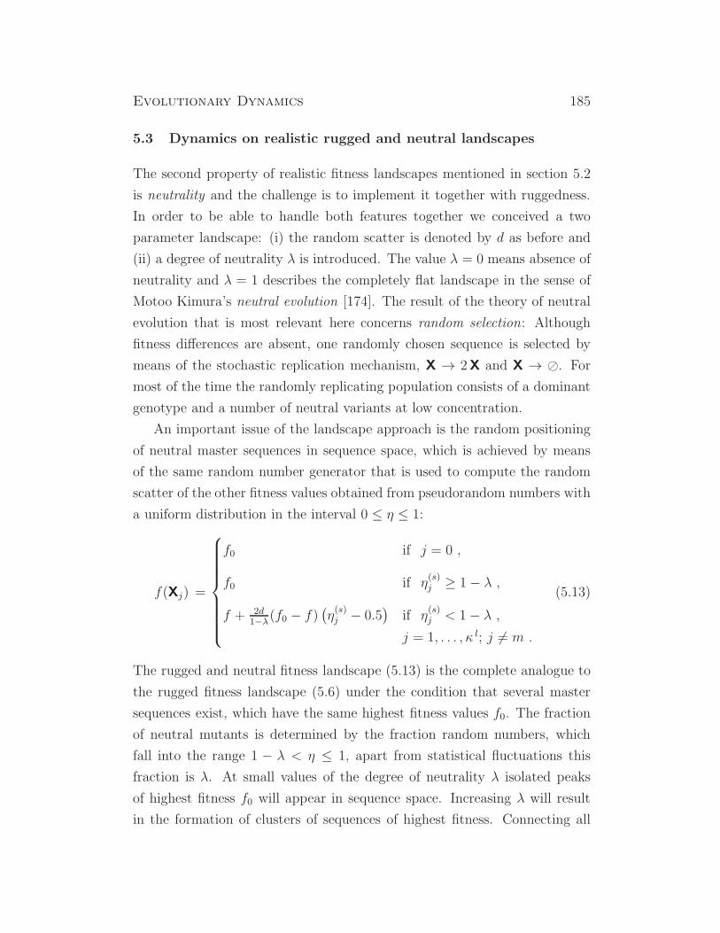
Evolutionary Dynamics 185
5.3 Dynamics on realistic rugged and neutral landscapes
The second property of realistic fitness landscapes mentioned in section 5.2
is neutrality and the challenge is to implement it together with ruggedness.
In order to be able to handle both features together we conceived a two
parameter landscape: (i) the random scatter is denoted by d as before and
(ii) a degree of neutrality λ is introduced. The value λ = 0 means absence of
neutrality and λ = 1 describes the completely flat landscape in the sense of
Motoo Kimura’s neutral evolution [174]. The result of the theory of neutral
evolution that is most relevant here concerns random selection: Although
fitness differences are absent, one randomly chosen sequence is selected by
means of the stochastic replication mechanism, X → 2X and X → ⊘. For
most of the time the randomly replicating population consists of a dominant
genotype and a number of neutral variants at low concentration.
An important issue of the landscape approach is the random positioning
of neutral master sequences in sequence space, which is achieved by means
of the same random number generator that is used to compute the random
scatter of the other fitness values obtained from pseudorandom numbers with
a uniform distribution in the interval 0 ≤ η ≤ 1:
f(Xj) =
f0 if j = 0 ,
f0 if η(s)j ≥ 1− λ ,
f + 2d1−λ(f0 − f)
(
η(s)j − 0.5
)
if η(s)j < 1− λ ,
j = 1, . . . , κ l; j 6= m .
(5.13)
The rugged and neutral fitness landscape (5.13) is the complete analogue to
the rugged fitness landscape (5.6) under the condition that several master
sequences exist, which have the same highest fitness values f0. The fraction
of neutral mutants is determined by the fraction random numbers, which
fall into the range 1 − λ < η ≤ 1, apart from statistical fluctuations this
fraction is λ. At small values of the degree of neutrality λ isolated peaks
of highest fitness f0 will appear in sequence space. Increasing λ will result
in the formation of clusters of sequences of highest fitness. Connecting all
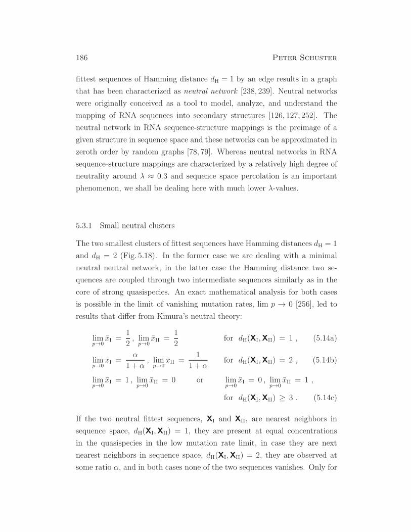
186 Peter Schuster
fittest sequences of Hamming distance dH = 1 by an edge results in a graph
that has been characterized as neutral network [238, 239]. Neutral networks
were originally conceived as a tool to model, analyze, and understand the
mapping of RNA sequences into secondary structures [126, 127, 252]. The
neutral network in RNA sequence-structure mappings is the preimage of a
given structure in sequence space and these networks can be approximated in
zeroth order by random graphs [78, 79]. Whereas neutral networks in RNA
sequence-structure mappings are characterized by a relatively high degree of
neutrality around λ ≈ 0.3 and sequence space percolation is an important
phenomenon, we shall be dealing here with much lower λ-values.
5.3.1 Small neutral clusters
The two smallest clusters of fittest sequences have Hamming distances dH = 1
and dH = 2 (Fig. 5.18). In the former case we are dealing with a minimal
neutral neutral network, in the latter case the Hamming distance two se-
quences are coupled through two intermediate sequences similarly as in the
core of strong quasispecies. An exact mathematical analysis for both cases
is possible in the limit of vanishing mutation rates, lim p → 0 [256], led to
results that differ from Kimura’s neutral theory:
limp→0
xI =1
2, lim
p→0xII =
1
2for dH(XI,XII) = 1 , (5.14a)
limp→0
xI =α
1 + α, lim
p→0xII =
1
1 + αfor dH(XI,XII) = 2 , (5.14b)
limp→0
xI = 1 , limp→0
xII = 0 or limp→0
xI = 0 , limp→0
xII = 1 ,
for dH(XI,XII) ≥ 3 . (5.14c)
If the two neutral fittest sequences, XI and XII, are nearest neighbors in
sequence space, dH(XI,XII) = 1, they are present at equal concentrations
in the quasispecies in the low mutation rate limit, in case they are next
nearest neighbors in sequence space, dH(XI,XII) = 2, they are observed at
some ratio α, and in both cases none of the two sequences vanishes. Only for
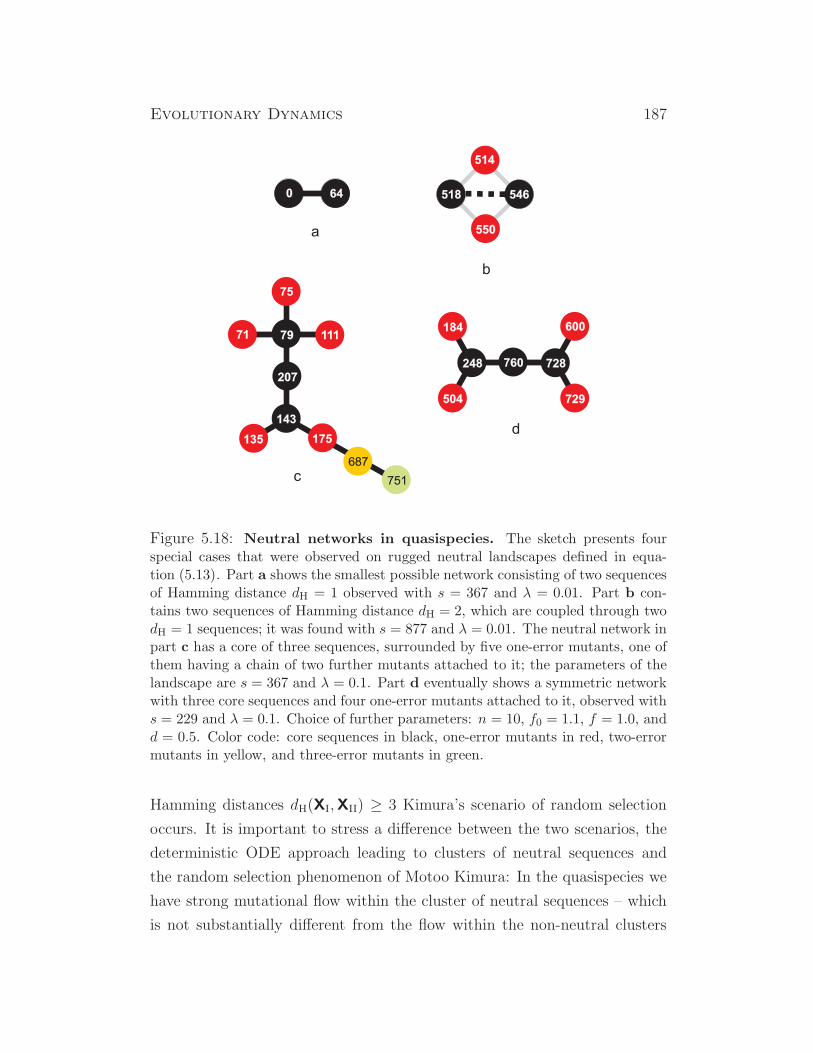
Evolutionary Dynamics 187
Figure 5.18: Neutral networks in quasispecies. The sketch presents fourspecial cases that were observed on rugged neutral landscapes defined in equa-tion (5.13). Part a shows the smallest possible network consisting of two sequencesof Hamming distance dH = 1 observed with s = 367 and λ = 0.01. Part b con-tains two sequences of Hamming distance dH = 2, which are coupled through twodH = 1 sequences; it was found with s = 877 and λ = 0.01. The neutral network inpart c has a core of three sequences, surrounded by five one-error mutants, one ofthem having a chain of two further mutants attached to it; the parameters of thelandscape are s = 367 and λ = 0.1. Part d eventually shows a symmetric networkwith three core sequences and four one-error mutants attached to it, observed withs = 229 and λ = 0.1. Choice of further parameters: n = 10, f0 = 1.1, f = 1.0, andd = 0.5. Color code: core sequences in black, one-error mutants in red, two-errormutants in yellow, and three-error mutants in green.
Hamming distances dH(XI,XII) ≥ 3 Kimura’s scenario of random selection
occurs. It is important to stress a difference between the two scenarios, the
deterministic ODE approach leading to clusters of neutral sequences and
the random selection phenomenon of Motoo Kimura: In the quasispecies we
have strong mutational flow within the cluster of neutral sequences – which
is not substantially different from the flow within the non-neutral clusters
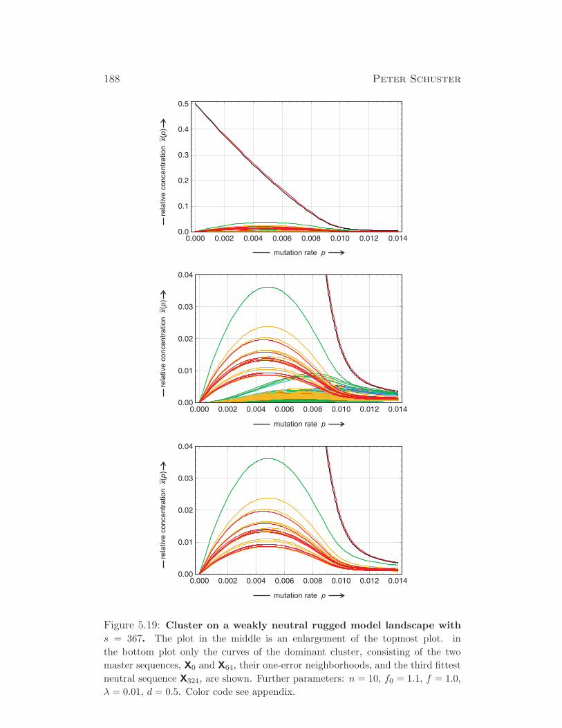
188 Peter Schuster
mutation rate p
rela
tive c
oncentr
ation
()
xp
mutation rate p
rela
tive
co
nce
ntr
atio
n(
)x
p
Figure 5.19: Cluster on a weakly neutral rugged model landscape with
s = 367. The plot in the middle is an enlargement of the topmost plot. in
the bottom plot only the curves of the dominant cluster, consisting of the two
master sequences, X0 and X64, their one-error neighborhoods, and the third fittest
neutral sequence X324, are shown. Further parameters: n = 10, f0 = 1.1, f = 1.0,
λ = 0.01, d = 0.5. Color code see appendix.
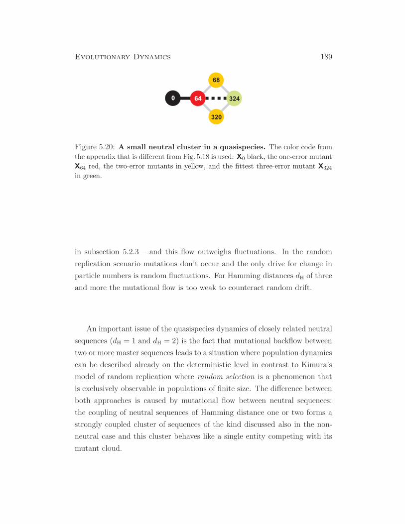
Evolutionary Dynamics 189
Figure 5.20: A small neutral cluster in a quasispecies. The color code from
the appendix that is different from Fig. 5.18 is used: X0 black, the one-error mutant
X64 red, the two-error mutants in yellow, and the fittest three-error mutant X324
in green.
in subsection 5.2.3 – and this flow outweighs fluctuations. In the random
replication scenario mutations don’t occur and the only drive for change in
particle numbers is random fluctuations. For Hamming distances dH of three
and more the mutational flow is too weak to counteract random drift.
An important issue of the quasispecies dynamics of closely related neutral
sequences (dH = 1 and dH = 2) is the fact that mutational backflow between
two or more master sequences leads to a situation where population dynamics
can be described already on the deterministic level in contrast to Kimura’s
model of random replication where random selection is a phenomenon that
is exclusively observable in populations of finite size. The difference between
both approaches is caused by mutational flow between neutral sequences:
the coupling of neutral sequences of Hamming distance one or two forms a
strongly coupled cluster of sequences of the kind discussed also in the non-
neutral case and this cluster behaves like a single entity competing with its
mutant cloud.

190 Peter Schuster
rela
tive c
oncentr
ation
()
xp
mutation rate p
rela
tive
co
nce
ntr
atio
n(
)x
p
mutation rate p
Figure 5.21: Quasispecies on weakly neutral rugged model landscape
with s = 877. The topmost part of the figure refers to the landscape with s = 877
and presents the solution curves for the master pair, X518,X546 and their one-
error mutants. The plot in the middle is an enlargement and highlights the curves
for the two intermediate sequences X514 and X550 in pastel blue. The plot at the
bottom shows the ratio between the stationary concentrations of the two master
sequences, α(p). Further parameters: n = 10, f0 = 1.1, f = 1.0, λ = 0.01, d = 0.5.
Color code see appendix.
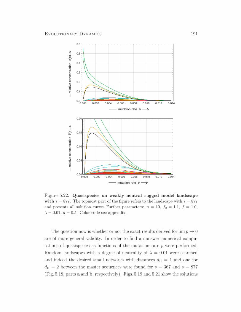
Evolutionary Dynamics 191
mutation rate p
rela
tive
co
nce
ntr
atio
n(
)x
p
mutation rate p
rela
tive
co
nce
ntr
atio
n(
)x
p
Figure 5.22: Quasispecies on weakly neutral rugged model landscape
with s = 877. The topmost part of the figure refers to the landscape with s = 877
and presents all solution curves Further parameters: n = 10, f0 = 1.1, f = 1.0,
λ = 0.01, d = 0.5. Color code see appendix.
The question now is whether or not the exact results derived for lim p→ 0
are of more general validity. In order to find an answer numerical compu-
tations of quasispecies as functions of the mutation rate p were performed.
Random landscapes with a degree of neutrality of λ = 0.01 were searched
and indeed the desired small networks with distances dH = 1 and one for
dH = 2 between the master sequences were found for s = 367 and s = 877
(Fig. 5.18, parts a and b, respectively). Figs. 5.19 and 5.21 show the solutions

192 Peter Schuster
Figure 5.23: Quasispecies with two neutral master sequences. The sketchcontains a set of sequences in order to demonstrate the role of neutrality in the de-termination of the consensus sequence of a population. Two fittest sequences withHamming distance dH = 1 (upper picture) lead to an ambiguity at one position.Mutations at other positions are wiped out by statistics whereas the one-to-oneratio of the two mater sequences leads to a 50/50 ratio of two nucleobases atthe position of the mutation. The lower picture refers to two master sequenceswith Hamming distance dH = 2: Ambiguities are obtained at two positions andthe ratios of the nucleobases are given approximately by the value of α in equa-tion(5.14b). The two intermediates are present in small stationary concentrationsonly but they are, nevertheless, more frequent than the other one-error mutants(see Fig. 5.21).
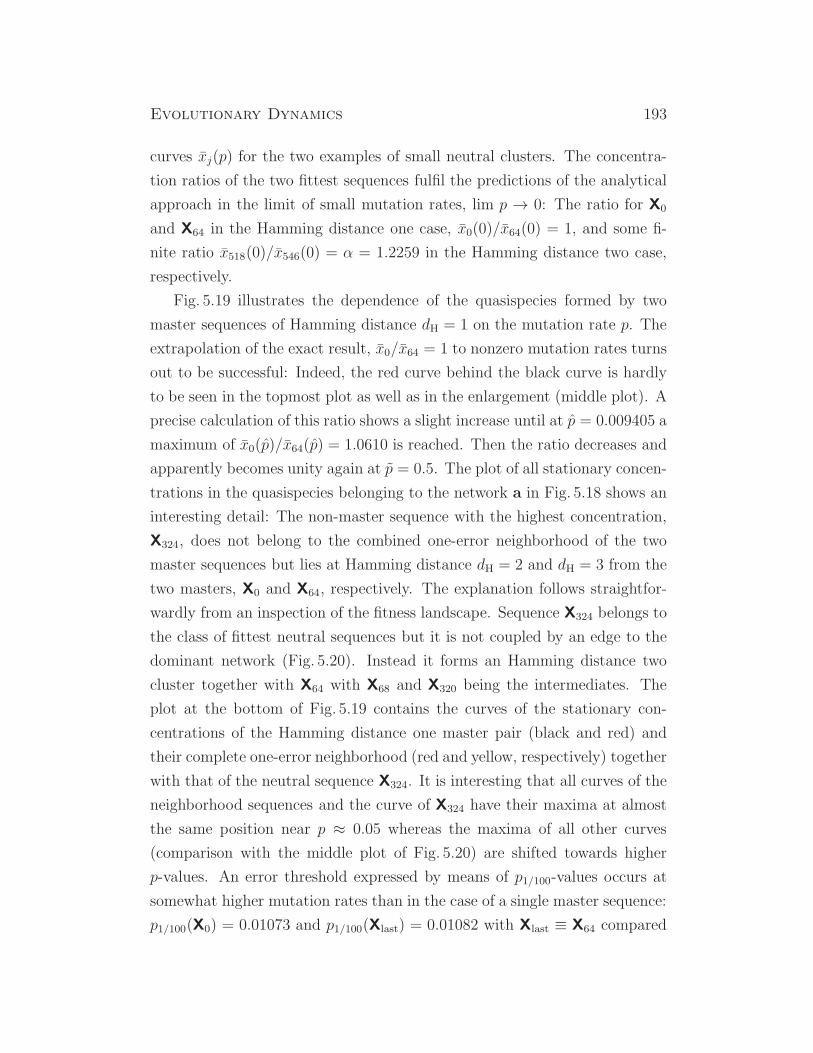
Evolutionary Dynamics 193
curves xj(p) for the two examples of small neutral clusters. The concentra-
tion ratios of the two fittest sequences fulfil the predictions of the analytical
approach in the limit of small mutation rates, lim p → 0: The ratio for X0
and X64 in the Hamming distance one case, x0(0)/x64(0) = 1, and some fi-
nite ratio x518(0)/x546(0) = α = 1.2259 in the Hamming distance two case,
respectively.
Fig. 5.19 illustrates the dependence of the quasispecies formed by two
master sequences of Hamming distance dH = 1 on the mutation rate p. The
extrapolation of the exact result, x0/x64 = 1 to nonzero mutation rates turns
out to be successful: Indeed, the red curve behind the black curve is hardly
to be seen in the topmost plot as well as in the enlargement (middle plot). A
precise calculation of this ratio shows a slight increase until at p = 0.009405 a
maximum of x0(p)/x64(p) = 1.0610 is reached. Then the ratio decreases and
apparently becomes unity again at p = 0.5. The plot of all stationary concen-
trations in the quasispecies belonging to the network a in Fig. 5.18 shows an
interesting detail: The non-master sequence with the highest concentration,
X324, does not belong to the combined one-error neighborhood of the two
master sequences but lies at Hamming distance dH = 2 and dH = 3 from the
two masters, X0 and X64, respectively. The explanation follows straightfor-
wardly from an inspection of the fitness landscape. Sequence X324 belongs to
the class of fittest neutral sequences but it is not coupled by an edge to the
dominant network (Fig. 5.20). Instead it forms an Hamming distance two
cluster together with X64 with X68 and X320 being the intermediates. The
plot at the bottom of Fig. 5.19 contains the curves of the stationary con-
centrations of the Hamming distance one master pair (black and red) and
their complete one-error neighborhood (red and yellow, respectively) together
with that of the neutral sequence X324. It is interesting that all curves of the
neighborhood sequences and the curve of X324 have their maxima at almost
the same position near p ≈ 0.05 whereas the maxima of all other curves
(comparison with the middle plot of Fig. 5.20) are shifted towards higher
p-values. An error threshold expressed by means of p1/100-values occurs at
somewhat higher mutation rates than in the case of a single master sequence:
p1/100(X0) = 0.01073 and p1/100(Xlast) = 0.01082 with Xlast ≡ X64 compared
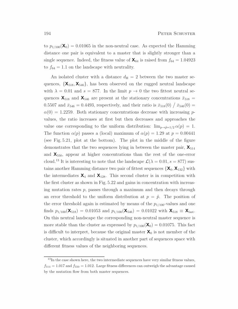
194 Peter Schuster
to p1/100(X0) = 0.01065 in the non-neutral case. As expected the Hamming
distance one pair is equivalent to a master that is slightly stronger than a
single sequence. Indeed, the fitness value of X64 is raised from f64 = 1.04923
to f64 = 1.1 on the landscape with neutrality.
An isolated cluster with a distance dH = 2 between the two master se-
quences, X518,X546, has been observed on the rugged neutral landscape
with λ = 0.01 and s = 877. In the limit p → 0 the two fittest neutral se-
quences X518 and X546 are present at the stationary concentrations x518 =
0.5507 and x546 = 0.4493, respectively, and their ratio is x518(0)/
x546(0) =
α(0) = 1.2259. Both stationary concentrations decrease with increasing p-
values, the ratio increases at first but then decreases and approaches the
value one corresponding to the uniform distribution: limp→p=1/2 α(p) = 1.
The function α(p) passes a (local) maximum of α(p) = 1.29 at p = 0.00441
(see Fig. 5.21, plot at the bottom). The plot in the middle of the figure
demonstrates that the two sequences lying in between the master pair, X514
and X550, appear at higher concentrations than the rest of the one-error
cloud.13 It is interesting to note that the landscape L(λ = 0.01, s = 877) sus-
tains another Hamming distance two pair of fittest sequences X0,X132 withthe intermediates X4 and X128. This second cluster is in competition with
the first cluster as shown in Fig. 5.22 and gains in concentration with increas-
ing mutation rates p, passes through a maximum and then decays through
an error threshold to the uniform distribution at p = p. The position of
the error threshold again is estimated by means of the p1/100-values and one
finds p1/100(X518) = 0.01053 and p1/100(X546) = 0.01022 with X518 ≡ Xlast.
On this neutral landscape the corresponding non-neutral master sequence is
more stable than the cluster as expressed by p1/100(X0) = 0.01075. This fact
is difficult to interpret, because the original master X0 is not member of the
cluster, which accordingly is situated in another part of sequences space with
different fitness values of the neighboring sequences.
13In the case shown here, the two intermediate sequences have very similar fitness values,
f514 = 1.017 and f550 = 1.012. Large fitness differences can outweigh the advantage caused
by the mutation flow from both master sequences.
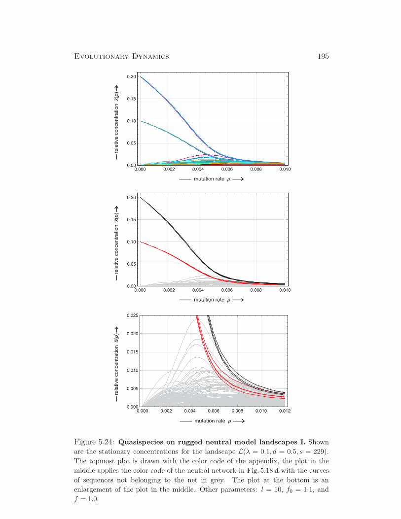
Evolutionary Dynamics 195
mutation rate p
rela
tive c
oncentr
ation
()
xp
mutation rate p
rela
tive c
oncentr
ation
()
xp
mutation rate p
rela
tive
co
nce
ntr
atio
n(
)x
p
Figure 5.24: Quasispecies on rugged neutral model landscapes I. Shown
are the stationary concentrations for the landscape L(λ = 0.1, d = 0.5, s = 229).
The topmost plot is drawn with the color code of the appendix, the plot in the
middle applies the color code of the neutral network in Fig. 5.18d with the curves
of sequences not belonging to the net in grey. The plot at the bottom is an
enlargement of the plot in the middle. Other parameters: l = 10, f0 = 1.1, and
f = 1.0.
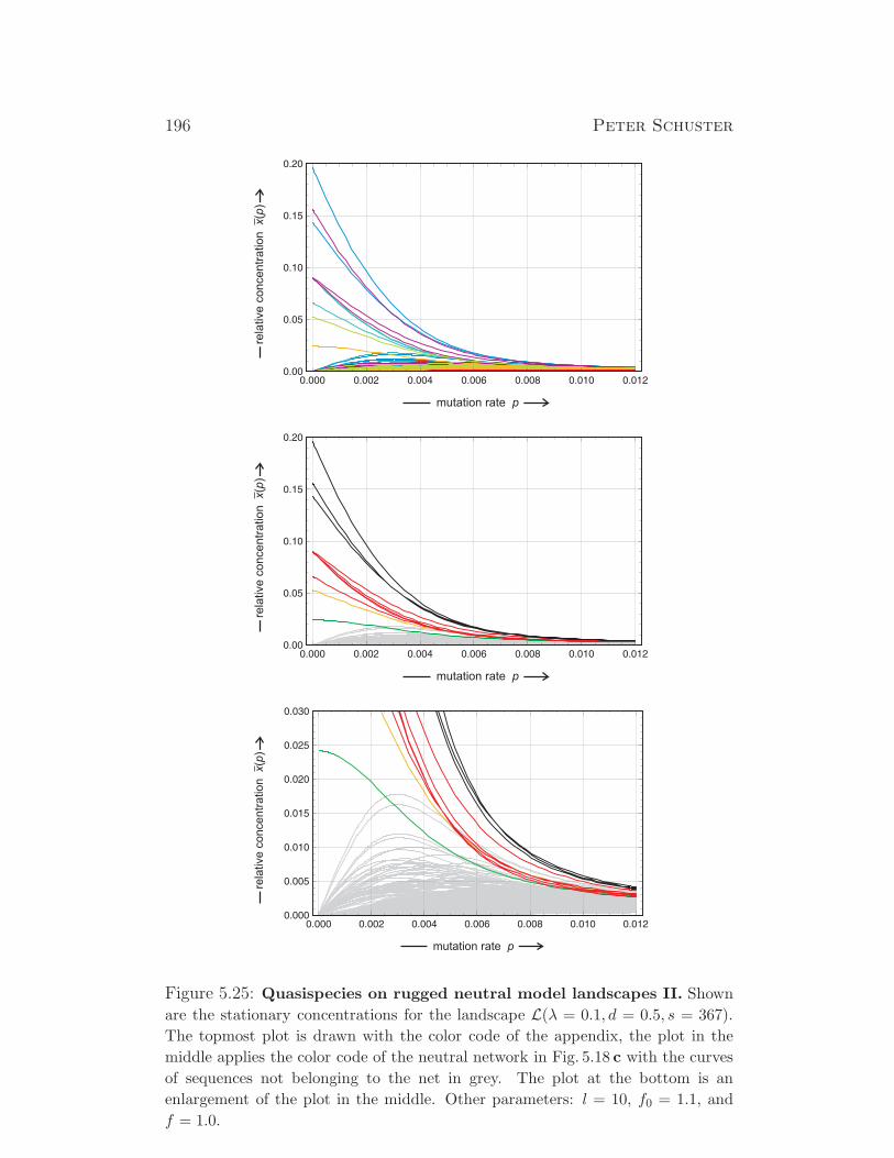
196 Peter Schuster
mutation rate p
rela
tive
co
nce
ntr
atio
n(
)x
p
mutation rate p
rela
tive
co
nce
ntr
atio
n(
)x
p
mutation rate p
rela
tive c
oncentr
ation
()
xp
Figure 5.25: Quasispecies on rugged neutral model landscapes II. Shown
are the stationary concentrations for the landscape L(λ = 0.1, d = 0.5, s = 367).
The topmost plot is drawn with the color code of the appendix, the plot in the
middle applies the color code of the neutral network in Fig. 5.18 c with the curves
of sequences not belonging to the net in grey. The plot at the bottom is an
enlargement of the plot in the middle. Other parameters: l = 10, f0 = 1.1, and
f = 1.0.
Evolutionary Dynamics 197
Eventually we consider a simple practical consequence of the existence
of fittest neutral pairs of Hamming distance dH = 1 and dH = 2 for the
sequence analysis in populations. Despite vast sequence heterogeneity [55],
in particular of virus populations, average or consensus sequences are fairly
insensitive to individual mutations provided the population size is sufficiently
large. Individual deviations in mutant sequences cancel through averaging
in population with single master sequences. This will not be the case in the
presence of neutral variants. In the 50/50 mixture of two master sequences
with mutant clouds surrounding both the sequence difference between the
masters is not going to cancel by averaging and ambiguities remain. Consid-
ering now the two cases discussed here: (i) two master sequences at Hamming
distance one present at equal concentrations and (ii) two master sequences
at Hamming distance two present at a concentration ratio α, we expect to
find sequence averages as sketched in Fig. 5.23. In the former case a 50/50
mixtures of two nucleotides is expected to occur at one position on the se-
quence, and in the latter case two positions will show nucleobase ambiguities
with the ratio α.
5.3.2 Medium size neutral clusters
An increase in the degree of neutrality λ will results in the appearance of
larger neutral networks that are scattered all over sequence space. We start
here by the introduction of the adjacency matrix as an appropriate reference
state of neutral networks and the discuss two examples of more complex
neutral networks that are observed in form of quasispecies on landscapes
Ln(λ = 0.1, d = 0.5, s).
The adjacency matrix of a graph contains an entry one at every off diago-
nal element that corresponds to an edge in the graph. We have, for example,
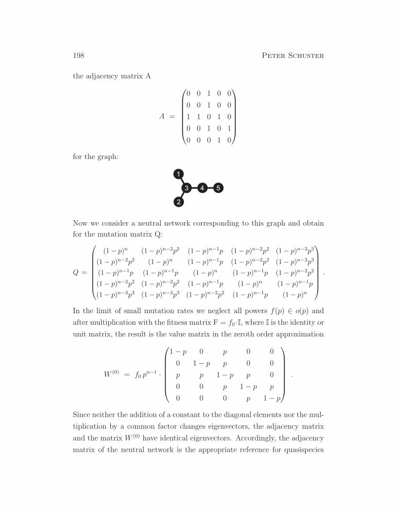
198 Peter Schuster
the adjacency matrix A
A =
0 0 1 0 0
0 0 1 0 0
1 1 0 1 0
0 0 1 0 1
0 0 0 1 0
for the graph:
Now we consider a neutral network corresponding to this graph and obtain
for the mutation matrix Q:
Q =
(1− p)n (1− p)n−2p2 (1− p)n−1p (1− p)n−2p2 (1− p)n−3p3
(1− p)n−2p2 (1− p)n (1− p)n−1p (1− p)n−2p2 (1− p)n−3p3
(1− p)n−1p (1− p)n−1p (1− p)n (1− p)n−1p (1− p)n−2p2
(1− p)n−2p2 (1− p)n−2p2 (1− p)n−1p (1− p)n (1− p)n−1p
(1− p)n−3p3 (1− p)n−3p3 (1− p)n−2p2 (1− p)n−1p (1− p)n
.
In the limit of small mutation rates we neglect all powers f(p) ∈ o(p) and
after multiplication with the fitness matrix F = f0·I, where I is the identity or
unit matrix, the result is the value matrix in the zeroth order approximation
W (0) = f0 pn−1 ·
1− p 0 p 0 0
0 1− p p 0 0
p p 1− p p 0
0 0 p 1− p p
0 0 0 p 1− p
.
Since neither the addition of a constant to the diagonal elements nor the mul-
tiplication by a common factor changes eigenvectors, the adjacency matrix
and the matrix W (0) have identical eigenvectors. Accordingly, the adjacency
matrix of the neutral network is the appropriate reference for quasispecies
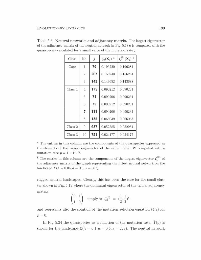
Evolutionary Dynamics 199
Table 5.3: Neutral networks and adjacency matrix. The largest eigenvector
of the adjacency matrix of the neutral network in Fig. 5.18 c is compared with the
quasispecies calculated for a small value of the mutation rate p.
Class No. j ζ0(Xj)a ζ
(0)0 (Xj)
b
Core 1 79 0.196220 0.196281
2 207 0.156240 0.156284
3 143 0.143652 0.143688
Class 1 4 175 0.090212 0.090231
5 71 0.090206 0.090231
6 75 0.090212 0.090231
7 111 0.090206 0.090231
8 135 0.066039 0.066053
Class 2 9 687 0.052585 0.052934
Class 3 10 751 0.024177 0.024177
a The entries in this column are the components of the quasispecies expressed as
the elements of the largest eigenvector of the value matrix W computed with a
mutation rate p = 1× 10−6.b The entries in this column are the components of the largest eigenvector ζ
(0)0 of
the adjacency matrix of the graph representing the fittest neutral network on the
landscape L(λ = 0.05, d = 0.5, s = 367).
rugged neutral landscapes. Clearly, this has been the case for the small clus-
ter shown in Fig. 5.19 where the dominant eigenvector of the trivial adjacency
matrix(
0 1
1 0
)
simply is ζ(0)0 = (
1
2,1
2)t ,
and represents also the solution of the mutation selection equation (4.9) for
p = 0.
In Fig. 5.24 the quasispecies as a function of the mutation rate, Υ(p) is
shown for the landscape L(λ = 0.1, d = 0.5, s = 229). The neutral network
200 Peter Schuster
consists of seven sequences, three of them form a linear inner core and four
are attached to it on the periphery (Fig. 5.18d). The dominant eigenvector
of the adjacency matrix is of the form
ζ(0)0 = (0.1, 0.1, 0.2, 0.2, 0.2, 0.1, 0.1) = (x184, x504, x248, x760, x728, x600, x729)
t .
The figure shows that the relative concentration within the quasispecies in
the sense of three more frequent and four less frequent sequences are perfectly
maintained almost up to the error threshold. The level crossing of the three
core sequences occurs at: p1/100(X248) = 0.007712, p1/100(X760) = 0.007307,
and p1/100(X728) = 0.007413.
The neutral network on the landscape L(λ = 0.1, d = 0.5, s = 367) has
a more complicated structure than the symmetric seven membered neutral
cluster discussed in the previous paragraph. It contains ten individual se-
quences and has the form shown in Fig. 5.18 c: A core of three sequences
is surrounded by five nearest neighbors and has a tail consisting of one
Hamming distance two and one Hamming distance three sequence. Also
for this more involved topology the low mutation rate limit of the quasis-
pecies, limp→0 Υ(p), converges exactly to the largest eigenvector of the ad-
jacency matrix (table 5.3). The three core sequences stay together for the
whole range of p-values up to the error threshold that is reached in terms
of level crossing at: p1/100(X79) = 0.007649, p1/100(X207) = 0.007462, and
p1/100(X143) = 0.007704. It is not easy to guess that four out of the five
nearest neighbor sequences have identical values in the eigenvector of the ad-
jacency matrix – and it is the tail-free sequence, X135, and not the sequence
carrying the tail, X175, which is different from the other four.
Further increase in the degree of neutrality, λ, gives rise to extended neu-
tral networks, which eventually percolate whole sequence space. Whether or
not such large clusters of neutral sequences play a role in real biology cannot
be said in the moment but more empirical knowledge on fitness landscapes
will help to decide this question.

6. Molecules in vitro and prokaryotes
6.1 Molecules in cell-free replication assays
6.2 Viroids and viruses
6.3 Bacteria under controlled conditions
201

202 Peter Schuster

7. Evolution of eukaryotes
203

204 Peter Schuster
8. Probability and stochasticity
An experimentalist reproduces an experiment. What can he expect to
find? There are certainly limits to precision and these limits confine the re-
producibility of experiments and at the same time restrict the predictability
of outcomes. The limitations of correct predictions are commonplace: We
witness them every day by watching the failures of various forecasts from the
weather to the stock market. Daily experience also tells us that there is an
enormous variability in the sensitivity of events with respect to precision of
observation. It ranges from the highly sensitive and hard to predict phenom-
ena like the ones just mentioned to the enormous accuracy of astronomical
predictions, for example, the precise dating of the eclipse of the sun in Europe
on August 11, 1999. Most cases lie between these two extremes and careful
analysis of unavoidable randomness becomes important. In this chapter we
are heading for a formalism, which allows for proper accounting of the lim-
itations of the deterministic approach and which extends the conventional
description by differential equations.
Modeling by differential equations makes one implicit assumption: The
use of continuous variables, xj(t), implies very large, in principle infinitely
large populations. Particles are discrete and countable objects and taking
into account the non-continuous nature of variables would be quite natural
therefore. The reason for using ODEs and PDEs instead is threefold: (i)
Large population sizes of 1020 particles and more do not allow for counting
particles because no experimental measuring technique exist, which could
possibly reach the required resolution, (ii) by equilibrium thermodynamics
stochastic fluctuation in populations of N particles are of the order√
N and√
1020 = 1010 particles is hardly detectable in populations of 1020 and more,
and (iii) last but not least the experience of modeling by means of differential
equations is enormous compared to other mathematical techniques – Leibniz
and Newton invented calculus almost 450 years ago.
205
206 Peter Schuster
In biology we can not always assume large particle numbers although
populations may reach appreciable sizes, for example the current human
population with 7×10⁹ individuals. In contrary, numbers are often very small
inevitably: Every mutation after all starts out from a single copy, regulatory
molecules are often present in a few copies only and due to recombination all
individuals in a population have different genomes with the only exception of
identical twins – this fact is used for unambiguous identification of individuals
in forensic genomics – to give just a few examples. Three different kinds of
models with discrete variables are important in biology: (i) Discrete time and
continuous population variables for modeling discrete generations obtained
through synchronization by day and night rhythms, by seasons or by other
pace makers lead to difference equations instead of differential equations,
(ii) continuous time and discrete population variables are typically used for
populations with small particle numbers and mixing generations and modeled
by a variety of stochastic processes, (iii) discrete time and discrete particle
numbers. Modeling deterministic discrete time processes is commonly done
by means of difference equations [44]. Modeling according to (ii) and (iii)
clearly requires probabilistic methods. For answering questions concerning
the three examples mentioned above and other similar cases of interest in
evolution research the modeling approach (ii) is most appropriate and we
shall in essence restrict here the discussion to continuous time stochastic
processes.
The conventional description by time dependent variables and functions
has to be replaced by a probabilistic view. We are no longer dealing with
exact values of variable but we shall use probabilities that variables take on
certain values. For example, the number of particles X is given by the time
dependent stochastic or random variable X (t),1 and this implies that the
values of X measured at some time, t = tr = t0 + ∆rt with t0 being the
initial time, will be different for different repetitions of an experiment under
identical conditions. In modern probability theory a rigorous definition of
1The notion of a random variable centers on the fact that the value of the variable
depends on the outcome of a random process. If an experiment is repeated under identical
conditions the value of a random variable will be different for every repetition.
Evolutionary Dynamics 207
random variables is given on the basis of sets on sample space.
Two introductory sections present the basic notations and definitions of
probability theory and stochastic processes for discrete and continuous ran-
dom variables. Then master equations as used in modeling chemical kinetics
will be presented. The advantage of modeling by means of chemical master
equations is twofold: (i) Since chemical master equations are based on chem-
ical kinetics they are very general and can be used for nonlinear and complex
reaction mechanisms, and (ii) numerical methods are available for the exact
simulation of the processes described by chemical master equations [117].
We shall also make a digression into the field of birth-and-death processes,
because this class of stochastic processes is most relevant for modeling evo-
lution. Eventually, we introduce and discuss Motoo Kimura’s neutral theory
of evolution.
8.1 Probabilities and probability theory
The concept of probability originated from the desire to analyze gambling
by rigorous mathematical thoughts. An early study that has largely re-
mained unnoticed but contained already the basic ideas of probability was
done in the sixteenth century by the Italian mathematician Gerolamo Car-
dano. The beginning of classical probability theory – 100 years after Cardano
– is associated with the story of French mathematician Blaise Pascal and the
professional gambler, the Chevalier de Mere that is told in almost ever intro-
duction to probability theory (see section 8.1.1). Classical probability theory
can handle all cases that are modeled by discrete quantities. It is based on
counting and accordingly fails when applied to uncountable sets. Uncount-
able sets are occur with continuous variables and these are indispensable for
migration in space as well as for large particle numbers that are described in
terms of concentrations. Current probability theory is based on set theory
and can handle discrete (and countable) as well as continuous (and uncount-
able) variables. We illustrate the historical probability theory my means of a
few examples and then provide a short introduction to modern probabilities
that are derived from set theoretical operations. In the third part we present
208 Peter Schuster
probability distributions and some of their properties that will be required
in the applications to stochastic processes.
8.1.1 Historical probability
The route to probability theory originated from risk and chance estimates in
gambling. The oldest well preserved document on a gambling problem mak-
ing correct use of probability theory is a letter of July 29, 1654, written by
Blaise Pascal to Pierre de Fermat in which he reports the careful observation
of a professional gambler, the Chevalier de Mere, which let . The Chevalier
observed that obtaining at least one “six” with one die in 4 throws is success-
ful in more than 50% in the cases whereas obtaining at least two times the
“six” with two dice in 24 throws has less than 50% chance to win. Chevalier
de Mere considered this finding as a paradox because he calculated naıvely
and erroneously that the chances should be the same:
4 throws with one die yields 4× 1
6=
2
3,
24 throws with two dice yields 24× 1
36=
2
3.
Blaise Pascal became interested in the problem and calculated the proba-
bilities correctly as we do it now in classical probability theory by careful
counting of events:
probability = Prob =number of favorable events
total number of events. (8.1)
A probability according to Equ. (8.1) is always a positive quantity between
zero and one, 0 ≤ Prob ≤ 1. The sum of the probabilities that an event has
occurred or did not occur thus has to be always one. Sometimes, as in the
gambler’s example, it is easier to calculate the probability of the unfavorable
case, q, and to obtain the desired probability as p = 1 − q. In the one-
die example the probability not to throw a “six” is 5/6, in the two-dice
example we have 35/36 as the probability of failure. In case of independent
events probabilities are multiplied2 and we finally obtain for 4 and 24 trials,
2We shall come back to the problem of independent events later when we introduce
current probability theory in subsection 8.1.2, which is based on set theory.
Evolutionary Dynamics 209
respectively:
q(1) =
(
5
6
)4
and p(1) = 1−(
5
6
)4
= 0.5177 ,
q(2) =
(
35
36
)24
and p(2) = 1−(
35
36
)24
= 0.4914 .
It is remarkable that the gambler could observe this rather small difference
in the probability of success – he must have tried the game very often indeed!
Classical probability theory centers around notions like independence of
events, joint and conditional probabilities, and many others, which are also
central issues of modern set theory based probability and we dispense here
from unnecessary repetition.
8.1.2 Sets, sample spaces, and probability
Sets are collections of objects with two restrictions: (i) Each object belongs
to one set cannot be a member of more sets and (ii) a member of a set must
not appear twice or more often. In other words, objects are assigned to
sets unambiguously. In application to probability theory we shall denote the
elementary objects by the small Greek letter omega, ω – if necessary with
various sub- and superscripts – and call them sample points or individual
results and the collection of all objects ω under consideration the sample
space is denoted by Ω with ω ∈ Ω. Events, A, are subsets of sample points
that fulfil some condition3
A =
ω, ωk ∈ Ω : f(ω) = c
(8.2)
with ω = ω1, ω2, . . . being some set of individual results and f(ω) = c
encapsulates the condition on ensemble of the sample points ωk.4
3What a condition means will become clear later. For the moment it is sufficient to
understand a condition as a function providing a restriction, which implies that not all
subsets of sample points belong to A.4In order to avoid misinterpretations we shall use different symbols for sets and strings:
· · · is a set, every element appears only once and the sequence of elements is irrelevant,
and (α2, α1, α1, · · · ) is a string where repetitions may occur and the sequence matters.
A nucleotide sequence (GAA· · · ) is a string and the nucleotide alphabet is a (sub)set:
A = A,U,G,C.
210 Peter Schuster
Any partial collection of points is a subset of Ω. We shall be dealing with
fixed Ω and, for simplicity, often call these subsets of Ω just sets. There
are two extreme cases, the entire sample space Ω and the empty set, ∅.The number of points in some set S is called its size, |S|, and thus is a
nonnegative integer or ∞. In particular, the size of the empty set is |∅| = 0.
The unambiguous assignment of points to sets can be expressed by5
ω ∈ S exclusive or ω /∈ S .
Consider two sets A and B. If every point of A belongs to B, then A is
contained in B. A is a subset of B and B is a superset of A:
A ⊂ B and B ⊃ A .
Two sets are identical if the contain exactly the same points and then we
write A = B. In other words, A = B iff (if and only if) A ⊂ B and B ⊂ A.
The basic operations with sets are illustrated in Fig. 8.1. We briefly repeat
them here:
Complement. The complement of the set A is denoted by Ac and consists of
all points not belonging to A:6
Ac = ω|ω /∈ A . (8.3)
There are three evident relations which can be verified easily: (Ac)c = A,
Ω c = ∅, and ∅ c = Ω.
Union. The union of the two sets A and B, A∪B, is the set of points which
belong to at least one of the two sets:
A ∪ B = ω|ω ∈ A or ω ∈ B . (8.4)
Intersection. The intersection of the two sets A and B, A ∩ B, is the set of
points which belong to both sets (For short A∩B is sometimes written AB):
A ∩ B = ω|ω ∈ A and ω ∈ B . (8.5)
5In order to be unambiguously clear we shall write or for and/or and exclusive or for
or in the strict sense.6Since we are considering only fixed sample sets Ω these points are uniquely defined.
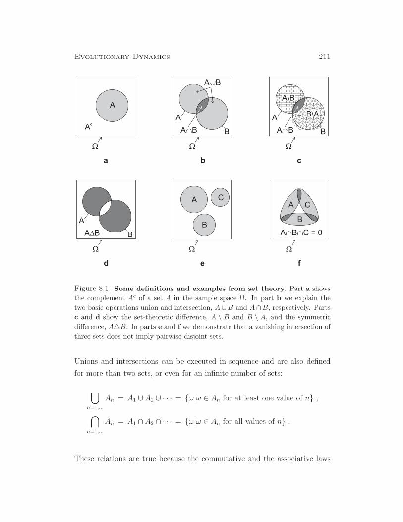
Evolutionary Dynamics 211
aaaaaaaaaaaaaaaaaaaaaaaaaaaaaaaaaaaaaaaaaaaaaaaaaaaaaaaaaaaaaaaaaaaaaaaaaaaaaaaaa
aaaaaaaaaaaaaaaaaaaaaaaaa
Figure 8.1: Some definitions and examples from set theory. Part a shows
the complement Ac of a set A in the sample space Ω. In part b we explain the
two basic operations union and intersection, A∪B and A∩B, respectively. Parts
c and d show the set-theoretic difference, A \ B and B \ A, and the symmetric
difference, AB. In parts e and f we demonstrate that a vanishing intersection of
three sets does not imply pairwise disjoint sets.
Unions and intersections can be executed in sequence and are also defined
for more than two sets, or even for an infinite number of sets:
⋃
n=1,...
An = A1 ∪ A2 ∪ · · · = ω|ω ∈ An for at least one value of n ,
⋂
n=1,...
An = A1 ∩ A2 ∩ · · · = ω|ω ∈ An for all values of n .
These relations are true because the commutative and the associative laws
212 Peter Schuster
are fulfilled by both operations, intersection and union:
A ∪ B = B ∪A , A ∩B = B ∩ A ;
(A ∪ B) ∪ C = A ∪ (B ∪ C) , (A ∩B) ∩ C = A ∩ (B ∩ C) .
Difference. The set A \B is the set of points, which belong to A but not to
B:
A \B = A ∩ Bc = ω|ω ∈ A and ω /∈ B . (8.6)
In case A ⊃ B we write A− B for A \B and have A \ B = A− (A ∩ B) as
well as Ac = Ω−A.
Symmetric difference. The symmetric difference A∆B is the set of points
which belongs exactly to one of the two sets A and B. It is used in advanced
theory of sets and is symmetric as it fulfils the commutative law, A∆B =
B∆A:
A∆B = (A ∩ Bc) ∪ (Ac ∩ B) = (A \B) ∪ (B \ A) . (8.7)
Disjoint sets. Disjoint sets A and B have no points in common and hence
their intersection, A ∩ B, is empty. They fulfill the following relations:
A ∩ B = ∅ , A ⊂ Bc and B ⊂ Ac . (8.8)
A number of sets are disjoint only if they are pairwise disjoint. For three sets,
A, B and C, this requires A∩B = ∅, B ∩C = ∅, and C ∩A = ∅. When
two sets are disjoint the addition symbol is (sometimes) used for the union,
A +B for A ∪B. Clearly we have always the decomposition: Ω = A+ Ac.
Sample spaces may contain finite or infinite numbers of sample points.
As shown in Fig. 8.2 it is important to distinguish further between different
classes of infinity: countable and uncountable numbers of points. The set of
rational numbers, for example, is a countably infinite since the numbers can
be labeled and assigned uniquely to the positive integers
1 < 2 < 3 < · · · < n < · · · .The set of real numbers cannot be ordered in such a way and hence it is
uncountable.
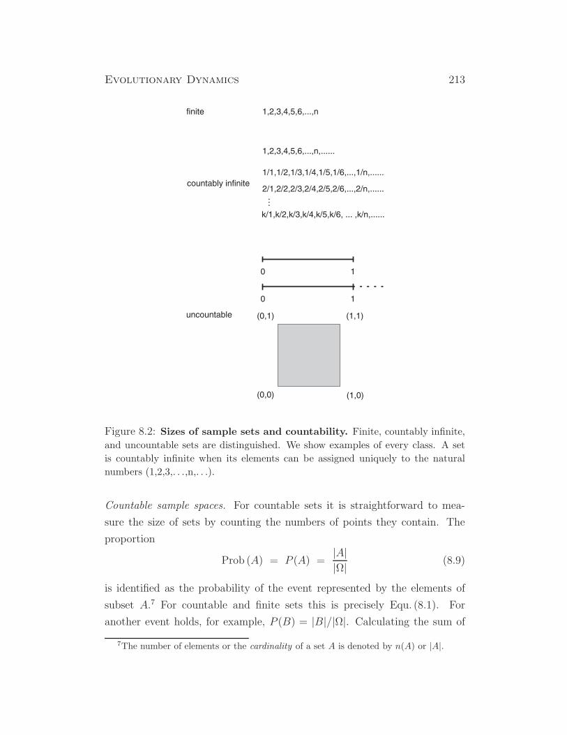
Evolutionary Dynamics 213
Figure 8.2: Sizes of sample sets and countability. Finite, countably infinite,
and uncountable sets are distinguished. We show examples of every class. A set
is countably infinite when its elements can be assigned uniquely to the natural
numbers (1,2,3,. . .,n,. . .).
Countable sample spaces. For countable sets it is straightforward to mea-
sure the size of sets by counting the numbers of points they contain. The
proportion
Prob (A) = P (A) =|A||Ω| (8.9)
is identified as the probability of the event represented by the elements of
subset A.7 For countable and finite sets this is precisely Equ. (8.1). For
another event holds, for example, P (B) = |B|/|Ω|. Calculating the sum of
7The number of elements or the cardinality of a set A is denoted by n(A) or |A|.
214 Peter Schuster
the two probabilities, P (A) + P (B), requires some care since we know only
(Fig. 8.1):
|A| + |B| ≥ |A ∪ B| .
The excess of |A|+ |B| over the size of the union |A∪B| is precisely the size
of the intersection |A ∩ B| and thus we find
|A| + |B| = |A ∪ B| + |A ∩ B|
or by division through the size of sample space Ω
P (A) + P (B) = P (A ∪ B) + P (A ∩B) .
Only in case the intersection is empty, A ∩ B = ∅, the two sets are disjoint
and their probabilities are additive, |A ∪ B| = |A|+ |B|, and hence
P (A+B) = P (A) + P (B) iff A ∩B = ∅ . (8.10)
It is important to memorize this condition for later use, because it represents
an implicitly made assumption for computing probabilities.
Now we can define a probability measure by means of the basic axioms
of probability theory (for alternative axioms in probability theory see, for
example [40, 164]):
A probability measure on the sample space Ω is a function of subsets of Ω,
P : S → P (S) or P (·) for short, which is defined by the three axioms:
(i) For every set A ⊂ Ω, the value of the probability measure is a nonneg-
ative number, P (A) ≥ 0 for all A,
(ii) the probability measure of the entire sample set – as a subset – is equal
to one, P (Ω) = 1, and
(iii) for any two disjoint subsets A and B, the value of the probability mea-
sure for the union, A ∪B = A+B, is equal to the sum of its value for
A and its value for B,
P (A ∪ B) = P (A+B) = P (A) + P (B) provided P (A ∩B) = ∅ .

Evolutionary Dynamics 215
Figure 8.3: The powerset. The powerset P(Ω) is a set containing all subsets
of Ω including the empty set ∅ and Ω itself. The figure sketches the powerset of
three events A, B, C.
Condition (iii) implies that for any countable – eventually infinite – collection
of disjoint or non-overlapping sets, Ai (i = 1, 2, 3, . . .) with Ai ∩ Aj = ∅ forall i 6= j, the relation called σ-additivity or countable additivity
P
(
⋃
i
Ai
)
=∑
i
P (Ai) or P
( ∞∑
k=1
Ak
)
=
∞∑
k=1
P (Ak) (8.11)
holds. Clearly we have also P (Ac) = 1− P (A), P (A) = 1− P (Ac) ≤ 1, and
P (∅) = 0. For any two sets A ⊂ B we have P (A) ≤ P (B) and P (B − A) =P (B) − P (A). For any two arbitrary sets A and B we can write a sum of
disjoint sets as follows
A ∪ B = A + Ac ∩ B and
P (A ∪ B) = P (A) + P (Ac ∩ B) .
Since B ⊂ Ac ∩ B we obtain P (A ∪ B) ≤ P (A) + P (B).
The set of all subsets of Ω is the powerset P(Ω) (Fig. 8.3). It contains the
empty set ∅, the sample space Ω and all subsets of Ω and this includes the
results of all set theoretic operations that were listed above. The powerset
216 Peter Schuster
of some given set S has cardinality 2|S|. The relation between the sample
point ω, an event A, the sample space Ω and the powerset P(Ω) is illustratedby means of an example taken from molecular evolution of nucleic acid se-
quences: single nucleotide exchanges or point mutations. Mutation in natural
DNA or RNA sequences may be considered like rolling dice with four out-
comes, e.g. A→T(U), A→G, and A→C, and the fourth outcome is A→A, no
change or correct reproduction. For the sake of simplicity we assume binary
sequences that correspond to Bernoulli trials discussed in subsection 8.2.1.
Events ω are mutations 0 → 1, and the sample points for flipping the coin
n-times are binary n-tuples or strings, ω = (ω1, ω2, . . . , ωn) with ωi ∈ 0, 1.8The powerset shown in Fig. 8.3 corresponds to sequences of length l = 3 with
the empty set, ∅, is represented by (000). Events indicate the appearance
of a 1 at a certain position: A ≡ 100, B ≡ 010, C ≡ 001, AB ≡ 110,
etc. Identifying some (reference) binary sequence X0 with the empty set
the analogy between the power set and the sequence space Q is recognized
straightforwardly. It is useful to consider also infinite numbers of repeats,
in particular for computing limits n → ∞: ω = (ω1, ω2, . . .) = (ωi)i∈N with
ωi ∈ 0, 1. Then we are dealing with infinitely long binary strings and the
sample space Ω = 0, 1N is the space of all infinitely long binary strings.
It is countable as can be easily verified: Every binary string represents the
binary encoding of a natural number (including ’0’) Nk ∈ N0 and hence Ω is
countable as the natural numbers are.
A subset of Ω will be called an event A iff a probability measure derived
from axioms (i), (ii), and (iii) has been assigned. Often one is not interested
in the full detail of a probabilistic result and events can be easily coarse
grained by lumping together sample points. We ask, for example, for the
probability A that n coin flips yield at least k-times tail, i.e. the score 1:
A =
ω = (ω1, ω2, . . . , ωn) ∈ Ω :
n∑
i=1
ωi ≥ k
,
8There is a trivial but important distinction between strings or n-tuples and sets: In
a string the position of an element matters, whereas in a set it does not. The following
three sets are identical: 1, 2, 3 = 3, 1, 2 = 1, 2, 2, 3. In order to avoid ambiguities
string are written in (normal) parentheses and sets in curly brackets.
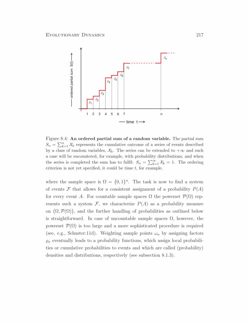
Evolutionary Dynamics 217
2 3 4 5 6 7 n1
X6X5
X1
X2
X3
X4
X7
Xn
time t
ord
ere
dpart
ial sum
S
(t)
Figure 8.4: An ordered partial sum of a random variable. The partial sum
Sn =∑n
k=1Xk represents the cumulative outcome of a series of events described
by a class of random variables, Xk. The series can be extended to +∞ and such
a case will be encountered, for example, with probability distributions, and when
the series is completed the sum has to fulfil: Sn =∑∞
k=1Xk = 1. The ordering
criterion is not yet specified, it could be time t, for example.
where the sample space is Ω = 0, 1n. The task is now to find a system
of events F that allows for a consistent assignment of a probability P (A)
for every event A. For countable sample spaces Ω the powerset P(Ω) rep-
resents such a system F , we characterize P (A) as a probability measure
on(
Ω,P(Ω))
, and the further handling of probabilities as outlined below
is straightforward. In case of uncountable sample spaces Ω, however, the
powerset P(Ω) is too large and a more sophisticated procedure is required
(see, e.g., Schuster:11d). Weighting sample points ωn by assigning factors
n eventually leads to a probability functions, which assign local probabili-
ties or cumulative probabilities to events and which are called (probability)
densities and distributions, respectively (see subsection 8.1.3).
218 Peter Schuster
Random variables and functions. For a precise definition of random variables
on countable sets a probability triple (Ω,P(Ω), P ) is required: Ω contains the
sample points or individual results, the powerset P(Ω) provides the events
A as subsets, and P eventually represents a probability measure that will be
precisely defined in Equ. (8.19). Based on such a probability triple we define
a random variable as a numerically valued function X of ω on the domain of
the entire sample space Ω,
ω ∈ Ω : ω → X (ω) . (8.12)
Random variables, X (ω) and Y(ω), can be subject to operations to yield
other random variables, such as
X (ω) + Y(ω) , X (ω)−Y(ω) , X (ω)Y(ω) , X (ω)/Y(ω) [Y(ω) 6= 0] ,
and, in particular, also any linear combination of random variables such as
αX (ω) + βY(ω) is a random variable too. Just as a function of a function is
still a function, a function of a random variable is a random variable,
ω ∈ Ω : ω → ϕ (X (ω),Y(ω)) = ϕ(X ,Y) .
Particularly important cases are the (partial) sums of n variables:
Sn(ω) = X1(ω) + . . . + Xn(ω) =
n∑
k=1
Xk(ω) . (8.13)
Such a partial sum Sn could be, for example, the cumulative outcome of
n successive throws of a die.9 Consider, for example, an ordered series of
events where the current cumulative outcome is given by the partial sum
Sn =∑n
k=1Xk as shown in Fig. 8.4. In principle, the series can be extended to
infinity and then the conservation relation of probabilities, Sn =∑∞
k=1Xk =
1, has to be fulfilled.
9The use of partial in this context implies that the sum does not cover the entire
sample space in the moment. Series of throws of dice, for example, could be continued in
the future.
Evolutionary Dynamics 219
Joint probabilities. Two (or more) random variables,10 X and Y , form a
random vector, ~Z = (X ,Y), which is defined by the probability
P (X = xi,Y = yj) = p(xi, yj) . (8.14)
These probabilities constitute the joint probability distribution (see subsec-
tion 8.1.3) of the random vector. By summation over one variable we obtain
the probabilities for the two marginal distributions :
P (X = xi) =∑
yj
p(xi, yj) = p(xi, ∗) and
P (Y = yj) =∑
xi
p(xi, yj) = p(∗, yj) ,(8.15)
of X and Y , respectively. In other words, the marginal distributions reduce
the multivariate function p(xi, yj) to functions of single variables, p(xi) and
p(yj) through summation over all possible values of the second variable.
Conditional probabilities. The conventional probability is defined on the en-
tire sample space Ω, P (A) = |A|/|Ω| =∑ω∈A P (ω)/∑
ω∈Ω P (ω).11 We shall
now define a probability of set A relative to another set, say S. This means
that we are interested in the proportional weight of the part of A in S which
is expressed by the intersection A ∩ S relative to S, and obtain
∑
ω∈A∩SP (ω)
/
∑
ω∈SP (ω) .
In other words, we switch from Ω to S as the new universe and consider the
conditional probability of A relative to S:
P (A|S) =P (A ∩ S)P (S)
=P (AS)
P (S)(8.16)
provided P (S) 6= 0. From here on we shall always use the a short notation
for the intersection, AS ≡ A∩S, in this section. Apparently, the conditional
probability vanishes if the intersection is empty: P (A|S) = 0 if P (AS) = ∅.10For simplicity we restrict ourselves to the two variable case here. The extension to
any finite number of variables is straightforward.11The sample space Ω is assumed to be countable and the weight P (ω) = P (ω) is
assigned to every point.
220 Peter Schuster
Next we mention several simple but fundamental relations involving con-
ditional probabilities that we present here, in essence, without proof (for
details see [36], pp.111-144). For n arbitrary events Ai we have
P (A1, A2, . . . , An) = P (A1)P (A2|A1)P (A3|A1A2) . . . P (An|A1A2 . . . An−1)
provided P (A1A2 . . . An−1) > 0. Under this proviso all conditional probabil-
ities are well defined since
P (A1) ≥ P (A1A2) ≥ . . . ≥ P (A1A2 . . . An−1) > 0 .
Let us assume that the sample space Ω is partitioned into n disjoint sets,
Ω =∑
nAn. For any set B we have then
P (B) =∑
n
P (An)P (B|An) .
From this relation it is straightforward to derive the conditional probability
P (Aj|B) =P (Aj)P (B|Aj)
∑
n P (An)P (B|An)
provided P (B) > 0.
Independence of random variables will be a highly relevant problem in
the forthcoming chapters. Countably-valued random variables X1, . . . ,Xn
are defined to be independent if and only if for any combination x1, . . . , xn
of real numbers the joint probabilities can be factorized:
P (X1 = x1, . . . ,Xn = xn) = P (X1 = x1) · . . . · P (Xn = xn) . (8.17)
A major extension of Equ. (8.17) replaces the single values xi by arbitrary
sets Si
P (X1 ∈ S1, . . . ,Xn ∈ Sn) = P (X1 ∈ S1) · . . . · P (Xn ∈ Sn) .
In order to proof this extension we sum over all points belonging to the sets
Evolutionary Dynamics 221
S1, . . . , Sn:
∑
x1∈S1
· · ·∑
xn∈Sn
P (X1 = x1, . . . ,Xn = xn) =
=∑
x1∈S1
· · ·∑
xn∈Sn
P (X1 ∈ S1) · . . . · P (Xn ∈ Sn) =
=
(
∑
x1∈S1
P (X1 ∈ S1)
)
· . . . ·(
∑
xn∈Sn
P (Xn ∈ Sn)
)
,
which is equal to the right hand side of the equation to be proven.
Since the factorization is fulfilled for arbitrary sets S1, . . . Sn it holds also
for all subsets of (X1 . . .Xn) and accordingly the events
X1 ∈ S1, . . . , Xn ∈ Sn
are also independent. It can also be verified that for arbitrary real-valued
functions ϕ1, . . . , ϕn on (−∞,+∞) the random variables ϕ1(X1), . . . , ϕn(Xn)
are independent too.
Independence can be extended in straightforward manner to the joint
distribution function of the random vector (X1, . . . ,Xn)
F (x1, . . . , xn) = F1(x1) · . . . · Fn(xn) ,
where the Fj ’s are the marginal distributions of the Xj’s , 1 ≤ j ≤ n. Thus,
the marginal distributions determine the joint distribution in case of inde-
pendence of the random variables.
8.1.3 Probability distributions
Depending on the nature of variables probability distributions are discrete
or continuous. We introduce probability distributions be discussing the con-
ceptually simpler discrete case and present then the differences encountered
for continuous probability functions.
Discrete probabilities. So far we have constructed and compared sets but
not yet introduced numbers, which are needed in actual computations. In
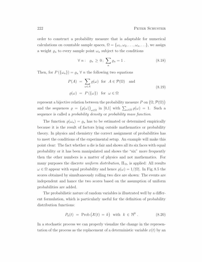
222 Peter Schuster
order to construct a probability measure that is adaptable for numerical
calculations on countable sample spaces, Ω = ω1, ω2, . . . , ωn, . . ., we assigna weight n to every sample point ωn subject to the conditions
∀ n : n ≥ 0 ;∑
n
n = 1 . (8.18)
Then, for P (ωn) = n ∀ n the following two equations
P (A) =∑
ω∈A(ω) for A ∈ P(Ω) and
(ω) = P (ω) for ω ∈ Ω
(8.19)
represent a bijective relation between the probability measure P on(
Ω,P(Ω))
and the sequences =(
(ω))
ω∈Ω in [0,1] with∑
ω∈Ω (ω) = 1. Such a
sequence is called a probability density or probability mass function.
The function (ωn) = n has to be estimated or determined empirically
because it is the result of factors lying outside mathematics or probability
theory. In physics and chemistry the correct assignment of probabilities has
to meet the conditions of the experimental setup. An example will make this
point clear: The fact whether a die is fair and shows all its six faces with equal
probability or it has been manipulated and shows the “six” more frequently
then the other numbers is a matter of physics and not mathematics. For
many purposes the discrete uniform distribution, ΠΩ, is applied: All results
ω ∈ Ω appear with equal probability and hence (ω) = 1/|Ω|. In Fig. 8.5 the
scores obtained by simultaneously rolling two dice are shown: The events are
independent and hance the two scores based on the assumption of uniform
probabilities are added.
The probabilistic nature of random variables is illustrated well by a differ-
ent formulation, which is particularly useful for the definition of probability
distribution functions:
Pk(t) = Prob(
X (t) = k)
with k ∈ N0 . (8.20)
In a stochastic process we can properly visualize the change in the represen-
tation of the process as the replacement of a deterministic variable x(t) by an
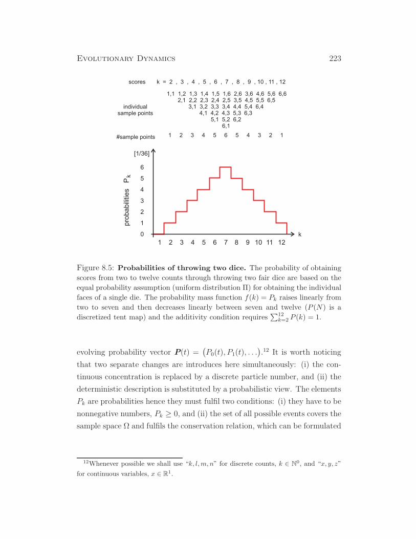
Evolutionary Dynamics 223
scores k = 2 , 3 , 4 , 5 , 6 , 7 , 8 , 9 , 10 , 11 , 12
1,1 1,2 1,3 1,4 1,5 1,6 2,6 3,6 4,6 5,6 6,62,1 2,2 2,3 2,4 2,5 3,5 4,5 5,5 6,5
3,1 3,2 3,3 3,4 4,4 5,4 6,44,1 4,2 4,3 5,3 6,3
5,1 5,2 6,26,1
1 2 3 4 5 6 5 4 3 2 1#sample points
individualsample points
k
1 2 3 4 5 6 7 8 9 10 11 12
6
5
4
3
2
1
0
[1/36]
pro
babili
ties
Pk
Figure 8.5: Probabilities of throwing two dice. The probability of obtaining
scores from two to twelve counts through throwing two fair dice are based on the
equal probability assumption (uniform distribution Π) for obtaining the individual
faces of a single die. The probability mass function f(k) = Pk raises linearly from
two to seven and then decreases linearly between seven and twelve (P (N) is a
discretized tent map) and the additivity condition requires∑12
k=2 P (k) = 1.
evolving probability vector P(t) =(
P0(t), P1(t), . . .)
.12 It is worth noticing
that two separate changes are introduces here simultaneously: (i) the con-
tinuous concentration is replaced by a discrete particle number, and (ii) the
deterministic description is substituted by a probabilistic view. The elements
Pk are probabilities hence they must fulfil two conditions: (i) they have to be
nonnegative numbers, Pk ≥ 0, and (ii) the set of all possible events covers the
sample space Ω and fulfils the conservation relation, which can be formulated
12Whenever possible we shall use “k, l,m, n” for discrete counts, k ∈ N0, and “x, y, z”
for continuous variables, x ∈ R1.
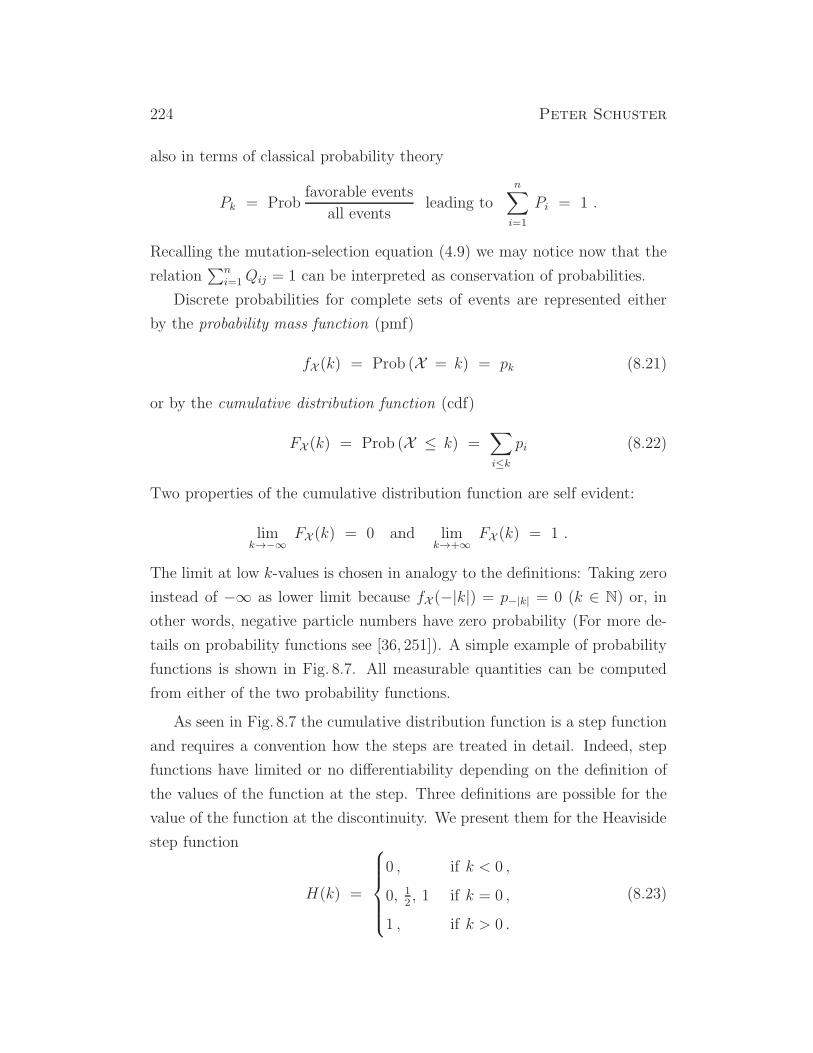
224 Peter Schuster
also in terms of classical probability theory
Pk = Probfavorable events
all eventsleading to
n∑
i=1
Pi = 1 .
Recalling the mutation-selection equation (4.9) we may notice now that the
relation∑n
i=1Qij = 1 can be interpreted as conservation of probabilities.
Discrete probabilities for complete sets of events are represented either
by the probability mass function (pmf)
fX (k) = Prob (X = k) = pk (8.21)
or by the cumulative distribution function (cdf)
FX (k) = Prob (X ≤ k) =∑
i≤kpi (8.22)
Two properties of the cumulative distribution function are self evident:
limk→−∞
FX (k) = 0 and limk→+∞
FX (k) = 1 .
The limit at low k-values is chosen in analogy to the definitions: Taking zero
instead of −∞ as lower limit because fX (−|k|) = p−|k| = 0 (k ∈ N) or, in
other words, negative particle numbers have zero probability (For more de-
tails on probability functions see [36, 251]). A simple example of probability
functions is shown in Fig. 8.7. All measurable quantities can be computed
from either of the two probability functions.
As seen in Fig. 8.7 the cumulative distribution function is a step function
and requires a convention how the steps are treated in detail. Indeed, step
functions have limited or no differentiability depending on the definition of
the values of the function at the step. Three definitions are possible for the
value of the function at the discontinuity. We present them for the Heaviside
step function
H(k) =
0 , if k < 0 ,
0, 12, 1 if k = 0 ,
1 , if k > 0 .
(8.23)

Evolutionary Dynamics 225
Figure 8.6: Continuity in probability theory and step processes. Threepossible choices of partial continuity at the steps of step functions are shown: (i)left-hand continuity (A), (ii) no continuity (B), and (iii) right-hand continuity (C).The step function in (A) is left-hand semi-differentiable, the step function in (C)is right-hand semi-differentiable, and the step function in (B) is neither right-handnor left-hand semi-differentiable. Choice (ii) allows for making use of the inherentsymmetry of the Heaviside function. Choice (iii) is the standard assumption inprobability theory and stochastic processes. It is also known as cadlag-property(subsection 8.2.1).
The value ’0’ at k = 0 implies left-hand continuity for H(k) and in terms of
a probability distribution would correspond to a definition Prob (X < k) in
Equ. (8.22), the value 12implies that H(k) is neither right-hand nor left-hand
semi-differentiable at k = 0 but is useful in many applications that make use
of the inherent symmetry of the Heaviside function, for example the relation
H(x) =(
1 + sgn(x))
/2 where sgn(x) is the sign or signum function:
sgn(x)
−1 if x < 0 ,
0 if x = 0 ,
1 if x > 0 .
The functions in probability theory make use of the third definition deter-
mined by P (X ≤ x) or H(0) = 1 in case of the Heaviside function. This
choice implies right-hand continuity or right-hand semi-differentiability and
is important in the conventional handling of stochastic processes.
Fig. (8.7) presents the probability mass function (pmf) and the cumulative
probability distribution function (cdf) for the scores of rolling two dice. The
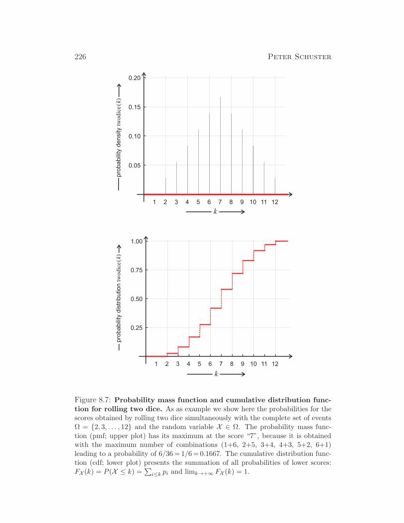
226 Peter Schuster
Figure 8.7: Probability mass function and cumulative distribution func-tion for rolling two dice. As as example we show here the probabilities for thescores obtained by rolling two dice simultaneously with the complete set of eventsΩ = 2, 3, . . . , 12 and the random variable X ∈ Ω. The probability mass func-tion (pmf; upper plot) has its maximum at the score “7”, because it is obtainedwith the maximum number of combinations (1+6, 2+5, 3+4, 4+3, 5+2, 6+1)leading to a probability of 6/36=1/6=0.1667. The cumulative distribution func-tion (cdf; lower plot) presents the summation of all probabilities of lower scores:FX (k) = P (X ≤ k) =
∑
i≤k pi and limk→+∞ FX (k) = 1.

Evolutionary Dynamics 227
former is given by the tent function
f(k) =
1s2(k − 1) for k = 1, 2, . . . , s ,
1s2(2s+ 1− k) for k = s+ 1, s+ 2, . . . , 2s
,
where k is the score and s the number of faces of the die, which is six in case
of the commonly used dice. The cumulative probability distribution is given
by the sum
F (k) =2s∑
i=2
f(i) .
Here the two-dice probability distribution is used only as an example for the
illustration of probability functions, but later on we shall extend to the n-dice
score problem in order to illustrate the law of large numbers.
The Poisson distribution. The Poisson distribution, a discrete probability
distribution, is of particular importance in the theory of stochastic processes,
because it expresses the probability that a given number of events occurs
within a fixed time interval (The corresponding stochastic process is the
Poisson process discussed in subsection 9.1.2). The events take place with a
known average rate and independently of the time that has elapsed since the
last event. An illustrative example is the arrival of (independent) e-mails:
We assume a person receiving on the average 50 e-mails per day, then the
Poisson probability mass function
Pois(k;λ) : f(k) =λk
k!e−λ with k ∈ N
0 = 0, 1, 2, . . . , (8.24)
returns the probability that exactly x are arriving in the same time interval,
i.e. per day. The corresponding cumulative distribution function is
Pois(k;λ) : F (k) =Γ(⌊k + 1⌋, λ)⌊k⌋! = e−λ
⌊k⌋∑
k=0
λk
k!for k ≤ 0 , (8.25)
with Γ(s, z) being the upper and γ(s, z) the lower incomplete Γ-function:
Γ(s, z) =
∫ ∞
zxs−1 e−x dx , γ(s, z) =
∫ z
0xs−1 e−x dx , Γ(s) = Γ(s, z) + γ(s, z) ,

228 Peter Schuster
Figure 8.8: Poisson density and distribution. In the plots the Poisson distri-bution, Pois(λ), is shown in from of the probability density f(k) and the probabilitydistribution F (k) as an example. The probability density f(k) is asymmetric forsmall λ-values (λ = 1, 2, 5) and steeper on the (left-hand) side of k-values blowthe maximum, whereas large λ’s give rise to more and more symmetric curves asexpected by the law of large numbers. Choice of parameters: λ = 1 (black), 2(red), 5 (green), 10 (blue) and 20 (yellow).
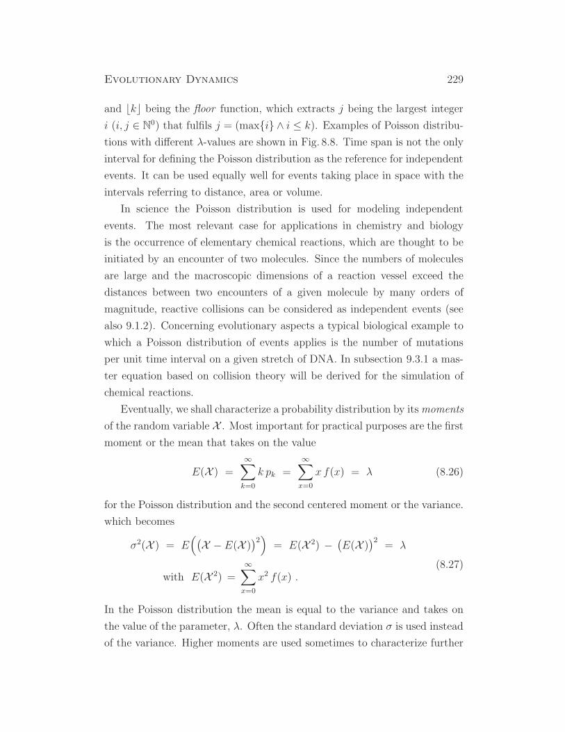
Evolutionary Dynamics 229
and ⌊k⌋ being the floor function, which extracts j being the largest integer
i (i, j ∈ N0) that fulfils j = (maxi ∧ i ≤ k). Examples of Poisson distribu-
tions with different λ-values are shown in Fig. 8.8. Time span is not the only
interval for defining the Poisson distribution as the reference for independent
events. It can be used equally well for events taking place in space with the
intervals referring to distance, area or volume.
In science the Poisson distribution is used for modeling independent
events. The most relevant case for applications in chemistry and biology
is the occurrence of elementary chemical reactions, which are thought to be
initiated by an encounter of two molecules. Since the numbers of molecules
are large and the macroscopic dimensions of a reaction vessel exceed the
distances between two encounters of a given molecule by many orders of
magnitude, reactive collisions can be considered as independent events (see
also 9.1.2). Concerning evolutionary aspects a typical biological example to
which a Poisson distribution of events applies is the number of mutations
per unit time interval on a given stretch of DNA. In subsection 9.3.1 a mas-
ter equation based on collision theory will be derived for the simulation of
chemical reactions.
Eventually, we shall characterize a probability distribution by itsmoments
of the random variable X . Most important for practical purposes are the first
moment or the mean that takes on the value
E(X ) =
∞∑
k=0
k pk =
∞∑
x=0
x f(x) = λ (8.26)
for the Poisson distribution and the second centered moment or the variance.
which becomes
σ2(X ) = E(
(
X − E(X ))2)
= E(X 2) −(
E(X ))2
= λ
with E(X 2) =
∞∑
x=0
x2 f(x) .(8.27)
In the Poisson distribution the mean is equal to the variance and takes on
the value of the parameter, λ. Often the standard deviation σ is used instead
of the variance. Higher moments are used sometimes to characterize further
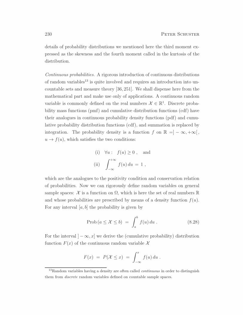
230 Peter Schuster
details of probability distributions we mentioned here the third moment ex-
pressed as the skewness and the fourth moment called in the kurtosis of the
distribution.
Continuous probabilities. A rigorous introduction of continuous distributions
of random variables13 is quite involved and requires an introduction into un-
countable sets and measure theory [36, 251]. We shall dispense here from the
mathematical part and make use only of applications. A continuous random
variable is commonly defined on the real numbers X ∈ R1. Discrete proba-
bility mass functions (pmf) and cumulative distribution functions (cdf) have
their analogues in continuous probability density functions (pdf) and cumu-
lative probability distribution functions (cdf), and summation is replaced by
integration. The probability density is a function f on R =] − ∞,+∞[ ,
u→ f(u), which satisfies the two conditions:
(i) ∀u : f(u) ≥ 0 , and
(ii)
∫ +∞
−∞f(u) du = 1 ,
which are the analogues to the positivity condition and conservation relation
of probabilities. Now we can rigorously define random variables on general
sample spaces: X is a function on Ω, which is here the set of real numbers R
and whose probabilities are prescribed by means of a density function f(u).
For any interval [a, b] the probability is given by
Prob (a ≤ X ≤ b) =
∫ b
a
f(u) du . (8.28)
For the interval ]−∞, x] we derive the (cumulative probability) distribution
function F (x) of the continuous random variable X
F (x) = P (X ≤ x) =
∫ x
−∞f(u) du .
13Random variables having a density are often called continuous in order to distinguish
them from discrete random variables defined on countable sample spaces.
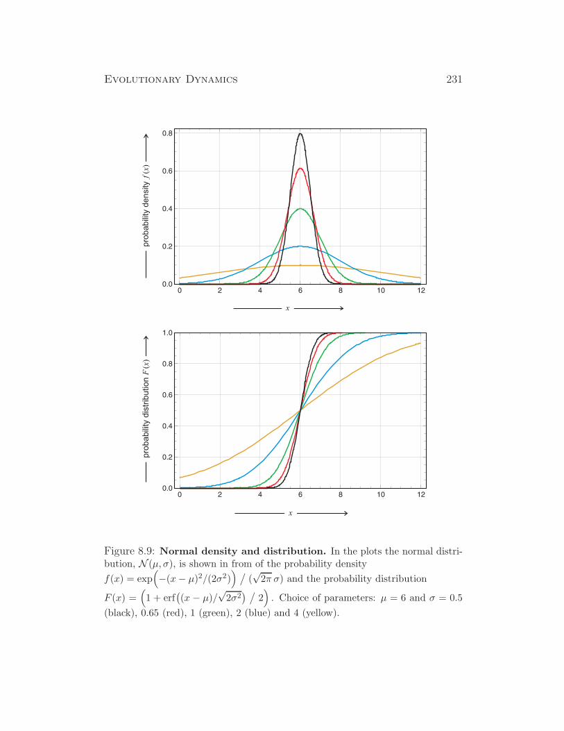
Evolutionary Dynamics 231
Figure 8.9: Normal density and distribution. In the plots the normal distri-bution, N (µ, σ), is shown in from of the probability density
f(x) = exp(
−(x− µ)2/(2σ2))
/
(√2π σ) and the probability distribution
F (x) =(
1 + erf(
(x − µ)/√2σ2) /
2)
. Choice of parameters: µ = 6 and σ = 0.5
(black), 0.65 (red), 1 (green), 2 (blue) and 4 (yellow).
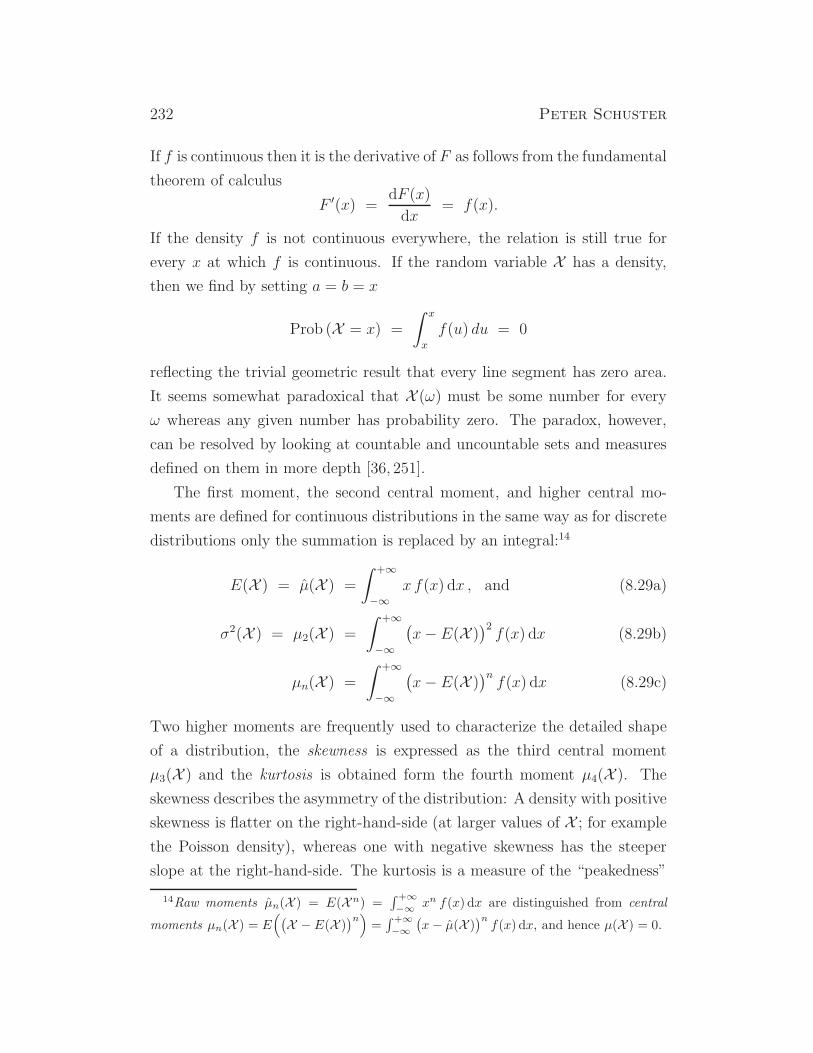
232 Peter Schuster
If f is continuous then it is the derivative of F as follows from the fundamental
theorem of calculus
F ′(x) =dF (x)
dx= f(x).
If the density f is not continuous everywhere, the relation is still true for
every x at which f is continuous. If the random variable X has a density,
then we find by setting a = b = x
Prob (X = x) =
∫ x
x
f(u) du = 0
reflecting the trivial geometric result that every line segment has zero area.
It seems somewhat paradoxical that X (ω) must be some number for every
ω whereas any given number has probability zero. The paradox, however,
can be resolved by looking at countable and uncountable sets and measures
defined on them in more depth [36, 251].
The first moment, the second central moment, and higher central mo-
ments are defined for continuous distributions in the same way as for discrete
distributions only the summation is replaced by an integral:14
E(X ) = µ(X ) =
∫ +∞
−∞x f(x) dx , and (8.29a)
σ2(X ) = µ2(X ) =
∫ +∞
−∞
(
x− E(X ))2f(x) dx (8.29b)
µn(X ) =
∫ +∞
−∞
(
x− E(X ))nf(x) dx (8.29c)
Two higher moments are frequently used to characterize the detailed shape
of a distribution, the skewness is expressed as the third central moment
µ3(X ) and the kurtosis is obtained form the fourth moment µ4(X ). The
skewness describes the asymmetry of the distribution: A density with positive
skewness is flatter on the right-hand-side (at larger values of X ; for example
the Poisson density), whereas one with negative skewness has the steeper
slope at the right-hand-side. The kurtosis is a measure of the “peakedness”
14Raw moments µn(X ) = E(Xn) =∫ +∞
−∞xn f(x) dx are distinguished from central
moments µn(X ) = E(
(
X − E(X ))n)
=∫ +∞
−∞
(
x− µ(X ))n
f(x) dx, and hence µ(X ) = 0.
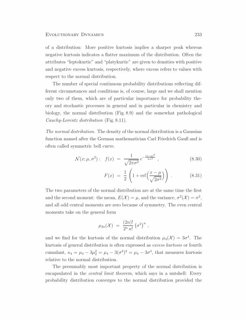
Evolutionary Dynamics 233
of a distribution: More positive kurtosis implies a sharper peak whereas
negative kurtosis indicates a flatter maximum of the distribution. Often the
attributes “leptokurtic” and “platykurtic” are given to densities with positive
and negative excess kurtosis, respectively, where excess refers to values with
respect to the normal distribution.
The number of special continuous probability distributions reflecting dif-
ferent circumstances and conditions is, of course, large and we shall mention
only two of them, which are of particular importance for probability the-
ory and stochastic processes in general and in particular in chemistry and
biology, the normal distribution (Fig. 8.9) and the somewhat pathological
Cauchy-Lorentz distribution (Fig. 8.11).
The normal distribution. The density of the normal distribution is a Gaussian
function named after the German mathematician Carl Friedrich Gauß and is
often called symmetric bell curve.
N (x;µ, σ2) : f(x) =1
√
2πσ2e−
(x−µ)2
2σ2 , (8.30)
F (x) =1
2
(
1 + erf(x− µ√
2σ2
)
)
. (8.31)
The two parameters of the normal distribution are at the same time the first
and the second moment: the mean, E(X ) = µ, and the variance, σ2(X ) = σ2,
and all odd central moments are zero because of symmetry. The even central
moments take on the general form
µ2n(X ) =(2n)!
2n n!
(
σ2)n,
and we find for the kurtosis of the normal distribution µ4(X ) = 3σ4. The
kurtosis of general distribution is often expressed as excess kurtosis or fourth
cumulant, κ4 = µ4 − 3µ22 = µ4 − 3(σ2)2 = µ4 − 3σ4, that measures kurtosis
relative to the normal distribution.
The presumably most important property of the normal distribution is
encapsulated in the central limit theorem, which says in a nutshell: Every
probability distribution converges to the normal distribution provided the
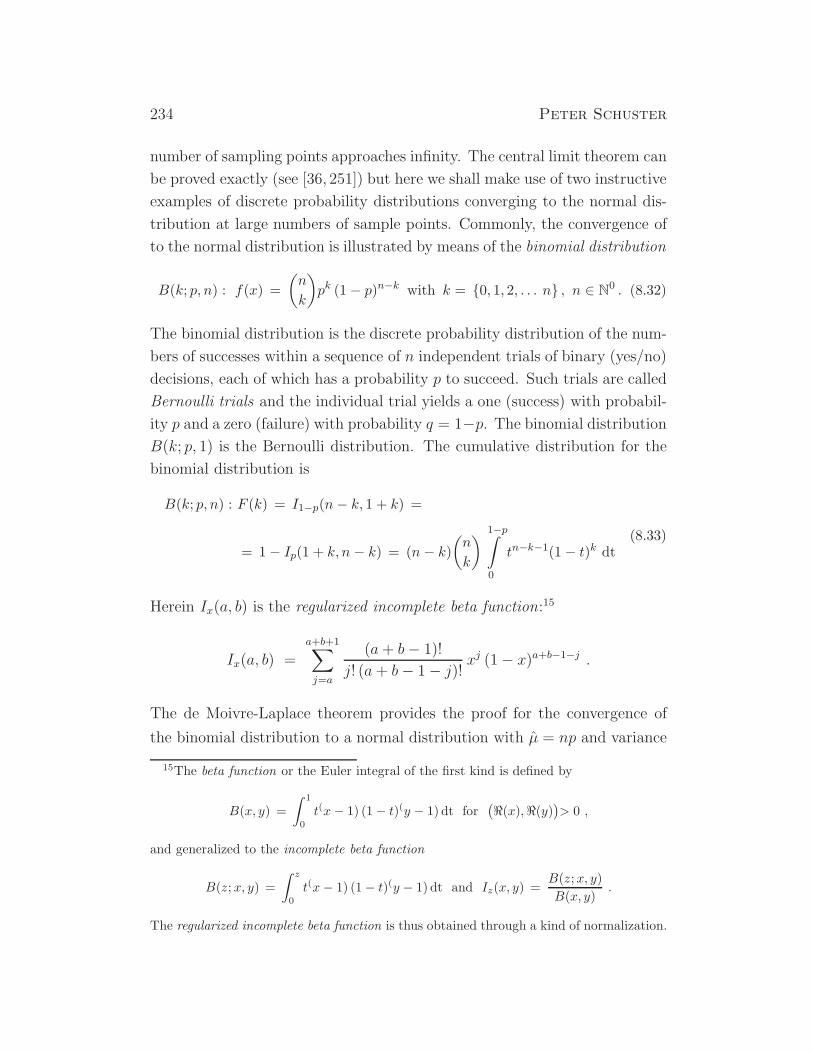
234 Peter Schuster
number of sampling points approaches infinity. The central limit theorem can
be proved exactly (see [36, 251]) but here we shall make use of two instructive
examples of discrete probability distributions converging to the normal dis-
tribution at large numbers of sample points. Commonly, the convergence of
to the normal distribution is illustrated by means of the binomial distribution
B(k; p, n) : f(x) =
(
n
k
)
pk (1− p)n−k with k = 0, 1, 2, . . . n , n ∈ N0 . (8.32)
The binomial distribution is the discrete probability distribution of the num-
bers of successes within a sequence of n independent trials of binary (yes/no)
decisions, each of which has a probability p to succeed. Such trials are called
Bernoulli trials and the individual trial yields a one (success) with probabil-
ity p and a zero (failure) with probability q = 1−p. The binomial distribution
B(k; p, 1) is the Bernoulli distribution. The cumulative distribution for the
binomial distribution is
B(k; p, n) : F (k) = I1−p(n− k, 1 + k) =
= 1− Ip(1 + k, n − k) = (n− k)
(
n
k
)
1−p∫
0
tn−k−1(1− t)k dt(8.33)
Herein Ix(a, b) is the regularized incomplete beta function:15
Ix(a, b) =a+b+1∑
j=a
(a+ b− 1)!
j! (a+ b− 1− j)! xj (1− x)a+b−1−j .
The de Moivre-Laplace theorem provides the proof for the convergence of
the binomial distribution to a normal distribution with µ = np and variance
15The beta function or the Euler integral of the first kind is defined by
B(x, y) =
∫ 1
0
t(x− 1) (1− t)(y − 1) dt for(
ℜ(x),ℜ(y))
> 0 ,
and generalized to the incomplete beta function
B(z;x, y) =
∫ z
0
t(x− 1) (1− t)(y − 1) dt and Iz(x, y) =B(z;x, y)
B(x, y).
The regularized incomplete beta function is thus obtained through a kind of normalization.
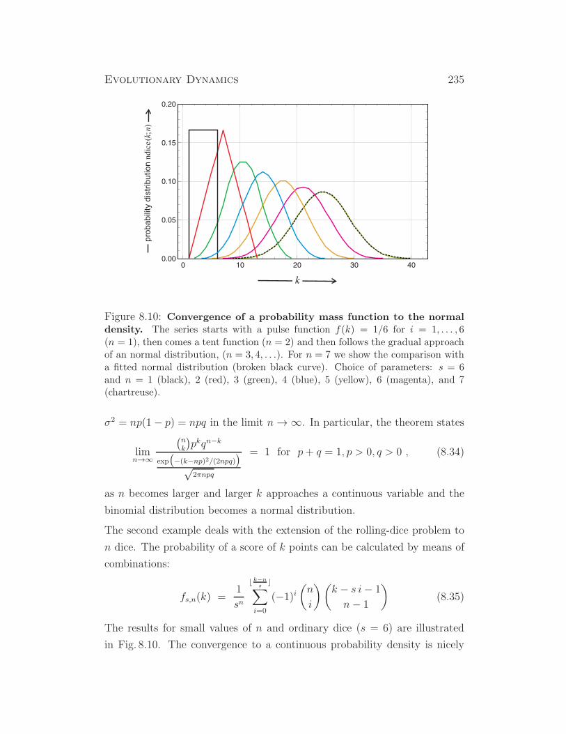
Evolutionary Dynamics 235
Figure 8.10: Convergence of a probability mass function to the normaldensity. The series starts with a pulse function f(k) = 1/6 for i = 1, . . . , 6(n = 1), then comes a tent function (n = 2) and then follows the gradual approachof an normal distribution, (n = 3, 4, . . .). For n = 7 we show the comparison witha fitted normal distribution (broken black curve). Choice of parameters: s = 6and n = 1 (black), 2 (red), 3 (green), 4 (blue), 5 (yellow), 6 (magenta), and 7(chartreuse).
σ2 = np(1− p) = npq in the limit n→∞. In particular, the theorem states
limn→∞
(
nk
)
pkqn−k
exp(
−(k−np)2/(2npq))
√2πnpq
= 1 for p+ q = 1, p > 0, q > 0 , (8.34)
as n becomes larger and larger k approaches a continuous variable and the
binomial distribution becomes a normal distribution.
The second example deals with the extension of the rolling-dice problem to
n dice. The probability of a score of k points can be calculated by means of
combinations:
fs,n(k) =1
sn
⌊k−ns⌋
∑
i=0
(−1)i(
n
i
)(
k − s i− 1
n− 1
)
(8.35)
The results for small values of n and ordinary dice (s = 6) are illustrated
in Fig. 8.10. The convergence to a continuous probability density is nicely
236 Peter Schuster
illustrated. For n = 7 the deviation from a the Gaussian curve of the normal
distribution is hardly recognizable.
The central limit theorem (CLT) is the generalization of the two examples
shown here to arbitrary probability distributions.16 In the traditional form it
is expressed as:
Central limit theorem. Let X1,X2, . . . ,Xn be a random sample of size n that
is obtained as a sequence of independent and identically distributes random
variables drawn from distributions with expectation values, E(X ) = µ and
variances, σ2(X ) = σ2. Then the sample average of these random variables
is defined by Sn := (X1 +X2 + . . .+Xn)/n. The central limit theorem states
that as n gets larger the distribution of the difference between Sn and its limit
µ multiplied by√n, i.e.
√n(Sn − µ), approximates a normal distribution
with mean zero and variance σ2. For fixed large n this is tantamount to the
statement that for fixed large n the distribution Sn is close to the normal
distribution with expectation value µ and variance σ2/n. In other words the
distribution of√n(Sn−µ) approaches normality regardless of the distribution
of the individual Xi’s.
The law of large numbers follows as a straightforward consequence of the
central limit theorem. Its main message says that for a sufficiently large
number of independent events the statistical errors will vanish by summation
and the mean of any finite sample converges to the (exact) expectation values
and higher moments:
m =1
n
n∑
i=1
xi and limn→∞
m = µ , and
m2 =1
n− 1
n∑
i=1
(xi − m)2 and limn→∞
m2 = var(x) = σ2(x),
(8.36)
where n denotes here the sample size. The sample mean m and the sample
variance m2 converge to the expectation value µ and the variance σ2 in the
16For some distributions, which have no defined moments like the Cauchy-Lorentz dis-
tribution neither the central limit theorem nor the law of large numbers are fulfilled.
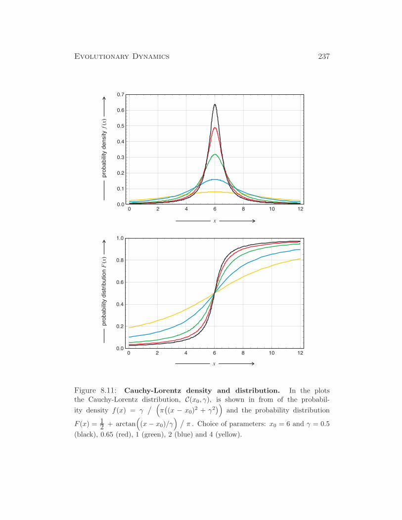
Evolutionary Dynamics 237
x
pro
babili
ty d
ensity
()
fx
x
pro
ba
bili
ty d
istr
ibu
tio
nF
x()
Figure 8.11: Cauchy-Lorentz density and distribution. In the plotsthe Cauchy-Lorentz distribution, C(x0, γ), is shown in from of the probabil-
ity density f(x) = γ/
(
π(
(x − x0)2 + γ2
)
)
and the probability distribution
F (x) = 12 + arctan
(
(x− x0)/γ)
/
π . Choice of parameters: x0 = 6 and γ = 0.5
(black), 0.65 (red), 1 (green), 2 (blue) and 4 (yellow).
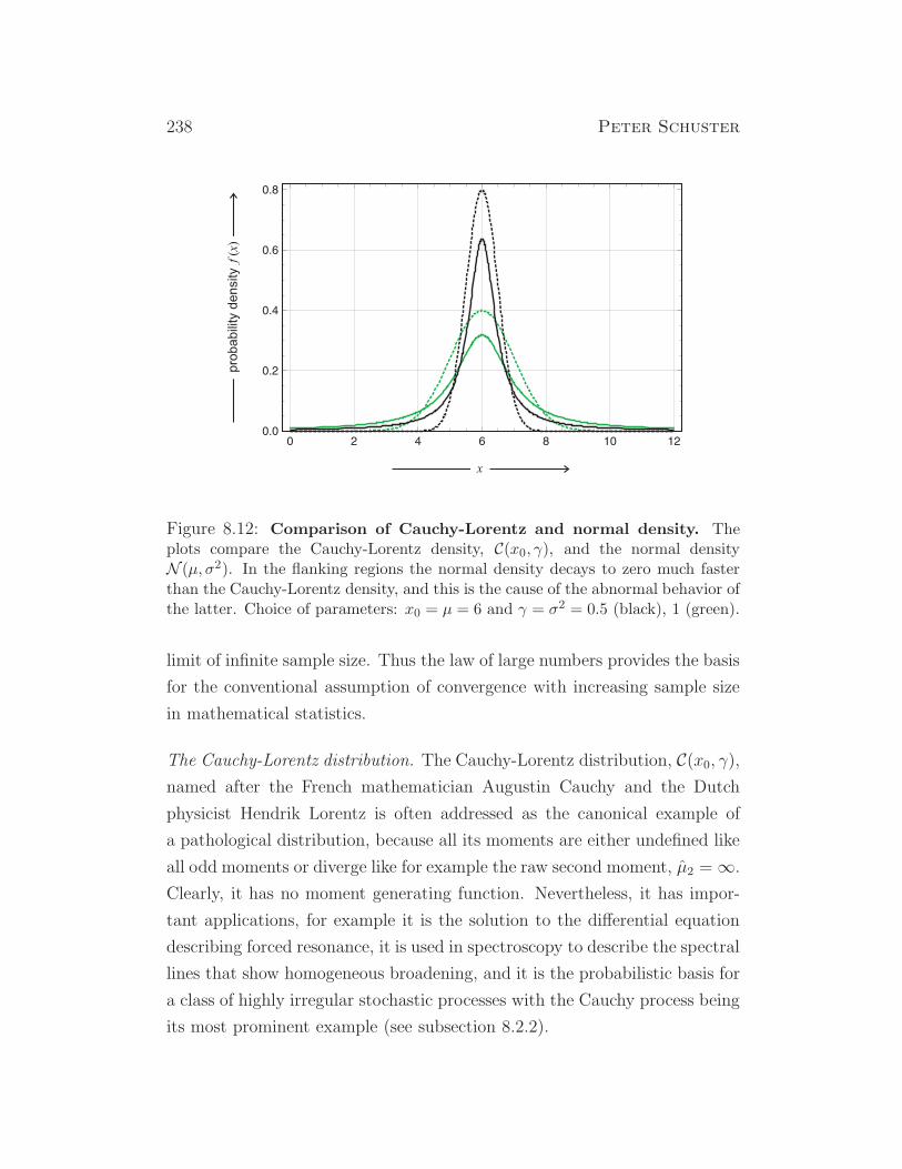
238 Peter Schuster
x
pro
babili
ty d
ensity
()
fx
Figure 8.12: Comparison of Cauchy-Lorentz and normal density. Theplots compare the Cauchy-Lorentz density, C(x0, γ), and the normal densityN (µ, σ2). In the flanking regions the normal density decays to zero much fasterthan the Cauchy-Lorentz density, and this is the cause of the abnormal behavior ofthe latter. Choice of parameters: x0 = µ = 6 and γ = σ2 = 0.5 (black), 1 (green).
limit of infinite sample size. Thus the law of large numbers provides the basis
for the conventional assumption of convergence with increasing sample size
in mathematical statistics.
The Cauchy-Lorentz distribution. The Cauchy-Lorentz distribution, C(x0, γ),named after the French mathematician Augustin Cauchy and the Dutch
physicist Hendrik Lorentz is often addressed as the canonical example of
a pathological distribution, because all its moments are either undefined like
all odd moments or diverge like for example the raw second moment, µ2 =∞.
Clearly, it has no moment generating function. Nevertheless, it has impor-
tant applications, for example it is the solution to the differential equation
describing forced resonance, it is used in spectroscopy to describe the spectral
lines that show homogeneous broadening, and it is the probabilistic basis for
a class of highly irregular stochastic processes with the Cauchy process being
its most prominent example (see subsection 8.2.2).
Evolutionary Dynamics 239
The probability density function and cumulative distribution function are
of the form
N (x; x0, γ) : f(x) =1
π
γ
(x− x0)2 + γ2, (8.37)
F (x) =1
2+
1
πarctan
(
x− x0γ
)
. (8.38)
In Fig. 8.11 the Cauchy-Lorentz density and distribution are shown for differ-
ent parameter values. At a first glance the family of curves looks very similar
to the analogous family of the normal distribution. A more close inspection,
however, shows the flanking regions are much flatter in the Cauchy-Lorentz
case (Fig. 8.12), and the slow convergence towards zero is the ultimate cause
for the pathological values of the moments.
240 Peter Schuster
8.2 Stochastic processes
In 1827 the British botanist Robert Brown detected and analyzed irregular
motions of particles in aqueous suspensions that turned out to be indepen-
dent of the nature of the suspended materials – pollen grains, fine particles
of glass or minerals [28]. Although Brown himself had already demonstrated
that Brownian motion is not caused by some (mysterious) biological effect,
its origin remained kind of a mystery until Albert Einstein [74], and inde-
pendently by Marian von Smoluchowski [296], published a satisfactory ex-
planation in 1905 and 1906, respectively, which contained two main points:
(i) The motion is caused by highly frequent impacts on the pollen grain of
the steadily moving molecules in the liquid in which it is suspended.
(ii) The motion of the molecules in the liquid is so complicated in detail
that its effect on the pollen grain can only be described probabilistically
in terms of frequent statistically independent impacts.
In particular, Einstein showed that the number of particles per unit volume,
ρ(x, t),17 fulfils the already known differential equation of diffusion,
∂ρ
∂t= D
∂2ρ
∂x2with the solution ρ(x, t) =
N√4πD
exp(
−x2/(4Dt))
√t
,
where N is the total number of particles. From the solution of the diffusion
equation Einstein computes the square root of the mean square displacement,
λx, the particle experiences in x-direction:
λx =√x2 =
√2Dt .
Einstein’s treatment is based on discrete time steps and thus contains an
approximation – that is not well justified – but it represents the first analysis
based on a probabilistic concept of a process that is comparable to the current
theories and we may consider Einstein’s paper as the beginning of stochastic
modeling. Brownian motion was indeed the first completely random process
that became accessible to a description that was satisfactory by the standards
17For the sake of simplicity we consider only motion in one spatial direction, x.

Evolutionary Dynamics 241
of classical physics. Thermal motion as such had been used previously as the
irregular driving force causing collisions of molecules in gases by James Clerk
Maxwell and Ludwig Boltzmann. The physicists in the second half of the
nineteenth century, however, were concerned with molecular motion only as it
is required to describe systems in the thermodynamic limit. They derived the
desired results by means of global averaging statistics. For scholars interested
in a mathematically rigorous history of stochastic processes we recommend
the comprehensive review by Subrahmanyan Chandrasekhar [35].
Systems evolving probabilistically in time can be rigorously described
and modeled in mathematical terms by stochastic processes. More precisely,
we postulate the existence of a time dependent random variable or random
vector, X (t) or ~X (t) =(
X1(t),X2(t), . . . ,Xn(t))
, respectively. Depending
on the nature of the process a discrete or a continuous variable may be
appropriate for modeling and we shall distinguish and consider both cases
here: (i) the simpler discrete case, in which the variables refer, for example,
to particle numbers
Xk(t) = P(
X (t) = k)
with k ∈ N0 , (8.39)
and (ii) the continuous probability density case, where the variable are con-
centrations
dF (x, t) = f(x, t) dx = P(
x ≤ X (t) ≤ x+ dx)
with x ∈ R1 . (8.40)
The latter case, of course, requires that dF (x, t) is differentiable. In both
cases a trajectory is understood as a recording of the particular values of Xat certain times:
T =(
(x1, t1), (x2, t2), (x3, t3), · · · , (y1, τ1), (y2, τ2), · · ·)
. (8.41)
As the repeated measurement of a stochastic variable yields different values,
the repetition of a stochastic process through reproducing an experiment
yields a different trajectory and the full description of the process requires
knowledge on the time course of the probability distribution. In experiments
and in computer simulation the probability distribution is usually derived
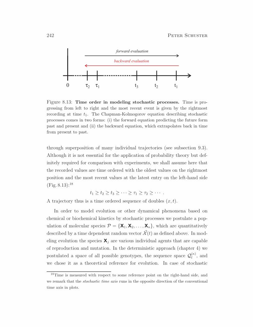
242 Peter Schuster
0 t2 t1 t3 t2 t1
backward evaluation
forward evaluation
Figure 8.13: Time order in modeling stochastic processes. Time is pro-
gressing from left to right and the most recent event is given by the rightmost
recording at time t1. The Chapman-Kolmogorov equation describing stochastic
processes comes in two forms: (i) the forward equation predicting the future form
past and present and (ii) the backward equation, which extrapolates back in time
from present to past.
through superposition of many individual trajectories (see subsection 9.3).
Although it is not essential for the application of probability theory but def-
initely required for comparison with experiments, we shall assume here that
the recorded values are time ordered with the oldest values on the rightmost
position and the most recent values at the latest entry on the left-hand side
(Fig. 8.13):18
t1 ≥ t2 ≥ t3 ≥ · · · ≥ τ1 ≥ τ2 ≥ · · · .A trajectory thus is a time ordered sequence of doubles (x, t).
In order to model evolution or other dynamical phenomena based on
chemical or biochemical kinetics by stochastic processes we postulate a pop-
ulation of molecular species P = X1,X2, . . . ,Xn, which are quantitatively
described by a time dependent random vector ~X (t) as defined above. In mod-
eling evolution the species Xj are various individual agents that are capable
of reproduction and mutation. In the deterministic approach (chapter 4) we
postulated a space of all possible genotypes, the sequence space Q(κ)l , and
we chose it as a theoretical reference for evolution. In case of stochastic
18Time is measured with respect to some reference point on the right-hand side, and
we remark that the stochastic time axis runs in the opposite direction of the conventional
time axis in plots.
Evolutionary Dynamics 243
processes it is much more appropriate to restrict the population to the actu-
ally present variants and to introduce a new variable whenever a mutation
leads to a genotype that was not present in the population before. Then,
the size of the population support Σ(P) is changing and can be considered
as a function of time, |Σ(P)| = nΣ(t). Variable population size N and vari-
able species diversity nΣ have great impact on the evolutionary process. For
example bottle necks and broad regions shape evolution as will be discussed
later in section 10.2 [101, 246, 247].
8.2.1 Markov and other simple stochastic processes
A stochastic process, as we shall assume, is determined by a set of joint prob-
ability densities the existence and analytical form of which is presupposed.19
The probability density encapsulates the physical nature of the process and
contains all parameters and data on external conditions and hence we can
assume that they determine the system completely:
p(
x1, t1; x2, t2; x3, t3; · · ·)
. (8.42)
By the phrase “determine completely” we mean that no additional informa-
tion is required for a description of the progress in terms of the time ordered
series (8.41) and we shall call such a process a separable stochastic process.
Although more general processes are conceivable, they play little role in cur-
rent physics, chemistry, and biology and therefore we shall not consider them
here.
Calculation of probabilities from (8.42) is straightforward by application
of marginal densities. For the discrete case the result is obvious
P (X = x1) = p(x1, ∗) =∑
xk 6=x1
p (x1, t1; x2, t2; x3, t3; · · · ; xn, tn; · · · ) .
19The joint density p (8.14) is defined by Prob(
X = xi,Y = yj)
= p(xi, yj) or
Prob(
X ≤ x,Y ≤ y)
=∫ x
−∞
∫ x
−∞f(u, v) du dv in the continuous case. Since we are always
dealing with doubles (x, t) we modify the notation slightly and separate individual doubles
by semicolons: · · · ;xk, tk;xk+1, tk+1; · · · .
244 Peter Schuster
and in the continuous case we obtain
P (X1 = x1 ∈ [a, b]) =
∫ b
a
dx1
∫∫∫ ∞
−∞dx2dx3 · · ·dxn · · ·
p (x1, t1; x2, t2; x3, t3; · · · ; xn, tn; · · · )
Time ordering allows for the formulation of predictions on future values from
the known past in terms of conditional probabilities:
p (x1, t1; x2, t2; · · · | y1, τ1; y2, τ2, · · · ) =p (x1, t1; x2, t2; · · · ; y1, τ1; y2, τ2, · · · )
p (y1, τ1; y2, τ2, · · · ),
with t1 ≥ t2 ≥ · · · ≥ τ1 ≥ τ2 ≥ · · · . In other words, we may compute
(x1, t1), (x2, t2), · · · from known (y1, τ1), (y2, τ2), · · · .Three simple stochastic processes will be discussed here: (i) the factoriz-
able process with probability densities that are independent of the event with
the special case of the Bernoulli process where the probability densities are
also independent of time, (ii) the martingale where the (sharp) initial value of
the stochastic variable is equal to the conditional mean value of the variable
in the future, and (iii) the Markov process where the future is completely
determined by the presence.
The simplest class of stochastic processes is characterized by complete
independence of events,
p (x1, t1; x2, t2; x3, t3; · · · ) =∏
i
p (xi, ti) , (8.43)
which implies that the current value X (t) is completely independent of its
values in the past. A special case is the sequence of Bernoulli trials where
the probability densities are also independent of time: p (xi, ti) = p (xi), and
then we have
p (x1, t1; x2, t2; x3, t3; · · · ) =∏
i
p (xi) . (8.44)
Further simplification occurs, of course, when all trials are based on the same
probability distribution – for example, if the same coin is tossed in Bernoulli
trials – and then the product is replaced by p(x)n.

Evolutionary Dynamics 245
Figure 8.14: The one-dimensional random walk. The one-dimensional
random is shown as an example of a martingale. Five trajectories were calcu-
lated with different seeds for the random number generator. The expectation
value E(
X (t))
= x0 = 0 is constant and the variance grows linearly with time
σ2(
X (t))
= 2dt, Accordingly, the standard deviation grows with√
t. The three
black lines in the figure correspond to E and E±σ(t), and the grey area represent
the confidence interval of 68,2%. Choice of parameters: ϑ = 12; random number
generator: Mersenne Twister ; seeds: 491 (yellow), 919 (blue), 023 (green), 877
(red), 127 (violet).
The notion of martingale has been introduced by the French mathemati-
cian Paul Pierre Levy and the development of the theory of martingales is
due to the American mathematician Joseph Leo Doob. The conditional mean
value of the random variable X (t) provided X (t0) = x0 is defined as
E(
X (t)|(x0, t0)) .
=
∫
dx p(x, t|x0, t0) .
In a martingale the conditional mean is simple given by
E(
X (t)|(x0, t0))
= x0 . (8.45)
The mean value at time t is identical to the initial value of the process
(Fig. 8.14). The martingale property is rather strong and restrictive and
246 Peter Schuster
applies only to relatively few cases to which we shall refer only in some
specific situations.
The somewhat relaxed notion of a semimartingale is of importance be-
cause it covers the majority of processes that are accessible to modeling by
stochastic differential equations. A semimartingale is composed of a local
martingale and a cadlag adapted process with bounded variation20
X (t) = M(t) + A(t)
A local martingale is a stochastic process that satisfies locally the martingale
property (8.45) but its expectation value 〈M(t)〉 may be distorted at long
times by large values of low probability. Hence, every martingale is a local
martingale and every bounded local martingale is a martingale. In particu-
lar, every driftless diffusion process is a local martingale but need not be a
martingale. An adapted or nonanticipating process is a process that cannot
see into the future. An informal interpretation [310, section II.25] would say:
A stochastic process X (t) is adapted iff for every realization and for every
time t, X (t) is known at time t and not before.
Another simple concept assumes that knowledge of the present only is
sufficient to predict the future. It is realized in Markov processes named after
the Russian mathematician Andrey Markov21 and can formulated easily in
terms of conditional probabilities:
p (x1, t1; x2, t2; · · · | y1, τ1; y2, τ2, · · · ) = p (x1, t1; x2, t2; · · · | y1, τ1) . (8.46)
In essence, the Markov condition expresses independence of the history of
the process prior to time τ1 or in other words and said more sloppily: “A
Markov process has no memory and the future is completely determined by
20The property cadlag is an acronym from French for “continue a droite, limites a
gauche”. It is a common property in statistics (section 8.1).21The Russian mathematician Andrey Markov (1856-1922) is one of the founders of
Russian probability theory and pioneered the concept of memory free processes, which
is named after him. He expressed more precisely the assumptions that were made by
Albert Einstein [74] and Marian von Smoluchowski [296] in their derivation of the diffusion
process.
Evolutionary Dynamics 247
the presence.” In particular, we have
p (x1, t1; x2, t2; y1, τ1) = p (x1, t1| x2, t2) p (x2, t2| y1, τ1) .
Any arbitrary joint probability can be simply expressed as products of con-
ditional probabilities:
p (x1, t1; x2, t2; x3, t3; · · · ; xn, tn) =
= p (x1, t1| x2, t2) p (x2, t2| x3, t3) · · · p (xn−1, tn−1| xn, tn) p (xn, tn) (8.46’)
under the assumption of time ordering t1 ≥ t2 ≥ t3 ≥ . . . tn−1 ≥ tn.
8.2.2 Continuity and the Chapman-Kolmogorov equation
Prior to the discussion of the mathematical approach to model step-processes,
continuous processes, and combinations of both we shall consider a classifi-
cation of stochastic processes. Assuming a discrete representation of particle
numbers as in Equ. (8.39) the probability functions of the stochastic variable
X (t) can change only in steps or jumps. A continuous stochastic variable
X (t) with a suitable probability function, however, need not exclude the oc-
currence of jumps. Accordingly, we expect to be dealing with several classes
of processes: (i) pure deterministic or drift processes, (ii) pure driftless and
jump free diffusion processes, (iii) pure jump processes, (iv) a combination of
(i) and (ii) being processes with drift and diffusion, and (v) a combination of
(i), (ii), and (iii) and others. At first we introduce the notion of continuity in
stochastic processes be means of two examples, the Wiener and the Cauchy
process. Then, we shall discuss a very general equation for the description of
stochastic processes, which contains all above mentioned processes as special
cases.
Continuity in stochastic processes. The condition of continuity in Markov
processes requires a more detailed discussion. The process goes from position
z at time t to position x at time t + ∆t. Continuity of the process implies
that the probability of x to be finitely different from z goes to zero faster
than ∆t in the limit lim∆t→ 0:
lim∆t→0
1
∆t
∫
|x−z|>ε
dx p (x, t+∆t|z, t) = 0 , (8.47)
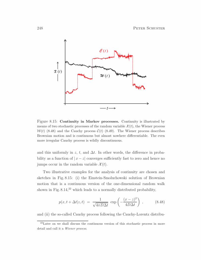
248 Peter Schuster
Figure 8.15: Continuity in Markov processes. Continuity is illustrated by
means of two stochastic processes of the random variable X (t), the Wiener process
W(t) (8.48) and the Cauchy process C(t) (8.49). The Wiener process describes
Brownian motion and is continuous but almost nowhere differentiable. The even
more irregular Cauchy process is wildly discontinuous.
and this uniformly in z, t, and ∆t. In other words, the difference in proba-
bility as a function of | x− z| converges sufficiently fast to zero and hence no
jumps occur in the random variable X (t).Two illustrative examples for the analysis of continuity are chosen and
sketches in Fig. 8.15: (i) the Einstein-Smoluchowski solution of Brownian
motion that is a continuous version of the one-dimensional random walk
shown in Fig. 8.14,22 which leads to a normally distributed probability,
p(x, t+∆t|z, t) =1√
4πD∆texp
(
−(x− z)2
4D∆t
)
, (8.48)
and (ii) the so-called Cauchy process following the Cauchy-Lorentz distribu-
22Later on we shall discuss the continuous version of this stochastic process in more
detail and call it a Wiener process.

Evolutionary Dynamics 249
tion,
p(x, t+∆t|z, t) =∆t
π
1
(x− z)2 +∆t2. (8.49)
In case of the Wiener process we exchange the limit and the integral, intro-
duce ϑ = (∆t)−1, perform the limit ϑ→∞, and have
lim∆t→0
1
∆t
∫
|x−z|>ε
dx1√4πD
1√∆t
exp
(
−(x− z)2
4D∆t
)
=
=
∫
|x−z|>ε
dx lim∆t→0
1
∆t
1√4πD
1√∆t
exp
(
−(x− z)2
4D∆t
)
=
=
∫
|x−z|>ε
dx limϑ→∞
1√4πD
ϑ3/2
exp(
(x−z)24D
ϑ) , where
limϑ→∞
ϑ3/2
1 + (x−z)24D· ϑ + 1
2!
(
(x−z)24D
)2
· ϑ2 + 13!
(
(x−z)24D
)3
· ϑ3 + . . .= 0 .
Since the power expansion of the exponential in the denominator increases
faster than every finite power of ϑ, the ratio vanishes in the limit ϑ →∞, the value of the integral is zero, and the Wiener process is continuous
everywhere. Although it is continuous, the curve of Brownian motion [28] is
indeed extremely irregular since it is nowhere differentiable (Fig. 8.15).
In the second example, the Cauchy process, we exchange limit and integral
as in case of the Wiener process, and perform the limit ∆t→ 0:
lim∆t→0
1
∆t
∫
|x−z|>ε
dx∆t
π
1
(x− z)2 +∆t2=
=
∫
|x−z|>ε
dx lim∆t→0
1
∆t
∆t
π
1
(x− z)2 +∆t2=
=
∫
|x−z|>ε
dx lim∆t→0
1
π
1
(x− z)2 +∆t2=
∫
|x−z|>ε
1
π(x− z)2 dx 6= 0 .
The value of the last integral, I =∫∞|x−z|>ε
dx/(x− z)2 = 1/(
π(x− z))
, is of
the order I ≈ 1/ε and the curve for the Cauchy-process is also irregular but
even discontinuous.
Both processes, as required for consistency, fulfill the relation
lim∆t→0
p (x, t+∆t| z, t) = δ(x− z) ,
250 Peter Schuster
where δ(·) is the so-called delta-function.23
Chapman-Kolmogorov equation. From joint probabilities follows that sum-
mation of all mutually exclusive events of one kind eliminates the correspond-
ing variable:
∑
i
P (A ∩ Bi ∩ C · · · ) = P (A ∩ C · · · ) ,
where the subsets Bi fulfil the conditions
Bi ∩Bj = ∅ and⋃
i
Bi = Ω .
Applied to stochastic processes we find by the same token
p (x1, t1) =
∫
dx2 p (x1, t1; x2, t2) =
∫
dx2 p (x1, t1| x2, t2) p (x2, t2) .
Extension to three events leads
p (x1, t1|x3, t3) =
∫
dx2 p (x1, t1; x2, t2| x3, t3) =
=
∫
dx2 p (x1, t1| x2, t2; x3, t3) p (x2, t2| x3, t3) .
For t1 ≥ t2 ≥ t3 and making use of the Markov assumption we obtain the
Chapman-Kolmogorov equation, which is named after the British geophysi-
cist and mathematician Sydney Chapman and the Russian mathematician
Andrey Kolmogorov:
p (x1, t1|x3, t3) =
∫
dx2 p (x1, t1| x2, t2) p (x2, t2| x3, t3) . (8.50)
In case of discrete random variable N ∈ N0 = 0, 1, . . . , k, . . . defined on the
integers we replace the integral by a sum and obtain
P (k1, t1| k3, t3) =∑
k2
P (k1, t1| k2, t2) P (k2, t2| k3, t3) . (8.51)
23The delta-function is no proper function but a generalized function or distribution. It
was introduced by Paul Dirac in quantum mechanics. For more details see, for example,
[244, pp.585-590] and [241, pp.38-42].
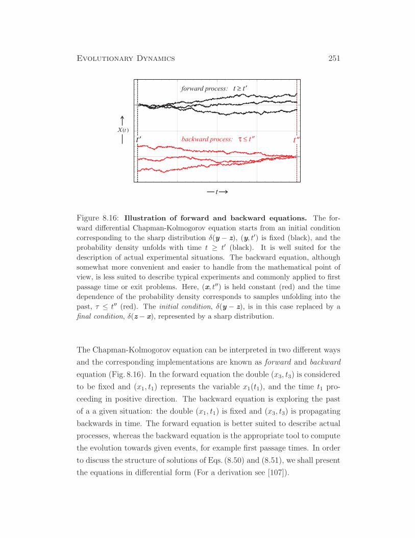
Evolutionary Dynamics 251
Figure 8.16: Illustration of forward and backward equations. The for-
ward differential Chapman-Kolmogorov equation starts from an initial condition
corresponding to the sharp distribution δ(y − z), (y, t′) is fixed (black), and the
probability density unfolds with time t ≥ t′ (black). It is well suited for the
description of actual experimental situations. The backward equation, although
somewhat more convenient and easier to handle from the mathematical point of
view, is less suited to describe typical experiments and commonly applied to first
passage time or exit problems. Here, (x, t′′) is held constant (red) and the time
dependence of the probability density corresponds to samples unfolding into the
past, τ ≤ t′′ (red). The initial condition, δ(y − z), is in this case replaced by a
final condition, δ(z − x), represented by a sharp distribution.
The Chapman-Kolmogorov equation can be interpreted in two different ways
and the corresponding implementations are known as forward and backward
equation (Fig. 8.16). In the forward equation the double (x3, t3) is considered
to be fixed and (x1, t1) represents the variable x1(t1), and the time t1 pro-
ceeding in positive direction. The backward equation is exploring the past
of a a given situation: the double (x1, t1) is fixed and (x3, t3) is propagating
backwards in time. The forward equation is better suited to describe actual
processes, whereas the backward equation is the appropriate tool to compute
the evolution towards given events, for example first passage times. In order
to discuss the structure of solutions of Eqs. (8.50) and (8.51), we shall present
the equations in differential form (For a derivation see [107]).
252 Peter Schuster
The differential version of the Chapman-Kolmogorov equation is based
on the continuity condition already discussed for the Wiener and the Cauchy
process. In the derivation of the differential form the general equations (8.50)
and (8.51) have to be partitioned with respect to differentiability conditions
corresponding either to continuous motion under generic conditions or to
discontinuous motion. This partitioning is based on the following conditions
for all ε > 0: (8.52)
(i) lim∆t→01∆tp(x, t+∆t|z, t) t = W (x|z, t) , uniformly in x, z, and t
for |x− z| ≥ ε,
(ii) lim∆t→01∆t
∫
|x−z|<εdx (xi − zi) p(x, t+∆t|z, t) = Ai(z, t) + O(ε) ,
uniformly in z, and t, and
(iii) lim∆t→01∆t
∫
|x−z|<εdx (xi − zi)(xj − zj) p(x, t+∆t|z, t) =
= Bij(z, t) + O(ε) , uniformly in z, and t.
where xi, xj , zi, and zj , refer to particular components of the vectors x and
z, respectively. It is important to notice that all higher-order coefficients
of motion Cijk, defined in analogy to Ai in (ii) or Bij in (iii), must vanish
by symmetry considerations [107, p.47-48]. In essence, the three terms in
Equ. (8.52) refer to different behavior with respect to continuity: (i) (deter-
ministic) drift, (ii) diffusion in the sense of a Wiener process, and (iii) a jump
process, with the attributes (i) continuous and differentiable, (ii) continuous
and nowhere differentiable, and (iii) discontinuous, respectively.
The partial differential equation for the evolution of the probability distri-
bution has been called differential Chapman-Kolmogorov equation by Crispin
Gardiner. Neglect of surface terms at the boundary of the domain of z leads
to the expression:
∂p (z, t |y, t′)∂t
= −∑
i
∂
∂zi
(
Ai(z, t) p (z, t|y, t′))
+ (8.53a)
+1
2
∑
i,j
∂2
∂zi∂zj
(
Bij(z, t) p (z, t|y, t′))
+ (8.53b)
+
∫
dx(
W (z |x, t) p (x, t|y, t′)−W (x |z, t) p (z, t|y, t′))
. (8.53c)
Evolutionary Dynamics 253
Under certain conditions, A(x, t) real, B(x, t) positive semi-definite, and
W (x| y, t) non-negative, a non-negative solution to to the differential Chapman-
Kolmogorov equation (8.53), which fulfils the continuous Chapman-Kolmogorov
equation (8.50), exists for the initial condition p (z, t| y, t) = δ(y− z).
The nature of the different stochastic processes associated with the three
terms in Equ. (8.53) is visualized by setting some parameters, A(z, t), B(z, t),
and W (x |z, t) equal to zero and analyzing the remaining equation. We shall
discuss here the four cases that are modeled by different equations
(i) B = 0, W = 0, deterministic drift process: Liouville equation,
(ii) A = 0, W = 0, diffusion process: drift free Fokker-Planck equation,
(iii) W = 0, drift and diffusion process: Fokker-Planck equation, and
(iv) A = 0, B = 0, pure jump process: master equation.
The first three processes can be modeled very efficiently by stochastic dif-
ferential equations (SDE) often called Langevin equations after the French
physicist Paul Langevin [186]. Examples of SDEs will mentioned for the
Wiener process and the Ornstein-Uhlenbeck process. We shall mention them
only briefly here, refrain from a detailed discussion, and refer to the literature
[107, 251].
Chapman-Kolmogorov backward equation. Equ. (8.53) has been derived for
the forward direction and according to Fig. 8.16 a differential Chapman-
Kolmogorov equation can also be derived for the backward process. Then
the limit has to be taken with respect to the initial variables (y, τ) of the
probability p (x, t| y, τ) and the limit of the vanishing time interval is of the
form
lim∆τ→0
1
∆τ
(
p (x, t|y, τ +∆τ) − p(x, t|y, τ))
=
= lim∆τ→0
1
∆τ
∫
dz p (z, τ +∆τ |y, τ)(
p (x, t|y, τ +∆τ) − p (x, t| z, τ +∆τ))
,
where the Chapman-Kolmogorov equation (8.50) was used to derive the sec-
ond line. The derivation of the differential from of the backward equation
follows essentially the same steps as in case of the forward equation [107] and
254 Peter Schuster
eventually we obtain a probabilistic differential equation that is equivalent
to the forward equation:
∂p (x, t |y, τ)∂t
= −∑
i
Ai(y, τ)∂p (x, t|y, τ)
∂yi+ (8.54a)
+1
2
∑
i,j
Bij(z, t)∂2p (x, t|y, τ)
∂yi∂yj+ (8.54b)
+
∫
dx W (z |y, τ)(
p (x, t|y, τ) − p (z, t|z, τ))
. (8.54c)
As we have stated for the forward equation the appropriate initial condition
is p (x, t| y, t) = δ(x− y) for all t.
Liouville equation. In the limiting case of a stochastic process with vanish-
ing probabilistic contributions, diffusion and jump processes, one obtains a
differential equation that is a Liouville equation well known from classical
mechanics:
∂p(z, t|y, t′)∂t
= −∑
i
∂
∂zi
(
Ai(z, t) p(z, t|y, t′))
, (8.55)
Equ. (8.55) describes a completely deterministic motion, which is a solution
of the ordinary differential equation
dx(t)
dt= a
(
x(t), t)
with x(y, t′) = y . (8.56)
The (probabilistic) solution of the differential Equ. (8.55) with the initial
condition p(z, t′|y, t′) = δ(z − y) is p(z, t|y, t′) = δ(
z − x(y, t))
, or in other
words z(0) = z(t′) = y(t′) represents the initial conditions of the ODE (8.56).
The proof of this assertion is obtained by direct substitution [107, p.54].
∑
i
∂
∂zi
(
A(z, t) δ(
z− x(y, z))
)
=∑
i
∂
∂zi
(
Ai(x(y, t), t) δ(
z− x(y, t))
)
,
=∑
i
(
Ai(x(y, t), t)∂
∂ziδ(
z− x(y, t))
)
,
and∂
∂tδ(
z− x(y, t))
= −∑
i
∂
∂ziδ(
z− x(y, t)) dxi(y, t)
dt,
and by means of Equ. (8.56) the last two lines become equal.

Evolutionary Dynamics 255
pw
tw
t(
,,
)|
00
w
Figure 8.17: Evolution of the probability density in the Wiener process.
In the figure we show the conditional probability density of the Wiener process
which is identical with the normal distribution (Fig. 8.9),
p(w, t|w0, t0) = exp(
−(w − w0)2/(
2(t− t0))
)
/√
2π(t− t0).
The values used are w0 = 5 and t − t0 = 0 (black), 0.05 (purple), 0.5
(red), 1.0 (green), 2.0 (blue), and 4.0 (yellow). The initially sharp distribution,
p(w, t|w0, t0) = δ(w−w0) spreads with increasing time until it becomes completely
flat in the limit t→∞.
If a particle is in a well-defined position y at time t′ it will remain on the tra-
jectory obtained by solving the corresponding ordinary differential equation
(ODE). Deterministic motion can be visualized therefore as an elementary
form of Markov process, which can be formulated by a drift-diffusion process
with a zero diffusion matrix B. A generalization of the initial conditions is
straightforward: If we are dealing with a probability distribution rather than
a δ-function this distribution is traveling along the trajectory.
Wiener process. If only the diffusion matrix B has nonzero entries and all
terms of A(z, t) and W (x |z, t) vanish, we are dealing with a Wiener process
named after the American mathematician and logician Norbert Wiener. It is
synonymous to (continuous) Brownian motion or white noise and describes
among other things random fluctuations caused by thermal motion. The

256 Peter Schuster
trajectories in Fig. 8.14 are almost indistinguishable from those of a Wiener
process because a small increment of the random walk was chosen. From
the point of view of stochastic processes the probability density of a Wiener
process is a solution of the differential equation24
∂p (w, t|w0, t0)
∂t=
1
2
∂2
∂w2p (w, t|w0, t0) (8.57)
in one random variable, W(t). The probability distribution of W(t) is given
by
P (W(t) ≤ w′) =
∫ w′
−∞p (w, t) dw .
Equ. (8.57) can be understood as a Fokker-Planck equation with drift co-
efficient zero and diffusion coefficient D = 1. Fokker-Planck equations are
partial differential equations named after two physicists, the Dutchman Adri-
aan Daniel Fokker and the German Max Planck and in one dimension, in the
forward direction, and for the initial conditions p (x0, t0) they are of the gen-
eral form
∂p (x, t)
∂t= − ∂
∂x
(
A(x, t) p (x, t))
+1
2
∂2
∂x2
(
B(x, t) p (x, t))
. (8.58)
An example of a full Fokker-Planck equation modeling the Ornstein-Uhlenbeck
process will be discussed in the next paragraph. Fokker-Planck equations can
be easily converted into stochastic differential equations (SDEs), which are
convenient for analysis and computer simulation [107]. The probability dis-
tribution of the Fokker-Planck equation (8.58) is equivalent to the ensemble
of trajectories described by
dx = a(x, t) dt + b(x, t) dW (t) , (8.59)
where dW (t) corresponds to a Wiener process.25 Integration of stochastic
differential equation requires special definitions that will not be discussed
here.24In application in physics and chemistry diffusion occurs in space and it would be
natural to use X (t) as stochastic variable and x as coordinate. Because of the key role of
the Wiener process in stochasticity we shall use W(t) and w instead.25The original formulation by Paul Langevin was different:
dxdt = a(x, t) + b(x, t) ξ(t) ,
Evolutionary Dynamics 257
The solution of (8.57) for the initial condition on the conditional proba-
bility p (w, t0|w0, t0) = δ(w−w0) can be obtained by using the characteristic
function
φ(s, t) =
∫
dw p (w, t|w0, t0) exp(ı.ıs w) ,
which fulfils ∂φ(s, t)/∂t = −12s2 φ(s, t) as can be shown by applying integra-
tion in parts twice and making use of the fact that p (w, t|w0, t0) like every
probability density has to vanish in the limits w → ±∞ and the same is true
for the first partial derivative, ∂p/∂w. Next we compute the characteristic
function by integration:26
φ(s, t) = φ(s, t0) · exp(
−12s2 (t− t0)
)
. (8.60)
Insertion of the initial condition φ(s, t0) = exp(ı.ıs w0) completes the calcula-
tion of the characteristic function
φ(s, t) = exp(
ı.ıs w0 −
1
2s2 (t− t0)
)
. (8.61)
The probability density is now obtained through inversion of Fourier trans-
formation
p (w, t|w0, t0) =1
√
2π (t− t0)exp
(
−(w − w0)2
2 (t− t0)
)
. (8.62)
It is straightforward to identify the density function of the Wiener process as
a normal distribution with an expectation value of E(
W(t))
= w0 = ν and
variance of E(
(
W(t)−w0
)2)
= t−t0 = σ(t)2. Accordingly, an initially sharp
where ξ(t) is a stochastic variable representing the noise term. Rigorous mathematical
handling of this equation leads to problems related to the fact that the Wiener process
and ξ(t) are nowhere differentiable and integration raises problems that can be avoided
by the formulation (8.59).
26The characteristic of a probability distribution is defined as
φ(s) =
∫ +∞
−∞
exp(ı.ısx) dF (x) =
∫ +∞
−∞
exp(ı.ısx) f(x) dx ,
and fulfils φ(s) = E(eı.ısX ). Apart from constant factors the characteristic function is the
Fourier transform of the probability density.
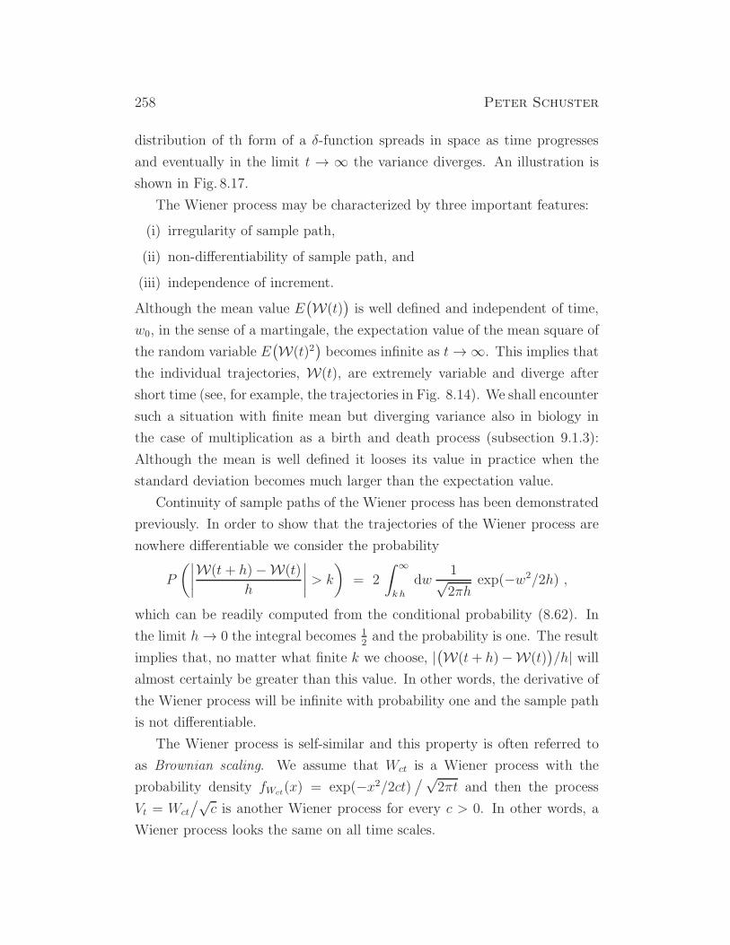
258 Peter Schuster
distribution of th form of a δ-function spreads in space as time progresses
and eventually in the limit t → ∞ the variance diverges. An illustration is
shown in Fig. 8.17.
The Wiener process may be characterized by three important features:
(i) irregularity of sample path,
(ii) non-differentiability of sample path, and
(iii) independence of increment.
Although the mean value E(
W(t))
is well defined and independent of time,
w0, in the sense of a martingale, the expectation value of the mean square of
the random variable E(
W(t)2)
becomes infinite as t→∞. This implies that
the individual trajectories, W(t), are extremely variable and diverge after
short time (see, for example, the trajectories in Fig. 8.14). We shall encounter
such a situation with finite mean but diverging variance also in biology in
the case of multiplication as a birth and death process (subsection 9.1.3):
Although the mean is well defined it looses its value in practice when the
standard deviation becomes much larger than the expectation value.
Continuity of sample paths of the Wiener process has been demonstrated
previously. In order to show that the trajectories of the Wiener process are
nowhere differentiable we consider the probability
P
(∣
∣
∣
∣
W(t + h)−W(t)
h
∣
∣
∣
∣
> k
)
= 2
∫ ∞
k h
dw1√2πh
exp(−w2/2h) ,
which can be readily computed from the conditional probability (8.62). In
the limit h→ 0 the integral becomes 12and the probability is one. The result
implies that, no matter what finite k we choose, |(
W(t+ h)−W(t))
/h| willalmost certainly be greater than this value. In other words, the derivative of
the Wiener process will be infinite with probability one and the sample path
is not differentiable.
The Wiener process is self-similar and this property is often referred to
as Brownian scaling. We assume that Wct is a Wiener process with the
probability density fWct(x) = exp(−x2/2ct)/√
2πt and then the process
Vt = Wct
/√c is another Wiener process for every c > 0. In other words, a
Wiener process looks the same on all time scales.
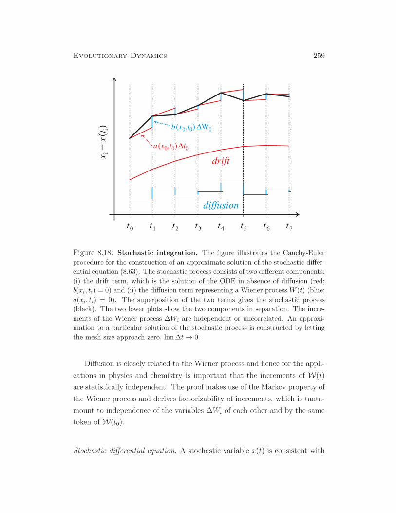
Evolutionary Dynamics 259
Figure 8.18: Stochastic integration. The figure illustrates the Cauchy-Euler
procedure for the construction of an approximate solution of the stochastic differ-
ential equation (8.63). The stochastic process consists of two different components:
(i) the drift term, which is the solution of the ODE in absence of diffusion (red;
b(xi, ti) = 0) and (ii) the diffusion term representing a Wiener process W (t) (blue;
a(xi, ti) = 0). The superposition of the two terms gives the stochastic process
(black). The two lower plots show the two components in separation. The incre-
ments of the Wiener process ∆Wi are independent or uncorrelated. An approxi-
mation to a particular solution of the stochastic process is constructed by letting
the mesh size approach zero, lim∆t→ 0.
Diffusion is closely related to the Wiener process and hence for the appli-
cations in physics and chemistry is important that the increments of W(t)
are statistically independent. The proof makes use of the Markov property of
the Wiener process and derives factorizability of increments, which is tanta-
mount to independence of the variables ∆Wi of each other and by the same
token of W(t0).
Stochastic differential equation. A stochastic variable x(t) is consistent with
260 Peter Schuster
an Ito stochastic differential equation (SDE) [159, 160]27
dx(t) = a(
x(t), t)
dt + b(
x(t), t)
dW (t) , (8.63)
if for all t and t0 = 0 the integral equation
x(t) − x(0) =
∫ t
0
a(
x(τ), τ)
dτ +
∫ t
0
b(
x(τ), τ)
dW (τ) (8.64)
is fulfilled. Time is ordered,
t0 < t1 < t2 < · · · < tn = t ,
and the time axis may be assumed to be split into (equal or unequal) incre-
ments, ∆ti = ti+1 − ti. We visualize a particular solution curve of the SDE
for the initial condition x(t0) = x0 by means of a discretized version
xi+1 = xi + a(xi, ti)∆ti + b(xi, ti)∆Wi , (8.64’)
wherein xi = x(ti), ∆ti = ti+1 − ti, and ∆Wi = W (ti+1) − W (ti). Fig-
ure 8.18 illustrates the partitioning of the stochastic process into a deter-
ministic drift component, which is the discretized solution curve of the ODE
obtained by setting b(
x(t), t)
= 0 in equation (8.64’) and stochastic diffusion
component, which is a random Wiener process W (t) that is obtained by set-
ting a(
x(t), t)
= 0 in the SDE. The increment of the Wiener process in the
stochastic term, ∆Wi, is independent of xi provided (i) x0 is independent of
all W (t) −W (t0) for t > t0 and (ii) a(x, t) is a nonanticipating function of
t for any fixed x. Condition (i) is tantamount to the requirement that any
random initial condition must be nonanticipating.
27Stochastic integration requires the definition of a reference point. The definition by
Ito choosing the reference point at the beginning of the interval is frequently used in the
theory of stochastic processes, because it facilitates integration of stochastic differential
equations, but Ito calculus is different from conventional calculus. An alternative definition
due to the Russian physicist and engineer Ruslan Leontevich Stratonovich [277] and the
American mathematician Donald LeRoy Fisk [94] puts the reference point in the middle
of the interval and retains thereby the conventional integration formulas, suffers, however,
from being more sophisticated.
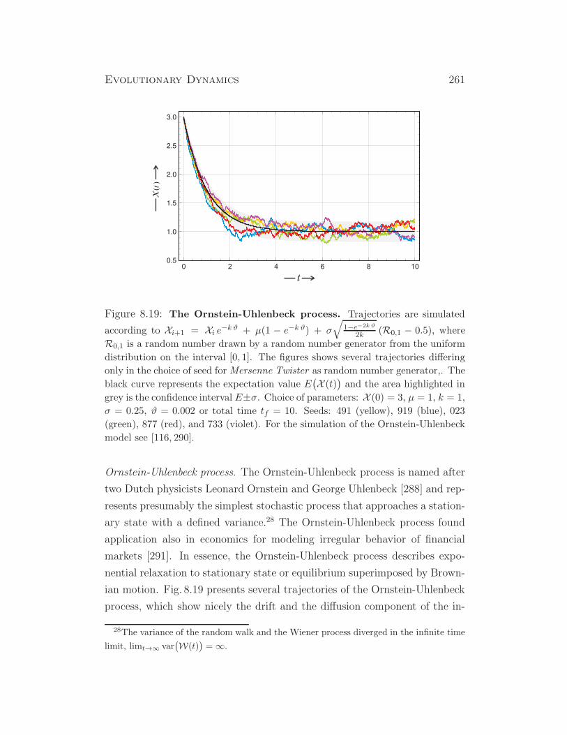
Evolutionary Dynamics 261
X(
)t
t2 4 6 8 100
Figure 8.19: The Ornstein-Uhlenbeck process. Trajectories are simulated
according to Xi+1 = Xi e−k ϑ + µ(1 − e−k ϑ) + σ
√
1−e−2k ϑ
2k (R0,1 − 0.5), where
R0,1 is a random number drawn by a random number generator from the uniform
distribution on the interval [0, 1]. The figures shows several trajectories differing
only in the choice of seed for Mersenne Twister as random number generator,. The
black curve represents the expectation value E(
X (t))
and the area highlighted in
grey is the confidence interval E±σ. Choice of parameters: X (0) = 3, µ = 1, k = 1,
σ = 0.25, ϑ = 0.002 or total time tf = 10. Seeds: 491 (yellow), 919 (blue), 023
(green), 877 (red), and 733 (violet). For the simulation of the Ornstein-Uhlenbeck
model see [116, 290].
Ornstein-Uhlenbeck process. The Ornstein-Uhlenbeck process is named after
two Dutch physicists Leonard Ornstein and George Uhlenbeck [288] and rep-
resents presumably the simplest stochastic process that approaches a station-
ary state with a defined variance.28 The Ornstein-Uhlenbeck process found
application also in economics for modeling irregular behavior of financial
markets [291]. In essence, the Ornstein-Uhlenbeck process describes expo-
nential relaxation to stationary state or equilibrium superimposed by Brown-
ian motion. Fig. 8.19 presents several trajectories of the Ornstein-Uhlenbeck
process, which show nicely the drift and the diffusion component of the in-
28The variance of the random walk and the Wiener process diverged in the infinite time
limit, limt→∞ var(
W(t))
=∞.

262 Peter Schuster
px t
(,
)
x
0
2
4
6
time t 1
2
3
x
0
2
4
6
pHx,tL
Figure 8.20: The probability density of the Ornstein-Uhlenbeck process.
Starting from the initial condition p (x, t0) = δ(x − x0) (black) the probability
density (8.66) broadens and migrates until it reaches the stationary distribution
(yellow). The lower plot presents an illustration in 3D. Choice of parameters:
x0 = 3, µ = 1, k = 1, and σ = 0.25. Times: t = 0 (black), 0.12 (orange), 0.33
(violet), 0.67 (green), 1.5 (blue), and 8 (yellow).
Evolutionary Dynamics 263
dividual runs.
The Fokker-Planck equation of the Ornstein-Uhlenbeck process for the
probability density p (x, t) = p (x, t| x0, 0) is of the form
∂p (x, t)
∂t= k
∂
∂x
(
(x− µ) p (x, t))
+σ2
2
∂2p (x, t)
∂x2, (8.65)
with k is the rate parameter of the exponential decay, µ the expectation
value of the random variable in the long time limit, µ = limt→∞E(
X (t))
,
and σ2/(2k) being the long time variance. Applying the initial condition
p (x, 0) = p (x, 0| x0, 0) = δ(x − x0) the probability density can be obtained
by standard techniques
p (x, t) =
√
k
πσ2 (1− e−2k t)exp
(
− k
σ2
(x− µ− (x0 − µ)e−kt)2
1− e−2kt
)
. (8.66)
This expression can be easily checked by performing the two limits t → 0
and t → ∞. The first limit has to yield the initial conditions and indeed
recalling a common definition of the Dirac delta-function
δα(x) = limα→0
1
α√πe−x
2/α2
, (8.67)
and inserting α2 = σ2(1− e−2kt)/k leads to
limt→0
p (x, t) = δ(x− x0) .
The long time limit of the probability density is calculated straightforwardly:
limt→∞
p (x, t) =
√
k
πσ2e−k (x−µ)2/σ2
,
which is a normal density with expectation value µ and variance σ2/(2k).
The evolution of probability density p (x, t) from the δ-function at t = 0 to
the stationary density limt→∞ p (x, t) is shown in Fig. 8.20.
The Ornstein-Uhlenbeck process can be modeled efficiently by a stochas-
tic differential equation
dx(t) = k(
µ− x(t))
dt + σ dW (t) . (8.68)
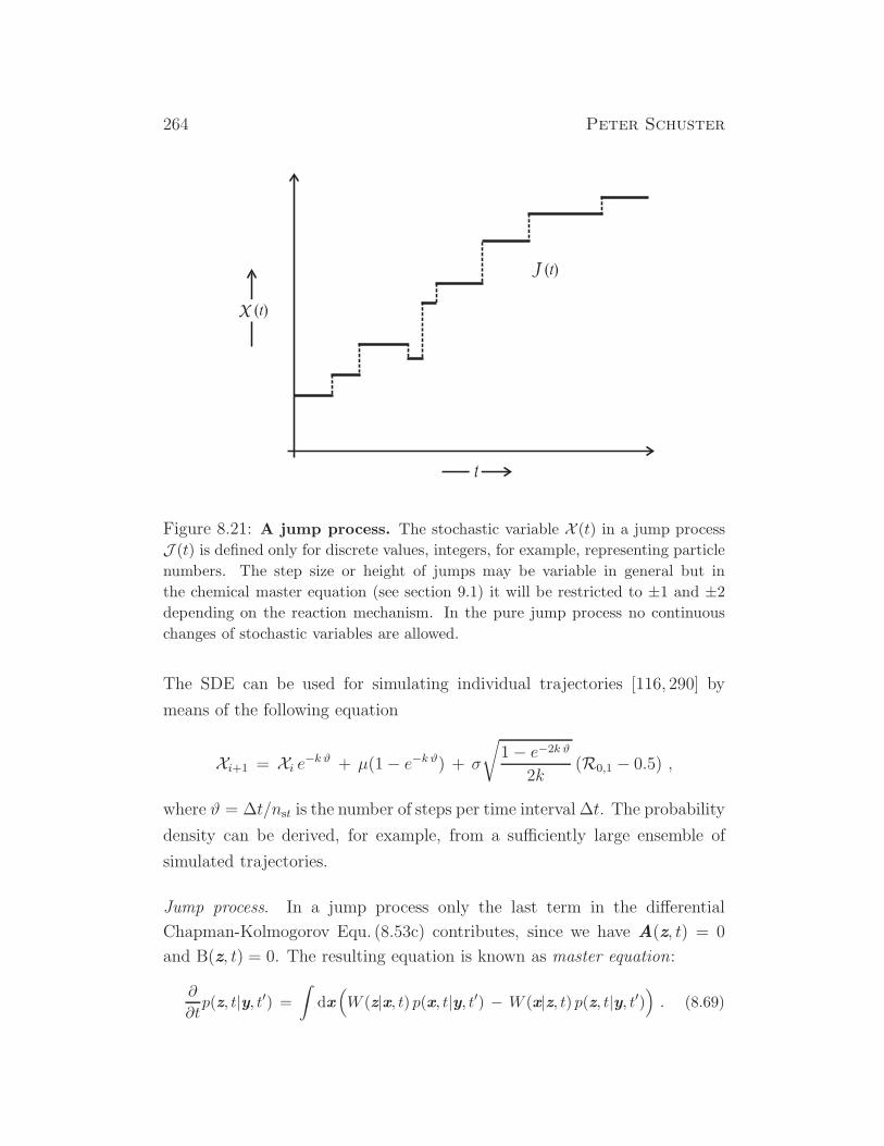
264 Peter Schuster
Figure 8.21: A jump process. The stochastic variable X (t) in a jump process
J (t) is defined only for discrete values, integers, for example, representing particle
numbers. The step size or height of jumps may be variable in general but in
the chemical master equation (see section 9.1) it will be restricted to ±1 and ±2depending on the reaction mechanism. In the pure jump process no continuous
changes of stochastic variables are allowed.
The SDE can be used for simulating individual trajectories [116, 290] by
means of the following equation
Xi+1 = Xi e−k ϑ + µ(1− e−k ϑ) + σ
√
1− e−2k ϑ
2k(R0,1 − 0.5) ,
where ϑ = ∆t/nst is the number of steps per time interval ∆t. The probability
density can be derived, for example, from a sufficiently large ensemble of
simulated trajectories.
Jump process. In a jump process only the last term in the differential
Chapman-Kolmogorov Equ. (8.53c) contributes, since we have A(z, t) = 0
and B(z, t) = 0. The resulting equation is known as master equation:
∂
∂tp(z, t|y, t′) =
∫
dx(
W (z|x, t) p(x, t|y, t′) − W (x|z, t) p(z, t|y, t′))
. (8.69)
Evolutionary Dynamics 265
In order to illustrate the general process described by the master equation
(8.69) we consider the evolution in a short time interval. For this goal we solve
approximately to first order in ∆t and use the initial condition p (z, t| y, t) =δ(y− z) representing a sharp probability density at t = 0:29
p(z, t+∆t|y, t) = p(z, t|y, t) + ∂
∂tp(z, t|y, t)∆t + . . . ≈
≈ p(z, t|y, t) + ∂
∂tp(z, t|y, t)∆t =
= δ(y− z) +
(
W (z|y, t)−∫
dxW (x|y, t) δ(y− z)
)
∆t =
=
(
1−∫
dxW (x|y, t)∆t)
δ(y− z) + W (z|y, t)∆t .
In the first term, the coefficient of δ(y− z) is the (finite) probability for the
particle to stay in the original position y, whereas the distribution of particles
that have jumped is given after normalization by W (z | y, t). A typical path
~X (t) thus will consist of constant sections, ~X (t) = const, and discontinuous
jumps which are distributed according to W (z | y, t) (Fig. 8.21). It is worth
noticing that a pure jump process does occur here even though the variable
~X (t) can take on a continuous range of values.
In a special case of the master equations, which nevertheless is funda-
mental for modeling processes in chemistry and biology, the sample space is
mapped onto the space of integers, Ω → Z = ..,−2,−1, 0, 1, 2, ... Then,
we can use conditional probabilities rather than probability densities in the
master equation:
∂P (n, t|n′, t′)∂t
=∑
m
(
W (n|m, t)P (m, t|n′, t′)−W (m|n, t)P (n, t|n′, t′))
. (8.69’)
Clearly, this process is confined to jumps since only discrete values of the
random variable ~N (t) are allowed. The master equation on the even more
restricted sample space Ω→ N0 = 0, 1, 2, . . . is of particular importance in
chemical kinetics. The random variable N (t) then counts particle numbers
which are necessarily non-negative integers. Furthermore, conservation of
29We recall a basic property of the delta-function:∫
f(x)δ(x − y) dx = f(y).
266 Peter Schuster
mass introduces an upper bound, for the random variable, N ≤ N , and
restricting reaction kinetics to elementary step limits the changes in particle
numbers to ∆N = 0,±1, and ±2.Noting initial conditions separate from the differential equation, recalling
that time t is the only continuous variable when diffusion and other spatial
phenomena are not considered, and introducing the physical limitations on
particle numbers we obtain eventually
dPn(t)
dt=
n+2∑
m=n−2
(
W (n|m, t)Pm(t − W (m|n, t)Pn(t))
(8.70)
The transition probabilities are assumed to be time-dependent here and this
is commonly not the case in chemistry and here we shall assume time inde-
pendence in general. The transition probabilities W (n|m) are understood as
the elements of a transition matrix
W.= Wnm;n,m ∈ N
0 (8.71)
Diagonal elements Wnn cancel in the master Equ. (8.70) and hence need not
be defined. According to their nature as transition probabilities, allWnm with
n 6= m have to be nonnegative. Two definitions of the diagonal elements are
common (i) normalization
Wnn = 1 −∑
m6=n
Wmn with∑
m
Wmn = 1
as used for example in the mutation selection problem (4.9), or (ii) we may
define∑
mWmn = 0 which implies Wnn = −∑m6=nWmn and then insertion
into (8.70) leads to a compact form of the master equation
dPn(t)
dt=∑
m
WnmPm(t) . (8.70’)
In subsection 9.1.1 we shall discuss specific examples of chemical master
equations and methods to drive analytical solutions. Here, we illustrate by
means of a simple example that became a standard problem in stochasticity:
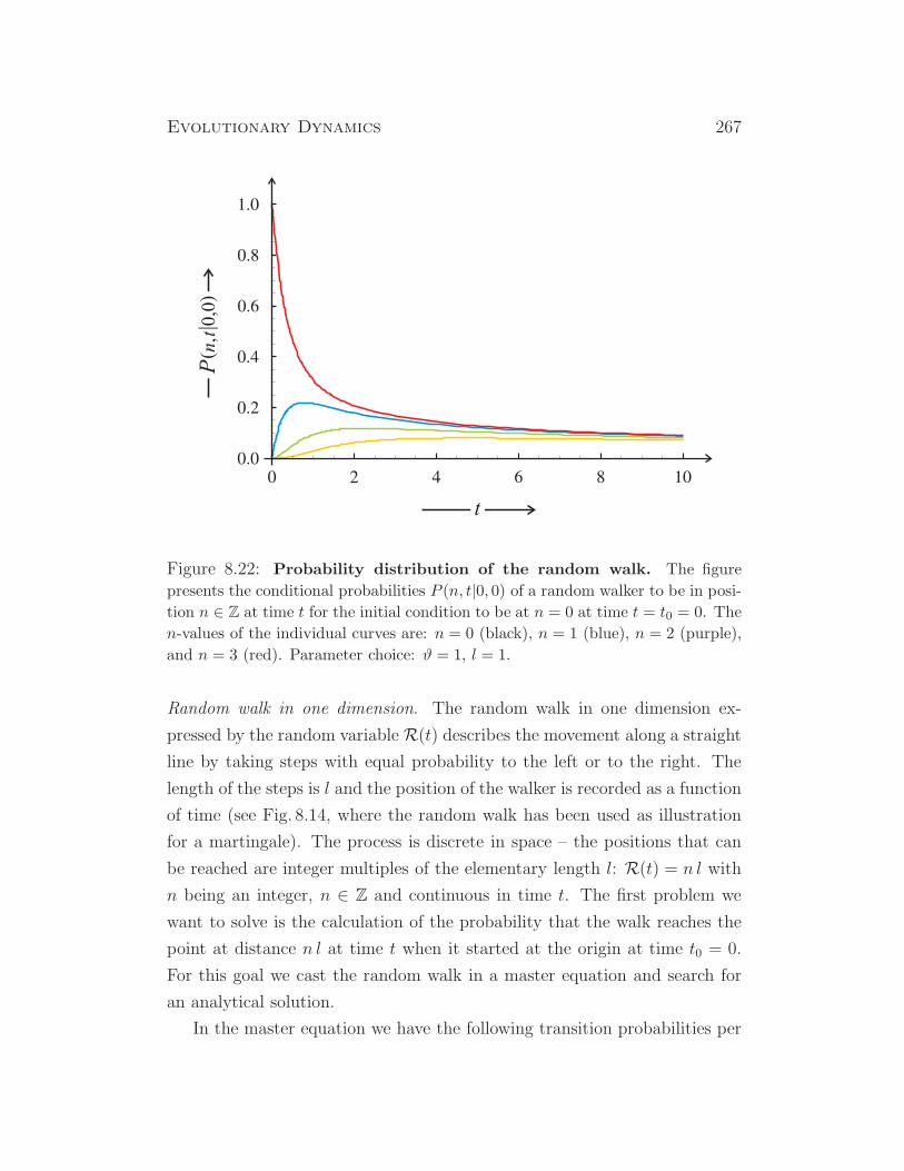
Evolutionary Dynamics 267
Figure 8.22: Probability distribution of the random walk. The figure
presents the conditional probabilities P (n, t|0, 0) of a random walker to be in posi-
tion n ∈ Z at time t for the initial condition to be at n = 0 at time t = t0 = 0. The
n-values of the individual curves are: n = 0 (black), n = 1 (blue), n = 2 (purple),
and n = 3 (red). Parameter choice: ϑ = 1, l = 1.
Random walk in one dimension. The random walk in one dimension ex-
pressed by the random variable R(t) describes the movement along a straight
line by taking steps with equal probability to the left or to the right. The
length of the steps is l and the position of the walker is recorded as a function
of time (see Fig. 8.14, where the random walk has been used as illustration
for a martingale). The process is discrete in space – the positions that can
be reached are integer multiples of the elementary length l: R(t) = n l with
n being an integer, n ∈ Z and continuous in time t. The first problem we
want to solve is the calculation of the probability that the walk reaches the
point at distance n l at time t when it started at the origin at time t0 = 0.
For this goal we cast the random walk in a master equation and search for
an analytical solution.
In the master equation we have the following transition probabilities per
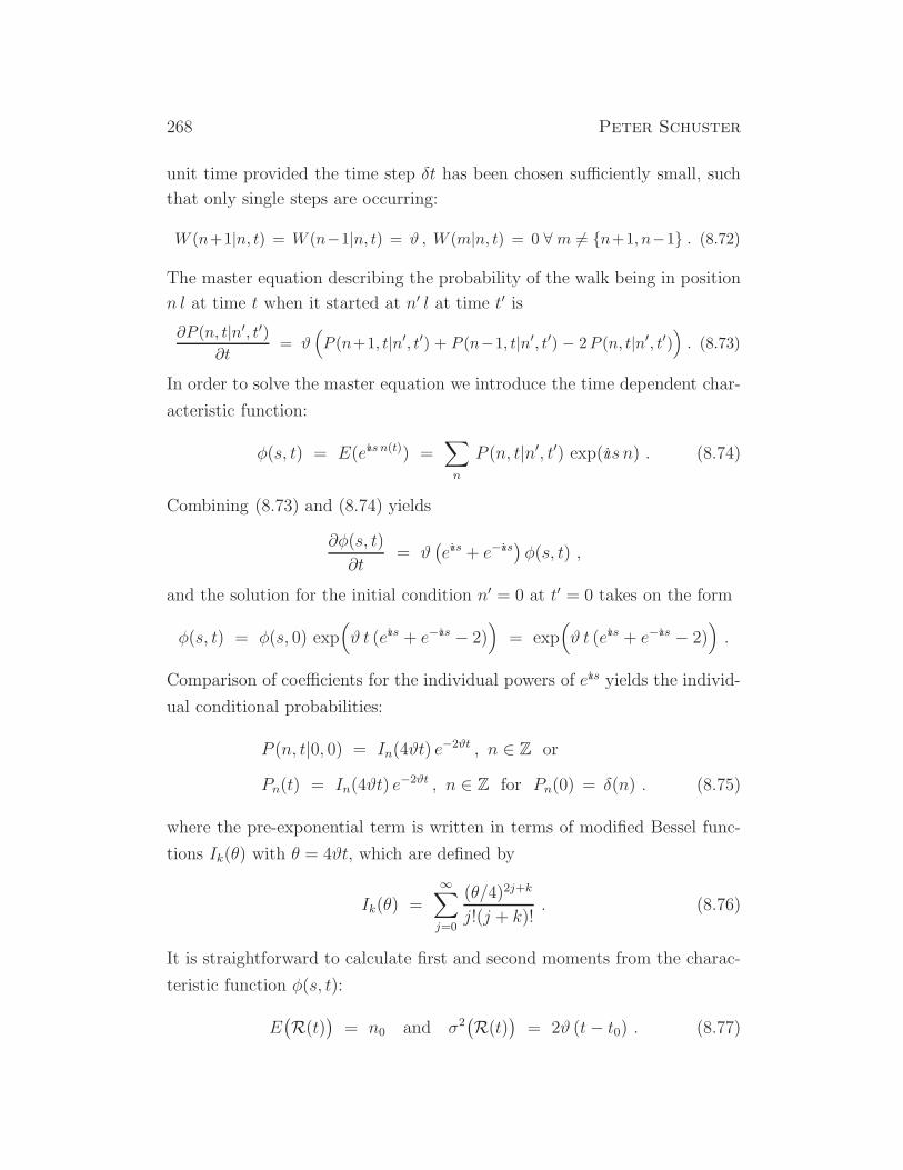
268 Peter Schuster
unit time provided the time step δt has been chosen sufficiently small, such
that only single steps are occurring:
W (n+1|n, t) = W (n−1|n, t) = ϑ , W (m|n, t) = 0 ∀ m 6= n+1, n−1 . (8.72)
The master equation describing the probability of the walk being in position
n l at time t when it started at n′ l at time t′ is
∂P (n, t|n′, t′)∂t
= ϑ(
P (n+1, t|n′, t′) + P (n−1, t|n′, t′) − 2P (n, t|n′, t′))
. (8.73)
In order to solve the master equation we introduce the time dependent char-
acteristic function:
φ(s, t) = E(eı.ıs n(t)) =
∑
n
P (n, t|n′, t′) exp(ı.ıs n) . (8.74)
Combining (8.73) and (8.74) yields
∂φ(s, t)
∂t= ϑ
(
eı.ıs + e−ı
.ıs)
φ(s, t) ,
and the solution for the initial condition n′ = 0 at t′ = 0 takes on the form
φ(s, t) = φ(s, 0) exp(
ϑ t (eı.ıs + e−ı
.ıs − 2)
)
= exp(
ϑ t (eı.ıs + e−ı
.ıs − 2)
)
.
Comparison of coefficients for the individual powers of eı.ıs yields the individ-
ual conditional probabilities:
P (n, t|0, 0) = In(4ϑt) e−2ϑt , n ∈ Z or
Pn(t) = In(4ϑt) e−2ϑt , n ∈ Z for Pn(0) = δ(n) . (8.75)
where the pre-exponential term is written in terms of modified Bessel func-
tions Ik(θ) with θ = 4ϑt, which are defined by
Ik(θ) =
∞∑
j=0
(θ/4)2j+k
j!(j + k)!. (8.76)
It is straightforward to calculate first and second moments from the charac-
teristic function φ(s, t):
E(
R(t))
= n0 and σ2(
R(t))
= 2ϑ (t− t0) . (8.77)
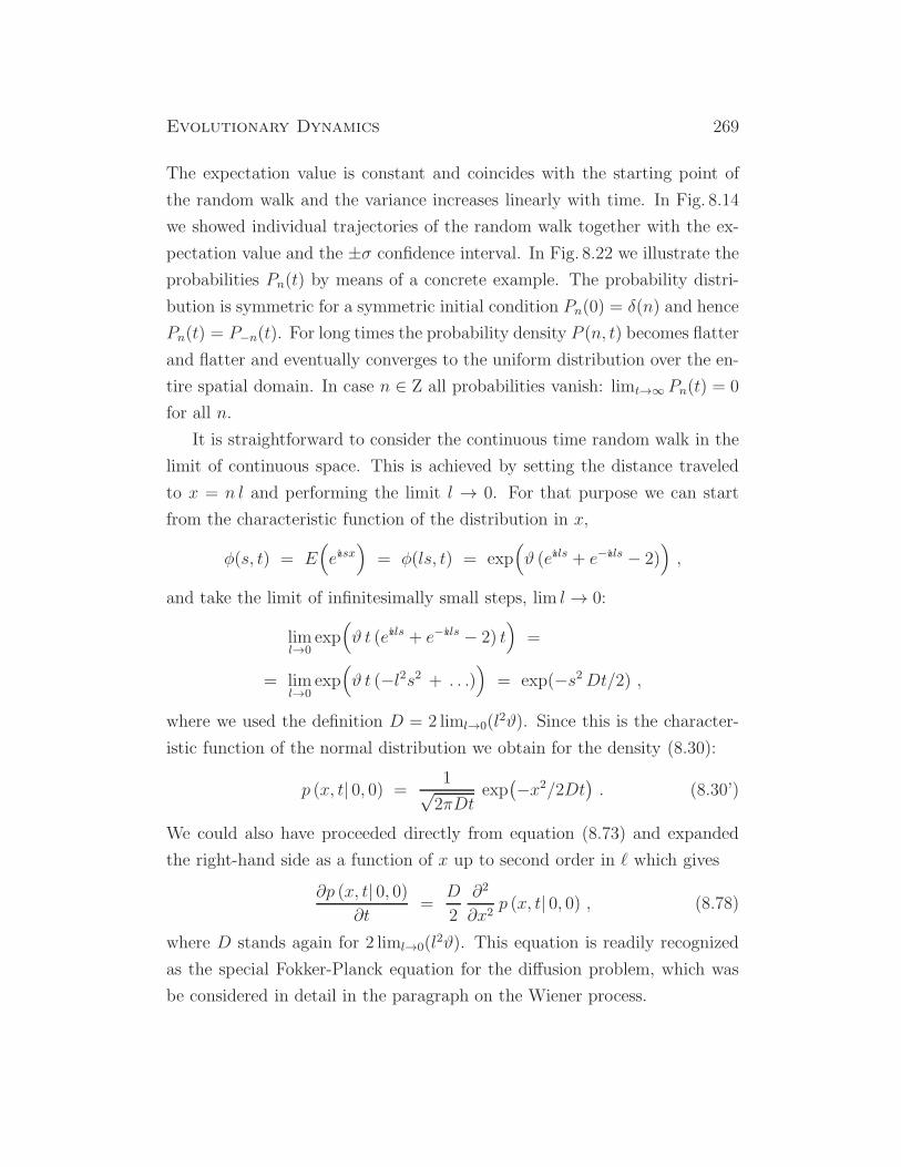
Evolutionary Dynamics 269
The expectation value is constant and coincides with the starting point of
the random walk and the variance increases linearly with time. In Fig. 8.14
we showed individual trajectories of the random walk together with the ex-
pectation value and the ±σ confidence interval. In Fig. 8.22 we illustrate the
probabilities Pn(t) by means of a concrete example. The probability distri-
bution is symmetric for a symmetric initial condition Pn(0) = δ(n) and hence
Pn(t) = P−n(t). For long times the probability density P (n, t) becomes flatter
and flatter and eventually converges to the uniform distribution over the en-
tire spatial domain. In case n ∈ Z all probabilities vanish: limt→∞ Pn(t) = 0
for all n.
It is straightforward to consider the continuous time random walk in the
limit of continuous space. This is achieved by setting the distance traveled
to x = n l and performing the limit l → 0. For that purpose we can start
from the characteristic function of the distribution in x,
φ(s, t) = E(
eı.ısx)
= φ(ls, t) = exp(
ϑ (eı.ıls + e−ı
.ıls − 2)
)
,
and take the limit of infinitesimally small steps, lim l → 0:
liml→0
exp(
ϑ t (eı.ıls + e−ı
.ıls − 2) t
)
=
= liml→0
exp(
ϑ t (−l2s2 + . . .))
= exp(−s2Dt/2) ,
where we used the definition D = 2 liml→0(l2ϑ). Since this is the character-
istic function of the normal distribution we obtain for the density (8.30):
p (x, t| 0, 0) =1√2πDt
exp(
−x2/2Dt)
. (8.30’)
We could also have proceeded directly from equation (8.73) and expanded
the right-hand side as a function of x up to second order in ℓ which gives
∂p (x, t| 0, 0)∂t
=D
2
∂2
∂x2p (x, t| 0, 0) , (8.78)
where D stands again for 2 liml→0(l2ϑ). This equation is readily recognized
as the special Fokker-Planck equation for the diffusion problem, which was
be considered in detail in the paragraph on the Wiener process.
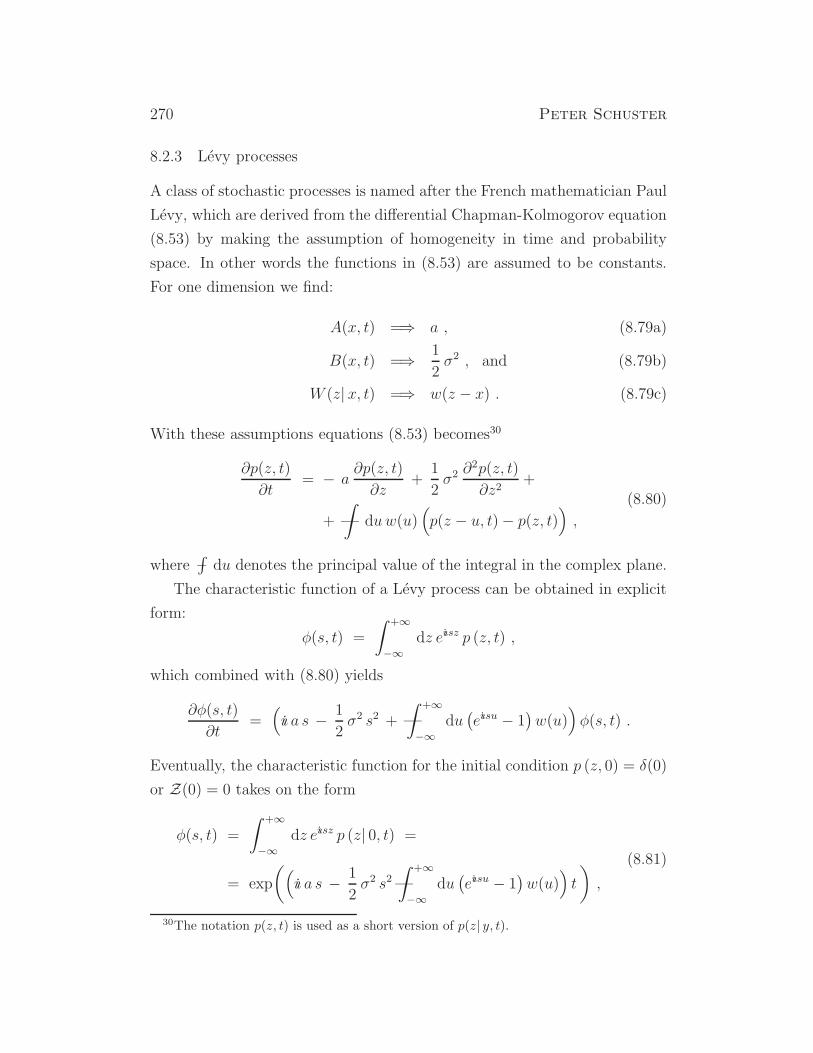
270 Peter Schuster
8.2.3 Levy processes
A class of stochastic processes is named after the French mathematician Paul
Levy, which are derived from the differential Chapman-Kolmogorov equation
(8.53) by making the assumption of homogeneity in time and probability
space. In other words the functions in (8.53) are assumed to be constants.
For one dimension we find:
A(x, t) =⇒ a , (8.79a)
B(x, t) =⇒ 1
2σ2 , and (8.79b)
W (z| x, t) =⇒ w(z − x) . (8.79c)
With these assumptions equations (8.53) becomes30
∂p(z, t)
∂t= − a
∂p(z, t)
∂z+
1
2σ2 ∂
2p(z, t)
∂z2+
+ —
∫
duw(u)(
p(z − u, t)− p(z, t))
,
(8.80)
where –∫
du denotes the principal value of the integral in the complex plane.
The characteristic function of a Levy process can be obtained in explicit
form:
φ(s, t) =
∫ +∞
−∞dz eı
.ısz p (z, t) ,
which combined with (8.80) yields
∂φ(s, t)
∂t=(
ı.ı a s − 1
2σ2 s2 + —
∫ +∞
−∞du(
eı.ısu − 1
)
w(u))
φ(s, t) .
Eventually, the characteristic function for the initial condition p (z, 0) = δ(0)
or Z(0) = 0 takes on the form
φ(s, t) =
∫ +∞
−∞dz eı
.ısz p (z| 0, t) =
= exp
(
(
ı.ı a s − 1
2σ2 s2—
∫ +∞
−∞du(
eı.ısu − 1
)
w(u))
t
)
,
(8.81)
30The notation p(z, t) is used as a short version of p(z| y, t).
Evolutionary Dynamics 271
which turns out to be quite useful for analyzing special cases.
Levy processes are or interest because several fundamental processes like
the Wiener process and the Poisson process belong to this class. They re-
ceived plenty of attention outside science and became really important in
financial applications like modeling the financial markets, in particular the
stock exchange market [107, pp.235-263].
Closing this section on stochastic processes we recall that three different
behaviors in the limit of vanishing time intervals resulted from the differen-
tial form of the Chapman-Kolmogorov equation and refer to three classes of
processes characterized as (i) drift processes, (ii) diffusion processes , and
(iii) jump processes. The jump process will turn to be most relevant for
our intentions here because it is the basis of the chemical master equation
(section 9.1) and it provides the most straightforward access to handling
stochasticity in biology. The Fokker-Planck equation will be encountered
again in the discussion of Motoo Kimura’s neutral theory of evolution.

272 Peter Schuster
9. Stochasticity in chemical reactions
Conventional chemical kinetics as said before does not require rigorous
stochastic description, because fluctuations are extremely small and ample
is fluctuation spectroscopy, which aims at direct recordings of fluctuations
[315, 321]. In particular, very accurate measurements of fluorescence corre-
lation signals have been successful [63, 69, 190, 240]. The breakthrough was
achieved here through the usage of high-performance lasers. Direct experi-
mental observations of individual processes are now accessible by means of
single molecule techniques. The best studied examples are, for example,
the experimental recording of single trajectories of biopolymer folding and
unfolding (see, for example, [121, 148, 163, 323]).
The role of fluctuations is especially interesting in situations where fluc-
tuations can be amplified by reaction dynamics. Such situations occur with
reaction mechanisms involving nonlinear terms and giving rise to highly sen-
sitive oscillations and deterministic chaos. Other examples are pattern for-
mation in space and time, Turing patterns, migrating spirals, and spatiotem-
poral chaos. Here, we focus on modeling stochastic chemical phenomena by
means of master equations, which have the advantage to be accessible to
numerical computation. Master equations applied in chemical kinetics are
discussed first, we pay particular attention to the Poisson process that is
essential for the analysis of probability distributions of independent events,
next we discuss master equations derived from birth-and-death processes,
then we review exactly solvable cases of elementary steps in chemical kinet-
ics, and eventually we present and discuss an efficient numerical method for
the calculation of stochastic trajectories of chemical reaction networks.
273
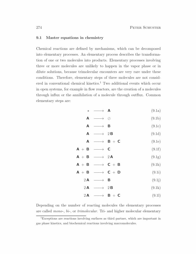
274 Peter Schuster
9.1 Master equations in chemistry
Chemical reactions are defined by mechanisms, which can be decomposed
into elementary processes. An elementary process describes the transforma-
tion of one or two molecules into products. Elementary processes involving
three or more molecules are unlikely to happen in the vapor phase or in
dilute solutions, because trimolecular encounters are very rare under these
conditions. Therefore, elementary steps of three molecules are not consid-
ered in conventional chemical kinetics.1 Two additional events which occur
in open systems, for example in flow reactors, are the creation of a molecules
through influx or the annihilation of a molecule through outflux. Common
elementary steps are:
⋆ −−−→ A (9.1a)
A −−−→ ⊘ (9.1b)
A −−−→ B (9.1c)
A −−−→ 2B (9.1d)
A −−−→ B + C (9.1e)
A + B −−−→ C (9.1f)
A + B −−−→ 2A (9.1g)
A + B −−−→ C + B (9.1h)
A + B −−−→ C + D (9.1i)
2A −−−→ B (9.1j)
2A −−−→ 2B (9.1k)
2A −−−→ B + C (9.1l)
Depending on the number of reacting molecules the elementary processes
are called mono-, bi -, or trimolecular. Tri- and higher molecular elementary
1Exceptions are reactions involving surfaces as third partner, which are important in
gas phase kinetics, and biochemical reactions involving macromolecules.
Evolutionary Dynamics 275
steps are excluded in conventional chemical reaction kinetics as said above.
The example show in Equ. (9.1g) is a simple autocatalytic elementary
process. In practice autocatalytic chemical reactions commonly involve many
elementary steps and thus are the results of complex reaction mechanisms. In
evolution reproduction and replication are obligatory autocatalytic processes,
which involve a complex molecular machinery. In order to study the basic
features of autocatalysis or chemical self-enhancement and self-organization,
single step autocatalysis is often used as in model systems. One particular
trimolecular autocatalytic process invented by Ilya Prigogine and Gregoire
Nicolis
2A + B −−−→ 3A , (9.2)
became very famous [223] despite its trimolecular nature, which makes it un-
likely to occur in real systems. The elementary step (9.2) is the essential step
in the so-called Brusselator model that can be analyzed straightforwardly by
rigorous mathematical techniques. The Brusselator model gives rise to com-
plex dynamical phenomena in space and time, which are rarely observed
in standard chemical reaction systems. Among other features such special
phenomena are: (i) multiple stationary states, (ii) chemical hysteresis, (iii)
oscillations in concentrations, (iv) deterministic chaos, and (v) spontaneous
formation of spatial structures. The last example is known as Turing insta-
bility named after the English computer scientist Alan Turing [287] and is
frequently used as a model for certain classes of pattern formation in biology
[204]. The original concept Turing’s was based on a reaction-diffusion equa-
tion and aimed at a universal model of morphogenesis in development. It
has been worked out later in great detail by Alfred Gierer, Hans Meinhardt
and others [110, 205]. Molecular genetics, however, has shown that nature is
using direct genetic control through cascades of gene regulation rather than
self-organized reaction-diffusion patterns [111, 192].
9.1.1 Chemical master equations
Provided particle numbers are used as variables to model the progress of
chemical reactions, stochastic variables N (t) are described by the probabil-
276 Peter Schuster
ities Pn(t) = Prob (N (t) = n) and take only nonnegative integer values,
n ∈ N0. As mentioned already in the previous subsection 8.2.2 we introduce
a few simplifications and conventions in th notation: (i) We shall use the
forward equation unless stated differently, (ii) we assume an infinitely sharp
initial density, P (n, 0|n0, 0) = δn,n0 with n0 = n(0), and (iii) we simplify the
full notation P (n, t|n0, 0) ⇒ Pn(t) with the implicit assumption of the sharp
initial condition (ii). Handling extended probability densities as initial con-
ditions will be discussed explicitly. The expectation value of the stochastic
variable N (t) is denoted by
E(
N (t))
= 〈n(t)〉 =∞∑
n=0
n · Pn(t) , (9.3)
and its stationary value, provided it exists, will be written
n = limt→∞〈n(t)〉 . (9.4)
Almost always n will be identical with the long time value of the correspond-
ing deterministic variable. The running index of integers will be denoted
by either m or n′. Then the chemical master equation is of the previously
presented form
dPn(t)
dt=∑
m
(
W (n|m)Pm(t) − W (m|n)Pn(t))
=∑
m
WnmPm(t) , (8.70)
where the compact form requires the definition∑
mWmn = 0 and accordingly
Wnn = −∑m6=nWmn.
Introducing vector notation, P(t) = (P1(t), . . . , Pn(t), . . .), we obtain
∂P(t)
∂t= W ×P(t) . (8.70”)
With the initial condition Pn(0) = δn,n0 we can formally solve Equ. (8.70”)
for each n0 and obtain
P (n, t|n0, 0) =(
exp(W t))
n,n0,
where the element (n, n0) of the matrix exp(Wt) is the probability to have
n particles at time t, N (t) = n, when there were n0 particles at time t0 = 0.
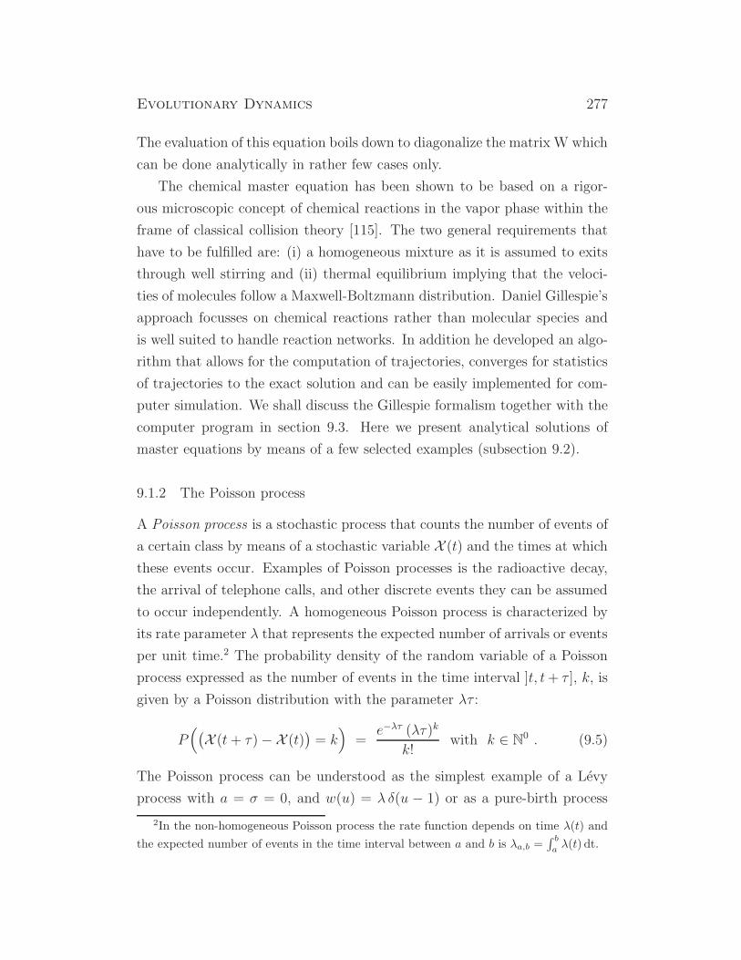
Evolutionary Dynamics 277
The evaluation of this equation boils down to diagonalize the matrix W which
can be done analytically in rather few cases only.
The chemical master equation has been shown to be based on a rigor-
ous microscopic concept of chemical reactions in the vapor phase within the
frame of classical collision theory [115]. The two general requirements that
have to be fulfilled are: (i) a homogeneous mixture as it is assumed to exits
through well stirring and (ii) thermal equilibrium implying that the veloci-
ties of molecules follow a Maxwell-Boltzmann distribution. Daniel Gillespie’s
approach focusses on chemical reactions rather than molecular species and
is well suited to handle reaction networks. In addition he developed an algo-
rithm that allows for the computation of trajectories, converges for statistics
of trajectories to the exact solution and can be easily implemented for com-
puter simulation. We shall discuss the Gillespie formalism together with the
computer program in section 9.3. Here we present analytical solutions of
master equations by means of a few selected examples (subsection 9.2).
9.1.2 The Poisson process
A Poisson process is a stochastic process that counts the number of events of
a certain class by means of a stochastic variable X (t) and the times at which
these events occur. Examples of Poisson processes is the radioactive decay,
the arrival of telephone calls, and other discrete events they can be assumed
to occur independently. A homogeneous Poisson process is characterized by
its rate parameter λ that represents the expected number of arrivals or events
per unit time.2 The probability density of the random variable of a Poisson
process expressed as the number of events in the time interval ]t, t+ τ ], k, is
given by a Poisson distribution with the parameter λτ :
P(
(
X (t+ τ)− X (t))
= k)
=e−λτ (λτ)k
k!with k ∈ N
0 . (9.5)
The Poisson process can be understood as the simplest example of a Levy
process with a = σ = 0, and w(u) = λ δ(u − 1) or as a pure-birth process
2In the non-homogeneous Poisson process the rate function depends on time λ(t) and
the expected number of events in the time interval between a and b is λa,b =∫ b
aλ(t) dt.
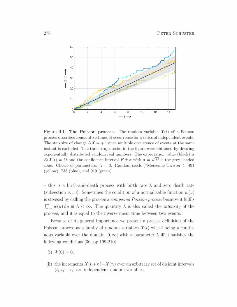
278 Peter Schuster
X(
)t
t
Figure 9.1: The Poisson process. The random variable X (t) of a Poisson
process describes consecutive times of occurrence for a series of independent events.
The step size of change ∆X = +1 since multiple occurrence of events at the same
instant is excluded. The three trajectories in the figure were obtained by drawing
exponentially distributed random real numbers. The expectation value (black) is
E(X (t) = λt and the confidence interval E ± σ with σ =√λt is the grey shaded
zone. Choice of parameters: λ = 3. Random seeds (“Mersenne Twister”): 491
(yellow), 733 (blue), and 919 (green).
– this is a birth-and-death process with birth rate λ and zero death rate
(subsection 9.1.3). Sometimes the condition of a normalizable function w(u)
is stressed by calling the process a compound Poisson process because it fulfils∫ +∞−∞ w(u) du ≡ λ < ∞. The quantity λ is also called the intensity of the
process, and it is equal to the inverse mean time between two events.
Because of its general importance we present a precise definition of the
Poisson process as a family of random variables X (t) with t being a contin-
uous variable over the domain [0,∞[ with a parameter λ iff it satisfies the
following conditions [36, pp.199-210]
(i) X (0) = 0,
(ii) the increments X (ti+τi)−X (τi) over an arbitrary set of disjoint intervals(ti, ti + τi) are independent random variables,

Evolutionary Dynamics 279
Figure 9.2: Sketch of the transition probabilities in master equations. In
the general jump process steps of any size are admitted (upper drawing) whereas
in birth-and-death processes all jumps have the same size. The simplest and most
common case is dealing with the condition that the particles are born and die one
at a time (lower drawing).
(iii) the general increment X (t + τ)− X (τ) is distributed according to thePoisson density Pois(λt) for each pair (t ≥ 0, τ ≥ 0).
The Poisson process is an excellent model for chemical reactions in a given
reaction volume. If we choose the occurrence of reactive collision as event,
the individual collisions – no matter whether taking place in the vapor phase
or in solution – are to a very good approximation independent events, and
the prerequisites for a Poisson process are fulfilled.
9.1.3 Birth-and-death processes
The concept of birth-and-death processes has been created in biology and is
based on the assumption that only a finite number of individuals are produced
– born – or destroyed – die – in a single event. The simplest and the only case,
we shall discuss here, is occurs when birth and death is confined to single
280 Peter Schuster
individuals of only one species. These processes are commonly denoted as
one step birth-and-death processes.3 In Fig. 9.2 the transitions in a general
jump process and a birth-and-death process are illustrated. Restriction to
single events is tantamount to the choice of a sufficiently small time interval
of recording, ∆t, such that the simultaneous occurrence of two events has
a probability of measure zero (see also section 9.3). This small time step is
often called the blind interval, because no information on things happening
within ∆t is available.
Then, the transition probabilities can be written in the form
W (n|m, t) = w+(m) δn,m+1 + w−(m) δn,m−1 , (9.6)
since we are dealing with only two allowed processes:
n −→n+ 1 with w+(n) as transition probability per unit time and
n −→n− 1 with w−(n) as transition probability per unit time.
Modeling of chemical reactions by birth-and-death processes turns out to
be a very useful approach for reaction mechanisms that can be described
by changes in a single variable. Another special case of a birth-and-death
process is the Poisson process on n ∈ N0: It has zero death rate and describes
the occurrence of independent events (see also the Poisson distribution in
subsection 8.1.3 and the Poisson process in subsection 9.1.2). We shall make
use of the Poisson process in describing the occurrence of chemical reaction
in subsection 9.3.
The stochastic process can now be described by a birth-and-death master
equation
dPn(t)
dt= w+(n− 1)Pn−1(t) + w−(n+ 1)Pn+1(t)−
−(
(w+(n) + w−(n))
Pn(t) .
(9.7)
3In addition, one commonly distinguishes between birth-and-death processes in one
variable and in many variables [107]. We shall restrict the analysis here to the simpler
single variable case here.

Evolutionary Dynamics 281
There is no general technique that allows to find the time-dependent solutions
of equation (9.7) and therefore we shall present some special cases later on.
Only few single step birth-and-death processes can be solved analytically.
The stationary case, however, can be analyzed in full generality. Provided
a stationary solution of equation (9.7) exists, limt→∞ Pn(t) = Pn, we can
compute it in straightforward manner. It is useful to define a probability
current J(n) for the n-th step in the series,
Particle number 0 1 . . . n− 1 n n+ 1 . . .
Reaction step 1 2 . . . n− 1 n n+ 1 . . .
which is of the form
J(n) = w− n P (n) − w+ (n− 1) P (n− 1) . (9.8)
The conditions for the stationary solution are given by vanishing time deriva-
tives of the probabilities
dPn(t)
dt= 0 = J(n+ 1) − J(n) . (9.9)
Restriction to positive particle numbers, n ∈ N0, implies w−(0) = 0 and
Pn(t) = 0 for n < 0, which in turn leads to J(0) = 0. Now we sum the
vanishing flow terms according to equation (9.9) and obtain:
0 =
n−1∑
z=0
(
J(z + 1) − J(z))
= J(n) − J(0) .
Accordingly we find J(n) = 0 for arbitrary n, which leads to
Pn =w+(n− 1)
w−(n)Pn−1 and finally Pn = P0
n∏
z=1
w+(z − 1)
w−(z).
The condition J(n) = 0 for every reaction step is known in chemical kinetics
as the principle of detailed balance: At equilibrium the reaction flow has
to vanish for every reaction step. The principle of detailed balance was
formulated first by the American mathematical physicist Richard Tolman
[286] (see also [107, pp.142-158]).
282 Peter Schuster
The macroscopic rate equations are readily derived from the master equa-
tion through calculation of the expectation value:
d
dtE(
n(t))
=d
dt
( ∞∑
n=0
nPn(t)
)
=
=∞∑
n=0
n(
w+(n− 1)Pn−1(t) − w+(n)Pn(t))
+
+∞∑
n=0
n(
w−(n + 1)Pn+1(t) − w−(n)Pn(t))
=
=
∞∑
n=0
(
(n+ 1)w+(n) − nw+(n) + (n− 1)w−(n) − nw−(n))
Pn(t) =
=
∞∑
n=0
w+(n)P n(t) −∞∑
n=0
w−(n)Pn(t) = E(
w+(n))
− E(
w−(n))
.
Neglect of fluctuations yields the deterministic rate equation of the birth-
and-death process
d〈n〉dt
= w+(
〈n〉)
− w−(
〈n〉)
. (9.10)
The condition of stationary yields: n = limt→∞ 〈n(t)〉 forwhich holdsw+(n) =
w−(n). Compared to this results we note that the maximum value of the
stationary probability density, maxPn, n ∈ N0, is defined by Pn+1 − Pn ≈−(Pn − Pn−1) or Pn+1 ≈ Pn−1, which coincides with the deterministic value
for large n.
9.2 Examples of solvable master equations
Although only a small minority of master equations in chemical reaction ki-
netics can be solved analytically, these cases provide the best insight into the
role of stochasticity in chemical reactions, and they reflect well the repertoire
of methodological tricks that are applied in modeling of stochastic processes
in chemistry and biology. Here we shall solve the equilibration of the flow
in the flow reactor, examples of unimolecular reactions, and one solvable
bimolecular reaction.
Evolutionary Dynamics 283
The flow reactor. In section 4.2 the flow reactor has been introduced as a de-
vice for the experimental and theoretical analysis of systems under controlled
conditions away from thermodynamic equilibrium (Fig. 4.3). Here we shall
use it for analyzing the simplest conceivable process, the non-reactive flow
of a single compound, A, through the reactor. The stock solution contains
A at the concentration [A]influx = a = a. The influx concentration a is
equal to the stationary concentration a, because no reaction is assumed and
after sufficiently long time the content of the reactor will be stock solution.
The intensity of the flow is measured by means of the flow rate r and this
implies an influx of a · r of A into the reactor, instantaneous mixing with the
content of the reactor, and an outflux of the mixture in the reactor at the
same flow rate r.4 If the volume of the reactor is V , the mean residence time
of a volume element dV in the reactor is τR = V · r−1.In- and outflux of compound A into and from the reactor are modeled by
two formal elementary steps or pseudo-reactions
⋆ −−−→ A
A −−−→ ⊘ .(9.11)
In chemical kinetics the differential equations are almost always formulated in
molecular concentrations. For the stochastic treatment, however, we replace
concentrations by the numbers of particles, n = a · V ·NL with n ∈ N0 and
NL being Loschmidt’s or Avogadro’s number,5 the number of particles per
mole.
The particle number of A in the reactor is a stochastic variable with the
probability Pn(t) = P(
N (t) = n)
. The time derivative of the probability
4The assumption of equal influx and outflux rate is required because we are dealing
with a flow reactor of constant volume V (CSTR, Fig. 4.3).5As a matter of fact there is a difference between Loschmidt’s and Avogadro’s number
that is often ignored in the literature: Avogadro’s number, NL = 6.02214179×10²³mole−1
refers to one mole substance whereas Loschmidt’s constant n0 = 2.6867774 × 1025m−3
counts the number of particles in one liter gas under normal conditions. The conver-
sion factor between both constants is the molar volume of an ideal gas that amounts to
22.414 dm−3 ·mole−1.

284 Peter Schuster
distribution is described by means of the master equation
dPn(t)
dt= r
(
n Pn−1(t) + (n+1)Pn+1(t) − (n+n)Pn(t))
; n ∈ N0 . (9.12)
Here we have implicitly assumed Equ. (9.12) describes a birth-and-death pro-
cess with w+(n) = rn and w−(n) = rn. Thus we have a constant birth rate
and a death rate which is proportional to n. see next subsection 9.1.3
Solutions of the master equation can be found in text books listing stochas-
tic processes with known solutions, for example [118]. Here we shall derive
the solution by means of probability generating functions in order to illustrate
this particularly powerful approach. The probability generating function of
a nonnegative valued random variable is defined by
g(s, t) =
∞∑
n=0
Pn(t) sn . (9.13)
In general the auxiliary variable s is real valued, s ∈ R1, although generating
functions with complex s can be of advantage. Sometimes the initial state is
included in the notation: gn0(s, t) implies Pn(0) = δn,n0. Partial derivatives
with respect to time t and the variable s are readily computed:
∂g(s, t)
∂t=
∞∑
n=0
∂Pn(t)
∂t· sn =
= r
∞∑
n=0
(
n Pn−1(t) + (n+ 1)Pn+1(t) − (n+ n)Pn(t))
sn and
∂g(s, t)
∂s=
∞∑
n=0
nPn(t) sn−1 .
Proper collection of terms and arrangement of summations – by taking into
account: w−(0) = 0 – yields
∂g(s, t)
∂t= rn
∞∑
n=0
(
Pn−1(t) − Pn(t))
sn + r∞∑
n=0
(
(n+ 1)Pn+1(t) − nPn(t))
sn .

Evolutionary Dynamics 285
Evaluation of the four infinite sums∑∞
n=0Pn−1(t) s
n = s∑∞
n=0Pn−1(t) s
n−1 = s g(s, t) ,
∑∞
n=0Pn(t) s
n = g(s, t) ,
∑∞
n=0(n+ 1)Pn+1(t) s
n =∂g(s, t)
∂t, and
∑∞
n=0nPn(t) s
n = s∑∞
n=0nPn(t) s
n−1 = s∂g(s, t)
∂t,
and regrouping of terms yields a linear partial differential equation of first
order∂g(s, t)
∂t= r
(
n(s− 1) g(s, t) − (s− 1)∂g(s, t)
∂s
)
. (9.14)
The partial differential equation (PDE) is solved through consecutive sub-
stitutions
φ(s, t) = g(s, t) exp(−n s) −→ ∂φ(s, t)
∂t= −r(s− 1)
∂φ(s, t)
∂s,
s− 1 = eρ and ψ(ρ, t) = φ(s, t) −→ ∂ψ(ρ, t)
∂t+ r
∂ψ(ρ, t)
∂ρ.
Computation of the characteristic manifold is equivalent to solving the
ordinary differential equation (ODE) r dt = −dρ. We find: rt − ρ = C
where C is the integration constant. The general solution of the PDE is an
arbitrary function of the combined variable rt− ρ:
ψ(ρ, t) = f(
exp(−rt + ρ))
· e−n and φ(s, t) = f(
(s− 1) e−rt)
· e−n ,
and the probability generating function
g(s, t) = f(
(s− 1) e−rt))
· exp(
(s− 1)n)
.
Normalization of probabilities (for s = 1) requires g(1, t) = 1 and hence
f(0) = 1. The initial conditions as expressed by the conditional probability
P (n, 0|n0, 0) = Pn(0) = δn,n0 leads to the final expression
g(s, 0) = f(s− 1) · exp(
(s− 1)n)
= sn0 ,
f(ζ) = (ζ + 1)n0 · exp(−ζn) with ζ = (s − 1) e−rt ,
g(s, t) =(
1 + (s− 1) e−rt)n0 · exp
(
−n(s− 1) e−rt)
· exp(
n(s − 1))
=
=(
1 + (s− 1) e−rt)n0 · exp
−n(s− 1) (1 − e−rt)
.
(9.15)
286 Peter Schuster
From the generating function we compute with somewhat tedious but straight-
forward algebra the probability distribution
Pn(t) =
minn0,n∑
k=0
(
n0
k
)
nn−k · e−krt (1− e−rt
)n0+n−2k
(n− k)!· e−n (1−e−rt) (9.16)
with n, n0, n ∈ N0. In the limit t → ∞ we obtain a non-vanishing contri-
bution to the stationary probability only from the first term, k = 0, and
find
limt→∞
Pn(t) =nn
n!exp(−n) .
This is a Poissonian distribution with parameter and expectation value α =
n. The Poissonian distribution has also a variance which is numerically
identical with the expectation value, σ2(NA) = E(NA) = n, and thus the
distribution of particle numbers fulfils the√N -law at the stationary state.
The time dependent probability distribution allows to compute the expecta-
tion value and the variance of the particle number as a function of time
E(
N (t))
= n + (n0 − n) · e−rt ,
σ2(
N (t))
=(
n + n0 · e−rt)
·(
1 − e−rt)
.(9.17)
As expected the expectation value apparently coincides with the solution
curve of the deterministic differential equation
dn
dt= w+(n) − w−(n) = r (n− n) , (9.18)
which is of the form
n(t) = n + (n0 − n) · e−rt . (9.18’)
Since we start from sharp initial densities variance and standard deviation are
zero at time t = 0. The qualitative time dependence of σ2(
NA(t))
, however,
depends on the sign of (n0 − n):
(i) For n0 ≤ n the standard deviation increases monotonously until it
reaches the value√n in the limit t→∞, and

Evolutionary Dynamics 287
Figure 9.3: Establishment of the flow equilibrium in the CSTR. The
upper part shows the evolution of the probability density, Pn(t), of the number of
molecules of a compound A which flows through a reactor of the type illustrated in
Fig. 4.3. The initially infinitely sharp density becomes broader with time until the
variance reaches its maximum and then sharpens again until it reaches stationarity.
The stationary density is a Poissonian distribution with expectation value and
variance, E(N ) = σ2(N ) = n. In the lower part we show the expectation value
E(
N (t))
in the confidence interval E ± σ. Parameters used: n = 20, n0 = 200,
and V = 1; sampling times (upper part): τ = r · t = 0 (black), 0.05 (green), 0.2
(blue), 0.5 (violet), 1 (pink), and ∞ (red).
288 Peter Schuster
(ii) for n0 > n the standard deviation increases until it passes through a
maximum at
t(σmax) =1
r
(
ln 2 + lnn0 − ln(n0 − n))
and approaches the long-time value√n from above.
In figure 9.3 we show an example for the evolution of the probability den-
sity (9.16). In addition, the figure contains a plot of the expectation value
E(
N (t))
inside the band E − σ < E < E + σ. In case of a normally dis-
tributed stochastic variable we find 68.3% of all values within this confidence
interval. In the interval E − 2σ < E < E + 2σ we would find even 95.4% of
all stochastic trajectories as derived in case of the normal distribution.
The monomolecular reaction. The reversible mono- or unimolecular chemical
reaction can be split into two irreversible elementary reactions
Ak1−−−→ B (9.19a)
Ak2
←−−− B , (9.19b)
wherein the reaction rate parameters, k1 and k2, are called reaction rate
constants. The reaction rate parameters depend on temperature, pressure,
and other environmental factors. At equilibrium the rate of the forward
reaction (9.19a) is precisely compensated by the rate of the reverse reac-
tion (9.19b), k1 ·[A] = k2 ·[B], leading to the condition for the thermodynamic
equilibrium:
K =k1k2
=[B]
[A]. (9.20)
The parameter K is called the equilibrium constant that depends on tem-
perature, pressure, and other environmental factors like the reaction rate
parameters. In an isolated or in a closed system we have a conservation law:
NA(t) + NB(t)
V ·NA
= [A] + [B] = c(t) = c0 = c = constant , (9.21)
with c being the total concentration and c the corresponding equilibrium
value, limt→∞ c(t) = c.

Evolutionary Dynamics 289
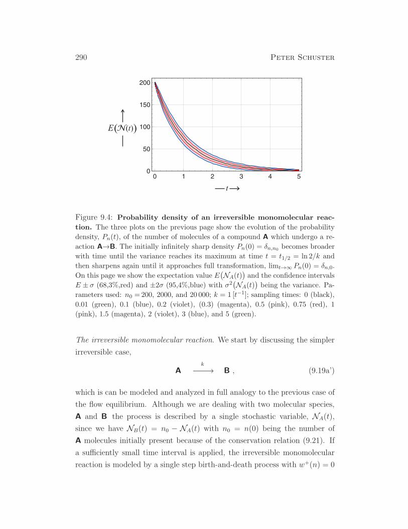
290 Peter Schuster
Figure 9.4: Probability density of an irreversible monomolecular reac-
tion. The three plots on the previous page show the evolution of the probability
density, Pn(t), of the number of molecules of a compound A which undergo a re-
action A→B. The initially infinitely sharp density Pn(0) = δn,n0 becomes broader
with time until the variance reaches its maximum at time t = t1/2 = ln 2/k and
then sharpens again until it approaches full transformation, limt→∞ Pn(0) = δn,0.
On this page we show the expectation value E(
NA(t))
and the confidence intervals
E ± σ (68,3%,red) and ±2σ (95,4%,blue) with σ2(
NA(t))
being the variance. Pa-
rameters used: n0 =200, 2000, and 20 000; k = 1 [t−1]; sampling times: 0 (black),
0.01 (green), 0.1 (blue), 0.2 (violet), (0.3) (magenta), 0.5 (pink), 0.75 (red), 1
(pink), 1.5 (magenta), 2 (violet), 3 (blue), and 5 (green).
The irreversible monomolecular reaction. We start by discussing the simpler
irreversible case,
Ak
−−−→ B , (9.19a’)
which is can be modeled and analyzed in full analogy to the previous case of
the flow equilibrium. Although we are dealing with two molecular species,
A and B the process is described by a single stochastic variable, NA(t),
since we have NB(t) = n0 − NA(t) with n0 = n(0) being the number of
A molecules initially present because of the conservation relation (9.21). If
a sufficiently small time interval is applied, the irreversible monomolecular
reaction is modeled by a single step birth-and-death process with w+(n) = 0
Evolutionary Dynamics 291
and w−(n) = kn.6 The probability density is defined by Pn(t) = P (NA = n)
and its time dependence obeys
∂Pn(t)
∂t= k (n+ 1)Pn+1(t) − k nPn(t) . (9.22)
The master equation (9.22) is solved again by means of the probability gen-
erating function,
g(s, t) =
∞∑
n=0
Pn(t) sn ; |s| ≤ 1 ,
which is determined by the PDE
∂g(s, t)
∂t− k (1− s) ∂g(s, t)
∂s= 0.
The computation of the characteristic manifold of this PDE is tantamount
to solving the ODE
k dt =ds
s− 1=⇒ ekt = s− 1 + const .
With φ(s, t) = (s − 1) exp(−kt) + γ, g(s, t) = f(φ), the normalization con-
dition g(1, t) = 1, and the boundary condition g(s, 0) = f(φ)t=0 = sn0 we
find
g(s, t) =(
s · e−kt + 1 − e−kt)n0
. (9.23)
This expression is easily expanded in binomial form, which orders with re-
spect to increasing powers of s,
g(s, t) = (1− e−kt)n0+
(
n0
1
)
se−kt(1− e−kt)n0−1 +
(
n0
2
)
se−2kt(1− e−kt)n0−2+
+ . . .+
(
n0
n0 − 1
)
sn0−1e−(n0−1)kt(1− e−kt) + sn0e−n0kt .
Comparison of coefficients yields the time dependent probability density
Pn(t) =
(
n0
n
)
(
exp(−kt))n (
1− exp(−kt))n0−n
. (9.24)
6We remark that w−(0) = 0 and w+(0) = 0 are fulfilled, which are the conditions for
a natural absorbing barrier at n = 0.
292 Peter Schuster
It is straightforward to compute the expectation value of the stochastic vari-
able NA, which coincides again with the deterministic solution, and its vari-
ance
E(
NA(t))
= n0 e−kt ,
σ2(
NA(t))
= n0 e−kt (1− e−kt
)
.(9.25)
The half-life of a population of n0 particles,
t1/2 : ENA(t) =n0
2= n0 · e−ktm =⇒ t1/2 =
1
kln 2 ,
is time of maximum variance or standard deviation, dσ2/ dt = 0 or dσ/ dt =
0, respectively. An example of the time course of the probability density of
an irreversible monomolecular reaction is shown in Fig. 9.4.
The reversible monomolecular reaction. The analysis of the irreversible re-
action is readily extended to the reversible case (9.19), where we are again
dealing with a one step birth-and-death process in a closed system: The con-
servation relation NA(t) +NB(t) = n0 – with n0 being again the number of
molecules of class A initially present, Pn(0) = δn,n0 – holds and the transi-
tion probabilities are given by: w+(n) = k2(n0 − n) and w−(n) = k1n.7 The
master equation is now of the form
∂Pn(t)
∂t= k2(n0 − n + 1)Pn−1(t) + k1(n + 1)Pn+1(t)−
−(
k1n + k2(n0 − n))
Pn(t) .
(9.26)
Making use of the probability generating function g(s, t) we derive the PDE
∂g(s, t)
∂t=(
k1 + (k2 − k1)s− k1s2)∂g(s, t)
∂s+ n0 k2(s− 1) g(s, t) .
The solutions of the PDE are simpler when expressed in terms of parameter
combinations, κ = k1 + k2 and λ = k1/k2, and the function
7Here we note the existence of barriers at n = 0 and n = n0, which are characterized
by w−(0) = 0, w+(0) = k2n0 > 0 and w+(n0) = 0, w−(n0) = k1n0 > 0, respectively.
These equations fulfil the conditions for reflecting barriers.
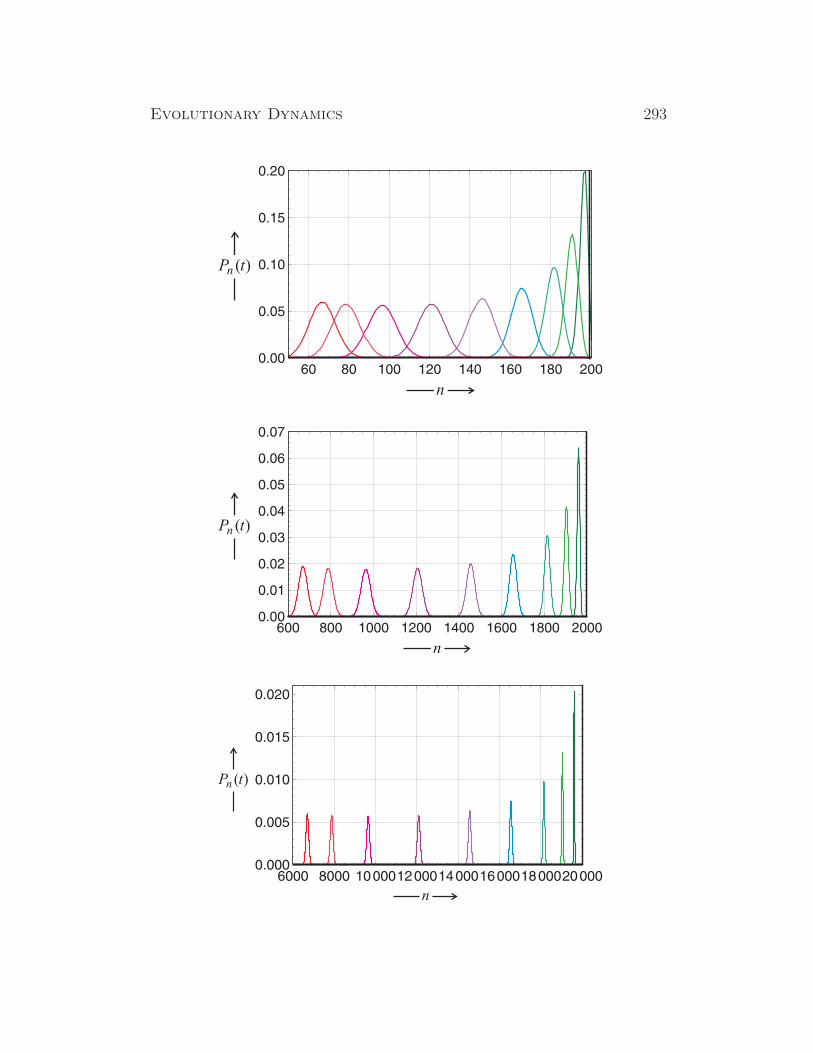
Evolutionary Dynamics 293
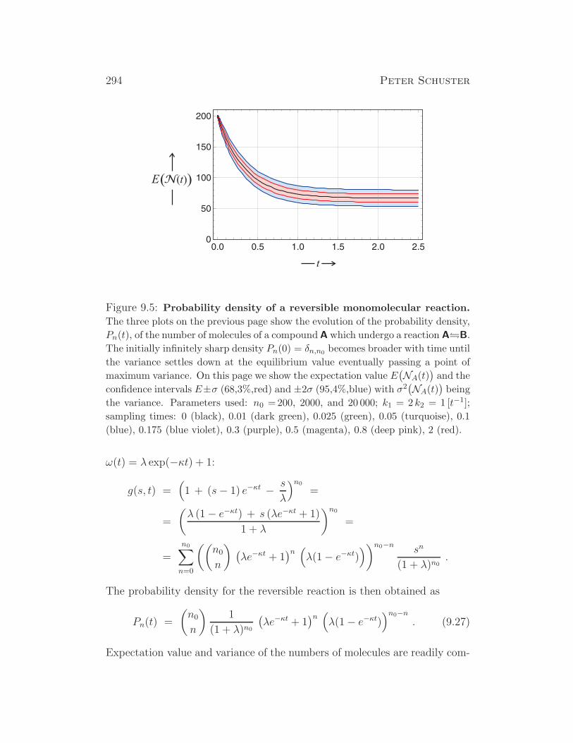
294 Peter Schuster
Figure 9.5: Probability density of a reversible monomolecular reaction.
The three plots on the previous page show the evolution of the probability density,
Pn(t), of the number of molecules of a compoundA which undergo a reaction AB.
The initially infinitely sharp density Pn(0) = δn,n0 becomes broader with time until
the variance settles down at the equilibrium value eventually passing a point of
maximum variance. On this page we show the expectation value E(
NA(t))
and the
confidence intervals E±σ (68,3%,red) and ±2σ (95,4%,blue) with σ2(
NA(t))
being
the variance. Parameters used: n0 =200, 2000, and 20 000; k1 = 2 k2 = 1 [t−1];sampling times: 0 (black), 0.01 (dark green), 0.025 (green), 0.05 (turquoise), 0.1
(blue), 0.175 (blue violet), 0.3 (purple), 0.5 (magenta), 0.8 (deep pink), 2 (red).
ω(t) = λ exp(−κt) + 1:
g(s, t) =(
1 + (s− 1) e−κt − s
λ
)n0
=
=
(
λ (1− e−κt) + s (λe−κt + 1)
1 + λ
)n0
=
=n0∑
n=0
((
n0
n
)
(
λe−κt + 1)n(
λ(1− e−κt))
)n0−n sn
(1 + λ)n0.
The probability density for the reversible reaction is then obtained as
Pn(t) =
(
n0
n
)
1
(1 + λ)n0
(
λe−κt + 1)n(
λ(1− e−κt))n0−n
. (9.27)
Expectation value and variance of the numbers of molecules are readily com-

Evolutionary Dynamics 295
puted (with ω(t) = λ exp(−κt) + 1):
E(
NA(t))
=n0
1 + λω(t) ,
σ2(
NA(t))
=n0 ω(t)
1 + λ
(
1− ω(t)
1 + λ
)
,(9.28)
and the stationary values are
limt→∞
E(
NA(t))
= n0k2
k1 + k2,
limt→∞
σ2(
NA(t))
= n0k1 k2
(k1 + k2)2,
limt→∞
σ(
NA(t))
=√n0
√
k1 k2k1 + k2
.
(9.29)
This result shows that the√N -law is fulfilled up to a factor that is indepen-
dent of N : E/σ =√n0 k2/
√
k1 k2.
Starting from a sharp distribution, Pn(0) = δn,n0, the variance increases,
may or may not pass through a maximum and eventually reaches the equi-
librium value, σ2 = k1k2 n0/(k1 + k2)2. The time of maximal fluctuations,
tmax, is easily calculated from the condition dσ2/ dt = 0 and one obtains
tmax =1
k1 + k2ln
(
2 k1k1 − k2
)
. (9.30)
Depending on the sign of (k1−k2) the approach towards equilibrium passes a
maximum value or not. The maximum is readily detected from the height of
the mode of Pn(t) as seen in Fig. 9.5 where a case with k1 > k2 is presented.
In order to illustrate fluctuations and their value under equilibrium con-
ditions the Austrian physicist Paul Ehrenfest designed a game called Ehren-
fest’s urn model [64], which was indeed played in order to verify the√N -law.
Balls, 2N in total, are numbered consecutively, 1, 2, . . . , 2N , and distributed
arbitrarily over two containers, say A and B. A lottery machine draws lots,
which carry the numbers of the balls. When the number of a ball is drawn,
the ball is put from one container into the other. This setup is already suffi-
cient for a simulation of the equilibrium condition. The more balls are in a
container, the more likely it is that the number of one of its balls is drawn
296 Peter Schuster
and a transfer occurs into the other container. Just as it occurs with chem-
ical reactions we have self-controlling fluctuations: Whenever a fluctuations
becomes large it creates a force for compensation which is proportional to
the size of the fluctuation.
Two examples of bimolecular reactions (9.1f) and (9.1j) as well as their
solutions are presented here in order to illustrate the enormous degree of
sophistication that is required to derive analytical solutions,
A + Bk
−−−→ C and (9.31a)
2Ak
−−−→ B , (9.31b)
and we discuss them in this sequence.
The irreversible bimolecular addition reaction. As first example of a bimolec-
ular process we choose the simple irreversible bimolecular addition reaction
(9.31a). In this case we are dealing with three dependent stochastic vari-
ables NA(t), NB(t), and NC(t). Following McQuarrie we define the prob-
ability Pn(t) = P(
NA(t) = n)
and apply the standard initial condition
Pn(0) = δn,n0, P (NB(0) = b) = δb,b0 , and P (NC(0) = c) = δc,0. Accord-
ingly, we have from the laws of stoichiometry NB(t) = b0 − n0 +NA(t) and
NC(t) = n0−NA(t). For simplicity we denote b0−n0 = ∆0. Then the master
equation for the chemical reaction is of the form
∂Pn(t)
∂t= k (n+ 1) (∆0 + n+ 1)Pn+1(t) − k n (∆0 + n)Pn(t) . (9.32)
We remark that the birth and death rates are no longer linear in n. The
corresponding PDE for the generating function is readily calculated
∂g(s, t)
∂t= k (∆0 + 1)(1− s)∂g(s, t)
∂s+ k s(1− s) ∂
2g(s, t)
∂s2. (9.33)
The derivation of solutions or this PDE is quite demanding. It can be
achieved by separation of variables:
g(s, t) =
∞∑
m=0
Am Zm(s) Tm(t) . (9.34)
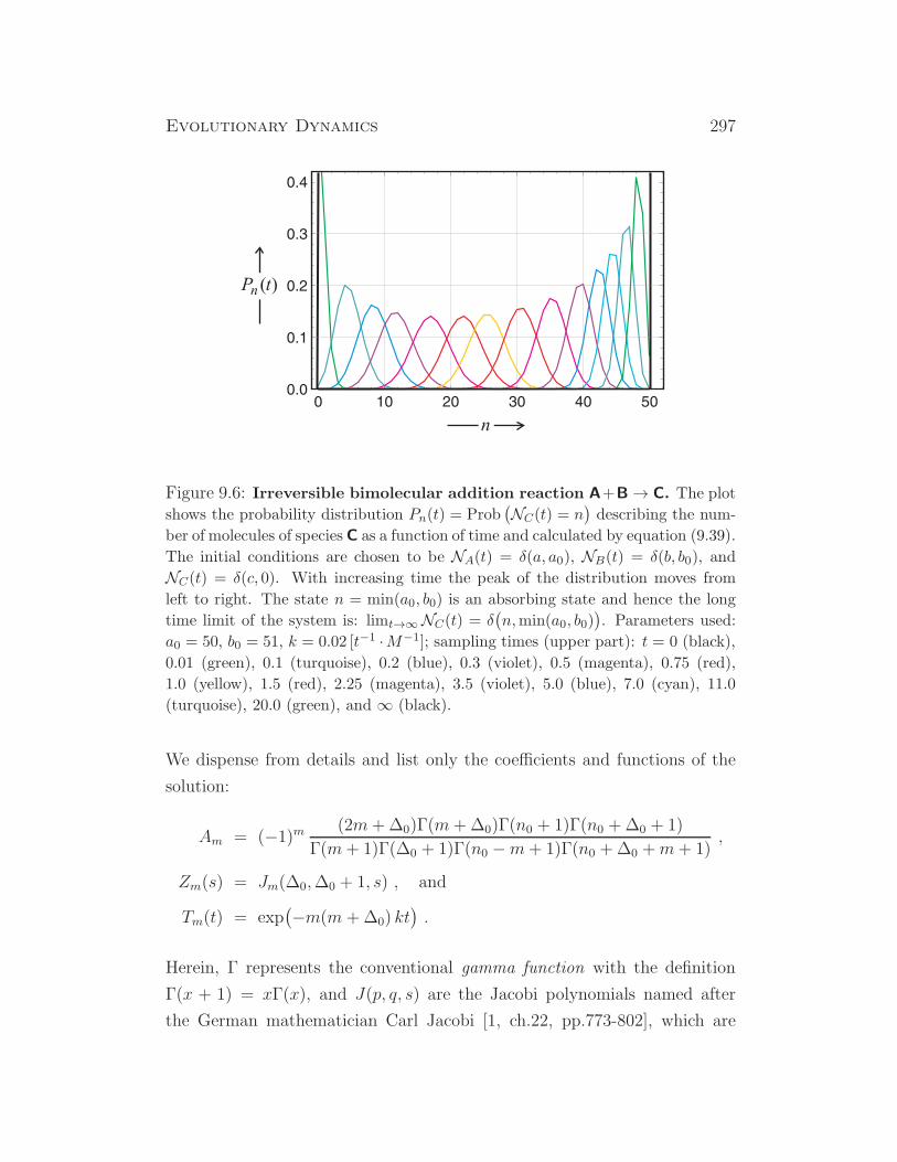
Evolutionary Dynamics 297
Figure 9.6: Irreversible bimolecular addition reaction A+B→ C. The plot
shows the probability distribution Pn(t) = Prob(
NC(t) = n)
describing the num-
ber of molecules of species C as a function of time and calculated by equation (9.39).
The initial conditions are chosen to be NA(t) = δ(a, a0), NB(t) = δ(b, b0), and
NC(t) = δ(c, 0). With increasing time the peak of the distribution moves from
left to right. The state n = min(a0, b0) is an absorbing state and hence the long
time limit of the system is: limt→∞NC(t) = δ(
n,min(a0, b0))
. Parameters used:
a0 = 50, b0 = 51, k = 0.02 [t−1 ·M−1]; sampling times (upper part): t = 0 (black),
0.01 (green), 0.1 (turquoise), 0.2 (blue), 0.3 (violet), 0.5 (magenta), 0.75 (red),
1.0 (yellow), 1.5 (red), 2.25 (magenta), 3.5 (violet), 5.0 (blue), 7.0 (cyan), 11.0
(turquoise), 20.0 (green), and ∞ (black).
We dispense from details and list only the coefficients and functions of the
solution:
Am = (−1)m (2m+∆0)Γ(m+∆0)Γ(n0 + 1)Γ(n0 +∆0 + 1)
Γ(m+ 1)Γ(∆0 + 1)Γ(n0 −m+ 1)Γ(n0 +∆0 +m+ 1),
Zm(s) = Jm(∆0,∆0 + 1, s) , and
Tm(t) = exp(
−m(m +∆0) kt)
.
Herein, Γ represents the conventional gamma function with the definition
Γ(x + 1) = xΓ(x), and J(p, q, s) are the Jacobi polynomials named after
the German mathematician Carl Jacobi [1, ch.22, pp.773-802], which are
298 Peter Schuster
solutions of the differential equation
s(1−s)d2Jn(p, q, s)
ds2+(
q− (p+1)s)dJn(p, q, s)
ds+ n(n+p) Jn(p, q, s) = 0 .
These polynomials fulfil the following conditions:
dJn(p, q, s)
ds= − n(n + p)
sJn−1(p+ 2, q + 1, s) and
∫ 1
0
sq−1(1− s)p−qJn(p, q, s)Jℓ(p, q, s) ds =n!(
Γ(q))2
Γ(n + p− q + 1)
(2n+ p)Γ(n + p)Γ(n+ q)δℓ,n .
At the relevant value of the auxiliary variable, s = 1, we differentiate twice
and find:(
∂g(s, t)
∂s
)
s=1
=
n0∑
m=1
(2m+∆0)Γ(n0 + 1)Γ(n0 +∆0 + 1)
Γ(n0 −m+ 1)Γ(n0 +∆0 +m+ 1)Tm(t) , (9.35)
(
∂2g(s, t)
∂s2
)
s=1
=
=
n0∑
m=2
(m− 1)(m+∆0 + 1)(2m +∆0)Γ(n0 + 1)Γ(n0 +∆0 + 1)
Γ(n0 −m+ 1)Γ(n0 −∆0 +m+ 1)Tm(t) (9.36)
from which we obtain expectation value and variance
E(
NA(t))
=
(
∂g(s, t)
∂s
)
s=1
and
σ2(
NA(t))
=
(
∂2g(s, t)
∂s2
)
s=1
+
(
∂g(s, t)
∂s
)
s=1
−(
(
∂g(s, t)
∂s
)
s=1
)2
. (9.37)
As we see in the current example, bimolecularity complicates the solution of
the chemical master equations substantially and makes analytical solutions
quite sophisticated. We dispense here from the detailed expressions but
provide the results for the special case of vast excess of one reaction partner,
|∆0| ≫ n0 > 1, which is known as pseudo first order condition. Then,
the sums can be approximated well be the first terms and we find (with
k′ = ∆0k):(
∂g(s, t)
∂s
)
s=1
≈ n0∆0 + 2
n0 +∆0 + 1e−(∆0+1)kt ≈ n0 e
−k′t and
(
∂2g(s, t)
∂s2
)
s=1
≈ n0 (n0 − 1) e−2 k′t ,

Evolutionary Dynamics 299
and we obtain finally,
E(
NA(t))
= n0 e−k′t and
σ2(
NA(t))
= n0 e−k′t
(
1− e−k′t)
,(9.38)
which is essentially the same result as obtained for the irreversible first order
reaction.
For the calculation of the probability density we make use of a slightly
different definition of the stochastic variables and use NC(t) counting the
number of molecules C in the system: Pn(t) = P(
NC(t) = n)
. With the
initial condition Pn(0) = δ(n, 0) and the upper limit of n, limt→∞ Pn(t) = c
with c = mina0, b0 where a0 and b0 are the sharply defined numbers of A
and B molecules initially present (NA(0) = a0, NB(0) = b0), we have
c∑
n=0
Pn(t) = 1 and thus Pn(t) = 0 ∀ (n /∈ [0, c], n ∈ Z)
and the master equation is now of the form
∂Pn(t)
∂t= k
(
a0 − (n− 1))(
b0 − (n− 1))
Pn−1(t)−
− k (a0 − n)(b0 − n)Pn(t) . (9.32’)
In order to solve the master equation (9.32’) the probability distribution Pn(t)
is Laplace transformed in order to obtain a set of pure difference equation
from the master equation being a set of differential-difference equation
qn(s) =
∫ ∞
0
exp(− s · t)Pn(t) dt
and with the initial condition Pn(0) = δ(n, 0) we obtain
−1 + s q0(s) = − k a0 b0 q0(s) ,
s qn(s) = k(
a0 − (n− 1))(
b0 − (n− 1))
qn−1(s)−
− k (a0 − n)(b0 − n) qn(s) , 1 ≤ n ≤ c .
Successive iteration yields the solutions in terms of the functions qn(s)
qn(s) =
(
a0n
)(
b0n
)
(n!)2knn∏
j=0
1
s+ k(a0 − j)(b0 − j), 0 ≤ n ≤ c

300 Peter Schuster
Figure 9.7: Irreversible dimerization reaction 2A → C. The plot shows
the probability distribution Pn(t) = Prob(
NA(t) = n)
describing the number of
molecules of species C as a function of time and calculated by equation (9.45). The
number of molecules C is given by the distribution Pm(t) = Prob(
NC(t) = m)
.
The initial conditions are chosen to be NA(t) = δ(n, a0), and NC(t) = δ(m, 0) and
hence we have n + 2m = a0. With increasing time the peak of the distribution
moves from right to left. The state n = 0 is an absorbing state and hence the long
time limit of the system is: limt→∞NA(t) = δ(n, 0) limt→∞NC(t) = δ(m,a0/2).
Parameters used: a0 = 100 and k = 0.02[t−1 ·M−1]; sampling times (upper part):
t = 0 (black), 0.01 (green), 0.1 (turquoise), 0.2 (blue), 0.3 (violet), 0.5 (magenta),
0.75 (red), 1.0 (yellow), 1.5 (red), 2.25 (magenta), 3.5 (violet), 5.0 (blue), 7.0
(cyan), 11.0 (turquoise), 20.0 (green), 50.0 (chartreuse), and ∞ (black).
and after converting the product into partial fractions and inverse transfor-
mation one finds the result
Pn(t) = (−1)n(
a0n
)(
b0n
) n∑
j=0
(−1)j(
1 +n− j
a0 + b0 − n− j
)
×
×(
n
j
)(
a0 + b0 − jn
)−1e−k(a0−j)(b0−j)t .
(9.39)
An illustrative example is shown in Fig. 9.6. The difference between the
irreversible reactions monomolecular conversion and the bimolecular addition
reaction (Fig. 9.4) is indeed not spectacular.
Evolutionary Dynamics 301
The dimerization reaction. When the dimerization reaction (9.1j) is modeled
by means of a master equation [203] we have to take into account that two
molecules A vanish at a time, and an individual jump involves always ∆n = 2:
∂Pn(t)
∂t=
1
2k (n + 2)(n+ 1)Pn+2(t) −
1
2k n(n− 1)Pn(t) , (9.40)
which gives rise to the following PDE for the probability generating function
∂g(s, t)
∂t=
k
2(1− s2) ∂
2g(s, t)
∂s2. (9.41)
The analysis of this PDE is more involved than it might look at a first glance.
Nevertheless, an exact solution similar to (9.34) is available:
g(s, t) =∞∑
m=0
AmC− 1
2m (s) Tm(t) , (9.42)
wherein the parameters and functions are defined by
Am =1− 2m
2m· Γ(n0 + 1) Γ[(n0 −m+ 1)/2]
Γ(n0 −m+ 1) Γ[(n0 +m+ 1)/2],
C− 1
2m (s) : (1− s2) d
2C− 1
2m (s)
ds2+ m(m− 1)C
− 12
m (s) = 0 ,
Tm(t) = exp−12km(m− 1) t .
The functions C− 1
2m (s) are ultraspherical or Gegenbauer polynomials named
after the German mathematician Leopold Gegenbauer [1, ch.22, pp.773-802].
They are solution of the differential equation shown above and belong to
the family of hypergeometric functions. It is straightforward to write down
expressions for the expectation values and the variance of the stochastic
variable NA(t) (µ stands for an integer running index, µ ∈ N):
E(
NA(t))
= −2⌊n0
2⌋
∑
m=2µ=2
Am Tm(t) and
σ2(
NA(t))
= −2⌊n0
2⌋
∑
m=2µ=2
(1
2(m2 −m+ 2)Am Tm(t) + A 2
m T2m(t)
)
.
(9.43)

302 Peter Schuster
In order to obtain concrete results these expressions can be readily evaluated
numerically.
There is one interesting detail in the deterministic version of the dimer-
ization reaction. It is conventionally modeled by the differential equation
(9.44a), which can be solved readily. The correct ansatz, however, would
be (9.44b) for which we have also an exact solution (with [A]=a(t) and
a(0) = a0):
−dadt
= k a2 =⇒ a(t) =a0
1 + a0 ktand (9.44a)
−dadt
= k a(a− 1) =⇒ a(t) =a0
a0 + (1− a0)e−kt. (9.44b)
The expectation value of the stochastic solution lies always between the solu-
tion curves (9.44a) and (9.44b). An illustrative example is shown in figure 9.7.
As the previous paragraph we consider also a solution of the master equa-
tion by means of a Laplace transformation [158]. Since we are dealing with a
step size of two molecules A converted into one molecule C, the master equa-
tion is defined only for odd or only for even numbers of molecules A. For an
initial number of 2a0 molecules and a probability P2n(t) = P(
NA(t) = 2n)
we have for the initial conditions NA(0) = 2a0, NC(0) = 0 and the con-
dition that all probabilities outside the interval [0, 2a0] as well as the odd
probabilities P2n−1 (n = 1, . . . , 2a0 − 1) vanish
∂P2n(t)
∂t= −1
2k (2n)(2n − 1)P2n(t) +
1
2k (2n+ 2)(2n + 1)P2n+2(t) (9.40’)
The probability distribution P2n(t) is derived as in the previous subsection
by Laplace transformation
q2y(s) =
∫ ∞
0
exp(− s · t)P2y(t) dt
yielding the set of difference equations
−1 + s q2a0(s) = −12k (2a0)(2a0 − 1) q2a0(s) ,
s q2n(s) = −12k (2n)(2n− 1) q2n(s) +
+1
2k (2n+ 2)(2n+ 1) q2n+2(s) , 0 ≤ y ≤ a0 − 1 ,
Evolutionary Dynamics 303
which again can be solved by successive iteration. It is straightforward to cal-
culate first the Laplace transform for 2µ, the number of molecules of species
A that have reacted to yield C: 2µ = 2(a0−m) withm = [C] and 0 ≤ m ≤ a0:
q2(a0−m)(s) =
(
k
2
)m (2a02m
)
(2m)!
m∏
j=1
(
s+k
2
(
2(a0 − j))
·(
2(a0 − j)− 1)
)−1,
and a somewhat tedious but straightforward exercise in algebra yields the
inverse Laplace transform:
P2(a0−m)(t) = (−1)m a0! (2a0 − 1)!!
(a−m)! (2a0 − 2m− 1)×
×m∑
j=0
(−1)j (4a0 − 4j − 1)(4a0 − 2m− 2j − 3)!!
j!(m− j)!(4a0 − 2j − 1)!!×
× e−k (a0−j)·(
2(a0−j)−1)
t .
The substitution i = a0 − j leads to
P2(a0−m)(t) = (−1)m a0! (2a0 − 1)!!
(a−m)! (2a0 − 2m− 1)×
×a0∑
i=a0−m(−1)a0−i (4i− 1)(2a0 − 2m+ 2i− 3)!!
(a0 − i)!(a0 − i+m)!(2a0 + 2i− 1)!!×
× e−k 2i·(
2i−1)
t .
Setting now n = a0 − m in accord with the definition of m we obtain the
final result
P2n(t) = (−1)n a0!(2a0 − 1)!!
n!(2n− 1)!!×
×n∑
i=1
(−1)i (4i− 1)(2n+ 2i− 3)!!
n!(2n− 1)!!× e−k i(2i−1)t .
(9.45)
The results are illustrated be means of a numerical example in figure 9.7.
The examples discussed here provide detailed information on the analyt-
ically analyzable cases. The majority of systems, however, is to complicated
for the analytical approach and here numerical simulation has to fill the gap

304 Peter Schuster
between model building and exact analysis. One major result concerns the
double role of nonlinearity in chemistry. Like in deterministic reaction ki-
netics we encounter substantial complication in the mathematical handling
of bi- and higher molecular processes, which do not manifest themselves in
spectacular qualitative changes in reaction dynamics. On the other hand
nonlinearities based on autocatalytic reaction steps may have rather drastic
influence on the appearance of the reactions.
9.3 Computer simulation of master equations
In this section we introduce a model for computer simulation of stochastic
chemical kinetics that has been developed and put upon a solid basis by the
American physicist and mathematical chemist Daniel Gillespie [112, 113, 115,
117]. Considered is a population of N molecular species, S1,S2, . . . ,SNin the gas phase, which interact through M elementary chemical reactions
(R1,R2, . . . ,RM).8 Two conditions are assumed to be fulfilled by the system:
(i) the container with constant volume V in the sense of a flow reactor (CSTR
in Fig. 4.3) is assumed to be well mixed by efficient stirring and (ii) the
system is assumed to be in thermal equilibrium at constant temperature T .
The goals of the simulation are the computation of the time course of the
stochastic variables – Xk(t) being the number of molecules (K) of species
Sk at time t – and the description of the evolution of the population. A
single computation yields a single trajectory, very much in the sense of a
single solution of a stochastic differential equation (Fig. 8.18) and observable
results are commonly derived through sampling of a sufficiently large number
of trajectories.
For a reaction mechanism involving N species in M reactions the entire
population is characterized by an N -dimensional random vector counting
numbers of molecules for the various species Sk,
~X (t) =(
X1(t),X2(t), . . . ,XN(t))
. (9.46)
The common variables in chemistry are concentrations rather than particle
8Elementary steps of chemical reactions were defined and discussed in subsection 9.1.1.
Evolutionary Dynamics 305
numbers:
x =(
x1(t), x2(t), . . . , xN (t))
with xk =Xk
V ·NL, (9.47)
where the volume V is the appropriate expansion parameter Ω for the system
size.9 The following derivation of the chemical master equation [115, pp. 407-
417] focuses on reaction channels Rµ of bimolecular nature
Sa + Sb −−−→ Sc + . . . (9.48)
like (9.1f,9.1i,9.1j and 9.1k) shown in the list (9.1). An extension to monomolec-
ular and trimolecular reaction channels is straightforward, and zero-molecular
processes like the influx of material into the reactor in the elementary step (9.1a)
provide no major problems. Reversible reactions, for example (9.19), are
handled as two elementary steps, A + B −→ C + D and C +D −→ A + B.
In equation (9.48) we distinguish between reactant species, A and B, and
product species, C . . . , of a reaction Rµ.
9.3.1 Master equations from collision theory
Molecules in the vapor phase change their directions of flight irregularly
through collisions. Collisions in the gaseous state are classified as elastic,
inelastic, and reactive collisions. Because of the large numbers of molecules
in the reaction volume the collisions occur – for all practical implications –
independently of previous collisions, and hence follow a Poisson distribution
(subsections 8.1.3 and 9.1.2) with the mean number of reactive collisions
per time interval or reaction rate r as parameter λ = r. The reaction rate
for reactive collisions of molecules A and B can be obtained from statistical
mechanics of collisions in an ideal gas mixture and is given by10
d[A]
dt=
d[B]
dt= r = Z ρ [A] [B] exp
(
− Ea
RT
)
,
9In order to distinguish random and deterministic variables, stochastic concentrations
are indicated by upright fonts.10The mass action relevant variable of compound A is denoted by [A]. It may be a
particle number, NA, a partial pressure pA typical for the vapor phase, or a concentration
cA or activity aA in solution.

306 Peter Schuster
where ρ is a steric factor, Ea is the energy of activation of the reaction, T
is the absolute temperature, R is the gas constant and Z is the frequency of
collisions between molecules A and B,
Z = σAB
√
8kB T
π µAB
NL with σAB ≈ π(dA + dB)2 and µAB =
mAmB
mA +mB
.
Here, σAB is the reaction cross section that can be estimated from the di-
ameter of the collision complex, which for hard spheres simply is the sum of
the diameters of the molecules: dAB = dA + dB and µAB is the reduced mass
(see Fig. 9.8). In solution collision are replaced by molecular encounters since
molecules move by diffusion in a random walk like manner with very small
steps. The basic equations remain the same but the individual parameters
have to be interpreted completely differently from the vapor phase. Reac-
tions in biochemistry follow essentially the same rate laws as in chemistry
although special notations and approximations are used for enzyme catalyzed
reactions.
The two stipulations (i) perfect mixture and (ii) thermal equilibrium can
now be cast into precise physical meanings. Premise (i) requires that the
probability of finding the center of an arbitrarily chosen molecule inside a
container subregion with a volume ∆V is equal to ∆V/V . The system is
spatially homogeneous on macroscopic scales but it allows for random fluctu-
ations from homogeneity. Formally, requirement (i) asserts that the position
of a randomly selected molecule is described by a random variable, which is
uniformly distributed over the interior of the container. Premise (ii) implies
that the velocity of a randomly chosen molecule of mass m will be found to
lie within an infinitesimal region dv3 around the velocity v is equal to
PMB =
(
m
2πkBT
)
e−mv2/(2kBT ) .
Here, the velocity vector is denoted by v = (vx, vy, vz) in Cartesian coordi-
nates, the infinitesimal volume element fulfils dv3 = dvx dvy dvz, the square
of the velocity is v2 = v2x+ v2y + v2z , and kB is Boltzmann’s constant. Premise
(ii) asserts that the velocities of molecules follow a Maxwell-Boltzmann dis-
tribution or formally it states that each Cartesian velocity component of a
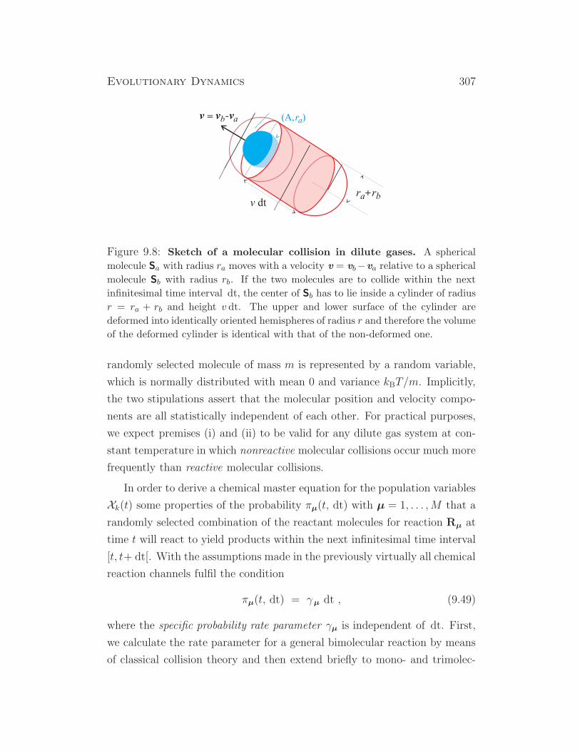
Evolutionary Dynamics 307
Figure 9.8: Sketch of a molecular collision in dilute gases. A spherical
molecule Sa with radius ra moves with a velocity v = vb−va relative to a spherical
molecule Sb with radius rb. If the two molecules are to collide within the next
infinitesimal time interval dt, the center of Sb has to lie inside a cylinder of radius
r = ra + rb and height v dt. The upper and lower surface of the cylinder are
deformed into identically oriented hemispheres of radius r and therefore the volume
of the deformed cylinder is identical with that of the non-deformed one.
randomly selected molecule of mass m is represented by a random variable,
which is normally distributed with mean 0 and variance kBT/m. Implicitly,
the two stipulations assert that the molecular position and velocity compo-
nents are all statistically independent of each other. For practical purposes,
we expect premises (i) and (ii) to be valid for any dilute gas system at con-
stant temperature in which nonreactive molecular collisions occur much more
frequently than reactive molecular collisions.
In order to derive a chemical master equation for the population variables
Xk(t) some properties of the probability πµ(t, dt) with µ = 1, . . . ,M that a
randomly selected combination of the reactant molecules for reaction Rµ at
time t will react to yield products within the next infinitesimal time interval
[t, t+ dt[. With the assumptions made in the previously virtually all chemical
reaction channels fulfil the condition
πµ(t, dt) = γµ dt , (9.49)
where the specific probability rate parameter γµ is independent of dt. First,
we calculate the rate parameter for a general bimolecular reaction by means
of classical collision theory and then extend briefly to mono- and trimolec-

308 Peter Schuster
ular reactions. Apart from the quantum mechanical approach the theory of
collisions in dilute gases is the best developed microscopic model for chemi-
cal reactions and well suited for a rigorous derivation of the master equation
from molecular motion and events.
Bimolecular reactions. The occurrence of a reaction A+B has to be preceded
by a collision of an Sa molecule with an Sb molecule, and first we shall
calculate the probability of such a collision in the reaction volume V . For
simplicity molecular species are regarded as spheres with specific masses and
radii, for example ma and ra for Sa, and mb and rb for Sb, respectively. A
collision occurs whenever the center-to center distance of the two molecules
RAB decreases to (RAB)min = ra + rb. Next we define the probability that a
randomly selected pair of Rµ reactant molecules at time t will collide within
the next infinitesimal time interval [t, t + dt[ by π∗µ(t, dt) and calculate it
from the Maxwell-Boltzmann distribution of molecular velocities according
to Fig. 9.8.
The probability that a randomly selected pair of reactant molecules Rµ,
one molecule Sa and one molecule Sb, has a relative velocity v = vb − va
lying in an infinitesimal volume element dv3 about v at time t is denoted by
P (v(t),Rµ) and can be readily obtained from kinetic theory of gases:
P (v(t),Rµ) =
(
µ
2π kBT
)
exp(
−µv2/(2kBT ))
dv3 .
Herein v = |v| =√
v2x + v2y + v2z is the value of the relative velocity and
µ = mamb/(ma + mb) is the reduced mass of the two Rµ molecules. Two
properties of the probabilities P (v(t),Rµ) for different velocities v are im-
portant:
(i) The elements in the set of all velocity combinations, Ev(t),Rµ are mutu-
ally exclusive, and
(ii) they are collectively exhaustive since v is varied over the entire three
dimensional velocity space.
Now we relate the probability P (v(t),Rµ) to a collision event Ecol by calcu-
lating the conditional probability P (Ecol(t, dt)|Ev(t),Rµ). In Fig. 9.8 we sketch
the geometry of the collision event between to randomly selected spherical
Evolutionary Dynamics 309
molecules Sa and Sb that is assumed to occur with an infinitesimal time in-
terval dt:11 A randomly selected molecule Sa moves along the vector v of the
relative velocity vb − vb between Sa and an also randomly selected molecule
Sb. A collision between the molecules will take place in the interval [t, t+ dt
if and only if the center of molecule Sb is inside the spherically distorted
cylinder (Fig. 9.8) at time t. Thus P (Ecol(t, dt)|Ev(t),Rµ) is the probability
that the center of a randomly selected Sb molecule moving with velocity v(t)
relative to the randomly selected Sa molecule will be situated at time t with
a certain subregion of V , which has a volume Vcol = v dt ·π(ra+ rb)2, and by
scaling with the total volume V we obtain:12
P(
Ecol(t, dt)|Ev(t),Rµ
)
=v(t) dt · π(ra + rb)
2
V. (9.50)
By substitution and integration over the entire velocity space we can calculate
the desired probability
π∗µ(t, dt) =
∫∫∫
v
(
µ
2π kBT
)
e−µv2/(2kBT ) · v(t) dt · π(ra + rb)
2
Vdv3 .
Evaluation of the integral is straightforward and yields
π∗µ(t, dt) =
(
8π kBT
V
)1/2(ra + rb)
2
µdt . (9.51)
The first factor contains only constants and the macroscopic quantities, vol-
ume V and temperature T , whereas the molecular parameters, the radii ra
and rb and the reduced mass µ.
A collision is a necessary but not a sufficient condition for a reaction to
take place and therefore we introduce a collision-conditioned reaction prob-
ability pµ that is the probability that a randomly selected pair of colliding
Rµ reactant molecules will indeed react according to Rµ. By multiplication
11The absolute time t comes into play because the positions of the molecules, ra and
rb, and their velocities, va and vb, depend on t.12Implicitly in the derivation we made use of the infinitesimally small size of dt. Only
if the distance v dt is vanishingly small, the possibility of collisional interference of a third
molecule can be neglected.

310 Peter Schuster
of independent probabilities we have
πµ(t, dt) = pµ π∗µ(t, dt) ,
and with respect to equation (9.49) we find
γµ = pµ
(
8π kBT
V
)1/2(ra + rb)
2
µ. (9.52)
As said before, it is crucial for the forthcoming analysis that γµ is independent
of dt and this will be the case if and only if pµ does not depend on dt. This
is highly plausible for the above given definition, and an illustrative check
through the detailed examination of bimolecular reactions can be found in
[115, pp.413-417]. It has to be remarked, however, that the application of
classical collision theory to molecular details of chemical reactions can be
an illustrative and useful heuristic at best, because the molecular domain
falls into the realm of quantum phenomena and any theory that aims at a
derivation of reaction probabilities from first principles has to be built upon
a quantum mechanical basis.
Monomolecular, trimolecular, and other reactions. A monomolecular reac-
tion is of the form A −→ C and describes the spontaneous conversion
Sa −−−→ Sc . (9.53)
One molecule Sa is converted into one molecule Sc. This reaction is different
from a catalyzed conversion
Sa + Sb −−−→ Sc + Sb , (9.48’)
where the conversion A −→ C is initiated by a collision of an A molecule
with a B molecule,13 and a description as an ordinary bimolecular process is
straightforward.
13The two reactions are related by rigorous thermodynamics: Whenever a catalyzed re-
action is part of a mechanism an incorporation of the corresponding uncatalyzed process in
the reaction mechanism is required in order to fulfill the requirements of thermodynamics.
Evolutionary Dynamics 311
The true monomolecular conversion (9.53) is driven by some quantum
mechanical mechanism similar as in the case of radioactive decay of a nu-
cleus. Time-dependent perturbation theory in quantum mechanics [209,
pp.724-739] shows that almost all weakly perturbed energy-conserving tran-
sitions have linear probabilities of occurrence in time intervals δt, when δt
is microscopically large but macroscopically small. Therefore, to a good ap-
proximation the probability for a radioactive nucleus to decay within the
next infinitesimal time interval dt is of the form α dt, were α is some time-
independent constant. On the basis of analogy we may expect πµ(t, dt) the
probability for a monomolecular conversion to be approximately of the form
γµ dt with γµ being independent of dt.
Trimolecular reactions of the form
Sa + Sb + Sc −−−→ Sd + . . . (9.54)
should not be considered because collisions of three particles do not occur
with a probability larger than of measure zero. There may be, however, spe-
cial situations where approximations of complicated processes by trimolecular
events is justified. One example is a set of three coupled reactions with four
reactant molecules [114, pp.359-361] where is was shown that πµ(t, dt) is
essentially linear in dt.
The last class of reaction to be considered here is no proper chemical
reaction but an influx of material into the reactor. It is often denoted as a
the zeroth order reaction (9.1a):
∗ −−−→ Sa . (9.55)
Here, the definition of the influx and the efficient mixing or homogeneity
condition is helpful, because it guarantees that the number of molecules
entering the homogeneous system is a constant and does not depend on dt.
9.3.2 Simulation of master equations
So far we succeeded to derive the fundamental fact that for each elementary
reaction channel Rµ with µ = 1, . . . ,M , which is accessible to the molecules
312 Peter Schuster
of a well-mixed and thermally equilibrated system in the gas phase or in
solution, exists a scalar quantity γµ, which is independent of dt such that
[115, p.418]
γµ dt = probability that a randomly selected combination of
Rµ reactant molecules at time t will react accordingly
in the next infinitesimal time interval [t, t+ dt[ .
(9.56)
The specific probability rate constant, γµ is one of three quantities that are
required to fully characterize a particular reaction channelRµ. In addition we
shall require a function hµ(n) where the vector n = (n1, . . . , nn)′ contains the
exact numbers of all molecules at time t, ~N (t) =(
N1(t), . . . ,NN(t))′= n(t),
hµ(n) ≡ the number of distinct combinations of Rµ reactant
molecules in the system when the numbers of molecules
Sk are exactly nk with k = 1, . . . , N ,
(9.57)
and an N ×M matrix of integers S = νkµ; k = 1, . . . , N, µ = 1, . . . ,M,where
νkµ ≡ the change in the Sk molecular population caused by the
occurrence of one Rµ reaction.(9.58)
The functions hµ(n) and the matrix N are readily deduced by inspection of
the algebraic structure of the reaction channels. We illustrate by means of
an example:
R1 : S1 + S2 −−−→ S3 + S4 ,
R2 : 2S1 −−−→ S1 + S5 , and (9.59)
R3 : S3 −−−→ S5 .
The functions hµ(n) are obtained by simple combinatorics
h1(n) = n1 n2 ,
h2(n) = n1 (n1 − 1)/2 , and
h3(n) = n3 ,
Evolutionary Dynamics 313
and the matrix S is of the form
S =
−1 −1 0
−1 0 0
+1 0 −1+1 0 0
0 +1 +1
.
It is worth noticing that the functional form of hµ is determined exclusive
by the reactant side of Rµ. In particular, has precisely the same form de-
termined by mass action in the deterministic kinetic equations with the ex-
ception that the particle numbers have to counted exactly in small systems,
n(n − 1) instead of n2 for example. The stoichiometric matrix S refers to
the product side of the reaction equations and counts the net production of
molecular species per one elementary reaction event: νkµ is the number of
molecules Sk produces by reaction Rµ, these numbers are integers and nega-
tive values indicate the number of molecules, which have disappeared during
one reaction. In the forthcoming analysis we shall make use of vectors cor-
responding to individual reactions Rµ: νµ = (ν1µ, . . . , νNµ)′.
Analogy to deterministic kinetics. It is illustrative to consider now the anal-
ogy to conventional chemical kinetics. If we denote the concentration vec-
tor of our molecular species Sk by x = (x1, . . . , xN)′ and the flux vector
ϕ = (ϕ1, . . . , ϕN)′ the kinetic equation can be expressed by
dx
dt= S · ϕ . (9.60)
The individual elements of the flux vector in mass action kinetics are
ϕµ = kµ
n∏
k=1
xgkµk for g1µ S1 + g2µ S2 + . . . + gNµ SN −−−→
wherein the factors gkµ are the stoichiometric coefficients on the reactant
side of the reaction equations. It is sometimes useful to define analogous
factors qkµ for the product side, both classes of factors can be summarized
in matrices G and Q and then the stochastic matrix is simply given by the
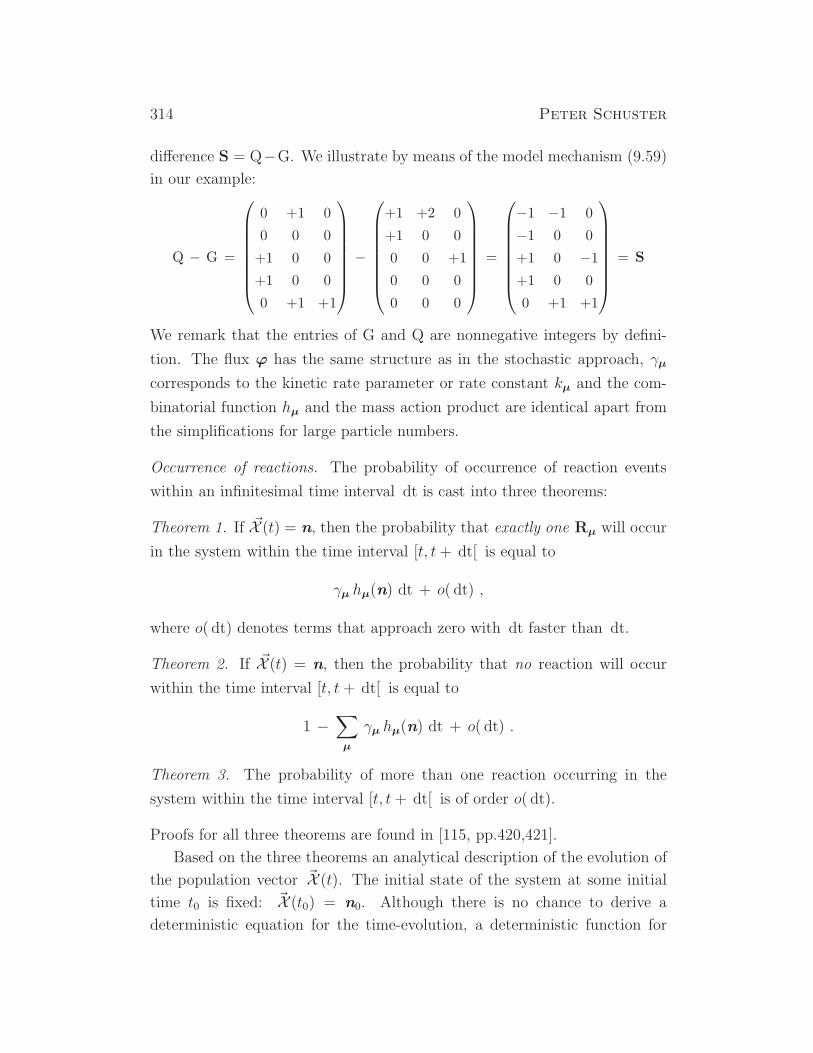
314 Peter Schuster
difference S = Q−G. We illustrate by means of the model mechanism (9.59)
in our example:
Q − G =
0 +1 0
0 0 0
+1 0 0
+1 0 0
0 +1 +1
−
+1 +2 0
+1 0 0
0 0 +1
0 0 0
0 0 0
=
−1 −1 0
−1 0 0
+1 0 −1+1 0 0
0 +1 +1
= S
We remark that the entries of G and Q are nonnegative integers by defini-
tion. The flux ϕ has the same structure as in the stochastic approach, γµ
corresponds to the kinetic rate parameter or rate constant kµ and the com-
binatorial function hµ and the mass action product are identical apart from
the simplifications for large particle numbers.
Occurrence of reactions. The probability of occurrence of reaction events
within an infinitesimal time interval dt is cast into three theorems:
Theorem 1. If ~X (t) = n, then the probability that exactly one Rµ will occur
in the system within the time interval [t, t+ dt[ is equal to
γµ hµ(n) dt + o( dt) ,
where o( dt) denotes terms that approach zero with dt faster than dt.
Theorem 2. If ~X (t) = n, then the probability that no reaction will occur
within the time interval [t, t + dt[ is equal to
1 −∑
µ
γµ hµ(n) dt + o( dt) .
Theorem 3. The probability of more than one reaction occurring in the
system within the time interval [t, t+ dt[ is of order o( dt).
Proofs for all three theorems are found in [115, pp.420,421].
Based on the three theorems an analytical description of the evolution of
the population vector ~X (t). The initial state of the system at some initial
time t0 is fixed: ~X (t0) = n0. Although there is no chance to derive a
deterministic equation for the time-evolution, a deterministic function for
Evolutionary Dynamics 315
the time-evolution of the probability function P (n, t|n0, t0) for t ≥ t0 will
be obtained. We express the probability P (n, t|n0, t0) as the sum of the
probabilities of several mutually exclusive and and collectively exhaustive
routes from ~X (t0) = n0 to ~X (t + dt) = n. These routes are distinguished
from one another with respect to the event that happened in the time interval
[t, t + dt[:
P (n, t+ dt|n0, t0) = P (n, t|n0, t0) ×
1−M∑
µ=1
γµ hµ(n) dt + o( dt)
+
+M∑
µ=1
P (n− νµ, t|n0, t0) ×(
γµ hµ(n− νµ) dt + o( dt))
+
+ o( dt) .
(9.61)
The different routes from ~X (t0) = n0 to ~X (t + dt) = n are obvious from
the balance equation (9.61):
(i) One route from ~X (t0) = n0 to ~X (t + dt) = n is given by the first
term on the right-hand side of the equation: No reaction is occurring in the
time interval [t, t + dt[ and hence ~X (t) = n was fulfilled at time t. The
joint probability for route (i) is therefore the probability to be in ~X (t) = n
conditioned by ~X (t0) = n0 times the probability that no reaction has occurred
in [t, t+ dt[. In other words, the probability for this route is the probability
to go from n0 at time t0 to n at time t and to stay in this state during the
next interval dt.
(ii) An alternative route from ~X (t0) = n0 to ~X (t + dt) = n accounted
for by one particular term in sum of terms on the right-hand side of the
equation: An Rµ reaction is occurring in the time interval [t, t + dt[ and
hence ~X (t) = n − νµ was fulfilled at time t. The joint probability for
route (ii) is therefore the probability to be in ~X (t) = n − νµ conditioned by
~X (t0) = n0 times the probability that exactly one Rµ reaction has occurred
in [t, t+ dt[. In other words, the probability for this route is the probability
to go from n0 at time t0 to n − νµ at time t and to undergo an Rµ during
the next interval dt. Obviously, the same consideration is valid for every
elementary reaction and we have M terms of this kind.
316 Peter Schuster
(iii) A third possibility – neither no reaction nor exactly one reaction
chosen from the set Rµ;µ = 1, . . . ,M – must inevitably invoke more than
one reaction within the time interval [t, t + dt[. The probability for such
events, however, is o( dt) or of measure zero by theorem 3.
All routes (i) and (ii) are mutually exclusive since different events are
taking place within the last interval [t, t+ dt[.
The last step to derive a simulation friendly form of the chemical master
equation is straightforward: P (n, t|n0, t0) is subtracted from both sides in
Equ. (9.61), then both sides are divided by dt, the limit dt ↓ 0 is taken, all
o( dt) terms vanish and finally we obtain
∂
∂tP (n, t|n0, t0) =
M∑
µ=1
(
γµ hµ(n− νµ)P (n− νµ|n0, t0)−
− γµ hµ(n)P (n, t|n0, t0))
.
(9.62)
Initial conditions are required to calculate the time evolution of the proba-
bility P (n, t|n0, t0) and we can easily express them in the form
P (n, t0|n0, t0) =
1 , if n = n0 ,
0 , if n 6= n0 ,(9.62’)
which is precisely the initial condition used in the derivation of equation (9.61).
Any sharp probability distribution P(
nk, t0|n(0)k , t0
)
= δ(nk − n(0)k ) is admit-
ted for the molecular particle numbers at t0. The assumption of extended
initial distributions is, of course, also possible but the corresponding master
equation becomes more sophisticated.
9.3.3 The simulation algorithm
The chemical master equation (9.62) as derived in the last subsection 9.3.1
was found to be well suited for the derivation of a stochastic simulation
algorithm for chemical reactions [112, 113, 117] and it is important to see
how the simulation tool fits into the general theoretical framework of the
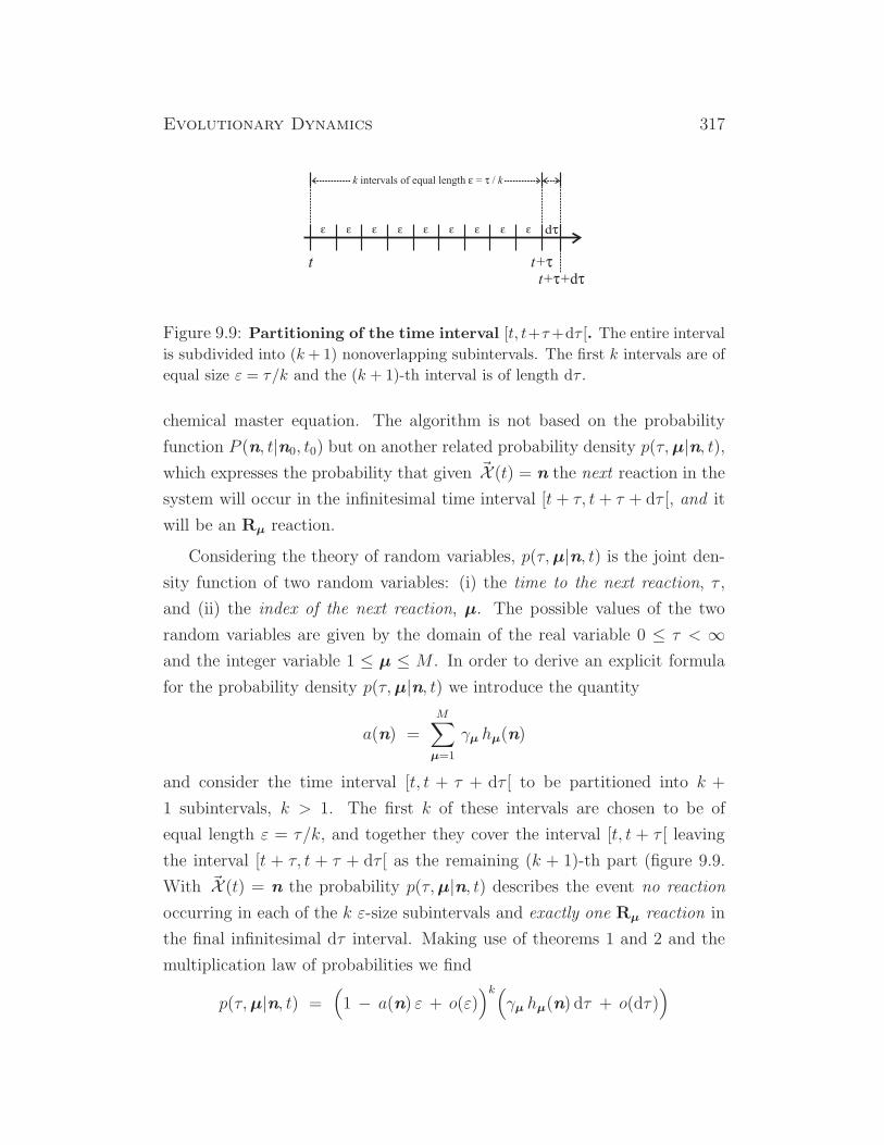
Evolutionary Dynamics 317
Figure 9.9: Partitioning of the time interval [t, t+τ+dτ [. The entire interval
is subdivided into (k+1) nonoverlapping subintervals. The first k intervals are of
equal size ε = τ/k and the (k + 1)-th interval is of length dτ .
chemical master equation. The algorithm is not based on the probability
function P (n, t|n0, t0) but on another related probability density p(τ,µ|n, t),which expresses the probability that given ~X (t) = n the next reaction in the
system will occur in the infinitesimal time interval [t+ τ, t+ τ + dτ [, and it
will be an Rµ reaction.
Considering the theory of random variables, p(τ,µ|n, t) is the joint den-
sity function of two random variables: (i) the time to the next reaction, τ ,
and (ii) the index of the next reaction, µ. The possible values of the two
random variables are given by the domain of the real variable 0 ≤ τ < ∞and the integer variable 1 ≤ µ ≤ M . In order to derive an explicit formula
for the probability density p(τ,µ|n, t) we introduce the quantity
a(n) =M∑
µ=1
γµ hµ(n)
and consider the time interval [t, t + τ + dτ [ to be partitioned into k +
1 subintervals, k > 1. The first k of these intervals are chosen to be of
equal length ε = τ/k, and together they cover the interval [t, t + τ [ leaving
the interval [t + τ, t + τ + dτ [ as the remaining (k + 1)-th part (figure 9.9.
With ~X (t) = n the probability p(τ,µ|n, t) describes the event no reaction
occurring in each of the k ε-size subintervals and exactly one Rµ reaction in
the final infinitesimal dτ interval. Making use of theorems 1 and 2 and the
multiplication law of probabilities we find
p(τ,µ|n, t) =(
1 − a(n) ε + o(ε))k(
γµ hµ(n) dτ + o(dτ))

318 Peter Schuster
Dividing both sides by dτ and taking the limit dτ ↓ 0 yields
p(τ,µ|n, t) =(
1 − a(n) ε + o(ε))k
γµ hµ(n)
This equation is valid for any integer k > 1 and hence its validity is also
guaranteed for k → ∞. Next we rewrite the first factor on the right-hand
side of the equation
(
1 − a(n) ε + o(ε))k
=
(
1 − a(n) kε + k o(ε)
k
)k
=
=
(
1 − a(n) τ + τ o(ε)/ε
k
)k
,
and take now the limit k → ∞ whereby we make use of the simultaneously
occurring convergence o(ε)/ε ↓ 0:
limk→∞
(
1 − a(n) ε + o(ε))k
= limk→∞
(
1− a(n) τ
k
)k
= e−a(n) τ .
By substituting this result into the initial equation for the probability density
of the occurrence of a reaction we find
p(τ,µ|n, t) = a(n) e−a(n) τγµ hµ(n)
a(n)= γµ hµ(n) e
−∑M
ν=1 γνhν(n) τ . (9.63)
Equ. (9.63) provides the mathematical basis for the stochastic simulation
algorithm. Given ~X (t) = n, the probability density consists of two inde-
pendent probabilities where the first factor describes the time to the next
reaction and the second factor the index of the next reaction. These factors
correspond to two statistically independent random variables r1 and r2.
9.3.4 Implementation of the simulation algorithm
Equ. (9.63) is implemented now for computer simulation and we inspect the
probability densities of the two unit-interval uniform random variables r1
and r2 in order to find the conditions to be imposed of a statistically exact
Evolutionary Dynamics 319
sample pair (τ,µ): r1 has an exponential density function with the decay
constant a(n),
τ =1
a(n)ln(
1/
r1)
, (9.64a)
and taking m to be the smallest integer which fulfils
µ = inf
m∣
∣
∣
m∑
µ=1
cµ hµ(n) > a(n) r2
. (9.64b)
After the values for τ and µ have been determined accordingly the action
advance the state vector ~X (t) of the system is taking place:
~X (t) = n −→ ~X (t+ τ) = n+ νµ .
Repeated application of the advancement procedure is the essence of the
stochastic simulation algorithm. It is important to realize that this advance-
ment procedure is exact as far as r1 and r2 are obtained by fair samplings
from a unit-interval uniform random number generator or, in other words,
the correctness of the procedure depends on the quality of the random num-
ber generator applied. Two further issues are important: (i) The algorithm
operates with internal time control that corresponds to real time of the chem-
ical process, and (ii) contrary to the situation in differential equation solvers
the discrete time steps are not finite interval approximations of an infinites-
imal time step and instead, the population vector ~X (t) maintains the value
~X (t) = n throughout the entire finite time interval [t, t + dτ [ and then
changes abruptly to ~X (t + τ) = n + νµ at the instant t + τ when the Rµ
reaction occurs. In other words, there is no blind interval during which the
algorithm is unable to record changes.
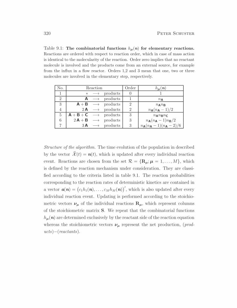
320 Peter Schuster
Table 9.1: The combinatorial functions hµ(n) for elementary reactions.
Reactions are ordered with respect to reaction order, which in case of mass action
is identical to the molecularity of the reaction. Order zero implies that no reactant
molecule is involved and the products come from an external source, for example
from the influx in a flow reactor. Orders 1,2 and 3 mean that one, two or three
molecules are involved in the elementary step, respectively.
No. Reaction Order hµ(n)
1 ∗ −→ products 0 1
2 A −→ products 1 nA
3 A+ B −→ products 2 nAnB
4 2A −→ products 2 nA(nA − 1)/2
5 A+ B+ C −→ products 3 nAnBnC
6 2A + B −→ products 3 nA(nA − 1)nB/27 3A −→ products 3 nA(nA − 1)(nA − 2)/6
Structure of the algorithm. The time evolution of the population in described
by the vector ~X (t) = n(t), which is updated after every individual reaction
event. Reactions are chosen from the set R = Rµ;µ = 1, . . . ,M, whichis defined by the reaction mechanism under consideration. They are classi-
fied according to the criteria listed in table 9.1. The reaction probabilities
corresponding to the reaction rates of deterministic kinetics are contained in
a vector a(n) =(
c1h1(n), . . . , cMhM(n))′, which is also updated after every
individual reaction event. Updating is performed according to the stoichio-
metric vectors νµ of the individual reactions Rµ, which represent columns
of the stoichiometric matrix S. We repeat that the combinatorial functions
hµ(n) are determined exclusively by the reactant side of the reaction equation
whereas the stoichiometric vectors νµ represent the net production, (prod-
ucts)−(reactants).
Evolutionary Dynamics 321
The algorithm comprises five steps:
(i) Step 0. Initialization: The time variable is set to t = 0, the initial
values of all N variables X1, . . . ,XN for the species – Xk for species
Sk – are stored, the values for the M parameters of the reactions Rµ,
c1, . . . , cM , are stored, and the combinatorial expressions are incorpo-
rated as factors for the calculation of the reaction rate vector a(n)
according to table 9.1 and the probability density P (τ,µ). Sampling
times, t1 < t2 < · · · and the stopping time tstop are specified, the first
sampling time is set to t1 and stored and the pseudorandom number
generator is initialized by means of seeds or at random.
(ii) Step 1. Monte Carlo step: A pair of random numbers is created (τ,µ)
by the random number generator according to the joint probability
function P (τ,µ). In essence two explicit methods can be used: the
direct method and the first-reaction method.
(iii) Step 2. Propagation step: (τ,µ) is used to advance the simulation time
t and to update the population vector n, t → t + τ and n → n + νµ,
then all changes are incorporated in a recalculation of the reaction rate
vector a.
(iv) Step 3. Time control : Check whether or not the simulation time has
been advanced through the next sampling time ti, and for t > ti send
current t and current n(t) to the output storage and advance the sam-
pling time, ti → ti+1. Then, if t > tstop or if no more reactant molecules
remain leading to hµ = 0 ∀ µ = 1, . . . ,M , finalize the calculation by
switching to step 4, and otherwise continue with step 1.
(v) Step 4. Termination: Prepare for final output by setting flags for early
termination or other unforseen stops and send final time t and final n
to the output storage and terminate the computation.
A caveat is needed for the integration of stiff systems where the values of in-
dividual variable can vary by many orders of magnitude and such a situation
might caught the calculation in a trap by slowing down time progress.
322 Peter Schuster
The Monte Carlo step. Pseudorandom numbers are drawn from a random
number generator of sufficient quality whereby quality is meant in terms of
no or very long recurrence cycles and a the closeness of the distribution of the
pseudorandom numbers r to the uniform distribution on the unit interval:
0 ≤ α < β ≤ 1 =⇒ P (α ≤ r ≤ β) = β − α .
With this prerequisite we discuss now two methods which use two output
values r of the pseudorandom number generator to generate a random pair
(τ,µ) with the prescribed probability density function P (τ,µ). Two imple-
mentations are frequently used:
(i) The direct method. The two-variable probability density is written as the
product of two one-variable density functions:
P (τ,µ) = P1(τ) · P2(µ|τ) .
Here, P1(τ) dτ is the probability that the next reaction will occur between
times t + τ and t + τ + dτ , irrespective of which reaction it might be, and
P2(µ|τ) is the probability that the next reaction will be an Rµ given that
the next reaction occurs at time t+ τ .
By the addition theorem of probabilities, P1(τ) dτ is obtained by summa-
tion of P (τ,µ) dτ over all reactions Rµ:
P1(τ) =
M∑
µ=1
P (τ,µ) . (9.65)
Combining the last two equations we obtain for P2(µ|τ)
P2(µ|τ) = P (τ,µ)/
M∑
ν
P (τ,ν) (9.66)
Equations (9.65) and (9.66) express the two one-variable density functions
in terms of the original two-variable density function P (τ,µ). From equa-
tion (9.63) we substitute into P (τ,µ) = p(τ,µ|n, t) through simplifying the
notation by using
aµ ≡ γµhµ(n) and a =
M∑
µ=1
aµ ≡M∑
µ=1
γµhµ(n)
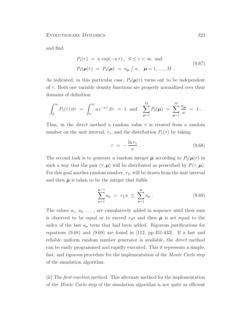
Evolutionary Dynamics 323
and find
P1(τ) = a exp(−a τ) , 0 ≤ τ <∞ and
P2(µ|τ) = P2(µ) = aµ/
a , µ = 1, . . . ,M .(9.67)
As indicated, in this particular case, P2(µ|τ) turns out to be independent
of τ . Both one variable density functions are properly normalized over their
domains of definition:
∫ ∞
0
P1(τ) dτ =
∫ ∞
0
a e−a τ dτ = 1 and
M∑
µ=1
P2(µ) =
M∑
µ=1
aµa
= 1 .
Thus, in the direct method a random value τ is created from a random
number on the unit interval, r1, and the distribution P1(τ) by taking
τ = − ln r1a
. (9.68)
The second task is to generate a random integer µ according to P2(µ|τ) insuch a way that the pair (τ,µ) will be distributed as prescribed by P (τ,µ).
For this goal another random number, r2, will be drawn from the unit interval
and then µ is taken to be the integer that fulfils
µ−1∑
ν=1
aν < r2 a ≤µ∑
ν=1
aν . (9.69)
The values a1, a2, . . . , are cumulatively added in sequence until their sum
is observed to be equal or to exceed r2a and then µ is set equal to the
index of the last aν term that had been added. Rigorous justifications for
equations (9.68) and (9.69) are found in [112, pp.431-433]. If a fast and
reliable uniform random number generator is available, the direct method
can be easily programmed and rapidly executed. This it represents a simple,
fast, and rigorous procedure for the implementation of the Monte Carlo step
of the simulation algorithm.
(ii) The first-reaction method. This alternate method for the implementation
of the Monte Carlo step of the simulation algorithm is not quite as efficient
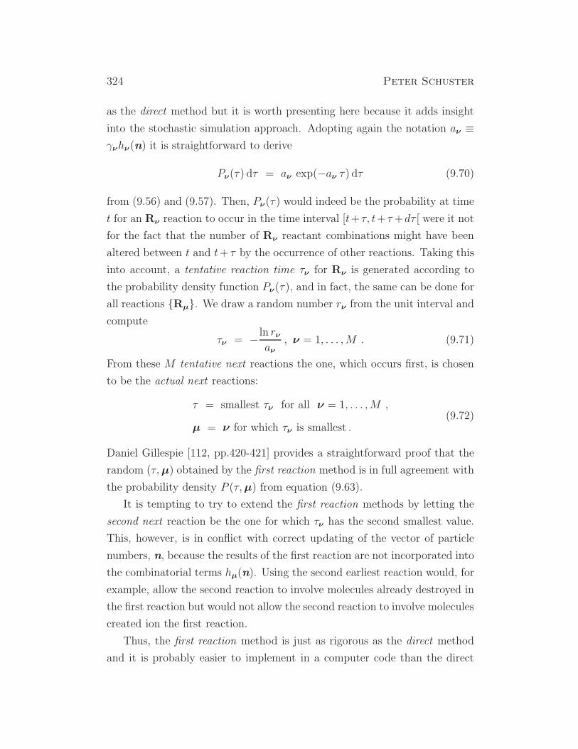
324 Peter Schuster
as the direct method but it is worth presenting here because it adds insight
into the stochastic simulation approach. Adopting again the notation aν ≡γνhν(n) it is straightforward to derive
Pν(τ) dτ = aν exp(−aν τ) dτ (9.70)
from (9.56) and (9.57). Then, Pν(τ) would indeed be the probability at time
t for an Rν reaction to occur in the time interval [t+ τ, t+ τ+dτ [ were it not
for the fact that the number of Rν reactant combinations might have been
altered between t and t+ τ by the occurrence of other reactions. Taking this
into account, a tentative reaction time τν for Rν is generated according to
the probability density function Pν(τ), and in fact, the same can be done for
all reactions Rµ. We draw a random number rν from the unit interval and
compute
τν = − ln rνaν
, ν = 1, . . . ,M . (9.71)
From these M tentative next reactions the one, which occurs first, is chosen
to be the actual next reactions:
τ = smallest τν for all ν = 1, . . . ,M ,
µ = ν for which τν is smallest .(9.72)
Daniel Gillespie [112, pp.420-421] provides a straightforward proof that the
random (τ,µ) obtained by the first reaction method is in full agreement with
the probability density P (τ,µ) from equation (9.63).
It is tempting to try to extend the first reaction methods by letting the
second next reaction be the one for which τν has the second smallest value.
This, however, is in conflict with correct updating of the vector of particle
numbers, n, because the results of the first reaction are not incorporated into
the combinatorial terms hµ(n). Using the second earliest reaction would, for
example, allow the second reaction to involve molecules already destroyed in
the first reaction but would not allow the second reaction to involve molecules
created ion the first reaction.
Thus, the first reaction method is just as rigorous as the direct method
and it is probably easier to implement in a computer code than the direct
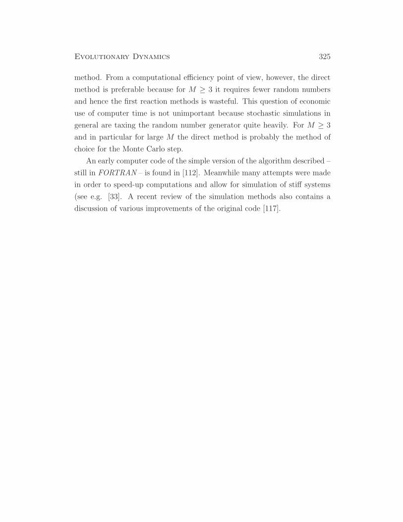
Evolutionary Dynamics 325
method. From a computational efficiency point of view, however, the direct
method is preferable because for M ≥ 3 it requires fewer random numbers
and hence the first reaction methods is wasteful. This question of economic
use of computer time is not unimportant because stochastic simulations in
general are taxing the random number generator quite heavily. For M ≥ 3
and in particular for large M the direct method is probably the method of
choice for the Monte Carlo step.
An early computer code of the simple version of the algorithm described –
still in FORTRAN – is found in [112]. Meanwhile many attempts were made
in order to speed-up computations and allow for simulation of stiff systems
(see e.g. [33]. A recent review of the simulation methods also contains a
discussion of various improvements of the original code [117].

326 Peter Schuster
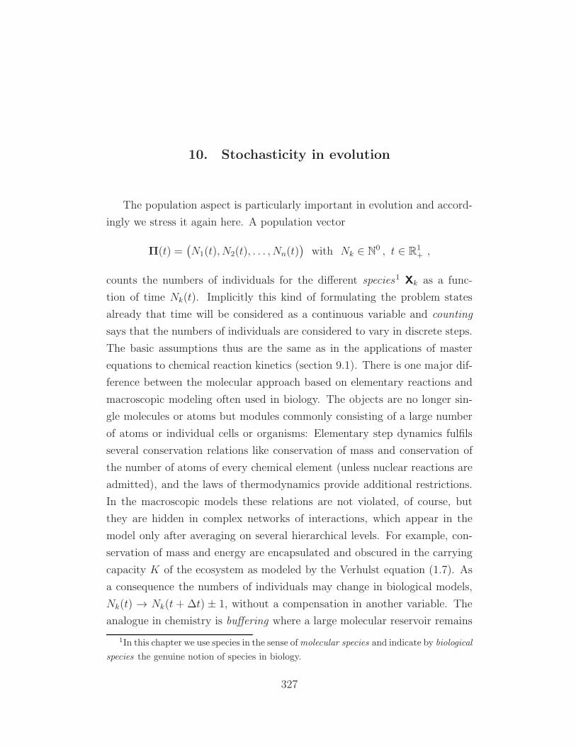
10. Stochasticity in evolution
The population aspect is particularly important in evolution and accord-
ingly we stress it again here. A population vector
Π(t) =(
N1(t), N2(t), . . . , Nn(t))
with Nk ∈ N0 , t ∈ R
1+ ,
counts the numbers of individuals for the different species1 Xk as a func-
tion of time Nk(t). Implicitly this kind of formulating the problem states
already that time will be considered as a continuous variable and counting
says that the numbers of individuals are considered to vary in discrete steps.
The basic assumptions thus are the same as in the applications of master
equations to chemical reaction kinetics (section 9.1). There is one major dif-
ference between the molecular approach based on elementary reactions and
macroscopic modeling often used in biology. The objects are no longer sin-
gle molecules or atoms but modules commonly consisting of a large number
of atoms or individual cells or organisms: Elementary step dynamics fulfils
several conservation relations like conservation of mass and conservation of
the number of atoms of every chemical element (unless nuclear reactions are
admitted), and the laws of thermodynamics provide additional restrictions.
In the macroscopic models these relations are not violated, of course, but
they are hidden in complex networks of interactions, which appear in the
model only after averaging on several hierarchical levels. For example, con-
servation of mass and energy are encapsulated and obscured in the carrying
capacity K of the ecosystem as modeled by the Verhulst equation (1.7). As
a consequence the numbers of individuals may change in biological models,
Nk(t) → Nk(t + ∆t) ± 1, without a compensation in another variable. The
analogue in chemistry is buffering where a large molecular reservoir remains
1In this chapter we use species in the sense ofmolecular species and indicate by biological
species the genuine notion of species in biology.
327

328 Peter Schuster
practically unchanged when a single molecule is added or subtracted (see
section 9.2, irreversible addition reaction). Changes ±1 in the numbers of
individuals imply that the time interval considered is sufficiently short that
multiple events can be excluded. In biology we can understand the flow reac-
tor (section 4.2) as an idealized version of an ecosystem. Then the biological
analogues to influx (4.1a) and outflux (4.1d) are migration, immigration and
emigration, respectively.
A stochastic process on the population level is a recording of ordered
successive events at times Ti:
T0 < T1 < T2 < . . . < Tj < Tk . . . ,
along a continuous time axis t.2 A birth or death event at some time t = Tr,
for example, creates, Xj → 2Xj , or consumes one individual, Xj → ⊘, andthe population changes accordingly:
Π =
(
. . . , Nj(t) = Nj(Tr−1), Nk(t) = Nk(Tr−1), . . .)
if Tr−1 ≤ t < Tr
(
. . . , Nj(t) = Nj(Tr−1)± 1, Nk(t) = Nk(Tr−1), . . .)
if Tr ≤ t < Tr+1
.
This formulation of a biological birth or death events reflects the previously
mentioned convention in probability theory: Right-hand continuity is as-
sumed for steps in stochastic processes (see Fig. 8.6).
Compared to stochasticity in chemistry stochastic phenomena in biology
are not only more important but also much harder to control. The major
sources of the problem are small population numbers and the lack of suffi-
ciently simple references systems that are accessible to experimental studies.
In biology we are regularly encountering reaction mechanisms that lead to
enhancement of fluctuations at non-equilibrium conditions and biology in
essence is dealing with processes and stationary states far away from equilib-
rium whereas in chemistry autocatalysis in non-equilibrium systems became
an object of general interest and intensive investigation not before some forty
years ago. We start therefore with the analysis of simple autocatalysis mod-
eled by means of a simple birth-and-death process. Then we present an
2The application of discretized time in evolution – mimicking synchronized generations,
for example – is straightforward but we shall mention only briefly here because we focus
on continuous time birth-and-death processes and master equations.

Evolutionary Dynamics 329
overview over solvable birth-and-death processes (section 10.1) and discuss
the role of boundaries in form of different barriers (section 10.1.2).
10.1 Autocatalysis, replication, and extinction
In the previous chapter we analyzed already bimolecular reactions, the ad-
dition and the dimerization reaction, which gave rise to perfectly normal
behavior although the analysis was shown to be quite sophisticated (sec-
tion 9.2). The nonlinearity manifested itself only in task to find solutions
and did not change effectively the qualitative behavior of the reaction sys-
tems, for example the√N -law for the fluctuations in the stationary states
retained its validity. As an exactly solvable example we shall study first a
simple reaction mechanism consisting of two elementary steps, autocatalytic
replication and extinction. In this case the√N -law is not valid and fluctu-
ations do not settle down to some value which is proportional to the square
root of the size of the system but grow in time without limit as we saw in
case of the Wiener process (8.2.2).
10.1.1 Autocatalytic growth and death
Reproduction of individuals is modeled by a simple duplication mechanism
and death is represented by first order decay. In the language of chemical
kinetics these two steps are:
A + Xλ
−−−→ 2X , (10.1a)
Xµ
−−−→ ⊘ . (10.1b)
The rate parameters for reproduction and extinction are denoted by λ and
µ, respectively.3 The material required for reproduction is assumed to be
replenished as it is consumed and hence the amount of A available is constant
and assumed to be included in the birth parameter: λ = f · [A]. Degradation
products of X do not enter the kinetic equation because reaction (10.1b) is
3Reproduction is to be understood a asexual reproduction here. Sexual reproduction,
of course, requires two partners and gives rise to a process of order two (table 9.1).
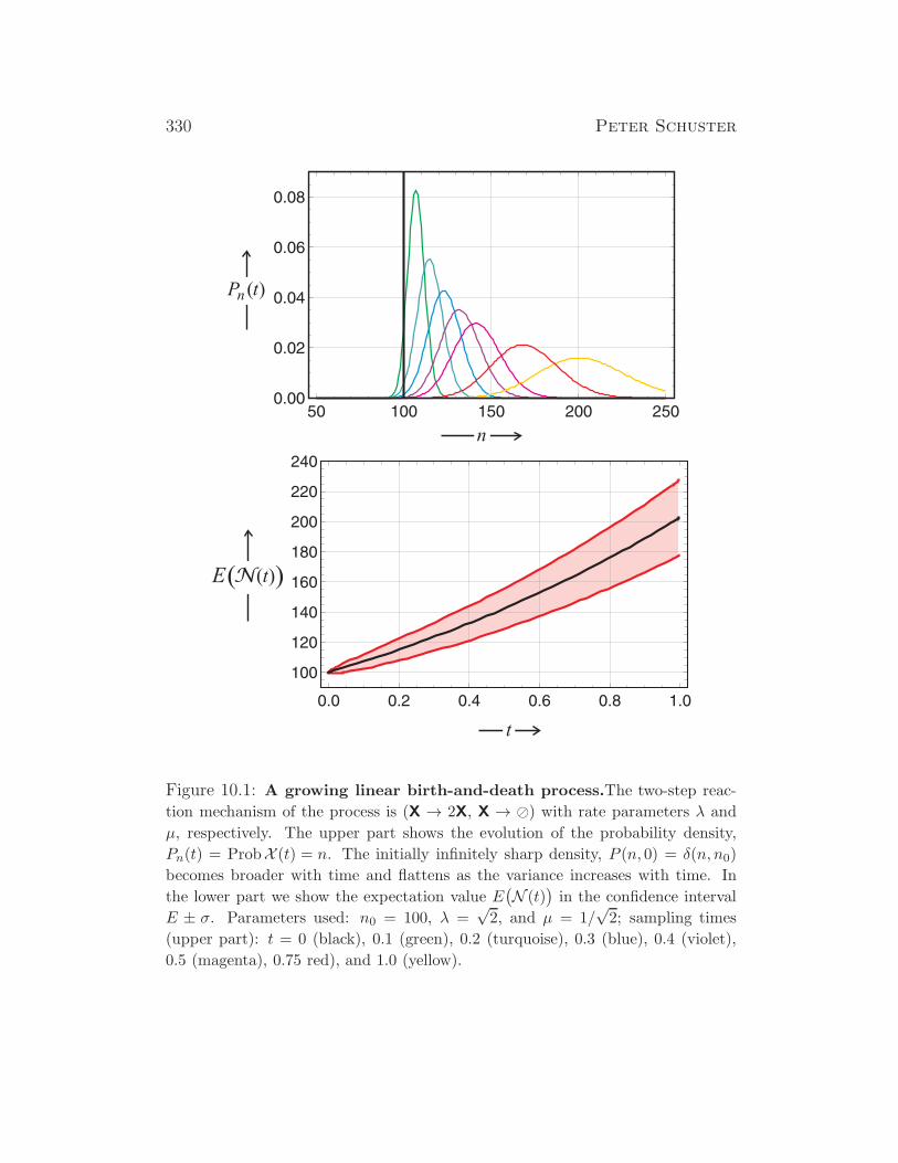
330 Peter Schuster
t
E( )N( )t
Figure 10.1: A growing linear birth-and-death process.The two-step reac-
tion mechanism of the process is (X → 2X, X → ⊘) with rate parameters λ and
µ, respectively. The upper part shows the evolution of the probability density,
Pn(t) = ProbX (t) = n. The initially infinitely sharp density, P (n, 0) = δ(n, n0)
becomes broader with time and flattens as the variance increases with time. In
the lower part we show the expectation value E(
N (t))
in the confidence interval
E ± σ. Parameters used: n0 = 100, λ =√2, and µ = 1/
√2; sampling times
(upper part): t = 0 (black), 0.1 (green), 0.2 (turquoise), 0.3 (blue), 0.4 (violet),
0.5 (magenta), 0.75 red), and 1.0 (yellow).
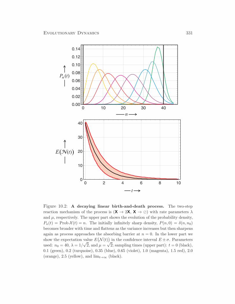
Evolutionary Dynamics 331
t
E( )N( )t
Figure 10.2: A decaying linear birth-and-death process. The two-step
reaction mechanism of the process is (X → 2X, X → ⊘) with rate parameters λ
and µ, respectively. The upper part shows the evolution of the probability density,
Pn(t) = ProbX (t) = n. The initially infinitely sharp density, P (n, 0) = δ(n, n0)
becomes broader with time and flattens as the variance increases but then sharpens
again as process approaches the absorbing barrier at n = 0. In the lower part we
show the expectation value E(
N (t))
in the confidence interval E±σ. Parameters
used: n0 = 40, λ = 1/√2, and µ =
√2; sampling times (upper part): t = 0 (black),
0.1 (green), 0.2 (turquoise), 0.35 (blue), 0.65 (violet), 1.0 (magenta), 1.5 red), 2.0
(orange), 2.5 (yellow), and limt→∞ (black).

332 Peter Schuster
irreversible. The stochastic process corresponding to equations (10.1) belongs
to the class of linear birth-and-death processes with w+(n) = λ · n and
w−(n) = µ · n.4 The master equation is of the form,
∂Pn(t)
∂t= λ (n− 1)Pn−1(t) + µ (n+ 1)Pn+1(t) − (λ+ µ)nPn(t) , (10.2)
and after introduction of the probability generating function g(s, t) gives rise
to the PDE∂g(s, t)
∂t− (s− 1) (λs− µ) ∂g(s, t)
∂s= 0 . (10.3)
Solution of this PDE yields different results for equal or different replication
and extinction rate coefficients, λ 6= µ and λ = µ, respectively. In the first
case we substitute γ = λ/µ ( 6= 1) and η(t) = exp(
(λ− µ)t)
, and find:
g(s, t) =
(
η(t)− 1)
+(
γ − η(t))
s(
γη(t)− 1)
+ γ(
1− η(t))
s
n0
and
Pn(t) = γnmin(n,n0)∑
m=0
(−1)m(
n0 + n−m− 1
n−m
)(
n0
m
)
×
×(
1− η(t)1− γη(t)
)n0+n−m(
γ − η(t)γ(
1− η(t))
)m
.
(10.4)
In the derivation of the expression for the probability distributions we ex-
panded enumerator and denominator of the expression in the generating
function g(s, t), by using expressions for the sums (1 + s)n =∑n
k=0
(
nk
)
sk
and (1+ s)−n = 1+∑∞
k=1(−1)k n(n+1)...(n+k−1)k!
sk, multiply, order terms with
respect to powers of s, and compare with the expansion of the generating
function, g(s, t) =∑∞
n=0 Pn(t) sn.
4Here we use the symbols commonly applied in biology: λ(n) for birth, µ(n) for death,
ν for immigration, and ρ for emigration (tables 10.1 and 10.2). These notions were created
especially for application to biological problems, in particular for problems in theoretical
ecology. Other notions and symbols are common in chemistry: A birth corresponds to the
production of a molecule, f ≡ λ, a death to its decomposition or degradation through a
chemical reaction, d ≡ µ. Influx and outflux are the proper notions for immigration and
emigration.
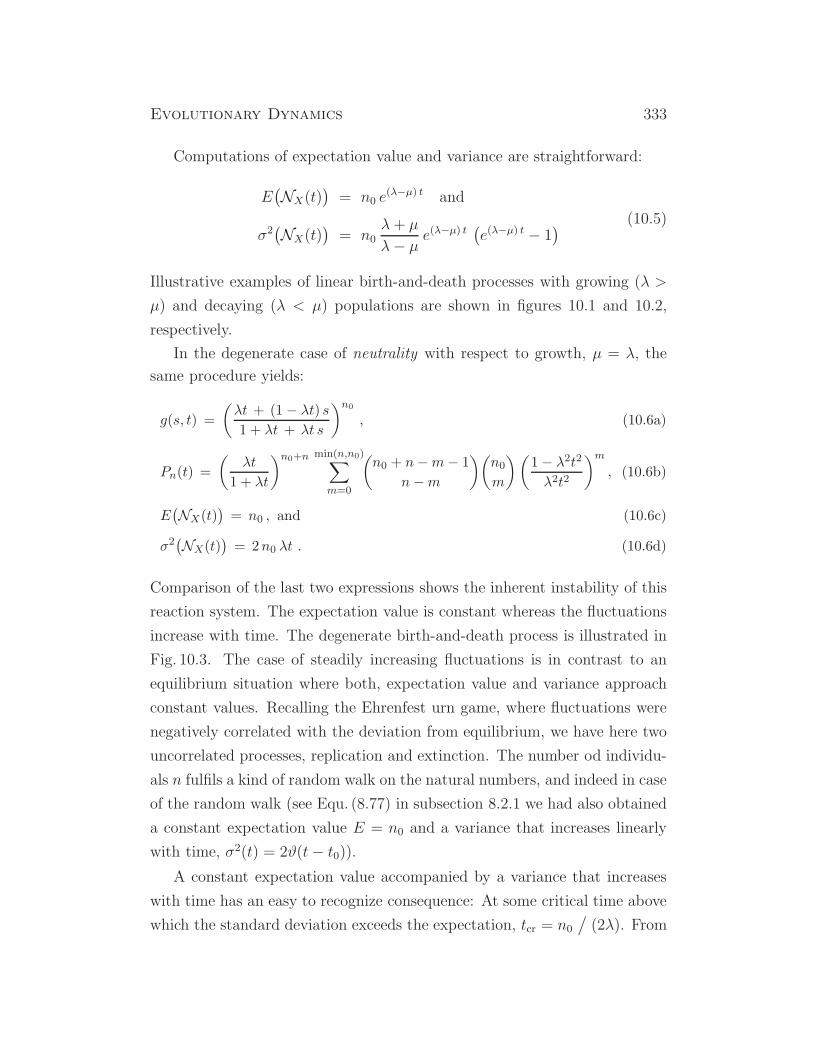
Evolutionary Dynamics 333
Computations of expectation value and variance are straightforward:
E(
NX(t))
= n0 e(λ−µ) t and
σ2(
NX(t))
= n0λ+ µ
λ− µ e(λ−µ) t (e(λ−µ) t − 1
)
(10.5)
Illustrative examples of linear birth-and-death processes with growing (λ >
µ) and decaying (λ < µ) populations are shown in figures 10.1 and 10.2,
respectively.
In the degenerate case of neutrality with respect to growth, µ = λ, the
same procedure yields:
g(s, t) =
(
λt + (1− λt) s
1 + λt + λt s
)n0
, (10.6a)
Pn(t) =
(
λt
1 + λt
)n0+n min(n,n0)∑
m=0
(
n0 + n−m− 1
n−m
)(
n0
m
)(
1− λ2t2
λ2t2
)m
, (10.6b)
E(
NX(t))
= n0 , and (10.6c)
σ2(
NX(t))
= 2n0 λt . (10.6d)
Comparison of the last two expressions shows the inherent instability of this
reaction system. The expectation value is constant whereas the fluctuations
increase with time. The degenerate birth-and-death process is illustrated in
Fig. 10.3. The case of steadily increasing fluctuations is in contrast to an
equilibrium situation where both, expectation value and variance approach
constant values. Recalling the Ehrenfest urn game, where fluctuations were
negatively correlated with the deviation from equilibrium, we have here two
uncorrelated processes, replication and extinction. The number od individu-
als n fulfils a kind of random walk on the natural numbers, and indeed in case
of the random walk (see Equ. (8.77) in subsection 8.2.1 we had also obtained
a constant expectation value E = n0 and a variance that increases linearly
with time, σ2(t) = 2ϑ(t− t0)).A constant expectation value accompanied by a variance that increases
with time has an easy to recognize consequence: At some critical time above
which the standard deviation exceeds the expectation, tcr = n0
/
(2λ). From
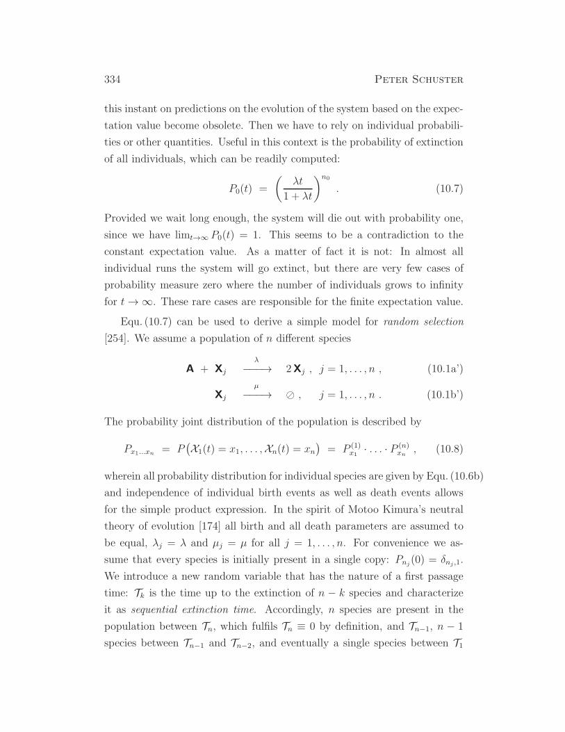
334 Peter Schuster
this instant on predictions on the evolution of the system based on the expec-
tation value become obsolete. Then we have to rely on individual probabili-
ties or other quantities. Useful in this context is the probability of extinction
of all individuals, which can be readily computed:
P0(t) =
(
λt
1 + λt
)n0
. (10.7)
Provided we wait long enough, the system will die out with probability one,
since we have limt→∞ P0(t) = 1. This seems to be a contradiction to the
constant expectation value. As a matter of fact it is not: In almost all
individual runs the system will go extinct, but there are very few cases of
probability measure zero where the number of individuals grows to infinity
for t→∞. These rare cases are responsible for the finite expectation value.
Equ. (10.7) can be used to derive a simple model for random selection
[254]. We assume a population of n different species
A + Xj
λ
−−−→ 2Xj , j = 1, . . . , n , (10.1a’)
Xj
µ
−−−→ ⊘ , j = 1, . . . , n . (10.1b’)
The probability joint distribution of the population is described by
Px1...xn = P(
X1(t) = x1, . . . ,Xn(t) = xn)
= P (1)x1· . . . · P (n)
xn, (10.8)
wherein all probability distribution for individual species are given by Equ. (10.6b)
and independence of individual birth events as well as death events allows
for the simple product expression. In the spirit of Motoo Kimura’s neutral
theory of evolution [174] all birth and all death parameters are assumed to
be equal, λj = λ and µj = µ for all j = 1, . . . , n. For convenience we as-
sume that every species is initially present in a single copy: Pnj(0) = δnj ,1.
We introduce a new random variable that has the nature of a first passage
time: Tk is the time up to the extinction of n − k species and characterize
it as sequential extinction time. Accordingly, n species are present in the
population between Tn, which fulfils Tn ≡ 0 by definition, and Tn−1, n − 1
species between Tn−1 and Tn−2, and eventually a single species between T1
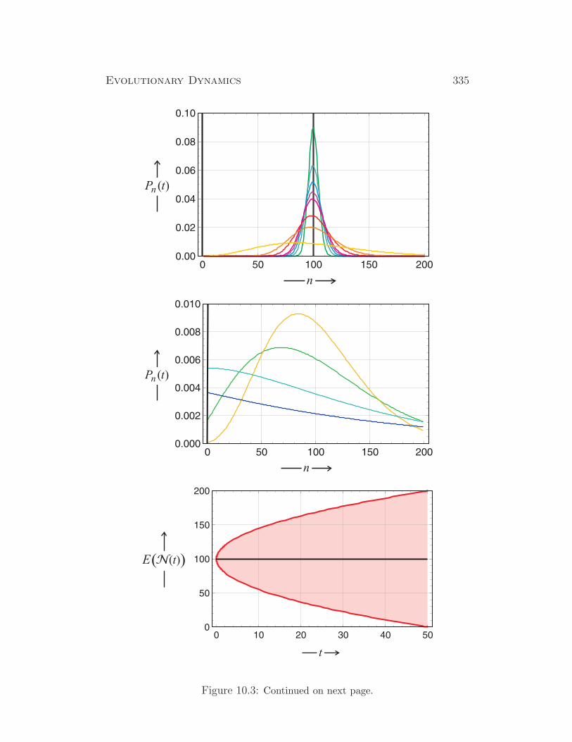
Evolutionary Dynamics 335
n
P tn ( )
Figure 10.3: Continued on next page.

336 Peter Schuster
Figure 10.3: Probability density of a linear birth-and-death with equal
birth and death rate. The two-step reaction mechanism is: (X→ 2X, X→ ⊘)with rate parameters λ = µ. The upper and the middle part show the evolution
of the probability density, Pn(t) = Prob(
X (t) = n)
. The initially infinitely sharp
density, P (n, 0) = δ(n, n0) becomes broader with time and flattens as the vari-
ance increases but then sharpens again as the process approaches the absorbing
barrier at n = 0. In the lower part, we show the expectation value E(
N (t))
in
the confidence interval E ± σ. The variance increases linearly with time and at
t = n0/(2λ) = 50 the standard deviation is as large as the expectation value.
Parameters used: n0 = 100, λ = 1; sampling times, upper part: t = 0 (black), 0.1
(green), 0.2 (turquoise), 0.3 (blue), 0.4 (violet), 0.49999 (magenta), 0.99999 red),
2.0 (orange), 10 (yellow), and middle part: t = 10 (yellow), 20 (green), 50 (cyan),
100 (blue), and limt→∞ (black).
Figure 10.4: The distribution of sequential extinction times Tk. Shown are
the expectation values E(Tk) for n = 20 according to equation(10.10). Since E(T0)diverges, T1 is the extinction that appears on the average at a finite value. A single
species is present above T1 and random selection has occurred in the population.
and T0, which is the moment of extinction of the entire population. After T0no individual of type X exists any more.
Evolutionary Dynamics 337
Next we consider the probability distribution of the sequential extinction
times
Hk(t) = P (Tk < t) . (10.9)
The probability of extinction of the population is readily calculated: Since
individual reproduction and extinction events are independent we find
H0 = P0,...,0 = P(1)0 · . . . · P (n)
0 =
(
λt
1 + λt
)n
.
The event T1 < t can happen in several ways: Either X1 is present and all
other species have become extinct already, or only X2 is present, or only X3,
and so on, but T1 < t is also fulfilled if the whole population has died out:
H1 = Px1 6=0,0,...,0 + P0,x2 6=0,...,0 + P0,0,...,xn 6=0 + H0 .
The probability that a given species has not yet disappeared is obtained by
exclusion since existence and nonexistence are complementary,
Px 6=0 = 1 − P0 = 1 − λt
1 + λt=
1
1 + λt,
which yields the expression for the presence of a single species
H1(t) = (n + λt)(λt)n−1
(1 + λt)n,
and by similar arguments a recursion formula is found for the extinction
probabilities with higher indices
Hk(t) =
(
n
k
)
(λt)n−k
(1 + λt)n+ Hk−1(t) ,
that eventually leads to the expression
Hk(t) =k∑
j=0
(
n
j
)
(λt)n−j
(1 + λt)n.
The moments of the sequential extinction times are computed straightfor-
wardly by means of a handy trick: Hk is partitioned into terms for the
338 Peter Schuster
individual powers of λt, Hk(t) =∑k
j=0 hj(t) and then differentiated with
respect to time t
hj(t) =
(
n
j
)
(λt)n−k
(1 + λt)n,
dhj(t)
dt= h′j =
λ
(1 + λt)n+1
((
n
j
)
(n− j)(λt)n−j−1 −(
n
j
)
j(λt)n−j)
.
The summation of the derivatives is simple because h′k + h′k−1 + . . .+ h′0 is a
telescopic sum and we find
dHk(t)
dt=
(
n
k
)
(n− k) λn−k tn−k−1
(1 + λt)n+1.
Making use of the definite integral [123, p.338]
∫ ∞
0
tn−k
(1 + λt)n+1dt =
λ−(n−k+1)
(
nk
)
k,
we finally obtain for the expectation values of the sequential extinction times
E(Tk) =
∫ ∞
0
dHk(t)
dtt dt =
n− kk· 1λ, n ≥ k ≥ 1 , (10.10)
and E(T0) =∞ (see Fig. 10.4). It is worth recognizing here another paradox
of probability theory: Although extinction is certain, the expectation value
for the time to extinction diverges. Similarly as the expectation values, we
calculate the variances of the sequential extinction times:
σ2(Tk) =n(n− k)k2(k − 1)
· 1λ2, n ≥ k ≥ 2 , (10.11)
from which we see that the variances diverges for k = 0 and k = 1.
For distinct birth parameters, λ1, . . . , λn, and different initial numbers
of individuals, x1(0), . . . , xn(0), the expressions for the expectation values
become considerably more complicated, but the main conclusion remains
unaffected: E(T1) is finite whereas E(T0) diverges.
Evolutionary Dynamics 339
10.1.2 Boundaries in one step birth-and-death processes
One step birth-and-death processes have been studied extensively and ana-
lytical solutions are available in table form [118]. For transition probabilities
at most linear in n, w+(n) = ν + λn and w−(n) = ρ + µn, one distin-
guishes birth (λ), death (µ), immigration (ν), and emigration (ρ) terms.
Analytical solutions for the probability distributions were derived for all one
step birth-and-death processes whose transitions probabilities are constant
or maximally linear in the numbers of individuals n.
It is necessary, however, to consider also the influence of boundaries on
these stochastic processes. For this goal we define an interval [a, b] as domain
of the stochastic variable N (t). Here we are dealing with classes of boundary
conditions, absorbing and reflecting boundaries. In the former case, a par-
ticle that left the interval is not allowed to return, whereas the latter class
of boundary implies that it is forbidden to exit from the interval. Bound-
ary conditions can be easily implemented by ad hoc definitions of transition
probabilities:
Reflecting Absorbing
Boundary at a w−(a) = 0 w+(a− 1) = 0
Boundary at b w+(b) = 0 w−(b+ 1) = 0
The reversible chemical reaction with w−(n) = k1 n and w+(n) = k2 (n0−n),for example, had two reflecting barriers at a = 0 and b = n0. Among the
examples we have studied so far we were dealing with an absorbing boundary
in the replication-extinction process between N = 1 and N = 0 that is
tantamount to the lower barrier at a = 1 fulfilling w+(0) = 0: The state
n = 0 is the end point or ω-limit of all trajectories reaching it.
Compared, for example, to an unrestricted random walk on positive and
negative integers, n ∈ Z, a chemical reaction or a biological process has to
be restricted by definition, n ∈ N0, since negative particle numbers are not
allowed. In general, the one step birth-and-death master Equ. (9.7),
∂Pn(t)
∂t= w+(n−1)Pn−1(t) + w−(n+1)Pn+1(t)−
(
(w+(n)+w−(n))
Pn(t) ,
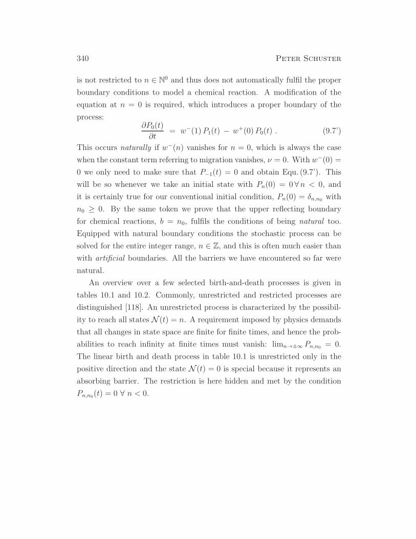
340 Peter Schuster
is not restricted to n ∈ N0 and thus does not automatically fulfil the proper
boundary conditions to model a chemical reaction. A modification of the
equation at n = 0 is required, which introduces a proper boundary of the
process:∂P0(t)
∂t= w−(1)P1(t) − w+(0)P0(t) . (9.7’)
This occurs naturally if w−(n) vanishes for n = 0, which is always the case
when the constant term referring to migration vanishes, ν = 0. With w−(0) =
0 we only need to make sure that P−1(t) = 0 and obtain Equ. (9.7’). This
will be so whenever we take an initial state with Pn(0) = 0 ∀n < 0, and
it is certainly true for our conventional initial condition, Pn(0) = δn,n0 with
n0 ≥ 0. By the same token we prove that the upper reflecting boundary
for chemical reactions, b = n0, fulfils the conditions of being natural too.
Equipped with natural boundary conditions the stochastic process can be
solved for the entire integer range, n ∈ Z, and this is often much easier than
with artificial boundaries. All the barriers we have encountered so far were
natural.
An overview over a few selected birth-and-death processes is given in
tables 10.1 and 10.2. Commonly, unrestricted and restricted processes are
distinguished [118]. An unrestricted process is characterized by the possibil-
ity to reach all states N (t) = n. A requirement imposed by physics demands
that all changes in state space are finite for finite times, and hence the prob-
abilities to reach infinity at finite times must vanish: limn→±∞ Pn,n0 = 0.
The linear birth and death process in table 10.1 is unrestricted only in the
positive direction and the state N (t) = 0 is special because it represents an
absorbing barrier. The restriction is here hidden and met by the condition
Pn,n0(t) = 0 ∀ n < 0.

Evolutionary
Dynamics
341Table 10.1: Comparison of of results for some unrestricted processes. Data are taken from [118, pp.10,11]. Abbre-
viation and notations: γ ≡ λ/µ, σ ≡ e(λ−µ)t, (n, n0) ≡ minn, n0, and In(x) is the modified Bessel function.
Process λn µn gn0(s, t) Pn,n0(t) Mean Variance Ref.
Poisson ν 0 sn0 eν(s−1) t (νt)n−n0 eν t
(n−n0)!, n ≥ n0; n0 > (0, n) n0 + νt νt [39]
Poisson 0 ρ sn0 eρ(1−s) t/s (ρt)n−n0 eρ t
(n0−n)! , n ≤ n0; n0 < (0, n) n0 − ρt ρt [39]
ν ρ sn0 e−(ν+ρ)t+(νs+ρ/s)t(
νρ
)(n−n0)/2 In0−n(2t√νρ) e−(ν+ρ)t n0 + (ν − ρ)t (ν + ρ)t [141]
Birth λn 0(
1− eλt(1− 1/s))−n0 (
nn0
)
e−n0λ t(1− e−λ t)n−n0 , n ≥ n0; n0 > (0, n) n0 eλt n0 e
λt(eλt − 1) [10]
Death 0 µn(
1− e−µt(1− s))n0 (n0
n
)
e−nµ t(1− e−µ t)n0−n , n ≤ n0; n0 < (0, n) n0 e−µt n0 e
−µt(1− e−µt) [10]
ν µn(
1− e−µt(1− s))n0 × exp
(
− νµ(1− e−µt)
)
× n0 e−µt+
(
νµ + n0e
−µt)
× [39]
× exp(
ν(s− 1)(1 − e−µt)/µ)
×(n,n0)∑
k=0
e−µtk(1−e−µt)n+n0−2k
(n−k)!
(
νµ
)n−k+ν(1−e−µt)
µ ×(1− e−µt)
Birth& λn µn(
(σ−1)+(γ−σ)s(γσ−1)γ(1−σ)s
)n0
γn(n,n0)∑
k=0
(−1)k(n+n0−k−1
n−k)(n0
k
)
× n0 σn0σ(γ+1)(σ−1)
γ−1 [10]
Death ×(
1−σ1−γσ
)n+n0−k (1−σ/γ1−σ
)k
λn λn(
λt+(1−λt)s1+λt−λt s
)n (
λt1+λt
)n+n0∑(n,n0)k=0
(n0
k
)
× n0 2n0λ t
×(n+n0−k−1
n−k)
(
1−λ2t2
λ2t2
)k
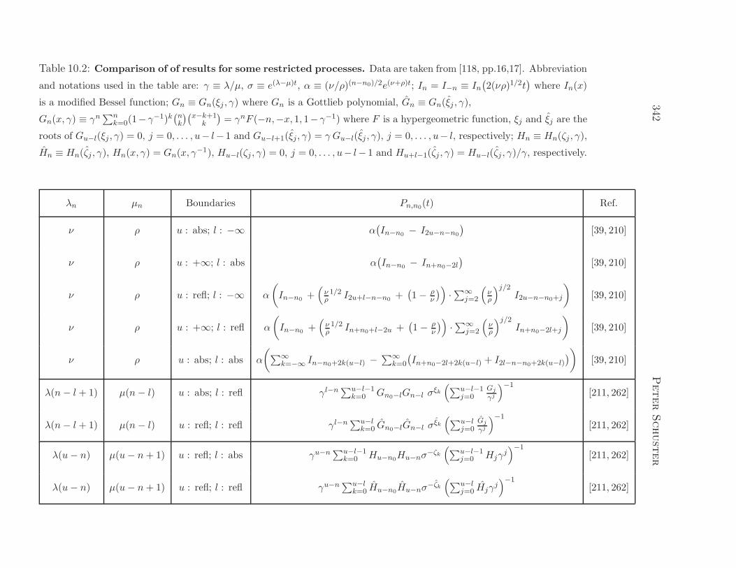
342PeterSchuster
Table 10.2: Comparison of of results for some restricted processes. Data are taken from [118, pp.16,17]. Abbreviation
and notations used in the table are: γ ≡ λ/µ, σ ≡ e(λ−µ)t, α ≡ (ν/ρ)(n−n0)/2e(ν+ρ)t; In = I−n ≡ In(
2(νρ)1/2t)
where In(x)
is a modified Bessel function; Gn ≡ Gn(ξj , γ) where Gn is a Gottlieb polynomial, Gn ≡ Gn(ξj , γ),
Gn(x, γ) ≡ γn∑n
k=0(1− γ−1)k(
nk
)(
x−k+1k
)
= γnF (−n,−x, 1, 1− γ−1) where F is a hypergeometric function, ξj and ξj are the
roots of Gu−l(ξj , γ) = 0, j = 0, . . . , u− l− 1 and Gu−l+1(ξj, γ) = γ Gu−l(ξj , γ), j = 0, . . . , u− l, respectively; Hn ≡ Hn(ζj , γ),
Hn ≡ Hn(ζj , γ), Hn(x, γ) = Gn(x, γ−1), Hu−l(ζj , γ) = 0, j = 0, . . . , u− l− 1 and Hu+l−1(ζj , γ) = Hu−l(ζj , γ)/γ, respectively.
λn µn Boundaries Pn,n0(t) Ref.
ν ρ u : abs; l : −∞ α(
In−n0 − I2u−n−n0
)
[39, 210]
ν ρ u : +∞; l : abs α(
In−n0 − In+n0−2l)
[39, 210]
ν ρ u : refl; l : −∞ α
(
In−n0 +(
νρ1/2 I2u+l−n−n0 +
(
1− ρν
)
)
·∑∞j=2
(
νρ
)j/2I2u−n−n0+j
)
[39, 210]
ν ρ u : +∞; l : refl α
(
In−n0 +(
νρ1/2 In+n0+l−2u +
(
1− ρν
)
)
·∑∞j=2
(
νρ
)j/2In+n0−2l+j
)
[39, 210]
ν ρ u : abs; l : abs α
(
∑∞k=−∞ In−n0+2k(u−l) −
∑∞k=0
(
In+n0−2l+2k(u−l) + I2l−n−n0+2k(u−l))
)
[39, 210]
λ(n− l + 1) µ(n− l) u : abs; l : refl γl−n∑u−l−1
k=0 Gn0−lGn−l σξk(
∑u−l−1j=0
Gj
γj
)−1[211, 262]
λ(n− l + 1) µ(n− l) u : refl; l : refl γl−n∑u−l
k=0 Gn0−lGn−l σξk(
∑u−lj=0
Gj
γj
)−1[211, 262]
λ(u− n) µ(u− n+ 1) u : refl; l : abs γu−n∑u−l−1
k=0 Hu−n0Hu−nσ−ζk(
∑u−l−1j=0 Hjγ
j)−1
[211, 262]
λ(u− n) µ(u− n+ 1) u : refl; l : refl γu−n∑u−l
k=0 Hu−n0Hu−nσ−ζk(
∑u−lj=0 Hjγ
j)−1
[211, 262]

Evolutionary Dynamics 343
10.1.3 Branching processes in evolution
According to David Kendall’s historical accounts on the centennial of the
origins of stochastic thinking in population mathematics [171, 172] the name
branching process was coined relatively late by Kolmogorov and Dmitriev in
1947 [180]. The interest in stochasticity of the evolution of reproducing pop-
ulations, however, is much older. The origin of the problem is the genealogy
of human males, which is reflected by the development of family names or
surnames in the population. Commonly the stock of family names is eroded
in the sense of steady disappearance of families in particular in small com-
munities. The problem was clearly stated in a book by Alphonse de Candolle
[47] and has been brought up by Sir Francis Galton after he had read de Can-
dolle’s book. The first rigorous mathematical analysis of a problem by means
of a branching problem is commonly assigned to Galton and Reverend Henry
William Watson [301] and the Galton-Watson process named after them has
become a standard problem in branching processes. Apparently, Galton and
Watson were not aware of earlier work on this topic [142], that had been
performed almost thirty years earlier by Jules Bienayme and reported in a
publication [20]. Most remarkable Bienayme discussed already the criticality
theorem, which expresses different behavior of the Galton-Watson process
for m < 1, m = 1, and m < 1, where m denotes the expected or mean
number of sons per father. The three cases were called subcritical, critical,
and supercritical, respectively, by Kolmogorov [179]. Watson’s original work
contained a serious error in the analysis of the supercritical case and this has
been detected only by Johan Steffensen [275]. In the years after 1940 the
Galton-Watson model received plenty of attention because of the analogies
of genealogies and nuclear chain reactions. In addition, mathematicians be-
came generally more interested in probability theory and stochasticity. The
pioneering work related to nuclear chain reactions and criticality of nuclear
reactors was done by Stan Ulam at the Los Alamos National Laboratory
[82–85, 138]. Many other applications to biology and physics were found and
branching processes have been studied intensively. By now, it seems, we have
a clear picture on the Galton-Watson process and its history [172].
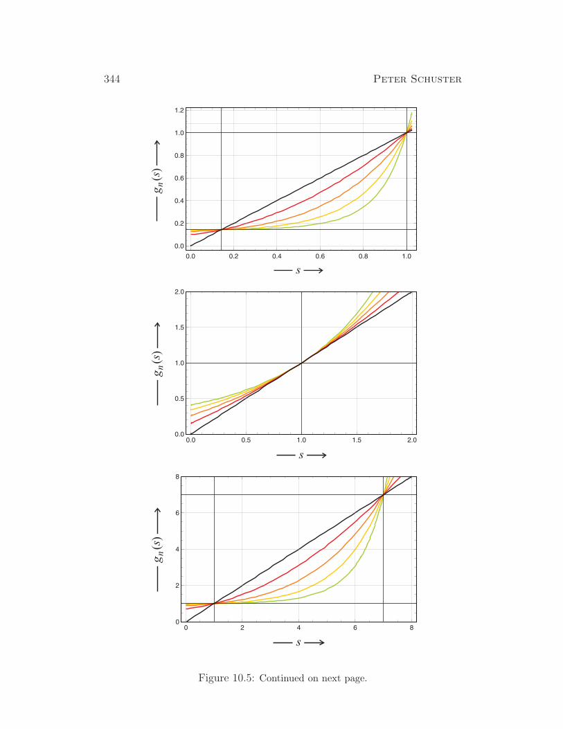
344 Peter Schuster
Figure 10.5: Continued on next page.

Evolutionary Dynamics 345
Figure 10.5: Calculation of extinction probabilities for the Galton-
Watson process. The individual curves show the iterated generating functions
of the Galton-Watson process, g0(s) = s (black), g1(s) = g(s) = p0 + p1s + p2s2
(red), g2(s) (orange), g3(s) (yellow), and g4(s) (green), for different probability
densities p = (p0, p1, p2). Choice of parameters: supercritical case (upper part)
p = (0.1, 0.2, 0.7), m = 1.6; critical case (middle part) p = (0.15, 0.7, 0.15), m = 1;
subcritical case (lower part) p=(0.7,0.2,0.1), m = 0.4.
The Galton-Watson process. A Galton-Watson process [301] deals with the
generation of objects from objects of the same kind in the sense of reproduc-
tion. These objects can be neutrons, bacteria, or higher organisms, or men
as in the family name genealogy problem. The Galton-Watson process is the
simplest possible description of consecutive reproduction and falls into the
class of branching processes. Recorded are only the population sizes of succes-
sive generations, which are considered as random variables: Z0,Z1,Z2, . . . .
A question of interest is the extinction of a population in generation n, and
this simply means Zn = 0 from which follows that all the random variable
is zero in all future generations: Zn+1 = 0 if Zn = 0. Indeed, the extinction
or disappearance of aristocratic family names was the problem that Galton
wanted to model by means of a stochastic process. In the following presen-
tation and analysis we make use of the two books [8, 135].
In mathematical terms the Galton-Watson process is a Markov chain
(Zn; n ∈ N0) on the nonnegative integers. The transition probabilities are
defined in terms of a given probability function Prob Z1 = k) = pk; k ∈ N0
with pk ≤ 0,∑
pk = 1 have the
P (i, j) = Prob Zn+1 = j|Zn = i =
p∗ij if i ≥ 1, j ≥ 0 ,
δ0,j if i = 0, j ≥ 0 ,(10.12)
wherein δij is the Kronecker delta5 and p∗ik ; k ∈ N0 is the i-fold convolution
of pk; k ∈ N0, and accordingly the probability mass function f(k) = pk is
the only datum of the process. The use of the convolution of the probability
distribution is an elegant mathematical trick for the rigorous analysis of the
5The Kronecker delta is named after the German mathematician Leopold Konecker
346 Peter Schuster
problem. Convolutions in explicit form are quite difficult to handle as we shall
see in the case of the generating function. Nowadays one can use computer
assisted symbolic computation but in Galton’s times, in the 19th century
handling of higher convolutions was quite hopeless.
The process describes an evolving population of particles or individuals
and it might be useful although not necessary to define a time axis. The
process starts with Z0 particles at time T = 0, each if which produces –
independently of the others – a random number of offspring offspring at time
T = 1 according to the probability density f(k) = pk. The total number
of particles in the first generation, Z1 is the sum of all Z0 random variables
where each was drawn according to the pmf f(pk). The first generation
produces Z2 particles at time T = 2, the second generation gives rise to the
third with Z3 particles at time T = 3, and so on. Since discrete times Tn are
equivalent to the numbers of generations n we shall refer only to generations
ion the following. From (10.12) follows that the future development of the
process at any time is independent of the history and this constitutes the
Markov property.
The number of offspring produced by a single parent particle in the n-th
generation is a random variable Z(1)n where the superscript indicates Z0 = 1.
In general we shall write for the branching process (Z(i)n ; n ∈ N0) when we
want to express that the process started with i particles. Since i = 1 is the
by far most common case, we write simply Z(1)n = Zn. Equ. (10.12) tells that
Zn+k = 0 ∀ k ≥ 0. Accordingly, the state Z = 0 is absorbing and reaching
Z = 0 is tantamount to becoming extinct.
In order to analyze the process we shall make use of the probability gen-
erating function
g(s) =∞∑
k=0
pk sk , |s| ≤ 1 , (10.13)
and represents the discrete analogue of Dirac’s delta function:
δij =
0 if i 6= j ,
1 if i = j .
Evolutionary Dynamics 347
where s is complex in general but we shall assume here s ∈ R1. In addition,
we define the iterates of the generating function:
g0(s) = s , g1(s) = g(s) , gn+1(s) = g(
gn(s))
, n = 1, 2, . . . . (10.14)
Expressed in terms of transition probabilities the generating function is of
the form
∞∑
j=0
P (1, j) sj = g(s) and
∞∑
j=0
P (i, j) sj =(
g(s))i, i ≥ 1 . (10.15)
Denoting the n-step transition probability by Pn(i, j) and using the Chapman-
Kolmogorov equation we obtain
∞∑
j=0
Pn+1(1, j) sj =
∞∑
j=0
∞∑
k=0
Pn(1, k)P (k, j) sj =
=
∞∑
k=0
Pn(1, k)
∞∑
j=0
P (k, j) sj =
=
∞∑
k=0
Pn(1, k)(
g(s))k.
Writing g(n) =∑
j Pn(1, j) sj the last equation has shown that
g(n+1)(s) = g(n)(
g(s))
which yields the fundamental relation
g(n)(s) = gn(s) , (10.16)
and by making use of Equ. (10.15) we find
∞∑
j=0
Pn(i, j) sj =
(
gn(s))i
. (10.17)
Equ. (10.16) expressed as “The generating function of Zn is the n-iterate
gn(s)”, provides a tool for the calculation of the generating function. As
stated in Equ. (10.12) the probability distribution of Zn is obtained as the
348 Peter Schuster
n-th convolution or iterate of g(s). The explicit form of an n-th convolution
is hard to compute and the true value of (10.16) lies in the calculation of the
moments of Zn and in the possibility to derive asymptotic laws for large n.
For the purpose of illustration we present the first iterates of the simplest
useful generating function
g(s) = p0 + p1 s + p2 s2 .
The first convolution g2(s) = g(
g(s))
contains ten terms already:
g2(s) = p0 + p0p1 + p20p2 + (p21 + 2p0p1p2) s+
+ (p1p2 + p21p2 + 2p0p22) s
2 + 2p1p22 s
3 + p32 s4.
The next convolution, g3(s), contains already nine constant terms that con-
tribute to the probability of extinction gn(0), and g4(s) already 29 terms.
It is straightforward to compute the moments of the probability distribu-
tions from the generating function:
∂g(s)
∂s=
∞∑
k=0
k pk sk−1 and
∂g(s)
∂s
∣
∣
∣
s=1= E(Z1) = m , (10.18a)
∂2g(s)
∂s2=
∞∑
k=0
k(k − 1) pk sk−2 and
∂2g(s)
∂s2
∣
∣
∣
s=1= E(Z2
1 ) − m ,
var(Z1) =∂2g(s)
∂s2
∣
∣
∣
s=1+m − m2 = σ2 . (10.18b)
Next we calculate the moments of the distribution in higher generations and
differentiate the last expression in Equ. 10.14 at |s| = 1:
∂gn+1(s)
∂s
∣
∣
∣
s=1=
∂g(s)
∂s
(
gn(s)∣
∣
∣
s=1
) ∂gn(s)
∂s
∣
∣
∣
s=1=
=∂g(s)
∂s
∣
∣
∣
s=1
∂gn(s)
∂s
∣
∣
∣
s=1and
E(Zn+1) = E(Z)E(Zn) or E(Zn) = mn ,
(10.19)
by induction. Provided the second derivative of the generating function at
|s| = 1 is finite, Equ. 10.14 can be differentiated twice:
∂2gn+1(s)
∂s2
∣
∣
∣
s=1=
∂g(s)
∂s
∣
∣
∣
s=1
∂2gn(s)
∂s2
∣
∣
∣
s=1+∂2g(s)
∂s2
∣
∣
∣
s=1
(∂gn(s)
∂s
∣
∣
∣
s=1
)2
,

Evolutionary Dynamics 349
and ∂2g(s)/
∂s2∣
∣
s=1is obtained by repeated application. The final result
is:
var(Zn) = E(Z2n) − E(Zn)
2 =
σ2 mn (mn−1)m (m−1) , if m 6= 1
nσ2 , if m = 1. (10.20)
Thus, we have E(Zn) = mn and provided σ = var(Z1) < ∞ the variances
are given by Equ. (10.20).
Two more assumptions are made in order to facilitate the analysis: (i)
Neither the probabilities p0 and p1 nor their sum are equal to one, p0 < 1,
p1 < 1, and p0 + p1 < 1, and this implies that g(s) is strictly convex on the
unit interval 0 ≤ s ≤ 1, and (ii) the expectation value E(Z1) =∑∞
k=0 k pk is
finite, and from the finiteness of the expectation value follows ∂g/∂s|s=1 is
finite too since |s| ≤ 1.
Eventually we can now consider Galton’s extinction problem of family
names. The straightforward definition of extinction is given in terms of a
random sequence (Zn; n = 0, 1, 2, . . . ,∞), which consists of zeros except a
finite number of positive integer value at the beginning of the series. The
random variable Zn is integer valued and hence extinction is tantamount to
the event Zn → 0. From P (Zn+1 = 0|Zn = 0) = 1 follows the equality
P (Zn → 0) = P (Zn = 0 for some n) =
= P(
(Z1 = 0) ∪ (Z2 = 0) ∪ · · · ∪ (Zn = 0))
=
= limn→∞
P(
(Z1 = 0) ∪ (Z2 = 0) ∪ · · · ∪ (Zn = 0))
=
= limP (Zn = 0) = lim gn(0) ,
(10.21)
and the fact that gn(0) is a nondecreasing function of n (see also Fig. 10.6).
We define a probability of extinction, q = P (Zn → 0) = lim gn(0) and
show that m = E(Z1) ≤ 1 the probability of extinction fulfils q = 1, and the
family names disappear in finite time. For m > 1, however, the extinction
probability is the unique solution less than one of the equation
s = g(s) for 0 ≤ s < 1 . (10.22)
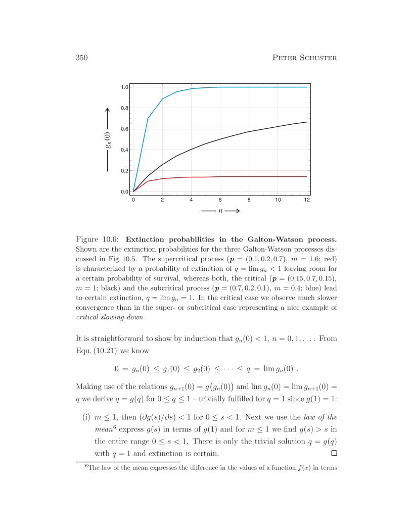
350 Peter Schuster
Figure 10.6: Extinction probabilities in the Galton-Watson process.
Shown are the extinction probabilities for the three Galton-Watson processes dis-
cussed in Fig. 10.5. The supercritical process (p = (0.1, 0.2, 0.7), m = 1.6; red)
is characterized by a probability of extinction of q = lim gn < 1 leaving room for
a certain probability of survival, whereas both, the critical (p = (0.15, 0.7, 0.15),
m = 1; black) and the subcritical process (p = (0.7, 0.2, 0.1), m = 0.4; blue) lead
to certain extinction, q = lim gn = 1. In the critical case we observe much slower
convergence than in the super- or subcritical case representing a nice example of
critical slowing down.
It is straightforward to show by induction that gn(0) < 1, n = 0, 1, . . . . From
Equ. (10.21) we know
0 = gn(0) ≤ g1(0) ≤ g2(0) ≤ · · · ≤ q = lim gn(0) .
Making use of the relations gn+1(0) = g(
gn(0))
and lim gn(0) = lim gn+1(0) =
q we derive q = g(q) for 0 ≤ q ≤ 1 – trivially fulfilled for q = 1 since g(1) = 1:
(i) m ≤ 1, then (∂g(s)/∂s) < 1 for 0 ≤ s < 1. Next we use the law of the
mean6 express g(s) in terms of g(1) and for m ≤ 1 we find g(s) > s in
the entire range 0 ≤ s < 1. There is only the trivial solution q = g(q)
with q = 1 and extinction is certain.
6The law of the mean expresses the difference in the values of a function f(x) in terms
Evolutionary Dynamics 351
(ii) m > 1, then g(s) < s for s sightly less than one because (∂g/∂s)|s=1 =
m > 1, whereas for s = 0 we have g(0) > 0 and hence we have at least
one solution s = g(s) in the half-open interval [0, 1[. Assume there
were two solutions, for example s1 and s2 with 0 ≤ s1 < s2 < 1 than
Rolle’s theorem named after the French mathematician Michel Rolle
would demand the existence of ξ and η with s1 < ξ < s2 < η < 1
such that (∂g(s)/∂s)|s=ξ = (∂g(s)/∂s)|s=η = 1 but this contradicts the
fact that that g(s) is strictly convex. In addition lim gn(0) cannot be
one because (gn(0);n = 0, 1, . . .) is a nondecreasing sequence. If gn(0)
were slightly less than one then gn+1(0) = g(
gn(0))
would be less than
gn(0) and the series were decreasing. Accordingly, q < 1 is the unique
solution of Equ. 10.22 in [0, 1[.
The answer is simple and straightforward: When a father has on the average
one son or less, the family name is doomed to disappear, when he has more
than one son there is a finite probability of survival 0 < (1−q) < 1, which, of
course, increases with increasing expectation value m, the average number of
sons. Reverend Henry William Watson correctly deduced that the extinction
probability is given by a root of Equ. (10.22). He failed, however, to recognize
that for m > 1 the relevant root is the one with q < 1 [105, 301]. It is
remarkable that it took almost fifty years for the mathematical community
to detect the error that has a drastic consequence for the result.
Replication and mutation as multitype branching process.
of the derivative at one particular point x = x1 and the difference in the arguments
f(b) − f(a) = (b − a) (∂f/∂x)|x=x1, a < x < b .
The law of the mean is fulfilled at least at one point x1 on the arc between a and b.
352 Peter Schuster
10.1.4 The Wright-Fisher and the Moran process
Here we shall introduce two common stochastic models in population biol-
ogy, the Wright-Fisher model named after Sewall Wright and Ronald Fisher
and the Moran model named after the Australian statistician Pat Moran.
The Wright-Fisher model and the Moran model are stochastic models for
evolution of allele distributions in populations with constant population size
[22]. The first model [92, 318] also addressed as beanbag population genetics
is presumably the simplest process for the illustration of genetic drift and
definitely the most popular one [43, 88, 136, 198] deals with strictly separated
generations, whereas the Moran process [212, 213] based on continuous time
and overlapping generations is generally more appealing to statistical physi-
cists. Both processes are introduced here for the simplest scenarios: haploid
organisms, two alleles of the gene under consideration and no mutation. Ex-
tension to more complicated cases is readily possible. The primary question
that was thought to be addressed by the two models is the evolution of
populations in case of neutrality for selection.
The Wright-Fisher process. The Wright-Fisher process is illustrated in Fig. 10.7.
A single reproduction event is modeled by a sequence of four steps: (i) A gene
is randomly chosen from the gene pool of generation T containing exactly N
genes distributed over m alleles, (ii) it is replicated, (iii) the original is put
back into the gene pool T , and (iv) the copy is put into the gene pool of
the next generation T + 1. The process is terminated when the next genera-
tion gene pool has exactly N genes. Since filling the gene pool of the T + 1
generation depends exclusively on the distribution of genes in the pool of
generation T , and earlier gene distributions have no influence on the process
the Wright-Fisher model is Markovian.
In order to simplify the analysis we assume two alleles A and B, which
are present in aT and bT copies in the gene pool at generation T . Since
the total number of genes is constant, aT + bT = N and bT = N − aT , weare dealing with a single discrete variable, aT , T ∈ N. A new generation
T + 1 is produced from the gene pool at generation T through picking with
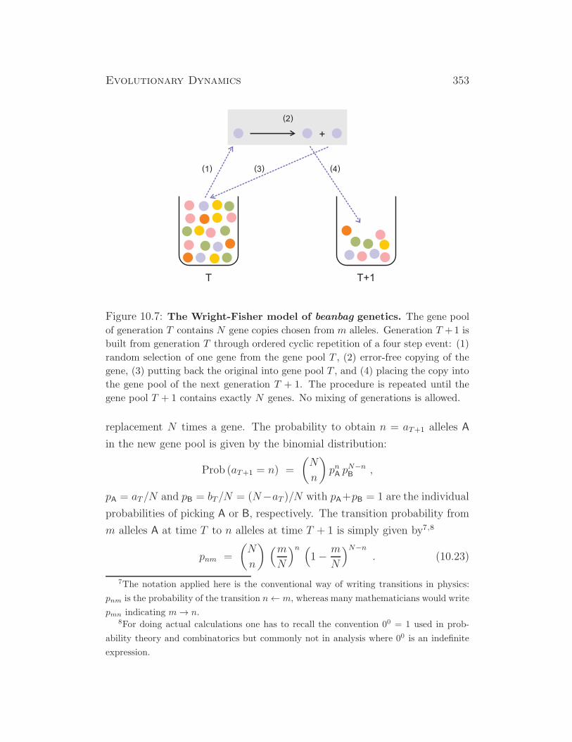
Evolutionary Dynamics 353
Figure 10.7: The Wright-Fisher model of beanbag genetics. The gene pool
of generation T contains N gene copies chosen from m alleles. Generation T +1 is
built from generation T through ordered cyclic repetition of a four step event: (1)
random selection of one gene from the gene pool T , (2) error-free copying of the
gene, (3) putting back the original into gene pool T , and (4) placing the copy into
the gene pool of the next generation T + 1. The procedure is repeated until the
gene pool T + 1 contains exactly N genes. No mixing of generations is allowed.
replacement N times a gene. The probability to obtain n = aT+1 alleles A
in the new gene pool is given by the binomial distribution:
Prob (aT+1 = n) =
(
N
n
)
pnApN−nB
,
pA = aT/N and pB = bT/N = (N−aT )/N with pA+pB = 1 are the individual
probabilities of picking A or B, respectively. The transition probability from
m alleles A at time T to n alleles at time T + 1 is simply given by7,8
pnm =
(
N
n
)
(m
N
)n (
1− m
N
)N−n. (10.23)
7The notation applied here is the conventional way of writing transitions in physics:
pnm is the probability of the transition n← m, whereas many mathematicians would write
pmn indicating m→ n.8For doing actual calculations one has to recall the convention 00 = 1 used in prob-
ability theory and combinatorics but commonly not in analysis where 00 is an indefinite
expression.
354 Peter Schuster
Since the construction of th e gene pool at generation T+1 is fully determined
by the gene distribution at generation T , the process is Markovian.
In order to study the evolution of a population an initial state has to be
specified. We assume that the number of alleles A has been n0 at generation
T = 0 and accordingly we are calculating the probability P (n, T |n0, 0). Since
the Wright-Fisher model does not contain any interactions between alleles or
mutual dependencies between processes involving alleles, the process can be
modeled by means of linear algebra. We define a probability vector p and a
transition matrix, P:
P(T ) = p(T ) =
p0(T )
p1(T )
p2(T )...
and P =
p00 p01 p02 · · ·p10 p11 p12 · · ·p20 p21 p22 · · ·...
......
. . .
.
Conservation of probability provides two conditions: (i) The probability vec-
tor has be normalized,∑
n pn(T ) = 1 and (ii) has to remain normalized in
future generations,∑
n pnm = 1.9 The evolution is now simply described by
the matrix equation
p(T + 1) = P · p(T ) or p(T ) = PT · p(0) . (10.24)
Equ. (10.24) is formally identical with the matrix formulation of linear dif-
ference equations, which are extensively discussed in [44, pp.179-216]. The
solutions of (10.24) are commonly analyzed in terms of the eigenvalues of
matrix P [89]
λk =
(
N
k
)
k!
Nk; k = 0, 1, 2, . . . , (10.25)
and the corresponding eigenvectors. In case of the long-time behavior we only
consider the largest eigenvector or in case of degeneracy all eigenvectors be-
longing to the largest eigenvalue. Stationarity implies p(T + 1) = p(T ) = p,
or P p = p, a stationary probability distribution is an eigenvector p associ-
ated with an eigenvalue λ = 1 of the transition matrix P.
9A matrix P with this property is called a stochastic matrix.
Evolutionary Dynamics 355
Here we are dealing with a case of degeneracy since the largest eigenvalue
λ = 1 is obtained twice from Equ. (10.25): λ0 = λ1 = 1. The corresponding
two eigenvectors are of the form
ζ0 = (1, 0, 0, 0, 0, . . . , 0)t and
ζ1 = (0, 0, 0, 0, 0, . . . , 1)t .(10.26)
We have to recall that in case of degenerate eigenvalue any properly normal-
ized linear combination of the eigenvectors is also a legitimate solution of the
eigenvalue problem. Here we have to apply the L1-norm and obtain
η = α ζ0 + β ζ1 and α + β = 1 ,
and find for the general solution of the stationary state
η = (1− π, 0, 0, 0, 0, . . . , π)t . (10.27)
The interpretation of the result is straightforward: The allele A becomes
fixated in the population with probability π and is lost with probability
1 − π, and the Wright-Fisher model provides a simple explanation for gene
fixation by random drift. What remains to be calculated is the value of π.10
For this goal we make use of expectation vale of the number of alleles A and
show first that it does not change with generations:
E(aT+1) =∑
n
npn(T+1) =∑
n
n∑
m
pnmpm(T ) =∑
m
mpm(T ) = E(aT ) ,
where we made use of the relation
N∑
n=0
n pnm =
N∑
n=0
n
(
N
n
)
(m
N
)n (
1− m
N
)N−n
=(
1− m
N
)NN∑
n=0
n
(
N
n
)(
m
N −m
)n
= m ,
10Although a stationary state does not depend on initial conditions in the nondegenerate
case, this is not true for the linear combination of degenerate eigenvectors: α and β, and
π are functions of the initial state.
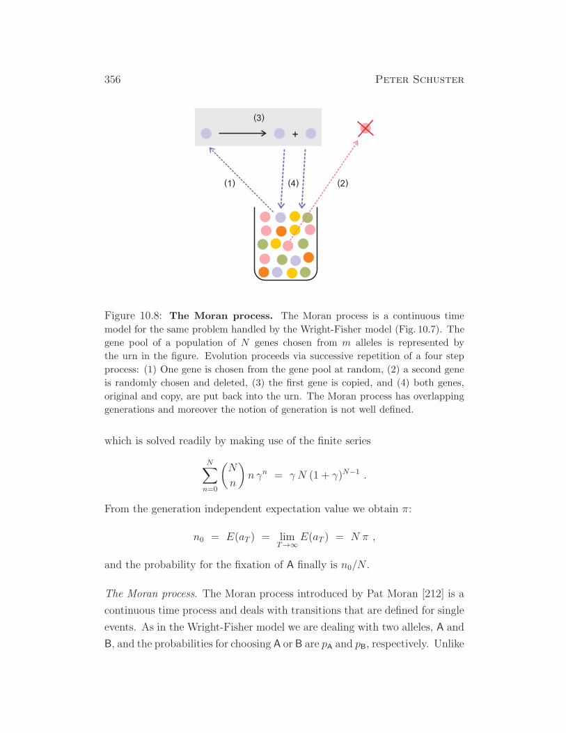
356 Peter Schuster
Figure 10.8: The Moran process. The Moran process is a continuous time
model for the same problem handled by the Wright-Fisher model (Fig. 10.7). The
gene pool of a population of N genes chosen from m alleles is represented by
the urn in the figure. Evolution proceeds via successive repetition of a four step
process: (1) One gene is chosen from the gene pool at random, (2) a second gene
is randomly chosen and deleted, (3) the first gene is copied, and (4) both genes,
original and copy, are put back into the urn. The Moran process has overlapping
generations and moreover the notion of generation is not well defined.
which is solved readily by making use of the finite series
N∑
n=0
(
N
n
)
n γn = γ N (1 + γ)N−1 .
From the generation independent expectation value we obtain π:
n0 = E(aT ) = limT→∞
E(aT ) = N π ,
and the probability for the fixation of A finally is n0/N .
The Moran process. The Moran process introduced by Pat Moran [212] is a
continuous time process and deals with transitions that are defined for single
events. As in the Wright-Fisher model we are dealing with two alleles, A and
B, and the probabilities for choosing A or B are pA and pB, respectively. Unlike
Evolutionary Dynamics 357
the Wright-Fisher model there is no defined previous generation from which
a next generation is formed by sampling N genes. Overlapping generations
make it difficult – if not impossible – to define generations unambiguously.
The event in the Moran process is a combined birth-and-death step: Two
genes are picked, one is copied and both template and copy are put back
into the urn, and the second one is deleted (see Fig. 10.8). The probabilities
are calculated form the state of the urn just before the event pA = n(t)/N
and pB =(
N − n(t))
/N where n(t) is the number of alleles A, N − n(t) thenumber of alleles B, and N is the constant total number of genes.
The transition matrix P of the Moran model is tridiagonal since only
the changes ∆n = 0,±1 can occur: The number of alleles A, n, remains
unchanged if two A’s or two B’s are chosen, if a pair A+ B is chosen and A
dies n decreases by one, and eventually if A reproduces n goes up by one:
pnm =
(
1− mN
)
pA(m) =(
1− mN
) (
mN
)
, if n = m+ 1
(
mN
)
pA(m) +(
1− mN
)
pB(m) =(
mN
)2+(
1− mN
)2, if n = m
(
mN
)
pB(m) =(
mN
) (
1− mN
)
, if n = m− 1
0 , otherwise ,
and probability conservation,∑
n pnm = 1, is easily verified.
The transition matrix P = pnm has tridiagonal form and eigenvalues
and eigenvectors are readily calculated [212, 213]:
λk = 1 − k(k − 1)
N2; k = 0, 1, 2, . . . , (10.28)
The first two eigenvectors are the same as found for the Wright-Fisher-model.
The third eigenvector can be used to calculate the evolution towards fixation:
p(t) ≈
1− n0
N
0...
0n0
N
+6n0(N − n0)
N(N2 − 1)
−N−12
1...
1
−N−11
(
1− 2
N2
)t
,
where n0 is the initial number of A alleles [22]. The stationary state is
identical with the fixation equilibrium in the Wright-Fisher model.

358 Peter Schuster
10.2 Master equations in biology
10.3 Neutrality and Kimura’s theory of evolution

11. Perspectives and Outlook
359

360 Peter Schuster
Bibliography
[1] M. Abramowitz and I. A. Segun, editors. Handbook of MathematicalFunctions with Formulas, Graphs, and Mathematical Tables. DoverPublications, New York, 1965.
[2] R. Aguirre-Hernandez, H. H. Hoos, and A. Condon. Computational RNAsecondary structure design: Empirical complexity and improved methods.BMC Bioinformatics, 8:e34, 2007.
[3] T. Aita, Y. Hayashi, H. Toyota, Y. Husimi, I. Urabe, and T. Yomo.Extracting characteristic properties of fitness landscape from in vitromolecular evolution: A case study on infectivity of fd phage to e. coli .J.Theor. Biol., 246:538–550, 2007.
[4] E. Akin. The Geometry of Population Genetics, volume 31 of LectureNotes in Biomathematics. Springer-Verlag, Berlin, 1979.
[5] B. Alberts, A. Johnson, J. Lewis, M. Raff, K. Roberts, and P. Walter.Molecular Biology of the Cell. Garland Science, Taylor &Francis Group,New York, fifth edition, 2008.
[6] L. W. Ancel and W. Fontana. Plasticity, evolvability, and modularity inRNA. J. Exp. Zool.(Mol. Dev.Evol.), 288:242–283, 2000.
[7] L. W. Ancel-Meyers and W. Fontana. Evolutionary lock-in and the originof modularity in RNA structure. In W. Callebaut and D. Rasskin-Gutman,editors, Modularity – Understanding the Development and Evolution ofNatural Complex Systems, pages 129–141. MIT Press, Cambridge, MA,2005.
[8] K. B. Athreya and P. E. Ney. Branching Processes. Springer-Verlag,Heidelberg, DE, 1972.
[9] J. F. Atkins, R. F. Gesteland, and T. R. Cech, editors. RNA Worlds. FromLife’s Origins to Diversity in Gene Regulation. Cold Spring HarborLaboratory Press, Cold Spring Harbor, NY, 2011.
[10] N. T. J. Bailey. The Elements of Stochastic Processes with Application inthe Natural Sciences. Wiley, New York, 1964.
[11] T. S. Bayer and C. D. Smolke. Programmable ligand-controlledriboregulators of eukaryotic gene expression. Nat. Biotechnol., 23:337–343,2005.
361
362 BIBLIOGRAPHY
[12] G. W. Beadle and E. L. Tatum. Genetic control of biochemical reactions inneuspora. Proc. Natl. Acad. Sci. USA, 27:499–506, 1941.
[13] A. Becskei, B. Seraphin, and L. Serrano. Positive feedback in eukaryoticgene networks: Cell differentiation by graded to binary responseconversion. EMBO J., 20:2528–2535, 2001.
[14] C. K. Biebricher. Darwinian selection of self-replicating RNA molecules. InM. K. Hecht, B. Wallace, and G. T. Prance, editors, Evolutionary Biology,Vol. 16, pages 1–52. Plenum Publishing Corporation, 1983.
[15] C. K. Biebricher. Quantitative analysis of mutation and selection inself-replicating RNA. Adv. Space Res., 12(4):191–197, 1992.
[16] C. K. Biebricher and M. Eigen. The error threshold. Virus Research,107:117–127, 2005.
[17] C. K. Biebricher, M. Eigen, and J. William C. Gardiner. Kinetics of RNAreplication. Biochemistry, 22:2544–2559, 1983.
[18] C. K. Biebricher, M. Eigen, and J. William C. Gardiner. Kinetics of RNAreplication: Plus-minus asymmetry and double-strand formation.Biochemistry, 23:3186–3194, 1984.
[19] C. K. Biebricher, M. Eigen, and J. William C. Gardiner. Kinetics of RNAreplication: Competition and selection among self-replicating RNA species.Biochemistry, 24:6550–6560, 1985.
[20] I. J. Bienayme. “da la loi de multiplication et de la duree des familles”.Soc. Philomath. Paris Extraits, Ser. 5:37–39, 1845.
[21] J. Binet. “memoire sur l’integration des equations lineaires aux differencesfinies, d’un ordre quelconque, a coefficients variables”. Comptes RendueHebdomadaires des Seances de l’Academie des Sciences (Paris),17:559–567, 1843.
[22] R. A. Blythe and A. J. McKane. Stochastic models of evolution in genetics,ecology and linguistics. J. Stat.Mech,: Theor. Exp., 2007. P07018.
[23] M. N. Boddy, P. L. Gaillard, W. H. McDonald, P. Shanahan, J. R. Yates3rd, and P. Russell. Mus81-Eme1 are essential components of a hollidayjunction resolvase. Cell, 107:537–548, 2001.
[24] P. M. Boyle and P. A. Silver. Harnessing nature’s toolbox: Regulatoryelements for synthetic biology. J.Roy. Soc. Interface, 6:S535–S546, 2009.
[25] S. Brakmann and K. Johnsson, editors. Directed Molecular Evolution ofProteins or How to Improve Enzymes for Biocatalysis. Wiley-VCH,Weinheim, DE, 2002.

BIBLIOGRAPHY 363
[26] S. Brenner. Theoretical biology in the third millenium.PhilTrans. Roy. Soc. London B, 354:1963–1965, 1999.
[27] S. Brenner. Hunters and gatherers. The Scientist, 16(4):14, 2002.
[28] R. Brown. A brief description of microscopical observations made in themonths of June, July and August 1827, on the particles contained in thepollen of plants, and on the general existence of active molecules in organicand inorganic bodies. Phil.Mag., Series 2, 4:161–173, 1828. FirstPublication: The Edinburgh New Philosophical Journal. July-September1828, pp.358-371.
[29] V. Bryson and W. Szybalski. Microbial selection. Science, 116:45–46, 1952.
[30] J. J. Bull, L. Ancel Myers, and M. Lachmann. Quasispecies made simple.PLoS Comp. Biol., 1:450–460, 2005.
[31] J. J. Bull, R. Sanjuan, and C. O. Wilke. Theory for lethal mutagenesis forviruses. J.Virology, 81:2930–2939, 2007.
[32] W. Bussen, S. Raynard, V. Busygina, A. K. Singh, and P. Sung. Hollidayjunction processing activity of the BLM-TopoIIIα-BLA75 complex.J.Biol. Chem., 282:31484–31492, 2007.
[33] Y. Cao, D. T. Gillespie, and L. R. Petzold. Efficient step size selection forthe tau-leaping simulation method. J.Chem. Phys., 124:044109, 2004.
[34] E. A. Carlson. Mutation. The History of an Idea from Darwin to Genomics.Cold Spring Harbor Laboratory Press, Cold Spring Harbor, NY, 2011.
[35] S. Chandrasekhar. Stochastic problems in physics and astronomy.Rev.Mod. Phys., 15:1–89, 1943.
[36] K. L. Chung. Elementary Probability Theory with Stochastic Processes.Springer-Verlag, New York, 3rd edition, 1979.
[37] A. Constnatinou, X. Chen, C. H. McGowan, and S. C. West. Hollidayjunction resolution in human cells: Two junction endonucleases withdistinct substrate specificities. EMBO Journal, 21:5577–5585, 2002.
[38] M. Costanzo, A. Baryshnikova, J. Bellay, Y. Kim, E. D. Spear, C. S.Sevier, H. Ding, J. L. Y. Koh, K. Toufighi, S. Mostafavi, J. Prinz, R. P. S.Onge, B. Van der Sluis, T. Makhnevych, F. J. Vizeacoumar, S. Alizadeh,S. Bahr, R. L. Brost, Y. Chen, M. Cokol, R. Deshpande, Z. Li, Z.-Y. Li,W. Liang, M. Marback, J. Paw, B.-J. San Luis, E. Shuteriqi, A. H. Y.Tong, N. van Dyk, I. M. Wallace, J. A. Whitney, M. T. Weirauch,G. Zhong, H. Zhu, W. A. Houry, M. Brudno, S. Ragibizadeh, B. Papp,C. Pal, F. P. Roth, G. Giaver, C. Nislow, O. G. Troyanskaya, H. Bussey,

364 BIBLIOGRAPHY
G. D. Bader, A.-C. Gingras, Q. D. Morris, P. M. Kim, C. A. Kaiser,C. L.Myers, B. J. Andrews, and C. Boone. The genetic landscape of a cell.Science, 327:425–431, 2010.
[39] D. R. Cox and H. D. Miller. The Theory of Stochastic Processes. Methuen,London, 1965.
[40] R. T. Cox. The Algebra of Probable Inference. The John Hopkins Press,Baltimore, MD, 1961.
[41] J. A. Coyne, N. H. Barton, and M. Turelli. Perspective: A critique ofSewall Wright’s shifting balance theory of evolution. Evolution, 51:643–671,1997.
[42] J. A. Coyne, N. H. Barton, and M. Turelli. Is Wright’s shifting balanceprocess important in evolution? Evolution, 54:306–317, 2000.
[43] J. F. Crow and M. Kimura. An Introduction to Population GeneticsTheory. Sinauer Associates, Sunderland, MA, 1970.
[44] P. Cull, M. Flahive, and R. Robson. Difference Equations. From Rabbits toChaos. Undergraduate Texts in Mathematics. Springer, New York, 2005.
[45] C. Darwin. On the Origin of Species by Means of Natural Selection of theor the Preservation of Favoured Races in the Struggle for Life. JohnMurray, London, first edition, 1859.
[46] R. Dawkins. The Selfish Gene. Oxford Unversity Press, Oxford, UK, 1976.
[47] A. de Candolle. Zur Geschichte der Wissenschaften und Gelehrten seitzwei Jahrhunderten nebst anderen Studien uber wissenschaftlicheGegenstande insbesondere uber Vererbung und Selektion beim Menschen.Akademische Verlagsgesellschaft, Leipzig, DE, 1921. Deutsche Ubersetzungder Originalausgabe “Histoire des sciences et des savants depuis deuxsiecle”, Geneve 1873, durch Wilhelm Ostwald.
[48] L. Demetrius. Demographic parameters and natural selection.Proc. Natl. Acad. Sci. USA, 71:4645–4647, 1974.
[49] L. Demetrius. Directionality principles in thermodynamics and evolution.Proc. Natl. Acad. Sci. USA, 94:3491–498, 1997.
[50] B. Devlin and N. Risch. A comparison of linkage disequilibrium measuresfor fine-scale mapping. Genomics, 29:311–322, 1995.
[51] E. Domingo, editor. Quasispecies: Concepts and Implications for Virology.Springer Verlag, Berlin, 2006.

BIBLIOGRAPHY 365
[52] E. Domingo and J. J. Holland. RNA virus mutations and fitness forsurvival. Annu.Rev.Microbiol., 51:151–178, 1997.
[53] E. Domingo, J. J. Holland, C. Biebriher, and M. Eigen. Quasispecies: Theconcept and the world. In A. Gibbs, C. Calisher, and F. Garcia-Arenal,editors, Molecular Evolution of the Viruses, pages 171–180. CambridgeUniversity Press, Cambridge, UK, 1995.
[54] E. Domingo, C. R. Parrish, and H. John J, editors. Origin and Evolution ofViruses. Elsevier, Academic Press, Amsterdam, NL, second edition, 2008.
[55] E. Domingo, D. Szabo, T. Taniguchi, and C. Weissmann. Nucleotidesequence heterogeneity of an RNA phage population. Cell, 13:735–744,1978.
[56] E. Domingo, ed. Virus entry into error catastrophe as a new antiviralstrategy. Virus Research, 107(2):115–228, 2005.
[57] J. W. Drake. Rates of spontaneous mutation among RNA viruses.Proc. Natl. Acad. Sci. USA, 90:4171–4175, 1993.
[58] J. W. Drake, B. Charlesworth, D. Charlesowrth, and J. F. Crow. Rates ofspontaneous mutation. Genetics, 148:1667–1686, 1998.
[59] D. Duboule. The rise and fall of the Hox gene clusters. Development,134:2549–2560, 2007.
[60] H. J. Dunderdale, F. E. Benson, C. A. Parson, G. J. Sharpless, and S. C.West. Formation and resolution of recombination intermediates by E. coliRecA and RuvC proteins. Nature, 354:506–510, 1991.
[61] R. A. Dunlap. The Golden Ratio and Fibonacci Numbers. World Sceintific,Singapore, 1997.
[62] A. W. F. Edwards. The fundamental theorem of natural selection.Biological Reviews, 69:443–474, 1994.
[63] M. Ehrenberg and R. Rigler. Rotational Brownian motion and fluorescenceintensity fluctuations. Chem. Phys., 4:390–401, 1974.
[64] P. Ehrenfest and T. Ehrenfest. Uber zwei bekannte Einwande gegen dasBoltzmannsche H-Theorem. Z.Phys., 8:311–314, 1907.
[65] M. Eigen. Selforganization of matter and the evolution of biologicalmacromolecules. Naturwissenschaften, 58:465–523, 1971.
[66] M. Eigen. On the nature of viral quasispecies. Trends Microbiol.,4:212–214, 1994.
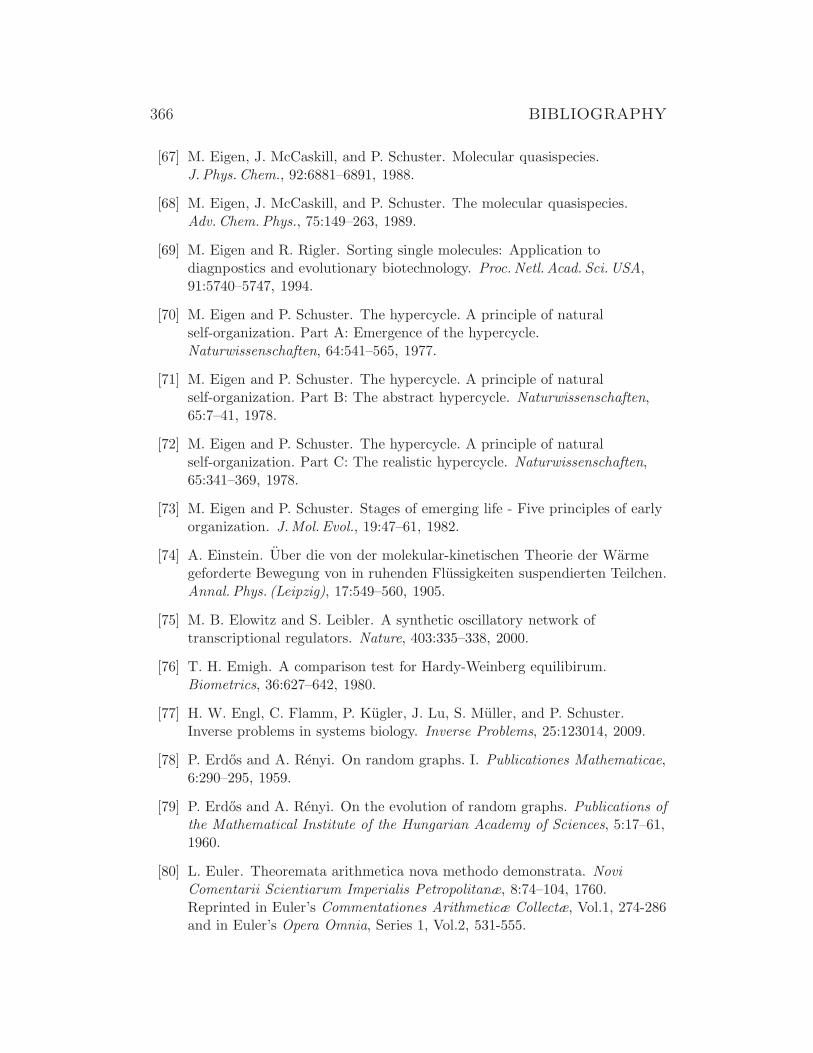
366 BIBLIOGRAPHY
[67] M. Eigen, J. McCaskill, and P. Schuster. Molecular quasispecies.J. Phys. Chem., 92:6881–6891, 1988.
[68] M. Eigen, J. McCaskill, and P. Schuster. The molecular quasispecies.Adv. Chem. Phys., 75:149–263, 1989.
[69] M. Eigen and R. Rigler. Sorting single molecules: Application todiagnpostics and evolutionary biotechnology. Proc. Netl. Acad. Sci. USA,91:5740–5747, 1994.
[70] M. Eigen and P. Schuster. The hypercycle. A principle of naturalself-organization. Part A: Emergence of the hypercycle.Naturwissenschaften, 64:541–565, 1977.
[71] M. Eigen and P. Schuster. The hypercycle. A principle of naturalself-organization. Part B: The abstract hypercycle. Naturwissenschaften,65:7–41, 1978.
[72] M. Eigen and P. Schuster. The hypercycle. A principle of naturalself-organization. Part C: The realistic hypercycle. Naturwissenschaften,65:341–369, 1978.
[73] M. Eigen and P. Schuster. Stages of emerging life - Five principles of earlyorganization. J.Mol. Evol., 19:47–61, 1982.
[74] A. Einstein. Uber die von der molekular-kinetischen Theorie der Warmegeforderte Bewegung von in ruhenden Flussigkeiten suspendierten Teilchen.Annal. Phys. (Leipzig), 17:549–560, 1905.
[75] M. B. Elowitz and S. Leibler. A synthetic oscillatory network oftranscriptional regulators. Nature, 403:335–338, 2000.
[76] T. H. Emigh. A comparison test for Hardy-Weinberg equilibirum.Biometrics, 36:627–642, 1980.
[77] H. W. Engl, C. Flamm, P. Kugler, J. Lu, S. Muller, and P. Schuster.Inverse problems in systems biology. Inverse Problems, 25:123014, 2009.
[78] P. Erdos and A. Renyi. On random graphs. I. Publicationes Mathematicae,6:290–295, 1959.
[79] P. Erdos and A. Renyi. On the evolution of random graphs. Publications ofthe Mathematical Institute of the Hungarian Academy of Sciences, 5:17–61,1960.
[80] L. Euler. Theoremata arithmetica nova methodo demonstrata. NoviComentarii Scientiarum Imperialis Petropolitanæ, 8:74–104, 1760.Reprinted in Euler’s Commentationes Arithmeticæ Collectæ, Vol.1, 274-286and in Euler’s Opera Omnia, Series 1, Vol.2, 531-555.
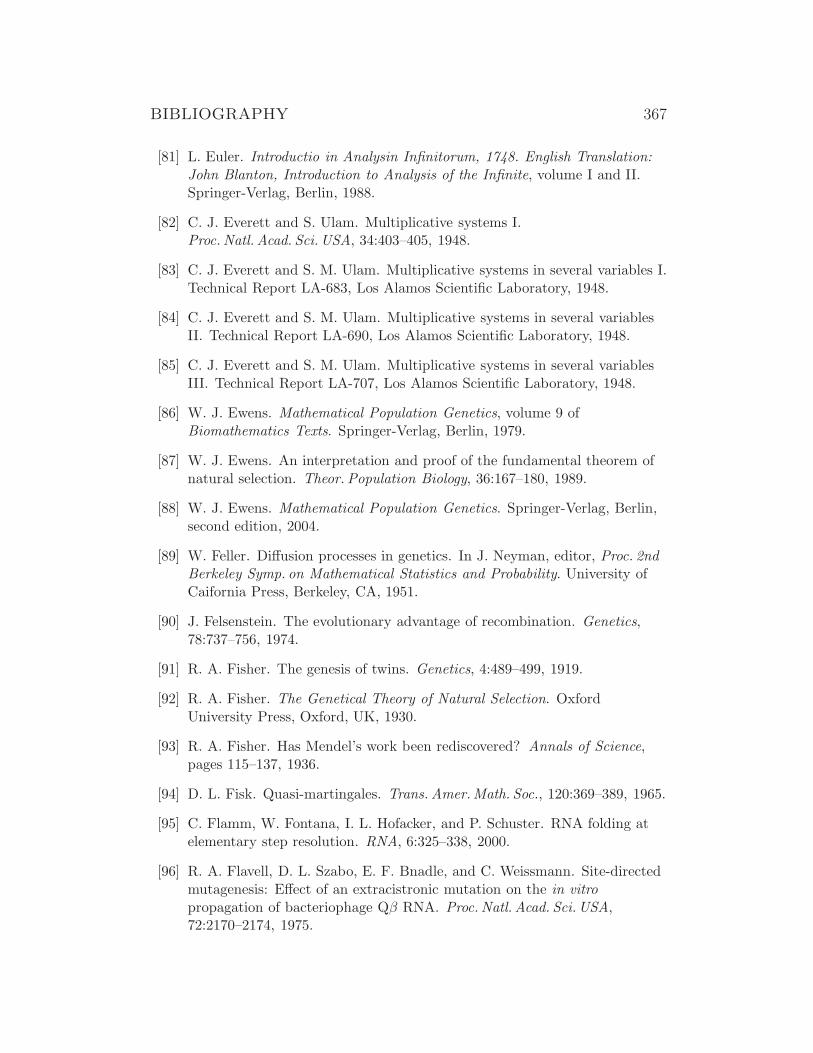
BIBLIOGRAPHY 367
[81] L. Euler. Introductio in Analysin Infinitorum, 1748. English Translation:John Blanton, Introduction to Analysis of the Infinite, volume I and II.Springer-Verlag, Berlin, 1988.
[82] C. J. Everett and S. Ulam. Multiplicative systems I.Proc. Natl. Acad. Sci. USA, 34:403–405, 1948.
[83] C. J. Everett and S. M. Ulam. Multiplicative systems in several variables I.Technical Report LA-683, Los Alamos Scientific Laboratory, 1948.
[84] C. J. Everett and S. M. Ulam. Multiplicative systems in several variablesII. Technical Report LA-690, Los Alamos Scientific Laboratory, 1948.
[85] C. J. Everett and S. M. Ulam. Multiplicative systems in several variablesIII. Technical Report LA-707, Los Alamos Scientific Laboratory, 1948.
[86] W. J. Ewens. Mathematical Population Genetics, volume 9 ofBiomathematics Texts. Springer-Verlag, Berlin, 1979.
[87] W. J. Ewens. An interpretation and proof of the fundamental theorem ofnatural selection. Theor. Population Biology, 36:167–180, 1989.
[88] W. J. Ewens. Mathematical Population Genetics. Springer-Verlag, Berlin,second edition, 2004.
[89] W. Feller. Diffusion processes in genetics. In J. Neyman, editor, Proc. 2ndBerkeley Symp. on Mathematical Statistics and Probability. University ofCaifornia Press, Berkeley, CA, 1951.
[90] J. Felsenstein. The evolutionary advantage of recombination. Genetics,78:737–756, 1974.
[91] R. A. Fisher. The genesis of twins. Genetics, 4:489–499, 1919.
[92] R. A. Fisher. The Genetical Theory of Natural Selection. OxfordUniversity Press, Oxford, UK, 1930.
[93] R. A. Fisher. Has Mendel’s work been rediscovered? Annals of Science,pages 115–137, 1936.
[94] D. L. Fisk. Quasi-martingales. Trans. Amer.Math. Soc., 120:369–389, 1965.
[95] C. Flamm, W. Fontana, I. L. Hofacker, and P. Schuster. RNA folding atelementary step resolution. RNA, 6:325–338, 2000.
[96] R. A. Flavell, D. L. Szabo, E. F. Bnadle, and C. Weissmann. Site-directedmutagenesis: Effect of an extracistronic mutation on the in vitropropagation of bacteriophage Qβ RNA. Proc. Natl. Acad. Sci. USA,72:2170–2174, 1975.
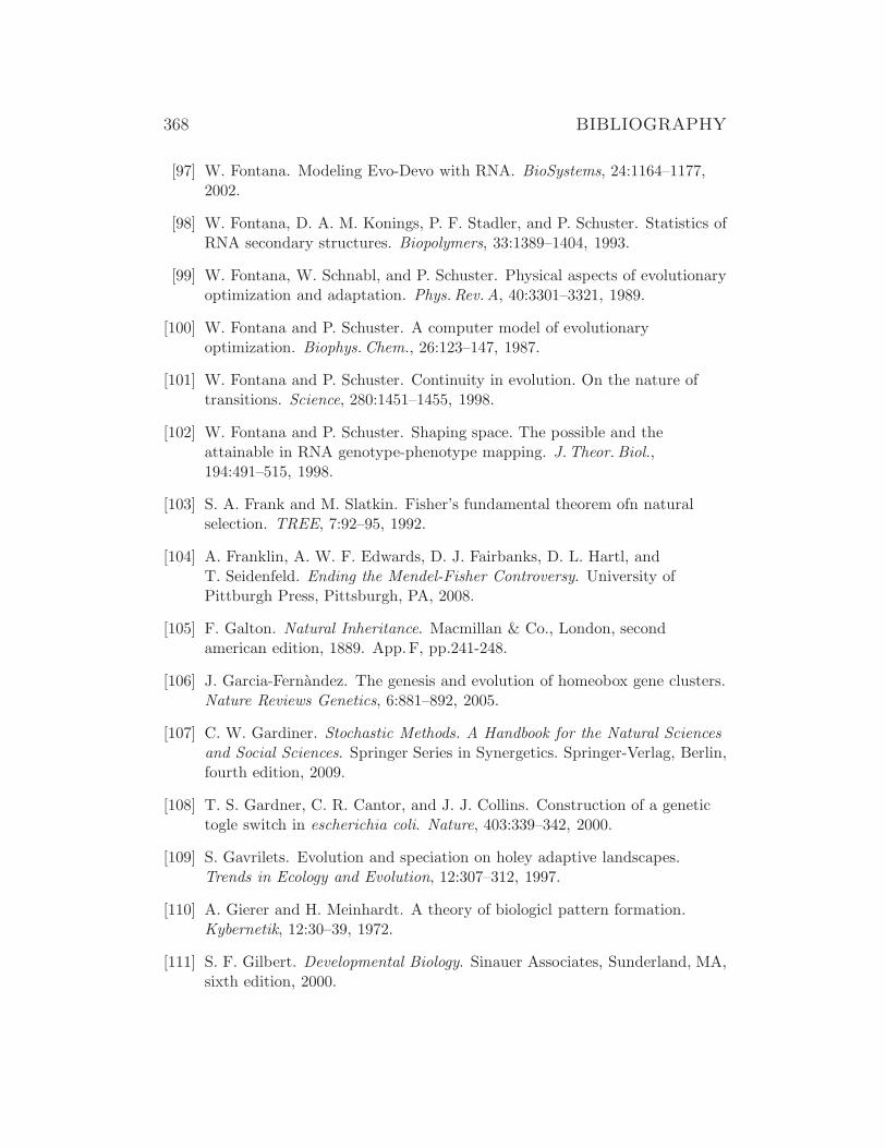
368 BIBLIOGRAPHY
[97] W. Fontana. Modeling Evo-Devo with RNA. BioSystems, 24:1164–1177,2002.
[98] W. Fontana, D. A. M. Konings, P. F. Stadler, and P. Schuster. Statistics ofRNA secondary structures. Biopolymers, 33:1389–1404, 1993.
[99] W. Fontana, W. Schnabl, and P. Schuster. Physical aspects of evolutionaryoptimization and adaptation. Phys. Rev.A, 40:3301–3321, 1989.
[100] W. Fontana and P. Schuster. A computer model of evolutionaryoptimization. Biophys. Chem., 26:123–147, 1987.
[101] W. Fontana and P. Schuster. Continuity in evolution. On the nature oftransitions. Science, 280:1451–1455, 1998.
[102] W. Fontana and P. Schuster. Shaping space. The possible and theattainable in RNA genotype-phenotype mapping. J.Theor. Biol.,194:491–515, 1998.
[103] S. A. Frank and M. Slatkin. Fisher’s fundamental theorem ofn naturalselection. TREE, 7:92–95, 1992.
[104] A. Franklin, A. W. F. Edwards, D. J. Fairbanks, D. L. Hartl, andT. Seidenfeld. Ending the Mendel-Fisher Controversy. University ofPittburgh Press, Pittsburgh, PA, 2008.
[105] F. Galton. Natural Inheritance. Macmillan & Co., London, secondamerican edition, 1889. App.F, pp.241-248.
[106] J. Garcia-Fernandez. The genesis and evolution of homeobox gene clusters.Nature Reviews Genetics, 6:881–892, 2005.
[107] C. W. Gardiner. Stochastic Methods. A Handbook for the Natural Sciencesand Social Sciences. Springer Series in Synergetics. Springer-Verlag, Berlin,fourth edition, 2009.
[108] T. S. Gardner, C. R. Cantor, and J. J. Collins. Construction of a genetictogle switch in escherichia coli. Nature, 403:339–342, 2000.
[109] S. Gavrilets. Evolution and speciation on holey adaptive landscapes.Trends in Ecology and Evolution, 12:307–312, 1997.
[110] A. Gierer and H. Meinhardt. A theory of biologicl pattern formation.Kybernetik, 12:30–39, 1972.
[111] S. F. Gilbert. Developmental Biology. Sinauer Associates, Sunderland, MA,sixth edition, 2000.

BIBLIOGRAPHY 369
[112] D. T. Gillespie. A general method for numerically simulating the stochastictime evolution of coupled chemical reactions. J.Comp. Phys., 22:403–434,1976.
[113] D. T. Gillespie. Exact stochastic simulation of coupled chemical reactions.J. Phys. Chem., 81:2340–2361, 1977.
[114] D. T. Gillespie. Markov Processes: An Introduction for Physical Scientists.Academic Press, San Diego, CA, 1992.
[115] D. T. Gillespie. A rigorous derivation of the chemical master equation.Physica A, 188:404–425, 1992.
[116] D. T. Gillespie. Exact numerical simulation of the Ornstein-Uhlenbeckprocess and its integral. Phys. Rev. E, 54:2084–2091, 1996.
[117] D. T. Gillespie. Stochastic simulation of chemical kinetics.Annu.Rev. Phys. Chem., 58:35–55, 2007.
[118] N. S. Goel and N. Richter-Dyn. Stochastic Models in Biology. AcademicPress, New York, 1974.
[119] P. Gonczy and L. S. Rose. Asymmetric cell division and axis formation inthe embryo. In TheC. elegans Research Community, editor, WormBook.1.30.1. http://www.wormbook.org, WormBook, 2005.
[120] C. J. Goodnight and M. J. Wade. The ongoing synthesis: A reply toCoyne, Barton and Turelli. Evolution, 54:317–324, 2000.
[121] M. Gosch and R. Rigler. Fluorescence correlation spectroscopy of molecularmotions and kinetics. Advanced Drug Delivery Reviews, 57:169–190, 2005.
[122] S. Gottesman. The small RNA regulators of escherichia coli: Roles andmechanisms. Annu.Rev.Microbiol., 58:303–328, 2004.
[123] I. S. Gradstein and I. M. Ryshik. Tables of Series, Products, and Integrals,volume 1. Verlag Harri Deutsch, Thun, DE, 1981. In German and English.Translated from Russian by Ludwig Boll, Berlin.
[124] R. L. Graham, D. E. Knuth, and O. Patashnik. Concrete Mathematics.Addison-Wesley Publishing Co., Reading, MA, second edition, 1994.
[125] A. J. F. Griffiths, J. H. Miller, D. T. Suzuki, R. C. Lewontin, and W. M.Gelbart. An Introduction to Genetic Analysis. W. H. Freeman, New York,seventh edition, 2000.
[126] W. Gruner, R. Giegerich, D. Strothmann, C. Reidys, J. Weber, I. L.Hofacker, and P. Schuster. Analysis of RNA sequence structure maps byexhaustive enumeration. I. Neutral networks. Mh.Chem., 127:355–374,1996.
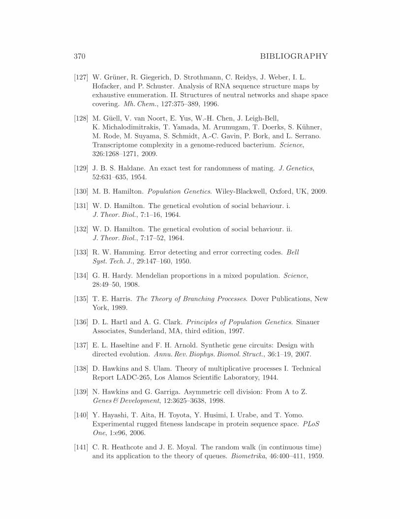
370 BIBLIOGRAPHY
[127] W. Gruner, R. Giegerich, D. Strothmann, C. Reidys, J. Weber, I. L.Hofacker, and P. Schuster. Analysis of RNA sequence structure maps byexhaustive enumeration. II. Structures of neutral networks and shape spacecovering. Mh.Chem., 127:375–389, 1996.
[128] M. Guell, V. van Noort, E. Yus, W.-H. Chen, J. Leigh-Bell,K. Michalodimitrakis, T. Yamada, M. Arumugam, T. Doerks, S. Kuhner,M. Rode, M. Suyama, S. Schmidt, A.-C. Gavin, P. Bork, and L. Serrano.Transcriptome complexity in a genome-reduced bacterium. Science,326:1268–1271, 2009.
[129] J. B. S. Haldane. An exact test for randomness of mating. J.Genetics,52:631–635, 1954.
[130] M. B. Hamilton. Population Genetics. Wiley-Blackwell, Oxford, UK, 2009.
[131] W. D. Hamilton. The genetical evolution of social behaviour. i.J.Theor. Biol., 7:1–16, 1964.
[132] W. D. Hamilton. The genetical evolution of social behaviour. ii.J.Theor. Biol., 7:17–52, 1964.
[133] R. W. Hamming. Error detecting and error correcting codes. BellSyst. Tech. J., 29:147–160, 1950.
[134] G. H. Hardy. Mendelian proportions in a mixed population. Science,28:49–50, 1908.
[135] T. E. Harris. The Theory of Branching Processes. Dover Publications, NewYork, 1989.
[136] D. L. Hartl and A. G. Clark. Principles of Population Genetics. SinauerAssociates, Sunderland, MA, third edition, 1997.
[137] E. L. Haseltine and F. H. Arnold. Synthetic gene circuits: Design withdirected evolution. Annu.Rev. Biophys. Biomol. Struct., 36:1–19, 2007.
[138] D. Hawkins and S. Ulam. Theory of multiplicative processes I. TechnicalReport LADC-265, Los Alamos Scientific Laboratory, 1944.
[139] N. Hawkins and G. Garriga. Asymmetric cell division: From A to Z.Genes&Development, 12:3625–3638, 1998.
[140] Y. Hayashi, T. Aita, H. Toyota, Y. Husimi, I. Urabe, and T. Yomo.Experimental rugged fiteness landscape in protein sequence space. PLoSOne, 1:e96, 2006.
[141] C. R. Heathcote and J. E. Moyal. The random walk (in continuous time)and its application to the theory of queues. Biometrika, 46:400–411, 1959.
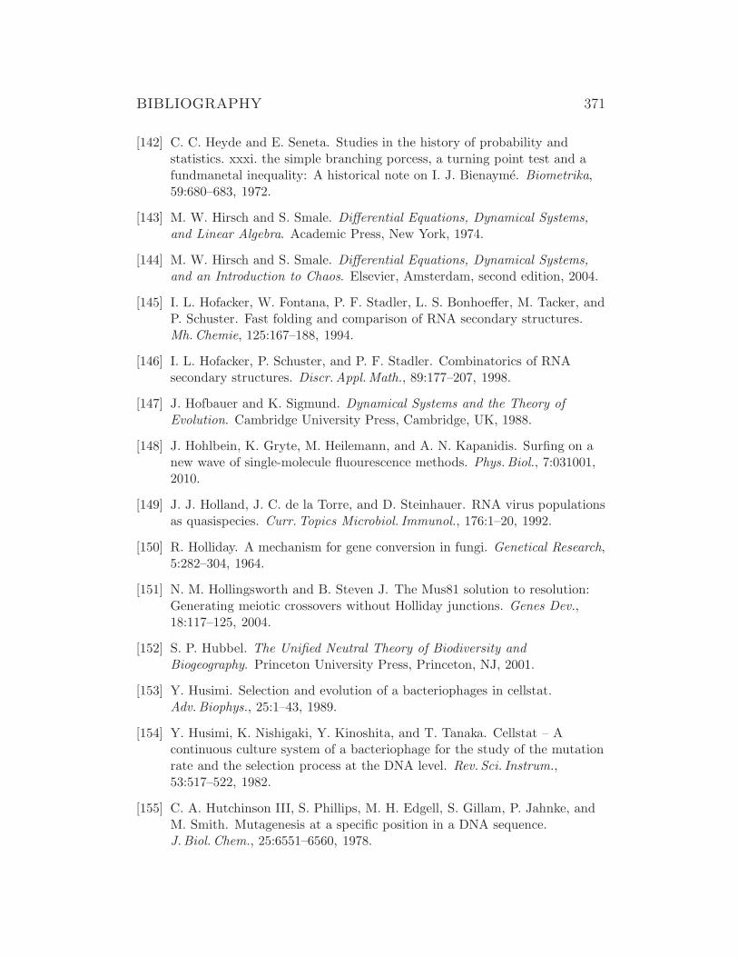
BIBLIOGRAPHY 371
[142] C. C. Heyde and E. Seneta. Studies in the history of probability andstatistics. xxxi. the simple branching porcess, a turning point test and afundmanetal inequality: A historical note on I. J. Bienayme. Biometrika,59:680–683, 1972.
[143] M. W. Hirsch and S. Smale. Differential Equations, Dynamical Systems,and Linear Algebra. Academic Press, New York, 1974.
[144] M. W. Hirsch and S. Smale. Differential Equations, Dynamical Systems,and an Introduction to Chaos. Elsevier, Amsterdam, second edition, 2004.
[145] I. L. Hofacker, W. Fontana, P. F. Stadler, L. S. Bonhoeffer, M. Tacker, andP. Schuster. Fast folding and comparison of RNA secondary structures.Mh.Chemie, 125:167–188, 1994.
[146] I. L. Hofacker, P. Schuster, and P. F. Stadler. Combinatorics of RNAsecondary structures. Discr.Appl.Math., 89:177–207, 1998.
[147] J. Hofbauer and K. Sigmund. Dynamical Systems and the Theory ofEvolution. Cambridge University Press, Cambridge, UK, 1988.
[148] J. Hohlbein, K. Gryte, M. Heilemann, and A. N. Kapanidis. Surfing on anew wave of single-molecule fluourescence methods. Phys. Biol., 7:031001,2010.
[149] J. J. Holland, J. C. de la Torre, and D. Steinhauer. RNA virus populationsas quasispecies. Curr. Topics Microbiol. Immunol., 176:1–20, 1992.
[150] R. Holliday. A mechanism for gene conversion in fungi. Genetical Research,5:282–304, 1964.
[151] N. M. Hollingsworth and B. Steven J. The Mus81 solution to resolution:Generating meiotic crossovers without Holliday junctions. Genes Dev.,18:117–125, 2004.
[152] S. P. Hubbel. The Unified Neutral Theory of Biodiversity andBiogeography. Princeton University Press, Princeton, NJ, 2001.
[153] Y. Husimi. Selection and evolution of a bacteriophages in cellstat.Adv. Biophys., 25:1–43, 1989.
[154] Y. Husimi, K. Nishigaki, Y. Kinoshita, and T. Tanaka. Cellstat – Acontinuous culture system of a bacteriophage for the study of the mutationrate and the selection process at the DNA level. Rev. Sci. Instrum.,53:517–522, 1982.
[155] C. A. Hutchinson III, S. Phillips, M. H. Edgell, S. Gillam, P. Jahnke, andM. Smith. Mutagenesis at a specific position in a DNA sequence.J.Biol. Chem., 25:6551–6560, 1978.
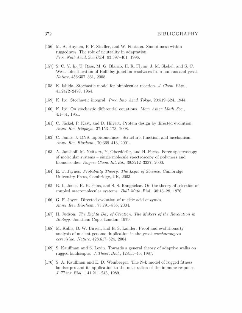
372 BIBLIOGRAPHY
[156] M. A. Huynen, P. F. Stadler, and W. Fontana. Smoothness withinruggedness. The role of neutrality in adaptation.Proc. Natl. Acad. Sci. USA, 93:397–401, 1996.
[157] S. C. Y. Ip, U. Rass, M. G. Blanco, H. R. Flynn, J. M. Skehel, and S. C.West. Identification of Holliday junction resolvases from humans and yeast.Nature, 456:357–361, 2008.
[158] K. Ishida. Stochastic model for bimolecular reaction. J.Chem. Phys.,41:2472–2478, 1964.
[159] K. Ito. Stochastic integral. Proc. Imp. Acad. Tokyo, 20:519–524, 1944.
[160] K. Ito. On stochastic differential equations. Mem.Amer.Math. Soc.,4:1–51, 1951.
[161] C. Jackel, P. Kast, and D. Hilvert. Protein design by directed evolution.Annu.Rev. Biophys., 37:153–173, 2008.
[162] C. James J. DNA topoisomerases: Structure, function, and mechanism.Annu.Rev. Biochem., 70:369–413, 2001.
[163] A. Janshoff, M. Neitzert, Y. Oberdorfer, and H. Fuchs. Force spectroscopyof molecular systems – single molecule spectroscopy of polymers andbiomolecules. Angew.Chem. Int. Ed., 39:3212–3237, 2000.
[164] E. T. Jaynes. Probability Theory. The Logic of Science. CambridgeUniversity Press, Cambridge, UK, 2003.
[165] B. L. Jones, R. H. Enns, and S. S. Rangnekar. On the theory of selection ofcoupled macromolecular systems. Bull.Math. Biol., 38:15–28, 1976.
[166] G. F. Joyce. Directed evolution of nucleic acid enzymes.Annu.Rev. Biochem., 73:791–836, 2004.
[167] H. Judson. The Eighth Day of Creation. The Makers of the Revolution inBiology. Jonathan Cape, London, 1979.
[168] M. Kallis, B. W. Birren, and E. S. Lander. Proof and evolutionartyanalysis of ancient genome duplication in the yeast saccharomycescerevisiae. Nature, 428:617–624, 2004.
[169] S. Kauffman and S. Levin. Towards a general theory of adaptive walks onrugged landscapes. J.Theor. Biol., 128:11–45, 1987.
[170] S. A. Kauffman and E. D. Weinberger. The N-k model of rugged fitnesslandscapes and its application to the maturation of the immune response.J.Theor. Biol., 141:211–245, 1989.
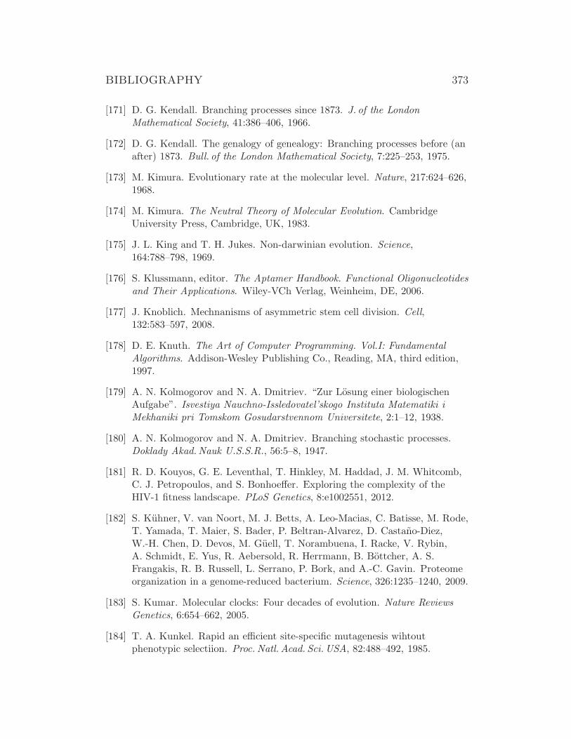
BIBLIOGRAPHY 373
[171] D. G. Kendall. Branching processes since 1873. J. of the LondonMathematical Society, 41:386–406, 1966.
[172] D. G. Kendall. The genalogy of genealogy: Branching processes before (anafter) 1873. Bull. of the London Mathematical Society, 7:225–253, 1975.
[173] M. Kimura. Evolutionary rate at the molecular level. Nature, 217:624–626,1968.
[174] M. Kimura. The Neutral Theory of Molecular Evolution. CambridgeUniversity Press, Cambridge, UK, 1983.
[175] J. L. King and T. H. Jukes. Non-darwinian evolution. Science,164:788–798, 1969.
[176] S. Klussmann, editor. The Aptamer Handbook. Functional Oligonucleotidesand Their Applications. Wiley-VCh Verlag, Weinheim, DE, 2006.
[177] J. Knoblich. Mechnanisms of asymmetric stem cell division. Cell,132:583–597, 2008.
[178] D. E. Knuth. The Art of Computer Programming. Vol.I: FundamentalAlgorithms. Addison-Wesley Publishing Co., Reading, MA, third edition,1997.
[179] A. N. Kolmogorov and N. A. Dmitriev. “Zur Losung einer biologischenAufgabe”. Isvestiya Nauchno-Issledovatel’skogo Instituta Matematiki iMekhaniki pri Tomskom Gosudarstvennom Universitete, 2:1–12, 1938.
[180] A. N. Kolmogorov and N. A. Dmitriev. Branching stochastic processes.Doklady Akad.Nauk U.S.S.R., 56:5–8, 1947.
[181] R. D. Kouyos, G. E. Leventhal, T. Hinkley, M. Haddad, J. M. Whitcomb,C. J. Petropoulos, and S. Bonhoeffer. Exploring the complexity of theHIV-1 fitness landscape. PLoS Genetics, 8:e1002551, 2012.
[182] S. Kuhner, V. van Noort, M. J. Betts, A. Leo-Macias, C. Batisse, M. Rode,T. Yamada, T. Maier, S. Bader, P. Beltran-Alvarez, D. Castano-Diez,W.-H. Chen, D. Devos, M. Guell, T. Norambuena, I. Racke, V. Rybin,A. Schmidt, E. Yus, R. Aebersold, R. Herrmann, B. Bottcher, A. S.Frangakis, R. B. Russell, L. Serrano, P. Bork, and A.-C. Gavin. Proteomeorganization in a genome-reduced bacterium. Science, 326:1235–1240, 2009.
[183] S. Kumar. Molecular clocks: Four decades of evolution. Nature ReviewsGenetics, 6:654–662, 2005.
[184] T. A. Kunkel. Rapid an efficient site-specific mutagenesis wihtoutphenotypic selectiion. Proc. Natl. Acad. Sci. USA, 82:488–492, 1985.
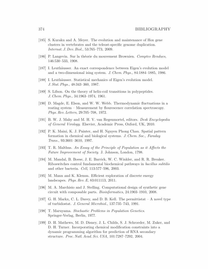
374 BIBLIOGRAPHY
[185] S. Kuraku and A. Meyer. The evolution and maintenance of Hox geneclusters in vertebrates and the teleost-specific genome duplication.Internat. J.Dev.Biol., 53:765–773, 2009.
[186] P. Langevin. Sur la theorie du mouvement Brownien. Comptes Rendues,146:530–533, 1908.
[187] I. Leuthausser. An exact correspondence between Eigen’s evolution modeland a two-dimensional ising system. J.Chem. Phys., 84:1884–1885, 1986.
[188] I. Leuthausser. Statistical mechanics of Eigen’s evolution model.J. Stat. Phys., 48:343–360, 1987.
[189] S. Lifson. On the theory of helix-coil transitions in polypeptides.J.Chem. Phys., 34:1963–1974, 1961.
[190] D. Magde, E. Elson, and W. W. Webb. Thermodynamic fluctuations in areating system – Measurement by flourescence correlation spectroscopy.Phys. Rev. Letters, 29:705–708, 1972.
[191] B. W. J. Mahy and M. H. V. van Regenmortel, editors. Desk Encyclopediaof General Virology. Elsevier, Academic Press, Oxford, UK, 2010.
[192] P. K. Maini, K. J. Painter, and H. Nguyen Phong Chau. Spatial patternformation in chemical and biological systems. J.Chem. Soc., FaradayTrans., 93:3601–3610, 1997.
[193] T. R. Malthus. An Essay of the Principle of Population as it Affects theFuture Improvement of Society. J. Johnson, London, 1798.
[194] M. Mandal, B. Boese, J. E. Barrick, W. C. Winkler, and R. R. Breaker.Riboswitches control fundamental biochemical pathways in bacillus subtilisand other bacteria. Cell, 113:577–596, 2003.
[195] M. Mann and K. Klemm. Efficient exploration of discrete energylandscapes. Phys. Rev. E, 83:011113, 2011.
[196] M. A. Marchisio and J. Stelling. Computational design of synthetic genecircuit with composable parts. Bioinformatics, 24:1903–1910, 2008.
[197] G. H. Markx, C. L. Davey, and D. B. Kell. The permittistat – A novel typeof turbidostat. J.General Microbiol., 137:735–743, 1991.
[198] T. Maruyama. Stochastic Problems in Population Genetics.Springer-Verlag, Berlin, 1977.
[199] D. H. Mathews, M. D. Disney, J. L. Childs, S. J. Schroeder, M. Zuker, andD. H. Turner. Incorporating chemical modification constraints into adynamic programming algorithm for prediction of RNA secondarystructure. Proc. Natl. Acad. Sci. USA, 101:7287–7292, 2004.
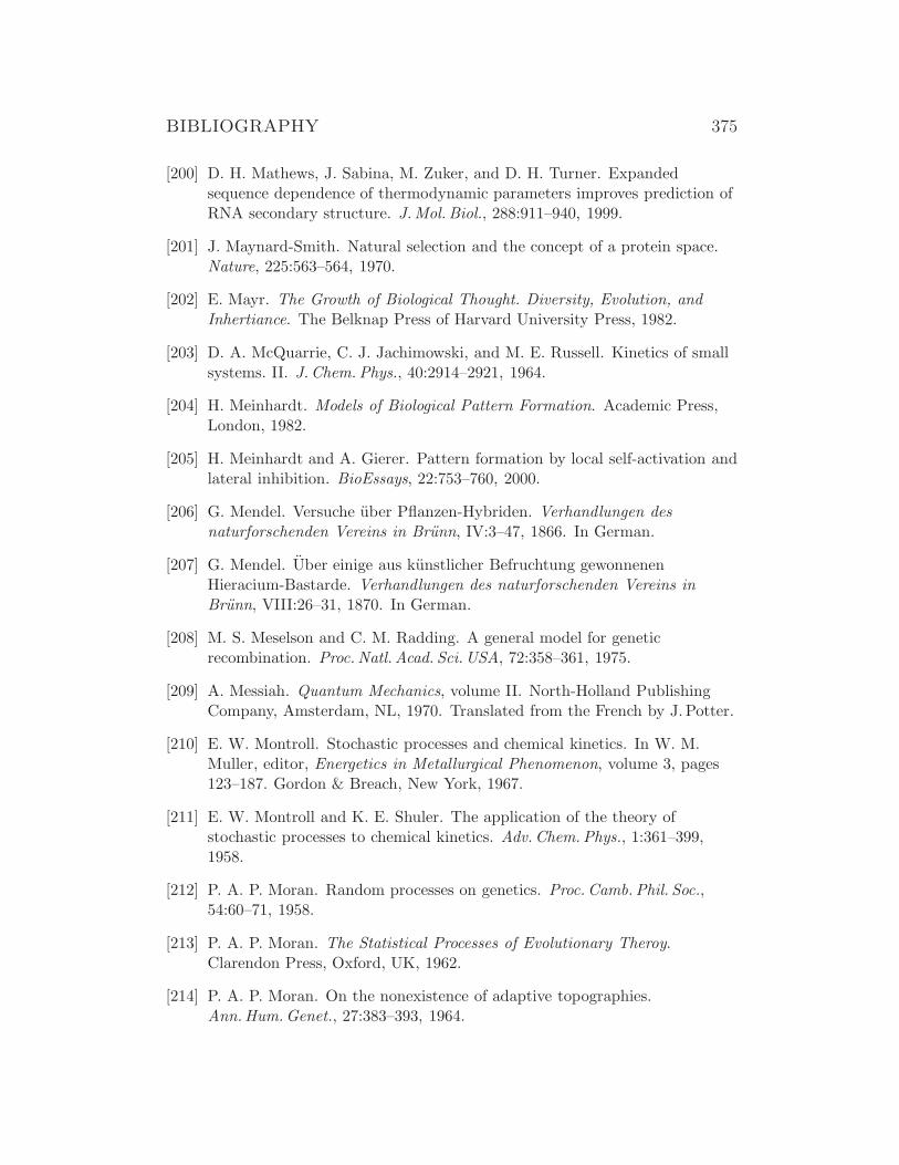
BIBLIOGRAPHY 375
[200] D. H. Mathews, J. Sabina, M. Zuker, and D. H. Turner. Expandedsequence dependence of thermodynamic parameters improves prediction ofRNA secondary structure. J.Mol. Biol., 288:911–940, 1999.
[201] J. Maynard-Smith. Natural selection and the concept of a protein space.Nature, 225:563–564, 1970.
[202] E. Mayr. The Growth of Biological Thought. Diversity, Evolution, andInhertiance. The Belknap Press of Harvard University Press, 1982.
[203] D. A. McQuarrie, C. J. Jachimowski, and M. E. Russell. Kinetics of smallsystems. II. J.Chem. Phys., 40:2914–2921, 1964.
[204] H. Meinhardt. Models of Biological Pattern Formation. Academic Press,London, 1982.
[205] H. Meinhardt and A. Gierer. Pattern formation by local self-activation andlateral inhibition. BioEssays, 22:753–760, 2000.
[206] G. Mendel. Versuche uber Pflanzen-Hybriden. Verhandlungen desnaturforschenden Vereins in Brunn, IV:3–47, 1866. In German.
[207] G. Mendel. Uber einige aus kunstlicher Befruchtung gewonnenenHieracium-Bastarde. Verhandlungen des naturforschenden Vereins inBrunn, VIII:26–31, 1870. In German.
[208] M. S. Meselson and C. M. Radding. A general model for geneticrecombination. Proc. Natl. Acad. Sci. USA, 72:358–361, 1975.
[209] A. Messiah. Quantum Mechanics, volume II. North-Holland PublishingCompany, Amsterdam, NL, 1970. Translated from the French by J. Potter.
[210] E. W. Montroll. Stochastic processes and chemical kinetics. In W. M.Muller, editor, Energetics in Metallurgical Phenomenon, volume 3, pages123–187. Gordon & Breach, New York, 1967.
[211] E. W. Montroll and K. E. Shuler. The application of the theory ofstochastic processes to chemical kinetics. Adv. Chem. Phys., 1:361–399,1958.
[212] P. A. P. Moran. Random processes on genetics. Proc. Camb. Phil. Soc.,54:60–71, 1958.
[213] P. A. P. Moran. The Statistical Processes of Evolutionary Theroy.Clarendon Press, Oxford, UK, 1962.
[214] P. A. P. Moran. On the nonexistence of adaptive topographies.Ann.Hum.Genet., 27:383–393, 1964.

376 BIBLIOGRAPHY
[215] D. W. Mount. Bioinformatics. Sequence and Genome Analysis. ColdSpring Harbor Laboratory Press, Cold Spring Harbor, NY, second edition,2004.
[216] A. E. Mourant, A. Kopec, and K. Domaniewska-Sobczak. The Distributionof Human Blood Groups and Other Polymorphisms. Oxford UniversityPress, New York, second edition, 1976.
[217] S. Munoz-Galvan, C. Tous, M. G. Blanco, E. K. Schwartz, K. T. Emsen,S. C. West, Wolf-Dietrich, and A. Aguilera. Distinct roles of Mus81, Yen1,Slx1-Slx4, and Rad1 nucleases in the repair of replication-borndouble-strand breaks by sister chromatid exchange. Molecular and CellularBiology, 32:1592–1603, 2012.
[218] H. J. Muller. Variation due to change in the individual gene. AmericanNaturalist, 56:32–50, 1922.
[219] H. J. Muller. Artificial transmutation of the gene. Science, 66:84–87, 1927.
[220] H. J. Muller. Some genetic aspects of sex. American Naturalist,66:118–138, 1932.
[221] H. J. Muller. The relation of recombination to mutational advance.Mutat. Res., 106:2–9, 1964.
[222] K. Nasmyth. Disseminating the genome: Joining, resolving, and separatingsister chromatids during mitosis and meiosis. Annu.Rev.Genet.,35:673–745, 2001.
[223] G. Nicolis and I. Prigogine. Self-Organization in Nonequilibrium Systems.John Wiley & Sons, New York, 1977.
[224] M. Nowak and P. Schuster. Error thresholds of replication in finitepopulations. Mutation frequencies and the onset of Muller’s ratchet.J.Theor. Biol., 137:375–395, 1989.
[225] M. Nowak, C. E. Tarnita, and E. O. Wilson. The evolution of eusociality.Nature, 466:1057–1062, 2010.
[226] S. Ohno. Evolution by Gene Duplication. Springer-Verlag, New York, 1970.
[227] T. Ohta. Mechanisms of molecular evolution. Phil. Trans. Roy. Soc. LondonB, 355:1623–1626, 2000.
[228] S. Okasha. Fisher’s fundamental theorem of natural selection – Aphilosophical analysis. Brit. J. Phil. Sci., 59:319–351, 2008.
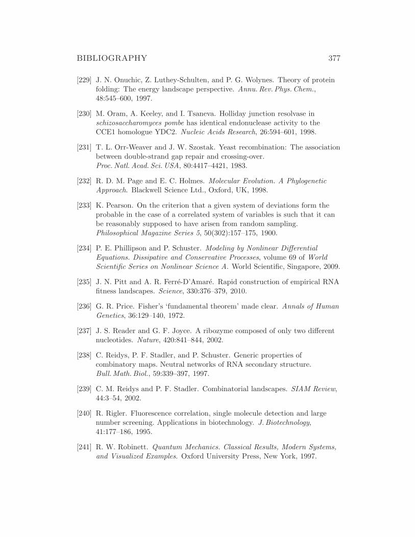
BIBLIOGRAPHY 377
[229] J. N. Onuchic, Z. Luthey-Schulten, and P. G. Wolynes. Theory of proteinfolding: The energy landscape perspective. Annu.Rev. Phys. Chem.,48:545–600, 1997.
[230] M. Oram, A. Keeley, and I. Tsaneva. Holliday junction resolvase inschizosaccharomyces pombe has identical endonuclease activity to theCCE1 homologue YDC2. Nucleic Acids Research, 26:594–601, 1998.
[231] T. L. Orr-Weaver and J. W. Szostak. Yeast recombination: The associationbetween double-strand gap repair and crossing-over.Proc. Natl. Acad. Sci. USA, 80:4417–4421, 1983.
[232] R. D. M. Page and E. C. Holmes. Molecular Evolution. A PhylogeneticApproach. Blackwell Science Ltd., Oxford, UK, 1998.
[233] K. Pearson. On the criterion that a given system of deviations form theprobable in the case of a correlated system of variables is such that it canbe reasonably supposed to have arisen from random sampling.Philosophical Magazine Series 5, 50(302):157–175, 1900.
[234] P. E. Phillipson and P. Schuster. Modeling by Nonlinear DifferentialEquations. Dissipative and Conservative Processes, volume 69 of WorldScientific Series on Nonlinear Science A. World Scientific, Singapore, 2009.
[235] J. N. Pitt and A. R. Ferre-D’Amare. Rapid construction of empirical RNAfitness landscapes. Science, 330:376–379, 2010.
[236] G. R. Price. Fisher’s ‘fundamental theorem’ made clear. Annals of HumanGenetics, 36:129–140, 1972.
[237] J. S. Reader and G. F. Joyce. A ribozyme composed of only two differentnucleotides. Nature, 420:841–844, 2002.
[238] C. Reidys, P. F. Stadler, and P. Schuster. Generic properties ofcombinatory maps. Neutral networks of RNA secondary structure.Bull.Math. Biol., 59:339–397, 1997.
[239] C. M. Reidys and P. F. Stadler. Combinatorial landscapes. SIAM Review,44:3–54, 2002.
[240] R. Rigler. Fluorescence correlation, single molecule detection and largenumber screening. Applications in biotechnology. J.Biotechnology,41:177–186, 1995.
[241] R. W. Robinett. Quantum Mechanics. Classical Results, Modern Systems,and Visualized Examples. Oxford University Press, New York, 1997.
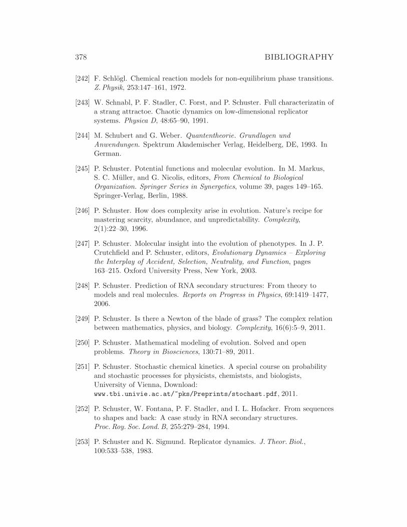
378 BIBLIOGRAPHY
[242] F. Schlogl. Chemical reaction models for non-equilibrium phase transitions.Z.Physik, 253:147–161, 1972.
[243] W. Schnabl, P. F. Stadler, C. Forst, and P. Schuster. Full characterizatin ofa strang attractoe. Chaotic dynamics on low-dimensional replicatorsystems. Physica D, 48:65–90, 1991.
[244] M. Schubert and G. Weber. Quantentheorie. Grundlagen undAnwendungen. Spektrum Akademischer Verlag, Heidelberg, DE, 1993. InGerman.
[245] P. Schuster. Potential functions and molecular evolution. In M. Markus,S. C. Muller, and G. Nicolis, editors, From Chemical to BiologicalOrganization. Springer Series in Synergetics, volume 39, pages 149–165.Springer-Verlag, Berlin, 1988.
[246] P. Schuster. How does complexity arise in evolution. Nature’s recipe formastering scarcity, abundance, and unpredictability. Complexity,2(1):22–30, 1996.
[247] P. Schuster. Molecular insight into the evolution of phenotypes. In J. P.Crutchfield and P. Schuster, editors, Evolutionary Dynamics – Exploringthe Interplay of Accident, Selection, Neutrality, and Function, pages163–215. Oxford University Press, New York, 2003.
[248] P. Schuster. Prediction of RNA secondary structures: From theory tomodels and real molecules. Reports on Progress in Physics, 69:1419–1477,2006.
[249] P. Schuster. Is there a Newton of the blade of grass? The complex relationbetween mathematics, physics, and biology. Complexity, 16(6):5–9, 2011.
[250] P. Schuster. Mathematical modeling of evolution. Solved and openproblems. Theory in Biosciences, 130:71–89, 2011.
[251] P. Schuster. Stochastic chemical kinetics. A special course on probabilityand stochastic processes for physicists, chemiststs, and biologists,University of Vienna, Download:www.tbi.univie.ac.at/~pks/Preprints/stochast.pdf, 2011.
[252] P. Schuster, W. Fontana, P. F. Stadler, and I. L. Hofacker. From sequencesto shapes and back: A case study in RNA secondary structures.Proc. Roy. Soc. Lond. B, 255:279–284, 1994.
[253] P. Schuster and K. Sigmund. Replicator dynamics. J.Theor. Biol.,100:533–538, 1983.
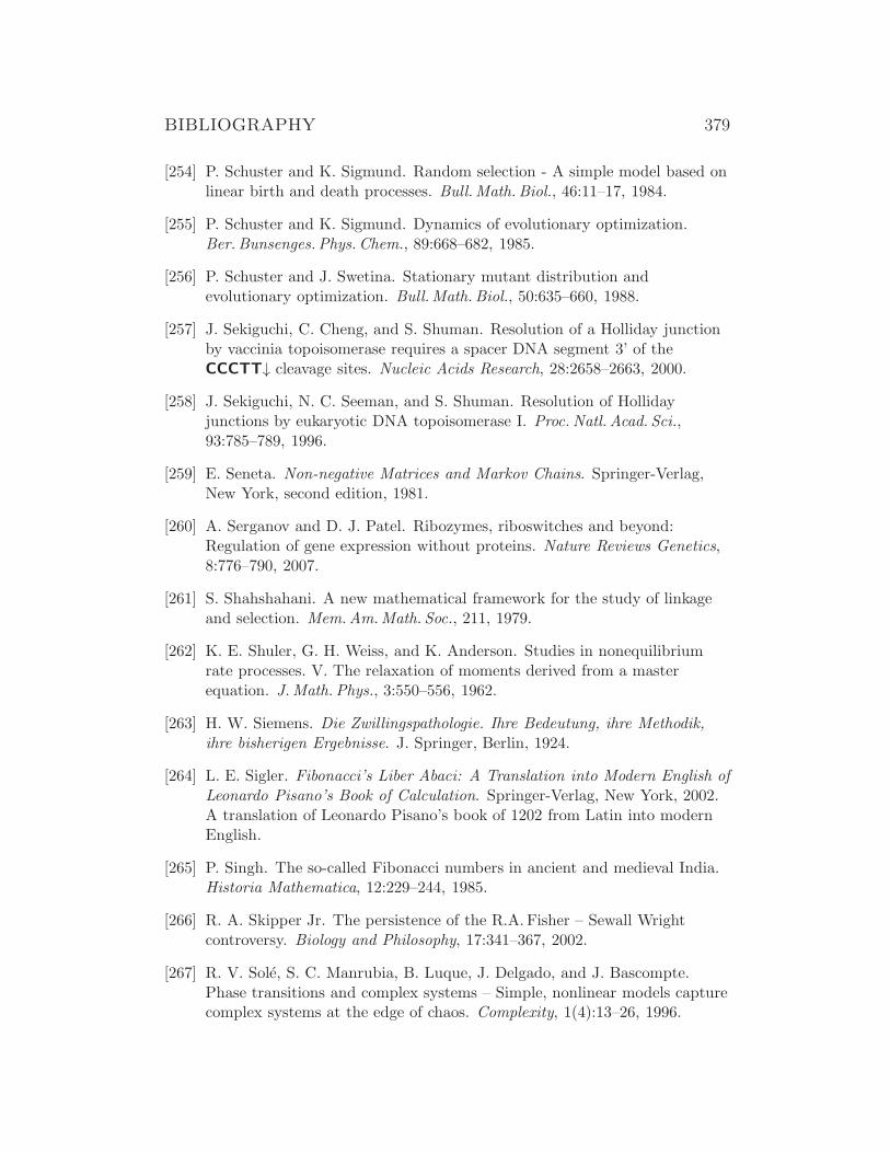
BIBLIOGRAPHY 379
[254] P. Schuster and K. Sigmund. Random selection - A simple model based onlinear birth and death processes. Bull.Math. Biol., 46:11–17, 1984.
[255] P. Schuster and K. Sigmund. Dynamics of evolutionary optimization.Ber. Bunsenges. Phys. Chem., 89:668–682, 1985.
[256] P. Schuster and J. Swetina. Stationary mutant distribution andevolutionary optimization. Bull.Math. Biol., 50:635–660, 1988.
[257] J. Sekiguchi, C. Cheng, and S. Shuman. Resolution of a Holliday junctionby vaccinia topoisomerase requires a spacer DNA segment 3’ of theCCCTT↓ cleavage sites. Nucleic Acids Research, 28:2658–2663, 2000.
[258] J. Sekiguchi, N. C. Seeman, and S. Shuman. Resolution of Hollidayjunctions by eukaryotic DNA topoisomerase I. Proc. Natl. Acad. Sci.,93:785–789, 1996.
[259] E. Seneta. Non-negative Matrices and Markov Chains. Springer-Verlag,New York, second edition, 1981.
[260] A. Serganov and D. J. Patel. Ribozymes, riboswitches and beyond:Regulation of gene expression without proteins. Nature Reviews Genetics,8:776–790, 2007.
[261] S. Shahshahani. A new mathematical framework for the study of linkageand selection. Mem.Am.Math. Soc., 211, 1979.
[262] K. E. Shuler, G. H. Weiss, and K. Anderson. Studies in nonequilibriumrate processes. V. The relaxation of moments derived from a masterequation. J.Math. Phys., 3:550–556, 1962.
[263] H. W. Siemens. Die Zwillingspathologie. Ihre Bedeutung, ihre Methodik,ihre bisherigen Ergebnisse. J. Springer, Berlin, 1924.
[264] L. E. Sigler. Fibonacci’s Liber Abaci: A Translation into Modern English ofLeonardo Pisano’s Book of Calculation. Springer-Verlag, New York, 2002.A translation of Leonardo Pisano’s book of 1202 from Latin into modernEnglish.
[265] P. Singh. The so-called Fibonacci numbers in ancient and medieval India.Historia Mathematica, 12:229–244, 1985.
[266] R. A. Skipper Jr. The persistence of the R.A. Fisher – Sewall Wrightcontroversy. Biology and Philosophy, 17:341–367, 2002.
[267] R. V. Sole, S. C. Manrubia, B. Luque, J. Delgado, and J. Bascompte.Phase transitions and complex systems – Simple, nonlinear models capturecomplex systems at the edge of chaos. Complexity, 1(4):13–26, 1996.
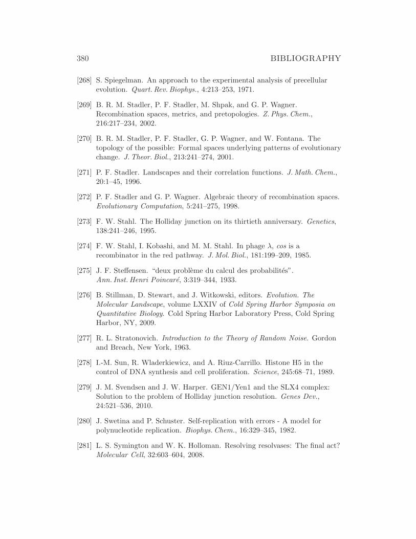
380 BIBLIOGRAPHY
[268] S. Spiegelman. An approach to the experimental analysis of precellularevolution. Quart. Rev. Biophys., 4:213–253, 1971.
[269] B. R. M. Stadler, P. F. Stadler, M. Shpak, and G. P. Wagner.Recombination spaces, metrics, and pretopologies. Z.Phys. Chem.,216:217–234, 2002.
[270] B. R. M. Stadler, P. F. Stadler, G. P. Wagner, and W. Fontana. Thetopology of the possible: Formal spaces underlying patterns of evolutionarychange. J.Theor. Biol., 213:241–274, 2001.
[271] P. F. Stadler. Landscapes and their correlation functions. J.Math. Chem.,20:1–45, 1996.
[272] P. F. Stadler and G. P. Wagner. Algebraic theory of recombination spaces.Evolutionary Computation, 5:241–275, 1998.
[273] F. W. Stahl. The Holliday junction on its thirtieth anniversary. Genetics,138:241–246, 1995.
[274] F. W. Stahl, I. Kobashi, and M. M. Stahl. In phage λ, cos is arecombinator in the red pathway. J.Mol. Biol., 181:199–209, 1985.
[275] J. F. Steffensen. “deux probleme du calcul des probabilites”.Ann. Inst. Henri Poincare, 3:319–344, 1933.
[276] B. Stillman, D. Stewart, and J. Witkowski, editors. Evolution. TheMolecular Landscape, volume LXXIV of Cold Spring Harbor Symposia onQuantitative Biology. Cold Spring Harbor Laboratory Press, Cold SpringHarbor, NY, 2009.
[277] R. L. Stratonovich. Introduction to the Theory of Random Noise. Gordonand Breach, New York, 1963.
[278] I.-M. Sun, R. Wladerkiewicz, and A. Riuz-Carrillo. Histone H5 in thecontrol of DNA synthesis and cell proliferation. Science, 245:68–71, 1989.
[279] J. M. Svendsen and J. W. Harper. GEN1/Yen1 and the SLX4 complex:Solution to the problem of Holliday junction resolution. Genes Dev.,24:521–536, 2010.
[280] J. Swetina and P. Schuster. Self-replication with errors - A model forpolynucleotide replication. Biophys. Chem., 16:329–345, 1982.
[281] L. S. Symington and W. K. Holloman. Resolving resolvases: The final act?Molecular Cell, 32:603–604, 2008.
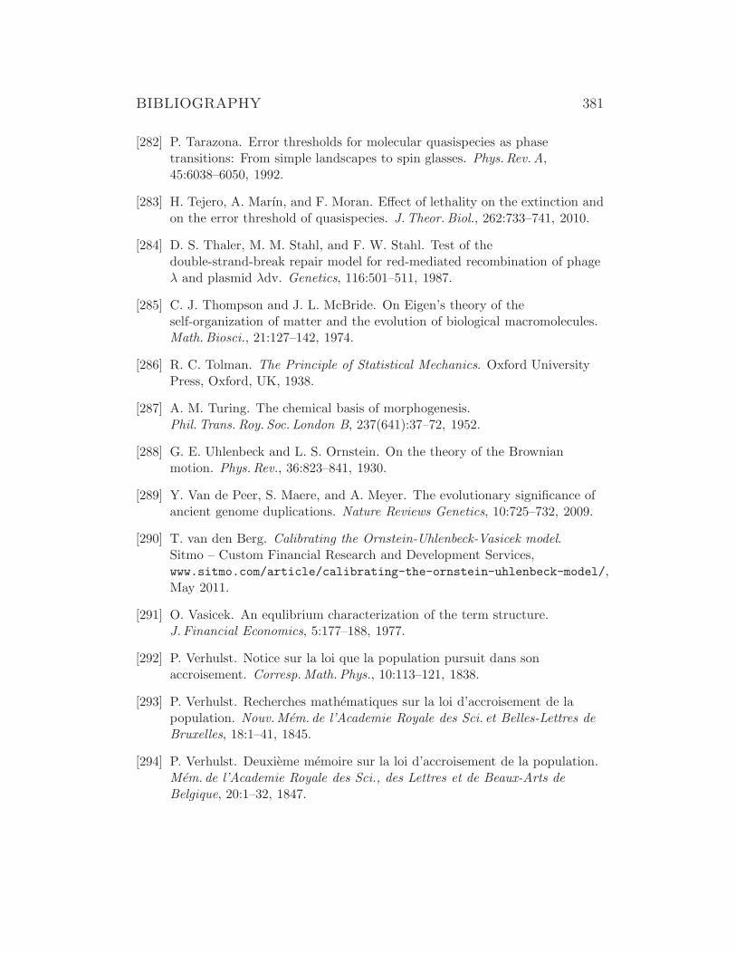
BIBLIOGRAPHY 381
[282] P. Tarazona. Error thresholds for molecular quasispecies as phasetransitions: From simple landscapes to spin glasses. Phys.Rev. A,45:6038–6050, 1992.
[283] H. Tejero, A. Marın, and F. Moran. Effect of lethality on the extinction andon the error threshold of quasispecies. J.Theor. Biol., 262:733–741, 2010.
[284] D. S. Thaler, M. M. Stahl, and F. W. Stahl. Test of thedouble-strand-break repair model for red-mediated recombination of phageλ and plasmid λdv. Genetics, 116:501–511, 1987.
[285] C. J. Thompson and J. L. McBride. On Eigen’s theory of theself-organization of matter and the evolution of biological macromolecules.Math. Biosci., 21:127–142, 1974.
[286] R. C. Tolman. The Principle of Statistical Mechanics. Oxford UniversityPress, Oxford, UK, 1938.
[287] A. M. Turing. The chemical basis of morphogenesis.Phil. Trans. Roy. Soc. London B, 237(641):37–72, 1952.
[288] G. E. Uhlenbeck and L. S. Ornstein. On the theory of the Brownianmotion. Phys. Rev., 36:823–841, 1930.
[289] Y. Van de Peer, S. Maere, and A. Meyer. The evolutionary significance ofancient genome duplications. Nature Reviews Genetics, 10:725–732, 2009.
[290] T. van den Berg. Calibrating the Ornstein-Uhlenbeck-Vasicek model.Sitmo – Custom Financial Research and Development Services,www.sitmo.com/article/calibrating-the-ornstein-uhlenbeck-model/,May 2011.
[291] O. Vasicek. An equlibrium characterization of the term structure.J. Financial Economics, 5:177–188, 1977.
[292] P. Verhulst. Notice sur la loi que la population pursuit dans sonaccroisement. Corresp.Math. Phys., 10:113–121, 1838.
[293] P. Verhulst. Recherches mathematiques sur la loi d’accroisement de lapopulation. Nouv.Mem. de l’Academie Royale des Sci. et Belles-Lettres deBruxelles, 18:1–41, 1845.
[294] P. Verhulst. Deuxieme memoire sur la loi d’accroisement de la population.Mem. de l’Academie Royale des Sci., des Lettres et de Beaux-Arts deBelgique, 20:1–32, 1847.
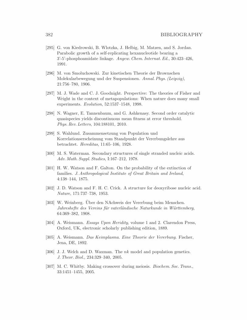
382 BIBLIOGRAPHY
[295] G. von Kiedrowski, B. Wlotzka, J. Helbig, M. Matzen, and S. Jordan.Parabolic growth of a self-replicating hexanucleotide bearing a3’-5’-phosphoamidate linkage. Angew.Chem. Internat. Ed., 30:423–426,1991.
[296] M. von Smoluchowski. Zur kinetischen Theorie der BrownschenMolekularbewegung und der Suspensionen. Annal. Phys. (Leipzig),21:756–780, 1906.
[297] M. J. Wade and C. J. Goodnight. Perspective: The theories of Fisher andWright in the context of metapopulations: When nature does many smallexperiments. Evolution, 52:1537–1548, 1998.
[298] N. Wagner, E. Tannenbaum, and G. Ashkenasy. Second order catalyticquasispecies yields discontinuous mean fitness at error threshold.Phys. Rev. Letters, 104:188101, 2010.
[299] S. Wahlund. Zusammensetzung von Population undKorrelationserscheinung vom Standpunkt der Vererbungslehre ausbetrachtet. Hereditas, 11:65–106, 1928.
[300] M. S. Waterman. Secondary structures of single stranded nucleic acids.Adv.Math. Suppl. Studies, I:167–212, 1978.
[301] H. W. Watson and F. Galton. On the probability of the extinction offamilies. J.Anthropological Institute of Great Britain and Ireland,4:138–144, 1875.
[302] J. D. Watson and F. H. C. Crick. A structure for deoxyribose nucleic acid.Nature, 171:737–738, 1953.
[303] W. Weinberg. Uber den NAchweis der Vererbung beim Menschen.Jahreshefte des Vereins fur vaterlandische Naturkunde in Wurttemberg,64:369–382, 1908.
[304] A. Weismann. Essays Upon Heridity, volume 1 and 2. Clarendon Press,Oxford, UK, electronic scholarly publishing edition, 1889.
[305] A. Weismann. Das Keimplasma. Eine Theorie der Vererbung. Fischer,Jena, DE, 1892.
[306] J. J. Welch and D. Waxman. The nk model and population genetics.J.Theor. Biol., 234:329–340, 2005.
[307] M. C. Whitby. Making crossover during meiosis. Biochem. Soc. Trans.,33:1451–1455, 2005.
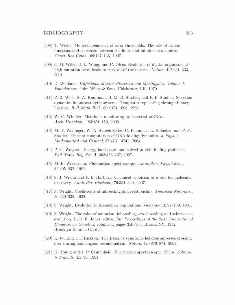
BIBLIOGRAPHY 383
[308] T. Wiehe. Model dependency of error thresholds: The role of fitnessfunctions and contrasts between the finite and infinite sites models.Genet. Res. Camb., 69:127–136, 1997.
[309] C. O. Wilke, J. L. Wang, and C. Ofria. Evolution of digital organisms athigh mutation rates leads to survival of the flattest. Nature, 412:331–333,2001.
[310] D. Williams. Diffusions, Markov Processes and Martingales. Volume 1:Foundations. John Wiley & Sons, Chichester, UK, 1979.
[311] P. R. Wills, S. A. Kauffman, B. M. R. Stadler, and P. F. Stadler. Selectiondynamics in autocatalytic systems: Templates replicating through binaryligation. Bull.Math. Biol., 60:1073–1098, 1998.
[312] W. C. Winkler. Metabolic monitoring by bacterial mRNAs.Arch.Microbiol., 183:151–159, 2005.
[313] M. T. Wolfinger, W. A. Svrcek-Seiler, C. Flamm, I. L. Hofacker, and P. F.Stadler. Efficient computation of RNA folding dynamics. J. Phys. A:Mathematical and General, 37:4731–4741, 2004.
[314] P. G. Wolynes. Energy landscapes and solved protein-folding problems.Phil. Trans. Roy. Soc. A, 363:453–467, 1997.
[315] M. B. Wreissman. Fluctuation spectroscopy. Annu.Rrev. Phys. Chem.,32:205–232, 1981.
[316] S. J. Wrenn and P. B. Harbury. Chemical evolution as a tool for moleculardiscovery. Annu.Rev. Biochem., 76:331–349, 2007.
[317] S. Wright. Coefficients of inbreeding and relationship. American Naturalist,56:330–338, 1922.
[318] S. Wright. Evolution in Mendelian populations. Genetics, 16:97–159, 1931.
[319] S. Wright. The roles of mutation, inbreeding, crossbreeding and selection inevolution. In D. F. Jones, editor, Int. Proceedings of the Sixth InternationalCongress on Genetics, volume 1, pages 356–366, Ithaca, NY, 1932.Brooklyn Botanic Garden.
[320] L. Wu and I. D.Hickson. The Bloom’s syndrome helicase sipresses crossingover during homologous recombination. Nature, 426:870–874, 2003.
[321] K. Young and J. P. Crutchfield. Fluctuation spectroscopy. Chaos, Solitons& Fractals, 4:5–39, 1994.
384 BIBLIOGRAPHY
[322] E. Yus, T. Maier, K. Michalodimitrakis, V. van Noort, T. Yamada, W.-H.Chen, J. A. Wodke, M. Guell, S. Martınez, R. Bourgeois, S. Kuhner,E. Raineri, I. Letunic, O. V. Kalinina, M. Rode, R. Herrmann,R. Gutierez-Gallego, R. B. Russell, A.-C. Gavin, P. Bork, and L. Serrano.Impact of genome reduction on bacterial metabolism and its regulation.Science, 326:1263–1268, 2009.
[323] W. K. Zhang and X. Zhang. Single molecule mechanochemistry ofmacromolecules. Prog. Polym. Sci., 28:1271–1295, 2003.
[324] B. H. Zimm. Theory of “melting” of the helical form in double chains ofthe DNA type. J.Chem. Phys., 33:1349–1356, 1960.
[325] B. H. Zimm and J. K. Bragg. Theory of the phase transition between helixand coil in polypeptide chains. J.Chem. Phys., 31:526–535, 1959.
[326] M. Zuker. On finding all suboptimal foldings of an RNA molecule. Science,244:48–52, 1989.
[327] M. Zuker. The use of dynamic programming algorithms in RNA secondarystructure prediction. In M. S. Waterman, editor, Mathematical Methods forDNA Sequences, pages 159–184. CRC Press, Boca Raton (FL), 1989.
[328] M. Zuker and P. Stiegler. Optimal computer folding of larger RNAsequences using thermodynamics and auxiliary information. Nucleic AcidsResearch, 9:133–148, 1981.
[329] D. Zwillinger. Handbook of Differential Equations. Academic Press, SanDiego, CA, third edition, 1998.
Contents
1 Darwin’s principle in mathematical language 5
1.1 Counting and modeling before Darwin . . . . . . . . . . . . . 61.2 The selection equation . . . . . . . . . . . . . . . . . . . . . . 121.3 Variable population size . . . . . . . . . . . . . . . . . . . . . 161.4 Optimization . . . . . . . . . . . . . . . . . . . . . . . . . . . 191.5 Growth functions and selection . . . . . . . . . . . . . . . . . 23
2 Mendel’s genetics and recombination 27
2.1 Mendel’s experiments . . . . . . . . . . . . . . . . . . . . . . . 282.2 The mechanism of recombination . . . . . . . . . . . . . . . . 35
2.2.1 Chromosomes . . . . . . . . . . . . . . . . . . . . . . . 372.2.2 Chromosomes and sex determination . . . . . . . . . . 402.2.3 Mitosis and meiosis . . . . . . . . . . . . . . . . . . . . 412.2.4 Molecular mechanisms of recombination . . . . . . . . 49
2.3 Recombination and population genetics . . . . . . . . . . . . . 572.4 Hardy-Weinberg equilibrium . . . . . . . . . . . . . . . . . . . 572.5 Fisher’s selection equation and the fundamental theorem . . . 612.6 Evaluation of data and the Fisher-Mendel controversy . . . . . 67
2.6.1 The χ2-distribution . . . . . . . . . . . . . . . . . . . . 672.6.2 Fisher’s exact test . . . . . . . . . . . . . . . . . . . . . 72
3 Fisher-Wright debate and fitness landscapes 75
3.1 Fisher’s fundamental theorem revisited . . . . . . . . . . . . . 753.2 The Fisher-Wright controversy . . . . . . . . . . . . . . . . . . 793.3 Fitness landscapes on sequence spaces . . . . . . . . . . . . . . 81
4 Mutation and selection 87
4.1 The historical route to mutation . . . . . . . . . . . . . . . . . 894.2 The flow reactor . . . . . . . . . . . . . . . . . . . . . . . . . . 944.3 Replication and mutation . . . . . . . . . . . . . . . . . . . . 99
4.3.1 Mutation-selection equation . . . . . . . . . . . . . . . 1014.3.2 Quasispecies and optimization . . . . . . . . . . . . . . 1064.3.3 Error thresholds . . . . . . . . . . . . . . . . . . . . . . 1104.3.4 Complementary replication . . . . . . . . . . . . . . . . 1284.3.5 Quasispecies on ”simple” model landscapes . . . . . . . 1304.3.6 Error thresholds on “simple” model landscapes . . . . 140
I
II CONTENTS
5 Fitness landscapes and evolutionary dynamics 147
5.1 RNA landscapes . . . . . . . . . . . . . . . . . . . . . . . . . . 1485.1.1 The paradigm of structural biology . . . . . . . . . . . 1495.1.2 RNA secondary structures . . . . . . . . . . . . . . . . 1545.1.3 Sequences with multiple structures . . . . . . . . . . . 159
5.2 Dynamics on realistic rugged landscapes . . . . . . . . . . . . 1625.2.1 Single master quasispecies . . . . . . . . . . . . . . . . 1645.2.2 Transitions between quasispecies . . . . . . . . . . . . 1735.2.3 Clusters of coupled sequences . . . . . . . . . . . . . . 176
5.3 Dynamics on realistic rugged and neutral landscapes . . . . . 1855.3.1 Small neutral clusters . . . . . . . . . . . . . . . . . . . 1865.3.2 Medium size neutral clusters . . . . . . . . . . . . . . . 197
6 Molecules in vitro and prokaryotes 201
6.1 Molecules in cell-free replication assays . . . . . . . . . . . . . 2016.2 Viroids and viruses . . . . . . . . . . . . . . . . . . . . . . . . 2016.3 Bacteria under controlled conditions . . . . . . . . . . . . . . . 201
7 Evolution of eukaryotes 203
8 Probability and stochasticity 205
8.1 Probabilities and probability theory . . . . . . . . . . . . . . . 2078.1.1 Historical probability . . . . . . . . . . . . . . . . . . . 2088.1.2 Sets, sample spaces, and probability . . . . . . . . . . . 2098.1.3 Probability distributions . . . . . . . . . . . . . . . . . 221
8.2 Stochastic processes . . . . . . . . . . . . . . . . . . . . . . . . 2408.2.1 Markov and other simple stochastic processes . . . . . 2438.2.2 Continuity and the Chapman-Kolmogorov equation . . 2478.2.3 Levy processes . . . . . . . . . . . . . . . . . . . . . . 270
9 Stochasticity in chemical reactions 273
9.1 Master equations in chemistry . . . . . . . . . . . . . . . . . . 2749.1.1 Chemical master equations . . . . . . . . . . . . . . . . 2759.1.2 The Poisson process . . . . . . . . . . . . . . . . . . . 2779.1.3 Birth-and-death processes . . . . . . . . . . . . . . . . 279
9.2 Examples of solvable master equations . . . . . . . . . . . . . 2829.3 Computer simulation of master equations . . . . . . . . . . . . 304
9.3.1 Master equations from collision theory . . . . . . . . . 3059.3.2 Simulation of master equations . . . . . . . . . . . . . 3119.3.3 The simulation algorithm . . . . . . . . . . . . . . . . 3169.3.4 Implementation of the simulation algorithm . . . . . . 318
CONTENTS III
10 Stochasticity in evolution 327
10.1 Autocatalysis, replication, and extinction . . . . . . . . . . . . 32910.1.1 Autocatalytic growth and death . . . . . . . . . . . . . 32910.1.2 Boundaries in one step birth-and-death processes . . . 33910.1.3 Branching processes in evolution . . . . . . . . . . . . . 34310.1.4 The Wright-Fisher and the Moran process . . . . . . . 352
10.2 Master equations in biology . . . . . . . . . . . . . . . . . . . 35810.3 Neutrality and Kimura’s theory of evolution . . . . . . . . . . 358
11 Perspectives and Outlook 359

IV CONTENTS

Index
Avogadro, Amedeo, 283
Barton, Nicholas, 75Beadle, George Wells, 90Bernoulli, Jakob I, 234, 244Biebricher, Christof, 87Bienayme, I. Jules, 343Binet, Jacques, 9Blackburn, Elizabeth, 39Boltzmann, Ludwig, 241, 306Boveri, Theodor, 36Brown, Robert, 240, 249
Cardano, Gerolamo, 207Carroll, Lewis, 78Cauchy, Augustin Louis, 238Chandrasekhar, Subrahmanyan, 241Chapman, Sydney, 250Coyne, Jerry, 75Crick, Francis, 90
Darwin, Charles, 3, 5, 9, 27Dawkins, Richard, 76de Candolle, Alphonse, 343de Fermat, Pierre, 208de Moivre, Abraham, 234Dirac, Paul, 250, 263Dmitriev, N. A., 343Dobzhansky, Theodosius, 3Domingo, Esteban, 88Doob, Joseph, 245Drake, John, 127
Ehrenfest, Paul, 295Eigen, Manfred, 87, 101Einstein, Albert, 240, 246Euler, Leonhard, 9
Fisher, Ronald, 3, 27, 61, 352Fisk, Donald LeRoy, 260Fokker, Adriaan Daniel, 256Frobenius, Georg, 118
Galton, Francis, 27, 343Gardiner, Crispin, 252Gauß, Carl Friedrich, 233Gavrilets, Sergey, 158Gegenbauer, Leopold, 301Gierer, Alfred, 275Gillespie, Daniel, 277, 304Goodnight, Charles J., 75Greider, Carol, 39
Haldane, J.B.S., 3Hamming, Richard, 105Hardy, Godfrey Harold, 57Heaviside, Oliver, 224Holliday, Robin, 49
Ito, Kiyoshi, 260
Jacobi, Carl, 297
Kauffman, Stuart, 163Kendall, David George, 343Kimura, Motoo, 85, 187, 207, 271,
334Kolmogorov, Andrey Nikolaevich,
250, 343Kronecker, Leopold, 345
Levy, Paul Pierre, 245, 270Langevin, Paul, 253Laplace, Pierre-Simon, 234Lederberg, Joshua, 90Leibniz, Gottfried Wilhelm, 205
I

II INDEX
Liouville, Joseph, 254Lorentz, Hendrik, 238Loschmidt, Joseph, 283
Malthus, Thomas Robert, 9Markov, Andrey Andreyevich, 246Maxwell, James Clerk, 80, 241, 306McQuarrie, Donald Allan, 296Meinhardt, Hans, 275Mendel, Gregor, 3, 28, 87Moran, Patrick, 352, 356Morgan, Thomas Hunt, 37, 89Muller, Hermann Joseph, 80, 89
Newton, Isaac, 205Nicolis, Gregoire, 275
Ohno, Susumo, 92Ornstein, Leonard Salomon, 261
Pascal, Blaise, 207, 208Pearson, Karl, 32Perron, Oskar, 118Person, Karl, 67Pisano, Leonardo, 6Planck, Max, 256Poisson, Simeon Denis, 227, 277Prigogine, Ilya, 275
Raleigh, Sir Walter, 118Rolle, Michel, 351
Schrodinger, Erwin, 118Serrano, Luis, 88Siemens, Hermann Werner, 27Skipper Jr., Robert A., 75Steffensen, Johan Frederik, 343Stratonovich, Ruslan Leontevich, 260Sutton, Walter, 36Szostak, Jack, 39
Tatum, Edward Lawrie, 90Tolman, Richard Chace, 281
Turelli, Michael, 75Turing, Alan, 275
Uhlenbeck, George Eugene, 261Ulam, Stan M., 343
van Valen, Leigh, 78Verhulst, Jean Francois, 10von Smoluchowski, Marian, 240, 246
Wade, Michael J., 75Wahlund, Sten, 61Wallace, Alfred Russel, 9Watson, Henry William, 343Watson, James, 90Weinberg, Wilhelm, 27, 57Weismann, August, 35Wiener, Norbert, 247, 255Wright, Sewall, 3, 67, 79, 352