Evolutionary and ecological interactions affecting seaweeds
212
AN ABSTRACT OF THE THESIS OF Annette M. Olson for the degree of Doctor of Philosophy in Zoology presented on 18 June 1992 Title: Evolutionary and Ecological Interactions Affecting Seaweeds Abstract approved: Jane Lubchenco The term "interaction" in evolutionary biology and ecology describes the relationships among variables in two classes of causal models. In the first, "interaction" refers to the influence of a single putatively causal variable on a variable of interest. In the second class of models, the term applies when a third variable mediates the relationship between two variables in the first class of models. The development of multi-factor causal models in evolutionary biology and ecology represents a stage in the construction of theory that usually follows from complexities discovered in single-factor analyses. In this thesis, I present three cases that illustrate how results of simple single-factor models in the population genetics and community ecology of seaweeds may be affected by incorporation of a second causal factor. In Chapter II, we consider how the effect of natural selection on genetic variability in seaweeds and other plants may be mediated by life history variation. Many seaweeds have haplodiplontic life histories in which haploid and diploid stages alternate. Our theoretical analysis and review of the electrophoretic literature show 2 38711OR TH 7/93 31805-66 Redacted for Privacy
-
Upload
khangminh22 -
Category
Documents
-
view
1 -
download
0
Transcript of Evolutionary and ecological interactions affecting seaweeds
AN ABSTRACT OF THE THESIS OF
Annette M. Olson for the degree of Doctor of Philosophy in
Zoology presented on 18 June 1992
Title: Evolutionary and Ecological Interactions Affecting Seaweeds
Abstract approved:
Jane Lubchenco
The term "interaction" in evolutionary biology and ecology
describes the relationships among variables in two classes of causal
models. In the first, "interaction" refers to the influence of a
single putatively causal variable on a variable of interest. In the
second class of models, the term applies when a third variable
mediates the relationship between two variables in the first class of
models. The development of multi-factor causal models in evolutionary
biology and ecology represents a stage in the construction of theory
that usually follows from complexities discovered in single-factor
analyses. In this thesis, I present three cases that illustrate how
results of simple single-factor models in the population genetics and
community ecology of seaweeds may be affected by incorporation of a
second causal factor.
In Chapter II, we consider how the effect of natural selection
on genetic variability in seaweeds and other plants may be mediated by
life history variation. Many seaweeds have haplodiplontic life
histories in which haploid and diploid stages alternate. Our
theoretical analysis and review of the electrophoretic literature show
2 38711OR TH
7/93 31805-66
Redacted for Privacy
that the level of genetic polymorphism in haplodiplonts is not
necessarily reduced relative to that in diploids. In Chapter III, I
take an experimental approach to understanding how herbivory may
mediate the effect of desiccation on the upper intertidal limit of a
red alga, Iridaea cornucopiae. Iridaea appears to be grazer-limited
in dry, but grazer-dependent in moist environments, suggesting that a
third factor may mediate the interaction of desiccation and herbivory.
Finally, in Chapter IV, we consider research strategies for studying
how the outcome of competitive interactions is affected by seaweed
traits. Some of the problems that arise in applying simple models of
competition to plants suggest the need for theory that explicitly
incorporates plant traits in two- (or more) factor models of
interspecific competition. In particular, we note that unique traits
of seaweeds require development of new approaches to understanding
competition.
Single-factor causal models represent an indispensable stage in
the development of evolutionary and ecological theory. Properly
conceived theoretical and empirical studies focus attention on the
assumptions under which such models will hold and suggest lines of
inquiry that ultimately lead to the integration of additional causal
factors in conceptual models of natural processes. Identifying the
circumstances under which simple models will suffice remains one of
the most important challenges of evolutionary and ecological
scholarship.
Evolutionary and Ecological InteractionsAffecting Seaweeds
by
Annette M. Olson
A THESIS
submitted to
Oregon State University
in partial fulfillment ofthe requirements for the
degree of
Doctor of Philosophy
Completed June 29, 1992
Commencement June 1993

APPROVED:
Professor of oology in charge of major
Head of D par ment of Zoology
Dean of Gradua chool
Date thesis is presented June 29, 1992
Typed by Annette M. Olson
Redacted for Privacy
Redacted for Privacy
Redacted for Privacy

In memory of Marilyn Potts Guin
ACKNOWLEDGEMENT
The completion of this thesis would not have been possible
without the inspiration, guidance, assistance, and encouragement of
many friends and colleagues. I am especially grateful to Jane
Lubchenco and Bruce Menge, my advisor and co-advisor, for their
ongoing support, guidance, and friendship. I thank Pete Dawson, Doug
Markle, Mark Wilson, and Erwin Pearson for serving on my thesis
committee, and for commenting on earlier drafts of this thesis. Gerry
Allen, Joe Antos, Susan Brawley, Terry Farrell, Charlie Halpern,
Charles King, Bob Paine, Jon Roughgarden, Liz Walsh, and anonymous
reviewers provided helpful critiques of one or more chapters.
I thank Ms. Dianne Rowe and the staff of the Department of
Zoology for competent and friendly support services. I also thank
Lavern Weber and the staff of the Hatfield Marine Science Center for
use of the facility. I gratefully acknowledge the technical
assistance of Donna Frostholm, Charlie Halpern, Michael Mungoven, Mara
Spencer, and others in the field, laboratory, and library. Sedonia
Washington, Shawnie Worrell, Suanty Kaghan, and Jill Meiser assisted
with word processing for Chapter II. Charlie Halpern drafted Figure
IV.1. The contributions of several other colleagues are noted in
acknowledgements associated with individual chapters.
Special thanks go to my husband, Charlie Halpern, for his help
and encouragement and to my parents, Oscar and Mary Olson, for their
loving support.
This work was supported in part by grants from the National
Science Foundation to B. A. Menge (OCE-8415609, OCE-8811369) and to J.

Lubchenco and D. Carlson (OCE-8600523), by a grant from the Andrew W.
Mellon Foundation to J. Lubchenco, and by a DeLoach Graduate
Fellowship from Oregon State University to A. M. Olson.
TABLE OF CONTENTS
Chapter Page
I. INTRODUCTION 1
II. NATURAL SELECTION AND GENETIC POLYMORPHISM INHAPLODIPLONTIC ORGANISMS 9
ABSTRACT 9
INTRODUCTION 11
THE MODEL 19
PREDICTIONS OF THE MODEL 25
Reinforcing Selection 26
Opposing Selection 30
THE PROBABILITY OF POLYMORPHISM 35
An Analytical Approach 38
EVIDENCE FOR HDM DYNAMICSIN NATURAL POPULATIONS 47
ENZYME POLYMORPHISMIN HAPLODIPLONTIC POPULATIONS 53
GENERAL DISCUSSION 72
ACKNOWLEDGMENTS 81
APPENDIX A 82
APPENDIX B 83
APPENDIX C 87
III. DESICCATION AND HERBIVORY INTERACT TO REGULATE THEUPPER LIMIT OF AN INTERTIDAL RED ALGA 95
ABSTRACT 95
INTRODUCTION 96
NATURAL HISTORY 104
METHODS 111
Desiccation x Herbivory Experiment 111
Manipulations 111
Treatment effectiveness 117
Measures of plant performance 118
Feeding Experiments 122
Analyses 124
RESULTS 125
Desiccation x Herbivory Experiment 125
Feeding Experiments 138
DISCUSSION 147
Predictions of the Models 147
Causal Mechanisms 151
Herbivore abundance 151
Plant susceptibility 154
Plant recovery 157
Herbivore movement 157
ACKNOWLEDGMENTS 161

Chapter Page
IV. COMPETITION IN SEAWEEDS: LINKING PLANT TRAITS TOCOMPETITIVE OUTCOMES 162
INTRODUCTION 162
DEFINING COMPETITION 166
DETECTING COMPETITION 169
CONSEQUENCES OF PLANT TRAITSAND THE MECHANISMS OF COMPETITION 174
CONCLUSIONS 177
ACKNOWLEDGMENTS 179
QUESTIONS 180
BIBLIOGRAPHY 182
LIST OF FIGURES
Figure Page
1.1 Single- and two-factor causal models for evolutionaryand ecological interactions affecting seaweeds. 2
I1.1 Idealized life histories (after Searles 1980). 12
11.2 Features of a generalized haplodiplontic life historyand parameters of the haplodiplontic model (HDM). 17
11.3 Parameter space of the haplodiplontic model in twodimensions. 23
11.4 Results of simulations in which the strength ofreinforcing selection in haplophase was varied, whilethe selection regime in diplophase was held constant. 27
II.5
11.6
Results of simulations in which the strength ofopposing selection in haplophase was varied, while theselection regime in diplophase was held constant.
Effects of selection in diplophase (dominance andfitness of the inferior homozygote) on the range ofhaplophase selection differentials that permit "new"polymorphism under opposing selection in the HDM.
31
36
Parameter space of the HDM in three dimensions (the unitcube). 39
Volume of the parameter space supporting polymorphismas a function of selection in haplophase (Q) 42
A schematic representation of gene expression in thehaplodiplontic genome, indicating the regions ofapplicability of the HM (shaded), the DM (hatched),and the HDM (both) (after Heslop-Harrison 1980).
11.10 Polymorphism within plant populations that representregions on a continuum of life history variation (fromTable 2 and Hamrick and Godt 1989).
Outline of arguments linking population-geneticconsequences of natural selection in haplodiplonts withexplanations for the evolution of life histories inplants.
Contrasting assumptions and predictions of theconsumer stress and prey stress models (CSM andPSM, respectively).
48
63
73
97
Figure Page.
111.2 Vertical distribution of limpets on the shore nearthe upper limit of the Iridaea bed. 106
111.3 Aggregations of limpets (A) and grazing damage (B)near the upper limit of Iridaea. 109
111.4 Experimental treatments for moisture addition xlimpet removal experiment. 112
111.5 Desiccation of Iridaea blades in experimental plots. 115
111.6 Limpet densities in experimental plots. 119
111.7 Change in canopy cover of Iridaea in upper half(225 cm2) of experimental plots. 126
111.8 Vegetative advance of the upper limit of Iridaea. 128
111.9 Average reproduction and number of recruits in allexperimental plots. 130
111.10 Reproduction of Iridaea in experimental plots. 132
111.11 Recruitment of Iridaea in experimental plots. 135
111.12 Effect of reproductive status of Iridaea on feedingby free-ranging limpets. 141
111.13 Association of desiccation status of Iridaea withherbivore damage. 143
111.14 A conceptual model for a hypothetical effect ofdesiccation regime on interactions between limpets(Lottia) and Iridaea, mediated by competing algae. 149
IV. 1
Explanatory mechanisms potentially accounting forcorrelations between environmental stress and theeffect of consumers on prey. 152
A schematic representation of some mechanisms ofcompetition (Schoener 1983) in seaweeds. 171
LIST OF TABLES
Table Page
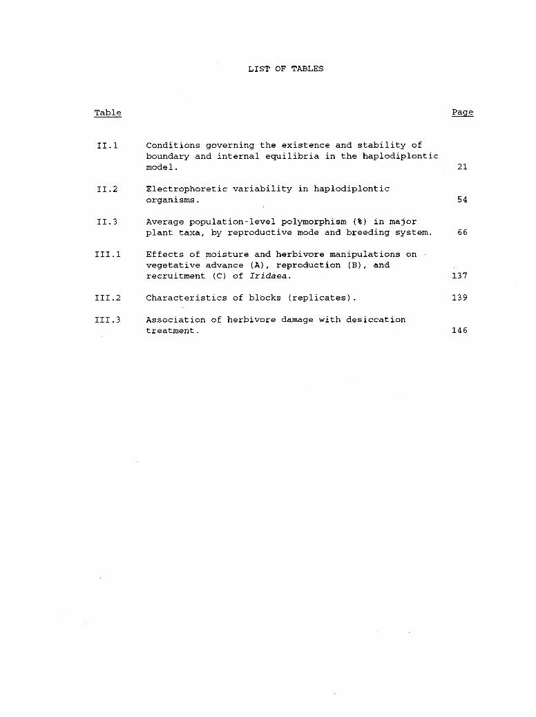
11.1 Conditions governing the existence and stability ofboundary and internal equilibria in the haplodiplonticmodel. 21
11.2 Electrophoretic variability in haplodiplonticorganisms. 54
11.3 Average population-level polymorphism (%) in majorplant taxa, by reproductive mode and breeding system. 66
111.1 Effects of moisture and herbivore manipulations onvegetative advance (A), reproduction (B), andrecruitment (C) of Iridaea. 137
111.2 Characteristics of blocks (replicates). 139
111.3 Association of herbivore damage with desiccationtreatment. 146
LIST OF APPENDICES FIGURES
Figure Page
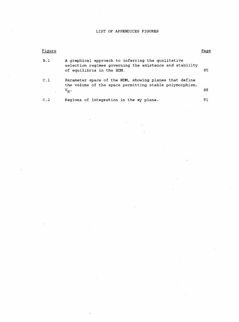
B.1
C.1
A graphical approach to inferring the qualitativeselection regimes governing the existence and stabilityof equilibria in the HDM. 85
Parameter space of the HDM, showing planes that definethe volume of the space permitting stable polymorphism,VH. 88
C.2 Regions of integration in the xy plane. 91
Evolutionary and Ecological Interactions
Affecting Seaweeds
Chapter I
INTRODUCTION
The term "interaction" in evolutionary biology and ecology
refers to the relationships among variables in causal models. There
are two main ways in which the term is used. The first use is the
common-sense definition of "interaction" as the influence of one
evolutionary or ecological factor on a second object, process, or
class of objects or processes. It is relevant to a class of models
(Fig. I.1) that relate the quantity or rate of a dependent variable to
a single putative independent variable (although the influence may be
reciprocal). The shape of the function describing that relationship
may be linear or non-linear. Non-linear relationships may display
thresholds, attenuation, and unimodal or cyclical effects. The
presence of a non-linear relationship between variables in a single-
factor model suggests that constituent or extrinsic variables may
mediate the interaction between the two variables in the first class
of models. This is the second definition of "interaction"--the
dependence of a relationship between two variables on the level of a
third variable (Fig. I.1). In two-factor analyses of variance, the
presence of this type of relationship is reflected in a significant
two-way interaction term. The development of two- (and more) factor
causal models in evolutionary biology and ecology represents a stage

2
Figure. 1.1. Single- and two-factor causal models for evolutionaryand ecological interactions affecting seaweeds.
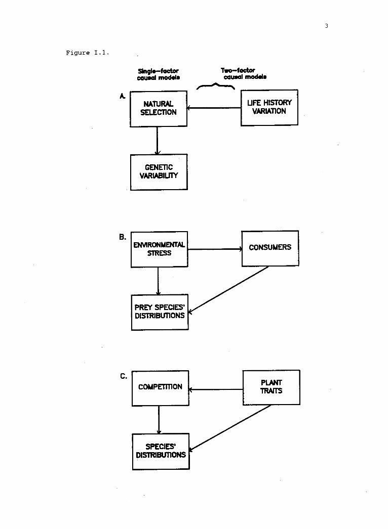
Figure 1.1.
Singlefactorcausal modals
NATURAL.SELECTION
Twofactorcausal modals
GENETICVARIABILITY
ENVIRONMENTALSTRESS
UFE HISTORYVARIATION
PREY SPECIES'DISTRIBUTIONS
COMPETITION
CONSUMERS
SPECIES'DISTRIBUTIONS
PLANTTRAITS
3

4
in the construction of theory that usually follows from complexities
discovered in single-factor analyses.
In this thesis, I present three cases that illustrate how
results of simple single-factor models in the population genetics and
community ecology of seaweeds may be affected by incorporation of a
second causal factor. In Chapter II (Olson and Murphy, in revision)
we consider how life history variation in many seaweeds may mediate
the effect of natural selection on genetic variability--the
interaction (in the first sense) between the fitness of genotypes and
allele frequencies. The classical haploid and diploid models predict
the effect of natural selection on allele frequencies (Fig. I.lA),
with emphasis on the rather restrictive conditions for retention of
genetic variability under natural selection. Numerous two-factor
models have considered the ways that intrinsic (stage of the life
history, gender) or extrinsic (temporal or spatial environmental
heterogeneity) factors mediate the effect of natural selection on
genetic variability, by permitting balancing selection to expand the
conditions for maintenance of genetic variability.
Many seaweeds and most other plants have haplodiplontic life
histories in which haploid and diploid stages alternate. In verbal
models it has been predicted that selection in haplophase should
result in levels of genetic polymorphism intermediate between those in
organisms with strictly haploid or diploid life cycles. However,
mathematical models predict that, under certain conditions, genetic
polymorphism could be maintained in haploidplonts under conditions
that would preclude polymorphism in diploids.
We use a comparative approach to explore the theoretical and
empirical evidence concerning the consequences of variation in life
history--from haploid, to haplodiplontic, to diploid--for the
maintenance of genetic polymorphism. In a new analysis of the
haplodiplontic model, we show that the probability of polymorphism in
haplodiplontic populations is not necessarily lower than that in
diploid populations. We also review electrophoretic evidence that
suggests that levels of enzyme polymorphism in natural populations of
haplodiplonts are comparable to those in predominantly diploid plant
and animal taxa. By using a comparative approach to evaluate the
relationship of life history variation to the maintenance of
polymorphism, we call into question the basic assumptions of previous
verbal arguments regarding the evolution of life histories in plants.
In Chapter III, I take an experimental approach to understanding
how herbivory may mediate the effect of desiccation in regulating the
upper intertidal limit of a red alga. Early models of intertidal
zonation suggest that a single-factor model--the effect of desiccation
on plant distribution--is sufficient to explain the upper limits of
species (Fig. I.1B). However, a class of two-factor models,
environmental stress models, suggests that the effect of stress may be
mediated by the effects of consumers (Fig. I.1B). In particular, the
consequences of the interaction for the distribution of prey species
is predicted to depend on the relative susceptibility to stress of
consumers and prey. If consumers are more affected than prey, the
consumer stress model predicts that prey species will find refuge from
consumers in stressful environments. On the other hand, if prey are
relatively more susceptible to stress, the prey stress model predicts
that consumers may eliminate prey from stressful habitats. In
6
numerous terrestrial systems, desiccation stress is correlated with
susceptibility to herbivory (consistent with the prey stess model).
Consequently, I tested a two-factor model for the interaction of
desiccation and herbivory.
I manipulated both desiccation (rock-surface moisture) and
herbivory (limpet abundance) in a factorial experiment designed to
evaluate their separate and joint effects on the upper intertidal
limit of a perennial red alga, Iridaea cornucopiae. I found that in
the presence of limpets, desiccation inhibited upward vegetative
growth. A significant desiccation-by-grazer interaction affected both
reproduction near, and recruitment above, the initial upper limit of
Iridaea. In dry plots, grazers inhibited recruitment; in moist plots,
grazers enhanced vegetative growth. Thus, Iridaea appears to be
grazer-limited in dry environments, but grazer-dependent in moist
environments, results that are not consistent with either the consumer
or the prey stress models. These results suggest that a two-factor
model is not sufficient to explain the interaction of desiccation and
grazing.
It is likely that a third factor, the abundance or productivity
of microalgae, may mediate the effects on recruitment. Limpets may
remove competing microalgae from moist plots, enhancing establishment
of Iridaea. In dry plots, where microalgal production is likely to be
lower, limpets may switch to Iridaea.
Finally, in Chapter IV (Olson and Lubchenco 1990), we consider
research strategies for investigating the effect of plant traits on
the outcome of competitive interactions in seaweed communities.
Simple models of competition (Fig. I.1C) assume a constant,
7
homogeneous environment and invariant plant traits. Some of the
problems that arise in applying such simple models to plants suggest
the need for theory that explicitly incorporates plant traits in two-
(or more) factor models of interspecific competition (Fig. I.1C). For
example, competitive interactions among seaweeds depend upon the
position, biomass, architecture and potential for vegetative expansion
or plasticity of response of competitors. Interactions with consumers
may also affect competitive outcomes. Recent theoretical developments
incorporate some of these factors in more complex models; we identify
other priorities. In particular, we note that unique traits of
seaweeds--such as isomorphic life histories, somatic polyploidy, and
thallus fusion--require development of new approaches to understanding
competition.
In addition, we note that historically, empirical studies of
seaweeds have followed separate but parallel lines of inquiry in the
lab and field. Lab studies have focused on variation in plant traits
assumed to be associated with competitive performance; field studies
have tended to focus on competitive outcomes, with less attention to
the plant traits that influence competition. Consequently, the causal
relationships between plant traits and competitive outcomes (Fig.
I.1C) remain a crucial gap in understanding competition among
seaweeds. To bridge this gap, we identify two research priorities:
(1) establish rigorously the competitive consequences of variation in
traits (among and within species) observed in laboratory studies, and
(2) evaluate experimentally the hypothesized mechanisms of competition
(in the context of other ecological interactions) proposed as a result
of field studies. Single-factor causal models represent an
8
indispensable stage in the development of evolutionary and ecological
theory. Properly conceived theoretical and empirical studies focus
attention on the assumptions under which such models will hold and
suggest lines of inquiry that ultimately lead to the integration of
additional causal factors in conceptual models of natural processes.
Identifying the circumstances under which simple models will suffice
remains one of the most important challenges of evolutionary and
ecological scholarship.
9
Chapter II
NATURAL SELECTION AND GENETIC POLYMORPHISM
IN HAPLODIPLONTIC ORGANISMS
Annette M. Olson
Department of Zoology
Oregon State University
Corvallis, OR 97331-2914
and
Lea F. Murphy
Department of Mathematics
Oregon State University
Corvallis, OR 97331-4605
ABSTRACT
In the haplodiplontic life history of most plants, both haploid
(gametophytic) and diploid (sporophytic) stages are multicellular.
Natural selection in haplophase is often assumed to reduce genetic
variability in populations of haplodiplonts. In a new analysis of the
haplodiplontic model (HDM)--a one-locus, two-allele deterministic
model with selection in both phases--we show that the probability of
polymorphism in haplodiplontic populations is not necessarily lower
than that in diploid populations.
The sign of correlations in fitness of alleles between the two
life-history phases determines whether genetic variability will tend
to be lost or retained. We introduce two new terms, reinforcing and
10
opposing selection, to describe those cases where correlations in
fitness between the two phases are positive or negative, respectively.
Reinforcing selection reduces the probability of polymorphism in the
HDM; under opposing selection of intermediate intensity, stable poly-
morphism is more likely than in the diploid model. Furthermore,
electrophoretic evidence suggests that levels of enzyme polymorphism
in natural populations of haplodiplonts are comparable to those in
predominantly diploid plant and animal taxa. Observed levels of
polymorphism do not appear to be correlated with the size, complexity,
or duration of haplophase in the life history of haplodiplonts. These
results call into question the basic assumptions of theories that link
the population-genetic consequences of the haplodiplontic life history
with explanations for the evolution of the life history itself.
11
INTRODUCTION
The maintenance of genetic polymorphism is a central issue in
evolutionary population biology both because it reflects evolutionary
processes within populations, and because it potentially has important
evolutionary consequences. The ability of natural selection to
maintain genetic variation within populations is powerfully affected
by the life histories of organisms. In the vast majority of plants
the life history is haplodiplontic (fig. II.lA), i.e., both diploid
(sporophytic) and haploid (gametophytic) stages are multicellular and
sometimes physiologically independent (Bold et al. 1987). Because
each stage is developmentally complex and often long-lived, the poten-
tial exists for natural selection to alter allele frequencies in both
stages. In this paper, we explore theoretical and empirical evidence
concerning the consequences of life history variation for the
maintenance of genetic polymorphism in haplodiplontic populations.
The haplodiplontic life history is one of three life history
patterns that differ in the ploidy level of the dominant phase (fig.
II.1). Each of these life histories presents different constraints on
the maintenance of genetic polymorphism by natural selection. For
example, in diploid populations (fig. II.1B), simple, deterministic,
single-locus models (e.g., Wright 1969) predict that heterozygote
superiority is both necessary and sufficient for the maintenance of
stable genetic polymorphism. In haploid populations (fig. II.1C), on
the other hand, natural selection alone is insufficient to maintain
stable polymorphism (e.g., Haldane and Jayakar 1963), because the
heterozygote does not exist in haploid organisms. In diploid
12
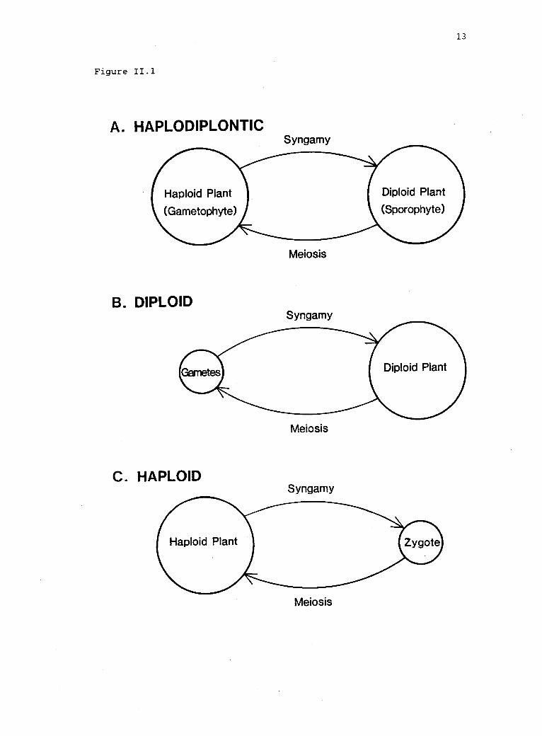
Figure II.1. Idealized life histories (after Searles 1980). A.
Haplo-diplontic, with sporic meiosis and mitotic gametogenesis (e.g.,most plants and algae). B. Diploid, with gametic meiosis (e.g.,fucoid algae, most metazoa). C. Haploid, with zygotic meiosis (e.g.,many flagellates). Departures from idealized life cycles includeasexual reproduction in either the haploid or diploid stage andplasticity in the degree of coordination among nuclear (haploid versusdiploid), reproductive (gametophytic versus sporophytic), andmorphological phases (Clayton 1988, Maggs 1988).
NOTE.--Among haplodiplontic life histories, haploid and diploidstages may be isomorphic (i.e., morphologically similar) or they maybe heteromorphic (i.e., dissimilar), with either stage more prominent.Haplophase is dominant among bryophytes (mosses and liverworts,Divisions Bryophyta and Hepatophyta, respectively), where the diploidsporophyte is smaller and more short-lived than the haploidgametophyte. Multicellular algae (chiefly in the Divisions Chloro-phyta, Phaeophyta, and Rhodophyta) display the full range of lifehistories including haploid, haplodiplontic, and diploid. Amonghigher plants, the diploid sporophyte dominates the life history: In
pteridophytes (ferns, clubmosses, and horsetails; DivisionsPteridophyta, Microphyllophyta, and Arthrophyta, respectively), theindependent haploid gametophyte is reduced in size and usually diesfollowing development in situ of the large, often long-livedsporophyte. Among gymnosperms (largely conifers, DivisionConiferophyta) and angiosperms (flowering plants, DivisionAnthophyta), the female gametophyte is enclosed in, and dependentupon, sporophytic tissue; the male gametophyte is contained in thepollen grains. The female gametophytes of gymnosperms are both larger(-104 cells) and more differentiated than those of angiosperms, whichare reduced to fewer than 10 cells. (See Bold 1970 and Bold et al.1987 for recent classifications of the plant kingdom and descriptionsof life cycles.)
13
Figure 11.1
A. HAPLODIPLONTIC
B. DIPLOID
Meiosis
Syngamy
C. HAPLOID
Meiosis
Syngamy
Meiosis
14
populations, the fitness of heterozygotes relative to that of the
homozygotes both regulates the rate at which deleterious alleles are
eliminated and determines whether natural selection can maintain
stable polymorphism. Populations of haploid organisms lack this
mechanism for retaining genetic variability.
Some authors have inferred from this difference between haploid
and diploid populations that the potential for natural selection to
maintain genetic polymorphism should be intermediate in populations of
haplodiplonts (e.g., Stebbins 1950, 1960; Bonner 1965; reviews in
Willson 1981; Szweykowski 1984; Wyatt 1985; Wyatt et al. 1989b; Ennos
1990). In particular, it is commonly thought that genes should be
exposed to intense purifying selection in the gametophytic stage of
the haplodiplontic life history, due to the absence of heterozygotes
in haplophase (e.g., Yamazaki 1981, 1984; Pfahler 1983; Weeden 1986).
Selection in haplophase is thus considered to be inherently "strong,"
quickly eliminating inferior variants and reducing the probability of
stable genetic polymorphism in haplodiplontic relative to diploid
populations. Populations with a prominent haploid stage are therefore
expected to harbor less genetic variation affecting fitness than are
populations of predominantly diploid organisms.
In this paper we examine the validity of such expectations in
order to better understand the conditions governing evolution in
haplodiplontic populations. Existing theoretical studies of natural
selection in populations of haplodiplonts predict that conditions
governing polymorphism in the haplodiplontic model (HDM) may be either
mere restrictive or more lenient than in the classical diploid model
(DM) (Scudo 1967; Wright 1969; Hartl 1975; Ewing 1977; Gregorius
15
1982). Specifically, these authors note that certain fitness combi-
nations in the HDM preclude stable polymorphism despite heterozygote
superiority in diplophase, while others permit polymorphism in the
absence of heterozygote superiority. However, the net effect of
natural selection in haplophase on the maintenance of polymorphism was
not analyzed in any of these studies. We address two related
questions (1) "What are the fitness combinations under which natural
selection tends to eliminate or retain genetic variation in
populations of haplodiplonts?" and (2) "How does the presence of
haplophase in the life cycle affect the maintenance of genetic
polymorphism?" To address the first question, we review the results
of the HDM, demonstrating how selection in each phase constrains or
potentiates the effects of selection in the alternate phase and
clarifying the conditions under which polymorphism is disrupted or
enhanced by selection in haplophase.
To address the second question, we compare predicted and
observed levels of polymorphism in populations that differ in the
presence, or the prominence, of haplophase in the life history. We
present a new analysis of the HDM that gives the first quantitative
comparison of the probability of polymorphism in the HDM (where
haplophase is present) and in the DM (where it is absent). We also
compare the frequency of polymorphism among haplodiplontic populations
that differ in the relative prominence of haplophase. To the extent
that selection in haplophase tends to eliminate genetic variation,
levels of polymorphism within natural populations of haplodiplonts
should be inversely correlated with the relative prominence of the
gametophytic and sporophytic stages. Few empirical studies exist on
16
genetic variation in species with a prominent or independent haploid
stage; none compare polymorphism among taxa that differ in the
relative duration or development of the two phases. Ours is the first
comprehensive survey of the literature on electrophoretic variation
among several plant divisions that represent a continuum of life-
history variation from gametophyte- to sporophyte-dominance.
We conclude our discussion by considering the relevance of our
results and approach to arguments concerning both the population-
genetic consequences, and the evolutionary causes, of life-history
variation in plants. Selection in haplophase potentially has
important evolutionary implications in haplodiplontic populations.
However, at least two contrasting accounts of its significance have
been proposed. Some authors have suggested that retention of a
discrete haplophase in the life history is favored because it serves a
"cleansing" function, rapidly eliminating deleterious mutations (e.g.,
Mulcahy and Mulcahy 1987; Klekowski 1988). In contrast, others have
predicted that a diplophase-dominant life history should evolve in the
absence of constraints, in part, because selection in haplophase can
eliminate potentially adaptive genetic variation from populations
(e.g., Stebbins 1950, 1960; Bonner 1965). Each of these arguments is
dependent on the expectation that levels of polymorphism in
haplodiplonts are reduced relative to those in diploids. Our results
indicate that this expectation is not necessarily warranted.
17
Figure 11.2. Features of a generalized haplodiplontic life historyand parameters of the haplodiplontic model (HDM). R! denotes meiosis;S!, syngamy. (Modified from Roughgarden 1979, figure 3.1.)

Figure 11.2
LIFE HISTORY:Diplophase
SporophytesZygotes
18
Haplophase
GometophytesSpores Gametes Zygotes
(ipr
g zrli 6 S!s6
MODEL PARAMETERS:Genotypes: Al A1, Al A2, A2A2
Fitnesses of<Genotypes: E Wij )
Generation: t+0.5Allele
Frequency: Pt
A1, A2
Wi, Wi
t+ 1
Pt+0.5 Pt+ 1
19
THE MODEL
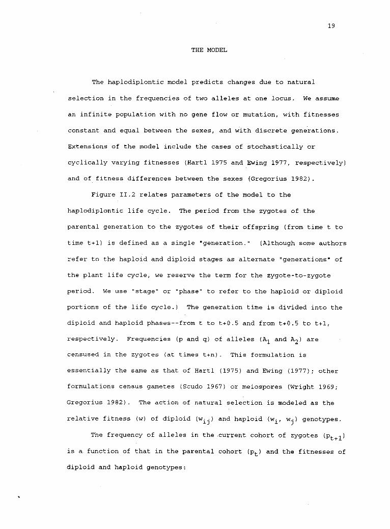
The haplodiplontic model predicts changes due to natural
selection in the frequencies of two alleles at one locus. We assume
an infinite population with no gene flow or mutation, with fitnesses
constant and equal between the sexes, and with discrete generations.
Extensions of the model include the cases of stochastically or
cyclically varying fitnesses (Hartl 1975 and Ewing 1977, respectively)
and of fitness differences between the sexes (Gregorius 1982).
Figure 11.2 relates parameters of the model to the
haplodiplontic life cycle. The period from the zygotes of the
parental generation to the zygotes of their offspring (from time t to
time t+1) is defined as a single "generation." (Although some authors
refer to the haploid and diploid stages as alternate "generations" of
the plant life cycle, we reserve the term for the zygote-to-zygote
period. We use "stage" or "phase" to refer to the haploid or diploid
portions of the life cycle.) The generation time is divided into the
diploid and haploid phases--from t to t+0.5 and from t+0.5 to t+1,
respectively. Frequencies (p and q) of alleles (A1 and A2) are
censused in the zygotes (at times t+n). This formulation is
essentially the same as that of Hartl (1975) and Ewing (1977); other
formulations census gametes (Scudo 1967) or meiospores (Wright 1969;
Gregorius 1982). The action of natural selection is modeled as the
relative fitness (w) of diploid (wig) and haploid (wi, wj) genotypes.
The frequency of alleles in the current cohort of zygotes (Pt+1)is a function of that in the parental cohort (pt) and the fitnesses of
diploid and haploid genotypes:
20
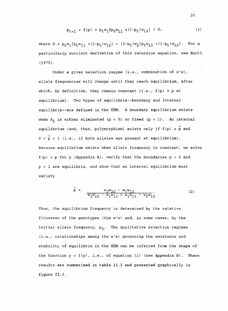
Pt+1 = f(P) = Ptwl[Ptw11 +(l-Ww12] / D, (1)
where D = ptwl[ptwll +(1-Pt)w12] (1-Ww2[Ptw12 +(l-Pt)w22]* For a
particularly succinct derivation of this recursion equation, see Hartl
(1975).
Under a given selection regime (i.e., combination of w's),
allele frequencies will change until they reach equilibrium, after
which, by definition, they remain constant [i.e., f(p) = p at
equilibrium]. Two types of equilibria--boundary and internal
equilibria--are defined in the HDM. A boundary equilibrium exists
when Al is either eliminated (p = 0) or fixed (p = 1). An internal
equilibrium (and, thus, polymorphism) exists only if f(p) = p and
0 < p < 1 (i.e., if both alleles are present at equilibrium).
Because equilibrium exists when allele frequency is constant, we solve
f(p) = p for p (Appendix A), verify that the boundaries p = 0 and
p = 1 are equilibria, and show that an internal equilibrium must
satisfy
P = w2w22 w1w12w2w22 w1w12 w1w11 w2w12
(2)
Thus, the equilibrium frequency is determined by the relative
fitnesses of the genotypes (the w's) and, in some cases, by the
initial allele frequency, p0. The qualitative selection regimes
(i.e., relationships among the w's) governing the existence and
stability of equilibria in the HDM can be inferred from the shape of
the function y = f(p), i.e., of equation (1) (see Appendix B). These
results are summarized in table 11.1 and presented graphically in
figure 11.3.
21
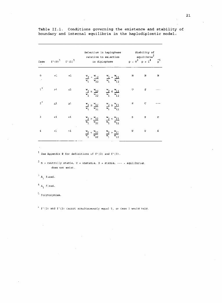
Table 11.1. Conditions governing the existence and stability ofboundary and internal equilibria in the haplodiplontic model.
Case f'(0)1
f'(1)1
Selection in haplophase
relative to selection
in diplophase
Stability of
equilibria2
p = 03
p = 14 ^5
0 =1 =1w2 = w12 w2 = W11
w1 w22w1 W12
Zl S1w2 < w12 w2 w11
w1 w22 w1 w12
2+ 1
3 <1
4 >1
w2 Z w12 w2 L w11
wl w22 wl w12
<1w2 > w12 w2 < w11
wl w22 wl w12
>1w2 < w12 w2 > w11w1
w22 w1 w12
1See Appendix B for definitions of f'(0) and f'(1).
2N = neutrally stable, U = unstable, S = stable,
does not exist.
3A
2fixed.
4Al fixed.
5Polymorphism.
equilibrium
f'(0) and f'(1) cannot simultaneously equal 1, or Case 0 would hold.
22
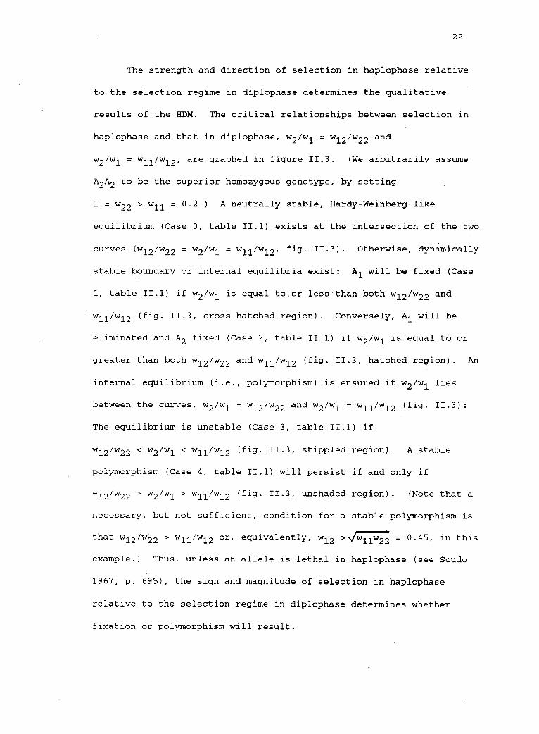
The strength and direction of selection in haplophase relative
to the selection regime in diplophase determines the qualitative
results of the HDM. The critical relationships between selection in
haplophase and that in diplophase, w2/w1 = w12/w22 and
w2/w1 = w11/w12, are graphed in figure 11.3. (We arbitrarily assume
A2A2
to be the superior homozygous genotype, by setting
1 = w22 > w11 = 0.2.) A neutrally stable, Hardy-Weinberg-like
equilibrium (Case 0, table II.1) exists at the intersection of the two
curves (w12/w2212w 22 = w2/w1 = w11/w12' fig. 11.3). Otherwise, dynamically
stable boundary or internal equilibria exist: Al will be fixed (Case
1, table II.1) if w2/wi is equal to.or less than both w12/w and22
w11/w12 (fig. 11.3, cross-hatched region). Conversely, Al will be
eliminated and A2 fixed (Case 2, table 11.1) if w2/w1 is equal to or
greater than both w12/w22 and wil /w12 (fig. 11.3, hatched region). An
internal equilibrium (i.e., polymorphism) is ensured if w2/w1 lies
between the curves, w /2.w1 = w12/w22 and w2/wi = w11/w12 (fig.
The equilibrium is unstable (Case 3, table II.1) if
11.3):
w12/w22 < w2/w1 < w11/w12 (fig. 11.3, stippled region). A stable
polymorphism (Case 4, table II.1) will persist if and only if
w12/w22 > w2/w1 > w11/w12 (fig. 11.3, unshaded region). (Note that a
necessary, but not sufficient, condition for a stable polymorphism is
that w12/w22 > w11/w12 or, equivalently, w12 >4777 = 0.45, in this
example.) Thus, unless an allele is lethal in haplophase (see Scudo
1967, p. 695), the sign and magnitude of selection in haplophase
relative to the selection regime in diplophase determines whether
fixation or polymorphism will result.
23
Figure 11.3. Parameter space of the haplodiplontic model in twodimensions. Selection regime in diplophase: Fitnesses of thehomozygotes are fixed (w11 = 0.2, w22 = 1). Fitness of theheterozygote, w12, relative to that of the homozygotes (i.e., thedegree of dominance) varies from inferior (to the left of line A); tointermediate (incomplete dominance, between lines A and B); tosuperior (to the right of line B).
Selection regime in haplophase: The ratio w2/wi representsrelative fitnesses of the haploid genotypes. The DM holds whenselection is absent in haplophase (i.e., w2 = w1, or w2/w1 = 1; pointsalong the horizontal dashed line).
The critical relationships between the selection regimes inhaplophase and diplophase (table 1, Appendix B), are graphed as
d w2/wl = w11/w12, defining regions of, the parameterw2/w1 = w12/w22 anspace corresponding to Cases 1-4 in table 1. Note that all points onthe curves w2/w1 = w12/w22 and w2/w1 = w11/w12 are associated withregions of stable boundary equilibrium (table 1), exceptw12/w22 = w11/w12, where a neutrally stable equilibrium (Case 0)results.
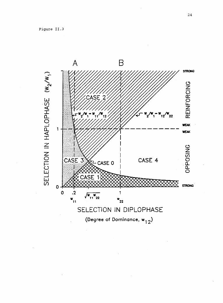
Figure 11.3
N
A
.2
1111 22
1
22
SELECTION IN DIPLOPHASE(Degree of Dominance, w 12)
24
STRONG
WEAR
WEAK
STRONG
25
PREDICTIONS OF THE MODEL
In this section we examine the equilibrium conditions in detail,
exploring the predictions of the haplodiplontic model relative to
those of the classical diploid model. First we note that the DM is a
special case of the HDM (also see Ewing 1977). The DM assumes the
absence of selection in haplophase (i.e., w2/w1 = 1, fig. 11.3, all
points on the horizontal dashed line). A neutrally stable (Hardy-
Weinberg) equilibrium exists if selection is also absent in diplophase
(i.e., w2/w1 = w12/w22 = w11/w12 = 1). Further, with partial or
complete dominance (ws- 11
< w12 < w22, w11 # w22), the allele that is
favored when homozygous in diplophase (henceforth A2) will be fixed.
Finally, internal equilibria exist when the heterozygote is inferior
[p unstable for 0 < w12 < min(w11, w22)] or superior [p stable for
> max (w11,(1'711 '
w2z-)] to the two homozygotes. Thus, when w1 = w2, the
conditions permitting stable polymorphism in the DM [i.e.,
w12 max(w11, w22)] are satisfied by conditions for polymorphism in
the HDM (i.e.,w.12/w22 > w2/w1 > w11/w12; table II.1)
With selection in haplophase, however, the HDM differs from the
DM in the conditions for the existence and stability of internal
equilibria and in the rate of approach to stable equilibria. First, a
neutrally stable equilibrium exists if and only if
w12 =.Jw11w22 = w2 /w1 (or w2/w1 = w12/w22 = w11/w12 1) (fig. 11.3;
Scudo 1976), Second, the degree of dominance in diplophase constrains
the effect of haplophase selection--increasing dominance enhances the
likelihood of stable polymorphism (Hartl 1975). Third, selection in
haplophase may either reinforce or oppose selection in diplophase.
26
Here we introduce two new terms to differentiate these contrasting
patterns of selection. Specifically, haplophase selection is
considered reinforcing if an allele that is advantageous when
homozygous in diplophase (henceforth, A2) is also advantageous in
haplophase (i.e., if w11 < w22 and w1 < w2, fig. 11.3, upper half).
Opposing selection occurs, however, if an allele is advantageous in
diplophase and disadvantageous in haplophase (i.e., if w11 < w22 and
w1
> w2, fig. 11.3, lower half). Opposing selection between the
phases of haplodiplonts is one type of balancing selection considered
by Haldane and Jayakar (1963). Next we show that the results under
reinforcing or opposing selection depend on the degree of dominance
expressed and the magnitude of selection in diplophase.
Reinforcing Selection
Reinforcing selection in the HDM (w2/w1 > 1, fig. 11.3, area
above the horizontal dashed line) accelerates fixation of the favored
allele and restricts the conditions under which polymorphism will be
maintained. With homozygote advantage (selection against the
heterozygote) in diplophase [1'112 < min(w11, w22), fig. 11.3, area to
the left of vertical line A], an unstable internal equilibrium will
exist as long as haplophase selection is weak relative to the
selection differential between the heterozygote and the disad-
vantageous homozygote in diplophase (w2/w1 < w11/w12, fig. 11.3,
stippled region; or w1 > w12-
/w11' fig. II.4A). Either Al or A2 may be
fixed, depending on the initial allele frequency, pip. The
equilibrium, p, is shifted toward p = 1 and the approach to p = 1 is
27
Figure 11.4. Results of simulations in which the strength ofreinforcing selection in haplophase was varied, while the selectionregime in diplophase was held constant. Because we arbitrarily assume
w22 > w11, then 1 = w2 > w1 implies reinforcing selection under theHDM. (Note that w2 = w1 implies the DM.) A. Homozygote advantage indiplophase: w12 < min(w11' w22 = 1). Reinforcing selection (HDM):
weak, wl > w12/w11; strong, w1 < w12/w11' B. Intermediateheterozygote (partial or complete dominance) in diplophase:
w11 w12 w22 = 1. Reinforcing selection (HDM): strong, anyw1 < w2 = 1. C. Heterozygote advantage in diplophase:1 = w12 > max(w11' w22)* Reinforcing selection (HDM): weak,w1 w22; strong, w1 < w
1w22.
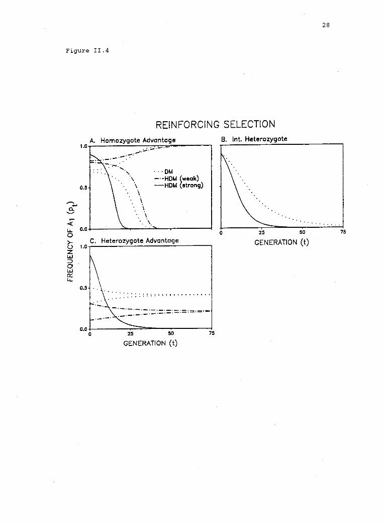
Figure 11.4
1.0
0.5
0.0
1.0
0.5
REINFORCING SELECTIONA. Homozygote Advantage B. Int. Heterozygote
DM-HDM (weak)HDM (strong)
C. Heterozygote Advantage
............
0.00 25 50
GENERATION (t)75
28
25 50
GENERATION (t)75
29
slowed, while the approach to p = 0 is accelerated (fig. II.4A).
Strong selection in haplophase (w2/w1 w11 /w12, fig. 11.3, hatched
region; or w1 w12 /w11, fig. II.4A), however, precludes an internal
equilibrium. Thus, Al is eliminated and A2 is fixed (fig. II.4A).
With reinforcing selection in haplophase and partial or complete
dominance (intermediate heterozygote) in diplophase
(w11 I w12 I w22, w11 w22, fig. 11.3, area between vertical lines
A and B), Al will be eliminated (fig. 11.3, hatched region). Thus,
the stable boundary equilibrium (p = 0) under reinforcing selection is
identical to that in the DM (Hartl 1975). However, the rate at which
the inferior allele is eliminated increases with any amount of
reinforcing selection (fig. II.4B).
Finally, with heterozygote advantage (selection against
homozygotes) in diplophase [w12 max(w11, w22), fig. 11.3, area to
the right of vertical line B], a stable internal equilibrium will
persist in the HDM, as long as reinforcing selection in haplophase is
weak relative to selection on the alternate allele in diplophase
(w2/w1 < w12/w22, fig. 11.3, unshaded region; or w1 > w22, fig.
II.4C). Weak reinforcing selection shifts the polymorphism frequency
toward the boundary (p = 0) and slows the rate of approach to
equilibrium (fig. II.4C). However, when reinforcing selection is
strong (w2/w1 > w12/w22, fig. 11.3, hatched region; or w1 < w22'
fig. II.4C), it disrupts the equilibrium produced by the diplophase
selection regime (Wright 1969; Ewing 1977) and results in fixation of
the allele favored in haplophase (fig. II.4C). Thus, under reinforc-
ing selection, the conditions favoring polymorphism are restricted in
the HDM, relative to those in the DM. In general, polymorphism
30
persists only when selection in haplophase is weak relative to the
selection regime in diplophase.
Opposing Selection
In contrast, the conditions for stable polymorphism may be
either restricted or expanded under opposing selection in haplophase
(w2/w1 < 1, fig. 11.3, area below the horizontal dashed line). First,
the selection regime in diplophase sets the necessary conditions for
polymorphism (i.e., w12/w 22 > w11 /w12, or w12 > \/w11w22) This set of
necessary (but not sufficient) conditions for polymorphism is less
stringent than that in the DM, because V-wl1w22 is always less than or
equal to max(w11' w22). Second, the relative strength of opposing
selection determines whether an internal equilibrium exists and, if
not, which allele is fixed. When homozygotes are favored in
diplophase [w12 < min(w11, w22), fig. 11.3, area to the left of verti-
cal line A], an unstable internal equilibrium exists, as long as
opposing selection is weak (w2/w1 > w12/w22, fig. 11.3, stippled
region; or w2 > w12, fig. II.5A). The equilibrium frequency is
shifted toward p = 0 and the rate of approach is slowed, while the
approach to p = 1 is accelerated (fig. II.5A). Strong opposing
selection (w w w2.
/1
<12/w 22' fig. 11.3, cross-hatched region; or
w2 < w12, fig. II.5A) ^precludes internal equilibrium (Scudo 1967),
resulting in fixation of Al, the allele favored in haplophase (fig.
II.5A).
The results are more complex, however, under opposing selection
in haplophase with partial or complete dominance (intermediate
31
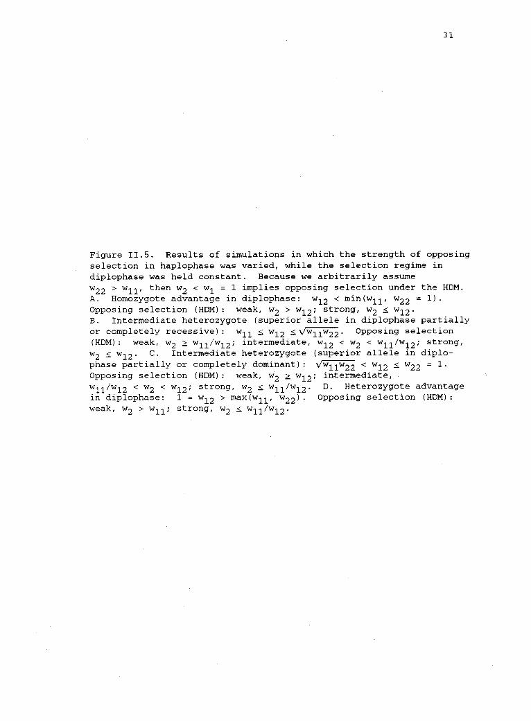
Figure II.S. Results of simulations in which the strength of opposingselection in haplophase was varied, while the selection regime indiplophase was held constant. Because we arbitrarily assume
w22 > w11, then w2 < w1 = 1 implies opposing selection under the HDM.A. Homozygote advantage in diplophase: w12 < min(w11' w22 = 1).
Opposing selection (HDM): weak, w2 w12; strong, w 2 < w 12'B. Intermediate heterozygote (superior allele in diplophase partiallyor completely recessive): w11 I w12 <"11w22' Opposing selection(HDM): weak, w2 > w11/w12; w
2 11'/w 12; w12 < w2 < w11/w12; strong,
w2 < w12. C. Intermediate heterozygote (superior allele in diplo-phase partially or completely dominant) : °7117"22 < w12 I w22 = 1'Opposing selection (HDM): weak, w2 > w12; intermediate,
w11/w12 < w2 < w12; strong, w2 < w 11/w 12' D. Heterozygote advantagein diplophase: 1 = w12 > max(w11, w22). Opposing selection (HDM):weak, w2 > w11; strong, w2 I w11/w12'
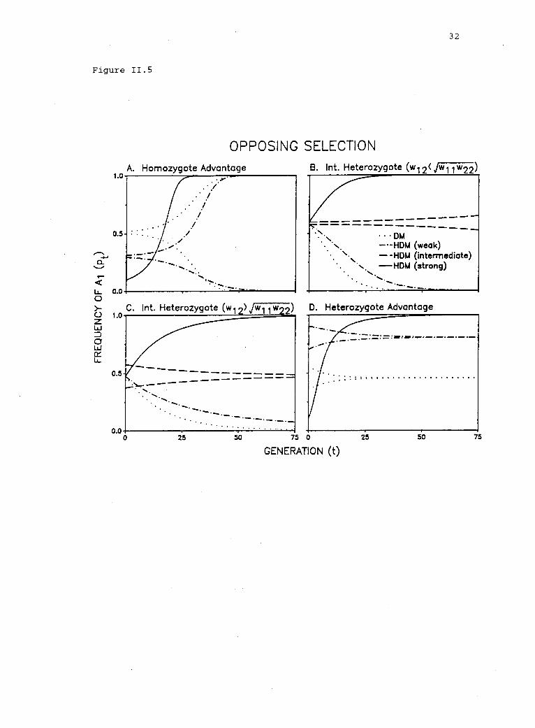
Figure 11.5
1.0
0.5
0.0
OPPOSING SELECTION
A. Homozygote Advantage B. Int. Heterozygote (w
C.1.0-
0.5
0.00 25 50
Int. Heterozygote (w1 2 vri7v w22
........
32
2 vi7171741222
DM--HDM (weak)--HDM (intermediate)HDM (strong)
--D. Heterozygote Advantage
.......
:...=.=:=,1=...
75 0
GENERATION (t)25 50 75
33
heterozygote) in diplophase (w11 w12 w22' wll # w22' fig. 11.3,
area between vertical lines A and B). Weak opposing selection
[w2/w1 > wmax(12.
/w22' w11 /w12), fig. 11.3, hatched region; or
w2 > max(w12' w11/w12) figs. II.5B and C] slows the rate of fixation
of A2, the allele favored in diplophase (figs. II.5B and C) (Scudo
1967). Strong opposing selection [w2/w1 < min(ws 12.
/w22' w11/w12"
fig. 11.3, cross-hatched region; or w2 < min (w12, wil/w12), fig.
II.5B and C] reverses the effect of diplophase selection and fixes Al,
an allele that is deleterious in diplophase, but advantageous in
haplophase (figs. II.5B and C) (Scudo 1967). Intermediate values of
opposing selection, however, permit an internal equilibrium: If the
superior allele in diplophase is partially or completely recessive
(i.e., w12 < \'`/-17177-122)'then w..iz' -/w22 < w2/w1 < w11/w12 results in
unstable equilibrium (figs. 11.3, stippled region, and II.5B).
However, if the superior allele in diplophase is partially or
completely dominant (i.e., w12 >\/w11w22" then
w12/w22 > w2/w1 > w11/w12 results in a stable equilibrium (figs. 11.3,
unshaded region, and II.5C). Thus, under opposing selection in the
HDM, stable polymorphism may be maintained in the absence of
heterozygote advantage in diplophase (Wright 1969; Ewing 1977).
Finally, with heterozygote advantage in diplophase
[w12 > max(w11, w22), fig. 11.3, area to the right of vertical line
B], and with weak opposing selection (w2'/w
1w11.
/w12' fig. 11.3,
unshaded region; or w2 > w11, fig. II.SD), polymorphism persists, but
the equilibrium frequency is shifted toward the boundary (p = 1) and
the rate of approach to equilibrium is slowed (fig. II.SD). Strong
opposing selection w2/wi < w11/w12, fig. 11.3, cross-hatched region;
34
or w2 < w11, fig. II.5D), however, precludes a stable
polymorphism--the allele that is deleterious in diplophase (A1) is
fixed (fig. II.5D) (Scudo 1967).
In summary, reinforcing selection should tend to reduce genetic
variation by speeding the rate of elimination of deleterious alleles
and by disrupting polymorphism that could otherwise be maintained by
the selection regime in diplophase. The consequences of opposing
selection, however, are more complex. On the one hand, strong
opposing selection disrupts polymorphism that would persist under
selection in diplophase and results in fixation of alleles that are
deleterious or even lethal in the homozygous state in diplophase. On
the other hand, opposing selection potentially enhances genetic
variation by slowing the loss of alleles that are deleterious in
diplophase and by maintaining stable polymorphism that would not
otherwise persist under selection in diplophase.
35
THE PROBABILITY OF POLYMORPHISM
What is the net effect of haplophase selection on the
probability of polymorphism in the HDM? The results outlined above
indicate that under reinforcing selection and with heterozygote
advantage under opposing selection, conditions permitting polymorphism
are more stringent in the HDM than in the DM. However, under opposing
selection, conditions permitting polymorphism in the HDM are expanded
if the fitness of the heterozygote is greater than the geometric mean
of the fitnesses of the homozygotes (given partial or complete
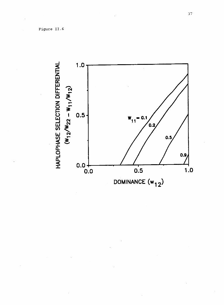
dominance of the advantageous allele). The range of values over which
haplophase selection will increase the likelihood of polymorphism is
defined by w12/w22 w11/w12 (i.e., by the vertical distance between
w2/w1 = w12/w22 and w2 /`al = w11 /w12 in fig. 11.3). This distance is
correlated with the degree of dominance (Hartl 1975; Ewing 1977), as
illustrated in figures 11.4 and 11.6: As dominance in diplophase
(w12) increases, the range of values over which haplophase selection
will permit stable polymorphism increases monotonically for a given
fitness differential between homozygotes (w22 w11) (fig. 11.6).
Hence, the degree of dominance in diplophase defines the range of
haplophase selection in the HDM that would permit "new" stable
polymorphism otherwise precluded in the DM.
The potential for gain in polymorphism under opposing selection
depends not only upon the degree of dominance, but upon the relative
fitness of the two homozygotes. In figure 11.3 the fitness (w11) of
the inferior homozygote (A1A1) is set at 0.2. Relative to the
alternate homozygote, selection against the A1A1 genotype is strong in
36
Figure 11.6. Effects of selection in diplophase (dominance andfitness of the inferior homozygote) on the range of haplophaseselection differentials that permit "new" polymorphism under opposingselection in the HDM. Note that with heterozygote advantage indiplophase, there is no potential for gain in stable polymorphism inthe HDM, under either reinforcing or opposing selection. Sufficientlystrong haplophase selection disrupts the stable polymorphism thatwould otherwise exist under the DM.
HA
PLO
PH
AS
E S
ELE
CTI
ON
DIF
FER
EN
TIA
L
(w12
M22
- W1
1/W
12)
0 ulP o°
OM
&
38
this example. If dominance is also high (i.e., w12 close to w22),
then the range of allowable values in haplophase supporting "new"
polymorphism approaches 1 -11' 12 = 0.9 (fig. 11.6). That is, even
quite strong opposing selection will result in a gain in polymorphism.
However, if the fitness differential between the two homozygotes is
small (e.g., w11 =0.9, w22 = 1, fig. 11.6), then the maximum range of
haplophase fitness resulting in a gain in polymorphism would be small.
An Analytical Approach
The net gain or loss of polymorphism under the HDM relative to
the DM is difficult to evaluate using qualitative, case-by-case
analyses (e.g., figs. 11.3-11.6). A more general analysis is possible
if the entire parameter space of the models (i.e., all possible
combinations of wig, wi, wj) is abstracted. For example, two-
dimensional formulations of the parameter space of the HDM facilitate
comparison of the results of the HDM and the DM (e.g., fig. 11.3;
Scudo 1967, figs. 1 and 2; Wright 1969, fig. 3.8; Ewing 1977, fig. 1).
However, these analyses do not permit a quantitative assessment of the
probability of polymorphism under the two models. By representing the
parameter space in three, rather than two, dimensions we derive the
first general, quantitative assessment of the net effect of selection
in haplophase on the maintenance of polymorphism. (For more complex
models, it may be necessary to use numerical techniques to explore the
relative sizes of various regions of the parameter space, e.g.,
Feldman and Liberman 1984.)
The conditions permitting stable polymorphism in the DM are
39
Figure 11.7. Parameter space of the HDM in three dimensions (the unitcube). The shaded regions indicate the conditions permitting stablepolymorphism: A. In the DM; B. and C. In the HDM. The figure inpanel C is rotated to show a top view of the cube in panel B underreinforcing and opposing selection in the HDM. (See Appendix C forproofs.)
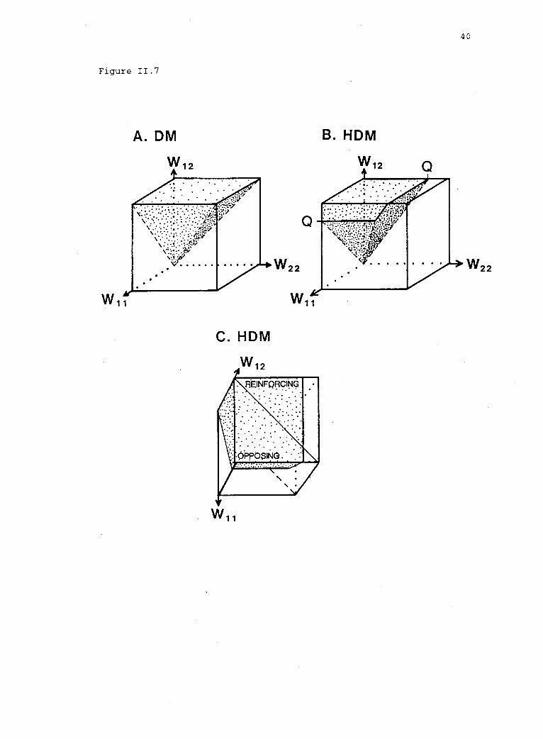
Figure 11.7
A. DM B. HDM
40
C. HDM
W11
W22
41
represented by the shaded volume (VD) of figure II.7A--the space in
which w12 > max(w11, w22). One can easily confirm that the volume of
this space is one-third of the unit cube (i.e., VD = 1/3). In the HDM
(fig. II.7B), the shape of the shaded volume changes as a function of
the strength of haplophase selection (sH = 1 Q, where Q = w1 /w2,
w1 < w2, and 0 < Q 1). (See Appendix C for definition of terms
and proof.) With haplophase selection, the volume of the space in
which polymorphism is possible is given by
V Q Q3
2 6(3)
For all defined values of Q < 1, the volume VH is smaller than the
equivalent volume for the diploid model, VD (fig. II.8A).
Consequently, for the entire parameter space, additional selection in
haplophase creates more stringent conditions for stable polymorphism
than selection in diplophase alone. The net effect of haplophase
selection is to reduce the probability that polymorphism will occur.
However, reinforcing and opposing selection may also be
considered separately. The diagonal plane in figure II.7C divides the
unit cube into regions of reinforcing and opposing selection. Under
reinforcing selection, the volume of the space permitting polymorphism
is
VHr =n2
6
(See Appendix C for proof.) For any defined value of Q < 1, VHr is
smaller than half the volume for the DM (VD/2 = 1/6, fig. II.8B).
(4)
42
Figure 11.8. Volume of the parameter space supporting polymorphism asa function of selection in haplophase (Q). A. Polymorphism in the DM(VD) and in the HDM [VH(Q)] (see eq. 3 in text). B. Polymorphismunder reinforcing [VHr(Q)] (eq. 4) and opposing [VH0(Q)] (eq. 5)
selection, compared to the DM (VD/2).
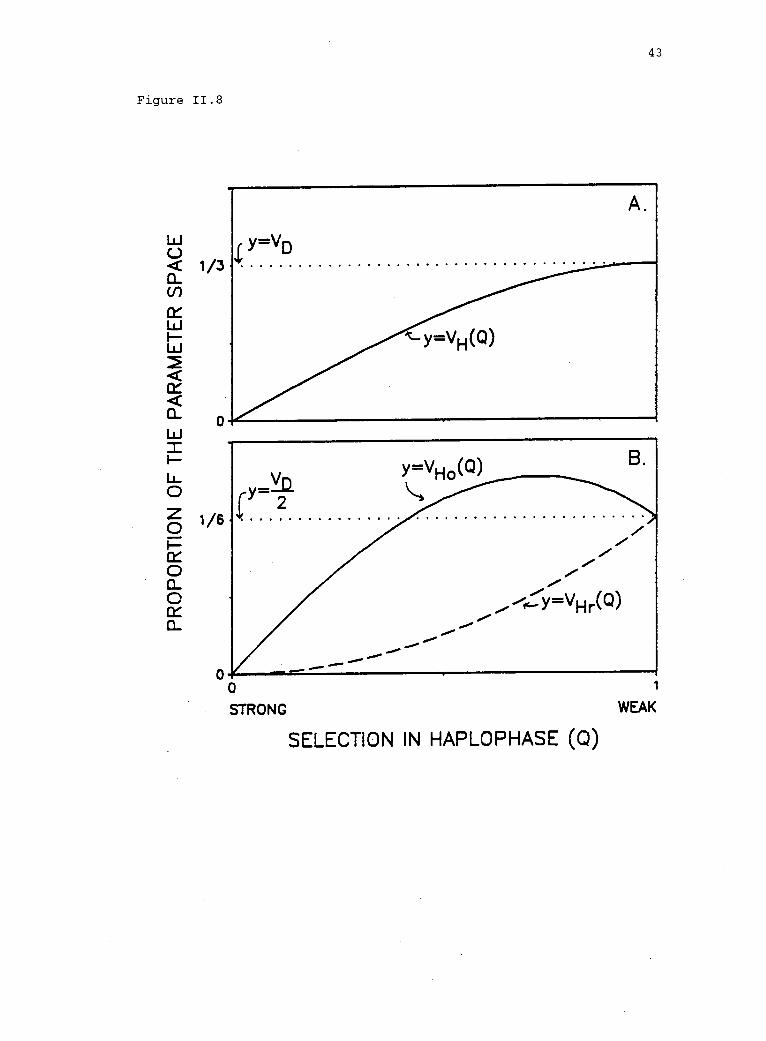
Figure 11.8
43
1/6
Y=v1-10(0)B.
_....../....-..............
/%c--r--AiHr(C))
..........0......
0 1
STRONG WEAK
SELECTION IN HAPLOPHASE (Q)
44
(This qualitative result also can be seen in figure 11.3 where, with
increasing reinforcing selection, the horizontal width of the region
permitting polymorphism decreases monotonically.) Consequently, any
reinforcing selection will reduce the probability of polymorphism.
Polymorphism is lost under reinforcing selection, because selection in
haplophase disrupts the equilibrium obtained under heterozygote
advantage in diplophase. In addition, reinforcing selection never
results in polymorphism that would not otherwise exist in the DM.
The effect of opposing selection, on the other hand, depends on
the strength of selection in haplophase. The volume of the space
permitting polymorphism under opposing selection is
VHo Q3
Q2
.
7 6 6(5)
(See Appendix C for proof.) When opposing selection in haplophase is
very strong [i.e., Q < VT 1) = 0.414], the space permitting
stable polymorphism, VH0, is less than VD/2 (fig. II.8B). Here the
loss in polymorphism due to selection within haplophase overwhelms any
gains due to balancing selection between the phases.
For a broad range of selection intensities in haplophase [i.e.,
1 > Q > (N/7 1)], however, VH0 is greater than VD/2 (fig. II.8B).
Consequently, the probability of polymorphism may be enhanced under
opposing selection, if sH < (2 -VT) . Further, the potential for
enhancement is at its maximum when Q = 0.72. (This result also is
reflected in figure 11.3, where the horizontal width of the region
permitting polymorphism reaches a maximum at intermediate levels of
opposing selection.) Thus, intermediate levels of opposing selection
45
(sH = 0.28) have the most potential to enhance the probability of
polymorphism, relative to the DM. Polymorphism is gained under
opposing selection because balancing selection between the phases
produces a stable internal equilibrium, where none would exist under
the DM. This gain in polymorphism more than offsets the loss due to
disruption by haplophase selection of the equilibrium under
heterozygote advantage in diplophase.
The role of dominance in diplophase in the HDM suggests that to
the extent that dominance evolves, the potential for maintaining
polymorphism in haplodiplontic populations should increase. That is,
as the relative fitness of the heterozygote increases (upward motion
in the unshaded region of fig. II.7A), the more likely it is that the
diplophase fitness regime falls within the parameter space supporting
polymorphism under opposing selection (i.e., the shaded region of fig.
II.7C). Moreover, if most mutations are either lethal recessive or
deleterious semi-recessive in their diplophase expression (as
suggested by Charlesworth 1979; Klekowski 1988), the potential for
polymorphism is patticularly great if they also happen to confer an
advantage in haplophase. Under opposing selection, the proportion of
homozygous lethal recessive and deleterious semi-recessive fitness
combinations that fall within the polymorphism space of the HDM (fig.
II.7C) reaches a maximum at Q = 0.72 (fig. II.8B). Thus, opposing
selection has the potential to retain alleles that would ultimately be
lost under selection in diplophase alone.
Opposing selection is a type of balancing selection between the
discrete haploid and diploid stages of the life history (Haldane and
Jayakar 1963). As such, it may be viewed as a special case of
46
antagonistic pleiotropy (Rose 1982). In both the HDM and Rose's
model, dominance has the effect of enhancing the probability of
polymorphism. The models differ, however, in that reversal of the
relative fitness of alleles occurs between different developmental
stages of the same ploidy in antagonistic pleiotropy, but between
differing ploidy levels in opposing selection. Thus, opposing
selection represents a unique mechanism for retaining genetic
variability in populations of haplodiplonts.
47
EVIDENCE FOR HDM DYNAMICS IN NATURAL POPULATIONS
The importance of HDM dynamics for reducing or maintaining
genetic variation in natural populations of haplodiplonts is almost
entirely unexplored. Three conditions govern the potential effect of
HDM dynamics on polymorphism: The first two--that a gene is expressed
in both haploid and diploid phases and that alleles are not
selectively neutral--are necessary conditions for the HDM to apply.
The third condition--the relative sign and magnitude of selection in
the two phases--determines whether selection will tend to eliminate or
retain genetic variability within a population. These conditions
rarely have been documented in natural populations.
Gene expression in both phases is a necessary condition for HDM
dynamics to apply (fig. 11.9). Overlap in gene expression should be
greater, and more of the genome should be subject to HDM dynamics, in
taxa in which the gametophytic and sporophytic phases are similar in
morphology and physiology. Expression of certain loci in both phases
has been documented for isomorphic algae (Cheney and Babbel 1978) and
pteridophytes (Gastony and Gottlieb 1982, 1985; Haufler and Soltis
1984; Haufler 1985), but the extent of overlap in gene expression
between the phases has not been quantified. The little quantitative
information available on gene expression in the two phases derives
from studies of angiosperms (reviews in Heslop-Harrison 1980; Mulcahy
and Mulcahy 1987). Quantitative estimates of overlap in gene
expression between male gametophytes (pollen) and sporophytes range
from 34 to 72% for plants grown in greenhouse or laboratory
(Lycopersicon esculenta, 58%, Tanksley et al. 1981; Tradescantia
48
Figure 11.9. A schematic representation of gene expression in thehaplodiplontic genome, indicating the regions of applicability of theHM (shaded), the DM (hatched), and the HDM (both) (after Heslop-Harrison 1980). Gene expression in both phases is a necessarycondition for the HDM. If a locus is not expressed in one phase, itsalleles are effectively neutral in that phase (Hartl 1970). The HDMthen reduces to either the HM or the DM, depending on whether thelocus is silent in diplophase or in haplophase, respectively.
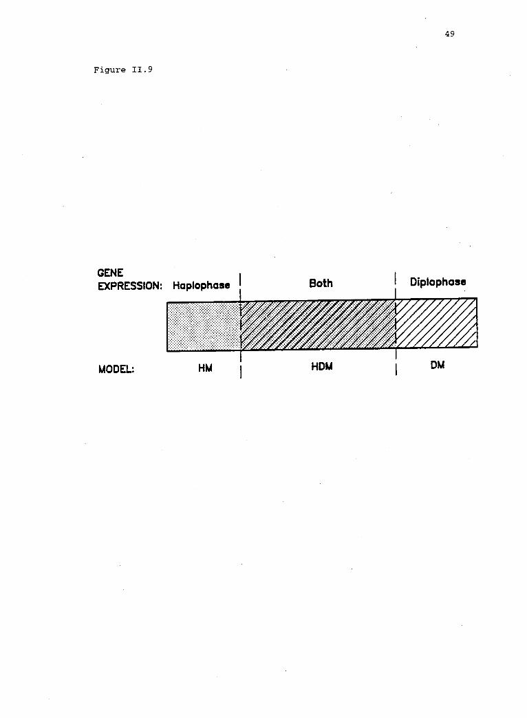
Figure 11.9
GENEEXPRESSION: Haplophase I
MODEL: HM
Both
49
Diplophase
HDM DM
50
paludosa, 34-56%, Willing and Mascarenhas 1984; and Zea mays, 72%,
Sari-Gorla et al. 1986). Thus, even among these plants with a highly
reduced haplophase, the first necessary condition exists for HDM
dynamics to apply, because a significant proportion of the genome is
expressed in both phases.
A second necessary condition is that selection occurs in both
phases. Although selection studies are lacking for bryophytes,
pteridophytes, and multicellular algae, studies of angiosperms have
demonstrated that pollen competition (review in Mulcahy and Mulcahy
1987; also see contributions to Mulcahy et al. 1986) and pollen
selection (e.g., Searcy and Mulcahy 1985) may affect the frequency of
traits expressed in the sporophyte. Moreover, the third condition
governing HDM dynamics has been explored in studies demonstrating the
sign of correlations in fitness between the two phases. A positive
correlation in fitness (i.e., reinforcing selection) between
gametophytic and sporophytic traits has been found in studies of
pollen (Mulcahy and Mulcahy 1987; Mulcahy et al. 1986; Searcy and
Mulcahy 1985). This evidence of reinforcing selection presumably
reflects selective elimination of inferior variants in the
gametophytic stage. In contrast, negative correlations in fitness
(i.e., opposing selection) between gametophytes and sporophytes have
been observed in studies of non-Mendelian transmission during plant
life cycles (e.g., Muntzing 1968, Clegg et al. 1978, Clegg and
Epperson 1988). This evidence of opposing selection was detectable,
in part, because traits deleterious in diplophase persist (Heslop-
Harrison 1980). To evaluate the importance of HDM dynamics in natural
populations, studies are needed that document the relative magnitude,
51
as well as the sign, of selection in both phases.
Several factors complicate the study of HDM dynamics in higher
plants. Studies of pollen competition, for example, have detected
only reinforcing selection between the phases. Further, special care
must be taken to eliminate non-genetic causes (e.g., maternal effects
or environmental effects on pollen quality) of correlations between
conditions favoring pollen competition and vigor of sporophytes
(Charlesworth et al. 1987; Charlesworth 1988; Young and Stanton 1990).
In addition, the frequency of pollen competition in nature is
presently unknown for most taxa (Snow 1986, 1990). Studies of
selective transmission of traits in both phases are complicated by the
small size of gametophytes and the difficulty of replicating
gametophytic genotypes. Further, the dependence of the female
gametophyte on the sporophyte makes it difficult to determine whether
biased transmission is due to gametophytic or early zygotic selection.
There are a number of advantages to using lower plants (algae,
bryophytes, and pteridophytes) as model systems for studying HDM
dynamics. In lower plants, a larger portion of the genome should be
subject to HDM dynamics, because both phases undergo relatively
extensive development. Both phases tend to be macroscopic and
gametophytes may produce numbers of genetically identical gametes.
Gametophytes of algae and pteridophytes are physiologically
independent of parental sporophytes, facilitating the separation of
components of selection in each phase. Finally, ecological
differentiation between the phases of pteridophytes (e.g., Sato 1982)
and algae (e.g., Luxoro and Santelices 1989; Olson 1990; Zupan and
West 1990) suggest that the relative fitness of individuals with
52
certain traits may vary between the phases temporally or spatially.
Thus, selection should act on the vegetative, as well as the
reproductive functions of both phases. Although direct evidence for
selection and HDM dynamics is scant, it is possible to test the
hypothesis that the presence of a prominent haploid phase is
associated with reduced levels of genetic polymorphism in natural
populations.
53
ENZYME POLYMORPHISM IN HAPLODIPLONTIC POPULATIONS
Opposing selection between haplophase and diplophase has a
presently unquantified, but potentially important, role in maintaining
genetic variation in populations of haplodiplonts (Ennos 1983). If
the net effect of selection in haplophase were to more rapidly
eliminate alleles from a population, then there would be a negative
relationship between the prominence of haplophase in the life
histories of species and the occurrence of polymorphism within spe-
cies' populations. We test this hypothesis by comparing levels of
polymorphism among several plant divisions whose life cycles represent
a continuum from dominance of the haploid phase, through isomorphy of
haploid and diploid stages, to diplophase dominance.
If haplophase selection reduces genetic variability in natural
populations, occurrence of polymorphism should be lowest in
gametophyte-dominant algae and bryophytes, intermediate among
isomorphic algae, and highest among sporophyte-dominant algae,
pteridophytes, gymnosperms, and angiosperms. Estimates of
polymorphism have been compiled for gymnosperms and angiosperms
(Hamrick and Godt 1989). However, despite reports of high levels of
polymorphism among bryophytes (Yamazaki 1981, 1984; Szweykowski 1984;
Wyatt 1985; Wyatt et al. 1989b), a comprehensive comparison of
polymorphism among bryophytes, algae, and pteridophytes has not been
previously published. To evaluate the extent of polymorphism in
populations of these taxa, we compiled data from literature published
between 1970 and 1989 (table 11.2). Studies were included only if a
genetic interpretation of the data was possible. Thirty-two studies
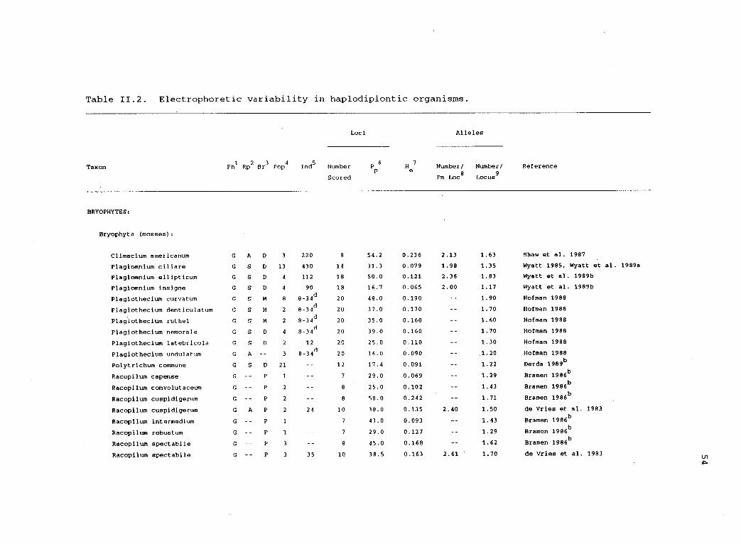
Table 11.2. Electrophoretic variability in haplodiplontic organisms.
Taxon
Loci Alleles
Ph1
Rp2
Br3
Pop4
Ind5
Number Pp6 He7
Number/ Number/ Reference
Scored Pm Loc8
Locus
BRYOPHYTES:
Bryophyta (mosses):
Climacium americanum G A D 3 220 8 54.2 0.236 2.13 1.63 Shaw et al. 1987
Plagiomnium ciliare G S D 13 430 14 31.3 0.079 1.98 1.35 Wyatt 1985, Wyatt et al.
Plagiomnium ellipticum G S D 4 112 18 50.0 0.121 2.36 1.83 Wyatt et al. 1989b
Plagiomnium insigne G S D 4 90 18 16.7 0.065 2.00 1.17 Wyatt et al. 1989b
Plagiothecium curvatum G S M 8 8-34d
20 46.0 0.190 1.90 Hofman 1988
Plagiothecium denticulatum G S M 2 8-34d
20 37.0 0.170 1.70 Hofman 1988
Plagiothecium ruthei G S M 2 8-34d
20 35.0 0.160 1.60 Hofman 1988
Plagiothecium nemorale G S D 4 8-34d
20 39.0 0.160 1.70 Hofman 1988
Plagiothecium latebricola G S D 2 12 20 25.0 0.110 1.30 Hofman 1988
Plagiothecium undulatum G A -- 3 8-34d
20 16.0 0.090 1.20 Hofman 1988
Polytrichum commune G S D 21 12 17.4 0.091 1.22 Derda 1989b
Racopilum capense G P 1 7 29.0 0.069 1.29 Bramen 1986b
Racopilum convolutaceum G P 2 8 25.0 0.102 1.43 Bramen 1986b
Racopilum cuspidigerum G P 2 8 50.0 0.242 1.71 Bramen 1986b
Racopilum cuspidigerum G A P 2 24 10 30.0 0.135 2.40 1.50 de Vries et al. 1983
Racopilum intermedium G -- P 1 7 43.0 0.093 1.43 Bramen 1986b
Racopilum robustum G P 1 7 29.0 0.127 1.29 Bramen 1986b
Racopilum spectabile G P 3 8 45.0 0.168 1.62 Bramen 1986b
Racopilum spectabile G P 3 35 10 38.5 0.163 2.61 1.70 de Vries et al. 1983
1989a
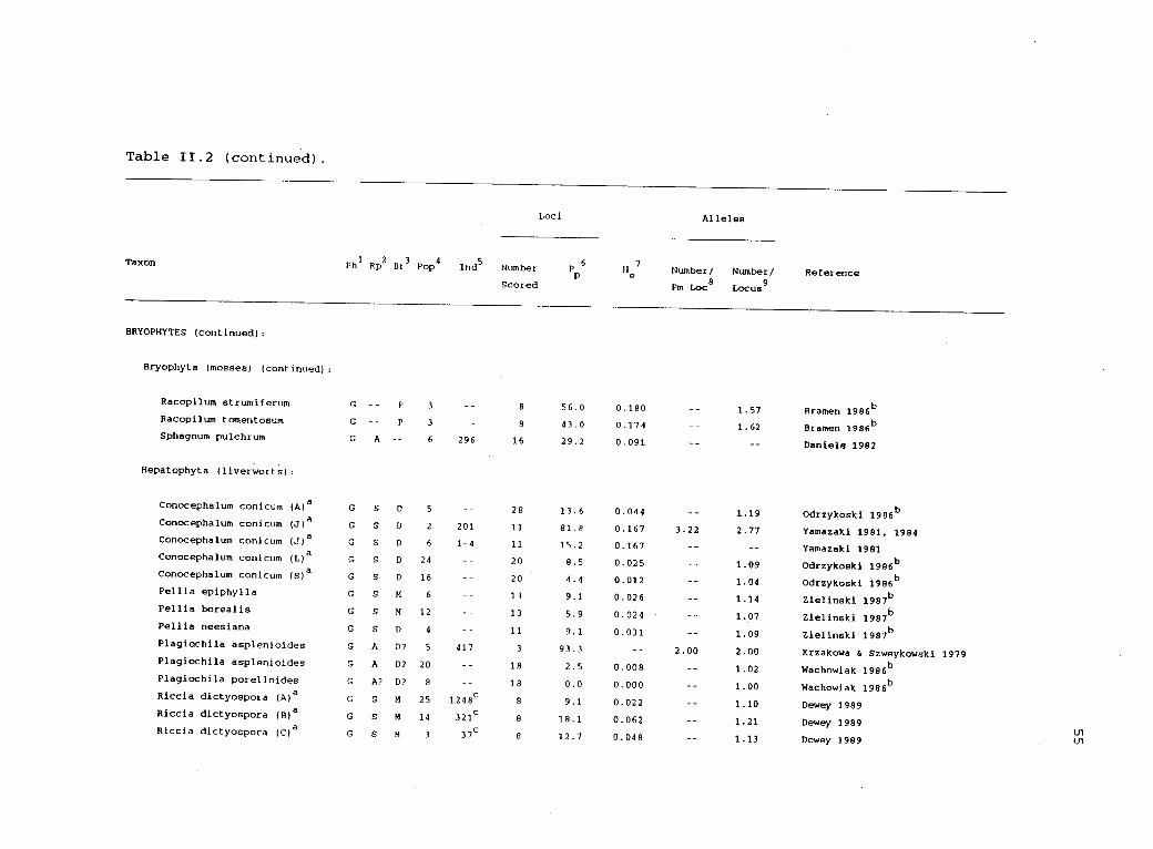
Table 11.2 (continued).
Taxon
Loci Alleles
Ph1
Rp2
Br3
Pop4
Inds
Number Pp6e7
Number/ Number/ ReferenceScored Pm Loc
8Locus
BRYOPHYTES (continued):
Bryophyta (mosses) (continued):
Racopilum strumiferum G P 3 8 56.0 0.180 1.57 Bramen 1986b
Racopilum tomentosum G -- P 3 8 43.0 0.174 1.62 Bramen 1986 b
Sphagnum pulchrum G A 6 296 16 29.2 0.091 Daniels 1982
Hepatophyta (liverworts):
Conocephalum conicum (A)a G S D 5 28 13.6 0.044 1.19 Odrzykoski 1986b
Conocephalum conicum (J)a G S D 2 201 11 81.8 0.167 3.22 2.77 Yamazaki 1981, 1984Conocephalum conicum (J)a G S D 6 1-4 11 15.2 0.167 Yamazaki 1981Conocephalum conicum (L)a G S D 24 20 8.5 0.025 1.09 Odrzykoski 1986b
Conocephalum conicum (S)a G S D 16 20 4.4 0.012 1.04 Odrzykoski 1986b
Pellia epiphylla G S M 6 13 9.1 0.026 1.14 Zielinski 1987bPellia borealis G S M 12 13 5.9 0.024 1.07 Zielinski 1987
b
Pellia neesiana G S D 4 11 9.1 0.031 1.09 Zielinski 1987b
Plagiochila asplenioides G A D? 5 417 3 93.3 2.00 2.00 Krzakowa & SzweykowskiPlagiochila asplenioides G A D? 20 18 2.5 0.008 1.02 Wachowiak 1986b
Plagiochila porelloides G A? D? 8 18 0.0 0.000 1.00 Wachowiak 1986b
Riccia dictyospora (A)a G S M 25 1248c 8 9.1 0.022 1.10 Dewey 1989Riccia dictyospora (B)a G S M 14 321c 8 18.1 0.062 1.21 Dewey 1989Riccia dictyospora (C)a G S M 3 37c 8 12.7 0.048 1.13 Dewey 1989
1979
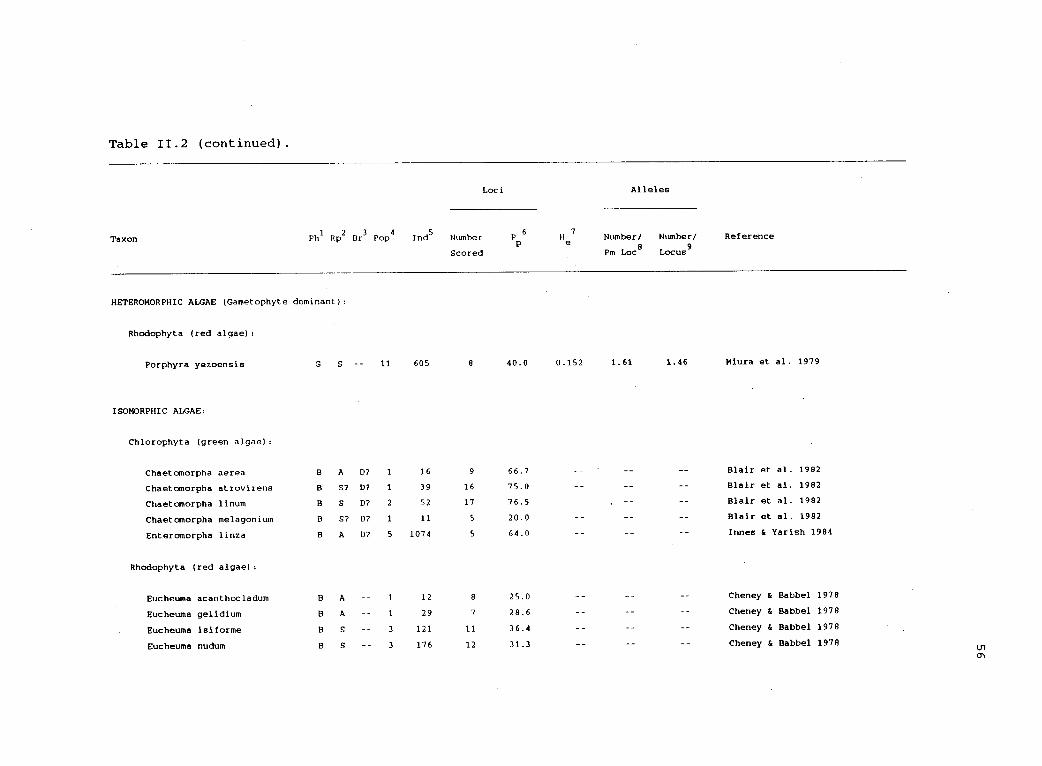
Table 11.2 (continued).
Taxon
Loci Alleles
Ph1 Rp
2Br
3Pop
4Ind
5Number Pp6 H
e7
Number/ Number/ Reference
Scored Pm Loc8
Locus
HETEROMORPHIC ALGAE (Gametophyte dominant):
Rhodophyta (red algae):
Porphyra yezoensis G S 11 605 8 40.0 0.152 1.61 1.46 Miura et al. 1979
ISOMORPHIC ALGAE:
Chlorophyta (green algae):
Chaetomorpha aerea B A D? 1 16 9 66.7 Blair et al. 1982
Chaetomorpha atrovirens B S7 D? 1 39 16 75.0 Blair et al. 1982
Chaetomorpha linum B S D? 2 52 17 76.5 Blair et al. 1982
Chaetomorpha melagonium B S7 D7 1 11 5 20.0 Blair et al. 1982
Enteromorpha linza B A D7 5 1074 5 64.0 Innes & Yarish 1984
Rhodophyta (red algae):
Eucheuma acanthocladum B A 1 12 8 25.0 Cheney & Babbel 1978
Eucheuma gelidium B A 1 29 7 28.6 Cheney & Babbel 1978
Eucheuma isiforme B S 3 121 11 36.4 Cheney & Babbel 1978
Eucheuma nudum B S 3 176 12 31.3 Cheney & Babbel 1978
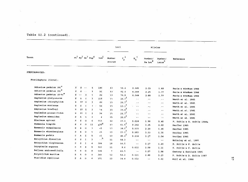
Table 11.2 (continued).
Taxon
Loci
Phi Rp2 Bra Pop4 Ind5 Number Pp6
Scored
He
7
Alleles
Number/ Number/ Reference
Pm Loc8 Locus9
PTERIDOPHYTES:
Pteridophyta (ferns):
Adiantum pedatum (W)e S S -- 6 186 13 56.4 0.185 2.33 1.83 Paris & Windham 1988Adiantum pedatum (s)e S S 1 11 13 61.4 0.166 2.25 1.77 Paris & Windham 1988Adiantum pedatum (S-T)e S -- Z 1 22 13 76.9 0.348 2.00 1.77 Paris & Windham 1988Asplenium platyneuron S S I 3 119 15 26.7E Werth et al. 1985
fAsplenium rhizophyllum S S? 0 3 49 15 26.7 Werth et al. 1985fAsplenium montanum S S I 3 56 15 13.3 Werth et al. 1985
Asplenium bradleyi S S? Z 2 54 15 20.0t Werth et al. 1985Asplenium pinnatifidum S S? Z 2 34 15 26.7
f
Werth et al. 1985Asplenium ebenoides S A Z 2
415 20.01 -- -- Werth et al. 1985
Blechnum spicant S S 0 6 553 12 23.6 0.024 1.96 1.40 P. Soltis & D. Soltis 1988aBommeria hispida S S 0 12 S30g 13 61.5
f0.262 3.25 2.69 Haufler 1985
fBommeria subpaleacea S S 0 3 <5 13 38.5 0.133 2.20 1.46 Haufler 1985Bommeria ehrenbergiana S S 0 1 <5 13
f23 . 1 .0.103 2.33 1.31 Haufler 1985
Bommeria pedata S A Z 5 <5 13f
4 6 . 2 .0.218 2.17 1.54 Haufler 1985Botrychium dissectum S S I 3
h11 18.2 -- McCauley et al. 1985
Botrychium virginianum S S I 4 184 18 16.5 2.17 1.20 D. Soltis & P. SoltisDryopteris expansa S S X 9 502 11 9.6 0.032 2.00 1.11 D. Soltis & P. SoltisPellaea andromedifolia S S 0 9 146 7 63.5 2.07 1.68 Gastony & Gottleib 1985Polystichum munitum S S 0 4 341 12 54.2 0.111 2.80 2.23 P. Soltis & D. Soltis 1987Pteridium aguilinum S A 0 4 191 13 34.6 0.122 1.62 Wolf et al. 1988
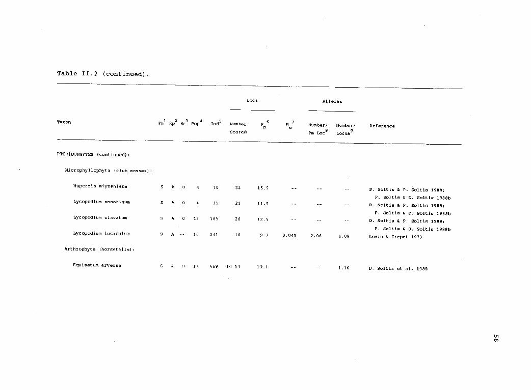
Table 11.2 (continued).
Taxon
Loci Alleles
Ph1
Rp2
Br3
Pop4
Inds
Number 6
e Number/ Number/ ReferenceScored Pm Loc
8Locus
PTERIDOPHYTES (continued):
Microphyllophyta (club mosses):
Huperzia miyoshiana S A 0 4 70 22 15.9 D. Soltis & P. Soltis 1988;
P. Soltis & D. Soltis 1988bLycopodium annotinum S A 0 4 35 21 11.9 D. Soltis & P. Soltis 1988;
P. Soltis & D. Soltis 1988bLycopodium clavatum S A 0 12 165 20 12.5 D. Soltis & P. Soltis 19881
P. Soltis & D. Soltis 1999bLycopodium lucidulum S A 16 241 18 9.7 0.041 2.06 1.08 Levin & Crepet 1973
Arthrophyta (horsetails):
Equisetum arvense S A 0 17 669 10-13 19.1 1.16 D. Soltis et al. 1988
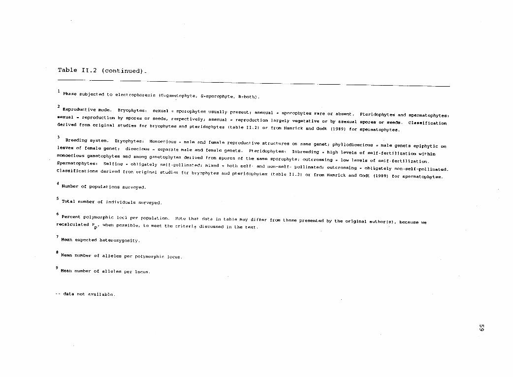
Table 11.2 (continued).
1Phase subjected to electrophoresis (G=gametophyte, S= sporophyte, B.both).
2Reproductive mode. Bryophytes: sexual = sporophytes usually present; asexual = sporophytes rare or absent. Pteridophytes and spermatophytes:
sexual . reproduction by spores or seeds, respectively; asexual = reproduction largely vegetative or by asexual spores or seeds. Classificationderived from original studies for bryophytes and pteridophytes (table 11.2) or from Hamrick and Godt (1989) for spermatophytes.
3Breeding system. Bryophytes: Monoecious male and female reproductive structures
on same genet; phyllodioecious . male genets epiphytic onleaves of female genet; dioecious = separate male and female genets. Pteridophytes: Inbreeding . high levels of self-fertilization withinmonoecious gametophytes and among gametophytes derived from spores of the same sporophyte; outcrossing = low levels of self-fertilization.Spermatophytes: Selfing obligately self-pollinated; mixed = both self- and non-self- pollinated; outcrossing = obligately non-self-pollinated.Classifications derived from original studies for bryophytes and pteridophytes {table 11.2) or from Hamrick and Godt (1989) for spermatophytes.
4Number of populations surveyed.
5Total number of Individuals surveyed.
6Percent polymorphic loci per population. Note that data in table may differ from those presented by the original author(s), because we
recalculated PP'
when possible, to meet the criteria discussed in the text.
7Mean expected heterozygosity.
8Mean number of alleles per polymorphic locus.
9Mean number of alleles per locus.
-- data not available.
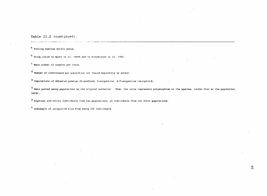
Table 11.2 (continued).
a Sibling species within genus.
bStudy cited in Wyatt et al. 1989b and in Stoneburner et al. 1990.
Mean number of samples per locus.
dNumber of individuals per population not listed separately by author.
e Populations of Adiantum pedatum (W.woodland, S= serpentine, S -T= serpentine tetraploid).
Data pooled among populations by the original author(s). Thus, the value represents polymorphism at the species, rather than at the population,
level.
g Eighteen and thirty individuals from two populations, 55 individuals from ten other populations.
hSubsample of unreported size from among 209 individuals
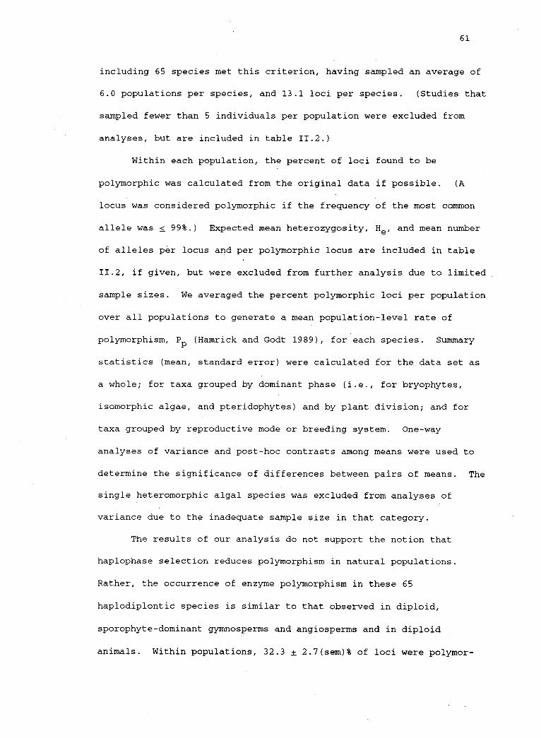
61
including 65 species met this criterion, having sampled an average of
6.0 populations per species, and 13.1 loci per species. (Studies that
sampled fewer than 5 individuals per population were excluded from
analyses, but are included in table 11.2.)
Within each population, the percent of loci found to be
polymorphic was calculated from the original data if possible. (A
locus was considered polymorphic if the frequency of the most common
allele was < 99%.) Expected mean heterozygosity, He and mean number
of alleles per locus and per polymorphic locus are included in table
11.2, if given, but were excluded from further analysis due to limited
sample sizes. We averaged the percent polymorphic loci per population
over all populations to generate a mean population-level rate of
polymorphism, P (Hamrick and Godt 1989), for each species. Summary
statistics (mean, standard error) were calculated for the data set as
a whole; for taxa grouped by dominant phase (i.e., for bryophytes,
isomorphic algae, and pteridophytes) and by plant division; and for
taxa grouped by reproductive mode or breeding system. One-way
analyses of variance and post-hoc contrasts among means were used to
determine the significance of differences between pairs of means. The
single heteromorphic algal species was excluded from analyses of
variance due to the inadequate sample size in that category.
The results of our analysis do not support the notion that
haplophase selection reduces polymorphism in natural populations.
Rather, the occurrence of enzyme polymorphism in these 65
haplodiplontic species is similar to that observed in diploid,
sporophyte-dominant gymnosperms and angiosperms and in diploid
animals. Within populations, 32.3 ± 2.7(sem)% of loci were polymor-
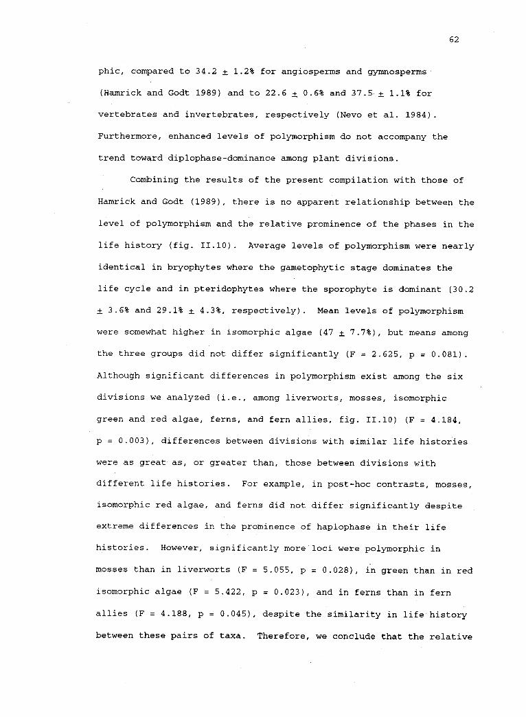
62
phic, compared to 34.2 ± 1.2% for angiosperms and gymnosperms
(Hamrick and Godt 1989) and to 22.6 + 0.6% and 37.5 -± 1.1% for
vertebrates and invertebrates, respectively (Nevo et al. 1984).
Furthermore, enhanced levels of polymorphism do not accompany the
trend toward diplophase-dominance among plant divisions.
Combining the results of the present compilation with those of
Hamrick and Godt (1989), there is no apparent relationship between the
level of polymorphism and the relative prominence of the phases in the
life history (fig. 11.10). Average levels of polymorphism were nearly
identical in bryophytes where the gametophytic stage dominates the
life cycle and in pteridophytes where the sporophyte is dominant (30.2
± 3.6% and 29.1% ± 4.3%, respectively). Mean levels of polymorphism
were somewhat higher in isomorphic algae (47 ± 7.7%), but means among
the three groups did not differ significantly (F = 2.625, p = 0.081).
Although significant differences in polymorphism exist among the six
divisions we analyzed (i.e., among liverworts, mosses, isomorphic
green and red algae, ferns, and fern allies, fig. 11.10) (F = 4.184,
p = 0.003), differences between divisions with similar life histories
were as great as, or greater than, those between divisions with
different life histories. For example, in post-hoc contrasts, mosses,
isomorphic red algae, and ferns did not differ significantly despite
extreme differences in the prominence of haplophase in their life
histories. However, significantly more loci were polymorphic in
mosses than in liverworts (F = 5.055, p = 0.028), in green than in red
isomorphic algae (F = 5.422, p = 0.023), and in ferns than in fern
allies (F = 4.188, p = 0.045), despite the similarity in life history
between these pairs of taxa. Therefore, we conclude that the relative

63
Figure II.10. Polymorphism within plant populations that representregions on a continuum of life history variation (from table 11.2 andHamrick and Godt 1989). Non-vascular plants: Bryophytes(Br = Bryophyta; He = Hepatophyta); and algae (Het Rh = heteromorphicRhodophyta; Iso Ch and Iso Rh = isomorphic Chlorophyta and Rhodophyta,respectively). Vascular plants: Pteridophytes (Pt = Pteridophyta;FA = fern allies, Arthrophyta and Microphyllophyta) and spermatophytes(Gy = gymnosperms; Mo and Di = angiosperms, Monocotyledonae andDicotyledonae, respectively). Dominant phase: h = haplophasedominant; hd = isomorphic phases; d = diplophase dominant. Samplesizes (numbers of species) given in parentheses.
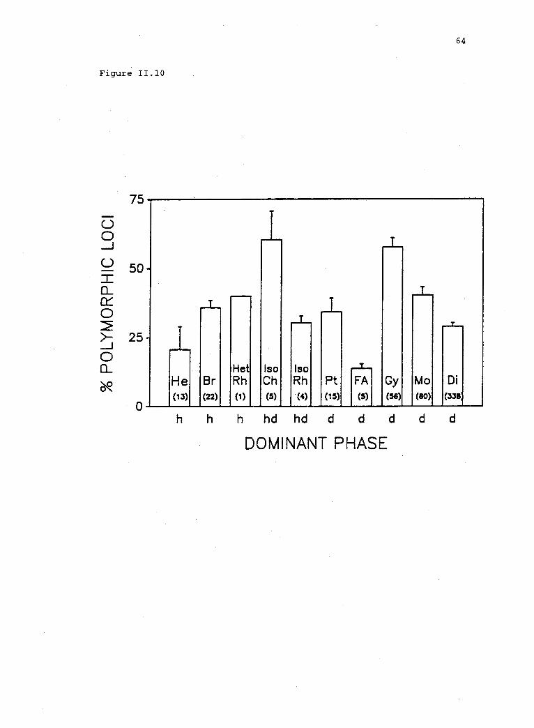
Figure 11.10
75
64
50 -
25 -
He Br(13) (22)
h h
HetRh(1)
isoCh(5)
IsoRh(4)
Pt(15)
FA(5)
Gy(56)
h hd hd d d d
DOMINANT PHASE
M 0 Di(80) (338:
d d

65
prominence of the gametophyte is not a good predictor of the level of
genetic polymorphism present in a population.
Differences among taxa in mode of reproduction (i.e., sexual
versus asexual) and in breeding system also were not consistently
associated with variation in the percentage of loci observed to be
polymorphic. Sexual and asexual taxa were similar, with 32.1 ± 6.3%
and 31.2 ± 3.7% of loci polymorphic, respectively (F = 0.027,
p = 0.871). Similarly, mode of reproduction was not related to levels
of genetic variability within plant divisions or within the three
groups of divisions (bryophytes, isomorphic algae, and pteridophytes)
(table 11.3, p > 0.05 in all ANOVA's). These results are consistent
with those observed for higher plants where levels of polymorphism
were not significantly different between sexual and asexual
populations (Hamrick and Godt 1989, table 11.3). Likewise, variation
in breeding system was not correlated with levels of polymorphism,
except in ferns where inbreeders exhibited significantly lower levels
of polymorphism than outcrossers (F = 7.285, p = 0.027). Negative
results such as ours must be interpreted with caution, especially in
light of the relatively small sample sizes. Nevertheless, they do
suggest that patterns of enzyme polymorphism among plant divisions
cannot be explained by differences among divisions in the mode of
reproduction or in breeding system.
An important limitation of our analysis is that we have compared
polymorphism among plant divisions which differ in many ways, in
addition to the prominence of haplophase in the life history.
Ideally, comparisons should be made at the lowest taxonomic level
possible within a plant division, i.e., between species in the same
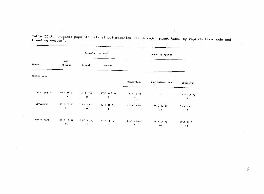
Table 11.3. Average population-level polymorphism (%) in major plant taxa, by reproductive mode andbreeding system'.
Reproductive Mode2
All
Taxon Species Sexual Asexual
Breeding System 2
BRYOPHYTES:
Monoecious Phyllodioecious Dioecious
Hepatophyta 20.3 (8.4) 17.2 (7.3) 47.9 (45.4) 11.0 (2.1) 23.5 (14.7)13 10 2 5 5
Bryophyte 35.8 (2.6) 36.6 (2.7) 32.4 (8.0) 40.0 (4.0) 38.9 (3.3) 33.4 (5.7)22 18 4 3 10 7
GRAND MEAN: 30.2 (3.6) 29.7 (3.5) 37.5 (13.2) 21.9 (5.6) 38.9 (3.3) 29.3 (6.7)35 28 6 8 10 12

Table 11.3 (continued).
Reproductive Model Breeding System2
All
Taxon Species Sexual Asexual
PTERIDOPHYTES:
Inbreeding Outcrossing
Pteridophyta 34.2 (5.0) 36.8 (6.7) 34.6 (0.0) 18.7 (2.9)a 44.0 (7.3)b15 11 1 4 6
Fern Allies 13.8 (1.7) 13.8 (1.7) 14.9 (1.7)
5 5 4
GRAND MEAN: 29.1 (4.3) 36.8 (6.7) 17.3 (3.7) 18.7 (2.9) 32.4 (6.4)
20 11 6 4 10
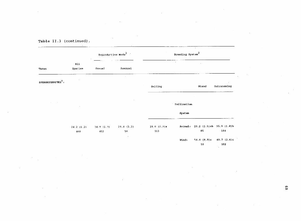
Table 11.3 (continued).
Reproductive Model Breeding System2
All
Taxon Species Sexual Asexual
SPERMATOPHYTES :
Selfing Mixed Outcrossing
Pollination
System
34.2 (1.2) 34.9 (1.3) 29.4 (3.3) 20.0 (2.3)a Animal: 29.2 (2.5)ab 35.9 (1.8)b
468 413 56 113 85 164
Wind: 54.4 (8.9)c 49.7 (2.6)c
10 102
Table 11.3 (continued).
1Data for bryophytes and pteridophytes are derived from table 11.2 and for spermatophytes from Hamrick and Godt (1989). Mean (standard error); sample
size, below. Means within a row that are followed by the same letter or by a blank are not significantly different at the o(= 0.05 level.
2See table 11.2 caption for definitions.
. data not available.
Coniferophyta (gymnosperms) and Anthophyta (angiosperms). Data are from Hamrick and Godt (1989).
Microphyllophyta (club mosses) and Arthrophyta (horsetails).
70
order, family, or genus. Multicellular algae are particularly
suitable for such a survey, because many pairs of closely-related taxa
differ in the relative importance of the haploid and diploid phases in
the life cycle (see taxa described in Tanner 1981, Pedersen 1981, West
and Hommersand 1981, Bold and Wynne 1985). Unfortunately, despite
increasing numbers of electrophoretic studies of algae (Cheney 1985),
few have addressed the problem of genetic variability. To date, only
four studies of haplodiplontic algae (table 11.2) offer genetic
interpretations of the data that permit comparison with studies of
electrophoretic variability in other plants or in strictly haploid or
diploid algae.
Future studies could test whether P is inversely correlated
with the relative size or duration of haplophase, by determining
levels of polymorphism for pairs of species that differ in the
relative prominence of haplophase. It should be noted, however, that
interpretation of such comparisons could be confounded by the presence
of alternate asexual pathways (e.g., apogamy, parthenogenesis, and
apomeiosis) (Bold and Wynne 1985) and by absence of coordination among
nuclear (haploid versus diploid), reproductive (gametophytic versus
sporophytic), and morphological phases (Clayton 1988; Maggs 1988).
Furthermore, the life cycles of certain algae may be labile under
varied environmental conditions, both in switching between sexual and
asexual pathways and in the degree of coordination between nuclear,
reproductive, and morphological phases. Thus, independent
confirmation of the life cycle would be required for many species
pairs.
Opposing selection between the phases is one mechanism that
71
might contribute to the maintenance of high levels of polymorphism
among haplodiplonts, because it may partially counterbalance
reinforcing selection and other factors that tend to reduce
polymorphism. Alternative explanations for the observed rates of
polymorphism in haplodiplonts include (1) neutrality of alleles (e.g.,
Yamazaki 1981, 1984; review in Nei 1983) or (2) balancing selection
between habitats (e.g., Nevo et al. 1984), between developmental
stages of the same ploidy level (e.g., Rose 1982), or between the
sexes (e.g., Gregorius 1982). Unfortunately, the small sample size in
our compilation does not permit further analyses of correlated
ecological variables (e.g., geographic range, habitat type) that might
suggest mechanisms for maintenance of this high level of polymorphism
in haplodiplontic organisms. Nevertheless, there is no evidence to
suggest that selection in haplophase reduces polymorphism in
populations of organisms with a prominent gametophytic stage.
72
GENERAL DISCUSSION
In this paper we have examined the validity of two common-sense
notions about selection during haplophase (fig. II.11, center box):
(A) that it is inherently "strong" (i.e., that it rapidly eliminates
inferior variants) and, consequently, (B) that it results in the
maintenance of reduced levels of genetic polymorphism in populations
of haplodiplonts. These two ideas are central to a loose system of
arguments (review in Willson 1981) linking an understanding of the
population-genetic consequences of life histories (fig. II.11, upper
box) with explanations for the evolution of the haplodiplontic life
history itself (fig. II.11, lower box). Our results show that these
central ideas are only partially correct. Furthermore, we suggest
that identifying functional or adaptive differences between haploids
and diploids is only a first step in understanding both the
consequences and the evolutionary causes of the haplodiplontic life
history. A more comprehensive approach must also explicitly consider
(1) the net effect of evolutionary processes within both phases of the
life history and (2) the consequences of variation among life
histories that differ in their allocation to each phase. We
illustrate these points in the discussion that follows.
Inferences about the dynamics of gametophytic selection often
have been based on implicit or explicit comparisons of the consequeces
of haploidy versus diploidy (fig. II.11, upper box) at the individual
and population levels (e.g., Stebbins 1950, 1960; Bonner 1965;
Stebbins and Hill 1980; Yamazaki 1981, 1984; Pfahler 1983; Graham
1985; Weeden 1986; reviews in Willson 1981; Szweykowski 1984; Wyatt

73
Figure 11.11. Outline of arguments linking population-geneticconsequences of natural selection in haplodiplonts with explanationsfor the evolution of life histories in plants. Conclusions A and B(center box) are inferences based on comparisons of the haploid anddiploid life histories (upper box). Taken together, A and B have beeninvoked in two lines of argument (lower box) leading to contrastinghypotheses regarding the evolution of life histories in plants. (See
text for details and references.)
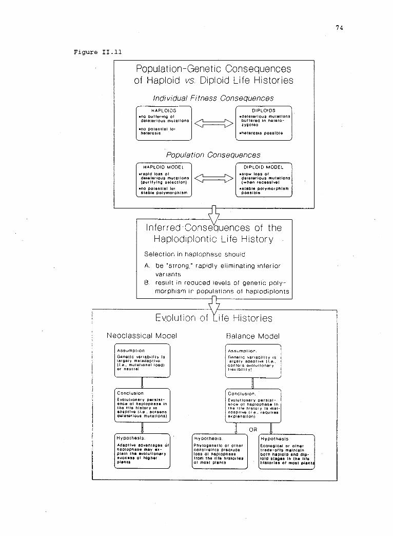
Figure 11.11
Population-Genetic Consequencesof Haploid vs. Diploid Life Histories
Individual Fitness ConsequencesHAPLOIDS
no but tering ofdeleterious mutations
.no potential forheterosis
<DIPLOIDS
deleterious mutationsbuttered in netero-zygotes
. heterosis possible
Population ConsequencesHAPLOID MODEL
.rapid loss ofdeleterious mutations(purifying selection)
no potential forstable polymorphism
<DIPLOID MODEL
. slow loss ofdeleterious mutations(when recessive)
. stable polymorphismpossible
_
Inferred Consequences of theHaplodiplontic Life History
Selection in haplophase shouldA. be "strong," rapidly eliminating inferior
variantsB. result in reduced levels of genetic poly-
morphism in populations of haplodiplonts
74
Evolution of ife Histories
Neoclassical Model Balance Model
Assumption:Genetic variability Islargely maladaptive(Ls., mutational load)or neutral
Conclusion:Evolutionary persist-ence of haplophase inthe file history isadaptive (i.e .. screensdeleterious mutations)
Hypothesis:Adaptive advantages ofhaplophase may ex-plain the evolutionarysuccess of higherplants
Assumption.Genetic variability Islargely aaaptiveconfers evolutionaryflexibility)
Conclusion.Evolutionary persist-ence of napiophase Intne life history Is Mal-sOaptive (i.e., requires
( ex planation)
tOR
Hypothesis Hypothesis.Phytogenetic or otherconstraints precludeloss of naplopnasefrom the lite historiesof most plants
Ecological or othertrade-offs maintainboth haploid and dip-loid stages in the Illehistories of most plant
75
1985; Wyatt et al. 1989b; Ennos 1990). From these straightforward
comparisons, it might be tempting to conclude that the presence of a
haplophase in the life cycle should speed the loss of deleterious
alleles and reduce the occurrence of polymorphism. However, our
results show that this inference is only partially correct because it
does not recognize the complex dynamics of selection acting in both
phases of the life cycle. That is, the maintenance of polymorphism
depends on the relative sign and magnitude of selection regimes in the
two phases.
First, analysis of the HDM indicates that the sign of
correlations in fitness of alleles between the two phases is of
overriding importance in predicting the outcome of natural selection
in the HDM. With reinforcing selection (positive correlation in
fitness), gametophytic selection will tend to speed the elimination of
deleterious alleles (fig. II.4B) or to disrupt equilibria (fig. II.4A
and C), reducing the probability of stable polymorphism (fig. II.8B)
and lowering mutational load, as predicted by many authors. However,
under opposing selection (negative correlation in fitness), new
opportunities for retaining genetic variability arise in the HDM.
Opposing selection may slow or reverse the loss of alleles that are
deleterious in diplophase and can result in polymorphism under
conditions where none would exist in the DM (fig. II.SB and C), thus
enhancing the probability of stable polymorphism (fig. II.8B).
Indeed, our results show that even quite strong opposing selection
[sH < (2 -VT)] may increase the probability of polymorphism in the
HDM up to 25% over that in the DM (fig. II.8B).
Second, specific quantitative relationships between the two
76
phases in the magnitude of selection affect the qualitative outcome of
selection in the HDM (table II.1; figs. 11.3-11.5). That is, the
intensity of haplophase selection needed to permit or preclude
polymorphism depends on the selection regime in diplophase. For
example, given a particular sporophytic selection regime, the
qualitative outcome switches from elimination of. Al to the maintenance
of stable polymorphism (fig. II.5C) as gametophytic selection changes
from weak (w2 w12) to intermediate (w2 w12) intensity. Briefly,
analysis of the HDM indicates that the rate of change of allele
frequencies, the existence and stability of equilibria, and the
polymorphism frequency all depend on the qualitative and quantitative
relationship between fitness coefficients in the two phases.
These results underscore the dynamic complexity of the HDM and
highlight a previously under-appreciated mechanism (opposing
selection) for retaining genetic variability in populations of
haplodiplonts. Furthermore, our survey of enzyme polymorphism
provides empirical evidence that levels of polymorphism are not
inversely correlated with the prominence of haplophase in the life
histories of plants. Consequently, we conclude on both theoretical
and empirical grounds that the conventional wisdom about the
consequences of gametophytic selection (fig. II.11, center box)
derives from an incomplete predictive context (fig. I1.11, upper box).
Specifically, to adequately predict the population-genetic
consequences of the haplodiplontic life history, it is insufficient to
compare haploids (HM) and diploids (DM) and to infer that HDM dynamics
should be intermediate. Indeed, our results illustrate that there is
a non-linear relationship between life history variation (from haploid
77
to haplodiplontic to diploid) and variation in the potential for
maintaining genetic variability, due to interaction between selective
processes occurring within each phase (i.e., opposing selection).
Thus, it is necessary to consider the unique dynamics of each complete
life history in order to understand how the consequences of distinct
life histories differ.
An appreciation of the complexity of HDM dynamics, and of their
consequences for the maintenance of polymorphism, can also contribute
to a better understanding of the evolutionary processes affecting the
life histories of plants (fig. 11.11, lower box). A bewildering array
of explanations has been offered for the evolution of the
haplodiplontic life history (and of the related phenomema of diploidy
and sex) (e.g., reviews in Ghiselin 1974; Willson 1981; Bell 1982).
We consider only two arguments (fig. II.11, lower box), each based on
the presumption that gametophytic selection efficiently removes
genetic variation from populations of haplodiplonts (fig. II.11,
center box).
The two arguments are similar in that they consider the relative
advantages of haploidy versus diploidy in explaining the persistence
of both phases in the life histories of plants. Their predictions
diverge, however, depending on whether genetic variation due to
mutation is perceived as playing primarily a destructive or a
constructive role in evolution (i.e., respectively, the neoclassical
versus balance schools of population genetics, sensu Lewontin 1974).
Specifically, some authors have suggested that haplophase is
advantageous because selection can rapidly eliminate deleterious
mutations (e.g., in angiosperms and pteridophytes, Mulcahy and Mulcahy
78
1987; Klekowski 1988; discussions in Charlesworth 1991, Kondrashov and
Crow 1991, Perrot et al. 1991). Mulcahy (1979), for example,
attributes the evolutionary success of angiosperms to their capacity
for intensive "screening" of the genome via pollen selection.
On the other hand, some authors have viewed the presence of a
haploid stage in the life cycle as detrimental, precisely because
gametophytic selection has the potential to rapidly eliminate genetic
variability from populations (e.g., Stebbins 1950, 1960; Bonner 1965).
These arguments, based on the presumption of individual- and
population-level advantages of diploidy over haploidy (fig. 11.11,
upper box), predict that a diplophase-dominant life history should
evolve in the absence of constraints (Stebbins and Hill 1980; Graham
1985; review in Willson 1981). This prediction has led, in turn, to
numerous ad hoc explanations for the persistence of a prominent
haploid stage in the life histories of many plants (e.g., phylogenetic
constraints, Stebbins 1960; Littler et al. 1987; the potential
adaptive advantages of haploidy, Cavalier-Smith 1978; Lewis 1985; or
tradeoffs between the haploid and diploid stages, Stebbins and Hill
1980; Keddy 1981; Willson 1981).
As discussed earlier, our theoretical and empirical results call
into question the basic assumptions (fig. 11.11, center box) of both
lines of reasoning. That is, reduced levels of polymorphism are not
necessarily predicted or observed in populations of haplodiplonts.
Furthermore, we suggest that a comparative approach (similar to the
one we have used to evaluate the population-genetic consequences of
the haplodiplontic life history) could lead to a better understanding
of the evolution of the haplodiplontic life history itself. Many
79
authors address the general issue of why two phases persist in plant
life cycles by asking "What are the adaptive advantages of being
haploid or diploid?" We argue that answers to this question are
necessary, but not sufficient, for understanding the factors that
drive the evolution of life cycles. Rather, the problem must be
framed in a broader context: "Under what conditions should organisms
alter the relative size, duration, or complexity of discrete life
history stages?" (See Willson 1981 for a similar approach.) In
addition to the discovery of differences and similarities between the
phases, answering this question necessitates (1) increased
understanding of the interplay between the phases within the life
history (e.g., reinforcing versus opposing selection, ecological
trade-offs), and (2) exploration of the theoretical and empirical
links between exogenous variation (i.e., selection regimes) and
variation among life histories that differ in their allocation to each
phase.
This reframing of the problem has implications for the types of
research needed to integrate existing knowledge and to further
elucidate evolution of the haplodiplontic life history. For example,
analyses of life history evolution that implicitly assume reinforcing
selection between haploid and diploid stages (e.g., Kondrashov and
Crow 1991, Perrot et al. 1991; discussion in Charlesworth 1991) should
be extended to consider the case of opposing selection. Furthermore,
theory is needed that explicitly links variation in the relative size
or duration of the phases with ecological or other selection
gradients. To begin to tease apart the conditions that favor one
life-history variant over another, future empirical studies could take
80
advantage of fixed or plastic life-history variation within species
(or among closely related taxa) of lower plants. By explicitly
incorporating the full range of population genetic dynamics and life-
history variants in future theoretical and empirical studies, progress
in understanding the evolution of the haplodiplontic life history will
be enhanced.
81
ACKNOWLEDGMENTS
We wish to thank P. S. Dawson, T. M. Farrell, C. B. Halpern, C.
E. King, J. Lubchenco, B. A. Menge, J. Roughgarden and L. Walsh for
their comments on earlier versions of this manuscript. J. Lubchenco
was instrumental in encouraging one of us (AMO) to consider the
evolutionary causes and consequences of life history variation in
lower plants. J. L. Hamrick and A. Stoneburner kindly provided copies
of manuscripts prior to their publication. M. Mungoven assisted with
literature searches. Sedonia Washington, Shawnie Worrell, Suanty
Kaghan, and Jill Meiser assisted with word processing. This work was
supported in part by grants from the National Science Foundation to B.
A. Menge (OCE-8415609, OCE-8811369) and to J. Lubchenco and D. Carlson
(OCE-8600523), by a grant from the Andrew W. Mellon Foundation to J.
Lubchenco, and by a DeLoach Graduate Fellowship from Oregon State
University to A. M. Olson.

APPENDICES

82
APPENDIX A
DERIVATION OF THE EQUILIBRIUM FREQUENCY, p,
FOR THE HAPLODIPLONTIC MODEL
At equilibrium, f(p) = p, so from equation (1),
P = Pwl[Pw11 +(l- p)w12] / D,
where D = Pwl[Pw11 1-(1-P)w12] (1-P)w2[Pw12 +(l-P)w22] Clearly,
p = 0 is one equilibrium. To find the others, we divide by p. Then
wl[Pwil (1-P),412] = Pwl[Pwil (1-P),412] (1-P)w2[P,412 i-(1-10)w22],
or, equivalently,
(1-P)w1[Pwil (1-P)w12] = (1-r)w2[Pw12 +(l-P)w22).
It is clear that p = 1 (1 p = 0) is also an equilibrium. We find
the remaining equilibrium by dividing by (1-p) and solving for p,
giving
P = w2w22 w1w12w2w22 w1w12 w1w11 w2w12
Similarly, it can be shown that the equilibrium frequency of A2 is
q = w1w11 w2w12w2w22 w1w12 w1w11 w2w12
AThus, we have shown that p = 0, p = 1, and p = p are the only
possible equilibria.
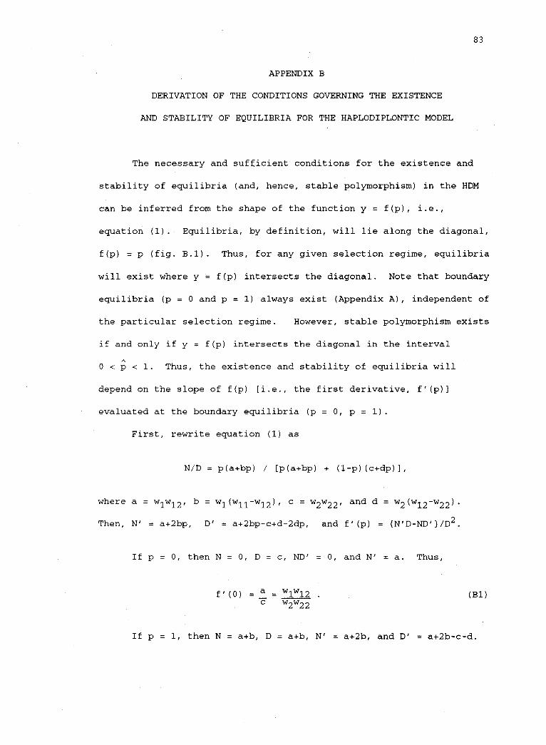
83
APPENDIX B
DERIVATION OF THE CONDITIONS GOVERNING THE EXISTENCE
AND STABILITY OF EQUILIBRIA FOR THE HAPLODIPLONTIC MODEL
The necessary and sufficient conditions for the existence and
stability of equilibria (and, hence, stable polymorphism) in the HDM
can be inferred from the shape of the function y = f(p), i.e.,
equation (1). Equilibria, by definition, will lie along the diagonal,
f(p) = p (fig. B.1). Thus, for any given selection regime, equilibria
will exist where y = f(p) intersects the diagonal. Note that boundary
equilibria (p = 0 and p = 1) always exist (Appendix A), independent of
the particular selection regime. However, stable polymorphism exists
if and only if y = f(p) intersects the diagonal in the interval
0 < p < 1. Thus, the existence and stability of equilibria will
depend on the slope of f(p) [i.e., the first derivative, f'(p)]
evaluated at the boundary equilibria (p = 0, p = 1).
First, rewrite equation (1) as
N/D = p(a+bp) / [p(a +bp) + (1-p)(c+dP)],
where a = w1w12'1-w12' b = w1 (w11-w12), c = w2w22' and d = w lw w
Then, N' = a+2bp, D' = a+2bp-c+d-2dp, and f'(p) = (N'D-ND')/D2.
If p = 0, then N = 0 , D = c, ND' = 0, and N' = a. Thus,
f'(0) = a = w1w12 . (B1)
w2w22
If p = 1, then N = a+b, D = a+b, N' = a+2b, and D' = a+2b-c-d.
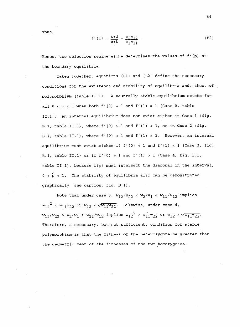
Thus,c+d = w2w12a+b wiwii
84
(B2)
Hence, the selection regime alone determines the values of f'(p) at
the boundary equilibria.
Taken together, equations (B1) and (B2) define the necessary
conditions for the existence and stability of equilibria and, thus, of
polymorphism (table I1.1). A neutrally stable equilibrium exists for
all 0 < p < 1 when both f'(0) = 1 and f'(1) = 1 (Case 0, table
II.1). An internal equilibrium does not exist either in Case 1 (fig.
B.1, table II.1), where f'(0) > 1 and f'(1) < 1, or in Case 2 (fig.
B.1, table II.1), where f'(0) < 1 and f'(1) > 1. However, an internal
equilibrium must exist either if f'(0) < 1 and f'(1) < 1 (Case 3, fig.
B.1, table II.1) or if f'(0) > 1 and f'(1) > 1 (Case 4, fig. B.1,
table II.1), because f(p) must intersect the diagonal in the interval,
0 < p < 1. The stability of equilibria also can be demonstrated
graphically (see caption, fig. B.1).
Note that under case 3, w12/w22 < w2/w1 < w11/w12
w122< w11w22 or w12 < 1w22. Likewise, under case 4,
implies
w12/w22 w2/w1 w11/w12 implies w122 > w11w22 w12 >717.7E-
Therefore, a necessary, but not sufficient, condition for stable
polymorphism is that the fitness of the heterozygote be greater than
the geometric mean of the fitnesses of the two homozygotes.
85
Figure B.1. A graphical approach to inferring the qualitativeselection regimes governing the existence and stability of equilibriain the HDM. Equilibria lie along the diagonal dashed line, f(p) = p;selection regimes are represented by the curve, y = f(p). Boundaryequilibria exist at p = 0 and p =1 (Cases 1-4); an internalequilibrium is defined if f(p) = p and 0 < p < 1 (Cases 3 and 4).The stability of equilibria is illustrated graphically for Case 2:The initial allele frequency (pt) is indicated on the abscissa. Theallele frequency in the next generation (Pt+1) is found by projectingthis point to the curve y = f(p) and reading its value on theordinate. This value, plotted on the abscissa, is then used topredict the frequency in the subsequent generation ap( t+2" and so on.The sequence of points moves along the graph of y = f(p) toward stableequilibria (solid symbols) and away from unstable equilibria (opensymbols), as indicated by the arrows in each panel.
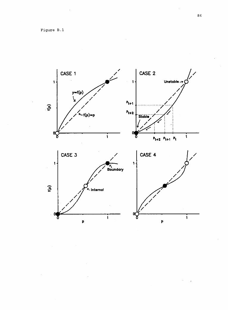
86
Figure B.1
87
APPENDIX C
COMPARISON OF THE PARAMETER SPACE SUPPORTING POLYMORPHISM
IN THE DIPLOID AND HAPLODIPLONTIC MODELS
The unit cube (figs. II. 7A and C.1) denotes the parameter space
of the DM (i.e., x = w11, y = w22, z = w12' 0 < wij < 1). The
proportion of the parameter space supporting polymorphism (i.e.,
w12 max(w11, w22) is VD = 1/3 (fig. II.7A). Next we determine the
proportion of the points (x, y, z) in the unit cube that satisfy the
conditions for polymorphism in the HDM, i.e.,
w12 /w22 > w2 /w1 > w 11 /w1 2
First, assume 0 < wi < 1 and w1 < w2. Let w2/w1 = R > 1 and
Q = 1/R < 1. Then (C1) can be rewritten
(z/y > R > x/z) <=> (z > x/R = Qx and z > Ry).
(C1)
Thus, the volume of the space supporting polymorphism is defined by
two planes, z = xQ and z = Ry, which intersect along the line
z = xQ = Ry (fig. C.1). The projection of this line in the xy plane
is xQ = Ry or y = xQ2 (figs. C.1, C.2A). The regions of integration
are shown in figure C.2A. The volume, VH, above the two planes, I and
II, is thus
JrVH = (1 xQ) dA + ,f (1 Ry) dA
I II
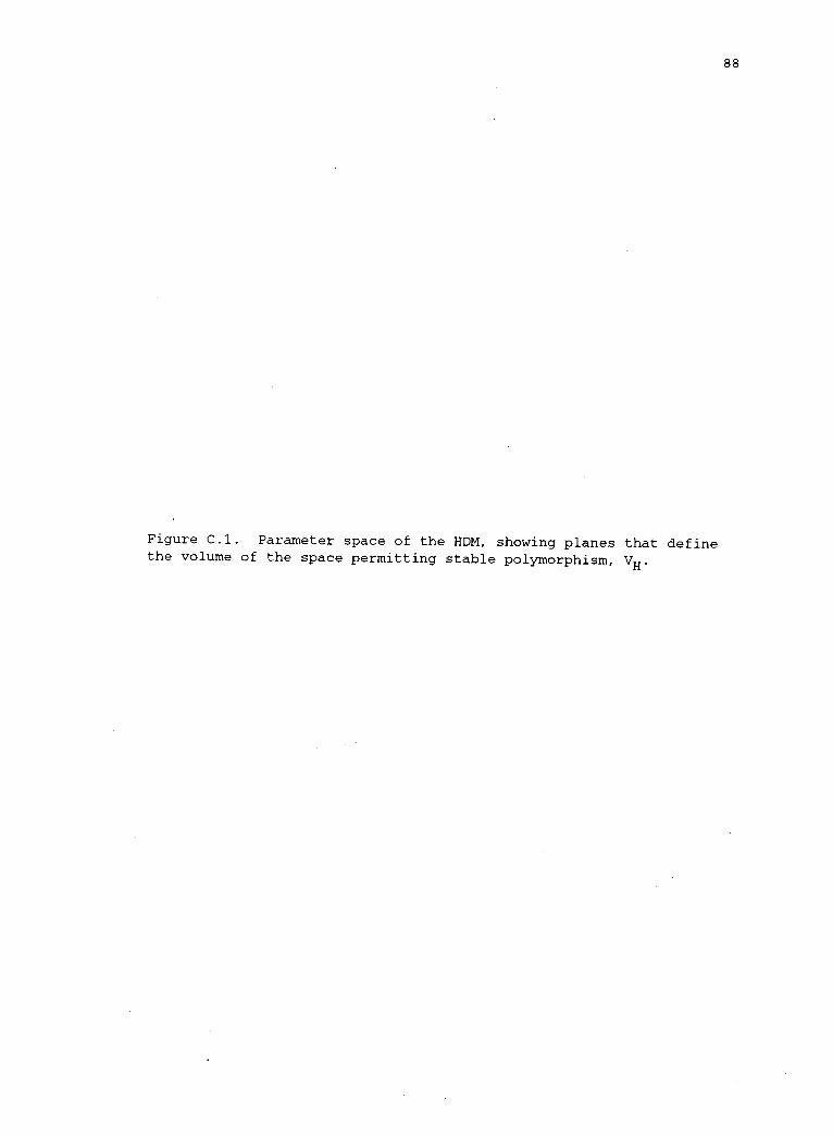
88
Figure C.1. Parameter space of the HDM, showing planes that definethe volume of the space permitting stable polymorphism, VH.

89
Figure C.1
z
(0,Q,1)
Ac/-- z = Ry
90
cl rxQ2 1
VH = (1 xQ) dy dx (1 Ry) dy dx.JO JO 0 xQ2
Performing the integration and keeping in mind that R = 1/Q,
VH = Q Q3.2 6
Note that VH = 1/3 if Q = 1 (i.e., if w1 = w2). Thus, in the absence
of selection in haplophase, the volume of the parameter space
supporting polymorphism in the HDM is identical to that in the DM. In
addition, as a function of Q, V(Q) reaches a local maximum at Q = 1
(fig. II.8A) for all defined values of Q.
COMPARISON OF THE PARAMETER SPACE SUPPORTING POLYMORPHISM
UNDER REINFORCING AND OPPOSING SELECTION
The diagonal plane x = y divides the parameter space into
regions representing reinforcing and opposing selection. Because we
assume at w2 > wl the outset, w22 > w11 or y > x implies reinforcing
selection. The regions of integration for reinforcing and opposing
selection are shown in figure C.2B. Under reinforcing selection, the
volume of the parameter space supporting polymorphism is thus
-Q fQVHr = (1 Ry) dy dx.
`0 six
Again, performing the integration and recalling that R = 1/Q,
2VHr = Q /6.
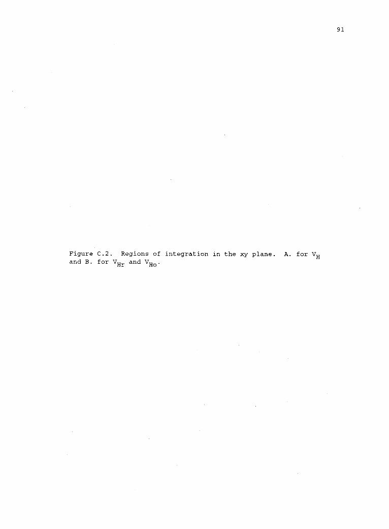
91
Figure C.2. Regions of integration in the xy plane. A. for VHand B. for VHr and VHo'
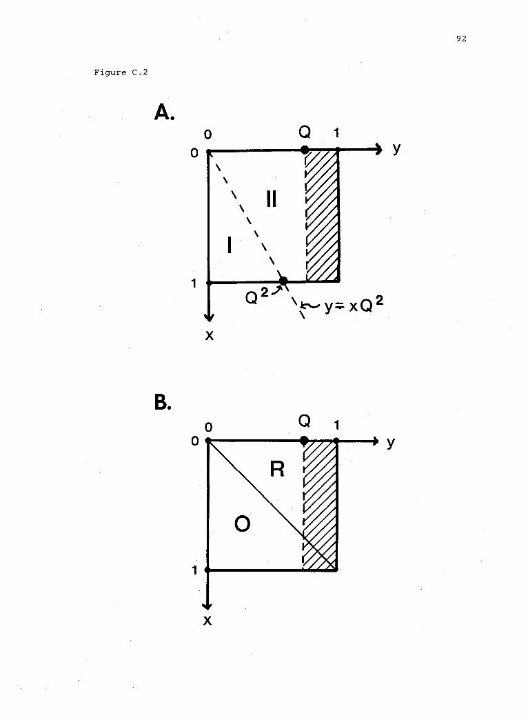
Figure C.2
A.
B.
0
1
92
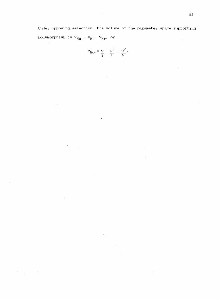
93
Under opposing selection, the volume of the parameter space supporting
polymorphism is VH0 = VH VHr' or
VHo =3 _ 2
2 3 6

94
95
Chapter III
DESICCATION AND HERBIVORY INTERACT TO
REGULATE THE UPPER LIMIT
OF AN INTERTIDAL RED ALGA
ABSTRACT
Physical factors are presumed to determine the upper limits of
most intertidal organisms, but the relative importance of biotic
factors is poorly understood. I manipulated both desiccation and
grazers (limpets) in a factorial experiment designed to evaluate their
separate and joint effects on the upper intertidal limit of a
perennial red alga, Iridaea cornucopiae. Desiccation inhibited upward
vegetative growth. A significant desiccation-by-grazer interaction
affected both reproduction and recruitment. In dry plots, grazers
inhibited recruitment; in moist plots, grazers enhanced vegetative
growth of Iridaea. Thus, Iridaea appears to be grazer-limited in dry,
but grazer- dependent in moist environments.
Microalgae may mediate these effects on recruitment. Limpets
often remove competing microalgae. In moist plots this probably
enhances establishment of Iridaea. In dry plots, where microalgal
production is likely to be lower, limpets may switch to Iridaea.
Thus, both physical and biotic factors appear to set the upper limit
of this alga.
96
INTRODUCTION
Limits to species' distributions are often correlated with
gradients in environmental harshness. Such correlations may arise
because abiotic factors impose direct physiological limits on species.
However, abiotic factors may also indirectly affect species'
distributions by altering the outcome of species' interactions such as
competition or predation. Recent conceptual advances in community
ecology focus on the interplay between physical factors and species'
interactions. Specifically, environmental stress models (ESMs; Menge
and Olson 1990) predict how gradients in environmental stress limit
the abundance of prey (animals or plants) by altering the effects of
consumers (carnivores or herbivores). Two alternative sub-models (see
below), each supported by an impressive array of empirical evidence,
make contrasting predictions regarding the effects of environmental
stress on species' distributions. Because they predict that the
consequences of stress may vary, depending on species' interactions,
ESMs are significant for understanding the effects of natural and
anthropogenic environmental change on species' distributions. The
object of this study is to evaluate ESMs in light of experimental
evidence from a marine algae-molluscan herbivore system.
Two ESM sub-models reflect the likelihood that interacting
species will respond differently to a given stress. In the two sub-
models, the specific effect of environmental stress on a species'
abundance and distribution depends on the differential responses to
stress of consumers and prey (fig. III.1). The consumer stress model
(CSM; Menge and Olson 1990) assumes that environmental stress
97
Figure 111.1. Contrasting assumptions and predictions of the consumerstress and prey stress models (CSM and PSM, respectively).Assumptions (open symbols) include the direct physiological orbehavioral effect of stress on consumers (open trianglesZ) and onprey in the absence of consumers (open circles,()). Predictions(solid symbols) include the indirect effect of stress on prey,mediated by consumers (solid circles,410).
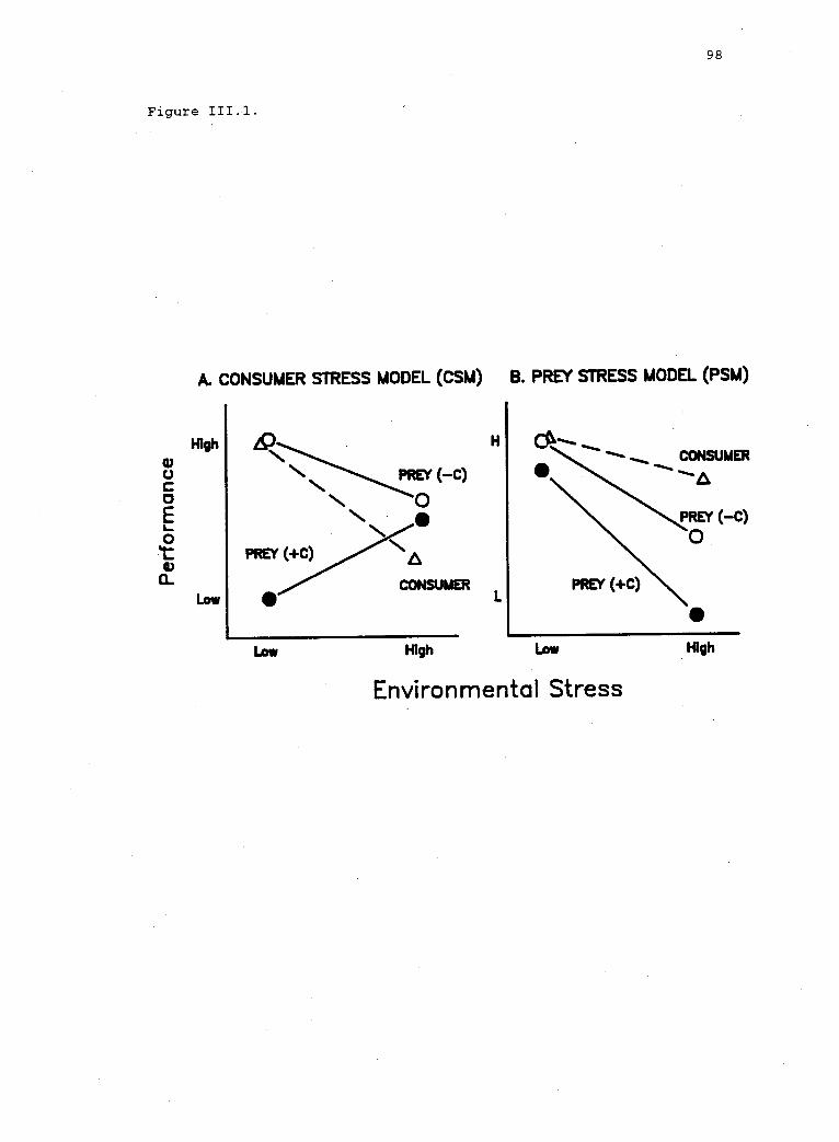
Figure 111.1.
98
A. CONSUMER STRESS MODEL (CSM) B. PREY STRESS MODEL (PSM)
High
Low
H
PREY (-0
N 0
ACONSUMER
PREY ( +C)
Low
L
High
PREY ( +C)
Low High
Environmental Stress
99
disproportionately affects the numbers or foraging efficiency of
consumers, relative to its direct effect on the performance of prey
(fig. III.1A; open symbols) (reviews in Connell 1972, 1974, 1975,
1985, Menge and Sutherland 1987, Menge and Farrell 1989). Thus, the
CSM predicts that the effect of consumers on prey will be negatively
correlated with stress--prey performance in the presence of consumers
should improve with increased stress (fig. III.1A; solid symbols).
That is, in benign conditions, prey should be limited by consumers,
but where environmental conditions are too harsh for effective
consumer foraging, prey should find a refuge from consumers and should
be limited instead by their physiological tolerances. Classical
demonstrations of this model are found in the work of Paine (1984,
Paine et al. 1985) and Connell (1961a, b, 1970) in rocky intertidal
systems where prey (mussels and barnacles, respectively) escape
predation at elevations too high for effective foraging by consumers
(seastars and whelks, respectively).
In contrast, the prey stress model (PSM; Menge and Olson 1990)
assumes that environmental stress diminishes the performance of the
prey more than that of consumers (fig. III.1B, open symbols).
Accordingly the PSM predicts that the effect of consumers on prey will
be positively correlated with stress (fig. III.1B, solid symbols),
because stress increases prey susceptibility to consumer attack
(reviews in Mattson and Addy 1975, Mattson 1980, White 1984, Waring
and Schlesinger 1985, Louda 1988). Thus, prey are expected to persist
in benign environments, but to be limited by consumers where
conditions are harsh, even where levels of stress otherwise might be
tolerated. Numerous studies report a positive correlation between
100
plant stress factors and frequency of attack by insect herbivores
(e.g., White 1969, 1974, Webb 1981, Louda 1988). Others
experimentally demonstrate higher rates of attack (e.g., Larsson et
al. 1983, Louda and Rodman 1983, Mitchell et al. 1983, Waring and
Pitman 1985) or increases in feeding preference (e.g., Lewis 1979,
1982, 1984, Hughes et al. 1982) for plants subjected to "high stress"
treatments.
To test the predictions of ESMs, it is necessary to separate the
direct effects of stress on prey species from its indirect effects
mediated by species' interactions. In the present study, I attempted
to experimentally tease apart the separate and joint effects of
desiccation stress and molluscan herbivory in setting the upper
intertidal limit of a marine red alga. Intertidal communities are
good model systems for assessing the direct and indirect effects of
environmental stress on species' distributions, because the
elevational limits of both consumers and prey are often juxtaposed
with steep gradients in physical factors (Lewis 1964). In particular,
intertidal elevation and, thus, the vertical limits of species tend to
be correlated with desiccation stress. Furthermore, the spatial and
temporal scales of dominant processes make rocky intertidal
communities particularly amenable to experimental investigations
(Connell 1974). Consequently, experimental studies of intertidal
zonation historically have been important in elucidating how abiotic
and biotic factors regulate species' distributions (reviews in Connell
1972, 1974, Chapman 1973, 1974, Underwood and Denley 1984, Underwood
1985).
Both CSM and PSM dynamics have been suggested to explain the
101
vertical limits of intertidal species. Many experimental studies in
intertidal systems lend support to the CSM scenario (review in Menge
and Farrell 1989): Both consumers and prey tend to decrease in
abundance and/or activity near their upper limits (e.g., Dayton 1971,
Seapy and Littler 1982). However, because many consumers appear to be
more susceptible than their prey to the stresses associated with
emersion, prey may escape consumption at elevations presumed to be too
stressful for effective consumer foraging (e.g., Connell 1961a, b,
1970, Dayton 1971, Menge 1978a, b, Paine 1984, Paine et al. 1985).
Thus, consistent with the CSM, the lower limits of prey species tend
to be set by consumption (or other biotic factors), while their upper
limits are thought to be set by physical factors (Connell 1972).
Ample experimental evidence supports the contention that
consumers have the potential to limit their prey at lower intertidal
elevations (e.g., Menge 1976, Lubchenco 1980, Menge and Lubchenco
1981, Menge et al. 1986). Evidence that physical factors set the
upper limits of prey species, however, is less compelling. Three
types of evidence support the CSM prediction that upper limits are set
by physical factors (reviews in Underwood and Denley 1984, Underwood
1985): First, the importance of physical factors may be inferred from
a lack of response of prey to manipulations of predation and
competition near their upper limits (e.g., Menge 1978a, b, Raffaelli
1979, Paine 1984). Second, transplants of organisms above the normal
limits of distribution of the species (e.g., Schonbeck and Norton
1978) may demonstrate that mature individuals are intolerant of
physical conditions, although recruitment limitation cannot be ruled
out by these studies (Underwood and Denley 1984). Third,

102
experimentally ameliorated environmental conditions may raise the
upper limit of some species (e.g., Castenholz 1961, Dayton 1971,
Wethey 1984).
Relatively few studies in intertidal systems reveal a positive
correlation between stress and predation or herbivory, consistent with
the PSM. However, some experimental studies have demonstrated that
grazing may in part explain the upper intertidal limits of some algae
(Hay 1979, Underwood 1980, Cubit 1984). Because manipulation of
abiotic factors was not attempted (Hay 1979, Cubit 1984) or was
confounded by artifact (Underwood 1980; see Methods, below), the
precise nature of the interaction between stress and herbivory was not
elucidated in these studies.
In the present study, I evaluated how desiccation stress
affected limpet grazing near the upper limit of a perennial red alga,
Iridaea cornucopiae Postels & Ruprecht (Rhodophyta: Gigartinaceae)
(henceforth, Iridaea). The objectives of this study were (1) to
assess whether desiccation stress would alter the effect of herbivory
on Iridaea; (2) if so, to determine whether the effect was consistent
with the CSM or the PSM; and (3) to evaluate whether desiccation of
Iridaea affected the feeding preferences of grazers. In a long-term
field experiment, I altered both rock-surface moisture (during low
tide) and limpet abundances, to evaluate their effects (separately and
in combination) on the performance of Iridaea near its upper
intertidal limit. I also conducted short-term feeding experiments in
the field to determine the effect of plant condition on limpet feeding
rates.
The CSM predicts that the deleterious effects of herbivores
103
should decline with increased desiccation and that the upper limit of
Iridaea should set by desiccation. In contrast, the PSM predicts that
the effects of herbivory should increase with stress and that
herbivory should set the upper limit of Iridaea. Results of the
present study are consistent with the ESMs, in that the effects of
limpet grazing depended on the desiccation regime. Furthermore, the
deleterious effects of herbivory were positively correlated with
desiccation, consistent with the PSM. However, by some measures, the
performance of Iridaea appeared to be grazer-enhanced under moist, but
grazer-limited under dry, conditions. This result--not predicted by
either the CSM or the PSM--suggests that more complex models may be
needed to fully define the dynamics of this system.
104
NATURAL HISTORY
Beds of Iridaea dominate the high intertidal, 2.0-4.6 m above
mean lower low water (MLLW), on many wave-exposed rocky shores of the
northeast Pacific (Lebednik and Palmisano 1974, Kozloff 1983, Olson
1985, Hannach and Waaland 1986, Leigh et al. 1987). Short blades
(usually < 5 cm in length) form a dense turf arising from a persistent
basal crust (Abbott and Hollenberg 1976) that may occupy 25-40% of the
substratum (Olson 1985). A canopy of blades averages 50-75% cover in
undisturbed areas (Olson 1985). Blades of Iridaea species tend to
have determinate development. A period of vegetative growth is
followed by reproduction, senescence, and dehiscence of blades
(Hannach and Waaland 1986, A. M. Olson, personal observation).
Reproduction is correlated with declining growth rate and breakdown of
the cuticle, a structure that deters grazing by some invertebrates on
Iridaea cordata (Gaines 1985). The basal crust is a perennating
structure--if it is killed, vegetative recovery is precluded.
However, when the crust remains intact following experimental or
natural defoliation, it may initiate new blades after conditions
improve (Olson 1985, personal observation). Thus, Iridaea may assume
its dominance by vegetatively pre-empting space.
The rather discrete upper boundary of Iridaea beds is a
convenient local distributional limit for study. At the upper limit,
canopy cover declines abruptly from >75% in some areas to 0% over a
vertical distance of several centimeters. It is not unusual to see
vigorously growing patches of Iridaea with 100% cover extending up to
its extreme upper limit.
105
Where Iridaea occurs on steep, north-facing slopes, limpets are
the dominant herbivore. Limpet densities typically exceed 400/m2 in
Iridaea beds at these sites (Olson 1985). On horizontal surfaces,
however, limpets are relatively rare, due to avian predation (Frank
1982, Marsh 1986). In experimentally denuded areas within established
beds, limpet grazing enhances the recruitment of Iridaea sporelings,
presumably by removing competitively superior early and mid-
successional algae (Olson 1985, Paine 1983). Thus, recruitment of
Iridaea within established beds is grazer-dependent.
Several observations suggest that desiccation and limpet grazing
may each play a role in determining the upper limit of Iridaea on
steeply sloping surfaces. In more desiccating microsites, Iridaea is
less abundant. From northwestern Washington to its southern limit in
northern California, beds of Iridaea tend to be restricted to north-
facing slopes; Iridaea occurs on horizontal or south-facing slopes
only in areas of extreme wave-exposure. In contrast, beds on north-
facing slopes are wider, higher, and extend farther into sheltered
locations. Both the elevation and extent of Iridaea beds decreases
from north to south over this range (A. M. Olson, personal observation
and unpublished data). In addition, following bouts of prolonged
aerial exposure, blades of Iridaea appear bleached, and this damage is
more pronounced near the upper limit of Iridaea beds. Eventually the
damaged portions of blades are removed by wave action and grazers. If
previous damage to the blades exposes the basal crust to insolation,
it may also become bleached and dislodge from the rock (Olson 1985).
Limpet grazing may also prevent the expansion of Iridaea above
its normal limit and may help explain the relatively discrete upper
106
Figure 111.2. Vertical distribution of limpets on the shore near theupper limit of the Iridaea bed. Density is given for contiguous 10 cmx 50 cm horizontal quadrats monitored in April 1987. Data for Lottiadigitalis include small individuals (< 6 mm shell length) of all threespecies that are not readily identifiable to species.
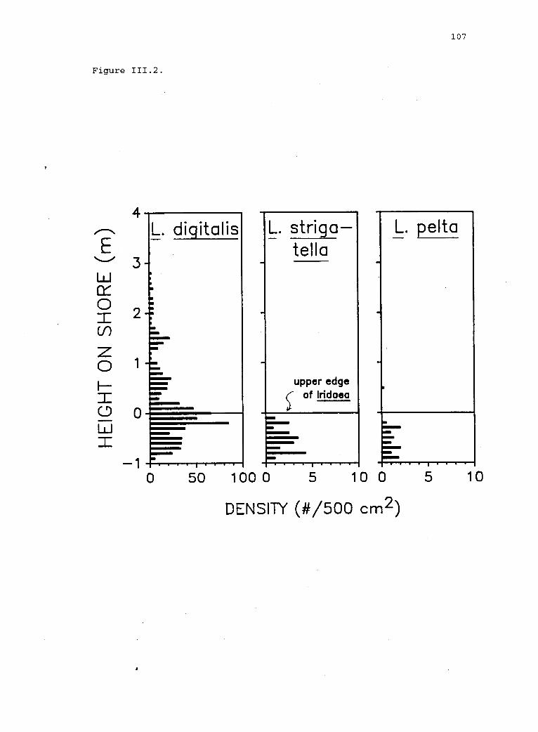
Figure 111.2 .
O
4L. digitalis
3
2'
1
-1 ,"0
I V
L. strigatella
upper edgeof Iridoea
V I
107
L. pelta
PIM
50 100 0 5 10 0 5
DENSITY (#/500 cm2)
10
108
boundary of Iridaea beds on north-facing slopes. In winter, the most
abundant limpet, Lottia (=Collisella) digitalis, ranges high in the
splash zone above the Iridaea beds (A. M. Olson, personal
observation), foraging on diatoms and ephemeral algae (Castenholz
1961, 1963, Frank 1965, Cubit 1984). In late spring, as wave heights
decline and drier weather ensues, desiccation increases and microalgal
productivity declines in the splash zone (Cubit 1984). Concurrently,
Lottia digitalis moves down in the intertidal (Frank 1965, Breen 1972,
A. M. Olson, personal observation), presumably to avoid desiccation or
to forage for alternative foods. As a consequence of this behavior,
individuals of Lottia digitalis aggregate along the upper margin of
Iridaea beds in late spring (figs. 111.2 and III.3A) and limpet
abundances within the bed are higher in dry than in wet months (Olson
1985 and personal observation). At high densities, limpets damage
blades at the edges of Iridaea clumps (fig. III.3B) and remove entire
blades from newly recruited plants (Olson 1985 and personal
observation). Thus, limpets may prevent lateral vegetative growth and
establishment of sporelings above the normal limit of the species.

109
Figure 111.3. Aggregations of limpets (A) and grazing damage (B) nearthe upper limit of Iridaea. A. Lottia digitalis (most in the 6-9 mmshell length class) aggregated at the upper limit of Iridaea bed. In
such aggregations, limpets are occasionally "stacked" two or more deepon the rock. Scale: 15 cm between X's marked on photo framer. B.
Damage to outer blades of Iridaea clump located near upper limit ofIridaea bed. X = holes and excavations due to limpet grazing; B =bases of blades that have been removed by grazing.
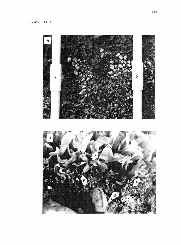
Figure 111.3.
x x
,
A
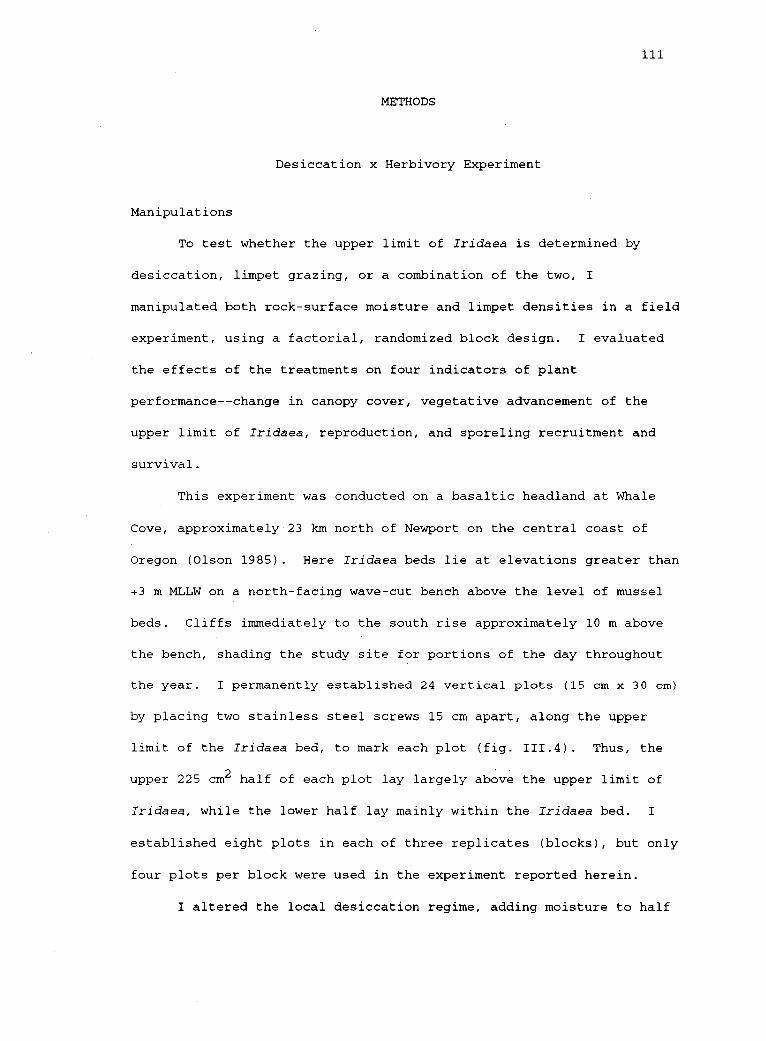
111
METHODS
Desiccation x Herbivory Experiment
Manipulations
To test whether the upper limit of Iridaea is determined by
desiccation, limpet grazing, or a combination of the two, I
manipulated both rock-surface moisture and limpet densities in a field
experiment, using a factorial, randomized block design. I evaluated
the effects of the treatments on four indicators of plant
performance--change in canopy cover, vegetative advancement of the
upper limit of Iridaea, reproduction, and sporeling recruitment and
survival.
This experiment was conducted on a basaltic headland at Whale
Cove, approximately 23 km north of Newport on the central coast of
Oregon (Olson 1985). Here Iridaea beds lie at elevations greater than
+3 m MLLW on a north-facing wave-cut bench above the level of mussel
beds. Cliffs immediately to the south rise approximately 10 m above
the bench, shading the study site for portions of the day throughout
the year. I permanently established 24 vertical plots (15 cm x 30 cm)
by placing two stainless steel screws 15 cm apart, along the upper
limit of the Iridaea bed, to mark each plot (fig. 111.4). Thus, the
upper 225 cm2 half of each plot lay largely above the upper limit of
Iridaea, while the lower half lay mainly within the Iridaea bed. I
established eight plots in each of three replicates (blocks), but only
four plots per block were used in the experiment reported herein.
I altered the local desiccation regime, adding moisture to half

112
Figure 111.4. Experimental treatments for moisture addition x limpetremoval experiment. M = moisture addition treatment (stacked sheetsof polyester); D = dry control treatment (narrow strips of polyester);F = fences to limit lateral movement of limpets between plots. Two ofthe four possible treatment combinations are shown: Moist -Limpets(two plots on the left) and Dry +Limpets (two plots on the right).Scale is 15 cm between screws (S) marking mid-line of each plot(initial upper limit of Iridaea).
Figure 111.4.
114
the plots (moist plots) by attaching three stacked layers of a sponge-
like polyester material (each 2 cm thick and 15 cm wide) to the rock
with stainless steel screws immediately up-slope from each moist plot
(fig. 111.4). The polyester mimics patches of algae by retaining
water at high tide and releasing it across the entire width of the
subtending plot for up to several hours after the tide has receded.
The polyester is strong enough to withstand heavy wave action and it
is biologically inert. (Cellulose sponges, in contrast, were consumed
by littorinid snails in preliminary trials.) On days when the
polyester was not wetted at high tide (e.g., during periods of calm
seas and neap tides), I manually poured seawater over the polyester
above the moist plots at least once per day.
Because the polyester potentially restricted limpet movement
into or out of the plots, I attached a single, narrow layer of
polyester (4 cm wide) up-slope from the control (dry) plots (fig.
111.4). These control strips retained little moisture and dried
rapidly, so they had relatively little effect on the moisture regime
in the dry plots. The moist and dry treatments were maintained in the
"dry season" (July to October 1987 and May to October 1988) and
removed prior to the onset of winter storms.
I altered limpet densities by manually removing limpets from
half the plots (-L) and adding limpets to the other half (+L),
approximately biweekly from May to October 1987 and every 2 to 4 wk
from May to October 1988. Movement of limpets between plots was
restricted with small epoxy-putty ridges (fig. 111.4), topped with
plastic mesh fences and/or copper-based antifouling paint. Moisture
addition potentially could attract limpets, confounding the limpet
115
Figure 111.5. Desiccation of Iridaea blades in experimental plots.Data are mean (± standard error of the mean, SEM) for n = 3 replicateblocks. Three sub-samples from each plot were pooled prior tocalculating treatment mean and SEM. A. August 1988. B. September1988. +Limpets, solid triangles (A); -Limpets, solid circles (40).See text for explanation of treatments.
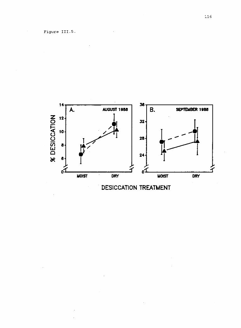
Figure 111.5.
14A.
12
10.
8.
6.
AUGUST 198836
32
28
24
116
B. SEPTEMBER 1988
o-r -f 0-f ,r
MOIST DRY MOIST
DESICCATION TREATMENT
DRY
117
density manipulation (e.g., Underwood 1980). To remove this potential
confounding effect, I adjusted densities monthly to 10 large (> 9 mm)
and 25 small (6-9 mm) limpets in limpet addition plots. Occasional
mid-winter manipulations were made as weather and wave conditions
permitted. To assess the effectiveness of the limpet removal
treatment, I counted limpets monthly, from June to September 1987 and
May to September 1988, and subjected the data to a two-factor ANOVA.
Treatment effectiveness
To assess the effectiveness of the moisture addition treatment,
I measured the relative moisture content of Iridaea blades in each of
the treatment groups on 9 August and 3 September 1988. Near the end
of the period of emersion, I collected 3 blades from within 1 cm of
the upper limit of Iridaea in each plot. Each blade was immediately
placed in a sealed 0.5 ml microfuge tube, labeled, and stored in the
dark on ice for transport to the lab. Within 1.5 to 5.5 hr, I
determined the field mass (F) of each blade by weighing it immediately
after removing it from its microfuge tube. Blades were then
rehydrated to constant mass (-12 hr) and reweighed to determine their
fully rehydrated mass (R). Subsequently, blades were dried in an oven
at 50 C to constant mass and reweighed to determine their dry mass
(D). I then calculated percent desiccation of each blade as D% = [(R-
F)x100]/[R-D]) (Schonbeck and Norton 1979). Analysis of covariance
was used to assess the main effects and two-way interaction of the
moisture addition and limpet removal treatments. Dry mass of blades
was included as a covariate, after determining that there were no
118
significant treatment by covariate interactions (i.e., parallel
slopes, Sokal and Rohlf 1981).
The moisture addition and limpet removal treatments were
effective in reducing desiccation and limpet densities, respectively,
and manipulations of desiccation and herbivores were independent.
Blades in moisture addition plots were significantly less desiccated
(D%) than those in dry plots on 9 August (a cool, foggy day) (fig.
III.5A; main effect of moisture addition, p < 0.01; F-test, ANOVA). A
similar pattern on 3 September (a dry, but overcast day) was not
significant (fig. III.SB; p > 0.10). Desiccation of Iridaea was not
affected by the limpet removal: Neither the main effect of limpet
removal nor the two-way interaction between limpet removal and
moisture addition significantly affected blade moisture status
(p > 0.10). Limpet densities were significantly lower in limpet
removal than in limpet addition plots on most dates (fig. 111.6; main
effect of limpet removal, p < 0.01 on all dates except May and June
1988). Limpet abundance was not affected by the moisture addition:
Significant variation in limpet densities could not be attributed
either to the main effect of moisture addition (p > 0.10) or to the
two-way interaction (p > 0.05), for any date. Thus, effects of the
two experimental factors on plant performance were not confounded.
Measures of plant performance
The effects of the treatments on plant performance were
monitored in the field or from photographs. Reproduction and
recruitment were assessed in the field. Reproduction (the ripening
and release of spores) was limited to brief periods in late fall and
119
Figure 111.6. Limpet densities in experimental plots. Data are mean(± SEM) for all limpet species in whole (15 cm x 30 cm) plots. Moist+Limpets, solid triangles (AL); Dry +Limpets, open triangles (LS);Moist -Limpets, solid circles (40); Dry -Limpets, open circles (0) -
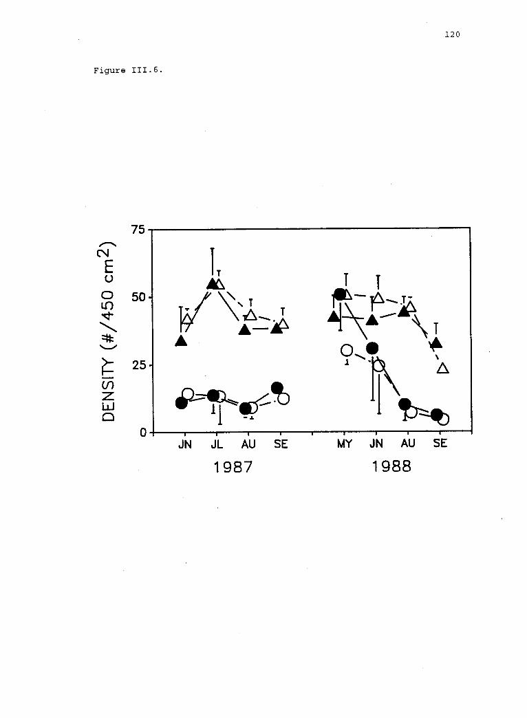
Figure 111.6.
75
50-
120
25-
0JN SIE MY J N AU SE
1987 1988

121
early winter, after which vegetative growth resumed. I periodically
estimated the relative reproduction of Iridaea in each treatment group
by the following method. Over the lower half of each plot, I placed a
15 cm x 15 cm vinyl quadrat on which were painted 34 uniformly spaced
dots. The proportion of dots lying over Iridaea blades is an estimate
of the total canopy cover of Iridaea; the proportion lying over
reproductive blades is an estimate of reproductive cover. I
calculated the relative reproduction as the ratio of reproductive to
total canopy cover. Initial recruitment into the upper half of each
plot was estimated in the field by counting sporelings in January
1988.
Other measures of plant performance were assessed from
photographs. I periodically photographed each plot, using a framer
with holes that fit over the screws (fig. 111.4) marking the mid-line
of the plot. From the photographs, I monitored changes in total
canopy cover of Iridaea, vegetative advance or retreat of the upper
limit of Iridaea, and survival of sporelings in each treatment group.
Canopy cover and vegetative growth were measured using a digitizer.
Change in total canopy cover was calculated separately for the upper
half of each plot. Because blades of Iridaea obscure the extent of
the basal crust in photographs, vegetative advance or retreat was
defined as a change in the upper limit of blades visible in
photographs. Survival of sporelings that had recruited into the upper
half of each plot was determined by tracking the fate of small plants
visible in the photographs taken in June 1988.
122
Feeding Experiments
The feeding preferences of limpets were studied in field
experiments. The study site was located on vertical sandstone walls
at Boiler Bay, approximately 28 km north of Newport, Oregon. In the
first set of experiments, choices of reproductive vs. non-reproductive
blades of Iridaea were installed at six feeding stations where limpets
were abundant. At each station, four pre-weighed blades (two
reproductive and two non-reproductive) were clamped under the edge of
a flexible plastic washer (a film-cannister cap) attached to the rock
with a stainless steel screw and washer. Adjacent to each feeding
station, a control was installed that consisted of similarly sized
blades attached within a limpet exclosure of copper-based anti-fouling
paint. Limpets were allowed to feed for 7 to 10 d. The percent
change in mass of the blades was used to estimate feeding. Two trials
of this experiment were conducted in August and September 1987.
Because the limpets were free-ranging, they had access to alternative
foods, but other perennial algae were essentially absent from the
rapidly eroding sandstone surface (Farrell 1988).
In the second set of feeding experiments, limpets were offered
desiccated and non-desiccated blades of Iridaea. Limpets were
confined on a shady vertical wall in 30 cm x 40 cm arenas consisting
of plastic mesh fences attached to the rock with epoxy putty. The
outside edge of each arena was painted with copper-based antifouling
paint to further inhibit limpet movement into or out of the arena. An
equal number of control arenas did not contain limpets.
In the lab, blades of Iridaea were weighed, then assigned
123
randomly to the desiccation (+D) or non-desiccation (-D) treatment.
Desiccated blades were held overnight (-8 h) in a drying oven (35 C in
the first trial, 27 C in the second, and 30 C in the third), then
rehydrated before use in a feeding trial. Non-desiccated blades were
held in seawater in a refrigerator (4 C) or cold room (12 C) for the
same period. Blades in each desiccation treatment were randomly
assigned to one of eight arenas--four with limpets (+L) and four
without limpets (-L). Next, all blades were arranged in a randomly
determined order in plexiglass brackets. Each bracket consisted of
two 3.7 cm x 17.7 cm sheets of plexiglass between which a sheet of
polyurethane rubber and four to eight algal blades were clamped. The
bases of blades were held firmly in each bracket, while the distal
portions protruded to allow feeding by limpets. The blades, mounted
in brackets, were then transported in a cooler to the field and bolted
to the rock within the experimental and control arenas. Lottia
digitalis were permitted to feed for 12 d in the first trial (July
1988) and 23 d in the second (August 1988); Lottia pelta were
permitted to feed for 3 d in the third trial (September 1988).
Following each feeding trial, blades were returned to the lab
for re-weighing and evaluation of herbivore damage. Herbivore damage
was evaluated by examining each blade under a dissecting microscope
and scoring damage in one of 7 subjective damage classes (see caption,
fig. 111.13). Change in mass of blades was used to estimate feeding.
124
Analyses
Experimental results were subjected to Chi-square analysis,
analysis of variance (ANOVA), or analysis of covariance (ANCOVA),
using SYSTAT@ software. If, and only if, significant heterogeneity of
variances existed among ANOVA cells (Fmax' Sokal and Rohlf 1981), data
were transformed prior to analysis. For ease of interpretation,
untransformed data are plotted in all figures. Transformations are
indicated in the table captions.
For number of recruits, the mean and variance of one treatment
combination was zero. In such cases, transformation cannot correct
the heterogeneity of variances. To determine whether the qualitative
result of the ANOVA was altered by this uncorrectable heterogeneity of
variance, a second ANOVA was conducted. A small artificial variance
was introduced, such that the mean for the treatment combination
remained zero, but the FMaX test was not significant. Results of this
ANOVA were qualitatively the same as that without the artificial
variance.

125
RESULTS
Desiccation x Herbivory Experiment
Canopy cover in the upper half of the experimental plots changed
during the study period (fig. 111.7). Although the pattern of change
suggests that the effect of limpet grazing was dependent on the
moisture regime, the two-way interaction term in the ANOVA was not
significant for either period tested (p > 0.10, F-tests). Patterns of
change in canopy cover, however, integrate the effect of the
experimental treatments on vegetative advance, reproduction, and
recruitment of Iridaea.
Vegetative growth of Iridaea from May to October 1987, was
enhanced by moisture addition (fig. III.8A, table III.lA). Iridaea
advanced farther up the rock in moist plots with limpets than in the
other treatment groups (p < 0.05, Newman-Keuls post-hoc comparison of
means). Vegetative growth from October 1987 to April 1988 (when the
treatments were not maintained) (fig. III.8B, table III.lA) and the
cumulative vegetative advancement from May 1987 to April 1988 were not
significantly affected by the treatments (table III.lA).
Reproduction of Iridaea near its upper limit began in early fall
(fig. 111.9, solid symbols) and tapered off in early spring. The
effect of limpet removal on the onset of reproduction of Iridaea
(October 1987) depended on the moisture regime (fig. III.10), as
indicated by the significant interaction term (table III.1B). The
interaction reflected a pattern of grazer-induced reduction of
reproduction in dry plots, but treatment means were not significantly

126
Figure 111.7. Change in canopy cover of Iridaea in upper half (225cm) of experimental plots. A. June 1987 to June 1988. B. June1987-September 1988. See fig. 111.5 caption for explanation ofsymbols.

Figure 111.7.
MOIST DRY
127
MOIST
DESICCATION TREATMENT
DRY
128
Figure 111.8. Vegetative advance of the upper limit of Iridaea.A. May 1987 to October 1987. B. October 1987 to April 1988. Seefig. 111.5 caption for explanation of symbols.
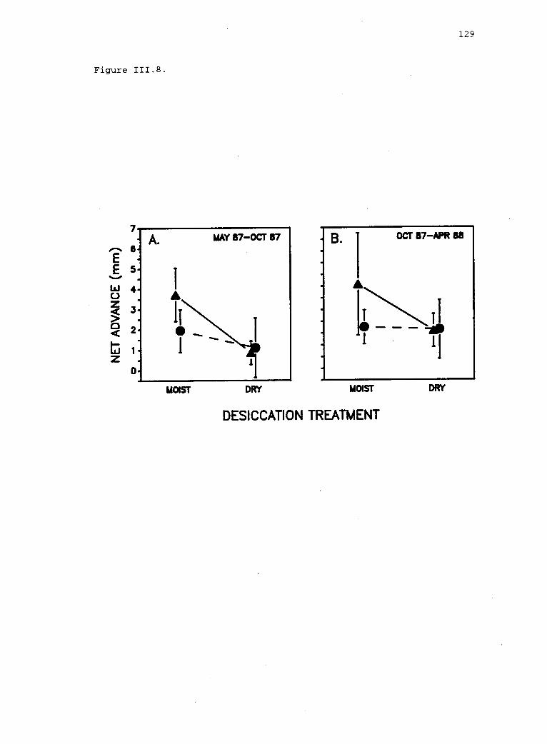
Figure 111.8.
MOIST DRY
129
OCT 137-APR 88
1
MOIST
DESICCATION TREATMENT
DRY
130
Figure 111.9. Average reproduction and number of recruits in allexperimental plots. Data are mean (± SEM) for n = 12 plots.Relative cover (%) of reproductive blades, left axis, solid symbols(40); number of sporelings that recruited during winter, 1987-1988,right axis, open symbols (C)).
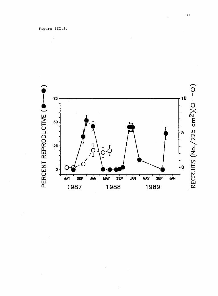
PE
RC
EN
T R
EP
RO
DU
CTI
VE
(
0N
to O
0cr
i"O
RE
CR
UIT
S (N
o./2
25 c
m2)
(O 0
)
132
Figure 111.10. Reproduction of Iridaea in experimental plots. See
fig. 111.5 caption for explanation of symbols.
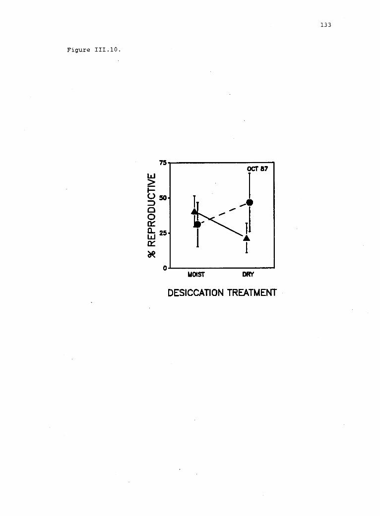
Figure 111.10.
ae
0MOIST DRY
DESICCATION TREATMENT
133
134
different (p > 0.05, Neuman-Keuls). A similar pattern was observed
throughout the 1987-88 and 1988-89 reproductive seasons, but the
interaction term in the ANOVA was not significant on any other dates.
Visible recruitment of sporelings began in Fall 1987 (fig.
111.9, open symbols). The effect of limpet removal on the number of
sporelings recruiting in January 1988 depended on the moisture regime
(fig. III.11, table III.1C). In moist plots, limpets tended to
enhance the recruitment of Iridaea. An average of 5.00 sporelings
recruited to moist plots with limpets, while only 2.33 sporelings
recruited to moist plots without limpets, although these means did not
differ in a post hoc comparison (p > 0.05, Newman-Keuls). In
contrast, in dry plots, Iridaea did not recruit in the presence of
limpets, but limpet removal permitted recruitment of an average of
2.67 sporelings per plot (p < 0.05, Newman-Keuls). Following initial
recruitment, limpet grazing removed sporelings from moist plots. By
June 1988, all sporelings that had recruited to limpet removal plots
(moist or dry) remained visible in photographs, while only 63% of
sporelings persisted in moist limpet addition plots. Thus, by June
1988, the number of recruits did not differ among the three treatment
combinations in which recruitment initially occurred (dry -L, moist
-L, moist +L; p > 0.05, one-way ANOVA).
Significant block effects were observed for three measures of
plant performance--vegetative advance, onset of reproduction, and
recruitment (table III.1). Blocks were established within 1 m
elevation along a horizontal gradient of relative wave-exposure, from
sheltered (Block 1) to exposed (Block 3). Other differences in
environmental conditions also occurred among the blocks. For example,
135
Figure 111.11. Recruitment of Iridaea in experimental plots. Seefig. 111.5 caption for explanation of symbols.
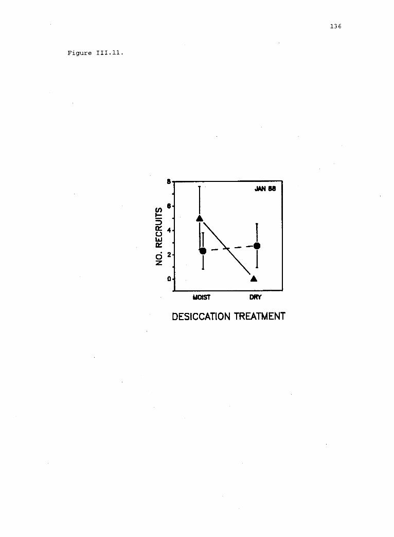
Figure 111.11.
MOIST DRY
DESICCATION TREATMENT
136
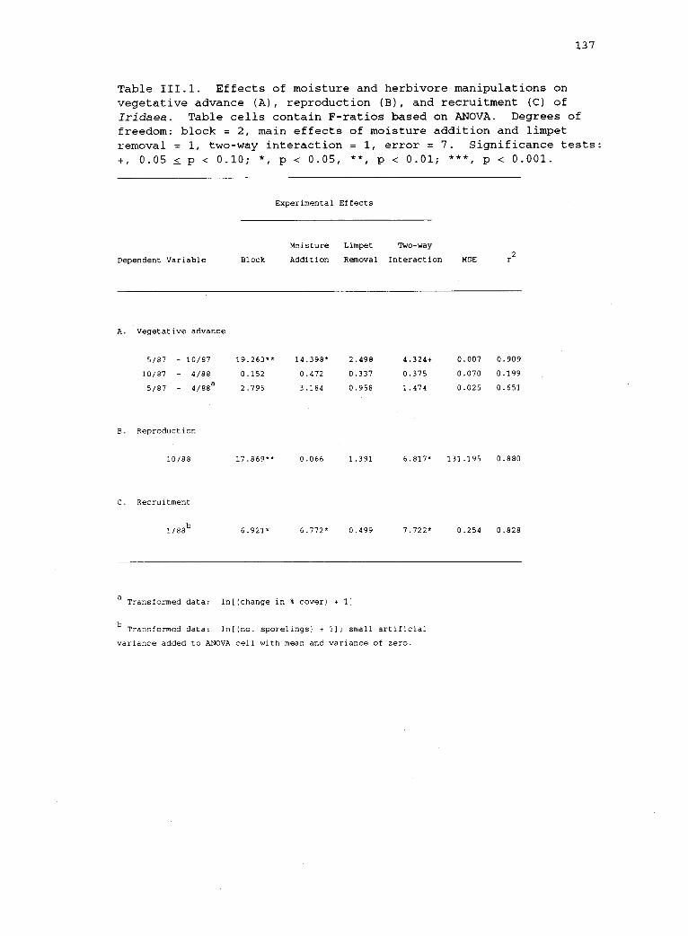
137
Table 111.1. Effects of moisture and herbivore manipulations onvegetative advance (A), reproduction (B), and recruitment (C) ofIridaea. Table cells contain F-ratios based on ANOVA. Degrees offreedom: block = 2, main effects of moisture addition and limpetremoval = 1, two-way interaction = 1, error = 7. Significance tests:+, 0.05 < p < 0.10; *, p < 0.05, **, p < 0.01; ***, p < 0.001.
Dependent Variable
Experimental Effects
Moisture Limpet Two-way
Block Addition Removal Interaction MSE r2
A. Vegetative advance
5/87 10/87 19.263** 14.398* 2.498 4.324+ 0.007 0.909
10/87 4/88 0.152 0.472 0.337 0.375 0.070 0.199
5/87 4/88a 2.795 3.184 0.958 1.474 0.025 0.651
B. Reproduction
10/88 17.869** 0.066 1.391 6.817* 131.195 0.880
C. Recruitment
1/88b
6.921* 6.772* 0.499 7.722* 0.254 0.828
a Transformed data: ln[(change in % cover) + 1]
b Transformed data: ln[(no. sporelings) + 1]; small artificial
variance added to ANOVA cell with mean and variance of zero.
138
block position was correlated with relative insolation. Because all
three blocks had a northerly aspect, steeper slopes resulted in less
insolation. At this site, wave-sheltered plots happened to be steeper
(table III.2A) and, thus, received less insolation (table III.2B) than
wave-exposed plots. In addition, the steeper plots of Block 1 were
shaded for longer periods of the day by cliffs rising to the south.
These differences in solar input were reflected in mean rates of
desiccation (table III.2C). Furthermore, limpet abundances declined
along the gradient of increasing wave exposure and insolation (table
III.2D). Finally, vegetative advance, reproduction, and recruitment
were highest in the sheltered, shady block (table III.2E-G).
Feeding Experiments
In the feeding experiments, limpet feeding was not affected by
senescence (reproductive status) or desiccation history of Iridaea
blades. During the 1987 feeding trials (fig. 111.12), limpets
appeared to prefer reproductive to non-reproductive blades in the
first trial (fig. III.12A), but the term for the interaction of limpet
feeding and reproductive status was not significant for either trial
(p > 0.10, F-ratio for two-way interaction, ANOVA). Trials in 1988
involving desiccated and non-desiccated blades of Iridaea also were
inconclusive. As measured by change in mass of blades, neither Lottia
digitalis nor Lottia pelta displayed a measurable preference by
desiccation status (p > 0.05, F-ratio for two-way interaction, ANOVA).
Subjective assessments of herbivore damage, however, were
associated with desiccation treatments in trials 1 and 2 (fig. III.13A
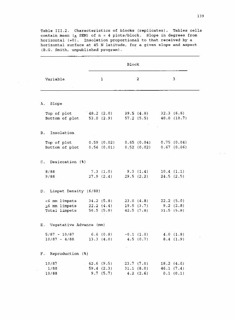
139
Table 111.2. Characteristics of blocks (replicates). Tables cellscontain mean (+ SEM) of n = 4 plots/block. Slope in degrees fromhorizontal (=0). Insolation proportional to that received by ahorizontal surface at 45 N latitude, for a given slope and aspect(B.G. Smith, unpublished program).
Variable
Block
1 2 3
A. Slope
Top of plot 48.2 (2.0) 39.5 (4.0) 32.3 (6.6)
Bottom of plot 53.0 (2.9) 57.2 (5.5) 40.0 (10.7)
B. Insolation
Top of plot 0.59 (0.02) 0.65 (0.04) 0.75 (0.04)
Bottom of plot 0.56 (0.01) 0.52 (0.02) 0.67 (0.06)
C. Desiccation (%)
8/88 7.3 (1.0) 9.3 (1.4) 10.4 (1.1)
9/88 27.9 (2.4) 29.5 (2.2) 24.5 (2.5)
D. Limpet Density (6/88)
<6 mm limpets 34.2 (5.8) 23.0 (4.8) 22.2 (5.0)
>6 mm limpets 22.2 (4.4) 19.5 (3.7) 9.2 (2.8)
Total limpets 56.5 (5.8) 42.5 (7.8) 31.5 (5.8)
E. Vegetative Advance (mm)
5/87 10/87 6.6 (0.8) -0.1 (1.0) 4.0 (1.8)
10/87 4/88 13.3 (4.0) 4.5 (0.7) 8.4 (1.9)
F. Reproduction (%)
10/87 62.6 (9.5) 23.7 (7.0) 18.2 (4.0.)
1/88 59.4 (2.3) 31.1 (8.0) 46.1 (7.4)
10/88 9.7 (5.7) 4.2 (2.6) 0.1 (0.1)
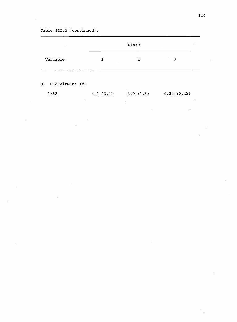
140
Table 111.2 (continued).
Variable
Block
1 2 3
G. Recruitment (#)
1/88 4.2 (2.2) 3.0 (1.3) 0.25 (0.25)
141
Figure 111.12. Effect of reproductive status of Iridaea on feeding byfree-ranging limpets. Data are mean (± SEM) for six replicatefeeding stations, triangles (A), and six controls (limpetexclosures), circles (41).
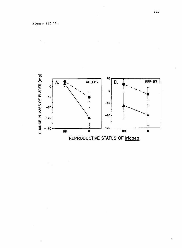
0-
142
40
-40.
Figure 111.12.
0.11
0 -L--1
CO 40-0Cf)
<In -BO-
-120-
-180NR
REPRODUCTIVE STATUS OF Iridaea
-so-
-120
SEP 87
NR R
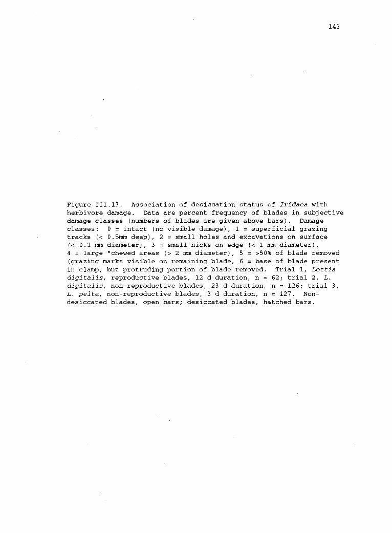
143
Figure 111.13. Association of desiccation status of Iridaea withherbivore damage. Data are percent frequency of blades in subjectivedamage classes (numbers of blades are given above bars). Damageclasses: 0 = intact (no visible damage), 1 = superficial grazingtracks (< 0.5mm deep), 2 = small holes and excavations on surface(< 0.1 mm diameter), 3 = small nicks on edge (< 1 mm diameter),4 = large "chewed areas (> 2 mm diameter), 5 = >50% of blade removed(grazing marks visible on remaining blade, 6 = base of blade presentin clamp, but protruding portion of blade removed. Trial 1, Lottiadigitalis, reproductive blades, 12 d duration, n = 62; trial 2, L.digitalis, non-reproductive blades, 23 d duration, n = 126; trial 3,L. pelta, non-reproductive blades, 3 d duration, n = 127. Non-desiccated blades, open bars; desiccated blades, hatched bars.
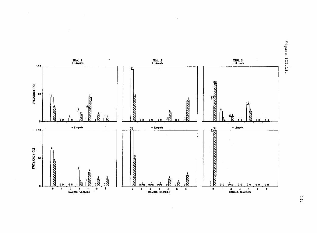
100
9
. 100
TRIAL 1+ Limpets
0 0 n0
limpets
0
00 002 3 4
DAMAGE CLASSES
2
0
5
TRIAL 2+ Limpets
31
4
s 00 00 00 00
12
32 LlittpofI
5
..,,
k`,
KN.
Z..741
4ts 0 pa 0 ra Om 0 M 0 RI 0
;., 4
-N, 1 1 1
6
0 1 2 3 4 5DAMAGE CLASSES
6
TRIAL 3+ Limpets
33
0
00
limpets
00 00
T
00 t-10 00 00 00 000 1 2 3 4 5
DAMAGE CLASSES6
145
and B), but not in trial 3 (fig. III.13C). In trials 1 and 2,
desiccated blades were significantly more likely than non-desiccated
blades to suffer substantial tissue damage (damage classes 4-6, see
fig. 111.13 caption), while non-desiccated blades were more likely to
have minimal tissue loss (damage classes 0-3), in both limpet arenas
and controls (table 111.3). These results suggest that grazing by
non-limpet herbivores (e.g., littorinid snails or dipteran larvae) may
account for some of the damage to desiccated Iridaea blades, and may
confound long-term field studies of limpet feeding preferences.

146
Table 111.3. Association of herbivore damage with desiccationtreatment. Table cells contain Pearson X2 statistics for a 2 x 2model of desiccation x damage, with 1 degree of freedom (n = number ofblades in parentheses). For X2 analysis, the seven subjective damageclasses (see caption, fig. 111.13) were collapsed into two classes:0 = minimal tissue loss (classes 0, 1, 2, and 3); 1 = substantialtissue loss (classes 4, 5 and 6). Significance tests: +,0.05 < p < 0.10; *, p < 0.05, **, p < 0.01; ***, p < 0.001.
Feeding Trialsa
Limpets 1 2 3
Present
Absent
2.95+(32)
5.93*(30)
17.49***(64)
14.87***(62)
1.27(64)
0.00(63)
a See fig. 111.13 caption for details of trials.
147
DISCUSSION
Predictions of the Models
Desiccation alters the effects of limpet grazing on the
reproduction and recruitment of Iridaea at this site, and it appears
to have a similar (but non-significant) effect on vegetative growth
and canopy cover. Thus, it is likely that desiccation alone does not
set the upper limit of Iridaea limpet grazers probably also play a
role. However, the interaction between desiccation and grazing is
more complex than that predicted by either the CSM or the PSM (fig.
III.1). Specifically, Iridaea appears to be grazer-limited in dry,
but grazer-dependent in moist, microsites. These results suggest that
a two-species model such as the CSM or PSM is insufficient to explain
the interaction of desiccation and herbivory. Furthermore, these
results and those of the feeding studies are not consistent with the
mechanisms proposed by either model to explain correlations between
stress and intensity of herbivory.
The CSM and PSM make contrasting predictions (Menge and Olson
1990) about the effect that reduced desiccation stress (i.e., moisture
addition) should have on herbivory. The CSM predicts that moisture
addition should exacerbate the effect of limpet grazing (fig. III.1A);
the PSM predicts that it should ameliorate the effect of herbivory
(fig. III.1B). Moisture addition reduced the negative effects of
grazers on Iridaea, in particular, by permitting recruitment in the
presence of grazers that was precluded in dry plots--results
consistent with PSM. However, grazing by limpets tended to enhance

148
plant performance in moist plots, by increasing vegetative advance
above the initial upper limit--a result not predicted by either model.
A simple two-species model, such as PSM, is probably not
adequate to explain the beneficial effects of grazing under moist
conditions observed in this study. It is likely that competitive
interactions with microalgae (which may foul mature red algae, D'
Antonio 1985; and inhibit germination of spores and growth of
sporelings, Huang and Boney 1984, 1985) mediate the grazer-dependence
of Iridaea in moist plots (fig. III.14A). Lottia digitalis, for
exammple, preferentially feeds on microalgae and small-bodied
ephemeral algae (Castenholz 1961, Frank 1965). Predation or grazing
should increase the abundance of competitively inferior prey (e.g.,
Iridaea), if competitive dominants (e.g., microalgae) are
preferentially attacked (Lubchenco 1978). In moist plots, where
productivity of both Iridaea and microalgae should be greater, limpets
may primarily remove microalgae, facilitating recruitment of Iridaea
(fig. III.14A). A similar effect of molluscan grazers has been
demonstrated in this (Paine 1981, Olson 1985) and other systems (e.g.,
review in Lubchenco and Gaines 1981). Thus, in the absence of
limpets, moisture addition may have little effect on the performance
of Iridaea, because gains in potential production are offset by losses
due to competition.
Where desiccation suppresses the productivity of microalgae,
limpets may feed more intensively (Castenholz 1961, 1962, Cubit 1984),
including in their diets more spores and sporelings of Iridaea,
inhibiting its growth and recruitment (fig. III.14B). During a series
of feeding studies in 1987, limpets ate less Iridaea at naturally
149
Figure 111.14. A conceptual model for a hypothetical effect ofdesiccation regime on interactions between limpets (Lottia) andIridaea, mediated by competing algae. A. In moist environments, highproductivity of other algae provides Lottia with an alternative foodsource reducing direct grazing (direct effect) on Iridaea andindirectly benefitting Iridaea by removing competitors. B. In dryenvironments, low productivity of other algae reduces competitiveinhibition of Iridaea, but direct limpet herbivory on Iridaea isincreased.
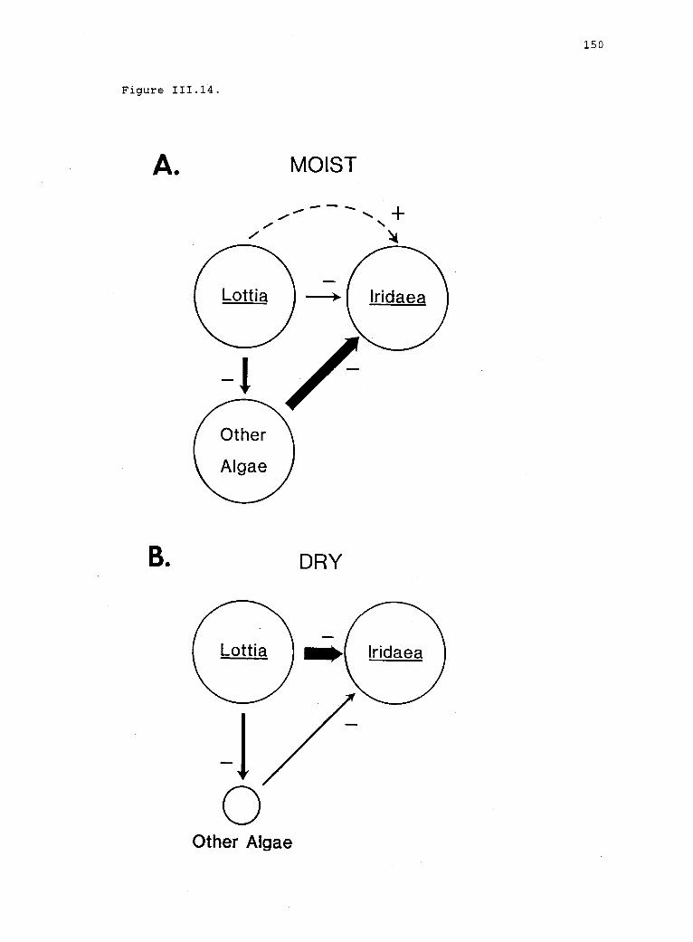
150
Figure 111.14.
00'
MOIST
Other
B. DRY
Other Algae

151
moist, shady feeding stations (where a visible standing stock of
diatoms and ephemeral algae persisted throughout the summer) than at
dry, sunny stations (where the rock appeared bare). The strong effect
of moisture addition in the presence of limpets may be mediated by the
response of limpets to the availability of their preferred microalgal
food. Thus, where desiccation is low and productivity is high,
limpets may subsist on microalgae (and release Iridaea from
competition) (fig. III.14A); where desiccation is high and
productivity low, limpets may begin to consume Iridaea and inhibit its
recruitment (fig. III.14B). Thus, desiccation may alter limpet
herbivory on Iridaea indirectly via its effects on the availability of
alternative algal foods.
Causal Mechanisms
Several proximal mechanisms potentially explain the predicted
association of herbivore impact with environmental stress (fig.
111.15). The CSM and PSM identify certain of these mechanisms (figs.
III.15A and D1); results of this study suggest other factors that may
also contribute to positive or negative correlations between stress
and herbivory (figs. III.15B, C, and D2).
Herbivore abundance
Decreasing herbivore abundance or effectiveness with stress
(fig. III.15A) is usually invoked to explain the negative correlation
of herbivory (and the positive correlation of plant performance) with
stress predicted by the CSM (review in Menge and Olson 1990). Harsh
conditions are consequently hypothesized to provide prey with a refuge
152
Figure 111.15. Explanatory mechanisms potentially accounting forcorrelations between environmental stress and the effect of consumerson prey. The consumer stress model (CSM) predicts a negativecorrelation, the prey stress model (PSM), a positive correlation,between stress and the impact of consumers. Cells A and D1 reflectmechanisms usually associated with the respective models.
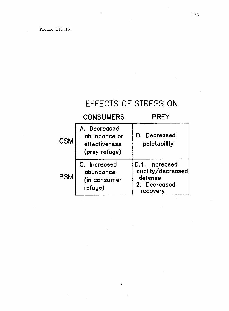
Figure 111.15.
CSM
PSM
EFFECTS OF STRESS ON
CONSUMERS PREY
A. Decreasedabundance or B. Decreasedeffectiveness(prey refuge)
palatability
C. Increased D.1. Increasedabundance quality/decreased(in consumer defenserefuge) 2. Decreased
recovery
153
154
from herbivory. The preditions of the CSM would also hold if prey
palatability declined with stress (fig. III.15B) (regardless of
changes in consumer abundance or effectiveness) as when herbivores
prefer young, vigorous leaves (e.g., Coley 1983, Rauscher 1981).
In the present study, limpet abundance was negatively correlated
with desiccation intensity on a large scale, a pattern expected under
the CSM. Significant block effects in several analyses (table 111.2)
were associated with a gradient of increased insolation and
desiccation, from block 1 (which is steeper and more shaded by cliffs
to the south) to block 3 (which is more nearly horizontal and less
shaded). Despite biweekly additions, total limpet abundances were
higher at the shady than at the sunny end of this gradient in
midsummer. Similarly, Louda and Rodman (1983) observed a negative
correlation of herbivore damage with elevation in subalpine
populations of a native mustard that appears, on a local scale, to be
more susceptible to grazers when stressed by low soil moisture. In
this study, the cline could be produced by desiccation-induced limpet
mortality or migration (e.g., Wolcott 1973) or by bird predation in
more horizontal plots (e.g., Frank 1982, Marsh 1986), but the relative
contribution of each of these and other factors is not known. Within
blocks, among treatments, however, the interaction of desiccation and
herbivory was consistent with the PSM.
Plant susceptibility
Under the PSM, the predicted positive correlation of herbivore
damage with stress has usually been attributed to a stress-induced
changes in plant susceptibility to herbivory (fig. III.15D1). Stress
155
may induce changes in plant quality (Mattson and Addy 1975), such as
increased nutrient availability (White 1984) or decreased defense
(Waring and Schlesinger 1985), that lead to higher rates of feeding on
stressed plants. For example, Lewis (1979, 1982, 1984) found that
grasshoppers preferred wilted, senescent, or previously damaged leaves
of sunflower species to vigorous, undamaged leaves. Hughes et al.
(1982), also observed increased rates of feeding by Mexican bean
beetles on soybean leaves that had been stressed by exposure to S02.
In the present study, nutrient availability and plant defenses
were not directly measured. However, results of the feeding studies
do not support the hypotheses that senescence (due to reproduction) or
desiccation increase the susceptibility of Iridaea to limpet grazing.
During feeding trials, reproductive blades were senescent. In the
absence of limpets, non-reproductive blades appeared vigorous and
tended to grow, while reproductive blades either failed to grow or
lost mass. However, limpets did not preferentially feed on
reproductive blades. Furthermore, desiccation treatments also did not
result in measurably higher rates of feeding by limpets in repeated
trials.
These results are not consistent with the hypothesis that
desiccation affects plant susceptibility to limpets. However, they
should not be considered conclusive for several reasons. First, the
effect of chronic, non-lethal desiccation was not investigated nor
were spores, small blades, or crusts used in feeding trials. Only
acute, simulated desiccation damage to mature blades was tested.
Results of the moisture addition X limpet removal experiment, however,
suggest that the effect of desiccation on the vulnerability of spores
156
and small plants may differ from its effect on susceptibility of
larger plants to grazers. Thus, desiccation stress may influence the
likelihood that a sporeling will survive to attain a size-escape from
predation (e.g., Paine 1976, Lubchenco 1983).
Second, artificially desiccated blades may not be comparable to
naturally desiccated blades, which appear to become infested by micro-
organisms. Following prolonged aerial exposure, blades normally
become bleached, then within a few days the bleached tissue becomes
"slimy." Both limpets and littorinid snails appear attracted to these
damaged thalli; all the necrotic tissue is usually removed within
several days, provided further desiccation does not occur.
Artificially desiccated blades, on the other hand, became bleached,
but tended to remain firm and intact (unless eaten) throughout the
feeding trials. Thus, the effect of severe desiccation damage on
herbivore feeding preferences may depend on micro-organisms (see White
1984 for a review of evidence for links between stress, pathogens, and
susceptibility to grazers in vascular plants). Studies employing
naturally desiccated blades, with control for infestation by
microorganisms, could further resolve this question.
Third, subjective estimates of herbivore damage suggest that
some unidentified members of the herbivore guild prefer desiccated to
non-desiccated blades of Iridaea. If so, their feeding may have
introduced uncontrolled variability into tests of limpet feeding
preferences, particularly in the longer-term trials (1 and 2)
involving L. digitalis. Nevertheless, desiccation of mature blades
did not markedly change limpets' feeding preferences, suggesting that
157
other factors may account for the interaction of desiccation and
herbivory observed in the long-term experiment.
Plant recovery
Recovery from herbivory may be inhibited by stress, resulting in
a positive correlation of herbivory with desiccation (fig. III.15D2),
consistent with the PSM, independent of changes in plant
susceptibility to grazing. For example, Chater (1931) noted that
isolated gorse plants vigorously sprouted from basal nodes after
rabbit grazing, while those in competition with grasses failed to
sprout and often died. In a prospective study, Webb (1981) found that
the potential for Douglas-fir and white fir twigs to recover from
tussock moth defoliation was positively correlated with starch content
prior to attack (an indicator of plant vigor).
Although the present study does not address the effects of
stress on recovery of Iridaea, preliminary results of other studies
(A. M. Olson, in preparation) suggest that experimentally defoliated
Iridaea loses less basal area and recovers canopy faster in moist than
in dry treatments. For clonal organisms, with the potential to
respond vegetatively to herbivory, this effect of stress on recovery
from herbivory may be as important as stress-induced changes in
initial susceptibility to herbivory.
Herbivore movement
Additional mechanisms that potentially result in the positive
correlation between stress and herbivory predicted by the PSM are
factors that directly or indirectly affect herbivore abundance or
behavior (fig. III.15C), independent of their effects on plant quality
158
and recovery. For example, Huffaker and Kennett (1959), hypothesized
that the thermal requirements of leaf beetles restrict foraging on St.
Johnswort to sunny habitats, where plants may experience more heat and
desiccation stress. The retreat of consumers to refuges to avoid
physiological stress (Menge 1978a, b) may create high consumer
densities in some microhabitats during stressful episodes (fig.
III.15C). For example, Lottia digitalis often aggregates during
daytime low tides (Frank 1965, Millard 1968, Gallien 1985) and
migrates downward during summer months (Frank 1965, Breen 1972, A.M.
Olson, personal observation). Thus, in consumer refuges, high
environmental stress would be temporally correlated with herbivore
abundance and perhaps with feeding activity.
Observations of limpet behavior lend support to the notion that
desiccation magnifies the detrimental effects of grazing, in part,
because limpets limit their foraging to areas close to the moist
refuge provided by Iridaea beds. For example, in this study, limpets
tended to stay within the Iridaea bed in dry plots; in moist plots
they aggregated near the moisture-retaining polyester (A. M. Olson,
personal observation). Thus, limpet foraging is probably concentrated
nearer to patches of Iridaea or other algae under more desiccating
conditions.
To understand spatial variation in prey abundance and
performance it is necessary to distinguish between the pattern of
consumer effects and the mechanism that produces the pattern. The
impact of herbivory may increase with stress as predicted by the PSM,
independent of changes in plant quality and grazer feeding rate.
Plant recovery may be inhibited, or herbivore activity locally
159
intensified, by stress. On the other hand, stress-induced changes in
consumer abundance or effecctiveness are not necessary for the impact
of consumers to decline with stress. For example, when herbivores
prefer vigorous tissue, plant susceptibility may decline with stress
(the "plant vigor hypothesis" of Price 1991). Future empirical work
should thus focus on the mechanisms which mediate the effects of
stress on consumer-prey interactions.
In particular, a key issue seems to be the conditions under
which either consumers or prey are relatively more affected by
physical factors. The preponderance of support for CSM comes from
freshwater and marine environments (reviews in Menge and Sutherland
1987, Menge and Farrell 1989), while that for PSM is mainly from
terrestrial insect-plant systems (e.g., Waring and Schlesinger 1985).
This observation suggests that perhaps when plant and herbivore are
immersed in the same medium, CSM may apply, while PSM dynamics may be
more relevant when stress factors affecting plants (e.g., soil
moisture) differ from those affecting herbivores (e.g., air
temperature). If this pattern holds, sub-surface (soil) plant-
herbivore interactions might be expected to follow the CSM model.
Defining the domains of the CSM and PSM is not a trivial
endeavor. Distributions of species predicted under each of these
models will differ in specific ways from those expected on the basis
of single-species models. Single-species models often will be
inadequate to predict species' responses to environmental change.
Consequently, identifying the domains of the models has important
implications for predicting the responses of species to anthropogenic
effects such as pollution or climate change (Lubchenco et al. 1991).
160
For environmental decision-makers, it may be critical to know whether
the CSM or the PSM holds in a particular situation, because the CSM
makes the counter-intuitive prediction that prey species' abundances
may increase with stress, while the PSM predicts that species may be
excluded (even from regions where anthropogenic stress is
physiologically tolerable) by the combined effect of consumers and
stress. The differences in these predictions suggest that setting
acceptable levels of a pollutant, or forecasting the effect of climate
change on species distributions, will require more than an assessment
of the physiological responses of individual species. Instead,
scientists and decision-makers will need to consider the interplay
between stress and the interactions among a suite of species in order
to predict, understand, and prepare for natural and anthropogenic
environmental change.

161
ACKNOWLEDGMENTS
I gratefully acknowledge the technical assistance of D.
Frostholm, C. Halpern, M. Spencer, and others. G. Allen, J. Antos,
Farrell, C. Halpern, J. Lubchenco, and B. Menge kindly made comments
on an earlier draft of the manuscript. This work was supported in
part by grants from the National Science Foundation to B. Menge (OCE-
8415609, OCE-8811369) and to J. Lubchenco and D. Carlson (OCE-
8600523), by grants-in-aid of research from Sigma Xi and the
Phycological Society of America to A. Olson, and by a DeLoach Graduate
Fellowship from Oregon State University to A. Olson.
162
Chapter IV
COMPETITION IN SEAWEEDS:
LINKING PLANT TRAITS TO COMPETITIVE OUTCOMES
Annette M. Olson
and
Jane Lubchenco
Department of Zoology
Cordley Hall 3029
Oregon State University
Corvallis, OR 97331-2914
INTRODUCTION
Competition for resources among seaweeds is potentially
important at several levels of organization. Competition may
influence community-level patterns (e.g., species diversity,
succession, and stability) both directly and by mediating the effect
of other structuring agents, such as herbivory and physical
disturbance (Lubchenco and Gaines 1981). At the population level,
competition may affect size and age structure and other determinants
of population growth. Finally, competition may influence individual
survival and reproduction (fitness), with potential evolutionary
consequences. In natural systems, community-, population-, and
individual-level processes are intricately interwoven, making it
difficult to disentangle the potential causes and consequences of
163
competition. We will focus on the consequences of seaweed traits for
the outcome of competitive interactions.
Historically, culture and field studies have followed separate
but parallel lines of inquiry. As a result, we currently lack a
rigorous understanding of the consequences of particular seaweed
traits for competition and of the trade-offs involved in competition
and other biotic and abiotic interactions. Culture studies have
tended to focus on the physiological, morphological, or life history
characteristics that potentially affect competition--directing
attention to the way these plant traits affect resource capture and
how environmental variation affects their expression. However, most
culture studies stop short of experimentally demonstrating the
consequences of plant traits for competitive outcomes, simply assuming
that differences in traits will result in competitive differences. On
the other hand, field studies of competition have tended to focus on
competitive outcomes--the fates of competing populations under
differing environmental conditions (e.g., Paine 1990). The emphasis
has been on the way that variation in stress (e.g., desiccation, high
or low temperature), disturbance (e.g., log-bashing, sand-scour), or
herbivory determines whether competition occurs and, if so, the sign
or magnitude of competitive interactions. However, mechanistic
explanations, often involving trade-offs at the individual level
(e.g., between competitive ability and susceptibility to herbivory)
have not been tested by measurements of physiological costs and
benefits. Thus, the causal relationships between plant traits and
competitive outcomes remain a crucial gap in our understanding of
competition among seaweeds. To bridge this gap, we see a need to (1)
164
establish rigorously the competitive consequences of variation in
traits (among and within species) observed in culture studies and (2)
evaluate the hypothesized mechanisms of competition (and other
ecological interactions) proposed as a result of field studies.
The contributors to this series of minireviews highlight a set
of familiar and novel plant traits and suggest hypotheses regarding
their significance for competitive interactions: Carpenter (1990)
focuses on traits associated with the capture of space, light, carbon,
and nutrients. He shows how morphological traits--such as growth
form, thickness, degree of branching and surface texture--and
physiological traits--such as photoadaptation, alternate carbon
fixation pathways, and nutrient uptake and storage
strategies--interact to determine the internal resources available for
allocation to competitive interactions, as well as to other plant
functions. Next, Paine (1990) offers a wide-angle view--from the
individual to the community levels--of plant traits that may interact
to alter competitive interactions. He reviews field observations of
(1) thallus fusion or redirected growth following contact with other
thalli that may represent "cooperation" within and among species, (2)
epithallial sloughing or antibiotics serving as "defenses" against
epiphytes, and (3) resistance to herbivory and the associated grazer-
dependence of competitive outcomes. Finally, Maggs and Cheney (1990)
narrow the focus to thallus fusion a novel seaweed trait also
discussed by Paine. They review laboratory observations of
coalescence, secondary pit connections, and fusion cells between
sporelings differing in relatedness, ranging from genetically
identical sporelings to those differing in ploidy or species. In this

165
introduction to the series, we briefly review theoretical and
empirical approaches to competition and suggest research strategies
for linking the traits and fates of seaweeds.
166
DEFINING COMPETITION
Although the early competition models were very simple, their
assumptions and predictions reflect much of our common sense
understanding of competition. The Lotka-Volterra model translates the
deleterious effect of a competitor into a cost expressed in terms of
population growth (Roughgarden 1979). This cost is proportional to
the ratio between inter- (cq) and intraspecific (cXii) effects for
each species. According to the simplest form of the model, the
outcome of competition (i.e., whether there is a winner and, if so,
which species wins) depends both on the cost of competition and on the
carrying capacity (Ki, or number individuals of each species that can
be supported in a given environment in the absence of competition).
If the carrying capacities of the two species are equal (i.e.,
K1 = K2), one species (e.g., species 1) will dominate only if the
competitive effects are asymmetrical--that is, if°(21 (the effect of
species 1 on species 2) is greater than DI22 (the effect of species 2
on itself) and, simultaneously, if°(12 is less than a11. Thus, a
species' competitive position depends on its ability to harm its
competitor (e.g., by preempting space) or to reduce the deleterious
effects of its competitor (e.g., by preventing colonization or
overgrowth). However, when carrying capacities are not equal (e.g.,
K1 > K2), the likelihood of coexistence, is reduced and the balance is
tipped in favor of the species with higher K. Thus, a species with
greater efficiency of resource use (e.g., nutrient assimilation) may
exclude its competitor, even when the balance of intra- vs.
interspecific effects favors the competitor (Roughgarden 1979).
167
Modern competition theory continues to evolve as a result of the
interplay between theoretical and empirical studies (see reviews in
Pacala 1989, Kareiva 1989). Problems that arise in applying the
Lotka-Volterra model to plants (Schaffer and Leigh 1976, Pacala 1989)
have stimulated refinement of existing theory and development of new
theoretical approaches. In the following paragraphs we present four
examples of problems with the Lotka-Volterra model that are
particularly relevant to seaweeds, noting some recent theoretical
developments and some outstanding problems.
(1) The Lotka-Volterra model assumes that the environment is
spatially homogeneous and that resource limitation or crowding can be
expressed in terms of K, the maximum density of individuals in a
population. However, because seaweeds and other plants are attached
to the substratum, their environments are not homogeneous, the
intensity of interactions among plants varies with the spatial
arrangement of competitors (Pacala 1989). In addition, the number of
individuals is a poor measure of crowding in plants (Schaffer and
Leigh 1976). Indeterminate growth and variation in plant architecture
may result in increased crowding, despite decreasing numbers of
individuals. Thus, interactions among seaweeds depend upon the
position, biomass, architecture, and potential for vegetative
expansion of competitors, as well as on their population density.
Spatially explicit models of interactions among plants have been
developed (review in Pacala 1989), but these need to be linked to
models of clonal growth and reproduction (e.g., Bell 1984, Caswell
1985).
(2) The Lotka-Volterra model also assumes that the cost of

168
competition (6(1j/ii) is constant and independent of density (i.e.,
the effects of species on each other do not change). Thus,
interacting populations lack age or size structure, genetic variation,
and phenotypic plasticity (i.e., all individuals are identical).
Empirical studies (see "Detecting Competition," below) suggest,
however, that competitive effects vary considerably with the age or
size at which species interact. Although modern competition models
have incorporated age or size structure (reviews in Pacala 1989,
Kareiva 1989), theory that predicts the effects of genetic or plastic
variability on competitive interactions is presently lacking (Kareiva
1989). (3) The Lotka-Volterra model lacks density-independent sources
of mortality, such as herbivory or extreme environmental conditions.
Models incorporating consumers (e.g., Caswell 1978) more realistically
portray the dependence of competitive outcomes on grazing regimes
(e.g., Paine 1990). (4) Unique traits of seaweeds, including
isomorphic life histories and somatic polyploidy (Goff and Coleman
1986), as well as thallus fusion, suggest areas for future elaboration
of plant-specific theory.
169
DETECTING COMPETITION
Experimental detection of competition is achieved by
manipulating the abundance of competing species or the resource. The
strength of competition is measured by the effect of experimentally
varied plant density on abundance (e.g., density, percent cover) or on
rates affecting abundance (e.g., fecundity, growth, mortality, or
physiological condition) (Connell 1983, Schoener 1983). Harper
(1977), Connell (1983), Underwood (1986), and Denley and Dayton (1985)
provide useful discussions of appropriate experimental designs that
may be applied in laboratory, mesocosm, or field settings.
Competition experiments ideally should be conducted in the field
with adequate replication and controls (Connell 1983, Schoener 1983),
in order to evaluate competition as a natural process. Competitor-
removal experiments and transplants can be an effective way to
manipulate the density of larger sporelings and established seaweeds
(e.g., Schonbeck and Norton 1980; also see reviews in Denley and
Dayton 1985, Chapman 1986). However, the microscopic spores of
seaweeds make the field study of competition difficult for the
earliest stages of development. For these stages, alternative
approaches include experiments in the laboratory (Russell and Fielding
1974, Fletcher 1975) or in semi-natural tank culture (mesocosms),
"seeding" spores (Dion and Delepine 1983) of competing species at
different densities onto artificial substrata for later outplanting,
or applying spore suspensions directly to natural substrata
(L. Druehl, pers. comm.).
Competition will not be detectable in nature, however, if
170
resources are superabundant or if herbivory, low recruitment, or
physical factors (e.g., storm damage, desiccation) reduce the density
of potentially competing populations. Thus, it is frequently
necessary to vary the context in which competition experiments are
conducted, for example, by simultaneously manipulating herbivores (see
Sih et al. 1985 for design suggestions) or by replicating field
experiments along gradients of wave force or desiccation (e.g.,
Lubchenco 1986), in order to determine the conditions under which
competition occurs. Alternatively, laboratory competition experiments
can be made more realistic by including herbivore treatments or by
mimicking desiccation (e.g., Luxoro and Santelices 1989) or water
motion (e.g., Denny 1988) regimes. Such improvements in experimental
design and technique will yield valuable information on the relative
importance of competition for seaweeds under different conditions
(Lubchenco 1986).
In the following examples we illustrate several factors that can
affect the outcome of competition in the field. First, Fujita (1985a,
b) suggests that the pattern of nutrient availability can determine
the competitive dominant. When nutrients are continuously available,
Ehteromorpha spp., by virtue of their faster uptake rate, can out-
compete Gracilaria tikvahiae (e.g., fig. IV.lA). However, Gracilaria
has a greater nutrient storage capacity. Consequently, when the
nutrient supply is pulsed and the interval between pulses exceeds the
storage capacity of Enteromorpha, Gracilaria is the competitive
dominant.
Second, competitive interactions in the mid-intertidal zone in
New England illustrate the importance of timing and grazers on the
171
Figure IV.1. A schematic representation of some mechanisms ofcompetition (Schoener 1983) in seaweeds. A. Consumption of nutrientsmediates the interaction between Gracilaria tikvahiae and Enteromorphaspp. in the field (Fujita 1985a, b). B. A dense turf of Enteromorphaintestinalis preempts space, preventing colonization by spores ofUlothrix pseudoflacca in culture (Hruby & Norton 1979).C. Pseudolithophyllum muricatum overgrows Lithothamnion phymatodeum inthe field on a smooth, artificial surface in the absence of grazers(Paine 1984). D. An alga uses allelochemicals to exclude a competitor(hypothetical interaction).
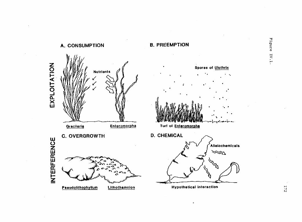
A. CONSUMPTION
Gracilaria
C. OVERGROWTH
Enteromorpha
Pseudolithophylium Lithothamnion
B. PREEMPTION
Spores of Ulothrix
Turf of Enteromorpha
D. CHEMICAL
Allelochemicals
Hypothetical interaction
173
outcome of competition. Fucus vesiculosus colonizes freely in the
presence of grazers that selectively remove Enteromorpha spp.
(Lubchenco 1983). In the absence of grazers, however, Enteromorpha
initially outcompetes Fucus germlings early in succession, presumably
by its faster growth rate. Because grazers are usually effective,
Fucus becomes established and overtops Enteromorpha. Over the long
term, Fucus excludes Enteromorpha from the rock surface by preempting
space, although Enteromorpha can occur as an epiphyte on Fucus when
mesoherbivores are absent or ineffective. This example illustrates
two effects of timing in competitive interactions: First, the outcome
of competition depends on the developmental stages that are competing
(i.e., germling vs. germling or germling vs. adult). Thus, a single
trait, such as rapid growth, that confers superiority on Enteromorpha
when germlings compete is not effective when competing against adult
Fucus for attachment space. Second, the arena of competition changes
during succession, expanding to include competition for light by
epiphytes, as well as for attachment space on the rock surface.
The above example also illustrates the potential importance of
trade-offs between competitive ability and other demands on plants'
resources. In this case, the outcome of competition is grazer-
dependent, because competitive ability is negatively correlated with
susceptibility to herbivory. Currently, we know little about the
physiological mechanisms underlying such trade-offs. In the following
section, we suggest research strategies that link seaweed traits to
competitive outcomes in a way that may be helpful in understanding the
physiological and morphological bases of trade-offs.
174
CONSEQUENCES OF PLANT TRAITS AND THE MECHANISMS OF COMPETITION
Different plant traits may be associated with competitive
dominance, depending on the mechanism of competition (fig. IV.1).
Exploitation mechanisms include consumption (depletion of resources)
and preemption (passive prior occupation of space) (Schoener 1983).
Where consumption is the mechanism, higher rates of resource capture
(Carpenter 1990) may afford competitive superiority. If the
interaction is preemptive, then larger size, spreading habit, and the
ability to perennate may be associated with dominance. Interference
includes overgrowth (including epiphytic interactions), and chemical
(toxic or hormonal) mechanisms (Schoener 1983). Rapid lateral growth,
ability to raise the growing edge off the substratum, and production
of toxins are traits that may affect the outcome of interference
interactions. It is often difficult to identify a single
mechanism--for example, consumption of light interferes with other
species by shading, preemption may be accompanied by chemical effects.
Finally, asymmetry is to be expected in the mechanism, as well as in
the strength of competitive interactions. For example, Fucus may
preempt space, preventing subsequent colonization of the rock surface
by ephemerals, whereas ephemerals interfere with Fucus by growing on
it as epiphytes and increasing the drag on Fucus (Lubchenco 1983).
The association of seaweed traits with competitive mechanisms,
however, is largely hypothetical. The ecological and fitness
consequences of particular traits await experimental analysis. Which
seaweed traits are associated with competitive dominance? How does
variation in a single trait affect competitive performance? We
175
suggest that a research strategy that explicitly focuses on the
functional significance of plant traits could provide substantial
insights into competition among seaweeds.
Several studies have quantified variation in a suite of
morphological and physiological traits both among (e.g., Littler et
al. 1983, Hay 1986) and within (e.g., Hanisak et al. 1988) seaweed
species and have identified possible trade-offs between potential
growth rate and a variety of other traits. We suggest that this
correlative approach could be made more rigorous and definitive by
simultaneously conducting competition experiments to determine species
competitive rankings (e.g., Harper 1977, Gaudet and Keddy 1988).
Seaweed traits and competitive ability could then be linked by
multiple regression techniques (Gaudet and Keddy 1988). This approach
would be particularly useful in identifying potential trade-offs
between seaweed performance in competition and other ecological
interactions, if experimental tests of susceptibility to herbivores,
physiological stress, or mechanical disturbance (e.g., Koehl 1986)
were also included in the analysis.
It is a somewhat different problem to determine the effect on
competition of variation in a single trait. One must manipulate not
only the densities of competing species, but the trait of interest.
Sometimes it is possible to manipulate a trait directly, for example,
by pinning down the upper branches of a plant to test the effect of
height (Benjamin 1984). In other cases the investigator can take
advantage of natural or induced (mutant) variation in a trait. For
example, to understand the significance of thallus fusion for
competitive outcomes, the performance (e.g., growth rate, ultimate
176
size, or reproduction) of fused and non-fused thalli must be tested,
alone and in the presence of a competitor. If fusion has consequences
for interspecific competition, performance of the fusion chimera
should be better than that of non-fused thalli in the presence of the
competitor. Thallus fusion may also affect competition
indirectly--for example, by increasing resistance to desiccation or
herbivory.
A remaining question is how any ecological benefit of thallus
fusion may be distributed among the individual members of a fusion
chimera. The interaction between members of a chimera may range from
mutualism (both members benefit) to somatic parasitism (one member
benefits at the expense of the other). Both mutualistic and parasitic
intraspecific interactions have been observed in fungi and sessile
invertebrates (e.g., Buss 1981, 1982, Weissman et al. 1988). The
costs and benefits of these interactions depend on the genetic
relatedness of the participants (Weissman et al. 1988, Grosberg and
Quinn 1988). Formation of pit connections and fusion cells can be
associated with parasitic or aggressive interactions in algae (e.g.,
Goff and Coleman 1985, Koslowsky and Waaland 1984). The potential
that, in some circumstances, thallus fusion may represent parasitism
needs to be explored by evaluating the fitness consequences of fusion
for both members of the chimera. Further investigation of
physiological integration between fused sporelings would be
facilitated by use of modern molecular techniques, including tracer
studies of photosynthate and nutrients, monoclonal antibody labeling
to track transport of growth factors and other hormones, and molecular
probes for genes or gene transcripts unique to one member of the pair.
177
CONCLUSIONS
In conclusion, we would like to emphasize the following points:
1. Ecological theory can be useful in identifying critical
factors in competitive interactions and in predicting the logical
consequences of variation in those factors. We see a need to
incorporate recent theory into our thinking about competition in
seaweeds and to evaluate the implications of unique seaweed traits for
future theoretical treatment.
2. Because the traits of seaweeds have evolved in a context of
multiple selection pressures, the consequences of traits will vary
with environmental conditions. Thus, to link the traits of seaweeds
with the outcome of competition, it is essential to demonstrate
competitive effects in the context of environmental gradients in
herbivory, stress, and disturbance.
3. A focus on the functional significance of seaweed traits can
help integrate laboratory and field studies, by directing our
attention to the ecological consequences of traits and to the
underlying mechanisms of ecological patterns. (Similar
recommendations regarding terrestrial systems have been made by Arnold
1983, McGraw and Wulff 1983, and Ehleringer et al. 1986.)
4. Seaweeds have much to offer as model systems for the study
of competition: studies of seaweeds have contributed to a general
understanding of the trade-offs between morphological and
physiological traits and of the relative importance of competition for
communities. Incorporating novel seaweed traits (e.g., coalescence)
into studies of competition will put our understanding on a broader
178
evolutionary basis. Areas needing further investigation include the
importance for competitive interactions of allelochemical
interactions, of vegetative reproduction, and of variation in ploidy
and morphology within the life history.
As demonstrated in this series of mini-reviews, the study of
competition in seaweeds is at a crossroads. By linking the techniques
of laboratory and field studies, we have a unique opportunity to
develop an integrated view of seaweeds in their environments.
179
ACKNOWLEDGMENTS
We wish to thank S. Brawley, C. Halpern, R. Paine and an
anonymous reviewer for comments on earlier versions of this
manuscript. J. Teeri and J. McGraw directed us to readings in the
terrestrial literature. Our special thanks go to Charlie Halpern for
drafting the figure. This work was supported in part by grant OCE-
8600523 to J. Lubchenco and D. J. Carlson from the National Science
Foundation.

180
QUESTIONS
Question (Carpenter): You have recommended the incorporation of
simple ecological models as one basis for further experimentation to
examine competition within and between algae. Given the demonstrated
variability in the carrying capacity of an environment, due to either
environmental changes over short time scales and/or to physiological
plasticity exhibited by algae, how useful will such simple models be
in predicting competitive relationships?
Answer: We view the simplest competition models as a useful framework
for organizing a discussion of competition. More sophisticated
models, however, make predictions that can be tested in order to
further both empirical and theoretical understanding of competition.
All ecological models simplify complex phenomena, making it
possible to explore the logical consequences of varying some set of
factors, assuming a given biological background. Theoretical models
can contribute to empirical studies by suggesting the kinds of factors
that should affect competitive outcomes. Toward this end, Kareiva
(1989) lists ten critical experiments suggested by modern theoretical
developments. Your question regarding the effect of environmental
variation on competitive interactions has been addressed in models by
Chesson (e.g., 1986) that make several explicit predictions. These
predictions remain to be tested (Kareiva 1989) and seaweeds may
provide good model systems for doing so.
Ecological theory benefits from empirical feedback, as well.
Theory necessarily makes its assumptions explicit. As "consumers" of
181
theory, empiricists are especially sensitive to whether particular
assumptions are warranted in a given system. As you point out, real
systems often violate the Lotka-Volterra assumptions of constant
environment and identical individuals. Recognizing these and other
limitations of the simplest models, theorists have elaborated existing
theory and constructed entirely new theory that is more realistic
(reviews in Pacala 1989, Kareiva 1989).
Question (Paine): To what extent are seaweed traits, expressed under
laboratory conditions, accurate reflections of possible conditions or
even responses in the "real world"?
Answer: Some algal traits are notoriously variable. This variation
is probably expressed in both the laboratory and the field. In the
past variation has either been ignored or treated as "noise", but
intraspecific variation potentially has important ecological as well
as evolutionary implications. Understanding the causes and
consequences of such variation represents an important challenge.
Both field and laboratory approaches are appropriate: In the field,
transplants between habitats and experimental alteration of habitats
permit evaluation of environmental effects on seaweed traits.
Laboratory studies can explore the relative contribution of genetic
and plastic variation that sets boundaries on the ecological responses
of seaweeds in nature.
182
BIBLIOGRAPHY
Abbott, I. A., and C. J. Hollenberg. 1976. Marine algae of
California. Stanford University Press, Stanford, California, USA.
Arnold, S. J. 1983. Morphology, performance and fitness. American
Zoologist 23:347-361.
Bell, A. D. 1984. Dynamic morphology: a contribution to plant
population ecology. Pages 48-65 in R. Dirzo and J. Sarukhan, editors.Perspectives on plant population ecology. Sinauer Press, Sunderland,
Massachusetts, USA.
Bell, G. 1982. The masterpiece of nature. Croon Helm, London,
England.
Benjamin, L. R. 1984. Role of foliage habit in the competitionbetween differently sized plants in crop carrots. Annals of Botany
53:549-557.
Bernstein, H., G. S. Byers, and R. E. Michod. 1981. Evolution of
sexual reproduction: importance of DNA repair, complementation, andvariation. American Naturalist 117:537-549.
Blair, S. M., A. C. Mathieson, and D. P. Cheney. 1982. Morphologicaland electrophoretic investigations of selected species of Chaetomorpha(Chlorophyta: Cladophorales). Phycologia 21:164-172.
Bold, H. C. 1970. The plant kingdom. Prentice-Hall, EnglewoodCliffs, New Jersey, USA.
Bold, H. C., and M. J. Wynne. 1985. Introduction to the algae:structure and function. Prentice-Hall, Englewood Cliffs, New Jersey,USA.
Bold, H. C., C. J. Alexopoulos, and T. Delevoryas. 1987. Morphology
of plants and fungi. Harper & Row, New York, New York, USA.
Bonner, J. T. 1965. Size and cycle. Princeton University Press,Princeton, New Jersey, USA.
Bramen, J. P. J. 1986. De systematiek van de Racopilaceae met behulpvan electroforese. M.S. Thesis. University of Groningen, Haren, TheNetherlands.
Breen, P. A. 1972. Seasonal migration and population regulation inthe limpet Acmaea (Collisella) digitalis. Veliger 15:133-141.
Buss, L. W. 1981. Group living, competition, and the evolution oficooperation in a sessile invertebrate. Science (Washington, D.C.)
213:1012-1014.
183
. 1982. Somatic cell parasitism and the evolution of somatictissue compatibility. Proceedings of the National Academy of Sciences79:5337-5341.
Carpenter, R. C. 1990. Competition among marine macroalgae: aphysiological perspective. Journal of Phycology 26:6-12.
Castenholz, R. W. 1961. The effect of grazing on marine littoraldiatom populations. Ecology 42:783-794.
. 1963. An experimental study of the vertical distribution oflittoral marine diatoms. Limnology and Oceanography 8:450-462.
Caswell, H. 1978. Predator mediated coexistence: a nonequilibriummodel. American Naturalist 112:127-154.
. 1985. The evolutionary demography of clonal reproduction.Pages 187-224 in J. B. C. Jackson, L. W. Buss, and R. E. Cook,editors. Population biology and evolution of clonal organisms. YaleUniversity Press, New Haven, Connecticut, USA.
Cavalier-Smith, T. 1978. Nuclear volume control by nucleoskeletalDNA, selection for cell volume and cell growth rate, and the solutionof the DNA C-value paradox. Journal of Cell Science 34:247-278.
Chapman, A. R. 0. 1973. A critique of prevailing attitudes towardsthe control of seaweed zonation on the sea shore. Botanica Marina16:80-82.
. 1974. The ecology of macroscopic marine algae. Annual Reviewof Ecology and Systematics 5:65-80.
. 1986. Population and community ecology of seaweeds. Advancesin Marine Biology 23:1-161.
Charlesworth, B. 1979. Evidence against Fisher's theory ofdominance. Nature (London) 278:848-849.
. 1991. When to be diploid. Nature (London) 351:273-274.
Charlesworth, D. 1988. Evidence for pollen competition in plants andits relation to progeny fitness: a comment. American Naturalist132:298-302.
Charlesworth, D., D. W. Schemske, and V. L. Sork. 1987. Theevolution of plant reproductive characters; sexual versus naturalselection. Pages 317-335 in S. C. Stearns, editor. The evolution ofsex and its consequences. Birkhauser Verlag, Basel, Switzerland.
Chater, E. H. 1931. A contribution to the study of the naturalcontrol of gorse. Bulletin of Entomological Research 22:225-235.
184
Cheney, D. P. 1985. Electrophoresis. Pages 87-119 in M. M. Littler
and D. S. Littler, editors. Handbook of phycological methods.Ecological field methods: macroalgae. Cambridge University Press,
Cambridge, England.
Cheney, D. P., and G. R. Babbel. 1978. Biosystematic studies of the
red algal genus Eucheuma. I. Electrophoretic variation among Florida
populations. Marine Biology 47:251-264.
Chesson, P. 1986. Environmental variation and the coexistence of
species. Pages 240-256 in J. Diamond and T. J. Case, editors.Community ecology.. Harper & Row, New York, New York, USA.
Clayton, M. N. 1988. Evolution and life histories of brown algae.Botanica Marina 31:379-387.
Clegg, M. T., and B. K. Epperson. 1988. Natural selection of flower
color polymorphisms in morning glory populations. Pages 255-273 in L.
D. Gottlieb and S. K. Jain, editors. Plant evolutionary biology.
Chapman and Hall, London, England.
Clegg, M. T., A. L. Kahler, and R. W. Allard. 1978. Estimation oflife cycle components of selection in an experimental plantpopulation. Genetics 89:765-792.
Coley, P. D. 1983. Herbivory and defensive characteristics of treespecies in a lowland tropical forest. Ecological Monographs 53:209-
233.
Connell, J. H. 1961a. Effects of competition, predation by Thaislapillus, and other factors on natural populations of the barnacleBalanus balanoides. Ecological Monographs 31:61-104.
. 1961b. The influence of interspecific competition and otherfactors on the distribution of the barnacle Chthamalus stellatus.Ecology 42:710-723.
. 1970. A predator-prey system in the marine intertidal region.I. Balanus glandula and several predatory species of Thais.Ecological Monographs 40:49-78.
. 1972. Community interactions on marine rocky intertidalshores. Annual Review of Ecology and Systematics 3:169-192.
. 1974. Ecology: field experiments in marine ecology. Pages
21-54 in R. H. Mariscal, editor. Experimental marine biology.Academic Press, New York, New York, USA.
. 1975. Some mechanisms producing structure in naturalcommunities: a model and evidence from field experiments. Pages 460-490 in M. L. Cody and J. M. Diamond, editors. Ecology and evolutionof communities. Harvard University Press, Cambridge, Massachusetts,USA.
185
. 1983. On the prevalence and relative importance ofinterspecific competition: evidence from field experiments. AmericanNaturalist 122:661-696.
. 1985. The consequences of variation in initial settlement vs.post-settlement mortality in rocky intertidal communities. Journal ofExperimental Marine Biology and Ecology 93:11-45.
Cubit, J. D. 1984. Herbivory and the seasonal abundance of algae ona high intertidal rocky shore. Ecology 65:1904-1917.
Daniels, R. E. 1982. Isozyme variation in British populations ofSphagnum pulchrum (Braithw.) Warnst. Journal of Bryology 12:65-76.
D'Antonio, C. 1985. Epiphytes on the rocky intertidal red algaRhodomela larix (Turner) C. Agardh: negative effects on the host andfood for herbivores? Journal of Experimental Marine Biology andEcology 86:197-218.
Dayton, P. K. 1971. Competition, disturbance, and communityorganization: the provision and subsequent utilization of space in arocky intertidal community. Ecological Monographs 41:131-389.
Denley, E. J., and P. K. Dayton. 1985. Competition among macroalgae.Pages 511-530 in M. M. Littler and D. S. Littler, editors. Handbookof phycological methods. Ecological field methods: macroalgae.Cambridge University Press, Cambridge, England.
Denny, M. W. 1988. Biology and the mechanics of the wave-sweptenvironment. Princeton University Press, Princeton, New Jersey, USA.
Derda, G. S. 1989. Genetic variation in the common hair-cap moss,Polytrichum commune. M.S. Thesis. University of Georgia, Athens,Georgia, USA.
Dewey, R. 1989. Genetic variation in the liverwort Ricciadictyospora (Ricciaceae, Hepaticopsida). Systematic Botany 14:155-167.
Dion, P., and R. Delepine. 1983. Experimental ecology of Gigartinastellata (Rhodophyta) at Roscoff, France, using an in situ culturemethod. Botanica Marina 26:201-11.
Doty, M. S. 1946. Critical tide factors that are correlated with thevertical distribution of marine algae and other organisms along thePacific coast. Ecology 27:315-328.
Druehl, L. D., and J. M. Green. 1982. Vertical distribution ofintertidal seaweeds as related to patterns of submersion and emersion.Marine Ecology--Progress Series 9:163-170.
186
Ehleringer, J. R., R. W. Pearcy, and H. A. Mooney. 1986.
Recommendations of the western workshop on the future development ofplant physiological ecology. Bulletin of the Ecological Society of
America 67:48-58.
Ennos, R. A. 1983. Maintenance of genetic variation in plant
populations. Evolutionary Biology 16:129-155.
. 1990. Population genetics of bryophytes. Trends in Ecology
and Evolution 5:38-39.
Ewing, E. P. 1977. Selection at the haploid and diploid phases:
cyclical variation. Genetics 87:195-208.
Farrell, T. M. 1988. Community stability: effects of limpet removaland reintroduction in a rocky intertidal community. Oecologia
(Berlin) 68:358-366.
Feldman, M. W., and U. Liberman. 1984. A symmetric two-locus
fertility model. Genetics 109:229-253.
Fletcher, R. L. 1975. Heteroantagonism observed in mixed algal
cultures. Nature (London) 253:534-35.
Frank, P. W. 1965. The biodemography of an intertidal snail
population. Ecology 46:831-844.
. 1982. Effects of winter feeding on limpets by blackoystercatchers, Haematopus bachmani. Ecology 63:1352-1362.
Fujita, R. M. 1985a. The role of nitrogen supply variability inregulating nitrogen uptake by macroalgae and in structuring amacroalgal community. Dissertation. Boston University, Boston,
Massachusetts, USA.
. 1985b. The role of nitrogen status in regulating transientammonium uptake and nitrogen storage by macroalgae. Journal ofExperimental Marine Biology and Ecology 92:283-301.
Gaines, S. D. 1985. Herbivory and between-habitat diversity: the
differential effectiveness of defenses in a marine plant. Ecology
66:473-485.
Gallien, W. B. 1985. The effects of aggregations on water loss inCollisella digitalis. Veliger 28:14-17.
Gastony, G. J., and L. D. Gottlieb. 1982. Evidence for geneticheterozygosity in a homosporous fern. American Journal of Botany
69:634-637.
. 1985. Genetic variation in the homosporous fern Pellaeaandromedifolia. American Journal of Botany 72:257-267.
187
Gaudet, C. L., and P. A. Keddy. 1988. Predicting competitive abilityfrom plant traits: a comparative approach. Nature (London) 334:242-243.
Ghiselin, M. T. 1974. The economy of nature and the evolution ofsex. University of California Press, Berkeley, California, USA.
Goff, L. J., and A. W. Coleman. 1985. The role of secondary pitconnections in red algal parasitism. Journal of Phycology 21:483-508.
. 1986. A novel pattern of apical cell polyploidy, sequentialpolyploidy reduction and intercellular nuclear transfer in the redalga Polysiphonia. American Journal of Botany 73:1109-30.
Graham, L. E. 1985. The origin of the life cycle of land plants.American Scientist 73:178-186.
Gregorius, H.-R. 1982. Selection in diplo-haplonts. TheoreticalPopulation Biology 21:289-300.
Grosberg, R. K., and J. F. Quinn. 1988. The evolution ofallorecognition specificity. Pages 157-167 in R. K. Grosberg, D.Hedgecock, and K. Nelson, editors. Invertebrate historecognition.Plenum Press, New York, New York, USA.
Haldane, J. B. S., and S. D. Jayakar. 1963. Polymorphism due toselection of varying direction. Journal of Genetics 58:237-242.
Hamrick, J. L., and M. J. Godt. 1989. Allozyme diversity in plantspecies. Pages 43-63 in A. D. H. Brown, M. T. Clegg, B. S. Weir, andA. L. Kahler, editors. Population genetics and germplasm resources incrop improvement. Sinauer Press, Sunderland, Massachusetts, USA.
Hanisak, M. D., M. M. Littler, and D. S. Littler. 1988. Significanceof macroalgal polymorphism: intraspecific tests of the functionalform model. Marine Biology 99:157-65.
Hannach, G., and J. R. Waaland. 1986. Environment, distribution andproduction of Iridaea. Aquatic Botany 26:51-76.
Harper, J. L. 1977. Population biology of plants. Academic Press,London, England.
Hartl, D. L. 1970. Population consequences of non-Mendeliansegregation among multiple alleles. Evolution 24:415-423.
. 1975. Stochastic selection of gametes and zygotes. Pages233-242 in D. L. Mulcahy, editor. Gamete competition in plants andanimals. North-Holland Publishing Co., Amsterdam, The Netherlands.
Haufler, C. H. 1985. Enzyme variability and modes of evolution inBommeria (Pteridaceae). Systematic Botany 10:92-104.
188
Haufler, C. H., and D. E. Soltis. 1984. Obligate outcrossing in a
homosporous fern: field confirmation of a laboratory prediction.American Journal of Botany 71:878-881.
Hay, C. H. 1979. Some factors affecting the upper limit of thesouthern bull kelp Durvillaea antarctica (Chamisso) Hariot on two NewZealand shores. Journal of the Royal Society of New Zealand 9:279-
289.
Hay, M. E. 1986. Functional geometry of seaweeds: ecologicalconsequences of thallus layering and shape in contrasting light
environments. Pages 635-666 in T. J. Givnish, editor. On the economy
of plant form and function. Cambridge University Press, Cambridge,
England.
Heslop-Harrison, H. 1980. The forgotten generation: some thoughtson the genetics and physiology of angiosperm gametophytes. Pages 1-14
in D. R. Davies and D. A. Hopwood, editors. The plant genome. The
John Innes Institute, Norwich, England.
Hofman, A. 1988. A preliminary survey of allozyme variation in thegenus Plagiothecium (Plagiotheciaceae, Bryopsida). Journal of the
Hattori Botanical Laboratory 64:143-150.
Hruby, T., and T. A. Norton. 1979. Algal colonization on rockyshores in the Firth of Clyde. Journal of Ecology 67:65-77.
Huang, R., and A. D. Boney. 1984. Growth interactions betweenlittoral diatoms and juvenile marine algae. Journal of ExperimentalMarine Biology and Ecology 81:21-45.
. 1985. Individual and combined interactions between littoraldiatoms and sporelings of red algae. Journal of Experimental MarineBiology and Ecology 85:101-111.
Huffaker, C. B., and C. E. Kennett. 1959. A ten-year study ofvegetational changes associated with biological control of Klamathweed. Journal of Range Management 12:69-82.
Hughes, P. R., J. E. Potter, and L. H. Weinstein. 1982. Effects of
air pollution on plant-insect interactions: increased susceptibilityof greenhouse grown, soybeans to the Mexican bean beetle after plantexposure to SO2. Environmental Entomology 11:173-176.
Innes, D. J., and C. Yarish. 1984. Genetic evidence for theoccurrence of asexual reproduction in populations of Enteromorphalinza (L.) J. Ag. (Chlorophyta, Ulvales) from Long Island Sound.Phycologia 23:311-320.
Kareiva, P. 1989. Renewing the dialogue between theory andexperiments in population ecology. Pages 68-88 in J. Roughgarden, R.M. May, and S. A. Levin, editors. Perspectives in ecological theory.Princeton University Press, Princeton, New Jersey, USA.

189
Keddy, P. A. 1981. Why gametophytes and sporophytes are different:form and function in a terrestrial environment. American Naturalist118:452-454.
Klekowski, E. J., Jr. 1988. Mutation, developmental selection, andplant evolution. Columbia University Press, New York, New York, USA.
Koehl, M. A. R. 1986. Seaweeds in moving water: form and mechanical
function. Pages 603-634 in T. J. Givnish, editor. On the economy ofplant form and function. Cambridge University Press, Cambridge,England.
Kondrashov, A. S., and J. F. Crow. 1991. Haploidy or diploidy:which is better? Nature (London) 351:314-315.
Koslowsky, D. J., and S. D. Waaland. 1984. Cytoplasmicincompatibility following somatic cell fusion in Griffithsia pacificaKylin, a red alga. Protoplasma 123:8-17.
Krzakowa, M., and J. Szweykowski. 1979. Isozyme polymorphism innatural populations of a liverwort Plagiochila asplenioides. Genetics93:711-719.
Larsson, S., R. Oren, R. H. Waring, and J. W. Barrett. 1983. Attacksof mountain pine beetle as related to tree vigor of ponderosa pine.Forest Science 29:395-402.
Lebednik, P. A., and J. F. Palmisano. 1974. Ecology of marine algae(at Amchitka Island Alaska). Pages 353-393 in M. L. Merrill and R. G.Fuller, editors. The environment of Amchitka Island, Alaska. U.S.
Energy Research and Development Administration. TID-26712.
Leigh, E. G., Jr., R. T. Paine, J. F. Quinn, and T. H. Suchanek.1987. Wave energy and intertidal productivity. Proceedings of theNational Academy of Sciences 84:1314-1318.
Levin, D., and W. L. Crepet. 1974. Genetic variation in Lycopodiumlucidulum: a phylogenetic relic. Evolution 27:622-632.
Lewis, A. C. 1979. Feeding preference for diseased and wiltedsunflower in the grasshopper, Melanoplus differentialis. Entomologiaexperimentalis et Applicata 26:202-207.
. 1982. Leaf wilting alters plant species ranking by agrasshopper, Melanoplus differentialis. Ecological Entomology 7:391-395.
. 1984. Plant quality and grasshopper feeding: effects ofsunflower condition on preference and performance of Melanoplusdifferentialis. Ecology 65:836-843.
Lewis, J. R. 1964. The ecology of rocky coasts. The EnglishUniversities Press, London, England.
190
Lewis, W. M., Jr. 1985. Nutrient scarcity as an evolutionary causeof haploidy. American Naturalist 125:692-701.
Lewontin, R. C. 1974. The genetic basis of evolutionary change.Columbia University Press, New York, New York, England.
Littler, M. M., D. S. Littler, and P. R. Taylor. 1983. Evolutionarystrategies in a tropical barrier reef system: functional form groupsof marine macroalgae. Journal of Phycology 19:229-37.
. 1987. Functional similarity among isomorphic life historyphases of Polycavernosa debilis (Rhodophyta, Gracilariaceae). Journal
of Phycology 23:501-505.
Louda, S. M. 1988. Insect pests and plant stress as considerationsfor revegetation of disturbed ecosystems. Pages 51-67 in J. Cairns,editor. Rehabilitation of damaged ecosystems. CRC Press, Boca Raton,Florida, USA.
Louda, S. M., and J. E. Rodman. 1983. Concentration ofglucosinolates in relation to habitat and insect herbivory for anative crucifer, Cardamine cordifolia. Biochemical Systematics andEcology 11:199-207.
Lubchenco, J. 1978. Plant species diversity in a marine intertidalcommunity: importance of herbivore food preference and algalcompetitive abilities. American Naturalist 112:23-39.
. 1983. Littorina and Fucus: effects of herbivores, substratumheterogeneity and plant escapes during succession. Ecology 64:1116-1123.
. 1986. Relative importance of competition and predation:early colonization by seaweeds in new England. Pages 537-555 in J.Diamond and T. J. Case, editors. Community ecology. Harper & Row,New York, New York, USA.
Lubchenco, J., and S. D. Gaines. 1981. A unified approach to marineplant-herbivore interactions. I. Populations and communities.Annual Review of Ecology and Systematics 12:405-437.
Luxoro, C., and B. Santelices. 1989. Additional evidence forecological differences among isomorphic reproductive phases of Iridaealaminarioides (Rhodophyta: Gigartinales). Journal of Phycology25:206-212.
Maggs, C. A. 1988. Intraspecific life history variability in theFlorideophyceae (Rhodophyta). Botanica Marina 31:465-490.
Maggs, C. A., and D. P. Cheney. 1990. Competition studies of marinemacroalgae in laboratory culture. Journal of Phycology 26:18-24.
191
Marsh, C. P. 1986. Impact of avian predators on high intertidallimpet populations. Journal of Experimental Marine Biology and
Ecology 104:185-201.
Mattson, W. J. 1980. Herbivory in relation to plant nitrogen
content. Annual Review of Ecology and Systematics 11:119-161.
Mattson, W. J., and N. D. Addy. 1975. Phytophagous insects as
regulators of forest primary production. Science (Washington, D.C.)
190:515-522.
McCauley, D. E., D. P. Whittier, and L. M. Reilly. 1985. Inbreeding
and the rate of self-fertilization in a grape-fern Botrychiumdissectum. American Journal of Botany 72:1978-1981.
McGraw, J. B., and R. D. Wulff. 1983. The study of plant growth: a
link between the physiological ecology and population biology ofplants. Journal of Theoretical Biology 103:21-28.
Menge, B. A. 1976. Organization of the New England rocky intertidal
community: role of predation, competition, and environmentalheterogeneity. Ecological Monographs 46:355-393.
. 1978a. Predation intensity in a rocky intertidal community:relation between predator foraging activity and environmentalharshness. Oecologia (Berlin) 34:1-16.
. 1978b. Predation intensity in a rocky intertidal community:effect of an algal canopy, wave action and desiccation on predatorfeeding rates. Oecologia (Berlin) 34:17-35.
Menge, B. A., and T. M. Farrell. 1989. Community structure andinteraction webs in shallow marine hard-bottom communities: tests of
an environmental stress model. Advances in Ecological Research
19:189-262.
Menge, B. A., and J. Lubchenco. 1981. Community organization intemperate and tropical rocky intertidal habitats: prey refuges inrelation to consumer pressure gradients. Ecological Monographs
51:429-450.
Menge, B. A., J. Lubchenco, S. D. Gaines, and L. R. Ashkenas. 1986.
A test of the Menge-Sutherland model of community organization in a
tropical rocky intertidal food web. Oecologia (Berlin) 71:75-89.
Menge, B. A., and A. M. Olson. 1990. Role of scale and environmnetalfactors in regulation of community structure. Trends in Ecology and
Evolution 5:52-57.
Menge, B. A., and J. P. Sutherland. 1987. Community regulation:variation in disturbance, competition, and predation in relation toenvironmental stress and recruitment. American Naturalist 130:730-
757.
192
Millard, C. S. 1968. The clustering behavior of Acmaea digitalis.Veliger 11(Supplement):45-51.
Mitchell, R. G., R. H. Waring, and G. B. Pitman. 1983. Thinninglodgepole pine increases tree vigor and resistance to mountain pinebeetle. Forest Science 29:204-211.
Miura, W., Y. Fujio, and S. Suto. 1979. Genetic differentiationbetween the wild and cultured populations of Porphyra yezoensis.Tohoku Journal of Agricultural Research 30:114-125.
Mulcahy, D. L. 1979. The rise of the angiosperms: a genecologicalfactor. Science (Washington, D.C.) 206:20-23.
Mulcahy, D. L., and G. B. Mulcahy. 1987. The effects of pollencompetition. American Scientist 75:44-50.
Mulcahy, D. L., G. B. Mulcahy, and E. Ottaviano. 1986. Biotechnologyand ecology of pollen. Springer-Verlag, New York, New York, USA.
Muntzing, A. 1968. A case of differential fertilization in inbredrye. 'Hereditas 59:298-302.
Nei, M. 1983. Genetic polymorphism and the role of mutation inevolution. Pages 165-190 in M. Nei and R. K. Koehn, editors.Evolution of genes and proteins. Sinauer, Sunderland, Massachusetts,USA.
Nevo, E., A. Beiles, and R. Ben-Shlomo. 1984. The evolutionarysignificance of genetic diversity: ecological, demographic, and lifehistory correlates. Lecture Notes in Biomathematics 53:13-213.
Odrzykoski, I. J. 1986. Genetic structure of natural populations ofConocephalum conicum. Dissertation. Adam Mickiewicz University,Posnan, Poland.
Olson, A. M. 1985. Early succession in beds of the red alga Iridaeacornucopiae Post. & Rupr. (Gigartinaceae): alternate pathways. M.S.Thesis. Oregon State University, Corvallis, Oregon, USA.
. 1990. Algal life history stages respond differently todesiccation and herbivory (Abstract). Bulletin of the EcologicalSociety of America 71(Supplement):274.
Olson, A. M., and J. Lubchenco. 1990. Competition in seaweeds:linking plant traits to competitive outcomes. Journal of Phycology26:1-6.
Pacala, S. W. 1989. Plant population dynamic theory. Pages 54-67 inJ. Roughgarden, R. M. May, and S. A. Levin, editors. Perspectives inecological theory. Princeton University Press, Princeton, New Jersey,USA.
193
Paine, R. T. 1976. Size-limited predation: an observational andexperimental approach with the Mytilus-Pisaster interaction. Ecology57:858-873.
. 1981. Barnacle ecology: is competition important? Theforgotten roles of disturbance and predation. Paleobiology 7:553-560.
. 1984. Ecological determinism in the competition for space.Ecology 65:1339-1348.
. 1990. Benthic macroalgal competition: complications andconsequences. Journal of Phycology 26:12-17
Paine, R. T., J. C. Castillo, and J. Cancino. 1985. Perturbation andrecovery patterns of starfish-dominated assemblages in Chile, NewZealand, and Washington State. American Naturalist 125:679-691.
Paris, C. A., and M. D. Windham. 1988. A biosystematic investigationof the Adiantum pedatum complex in eastern North America. SystematicBotany 13:240-255.
Pedersen, P. M. 1981. Phaeophyta: life histories. Pages 194-217 inC. S. Lobban and M. J. Wynne, editors. The biology of seaweeds.University of California Press, Berkeley, California, USA.
Perrot, V., S. Richerd, and M. Valero. 1991. Transition fromhaploidy to diploidy. Nature (London) 351:315-317.
Pfahler, P. L. 1983. Comparative effectiveness of pollen genotypeselection in higher plants. Pages 361-366 in D. L. Mulcahy and E.Ottaviano, editors. Pollen: biology and implications for plantbreeding. Elsevier Science Publishing Co., Amsterdam, TheNetherlands.
Price, P. W. 1991. The plant vigor hypothesis and herbivore attack.Oikos 62:244-251.
Raffaelli, D. 1979. The grazer-algae interaction in the intertidalzone on New Zealand rocky shores. Journal of Experimental MarineBiology and Ecology 38:81-100.
Rauscher, M. D. 1981. Host selection by Battus philenor: the rolesof predation, nutrition and plant chemistry. Ecological Monographs51:1-20.
Rose, M. R. 1982. Antagonistic pleiotropy, dominance, and geneticvariation. Heredity 48:63-78.
Roughgarden, J. 1979. The theory of population genetics andevolutionary ecology: an introduction. MacMillan Publishing Co.,Inc., New York, New York, USA.
194
Russell, G., and A. Fielding. 1974. The competitive properties ofmarine algae in culture. Journal of Ecology 62:689-98.
Sari-Gorla, M., C. Frova, and E. Redaelli. 1986. The extent of geneexpression at the gametophytic phase in maize. Pages 27-32 in D. L.Mulcahy, G. B. Mulcahy, and E. Ottaviano, editors. Biotechnology andecology of pollen. Springer-Verlag, New York, New York, USA.
Sato, T. 1982. Phenology and wintering capacity of sporophytes andgametophytes of ferns native to northern Japan. Oecologia (Berlin)55:53-61.
Schaffer, W. M., and E. G. Leigh. 1976. The prospective role ofmathematical theory in plant ecology. Systematic Botany 1:209-232.
Schoener, T. W. 1983. Field experiments on interspecificcompetition. American Naturalist 122:240-85.
Schonbeck, M. W., and T. A. Norton. 1978. Factors controlling theupper limits of fucoid algae on the shore. Journal of ExperimentalMarine Biology and Ecology 31:303-314.
. 1979. An investigation of drought avoidance in intertidalfucoid algae. Botanica Marina 22:133-144.
. 1980. Factors controlling the lower limits of fucoid algae onthe shore. Journal of Experimental Marine Biology and Ecology 43:131-150.
Scudo, F. M. 1967. Selection on both haplo and diplophase. Genetics56:693-704.
Seapy, R. R., and M. M. Littler. 1982. Population and speciesdiversity fluctuations in a rocky intertidal community relative tosevere aerial exposure and sediment burial. Marine Biology 71:87-96.
Searcy, K. B., and D. L. Mulcahy. 1985. Pollen selection and thegametophytic expression of metal tolerance in Silene dioica(Caryophyllaceae) and Mimulus guttatus (Scrophulariaceae). AmericanJournal of Botany 72:1700-1706.
Searles, R. B. 1980. The strategy of the red algal life history.American Naturalist 115:113-120.
Shaw, J., T. R. Meagher, and P. Harley. 1987. Electrophoreticevidence of reproductive isolation between two varieties of the moss,Climacium americanum. Heredity 59:337-343.
Sih, A., P. Crowley, M. McPeek, J. Petranka, and K. Strohmeier. 1985.
Predation, competition, and prey communities: a review of fieldexperiments. Annual Review of Ecology and Systematics 16:269-311.
195
Snow, A. A. 1986. Pollination dynamics in Epilobium canum
(Onagraceae): consequences for gametophytic selection. American
Journal of Botany 73:139-151.
. 1990. Effects of pollen-load size and number of donors onsporophyte fitness in wild radish (Raphanus raphanistrum). American
Naturalist 136:742-758.
Sokal, R. R., and F. J. Rohlf. 1981. Biometry. W. H. Freeman, San
Francisco, California, USA.
Soltis, D. E., and P. S. Soltis. 1986. Electrophoretic evidence for
inbreeding in the fern Botrychium virginianum (Ophioglossaceae).American Journal of Botany 73:588-592.
. 1987. Breeding system of the fern Dryopteris expansa:evidence for mixed mating. American Journal of Botany 74:504-509.
. 1988. Are lycopods with high chromosome numbers ancient
polyploids? American Journal of Botany 75:238-247.
Soltis, D. E., P. S. Soltis, and R. D. Noyes. 1988. An
electrophoretic investigation of intragametophytic selfing inEquisetum arvense. American Journal of Botany 75:231-237.
Soltis, P. S., and D. E. Soltis. 1987. Population structure and
estimates of gene flow in the homosporous fern Polystichum munitum.Evolution 41:620-629.
. 1988a. Genetic variation and population structure in Blechnumspicant (Blechnaceae) in western North America. American Journal of
Botany 75:37-44.
. 1988b. Estimated rates of intragametophytic selfing inlycopods. American Journal of Botany 75:248-256.
Stebbins, G. L. 1950. Variation and evolution in plants. ColumbiaUniversity Press, New York, New York, USA.
. 1960. Comparative evolution of genetic systems. Pages 197-
226 in S. Tax, editor. Evolution after Darwin. Volume I. University
of Chicago Press, Chicago, Illinois, USA.
Stebbins, G. L., and G. H. C. Hill. 1980. Did multicellular plants
invade the land? American Naturalist 115:342-353.
Stoneburner, A., R. Wyatt, and I. J. Odrzykoski. 1991. Applications
of enzyme electrophoresis to bryophyte systematics and population
biology. Advances in Bryology 4:1-27.
Szweykowski, J. 1984. What do we know about the evolutionary processin bryophytes? Journal of the Hattori Botanical Laboratory 55:209-218.
196
Tanksley, S. D., D. Zamir, and C. M. Rick. 1981. Evidence forextensive overlap of sporophytic and gametophytic gene expression inLycopersicon esculentum. Science (Washington, D.C.) 213:453-455.
Tanner, C. E. 1981. Chlorophyta: life histories. Pages 218-247 inC. S. Lobban and M. J. Wynne, editors. The biology of seaweeds.University of California Press, Berkeley, California, USA.
Underwood, A. J. 1980. The effects of grazing by gastropods andphysical factors on the upper limits of distribution of intertidalmacroalgae. Oecologia (Berlin) 46:201-213.
. 1985. Physical factors and biological interactions: thenecessity and nature of ecological experiments. Pages 372-390 in P.G. Moore and R. Seed, editors. The ecology of rocky coasts. Hodderand Stoughton, London, England.
. 1986. The analysis of competition by field experiments.Pages 240-268 in J. Kikkawa and D. J. Anderson, editors. Communityecology: pattern and process. Blackwell Scientific, Oxford, England.
Underwood, A. J., and E. J. Denley. 1984. Paradigms, explanations,and generalizations in models for the structure of intertidalcommunities on rocky shores. Pages 151-180 in D. Strong, D. S.Simberloff, L. G. Abele, and A. B. Thistle, editors. Ecologicalcommunities: conceptual issues and the evidence. PrincetonUniversity Press, Princeton, New Jersey, USA.
de Vries, A., B. 0. van Zanten, and H. van Dijk. 1983. Geneticvariability within and between populations of two species of Racopilum(Racopilaceae, Bryopsida). Lindbergia 9:73-80.
Wachowiak, M. 1986. Enzyme polymorphism in populations ofPlagiochila asplenioides and P. porelloides. M.S. Thesis. AdamMickiewicz University, Poznan, Poland.
Waring, R. H., and G. B. Pitman. 1985. Modifying lodgepole pinestands to change susceptibility to mountain pine beetle attack.Ecology 66:889-897.
Waring, R. H., and W. H. Schlesinger. 1985. Forest ecosystems:concepts and management. Academic Press, New York, New York, USA.
Webb, W. L. 1981. Relation of starch content to conifer mortalityand growth loss after defoliation by the Douglas-fir tussock moth.Forest Science 27:224-232.
Weeden, N. F. 1986. Identification of duplicate loci and evidencefor post-meiotic gene expression in pollen. Pages 9-14 in D. L.Mulcahy, G. B. Mulcahy, and E. Ottaviano, editors. Biotechnology andecology of pollen. Springer-Verlag, New York, New York, USA.
197
Weissman, I. L., V. Scofield, Y. Saito, H. Boyd, and B. Rinkevich.1988. Speculations on the relationships of two Botryllusallorecognition reactions--colony specificity and resorption--tovertebrate histocompatibility. Pages 67-78 in R. K. Grosberg, D.Hedgecock, and K. Nelson, editors. Invertebrate historecognition.Plenum Press, New York, New York, USA.
Werth, C. R., S. I. Guttman, and W. H. Eshbaugh. 1985.Electrophoretic evidence of reticulate evolution in the AppalachianAsplenium complex. Systematic Botany 10:184-192.
West, J. A., and M. H. Hommersand. 1981. Rhodophyta: lifehistories. Pages 133-193 in C. S. Lobban and M. J. Wynne, editors.The biology of seaweeds. University of California Press, Berkeley,California, USA.
Wethey, D. S. 1984. Sun and shade mediate competition in thebarnacles Chthamalus and Semibalanus: a field experiment. BiologicalBulletin 167:176-185.
White, T. C. R. 1969. An index to measure weather-induced stress oftrees associated with outbreaks of psyllids in Australia. Ecology50:905-909.
. 1974. A hypothesis to explain outbreaks of loopercaterpillars, with special reference to populations of Solidosemasuavis in a plantation of Pinus radiata in New Zealand. Oecologia(Berlin) 16:279-301.
. 1984. The abundance of invertebrate herbivores in relation tothe availability of nitrogen in stressed food plants. Oecologia(Berlin) 63:90-105.
Willing, R. P., and J. P. Mascarenhas. 1984. Analysis of thecomplexity and diversity of RNA's from pollen and shoots ofTradescantia. Plant Physiology (Bethesda) 75:865-868.
Willson, M. F. 1981. On the evolution of complex life cycles inplants: a review and an ecological perspective. Annals of theMissouri Botanical Garden 68:275 -300.
Wolcott, T. G. 1973. Physiological ecology and intertidal zonationin limpets (Acmaea): a critical look at "limiting factors."Biological Bulletin 145:389-422.
Wolf, P. G., C. H. Haufler, and E. Sheffield. 1988. Geneticvariation and mating system of the clonal weed Pteridium aquilinum L.Kuhn (Bracken). Evolution 42:1350-1354.
Wright, S. 1969. Evolution and the genetics of populations. Volume2. The theory of gene frequencies. University of Chicago Press,Chicago, Illinois, USA.

198
Wyatt, R. 1985. Species concepts in bryophytes: input frompopulation biology. The Bryologist 88:182-189.
Wyatt, R., I. J. Odrzykoski, and A. Stoneburner. 1989a. High levelsof genetic variability in the haploid moss Plagiomnium ciliare.Evolution 43:1085-1096.
Wyatt, R., A. Stoneburner, and I. J. Odrzykoski. 1989b. Bryophyteisozymes: systematic and evolutionary implications. Pages 221-240 inD. E. Soltis and P. S. Soltis, editors. Isozymes in plant biology.Dioscorides Press, Portland, Oregon, USA.
Yamazaki, T. 1981. Genic variabilities in natural population [sic]of haploid plant, Conocephalum conicum. I. The amount ofheterozygosity. Japanese Journal of Genetics 56:373-383.
. 1984. The amount of polymorphism and genetic differentiationin natural populations of the haploid liverwort Conocephalum conicum.Japanese Journal of Genetics 59:133-139.
Young, J. J., and M. L. Stanton. 1990. Influence of environmentalquality on pollen competitive ability in wild radish. Science(Washington, D.C.) 248:1631-1633.
Zielinski, R. 1987. Genetic variation and evolution of the liverwortgenus Pellia. University of Szczecin Press, Szczecin, Poland.
Zupan, J. R., and J. A. West. 1990. Photosynthetic responses tolight and temperature of the heteromorphic marine alga Mastocarpuspapillatus (Rhodophyta). Journal of Phycology 26:232-239.