evidence from the main Spanish stock market (IBEX-35) over th

TFG – Carmen Sánchez-Cantalejo Hevia

1

COLEGIO UNIVERSITARIO DE ESTUDIOS FINANCIEROS

GRADO EN ADE

Trabajo Fin de GRADO

Comparison of the CAPM and the Three-Factor Fama and French

Model: Evidence from the main Spanish Stock Market (IBEX-35) over

the European Average Stock Market Index

Author: Carmen Sánchez-Cantalejo Hevia

Tutor: Dr. Eric Duca

Madrid, April 2019


2

Table of Contents

I. Introduction………………………………………………………………3

II. Literature Review……………………………………………………….6

i. Origins: Modern Portfolio Theory (MPT)…………………………….7

ii. Capital Asset Pricing Model (CAPM)………………………………...9

iii. Arbitrage Pricing Theory (APT)……………………………………..12

iv. Three-Factor Model (3-FFM)………………………………………..13

i. Description and mathematical expression

ii. Analysis of the variables SMB and HML

III. Hypotheses Development……………………………………………..17

IV. Methodology and Data ……………………………………………….20

i. Methodology…………………………………………………………20

ii. Data…………………………………………………………………..21

V. Regression Results…………………………………………………….26

i. Testing H1a and H1b: Market beta

ii. Testing H2a and H2b: Size

iii. Testing H3a and H3b: Value

iv. Testing H4a and H4b: Alpha

VI. Conclusion…………………………………………………………….29

VII. Reference List………………………………………………………..30

VIII. Appendix……………………………………………………………34


3

I. Introduction

There are several theories from prestigious economists on investing according to

distinct factors. Two of the most famous ones are the Capital Asset Pricing Model

(CAPM) and the Three-Factor Fama French model. This report will critically analyse how

these models differ when comparing the IBEX-35 Spanish stock index with the European

Fama French average stock index. For this reason, it is a double goal thesis. On the one

hand, getting to know with fundamental analysis the expected returns for the IBEX-35

using the CAPM model compared to the European market in ten years; and, on the other

hand, checking the capacity of adding two more risk factors to the CAPM expression,

using the Fama & French model, to analyse which are the changes of these expected

returns. This is important because, as per theory, it has to be more explicative than the

sole factor model.

My motivation to conduct a research on these asset valuation models is understanding the

evolution of returns depending on different factor philosophies. The goal of this essay is

to personally get to analyse the IBEX-35 Spanish stock market for a period of ten years

(2008-2018) in order to check the returns gotten with the CAPM model developed by

Sharpe, Treynor and Lintner in 1960; and the returns obtained using the three-factor

model developed by Fama and French in 1993. For this comparison analysis, I have tried

to understand which factors of risk do influence more when valuating an asset and how

can this risk be diminished. The CAPM model was refined as a rule to measure an asset’s

risk. Since then, there have been many improved theories based on it that try to innovate

and further correct the model by adding more elements. The most famous one is the one

I chose for the analysis, the Fama French model that includes three risk factors.

The problem of these theories is determining how good or feasible a factor is in explaining

positively the returns of an investment in order to better understand these and therefore

try to achieve bigger expected returns over time and, thus, obtain too more stability. For

this reason, establishing an optimal combination of factors implies a superior complexity

compared to other investment strategies. This is due to the fact that predicting and

guessing correctly the future makes the diversification of these factors the unique

possibility of mitigating the implicit risks of a bad decision. It is obvious that finding the

key factor would be the ideal of the method because it would reduce the useless

investments, but it is very hard to get. Therefore, the general “know-how”, together with

a precise knowledge about a set of sectors and assets, makes that by merging several


4

factors in a portfolio, we can increase the efficiency and diminish the risk, which is

convenient in all investment types.

In my study I am going to test whether the difference between the two valuation methods

is significant or not. During my research, I started feeling an increased curiosity for the

topic of asset pricing and valuation. For this reason, I want to check if the Fama French

three-factor model explains the required returns better than the CAPM for the same period

of time, thanks to adding the size and value risk factors to the CAPM mathematical

expression. At first, my research was focused in the United States market, in particular

the Dow Jones Index. However, I felt that I could improve my knowledge about the stock

market of my own country: the IBEX-35 of Spain. The period is ten years as I consider it

is an enough timeframe to check the recovery of the country since the financial and real

estate bubble crisis (January 2008 – December 2018).

The comparison with the European average index comes from the thought that Spain is

exposed to Europe, so I want to see if the stocks listed on the IBEX-35 are also exposed.

The European community is a homogeneous region, as almost every country taken into

account is part of the European Union, like Spain. However, the results will tell how

correlated these two markets are and from which factor the main difference comes form.

Furthermore, my contribution to the current literature is that there aren’t any published

studies yet that compare specifically the Spanish market. I am going to follow an existing

research study but covering this time the Spanish market for the past ten years. I would

like my paper to make an impact in the theoretical field of portfolio valuations. I believe

that the more factors or variables added into an analysis, the more reliable and valid a

study is. For this reason, my supporting evidence is that data is managed easily from

accurate and trustworthy websites in order to make it easy to replicate and, with my

analysis, check the veracity.

This paper offers different possible solutions for the regression results due to the fact that,

statistically, each factor analysed can be positively or negatively correlated to the main

sample. Hopefully, if I take any finance master’s degree in the future, I could develop this

comparison with a deeper knowledge, further including more risk factors until achieving

a more accurate representation of reality.


5

Markowitz (1952) is the father of the CAPM and Fama-French models, as it is the theory

on which the last two ones are developed. This author introduces the relationship between

risk and returns in the valuation of an asset to be efficient in the pricing.

The structure of the paper is a Literature review of the topic in which the evolution of the

chosen asset valuation strategies to analyse the Spanish IBEX-35 stock market through

the years until today is explained in detail. It includes a description of the models and

their assumptions, the variables taken into account and the methodology to perform them.

Also, a brief limitation recall in each theory developed in order to add rubustness. Then

a Hypothesis development, where I have proposed which results, I can get from the paper

analysing data from the IBEX-35 using the different risk factors; there are two possible

hypotheses for each of the 3 factors plus an alpha analysis. Thus, four hypotheses to take

into account. Afterwards, in the Methodology and Data section, it appears the empirical

sources of data and methods that I have used in order to investigate my previous

assumptions. These come from the analysis of the authors of each model but applied to

my samples. Next, it comes a Regression analysis in which I have discussed the results

given and its implication for my study, explaining which factor hypotheses have been

proven to be true in my comparison. Finally, there is a Conclusion part, where I have

summed up the whole investigation in the most significant findings by also taking into

account the constraints and impediments of the analysis. A Bibliography and an Annex

are included at the end of the paper.


6

II. Literature Review

The directly proportional relationship of risk-return is widely known by every

investor in the world. The purpose of this thesis will be to study the portfolio management

theory and the different asset pricing models. The amount of data that must be input in

the mean and variance models is extremely large, and it further increases as the amount

of assets that we are trying to analyse rises. However, what may seem as random returns

from an asset, can fortunately be attributed to certain sources of returns, called factors,

which are able to impact the performance of individual assets. Factor models that are able

to express the relationship between certain factors and the returns of specific assets allow

us to perform more thorough and productive investigations about the correlations between

different assets. (Bender, Briand, Melas & Subramanian, 2013). These factors must be

chosen wisely and taking into account many things (due to the fact that their purpose is

to identify the different sources of returns), such as the class of asset that we are trying to

price for example; it isn’t the same to price an equity instrument than pricing a bond

because they are subject to different risks and exposed to different sources of returns.

Hence, its common to identify the correct factors after failing to do so with many others

before; after all there are infinite possibilities and not all have the ability to impact returns.

Asset pricing models that are dependent on factors, base their theories on the existence of

different determinants that can provide a competitive advantage in terms of obtaining

better returns. These must be adjusted to risk and diversified compared to benchmarks of

investor’s portfolios. Currently, there are an infinity of factors; however, there are only a

few that are used by most expert investors who choose this investment strategy. These

factors are representative in relation to a series of common characteristics between a small

group of assets that make up a portfolio, determining the risk and return in a long-term

horizon. There are mainly two categories of factors that drive higher returns: style factors

and macroeconomic factors. The first one focuses on explaining the risk and return

relationship within an asset class; meanwhile, the second one captures the risks of the

circumstances in a specific location. (Bender et al., 2013).

This strategy arose in the 20th century thanks to the evolution of portfolio models that

start with the portfolio selection in a market efficiency model (Markowitz, 1952), the

Capital Asset Pricing Model (Sharpe, Treynor & Lintner 1964), the Arbitrage Pricing

Theory model (Ross, 1976), the Three-Factor model (Fama & French, 1993), the Four-

Factor model (Carhart, 1997), and the current multifactorial model (Frazzini and


7

Pedersen, 2013). Its use is rising; therefore, the analysis of empirical studies is helping to

the further development, improvement and diffusion of the methodologies.

One-factor models are logically the simplest amongst them all, but their simplicity makes

them suitable for didactic purposes. They help understand the theory behind a factor

model without much complication. Probably, the most studied one factor model is the

Capital Asset Pricing Model (CAPM), which we will cover later.

As mentioned earlier, selecting the factors to introduce in a model is something extremely

difficult, and not always easily to find the most adequate and accurate one to explain the

returns. Meanwhile, we can attend to the three categories in which these factors usually

fall when classifying them. In asset pricing models we can find the following kind of

factors:

- Macroeconomic factors: some of these may be factors such as unemployment,

inflation, GDP or interest rates.

- Statistical factors: these compare the returns of different securities based on the

statistical performance of each security in and of itself. They use already known

returns to explain those of other assets. An example would be the return of a

particular index.

- Fundamental factors: it makes reference to the fundamentals of a company, for

example their ratios. Returns are therefore explained by the underlying financials

of the company. Examples are the Price Earnings Ratio (PER), book to market

value or the Return on Equity (ROE), but there are many others.

Moving on, we will now see the origin of portfolio theory and some of the most important

asset pricing models, which are factor models. Going through this will then allow us to

better understand the Fama-French three-factor model and the differences with respect

the prior models.

i. Modern Portfolio Theory (MPT) – Markowitz

Modern Portfolio Theory (MPT) as we know it nowadays, together with asset

pricing was pioneered by Markowitz’s model on how to construct efficient portfolios.

The model caters itself from the mean analysis to represent the expected profitability of

a security and from the standard deviation analysis to compute the risk or volatility for


8

that same asset. When building a portfolio with two or more securities, we find ourselves

with infinite possible combinations of those assets which represent in turn infinite

different portfolio structures; this universe of possible portfolios is called the ‘Feasible

Set’. (Markowitz, 1962).

Markowitz’s model was built according to several assumptions, being the most prevalent

the fact that all investment decisions are measured regarding to the risk-return

relationship. Furthermore, this model considers that investors are risk averse and tend to

go always for higher returns (within the possibilities given). It is also assumed that

markets are efficient and therefore absorb and reflect information instantly to all agents.

Therefore, the most efficient portfolios out of the feasible set are those that offer the

highest returns whilst minimizing risk. This can be achieved through diversification; the

unsystematic risk of companies, which are intrinsic and unique to each company can be

reduced by the means of diversification, which achieves to offset these risks through the

combination of negatively correlated assets. Hence, in the feasible set, we are able to

identify what is called the efficient frontier, a curved-like frontier formed by all of those

portfolios that manage to maximize returns for each given level of risk. In other words, it

offers the best combinations of assets to harness the risk-return (mean-variance)

relationship. Even though this model has served to develop more recent ones, it can’t be

used in current times because of the limitations it presents; it is a very simplistic model

as it just extracts information from the mean and variance analysis as mentioned earlier

along with the fact that is a static model. (Markowitz, 1952).

When adding a risk-free asset, for which the most widespread choice usually is countries’

10-year bonds, we are approximating the model closer to reality. The reason behind this

is that Markowitz’s model only took into account risk bearing securities, when in real life

investors have the alternative of investing in risk free assets as the ones already proposed.

Adding this characteristic allows us to combine the risk-free assets with the assets with

risk to build more realistic portfolios and a new efficient frontier. Thus, by including all

the assets with risk in a fund, we could obtain all the efficient combinations of that fund

and the risk-free asset. From here we will be able to move forward to the Capital Asset

Pricing Model, the best-known asset pricing model. (Markowitz, 1962).

On the whole, the analysis of investments uses as its main instrument the returns of the

assets. However, these returns are uncertain and therefore difficult to predict, so returns

must be considered a random variable. In the models that we are discussing later, the


9

weights of the assets that form the portfolios must add up to 100%, though when allowed

to open short positions, the weights can be negative. Moreover, when building a feasible

set of portfolios according to their risk and return characteristics of each, investors will

choose those of them that lie on the efficient frontier, located on the upper curve of the

feasible set. When adding a risk-free asset, the efficient frontier will be composed of

portfolios that include funds, with different combinations of risk bearing assets, along

with the risk-free asset. (Markowitz, 1952).

However, this MPT model assumptions are restrictions that cannot be practically applied

in today’s finance and investment world. This is due to the fact that it only takes into

account one temporary period and decisions are based on the mean and the standard

deviation, without taking into account other factors that are relevant for valuation.

ii. Capital Asset Pricing Model (CAPM) – Sharpe, Treynor, Lintner and

Mossin

The Capital Asset Pricing model is the next step in the estimations made by

Markowitz. This theory is based on the assumption that higher expected returns for an

asset have to be proportionally related to a wider portfolio, as the risk (beta – β) is a

proportional factor. The CAPM is the most popular asset pricing model. Nonetheless,

apart from the obvious purpose of the model of pricing assets, it can also be used to

calculate the cost of capital of a company, as it takes into account the risk-return

relationship. (Lintner, 1965a).

According to this model, there are two determinant factors that involve in an investor’s

decision. On the one hand, he has to buy the market portfolio composed by all existent or

available assets; and, on the other hand, he has to proportionally weigh the quantity of the

offered assets or security he wants. (Sharpe, 1964). Additionally, this model assumes that

investors optimise the mean and variance, and that markets are efficient, where all

investors negotiate the same portfolio of securities and there is only one risk-free asset.

In other words, prices are adjusted to bring efficiency to the market. (Treynor, 1964).

There is the Capital Market Line (CML), which is formed by the risk-free asset and the

market portfolio. For this reason, some individual assets could be well valued and be part

of the market portfolio, but not be efficient itself. The CML line has a positive direct


10

relationship between risk and return, where the leverage is zero. It represents the expected

returns of a portfolio in relation with its standard deviation. However, it does not show

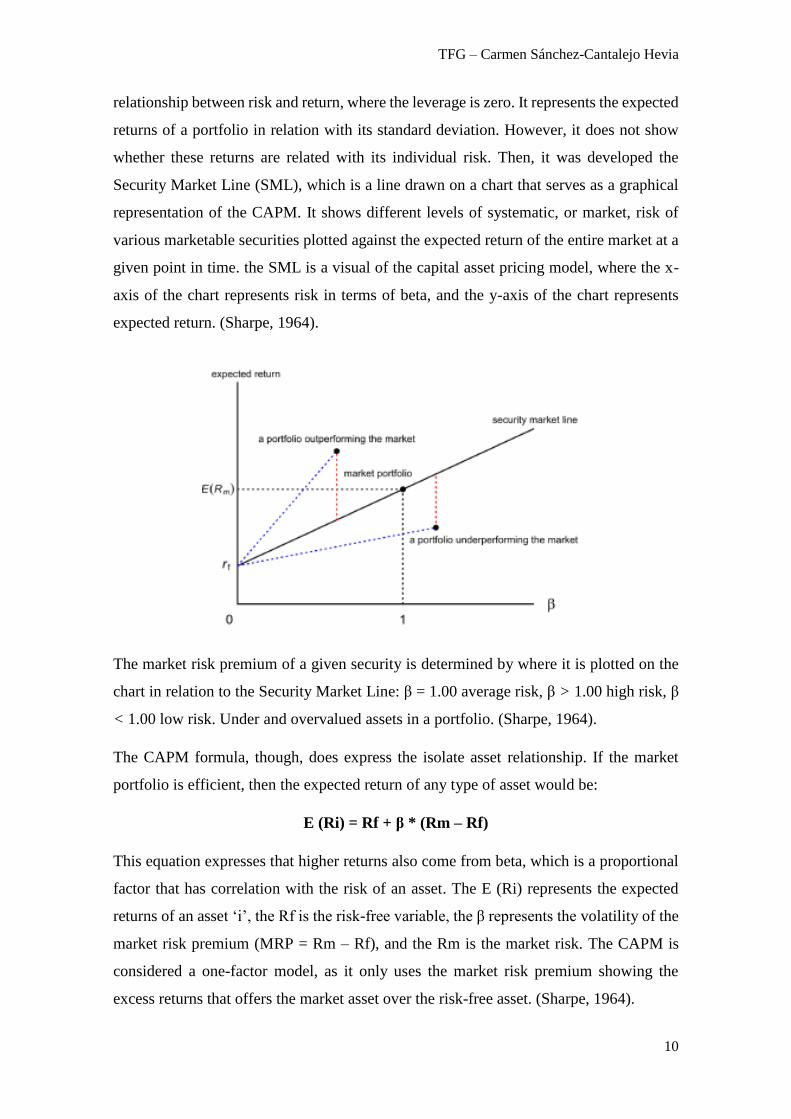
whether these returns are related with its individual risk. Then, it was developed the

Security Market Line (SML), which is a line drawn on a chart that serves as a graphical

representation of the CAPM. It shows different levels of systematic, or market, risk of

various marketable securities plotted against the expected return of the entire market at a

given point in time. the SML is a visual of the capital asset pricing model, where the x-

axis of the chart represents risk in terms of beta, and the y-axis of the chart represents

expected return. (Sharpe, 1964).

The market risk premium of a given security is determined by where it is plotted on the

chart in relation to the Security Market Line: β = 1.00 average risk, β > 1.00 high risk, β

< 1.00 low risk. Under and overvalued assets in a portfolio. (Sharpe, 1964).

The CAPM formula, though, does express the isolate asset relationship. If the market

portfolio is efficient, then the expected return of any type of asset would be:

E (Ri) = Rf + β * (Rm – Rf)

This equation expresses that higher returns also come from beta, which is a proportional

factor that has correlation with the risk of an asset. The E (Ri) represents the expected

returns of an asset ‘i’, the Rf is the risk-free variable, the β represents the volatility of the

market risk premium (MRP = Rm – Rf), and the Rm is the market risk. The CAPM is

considered a one-factor model, as it only uses the market risk premium showing the

excess returns that offers the market asset over the risk-free asset. (Sharpe, 1964).


11

This model most important factor is β, as it is the systematic risk and it is dependent on

the market risk where an asset is traded. So, this risk cannot be diminished by diversifying

the portfolio. Then, according to the CAPM model, an investor would never assume a

diversified risk because he would only obtain higher profitability by assuming market

risk. Beta factor can have different values, such as:

β

>1 Higher risk, the asset return is more volatile than the market

return

1 Average risk, the asset return moves along the market return

<1 Lower risk, the asset return is less volatile than the market

return

Source: Own elaboration. (Sharpe, 1964).

Beta links the covariance between an asset return and the market return with the market

variance, which represents the market volatility. It is a measure of how much risk the

investment will add to a portfolio that looks like the market. If a stock is riskier than the

market, it will have a beta greater than one. If a stock has a beta of less than one, the

formula assumes it will reduce the risk of a portfolio. (Treynor, 1999). The following

expression can estimate β factor:

β = [Cov (Ri, Rm)] / [Var (Rm)]

In terms of robustness for the model, it is proved that its application is not that credible.

As the Markowitz model, the CAPM methodology has complications because it requires

several restrictions or hypotheses that are not feasible for application in real life for its

own. These are that investors optimise the portfolio basing their decisions on only the

mean and the variance. Therefore, in spite of the benefits from the CAPM model, there

are some complications in applying it to the real world:

- Several assumptions behind the CAPM formula that have been shown not to hold

in reality. Despite these issues, the CAPM formula is still widely used because it

is simple and allows for easy comparisons of investment alternatives.

- Including beta in the formula assumes that risk can be measured by a stock’s price

volatility. However, price movements in both directions are not equally risky. The

look-back period to determine a stock’s volatility is not standard because stock


12

returns (and risk) are not normally distributed. Unlike the CAPM assumption,

return’s volatility changes over time. (Jensen, 1972).

- The CAPM also assumes that the risk-free rate will remain constant over the

discounting period. An increase in the risk-free rate also increases the cost of the

capital used in the investment and could make the stock look overvalued.

- The market portfolio that is used to find the market risk premium is only a

theoretical value and is not an asset that can be purchased or invested in as an

alternative to the stock. Most of the time, investors will use a major stock index,

like the S&P 500, to substitute for the market, which is an imperfect comparison.

(Klarman & Williams, 1991).

iii. Arbitrage Pricing Theory (APT) – Ross

The Arbitrage Pricing Theory model (APT) arose, as the CAPM model, thanks to

the Markowitz MPT further research and improvement in the 20th century. It is a more

general model than the CAPM because it allows including multiple risk factors and it

does not require identifying the market portfolio.

This investment strategy is an alternative to the CAPM model. It does not require the

assumption that investors make a decision on an asset portfolio regarding their mean and

variance. The ATP model claims that the assets universe is infinite, and investors seek

for higher returns rather than lower ones without taking into account statistical studies. It

is not conditional to identify the market portfolio. Therefore, this model is essentially

sensitive to the macroeconomic influence that affects the expected returns of an asset.

(Ross, 1976). However, the specific influences over an asset can be infinite as well. So,

it has to be the market individual the one that analyses the effect of a risk factor to an

asset. The risk factors can be categorised in two groups: systemic risk and idiosyncratic

risk. On the one hand, the systemic risk represents the factors that are common to all

assets in a market; and, on the other hand, the idiosyncratic risk shows the individual risk

factors for each asset. This last one can be diversified thanks to creating a portfolio with

several types of assets. (Ross, 1976).

Furthermore, this model has a huge utility due to fact that it can measure the effect of one

factor of risk over a determined fund portfolio, making sure it is adapted to each security

included in it. Although, it has limitations in terms of applying it to real life as the market


13

is very dynamic and volatile, it is difficult to address which factor has provoked a

movement. The most used factors in the APT model are the Gross Domestic Product

(GDP), the customer confidence, the inflation and the interest rates. (Chen, Roll & Ross,

1986).

iv. Three-Factor Model – Fama and French

This three-factor model developed by Fama and French in 1993 for asset pricing

explains better the average expected returns of the securities. The model supports the idea

that the returns of a certain asset or portfolio are defined by the return’s sensitivity to the

three following factors:

a. The excess return over the risk-free asset.

b. The difference between the returns of small capitalization stocks and those of the

larger stocks (small minus big).

c. The difference between the returns of companies with high book to market value

and the returns of those with low book to market ratios.

Hence, the expected return of a portfolio or individual asset would be:

E (Ri) = Rf + β * (Rm – Rf) + βs * (SML) + βv * (HML)

The first part of the equation is equal to the CAPM expression. This model

characterisictics come in the second and third elements of the mathematical statement.

The first factor added to the CAPM formula is the size, represented by the difference

between the small and big capitalization companies (SML) of a portfolio times the size

risk premium (βs). The second risk factor is the value risk premium (βv) multiplied by

the difference between the companies with a high B/M ratio and a low B/M ratio (HML).

(Fama & French, 1993).

o Model development

The three-factor model identifies three risk factors which are present when attending

to bond’s and stock’s returns. Regarding stocks, the model diagnoses three risk factors:

the first is the market, which we have already seen expressed in the CAPM, represented

by the market or equity risk premium (Rm-Rf). The second risk mentioned is the

company’s size (in terms of market capitalization, not enterprise value). Lastly, the value

of the stock in the books, relative to its value in the stock market (book to market ratio).


14

Before building their model, Fama and French analyzed the impact of several variables,

coming to the conclusion that the Beta of a stock (the measure of the systematic risk of

an individual stock in comparison to the unsystematic risk of the entire market) wasn’t

able to explain much of the average expected returns of a stock. On the contrary, when

carrying out the same analysis for other factors such as the company’s size, its price to

earnings ratio (PER), the leverage of the company and its book to market ratio, they found

that they had the ability to explain better these returns. What they further discovered is

that when combining the variables of company’s size and book to market ratio, these were

also able transmit the part of the returns explained by the PER and the leverage of the

firm. Therefore, these two variables (B/M and market cap) are able to explain most part

of the average returns of a stock. (Fama & French, 1993)

o Elements that compose the regression

First and most importantly, the portfolios’ returns that are trying to be explained. 25

different portfolios, in terms of company size and book to market ratio, are being studied.

Regarding the variables whose purpose is to explain these returns, the companies which

have higher book to market values (meaning that they have low market value in

comparison to their book value) tend to have lower returns on assets (ROA). This can be

observed from 5 years before measuring the variable up to 5 years after. Meanwhile, the

companies with low book to market ratio have proven to have more stable returns over

time, and higher than those of the companies with high B/M ratios. Moreover, about the

size of the company, large caps usually have lower returns than small caps, which tend to

grow faster. From this, we can conclude that the size of a company is capable of

explaining the average returns of a stock through a negative correlation. The same

happens with the book to market ratio of a company. (Fama & French, 1993).

The study carried out by Fama and French had as purpose to have certain portfolios that

would pick the risk factors of their returns in relation to the size and book to market ratio.

For this reason, the listed US companies get divided into large caps and small caps. Even

though the small companies are greater in number, they represent a very small part of the

market. Similarly, companies get divided in three groups, attending to their book to

market ratios: low B/M, those in the lower 30%; medium B/M, those in the middle 40%;

and, high B/M, those in the top 30%. (Fama & French, 1993).


15

The parameters according to which the distribution of groups is made, come from the

evidence of Fama and French (1993), where they prove that the book to market ratio has

a higher power of explanation of the average returns of stocks than the company’s size.

Consequently, six different portfolios are built (all the possible combinations of the two

factors with the 25 portfolios):

Size - capitalization

Small Big

Value -

B/M ratio

Low S/L B/L

Medium S/M B/M

High S/H B/H

Source: Own elaboration (Fama & French, 1992; and WWW1, 2019).

Notes:

- S/L: Small cap, low B/M ratio

- S/M: Small cap, medium B/M ratio

- S/H: Small cap, high B/M ratio

- B/L: Large cap, low B/M ratio

- B/M: Large cap, medium B/M ratio

- B/H: Large cap, high B/M ratio

Therefore, to convey the three factors of the model, we do the following (Fama & French,

1992):

1. Size: the SMB (small minus big) portfolio is built to represent the risk factor of a

company’s size. This is the excess returns between the average monthly returns

of the three portfolios with small caps (S/L, S/M and S/H) and the average

monthly returns of the three portfolios with large caps (B/L, B/M and B/H). This

way, the SMB reflects the difference in returns between the large caps and small

caps independent of the book to market ratio.

2. B/M: the portfolio HML (high minus low) is created to represent the risk factor

of the book to market ratio. This will be given by the excess returns between the

average returns of the two portfolios with high B/M ratios (S/H and B/H) and the

two portfolios with low B/M ratios (S/L and B/L). Just as before, the returns of


16

these portfolios are neutralized against any influence coming from the size of the

company.

3. Market factor: in this case we will use what we have seen previously in other

models like the CAPM, Rm-Rf (the market risk premium). Rm will be represented

by the average performance of all six portfolios previously discussed and Rf by

the average returns of the US 1month bond.

According to the authors’ study, the main conclusions that their study showed for their

data period after the regressions is that there is a negative relationship between size and

average returns; and, a strong positive relationship between the book-to-market ratio and

the average returns of the portfolios. (Fama & French, 1992).


17

III. Hypothesis

The development made in the following sections (IV and V) is based on a comparison

of two stocks valuation methodologies: the Capital Asset Pricing Model and the Fama-

French Three-Factor Model. There have been several studies before that compare the

variations between these two theories in some stock markets such as, among many others,

the Italian (Rossi, 2012), the Emerging (Anmwalla and Karasneh, 2011), or the Turkish

(Erdinç, 2017). However, my goal is to make a comparison between CAPM and FF three-

factor model for the main Spanish stock market, the IBEX-35, for the past ten years (Jan.

2008 – Dec. 2018) compared to the European stock market average index from Kenneth

French database for the same period (WWW1, 2019).

There will be four hypothetical cases. The first three related to the three factors analysed

on the Fama & French regression analysis, and the last one on the intercept (alpha) of the

unexplained returns. The objective of this main model is to further develop the CAPM

model conclusions by including more factors to the expected return of the IBEX-35

portfolio for ten years assuming that with smaller capitalization and higher book-to-

market equity ratio, the returns will be larger. The hypothesis 1 and the hypothesis 4 are

common for the two asset valuation methodologies: CAPM and Fama French 3-factor

model. All my developed hypotheses will be set as a two-possible solution analysis.

H1: Analysis on the market risk premium element. Comparison between the Spanish beta

factor with regards to the European beta factor. As mentioned before, this supposition is

applicable to both valuation models. As there can be two options for the MRP element,

and there are two possible results for this study.

- H1a: Spanish market beta > 1. This would mean that the market risk premium for

the Spanish stock index, IBEX-35, is more volatile than the market. So, as the risk

would be higher than the one of Europe, then the returns would also be greater

than the ones expected for Europe stock average index for the chosen period.

- H1b: Spanish market beta < 1. In this case, the MRP factor for my sample is less

volatile than the market return. Therefore, at a lower risk, lower returns for the

IBEX-35 vs. the European sample index for the chosen period.

My thoughts about this hypothesis is confused, as I cannot predict which sample is riskier.

Although, covering an average of the most relevant countries of a continent should be

safer than using only one of them.


18

H2: Analysis on the size factor (small minus big). The difference between portfolios

composed by companies with small market capitalisation versus companies with big

capitalisation. There can be given two possible outcomes depending on the capitalisations

of the samples.

- H2a: SMB > 0. This result would mean that the returns on the portfolios formed

by smaller capitalisation companies are greater than the returns on bigger

capitalisation companies. So, if this factor is positive, the returns on the IBEX-35

companies are better because their portfolio is constituted by smaller companies.

Thus, accomplishing the theory developed by the economists Fama & French

(1992).

- H2b: SMB < 0. This situation would implicate that the returns on smaller

capitalisation companies are lower than the returns of bigger capitalisation. This

outcome contradicts the theory of FF (1992). So, in my study, means that the

IBEX-35 would have bigger capitalisation companies in its portfolio compared to

the European index portfolio.

From my point of view, the IBEX-35 regression result should be H2b. This is due to the

fact that the Spanish stock index has smaller capitalisation companies than the whole

Europe. However, the result will be shown in the Section V.

H3: Analysis on the value factor (high minus low). This reflects the difference between

the companies with a high book-to-market ration compared to low book-to-market ratio.

This product can be positive or negative, getting to distinct results.

- H3a: HML > 0. This event represents that the portfolio of higher B/M ratios has

greater returns compared to the lower B/M ratios. Meaning that, if this happens in

my study, the IBEX-35 portfolio has a higher book value or a lower market value

than the European average index.

- H3b: HML < 0. This case would be the contrary than the above one, as it is proved

that with a lower book value or a higher market value, the IBEX-35 portfolio

would become negative versus the European index sample.

My judgement beforehand from the news read in the recent years, is that the Spanish

stock market has lower book value than market value. Nonetheless, the results regressing

my samples will show if this is the situation of the past ten years (2008-2018).


19

H4: Analysis on the intercept or alpha value. Unexplained returns are difficult to find, as

it is the job of all investment managers that want to achieve extra returns in their

transactions. If alpha is greater than zero, the asset or portfolio offers free returns for

exogenous variables. The intercept is represented in both asset valuation models (CAPM

and FF).

- H4a: Alpha > 0. The portfolio IBEX-35 has unexplained returns compared to the

European average index.

- H4b: Alpha < 0. The portfolio does not give unexplained returns.

The most common and possible outcome is H4b, as alpha value is not easy to get. If not,

everyone would invest in our stock market portfolio.

In the following section, there is the explanation and development of the paper objective;

and, in the next one, there are the outcomes gotten that relate to the possible hypotheses

mentioned.


20

IV. Methodology and Data

My thesis is a cross-sectional study where data depends on the CAPM and Fama

French risk factor variables in a 10-year timeframe (2008-2018). This section explains

how I am going to manage and develop the data to analyse the hypotheses mentioned in

the former section III.

i. Methodology

Fama & French (1992) based their study on analysing the average returns of 25 stock

portfolios that are used as dependent variables to give a range of the returns that the risk

factors must explain. The economists got that the portfolios with higher B/M ratios

present average returns of 0.19% monthly; whilst the ones with lower B/M ratios have an

average return of 0.62% monthly. Regarding the market risk premium, the average return

is 0.43% monthly. In terms of size, the SMB factor represents a 0.27% monthly; and, the

value factor is around 0.40% per month. Additionally, the authors made a regression to

get the coefficients associated to each factor.

The data interpretation, thus, is the following;

- MRP: the stock market portfolios reflect an excess monthly return of 0.43% over

the fixed income return of the one-month U.S. T-Bill.

- SMB: the companies in the portfolio with smaller capitalisation have an excess

return of 0.27% per month over the higher cap ones.

- HML: the corporations that have a higher book-to-market ratio in their books

obtain a 0.40% excess return each month over the low B/M ones.

These portfolios are calculated with the formulas expressed below, from the in the table

of page 15, where the six portfolios are categorised.

According to the authors in WWW1, constructing the SMB and HML factors requires

sorting stocks in a region into two market cap and three book-to-market equity (B/M)

groups. Big stocks are those in the top 90% of market cap for the region, and small stocks

are those in the bottom 10%. The B/M breakpoints for a region are the 30th and 70th

percentiles of B/M for the big stocks of the region. The global portfolios use global size

breaks, but we use the B/M breakpoints for the four regions to allocate the stocks of these

regions to the global portfolios. Similarly, the global ex us portfolios use global ex us size

breaks and regional B/M breakpoints. The independent 2x3 sorts on size and B/M produce

six value-weight portfolios, SG, SN, SV, BG, BN, and BV, where S and B indicate small


21

or big and G, N, and V indicate growth (low B/M), neutral, and value (high B/M).

(WWW1, 2019). See table on page 15.

▪ SMB is the equal-weight average of the returns on the three small stock portfolios

for the region minus the average of the returns on the three big stock portfolios:

SMB = 1/3 (Small Value + Small Neutral + Small Growth) – 1/3 (Big Value +

Big Neutral + Big Growth).

▪ HML is the equal-weight average of the returns for the two high B/M portfolios

for a region minus the average of the returns for the two low B/M portfolios:

HML = 1/2 (Small Value + Big Value) – 1/2 (Small Growth + Big Growth).

For my study, the steps are simpler as French has his own website where data for the three

factors and the six portfolios regarding size and value are made. Therefore, I used a

database which was professionally made for the whole European stock market. The

comparable stock or portfolio, as mentioned during the paper, is the Spanish IBEX-35

stock market. After the regression to obtain the coefficients from the variables mentioned

is done, we can apply the formula to get the expected returns:

E (Ri) = Rf + β * (Rm – Rf) + βs * (SML) + βv * (HML)

The CAPM follows a very similar process but shorter as it only uses the first factor from

the Fama & French model. Therefore, I am not going to enter into depth with it. It is

getting the excess returns of a portfolio (IBEX-35 and European average index) and

regress it with the market risk premium for these markets. Afterwards, we apply the

mathematical expression in order to get the expected returns outcome:

E (Ri) = Rf + β * (Rm – Rf)

ii. Data

Fama and French (1992) first built their model to be used with traded companies

belonging to the US market. It is then when the doubt of if this model applicable to other

equity markets/regions arise. Therefore, the authors carried out a study in which they

apply the same methodology across four different regions: North America, Europe, Japan

and Pacific Asia. It is of our interest to see if the model is able to predict correctly the

average returns of European stocks because we will be working with European and


22

Spanish factors. In this study, we must highlight that the authors introduce a fourth factor

called return momentum factor, which represents the excess monthly returns of the best

portfolios over the monthly returns of the worst behaved portfolios. Despite the fact that

the inclusion of this fourth factor is considered a possible improvement of the three-factor

model, we won’t be using it in our study. (Fama & French, 2012).

Data is extracted from 23 representative countries from the four regions, which are:

Australia, Austria, Belgium, Canada, Denmark, Finland, France, Germany, Hong Kong,

Ireland, Italy, Japan, Holland, New Zealand, Norway, Portugal, Singapore, Spain,

Switzerland, Sweden, United Kingdom and the United States. The distribution in terms

of market cap throughout the world are the following: North America (47,3%), Europe

(30,0%), Japan (18,4%) and Pacific Asia (4,3%). (WWW1, 2019).

Source: Description of Fama/French 3 Factors for Developed Markets.

http://mba.tuck.dartmouth.edu/pages/faculty/ken.french/Data_Library/f-

f_3developed.html (WWW1).

Subsequently, we can enumerate the conclusions to which the authors arrived to when

running the model across the different geographies. For the four regions, except for Japan,

http://mba.tuck.dartmouth.edu/pages/faculty/ken.french/Data_Library/f-f_3developed.html

http://mba.tuck.dartmouth.edu/pages/faculty/ken.french/Data_Library/f-f_3developed.html


23

there exists a premium in the average returns of the stocks which decreases as the size of

the company increases (inverse relationship). Moreover, even though we have already

said we won’t be using momentum as a factor, we can highlight how in all regions (except

for Japan once more) the returns explained by the momentum factor could be seen; these

also decrease as the market capitalization of the companies increase. We could run the

model at a global scale, nevertheless, the model offers better results when applying it at

a smaller scale (regionally). For the portfolios that have been composed according to the

book to market value, the regional models have been able to represent correctly the

average returns, except for those with high exposure to the momentum factor. However,

these types of portfolios are not seen very often in reality, as for example a pension fund

will be highly diversified and will not have these extreme values. (Fama & French, 2012).

Even though they created portfolios according to book to market ratios and size and

according to size and momentum, we will only build portfolios such as the first example

(B/M ratio and size). This is because is the most representative when trying to analyse the

three-factor model, which is what we are doing. The process to build the portfolios that

will replicate the behaviour of the two factors is exactly the same as the process we have

already described when doing the 6 portfolios extracted from the 25 market portfolios.

(Griffin, 2002).

We can now interpret the data from the regression done by the economists for the factors.

The excess returns for the market factor (Rm-Rf) are big for the period comprising from

1991 to 2010 for three of the four regions studied. Japan is the exception, with a negative

excess return with respect to the risk-free asset. Regarding the SMB, we can observe that

the average returns for this factor are all close to cero. However, the HML dose represent

an important premium for all regions. As it had already been proved by Fama and

French’s study (1993) on the US market, the premiums for the book to market ratio were

bigger for those companies of smaller market capitalization. Again, the only exception

was Japan, where this premium is very similar in both small and large companies.

(Griffin, 2002).

The excess returns for the 25 portfolios built according to book to market ratios and size

for each region. The stocks from companies with low book to market values, continue

giving small returns. Within the companies with low B/M, the bigger ones show greater

returns than the smaller ones in size. For those companies with high B/M, the smaller

companies beat in returns to those which are bigger. We can therefore assert that as the


24

B/M value increases, the returns do so too. Similarly, we can conclude that when

comparing companies with small B/M ratios, the smaller companies are outperformed by

the bigger ones. This relationship reverts when talking about companies with higher B/M

values.

After arriving to these conclusions, the authors perform one other regression, to see if

both the global model and the regional model are able to explain the average returns of

the stocks. As a result, they conclude that the explaining capacity or power of the global

model is much weaker than that of the local model. In a nutshell, the three-factor model

works well at a regional level, especially for the case of European portfolios. The

inclusion of companies with a very small market capitalization hinders the ability of the

model to explain correctly the average returns of stocks in markets such as the US one.

With regards to Europe, one of the conclusions drawn is that there is barely no difference

when using the three-factor model or the four-factor model, which adds the momentum

factor to the other three, as explained above.

Overall, then the summary is that they found premiums in the average returns of the stocks

in the four regions studied, and that these are larger for companies with smaller

capitalization. The three-factor model does not explain successfully the average returns

at a global scale, whilst succeeding to do it at a regional level. For this reason, I decided

to analyse my own country stock market to the European stock average. (Fama & French,

2012).

Then, after downloading the data from the Kenneth French website (WWW1, 2019) for

the European countries average with the three-factors to analyse, I only kept the period

that covers my study. The stock markets used for the European data are Austria, Belgium,

Denmark, Finland, France, Germany, Greece, Ireland, Italy, the Netherlands, Norway,

Portugal, Spain, Sweden, Switzerland and the United Kingdom. There are compatible and

consistent as the community has similar monetary policies and even currency for almost

all of them.

Afterwards, for the main sample of the paper, I download from Yahoo Finance (WWW2,

2019) the monthly historical prices data for the IBEX-35 stock market portfolio for the

same 10-year period. This database needs to be reordered as it only records the adjusted

close price for each month. Later, I calculate the natural logarithm division of the adjusted

close price compared to the previous one in order to get to the excess returns for each


25

month. So, I am able to add it and use it in the Excel table, together with the previous

three-factors database for the European stocks.

Furthermore, I used the Excel function of ‘regression’ in order to link both databases and

get outcomes from my samples. See Appendix tables.

For the CAPM model, as mentioned in the Methodology part of the section, the process

to get data is simpler as only one factor is used for the regression. In order to use the same

database for the sample. I used the French one (WWW1, 2019) but deleting the risk

factors that were unnecessary.


26

V. Regression Results

For the authors analysis in their report (Fama & French, 1992) they check if the three

factors together are correlated. Their main result is that these elements are strongly related

to the stocks returns. The point here is the value of R square, which is an indicator to

evidence if factor risks gather the variation in stock returns. Thus, they check that whilst

the MRP factor itself only achieves two values of R square higher than 0,9 from the 25

portfolios; when adding the two SMB and HML factors, the 0,9 is achieved in 21 from

the 25 portfolios. Therefore, it is proven that this value increases for portfolios with low

capitalisation companies. However, the two factors by themselves, only get R squares

that go from a arrange of 0,2 until 0,6. So, it is evident that the market risk premium is an

important factor that leads to higher returns.

Analysing the factors in isolated cases, the authors conclude that all of them have an

impact on returns, but that they are not related. Nevertheless, when doing the regression

using the three of them, they do make a good summary on variable returns.

Once the Excel regression is done and the results come out for both theories. There are

small differences and particularities to take into account for the analysis. I am going to

explain these according to their hypotheses in section III. In the Appendix of Section VIII,

there are the tables resulted from the function. However, the mathematical expressions

are explained below.

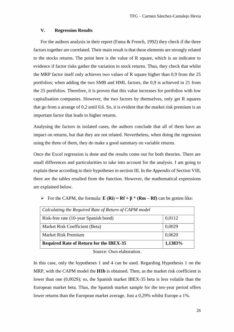
➢ For the CAPM, the formula: E (Ri) = Rf + β * (Rm – Rf) can be gotten like:

Calculating the Required Rate of Return of CAPM model

Risk-free rate (10-year Spanish bond) 0,0112

Market Risk Coefficient (Beta) 0,0029

Market Risk Premium 0,0620

Required Rate of Return for the IBEX-35 1,1383%

Source: Own elaboration.

In this case, only the hypotheses 1 and 4 can be used. Regarding Hypothesis 1 on the

MRP, with the CAPM model the H1b is obtained. Then, as the market risk coefficient is

lower than one (0,0029); so, the Spanish market IBEX-35 beta is less volatile than the

European market beta. Thus, the Spanish market sample for the ten-year period offers

lower returns than the European market average. Just a 0,29% whilst Europe a 1%.


27

The Hypothesis 4 relates to the alpha intercept, it can be checked in Table 1 form the

Appendix. The outcome obtained for this model is H4b lower than zero, which means

that negative alpha does not offer unexplained returns for our comparison. It was quite

expected, as it is very complicated to get. Then, the IBEX-35 gives 4,15% (-0,04154)

lower returns than Europe. So, the Spanish market has behaved worse than the European

market.

Moreover, the formula obtained with the regression results gives us that the required

return for the IBEX-35 compared to the average European stock index form Fama and

French is 1,14%.

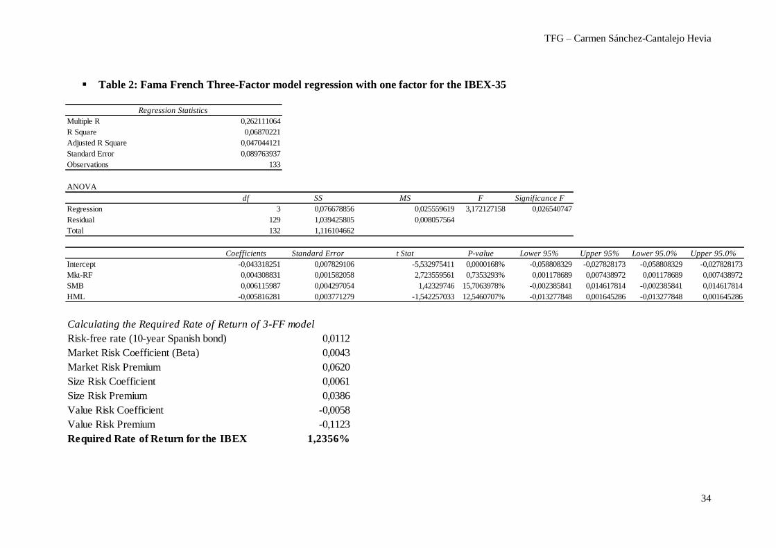
➢ For the Fama French three-factor model, the formula: E (Ri) = Rf + β * (Rm –

Rf) + βs * (SML) + βv * (HML) can be performed as this table:

Calculating the Required Rate of Return of 3-FF model




Size Risk Coefficient 0,0061

Size Risk Premium 0,0386

Value Risk Coefficient -0,0058

Value Risk Premium -0,1123

Required Rate of Return for the IBEX 1,2356%

Source: Own elaboration.

Firstly, the Hypothesis 1 is the analysis of the market risk factor, where for this model the

assumption accomplished is, like in the previous one, H1b because the beta coefficient

after the regression gives a value inferior to one (0,0043). This means that when the

European stocks exceed by a 1% the return of the risk-free asset, the IBEX-35 only does

it for a 0,43%.

Secondly, the Hypothesis 2 outcome is positive (0,0061). For this reason, the H2a is of

the Fama & French model is proved. It represents that Spanish companies that compose

the IBEX-35 index have a smaller capitalisation than the European companies. This is

due to the fact that the IBEX-35 is composed by firms riskier than the European ones,

whose size are smaller. Then, at a higher risk, higher returns. For each 1% of returns

obtained in the European market, the IBEX-35 returns rise a 0,61%.


28

In third place, the Hypothesis 3 gives a negative result of -0,0058. This means that H3b

is accomplished, where the HML factor of the IBEX-35 is formed up by lower book-to-

market ratio companies. Meaning that from 2008 until 2018, the IBEX-35 is safer in terms

of company value than the European stock portfolio. For this reason, at each 1% of

European index return, the Spanish index goes down by a 0,58%.

Lastly, the H4 is the most expected one as the intercept is almost in every case is negative.

Coming out with H4b of alpha lower than zero. As with the CAPM model, the Fama &

French study in this situation shows that per each 1% of European returns, the IBEX-35

returns are a 4,3% lower. Our stock market behaviour is worse than the regional sample

one.

Furthermore, the formula developed with the regression results is applied to get the

expected required returns for our market. This outcome is 1,24%, only a 0,1% above the

CAPM required return. Therefore, the excess return needed for the IBEX-35 over the

European stock market index is this 1,24%.

Regarding the R square regression values, the results for both models are very similar due

to the similarities among the two stock market samples. However, these values are

extremely low. So, the model factor applications are not much significant. This means

that, on the one hand, for the CAPM case, the excess returns variation is 3,38% explained

by the MRP factor; and, on the other hand, for the FF three-factor model, the excess

returns variation is explained by a 6,86% by the MRP, the SMB and the HML factors. It

is important to understand that the implications of the risk factors for this period are not

well developed here, as the model is rarely accomplished. Lately, in terms of statistical

values, the P-value result obtained from the regressions are not lower than 5% for the

SMB and HML factors. This means that size and value are not very significant in my

analysis.


29

VI. Conclusion

My analysis proofs that the Fama and French three-factor theory is accomplished in

the Spanish IBEX-35 market compared to its homogeneous region of the main Europe

stock markets. The European community is similar to the Spanish one, but not totally

correlated as, for instance, Spain has smaller companies than Europe as a whole.

In further analysis of the Fama & French three-factor model, the Rm-Rf factor (MRP)

cannot explain the big differences between the returns in the stock markets; but this can

be explained with the size and value elements if used all together. The SMB factor is

essential to understand the reason behind why a smaller capitalisation company has

returns which are more volatile than a bigger capitalisation firm. Though, for the HML

factor, it has not been found that companies with a lower B/M ratio have more volatile

returns than the ones with a higher B/M ratio.

In my study, where data is analysed from the period that goes from January 2008 to

December 2018, there are not major differences in the results of the market risk factor

with the CAPM or the FF model. However, in terms of the size factor, my sample

covering the IBEX-35 proves that it gets higher returns than the European average index

due to being composed of smaller capitalisation companies. The value size achieved is

negative, so it accomplishes that due to having more lower book-to-market ratios in the

IBEX-35 companies’ book, their returns are lower. There were different possible

solutions for each factor. But my conclusion is that according to hypotheses one and four,

the common factors for both models, CAPM and Fama & French three-factors, are very

similar despite including SMB and HML. So, there is a need to add more factors.

Summarising, after this study analysis I consider each case is unique and has to be

analysed in more different ways in order to understand the relationship between any

model. Maybe this two were not enough to understand what I was looking for, but I

enjoyed the process. This is due to the fact that there are external circumstances that affect

the price of a stock not only in a region or market but in the economic cycle as well. I

have to admit that I ended I bit disappointed with the results, as I believed that adding

more risk factors to the required return equation gave much higher returns.


30

VII. Reference List

o Almwalla, M. and Karasneh, M.M. (2011). “Fama & French Three Factor Model:

Evidence from Emerging Market”. European Journal of Economics, Finance and

Administrative Sciences, 41: 132-140.

o Baker M., Bradley B. and Wurgler J. (2011), “Benchmarks as Limits to Arbitrage:

Understanding the Low-Volatility Anomaly”. Financial Analyst Journal, 67(1).

o Banz, R. W. (1981), "The Relationship Between Return and Market Value of

Common Stocks". Journal of Financial Economics, 9(1): 3-18.

o Basu, S. (1983), "The Relationship Between Earnings Yield, Market Value, and

Return for NYSE Common Stocks: Further Evidence". Journal of Financial

Economics, 12(1): 129-156.

o Bender, J., Briand, R., Melas, D. and Subramanian, R. (2013). “Foundations on

Factor Investing”. MSCI Index Research Insight.

o Black, F. (1993a), "Beta and Return". The Journal of Portfolio Management,

20(1): 8-18.

o Black, F. (1993b), "Estimating Expected Return". Financial Analysts Journal,

49(5): 36-38.

o Blume, M. E. (1970), "Portfolio Theory: A Step Toward its Practical Application.

Journal of Business,43(2): 152-173.

o Carhart, M. M. (1997), "On Persistence in Mutual Fund Performance". Journal of

Finance, 52(1): 57-82.

o Chavarría Mayorga, J.A. (2013). “Estudio comparativo entre del modelo de Fama

y French y el modelo de Carhart”. Revista Electrónica de Investigación en

Ciencias Económicas, Vol.1(1): 45-62.

o Chen, N. F., Roll, R., and Ross, S. A. (1986), "Economic Forces and the Stock

Market". Journal of Business, 59(3): 383-403.

o Erdinç, Y. (2017). “Comparison of CAPM, Three-Factor Fama-French Model and

Five-Factor Fama-French Model for the Turkish Stock Market”. Financial

Management from an Emerging Market Perspective: 69-92.

o Fama, E.F., & Macbeth, J.D. (1973), “Risk, Return, and Equilibrium: Empirical

Tests”. Journal of Political Economy, 81: 607-36.

o Fama, E. F. and French, K. R. (1988). "Permanent and Temporary Components

of Stock Prices". Journal of Political Economy. 96 (2): 246–273.


31

o Fama, E.F., & French, K.R. (1992), “The Cross-Section of Expected Stock

Returns”. Journal of Finance, 47: 427-465.

o Fama, E.F., & French, K.R. (1993), “Common risk factors in the returns on stocks

and bonds”. Journal of Financial Economics, 33: 3-56.

o Fama, E.F., & French, K.R. (1995), “Size and Book-to-Market Factors in Earning

and Returns”. Journal of Finance, 50: 131-55.

o Fama, E.F., & French, K.R. (1998), “Value versus growth: The international

evidence”. Journal of Finance, 53: 1975-1999.

o Fama, E. F.; French, K. R. (2012). "Size, value, and momentum in international

stock returns". Journal of Financial Economics 105 (3): 457.

o French, K. (1987). “Expected Stock Returns and Volatility”. Journal of Financial

Economics, 19: 3-29.

o Foye, J., Mramor, D. A., Pahor, M. (2013). "A Respecified Fama French Three-

Factor Model for the New European Union Member States". Journal of

International Financial Management & Accounting, 24: 3.

o Graham, B. and Dodd D. (1934). Security Analysis (5th edition). Whittlesey

House U.S.A., McGraw-Hill Book Co.

o Griffin, J. M. (2002). "Are the Fama and French Factors Global or Country

Specific?". Review of Financial Studies 15(3): 783–803.

o James D., Fama E. F. and French, K.R. (2000). “Characteristics, Covariances, and

Average Returns: 1929 to 1997”. The Journal of Finance, 55: 389-406.

o Jensen, M. (1969). "Risk, the Pricing of Capital Assets, and the Evaluation of

Investment Portfolios." Journal of Business, 42(2): 167-247.

o Jensen M., Black, F. and Scholes, M. (1972). “The Capital Asset Pricing Model:

Some Empirical Tests”. Studies in the Theory of Capital Markets.

o Klarman, S. and Williams, J. (1991) “Beta”. Journal of Financial Economic.

o Lintner, J. (1965a), "The Valuation of Risk Assets and the Selection of Risky

Investments in Stock Portfolios and Capital Budgets". Review of Economics and

Statistics, 73: 13-37.

o Lintner, J. (1965b), "Security Prices, Risk and Maximal Gains from

Diversification". Journal of Finance, 20: 587-615.

o Markowitz, H. (1952), "Portfolio Selection". Journal of Finance, 7(1): 77-91.

o Michaelides, M. and Spanos, A. (2016). “Validating the CAPM and the Fama-

French three-factor model”. Virginia Tech, USA.


32

o Modigliani, F., and Miller, H. M. (1958), "The Cost of Capital, Corporation

Finance and the Theory of Investment". American Economic Review, 48(3): 261-

297.

o Rosenberg, B., Reid, K., and Lanstein, R. (1985), "Persuasive Evidence of Market

Inefficiency". Journal of Portfolio Management, 11(3): 9-17.

o Ross, S. A. (1976), "The Arbitrage Theory of Capital Asset Pricing". Journal of

Economic Theory, 13(3): 341-360.

o Rossi, F. (2012). “The Three-Factor Model: Evidence from the Italian Stock

Market”. Research Journal of Finance and Accounting, 3(9): 151-159.

o Sharpe, W. F. (1964), "Capital Asset Prices: A Theory of Market Equilibrium

under Conditions of Risk". Journal of Finance, 19(3): 425-442.

o Sharpe, W. F., Alexander G. J., and Bailey J. V. (1998). Investments (5th Edition).

Prentice Hall.

o Treynor, J. L. (1999), "Toward a Theory of Market Value of Risky assets". Robert

Korajczyk (Ed.), Asset Pricing and Portfolio Performance. London: Risk Books.

o WWW1:

http://mba.tuck.dartmouth.edu/pages/faculty/ken.french/data_library.html

(Assessed last time on the 18th March 2019).

o WWW2:

https://finance.yahoo.com/quote/%5EIBEX/history?period1=1514761200&perio

d2=1546210800&interval=1mo&filter=history&frequency=1mo (Assessed last

time on the 18th March 2019).

o WWW3: https://www.bloomberg.com/markets/stocks (Assed las time on the 18th

March 2019).

http://mba.tuck.dartmouth.edu/pages/faculty/ken.french/data_library.html

https://finance.yahoo.com/quote/%5EIBEX/history?period1=1514761200&period2=1546210800&interval=1mo&filter=history&frequency=1mo

https://finance.yahoo.com/quote/%5EIBEX/history?period1=1514761200&period2=1546210800&interval=1mo&filter=history&frequency=1mo

https://www.bloomberg.com/markets/stocks


33

VIII. Appendix

▪ Table 1: CAPM regression with one factor for the IBEX-35

Regression Statistics

Multiple R 0,183991677

R Square 0,033852937

Adjusted R Square 0,026477769

Standard Error 0,090727393

Observations 133

ANOVA

df SS MS F Significance F

Regression 1 0,037783421 0,037783421 4,590123976 0,034006039

Residual 131 1,078321241 0,00823146

Total 132 1,116104662

Coefficients Standard Error t Stat P-value Lower 95% Upper 95% Lower 95.0% Upper 95.0%

Intercept -0,041540761 0,007870713 -5,277890413 0,0000527013% -0,057110909 -0,025970613 -0,057110909 -0,025970613

Mkt-RF 0,002946367 0,001375228 2,142457462 3,4006039278% 0,000225838 0,005666895 0,000225838 0,005666895

Calculating the Required Rate of Return of CAPM model






34

▪ Table 2: Fama French Three-Factor model regression with one factor for the IBEX-35

Regression Statistics

Multiple R 0,262111064

R Square 0,06870221

Adjusted R Square 0,047044121

Standard Error 0,089763937

Observations 133

ANOVA

df SS MS F Significance F

Regression 3 0,076678856 0,025559619 3,172127158 0,026540747

Residual 129 1,039425805 0,008057564

Total 132 1,116104662

Coefficients Standard Error t Stat P-value Lower 95% Upper 95% Lower 95.0% Upper 95.0%

Intercept -0,043318251 0,007829106 -5,532975411 0,0000168% -0,058808329 -0,027828173 -0,058808329 -0,027828173

Mkt-RF 0,004308831 0,001582058 2,723559561 0,7353293% 0,001178689 0,007438972 0,001178689 0,007438972

SMB 0,006115987 0,004297054 1,42329746 15,7063978% -0,002385841 0,014617814 -0,002385841 0,014617814

HML -0,005816281 0,003771279 -1,542257033 12,5460707% -0,013277848 0,001645286 -0,013277848 0,001645286

Calculating the Required Rate of Return of 3-FF model




Size Risk Coefficient 0,0061

Size Risk Premium 0,0386

Value Risk Coefficient -0,0058

Value Risk Premium -0,1123


evidence from the main Spanish stock market (IBEX-35) over th

Documents

Transcript of evidence from the main Spanish stock market (IBEX-35) over th