UNIVERSITY OF CALIFORNIA

Los Angeles

Quasi-experiments in Competition and Public Policy: Evidence from Chilean Economic History

A dissertation submitted in partial satisfaction

of the requirements for the degree Doctor

of Philosophy in Economics

by

Felipe B. Carrera Galleguillos

2020

© Copyright by

Felipe B. Carrera Galleguillos

2020

ABSTRACT OF THE DISSERTATION

Quasi-experiments in Competition and Public Policy: Evidence from Chilean Economic History

by

Felipe B. Carrera Galleguillos

Doctor of Philosophy in Economics

University of California, Los Angeles, 2020

Professor Simon Adrian Board, Chair

Compared to other disciplines, one of the distinctive features of Economics is the impossibility

of doing experiments to study empirically relevant questions. In this dissertation, I use two episodes

from the past where the unique features of the institutional environment created quasi-experiments

that help us understand relevant issues relate to cartels and neighborhood effects. In the fist two

chapters, I use the Chilean nitrate industry between the War of the Pacific and the start of the

First World War (1880-1914) to shed light on the effects of entry for cartels and the importance

of learning for effective cartel organization. The Chilean nitrate industry was very important at

the time: Chilean nitrate was the main commercial fertilizer used in the world. Also, it was the

main industry of Chile, the only country where it is found, where it represented 70% of exports

and 45% of government revenues. Importantly, there was no antitrust legislation and no domestic

consumer surplus to protect in Chile. Thus, cartels could be freely formed by nitrate producers.

Moreover, these cartels were completely public: Their decisions were publicly discussed by the press

and the public and they would be formed by the signature of a public contract. I collected from

handwritten archival records an original data set of monthly output and inputs that covers 35 yearsii

of this industry, period over which 5 cartels were organized. In the third chapter, I introduce a novel

new dataset to study neighborhood effects that uses a massive program of forced-displacement of

population within the city of Santiago in the context of the Chilean dictatorship in the early 1980s.

Chapter 1 studies the effect of cartels on entry, and the long-term effect of cartel-induced entry

for the evolution of industry productivity. Intuitively, as cartels artificially increase prices entry

becomes more attractive and less productive firms may decide to enter. Because of data limitations,

previous researchers have not quantified the extensive margin mechanism. My analysis has 3 steps.

First, I evaluate if nitrate cartels caused more entry of new firms. I find that cartels generated

an additional entry of 4 plants per year or about 5% of the initial number of plants in my main

period of interest. Second, I estimate the productivity of all the plants in the industry to analyze

if firms that entered during cartel periods where less productive. I find that there is a sizable gap

in average productivity between entrants during competition and cartel periods: If the median-

sized plant in the industry had received this productivity gap its revenue would have increases by

one-third. Third, I conduct two counterfactual simulations. The first, studies the effect of entry

on cartel profits by estimating incumbent cartel members counterfactual profits if they had been

able to prevent any additional entry. I find their counterfactual profits would have been 40% larger

had there been no entry. The second counterfactual studies the effect of having a cartel on entry.

Specifically, what would the number of new firms and their productivity have been, if during the

Fourth and Fifth Cartels there had been competition? I find that 18% of the plants that entered

in the data would have not entered. This translates into an increase on mean plant productivity of

3%.

Chapter 2 studies the degree to which experience helps firms to organize successful cartels.

Unlike in most of the previous literature on cartels, in the nitrate cartels issues related to monitoring

and enforcement were of secondary importance with respect to the challenge of allocating the

collusive surplus among the colluding firms. I document that cartel contracts gradually became

more complete, generated a smoother transition from competition to collusion, and that producers

eventually discarded inefficient methods of market share allocation, associated to larger production

costs, in favor of better alternatives. In particular, I am able to estimate that the time method

used during the Second Cartel directly caused higher production costs of about 10%, while the trial

method implemented during the Third Cartel caused higher costs of approximately 20%.iii

Finally, Chapter 3 describes a novel large dataset that combines archival records and adminis-

trative data to study a natural experiment that occurred during the Chilean dictatorship between

1979 and 1985, when the government mandated the relocation of a large number of slums in the

city of Santiago, Chile. Some features of the program’s implementation make it of unique interest

to study the broad effects of neighborhoods on social mobility and inequality: the unit of treat-

ment was the slum, participation was mandatory and compliance was very high, since the policy

was implemented during a highly repressive dictatorial government. In addition, and only some of

the slums were removed from their original location creating two groups of families: movers and

non-movers, which allows me to identify a causal displacement effect. The dataset comprises data

for more than 26,000 households that were part of this program (out of a total of 40,000 house-

holds) and more than 58,000 of their children, providing the potential for causal estimation of the

long-term and inter-generational effects of moving to a high-poverty neighborhood on education,

mortality, income, and crime.

iv

The dissertation of Felipe B. Carrera Galleguillos is approved.

John William Asker

Sarah J. Reber

Adriana Lleras-Muney

Simon Adrian Board, Committee Chair

University of California, Los Angeles

2020

v

Contents

1 Cartels, Entry, and Productivity 1

1.1 Introduction . . . . . . . . . . . . . . . . . . . . . . . . . . . . . . . . . . . . . . . . . 2

1.2 Related Literature . . . . . . . . . . . . . . . . . . . . . . . . . . . . . . . . . . . . . 5

1.3 Industry Background . . . . . . . . . . . . . . . . . . . . . . . . . . . . . . . . . . . . 6

1.3.1 Historical development and expansion . . . . . . . . . . . . . . . . . . . . . . 6

1.3.2 Public cartels in the Chilean nitrate industry . . . . . . . . . . . . . . . . . . 10

1.4 Data and Summary Statistics . . . . . . . . . . . . . . . . . . . . . . . . . . . . . . . 12

1.5 Reduced-form Evidence on Entry . . . . . . . . . . . . . . . . . . . . . . . . . . . . . 16

1.6 Productivity Estimation and Dispersion . . . . . . . . . . . . . . . . . . . . . . . . . 22

1.6.1 Extraction-stage Estimates . . . . . . . . . . . . . . . . . . . . . . . . . . . . 24

1.6.2 Analysis of the Productivity Distribution . . . . . . . . . . . . . . . . . . . . 28

1.6.3 Refining-stage Estimates . . . . . . . . . . . . . . . . . . . . . . . . . . . . . . 30

1.7 Plant Entry Decision . . . . . . . . . . . . . . . . . . . . . . . . . . . . . . . . . . . . 30

1.7.1 Model of Entry . . . . . . . . . . . . . . . . . . . . . . . . . . . . . . . . . . . 31

1.7.2 Revenue estimation . . . . . . . . . . . . . . . . . . . . . . . . . . . . . . . . . 33

1.7.3 Cost Function Estimation . . . . . . . . . . . . . . . . . . . . . . . . . . . . . 36

1.7.4 Entry Values Results . . . . . . . . . . . . . . . . . . . . . . . . . . . . . . . . 40

1.7.5 Demand elasticity estimation . . . . . . . . . . . . . . . . . . . . . . . . . . . 43

1.7.6 Entry Costs . . . . . . . . . . . . . . . . . . . . . . . . . . . . . . . . . . . . . 44

1.8 Counterfactual Analysis . . . . . . . . . . . . . . . . . . . . . . . . . . . . . . . . . . 45

1.8.1 Cartel Profits with Barriers to Entry . . . . . . . . . . . . . . . . . . . . . . . 46

1.8.2 Entry without cartels . . . . . . . . . . . . . . . . . . . . . . . . . . . . . . . 48

1.9 Final Remarks . . . . . . . . . . . . . . . . . . . . . . . . . . . . . . . . . . . . . . . 51vi

Appendices 53

1.A Nitrate Industry . . . . . . . . . . . . . . . . . . . . . . . . . . . . . . . . . . . . . . 53

1.A.1 Industry Location and History . . . . . . . . . . . . . . . . . . . . . . . . . . 53

1.A.2 Nitrate Lands Ownership . . . . . . . . . . . . . . . . . . . . . . . . . . . . . 57

1.B Data . . . . . . . . . . . . . . . . . . . . . . . . . . . . . . . . . . . . . . . . . . . . . 62

1.C Additional Tables . . . . . . . . . . . . . . . . . . . . . . . . . . . . . . . . . . . . . . 68

1.4 Additional Figures . . . . . . . . . . . . . . . . . . . . . . . . . . . . . . . . . . . . . 72

2 Experience and Efficacy of Cartels 79

2.1 Introduction . . . . . . . . . . . . . . . . . . . . . . . . . . . . . . . . . . . . . . . . . 80

2.2 Industry Background . . . . . . . . . . . . . . . . . . . . . . . . . . . . . . . . . . . . 81

2.2.1 Historical development and industry characteristics . . . . . . . . . . . . . . . 81

2.3 Nitrate Cartels and Learning . . . . . . . . . . . . . . . . . . . . . . . . . . . . . . . 85

2.3.1 General Description . . . . . . . . . . . . . . . . . . . . . . . . . . . . . . . . 85

2.3.2 Relevant Dimensions of Learning . . . . . . . . . . . . . . . . . . . . . . . . . 88

2.3.3 Evolution of Nitrate Cartel Contracts . . . . . . . . . . . . . . . . . . . . . . 92

2.4 Data and Summary Statistics . . . . . . . . . . . . . . . . . . . . . . . . . . . . . . . 92

2.5 Allocation of Cartel Market Shares . . . . . . . . . . . . . . . . . . . . . . . . . . . . 96

2.5.1 First Cartel: Early theoretical-capacity Method . . . . . . . . . . . . . . . . . 97

2.5.2 Second Cartel: Time method . . . . . . . . . . . . . . . . . . . . . . . . . . . 98

2.5.3 Third Cartel: Trial Method and Menu of Options . . . . . . . . . . . . . . . . 100

2.5.4 Fourth and Fifth Cartels: Theoretical-capacity Method . . . . . . . . . . . . 104

2.5.5 Comparing Cartel Market Shares Allocation in the Nitrate Cartels . . . . . . 106

2.6 Other Dimensions of Learning . . . . . . . . . . . . . . . . . . . . . . . . . . . . . . . 106

2.6.1 Transition to Collusion . . . . . . . . . . . . . . . . . . . . . . . . . . . . . . . 106

2.6.2 Flexibility For Adjustments and Duration . . . . . . . . . . . . . . . . . . . . 109

2.7 Final Remarks . . . . . . . . . . . . . . . . . . . . . . . . . . . . . . . . . . . . . . . 112

Appendices 115

2.A Election of Allocation Method in Third Cartel . . . . . . . . . . . . . . . . . . . . . 115

2.B Enforcement Evidence . . . . . . . . . . . . . . . . . . . . . . . . . . . . . . . . . . . 116vii

2.C First Cartel Contract . . . . . . . . . . . . . . . . . . . . . . . . . . . . . . . . . . . . 117

2.D Second Cartel Contract . . . . . . . . . . . . . . . . . . . . . . . . . . . . . . . . . . 125

2.E Third Cartel Contract . . . . . . . . . . . . . . . . . . . . . . . . . . . . . . . . . . . 132

2.F Fourth Cartel Contract . . . . . . . . . . . . . . . . . . . . . . . . . . . . . . . . . . 142

2.G Fifth Cartel Contract . . . . . . . . . . . . . . . . . . . . . . . . . . . . . . . . . . . 155

3 Long-Term Effects of Forced Displacements 167

3.1 Introduction . . . . . . . . . . . . . . . . . . . . . . . . . . . . . . . . . . . . . . . . . 168

3.1.1 Motivation . . . . . . . . . . . . . . . . . . . . . . . . . . . . . . . . . . . . . 168

3.1.2 Related literature . . . . . . . . . . . . . . . . . . . . . . . . . . . . . . . . . . 169

3.2 Historical Background . . . . . . . . . . . . . . . . . . . . . . . . . . . . . . . . . . . 170

3.3 Data Collection . . . . . . . . . . . . . . . . . . . . . . . . . . . . . . . . . . . . . . . 173

3.3.1 Archival Data: Parents sample . . . . . . . . . . . . . . . . . . . . . . . . . . 174

3.3.2 Matching process: Children sample . . . . . . . . . . . . . . . . . . . . . . . . 175

3.3.3 Locating slums and destination neighborhoods . . . . . . . . . . . . . . . . . 177

3.3.4 Measuring outcomes: matching to administrative data . . . . . . . . . . . . . 178

3.4 Summary Statistics . . . . . . . . . . . . . . . . . . . . . . . . . . . . . . . . . . . . . 178

3.5 Final Remarks . . . . . . . . . . . . . . . . . . . . . . . . . . . . . . . . . . . . . . . 180

List of Figures

1.1 Nitrate Plant Example: La Patria Plant . . . . . . . . . . . . . . . . . . . . . . . . 8

1.2 Industry Output and Consumption . . . . . . . . . . . . . . . . . . . . . . . . . . . 10

1.3 Industry yearly output (tons) . . . . . . . . . . . . . . . . . . . . . . . . . . . . . . 12

1.4 New Plants per Year . . . . . . . . . . . . . . . . . . . . . . . . . . . . . . . . . . . 17

1.5 Industry Capacity and Monthly Output . . . . . . . . . . . . . . . . . . . . . . . . 20

1.6 Plants in Shutdown . . . . . . . . . . . . . . . . . . . . . . . . . . . . . . . . . . . . 25

1.7 Estimated Distribution of Plant Productivity . . . . . . . . . . . . . . . . . . . . . 27viii

1.8 Productivity vs Period of Entry . . . . . . . . . . . . . . . . . . . . . . . . . . . . . 29

1.9 Productivity Distributions of Entrants . . . . . . . . . . . . . . . . . . . . . . . . . 29

1.10 Average Output by Productivity Type and Number of Plants . . . . . . . . . . . . 34

1.11 Total Costs by Productivity Type . . . . . . . . . . . . . . . . . . . . . . . . . . . . 39

1.12 Estimated Entry Values Pena Chica plant . . . . . . . . . . . . . . . . . . . . . . . 41

1.13 Estimated Plant Entry Values . . . . . . . . . . . . . . . . . . . . . . . . . . . . . . 42

1.14 Industry Output and Capacity at the start of the Fourth Cartel . . . . . . . . . . . 49

1.15 Effect of Competition on Plant Entry . . . . . . . . . . . . . . . . . . . . . . . . . . 50

1.A.1 Nitrate Region and Deposits . . . . . . . . . . . . . . . . . . . . . . . . . . . . . . . 54

1.A.2 Industry Evolution . . . . . . . . . . . . . . . . . . . . . . . . . . . . . . . . . . . . 55

1.A.3 HHI Nitrate Industry . . . . . . . . . . . . . . . . . . . . . . . . . . . . . . . . . . . 56

1.B.1 Coverage Main Data Sources . . . . . . . . . . . . . . . . . . . . . . . . . . . . . . 63

1.B.2 Weekly Nitrate Prices in U.K. by Source . . . . . . . . . . . . . . . . . . . . . . . . 63

1.B.3 Monthly Nitrate Prices in the U.K and Chile . . . . . . . . . . . . . . . . . . . . . 64

1.B.4 NPA Monthly Output Statistics (June 1900) . . . . . . . . . . . . . . . . . . . . . . 65

1.B.5 Nitrate Agency Monthly Report (November 1899) . . . . . . . . . . . . . . . . . . . 66

1.B.6 Second Cartel Contract . . . . . . . . . . . . . . . . . . . . . . . . . . . . . . . . . 67

1.4.1 Net-entry of Plants during Nitrate Age . . . . . . . . . . . . . . . . . . . . . . . . . 72

1.4.2 Exiting Plants during Nitrate Age . . . . . . . . . . . . . . . . . . . . . . . . . . . 72

1.4.3 Comparison Plant Productivity Estimates . . . . . . . . . . . . . . . . . . . . . . . 73

1.4.4 Productivity vs residuals (points) for Plants with more than 95 observations . . . . 73

1.4.5 Relation between Energy Input and Nitrate Output in Refining Stage . . . . . . . 74

1.4.6 Estimated Plant Productivity vs Time of Entry . . . . . . . . . . . . . . . . . . . . 74

1.4.7 Estimated Monthly Profits by Productivity Type . . . . . . . . . . . . . . . . . . . 75

1.4.8 Seasonality of Monthly Output by Productivity Type . . . . . . . . . . . . . . . . . 75

1.4.9 Plant Values Net of Entry Costs: 4th & 5th Cartels . . . . . . . . . . . . . . . . . . 76

1.4.10 Observed and Counterfactual Industry Output . . . . . . . . . . . . . . . . . . . . 76

1.4.11 Observed (continuous line) and Counterfactual Number of Plants . . . . . . . . . . 77

1.4.12 Observed (continuous line) and Counterfactual Industry Capacity . . . . . . . . . . 77

1.4.13 Observed (continuous line) and Counterfactual Mean Industry Productivity . . . . 78ix

1.4.14 Observed and Counterfactual Productivity Distributions . . . . . . . . . . . . . . . 78

2.2.1 Nitrate Plant Example: Bearnes Plant . . . . . . . . . . . . . . . . . . . . . . . . . 83

2.2.2 Industry-level Output and Consumption . . . . . . . . . . . . . . . . . . . . . . . . 85

2.3.1 Industry yearly output (tons) . . . . . . . . . . . . . . . . . . . . . . . . . . . . . . 87

2.3.2 Example of Monitoring: Nitrate Shipment Magazine (February 1895) . . . . . . . . 90

2.4.1 Second Cartel Contract . . . . . . . . . . . . . . . . . . . . . . . . . . . . . . . . . 93

2.5.1 Allocation Methods used by Nitrate Cartels . . . . . . . . . . . . . . . . . . . . . . 97

2.5.2 Time Method Examples (selected plants) . . . . . . . . . . . . . . . . . . . . . . . . 99

2.5.3 Illustration of Time Method Counterfactual (Agua Santa plant) . . . . . . . . . . . 100

2.5.4 Selection of Allocation Method in Third Cartel . . . . . . . . . . . . . . . . . . . . 102

2.5.5 Trial Method Examples (selected plants) . . . . . . . . . . . . . . . . . . . . . . . . 103

2.5.6 Illustration of Third Cartel Counterfactual (Agua Santa plant) . . . . . . . . . . . 104

2.6.1 Transition to Collusion in First Cartel . . . . . . . . . . . . . . . . . . . . . . . . . 108

2.6.2 Transition to Collusion in the Third Cartel . . . . . . . . . . . . . . . . . . . . . . 109

2.6.3 Transition to Collusion in the Fourth Cartel . . . . . . . . . . . . . . . . . . . . . . 110

2.B.1 Example of Threat to Intermediaries Dealing with Non-cartel Producers . . . . . . 117

3.2.1 Example of slum (Nueva Habana) and destination neighborhoods . . . . . . . . . . 170

3.2.2 Population movements from (left) and to (right) the Renca district of Santiago . . 172

3.2.3 Characteristics of origin and destination districts . . . . . . . . . . . . . . . . . . . 172

3.2.4 Location of treated population before and after the program . . . . . . . . . . . . . 173

3.3.1 Example of archival record. Jose Miguel Infante neighborhood in Renca district . . 174

3.3.2 Diagram of process to match children to parents sample . . . . . . . . . . . . . . . 176

3.3.3 Summary of results data collection process . . . . . . . . . . . . . . . . . . . . . . . 176

3.3.4 Number of families by type and year of treatment in our sample . . . . . . . . . . . 177x

List of Tables

1.1 Evolution of the Nitrate Industry . . . . . . . . . . . . . . . . . . . . . . . . . . . . 7

1.2 List of Nitrate Cartels . . . . . . . . . . . . . . . . . . . . . . . . . . . . . . . . . . 11

1.3 Cartel Effects Regressions . . . . . . . . . . . . . . . . . . . . . . . . . . . . . . . . 13

1.4 Summary of Data Sources . . . . . . . . . . . . . . . . . . . . . . . . . . . . . . . . 15

1.5 Summary Statistics: Nitrate Plants . . . . . . . . . . . . . . . . . . . . . . . . . . . 16

1.6 Entry Regressions . . . . . . . . . . . . . . . . . . . . . . . . . . . . . . . . . . . . . 18

1.7 Summary of Nitrate Land Auctions . . . . . . . . . . . . . . . . . . . . . . . . . . . 22

1.8 Production Function Extraction-stage . . . . . . . . . . . . . . . . . . . . . . . . . 26

1.9 Summary Statistics: Plant Productivity . . . . . . . . . . . . . . . . . . . . . . . . 27

1.10 Effect of Cartels on Productivity of Entrants . . . . . . . . . . . . . . . . . . . . . 28

1.11 Refining-stage Production Function . . . . . . . . . . . . . . . . . . . . . . . . . . . 31

1.12 Determinants of Monthly Plant Output . . . . . . . . . . . . . . . . . . . . . . . . 33

1.13 Summary Statistics: Estimated Plant Entry Values . . . . . . . . . . . . . . . . . . 40

1.14 Demand Elasticity Estimation . . . . . . . . . . . . . . . . . . . . . . . . . . . . . . 43

1.15 Counterfactual Fourth Cartel Profits . . . . . . . . . . . . . . . . . . . . . . . . . . 46

1.16 Counterfactual Plant Profits in Fourth Cartel . . . . . . . . . . . . . . . . . . . . . 48

1.17 Counterfactual Industry Characteristics by end of Fifth Cartel (1909) . . . . . . . 51

1.A.1 Nitrate Exports by Country (selected years) . . . . . . . . . . . . . . . . . . . . . . 56

1.A.2 Status of Nitrate Lands by 1925 . . . . . . . . . . . . . . . . . . . . . . . . . . . . . 60

1.A.3 Nitrate Industry Ownership by Nationality . . . . . . . . . . . . . . . . . . . . . . 60

1.B.1 Summary Statistics Prices UK (£/ton) . . . . . . . . . . . . . . . . . . . . . . . . . 62

1.C.1 Logit Regression Shutdown Probability . . . . . . . . . . . . . . . . . . . . . . . . . 68

1.C.2 Chi-Square Test . . . . . . . . . . . . . . . . . . . . . . . . . . . . . . . . . . . . . . 68

1.C.3 Regression Prices U.K. and Chile . . . . . . . . . . . . . . . . . . . . . . . . . . . . 69xi

1.C.4 Discretization of Nitrate Price (pt) . . . . . . . . . . . . . . . . . . . . . . . . . . . 69

1.3.8 Summary Statistics Observed Plant Values . . . . . . . . . . . . . . . . . . . . . . . 69

1.3.9 Parameters Cost Function Estimation . . . . . . . . . . . . . . . . . . . . . . . . . 70

1.3.10 Parameters Entry Costs Estimation . . . . . . . . . . . . . . . . . . . . . . . . . . . 70

1.3.11 Parameters used for Currency Conversion . . . . . . . . . . . . . . . . . . . . . . . 70

1.3.12 Discretization of Productivity types . . . . . . . . . . . . . . . . . . . . . . . . . . . 71

1.3.13 Discretization of Capacity types (tons) . . . . . . . . . . . . . . . . . . . . . . . . . 71

2.2.1 Evolution of Nitrate Industry . . . . . . . . . . . . . . . . . . . . . . . . . . . . . . 82

2.3.1 List of Nitrate Cartels . . . . . . . . . . . . . . . . . . . . . . . . . . . . . . . . . . 86

2.3.2 Cartel Effects Regression . . . . . . . . . . . . . . . . . . . . . . . . . . . . . . . . . 89

2.3.3 Evolution of Nitrate Cartel Contracts . . . . . . . . . . . . . . . . . . . . . . . . . 94

2.4.1 Summary of Data Sources . . . . . . . . . . . . . . . . . . . . . . . . . . . . . . . . 95

2.4.2 Summary Statistics: Nitrate Plants . . . . . . . . . . . . . . . . . . . . . . . . . . . 95

2.5.1 Cartel Market Shares Allocation Methods . . . . . . . . . . . . . . . . . . . . . . . 96

2.5.2 Counterfactual Costs Time Method . . . . . . . . . . . . . . . . . . . . . . . . . . . 101

2.5.3 Counterfactual Costs Trial Method . . . . . . . . . . . . . . . . . . . . . . . . . . . 104

2.5.4 Market Shares Allocation in Various Cartels . . . . . . . . . . . . . . . . . . . . . . 106

2.6.1 Nitrate Cartels by Duration Characteristics . . . . . . . . . . . . . . . . . . . . . . 110

3.2.1 Urban Marginality Program (1979-1985) . . . . . . . . . . . . . . . . . . . . . . . . 171

3.2.2 Characteristics of both program versions . . . . . . . . . . . . . . . . . . . . . . . . 173

3.3.1 Archival Data 1976-1985 . . . . . . . . . . . . . . . . . . . . . . . . . . . . . . . . . 175

3.4.1 Summary Statistics: Families . . . . . . . . . . . . . . . . . . . . . . . . . . . . . . 179

3.4.2 Summary Statistics: Children . . . . . . . . . . . . . . . . . . . . . . . . . . . . . . 180

3.4.3 Destination attributes and family characteristics at time of displacement (sub-

sample of movers) . . . . . . . . . . . . . . . . . . . . . . . . . . . . . . . . . . . . . 180

xii

Acknowledgments

Chapters 1 and 2 are based on papers in preparation for publication with Vitaly Titov. Chap-

ter 3 is a preliminary version of a paper currently in preparation for publication with Fernanda

Ampuero-Rojas.

xiii

VITA

Felipe B. Carrera Galleguillos

EDUCATION

PhD. (c) in Economics, UCLA 2014–2020 (Expected)

M.A. in Economics, UCLA 2016

M.A. in Applied Economics, University of Chile 2014

B.A. in Industrial Engineering, PUC Chile 2009

RESEARCH IN PROGRESS

Cartels, Entry and Productivity: Evidence from the Chilean Nitrate Cartels.

Job Market Paper. Coauthored with Titov, V.

Learning-by-colluding: Experience and Effectiveness of Cartels in the Chilean Nitrate Industry.

Coauthored with Titov, V.

Liquidity, Networks, and Unintended Consequences: The Founding of the Fed and the

Great Depression. Coauthored with Arroyo F. and Richardson G.

Sent Away: Long-Term Effects of Forced Displacements. Coauthored with Ampuero-Rojas F.

Production Efficiency of Cartels with Transferable Market Shares

HONORS & FELLOWSHIPS

UCLA Graduate Division. Dissertation Year Fellowship.

California Center Population Research, Donald J. Treiman Research Fellowship

UCLA Economics Department. PhD Fellowship.

University of Chile. Maximum Distinction. – M.A. in Applied Economics.xiv

Economic Society of Chile. First Prize, Graduate Student Poster Session. Annual Meeting 2013

RESEARCH EXPERIENCE

Research Assistant, Professor Gary Richardson (2017-2018).

Research Assistant, Central Bank of Chile (2017).

PRESENTATIONS

“Cartels, Entry and Productivity: Evidence from the Chilean Nitrate Cartels”,

coauthored with Titov V., Central Bank of Chile (2017), UCI (2019),

Reed College (2020), University of Utah (2020).

TEACHING EXPERIENCE

Instructor

University of Chile. Undergraduate. Introduction to Economics (Fall, 2014).

Adolfo Ibanez University. Undergraduate. Introduction to Economics (Fall & Spring , 2013).

Adolfo Ibanez University. Undergraduate. Industrial Organization (Fall & Spring, 2013).

Teaching Assistant

University of Chile. Undergraduate. Game theory (2012 - 2013).

University of Chile. Graduate. Game theory (2013).

UCLA. Undergraduate. Principles of Economics (2015 - 2019).

UCLA. Undergraduate. Statistics for Economists (2016 - 2018).

UCLA. Graduate. Incentives, Information & Markets (2018 - 2019).

xv

Chapter 1

Cartels, Entry, and Productivity:

Evidence from the Chilean Nitrate

Cartels

This paper studies the effect of cartels on the quantity and quality of new firms in an industry with

low barriers to entry. Intuitively, since cartels generate artificially high profits, low-productivity

firms may enter and erode the industry’s productivity, raise dispersion, and reduce total surplus.

To quantify these effects, we analyze Chile’s nitrate cartel in the early 20th Century, an industry

that dominated Chile’s economy at the time. We show that during cartel periods, entry was higher

(by 4 plants per year) and that these entrants had substantially lower productivity (by roughly

one-third of the mean TFP). We show that low barriers to entry reduced the profits of incumbent

cartel members by 40%. Moreover, we simulate each firm’s entry decision and show that, had

prices been determined competitively, 25% of the new plants would have postponed or canceled

their entry to the industry.1

1.1 Introduction

Cartels are a common feature in most economies. For instance, in the period 2015-19, the European

Commission imposed fines in excess of €8.3 billion in 27 cartel cases.1 Moreover, it is likely they

are present in even greater numbers in nations with weaker antitrust systems than those of the EU

or the United States.

As is well understood, cartels impose costs to society by increasing prices, and thereby reducing

consumer surplus (e.g., Harberger (1954)). In addition, recent papers have shown that cartels reduce

productive efficiency by misallocating output to less efficient cartel members (e.g., Asker, Collard-

Wexler, and De Loecker (2019)). This paper considers a new channel through which cartels lead to

productive inefficiency: By artificially making entry more attractive, they induce less productive

inefficient firms to enter the industry.

We quantify the effect of cartels on entry by studying the Chilean nitrate cartel in the early

20th Century. This industry is attractive because the cartel was legally enforceable, entry barriers

were low, and, over 35 years, the industry switched between cartel and perfect competition multiple

times. Using a newly collected dataset, we show that during cartel periods, average entry increased

from 5 to 9 plants per year. Moreover, entrants during cartel periods were less productive by

one-third of the mean TFP. We conduct two counterfactuals. First, using detailed accounts from

historical records about these cartels’ inner workings, together with our structural estimates, we

show that low barriers to entry lowered incumbent profits by 40%. Second, we estimate a model of

firm dynamics and show that had the cartel not existed, 25% of plants would have postponed or

cancel their entry.

These findings are important from a historical and present day perspective. At the time,

Chile’s nitrate industry dominated Chile’s economy, accounting for 65% of exports and 45% of

government revenues. The excess entry lowered the mean productivity of the industry by 3%

and had a measurable effect on tax revenue and GDP. This poses important lessons for other

developing countries that are dominated by extractive industries. Moreover, the paper speaks to

the literature on productivity dispersion (e.g., Syverson (2004)) by showing that market power

caused by coordinated action by otherwise independent firms can generate inefficient entry.

1European Commision, Directorate-General for Competition (2019).

2

Our analysis proceeds in four steps. First, we obtain reduced-form evidence about the effect

of cartels on entry. Second, we estimate the productivity of the nitrate-producing plants. Third,

combining the distribution of productivity in the industry with additional cost data, we compute

plant-level continuation values. Fourth, we perform counterfactual estimations.

The Chilean nitrate industry between 1880 and 1914 is well suited to answer our research

question. The industry had low concentration, a large number of firms and potential entrants, and

low barriers to entry. In this period, nitrate producers periodically formed quantity-setting cartels

with the goal of raising prices. These cartels were completely public, and produced abrupt shifts

between perfect competition and cartel settings. Moreover, these shifts were exogenous from the

point of view of potential entrants. We focus our analysis on two incarnations of the nitrate cartel,

which are regarded as the most efficiently organized according to historical records and for which

we have extensive data.2 Finally, all producers used the same technology of production, which

remained unchanged throughout this period.

We collect new plant-level and industry-level data from several archival sources in Chile: plant-

level inputs and outputs; plant characteristics; industry-level output, exports, and consumption;

market prices; and contracts used to implement each cartel. These rich data allow us to estimate

the production function for each plant in the industry, and to study their entry problem.

We first explore the relationship between a competitive regime and the amount of entry and

exit. The cartel generated an increase in prices by reducing aggregate output. We show that

cartels, even controlling for contemporaneous price, generated a significant additional entry of new

plants of more than 2 plants per year (4 plants per year for the cartels that are our main focus of

analysis). Moreover, a competitive regime was not significantly related to plant exit.

In order to compare the productivity of firms that entered in periods of cartel and competition,

we estimate the productivity of the plants in the industry. We implement a control function

method based on Olly and Pakes (1996) to generate consistent productivity estimates. We find

the productivity distribution of entrants to be significantly different depending on the competitive

regime at the moment of entry. The average productivity of plants that entered during cartel

periods was smaller than that of plants that entered during competition by about one-third of the

mean TFP. This difference in productivity is economically significant: A median-sized plant would2The organization of nitrate cartels is explained in detail in a complementary paper, Carrera and Titov (2020).

3

increase revenue by one-third, or $400k in current dollars, if it increased its productivity by the

average productivity difference between entrants in competition and cartel periods.

We then compute continuation values for the plants in the industry in order to perform counter-

factual simulations. To do this, we use our productivity estimates to develop a simple model that

combines empirically expected levels of output with a Markov model that regulates the transition

across prices and competition regimes and a plant-specific cost function. Median plant value at

moment of entry is estimated at approximately $25m (in current dollars), although there is signif-

icant dispersion. Once entry costs are incorporated, estimates are consistent with observed entry

behavior.

We use two counterfactuals to further explore the relationship between cartels, productivity,

and entry. First, we evaluate the effect of low barriers to entry on cartel profits by computing

counterfactual profits for incumbent cartel members, assuming they are able to prevent entry.

We estimate that aggregate profits for those firms would have been 39% larger than observed,

demonstrating that low barriers to entry are quite costly for cartels.

In the second counterfactual, we estimate how industry composition would have changed if two

cartel episodes, between 1901 and 1909, had not occurred. We find that 18% of observed new plants

would have not entered, and an additional 6% would have postponed their entry in the absence of

the cartel. Plants that would not have entered in the counterfactual case had lower productivity,

which translates into a 3% decrease, over 8 years, in mean industry productivity.

Our main results indicate that cartels have a substantial positive effect on the number of entrants

to an industry and a negative effect on their productivity—eroding industry’s productivity and

reducing total surplus in the long run. Low barriers to entry are also shown to be costly to

incumbent cartel members, as entry induced by cartel profits will significantly reduce their initial

market shares.

Our paper is organized as follows. Section 3 presents the industry, emphasizing relevant features

for identification and modeling decisions presented later in the paper. Section 4 introduces our

datasets and summary statistics for the plants in the industry. In Section 5, we perform a reduced-

form analysis of the effect of cartels on entry. In Section 6, we estimate plant-level productivity

and compute the effect of cartels on mean productivity of entrants. In Section 7, we introduce a

simple model of plant entry decision and we estimate plant-level continuation values. Finally, in4

Section 8 we describe our counterfactual simulations. The appendix presents additional industry

background, tables, and figures that complement the main text.

1.2 Related Literature

Our paper studies the welfare consequences of cartels through their effect on productivity—unlike

most of the literature, which has focused on surplus losses due to output restrictions and higher

prices. Our work is closely related to a broader literature on the welfare costs of monopolies

that dates to Harberger (1954), who understood the potential distorting effect of market power on

resource allocation. Modern examples include applications on settings with cartels (e.g., Bridgman,

Qi, and Schmitz Jr (2015)) and trade liberalization (e.g., Schmitz Jr (2005), Pavcnik (2002) and

Dunne, Klimek, and Schmitz (2010)).3

Our paper is most closely related to Asker, Collard-Wexler, and De Loecker (2019), who study

the misallocation of output in the global oil industry due to OPEC’s market power. The focus of

each paper is different, since our paper deals with extensive margin productive inefficiency while

theirs studies the inefficiency caused by the suboptimal timing of oil field exploitation. Moreover,

there are two significant differences in the setting of each paper. First, productivity dispersion in

the nitrate industry is more representative of a typical industry, with a TFP ratio between a firm

in the 90th decile of the productivity distribution and a firm in the 10th decile (90-10 TFP ratio)

of 2.67. This value is on the same order of magnitude of the average 90-10 TFP ratio in the U.S.

manufacturing sector of 1.92 (Syverson, 2004).4 In contrast, the oil industry presents a much larger

90-10 TFP ratio of 9 (Asker, Collard-Wexler, and De Loecker, 2019). Second, the OPEC is an

international permanent cartel formed by national governments and dominated by members with

a permanent and large cost advantage. These characteristics distinguish OPEC from a standard

intranational cartel.

So far, works dealing with the relationship between cartels and productivity have used settings

with important barriers to entry. Bridgman, Qi, and Schmitz Jr (2015) and Rucker, Thurman, and

Sumner (1995) analyze deadweight losses in industries in which incumbent producers cannot trans-

3See Holmes and Schmitz Jr (2010) for a short survey.4In developing countries, productivity dispersion seems to be larger. For instance, Hsieh and Klenow (2009) find

an average 90-10 TFP ratios of about 5 for China and India.

5

fer their production quotas outside a limited geographic area. Monke, Pearson, and Silva-Carvalho

(1987) analyze the outcomes of a flour-milling cartel in Portugal, and find large productivity losses

from both misallocation of production and capacity restrictions imposed by the cartel together with

the government. Similarly, in the case of the Norwegian cement industry analyzed by Roller and

Steen (2006), industry productivity suffered as incumbent firms raced to expand capacity, given

the quota allocation rules of the cartel, before merging to form a monopoly.

Some studies take a cross-industry or aggregate approach. Cole and Ohanian (2004) study the

economy-wide effect of New Deal cartels, and show that they negatively affected economic activity.

Symeonidis (2008) does a reduced-form analysis of the effects of competition on productivity and

wages in a large sample of manufacturing sectors in the United Kingdom during the 1960s, taking

advantage of passage of the Restrictive Practices Act in 1956 as a natural experiment. In contrast,

we choose to study a single industry to understand fundamentals behind productivity and costs,

which allow us to conduct counterfactual simulations.

Finally, our work contributes to the literature that studies cartel organization (an extensive

survey is provided by Levenstein and Suslow (2006)) by being the first to quantify the effect of

cartels on the amount of entry in a low-barriers-to-entry industry. This literature has identified four

key challenges cartels must address in order to succeed (McAfee and McMillan, 1992): bargain-

ing, monitoring, entry, and resistance from authorities. However, because of the demanding data

requirements to study entry, this aspect of cartel organization has thus far been largely overlooked.

1.3 Industry Background

This section describes some important institutional details of the nitrate of soda industry, with a

focus on the Chilean Nitrate Age (1884-1914). In particular, it presents industry characteristics

important for identification and for understanding the modeling decisions implemented later. For

additional details on the Chilean nitrate industry, please go to Section 1.A of the Appendix.

1.3.1 Historical development and expansion

The period between the War of the Pacific (1879-84) and the outbreak of the First World War

is often referred to as the Chilean Nitrate Age. During this period, nitrate of soda was the main6

Table 1.1: Evolution of the Nitrate Industry

Year Plants (number) Output (thous. of tons) Workers (thous.)1882 43 492 7.11887 57 713 7.21892 NA 804 13.51897 42 1,187 16.71901 66 1,329 20.31906 96 1,822 NA1910 102 2,465 43,51914 137 2,463 44,0

Sources: Cariola, Sunkel, and Sagredo (1991), Semper et al. (1908), and GodoyOrellana (2016).

commercial fertilizer used in the world. For instance, by 1900, nitrate of soda represented two-thirds

of the world’s total supply of commercial fertilizers (Wisniak and Garces, 2001). At the same time,

the entirety of the industry was, for the first time, located in a single nation.

Nitrate of soda is a natural fertilizer used to transfer nitrogen to the soil. The only commercially

viable deposits are found in two provinces of the Chilean Atacama Desert (Vicuna, 1931).5 It is

an homogeneous product, since it was only sold in two versions6 without any differentiation across

producers. The closest available substitute during this period was sulphate of ammonia. Besides

its use as a fertilizer, which accounted for roughly three-quarters of consumption, it had some

alternative uses, the most important of which was as an input in the manufacture of explosives.

Nitrate was produced by private firms in purpose-built plants located on the desert. Figure

2.2.1 shows La Patria nitrate plant as a representative example. The basic configuration of a

nitrate plant consisted of a central refining facility in the midst of the nitrate-bearing grounds that

would feed it.7 Packaged nitrate would then be dried and stored near the refining facility before

being transported by railroad to the nearest port. In a standard transaction, producers would sell

ready-for-export nitrate at the port. Traders would then transport it by boat to the consuming

markets of Western Europe and the United States.

The nitrate industry featured a large number of firms and experienced constant expansion5The two provinces were Tarapaca (previously owned by Peru) and Antofagasta (shared by Bolivia and Chile

before the war).6The two versions were ordinary (95% purity) and refined (98% purity), with ordinary constituting almost all of

output.7The only exception to this configuration was the Antofagasta Company before 1907, which instead used a central

refining facility in the port of the same name.

7

Figure 1.1: Nitrate Plant Example: La Patria Plant

Sources: Boudat (1889).

8

during the Nitrate Age. Table 2.2.1 presents basic statistics regarding the industry’s evolution

during our period of interest. As a consequence of the large number of firms,8 the industry had

persistently low levels of concentration. For instance, in 1901 the largest firm had a market share

of 6.4%, while in 1907 the largest market share was 7.6%. Firms were owned mostly by British,

German, and Chilean entrepreneurs.

A distinct industry characteristic is that demand and prices were very volatile. This came as

a result of three market characteristics (Bertrand, 1910). First, most nitrate was used during the

European harvest season, between March and June of each year, which corresponded to about

90% of the agricultural consumption of nitrate. Second, the European demand had high variance,

depending on the current year’s weather shocks. Third, the large distance between Europe and

Chile meant that nitrate producers were not able to react to same-year demand shocks,9 since

nitrate production, due to economies of scale, was bound to be year-round. These patterns are

summarized in Figure 2.2.2. This situation was reinforced by the fact that nitrate intermediaries

provided only minimal storage, because of the financial risks associated with its wide fluctuations

in price.

The Chilean government implemented a nitrate policy based on two pillars: private ownership

of the industry with low regulation, inspired by laissez faire principles, and heavy taxation using

a per-unit export tax of approximately 2.54 pounds sterling per ton exported (this corresponds to

about $400 per ton in current dollars) (Brown, 1963).10 Nitrate of soda rapidly became the most

important export of Chile, accounting for approximately 65% of exports.11 At the same time, the

nitrate export tax became the most important source of government revenues and explained, on

average, 45% of total tax revenues between 1885 and 1914 (Chilean Ministry of Finance, 1925).

The First World War fundamentally changed the market for nitrate of soda,12 as Chile lost its

monopoly on nitrate of soda due to the invention of the Haber-Bosch method for production of8Some firms owned more than one plant. Most of the firms that entered during our main period of interest were

single-firm plants.9Semper et al. (1908) estimate average times of travel of 90 to 100 days for sailboats and 45 to 65 days for

steamboats.10Figures regarding the nitrate export tax also include the export tax collected on iodine exports. Iodine is a

by-product of the elaboration of nitrate of soda.11Computed from Cariola, Sunkel, and Sagredo (1991, p. 139), as the average of nitrate participation on exports

in years ending in 0 or 5 during the Nitrate Age.12The outbreak of the war also greatly disrupted the industry, as the blockade of the Central Powers closed some

of the most important export markets overnight at the same time as the industry experienced a positive demandshock, driven by sales to the Allied powers.

9

Figure 1.2: Industry Output and Consumption

Notes: Monthly industry-level output (dashed line) and consumption (solid line) between the years 1905 and 1908.

synthetic nitrate. The effects of this event for the Chilean nitrate industry were devastating; it

never recovered its previous levels of profitability.

1.3.2 Public cartels in the Chilean nitrate industry

Nitrate of soda producers formed cartels on five separate occasions (see Table 2.3.1). These car-

tels lasted from a minimum of 17 months to a maximum of 5 years, and had almost unanimous

participation by nitrate firms.13

Historical records show that producers formed cartels to take advantage of their joint market

power in the global fertilizer market. For instance, during a competitive period, a nitrate producers’

publication states:14

Currently, it can be said the industry is producing as much as it is allowed by the potency

of the elements at its disposal . . . On the other hand, it is the conviction of every and

each producer that today they deliver their valuable product . . . depressed by at least a

shilling in the price consumers can still pay at great advantage for their economy . . . The13Collusive agreements generally required the participation of at least 95% of industry output for the cartel to

become operative.14NPA Quarterly Circular, Number 18, May 25, 1899, p. 6.

10

Table 1.2: List of Nitrate Cartels

Cartel Start Date End Date Early terminationFirst 1884-August 1886-December NoSecond 1891-March 1894-March NoThird 1896-April 1897-October YesFourth 1901-April 1906-March NoFifth 1906-April 1909-March No

Notes: Early termination indicates whether the End Date corresponds tothe original termination date agreed on in the collusive contract or if anearly termination clause of the collusive contract was invoked. Source:Brown (1963).

result, therefore, of sound advice and mere commercial foresight would be to agree on

a formula under which all [producers] consulted their interests and marched together in

pursuit of own and general welfare.

Before the start of each cartel, a collusive contract would be signed by all participating produc-

ers. Among the aspects regulated by these contracts were cartel duration, allocation of collusive

quotas, dispute resolution mechanisms, rules regarding a potential early dissolution of the cartel,

and norms for inclusion of new producers. Day-to-day operations of the cartel were managed by

an elected board of producers, who were supported by the permanent staff of the trade association

of nitrate producers (called the “Nitrate Propaganda Association,” or NPA henceforth) after its

creation in 1894.

A distinctive feature of these cartels is that they were completely public, including their collusive

contracts. This was the result of the absence of any antitrust legislation in Chile at the time.

Cartel duration was explicitly agreed upon in the collusive contracts.15 In the case of the

first two cartels, duration was initially set for a short period of time (1 or 2 years), under the

understanding that the cartel would, at the expiration date, be renewed under the same basic

collusive contract. After the Third Cartel, duration of the contract became longer (3 or 5 years),

and to extend collusion after that date, a whole new contract would have to be agreed upon by

producers, allowing for a more complete renegotiation of the terms.

Regarding the effects of nitrate cartels, as an illustration, Figure 2.3.1 shows the industry yearly15After the Second Cartel, a specific procedure to trigger an early dissolution of the cartel was also included in the

contracts. This procedure required the agreement of a super-majority of producers as a fraction of industry output.Only in the case of the Third Cartel was an early dissolution discussed and approved.

11

Figure 1.3: Industry yearly output (tons)

Notes: Yearly industry output shown as circles (triangles) for competition (cartel) years. The dashed line presentsa nonparametric trend, computed only using industry output observed during years in competition. Cartel and Warof Pacific periods are shaded. Each cartel’s number by chronological order is written on its respective period.

output, together with a trend that considers only years with free competition, showing that output

during cartel years was always below what could be expected given the previous trend of output

during competition.

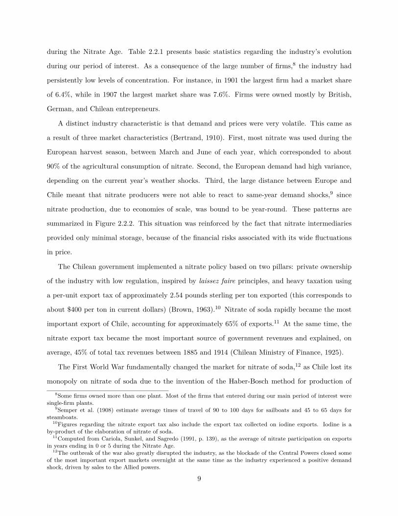
Table 2.3.2 summarizes the effect of cartels on industry output. In this table, the dependent

variable is monthly industry-level output, while the main independent variables of interest are

individual cartel dummies. The regression also includes dummies related to high-and-low-demand

seasons and a time trend. The main result of Table 2.3.2 is that going from competition to cartel

was correlated with an industry output reduction of around 18%. Cartels had heterogeneous results,

which is consistent with contemporaneous descriptions.16

1.4 Data and Summary Statistics

Unlike most industries in the developing world at the time, producers and government agencies that

were related to the nitrate industry placed great importance on the collection of detailed statistics.16Sources emphasize how the use of different contractual rules led to disparate degrees of success. In particular,

Cartels Fourth and Fifth had a significant effect on aggregate output. Cartel rules are explained in detail in acomplementary paper, Carrera and Titov (2020).

12

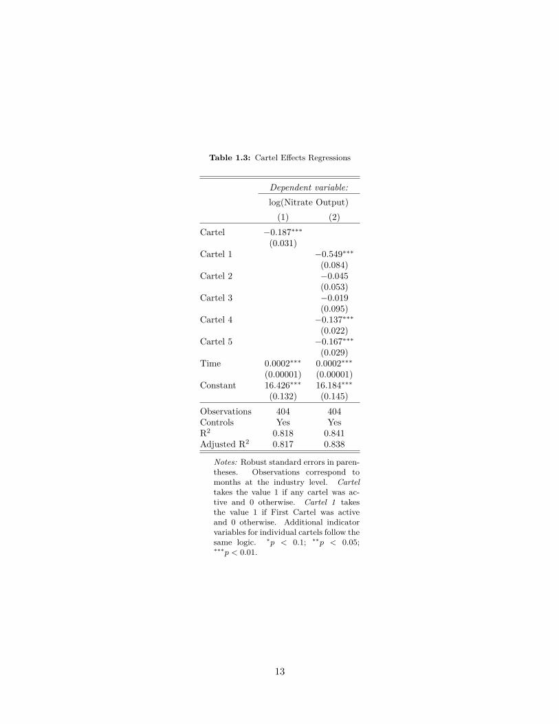
Table 1.3: Cartel Effects Regressions

Dependent variable:log(Nitrate Output)

(1) (2)Cartel −0.187∗∗∗

(0.031)Cartel 1 −0.549∗∗∗

(0.084)Cartel 2 −0.045

(0.053)Cartel 3 −0.019

(0.095)Cartel 4 −0.137∗∗∗

(0.022)Cartel 5 −0.167∗∗∗

(0.029)Time 0.0002∗∗∗ 0.0002∗∗∗

(0.00001) (0.00001)Constant 16.426∗∗∗ 16.184∗∗∗

(0.132) (0.145)Observations 404 404Controls Yes YesR2 0.818 0.841Adjusted R2 0.817 0.838

Notes: Robust standard errors in paren-theses. Observations correspond tomonths at the industry level. Carteltakes the value 1 if any cartel was ac-tive and 0 otherwise. Cartel 1 takesthe value 1 if First Cartel was activeand 0 otherwise. Additional indicatorvariables for individual cartels follow thesame logic. ∗p < 0.1; ∗∗p < 0.05;∗∗∗p < 0.01.

13

Meticulous record-keeping was also helped by the isolated nature of the industry’s environment,

where it was the solely economic activity of importance.

The main dataset is a panel describing plant-level output and input decisions with a monthly

frequency. This dataset, put together for the first time, was compiled from two main contempora-

neous sources. The first corresponds to monthly plant-level industry reports compiled in the form

of handwritten spreadsheets by the Nitrate Agency, which cover the period 1883 to 1909.17 The

second source is plant-level output and export monthly reports produced by the NPA, which mostly

cover the period 1900-1914.

For the complete sample of months and plants, the data contained in the Nitrate Agency

spreadsheets include nitrate output, exports, and stocks; iodine output, exports, and stocks; number

and nationality of workers; and number and type of animals. There was also a partial collection of

statistics on days worked and energy inputs. In total, we were able to collect spreadsheets for 228

months over this period, with 15, 804 observations at the plant-month level The dataset generated

using Nitrate Agency data was complemented by monthly plant-level output data from the NPA

monthly output reports (our second source). In this case, records are available for 21 months before

1900 and for every month after that year, for a total of 23, 518 observations. The merged dataset,

once redundant observations were removed, contains a total of 32, 623 plant-month observations.18

Constructing the main dataset proved challenging at times. Both of our main sources come from

physical archives and had never before been assembled into a single dataset. Spreadsheets produced

by the Nitrate Agency were scattered in several archives located in Santiago and the Nitrate Re-

gion.19 Moreover, these spreadsheets are original internal reports, produced to be sent from the

agency’s local office in the Nitrate Region to the Ministry of Finance in Santiago, which means that

they are handwritten. Additional archival work took place in order to gather complementary data:

Supplementary spreadsheets were gathered from reprints of the Official Journal of the Republic of

Chile and local newspapers from the Nitrate Region, and NPA monthly output and exports reports

were available in physical format at the Chilean National Library. Furthermore, data processing

imposed additional challenges. For instance, several plants shared the same name (e.g., there were

17For an example of a typical spreadsheets, see Figure 1.B.5 in Appendix 1.B.18A summary of the coverage of both primary sources can be seen in Figure 1.B.1 in Appendix 1.B.19Specifically, from the Ministry of Finance Section of both the National Historical Archives and the National

Archives of the Administration in Santiago, Chile; and the Tarapaca Regional Archives in Iquique, Chile.

14

Table 1.4: Summary of Data Sources

Data SourcesPrices UK The Economist, Chemical Trade JournalPrices Chile Nitrate Agency, NPACost parameters Semper et al. (1908)Plant characteristics Narro (several issues), Boudat (1889)1st Cartel contract Comite Salitrero (1884)2nd Cartel contract National Notarial Archive. Iquique Notaries. Volume 132.3rd Cartel contract National Notarial Archive. Iquique Notaries. Volume 141.4th Cartel contract NPA (1900)5th Cartel contract Semper et al. (1908, p. 321)

five plants named “Sacramento” and seven named “Rosario”). To distinguish between them, the

Nitrate Agency and the NPA used naming conventions, such as adding a geographical or ownership

reference to the name, which were not always consistent. Finally, industry sources did not use a

standard set of units to produce their reports. Hence, each reporting agency would use a different

units convention.

The main dataset was complemented by data from several other sources, which are summarized

on Table 2.4.1.20 From sources in the National Notarial Archive and the National Library, we

collected the five collusive agreements signed by the nitrate producers between 1884 and 1909. UK

price data, for nitrate of soda and related products, was obtained from The Economist and The

Chemical Trade Journal. Chilean prices were gathered from the Annual Report of the Nitrate

Agency and the “Estadıstica Comparada de Anos Salitreros,” which is a compendium of aggregate

statistics published by the NPA. Extensive historical evidence from nitrate producers’ internal

discussions was obtained from the Quarterly Circulars published by the NPA and the nitrate

producers’ meeting minutes (NPA, 1909). Additional qualitative evidence comes from the internal

correspondence of one of the main nitrate firms, the Antofagasta Company.

Some limitations remain regarding our data. First, before 1890, Nitrate Agency spreadsheets

included only the Tarapaca Province (which, at that time, corresponded to around 90% of industry

output). Second, there are 22 months between March 1883 and February 1897 for which we do

not possess output plant-level data. Third, our inputs data ends in 1909 which means that we

can’t estimate productivity for plants that entered after that year. Finally, one company (the20Additional details are found in Appendix 1.B.

15

Table 1.5: Summary Statistics: Nitrate Plants

Statistic Workers Animals Capacity (tons) Avg. output (tons)N 176 178 200 200Mean 289 103 3,494 1,703St. Dev. 179 64 2,861 1,239Min 5 2 30 18Pctl(25) 167 57 1,610.2 932Median 245 89 2,663.7 1,337Pctl(75) 383 139 4,267.1 2,161Max 1,038 309 15,647 6,721

Notes: Capacity estimated as maximum monthly observed output in moving periodof five years (observations from year 1896 were dropped). Workers, animals, capac-ity, and average output correspond to mean monthly values, excluding zero outputobservations. Sources: Authors’ calculations using main dataset.

Antofagasta Company) refused to report its output before 1895 (however, they did report their

inputs).

Table 2.4.2 shows summary statistics for the 200 plants in our main dataset. The median nitrate

plant had 245 workers and 89 animals, although there was a significant dispersion. Column 3 shows

capacity, which was estimated as the maximum plant-level monthly output observed in any month

of a moving 5-year interval.21 Column 4 presents the average monthly output, conditional on plants

being active. The industry presents a large amount of excess capacity, with average output doubling

the average monthly output. Figure 1.5 complements Table 2.4.2 by illustrating the relationship

between industry capacity and monthly output.

1.5 Reduced-form Evidence on Entry

The first step in the analysis explores the relationship between cartel episodes and the entry and

exit of plants. Extensive narrative historical evidence documents a relationship between cartels

and entry in this industry. For instance, the testimony of H.H. Gibbs, cited earlier, includes the

following exchange:22

—Now you said, with respect to your nitrate of soda, that it is a bit of a monopoly?21For the estimation of capacity, we did not consider observations from the year 1896, since the rules of the Third

Cartel induced abnormal levels of output in that year.22Gold and Silver Commission (1887, p. 157).

16

Figure 1.4: New Plants per Year

Notes: Number of nitrate plants that started operating each year. Competition (cartel) years are shown in black(gray).

—A monopoly of the province, you may say the whole of that part of Chili. Well, the

effect of this stimulus given to that production is that a multitude of producers turn

up.

Table 1.6 summarizes entry and exit patterns for the industry between 1885 and 1914, and

shows that cartel periods are associated with a significant increase in the entry of new plants. The

dependent variable in these regressions is the number of entering and exiting plants per period.

We identify the entry date of each plant as the first month in which it had a positive output (the

yearly entry of plants is summarized in Figure 1.4). Observations have been grouped in periods of

6 months, which are then classified as competitive or cartel periods.

The results in columns 1 and 2 of Table 1.6 suggest that even after controlling for contempo-

raneous nitrate price level, cartels have a significant effect on the entry of new plants,23 and this

effect has a large magnitude with respect to industry size. In a specification that uses a dummy to

account for all cartels together, the effect is roughly 2 new plants per year. On the other hand, in

a specification considering only the Fourth and Fifth Cartels (which are the focus of our analysis),23For a visual illustration, see Figure 1.4.1 in Appendix 1.4.

17

Table 1.6: Entry Regressions

Dependent variable:Entrants per period

(1) (2)Cartel 1.069∗∗

(0.516)Cartels 4th & 5th 2.212∗∗∗

(0.591)log(Price) 7.079∗∗∗ 6.437∗∗∗

(2.211) (2.026)Time 0.002 -0.019

(0.016) (0.015)Constant -13.863∗∗∗ -11.809∗∗∗

(4.800) (4.339)Observations 60 60R2 0.228 0.328Adjusted R2 0.186 0.292

Notes: Robust standard errors in parenthe-ses. Periods correspond to 6 months. Carteltakes the value 1 if any cartel was active and0 otherwise. Cartels 4th & 5th takes the value1 if Fourth or Fifth Cartels were active and 0otherwise. Price is contemporaneous nitrateof soda price in UK. ∗p < 0.1; ∗∗p < 0.05;∗∗∗p < 0.01.

the magnitude increases further to more than 4 plants per year.

Exit patterns in our data are observed with more noise than entry patterns because of the

presence of a large number of shutdowns. Particularly, it is likely that what we observe as exits in

the data, near the end of our database, were instead originally intended to be temporary shutdowns

that became permanent after the start of World War One. The main factor that explains observed

plant exits in this industry is obsolescence. For example, approximately 30% of all exiting plants

are units that were never updated to the Shanks refining method.24

Identification of the effect of cartels on entry relies on the fact that the competitive regime of

the industry was public, and that both the competitive regime of the industry and nitrate price

were exogenous from the point of view of a potential entrant. The competitive regime of the in-

dustry was exogenous because, if the current competitive regime was collusion, cartel rules implied

24This refining method was the industry standard during the Nitrate Age, and was introduced only a few yearsbefore the start of our dataset.

18

that entry would be accommodated and the new producers incorporated into the cartel.25 On the

other hand, if the current competitive regime was competition, forming a new cartel required the

approval of a large majority of producers. Since market shares in the industry were very low, it

was highly improbable that the entry of a single new producer would affect the existence of such a

majority. Thus, potential entrants knew that their individual entry decision was unlikely to affect

the collective decision about the industry’s competitive regime. Nitrate price was exogenous given

the extremely low concentration of the nitrate industry, which meant that firms had a behavior con-

sistent with perfect competition. Finally, the competitive regime was public since cartel contracts,

once signed, were public and had a known fixed term.

The previous argument does not imply that incumbent producers were unaware of the fact that

the existence of a cartel changed entry patterns. For instance, during the failed negotiations to

form a cartel in 1909, the manager of the NPA stated:26

Regarding the reduction of the [cartel] duration from 5 to 3 years, it is true that with

a 5 years [contract] there is the risk that new plants will be built, since it offers a wider

base for the investment of capitals . . . On the other hand, a 3 year [contract] generates

another challenge, which is that one year before that period is completed the market

becomes unstable, due to the uncertainty about whether a new collusive contract will

be signed or not.

The nitrate industry had low barriers to entry.27 To install a new nitrate firm, an entrepreneur

needed two things: to obtain the rights to nitrate-bearing land and to install a refining facility.

With respect to the refining facility, all new nitrate plants in the Nitrate Age used the Shanks

Method, which was not patent protected.

Nitrate rights in private hands was abundant. An official report of the Nitrate Agency estimated

in 1908 that nitrate reserves owned by private producers were more than three times larger than

the total industry output in its first century.28 Ownership of nitrate lands was very atomized,

which made it impossible for incumbent producers to prevent entry by restricting access to nitrate25For an example of a cartel contract see Appendix ??.26NPA (1909), minutes from the meeting on March 23, 1909, p. 3.27Low barriers to entry, defined here simply as the fact that any firm willing to pay an entry cost could become

active in the industry.28Bertrand (1910).

19

Figure 1.5: Industry Capacity and Monthly Output

Notes: Estimated industry capacity (dashed line) and monthly industry output. Capacity computed by addingestimated individual plant capacity. Individual plant capacity, estimated as the largest observed output in 5-yearintervals (the year 1896 is not considered in computation, due to exceptional output levels caused by Third Cartelrules). Cartel and War of Pacific periods are shaded. Each cartel’s number by chronological order is written on itsrespective period.

20

rights.29 H.H. Gibbs stated about the availability of nitrate land: “. . . the land is of no value at all,

it is prairie value really until you put up a manufactory. Well, the fear of having to invest capital

in that manufactory . . . deters people.”30

Contemporaneous narrative evidence shows that nitrate producers would hold on to their nitrate

land, waiting for the right moment to purchase the necessary equipment to start producing:31

Owners [of nitrate lands] limit themselves to keep their property waiting that more

prosperous years for the industry would allow them to start obtaining commercial profits

from their immobilized capital . . . These legitimate aspirations have finally materialized,

sheltered by the prosperity brought to the industry, thanks to the combination formed

by those same owners.

Nitrate land holdings by the Chilean state were even more extensive. By 1925, the Ministry

of Finance claimed that nitrate land owned by the government and still unmeasured, in terms of

surface, was almost five times larger than that already in private hands.32

The Chilean government periodically auctioned nitrate lands in its possession (see Table 1.7).

This could potentially be a threat to our identification, if the entry of new plants was induced by

Chilean government auctions and land auctions coincided with cartel periods. Table 1.7 summarizes

all nitrate land auctions conducted by the Chilean government during the study period. Only 3 out

of 12 auctions occurred during cartels. Moreover, the amount of nitrate content transferred in those

auctions was equivalent to only 6% of the reserves already in private hands (Semper et al., 1908).33

In addition, the auctions in the period 1894-95 (competition years) were the only ones directly

motivated by a desire to induce entry (Brown, 1963). Finally, from a directory that encompasses

all Chilean nitrate firms in 1907 (Nitrate Credit Association, 1909), we know that out of 28 new

plants built by these firms, only one can be traced directly to a recent land auction.

29Patterns of nitrate land ownership across different districts are explained in Appendix 1.A.30Gold and Silver Commission (1887, p. 157).31NPA Quarterly Circular, Number 27, April 21, 1902, p. 4.32Detailed statistics can be seen in Table 1.A.2 of Appendix 1.A. Estimation based on the minimum nitrate content

required by the Shanks refining method, which was 12%.33Estimation in the Nitrate Agency’s annual report for 1900, p. 53. This annual report has yet to be obtained by

us.

21

Table 1.7: Summary of Nitrate Land Auctions

Year Auction no. Competitive regime Nitrate reserves (tons) Price (£/ton)1882 First Competition 30,144,060 0.211894 Second & Third Competition 43,640,414 0.241895 Fourth Competition 5,000,000 0.201897 Fifth Cartel 1,842,000 0.161901 Sixth Cartel 11,144,368 0.171903 Seventh Cartel 12,559,413 0.251912 Eighth Competition 8,203,185 0.501917 Ninth Competition 27,686,184 0.191917 Tenth Competition 30,786,675 0.331918 Eleventh Competition 6,668,953 0.231924 Twelfth Competition 38,046,630 0.36

Sources: Chilean Ministry of Finance (1925), p. 53.

1.6 Productivity Estimation and Dispersion

Using our detailed output and input plant-level database, we estimate the productivity of each plant in the

industry. The estimated productivity distribution exhibits a large cross-sectional dispersion. We also show

that plants that entered the industry during cartels had significantly lower productivity.

The production of nitrate consisted of two distinct main stages: extraction and refining. The extraction

stage was the labor-intensive process by which the raw material,34 which would later be refined into nitrate of

soda, was extracted from the desert soil and transported to the nitrate plant’s refining facility. The refining

stage refers to the leaching process by which the nitrate of soda was separated from the other materials

present in the raw material, such as diverse salts and sulfites.

In line with the previous description, we model the overall production process using a Leontief production

function. At the same time, each of the main stages of production is separately assumed to follow a Cobb-

Douglas production function. In the extraction stage, the relevant inputs are workers and animals used to

transport the raw material. Meanwhile, on the refining stage, the relevant input is the energy used to heat

the raw material during the leaching process. Finally, since most of the energy used in the extraction stage

corresponds to animal traction, and the refining stage was energy intensive, it is realistic to assume that the

observed energy input was only used in the refining stage. For plant i in period t, its output will be given by

qit = min{φiLαitAβitε1it︸ ︷︷ ︸

extractionstage

, θφδiEγitε2it︸ ︷︷ ︸

refiningstage

} (1.1)

34Raw material was denominated “caliche” in Spanish.

22

s.t. qit ≤ kit︸︷︷︸refiningcapacity

,

where qit is nitrate output, φi is a time-invariant TFP term, Ait are animals, Lit are workers, and Cit are

energy (coal) units. In addition, θ is a common scaling factor and εjit are lognormal iid shocks to output with

zero mean. Similarly, kit corresponds to the maximum refining capacity of the plant, which is unobserved

but which we can infer from the monthly output data. Notice that we observe the output of nitrate plants

in physical units (tons), not in sales.

The term φi is present in both stages of the production process. Intuitively, φi is related to the geological

properties of the raw material; in particular, to its nitrate grade, which should affect both stages of the

production process. To illustrate, suppose one plant has a value of φ that is twice as large as that of a second

plant. Then, the first (high-productivity plant), to produce each unit of final product, will have to extract,

transport, and apply the leaching process to only half as much raw material as the second (low-productivity)

plant.

During the period studied there was no significant technological change, since the Shanks method to

leach nitrate, introduced in the late 1870s, remained the industry standard until the 1920s. Moreover, all

new plants built during the Nitrate Age were based on this technology. At the same time, the extraction

stage did not experience significant improvements (Reyes, 1994).35

There is ample evidence that costs—and therefore productivity—were heterogeneous across nitrate

plants. The main driver of productivity differences, as the technology used by all firms was the same,

was the geological characteristics of the nitrate-bearing grounds where each plant was located. Contempo-

raneous sources support this claim; for instance, Semper et al. (1908) state, “the cost of production varies

widely depending on numerous factors. Mainly the nitrate grade, the hardness, and the specific type of raw

material.”36

We estimate the parameters of equation 1.1 in two steps. Our main dataset includes workers, animals,

and nitrate output for all plants. In the first step, we use these variables to estimate the parameters from

the extraction stage. We will take the following expression in log-form to the data:

log(qit) = log(φi) + αlog(Lit) + βlog(Ait) + log(ε1it). (1.2)

In the second step, we use the productivity estimated in the first step as an input to estimate the

parameters in the refining stage, using the subsample of observations that include the energy variable, which

corresponds to approximately 15% of the observations in the full sample.35In particular, mechanization of the extraction stage would only occur in the 1920s, with introduction of the

Guggenheim method of production.36Semper et al. (1908, p. 71).

23

1.6.1 Extraction-stage Estimates

To obtain consistent estimators in the first step, we must address two potential main concerns: simultaneity

and selection. Simultaneity arises if the productivity shock ε1it is observed by the firm before it makes

its input decisions. Selection refers to the fact that plants choose whether to operate or not, causing the

observed set of active plants to be not a random sample from the population of plants.

Notice that for simultaneity to be a problem after including fixed effects in the extraction stage, firms

should be able to predict the sign and direction of the deviations from the mean and then be able to adjust

the number of workers and animals accordingly.

We believe that simultaneity in this particular case is not an issue for two reasons. First, there is evidence

that productivity shocks were hard to predict. Second, it was hard for firms to adjust their relevant inputs

to short-term productivity shocks. In the nitrate industry, shocks to productivity correspond to deviations

from the plant mean level in raw material quality.

First, because of the nature of the technology and the production process, it is unlikely that firms were

able to predict deviations from mean productivity before the end of the leaching process. Historical evidence

supporting this claim is found in the Antofagasta Company archives,37 particularly in the periodic reports

sent by plant managers to central headquarters. In February 1892, for example, the manager states that “last

month production was only 45,890 quintals . . . the result is unsatisfactory . . . The first days of the month were

very productive and we expected to reach a production of 55,000 quintals, but then [productivity] diminished

because of the presence of sulfate and boric acid . . . which prevented the cristalization of nitrate.”38 Similarly,

in May 1893, the plant manager reports that “output in April was only 42,300 quintals. This reduced amount

was due to the small number of leaching tanks [available], and the poor quality of the raw material whose

high concentration of sodium sulfate forced us to repeat the crystallization process.”39

Second, nitrate firms faced severe frictions in the input markets for workers and animals, which makes

it less likely that they adjusted their level of inputs as a function of monthly productivity shocks even if

they were able to perceive them. Since the industry was located in a previously uninhabited desert, mules

had to be imported from Argentina and workers had to be brought from other regions of Chile or Bolivia.

The industry suffered periodic labor shortages, which motivated the NPA to organize joint labor recruitment

efforts in Central and Southern Chile. The reports of the Antofagasta Company manager illustrate the great

lengths companies had to go to recruit labor:40

By telegram, I was informed 247 males, 128 women, and 30 children embarked in [the province37This company was one of the largest in the industry, and company archives are preserved in the Historical

National Archives of Chile.38Report number 87, February 2, 1892, p. 4.39Report number 224, May 2, 1893, p. 1.40Report number 225, May 5, 1893, p. 1.

24

Figure 1.6: Plants in Shutdown

Notes: Plants in shutdown are defined as plants with zero observed current output and that have at least one positiveoutput period later in time. Cartel and War of Pacific periods are shaded. Each cartel’s number by chronologicalorder is written on its respective period.Source: Authors’ calculations based on official publications.

of] Coquimbo bound to Pampa Central [plant].

To ensure the success of this important recruitment effort I took the following measures: The

railroad will have a special service on Sunday, day of their arrival, waiting on the docks . . . Five

boats will be ready to transport them to the company warehouse, . . . and the Governor will send

all available police to prevent any contact with locals.

The selection problem arises in this case because there is censoring on the observed distribution of

active plants. In the particular case of the nitrate industry, this problem would arise because of the large

number of shutdown plants we observe in the data (see Figure 1.6).41 Intuitively, plants that have already

invested in accumulating workers and animals may decide to remain in operation, even if they have a lower

productivity than a second plant that had not made those investments in the past, which introduces a bias

in our estimates. To address this issue, we use the method proposed by Olly and Pakes (1996), who use a

control function approach.

In this case, we augment equation 1.5 by adding a nonparametric function λ(·) of the propensity score

of shutdown to control for the differential probabilities a plant had of being active given its observables.

Intuitively, under mild conditions, there is a one-to-one relationship between the true selection function41Interestingly, shutdowns are far more numerous than exiting plants; see Figure 1.4.2 in Appendix 1.4.

25

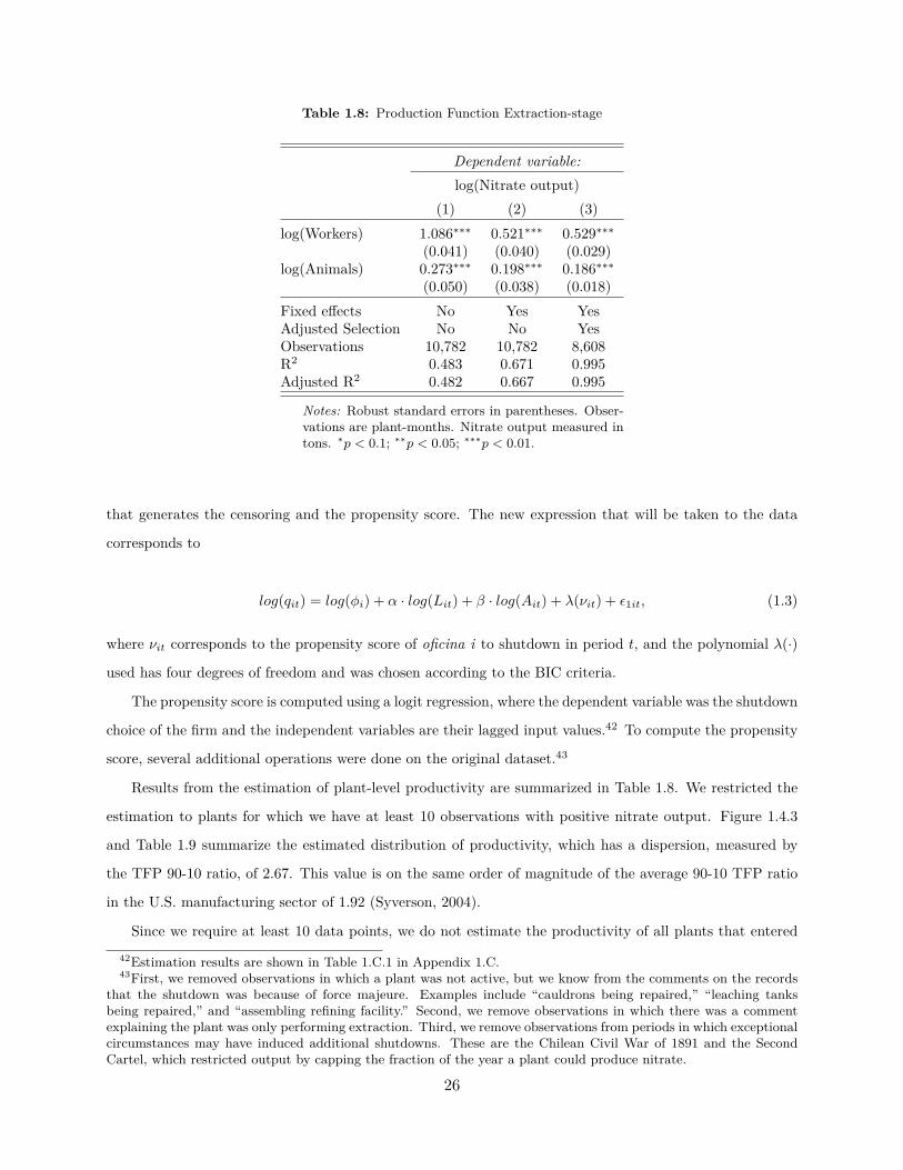
Table 1.8: Production Function Extraction-stage

Dependent variable:log(Nitrate output)

(1) (2) (3)log(Workers) 1.086∗∗∗ 0.521∗∗∗ 0.529∗∗∗

(0.041) (0.040) (0.029)log(Animals) 0.273∗∗∗ 0.198∗∗∗ 0.186∗∗∗

(0.050) (0.038) (0.018)Fixed effects No Yes YesAdjusted Selection No No YesObservations 10,782 10,782 8,608R2 0.483 0.671 0.995Adjusted R2 0.482 0.667 0.995

Notes: Robust standard errors in parentheses. Obser-vations are plant-months. Nitrate output measured intons. ∗p < 0.1; ∗∗p < 0.05; ∗∗∗p < 0.01.

that generates the censoring and the propensity score. The new expression that will be taken to the data

corresponds to

log(qit) = log(φi) + α · log(Lit) + β · log(Ait) + λ(νit) + ε1it, (1.3)

where νit corresponds to the propensity score of oficina i to shutdown in period t, and the polynomial λ(·)

used has four degrees of freedom and was chosen according to the BIC criteria.

The propensity score is computed using a logit regression, where the dependent variable was the shutdown

choice of the firm and the independent variables are their lagged input values.42 To compute the propensity

score, several additional operations were done on the original dataset.43

Results from the estimation of plant-level productivity are summarized in Table 1.8. We restricted the

estimation to plants for which we have at least 10 observations with positive nitrate output. Figure 1.4.3

and Table 1.9 summarize the estimated distribution of productivity, which has a dispersion, measured by

the TFP 90-10 ratio, of 2.67. This value is on the same order of magnitude of the average 90-10 TFP ratio

in the U.S. manufacturing sector of 1.92 (Syverson, 2004).

Since we require at least 10 data points, we do not estimate the productivity of all plants that entered42Estimation results are shown in Table 1.C.1 in Appendix 1.C.43First, we removed observations in which a plant was not active, but we know from the comments on the records

that the shutdown was because of force majeure. Examples include “cauldrons being repaired,” “leaching tanksbeing repaired,” and “assembling refining facility.” Second, we remove observations in which there was a commentexplaining the plant was only performing extraction. Third, we remove observations from periods in which exceptionalcircumstances may have induced additional shutdowns. These are the Chilean Civil War of 1891 and the SecondCartel, which restricted output by capping the fraction of the year a plant could produce nitrate.

26

Table 1.9: Summary Statis-tics: Plant Productivity

Statistic ProductivityN 148Mean 44.4St. Dev. 15.6Min 10.2Pctl(25) 33.7Pctl(75) 53.7Max 97.1

Figure 1.7: Estimated Distribution of Plant Productivity

Notes: Each bar represents the estimated productivity of a nitrate plants (N=148). Values ordered in descendingorder.

27

Table 1.10: Effect of Cartels on Productivity ofEntrants

Dependent variable:Productivity

(1) (2)Cartel −10.630∗∗∗

(3.575)Cartels 4th & 5th −13.365∗∗

(5.705)log(Price) −28.425∗∗ −27.386∗∗

(13.830) (13.110)Time 0.490∗∗∗ 0.924∗∗∗

(0.158) (0.292)Constant 108.835∗∗∗ 97.738∗∗∗

(30.260) (29.631)Observations 108 108R2 0.154 0.122Adjusted R2 0.130 0.097

Notes: Robust standard errors in parenthe-ses. Observations are individual plants at mo-ment of entry. Dependent variable is estimatedplant-level productivity. Cartel takes the value1 if any cartel was active and 0 otherwise.Cartels 4th & 5th takes the value 1 if Fourthor Fifth Cartels were active and 0 otherwise.Price is contemporaneous nitrate of soda pricein UK. ∗p < 0.1; ∗∗p < 0.05; ∗∗∗p < 0.01.

the industry in the period before World War One. In particular, of the 71 plants that started operating

during the Fourth and Fifth Cartels, we are able to estimate the productivity of only 48 (slightly less than

70% of the total). However, since the probability of shutdown is negatively correlated to productivity, the

set of plants without a productivity estimate is a negatively selected sample of the population.

1.6.2 Analysis of the Productivity Distribution

An additional question we can explore using the obtained distribution of productivity is whether cartels

negatively affected the “quality” of the entrants. Intuitively, as nitrate cartels generated artificially high

prices for an ex ante known period of time, some low-productivity plants, which would have not entered in

a competitive environment, could have decided otherwise. Table 1.10 shows that cartels had a significantly

negative effect on the productivity of new plants, even when we control for the contemporaneous nitrate

price level.

Furthermore, the distribution of entrants during cartels was different than the distribution of entrants

28

Figure 1.8: Productivity vs Period of Entry

Notes: Each bar represents the mean productivity of entrants by period. Standard errors shown over the bars. Cartel(competition) periods are shown in darkest (lightest) shade.

Figure 1.9: Productivity Distributions of Entrants

Notes: Productivity distribution of entrants during competition periods (lighter shade) and cartel periods (darkershade).

29

during competition (see Figure 1.9). A Chi-square test of the homogeneity of the distributions rejects that

both distributions are the same, at levels of significance of less than 1% or 2.6%, depending on the number

of categorical intervals used to split the sample.44

The difference in productivity is significant. The median-size plant in the industry would enjoy an

additional monthly gross revenue of approximately $410, 000 (in current dollars) if it went from the mean

productivity of an entrant during a cartel to the mean productivity of an entrant during competition.

1.6.3 Refining-stage Estimates

Lastly, using the productivity estimates from the extraction-stage, we estimate the parameters for the

refining-stage production function. The original production function equation for this stage, in logs, is

given by

log(qit) = log(θ) + δ · log(φi) + γ · log(Eit) + log(ε2it) (1.4)

Since we do not directly observe plant i´s productivity term, φi, we use the estimated value obtained

for the extraction stage. Thus, the equation we estimate is

log(qit) = log(θ) + δ · log(φi) + γ · log(Eit) + log(ε2it), (1.5)

where φi corresponds to the estimated productivity in the extraction stage.

An additional challenge in this case is that the Nitrate Agency’s inputs data only contain energy (specif-

ically, coal) for a subsample of the observations. Thus, we assume that the relationship between coal and

nitrate output in observed plants and periods is representative of the full population.

Table 1.11 shows the results of the production function estimation. Notice that the parameter associated

with log(φ), δ, is highly significant and close to one.45

1.7 Plant Entry Decision

In this section, we develop a simple entry model for potential entrants in the industry. We then separately

estimate its building blocks: the determinants of the plants’ output decision, the probabilities that ruled the

transition across state variables (price level and competitive regimes), and the total cost function. Later,

these pieces are combined to compute continuation values for potential entrants in the industry.

44Estimation details can be found in Table 1.C.2 in Appendix 1.C.45In addition, Figure 1.4.5 of Appendix 1.4 displays the relationship between energy (coal) and nitrate output.

30

Table 1.11: Refining-stage Production Func-tion

Dependent variable:Nitrate Output

log(Coal) 0.643∗∗∗(0.053)

log (Productivity) 0.956∗∗∗(0.076)

Constant 0.153(0.161)

Observations 2,326R2 0.641Adjusted R2 0.641

Notes: Robust standard errors in paren-theses. Observations are plant-months.Nitrate output and coal measured in tons.∗p < 0.1; ∗∗p < 0.05; ∗∗∗p < 0.01.

1.7.1 Model of Entry

The main elements of our entry model are described next.

Time: Time is discrete and infinite. Periods consist of 6 months and are indexed by t ∈ {1, . . . ,+∞}.

Entry takes one period.

Plants: There is a set I = {1, . . . , NI} of potential plants in the industry, which are owned by a set

F = {0, . . . , NF } of existing firms. We consider the entry problem of each plant independently (hence, we

abstain from considering potential cost synergies across plants), so each plant is effectively treated as an

independent firm.

Plants are characterized by a vector of characteristics. Thus Plant i in time t is described by character-

istics

τit = (φi, kit) ,

where φi ∈ R+ is a constant productivity term and kit ∈ R+ is the maximum refining capacity of the plant.

We consider kit to be an exogenous characteristic of the plants for now.

State space: Market conditions at any period t are summarized by a vector of state variables ψt ∈ Ψ,

where ψt = (pt, ct).

• pt ∈ {p1, p2, p3, p4, p5} is the price of nitrate of soda in Chile. We discretize the space of prices into

five intervals pN , according to the empirically observed frequency of prices.

• ct ∈ {c0, c1, c2, c3, . . . , c10} is the current competitive regime of the industry. State c0 corresponds

31

to free competition, while states {c1, . . . , c10} are cartel states. Specifically, for cartel states, their

index corresponds to the number of remaining periods in collusion, as established in the current cartel

contract. For instance, c3 means that after the current period concludes, there will be two more cartel

periods before competition resumes.

Plant entry decision: Current period profits for plant i of type τit are given by

π(pt, qit, τit) = pt · qit − TCi(qit)

where pt is the price in Chile, qit is plant’s i output, and TCi(qit) is the production cost. Notice that τit

implicitly affects qit and TCi(·) through the productivity term φi.

Thus, a potential entrant of type τit faces at time 0 the following problem,

max{t0}

Et

[ ∞∑t=0

βtπ(pt, qit, τit)1t0

]︸ ︷︷ ︸

V (τit,ψt)

−βt0FC(kit)

, (1.6)

where t0 is the period the firm enters; FC(·) is a sunk cost of entry that increases on plant size and is

independent of market conditions; β is the discount factor; and 1t0 is an indicator function that takes value

of 1 iif t ≥ t0.

Our main challenge consists in estimating the entry value V (τit, ψt), in order to evaluate counterfactual

levels of entry in a case without cartels. In the next subsections, we detail the process of estimation by

first explaining the estimation of revenue components and later the estimation of the cost function. Finally,

since the nitrate industry eventually declined due to the invention of a technological substitute, a potential

concern regarding our general approach is that potential entrants may have internalized in their entry

decision the probability that synthetic nitrate would be invented at some point in the future. However,

evidence from contemporaneous sources suggest that the invention of synthetic nitrate came as a surprise to

nitrate producers. For instance, the following commentary was included in NPA’s Quarterly Circular in 1904:

“Happily for country and industry, there is no close danger and, even as chemists and men of science work

tirelessly, it is impossible to foresee a time when nitrate has been dislodged, given the economic conditions

of its production, which seldom could be matched by a different industry.”46

46NPA Quarterly Circular, Number 34, May 31, 1904, p. 10.

32

1.7.2 Revenue estimation

Output Determination Function

The main difficulty in the estimation of revenue is characterizing the output decisions of plants as a function

of own-characteristics and market conditions. That is, we look to estimate, for each plant i, a function of

the state variables, qi : ψ ≡ (c, p)→ R+.

Table 1.12: Determinants of Monthly Plant Out-put

Dependent variable:log(Nitrate Output)

log(Price) −1.174∗∗∗(0.065)

Age −0.020∗∗∗(0.001)

Productivity 0.031∗∗∗(0.0003)

Cartel −0.059∗∗∗(0.011)

Number Active Plants −0.006(0.005)

Time 0.025∗∗∗(0.002)

Constant 8.176∗∗∗(0.133)

Observations 21,197R2 0.390Adjusted R2 0.390

Notes: Robust standard errors in parenthe-ses. Dependent variable is plant-month output.Cartel takes the value 1 if any cartel was activeand 0 otherwise. Age is the number of peri-ods since start of operations. Number of Ac-tive Plants is the number of active plants, ex-pressed in tens. Price is contemporaneous ni-trate of soda price in UK. ∗p < 0.1; ∗∗p < 0.05;∗∗∗p < 0.01.

Notice that in the specification, we have not included any terms related to a potential strategic interaction

across plants. In fact, although the operation of the nitrate market closely resembled a Cournot model, the

low levels of concentration in practice caused firms to behave as in a perfectly competitive environment.

Evidence supporting this statement is found in Table 1.12, in which we regressed monthly nitrate output for

all plants in our dataset with respect to several potential explanatory variables. In particular, the number of

plants active in the industry is not significant. Figure 1.10 further illustrates the lack of correlation between

33

Figure 1.10: Average Output by Productivity Type and Number of Plants

Notes: Vertical axis on the left is in tons and corresponds to monthly average plant-level output, which is indicatedfor each productivity type by a solid line. Horizontal axis is time in years from the beginning of our data set in1883. Vertical axis on the right is the number of active plants in the industry, and is indicated by the dashed blackline. Productivity types are described below the horizontal axis, with Φ1 being the lowest and Φ5 being the highestproductivity type.

number of plants and nitrate output.47

To estimate the output function, we use our main dataset in a two-step approach. First, for all points

in the state space ψ such that we have 10 or more observations per plant, we use the average of these

observations as our estimate of qi(ψ). Second, we discretize the space of plant types τ by creating 15 cells of

plants grouped according to their productivity level (5 groups) and their effective size (3 groups for each of

the productivity groups).48 The identifying assumption is that plants within the same cell should be similar

enough to have similar levels of output conditional on specific values of ψ and that, by law of large numbers,

deviations from the mean level of output of each cell should cancel out.

Finally, prices in Chile are directly observed from 1893 onward. We use UK prices to complete the series

of prices FOB for previous dates, taking advantage of the fact that the difference between Chile nitrate prices

and UK nitrate prices was extremely stable across the years.49

47In addition, we test whether it is necessary to control for seasonality. Figure 1.4.8 in Appendix 1.4 shows thatnitrate output tended to be evenly distributed across the year, and hence we do not need to consider seasonality inour estimation.

48Computed as their mean effective output when active, once they had been already sorted by productivity. Thediscretization is shown in Tables 1.3.12 and 1.3.13 of Appendix 1.C.

49See Figure 1.B.3 in Appendix 1.4 and Table 1.C.3 in Appendix 1.C for more details.

34

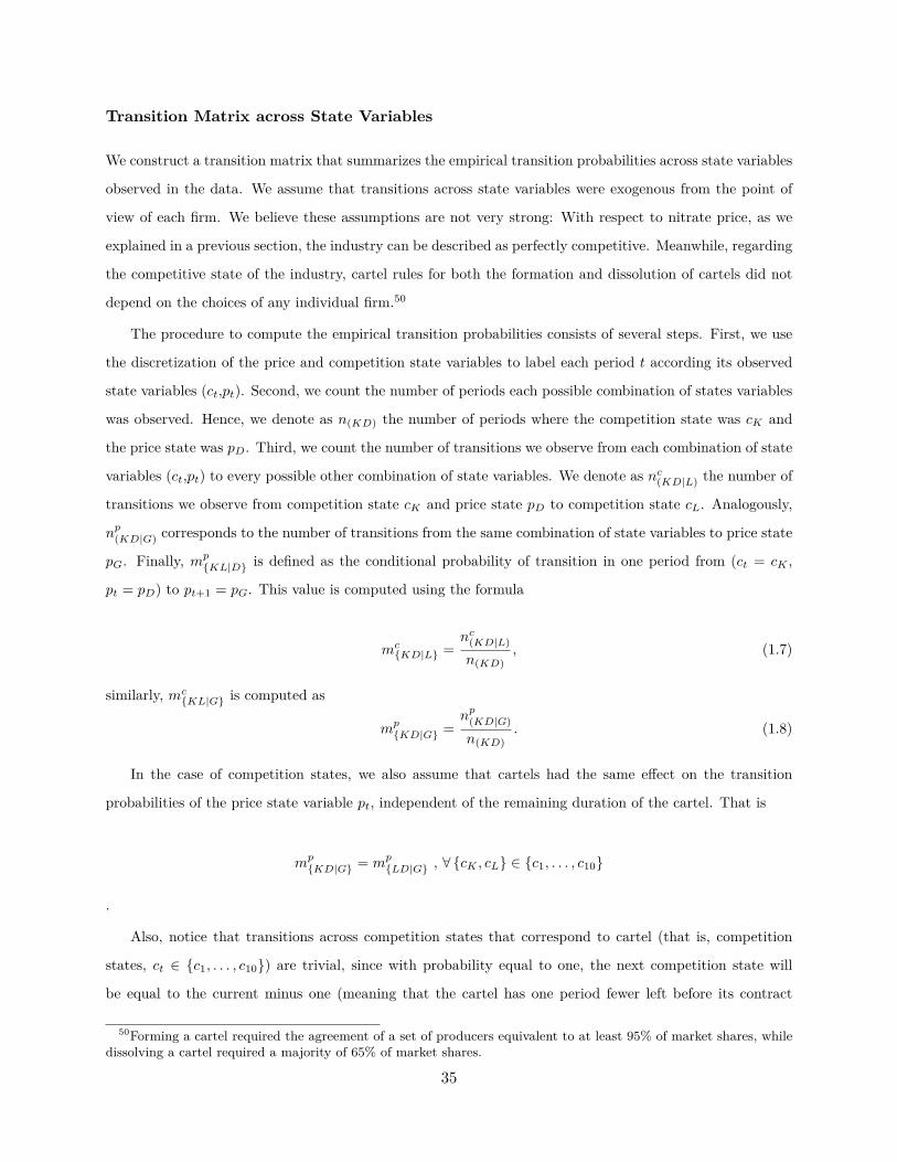
Transition Matrix across State Variables

We construct a transition matrix that summarizes the empirical transition probabilities across state variables

observed in the data. We assume that transitions across state variables were exogenous from the point of

view of each firm. We believe these assumptions are not very strong: With respect to nitrate price, as we

explained in a previous section, the industry can be described as perfectly competitive. Meanwhile, regarding

the competitive state of the industry, cartel rules for both the formation and dissolution of cartels did not

depend on the choices of any individual firm.50

The procedure to compute the empirical transition probabilities consists of several steps. First, we use

the discretization of the price and competition state variables to label each period t according its observed

state variables (ct,pt). Second, we count the number of periods each possible combination of states variables

was observed. Hence, we denote as n(KD) the number of periods where the competition state was cK and

the price state was pD. Third, we count the number of transitions we observe from each combination of state

variables (ct,pt) to every possible other combination of state variables. We denote as nc(KD|L) the number of

transitions we observe from competition state cK and price state pD to competition state cL. Analogously,

np(KD|G) corresponds to the number of transitions from the same combination of state variables to price state

pG. Finally, mp{KL|D} is defined as the conditional probability of transition in one period from (ct = cK ,

pt = pD) to pt+1 = pG. This value is computed using the formula

mc{KD|L} =

nc(KD|L)

n(KD), (1.7)

similarly, mc{KL|G} is computed as

mp{KD|G} =

np(KD|G)

n(KD). (1.8)

In the case of competition states, we also assume that cartels had the same effect on the transition

probabilities of the price state variable pt, independent of the remaining duration of the cartel. That is

mp{KD|G} = mp

{LD|G} , ∀ {cK , cL} ∈ {c1, . . . , c10}

.

Also, notice that transitions across competition states that correspond to cartel (that is, competition

states, ct ∈ {c1, . . . , c10}) are trivial, since with probability equal to one, the next competition state will

be equal to the current minus one (meaning that the cartel has one period fewer left before its contract

50Forming a cartel required the agreement of a set of producers equivalent to at least 95% of market shares, whiledissolving a cartel required a majority of 65% of market shares.

35

expires).51

1.7.3 Cost Function Estimation

To estimate the total cost function of nitrate firms, we complement the production function estimates,

which were the focus of the last section, with additional contemporaneous measures of costs, summarized in

contemporaneous technical sources. The total cost expression we use, divided into its components, can be

written as

TCi(qit) = ECi(qit)︸ ︷︷ ︸extraction

cost

+RCi(qit)︸ ︷︷ ︸refining

cost

+GC(qit)︸ ︷︷ ︸taxcost

+ PC(qit)︸ ︷︷ ︸transportation

cost

+OC(qit)︸ ︷︷ ︸othercost

, (1.9)

where the first two components ECi(·) and RCi(·) correspond to extraction stage and refining stage costs,

respectively. Notice these components are plant specific, since they are directly affected by the plant-specific

productivity term φi. On the other hand, the terms GC(·), PC(·), and OC(·) are cost components common

to all plants in the industry. For these components, the approach is simply the use of technical sources that

describe variable costs in the industry, using what is known as the “engineering method.” The main source

in this case is the technical description of the industry provided by Semper et al. (1908).52

One of the data-related challenges for this industry is the relative scarcity of direct sources for input

prices. In our computation, we use the values provided by Semper et al. (1908), who compiled cost statistics

from an extensive field visit to the industry in 1901 and 1902. Additionally, when this source was translated

into Spanish in 1908, the edition was augmented by adding cost data from that date. Hence, we mostly have

cost data without time-series variation, although our main source centers precisely on the period of time

that is our focus of interest.

Extraction-stage Costs

Extraction-stage costs are derived directly from its production function. The cost minimization problem

plant i faces each period, in order to produce an output of at least q, can be written as

min{Lit,Ait}

ECi(qit) = w · Lit + canim ·Ait (1.10)

s.t. qit ≥ q,

51Examples of the transition matrices can be observed in Appendix 1.C. Table ?? shows the transition matrixfor competition states, when pt = p1; Tables ?? and ?? present the transition probabilities for the state variable ptfor cartel and competition periods, respectively. Transition matrices not included in the text are analogous to thoseshown.

52For a brief description of the engineering method, see Davis and Garces (2009, p. 157).

36

where w is wages, and canim is the monthly cost per animal in period t.

From that minimization problem, it is easy to obtain the following cost function:

ECi(q) = q1

α+β

(1φi

) 1α+β

((α

β

)β+(β

α

)α) 1α+β

︸ ︷︷ ︸ci

(wαcβanim)1

α+β︸ ︷︷ ︸ω

,

which can be rewritten (replacing q for qit) as

ECi(qit) = ρiωqψit, (1.11)

where, ρi is a plant-specific cost parameter, ω is an industry-wide cost factor, and ψ = 1α+β is an

economy-of-scale parameter.

Refining-stage costs

The estimation of refining-stage costs is done in two steps. Since we do not observe the usage of

energy inputs for the whole sample, in the first step we use the estimated values of the parameters

for the refining-stage production function to estimate the coal consumption of those plants with

missing energy input:

Eit(qit) = q1γ

it

(1θφi

) 1γ

. (1.12)

In the second step, the refining cost RC(·) is estimated using the following relationship:

RCi(qit) =

ccoalEit(qit) ,if Eit is observed

ccoalEit(qit) ,if Eit is not observed ,

(1.13)

where ccoal is the price of coal in Chile.

Tax costs

The Chilean government collected a per unit export tax on nitrate of soda equivalent to approx-

imately 2.54 pounds per ton (roughly, $400 per ton in current dollars). This tax rate remained

constant throughout the Nitrate Age. Thus, the tax cost is computed as37

GCi(qit) = Tqit, (1.14)

where T is the nitrate tax rate.

Transportation and other costs

The final two components of the total cost function are the expenses necessary to the commercial-

ization of nitrate that were incurred after production had concluded. Parameters for these costs

were obtained from Semper et al. (1908), and when a range was provided, we use the inferior value

in the interval.

First, there were costs associated with the packaging and transportation of nitrate to the port

(where it was sold to nitrate traders). These costs include the cost of the sacks used to transport

nitrate, cpack; the railroad cost to the port, crail; and port costs, cport:

PCi(qit) = cpackqit + cportqit + crailqit (1.15)

Second, there are others costs, which include plant administration costs cadm and advertising

costs cadv. This last item corresponds to the mandatory contribution the NPA collected from

producers to fund their joint marketing effort in the destination markets:

OCi(qit) = cadmqit + cadvqit. (1.16)

Total Costs

Putting all of the cost components together, we obtain the final expression we take to the data:

TCi(qit) = ρiωqψit︸ ︷︷ ︸

extractioncost

+ ccoalEit(qit)︸ ︷︷ ︸refining

cost

+Tqit︸︷︷︸taxcost

+ qit (cpack + cport + crail)︸ ︷︷ ︸transportation

cost

+ qit (cadm + cadv)︸ ︷︷ ︸othercost

. (1.17)

Table 1.11 presents estimated costs for the observations in our sample, with plants grouped

for illustrative purposes according to their productivity in three groups (low, medium, and high38

Figure 1.11: Total Costs by Productivity Type

Notes: Vertical axis is total estimated cost in pounds sterling in 1900. Horizontal axis is nitrate output expressedin tons. Each point corresponds to a plant-month level observation, where coordinates are observed output andestimated total cost, respectively. Points are colored by productivity type. Productivity types are described belowthe horizontal axis.

39

Table 1.13: Summary Statistics: Estimated Plant Entry Values

Statistic Discounted value (£1900) Discounted value ($2018)N 148 148Mean 306,598 45,099,752St. Dev. 362,009 53,250,692Min -64,879 -9,543,475Pctl(25) 68,754 10,113,555Median 165,442 24,336,110Pctl(75) 434,211 63,871,440Max 1,944,433 286,021,351

Notes: Observations are plants. In the second column, figures presented incontemporaneous pounds sterling. In the third column, figures presentedin current dollars. See main body of the text for detailed explanation ofthe estimation procedure.

productivity).

1.7.4 Entry Values Results

The three building blocks described in the previous subsections are combined to compute the entry

values of the plants observed as entrants in the data as a function of the state variables. The entry

value of each plant is separately estimated using value function iteration.

Figure 1.12 shows an example of the resulting estimated values, as a function of both ct and pt.

Plant values increase together with the competition state ct and, conditioning on ct, plant values

are also increasing in pt. These basic patterns are observed in the whole cross-section of estimated

plant values. Moreover, plant values increase together with the TFP term φi.

Table 1.13 presents summary statistics for the estimated plant values, both in contemporaneous

currency (£1900) and present-day currency ($2018)53. The median (mean) plant in the industry had

a value in present dollars of approximately 25m (45m).54

There is highly significant dispersion in plant values, as exemplified by the fact that the standard

deviation is larger than the mean plant value. Graphically, the cross-sectional dispersion of values

can be seen in Figure 1.13, which shows plant values arranged by date of entry.

53Parameters used to do the conversion are found in Table 1.3.11.54Estimated monthly profits, grouped by productivity groups, are shown in Figure 1.4.7 of Appendix 1.4.

40

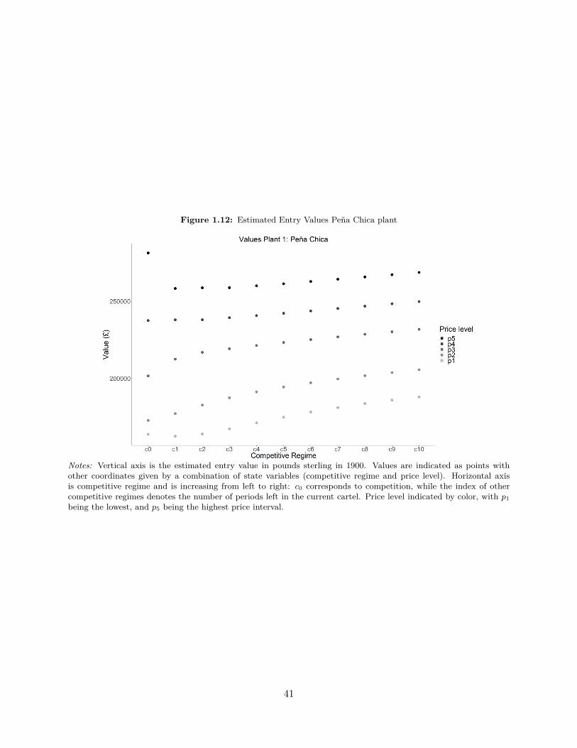
Figure 1.12: Estimated Entry Values Pena Chica plant

Notes: Vertical axis is the estimated entry value in pounds sterling in 1900. Values are indicated as points withother coordinates given by a combination of state variables (competitive regime and price level). Horizontal axisis competitive regime and is increasing from left to right: c0 corresponds to competition, while the index of othercompetitive regimes denotes the number of periods left in the current cartel. Price level indicated by color, with p1being the lowest, and p5 being the highest price interval.

41

Figure 1.13: Estimated Plant Entry Values

Notes: Vertical axis is total estimated cost in pounds sterling in 1900. Horizontal axis is entry date. Each pointcorresponds to a single plant’s estimated value at the moment of entry. Points are colored by productivity type.Productivity types are described below the horizontal axis, with Φ1 being the lowest and Φ5 being the highestproductivity type.

42

Table 1.14: Demand Elasticity Estimation

Dependent variable:log(Nitrate Output) log(Price)

OLS IV First stage(1) (2) (3)

log(Price) −0.445∗ −0.328∗∗(0.231) (0.166)

log(Price Last Year) 0.649∗∗∗(0.072)

Time 0.061∗∗∗ 0.060∗∗∗ 0.006∗∗∗(0.005) (0.004) (0.002)

Cartel −0.185∗∗∗ −0.194∗∗∗ 0.058∗(0.048) (0.054) (0.035)

Constant 13.945∗∗∗ 13.753∗∗∗ 0.522∗∗∗(0.354) (0.268) (0.139)

Observations 31 31 31R2 0.933 0.932 0.709Adjusted R2 0.926 0.925 0.677F Statistic (df = 3; 27) 126.159∗∗∗ 21.975∗∗∗

Notes: Robust standard errors in parentheses. Periods are years.Dependent variable in OLS and IV columns is log of industry out-put in tons. Dependent variable in First state column is contempo-raneous UK nitrate price. Variable Cartel takes value 1 if a cartelwas active. Prices correspond to mean period price.

1.7.5 Demand elasticity estimation

Using our data on prices and aggregate industry output, we estimate the demand elasticity for

nitrate of soda, which we will use to perform counterfactual simulations.

To deal with the endogeneity of observed prices caused by the simultaneity problem, we use

the lagged price of nitrate as an instrument. Our choice of this instrument is based on the specific

characteristics of the nitrate market described in Section 2 and summarized in Figure 2.2.2: Demand

shocks are realized once per year (in a few months of very heavy consumption); shocks can’t

be anticipated by producers, since they are caused by weather conditions iid across years; and

consumption markets are too distant for producers to be able to react to contemporaneous demand

shocks.

These facts, put together, mean that nitrate firms made a yearly output-level decision influenced

by the market conditions at the end of the last consumption cycle. Since demand shocks to current

year’s price will be determined by current year’s weather shocks, this instrument should provide43

supply variation independent of contemporaneous demand shocks.

Contemporaneous discussions among producers support the mechanism proposed: “Given the

news received about small existing stocks in Europe in the last few months, which created fears of

reduction in consumption due to lack of supply . . . a majority of the board agreed upon requesting

the assembly of producers to change the [aggregate] quota to 33, 000, 000 quintals.”55

Table 1.14 shows the results obtained by using a simple OLS and implementing our IV strategy.

Results show that nitrate of soda had a price demand elasticity of −0.33.

A potential issue regarding this instrument could be present if there is temporal interdependence

in the consumption of nitrate—that is, if farmers could strategically postpone or move forward their

consumption of nitrate given current prices and the content of nitrogen present in their fields.

1.7.6 Entry Costs

There are two main costs to enter the industry: the cost of acquiring nitrate land and the capital

cost of installing a refining facility. The parameters used to estimate the entry cost of each plant

are taken from Semper et al. (1908)56:

FC(kit)︸ ︷︷ ︸entrycosts

= KC(kit)︸ ︷︷ ︸capitalcosts

+LC(kit)︸ ︷︷ ︸landcosts

(1.18)

FC(·) can be written as a function only of kit under an assumption that there is a function that

maps refining capacity to nitrate reserves R(·) or, equivalently, that the amount of nitrate reserves

available in the nitrate property land uniquely determined the capacity of the refining facility.

Narrative evidence suggests that the cost of nitrate land was moderate, highly variable, and

increasing with time. This is consistent with a complex history of nitrate ownership rights and a

large aggregate supply of nitrate-rich land. For our estimations, we use the minimum value of the

range provided for nitrate land costs during the early years of the Fourth Cartel (denoted as cl).

It is worth noting that when nitrate land was traded, its aggregate nitrate content would be

measured; hence the cost of land corresponds to a price per unit of reserves.

We do not directly observe reserves, so they are estimated by adding up the nitrate output55NPA Quarterly Circular, Number 31, July 28, 1903, p. 17.56Parameters are summarized in Table 1.3.10 of Appendix 1.C. It is worth mentioning that this source was written

as a technical report requested by potential German investors to assess the industry’s profitability.

44

observed in each plant. However, since the industry experienced an abrupt collapse, the amount

of time we see in operation plants that entered near the end of our dataset is censored. To correct

for this, we assume that each plant had reserves to operate at its mean output level for 20 years

before being depleted, and apply this correction to obtain a value R(kit). Hence, we compute land

costs using

LC(kit) = cl · R(kit). (1.19)

Regarding capital costs, Semper et al. (1908) describe a concave cost function for the capital

costs that is supported with detailed itemized budgets for a plant installation. When this source

was published in Spanish in 1908, the translators added an updated estimation for the capital costs

of installation.57 We assume a linear progression on time between our two cost estimates. Equation

1.20 shows the base formula used to compute capital costs, as a function of refining capacity:

KC(kit) =

ck1 · kit , if kit ≤ 100, 000

100, 000 · ck1 + (kit − 100, 000) · ck2 , if 100, 000 ≤ kit ≤ 150, 000

100, 000 · ck1 + 50, 000 · ck2 + (kit − 150, 000) · ck3 , if kit > 150, 000

(1.20)

1.8 Counterfactual Analysis

We use the estimates obtained in the previous sections to implement two counterfactual scenarios.

In the first, we compute counterfactual cartel profits under an assumption that incumbent cartel

members were able to restrict entry for the duration of the Fourth Cartel. In the second, we

estimate counterfactual industry levels of entry under the assumption that instead of the Fourth

and Fifth Cartels, the industry remained under a competitive regime.

57Itemized costs increased by 50% between 1901 and 1908.

45

Table 1.15: Counterfactual Fourth Cartel Profits

Case Total Cartel Profits (£1900) Total Cartel Profits ($2018)Observed 10,175,654 1,496,813,758Counterfactual 14,166,612 2,083,873,750Difference (%) -39.2 -39.2

Notes: The second column presents results in contemporaneous pounds sterling. Thethird column presents results in current dollars. For a detailed explanation of the com-putation procedure, see the main body of the text.

1.8.1 Cartel Profits with Barriers to Entry

In this section, we leverage our estimated parameters to compute the negative effect of low barriers

to entry on cartel profits. The previously described low barriers to entry meant that, when a cartel

was formed, producers would incorporate new entrants into the cartel. As a result, market shares

for incumbent producers gradually shrank, eroding their profits as time went by. In this section,

we compute the counterfactual profits incumbent firms would have achieved had they been able to

completely exclude new plants from entering the nitrate industry.

We estimate plant-level profits in a counterfactual case in which cartel members are able to

prevent any entry to the industry, for the case of the Fourth Cartel. This episode of collusion is

especially well suited to explore this question. First, unlike previous cartels, the Fourth Cartel

had both a long cartel duration (5 years) and collusive market shares, determined at the onset of

the cartel, that would remain valid by contract for its entire duration. Second, our productivity

estimates include the almost full population of plants present in the industry at the beginning of

this cartel, meaning that we can accurately estimate aggregate cartel profits in the counterfactual

case.58 In contrast, for the Fifth Cartel (the only collusive episode after the Fourth Cartel), because

less data from that period are available, there is a larger number of plants whose productivity we

are still not able to estimate, which renders our potential estimation of total cartel profits less

precise.

Three assumptions are made to perform the estimation. The first is that both aggregate industry

output and nitrate prices would have been the same in the counterfactual case without entry. This

is, cartel members would have chosen the same aggregate output levels in the absence of entry.58We have estimates of productivity for plants corresponding to 98.5% of total industry output in the year 1901.

46

Narrative sources from the time show that when determining cartel output levels, the main concern

was to match expected consumption growth conditional on current market conditions. Moreover,

individual producers could only directly affect the aggregate output decision after a proposal was

first made by the NPA, based on the expertise of its permanent staff.59 Hence, it is not obvious

how the absence of potential entry would have modified the cartel decision-making process in this

respect. The second assumption is that in the counterfactual case, the observed allocated collusive

market shares would also not have changed, with the implication that we can use the market

shares in the Fourth Cartel contract to construct counterfactual plant-level output levels. A final

assumption is that plants would have had a constant monthly output level (and so we are refraining

from considering, for instance, potential shutdowns).

To estimate counterfactual cartel profits, the procedure consists of two steps. First, using the

already mentioned collusive market shares, we obtain annual output levels for each plant during

the cartel period. Using the third assumption, we transform those into monthly output levels.

Second, using the cost function estimated before, we compute counterfactual monthly costs. Finally,

revenues and costs are discounted and aggregated.

The main results of this section are shown in Tables 1.15 and 1.16. Aggregate cartel profits in

the counterfactual scenario would have been 39.2% larger than they were in the low-barriers-to-

entry case, which translates to approximately $585m of additional profits (in current dollars). This

result is generated by an increase in the median monthly plant-level profits of almost $100,000.

A potential concern in this case is that without the entry of new plants, incumbent producers

may not have had enough excess capacity to supply the observed industry outputs during the rest of

the Fourth Cartel. We do not find evidence to substantiate this concern. A relevant detail for this

point is that the Fourth Cartel contract allocated market shares based on plant capacity. Hence,

since market shares remained constant during the cartel, and these were based on individual plant

capacity, and it was feasible for all plants to satisfy their allocated quota during the first year of

the cartel, we only need to show that the aggregate capacity of the incumbent plants was large

enough to accommodate the additional supply. In fact, Figure 1.14 shows that industry capacity

at the onset of the Fourth Cartel was significantly larger than the aggregate output level chosen by

59Cartel contracts also required a large majority of producers to agree in order to introduce modifications to theNPA proposal.

47

Table 1.16: Counterfactual Plant Profits in Fourth Cartel

Statistic Monthly profit observed ($) Monthly profit counterfactual ($)N 4,070 4,070Mean 455,751 609,454St. Dev. 477,135 545,602Min −180,587 −30,298Pctl(25) 90,790 236,998Median 353,637 446,888Pctl(75) 684,760 808,068Max 3,722,985 4,605,773

Notes: Observations correspond to plant-month pairs. Figures presented in current dol-lars.

the nitrate producers by the end of that collusive episode.

1.8.2 Entry without cartels

In this section, we study what entry patterns for the industry would have been like in a counter-

factual case in which the Fourth and Fifth Cartels did not occur. Intuitively, as cartels decrease

aggregate output and have a known fixed-term length, potential low-productivity entrants may find

it more attractive to enter the industry during cartel periods.

To estimate the effect of these cartels on the number and productivity of entrants, we use the

building blocks estimated in the previous sections and follow the following procedure:

• Periods are years. The simulation covers 8 periods corresponding to the sum of the duration

of the Fourth and Fifth Cartels (which were consecutive), between 1901 and 1909, plus an

additional year 0 to start the simulation.

• At year 0, we start from market conditions ψ0, observed in the period before the start of the

Fourth Cartel.

• Evolution of the state variables is governed by following process:

1. Counterfactual levels of industry output are obtained from cubic spline computed using

only the values of industry output in competitive years.60

60See Figure 1.4.10 in Appendix 1.4 for counterfactual output levels.

48

Figure 1.14: Industry Output and Capacity at the start of the Fourth Cartel

Notes: Vertical axis is tons. Horizontal axis is time in years. The black solid line is the observed industry leveloutput, and the black dashed line is the estimated industry level capacity at the beginning of the Fourth Cartel. Thetime period of the Fourth Cartel is shaded.

2. Using the counterfactual level of output, we compute

∆Qt = Qt,count −Qt,obs.

This is the difference between counterfactual and observed industry outputs.

3. We use ∆Qt and demand elasticity η to compute ∆Pt, the difference between observed

and counterfactual nitrate prices.

4. We update the counterfactual price as

Pt,count = Pt,obs + ∆Pt.

• We construct a set of potential entrants for each year, formed by those plants that were

observed entering in reality plus those plants that were potential entrants in a previous year,

but decided against entering at that point.

• Entry decisions are made simultaneously by all potential entrants at the end of each period.49

Figure 1.15: Effect of Competition on Plant Entry

Notes: Vertical axis is total plant productivity. Horizontal axis is entry date. Each point corresponds to a singleplant. Entry date is the observed moment of entry (first positive output) in the data. Shapes and colors, describedbelow the horizontal axis, show the effect on entry decisions of the counterfactual change in competitive regime ofthe industry.

Firms that decide to enter are observed entering one period later. Firm i will enter in period

(t+ 1) iff:

V (τit, ψt)− FC(kit) > 0.

The reason for estimating counterfactual output using a nonparametric approximation is derived

from the fact that there is a subset of plants that entered the industry during these cartels, for

which we do not have a productivity estimate yet (23 out of 71 plants). Hence, it is not possible

to establish what their counterfactual output levels would have been without making extreme

assumptions.

However, plants that do not enter into our analysis are those that accumulated very few observa-

tions during the monthly Nitrate Agency reports we collected. Since the probability of shutdown is

negatively correlated with productivity, we can infer that those unobserved plants are a negatively

selected subsample. Thus, we can safely interpret our results regarding entry as a lower bound of

the true effects of these cartels on the number and quality of entrants.50

Table 1.17: Counterfactual Industry Characteristics by end of Fifth Cartel (1909)

Case Observed Counterfactual Difference (%)New plants (number, by 1909) 48 39 -18.8%Mean productivity entrants 44.4 48.0 +8.3%Mean industry productivity (1909) 45.9 47.3 +3.1%Total number plants (1909) 145 136 -6.2%Industry monthly capacity (1909, tons) 538,280 518,443 -3.7%

Notes: New plants: defined as plants with first positive output in the period. Industry monthly capacity:computed from estimates in Section 4. Second and third rows are arithmetic means. Figures on firstthree rows referred to subsample of plants with productivity estimates.

The results of this exercise are summarized in Table 1.17. The main results indicate that out

of the 48 plants in our analysis, 9 plants would not have entered by 1909 and 3 more would have

postponed entry to a later moment within the counterfactual simulation (Figure 1.15). Moreover,

plants that do not enter, or that postpone entry, are those with the lowest productivity levels. This

translates into the mean productivity of new plants in the counterfactual case increasing by 8.3%.61

1.9 Final Remarks

This paper studies the interaction between cartels, productivity, and entry. As cartels temporarily

increase profits, in a low-barriers-to-entry industry, more firms may decide to enter. As cartels have

a greater influence on the profitability of low-productivity firms, this effect should disproportion-

ately increase the entry of this type of firm. Over time, this mechanism may erode the industry’s

productivity.

To study this question, we focus on the Chilean nitrate industry as an application. We use a

new dataset with rich cross-sectional variation in plant characteristics. Our analysis proceeds in

several steps. First, we do a reduced-form analysis to describe the effect of cartels on the quantity of

entrants. Second, we estimate plant-level productivity and compute by how much cartels reduced

the productivity of new entrants. Third, we implement a simple entry model to obtain plant-

level continuation values. Finally, we perform two counterfactual simulations. The first computes

incumbent cartel members’ profits in a case without entry. The second estimates counterfactual

61Additional results can be seen in Figures 1.4.14, 1.4.11, 1.4.13, and 1.4.12 of Appendix 1.4.

51

levels of entry and productivity for a case in which two cartels in the study period did not occur.

Results show that cartels have a large effect on both the quantity and quality of new firms in

the industry. Moreover, from the first counterfactual, we learn that low barriers to entry had a

large and negative effect on the cartel profits of incumbent firms. Lastly, the second counterfactual

shows that a large fraction of the least productive new firms would not have entered the industry in

a case without cartels. Our results suggest that robust antitrust enforcement not only protects the

short-term surplus of consumers, but may also have an important long-term effect on productivity

by disciplining the quality of entrants. Furthermore, lowering barriers to entry, conditional on

the absence of other negative consumer surplus effects, may be an effective tool at the disposal of

antitrust agencies by severely reducing the potential profitability of cartels. A tentative application

for this mechanism may be found in the wide range of professional activities that require state

licensing in the United States.

Our study can be expanded in several directions. In our current period of interest, the inter-

esting margin is the extensive one. However, in the period after the First World War, contractual

innovations motivated by the declining prospects of nitrate of soda caused the intensive margin to

acquire a far larger importance, giving us the opportunity the compare production efficiency under

both contractual regimes. In addition, nitrate cartels used dramatically different rules of organi-

zation. This fact may allow us to enrich our current analysis by directly mapping the relationship

between plant characteristics and the specific rules governing cartels.

52

Appendix

Appendix 1.A Nitrate Industry

1.A.1 Industry Location and History

The nitrate industry was located in the Atacama Desert of South America, within a narrow and

long strip of land that covers a substantial fraction of the Regions of Tarapaca and Antofagasta in

modern day Chile. Figure 1.A.1 describes the location of nitrate deposits within this region.

Table 1.A.1 describes the evolution of the industry before the War of the Pacific (1879-84).

Before the Nitrate Age, the industry was in its early stages of development and, politically, was

fragmented between Peru, Bolivia, and Chile. The presence of nitrate of soda in the Atacama

Desert was known since Spanish colonial times (Cuevas, 1917), when the desertic territories, where

the industry would later developed, were virtually uninhabited. Although the very first shipments

of nitrate of soda to Europe date as early as the 1830s, consumption of nitrates was small, produc-

tion process remained primitive and the main fertilizer exported from South America was guano

(Bermudez Miral, 1963). The modern phase of the industry began in 1853, when steam-based

refining machines were first introduced and on-site elaboration of the product on isolated facilities

became the industry norm. The following decades would witness a gradual growth of the industry

and its expansion into the territories controlled by Bolivia and Chile, although the bulk of the

production was still located in Peruvian territory.

Chile enters its Nitrate Age after the War of the Pacific (1884-1914). At the end of the conflict,

all nitrate-producing territories of Peru and Bolivia were transferred to Chile. The evolution of

industry during the Nitrate Age is described in Figure ??.

With the breakout of the World War I, nitrate of soda gained additional importance as a major53

Figure 1.A.1: Nitrate Region and Deposits

Notes: Illustration shows the northern Chilean provinces of Tacna, Tarapaca, and Antofagasta, according to theirlimits in 1913. Areas with nitrate deposits are marked in black. Name of ports are written to the left of the illustration.Source: Popular Science Monthly Volume 83, September 1913.

54

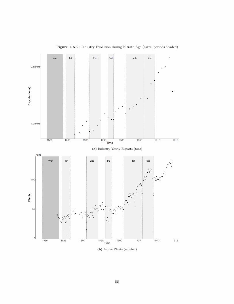
Figure 1.A.2: Industry Evolution during Nitrate Age (cartel periods shaded)

(a) Industry Yearly Exports (tons)

(b) Active Plants (number)

55

Table 1.A.1: Nitrate Exports by Country (selected years)

Exports (tons) Plants (number)Year Peru Bolivia Chile∗ Peru Bolivia Chile1855 51,900∗∗ 0 0 NA 0 01866 97,500∗∗∗ 0 97 NA 0 01872 200,943 6,164 203 18 1 01878 268,601 55,765 741 30 1 5

Sources: Cariola, Sunkel, and Sagredo (1991), O’Brien (1980),Luders, Dıaz, and Wagner (2016), Semper et al. (1908), and GodoyOrellana (2016).Note: ∗, value for Chile corresponds to output (tons).Note: ∗∗, average for period 1855-59.Note: ∗∗∗, average for period 1865-69.

Figure 1.A.3: HHI Nitrate Industry

Notes: Each bar represents the HHI index of the industry for a year. Computed using total yearly plant outputs.Notice that index is computed at the plant, not the firm level. Cartels periods are shaded.

56

ingredient in production of munitions. The allied blockade of the Central Powers (Germany and

Austria-Hungary) triggered the rapid expansion in production of synthetic nitrate of soda by those

countries, using the newly invented Haber-Bosch process. As a result of this invention and the

expansion of synthetic nitrate’s supply, after the end of World War I Chile’s monopoly had been

broken and the industry’s conditions had substantially changed.

1.A.2 Nitrate Lands Ownership

The history of the ownership of nitrate rights is complex and heavily dependent on which country

each deposit was originally located (Peru, Bolivia, or Chile). We provide a brief summary of the

main facts related to nitrate lands ownership in each of these countries.

Old Peruvian Nitrate Regions

The thin presence of the Peruvian state in the Tarapaca Province, together with the various legal

sources of ownership of nitrate rights, caused nitrate rights in this region to be poorly registered

and, in some case, disputed.

Mining laws of Peru descended from Real Ordenanza Minerıa de Nueva Espana (Royal Mining

Ordinances). Under this framework, underground resources do not belong to owner of the surface

and must be adjudicated by the state. Moreover, local authorities could grant exploitation licenses,

as a form to “promote industry”, but these were not always officially recorded. Finally, if a con-

cession was not being actively “used” by the owner, the state (or a third party) could claim it,

according to the despueble clause.

In addition, the Peruvian government implemented erratic policies regarding its nitrate industry

(hoping to protect its competing guano industry) which made even more difficult to account for

nitrate rights by the time of the Chilean occupation of the Tarapaca Province in 1880.

In chronological order, the main policies implemented by the Peruvian government were:

• 1868: Peruvian government stops granting new concessions on nitrate lands and claims for

the state all unclaimed nitrate rights.

• 1873: Peru starts a “soft” export monopoly on nitrate.57

– Government sets a fixed price at which it buys nitrate.

– Private firms can still export nitrate autonomously, but paying a larger export tax.

• 1875: Peru begins the nationalization of the nitrate industry, this process also involved several

options, depending on the willingness of the owner to sell:

– Case 1: If the nitrate plant’s owner was willing to sell.

∗ Nitrate plants would be exchanged by bonds (certificados), according to price set

by an appraisal committee.

∗ Bonds would be paid by a loan taken by the Peruvian government in the U.K., using

nitrate plants as collateral.

∗ The necessary loan could not be obtained before the outbreak of war with Chile.

– Case 2: If the nitrate plant’s owner was not willing to sell.

∗ Producer could still produce and sell his production, however paying a more onerous

export tax.

.

– Case 3: Owners of inactive plants or plants in construction.

∗ These plants were not considered by the appraisal committee. Subsequently, the

Peruvian government announce the use of the despueble clause to expropiate them.

Depending on the legal situation of the original Peruvian concession, the Chilean policy was:

• Plants with outstanding bonds or certificados would be returned to whoever was in possession

of at least 50% of the certificados.

– In many cases, this was not feasible due to the dispersion of the certificados,since many

had been “fire saled” when it became clear Peru would lose the war.

– The Chilean government auctioned in 1882 the oficinas that had not been claimed, the

proceeds of the auction were distributed between the owners of the certificados.

– In 1887, the Chilean government paid a flat conversion rate to buy all remaining out-

standing certificados.58

• Owners of oficinas that had been declared in despueble by the Peruvian government tried to

regain possession in the Chilean courts. After an initial success in 1893, the Chilean Supreme

Court declared all of their property rights to be void between 1894 and 1896

As a result, the Chilean government progressively became the owner of a large fraction of the

nitrate rights in the Tarapaca Province. Notice the main reason for this was that government

intervention was thought to be most practical way to provide clear property right to the industry.

Old Bolivian Nitrate Regions

The Bolivian territories in the Atacama Desert were far from the center of the Bolivian nation.

Communications were poor and the population of the (then called) Bolivian Litoral Department

was small and mostly Chilean. In fact, the incipient nitrate industry in the region can be described

as a Chilean-owned industry. Unlike the industry in the Peruvian Tarapaca Province, the industry

in the Bolivian territory was centered around a single firm, since the Bolivian government granted

a concession to produce nitrate, build a railroad, and gave tax-exempt status to the Antofagasta

Nitrate Company (a Chilena-British firm). After the War of the Pacific, this company continued

its operations uninterrupted.

In addition, to prevent the entry of competition to their Tarapaca Province, the Peruvian

government had commissioned Juan Meiggs in 1876 to lease some nitrate rich lands in hands of

the Bolivian government. After the War, Chile had to negotiate a settlement with the descendants

of Juan Meiggs (since the Peruvian government had promised to Meiggs rights to extract nitrate

from the leased lands). A fraction of those lands, then, were ceded to the family as part of the so

called Transaction Squire of 1883.

The rest of the government-owned nitrate lands in the former Bolivian territory were transferred

to the Chilean government as part of the peace treaty. As in the case of Tarapaca Province, the

Chilean government then became the owner of a large majority of nitrate rights in this region.

Old Chilean Nitrate Regions

A decree from 1877, granted to the discoverer of a nitrate deposit the right to claim 3 Chilean

stakes (each Chilean stake corresponds to an hectare). In most cases, entrepreneurs would then59

Table 1.A.2: Status of Nitrate Lands by 1925

Status Property Surface (km2)Exploited Private 550Measured, not exploited Private 5,811Unmeasured Public 25,000

Notes: Table shows status of nitrate lands, measured in termsof area, by 1925. Nitrate content around this period var-ied between 10% and 20%, hence surface area is informativeabout the relative amounts of nitrate contained in differentcategories. Exploited: nitrate lands already used. Measured,not exploited nitrate lands whose total nitrate content hadbeen estimated in detail, and were owned by a private firm.Unmeasured: state lands on which nitrate presence had beenestablished, but without detailed estimates of total content.Sources: Chilean Ministry of Finance (1925, p. 11).

Table 1.A.3: Nitrate Industry Ownership by Nationality

Fraction of total industry outputYear Peruvian British Anglo-Chilean Chilean German Other1878 58 13.5 - 19 8 1.51884 - 20 14 36 17 131895 - 60 - 13 8 191901 - 55 - 14 15 161912 - 38.5 - 37 15 9.5

Sources: Cariola, Sunkel, and Sagredo (1991).

have family members or associates to petition for additional rights, until a sizable property had been

acquired. In 1884, a new decree forbid new claims of nitrate rights. Finally, in 1888 the new Mining

Law declared all new nitrate deposits to be exclusive property of the Chilean state. However, a

sizable number of nitrate rights had been allocated under the previous liberal legislation.

As a summary, after the War of the Pacific, nitrate rights were held both by private en-

trepreneurs and, the largest part, by the Chilean state. Table 1.A.2 shows the estimated status of

nitrate lands, according to the Chilean Ministry of Finance, by the year 1925.

Entrepreneurs from various origins were attracted by the nitrate industry, besides the native

Chilean and Peruvian businessmen. Table 1.A.3 presents a summary of the ownership evolution of

the industry, were firm owners have been group according to their nationality.60

Nitrate tax and Government Revenues

During the War of the Pacific, the Chilean government decided to implement an export tax on

nitrate of soda. The tax rate was determined as 28 pence per Spanish quintal. A pound under

the Imperial System had 240 pence, and a Spanish quintal corresponds to, approximately, 101.44

pounds. Thus, the nitrate export tax is roughly equivalent in modern dollars to $400 per ton. The

export tax remained constant throughout the Nitrate Age in value and accounted for a significant

fraction of the price of nitrate.

In addition, the Chilean government periodically sold rights to extract nitrate in state-owned

lands. However, this revenue was only equivalent to 3% of the export tax revenue (Chilean Ministry

of Finance, 1925). Nitrate lands auctions seem to have been motivated by the opportunity of

obtaining a good selling price, given high demand for nitrate lands, as explained on one of the bills

submitted to the Chilean Congress:62

It is in the interests of the [Chilean] state to dispose of some of its nitrate properties

that can be sold under advantageous conditions, without disturbing the prosperous state

the nitrate industry presents today . . . Making the auction of the properties referred to

in this bill, the government has the purpose of not offering new nitrate lands for sale

but in accordance with the interests of the industry . . . which will lead to considerable

advantages for the state as well as for private interests.

Government attitude towards Nitrate Cartels

During the Nitrate Age there was no systematic antitrust concern on the part of the Chilean

authorities. The Chilean legislation did not forbid or regulated cartels or trusts (the first antitrust

legislation was not promulgated until 1959 (Bernedo, 2013). In addition, government policy regard-

ing combinations was influenced by laissez faire ideology that predominated at the time among the

Chilean elite. Moreover, Chilean consumption of nitrate of soda remained negligible with respect

to the total volume of product sales. Hence, consumer surplus considerations were absent from the

policy discussions regarding competition in this market.62Bill presented by Chilean Government on March 2nd 1902. Proyecto de Lei que autoriza enajenacion de ciertos

terrenos salitrales (Republica de Chile, 1903). Bill message cited from NPA Quarterly Circular, Number 27, April21, 1902, p. 7.

61

Although the use of a per-volume tax made cartels to have a negative effect on short-term tax

revenues, other factors partially balanced this concern. First, the sheer importance of the industry

made crisis in the nitrate sector highly damaging to the whole Chilean economy. Hence, cartels

were regarded as a policy tool, that helped to ensure the stability of the wider economy. As an

example, Chilean financial sector provided short and long-term finance to the nitrate industry, hence

cartels were favoured by them, as decreased the risk on their loans (O’Brien, 1982). Second, during

the decade of the 1900’s, mode Chilean entrepreneurs became directly involved in the industry as

owners. A large fraction of them were also members of Congress or held high political offices. Thus,

the private interests of part of the elite partially counterbalanced the fiscal interest of the republic.

As a consequence, the attitude of Chilean government towards the organization of cartels changed

on time and depended of the specific short-term economic and political circumstances (Brown,

1963).

Appendix 1.B Data

Table 1.B.1: Summary Statistics Prices UK (£/ton)

Statistic Nitrate of soda Ammonium sulfate Beet sugar IodineN 407 408 408 398Mean 10.0 12.5 12.4 1,097.9St. Dev. 1.8 3.0 4.2 272.0Min 6.8 6.8 5.8 587.9Pctl(25) 8.7 11.0 9.2 881.8Median 9.7 11.9 11.2 1,102.3Pctl(75) 11.0 12.8 14.1 1,322.8Max 18.7 21.8 30.2 2,131.1

Sources: The Economist, Chemical Trade Journal.

62

Figure 1.B.1: Coverage Main Data Sources

Notes: Vertical values represent the two main sources of plant-level data. Horizontal axis is time. Each black barcorresponds to a month of data.

Figure 1.B.2: Weekly Nitrate Prices in U.K. by Source

Notes: Vertical axis is prices in contemporaneous pounds. Horizontal axis is time. Observations obtained from TheEconomist are in black, while observations from the Chemical Trade Journal are in grey.

63

Figure 1.B.3: Monthly Nitrate Prices in the U.K and Chile

Notes: Vertical axis is prices in contemporaneous pounds. Horizontal axis is time. Prices in the U.K. arein black,while prices in Chile are in grey.

64

Figure 1.B.4: NPA Monthly Output Statistics (June 1900)

Notes: Periodic publication of the NPA. Each row corresponds to a nitrate plant. Output expressed in metric quintals.Obtained from the Chilean National Library, Santiago, Chile.

65

Figure 1.B.5: Nitrate Agency Monthly Report (November 1899)

Notes: Periodic publication of the Nitrate Agency. Each row corresponds to a nitrate plant. Output expressed inSpanish quintals. Obtained from the Tarapaca Regional Archives, Iquique, Chile.

66

Figure 1.B.6: Second Cartel Contract

Sources: Chilean National Notarial Archives, Santiago, Chile. Iquique Notaries. Volume 132.

67

Appendix 1.C Additional Tables

Table 1.C.1: Logit Regression ShutdownProbability

Dependent variable:Plant shutdown

lagged(Workers) −1.030∗∗∗(0.060)

lagged(Animals) 0.194∗∗∗(0.057)

Constant 2.668∗∗∗(0.171)

Observations 10,349Log Likelihood −3,738.645Akaike Inf. Crit. 7,483.289

Notes: Robust standard errors in paren-theses. Observations are plant-months.Plant shutdown takes value of 1 if theplant was inactive in a given month butis observed in operation later in the data.

Table 1.C.2: Chi-Square Test

Number intervals:Two Three8.56 7.26(1) (2)

Notes: Degrees offreedom in paren-theses.

68

Table 1.C.3: Regression Prices U.K. and Chile

Dependent variable:Nitrate price UK

Nitrate price Chile 0.957∗∗∗(0.027)

Constant 3.399∗∗∗(0.172)

Observations 250R2 0.809Adjusted R2 0.809Residual Std. Error 0.553 (df = 248)F Statistic 1,053.463∗∗∗ (df = 1; 248)

Note: ∗p<0.1; ∗∗p<0.05; ∗∗∗p<0.01Notes: Robust standard errors in parentheses. Obser-vations are monthly prices.

Table 1.C.4: Discretization of Nitrate Price (pt)

Interval Lower bound (£/ton) Upper bound (£/ton)p1 4.44 5.32p2 5.32 5.91p3 5.91 6.74p4 6.74 7.57p5 7.57 9.35

Table 1.3.8: Summary Statistics Observed Plant Values

Statistic Periods observed Discounted value ($) Mo. Profit ($)N 148 148 28,084Mean 214 33,802,826 378,945St. Dev. 119 37,172,924 506,587Min 10 -7,936,688 -6,461,858Pctl(25) 106.5 9,364,678 0Median 214 20,687,580 226,831Pctl(75) 342.2 47,631,551 566,686Max 381 224,558,616 6,274,296

69

Table 1.3.9: Parameters Cost Function Estimation

Variable Description Value Unitsε Exchange rate 16 p/CLP$w Monthly average wage 90 CLP$canim Monthly cost per animal 30 CLP$ccoal Coal price 1.55 CLP$/SPQT Export tax nitrate 28 p/SPQcpack Packaging cost 2 p/SPQcport Port services cost 1 p/SPQcrail Railroad cost 3.5 p/SPQcadm Plant administration costs 1.5 p/SPQcadv Contribution to nitrate advertising 5/16 p/SPQ

Notes: p: pence (1900); CLP$: Chilean peso (1900); SPQ: Spanish quintal.Sources: Semper et al. (1908).

Table 1.3.10: Parameters Entry Costs Estimation

Variable Description Value Unitsβ Discount factor (yearly) 0.92cl Cost nitrate reserves 2 p/SPQck1 Capital cost interval 1 1 £1900/SPQck2 Capital cost interval 2 18/20 £1900/SPQck3 Capital cost interval 3 3/4 £1900/SPQ

Note 1: p: pence (1900); CLP$: Chilean peso (1900); SPQ: Span-ish quintal.Note 2: In capital cost parameters, SQP refers to monthly produc-tion capacity measured in this unit.Sources: Semper et al. (1908).

Table 1.3.11: Parametersused for Currency Conversion

Exchange rate Value£2018/£1900 120.74US$/£2018 1.22

Sources: boe˙exchange,boe˙inflation.

70

Table 1.3.12: Discretization of Productivity types

Number of groups:5 groups 3 groups

Productivity group Lower bound Upper bound Lower bound Upper boundφ1 10.2 32.6 10.2 36.2φ2 32.6 39.0 36.2 50.4φ3 39.0 45.2 50.4 97.1φ4 45.2 55.3 - -φ5 55.3 97.1 - -

Table 1.3.13: Discretization of Capacity types (tons)

Capacity groups:Group 1 bounds Group 2 bounds Group 3 bounds

Prod. group Lower Upper Lower Upper Lower Upperφ1 39.2 342.0 342.0 759.0 759.0 1217.9φ2 215.7 664.4 664.4 895.6 895.6 1439.2φ3 182.4 736.7 736.7 1221.6 1221.6 2967.8φ4 595.7 976.1 976.1 1722.4 1722.4 4033.8φ5 222.4 2032.0 2032.0 3045.3 3045.3 5605.0

71

1.4 Additional Figures

Figure 1.4.1: Net-entry of Plants during Nitrate Age

Notes: Vertical axis is plants (number). Horizontal axis is time. Net-entry computed as plants that enter minusplants that exit in a given month. Cartel periods are shaded.

Figure 1.4.2: Exiting Plants during Nitrate Age

Notes: Vertical axis is plants (number). Horizontal axis is time. Exiting plants variable determined by the lastobservation of an establishment in the data. Cartel periods are shaded.

72

Figure 1.4.3: Comparison Plant Productivity Estimates

Notes: Vertical axis is productivity after implementation of correction by selection. Horizontal axis is productivitybefore implementation of correction by selection. Each point corresponds to a plant.

Figure 1.4.4: Productivity vs residuals (points) for Plants with more than 95 observations

Notes: Each plot corresponds to a plant. Horizontal axis is time. Plant FE is plotted as an horizontal line. Estimatedresiduals plotted as points.

73

Figure 1.4.5: Relation between Energy Input and Nitrate Output in Refining Stage

Notes: Each point is a plant-month observation. Horizontal axis is coal usage (tons). Vertical axis is nitrate output(tons).

Figure 1.4.6: Estimated Plant Productivity vs Time of Entry

Notes: Each observation corresponds to a plant. Horizontal axis is time. Vertical axis is productivity.

74

Figure 1.4.7: Estimated Monthly Profits by Productivity Type

Notes: Each point corresponds to a plant-month observation. Horizontal axis is time. Vertical axis is profits currentdollars.

Figure 1.4.8: Seasonality of Monthly Output by Productivity Type

Notes: Horizontal axis are months of the year. Vertical axis is nitrate output (tons). Each line corresponds to theaverage nitrate output per productivity type in a given month.

75

Figure 1.4.9: Plant Values Net of Entry Costs: 4th & 5th Cartels

Notes: Each point corresponds to a plant. Horizontal axis is moment of entry (time). Vertical axis is estimated valuein current dollars.

Figure 1.4.10: Observed and Counterfactual Industry Output

Notes: Horizontal axis is time. Vertical axis is nitrate output (tons). Continuous line is the observed industry output,while the dashed line is the counterfactual output, computed as a cubic spline.

76

Figure 1.4.11: Observed (continuous line) and Counterfactual Number of Plants

Notes: Horizontal axis is time. Vertical axis is number of plants. The continuous line represents the observed numberof plants in the industry, while the dashed line represents the counterfactual number of plants.

Figure 1.4.12: Observed (continuous line) and Counterfactual Industry Capacity

Notes: Horizontal axis is time. Vertical axis is industry capacity. The continuous line represents the observed numberof plants in the industry, while the dashed line represents the counterfactual industry capacity.

77

Figure 1.4.13: Observed (continuous line) and Counterfactual Mean Industry Productivity

Notes: Horizontal axis is time. Vertical axis is productivity. The continuous line represents the observed meanproductivity in the industry, while the dashed line represents the counterfactual mean productivity.

Figure 1.4.14: Observed and Counterfactual Productivity Distributions

Notes: Productivity distributions of entrants during Fourth and Fifth Cartels. Observed distribution is shown inlighter shade, while counterfactual distribution is shown in darker shade.

78

Chapter 2

Learning-by-colluding: Experience

and Efficacy of Cartels in the Chilean

Nitrate Industry

This paper studies the degree to which experience helps firms to organize successful cartels. Between

1884 and 1909, Chilean producers of nitrate of soda organized cartels on five separate occasions

which allow us to explore how collusive agreements evolved as producers accumulated experience in

their organization. Our setting has absence of antitrust regulation and perfect monitoring, which

translated in completely public cartels. Thus, unlike most of the previous literature on cartels,

issues related to monitoring and enforcement were of secondary importance with respect to the

challenge of allocating the collusive surplus among the colluding firms. We document that cartel

contracts gradually became more complete, generated a smoother transition from competition to

collusion, and that producers eventually discarded inefficient methods of market share allocation,

associated to larger production costs, in favor of better alternatives.79

2.1 Introduction

Although cartels are ubiquitous and very costly in terms of economic efficiency little is known about

the process of cartel organization that eventually leads to the organization of successful cartels

and the role of learning-by-doing in it. Do firms intuitively “know” how to optimally organize

collusion once an opportunity arises? Or, alternatively, do firms learn as they go about cartel

organization? Shedding light on these questions could greatly help prevention, detection, and the

design of remedial measures for detected cartels.

We use the Chilean nitrate industry between 1880 and the First World War to explore this

research question. Over this extended period of time nitrate producers organized cartels on five

separate occasions. Moreover, collusion was both legal and public, which allow us to use sources of

qualitative evidence not distorted by the fear of prosecution.

We find that collusive agreements in this industry gradually became more complex and complete,

incorporating new contractual dimensions such as regulating firms’ behavior during the transition

to collusion. Moreover, through a process of experimentation that lasted for four cartel episodes,

the producers were able to discard inefficient market share allocation methods. Furthermore, we

are able to show using counterfactual simulations that the discarded methods increased production

cost at least by 10%. Finally, we are able to document the process by which producers converged

to a system of periodic fixed-term collusion episodes instead of organizing a permanent cartel.

Ours is, to the best of our knowledge, the first paper to document the dynamic learning process

leading to the organization of a successful cartel. Our rich sources allows us to describe the evolution

of producers’ understanding about relevant contractual dimensions and to trace how they dealt with

challenges that affected the cartel’s efficacy through contractual innovations. In addition, our paper

identifies a novel mechanism that hampers the organization of collusion in durable goods markets:

the preemptive cheating motive. Finally, this papers contributes to our knowledge about the role

of trade associations as cartel facilitators, especially in industries with a large number of producers

and to explain the existence of periodic episodes of collusion, which have been observed in a wide

variety of industries.

Main among the reasons for our lack of knowledge about learning in cartel organization is that

cartels in most of the developed word have been illegal since about the end of WW2. Even when80

a cartel is exposed, it is safe to assume that the discovered evidence has been distorted in order

to limit the potential future legal liabilities, which makes very hard to address this question in a

modern setting.

We are able to surpass this challenge due to the fact that nitrate cartels were legal and public,

which made possible the survival of a large number of truthful qualitative sources that include full

texts of the implemented collusive agreements, the minutes of producers’ meetings, and the periodic

publications of their trade association. We supplement this evidence with newly assembled data,

including the detailed output and export statistics at the plant level.

Several features of this industry make it especially suitable for studying cartel organization.

Nitrate of soda was the main fertilizer used at the time, and Chile was the sole producer. Since

the domestic market for the product was negligible, every industry stakeholder in Chile was funda-

mentally concerned only about the maximization of producer surplus. The production process of

nitrate was simple and the technology remained without significant changes. Finally, the product

was completely homogeneous across firms.

The remainder of the paper is organized in the following way. Section 2.2 describes the main

relevant features of the industry; Section 2.3 presents the main characteristics of the nitrate cartels

and, specifically, their contract and their evolution; Section 2.4 outlines the data sources and

presents summary statistics; The main aspect of learning, the allocation of collusive market shares,

is explored in section 2.5; Finally, Section 2.6 describes two other important dimensions of learning:

The regulation of transition from competition to collusion, and the choice of fixed-terms agreements

and inter-cartel bargaining instead of permanent cartels with flexible market share allocation.

2.2 Industry Background

2.2.1 Historical development and industry characteristics

The period between the annexation by Chile of the nitrate rich territories of Peru and Bolivia

during the War of the Pacific (1879-84) and the outbreak of WWI was the zenith of the nitrate

of soda industry. During this period, nitrate of soda, became the main commercial fertilizer used

in the world: By 1900, nitrate of soda represented two thirds of the world’s total supply of com-

mercial fertilisers (Wisniak and Garces, 2001). Moreover, nitrate of soda almost instantly turned81

Table 2.2.1: Evolution of Nitrate Industry

Year Plants (number) Output (thous. of tons) Workers (thous.)1882 43 492 7.11887 57 713 7.21892 - 804 13.51897 42 1,187 16.71901 66 1,329 20.31906 96 1,822 -1910 102 2,465 43,51914 137 2,463 44,0

Sources: Cariola, Sunkel, and Sagredo (1991), Semper et al. (1908), and GodoyOrellana (2016).

into the most important export and source of revenue for the Chilean government, accounting for

approximately 65% of exports.1. Hence, this period of Chilean history is often called the Chilean

Nitrate Age.

Nitrate of soda is a natural fertilizer used to transfer nitrogen to the soil. The only commercially

viable deposits in the world were found in the newly acquired Chilean provinces of the Atacama

Desert (Vicuna, 1931).2 It was an homogeneous product and its main uses were as a fertilizer,

which accounted for roughly three-quarters of consumption, and as an input in the manufacture of

explosives.3 The closest available substitute during this period was sulphate of ammonia.

Nitrate was produced by private firms, in purposefully built plants located on the desert. Figure

2.2.1 shows La Patria nitrate plant, as a representative example. The basic configuration of a nitrate

plant consisted of a central refining facility, placed in the midst of the nitrate-bearing grounds that

would feed it.4 The packaged nitrate would then be dried and stored near the refining facility,

before its transportation via railroad to the nearest port. In a standard transaction, producers

would sell ready for export nitrate at the port. Traders would then transport it by boat to the

consuming markets of Western Europe and the United States.

The nitrate industry featured a large number of firms and experienced a constant expansion1Computed from Cariola, Sunkel, and Sagredo (1991, p. 139) as average of nitrate participation on exports in

years ended with 0 or 5 during the Nitrate Age2The provinces were Tarapaca (previously owned by Peru), and Antofagasta, shared between Bolivia and Chile

before the War).3It was sold in two versions: Ordinary (95% purity) and refined (98% purity), with ordinary constituting almost

all of output.4The only exception to this configuration was the Antofagasta Company before 1907, which used instead a central

refining facility in the port of the same name.

82

Figure 2.2.1: Nitrate Plant Example: Bearnes Plant

Sources: Boudat (1889).

83

during the Nitrate Age. Table 2.2.1 presents basic statistics regarding the industry evolution during

our period of interest. As a consequence of the large number of firms,5 the industry had persistent

low levels of concentration. For instance, in 1901 the largest firm had a market share of 6.4%, while

in 1907 the largest market share was 7.6%. Firms were owned mostly by British, German, and

Chilean entrepreneurs.

A distinct industry characteristic is that demand and prices were very volatile. This came as

a result of three market characteristics (Bertrand, 1910). First, most nitrate was used during the

European harvest season, between March and June of each year, which corresponded to about

90% of the agricultural consumption of nitrate. Second, the European demand had high variance

depending on current year’s weather shocks. Third, the large distance between Europe and Chile

meant nitrate producers were not able to react to same-year demand shocks,6 since nitrate produc-

tion, due to economies of scale, was bound to be year-round. These patterns are summarized in

Figure 2.2.2. This situation was reinforced by the fact nitrate intermediaries did minimum storage,

because of the financial risks associated to its wide fluctuations in price.

The Chilean government implemented a nitrate policy based on two pillars: private-ownership

of the industry with low regulation, inspired by laissez faire principles; and heavy taxation using a

per-unit export tax of, approximately, 2.54 pounds sterling per ton exported (this corresponds to

about $400 per ton, in current dollars) (Brown, 1963).7 At the same time, the nitrate export tax

became the most important source of government revenues explaining, on average, 45% of total tax

revenues between 1885 and 1914 (Chilean Ministry of Finance, 1925).

The great economic and fiscal importance of the industry motivated the development of the

Nitrate Agency,8 a specialized state institution solely tasked with monitoring the industry’s op-

eration and development. Among its most important tasks, were to establish government policy5Some firms owned more than one plant. Most of the firms that entered during our main period of interest were

single-firm plants.6Semper et al. (1908) estimates average times of travel of 90 to 100 days for sailboats and 45 to 65 days for

steamboats.7Figures regarding nitrate export tax also include the export tax collected on iodine exports. Iodine is a sub-

product of the elaboration of nitrate of soda.8The name of the agency in Spanish was Delegacion Fiscal de Salitreras y Guaneras. It was based on the city of

Iquique, main city of the Chilean nitrate region. Immediately after the occupation of the Peruvian nitrate territories,in December 1879, the Chilean government named a general representative to the region to oversee the territory,including its nitrate industry (Ministerio de Hacienda, Chile, 1880, p. 46). A specialized General Inspectorate ofNitrate (In Spanish, Inspeccion General de Salitreras) existed by 1885 (Ministerio de Hacienda, Chile, 1885, p. 395).Finally, in 1889, the Chilean government increased the budget and rank of its nitrate agency, obtaining the nameand features that would persist until 1914.

84

Figure 2.2.2: Industry-level Output and Consumption

Notes: Monthly industry-level output (dashed line) and consumption (continuous line) between the years 1905 and1908.

towards the industry, the collection of industry and plant-level statistics, and the management of

government-owned nitrate assets, particularly state-owned nitrate lands.

The First World War fundamentally changed the market for nitrate of soda, 9 as Chile lost its

monopoly on nitrate of soda due to the invention of the Haber-Bosch method for production of

synthetic nitrate. The effects of this event for the Chilean nitrate industry were devastating, never

recovering its previous levels of profitability.

2.3 Nitrate Cartels and Learning

2.3.1 General Description

Nitrate of soda producers formed cartels on five separate occasions (see Table 2.3.1) to take ad-

vantage of their joint market power in the fertilizer world market.10 These cartels lasted from a9The breakout of the war, also greatly disrupted the industry, as the blockade of the Central Powers closed overnight

some of the most important export markets at the same time as the industry experienced a positive demand shock,driven by sales to the Allied powers.

10For instance, during a competitive period, a nitrate producers’ publication reads, “Currently, it can be said theindustry is producing as much as it is allowed by the potency of the elements at its disposal . . . On the other hand, isthe conviction of every and each producer that today they deliver their valuable product . . . depressed by at least ashilling in the price consumers can still pay at great advantage for their economy . . . The result, therefore, of sound

85

Table 2.3.1: List of Nitrate Cartels

Cartel Start Date End Date Early terminationFirst 1884-August 1886-December NoSecond 1891-March 1894-March NoThird 1896-April 1897-October YesFourth 1901-April 1906-March NoFifth 1906-April 1909-March No

Notes: Early termination indicates whether the End Date corresponds tothe original termination date agreed on collusive contract, or if an earlytermination clause of the collusive contract was invoked. Sources: Brown(1963).

minimum of seventeen months to a maximum of five years, and had almost unanimous participa-

tion among nitrate firms. Moreover, the start of the first three cartels followed drops in the nitrate

price.

All nitrate cartels share some distinctive features. First, before the start of each cartel, a

collusive contract would be signed by all participating producers, stipulating all the relevant rules

that would govern its operation. Second, as a result of the absence of any antitrust legislation at

the time in Chile, they were completely public (including their contracts) and the large importance

of the industry guaranteed their actions received a great deal of attention by the press and the

general public. Third, nitrate producers’ limited capacity to respond to contemporaneous demand

shocks, due to their long time-to-market, made unpractical for them to try to directly set the price

of nitrate of soda. As a result, all nitrate cartels were limited to being quantity-setting agreements.

The management of the nitrate cartels, given their large number of firms and their geographic

dispersion, required the existence of a executive body with enough power to make operational

decisions in short order. The first two cartels were managed by a board of producers (denominated

Nitrate Committees) elected by cartel members after the signature of the collusive agreement. In the

first two cartels the group of producers that promoted their organization were heavily represented

in their cartel boards. A pivotal change in the organization of the industry was the creation in

1894 of a permanent trade association, called Nitrate Propaganda Association (NPA from now on)

which took over and expanded the staff and organization developed during the Second Cartel after

advice and mere commercial foresight would be to agree on a formula under which all [producers] consulted theirinterests and marched together in pursuit of own and general welfare (NPA, 1899, p. 6).”

86

Figure 2.3.1: Industry yearly output (tons)

Notes: Yearly industry output shown as circles (triangles) for competition (cartel) years. Dashed line presents anon-parametric trend, computed only using industry output observed during years in competition. Cartel periodsare shaded. Texts correspond to cartel number by chronological order and to the War of the Pacific period.

its conclusion in 1894. The NPA retained from the initial cartels an elected board of producers

(elected for one-year terms) as its governing body but its reach was limited mostly to strategic

aspects, leaving day-to-day operations in hands of its manager and a permanent professional staff.

Starting from the Third Cartel, the NPA manager was the main organizer of the successive nitrate

cartels.

Regarding the effects of nitrate cartels, as an illustration, Figure 2.3.1 shows the industry yearly

output, together with a trend that considers only years with free competition, showing that output

during cartel years were always below what it could be expected given the previous trend of output

during competition.

On the other hand, Table 2.3.2 summarizes the effect cartels had on aggregate industry output.

On this Table, the dependent variable is monthly industry-level output, while the main independent

variables of interest are individual cartel dummies. The regression also includes dummies related

to high and low-demand seasons and a time trend. The main result from Table 2.3.2 is that going

from competition to cartel was correlated with an average industry output reduction of around87

18%.

2.3.2 Relevant Dimensions of Learning

A successful cartel must solve four fundamental organizational issues: monitoring and enforcement,

resistance from related firms and authorities, bargaining, and entry.11

The special characteristics of this industry’s physical and institutional environment made the

nitrate industry to develop in a perfect-monitoring setting. Nitrate production was the only eco-

nomic activity developed in the Atacama Desert and all plants, grouped in distinctive districts, were

situated nearby from each other, sharing the same railroad networks to transport their outputs to

port. Moreover, the sheer importance of the industry ensured that the Chilean state developed

monitoring institutions that could compile public statistics and prevent the evasion of the nitrate

export tax. As mentioned above, nitrate producers followed the lead of the Chilean state and used

the NPA as an statistical agency for monitoring purposes. As an example of the detailed monitoring

system put in place by the NPA, Figure 2.B.1 shows an example of the Nitrate Shipment Magazine,

published by the NPA from at least 1894, which contained information on all nitrate shipments

made from Chile in a given month, including the firm of origin, quantity exported, name of the

ship, and destination.

In addition, there is evidence that nitrate cartels had effective tools to enforce the fulfillment

of their agreements. Although nitrate cartels were based on legal contracts to the best of our

knowledge there is no evidence of litigation associated to contract infringements. However, there is

narrative evidence that failing to comply with cartel rules would translate into a strong retaliation:1213

To a person not resident in Iquique it is difficult to realise the power which the Nitrate

Committee possess.14 Firstly, they have the support and are recognised . . . by the

Republic. Secondly, the object of the combination, the banking interest, and of all11McAfee and McMillan (1992). Bargaining, refers to the division of the collusive surplus among the cartel members;

Entry corresponds to the presence of new producers, tempted by the large profits generated by the cartel; Monitoringand enforcement, corresponds to the mechanisms by which the cartel agreement will prevent cheating; and resistancefrom firms and authorities, relates to the potential actions that firms on the other side of a market and to enforcementby antitrust agencies.

12Russell (1890, p. 333)13See additional supporting evidence related to the power cartels had in Appendix 2.B.14Note: written as “Comite Salitreros” [sic] in the original text.

88

Table 2.3.2: Cartel Effects Regression

Dependent variable:log(Nitrate Output)

(1) (2)Cartel −0.187∗∗∗

(0.031)Cartel 1 −0.549∗∗∗

(0.084)Cartel 2 −0.045

(0.053)Cartel 3 −0.019

(0.095)Cartel 4 −0.137∗∗∗

(0.022)Cartel 5 −0.167∗∗∗

(0.029)Time 0.0002∗∗∗ 0.0002∗∗∗

(0.00001) (0.00001)High season −0.031 −0.020

(0.051) (0.045)Low season −0.042 −0.047

(0.040) (0.038)Constant 16.426∗∗∗ 16.184∗∗∗

(0.132) (0.145)Observations 404 404R2 0.818 0.841Adjusted R2 0.817 0.838

Notes: Robust standard errors in paren-thesis. Observations correspond tomonths at the industry level. Carteltakes the value 1 if any cartel was ac-tive, and 0 otherwise. Cartel 1 takesthe value 1 if First Cartel was active,and 0 otherwise. Additional indica-tor variables for individual cartels fol-low the same logic.∗p<0.1; ∗∗p<0.05;∗∗∗p<0.01.

89

Figure 2.3.2: Example of Monitoring: Nitrate Shipment Magazine (February 1895)

Notes: The Nitrate Shipment Magazine (Revista del Carguıo de Salitre) was a monthly publication of the NPA fromat least 1895 until 1929. It summarized all the nitrate shipments made in Chile, including the producer of origin,quantity of nitrate, ship name, date of shipment, port of origin, and port of destination. Source: Vol. 2659, Ministryof Finance Collection, Chilean Historical Archives.

90

trade depending on the manufacture of nitrate, are so closely bound together, that a

fiat issued with regard to any firm or individual who has persistently offended against

the Articles of Association means to them immediate ruin. The form or individual is

treated as one whose signature is not worth the paper it is written upon; he or they are

in every form boycotted.

These characteristics that promoted “good behaviour” on the part of cartel members were

reflected in a very small number of deviations from the agreed-upon firm level quotas. For instance,

by the end of the first year of the Fourth Cartel only 5 plants had excess output over their quotas,

for an amount equivalent to less than 0.15% of the total industry quota.15 During the second year

of the same agreement, the deviations were even smaller. 16

Finally, the absence of antitrust legislation in Chile meant that the usual concerns colluding

firms face when organizing collusion regarding detection and potential antitrust litigation were

absent from this setting. Furthermore, local consumption of nitrate in Chile was negligible. Hence,

authorities had no local consumer surplus to protect from the high prices induced by the cartel.

As a result, in contrast to a large fraction of the cases studied in the previous literature, in the

nitrate cartels the challenges faced by producers were mostly related to the issues of bargaining and

entry. The focus of this paper is to describe the learning process associated to bargaining problems

while a companion paper17 studies how entry affected these cartels and the solutions implemented

by incumbent nitrate producers. Besides the topical differences between the two papers there is

also a chronological distinction: The bulk of the learning related to bargaining occurred during

the first three cartels, while the entry problem became crucial fundamentally during the last two

cartels.

15NPA (1902, p. 6).16“The only excesses over the quotas established by the agreement were:

Output: Aguada plant, owned by Compania Comercial y Salitrera La Aguada. . . 1,836 Sp. quintals.Exports: Progreso plant, owned by Evaristo Quiroga and Bro. . . . 1,627 Sp. quintals.Although their insignificance suggest that these violations were involuntary errors, the producers have been fined asstipulated in articles 15 and 16 of the contract . . . ” NPA (1903, p. 4).

17Carrera and Titov (2019).

91

2.3.3 Evolution of Nitrate Cartel Contracts

Nitrate cartel contracts exhibited a relevant evolution.18 As nitrate producers gained more practical

experience at the organization of cartels they incorporated clauses about additional contractual

dimensions, making contracts more complete. Table 2.3.3 summarizes this trend. Quantitative

measures of the length of the contracts together with qualitative description of the new topics

added in each of them show the collusive contracts’ increasing complexity. Specifically, cartels

organized by the NPA are at least twice as long as the firsts two agreements an incorporated

regulations in topics that were perceived as greatly damaging to the success of previous cartels

(e.g., regulation of transition to collusion). Moreover, after the success of the Fourth Cartel there

was a remarkable degree of continuity in the contract used in the Fifth Cartel.

In terms of structure, the contracts also had a clear evolution: A large fraction of the First

Cartel contract described the attributions and tasks of the Nitrate Committee, while at the same

time setting only very general rules for the cartel itself; the Second Cartel contract reads included

rules that were conditional on a satisfactory conclusion of the negotiations and left the regulation

of some aspects of the cartel to a general meeting to be held after the agreement was signed. On

the other hand, all cartel contracts negotiated under the umbrella of the NPA share a common

structure.

2.4 Data and Summary Statistics

We use two main sources of data: All the collusive agreements signed by the nitrate cartels between

1884 and 1909, and a monthly plant-level panel dataset describing the output of each nitrate plant

between 1883 and 1914. Table 2.4.1 describes the location of our main sources.

The cartel contracts were collected from the National Notarial Archives and other sources

located in the National Library of Chile. Figure 2.4.1 presents an example of a cartel contract.

Our output data was compiled from two main contemporaneous sources. The first corresponds

to monthly plant-level industry reports compiled by the Nitrate Agency, which cover the period

1883 to 1909, and include nitrate output, exports, and stocks, in addition to input data. We are

able to collect spreadsheets for 228 months over this period, with 15, 804 observations. The second18To see the full text of the contracts and their translation go to the Appendixes.

92

Figure 2.4.1: Second Cartel Contract

Sources: Chilean National Notarial Archives, Santiago, Chile. Iquique Notaries. Volume 132.

93

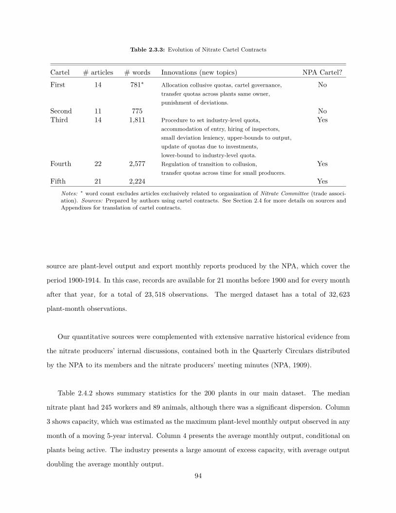
Table 2.3.3: Evolution of Nitrate Cartel Contracts

Cartel # articles # words Innovations (new topics) NPA Cartel?First 14 781∗ Allocation collusive quotas, cartel governance, No

transfer quotas across plants same owner,punishment of deviations.

Second 11 775 NoThird 14 1,811 Procedure to set industry-level quota, Yes

accommodation of entry, hiring of inspectors,small deviation leniency, upper-bounds to output,update of quotas due to investments,lower-bound to industry-level quota.

Fourth 22 2,577 Regulation of transition to collusion, Yestransfer quotas across time for small producers.

Fifth 21 2,224 YesNotes: ∗ word count excludes articles exclusively related to organization of Nitrate Committee (trade associ-ation). Sources: Prepared by authors using cartel contracts. See Section 2.4 for more details on sources andAppendixes for translation of cartel contracts.

source are plant-level output and export monthly reports produced by the NPA, which cover the

period 1900-1914. In this case, records are available for 21 months before 1900 and for every month

after that year, for a total of 23, 518 observations. The merged dataset has a total of 32, 623

plant-month observations.

Our quantitative sources were complemented with extensive narrative historical evidence from

the nitrate producers’ internal discussions, contained both in the Quarterly Circulars distributed

by the NPA to its members and the nitrate producers’ meeting minutes (NPA, 1909).

Table 2.4.2 shows summary statistics for the 200 plants in our main dataset. The median

nitrate plant had 245 workers and 89 animals, although there was a significant dispersion. Column

3 shows capacity, which was estimated as the maximum plant-level monthly output observed in any

month of a moving 5-year interval. Column 4 presents the average monthly output, conditional on

plants being active. The industry presents a large amount of excess capacity, with average output

doubling the average monthly output.94

Table 2.4.1: Summary of Data Sources

Data SourcesPrices UK The Economist, Chemical Trade JournalPrices Chile Nitrate Agency, NPACost parameters Semper et al. (1908)Plant characteristics Narro (several issues), Boudat (1889)1st Cartel contract Comite Salitrero (1884)2nd Cartel contract National Notarial Archives. Iquique Notaries. Volume 132.3rd Cartel contract National Notarial Archives. Iquique Notaries. Volume 141.4th Cartel contract NPA (1900)5th Cartel contract Semper et al. (1908, p. 321)

Table 2.4.2: Summary Statistics: Nitrate Plants

Statistic Workers Animals Capacity (tons) Avg. output (tons)N 176 178 200 200Mean 289 103 3,494 1,703St. Dev. 179 64 2,861 1,239Min 5 2 30 18Pctl(25) 167 57 1,610.2 932Median 245 89 2,663.7 1,337Pctl(75) 383 139 4,267.1 2,161Max 1,038 309 15,647 6,721

Notes: Capacity estimated as maximum monthly observed output in moving periodof five years (observations from year 1896 were dropped). Workers, animals, capac-ity, and average output correspond to mean monthly values, excluding zero outputobservations. Sources: Authors’ calculations using main dataset.

95

Table 2.5.1: Cartel Market Shares Allocation Methods

Method DescriptionTime Mandatory shutdown for predetermined

number of months each year.Trial Determination of capacity according to output

during a “trial period” after negotiations.Past-output Determination of capacity based on previously

realized outputs.Theoretical capacity Determination of capacity based on assessment of theoretical

production capacity by experts.

2.5 Allocation of Cartel Market Shares

The allocation of collusive market shares was the main challenge that nitrate producers faced when

trying to implement stable cartels. In consequence, this was the contractual aspect that received

by far the most attention, as it was explicitly declared by the NPA:19

“The main challenge for a cartel resides in finding an adaptable formula, permanent in

a way, that allows the survival of all the plants through an agreement that limits the

output of each of them in harmony with some general requirements, including those

originated by the cartel’s own existence. ”

In particular, producers hoped to find a way of allocating production under collusion that

ideally: (i) satisfied the incentive compatibility restrictions of all the producers, so that they will

decide to join the cartel; (ii) was perceived as “fair”; (iii) did not introduce additional production

costs (iii); (iv) did not provide incentives for new investments.

Several methods for allocating market shares under collusion were used: direct negotiation of

market shares, the periodic suspension of production for a fixed length of time each year (which will

be referred to as “time-method”), and three methods based on assessing the production capacity of

each plant, which we collectively denominate as “capacity methods”: the trial, past-outputs, and

theoretical capacity methods. Table 2.5.1 and Figure 2.5.1 present a description of the methods

and the cartels when they were used.

Notice that the methods tried by the nitrate producers inherently emphasize only subset of19NPA (1898a, p. 4)

96

Figure 2.5.1: Allocation Methods used by Nitrate Cartels

their objectives. Thus, using each method presented the producers with a different trade-off. For

instance, the time method generates a perfectly proportional reduction in output across produc-

ers (maximizing the “fairness” objective) and it does not induce investments. However, imposes

additional costs associated to periodical shutdowns and an inefficient scale of production.

Given that the quota-allocation method was the central feature that made each nitrate cartel

unique, next we provide a chronological description of each cartel.

2.5.1 First Cartel: Early theoretical-capacity Method

The First Cartel operated between August of 1884 and the end of 1886. Its beginning is related

to a sharp reduction in nitrate prices due to the end of the War of the Pacific. A general meeting

of producers determined that collusive market share would be based on each plant’s production

capacity, which would be assessed by a committee of producers which would visit each plant shortly

before the start date of the cartel. The committee, however, only had ten days to visit all the

plants in Tarapaca Province, which signals a potentially shallow assessment of each facility (Comite

Salitrero, 1884, p. 20).

The result of this procedure was a generalized exaggeration of each firm’s production capacity.20

20“As we all remember in the cartel from 1884 to 1887 all the plants produced following quotas based on theproduction capacity estimated by committees of experts and the exaggerations that were incurred caused, among

97

For instance, total potential output was estimated as 17,000,000 Spanish quintals when the output

in the previous year had only been 12,000,000 Spanish quintals. As the British consul explained:21

“The principle over which limitation was agreed on was a percentage of the possible output of each

plant; consequently each plant claimed as large an output as possible.”

Contemporaneous narrative sources emphasize the lack of fairness had very detrimental effects

on the continuity of the cartel and its effectiveness. For instance, Cruchaga (1929, p. 205) claims:

More numerous are the defects due to the bad organization. Among them is the lack

of equity in the estimation of the production capacity of the plants, situation for which

there is substantiated evidence to consider as true and that naturally has brought about

conflict between the associates that want to take advantage of an irregular partition

and those that prefer the destruction of the cartel itself before accepting the lack of

proportionality.

2.5.2 Second Cartel: Time method

After the end of the First Cartel in December of 1886, the industry experience a period of free

competition that lasted for 4 years. By the end of 1890, however, nitrate prices had dropped and

producers started talks in order to form a new cartel. Interestingly, producers decided to use a

different system to allocate collusive market shares: the time method.

The time method, instead of using fixed quotas for each plant, consists on a restriction on the

amount of time each firm could refine nitrate, which was initially set at seven months of the year.

In this manner, producers hoped to achieve a reduction in output perfectly proportional for every

plant in the industry. Figure 2.5.2 illustrates how the system worked in practice for a subset of

plants.

Compared to the earlier theoretical capacity method, the time method imposed some important

trade-offs. Since each firm could produce at full capacity during the same amount of time, the

allocation of production during the cartel was perfectly “fair”. Also, it was not necessary to estimate

production capacities and there was no distortions in the investment decisions. Finally, this method

made monitoring very simple, since it was only necessary to control whether a plant was active

other factors, the posterior disagreement.”NPA (1898a, p. 3).21Great Britain (1889, p. 1).

98

Figure 2.5.2: Time Method Examples (selected plants)

Notes: Vertical axis is output in tons. Horizontal axis is time. Transition Period is the time interval between thesignature of the cartel contract and the start of collusion.

or not. However, the system also had important drawbacks. Complete shutdown of production

implied that workers had to be brought back to the plant before resuming activity. Furthermore,

with the time method there was no explicit aggregate production target for the industry.

To counteract the negative consequences of the time method, it was agreed that producers could

opt, after the first year of the cartel, to switch to a fixed quota system.22 Hence, during the second

and third years of this cartel there were some producers using the time method while others had

a fixed quota computed using the past-output method, considering output during the first year of

the cartel as a reference period.23

Table 2.5.2 shows the results of a counterfactual simulation of the production costs the industry

would have had if each plant in the industry produced its observed output in 1891, but with a

constant level of output instead of using the time-method. Results indicate that the additional

costs induced only by the temporal re-allocation of output within plant are very substantial (above

10%). Notice that this computation corresponds to a lower bound of the total costs, since it does

22Brown (1963).23NPA (1898a, p. 4).

99

Figure 2.5.3: Illustration of Time Method Counterfactual (Agua Santa plant)

Notes: Vertical axis is output in tons. Horizontal axis is time. Counterfactual case assumes that plants produce sametotal output during 1891, but that they produce it at a constant level.

not add up shutdown costs.24 Figure 2.5.3 illustrates the re-allocation of output used to compute

the counterfactual costs. Our results are further supported by the fact that in no other posterior

cartel nitrate producers used the time method.

2.5.3 Third Cartel: Trial Method and Menu of Options

After the end of the Second Cartel prices of nitrate of soda experienced a sharp decline. Moreover,

the existence of the NPA provided the industry for the first time with an impartial third party

to lead the negotiations. Nevertheless, negotiations were long and difficult. Several drafts of the

collusive agreement were circulated by the NPA before all producers could agree on a contract.

The organization of the cartel could only be completed by late February of 1896, after 16 months

of negotiations.25

The complex negotiation process translated into a collusive agreement full of intricacies and

special conditions. In particular, firms could choose how to determine their collusive quotas from

24However, the fact that most plants stopped operating more than once during 1891 signals that shutdown costsmust have not been extremely high.

25NPA (1896b, p. 6)

100

Table 2.5.2: Counterfactual Costs Time Method

Observed costs Counterfactual ∆ Costs (%)costs

1,831,362 1,617,994 -11.65Notes: Observed and counterfactual costs based on costestimations in Carrera and Titov (2019). Counterfactualcosts are estimated assuming that plants produce sametotal output during 1891, but that they produce it at aconstant level.

a menu of options:26

• It was established a reference period, going from July 1 of 1894 until July 1 of 1895.

• Plants that had been active during the reference period could opt to have their quotas set by

the past-output method based on their output on that period.

• Plants that did not want to use the past-output method and new plants could use the trial

method. NPA inspectors would estimate the capacity of each plant according to the output

generated during a trial period lasting 90 days.

• Additionally, some firms decided to negotiate their quotas directly with the NPA board.27

• Small plants, defined as those with exports smaller than 100, 000 Spanish quintals during

the reference period, would have a quota equal to their production on that period. Similarly,

plants with less than 200, 000 Spanish quintals of exports during the same period would suffer

only a fraction of the discount suffered by larger plants.

Interestingly, firms seem to have selected a quota allocation method in a non-strategic way.

Figure 2.5.4 suggests that, at least, productivity and size are not systematically correlated to the

method selected.26See Article 5 in 2.E. Appendix 2.A presents a list of the quota-allocation methods chosen by the firms.27The history of the negotiations between the Lautaro Nitrate Co. (owners of the Lautaro plant) and the NPA

board is illustrative. Lautaro Nitrate Co. initially demanded a quota of 1, 200, 000 Spanish quintals to join the cartel.In December of 1895, after the initial demand had been accepted by the NPA, the board of this firm demanded aneven larger quota of 1, 500, 000 (which would be later lowered to 1, 400, 000 Spanish quintals). The difference betweenthe initial and the final demand of the company were finally absorbed as a small discount on the quotas of some othersignatory firms.

101

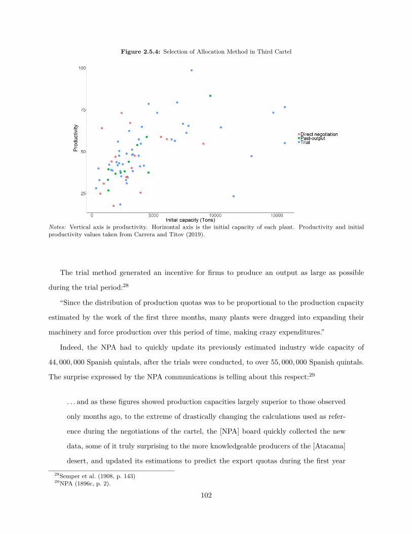
Figure 2.5.4: Selection of Allocation Method in Third Cartel

Notes: Vertical axis is productivity. Horizontal axis is the initial capacity of each plant. Productivity and initialproductivity values taken from Carrera and Titov (2019).

The trial method generated an incentive for firms to produce an output as large as possible

during the trial period:28

“Since the distribution of production quotas was to be proportional to the production capacity

estimated by the work of the first three months, many plants were dragged into expanding their

machinery and force production over this period of time, making crazy expenditures.”

Indeed, the NPA had to quickly update its previously estimated industry wide capacity of

44, 000, 000 Spanish quintals, after the trials were conducted, to over 55, 000, 000 Spanish quintals.

The surprise expressed by the NPA communications is telling about this respect:29

. . . and as these figures showed production capacities largely superior to those observed

only months ago, to the extreme of drastically changing the calculations used as refer-

ence during the negotiations of the cartel, the [NPA] board quickly collected the new

data, some of it truly surprising to the more knowledgeable producers of the [Atacama]

desert, and updated its estimations to predict the export quotas during the first year28Semper et al. (1908, p. 143)29NPA (1896c, p. 2).

102

Figure 2.5.5: Trial Method Examples (selected plants)

Notes: Vertical axis is output in tons. Horizontal axis is time. Transition Period is the time interval between thesignature of the cartel contract and the start of collusion.

of the cartel.

One effect of the trial method was that the quotas allocated during the first year of the cartel

were much smaller, as a percentage of capacity, than it was previously expected. Indeed, plants

were supposed to restrict their output to only 35% of their capacity instead of the 50% of capacity

that had be assumed during the negotiation of the agreement. However, since only a fraction of the

firms had used the trial method, firms that had chosen the past-output method instead suffered

the bulk of the reduction.

The problems described above contribute for the Third Cartel to be considered almost instantly

a failure. Instead of the 3 years stipulated on the contract it lasted only for eighteen months, after

an early termination clause was invoked.

Table 2.5.3 presents the counterfactual costs of the plants that used the trial method, assuming

they produce the same output observed during the first year of the Third Cartel, but with a

constant output level instead of using the trial method. Results show that savings of not using the

trial method would have been above 20% of the observed production costs. Notice that this figure

represents a lower bound, since it does not include the value of any additional investments made103

Figure 2.5.6: Illustration of Third Cartel Counterfactual (Agua Santa plant)

Notes: Vertical axis is output in tons. Horizontal axis is time. Counterfactual case assumes that plants produce sametotal output during 1891, but that they produce it at a constant level.

by the firms in order to be prepared for the trial period. Figure 2.5.6 illustrates the re-allocation

of output used to compute the counterfactual costs.

Table 2.5.3: Counterfactual Costs Trial Method

Observed costs Counterfactual ∆ Costs (%)costs

1,377,384 1,097,726 -20.3Notes: Observed and counterfactual costs based on costestimations in Carrera and Titov (2019). Counterfactualcosts are estimated assuming that plants produce sametotal output during 1891, but that they produce it at aconstant level.

2.5.4 Fourth and Fifth Cartels: Theoretical-capacity Method

Negotiations to resume collusion were started promptly after the collapse of the Third Cartel and

a new agreement was signed in October of 1900.30 The Fourth Cartel included several innovations.30NPA (1898b, p. 5)

104

The complex menu of options used in the Third Cartel was replaced by a single method for all

the plants in the industry. With only a single exception, direct negotiation was abandoned as a

quota allocation method, and small plants received the same proportional discount in their quotas,

although they were given the chance to roll-over their quotas from one year to the next.31

The failure of the trial and time methods used in previous cartels motivated the re-introduction

of the theoretical-capacity method in a more sophisticated version than the one used in the First

Cartel.32 The NPA board would assess the production capacity of each plant based on both its re-

fining capacity and the nitrate content of its lands. The resulting estimation of production capacity

would then remain confidential until all producers had signed the agreement. Theoretically, this

procedure would force producers to only focus on the fairness of their plant’s capacity assessment,

instead of negotiating directly for a larger market share. On the other hand, the reputation of

the NPA as a valid third party mediator would not survive if, once the market shares were finally

revealed, they seemed to be arbitrary or unfair.

The Fourth Cartel was contemporaneously regarded as very successful. This is reflected in the

fact that right before the expiration of the Fourth Cartel the nitrate producers agreed on extending

collusion for 3 more years, in what would be the fifth nitrate cartel of this period.

Contractually, the Fifth Cartel was a continuation of the previous agreement and the main

innovations regarding quota allocation were maintained and protected. In particular, when there

was a risk that the negotiations of the new contract would fail, the NPA did not show any flexibility

about the necessity to keep the estimated plant capacities confidential before all the firms signed

the agreement and refused to negotiate directly quotas for the firms that were initially blocking the

signature of the agreement.33 At the same time, the Antofagasta Nitrate Company lost the special

privilege it had during the Fourth Cartel and its quota was determined by theoretical capacity

instead of by direct negotiation.

31The only company that used direct negotiation was the Antofagasta Nitrate Company, which was the onlycompany to refine the untreated nitrate ore at a central location (O’Brien, 1980).

32NPA (1898a, p. 4).33In particular see minutes of the producers’ meetings held on March 26st and 31st of 1906 (NPA, 1909)

105

2.5.5 Comparing Cartel Market Shares Allocation in the Nitrate Cartels

Table 2.5.4 the coefficient of variation of the ratio between the output in a reference period before

the start of the cartel and the quota allocated to each plant in the industry. A higher dispersion of

this ratio means that some plants were suffering a proportionally larger reduction on their output

with respect to the previous competition period. In this comparison the Third Cartel has a much

lower performance with respect to the theoretical-capacity method cartels, which present relatively

similar levels of dispersion.

Table 2.5.4: Market Shares Allocationin Various Cartels

Cartel Coefficient of Variation(CV)

First 0.468Third 1.196Fourth 0.471

Notes: Coefficient of variation is com-puted taking the ratio between theaverage output in the last year be-fore the signature of the cartel con-tract and the monthly quota allo-cated to the plant. Computation usesa balanced panel with plants that hadpositive output in competitive periodprevious to the cartel.

2.6 Other Dimensions of Learning

This section describes other contractual dimensions over which the nitrate producers implemented

innovations to improve cartel organization as they gained experience.

2.6.1 Transition to Collusion

A very acute problem that harmed the effectiveness of earlier cartels was the handling of transition

from free competition to collusion. In the nitrate cartels, once a cartel contract was signed there

would be a period of a few weeks or months before each firms’ output had to be reduced. We

will refer to this period from signature until the effective start of collusion as the transition period.106

Their existence can be explained by the time it would take to conclude the market share allocation

across producers, for the adjustments firms had to make before significantly reducing their output

level, and for the already committed sales made by the colluding firms.

The existence of an unregulated transition period generated incentives detrimental for the suc-

cess of a cartel. Nitrate is a storable commodity, so during the transition period consumers had an

incentive to purchase the product while prices were still low. Thus, producers would be tempted

to to front-load sales, causing a negative externality for the rest of the producers in the form of a

reduced price effect of the cartel. We will denote this as the preemptive cheating motive.

The preemptive cheating motive caused the gradual introduction of transitory articles in the

collusive agreements aimed at generating a smoother transition to collusion.

In the case of the First Cartel the contract did not include any clauses regarding the transition

period, although they implemented a detailed procedure to verify the stocks held by each plant

at the start of the cartel.34 The result of an unregulated transition period was that producers

increased their output levels in the months before the official start of the cartel. This pattern is

shown in Figure 2.6.1.

Figure 2.6.2 shows the transition to collusion on the Third Cartel.35 In this case, the preemp-

tive cheating motive of producers was compounded by the use of the trial method that induced

an additional front-loading of production. The signature of the cartel contract was immediately

followed by a boom in industry output, reducing the quantity available to be allocated as export

quotas, as the NPA communicated to its members:36

“. . . the excessive and anticipated exports of the month of March . . . had already reduced to

20,300,000 the minimum amount of 22,000,000 [Spanish quintals], that at the time of the negotia-

tions was expected and was used as a reference to compute the export quotas of the present nitrate

year.”

Interestingly, recognizing the existence of a transition problem in the First Cartel, the cartel

contract had tried to solve the transition to collusion problem by fixing the total industry exports

for an extended transition period that encompassed the last year of competition before the cartel

34Comite Salitrero (1884).35Notice that one of the advantages of the time method used in the Second Cartel was the absence of the need for

regulating the transition period.36NPA (1896c, p. 2).

107

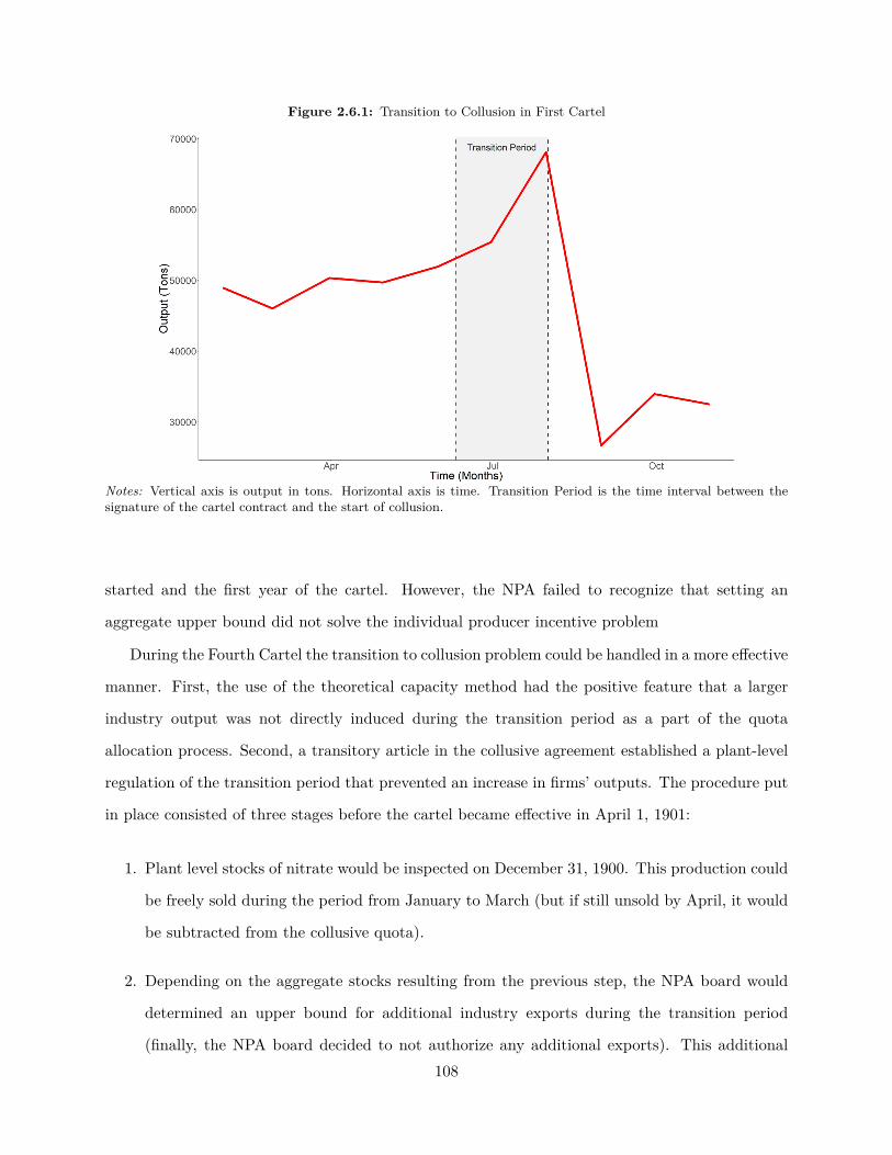
Figure 2.6.1: Transition to Collusion in First Cartel

Notes: Vertical axis is output in tons. Horizontal axis is time. Transition Period is the time interval between thesignature of the cartel contract and the start of collusion.

started and the first year of the cartel. However, the NPA failed to recognize that setting an

aggregate upper bound did not solve the individual producer incentive problem

During the Fourth Cartel the transition to collusion problem could be handled in a more effective

manner. First, the use of the theoretical capacity method had the positive feature that a larger

industry output was not directly induced during the transition period as a part of the quota

allocation process. Second, a transitory article in the collusive agreement established a plant-level

regulation of the transition period that prevented an increase in firms’ outputs. The procedure put

in place consisted of three stages before the cartel became effective in April 1, 1901:

1. Plant level stocks of nitrate would be inspected on December 31, 1900. This production could

be freely sold during the period from January to March (but if still unsold by April, it would

be subtracted from the collusive quota).

2. Depending on the aggregate stocks resulting from the previous step, the NPA board would

determined an upper bound for additional industry exports during the transition period

(finally, the NPA board decided to not authorize any additional exports). This additional108

Figure 2.6.2: Transition to Collusion in the Third Cartel

Notes: Vertical axis is output in tons. Horizontal axis is time. Transition Period is the time interval between thesignature of the cartel contract and the start of collusion.

exports would be assigned to the firms based on their collusive market shares.

3. Any other amount produced by the plants during the first quarter of 1901 could only be

exported after April 1 and would be counted as part of the respective collusive quota.

Figure 2.6.3 shows the industry output pattern at the beginning of the Fourth Cartel. The

new mechanism implemented by the NPA that tried to fully internalized the effects of increasing

production during the transition period seems to have been effective at solving the preemptive

cheating motive of producers since industry output had a monotonic downward trend.

2.6.2 Flexibility For Adjustments and Duration

A long-lasting cartel, concerned about the fairness of the allocation of its collusive surplus must

find a way to adjust its allocation of market shares when the relative situation of its members

change with respect to their initial allocation. In the case of the nitrate cartels this challenge is

interwined to the issue of cartel duration and the natural question of why nitrate producers could

never implemented a permanent cartel.109

Figure 2.6.3: Transition to Collusion in the Fourth Cartel

Notes: Vertical axis is output in tons. Horizontal axis is time. Transition Period is the time interval between thesignature of the cartel contract and the start of collusion.

Table 2.6.1: Nitrate Cartels by Duration Characteristics

Cartel Initial duration Effective duration Quota-allocation Automatically(months) (months) method (main) renewable

First 12 29 Theoretical-capacity NoSecond 24 36 Time NoThird 36 19 Trial YesFourth 60 60 Theoretical-capacity NoFifth 36 36 Theoretical-capacity No

Cartel duration was explicitly agreed upon in the collusive contracts.37 Table 2.6.1 presents

the characteristics of the duration on the 5 nitrate cartels. Initial duration corresponds to the

original duration of the agreement, effective duration is the actual time the collusion lasted, and

automatically renewable refers to whether the agreement would be extended automatically and

indefinitely after its initial duration had expired.

Based on this dimension of learning, we can divide nitrate cartels in two groups. The first

group are the first three cartels, characterized by a slow evolution towards the establishment of a37After the Second Cartel, a specific procedure to trigger an early dissolution of the cartel was also included in

the contracts. This procedure, required the agreement of an absolute majority of producers as a fraction of industryoutput. Only in the case of the Third Cartel, an early dissolution was discussed and approved.

110

permanent cartel. Earlier cartels were emergency arrangements made in order to face transitory

negative demand shocks.38 In the case of the first two cartels, duration was initially set for a

short period of time (1 or 2 years) under the implicit understanding that the cartel would, at the

expiration date, be renewed under the same basic collusive contract if market conditions made it

desirable. However, producers were tempted by the prospect of continued cooperation and the

cartel contracts they signed increasingly had the perpetuation of collusion as a concern. This

trend culminated in the Third Cartel contract which incorporated a clause that made its renewal

automatic (in the exact same way as the contract that created the NPA automatically renewed its

charter).

On the other hand, after the failure of the Third Cartel, producers never again attempted

forming permanent cartels. The last two cartels were fixed-term agreements, which implied a

complete renegotiation to form a “new” cartel in case that producers wanted to extend the collusive

period (as it was the case when the Fourth Cartel expired) since the default situation was the

resumption of competition once their terms expired .

Moreover, the cartel duration decision is linked to the question of how to implement adjustments

to collusive market shares in order to keep the allocation of surplus fair. During the first three

cartels the producers were looking for adjustment mechanisms that could work in the framework

of a permanent cartel, which explains in part the choices they made about what quota-allocation

methods they tried: Both the time and trial methods are good solutions for keeping market shares

allocation dynamically fair. The time method automatically transfers market shares from plants

that become relatively less efficient or lose capacity to those that become more productive or

increase capacity. Relatedly, the Third Cartel contract required that plants performed periodic

trials, which would generate approximate dynamic fairness in the same manner.

On the contrary, in the last two cartels instead of having a quota-allocation method that allowed

for both a fair initial allocation of market shares and a dynamic adjustment as conditions evolved,

the NPA could now focus only on the initial allocation leaving the adjustments for the inter-cartel

period (i.e., the renegotiation of the agreement). At the same time, the diminished focus on

dynamic fairness allowed the producers to reduce the incentives to invest in increased capacity, by

explicitly eliminating any sort of quota increases due to investments made after the signature of38Cruchaga (1929, p. 207) offers this interpretation for the First Cartel.

111

the agreement.

2.7 Final Remarks

This paper studies whether firms learn how to better organize collusion as they gain experience.

Since cartels are illegal organizations this remains an open question. To the best of our knowledge

this is the first paper to be able to explore learning in relation to cartels.

To study this research question we use the case of the cartels in the Chilean nitrate industry.

Between 1884 and 1909 there were five cartels in the nitrate industry. Since collusion was not

illegal in Chile at the time these cartels were completely public and their rules codified in legal

contracts. Moreover, there was no meaningful technological innovation in the industry. Thus, the

environment where these cartels developed was static throughout the period of study.

First, a descriptive analysis of the cartels contracts show that they grew more complex and

complete during the first four cartels as producers gained experience: New clauses were incorporated

that addressed issues that had mined the performance of previous cartels.

We then explore the main challenge that nitrate producers faced when organizing collusion: The

allocation of collusive market shares. We describe how nitrate cartels used a total of five different

methods to allocate market shares and are able to show that the additional costs caused by using

two methods of special interest, the time and trial methods, were very substantial and explain why

they were discarded in later cartels.

Finally, we describe how nitrate cartels were able to solve the incentive problems caused by the

transition from competition to collusion and the process by which the industry converged to having

periodical fixed-term agreements, instead of a permanent cartel.

Our results point to a large importance of learning in the organization of cartels. Even in an

advantageous setting for collusion as the nitrate industry many of the initial solutions employed

by the cartelized firms were shortsighted or sub-optimal, and only through trial and error they

were able to arrive to a model contract. At the same time, this paper highlights the relevance

of trade associations for cartels as a repository of relevant institutional knowledge about collusion

organization.

One important extension of this paper is to explore the relation between cartel leadership and112

observed distortions in the allocation of collusive surplus. Specifically, exploring whether cartel

organizers received a disproportionate share of collusive surplus

113

114

Appendix

Appendix 2.A Election of Allocation Method in Third Cartel

• Past production method was used by the following plants: Cala-Cala, Carolina39, Cruz de

Zapiga, Democracia, Mercedes, Paccha, Peruana, Progreso, Rosario de Huara, San Fernando,

Santa Rosa de Huara, and Sebastopol.40

• Quotas were determined by direct negotiations with the plants: Antofagasta, Atacama,

Cholita, Julia, Lautaro, Limenita, Paposo, Santa Ana, Santa Catalina, Santa Fe, Santa Luisa,

Virginia, Vis, and Yungay Bajo.41

• The rest of the plants had their quotas determined by the trial method. However, some

plants opted for trial method, but requested extension on the start of the trial period due

to investments: Agua Santa, Angela, Aragon, Compania, Providencia, Rosario de Negreiros,

San Antonio, Santiago, Tres Marias, and Valparaiso. A second group of plants requested

an extension due to other factors, which were resolved by the arbitration of mediators, as

described in article 14 of the cartel contract. The plants that appealed to the resolution

of the mediators in this specific case were: Aguada, Amelia, Josefina, Reducto, and Santa

Isabel.42

• By January of 1897 the plants Agua Santa, Angela, Aragon, Compania, Providencia, Re-

ducto, Rosario de Negreiros, San Antonio, Santa Rita, Santiago, Serena, and Tres Marias has

changes their initial capacity due to investments in refining capacity. The following plants39Note: In the text says it had been acquired by Santa Rita Company and was forming “a single plant” with Santa

Rita plant.40NPA (1896b, p. 6).41NPA (1896b, p. 6).42NPA (1896b, p. 6).

115

were planning on having new trial periods: Aguada, Buena Esperanza, Compania, Jazpampa,

Josefina, La Granja, Paccha, Peregrina, San Esteban, San Fernando, San Pedro, and Union.43

• In the fist four months of 1897, there were the following trial periods: Providencia, Serena,

Reducto, San Fernando due to new investments in refining capacity, and San Jose, Santa

Clara, and Puntilla de Huara as new plants starting operation. By May, the plants: La

Granja, Josefina, Union, San Esteban, Aguada, and Paccha started new trial periods invoking

also investments in refining facility or purchase of new nitrate lands. The plants Jazmpampa

and San Pedro were about to start a new trial due to the same reason, and Huascar as a new

plant.44

Appendix 2.B Enforcement Evidence

43NPA (1897b, p. 3).44NPA (1897a, p. 7).

116

Figure 2.B.1: Example of Threat to Intermediaries Dealing with Non-cartel Producers

Notes: Letter dated February 8, 1905 signed by the NPA manager.Text translation: As a consequence of some recent sales of nitrate manufactured on plants that still have not joinedthe nitrate cartel the [NPA] board has made the decision that, in case of this event happening again, none cartelmember will do business with the broker that intervened in said sale. To this effect it will be considered as the samebroker or firm both the Iquique office and its agents in Valparaiso. For your knowledge, find attached a list of thefirms and plants that currently form part of the cartel. You will receive opportunely notice of those that join in thefuture. In Valparaiso, our representation will give the same notice to interested parties. Source: Vol. 96, NitrateCollection, Chilean Historical Archives.

Appendix 2.C First Cartel Contract

Convenio para la Formacion del Comite Salitrero45

Artıculo 1: El presente convenio tiene por objeto obligarse, por el termino de un ano, a [sic]

no elaborar en las oficinas que en seguida se menciona i a no exportar mas [sic] cantidad de salitre

que la senalada por el Comite Salitrero permanente, la cual en ningun [sic] caso podra exceder de

diez millones de quintales espanoles para toda la costa.

45Comite Salitrero (1884).

117

Los duenos de varias oficinas en actual trabajo podran elaborar la cuota de todas sus oficinas en

una sola, pero los duenos de varias oficinas actualmente paralizadas deberan trabajar en cada una

de ellas la cuota que les fuere senalada.

Es entendido que ningun elaborador podra vender ni comprar cuota de elaboracion asignada a otro.

La cuota asignada a cada oficina actualmente paralizada no se contara sino desde la fecha en que

principie a trabajar.

El total de elaboracion i exportacion que se fijara sera prorateado [sic] entre dichas oficinas, tomando

por base la capacidad productora que a cada una asigna este convenio.

Las oficinas a que se refieren los incisos anteriores i su capacidad indicada son los siguientes:

(El cuadro sera presentado en la reunion que tendra lugar el proximo 10 de Junio.)

Artıculo 2: Por el termino de este convenio existira en Iquique una comision [sic] de elabo-

radores de salitre que se denominara Comite Salitrero, con las atribuciones que mas [sic] adelante

se indican.

Artıculo 3: El Comite Salitrero se compondra de nueve miembros propietarios i dos suplentes,

todos esplotadores [sic] de oficinas en actual trabajo o representantes de tales en la jestion jeneral

[sic] de sus negocios.

Todas las personas que concurren a este convenio son aptas para ser miembros del Comite, sea que

residan en Tarapaca, Tocopilla, Antofagasta, Aguas Blancas, Taltal o Valparaiso.

El miembro del Comite que residiere fuera de Iquique tendra la obligacion [sic] de atender personal-

mente o de hacerse representar, en el desempeno de las atribuciones que le corresponden, por un

esplotador de oficina en actual trabajo o representante de tal en la jestion jeneral de sus negocios.

Artıculo 4: Son atribuciones del Comite Salitrero:

1◦ Vijilar [sic] i hacer efectiva las obligaciones contraidas por el presente convenio, i representar

en todo sentido los intereses de la industria salitrera.

2◦ Resolver, con audiencia de los interesados i previos los estudios e informes del caso, las quejas

sobre falta de proporcionalidad entre la capacidad productora real de una oficina i la cuota

que se le haya asignado con relacion a la cantidad total fijada para la elaboracion i exporta-

cion, u [sic] otras.118

Si el representante de la oficina a que se refiere la resolucion del Comite sobre falta de propor-

cionalidad en la fijacion de la cuota, no se conformase [sic] con ella, sin perjuicio de empezar

a cumplirse dicha resolucion, podra apelar ante la comision [sic] de peritos mencionada en el

art. 7◦.

No habra recurso alguno contra la resolucion de esta segunda comision.

3◦ Acordar las medidas necesarias para imponer el cumplimiento de sus resoluciones i las que

fueren menester para vijilar la exportacion que a cada oficina corresponda.

Las medidas de coaccion que acordare [sic] el Comite consistira solo en multas, que no podran

exceder de un peso por cada quintal que se exportare [sic] de exceso sobre la cuota respectiva.

4◦ Fijar la cantidad con que cada oficina deba contribuir a los gastos que demande el ejercicio

de sus atribuciones.

Esta contribucion [sic] se distribuira a prorata [sic], fijandose a tanto por quintal de salitre

elaborado, i no podra exceder en ningun [sic] caso de un centavo por quintal.

El fondo para gastos del Comite se formara tambien con las multas indicadas en el numero

3◦ de este artıculo.

5◦ Nombrar i remover los empleados que sean necesarios para el objeto de este convenio i senalar

la remuneracion [sic] que deben gozar.

6◦ Acordar los gastos que exija el objeto de su institucion [sic].

7◦ Nombrar apoderados que representen al Comite fuera de Iquique i en los lugares que sea

menester que los haya.

8◦ Convocar a una reunion jeneral para resolver sobre los casos en los que encontrare resistencias

graves en el cumplimiento de sus reglamentos i resoluciones, o cuando la produccion [sic] de

oficinas nuevas que no acepten la presente combinacion [sic] comprometan el objeto con que

se forma.

9◦ Resolver i fijar las condiciones con que deban aceptarse las solicitudes de otras oficinas sobre

ingreso a la presente combinacion.119

Artıculo 5: Los miembros del Comite seran nombrados, en votacion secreta, por mayorıa

absoluta de votos, en reunion [sic] a que concurran a lo menos la mitad mas uno del total de las

personas naturales o fictıcias que forman este convenio.

Su nombramiento sera por un ano.

Artıculo 6: En la reunion jeneral del dia [sic] 10 se procedera a la eleccion [sic] del Comite

permanente en la forma en que indica el artıculo 5◦.

En esta reunion i las demas jenerales ninguna persona podra tener mas de dos votos, uno por sı

propio i otro en virtud de un poder conferido.

Es absolutamente prohibido conferir poderes a personas que no sean salitreras o representantes de

casas elaboradoras.

Artıculo 7: En la reunion indicada en el artıculo anterior se elejiran ademas, a mayorıa absoluta

de votos, dos inspectores propietarios i dos suplentes, encargados del examen de las cuentas i balance

del fondo de gastos del Comite, i una comision de peritos compuesta de siete propietarios i dos

suplentes, encargados de resolver en definitiva sobre las quejas a que se refiere el n◦ 2 del art. 4◦.

Para la comision de peritos puede ser nombrado cualquiera que ejerza la profesion de salitrero.

En la ultima reunion que celebre la comision de peritos para resolver en definitiva la queja sometida

a su conocimiento, tendra voz i voto el Presidente i en su ausencia el Vice del Comite Salitrero.

Los inspectores presentaran en cada reunion jeneral un informe sobre la inspeccion que hubieren

verificado.

Artıculo 8: El Comite elejira de entre sus miembros, en la primera reunion que celebre, un

Presidente i un Vice-presidente que lo seran tambien de las reuniones jenerales i designara el orden

en que deben reemplazarles los otros miembros.

Artıculo 9: Toda resolucion del Comite necesita, para que se tenga por tal, que haya sido

adoptada con el acuerdo uniforme de seis de sus miembros a lo menos.

Artıculo 10: El plazo de un ano mencionado en el primer inciso del art. 1◦, solo [sic] empezara

a contarse desde el dia 1◦ de agosto proximo.

Artıculo 11: Cada tres meses, contados desde el 1◦ de agosto proximo, habra una reunion120

jeneral con el objeto de oir el informe de los Inspectores, deliberar sobre los asuntos que el Comite

someta a su conocimiento i aprobar las cuentas del trimestre.

Artıculo 12: En la reunion jeneral del tercer trimestre se deliberara sobre si se prorroga o

no por un ano mas el compromiso contraido segun el presente acuerdo. El voto unanime de los

asistentes a esa reunion obligara a los inasistentes.

Artıculo 13: La obligacion del artıculo 1◦ con respecto a la exportacion no se refiere a la

existencia de salitre que cada cual tuviera en el dia, ni tampoco a las compras a adquisiciones que

se hicieren del salitre que se elabore con arreglo a este convenio.

Artıculo 14: Si alguno de los que concurren al presente convenio traspasase [sic] por cualquier

causa su derecho a la oficina u oficinas que le correspondan, el traspaso no podra hacerse sino con

la condicion expresa de que el nuevo adquiriente respetara i cumplira las obligaciones contraidas

por este convenio.

Agreement for the Formation of a Nitrate Committee46

Article 1: The present agreement has for object to bind [us], for the term of a year, not to

produce in the plants named below and not to export a larger amount of nitrate than the one

indicated by the permanent Nitrate Committee, which in any case will not exceed ten millions of

quintals for all the Nitrate Coast.

The owners of several plants currently in operation will be able to produce the quotas of all of their

plants in any of them, but the owners of several plants that are currently shutdown will have to

produce their quotas in the same plant to which it was allocated.

It is implicit that it is forbidden to sell or buy the quota assigned to a different producer.

The quota granted to a plant currently in shutdown will not be active until it resumes operation.

The total [industry-level] quantity of production and exports that will be set, will be allocated to

the plants using the production capacity estimated for each of them.

The plants alluded to in the previous subsections and their estimated capacity are the following:

(The table will be shown during the meeting that will take place on June 10.)

46Translated by author from Comite Salitrero (1884).

121

Article 2: For the duration this agreement there will be in Iquique a commission of nitrate

producers, denominated as Nitrate Committee, with the powers stated below.

Article 3: The Nitrate Committee [board] will be composed by nine owner-members and two

substitutes, all of them shall be exploiters of currently operating plants or their representatives

tasked with the management of their plants [managers].

All the signatories of this agreement are fit to be members of the Committee, whether they reside

in Tarapaca, Tocopilla, Antofagasta, Aguas Blancas, Taltal or Valparaiso.47

A member of the Committee that resides out of Iquique will be bound to attend in person or to

name a deputy for the performance of his responsibilities, among the plant owners or managers.

Article 4: The attributions of the Nitrate Committee are:

1◦ To monitor and to make effective the commitments contracted through this agreement, and

to broadly represent the interests of the nitrate industry.

2◦ To adjudicate, after having an audience with the interested parties and using prior studies

and reports regarding the case, complaints about lack of proportionality between the true

production capacity of a plant and its quota. If the representative of the plant declared his

disagreement with the ruling, he will be able to appeal before the commission of experts

mentioned in article 7. The ruling of this commission will not be subject to any instance of

appeal.

3◦ To agree on the necessary measures to enforce implementation its resolutions and to monitor

the exports of each plant to ensure quotas are respected. The coercitive measures will be

limited to fines, which will not be larger than one Chilean peso per quintal of excess exports

over the respective quota.

4◦ To set the amount with which each firm must contribute to finance the operation of the

Committee. The contribution will be allocated proportionally, on the basis of output and it

will not be larger in any case than one cent per Spanish quintal. The expense fund for the47Tarapaca, Tocopilla, Antofagasta, Aguas Blancas and Taltal correspond to localities or districts of Northern Chile

where nitrate deposits are found. Valparaiso was the main commercial and financial city of Chile at the time.

122

Committee will also receive the fines included in section 3 of this article.

5◦ To name and to remove the required personnel for the objectives of this agreement and to set

their wages.

6◦ To determine the necessary expenses for the fulfillment of its mission.

7◦ To name agents to represent the Committee outside of Iquique in the cities where this is

required.

8◦ To convene a general meeting on cases in which the Committee finds resistance to its regula-

tions and resolutions, or when the entry of new plants which refuse to join the cartel threatens

the fulfillment of its objectives.

9◦ To decide and to set the conditions on which the applications of other plants to join the cartel

will be resolved.

Article 5: The members of the Nitrate Committee [board] will be elected by secret ballot in a

meeting with the presence of an absolute majority of the signatories.

They will hold office for a period of one year.

Article 6: The election of the Nitrate Committee will be done using the procedure described

in article 5 during the general meeting on the 10 [of June].

On said occasion, and more generally at any general meeting, no person will be able to have more

than two votes, one for his own firm and one as a representative of a second firm.

It will be absolutely forbidden to name as a representative a person that is not an owner or a

manager.

Article 7: In the general meeting mentioned above will also be elected, by absolute majority of

votes, two owner-inspectors and two substitutes, which will be tasked with monitoring an adequate

use of the expense fund of the Committee, and a commission of experts formed by seven owners

and two substitutes, charged with resolving as last instance the complaints mentioned in number

2 of article 4.

Any person with practical experience can be nominated to be part of the commission of experts.123

In the meetings when the commission of experts resolve about complaints put in front of them, the

President of the Committee will have voice and vote (the Vice-president in case of absence of the

President).

The inspectors will present on each general meeting a report about their activities.

Article 8: The Committee will select from among its members, during its first meeting, a

President and a Vice-president who will preside the general meetings and will decide the order in

which the other members of the Committee will substitute them in case of absence.

Article 9: All the resolutions of the Committee will need an agreement of at least six of its

members to be approved.

Article 10: The one year term mentioned in the first paragraph of article 1 will start on August

1.

Article 11: Every three months, counted from August 1, there will be a general meeting with

the object to receive the report from the inspectors, discuss issues put forward by the Committee

and approving the expenses of the period.

Article 12: In the general meeting of the third quarter will be discussed the extension of the

present agreement for one more year. The unanimous vote of the presents will bind those that do

not attend the meeting.

Article 13: The commitment made regarding the nitrate exports in article 1 do not refer to

the nitrate stocks that each producer has on that day, nor to the purchases of nitrate manufactured

according to the rules of this agreement.

Article 14: In the event of transferring for any reason their rights to the plant or plants they

operate, the signatories of this agreement will clearly stipulate that the new owner will comply and

respect all the obligations originated on this agreement.

124

Appendix 2.D Second Cartel Contract

Convenio de Combinacion Salitrera48

Los infrascritos, todos productores de salitre, convienen en formar parte de una combinacion

salitrera, por el termino de dos anos, contados desde el 1◦ de Enero de 1891, con arreglo a las

siguientes estipulaciones:

Artıculo 1: Cada uno de los firmantes de este convenio, en el caracter [sic] en que comparece

o por la sociedad que representa, conviene con los demas [sic] otorgantes, en no trabajar en sus

respectivas oficinas salitreras sino siete meses en el ano 1891 i [sic] se obliga del mismo modo, a

suspender por completo la elaboracion [sic] por cinco meses en el mismo ano en la forma siguiente:

Cada productor podra elejir [sic] los siete meses de elaboracion [sic] que le conviniese, dando un

aviso anticipado por escrito de quince dias a lo menos, al consejo directivo de la combinacion, cada

vez que principie o suspenda el trabajo; no pudiendo hacerse estas operaciones sino el 1◦ o 15 de

cada mes. El productor que elijiere en la forma dicha los siete meses de trabajo que le convenga,

debera suspender por completo la elaboracion durante los ultimos cinco meses del presente ano.

Artıculo 2: El numero de meses que durara la elaboracion en 1892, sera fijado por el Consejo

Directivo de la combinacion, i sujetandose aesta fijacion, cada productor podra elejir los meses de

elaboracion en la forma y condiciones estipuladas en el artıculo 1◦.

Artıculo 3: La suspension de trabajo se refiere unicamente a la elaboracion de salitre, pudiendo

en consecuencia, extraerse y acumularse caliche durante la paralizacion de las oficinas.

Artıculo 4: Los firmates de este convenio pagaran al Consejo Directivo, la cuota que este juzgue

necesaria para atender a los gastos de propagacion de consumo de salitre, y a los que demanden

el sostenimiento y la administracion de la combinacion; no pudiendo dicha cuota exceder de medio

centavo por quintal de salitre embarcado.

Artıculo 5: Cualquier productor que elabore salitre fuera de los perıodos a que tenga derecho

segun este convenio, pagara por cada dia de esceso [sic] una multa cuyo monto sera fijado en

los estatutos y que ingresara a fondos comunes de la combinacion, sin perjuicio de obligarsele a48Combinacion Salitrera (1891).

125

paralizar la elaboracion por el tiempo que corresponda.

Artıculo 6: Los estatutos que por lo demas han de rejir la combinacion, seran acordados por

mayoria absoluta de votos en reunion jeneral, que se celebrara con los que asistan el dia que senale

el Consejo Directivo provisorio i en el local que este determine, previo aviso de quince dias que se

publicara en dos periodicos de Iquique. Los que no asistan a esa reunion por sı o por apoderado,

se obligan desde luego a someterse a los Estatutos que apruebe la mayorıa de los que concurran.

Artıculo 7: Los parecientes nombran a los senores J. Dawson, W. Patterson Roberson, F.G.

Lomax, P.G. Pascal, J. Vernal y B. Domınguez como propietarios y el senor H.W. Sillem como

suplente, teniendo cada uno facultad para hacerse representar por un reemplazante, para que desde

luego compongan el Consejo Directivo provisorio de la combinacion, cuyas funciones duraran hasta

que se elija el Consejo Directivo definitivo, una vez aprobados los estatutos. Se faculta a los

miembros del Consejo Provisorio para que conjunta y separadamente representen a todos y a cada

uno de los otorgantes judicial y extrajudicialmente, en todo lo que tenga por objeto hacer cumplir

las estipulaciones de este convenio; pudiendo delegar la representacion judicial, poner posiciones,

decir de nulidad, constituir compromisos, nombrar arbitros y arbitradores, percibir y transijir y

jurar de columnia, por sı o por el delegado.

Artıculo 8: Si alguno de los que concurren al presente convenio transfiriese por cualquiera

causa su derecho a la Oficina u oficinas que les corresponda, o la diese en arrendamiento, uso,

comodato, etc., o celebrase otro contrato semejante, debera en el estipular de una manera espresa,

con el nuevo adquiriente que este respetara y cumplira las obligaciones del presente convenio. De

no hacerse ası, quedara aquel personalmente obligado.

Artıculo 9: Este convenio dejara de ser obligatorio desde el momento que la comision a que

se refiere el artıculo 10◦ comunique al Consejo Directivo que no ha podido llegar a un acuerdo

con las companias Agua Santa, Antofagasta, Banco Mobiliario y los senores Pedro Perfetti y Jose

Devescovi; fijandose como plazo para este objeto hasta el 31 del presente mes.

Artıculo 10: Se nombrara una comision compuesta por los senores Pedro Pascal, E.W. Vincent,

Alfredo Quaest Faslem y F.G. Lomax, para que trate con los productores de salitre mencionados

en el artıculo anterior.126

Artıculo 11: Este convenio se reducira a escritura publica una vez que se haya llegado a un

acuerdo con los productores a que se refiere el artıculo 9◦.

Prorroga de la Combinacion Salitrera49

Reconvienen en continuar i formar parte de la asociacion o combinacion salitrera que fue re-

ducida aescritura publica, el ocho de Julio de mil ochocientos noventa i uno, quedando ahora dicho

convenio constituido por las estipulaciones i clausulas que mas adelante se insertan i el cual rejira

desde el primero de Enero de mil ochocientos noventa i tres hasta el treinta i uno de de Marzo de

mil ochocientos noventa i cuatro.

Artıculo 1: Cada uno de los firmantes de este convenio, en el caracter en que comparece o

por la sociedad que representa, conviene con los demas otorgantes en no trabajar en sus respectivas

oficinas salitreras, desde el primero de Enero de mil ochocientos noventa i tres hasta el treinta i uno

de Marzo de mil ochocientos noventa i cuatro, sino en conformidad a las reglas i con las limitaciones

que siguen.

Primero: Durante la vijencia de este convenio i de acuerdo con sus estipulaciones, cada produc-

tor de salitre podra optar entre trabajar por tiempo, suspendiendo la elaboracion en algunos meses

del ano, o trabajar por cuota, limitando la produccion a una cantidad fija de quintales espanoles

de salitre.

Segundo: El Directorio o Consejo Directivo de la Combinacion fijara el numero de meses

o tiempo en que no pueda elaborarse salitre en las Oficinas en que se trabaje por tiempo, en mil

ochocientos noventa i tres, i su fijacion se tendra desde luego como parte integrante de este convenio.

Cada productor por tiempo podra elejir los meses de elaboracion que le convenga, no excediendo del

numero de los fijados por el Directorio, debiendo dar a este un aviso por escrito con anticipacion de

quince dias a lo menos, cada vez que principie o suspenda el trabajo, sin que puedan hacerse estas

operaciones sino el primero o el quince de cada mes. El productor por tiempo que no diese aviso

para el principio i continuacion de la elaboracion estara obligado a paralizar luego que se complete

el tiempo fijado por el Consejo para la elaboracion. Esta suspension no implica la extraccion i49Combinacion Salitrera (1892).

127

acumulacion de caliche u otras obras que no sean de elaboracion.

Tercero: Durante la vijencia de este convenio la elaboracion por cuota se fijara como sigue, i de

acuerdo con los datos de la misma combinacion, previamente comprobados.

1◦ Para el que hubiere trabajado por tiempo en el ano de mil ochocientos noventa i dos se tomara

la cantiddad elaboro durante los seis meses de trabajo del mismo ano.

2◦ Para el que tiene cuota basada sobre el trabajo por tiempo de mil ochocientos noventa i uno

se tomara la cantidad que elaboro en ese ano, mas un diez por ciento; debiendo determinarse

la cuota por los datos de la misma Combinacion previamente comprobados. Esta cuota o

numero de quintales de salitre se entendera aumentada o disminuida en la proporcion que el

Directorio aumentare o disminuyere el numero de meses o parte de un mes de elaboracion

para los productores por tiempo.

El productor por cuota no tendra derecho para elaborar en una sola oficina, las cuotas de dos o

mas. Unicamente podran variarse las bases establecidas en este inciso mediante el acuerdo unanime

de todos los miembros de la Combinacion, sin perjuicio de lo establecido por el inciso segundo del

mismo artıculo.

Cuarto: La eleccion a que se refiere el parrafo primero de este artıculo debera hacerse, para

mil ochocientos noventa i tres, antes del treinta i uno de Marzo del mismo ano, por medio de una

carta dirijida i entregada al Directorio de la Combinacion; entendiendose que los que no llenen estos

requisitos optan definitivamente por la produccion por tiempo.

Quinto: Una vez elejido por el productor espresa o tacitamente el sistema de cuotas o el de

tiempo, no podra hacer nueva eleccion. Pero el productor que hubiese trabajado por sistema de

cuotas durante el ano mil ochocientos noventa i dos, podra elejir el de tiempo para mil ochocientos

noventa i tres, i vice versa, siempre que la eleccion la haga antes del primero de Abril de mil

ochocientos noventa i tres. Para hacer uso de esta facultad, el que haya trabajado por cuota durante

el ano mil ochocientos noventa i dos, debera haber dado los avisos de paralizacion i de principio de

trabajo correspondientes a los tres meses anteriores al primero de Abril de mil ochocientos noventa

i tres.

Sesto: Los productores por cuota podran trabajar en la forma que mas le conviniese, sin ser

limitados a periodos senalados anticipadamente.128

Artıculo 2: Los firmantes de este convenio pagaran al Consejo Directivo, hasta un centavo por

quintal espanol de salitre embarcado, para que atienda a los gastos de propagacion de consumo del

salitre i a los que demanden el sostenimiento i la administracion de la Combinacion.

Artıculo 3: Cualquier productor por tiempo que elabore salitre en contravencion al presente

convenio o a los acuerdos que se tomen en conformidad a el, pagara una multa de mil a quince

mil pesos diarios, segun lo determine el Directorio en atencion a la importancia de la Oficina; i si

el infractor fuere productor por cuota, la multa sera de tres pesos por cada quintal espanol que

elaborare en exceso sobre la cuota que le corresponda, todo lo cual se entiende sin perjuicio de

obligarles a cumplir el convenio. No obstante, si hubiere exceso en la elaboracion de una oficina que

trabaja por cuota no se impondra multa sino cuando el exceso sea mayor que un cinco por ciento de

la cuota correspondiente al ano. En el caso de un aumento dentro de este lımite, se computara como

parte de la elaboracion del ano siguiente; i solamente entonces podra embarcarse. De igual manera,

si resultare deficit en la elaboracion, siempre que no pase de cinco por ciento con relacion a la

cuota corespondiente, habra derecho para elaborarlo en el ano siguiente. Las multas se impondran

por el Directorio, i su valor ingresara a los fondos comunes de la Combinacion, principalmente con

el objeto espresado en el artıculo precedente. Por toda otra infraccion en las estipulaciones del

convenio o de los acuerdos debidamente tomados por el Directorio o juntas jenerales, el infractor

estara obligado a una indemnizacion proporcionada a los perjuicios que su falta ocasionare a la

asociacion; i la falta como tambien la cantidad que por ella haya de satisfacerse, sera resuelta en

un arbitraje de amigable composicion constituida en conformidad con las reglas establecidas en el

reglamento.

Artıculo 4: Si alguno de los que concurren al presente convenio trafiriese por cualquiera causa

su derecho a a Oficina u oficinas que le corresponda o le diese en arrendamiento, uso, comodato,

etcetera, o celebrase otro contrato semejante, debera en el estipular de una manera espresa, con

el nuevo adquiriente, que este respetara i cumplira las obligaciones del presente convenio. De no

hacerse ası quedara aquel personalmente obligado.

Artıculo 5: Forman tambien parte integrante de este convenio el reglamento que mas adelante

se inserta i los acuerdos que celebre el Directorio o Consejo Directivo, como los que se tomen en129

juntas jenerales, siempre que unos i otros esten conformes con las estipulaciones de esta escritura i

reunan la mayorıa de votos convenida.

Nitrate Cartel Agreement50

The undersigned, all nitrate producers, agree to be part of a nitrate cartel, for a term of two

years, starting from January 1, 1891, in accordance with the following stipulations:

Article 1: Each one of the signatories agree to operate in their respective plants for seven

months in the year 1891 and, at the same time they commit to completely suspend the production

in the same year according to the following rules:

Each producer will be able to choose the seven months of production that are more convenient to

him, giving advance notice of at least fifteen day to the board of the cartel each time that production

is resumed or suspended; The only days when it will be possible to change the operational status

of a plant will be the 1 and the 15 of each month. The producer that does not select in this manner

seven months of production, will have to stop working during the last five months of the year.

Article 2: The number of months each plant will be able to have active production during

1892 will be set by the cartel board and, subject to that decision, each producer will be able to

choose his months of operation in the same manner outlined in article 1.

Article 3: The suspension of operations refers only to the refining of nitrate. Thus, extraction

and accumulation of nitrate ore is allowed during the shutdown period.

Article 4: The signatories of this agreement will pay to the cartel board the fees that the

board deems necessary to promote the consumption of nitrate and to pay for the expenses caused

by the administration of this agreement. This fee will no exceed half a cent per Spanish quintal of

exports.

Article 5: Any producer that produces nitrate outside of the periods when he is authorized

according to this agreement will pay a fine for each day of excess production whose amount will be

set in the statutes. These fines will enter a common fund of the cartel and the producer will have

50Translated by author from Combinacion Salitrera (1891).

130

to suspend production to compensate for the unduly time of work of his plant.

Article 6: The statutes that are to rule the cartel will be approved by absolute majority of

votes in a general meeting that will be celebrated on a day and location chosen by the provisional

cartel, after a fifteen days notice that will be published in two Iquique newspapers. Producers that

do not attend the meeting will have to accept the statutes that are agreed upon the assistants.

Article 7: The signatories name the Misters J. Dawson, W. Patterson Roberson, F.G. Lomax,

P.G. Pascal, J. Vernal y B. Domınguez as owners and Mister H.W. Sillem as alternate, having each

one of them the ability to be represented by a substitute, to compose the provisional cartel board

whose functions will last until the election of a definitive cartel board once the statutes have been

approved. The members of the provisional cartel board will have, jointly and separately, ample

powers of legal and administrative representation.

Article 8: In the event of transferring for any reason or in any form their rights on the plant or

plants they produce, or to give them in lease, use, loan, or to celebrate any other similar contract,

the signatories of this agreement are expressly obligated to clearly stipulate with the new owner

that he will inherit all the obligations originated on this agreement and to produce the export

quota corresponding to each plant in the same plant. In contrary case the original owner will be

personally liable.

Article 9: This agreement will stop being valid in the moment the commission refereed to

in article 10 communicates the board that the negotiations with the companies: Agua Santa,

Antofagasta, Banco Mobiliario and the Misters Pedro Perfetti and Jose Devescovi. The deadline

for achieving this objective will the 31 of the present month [January].

Article 10: A commission composed by the Misters Pedro Pascal, E.W. Vincent, Alfredo

Quaest Faslem y F.G. Lomax will be tasked with negotiating with the companies mentioned in

article 9.

Article 11: This agreement will be transferred to a public deed as soon as a consensus has

been reached with the firms mentioned in article 9.

131

Appendix 2.E Third Cartel Contract

Convenio de la Combinacion Salitrera51

Artıculo 1: Los que suscriben convienen en no exportar ni elaborar Salitre de la Oficina u

[sic] Oficinas que actualmente poseen o explotan y de las que poseyeren o explotaren despues de

esta fecha y durante la vigencia del presente Convenio, sino en la cantidad o cuota anual que le

corresponda a cada Oficina en conformidad a las reglas y con las limitaciones que a continuacion

se expresan.

Artıculo 2: El presente Convenio regira desde el 1◦ de Enero de 1896 hasta el 31 de Marzo

de 1899, pero si ninguno de los Asociados, diese aviso por escrito al Gerente de la Asociacion,

antes de seis meses de su termino, que desea retirarse, continuara en vigencia por otro ano y ası,

sucesivamente, hasta que se cumpla esa condicion y ası lo acordase la mayorıa de las tres cuartas

partes de los Asociados en Junta General convocada especialmente para ese fin.

Artıculo 3: Tanto la fijacion y distribucion, como las modificaciones en las cuotas que corre-

spondan anualmente a cada Oficina, seran establecidas por el Directorio de la Asociacion Salitrera

de Propaganda con sujecion a las prescripciones de este Convenio; y la cifra que se senale a cada

Productor se tendra como parte integrante del mismo Convenio.

Artıculo 4: Se conviene con todos los Productores en que la exportacion desde el 1◦ de Abril

de 1895 hasta el 31 de Marzo de 1897 no excedera de 49.000.000 de quintales espanoles; pero en el

caso de que el precio del Salitre en la Costa suba a mas de 6 chelines por quintal espanol, ley de

95 por ciento, el Directorio queda facultado para aumentar la exportacion del segundo ano en la

cantidad que juzgare conveniente.

Sera atribucion exclusiva de dicho Directorio fijar la exportacion en los anos siguientes y modificarla

segun las circunstancias del mercado, pero en ningun caso podra limitarla a menos de 23.500.000

quintales espanoles en cada ano.

El Directorio fijara la cantidad de la exportacion de cada ano a mas tardar en el primer trimestre,

esto es, entre el 1◦ de Abril y 30 de Junio y las modificaciones que acordare antes del 30 de51NPA (1896a).

132

Septiembre.

Artıculo 5: Se tomara como base para las cuotas de embarque de cada Oficina la cifra que

se acuerde para la exportacion del ano, de conformidad con el artıculo anterior; y el Directorio

distribuira anualmente esa cantidad entre todos los Productores segun las reglas siguientes:

A. Las Oficinas que hayan elaborado los doce meses comprendidos entre el 1◦ de Julio de 1894

y el 1◦ de Julio de 1895 podran tener en el primer ano la cuota proporcional por sus embar-

ques efectivos hechos durante ese mismo perıodo, segun total comprobado por la Asociacion

Salitrera de Propaganda.

Las Oficinas que no se conformasen con la cuota que les correspondiere por este inciso tendran

derecho a que se les fije la que resultare despues de someterse al perıodo de prueba de la que

habla el insciso siguiente.

B. Las Oficinas que no hayan trabajado durante todo el perıodo antedicho o que hayan comen-

zado a elaborar despues, pero antes del 1◦ de Enero de 1896, tendran en el primer ano la cuota

que les corresponda por la produccion calculada en un perıodo de prueba de 90 dıas contınuos

de trabajo, debiendo paralizar despues dos meses seguidos para verificar las existencias.

Este termino de prueba puede ser escogido dentro del perıodo de seis meses comprendido

entre el 1◦ de Octubre de 1895 y el 1◦ de Abril de 1896, de modo que dicho termino de prueba

debera terminar para todas las Oficinas, a mas tardar, el 30 de Junio de 1896.

Es entendido que el termino de prueba a que se someta cualquiera Oficina, sea de las compren-

didas en este artıculo o en otro de este Convenio, se contara de fecha a fecha, dıas seguidos,

sin lugar a reclamos por interrupciones en la elaboracion, salvo que esta deba suspenderse

por causas de fuerza mayor, cuya calificacion correspondera al Directorio.

Para establecer la cifra de produccion y la cuota de embarque a que tendran derecho se pro-

cedera como sigue:

Antes y despues de la prueba, el Directorio, por medio de Inspectores, tomara razon de las

existencias de Salitre en esta forma:

Antes de la prueba:

133

Existencia a bordo de buques a la carga.

Existencia en bodega en puerto.

Existencia en camino al puerto.

Existencia en canchas y bateas.

Despues de la prueba:

Cantidad embarcada en los cinco meses.

Cantidad adicional a la anterior sobre la cual se ha pagado flete por ferrocarril.

Cantidad en camino al puerto.

Cantidad en canchas y bateas.

Cantidad gastada en el consumo de la Oficina.

Deducida la partida “Antes de la prueba” de la que resulte “Despues de la prueba”, la cantidad

que quede sera la elaboracion total de los 90 dıas y, descontando de esta la duodecima parte,

se tendra la produccion neta o efectiva para servir de base a la fijacion de la cuota anual.

(Ejemplo: Supongase que en los 90 dıas resultaran 400.000. Deducida la duodecima parte,

33.334, quedan 366.666 o sea 1.466.664 de produccion anual; por consiguiente, la cuota de

embarque sera la proporcional entre esa suma y la que se fije para la exportacion del ano.)

C. Las Oficinas que comiencen a elaborar despues del 1◦ de Enero de 1896 deberan someterse a

un termino de prueba de 90 dıas contınuos a contar desde dos meses despues de la fecha en

que principien a trabajar; y para fijar la cifra de su produccion y la cuota de sus embarques

en el primer ano, se procedera como queda determinado en el inciso anterior.

D. Las Oficinas cuyos embarques totales en los doce meses comprendidos desde el dıa 1◦ de Julio

de 1894 hasta el 1◦ de Julio de 1895 han sido menores de 100.000 quintales espanoles, tendran

una cuota igual a la cantidad embarcada.

Las que en el mismo perıodo han embarcado mas de 100.000 quintales espanoles y menos de

150.000 tendran una cuota igual a la cantidad embarcada rebajada en el 50 por ciento de la

reduccion general.134

Y las que en el igual perıodo antedicho embarcaron mas de 150.000 y menos de 200.000, su

cuota sera la cantidad embarcada reducida en un 75 por ciento de la reduccion general.

Las cuotas de estas Oficinas en los anos siguientes seran fijadas de acuerdo con lo establecido

en este inciso y con relacion a lo embarcado en el ano anterior.

E. Las Oficinas que por sus contratos actualmente vigentes con el ferrocarril estan obligadas

a bajar una cantidad mınima de salitre y las que se hallan en condiciones tales que les

impiden formar parte del Convenio, segun sus estipulaciones generales, tendran la cuota que

les acuerde el Directorio por el voto unanime de todos sus miembros. A este efecto cada

uno de los firmantes del presente Convenio faculta ampliamente al Directorio para fijar dicha

cuota y arreglar las bases de la adhesion de ellas por convenios especiales.

F. Las Oficinas que hagan mejoras que aumenten el poder productivo de sus maquinas o adquiriesen

nuevos terrenos tendran derecho a exigir que se constate la mayor produccion, sujetandose

al mismo perıodo de prueba de que habla el inciso B de este artıculo, y a que se aumente en

proporcion la cuota que podrıa corresponderles.

Artıculo 6: Ninguna Oficina podra elaborar en caso alguno mas de quince por ciento en exceso

de la cuota de embarque que le haya correspondido en cada ano; y este exceso debera quedar en la

Costa como existencias de la respectiva Oficina para el ano siguiente.

Artıculo 7: Toda Oficina esta obligada a someterse a un nuevo termino de prueba despues de

cada dos anos de trabajo, a contar desde el 1◦ de Enero de 1896 y las cuotas seran rectificadas de

conformidad con el resultado de cada nueva prueba.

Artıculo 8: El productor que es actualmente dueno de varias Oficinas no podra elaborar en

cualesquiera de ellas la cuota de una o de todas sus demas Oficinas, sino la de aquella en que haya

elaborado despues del 1◦ de Enero 1894; y perdera este derecho si la maquina de la Oficina que

paralice sufre despues cualquier modificacion que disminuya el poder productivo que tenıa cuando

dejo de elaborar y si no suspende en absoluto la extraccion de caliche desde el momento mismo

en que decida hacer uso de esta facultad que le otorga este inciso, segun aviso que debera dar por

escrito al Gerente de la Asociacion.135

La Oficina que paralice a virtud del inciso anterior debera comenzar la nueva prueba de que habla

el artıculo 7◦, a mas tardar, el 1◦ de Marzo del ano que corresponda.

Artıculo 9: Cualquier productor que exporte o elabore en exceso de la cuota anual que le

corresponda por los artıculos 5◦ y 6◦ de este Convenio pagara una multa que impondra el Directorio

de la Asociacion Salitrera de Propaganda de tres pesos mınimum por cada quintal espanol de exceso

y su valor ingresara a los fondos comunes de este mismo Convenio.

Sin embargo, no habra lugar a multa si el exceso no es mayor de 2.5 por ciento de la cuota

correspondiente al ano, pero este aumento se descontara de la cuota del ano siguiente.

Artıculo 10: Queda autorizado el mismo Directorio para nombrar los Inspectores que creyere

necesarios y asignarles sueldos convenientes.

Los firmantes de este Convenio tendran la obligacion de dar a dichos Inspectores libre acceso a sus

Oficinas a cualquier hora y con todas las facilidades posibles para el debido cumplimiento de su

mision.

Los Inspectores ejerceran sus funciones de conformidad con el Reglamento que dictara el expresado

Directorio.

Artıculo 11: Para los gastos que origine este Convenio los Asociados se comprometen a pagar

una contribucion especial que no excedera de tres octavos de centavo por quintal espanol esportado

y sera cobrada mes a mes por la Asociacion Salitrera de Propaganda.

Artıculo 12: En caso que cualquier productor nuevo haya principiado a elaborar sin haber

dado previamente su entera adhesion a este Convenio, el Directorio tendra la facultad de declarar

desahuciado el Convenio por la mayorıa absoluta de todos sus miembros.

Artıculo 13: En caso que cualquiera de los firmantes transferiese por cualquier motivo o en

cualquier forma sus derechos en la Oficina u Oficinas en que elabora o la diese en arrendamiento,

uso, comodato o celebrase otro contrato semejante, debera en el expresar claramente con el nuevo

adquirente que este se obliga a cumplir las obligaciones de este Convenio y a trabajar la cuota que

le correponda a cada Oficina en la misma Oficina. En caso contrario quedara aquel personalmente

responsable.136

Artıculo 14: Toda divergencia sobre infraccion de las estipulaciones de este Convenio y toda

otra dificultad cuya resolucion no estuviese prevista en el sera resuelta en arbitraje de amigable

composicion constituido en conformidad de las reglas que establecen los Estatutos de la Asociacion

Salitrera de Propaganda.

Nitrate Cartel Agreement52

Article 1: The subscribers agree not to export or produce nitrate from the plant or plants

they currently own or exploit, and from those they will own and exploit after this date and during

the term of this agreement, but in the amount and annual quota that to each is allocated according

to the the rules detailed below.

Article 2: The present agreement will be valid from January 1, 1896 to March 31, 1899, but if

none of the signatories declares in writing his desire to withdraw from the agreement in six months

period before right before its conclusion, the agreement will be extended for an additional year.

After this extension, the agreement could be likewise extended indefinitely for one year increments

every time, if no notice of the type described above is given and three quarters of the signatories

reunited in a special general meeting approve it.

Article 3: The export quotas of every plant will be set, allocated, and modified by the Nitrate

Propaganda Association [NPA] board according to the rules of this agreement, and the quota that

will be allocated to each producer will be considered as an integral part of this contract.

Article 4: It is agreed by all signatories that the industry export from April 1 1895 to March

31 1897 will not exceed 49,000,000 Spanish quintals. However, in the case that the nitrate price

in the Nitrate Coast surpasses 6 shillings per Spanish quintal of 95 percent purity, the NPA board

will have the power to increase the amount to be exported during the second year in the quantity

that it deemed convenient.

The total export on each nitrate year of the agreement will be set by the board which is also

authorized to modify it as a function of market conditions, as along as it is never smaller than

23,000,000 Spanish quintals.

Total exports on each nitrate year during the duration of this agreement will be determined by the52Translated by author from NPA (1896a).

137

board and notified to the producers during the first quarter, this is, between April 1 and June 30.

Any modifications to the total exports figure will be communicated before September 30.

Article 5: To obtain the export quotas of all the plants in the agreement, the annual industry

exports figure will be allocated to the producers according to the following rules:

A. Plants that have operated in the twelve months between July 1 of 1894 and July 1 1895 may

choose to have during the first year of the agreement an export quota proportional to their

shipments made during the same period, according to total verified by the NPA.

The plants that are not satisfied with the quota they would obtain in this manner, will have

the right to obtain a different export quota by using the trial period described in the next

subsection.

B. Plants that not have operated during the entirety of the period described above or that

started operations afterwards but before January 1 1896, will have during the first year an

export quota based on a trial period of 90 continuous working days, having to completely

stop production for two consecutive months so that their nitrate stocks are verified.

When the trial period will be, can be chosen by each firm within the six months period be-

tween October 1 1895 and April 1 1896, so that the trial periods for every plant has concluded

by June 30 1896.

The trial period for all plants, be those included in this article or in any other article of this

agreement, will be counted using consecutive days without any kind of exceptions for inter-

ruptions in the production unless reasons of force majeure, which will be qualified exclusively

by the NPA board.

To compute the production figure and the export quota the procedure will be the following:

Before and after the trial period, the board through its inspectors will verify the nitrate stocks:

Before the trial period:

138

Stocks on board of cargo ships being loaded.

Stocks in warehouses at the port.

Stocks on the way to the port.

Stocks in crystallizing tanks and drying floors.

After the trial period:

Nitrate production shipped during the five months.

Production (in addition to the shipped quantity) for which the railroad fee has already

been paid.

Stocks on the way to the port.

Stocks in crystallizing tanks and drying floors.

Nitrate production used as input in the plant itself.

Deducting from the “After the trial” the “Before the trial” number it is obtained the total

production during the trial period. Discounting from this last number the twelfth part, the

resulting figure will be the effective or net production that will be used to compute the export

quota of the plant.

(Example: suppose that the resulting number for the 90 days was 400,000. Deducting the

twelfth part, 33,334, the resulting figure is 366,666 or 1,466,664 of estimated annual produc-

tion; therefore the the export quota of this plant will be the ratio between this last figure and

the total industry exports for the year.)

C. Plants that start operations after January 1 1896 will be subject to a trial period of 90 days

continuous no later than two months after the date when they began operating. Its annual

production and export quota will be determined using the rules described in the previous

subsection.

D. Plants whose total shipments in the twelve months between July 1, 1894 and July 1, 1895

were smaller than 100,000 Spanish quintals will have an export quota equal to the quantity

shipped.139

Similarly, plants whose total shipments in the same period were between 100,000 and 150,000

Spanish quintals will have an export quota equal to the quantity shipped minus a deduction

equivalent to 50 per cent of the general reduction.

Finally, plants whose total shipments in the same period were between 150,000 and 200,000

Spanish quintals will have an export quota equal to the quantity shipped minus a deduction

equivalent to 75 per cent of the general reduction.

The quotas of these plants will be set in subsequent years according to the rules on this article

and in relation to the quantity shipped in the previous year.

E. Those plants whose currently valid contracts with the railroad force them to ship a minimum

amount of nitrate, and those whose current circumstances prevent to join the cartel under

its general rules, will have an export quota agreed upon the NPA board by unanimous vote

of all of its members. To this effect, each of the signatories agree to empower the board to

set those quotas and to arrange the incorporation of these firms to the cartel using special

agreements.

F. Plants that during the term of this agreement make investments in their refining facility or

purchase new nitrate lands, will have the right to request a trial period, with the same char-

acteristics as the one described in subsection B, to verify their increased annual production

and to obtain a proportional increase on its export quota.

Article 6: Plants will not produce more than 15% in excess of their export quota in any nitrate

year. Any production above the effective export quota of the plant will be exported in the following

nitrate year.

Article 7: Starting on January 1, 1896, all plants will be forced to have a new trial period

every two years of operations, and the export quotas will be rectified according to the results of

each test.

Article 8: A producer who owns several plants will be able to produce their quotas in any of

them, as long as the recipient plant has been operative after January 1, 1894. However, he will140

lose this benefit if the refining facility of the plant that shutdowns suffers any reduction on its

production capacity or if the extraction of nitrate ore is not completely stopped from the moment

on which it decides to transfer its quota, by giving notice in writing to the manager of the NPA.

The plant that shutdowns as part of the previous subsection must start the new trial period

described in article 7 on March 1 of the respective year, at the latest.

Article 9: Any producer who exports or produces in excess of his annual quotas determined

according to articles 5 and 6 of this agreement will pay a fine that will be determined by the NPA

board, of a minimum of 3 Chilean pesos for each Spanish quintal of excess which will enter the

common funds of the cartel.

The fine will be waived if the excess is not greater than 2 1/2% of the export quota of the respective

year, but the excess exports will be deducted from the quota of the following nitrate year.

Article 10: The NPA board of directors is authorized to hire inspectors when it deems neces-

sary and to assign them the salaries it deems appropriate.

The signatories of this agreement will be bound to give inspectors free access to their plants at any

time and to provide any additional information they may require for the proper fulfillment of their

mission.

The inspectors will perform their duties according to the regulations issues by the board of directors.

Article 11: For the expenses caused by this agreement, the associates commit to pay a special

fee, which will not exceed three eighths of a cent per Spanish quintal exported and will be charged

month by month by the Nitrate Propaganda Association.

Article 12: If any new producer starts operating without first declaring his full adhesion to

this agreement, the board may declare the present agreement terminated by the absolute majority

of its members

Article 13: In the event of transferring for any reason or in any form their rights on the plant

or plants they produce, or to give them in lease, use, loan, or to celebrate any other similar contract,

the signatories of this agreement are expressly obligated to clearly stipulate with the new owner

that he will inherit all the obligations originated on this agreement and to produce the export141

quota corresponding to each plant in the same plant. In contrary case the original owner will be

personally liable.

Article 14: Any disagreement over any potential infringements of the clauses of this agreement

and any other conflicts over issues not explicitly contained within this agreements will be resolved

in friendly arbitration by mediators appointed in conformity to the rules established by the Nitrate

Propaganda Association Statutes.

Appendix 2.F Fourth Cartel Contract

Escrituras Publicas de la Combinacion Salitrera de 1901 a 190653

Artıculo 1: Los que suscriben convienen en no exportar ni elaborar salitre de los terrenos que

actualmente poseen o explotan y de los que poseyeren y explotaren despues de esta fecha y durante

la vigencia de este Convenio, sino en la cantidad y cuota anual que, con sujecion a [sic] las reglas

que se expresaran a continuacion, fijara el Directorio de la Asociacion Salitrera de Propaganda.

El Directorio de la Asociacion Salitrera de Propaganda lo sera a la vez de la Combinacion Salitrera

establecida por el presente Convenio en virtud de lo autorizado en el inciso IV del artıculo 2◦ de

los Estatutos de esa Asociacion.

Dicho Directorio debera ser nombrado anualmente, procediendose a su eleccion conforme al artıculo

9◦ de los Estatutos mencionados y debiendo tener lugar la primera eleccion en la primera Junta

General ordinaria de la Asociacion Salitrera.

Artıculo 2: El presente Convenio regira por cinco anos forzosos desde el 1◦ de Abril de 1901

hasta el 31 de Marzo de 1906, salvo lo dispuesto en lo numeros 5◦ y 6◦ del artıculo 12.

Artıculo 3: La exportacion total del primer ano salitrero sera la que senala el cuadro general

de que se habla en el artıculo 6◦.

La exportacion total en cada uno de los anos salitreros siguientes sera fijada por el Directorio

y avisada a los productores a mas tardar el 15 de Mayo de cada ano; sin embargo podra ser

modificada, a mas tardar, en la primera semana de Julio de cada ano, si ası lo acuerda un numero53NPA (1900).

142

de asociados que represente a lo menos el sesenta y cinco por ciento (65%) del total de las cuotas

de las Oficinas segun el cuadro mencionado en los artıculos 6◦ y 7◦, debiendo el Directorio convocar

a Junta General extraordinaria con ese fin.

Artıculo 4: La exportacion de cada ano salitrero siguiente al primero de este Convenio no

podra fijarla el Directorio en cantidad menor que la del consumo total en los doce ultimos meses

comprendidos entre el 1◦ de Mayo y 30 de Abril.

Artıculo 5: El Directorio tendra la facultad para fijar, a mas tardar, el 15 de Mayo de cada

ano la proporcion de lo que convenga exportar en los nueve meses de Abril a Diciembre a partir

desde el de 1901, pero no podra reducirla a menos del 75% de la exportacion total del ano salitrero

respectivo.

Artıculo 6: La cuota anual de exportacion que corresponde a cada Oficina en el primer ano de

este Convenio sera asignada en el cuadro general de todas las Oficinas que se suscribira en escritura

publica adicional, la cual sera considerada como parte integrante de este mismo Convenio.

Artıculo 7: Dicho cuadro servira de base para la fijacion de las cuotas de exportacion a cada

una de las Oficinas en los cuatro anos siguientes de este Convenio, salvo las modificaciones que

unicamente pueden introducirse en el por la construccion de nuevas maquinas o por el ingreso de

nuevos productores conforme a lo dispuesto en el segundo parrafo del artıculo 10 y a lo prescrito

en los artıculos 11 y 12.

Artıculo 8: Tanto la fijacion y distribucion, como las modificaciones en las cuotas que, con-

forme al cuadro de que hablan los dos articulos anteriores, corresponda anualmente a cada Oficina,

seran senaladas por el Directorio.

La relacion ente cada cuota y el total que suma el cuadro de que habla el artıculo anterior da [sic]

el porcentaje que corresponde a todas y cada una de las Oficinas, sin excepcion, en la cifra de la

exportacion general fijada conforme a los artıculos 3◦ y 4◦. (Ejemplo: Si la cuota de una Oficina

es de 500.000 y el total del cuadro es 30.000.000, esa Oficina tendra el 1.6666% como cuota en la

exportacion que se fije.)

Artıculo 9: No se concedera durante la vigencia de este Convenio aumento de cuotas por143

mejoras o aumento de maquina, ni por mejora en la ley de los caliches, ni por la elaboracion de

nuevos terrenos en la maquina o maquinas existentes, ni por construccion de nuevas maquinas en

terrenos que sean propiedad de un productor al tiempo de firmar este Convenio y que hayan sido

consideradas parte integrante de la Oficina al asignarse la cuota de la Oficina.

Durante la vigencia de este Convenio sera prohibido en absoluto disminuir el numero y cubicaje de

los cachuchos, bateas y calderos de la maquina que existıa al asignarse la cuota de la Oficina.

Artıculo 10: El productor asociado que durante la vigencia de este Convenio adquiriese ter-

renos de persona que no forma parte de la Combinacion y quisiera trabajarlos en una de sus Oficinas

no tiene derecho para pedir nueva o mayor cuota para la misma Oficina.

Si dicho productor construye maquina en terreno no considerado en la cuota de que goza, la de la

nueva maquina se fijara como lo determina el artıculo 11, pero solo comenzara a regir desde el mes

siguiente al en que se compruebe que la maquina esta concluıda [sic] definitivamente. El salitre que

haya elaborado hasta ahora formara parte de la cuota.

Artıculo 11: En el caso contemplado en el artıculo anterior la cuota de exportacion de la

Oficina sera establecida por una comision de tres salitreros practicos nombrados por el Directorio,

los que no procederan a la apreciacion sin exigir previamente del productor que senale el terreno

que va a explotar.

Si el productor no acepta la cuota dentro de quince dias, esta sera fijada por un tribunal arbitral

compuesto de peritos salitreros nombrados uno por cada parte, los que de comun acuerdo designaran

un tercero de igual categorıa para que, en caso de discordia, este falle en ultima instancia sin ulterior

reclamo de ninguna clase. Los peritos nombrados quedaran obligados a presentar su fallo dentro

de quince dıas, a mas tardar, de recibir los datos.

Artıculo 12: El Directorio tendra la facultad de hacer arreglos con los productores nuevos que

instalen Oficinas despues de entrar en vigencia este Convenio, bajo las siguientes bases:

1◦ Cuando segun el estado de adelanto de la construccion de la maquinaria lo juzgue conveniente,

el Directorio nombrara una comision compuesta de tres salitreros practicos para que, en vista

de los planos de la maquina, la parte ya instalada, estudio de los terrenos, etc., determine la

cuota de exportacion aproximada que debe senalarse a la nueva Oficina.144

2◦ Si el productor nuevo declara su entera adhesion al presente Convenio y acepta dicha cuota,

quedara esta [sic] como definitiva si la maquina ha sido concluida a juicio de la misma comision

u [sic] otra en su defecto, nombrada tambien por el Directorio, con arreglo a los planos

estudiados previamente.

3◦ Si el productor nuevo declara su entera adhesion al presente Convenio y no acepta dicha cuota

dentro de los quince dıas de habersela comunicado en carta certificada, se sometera la cuota a

arbitraje constituido conforme al artıculo 11, una vez concluida la maquinaria de la Oficina.

4◦ La cuota del productor nuevo comenzara a regir desde el mes siguiente al en que se compruebe

por la comision del inciso 2◦ que la maquina esta terminada definitivamente. El salitre que

se haya elaborado hasta entonces formara parte de su cuota.

5◦ Si el productor nuevo se niega a declarar su entera adhesion al presente Convenio y a aceptar

la cuota o el arbitraje dentro de los quince dıas de habersele comunicado en carta certificada

la cuota senalada por la comision, el Directorio podra declarar desahuaciado el presente

Convenio por la mayorıa absoluta de todos sus miembros, previa consulta de los Asociados

en Junta General convocada al efecto.

6◦ Si el productor nuevo se negara a entrar en arreglos o permitir las funciones de la comision

pericial, el Directorio, previa las formalidades prescritas en el inciso 5◦ anterior, podra declarar

desahuciado este Convenio por la mayorıa absoluta de todos sus miembros.

Artıculo 13: La Oficina que no elabora su cuota o parte de ella en el primer ano salitrero pierde

todo derecho de elaborar la cuota de ese ano o esa parte en el ano siguiente y ası sucesivamente.

Sin embargo, el productor propietario de varias Oficinas podra trabajar la cuota que les corresponde

en cualquiera de ellas bajo la condicion de que ninguna de las Oficinas produzca mayor cantidad

que la del total de su cuota en los anos de vigencia de este Convenio. Para hacer uso de esta

facultad, el productor debera dar aviso por escrito al Gerente de la Asociacion, a mas tardar, el

1◦ de Abril de cada ano, de la forma como [sic] distribuira el trabajo de sus cuotas en sus diversas

oficinas.

Asimismo, las Oficinas con cuotas anuales de 90,000 quintales o menos podran acumular sus cuotas

de dos o mas anos. Para hacer uso de esta concesion el productor debera declarar por escrito al145

Gerente de la Asociacion, a mas tardar el 30 de Junio de cada ano, si opta por trabajar en el ano

o acumular para el siguiente. En los anos que tengan dos o mas cuotas acumuladas y que opte por

trabajar, debera expresar ademas el total de cuotas que elaborara en el ano salitrero respectivo.

Tanto en el caso del productor propietario de varias Oficinas que trabaje la cuota de una de ellas

en otra, como en el caso de las Oficinas con cuotas acumuladas, no habra derecho a elaborar en

el ano siguiente la parte de cuota dejada de producir en el ano que haya expresado la declaracion

dada por el productor en cumplimiento de lo prescrito en los dos incisos anteriores.

Artıculo 14: La Oficina que no exporte ıntegramente su cuota en el ano salitrero podra

embarcar el saldo en el ano siguiente, pero solo en el caso que lo haya elaborado en el ano anterior.

Artıculo 15: Ningun productor podra elaborar en caso alguno en el ano salitrero mas de 15%

en exceso de su cuota anual de exportacion, sin incurrir en una multa de seis peniques esterlinos

por cada quintal espanol de exceso.

Tanto dicho 15%, como lo producido de mas, no podran exportarse en dicho ano y se computaran

como parte de la cuota del ano salitrero siguiente. El salitre usado para polvora y consumo propio

de la Oficina no forma parte de dicho 15%.

Artıculo 16: Cualquier productor que exporte en exceso de la cuota anual que le corresponde

pagara una multa de diez y ocho peniques esterlinos por cada quintal espanol de exceso, y la

cantidad exportada de mas se le descontara de la cuota del ano salitrero siguiente.

Sin embargo, si el exceso no es mayor del 2.5% de la cuota de exportacion podra saldarse, sin

incurrir en multa, por traspaso de otra Oficina que haya producido el salitre dentro de su propia

cuota y no lo haya exportado, debiendo dicho transpaso ser indicado a la Gerencia de la Asociacion

de comun acuerdo entre los interesados. Las multas expresadas en este artıculo y el anterior seran

impuestas por el Directorio y sus valores ingresaran a los fondos comunes de la Combinacion.

Artıculo 17: El Directorio nombrara comisiones que verificaran las existencia de salitre tanto

en las Oficinas como en camino y en los puertos al fin de cada ano salitrero.

Queda autorizado el Directorio para nombrar Inspectores cuando lo creyera necesario y asignarles

los sueldos que estime conveniente. Los firmantes de este Convenio tendran la obligacion de dar a146

dichas comisiones e Inspectores libre acceso a sus Oficinas con todas las facilidades posibles para el

debido cumplimiento de su mision.

Los Inspectores ejerceran sus funciones de conformidad con el reglamento que dictara el Directorio.

Artıculo 18: Tanto los acuerdos de las Juntas Generales como las proposiciones que el Direc-

torio someta a la aprobacion de los productores, seran obligatorios para todos los miembros de la

Combinacion, siempre que sean aceptados por un numero de Asociados que represente, a lo menos,

el 80% del total de las cuotas de las Oficinas, segun el cuadro mencionado en los artıculos 6◦ y 7◦.

Artıculo 19: Para los gastos que origine este Convenio, los Asociados se comprometen a pagar

una contribucion especial que no excedera de un cuarto de centavo por quintal espanol exportado

y sera cobrada mes a mes por la Asociacion Salitrera de Propaganda.

Artıculo 20: Los firmantes de este Convenio se obligan expresamente, en el evento de transferir

por cualquier motivo o en cualquier forma sus derechos en los terrenos que poseen o exploten,

u Oficinas en que elaboran, o de darlos en arrendamiento, uso, comodato, o de celebrar otro

contrato semejante, a estipular claramente con el nuevo adquirente que este tomara a su cargo

todas las obligaciones del presente Convenio; y para que esta clausula surta todos los efectos legales

y obligue a terceros, aun [sic] cuando no se estampe tal condicion en dichos contratos, los firmantes

facultan para que de esta clausula se tome razon en los Conservadores de Bienes Raices y de Minas

correspondientes como una limitacion a su dominio.

Artıculo 21: Todas divergencia sobre infraccion de las estipulaciones de este Convenio y toda

otra dificultad cuya resolucion no estuviera prevista en el, sera resuelta en arbitraje de amigable

composicion de arbitros arbitradores nombrados de entre los miembros de la Combinacion uno por

el Directorio y otro por el Productor divergente, y estos dos arbitros designaran de comun acuerdo

un tercero de igual categorıa para que, en caso de discordia, este falle en ultima instancia sin ulterior

recurso de ninguna clase.

Artıculo Transitorio

A. El Directorio de la Asociacion Salitrera de Propaganda hara tomar las existencias de salitre147

de todas y cada una de las Oficinas el 31 de Diciembre de 1900. Dichas existencias seran de

libre exportacion durante los meses de Enero a Marzo de 1901.

Es entendido que el todo o parte de la cantidad que cada Oficina haya podido embarcar y

no la haya exportado antes del 31 de Marzo de 1901, quedara por cuenta de la cuota de la

Combinacion de la Oficina respectiva en el primer ano de este Convenio.

(Se calcula que si la exportacion de los meses de Junio a Diciembre de 1900 llega a 21.000000

de quintales espanoles, quedara como existencia en la Costa el 31 de Diciembre de 1900 del

mismo ano de 7.000.000 a 8.000.000 para exportarse libremente de Enero a Marzo de 1901,

conforme con el inciso precedente.)

B. El mismo Directorio podra disponer que se exporte durante los meses de Enero a Marzo de

1901 la mayor cantidad que estime por conveniente en vista de las necesidades del mercado.

Esta mayor cantidad sera senalada por el Directorio, a mas tardar, en la segunda quincena

de Enero de 1901, una vez conocidas las cifras de las existencias en 31 de Diciembre de 1900

y se distribuira entre todas las Oficinas a prorrata de la cuota de exportacion fijada a cada

una de ellas en el cuadro de que habla el artıculo 6◦ de este Convenio.

C. El salitre que produzcan las Oficinas en los meses de Enero a Marzo de 1901 no podra

exportarse sino despues del 1◦ de Abril de ese mismo ano y por cuenta de las cuotas de la

Combinacion, salvo lo prescrito en el inciso B anterior.

D. Las existencias de salitre que tengan en cualquier forma las Oficinas en la Costa el 31 de

Marzo de 1901, menos las que esten a bordo de buques despachados de aduana, aunque no

zarpados, formaran parte de la cuota de exportacion que corresponda a cada Oficina desde el

1◦ de Abril de ese mismo ano.

Public Deed Nitrate Cartel from 1901 to 190654

Article 1: The subscribers agree not to export or produce nitrate from the grounds they cur-

rently own or exploit, and from those they will own and exploit after this date and during the term

of this agreement, but in the amount and annual quota that, subject to the rules detailed below,54Translated by author from NPA (1900).

148

will be set by the board of the Nitrate Propaganda Association.

The board of directors of the the Nitrate Propaganda Association [note: NPA] will serve simulta-

neously as the board of the nitrate cartel established by this agreement in virtue the authorization

in paragraph IV of article 2 of the statutes of that Association. Said board shall be appointed

annually, its election proceeding according to article 9 of said statutes. The first election shall take

place during the first ordinary general meeting of the Nitrate Association.

Article 2: The present agreement will last for five years from April 1, 1901 to March 31, 1906,

except as provided in Numbers 5 and 6 of Article 12.

Article 3: Total exports during the first nitrate year55 of this agreement will be given be the

figure shown on the table mentioned in article 6.

Total exports in each of the following nitrate years will be determined by the NPA board and

notified to the producers no later than May 15 of each year; however, this figure may be modified

at the latest in the first week of July of each year, if so agreed by a number of producers equivalent

to at least sixty-five percent of total market shares according to the table mentioned in articles 6

and 7. The board will have to convene an extraordinary general meeting for that end.

Article 4: The export of each of the successive nitrate years after the first year of the agreement

will not be set by the board in a smaller quantity than that of the total consumption in the last

twelve months between May 1 and April 30.

Article 5: The board of directors will have the power to set, at the latest on May 15 of each

year, the fraction of the output that will be exported in the nine months from April to December

of each year, beginning in 1901, but this fraction will not be smaller than 75% of the total exports

of the respective nitrate year.

Article 6: The export quota of each plant in the first year of this agreement will be the one

shown on the table attached to this public deed. Said table will be considered as an integral part

of this agreement.

55The nitrate year corresponded to the twelve months starting in April 1 and ending in March 31. The use of thisspecific year was given by the period of peak demand before the European harvest season from March to June ofeach year.

149

Article 7: This table will be the basis to determine plant-level export quotas for the following

four years of this agreement, changes to the quotas will occur due to the construction of new plants

or the entry of new producers, according to the provisions of the second paragraph of Article 10

and as prescribed in Articles 11 and 12.

Article 8: The values of the initial plant-level quotas as their annual updates due to entry,

will be opportunely communicated to each firm by the board of directors.

The relation between each plant’s initial quota and the total sum of initial quotas on the table

previously mentioned gives the percentage [note: market share] that corresponds to every plant in

the cartel, according to Articles 3 and 4.

(Example: If a plant’s initial quota is 500,000 quintals and the total sum on the table is 30,000,000,

that plant will have an export quota equivalent to a market share of 1.6666% over the industry-level

quota determined by the board.)

Article 9: During the term of this agreement, quota increases will not be granted for improve-

ments or investments in a refining facility, nor for an increase in the nitrate content of the nitrate

ores, nor for the use of new lands in the existing plant or plants, nor for the construction of new

plants in lands that were already owned by the producer at the time of signing this agreement and

were accounted as a part of an existing plant when the quotas were determined.

During the validity of this agreement it will be completely forbidden to reduce the number and

cubic capacity of the leaching tanks, crystallizing tanks and boilers of the refining facility that

existed when the plant’s quota was assigned.

Article 10: The associated producer that during the validity of this agreement acquired nitrate

land from a person that not part of the cartel and would like to extract its nitrate ore to refine it

in one of its plants, will not have the right to request a larger quota for said plant.

If a producer builds a new plant on newly acquired land which was not considered as part of any of

his plants when quotas were determined, the new plant will have its quota determined as specified

in Article 11. This quota will become active one month after the plant’s construction has been

verified as completed. The nitrate produced until that moment will be deducted from the plant’s

quota.150

Article 11: In the case described in the previous article, the export quota of the plant will be

determined by a commission of three members with practical experience in the industry, appointed

by the NPA board of directors, which will not start their assessment until the producer specifies

the nitrate land to be exploited.

If a producer does not accept the quota allocated to one of his plants within fifteen days, the quota

will be set by an arbitral tribunal composed by three nitrate experts. Each of the partied will

appoint one expert, and then the third expert will be nominated by mutual agreement of the initial

two, so that in case of a disagreement, he will make the final determination. There will not be any

further appeals of any kind. The appointed experts will submit their decision within fifteen days,

at the latest, after receiving the data.

Article 12: The NPA board will have the power to sign agreements with new producers who

install plants after the cartel contract enters into force, under the following procedure:

1. When, given the progress in the construction of the new plant the NPA board deems it

convenient, the board will appoint a commission of three expert nitrate producers to estimate

using the plant’s blueprints, the progress on its installation, an assessment of the quality of

its nitrate lands, etc., the approximate export quota that probably will be allocated to the

new plant.

2. If the new producer declares his conformity with both the cartel agreement and its the prelim-

inary quota, the preliminary quota will be understood as the plant’s definitive quota after it

is ratified when the plant’s construction has been concluded by the same or a new commission

(also named by the board) which will use as inputs the studies previously enumerated.

3. If the new producer declares his full adhesion to this agreement but does not accept the

preliminary quota within fifteen days of being notified by official letter, then the plant quota

shall be submitted to arbitration according to Article 11, once the plant has been completed.

4. This quota will become active one month after the plant’s construction has been verified as

completed by the commission described in number 2. The nitrate produced until that moment151

will be deducted from the plant’s quota.

5. If the new producer refuses to declare his full adhesion to this agreement and to accept the

quota or arbitration within fifteen days of being notified by official letter, the board may

declare the present agreement terminated by the absolute majority of its members, after

consulting all signatories in a special general meeting convened for that purpose.

6. If the new producer refuses to enter into arrangements or to allow the inspection of the

commission of experts, the board, after following the procedure described in number 5 above,

may declare this agreement terminated by the absolute majority of all its members.

Article 13: The plant that does not produce its quota, or part of it, in the first nitrate year of

the agreement will not have the right to produce the missing quantity in the following year. The

same will apply in the successive years of the agreement.

However, a producer who owns several plants will be able to produce their quotas in any of them,

under the condition that none of the plants produce a quantity greater than its total quota during

the duration of this agreement. To make use of this clause, the producer must give written notice

to the manager of the association, no later than April 1 of each year, describing how his firm will

allocate the production of their quotas among its plants.

In addition, plants with effective quotas of 90,000 quintals or less may accumulate their quotas

for two or more years. To make use of this clause the producer must communicate in writing to

the manager of the association, no later than June 30 of each year, if he chooses to work during

the current year or to accumulate for the next. In the years a producer will produce two or more

accumulated quotas, he must also express the total number of quotas that will be used in current

nitrate year.

Article 14: The plant that does not fully export its quota in a nitrate year will be able to

export the balance in the following year, on the condition that the nitrate was produced in the

preceding year.

Article 15: Plants will not produce more than 15% in excess of their annual export quota in

any nitrate year. Each Spanish quintal of excess production over this threshold will be fined with152

six pennies sterling.

Any production above the export quota of the plant will be exported in the following nitrate year

and deducted from that nitrate year’s export quota. The nitrate used to manufacture gunpowder

and other uses related to production will not be counted as part of said 15% margin.

Article 16: Any producer who exports in excess of his annual export quota will pay a fine of

eighteen pennies sterling for each Spanish quintal of excess, and the excess exports will be deducted

from the quota of the following nitrate year.

However, if the excess is not greater than 2 1/2% of the export quota, this situation may be settled

without incurring a fine if a second plant that has not yet completed its export quota yields a

fraction of it, of equal amount as the excess exports, to the first plant. This transaction shall be

communicated to the management of the association.

The fines described in the current and the previous articles will be imposed by the board and will

enter the common funds of the cartel.

Article 17: The board will appoint commissions that will verify nitrate stocks in the plants,

roads, and ports at the end of each nitrate year.

The NPA board of directors is authorized to hire inspectors when it deems necessary and to assign

them the salaries it deems appropriate.

The signatories of this agreement will be bound to give both commissions and inspectors free access

to their plants and to provide any additional information they require for the proper fulfillment of

their mission.

The inspectors will perform their duties according to the regulations issues by the board of directors.

Article 18: All the decisions made during a general meeting and the suggestions the NPA

board submits for the producers’ approval will be mandatory for all cartel members, as long as

they are accepted by a number of members equivalent to, at least, 80% of total market shares

according to the table mentioned in articles 6 and 7.

Article 19: For the expenses caused by this agreement, the associates commit to pay a special

fee, which will not exceed a quarter of a cent per Spanish quintal exported and will be charged

month by month by the Nitrate Propaganda Association.153

Article 20: In the event of transferring for any reason or in any form their rights in the

land they own or operate, or plants in which they produce, or to give them in lease, use, loan, or

to celebrate any other similar contract, the signatories of this agreement are expressly obligated

to clearly stipulate with the new owner that he will inherit all the obligations originated on this

agreement; and in order for this clause to have all the legal effects and bind third parties, even

if such conditions are not stated in said contracts, the signatories authorize that this clause be

transmitted to the corresponding Real Estate Conservators and Mines Conservators as a limitation

to their domain.

Article 21: Any disagreement over any potential infringements of the clauses of this agreement

and any other conflicts over issues not explicitly contained within this agreements will be resolved in

friendly arbitration by mediators appointed from the members of the cartel, one by the NPA board

and another by the disaffected producer. These two mediators will designate of common agreement

a third arbitrator so that, in case of disagreement among each other, this third arbitrator will make

a last instance decision without ulterior appeal of any class.

Transitory Article:

A. The board of the Nitrate Propaganda Association will measure the nitrate stocks of every

plant on December 31, 1900. These stocks can be freely exported during the months between

January to March of 1901.

The nitrate stocks that have not been exported before March 31, 1901, will be deducted from

the respective plant quota during the first nitrate year of this agreement. (It is estimated

that if the exports between June and December of 1900 reach 21,000,000 of Spanish quintals,

there will be total stocks in the Nitrate Coast of about 7,000,000 to 8,000,000 to be freely

exported from January to March 1901, according to the previous clause.)

B. The same board will decide the maximum amount to be exported in addition to the stocks

enumerated in the previous subsection during the months of January to March, 1901. This

quantity will be determined based on current market conditions.

The decision regarding the additional amount to be exported will be communicated by the

board in the second half of January of 1901, once the stocks measured on December 31, 1900154

are known, and will be allocated among all the plants in proportion to their export quotas as

expressed on the table mentioned in article 6 of this agreement.

C. The nitrate produced by the plants in the months of January to March of 1901 will not be

exported until after April 1 of that same year and will be deducted from the cartel quotas,

except as prescribed in subsection B above.

D. Nitrate stocks stored in any form at the plants of the Nitrate Coast on March 31, 1901, with

the exception of those on board of ships that have cleared customs but not yet sailed, will

be deducted from the export quota corresponding to each plant from on April 1 of that same

year.

Appendix 2.G Fifth Cartel Contract

Escrituras Publicas de la Combinacion Salitrera de 1906 a 190956

Artıculo 1: Los que suscriben convienen en no exportar ni elaborar salitre de los terrenos

que actualmente poseen o explotan i [sic] de los que poseyeren i esplotaren [sic] de esta fecha

i durante la vijencia [sic] de este Convenio, sino en la cantidad i cuota anual que con sujecion

a las reglas que se espresaran [sic] a continuacion, fijara el Directorio de la Asociacion Salitrera

de Propaganda. El Directorio de la Asociacion Salitrera de Propaganda lo sera a la vez de la

Combinacion Salitrera establecida por el presente Convenio en virtud de lo autorizado en el inciso

cuarto del artıculo segundo de los Estatutos de esa Asociacion [sic]. Dicho Directorio debera ser

nombrado anualmente, procediendose a su eleccion conforme al artıculo noveno de los Estatutos

mencionados.

Artıculo 2: El presente convenio rejira [sic] por tres anos forzosos desde el 1◦ de Abril de 1906

hasta el 31 de Marzo de 1909, salvo lo dispuesto en el inciso 2◦ del artıculo 7◦.

Artıculo 3: La esportacion [sic] total en cada uno de los anos salitreros sera fijada provision-

almente por el Directorio i avisada a los productores a mas [sic] tardar el 15 de Mayo. Esta cifra

podra ser aumentada a mas tardar en la primera semana de Julio de cada ano, si ası lo acuerda un56Semper et al. (1908, p. 321).

155

numero de asociados que represente a lo menos el 65% del total de las cuotas de las Oficinas, segun

[sic] el cuadro mencionado en los artıculos 6◦, debiendo el Directorio convocar a Junta Jeneral [sic]

estraordinaria [sic] con ese fin. Si no hai [sic] la mayorıa requerida, quedara como definitiva la cifra

provisional.

Artıculo 4: La esportacion de cada ano salitrero no podra fijarla el Directorio en cantidad

menor que la del consumo total en los doce ultimos meses comprendidos entre el 1◦ de Mayo y 30

de Abril.

Artıculo 5: El Directorio tendra la facultad para fijar, a mas tardar el 15 de Mayo, la pro-

porcion de lo que convenga exportar en los nueve meses de abril a diciembre, pero no podra reducirla

a menos [sic] del 75% de la esportacion total del ano salitrero respectivo.

Los saldos a que se refiere el artıculo 14 no estaran sujetos a esta restriccion [sic]. Para la liquidacion

[sic] de lo esportado por dicha proporcion se seguiran las reglas establecidas en el artıculo 15 para

determinar las existencias a bordo.

Artıculo 6: Se formara un cuadro jeneral de las cuotas convenidas para sus oficinas con cada

productor, que se suscribira en escritura publica adicional, la cual sera considerada como parte

integrante de este convenio.

Dichas cuotas iniciales serviran de factor para la liquidacion de la cuota efectiva de cada Oficina

en cada uno de los anos de la Combinacion en esta forma:

Deducidas de la cifra jeneral de esportacion que se acuerde para el ano respectivo, las cantidades

necesarias, como provision para las cuotas que se calcule, se daran en el ano por la construccion

de nuevas Oficinas o por el ingreso de nuevos productores i tomados en consideracion los saldos

por esportar del ano anterior, i agregado lo que se estime dejaran de elaborar o esportar algunas

Oficinas, se tendra el saldo realmente prorrateable.

La relacion [sic] entre esta cantidad i el total de las cuotas iniciales dara el porcentaje de rebaja o

aumento que correspondera en ese ano a todas i cada una de las Oficinas i aplicado ese porcentaje

a la cuota inicial se llegara a la cuota anual efectiva de cada una de ellas.

Ejemplo: supongamos que el total de las cuotas iniciales sea de 60.000.000 de quintales i que la cuota

jeneral de esportacion sea de 40.000.000 de quintales i se estime que hai que hacer provision para156

nuevas oficinas i para saldos sobrantes del ano anterior [de] 5.000.000 de quintales, quedarian [sic]

35.000.000 de quintales. Si se agrega a este saldo lo que se calcula que no alcanzaran o no podran

elaborar o esportar algunas oficinas [de] un millon de quintales, quedarıan para ser prorrateados

36.000.000 de quintales.

Hecha la relacion entre esta cifra i los 60.000.000 de quintales, se ve que representa el 60%; luego

la rebaja jeneral es de 40%, que aplicada a una Oficina cuya cuota fuera, digamos de 1.200.000

quintales, su cuota efectiva resultaria [sic] ser de 720.000 quintales.

Queda el Directorio facultado para liquidar i distribuir las cuotas en conformidad a las disposiciones

de los incisos anteriores.

Artıculo 7: El Directorio queda ampliamente facultado para hacer arreglos con nuevos sal-

itreros para su adhesion [sic] a este Convenio.

Si el productor nuevo se niega a entrar en arreglo con el Directorio o [sic] adherirse por escritura

publica a la Asociacion Salitrera de Propaganda i a la Combinacion Salitrera, el Directorio podra

declarar desahuciado el presente Convenio por la mayorıa absoluta de todos sus miembros, previa

consulta de los asociados en Junta Jeneral convocada al efecto.

Artıculo 8: Toda nueva Oficina sufrira desde el primer ano de su elaboracion la misma rebaja

del tanto por ciento que corresponda en ese ano a las cuotas iniciales de las demas oficinas i la

cuota ası rebajada solo rejira por la parte proporcional de los meses que faltan del ano.

Las cuotas se asignan por anos salitreros, o sea desde el 1◦ de Abril al 31 de Marzo.

La cuota de toda oficina nueva comenzara a rejir desde el mes siguiente al en que se compruebe

por una comision designada por el Directorio, que la maquina esta concluida definitivamente. El

salitre que [se] haya elaborado hasta entonces forma parte de la cuota.

Ejemplo: Una Oficina que recibe como cuota inicial 1.200.000 quintales espanoles i en ese ano la

reduccion [sic] jeneral es de 40%, su cuota [e]fectiva [sic] sera de 720.000 quintales, i en caso de

estar definitivamente instalada su maquina en el curso mayo [sic], rejira desde el 1◦ de junio [sic],

o sea por diez meses, lo que le daria [sic] derecho a esportar 600.000 quintales.

Artıculo 9: Si un productor asociado construye maquina en terreno no considerado en la cuota

de su oficina o de cualquier otra, la de la nueva oficina se fijara i rejira en la forma determinada en157

los artıculos 7◦ i 8◦.

Artıculo 10: No se concedera durante la vijencia de este Convenio aumento de cuotas por

mejoras o aumento de maquina, ni por mejora en la lei de los caliches, ni por la elaboracion de

nuevos terrenos en la maquina o maquinas existentes, ni por construccion de nuevas maquinas en

terrenos que sean propiedad de un productor al tiempo de firmar este Convenio i que hayan sido

considerados parte integrante de la Oficina al asignarse la cuota.

Durante la vijencia de este Convenio sera prohibido en absoluto disminuir el numero y cubicaje de

los cachuchos, bateas i calderos de la maquina que existia al asignarse la cuota de la Oficina.

Artıculo 11: La Oficina que no elabora su cuota o parte de ella en el primer ano salitrero pierde

todo derecho de elaborar la cuota de ese ano o esa parte en el ano siguiente i ası sucesivamente.

Sin embargo, el productor propietario de varias Oficinas tendra la facultad de trabajar las cuotas

que correspondan a cada una de sus oficinas indistintamente en cualquiera de ellas.

Se esceptuan de esta concesion las oficinas que adquiera por compra, traspaso o cualquiera otro

concepto, o tome en arriendo, uso o comodato, a partir del 1◦ de Julio de 1905 i durante la vijencia

de este Convenio, las que deberan ser trabajadas i sus cuotas liquidadas separadamente.

Igualmente toda nueva Oficina que ingrese a la Combinacion debera trabajar i se le liquidara

separadamente su cuota.

Las oficinas con cuotas iniciales de 300.000 quintales, o menos [sic], podran acumular sus cuotas de

esportacion de dos o mas anos.

Para hacer uso de esta concesion el productor debera declarar por escrito al Jerente de la Asociacion,

a mas tardar el 15◦ de Abril de cada ano, si opta por trabajar en el ano o acumular para el siguiente.

En los anos que tenga dos o mas cuotas acumuladas i que opte por trabajar, debera espresar ademas

el total de cuotas que elaborara en el ano salitrero respectivo.

No habra derecho a elaborar en el ano siguiente la parte de [la] cuota dejada de producir en el ano

que haya espresado esta declaracion.

La Oficina que acumule su cuota en la forma dispuesta en el inciso anterior debera trabajarla en la

misma Oficina, no siendo permitido traspasarla o hacerla en otra, aunque sea del mismo productor.

158

Artıculo 12: Ningun productor podra elaborar en caso alguno en el ano salitrero mas del

quince por ciento en exceso de su cuota anual de esportacion, sin incurrir en multa de seis peniques

esterlinos por cada quintal de exceso.

Tanto dicho quince por ciento, como lo producido demas [sic] no podra esportarse en dicho ano i

se computaran como parte de la cuota del ano salitrero siguiente.

El salitre usado para polvora i consumo propio de la Oficina no forma parte de dicho quince por

ciento.

Artıculo 13: Cualquier productor que esporte en exceso de la cuota anual que le corresponde

pagara una multa de diez i ocho peniques esterlinos por cada quintal espanol de exceso, i la cantidad

exportada de mas se le descontara de la cuota del ano salitrero siguiente.

Igual multa pagara el que esporte el exceso de la cantidad fijada a su Oficina como maximum [sic]

de esportacion en los meses de abril a diciembre de cada ano.

Sin embargo, si el exceso no es mayor del dos i medio por ciento de la cuota de esportacion, podra

saldarse sin incurrir en multa por traspaso de otra Oficina que haya producido el salitre dentro de

su propia cuota i no lo haya esportado, debiendo dicho transpaso ser indicado a la Jerencia de la

Asociacion de comun acuerdo entre los interesados.

Las multas expresadas en este artıculo i el anterior seran impuestas por el Directorio i sus valores

ingresaran a los fondos comunes de la Combinacion.

Artıculo 14: La Oficina que no esporte ıntegramente su cuota en el ano salitrero podra

embarcar el saldo en el ano siguiente, pero solo en el caso de que lo haya elaborado en el ano

anterior.

Artıculo 15: El Directorio nombrara comisiones que verificaran las existencia de salitre tanto

en las Oficinas como en camino i en los puertos al fin de cada ano salitrero.

Para esta operacion se considerara como existencias las cantidades que esten a bordo de vapores

o buques que no hayan salido definitivamente de los puertos de la Zona Salitrera por no haber

completado su cargamento, pero si dichas naves han contemplado su cargamento i tienen el despacho

de aduana, se considerara este salitre como esportado, aunque el buque no haya zarpado.

En el caso de no ponerse de acuerdo la comision con el productor con respecto al monto de las159

existencias, el Directorio tendra la facultad de nombrar una nueva comision cuyo fallo sera definitivo.

Artıculo 16: Queda autorizado el Directorio para nombrar inspectores cuando lo creyera

necesario i asignarles los sueldos que estime conveniente. Los inspectores ejerceran sus funciones

de acuerdo con el reglamento que dictara el Directorio.

Artıculo 17: Los firmantes de este Convenio tendran la obligacion de dar a las comisiones e

inspectores de que hablan los dos artıculos anteriores libre acceso a sus Oficinas i bodegas, donde

tengan depositado su salitre, con todas las facilidades posibles para el debido cumplimiento de su

mision.

Artıculo 18: Tanto los acuerdos de las Juntas Jenerales como las proposiciones que el Di-

rectorio someta a la aprobacion de los productores, o la modificacion de cualquiera parte de este

Convenio, seran obligatorios para todos los miembros de la Combinacion, siempre que sean acep-

tados por un numero de Asociados que represente, a lo menos, el 85% del total de las cuotas de las

Oficinas, segun el cuadro mencionado en el artıculos 6◦.

Artıculo 19: Para los gastos que orijine este Convenio los Asociados se comprometen a pagar

una contribucion especial que no excedera de un cuarto de centavo por quintal espanol exportado

i sera cobrada mes a mes por la Asociacion Salitrera de Propaganda.

Artıculo 20: Los firmantes de este Convenio se obligan espresamente en el evento de transferir

por cualquier motivo o en cualquier forma sus derechos en los terrenos que poseen o explotan, u

oficinas en que elaboran, o en caso de darlos en arrendamiento, uso, comodato, o de celebrar otro

contrato semejante, a estipular claramente con el nuevo adquirente que este tomara a su cargo

todas las obligaciones del presente Convenio, i para que esta clausula surta todos los efectos legales

i obligue a terceros, aun [sic] cuando no se estampe tal condicion en dichos contratos, los firmantes

facultan para que de esta clausula se tome razon en los Conservadores de Bienes Raices i de Minas

correspondientes, como una limitacion de su dominio.

Artıculo 21: Toda diverjencia sobre infraccion de las estipulaciones de este Convenio i toda

otra dificultad cuya resolucion no estuviese prevista en el, sera resuelta en arbitraje de amigable160

composicion de arbitros arbitradores nombrados de entre los miembros de la Combinacion, uno por

el Directorio i otro por el Productor divergente, i estos dos arbitros designaran de comun acuerdo un

tercero de igual categorıa para que, en caso de discordia, este falle en ultima instancia sin ulterior

recurso de ninguna clase.

En caso de negarse alguno de los arbitros a concurrir a las decisiones del Tribunal o a firmar la

sentencia, las decisiones i sentencia que pronuncien los otros dos seran validas.

Public Deed Nitrate cartel from 1906 to 190957

Article 1: The subscribers agree not to export or produce nitrate from the grounds they cur-

rently own or exploit, and from those they will own and exploit after this date and during the term

of this agreement, but in the amount and annual quota that, subject to the rules detailed below,

will be set by the board of the Nitrate Propaganda Association.

The board of directors of the the Nitrate Propaganda Association [note: NPA] will serve simulta-

neously as the board of the nitrate cartel established by this agreement in virtue the authorization

in paragraph IV of article 2 of the statutes of that Association. Said board shall be appointed

annually, its election proceeding according to article 9 of said statutes.

Article 2: The present agreement will last for five years from April 1, 1906 to March 31, 1909,

except as provided in subsection 2 Article 7.

Article 3: Total exports on each nitrate year during the duration of this agreement will be

determined by the NPA board and notified to the producers no later than May 15 of each year.

The total exports quantity may be increased at the latest in the first week of July of each year, if

so agreed by a number of producers equivalent to at least sixty-five percent of total market shares

according to the table mentioned in article 6. The board will have to convene an extraordinary

general meeting for that end. If the required majority is not reached, the figure proposed by the

NPA board will remain as definitive.

Article 4: The total export on each nitrate year of the agreement will not be set by the board

in a smaller quantity than that of the total consumption in the last twelve months between May 157Translated by author from Semper et al. (1908).

161

and April 30.

Article 5: The board of directors will have the power to set, at the latest on May 15 of each

year, the fraction of the output that will be exported in the nine months from April to December

of each year, but this fraction will not be smaller than 75% of the total exports of the respective

nitrate year. If a plant has not fully exported its quota during a nitrate year and decides to export

it in the following year (as described in article 14), the restriction on this article will not affect the

transferred amount from the previous nitrate year. The amount exported under this clause will be

determined following the rules in article 15.

Article 6: A table, summarizing all plant-level initial exports quotas will be published. This

table will be considered as an integral part of this agreement.

The table with the initial export quotas will be the basis to determine the export quotas in the

following years of the agreement in the following manner: By deducting from the total quantity

to be exported in each nitrate year, the quantities deemed likely to be allocated to new plants

and firms, and considering the amount that will be exported from unfulfilled quotas from previous

years and the quantities that probably will not be produced or exported by some plants, the total

exports quantity that can be in practice be allocated among the producers will be obtained.

The ratio between the sum of the initial export quotas and the quantity available to be allocated

among the producers each year will correspond to the discount that will be used to compute the

effective export quota of every plant.

Example: assuming that the total sum of initial quotas is 60,000,000 quintals, the industry quantity

to be exported corresponds to 40,000,0000 quintals, and it is estimated that 5,000,000 must be

reserved for quotas of new plants and unfulfilled quotas from the previous year, 35,000,000 quintals

would remain. If to this number we add one million quintals, which is the estimated quantity that

existing plants will not be able to produce during the current year, there are in total 36,000,000

quintals to be allocated among the producers in the current period.

Taking the ratio between this figure and the total sum of initial quotas, the quantity to allocate

corresponds to 60% of the initial quotas. Thus, a plant with an initial quota, for instance, of

1,200,000 quintals will have an effective quota of 720,000 quintals.

The NPA board will have the power to compute and allocate the quotas according to the previous162

clauses.

Article 7: The NPA board will have broad powers to make agreements with new producers in

order to incorporate them to the cartel.

If the new producer refuses to negotiate with the NPA board, or to join by public deed to the Nitrate

Propaganda Association and to the nitrate cartel, the board may declare the present agreement

terminated by the absolute majority of its members, after consulting all signatories in a special

general meeting convened for that purpose.

Article 8: Every new plant will experience from its first year of operation the same discount

between initial and effective quotas that applies to all already existing plants, and during its first

year of operation will enjoy an effective export quota proportional to the remaining fraction of the

year at the moment it becomes fully operational.

Export quotas are allocated according to nitrate years, which go from April 1 to March 31.

The quota of every new plant will become active one month after the plant’s construction has been

verified as completed. The nitrate produced until that moment will be deducted from the plant’s

quota.

Example: A plant that obtains an export quota of 1,200,000 Spanish quintals and starts operation

in a year when the general discount is 40% will have an effective export quota will be 720,000. If

its construction is completed in the month of May its quota would become active in the month of

June, meaning that the plant will receive ten months of its effective quota, ending with a right to

export 600,000 quintals during its first year of operation.

Article 9: If an associated producer builds a plant on nitrate lands that have not been included

among the feeding grounds of any other of its plants, the export quota of the new plant will be

determined as explained in articles 7 and 8.

Article 10: During the term of this agreement, quota increases will not be granted for im-

provements or investments in a refining facility, nor for an increase in the nitrate content of the

nitrate ores, nor for the use of new lands in the existing plant or plants, nor for the construction of

new plants in lands that were already owned by the producer at the time of signing this agreement

and were accounted as a part of an existing plant when the quotas were determined.163

During the validity of this agreement it will be completely forbidden to reduce the number and

cubic capacity of the leaching tanks, crystallizing tanks and boilers of the refining facility that

existed when the plant’s quota was assigned.

Article 11: The plant that does not produce its quota, or part of it, in the first nitrate year of

the agreement will not have the right to produce the missing quantity in the following year. The

same will apply in the successive years of the agreement.

However, a producer who owns several plants will be able to produce their quotas in any of them.

This option will not be available for plants that were bought, loaned, or leased after July 1, 1905

and during the validity of this agreement. These plants will have to produce their effective quotas

individually.

Likewise, every new plant that enters the cartel will have to produce their effective quotas individ-

ually.

In addition, plants with initial quotas of 300,000 quintals or less may accumulate their quotas for

two or more years.

To make use of this clause the producer must communicate in writing to the manager of the as-

sociation, no later than April 15 of each year, if he chooses to work during the current year or to

accumulate for the next.

In the years a producer will produce two or more accumulated quotas, he must also express the

total number of quotas that will be used in current nitrate year.

If the producer declared that he would produce a given quota and he is unable to complete its

production, the remainder of the export quota cannot be produced in a different year.

The plant that saves its quota in the manner described above for a future nitrate year will not be

able to transfer in any way the production of the postponed quota to a different plant of the same

producer.

Article 12: Plants will not produce more than 15% in excess of their effective export quota in

any nitrate year. Each Spanish quintal of excess production over this threshold will be fined with

six pennies sterling.

Any production above the effective export quota of the plant will be exported in the following

nitrate year and deducted from that nitrate year’s export quota. The nitrate used to manufacture164

gunpowder and other uses related to production will not be counted as part of said 15% margin.

Article 13: Any producer who exports in excess of his annual export quota will pay a fine of

eighteen pennies sterling for each Spanish quintal of excess, and the excess exports will be deducted

from the quota of the following nitrate year.

The same fine will be imposed on the producers that export in excess of the maximum fraction

allowed between the months of April and December.

However, if the excess is not greater than 2 1/2% of the export quota, this situation may be settled

without incurring a fine if a second plant that has not yet completed its export quota yields a

fraction of it, of equal amount as the excess exports, to the first plant. This transaction shall be

communicated to the management of the association.

The fines described in the current and the previous articles will be imposed by the board and will

enter the common funds of the cartel.

Article 14: The plant that does not fully export its quota in a nitrate year will be able to

export the balance in the following year, on the condition that the nitrate was produced in the

preceding year.

Article 15: The board will appoint commissions that will verify nitrate stocks in the plants,

roads, and ports at the end of each nitrate year.

For this purpose it will be considered as stocks the quantities of nitrate that are on board of ships

that have not yet sailed out of the Nitrate Region’s ports for still not being completely loaded.

However, if the ship has bee loaded and has cleared customs, its nitrate will be considered as

exported.

In case of disagreement between the commission and the producer regarding the precise quantity

of stocks, the NPA board will be able to name a new commission whose opinion will be definitive.

Article 16: The NPA board of directors is authorized to hire inspectors when it deems neces-

sary and to assign them the salaries it deems appropriate.The inspectors will perform their duties

according to the regulations issues by the board of directors.

Article 17: The signatories of this agreement will be bound to give both commissions and

inspectors free access to their plants and warehouses and to provide any additional information165

they may require for the proper fulfillment of their mission.

Article 18: All the decisions made during a general meeting and the suggestions the NPA

board submits for the producers’ approval will be mandatory for all cartel members, as long as

they are accepted by a number of members equivalent to, at least, 85% of total market shares

according to the table mentioned in article 6.

Article 19: For the expenses caused by this agreement, the associates commit to pay a special

fee, which will not exceed a quarter of a cent per Spanish quintal exported and will be charged

month by month by the Nitrate Propaganda Association.

Article 20: In the event of transferring for any reason or in any form their rights in the

land they own or operate, or plants in which they produce, or to give them in lease, use, loan, or

to celebrate any other similar contract, the signatories of this agreement are expressly obligated

to clearly stipulate with the new owner that he will inherit all the obligations originated on this

agreement; and in order for this clause to have all the legal effects and bind third parties, even

if such conditions are not stated in said contracts, the signatories authorize that this clause be

transmitted to the corresponding Real Estate Conservators and Mines Conservators as a limitation

to their domain.

Article 21: Any disagreement over any potential infringements of the clauses of this agreement

and any other conflicts over issues not explicitly contained within this agreements will be resolved in

friendly arbitration by mediators appointed from the members of the cartel, one by the NPA board

and another by the disaffected producer. These two mediators will designate of common agreement

a third arbitrator so that, in case of disagreement among each other, this third arbitrator will make

a last instance decision without ulterior appeal of any class.

In case that any of the mediators refuses to concur in the decisions of the panel or to sign the

judgement, the decisions and judgements made by the other two will be valid.166

Chapter 3

Sent Away: Long-Term Effects of

Forced Displacements

There is great interest in understanding the extent to which low-income neighborhoods have a

negative causal effect on the outcomes of families and, especially, on the future outcomes of children.

This paper describes a novel large data set that combines archival records and administrative data

regarding a natural experiment that occurred during the Chilean dictatorship between 1979 and

1985, when the government mandated the relocation of a large number of slums in the city of

Santiago, Chile. Three facts about the program’s implementation make it of unique interest to

study the broad effects of neighborhoods on social mobility and inequality: the unit of treatment

was the slum (not specific households); participation was mandatory and compliance was very

high, since the policy was implemented during a highly repressive dictatorial government; and

only some of the slums were removed from their original location, creating two groups of families:

movers and non-movers, which allows us to identify a causal displacement effect. Our data set

comprises data for more than 26,000 households that were part of this program (out of a total of

40,000 households) and more than 58,000 of their children, which allows us to perform a causal

estimation of the long-term and inter-generational effects of moving to a high-poverty neighborhood

on education, mortality, income and crime.167

3.1 Introduction

3.1.1 Motivation

A key question in the modern policy debate centers around the extent to which the environment

affects the outcomes of families and, particularly, children. For adults, living in a low-income

neighborhood could impact their access to labor market, expose them to higher levels of crime, and

increase their mortality. Meanwhile, growing up in a low-income neighborhood has the potential

to affect children’s future educational attainment, labor income, and incarceration rates. Chetty,

Hendren, Kline, et al. (2014) shows that neighborhood quality is associated to education, income

inequality, and social mobility in the United States.

The fundamental challenge to identify a causal effect of neighborhoods is a selection problem:

In most cases families decide where they live creating endogeneity between unobserved household

characteristics and their selected neighborhood.

In this project we contribute to this literature by exploiting a policy implemented during the

Chilean dictatorship between 1979 and 1985 that forced the displacement of entire slums from high-

and median-income districts to low-income districts on the periphery of the city, creating ghettos of

poverty in public housing. Moreover, the places where people moved where characterized by high

poverty rates, low provision of public goods, and in some cases political violence, exposing children

to worse neighborhoods on average.

A key aspect of our approach is that in our context families did not decide when and where

to move. Chile at the time was a dictatorship and planners at the central government determined

what and when each slum would be treated. An addition, most districts in low-income areas of

the city both received and expelled groups of families. This exogenous variation permit us to

estimate a causal displacement effect separate from the fixed effect of each destination. Moreover,

the characteristics of the dataset will allow for future work to match our sample to a large number

of administrative databases, allowing to pin down the specific mechanisms affecting the treated

families.

Our setting has other distinctive features with respect to the previous literature on neighbor-

hoods effects. First, the dataset we construct encompasses both parents and children. Hence, we

are able to estimate effects of the displacement policy on all family members and to understand the168

mediation mechanisms between the effects of parents and children (e.g., does the higher mortality

of the parents have a direct effect on the lower high-school graduation rates of their children?).

Second, since the program ended approximately 35 years ago, we can evaluate the long-term out-

comes of the policy. Third, as entire slums are displaced by the policy, the social networks within

the slums remained intact. Thus, we can clearly identify the mechanisms behind the observed out-

comes without worrying about the disruption to social networks (For instance, in our case children’s

social networks are not disrupted as they are forced to attend a worse school and exposed to more

criminal activity).

3.1.2 Related literature

The literature on neighborhoods effects has grown considerably in the last decade. A first strand

of the literature studies neighborhood effects using experimental data. Oreopoulos (2003) uses

variation in the quality of public housing in Toronto to estimate long-term effects in labor market

outcomes finding small effects. In the U.S. several works have used the Moving to Opportunity

(MTO) experiment (Chetty, Hendren, and Katz (2016), Pinto (2018)). In particular, Chetty,

Hendren, and Katz (2016) shows that when families move from high poverty to low poverty neigh-

borhoods the outcomes of children, such as education and income, improve linearly as a function of

the time spent in the new area, a result consistent with previous findings in the literature (Chetty

and Hendren (2018a), Chetty and Hendren (2018b)).

Displaced families in our sample were moved to higher poverty neighborhoods, located mainly

on the periphery of the city where access to public services such as schools, hospitals and public

transportation was of lower quality than in the original location. This pattern is similar to the

Indian experiment studied in Barnhardt, Field, and Pande (2017) which finds only positive effects

on housing quality fourteen years after participation in a housing lottery.

A second strand of the literature uses quasi-experimental data, particularly from demolitions

of housing projects (Jacob (2004), Chyn (2018)). In a very recent work, Chyn (2018) finds large

positive effects on the outcomes of children that moved to better neighborhoods due to demolitions

in Chicago. In this case, the large magnitude of the estimated effects corresponds to a smaller degree

of selection in the population treated by the program with respect to programs in the experimental

literature where families have to apply, inducing a positive sample selection.169

Figure 3.2.1: Example of slum (Nueva Habana) and destination neighborhoods

Finally, our project also speaks to the literature on the effects of re-settlements ( Damm and

Dustmann (2014), Deryugina, Kawano, and Levitt (2018), Abel (2019)). The closest study to our

case is Damm and Dustmann (2014) that studies the case of refugees in Denmark and finds that

children of refugee families who were exposed to high-crime neighborhoods were more likely to

commit a crime in their adulthood.

3.2 Historical Background

By the late 1970s, out of the more than million inhabitants of the city of Santiago, capital of Chile,

more than 15% lived in slums (INE, 1970).1

Slums at the time were squatter settlements without access to drinking water, electricity, and

sewage. The median slum had between between 100-150 families, with an average size of 5.2 persons

per family, although there was a large dispersion in slum size. The vast majority had their origin

in a land seizure by a organized group of families. Hence, slum inhabitants lacked property rights

over the land they used. Figure 3.2.1 shows an example of a typical slum.

From 1979 to 1985, the central government of Chile implemented a set of policies with the

goal of eradicating poverty. One of the main programs of this effort was a large re-allocation1Santiago at the time concentrated 34.8% of Chile’s population.

170

Table 3.2.1: Urban Marginality Program (1979-1985)

Treatment Movers Non-movers TotalNumber of families 26,291 14,200 40,491Share % 65% 35% 100 %Number of slums 211 67 278Number of neighborhoods 63 67 130

Sources: Molina (1985, p. 53).

program to transform slums into neighborhoods.2 The central idea behind the program was to move

slum dwellers into newly built neighborhoods where they would become home-owners receiving a

government subsidized property title.

The costs of the program were low. The average housing unit cost was $7,000 and the average

total annual cost of the program was $34m, which was about 0.2% of Chilean GDP at the time.

The families had to pay 25% of the cost of their new property in installments.

At the program onset in 1979 the government chose 340 slums to be treated as part of the

program. There were two versions of the treatment: Some slums were kept at their original location

receiving property rights over their land. Families and slums from this treatment are called non-

movers. On the contrary, some slums were displaced from their original location, their inhabitants

receiving housing units in a new neighborhood located in the periphery of the city. The families

and slums from this treatment are called movers. More than 40,000 families participated in the

program and approximately a third were non-movers. Table 3.2.1 presents basic statistics about

both versions of the program, while Table 3.2.2 describes the main features of both versions of the

program.

The allocation of slums into these two groups was not random but a function of slums character-

istics. According to geographers and historians, the density of the slum and the potential difficulties

for the provision of sewage and electricity were good predictors of displacement. However, other

considerations were also important Rodrıguez and Icaza (1998) explain “. . . these other criteria in-

cluded the reputation of the district, especially in the of upper- and middle-income sectors, their

land values, and the speculation about future prices.”

2The program was known as Urban Marginality Program (Programa de Marginalidad Urbana), enacted under law2552.

171

Figure 3.2.2: Population movements from (left) and to (right) the Renca district of Santiago

Sources: Molina (1985).

Figure 3.2.3: Characteristics of origin and destination districts

(a) Years of schooling (1982) (b) Schools/1000 students (1982)

Sources: INE (1982). Chilean Ministry of Education.

172

Figure 3.2.4: Location of treated population before and after the program

(a) Before 1979 (b) After 1985

Sources: Benavides, Morales, and Rojas (1982), Molina (1985).

Table 3.2.2: Characteristics of both program versions

Treatment Location Property Type of Public Cost

Right dwelling Services for family

Non-movers Same Yes Starting Kit (*) Yes 25%

Movers New Yes Apartment Yes 25%

(periphery) or houseNotes: (*) Starting kit includes a living room, a bathroom and a kitchen. Sources: Molina(1985), Morales and Rojas (1986).

3.3 Data Collection

In order to study the causal effects of the program on the treated population’s outcomes it is

necessary to have a dataset that contains both parents and their children, their slum of origin and173

Figure 3.3.1: Example of archival record. Jose Miguel Infante neighborhood in Renca district

destination neighborhood. These records are then matched to administrative data from the Chilean

Ministry of Education and Ministry of Social Development.

3.3.1 Archival Data: Parents sample

The initial source of data are the original lists of participants in the program, which are located

in the Santiago Region Urban Development and Housing Service section of the Chilean National

Administration Archives in Santiago, Chile.3 From this source, we construct a database with the

parents that were treated as part of the program.

The records are a detailed list of the people who were assigned property deeds by the Ministry of

Housing as part of this program. Each destination neighborhood has one or more lists, depending

on the number of stages on which its new residents arrived. Figure 3.3.1 shows an example of

the records. The lists contain information on the head of the household and the spouse, their full

names, national identification numbers (NID) and the address of their new house. Using the names

of the neighborhood of destination, we can classify people as movers and non-movers. We digitized

records that correspond to 26,283 families treated by the policy between 1979 and 1984, of which

18,690 families are movers and 7,593 are non-movers.

3Each region of Chile has a Urban Development and Housing Service, dependant of the National Ministry ofHousing and Urban Development to implement housing policies at the local level.

174

Table 3.3.1: Archival Data 1976-1985

Treatment Movers Non-movers TotalNumber of families 18,690 7,593 26,283Share % 71.1% 28.9% 100%Number of slums 98 50 145Number of neighborhoods 69 50 114

3.3.2 Matching process: Children sample

The second stage in the construction of the full database consists in finding the children of each

family. Notice that the children that had already been born by the time of the displacement are

not included in the lists that conform the archival data. Moreover, we want to have not only the

children that had been already born but all the children these families eventually had. Figure 3.3.2

presents a simple diagram with the main steps of the process. The strategy to find the children is

based on three features of the Chilean case. First, each potential child of these families would have

as his/her last-names a combination of the last-names of their parents, which we know from the

parents sample originated in the archival records.4 Second, the ubiquitous use in Chile of a unique

national identification numbers (NID) to identify citizens in all official documents including birth,

marriage, and death certificates.5 Third, the electoral records in Chile are public and the country

has automatic voter registration.

The first step of the process is to construct a list of all the potential combinations of last-

names the potential children of the treated families would have, by combining the first last-names

of the spouses included in the archival records. The second step is to construct a second list

with all the citizens in the electoral records that have the same combination of last-names as the

potential children of the families in the parents sample. To do this step, we partner with Genealog

Chile, a group of nonprofit genealogists that work reconstructing family trees in Chile. They are

currently collecting administrative data for the Chilean population, including the electoral records,

and marriage, birth, and death certificates of the entire population. Finally, the third step consists

4In Spanish speaking countries people have two last-names. The first last-name of a child (in order from left toright) corresponds to the first last-name of the father, while the second last-name is the first last-name of the mother.Hence, both paternal last-names from the parents are transmitted to their children.

5Every citizen in the country is assigned, at the moment of birth, with an unique national identification number(NID). In Spanish the name of the identification number is Rol Unico Nacional and is usually called by its acronym,RUN. Importantly, this number is not considered as sensitive information and is used periodically by Chileans intheir daily life while, at the same time, being used by all government agencies to identify citizens.

175

Figure 3.3.2: Diagram of process to match children to parents sample

Figure 3.3.3: Summary of results data collection process

on linking children to parents using the information on their birth certificates. As shown in Figure

3.3.2, Chilean birth certificates include the NID number of both of the parents. Hence, we search

among of potential children for a match with the NID numbers of the families in the parents sample.

Figure 3.3.3 shows the results of the matching process. From the initial sample of 26,309 families

we are able to link 58,857 children, which correspond to 19,104 of the initial families.176

Figure 3.3.4: Number of families by type and year of treatment in our sample

3.3.3 Locating slums and destination neighborhoods

Our archival records are based on the destination neighborhoods, so it is necessary to assign each

family also to a slum of origin in order to complete the database. For doing this, we use infor-

mation from three main sources sources. The housing programs of the Chilean dictatorship were

contemporaneously studied by the Latin American Faculty of Social Sciences (FLACSO) in Santi-

ago. We draw intensively from two of their studies. Benavides, Morales, and Rojas (1982) compiled

a comprehensive list of existing slums in the year 1982, including characteristics such as surface,

number of families and location. Morales and Rojas (1986), describe the treatment of slums, iden-

tifying neighborhoods of destination and providing a list of non-mover slums. We complement

FLACSO sources with Molina (1985) that documents the treatment of slums that were moved

before the year 1984 and contemporaneous internal documents from the Ministry of Housing and

Urban Development.6

There are two main challenges in the allocation process of families to slums of origin. First,

6The identification of slums is challenging given their dynamic nature. Slums names often changed for a myriadof reasons.For instance, after the military coup of 1973 several slums with left-wing related names were forced tochange their names.

177

since the archival records are ordered by the date on which the families moved to the destination

neighborhoods. Thus, in same cases they include groups of families with more than one slum of

origin. Second, when a non-mover slum was treated, often the new neighborhood had a different

name from the original slum. Moreover, adjacent non-mover slums were sometimes treated in a

single new neighborhood of destination.

To solve the first challenge we use the number of mover families treated at every slum of origin,

which we obtain from the sources above, together with the Place of Registration variable included

in the archival records.7 In order to identify non-mover slums of origin we match the address of

the destination neighborhoods with the location of known non-mover slums and number of families

treated.

3.3.4 Measuring outcomes: matching to administrative data

The last step in the construction of the database consists on matching our sample of families to

administrative data of the Ministry of Education using the NID numbers of the children. Unfor-

tunately, the Ministry of Education data only covers the years 2002 to 2018, reducing the total

number of observations we are able to match. We obtain educational records for 13,181 children

that belong to approximately 8,500 families.

3.4 Summary Statistics

This section presents descriptive information about our dataset with a focus on examining the

balance of the sample between families that received different versions of the treatment.

Our basic empirical methodology is based on the estimation of the two following equations.

Yi =α+ βMovers{i} +X ′iθ + ψo + εi (3.1)

Yi =α+ β′Movers{i} +X ′iθ + ψo + ψd + εi (3.2)

where Yi is current outcome for individual i; o is district of origin and d is district of destination;7Place of Registration is called as Gabinete on the records and corresponds to the Civil Registry and Identification

Service (CRIS) office where the person was first registered. Most districts of Santiago had at the time a CRIS office.

178

Table 3.4.1: Summary Statistics: Families

Mover mean Non-mover mean Difference (within district)Demographics at displacementHead of Household age 35.29 36.51 -0.61

(0.51)Wife age 33.63 34.90 -0.64

(0.50)Husband age 35.23 36.54 -0.79

(0.48)Female HH 0.32 0.31 0.02

(0.02)Single 0.20 0.16 0.04***

(0.01)Widowed 0.02 0.02 0.00

(0.00)# Children 2.23 2.28 -0.05

(0.05)No children 0.11 0.11 0.01

(0.01)Demographics after displacementTotal # children 2.80 2.72 0.03

(0.04)Wife died 0.22 0.20 0.04**

(0.01)Husband died 0.33 0.31 0.04**

(0.02)Observations 15,679 5,869 21,548Notes: Within difference corresponds to the coefficient of mover in equation (1) stratified by origin FE and without controls.Clustered standard errors at the slum level. 10%*, 5%**, 1%***.

s(i) indexes the slum of origin for individual i; ψo and ψd are district of origin and district of

destination fixed effects; and Movers{i} takes the value of 1 if an individual’s family lived in a

displaced slum. Finally, Xi is a set of control variables: age, gender, family characteristics, and

year of treatment.

Table 3.4.1 presents summary statistics at the family level, while Table 3.4.1 shows summary

statistics for the children in our sample. Characteristics between the two sub-samples are very

balanced. Importantly, age of the parents at the time of displacement presents a statistically non-

significant difference of less than one year. The only characteristic on which there is a relevant

difference is marriage status, since movers are more likely to be single at the moment of displace-

ment.

Finally, Table 3.4.3 describes the correlation between characteristics of the families in the sub-

sample of movers and attributes of their destination district. We find no evidence that mover-

families were selected on observable characteristics when they were assigned a district of destination.179

Table 3.4.2: Summary Statistics: Children

All children Children with educ. recordsNon-mover mean Difference (within district) Non-mover mean Difference (within district)

Demographics at displacementFemale 0.5 0.01 0.49 0.01

(0.01) (0.01)Age 7.63 -0.66 -2.24 0.23

(0.41) (0.37)Older than 18 yo 0.10 0.00 0.01 0.00

(0.01) (0.00)# Siblings 2.81 0.19*** 2.85 0.13

(0.06) (0.09)Mother age 33.96 -0.81* 29.45 -0.91**

(0.43) (0.41)Father age 36.23 -0.83* 32.23 -1.11**

(0.44) (0.44)Mother is HH 0.28 0.01 0.26 -0.03

(0.02) (0.02)Single Parent 0.12 0.04*** 0.15 0.03*

(0.01) (0.02)School Outcomes after displacementSchooling (years) 11.21 -0.41***

(0.08)HS graduate 0.73 -0.09***

(0.02)ObservationsIndividuals 15,987 59,857 2,749 13,181Families 5,214 19,104 1,938 8,587Notes: Within difference corresponds to the coefficient of mover in equation (1) stratified by origin FE and without controls.Clustered standard errors at the slum level. 10%*, 5%**, 1%***.

Table 3.4.3: Destination attributes and family characteristics at time of displacement (sub-sample of movers)

Location Av. Years Literacy Unempl. # Primary Care # Hospitals/ # schools/ # pub. schools/Atributtes of Schooling rate rate Cent./1000 pers. 1000 pers. 1000 stud. 1000 stud.

(1) (2) (3) (4) (5) (6) (7)

HH’s age 0.000 0.000 0.000 0.000 -0.000 -0.001 -0.000(0.001) (0.000) (0.000) (0.000) (0.000) (0.001) (0.001)

Female HH -0.019 -0.000 0.002** 0.001** -0.000 0.001 0.004(0.018) (0.001) (0.001) (0.000) (0.000) (0.009) (0.007)

Single HH 0.008 -0.001 -0.001 -0.000 0.000** 0.012* 0.009*(0.013) (0.001) (0.001) (0.000) (0.000) (0.007) (0.006)

Widowed HH -0.004 -0.002 -0.001 -0.000 0.001 0.010 0.008(0.043) (0.002) (0.002) (0.000) (0.000) (0.015) (0.010)

# children 0.002 0.000 0.000 0.000 -0.000 -0.000 -0.001(0.003) (0.000) (0.000) (0.000) (0.000) (0.002) (0.002)

Test of joint significance of controlsF 0.281 0.527 1.708 2.395 0.855 0.683 0.596p > F 0.922 0.755 0.140 0.043 0.514 0.637 0.702Dependent variable mean 6.53 0.63 0.28 0.018 0.004 0.67 0.56District of origin FE yes yes yes yes yes yes yesObservations 15,679 15,679 15,679 15,679 15,679 15,679 15,679Notes: Clustered standard errors at the slum level. 10%*, 5%**, 1%***. Attributes in columns 1-3 are measured at the districtlevel in 1982 when census data is available, while schools and hospitals are measured in 1985.

3.5 Final Remarks

This paper presents a novel large dataset that includes family members from two generations

affected by a disruptive housing policy implemented by the Chilean dictatorial government between180

1979 and 1985.

The program had two versions which differed regarding the location of the housing units the

families received: Some remained in the same location where they already lived, while others were

displaced to the periphery of the city where public services and labor market opportunities were

scarcer. An analysis of the observable characteristics of families under the two versions indicate

that both groups had similar characteristics at the moment of treatment.

Our dataset opens important opportunities to understand the mechanisms behind the neigh-

borhood effects described by the previous literature. In particular, the existence of a NID number

for every individual in our sample offers the potential to match it with existing administrative

databases from the Chilean government (in addition to the Ministry of Education data) on social

outcomes including incarceration rates, labor income, and causes of mortality.

181

182

Bibliography

Abel, Martin (2019). “Long-run effects of forced resettlement: evidence from Apartheid South

Africa”. The Journal of Economic History 79.4, pp. 915–953.

Asker, John, Allan Collard-Wexler, and Jan De Loecker (2019). “(Mis) Allocation, Market Power,

and Global Oil Extraction”. American Economic Review 109.4, pp. 1568–1615.

Barnhardt, Sharon, Erica Field, and Rohini Pande (2017). “Moving to opportunity or isolation?

Network effects of a randomized housing lottery in urban India”. American Economic Journal:

Applied Economics 9.1, pp. 1–32.

Benavides, Leopoldo, Eduardo Morales, and Sergio Rojas (1982). “Campamentos y poblaciones de

las comunas del Gran Santiago. Una sıntesis informativa”. Documento de Trabajo Programa

FLACSO-Santiago 154.

Bermudez Miral, Oscar (1963). “Historia del salitre, desde sus orıgenes hasta la Guerra del Pacıfico”.

Santiago: Ediciones de la Universidad de Chile.

Bernedo, Patricio (2013). Historia de la libre competencia en Chile 1959-2010. Fiscalia Nacional

Economica Santiago.

Bertrand, Alejandro (1910). La crisis salitrera (1910), estudio de sus causas y caracteres y de las

condiciones favorables que caracterizan a la industria y comercio del salitre para evolucionar en

el sentido de su concentracion economica. L. Michaud, Paris.

Boudat, Louis (1889). “Salitreras de Tarapaca”. L. Boudat y Companıa Editores, Iquique.

Bridgman, Benjamin, Shi Qi, and James A Schmitz Jr (2015). Cartels Destroy Productivity: Ev-

idence from the New Deal Sugar Manufacturing Cartel, 1934-74. Tech. rep. Federal Reserve

Bank of Minneapolis.

183

Brown, Joseph R (1963). “Nitrate crises, combinations, and the Chilean government in the nitrate

age”. The Hispanic American Historical Review 43.2, pp. 230–246.

Cariola, Carmen, Osvaldo Sunkel, and Rafael Sagredo (1991). Un siglo de historia economica de

Chile, 1830-1930. Universitaria Santiago.

Carrera, Felipe and Vitaly Titov (2019). “Cartels, Entry and Productivity: Evidence from the

Chilean Nitrate Cartels”. UCLA Working Paper.

— (2020). “Learning-by-colluding: Experience and Efficacy of Cartels in the Chilean Nitrate In-

dustry”. UCLA Working Paper.

Chetty, Raj and Nathaniel Hendren (2018a). “The impacts of neighborhoods on intergenerational

mobility I: Childhood exposure effects”. The Quarterly Journal of Economics 133.3, pp. 1107–

1162.

— (2018b). “The impacts of neighborhoods on intergenerational mobility II: County-level esti-

mates”. The Quarterly Journal of Economics 133.3, pp. 1163–1228.

Chetty, Raj, Nathaniel Hendren, and Lawrence F Katz (2016). “The effects of exposure to bet-

ter neighborhoods on children: New evidence from the Moving to Opportunity experiment”.

American Economic Review 106.4, pp. 855–902.

Chetty, Raj, Nathaniel Hendren, Patrick Kline, et al. (2014). “Where is the land of opportunity?

The geography of intergenerational mobility in the United States”. The Quarterly Journal of

Economics 129.4, pp. 1553–1623.

Chilean Ministry of Finance (1925). Antecedentes sobre la industria salitrera.

Chyn, Eric (2018). “Moved to opportunity: The long-run effects of public housing demolition on

children”. American Economic Review 108.10, pp. 3028–56.

Cole, Harold L and Lee E Ohanian (2004). “New Deal policies and the persistence of the Great

Depression: A general equilibrium analysis”. Journal of Political Economy 112.4, pp. 779–816.

Combinacion Salitrera (1891). Convenio de Combinacion Salitrera. Iquique Notaries, Volume 132.

Chilean National Archives of the Administration.

— (1892). Prorroga de la Combinacion Salitrera. Iquique Notaries, Volume 141. Chilean National

Archives of the Administration.

Comite Salitrero (1884). Memorandum del Comite Salitrero. Imprenta del Veintiuno de Mayo.

Cruchaga, Miguel (1929). Salitre y guano. Vol. 7. Editorial Reus.184

Cuevas, Enrique (1917). “The Nitrate Industry.” Proceedings of the Second Pan American Scientific

Congress:(section VII) Mining, metallurgy, economic geology and applied chemistry. Hennen

Jennings, chairman. Vol. 8. US Government Printing Office, p. 37.

Damm, Anna Piil and Christian Dustmann (2014). “Does growing up in a high crime neighborhood

affect youth criminal behavior?” American Economic Review 104.6, pp. 1806–32.

Davis, Peter and Eliana Garces (2009). Quantitative techniques for competition and antitrust anal-

ysis. Princeton University Press.

Deryugina, Tatyana, Laura Kawano, and Steven Levitt (2018). “The economic impact of hurricane

katrina on its victims: evidence from individual tax returns”. American Economic Journal:

Applied Economics 10.2, pp. 202–33.

Dunne, Timothy, Shawn D Klimek, and James A Schmitz (2010). “Competition and productivity:

Evidence from the post wwii us cement industry”. US Census Bureau Center for Economic

Studies Paper No. CES-WP-10-29.

European Commision, Directorate-General for Competition (2019). Cartel Statistics. https://ec.

europa.eu/competition/cartels/statistics/statistics.pdf. Accessed: 2019-10-24.

Godoy Orellana, Milton (2016). “Los prolegomenos de una crisis episodica: El canton de Taltal y

la ley de impuesto a la produccion salitrera, 1873-1883”. Historia (Santiago) 49.2, pp. 455–486.

Gold and Silver Commission (1887). First report of the Royal Commission appointed to inquire into

the recent changes in the relative values of the precious metals; with minutes of evidence and

appendixes.

Great Britain (1889). Diplomatic and Consular Reports: Miscellaneous Series.

Harberger, Arnold C (1954). “Monopoly and resource allocation”. American Economic Association,

Papers and Proceedings. Vol. 44. 2, pp. 77–87.

Holmes, Thomas J and James A Schmitz Jr (2010). “Competition and productivity: a review of

evidence”. Annu. Rev. Econ. 2.1, pp. 619–642.

Hsieh, Chang-Tai and Peter J Klenow (2009). “Misallocation and manufacturing TFP in China

and India”. The Quarterly Journal of Economics 124.4, pp. 1403–1448.

INE (1970). XIV Censo Nacional de Poblacion y III de Vivienda.

— (1982). XV Censo Nacional de Poblacion y IV de Vivienda.

185

Jacob, Brian A (2004). “Public housing, housing vouchers, and student achievement: Evidence from

public housing demolitions in Chicago”. American Economic Review 94.1, pp. 233–258.

Levenstein, Margaret C and Valerie Y Suslow (2006). “What determines cartel success?” Journal

of Economic Literature 44.1, pp. 43–95.

Luders, Rolf, Jose Dıaz, and Gert Wagner (2016). La Republica en cifras: Historical statistics.

Ediciones UC.

McAfee, R Preston and John McMillan (1992). “Bidding rings”. The American Economic Review,

pp. 579–599.

Ministerio de Hacienda, Chile (1880). Memoria del Ministerio de Hacienda presentada al Congreso

Nacional por el Ministro del Ramo en 1880. Imprenta Nacional.

— (1885). Memoria del Ministerio de Hacienda presentada al Congreso Nacional por el Ministro

del Ramo en 1885. Imprenta Nacional.

Molina, Irene (1985). “El Programa de Erradicacion de Campamentos en la Region Metropolitana

de Santiago (1979-1984): Implicancias Socioeconomicas y Espaciales.” unpublished thesis.

Monke, Eric A, Scott R Pearson, and Jose-Paulo Silva-Carvalho (1987). “Welfare effects of a pro-

cessing cartel: Flour milling in Portugal”. Economic Development and Cultural Change 35.2,

pp. 393–407.

Morales, Eduardo and Sergio Rojas (1986). Relocalizacion socio-espacial de la pobreza: Polıtica

estatal y presion popular, 1979-1985. 280. Programa FLACSO.

Narro, Domingo Silva (several issues). Guia administrativa, industrial y comercial de las provincias

de Tarapaca y Antofagasta. Impr. Universitaria.

Nitrate Credit Association (1909). Sociedades anonimas salitreras que han elaborado salitre en el

ano 1907 constituidas en conformidad a las leyes chilenas.

NPA (1896a). “Convenio de la Combinacion Salitrera.” Quarterly Circular 19, pp. 3–6.

— (May 1896b). Quarterly Circular 8.

— (1896c). Quarterly Circular 9.

— (May 1897a). Quarterly Circular 11.

— (Aug. 1897b). Quarterly Circular 12.

— (May 1898a). Quarterly Circular 15.

— (Aug. 1898b). Quarterly Circular 16.

186

— (May 1899). Quarterly Circular 18.

— (1900). Escrituras publicas de la Combinacion Salitrera de 1901 a 1906. Imprenta de La Patria.

— (July 1902). Quarterly Circular 28.

— (July 1903). Quarterly Circular 31.

— (1909). General Meetings of Producers’ Minutes.

O’Brien, Thomas F (1980). “The Antofagasta Company: A case study of peripheral capitalism”.

The Hispanic American Historical Review 60.1, pp. 1–31.

— (1982). The Nitrate Industry and Chile’s Crucial Transition, 1870-1891. New York University

Press.

Olly, Stephen and Ariel Pakes (1996). “The dynamics of productivity in the telecommunications

equipment industry”. Econometrica 64.6, pp. 1263–1297.

Oreopoulos, Philip (2003). “The long-run consequences of living in a poor neighborhood”. The

quarterly journal of economics 118.4, pp. 1533–1575.

Pavcnik, Nina (2002). “Trade liberalization, exit, and productivity improvements: Evidence from

Chilean plants”. The Review of Economic Studies 69.1, pp. 245–276.

Pinto, Rodrigo (2018). “Noncompliance as a Rational Choice: A Framework That Exploits Com-

promises in Social Experiments to Identify Causal Effects”. UCLA, unpublished manuscript.

Republica de Chile (1903). Ley no 1594, que autoriza enajenacion de ciertos terrenos salitrales.

http://bcn.cl/2bgah. Accessed: 2019-08-25.

Reyes, Enrique (1994). “Salitre de Chile, Apertura, Inversion y Mercado Mundial: 1880–1925”.

Santiago de Chile, Chile: Universidad Catolica Blas Canas.

Rodrıguez, Alfredo and Ana Marıa Icaza (1998). “Eviction of low-income residents from Central

Santiago de Chile”. Evictions and the right to housing: experience from Canada, Chile, the Do-

minican Republic, South Africa, and South Korea. International Development Research Center.

Chap. 2.

Roller, Lars-Hendrik and Frode Steen (2006). “On the workings of a cartel: Evidence from the

Norwegian cement industry”. American Economic Review 96.1, pp. 321–338.

Rucker, Randal R, Walter N Thurman, and Daniel A Sumner (1995). “Restricting the market for

quota: an analysis of tobacco production rights with corroboration from congressional testi-

mony”. Journal of Political Economy 103.1, pp. 142–175.187

Russell, William Howard (1890). A Visit to Chile and the Nitrate Fields of Tarapaca, etc. JS Virtue

& Company, limited.

Schmitz Jr, James A (2005). “What determines productivity? Lessons from the dramatic recovery of

the US and Canadian iron ore industries following their early 1980s crisis”. Journal of Political

Economy 113.3, pp. 582–625.

Semper, Erwin et al. (1908). La industria del salitre en Chile. Impr. Barcelona.

Symeonidis, George (2008). “The effect of competition on wages and productivity: evidence from

the United Kingdom”. The Review of Economics and Statistics 90.1, pp. 134–146.

Syverson, Chad (2004). “Market structure and productivity: A concrete example”. Journal of Po-

litical Economy 112.6, pp. 1181–1222.

Vicuna, Santiago Marın (1931). “El salitre de Chile 1830–1930”. Anales del Instituto de Ingenieros

de Chile. 4, pp. 227.

Wisniak, Jaime and Ingrid Garces (2001). “The rise and fall of the salitre (sodium nitrate) industry”.

Indian Journal of Chemical Technology 8, pp. 427–438.

188