Evaluation of Hybrid Electrically

Conductive Adhesives

by

Ephraim Trinidad

A thesis

presented to the University of Waterloo

in fulfillment of the

thesis requirement for the degree of

Master of Applied Science

in

Chemical Engineering (Nanotechnology)

Waterloo, Ontario, Canada, 2016

©Ephraim Trinidad 2016

ii

AUTHOR'S DECLARATION

I hereby declare that I am the sole author of this thesis. This is a true copy of the thesis,

including any required final revisions, as accepted by my examiners.

I understand that my thesis may be made electronically available to the public.

iii

Abstract

An electrically conductive adhesive (ECA) is a composite material acting as a conductive

paste, which consists of a thermoset loaded with conductive fillers (typically silver (Ag)).

Many works that focus on this line of research were successful at making strides to

improve its main weakness of low electrical conductivity. Most research focused on

developing better silver fillers and co-fillers, or utilizing conductive polymers to improve

its electrical conductivity, however, most of these works are carried out on small scale. In

this work, we aim to produce larger quantities of hybrid ECA to successfully test its

properties.

Industry is interested in materials with superior physical properties. As such, rheological

behavior and mechanical strength were explored as it has been theoretically hinted that

incorporation of exfoliated graphene within the composite could impact those factors

listed in a positive manner.

In the first step of this project, pre-treated sodium dodecyl sulfate (SDS)-decorated

graphene’s rheological properties were examined. An epoxy resin diglycidylether of

bisphenol-A (DGEBA) was the main polymer used for this study: a well-known material

that can behave either as a shear-thinning or shear-thickening material depending on the

supplier. We showed how composites that contain graphene (Gr) had higher viscosities

than ones that contained SDS decorated graphene Gr(s). Not only did we confirm that

surfactant was a key factor in the decrease of viscosity, but we also report how Gr and

Gr(s) had a special effect that suppresses the intrinsic shear thickening behavior of epoxy

resin at weight concentrations (wt%) higher than 0.5 wt%. The results showed that Gr(s)

is not only beneficial in terms of improving the conductivity of conventional ECAs, but it

also acts as a solid lubricant that decreases the viscosity of the composite paste at higher

weight concentrations.

In the second step of the project, pre-treated SDS decorated graphene’s mechanical

properties were examined. In specific, its lap-shear strength (LSS) as well as the effect of

residual solvent when present in our hybrid ECA system were studied in order to follow

up on the thermal results obtained from a previous study. We showed that our initial

iv

suspicion was correct as the LSS did decrease for all of the solvent-assisted formulations

that contained Gr(s) ranging from 66 to 84%, however, we were not able to tell whether

or not that decrease was caused by lower crosslinking density. Instead, we uncovered

another reason for this decrease: bubble formation during the curing step. This suspicion

was confirmed qualitatively through light microscopy and quantitatively through optical

profilometry, where we present an increase in surface roughness for the solvent-assisted

samples. Furthermore, by using SEM, we also confirmed that this bubble formation

extends throughout the entire bulk material rather than just at the interface. Lastly, we

investigated whether the use of solvent to assist in the mixing process significantly

improves the electrical conductivity at a lower weight loading of Ag, and compared the

electrical conductivity with that of the products prepared under the same higher weight

loading of Ag using a solvent-free mixing method from previous work.

Thirdly, we investigated another mechanical property of our hybrid ECAs through

indentation tests, where we use Hertizan equations to characterize elastic modulus. Since

we learned that the addition of Ag flakes is detrimental to the mechanical strength, we

focused on the difference between the elastic moduli for Gr and Gr(s) in a solvent-free

environment.

In the last step of this project, we explored the use of a liquid-suspended co-filler (instead

of carbon filler-based materials) in Poly(3,4-ethylenedioxythiophene) polystyrene

sulfonate (PEDOT:PSS): a conductive polymer that is frequently in conductive thin-

films. We report that by using PEDOT:PSS as a conductive co-filler into the conventional

ECA with 60 wt% of Ag, we observed higher conductivity equivalent to adding an extra

20 wt% of Ag into the system. Furthermore, we report that an increase of PEDOT:PSS in

the composite appears to decrease the LSS of the material by 20%.

v

Acknowledgements

I want to firstly express my deepest gratitude to my supervisor, Professor Boxin Zhao, for

his guidance, support, constructive criticism, advice and encouragement. Thanks to him,

my graduate study experience became rich with challenges and opportunities, as I was

consistently encouraged to be surrounded by experts in my field of research, and was

provided with many opportunities to learn, network and build my reputation within my

field of study. His support and understanding as I wrote this thesis allowed me to have a

writing process that is less frustrating and difficult than it could have been.

Secondly, I want to express my deepest gratitude to Dr. Behnam Meschi Amoli for

mentoring me from scratch. Without you, I would not have been able to learn as much as

I was able to, and my graduate studies would not be as successful as it is. From literature

knowledge to paper writing, to fundamental training in the laboratory and even as far as

brainstorming novel ideas for my work, Dr. Amoli has given great dedication, one-on-

one attention and countless hours to ensure that I grew professionally, academically and

personally throughout my graduate studies and I cannot stress enough how much I value

all that he has done.

Thirdly, I want to thank Dr. Wei Zhang for teaching me a variety of details that I would

otherwise have not learned on my own, improving both my ability to present, package

reports, create vibrant figures and images and overall adapt a scientific mindset in all my

work.

Besides my research supervisor and two mentors, I would like to thank all of my lab

mates: Zihe Pan, Kelvin Liew, Fatemah Ferdosian, Alek Cholewinski, Kuo Yang, Jeremy

Vandenberg and Hamed Shasavan for all of their contributions, educational discussions

and assistance to my work and ideas that helped me solve all kinds of problems.

I also want to give a special mention to Mr. Geoff Rivers, who although is not in our

immediate research group has given me plenty of ideas, advice and support on both my

academic graduate studies and ongoing projects.

Lastly, wish to acknowledge financial support from both the Natural Sciences and

Engineering Research Council (NSERC) as well as ReMAP for helping fund my projects.

vi

Dedication

I dedicate this to my beloved parents, Grace and Raymund Trinidad and the love of my

life Anna Tsao. With this, I hope that you are all truly proud that I am not only exerting

the potential you all see in me, but also, I hope you realize that thanks to the sacrifices,

encouragement and support that you provided me throughout this pursuit, I now have the

capacity to go beyond the limits I had when I graduated from BASc.

vii

Table of Contents

AUTHOR'S DECLARATION ...................................................................................................... ii

Abstract ...................................................................................................................................... iii

Acknowledgements .................................................................................................................. v

Dedication .................................................................................................................................. vi

List of Figures ............................................................................................................................ ix

List of Tables .......................................................................................................................... xiii

Chapter 1 Introduction ........................................................................................................ 1

Chapter 2 Literature Background and Review ........................................................... 6 2.1 Interconnection Materials: Electronic Packaging for ICs .......................................... 6 2.2 Three Interconnecting Materials: Pb/Sn, SAC305 and ECAs .................................... 7

2.2.1 Traditional Lead-based Solder (Pb/Sn) ................................................................................ 8 2.2.2 The current Lead-free alternative: SAC305 (Sn/Ag/Cu) ............................................. 10 2.2.3 Electrically Conductive Adhesives (ECAs) ......................................................................... 11

2.3 Conventional ECAs and Recent Progresses ................................................................. 14 2.3.1 Conductive metallic filler materials: silver in various forms ..................................... 15 2.3.2 Conductive Non-metallic Co-fillers: Carbon based nanoparticles and the potential of Graphene ................................................................................................................................ 17 2.3.3 Conductive Non-metallic Co-fillers: Conductive Polymers and PEDOT:PSS as an Alternative ..................................................................................................................................................... 19

2.4 The Material Properties of ECAs ..................................................................................... 21 2.4.1 The Mechanism behind Conductivity in ECAs: The Percolation Theory .............. 21 2.4.2 The Mechanism behind Conductivity in ECAs: Contact Resistance for a Bulk Composite ....................................................................................................................................................... 25 2.4.3 Epoxy Resin: A Better Understanding of the Polymer Matrix and its Role in ECAs ............................................................................................................................................................. 27 2.4.4 The Rheological Properties of a Composite: Flow and Workability ....................... 30 2.4.5 Mechanical Properties of a Composite: Lap Shear Strength ...................................... 32 2.4.6 Mechanical Properties of a Composite: Elastic Modulus ............................................. 33

Chapter 3 SDS Decoration of Graphene and its Effect on the Rheological and Electrical Properties of Epoxy/Silver Composites ..................................................... 36

3.1 Introduction ........................................................................................................................... 36 3.2 Experimental .......................................................................................................................... 37

3.2.1 Stabilizing/Decorating graphene nanosheets with SDS .............................................. 37 3.2.2 Preparing the nanocomposites .............................................................................................. 39 3.2.3 Measuring Viscosity .................................................................................................................... 39 3.2.4 SEM of Nanocomposites ............................................................................................................ 41 3.2.5 Electrical Conductivity Measurement ................................................................................. 41

3.3 Results and Discussion ....................................................................................................... 42 3.3.1 Viscosity behavior of composites .......................................................................................... 42 3.3.2 Morphology and electrical conductivity of composites ............................................... 49

3.4 Conclusions ............................................................................................................................. 52

viii

Chapter 4 Residual Solvent and its Negative Effect on the Lap-Shear Strength of SDS-Decorated Graphene Hybrid ECAs ..................................................................... 54

4.1 Introduction ........................................................................................................................... 54 4.2 Experimental .......................................................................................................................... 55

4.2.1 Materials .......................................................................................................................................... 55 4.2.2 ECA Preparation ........................................................................................................................... 55 4.2.3 Lap Shear Test ............................................................................................................................... 56 4.2.4 Electrical Conductivity Test ..................................................................................................... 57 4.2.5 Optical Microscopy and Optical Profiler ............................................................................ 58 4.2.6 Scanning Electron Microscopy ............................................................................................... 58

4.3 Results and Discussion ....................................................................................................... 59 4.3.1 Solvent-free method ................................................................................................................... 59 4.3.2 The effect of Gr(s) on LSS of ECA without Solvent ......................................................... 59 4.3.3 The effect of Ag on LSS of ECA without solvent ............................................................... 60 4.3.4 The effect of Ag on LSS of ECA with solvent ..................................................................... 61 4.3.5 Electrical conductivity ............................................................................................................... 63 4.3.6 Optical microscopy and profiler ............................................................................................ 65 4.3.7 Optical microscopy results....................................................................................................... 66 4.3.8 Optical microscopy results....................................................................................................... 68 4.3.9 Scanning electron microscopy results ................................................................................ 71

4.4 Conclusions ............................................................................................................................. 74

Chapter 5 Elastic Modulus of Epoxy Composites Filled with Graphene as ECAs .............................................................................................................................. 76

5.1 Introduction ........................................................................................................................... 76 5.2 Experimental .......................................................................................................................... 76

5.2.1 Preparation of hybrid composite ECA ................................................................................. 76 5.2.2 Hertzian Indentation .................................................................................................................. 77

5.3 Results and Discussion ....................................................................................................... 79 5.4 Conclusion ............................................................................................................................... 80

Chapter 6 PEDOT:PSS as a co-filler for ECAs ............................................................. 81 6.1 Introduction ........................................................................................................................... 81 6.2 Experimental .......................................................................................................................... 83

6.2.1 Conductive composite preparation ...................................................................................... 83 6.2.2 Characterization ........................................................................................................................... 84

6.3 Results and Discussion ....................................................................................................... 86 6.3.1 Electrical Conductivity ............................................................................................................... 86 6.3.2 Lap shear strength ....................................................................................................................... 88

6.4 Conclusion ............................................................................................................................... 91

Chapter 7 Concluding Remarks, Recommendations and Future Research ... 92 7.1 Concluding Remarks ............................................................................................................ 92 7.2 Future Research .................................................................................................................... 94

Bibliography ............................................................................................................................ 97

ix

List of Figures

Figure 1-1: Schematic example of an electrically conductive adhesive bonded to an

electrical component and connecting pad (printed circuit board) (Reproduced with

permission Copyright 2008, Taylor & Francis) [13] ...................................................................... 2

Figure 1-2: a) Graphene in polymer composites (Reproduced with permission Copyright

2012, Wiley) [22]; b) Atomic resolution of graphene from annular dark-field scanning

transmission electron microscopy (ADF-STEM) (Reproduced with permission Copyright

2011, Nature) [23] .................................................................................................................................... 3

Figure 2-1: a) Schematic illustration of how an interconnect material joins a functional

component onto a PCB (Reproduced with permission Copyright 2006, Elsevier) [1]; b)

Example of fully-assembled circuit board that used surface mount technology to join the

component to the PCB (Reproduced with permission Copyright 2016, Elsevier) [28]. ...... 6

Figure 2-2: Summary of different materials used to create electrical interconnections

(inspired by I. Mir [32]) .......................................................................................................................... 8

Figure 2-3: a) Fracture behavior of SAC105 during drop test; b) Fracture behavior of

SAC105 during impact test PCB (Reproduced with permission Copyright 2012, Elsevier)

[34]; c) Plastic deformation near the grain boundaries due to thermal cycling; d) Fatigue

cracking at interface PCB (Reproduced with permission Copyright 2011, Elsevier) [15]

..................................................................................................................................................................... 11

Figure 2-4: a) Polymeric binder: Epoxy resin (DGEBA); b) Conductive filler: Silver

Flakes ........................................................................................................................................................ 12

Figure 2-5: a) Schematic of ACA; b) Schematic of ICA; c) Schematic of NCA

(Reproduced with permission Copyright 2006, Elsevier) [1]; d) Schematic of the

percolation curve of conductive adhesives that determine the classification of the ECA as

either ACA or ICA (Reproduced with permission Copyright 2008, Taylor & Francis) [13]

..................................................................................................................................................................... 13

Figure 2-6: a) Example of Ag nanoparticles (0-D); b) Example of Ag nanowires (1-D); c)

Example of Ag nanobelts (1-D) (Reproduced with permission Copyright 2005, Wiley)

[54] ............................................................................................................................................................. 16

x

Figure 2-7: a) TEM image of CB; b) TEM image of CNT (Reproduced with permission

Copyright 2009, ACS) [71]; c) TEM image of Gr (Reproduced with permission

Copyright 2015, Elsevier) [18]; d) TEM image of GNR [83] .................................................. 18

Figure 2-8: Schematic of electrically conducting polymers divided into groups. .............. 20

Figure 2-9: Schematic of Percolation curve to explain percolation theory. As the polymer

network is slowly saturated with conductive filler, more metallurgical connections are

made between filler particles resulting in an increase in conductivity. ................................. 23

Figure 2-10: a) Image for explaining constriction resistance where electrons attempt to

travel from one end of the composite to the other, but only few succeed resulting in a

drop in current; b) Image for explaining tunneling resistance where only very few

electrons succeed in conquering the Φ barrier, resulting in a drop in current. .................... 27

Figure 2-11: Schematic representation of epoxy resin and curing agent chemical structure

(Reproduced with permission Copyright 1990, Wiley) [109] .................................................. 29

Figure 2-12: Viscosity as a function of shear rate to show the different rheological

behaviors of fluids using flow curves .............................................................................................. 30

Figure 2-13: MATLAB program designed to do an analytical VS experimental

comparison for bonded joints (Reproduced with permission Copyright 2012, Elsevier)

[121]. ......................................................................................................................................................... 32

Figure 2-14: Adhesion as a function of elastic modulus for ECA composites (Reproduced

with permission Copyright 2008, Taylor & Francis) [41] ......................................................... 34

Figure 3-1: Schematic illustration showing the decoration of the graphene nanosheets

with surfactant SDS .............................................................................................................................. 38

Figure 3-2: a) Optical image of the cone & plate viscometer; b) zoom-in of cone & plate

loaded with epoxy resin; c) cross-sectional diagram of the cone & plate with the terms

used in the viscosity equation ............................................................................................................ 40

Figure 3-3: a) Viscosity as a function of weight loading of the pristine graphene (Gr) in

epoxy resin at 20 RPM; b) viscosity as a function of weight loading of SDS-decorated

graphene Gr(s) in epoxy resin at 20 RPM. ..................................................................................... 44

Figure 3-4: Viscosity in log scale as a function of Shear Rate of Gr and Epoxy where

dotted lines indicate viscosity readings too high for the viscometer to display; ................. 45

xi

Figure 3-5: Viscosity in log scale as a function of Shear Rate of Gr(s) and Epoxy where

dotted lines indicate viscosity readings too high for the viscometer to display; ................. 46

Figure 3-6: SEM images of the epoxy composites with 60% silver and Gr or Gr(s); a)

Low zoom view of Graphene and epoxy [Gr] at 0.25 wt%; b) Highest zoom view of Gr

0.25 wt% on a large flake; c) Low zoom view of Gr 2 wt% showing a mountainous

morphology; d) Highest zoom view of Gr 2 wt% taken of an area from 6c; e) Low zoom

view of Gr(s) 2 wt% showing a similar morphology to 6c; f) Highest zoom view of Gr(s)

2 wt% showing smoother morphology likely as a result of the SDS decoration ................ 50

Figure 3-7: Bulk resistivity as a function of weight percent comparison graph between Gr

and Gr(s). The solid lines denote (solvent-free) results from our work. The dotted lines

show results from previous work that used ethanol to assist in the dispersion of filler

content. ...................................................................................................................................................... 51

Figure 4-1: Schematic illustration of how the ECAs were mixed and prepared for testing

..................................................................................................................................................................... 56

Figure 4-2: a) Schematic cross-section illustration of ASTM D1002 test coupon and its

modified paste measurements; b) schematic top view illustration of ASTM D1002 test

coupon and its modified paste measurements; c) example of test sample used for optical

microscopy and optical profiling; d) example of test sample used for ASTM D1002 lap

shear testing ............................................................................................................................................. 57

Figure 4-3: a) Solvent-free LSS as Gr(s) is increased; b) Solvent-free LSS as Ag is

increased ................................................................................................................................................... 59

Figure 4-4: a) Solvent-assisted LSS as Gr(s) is increased; b) Solvent-assisted LSS as Ag

is increased .............................................................................................................................................. 62

Figure 4-5: a) Solvent-free LSS in 3D format; b) Solvent-assisted LSS in 3D format ..... 63

Figure 4-6: Bulk resistivity comparison of solvent-assisted and solvent-free ..................... 64

Figure 4-7: a) Optical microscopy image of 40 wt% Ag/0.75 wt% Gr(s) at low power for

solvent-free formulation; b) low power for solvent-assisted formulation; c) high power

for solvent-free formulation; d) high power for solvent-assisted formulation ..................... 66

Figure 4-8: a) Optical microscopy image of 60 wt% Ag/0.75 wt% Gr(s) at low power for

solvent-free formulation; b) low power for solvent-assisted formulation; c) high power

for solvent-free formulation; d) high power for solvent-assisted formulation ..................... 67

xii

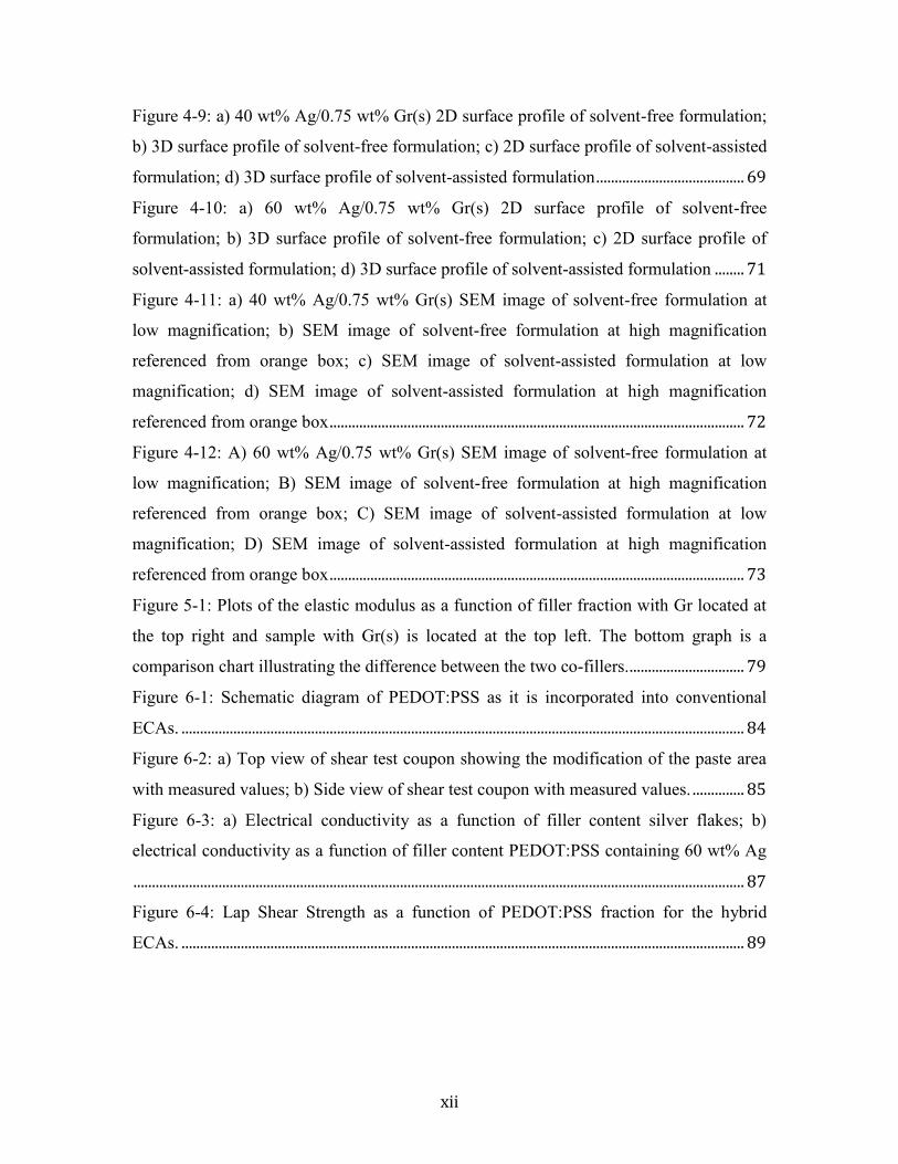
Figure 4-9: a) 40 wt% Ag/0.75 wt% Gr(s) 2D surface profile of solvent-free formulation;

b) 3D surface profile of solvent-free formulation; c) 2D surface profile of solvent-assisted

formulation; d) 3D surface profile of solvent-assisted formulation ........................................ 69

Figure 4-10: a) 60 wt% Ag/0.75 wt% Gr(s) 2D surface profile of solvent-free

formulation; b) 3D surface profile of solvent-free formulation; c) 2D surface profile of

solvent-assisted formulation; d) 3D surface profile of solvent-assisted formulation ........ 71

Figure 4-11: a) 40 wt% Ag/0.75 wt% Gr(s) SEM image of solvent-free formulation at

low magnification; b) SEM image of solvent-free formulation at high magnification

referenced from orange box; c) SEM image of solvent-assisted formulation at low

magnification; d) SEM image of solvent-assisted formulation at high magnification

referenced from orange box ................................................................................................................ 72

Figure 4-12: A) 60 wt% Ag/0.75 wt% Gr(s) SEM image of solvent-free formulation at

low magnification; B) SEM image of solvent-free formulation at high magnification

referenced from orange box; C) SEM image of solvent-assisted formulation at low

magnification; D) SEM image of solvent-assisted formulation at high magnification

referenced from orange box ................................................................................................................ 73

Figure 5-1: Plots of the elastic modulus as a function of filler fraction with Gr located at

the top right and sample with Gr(s) is located at the top left. The bottom graph is a

comparison chart illustrating the difference between the two co-fillers. ............................... 79

Figure 6-1: Schematic diagram of PEDOT:PSS as it is incorporated into conventional

ECAs. ........................................................................................................................................................ 84

Figure 6-2: a) Top view of shear test coupon showing the modification of the paste area

with measured values; b) Side view of shear test coupon with measured values. .............. 85

Figure 6-3: a) Electrical conductivity as a function of filler content silver flakes; b)

electrical conductivity as a function of filler content PEDOT:PSS containing 60 wt% Ag

..................................................................................................................................................................... 87

Figure 6-4: Lap Shear Strength as a function of PEDOT:PSS fraction for the hybrid

ECAs. ........................................................................................................................................................ 89

xiii

List of Tables

Table 2-1: A summary outlining the material properties of eutectic Pb/Sn [1] .................. 9

Table 2-2: A summary outlining the advantages and limitations of ECAs ...................... 13

Table 3-1: List of the combinations of compositions used for nanocomposites ............... 39

Table 3-2: Viscosities for the different compositions at 10 RPM .................................... 42

Table 4-1: List of the combinations of compositions used for nanocomposites ............... 56

Table 4-2: Summary of surface roughness values from optical profiler .......................... 70

Table 6-1: Summary of different sample compositions and the masses of the conductive

filler material ..................................................................................................................... 86

1

Chapter 1 Introduction

Today is an age of unprecedented technological growth as the semiconductor electronics

industry continues to make advancements, spanning over the past few decades [1–3].

With it comes the constant demand for improving interconnection technology: an

essential requirement that supports the components necessary for the electronic systems

to function [1]. However, one of the consequences that comes with the rapid growth of

technology is that mass produced electronic devices suffer from a short product life cycle

[2,4,5], leading to many of these Printed Circuit Boards (PCBs) to be thrown out into

landfills to become what is known as e-waste [2]. Most interconnection technologies

responsible for creating a continuous bridge between the PCB and electrical components

traditionally utilize a material known as eutectic Lead/Tin (Pb/Sb) solder [2,3,5–11]. First

of all, it is important to state that Pb is a toxic material [2,3,5,11,12]. The primary reason

why Pb/Sn solder is a concern stems from the fact that as of 2006, 90% of e-waste was

deposited into landfills without pre-treatment or prior action taken to remove such

hazardous chemicals before being incinerated [4]. When incinerated, the Pb/Sn liquefies

and finds its way into groundwater or rivers, causing massive damage as an

environmental contamination risk. In response to this, legislative bodies in EU [2–

4,6,13,14] and Japan [1,3,6,14] have made laws that ban the use of hazardous substances

within their electronic packaging and component interconnections. In order to meet these

laws, both electronics producing companies and researchers have begun looking into

alternative electronic packaging materials that can completely replace Pb/Sn [3,5,11,12].

Among these alternatives, two options proved promising: lead-free metal alloy-based

solutions (Sn/Ag/Cu or SAC representing the first letter of each element, is an alloy

series that are the most dominant) [1,2,6,15] and a polymer composite-based material

known as electrically conductive adhesives [1,3–7,9,10,13,14,16]. Although the SAC

series are already commercial and a popular alternative to Pb/Sn solders, they suffer from

thermal cycling issues, high temperature requirements that risk device damage during

reflow, as well as a low drop performance [1,15] making it a temporary solution for the

time being. As such, great focus is placed onto ECAs as the next alternative electronic

packaging material, owing to many desirable properties such as high shear strength, low

2

temperature requirements, fewer processing steps, finer pitch capabilities and

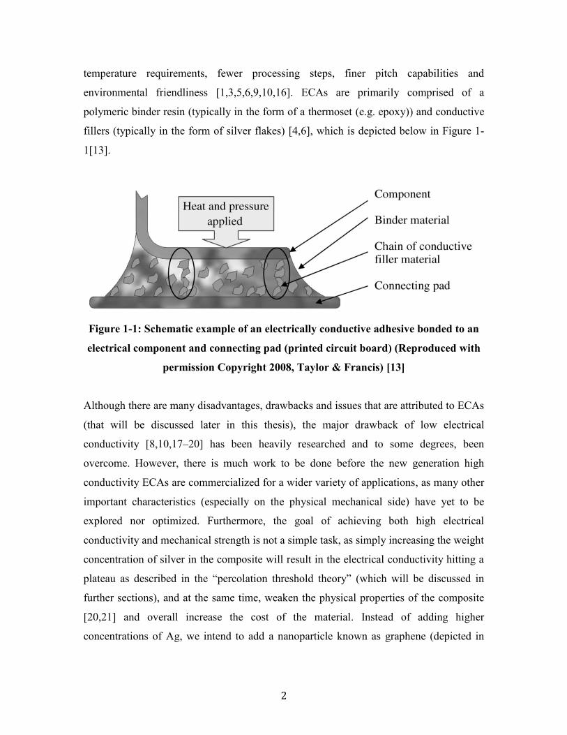
environmental friendliness [1,3,5,6,9,10,16]. ECAs are primarily comprised of a

polymeric binder resin (typically in the form of a thermoset (e.g. epoxy)) and conductive

fillers (typically in the form of silver flakes) [4,6], which is depicted below in Figure 1-

1[13].

Figure 1-1: Schematic example of an electrically conductive adhesive bonded to an

electrical component and connecting pad (printed circuit board) (Reproduced with

permission Copyright 2008, Taylor & Francis) [13]

Although there are many disadvantages, drawbacks and issues that are attributed to ECAs

(that will be discussed later in this thesis), the major drawback of low electrical

conductivity [8,10,17–20] has been heavily researched and to some degrees, been

overcome. However, there is much work to be done before the new generation high

conductivity ECAs are commercialized for a wider variety of applications, as many other

important characteristics (especially on the physical mechanical side) have yet to be

explored nor optimized. Furthermore, the goal of achieving both high electrical

conductivity and mechanical strength is not a simple task, as simply increasing the weight

concentration of silver in the composite will result in the electrical conductivity hitting a

plateau as described in the “percolation threshold theory” (which will be discussed in

further sections), and at the same time, weaken the physical properties of the composite

[20,21] and overall increase the cost of the material. Instead of adding higher

concentrations of Ag, we intend to add a nanoparticle known as graphene (depicted in

3

Figure 1-2), a co-filler that has recently proven useful for improving the electrical

conductivity of conventional ECAs.

Figure 1-2: a) Graphene in polymer composites (Reproduced with permission

Copyright 2012, Wiley) [22]; b) Atomic resolution of graphene from annular dark-

field scanning transmission electron microscopy (ADF-STEM) (Reproduced with

permission Copyright 2011, Nature) [23]

It is important to note, however, that graphene on its own will not be successful in this

effort because of the difficulty in handling. For example, it suffers from poor dispersion

in many common solvents, having a tendency to aggregate/agglomerate [22,24–26]. One

work intending to use graphene as a co-filler in ECAs reports the use of Ag nanoparticles

grown on graphene to covalently stabilize the carbon-based nanoparticles, however, this

resulted in the disruption of its pi-bond resonance and overall decrease of its conductivity

[17]. Another work reports the use of a non-covalent stabilization method, where

surfactant SDS was used to decorate the graphene so as to prevent further aggregation

without disrupting the resonance of the graphene [18]. This SDS-decorated graphene

(Gr(s)) is the main co-filler that is chosen for this study, as it was shown to have provided

a significant increase in electrical conductivity and overall and great promise as co-filler

for hybrid ECAs. It must be noted that the procedure involved with making this lab-grade

a

4

conductive hybrid ECA is complex and difficult (when attempting to make larger

amounts), thus preventing us from conducting further physical tests.

As such, this study changed the synthesis method of Gr(s) in such a way that it is easier

to produce in large quantities. In order to produce larger volumes of the composite, we

used what is known as a planetary shear mixer (PSM). After this was achieved, the next

step of this study was to produce this Gr(s)-filled ECA at varying parameters so that its

physical properties could be characterized.

The purpose of this thesis is to present the results of the physical properties found when

preparing hybrid ECAs, as well as the usefulness and impact that Gr(s) provides to the

composite. Since graphene is known to have excellent mechanical properties, it would be

very useful to know whether or not these benefits could act to reinforce the composite’s

mechanical properties, besides just improving the electrical conductivity of the material,

while at the same time, reducing the need to use higher Ag concentrations thereby

negating the negative aspects associated with the addition of Ag flakes.

This thesis contains seven chapters. The first two chapters act to inform the reader of the

field of study, as well as particular literature information intended to explain mechanisms,

theories and useful knowledge surrounding the topic of conductive adhesives. Chapter

three outlines the work on characterizing the rheological properties of epoxy-based

composites that use graphene (Gr) and SDS decorated graphene (Gr(s)) as fillers. Chapter

four outlines the work on characterizing one of the practical mechanical properties of

interest to this field describing the adhesive strength between the PCB boards and the

conductive paste: Lap shear strength (LSS). Furthermore, this chapter will discuss how

the use of solvent in certain formulations affects the LSS of the composite, as well as

potential factors that could elucidate the results. Chapter five outlines the work on

characterizing the elastic modulus of the epoxy-based composites using Gr and Gr(s) to

further understand any potential reinforcing effects that these nanoparticles offer the

composite. Chapter six outlines the possibility of using PEDOT:PSS as a co-filler for

ECAs, in hopes that we could find further alternatives for making ECAs with higher

5

electrical conductivities even at low weight loadings of Ag. Finally, the last chapter

concludes the entire scope of this thesis, and closes off with future work,

recommendations and ideas that should be further pursued to gain even higher levels of

understanding for the field of conductive adhesives. The work described in chapter three

was formatted for publication in the journal – Journal of Materials Science: Materials in

Electronics, and cited as reference [27] in this thesis. The work described in chapter four

was formatted for publication in the journal – International Journal of Adhesion and

Adhesives; the manuscript is currently in preparation for submission and cited as

reference [21] in this thesis. The work described in chapter five was submitted to

Thermoset Resin Formulators Association (TRFA 2015) for a conference contest cited as

reference [3] in this thesis. The work described in chapter six was submitted to Surface

Mount Technology Association (SMTA 2016) as a technical paper cited as reference [5]

in this thesis.

6

Chapter 2 Literature Background and Review

2.1 Interconnection Materials: Electronic Packaging for ICs

Electronic packaging is a field of electrical engineering that studies ways to attach,

enclose and protect electronic components on devices, where soldering is currently the

most cost-effective method for both small and large-scale assembly/manufacturing

[28,29]. The main principle behind electronic packaging lies with the task of joining two

components together: a) the electrical devices, for example, integrated circuit chips,

resistors, capacitors etc. that are needed to create the circuit; b) the circuit board known

as a printed circuit board (PCB) that acts as a substrate to hold these electrical devices in

place [29]. Figure 2-1 shows an illustration to summarize the above statement, including

an example of a fully assembled circuit board using what is known as surface mount

technology: a method that has recently begun to replace pin through hole technology

[28,30,31].

Figure 2-1: a) Schematic illustration of how an interconnect material joins a

functional component onto a PCB (Reproduced with permission Copyright 2006,

Elsevier) [1]; b) Example of fully-assembled circuit board that used surface mount

technology to join the component to the PCB (Reproduced with permission

Copyright 2016, Elsevier) [28].

Both of these components must be connected in such a way where the circuit has access

to power, signal transmissions (i.e. data) and ground in order to function [1]. Besides

a b

7

simply joining the electrical device onto the PCB, the interconnecting material is tasked

with providing the following: a) electrical connectivity between the device and the board;

b) thermal conductivity for heat dissipation; c) mechanical continuity so as to ensure that

the components have intimate contact between one another even through physical

agitation [12]. In order to bridge these two components, interconnection materials and

technologies were engineered through techniques such as pin through hole (PTH), surface

mount technology (SMT), ball grid array (BGA), chip scale packaging (CSP), and finally,

flip-chip technology [1].

2.2 Three Interconnecting Materials: Pb/Sn, SAC305 and ECAs

As was mentioned in the previous section, interconnection materials are tasked with

providing continuity on various levels between the PCB and electronic device. It was also

mentioned that soldering is the most common method, however, the material that is

responsible for creating this continuity is also important. Figure 2-2 summarizes these

materials by classification [32].

8

Figure 2-2: Summary of different materials used to create electrical

interconnections (inspired by I. Mir [32])

The first group, also the most commercially available and the most commonly used, is

metallic-based solders. Traditional lead-based solders (Pb/Sn) for decades, acted as the

go-to material for electronic packaging [11,12,29,31]. Due to the health and

environmental concerns mentioned earlier, lead-free alloys have taken over as the more

popular choices in today’s market [12]. The second group of interconnecting materials is

a composite-based material known as electrically conductive adhesives (ECAs).

Although it brings interesting properties that are useful as interconnecting materials, more

research is needed in order for ECAs to fully mature and realize its full potential before

becoming a major commercial interconnecting material. Each material will be expanded

upon in the upcoming sections.

2.2.1 Traditional Lead-based Solder (Pb/Sn) Traditional lead-based solder (Pb/Sn) has for decades been the dominant material chosen

to join devices onto PCBs at large scale and low cost in industrial manufacturing [29] as

9

well as for smaller scale electronic processes such as in laboratories or small shops. In

specific, Pb/Sn solders are comprised of two elements-lead and tin as an alloy typically in

a ratio that allows it to be considered a eutectic system: a system containing two elements

with a specific compositional ratio in equilibrium with each other. This means that, a

specific ratio of material A and B (according to their phase diagrams) experiences infinite

diffusivity in the liquid state at a certain temperature [33]. In the case of eutectic Pb/Sn,

the melting temperature is 183ºC[2,15,29], and the eutectic system ratio for the Pb/Sn

alloy in specific is 63% Sn and 37% Pb, however, a near-eutectic formulation of 60% Sn

and 40% Pb is also widely used for most PCB assemblies [29]. The material properties of

eutectic Pb/Sn is summarized below in Table 2-1.

Table 2-1: A summary outlining the material properties of eutectic Pb/Sn [1]

Material Properties

Volume/Bulk Resistivity (Ω cm) 1.5 × 10−5 Typical Junction R (mΩ) 10-15

Thermal Conductivity (W/m K) 30

Shear Strength (psi) 2200

Finest pitch (mil) 12

Minimum processing temperature (ºC) 215

Environmental impact Negative

Thermal Fatigue Yes

The traditional eutectic Pb/Sn solder is still the best electronic packaging material in

terms of fulfilling its purpose. However, due to the negative environmental and health

impact it possesses, alternate solutions need to take over as the primary electronic

packaging material. The Pb “impurity” provides the traditional soldering material with a

few advantages [2,12,29]:

Pb impurity acts as a surface tension reducing agent for pure tin (550 mN/m at

232ºC, which in turn improves solderability through easy wetting of the material

(giving access to small crevices, holes and gaps on the PCB)

Pb impurity prevents unwanted transformation of tin upon cooling

(transformation that leads to a volume increase and loss of structural integrity in

the joint)

Pb impurity acts as a solvent metal, diffusing rapidly in the liquid state as

intermetallic bonds are formed

10

Pb provides ductility to Pb/Sn solders

Pb impurity forms an oxide layer that protects the pure tin from forming its own

oxide layer

Pb is an overall inexpensive material

It is important to note that it is unlikely for eutectic Pb/Sn solder to be fully replaced by

an alternate material until a suitable replacement is found; mainly due to the continued

demand of certain specific electronic applications that require high reliability and long

lifespan (i.e. military equipment, aerospace and automotive applications [15,31]).

2.2.2 The current Lead-free alternative: SAC305 (Sn/Ag/Cu)

Lead-free solders have already begun its emergence in the market as another major

electronic packaging material, owing to the recent laws passed in the European Union

(EU) in 2006, as well as in Japan that have banned the use of lead-containing substances.

Similar to its predecessor, the lead-free alternatives are also alloys comprised primarily of

tin followed by other metals incorporated into its matrix (e.g. bismuth, indium, zinc,

copper, silver, and antimony) [2,12,15]. There are many combinations that have been

proposed and studied [2,12,15], however, there has been no successful formulation that

can be considered a replacement for all applications. Instead, researchers identified a core

group of elements comprised of Sn-Ag-Cu also known as SAC to be the base alloy to

work with [2,12,15]. Unlike the well-known eutectic ratio for Pb/Sn that is widely used,

industrial consortiums have proposed differing ratios depending on the country. For

example, the USA uses 95.5 Sn – 3.9 Ag – 0.6 Cu (SAC396), while the EU uses 95.5 Sn

– 3.8 Ag – 0.7 Cu (SAC387), and Japan uses 95.5 Sn – 3.0 Ag – 0.5 Cu (SAC305 [2]).

An example of a different formulation that is application specific would be for a process

known as ball-grid array (BGA) that uses 95.5 Sn – 4.0 Ag – 0.5 Cu (SAC405) for the

BGA solder joints [2]. The SAC series is not without drawbacks despite being accepted

as the lead-free alternative material for electronic packaging. One major problem of the

SAC series when compared to eutectic Pb/Sn is the operating and melting temperature

(with SAC series sitting at 217ºC and eutectic Pb/Sn sitting at 183ºC), which leads to

higher reflow temperature and thermal reliability issues with the components [2,15].

Another issue that plagues the SAC series is its solder joint reliability in that it has weak

11

drop strength, a major problem especially for both portable and handheld devices [2,15].

Furthermore, the SAC series faces issues with uneven distribution, which leads to lower

elastic modulus and impact strength [34]. Lastly, issues in the overall cost of SAC alloys

contribute to its inability to truly replace eutectic Pb/Sn. Examples of the issues that lead-

free SAC series faces can be seen below in Figure 2-3.

Figure 2-3: a) Fracture behavior of SAC105 during drop test; b) Fracture behavior

of SAC105 during impact test PCB (Reproduced with permission Copyright 2012,

Elsevier) [34]; c) Plastic deformation near the grain boundaries due to thermal

cycling; d) Fatigue cracking at interface PCB (Reproduced with permission

Copyright 2011, Elsevier) [15]

2.2.3 Electrically Conductive Adhesives (ECAs) Another alternative to traditional eutectic Pb/Sn solder is a composite material known as

electrically conductive adhesives (ECAs [6,9,11,13,16,17,19,35–42]). The emergence of

the first ECAs dates back to 1950s especially with Henry Wolfson et al earning a patent

12

on “electrically conducting cements containing epoxy and silver [43].” This composite

would then become the foundation from which present-day ECAs would be based upon.

ECAs are composed of two main components: a polymer matrix (usually a thermoset

such as epoxy) and conductive filler material (usually silver based [6,8,10,11,13,19,40–

42]) as seen in Figure 2-4.

Figure 2-4: a) Polymeric binder: Epoxy resin (DGEBA); b) Conductive filler: Silver

Flakes

ECAs can be further divided into two types of materials: anisotropic conductive

adhesives (ACAs) and isotropic conductive adhesives (ICAs) [13,32,36,37]. Anisotropic

conductive adhesives usually refer to ECAs that exhibit unidirectional conductivity (or in

one direction only) and can take either paste form or film form. A schematic of all three

forms (including the non-conductive variant can be seen in Figure 2-5 letter a to c.

Anisotropic conductive adhesives have characteristically low conductive filler

concentrations as can be seen in Figure 2-5 letter d, as it is in the lower region of the

percolation curve (a topic that will be further explained in another section).

(a) (b)

13

Figure 2-5: a) Schematic of ACA; b) Schematic of ICA; c) Schematic of NCA

(Reproduced with permission Copyright 2006, Elsevier) [1]; d) Schematic of the

percolation curve of conductive adhesives that determine the classification of the

ECA as either ACA or ICA (Reproduced with permission Copyright 2008, Taylor &

Francis) [13]

As the concentration of conductive filler content increases in the polymer matrix, a shift

in the direction of conductivity begins to form, as it goes from 1-dimensions to 3-

dimensions. ECAs that exhibit conductivity in 3 dimensions are known as isotropic

conductive adhesives [11,13,41] and will primarily be the ECA this thesis will focus on

and refer to throughout the subsequent sections. The advantages and challenges of ECAs

are summarized in Table 2-2 below [4,7–11,16,17,19,35–40,44].

Table 2-2: A summary outlining the advantages and limitations of ECAs

Advantages Disadvantages

Low processing Temperatures Low Bulk Electrical Conductivity

Fine-Pitch Capabilities Unstable Contact Resistances

Excellent Adhesion to Numerous Surfaces Hard to Remove After Cured

Directional Conductivity Possible Adhesion Strength Needs Improvement

Environmentally Friendly Alternative Joint Resistance from Oxidation/Corrosion

Minimal Thermal Fatigue & Stress Cracks High Ag Content is Expensive

Low Dielectric Constant Limited Impact Resistance

Works with Non-Solder Components Environmental Reliability Unconfirmed

Less Processing Steps & Operation Cost Longer Curing Times

Higher Flexibility Silver Migration Issue

No Flux or Secondary Underfill Needed Incorrect Spreading from High Viscosity

(d)

NCA/ACA ICA

14

Before a new type of ECA is considered commercially available for a variety of

applications, it is important to gain a better understanding of the material properties,

processability and mechanisms before further progressing. Doing so will give researchers

and industry a chance at improving the understanding of these challenges, or using

external agents that will alleviate or protect the performance of the composite. For the

sake of communication, this thesis will from here on refer to the basic epoxy and silver

flake-filled composite mentioned above as conventional conductive adhesives (CCAs).

The next sections will discuss recent works and progress regarding the improvement of

CCAs.

2.3 Conventional ECAs and Recent Progresses

This section will focus on some of the recent progresses that have been made to address

the main challenge that ECAs must overcome to be applicable to more fields: low (bulk)

electrical conductivity. All of these topics will be only briefly explained with limited

explanations on the mechanism, as the purpose of this section is to share the current

discoveries related to the improvement of ECAs.

Researchers have taken three different kinds of approaches to improve the electrical

conductivity of the composite (some of which deal with using high-aspect ratio/surface-

to-volume ratio materials, many of which are linked to the improvement of composites)

[45,46]. The first approach deals with modifying the most utilized conductive filler:

silver. By changing shape, size and other factors such as surface functionalization of the

Ag flakes, researchers are able to improve the bulk electrical conductivity of ECAs. The

second approach researchers take to overcome the low bulk conductivity of ECAs reports

the use of non-metallic carbon-based solid materials that act as co-fillers with the purpose

of working together with the Ag flakes within CCAs so as to create more metallurgical

connections between the Ag flakes without excess weight loadings of Ag. The third

method researchers report is the incorporation of conductive polymers within the CCA

composite again acting as a co-filler material, in hopes of providing more metallurgical

ions that will assist in the increase in bulk conductivity within the system.

15

2.3.1 Conductive metallic filler materials: silver in various forms One method that researchers have attempted in order to improve electrical conductivity is

to change the size and geometry of the conductive filler so as to increase the

metallurgical connections between each individual silver flake.

It is known that nanoparticles behave differently and even show different material

properties when compared to its bulk counterpart [47] and silver is no different. The size

of the silver fillers uniquely impacts the electrical conductivity of ECAs as it offers

interesting possibilities (e.g. sintering) that are not possible in the micron level [6,47–51].

As a simple explanation, sintering is a process upon which a metallic particle is heated,

and as a result, the atoms within the metallic particles begin to diffuse across its surface

to create a different shape, or even potentially join together with separate particles of the

same element [52,53]. This joining process under heat results in the formation of a three

dimensional network among Ag flakes that are otherwise not joined together, creating

new metallurgic connections that will decrease the bulk resistance of the material (or

increase the conductivity of the material).

The geometry of the silver fillers also plays a significant role in improving the

conductivity of CCAs. As explained above, there are Ag nanoparticles (0 dimensional),

and there are other geometries that silver can adapt such as silver nanowires and silver

nanobelts (1 dimensional). Figure 2-6 shows the three different geometries under TEM

that can be adapted by Ag and used to improve the electrical conductivity of CCAs by

increasing the metallurgical connections between silver flakes.

16

Figure 2-6: a) Example of Ag nanoparticles (0-D); b) Example of Ag nanowires (1-

D); c) Example of Ag nanobelts (1-D) (Reproduced with permission Copyright 2005,

Wiley) [54]

It is interesting to note that one potential drawback of using these silver nanoparticles

would be the introduction of more contact points. Literature reports that although

multiple contact points are made, there is little evidence pointing to an increase in

continuous linkages made as more nanoparticles are added into the composite [55]. An

excess amount of nanoparticles in the composite may even cause a decrease in

conductivity in some instances [19,51].

The incorporation of one-dimensional Ag nanowires into CCAs has been reported to

improve the electrical conductivity by D. Chen et al [56]. This group also performed an

interesting experiment where a CCA was loaded with both Ag nanowires and Ag

nanoparticles. They found that the electrical conductivity of the system is better than that

with either one of the two co-fillers [56]. Similarly, Z. Zhang et al reported the use of Ag

nanowires in CCAs, except that they used high temperatures to cure and sinter the hybrid

ECA [57]. As a result of the high sintering temperature, they were able to achieve bulk

conductivity values that were 1000x higher than what D. Chen et al reported [56,57].

However, operating temperatures in the 300ºC range is far too high for practical use,

therefore making their material unsuitable as a potential replacement for eutectic Pb/Sn

solder.

17

Literature also reports the use of another promising co-filler, a one-dimensional Ag

nanoparticle known as Ag nanobelts [19]. The Ag nanobelts have three distinct

advantages over Ag nanowires: a) Ag nanobelts are synthesized using a high yield self-

assembly method at room temperature; b) Ag nanobelts have a low weight-to-length ratio

meaning that the total mass of this co-filler is very small compared to that of other co-

fillers; c) Ag nanobelts possess the ability to form a percolated network at low

concentrations, meaning it can improve the electrical conductivity of the composite at

low weight loadings [19]. It is important to note that using excess amount of Ag

nanobelts also yielded similar results as excess amounts of Ag nanoparticles in CCA as

again, an increase in contact points leads to a decrease in electrical conductivity [19].

Lastly, researchers have attempted to change the surface functionalization of Ag flakes.

Ag flakes are made from mechanical milling and the product is coated with a thin layer of

lubricant: a non-conductive chemical that is intended to prevent the flakes from

aggregating, thus improve the dispersibility of the metal fillers (which in turn also

improves the rheological properties) [1,10,14,42,58–61]. Daoqiang Lu et al as well as

Fatang Tan et al have conducted extensive research in this field, and were able to

determine that the lubricant on the surface of Ag was a salt of the lubricant and silver.

Literature also suggests that replacing the carbon chain with shorter dicarboxylic acids or

even removing the organic lubricants off the surface of the Ag flakes will improve its

electrical conductivity [1,10,14,58,60], thanks to easier tunneling and electron transport

among flakes upon complete removal (removing the lubricant increases intimate contact

between flakes).

2.3.2 Conductive Non-metallic Co-fillers: Carbon based nanoparticles and the potential of Graphene

Researchers have also approached the conductivity problem of CCAs using non-metallic

co-fillers. In specific, they use inorganic carbon-based nanoparticles such as carbon black

(CB) [62–71], carbon nanotubes (CNT) [20,68,71–76], graphene (Gr)

[8,17,18,22,25,27,77–81], and even a combination of both known as graphene

nanoribbon (GNR) [82,83] as co-fillers in the polymer matrices that either do or do not

18

contain silver flakes together with it. Figure 2-7 below shows TEM examples of these

four types of carbon-based co-fillers.

Figure 2-7: a) TEM image of CB; b) TEM image of CNT (Reproduced with

permission Copyright 2009, ACS) [71]; c) TEM image of Gr (Reproduced with

permission Copyright 2015, Elsevier) [18]; d) TEM image of GNR [83]

These particles help improve the electrical conductivity of the system (CB and other

carbon-based particles can decrease electron tunneling resistance when added as a filler)

[8,17,52,62,78], or behave like metallic nanoparticles, owing to intrinsic material

properties such as high electrical and thermal conductivity [8,17,18,20,22,27,62–

19

66,68,71–74,77,79,80]. As such, the inclusion of these carbon-based co-fillers proves to

be useful as it offers the possibility of shifting the required amount of conductive fillers

within ECAs to lower concentrations.

Although carbon-based co-fillers offer plenty of attractive properties that can be utilized

by composite materials, there are a few challenges that must be first addressed before

being able to take full advantage of what carbon-based fillers (e.g. CB/CNT/Gr/GNR).

The most common problem is the agglomeration issue of carbon-based fillers that occurs

when incorporated within the polymer matrix [6,17,22,25,27,70,74,80,84,85]. This

problem leads to other issues, for example, increase in viscosity and poor dispersion,

which cause many of the beneficial properties to be suppressed, resulting in the

composite exhibiting minimal performance improvement [17,18,22,27,71,75,76,86].

Researchers have responded to this problem in two ways [17,18,25,75,87]: a) by

attempting to use methods that involve the surface functionalization/modification of the

carbon filler to allow for better chemical interactions between liquid media (either the

polymer itself or solvent) and the carbon filler; b) and using high shear mixing techniques

as a physical method of dispersing the carbon filler [76]. The first method of chemically

modifying the carbon filler (in this specific case, (Gr)) has been reported to prevent

aggregation, but also results in disappointing improvements to electrical conductivity

especially for graphene (this is because the pi-electron delocalization is disturbed when

covalent bonds are formed) [18]. The second method of using surfactants on carbon

fillers as a means to non-covalently exfoliate the carbon fillers was successful at

improving electrical conductivity and will be a central topic in this thesis [3,18,21,27].

2.3.3 Conductive Non-metallic Co-fillers: Conductive Polymers and PEDOT:PSS as an Alternative

Another approach that researchers are taking to improve the electrical conductivity of

CCAs involves mixing the composite with inherently conductive polymers such as

polyaniline (PANI) [88–90], polypyrrole (PPy) [91–93] or a polythiophene based

chemical known as poly(3,4-ethylenedioxythiophene) polystyrene-sulfonate

(PEDOT:PSS) [5]. An image depicting all known inherently conducting polymers is

shown below in Figure 2-8.

20

Figure 2-8: Schematic of electrically conducting polymers divided into groups.

While the first conductive polymer suggested (PANI) offers benefits such as easy

processability, low bulk cost [94] and has been proven useful as a co-filler that can

improve the properties of CCAs [88,90], researchers have also determined that PANI’s

benzidine moieties present on its backbone could yield carcinogenic products upon

degradation, which is counter-productive to the attempts of ECAs acting as greener

solutions [94].

PPy on the other hand has shown greater promise, owing to its biocompatibility, ease of

synthesis, stability, and low cost [91,95]. Interestingly enough, PPy is already enjoying

commercial use today as it offers other benefits such as corrosion inhibition, good

electrical conductivity, electroactivity, and electrocromism to applications including

rechargeable batteries, electrochromic displays, ion-exchangers, pH sensors, etc. [91].

Researchers, however, soon discovered the drawbacks of this conductive polymer:

insolubility in water and most organic solvents making it difficult to

process/functionalize, and poor mechanical/adhesion properties such as self-delamination

off common substrates such as glass [91,95]. To alleviate this problem, PPy has been

modified with other polymers to form a composite and mitigate its weaknesses while at

21

the same time, even provide newer strengths such as smoother percolation curves in the

context of electrical conductivity [91]. However, sometimes, the modifications use harsh

post-treatments that are detrimental to the overall products that result in the decrease of

PPy’s biocompatibility [95]. Reports of using PPy-epoxy have been made and

demonstrated to function as ICAs, showing great promise as a potential alternative to

eutectic Pb/Sn that can be used in industry [91,92]. There is also a report that uses

dopamine (DA) as the modification to PPy to form a functionalized PPy composite that

adapts a tunable fibrous morphology capable of exhibiting enhanced water dispersibility,

adhesion properties, and electrical conductivity [92]. Both of these reported modified PPy

composites were used in CCAs and were shown to improve both mechanical and

electrical conductivity, and overall displays excellent potential as a commercial ECA.

Finally, the incorporation of thiophene derivative PEDOT:PSS into CCAs will be shown

in this thesis to see whether or not it also had the potential to become the next

commercial ECAs in the market [5]. To the best of our knowledge, no work has been

published regarding the use of PEDOT:PSS as a bulk material acting as a co-filler for

improving the electrical conductivity of CCAs.

2.4 The Material Properties of ECAs

2.4.1 The Mechanism behind Conductivity in ECAs: The Percolation Theory

This section will concentrate on explaining a frequently used term throughout this thesis

that details the conduction mechanism responsible for making conductive adhesives

exhibit electrical conductivity upon loading the polymer matrix with conductive filler: the

percolation theory. The word percolation means to spread gradually through an area or

group according to various dictionaries, and is even explained in chemical/mathematical

terms by S.R. Broadbent and J.M. Hammersley [96]. However, if described in the context

of ECAs, this theory specifically refers to the gradual spreading of conductive filler

content within the insulating polymer matrix [32,40,52,61,97].

What the percolation theory tries to explain when it comes to ECAs is the critical volume

fraction (i.e. Vperc) of the conducting substance necessary to illicit electrical conductivity

22

within a medium presumed to be completely insulating. We call the point at which we

reach/exceed the Vperc as the percolation threshold (where the insulating material begins

to express electrical conductivity as a result of the conductive particles forming a network

throughout the entire composite) [32,40,52,61,97].

To simplify, we can divide this theory into three sections. Conductive filler is gradually

added into an insulating matrix, and as a result, will elicit a gradual electrical

conductivity increase within the insulating matrix (denote this as section I) owing to the

increasing amount of metallurgical connections being made as the polymer network is

saturated with conductive filler. After reaching and exceeding Vperc, the conductivity

increase will experience a sharp rise where the composite material transitions from a bulk

insulator into a bulk conductor (denote this as section II with the dotted line). Conductive

filler is added after the sharp rise, but once again experiences only a gradual increase in

electrical conductivity (denote this as section III). A schematic of this phenomenon can

be seen in Figure 2-9 where the increasing number of the section represents more silver

filler added (with different color to show particles overlapping).

23

Figure 2-9: Schematic of Percolation curve to explain percolation theory. As the

polymer network is slowly saturated with conductive filler, more metallurgical

connections are made between filler particles resulting in an increase in

conductivity.

We can also describe this phenomenon in mathematical terms based on equations stated

by N. Lebovka et al. Electrical conductivity 𝜎(𝑉) is dependent on volume fraction of

conductive filler (𝑉) and the area near section I (that approaches the dotted line and

begins to transition to section II), and can be summarized using equation 1 below:

𝒘𝒉𝒊𝒍𝒆 𝑽 > 𝑽𝒑𝒆𝒓𝒄: 𝝈(𝑽) = 𝒂(𝑽 − 𝑽𝒑𝒆𝒓𝒄)𝒕 Eq. 1

whereas area near section III (that passes the dotted line and begins to plateau) can be

summarized using equation 2 below:

24

𝒘𝒉𝒊𝒍𝒆 𝑽 < 𝑽𝒑𝒆𝒓𝒄: 𝝈(𝑽) = 𝒃(𝑽𝒑𝒆𝒓𝒄 − 𝑽)−𝒔

Eq. 2

where 𝑠 & 𝑡 denote the electrical conductivity exponents and 𝑎 & 𝑏 denote coefficients

for different materials [98]. N. Lebovka et al further explained that for random

percolation, variables 𝑠 & 𝑡 are expected to be 𝑠 = 𝑡 ≈ 4/3 for 2 Dimensional systems,

whereas 𝑠 ≈ 0.75, 𝑡 ≈ 2 for 3 Dimensional systems [98]. It is important to remember

that the 𝑡 value can change depending on a variety of factors, for example, B. Kilbride et

al noticed that charge transport through a 2 Dimensional object was unlikely when 𝑡 ≈

4/3 for their CNT system as the exact same values were observed for bulk structures as

well as films, indicating that such a phenomenon is possible only through electron

transport/tunneling of some sort within the bulk composite [99]. Other observations for

CNT systems have also mentioned the possibility of CNT aggregation as the cause of the

shift, as the above equations break down if random distribution is not achieved [100],

which is a large possibility for carbon-based fillers that tend to suffer from agglomeration

issues as mentioned earlier.

Some important remarks must be made to further clarify why this conductivity-shifting

phenomenon is possible. In order for electrical conductivity to occur, these conductive

particles must be properly distributed throughout the matrix such that the filler material

establishes particle-to-particle contacts (in this thesis, we denote this intimate contact

between particles as metallurgical connections). It is in this regard that we are able to

form a network of conductive particles that are in contact with each other, giving room

for electrons to travel through and as a result, express electrical conductivity.

Also, because this network of conductive particles must be in contact with each other to

make metallurgical connections (or close proximity between each other), various

parameters such as particle geometry, size, aspect ratio, nature and distribution are

important to consider [52]. It is precisely because of this fact that many of the recent

progresses mentioned earlier in this thesis were possible, as researchers modified particle

geometry (nanowires/nanobelts or CNT GNR), size (Ag nanoparticles and CB), aspect

25

ratio (exfoliated Gr and Ag nanobelts), nature (presence of lubricant on Ag), and

distribution (solvent effects that will be mentioned in later sections).

Furthermore, the idea of the conductive particles requiring intimate contact is easily

observed in the case of ECAs, as uncured composites despite being loaded with high

weight concentrations of Ag flakes will only exhibit conductivity after the curing process,

where the epoxy shrinks and compresses the flakes together [32,52], implying that higher

shrinkage leads to better conductivity as more conductive pathways are formed.

As supplementary information, Mikrajuddin et al referred to a model called effective

medium approximation (EMA) that incorporates this shrinkage concept into the

explanation as to how ECAs conduct electricity (similar to what was proposed by N.

Lebovka et al). EMA considers the volume fraction of filler particles to be small cubes

that make up the volume of the composite, and was established in order to solidify the

relationship between volume fraction of conductive filler, particle size, pressure, as well

as the possibility of having two percolation thresholds [97].

2.4.2 The Mechanism behind Conductivity in ECAs: Contact Resistance for a Bulk Composite

Building from what was mentioned from the previous section, this thesis will also touch

upon the concepts responsible for creating resistances within a composite system. Amoli

et al and other researchers explained that the overall resistivity value measured from

ECAs is a summation of a series of resistivities 𝑅 as seen below in equation 3 [6,52,101]:

𝑹 = 𝑹𝒃 + 𝑹𝒇−𝒇 Eq. 3

where 𝑅𝑏 is the bulk resistance of the conductive filler and 𝑅𝑓−𝑓 is the filler-filler contact

resistance. Moreover, the filler-filler contact resistance can be further broken down into

two specific types of resistivity values as seen below in equation 4:

𝑹𝒇−𝒇 = 𝑹𝒄𝒐𝒏𝒔 + 𝑹𝒕𝒖𝒏𝒏𝒆𝒍 Eq. 4

26

where 𝑅𝑐𝑜𝑛𝑠 is the constriction resistance that is responsible for restricting the free-

electron flow through sharp contact points, while 𝑅𝑡𝑢𝑛𝑛𝑒𝑙 is the tunneling resistance,

which is formed across two fillers that are not completely in contact with each other, yet

still close enough for the electron to tunnel through [52].

It was mentioned in previous sections that Ag nanoparticles begin to exhibit higher

resistivity values if the concentration loaded into the polymer matrix is too high. This

phenomenon is directly attributed to constriction resistance, since more contact points

lead to more bottlenecked electron pathways rather than one large continuous highway.

Figure 2-10a shows a cartoon as an example that explains how constriction resistance

reduces the current by separating the electrons into multiple roads; half of which do not

even reach the end of the material. This drop in current felt originates from the electrons

that become stuck among the many contact points within the composite (because the

smaller branches have smaller contact area) and is known as constriction resistance.

Figure 2-10b on the other hand shows a cartoon of how tunneling resistance requires the

electron to overcome an energy barrier (akin to uphill travelling needing more energy) to

pass through the gap. When an electron tries to go through this small gap, majority of the

signal (in our case current) is not 100% transferred since the probability of the successful

electron tunneling is low. This inefficiency known as the tunneling resistance or a drop in

current originates from the electron’s attempt to overcome the energy barrier at a very

low success rate.

27

Figure 2-10: a) Image for explaining constriction resistance where electrons attempt

to travel from one end of the composite to the other, but only few succeed resulting

in a drop in current; b) Image for explaining tunneling resistance where only very

few electrons succeed in conquering the Φ barrier, resulting in a drop in current.

2.4.3 Epoxy Resin: A Better Understanding of the Polymer Matrix and its Role in ECAs

Epoxy is a thermoset that has been preferred as polymer matrix for ECAs as well as many

other composite materials, as it possesses many attractive characteristics such as excellent

environmental and dimensional stabilities, good strength, modulus, hardness and

adhesion to a wide variety of filler materials [13,35,60,76,102–105]. But before delving

further into how to improve ECAs, it would be prudent to first explore the role of epoxy:

the ECA’s often overshadowed component.

Plastics, or synthetic polymers are a class of material that is used in all areas of life today,

and can be traced back to as early as 1830 when the first sticky latex from natural rubber

was used for tires [106]. Since then, synthetic polymers have increasingly grown in

production (especially after World War II) in order to mitigate the lack of trade for

naturally occurring materials [106]. Eventually, plastics began to compete with the use of

28

traditional materials such as metal for various mechanical applications especially during

the 1960s-1970s. Plastics can be divided into two categories according its behavior

during thermal processing: Thermoplastics and Thermosets [106]. Thermoplastics by

definition are polymers that are molded by applying heat as its primary means of

processing, possessing a special feature of being recoverable and re-fabricated through

the use of heat and pressure. Examples of thermoplastics include polyolefins, polyvinyl

chloride, polycarbonates, polyacrylics, nylons, etc.

On the other hand, thermoset resins are a class of polymers that account for about 10-

20% of the entire polymer market, where they are used as key components for

composites, adhesives, and coating technologies [76,106]. Examples of thermosets

include epoxy resins, phenol-formaldehyde resins, un-saturated polyesters such as

fiberglass and finally synthetic rubbers [106]. In specific, thermosets are polymers that

are typically pre-polymerized and then “crosslinked” through chemical or thermal

treatment to form chemically linked covalent bonds between individual polymeric chains

during fabrication [76,106]. After “setting,” the crosslinked networks are able to resist

many forms of stimuli (such as heat softening, mechanical deformation and solvent

attack) [106], virtually unable to further modify its physical state or chemical structure

[107]. Although traditional thermosets are excellent candidates for applications requiring

dimensional stability and environmental resistance [107], many shortcomings are

encountered because of the same behavior. Examples include the inability to exhibit

reusability, post-polymerization manipulation and decomposition [107].

From a chemical point of view, it was first synthesized in 1891 and was not

commercialized until 50 years after [105,108]. A prime example of a thermoset is epoxy:

a material that is useful in a variety of fields as it offers excellent properties. The

chemical structure of commercial epoxy resin and crosslinkers is shown below in Figure

2-11.

29

Figure 2-11: Schematic representation of epoxy resin and curing agent chemical

structure (Reproduced with permission Copyright 1990, Wiley) [109]

A few examples of these properties are as follows: adhesion (on a variety of surfaces),

high mechanical strength (tensile, compressive and flexural), resistance to chemical

attack and fatigue, as well as electrical resistance [102,103,105,108,110]. Furthermore,

epoxy exhibits a degree of tunability since a user can change the way either the resin or

the hardener is used or synthesized in order to achieve the kinds of properties he/she

wishes the epoxy to display. For example, its viscosity and final strength can be adjusted

by changing the monomer density, chain length, curing agent and catalyst if used [105].

These properties are ideal for engineering as not only is epoxy a flexible material with a

variety of possible properties, it also produces little to no harmful byproducts when

undergoing the curing procedure [105]. Many of these wonderful properties are heavily

attributed to a quantifiable means of determining how well epoxy is cured: the

crosslinking density [108].

30

With this knowledge in mind, it is clear that the mechanical and physical properties of

ECAs are heavily dependent on the type of polymer matrix chosen, influencing the

ECA’s rheology, adhesion strength and durability as will be seen in the coming sections.

2.4.4 The Rheological Properties of a Composite: Flow and Workability

As mentioned in the previous section, understanding the rheological and viscoelastic

behavior of a composite system is important in the perspective of engineers. Studies give

insight to the flow mechanics of the most common type of polymer liquid systems, and

non-Newtonian fluids are useful for a variety of applications such as paint systems, ink

printing processes or generally any system that handles dispersions [111,112]. Figure 2-

12 shows viscosity as a function of shear rate as well as different colored lines to denote

different flow curves for different rheological behaviors [113,114].

Figure 2-12: Viscosity as a function of shear rate to show the different rheological

behaviors of fluids using flow curves

An example of why rheology is important can be seen in the behavior of polymer liquids

under confinement (i.e. is very close to 2 Dimensions in that the paste is very thin).

Shear rate γ

Vis

co

sity η

NewtonianFluid

DilatantFluid

Lubricant/grease

Pseudoplastic

31

Systems exhibiting this confined nature tend to behave very differently when compared

to bulk behavior because the thickness of the polymer is approaching the magnitude of

the polymer coils, giving rise to interactions that do not exist in the bulk scale: a behavior

elucidated through only through rheology. The dynamics and statistics of these confined

polymers have great value for industrial fields concerned with tribology, adhesion,

lubrication and catalysis [115], while on a laboratory level they can help estimate

important properties that we are concerned with composites such as dispersion quality of

carbon fillers and the mechanical strength of composites [116]. Furthermore, viscosity

has been used as a practical tool for determining the percolation threshold and saturation

point of composites, which allow researchers spend less time on optimizing formulations

despite the many compounding conditions that are associated with mixing filler materials

in polymer matrices [117].

The understanding of rheological and viscoelastic behaviors is useful for different

applications in industry as it gives engineers a better idea of the conditions required for

easier processing control [118]. Moreover, this understanding can lead to the possibility

of researchers shedding light on properties that a filler material expresses only within the

polymer matrix. White et al reported that while graphene offers a variety of marvelous

properties that are required to produce excellent properties as a composite, more often

than not the resulting composite falls short. This problem could be caused by surface

defects, lack of exfoliation, aggregation, wrinkles, poor dispersion, unexpected interfacial

interactions and so fourth [118]. With rheological knowledge, it is possible to

characterize particle structure and interactions for specific applications such as ECAs that

require specific viscosity parameters for proper paste spreading as specified by A. Ryan

et al [4]. Finally, it is important to realize that rheology is not a mature field as it still has

not reached the point where researchers can develop high-level computational

simulations and models that can simulate how the flow mechanics affect the composite

performance without being limited to the existing continuum-level models [118]. As

such, it is good to continue researching and expanding our knowledge regarding the

rheological behavior of composites so that one day, researchers can have enough data to

be able to create models and simulations that help draw out the full potential that

32

composites can offer. This thesis presents rheological work on Gr- and Gr(s)-loaded

epoxy using a cone and plate viscometer at room temperature to help understand the

impact of carbon fillers on the composite.

2.4.5 Mechanical Properties of a Composite: Lap Shear Strength

ECAs are first and foremost adhesives with the task of adhering electrical components

down onto a substrate (PCB). As such, ECAs are required to exhibit good adhesion

strength to be able to fulfill its purpose. Many works have focused on improving the

electrical conductivity of ECAs as outlined in previous sections of this thesis. However,

there is a significantly smaller number of works that focus on the characterization and

improvement of ECA’s mechanical properties such as adhesion strength [36]. It is

mentioned in one of the upcoming chapters that quantifiably predicting both the

performance and strength of an adhesive is difficult and complex, owing to the many

factors that must be accounted for between the adhesive and the surface where it is

bonded to [119,120]. Moreover, predicting the failure mechanisms occurring at the

microscopic level is not a simple task without using complicated models and software.

Figure 2-13 shows an example of a MATLAB software used by researchers that

compares between analytical and experimental data for adhesive lap-shear joint failures.

Figure 2-13: MATLAB program designed to do an analytical VS experimental

comparison for bonded joints (Reproduced with permission Copyright 2012,

Elsevier) [121].

In order to work around this problem, efforts were made to simplify the mechanical

testing of adhesives by focusing on identifying stress distribution for the lap-joint of

interest [122]. It is in the interest of both researchers and industry to adapt similar test

33

procedures so that both parties can accept a universal practice of determining the

adhesive’s mechanical strength. The way both researchers and industry achieved this is

through the formation of test such as American Society for Testing and Materials

(ASTM), which is a test standard association responsible for developing strict black-box

protocols that heavily simplify the test procedure, preparation and calculations involved

with finding a property of interest. In other words, as long as the tester follows the

standard, they can then not only avoid experiencing issues with calculations and

invalidating any approximations or assumptions made by the test standard, but also, the

tester will have full confidence that their results are relevant and universally acceptable.

In the case of adhesion strength, ASTM uses the lap-shear strength (ASTM D1002) [123]

to quantify the adhesion strength of metal-to-metal joints, and is a commonly recurring

mechanical property found in technical datasheets. Further examples of this test can be

seen in subsequent chapters that utilize this test standard in hopes of determining the

mechanical performance of ECAs.

2.4.6 Mechanical Properties of a Composite: Elastic Modulus

The concept of understanding the macro-scale mechanical properties of a given material

using information gained from the micro-scale structure has been a recurring objective of

material science and researchers [124]. As was discussed in the previous section, the

adhesion strength is a mechanical property of great importance to ECAs. It is known that

there are two ways to improve this property: a) using surface functionalization by adding

a chemical that contains both an organic component and metallic component thereby

assisting in the “coupling” of the two different solid surfaces; b) decreasing the elastic

modulus of the resin to acceptable levels that do not encourage the adhesive from

experiencing cohesive failure [41]. Although the method of using coupling agents has

been well explored by other researchers [38], the studies outlined in this thesis

concentrate on the latter, using micro-indentation in order to characterize the elastic

modulus of ECAs. Figure 2-14 shows adhesion strength as a function of elastic modulus

to illustrate how there is an optimal point at which the material enjoys high adhesion

strength without decreasing the elastic modulus too far to the point of provoking cohesion

failure.

34

Figure 2-14: Adhesion as a function of elastic modulus for ECA composites

(Reproduced with permission Copyright 2008, Taylor & Francis) [41]

By definition, the elastic modulus of a material is a measure of a material’s ability to

resist deformation within the elastic region (the area that permits deformation before

irreversible deformation occurs) as an external force is applied [125]. Although it is

simple to just characterize elastic modulus of ECA composites to see if it is possible to

obtain a map to determine at which point we are able to have high adhesion strength yet

high elastic modulus to prevent cohesive failure, predicting the elastic moduli of systems

that are comprised of more than one component is not simple because many factors affect

the readings, for example, system morphology, shape of the components as well as any

interaction effects (i.e. if the components bond to themselves) [126]. Therefore, results

from our studies will be focused on observable trends rather than focus on single values

that fully define our composite system.

35

This study uses indentation as the primary method to determine elastic modulus (dubbed

as Hertzian indentation in this thesis). According to Oliver and Pharr, elastic modulus E

and hardness H are the two most common mechanical properties that are characterized

using indentation [127]. The elastic modulus is connected to the force VS displacement

curve generated from the indentation test using an equation solved by Hertz [128,129]

and Reine [128] (dubbed Hertzian equation in this thesis) and can be seen below as

equation 5:

𝑎3 =3𝑃𝑅

4𝐸∗ Eq. 5

where 𝑎3 is the radius of the contact area, 𝑃 is the indentation load (in force), 𝑅 is the

radius of the indenting tip, and 𝐸∗ is the elastic modulus [128,129]. This equation acts as

the basis upon which our elastic modulus information was calculated and will be

explained further in a future chapter.

36

Chapter 3 SDS Decoration of Graphene and its Effect on the Rheological and Electrical

Properties of Epoxy/Silver Composites

3.1 Introduction

As was discussed in the previous chapter, engineers consider the rheological and

viscoelastic behaviors of a composite system as important physical properties to

understand. The rheological and viscoelastic behavior can be used to give a better idea of

the conditions required for easier processing control and in the end, workability that is

essential to making ECAs become commercially friendly and practical to manufacture.

This study uses SDS decorated graphene (Gr(s)) because previous works by T. Filleter et

al and J. Lin et al suggest that single layer graphene possesses properties that allow it to

behave as a solid lubricant [130,131]. This concept is useful as J. Coo et al and R.

Bowman et al explained that frictional force (that lubricants decrease) is proportional to

viscosity [132,133]. These rheological studies for graphene and epoxy composites are in

specific useful for electrically conductive adhesives (ECAs); a material intended for

replacing traditional alloy-based solders [134]. The viscosity and rheological properties

of an ECA is key to determining its performance and feasibility as it is applied to stencil

and screen-printing techniques [134].

It is important to note that this study cannot use a solvent-assisted approach, because both

trace amounts of solvent and bubbles formed during the curing are unavoidable even with

long desiccation time [76,135]. Furthermore, the yield from such a process is expected to

be very low because of a small amount of material, as a large amount of solvent is needed

[18]. M. L. Gupta et al addressed a similar problem when it came to making composites,

however, instead of using graphene, they used carbon nanotubes (CNTs) as the

nanofiller. They successfully determined how to disperse and mix the nanofiller without

solvent when it came to forming composites through the use of a planetary shear mixer

(PSM), as well as other high shear mixing machines [76]. Our method also used a PSM to

carry out a solvent-free method to disperse nanofillers, synthesize hybrid ECAs, as well

as investigate nanocomposites that were not loaded with silver flakes. This work

37

systematically investigated how adding graphene and SDS decorated graphene will affect

the viscosity and the electrical performance of the composite. The way this mixing

method affects the ECA properties will be briefly discussed by examining the

morphology of the ECA using SEM. We will also determine the electrical conductivity of

the material as it is suspected that the absence of the solvent will directly affect the

dispersion of graphene and thus affect its ability to decrease bulk resistivity.

3.2 Experimental

3.2.1 Stabilizing/Decorating graphene nanosheets with SDS

Graphene nanosheets (Gr) were purchased from ACS Materials (USA) and used as

received. The size of the graphene nanosheets according to the supplier is 0.5 to 5 µm

and is confirmed using TEM by Amoli et al to be around 1 µm [18]. SDS was purchased

and used as received from Sigma Aldrich. Although the procedure before the

nanocomposites preparation requires the use of solvents (ultra-pure water and HPLC

Ethanol) in order to properly functionalize and stabilize the Gr with surfactant, the

mixing procedure for preparing the nanocomposites is solvent-free.

Our previous work provided us with the inspiration to decorate graphene with the non-

covalent surfactant method, which is illustrated below as a schematic in Figure 3-1:

38

Figure 3-1: Schematic illustration showing the decoration of the graphene

nanosheets with surfactant SDS

This process uses a liquid solution that is prepared by mixing SDS powder with ultra-

pure water at a concentration of 60 mmol L-1, which is 20 mmol L-1 lower than the critical

micelle concentration (CMC) of SDS in water [136,137]: the point where the excess

surfactant forms micelles. The aim of the SDS decoration is not to make micelles, but

rather, to decorate and self-assemble onto the graphene and non-covalently exfoliate the

graphene sheets. This solution was then placed in low power sonic bath (Branson 2510R-

MT) to undergo ultrasonication for 30 minutes, and allows for the hydrophobic backbone

of the SDS to adsorb onto graphene’s surface. The solution is centrifuged at 8500 RPM

for 10 minutes and the supernatant is removed. The remaining precipitate is washed four

39

times using HPLC ethanol as its dispersant which is then sonicated for 5 minutes. This

process is repeated three times in order to remove remaining un-bonded SDS from the

precipitate. Finally, after completing the repetitions, the precipitate is then placed in a

vacuum oven at 75°C overnight to allow any remaining solvent to evaporate wherein the

leftover precipitate of SDS stabilized graphene (Gr(s)) is harvested.

3.2.2 Preparing the nanocomposites

Liquid epoxy resin (D.E.R.™ 331) Diglycidyl Ether Bisphenol-A (DGEBA) and curing

agent (D.E.H.™ 24) triethylenetetraamine (TETA) were purchased and used as received

from DOW Chemical Company (USA). Silver flakes (~10 μm) were purchased from

Sigma Aldrich and used as received. The following combinations denoted below in Table

3-1 were combined in one container where they were mixed at 2000 RPM for 4 minutes

and de-foamed at a speed of 2200 RPM afterwards for 1 minute using a Thinky Mixer

(ARE-310).

Table 3-1: List of the combinations of compositions used for nanocomposites

Sample Composition Ag flakes

[wt %]

Gr/Gr-s

[wt %]

1 Epoxy 0 0

2 Epoxy + Silver flakes 60 0

3 Epoxy + Graphene 0 0.25, 0.5, 1, 1.5 and 2

4 Epoxy + Graphene-SDS 0 0.25, 0.5, 1, 1.5 and 2

5 Epoxy + Silver flakes + Graphene 60 1

6 Epoxy + Silver flakes + Graphene-SDS 60 1

3.2.3 Measuring Viscosity

A cone & plate viscometer (Brookfield CAP2000H+, USA) was used to determine the

effects of filler concentration on the viscosity of the system at room temperature. Cone &

plate viscometers operate under the principle of measuring a torque felt by a cone shaft

undergoing a constant shear rate and known spindle dimensions. As seen in Figure 3-2,

this viscometer is comprised of a flat plane where the sample is located and a rotating

shaft (housing a cone shaped spindle at the end).

40

Figure 3-2: a) Optical image of the cone & plate viscometer; b) zoom-in of cone &

plate loaded with epoxy resin; c) cross-sectional diagram of the cone & plate with

the terms used in the viscosity equation

The cone itself has an obtuse angle propagating away from the apex of the shaft; the gap

between the cone and plate once the apex touches the plane is filled with the sample

where the linear velocity is proportionate to the radial distance resulting in a constant

shear rate as the spindle rotates [138]. Shear stress 𝜏 is denoted below as a ratio between

torque G felt by the spring and radius r of the cone [138]:

𝜏 =3𝐺

2𝜋𝑅 Eq. 6

41

Moreover, the shear rate 𝛾 is determined through the ratio between the velocity of the

cone Ω𝑟 and cone gap C:

𝛾 =Ω𝑟𝐶

=Ω𝜓

Eq. 7

The viscosity 𝜂 obtained using a cone & plate viscometer is defined as the ratio between

shear stress and shear rate:

𝜂 =𝜏

𝛾=

3𝐺2𝜋𝑅

Ω𝜓

⁄ Eq. 8

The above equation for determining the viscosity of a material under a cone & plate

viscometer is heavily dependent on the both the torque felt by the spring as well as the

rotation speed of the cone. In this viscometer, a cone CAP-05 ™ was used, having a

radius 𝑟 = 0.953 𝑐𝑚 , a cone angle 𝜓 = 0.0314 , and finally, a cone gap of 𝐶 =

0.0299 𝑐𝑚.

3.2.4 SEM of Nanocomposites

A Field Emission Scanning Electron Microscope (FE-SEM, LEO-Ultra, Gemini,

Germany) was used in order to carry out a qualitative study on the morphology and

degree of dispersion of graphene nanosheets within the nanocomposites produced. The

samples were placed on a 90-degree stub to view the cross-section of the ECA.

3.2.5 Electrical Conductivity Measurement

The resulting composites that contained silver flakes were casted into a glass slide that

had a square mold (7mm x 7mm x 0.5 mm) made of adhesive tape. A clean, flat copper

sheet was placed on top of the paste in the mold to ensure a flat surface and consistent

thickness. The sample was then inserted into the oven and pre-cured at 60°C for 30

minutes, and then cured at 150°C for two hours. Once the curing was complete, the

copper sheet and adhesive tape were removed in order to determine the bulk resistivity of

42

the sample using a sheet-resistance four-point probe measurement setup. The

configuration consists of the probe unit (Cascade Microtech Inc.) and the digital

multimeter & function generator unit (Keithley 2440 5A SourceMeter®, Keithley

Instruments Inc.). The sheet resistance readings acquired from this configuration can then

be converted into bulk resistance readings using the following equation [17,52,92]:

𝜌 = 𝐹𝑡𝜋

ln 2(

𝑉

𝐼) Eq. 9

The t in the above equation is the thickness of the sample, I is the applied current, and V

is the voltage drop measured by the SourceMeter®. The F in equation 9 is a correction

factor for samples that have a finite thickness that is defined by the ratio between the

sample thickness t and probe spacing s (1 mm). The correction factor F can be

approximated to 1 if 0.4 <𝑡

𝑠< 1. The mold is 0.5 mm while the probe spacing is 1 mm,

which leads to a ratio of 0.5: a value that allows F to be approximated to 1.

3.3 Results and Discussion

3.3.1 Viscosity behavior of composites

Six samples of varying compositions were measured for viscosity (summarized in Table

3-2) at room temperature and a shear rate of 33.3s-1 (or 10 RPM). We quantified the

behavior and characteristics of the uncured composites in order to obtain a preliminary

dataset that will assist us in figuring out where our composite stands.

Table 3-2: Viscosities for the different compositions at 10 RPM

Sample Composition Viscosity

[cP]

1 Epoxy 11400

2 Epoxy + Silver flakes (60 wt%) 30660

3 Epoxy + Graphene (1 wt%) 49470

4 Epoxy + Graphene-SDS (1 wt%) 18263

5 Epoxy + Silver flakes + Graphene Above 1000000

6 Epoxy + Silver flakes (60 wt%)+ Graphene-SDS (1 wt%) 160500

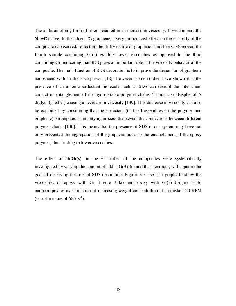
43

The addition of any form of fillers resulted in an increase in viscosity. If we compare the

60 wt% silver to the added 1% graphene, a very pronounced effect on the viscosity of the

composite is observed, reflecting the fluffy nature of graphene nanosheets. Moreover, the

fourth sample containing Gr(s) exhibits lower viscosities as opposed to the third

containing Gr, indicating that SDS plays an important role in the viscosity behavior of the

composite. The main function of SDS decoration is to improve the dispersion of graphene

nanosheets with in the epoxy resin [18]. However, some studies have shown that the

presence of an anionic surfactant molecule such as SDS can disrupt the inter-chain

contact or entanglement of the hydrophobic polymer chains (in our case, Bisphenol A

diglycidyl ether) causing a decrease in viscosity [139]. This decrease in viscosity can also

be explained by considering that the surfactant (that self-assembles on the polymer and

graphene) participates in an untying process that severs the connections between different

polymer chains [140]. This means that the presence of SDS in our system may have not

only prevented the aggregation of the graphene but also the entanglement of the epoxy

polymer, thus leading to lower viscosities.

The effect of Gr/Gr(s) on the viscosities of the composites were systematically

investigated by varying the amount of added Gr/Gr(s) and the shear rate, with a particular

goal of observing the role of SDS decoration. Figure. 3-3 uses bar graphs to show the

viscosities of epoxy with Gr (Figure 3-3a) and epoxy with Gr(s) (Figure 3-3b)

nanocomposites as a function of increasing weight concentration at a constant 20 RPM

(or a shear rate of 66.7 s-1).

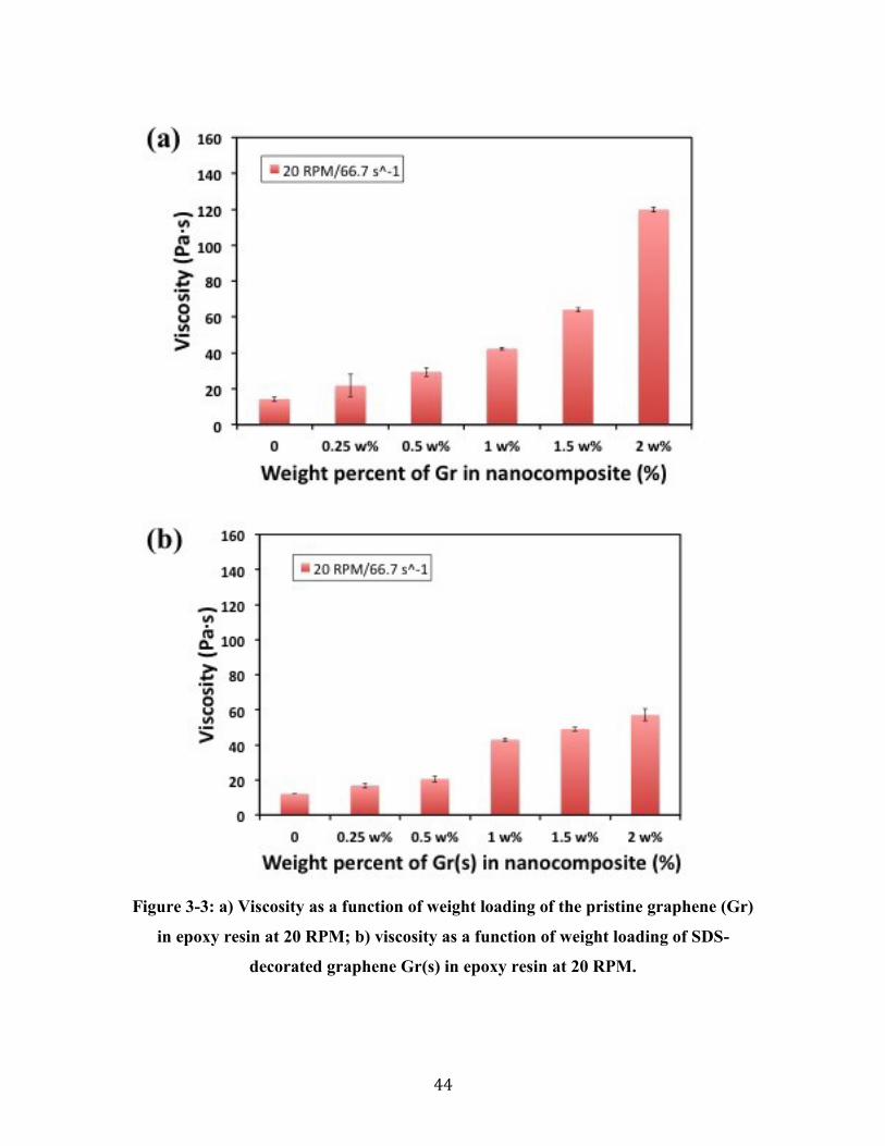
44

Figure 3-3: a) Viscosity as a function of weight loading of the pristine graphene (Gr)

in epoxy resin at 20 RPM; b) viscosity as a function of weight loading of SDS-

decorated graphene Gr(s) in epoxy resin at 20 RPM.

45

It is seen that the Gr(s) graphs show much lower values when compared to the Gr graphs.

The maximum value in Gr(s) graphs is close to 60,000 cP whereas the maximum value of

the Gr graphs is doubled, almost exceeding 120,000 cP. The dependence of viscosity on

the weight concentration of pristine Gr is an exponential increase; this same trend was not

seen for Gr(s).

Figure 3-4 and Figure 3-5 show plots of viscosity as a function of shear rate in log base 2,

providing a different perspective on what happens to the viscosity of the system as the

rotational speed of the cone & plate is increased, where Figure 3-4 is Gr and Fig 3-5 is

Gr(s). It can be observed that the way shear rate affects the viscosity depends on the

amount graphene added to epoxy.

Figure 3-4: Viscosity in log scale as a function of Shear Rate of Gr and Epoxy where

dotted lines indicate viscosity readings too high for the viscometer to display;

Note: All values in graphs that contain error bars represent standard error.

46

Figure 3-5: Viscosity in log scale as a function of Shear Rate of Gr(s) and Epoxy

where dotted lines indicate viscosity readings too high for the viscometer to display;

Note: All values in graphs that contain error bars represent standard error.

For the samples of lower wt% (0-0.5 wt%), the viscosity increased with the shear rate,

following a known behavior where the non-aggregated solid particles show high

viscosities at low shear rates, but then begin showing lower viscosities upon higher shear

rates [141]. On the other hand, for the samples of higher wt% (1-2 wt%), the viscosity

first decreased with the shear rate but exhibited spikes (i.e. sharp increase) that thus far

appears after going past what appears to be a critical shear rate of 167 s-1. The dotted

lines indicate spikes in the viscosity that can no longer be measured by the cone and plate

viscometer as the viscosity rapidly increased at those high shear rates. This type of spike

was observed both in Figure 3-4 and Figure 3-5, occurring at higher shear rates for

sample loadings of 1-2 wt%.

The effects of increasing shear rate on the viscosity of the nanocomposites system are

further interpreted in terms of the concepts of shear thickening and shear-thinning. Shear

47

thickening is a behavior seen in fluids that experience a sharp increase in viscosity above

a critical shear rate, where the fluid often transitions from a liquid-like dispersion into a

solid-like material as a result of the particles forming clusters [142]. Conversely, fluids

that behave in the opposite manner are known as shear-thinning fluids; for example,

colloidal dispersions are typically shear-thinning fluids [143]. When this type of fluid is

subjected to flow, the colloidal particles begin to form layers resulting in lower flow

resistance as well as lower viscosity [142]. As shown in Fig. 4 and Fig. 5, the viscosity of

the pure epoxy (D.E.R. 331 DGEBA) increases with the shear rate, behaving as a shear

thickening liquid. Note that DGEBA can render either shear thickening or shear-thinning

behavior depending on the supplier [144]. The viscosity of the epoxy nanocomposites

with 0.25 and 0.5 wt % Gr and Gr(s) are almost constant with higher shear rate. An

explanation for this shear-thickening behavior of the nanocomposites containing low

loading of graphene (0 to 0.5 wt%) is that the composite is in a regime where the system

is dominated by the molecular strands of the epoxy resin, which is similar to the one-

dimensional particle arrangement discussed by D. Smith et al [145]. As a result of the

viscometer applying force, the polymer strands become entangled and take a three-

dimensional arrangement, resulting in higher viscosities [141] within the higher shear rate

region. On the other hand, the behavior of the epoxy composite with higher loadings (1-2

wt%) of Gr and Gr(s) starts to show signs of shear-thinning, hinting the possibility that

the addition of graphene nanosheets suppressed the shear thickening properties of the

epoxy. It is well known that the presence of a layered structure (in our case, graphene)

can suppress the onset of shear thickening, as it reduces the efficacy of the shear flow to

create the hydrodynamic clusters [143]. Similar results indicating that shear-thinning of

polymer-filled graphene at higher weight concentrations are found in D. Wu et al’s work,

where they reported that graphene at 1 wt% showed stronger shear-thinning behavior,

and further reported that graphene nanosheets were responsible for the suppression of the

shear flow of their polylactide polymer chains [146].

Figure 3-5 revealed a stronger shear-thinning behavior in Gr(s) when compared to Figure

3-4, which happens at higher loadings of the Gr: in particular, at the 1 wt %, suggesting

the some influence resulting from the SDS molecules decorated on the graphene surface.

48

It was suspected that the SDS molecules formed additional intermolecular bonds between

the graphene and epoxy [147], which resulted in the increase of viscosity at low shear

rates. However, applied force at high shear rates break the bonds thus resulting in the

shear-thinning behavior. Other than the 1 wt% Gr(s) curve, all other curves at higher

loadings above 0.5 wt % in Figure 3-4 and 3-5 show an initial shear-thinning behavior,

followed by a sharp increase in viscosity at higher shear rates. This phenomenon is

similar to the typical Order-Disorder flow curve of stable suspensions of Brownian hard

particles [142,148]. The Order-Disorder theory describes the sliding of particles over one

another, forming layers during shearing; after exceeding a critical shear rate, the

hydrodynamic forces would pull out the particles from their ordered layers to enter a

different regime where the particles agglomerate with one another to form a disordered

state resulting in a sharp increase in viscosity [142].

Overall, Figure 3-4 and 3-5 reveal that the addition of Gr(s) led to lower viscosities for

the epoxy nanocomposites than the pristine graphene Gr. This finding has profound

implications for the future applicability on these conductive composites as some printing

techniques that already focus on dispensing conductive ink are concentrating on ways to

improve their printing process (which involves the use of shear-thinning conductive inks)

[149]. Furthermore, conductive adhesives used for surface mount assemblies are

recommended to exhibit strong shear-thinning, highly stable yet low viscosities at high

shear rates, and good recovery of the pastes after the process is complete [150]. This

suggests that Gr(s) may be useful as a dilatant-suppressor when formulating ECAs that

are dispensed through printing techniques.

On another note, it has been reported that negative effects (such as excess deposition or

non-smooth flow across the stencil) are associated with conductive adhesives that do not

fall within the desired viscosity ranges (recommending a range of 100,000 cP, although

the conductive adhesive used in that work was 70,000 cP) [4]. It can be seen that sample

6 is reaching the range of the recommended viscosity and that the use of exfoliated

graphene as a lubricant is indeed successful. Further work for optimization can give us

the opportunity to reduce the viscosity to even lower, more acceptable levels, which is

49

especially relevant for other applications such as dispensing through printing technology

[134].

3.3.2 Morphology and electrical conductivity of composites

The morphology and conductivity of the cured nanocomposites were characterized. The

SEM images in Figure 3-6 show the morphologies of the epoxy and Gr/Gr(s)

nanocomposites at different magnifications. Figure 3-6a and 3-6b compare the difference

between low weight percent and high weight percent of Gr as seen in Figure 3-6c and 3-

6d. It is seen that the increase of filler content changes the morphology from a smooth,

flat surface to a flakier and mountainous appearance. As such, the higher weight percent

Gr contains a morphology that is overall sharper and higher in surface area even when

compared to Gr(s) at the same weight percent. Figure 3-6e is the SEM image of the

nanocomposite with 2 wt% Gr(s), showing a similar morphologies to that of 2 wt % Gr,

containing moderately hilly or mountainous terrain. The transparent-looking sheets at the

edge of the flakes found in the high magnification zoom in Figure 3-6f indicate that the

Gr(s) are better exfoliated.

50

Figure 3-6: SEM images of the epoxy composites with 60% silver and Gr or Gr(s);

a) Low zoom view of Graphene and epoxy [Gr] at 0.25 wt%; b) Highest zoom view

of Gr 0.25 wt% on a large flake; c) Low zoom view of Gr 2 wt% showing a

mountainous morphology; d) Highest zoom view of Gr 2 wt% taken of an area from

6c; e) Low zoom view of Gr(s) 2 wt% showing a similar morphology to 6c; f)

Highest zoom view of Gr(s) 2 wt% showing smoother morphology likely as a result

of the SDS decoration

51

The electrical conductivities for the synthesized hybrid ECAs were investigated using a

four-point probe method. Figure 3-7 plots the electrical bulk resistivity of the ECAs as a

function of the weight loading of two nanofillers Gr and Gr(s) added into the composites

without the use of solvent (identified as solvent-free method and denoted by solid lines)

in this work and with the assistance of ethanol solvent used in our previous work

(identified as solvent-assisted and denoted by dashed lines) [18].

Figure 3-7: Bulk resistivity as a function of weight percent comparison graph

between Gr and Gr(s). The solid lines denote (solvent-free) results from our work.

The dotted lines show results from previous work that used ethanol to assist in the

dispersion of filler content.

The electrical resistivity values of the ECAs filled with Gr(s) are in the same order of

magnitude as those of the ECAs filled with Gr; in general, the resistivity decreased with

the addition of graphene. This observation confirms the positive effect of adding

graphene on improving the electrical conductivity when compared to conventional ECAs

52

and suggests that the SDS decoration of graphene has a negligible effect on the

conductivity improvement. However, a slight increase in the resistivity between 1-1.5%

wt Gr was noticed, perhaps because of the uneven dispersion of the Gr at higher

concentrations. The bulk resistivity values for the solvent-free method are in the range of

1 × 10−2 Ω ∙ 𝑐𝑚 , which is one magnitude higher compared to the solvent assisted

method. This is reasonable considering the role of solvent was to improve the filler

dispersion and deliver better conductivity. It is important to note that we see this solvent

effect even for conventional ECAs that do not contain graphene nanofillers. Even though

the solvent-free method may hold the advantage in the simplicity of the manufacturing

process and the workability of the paste itself, the graphene-filled ECAs prepared in this

work may be suitable for the applications where only moderate conductivity is needed.

Further work is necessary to improve the electrical conductivity and as a result, broaden

its potential applications.

3.4 Conclusions

We systematically investigated the rheological and electrical properties of

graphene/silver-filled composites, and particularly focused on elucidating the effect of

SDS decoration of graphene. Gr(s) exhibited lower viscosities when compared to Gr

(with or without the presence of silver), revealing a positive effect of SDS on reducing

the viscosity. Our findings also show that weight concentrations from both Gr and Gr(s)

appeared to exhibit shear thickening from 0 to 0.5 wt% owing to the potential transition

of the resin going from 2 dimensional to 3 dimensional conformation as well as the

intrinsic properties of the epoxy chosen. However, above 0.5 wt%, it is suggested that

due to the presence of a layered structure suppressing the shear thickening behavior of the

system, the Gr and Gr(s) viscosities began exhibiting shear-thinning behavior. Both

systems follow the order-to-disorder theory and curve at higher weight concentrations.

Gr(s) has been shown to follow the typical curve for stable suspension of Brownian hard

particles after a high enough concentration is present within the epoxy matrix. As a result,

the presence of graphene in general has been shown to play a key role in the shear-

thinning behavior of these composites. The compositions that use Gr(s) were shown to

exhibit better workability, while also falling within the higher section of the

53

recommended viscosity range. Furthermore, this work revealed new rheological behavior

upon the addition of surfactant SDS on graphene as the decoration of graphene is usually

exploited to improve dispersion; however, in our case it has an added unique effect. It is

clear that the multiple effects of surfactant should be considered in the development of

ECAs: not simply for the improvement of filler dispersion, but also the suppression of

dilatant behavior. Future work can incorporate this finding into the optimization of ECA

fabrication processes, as well as any other endeavors that require a shift in rheological

behavior.

54

Chapter 4 Residual Solvent and its Negative Effect on the Lap-Shear Strength of SDS-

Decorated Graphene Hybrid ECAs

4.1 Introduction

Most ECA research today focuses on improving its electrical conductivity

[6,17,18,47,151] instead of on its mechanical properties [36] because quantifiably

predicting the performance and the strength of the bond is difficult and complex without

using simulations and modelling software, since it must account for factors such as

geometric complexity, inherent discontinuity signature between the adhesive and the

surface it is being bonded to, or even the failure mechanisms happening in the

microscopic level [119,120]. As a result, there are limited studies that evaluate the

mechanical properties of ECAs [36]. This work is focused on using lap shear testing as a

way to determine how well nine different formulations of conductive adhesives bond

onto the FR-4 surface using the most common test standard: ASTM D1002 [121,122].

This work investigates the influence of residual solvent presence (within the composite)

on the mechanical properties (and to a smaller degree, the electrical properties) of both

hybrid and conventional ECAs compared to solvent-free formulations. Although the

utilization of solvent is integral for properly dispersing the SDS modified graphene

nanofiller [18,27] within the composite, the presence of solvent within the system was

suspected to have a negative impact on the mechanical properties of the cured adhesive.

This is especially true if the functional groups of the solvent unfavorably interact with

either the polymer matrix or the surfactant in our case based on previous works that also

attempted to disperse carbon-based nanofillers within a polymer matrix [76,135,152,153].

Our suspicion was further outlined in a previous work according to the TGA and DSC,

which will be explained in a later section [18]. To follow up on these results, we will

compare the solvent-assisted formulation results to the solvent-free formulation and in

the end, shed light on whether or not residual solvent indeed has a negative impact on the

curing mechanics as it will become evident in the mechanical properties of the ECA.

Moreover, we will confirm that solvent presence has negative effects on the mechanical

55

properties of the system; we will then take a closer look to identify any potential factors

that could directly impact the mechanical strength so as to gain a better understanding on

what is happening to the post-cured material. This work also plans to identify an optimal

composition that possesses both high shear strength and electrical conductivity for further

investigation and future work that can be further tested in practical settings.

4.2 Experimental

4.2.1 Materials

The polymer matrix used in this study was the liquid epoxy resin (D.E.R 331™)

Diglycidyl Ether Bisphenol-A (DGEBA) and amine-based curing agent

triethylenetetraamine (TETA). Both were purchased and used as received from DOW

Chemical Company (USA). Silver flakes (~10 μm) purchased from Sigma Aldrich were

used as received, and acted as the conductive filler for the composite. Graphene

nanosheets with a size range of 0.5 to 5 μm were purchased from ACS Materials (USA)

and were used as received [18,27]. The surfactant Sodium dodecyl Sulfate (SDS) was

purchased and used as received from Sigma Aldrich and was responsible for exfoliating

the graphene nanosheets. HPLC ethanol solvent at 99.8% purity was purchased and used

as received from Fisher Scientific (USA).

4.2.2 ECA Preparation

The process for preparing the composites required the following steps: (a) adding the

appropriate amounts of epoxy resin and silver flakes according to the desired composition

as denoted in Table 4-1; (b) adding SDS modified graphene that was prepared by

suspending SDS and graphene in ultra pure water, using an ultra sonic bath to allow the

surfactant so self-assemble onto the graphene sheets, and finally extraction by

centrifugation and evaporation of any remaining supernatant [27]; (c) steps exclusively

for solvent-assisted formulations include taking the mixture and adding 250 mL HPLC

ethanol, running the mixture through a planetary shear mixer (PSM), and then doing a

combination of vortex mixing and desiccation [18,27]; (d) adding curing agent, mixing

the composite via PSM to form the ECA paste [18,27] and then applying the paste onto

56

the appropriate test coupons (i.e. FR-4/electrical/microscopy). A schematic in Figure 4-1

illustrates the above method.

Table 4-1: List of the combinations of compositions used for nanocomposites

Composition Ag flakes

[wt %]

Gr(s)

[wt %]

Epoxy + Silver 20, 40, 60 0

Epoxy + Silver + solvent 20, 40, 60 0

Epoxy + Silver + Graphene-SDS 20, 40, 60 0.75, 1.5

Epoxy + Silver + Graphene-SDS + solvent 20, 40, 60 0.75, 1.5

Figure 4-1: Schematic illustration of how the ECAs were mixed and prepared for

testing

4.2.3 Lap Shear Test The Universal Material Tester (UMT) Tribological Test Equipment (CETR Campbell),

equipped with a pair of tensile wedge grips (G1061-2, Mark-10 Corp) was used to

evaluate the lap shear strength (LSS) of varying ECA compositions. Test coupons (1/16”

double-sided FR-4 boards, 590-540) were purchased and used as received from MG

Chemicals. The specifications of the FR-4 boards were machined to follow the

dimensions presented in Figure 4-2. The test procedure and calculations followed ASTM

D1002 [123] with the exception of reducing the contact area of the joint to 12.7 mm x

12.7 mm in order to accommodate the limitations of the load cell used in the experiment.

57

Figure 4-2: a) Schematic cross-section illustration of ASTM D1002 test coupon and

its modified paste measurements; b) schematic top view illustration of ASTM D1002

test coupon and its modified paste measurements; c) example of test sample used for

optical microscopy and optical profiling; d) example of test sample used for ASTM

D1002 lap shear testing

4.2.4 Electrical Conductivity Test

A four-point probe fixture (Cascade Microtech Inc.) that is connected to a micro-ohm

meter (Keithley 2440 5A Source Meter, Keithley Instruments Inc.) was used to measure

the electrical sheet-resistance values of varying ECA compositions. These values were

then converted to bulk resistance using the following equations [18,52]:

𝜌 = 𝑅𝑠 ∙ 𝑡 = 𝐹𝑡𝜋

ln 2(

𝑉

𝐼) Eq. 10

58

The sheet resistance (𝑅𝑠) obtained from the reading was used together with the caliper-

measured ECA thickness (𝑡). The (𝑉) and (𝐼) represent the applied current and measured

voltage drop across the probe pins, from which the sheet-resistance is based upon. The

correction factor (𝐹) is ratio between the thickness of the ECA sample (𝑡) and the probe

gap (𝑠) [18,52]. Under the condition where 0.4 < 𝑡

𝑠 < 1, it is safe to approximate the

correction factor (𝐹) to equal 1 [18,52]. As the probe gap is 1 mm wide, the ECAs

prepared were designed to have an average thickness of 0.5 to 0.7 mm, resulting in the

fulfillment of the above stated condition.

4.2.5 Optical Microscopy and Optical Profiler

The cross sections of two ECA formulations were observed under manual operation using

an inverted optical microscope (Carl Zeiss Axio Observer Z1m; Magnification 5x and

50x) equipped with a CCD camera (Axio Cam).

An optical profiler (MFP-D WLI 3D Surface Profilometer, RTEC Instruments USA) was

used to observe the degree of flatness exhibited by the solvent-assisted and solvent-free

ECAs as well as to generate a 3D plot to further illustrate the presence of bubbles as well

as any other defects that are not easily detectable by optical imaging.

4.2.6 Scanning Electron Microscopy

A Field Emission Scanning Electron Microscope (FE-SEM, LEO-Ultra, Gemini,

Germany) was used in order to investigate the morphology and find potential defects or

bubbles associated with the solvent-assisted method compared to the solvent-free method

of preparing the ECAs. ECA pastes were prepared and casted into a glass mold and

thermally resistant tape onto a ½” x ½” area with a thin sheet of copper as a cover. The

glass slide was then sliced and bent (at the middle of the copper sheet) in order to obtain a

flattened cross-sectional sample of the ECA. The samples were placed on a 90-degree

stub to view the cross-section of the ECA.

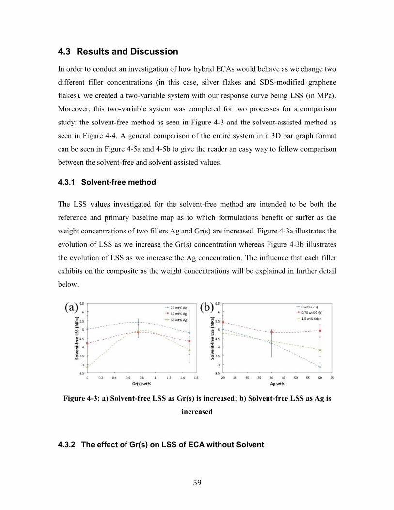
59

4.3 Results and Discussion

In order to conduct an investigation of how hybrid ECAs would behave as we change two

different filler concentrations (in this case, silver flakes and SDS-modified graphene

flakes), we created a two-variable system with our response curve being LSS (in MPa).

Moreover, this two-variable system was completed for two processes for a comparison

study: the solvent-free method as seen in Figure 4-3 and the solvent-assisted method as

seen in Figure 4-4. A general comparison of the entire system in a 3D bar graph format

can be seen in Figure 4-5a and 4-5b to give the reader an easy way to follow comparison

between the solvent-free and solvent-assisted values.

4.3.1 Solvent-free method

The LSS values investigated for the solvent-free method are intended to be both the

reference and primary baseline map as to which formulations benefit or suffer as the

weight concentrations of two fillers Ag and Gr(s) are increased. Figure 4-3a illustrates the

evolution of LSS as we increase the Gr(s) concentration whereas Figure 4-3b illustrates

the evolution of LSS as we increase the Ag concentration. The influence that each filler

exhibits on the composite as the weight concentrations will be explained in further detail

below.

Figure 4-3: a) Solvent-free LSS as Gr(s) is increased; b) Solvent-free LSS as Ag is

increased

4.3.2 The effect of Gr(s) on LSS of ECA without Solvent

60

In order to understand how increasing the Gr(s) content affects the LSS of the composite,

Figure 4-3a was examined. For a constant Ag wt%, a parabolic trend can be seen where

the LSS of the material is at its highest for a weight loading of 0.75 wt% Gr(s), and lower

for both 0 wt% and 1.5 wt% Gr(s) (which applies for all three weight concentrations of

Ag) in similar fashion to CNTs as demonstrated by H.P. Wu et al’s work for aluminum

substrate [20]. Furthermore, it is observed that 0.75 wt% Gr(s) has the smallest deviation

among all of the formulations, hinting that Gr(s) has excellent potential to ensure that

ECA is reliable on top of being mechanically robust. We suspect that the following

reasons for the parabolic trend:

Gr(s) is successfully increasing the strength of the composite, however, after a

critical concentration, it begins to aggregate and act as a detriment to the system

(possibly promotes bubble formation or something equivalent, creating defect

sites, which will be examined further in this work)

Gr(s) is unfavorably interacting with the epoxy curing process at higher weight

concentrations (in particular the increase of SDS in the system) [18], and as a

result is overtaking its potential to reinforce the composite

A Combination of both

More experimentation where the Gr(s) is varied in smaller step sizes is recommended so

as to generate a more comprehensive surface response plot and further verify this trend,

giving better justification to the provided explanations above. Overall, by looking at

Figure 4-3a and 4-3b, it is evident that the strongest formulations are those that contain

0.75 wt% Gr(s); among these, 0.75 wt% Gr(s) with 60 wt% Ag will be further tested for

electrical conductivity and by microscopy techniques for a view of its morphology. The

reason why the highest LSS value in the solvent-free process (20 wt% Ag and 0.75 wt%

Gr(s)) was not chosen for further testing is because formulations with low silver content

(20 wt%) express little to no electrical conductivity, thereby eliminating its potential to be

used as a functioning ECA.

4.3.3 The effect of Ag on LSS of ECA with solvent

In order to understand how increasing the Ag content affects the LSS of the composite,

Figure 4-3b was examined. It is evident that as the Ag wt% is increased for a constant

61

Gr(s) wt%, the LSS of the composite decreases. Formulations that contain 0.75 wt%

Gr(s) display smallest decline while the sharpest decline is observed for formulations that

do not contain Gr(s). It is also interesting to note that the LSS deviation from our results

are consistently large for the formulations that only contain Ag, hinting that on its own,

Ag is more of a detriment to the composite’s LSS either through increasing unreliability

(large error bars) or through the fact that higher weight concentration in hopes of

attaining better electrical performance of the composite results in the compromising of its

mechanical strength, similar to work reported by Wu et al [20]. The author suspects that

the reason for this behavior is because the Ag flakes have an effect where the increase of

the silver filler content in epoxy means the decrease of epoxy’s shear strength since more

of the composite is comprised of the filler rather than the actual binding component [20].

Furthermore, unlike Gr(s), Ag does not show any signs of composite reinforcement. It

has been known that excess Ag content in conventional ECAs leads to issues such as

higher material costs, little to no electrical conductivity improvement past the percolation

threshold, and issues with environmental reliability [7,8,19,20,154]. However, this work

also shows there is a detrimental effect to the LSS of the composite when using an excess

amount of Ag filler content, which supports the need to reduce the amount of Ag in

conventional ECAs.

When comparing the two filler materials, it has been shown that Gr(s) has the potential to

act as a reinforcing agent upon a critical concentration. Moreover, there is little variance

between samples resulting in a mechanically reliable and robust ECA. On the other hand,

it has been shown that excess addition of Ag into the composite is detrimental to its

mechanical strength and should be avoided to prevent introducing weakness into the

composite, and also to reduce cost and to avoid issues with environmental reliability at

the same time.

4.3.4 The effect of Ag on LSS of ECA with solvent

The LSS values investigated for the solvent-assisted method are intended to follow up

initial suspicions from other references that hinted potential repercussions involved with

the presence of residual solvent in the ECA composite, in particular, on its mechanical

62

properties [18,76]. Experimental results in Figure 4-4a when compared to Figure 4-3a

illustrate a significant drop in LSS: in particular for the formulations containing Gr(s).

Figure 4-4: a) Solvent-assisted LSS as Gr(s) is increased; b) Solvent-assisted LSS as

Ag is increased

According to our previous work, three findings were stated that would help elucidate the

results seen in Figure 4-4: (a) it is known and accepted that silver flakes have no

significant effect on the curing of epoxy [155]; (b) the presence of trace ethanol in the

composite reduced both the ∆HTot and Tg∞ indicating a drop in epoxy’s crosslinking

density [18]; (c) the DSC data experienced a sudden increase to ∆Hnorm for ethanol-

diluted epoxy VS neat epoxy, and again for the hybrid ECA containing graphene VS the

hybrid ECA containing SDS decorated graphene [18].

The results from Amoli et al’s thermal test indicate that despite the lack of change in Tg∞,

the change in ∆Hnorm and ∆HTot point to an unknown mechanism that is caused by the

presence of SDS [18]. Moreover, it has been suspected that SDS and ethanol are

interacting with each other resulting in the changes in thermal data and inevitably, the

crosslinking density of the final product.

From the above statements, we can firstly rule out any effect that Ag flakes have on the

solvent-assisted system [155], which explains why the samples that had 0 wt% Gr(s)

exhibited very similar LSS results to the solvent-free system. Note that the outlier for 60

wt% Ag in Figure 4-3b was noticed but not further investigated because: a) the standard

deviation is large enough that if more tests were done, the option that it is in the lower

63

bounds exists; b) further investigation of this incident will go beyond the scope of what

this work is investigating. Secondly, we can confirm that the presence of residual ethanol

alone in the system is in fact not enough to disrupt the curing mechanism of the ECA.

According to the data, it appears that both SDS and residual ethanol are required to

generate the competing mechanism that is responsible for the drop in crosslinking

density, as residual ethanol was not enough to cause a significant drop in LSS for the

formulations that did not contain Gr(s). Thirdly, the formulations that did contain Gr(s)

were shown to experience a drop in LSS, and as such, at the very least, these results

support the initial suspicion of a drop in crosslinking density (a factor that is heavily

related to the mechanical strength of the bulk material) for the solvent-assisted Gr(s)

containing formulations. Although the mechanism itself was not discovered, findings in

this work prove that the initial suspicions outlined in previous work coincides with what

is happening in the composite system, as the presence of solvent and surfactant

negatively impacts one of the mechanical properties of the cured adhesive. Further work

using thermal characterization techniques is recommended to verify that the interaction of

solvent with surfactant negatively affects the crosslinking density. Figure 4-5 is shown

below to illustrate a summary of what was found in this study.

Figure 4-5: a) Solvent-free LSS in 3D format; b) Solvent-assisted LSS in 3D format

4.3.5 Electrical conductivity

64

Although the intention of this work is not to optimize or improve the electrical

conductivity of the conductive adhesive, it is still important to choose an adhesive that

not only exhibits excellent LSS, but also possesses sufficient electrical conductivity to

ensure that the composite continues to perform as a conductive adhesive. As such, the

formulations that exhibit the strongest LSS: 20 wt% Ag/0.75 wt% Gr(s), 20 wt% Ag/0

wt% Gr(s), 40 wt% Ag/0.75 wt% Gr(s) and 60 wt% Ag/0.75 wt% Gr(s) were measured

for bulk resistivity. The first two samples exhibited no electrical conductivity despite the

highest LSS values and as a result, will not be further tested or looked into within this

work. However, the next two formulations exhibited bulk resistivity values ranging from

2.5 × 10−1 Ω ∙ 𝑐𝑚 𝑡𝑜 1 × 10−2 Ω ∙ 𝑐𝑚 and is presented below in Figure 4-6 (where a

current of 1 mA was used for all of the values measured).

Figure 4-6: Bulk resistivity comparison of solvent-assisted and solvent-free

40 wt% Ag/0.75 wt% Gr(s) and 60 wt% Ag/0.75 wt% Gr(s) formulations

It can be seen that the presence of solvent matters for the 40 wt% Ag/0.75 wt% Gr(s)

formulation as the solvent-assisted method is observed to have bulk resistivity that is 18x

smaller than the solvent-free method. However, similar results were not observed for the

65

60 wt% Ag/0.75 wt% formulation as the two samples regardless of solvent presence

exhibit roughly the same bulk resistivity values of 1 × 10−2 Ω ∙ 𝑐𝑚. As such, a difference

exists, further values are required to gain a thorough understanding of the solvent effect

on conductivity. Instead, it is better allocated for future work, as it is not within the scope

of this work to further elucidate the details of the differences between bulk resistivity

values.

It should be noted that the electrical conductivity values are congruent with Trinidad et

al’s findings [27]. However, when it came to Amoli et al’s findings using their own

solvent-assisted method, the electrical conductivities found in this work were lower by a

factor of 10 [18]. This was to be expected due to the different process that Trinidad et al’s

work utilized, where SDS decoration of graphene was conducted independently from the

composite itself and the PSM was applied over regular vortex mixer (which is known for

better dispersion efficiency) [27]. As such, it is expected that the pre-treated Gr(s) would

benefit less from the presence of ethanol when compared to Amoli et al’s process that

fully utilized the solvent, achieving higher success with the mixing process at obtaining

well dispersed and decorated graphene.

This study verified that the chosen solvent-free composites exhibited conductivity values

acceptable for electrically conductive adhesives, while also showing high LSS values.

These findings conclude that 60 wt% Ag/0.75 wt% formulation is the optimal

formulation for high LSS and high conductivity while retaining a relatively simple

preparation method when compared to the solvent-assisted approach.

4.3.6 Optical microscopy and profiler

Another factor that is suspected to contribute to the decrease of the mechanical strength

of the solvent-assisted mechanism is the formation of bubbles during the curing process.

The presence of bubbles will inevitably decrease the smoothness of the paste as well as

the contact area between the adhesive and substrate. If the paste is not smooth on the

microscopic level, the actual contact area of the adhesive is reduced, leading to the

adhesive failing at lower applied forces.

66

In order to verify this, we assumed that bubbles would form in the paste regardless of the

type of surface it is embedded to; as such, other factors besides substrate choice are kept

constant (for example, applied pressure and curing time/temperature). We chose to use

glass as the alternate substrate for its transparency so that optical microscopy and optical

profilometry techniques could be used to inspect the surface of both the solvent-free and

solvent-assisted method. The goal was to search for any evidence of bubbling at the

interface or cross-section of the paste. Optical microscopy is used to qualitatively check

for pits, dimples or other forms of discontinuity when adhering to the surface of the glass,

while the optical profiler is used to generate a 3D plot to show any possible changes in

flatness as well as obtain a quantitative measure of the sample’s surface roughness.

4.3.7 Optical microscopy results

The first method used to characterize the surface between the substrate and paste is the

optical microscope. Both solvent-free and solvent-assisted 40 wt% Ag/0.75 wt% Gr(s)

and 60 wt% Ag/0.75 wt% Gr(s) formulations were observed at 5x and 50x

magnifications. Figure 7-7 is for 40 wt% Ag/0.75 wt% Gr(s), where 7-7a and 7-7b is

solvent-free and solvent-assisted at low magnification, and 7-7c and 7-7d is solvent-free

and solvent-assisted at high magnification.

Figure 4-7: a) Optical microscopy image of 40 wt% Ag/0.75 wt% Gr(s) at low power

for solvent-free formulation; b) low power for solvent-assisted formulation; c) high

power for solvent-free formulation; d) high power for solvent-assisted formulation

A similar pattern is followed for the next formulation as Figure 4-8 is for 60 wt%

Ag/0.75 wt% Gr(s), where 4-8a and 4-8b is solvent-free and solvent-assisted at low

magnification, and 4-8c and 4-8d is solvent-free and solvent-assisted at high

magnification.

67

Figure 4-8: a) Optical microscopy image of 60 wt% Ag/0.75 wt% Gr(s) at low power

for solvent-free formulation; b) low power for solvent-assisted formulation; c) high

power for solvent-free formulation; d) high power for solvent-assisted formulation

Based on the optical microscope images at low magnification for 40 wt% Ag/0.75 wt%

Gr(s), Figure 4-7a shows a smooth speckled pattern (indicating a smooth surface) as

opposed to its solvent-assisted counterpart Figure 4-7b, which shows many light-colored

lines and grooves, as well as what appears to be rough patches resulting in lower contact

with the glass substrate. Under higher magnification, it is seen that the solvent-free

formulation in Figure 4-7c contains less of the light-speckled patterns as opposed to

Figure 4-7d, hinting that there are more pits and holes in the solvent-assisted formulation

compared to the solvent-free formulation, which agrees with the findings from the lower

magnification images that the solvent is causing pitting and contact area reduction

between the substrate and the paste.

68

The next formulation observed with the optical microscope is 60 wt% Ag/0.75 wt% Gr(s)

at low magnification. Figure 4-8a shows a speckled pattern that is similar to Figure 4-7a

except that it is not as smooth, contains larger light speckles and overall higher particle

density, likely due to the increase in Ag wt%. Figure 4-8b shows smaller light speckles

but in more clumps, indicating that some form of aggregation may be occurring or that

certain spots have more adhesion to the substrate than others. However, this still hints

that the solvent-assisted formulations have smaller contact area to the substrate compared

to the solvent-free formulations. This is again evident in the higher magnification in

Figure 4-8c and 4-8d as there are more clumps visible for the solvent-assisted

formulations.

These qualitative findings support the idea that the solvent-assisted formulations are

indeed forming more bubbles post-cure as opposed to the solvent-free formulations,

because the solvent-free formulations tend to exhibit better smoothness and uniformity,

resulting in higher contact area between the paste and substrate and thus leading to higher

LSS. However, a more quantitative approach will be presented below in order to verify

and further support these observations.

4.3.8 Optical microscopy results

In order to quantitatively determine the roughness of the surface between the paste and

substrate, an optical profiler was used to find any pits and dimples that were suspected to

form bubbles during the curing procedure. Similar to the optical microscope, both

solvent-free and solvent-assisted 40 wt% Ag/0.75 wt% Gr(s) and 60 wt% Ag/0.75 wt%

Gr(s) formulations were observed at a magnification of 10x. Figure 4-9a and 4-9b show

the optical profile of the solvent-free paste surface and the 3D render of the surface,

respectively. Figure 4-9c and 4-9d show the optical profile of the solvent-assisted paste

surface and the 3D render of the surface, respectively.

69

Figure 4-9: a) 40 wt% Ag/0.75 wt% Gr(s) 2D surface profile of solvent-free

formulation; b) 3D surface profile of solvent-free formulation; c) 2D surface profile

of solvent-assisted formulation; d) 3D surface profile of solvent-assisted formulation

The surface roughness values are presented below in Table 2. After comparing the

solvent-free and solvent-assisted surfaces for the 40 Ag – 0.75 Gr(s) composites, it was

found that the solvent-assisted formulations exhibited both lower average roughness (Ra)

as well as root-mean square roughness (Rms) when compared to the solvent-assisted

formulations for each corresponding formulation counterparts. It is important to note that

larger dimples and pits are observed for the solvent-assisted 40 Ag – 0.75 Gr(s) when

compared to the solvent-assisted 60 Ag – 0.75 Gr(s) which skews the surface roughness

to a higher Ra value. One explanation for this occurrence is that the lower Ag content

prevents resistance to larger bubble formation; however, more investigation is needed to

verify this phenomenon.

a c

b d

70

Table 4-2: Summary of surface roughness values from optical profiler

Formulation Ra (µm) Rms (µm)

40 Ag – 0.75 Gr(s) solvent-free 0.59 1.27

40 Ag – 0.75 Gr(s) solvent-assisted 5.27 6.48

60 Ag – 0.75 Gr(s) solvent-free 3.68 4.52

60 Ag – 0.75 Gr(s) solvent-assisted 3.77 4.65

Moreover, the same can be observed with the 60 Ag – 0.75 Gr(s) composites as seen

below in Figure 4-10a and 4-10b for the solvent-free optical surface profile and 3D

render respectively, and correspondingly Figure 4-10c and 4-10d for the solvent-assisted

formulation. This finding leads to the conclusion that overall, the solvent-free

formulations have smoother surfaces that contain less pits and dimples when compared to

the solvent-assisted formula. This conclusion can be seen visually through the surface

diagrams of 40 Ag – 0.75 Gr(s) composites in Figure 4-9a and 4-9c where Fig 4-9a

contains little to no blue areas – blue regions correspond to pits and dimples found on the

surface of the paste that are not in contact with the glass substrate while Figure 4-9c in

comparison contains many. The same can be said for 60 Ag – 0.75 Gr(s) composites in

Figure 4-10a and 4-10c where Figure 4-10a contains fewer blue areas in comparison to

Figure 4-10c further supporting the idea that bubble forming during curing is decreasing

the contact area between the paste and substrate and as a result, exhibiting weaker LSS.

71

Figure 4-10: a) 60 wt% Ag/0.75 wt% Gr(s) 2D surface profile of solvent-free

formulation; b) 3D surface profile of solvent-free formulation; c) 2D surface profile

of solvent-assisted formulation; d) 3D surface profile of solvent-assisted formulation

4.3.9 Scanning electron microscopy results

We further verified the results by characterizing the morphology at the micron range by

using a scanning electron microscope on the cross-section of the paste. Because the two

strongest formulations 20 wt% Ag/0.75 wt% Gr(s) and 20 wt% Ag/0 wt% Gr(s) exhibited

electrical resistivity values too high for ECAs, and were therefore deemed unsuitable for

further investigation. The next two strongest formulations were chosen instead. Below

shows the SEM images for 40 wt% Ag/0.75 wt% Gr(s) in Figure 4-11.

a c

b d

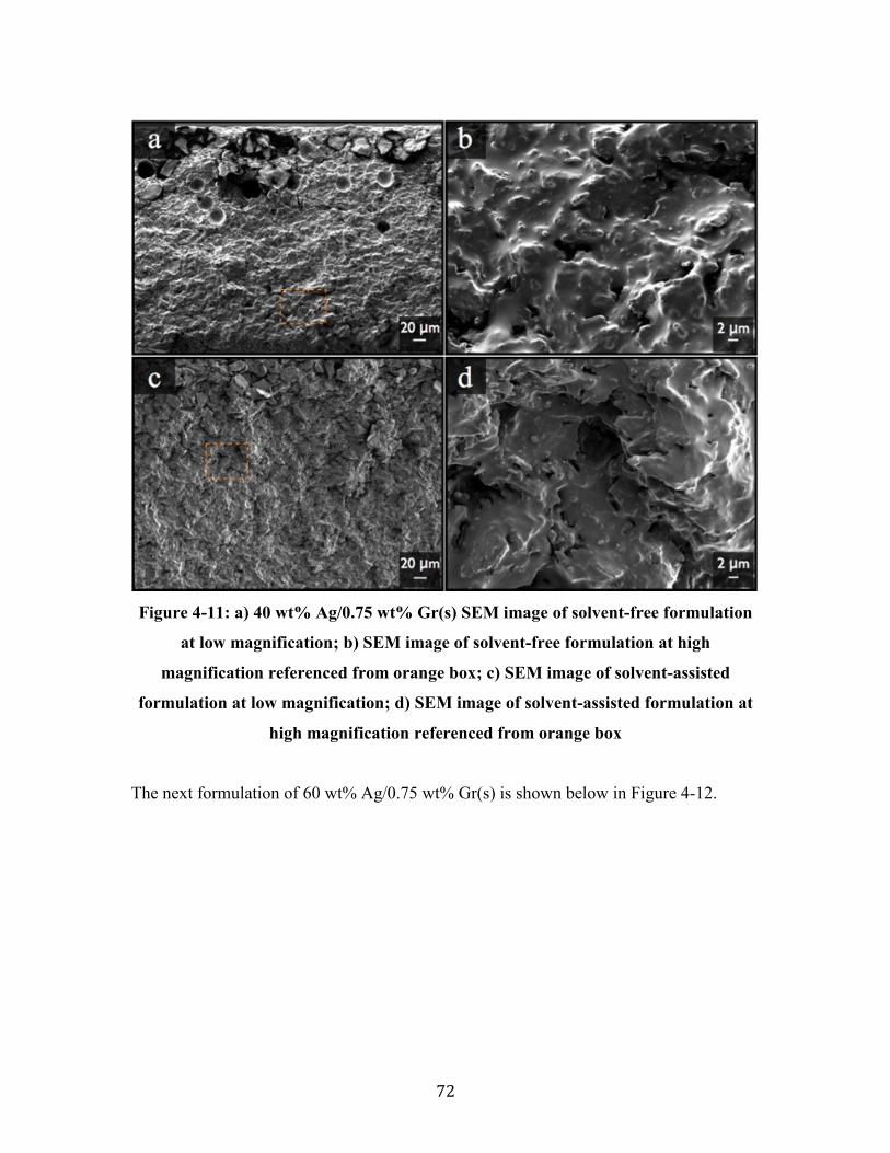
72

Figure 4-11: a) 40 wt% Ag/0.75 wt% Gr(s) SEM image of solvent-free formulation

at low magnification; b) SEM image of solvent-free formulation at high

magnification referenced from orange box; c) SEM image of solvent-assisted

formulation at low magnification; d) SEM image of solvent-assisted formulation at

high magnification referenced from orange box

The next formulation of 60 wt% Ag/0.75 wt% Gr(s) is shown below in Figure 4-12.

73

Figure 4-12: A) 60 wt% Ag/0.75 wt% Gr(s) SEM image of solvent-free formulation

at low magnification; B) SEM image of solvent-free formulation at high

magnification referenced from orange box; C) SEM image of solvent-assisted

formulation at low magnification; D) SEM image of solvent-assisted formulation at

high magnification referenced from orange box

In each of these figures, their respective a and c images denote a low power view of the

cross-section of solvent-free and solvent-assisted formulations, respectively. Their b and

d images show a high power view of the solvent-free and solvent-assisted formulations,

respectively, with corresponding orange boxes in a and c that detail where these high

power images are taken from. The compressed cross-sections of the solvent-assisted and

non-solvent methods were compared. The images obtained from the SEM agree with the

optical microscope and optical profiler, as the non-solvent methods for both formulations

exhibit a smoother morphology and fewer pockets or dimples when compared to the

solvent-assisted method. However, since the SEM images are able to capture the interior

74

structure of the composite (via cross-section), it is now clear that the phenomena

observed on the surface extends all the way through the entire cross section, showing that

bubbles are not limited to the surface alone, but are present throughout the entire paste.

As such, it is confirmed that the detrimental effects of residual solvent within the

composite can be attributed to the formation of dimples, bubbles and hollow structures

both within the composite as well as on the surface, resulting in the weakening of its

mechanical properties.

4.4 Conclusions

The LSS of both solvent-free and solvent-assisted formulations were systematically

tested in this work. It has been determined that the combination of solvent presence and

Gr(s) within the composite has a negative effect on the LSS of the material. We also

determined that the two formulations exhibiting the highest LSS are 20 wt% Ag/0.75

wt% Gr(s) and 20 wt% Ag/0 wt% Gr(s). However, these formulations did not exhibit

sufficient conductivity and therefore could not be considered for applications in ECAs.

As such, the next two formulations that exhibited high LSS and electrical conductivity

(60 wt% Ag/0.75 wt% Gr(s) and 40 wt% Ag/0.75 wt% Gr(s)) were further examined,

primarily to determine why the LSS was lower for the solvent-assisted formulations and

secondly, to verify that these formulations work as functional ECAs. The first property

investigated was the electrical conductivity of these formulations to verify that these

function as ECAs. It was found that the bulk resistivity (our measure of conductivity) of

these two formulations ranged between 2.5 × 10−1 Ω ∙ 𝑐𝑚 𝑡𝑜 1 × 10−2 Ω ∙ 𝑐𝑚 .

Furthermore, it was determined that 40 wt% Ag/0.75 wt% Gr(s) exhibited lower bulk

resistivity when assisted with solvent, whereas solvent assistance for 60 wt% Ag/0.75

wt% Gr(s) showed little improvement of the electrical conductivity of the ECA.

The next investigation was made in order to follow up on two suspicions that could help

explain the massive drop in LSS: the first is that a drop in crosslinking density has

occurred either because of the presence of solvent, or due to the interaction between

solvent and surfactant during the curing process. This factor was not further explored in

this work, however, it is a recommended topic for future research. The second factor that

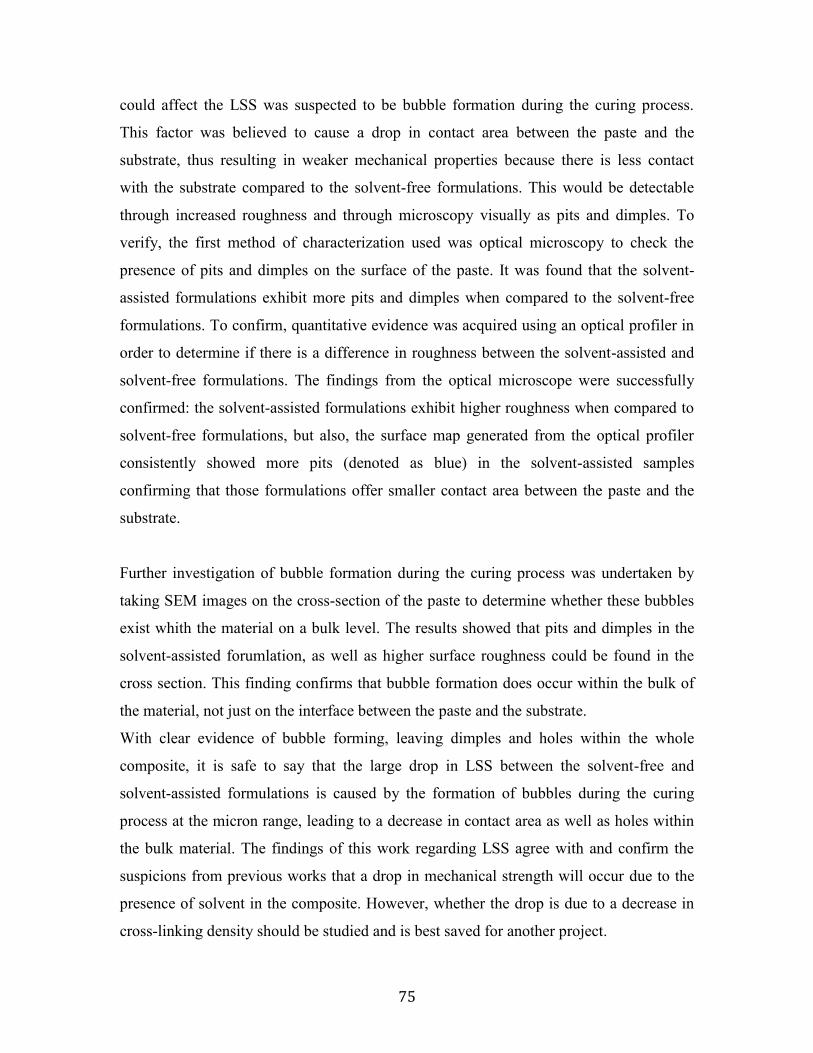
75

could affect the LSS was suspected to be bubble formation during the curing process.

This factor was believed to cause a drop in contact area between the paste and the

substrate, thus resulting in weaker mechanical properties because there is less contact

with the substrate compared to the solvent-free formulations. This would be detectable

through increased roughness and through microscopy visually as pits and dimples. To

verify, the first method of characterization used was optical microscopy to check the

presence of pits and dimples on the surface of the paste. It was found that the solvent-

assisted formulations exhibit more pits and dimples when compared to the solvent-free

formulations. To confirm, quantitative evidence was acquired using an optical profiler in

order to determine if there is a difference in roughness between the solvent-assisted and

solvent-free formulations. The findings from the optical microscope were successfully

confirmed: the solvent-assisted formulations exhibit higher roughness when compared to

solvent-free formulations, but also, the surface map generated from the optical profiler

consistently showed more pits (denoted as blue) in the solvent-assisted samples

confirming that those formulations offer smaller contact area between the paste and the

substrate.

Further investigation of bubble formation during the curing process was undertaken by

taking SEM images on the cross-section of the paste to determine whether these bubbles

exist whith the material on a bulk level. The results showed that pits and dimples in the

solvent-assisted forumlation, as well as higher surface roughness could be found in the

cross section. This finding confirms that bubble formation does occur within the bulk of

the material, not just on the interface between the paste and the substrate.

With clear evidence of bubble forming, leaving dimples and holes within the whole

composite, it is safe to say that the large drop in LSS between the solvent-free and

solvent-assisted formulations is caused by the formation of bubbles during the curing

process at the micron range, leading to a decrease in contact area as well as holes within

the bulk material. The findings of this work regarding LSS agree with and confirm the

suspicions from previous works that a drop in mechanical strength will occur due to the

presence of solvent in the composite. However, whether the drop is due to a decrease in

cross-linking density should be studied and is best saved for another project.

76

Chapter 5 Elastic Modulus of Epoxy Composites Filled with Graphene

5.1 Introduction

Graphene holds great potential as a co-filler alongside silver in hybrid ECAs and has

been shown by N.W. Pu et al to perform better in comparison to carbon black and CNTs

[8]. Even so, graphene faces challenges toward its use in ECA fabrication such as the

achievement of homogeneous dispersion and the preservation of its single-layer structure

within the composite [18]. In our recent work [18], we employed sodium dodecyl sulfate

(SDS) to decorate graphene in order to overcome these two concerns. In addition, it is

known that increasing metal filler content in ECAs leads to a decrease in mechanical

properties [20]. Therefore, SDS-decorated graphene is not only meant to help decrease

the amount of silver necessary to retain acceptable conductivity values, but also meant to

prevent the ECA from losing mechanical strength.

In this work, epoxy resin is loaded with two fillers: pristine commercial graphene

nanosheets (Gr), and SDS-modified graphene nanosheets (Gr(s)). Different from our

recent work [18], each nanocomposite is prepared using a solvent-free mixing procedure

[27], giving rise to the ability to further scale up. The mechanical properties of cured

epoxy with Gr(s) were evaluated and compared to those of epoxy with pristine graphene

through Hertzian indentation studies. We observed that modifying graphene with SDS

increased its maximum elastic bulk modulus at lower weight percentages compared to its

unmodified counterpart.

5.2 Experimental

5.2.1 Preparation of hybrid composite ECA

The epoxy composites are primarily comprised of two components: the epoxy component

that requires both the resin itself as well as the curing agent, and the filler material that

usually comes in the form of a powder. Bisphenol-A liquid epoxy resin (D.E.R. 331) and

epoxy curing agent (D.E.H. 24) triethylenetetraamine (TETA) were purchased from

DOW Chemical Company and used as received. Graphene nanosheets with sizes ranging

77

from 0.5 to 5 μm were purchased from ACS Materials (USA) and were used as received

[18,27]. The surfactant sodium dodecyl sulfate (SDS) responsible for exfoliating the

graphene nanosheets was purchased and used as received from Sigma Aldrich. HPLC

ethanol solvent at 99.8% purity was purchased and used as received from Fisher

Scientific (USA). Gr(s) was prepared using the same procedure outlined in J. Trinidad et

al’s work [27] and was added into the vial together with all other materials before mixing.

These materials (which include the graphene/modified graphene in the case of the hybrid

ECAs) are combined within the same container where they are mixed at 2000 RPM for 4

minutes and de-foamed afterwards at 2200 RPM for 1 minute using a Thinky Mixer

(ARE 310). After complete mixing of the materials, a paste-like substance is obtained

and casted into a PDMS mold that holds the shape of a mechanical test coupon

(following dimensions recommended by the ASTM D638 [156] standard for dogbone

type IV). Afterwards, a copper sheet with dimensions 2 cm x 7.6 cm is placed on top.

Finally, the sample is placed in the oven with a metallic block for compressing the mold.

The material is heated at 60oC for 30 minutes, and then ramped to 150oC where it cures

for 2 hours. Upon completion, the sample is removed from the mold and stored within a

Ziploc bag.

5.2.2 Hertzian Indentation

In this study, we concentrate on determining the effects of Gr and Gr-s when mixed with

epoxy. More specifically, our property of interest when investigating the mechanical

strength for the nanocomposite is the elastic modulus. A Universal Material Tester

(UMT) Tribological Test Equipment (CETR Campbell, CA USA) is equipped with an

indenting tip used to record compression force and distance as the sample carries a

maximum load of 750g at 1 mm/sec.

An estimation of its bulk modulus is determined by inputting the experimental data

within the Hertzian indentation model that works under the principle of a hemispherical

indenter indenting a flat surface [127]. The Hertzian equation is an indentation model for

finding the elastic modulus [128,129]:

78

𝑎3 =3𝑃𝑅

4𝐸∗ Eq. 11

The above formula was rearranged in order to plot load P VS displacement d. But first, it

is important to note that contact radius a found in the above equation is related to the

displacement d as seen in the following equation:

𝑑 =𝑎2

𝑅 𝑜𝑟 𝑎 = √𝑅𝑑 Eq. 12

With the above equation being substituted into the contact radius equation, we can then

rearrange it to take a form where load is a function of distance:

𝑃 =4𝐸

∗𝑑

1.5

3√𝑅 𝑜𝑟 𝑃 =

43√𝑅

× 𝐸∗ × 𝑑1.5 Eq. 13

E* is the modulus and R is the radius of the AISI Type 440-C stainless steel probe

(R=4.63 x 10-4 m) used for indenting the sample.

With this equation, we apply a theoretical model to compare the data gained from the

experimental results of the indentation. The way elastic modulus is estimated involves

calculating the forward and backward force using the Hertzian equation and comparing

those two forces to the actual forces reported by the UMT. We then take the square of the

difference between the theoretical value and experimental value and add up all of those

values: one for forward and one for backward force. Finally, we add those two values that

were just obtained to be called the total sum of error and then use a solver function to

estimate what the elastic modulus should be to best fit the model.

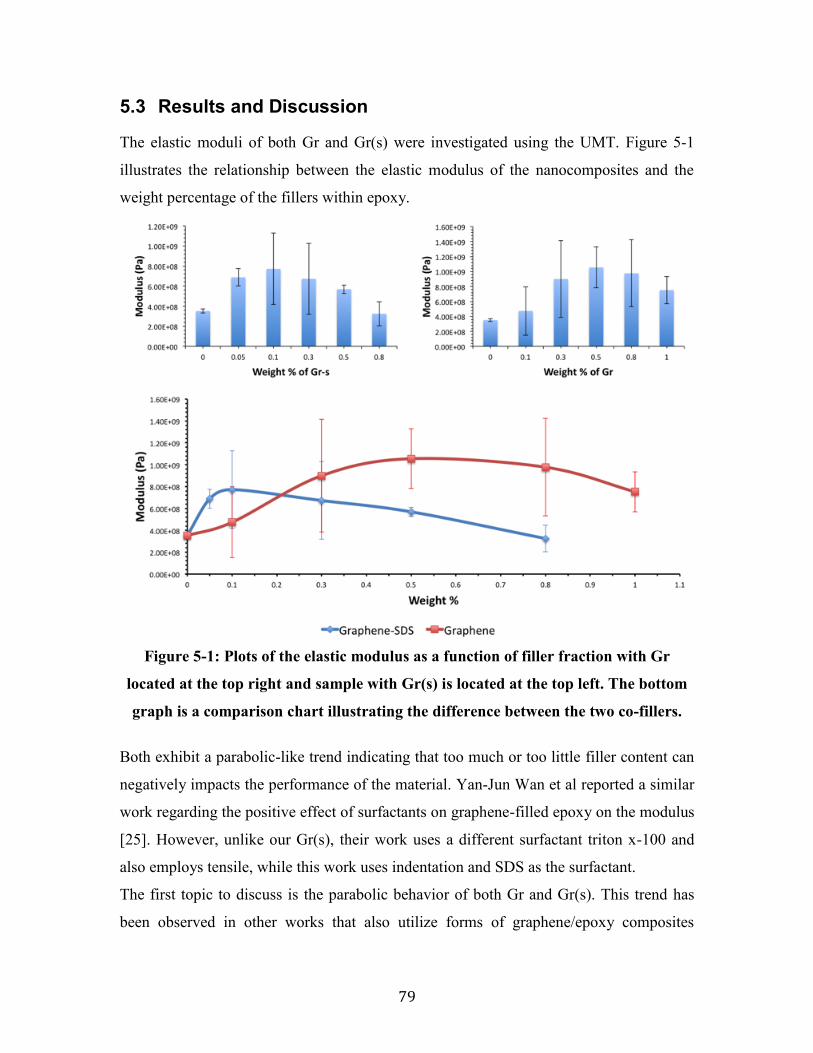
79

5.3 Results and Discussion

The elastic moduli of both Gr and Gr(s) were investigated using the UMT. Figure 5-1

illustrates the relationship between the elastic modulus of the nanocomposites and the

weight percentage of the fillers within epoxy.

Figure 5-1: Plots of the elastic modulus as a function of filler fraction with Gr

located at the top right and sample with Gr(s) is located at the top left. The bottom

graph is a comparison chart illustrating the difference between the two co-fillers.

Both exhibit a parabolic-like trend indicating that too much or too little filler content can

negatively impacts the performance of the material. Yan-Jun Wan et al reported a similar

work regarding the positive effect of surfactants on graphene-filled epoxy on the modulus

[25]. However, unlike our Gr(s), their work uses a different surfactant triton x-100 and

also employs tensile, while this work uses indentation and SDS as the surfactant.

The first topic to discuss is the parabolic behavior of both Gr and Gr(s). This trend has

been observed in other works that also utilize forms of graphene/epoxy composites

80

[25,82]. A hypothesized reason for this parabolic characteristic that Gr exhibits could be

the following: the segment before the maximum modulus value is the region that follows

an increasing trend, where the modulus increased as the amount of filler content

increased; whereas a decrease of the modulus could also be due to excess graphene

interfering with the crosslinking of epoxy. Further studies must be conducted to verify

this.

The second topic to discuss looks into the differences between the elastic modulus of the

composites as we add Gr and Gr(s). While Gr(s) also follows a parabolic characteristic

similar to Gr, its optimal point arises at a lower weight percent and begins its fall at a

lower weight percent. One explanation for this could be that the SDS aids in dispersing

and exfoliating the graphene nanosheets more effectively. This modification could

therefore play a key role in taking advantage single layer graphene’s exceptional

mechanical properties as a means to enhance epoxy’s modulus. The decrease in

mechanical properties on the other hand, could be caused by excess amounts of SDS

interfering with the cross-linking procedure of epoxy as suggested in previous work by

Amoli et al [18].

5.4 Conclusion

Hertzian indentation was used to determine how these epoxy nanocomposites behave

mechanically by observing changes in elastic modulus. It was found that increasing

graphene and SDS modified graphene as a function of weight percent yields an elastic

modulus profile that roughly appears like a parabola. SDS modified graphene was

determined to be inferior to the non-modified samples when it came to overall improving

the mechanical properties of the nanocomposite. However, SDS modified graphene

peaked at lower weight percentages compared to non-modified graphene indicating that

less filler content is required to improve its elastic modulus. Overall, it was verified that

the addition of either graphene or SDS modified graphene for a critical weight

concentration generally yielded higher elastic modulus compared to that of pure epoxy.

81

Chapter 6 PEDOT:PSS as a co-filler for ECAs

6.1 Introduction

PEDOT is a conducting polymer classified as a polythiophene derivative [94,157–160].

PSS is another polymer with three functions: first, it acts as the medium at which PEDOT

polymerizes and becomes stable in water [94,161]; second, it acts as a large dopant for

PEDOT allowing for the introduction of charge carriers within the polymer backbone of

PEDOT [158]; finally, PSS functions as a charge-balancing group (or counterions),

providing a negative charge from the SO3- end-group for the positive charge on the

thiophene group in PEDOT [94,161,162].

It has been a few decades since Shirakawa et al discovered the very first conductive

polymers in 1977, but now, there are handfuls available in the market as outlined by R.

Balint et al [158]. Conductive polymers are divided into three organic groups: sulfur-

containing heteroatoms (thiophenes and sulfides), nitrogen-containing heteroatoms

(polymerized pyrrole, aniline, etc), and non-heteroatom containing polymers with

numerous alkenes. In specific, PEDOT:PSS was first produced by Bayer AG research

laboratories in Germany [94,160] in the 1980s and has since been the topic of great

research and industrial interest, being hailed as one of the most successful conductive

polymers in commercial use today [159,160,163,164]. PEDOT:PSS has already been

applied in many fields such as energy-based PV technologies [157,159–163,165],

electronic semiconductor devices that require excellent electron/hole transport (e.g. field-

effect transistors, LCDs, LED based technologies, and anti-static bags) [94,159,161–

164,166], and bio-sensing/bioengineering applications [157,158].

PEDOT:PSS films contain work functions ranging from 5-5.2 eV and induces charge

transfer at very high kinetic rates [160]. Its conductivity comes from a variety of factors,

however, only two will be mentioned in this work. The first is its conjugated backbone

that forms alternating double bonds. The weakly localized π-bonds overlap with each

other, giving rise to the possibility for electrons to become delocalized and move or

“jump” through the polymer backbone and as a result, move between groups of atoms

82

[158]. The second factor that makes conductivity possible is the presence of dopant(s)

that act as counterions keeping the conducting polymer stable but at the same time is a

charge carrier source that is responsible for adding/removing electrons from the polymer

chains to become what are known as polarons or bipolarons [158]. These

polarons/bipolarons move through the polymer chain as an electric potential is applied

onto the system, which in turn allow for charges to pass through the backbone resulting in

electrical conductivity. A more comprehensive explanation on what polarons/bipolarons

are can be found from Bredas and Steer, who also explain the entire conducting

mechanism of conductive polymers from a chemist’s point of view, as well as explain the

possible miscommunications that can arise as a consequence of using the term “dopants”

to explain the conductivity mechanism in conductive polymers [167], whereas good

diagrams and cartoons for the explanation of this mechanism in a simpler manner can be

found in Balint et al’s work [158]. In addition to this, Crispin et al presents a chart

illustrating the conductive evolution of PEDOT:PSS as a function of weight percentage

with the addition of diethylene glycol (DEG) [161]. Their chart shows a percolation curve

between 0.1 and 1 weight percent showing synonymous trends to the percolation curves

for conventional ECAs. As such, this work was inspired to explore the use of

PEDOT:PSS as a co-filler within the conventional ECA in hopes of being able to either

improve the conductivity limits of the conventional ECA, or at least reduce the silver

content required to decrease material costs. In specific, this work will explore the

electrical conductivity of a hybrid ECA that uses PEDOT:PSS as its co-filler, as well as

investigate how adding increasing amounts of PEDOT:PSS will affect the mechanical

properties (in this case, adhesion strength by means of evaluating shear strength). To the

knowledge of the author, no work regarding the use of PEDOT:PSS in composite systems

for the sake of improving electrical conductivity has been undertaken, as most current

work utilizes PEDOT:PSS as a film for varying applications rather than a solution-based

component. Therefore, this work will be primarily act as a preliminary study to determine

its feasibility as a solution-based co-filler in hopes of opening a new avenue for

modifying and improving the performance of conventional ECAS.

83

6.2 Experimental

6.2.1 Conductive composite preparation Diglycidyl ether of Bisphenol-A liquid epoxy resin (D.E.R. 331) and

Triethylenetetramine (TETA) epoxy hardener (D.E.H. 24) was supplied by DOW

Chemical Company and were used as the resin base and the hardener respectively. A high

conductive grade of Poly(3,4-ethylenedioxythiophene)-Poly(styrenesulfonate)

(PEDOT:PSS 1.1% in water solution) was purchased from Sigma-Aldrich and used as the

conductive filler material for the composite. Methanol in HPLC grade was purchased

from Sigma-Aldrich and used as a common solvent between the water and the resin to

assist with dispersion and mixing, as well as to wash out the PSS content in the solution.

Silver micro-flakes (a density of 10.49 g/cm3, a particle size of 10 μm) were purchased

and received to act as the principle conductive material of the composite.

The procedure for making the conductive composites begins by adding the epoxy resin

with both PEDOT:PSS solution and methanol solvent [162]. The resulting mixture is first

mixed vigorously using a vortex mixer to ensure that the PEDOT:PSS solution is

dispersed in the epoxy resin. Once completed, silver flakes are added into the mixture and

then further mixed at 2000 RPM for 5 minutes using a Thinky Mixer (ARE 310). The

mixture is then placed into the oven at 90 °C in order to allow both methanol and water to

evaporate. Finally, epoxy hardener TETA is added into the system and again mixed at

2000 RPM for 5 minutes. The mixture is then placed into either a pre-cleaned 7 mm x 7

mm mold made of a glass slide, thermally resistant tape and a copper sheet (to ensure that

the sample thickness remains constant) or a shear test coupon that is explained in an

upcoming section. The samples are then placed into an oven to be baked at 150 °C for 2

hours. Below in Figure 6-1 is a schematic that illustrates and summarizes the entire

procedure.

84

Figure 6-1: Schematic diagram of PEDOT:PSS as it is incorporated into

conventional ECAs.

6.2.2 Characterization The electrical sheet-resistance values of the cured composites were measured using a

four-point probe setup that includes a probe fixture (Cascade Microtech Inc.) and a

micro-ohm meter (Keithley 2440 5A Source Meter, Keithley Instruments Inc.). The sheet

resistance Rs obtained can then be inserted into the bulk resistivity equation and then

converted into conductivity with the following equations [17,27,52]:

𝜌 = 𝑅𝑠 ∙ 𝑡 = 𝐹 ∙ 𝑡 (𝜋

𝐿𝑛 2)

𝑉𝐼 Eq. 14

as the bulk resistivity equation. However, bulk resistivity 𝜌 can be converted to

conductivity 𝜎 with the equation below:

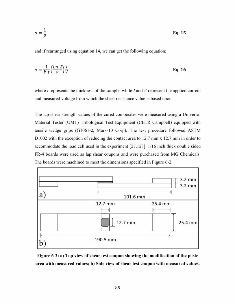
85

𝜎 =1𝜌 Eq. 15

and if rearranged using equation 14, we can get the following equation:

𝜎 =1

𝐹∙𝑡 (𝐿𝑛 2

𝜋 )𝐼𝑉 Eq. 16

where t represents the thickness of the sample, while I and V represent the applied current

and measured voltage from which the sheet resistance value is based upon.

The lap-shear strength values of the cured composites were measured using a Universal

Material Tester (UMT) Tribological Test Equipment (CETR Campbell) equipped with

tensile wedge grips (G1061-2, Mark-10 Corp). The test procedure followed ASTM

D1002 with the exception of reducing the contact area to 12.7 mm x 12.7 mm in order to

accommodate the load cell used in the experiment [27,123]. 1/16 inch thick double sided

FR-4 boards were used as lap shear coupons and were purchased from MG Chemicals.

The boards were machined to meet the dimensions specified in Figure 6-2.

Figure 6-2: a) Top view of shear test coupon showing the modification of the paste

area with measured values; b) Side view of shear test coupon with measured values.

86

6.3 Results and Discussion

6.3.1 Electrical Conductivity

The electrical conductivity of pristine PEDOT:PSS was characterized by a standard four-

point probe setup in solution cast films. It was found that the electrical conductivity of

pure PEDOT:PSS was about 15 S/cm. However, despite knowing how methanol

treatment of PEDOT:PSS will improve electrical conductivity [162], we were unable to

apply such a procedure to our samples as a perfect procedure that involved methanol

treatment for the composite was not fully developed before the electrical conductivity

testing commenced. This therefore meant that the samples were measured with the PSS

still prevalent in the composite.

In order to investigate how PEDOT:PSS influences the overall electrical conductivity of

their polymer composites, we used conventional ECAs containing only silver flakes at

various weight fractions as a control. For all hybrid ECA samples with PEDOT:PSS co-

fillers, the absolute amount of sliver flakes was kept constant, whereas the amount of

PEDOT:PSS solution was increased. The formulations used for testing are summarized

below in Table 6-1.

Table 6-1: Summary of different sample compositions and the masses of the

conductive filler material

Sample Composition PEDOT:PSS+

H2O mass

(mg)

PEDOT:PSS

mass (mg)

A Epoxy + Ag 60 wt% 0 0

B Epoxy + Ag 60 wt% + PEDOT:PSS 0.1 wt% 33.9 0.339

C Epoxy + Ag 60 wt% + PEDOT:PSS 0.2 wt% 67.9 0.679

D Epoxy + Ag 60 wt% + PEDOT:PSS 0.5 wt% 170.3 1.703

E Epoxy + Ag 60 wt% + PEDOT:PSS 1 wt% 342.4 3.424

87

Figure 6-3a below illustrates the expected conductivity of conventional ECAs that

typically contain only silver flakes as its main conductive filler as a function of weight

percent loading. It is seen that past a certain point in the curve known as percolation

threshold (within the range of 40 wt% loading), the composite transitioned from being an

insulating material into a conductive material. Furthermore, by looking at the higher

weight loadings, it is seen that adding more silver flakes into the epoxy matrix did not

significantly improve electrical conductivity. In contrast, the electrical conductivities of

the hybrid ECAs with a constant total amount of silver flakes at various PEDOT:PSS

weight concentrations were plotted in Figure 6-3b below.

Figure 6-3: a) Electrical conductivity as a function of filler content silver flakes; b)

electrical conductivity as a function of filler content PEDOT:PSS containing 60 wt%

Ag

88

It was found that adding a small amount of PEDOT:PSS (0.1 wt%) remarkably improved

the electrical conductivity to 289 S/cm, which is 3 times higher than that of the

conventional ECA with 60 wt% sliver flakes. The maximum conductivity of 2422 S/cm

was achieved at a weight loading of 0.89 wt% PEDOT:PSS showing that the combination

of PEDOT:PSS and conventional ECAs produces highly conductive composites. Similar

to conventional ECAs, excess PEDOT:PSS in the composite above a certain

concentration yields appears to show diminishing improvement of electrical conductivity

as seen in Figure 6-3b for higher weight loadings, however needs more experimental data

to verify. This decrease in electrical conductivity may be attributed to the fact that

increasing the amount of PEDOT:PSS into the system also increases the potential of

residual water molecules from the PEDOT:PSS solution thereby decreasing the

crosslinking density of the epoxy as it is being cured leading to fewer metallurgic

interconnections between the silver flakes [7,11]. Thermal studies can be done to further

investigate and verify this behavior.

6.3.2 Lap shear strength The shear strength of the adhesive was measured in order to determine if the composite

remains functional as a joining material after adding co-filler PEDOT:PSS into the

system. The shear strength was investigated using (CETR UMT) universal mechanical

tester with a load cell of 100 Kg and Mark-10 wedge grips G1061-2 with gripping force

of 1-9 kN, while following ASTM D1002 with exceptions that were specified in a

previous section. The shear strength as a function of PEDOT:PSS weight loading was

investigated with the results summarized below in figure 6-4.

89

Figure 6-4: Lap Shear Strength as a function of PEDOT:PSS fraction for the hybrid

ECAs.

Overall, it was observed that addition of PEDOT:PSS into the conventional ECA (where

the weight loading of silver flakes was kept constant) shows an increase in variance with

an increase in PEDOT:PSS. One possible explanation for this is that the addition of

another component into the epoxy matrix resulted in more variability in the system

(whether it comes from change in dispersion efficiency, addition of processing steps

giving room for error, contamination issues or thermal instability), leading to weakened

adhesion. However, it is important to note that the change in shear strength is

insignificant when compared to the increase in electrical conductivity of the similar

weight loading of PEDOT:PSS. Therefore, the addition of PEDOT:PSS as a co-filler

towards conventional ECAs has not been found to negatively affect or compromise the

shear strength of the bulk material in any statistically significant manner (only dropping

around 1 MPa at worst case)

90

It is important however, to examine the reason for why the graph tends to decrease. One

explanation must be taken into consideration is that the PEDOT:PSS comes as a polymer

blend at a concentration of ~1%, whereas the rest of the solution is primarily water-based.

As such, it is highly likely that the evaporation step intended to release all of the water

introduced after adding PEDOT:PSS does not release all of the water in the system,

leaving trapped water molecules within the resin.

It is well known that the presence of water in epoxy resin results in the compromising of

its crosslinking density [168,169], thus leading to the degradation of both electrical

conductivity and mechanical strength. With this in mind, it is very likely that the

variability of how much water molecules are evaporated out of the system is directly

related to both the bulk strength of the material, as well as its electrical conductivity. It is

intuitive to know how increasing the crosslinking density results in better mechanical

strength, however, the reason that crosslinking density is related to the bulk resistivity of

the system needs to be explained through the concept of increasing shrinkage in epoxy.

Increased shrinkage within the thermoset leads to better intimate contact between silver

flakes, resulting in the formation of more conducting pathways [7,10,17,41,42,91]. Two

avenues that were not explored in this study are the effects of methanol on the

crosslinking density of the epoxy. Firstly, no explicit mention that methanol has a

negative effect on crosslinking density of epoxy was found, however, it is suspected to be

a potential contributing factor when it comes to the incomplete curing of the epoxy, or

even the formation of air bubbles during evaporation. Secondly, dispersion issues could

lead to problems in the utilization of PEDOT:PSS as it is not well known whether the

actual active component is aggregated or isolated in small pockets within the composite

system upon curing. Furthermore, poor dispersion is suspected to also act as potential

weakness in the structure of the cured composite, leading to variance in its mechanical

strength.

91

6.4 Conclusion

PEDOT:PSS was successfully introduced into a conventional ECA formulation; its

electrical conductivity and shear strength were investigated. The electrical conductivity

results have shown that the incorporation of PEDOT:PSS improves the conductivity of

conventional ECAs to 289 S/cm, which is three times more conductive than without the

co-filler. The maximum conductivity found in this investigation when incorporating 0.89

wt% PEDOT:PSS into the conventional formulation has a conductivity value of 2422

S/cm. The co-filler system is successful at reaching high conductivity values without

introducing an extra 10-20 wt% of silver content within the ECA to achieve the same

results.

The mechanical strength of the hybrid ECA was also investigated. By varying only the

weight loading of PEDOT:PSS, it was found that the increase of the co-filler increased

the variance of the shear strength of the system, as well as an insignificant decrease in

shear strength of 1 MPa at worst case. It has been explained that the increase in variance

could be from a variety of factors, however, it is suspected that the introduction of

PEDOT:PSS at higher weight loadings resulted in excess water molecules that were

trapped in the composite because of insufficient evaporation, leading to the varying shear

values. Overall, it has been found that the incorporation of PEDOT:PSS on the point of

view of both electrical conductivity and mechanical strength is positive. It increases the

electrical conductivity of the conventional ECA while simultaneously reducing the

required amount of silver to be functional, as well as exhibits negligible impact on its

shear strength. This newfound use of PEDOT:PSS as a co-filler in conventional ECAs

can lead to a variety of innovative applications in solder mount technologies, as well as

flexible electronic joining materials.

92

Chapter 7 Concluding Remarks, Recommendations and Future Research

7.1 Concluding Remarks

We explored the use of Gr(s) as a co-filler for CCAs using a PSM as a modified method

of composite preparation and high shear mixing. The rheological properties of epoxy-

based composites that are loaded with Gr and Gr(s), as well as combinations with silver

and Gr/Gr(s) were successfully investigated. Although the total viscosity of the system

increases upon addition of any filler in epoxy, the addition of Gr or Gr(s) in specific

produces a shear-thickening suppression effect that is clear and visible at weight

concentrations above 0.5 wt%. This new phenomenon could prove useful to future

applications that involve the need for shear-thinning liquids, especially those used for

electronic printing techniques.

Furthermore, a comparative study between the LSS of Gr(s) and Ag (both independently

and in combination of one another) using a solvent-free and solvent-assisted environment

was undertaken. It was found that samples containing Gr(s) prepared by solvent-assisted

method show significantly weaker LSS values when compared to those that do not use

solvent. It was initially suspected that solvent and surfactant were the primary cause for

the decrease in the cross-linking density of epoxy; however, this was not proven in our

work. Instead, we noticed another factor that could cause the decrease in LSS: formation

of bubbles during cure, resulting in dimples and pits post-cure. We used multiple forms

of microscopy to qualitatively and quantitatively determine that there are more dimples

and pits found in the entire bulk of the structures prepared by the solvent-assisted. This

finding gave traction to our suspicion that the pits and dimples were in effect decreasing

the contact area between the paste and the substrate, and as a result, decreasing the

amount of force required to fail as well as decreasing the LSS of the system. Electrical

conductivity was also examined using the same procedure for making the LSS samples.

The experimental results indicate that conductivity was increased with solvent assistance

for samples of lower silver content (40%), but for a content of 60 wt% Ag, solvent

assistance barely helped improve electrical conductivity. As such, we concluded that

93

since no benefit comes from using solvent for higher silver loadings, the solvent-free

method was the best way to prepare that formulation. Furthermore, we found the optimal

solvent-free formulation with 60 wt% Ag and 0.75 wt% Gr(s) exhibited the best LSS and

electrical conductivity.

Next, we studied how the elastic modulus (from an indentation method) would change as

we increased the weight loading of Gr/Gr(s). We learned that Gr(s) peaks at much lower

weight concentrations (0.05 wt% to 0.15 wt%) when compared to Gr. On the other hand,

Gr peaks at higher weight concentrations (0.5 wt% to 0.8 wt%) and overall reinforces the

material more effectively, as using Gr obtains the highest elastic modulus values for the

epoxy-based composite.

Our final study used water-based PEDOT:PSS as co-filler for conventional ECAs and

successfully improved the electrical conductivity of the composite. It was observed that

with a constant Ag weight concentration, an increase in PEDOT:PSS resulted in an

increase in conductivity akin to adding more Ag into the system, but with the added

benefit of not using as much Ag to achieve the same values. However, since PEDOT:PSS

is water-based, we followed up on a suspicion that adding higher concentrations of the

co-filler would weaken the mechanical properties of the composite especially because the

polymer matrix epoxy is hydrophobic and typically loses cross-linking density upon the

presence of residual water molecules during cure. We learned that the LSS showed an

apparent drop as the content of PEDOT:PSS increased, concluding that PEDOT:PSS is

responsible for weakening the mechanical properties is inaccurate. Instead, it would be

more suitable to conclude that introducing higher concentrations of PEDOT:PSS into

they system adds higher variability, as each increasing concentration of PEDOT:PSS into

the composite exhibited higher standard deviation. This result is reasonable as adding

more material into the composite could result in more variability using the same

procedure, for example, different mixing results, more inconsistencies with dispersion,

gradual ineffectiveness of desiccation, etc. Overall, PEDOT:PSS as a co-filler holds

promise as it not only keeps the material low in viscosity, but also exhibits high

conductivities at low Ag loadings.

94

7.2 Future Research

This thesis has explored a variety of different aspects regarding ECAs, however, left

room for further investigations, which are recommended to be followed up for a more

comprehensive understanding. Topics below will outline questions and ideas that would

require further investigation.

In chapter 3, we discussed the idea of using these solvent-free ECA formulations for

printer technologies that dispense conductive ink, thereby making the traces and landing

spots for the electrical components at an industrial scale. However, although this idea has

great traction and in theory should work, it is important to use an actual printer loaded

with our hybrid ECA paste to prove that this concept is feasible for further

commercialization of ECAs. Needless to say, extra work will be required to find the

optimal formulation that fits both the capabilities of the printer’s dispensing head as well

as the conductivity requirements in order to guarantee the smooth operation of the PCB.

With this follow-up, we can fully conclude that the incorporation of Gr(s) is an important

component that the ECAs require in order to be usable in an industrial level, and in effect,

an important part of commercializing ECAs.

Furthermore, in chapter 4, many questions were formed or left unanswered upon

completion. The first question that needs to be addressed is whether or not the cross-

linking density was dropping for formulations that used solvent to disperse and mix the

fillers, or if it was a combination of solvent and surfactant from Gr(s) that was

responsible for this drop. Since thermal studies have already alluded to this phenomenon

occurring, it is worth pursuing this question using a different characterization method to

confirm that this is indeed happening, as it affects the mechanical properties of the final

composite for better or worse. The second question to address is what the LSS surface

response plot would look like, had we incorporated more data points in between and

possibly above and beyond the ones we used in order to form a comprehensive map of

how the addition of either Gr(s) and or Ag affects the system’s shear strength for both

solvent-free and solvent-assisted formulations. Aside from these questions, it would also

be beneficial to conduct the following experiments for a complete understanding of our

95

hybrid ECA system: a) creating another 3D graph where the second independent variable

uses non-decorated Graphene to determine if Graphene is a better reinforcing agent than

Gr(s) for both solvent-free and solvent-assisted environments; b) creating another 3D

graph where the response surface is electrical conductivity as opposed to LSS; c) setting

up a practical test that involves using SMD resistors/capacitors that are attached onto an

FR-4 board using our ECAs, which are then tested for adhesion through dye shear testing.

Moreover, in chapter 5, it has to be noted that we were unsuccessful at determining how

to incorporate co-solvent methanol into the hybrid ECA and then casting it into the

electrical conductivity measurement molds successfully. If future work could solve this

problem and do a comparative study in hopes of seeing if the assistance of the co-solvent

has a positive effect on the electrical conductivity of the hybrid ECA, we would then be

able to fully complete our study in the use of PEDOT:PSS as a co-filler for conventional

ECAs.

Other topics that have not been discussed, but would further enhance our general

understanding of the physical properties of ECAs include: tensile strength tests, drop

tests, and bend tests.

Finally, one topic that the author wished to explore but was not able to complete was the

search for an epoxy resin that exhibited reversible crosslinking after cure. This idea was

conceived in order to address a practical problem that surrounded the recycling and re-

working of PCBs, because when a thermoset such as epoxy is fully cured, further

processing, reclaiming and removal is extremely difficult especially without damaging

either of the components it is attached to. Because the knowledge of thermally degradable

ECAs is already explored, the next step is naturally to determine if there is a way to make

the bond between the FR-4 board and the component reversible, similar to the way how

traditional Pb/Sn can be reversed and then reclaimed using the solder irons. Works that

involve reversible cross-linkers were touched upon in this thesis, but extensive work need

to be carried out in order to realize a fully reversible and functioning ECA that has cured.

The most important part about this idea is that only the cross-linker is substituted into the

96

system and as such, will likely not change the function of the other components, meaning

the incorporation of the co-fillers like Gr/Gr(s) should not be a problem. With these ideas

and potential future works in mind, the understanding of the physical properties of hybrid

ECAs utilizing Gr(s) as a co-filler has been outlined in this thesis to provide the field with

a greater understanding of a material holding the potential to replace traditional Sn/Pb

solders as a fully commercial electronic packaging material.

97

Bibliography

[1] Y. Li, C.P. Wong, Recent advances of conductive adhesives as a lead-free

alternative in electronic packaging: Materials, processing, reliability and

applications, Mater. Sci. Eng. R Reports. 51 (2006) 1–35.

doi:10.1016/j.mser.2006.01.001.

[2] H. Ma, J.C. Suhling, A review of mechanical properties of lead-free solders for

electronic packaging, J. Mater. Sci. 44 (2009) 1141–1158. doi:10.1007/s10853-

008-3125-9.

[3] J. Trinidad, B. Amoli, B. Zhao, The Investigation of Physical Properties of Epoxy

Nanocomposites Filled with Graphene as Electrically Conductive Adhesives,

2014. (Technical Paper)

[4] H.J. Lewis, A.. Ryan, Using Electrically Conductive Inks and Adhesives as a

Means to Satisfy European PCB Manufacturing Directives, J. Adhes. Sci. Technol.

22 (2008) 893–913. doi:10.1163/156856108X305534.

[5] J. Trinidad, W. Zhang, A. Chen, B. Zhao, J. Persic, R. Lyn, IMPLEMENTING

PEDOT : PSS AS A CO-FILLER FOR ELECTRICALLY CONDUCTIVE

ADHESIVE APPLICATIONS, (2016) (Technical Paper)

[6] H. Jiang, K.S. Moon, Y. Li, C.P. Wong, Surface functionalized silver

nanoparticles for ultrahigh conductive polymer composites, Chem. Mater. 18

(2006) 2969–2973. doi:10.1021/cm0527773.

[7] D. Lu, Q.K. Tong, C.P. Wong, Mechanisms underlying the unstable contact

resistance of conductive adhesives, IEEE Trans. Electron. Packag. Manuf. 22

(1999) 228–232. doi:10.1109/6104.795858.

[8] N.-W. Pu, Y.-Y. Peng, P.-C. Wang, C.-Y. Chen, J.-N. Shi, Y.-M. Liu, M.-D. Ger,

C.-L. Chang, Application of nitrogen-doped graphene nanosheets in electrically

conductive adhesives, Carbon N. Y. 67 (2014) 449–456.

doi:10.1016/j.carbon.2013.10.017.

[9] S. Xu, D. a Dillard, J.. Dillard, Environmental aging effects on the durability of

electrically conductive adhesive joints, Int. J. Adhes. Adhes. 23 (2003) 235–250.

doi:10.1016/S0143-7496(03)00027-7.

[10] Y. Li, K.-S. Moon, A. Whitman, C.P. Wong, Enhancement of Electrical Properties

of Electrically Conductive Adhesives (ECAs) by Using Novel Aldehydes, IEEE

Trans. Components Packag. Technol. 29 (2006) 758–763.

doi:10.1109/TCAPT.2006.885940.

98

[11] B.-S. Yim, J.-M. Kim, S.-H. Jeon, S.H. Lee, J. Kim, J.-G. Han, M. Cho, Hybrid

Interconnection Process Using Solderable ICAs (Isotropic Conductive Adhesives)

with Low-Melting-Point Alloy Fillers, Mater. Trans. 50 (2009) 2649–2655.

doi:10.2320/matertrans.M2009109.

[12] M. Abtew, G. Selvaduray, Lead-free Solders in Microelectronics, Mater. Sci. Eng.

R Reports. 27 (2000) 95–141. doi:10.1016/S0927-796X(00)00010-3.

[13] H.J. Lewis, F.M. Coughlan, An Overview of the Use of Electrically Conductive

Adhesives (ECAs) as a Solder Replacement, J. Adhes. Sci. Technol. 22 (2008)

801–813. doi:10.1163/156856108X305543.

[14] Y. Rao, D. Lu, C.P. Wong, A study of impact performance of conductive

adhesives, Int. J. Adhes. Adhes. 24 (2004) 449–453.

doi:10.1016/j.ijadhadh.2003.12.003.

[15] D.A. Shnawah, M.F.M. Sabri, I.A. Badruddin, A review on thermal cycling and

drop impact reliability of SAC solder joint in portable electronic products,

Microelectron. Reliab. 52 (2012) 90–99. doi:10.1016/j.microrel.2011.07.093.

[16] Shuangyan Xu, D.A. Dillard, Determining the impact resistance of electrically

conductive adhesives using a falling wedge test, IEEE Trans. Components Packag.

Technol. 26 (2003) 554–562. doi:10.1109/TCAPT.2003.817646.

[17] B. Meschi Amoli, J. Trinidad, A. Hu, Y.N. Zhou, B. Zhao, Highly electrically

conductive adhesives using silver nanoparticle (Ag NP)-decorated graphene: the

effect of NPs sintering on the electrical conductivity improvement, J. Mater. Sci.

Mater. Electron. 26 (2015) 590–600. doi:10.1007/s10854-014-2440-y.

[18] B. Meschi Amoli, J. Trinidad, G. Rivers, S. Sy, P. Russo, A. Yu, N.Y. Zhou, B.

Zhao, SDS-stabilized graphene nanosheets for highly electrically conductive

adhesives, Carbon N. Y. 91 (2015) 188–199. doi:10.1016/j.carbon.2015.04.039.

[19] B.M. Amoli, E. Marzbanrad, A. Hu, Y.N. Zhou, B. Zhao, Electrical Conductive

Adhesives Enhanced with High-Aspect-Ratio Silver Nanobelts, Macromol. Mater.

Eng. 299 (2014) 739–747. doi:10.1002/mame.201300295.

[20] H. WU, X. WU, M. GE, G. ZHANG, Y. WANG, J. JIANG, Properties

investigation on isotropical conductive adhesives filled with silver coated carbon

nanotubes, Compos. Sci. Technol. 67 (2007) 1182–1186.

doi:10.1016/j.compscitech.2006.05.010.

[21] J. Trinidad, K. Liew, A. Cholewinski, B. Zhao, The Negative Effect of Residual

Solvent on the Lap-Shear Strength of SDS-Decorated Graphene Hybrid ECAs, (In

preparation for publishing)

99

[22] J. Du, H.-M. Cheng, The Fabrication, Properties, and Uses of Graphene/Polymer

Composites, Macromol. Chem. Phys. 213 (2012) 1060–1077.

doi:10.1002/macp.201200029.

[23] P.Y. Huang, C.S. Ruiz-Vargas, A.M. van der Zande, W.S. Whitney, M.P.

Levendorf, J.W. Kevek, S. Garg, J.S. Alden, C.J. Hustedt, Y. Zhu, J. Park, P.L.

McEuen, D. a Muller, Grains and grain boundaries in single-layer graphene atomic

patchwork quilts., Nature. 469 (2011) 389–92. doi:10.1038/nature09718.

[24] S.G. Prolongo, A. Jimenez-Suarez, R. Moriche, A. Ureña, In situ processing of

epoxy composites reinforced with graphene nanoplatelets, Compos. Sci. Technol.

86 (2013) 185–191. doi:10.1016/j.compscitech.2013.06.020.

[25] Y.J. Wan, L.C. Tang, D. Yan, L. Zhao, Y.B. Li, L. Bin Wu, J.X. Jiang, G.Q. Lai,

Improved dispersion and interface in the graphene/epoxy composites via a facile

surfactant-assisted process, Compos. Sci. Technol. 82 (2013) 60–68.

doi:10.1016/j.compscitech.2013.04.009.

[26] D. Galpaya, M. Wang, G. George, N. Motta, E. Waclawik, C. Yan, Preparation of

graphene oxide/epoxy nanocomposites with significantly improved mechanical

properties, J. Appl. Phys. 116 (2014) 53518. doi:10.1063/1.4892089.

[27] J. Trinidad, B.M. Amoli, W. Zhang, R. Pal, B. Zhao, Effect of SDS decoration of

graphene on the rheological and electrical properties of graphene-filled epoxy/Ag

composites, J. Mater. Sci. Mater. Electron. (2016). doi:10.1007/s10854-016-5434-

0.

[28] P.T. Vianco, Y. Feng, Electronic Packaging: Solder Mounting Technologies, in:

Ref. Modul. Mater. Sci. Mater. Eng., Elsevier, 2016: pp. 2705–2715.

doi:10.1016/B978-0-12-803581-8.10099-2.

[29] P.T. Vianco, D.R. Frear, Issues in the replacement of lead-bearing solders, JOM.

45 (1993) 14–19. doi:10.1007/BF03222374.

[30] J.F. Bard, R.W. Clayton, T.A. Feo, Machine setup and component placement in

printed circuit board assembly, Int. J. Flex. Manuf. Syst. 6 (1994) 5–31.

doi:10.1007/BF01324873.

[31] C. Basaran, R. Chandaroy, Mechanics of Pb40/Sn60 near-eutectic solder alloys

subjected to vibrations, Appl. Math. Model. 22 (1998) 601–627.

doi:10.1016/S0307-904X(98)10059-8.

[32] I. Mir, D. Kumar, Recent advances in isotropic conductive adhesives for

electronics packaging applications, Int. J. Adhes. Adhes. 28 (2008) 362–371.

doi:10.1016/j.ijadhadh.2007.10.004.

100

[33] R.H. Tien, G.E. Geiger, A Heat-Transfer Analysis of the Solidification of a Binary

Eutectic System, J. Heat Transfer. 89 (1967) 230. doi:10.1115/1.3614365.

[34] W.-L. Jang, T.-S. Wang, Y.-F. Lai, K.-L. Lin, Y.-S. Lai, The performance and

fracture mechanism of solder joints under mechanical reliability test,

Microelectron. Reliab. 52 (2012) 1428–1434. doi:10.1016/j.microrel.2012.03.011.

[35] H. Li, C.P. Wong, A Reworkable Epoxy Resin for Isotropically Conductive

Adhesive, IEEE Trans. Adv. Packag. 27 (2004) 165–172.

doi:10.1109/TADVP.2004.824939.

[36] M.A. Uddin, M.O. Alam, Y.C. Chan, H.P. Chan, Adhesion strength and contact

resistance of flip chip on flex packages - Effect of curing degree of anisotropic

conductive film, Microelectron. Reliab. 44 (2004) 505–514. doi:10.1016/S0026-

2714(03)00185-9.

[37] J.E. Morris, J. Lee, Drop Test Performance of Isotropic Electrically Conductive

Adhesives, J. Adhes. Sci. Technol. 22 (2008) 1699–1716.

doi:10.1163/156856108X320546.

[38] F. Tan, X. Qiao, J. Chen, H. Wang, Effects of coupling agents on the properties of

epoxy-based electrically conductive adhesives, Int. J. Adhes. Adhes. 26 (2006)

406–413. doi:10.1016/j.ijadhadh.2005.06.005.

[39] Z. Zhang, X. Chen, H. Yang, H. Fu, F. Xiao, Electrically conductive adhesives

with sintered silver nanowires, in: 2009 Int. Conf. Electron. Packag. Technol. High

Density Packag., IEEE, 2009: pp. 834–837. doi:10.1109/ICEPT.2009.5270629.

[40] E. Sancaktar, L. Bai, Electrically Conductive Epoxy Adhesives, Polymers (Basel).

3 (2011) 427–466. doi:10.3390/polym3010427.

[41] M.J. Yim, Y. Li, K. Moon, K.W. Paik, C.P. Wong, Review of Recent Advances in

Electrically Conductive Adhesive Materials and Technologies in Electronic

Packaging, J. Adhes. Sci. Technol. 22 (2008) 1593–1630.

doi:10.1163/156856108X320519.

[42] S.-L.F. Huann-Wu Chiang, Cho-Liang Chung, Liu-Chin Chen, Yi Li, C.P. Wong,

Processing and shape effects on silver paste, J. Adhes. Sci. Technol. 19 (2005)

565–578. doi:10.1163/1568561054352487.

[43] H. Wolfson, G. Elliot, Electrically Conducting cements containing epoxy resins

and silver, US patent 2774, 747, 1957.

https://patentimages.storage.googleapis.com/pdfs/US2807013.pdf.

[44] H.-W. Cui, J.-T. Jiu, S. Nagao, T. Sugahara, K. Suganuma, H. Uchida, Using

Ozawa method to study the curing kinetics of electrically conductive adhesives, J.

Therm. Anal. Calorim. 117 (2014) 1365–1373. doi:10.1007/s10973-014-3902-4.

101

[45] F. Hussain, Polymer-matrix Nanocomposites, Processing, Manufacturing, and

Application: An Overview, J. Compos. Mater. 40 (2006) 1511–1575.

doi:10.1177/0021998306067321.

[46] S. Stankovich, D.A. Dikin, G.H.B. Dommett, K.M. Kohlhaas, E.J. Zimney, E.A.

Stach, R.D. Piner, S.T. Nguyen, R.S. Ruoff, Graphene-based composite materials,

Nature. 442 (2006) 282–286. doi:10.1038/nature04969.

[47] W.-J. Jeong, H. Nishikawa, D. Itou, T. Takemoto, Electrical Characteristics of a

New Class of Conductive Adhesive, Mater. Trans. 46 (2005) 2276–2281.

doi:10.2320/matertrans.46.2276.

[48] R. Zhang, W. Lin, K.S. Moon, C.P. Wong, Fast preparation of printable highly

conductive polymer nanocomposites by thermal decomposition of silver

carboxylate and sintering of silver nanoparticles, ACS Appl. Mater. Interfaces. 2

(2010) 2637–2645. doi:10.1021/am100456m.

[49] R. Zhang, K. Moon, W. Lin, C.P. Wong, Preparation of highly conductive polymer

nanocomposites by low temperature sintering of silver nanoparticles, J. Mater.

Chem. 20 (2010) 2018–2023. doi:10.1039/b921072e.

[50] H. Gao, L. Liu, K. Liu, Y. Luo, D. Jia, J. Lu, Preparation of highly conductive

adhesives by in situ generated and sintered silver nanoparticles during curing

process, J. Mater. Sci. Mater. Electron. 23 (2011) 22–30. doi:10.1007/s10854-011-

0388-8.

[51] B.M. Amoli, S. Gumfekar, A. Hu, Y.N. Zhou, B. Zhao, Thiocarboxylate

functionalization of silver nanoparticles: effect of chain length on the electrical

conductivity of nanoparticles and their polymer composites, J. Mater. Chem. 22

(2012) 20048. doi:10.1039/c2jm33280a.

[52] B. Meschi Amoli, A. Hu, N.Y. Zhou, B. Zhao, Recent progresses on hybrid micro–

nano filler systems for electrically conductive adhesives (ECAs) applications, J.

Mater. Sci. Mater. Electron. 26 (2015) 4730–4745. doi:10.1007/s10854-015-3016-

1.

[53] Y. Kornyushin, Thermodynamic theory of sintering and swelling, Metallofiz. I

Noveishie Tekhnologii. 29 (2007) 949–970.

[54] B. Wiley, Y. Sun, B. Mayers, Y. Xia, Shape-controlled synthesis of metal

nanostructures: The case of silver, Chem. - A Eur. J. 11 (2005) 454–463.

doi:10.1002/chem.200400927.

[55] Lilei Ye, Zonghe Lai, Johan Liu, A. Tholen, Effect of Ag particle size on electrical

conductivity of isotropically conductive adhesives, IEEE Trans. Electron. Packag.

Manuf. 22 (1999) 299–302. doi:10.1109/6104.816098.

102

[56] D. Chen, X. Qiao, X. Qiu, F. Tan, J. Chen, R. Jiang, Effect of silver nanostructures

on the resistivity of electrically conductive adhesives composed of silver flakes, J.

Mater. Sci. Mater. Electron. 21 (2010) 486–490. doi:10.1007/s10854-009-9943-y.

[57] Z.X. Zhang, X.Y. Chen, F. Xiao, The sintering behavior of electrically conductive

adhesives filled with surface modified silver nanowires., J. Adhes. Sci. Technol.

25 (2011) 1465–1480. doi:10.1163/016942410X549924.

[58] D. Lu, C.P. Wong, Q.K. Tong, A fundamental study on silver flakes for

conductive adhesives, Adv. Packag. Mater. 1998. Proceedings. 1998 4th Int.

Symp. (1998) 256–260. doi:10.1109/ISAPM.1998.664466.

[59] C.P. Wong, D. Lu, Q.K. Tong, Lubricants of silver fillers for conductive adhesive

applications, Proc. 3rd Int. Conf. Adhes. Join. Coat. Technol. Electron. Manuf.

1998 (Cat. No.98EX180). (1998) 184–192. doi:10.1109/ADHES.1998.742025.

[60] F. Tan, X. Qiao, J. Chen, Removal of chemisorbed lubricant on the surface of

silver flakes by chemicals, Appl. Surf. Sci. 253 (2006) 703–707.

doi:10.1016/j.apsusc.2005.12.163.

[61] A.J. Lovinger, Development of Electrical Conduction in Silver-filled Epoxy

Adhesives, J. Adhes. 10 (1979) 1–15. doi:10.1080/00218467908544607.

[62] I. Balberg, A comprehensive picture of the electrical phenomena in carbon black-

polymer composites, Carbon N. Y. 40 (2002) 139–143. doi:10.1016/S0008-

6223(01)00164-6.

[63] L. Flandin, T. Prasse, R. Schueler, K. Schulte, W. Bauhofer, J.-Y. Cavaille,

Anomalous percolation transition in carbon-black–epoxy composite materials,

Phys. Rev. B. 59 (1999) 14349–14355. doi:10.1103/PhysRevB.59.14349.

[64] F. Gubbels, S. Blacher, E. Vanlathem, R. Jérôme, R. Deltour, F. Brouers, P.

Teyssié, Design of electrical conductive composites: key role of the morphology

on the electrical properties of carbon black filled polymer blends, Macromolecules.

28 (1995) 1559–1566. doi:10.1021/ma00109a030.

[65] K. Dai, X. Bin Xu, Z.M. Li, Electrically conductive carbon black (CB) filled in

situ microfibrillar poly(ethylene terephthalate) (PET)/polyethylene (PE) composite

with a selective CB distribution, Polymer (Guildf). 48 (2007) 849–859.

doi:10.1016/j.polymer.2006.12.026.

[66] I. Novák, I. Krupa, I. Janigová, Hybrid electro-conductive composites with

improved toughness, filled by carbon black, Carbon N. Y. 43 (2005) 841–848.

doi:10.1016/j.carbon.2004.11.019.

103

[67] F. El-Tantawy, K. Kamada, H. Ohnabe, In situ network structure, electrical and

thermal properties of conductive epoxy resin-carbon black composites for

electrical heater applications, Mater. Lett. 56 (2002) 112–126. doi:10.1016/S0167-

577X(02)00401-9.

[68] J. Sumfleth, X.C. Adroher, K. Schulte, Synergistic effects in network formation

and electrical properties of hybrid epoxy nanocomposites containing multi-wall

carbon nanotubes and carbon black, J. Mater. Sci. 44 (2009) 3241–3247.

doi:10.1007/s10853-009-3434-7.

[69] C.K. Leong, D.D.L. Chung, Improving the electrical and mechanical behavior of

electrically conductive paint by partial replacement of silver by carbon black, J.

Electron. Mater. 35 (2006) 118–122. doi:10.1007/s11664-006-0193-y.

[70] R. Schueler, R. Schueler, J. Petermann, J. Petermann, K. Schulte, K. Schulte, H.

Wentzel, H. Wentzel, Agglomeration and electrical percolation behavior of carbon

black dispersed in epoxy resin, J. Appl. Polym. Sci. 63 (1997) 1741–1746.

doi:10.1002/(SICI)1097-4628(19970328)63:13<1741::AID-APP5>3.3.CO;2-S.

[71] P.-C. Ma, M.-Y. Liu, H. Zhang, S.-Q. Wang, R. Wang, K. Wang, Y.-K. Wong, B.-

Z. Tang, S.-H. Hong, K.-W. Paik, J.-K. Kim, Enhanced Electrical Conductivity of

Nanocomposites Containing Hybrid Fillers of Carbon Nanotubes and Carbon

Black, ACS Appl. Mater. Interfaces. 1 (2009) 1090–1096.

doi:10.1021/am9000503.

[72] S.P. Bao, S.C. Tjong, Mechanical behaviors of polypropylene/carbon nanotube

nanocomposites: The effects of loading rate and temperature, Mater. Sci. Eng. A.

485 (2008) 508–516. doi:10.1016/j.msea.2007.08.050.

[73] F. Marcq, P. Demont, P. Monfraix, A. Peigney, C. Laurent, T. Falat, F. Courtade,

T. Jamin, Carbon nanotubes and silver flakes filled epoxy resin for new hybrid

conductive adhesives, Microelectron. Reliab. 51 (2011) 1230–1234.

doi:10.1016/j.microrel.2011.03.020.

[74] C. Schilde, M. Schlömann, A. Overbeck, S. Linke, A. Kwade, Thermal,

mechanical and electrical properties of highly loaded CNT-epoxy composites - A

model for the electric conductivity, Compos. Sci. Technol. 117 (2015) 183–190.

doi:10.1016/j.compscitech.2015.06.013.

[75] S.A. Sydlik, J.H. Lee, J.J. Walish, E.L. Thomas, T.M. Swager, Epoxy

functionalized multi-walled carbon nanotubes for improved adhesives, Carbon N.

Y. 59 (2013) 109–120. doi:10.1016/j.carbon.2013.02.061.

[76] M.L. Gupta, S.A. Sydlik, J.M. Schnorr, D.J. Woo, S. Osswald, T.M. Swager, D.

Raghavan, The effect of mixing methods on the dispersion of carbon nanotubes

during the solvent-free processing of multiwalled carbon nanotube/epoxy

composites, J. Polym. Sci. Part B Polym. Phys. 51 (2013) 410–420.

doi:10.1002/polb.23225.

104

[77] K. Liu, S. Chen, Y. Luo, D. Jia, H. Gao, G. Hu, L. Liu, Edge-functionalized

graphene as reinforcement of epoxy-based conductive composite for electrical

interconnects, Compos. Sci. Technol. 88 (2013) 84–91.

doi:10.1016/j.compscitech.2013.08.032.

[78] C. Mette, E. Stammen, K. Dilger, Challenges in joining conductive adhesives in

structural application-Effects of tolerances and temperature, Int. J. Adhes. Adhes.

67 (2016) 49–53. doi:10.1016/j.ijadhadh.2015.12.025.

[79] X. Peng, F. Tan, W. Wang, X. Qiu, F. Sun, X. Qiao, J. Chen, Conductivity

improvement of silver flakes filled electrical conductive adhesives via introducing

silver-graphene nanocomposites, J. Mater. Sci. Mater. Electron. 25 (2014) 1149–

1155. doi:10.1007/s10854-013-1671-7.

[80] R. Verdejo, M.M. Bernal, L.J. Romasanta, M. a. Lopez-Manchado, Graphene

filled polymer nanocomposites, J. Mater. Chem. 21 (2011) 3301–3310.

doi:10.1039/c0jm02708a.

[81] R.J. Young, I.A. Kinloch, L. Gong, K.S. Novoselov, The mechanics of graphene

nanocomposites: A review, Compos. Sci. Technol. 72 (2012) 1459–1476.

doi:10.1016/j.compscitech.2012.05.005.

[82] M. a. Rafiee, W. Lu, A. V. Thomas, A. Zandiatashbar, J. Rafiee, J.M. Tour, N. a.

Koratkar, Graphene nanoribbon composites, ACS Nano. 4 (2010) 7415–7420.

doi:10.1021/nn102529n.

[83] C. Jin, H. Lan, L. Peng, K. Suenaga, S. Iijima, Deriving carbon atomic chains from

graphene, Phys. Rev. Lett. 102 (2009) 1–4. doi:10.1103/PhysRevLett.102.205501.

[84] S. Chatterjee, F. a Nüesch, B.T.T. Chu, Comparing carbon nanotubes and

graphene nanoplatelets as reinforcements in polyamide 12 composites.,

Nanotechnology. 22 (2011) 275714. doi:10.1088/0957-4484/22/27/275714.

[85] M. Fang, K. Wang, H. Lu, Y. Yang, S. Nutt, Covalent polymer functionalization

of graphene nanosheets and mechanical properties of composites, J. Mater. Chem.

19 (2009) 7098. doi:10.1039/b908220d.

[86] M. Kotaki, K. Wang, M.L. Toh, L. Chen, Electrically Conductive Epoxy / Clay /

Vapor Grown Carbon Fiber Hybrids, Communications. (2006) 908–911.

[87] K.-S. Kim, I.-Y. Jeon, S.-N. Ahn, Y.-D. Kwon, J.-B. Baek, Edge-functionalized

graphene-like platelets as a co-curing agent and a nanoscale additive to epoxy

resin, J. Mater. Chem. 21 (2011) 7337. doi:10.1039/c0jm03504a.

[88] S.P. Gumfekar, A. Chen, B. Zhao, Silver-polyaniline-epoxy electrical conductive

adhesives - A percolation threshold analysis, 2011 IEEE 13th Electron. Packag.

Technol. Conf. EPTC 2011. (2011) 180–184. doi:10.1109/EPTC.2011.6184411.

105

[89] S. Desvergne, A. Gasse, A. Pron, Electrical characterization of polyaniline-based

adhesive blends, J. Appl. Polym. Sci. 120 (2011) 1965–1973.

doi:10.1002/app.33292.

[90] I.A. Mir, D. Kumar, Development of Polyaniline / Epoxy Composite as a

Prospective Solder Replacement Material, Int. J. Polym. Mater. Polym. Biomater.

59 (2010) 994–1007. doi:10.1080/00914037.2010.504150.

[91] I.A. Mir, D. Kumar, Development of Polypyrrole/Epoxy Composites as

Isotropically Conductive Adhesives, J. Adhes. 86 (2010) 447–462.

doi:10.1080/00218461003704519.

[92] W. Zhang, Y. Zhou, K. Feng, J. Trinidad, A. Yu, B. Zhao, Morphologically

Controlled Bioinspired Dopamine-Polypyrrole Nanostructures with Tunable

Electrical Properties, Adv. Electron. Mater. 1 (2015) 1500205.

doi:10.1002/aelm.201500205.

[93] F. Kuechenmeister, E. Meusel, Polypyrrole as an interlayer for bonding conductive

adhesives to activated aluminum bond pads, IEEE Trans. Components, Packag.

Manuf. Technol. Part A. 20 (1997) 9–14. doi:10.1109/95.558538.

[94] L. Groenendaal, F. Jonas, D. Freitag, H. Pielartzik, J.R. Reynolds, Poly(3,4-

ethylenedioxythiophene) and Its Derivatives: Past, Present, and Future, Adv.

Mater. 12 (2000) 481–494. doi:10.1002/(SICI)1521-4095(200004)12:7<481::AID-

ADMA481>3.0.CO;2-C.

[95] W. Zhang, F.K. Yang, Z. Pan, J. Zhang, B. Zhao, Bio-inspired dopamine

functionalization of polypyrrole for improved adhesion and conductivity,

Macromol. Rapid Commun. 35 (2014) 350–354. doi:10.1002/marc.201300761.

[96] S.R. Broadbent, J.M. Hammersley, Percolation processes, Math. Proc. Cambridge

Philos. Soc. 53 (1957) 629. doi:10.1017/S0305004100032680.

[97] A. Mikrajuddin, F.G. Shi, S. Chungpaiboonpatana, K. Okuyama, C. Davidson,

J.M. Adams, Onset of electrical conduction in isotropic conductive adhesives: A

general theory, Mater. Sci. Semicond. Process. 2 (1999) 309–319.

doi:10.1016/S1369-8001(99)00035-9.

[98] N. Lebovka, M. Lisunova, Y.P. Mamunya, N. Vygornitskii, Scaling in percolation

behaviour in conductive–insulating composites with particles of different size, J.

Phys. D. Appl. Phys. 39 (2006) 2264–2271. doi:10.1088/0022-3727/39/10/040.

[99] B.E. Kilbride, J.N. Coleman, J. Fraysse, P. Fournet, M. Cadek, A. Drury, S.

Hutzler, S. Roth, W.J. Blau, Experimental observation of scaling laws for

alternating current and direct current conductivity in polymer-carbon nanotube

composite thin films, J. Appl. Phys. 92 (2002) 4024–4030. doi:10.1063/1.1506397.

106

[100] J.K.W. Sandler, J.E. Kirk, I.A. Kinloch, M.S.P. Shaffer, A.H. Windle, Ultra-low

electrical percolation threshold in carbon-nanotube-epoxy composites, Polymer

(Guildf). 44 (2003) 5893–5899. doi:10.1016/S0032-3861(03)00539-1.

[101] L. Li, J.E. Morris, S. Member, Electrical Conduction Models for Isotropically

Conductive Adhesive Joints, 20 (1997) 3–8.

[102] J.-S. Chen, C.K. Ober, M.D. Poliks, Characterization of thermally reworkable

thermosets: materials for environmentally friendly processing and reuse, Polymer

(Guildf). 43 (2002) 131–139. doi:10.1016/S0032-3861(01)00605-X.

[103] S.L. Buchwalter, L.L. Kosbar, Cleavable epoxy resins: design for disassembly of a

thermoset., J. Polym. Sci. Part A Polym. Chem. 34 (1996) 249–260.

doi:10.1002/(SICI)1099-0518(19960130)34:2<249::AID-POLA11>3.0.CO;2-Q.

[104] N.I. Khan, S. Halder, M.S. Goyat, Effect of epoxy resin and hardener containing

microcapsules on healing efficiency of epoxy adhesive based metal joints, Mater.

Chem. Phys. 171 (2016) 267–275. doi:10.1016/j.matchemphys.2016.01.017.

[105] B. Bilyeu, W. Brostow, K.P. Menard, Epoxy Thermosets and Their Applications I:

Chemical Structures and Applications, J. Mater. Educ. 22 (1999) 107–129.

[106] J.R. Fried, Polymer Science and Technology 3rd Edition, Pearson Education,

Cambridge, 2012. http://ebooks.cambridge.org/ref/id/CBO9781107415324A009.

[107] C.J. Kloxin, T.F. Scott, B.J. Adzima, C.N. Bowman, Covalent Adaptable

Networks (CANs): A Unique Paradigm in Cross-Linked Polymers,

Macromolecules. 43 (2010) 2643–2653. doi:10.1021/ma902596s.

[108] J.S. Chen, C.K. Ober, M.D. Poliks, Y. Zhang, U. Wiesner, C. Cohen, Controlled

degradation of epoxy networks: Analysis of crosslink density and glass transition

temperature changes in thermally reworkable thermosets, Polymer (Guildf). 45

(2004) 1939–1950. doi:10.1016/j.polymer.2004.01.011.

[109] P.I. Engelberg, G.C. Tesoro, Mechanical and thermal properties of epoxy resins

with reversible crosslinks, Polym. Eng. Sci. 30 (1990) 303–307.

doi:10.1002/pen.760300507.

[110] L. González, X. Ramis, J.M. Salla, A. Mantecón, A. Serra, The degradation of new

thermally degradable thermosets obtained by cationic curing of mixtures of

DGEBA and 6,6-dimethyl (4,8-dioxaspiro[2.5]octane-5,7-dione), Polym. Degrad.

Stab. 92 (2007) 596–604. doi:10.1016/j.polymdegradstab.2007.01.007.

[111] M.M. Cross, Rheology of non-Newtonian fluids: A new flow equation for

pseudoplastic systems, J. Colloid Sci. 20 (1965) 417–437. doi:10.1016/0095-

8522(65)90022-X.

107

[112] J. Singh, M. Rudman, H.M. Blackburn, A. Chryss, L. Pullum, L.J.W. Graham, The

importance of rheology characterization in predicting turbulent pipe flow of

generalized Newtonian fluids, J. Nonnewton. Fluid Mech. 232 (2016) 11–21.

doi:10.1016/j.jnnfm.2016.03.013.

[113] S.M. Richardson, NON-NEWTONIAN FLUIDS, in: A-to-Z Guid. to Thermodyn.

Heat Mass Transf. Fluids Eng., Begell House, 2014: pp. 1–6.

doi:10.1615/AtoZ.n.non-newtonian_fluids.

[114] P. Lugt, Grease Lubrication Mechanisms in Rolling Bearing Systems, Evol. Bus.

Technol. Mag. SKF. (2013) 36–39. http://evolution.skf.com/grease-lubrication-

mechanisms-in-rolling-bearing-systems/.

[115] R. Krishnamoorti, R.A. Vaia, E.P. Giannelis, Structure and Dynamics of Polymer-

Layered Silicate Nanocomposites, Chem. Mater. 8 (1996) 1728–1734.

doi:10.1021/cm960127g.

[116] J. Zhu, S. Wei, A. Yadav, Z. Guo, Rheological behaviors and electrical

conductivity of epoxy resin nanocomposites suspended with in-situ stabilized

carbon nanofibers, Polymer (Guildf). 51 (2010) 2643–2651.

doi:10.1016/j.polymer.2010.04.019.

[117] R. Kotsilkova, D. Nesheva, I. Nedkov, E. Krusteva, S. Stavrev, Rheological,

electrical, and microwave properties of polymers with nanosized carbon particles,

J. Appl. Polym. Sci. 92 (2004) 2220–2227. doi:10.1002/app.20240.

[118] K.L. White, S. Hawkins, M. Miyamoto, A. Takahara, H.-J. Sue, Effects of aspect

ratio and concentration on rheology of epoxy suspensions containing model plate-

like nanoparticles, Phys. Fluids. 27 (2015) 123306. doi:10.1063/1.4937145.

[119] T. Hattori, A stress-singularity-parameter approach for evaluating the adhesive

strength of single-lap joints, JSME Int. J. 34 (1991) 326–331.

doi:10.1299/kikaia.56.618.

[120] H.S. da Costa Mattos, E.M. Sampaio, A.H. Monteiro, Static failure analysis of

axially loaded aluminium–epoxy butt joints, Int. J. Adhes. Adhes. 30 (2010) 774–

780. doi:10.1016/j.ijadhadh.2010.08.004.

[121] R. Quispe Rodríguez, W.P. de Paiva, P. Sollero, M.R. Bertoni Rodrigues, É.L. de

Albuquerque, Failure criteria for adhesively bonded joints, Int. J. Adhes. Adhes.

37 (2012) 26–36. doi:10.1016/j.ijadhadh.2012.01.009.

[122] S.C. Her, Stress analysis of adhesively-bonded lap joints, Compos. Struct. 47

(1999) 673–678. doi:10.1016/S0263-8223(00)00052-0.

[123] ASTM, ASTM D1002: Standard Test Method for Apparent Shear Strength of

Single-Lap-Joint Adhesively Bonded Metal Specimens by Tension Loading (

Metal-to-Metal), Standards. (2005) 1–5.

108

[124] R.B. Thompson, K.O. Rasmussen, T. Lookman, Elastic moduli of multiblock

copolymers in the lamellar phase, J. Chem. Phys. 120 (2004) 3990.

doi:10.1063/1.1643899.

[125] S. Karthiyayini, G. Amaranath, Debye Temperature and the Structure of

Nanocrystalline materials, Int. J. Emerg. Trends Electr. Electron. xx (2015) 142–

144.

[126] A.J. Owen, I. Koller, A note on the young’s modulus of isotropic two-component

materials, Polymer (Guildf). 37 (1996) 527–530. doi:10.1016/0032-

3861(96)82926-0.

[127] W.C. Oliver, G.M. Pharr, An improved technique for determining hardness and

elastic modulus using load and displacement sensing indentation experiments, J.

Mater. Res. 7 (1992) 1564–1583. doi:10.1557/JMR.1992.1564.

[128] K.R. Shull, Contact mechanics and the adhesion of soft solids, Elsevier B.V.,

2002.

[129] K. Zeng, K. Breder, D.J. Rowcliffe, C. Herrstrom, Elastic modulus determined by

Hertzian indentation, J. Mater. Sci. 27 (1992) 3789–3792.

doi:10.1007/BF00545457.

[130] T. Filleter, J.L. McChesney, A. Bostwick, E. Rotenberg, K. V. Emtsev, T. Seyller,

K. Horn, R. Bennewitz, Friction and dissipation in epitaxial graphene films, Phys.

Rev. Lett. 102 (2009) 1–4. doi:10.1103/PhysRevLett.102.086102.

[131] J. Lin, L. Wang, G. Chen, Modification of Graphene Platelets and their

Tribological Properties as a Lubricant Additive, Tribol. Lett. 41 (2011) 209–215.

doi:10.1007/s11249-010-9702-5.

[132] J. Koo, C. Kleinstreuer, Viscous dissipation effects in microtubes and

microchannels, Int. J. Heat Mass Transf. 47 (2004) 3159–3169.

doi:10.1016/j.ijheatmasstransfer.2004.02.017.

[133] R.M. Bowman, K.B. Eisenthal, The role of translational friction in isomerization

reactions, Chem. Phys. Lett. 155 (1989) 99–101. doi:10.1016/S0009-

2614(89)87367-1.

[134] M. Pudas, N. Halonen, P. Granat, J. Vähäkangas, Gravure printing of conductive

particulate polymer inks on flexible substrates, Prog. Org. Coatings. 54 (2005)

310–316. doi:10.1016/j.porgcoat.2005.07.008.

[135] K. LAU, M. LU, H. CHEUNG, F. SHENG, H. LI, Thermal and mechanical

properties of single-walled carbon nanotube bundle-reinforced epoxy

nanocomposites: the role of solvent for nanotube dispersion, Compos. Sci.

Technol. 65 (2005) 719–725. doi:10.1016/j.compscitech.2004.10.005.

109

[136] F.H. Quina, P.M. Nassar, J.B.S. Bonilha, B.L. Bales, Growth of sodium dodecyl

sulfate micelles with detergent concentration, J. Phys. Chem. 99 (1995) 17028–

17031. doi:10.1021/j100046a031.

[137] P. Muller, Glossary of terms used in physical organic chemistry (IUPAC

Recommendations 1994), Pure Appl. Chem. 66 (1994) 2014.

doi:10.1351/pac199466051077.

[138] R. McKennell, Cone-Plate Viscometer, Anal. Chem. 28 (1956) 1710–1714.

doi:10.1021/ac60119a021.

[139] S. Biggs, J. Selb, F. Candau, Effect of surfactant on the solution properties of

hydrophobically modified polyacrylamide, Langmuir. 8 (1992) 838–847.

doi:10.1021/la00039a018.

[140] S. Nilsson, K. Thuresson, P. Hansson, B. Lindman, Mixed Solutions of Surfactant

and Hydrophobically Modified Polymer. Controlling Viscosity with Micellar Size,

J. Phys. Chem. B. 102 (1998) 7099–7105. doi:10.1021/jp9812379.

[141] A. Zupančič, R. Lapasin, M. Sumer, Rheological characterisation of shear

thickening TiO2 suspensions in low molecular polymer solution, Prog. Org.

Coatings. 30 (1997) 67–78. doi:10.1016/S0300-9440(96)00670-4.

[142] a. Srivastava, A. Majumdar, B.S. Butola, Improving the Impact Resistance of

Textile Structures by using Shear Thickening Fluids: A Review, Crit. Rev. Solid

State Mater. Sci. 37 (2012) 115–129. doi:10.1080/10408436.2011.613493.

[143] J. Bender, Reversible shear thickening in monodisperse and bidisperse colloidal

dispersions, J. Rheol. (N. Y. N. Y). 40 (1996) 899. doi:10.1122/1.550767.

[144] M. Wang, X. Fan, W. Thitsartarn, C. He, Rheological and mechanical properties of

epoxy/clay nanocomposites with enhanced tensile and fracture toughnesses,

Polymer (Guildf). 58 (2015) 43–52. doi:10.1016/j.polymer.2014.12.042.

[145] D.E. Smith, H.P. Babcock, S. Chu, Single-polymer dynamics in steady shear flow.,

Science. 283 (1999) 1724–7. doi:10.1126/science.283.5408.1724.

[146] D. Wu, Y. Cheng, S. Feng, Z. Yao, M. Zhang, Crystallization Behavior of

Polylactide/Graphene Composites, Ind. Eng. Chem. Res. 52 (2013) 6731–6739.

doi:10.1021/ie4004199.

[147] B. Briscoe, P. Luckham, S. Zhu, The effects of hydrogen bonding upon the

viscosity of aqueous poly(vinyl alcohol) solutions, Polymer (Guildf). 41 (2000)

3851–3860. doi:10.1016/S0032-3861(99)00550-9.

110

[148] W.J. Frith, P. Haene, R. Buscall, J. Mewis, Shear thickening in model suspensions

of sterically stabilized particles Shear thickening in model suspensions of sterically

stabilized particles, J. Rheol. (N. Y. N. Y). 40 (1996) 531–547.

doi:10.1122/1.550791.

[149] J. Noh, D. Yeom, C. Lim, H. Cha, J. Han, J. Kim, Y. Park, V. Subramanian, G.

Cho, Scalability of roll-to-roll gravure-printed electrodes on plastic foils, IEEE

Trans. Electron. Packag. Manuf. 33 (2010) 275–283.

doi:10.1109/TEPM.2010.2057512.

[150] H.-V. Nguyen, E. Andreassen, H. Kristiansen, K.E. Aasmundtveit, Die Shear

Testing of a Novel Isotropic Conductive Adhesive—Epoxy Filled With Metal-

Coated Polymer Spheres, IEEE Trans. Components, Packag. Manuf. Technol. 3

(2013) 1084–1093. doi:10.1109/TCPMT.2013.2259166.

[151] H. Jiang, K.-S. Moon, J. Lu, C.P. Wong, Conductivity enhancement of nano silver-

filled conductive adhesives by particle surface functionalization, J. Electron.

Mater. 34 (2005) 1432–1439. doi:10.1007/s11664-005-0202-6.

[152] U. Khan, K. Ryan, W.J. Blau, J.N. Coleman, The effect of solvent choice on the

mechanical properties of carbon nanotube-polymer composites, Compos. Sci.

Technol. 67 (2007) 3158–3167. doi:10.1016/j.compscitech.2007.04.015.

[153] J.N. Coleman, U. Khan, W.J. Blau, Y.K. Gun’ko, Small but strong: A review of

the mechanical properties of carbon nanotube-polymer composites, Carbon N. Y.

44 (2006) 1624–1652. doi:10.1016/j.carbon.2006.02.038.

[154] M. Zwolinski, J. Hickman, H. Rubin, Y. Zaks, S. McCarthy, T. Hanlon, P.

Arrowsmith, A. Chaudhuri, R. Hermansen, S. Lan, D. Napp, Electrically

conductive adhesives for surface mount solder replacement, IEEE Trans.

Components, Packag. Manuf. Technol. Part C. 19 (1996) 241–250.

doi:10.1109/3476.558550.

[155] G. Rivers, A. Rogalsky, P. Lee-Sullivan, B. Zhao, Thermal analysis of epoxy-

based nanocomposites: Have solvent effects been overlooked?, J. Therm. Anal.

Calorim. 119 (2015) 797–805. doi:10.1007/s10973-013-3613-2.

[156] ASTM, ASTM D638: Standard test method for tensile properties of plastics,

Standards. (2013) 1–16.

[157] L. Jin, T. Wang, Z.-Q. Feng, M.K. Leach, J. Wu, S. Mo, Q. Jiang, A facile

approach for the fabrication of core–shell PEDOT nanofiber mats with superior

mechanical properties and biocompatibility, J. Mater. Chem. B. 1 (2013) 1818.

doi:10.1039/c3tb00448a.

[158] R. Balint, N.J. Cassidy, S.H. Cartmell, Conductive polymers: Towards a smart

biomaterial for tissue engineering, Acta Biomater. 10 (2014) 2341–2353.

doi:10.1016/j.actbio.2014.02.015.

111

[159] R. Yue, J. Xu, Poly(3,4-ethylenedioxythiophene) as promising organic

thermoelectric materials: A mini-review, Synth. Met. 162 (2012) 912–917.

doi:10.1016/j.synthmet.2012.04.005.

[160] K. Sun, S. Zhang, P. Li, Y. Xia, X. Zhang, D. Du, F.H. Isikgor, J. Ouyang, Review

on application of PEDOTs and PEDOT:PSS in energy conversion and storage

devices, J. Mater. Sci. Mater. Electron. 26 (2015) 4438–4462. doi:10.1007/s10854-

015-2895-5.

[161] X. Crispin, F.L.E. Jakobsson, A. Crispin, P.C.M. Grim, P. Andersson, A. Volodin,

C. van Haesendonck, M. Van der Auweraer, W.R. Salaneck, M. Berggren, The

origin of the high conductivity of poly(3,4-ethylenedioxythiophene)-

poly(styrenesulfonate) (PEDOT- PSS) plastic electrodes, Chem. Mater. 18 (2006)

4354–4360. doi:10.1021/cm061032+.

[162] J.E. McCarthy, C.A. Hanley, L.J. Brennan, V.G. Lambertini, Y.K. Gun’ko,

Fabrication of highly transparent and conducting PEDOT:PSS films using a formic

acid treatment, J. Mater. Chem. C. 2 (2014) 764–770. doi:10.1039/C3TC31951B.

[163] M. Döbbelin, R. Marcilla, M. Salsamendi, C. Pozo-Gonzalo, P.M. Carrasco, J. a

Pomposo, D. Mecerreyes, Influence of Ionic Liquids on the Electrical

Conductivity and Morphology of PEDOT:PSS Films, Chem. Mater. 19 (2007)

2147–2149. doi:10.1021/cm070398z.

[164] S.K.. Jönsson, J. Birgerson, X. Crispin, G. Greczynski, W. Osikowicz, A.. Denier

van der Gon, W.. Salaneck, M. Fahlman, The effects of solvents on the

morphology and sheet resistance in poly(3,4-ethylenedioxythiophene)–

polystyrenesulfonic acid (PEDOT–PSS) films, Synth. Met. 139 (2003) 1–10.

doi:10.1016/S0379-6779(02)01259-6.

[165] H. Spanggaard, F.C. Krebs, A brief history of the development of organic and

polymeric photovoltaics, Sol. Energy Mater. Sol. Cells. 83 (2004) 125–146.

doi:10.1016/j.solmat.2004.02.021.

[166] G. Greczynski, T. Kugler, M. Keil, W. Osikowicz, M. Fahlman, W.R. Salaneck,

Photoelectron spectroscopy of thin films of PEDOT – PSS conjugated polymer

blend : a mini-review and some new results, J. Electron Spectros. Relat.

Phenomena. 121 (2001) 1–17. doi:10.1016/S0368-2048(01)00323-1.

[167] J. Bredas, G. Street, Polarons, bipolarons, and solitons in conducting polymers,

Acc. Chem. Res. 1305 (1985) 309–315. doi:10.1021/ar00118a005.

[168] J.B. Enns, J.K. Gillham, Effect of the Extent of Cure on the Modulus, Glass

Transition, Water Absorption, and Density of an Amine-Cured Epoxy., J. Appl.

Polym. Sci. 28 (1983) 2831–2846. doi:10.1002/app.1983.070280914.

112

[169] P. Nogueira, C. Ramirez, A. Torres, M.J. Abad, J. Cano, J. Lopez, I. Lopez-Bueno,

L. Barral, Effect of water sorption on the structure and mechanical properties of an

epoxy resin system, J. Appl. Polym. Sci. 80 (2001) 71–80. doi:10.1002/1097-

4628(20010404)80:1<71::AID-APP1077>3.0.CO;2-H.