Evaluation of a Magnetic Harmonic Traction Drive

ERIK LADUFJÄLL

Master of Science Thesis Stockholm, Sweden 2008

Evaluation of a Magnetic Harmonic Traction Drive

by

Erik Ladufjäll

Master of Science Thesis MMK 2008:63 MKN 007 KTH Industrial Engineering and Management

Machine Design SE-100 44 STOCKHOLM

1

Examensarbete MMK 2008:63 MKN 007

Utvärdering av en Magnetic Harmonic Traction Drive

Erik Ladufjäll Godkänt

2008-12-15

Examinator

Ulf Sellgren

Handledare

Ulf Sellgren Uppdragsgivare

ABB CRC Kontaktperson

Daniel Sirkett

Sammanfattning I denna rapport utreds ett nytt växelkoncept med hjälp av magnetiska simuleringar baserade på finita element metoden (FEM) med programmen MagNet och Ansys samt mekaniska FEM-simuleringar med programmet Abaqus. Växelkonceptet utreds med avseende på maximalt momentkapacitet, vridstyvhet, utväxling och verkningsgrad.

ABB Corporate Research har föreslagit ett nytt växelkoncept som har potentialen att bli billigare än existerande växlar. Det nya konceptet heter Magnetic Harmonic Traction Drive och använder sig av samma principer som en traditionell harmonic drive för att åstadkomma en högt utväxlad växellåda. I konceptet ersätts våggeneratorn som används i traditionella harmonic drives med magneter och istället för kuggtänder används friktion för att överföra moment. Huvudkomponenterna i växellådan är magneter, flexspline, circular spline och magnetic portion. Målet med växeln är att kunna överföra ett moment på 5 Nm, ha en vridstyvhet på 2000 Nm/rad, ha en utväxling på 100, ha en verkningsgrad över 50 % och ha en maximal diameter på 100 mm.

En modell av växelkonceptet byggs upp i FEM-programmet MagNet för att utvärdera valet av magneter som används i växelkonceptet samt storleken på den magnetiska portionen. Resultaten från MagNet visar att en kraft på 120 N kan förväntas från magneterna som används i växelkonceptet samt vilken fördelning av kraften som fås. Förluster på grund av hysteres och eddy currents beräknas vara större än den ideala ingående effekten vilket ger en verkningsgrad på mindre än 50 %. Finit elementmetod-programmet Ansys används för att validera resultaten från MagNet. En jämförelse mellan programmen visar på en viss överensstämmelse då totala krafterna jämförs men dålig överensstämmelse då kraftfördelningen jämförs.

FEM-programmet Abaqus används för att simulera de mekaniska egenskaperna hos växelkonceptet. En model av konceptet byggs upp med hjälp av flexsplinen och circular splinen. Krafter och kraftfördelningar förs in modellen genom att använda resultaten från MagNet simuleringarna. Abaqus modellen förutser ett maximalt moment på 1.5 Nm, en vridstyvhet på över 2000 Nm/rad och en utväxling på cirka 80.

Resultaten från simuleringar används för att ge rekommendationer till konstruktionsarbetet av växeln. Rekommendationer som ges är vilka magneter som bör användas, vilken form de skall ha, vilken storlek de bör ha och av vilket material de bör vara tillverkade av. Rekommendationer för flexsplinen och circular splinen ges också i form av rekommenderade material och materialtjocklekar. Rekommendationer och förslag på framtida arbeten på växeln ges också.

2

3

Master of Science Thesis MMK 2008:63 MKN 007

Evaluation of a Magnetic Harmonic Traction Drive

Erik Ladufjäll Approved

2008-12-15 Examiner

Ulf Sellgren Supervisor

Ulf Sellgren Commissioner

ABB CRC Contact person

Daniel Sirkett

Abstract In this report a new gear concept is evaluated using the magnetic finite element method (FEM) software MagNet and Ansys as well as the mechanical FEM software Abaqus. The gear concept is evaluated in terms of maximum torque capability, torsional stiffness, gear ratio and efficiency.

ABB Corporate Research has proposed a new gear concept which should be less expensive than gearboxes used today. The new concept is called a Magnetic Harmonic Traction Drive and uses the principles of a harmonic drive gear to achieve a high reduction ratio. The gear concept replaces the wave generator used in traditional harmonic drives with magnets and uses traction instead of gear teeth to transfer the torque. The main components in the gearbox are the magnets, the flexspline, the magnetic portion and the circular spline. The goal of the gearbox is a maximum torque capability of 5 Nm, a torsional stiffness of 2000 Nm/rad, a gear ratio of 100, an efficiency of 50 % and a maximum diameter of 100 mm.

A model of the gear concept is built in the magnetic FEM simulations software MagNet to evaluate the choice of magnets used in the gearbox as well as the dimensions of the magnetic portion. The results from MagNet show that a magnitude of 120 N can be expected from the magnets used in the gear concept and the force distribution. The losses caused by hysteresis and eddy currents are calculated to be bigger then ideal ingoing effect, giving an efficiency lower then 50 %. The magnetic finite element software Ansys is used to validate the results from MagNet, a comparison between the two programs shows some correspondence when comparing the total force but poor correspondence when comparing the force distribution.

The FEM software Abaqus is used to simulate the mechanical behaviour of the gear concept. A model is built up using the flexspline and the circular spline. The total force and the force distribution from the MagNet simulations are applied to the model to represent the magnets in the gearbox. The model predicts a torque capability of 1.5 Nm for the gear concept, a torsional stiffness of over 2000 Nm/rad and an expected gear ratio of around 80.

The results from the simulations are used to give recommendations to the construction work of the gear concept. Recommendations are given for which type of magnets should be used, their shape and size and of which material they should be made. Suggestions for appropriate materials and dimensions for both the flexspline and the circular spline are given, as well as recommendations of possible future work for the gearbox.

4

5

FOREWORD This thesis work was performed at ABB Corporate Research in Västerås, Sweden, during the period August 2008 to December 2008. I would like to thank my supervisor Daniel Sirkett for good support, interesting discussions and many good ideas during the work. I would also like to thank my co-worker Horst Orsolits for the corporation during the project, the discussions and encouragement during the ups and downs in the project. Finally I would like to thank all the staff at ABB Corporate Research for help with experiments, simulations and general discussions. November 2008 Västerås Erik Ladufjäll

6

7

NOMENCLATURE Symbol Description Acs Area of the circular shaped magnet (m2) Ars Area of the rectangular shaped magnet (m2) B Magnetic induction (Wb/m2) Bd Point of remanence (Wb/m2) BHmax Maximum energy product (GOe) Br Residual induction (T) ccs Angular width of the circular shaped magnet (rad) Ealu Young’s modulus for aluminium (Pa) Epoly Young’s modulus for polymer material (Pa) Esteel Young’s modulus for steel (Pa) f Lorentz force density (N/m) F Magnetic force (N) f Frequency (1/s) fmf frequency on the magnetic field change (1/s) FA,r,sum Summation of forces in radial direction (N) FA,y,sum Summation of forces in y-axis direction (N) Fb Reaction force in beam (N) FM,r,sum Summation of forces in radial direction (N) FM,y,sum Summation of forces in y-axis direction (N) Fp Magnetic force (N) Fr Force in radial direction (N) Fx Force in x-axis direction (N) Fy Force in y-axis direction (N) G Shear modulus (Pa) g Gap between magnets and circular spline (m) GR Gear reduction (1) Graba Gear ratio according to Abaqus (1) H Magnetic field strength (A/m) Hc Coercive force (A/m) Hci Intrinsic Coercive Force (A/m) hrs Height of rectangular shaped magnet (m) I Unit vector (1) Is Current running through a solenoid (A) J Current density (A/m2) Jp Polar moment of inertia (m4) kaba Torsional stiffness in Abaqus (Nm/rad) kan Torsional stiffness analytical (Nm/rad) kb Stiffness of beam (N/m) Lc Length of circular spline (m) Lf Length of flexspline (m) LL Length of steel piece used for experiments (m) Lm Length of membrane (m) Lma Length of magnets (m) M Magnetization (Wb/m2)

8

mcs Mass of the circular shaped magnet (kg) mrs Mass of the rectangular shaped magnet (kg) n Number of magnets (1) n rotaional speed (rpm) Nc Number of gear teeth on an outer ring (1) Nf Number of gear teeth on an inner ring (1) ns Number of turns per unit length in a solenoid (1) Pe Eddy current loss (W) Peddy Losses due to eddy current effect in circular spline (W) Pin Ideal ingoing effect (W) Ptab Calculated losses due to magnetic losses in the magnetic portion (W) r Radius of contact point between circular spline and flexspline (m) R Gear ratio (1) r´ Alternative radius of rectangular shaped magnet (m) rc Radius circular spline (m) rf Radius flexspline (m) rf Inner radius of the flexspline (m) ri,cs Inner radius of circular shaped magnet (m) rL Radius of steel piece used for experiments (m) rm Radius membrane (m) rrs Radius of rectangular shaped magnet (m) S Bounding surface (m2) T Second Maxwell tensor ((Wb/m2)2) T Torque (Nm) Taba Torque (Nm) tc Thickness of the circular spline (m) tcs Thickness of the circular shaped magnet (m) tf Thickness of the flexspline (m) Tload Torque loaded to circular spline (Nm) tm Thickness of the membrane (m) Tcurie Curie temperature (°C) Tmax Maximum output torque (Nm) Ub Deflection of beam (m) umax Maximum deformation (m) W Magnetic loss (W) Vcs Volume of the circular shaped magnet (m3) wg Width of gap on the V-bracket (m) Wh Hysteresis loss per cycle (W) wp Width of platform on the V-bracket (m) Vrs Volume of the rectangular shaped magnet (m3) wrs Width of rectangular shaped magnet (m) αaba Angular displacement (rad) αm Angular width of membrane (rad) μ Absolute permeability (H/m) μ0 Magnetic permeability of free space (H/m) μf Friction coefficient (1) ν Poisson’s ratio (1) ρm Density of magnets (kg/m3)

9

TABLE OF CONTENTS Evaluation of a Magnetic Harmonic Traction Drive...........................................................1

Sammanfattning .............................................................................................................................1

Abstract ...........................................................................................................................................3

FOREWORD..................................................................................................................................5

FOREWORD..................................................................................................................................5

NOMENCLATURE........................................................................................................................7

TABLE OF CONTENTS ...............................................................................................................9

1. INTRODUCTION ....................................................................................................................11 1.1 Background .................................................................................................................................... 11 1.2 Purpose............................................................................................................................................ 11 1.3 Delimitations................................................................................................................................... 11 1.4 Method ............................................................................................................................................ 11

2. FRAME OF REFERENCE.....................................................................................................13 2.1 Harmonic drive .............................................................................................................................. 13 2.2 Magnetism ...................................................................................................................................... 17 2.3 The magnetic harmonic traction drive......................................................................................... 21

3. THE EVALUATION PROCESS .............................................................................................23 3.1 Evaluation process explained........................................................................................................ 23

4. MAGNETIC SIMULATIONS .................................................................................................25 4.1 Magnet shapes ................................................................................................................................ 25 4.2 Number of magnets........................................................................................................................ 32 4.3 Flexspline thickness........................................................................................................................ 33 4.4 Magnetic losses ............................................................................................................................... 34 4.5 Ansys simulations........................................................................................................................... 39

5. MECHANICAL SIMULATIONS............................................................................................45 5.1 Abaqus simulations ........................................................................................................................ 45 5.2 Model............................................................................................................................................... 45 5.3 Size of the membrane..................................................................................................................... 47 5.4 Number of magnets........................................................................................................................ 48 5.6 Dimension of the flexspline............................................................................................................ 49 5.7 Torsional stiffness of the Flexspline ............................................................................................. 52 5.8 The circular spline ......................................................................................................................... 54 5.9 Stresses in the Flexspline and Circular Spline ............................................................................ 55 5.10 Gear ratio...................................................................................................................................... 58 5.11 A model of the magnetic portion on the flexspline.................................................................... 59 5.12 Maximum output torque using the magnetic portion............................................................... 65

10

6. RECOMMENDATIONS AND FUTURE WORK ..................................................................67 6.2 Magnets and magnetic portion ..................................................................................................... 67 6.3 Flexspline and Circular Spline...................................................................................................... 68 6.4 Magnetic portion............................................................................................................................ 68 6.5 Efficiency ........................................................................................................................................ 69 6.6 Future work.................................................................................................................................... 69

7. CONCLUSIONS.......................................................................................................................71

8. REFERENCES ........................................................................................................................73

APPENDIX A..................................................................................................................................i A.1 Material data for NdFeB magnet of grade N48 [8] ....................................................................... i A.2 Material data for material 36F155 [8]............................................................................................ i A.3 Material data for aluminium [8] ..................................................................................................... i A.4 Material data for stainless steel [8]................................................................................................ ii A.5 Material data for M350-50A [8]..................................................................................................... ii

11

1. INTRODUCTION In this chapter the background, the purpose, delimitations and the method used in this project is presented. 1.1 Background A new gearing concept has been proposed by ABB Corporate Research. This gearing concept uses the principles of a harmonic drive gear to achieve a high ratio gearbox. Harmonic drive is currently a very suitable gearing solution because it is lightweight, has low backlash, is compact and has a low part-count. The draw back is that it is expensive. ABB Corporate Research has proposed a toothless magnetic harmonic traction drive which hopefully won’t be as expensive as a traditional harmonic drive. Two student projects have been proposed to further investigate the possibilities of using the gear concept in future applications. Each is concerned with a particular task, the first responsible for evaluating the concept using finite element method software and the second responsible for construction and design. This project is responsible for the first task. 1.2 Purpose The purpose of this project is to evaluate the gearing concept theoretically through the creation of a computer simulation of its operation. Magnetic finite element method software MagNet [1] and Ansys [2] will be used in combination with the finite element analysis software Abaqus [3]. The primary objective is to determine the performance characteristics that may be expected from such a gearbox in terms of such measures as efficiency, torsional stiffness, gear ratio and torque capability. It is a further objective to devise a means for optimising the design of the gearbox in terms of a given performance characteristic. The results from this evaluation should then be used in further work of building an actual toothless magnetic harmonic drive. The aim is to create a gearbox with the following requirement specification

• Rated output torque: 5 Nm • Overload (slip) torque: 10 Nm • Max diameter (inc. housing): 100 mm • Max input speed: 5000 rev/min • Reduction ratio: 100:1 • Torsional stiffness: 2000 Nm/rad • Mass (excl. bearings and housing): 0.5 kg • Efficiency: 50 % • Lifetime: 20000 hours

1.3 Delimitations The goal of this thesis work is to evaluate this specific gearing concept. It is not the intention to evaluate the general harmonic drive concept. The results of the evaluation should be used in the construction work of the concept and in evaluation work of the manufactured gear. This project will evaluate the choice of magnets and predict the function of the gearing concept using simulation. It will aid in the design work of the gear concept but will not result in detail drawings or a description of the final gear. 1.4 Method A pre study will be performed to investigate the function of harmonic gears in general and the specific concept being evaluated. General harmonic gears are investigated via a literature study and the specific concept is investigated via literature study and by looking at an already

12

manufactured prototype. The characteristic of permanent magnets and magnetic characteristic of other materials used in the gear concept will also be investigated via a literature study and experiments. The evaluation of the gear concept will then be performed using finite element method simulations. The characteristics involving permanent magnets will be evaluated using the magnetic finite element software MagNet [1] and Ansys [2], different shapes, sizes and strength of permanent magnets will be evaluated. A model of the gear concept will then be made using the finite element software Abaqus [3] where results from the MagNet and Ansys simulations will be used to define magnetic source magnitudes and distribution. The Abaqus model will be used to predict the behaviour of the gear concept, such as maximum torque output and torsional stiffness. The results from the evaluation will be used to make construction decisions in the following construction work. If time allows, the results will also be used to evaluate the performance characteristics of the manufactured gearbox.

13

2. FRAME OF REFERENCE In this chapter the harmonic drive will be presented, some fundamental magnetism theory will be shown and a short description of the magnetic harmonic traction drive concept will be given. 2.1 Harmonic drive In this section the history of harmonic drives is told. The original harmonic drive is presented and a number of harmonic drive patents are presented.

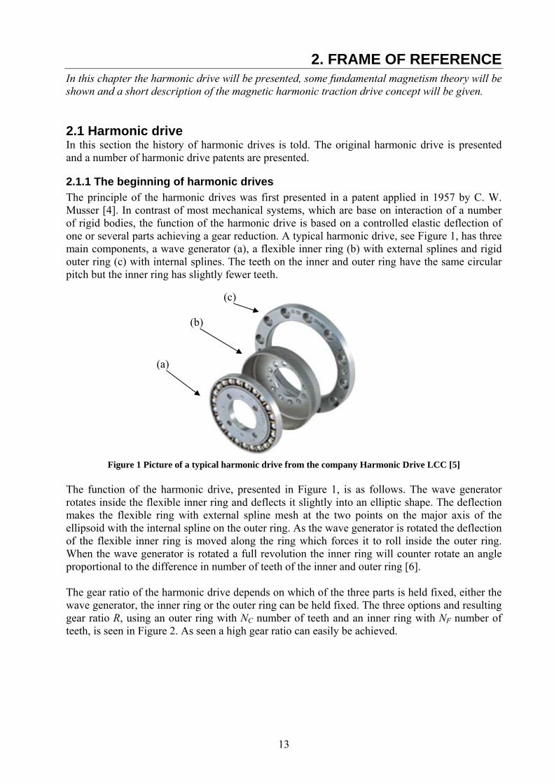
2.1.1 The beginning of harmonic drives The principle of the harmonic drives was first presented in a patent applied in 1957 by C. W. Musser [4]. In contrast of most mechanical systems, which are base on interaction of a number of rigid bodies, the function of the harmonic drive is based on a controlled elastic deflection of one or several parts achieving a gear reduction. A typical harmonic drive, see Figure 1, has three main components, a wave generator (a), a flexible inner ring (b) with external splines and rigid outer ring (c) with internal splines. The teeth on the inner and outer ring have the same circular pitch but the inner ring has slightly fewer teeth.

Figure 1 Picture of a typical harmonic drive from the company Harmonic Drive LCC [5]

The function of the harmonic drive, presented in Figure 1, is as follows. The wave generator rotates inside the flexible inner ring and deflects it slightly into an elliptic shape. The deflection makes the flexible ring with external spline mesh at the two points on the major axis of the ellipsoid with the internal spline on the outer ring. As the wave generator is rotated the deflection of the flexible inner ring is moved along the ring which forces it to roll inside the outer ring. When the wave generator is rotated a full revolution the inner ring will counter rotate an angle proportional to the difference in number of teeth of the inner and outer ring [6]. The gear ratio of the harmonic drive depends on which of the three parts is held fixed, either the wave generator, the inner ring or the outer ring can be held fixed. The three options and resulting gear ratio R, using an outer ring with NC number of teeth and an inner ring with NF number of teeth, is seen in Figure 2. As seen a high gear ratio can easily be achieved.

(c)

(b)

(a)

14

Figure 2 Formulas for calculating the gear ratio for the harmonic drive when different components are held

fixed [6] The wave generator can be either internal or external. In the latter case it deflects a flexible outer ring to engage with a rigid inner ring. In [6] several different wave generator configurations are presented, see Figure 3. First (a) an ellipsoidal cam is used with either a roller bearing or a sliding bearing in the contact with the flexible ring. Second (b) rollers are used to deflect the flexible ring; the numbers of rollers can be varied. This solution is presented as an inexpensive solution. A third configuration (c) is the ball planetary; the inner roller drives the two outer rollers who are in contact with flexible ring. The final suggestion (d) of wave generator configuration is the variable ball planetary where balls of different sizes are used to deflect the flexible ring. One advantage with this configuration compared to the ball planetary is the added support to the flexible ring which increased the torque capability [6].

Figure 3 Different methods described in C.W. Musser article to create a wave generator [6]

2.1.2 Harmonic traction drive There are several patents describing how traction can be used instead of teeth to transfer the torque. David G. Duff applied in 2000 a patent [7] using friction to transfer energy between a flexible inner ring to the rigid outer ring. The harmonic drive described in the patent uses three preloaded rollers to deflect the flexible inner ring and make contact against the rigid outer ring.

15

Figure 4 An example of a harmonic friction drive presented in a patent applied by David G. Duff [7]

Another example of a harmonic drive which uses traction to transfer torque is presented in a patent applied by Donald R. Humphreys in 1969 [8]. This patent present a traditional harmonic drive which uses friction between the flexible ring and the rigid ring to transfer torque.

Figure 5 A picture from a patent of a traction harmonic drive applied by Donald R. Humphrey [8]

There are many reasons for choosing traction instead of teeth to transfer the torque. One of the main reasons for choosing traction instead of teeth to transfer the torque is the cost. The cost of making small high precision teeth is thought to be higher than using traction. Another advantage is that a higher reduction ratio is possible since no minimum tooth height clearance is required. The torque transfer can also be ripple-free due to continuous rolling contact. Since the contact has the ability to slip there is also an inherent overload protection. A final advantage is that the gear is non-back driveable which obviates the need for a motor brake. Even though the slip can be used as overload protection the slip causes problem. For a certain load there will always be a small slip so the position of the output shaft is undefined. To solve this problem an extra position sensor may be used to measure the position of the output shaft. However, this adds complexity to the system.

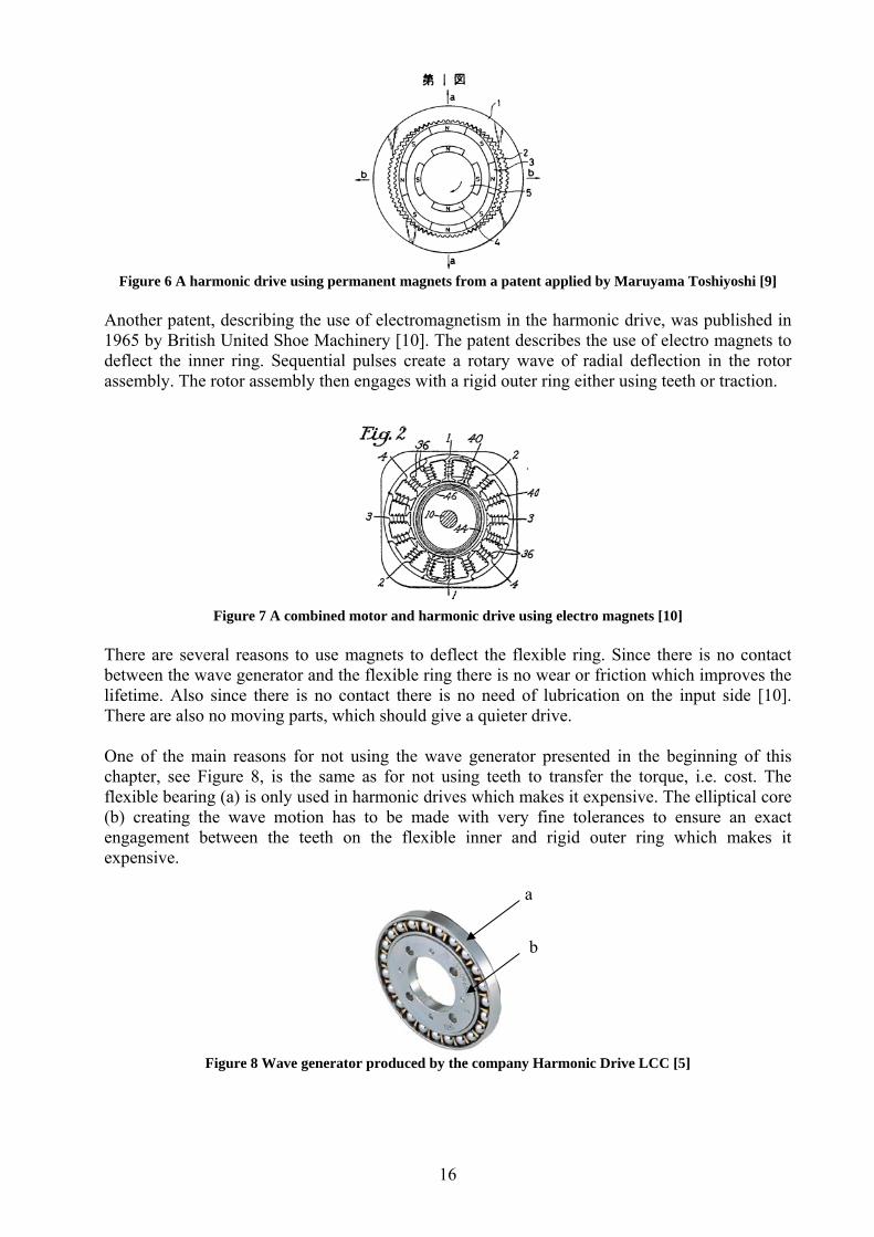
2.1.3 Magnetic Harmonic Drive In 1988 Maruyama Toshiyoshi applied for a patent [9] describing a harmonic drive gear which uses permanent magnets to induce the deflection of the flexible ring, (see Figure 6). The gear has permanent magnets (3) continuously arranged at equal intervals at the interior of a flexible inner ring (2). Another set of magnets (4) are mounted on a shaft inside the flexible inner ring which forces the flexible inner ring to deflect and engage with the rigid outer ring (1). In the patent the motivation for using permanent magnets is weight reduction. Another advantage of this design is the low number of moving parts and the mechanical wave generator is replaced by a magnetic one.

16

Figure 6 A harmonic drive using permanent magnets from a patent applied by Maruyama Toshiyoshi [9]

Another patent, describing the use of electromagnetism in the harmonic drive, was published in 1965 by British United Shoe Machinery [10]. The patent describes the use of electro magnets to deflect the inner ring. Sequential pulses create a rotary wave of radial deflection in the rotor assembly. The rotor assembly then engages with a rigid outer ring either using teeth or traction.

Figure 7 A combined motor and harmonic drive using electro magnets [10]

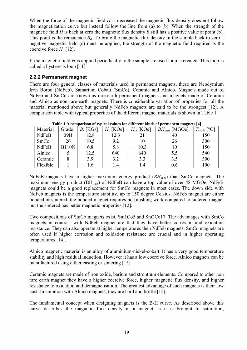
There are several reasons to use magnets to deflect the flexible ring. Since there is no contact between the wave generator and the flexible ring there is no wear or friction which improves the lifetime. Also since there is no contact there is no need of lubrication on the input side [10]. There are also no moving parts, which should give a quieter drive. One of the main reasons for not using the wave generator presented in the beginning of this chapter, see Figure 8, is the same as for not using teeth to transfer the torque, i.e. cost. The flexible bearing (a) is only used in harmonic drives which makes it expensive. The elliptical core (b) creating the wave motion has to be made with very fine tolerances to ensure an exact engagement between the teeth on the flexible inner and rigid outer ring which makes it expensive.

Figure 8 Wave generator produced by the company Harmonic Drive LCC [5]

a

b

17

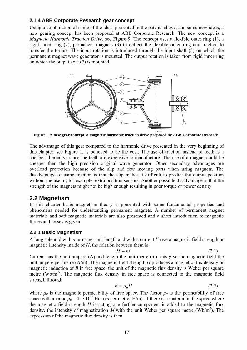
2.1.4 ABB Corporate Research gear concept Using a combination of some of the ideas presented in the patents above, and some new ideas, a new gearing concept has been proposed at ABB Corporate Research. The new concept is a Magnetic Harmonic Traction Drive, see Figure 9. The concept uses a flexible outer ring (1), a rigid inner ring (2), permanent magnets (3) to deflect the flexible outer ring and traction to transfer the torque. The input rotation is introduced through the input shaft (5) on which the permanent magnet wave generator is mounted. The output rotation is taken from rigid inner ring on which the output axle (7) is mounted.

B

B

B-B

5

7

A

A-A A

1

2

3

4

6

Figure 9 A new gear concept, a magnetic harmonic traction drive proposed by ABB Corporate Research.

The advantage of this gear compared to the harmonic drive presented in the very beginning of this chapter, see Figure 1, is believed to be the cost. The use of traction instead of teeth is a cheaper alternative since the teeth are expensive to manufacture. The use of a magnet could be cheaper then the high precision original wave generator. Other secondary advantages are overload protection because of the slip and few moving parts when using magnets. The disadvantage of using traction is that the slip makes it difficult to predict the output position without the use of, for example, extra position sensors. Another possible disadvantage is that the strength of the magnets might not be high enough resulting in poor torque or power density. 2.2 Magnetism In this chapter basic magnetism theory is presented with some fundamental properties and phenomena needed for understanding permanent magnets. A number of permanent magnet materials and soft magnetic materials are also presented and a short introduction to magnetic forces and losses is given.

2.2.1 Basic Magnetism A long solenoid with n turns per unit length and with a current I have a magnetic field strength or magnetic intensity inside of H, the relation between them is nIH = (2.1) Current has the unit ampere (A) and length the unit metre (m), this give the magnetic field the unit ampere per metre (A/m). The magnetic field strength H produces a magnetic flux density or magnetic induction of B in free space, the unit of the magnetic flux density is Weber per square metre (Wb/m2). The magnetic flux density in free space is connected to the magnetic field strength through HB 0μ= (2.2) where μ0 is the magnetic permeability of free space. The factor μ0 is the permeability of free space with a value μ0 = 4π · 10-7 Henrys per metre (H/m). If there is a material in the space where the magnetic field strength H is acting one further component is added to the magnetic flux density, the intensity of magnetization M with the unit Weber per square metre (Wb/m2). The expression of the magnetic flux density is then

18

MHB += 0μ . (2.3) A material is said to have an absolute permeability μ, with the unit Henry par metre (H/m) defined as

HB

=μ . (2.4)

The absolute permeability contains the contribution both from free space and the material it self [12]. Three different systems of units are used to describe magnetic properties, the one presented above is the SI system bases on metre, kilogram, second, another is the cgs system based on centimeter, gram. The third and the final is the English system based on inch, pound, second [12]. There are several material classifications depending on the relation between the magnetic field strength H and the magnetic flux density B. In this text materials classified as ferromagnetic will be discussed, these materials are characterised by the fact that the contribution from the material it self to the absolute permeability μ is much greater than the contribution from free space [13]. The general behaviour of a ferromagnetic material in a magnetic field can be exemplified by the B-H curve, see Figure 10, which shows the relationship between the magnetic field strength H and the magnetic flux density B. The B-H curve describes the cycle of a magnet as it is brought to saturation, demagnetised, saturated in the opposite direction, and then demagnetised again under the influence of an external magnetic field. Saturation occurs when all atoms in the material have aligned with the external magnetic field and the magnetization of the material can increase no further [12]. The origin of the coordinate system (0) represents a demagnetised sample of a ferromagnetic material. When a magnetic field H is applied to the sample the magnetic flux density B in the material follows the black line from (0) to (a), the magnetization curve. If the magnetic field is strong enough the material sample will begin to saturate and finally the increase of intensity of magnetization M will cease. The increase in magnetic flux density B will then only get a contribution from the permeability of free space [12].

Figure 10 B-H curve of a ferromagnetic material

H

B

19

When the force of the magnetic field H is decreased the magnetic flux density does not follow the magnetization curve but instead follow the line from (a) to (b). When the strength of the magnetic field H is back at zero the magnetic flux density B still has a positive value at point (b). This point is the remanence Bd. To bring the magnetic flux density in the sample back to zero a negative magnetic field (c) must be applied, the strength of the magnetic field required is the coercive force Hc [12]. If the magnetic field H is applied periodically to the sample a closed loop is created. This loop is called a hysteresis loop [11].

2.2.2 Permanent magnet There are four general classes of materials used in permanent magnets, these are Neodymium Iron Boron (NdFeb), Samarium Cobalt (SmCo), Ceramic and Alnico. Magnets made out of NdFeb and SmCo are known as rare-earth permanent magnets and magnets made of Ceramic and Alnico as non rare-earth magnets. There is considerable variation of properties for all the material mentioned above but generally NdFeb magnets are said to be the strongest [12]. A comparison table with typical properties of the different magnet materials is shown in Table 1.

Table 1 A comparison of typical values for different kinds of permanent magnets [4] Material Grade Br [KGs] Hc [KOe] Hci [KOe] BHmax [MGOe] Tcurie [°C] NdFeB 39H 12.8 12.3 21 40 150 SmCo 26 10.5 9.2 10 26 300 NdFeB B110N 6.8 5.8 10.3 10 150 Alnico 5 12.5 640 640 5.5 540 Ceramic 8 3.9 3.2 3.3 3.5 300 Flexible 1 1.6 1.4 1.4 0.6 100

NdFeB magnets have a higher maximum energy product (BHmax) than SmCo magnets. The maximum energy product (BHmax) of NdFeB can have a top value of over 48 MGOe. NdFeB magnets could be a good replacement for SmCo magnets in most cases. The down side with NdFeb magnets is the temperature stability, up to 150 degree Celsius. NdFeb magnet are either bonded or sintered, the bonded magnet requires no finishing work compared to sintered magnet but the sintered has better magnetic properties [12]. Two compositions of SmCo magnets exist, Sm1Co5 and Sm2Co17. The advantages with SmCo magnets in contrast with NdFeb magnet are that they have better corrosion and oxidation resistance. They can also operate at higher temperatures then NdFeb magnets. SmCo magnets are often used if higher corrosion and oxidation resistance are crucial and in higher operating temperatures [14]. Alnico magnetic material is an alloy of aluminium-nickel-cobalt. It has a very good temperature stability and high residual induction. However it has a low coercive force. Alnico magnets can be manufactured using either casting or sintering [15]. Ceramic magnets are made of iron oxide, barium and strontium elements. Compared to other non rare earth magnet they have a higher coercive force, higher magnetic flux density, and higher resistance to oxidation and demagnetisation. The greatest advantage of such magnets is their low cost. In common with Alnico magnets, they are hard and brittle [15]. The fundamental concept when designing magnets is the B-H curve. As described above this curve describes the magnetic flux density in a magnet as it is brought to saturation,

20

demagnetised, saturated in the opposite direction, and then demagnetised again under the influence of an external magnetic field. There are three important properties of the magnet that can be found in the B-H curve. The residual induction (Br) is the point where the curve crosses the B-axis, the residual induction is the maximum magnetic flux density output of the magnet without an external magnetic field [11]. The coercive force (Hc) is the point where the curve crosses the H-axis, the coercive force is the strength of the external magnetic field that will decrease the observed magnetic flux density of a previously saturated magnet to zero [16]. The final property is the maximum energy product (BHmax). There is a point on the B-H curve where the product of magnetic field H and magnetic flux density B reaches a maximum. At this point, the volume of magnet material required to project certain energy is a minimum. This is a parameter of how strong the magnetic material is and can be used to compare different materials [16].

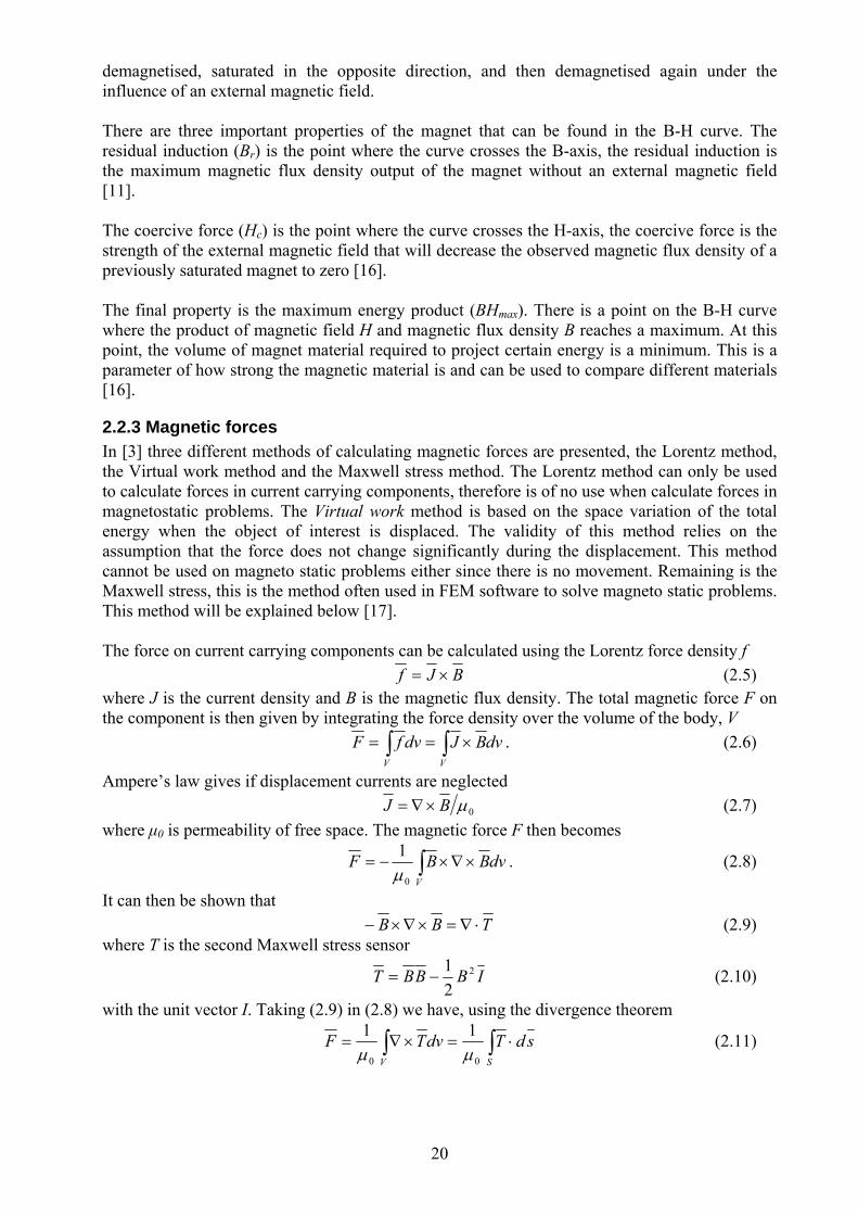
2.2.3 Magnetic forces In [3] three different methods of calculating magnetic forces are presented, the Lorentz method, the Virtual work method and the Maxwell stress method. The Lorentz method can only be used to calculate forces in current carrying components, therefore is of no use when calculate forces in magnetostatic problems. The Virtual work method is based on the space variation of the total energy when the object of interest is displaced. The validity of this method relies on the assumption that the force does not change significantly during the displacement. This method cannot be used on magneto static problems either since there is no movement. Remaining is the Maxwell stress, this is the method often used in FEM software to solve magneto static problems. This method will be explained below [17]. The force on current carrying components can be calculated using the Lorentz force density f BJf ×= (2.5) where J is the current density and B is the magnetic flux density. The total magnetic force F on the component is then given by integrating the force density over the volume of the body, V ∫∫ ×==

VV

dvBJdvfF . (2.6)

Ampere’s law gives if displacement currents are neglected 0μBJ ×∇= (2.7) where μ0 is permeability of free space. The magnetic force F then becomes

∫ ×∇×−=V

dvBBF0

1μ

. (2.8)

It can then be shown that TBB ⋅∇=×∇×− (2.9) where T is the second Maxwell stress sensor

IBBBT 2

21

−= (2.10)

with the unit vector I. Taking (2.9) in (2.8) we have, using the divergence theorem

∫∫ ⋅=×∇=SV

sdTdvTF00

11μμ

(2.11)

21

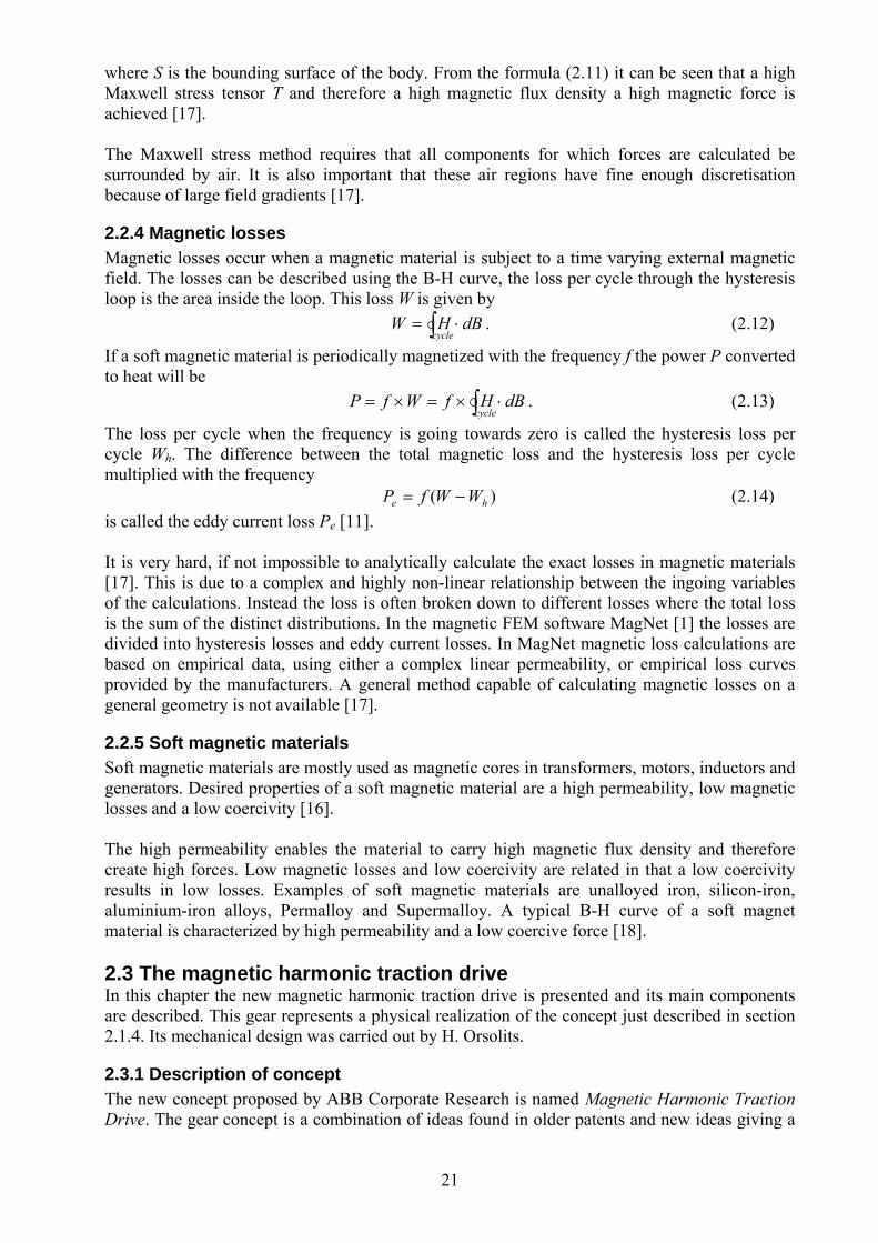
where S is the bounding surface of the body. From the formula (2.11) it can be seen that a high Maxwell stress tensor T and therefore a high magnetic flux density a high magnetic force is achieved [17]. The Maxwell stress method requires that all components for which forces are calculated be surrounded by air. It is also important that these air regions have fine enough discretisation because of large field gradients [17].

2.2.4 Magnetic losses Magnetic losses occur when a magnetic material is subject to a time varying external magnetic field. The losses can be described using the B-H curve, the loss per cycle through the hysteresis loop is the area inside the loop. This loss W is given by ∫ ⋅=

cycledBHW . (2.12)

If a soft magnetic material is periodically magnetized with the frequency f the power P converted to heat will be ∫ ⋅×=×=

cycledBHfWfP . (2.13)

The loss per cycle when the frequency is going towards zero is called the hysteresis loss per cycle Wh. The difference between the total magnetic loss and the hysteresis loss per cycle multiplied with the frequency )( he WWfP −= (2.14) is called the eddy current loss Pe [11]. It is very hard, if not impossible to analytically calculate the exact losses in magnetic materials [17]. This is due to a complex and highly non-linear relationship between the ingoing variables of the calculations. Instead the loss is often broken down to different losses where the total loss is the sum of the distinct distributions. In the magnetic FEM software MagNet [1] the losses are divided into hysteresis losses and eddy current losses. In MagNet magnetic loss calculations are based on empirical data, using either a complex linear permeability, or empirical loss curves provided by the manufacturers. A general method capable of calculating magnetic losses on a general geometry is not available [17].

2.2.5 Soft magnetic materials Soft magnetic materials are mostly used as magnetic cores in transformers, motors, inductors and generators. Desired properties of a soft magnetic material are a high permeability, low magnetic losses and a low coercivity [16]. The high permeability enables the material to carry high magnetic flux density and therefore create high forces. Low magnetic losses and low coercivity are related in that a low coercivity results in low losses. Examples of soft magnetic materials are unalloyed iron, silicon-iron, aluminium-iron alloys, Permalloy and Supermalloy. A typical B-H curve of a soft magnet material is characterized by high permeability and a low coercive force [18]. 2.3 The magnetic harmonic traction drive In this chapter the new magnetic harmonic traction drive is presented and its main components are described. This gear represents a physical realization of the concept just described in section 2.1.4. Its mechanical design was carried out by H. Orsolits.

2.3.1 Description of concept The new concept proposed by ABB Corporate Research is named Magnetic Harmonic Traction Drive. The gear concept is a combination of ideas found in older patents and new ideas giving a

22

whole new concept. One of the earlier models from the beginning steps of the design work, see Figure 11, is used to describe the main parts and the function of the gear concept. The gearbox is built of 5 main parts, first (1) is the two piece outer housing whose main function is to stabilize the gear and maintain the relative positions of the parts. Second (2) is the frameless servo motor and motor housing. To save space the motor is placed inside the gear. To be able to fit the motor inside the gearbox a frameless motor with a housing (2a) integrated in the outer housing is used. Third (3) is the input shaft onto which the magnets are mounted, its function is to transfer torque from the motor and to enable radial adjustment of the magnets. The fourth part (4) is the circular spline onto which the output shaft is mounted via a base plate, the circular spline should be very rigid but still be thin, and the surface of the surface on the circular spline should enable a high friction coefficient and be hard wearing. The fifth part (5) is the flexspline with a magnetic portion (6) mounted inside. The flexspline should have a low radial stiffness but a high torsional stiffness. The Flexspline is bonded with glue to the outer housing. The magnetic portion should be a highly magnetic material but should not add any radial stiffness to the flexspline. Due to an ongoing patent process, details of the construction of the magnetic portion are not disclosed in this report.

Figure 11 Model of the magnetic harmonic traction drive from early stages of the construction work

(courtesy of H. Orsolits) The function of the magnetic harmonic traction drive can be described as follows. The magnets attract the magnet portion on the flexspline and the inner surface on the magnetic portion makes contact to the circular spline. A different number of magnets can be used, giving different numbers of contact points. When the motor is turning the input shaft the magnets, and therefore the contact points between flexspline and circular spline are rotating. The rotating deflection of the flexspline forces the circular spline to rotate inside the flexspline giving a gear reduction.

1.

2.

3.

4.

5.

2a.

23

3. THE EVALUATION PROCESS In this chapter the evaluation process is explained, components used in the evaluation are presented and which parameters will be evaluated are mentioned. 3.1 Evaluation process explained The evaluation process is divided in to two sub processes, one in which magnetic aspects are investigated and one where mechanical aspects are investigated. The magnetic aspects will be investigated using the magnetic finite element software MagNet [1] and Ansys Workbench [2]. The mechanical aspects are investigated using the finite element software Abaqus [3]. In this report focus will be on four of the components building up the gearbox, the flexspline, the magnetic portion, the magnets and the circular spline. These are the components most important for the function of the gear. Characteristics that will be evaluated are magnetic forces and force distribution, torque capability, and torsional stiffness.

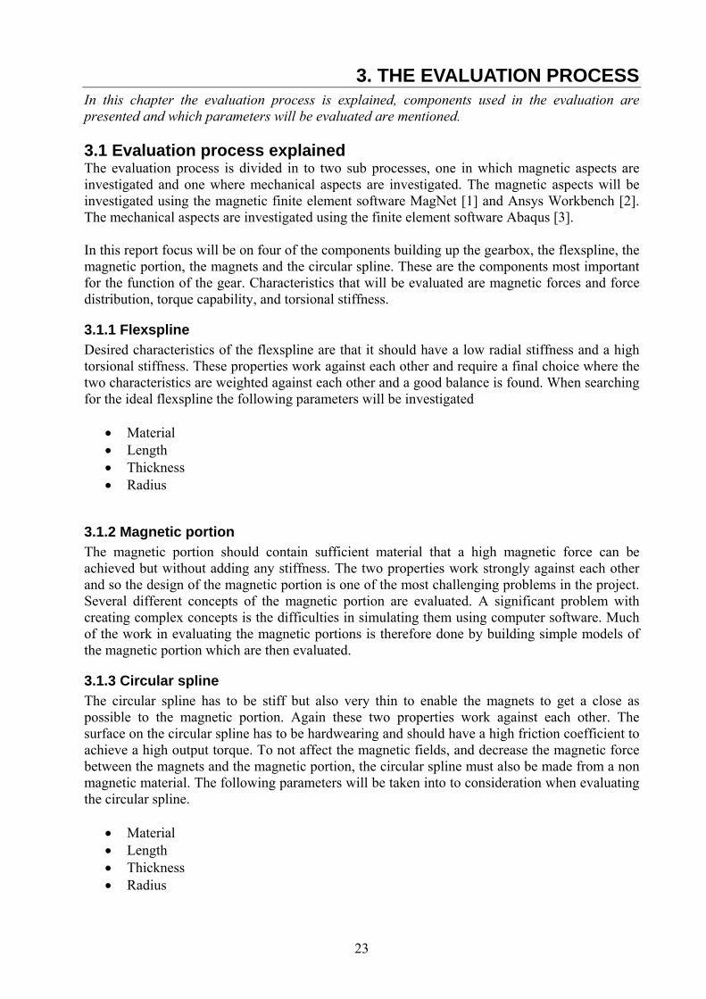
3.1.1 Flexspline Desired characteristics of the flexspline are that it should have a low radial stiffness and a high torsional stiffness. These properties work against each other and require a final choice where the two characteristics are weighted against each other and a good balance is found. When searching for the ideal flexspline the following parameters will be investigated

• Material • Length • Thickness • Radius

3.1.2 Magnetic portion The magnetic portion should contain sufficient material that a high magnetic force can be achieved but without adding any stiffness. The two properties work strongly against each other and so the design of the magnetic portion is one of the most challenging problems in the project. Several different concepts of the magnetic portion are evaluated. A significant problem with creating complex concepts is the difficulties in simulating them using computer software. Much of the work in evaluating the magnetic portions is therefore done by building simple models of the magnetic portion which are then evaluated.

3.1.3 Circular spline The circular spline has to be stiff but also very thin to enable the magnets to get a close as possible to the magnetic portion. Again these two properties work against each other. The surface on the circular spline has to be hardwearing and should have a high friction coefficient to achieve a high output torque. To not affect the magnetic fields, and decrease the magnetic force between the magnets and the magnetic portion, the circular spline must also be made from a non magnetic material. The following parameters will be taken into to consideration when evaluating the circular spline.

• Material • Length • Thickness • Radius

24

3.1.4 Magnets The magnets should be strong to provide high torque capability. The magnets should not be too strong since in a rolling contact the rolling resistance is a function of the contact force [19]. So the magnets should only be strong enough. The weight of the magnets should also be low to keep the moment of inertia low. When choosing magnets the following parameters will be taken into consideration

• Shape • Width • Length • Height • Mass

25

4. MAGNETIC SIMULATIONS In this chapter the magnetic simulations are presented, the models used, the results and the discussions and conclusions. In the first chapter the model used is presented and the following chapters different parameters are evaluated. In the last chapter a comparison of using MagNet or Ansys is performed. 4.1 Magnet shapes There are two properties of interest when performing the magnet shape simulations, the total force and the force distribution over the flexspline. In this section several different aspects are investigated and the results are intended to be used to decide the dimensions for the concept.

4.1.1 Model When building the MagNet model used in the simulations the gear concept is simplified into two kinds of components, magnets and the flexspline. Several different shapes of magnets will be tested and the thickness and size of the flexspline will be varied. A surrounding air is also added to the model to allow forces to be calculated.

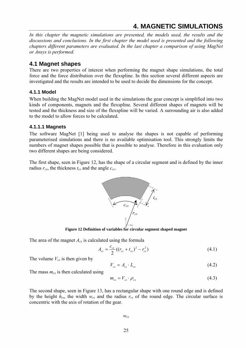
4.1.1.1 Magnets The software MagNet [1] being used to analyse the shapes is not capable of performing parameterised simulations and there is no available optimisation tool. This strongly limits the numbers of magnet shapes possible that is possible to analyse. Therefore in this evaluation only two different shapes are being considered. The first shape, seen in Figure 12, has the shape of a circular segment and is defined by the inner radius rcs, the thickness tcs and the angle ccs.

Figure 12 Definition of variables for circular segment shaped magnet

The area of the magnet Acs is calculated using the formula

))((2

22cscscs

cscs rtrcA −+= (4.1)

The volume Vcs is then given by cscscs LAV ⋅= (4.2) The mass mcs is then calculated using cscscs Vm ρ⋅= (4.3) The second shape, seen in Figure 13, has a rectangular shape with one round edge and is defined by the height hrs, the width wrs and the radius rrs of the round edge. The circular surface is concentric with the axis of rotation of the gear.

tcs

rcs ccs

wrs

26

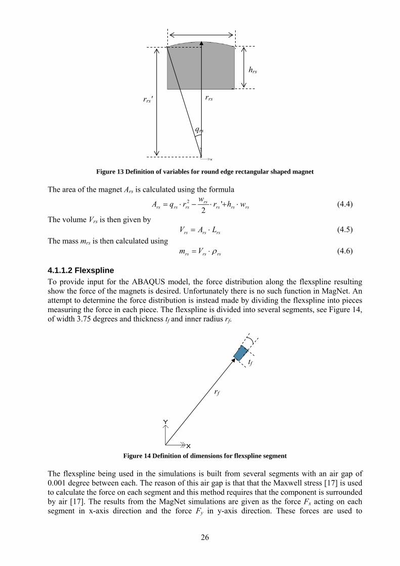
Figure 13 Definition of variables for round edge rectangular shaped magnet

The area of the magnet Ars is calculated using the formula

rsrsrsrs

rsrsrs whrwrqA ⋅+⋅−⋅= '2

2 (4.4)

The volume Vrs is then given by rsrsrs LAV ⋅= (4.5) The mass mrs is then calculated using rsrsrs Vm ρ⋅= (4.6)

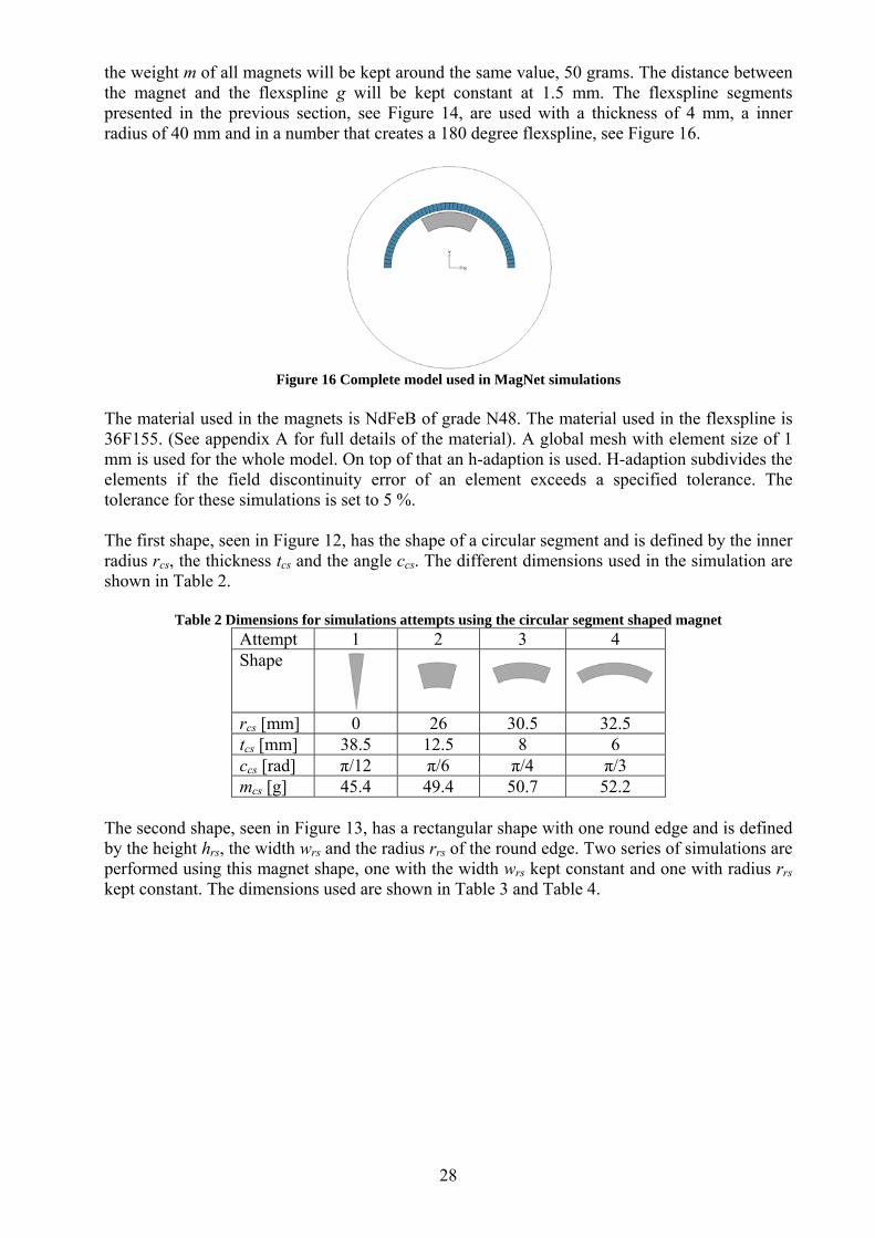
4.1.1.2 Flexspline To provide input for the ABAQUS model, the force distribution along the flexspline resulting show the force of the magnets is desired. Unfortunately there is no such function in MagNet. An attempt to determine the force distribution is instead made by dividing the flexspline into pieces measuring the force in each piece. The flexspline is divided into several segments, see Figure 14, of width 3.75 degrees and thickness tf and inner radius rf.

Figure 14 Definition of dimensions for flexspline segment

The flexspline being used in the simulations is built from several segments with an air gap of 0.001 degree between each. The reason of this air gap is that that the Maxwell stress [17] is used to calculate the force on each segment and this method requires that the component is surrounded by air [17]. The results from the MagNet simulations are given as the force Fx acting on each segment in x-axis direction and the force Fy in y-axis direction. These forces are used to

rrs

hrs

qrs

rrs'

rf

tf

27

calculate the resulting inward radial force Fr. The method of calculating the radial force Fr is explained with reference to Figure 15 and the formulae below.

Figure 15 Forces on the flexspline

The inward radial force Fr is given by ))sin()cos(( aFaFF yxr ⋅+⋅−= (4.7) where Fx is the force acting in the x-axis direction and Fy is the force acting in y-axis direction in the flexspline segment and a is the angle to from the x-axis to the flexspline segment.

4.1.1.4 Total force and distribution The total force on the flexspline is determined by summing the force in negative y-axis direction of all the flexspline segments. Depending on how many magnets are used, a different number of flexspline segments are summated, if 2 magnets are used the force on segments creating a 180 degree angle is summated and if 3 magnets are used the force on segments creating a 120 degree angle is summated. The force distribution is presented by plotting the radial force on each flexspline segment as a function of its position.

4.1.2 Magnet shape simulations In this section the difference when changing the shape of the magnet is investigated and evaluated.

4.1.2.1 Purpose To optimise the shapes of the magnet is a non trivial task. One problem is that there are an infinite number of shapes and another problem is to decide what the goal of the optimisation is. In this case the number of shapes is limited firstly by the fact that the magnet will only be optimised in 2-D and secondly by the fact that it should fit inside the gear concept. The goal of these simulations is to show how the different magnet shapes deform the force distribution that will affect the flexspline. The results from this evaluation are used together with the Abaqus model to be to determine the optimal shape.

4.1.2.2 Model As earlier mentioned there are many different magnet shapes and to analyse them all is not possible. The software MagNet [10] being used to analyse the shapes is not capable of parameterised simulations and there no available optimisation tool. This strongly limits the numbers of magnets shapes that may reasonably be analysed. In this evaluation the two different shapes presented in the previous chapter are used. Different variables will be varied but the length L of the magnets will be held constant at 15 mm. The density ρ will be 7800 kg/m3 and

Fx

Fy

x

y

Fr

a

28

the weight m of all magnets will be kept around the same value, 50 grams. The distance between the magnet and the flexspline g will be kept constant at 1.5 mm. The flexspline segments presented in the previous section, see Figure 14, are used with a thickness of 4 mm, a inner radius of 40 mm and in a number that creates a 180 degree flexspline, see Figure 16.

Figure 16 Complete model used in MagNet simulations

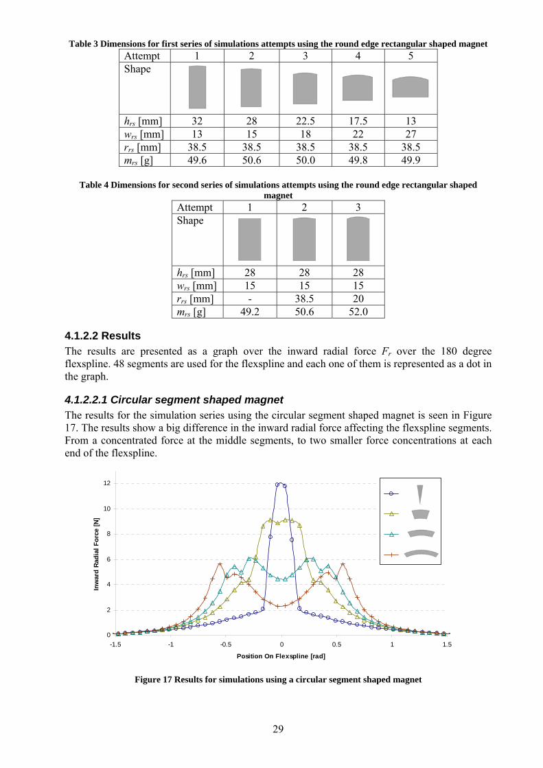
The material used in the magnets is NdFeB of grade N48. The material used in the flexspline is 36F155. (See appendix A for full details of the material). A global mesh with element size of 1 mm is used for the whole model. On top of that an h-adaption is used. H-adaption subdivides the elements if the field discontinuity error of an element exceeds a specified tolerance. The tolerance for these simulations is set to 5 %. The first shape, seen in Figure 12, has the shape of a circular segment and is defined by the inner radius rcs, the thickness tcs and the angle ccs. The different dimensions used in the simulation are shown in Table 2.

Table 2 Dimensions for simulations attempts using the circular segment shaped magnet Attempt 1 2 3 4 Shape

rcs [mm] 0 26 30.5 32.5 tcs [mm] 38.5 12.5 8 6 ccs [rad] π/12 π/6 π/4 π/3 mcs [g] 45.4 49.4 50.7 52.2

The second shape, seen in Figure 13, has a rectangular shape with one round edge and is defined by the height hrs, the width wrs and the radius rrs of the round edge. Two series of simulations are performed using this magnet shape, one with the width wrs kept constant and one with radius rrs kept constant. The dimensions used are shown in Table 3 and Table 4.

29

Table 3 Dimensions for first series of simulations attempts using the round edge rectangular shaped magnet Attempt 1 2 3 4 5 Shape

hrs [mm] 32 28 22.5 17.5 13 wrs [mm] 13 15 18 22 27 rrs [mm] 38.5 38.5 38.5 38.5 38.5 mrs [g] 49.6 50.6 50.0 49.8 49.9

Table 4 Dimensions for second series of simulations attempts using the round edge rectangular shaped

magnet Attempt 1 2 3 Shape

hrs [mm] 28 28 28 wrs [mm] 15 15 15 rrs [mm] - 38.5 20 mrs [g] 49.2 50.6 52.0

4.1.2.2 Results The results are presented as a graph over the inward radial force Fr over the 180 degree flexspline. 48 segments are used for the flexspline and each one of them is represented as a dot in the graph.

4.1.2.2.1 Circular segment shaped magnet The results for the simulation series using the circular segment shaped magnet is seen in Figure 17. The results show a big difference in the inward radial force affecting the flexspline segments. From a concentrated force at the middle segments, to two smaller force concentrations at each end of the flexspline.

0

2

4

6

8

10

12

-1.5 -1 -0.5 0 0.5 1 1.5

Position On Flexspline [rad]

Inw

ard

Radi

al F

orce

[N]

Figure 17 Results for simulations using a circular segment shaped magnet

30

The summation of the total force in y-axis FM,y,sum and in the radial direction FM,r,sum can be seen in Figure 18. The results show a large difference between the summation in y-axis and the summation in the radial direction. The see which of them show the real results requires further studies which is done in chapter 4.4.

0

20

40

60

80

100

120

1 2 3 4

Forc

e Fs

um [N

]

Y-axis Dir. Radial Dir.

Figure 18 Summation of the forces in y/axis direction and in radial direction for circular segment shaped

magnets

4.1.2.2.2 Rectangular magnet with one rounded edge The results of the first series of simulations using the rectangular magnet with one rounded edge are seen in Figure 19. In the first series the radius of the rounded edge were kept constant and the width and height were altered. Each of the two extreme shapes in the series is shown in the graph. The result shows a concentrated force for the less wide magnet which is what you can expect.

0

2

4

6

8

10

12

14

16

-1.5 -1 -0.5 0 0.5 1 1.5

Position On Flexspline [rad]

Inw

ard

Rad

ial F

orce

[N]

Figure 19 Results for the first series of simulations using a round edge rectangular shaped magnet

The summation of the total force in y-axis FM,y,sum and in the radial direction FM,r,sum can be seen in Figure 20. The results show a big difference between the summation in y-axis and the summation in the radial direction. The see which of them show the real results requires further studies which is done in chapter 4.4.

31

0

50

100

150

200

1 2 3 4 5Fo

rce

Fsum

[N]

Y-axis Dir. Radial Dir.

Figure 20 Summation of the forces in y/axis direction and in radial direction for rectangular shaped magnets

with one rounded edge varying the width and height The results of the second series of simulations using the rectangular magnet with one rounded edge are seen in Figure 21. In this series the width wrs of the magnet is kept constant as the radius rrs of the rounded edge and height hrs of the magnet are varied. The purpose of this simulation was to see what happened to the “valley” seen in previous simulations when the radius of the magnet close to the flexspline was altered. The series starts with a valley in the force curve but when the radius of the edge is made smaller the valley becomes smaller and finally turns in to peek instead. The maximum force is lower but the magnetic force becomes more even at the top.

0

2

4

6

8

10

12

14

16

18

-1.5 -1 -0.5 0 0.5 1 1.5

Position On Flexspline [rad]

Inw

ard

Rad

ial F

orce

[N]

Figure 21 Results for the second series of simulations using a round edge rectangular shaped magnet

The summation of the total force in y-axis FM,y,sum and in the radial direction FM,r,sum can be seen in Figure 22. The results show a large difference between the summation in y-axis and the summation in the radial direction. The see which of them show the real results requires further studies which is done in chapter 4.4.

32

77 83 80

197 206 204

0

50

100

150

200

1 2 3

Forc

e Fs

um [N

]

Y-axis Dir. Radial Dir.

Figure 22 Summation of the forces in y/axis direction and in radial direction for rectangular shaped magnets

with one rounded edge varying the radius

4.1.2.2 Discussion and conclusion The purpose of these simulations was to see how the total forces and the force distributions along the flexspline changes as the shape of the magnets were varied. The given results show a significant difference in both the total force and the force distribution when different shapes are used. The shapes looking most promising are the graphs for the narrower magnets which are showing a smooth concentrated force right above the magnets. The magnets having a rectangular with one rounded edge shape seem to be able to achieve a much higher peak force and total force then using a circular segment shaped magnet. It therefore seems that a magnet with that shape would be a better choice. The comparison between the sum of radial force and radial force shows a big difference, this suggests that the method used might not be entirely reliable. This is the reason that simulation results are compared against results from the Ansys simulations which also are being performed. A comparison between the two methods is performed in a later chapter. 4.2 Number of magnets The purpose of these simulations is to show the effects of the numbers of magnets used. It is believed that the magnets will affect each other. Simulations are performed using one, two and three magnets.

4.2.1 Model In these simulations the rectangular magnet with a rounded edged presented in chapter 4.1.1.1 will be used. The magnet will have a height hrs of 28 mm, and width wrs of 15 mm and a top radius rrs of 38.5 mm. A 360 degree flexspline will be used built up from the flexspline segments previously introduced. The flexspline will have an inner radius rf of 40 mm and a thickness tf of 4 mm. The distance between the magnet and the flexspline g will be kept constant at 1.5 mm. The material in the magnet will be NdFeb N48 and the material in the flexspline will be 36F155. Details of the materials are seen in appendix A. The magnets will be evenly spread along the flexspline, the case when using three magnets can be seen in Figure 23.

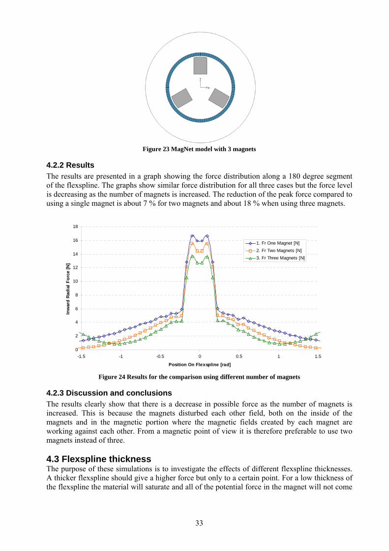
33

Figure 23 MagNet model with 3 magnets

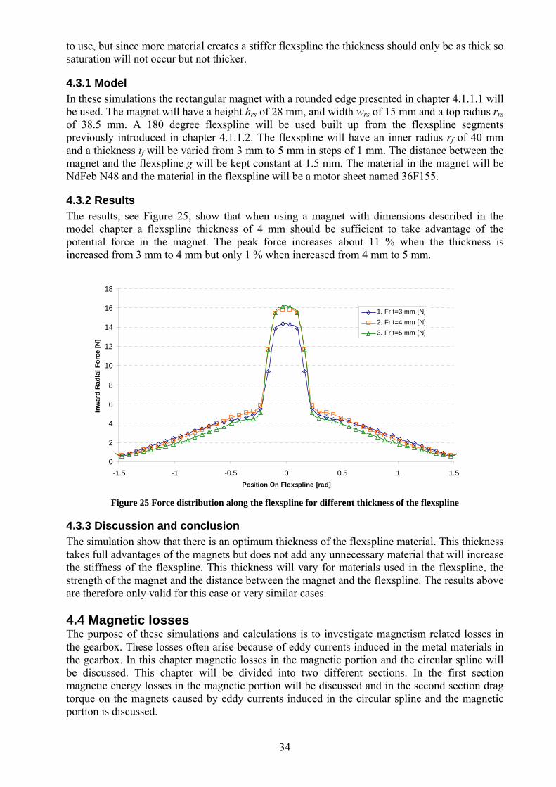
4.2.2 Results The results are presented in a graph showing the force distribution along a 180 degree segment of the flexspline. The graphs show similar force distribution for all three cases but the force level is decreasing as the number of magnets is increased. The reduction of the peak force compared to using a single magnet is about 7 % for two magnets and about 18 % when using three magnets.

0

2

4

6

8

10

12

14

16

18

-1.5 -1 -0.5 0 0.5 1 1.5

Position On Flexspline [rad]

Inw

ard

Rad

ial F

orce

[N]

1. Fr One Magnet [N]2. Fr Two Magnets [N]3. Fr Three Magnets [N]

Figure 24 Results for the comparison using different number of magnets

4.2.3 Discussion and conclusions The results clearly show that there is a decrease in possible force as the number of magnets is increased. This is because the magnets disturbed each other field, both on the inside of the magnets and in the magnetic portion where the magnetic fields created by each magnet are working against each other. From a magnetic point of view it is therefore preferable to use two magnets instead of three. 4.3 Flexspline thickness The purpose of these simulations is to investigate the effects of different flexspline thicknesses. A thicker flexspline should give a higher force but only to a certain point. For a low thickness of the flexspline the material will saturate and all of the potential force in the magnet will not come

34

to use, but since more material creates a stiffer flexspline the thickness should only be as thick so saturation will not occur but not thicker.

4.3.1 Model In these simulations the rectangular magnet with a rounded edge presented in chapter 4.1.1.1 will be used. The magnet will have a height hrs of 28 mm, and width wrs of 15 mm and a top radius rrs of 38.5 mm. A 180 degree flexspline will be used built up from the flexspline segments previously introduced in chapter 4.1.1.2. The flexspline will have an inner radius rf of 40 mm and a thickness tf will be varied from 3 mm to 5 mm in steps of 1 mm. The distance between the magnet and the flexspline g will be kept constant at 1.5 mm. The material in the magnet will be NdFeb N48 and the material in the flexspline will be a motor sheet named 36F155.

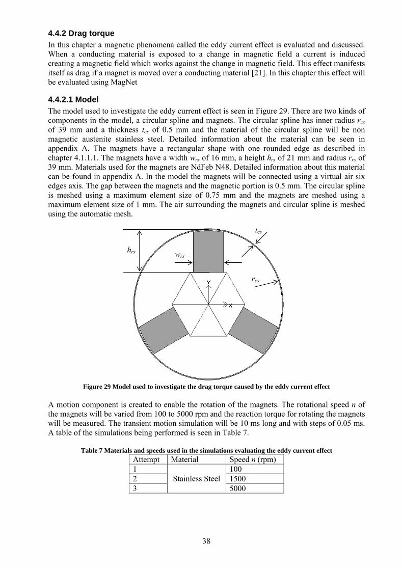
4.3.2 Results The results, see Figure 25, show that when using a magnet with dimensions described in the model chapter a flexspline thickness of 4 mm should be sufficient to take advantage of the potential force in the magnet. The peak force increases about 11 % when the thickness is increased from 3 mm to 4 mm but only 1 % when increased from 4 mm to 5 mm.

0

2

4

6

8

10

12

14

16

18

-1.5 -1 -0.5 0 0.5 1 1.5Position On Flexspline [rad]

Inw

ard

Rad

ial F

orce

[N]

1. Fr t=3 mm [N]2. Fr t=4 mm [N]3. Fr t=5 mm [N]

Figure 25 Force distribution along the flexspline for different thickness of the flexspline

4.3.3 Discussion and conclusion The simulation show that there is an optimum thickness of the flexspline material. This thickness takes full advantages of the magnets but does not add any unnecessary material that will increase the stiffness of the flexspline. This thickness will vary for materials used in the flexspline, the strength of the magnet and the distance between the magnet and the flexspline. The results above are therefore only valid for this case or very similar cases. 4.4 Magnetic losses The purpose of these simulations and calculations is to investigate magnetism related losses in the gearbox. These losses often arise because of eddy currents induced in the metal materials in the gearbox. In this chapter magnetic losses in the magnetic portion and the circular spline will be discussed. This chapter will be divided into two different sections. In the first section magnetic energy losses in the magnetic portion will be discussed and in the second section drag torque on the magnets caused by eddy currents induced in the circular spline and the magnetic portion is discussed.

35

4.4.1 Magnetic losses in the magnetic portion In this chapter the magnetic losses in the magnetic portion will be discussed, the losses will be calculated for different speeds and by the use of tables and using the magnetic finite element software MagNet.

4.4.1.1 Model and method When evaluating the magnetic losses in the magnetic portion two components are taken into consideration, the magnetic portion and the magnets. The models used in the MagNet simulations can be seen in Figure 26. The model has a magnetic portion with an inner radius rmp of 39 mm and a thickness tmp of 4 mm, the depth dmp of the model is 30 mm. Material used in the magnetic portion is M350-50A which is a type of metal sheet used in electrical motors, detailed material data can be seen in appendix A. The model also includes the magnets. Simulations are performed for both two and three magnets. The magnets have a rectangular shape with one rounded edge as the magnet descried in chapter 4.1.1.1. The magnets have a width wrs of 16 mm, a height hrs of 21 mm and radius rrs of 39 mm. Materials used for the magnets are NdFeb N48, detail information about this material can be found in appendix A. The gap between the magnets and the magnetic portion is 1 mm.

Figure 26 Models used in the MagNet simulations to investigate the magnetic losses

The magnets are meshed using a maximum element size of 2 mm and the magnetic portion with a maximum element size of 1 mm, to further improve the mesh h-adaption is also used with a tolerance of 5 %. H-adaption compares the stored energy between every step and if the change in stored energy is bigger then 5 % the mesh is refined. For the MagNet simulations two more components are added, the surrounding air and piece of virtual air, the surrounding air is required for the simulation and the virtual air is added to connect the magnets. The cases for which the losses are calculated can be seen in Table 5. Three different speeds n are investigated, 100 rpm, 1500 rpm and 5000 rpm. The frequency for variations in the magnetic field for the different speeds of the magnets can be calculated using

Nnf mf 60= (4.8)

where n is the rotational speed and N the number of magnets.

g

wrs

tmp

hrs

R rmp

36

Table 5 Combinations of speed and number of magnets used in simulations Attempt Speed n (rpm) Frequency fmf (Hz) Number of magnets N

1 100 3.3 2 2 1500 50 2 3 5000 167 2 4 100 5 3 5 1500 75 3 6 5000 250 3

The losses are calculated using tabular data of losses, see Figure 27. From this graph the losses can be read as Watt per kg material for different variations in the magnetic fields strength and for different frequencies. This graph does not show the losses of the M350-50A material but the losses of the material should be somewhere in between M310-50A and M400-50A.

Figure 27 Tabular loss data for M350-50A [22]

The total mass of the magnetic portion used in this evaluation can be calculated using mpmpmpmpmpmp drtrm ρπ ))(( 22 −+= (4.9) to 240 g if using a density ρmp of 7800 kg.

37

4.4.1.2 Results The magnetic field for using two and three magnets can be seen in Figure 28. The results show that the peak in magnetic field strength is 1.83 Tesla when using two magnets and 1.75 when using three magnets, it can also been seen that the minimum field strength is 0 Tesla in both cases.

Figure 28 Magnetic field for at the start point using two and three magnets

The change in magnetic field strength is used in Figure 27 to calculate the magnetic losses Ptab. The resulting losses are compared with the ideal effect Pin going in to the gear with a load of 5 Nm. The ingoing effect is calculated by multiplying the outgoing velocity with the torque. The results show that the losses are about 15 % of the ideal effect.

Table 6 Losses due to changing magnetic field in the magnetic portion Attempt Pin (W) Ptab (W)

1 0.5 n/a 2 8 1.1 3 26 3.6 4 0.5 n/a 5 8 1.6 6 26 7.2

4.4.1.3 Discussion and conclusions The magnetic losses in the magnetic portion are calculated by considering the variation in magnetic field strength, the variation is then used to determine the losses looking in graphs. The purpose of these calculations was not to determine the exact losses but to obtain an estimation of the losses and determine if they are an important factor for the gear concept. The result show that the losses are about 15% of the ideal effect going into the gear which may be considered comparatively large since this is unlikely to be the only source of losses in the gear. The magnetic losses can be divided into two sources, the eddy current loss and the hysteresis loss. The eddy current losses is caused by electrical currents in the material and the hysteresis losses is the energy associated with energy required to move the magnetic domain walls over the full cycle [23]. It is difficult to lower the hystersis losses since the same amount of material has to be used to achieve a given magnetic force. In transformers and motors, metal sheets coated with insulating material are used to build a laminate. This isolates the plates from each other and decreases the currents. The same method could be possible to use in the gear as well.

38

4.4.2 Drag torque In this chapter a magnetic phenomena called the eddy current effect is evaluated and discussed. When a conducting material is exposed to a change in magnetic field a current is induced creating a magnetic field which works against the change in magnetic field. This effect manifests itself as drag if a magnet is moved over a conducting material [21]. In this chapter this effect will be evaluated using MagNet

4.4.2.1 Model The model used to investigate the eddy current effect is seen in Figure 29. There are two kinds of components in the model, a circular spline and magnets. The circular spline has inner radius rcs of 39 mm and a thickness tcs of 0.5 mm and the material of the circular spline will be non magnetic austenite stainless steel. Detailed information about the material can be seen in appendix A. The magnets have a rectangular shape with one rounded edge as described in chapter 4.1.1.1. The magnets have a width wrs of 16 mm, a height hrs of 21 mm and radius rrs of 39 mm. Materials used for the magnets are NdFeb N48. Detailed information about this material can be found in appendix A. In the model the magnets will be connected using a virtual air six edges axis. The gap between the magnets and the magnetic portion is 0.5 mm. The circular spline is meshed using a maximum element size of 0.75 mm and the magnets are meshed using a maximum element size of 1 mm. The air surrounding the magnets and circular spline is meshed using the automatic mesh.

Figure 29 Model used to investigate the drag torque caused by the eddy current effect

A motion component is created to enable the rotation of the magnets. The rotational speed n of the magnets will be varied from 100 to 5000 rpm and the reaction torque for rotating the magnets will be measured. The transient motion simulation will be 10 ms long and with steps of 0.05 ms. A table of the simulations being performed is seen in Table 7.

Table 7 Materials and speeds used in the simulations evaluating the eddy current effect Attempt Material Speed n (rpm) 1 100 2 1500 3

Stainless Steel 5000

rcs

tcs

wrs hrs

39

4.4.2.2 Results The resulting reaction torque on the magnets when using a stainless steel circular spline is seen in Figure 30, the results show a reaction around zero for low rotational velocity but when the speed is increased the reaction torque increases significantly. The reaction torque is about 0.5 Nm for a speed of 500 rpm and almost 4 Nm for 5000 rpm.

Eddy Current Effect Stainless Steel

-4.5

-4

-3.5

-3

-2.5

-2

-1.5

-1

-0.5

0

0.5

0 1 2 3 4 5 6 7 8 9 10

Time [ms]

Torq

ue [N

m]

100 rpm1500 rpm

5000 rpm

Figure 30 Reaction torque on a circular spline for different rotational speeds on the magnets when using a

stainless steel circular spline Recalculating these torques to loss effect Peddy, multiplying the torque and the velocities the losses can be seen in Table 8. The losses are compared to ideal ingoing effect Pin to gearbox, these effects are calculated multiplying the desired outgoing velocities with an output torque of 5 Nm. The results show that the losses are in the same size or bigger as the ideal ingoing effect, resulting in a poor efficiency of the gearbox.

Table 8 Losses because of eddy current effect in the circular spline Speed (rpm) Pout (W) Peddy (W)

100 0.5 0.5 1500 8 5 5000 26 40

4.4.2.3 Discussion and conclusions The goal with the gearbox was to achieve an efficiency of more than 50 %. Considering only the losses from the eddy current effect on the circular spline, the efficiency will be lower than 50 %. Eddy current is heavily dependent on the resistivity in the material. One way to lower the losses would be to use a material in the circular spline with high resitivity. The best would be to use a non conduction material, for example a ceramic material. The problem with ceramics is the difficulty manufacturing and that they are brittle. Another material that could be used is a polymer material; the problem is to find a polymer which is stiff enough. 4.5 Ansys simulations The purpose of the Ansys [2] simulations is to validate the method used when doing simulations in MagNet. The same models and materials data will be used and the results are compared. The differences between the MagNet simulations and the Ansys simulations are that the MagNet simulations are made in 2D while the ANSYS simulations are 3D. A further difference is that in

40

Ansys a direct method is used to calculate the force distribution and not an indirect method as in MagNet.

4.5.1 Model The shape and dimensions of the magnets are the same as for the MagNet simulations, see chapter 4.1.1.1, which means a circular shaped magnet and a rectangular shaped magnet with one rounded edge. The material of both the magnet and the flexpline is also the same as for the MagNet simulations, an NdFeB NA48 magnet and a 36F155 flexring, see Appendix A for detailed material information. ANSYS facilitates visualisation of the distribution of the force on a single component which makes the model much simpler since the flexspline doesn’t have to be divided into small segments. The complete model with a circular shaped magnet and 180 degree flexspline can be seen in Figure 31. The model is surrounded by air which is required to run the simulation, the air box has dimensions 115 x 180 x 150 mm.

Figure 31 Model of the magnet and flexspline in Ansys

The model is meshed with a global mesh of the magnet and the flexspline of 1.5 mm. The air is meshed using the automatic mesh tool in Ansys. A boundary condition for the outer limits of the magnetic field, the magnetic parallel flux, is placed on the outer wall of the air box surrounding the magnet and flexspline. The magnetic direction of the magnet is in the y-axis direction. The force distribution on the flexspline is measured along a line inside and in the middle of the flexspline. The total summation of the forces is taken from the whole component.

4.5.2 Comparisons The results from the MagNet and Ansys simulations are compared by looking at the force distribution and the total radial force and total force in y-axis direction. The force distribution is normalized with respect to the highest force for ease of comparison.

4.5.3 Results The results from the Ansys simulation are divided into two chapters, in the first the force distribution is evaluated and in the second the sum of forces is evaluated.

4.5.3.1 Force distribution The comparison between the force distributions from MagNet simulations and Ansys simulations is presented for just a selection of cases. In Figure 32 the distribution for the circular shaped magnets used in attempt 1 and 4, see Table 2, is shown. The graph shows a reasonably good correspondence for the magnet used in attempt 1, the force distribution from MagNet shows a broader force along the whole width of the flexspline which is not observed in the Ansys results. The width and shape of the peak force in the middle is similar though. The comparison between the magnets used in attempt 4 doesn’t show a good correspondence at all, the graph from Ansys

y

x

41

show a smooth force distribution while the graph from Magnet shows two peaks. The widths of the force peaks are also dissimilar.

0

0.2

0.4

0.6

0.8

1

-1.5 -1 -0.5 0 0.5 1 1.5Position along the flexspline [rad]

Nom

aliz

ed In

war

d Ra

dial

Ror

ce [N

]1. Fr Magnet1. Fr Ansys4. Fr Magnet4. Fr Ansys

Figure 32 Results from the comparison between MagNet and Ansys using the circular segment shaped

magnet In Figure 33 the distribution for the rectangular shaped magnet with one rounded edge used in attempt 1 and 5 is shown. The graph corresponds well for the magnet used in attempt 1, the force distribution from MagNet show a broader force along the whole width of the flexspline which the results from Ansys does not show. The width and shape of the peak force in the middle is similar though. The comparison between the magnets used in attempt 5 does not show a good correspondence at all, the graph from Ansys show a smooth force distribution while the graph from Magnet shows two peaks. The width of the force is not close to each other either.

0

0.2

0.4

0.6

0.8

1

-1.5 -1 -0.5 0 0.5 1 1.5Position along the flexspline [rad]

Nom

aliz

ed In

war

d Ra

dial

Ror

ce [N

]

1. Fr Magnet

1. Fr Ansys

5. Fr Magnet

5. Fr Ansys

Figure 33 Results from the comparison between MagNet and Ansys using the rectangular shaped magnet

with one rounded edge

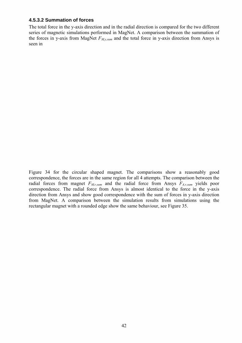
42

4.5.3.2 Summation of forces The total force in the y-axis direction and in the radial direction is compared for the two different series of magnetic simulations performed in MagNet. A comparison between the summation of the forces in y-axis from MagNet FM,y,sum and the total force in y-axis direction from Ansys is seen in

Figure 34 for the circular shaped magnet. The comparisons show a reasonably good correspondence, the forces are in the same region for all 4 attempts. The comparison between the radial forces from magnet FM,r,sum and the radial force from Ansys FA,r,sum yields poor correspondence. The radial force from Ansys is almost identical to the force in the y-axis direction from Ansys and show good correspondence with the sum of forces in y-axis direction from MagNet. A comparison between the simulation results from simulations using the rectangular magnet with a rounded edge show the same behaviour, see Figure 35.

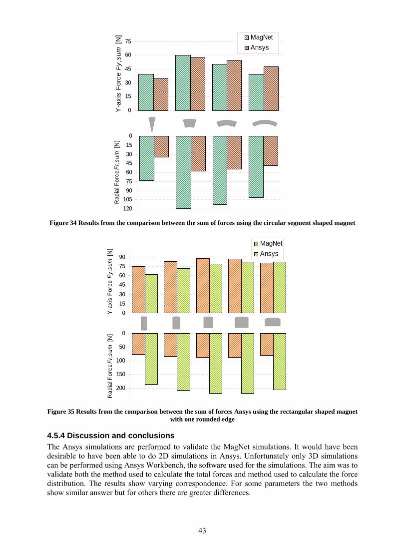
43

Figure 34 Results from the comparison between the sum of forces using the circular segment shaped magnet

Figure 35 Results from the comparison between the sum of forces Ansys using the rectangular shaped magnet

with one rounded edge

4.5.4 Discussion and conclusions The Ansys simulations are performed to validate the MagNet simulations. It would have been desirable to have been able to do 2D simulations in Ansys. Unfortunately only 3D simulations can be performed using Ansys Workbench, the software used for the simulations. The aim was to validate both the method used to calculate the total forces and method used to calculate the force distribution. The results show varying correspondence. For some parameters the two methods show similar answer but for others there are greater differences.

0

15

30

45

60

75

Y-a

xis

Forc

e Fy

,sum

[N] MagNet

Ansys

0153045607590

105120

Rad

ial F

orce

Fr,s

um [N

]

0153045607590

Y-ax

is F

orce

Fy,

sum

[N]

MagNetAnsys

0

50

100

150

200

Rad

ial F

orce

Fr,s

um [N

]

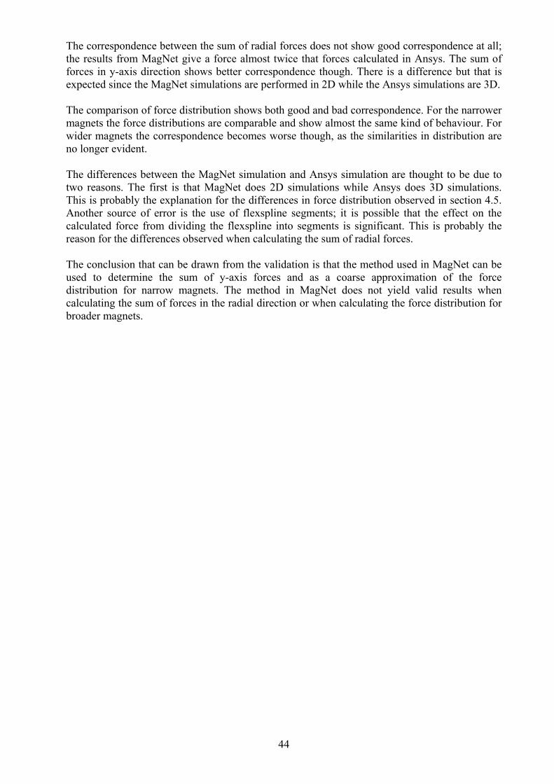
44

The correspondence between the sum of radial forces does not show good correspondence at all; the results from MagNet give a force almost twice that forces calculated in Ansys. The sum of forces in y-axis direction shows better correspondence though. There is a difference but that is expected since the MagNet simulations are performed in 2D while the Ansys simulations are 3D. The comparison of force distribution shows both good and bad correspondence. For the narrower magnets the force distributions are comparable and show almost the same kind of behaviour. For wider magnets the correspondence becomes worse though, as the similarities in distribution are no longer evident. The differences between the MagNet simulation and Ansys simulation are thought to be due to two reasons. The first is that MagNet does 2D simulations while Ansys does 3D simulations. This is probably the explanation for the differences in force distribution observed in section 4.5. Another source of error is the use of flexspline segments; it is possible that the effect on the calculated force from dividing the flexspline into segments is significant. This is probably the reason for the differences observed when calculating the sum of radial forces. The conclusion that can be drawn from the validation is that the method used in MagNet can be used to determine the sum of y-axis forces and as a coarse approximation of the force distribution for narrow magnets. The method in MagNet does not yield valid results when calculating the sum of forces in the radial direction or when calculating the force distribution for broader magnets.

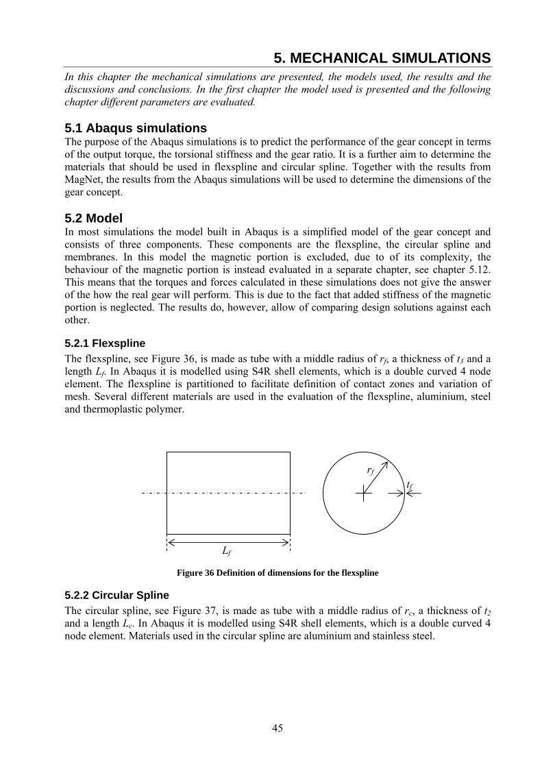
45

5. MECHANICAL SIMULATIONS In this chapter the mechanical simulations are presented, the models used, the results and the discussions and conclusions. In the first chapter the model used is presented and the following chapter different parameters are evaluated. 5.1 Abaqus simulations The purpose of the Abaqus simulations is to predict the performance of the gear concept in terms of the output torque, the torsional stiffness and the gear ratio. It is a further aim to determine the materials that should be used in flexspline and circular spline. Together with the results from MagNet, the results from the Abaqus simulations will be used to determine the dimensions of the gear concept. 5.2 Model In most simulations the model built in Abaqus is a simplified model of the gear concept and consists of three components. These components are the flexspline, the circular spline and membranes. In this model the magnetic portion is excluded, due to of its complexity, the behaviour of the magnetic portion is instead evaluated in a separate chapter, see chapter 5.12. This means that the torques and forces calculated in these simulations does not give the answer of the how the real gear will perform. This is due to the fact that added stiffness of the magnetic portion is neglected. The results do, however, allow of comparing design solutions against each other.

5.2.1 Flexspline The flexspline, see Figure 36, is made as tube with a middle radius of rf, a thickness of t3 and a length Lf. In Abaqus it is modelled using S4R shell elements, which is a double curved 4 node element. The flexspline is partitioned to facilitate definition of contact zones and variation of mesh. Several different materials are used in the evaluation of the flexspline, aluminium, steel and thermoplastic polymer.

Figure 36 Definition of dimensions for the flexspline

5.2.2 Circular Spline The circular spline, see Figure 37, is made as tube with a middle radius of rc, a thickness of t2 and a length Lc. In Abaqus it is modelled using S4R shell elements, which is a double curved 4 node element. Materials used in the circular spline are aluminium and stainless steel.

Lf

rf tf

46

Figure 37 Definition of dimensions for the circular spline

5.2.3 Membrane The influence of the magnets on the magnetic portion manifests itself of a rotating pressure load acting radially inwards on the surface of the flexspline. Since a means of applying such a rotating pressure is not available in Abaqus, the load case is simulated by mans of thin, flexible membranes in frictionless contact with the flexspline. Pressure loads are applied to external surface of the membranes and not directly to the flexspline in order to simulate the rotation of the magnets and the magnetic force. The membranes, see Figure 38, have a middle radius of rm, a thickness of tm, a length of Lm and angular width of αm. The size of membranes is varied to simulate effects of different magnets being used. The shell element S4R is used in Abaqus to model the membranes.

Figure 38 Definition of dimensions for the membranes

5.2.4 Contacts There are two kinds of contact in the Abaqus model of the gear concept, one between the membranes and the outer surface of the flexspline and one between the outer surface of the circular spline and the inner surface of the flexspline. The contact between the membrane and outer surface is defined as a node to surface contact with finite sliding. The shell thickness is also excluded and the contact is considered to be frictionless. When defining this contact the goal is to achieve a contact with the lowest possible influence on the problem since it is used to simulate the contact less magnetic force. The contact between the circular spline and inner surface of the flexspline is defined as a node to surface contact with finite sliding. The shell thickness is also excluded and a penalty friction formulation is used with a friction coefficient μ of 0.3 [24]. It is difficult to choose a value for the friction coefficient, especially for rolling contact as in this case. In this case an average value for gliding friction between steel and steel is used from [24].

Lc

rc tc

Lm

tm

rm

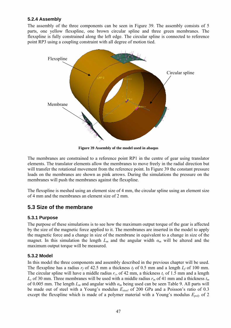
47

5.2.4 Assembly The assembly of the three components can be seen in Figure 39. The assembly consists of 5 parts, one yellow flexspline, one brown circular spline and three green membranes. The flexspline is fully constrained along the left edge. The circular spline is connected to reference point RP3 using a coupling constraint with all degree of motion tied.

Figure 39 Assembly of the model used in abaqus

The membranes are constrained to a reference point RP1 in the centre of gear using translator elements. The translator elements allow the membranes to move freely in the radial direction but will transfer the rotational movement from the reference point. In Figure 39 the constant pressure loads on the membranes are shown as pink arrows. During the simulations the pressure on the membranes will push the membranes against the flexspline. The flexspline is meshed using an element size of 4 mm, the circular spline using an element size of 4 mm and the membranes an element size of 2 mm. 5.3 Size of the membrane

5.3.1 Purpose The purpose of these simulations is to see how the maximum output torque of the gear is affected by the size of the magnetic force applied to it. The membranes are inserted in the model to apply the magnetic force and a change in size of the membrane in equivalent to a change in size of the magnet. In this simulation the length Lm and the angular width αm will be altered and the maximum output torque will be measured.

5.3.2 Model In this model the three components and assembly described in the previous chapter will be used. The flexspline has a radius rf of 42.5 mm a thickness tf of 0.5 mm and a length Lf of 100 mm. The circular spline will have a middle radius rc, of 42 mm, a thickness tc of 1.5 mm and a length Lc of 30 mm. Three membranes will be used with a middle radius rm of 41 mm and a thickness tm of 0.005 mm. The length Lm and angular width αm being used can be seen Table 9. All parts will be made out of steel with a Young’s modulus Esteel of 200 GPa and a Poisson’s ratio of 0.3 except the flexspline which is made of a polymer material with a Young’s modulus Epoly of 2

Circular spline

Flexspline

Membrane

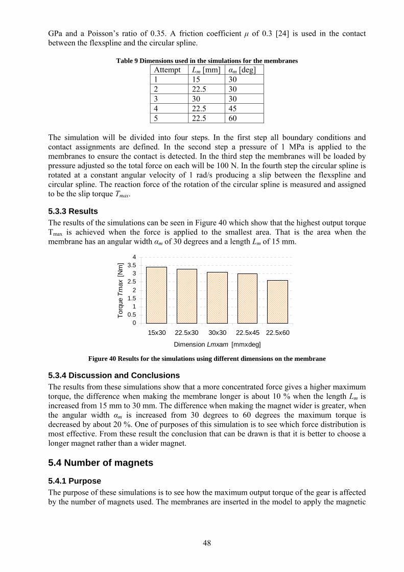
48

GPa and a Poisson’s ratio of 0.35. A friction coefficient μ of 0.3 [24] is used in the contact between the flexspline and the circular spline.

Table 9 Dimensions used in the simulations for the membranes Attempt Lm [mm] αm [deg] 1 15 30 2 22.5 30 3 30 30 4 22.5 45 5 22.5 60

The simulation will be divided into four steps. In the first step all boundary conditions and contact assignments are defined. In the second step a pressure of 1 MPa is applied to the membranes to ensure the contact is detected. In the third step the membranes will be loaded by pressure adjusted so the total force on each will be 100 N. In the fourth step the circular spline is rotated at a constant angular velocity of 1 rad/s producing a slip between the flexspline and circular spline. The reaction force of the rotation of the circular spline is measured and assigned to be the slip torque Tmax.

5.3.3 Results The results of the simulations can be seen in Figure 40 which show that the highest output torque Tmax is achieved when the force is applied to the smallest area. That is the area when the membrane has an angular width αm of 30 degrees and a length Lm of 15 mm.

00.5

11.5

22.5

33.5

4

15x30 22.5x30 30x30 22.5x45 22.5x60

Dimension Lmxam [mmxdeg]

Torq

ue T

max

[Nm

]

Figure 40 Results for the simulations using different dimensions on the membrane

5.3.4 Discussion and Conclusions The results from these simulations show that a more concentrated force gives a higher maximum torque, the difference when making the membrane longer is about 10 % when the length Lm is increased from 15 mm to 30 mm. The difference when making the magnet wider is greater, when the angular width αm is increased from 30 degrees to 60 degrees the maximum torque is decreased by about 20 %. One of purposes of this simulation is to see which force distribution is most effective. From these result the conclusion that can be drawn is that it is better to choose a longer magnet rather than a wider magnet. 5.4 Number of magnets

5.4.1 Purpose The purpose of these simulations is to see how the maximum output torque of the gear is affected by the number of magnets used. The membranes are inserted in the model to apply the magnetic

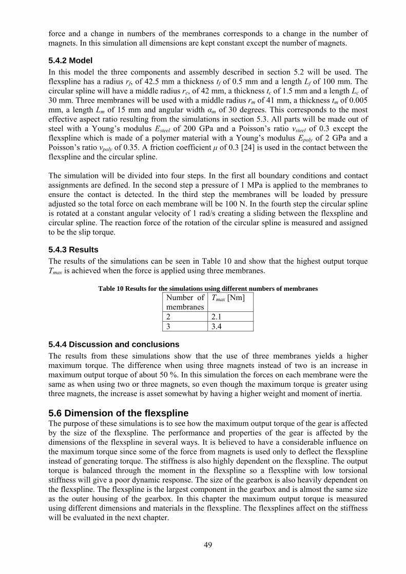
49

force and a change in numbers of the membranes corresponds to a change in the number of magnets. In this simulation all dimensions are kept constant except the number of magnets.

5.4.2 Model In this model the three components and assembly described in section 5.2 will be used. The flexspline has a radius rf, of 42.5 mm a thickness tf of 0.5 mm and a length Lf of 100 mm. The circular spline will have a middle radius rc, of 42 mm, a thickness tc of 1.5 mm and a length Lc of 30 mm. Three membranes will be used with a middle radius rm of 41 mm, a thickness tm of 0.005 mm, a length Lm of 15 mm and angular width αm of 30 degrees. This corresponds to the most effective aspect ratio resulting from the simulations in section 5.3. All parts will be made out of steel with a Young’s modulus Esteel of 200 GPa and a Poisson’s ratio νsteel of 0.3 except the flexspline which is made of a polymer material with a Young’s modulus Epoly of 2 GPa and a Poisson’s ratio νpoly of 0.35. A friction coefficient μ of 0.3 [24] is used in the contact between the flexspline and the circular spline. The simulation will be divided into four steps. In the first all boundary conditions and contact assignments are defined. In the second step a pressure of 1 MPa is applied to the membranes to ensure the contact is detected. In the third step the membranes will be loaded by pressure adjusted so the total force on each membrane will be 100 N. In the fourth step the circular spline is rotated at a constant angular velocity of 1 rad/s creating a sliding between the flexspline and circular spline. The reaction force of the rotation of the circular spline is measured and assigned to be the slip torque.

5.4.3 Results The results of the simulations can be seen in Table 10 and show that the highest output torque Tmax is achieved when the force is applied using three membranes.

Table 10 Results for the simulations using different numbers of membranes Number of membranes

Tmax [Nm]

2 2.1 3 3.4

5.4.4 Discussion and conclusions The results from these simulations show that the use of three membranes yields a higher maximum torque. The difference when using three magnets instead of two is an increase in maximum output torque of about 50 %. In this simulation the forces on each membrane were the same as when using two or three magnets, so even though the maximum torque is greater using three magnets, the increase is asset somewhat by having a higher weight and moment of inertia. 5.6 Dimension of the flexspline The purpose of these simulations is to see how the maximum output torque of the gear is affected by the size of the flexspline. The performance and properties of the gear is affected by the dimensions of the flexspline in several ways. It is believed to have a considerable influence on the maximum torque since some of the force from magnets is used only to deflect the flexspline instead of generating torque. The stiffness is also highly dependent on the flexspline. The output torque is balanced through the moment in the flexspline so a flexspline with low torsional stiffness will give a poor dynamic response. The size of the gearbox is also heavily dependent on the flexspline. The flexspline is the largest component in the gearbox and is almost the same size as the outer housing of the gearbox. In this chapter the maximum output torque is measured using different dimensions and materials in the flexspline. The flexsplines affect on the stiffness will be evaluated in the next chapter.

50

5.6.1 Length and radius of the flexspline

5.6.1.1 Purpose The purpose of this simulation is to see how the length Lm and the radius rf of the flexspline affects the maximum torque that could be achieved. A combination of dimensions will be tested.

5.6.1.2 Model In this model the three components and assembly described in section 5.2 will be used. For the flexspline a thickness t3 0.5 mm is used, the dimensions of a radius rf and length Lf used are seen in Table 11. The circular spline will have a middle radius rc, of 0.5 mm less then radius of the flexspline being simulated, a thickness tc of 1.5 mm and a length Lc of 30 mm. Three membranes will be used with the same middle radius rm as the flexspline, a thickness tm of 0.005 mm, a length Lm of 15 mm and angular width αm of 30 degrees. All parts will be made out of steel with a Young’s modulus Esteel of 200 GPa and a Poisson’s ratio νsteel of 0.3 except the flexspline which is made of a polymer material with a Young’s modulus Epoly of 2 GPa and a Poisson’s ratio νpoly of 0.35. A friction coefficient μ of 0.3 is used in the contact between the flexspline and the circular spline.

Table 11 Dimensions used in the simulation for the flexspline Attempt Lf [mm] rf [mm] 1 50 42.5 2 100 42.5 3 150 42.5 4 100 30 5 100 50

The simulation will be divided into four steps. In the first step all boundary conditions and contact assignments are defined. In the second step a pressure of 1 MPa is applied to the membranes to ensure the contact is detected. In the third step the membranes will be loaded by pressure adjusted so the total force on each will be 100 N. In the fourth step the circular spline is rotated at a constant angular velocity of 1 rad/s producing a slip between the flexspline and circular spline. The reaction force of the rotation of the circular spline is measured and assigned to be the slip torque Tmax.

5.6.1.3 Results The results of the simulations can be seen in Figure 41 and show that the highest output torque Tmax is achieved when the force is applied to a flexspline with a length Lf of 100 mm and a radius rf of 50 mm.

00.5

11.5

22.5

33.5

44.5

5

50x42.5 100x42.5 150x42.5 100x30 100x50

Dimension Lfxrf [mmxmm]

Torq

ue T

max

[Nm

]

Figure 41 Results for the simulations using different dimensions for the flexspline

51

5.6.1.4 Discussion and conclusions The increase of torque when increasing the radius is much bigger than when the flexspline is made longer. That increase in maximum torque when the radius is increased has two contributions; the greater radius reduces the radial stiffness of the tube while also increasing the lever arm which transfers the torque. The conclusion that can be drawn from this experiment is that if were permissible to enlarge the dimensions of the gear it would be better to increase the radius rather than the length.

5.6.2 Material and thickness of the flexspline

5.6.2.1 Purpose The purpose of this simulation is to see how the choice of material and the thickness tf of the flexspline affect the maximum torque that could be achieved. A combination of dimensions will be tested.

5.6.2.2 Model In this model the three components and assembly described in the section 5.2 will be used, the flexspline, the circular spline and the membranes. The flexspline have a radius rf, of 42.5 mm, a length L of 100 mm, the thickness t3 and material is seen in Table 12. The circular spline will have a middle radius rc, of 0.5 mm less then radius of the flexspline being simulated, a thickness tc of 1.5 mm and a length Lc of 30 mm. Three membranes will be used with the same middle radius rm as the flexspline, a thickness tm of 0.005 mm, a length Lm of 15 mm and angular width αm of 30 degrees. The circular spline and the membranes will be made out of steel with a Young’s modulus Esteel of 200 GPa and a Poisson’s ratio νsteel of 0.35. A friction coefficient μ of 0.3 [24] is used in the contact between the flexspline and the circular spline.

Table 12 Materials and wall thickness for the flexspline used in the simulations Attempt Material tf [mm] 1 0.3 2 Aluminium 0.5 3 1.0 4 Polymer 2.0 5 0.1 6 Steel 0.2

The simulation will be divided into four steps. In the first step all boundary conditions and contact assignments are defined. In the second step a pressure of 1 MPa is applied to the membranes to ensure the contact is detected. In the third step the membranes will be loaded by pressure adjusted so the total force on each will be 100 N. In the fourth step the circular spline is rotated at a constant angular velocity of 1 rad/s producing a slip between the flexspline and circular spline. The reaction force of the rotation of the circular spline is measured and assigned to be the slip torque Tmax.

5.6.2.3 Results The results of the simulations can be seen in Figure 42 and show a large variation in output torque Tmax. The interesting thing to see is comparing the results from attempt 1, 4, and 6. All these attempts show an output torque close to each other. This shows how thick the different materials have to be to achieve almost the same results.

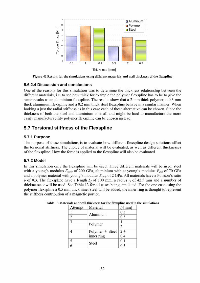
52

0

0.5

1

1.5

2

2.5

3

3.5

4

Thickness [mm]

Torq

ue T

max

[Nm

]

AluminumPolymerSteel

0.5 1 0.1 0.3 2 0.2

Figure 42 Results for the simulations using different materials and wall thickness of the flexspline

5.6.2.4 Discussion and conclusions One of the reasons for this simulation was to determine the thickness relationship between the different materials, i.e. to see how thick for example the polymer flexspline has to be to give the same results as an aluminium flexspline. The results show that a 2 mm thick polymer, a 0.3 mm thick aluminium flexspline and a 0.2 mm thick steel flexspline behave in a similar manner. When looking a just the radial stiffness as in this case each of these alternative can be chosen. Since the thickness of both the steel and aluminium is small and might be hard to manufacture the more easily manufacturability polymer flexspline can be chosen instead. 5.7 Torsional stiffness of the Flexspline

5.7.1 Purpose The purpose of these simulations is to evaluate how different flexspline design solutions affect the torsional stiffness. The choice of material will be evaluated, as well as different thicknesses of the flexspline. How the force is applied to the flexspline will also be evaluated.

5.7.2 Model In this simulation only the flexspline will be used. Three different materials will be used, steel with a young’s modulus Esteel of 200 GPa, aluminium with at young’s modulus Ealu of 70 GPa and a polymer material with young’s modulus Epoly of 2 GPa. All materials have a Poisson’s ratio υ of 0.3. The flexspline have a length Lf of 100 mm, a radius rf of 42.5 mm and a number of thicknesses t will be used. See Table 13 for all cases being simulated. For the one case using the polymer flexspline a 0.5 mm thick inner steel will be added, the inner ring is thought to represent the stiffness contribution of a magnetic portion

Table 13 Materials and wall thickness for the flexspline used in the simulations Attempt Material tf [mm] 1 0.3 2 Aluminum 0.5 3 1 Polymer 2 4 Polymer + Steel

inner ring 2 + 0.4

5 0.1 6 Steel 0.3

53

The load, a torque Tload of 5 Nm, will be applied in three different ways, Figure 43. Load case 1 where the load is applied to the whole free edge of the flexspline, load case 2 where the load is applied to two 15 mm long lines on the surface of the flexspline and load case 3 where load is applied to three 15 mm long lines on the surface of the flexspline. In all three cases the clamped edge of the flexspline is totally fixed.

Figure 43 Torque applied to the flexspline

With Abaqus the torsional stiffness kaba is calculated using

aba

abaaba

Tk

α= (5.1)

where αaba is the rotation of the flexspline. The stiffness is also calculated using analytical methods. The polar moment of inertia J for a thin walled cylinder is given by tRJ 32π= (5.2) where R is the radius of the cylinder and t the wall thickness. The relation between the Young’s modulus E and the shear modulus G is given by

)1(2 υ−

=EG (5.3)

where υ is the Poisson’s ratio. The torsional stiffness kan can then be calculated using the formula for the angle of twist

L

tERL

JGTkJGTL

an )1(22 3

υπ

φφ

−===⇒= . (5.4)

5.7.3 Results The results see Table 14 Resulting stiffness for different materials and wall thickness for the flexspline, show that the analytical results kan match the results from Abaqus when the load is applied to hole free edge of the flexspline kaba1. When the load is applied to smaller surfaces, as in load case 2 and 3, the results show a much smaller stiffness than in load case 1.

Table 14 Resulting stiffness for different materials and wall thickness for the flexspline

Material Thickness [mm]

kan [Nm/rad]

kaba1 [Nm/rad]

kaba2 [Nm/rad]

kaba3 [Nm/rad]

0.3 38500 38500 3300 4500 Aluminum 0.5 65000 65000 7700 9800 1 3700 3700 600 900 Polymer 2 7500 7500 1500 3500

Polymer + Steel inner ring

1 + 0.4 - 4200 - 3100

0.1 33300 33300 1250 2500 Steel 0.3 11100 11100 9400 13500

a b c

54

5.7.4 Discussion and conclusions A torsional stiffness of at least 2000 Nm/rad was required is this project, see section 1.2. This stiffness can be achieved using any of the material tested above. When using aluminium the stiffness when using either a 0.3 mm or a 0.5 mm thick flexspline is satisfactory. This flexspline is adequately stiff if either two or three connection points are used. If using steel a 0.3 mm thick flexspline provides adequate stiffness using either two magnets or three connection points. If using a 0.1 mm thick steel flexspline the torsional stiffness will not be high enough though. The use of only a polymer material in the flexspline is limited, in that the torsional stiffness is only high enough when using a 2 mm thickness. In one of the simulations the flexspline is reinforced using a 0.5 mm thick steel ring. This ring is intended to represent the additional stiffness of a magnetic portion being used in the full version of the gearbox. Using this ring the 1 mm thick polymer shows a torsional stiffness of over 2000 Nm/rad. In these simulations only the torsional stiffness of the flexspline is evaluated. The torsional stiffness of the complete gearbox is a result of many components and the contact between the flexspline and the circular spline. The total torsional stiffness of the gear is therefore presumably marginally lower than these results show. 5.8 The circular spline

5.8.1 Purpose The circular spline should be as thin as possible to enable the magnets to lie as close as possible to the flexspline, thereby maximising the magnetic force produced by the magnets. The circular spline still must also be stiff and should exhibit only small deformation when the flexspline makes contact. The purpose of these simulations is to see how thin the circular spline can be made without showing too much deformation.

5.8.2 Model Only the circular spline will be used in these simulations, see Figure 37, it will be fully constrained at one edge and the force will be applied on a patch which is 20 mm long and have angular width of 10 degrees. Both two and three forces will be used and size of the force will be 100 N. The circular spline will have a length of 40 mm and a middle radius of 40 mm. Two materials will be used, stainless steel, with a Young’s modulus of 200 GPa and Poisson’s ratio of 0.3, and aluminium with a Young’s modulus of 70 GPa and Poisson’s ratio of 0.3. The thickness of the circular spline will be varied, the thickness and material used can be seen in Table 15.

5.8.3 Results The results of the simulation can be seen in Table 15. It can be seen that there is a small difference in deformation depending whatever two or three forces are applied. There is however a greater difference between steel and aluminium as the circular spline material.

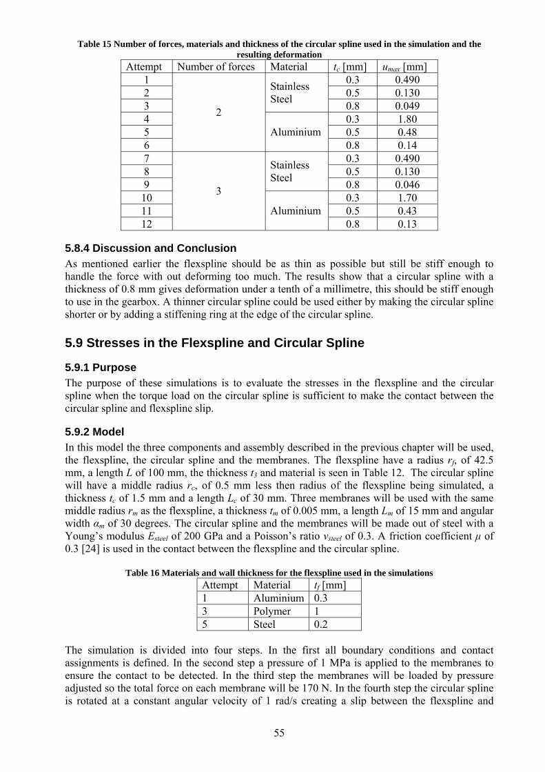
55

Table 15 Number of forces, materials and thickness of the circular spline used in the simulation and the resulting deformation

Attempt Number of forces Material tc [mm] umax [mm] 1 0.3 0.490 2 0.5 0.130 3

Stainless Steel 0.8 0.049

4 0.3 1.80 5 0.5 0.48 6

2

Aluminium 0.8 0.14

7 0.3 0.490 8 0.5 0.130 9

Stainless Steel 0.8 0.046

10 0.3 1.70 11 0.5 0.43 12

3

Aluminium 0.8 0.13

5.8.4 Discussion and Conclusion As mentioned earlier the flexspline should be as thin as possible but still be stiff enough to handle the force with out deforming too much. The results show that a circular spline with a thickness of 0.8 mm gives deformation under a tenth of a millimetre, this should be stiff enough to use in the gearbox. A thinner circular spline could be used either by making the circular spline shorter or by adding a stiffening ring at the edge of the circular spline. 5.9 Stresses in the Flexspline and Circular Spline

5.9.1 Purpose The purpose of these simulations is to evaluate the stresses in the flexspline and the circular spline when the torque load on the circular spline is sufficient to make the contact between the circular spline and flexspline slip.

5.9.2 Model In this model the three components and assembly described in the previous chapter will be used, the flexspline, the circular spline and the membranes. The flexspline have a radius rf, of 42.5 mm, a length L of 100 mm, the thickness t3 and material is seen in Table 12. The circular spline will have a middle radius rc, of 0.5 mm less then radius of the flexspline being simulated, a thickness tc of 1.5 mm and a length Lc of 30 mm. Three membranes will be used with the same middle radius rm as the flexspline, a thickness tm of 0.005 mm, a length Lm of 15 mm and angular width αm of 30 degrees. The circular spline and the membranes will be made out of steel with a Young’s modulus Esteel of 200 GPa and a Poisson’s ratio νsteel of 0.3. A friction coefficient μ of 0.3 [24] is used in the contact between the flexspline and the circular spline.

Table 16 Materials and wall thickness for the flexspline used in the simulations Attempt Material tf [mm] 1 Aluminium 0.3 3 Polymer 1 5 Steel 0.2

The simulation is divided into four steps. In the first all boundary conditions and contact assignments is defined. In the second step a pressure of 1 MPa is applied to the membranes to ensure the contact to be detected. In the third step the membranes will be loaded by pressure adjusted so the total force on each membrane will be 170 N. In the fourth step the circular spline is rotated at a constant angular velocity of 1 rad/s creating a slip between the flexspline and

56

circular spline. The reaction force of the rotation of the circular spline is measured and assigned to be the slip torque and the stresses in the flexspline and the circular spline will be measured and analysed. The flexspline is meshed using an element size of 2 mm, the circular spline using an element size of 2 mm and the membranes an element size of 2 mm.

5.9.3 Results A contour plot of the stresses using a 0.3 mm thick aluminium flexspline is seen in Figure 44. The load of 170 N per membranes gives a slip torque of around 4 Nm. The plot shows a maximum stress of 110 MPa in the area of the contact between the flexspline and the circular spline. In the other areas of the flexspline the stresses are in the range of around 40-60 MPa. The strength of a SS4425 aluminium is around 270 MPa [20] and it should therefore be possible to use this kind of flexspline in the gear concept.

Figure 44 Stresses in the 0.3 mm thick aluminium flexspline

A contour plot of the stresses using a 1 mm thick polymer flexspline is seen in Figure 45. The load of 170 N per membranes gives a slip torque of around 5.7 Nm. The plot shows a maximum stress of 10 MPa in the area of the contact between the flexspline and the circular spline. In the other areas of the flexspline the stresses are in the range of around 1-3 MPa. The strength of an M30i ABS polymer is around 30 MPa [21] and the polymer flexspline is strong enough.

Figure 45 Stresses in the 1 mm thick polymer flexspline

57

A contour plot of the stresses using a 0.2 mm thick steel flexspline is seen in Figure 46. The load of 170 N per membranes gives a slip torque of around 3 Nm. The plot shows a maximum stress of 290 MPa in the area of the contact between the flexspline and the circular spline. In the other areas of the flexspline the stresses are in the range of around 100 MPa. The strength of 141550 steel is around 270 MPa [20]. To use the 0.2 mm thick steel flexspline could be a problem, the general stress levels are low enough, only around 100 MPa but the stresses close to the contact point can get to high for the material.

Figure 46 Stresses in the 0.2 mm thick steel flexspline

The stresses in the circular spline are similar for all three load cases. A contour plot of the stresses in the circular spline from the simulation using a 0.3 aluminium flexspline is seen in Figure 47. The plot shows a maximum stress of around 60 MPa which is less then the strength of the 2344-02 stainless steel which has a strength of about 230 MPa [20].

Figure 47 Stresses in the 0.5 mm thick stainless steel circular spline

5.9.4 Discussion and conclusions In these simulations stresses in the flexspline are evaluated. In the simulations the magnetic portion is not included. If a magnetic portion were to be used the stresses in the contact would probably be lower since the stresses would be more evenly distributed. So when looking at the results of these simulations the general stress levels in the material is of more interest than looking just at the peak stresses. The results from these simulations show that the highest stress in the flexspline occur close to the contact between the flexspline and the circular spline. The general stresses in other parts of the flexspline are much lower. A comparison between the strength of the materials and the maximum stresses show that either a 0.3 mm thick aluminium

58

or a 1 mm thick polymer thick flexspline could be used in the gear concept. The maximum stress when using a 0.2 mm thick steel flexspline is at the same level as the material strength bur since an added magnetic portion would probably even out the stress this flexspline should be possible to use in the gear concept. 5.10 Gear ratio

5.10.1 Purpose The purpose of these simulations is to compare the analytical method of calculating the gear ratio with an analytical method of determine the gear ratio. The gear ratio will be tested for an unloaded gearbox and for the cases using two and three membranes.

5.10.2 Model In this model the three components and assembly described in the previous chapter will be used, the flexspline, the circular spline and the membranes. The flexspline have a radius rf, of 40 mm, a length Lf of 100 mm, the thickness tf of 1 mm. The circular spline will have a middle radius rc, of 39.5 mm, a thickness tc of 0.5 mm and a length Lc of 30 mm. Three membranes will be used with the same middle radius rm as the flexspline, a thickness tm of 0.005 mm, a length Lm of 30 mm and angular width αm of 40 degrees. The circular spline and the membranes will be made out of steel with a Young’s modulus Esteel of 200 GPa and a Poisson’s ratio νsteel of 0.3, the flexspline will be made of a polymer material with a Young’s modulus Epoly of 200 GPa and a Poisson’s ratio νpoly of 0.35. A friction coefficient μ of 0.3 is used in the contact between the flexspline and the circular spline. The simulation will be divided into four steps, in the first all boundary conditions and contact assignments are defined. In the second step a pressure of 1 MPa is applied to the membranes to ensure the contact to be detected. In the third step the membranes will be loaded by pressure adjusted so the total force on each membrane will be 130 N. In the fourth step the membranes are rotated an angle αm of 3 radians and the rotation of circular spline αc is measured. The gear ratio GRaba is then calculated using

c

mRabaG

αα

= (5.5)

The gear reduction GR is also calculated using traditional harmonic drive theory [12] and is given by

cf

fR RR

RG

−= (5.6)

where Rf is undeformed radius of the inside of the magnetic portion on the flexspline and Rc is the outer radius of the circular spline.

5.10.3 Results The resulting gear ratios using the analytical formulation and the gear ratio giving using Abaqus can be seen in Table 17. The results how that the gear ratios from the Abaqus simulations are up to 10 % lower than the gear ration calculated using analytical methods. The results also show that a higher gear ratio is achieved when using two membranes instead of three.

Table 17 Results from simulations investigating gear ratio Gear ratio

2 membranes 75.9 Abaqus 3 membranes 72.3 Analytical 80

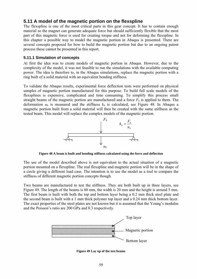
59

5.11 A model of the magnetic portion on the flexspline The flexspline is one of the most critical parts in this gear concept. It has to contain enough material so the magnet can generate adequate force but should sufficiently flexible that the most part of this magnetic force is used for creating torque and not for deforming the flexspline. In this chapter a possible way to model the magnetic portion in Abaqus is presented. There are several concepts proposed for how to build the magnetic portion but due to an ongoing patent process these cannot be presented in this report.

5.11.1 Simulation of concepts At first the idea was to create models of magnetic portion in Abaqus. However, due to the complexity of the model, it was not feasible to run the simulations with the available computing power. The idea is therefore to, in the Abaqus simulations, replace the magnetic portion with a ring built of a solid material with an equivalent bending stiffness. To validate the Abaqus results, experimental force deflection tests were performed on physical samples of magnetic portion manufactured for this purpose. To build full scale models of the flexsplines is expensive, complicated and time consuming. To simplify this process small straight beams of the magnetic portion are manufactured and a force Fb is applied to them. The deformation ub is measured and the stiffness kb is calculated, see Figure 48. In Abaqus a magnetic portion built from a solid material will then be created with the same stiffness as the tested beam. This model will replace the complex models of the magnetic portion.

Figure 48 A beam is built and bending stiffness calculated using the force and deflection

The use of the model described above is not equivalent to the actual situation of a magnetic portion mounted on a flexspline. The real flexspline and magnetic portion will be in the shape of a circle giving a different load case. The intention is to use the model as a tool to compare the stiffness of different magnetic portion concepts though. Two beams are manufactured to test the stiffness. They are both built up in three layers, see Figure 49. The length of the beams is 80 mm, the width is 20 mm and the height is around 5 mm. The first beam is built with both the top and bottom layer being a 0.2 mm thick steel plate and the second beam is built with a 1 mm thick polymer top layer and a 0.24 mm thick bottom layer. The exact properties of the steel plates are not known but it is assumed that the Young’s modulus and the Poisson’s ratio are 200 GPa and 0.3 respectively.

Figure 49 Lay up of the test beams

Fb

ub

b

bb u

Fk =

Top layer

Magnetic portion

Bottom layer

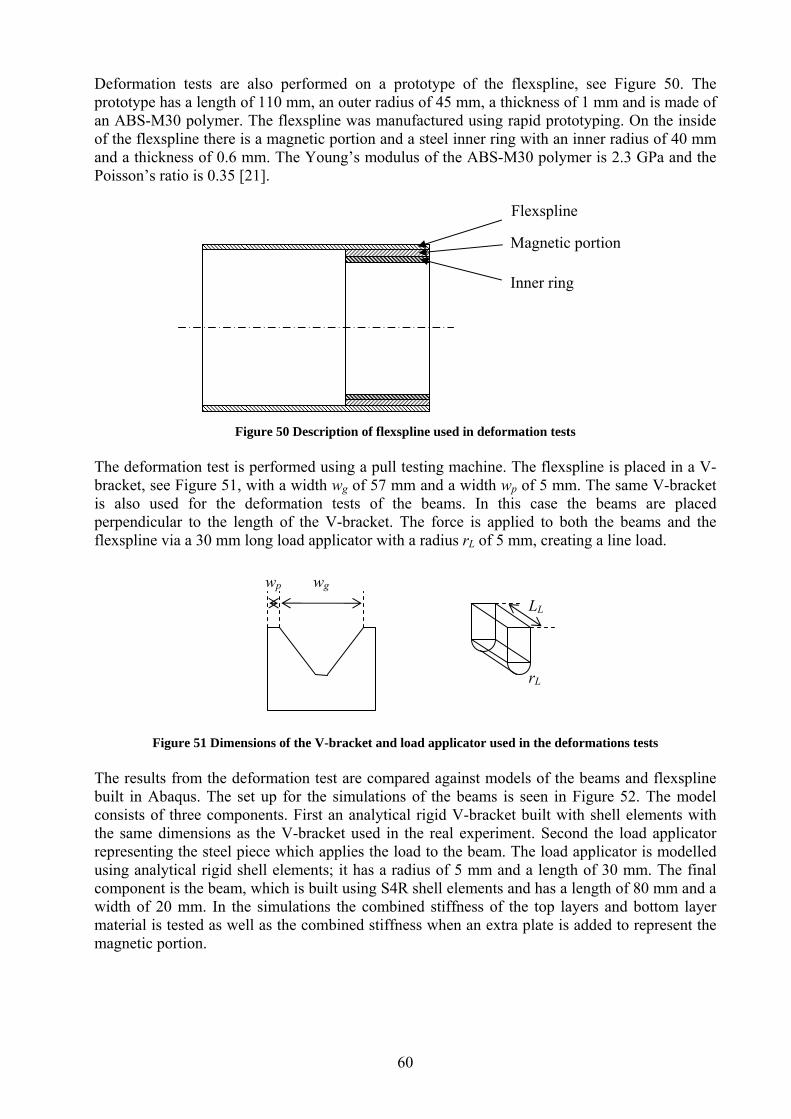
60

Deformation tests are also performed on a prototype of the flexspline, see Figure 50. The prototype has a length of 110 mm, an outer radius of 45 mm, a thickness of 1 mm and is made of an ABS-M30 polymer. The flexspline was manufactured using rapid prototyping. On the inside of the flexspline there is a magnetic portion and a steel inner ring with an inner radius of 40 mm and a thickness of 0.6 mm. The Young’s modulus of the ABS-M30 polymer is 2.3 GPa and the Poisson’s ratio is 0.35 [21].

Figure 50 Description of flexspline used in deformation tests

The deformation test is performed using a pull testing machine. The flexspline is placed in a V-bracket, see Figure 51, with a width wg of 57 mm and a width wp of 5 mm. The same V-bracket is also used for the deformation tests of the beams. In this case the beams are placed perpendicular to the length of the V-bracket. The force is applied to both the beams and the flexspline via a 30 mm long load applicator with a radius rL of 5 mm, creating a line load.

Figure 51 Dimensions of the V-bracket and load applicator used in the deformations tests

The results from the deformation test are compared against models of the beams and flexspline built in Abaqus. The set up for the simulations of the beams is seen in Figure 52. The model consists of three components. First an analytical rigid V-bracket built with shell elements with the same dimensions as the V-bracket used in the real experiment. Second the load applicator representing the steel piece which applies the load to the beam. The load applicator is modelled using analytical rigid shell elements; it has a radius of 5 mm and a length of 30 mm. The final component is the beam, which is built using S4R shell elements and has a length of 80 mm and a width of 20 mm. In the simulations the combined stiffness of the top layers and bottom layer material is tested as well as the combined stiffness when an extra plate is added to represent the magnetic portion.

Flexspline

Magnetic portion

Inner ring

wg wp LL

rL

61

Figure 52 Abaqus model used for deformation tests of beams

There are two contacts in the model; first between the V-bracket and the beams and second between the load applicator and the beam, both of these contacts are set to be frictionless. The element size of the beam is 1 mm and the rigid parts are not meshed. In the simulation the beam is constrained in the z-axis direction and the load applicator is displaced 3 mm. The force required to achieve that deformation is measured and the stiffness is calculated. The set up for the simulations using the flexspline is seen in Figure 53. Two parts are used to build the model, a flexspline and a load applicator used to apply the load. First a load applicator which is used to apply a load to the flexspline, the load applicator is modelled using analytical rigid shell elements, it has a radius of 5 mm and a length of 30 mm. The second part is the flexspline, the flexspline is built from S4R shell elements it has a length of 110 mm and a radius of 45 mm. The material in the flexspline differs, in the back end the flexspline is a 1 mm thick polymer material but in the front 30 mm the material is varied. Three combinations of material are tested, first a 1 mm polymer material and a 0.6 mm thick steel is used, in the second simulation a 0.2 mm thick steel ring is added and in the third simulation a composite shell is built up using 1 mm thick polymer material and 0.6 mm thick steel.

Figure 53 Abaqus model used for deformation tests of flexspline

There is one contact in the model, between the load applicator and the flexspline. This contact is set to be frictionless. The element size of the flexspline is 1 mm and the rigid part is not meshed.

Beam

V-Bracket

Load applicator

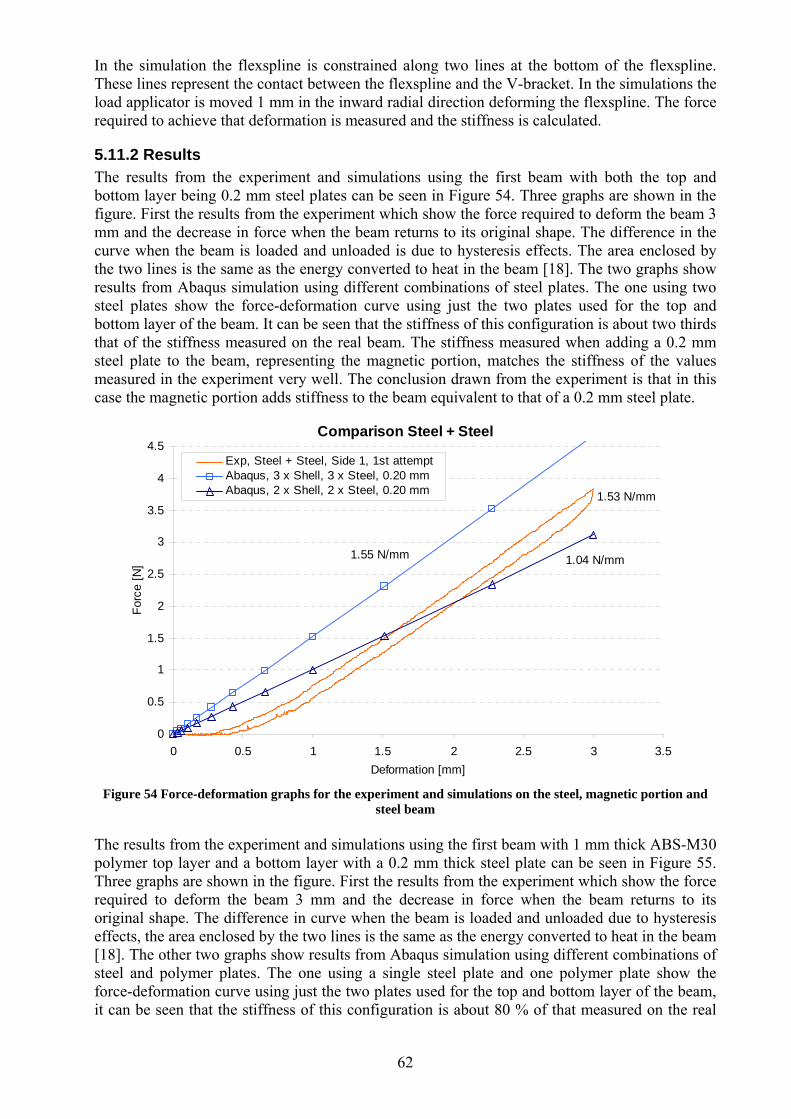
62

In the simulation the flexspline is constrained along two lines at the bottom of the flexspline. These lines represent the contact between the flexspline and the V-bracket. In the simulations the load applicator is moved 1 mm in the inward radial direction deforming the flexspline. The force required to achieve that deformation is measured and the stiffness is calculated.

5.11.2 Results The results from the experiment and simulations using the first beam with both the top and bottom layer being 0.2 mm steel plates can be seen in Figure 54. Three graphs are shown in the figure. First the results from the experiment which show the force required to deform the beam 3 mm and the decrease in force when the beam returns to its original shape. The difference in the curve when the beam is loaded and unloaded is due to hysteresis effects. The area enclosed by the two lines is the same as the energy converted to heat in the beam [18]. The two graphs show results from Abaqus simulation using different combinations of steel plates. The one using two steel plates show the force-deformation curve using just the two plates used for the top and bottom layer of the beam. It can be seen that the stiffness of this configuration is about two thirds that of the stiffness measured on the real beam. The stiffness measured when adding a 0.2 mm steel plate to the beam, representing the magnetic portion, matches the stiffness of the values measured in the experiment very well. The conclusion drawn from the experiment is that in this case the magnetic portion adds stiffness to the beam equivalent to that of a 0.2 mm steel plate.

Comparison Steel + Steel

0

0.5

1

1.5

2

2.5

3

3.5

4

4.5

0 0.5 1 1.5 2 2.5 3 3.5Deformation [mm]

Forc

e [N

]

Exp, Steel + Steel, Side 1, 1st attemptAbaqus, 3 x Shell, 3 x Steel, 0.20 mmAbaqus, 2 x Shell, 2 x Steel, 0.20 mm 1.53 N/mm

1.55 N/mm 1.04 N/mm

Figure 54 Force-deformation graphs for the experiment and simulations on the steel, magnetic portion and

steel beam The results from the experiment and simulations using the first beam with 1 mm thick ABS-M30 polymer top layer and a bottom layer with a 0.2 mm thick steel plate can be seen in Figure 55. Three graphs are shown in the figure. First the results from the experiment which show the force required to deform the beam 3 mm and the decrease in force when the beam returns to its original shape. The difference in curve when the beam is loaded and unloaded due to hysteresis effects, the area enclosed by the two lines is the same as the energy converted to heat in the beam [18]. The other two graphs show results from Abaqus simulation using different combinations of steel and polymer plates. The one using a single steel plate and one polymer plate show the force-deformation curve using just the two plates used for the top and bottom layer of the beam, it can be seen that the stiffness of this configuration is about 80 % of that measured on the real

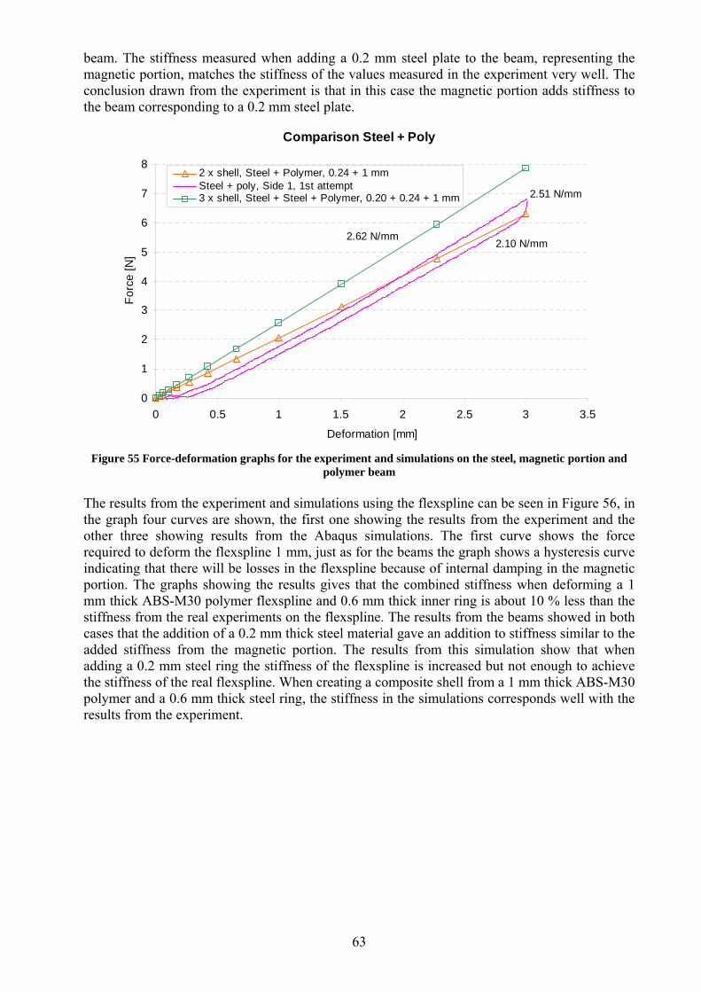
63

beam. The stiffness measured when adding a 0.2 mm steel plate to the beam, representing the magnetic portion, matches the stiffness of the values measured in the experiment very well. The conclusion drawn from the experiment is that in this case the magnetic portion adds stiffness to the beam corresponding to a 0.2 mm steel plate.

Comparison Steel + Poly

0

1

2

3

4

5

6

7

8

0 0.5 1 1.5 2 2.5 3 3.5

Deformation [mm]

Forc

e [N

]

2 x shell, Steel + Polymer, 0.24 + 1 mmSteel + poly, Side 1, 1st attempt3 x shell, Steel + Steel + Polymer, 0.20 + 0.24 + 1 mm

2.62 N/mm

2.51 N/mm

2.10 N/mm

Figure 55 Force-deformation graphs for the experiment and simulations on the steel, magnetic portion and

polymer beam The results from the experiment and simulations using the flexspline can be seen in Figure 56, in the graph four curves are shown, the first one showing the results from the experiment and the other three showing results from the Abaqus simulations. The first curve shows the force required to deform the flexspline 1 mm, just as for the beams the graph shows a hysteresis curve indicating that there will be losses in the flexspline because of internal damping in the magnetic portion. The graphs showing the results gives that the combined stiffness when deforming a 1 mm thick ABS-M30 polymer flexspline and 0.6 mm thick inner ring is about 10 % less than the stiffness from the real experiments on the flexspline. The results from the beams showed in both cases that the addition of a 0.2 mm thick steel material gave an addition to stiffness similar to the added stiffness from the magnetic portion. The results from this simulation show that when adding a 0.2 mm steel ring the stiffness of the flexspline is increased but not enough to achieve the stiffness of the real flexspline. When creating a composite shell from a 1 mm thick ABS-M30 polymer and a 0.6 mm thick steel ring, the stiffness in the simulations corresponds well with the results from the experiment.

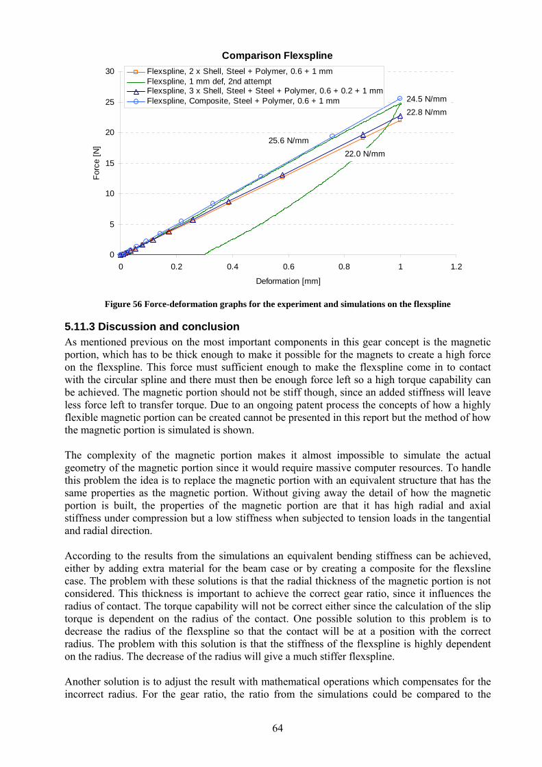
64

Comparison Flexspline

0

5

10

15

20

25

30

0 0.2 0.4 0.6 0.8 1 1.2

Deformation [mm]

Forc

e [N

]

Flexspline, 2 x Shell, Steel + Polymer, 0.6 + 1 mmFlexspline, 1 mm def, 2nd attemptFlexspline, 3 x Shell, Steel + Steel + Polymer, 0.6 + 0.2 + 1 mmFlexspline, Composite, Steel + Polymer, 0.6 + 1 mm

22.0 N/mm

22.8 N/mm

25.6 N/mm

24.5 N/mm

Figure 56 Force-deformation graphs for the experiment and simulations on the flexspline

5.11.3 Discussion and conclusion As mentioned previous on the most important components in this gear concept is the magnetic portion, which has to be thick enough to make it possible for the magnets to create a high force on the flexspline. This force must sufficient enough to make the flexspline come in to contact with the circular spline and there must then be enough force left so a high torque capability can be achieved. The magnetic portion should not be stiff though, since an added stiffness will leave less force left to transfer torque. Due to an ongoing patent process the concepts of how a highly flexible magnetic portion can be created cannot be presented in this report but the method of how the magnetic portion is simulated is shown. The complexity of the magnetic portion makes it almost impossible to simulate the actual geometry of the magnetic portion since it would require massive computer resources. To handle this problem the idea is to replace the magnetic portion with an equivalent structure that has the same properties as the magnetic portion. Without giving away the detail of how the magnetic portion is built, the properties of the magnetic portion are that it has high radial and axial stiffness under compression but a low stiffness when subjected to tension loads in the tangential and radial direction. According to the results from the simulations an equivalent bending stiffness can be achieved, either by adding extra material for the beam case or by creating a composite for the flexsline case. The problem with these solutions is that the radial thickness of the magnetic portion is not considered. This thickness is important to achieve the correct gear ratio, since it influences the radius of contact. The torque capability will not be correct either since the calculation of the slip torque is dependent on the radius of the contact. One possible solution to this problem is to decrease the radius of the flexspline so that the contact will be at a position with the correct radius. The problem with this solution is that the stiffness of the flexspline is highly dependent on the radius. The decrease of the radius will give a much stiffer flexspline. Another solution is to adjust the result with mathematical operations which compensates for the incorrect radius. For the gear ratio, the ratio from the simulations could be compared to the

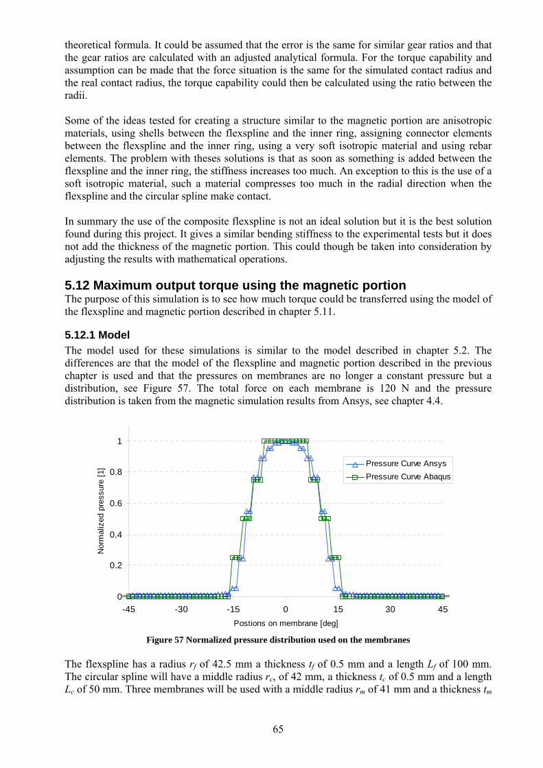
65

theoretical formula. It could be assumed that the error is the same for similar gear ratios and that the gear ratios are calculated with an adjusted analytical formula. For the torque capability and assumption can be made that the force situation is the same for the simulated contact radius and the real contact radius, the torque capability could then be calculated using the ratio between the radii. Some of the ideas tested for creating a structure similar to the magnetic portion are anisotropic materials, using shells between the flexspline and the inner ring, assigning connector elements between the flexspline and the inner ring, using a very soft isotropic material and using rebar elements. The problem with theses solutions is that as soon as something is added between the flexspline and the inner ring, the stiffness increases too much. An exception to this is the use of a soft isotropic material, such a material compresses too much in the radial direction when the flexspline and the circular spline make contact. In summary the use of the composite flexspline is not an ideal solution but it is the best solution found during this project. It gives a similar bending stiffness to the experimental tests but it does not add the thickness of the magnetic portion. This could though be taken into consideration by adjusting the results with mathematical operations. 5.12 Maximum output torque using the magnetic portion The purpose of this simulation is to see how much torque could be transferred using the model of the flexspline and magnetic portion described in chapter 5.11.

5.12.1 Model The model used for these simulations is similar to the model described in chapter 5.2. The differences are that the model of the flexspline and magnetic portion described in the previous chapter is used and that the pressures on membranes are no longer a constant pressure but a distribution, see Figure 57. The total force on each membrane is 120 N and the pressure distribution is taken from the magnetic simulation results from Ansys, see chapter 4.4.

0

0.2

0.4

0.6

0.8

1

-45 -30 -15 0 15 30 45Postions on membrane [deg]

Nor

mal

ized

pre

ssur

e [1

] Pressure Curve AnsysPressure Curve Abaqus

Figure 57 Normalized pressure distribution used on the membranes

The flexspline has a radius rf of 42.5 mm a thickness tf of 0.5 mm and a length Lf of 100 mm. The circular spline will have a middle radius rc, of 42 mm, a thickness tc of 0.5 mm and a length Lc of 50 mm. Three membranes will be used with a middle radius rm of 41 mm and a thickness tm

66

of 0.005 mm. The length Lm is 25 mm and angular width αm is 35 degrees. All part will be made out of steel with a Young’s modulus Esteel of 200 GPa and a Poisson’s ratio of 0.3 except the flexspline which is made of a polymer material with a Young’s modulus Epoly of 2 GPa and a Poisson’s ratio of 0.35. A friction coefficient of 0.3 is used in the contact between the flexspline and the circular spline The simulation is divided into four steps, in the first all boundary conditions and contact assignments is defined. In the second step a pressure of 1 MPa is applied to the membranes to ensure the contact to be detected. In the third step the membranes will be loaded with the full pressure. In the fourth step the circular spline is rotated at a constant angular velocity of 1 rad/s creating a sliding between the flexspline and circular spline. The reaction force of the rotation of the circular spline is measured and assigned to be the slip torque.

5.12.2 Results and conclusion The results show a maximum torque of 1.8 Nm, which is much lower then the goal of 5 Nm that was set when the project started. This torque is calculated using the composite to simulate the magnetic portion. The composite do not take the thickness of the magnetic portion into consideration, therefore the maximum torque is marginally lower. Dividing the thickness 4 mm of the magnetic portion with the simulated radius of the flexspline and magnetic portion, 42.5 mm suggests that the torque should be lowered by around 10 %, giving a maximum torque of around 1.6 Nm.

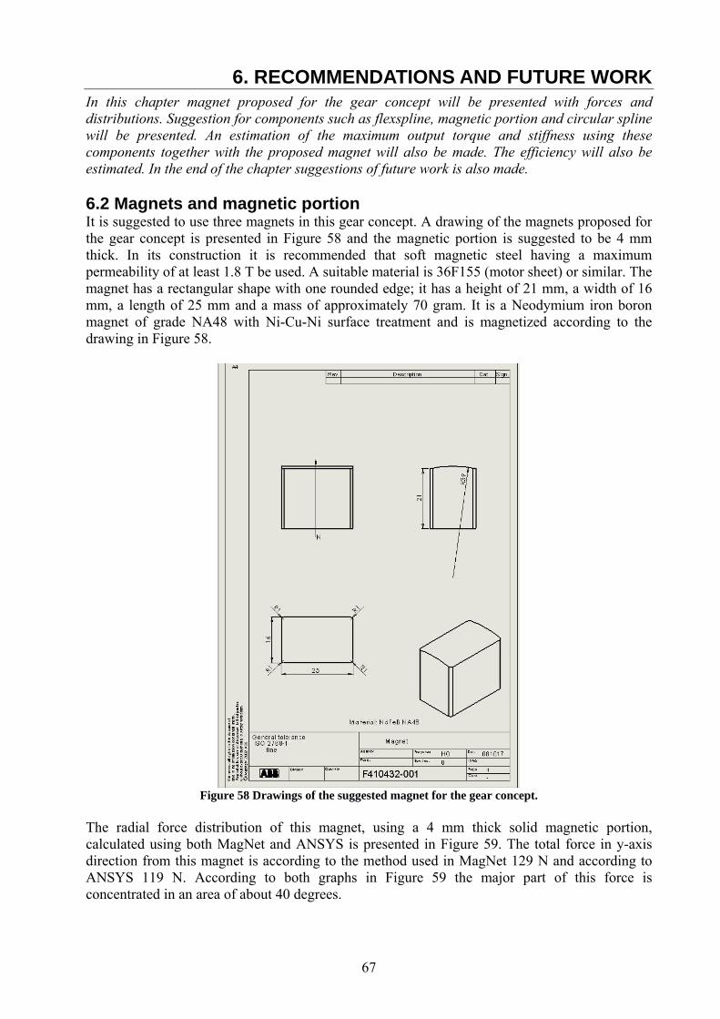
67

6. RECOMMENDATIONS AND FUTURE WORK In this chapter magnet proposed for the gear concept will be presented with forces and distributions. Suggestion for components such as flexspline, magnetic portion and circular spline will be presented. An estimation of the maximum output torque and stiffness using these components together with the proposed magnet will also be made. The efficiency will also be estimated. In the end of the chapter suggestions of future work is also made. 6.2 Magnets and magnetic portion It is suggested to use three magnets in this gear concept. A drawing of the magnets proposed for the gear concept is presented in Figure 58 and the magnetic portion is suggested to be 4 mm thick. In its construction it is recommended that soft magnetic steel having a maximum permeability of at least 1.8 T be used. A suitable material is 36F155 (motor sheet) or similar. The magnet has a rectangular shape with one rounded edge; it has a height of 21 mm, a width of 16 mm, a length of 25 mm and a mass of approximately 70 gram. It is a Neodymium iron boron magnet of grade NA48 with Ni-Cu-Ni surface treatment and is magnetized according to the drawing in Figure 58.

Figure 58 Drawings of the suggested magnet for the gear concept.

The radial force distribution of this magnet, using a 4 mm thick solid magnetic portion, calculated using both MagNet and ANSYS is presented in Figure 59. The total force in y-axis direction from this magnet is according to the method used in MagNet 129 N and according to ANSYS 119 N. According to both graphs in Figure 59 the major part of this force is concentrated in an area of about 40 degrees.

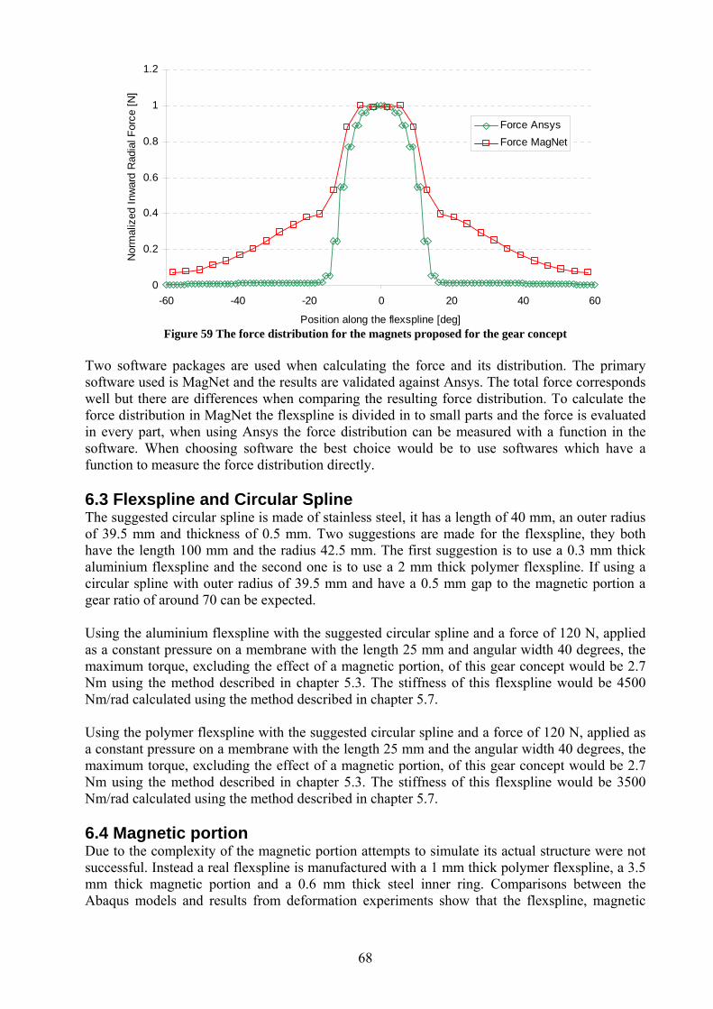
68

0

0.2

0.4

0.6

0.8

1

1.2

-60 -40 -20 0 20 40 60

Position along the flexspline [deg]

Nor

mal

ized

Inw

ard

Rad

ial F

orce

[N]

Force AnsysForce MagNet

Figure 59 The force distribution for the magnets proposed for the gear concept

Two software packages are used when calculating the force and its distribution. The primary software used is MagNet and the results are validated against Ansys. The total force corresponds well but there are differences when comparing the resulting force distribution. To calculate the force distribution in MagNet the flexspline is divided in to small parts and the force is evaluated in every part, when using Ansys the force distribution can be measured with a function in the software. When choosing software the best choice would be to use softwares which have a function to measure the force distribution directly. 6.3 Flexspline and Circular Spline The suggested circular spline is made of stainless steel, it has a length of 40 mm, an outer radius of 39.5 mm and thickness of 0.5 mm. Two suggestions are made for the flexspline, they both have the length 100 mm and the radius 42.5 mm. The first suggestion is to use a 0.3 mm thick aluminium flexspline and the second one is to use a 2 mm thick polymer flexspline. If using a circular spline with outer radius of 39.5 mm and have a 0.5 mm gap to the magnetic portion a gear ratio of around 70 can be expected. Using the aluminium flexspline with the suggested circular spline and a force of 120 N, applied as a constant pressure on a membrane with the length 25 mm and angular width 40 degrees, the maximum torque, excluding the effect of a magnetic portion, of this gear concept would be 2.7 Nm using the method described in chapter 5.3. The stiffness of this flexspline would be 4500 Nm/rad calculated using the method described in chapter 5.7. Using the polymer flexspline with the suggested circular spline and a force of 120 N, applied as a constant pressure on a membrane with the length 25 mm and the angular width 40 degrees, the maximum torque, excluding the effect of a magnetic portion, of this gear concept would be 2.7 Nm using the method described in chapter 5.3. The stiffness of this flexspline would be 3500 Nm/rad calculated using the method described in chapter 5.7. 6.4 Magnetic portion Due to the complexity of the magnetic portion attempts to simulate its actual structure were not successful. Instead a real flexspline is manufactured with a 1 mm thick polymer flexspline, a 3.5 mm thick magnetic portion and a 0.6 mm thick steel inner ring. Comparisons between the Abaqus models and results from deformation experiments show that the flexspline, magnetic

69

portion and inner steel ring will have similar stiffness to a shell composite of 1 mm polymer and 0.6 mm steel. Using a composite with a 1 mm thick polymer flexspline, a 3.5 mm thick magnetic portion and 0.4 mm thick steel inner ring together with the suggested magnets a maximum output torque of 1.6 Nm could be expected. This model would according to chapter 5.7 have a stiffness of around 3100 Nm/rad. 6.5 Efficiency There are many sources of losses, in this report the magnetic losses in the magnetic portion and the circular spline is evaluated. The results show that at 5000 rpm magnetic losses of 7.2 W could be expected in the magnetic portion, see chapter 4.4.1, and magnetic losses of 40 W in the circular spline, see chapter 4.4.2. These two losses should be compared to the ideal input power to gearbox when loaded at 5 Nm of 26 W. The efficiency would then be 0.36, which is lower than the goal of 50 %. It should be noted that efficiency would be even lower since there are several other sources of losses. 6.6 Future work When this project started all that were was an idea and a simple concept of how a magnetic harmonic traction gearbox could look like. During this project a more detailed model has been developed and the results from this thesis work have been used when choosing design solutions and dimensions for this model. Although, there are a lot of more work that can be done to improve and develop this gear concept. In this chapter suggestion of future work is presented.

6.6.2 Efficiency One of the goals of this project was to predict the efficiency of the gearbox. In this report magnetic losses in the magnetic portion and circular spline is evaluated. There are many other sources of losses in this gear concept, two examples are contact losses and viscous elastic losses. The contact between the flexspline and the circular spline is a significant source of losses, in this contact there are both a rolling friction and slip affecting gear ratio and efficiency. In a perfectly elastic flexspline and magnetic portion there will be no losses due to the cyclic deformation. The suggested magnetic portion is likely to have a significant internal damping which could give losses.

6.6.3 Optimisation of contact between Flexspline and Circular Spline In performing the evaluation described in this thesis it was not the intention to optimise the contact between the flexspline and the circular spline. Instead more focus has been placed on developing models of the magnetic situation and creating a model of the magnetic portion. A suggestion for future work is therefore to optimise the gear concept towards a better contact.

6.6.4 Materials What materials should be used in this gear concept for a long lifetime and optimal performance, this includes the material in flexspline, magnetic portion, circular spline etc. Could a material be found that offers a tube with high torsional stiffness and low radial stiffness? Does any highly flexible magnetic material exist? In this report a polymer flexspline is suggested, are there any suitable polymer material which have good enough fatigue properties?

6.6.5 Evaluation of the simulation models The main tool of predicting the behaviour of the suggested gear concept is finite element method simulations. Both magnetic model and mechanical models have been built using software such as MagNet, Ansys and Abaqus. When a model of the gearbox has been built test should be performed to verify the results and to adjust the models so a more accurate results can be given from them.

70

71

7. CONCLUSIONS A suggestion for which magnets should be used in the gearbox has been given. The magnets

should be rectangular with one round edge concentric to the axis of rotation. The magnets should have a height of 21 mm, a width of 16 mm, a depth of 25 mm and the rounded edge should have a radius of 39 mm. These magnets will have mass of around 70 gram and will be able to produce a force of at least 120 N per magnet at a distance of 1.5 mm.

Results show that it is preferable to use three instead of two magnets from a mechanical point

of view and the other way around from a magnetic point of view. Three forces give a higher torque but when using three magnets they influence each other which results in weaker force.

A comparison between using the magnetic simulations software MagNet and Ansys

Workbench is performed. The results show that both programs are able to predict the total force from the magnets but Ansys is better for determining the distribution of the force.

Suggestions for dimensions of the circular spline and the flexspline have been given. The

circular spline should have an outer radius of 39.5 mm, a thickness of 0.5 mm and should be made of a non magnetic stainless steel. The flexspline should have an inner radius of 42.5 mm and could either be made of 1 mm thick polymer or 0.3 mm thick aluminium.

The stiffness added by the magnetic portion is evaluated by performing experiments on a

prototype of the flexspline and magnet portion. A comparison is made with results from Abaqus simulations. The results show that an equivalent stiffness for the flexspline + magnetic portion + inner ring is obtain by building a composite shell in Abaqus comprising the flexspline and the inner ring, whose stiffness is equivalent to the magnetic portion.

According to the simulations results it will not be possible to transfer a load of 5 Nm through

the gearbox. Simulations show that when using a gearbox with the suggested magnets and dimension for flexspline and circular spline a torque of 1.5 Nm can be transferred if a friction coefficient of 0.3 can be achieved in the contact between the circular spline and the flexspline.

Torsional stiffness over the goal of 2000 Nm/rad can be achieved for a number of choices of

materials. A 0.1 mm thick steel flexspline gives a torsional stiffness of 2500 Nm/rad, a 1 mm thick polymer flexspline with a stiffening inner ring gives a torsional stiffness of 3100 Nm/rad and a 0.3 mm thick aluminium flexspline gives a torsional stiffness of 4500 Nm/rad.

Simulation results give a gear ratio of about 90 % of the value calculated using the classical

harmonic drive theory. Some of the magnetic losses in the gearbox have been evaluated. These are the eddy current

effect in the circular spline and the hysteresis and eddy current losses in the magnetic portion. The results show that the eddy current losses in the circular spline incur losses of about the same size as the ideal ingoing effect to the gearbox. The magnetic losses in the magnetic portion are shown to be about 15 % of the ideal ingoing effect. Regarding only these two sources an efficiency lower then the goal of 50 % should be expected.

There is an optimum thickness for the magnetic portion. The magnetic portion should be as

thin as possible to avoid added stiffness but should be thick enough that all the potential of the magnets are taken advantage of. The optimum thickness is the thickness when the material in the magnetic portion is just saturated.

72

73

8. REFERENCES

1. MagNet 32 bit Version 6.24. http://www.infolytica.com/en/products/magnet/. Infolytica Corporation.

2. Ansys Workbench 11.0, http://ansys.com, Ansys Inc. 3. Abaqus/CAE Version 6.7-EF1. http://www.simulia.com/products/abaqus_fea.html.

Dassault Systèmes. 4. Muser CW., Strain Wave Gearing, United States Patent, No. 2,906,143. 5. Harmonic Drive LCC. http://www.hamornicdrive.net. Boston, USA. 6. C. W. Musser, The Harmonic Drive, Machine Design, Apr. 1960. Pages 160-173. 7. Duff David G., Harmonic Friction Drive, United States Patent, US 6,439081 B1. 8. Humphreys Donald R., Modified Harmonic Drive Actuators, United States Patent.

3,604,287. 9. Toshiyoshi Muruyama, Harmonic gearing device using permanent magnet, Pat no.

JP2017246 (A). 10. British United Shoe Machinery, Improvements in or relating to Electro Mechanical

Rotary Drive Devices, Pat no. GB1123031. 11. Brailsford, F. (1966). Physical Principals of Magnetism. London, England: D. Van

Norstand Company LTD. 12. Magnet Sales & Manufacturing Inc. (1995). High Performance Magnets 7. (Electronic)

Available: http://www.magnetsales.com (2008-09-25) 13. Akaroni, A. (1996). Introduction to the Theory of Ferromagnetism. New York, USA:

Oxford University Press Inc. 14. Richman R.H., McNaughton W.P. (1997) Permanent Magnet Materials: Research

directions and opportunities. Journal of Electronic Materials. Volume 26, Number 5 / May, 1997.

15. Stanford Magnets Company, http://www.stanfordmagnets.com, 4 Meadowpoint, Aliso Viejo, CA 92656, U.S.A.

16. Buschow, K. H. J. & de Boer, F. R. (2003). Physics of Magnetism and Magnetic Materials. New York, USA: Kluwer Academic Publishers.

17. MagNet Documentation Center. http://www.infolytica.com/secured/customer/common/ doccenter/ (2008-10-25). Infolytica Corporation, Montréal, Québec, Canada.

18. Buschow, K.H. Jürgen; Cahn, Robert W.; Flemings, Merton C.; Ilschner, Bernhard; Kramer, Edward J.; Mahajan, Subhash. (2001). Encyclopedia of Materials - Science and Technology, Volumes 1-11. Oxford, UK. Elsevier Science Ltd.

19. Laminie J., Lowry J., (2003). Electrical Vehicle Technology Explained, Chichester, England, John Wiley & Sons Ltd.

20. Sundström B. (1998). Handbok och formelsamling i Hållfasthetslära. Stockholm, Sweden, Institutionen för Hållfasthetslära KTH.

21. Digital Mechanics AB. Materialdata FDM-teknik Polykarbonat och ABS. (Electronic) Available: http://www.digitalmechanics.se/ (2008-10-25)

22. Surahammars Bruk. M350-50A (Typical Data For Sura M350-50A). (Electronic) Available: http://www.sura.se/ (2008-11-04)

23. Barranger J., (1965). Hysteresis and eddy-current losses of a transformer lamination viewed as an application of the pointing theorem. Cleveland, Ohio. National Aeronautic and Space Administration.

24. Maskinelement, HANDBOK, (2005). Institutionen för maskinkonstruktion, Kungl Tekniska högskolan, Stockholm.

74

i

APPENDIX A A.1 Material data for NdFeB magnet of grade N48 [8] Intrinsic Coercive Force 11000 Oe Energy product (20 deg) 367.4 kJ/m3 Energy product 48 MGOe Residual induction (20 deg) 1.39 Tesla Relative permeability 1.03967 Coercivity -1060650 A/m Demagnetization (20 deg) 0.04192 Tesla Electric resistivity (20 deg) 1.5·10-6 ohm·m Electric permittivity (20 deg) 1 Thermal conductivity (20 deg) 9 W/(m·°C) A.2 Material data for material 36F155 [8] Lamination thickness: 0.014 in Grade ASTM A677 Electric resistivity (20 deg) 5.2·10-7 ohm·m Electric permittivity (20 deg) 1 Magnetic permeability: H (A/m) B (Tesla) 0 0 33.3 0.2 47.8 0.3 53.2 0.4 59 0.5 66 0.6 73.9 0.7 83.7 0.8 96.3 0.9 113 1 137 1.1 179 1.2 274 1.3 600 1.4 1710 1.5 3900 1.6 A.3 Material data for aluminium [8] Relative permeability (20 deg) 1 Coercivity (20 deg) 0 Amps/m Electric conductivity (20 deg) 38000000 Siemens/m Electric permittivity (20 deg) 1

ii

A.4 Material data for stainless steel [8] Relative permeability (20 deg) 1 Coercivity (20 deg) 0 Amps/m Electric conductivity (20 deg) 1200000 Siemens/m Electric permittivity (20 deg) 1 A.5 Material data for M350-50A [8] Non-oriented silicon steel Lamination thickness: 0.5mm Grade EN 10106 H (A/m) B (Tesla) 0 0 34.8 0.1 46 0.2 53.7 0.3 60.6 0.4 67.4 0.5 74.6 0.6 82.6 0.7 91.8 0.8 103 0.9 119 1 141 1.1 178 1.2 250 1.3 455 1.4 1180 1.5 3020 1.6 6100 1.7 10700 1.8 Electric resistivity 4.4e-7 Ohmm Relative permittivity 1 Mass density 7800 kg/m3