UNCORRECTE

D PROOF

Evaluation and numerical modeling of seawater intrusionin the Gaza aquifer (Palestine)

1

2

Khalid Qahman · Abdelkader Larabi3

Abstract A numerical assessment of seawater intrusion in4

Gaza, Palestine, has been achieved applying a 3-D variable5

density groundwater flow model. A two-stage finite dif-6

ference simulation algorithm was used in steady state and7

transient models. SEAWAT computer code was used for8

simulating the spatial and temporal evolution of hydraulic9

heads and solute concentrations of groundwater. A regular10

finite difference grid with a 400m 2 cell in the horizontal11

plane, in addition to a 12-layer model were chosen. The12

model has been calibrated under steady state and transient13

conditions. Simulation results indicate that the proposed14

schemes successfully simulate the intrusion mechanism.15

Two pumpage schemes were designed to use the calibrated16

model for prediction of future changes in water levels and17

solute concentrations in the groundwater for a planning18

period of 17 years. The results show that seawater intru-19

sion would worsen in the aquifer if the current rates of20

groundwater pumpage continue. The alternative, to elimi-21

nate pumpage in the intruded area, to moderate pumpage22

rates from water supply wells far from the seashore and to23

increase the aquifer replenishment by encouraging the im-24

plementation of suitable solutions like artificial recharge,25

may limit significantly seawater intrusion and reduce the26

current rate of decline of the water levels.27

Resume Un bilan numerique de l’intrusion de l’eau28

souterraine a Gaza, Palestine, a ete realise au moyen d’un29

modele 3D d’ecoulement des eaux souterraines a densite30

variable. Une simulation par differences finies a deux31

niveaux a ete utilisee en regime permanent et transitoire.32

Le code SEAWAT a ete utilise pour simuler l’evolution33

spatiale et temporelle des hauteurs piezometriques ainsi34

que les concentrations en solutes dans l’eau souterraine.35

Received: 2 May 2005 / Accepted: 29 September 2005

C© Springer-Verlag 2005

K. QahmanEnvironment Quality Authority, Palestinian Authority,Gaza, Palestine

A. Larabi (�)Department of Hydrogeological Engineering, LIMEN, EcoleMohammadia d’Ingenieurs, Universite Mohammed V- Agdal,B.P.765 Agdal Rabat, Moroccoe-mail: kqahman@gov.ps; larabi@emi.ac.ma

Une grille reguliere aux differences finies et des cellules 36

de 400m2, et douze couches horizontales constituent le 37

modele. Ce dernier a ete calibre en condition de regime 38

permanent et regime transitoire. Les resultats de la simula- 39

tion indiquent que les schemas proposes simules simulent 40

avec succes les mecanismes d’intrusion. Deux schemas de 41

pompages ont ete definis pour predire, grace au modele 42

calibre, a predire les changements des niveaux d’eau et des 43

concentrations dans l’eau souterraine, sur une periode de 17 44

ans. Les resultats montrent que l’intrusion de l’eau de mer 45

pourrait s’aggraver dans l’aquifere, si les pompages actuels 46

se poursuivent a ce niveau. L’alternative, eliminer le pom- 47

page dans la zone d’intrusion, serait de moderer les taux 48

de pompages des puits de production eloignes de la cote 49

et d’accroıtre le reapprovisionnement de l’aquifere en en- 50

courageant l’application de solutions telles que la recharge 51

artificielle, qui limiteraient significativement l’intrusion des 52

eaux souterraines et deduiraient le taux actuel de declin des 53

niveaux d’eau. 54

Resumen Se ha logrado una evaluacion numerica de la 55

intrusion de agua salada en Gaza, Palestina aplicando un 56

modelo de flujo 3-D de densidad variable de agua sub- 57

terranea. Se utilizo un algoritmo de simulacion de difer- 58

encia finita de dos etapas en modelos de regimen perma- 59

nente y transitorio. Se utilizo el codigo de computacion 60

SEAWAT para simular la evolucion espacial y temporal 61

de presiones hidraulicas y concentraciones de soluto de 62

agua subterranea. Se eligio una malla regular de diferencia 63

finita con una celda de 400m 2 en el plano horizontal en 64

adicion a un modelo de 12 capas. El modelo se ha calibrado 65

bajo condiciones de regimen permanente y transitorio. Los 66

resultados de la simulacion indican que los esquemas prop- 67

uestos simulan exitosamente el mecanismo de intrusion. Se 68

disenaron dos esquemas de bombeo para utilizar el modelo 69

calibrado para predecir los cambios futuros en niveles de 70

agua y concentraciones de soluto en el agua subterranea 71

para un periodo de planificacion de 17 anos. Los resultados 72

muestran que la intrusion de agua de mar empeorarıa en 73

el acuıfero si los ritmos actuales de bombeo de agua sub- 74

terranea continuan. La alternativa de eliminar el bombeo 75

en el area de intrusion, a ritmos de bombeo moderado 76

de pozos de abastecimiento de agua alejados de la costa, 77

a incrementar el reabastecimiento mediante el estımulo 78

de implementar soluciones disponibles como recarga 79

Hydrogeology Journal (2005) DOI 10.1007/s10040-005-003-2

UNCORRECTE

D PROOF

artificial puede limitar significativamente la intrusion de80

agua de mar y reducir el ritmo actual de descenso de nive-81

les de agua.82

Keywords Coastal aquifer . Hydrochemistry .83

Groundwater flow . Seawater intrusion . Numerical84

modeling85

Introduction86

Water is the most precious and valuable natural resource in87

the Middle East in general and in Palestine (Gaza Strip) in88

particular. It is vital for socio-economic growth and sustain-89

ability of the environment. The development of groundwa-90

ter resources in coastal areas is a sensitive issue, and careful91

management is required if water quality degradation, due92

to the encroachment of seawater, is to be avoided. In many93

cases, difficulties arise when aquifers are pumped at rates94

exceeding their natural capacity to transmit water, thus in-95

ducing seawater to be drawn into the system to maintain96

the regional groundwater balance. Problems can also oc-97

cur when excessive pumping at individual wells lowers the98

potentiometric surface locally and causes upconing of the99

natural interface between fresh water and saline water.100

The Gaza coastal aquifer, underlying an area of 365km101

2, is the only natural source for domestic, agricultural, and102

industrial purposes in the Gaza Strip with a population of103

about 1.2 million. Water is presently obtained by pumping104

more than 3000 wells, with a total estimated annual yield of105

about 140 million cubic meter (MCM). The total production106

presently exceeds natural recharge, and there is a net deficit107

in the aquifer water balance (PWA/USAID 2000). Current108

rates of aquifer abstraction are unsustainable and deterio-109

ration of groundwater quality is documented in many parts110

of the Gaza Strip. Saltwater intrusion presently poses the111

greatest threat to the municipal supply and continuous ur-112

ban and industrial growth is expected to further impact the113

water quality.114

The understanding of processes and chemical reactions115

related to seawater intrusion, and refreshening of water in116

coastal aquifers has been investigated by several authors,117

for instance, Gimenez and Morell (1997), using hydrogeo-118

chemical analyses, studied a coastal aquifer affected by119

salinization in Spain; Petalas and Diamantis (1999), iden-120

tified different sources of saline water with hydrochemical121

techniques in a coastal aquifer of northeastern Greece; and122

Stuyfzand (1999) showed chemical changes related to sea-123

water intrusion and refreshening of water in Dutch coastal124

dunes. A modeling approach to the multicomponent ion-125

exchange process in a coastal aquifer of Argentina was126

presented by Martınez and Bocanegra (2002). Lambrakis127

and Kallergis (2001), with a similar methodology, defined128

an estimate of the rate of water refreshening, under natural129

recharge conditions, for three coastal aquifers in Greece.130

In many cases, understanding of the mechanics of131

seawater intrusion has been incorporated into numerical132

models. Quantitative studies of modeling the seawater133

intrusion in coastal regions have been conducted by134

numerous authors worldwide (Andersen et al. 1988; 135

Rivera et al. 1990; Ghassemi et al. 1993, 1996; Calvache 136

and Pulido-Bosch 1994; Gangopadhyay and Gupta 1995; 137

Xue et al. 1995; Zhou et al. 2000; Sadeg and Karahonglu 138

2001; Langevin 2003). Two general approaches; the sharp 139

interface approach and the transition zone (dispersion) 140

approach; have been used to analyze seawater intrusion in 141

coastal aquifers. Two-dimensional and three-dimensional 142

models have been developed in both approaches to 143

simulate the steady state or unsteady state problem of 144

seawater intrusion. Numerical models based on the sharp 145

interface approximation assumption are reported in Mercer 146

et al. (1980), Polo and Ramis (1983), Essaid (1990), and 147

Larabi and De Smedt (1994, 1997). Numerical models 148

based on the second approach which is considering the 149

transition zone between seawater and freshwater are 150

reported in Huyakorn et al. (1987), Galeati et al. (1992), 151

Das and Datta (1995), Putti and Paniconi (1995), Guo and 152

Langevin (2002), and Aharmouch and Larabi (2004). 153

The seawater intrusion problem in the Gaza Strip has 154

been the subject of a number of studies (Yakirevich et al. 155

1998; Qahman and Zhou 2001; Moe et al. 2001; Qahman 156

and Larabi 2003a,b). Yakirevich et al. (1998), carried out 157

simulations of saltwater intrusion using a two-dimensional 158

density-dependent flow and transport model SUTRA (Voss 159

1984). This model was applied to the Khan Yunis section 160

of the Gaza Strip aquifer (Fig. 1). 161

Numerical simulations show that the rate of seawater in- 162

trusion during 1997–2006 is expected to be 20–45 m/year. 163

Qahman and Zhou (2001), carried out a simulation of sea- 164

water intrusion along a cross-section in the northern part of 165

the Gaza Strip using the SUTRA code. The results of the 166

simulation were used for identifying the number and loca- 167

tions of monitoring sites along the northern cross-section. 168

Moe et al. (2001), presented a 3-D coupled flow and trans- 169

port model for simulating the effects of a proposed manage- 170

ment plan for the aquifer. DYNCFT finite element computer 171

code (Fitzgerald et al. 2001) was used for the calculation. 172

Modeling results demonstrate that implementation of the 173

proposed management plan will have an overall beneficial 174

impact on the aquifer. In this work the period before year 175

1969, when most of the water level-drop occurred, was 176

not given enough importance in the northern area and, ac- 177

cordingly, the seawater intrusion results in that period were 178

not presented. Qahman and Larabi (2003a), showed chem- 179

ical changes related to seawater intrusion and refreshening 180

of water in the Gaza aquifer using the Stuyfzand (1999) 181

method and the groundwater flow patterns were also stud- 182

ied. The results indicated that about 10 coastal wells are af- 183

fected by seawater intrusion showing a deficit in the cation 184

exchange and a considerable high chloride concentration 185

(>250 mg/l). Qahman and Larabi (2003b) carried out a 186

simulation of seawater intrusion along a cross-section of 187

the Gaza Strip at Khan Younis using SEAWAT computer 188

code. The objective of the simulation was to compare the 189

SEAWAT results with the previous results of SUTRA for 190

the same cross-section using the same input data. The re- 191

sults of this work indicated that the SEAWAT code gave 192

very good results compared with the SUTRA code and it 193

Hydrogeology Journal (2005) DOI 10.1007/s10040-005-003-2

UNCORRECTE

D PROOF

Fig. 1 Location map of theGaza Strip (source:EPD/IWACO-EUROCONSULT1996)

was recommended to extend the work by making a 3-D194

model using the SEAWAT code.195

In the view of the previous studies, the present work196

was initiated to investigate the current status of the sea-197

water intrusion in the Gaza aquifer using the avail-198

able data. It was aimed at defining the hydrodynam-199

ics and hydrochemical behavior of the intrusion in the200

region and to assess its evolution, by applying the201

variable-density SEAWAT code using the 3-D finite dif-202

ference discretization. In this way it was planned to203

clarify when and where most of seawater intrusion oc-204

curred and to predict its future behavior along the Gaza205

Strip.206

Description of the study area207

The Gaza Strip is a part of the Mediterranean coastal plain208

between Egypt and Israel, where it forms a long and narrow209

rectangle (Fig. 1). Its area is about 365 km2 and its length210

is approximately 45 km. The population characteristics of211

the Gaza Strip are strongly influenced by political devel-212

opments which have played a significant role in the growth213

and population distribution of the Gaza Strip. In 1997 the214

Palestinian Bureau of Statistics estimated the population to215

be about 1 million (PCBS 1998).216

The average daily mean temperature ranges from 25◦C217

in summer to 13◦C in winter. Average daily maximum218

temperatures range from 29 to 17◦C and minimum tem- 219

peratures from 21 to 9◦C in the summer and winter 220

respectively. The daily relative humidity fluctuates be- 221

tween 65% in the daytime and 85% at night in the 222

summer, and between 60 and 80%, respectively in win- 223

ter. The mean annual solar radiation is 2,200/J/cm2/day 224

(EPD/IWACO-EUROCONSULT 1994). The average an- 225

nual rainfall varies from 450 mm/year in the north to 226

200mm(year in the south. Most of the rainfall occurs in 227

the period from October to March, the rest of the year 228

being completely dry. Precipitation patterns include thun- 229

derstorms and rain showers, but only a few days of the 230

wet months are rainy days. There is less areal variation 231

in evaporation than in rainfall in the Gaza Strip. Evapora- 232

tion measurements have clearly shown that the long term 233

average open water evaporation for the Gaza Strip is in 234

the order of 1300 mm/year. Maximum values in the order 235

of 140 mm/month are quoted for summer, while relatively 236

low pan-evaporation values of around 70 mm/month were 237

measured during the months of December and January. 238

Geological and hydrogeological setting 239

The Gaza Strip is essentially a foreshore plain gradually 240

sloping westward and is underlain by a series of Mesozoic 241

to the Quaternary geological formations. The hydroge- 242

ology of the coastal aquifer consists of one sedimentary 243

Hydrogeology Journal (2005) DOI 10.1007/s10040-005-003-2

UNCORRECTE

D PROOF

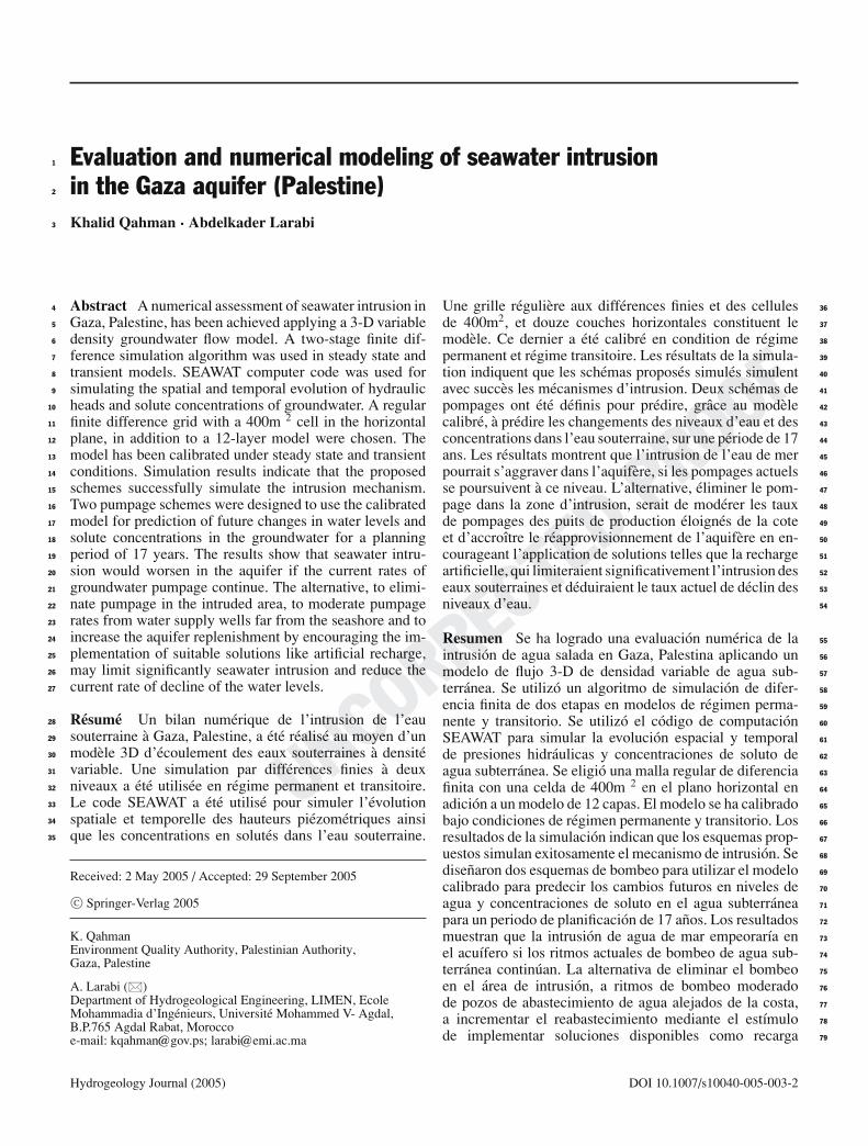
Fig. 2 Schematization of thehydrogeological cross-sectionof the Gaza Strip aquifer (from:PWA(USAID 2000); verticalscale in meters

basin, the post-Eocene marine clay (Saqiya Group), forms244

the bottom of the aquifer. Pleistocene sedimentary deposits245

of alluvial sands, graded gravel, conglomerates, pebbles246

and mixed soils constitute the regional hydrological sys-247

tem. Intercalated clay deposits of marine origin separate248

these deposits, and are randomly distributed in the area.249

The Gaza aquifer can be divided into three subaquifers250

(A, B, C). Schematization of the hydrogeological cross251

section of the Gaza Strip aquifer is shown in Fig. 2. It is252

implied that subaquifer A is phreatic, whereas subaquifers253

B and C become increasingly confined towards the254

sea.255

The regional groundwater flow is mainly westward to-256

wards the Mediterranean Sea. The maximum saturated257

thickness of the aquifer ranges from 120 m near the sea258

to a few meters near the eastern aquifer boundary. Natural259

average groundwater heads decline sharply east of the Gaza260

strip and then gradually decline towards the Sea. Depth to261

water level of the coastal aquifer varies between a few me-262

ters in the lowland area along the shoreline and about 70 m263

below the surface along the eastern border.264

The major source of renewable groundwater in the aquifer265

is rainfall. The total rainfall recharge to the aquifer is es-266

timated to be approximately 45 MCM/year. The remain-267

ing rainwater evaporates or dissipates as runoff during268

the short periods of heavy rainstorms. The lateral in-269

flow to the aquifer is estimated at between 10 and 15270

MCM/year. Some recharge is available from the major271

surface flow (Wadi Gaza). But because of the extensive272

extraction from Wadi Gaza by Israel, this recharge is lim-273

ited at its best to 2 MCM during the ten days the wadi274

actually flows in a normal year. As a result, the total275

freshwater recharge at present is limited to approximately276

60 MCM/year.277

Currently, the Gaza aquifer is monitored by a multipur-278

pose groundwater monitoring network which is used for ob-279

serving the groundwater levels and the nitrate and chloride280

content. The existing water level monitoring network in-281

clude: 135 wells and 39 piezometers (small-diameter pipes)282

distributed all over Gaza Strip since 1972 (PWA 1997a).283

The existing groundwater quality monitoring network has284

700 wells for chloride monitoring and 450 wells for nitrate285

monitoring (PWA 1997b).286

Seawater intrusion in Gaza aquifer 287

Under natural conditions, groundwater flow in the Gaza 288

Strip is discharging towards the Mediterranean Sea. How- 289

ever, pumping over 50 years has significantly disturbed nat- 290

ural flow patterns. Large cones of depression were formed 291

in the north and south where water levels are below mean 292

sea level, inducing inflow of seawater towards the major 293

pumping centers. 294

Surveys of hydrologic characteristics began under the 295

British Government of Palestine (1917–1948), and regular 296

monitoring throughout the region began in the early 1930s. 297

Between October 1934 and September 1935 a survey of 298

chloride concentration and water levels in wells was con- 299

ducted throughout the region (PWA(USAID 2000). 300

In order to figure out the extent of groundwater declines 301

and the changes in groundwater quality, historical changes 302

in groundwater levels and chloride concentrations were 303

analyzed for the period 1935–2000 (Figs. 3 and 4). The 304

kriging interpolation method was used to estimate the 305

spatial distribution of values depending on available data 306

from measurement points which are located on the figures. 307

Water level contours have declined from east towards 308

the west (Fig. 3a), in a smooth pattern almost parallel to 309

the coastline. This could well be thought of as an initial 310

(natural) condition of the aquifer where only a few wells 311

might be pumping under near-steady-state conditions. 312

A comparison of Figs. 3a and 4a shows that groundwater 313

levels dropped by as much as 8 meters between 1935–1969 314

in the northern area of the Gaza Strip. This drop is most 315

apparent in the north due to possible extensive exploitation 316

of groundwater at the eastern and northern borders of the 317

Gaza Strip between 1948–1969, in addition to the sudden 318

increase of the Gaza Strip population in 1948 which has 319

increased the water demand in this area. On the other hand, 320

a comparison of Figs. 3b and 4b indicates that there is no 321

considerable difference in the chloride spatial distribution. 322

This could be explained if, during this period, there was 323

enough water in storage and the total amount abstracted 324

from the aquifer, in general, did not exceed the total natural 325

recharge. 326

Between 1970 and 2000, groundwater levels dropped by 327

almost 3m on average. This drop is most apparent in the 328

Hydrogeology Journal (2005) DOI 10.1007/s10040-005-003-2

UNCORRECTE

D PROOF

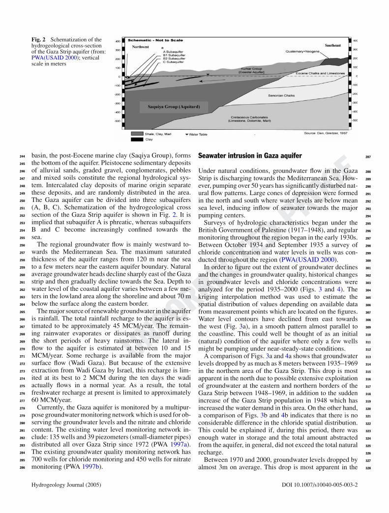
Fig. 3 a Groundwater level contours, b Chloride concentrationisolines in groundwater (year 1935); isoline interval 100 mg/l

Fig. 4 a Groundwater level contours, b Chloride concentrationisolines in groundwater (year 1969); isoline interval 100 mg/l

Hydrogeology Journal (2005) DOI 10.1007/s10040-005-003-2

UNCORRECTE

D PROOF

south where there is a lower recharge rate from rainfall.329

In the north, most wells exhibited a relatively small water330

level drop in this period due to the higher recharge rate331

(Figs. 4a and 5a). In addition, water levels often drop below332

sea level, presumably because of excessive discharge from333

a nearby well field. From Fig. 5a, it can be estimated that334

water levels are below mean sea level in area of more than335

100 km2 of the Gaza Strip. Comparison of Figs. 4b and 5b336

shows that there is a noticeable change in the position of337

the chloride isolines, especially near the coast, indicating338

possible landward migration of seawater.339

In recent years, the seawater intrusion effect is more evi-340

dent. High rates of urbanization and increased agricultural341

and industrial activities require more water to be pumped342

from the aquifer. This pumping has continually increased343

the risk of seawater intrusion and deterioration of freshwa-344

ter quality in the Gaza aquifer.345

Figure 6a shows a typical water level time series trend346

for well number E(32 along the coast of the Gaza Strip347

about 6 km south of the border. Figure 6b shows a sudden348

typical breakthrough of salinity for well number E/32. This349

could be due to either lateral encroachment of saline water350

(seawater intrusion) and/or vertical upconing in the summer351

season due to the increase of the abstraction rate from wells.352

Numerical simulation of coupled groundwater353

and solute transport354

Model development355

The regional scale model simulates transient groundwater356

flow for the period 1935–2003. The model was developed357

using the conceptual hydrologic model shown in Fig. 2.358

Governing equations359

Variable density groundwater flow is described by thefollowing partial differential equation as presented in(Langevin 2003).

∇ρ Kf +(

∇ hf + (ρ − ρf)ρf

∇z

)= ρ Sf

∂ hf

∂t

+ n∂ρ

∂C

∂C

∂t− ρq (1)

where z is a coordinate direction aligned with gravity (L).360

? is fluid density (ML−3). Kf is the equivalent fresh water361

hydraulic conductivity (LT−1). hf is the equivalent fresh362

water head (L). f is the density of fresh water (ML−3).363

Sf is equivalent fresh water storage coefficient (L−1). t is364

time (T). n is porosity (L0). C is the concentration of the365

dissolved constituent that affects fluid density (ML(3).ρ is366

the fluid density of a source or a sink (ML−3).q is the flow367

rate of the source or sink (T1).368

To solve the variable density ground water flow equation,369

the solute-transport equation also must be solved because370

fluid density is a function of solute concentration, and con-371

centration may change in response to the groundwater flow372

Fig. 5 a Groundwater level contours, b Chloride concentrationisolines in groundwater (year 2000); isoline interval 200 mg/l

Hydrogeology Journal (2005) DOI 10.1007/s10040-005-003-2

UNCORRECTE

D PROOFFig. 6 a Water level time series, b Chloride time series (well E-32near the coast in the north of the Gaza Strip)

field. For dissolved constituents that are conservative, such373

as those found in sea water, the solute transport equation is:374

∂C

∂t= ∇(D∇C) − ∇(νC) − qs

nCs (2)

where D is the dispersion coefficient (L2T−1). ( is the375

groundwater flow velocity (LT−1). qs is the flux of a source376

or sink (T−1). Cs is the concentration of the source or sink377

(ML−3).378

Simulation code379

To simulate variable density effects on groundwater flow,380

the coupled flow and transport code SEAWAT was used381

(Guo and Bennett 1998). Coupling flow and transport com-382

putations allows the effects of fluid density gradients as-383

sociated with solute concentration gradients to be incor-384

porated into groundwater flow simulations (i.e., density-385

dependent flow). It uses the finite difference method of386

numerical integration to solve 3-D confined and uncon-387

fined groundwater flow under many types of natural and388

artificial aquifer stresses.389

The original SEAWAT code was written by Guo and Ben-390

nett (1998) to simulate ground water flow and salt water in-391

trusion in coastal environments. SEAWAT uses a modified392

version of MODFLOW (McDonald and Harbaugh 1988)393

to solve the variable density, ground water flow Eq. (1) and394

MT3D (Zheng 1990) to solve the solute-transport Eq. (2).395

Spatial and temporal discretization396

The model domain and finite difference grid used to simu-397

late groundwater flow within the Gaza coastal aquifer are398

shown in Fig. 7. The model encompasses an area of about 399

365km2. The grid consists of 115 rows, 35 columns with 400

4025 regular cells in plan view. Each cell is 400 m 400 m 401

in the horizontal plane. 402

The model was discretized vertically into 12 layers, this 403

increased resolution is necessary because of transport con- 404

siderations and because vertical density gradients must be 405

resolved in order to calculate accurate flow velocities. The 406

top elevation of layer 1 is spatially variable and corresponds 407

with land surface elevation, based on a topographic map. 408

The bottom of layer 1 is set at an elevation of 5.0m below 409

sea level. The nearly 70-year simulation period is divided 410

into nine stress periods. For each stress period, the aver- 411

age hydrologic conditions for that period are assumed to 412

remain constant. Further temporal discretization is intro- 413

duced in the form of time steps within each stress period. 414

The length of the transport time step was assigned to start 415

with 1 day and to be increased by a multiplier factor of 1.2. 416

Assignment of values to aquifer parameters 417

The basis for assigning hydraulic properties were the ex- 418

isting data from pumping tests in the Gaza Strip, previous 419

modeling studies by Israeli organizations in the coastal 420

plain, and miscellaneous literature related to transport pa- 421

rameters. The distribution of hydraulic conductivity values 422

for tests carried out in Gaza show that values were from 423

20–80 m/day. 424

Pumping tests carried out in the Gaza Strip to date have 425

yielded unreliable values of storage coefficient; hence val- 426

ues were obtained from the literature for similar types 427

of sediments, as well as results from previous studies 428

(PWA/CAMP 2000). Specific yield values are estimated 429

to be about 15–30 percent while specific storage is about 430

10−4m−1 from tests conducted in Gaza. 431

Accordingly, the approach for assigning aquifer parame- 432

ter values that pertain to groundwater flow and solute trans- 433

port was to use the simplest distribution that would result in 434

adequate representation of the flow system. All parameter 435

values were adjusted during the model calibration process 436

until the model adequately reflected the observed water 437

level distribution and interpreted flow patterns throughout 438

the aquifer. 439

Boundary conditions 440

Constant head and concentration were specified to the 441

model cells along the coast. The specified constant con- 442

centration of TDS is 35 kg(m3. The head for each cell was 443

converted to freshwater head using the specified TDS con- 444

centration of 35 kg/m3 and the center elevation of the cell. 445

A reference density of 1000 kg/m3 was used for freshwater 446

and 1025 kg/m3 for seawater. The coupled flow and trans- 447

port model (SEAWAT) uses this reference value to calculate 448

and adjust fluid densities relative to simulated concentra- 449

tions of dissolved salts in the model. 450

To represent the lateral flow of groundwater from the in- 451

land perimeter of the model, injection wells were assigned 452

to the eastern boundary of the model with a specified salt 453

Hydrogeology Journal (2005) DOI 10.1007/s10040-005-003-2

UNCORRECTE

D PROOF

Fig. 7 Finite-difference gridand boundary conditions for theGaza regional model

concentration to be within the range of 0.2–3 kg/m3 from454

the north to the south of the eastern border. The rate of injec-455

tion was calculated from the available water level contour456

maps. For example, the lateral water inflow from the east457

was estimated to be about 6 MCM(year for the northern458

part of the Gaza strip (8 km length) according to the water459

table contours of 1935, considering the hydraulic conduc-460

tivity as 25 m/day and the aquifer thickness 70 m. The same461

method can be applied for other years and border sections.462

The value of lateral flow was adjusted during the model run.463

The lower boundary of the model represents the base of464

the aquifer. A Neumann-type of no-flux boundary condi-465

tions was assigned to the bottom of the aquifer (Guo and466

Langevin 2002).467

The northern and the southern boundaries are assumed468

to be no-flow boundaries, assuming that the flow lines are469

parallel to them under natural conditions. However, the470

exact position of this boundary is not known due to the471

scarcity and uncertainty of data. This assumption could be472

changed in case the water level data are obtained.473

Internal hydrologic stresses474

Hydrologic stresses that are internal to the model domain475

are represented with internal boundary conditions. Internal476

hydrologic stresses include: recharge from rainfall, return 477

flow, and municipal and agricultural withdrawals. 478

Recharge 479

The recharge (RCH) package in SEAWAT is used to apply 480

surface recharge from rainfall to the model with a specified 481

low salt concentration of 0.085 kg/m3. The general pro- 482

cedure for estimating recharge values was to multiply the 483

average annual rainfall quantity in each zone by infiltration 484

coefficient. The infiltration coefficient was estimated ac- 485

cording to soil type, land use and evapotranspiration rate. 486

According to the long term annual average of rainfall data 487

within the Gaza Strip area, the average rate of recharge 488

applied on the model was in the range of 0.0002–0.00045 489

m/day. 490

Return flow 491

Agriculture pumping within the Gaza Strip is on the order 492

of 80–100 MCM/year in any given year. A portion of this 493

applied water infiltrates back into the aquifer. The quan- 494

tities that infiltrate depend on methods of irrigation, crop 495

types, soil types, and irrigation schedules. Hence, in the 496

Gaza Strip, 25% of the pumping at individual wells was 497

recharged back to the aquifer (PWA CAMP 2000). 498

Hydrogeology Journal (2005) DOI 10.1007/s10040-005-003-2

UNCORRECTE

D PROOF

Fig. 8 a Residuals of waterlevel in year 1935 (steady state).b Observed heads versussimulated heads in year 1935(steady state)

Municipal and agricultural well fields499

More than 3000 pumping wells are inventoried and rep-500

resented in the model domain. The applied groundwater501

abstraction rate from the model domain is summarized in502

Table 1. The estimation was done according to the available503

data on population, population growth, number of wells,504

and groundwater abstraction rates between 1987 and 1993.505

Initial conditions506

A steady state simulation was performed using 1935 hy-507

drologic conditions. The results (water level and concentra-508

tions) from the steady state simulation were used as initial 509

conditions for transient simulation. 510

Calibration and model results 511

The numerical model was calibrated and tested against 512

both steady state and transient data. Two sets of tar- 513

get conditions were selected for calibration purposes, 514

steady state conditions in year 1935 and time varying 515

conditions between 1935 and 1969. Verification of the 516

model was done based on the average water level in year 517

2002. 518

Hydrogeology Journal (2005) DOI 10.1007/s10040-005-003-2

UNCORRECTE

D PROOF

Table 1 Estimated ground water abstraction from the Gaza aquifer

Abstraction period Period Abstraction rate (MCM/year)

1 1935–1949 162 1949–1955 223 1955–1960 554 1960–1969 785 1969–1975 986 1975–1982 1077 1982–1990 1168 1990–1998 1359 1998–2003 150

During calibration, measured and model-computed heads519

(water levels) are compared, and the difference is referred520

to as the residual. Figure 8a shows the calibrated, simulated521

flow field in the Gaza Strip for year 1935 conditions, and522

the spatial distribution of residuals. Average water levels523

of year 1935 for 50 wells within the model domain were524

used as calibration targets. Within the model domain, ob-525

served water levels range from 0.5 m above mean sea level526

(AMSL) to 15 m AMSL. The calculated residual mean527

error and absolute mean error are about (0.01 and 0.69528

m, respectively, with a standard deviation for the model529

domain of 0.96 m. In general, the residual values range530

from 1.95 to 1.25m. Comparison of calculated and mea-531

sured groundwater levels for year 1935 shows that they are532

compatible with each other (Fig. 8b).533

The results of steady state calibration show that there is no534

apparent trend related to the spatial distribution of residuals535

especially in the two-thirds of the model domain to the536

north of Khan-Younis, where there are a lack of targets and537

monitoring data. However, this area of the model contains538

bad water quality. In the southeastern part of the model539

domain and for very low abstraction rates, the calibration540

is regarded as acceptable in general.541

Transient calibration was conducted for the 1935–1969542

target period, using the calibrated 1935 steady state results543

as an initial condition. For the transient calibration, the544

major pumping and lateral fluxes were changed for the545

specified stress periods.546

For transient simulations, adjustments were made to the547

storage coefficients. A further calibration step of the model548

was done based on groundwater level data of year 2002.549

The results of calibration are presented in Table 2. For550

year 1969, the calculated residual mean error and absolute551

mean error are about 0.15 and 0.82 m, respectively, with552

a standard deviation for the model domain of 0.98 m. For553

Table 2 Statistical results of calibration processes

Year 1935 Year 1969 Year 2002

Mean residual (m) -0.01 -0.15 -0.01Absolute mean residual (m) 0.69 0.82 0.82Standard deviation of mean

residual0.96 0.98 1.09

year 2002, the calculated residual mean error and absolute 554

mean error are about 0.01 and 0.82 m, respectively, with 555

a standard deviation for the model domain of 1.09 m. The 556

results of transient calibration are considered as acceptable 557

for this study purpose. 558

Table 3 summarizes the mass balance calculated by the 559

model taking into consideration that amount between 20 560

and 30% is deducted from the total abstraction to repre- 561

sent the return flow which comes from irrigation, sewage 562

infiltration and leakages from water networks. This means 563

that the amount assigned for abstraction from the wells in 564

the table represents the net abstraction after deducting the 565

return flow from the total abstraction. This was done to sim- 566

plify the modification of recharge zones assigned for the 567

model and also it decreases the uncertainty coming from 568

assigning the location of return flow which is not known 569

very well. The steady state water balance for year 1935 570

shows that a large quantity of groundwater is discharged 571

to the sea (about 55MCM/year) which is enough to coun- 572

teract seawater intrusion. In years 1969, 1998, and 2003, 573

the discharge quantity to the sea is decreased to about 9.8 574

MCM/year where the seawater intrusion quantity reaches 575

about 46MCM/year. 576

As a preliminary check on the model simulation of sea- 577

water intrusion, results were compared with geophysical 578

survey results in the southern sector of the Gaza Strip which 579

was done with Italian cooperation (CISS/WRC 1997). The 580

geoelectrical section executed in the Deir El Balah area 581

(Fig. 9a) which is composed of ten numbered vertical elec- 582

trical soundings (VES) and extends from the borderline 583

to the sea in a southeast-northwest direction. From VES 584

number 64 to number 66 the interpretative model is com- 585

posed of a more conductive top layer (3�m) over a much 586

less resistive middle layer (10�m) overlapping the highly 587

conductive bottom layer (0.1–1�m). It was concluded that, 588

the general relative lowering of the resistivity is due to the 589

seawater intrusion inside the aquifer formation upper con- 590

ductive (clay) and resistive (sandstone and pebble) layers. 591

The results of the geophysical survey indicate that the ex- 592

tent of seawater intrusion along Deir El Balah profile in the 593

Table 3 Summary of thecalculated mass balance of theflow model

Year In (MCM/year) Out (MCM/year) In–OutStorage Lateral

flowSea Recharge Total in Storage Wells Sea Total

out

1935 0.00 26.64 7.15 38.81 73.94 0.00 17.64 55.07 73.94 0.0011969 9.64 16.59 24.50 38.81 89.53 0.00 61.74 27.79 89.53 0.0051998 2.65 27.30 42.80 38.81 111.56 0.00 100.27 11.29 111.56 0.0012003 5.13 27.30 46.16 38.56 117.14 0.00 107.36 9.78 117.14 0.002

Hydrogeology Journal (2005) DOI 10.1007/s10040-005-003-2

UNCORRECTE

D PROOF

Fig. 9 a Deir El Balahgeoelectrical section in year1996. b Isolines of calculatedTDS concentrations (kg/m3) bySEAWAT in year 1996 alongDeir El Balah geoelectricalcross section; isoline interval2kg/m3

Fig. 10 Isolines of calculated TDS concentration (kg/m3) by SEA-WAT in year 2003 along the Jabalya cross section

subaquifer A, may reach 1000 m inland which agrees in594

general with the simulation results as illustrated in Fig. 9b.595

In addition to the above, the model results for year 2000596

were compared with geophysical survey results obtained597

from PWA/CAMP (2000). In particular, the time-domain598

electromagnetic method (TDEM) survey results were used.599

The results of comparison show that the simulated ex-600

tent of the seawater wedge in year 2000 gave a reason-601

able agreement with the TDEM measurements at two cross602

section locations near the coast in Rafah and also in Deir603

El Balah also. Most values of the TDEM records within604

the intruded area identified by the simulation model have605

values less than 2.0�m of apparent resistivity, which is606

considered an indication for seawater intrusion in coastal607

areas.608

Fig. 11 Isolines of calculated TDS concentration (kg/m3) by SEA-WAT in year 2003 along the Khan Younis cross section

The model gave good agreement with results of previous 609

modeling studies of Gaza aquifer (Yakirevich et al. 1998; 610

Qahman and Zhou 2001; Moe et al. 2001). 611

A summary of the aquifer hydraulic and transport proper- 612

ties that best describes the aquifer behavior in steady state 613

and transient models after model calibration is presented in 614

Table 4. 615

Simulation results and discussions 616

Saltwater-freshwater transition zone 617

The estimated extent of the seawater wedge from seawater 618

intrusion modeling until year 2003 is presented in two 619

cross-sections (Figs. 10 and 11; Jabalya and Khan Younis, 620

Table 4 Aquifer parameter values after calibration

Stratigraphicunit

Horizontal hydraulicconductivity (m/day)

Vertical hydraulicconductivity (m/day)

Specificyield

Specificstorage(m−1)

Porosity Longitudinaldispersivity(m)

Transversedispersivity(m)

Sandstone 30 3 0.2 0.0001 0.35 10 0.1Clay 0.2 0.1 0.1 0.0001 0.4 50 0.1

Hydrogeology Journal (2005) DOI 10.1007/s10040-005-003-2

UNCORRECTE

D PROOFFig. 12 Simulated inland extent of TDS concentration (more than2.0kg/m3) in subaquifers A and C in year 2003

respectively). For the purpose of presentation, it is621

considered that the extent (wedge) of seawater intrusion is622

represented by the 2.0kg(m3 isoline of TDS concentrations.623

From Fig. 10 it is estimated that seawater intrusion near624

Jabalya may extend about 2 km inland in subaquifer B,625

and up to 3km in subaquifer C. Localized intrusion in sub-626

aquifer A is restricted to the coastal area.627

In Khan Younis (Fig. 11), seawater intrusion extends628

inland about 2km in subaquifer B2 and about 1.5 km in629

subaquifer B1.630

Figure 12 shows a plan view of simulated current (2003)631

intrusion in the A and C subaquifers in the Gaza aquifer. It632

is clear from the above results that most of the area affected633

by seawater intrusion is located in the north coast of the634

Gaza Strip to the north of Gaza city (from about 35,000 to635

45,000N). Extensive seawater intrusion also has occurred636

in the south from about 10,250 to 25,250N. Other sources637

of chloride, such as the Eocene age rocks (chalks and lime-638

stones) at the eastern model boundary (with chloride con-639

centrations less than 2000 mg/l) will not exert notable in-640

fluences on the water levels and water quality because of641

their generally low transmissivity.642

Predicted results 643

Because increased withdrawal of groundwater from the 644

water supply wells near the coast is the main cause of 645

seawater intrusion into the aquifer, a future decrease in 646

groundwater withdrawal is a very important consideration 647

to prevent further intrusion of the seawater into the aquifer. 648

In order to demonstrate the effect of future scenarios of 649

groundwater pumpage on seawater intrusion, two pumping 650

schemes were designed to use the calibrated model for 651

calculations of future changes in water levels and salinity 652

concentrations in a period of another 17 years. The two 653

management scenarios are presented as follow: 654

1. The first (worst) scenario where the pumping from the 655

aquifer continues to increase assuming that there is no 656

new water resources for the Gaza Strip. 657

2. The second scenario where pumping from the aquifer 658

is assumed to be decreased and the deficit in water de- 659

mand is covered by developing new water resources in 660

Gaza Strip like desalination of seawater, the import of 661

water from outside the Gaza Strip and reuse of treated 662

wastewater in agricultural irrigation. 663

664

Table 5 shows the amounts of abstracted water from the 665

aquifer for both scenarios. 666

Figures 13a and b show the future changes in water levels 667

in year 2020 for the two predictive scheme simulations. 668

Obviously, water levels in Fig. 13a dropped below MSL in 669

most of the Gaza Strip area. On the other hand, Fig. 13b 670

shows that in all the Gaza Strip, water levels are AMSL, 671

which means that there is improvement in the groundwater 672

balance. 673

Figures 14a and b show the comparison between the ex- 674

tent of seawater intrusion in subaquifer A in year 2003 and 675

2020 for both scenarios. It is predicted that between years 676

2003 and 2020, the first scenario will induce a considerable 677

quantity of seawater intrusion especially in the northern 678

part. Model results indicate that the extent of the isoline 679

(TDS concentration(2.0kg/m3) at the base of subaquifer A 680

will move about an additional 1.5 km in the northern part. 681

On the other hand, the results of comparison indicate that 682

the second scenario prevent any further seawater intrusion 683

after year 2003. In year 2020 the total inflow from the sea 684

is estimated to be 72 MCM/year and 32 MCM/year for the 685

first scenario and second scenario respectively, where the 686

discharge to the sea for the same year is estimated to be 687

about 3 and 18 MCM/year for the first and second scenarios. 688

Table 5 Abstraction amountsfor management scenarios

Stress period no Period length First scenario Abstraction(MCM/year)

Second scenarioAbstraction (MCM/year)

1 2003–2008 160 1402 2008–2011 170 1303 2011–2014 180 1204 2014–2017 190 1105 2017–2020 200 110

Hydrogeology Journal (2005) DOI 10.1007/s10040-005-003-2

UNCORRECTE

D PROOF

Fig. 13 a Predictedgroundwater level contour linesfor first scenario, b Predictedgroundwater level contour linesfor second scenario year (2020)

Hydrogeology Journal (2005) DOI 10.1007/s10040-005-003-2

UNCORRECTE

D PROOF

Fig. 14 Simulated extent ofTDS concentration insubaquifers A in years 2003 and2020. a under the first scenarioconditions, b under the secondscenario conditions

Hydrogeology Journal (2005) DOI 10.1007/s10040-005-003-2

UNCORRECTE

D PROOF

Conclusions689

The Gaza coastal aquifer is a dynamic groundwater system,690

with continuously changing inflow and outflow conditions.691

The equilibrium condition that once may have existed be-692

tween fresh and saline water has been disturbed by large693

scale pumping. The aquifer has been overexploited for the694

past 40 years; this has induced seawater flow towards the695

major pumping centers in the Gaza Strip to the north of the696

Gaza City and near Khan-Younis City.697

The understanding of the three dimensional pattern of698

groundwater flow and variation of groundwater quality are699

incomplete. All the wells tested and sampled in the Gaza700

Strip are located in the shallow portion of the aquifer, the701

deeper subaquifer was sampled in some deep municipal702

wells; however, many of these wells receive water from703

two or more subaquifers, so the water quality in the specific704

subaquifers could not be determined. Fresh groundwater705

(based on a TDS concentration of less than 250 mg/l) is706

only found in the north and in the southwest in sandy dune707

areas, and in shallow parts of the aquifer where recharge708

from rainfall is high.709

The coupled flow and transport finite difference code710

(SEAWAT) was applied to examine how far inland the sea-711

water transition zone has moved since intrusion began. The712

model gave good results for the evolution of salinity in the713

aquifer. The preliminary model results suggested that the714

seawater intrusion began in the 1960s which is in agreement715

with the available information about general pumping and716

well information. Most of the seawater intrusion has oc-717

curred to the north of Gaza city and also near Khan-Younis718

city in the south.719

The numerical model was applied to evaluate the over-720

all regional impact on the aquifer for two future scenar-721

ios of pumping. The first scenario is to pump from the722

aquifer continuously until the year 2020 when the pump-723

ing rate reaches 200 MCM/year; and the second scenario is724

to progressively decrease the pumping rate, starting at 140725

MCM/year in the year 2003, to 110 MCM/year from the726

existing wells. It is predicted that between years 2003 and727

2020, the first scenario will induce a considerable quan-728

tity of seawater intrusion especially in the northern part.729

Model results indicate that the extent of the isoline (TDS730

concentration(2.0 kg/m3) at the base of subaquifer A will731

move about an additional 1.5km in the northern part. On732

the other hand, the second scenario would prevent any fur-733

ther seawater intrusion after the year 2003. In the year 2020734

the total inflow from the sea is estimated to be 72 and 32735

MCM/year respectively for the first and second scenarios.736

The discharge to the sea for the same year is estimated to737

be about 3 and 18 MCM/year respectively for the first and738

second scenarios.739

For the regional scale model to accurately simulate the740

groundwater levels, the model must accurately simulate741

the three dimensional distribution of groundwater salinity.742

Unfortunately, data are lacking to adequately characterize743

the distribution because most of the monitoring wells are744

installed in the top layers of the aquifer. In addition, data745

are lacking on depths of the well screens and, as noted 746

above, the water quality in specific subaquifers could not 747

be determined. Given the uncertainties in the available data, 748

additional refinement of the model grid at this stage does 749

not provide more accuracy. However, in general, the model 750

reasonably simulates the position of the saltwater transition 751

zone, particularly near the coast. The current model is a rea- 752

sonable representation of the aquifer in an overall regional 753

context. In the future, as new data become available, the 754

model should be updated periodically to refine estimates 755

of input parameter values, and simulate new management 756

options. 757

Since the Gaza aquifer is the single most important source 758

of water for the Gaza strip, appropriate investments should 759

be made to ensure that each of the major components of 760

the hydrological water budget are adequately quantified, 761

understood, and incorporated into the regional groundwater 762

model. This requires installation of dedicated observation 763

wells (to obtain water levels and to define spatial variations 764

in water quality), implementation of systematic sampling 765

programs, and to carefully study the major factors that 766

influence the groundwater regime in the Gaza Strip. 767

Acknowledgments This work was done at LIMEN, Ecole Moham- 768

madia d’Ingenieurs (EMI) and supported primarily with research 769

funds from UNESCO(KEIZO OBUCHI fellowship Program. Addi- 770

tional support was made from of the SWIMED project under contract 771

number ICA3-CT2002-10004 funded by EU on behalf of Gaza Is- 772

lamic University partner-Palestine. 773

References 774

2.Aharmouch A, Larabi A (2004) 3-D finite element model for 775

seawater intrusion in coastal aquifers. In: Proceedings of 776

15th international conference computational methods in water 777

resources, North Carolina 778

Andersen PF, Mercer JW, White HO (1988) Numerical modeling 779

of saltwater intrusion at Hallandale, Florida. Ground Water 780

26:619–630, 23(2):293–312 781

Calvache ML, Pulido-Bosch A (1994) Modeling the effects of 782

salt-water intrusion dynamics for a coastal karstified block 783

connected to a detrital aquifer. Ground Water 32(5):767–771 784

CISS/WRC (1997) Geophysical study of the southern sector of 785

the Gaza Strip (Khan Younis area). Italian cooperation South 786

(CISS-Palermo) and Water Research Center (WRC Alazhar 787

University-Gaza), Palestine 788

Dan J, Greitzer Y (1967) The effect of soil landscape and Quaternary 789

geology on the distribution of saline and fresh water aquifers 790

in the Coastal Plain of Israel: Tahal Water Planning for Israel, 791

Publ. 670, Tel Aviv 792

Das A, Datta B (1995) Simulation of density dependent 2-D seawater 793

intrusion in coastal aquifers using nonlinear optimization algo- 794

rithm. In: Proceedings of American Water Resource Association 795

of annual summer symposium on water resource and environ- 796

mental emphasis on hydrology and cultural insight in Pacific 797

Rim. American Water Association, Herndon, VA, pp 277– 798

286 799

EPD/IWACO-EUROCONSULT (1994) Gaza environmental profile, 800

part one: inventory of resources. Environmental Planning 801

Directorate (EPD), Ministry of Planning and International 802

Cooperation (MOPIC), Palestine 803

Essaid HI (1990) A multi-layered sharp interface model of coupled 804

freshwater and saltwater in coastal systems: model development 805

and application. Water Resour Res 27(7):1431–1454 806

Hydrogeology Journal (2005) DOI 10.1007/s10040-005-003-2

UNCORRECTE

D PROOF

Fitzgerald R, Riordan P, Harely B (2001) An integrated set of807

modeling codes to support a variety of coastal aquifer modeling808

approaches. In: Proceedings of first international conference809

saltwater intrusion in coastal aquifers, Morocco810

Galeati G, Gambolati G, Neuman SP (1992) Coupled and partially811

coupled Eulerian-Lagrangian model of freshwater-seawater812

mixing. Water Resour Res 28(1):147–165813

Gangopadhyay S, Gupta AD (1995) Simulation of salt-water814

encroachment in a multi-layer ground water system, Bangkok,815

Thailand. Hydrogeol J 3(4):74–88816

Ghassemi F, Chen TH, Jakeman AJ, Jacobson G (1993) Two817

and three-dimensional simulation of sea water intrusion:818

Performances of the "SUTRA" and "HST3d" models. AGSO J819

Austr Geol Geophys 14(2(3):219–226820

Ghassemi F, Jakeman AJ, Jacobson G, Howard KWF (1996)821

Simulation of sea water intrusion with 2D and 3D Models:822

Nauru Island Case Study. J Hydrogeol 4(3):4–20823

Gimenez E, Morell I (1997) Hydrogeochemical analysis of salin-824

ization processes in the coastal aquifer of Oropesa (Castellon,825

Spain). Environ Geol 29:118–131826

Guo W, Bennett GD (1998). Simulation of saline(fresh water827

flows using MODFLOW. In: Proceedings of MODFLOW ’98828

conference at the international ground water modeling center,829

Golden, Colorado, vol 1, pp 267–274830

Guo W, Langevin C (2002) User’s Guide to SEAWAT, A computer831

program for simulation of three-dimensional variable density832

groundwater flow: techniques of water-resources investigations833

book 6. U.S. Geological Survey834

Huyakorn PS, Anderson PF, Mercer JW, White JRWO (1987)835

Saltwater intrusion in aquifers: development and testing of836

a three dimensional finite element model. Water Resour Res837

23(2):293–312838

Lambrakis N, Kallergis G (2001) Reaction of subsurface coastal839

aquifers to climate and land use changes in Greece; modeling840

of groundwater re-freshening patterns under natural recharge841

conditions. J Hydrol 245:19–31842

Langevin CD (2001). Simulation of ground-water discharge to843

Biscayne Bay, southeastern Florida. U.S. Geological Survey844

Water-Resources Investigations Report 00–4251845

Langevin CD (2003) Simulation of submarine groundwater dis-846

charge to a marine estuary: Biscayne Bay, Florida. Ground847

Water 41:758–771848

Larabi A, De Smedt F (1994) Solving 3-D hexahedral finite elements849

groundwater models by preconditioned conjugate gradient850

methods. Water Resour Res 30(2):509–521851

Larabi A, De Smedt F (1997) Numerical solution of 3-D groundwater852

flow involving free boundaries by a fixed finite element method.853

J Hydrol 201:161–182854

Martınez DE, Bocanegra EM (2002) Hydrogeochemistry and855

cation-exchange processes in the coastal aquifer of Mar Del856

Plata, Argentina. Hydrogeol J 10(3):393–408857

McDonald MG, Harbaugh AW (1988) A modular three dimensional858

finite-difference ground-water flow model. U.S. geological859

survey techniques of water resources investigations, Book 6860

Mercer JW, Larson SP, Paut CR (1980) Simulation saltwater861

interface motion. Groundwater 18(4):374–385862

Moe H, Hossain R, Fitzgerald R, Banna M, Mushtaha A, Yaqubi A863

(2001) Application of 3-dimensional coupled flow and transport864

model in the Gaza Strip. In: Proceedings of first international865

conference on saltwater intrusion in coastal aquifers (SWICA),866

Morocco867

PCBS (1998) Population data for the Gaza Strip. Palestinian Central 868

Bureau of Statistics (PCBS), Palestine 869

Petalas CP, Diamantis IB (1999) Origin and distribution of saline 870

groundwaters in the upper Miocene aquifer system, coastal 871

Rhodope area, northeastern Greece. Hydrogeol J 7(3):305– 872

316 873

Polo JF, Ramis FJR (1983) Simulation of salt water fresh water 874

interface motion. Water Resour Res 19(1):61–68 875

Putti M, Paniconi C (1995) Finite element modeling of saltwater 876

intrusion problems. In: Springer-Verlag (ed) Advanced Methods 877

for Groundwater Pollution Control. International Centre for 878

Mechanical Sciences, New York, 364, pp 65–84 879

PWA (1997a) Water level monitoring network review. Palestinian 880

Water Authority (PWA), Palestine 881

PWA (1997b) Water quality monitoring network review. Palestinian 882

Water Authority (PWA), Palestine 883

PWA/CAMP (2000) Coastal aquifer management program 884

(CAMP)(final model report (task 7). PWA, Palestine 885

PWA/USAID (2000) Summary of palestinian hydrologic data 886

2000—volume 2: Gaza. Palestinian Water Authority (PWA), 887

Palestine 888

Qahman K, Larabi A (2003a) Identification and modeling of 889

seawater intrusion of the Gaza Strip Aquifer—Palestine. In: 890

Proceedings of TIAC03 international conference, Alicante, 891

Spain, vol 1, pp 245–254. 892

Qahman K, Larabi A (2003b) Simulation of seawater intrusion 893

using SEAWAT code in Khan Younis Area of the Gaza Strip 894

aquifer, Palestine. In: Proceedings of JMP2003 international 895

conference, Toulouse, France 896

Qahman K, Zhou Y (2001) Monitoring of seawater intrusion in 897

the Gaza Strip, Palestine. In: Proceedings of first International 898

Conference on saltwater intrusion in coastal aquifers, Morocco 899

Rivera A, Ledoux E, Sauvagnac S (1990) A compatible single- 900

phase(two-phase numerical model: 2. Application to a coastal 901

aquifer in Mexico. Ground Water 28(2):215–223 902

Sadeg SA, Karahonglu N (2001) Numerical assessment of sea- 903

water intrusion in the Tripoli region, Libya. Environ Geol 904

40:1151–1168 905

Souza WR, Voss CI (1987) Analysis of an anisotropic coastal 906

aquifer system using variable-density flow and solute transport 907

simulation. J Hydrol 92:17–41 Q1908

Stuyfzand PJ (1999) Patterns in groundwater chemistry resulting 909

from groundwater flow. Hydrogeol J 7(1):15–27 910

Voss CI (1984) SUTRA, saturated–unsaturated transport a finite 911

simulation model. USGS, Reston, Virginia, U.S.A 912

Xue Y, Xie C, Wu J, Liu P, Wang J, Jiang Q (1995) A three 913

dimensional miscible transport model for sea water intrusion in 914

China. Water Resour Res 31(4):903–912 915

Yakirevich A, Melloul A, Sorek S, Shaat S (1998) Simulation of 916

seawater intrusion into the Khan Yunis area of the Gaza Strip 917

coastal. J Hydrogeol 6:549–559 918

Zheng C (1990). MT3D: A modular three-dimensional transport 919

model for simulation of advection, dispersion and chemical 920

reactions of contaminants in groundwater systems. Report to 921

the U.S. Environmental Protection Agency, Ada, Oklahoma 922

Zhou X, Chen M, Wan L, Wang J, Ning X (2000) Numerical 923

simulation of sea water intrusion near Beihai, China. Environ 924

Geol 40:223–233 925

Hydrogeology Journal (2005) DOI 10.1007/s10040-005-003-2

UNCORRECTE

D PROOF

Query

Q1: Author: Souza and Voss (1987) is not cited in the text. Please check.