Evaluation and application of a fine‐resolution global data set in a semiarid mesoscale river...

Evaluation and application of a fine‐resolution global data set in asemiarid mesoscale river basin with a distributedbiosphere hydrological model

Fuxing Wang,1,2 Lei Wang,2,3 Toshio Koike,2 Huicheng Zhou,1 Kun Yang,3 Aihui Wang,4

and Wenlong Li5

Received 24 March 2011; revised 12 September 2011; accepted 12 September 2011; published 10 November 2011.

[1] Accurate estimates of basin‐wide water and energy cycles are essential for improvingthe integrated water resources management (IWRM), especially for relatively dryconditions. This study aims to evaluate and apply a fine‐resolution global data set (GlobalLand Data Assimilation System with Noah Land Surface Model, GLDAS/Noah; 3‐h,0.25‐degree) in a semiarid mesoscale basin (∼15000 km2). Four supporting objectives areproposed: (1) validating a Water and Energy Budget‐based Distributed HydrologicalModel (WEB‐DHM) for GLDAS/Noah evaluation and application; (2) evaluating GLDASforcing data (precipitation; near‐surface air temperature, Tair; downward shortwaveradiation, Rsw,d; downward longwave radiation, Rlw,d); (3) investigating GLDAS/Noahoutputs (land surface temperature, LST; evapotranspiration; fluxes); (4) evaluating theapplicability of GLDAS forcing in modeling basin‐wide water cycles. Japanese 25‐yearreanalysis and in situ observations (precipitation; Tair; Rsw,d; discharge) are used forGLDAS/Noah evaluation. Main results include: (1) WEB‐DHM can reproduce dailydischarge, 8‐day LST and monthly surface soil moisture (point scale) fairly well; (2) theGLDAS is of high quality for daily and monthly precipitation, Tair, monthly Rlw,d, whileit overestimates monthly Rsw,d; (3) the GLDAS/Noah agrees well with the verifiedWEB‐DHM and JRA‐25 in terms of LST, upward shortwave and longwave radiation.While the net radiation, evapotranspiration, latent and sensible heat fluxes modeled byGLDAS/Noah are larger than WEB‐DHM and JRA‐25 simulations in wet seasons; (4) thebasin‐integrated discharges and evapotranspiration can be reproduced reasonably well byWEB‐DHM fed with GLDAS forcing except linear corrections of Rsw,d. These findingswould benefit the IWRM in ungauged or poorly gauged river basins around the world.

Citation: Wang, F., L. Wang, T. Koike, H. Zhou, K. Yang, A. Wang, and W. Li (2011), Evaluation and application of a fine‐resolution global data set in a semiarid mesoscale river basin with a distributed biosphere hydrological model, J. Geophys. Res.,116, D21108, doi:10.1029/2011JD015990.

1. Introduction

[2] Accurate mesoscale modeling of the surface water andenergy cycles is essential for proper understanding of hydro-logical and meteorological processes [e.g., Chen and Dudhia,2001] and for water resources management. Land surfacemodels (LSMs) are key tools for depicting interactionsbetween the land surface and atmosphere [e.g., Sellers et al.,

1986, 1997; Dirmeyer et al., 1999; Bowling et al., 2003;Rodell et al., 2005]. Over the past two decades, rapid progresshas been made in the development of LSMs [Sellers et al.,1986, 1996a; Xue et al., 1991; Koster and Suarez, 1992b;Liang et al., 1994;Henderson‐Sellers et al., 1995;Chen et al.,1996;Betts et al., 1997;Koren et al., 1999;Koster et al., 2000;Chen and Dudhia, 2001; Dai et al., 2003; Ek et al., 2003].However, these LSMs are usually one‐dimensional (1‐D)vertical models [Warrach et al., 2002; Rigon et al., 2006] andgenerally not suitable for basin‐scale water and energy stud-ies, due to the absence or incomplete descriptions of slopehydrology and river routing. The slope hydrology affects theland–atmosphere exchanges of momentum, heat, and waterthrough several nonlinear processes [Tang et al., 2007]. Arealistic representation of subgrid‐scale variability wouldimprove land surface modeling significantly [Koster andSuarez, 1992a; Tang et al., 2007]. The strategy of couplingLSMs and distributed hydrology models (DHMs) potentially

1Institute of Water Resources and Flood Control, Faculty ofInfrastructure Engineering, Dalian University of Technology, Dalian,China.

2Department of Civil Engineering, University of Tokyo, Tokyo, Japan.3Institute of Tibetan Plateau Research, Chinese Academy of Sciences,

Beijing, China.4Nansen‐Zhu International Research Center, Institute of Atmospheric

Physics, Chinese Academy of Sciences, Beijing, China.5Fengman Hydropower Plant, Jilin, China.

Copyright 2011 by the American Geophysical Union.0148‐0227/11/2011JD015990

JOURNAL OF GEOPHYSICAL RESEARCH, VOL. 116, D21108, doi:10.1029/2011JD015990, 2011

D21108 1 of 20

http://dx.doi.org/10.1029/2011JD015990

improves the land surface representation and hydrologicalmodel prediction capabilities [Pietroniro and Soulis, 2003].Inspired by this trend, several new DHMs appeared in recentyears [e.g., Tang et al., 2007; Rigon et al., 2006; Wigmostaet al., 1994].[3] The new generation DHMs provide improved esti-

mates of water and energy fluxes in basin scale with dif-ferent size, but they usually need more meteorologicalforcing data than traditional water‐balance DHMs. Theforcing data include precipitation, radiation, near surface airtemperature, humidity, pressure, and wind speed at subdailyresolution. The models will not produce realistic results ifthe forcing data are not accurate, no matter how sophisti-cated their depiction of land surface processes or howaccurate their initial and boundary conditions are [Cosgroveet al., 2003]. Errors in any of the forcing quantities (espe-cially precipitation and solar radiation) can greatly impactsimulations of soil moisture, runoff and latent and sensibleheat fluxes [Cosgrove et al., 2003; Luo et al., 2003]. Assuch, a more robust approach is to make use of as muchaccuracy forcing data as possible [Cosgrove et al., 2003].Unfortunately, the multidecadal, high‐resolution, realisticatmospheric forcing data are usually not readily availablefrom observations in most cases [Qian et al., 2006].[4] The Global Land Data Assimilation System (GLDAS

[Rodell et al., 2004a]; based on the North American LandData Assimilation System (NLDAS) project [Mitchell et al.,2004; Cosgrove et al., 2003]) ingests ground‐ and space‐based observations, and executes simulations with multipleadvanced LSMs driven by a land information system[Kumar et al., 2006], aiming to optimally estimate terrestrialwater and energy storages and fluxes. The observations areused in both model forcing (to avoid biases in atmosphericmodel‐based forcing) and parameterization (to curb unre-alistic model states) to constrain the modeled land surfacestates [Rodell et al., 2004a]. The data used in drivingGLDAS include precipitation (P), near‐surface air temper-ature (Tair), downward shortwave (Rsw,d) and longwave (Rlw,d)radiation, specific humidity (Qa), wind speed (U and V)and surface pressure (Ps) [Rodell et al., 2004a]. The NoahLSM [Chen et al., 1996; Koren et al., 1999; Betts et al.,1997; Ek et al., 2003] driven by GLDAS (hereafter,GLDAS/Noah) provides high resolution outputs both tem-porally and spatially (3‐h 0.25‐degree). Since 2004, severalevaluations and applications have been and are beingimplemented with GLDAS/Noah [Koster et al., 2004;Rodell et al., 2004b; Kato et al., 2007; Syed et al., 2008;Yang and Koike, 2008; Zhang et al., 2008; Yang et al.,2009b; Zaitchik et al., 2010].[5] The advanced GLDAS/Noah inspires us to investigate

its applicability for basin scale water and energy budgetstudy. Meanwhile, the high resolution inputs of GLDASprovide us the opportunity to force new generation DHMs inbasin scale using the GLDAS forcing data and thus improvethe integrated water resources management. The overarch-ing objective of this paper is to evaluate the applicability ofGLDAS/Noah (both inputs and outputs) for basin scalewater and energy studies. To achieve this goal, the over-arching objective is divided into 4 supporting objectives: (1)to validate a DHM in simulating water and energy budgetfor the evaluation and application of GLDAS/Noah (obj. 1);(2) to evaluate the accuracy of GLDAS forcing data (P, Tair,

Rsw,d, and Rlw,d; obj. 2); (3) to investigate the performanceof GLDAS/Noah outputs (LST, evapotranspiration, fluxes,etc.; obj. 3); and (4) to evaluate the applicability of GLDASforcing data (P, Tair, Rsw,d, Rlw,d, etc.) in modeling (byDHMs) basin scale water cycles (obj. 4). In the study,opportunity also arises to examine WEB‐DHM simulatedmonthly soil moisture compared with in situ observations(surface 10 cm). This paper is unique in that it tries toevaluate and apply a high‐resolution global scale opera-tional product (GLDAS/Noah) for basin scale water andenergy studies. These results would provide reference forother regions where the observations are not available (orlimited). The DHM used in this study is the Water andEnergy Budget‐based Distributed Hydrological Model(WEB‐DHM [Wang et al., 2009a, 2009b, 2009c]) and thestudy basin is a semi‐arid mesoscale river basin locates inthe Northeast part of China.[6] This paper is organized as follows. Section 2 describes

the methods. Section 3 provides results and discussionscorresponding to the 4 objectives: section 3.1 evaluatesWEB‐DHM with in situ discharges and MODIS/Terra V5land surface temperatures (LSTs); section 3.2 evaluatesGLDAS forcing data (P, Tair, Rsw,d and Rlw) against in situobservations (P, Tair, Rsw,d) and JRA‐25 (P, Tair, Rsw,d andRlw). They are evaluated because the observations are avail-able; section 3.3 investigates the performance of the GLDAS/Noah simulated LST, evapotranspiration (ET), upwardshortwave (Rsw,u) and longwave radiation (Rlw,u), net radia-tion (Rn), latent heat flux (LE), sensible heat flux (H) andground heat flux (G) through comparing with WEB‐DHMsimulations (LST, ET, Rsw,u, Rlw,u, Rn, LE,H,G) and JRA‐25product (ET, Rsw,u, Rlw,u, Rn, LE, H, G); section 3.4 verifiesthe applicability of GLDAS forcing data (P, Rsw,d, Rlw,d, Tair,Qa, Ps, U and V) in basin‐scale streamflow simulations.Conclusions and future directions are given in section 4.

2. Methods

2.1. Overview

[7] Four experiments (exp.1 – exp.4; Figure 1) aredesigned corresponding to 4 sub‐objectives (obj.1 – obj.4).First (exp.1), a validation of the WEB‐DHM (obj. 1) insimulating water and energy budgets is undertaken usingground‐based discharge (Q_obs) at 2 major stream gauges(Yangzishao and Wudaogou, Figure 2b) and MODIS/TerraV5 8‐day LSTs [Wan, 2008] (described in section 2.5)observations from 2000 to 2006 (Figure 1). River dischargesspatially integrate all upstream hydrological processesand are recorded with good accuracy [Zaitchik et al., 2010].Therefore, they can be used to evaluate the WEB‐DHMwater budget. The LST is a key parameter in the surfaceenergy budget [Bertoldi et al., 2010] since it is the resultof all surface–atmosphere interactions and energy fluxesbetween the atmosphere and ground. Furthermore, the LSTis available through remote sensing on a global scale withhigh resolution and can be used to validate the energybudget described by the WEB‐DHM.[8] Second (exp.2), an intercomparison (Figure 1) of

atmospheric forcing data is executed between GLDAS (P,Tair, Rsw,d and Rlw,d), ground‐based observations (P, Tairand Rsw,d), JRA‐25 (described in 2.6.2) operational product(P, Tair, Rsw,d and Rlw,d) and WEB‐DHM inputs (Rsw,d and

WANG ET AL.: GLDAS/NOAH EVALUATION AND APPLICATION D21108D21108

2 of 20

Figure 2. The upper reach of the Second Songhua River basin: (a) the location within China and (b andc) the data sets used in this study. The meteorological gauges in Figure 2c measure downward shortwaveradiation, while the meteorological gauges in Figure 2b measure relative humidity, wind speed, sunshineduration, daily maximum and minimum temperature, etc.

Figure 1. The flowchart of this study. The superscript ‘o’, ‘*’, and ‘m’mean observation (or observation‐based), assimilation, and model simulation, respectively (see sections 2.4 and 2.6); the shaded box meansmodel output variables; the dashed line means WEB‐DHM fed with GLDAS (and revised) forcing data.The exp.1 – exp.4 means four experiments, corresponding to obj.1 – obj.4. P: precipitation; Tair: near‐surface air temperature; Rsw,d, Rlw,d: downward shortwave and longwave radiation; Qa: specific humidity;RH: relative humidity; U, V: wind speed; Ps: surface pressure; Q: river discharge; LST: land surfacetemperature; ET: evapotranspiration; Rsw,u, Rlw,u: upward shortwave and longwave radiation; Rn: netradiation; LE, H, G: latent, sensible and ground heat fluxes. The LST (exp.3) is only available forGLDAS/Noah and WEB‐DHM.


3 of 20

Rlw,d) to evaluate the accuracy of the GLDAS forcing data(obj. 2).[9] Third (exp.3), the outputs of GLDAS/Noah (LST, ET,

Rsw,u Rlw,u, Rn, LE, H and G) are compared with WEB‐DHM simulations (LST, ET, Rsw,u, Rlw,u, Rn, LE, H, and G)and JRA‐25 operational product (ET, Rsw,u, Rlw,u, Rn, LE, H,and G) (Figure 1) to investigate the performance of GLDAS/Noah in reproducing water and energy cycles (obj. 3).[10] Fourth (exp.4), experiments are designed to test the

performance of GLDAS forcing data (P, Rsw,d, Rlw,d, Tair,Qa, Ps, U and V) in simulating discharge (obj.4) by usingWEB‐DHM (Figure 1). The experimental period is from24 February 2000 to 31 December 2006. Two experimentsare executed. (1) WEB‐DHM is driven by using all of theoriginal GLDAS forcing data. (2) According to evaluationresults of exp.2, the original GLDAS forcing is correctedbased on observation. The GLDAS forcing data correctionincludes two steps. First, the scatterplots of daily forcingdata (e.g., Rsw,d) between in situ observations and GLDASfrom March 2000 to December 2006 are drawn. Second, thelinear regression equations derived from the scatterplots areused as correction functions. And then the WEB‐DHM isdriven by using the corrected forcing and the other forcingdata remains the same. The output discharges (Q_GLDASand Q_GLDAS_rev) at Wudaogou station are examined byusing measured streamflows (Q_obs) (Figure 2b).[11] In this study, GLDAS/Noah and JRA‐25 data are

obtained from their operational products, while the WEB‐DHM outputs are obtained by running the model 3 timesdriven by different forcing data (see Table 1). (1) WEB‐DHM is forced by observed (or observation‐based) data (P,Rsw,d, Rlw,d, Tair, relative humidity‐RH, Ps, U and V). Thesimulated discharge (Q_WEB‐DHM) and LST are evaluatedthrough Q_obs and MODIS LST (described in 2.5). Thesimulated LST, ET, Rsw,u Rlw,u, Rn, LE, H and G are thencompared with corresponding GLDAS/Noah simulations;(2) WEB‐DHM is driven by original GLDAS forcing data(P, Rsw,d, Rlw,d, Tair, Qa, Ps, U and V); (3) WEB‐DHM isdriven by corrected GLDAS forcing data. The simulateddischarges from (2) and (3) (Q_GLDAS and Q_GLDAS_rev)are evaluated by comparing with Q_obs.[12] All experiments are carried out in the same semi‐arid

river basin. The period from March 2000 to December 2006was chosen for this study, as data exist in this period. Fur-thermore, this near 7‐year period includes both arid andsemiarid periods, which are helpful in understanding thewater and energy cycles under different climatic conditions.Sections 2.2 to 2.7 describe the study basin, the WEB‐DHMmodel, in situ observations, satellite observations, the opera-tional products (GLDAS/Noah and JRA‐25) and evaluationcriteria.

2.2. Study Region

[13] The upper Second Songhua River Basin (USSR)covers longitudes from 124.98°E to 127.06°E and latitudesfrom 41.83°N to 43.44°N (Figure 2a), and has a catchmentarea of about 14,700 km2. The average annual precipitationis approximately 700 mm. The mean annual temperatureranges from 1.4°C to 4.3°C, and the average maximum is23°C to 24°C in July and the average minimum is −17°C inJanuary. This region has been chosen because it is repre-sentative of a semiarid environment and comprehensive dataare available for this study. This basin is characterized bytemperate semiarid continental climate. The annual precip-itation is uneven with 60–90% precipitation concentrated inflood season (from June to September) [Asian DevelopmentBank, 2002]. This area is threatened by spring drought andsummer flood.

2.3. The WEB‐DHM Model

[14] The distributed biosphere hydrological model, WEB‐DHM [Wang et al., 2009a, 2009b, 2009c], was developedby fully coupling a simple biosphere scheme (SiB2) [Sellerset al., 1996a] with a geomorphology‐based hydrologicalmodel (GBHM) [Yang et al., 2002, 2004a; Wang et al.,2010a] toward the goal of consistent descriptions of water,energy and CO2 fluxes in a basin scale. Several evaluations,improvements and applications have been executed withWEB‐DHM [Wang et al., 2010b; Shrestha et al., 2010;Saavedra Valeriano et al., 2010; Jaranilla‐Sanchez et al.,2011]. The WEB‐DHM background in this study is thesame as in the study byWang et al. [2009b]. This paper onlybriefly summarizes the model’s structure and LST calcula-tion method, because the LST is used in this study to ana-lyze results. A complete description was given by Wanget al. [2009a, 2009b, 2009c].[15] Figure 3 illustrates the general model structure. First,

the land surface sub‐model (the hydrologically improvedSiB2 [Wang et al., 2009c]) is used to describe the turbulentfluxes (energy, water and CO2) between the atmosphere andland surface for each model cell. Second, the hydrologicalsub‐model simulates both surface and subsurface runoffwith cell‐hillslope discretization, and then calculates flowrouting in the river network.[16] In this study, the WEB‐DHM LST was estimated

following Wang et al. [2009b].

Tsim ¼ V � T4c þ 1� Vð Þ � T 4

g

h i1=4; ð1Þ

V ¼ LAI=LAImax; ð2Þ

Table 1. Table of WEB‐DHM Simulation Performeda

Experiment Purpose Input Output Period

Exp. 1 obj. 1 Observed (or observation‐based) P, Tair, Rsw,d, Rlw,d, U, V, RH, Ps LST, Q_WEB‐DHM 2000–2006Exp. 3 obj. 3 Observed (or observation‐based) P, Tair, Rsw,d, Rlw,d, U, V, RH, Ps LST, ET, Rsw,u, Rlw,u, Rn, LE, H, G 2000–2006Exp. 4 obj. 4 GLDAS forcing datab Q_GLDAS 2000–2006Exp. 4 obj. 4 Revised GLDAS forcing datab Q_GLDAS_rev 2000–2006

aSee section 2.1.bGLDAS forcing include P, Tair, Rsw,d, Rlw,d, Qa, Ps, U and V. It should be noted that the exp. 2 does not include any WEB‐DHM simulation. All the

experiments are executed in the same basin (USSR).


4 of 20

where Tsim is the simulated LST; V is green vegetationcoverage; Tc is the temperature of the canopy; Tg is thetemperature of the soil surface; LAI is the leaf area index;and LAImax is the maximum LAI value defined followingSellers et al. [1996b]. LAI is derived from MOD11A2 V51‐km 8‐day product (see section 2.5) and it is time‐varyingon both seasonal and inter‐annual scales.

2.4. In Situ Observations

[17] The ground‐based meteorological observationsinclude daily precipitation, relative humidity, wind speed,daily maximum temperature, daily minimum temperature,daily average temperature and sunshine duration. Theywere obtained from China Meteorological Administration(CMA). There are 15 rain gauges in the basin (Figure 2b)

and hourly precipitation data were downscaled from dailyrain gauge observation data using a stochastic method [Yanget al., 2004b]. Data from 6 meteorological sites (Figure 2b)in the basin were taken. Hourly temperatures were calcu-lated from daily maximum and minimum temperaturesusing the TEMP model [Parton and Logan, 1981]. Theestimated temperatures were further evaluated using thedaily average temperature. Downward solar radiation wasestimated from sunshine duration, temperature, and humid-ity using a hybrid model developed by Yang et al. [2001,2006]. Longwave radiation and the cloud fraction wereobtained from JRA‐25 data [Onogi et al., 2007] (http://jra.kishou.go.jp/). Air pressure was estimated according to thealtitude [Yang et al., 2006]. These meteorological datawere then interpolated to 1000 m model cells through

Figure 3. Overall structure of WEB‐DHM model: (a) division from a basin to sub‐basins; (b) subdivi-sion from a sub‐basin to flow intervals comprising several model grids; (c) discretization from a modelgrid to a number of geometrically symmetrical hillslopes and (d) process descriptions of the water mois-ture transfer from atmosphere to river. Here, SiB2 is used to describe the transfer of the turbulent fluxes(energy, water, and CO2 fluxes) between atmosphere and land surface for each model grid, where Rsw andRlw are downward shortwave radiation and longwave radiation, respectively; H is the sensible heat flux;and l is the latent heat of vaporization. GBHM simulates both surface and subsurface runoff using grid‐hillslope discretization, and then simulates flow routing in the river network.


5 of 20

inverse‐distance weighting. The surface air temperatureinputs were further modified with a lapse rate of 6.5 K/kmconsidering the elevation differences between the modelcells and meteorological stations.[18] The ground‐based daily streamflow is used to cali-

brate and evaluate the WEB‐DHMmodel. There are 2 majordischarge gauges located in the basin (Figure 2b); observa-tions are available for Yangzishao from 2000 to 2006 andfor Wudaogou from 2000 to 2005.[19] The surface soil moistures observed at Huadian sta-

tion (Figure 2b) are used here to evaluate WEB‐DHMsimulations. The soil moisture was measured at surface10 cm by the gravimetric technique in the warm season[Wang and Zeng, 2011]. The monthly values are availablefrom 2000 to 2006.

[20] The downward shortwave radiations observed atChangchun, Shenyang andYanji stations (Figure 2c) obtainedfrom China Meteorological Administration (CMA) are usedto evaluate the GLDAS/Noah product. The three stations arelocated around the study basin and the daily data are availablefrom 2000 to 2006.

2.5. Satellite Observations

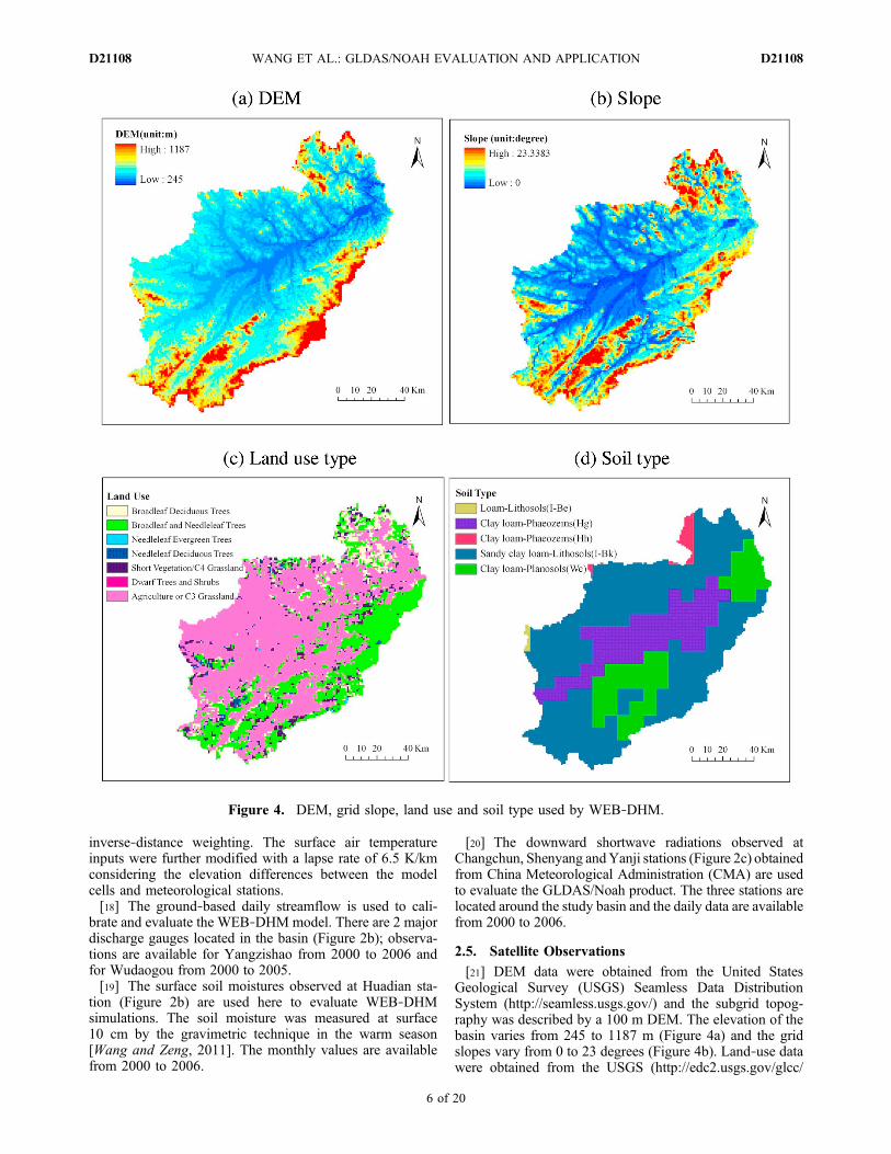
[21] DEM data were obtained from the United StatesGeological Survey (USGS) Seamless Data DistributionSystem (http://seamless.usgs.gov/) and the subgrid topog-raphy was described by a 100 m DEM. The elevation of thebasin varies from 245 to 1187 m (Figure 4a) and the gridslopes vary from 0 to 23 degrees (Figure 4b). Land‐use datawere obtained from the USGS (http://edc2.usgs.gov/glcc/

Figure 4. DEM, grid slope, land use and soil type used by WEB‐DHM.


6 of 20

glcc.php). The land‐use types have been reclassified to SiB2land‐use types for the study [Sellers et al., 1996a]. There are7 land‐use types, with agriculture or C3 grassland being themain type (Figure 4c). Soil data were obtained from theFood and Agriculture Organization (FAO) [2003] globaldata product. There are 5 kinds of soil in the basin, withsandy clay loam being the dominant type (Figure 4d).[22] Static vegetation parameters including morphologi-

cal, optical and physiological properties defined by Sellerset al. [1996b] were used in this study. Dynamic vegetationparameters including the leaf area index (LAI) and thefraction of photosynthetically active radiation (FPAR) ab-sorbed by the green vegetation canopy were obtained fromthe MOD15A2 1‐km 8‐day products [Myneni et al., 1997].They were downloaded through the Warehouse InventorySearch Tool (WIST, https://wist.echo.nasa.gov/~wist/api/imswelcome/). Data from 18 February 2000 are available.[23] LSTs obtained from the Moderate Resolution Imag-

ing Spectroradiometer (MODIS) aboard the Terra (EOSAM) satellite are used to validate the WEB‐DHM perfor-mance in representing the basin‐scale energy budget. TheMOD11A2 V5 1‐km 8‐day product [Wan, 2008], which isavailable from 5 March 2000, is used in this study. TheMODIS LSTs were observed during the day around 10:30and at night around 22:30 (both local time). These data weredownloaded through WIST.

2.6. The Operational Products

2.6.1. GLDAS/Noah[24] GLDAS [Rodell et al., 2004a] integrates satellite‐ and

ground‐based observations for parameterizing, forcing andconstraining a suite of offline (uncoupled) land surfacemodels. GLDAS aims to generate optimal fields of landsurface states and fluxes. Currently, GLDAS drives 4 LSMs:Mosaic [Koster and Suarez, 1992b], Noah [Chen et al., 1996;Koren et al., 1999; Ek et al., 2003; Betts et al., 1997], theCommunity Land Model (CLM) [Dai et al., 2003] and theVariable Infiltration Capacity (VIC) model [Liang et al.,1994]. In this study, we use the GLDAS/Noah Land Sur-face Model L4 3‐h 0.25‐degree × 0.25‐degree subsetted(GLDAS_NOAH025SUBP_3H) product (downloaded fromhttp://disc.sci.gsfc.nasa.gov/hydrology/data-holdings) sincethe high resolution data are more desirable for the basin‐scalestudy (14700 km2). The 3‐h GLDAS/Noah data are availablefrom 24 February 2000. The GLDAS data were described inmore detail by Rodell et al. [2004a] and Kato et al. [2007]. Atotal of 90 GLDAS/Noah cells are used for the study basin(see Figure 2b).[25] GLDAS precipitation is based on the NOAA Climate

Prediction Center’s operational global 2.5 degree 5‐dayMerged Analysis of Precipitation (CMAP) [Xie and Arkin,1997; Xie et al., 2003] which blends both satellite (IR andmicrowave) and gauge observations [Kato et al., 2007]. Byusing NOAA’s Global Data Assimilation System (GDAS)[Derber et al., 1991] precipitation analyses, GLDAS pre-cipitation is spatially and temporally downscaled [Rodellet al., 2004a; Kato et al., 2007]. GLDAS near‐surface airtemperature is obtained from NOAA’s GDAS operationalanalyses [Rodell et al., 2004a; Kato et al., 2007], and then itis adjusted adiabatically to the GLDAS elevation definitionbased on Cosgrove et al. [2003]. GLDAS Rsw,d and Rlw,d arederived from cloud and snow products of the U.S. Air Force

Weather Agency’s (AFWA) Agricultural Meteorologicalmodeling system (AGRMET) [Rodell et al., 2004a;Kato et al.,2007] by using AFWA‐supplied algorithms of Shapiro [1972]and Idso [1981], respectively.2.6.2. JRA‐25[26] Japan Meteorological Agency (JMA) and Central

Research Institute of Electric Power Industry (CRIEPI)jointly produced a Japanese 25‐year reanalysis product(JRA‐25 [Onogi et al., 2007]; http://jra.kishou.go.jp/)employing the JMA numerical assimilation and forecastsystem, with the goal of achieving high‐quality analysis inthe Asian region. The JRA‐25 forecast system employs alow‐resolution version of the operational JMA GlobalSpectral Model (GSM), which has a spectral resolution ofT106 (around 120 km horizontal grid size) and 40 verticallayers (L40) up to 0.4 hPa [Onogi et al., 2007; JapanMeteorological Agency (JMA), 2007, chapters 3.5, 3.11,and 4.2]. The assimilation system used in JRA‐25 isa 3‐dimentional variational (3D‐Var) analysis method with6‐h global data assimilation cycles [Onogi et al., 2007; JMA,2007, chapters 3.5, 3.11, and 4.2]. JRA‐25 data have beenrecorded every 6 h since 1979. Twelve JRA‐25 cells wereused in this study (Figure 2b).[27] The JRA‐25 variables are obtained from both model

simulations and data assimilation techniques. The Rsw,d

is calculated by a two‐stream formulation based on delta‐Eddington approximation [Joseph et al., 1976;Coakley et al.,1983; Briegleb, 1992]. The Rlw,d is modeled by a wide‐bandflux emissivity method for four spectral bands [Onogi et al.,2007]. The JRA‐25 assimilated variables include tempera-ture, wind speed, relative humidity, surface pressure at modelsurface, radiative brightness temperature and precipitablewater [Onogi et al., 2007]. The JRA‐25 Tair is assimilatedfrom radiosonde observations [Onogi et al., 2007]. The JRA‐25 precipitation is assimilated from microwave radiometersensor Special Sensor of Microwave Imager (SSM/I) onboard the Defense Meteorological Satellite Program (DMSP)satellite [Onogi et al., 2007]. The radiative brightness tem-perature (Tb) is assimilated from TIROS Operational VerticalSounder (TOVS). More detailed descriptions were providedby Onogi et al. [2007].

2.7. Evaluation Criteria

[28] Several statistical variables are used to evaluate theperformances of the WEB‐DHM, the GLDAS/Noah and theJRA‐25:

NS ¼ 1�Xni¼1

Xoi � Xsið Þ2=Xni¼1

Xoi � X 0

� �2; ð3Þ

RB ¼Xni¼1

Xsi �Xni¼1

Xoi

!=Xni¼1

Xoi

!� 100%; ð4Þ

MBE ¼Xni¼1

Xsi �Xni¼1

Xoi

!=n� 100%; ð5Þ

RMSE ¼ 1

n�Xni¼1

Xsi � Xoið Þ2" #1

2

; ð6Þ


7 of 20

where Xoi is the observed (ground‐based or satellite‐) value;Xsi is the simulated (WEB‐DHM, JRA‐25 or GLDAS/Noah)value; n is the total number of time series for comparison;and X 0 is the mean value of Xoi over the comparison period.NS refers to Nash Sutcliffe [Nash and Sutcliffe, 1970]. Thehigher NS is, the better the model performs. A perfect fitshould have a NS value equal to one. RB refers to relativebias. The lower RB, MBE or RMSE is, the better the modelperforms. A perfect fit should have RB, MBE or RMSEequal to zero. Since the observations are imperfect as well,the RB, MBE and RMSE should never be zero.

3. Results and Discussion

3.1. Evaluation of the WEB‐DHM for the Study Region

[29] The WEB‐DHM has been carefully calibrated withdaily discharges at Yangzishao station (Figure 2b) for 2001before its evaluation. The calibration has 2 steps. First, theinitial conditions were obtained by running the model sev-eral times with forcing data of year 2000 until a hydrologicalequilibrium was reached. Second, a trial and error method isused to optimize several parameters by matching the simu-lated and observed daily streamflow at Yangzishao station

(Figure 2b) using the data of year 2001. Both NS and RB(defined in equations (3) and (4)) are used to evaluate themodel performance. The calibrated parameters include sat-urated hydraulic conductivity for soil surface (Ks), hydraulicconductivity anisotropy ratio (anik), maximum surfacewater storage (Sstmax), and Van Genuchen’s parameter (aand n). The basin‐averaged parameters used in this modelare described in Table 2. An evaluation of the WEB‐DHMin simulating water and energy budgets is then undertakenusing ground‐based discharge at 2 major stream gauges(Yangzishao and Wudaogou, Figure 2b) and MODIS/TerraV5 8‐day LSTs [Wan, 2008] observations from 2000 to2006.3.1.1. Water Budget[30] Figure 5 shows the daily discharge (Q) at Yangzishao

and Wudaogou simulated by the WEB‐DHM comparedwith measured value (Figure 2b). Figure 5a reveals that boththe peak and base flows at Yangzishao are well reproducedfrom 2000 to 2006 with NS equal to 0.717 and RB equal to−6.37%. The simulated Q at Wudaogou (Figure 5b) from2000 to 2005 also agrees well with the observations withNS equal to 0.810 and RB equal to 5.60%.

Table 2. Basin‐Averaged Values of the Parameters Used in the Study

Symbol Parameters Basin‐Averaged Value Source

�s Saturated soil moisture content 0.48 FAO [2003]�r Residual soil moisture content 0.08 FAO [2003]a Van Genuchen’s parameter 0.02 Optimizationn Van Genuchen’s parameter 1.60 OptimizationDr(m) Root depth (D1 + D2) 1.17 Sellers et al. [1996b]Ks(mm/h) Saturated hydraulic conductivity for soil surface 37.81 Optimizationanik Hydraulic conductivity anisotropy ratio 53.83 OptimizationSstmax(mm) Maximum surface water storage 8.00 Optimization

Figure 5. Observed and WEB‐DHM simulated streamflows at (a) Yangzishao and (b) Wudaogoustation from 2000 to 2006.


8 of 20

[31] Figure 6 plots the monthly and 6‐years (2000–2005)mean monthly variations in Q simulated by the WEB‐DHMand compares them with observations. Time series ofmonthly observed precipitation (P), simulated evapotrans-piration (ET), and observed and simulated Q for theupstream of the Wudaogou gauge are shown in Figure 6a.The Q of WEB‐DHM simulations agree fairly well withobservations with RB and NS equal to 5.60% and 0.900,respectively. Figure 6b shows the 6‐years (2000–2005)mean monthly time series of water balance components,showing overall good agreement of Q between WEB‐DHMoutputs and observations with RB and NS equal to 5.60%and 0.937, respectively.3.1.2. Energy Budget[32] Figure 7 shows the 8‐day LSTs of the WEB‐DHM

simulation (LST_WEB‐DHM) and MODIS/Terra product(LST_MODIS) from March 2000 to December 2006 in thetime series. The valid time of MODIS LSTs for this regionis around 10:30 and 22:30 at local time. The simulationresults show that LSTs are well reproduced except thatLST_WEB‐DHM is slightly greater than LST_MODIS withMBE equal to 2.17 K during the day (Figure 7a) and MBEequal to 2.50 K at night (Figure 7b). The scatterplots ofLSTs are also given for both day and night (Figures 7c and7d), with the correlation coefficient (R) equal to 0.9856 and0.9896 for day and night, respectively. These results con-firm the general good performance of the WEB‐DHM insimulating basin‐averaged LSTs.[33] Figure 8 shows the seasonal spatial distribution dif-

ferences of the daytime LSTs between model simulations andMODIS/Terra observations (WEB‐DHM minus MODIS).In general, the spatial variations in LSTs are well simulatedby the WEB‐DHM. The basin average values of LSTs are287.49 K, 298.40 K, 285.31 K and 261.46 K for MODIS/Terra, while they are 290.16 K, 302.84 K, 288.09 K and259.83 K for WEB‐DHM. The LSTs of WEB‐DHM are

overestimated in spring (2.66 K), summer (4.44 K) andautumn (2.78 K) while they are underestimated in winter(−1.62 K). The uncertainty may be attributed to the homo-geneous lapse rate of temperature (g = 6.5 K/km) used inthis study for modifying Tair, since g is variable with season,altitude and region. The uncertainty in linear calculation ofgreen vegetation coverage (V, see equation (2)) also affectsthe simulation of soil surface temperature (Tg) and LST.3.1.3. Summary[34] The objective of section 3.1 was to validate the

WEB‐DHM in simulating spatially integrated streamflowsand the basin‐wide LSTs. In summary, the WEB‐DHM hasdemonstrated good accuracy in representing the water andenergy cycles in the upper Second Songhua River basin.This is the first study that WEB‐DHM is evaluated withcomprehensive observations in a semi‐arid environment.Results show that the outputs from the calibrated WEB‐DHM are reliable and thereby can be used to evaluate otheroperational products (e.g., GLDAS/Noah).

3.2. Comparing GLDAS Forcing Data With in SituObservations, JRA‐25, and WEB‐DHM

3.2.1. Daily Scale[35] Daily precipitation (P) and the near‐surface air tem-

perature (Tair) obtained from GLDAS and JRA‐25 arecompared with ground‐based observations in Figure 9.[36] Figures 9a and 9b plot the basin‐averaged daily P

used in GLDAS and JRA‐25 against ground‐based obser-vation. The R, MBE and RMSE between GLDAS resultsand observations are 0.7599, 0.06 mm/day and 3.48 mm/day, respectively, while they are 0.5851, 0.58 mm/day and6.39 mm/day between JRA‐25 results and observations. Allthe statistics show that GLDAS is more consistent thanJRA‐25 with the observations. The rough spatial resolutionof JRA‐25 data (about 1.125 degrees) may miss localizedprecipitation events. Many studies [e.g., Gottschalck et al.,

Figure 6. (a) Time series and (b) 6‐year inter‐annual mean monthly precipitation (P), WEB‐DHM sim-ulated evapotranspiration (ET_WEB‐DHM), observed discharge (Q_obs) and WEB‐DHM simulated dis-charge (Q_WEB‐DHM) for the Wudaogou subbasin from 2000 to 2005.


9 of 20

2005; Zaitchik et al., 2010] have shown that the precipita-tion used in GLDAS has low bias relative to a number ofearlier precipitation data sets that were used during devel-opment of LSMs. The results obtained in this study confirmthe relatively good accuracy of GLDAS precipitation.[37] Figures 9c and 9d plot the daily Tair used in GLDAS

and JRA‐25 and compare them with the ground‐based ob-servations. Tair is well represented by GLDAS and JRA‐25with R exceeding 0.9900 in both cases. The MBE and RMSEfor GLDAS are −0.40 K and 1.70 K, respectively, while forJRA‐25, the MBE and RMSE are 1.07 K and 2.09 K,respectively.3.2.2. Monthly Scale[38] Figures 10a and 10b compare monthly precipitation

(P) and near‐surface air temperature (Tair) between GLDAS,JRA‐25 and ground‐based observations in time series.Figures 10c and 10d compare monthly downward shortwave(Rsw,d) and longwave radiation (Rlw,d) between GLDAS,JRA‐25 and WEB‐DHM in time series. Figures 11a–11hare the corresponding scatterplots of Figures 10a–10d.[39] Figure 10a reveals that GLDAS precipitation agrees

fairly well with the observed precipitation, while JRA‐25precipitation has a large positive bias. The correspondingscatterplots (Figures 11a and 11b) show that the MBE is1.86 mm/month between GLDAS and the observations, and

this is much lower than that between JRA‐25 and theobservations. It has been reported [Yang et al., 2009b; Yangand Koike, 2008] that the accumulated precipitation amountof JRA‐25 is greater than that observed while GLDASperformed better than JRA‐25 in a study of the CentralTibetan Plateau and a Mongolian semiarid region. Thisresult further demonstrates the accuracy of precipitationused in GLDAS. This can be explained by the differentprecipitation products used in GLDAS and JRA‐25. TheGLDAS precipitation is based on the CMAP product [Xieand Arkin, 1997; Xie et al., 2003] which merged raingauge observations and five sets of satellite estimatesderived from the infrared (IR), outgoing longwave radiation(OLR), Microwave Sounding Unit (MSU), microwave(MW) scattering, and emission from SSM/I, while the JRA‐25 precipitation is assimilated from satellite (SSM/I). Asprevious studies mentioned [Xie and Arkin, 1997; Xie et al.,2003; Gottschalck et al., 2005], the rain gauge and satellitemerged precipitation tends to produce relatively betteranalysis of global precipitation than satellite‐only estimatesbecause it takes advantage of the strength of each individualsource.[40] Figure 10b shows the Tair of GLDAS, JRA‐25 and

ground‐based observations. There are no obvious differ-ences except that JRA‐25 gives slightly higher values than

Figure 7. Comparison of 8‐daily LSTs betweenWEB‐DHM simulations (Tsim) andMODIS observations(Tobs) during (a, c) daytime and (b, d) nighttime averaged for the basin from March 2000 to December2006. Time series (Figures 7a and 7b) and scatterplots (Figures 7c and 7d).


10 of 20

GLDAS and the observations in winter. The small MBEseen in Figures 11c and 11d (−0.40 K and 1.07 K) and thesmall RMSE (0.95 K and 1.68 K) also indicate good con-sistency in Tair between simulations and observations.[41] Figure 10c shows the level of downward shortwave

radiation (Rsw,d) for GLDAS, the WEB‐DHM and JRA‐25.It is clear that Rsw,d for GLDAS is obviously higher than thatof the WEB‐DHM and JRA‐25 in summer. Figures 11e and11f show that MBE between the WEB‐DHM and GLDASis −10.83 W/m2 and that between JRA‐25 and GLDAS is−11.01 W/m2.

[42] The Rsw,d of GLDAS is further investigated by usingground‐based observations. Table 3 compares Rsw,d atChangchun, Shenyang, Yanji stations (Figure 2c) and studybasin. GLDAS overestimates Rsw,d significantly during warmseason (from April to August) with MBE larger than52.66 W/m2 and during cold season (from September toMarch) with MBE larger than 15.14 W/m2 for all the threestations (Table 3). Averaged at the whole basin, GLDASoverestimates Rsw,d with MBE equal to 54.61 W/m2 and16.95W/m2 inwarm and cold seasons, respectively (Table 3).

Figure 8. The differences of daytime LSTs (unit: K) betweenWEB‐DHMandMODIS/Terra in (a) Spring(MAM), (b) Summer (JJA), (c) Autumn (SON), and (d) Winter (DJF) fromMarch 2000 to December 2006.

Figure 9. Scatterplots of daily values averaged at the whole basin between ground‐based observationsand GLDAS and JRA‐25 products from March 2000 to December 2006: (a and b) precipitation and (c andd) near‐surface air temperature.


11 of 20

[43] Figure 10d shows the level of downward longwaveradiation (Rlw,d) for GLDAS, WEB‐DHM and JRA‐25. TheRlw,d is consistent among the three models, where the WEB‐DHM uses the same data as JRA‐25. Figures 11g and 11hshow that R is as high as 0.9910 between GLDAS and theWEB‐DHM.3.2.3. Summary[44] The objective of section 3.2 was to evaluate the

accuracy of the GLDAS atmospheric forcing data (P, Tair,Rsw,d, and Rlw,d) comparing with JRA‐25 (P, Tair, Rsw,d,and Rlw,d), and in situ (P, Tair, and Rsw,d) observations. Insummary, the P, Tair (daily and monthly) and Rlw,d ofGLDAS agreed well with observed P, Tair and JRA‐25 Rlw,d,while the GLDAS Rsw,d (monthly) shown larger valuescompared with observed Rsw,d. In general, the GLDASatmospheric forcing data show 3 advantages: (1) the highresolution of GLDAS product with temporal scale of 3‐h andspatial scale of 0.25‐degree; (2) the reliability of GLDASforcing especially its precipitation (both daily and monthly);and (3) GLDAS is available at the global scale. Thesefindings are particularly important for ungauged or poorly

gauged river basins, due to their forcing data problems[e.g., Qian et al., 2006].

3.3. Comparing GLDAS/Noah Outputs With JRA‐25and WEB‐DHM

3.3.1. Daily Scale[45] Figure 12 shows the daily LST and ET as time series

and scatterplots. In sections 3.3.1 and 3.3.2, the MBE andRMSE are calculated by comparingWEB‐DHM (or JRA‐25)simulations with GLDAS/Noah outputs. It should be men-tioned that these statistical values (MBE and RMSE) do notnecessarily represent model errors, but examine the differ-ences among different models’ outputs.[46] Daily LSTs (Figure 12a) obtained with GLDAS/Noah

and the WEB‐DHM are quite comparable, with R, MBEand RMSE being 0.9764, 1.26 K and 3.59 K, respectively(Figure 12c). The underestimation of LST peak values byGLDAS/Noah has been reported [Yang et al., 2009a] andattributed to overestimation of the thermal roughness length(z0h; discussion of z0h is given in section 3.3.2).

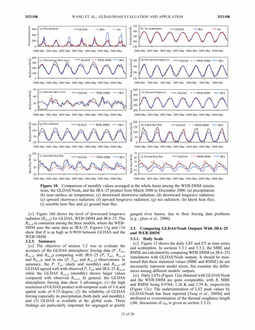
Figure 10. Comparison of monthly values averaged at the whole basin among the WEB‐DHM simula-tions, the GLDAS/Noah, and the JRA‐25 product from March 2000 to December 2006: (a) precipitation;(b) near‐surface air temperature; (c) downward shortwave radiation; (d) downward longwave radiation;(e) upward shortwave radiation; (f) upward longwave radiation; (g) net radiation; (h) latent heat flux;(i) sensible heat flux and (j) ground heat flux.


12 of 20

[47] As shown in Figure 12b, the daily ET variation is ingood agreement among the three models with R being0.9121 between WEB‐DHM and GLDAS/Noah and 0.9110between JRA‐25 and GLDAS/Noah. However, it is greaterin summer for GLDAS/Noah than for the WEB‐DHM andJRA‐25. The MBE is −0.39 mm/day between WEB‐DHMand GLDAS/Noah and −0.28 mm/day between JRA‐25 andGLDAS/Noah, respectively. Different net radiations are

mainly responsible for these differences, which is elaboratedon in the following section on latent heat flux.3.3.2. Monthly Scale[48] Figures 10e–10j and 11i–11t show the model output

variables of GLDAS/Noah, the WEB‐DHM and JRA‐25 astime series and scatterplots, respectively. The output vari-ables include upward shortwave radiation (Rsw,u), upward

Figure 11. Same as Figure 10, but in scatterplots. MBE and RMSE are calculated by comparing they axis with the x axis values.


13 of 20

longwave radiation (Rlw,u), net radiation (Rn), latent heatflux (LE), sensible heat flux (H) and ground heat fluxes (G).[49] The upward shortwave radiation (Rsw,u, Figure 10e)

is well reproduced although there are slight biases. Theextremely low values for GLDAS/Noah initially (Figure 10e)is mainly due to the uncertainty of albedo. R (Figures 11iand 11j) increases to 0.7773 and 0.7153 (data not shown)when the data for 2000, which are improperly initialized, areexempted. MBE decreases to −0.67 W/m2 and −0.01 W/m2

concurrently (data not shown). These results indicate thatRsw,u can be estimated well by all three models.

Table 3. Statistics of Rsw,d Between the GLDAS and in SituObservations for Warm Season (WS) and Cold Season (CS) FromMarch 2000 to December 2006

Meteorological Gauge

CS (April –August)

WS (September –March)

MBE RMSE MBE RMSE

Changchun (W/m2) 15.14 19.75 56.94 60.56Shenyang (W/m2) 25.63 28.13 65.43 70.56Yanji (W/m2) 19.61 22.94 52.66 57.98Basin average (W/m2) 16.95 20.54 54.61 59.45

Figure 12. Comparison of daily values averaged at the whole basin, among the WEB‐DHM simulations,the GLDAS/Noah, and the JRA‐25 product from March 2000 to December 2006: (a) land surface tem-perature (time series); (b) evapotranspiration (time series); (c) land surface temperature (scatterplots), and(d, e) evapotranspiration (scatterplots).


14 of 20

[50] The upward longwave radiation (Rlw,u, Figure 10f) iswell simulated by all three models, except that the WEB‐DHM gives slightly higher values for summer. Both theWEB‐DHM and the Noah LSM calculate Rlw,u from theLST using the Stefan–Boltzmann law and the two modelsassume blackbody radiation (i.e., " = 1) [Hong and Kim,2008]. Therefore, the higher level of Rlw,u of the WEB‐DHM is mainly due to its higher LSTs (Figures 12a and12c). The high R (0.9978 and 0.9976, Figures 11k and 11l)reveals that the three models reproduce the Rlw,u variationfairly well.[51] Figure 10g compares the net radiation (Rn) in the time

series. There is distinctive divergence in summer withGLDAS/Noah giving a higher level than JRA‐25 and theWEB‐DHM. The higher level of Rsw,d of GLDAS/Noahmostly accounts for this discrepancy. Although MBE andRMSE are as large as −31.32 W/m2 and −27.46 W/m2

(Figures 11m and 11n), R is quite high in both comparisons(0.9814 and 0.9876), indicating that all the three modelscapture the seasonal variations.[52] Figure 10h compares latent heat flux (LE). There are

conspicuous divisions for the wet seasons with GLDAS/Noah giving larger peak values than the WEB‐DHM andJRA‐25. It has been reported that Rn plays a more importantrole than soil moisture in controlling evaporation during wetseasons [Yang et al., 2009a]. Kato et al. [2007] also pointedout that a wetter condition and more radiation input can leadto a wider possible range of LE. Therefore, the LE ofGLDAS/Noah in summer is greater according to its higherlevel of Rn (Figure 10g). However, for dry seasons, ET ismainly controlled by soil surface resistance (rsoil) rather thannet radiation [Yang et al., 2009a]. rsoil is an empirical term torepresent the impedance of the soil pores to exchanges ofwater vapor between the top layer soil and the immediatelyoverlying air [Sellers et al., 1996a; van de Griend and Owe,1994]. Because all these models include rsoil [Sellers et al.,1996a; Betts et al., 1997; Ek et al., 2003], the simulatedphases of the monthly LE are similar among the threemodels in dry seasons. There is a typical drier case in 2002(see Figure 5), and the comparison of LE in 2002 shows betterconsistency than comparisons for other years (Figure 10h). Ingeneral, the three estimations of LE reveal good agreementswith R equal to 0.9732 between the WEB‐DHM and theGLDAS/Noah and 0.9583 between the JRA‐25 and theGLDAS/Noah (Figures 11o and 11p).[53] Figure 10i shows the variation in the sensible heat

flux (H). WEB‐DHM gives lower values than GLDAS/Noah and JRA‐25 but reproduces the seasonal variationsfairly well. The MBE values are −18.35 W/m2 and −2.79 W/m2 for the WEB‐DHM and JRA‐25 comparing withGLDAS/Noah (Figures 11q and 11r). Yang et al. [2009a]and Hong and Kim [2010] also found larger H for NoahLSM comparing with SiB2 and observations.[54] In the Noah LSM, the sensible heat flux (H) is cal-

culated through the bulk heat transfer equation [Chen et al.,1997]:

H ¼ �CPChjUaj �s � �að Þ; ð7Þ

where r is the air density; Cp is the specific heat capacityof air at constant pressure; Ch is the surface exchangecoefficient for heat; Ua is the wind speed; �a is the air

potential temperature; �s is the corresponding variable atthe surface.[55] Ch is a crucial parameter which governs the total

surface heat fluxes [Chen and Zhang, 2009; Chen et al.,2010]. Recent studies [e.g., Chen and Zhang, 2009] showthat the Noah LSM overestimates Ch (implying too efficientcoupling) for short vegetation (e.g., crops, grass, shrubs,sparsely vegetated area) and underestimates it (implyinginsufficient coupling) for tall vegetation (e.g., forests). Thisproblem is caused by the treatment of roughness length forheat (z0h) (or thermal roughness length) in the Noah LSM.z0h is the height at which the extrapolated air temperatureequals the actual surface skin (radiative) temperature and itplays a critical role in estimating the total surface heat fluxesfrom the surface to the atmosphere [e.g., Verhoef et al.,1997; Yang et al., 2008; Chen and Zhang, 2009]. NoahLSM uses Zilitinkevich’s [1995] scheme to calculate z0h,and this scheme possibly overestimates z0h in bare‐soil orsparsely vegetated area [e.g., LeMone et al., 2008; Yanget al., 2008]. According to Monin‐Obukhov similarity the-ory based stability functions of Paulson [see Paulson, 1970;Chen et al., 1997], the uncertainty of z0h results in uncer-tainty of Ch.[56] In the study basin (Figure 4c), most of the region

(around 60%) is covered by agriculture or C3 grassland(short vegetation) which implies the Ch of Noah is possiblyoverestimated (z0h overestimated). A higher Ch in equation(7) enhances the transport of heat H (Figures 10i, 11q,and 11r) from the surface to the atmosphere, resulting in adecrease in LST (Figures 12a and 12c) [LeMone et al.,2008].[57] All three models reproduce similar monthly varia-

tions in ground heat fluxes (G, Figure 10j), with the WEB‐DHM giving a larger amplitude. However, the annual meanG of GLDAS/Noah is nearly the same as that of the WEB‐DHM (Figure 11s). The same results were obtained by Hongand Kim [2010] when comparing SiB2 and Noah LSM forthe Tibetan plateau, which is due to SiB2 having a smallersoil heat capacity than Noah. Consequently, the range of Gis wider in the WEB‐DHM than that in GLDAS/Noah.Meanwhile, the lower peak value of LSTs (Figure 12a) inGLDAS/Noah would directly result in lower G, which isalso consistent with the higher H (Figure 10i).[58] Soil moisture (SM) is a highly variable parameter in

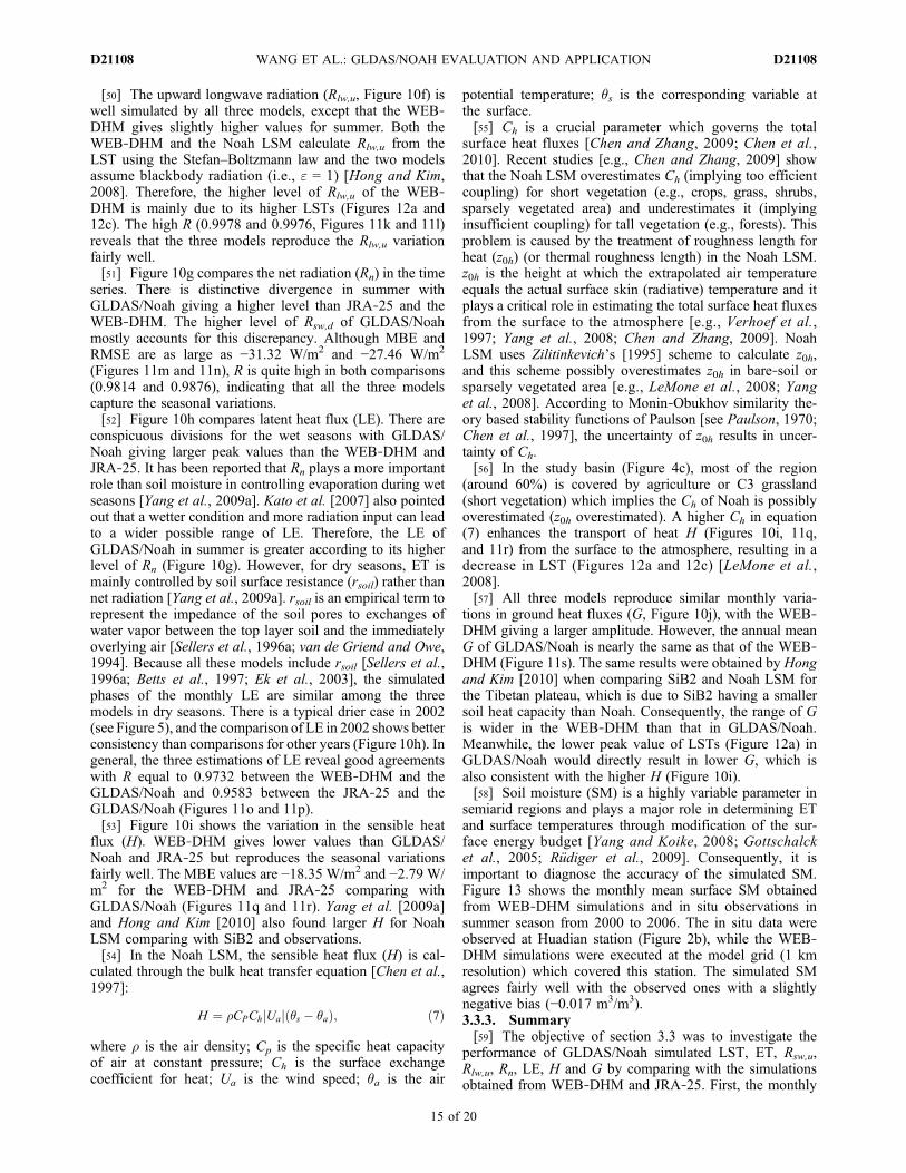
semiarid regions and plays a major role in determining ETand surface temperatures through modification of the sur-face energy budget [Yang and Koike, 2008; Gottschalcket al., 2005; Rüdiger et al., 2009]. Consequently, it isimportant to diagnose the accuracy of the simulated SM.Figure 13 shows the monthly mean surface SM obtainedfrom WEB‐DHM simulations and in situ observations insummer season from 2000 to 2006. The in situ data wereobserved at Huadian station (Figure 2b), while the WEB‐DHM simulations were executed at the model grid (1 kmresolution) which covered this station. The simulated SMagrees fairly well with the observed ones with a slightlynegative bias (−0.017 m3/m3).3.3.3. Summary[59] The objective of section 3.3 was to investigate the

performance of GLDAS/Noah simulated LST, ET, Rsw,u,Rlw,u, Rn, LE, H and G by comparing with the simulationsobtained from WEB‐DHM and JRA‐25. First, the monthly


15 of 20

Rn and LE (and daily ET) estimated by GLDAS/Noah in wetseasons were higher than those estimated by the WEB‐DHM and JRA‐25. Second, the peak values of GLDAS/Noah daily LSTs (monthly H) were slightly lower (higher)than WEB‐DHM simulations. Third, the Rsw,u and Rlw,u

were well estimated by all three models. Fourth, GLDAS/Noah gave smaller range of monthly G values than theWEB‐DHM. The performance of the simulated water andenergy fluxes by GLDAS/Noah would provide referencesfor other semi‐arid river basins.

3.4. Application of the GLDAS Forcing Data in DrivingBasin Scale Distributed Hydrological Model

[60] In the above study, WEB‐DHM was driven by theobservation‐based meteorological data, which may beunavailable or very scarce in many river basins (e.g.,ungauged basins). It will be helpful if the GLDAS forcingdata could be applicable to the basin–scale studies as theinputs for distributed hydrological models (DHMs). There-fore, as a demonstration, this section we will examine theapplicability of GLDAS global forcing data to the study basinby driving the WEB‐DHM using GLDAS forcing data.3.4.1. Experiment Results[61] Table 4 lists the monthly Rsw,d of GLDAS and in situ

observation and their differences. Two conclusions can bedrawn from this comparison: (1) GLDAS overestimates Rsw,d

for each month; (2) the largest differences happen from Aprilto August. Due to the overestimation of Rsw,d for GLDASproduct, it is necessary to correct the GLDAS Rsw,d by usingin situ observations. Two different correction functions arederived in warm season (WS, from April to August) and coldseason (CS, from September to March), respectively.

Warm season : Rsw;d;rev ¼ 0:7823� Rsw;d ; ð8Þ

Cold season : Rsw;d;rev ¼ 0:8563� Rsw;d ; ð9Þ

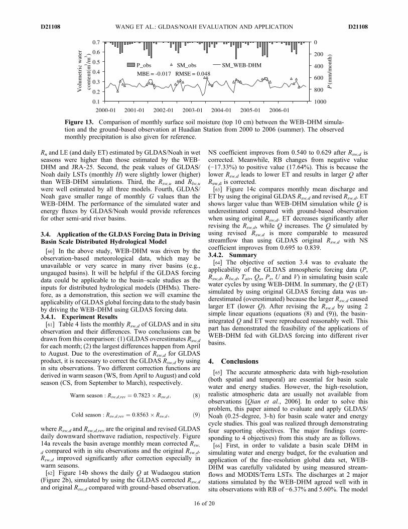
where Rsw,d and Rsw,d,rev are the original and revised GLDASdaily downward shortwave radiation, respectively. Figure14a reveals the basin average monthly mean corrected Rsw,

d compared with in situ observations and the original Rsw,d.Rsw,d improved significantly after correction especially inwarm seasons.[62] Figure 14b shows the daily Q at Wudaogou station

(Figure 2b), simulated by using the GLDAS corrected Rsw,d

and original Rsw,d compared with ground‐based observation.

NS coefficient improves from 0.540 to 0.629 after Rsw,d iscorrected. Meanwhile, RB changes from negative value(−17.33%) to positive value (17.64%). This is because thelower Rsw,d leads to lower ET and results in larger Q afterRsw,d is corrected.[63] Figure 14c compares monthly mean discharge and

ET by using the original GLDAS Rsw,d and revised Rsw,d. ETshows larger value than WEB‐DHM simulation while Q isunderestimated compared with ground‐based observationwhen using original Rsw,d. ET decreases significantly afterrevising the Rsw,d, while Q increases. The Q simulated byusing revised Rsw,d is more comparable to measuredstreamflow than using GLDAS original Rsw,d with NScoefficient improves from 0.695 to 0.839.3.4.2. Summary[64] The objective of section 3.4 was to evaluate the

applicability of the GLDAS atmospheric forcing data (P,Rsw,d, Rlw,d, Tair, Qa, Ps, U and V) in simulating basin scalewater cycles by using WEB‐DHM. In summary, the Q (ET)simulated by using original GLDAS forcing data was un-derestimated (overestimated) because the larger Rsw,d causedlarger ET (lower Q). After revising the Rsw,d by using 2simple linear equations (equations (8) and (9)), the basin‐integrated Q and ET were reproduced reasonably well. Thispart has demonstrated the feasibility of the applications ofWEB‐DHM fed with GLDAS forcing into different riverbasins.

4. Conclusions

[65] The accurate atmospheric data with high‐resolution(both spatial and temporal) are essential for basin scalewater and energy studies. However, the high‐resolution,realistic atmospheric data are usually not available fromobservations [Qian et al., 2006]. In order to solve thisproblem, this paper aimed to evaluate and apply GLDAS/Noah (0.25‐degree, 3‐h) for basin scale water and energycycle studies. This goal was realized through demonstratingfour supporting objectives. The major findings (corre-sponding to 4 objectives) from this study are as follows.[66] First, in order to validate a basin scale DHM in

simulating water and energy budget, for the evaluation andapplication of the fine‐resolution global data set, WEB‐DHM was carefully validated by using measured stream-flows and MODIS/Terra LSTs. The discharges at 2 majorstations simulated by the WEB‐DHM agreed well with insitu observations with RB of −6.37% and 5.60%. The model

Figure 13. Comparison of monthly surface soil moisture (top 10 cm) between the WEB‐DHM simula-tion and the ground‐based observation at Huadian Station from 2000 to 2006 (summer). The observedmonthly precipitation is also given for reference.


16 of 20

also reproduced LSTs well in terms of both the time seriesand seasonal spatial distribution when compared withMODIS/Terra V5 LSTs despite the WEB‐DHM givingslightly larger peak values. From this validation, it wasconcluded that the WEB‐DHM is able to predict water andenergy fluxes accurately over the semi‐arid river basin (theupper Second Songhua River basin).

[67] Second, in order to evaluate the accuracy of theGLDAS atmospheric forcing data (P, Tair, Rsw,d, and Rlw,d),they were compared with in situ observations (P, Tair, Rsw,d),and JRA‐25 product (P, Tair, Rsw,d, and Rlw,d). The P ofGLDAS was found to be more accurate on a monthly scalethan on a daily scale by comparing with ground‐basedobservations, but in both cases, GLDAS performed betterthan JRA‐25, which has coarse spatial resolution. Good

Figure 14. The correction results of GLDAS downward shortwave radiation (Rsw,d): (a) the correctedmonthly Rsw,d averaged at the whole basin compared with in situ observation and original GLDASRsw,d from March 2000 to December 2006, (b) simulated daily discharge (Q), and (c) inter‐annual meanmonthly Q, and evapotranspiration (ET) by using the original and the corrected GLDAS/Noah forcingdata for the Wudaogou subbasin from February 2000 to December 2005.

Table 4. Comparison of Monthly Rsw,d Between GLDAS/Noah and in Situ Observation From 2000 to 2006a

Month Jan Feb Mar Apr May Jun

GLDAS/Noah (W/m2) 82.88 119.68 172.62 212.33 245.26 246.82Observation (W/m2) 66.87 105.48 142.25 164.30 193.02 190.34Difference (W/m2) 16.02 14.20 30.37 48.03 52.25 56.48

Month Jul Aug Sep Oct Nov Dec

GLDAS/Noah (W/m2) 229.59 210.35 176.58 124.92 84.77 71.39Observation (W/m2) 172.87 168.59 152.30 109.31 75.02 60.62Difference (W/m2) 56.72 41.76 24.28 15.61 9.75 10.77

aThe bold values from April to August mean relatively larger differences than those for other months.


17 of 20

correlation was found for Tair when comparing GLDAS toground‐based observations and JRA‐25 on both dailyand monthly scales. GLDAS also had good performancefor monthly Rlw,d. However, GLDAS gave a higher level formonthly Rsw,d than the in situ observation.[68] Third, in order to analyze the performance of the

GLDAS/Noah outputs (LST, ET, Rsw,u, Rlw,u, Rn, LE, H,and G), they were compared with WEB‐DHM simulationsand JRA‐25 product. Because the roughness length for heat(z0h) in Noah LSM was improper treated [e.g., LeMoneet al., 2008; Yang et al., 2008], Noah overestimated Ch

(implying too efficient coupling) for short vegetations (e.g.,crops, sparsely vegetated area) [e.g., Chen and Zhang, 2009]which are the dominant land use type in the study basin. Ahigher Ch enhanced the transport of heat H from the surfaceto the atmosphere, resulting in a decrease in LST [LeMoneet al., 2008]. Therefore, GLDAS/Noah gave highermonthly H than the WEB‐DHM and JRA‐25, while thepeak values of GLDAS/Noah daily LSTs were lower thanWEB‐DHM. Because of the lower LST peaks for theGLDAS/Noah, the level of GLDAS/Noah monthly Rlw,u

was higher in summer, while the monthly Rsw,u was wellestimated by all three models. The higher level of monthlyRsw,d of GLDAS/Noah resulted in Rn being at a slightlyhigher level than that for the WEB‐DHM and JRA‐25.Daily ET and monthly LE estimated by GLDAS/Noah inwet seasons were higher than those estimated by the WEB‐DHM and JRA‐25 owing to the higher level of Rn. GLDAS/Noah gave a smaller range of monthly G values than theWEB‐DHM owing to the greater soil heat capacity used inNoah and a lower peak value of LSTs in GLDAS/Noah thanin the WEB‐DHM. The monthly mean surface 10 cm SMestimated by WEB‐DHM performed well compared with insitu observations at Huadian station.[69] Finally, in order to evaluate the applicability of

GLDAS global forcing data (P, Rsw,d, Rlw,d, Tair, near‐surfacespecific humidity, surface pressure and wind speed) forbasin scale water resources management, the WEB‐DHMwas driven by using original and revised GLDAS forcingdata. Because GLDAS overestimated Rsw,d, the ET wasoverestimated while discharge was underestimated whenusing original GLDAS forcing data. The performance ofsimulated ET and discharge were improved when revise theRsw,d by using simple linear equations for warm and coldseasons, respectively.[70] These results confirm the capability of WEB‐DHM

and GLDAS/Noah in modeling basin‐wide water and energybudget in semiarid basin. Meanwhile, GLDAS can givereliable fine‐resolution global atmospheric forcing datawhich are essential for WEB‐DHM (or other DHMs). Thecombination of GLDAS with WEB‐DHM (or other DHMs)would benefit more basins around the world (e.g., for waterresources management). Given the increasing world widewater resources problems [Intergovernmental Panel onClimate Change, 2007], further efforts are needed todeepen this combination.

[71] Acknowledgments. The authors are grateful to three reviewswhose comments are helpful to improve the quality of this paper. Theauthors also gratefully acknowledge financial support provided by theChina Scholarship Council. This study was supported by National NaturalScience Foundation of China (grant 50809010). Parts of this work were

also supported by grants from the Ministry of Education, Culture, Sports,Science and Technology of Japan. GLDAS data used in this study wereacquired as part of a mission of NASA’s Earth Science Division andarchived and distributed by the Data and Information Services Center ofGoddard Earth Sciences. The authors sincerely thank Hiroko Kato Beau-doing, who provided guidance in extracting GLDAS data. The JRA‐25 datasets used in this study are from the JRA‐25 long‐term reanalysis coopera-tive research project carried out by the Japan Meteorological Agency andthe Central Research Institute of Electric Power Industry.

ReferencesAsian Development Bank (2002), Report and recommendation of the pres-ident to the board of directors on a proposed loan to the People’s Repub-lic of China for the Songhua River flood management sector project, Rep.RRP: PRC 33437, Manila.

Bertoldi, G., C. Notarnicola, G. Leitinger, S. Endrizzi, M. Zebisch, S. D.Chiesa, and U. Tappeiner (2010), Topographical and ecohydrologicalcontrols on land surface temperature in an alpine catchment, Ecohydrology,3(2), 189–204, doi:10.1002/eco.129.

Betts, A. K., F. Chen, K. E. Mitchell, and Z. I. Janjic (1997), Assessmentof the land surface and boundary layer models in two operationalversions of the NCEP Eta model using FIFE data, Mon. Weather Rev.,125, 2896–2916, doi:10.1175/1520-0493(1997)125<2896:AOTLSA>2.0.CO;2.

Bowling, L. C., et al. (2003), Simulation of high‐latitude hydrological pro-cesses in the Torne–Kalix basin: PILPS Phase 2(e): 1: Experimentdescription and summary intercomparisons, Global Planet. Change,38(1–2), 1–30, doi:10.1016/S0921-8181(03)00003-1.

Briegleb, B. P. (1992), Delta‐Eddington approximation for solar radiationin the NCAR Community Climate Model, J. Geophys. Res., 97(D7),7603–7612, doi:10.1029/92JD00291.

Chen, F., and J. Dudhia (2001), Coupling an advanced land‐surface/hydrology model with the Penn State/NCARMM5 modeling system. PartI: Model description and implementation, Mon. Weather Rev., 129(4),569–585, doi:10.1175/1520-0493(2001)129<0569:CAALSH>2.0.CO;2.

Chen, F., and Y. Zhang (2009), On the coupling strength between the landsurface and the atmosphere: From viewpoint of surface exchange coeffi-cients, Geophys. Res. Lett., 36, L10404, doi:10.1029/2009GL037980.

Chen, F., K. Mitchell, J. Schaake, Y. Xue, H.‐L. Pan, V. Koren, Q. Y.Duan, M. Ek, and A. Betts (1996), Modeling of land surface evaporationby four schemes and comparison with FIFE observations, J. Geophys.Res., 101(D3), 7251–7268, doi:10.1029/95JD02165.

Chen, F., Z. Janjic, and K. Mitchell (1997), Impact of atmospheric surface‐layer parameterizations in the new land‐surface scheme of the NCEPMesoscale Eta Model, Boundary Layer Meteorol., 85, 391–421,doi:10.1023/A:1000531001463.

Chen, Y., K. Yang, D. Zhou, J. Qin, and X. Guo (2010), Improving theNoah land surface model in arid regions with an appropriate parameteri-zation of the thermal roughness length, J. Hydrometeorol., 11, 995–1006,doi:10.1175/2010JHM1185.1.

Coakley, J. A., R. D. Cess, and F. B. Yurevich (1983), The effect of tropo-spheric aerosols on the Earth’s radiation budget: A parameterization forclimate models, J. Atmos. Sci., 40(1), 116–138, doi:10.1175/1520-0469(1983)040<0116:TEOTAO>2.0.CO;2.

Cosgrove, B. A., et al. (2003), Real‐time and retrospective forcing inthe North American Land Data Assimilation System (NLDAS) project,J. Geophys. Res., 108(D22), 8842, doi:10.1029/2002JD003118.

Dai, Y., et al. (2003), The Common LandModel (CLM), Bull. Am. Meteorol.Soc., 84(8), 1013–1023, doi:10.1175/BAMS-84-8-1013.

Derber, J. C., D. F. Parrish, and S. J. Lord (1991), The new global opera-tional analysis system at the National Meteorological Center, WeatherForecast., 6, 538–547, doi:10.1175/1520-0434(1991)006<0538:TNGOAS>2.0.CO;2.

Dirmeyer, P. A., A. J. Dolman, and N. Sato (1999), The pilot phase of theGlobal Soil Wetness Project, Bull. Am. Meteorol. Soc., 80(5), 851–878,doi:10.1175/1520-0477(1999)080<0851:TPPOTG>2.0.CO;2.

Ek, M. B., K. E. Mitchell, Y. Lin, E. Rogers, P. Grunmann, V. Koren,G. Gayno, and J. D. Tarpley (2003), Implementation of Noah land sur-face model advances in the National Centers for Environmental Predic-tion operational mesoscale Eta model, J. Geophys. Res., 108(D22),8851, doi:10.1029/2002JD003296.

Food and Agriculture Organization (FAO) (2003), Digital soil map of theworld and derived soil properties, land and water digital media series[CD‐ROM], rev. 1, Rome.

Gottschalck, J., J. Meng, M. Rodell, and P. Houser (2005), Analysis ofmultiple precipitation products and preliminary assessment of theirimpact on Global Land Data Assimilation System (GLDAS) land surfacestates, J. Hydrometeorol., 6(5), 573–598, doi:10.1175/JHM437.1.


18 of 20

Henderson‐Sellers, A., A. J. Pitman, P. K. Love, P. Irannejad, and T. H.Chen (1995), The Project for Intercomparison of Land–surface Parame-terization Schemes (PILPS)‐Phase‐2 and Phase‐3, Bull. Am. Meteorol.Soc., 76(4), 489–503, doi:10.1175/1520-0477(1995)076<0489:TPFIOL>2.0.CO;2.

Hong, J., and J. Kim (2008), Simulation of surface radiation balance onthe Tibetan Plateau, Geophys. Res. Lett., 35, L08814, doi:10.1029/2008GL033613.

Hong, J., and J. Kim (2010), Numerical study of surface energy partitioningon the Tibetan plateau: Comparative analysis of two biosphere models,Biogeosciences, 7(2), 557–568, doi:10.5194/bg-7-557-2010.

Idso, S. (1981), A set of equations for the full spectrum and 8‐ to 14‐mmand 10.5‐ to 12.5‐mm thermal radiation from cloudless skies, WaterResour. Res., 17(2), 295–304, doi:10.1029/WR017i002p00295.

Intergovernmental Panel on Climate Change (2007), Climate Change 2007:Climate Change Impacts, Adaptation and Vulnerability, Summary forPolicymakers, Cambridge Univ. Press, Cambridge, U. K.

Japan Meteorological Agency (JMA) (2007), Outline of the operationalforecast and analysis system of the Japan Meteorological Agency, appen-dix to WMO technical progress report on the global data‐processing andforecasting system and numerical weather prediction, Tokyo. [Availableat http://www.jma.go.jp/jma/jma-eng/jma-center/nwp/outline‐nwp/index.htm]

Jaranilla‐Sanchez, P. A., L. Wang, and T. Koike (2011), Modeling thehydrologic responses of the Pampangga River Basin, Philippines: Aquantitative approach for identifying droughts, Water Resour. Res., 47,W03514, doi:10.1029/2010WR009702.

Joseph, J. H., W. J. Wiscombe, and J. A. Weinman (1976), The delta‐Eddington approximation for radiative flux transfer, J. Atmos. Sci.,33(12), 2452–2459, doi:10.1175/1520-0469(1976)033<2452:TDEAFR>2.0.CO;2.

Kato, H., M. Rodell, F. Beyrich, H. Cleugh, E. van Gorsel, H. Liu, andT. P. Meyers (2007), Sensitivity of land surface simulations to modelphysics, parameters, and forcings, at four CEOP sites, J. Meteorol.Soc. Jpn., 85A, 187–204, doi:10.2151/jmsj.85A.187.

Koren, V., J. Schaake, K. Mitchell, Q.‐Y. Duan, F. Chen, and J. M. Baker(1999), A parameterization of snowpack and frozen ground intendedfor NCEP weather and climate models, J. Geophys. Res., 104(D16),19,569–19,585, doi:10.1029/1999JD900232.

Koster, R. D., and M. J. Suarez (1992a), A comparative analysis of twoland surface heterogeneity representations, J. Clim., 5, 1379–1390,doi:10.1175/1520-0442(1992)005<1379:ACAOTL>2.0.CO;2.

Koster, R. D., andM. J. Suarez (1992b), Modeling the land surface boundaryin climate models as a composite of independent vegetation stands,J. Geophys. Res., 97(D3), 2697–2715, doi:10.1029/91JD01696.

Koster, R. D., M. J. Suarez, A. Ducharne, M. Stiglitz, and P. Kumar (2000),A catchment‐based approach to modeling land surface processes in aGCM: 1. Model structure, J. Geophys. Res., 105(D20), 24,809–24,822,doi:10.1029/2000JD900327.

Koster, R. D., M. J. Suarez, P. Liu, U. Jambor, A. Berg, M. Kistler,R. Reichle, M. Rodell, and J. Famiglietti (2004), Realistic initializationof land surface states: Impacts on subseasonal forecast skill, J. Hydrome-teorol., 5(6), 1049–1063, doi:10.1175/JHM-387.1.

Kumar, S. V., et al. (2006), Land information system: An interoperableframework for high resolution land surface modeling, Environ. Model.Softw., 21(10), 1402–1415, doi:10.1016/j.envsoft.2005.07.004.

LeMone, M., M. Tewari, F. Chen, J. Alfieri, and D. Niyogi (2008), Eval-uation of the Noah land surface model using data from a fair‐weatherIHOP_2002 day with heterogeneous surface fluxes, Mon. WeatherRev., 136, 4915–4941, doi:10.1175/2008MWR2354.1.

Liang, X., D. P. Lettenmaier, E. F. Wood, and S. J. Burges (1994), A sim-ple hydrologically based model of land surface water and energy fluxesfor GSMs, J. Geophys. Res., 99(D7), 14,415–14,428, doi:10.1029/94JD00483.

Luo, L., et al. (2003), Validation of the North American Land Data Assim-ilation System (NLDAS) retrospective forcing over the southern GreatPlains, J. Geophys. Res., 108(D22), 8843, doi:10.1029/2002JD003246.

Mitchell, K. E., et al. (2004), The multi‐institution North American LandData Assimilation System (NLDAS): Utilizing multiple GCIP productsand partners in a continental distributed hydrological modeling system,J. Geophys. Res., 109, D07S90, doi:10.1029/2003JD003823.

Myneni, R. B., R. R. Nemani, and S. W. Running (1997), Algorithm for theestimation of global land cover, LAI and FPAR based on radiative transfermodels, IEEE Trans. Geosci. Remote Sens., 35, 1380–1393, doi:10.1109/36.649788.

Nash, J. E., and J. V. Sutcliffe (1970), River flow forecasting through con-ceptual models part I—A discussion of principles, J. Hydrol., 10(3),282–290, doi:10.1016/0022-1694(70)90255-6.

Onogi, K., et al. (2007), The JRA‐25 reanalysis, J. Meteorol. Soc. Jpn.,85(3), 369–432, doi:10.2151/jmsj.85.369.

Parton, W. J., and J. A. Logan (1981), A model for diurnal variation in soiland air temperature, Agric. Meteorol., 23, 205–216, doi:10.1016/0002-1571(81)90105-9.

Paulson, C. A. (1970), The mathematical representation of wind speed andtemperature profiles in the unstable atmospheric surface layer, J. Appl.Meteorol., 9, 857–861, doi:10.1175/1520-0450(1970)009<0857:TMROWS>2.0.CO;2.

Pietroniro, A., and E. D. Soulis (2003), A hydrology modeling frameworkfor the Mackenzie GEWEX programme, Hydrol. Processes, 17(3),673–676, doi:10.1002/hyp.5104.

Qian, T., A. G. Dai, K. E. Trenberth, and K. W. Oleson (2006), Simulationof global land surface conditions from 1948 to 2004. Part I: Forcing dataand evaluations, J. Hydrometeorol., 7, 953–975, doi:10.1175/JHM540.1.

Rigon, R., G. Bertoldi, and T. M. Over (2006), GEOtop: A distributedhydrological model with coupled water and energy budgets, J. Hydrome-teorol., 7, 371–388, doi:10.1175/JHM497.1.

Rodell, M., et al. (2004a), The Global Land Data Assimilation System,Bull. Am. Meteorol. Soc., 85(3), 381–394, doi:10.1175/BAMS-85-3-381.

Rodell, M., J. S. Famiglietti, J. Chen, S. Seneviratne, P. Viterbo, S. Holl,and C. R. Wilson (2004b), Basin scale estimates of evapotranspirationusing GRACE and other observations, Geophys. Res. Lett., 31,L20504, doi:10.1029/2004GL020873.

Rodell, M., P. R. Houser, A. A. Berg, and J. S. Famiglietti (2005), Evalu-ation of ten methods for initializing a land surface model, J. Hydrome-teorol., 6(2), 146–155, doi:10.1175/JHM414.1.

Rüdiger, C., J.‐C. Calvet, C. Gruhier, T. Holmes, R. De Jeu, andW. Wagner (2009), An intercomparison of ERS‐Scat and AMSR‐E soilmoisture observations with model simulations over France, J. Hydrome-teorol., 10, 431–447, doi:10.1175/2008JHM997.1.

Saavedra Valeriano, O. C., T. Koike, K. Yang, T. Graf, X. Li, L. Wang, andX. Han (2010), Decision support for dam release during floods using adistributed biosphere hydrological model driven by quantitative precipi-tation forecasts, Water Resour. Res., 46, W10544, doi:10.1029/2010WR009502.

Sellers, P. J., Y. Mintz, Y. C. Sud, and A. Dalcher (1986), A simplebiosphere model (SiB) for use within general circulation models, J. At-mos. Sci., 43(6), 505–531, doi:10.1175/1520-0469(1986)043<0505:ASBMFU>2.0.CO;2.

Sellers, P. J., D. A. Randall, G. J. Collatz, J. A. Berry, C. B. Field, D. A.Dazlich, C. Zhang, G. D. Collelo, and L. Bounoua (1996a), A revisedland surface parameterization (SiB2) for atmospheric GCMs, part I:Model formulation, J. Clim., 9(4), 676–705, doi:10.1175/1520-0442(1996)009<0676:ARLSPF>2.0.CO;2.

Sellers, P. J., S. O. Los, C. J. Tucker, C. O. Justice, D. A. Dazlich, G. J.Collatz, and D. A. Randall (1996b), A revised land surface parameteriza-tion (SiB2) for atmospheric GCMs, part II: The generation of globalfields of terrestrial biophysical parameters from satellite data, J. Clim.,9, 706–737, doi:10.1175/1520-0442(1996)009<0706:ARLSPF>2.0.CO;2.

Sellers, P. J., et al. (1997), A modeling the exchanges of energy, water, andcarbon between continents and the atmosphere, Science, 275(5299),502–509, doi:10.1126/science.275.5299.502.

Shapiro, R. (1972), Simple model for the calculation of the flux of solarradiation through the atmosphere, Appl. Opt., 11(4), 760–764,doi:10.1364/AO.11.000760.

Shrestha, M., L. Wang, T. Koike, Y. Xue, and Y. Hirabayashi (2010),Improving the snow physics of WEB‐DHM and its point evaluationat the SnowMIP sites, Hydrol. Earth Syst. Sci., 14(12), 2577–2594,doi:10.5194/hess-14-2577-2010.

Syed, T. H., J. S. Famiglietti, M. Rodell, J. L. Chen, and C. R. Wilson(2008), Analysis of terrestrial water storage changes from GRACEand GLDAS, Water Resour. Res. , 44 , W02433, doi:10.1029/2006WR005779.

Tang, Q., T. Oki, S. Kanae, and H. Hu (2007), The influence of precipita-tion variability and partial irrigation within grid cells on a hydrologicalsimulation, J. Hydrometeorol., 8, 499–512, doi:10.1175/JHM589.1.

van de Griend, A., and M. Owe (1994), Bare soil surface resistance to evap-oration by vapor diffusion under semiarid conditions, Water Resour.Res., 30(2), 181–188, doi:10.1029/93WR02747.

Verhoef, A., H. A. R. De Bruin, and B. J. J. M. Van Den Hurk (1997),Some practical notes on the parameter kB−1 for sparse vegetation,J. Appl. Meteorol., 36, 560–572, doi:10.1175/1520-0450(1997)036<0560:SPNOTP>2.0.CO;2.

Wan, Z. M. (2008), New refinements and validation of the MODIS land‐surface temperature/emissivity products, Remote Sens. Environ., 112(1),59–74, doi:10.1016/j.rse.2006.06.026.


19 of 20

Wang, A., and X. Zeng (2011), Sensitivities of terrestrial water cycle simu-lations to the variations of precipitation and air temperature in China,J. Geophys. Res., 116, D02107, doi:10.1029/2010JD014659.

Wang, L., T. Koike, K. Yang, T. J. Jackson, R. Bindlish, and D. W. Yang(2009a), Development of a distributed biosphere hydrological model andits evaluation with the Southern Great Plains Experiments (SGP97 andSGP99), J. Geophys. Res., 114, D08107, doi:10.1029/2008JD010800.

Wang, L., T. Koike, K. Yang, and P. Yeh (2009b), Assessment of a distrib-uted biosphere hydrological model against streamflow and MODIS landsurface temperature in the upper Tone River Basin, J. Hydrol., 377(1–2),21–34, doi:10.1016/j.jhydrol.2009.08.005.

Wang, L., T. Koike, D. W. Yang, and K. Yang (2009c), Improving thehydrology of the Simple Biosphere Model and its evaluation within theframework of a distributed hydrological model, Hydrol. Sci. J., 54(6),989–1006, doi:10.1623/hysj.54.6.989.

Wang, L., Z. Wang, T. Koike, H. Yin, D. Yang, and S. He (2010a), Theassessment of surface water resources for the semi‐arid Yongding RiverBasin from 1956 to 2000 and the impact of land use change, Hydrol. Pro-cesses, 24, 1123–1132, doi:10.1002/hyp.7566.

Wang, L., T. Koike, K. Yang, R. Jin, and H. Li (2010b), Frozen soil param-eterization in a distributed biosphere hydrological model, Hydrol. EarthSyst. Sci., 14, 557–571, doi:10.5194/hess-14-557-2010.

Warrach, K., M. Stieglitz, H. Mengelkamp, and E. Raschke (2002), Advan-tages of a topographically controlled runoff simulation in a SVAT model,J. Hydrometeorol., 3, 131–148, doi:10.1175/1525-7541(2002)003<0131:AOATCR>2.0.CO;2.

Wigmosta, M. S., L. W. Vail, and D. P. Lettenmaier (1994), A distributedhydrology‐vegetation model for complex terrain, Water Resour. Res.,30(6), 1665–1679, doi:10.1029/94WR00436.

Xie, P. P., and P. A. Arkin (1997), Global precipitation: A 17‐year monthlyanalysis based on gauge observations, satellite estimates, and numericalmodel outputs, Bull. Am. Meteorol. Soc., 78, 2539–2558, doi:10.1175/1520-0477(1997)078<2539:GPAYMA>2.0.CO;2.

Xie, P. P., J. E. Janowiak, P. A. Arkin, R. Adler, A. Gruber, R. Ferraro,G. J. Huffman, and S. Curtis (2003), GPCP Pentad precipitation analyses:An experimental dataset based on gauge observations and satellite esti-mates, J. Clim., 16, 2197–2214, doi:10.1175/2769.1.

Xue, Y., P. J. Sellers, J. L. Kinter, and J. Shukla (1991), A simplified bio-sphere model for global climate studies, J. Clim., 4(3), 345–364,doi:10.1175/1520-0442(1991)004<0345:ASBMFG>2.0.CO;2.

Yang, D. W., S. Herath, and K. Musiake (2002), A hillslope‐based hydro-logical model using catchment area and width functions, Hydrol. Sci. J.,47(1), 49–65, doi:10.1080/02626660209492907.

Yang, D. W., T. Koike, and H. Tanizawa (2004a), Application of a distrib-uted hydrological model and weather radar observations for flood man-agement in the upper Tone River of Japan, Hydrol. Processes, 18(16),3119–3132, doi:10.1002/hyp.5752.

Yang, D. W., C. Li, G. H. Ni, and H. P. Hu (2004b), Application of a dis-tributed hydrological model to the Yellow River Basin [in Chinese], ActaGeogr. Sin., 59(1), 143–154.

Yang, K., and T. Koike (2008), Satellite monitoring of the surface waterand energy budget in the Central Tibetan Plateau, Adv. Atmos. Sci., 25,974–985, doi:10.1007/s00376-008-0974-8.

Yang, K., G. W. Huang, and N. Tamai (2001), A hybrid model for estimat-ing global solar radiation, Sol. Energy., 70(1), 13–22, doi:10.1016/S0038-092X(00)00121-3.

Yang, K., T. Koike, and B. S. Ye (2006), Improving estimation of hourly,daily, and monthly solar radiation by importing global data sets, Agric.For. Meteorol., 137(1–2), 43–55, doi:10.1016/j.agrformet.2006.02.001.

Yang, K., T. Koike, H. Ishikawa, J. Kim, X. Li, H.‐Z. Liu, S.‐M. Liu,Y.‐M. Ma, and J.‐M. Wang (2008), Turbulent flux transfer over baresoil surfaces: Characteristics and parameterization, J. Appl. Meteorol.Climatol., 47, 276–290, doi:10.1175/2007JAMC1547.1.

Yang, K., Y. Chen, and J. Qin (2009a), Some practical notes on the landsurface modeling in the Tibetan Plateau, Hydrol. Earth Syst. Sci., 13(5),687–701, doi:10.5194/hess-13-687-2009.

Yang, K., T. Koike, I. Kaihotsu, and J. Qin (2009b), Validation of a dual‐pass microwave land data assimilation system for estimating surface soilmoisture in semiarid regions, J. Hydrometeorol., 10(3), 780–793,doi:10.1175/2008JHM1065.1.

Zaitchik, B. F., M. Rodell, and F. Olivera (2010), Evaluation of the GlobalLand Data Assimilation System using global river discharge data and asource to sink routing scheme, Water Resour. Res., 46, W06507,doi:10.1029/2009WR007811.

Zhang, J., W.‐C. Wang, and J. Wei (2008), Assessing land‐atmospherecoupling using soil moisture from the Global Land Data AssimilationSystem and observational precipitation, J. Geophys. Res., 113,D17119, doi:10.1029/2008JD009807.

Zilitinkevich, S. S. (1995), Non‐local turbulent transport: Pollution disper-sion aspects of coherent structure of convective flows, in Air PollutionIII, vol. I, Air Pollution Theory and Simulation, edited by H. Power,N. Moussiopoulos, and C. A. Brebbia, pp. 53–60, Wessex Inst. ofTechnol., Southampton, U. K.

T. Koike, Department of Civil Engineering, University of Tokyo, 7‐3‐1Hongo, Bunkyo‐ku, Tokyo 113‐8656, Japan.W. Li, Fengman Hydropower Plant, Jilin 132108, China.A. Wang, Nansen‐Zhu International Research Center, Institute of

Atmospheric Physics, Chinese Academy of Sciences, Beijing 100029,China.F. Wang and H. Zhou, Institute of Water Resources and Flood Control,

Faculty of Infrastructure Engineering, Dalian University of Technology,Dalian 116024, China. ([email protected])L. Wang and K. Yang, Institute of Tibetan Plateau Research, Chinese

Academy of Sciences, Beijing 100085, China.


20 of 20

Evaluation and application of a fine‐resolution global data set in a semiarid mesoscale river...

Documents

Transcript of Evaluation and application of a fine‐resolution global data set in a semiarid mesoscale river...