energies

Article

Evaluating the Use of Displacement Ventilation for ProvidingSpace Heating in Unoccupied Periods Using LaboratoryExperiments, Field Tests and Numerical Simulations

Saqib Javed 1,* , Ivar Rognhaug Ørnes 2, Tor Helge Dokka 2, Maria Myrup 2 and Sverre Bjørn Holøs 3

�����������������

Citation: Javed, S.; Ørnes, I.R.;

Dokka, T.H.; Myrup, M.; Holøs, S.B.

Evaluating the Use of Displacement

Ventilation for Providing Space

Heating in Unoccupied Periods Using

Laboratory Experiments, Field Tests

and Numerical Simulations. Energies

2021, 14, 952. https://doi.org/

10.3390/en14040952

Academic Editor: John

Kaiser Calautit

Received: 16 January 2021

Accepted: 5 February 2021

Published: 11 February 2021

Publisher’s Note: MDPI stays neutral

with regard to jurisdictional claims in

published maps and institutional affil-

iations.

Copyright: © 2021 by the authors.

Licensee MDPI, Basel, Switzerland.

This article is an open access article

distributed under the terms and

conditions of the Creative Commons

Attribution (CC BY) license (https://

creativecommons.org/licenses/by/

4.0/).

1 Building Services, Lund University, 221 00 Lund, Sweden2 Climate, Energy and Building Physics, Skanska Norway, 0107 Oslo, Norway; ivar.ornes@skanska.no (I.R.Ø.);

Tor.helge.dokka@skanska.no (T.H.D.); maria.myrup@skanska.no (M.M.)3 Architectural Engineering, SINTEF Community, 0373 Oslo, Norway; SverreB.Holos@sintef.no* Correspondence: saqib.javed@hvac.lth.se; Tel.: +46-46-222-1745

Abstract: Displacement ventilation is a proven method of providing conditioned air to enclosedspaces with the aim to deliver good air quality and thermal comfort while reducing the amountof energy required to operate the system. Until now, the practical applications of displacementventilation have been exclusive to providing ventilation and cooling to large open spaces withhigh ceilings. The provision of heating through displacement ventilation has traditionally beendiscouraged, out of concern that warm air supplied at the floor level would rise straight to the ceilinglevel without providing heat to the occupied space. Hence, a separate heating system is regularlyintegrated with the displacement ventilation in cold climates, increasing the cost and energy use ofthe system. This paper goes beyond the common industry practice and explores the possibility ofusing displacement ventilation to provide heating without any additional heating system. It reportson experimental investigations conducted in laboratory and field settings, and numerical simulationof these studies, all aimed at investigating the application of displacement ventilation for providing acomfortable indoor environment in winter by preheating the space prior to occupancy. The experi-mental results confirm that the proposed concept of providing space heating in unoccupied periodswithout a separate heating system is possible with displacement ventilation.

Keywords: indoor air quality; thermal comfort; CO2 concentrations; classroom; preheating; stratification

1. Introduction

In modern societies, people are spending increasingly more time in indoor environ-ments. Due to the wide spectrum of pollutants and contaminants present in these confinedenvironments, indoor air quality (IAQ) has become a matter of great importance [1]. It hasbeen repeatedly and conclusively demonstrated that indoor air quality has a significantinfluence on human health, comfort, and productivity [2,3]. The most common methodfor controlling and improving indoor air quality is the dilution of indoor pollutants andcontaminants by providing clean air through ventilation. It is well-established that a higherventilation rate, i.e., bringing in more fresh outdoor air, is advantageous for reducing indoorair pollutants and thus achieving better indoor air quality [4]. However, improving indoorair quality by increasing ventilation rates is directly correlated with increased energy usein buildings [5]. Today, the energy demands of newly constructed and renovated buildingsare tightly controlled through legislative building regulations and codes. Furthermore,voluntary building certification programs like BREEAM (Building Research EstablishmentEnvironmental Assessment Method) [6] and LEED (Leadership in Energy and Environ-mental Design) [7] also require buildings to reduce their energy consumption. In order tofulfil the somewhat contradictory requirements of providing high indoor air quality whilesimultaneously satisfying the requirements of low energy consumption, displacement ven-

Energies 2021, 14, 952. https://doi.org/10.3390/en14040952 https://www.mdpi.com/journal/energies

Energies 2021, 14, 952 2 of 33

tilation has, in recent years, emerged as an efficient and a superior alternative to the morecommonly used mixing ventilation.

Figure 1 presents a conceptual illustration of the most salient aspects of displacementventilation. In displacement ventilation, relatively cold, and thus heavier air is suppliedto space at low levels. The cold air is warmed up by heat sources present in the space,including, for example, people, lighting and equipment, etc. The air moves upwards asthermal plumes due to buoyancy effects induced by density differences. The ascendingthermal plumes reach the equilibrium density level at the so-called stratification height,after which they spread horizontally. The warm and lighter air is thus accumulatedbelow the ceiling level and is extracted from the space at high levels. The thickness ofthe upper layer depends upon the plume and the supply airflows. The pollutants andcontaminants that are either warmer and/or lighter than the surrounding air are also ledupward by the ascending displacement flow. Wherefore the ventilated space becomesdivided into two zones: A lower occupied zone with clean air and an upper unoccupiedzone with contaminated air. In order to provide the same level of ventilation, displacementventilation requires considerably lower volume flows than the more commonly used mixingventilation. This is because the air distribution effectiveness of displacement ventilationsystems is significantly higher than that of mixed ventilation systems [8]. This, in turn,means lower energy consumption by fans as well as reduced energy consumption forthermal conditioning of the ventilation air.

Energies 2021, 14, x FOR PEER REVIEW 2 of 34

ship in Energy and Environmental Design) [7] also require buildings to reduce their en-

ergy consumption. In order to fulfil the somewhat contradictory requirements of provid-

ing high indoor air quality while simultaneously satisfying the requirements of low en-

ergy consumption, displacement ventilation has, in recent years, emerged as an efficient

and a superior alternative to the more commonly used mixing ventilation.

Figure 1 presents a conceptual illustration of the most salient aspects of displacement

ventilation. In displacement ventilation, relatively cold, and thus heavier air is supplied

to space at low levels. The cold air is warmed up by heat sources present in the space,

including, for example, people, lighting and equipment, etc. The air moves upwards as

thermal plumes due to buoyancy effects induced by density differences. The ascending

thermal plumes reach the equilibrium density level at the so-called stratification height,

after which they spread horizontally. The warm and lighter air is thus accumulated below

the ceiling level and is extracted from the space at high levels. The thickness of the upper

layer depends upon the plume and the supply airflows. The pollutants and contaminants

that are either warmer and/or lighter than the surrounding air are also led upward by the

ascending displacement flow. Wherefore the ventilated space becomes divided into two

zones: A lower occupied zone with clean air and an upper unoccupied zone with contam-

inated air. In order to provide the same level of ventilation, displacement ventilation re-

quires considerably lower volume flows than the more commonly used mixing ventila-

tion. This is because the air distribution effectiveness of displacement ventilation systems

is significantly higher than that of mixed ventilation systems [8]. This, in turn, means

lower energy consumption by fans as well as reduced energy consumption for thermal

conditioning of the ventilation air.

Figure 1. Illustration of displacement ventilation.

The supply air may quickly rise from the occupied zone to the unoccupied zone if its

temperature is too close or higher than the room temperature. In such a case, the effective-

ness of the displacement ventilation may well be reduced significantly due to the short-

circuiting of the supply air. Since the supply air in displacement ventilation is provided

at a temperature lower than the space temperature, the applications of displacement ven-

tilation have largely been confined to providing ventilation and cooling to the conditioned

spaces. Sometimes, displacement ventilation is also used together with radiant cooling

systems, e.g., chilled ceilings, and floor cooling. However, the provision of heating

through the displacement ventilation has generally been discouraged because of the po-

tential short-circuiting of the warm buoyant air to the unoccupied zone [9]. The use of an

auxiliary heating system, e.g., floor heating, ceiling panels, and wall radiators and con-

vectors, has been recommended for space heating when using displacement ventilation

[10]. Using a separate heating system not only inflates the capital and operating costs of

the overall system [11], but also leads to increased environmental impacts due to higher

material and energy use [12].

This paper is based on the hypothesis that displacement ventilation can be used for

providing space heating, primarily to avoid the added cost and environmental impacts of

a separate heating system. A few exploratory studies [13,14] have shown that there may

Figure 1. Illustration of displacement ventilation.

The supply air may quickly rise from the occupied zone to the unoccupied zone ifits temperature is too close or higher than the room temperature. In such a case, the ef-fectiveness of the displacement ventilation may well be reduced significantly due to theshort-circuiting of the supply air. Since the supply air in displacement ventilation is pro-vided at a temperature lower than the space temperature, the applications of displacementventilation have largely been confined to providing ventilation and cooling to the con-ditioned spaces. Sometimes, displacement ventilation is also used together with radiantcooling systems, e.g., chilled ceilings, and floor cooling. However, the provision of heat-ing through the displacement ventilation has generally been discouraged because of thepotential short-circuiting of the warm buoyant air to the unoccupied zone [9]. The useof an auxiliary heating system, e.g., floor heating, ceiling panels, and wall radiators andconvectors, has been recommended for space heating when using displacement ventila-tion [10]. Using a separate heating system not only inflates the capital and operating costsof the overall system [11], but also leads to increased environmental impacts due to highermaterial and energy use [12].

This paper is based on the hypothesis that displacement ventilation can be used forproviding space heating, primarily to avoid the added cost and environmental impacts of aseparate heating system. A few exploratory studies [13,14] have shown that there may existmore potential for heating with displacement ventilation using slightly elevated supplytemperatures than hitherto suggested in the literature. If the extraction and supply pointsare carefully located to avoid short-circuiting, e.g., at opposite ends of the room, supplyingwarm air through the displacement ventilation system destroys the vertical stratification in

Energies 2021, 14, 952 3 of 33

the space and results in mixing ventilation like air distribution [15]. Elsewise, special dis-placement diffusers with integrated heating sections, supplying slow-moving cold air forcooling from one part and fast-moving warm air for heating from the other part, may beused [16]. Another possible approach is to provide heating outside the occupied hoursthrough the ventilation system. This way, space can be preheated to a suitable temperaturelevel by supplying warm air during the non-occupancy periods, e.g., at night. In theoccupied hours, space can then be provided with normal displacement ventilation, i.e.,supplying air with a temperature a few degrees below the room temperature.

The objective of this paper is to increase understanding of the application of displace-ment ventilation systems for providing heating through supply air, without any separateheating system. This is accomplished through a field test in a real classroom environment,laboratory tests on a scaled model of a classroom, and simulation studies of these tests.The paper first provides an extensive review of literature on the use of displacement venti-lation. It then presents a field application of displacement ventilation providing night-timeheating. The paper next describes the methodology of the field and the laboratory tests,and the simulation study, followed by the results from these investigations. A comparativediscussion of the experimental and simulation results is then presented, together withdesign recommendations and lessons learned for practitioners and researchers interestedin applying displacement ventilation with night-time heating. Finally, conclusions andfinal remarks are presented.

2. Literature Review

Displacement ventilation has been extensively studied in the literature. Several ref-erence manuals and design guides [9,17–19] offering a detailed description of designprocedures and methods, design strategies and constraints, technical and performancerequirements, and application examples and case studies of displacement ventilation,have been published.

The typical installations of displacement ventilation include meeting rooms, lec-ture halls, auditoriums, theaters, conference rooms, shopping malls, and atriums, among oth-ers. One common application of displacement ventilation systems, also considered in thisstudy, is in classrooms and school buildings, where indoor air quality and thermal comfortare of great significance due to their impact on both the learning environment and onstudents’ health and wellness. Schools have considerably higher occupancy densities thanoffice buildings, which, in turn, results in higher internal gains and larger concentrationsof indoor pollutants. Several studies, including [20–23], have noted that indoor air qualityand thermal comfort problems are widespread in schools and other educational buildings.Ventilation rates are often inadequate in classrooms [24] and microbiological contaminants(e.g., allergens, fungi, and bacteria), formaldehyde, and total volatile organic compoundsare commonly found in school and classroom environments [25]. Displacement ventilationis often used in classrooms and schools to provide a high level of air quality. Compared tomixing ventilation, displacement ventilation has been shown to result in lower concentra-tions of pollutants and contaminants in classrooms, at least in the breathing zone, and toimprove the overall perception of air quality among students [26]. Moreover, displacementventilation has also been shown to yield significant energy savings in schools [27].

Modeling for the design and simulation of displacement ventilation systems has beenan open research topic. The most commonly used modeling approach for sizing displace-ment ventilation systems for non-industrial applications is the so-called temperature-baseddesign approach. In this approach, the supply airflow and the supply air temperature aredetermined based on the heat balance of the occupied and upper zones in the room [9].As stratification in the occupied zone is important for the thermal comfort of the occupants,the approach involves a calculation of the vertical air temperature gradient in the roomusing a temperature stratification model, such as those suggested presented by Mundt [28],Nielsen [29], or Mateus and da Graça [30], among others. These models differ in theirassumptions about the temperature distribution in the room, and the number of temper-

Energies 2021, 14, 952 4 of 33

ature nodes used to model the temperature profile. The Mundt model assumes a lineardistribution of the indoor air temperature over the entire room height. The temperatureprofile of the room air is obtained using two temperature nodes, one at the floor level andthe other at the ceiling level. The convective heat transfer from the floor surface to thesupply air is taken equal to the radiative heat exchange between the ceiling and the floorsurfaces. This model has been implemented in some building energy simulation software,such as EnergyPlus [31] and IDA Indoor Climate and Energy (IDA-ICE) [32]. The Nielsenmodel also considers a linear temperature distribution of indoor air but, unlike the Mundtmodel, the temperature gradient is only considered linear between the floor level and thestratification height, above which the air temperature is taken to be constant. The modelcalculates the vertical air temperature gradient based on the so-called Archimedes numberof the flow and the type of heat source in the occupied zone. The Mateus and da Graçamodel considers a non-linear temperature distribution in the room. The model predictsthe temperature profile of the indoor air using three temperature nodes, one at the floorlevel, one in the occupied zone, and one at the stratification height. Above the stratificationheight, the air temperature is considered constant by the model. The model considersfour room surfaces, i.e., floor, ceiling, and two lateral wall portions. The radiative heatexchange between these surfaces and the convective heat exchange between each roomsurface and the corresponding air temperature node connected to it is accounted for by themodel. The entrainment generated accumulated flows and the convective heat gains thatget mixed into the occupied zone, and, are not directly carried to the stratification heightare also considered by the model.

A more complicated and consequently less used, modeling approach for sizing dis-placement ventilation systems is the so-called shift zone design approach. In this approach,the supply airflow at the stratification height, taken above the breathing zone, is set equalto the total upwards convective flows. The supply airflow is chosen to ensure that thecontamination concentrations are below the threshold levels in the occupied zone and thatthe thermal comfort conditions in the occupied zone are met. Hence, in the shift zoneapproach, in addition to the modeling temperature gradient in the room, modeling contam-inant concentration gradients are equally desirable. Calculation of the vertical contaminantgradient is generally carried out using zonal models, such as those proposed by Skåret [33],Koganei et al., [34], Sandberg et al., [35] Dokka [36], or Yamanaka [37], among others.

Factors affecting the design and performance of displacement ventilation have beenextensively studied using simulations, experiments, and field tests. Several laboratoryand field studies have been undertaken to examine the underlying principles of thermalstratification and contaminant dilution. Okutan et al., [38] investigated the performance ofdisplacement ventilation systems in open-plan office environments using a scale model,focusing in particular on vertical temperature distribution. Brohus and Nielsen [39] exam-ined the effects of persons present in a displacement ventilated room on the contaminantdistribution through full-scale measurements. In another study, the authors also probed theexposure of a seated and a standing person in proportion to the stratification height [40].Akimoto et al., [41] studied the indoor thermal environment of the floor-supply displace-ment ventilation system in a controlled chamber altering the supply air volume, heat load,and position of heat sources. Yuan et al., [42,43] performed detailed measurements onthe age of air and the vertical profiles of air temperature, air velocity, and contaminantconcentration in a test chamber with displacement ventilation, simulating a small office,a large office with partitions, and a classroom. Xu et al., [44,45] examined the effect ofheat loss through walls upon the distribution of temperature and contaminant concen-tration in an experimental room with displacement ventilation. Mundt [46] evaluatedparticle transportation and ventilation efficiency in a displacement-ventilated room withnon-buoyant pollutant sources. Cheong et al., [47,48] assessed the effects of local andoverall thermal sensations and comfort in a field environmental chamber served by adisplacement ventilation system. Wachenfeldt et al., [49] evaluated the airflow rates andenergy-saving potential of demand-controlled displacement ventilation systems in two

Energies 2021, 14, 952 5 of 33

Norwegian schools. Trzeciakiewicz [50] investigated the two-zone airflow patterns anddetermined the stratification heights in a mock-up office room under conditions of variousheat sources and airflow rates. Yu et al., [51] investigated the thermal influence of tempera-ture gradient on overall and local thermal comfort at different room air temperatures in alarge environment chamber served by displacement ventilation. These studies suggest thatseveral factors are key to the design and performance of displacement ventilation systems,and thus must be considered in both modeling and experimental analysis of these systems.

The effects of supply air conditions, heat and contaminant sources, and other practicalissues concerning displacement ventilation have also been assessed using computer simula-tions. Lin et al., [52,53] and Kang et al., [54] examined the effects of supply air temperatureand supply air location on the performance of displacement ventilation using CFD (com-putational fluid dynamics) analysis. Yuan et al., [43], Kobayashi and Chen [55], and Linand Lin [56] studied the influence of supply airflow. Mathisen [57], Zhang et al., [58],and Cehlin and Moshfegh [59] reported on the effects of supply air diffuser on displace-ment ventilation. Several researchers including Park and Holland [60], Rees et al., [61],Deevy et al. [62], Zhong et al. [63], and Causone et al. [10] probed the effect of the heatand contaminant source location on the displacement ventilation performance using CFDsimulations. Matsumoto et al., [64], Matsumoto and Ohba [65], and Mazumdar et al. [66]studied the impact of moving sources on the displacement ventilation. Li et al., [67],Faure and Le Roux [68], and Wu et al., [69] investigated the effects of heat losses, gains,and transfers from different room-envelope elements on the distribution of temperatureand contaminant concentration in rooms with displacement ventilation. Lin et al., [70],and Hashimoto and Yoneda [71] studied the influence of ceiling height on the performanceof the displacement ventilation. Lin et al., [72] and Mazumdar et al., [66] explored theimpact of the door opening on thermal and contaminant distribution in the room throughcomputer simulations. The results of the simulation studies indicate that supply air condi-tions, heat and contaminant source characteristics, envelope properties, and movements inthe space all have a profound impact on displacement ventilation.

Some experimental studies have examined air terminal and air-jet characteristics fordisplacement ventilation under a variety of supply air and indoor conditions. Xing et al. [73]tested three different types of displacement diffusers, including a flat-wall diffuser, a semi-circular diffuser, and a floor swirl diffuser, and measured the age of air distribution,air exchange index, and ventilation effectiveness for each diffuser type in a mock-up officeroom with varying thermal loads. In a related study, Xing and Awbi [74] assessed therelationship between stratification height and ventilation load under similar experimentalsettings. Kobayashi and Chen [55], and Lau and Chen [75] studied the performance of floorsupply displacement ventilation system in a full-scale environmental chamber, simulatinga two-person office room with swirl diffusers and a workshop with perforated panels andswirl diffusers, respectively. Fatemi et al., [76] analyzed the flow physics of a non-isothermaljet stream in a large room supplied by a relatively large corner-mounted quarter-rounddisplacement diffuser. Fernández-Gutiérrez et al., [77] characterized a small-scale, low-velocity displacement diffuser in a laboratory test chamber through flow visualizationsand velocity field measurements. Magnier [78] investigated velocity and temperaturedistribution in air jets from two different wall-mounted displacement ventilation diffusers,for different supply conditions. The experimental studies show that the effectiveness ofthe displacement ventilation system is directly affected by the type of the diffuser andcharacteristics of the supply air jet.

A few studies have experimentally investigated the combination of displacementventilation with radiant heating and cooling systems. Causone et al., [79] experimentallyevaluated the possibilities and limitations of combining radiant floor heating and coolingwith displacement ventilation. The profiles of air temperature, velocity and ventilationeffectiveness were measured under typical office conditions. Wu et al., [69] investigated theair distribution and ventilation effectiveness of displacement ventilation systems with floorheating and ceiling heating systems in a laboratory investigation. Rees and Haves [80]

Energies 2021, 14, 952 6 of 33

studied airflow and temperature distribution in a test chamber with displacement ventila-tion and a chilled ceiling over a range of operating parameters typical of office applications.Schiavon et al., [81] performed laboratory experiments to study the room air stratificationand air change effectiveness in a typical office space with a combined radiant chilledceiling and displacement ventilation system. All these studies indicate that radiant systemsfor supplemental heating and cooling are well-suited for displacement ventilation. In aparticularly unique series of field studies in three Canadian schools, Ouazia et al., [14,82]evaluated the performance of displacement ventilation in heating mode with supplemen-tary perimeter heating systems. The contaminant removal effectiveness of the displacementventilation in the heating mode was found to be higher than previously suggested in theliterature. Moreover, thermal comfort indices, including vertical temperature gradient anddraft ratio, were also found to be satisfactory.

Several studies have focused on comparing the performance characteristics of dis-placement ventilation with mixing ventilation. Akimoto et al., [83] and Rimmer et al., [84]compared the two ventilation systems in terms of the mean age of the air in an environ-mental chamber simulating an office room, and an actual hospital building, respectively.Breum [85] studied the displacement and mixing ventilation systems in terms of exposureto a simulated body odor in an experimental chamber. Olmedo et al., [86] investigated thehuman exhalation flows for the two systems in a full-scale test chamber. Wu et al., [87]explored air distribution for the two systems with or without floor and ceiling heatingin a multi-occupant room. Behne [88] evaluated the two systems with chilled ceilings.Cermak et al., [89] analyzed air quality and thermal comfort with the two systems inan office room. In a related study, Cremak and Melikov [90] probed the performance ofpersonalized ventilation in conjunction with the two system types. Yin et al., [91] assessedthe performance of the two ventilation systems in relation to the location of the exhaustin a full-scale experimental chamber. Smedje et al., [92] examined the two systems inthe light of air quality, airborne cat allergen, and climate factors in the occupied zone infour classrooms of a school building. Hu et al., [93] carried out a comparison of energyconsumption between displacement and mixing ventilation systems for different buildingsand climates. Lin et al., [94,95] used CFD simulations to compare displacement and mixingventilation in terms of thermal comfort and indoor air quality. These studies demonstratethat displacement ventilation systems normally have higher values of contaminant removaleffectiveness and air change efficiency than mixing ventilation systems.

3. A Novel Application of Displacement Ventilation in Cold Climates

In Norway and other Scandinavian countries, the heating, ventilation, and air con-ditioning (HVAC) system for school and office buildings is typically a hybrid air-watersystem. It is customary to use balanced mechanical ventilation with heat recovery toprovide overall air quality, along with high energy efficiency in winter and thermal comfortin summer. In recent years, it has also become common to use mechanical cooling or freecooling from ground heat exchangers distributed centrally through the air system [96].Heating is generally provided through a hydronic system, with radiators and underfloorheating being the most used terminal types. However, ventilation air is usually heated cen-trally to a supply setpoint, generally a few degrees below the room temperature (typically17–20 ◦C).

Until recently, heating buildings and individual rooms with an all-air system have beenuncommon in Norway, except for storage facilities and certain industrial buildings withlower demands on thermal comfort. In recent years, however, the widespread introductionof low energy buildings and passive houses [97,98] have created new opportunities forinnovative heating solutions. For such buildings with low heating demands, using an all-airsystem for heating provides a simple and energy-efficient alternative to the conventionalhydronic heating systems [97,99]. Demand-controlled ventilation systems that vary airflowwith changing heat load in the occupied zone have been used in some passive houses orsimilar energy standard office buildings [100], and have also been examined in laboratory

Energies 2021, 14, 952 7 of 33

tests. These systems have been based primarily on the mixing ventilation principle, giving arather uniform temperature and air quality in the occupied space.

The concept of providing heating and cooling through an air system has been taken astep further in a newly built Montessori school in Drøbak, Norway. The lower secondaryschool for 60 students has been built with a heated area of approximately 900 m2. The schoolhas two levels, with the lower floor underparts of the building where the terrain has anatural fall. The building has a compact rectangular shape oriented southeast-northeastand is intersected by an inclined “solar slice”. A photograph of the front of the building isshown in Figure 2. The school has been built with a vision to become Norway’s most envi-ronmentally friendly school. It is the first school building to fulfil the requirements of theNorwegian Powerhouse-concept [101]. The basis for the design is a well-insulated buildingenvelope with minimized heat loss, a very efficient lighting system, a high-performanceventilation system, and a ground-source heat pump system that provides free cooling insummer. These measures reduce the demand for delivered energy radically, and a building-integrated system with high-efficiency photovoltaic (PV) modules makes the school into aplus energy building according to the Powerhouse-definition. The specifications for thedesign and simulated energy performance are given in Tables 1 and 2 below.

Energies 2021, 14, x FOR PEER REVIEW 7 of 34

with lower demands on thermal comfort. In recent years, however, the widespread intro-

duction of low energy buildings and passive houses [97,98] have created new opportuni-

ties for innovative heating solutions. For such buildings with low heating demands, using

an all-air system for heating provides a simple and energy-efficient alternative to the con-

ventional hydronic heating systems [97,99]. Demand-controlled ventilation systems that

vary airflow with changing heat load in the occupied zone have been used in some passive

houses or similar energy standard office buildings [100], and have also been examined in

laboratory tests. These systems have been based primarily on the mixing ventilation prin-

ciple, giving a rather uniform temperature and air quality in the occupied space.

The concept of providing heating and cooling through an air system has been taken

a step further in a newly built Montessori school in Drøbak, Norway. The lower secondary

school for 60 students has been built with a heated area of approximately 900 m2. The

school has two levels, with the lower floor underparts of the building where the terrain

has a natural fall. The building has a compact rectangular shape oriented southeast-north-

east and is intersected by an inclined “solar slice”. A photograph of the front of the build-

ing is shown in Figure 2. The school has been built with a vision to become Norway’s most

environmentally friendly school. It is the first school building to fulfil the requirements of

the Norwegian Powerhouse-concept [101]. The basis for the design is a well-insulated

building envelope with minimized heat loss, a very efficient lighting system, a high-per-

formance ventilation system, and a ground-source heat pump system that provides free

cooling in summer. These measures reduce the demand for delivered energy radically, and

a building-integrated system with high-efficiency photovoltaic (PV) modules makes the

school into a plus energy building according to the Powerhouse-definition. The specifica-

tions for the design and simulated energy performance are given in Tables 1 and 2 below.

Figure 2. Drøbak Montessori lower secondary school. (Credit: Robin Hyes, Skanska).

Figure 2. Drøbak Montessori lower secondary school. (Credit: Robin Hyes, Skanska).

Table 1. Design details of the Powerhouse Drøbak Montessori lower secondary school.

System Design Parameter Value

Floor area (heated)Air volume (heated) 886 m2

3340 m3

U-value external wall 0.14 W/m2K

U-value roof 0.09 W/m2K

U-value slab on ground 0.10 W/m2K

U-value window (average value) 0.75 W/m2K

Infiltration at 50 Pa 0.50 ach

Normalized heat capacity (medium-heavy building) 81 Wh/m2K

Average airflowHeat recovery efficiencySpecific fan power4.0–8.0 m3/hm2

86%0.60 kW/m3/s

Cooling capacity, cooling coilFree cooling from geothermal wells 17 W/m2

15 kW

Heating capacity, heating coilHeating from geothermal heat pump 20 W/m2

15 kW

Lighting average load 3 W/m2

PV-system module areaEfficiencyPeak load145 m2

21%30 kW

Energies 2021, 14, 952 8 of 33

Table 2. Simulated net energy demand and delivered energy for the school.

System Net Energy Demand(kWh/m2/year)

Coefficient ofPerformance

(COP)

Delivered Energy(kWh/m2/year)

Space heating (by air) 18.7 4.5 4.2Domestic hot water 3.2 3.0 1.1

Fans 3.7 - 3.7Pumps 1.0 - 1.0

Lighting 6.6 - 6.6Plug loads 13.0 - 13.0

Ventilation cooling 1.8 15.0 0.1Total 48.1 - 29.6

PV Production - - −37.0Net Delivered Energy - - −7.4

The HVAC system of the Drøbak Montessori has been designed to achieve the highperformance needed to be a plus energy building, but with as simple and robust technologyas possible. Heating and cooling to the school are provided by a central air system. The airdistribution is based on displacement ventilation that varies between fully mechanicaland hybrid ventilation depending on the time of the year. The supply air is provided toclassrooms and other spaces via rectangular perforated displacement diffusers installedin the interior walls at low levels. The extract air is removed from the occupied zones athigh levels by overflow to the adjacent areas. During summer, the exhaust air is directlydischarged to the outside through an opening in the top of the atrium in the center of thebuilding. During winters, the air is mechanically exhausted through the air handling unitafter heat recovery.

The HVAC system of the Drøbak Montessori is unique in the aspect that it is basedon the displacement ventilation principle and provides heating only outside the occupiedperiods. During the occupied hours between 7:30 to 16:00 h, the system operates in the“normal mode”, in which a VAV (variable air volume) damper regulates flow to each zoneto maintain the desired indoor CO2 (carbon dioxide) concentration and space temperatureset-points. The supply air temperature during the normal mode is outdoor temperature-compensated as shown in Figure 3. In the warmest periods, the supply air is providedat 18.5 ◦C, whereas, in the coldest periods, the supply air temperature is approximatelyisothermal with the zone air temperature (i.e., 21–22 ◦C). During occupied hours, the systemessentially operates as a conventional displacement ventilation system, by which the air issupplied to the conditioned space at a lower or at most equal temperature to the averageair temperature in the zone.

Energies 2021, 14, x FOR PEER REVIEW 9 of 34

The HVAC system of the Drøbak Montessori has been designed to achieve the high

performance needed to be a plus energy building, but with as simple and robust technol-

ogy as possible. Heating and cooling to the school are provided by a central air system.

The air distribution is based on displacement ventilation that varies between fully me-

chanical and hybrid ventilation depending on the time of the year. The supply air is pro-

vided to classrooms and other spaces via rectangular perforated displacement diffusers

installed in the interior walls at low levels. The extract air is removed from the occupied

zones at high levels by overflow to the adjacent areas. During summer, the exhaust air is

directly discharged to the outside through an opening in the top of the atrium in the center

of the building. During winters, the air is mechanically exhausted through the air han-

dling unit after heat recovery.

The HVAC system of the Drøbak Montessori is unique in the aspect that it is based

on the displacement ventilation principle and provides heating only outside the occupied

periods. During the occupied hours between 7:30 to 16:00 h, the system operates in the

“normal mode”, in which a VAV (variable air volume) damper regulates flow to each zone

to maintain the desired indoor CO2 (carbon dioxide) concentration and space temperature

set-points. The supply air temperature during the normal mode is outdoor temperature-

compensated as shown in Figure 3. In the warmest periods, the supply air is provided at

18.5 °C, whereas, in the coldest periods, the supply air temperature is approximately iso-

thermal with the zone air temperature (i.e., 21–22 °C). During occupied hours, the system

essentially operates as a conventional displacement ventilation system, by which the air

is supplied to the conditioned space at a lower or at most equal temperature to the average

air temperature in the zone.

In hot periods in summer the system operates in “night cooling mode” outside occu-

pied hours. The night-time cooling starts when the inside air temperature is above 23 °C

and stops when it reaches 20.5 °C. During the night cooling mode, only outside air is used

for cooling the space. In Norway and several other European countries, the outdoor air at

night, even in summer times, is frequently cooler than the indoor air and can thus provide

free cooling. In the night cooling mode, the system operates as a normal displacement

ventilation system as the temperature of the supply air is lower than the average air tem-

perature in the zone. However, as there are no heat sources to drive the displacement

process, the temperature stratification is less pronounced and there is almost an isother-

mal condition in the space.

Figure 3. Supply air temperature as a function of outdoor air temperature.

The “heating mode” outside occupied hours turns on when the outside air tempera-

ture is below 10 °C, and the room temperature in the three coldest rooms is below 20.5 °C.

The heating stops when the temperature is above 22.5 °C in all rooms. In the heating mode,

the ventilation system runs in recirculation with no fresh air intake to save energy for

18

20

22

24

26

28

30

32

−20 −10 0 10 20 30

Sup

ply

Air

Te

mp

era

ture

(⁰C

)

Outside Air Temperature (⁰C)

Normal mode (Occupied hours)

Heating mode (Non-occupied hours)

Figure 3. Supply air temperature as a function of outdoor air temperature.

Energies 2021, 14, 952 9 of 33

In hot periods in summer the system operates in “night cooling mode” outside occu-pied hours. The night-time cooling starts when the inside air temperature is above 23 ◦Cand stops when it reaches 20.5 ◦C. During the night cooling mode, only outside air is usedfor cooling the space. In Norway and several other European countries, the outdoor air atnight, even in summer times, is frequently cooler than the indoor air and can thus providefree cooling. In the night cooling mode, the system operates as a normal displacementventilation system as the temperature of the supply air is lower than the average air tem-perature in the zone. However, as there are no heat sources to drive the displacementprocess, the temperature stratification is less pronounced and there is almost an isothermalcondition in the space.

The “heating mode” outside occupied hours turns on when the outside air temperatureis below 10 ◦C, and the room temperature in the three coldest rooms is below 20.5 ◦C.The heating stops when the temperature is above 22.5 ◦C in all rooms. In the heatingmode, the ventilation system runs in recirculation with no fresh air intake to save energyfor heating. In both heating and night cooling modes, the airflow to a zone is set toits maximum design value. In the heating mode, the temperature of the supply air isoutdoor temperature-compensated as shown in Figure 3. In the coldest periods, the supplyair is provided at 30 ◦C but the supply air temperature decreases down to 25 ◦C withincreasing outside air temperature. Due to the elevated supply temperatures in heatingmode, the vertical stratification in the zone ought not to be the typical distribution ofdisplacement ventilation. The warm air supplied at low levels could rapidly move tothe upper level of the space, resulting in a temperature stratification in the space. On theother hand, descending air flows along cold surfaces like windows and, to some degree,external walls would counteract the stratification in the space. Depending on the balancebetween the plume effect of the elevated supply temperature and the descending air flowsfrom the cold surfaces, the hypothesis is that the temperature profile in the space will besomewhat intermediate between that of full mixing and displacement air distributions.

Still, several issues related to the application and modeling of displacement ventilationfor heating during non-occupied hours remain to be fully understood. Some of the mostsignificant and still unresolved questions include: (1) Is heating during the non-occupiedhours only enough and will it provide the desired thermal comfort level during theoccupied hours? (2) Will the temperature gradient in classrooms be too high at the start ofthe school day and during the non-occupied hours? (3) Will the warm air supplied withlow impulse just ascend to the ceiling, and not heat the lower and occupied space? (4) Isthere a risk that with low occupancy in a zone, the internal loads may not be enough toensure satisfactory thermal comfort conditions in the zone? And (5) is there a risk that withhigh occupancy in a zone after night mode preheating, the internal loads may be too highto ensure satisfactory thermal comfort conditions in the zone?

4. Method

This paper explores the above-mentioned questions using a combination of experi-mental tests and numerical simulations. Full details of the experimental and simulationmethods used in this study, for analyzing the aptness of displacement ventilation for pro-viding heating during non-occupied periods without a separate heating system, is providedin the following sections.

4.1. Experimental Tests

The experimental methods utilized in this study comprised of laboratory and fieldtests. The lab tests were performed on a scaled classroom model under carefully controlledlaboratory conditions. The field test was carried out in an actual classroom under realuncontrolled field conditions. The methodology of the experimental tests is describedbelow in detail.

Energies 2021, 14, 952 10 of 33

4.1.1. Lab Tests

The validity of the design concept has been verified through lab testing of a simplifiedunscaled model of the classroom. The laboratory testing was carried out at the Buildingand Infrastructure test facility of SINTEF in Oslo. The test room was built inside a lab hallwith controlled indoor conditions of 18 ◦C. The mock-up classroom had a floor area of4.0 m × 4.0 m and a height of 3.0 m. The room walls and ceiling were made of 100 mmpolyurethane foam/aluminum sandwich elements. The floor consisted of two 40 mmprecast concrete slabs bonded together with and overlaid with a bituminous mix, 10 mmEPS insulation, and 0.15 mm of building plastic. The joints between the constructionelements were filled with foundry sand and then spackled. The U-value for walls andceiling was 0.2854 W/m2K and for the floor was 0.2816 W/m2K.

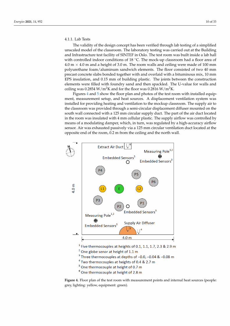
Figures 4 and 5 show the floor plan and photos of the test room with installed equip-ment, measurement setup, and heat sources. A displacement ventilation system wasinstalled for providing heating and ventilation to the mockup classroom. The supply air tothe classroom was provided through a semi-circular displacement diffuser mounted on thesouth wall connected with a 125 mm circular supply duct. The part of the air duct locatedin the room was insulated with 4 mm cellular plastic. The supply airflow was controlled bymeans of a modulating damper, which, in turn, was regulated by a high-accuracy airflowsensor. Air was exhausted passively via a 125 mm circular ventilation duct located at theopposite end of the room, 0.2 m from the ceiling and the north wall.

Energies 2021, 14, x FOR PEER REVIEW 11 of 34

the classroom was provided through a semi-circular displacement diffuser mounted on

the south wall connected with a 125 mm circular supply duct. The part of the air duct

located in the room was insulated with 4 mm cellular plastic. The supply airflow was

controlled by means of a modulating damper, which, in turn, was regulated by a high-

accuracy airflow sensor. Air was exhausted passively via a 125 mm circular ventilation

duct located at the opposite end of the room, 0.2 m from the ceiling and the north wall.

Figure 4. Floor plan of the test room with measurement points and internal heat sources (people:

grey, lighting: yellow, equipment: green).

Figure 5. Photos of the test room with measurement points and internal heat sources.

1

Figure 4. Floor plan of the test room with measurement points and internal heat sources (people:grey, lighting: yellow, equipment: green).

Energies 2021, 14, 952 11 of 33

Energies 2021, 14, x FOR PEER REVIEW 11 of 34

the classroom was provided through a semi-circular displacement diffuser mounted on

the south wall connected with a 125 mm circular supply duct. The part of the air duct

located in the room was insulated with 4 mm cellular plastic. The supply airflow was

controlled by means of a modulating damper, which, in turn, was regulated by a high-

accuracy airflow sensor. Air was exhausted passively via a 125 mm circular ventilation

duct located at the opposite end of the room, 0.2 m from the ceiling and the north wall.

Figure 4. Floor plan of the test room with measurement points and internal heat sources (people:

grey, lighting: yellow, equipment: green).

Figure 5. Photos of the test room with measurement points and internal heat sources.

1

Figure 5. Photos of the test room with measurement points and internal heat sources.

In the test room, internal heat gains from people, equipment and lighting, and trans-mission losses through the outer walls were simulated experimentally for two distinctscenarios with different occupancy patterns, and thus with different airflows, internal loads,and transmission losses. The first scenario, Scenario I, corresponded to a typical situa-tion in which the classroom is fully occupied throughout the day, from 8:00 until 16:00 h,except during the lunch break, between 11:00 and 12:00 h, when the classroom is empty.The second scenario, Scenario II, corresponded to a specific situation when the classroomis occupied only during the afternoon between 13:00 and 16:00 h with 50% of the designoccupancy level. Both scenarios were simulated experimentally for 48 h. During the ex-perimental testing, thermal manikins with a nominal power of 40–120 W and a convectiveheat fraction of approximately 0.5 were used for simulating heat loads from people andequipment. Heat loads from lighting were provided through incandescent bulbs with anominal power of 2 × 40 W. Figure 6 presents the daily internal loads from people, equip-ment and lighting, and supply air temperatures and flows simulated for the two scenarios.Transmission losses through the outer walls were simulated by circulating cold water inpipes integrated into the east and west side walls of the test room. The supply temperatureand mass flow of the circulating water were chosen to emulate the transmission lossesthrough the external walls during the occupied hours at an outside temperature of −15 ◦C.

Energies 2021, 14, x FOR PEER REVIEW 12 of 34

In the test room, internal heat gains from people, equipment and lighting, and trans-

mission losses through the outer walls were simulated experimentally for two distinct

scenarios with different occupancy patterns, and thus with different airflows, internal

loads, and transmission losses. The first scenario, Scenario I, corresponded to a typical

situation in which the classroom is fully occupied throughout the day, from 8:00 until

16:00 h, except during the lunch break, between 11:00 and 12:00 h, when the classroom is

empty. The second scenario, Scenario II, corresponded to a specific situation when the

classroom is occupied only during the afternoon between 13:00 and 16:00 h with 50% of

the design occupancy level. Both scenarios were simulated experimentally for 48 h. Dur-

ing the experimental testing, thermal manikins with a nominal power of 40–120 W and a

convective heat fraction of approximately 0.5 were used for simulating heat loads from

people and equipment. Heat loads from lighting were provided through incandescent

bulbs with a nominal power of 2 × 40 W. Figure 6 presents the daily internal loads from

people, equipment and lighting, and supply air temperatures and flows simulated for the

two scenarios. Transmission losses through the outer walls were simulated by circulating

cold water in pipes integrated into the east and west side walls of the test room. The sup-

ply temperature and mass flow of the circulating water were chosen to emulate the trans-

mission losses through the external walls during the occupied hours at an outside tem-

perature of −15 °C.

Figure 6. Specific internal heat gains, specific airflows, and supply air temperatures for Scenario I (left) and Scenario II (right).

The measurement setup used in the test room was shown above in Figures 4 and 5.

The supply and exhaust air temperatures were measured in the supply air diffuser and

the return air duct, respectively. The temperature profile of the room air was measured at

two different positions in the SW and NE parts of the room. Two vertical poles, each with

five measurement points at heights of 0.1, 1.1, 1.7, 2.3, and 2.9 m above the floor level,

were used for measuring air temperature stratification in the room. Temperature distri-

bution in the floor slab was measured at depths of 0, 4, and 8 cm below the floor level at

four different positions in the room, with two positions being directly below the vertical

poles. All the temperature measurements were made with calibrated thermocouples of

type T, class 1, which had an accuracy of ±0.5 K in the measured temperature range. Each

vertical pole also had an additional globe temperature sensor, with a measurement accu-

racy of ±0.1 K, installed at the sitting height to measure the radiant heat temperature in

the room. The airflow measurements were taken in the supply air duct using a differential-

pressure-based flow measurement station with a measurement tolerance of less than 4%.

The transmission losses from the external walls were measured using calibrated heat me-

ters.

4.1.2. Field Test

An in-situ field test was carried out in a pentagon-shaped classroom on the lower

level of the Drøbak Montessori school building. Figures 7 and 8 show the floor plan and

05

10152025303540

00

:00

02

:00

04

:00

06

:00

08

:00

10

:00

12

:00

14

:00

16

:00

18

:00

20

:00

22

:00

00

:00

He

at G

ain

/ T

em

pe

ratu

re /

Flo

w

Time (hours)

People (W/m²) Lighting (W/m²)Equipment (W/m²) Airflow (m³/h/m²)Supply Temperature (°C)

5.0

32.2

3.8

Temperature

Flow

Heat Gains

05

10152025303540

00

:00

02

:00

04

:00

06

:00

08

:00

10

:00

12

:00

14

:00

16

:00

18

:00

20

:00

22

:00

00

:00

He

at G

ain

/ T

em

pe

ratu

re /

Flo

w

Time (hours)

People (W/m²) Lighting (W/m²)Equipment (W/m²) Airflow (m³/h/m²)Supply Temperature (°C)

5.0

15.9

2.5

Temperature

Flow

Heat Gains

Figure 6. Specific internal heat gains, specific airflows, and supply air temperatures for Scenario I (left) and Scenario II (right).

Energies 2021, 14, 952 12 of 33

The measurement setup used in the test room was shown above in Figures 4 and 5.The supply and exhaust air temperatures were measured in the supply air diffuser and thereturn air duct, respectively. The temperature profile of the room air was measured at twodifferent positions in the SW and NE parts of the room. Two vertical poles, each with fivemeasurement points at heights of 0.1, 1.1, 1.7, 2.3, and 2.9 m above the floor level, were usedfor measuring air temperature stratification in the room. Temperature distribution in thefloor slab was measured at depths of 0, 4, and 8 cm below the floor level at four differentpositions in the room, with two positions being directly below the vertical poles. All thetemperature measurements were made with calibrated thermocouples of type T, class 1,which had an accuracy of ±0.5 K in the measured temperature range. Each verticalpole also had an additional globe temperature sensor, with a measurement accuracy of±0.1 K, installed at the sitting height to measure the radiant heat temperature in theroom. The airflow measurements were taken in the supply air duct using a differential-pressure-based flow measurement station with a measurement tolerance of less than4%. The transmission losses from the external walls were measured using calibratedheat meters.

4.1.2. Field Test

An in-situ field test was carried out in a pentagon-shaped classroom on the lower levelof the Drøbak Montessori school building. Figures 7 and 8 show the floor plan and photosof the classroom with the measurement setup. The classroom had a floor area of 52.2 m2

and a ceiling height of 3 m. It had a medium-weight construction, with a well-insulatedthermal envelope and a high window-to-wall ratio. The classroom had two exterior wallslocated on the southwest and southeast sides and three interior walls located on the north,east, and northwest sides. The total area of the interior and exterior walls was 44.7 m2,and 42.9 m2, respectively. The heat transfer coefficient (U-value) and heat capacity ofinterior walls were 0.26 W/m2K and 2.4 Wh/m2K, respectively. The exterior walls hada heat transfer coefficient and an inner heat capacity of 0.14 W/m2K and 2.4 Wh/m2K,respectively. Floor and ceiling had heat transfer coefficients of 0.10 and 0.25 W/m2K,respectively, and heat capacities of 63, and 3.0 Wh/m2K, respectively. Windows (glazingand frames, combined) covered 43.8% of the total exterior wall area and had a heat transfercoefficient of 0.75 W/m2K.

Energies 2021, 14, x FOR PEER REVIEW 13 of 34

photos of the classroom with the measurement setup. The classroom had a floor area of

52.2 m2 and a ceiling height of 3 m. It had a medium-weight construction, with a well-

insulated thermal envelope and a high window-to-wall ratio. The classroom had two ex-

terior walls located on the southwest and southeast sides and three interior walls located

on the north, east, and northwest sides. The total area of the interior and exterior walls

was 44.7 m2, and 42.9 m2, respectively. The heat transfer coefficient (U-value) and heat

capacity of interior walls were 0.26 W/m2K and 2.4 Wh/m2K, respectively. The exterior

walls had a heat transfer coefficient and an inner heat capacity of 0.14 W/m2K and 2.4

Wh/m2K, respectively. Floor and ceiling had heat transfer coefficients of 0.10 and 0.25

W/m2K, respectively, and heat capacities of 63, and 3.0 Wh/m2K, respectively. Windows

(glazing and frames, combined) covered 43.8% of the total exterior wall area and had a

heat transfer coefficient of 0.75 W/m2K.

Figure 7. Floor plan of the classroom with measurement points.

Figure 7. Floor plan of the classroom with measurement points.

Energies 2021, 14, 952 13 of 33

Energies 2021, 14, x FOR PEER REVIEW 13 of 34

photos of the classroom with the measurement setup. The classroom had a floor area of

52.2 m2 and a ceiling height of 3 m. It had a medium-weight construction, with a well-

insulated thermal envelope and a high window-to-wall ratio. The classroom had two ex-

terior walls located on the southwest and southeast sides and three interior walls located

on the north, east, and northwest sides. The total area of the interior and exterior walls

was 44.7 m2, and 42.9 m2, respectively. The heat transfer coefficient (U-value) and heat

capacity of interior walls were 0.26 W/m2K and 2.4 Wh/m2K, respectively. The exterior

walls had a heat transfer coefficient and an inner heat capacity of 0.14 W/m2K and 2.4

Wh/m2K, respectively. Floor and ceiling had heat transfer coefficients of 0.10 and 0.25

W/m2K, respectively, and heat capacities of 63, and 3.0 Wh/m2K, respectively. Windows

(glazing and frames, combined) covered 43.8% of the total exterior wall area and had a

heat transfer coefficient of 0.75 W/m2K.

Figure 7. Floor plan of the classroom with measurement points.

Figure 8. Photos of the classroom with measurement points for temperature and CO2.

The classroom was supplied with air from a central air handling unit. The airflow inthe classroom was driven by displacement ventilation. The supply air to the classroomwas provided through two wall-embedded supply air diffusers installed 50 mm above thefloor level at the far ends of the east-facing inner wall. The 600 mm × 900 mm rectangularair diffusers were connected to a 315 mm circular main supply duct via two feeder ducts.The airflow in the main duct was regulated by a modulating damper, which was controlledin response to air temperature and CO2 concentration in the classroom as described pre-viously in Section 3. The maximum allowable design airflow from each supply diffuserwas limited to 264 m3/h to not exceed a sound power level of 25 dB(A). At maximumairflow, each diffuser had a near-zone distance of less than 1.5 m to the 0.20 m/s isovel,measured 0.1 m above the floor level with a 3 K temperature difference between the roomand supply air temperatures. Air from the classroom was extracted via three extract airgrills installed 2.8 m above the floor level in the top center of the north-facing inner wall.Passive overflow elements with sound attenuators were used to transfer the extract airto the corridor outside the classroom, from where it was collected and returned to the airhandling unit.

Figure 9 presents the internal loads from people, equipment, and lighting, solar gainsthrough the room fabric, and supply air temperatures and flows for the field test. The fieldtest was performed for approximately 16 h on a cold winter day with ambient air tem-peratures ranging between −7 and +3 ◦C. From the start of the test at midnight, up until7:30 a.m., the displacement ventilation system operated in the heating mode, supplyingrecirculation air to the classroom at a rate of approximately 10.5 m3/h/m2 floor areaand at outdoor temperature-compensated supply temperatures between 27.1 and 28.1 ◦C.At 7:30 a.m., the displacement ventilation system switched from the heating mode to thenormal mode. In this mode, the supply air temperature and flow to the room were origi-nally designed to be regulated by outdoor temperature, and the indoor temperature andCO2 levels, respectively. However, for the field test, the supply air temperature and flow tothe classroom were purposefully chosen to represent a nearly impossible worst-case sce-nario. The supply air to the classroom was provided at temperatures between 16 and 18 ◦C,which were 3 to 4 ◦C below the actual design values. The supply airflow to the classroomwas set constant and approximately equal to the maximum design flow. The classroomwas occupied between 08:00 a.m. and 03:30 p.m. The internal loads in the classroom variedthroughout the day, as it normally happens in classroom contexts. Between 08:30 a.m. and02:30 p.m., thirteen to nineteen persons were present in the classroom at any one time,

Energies 2021, 14, 952 14 of 33

except the lunch break from 11:30 a.m. to 12:30 p.m. when the classroom was completelyunoccupied. Internal loads from equipment and lighting were fairly constant through-out the day. Solar heat gains transmitted through the room fabric, including windowsand walls deduced from the measured solar irradiance data from a nearby weather sta-tion using TEKNOsim 6 software [102] were as high as 450 W (i.e., 8.6 W/m2 floor area).Heat losses through classroom envelope and ventilation and infiltration were simulatedand are presented in Section 5.2.2.

Energies 2021, 14, x FOR PEER REVIEW 15 of 34

Figure 9. Specific internal heat gains, specific airflows, and supply air temperatures for the field test.

The measurement setup in the classroom consisted of sensors for measuring air tem-

perature, radiant temperature, CO2 concentration, and airflow and airspeed. The temper-

atures of supply and extract air to and from the room were measured by sensors installed

in supply air diffusers and return air grilles. Two instrumented vertical poles, placed in

the south and east corners of the classroom, were used for measuring air temperature and

CO2 stratification in the room. Each pole had a set of temperature and CO2 sensors in-

stalled at four different heights of 0.1, 1.1, 1.7, and 2.7 m. All air temperature sensors had

an operating range of −20 to 70 °C, an accuracy of ±0.21 °C, and a resolution of 0.024 °C.

The CO2 sensors had an accuracy of ±50 ppm over the measured concentration range. Each

vertical pole also had an additional globe temperature sensor and an omnidirectional an-

emometer installed at approximately the standing height for measuring the radiant heat

temperature and air velocity, respectively. The measurement accuracies of the globe sen-

sor and anemometer were ±0.1 K, and ±0.04 m/s, respectively. The supply airflow to the

room during the occupied period was measured using a thermal anemometer with a

measurement tolerance of less than ±4%. The airflow outside the operating hours was ob-

tained from the centrally measured BMS data.

4.2. Simulation Studies

Simulations of experimental studies of the previous sections were performed to as-

sess the suitability of a commonly used transient dynamic method for predicting the ther-

mal and contaminant stratification in the displacement ventilation systems. The simula-

tions were performed using IDA-ICE, which is a commercially available state-of-the-art

building performance simulation for performing a multi-zonal and dynamic study of in-

door climate, energy, and daylighting. The software is reported to be validated in accord-

ance with several European and International standards, including Standard EN 15265

[103] and ASHRAE Standard 140 [104], among others. The Climate model in IDA-ICE

version 4.8 SP1 was used for performing the transient simulations of temperature stratifi-

cation and CO2 concentrations. The Climate model uses multi-node calculations to deter-

mine temperatures of different surfaces in the zone and different layers in the construc-

tion. The indoor environmental conditions in both horizontal and vertical directions are

determined using a detailed physical model of the building and its components. A signif-

icant limitation of the Climate model is that it cannot be used for simulating irregular and

asymmetrical zone geometries. The zone geometry must be simplified to a rectangular

footprint before the simulations can be performed.

In the climate model, air distribution to a zone is classified as mixing or displacement

ventilation. For displacement ventilation, air temperature at the floor level is determined

by using an energy balance between the convective heat transfer from the floor surface to

05

10152025303540

00

:00

02

:00

04

:00

06

:00

08

:00

10

:00

12

:00

14

:00

16

:00

18

:00

20

:00

22

:00

00

:00

He

at G

ain

/ T

em

pe

ratu

re /

Flo

w

Time (hours)

People (W/m²) Lighting (W/m²)Equipment (W/m²) Solar (W/m²)Supply Temperature (°C) Airflow (m³/h/m²)

Temperature

Flow

Heat Gains

Figure 9. Specific internal heat gains, specific airflows, and supply air temperatures for the field test.

The measurement setup in the classroom consisted of sensors for measuring air temper-ature, radiant temperature, CO2 concentration, and airflow and airspeed. The temperaturesof supply and extract air to and from the room were measured by sensors installed insupply air diffusers and return air grilles. Two instrumented vertical poles, placed in thesouth and east corners of the classroom, were used for measuring air temperature and CO2stratification in the room. Each pole had a set of temperature and CO2 sensors installedat four different heights of 0.1, 1.1, 1.7, and 2.7 m. All air temperature sensors had anoperating range of −20 to 70 ◦C, an accuracy of ±0.21 ◦C, and a resolution of 0.024 ◦C.The CO2 sensors had an accuracy of ±50 ppm over the measured concentration range.Each vertical pole also had an additional globe temperature sensor and an omnidirectionalanemometer installed at approximately the standing height for measuring the radiantheat temperature and air velocity, respectively. The measurement accuracies of the globesensor and anemometer were ±0.1 K, and ±0.04 m/s, respectively. The supply airflow tothe room during the occupied period was measured using a thermal anemometer witha measurement tolerance of less than ±4%. The airflow outside the operating hours wasobtained from the centrally measured BMS data.

4.2. Simulation Studies

Simulations of experimental studies of the previous sections were performed to assessthe suitability of a commonly used transient dynamic method for predicting the thermaland contaminant stratification in the displacement ventilation systems. The simulationswere performed using IDA-ICE, which is a commercially available state-of-the-art buildingperformance simulation for performing a multi-zonal and dynamic study of indoor climate,energy, and daylighting. The software is reported to be validated in accordance withseveral European and International standards, including Standard EN 15265 [103] andASHRAE Standard 140 [104], among others. The Climate model in IDA-ICE version 4.8 SP1was used for performing the transient simulations of temperature stratification and CO2concentrations. The Climate model uses multi-node calculations to determine temperatures

Energies 2021, 14, 952 15 of 33

of different surfaces in the zone and different layers in the construction. The indoorenvironmental conditions in both horizontal and vertical directions are determined using adetailed physical model of the building and its components. A significant limitation of theClimate model is that it cannot be used for simulating irregular and asymmetrical zonegeometries. The zone geometry must be simplified to a rectangular footprint before thesimulations can be performed.

In the climate model, air distribution to a zone is classified as mixing or displacementventilation. For displacement ventilation, air temperature at the floor level is determined byusing an energy balance between the convective heat transfer from the floor surface to theair at the floor level and the ventilation heat flux from the supply air. The air temperatureat the ceiling level is computed by considering the heat capacity of the zone air volume andaccounting for all heat transfer to the zone air. Based on the calculated air temperatures atfloor and ceiling levels, a linear temperature gradient is calculated for the zone using theMundt model [28]. Temperatures at the zone surfaces are also interpolated between thefloor- and ceiling-level air temperatures. Alternatively, a fixed linear temperature gradientcan be specified directly by the user. In that case, the air temperature at the floor level isobtained using the air temperature at the ceiling level and the provided gradient. If thethermal gradient disappears or becomes negative, the air distribution is treated as mixingventilation instead.

The CO2 concentration in the Climate model is determined based on the balancebetween the CO2 generated in the zone and the CO2 concentration in the ventilation airsupplied to the zone. The CO2 generated from occupants is modeled as a function oftheir activity level. A significant limitation of the model is that the CO2 concentration foreach time step is calculated as a single average value over the zone volume. Therefore,the model does not account for the vertical stratification of the CO2 concentration in thezone. Moreover, it also does not consider the change in CO2 concentration with distancefrom the emission source.

4.2.1. Lab Test

A simulation model of the mock-up classroom used for the lab tests was built in IDA-ICE. The simulation model was constructed using the actual geometry and constructionparameters of the test room described in detail in Section 4.1.1. A constant temperatureboundary condition of 18 ◦C was imposed on all envelope elements except the externalwalls to match the onsite test conditions. The transmission heat losses through the outerwalls were modeled using a controller macro, which split the total losses equally overthe two external walls. Inputs to the simulation model included internal loads, operatingschedules, and supply air temperatures and flows. These inputs were acquired from thesite-controlled and measured test conditions shown in Figure 6. The test data was howeverprocessed to 15-min time steps used for the simulation. The Climate model in IDA-ICE wasused to simulate the vertical temperature gradients. Cyclic runs of each simulation scenariowere performed before the result-generating simulation run to ensure stable conditions.As there were no emission sources in the zone, the CO2 concentrations in the mock-upclassroom were not simulated.

4.2.2. Field Test

The simulation model of the whole school building including the classroom usedin the field test was built in IDA-ICE. For the simulation model, the geometry of theactual classroom used in the field test was simplified to a rectangular footprint. This wasbecause the climate model in IDA-ICE could not simulate irregular and asymmetrical zonegeometries. Nevertheless, the model was customized to match the volume, floor area, andclimate envelope area of the actual classroom. Figure 10 shows the geometries of both theactual room and the simplified simulation model built in IDA-ICE. The actual classroomwas shaded from terrain and trees surrounding it. The shading effect was estimated basedon onsite observations and was incorporated in the simulation model through vertical

Energies 2021, 14, 952 16 of 33

shading elements with 0% transparency for terrain-elements and 50% transparency fortree-elements. Figure 11 shows the building model with modified classroom geometry andthe surrounding vertical shading elements as implemented in IDA-ICE.

Energies 2021, 14, x FOR PEER REVIEW 17 of 34

Figure 10. Actual and modeled geometries of the classroom.

Figure 11. Implemented building model in IDA-ICE.

As for the lab model, the actual construction details of the classroom, presented ear-

lier in Section 4.1.2, were used to build the simulation model. The inputs to the simulation

model included the specific schedule used for the test, the dynamic internal loads, and the

actual supply air temperatures and flows. The climate file used for the simulation was

based on the combination of weather data for the actual area in the simulated period and

standardized values for a typical year for Oslo. The outdoor temperature and solar data

were based on actual measurements. The outdoor temperature data was measured on-site

whereas the solar data was taken from a nearby weather station. The solar data was pro-

cessed using TEKNOsim algorithms [102] to determine direct and diffused components

to be used in the climate file of IDA-ICE. Temperatures in adjacent rooms and spaces were

also based on measured values. The ground reflection (albedo) was set to 0.6 based on

observed values on the test day. The calculated solar heat gains were as high as 450 W

(i.e., 8.6 W/m2 floor area). The model simulated transmission losses through the classroom

envelope based on the room envelope areas, heat transfer coefficients, and the tempera-

ture difference on each side of the envelope. One issue in simulating the transmission heat

losses was to model the ground heat losses accurately. This was because the field test was

performed just after the completion of the building, which did not allow construction

Figure 10. Actual and modeled geometries of the classroom.

Energies 2021, 14, x FOR PEER REVIEW 17 of 34

Figure 10. Actual and modeled geometries of the classroom.

Figure 11. Implemented building model in IDA-ICE.

As for the lab model, the actual construction details of the classroom, presented ear-

lier in Section 4.1.2, were used to build the simulation model. The inputs to the simulation

model included the specific schedule used for the test, the dynamic internal loads, and the

actual supply air temperatures and flows. The climate file used for the simulation was

based on the combination of weather data for the actual area in the simulated period and

standardized values for a typical year for Oslo. The outdoor temperature and solar data

were based on actual measurements. The outdoor temperature data was measured on-site

whereas the solar data was taken from a nearby weather station. The solar data was pro-

cessed using TEKNOsim algorithms [102] to determine direct and diffused components

to be used in the climate file of IDA-ICE. Temperatures in adjacent rooms and spaces were

also based on measured values. The ground reflection (albedo) was set to 0.6 based on

observed values on the test day. The calculated solar heat gains were as high as 450 W

(i.e., 8.6 W/m2 floor area). The model simulated transmission losses through the classroom

envelope based on the room envelope areas, heat transfer coefficients, and the tempera-

ture difference on each side of the envelope. One issue in simulating the transmission heat

losses was to model the ground heat losses accurately. This was because the field test was

performed just after the completion of the building, which did not allow construction

Figure 11. Implemented building model in IDA-ICE.

As for the lab model, the actual construction details of the classroom, presented earlierin Section 4.1.2, were used to build the simulation model. The inputs to the simulationmodel included the specific schedule used for the test, the dynamic internal loads, and theactual supply air temperatures and flows. The climate file used for the simulation wasbased on the combination of weather data for the actual area in the simulated period andstandardized values for a typical year for Oslo. The outdoor temperature and solar datawere based on actual measurements. The outdoor temperature data was measured on-sitewhereas the solar data was taken from a nearby weather station. The solar data was pro-cessed using TEKNOsim algorithms [102] to determine direct and diffused components tobe used in the climate file of IDA-ICE. Temperatures in adjacent rooms and spaces were also

Energies 2021, 14, 952 17 of 33

based on measured values. The ground reflection (albedo) was set to 0.6 based on observedvalues on the test day. The calculated solar heat gains were as high as 450 W (i.e., 8.6 W/m2

floor area). The model simulated transmission losses through the classroom envelopebased on the room envelope areas, heat transfer coefficients, and the temperature differenceon each side of the envelope. One issue in simulating the transmission heat losses was tomodel the ground heat losses accurately. This was because the field test was performedjust after the completion of the building, which did not allow construction enough time todry out and stabilize before the field test. To overcome this issue, the external floor wasmodeled considering a constant ground temperature of 0 ◦C. Furthermore, the thermalconductivity of the insulation in the external floor construction was adjusted to accountfor the moisture in the slab. The model also simulated heat losses due to ventilation andinfiltration. The ventilation heat losses were modeled using the measured ventilation rates,whereas the infiltration heat losses were modeled based on the calculated air leakage to theoutside and surrounding zones.

The vertical temperature gradients were simulated using the Climate model in IDA-ICE. The simulations were performed using a dynamic startup and cyclic runs were madeto ensure stable conditions before the result-generating simulation. The measurementpoints in the simulation run corresponded to actual sensor locations used in the field test.The CO2 concentrations in the zone over time were also simulated using the Climate model.An activity level value of 1 MET, corresponding to sitting quietly, and an atmospheric CO2concentration of 400 ppm was used for the simulations.

5. Results

In this section, the results of experimental tests and numerical simulations describedabove are critically presented and discussed, giving a detailed insight into the performanceof the displacement ventilation for providing heating during non-occupied periods withoutthe need for a separate heating system.

5.1. Experimental Results

The results of two lab tests carried out in the scaled mock-up classroom under carefullycontrolled laboratory conditions and one field test performed in the full-scale classroomunder actual field conditions are presented in the following sections.

5.1.1. Lab Test

Figure 12, left and right, show measured values of supply, extract and operativetemperatures, and airflows for Scenario 1 and Scenario 2 of the lab test. The only noticeabledifference between the measured values of Figure 12 and the originally planned values ofFigure 6 is in the supply air temperature in the heating mode at night. For both scenarios,the actual supply air temperature in the heating mode was around 29 ◦C, which was1 K lower than the originally planned value. This discrepancy was caused because thesupply air temperature to the test room was regulated by a sensor located in the air duct,2.8 m above the supply air diffuser, whereas the measurements of supply air temperatureshown in Figure 12 were taken with a sensor placed in the supply air diffuser at 0.7 mheight. Hence, in the heating mode, there was a duct heat loss of 1 K to the room dueto the large difference in the temperature of the air in the duct and the temperature ofthe air in the room. In the normal mode, the supply air temperature in both scenarioswas approximately 22 ◦C as originally planned. For both scenarios, the room operativetemperature was between 22–24 ◦C when occupied. The extract air temperature fromthe room depended upon the operation mode of the system and the occupancy level.For both scenarios, the extract air temperature in the heating mode was 5–7 K lower thanthe supply air temperature. For Scenario 1, which corresponded to a situation in whichthe classroom was fully occupied between 8:00–11:00 and 12:00–16:00 h, the extract airtemperature in the normal mode was on average 1.7 K and maximum 2.2 K higher thanthe supply air temperature. For Scenario 2, which corresponded to a situation in which the

Energies 2021, 14, 952 18 of 33

classroom was occupied only during the afternoon between 13:00 and 16:00 h with 50% ofthe design occupancy level, the extract air temperature in the normal operating-mode wasonly occasionally and marginally higher (<0.5 K) than the supply air temperature.

Energies 2021, 14, x FOR PEER REVIEW 19 of 34

Figure 12. Measured supply, extract, and operative temperatures, and airflows for Scenario I (left) and Scenario II (right)

of the lab test.

Figure 13 shows the vertical temperature profiles at heights of 0.1, 1.1, 1.7, 2.3, and

2.9 m above the floor level for the two scenarios. Each curve represents an average of two

temperature sensors installed at the same height on the two instrumented poles in the

opposite corners of the test room. For Scenario 1, the average and maximum vertical tem-

perature gradient between the standing head height (1.7 m) and ankle height (0.1 m) was

1.2 K and 1.4 K, respectively, during the heating mode between 00:00–8:00, and 0.8 K and

1.2 K, respectively, during the normal mode between 8:00–11:00 and 12:00–16:00. During

periods of no ventilation between 16:00–00:00, there was no vertical temperature gradient

and consequently no stratification. For Scenario 2, the average and maximum vertical tem-

perature gradient between the standing head height (1.7 m) and ankle height (0.1 m) was

1.2 K and 1.4 K, respectively, during the heating mode between 00:00–7:30, and 0.4 K and

0.6 K, respectively, during the normal mode between 12:00–15:00. During periods of no

occupancy between 07:30–12:00 and 15:30–18:00, there was no vertical temperature gradi-

ent and consequently no stratification.

Figure 13. Measured vertical temperature profiles for Scenario I (left) and Scenario II (right) of the lab test.

Figure 14 presents the vertical temperature distribution in the floor slab at the depths

of 0, 4, and 8 cm below the floor level for the two test scenarios. Each curve represents an

average of four thermocouples installed at the same depths in different positions in the

room. In both scenarios, the slab temperatures increased with time in the heating mode,

and its thermal mass was charged. The slab temperatures also increased in the day oper-

ating mode, but at different rates, as occupancy levels were dissimilar for the two scenar-

ios. The discharging occurred in non-occupancy periods when the airflow to the test setup

was reduced to zero. Throughout the experiment, temperatures at 8 cm depth remain no-

ticeably higher than the temperatures at 0 and 4 cm depths.

0

3

6

9

12

15

18

20

22

24

26

28

30

32

00

:00

04

:00

08

:00

12

:00

16

:00

20

:00

00

:00

04

:00

08

:00

12

:00

16

:00

20

:00

00

:00

Air

flo

w (

m³/

h/m

²)

Tem

pe

ratu

re (

°C)

Time (hours)

Supply Temperature Extract Temperature

Operative Temperature Airflow

0

3

6

9

12

15

18

20

22

24

26

28

30

32

00

:00

04

:00

08

:00

12

:00

16

:00

20

:00

00

:00

04

:00

08

:00

12

:00

16

:00

20

:00

00

:00

Air

flo

w (

m³/

h/m

²)

Tem

pe

ratu

re (

°C)

Time (hours)

Supply Temperature Extract TemperatureOperative Temperature Airflow

20

21

22

23

24

25

00

:00

04

:00

08

:00

12

:00

16

:00

20

:00

00

:00

04

:00

08

:00

12

:00

16

:00

20

:00

00

:00

Tem

pe

ratu

re (

°C)

Time (hours)

Height 0.1 m Height 1.1 m Height 1.7 m

Height 2.3 m Height 2.9 m

20

21

22

23

24

25

00

:00

04

:00

08

:00

12

:00

16

:00

20

:00

00

:00

04

:00

08

:00

12

:00

16

:00

20

:00

00

:00

Tem

pe

ratu

re (

°C)

Time (hours)

Height 0.1 m Height 1.1 m Height 1.7 m

Height 2.3 m Height 2.9 m

Figure 12. Measured supply, extract, and operative temperatures, and airflows for Scenario I (left) and Scenario II (right) ofthe lab test.

Figure 13 shows the vertical temperature profiles at heights of 0.1, 1.1, 1.7, 2.3, and 2.9 mabove the floor level for the two scenarios. Each curve represents an average of two temper-ature sensors installed at the same height on the two instrumented poles in the oppositecorners of the test room. For Scenario 1, the average and maximum vertical temperaturegradient between the standing head height (1.7 m) and ankle height (0.1 m) was 1.2 Kand 1.4 K, respectively, during the heating mode between 00:00–8:00, and 0.8 K and 1.2 K,respectively, during the normal mode between 8:00–11:00 and 12:00–16:00. During pe-riods of no ventilation between 16:00–00:00, there was no vertical temperature gradientand consequently no stratification. For Scenario 2, the average and maximum verticaltemperature gradient between the standing head height (1.7 m) and ankle height (0.1 m)was 1.2 K and 1.4 K, respectively, during the heating mode between 00:00–7:30, and 0.4 Kand 0.6 K, respectively, during the normal mode between 12:00–15:00. During periodsof no occupancy between 07:30–12:00 and 15:30–18:00, there was no vertical temperaturegradient and consequently no stratification.

Energies 2021, 14, x FOR PEER REVIEW 19 of 34

Figure 12. Measured supply, extract, and operative temperatures, and airflows for Scenario I (left) and Scenario II (right)

of the lab test.

Figure 13 shows the vertical temperature profiles at heights of 0.1, 1.1, 1.7, 2.3, and

2.9 m above the floor level for the two scenarios. Each curve represents an average of two

temperature sensors installed at the same height on the two instrumented poles in the

opposite corners of the test room. For Scenario 1, the average and maximum vertical tem-

perature gradient between the standing head height (1.7 m) and ankle height (0.1 m) was

1.2 K and 1.4 K, respectively, during the heating mode between 00:00–8:00, and 0.8 K and

1.2 K, respectively, during the normal mode between 8:00–11:00 and 12:00–16:00. During

periods of no ventilation between 16:00–00:00, there was no vertical temperature gradient

and consequently no stratification. For Scenario 2, the average and maximum vertical tem-

perature gradient between the standing head height (1.7 m) and ankle height (0.1 m) was

1.2 K and 1.4 K, respectively, during the heating mode between 00:00–7:30, and 0.4 K and

0.6 K, respectively, during the normal mode between 12:00–15:00. During periods of no

occupancy between 07:30–12:00 and 15:30–18:00, there was no vertical temperature gradi-

ent and consequently no stratification.

Figure 13. Measured vertical temperature profiles for Scenario I (left) and Scenario II (right) of the lab test.

Figure 14 presents the vertical temperature distribution in the floor slab at the depths

of 0, 4, and 8 cm below the floor level for the two test scenarios. Each curve represents an

average of four thermocouples installed at the same depths in different positions in the

room. In both scenarios, the slab temperatures increased with time in the heating mode,

and its thermal mass was charged. The slab temperatures also increased in the day oper-

ating mode, but at different rates, as occupancy levels were dissimilar for the two scenar-

ios. The discharging occurred in non-occupancy periods when the airflow to the test setup

was reduced to zero. Throughout the experiment, temperatures at 8 cm depth remain no-

ticeably higher than the temperatures at 0 and 4 cm depths.

0

3

6

9

12

15

18

20

22

24

26

28

30

32

00

:00

04

:00

08

:00

12

:00

16

:00

20

:00

00

:00

04

:00

08

:00

12

:00

16

:00

20

:00

00

:00

Air

flo

w (

m³/

h/m

²)

Tem

pe

ratu

re (

°C)

Time (hours)

Supply Temperature Extract Temperature

Operative Temperature Airflow

0

3

6

9

12

15

18

20

22

24

26

28

30

32

00

:00

04

:00

08

:00

12

:00

16

:00

20

:00

00

:00

04

:00

08

:00

12

:00

16

:00

20

:00

00

:00

Air

flo

w (

m³/

h/m

²)

Tem

pe

ratu

re (

°C)

Time (hours)

Supply Temperature Extract TemperatureOperative Temperature Airflow

20

21

22

23

24

25

00

:00

04

:00

08

:00

12

:00

16

:00

20

:00

00

:00

04

:00

08

:00

12

:00

16

:00

20

:00

00

:00

Tem

pe

ratu

re (

°C)

Time (hours)

Height 0.1 m Height 1.1 m Height 1.7 m

Height 2.3 m Height 2.9 m

20

21

22

23

24

25

00

:00

04

:00

08

:00

12

:00

16

:00

20

:00

00

:00

04

:00

08

:00

12

:00

16

:00

20

:00

00

:00

Tem

pe

ratu

re (

°C)

Time (hours)

Height 0.1 m Height 1.1 m Height 1.7 m

Height 2.3 m Height 2.9 m

Figure 13. Measured vertical temperature profiles for Scenario I (left) and Scenario II (right) of the lab test.

Figure 14 presents the vertical temperature distribution in the floor slab at the depthsof 0, 4, and 8 cm below the floor level for the two test scenarios. Each curve representsan average of four thermocouples installed at the same depths in different positions inthe room. In both scenarios, the slab temperatures increased with time in the heatingmode, and its thermal mass was charged. The slab temperatures also increased in the dayoperating mode, but at different rates, as occupancy levels were dissimilar for the two

Energies 2021, 14, 952 19 of 33

scenarios. The discharging occurred in non-occupancy periods when the airflow to thetest setup was reduced to zero. Throughout the experiment, temperatures at 8 cm depthremain noticeably higher than the temperatures at 0 and 4 cm depths.

Energies 2021, 14, x FOR PEER REVIEW 20 of 34

Figure 14. Measured slab temperatures for Scenario I (left) and Scenario II (right) of the lab test.

5.1.2. Field Test

Figure 15 shows measured values of supply, extract and operative temperatures, and

airflows for the field test. Each temperature measurement in the figure is an average of

two different sensors. The supply air temperature was measured in each of the two supply

air diffusers. Similarly, the extract air temperature was measured in the two extract air

grilles. The radiant air temperature was measured by the globe temperature sensor in-

stalled on each measurement pole. The operative temperature was calculated based on

the measured air temperature, mean radiant temperature, and air velocity according to

ISO 7726 [105].

Figure 15. Measured supply, extract, and operative temperatures, and airflows for the field test.

As seen from the figure, the supply air temperature in the heating mode was approx-

imately between 27.3 and 28.3 °C. The supply air temperature in the normal mode varied

between 16.1 and 18.3 °C. In both heating and normal modes, the actual supply air tem-

peratures were different from the originally planned outdoor temperature-compensated

supply temperatures shown in Figure 3. In the normal mode, the supply temperature was

considerably lower than the anticipated value of around 20 °C, primarily due to an anom-

aly in the supply temperature curve in the control system. This was because the school

building was not fully finished at the time of field testing, and the control system was

being tested and commissioned. Nevertheless, supplying air at lower temperatures than

originally planned in the normal operation mode provided an even more stringent test of

the concept. As in the lab test, the extract air temperature from the room depended upon

the operation mode of the system and the occupancy level. In the heating mode, the extract

air temperature was 6–8 K lower than the supply air temperature, whereas, in the normal

operation mode, the extract air temperature was on average 3.0 K and at maximum 4.4 K

higher than the supply air temperature. During the lunch break, the extract air tempera-

ture was just under 19 °C due to lower internal heat loads. The operative temperature in

20

21

22

23

24

25

00

:00

04

:00

08

:00

12

:00

16

:00

20

:00

00

:00

04

:00

08

:00

12

:00

16

:00

20

:00

00

:00

Tem

pe

ratu

re (

°C)

Time (hours)

Depth 0 cm Depth 4 cm Depth 8 cm

20

21

22

23

24

25

00

:00

04

:00

08

:00

12

:00

16

:00

20

:00

00

:00

04

:00

08

:00

12

:00

16

:00

20

:00

00

:00

Tem

pe

ratu

re (

°C)

Time (hours)

Depth 0 cm Depth 4 cm Depth 8 cm

0

3

6

9

12

15

14

18

22

26

30

34

18

:00

20

:00

22

:00

00

:00

02

:00

04

:00

06

:00

08

:00

10

:00

12

:00

14

:00

16

:00

18

:00

Air

flo

w (

m3 /

h/m

2 )

Tem

pe

ratu

re (

°C)

Time (hours)

Supply Temperature Extract Temperature

Operative Temperature Airflow

Figure 14. Measured slab temperatures for Scenario I (left) and Scenario II (right) of the lab test.

5.1.2. Field Test

Figure 15 shows measured values of supply, extract and operative temperatures, and air-flows for the field test. Each temperature measurement in the figure is an average of twodifferent sensors. The supply air temperature was measured in each of the two supply airdiffusers. Similarly, the extract air temperature was measured in the two extract air grilles.The radiant air temperature was measured by the globe temperature sensor installed on eachmeasurement pole. The operative temperature was calculated based on the measured airtemperature, mean radiant temperature, and air velocity according to ISO 7726 [105].

Energies 2021, 14, x FOR PEER REVIEW 20 of 34

Figure 14. Measured slab temperatures for Scenario I (left) and Scenario II (right) of the lab test.

5.1.2. Field Test

Figure 15 shows measured values of supply, extract and operative temperatures, and

airflows for the field test. Each temperature measurement in the figure is an average of

two different sensors. The supply air temperature was measured in each of the two supply

air diffusers. Similarly, the extract air temperature was measured in the two extract air

grilles. The radiant air temperature was measured by the globe temperature sensor in-

stalled on each measurement pole. The operative temperature was calculated based on

the measured air temperature, mean radiant temperature, and air velocity according to

ISO 7726 [105].

Figure 15. Measured supply, extract, and operative temperatures, and airflows for the field test.

As seen from the figure, the supply air temperature in the heating mode was approx-

imately between 27.3 and 28.3 °C. The supply air temperature in the normal mode varied

between 16.1 and 18.3 °C. In both heating and normal modes, the actual supply air tem-

peratures were different from the originally planned outdoor temperature-compensated

supply temperatures shown in Figure 3. In the normal mode, the supply temperature was

considerably lower than the anticipated value of around 20 °C, primarily due to an anom-

aly in the supply temperature curve in the control system. This was because the school

building was not fully finished at the time of field testing, and the control system was

being tested and commissioned. Nevertheless, supplying air at lower temperatures than

originally planned in the normal operation mode provided an even more stringent test of

the concept. As in the lab test, the extract air temperature from the room depended upon

the operation mode of the system and the occupancy level. In the heating mode, the extract

air temperature was 6–8 K lower than the supply air temperature, whereas, in the normal

operation mode, the extract air temperature was on average 3.0 K and at maximum 4.4 K

higher than the supply air temperature. During the lunch break, the extract air tempera-

ture was just under 19 °C due to lower internal heat loads. The operative temperature in

20

21

22

23

24

250

0:0

0

04

:00

08

:00

12

:00

16

:00

20

:00

00

:00

04

:00

08

:00

12

:00

16

:00

20

:00

00

:00

Tem

pe

ratu

re (

°C)

Time (hours)

Depth 0 cm Depth 4 cm Depth 8 cm

20

21

22

23

24

25

00

:00

04

:00

08

:00

12

:00

16

:00

20

:00

00

:00

04

:00

08

:00

12

:00

16

:00

20

:00

00

:00

Tem

pe

ratu

re (

°C)

Time (hours)

Depth 0 cm Depth 4 cm Depth 8 cm

0

3

6

9

12

15

14

18

22

26

30

34

18

:00

20

:00

22

:00

00

:00

02

:00

04

:00

06

:00

08

:00

10

:00

12

:00

14

:00

16

:00

18

:00

Air

flo

w (

m3 /

h/m

2 )

Tem

pe

ratu

re (

°C)

Time (hours)

Supply Temperature Extract Temperature

Operative Temperature Airflow

Figure 15. Measured supply, extract, and operative temperatures, and airflows for the field test.

As seen from the figure, the supply air temperature in the heating mode was approxi-mately between 27.3 and 28.3 ◦C. The supply air temperature in the normal mode variedbetween 16.1 and 18.3 ◦C. In both heating and normal modes, the actual supply air tem-peratures were different from the originally planned outdoor temperature-compensatedsupply temperatures shown in Figure 3. In the normal mode, the supply temperaturewas considerably lower than the anticipated value of around 20 ◦C, primarily due to ananomaly in the supply temperature curve in the control system. This was because theschool building was not fully finished at the time of field testing, and the control system

Energies 2021, 14, 952 20 of 33

was being tested and commissioned. Nevertheless, supplying air at lower temperaturesthan originally planned in the normal operation mode provided an even more stringent testof the concept. As in the lab test, the extract air temperature from the room depended uponthe operation mode of the system and the occupancy level. In the heating mode, the extractair temperature was 6–8 K lower than the supply air temperature, whereas, in the normaloperation mode, the extract air temperature was on average 3.0 K and at maximum 4.4 Khigher than the supply air temperature. During the lunch break, the extract air temperaturewas just under 19 ◦C due to lower internal heat loads. The operative temperature in theroom was rather constant. In the heating mode, the operative temperature was between19.0 and 19.5 ◦C. In the normal mode, the operative temperature ranged between 19.3 to20.5 ◦C, with an average of 20.2 ◦C. During the lunch break, the operative temperature wasjust below 19 ◦C.

Figure 16 shows the vertical temperature profiles at heights of 0.1, 1.1, 1.7, and 2.7 mabove the floor level. Each curve is an average of two sensors mounted at the sameheight on different poles in the opposite corners of the classroom. As seen from the figure,a vertical temperature gradient was present in the room in both the day operating and theheating modes. The air temperature was lowest at the floor level and rose steadily withheight. The average and maximum vertical temperature gradient between the standinghead height (1.7 m) and ankle height (0.1 m) in the normal mode was 1.2 K and 1.6 K,respectively, and in the heating mode was 0.5 K, and 0.7 K, respectively.

Energies 2021, 14, x FOR PEER REVIEW 21 of 34

the room was rather constant. In the heating mode, the operative temperature was be-

tween 19.0 and 19.5 °C. In the normal mode, the operative temperature ranged between

19.3 to 20.5 °C, with an average of 20.2 °C. During the lunch break, the operative temper-

ature was just below 19 °C.

Figure 16 shows the vertical temperature profiles at heights of 0.1, 1.1, 1.7, and 2.7 m

above the floor level. Each curve is an average of two sensors mounted at the same height

on different poles in the opposite corners of the classroom. As seen from the figure, a

vertical temperature gradient was present in the room in both the day operating and the

heating modes. The air temperature was lowest at the floor level and rose steadily with

height. The average and maximum vertical temperature gradient between the standing

head height (1.7 m) and ankle height (0.1 m) in the normal mode was 1.2 K and 1.6 K,

respectively, and in the heating mode was 0.5 K, and 0.7 K, respectively.

Figure 16. Measured vertical temperature profiles for the field experiment.

Figure 17 presents the vertical CO2 profiles at heights of 0.1, 1.1, 1.7, and 2.7 m above

the floor level. Again, each curve represents an average of two measurements taken at the

same heights by sensors mounted on two different poles in two opposite corners of the

classroom. The figure shows that in the heating mode there was no vertical stratification

of CO2 in the classroom. This is because there were no CO2 sources in the classroom. In

the heating mode, the CO2 levels in the classroom decayed to nearly outdoor levels by

dilution with the recirculation air. During the normal mode, there was a vertical stratifi-

cation of CO2 in the classroom. The CO2 concentration was lowest at the floor level in the

classroom and increased non-linearly with height. Above the sitting head height (1.1 m),

the CO2 concentration had a rather flat gradient. During the lunch break between 11:00

and 12:00 h, and at the end of the school day, the CO2 concentration in the classroom de-

cayed very rapidly.

Figure 17. Measured vertical CO2 concentrations for the field experiment.

17

18

19

20

21

22

18

:00

20

:00

22

:00

00

:00

02

:00

04

:00

06

:00

08

:00

10

:00

12

:00

14

:00

16

:00

18

:00

Tem

pe

ratu

re (

°C)

Time (hours)

Height 0.1 m Height 1.1 m

Height 1.7 m Height 2.7 m

200

400

600

800

1000

1200

1400

18

:00

20

:00

22

:00

00

:00

02

:00

04

:00

06

:00

08

:00

10

:00

12

:00

14

:00

16

:00

18

:00

CO

2C

on

cen

trat

ion

(p

pm

)

Time (hours)

Height 0.1 m Height 1.1 m

Height 1.7 m Height 2.7 m

Figure 16. Measured vertical temperature profiles for the field experiment.

Figure 17 presents the vertical CO2 profiles at heights of 0.1, 1.1, 1.7, and 2.7 m abovethe floor level. Again, each curve represents an average of two measurements taken at thesame heights by sensors mounted on two different poles in two opposite corners of theclassroom. The figure shows that in the heating mode there was no vertical stratification ofCO2 in the classroom. This is because there were no CO2 sources in the classroom. In theheating mode, the CO2 levels in the classroom decayed to nearly outdoor levels by dilutionwith the recirculation air. During the normal mode, there was a vertical stratificationof CO2 in the classroom. The CO2 concentration was lowest at the floor level in theclassroom and increased non-linearly with height. Above the sitting head height (1.1 m),the CO2 concentration had a rather flat gradient. During the lunch break between 11:00 and12:00 h, and at the end of the school day, the CO2 concentration in the classroom decayedvery rapidly.

Energies 2021, 14, 952 21 of 33

Energies 2021, 14, x FOR PEER REVIEW 21 of 34

the room was rather constant. In the heating mode, the operative temperature was be-

tween 19.0 and 19.5 °C. In the normal mode, the operative temperature ranged between

19.3 to 20.5 °C, with an average of 20.2 °C. During the lunch break, the operative temper-

ature was just below 19 °C.

Figure 16 shows the vertical temperature profiles at heights of 0.1, 1.1, 1.7, and 2.7 m

above the floor level. Each curve is an average of two sensors mounted at the same height

on different poles in the opposite corners of the classroom. As seen from the figure, a

vertical temperature gradient was present in the room in both the day operating and the

heating modes. The air temperature was lowest at the floor level and rose steadily with

height. The average and maximum vertical temperature gradient between the standing

head height (1.7 m) and ankle height (0.1 m) in the normal mode was 1.2 K and 1.6 K,

respectively, and in the heating mode was 0.5 K, and 0.7 K, respectively.

Figure 16. Measured vertical temperature profiles for the field experiment.

Figure 17 presents the vertical CO2 profiles at heights of 0.1, 1.1, 1.7, and 2.7 m above

the floor level. Again, each curve represents an average of two measurements taken at the

same heights by sensors mounted on two different poles in two opposite corners of the

classroom. The figure shows that in the heating mode there was no vertical stratification

of CO2 in the classroom. This is because there were no CO2 sources in the classroom. In

the heating mode, the CO2 levels in the classroom decayed to nearly outdoor levels by

dilution with the recirculation air. During the normal mode, there was a vertical stratifi-

cation of CO2 in the classroom. The CO2 concentration was lowest at the floor level in the

classroom and increased non-linearly with height. Above the sitting head height (1.1 m),

the CO2 concentration had a rather flat gradient. During the lunch break between 11:00

and 12:00 h, and at the end of the school day, the CO2 concentration in the classroom de-

cayed very rapidly.

Figure 17. Measured vertical CO2 concentrations for the field experiment.

17

18

19

20

21

22

18

:00

20

:00

22

:00

00

:00

02

:00

04

:00

06

:00

08

:00

10

:00

12

:00

14

:00

16

:00

18

:00

Tem

pe

ratu

re (

°C)

Time (hours)

Height 0.1 m Height 1.1 m

Height 1.7 m Height 2.7 m

200

400

600

800

1000

1200

1400

18

:00

20

:00

22

:00

00

:00

02

:00

04

:00

06

:00

08

:00

10

:00

12

:00

14

:00

16

:00

18

:00

CO

2C

on

cen

trat

ion

(p

pm

)

Time (hours)

Height 0.1 m Height 1.1 m

Height 1.7 m Height 2.7 m

Figure 17. Measured vertical CO2 concentrations for the field experiment.

5.2. Simulation Results

The results of numerical simulation conducted using IDA-ICE simulation software forthe two lab tests and one field test performed, respectively, in the scaled mock-up and theactual classroom are presented in the following sections.

5.2.1. Lab Test

As mentioned earlier in Section 4.2.1, the simulation model of the test room wasconstructed using the actual geometry and construction details. The inputs to the simu-lation model including internal loads, operating schedules, and supply air temperaturesand flows were based on actual measured data from the lab test. The simulated energybalances of the test room are shown in Figure 18 for the two scenarios of the lab test.As seen from the figure, the heat provided through the displacement ventilation systemin the night heating mode was simulated to be partly stored in the room and partly lostthrough the room envelope. The simulation results implied that in normal mode the storedheat was released back to the room gradually over time, especially during periods of nooccupancy and reduced ventilation flows. Moreover, for both Scenario I and Scenario II,the stored heat was simulated not to be released to the room when occupied. This wasbecause the sum of internal heat gains from people, equipment and lighting, and heat gainsfrom ventilation airflow did not exceed heat losses through the room envelope during theoccupancy periods.

Figure 19 shows the simulated vertical temperature profiles at heights of 0.1, 1.1, 1.7,2.3, and 2.9 m above the floor level for the two scenarios of the lab test. For Scenario1, the model did not simulate any stratification for the heating mode between 00:00–8:00. For periods with normal mode between 8:00–11:00 and 12:00–16:00, the averageand maximum vertical temperature gradient between the standing head height (1.7 m)and ankle height (0.1 m) simulated by the model was 0.4, and 0.8 K, respectively. Forperiods of no ventilation between 16:00–00:00, no stratification was simulated by themodel, as expected. For Scenario 2, no stratification was predicted in heating or normalmodes. The simulated vertical temperature gradients in both scenarios were lower thanthe experimentally measured gradients.

Energies 2021, 14, 952 22 of 33

Energies 2021, 14, x FOR PEER REVIEW 22 of 34

5.2. Simulation Results

The results of numerical simulation conducted using IDA-ICE simulation software

for the two lab tests and one field test performed, respectively, in the scaled mock-up and

the actual classroom are presented in the following sections.

5.2.1. Lab Test

As mentioned earlier in Section 4.2.1, the simulation model of the test room was con-

structed using the actual geometry and construction details. The inputs to the simulation

model including internal loads, operating schedules, and supply air temperatures and

flows were based on actual measured data from the lab test. The simulated energy bal-

ances of the test room are shown in Figure 18 for the two scenarios of the lab test. As seen

from the figure, the heat provided through the displacement ventilation system in the

night heating mode was simulated to be partly stored in the room and partly lost through

the room envelope. The simulation results implied that in normal mode the stored heat

was released back to the room gradually over time, especially during periods of no occu-

pancy and reduced ventilation flows. Moreover, for both Scenario I and Scenario II, the

stored heat was simulated not to be released to the room when occupied. This was because

the sum of internal heat gains from people, equipment and lighting, and heat gains from

ventilation airflow did not exceed heat losses through the room envelope during the oc-

cupancy periods.

Figure 18. Simulated energy balance for Scenario I (top) and Scenario II (bottom) of the lab test.

Figure 19 shows the simulated vertical temperature profiles at heights of 0.1, 1.1, 1.7,

2.3, and 2.9 m above the floor level for the two scenarios of the lab test. For Scenario 1, the

model did not simulate any stratification for the heating mode between 00:00–8:00. For

Figure 18. Simulated energy balance for Scenario I (top) and Scenario II (bottom) of the lab test.

Energies 2021, 14, x FOR PEER REVIEW 23 of 34

periods with normal mode between 8:00–11:00 and 12:00–16:00, the average and maxi-

mum vertical temperature gradient between the standing head height (1.7 m) and ankle

height (0.1 m) simulated by the model was 0.4, and 0.8 K, respectively. For periods of no

ventilation between 16:00–00:00, no stratification was simulated by the model, as ex-

pected. For Scenario 2, no stratification was predicted in heating or normal modes. The

simulated vertical temperature gradients in both scenarios were lower than the experi-

mentally measured gradients.

Figure 19. Simulated vertical temperature profiles for Scenario I (left) and Scenario II (right) of the lab test.

5.2.2. Field Test

Figure 20 shows the simulated energy balance for the field test. As for the lab test,

the simulation results of the field test also demonstrated that part of the heat provided

through the displacement ventilation and stored in the room structure in the night heating

mode was released back to the room during the periods of no occupancy and reduced

ventilation in the normal operating mode. Unlike the lab test, heat gains from solar radi-

ation through the windows in the normal mode provided a useful contribution to the en-

ergy balance of the classroom. Moreover, ventilation losses in the normal mode had a

sizeable contribution to the energy balance of the classroom for the reason that ventilation

air to the classroom was supplied at fairly low temperatures in order to represent a worst-

case scenario.

Figure 20. Detailed energy balance for the simulated classroom model.

Figure 21 shows the simulated vertical temperature profiles at heights of 0.1, 1.1, 1.7,

and 2.7 m above the floor level. As seen from the figure, the model did not simulate any

temperature stratification in the heating mode between 20:00–8:00. In the normal mode,

the model simulated a vertical temperature gradient in the room. The air temperature was

lowest at the floor level and rose linearly with height. The average and maximum vertical

temperature gradient between the standing head height (1.7 m) and ankle height (0.1 m)

19

20

21

22

23

24

25

00

:00

04

:00

08

:00

12

:00

16

:00

20

:00

00

:00

04

:00

08

:00

12

:00

16

:00

20

:00

00

:00

Tem

pe

ratu

re (

°C)

Time (hours)

Height 0.1 m Height 1.1 m Height 1.7 mHeight 2.3 m Height 2.9 m

19

20

21

22

23

24

25

00

:00

04

:00

08

:00

12

:00

16

:00

20

:00

00

:00

04

:00

08

:00

12

:00

16

:00

20

:00

00

:00

Tem

pe

ratu

re (

°C)

Time (hours)

Height 0.1 m Height 1.1 m Height 1.7 mHeight 2.3 m Height 2.9 m

Figure 19. Simulated vertical temperature profiles for Scenario I (left) and Scenario II (right) of the lab test.

5.2.2. Field Test

Figure 20 shows the simulated energy balance for the field test. As for the lab test,the simulation results of the field test also demonstrated that part of the heat providedthrough the displacement ventilation and stored in the room structure in the night heatingmode was released back to the room during the periods of no occupancy and reducedventilation in the normal operating mode. Unlike the lab test, heat gains from solarradiation through the windows in the normal mode provided a useful contribution to theenergy balance of the classroom. Moreover, ventilation losses in the normal mode had asizeable contribution to the energy balance of the classroom for the reason that ventilation

Energies 2021, 14, 952 23 of 33

air to the classroom was supplied at fairly low temperatures in order to represent a worst-case scenario.

Energies 2021, 14, x FOR PEER REVIEW 23 of 34

periods with normal mode between 8:00–11:00 and 12:00–16:00, the average and maxi-

mum vertical temperature gradient between the standing head height (1.7 m) and ankle

height (0.1 m) simulated by the model was 0.4, and 0.8 K, respectively. For periods of no

ventilation between 16:00–00:00, no stratification was simulated by the model, as ex-

pected. For Scenario 2, no stratification was predicted in heating or normal modes. The

simulated vertical temperature gradients in both scenarios were lower than the experi-

mentally measured gradients.

Figure 19. Simulated vertical temperature profiles for Scenario I (left) and Scenario II (right) of the lab test.

5.2.2. Field Test

Figure 20 shows the simulated energy balance for the field test. As for the lab test,

the simulation results of the field test also demonstrated that part of the heat provided

through the displacement ventilation and stored in the room structure in the night heating

mode was released back to the room during the periods of no occupancy and reduced

ventilation in the normal operating mode. Unlike the lab test, heat gains from solar radi-

ation through the windows in the normal mode provided a useful contribution to the en-

ergy balance of the classroom. Moreover, ventilation losses in the normal mode had a

sizeable contribution to the energy balance of the classroom for the reason that ventilation

air to the classroom was supplied at fairly low temperatures in order to represent a worst-

case scenario.

Figure 20. Detailed energy balance for the simulated classroom model.

Figure 21 shows the simulated vertical temperature profiles at heights of 0.1, 1.1, 1.7,

and 2.7 m above the floor level. As seen from the figure, the model did not simulate any

temperature stratification in the heating mode between 20:00–8:00. In the normal mode,

the model simulated a vertical temperature gradient in the room. The air temperature was

lowest at the floor level and rose linearly with height. The average and maximum vertical

temperature gradient between the standing head height (1.7 m) and ankle height (0.1 m)

19

20

21

22

23

24

25

00

:00

04

:00

08

:00

12

:00

16

:00

20

:00

00

:00

04

:00

08

:00

12

:00

16

:00

20

:00

00

:00

Tem

pe

ratu

re (

°C)

Time (hours)

Height 0.1 m Height 1.1 m Height 1.7 mHeight 2.3 m Height 2.9 m

19

20

21

22

23

24

25

00

:00

04

:00

08

:00

12

:00

16

:00

20

:00

00

:00

04

:00

08

:00

12

:00

16

:00

20

:00

00

:00

Tem

pe

ratu

re (

°C)

Time (hours)

Height 0.1 m Height 1.1 m Height 1.7 mHeight 2.3 m Height 2.9 m

Figure 20. Detailed energy balance for the simulated classroom model.

Figure 21 shows the simulated vertical temperature profiles at heights of 0.1, 1.1, 1.7,and 2.7 m above the floor level. As seen from the figure, the model did not simulate anytemperature stratification in the heating mode between 20:00–8:00. In the normal mode,the model simulated a vertical temperature gradient in the room. The air temperature waslowest at the floor level and rose linearly with height. The average and maximum verticaltemperature gradient between the standing head height (1.7 m) and ankle height (0.1 m)simulated by the model was 1.5 K, and 1.8 K, respectively. The simulated gradient valueswere greater than the experimentally measured ones.

Energies 2021, 14, x FOR PEER REVIEW 24 of 34

simulated by the model was 1.5 K, and 1.8 K, respectively. The simulated gradient values

were greater than the experimentally measured ones.

Figure 21. Simulated vertical temperature profiles for the field experiment.

Figure 22 presents the simulated CO2 concentration in the classroom during the field

experiment. As noted earlier in Section 4.2, the IDA-ICE model could only apply a simple

CO2 balance in the zone and could not calculate vertical stratification or horizontal gradi-

ent of CO2 concentration in the zone. The figure shows that in the heating mode between

20:00–8:00 when there were no CO2 sources present in the classroom, the simulated CO2

concentration in the classroom was equal to the outdoor concentration. In the normal

mode between 8:00–11:00 and 12:00–16:00, the model only predicted an average value of

CO2 concentration at each time based upon the number of occupants in the classroom and

their assigned activity levels. During the lunch break between 11:00 and 12:00 h and at the

end of the school day, the model predicted a near exponential decay in CO2 concentration

in the classroom.

Figure 22. Simulated CO2 concentration for the field experiment.

6. Discussion and Conclusions

The primary objective of this paper is to study and to enhance the understanding of

using displacement ventilation for achieving a comfortable indoor environment in winter

without the requirement of a separate heating system. As a first step towards this objec-

tive, a set of experimental tests was conducted under various realistic operating condi-

tions. Firstly, a series of tests were performed in a scale model of a classroom under con-

trolled laboratory conditions. It was followed by a field test in a real classroom environ-

ment with several uncontrollable disturbances influencing the operation of the system.

17

18

19

20

21

22

23

18

:00

20

:00

22

:00

00

:00

02

:00

04

:00

06

:00

08

:00

10

:00

12

:00

14

:00

16

:00

18

:00

Tem

pe

ratu

re (

°C)

Time (hours)

Height 0.1 m Height 1.1 mHeight 1.7 m Height 2.7 m

200

400

600

800

1000

1200

1400

18

:00

20

:00

22

:00

00

:00

02

:00

04

:00

06

:00

08

:00

10

:00

12

:00

14

:00

16

:00

18

:00

CO

2C

on

cen

trat

ion

(p

pm

)

Time (hours)

Figure 21. Simulated vertical temperature profiles for the field experiment.

Figure 22 presents the simulated CO2 concentration in the classroom during the fieldexperiment. As noted earlier in Section 4.2, the IDA-ICE model could only apply a simpleCO2 balance in the zone and could not calculate vertical stratification or horizontal gradientof CO2 concentration in the zone. The figure shows that in the heating mode between20:00–8:00 when there were no CO2 sources present in the classroom, the simulated CO2concentration in the classroom was equal to the outdoor concentration. In the normal mode

Energies 2021, 14, 952 24 of 33

between 8:00–11:00 and 12:00–16:00, the model only predicted an average value of CO2concentration at each time based upon the number of occupants in the classroom and theirassigned activity levels. During the lunch break between 11:00 and 12:00 h and at the endof the school day, the model predicted a near exponential decay in CO2 concentration inthe classroom.

Energies 2021, 14, x FOR PEER REVIEW 24 of 34

simulated by the model was 1.5 K, and 1.8 K, respectively. The simulated gradient values

were greater than the experimentally measured ones.

Figure 21. Simulated vertical temperature profiles for the field experiment.

Figure 22 presents the simulated CO2 concentration in the classroom during the field

experiment. As noted earlier in Section 4.2, the IDA-ICE model could only apply a simple

CO2 balance in the zone and could not calculate vertical stratification or horizontal gradi-

ent of CO2 concentration in the zone. The figure shows that in the heating mode between

20:00–8:00 when there were no CO2 sources present in the classroom, the simulated CO2

concentration in the classroom was equal to the outdoor concentration. In the normal

mode between 8:00–11:00 and 12:00–16:00, the model only predicted an average value of

CO2 concentration at each time based upon the number of occupants in the classroom and

their assigned activity levels. During the lunch break between 11:00 and 12:00 h and at the

end of the school day, the model predicted a near exponential decay in CO2 concentration

in the classroom.

Figure 22. Simulated CO2 concentration for the field experiment.

6. Discussion and Conclusions

The primary objective of this paper is to study and to enhance the understanding of

using displacement ventilation for achieving a comfortable indoor environment in winter

without the requirement of a separate heating system. As a first step towards this objec-

tive, a set of experimental tests was conducted under various realistic operating condi-

tions. Firstly, a series of tests were performed in a scale model of a classroom under con-

trolled laboratory conditions. It was followed by a field test in a real classroom environ-

ment with several uncontrollable disturbances influencing the operation of the system.

17

18

19

20

21

22

23

18

:00

20

:00

22

:00

00

:00

02

:00

04

:00

06

:00

08

:00

10

:00

12

:00

14

:00

16

:00

18

:00

Tem

pe

ratu

re (

°C)

Time (hours)

Height 0.1 m Height 1.1 mHeight 1.7 m Height 2.7 m

200

400

600

800

1000

1200

1400

18

:00

20

:00

22

:00

00

:00

02

:00

04

:00

06

:00

08

:00

10

:00

12

:00

14

:00

16

:00

18

:00

CO

2C

on

cen

trat

ion

(p

pm

)

Time (hours)

Figure 22. Simulated CO2 concentration for the field experiment.

6. Discussion and Conclusions

The primary objective of this paper is to study and to enhance the understandingof using displacement ventilation for achieving a comfortable indoor environment inwinter without the requirement of a separate heating system. As a first step towardsthis objective, a set of experimental tests was conducted under various realistic operatingconditions. Firstly, a series of tests were performed in a scale model of a classroomunder controlled laboratory conditions. It was followed by a field test in a real classroomenvironment with several uncontrollable disturbances influencing the operation of thesystem. The experimental tests were specifically aimed to assess the technical and practicalsuitability of the proposed concept in terms of thermal comfort, temperature stratification,and CO2 concentration. For this purpose, the measured data can be assessed againstthe design criteria laid out in standard EN 16798-1 [106]. The standard specifies severalcategories of thermal comfort and indoor air quality and stipulates requirements foroperative temperature, vertical air temperature difference between head and ankle heights,and CO2 concentration above outdoor concentration, among others, for each category.Table 3 summarizes these requirements for various categories for classrooms.

Table 3. Design criteria for thermal comfort, temperature stratification, and CO2 concentrationaccording to EN 16798-1 [106].

CategoryMinimum Operative

Temperature forHeating (◦C)

Vertical AirTemperature

Difference [Seated](K)

CO2 Concentrationsabove Outdoors

(ppm)

I 21 2 550II 20 3 800III 19 4 13501V 18 - 1350

The lab tests were conducted in a scale model of the classroom using two distinctscenarios. The test conditions for both scenarios were carefully controlled to simulate an

Energies 2021, 14, 952 25 of 33

outside temperature of −15 ◦C. In the first scenario, the scale model of the classroom wassubjected to normal operating conditions of regular occupancy and typical internal heatgains from lighting and equipment during a school day. In the second scenario, the occu-pancy and internal load profiles were chosen to represent an extreme case. The classroomwas considered occupied only during the afternoon for three hours at half of its designoccupancy and with much lower heat gains from equipment. The results of the lab testsshowed that for the first scenario the operative temperatures during the occupancy periodsremained 1–2 K higher than the supply temperature of 22 ◦C. The average and maximumtemperature gradient between 0.1 and 1.1 m heights were approximately 0.7 and 1.0 K,respectively. The measured operative temperatures range under categories I of EN 16798-1,which correspond to a predicted percentage of dissatisfied (PPD) of 6%. Besides, the mea-sured vertical temperature difference between head and ankle heights was significantlysmaller than the design limit of 2 K for Category I of local thermal discomfort in EN 16798-1.For the second scenario, the operative temperature was below 21 ◦C at the beginning ofthe occupancy period but increased rapidly once the classroom was occupied. During theoccupancy period, the average and maximum temperature gradient between 0.1 and 1.1 mheights were approximately 0.3, and 0.5 K, respectively. For this scenario, the measuredoperative temperatures ranged under categories I and II of EN 16798-1 corresponding toPPD of 6, and 10%, respectively. The measured temperature gradient between head andankle heights was again significantly smaller than the 2 K design limit for Category I oflocal thermal discomfort in EN 16798-1. The occupancy and internal load profiles in thesecond scenario represented an extreme case. The case of no occupancy and no internalheat gains until noon, and lower than expected occupancy and internal heat gains in theafternoon, provided a stringent test of the concept under consideration.

The field test was performed in an actual classroom under real dynamic conditions ofoccupancy, transmission and ventilation losses, and solar gains, among others. The fieldtest lasted for approximately 20 h, during which the displacement ventilation systemwas operated in the heating mode during the first 12 h and in the normal mode for theremaining time. The supply air temperature and flow to the classroom used in the nor-mal mode represented rather extreme conditions unlikely to be encountered in actualpractice. During the test period, the outdoor temperature varied between −7 and +3 ◦C.The number and position of heat and pollutant sources, i.e., occupants, varied frequentlythroughout the testing period. Solar heat gains to the classroom varied with time of day,starting around mid-morning, peaking in late morning until mid-afternoon, and decliningin the late afternoon. Transmission heat losses to the ambient and the ground also variedin time, depending upon the temperature differences between inside and outside. Sim-ilarly, ventilation losses from the classroom varied in time due to changes in supply airtemperature and flow, as well as due to infiltration losses from recurring door openings.The results of the field test showed that even with the rather low supply temperaturesof between 16 and 18 ◦C, not likely to occur during the actual operation, the operativetemperatures during the occupancy periods were 2–4 K higher than the supply temperature.The average and maximum temperature and CO2 gradients between 0.1 and 1.1 m heightswere approximately 0.8 and 1.1 K, and 240, and 350 ppm, respectively. The maximumaverage room and breathing zone CO2 concentrations above outdoor concentration were670 and 730 ppm, respectively. The operative temperatures measured during the occupancyperiods fall under categories II and III of EN 16798-1. The lowest operative temperatures,corresponding to category III, occurred early in the morning when supply air temperatureswere at their minimum and solar heat gains were absent. As in the lab tests, the measuredvertical temperature difference between head and ankle heights was smaller than the 2 Kdesign limit for category I of local thermal discomfort in EN 16798-1. The measured CO2concentrations in the classroom corresponded to categories I and II of recommended CO2concentrations above the outdoor concentration in EN 16798-2 [107].

One type of commonly used indoor air quality indicator for displacement ventilationsystems is ventilation effectiveness [69,73,79,81,82]. It is the ability of the ventilation system

Energies 2021, 14, 952 26 of 33

to exchange the air in the zone and to remove air-borne contaminants from the zone [108].Based on the field test measurements, the ventilation effectiveness of the classroom systemcould be evaluated in terms of contaminant removal effectiveness and air change efficiency.The contaminant removal effectiveness, providing a measure of how quickly an airbornecontaminant is removed from the zone and determined as the ratio between the steady-state concentration of CO2 in the exhaust air and the steady-state mean concentrationin the classroom, is computed to be 1.2. The air change efficiency, providing a measureof how quickly the air is replaced in the zone and calculated from concentration decay(step-down) of CO2 during the lunch break and after the end of school when the classroomwas empty, using the method described in Mundt et al. [108], was found to be between55% and 60%. The ventilation effectiveness indices of contaminant removal effectivenessand air change efficiency are somewhat lower than reported for displacement ventilationpreviously, which may be attributed to differences in boundary conditions between this andearlier studies. Cold climates, such as the one investigated in this study, cause descendingair flows from cold surfaces like windows and external walls, which results in a mixingof contaminated air from the upper unoccupied zone air into the lower occupied zone,thus reducing the ventilation effectiveness. A few other studies have also reported similarresults, implying lower-than-normal ventilation effectiveness indices for displacementventilation systems in cold climates [45,109]. Nevertheless, the ventilation effectivenessindices calculated from the field measurements for the classroom are still superior to themaximum possible contaminant removal effectiveness of 1 and a maximum possible airchange efficiency of 50% for mixing ventilation.

The results of experimental tests clearly support the hypothesis that the proposed solu-tion of using displacement ventilation without a separate heating system is fully capable ofmaintaining a comfortable indoor climate in the classroom even in peak winter periods andunder extreme operating conditions. In fact, the experimental results provide answers tothe questions raised in Section 3 on the application of displacement ventilation for heatingduring non-occupied hours. In answer to the first question, it has been found through theseries of experiments that providing heating only during the non-occupied hours could besufficient to achieve good indoor thermal comfort conditions during the occupied hours.Thermal comfort corresponding to Category I of EN 16798-1 could be achieved undertypical winter operating conditions, whereas thermal comfort corresponding to CategoryII could be attained under extreme conditions, expected to occur only rarely in practice.In reply to the second question, it has been ascertained through the experimental tests thatthe vertical temperature gradient in classrooms would not be unreasonably high at the startof the school day and during the non-occupied hours. The experiments demonstrated thata temperature difference of less than 2 K between head and ankle heights, correspondingto Category I of local thermal discomfort in EN 16798-1, could be achieved during theoccupancy, as well as non-occupancy periods. In relation to the third question, it has beenexhibited both through the lab and field experiments that the warm air in heating modedoes not ascend to the ceiling unimpeded, but rather is stratified along the height of thezone. The vertical temperature distribution in the heating mode could be noted to be alinear function of the zone height for all experimental tests. It has also been demonstratedthat the warm air supplied with low impulse would indeed heat the floor and the spaceabove. In response to the fourth question, it has been validated through Scenario II of thelab test that satisfactory thermal comfort conditions could be ensured even with exception-ally low occupancy and internal heat gains in the zone. The field test results also reaffirmedthis conclusion. Finally, regarding the fifth question, while no specific experimental testswere conducted to directly analyze this issue, it could be deduced from the conductedexperimental tests that satisfactory thermal comfort conditions could be achieved evenif the occupancy and internal heat gains in the zone would be higher than the designvalues. The scenario I of the lab test showed that, under design conditions of occupancyand internal heat gains, thermal comfort in the zone could be comfortably maintained at alevel corresponding to Category I of EN 16798-1. Although, the greater-than-design levels

Energies 2021, 14, 952 27 of 33

of occupancy and internal loads would increase the operative temperatures and verticaltemperature gradient in the zone, but an increase beyond the threshold levels of 25 ◦Cfor operative temperature and 3 K for temperature gradient between the head and ankleheights, corresponding to Category II of thermal comfort in EN 16798-1, would be unlikely.Moreover, it has been demonstrated through the field test that in case of greater-than-designlevels of occupancy and internal loads, supply temperatures in heating mode could belowered to maintain satisfactory thermal comfort conditions in the zone.

As a second step towards realizing the research objective, numerical simulations of ex-perimental tests were carried out using a state-of-the-art building indoor climate simulationprogram. The purpose of this step was to assess whether numerical simulations and state-of-the-art modeling methods are capable of accurately capturing experimentally observedtemperature and CO2 distributions for the proposed concept. The results of numericalsimulation of the lab tests showed that for the first scenario the simulated average andmaximum temperature difference between head and ankle heights during the occupancyperiods was 0.3, and 0.5, respectively. The simulated temperature gradient between headand ankle heights was zero during the non-occupancy periods, except for lunch breakswhen internal loads from lighting and equipment were still present. For the occupancyperiods, the simulated temperature gradients between head and ankle heights are onlyhalf of the experimental values. This is despite a very good match between the simulatedand experimentally measured temperature gradients from floor to ceiling. This can beattributed to the stratification model used by the simulation program. The model hascertain limitations, in terms of accurately modeling temperature stratification in the zone,as well as identifying the stratification height in the space, as previously suggested by otherresearchers, including Mateus and da Graça [30] and Lastovets et al. [110], among others.For the non-occupancy period, numerical simulations were unable to provide a goodestimate of temperature gradient that can be compared to the experimental data. The nu-merical simulations were also unable to calculate the temperature stratification for boththe occupancy, as well as the non-occupancy periods of the second scenario and wereconsequently not able to replicate the thermal gradients observed experimentally in thelab test.

The results of the numerical simulation of the field test showed that the simulatedaverage and maximum temperature difference between head and ankle heights duringthe occupancy periods was 0.9, and 1.1, respectively. During the non-occupancy period,the temperature gradient was simulated to be zero. The temperature gradients simulatedbetween head and ankle heights for the occupancy periods were quite similar to theexperimental values. However, there was a pronounced mismatch between the simulatedand experimentally measured temperature gradients from floor to ceiling, with simulationsoverestimating the temperature gradients by a factor of over two. The simulated verticaltemperature gradient was modeled to be linear over the classroom height, while theexperimentally measured temperature gradient was observed to be non-linear. In point offact, the measured temperature and contaminant distribution in the classroom indicatedthat space was divided into two distinct zones separated by a stratification height. Belowthe stratification height, the air temperature increased with height, whereas, above thestratification height, there existed a small negative temperature gradient. The stratificationheight was not evident in the simulated vertical temperature profile. As in the case oflab tests, the numerical simulations could not predict the temperature gradients observedin the field test during the non-occupancy period. Numerical simulations also couldnot compute the vertical CO2 concentration gradients due to the model limitations andcould only predict the mean CO2 stratification. The simulated mean CO2 concentrationswere slightly lower than the average CO2 levels measured experimentally. This couldbe because the numerical simulations used a constant rate of CO2 generation for eachoccupant throughout the day. In reality, the CO2 generation rate per occupant could varywidely based upon factors, such as occupant’s activity level, metabolic rate, and bodysurface area, among others [111].

Energies 2021, 14, 952 28 of 33

It is evident from the above discussion that the results of numerical simulations areinconsistent with the experimental results. The numerical simulations completely failed topredict the vertical temperature profiles when providing heating through displacementventilation. The numerical simulations also could not correctly capture the experimentalresults in the normal mode when the supply air temperature was lower than the spacetemperature. This was even though the numerical simulations were carried out with greatcare and attention to detail to match the experimental conditions as closely as possible.The discrepancies between experimental and numerical results are relatively large andcould not be explained by experimental uncertainties of temperature measurements thatdid not exceed ±0.2 and ±0.5 K for lab, and field tests, respectively. Therefore, other factorsrelated to the experimental tests and/or the numerical analysis must be responsible for thedifferences in experimental and numerical results observed in this study.

Some of the discrepancies between experimental tests and simulation results might beattributed to uncertainties and limitations associated with the analysis, particularly withregard to the simulation of dynamic conditions during the tests. For instance, the typeand location of heat sources, such as occupants, equipment, and lights in numericalsimulations were considered not to influence the temperature stratification in the zone.Heat gains from these sources were taken to be evenly distributed over the zone volumeand zone surfaces. As a matter of fact, both the type and location of heat sources havea significant impact on the temperature stratification in the zone [10,60–63]. Moreover,while significant stochastic movements of occupants inside the classroom were observedduring the field test, numerical simulations of the field test could not account for theoccupant movement within the classroom. Previous research shows that movementsin a zone with displacement ventilation can substantially affect the stratification in thezone [65,112,113]. Similarly, although, the volumetric exchange of air due to the combinedeffect of natural convection and forced airflow through the classroom door was implicitlyincluded in the calculation of infiltration losses, the effect of classroom door openingson the temperature stratification could not be explicitly accounted for in the numericalsimulations. Some earlier studies have shown that door openings may influence the airflowpattern in rooms with displacement ventilation [66,72].

Moreover, another factor contributing to the discrepancy between the field test andsimulation might be the assumptions and simplifications made in developing the computa-tional model of the classroom. First of all, the geometry of the classroom was simplifiedto a rectangular footprint in the computational model. Second, there was some level ofuncertainty associated with estimating the heat loss to the ground. This was because thefield test was performed just after the completion of the building when the concrete slabhad not dried out completely. Next, the effects of external shading from terrain and vegeta-tion were approximated based on visual observations on the day of the field test. Finally,simulation inputs of direct and diffused components of solar radiation were approximatedfrom global radiation measurements over the test period from a nearby weather station.

Future work regarding this research should seek to repeat the numerical simulationsof experimental tests using more-sophisticated nodal models, such as those proposed byNielsen [29] and Mateus and da Graça [30]. At present, the implementation of these modelsin building performance simulation programs is largely lacking. Future work shouldalso focus on advanced transient CFD simulations of experimental tests using actual zonegeometries and design inputs matching experimental conditions. The future simulationsshould allow for a more precise analysis of displacement ventilation by capturing thenon-linear vertical temperature distribution in the zone, by determining the stratificationheight, and by accounting for heat exchange between the space and the surrounding sur-faces in a more comprehensive manner. These simulations are also expected to describethe thermal stratification in the heating mode more accurately, and thus, provide a bettermatch with experimental results for heating the classroom through displacement venti-lation. More broadly, future work should further develop the idea of providing heatingthrough displacement ventilation only. It should also include finding general rules of

Energies 2021, 14, 952 29 of 33

thumb regarding vertical temperature distribution in the zone when heating the zone withdisplacement ventilation.

To conclude, this study was designed to explore whether displacement ventilationcould be used for preheating a space outside occupancy periods to provide an accept-able indoor climate during the occupancy periods without utilizing any separate heatingsystem. In exploring this concept, a series of experimental tests were performed in lab-oratory and field settings, under conditions ranging from normal to extreme. Extensivemeasurements were made to characterize the temperature and CO2 distributions duringthe tests. Numerical simulations of the experimental tests were performed to assess thesuitability of a state-of-the-art building performance evaluation program that incorporatesa commonly used temperature stratification model for predicting the design and perfor-mance of the proposed concept. The experimental results clearly demonstrated that theproposed concept of using displacement ventilation without a separate heating system isfully capable of maintaining a comfortable indoor climate even in peak winter periods andunder extreme operating conditions. The results of numerical simulations suggested thatexisting design tools with simplistic stratification models are incapable of capturing thethermal behavior and actual performance of the proposed concept. Advanced numericalsimulations utilizing detailed stratification models and taking into account actual geometryand layout of the zone, and the transient aspects of the system would be a more effectiveway of analysis.

Author Contributions: S.J.: Conceptualization (equal); data curation (lead); formal analysis (lead);funding acquisition (supporting); investigation (equal); methodology (equal); project administration(equal); resources (equal); software (supporting); validation (lead); visualization (lead); writing–original draft (lead); writing–review and editing (lead). I.R.Ø.: formal analysis (supporting); inves-tigation (equal); methodology (equal); resources (equal); software (lead); validation (supporting);visualization (supporting); writing–original draft (supporting); writing–review and editing (support-ing). T.H.D.: conceptualization (equal); funding acquisition (lead); investigation (equal); methodology(equal); project administration (equal); resources (equal); validation (supporting); writing–originaldraft (supporting); writing–review and editing (supporting). M.M.: data curation (supporting);formal analysis (supporting); investigation (equal); methodology (equal); resources (equal); visual-ization (supporting). S.B.H.: data curation (supporting); formal analysis (supporting); investigation(equal); methodology (equal); resources (equal). All authors have read and agreed to the publishedversion of the manuscript.

Funding: The research reported in this article was partly funded by the Research Council of Norway(Norges Forskningsråd) national program ENERGIX through research grants LowEx (269705) andSynHouse (310121).

Institutional Review Board Statement: Not applicable.

Informed Consent Statement: Not applicable.

Data Availability Statement: The data presented in this study are available on request from thecorresponding author.

Acknowledgments: The authors acknowledge the support offered by Drøbak Montessori school.

Conflicts of Interest: The authors declare no conflict of interest. The funding source had no involve-ment in the study design; the collection, analysis, and interpretation of data; or in the decision tosubmit the article for publication.

References1. Zhang, J. Integrating IAQ control strategies to reduce the risk of asymptomatic SARS CoV-2 infections in classrooms and open

plan offices. Sci. Technol. Built Environ. 2020, 26, 1013–1018. [CrossRef]2. Dorgan, C.B.; Dorgan, C.E.; Kanarek, M.S.; Willman, A.J. Health and productivity benefits of improved indoor air quality. Ashrae

Trans. 1998, 104, 658–666.3. Šujanová, P.; Rychtáriková, M.; Sotto Mayor, T.; Hyder, A. A healthy, energy-efficient and comfortable indoor environment,

a review. Energies 2019, 12, 1414. [CrossRef]4. Maroni, M.; Seifert, B.; Lindvall, T. Indoor Air Quality: A Comprehensive Reference Book; Elsevier: Amsterdam, The Netherlands, 1995.

Energies 2021, 14, 952 30 of 33

5. Santos, H.R.; Leal, V.M. Energy vs. ventilation rate in buildings: A comprehensive scenario-based assessment in the Europeancontext. Energy Build. 2012, 54, 111–121. [CrossRef]

6. BRE. BREEAM International New Construction 2016; Building Research Establishment: Watford, UK, 2016.7. USGBC. LEED v4.1 Building Design and Construction; Green Building Council: Washington, DC, USA, 2020.8. ASHRAE. Ventilation for Acceptable Indoor Air Quality (ASHRAE Standard 62.1-2016); American Society of Heating, Refrigerating,

and Air-Conditioning Engineers, Inc.: Atlanta, GA, USA, 2016.9. Kosonen, R.; Melikov, A.; Mundt, E.; Mustakallio, P.; Nielsen, P.V. REHVA Guidebook, No. 23: Displacement Ventilation; REHVA:

Brussels, Belgium, 2017.10. Causone, F.; Olesen, B.W.; Corgnati, S.P. Floor heating with displacement ventilation: An experimental and numerical analysis.

HvacR Res. 2010, 16, 139–160. [CrossRef]11. Martinopoulos, G.; Papakostas, K.T.; Papadopoulos, A.M. A comparative review of heating systems in EU countries, based on

efficiency and fuel cost. Renew. Sustain. Energy Rev. 2018, 90, 687–699. [CrossRef]12. de Klijn-Chevalerias, M.; Javed, S. The Dutch approach for assessing and reducing environmental impacts of building materials.

Build. Environ. 2017, 111, 147–159. [CrossRef]13. Jiang, Z.; Chen, Q.; Lee, K. Air Distribution Effectiveness With Stratified Air Distribution Systems; Final Report for ASHRAE RP-1373;

ASHRAE: Atlanta, GA, USA, 2009.14. Ouazia, B.; Thompson, A.; Macdonald, I.; Booth, D.; Tardif, M. Contaminant Removal Effectiveness of Displacement Ventilation

Systems During Heating Season; Summary Results from Three Field Studies. Ashrae Trans. 2012, 118, 292–299.15. Halton Inc. Displacement Ventilation Design Guide; Halton Oy: Helsinki, Finland, 2000.16. Price Industries. Fundamentals of Displacement Ventilation. In Price Engineer’s HVAC Handbook–A Comprehensive Guide to HVAC

Fundamentals; Price Industries Limited: Winnipeg, MB, Canada, 2011.17. Skistad, H.; Mundt, E.; Nielsen, P.V.; Hagström, K.; Railio, J. REHVA Guidebook No. 1: Displacement Ventilation in Non-Industrial

Premises; REHVA: Brussels, Belgium, 2002.18. Chen, Q.; Glicksman, L. System Performance Evaluation and Design Guidelines for Displacement Ventilation; American Society of

Heating, Refrigerating, and Air-Conditioning Engineers, Inc.: Atlanta, GA, USA, 2003.19. AEC. Displacement Ventilation Design Guide: K-12 Schools. Final Report for Public Interest Energy Research Program, California Energy

Commission; Architectural Energy Corporation: Sacramento, CA, USA, 2006.20. Scheff, P.A.; Paulius, V.K.; Huang, S.W.; Conroy, L.M. Indoor air quality in a middle school, Part I: Use of CO2 as a tracer for

effective ventilation. Appl. Occup. Environ. Hyg. 2000, 15, 824–834. [CrossRef]21. de Gennaro, G.; Dambruoso, P.R.; Loiotile, A.D.; Di Gilio, A.; Giungato, P.; Tutino, M.; Marzocca, A.; Mazzone, A.; Palmisani, J.;

Porcelli, F. Indoor air quality in schools. Environ. Chem. Lett. 2014, 12, 467–482. [CrossRef]22. Jovanovic, M.; Vucicevic, B.; Turanjanin, V.; Živkovic, M.; Spasojevic, V. Investigation of indoor and outdoor air quality of the

classrooms at a school in Serbia. Energy 2014, 77, 42–48.23. Congedo, P.M.; D’Agostino, D.; Baglivo, C.; Tornese, G.; Zacà, I. Efficient solutions and cost-optimal analysis for existing school

buildings. Energies 2016, 9, 851. [CrossRef]24. Fisk, W.J. The ventilation problem in schools: Literature review. Indoor Air 2017, 27, 1039–1051. [CrossRef]25. Daisey, J.M.; Angell, W.J.; Apte, M.G. Indoor air quality, ventilation and health symptoms in schools: An analysis of existing

information. Indoor Air 2003, 13, 53–64. [CrossRef]26. Norbäck, D.; Wieslander, G.; Zhang, X.; Zhao, Z. Respiratory symptoms, perceived air quality and physiological signs in

elementary school pupils in relation to displacement and mixing ventilation system: An intervention study. Indoor Air 2011, 21,427–437. [CrossRef] [PubMed]

27. Holland, D.; Livchak, A. Improving indoor air quality in schools by utilizing displacement ventilation system. Proc. Indoor Air2002, 4, 278–282.

28. Mundt, E. The Performance of Displacement Ventilation Systems-Experimental and Theoretical Studies. Ph.D. Thesis, RoyalInstitute of Technology (KTH), Stockholm, Sweden, 1996.

29. Nielsen, P.V. Temperature and Air Velocity Distribution in Rooms Ventilated by Displacement Ventilation. In Proceedings of the7th International Symposium on Ventilation for Contaminant Control (Ventilation 2003), Sapporo, Japan, 5–8 August 2003.

30. Mateus, N.M.; da Graça, G.C. A validated three-node model for displacement ventilation. Build. Environ. 2015, 84, 50–59.[CrossRef]

31. DOE. “EnergyPlus.”; Version 9.2.0; US Department of Energy: Washington, DC, USA, 2019; [Computer Software].32. EQUA. “IDA Indoor Climate and Energy”; Version 4.8; Simulations AB: Stockholm, Sweden, 2018; [Computer Software].33. Skåret, E. Ventilasjonsteknikk; Institute of Heating, Ventilation and Sanitary Techniques: Trondheim, Norway, 1986. Textbook

(In Norwegian)34. Koganei, M.; Holbrook, G.T.; Olesen, B.W.; Woods, J.E. Modeling the Thermal and Indoor Air Quality Performance of the Vertical

Displacement Ventilation Systems. Indoor Air 1993, 93, 241–246.35. Sandberg, E.; Koskela, H.; Hautalampi, T. Convective Flows and Vertical Temperature Gradient with the Active Displacement Air

Distribution. In Proceedings of the Roomvent 98: 6th International Conference on Air Distribution in Rooms, Stockholm, Sweden,14–17 June 1998.

Energies 2021, 14, 952 31 of 33

36. Dokka, T.H. Modelling of Indoor Air Quality in Residential and Commercial Buildings. Ph.D. Thesis, Norwegian University ofScience and Technology (NTNU), Trondheim, Norway, 2020.

37. Yamanaka, T.; Kotani, H.; Xu, M. Zonal Models to Predict Vertical Contaminant Distribution in Room with DisplacementVentilation Accounting for Convection Flows Along Walls. In Proceedings of the Roomvent–10th International Conference on AirDistribution in Rooms, Helsinki, Finland, 13–15 June 2007; FINVAC; FINVAC.

38. Okutan, G.M. Scale Model Studies of Displacement Ventilation. Bachelor’s Thesis, Massachusetts Institute of Technology,Cambridge, MA, USA, 1995.

39. Brohus, H.; Nielsen, P.V. Contaminant Distribution Around Persons in Rooms Ventilated by Displacement Ventilation. In Proceedingsof the ROOMVENT ’94, Fourth International Conference on Air Distribution in Rooms, Cracow, Poland, 15–17 June 1994.

40. Brohus, H.; Nielsen, P.V. Personal exposure in displacement ventilated rooms. Indoor Air 1996, 6, 157–167. [CrossRef]41. Akimoto, T.; Nakano, J.; Tanabe, S.; Kimura, K. Experimental study on indoor thermal environment of floor-supply displacement

ventilation system under various heat load conditions. J. Archit. Plan. 1998, 63, 27–34. [CrossRef]42. Yuan, X.; Chen, Q.; Glicksman, L.R. Performance evaluation and design guidelines for displacement ventilation. Ashrae Trans.

1999, 105, 298.43. Yuan, X.; Chen, Q.; Glicksman, L.R.; Hu, Y.; Yang, X. Measurements and computations of room airflow with displacement

ventilation. Ashrae Trans. 1999, 105, 340.44. Xu, M.; Yamanaka, T.; Kotani, H.; Higashimoto, T. Effect of cooled or heated wall on vertical distribution of temperature and

contaminant concentration in rooms with displacement ventilation. J. Archit. Plan. Environ. Eng. 2001, 544, 17–23.45. Xu, M.; Yamanaka, T.; Kotani, H. Vertical profiles of temperature and contaminant concentration in rooms ventilated by

displacement with heat loss through room envelopes. Indoor Air 2001, 11, 111–119. [CrossRef]46. Mundt, E. Non-buoyant pollutant sources and particles in displacement ventilation. Build. Environ. 2001, 36, 829–836. [CrossRef]47. Cheong, K.W.D.; Yu, W.J.; Kosonen, R.; Tham, K.W.; Sekhar, S.C. Assessment of thermal environment using a thermal manikin in

a field environment chamber served by displacement ventilation system. Build. Environ. 2006, 41, 1661–1670. [CrossRef]48. Cheong, K.W.D.; Yu, W.J.; Sekhar, S.C.; Tham, K.W.; Kosonen, R. Local thermal sensation and comfort study in a field environment

chamber served by displacement ventilation system in the tropics. Build. Environ. 2007, 42, 525–533. [CrossRef]49. Wachenfeldt, B.J.; Mysen, M.; Schild, P.G. Air flow rates and energy saving potential in schools with demand-controlled

displacement ventilation. Energy Build. 2007, 39, 1073–1079. [CrossRef]50. Trzeciakiewicz, Z. An experimental analysis of the two-zone airflow Pattern Formed in a room with displacement ventilation. Int.

J. Vent. 2008, 7, 221–231. [CrossRef]51. Yu, W.J.; Cheong, K.W.D.; Tham, K.W.; Sekhar, S.C.; Kosonen, R. Thermal effect of temperature gradient in a field environment

chamber served by displacement ventilation system in the tropics. Build. Environ. 2007, 42, 516–524. [CrossRef]52. Lin, Z.; Chow, T.T.; Tsang, C.F.; Chan, L.S.; Fong, K.F. Effect of air supply temperature on the performance of displacement

ventilation (Part I)-thermal comfort. Indoor Built Environ. 2005, 14, 103–115. [CrossRef]53. Lin, Z.; Chow, T.T.; Tsang, C.F.; Fong, K.F.; Chan, L.S. CFD study on effect of the air supply location on the performance of the

displacement ventilation system. Build. Environ. 2005, 40, 1051–1067. [CrossRef]54. Kang, Y.; Wang, Y.; Zhong, K. Effects of supply air temperature and inlet location on particle dispersion in displacement ventilation

rooms. Particuology 2011, 9, 619–625. [CrossRef]55. Kobayashi, N.; Chen, Q. Floor-supply displacement ventilation in a small office. Indoor Built Environ. 2003, 12, 281–291. [CrossRef]56. Lin, Y.J.P.; Lin, C.L. A study on flow stratification in a space using displacement ventilation. Int. J. Heat Mass Transf. 2014, 73,

67–75. [CrossRef]57. Mathisen, H.M. Displacement ventilation-the influence of the characteristics of the supply air terminal device on the airflow

pattern. Indoor Air 1991, 1, 47–64. [CrossRef]58. Zhang, T.; Lee, K.; Chen, Q. A simplified approach to describe complex diffusers in displacement ventilation for CFD simulations.

Indoor Air 2009, 19, 255–267. [CrossRef]59. Cehlin, M.; Moshfegh, B. Numerical modeling of a complex diffuser in a room with displacement ventilation. Build. Environ.

2010, 45, 2240–2252. [CrossRef]60. Park, H.J.; Holland, D. The effect of location of a convective heat source on displacement ventilation: CFD study. Build. Environ.

2001, 36, 883–889. [CrossRef]61. Rees, S.J.; McGuirk, J.J.; Haves, P. Numerical investigation of transient buoyant flow in a room with a displacement ventilation

and chilled ceiling system. Int. J. Heat Mass Transf. 2001, 44, 3067–3080. [CrossRef]62. Deevy, M.; Sinai, Y.; Everitt, P.; Voigt, L.; Gobeau, N. Modelling the effect of an occupant on displacement ventilation with

computational fluid dynamics. Energy Build. 2008, 40, 255–264. [CrossRef]63. Zhong, K.; Kang, Y.; Wang, Y. Effect of source location on particle dispersion in displacement ventilation rooms. Particuology 2008,

6, 362–368. [CrossRef]64. Matsumoto, H.; Matsusaki, A.; Ohba, Y. CFD Simulation of Air Distribution in Displacement Ventilated Rooms with a Moving

Object. In Proceedings of the Roomvent Congress, University of Coimbra, Coimbra, Portugal, 5–8 September 2004.65. Matsumoto, H.; Ohba, Y. The influence of a moving object on air distribution in displacement ventilated rooms. J. Asian Archit.

Build. Eng. 2004, 3, 71–75. [CrossRef]

Energies 2021, 14, 952 32 of 33

66. Mazumdar, S.; Yin, Y.; Guity, A.; Marmion, P.; Gulick, B.; Chen, Q. Impact of Moving Objects on Contaminant ConcentrationDistributions in an Inpatient Ward with Displacement Ventilation. HvacR Res. 2010, 16, 545–563. [CrossRef]

67. Li, Y.; Fuchs, L.; Sandberg, M. Numerical prediction of airflow and heat-radiation interaction in a room with displacementventilation. Energy Build. 1993, 20, 27–43. [CrossRef]

68. Faure, X.; Le Roux, N. Time dependent flows in displacement ventilation considering the volume envelope heat transfers. Build.Environ. 2012, 50, 221–230. [CrossRef]

69. Wu, X.; Olesen, B.W.; Fang, L.; Zhao, J. A nodal model to predict vertical temperature distribution in a room with floor heatingand displacement ventilation. Build. Environ. 2013, 59, 626–634. [CrossRef]

70. Lin, Z.; Chow, T.T.; Tsang, C.F.; Fong, K.F.; Chan, L.S. Effects of headroom on the performance of the displacement ventilationsystem. Indoor Built Environ. 2006, 15, 333–346. [CrossRef]

71. Hashimoto, Y.; Yoneda, H. Numerical Study on the Influence of a Ceiling Height for Displacement Ventilation. In Proceedings ofthe 11th International IBPSA Conference, Glasgow, Scotland, UK, 27–30 July 2009.

72. Lin, Z.; Chow, T.T.; Tsang, C.F. Effect of door opening on the performance of displacement ventilation in a typical office building.Build. Environ. 2007, 42, 1335–1347. [CrossRef]

73. Xing, H.; Hatton, A.; Awbi, H.B. A study of the air quality in the breathing zone in a room with displacement ventilation. Build.Environ. 2001, 36, 809–820. [CrossRef]

74. Xing, H.; Awbi, H.B. Measurement and calculation of the neutral height in a room with displacement ventilation. Build. Environ.2002, 37, 961–967. [CrossRef]

75. Lau, J.; Chen, Q. Floor-supply displacement ventilation for workshops. Build. Environ. 2007, 42, 1718–1730. [CrossRef]76. Fatemi, I.; Wang, B.C.; Koupriyanov, M.; Tully, B. Experimental study of a non-isothermal wall jet issued by a displacement

ventilation system. Build. Environ. 2013, 66, 131–140. [CrossRef]77. Fernández-Gutiérrez, A.; González-Prieto, I.; Parras, L.; Gutiérrez-Castillo, P.; Cejudo-López, J.M.; del Pino, C. Experimental and

numerical study of a small-scale and low-velocity indoor diffuser for displacement ventilation: Isothermal floor. Appl. Therm.Eng. 2015, 87, 79–88. [CrossRef]

78. Magnier-Bergeron, L. Measurement, Analysis, and Modeling of Non-Isothermal Low-Velocity Displacement Ventilation Jets.Bachelor’s Thesis, Concordia University Montreal, Quebec, QC, Canada, 2015.

79. Causone, F.; Baldin, F.; Olesen, B.W.; Corgnati, S.P. Floor heating and cooling combined with displacement ventilation: Possibilitiesand limitations. Energy Build. 2010, 42, 2338–2352. [CrossRef]

80. Rees, S.J.; Haves, P. An experimental study of air flow and temperature distribution in a room with displacement ventilation anda chilled ceiling. Build. Environ. 2013, 59, 358–368. [CrossRef]

81. Schiavon, S.; Bauman, F.S.; Tully, B.; Rimmer, J. Chilled ceiling and displacement ventilation system: Laboratory study with highcooling load. Sci. Technol. Built Environ. 2015, 21, 944–956. [CrossRef]

82. Ouazia, B.; Tardif, M.; Macdonald, I.; Thompson, A.; Booth, D. In-situ performance of displacement ventilation system inCanadian schools with radiant heating systems. Ashrae Trans. 2011, 117, 207–220.

83. Akimoto, T.; Nobe, T.; Tanabe, S.; Kimura, K. Experimental Study on Indoor Thermal Environment and Ventilation Performanceof Floor-Supply Displacement Ventilation System. J. Archit. Plan. 1997, 62, 17–25. [CrossRef]

84. Rimmer, J.; Tully, B.; Guity, A. A Field Study of the Air Change Effectiveness of Overhead Air Distribution and DisplacementVentilation in Healthcare. Proceedings of IAQ 2010, Kuala Lumpur, Malaysia, 10–12 November 2010.

85. Breum, N.O. Ventilation efficiency in an occupied office with displacement ventilation—A laboratory study. Environ. Int. 1992, 18,353–361. [CrossRef]

86. Olmedo, I.; Nielsen, P.V.; Ruiz de Adana, M.; Jensen, R.L.; Grzelecki, P. Distribution of exhaled contaminants and personalexposure in a room using three different air distribution strategies. Indoor Air 2012, 22, 64–76. [CrossRef]

87. Wu, X.; Fang, L.; Olesen, B.W.; Zhao, J.; Wang, F. Air distribution in a multi-occupant room with mixing or displacementventilation with or without floor or ceiling heating. Sci. Technol. Built Environ. 2015, 21, 1109–1116. [CrossRef]

88. Behne, M. Indoor air quality in rooms with cooled ceilings.: Mixing ventilation or rather displacement ventilation? Energy Build.1999, 30, 155–166. [CrossRef]

89. Cermak, R.; Melikov, A.K.; Forejt, L.; Kovar, O. Performance of personalized ventilation in conjunction with mixing anddisplacement ventilation. HvacR Res. 2006, 12, 295–311. [CrossRef]

90. Cermak, R.; Melikov, A.K. Air quality and thermal comfort in an office with underfloor, mixing and displacement ventilation. Int.J. Vent. 2006, 5, 323–352. [CrossRef]

91. Yin, Y.; Xu, W.; Gupta, J.K.; Guity, A.; Marmion, P.; Manning, A.; Gulick, B.; Zhang, X.; Chen, Q. Experimental study ondisplacement and mixing ventilation systems for a patient ward. HvacR Res. 2009, 15, 1175–1191. [CrossRef]

92. Smedje, G.; Mattsson, M.; Wålinder, R. Comparing mixing and displacement ventilation in classrooms: Pupils’ perception andhealth. Indoor Air 2011, 21, 454–461. [CrossRef]

93. Hu, S.; Chen, Q.; Glicksman, L.R. Comparison of energy consumption between displacement and mixing ventilation systems fordifferent US buildings and climates. Ashrae Trans. 1999, 105, 453.

94. Lin, Z.; Chow, T.T.; Fong, K.F.; Wang, Q.; Li, Y. Comparison of performances of displacement and mixing ventilations. Part IThermal Comfort. Int. J. Refrig. 2005, 28, 276–287. [CrossRef]

Energies 2021, 14, 952 33 of 33

95. Lin, Z.; Chow, T.T.; Fong, K.F.; Tsang, C.F.; Wang, Q. Comparison of performances of displacement and mixing ventilations. PartII Indoor Air Quality. Int. J. Refrig. 2005, 28, 288–305.

96. ENOVA. Enovas Byggstatistikk 2017 (in Norwegian); ENOVA SF: Trondheim, Norway, 2018.97. Georges, L.; Berner, M.; Mathisen, H.M. Air heating of passive houses in cold climates: Investigation using detailed dynamic

simulations. Build. Environ. 2014, 74, 1–12. [CrossRef]98. Standard Norge. NS 3701: Kriterier for Passivhus Og Lavenergibygninger–Yrkesbygninger (Criteria for Passive Houses and Low Energy

Buildings Non-Residential Buildings); Standard Norge: Oslo, Norway, 2012.99. Feist, W.; Schnieders, J.; Dorer, V.; and Haas, A. Re-inventing air heating: Convenient and comfortable within the frame of the

Passive House concept. Energy Build. 2005, 37, 1186–1203. [CrossRef]100. Cablé, A.; Mysen, M.; Thunshelle, K. Can Demand-Controlled Ventilation replace space heating in buildings with low-energy

demand? In Proceedings of the Indoor Air 2014, Hong-Kong, 7–12 July 2014.101. Powerhouse. Powerhouse Drøbak Montessori School, 2020. Available online: https://www.powerhouse.no/en/prosjekter/

powerhouse-drobak-montesorri/ (accessed on 27 November 2020).102. Abugabbara, M.; Javed, S. Validation of TEKNOsim 6 According to CIBSE TM33. In Cold Climate HVAC Conference; Springer:

Cham, Switzerland, 2018; pp. 665–676.103. CEN. EN 15265:2007: Energy Performance of Buildings–Calculation of Energy Needs for Space Heating and Cooling Using Dynamic

Methods–General Criteria and Validation Procedures; CEN–European Committee for Standardization: Brussels, Belgium, 2007.104. ASHRAE. ASHRAE Standard 140-2014: Standard Method of Test for the Evaluation of Building Energy Analysis Computer Programs;

American Society of Heating, Refrigerating, and Air-Conditioning Engineers, Inc.: Atlanta, GA, USA, 2014.105. CEN. EN ISO 7726:2001: Ergonomics of the Thermal Environment-Instruments for Measuring Physical Quantities; CEN–European

Committee for Standardization: Brussels, Belgium, 2001.106. CEN. EN 16798-1:2019: Energy Performance of Buildings–Part 1: Indoor Environmental Input Parameters for Design and Assessment

of Energy Performance of Buildings Addressing Indoor Air Quality, Thermal Environment, Lighting and Acoustics; CEN–EuropeanCommittee for Standardization: Brussels, Belgium, 2019.

107. CEN. EN 16798-2:2019: Energy Performance of Buildings–Part 2: Indoor Environmental Input Parameters for Design and Assessment ofEnergy Performance of Buildings Addressing Indoor Air Quality, Thermal Environment, Lighting and Acoustics—Interpretation of theRequirements in EN 16798–1; CEN—European Committee for Standardization: Brussels, Belgium, 2019.

108. Mundt, E.; Mathisen, H.M.; Nielsen, P.V.; Moser, A. REHVA Guidebook, No. 2: Ventilation Effectiveness; REHVA: Brussels, Belgium,2004.

109. Hansson, P.; Stymne, H. A Technique to Improve the Performance of Displacement Ventilation During Cold Climate Conditions.In Proceedings of the 17th AlVC Conference, Gothenburg, Sweden, 17–20 September 1996.

110. Lastovets, N.; Kosonen, R.; Jokisalo, J. The comparison of design airflow rates with dynamic and steady-state displacementmodels in varied dynamic conditions. Build. Simul. 2020. [CrossRef]

111. ASHRAE. ASHRAE Handbook: Fundamentals 2017; American Society of Heating, Refrigerating, and Air-Conditioning Engineers,Inc.: Atlanta, GA, USA, 2017.

112. Sandberg, M.; Mattsson, M. The Effect of Moving Heat Sources Upon the Stratification in Rooms Ventilated by DisplacementVentilation. In Proceedings of the 3rd International Conference on Air Distribution in Rooms (ROOMENT 92), Aalborg, Denmark,2–4 September 1992.

113. Brohus, H.; Balling, K.D.; Jeppesen, D. Influence of movements on contaminant transport in an operating room. Indoor Air 2006,16, 356–372. [CrossRef] [PubMed]