Etude numérique 0D-MultiD pour l'Analyse de Perte de ...
263
Université de Marne-la-Vallée THÈSE pour obtenir le grade de Docteur de l’Université de Marne-La-Vallée Spécialité : Thermique et Système Energétique présentée et soutenue publiquement par Yong-Joon CHOI le 12 Décembre 2005 Etude numérique 0D-MultiD pour l’Analyse de Perte de Réfrigérant dans une Enceinte de Confinement d’un Réacteur Nucléaire A Numerical Study on a Lumped-Parameter Model and a CFD Code Coupling for the Analysis of the Loss of Coolant Accident in a Reactor Containment Directeur de thèse Guy LAURIAT Jury : Mme. L. BLUMENFELD MM. Y. FAUTRELLE D. GOBIN Rapporteur B. ROUX Rapporteur Y. H. RYU c - UMLV
-
Upload
khangminh22 -
Category
Documents
-
view
1 -
download
0
Transcript of Etude numérique 0D-MultiD pour l'Analyse de Perte de ...

Université de Marne-la-Vallée
THÈSEpour obtenir le grade de
Docteur de l’Université de Marne-La-Vallée
Spécialité : Thermique et Système Energétique
présentée et soutenue publiquement parYong-Joon CHOI
le 12 Décembre 2005
Etude numérique 0D-MultiD pour l’Analyse de Perte deRéfrigérant dans une Enceinte de Confinement d’un
Réacteur Nucléaire
A Numerical Study on a Lumped-Parameter Model and a CFD CodeCoupling for the Analysis of the Loss of Coolant Accident in a Reactor
Containment
Directeur de thèseGuy LAURIAT
Jury :
Mme. L. BLUMENFELD
MM. Y. FAUTRELLE
D. GOBIN Rapporteur
B. ROUX Rapporteur
Y. H. RYU
c©- UMLV


Résumé
Dans le cadre d’accident grave (perte de réfrigérant) de REP, les propriétés thermody-
namiques à l’intérieur de l’enceinte résultant de la condensation de la vapeur d’eau condi-
tionnent de manière importante le risque. Il est donc nécessaire de connaître précisément
les distributions de température, de pression et de concentrations des espèces gazeuses.
Cependant, la complexité des géométries et le coût élevé des calculs sont une forte con-
trainte pour mener des simulations entièrement 3D. Dans cette thèse, nous présentons donc
une approche alternative, à savoir le couplage entre un modèle-0D et un modèle-MultiD.
Ce couplage repose sur l’introduction d’une "fonction de transfert " entre les deux modèles
et vise à l’abaissement des temps de calcul.
En premier lieu, nous étudions les modèles de condensation en paroi d’Uchida et de Chilton-
Colburn qui sont utilisés dans le code CAST3M/TONUS. Nous procédons, pour ce faire,
à des calculs stationnaires avec le module TONUS-0D et nous comparons les résultats
obtenus avec ceux issus de la littérature.
Afin d’établir la "fonction de transfert", nous modélisons la convection naturelle au sein
d’une cavité rectangulaire partitionnée représentant une géométrie simplifiée de l’enceinte
réacteur, et nous étudions les transferts de chaleur au travers de la paroi centrale. Un
modèle incompressible avec approximation de Boussinesq et un modèle asymptotique bas
Mach sont utilisés pour résoudre les équations de conservation. La méthode des éléments
finis SUPG et un schéma implicite sont appliqués pour la discrétisation. La méthode
d’extrapolation de Richardson nous permet d’obtenir des valeurs "Exactes" indépendam-
ment des tailles de maillage. Ces méthodes sont validées sur un cas académique de cavité
carrée différentiellement chauffée. L’analyse des résultats porte sur les variations du nom-
bre de Nusselt (Nu) en fonction de l’épaisseur de paroi (0.01 ≤ γ ≤ 0.2) et du rapport des
conductivités entre la paroi et le fluide (1 ≤ σ ≤ 105).
Finalement, nous introduisons une "fonction de transfert" basée sur la résistance thermique
de la paroi et nous procédons à sa validation par la simulation d’une ’demi-cavité’.

Abstract
In the case of PWR severe accident (Loss of Coolant Accident, LOCA), the inner con-
tainment ambient properties such as temperature, pressure and gas species concentrations
due to the released steam condensation are the main factors that determine the risk. For this
reason, their distributions should be known accurately, but the complexity of the geometry
and the computational costs are strong limitations to conduct full three-dimensional numer-
ical simulations. An alternative approach is presented in this thesis, namely, the coupling
between a lumped-parameter model and a CFD. The coupling is based on the introduction
of a "heat transfer function" between both models and it is expected that large decreases in
the CPU-costs may be achieved.
First of all, wall condensation models, such as the Uchida or the Chilton-Colburn models
which are implemented in the code CAST3M/TONUS, are investigated. They are exam-
ined through steady-state calculations by using the code TONUS-0D, based on lumped-
parameter models. The temperature and the pressure within the inner containment are
compared with those reported in the archival literature.
In order to build the "heat transfer function", natural convection heat transfer is then studied
by using the code CAST3M for a partitioned cavity which represents a simplified geom-
etry of the reactor containment. At a first step, two-dimensional natural convection heat
transfer without condensation is investigated only. Either the incompressible-Boussinesq
fluid flow model or the asymptotic low Mach model are considered for solving the time de-
pendent conservation equations. The SUPG finite element method and the implicit scheme
are applied for the numerical discretization. The resolutions are qualified by the second-
order Richardson extrapolation method which allows obtaining the so-called "Exact val-
ues", i.e. grid size independent values. The computations are also validated through non-
partitioned cavity case studies. The discussion is focused on heat transfer characteristics
such as the variations of the average Nusselt number (Nu) versus the dimensionless thick-
ness of the partition (0.01 ≤ γ ≤ 0.2) and conductivity ratio of the partition wall to the fluid
(1 ≤ σ ≤ 105).
Finally, a "heat transfer function" is suggested based upon the thermal resistance of the par-
tition wall. The validity of the model is assessed thanks to comparisons with ’half-cavity’
simulations.

Contents
Title Page . . . . . . . . . . . . . . . . . . . . . . . . . . . . . . . . . . . . . . iDedication . . . . . . . . . . . . . . . . . . . . . . . . . . . . . . . . . . . . . . iiRésumé . . . . . . . . . . . . . . . . . . . . . . . . . . . . . . . . . . . . . . . iiiAbstract . . . . . . . . . . . . . . . . . . . . . . . . . . . . . . . . . . . . . . . ivContents . . . . . . . . . . . . . . . . . . . . . . . . . . . . . . . . . . . . . . . vList of Figures . . . . . . . . . . . . . . . . . . . . . . . . . . . . . . . . . . . . viiiList of Tables . . . . . . . . . . . . . . . . . . . . . . . . . . . . . . . . . . . . xiiNomenclature . . . . . . . . . . . . . . . . . . . . . . . . . . . . . . . . . . . . xiv
1 Introduction 11.1 Severe accident in a PWR nuclear power plant . . . . . . . . . . . . . . . . 11.2 Loss of coolant accident (LOCA) . . . . . . . . . . . . . . . . . . . . . . . 31.3 Zircaloy Oxidation . . . . . . . . . . . . . . . . . . . . . . . . . . . . . . 41.4 Hydrogen risk . . . . . . . . . . . . . . . . . . . . . . . . . . . . . . . . . 51.5 State of art . . . . . . . . . . . . . . . . . . . . . . . . . . . . . . . . . . . 7
1.5.1 Experiments . . . . . . . . . . . . . . . . . . . . . . . . . . . . . 71.5.2 Numerical approaches . . . . . . . . . . . . . . . . . . . . . . . . 9
1.6 Objectives and outlines . . . . . . . . . . . . . . . . . . . . . . . . . . . . 11
I Wall condensation 15Introduction . . . . . . . . . . . . . . . . . . . . . . . . . . . . . . . . . . . . . 17
2 Review of the wall condensation models 182.1 Review of thermodynamics . . . . . . . . . . . . . . . . . . . . . . . . . . 192.2 Uchida model . . . . . . . . . . . . . . . . . . . . . . . . . . . . . . . . . 242.3 Chilton-Colburn model . . . . . . . . . . . . . . . . . . . . . . . . . . . . 25
3 Application and simulation 303.1 Steady-state calculation . . . . . . . . . . . . . . . . . . . . . . . . . . . . 31
3.1.1 Calculation algorithm and results . . . . . . . . . . . . . . . . . . 313.2 TONUS-0D simulation . . . . . . . . . . . . . . . . . . . . . . . . . . . . 35
v

vi Contents
3.2.1 Lumped-parameter modeling . . . . . . . . . . . . . . . . . . . . . 353.2.2 Results . . . . . . . . . . . . . . . . . . . . . . . . . . . . . . . . 39
3.3 Comparison . . . . . . . . . . . . . . . . . . . . . . . . . . . . . . . . . . 40
4 Conclusion 43
II Natural convection heat transfer in partitioned cavity 45Introduction . . . . . . . . . . . . . . . . . . . . . . . . . . . . . . . . . . . . . 47
5 Problem description and mathematical model 535.1 Fundamental principles . . . . . . . . . . . . . . . . . . . . . . . . . . . . 53
5.1.1 Governing equations . . . . . . . . . . . . . . . . . . . . . . . . . 535.1.2 Flow models and hypotheses . . . . . . . . . . . . . . . . . . . . . 55
5.2 Problem description . . . . . . . . . . . . . . . . . . . . . . . . . . . . . . 595.2.1 Governing equations for non-partitioned cavity . . . . . . . . . . . 595.2.2 Governing equations for partitioned cavity . . . . . . . . . . . . . 62
5.3 Heat transfer analysis . . . . . . . . . . . . . . . . . . . . . . . . . . . . . 635.4 Numerical discretization . . . . . . . . . . . . . . . . . . . . . . . . . . . 67
6 Validation of the code and computation - Grid size convergence study 696.1 Mesh design and simulation conditions . . . . . . . . . . . . . . . . . . . . 706.2 Grid size convergence study . . . . . . . . . . . . . . . . . . . . . . . . . 76
6.2.1 Non-partitioned cavity . . . . . . . . . . . . . . . . . . . . . . . . 776.2.2 Partitioned cavity . . . . . . . . . . . . . . . . . . . . . . . . . . . 806.2.3 ’Half cavity’ study . . . . . . . . . . . . . . . . . . . . . . . . . . 84
7 Results and discussion 917.1 Non-partitioned cavity . . . . . . . . . . . . . . . . . . . . . . . . . . . . 927.2 Partitioned cavity . . . . . . . . . . . . . . . . . . . . . . . . . . . . . . . 100
7.2.1 General observations . . . . . . . . . . . . . . . . . . . . . . . . . 1007.2.2 Effect of γ . . . . . . . . . . . . . . . . . . . . . . . . . . . . . . . 1127.2.3 Effect of σ . . . . . . . . . . . . . . . . . . . . . . . . . . . . . . 116
8 Benchmark study - Low Mach number model 1298.1 Fundamental principles and mathematical model . . . . . . . . . . . . . . 130
8.1.1 Compressible flow . . . . . . . . . . . . . . . . . . . . . . . . . . 1308.1.2 Asymptotic low Mach flow model . . . . . . . . . . . . . . . . . . 1328.1.3 Problem description . . . . . . . . . . . . . . . . . . . . . . . . . 133
8.2 Numerical discretization . . . . . . . . . . . . . . . . . . . . . . . . . . . 1378.3 Validation of the computation . . . . . . . . . . . . . . . . . . . . . . . . . 138
8.3.1 Non-partitioned cavity . . . . . . . . . . . . . . . . . . . . . . . . 1398.3.2 Partitioned cavity . . . . . . . . . . . . . . . . . . . . . . . . . . . 141

Contents vii
8.4 Benchmark of the resolutions . . . . . . . . . . . . . . . . . . . . . . . . . 1438.4.1 Non-partitioned cavity . . . . . . . . . . . . . . . . . . . . . . . . 1438.4.2 Partitioned cavity . . . . . . . . . . . . . . . . . . . . . . . . . . . 145
9 Heat transfer function 1529.1 Partition wall surface temperature fit . . . . . . . . . . . . . . . . . . . . . 1539.2 Applications - ’Half cavity’ . . . . . . . . . . . . . . . . . . . . . . . . . . 157
10 Conclusion 161
III Conclusions and prospects 165
Bibliography 171
A Description of the iterative algorithm 179A.1 Uchida model . . . . . . . . . . . . . . . . . . . . . . . . . . . . . . . . . 179A.2 Chilton-Colburn model . . . . . . . . . . . . . . . . . . . . . . . . . . . . 182
B Meshes of the MICOCO benchmark study 185
C Finite element method and numerical discretization 186C.1 Finite element method . . . . . . . . . . . . . . . . . . . . . . . . . . . . 186C.2 Incompressible-Boussinesq fluid flow model . . . . . . . . . . . . . . . . . 188
C.2.1 Space discretization . . . . . . . . . . . . . . . . . . . . . . . . . 188C.2.2 Time discretization . . . . . . . . . . . . . . . . . . . . . . . . . . 198
C.3 Low Mach fluid flow model . . . . . . . . . . . . . . . . . . . . . . . . . . 199C.3.1 Space discretization . . . . . . . . . . . . . . . . . . . . . . . . . 199C.3.2 Time discretization . . . . . . . . . . . . . . . . . . . . . . . . . . 208
D Tables 210D.1 Grid size convergence study: Non-partitioned cavity . . . . . . . . . . . . . 210D.2 Grid size convergence study: Partitioned cavity . . . . . . . . . . . . . . . 214D.3 Grid size convergence study: ’Half cavity’ . . . . . . . . . . . . . . . . . . 218D.4 Numerical resolutions of partitioned cavity . . . . . . . . . . . . . . . . . 222
E Nusselt number correlations for AR = 1 and 2 non-partitioned cavity cases 232
F Development of an asymptotic low Mach model 234

List of Figures
1.1 Schematic diagram of a typical PWR nuclear power plant (1. Reactor con-tainment, 2. Crane, 3 Control rods and 4. Reactor vessel, Etc). . . . . . . . 2
1.2 Schematic diagram of the 2 loop primary system of the typical PWR nu-clear power plant. . . . . . . . . . . . . . . . . . . . . . . . . . . . . . . . 3
1.3 Theoretical estimates of the possibility of the detonation and the deflagra-tion processes in severe accidents. . . . . . . . . . . . . . . . . . . . . . . 6
1.4 Schematic diagram of the MISTRA. . . . . . . . . . . . . . . . . . . . . . 81.5 Schematic diagram of LOCA and the simplified geometry (inside the circle). 11
2.1 The influence of non-condensable gas on inter-facial resistance . . . . . . . 26
3.1 Schematic diagram of MISTRA facility (left) and MICOCO case (right). . . 313.2 Schematic diagram of the Uchida model calculation algorithm. . . . . . . . 333.3 Schematic diagram of the Chilton-Colburn model calculation algorithm. . . 343.4 Node of MICOCO case geometry for TONUS-0D simulation. . . . . . . . 353.5 Schematic diagram of TONUS-0D calculation algorithm. . . . . . . . . . . 383.6 Evaluation of mcond and min j with time by TONUS-0D. . . . . . . . . . . . 403.7 Evaluation of Tg with time by TONUS-0D. . . . . . . . . . . . . . . . . . 413.8 Evaluation of P with time by TONUS-0D. . . . . . . . . . . . . . . . . . . 41
5.1 Schematic diagram of 2-D non-partitioned and partitioned rectangular cav-ity with isothermal side walls (right to left). . . . . . . . . . . . . . . . . . 60
5.2 Schematic diagram of heat transfer between vertical partition by thermalresistance theory [53]. . . . . . . . . . . . . . . . . . . . . . . . . . . . . . 65
5.3 Fraction between different average Nusselt number definitions. . . . . . . . 675.4 The average Nusselt number comparison at RaH = 106. . . . . . . . . . . . 68
6.1 Schematic diagram of using the expansion ratio η. . . . . . . . . . . . . . . 706.2 Meshes of different grid sizes. AR = 1 non-partitioned cavity (top, four
meshes at one quarter of each clockwise) and γ = 0.1 partitioned cavity(bottom, three meshes clockwise). Symbol "X" indicates the monitoringpoint. . . . . . . . . . . . . . . . . . . . . . . . . . . . . . . . . . . . . . 73
viii

List of Figures ix
6.3 Rθ of AR = 1 non-partitioned cavity at RaH = 105 and 106. . . . . . . . . . 816.4 Rθ of AR = 2 non-partitioned cavity at RaH = 105 and 106. . . . . . . . . . 816.5 Rθ of AR = 1 and γ = 0.01 partitioned cavity at RaH = 105 and 106 and
σ = 105. . . . . . . . . . . . . . . . . . . . . . . . . . . . . . . . . . . . . 836.6 Rθ of AR = 1 and γ = 0.1 partitioned cavity at RaH = 105 and 106 and σ = 105. 846.7 Nu of the partitioned cavities at σ = 105 and the corresponding ’Half cavities’. 876.8 NuY of γ = 0.1 partitioned cavity at σ = 105 (RaH = 106) and ARγ = 2.22
’Half cavity’ (RaHγ = 5×10⁵). . . . . . . . . . . . . . . . . . . . . . . . . 886.9 θ distributions along the horizontal planes (Y =−0.45, -0.25, 0.0, 0.25 and
0.45) of γ = 0.1 partitioned cavity at σ = 105 (RaH = 106) and ARγ = 2.22’Half cavity’ (RaHγ = 5×10⁵). . . . . . . . . . . . . . . . . . . . . . . . . 89
6.10 V distributions along the horizontal planes (Y = −0.25, 0.0 and 0.25) ofγ = 0.1 partitioned cavity at σ = 105 (RaH = 106) and ARγ = 2.22 ’Halfcavity’ (RaHγ = 5×10⁵). . . . . . . . . . . . . . . . . . . . . . . . . . . . 90
7.1 Four heat transfer regimes for natural convection in a two-dimensional cav-ity with isothermal side walls Bejan [8]. . . . . . . . . . . . . . . . . . . . 93
7.2 The range of laminar flow (filled part) of natural convection heat transferin the cavity (Reproduced from the study of Chenoweth and Paolucci [15]). 95
7.3 NuY distribution along the ’Surfaces 1 and 2’ of AR = 1 and 2 non-partitionedcavities at RaH = 105 (Actual values in the insert and overlapped values inthe main graph). . . . . . . . . . . . . . . . . . . . . . . . . . . . . . . . . 97
7.4 Streamlines of AR = 1 non-partitioned cavity at different RaH (103, 104,105, 106 and 107, left to right and top to bottom). . . . . . . . . . . . . . . 99
7.5 Velocity fields of AR = 1 non-partitioned cavity at different RaH (103, 104,105, 106 and 107, left to right and top to bottom). . . . . . . . . . . . . . . 99
7.6 Temperature isolines of AR = 1 non-partitioned cavity at different RaH
(103, 104, 105, 106 and 107, left to right and top to bottom). . . . . . . . . . 1007.7 Schematic diagram of the boundary layer migration from the isothermal
wall regime to uniform wall heat flux regime. . . . . . . . . . . . . . . . . 1027.8 Streamlines of AR = 1 and γ = 0.1 partitioned cavity at σ = 105 and differ-
ent RaH (104, 105, 106 and 107, left to right and top to bottom). . . . . . . . 1067.9 Velocity fields of AR = 1 and γ = 0.1 partitioned cavity at σ = 105 and
different RaH (104, 105, 106 and 107, left to right and top to bottom). . . . . 1067.10 Temperature isolines of AR = 1 and γ = 0.1 partitioned cavity at σ = 105
and different RaH (105, 106 and 107, left to right and top to bottom). . . . . 1077.11 Streamlines of AR = 1 and γ = 0.1 partitioned cavity at σ = 1 and different
RaH (105, 106 and 107, left to right and top to bottom). . . . . . . . . . . . 1077.12 Velocity fields of AR = 1 and γ = 0.1 partitioned cavity at σ = 1 and differ-
ent RaH (104, 105, 106 and 107, left to right and top to bottom). . . . . . . . 1087.13 Temperature isolines of AR = 1 and γ = 0.1 partitioned cavity at σ = 1 and
different RaH (104, 105, 106 and 107, left to right and top to bottom). . . . . 108

x List of Figures
7.14 NuY distribution along the ’Surfaces 1, 2, 3 and 4’ of AR = 1 and γ = 0.1partitioned cavity at RaH = 106 (Actual values in the insert and overlappedvalues in the main graph). . . . . . . . . . . . . . . . . . . . . . . . . . . . 110
7.15 θ distributions along the horizontal planes (Y = −0.45, -0.25 0.0, 0.25 and0.45) of AR = 1 and γ = 0.1 partitioned cavity at σ = 1 (the main) and 105
(the insert) and RaH = 106. . . . . . . . . . . . . . . . . . . . . . . . . . . 1117.16 Nu of AR = 1 partitioned cavity. . . . . . . . . . . . . . . . . . . . . . . . 1137.17 NuY distributions along the ’Surfaces 1, 2, 3 and 4’ of AR = 1 partitioned
cavity at σ = 1 (the main) and 105 (the insert) and RaH = 106. . . . . . . . 1147.18 Nu of AR = 1 partitioned cavity at σ = 1 (the main) and 105 (the insert) cases.1157.19 Streamlines of AR = 1 and γ = 0.1 partitioned cavity at RaH = 106 (σ = 1,
10, 100 and 105, left to right and top to bottom). . . . . . . . . . . . . . . . 1167.20 Velocity fields of AR = 1 and γ = 0.1 partitioned cavity at RaH = 106 (σ = 1,
10 100 and 105, left to right and top to bottom). . . . . . . . . . . . . . . . 1177.21 Temperature isolines of AR = 1 and γ = 0.1 partitioned cavity at RaH = 106
(σ = 1, 10 100 and 105, left to right and top to bottom). . . . . . . . . . . . 1177.22 θ distributions along the horizontal planes (Y = 0.45, 0 and -0.45) of AR = 1
and γ = 0.1 partitioned cavity at RaH = 106. . . . . . . . . . . . . . . . . . 1187.23 Nu of AR = 1 and γ = 0.1 and 0.01 partitioned cavity at various σ. . . . . . 1197.24 θ distributions along the ’Surface 2’ of AR = 1 and γ = 0.1 partitioned
cavity at RaH = 106. . . . . . . . . . . . . . . . . . . . . . . . . . . . . . 1217.25 θ distributions along the ’Surface 2’ of AR = 1 and γ = 0.01 partitioned
cavity at RaH = 106. . . . . . . . . . . . . . . . . . . . . . . . . . . . . . 1227.26 The scale of heat flux from the horizontal (left) and vertical (right) temper-
ature differences. . . . . . . . . . . . . . . . . . . . . . . . . . . . . . . . 1227.27 NuY distributions along the ’Surface 2’ of AR = 1 and γ = 0.01 partitioned
cavity at RaH = 106. . . . . . . . . . . . . . . . . . . . . . . . . . . . . . 1247.28 NuY distributions along the ’Surface 2’ of AR = 1 and γ = 0.1 partitioned
cavity at RaH = 106. . . . . . . . . . . . . . . . . . . . . . . . . . . . . . 1257.29 ∆θw,Horizontal along the mid-plane (Y = 0) of AR = 1 partitioned cavity at
RaH = 106. . . . . . . . . . . . . . . . . . . . . . . . . . . . . . . . . . . 1267.30 ∆θw,Vertical along the ’Surface 2’ (X = −γ/2) of AR = 1 partitioned cavity
at RaH = 106. . . . . . . . . . . . . . . . . . . . . . . . . . . . . . . . . . 128
8.1 RT of AR = 1 non-partitioned cavity at RaH = 106 and ε = 0.01. . . . . . . 1408.2 RT of AR = 1 non-partitioned cavity at RaH = 106 and ε = 0.6. . . . . . . . 1408.3 RT of AR = 1 and γ = 0.1 partitioned cavity at RaH = 106, ε = 0.01 and
σ = 105. . . . . . . . . . . . . . . . . . . . . . . . . . . . . . . . . . . . . 1428.4 RT of AR = 1 and γ = 0.1 partitioned cavity at RaH = 106, ε = 0.6 and
σ = 105. . . . . . . . . . . . . . . . . . . . . . . . . . . . . . . . . . . . . 1428.5 Streamlines of AR = 1 non-partitioned cavity at RaH = 106 and ε = 0.01
(left) and 0.6 (right). . . . . . . . . . . . . . . . . . . . . . . . . . . . . . 143

List of Figures xi
8.6 Velocity fields of AR = 1 non-partitioned cavity at RaH = 106 and ε = 0.01(left) and 0.6 (right). . . . . . . . . . . . . . . . . . . . . . . . . . . . . . 144
8.7 Temperature isolines of AR = 1 non-partitioned cavity at RaH = 106 andε = 0.01 (left) and 0.6 (right). . . . . . . . . . . . . . . . . . . . . . . . . . 144
8.8 Nuy distributions along the ’Surfaces 1 and 2’ of AR = 1 non-partitionedcavity at RaH = 106 and ε = 0.01 (Actual values in the insert and over-lapped values in the main graph). . . . . . . . . . . . . . . . . . . . . . . . 145
8.9 Nuy distributions along the ’Surfaces 1 and 2’ of AR = 1 non-partitionedcavity at RaH = 106 and ε = 0.6 (Actual values in the insert and overlappedvalues in the main graph). . . . . . . . . . . . . . . . . . . . . . . . . . . . 146
8.10 Streamlines of AR = 1 and γ = 0.1 partitioned cavity at RaH = 106 andε = 0.01 (top) and 0.6 (bottom) (σ = 1, 100 and 105, left to right). . . . . . 147
8.11 Velocity fields of AR = 1 and γ = 0.1 partitioned cavity at RaH = 106 andε = 0.01 (top) and 0.6 (bottom) (σ = 1, 100 and 105, left to right). . . . . . 147
8.12 Temperature isolines of AR = 1 and γ = 0.1 partitioned cavity at RaH = 106
and ε = 0.01 (top) and 0.6 (bottom) (σ = 1, 100 and 105, left to right). . . . 1488.13 Nuy distribution along the ’Surface 2’ of AR = 1 and γ = 0.1 partitioned
cavity at RaH = 106 (ε = 0.6 in the main and ε = 0.01 in the insert graph). . 1498.14 Nu1 of AR = 1 and γ = 0.1 partitioned cavity at RaH = 106. . . . . . . . . . 1508.15 θ distributions along the ’Surface 2’ of AR = 1 and γ = 0.1 partitioned
cavity at RaH = 106. . . . . . . . . . . . . . . . . . . . . . . . . . . . . . 151
9.1 Schematic diagram of 2-D partitioned cavity and ’Half cavity’ with thedimensionless parameters. . . . . . . . . . . . . . . . . . . . . . . . . . . 153
9.2 θ distributions along the ’Surface 3’ of AR = 1 and γ = 0.1 partitionedcavity at RaH = 106 and their linear fit. . . . . . . . . . . . . . . . . . . . . 155
9.3 C and B of AR = 1 and γ = 0.1 partitioned cavity and their linear fit. . . . . 1569.4 Comparison of θ distributions along the ’Surface 3’ of AR = 1 and γ = 0.1
partitioned cavity at RaH = 106 and linear fit. . . . . . . . . . . . . . . . . 1569.5 Streamlines, velocity field and temperature isolines of AR = 2.22 ’Half cav-
ity’ corresponding to σ = 50 at RaH = 106 (left to right). . . . . . . . . . . 1599.6 Comparison of the temperature isolines (σ = 50 for main and 103 for insert). 159
B.1 Meshes of the MICOCO benchmark study in two (left) and three (right)dimensions. . . . . . . . . . . . . . . . . . . . . . . . . . . . . . . . . . . 185
C.1 Schematic diagram of the macro-Q1/P1-NC (Ki represents the i’th micro-element. . . . . . . . . . . . . . . . . . . . . . . . . . . . . . . . . . . . . 189
E.1 NuExact and correlations for AR = 1 and 2 non-partitioned cavity at variousRaH (Figure of table E.1). . . . . . . . . . . . . . . . . . . . . . . . . . . . 233

List of Tables
3.1 Results of steady-state calculation. . . . . . . . . . . . . . . . . . . . . . . 323.2 Thermal properties of steel [64]. . . . . . . . . . . . . . . . . . . . . . . . 363.3 Results of simplified geometry case in TONUS 0D simulation. . . . . . . . 393.4 Comparison of the results (S-S denotes the Steady-State). . . . . . . . . . . 42
6.1 Number of grids and micro-elements (in the parenthesis) of partitioned cavity. 726.2 Some parameters for the test cases at CFL = 10. . . . . . . . . . . . . . . . 756.3 Nu of AR = 1 non-partitioned cavity at various RaH and comparison (Per-
centage error between the results and those of de Vahl Davis [23] are shownin the brackets, N/A = Not Available). . . . . . . . . . . . . . . . . . . . . 78
6.4 Nu and ∆Nuerr (in the parenthesis) of AR = 1 non-partitioned cavity. . . . . 796.5 Nu and ∆Nuerr (in the parenthesis) of AR = 2 non-partitioned cavity. . . . . 806.6 Nu and ∆Nuerr (in the parenthesis) of AR = 1 and γ = 0.01 partitioned
cavity at σ = 105. . . . . . . . . . . . . . . . . . . . . . . . . . . . . . . . 826.7 Nu and ∆Nuerr (in the parenthesis) of AR = 1 and γ = 0.1 partitioned cavity
at σ = 105. . . . . . . . . . . . . . . . . . . . . . . . . . . . . . . . . . . 826.8 Nu and ∆Nuerr (in the parenthesis) of ARγ = 2.02 ’Half cavity’ (Percentage
error between the Exact value and those of corresponding partitioned cavitycase are shown in the brackets). . . . . . . . . . . . . . . . . . . . . . . . . 86
6.9 Nu and ∆Nuerr(in the parenthesis) of ARγ = 2.22 ’Half cavity’ (Percentageerror between the Exact value and those of corresponding partitioned cavitycase are shown in the brackets). . . . . . . . . . . . . . . . . . . . . . . . . 86
7.1 Numerical resolutions of AR = 1 non-partitioned cavity at RaH = 105 (N/A= Not Available, ∗: Exact value). . . . . . . . . . . . . . . . . . . . . . . . 96
7.2 Nu of AR = 1 partitioned cavity at RaH = 106. . . . . . . . . . . . . . . . . 1017.3 Nu of AR = 1 partitioned cavity at RaH = 106. . . . . . . . . . . . . . . . . 1127.4 Nu of AR = 1 partitioned cavity at RaH = 106. . . . . . . . . . . . . . . . . 119
8.1 Some parameters for the test cases at CFL = 10. . . . . . . . . . . . . . . . 138
xii
List of Tables xiii
8.2 Nu and ∆Nuerr (in the parenthesis) of AR = 1 non-partitioned cavity atRaH = 106 (Percentage error between the results and the reference valuesare shown in the brackets). . . . . . . . . . . . . . . . . . . . . . . . . . . 139
8.3 Nu and ∆Nuerr (in the parenthesis) of AR = 1 and γ = 0.1 partitioned cavityat RaH = 106 and σ = 105 (Percentage error between the results and thereference values are shown in the brackets). . . . . . . . . . . . . . . . . . 141
8.4 Nu1 of AR = 1 and γ = 0.1 partitioned cavity at RaH = 106. . . . . . . . . . 149
9.1 B and C of AR = 1 and γ = 0.1 partitioned cavity. . . . . . . . . . . . . . . 1549.2 Comparison of Nu between partitioned cavity and the ’Half cavity’ . . . . . 158
D.1 Grid size convergence solutions and Exact values of AR = 1 non-partitionedcavity (Percentage error between the results and the Exact values are shownin the parenthesis). . . . . . . . . . . . . . . . . . . . . . . . . . . . . . . 210
D.2 Grid size convergence solutions and Exact values of AR = 2 non-partitionedcavity (Percentage error between the results and the Exact values are shownin the parenthesis). . . . . . . . . . . . . . . . . . . . . . . . . . . . . . . 212
D.3 Grid size convergence solutions and Exact values of γ = 0.01 and AR =1 partitioned cavity (Percentage error between the results and the Exactvalues are shown in the parenthesis). . . . . . . . . . . . . . . . . . . . . . 214
D.4 Grid size convergence solutions and Exact values of γ = 0.1 and AR =1 partitioned cavity (Percentage error between the results and the Exactvalues are shown in the parenthesis). . . . . . . . . . . . . . . . . . . . . . 216
D.5 Grid size convergence solutions and Exact values of ARHal f cavity = 2.02’Half cavity’ (Percentage error between the results and the Exact valuesare shown in the parenthesis). . . . . . . . . . . . . . . . . . . . . . . . . . 218
D.6 Grid size convergence solutions and Exact values of ARHal f cavity = 2.22’Half cavity’ (Percentage error between the results and the Exact valuesare shown in the parenthesis). . . . . . . . . . . . . . . . . . . . . . . . . . 220
D.7 Nu of AR = 1 partitioned cavity. . . . . . . . . . . . . . . . . . . . . . . . 222D.8 NuMax along the ’Surface 1’ of AR = 1 partitioned cavity. . . . . . . . . . . 223D.9 NuMin along the ’Surface 1’ of AR = 1 partitioned cavity. . . . . . . . . . . 224D.10 θmon of AR = 1 partitioned cavity. . . . . . . . . . . . . . . . . . . . . . . 225D.11 ~Vmon of AR = 1 partitioned cavity. . . . . . . . . . . . . . . . . . . . . . . 226D.12 ~Umon of AR = 1 partitioned cavity. . . . . . . . . . . . . . . . . . . . . . . 227D.13 ~Vmax along the mid-plane of the hot cell (Y = 0) of AR = 1 partitioned cavity. 228D.14 ~Umax along the center of the hot cell (X = −DH/2) of AR = 1 partitioned
cavity. . . . . . . . . . . . . . . . . . . . . . . . . . . . . . . . . . . . . . 229D.15 ∆θw,Horizontal at horizontal mid-plane (Y = 0) of AR = 1 partitioned cavity. . 230D.16 ∆θw,Vertical along the ’Surface 2’ (X = −γ/2) of AR = 1 partitioned cavity. . 231
E.1 NuExact and correlation values for AR = 1 and 2 non-partitioned cavity atvarious RaH . . . . . . . . . . . . . . . . . . . . . . . . . . . . . . . . . . . 233
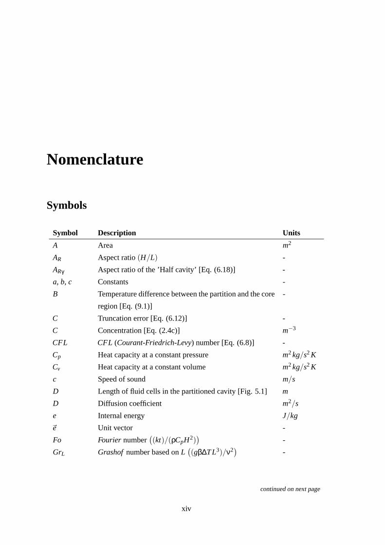
Nomenclature
Symbols
Symbol Description Units
A Area m2
AR Aspect ratio (H/L) -
ARγ Aspect ratio of the ’Half cavity’ [Eq. (6.18)] -
a, b, c Constants -
B Temperature difference between the partition and the core
region [Eq. (9.1)]
-
C Truncation error [Eq. (6.12)] -
C Concentration [Eq. (2.4c)] m−3
CFL CFL (Courant-Friedrich-Levy) number [Eq. (6.8)] -
Cp Heat capacity at a constant pressure m2 kg/s2 K
Cv Heat capacity at a constant volume m2 kg/s2 K
c Speed of sound m/s
D Length of fluid cells in the partitioned cavity [Fig. 5.1] m
D Diffusion coefficient m2/s
e Internal energy J/kg
~e Unit vector -
Fo Fourier number((kt)/(ρCpH2)
)-
GrL Grashof number based on L((gβ∆T L3)/ν2
)-
continued on next page
xiv
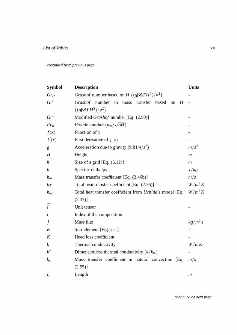
List of Tables xv
continued from previous page
Symbol Description Units
GrH Grashof number based on H((gβ∆T H3)/ν2
)-
Gr′ Grashof number in mass transfer based on H((gβ∆Y H3)/ν2
)-
Gr∗ Modified Grashof number [Eq. (2.50)] -
Fr∞ Froude number (u∞/√
gH) -
f (x) Function of x -
f ′(x) First derivative of f (x) -
g Acceleration due to gravity (9.81m/s2) m/s2
H Height m
h Size of a grid [Eq. (6.12)] m
h Specific enthalpy J/kg
hm Mass transfer coefficient [Eq. (2.46b)] m/s
hT Total heat transfer coefficient [Eq. (2.36)] W/m2 K
huch Total heat transfer coefficient from Uchida’s model [Eq.
(2.37)]
W/m2 K
¯I Unit tensor -
i Index of the composition −j Mass flux kg/m2 s
K Sub-element [Fig. C.1] -
K Head loss coefficient -
k Thermal conductivity W/mK
k∗ Dimensionless thermal conductivity (k/k∞) -
kc Mass transfer coefficient in natural convection [Eq.
(2.55)]
m/s
L Length m
continued on next page

xvi List of Tables
continued from previous page
Symbol Description Units
L Effective length [Eq. (3.11)] m
L Lagrange interpolation polynomial -
M Degree number of freedom for temperature and velocity
[Eq. (C.11a), (C.11b) and (C.11c)]
-
M Molar mass kg
Ma Mach number (v/c) -
Ma Modified Mach number [Eq. (8.7)] -
m Mass kg
m Number of iterations [Eq. (6.5)] -
m Mass flow rate kg/s
N Degree number of freedom for pressure [Eq. (C.12)] -
N Number of grids [Eq. (6.2)] -
NP, j j’th shape function for pressure [Eq. (C.12)] -
NU, j j’th shape function for velocity [Eq. (C.11a)] -
Nθ, j j’th shape function for fluid temperature [Eq. (C.11b)] -
Nθw, j j’th shape function for partition wall temperature [Eq.
(C.11c)]
-
NP,i i’th test function for pressure [Eq. (C.13a)] -
NU,i i’th test function for velocity [Eq. (C.13b)] -
Nθ,i i’th test function for fluid temperature [Eq. (C.13c)] -
Nθw,i i’th test function for partition wall temperature [Eq.
(C.13d)]
-
Nu Nusselt number((hH)/k f
)-
Nu Average Nusselt number -
continued on next page

List of Tables xvii
continued from previous page
Symbol Description Units
NuY Local Nusselt number in dimensionless form (= NuY,P)
[Eq. (5.50)]
-
Nuy Local Nusselt number in dimensional form (= Nuy,P) [Eq.
(5.49)]
-
n Number of iterations -
n Number of moles [Eq. (2.1)] -
nel Number of elements -
~n unit vector -
P Dimensionless pressure (pH2/ρα2) -
Pex Element Péclet number (uhh/2αh) -
Pr Prandtl number (ν/α) -
p Pressure Pa
p Perturbation parameter in test functions [Eq. (C.3b),
(C.3b), (C.3c) and (C.3d)]
-
p∗ Dimensionless pressure (p/p∞) -
p′ Hydrodynamic pressure Pa
ph Hydrostatic pressure Pa
p′∗ Dimensionless hydrodynamic pressure (p′/p′∞) -
p∗h Dimensionless hydrostatic pressure (ph/ph∞) -
Q Heat transfer rate W
q Test function for pressure [Eq. (C.3a)] -
q Test function for pressure in SUPG form [Eq. (C.3a)] -
q′′ Energy flux density W/m2
q′′r Energy flux density by radiation W/m2
q′′′ Internal heat generation rate W/m3
continued on next page

xviii List of Tables
continued from previous page
Symbol Description Units
R Real number -
R Thermal resistance K/W
R Gas constant of mixture (287J/kgK) J/kgK
R Average gas constant [Eq. (2.11)] J/kgK
Rg Universal constant of gas (8314J/kmoleK) J/kmoleK
RT Maximum temperature residual norms between two time
steps
-
Rθ Maximum dimensionless temperature residual norms be-
tween two time steps
-
RaL Rayleigh number based on L((gβ∆T L3)/(να)
)-
RaH Rayleigh number based on H((gβ∆T H3)/(να)
)-
RaHγ Rayleigh number for the ’Half cavity’ -
Re∞ Reynolds number ((ρ∞u∞H)/µ∞) -
S Trail solution space for finite element method -
s Entropy J/kg
Sh Sherwood number ((hmH)/(Dvap)) -
T Temperature K
Tγ Temperature for the ’Half cavity’ K
T ∗ Dimensionless temperature (T/T∞) -
t Time s
t∗ Dimensionless time (αt/H2) [Eq. (5.27)] -
t∗u Dimensionless time (tu∞/H) [Eq. (8.5)] -
U Dimensionless horizontal velocity (uH/α) -
u Horizontal velocity m/s
V Test function space for finite element method -
continued on next page

List of Tables xix
continued from previous page
Symbol Description Units
V Dimensionless vertical velocity (vH/α) -
V Volume m3
Vs Stefan velocity m/s
v Vertical velocity m/s
v Specific volume m3/kg~U U and V -
~u u and v m/s
W Width of partition wall [Fig. 5.1] m
w Test function for velocity [Eq. (C.3b)] -
w Test function for velocity in SUPG form [Eq. (C.3b)] -
X Dimensionless horizontal Cartesian coordinates (x/H) -
X Volume fraction [Eq. (2.4b)] -
x Horizontal Cartesian coordinates -
Y Dimensionless vertical Cartesian coordinates (y/H) -
Y Mass fraction [Eq. (2.4a)] -
y Vertical Cartesian coordinates -
Z Compressibility -

xx List of Tables
Greek letters
Symbol Description Units
α Thermal diffusion coefficient (k/(ρCp)) m2/kgs
βM Mass expansion coefficient -
β Thermal expansion coefficient -
βuch Proportion of the energy in the Uchida model [Eq. (2.40)
and (2.41)]
-
Γ Boundary of domain -
γuch Exponential parameter in the Uchida model [Eq. (2.40)
and (2.41)]
-
γ Dimensionless partition thickness (W/L) [Fig. 5.1] -
γc Specific heat ratio (Cp/Cv) -
∆ Differences -
∆Nuerr Percentage error between resolutions and the Exact values
of the Nusselt number [Eq. (6.17)]
-
∆T Temperature difference (Tw − T∞ for external flow and
Th −Tc for cavity case)
K
∆Tf ,Horizontal Horizontal temperature difference between partition wall
and bulk temperature of the fluid (Tw −Tf ,∞)
K
∆Tf ,Vertical Vertical temperature difference between fluid near top and
bottom of the partition wall (Tf ,top −Tf ,bottom)
K
∆Tw,Horizontal Horizontal temperature difference between both sides of
the partition wall (TWH −TWC)
K
∆Tw,Vertical Vertical temperature difference between top and bottom
of the partition wall (Tw,top −Tw,bottom)
K
∆θ f ,Horizontal Dimensionless form of ∆Tf ,Horizontal -
∆θ f ,Vertical Dimensionless form of ∆Tf ,Vertical -
∆θw,Horizontal Dimensionless form of ∆Tw,Horizontal -
∆θw,Vertical Dimensionless form of ∆Tw,Vertical -
continued on next page
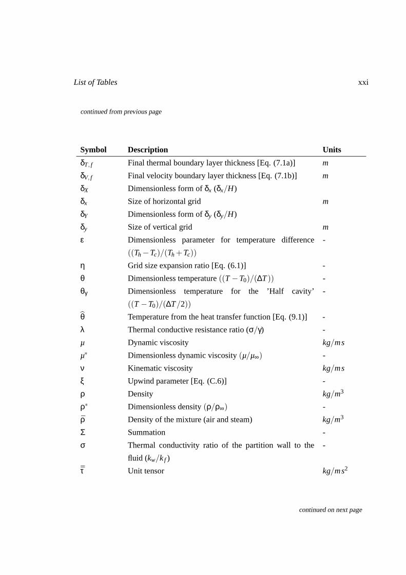
List of Tables xxi
continued from previous page
Symbol Description Units
δT, f Final thermal boundary layer thickness [Eq. (7.1a)] m
δV, f Final velocity boundary layer thickness [Eq. (7.1b)] m
δX Dimensionless form of δx (δx/H)
δx Size of horizontal grid m
δY Dimensionless form of δy (δy/H)
δy Size of vertical grid m
ε Dimensionless parameter for temperature difference
((Th −Tc)/(Th +Tc))
-
η Grid size expansion ratio [Eq. (6.1)] -
θ Dimensionless temperature ((T −T0)/(∆T )) -
θγ Dimensionless temperature for the ’Half cavity’
((T −T0)/(∆T/2))
-
θ Temperature from the heat transfer function [Eq. (9.1)] -
λ Thermal conductive resistance ratio (σ/γ) -
µ Dynamic viscosity kg/ms
µ∗ Dimensionless dynamic viscosity (µ/µ∞) -
ν Kinematic viscosity kg/ms
ξ Upwind parameter [Eq. (C.6)] -
ρ Density kg/m3
ρ∗ Dimensionless density (ρ/ρ∞) -
ρ Density of the mixture (air and steam) kg/m3
Σ Summation -
σ Thermal conductivity ratio of the partition wall to the
fluid (kw/k f )
-
¯τ Unit tensor kg/ms2
continued on next page

xxii List of Tables
continued from previous page
Symbol Description Units¯τ∗ Dimensionless unit tensor (¯τ/¯τ∞) [Eq. (8.11)] -
τSUPG SUPG stabilization factor [Eq. (C.5)] -
Φ Viscous dissipation function [Eq. (5.7)] s−2
Φ Test function for partition wall temperature [Eq. (C.3d)] -
Φ Test function for partition wall temperature in SUPG form
[Eq. (C.3d)]
-
φ Unknown value [Eq. (C.2) and (6.12)] -
Ψ Stream function [Eq. (7.6)] m2/s
Ψ Test function for fluid temperature [Eq. (C.3c)] -
Ψ Test function for fluid temperature in SUPG form [Eq.
(C.3c)]
-
χ Mass fraction of vapor to non-condensable gas
(Mvap/Mn−c)
-
Ω Domain -
ζ Thermal diffusivity ratio of the fluid to the solid (αw/α f ) -

List of Tables xxiii
Subscripts
Symbol Description
( )0 Initial
( )a, ( )air Air
( )C Cold fluid cell
( )c Convection
( )c Cold wall
( )chi Chilton-Colburn model
( )cond Condensation
( )Conduction Conduction
( )Convection Convection
( )Exact Exact
( )e Element
( )evap Evaporation
( ) f Fluid
( )g Gas
( )H Hot fluid cell
( )h Hot wall
( )i Index of the each mixture
( )in j Injection
( )k, ( )l , ( )m Compartment k, l and m
( )kl Junction from k to l
( )liq Liquid
( )max Maximum
( )min Minimum
( )mon Monitoring point
( )NP Non-partitioned cavity
( )n−c Non-condensable
continued on next page

xxiv List of Tables
continued from previous page
Symbol Description
( )P Pressure
( )P Partitioned cavity
( )S Sump
( )s, ( )sat Saturation
( )T Total
( )U Velocity
( )uch Uchida model
( )V Velocity
( )v, ( )vap Vapor
( )W Partition wall
( )w (Cold) Wall
( )WC Partition wall of cold fluid cell side
( )WH Partition wall of cold hot cell side
( )Y Local on vertical direction in dimensionless
( )y Local on vertical direction
( )γ ’Half cavity’
( )θ Temperature in dimensionless
( )∞ Reference (Bulk)

List of Tables xxv
Superscripts
Symbol Description
( )h Element order
( )i Index of the each mixture
( )liq Liquid
( )∗ Parametric value from non-linear equations
( )∗ Dimensionless

xxvi List of Tables
Abbreviations
Symbol Description
BWR Boiling Water Reactor
CFD Computational Fluid Dynamics
CPU Computer Processor Unit
DBA Design Basis Accident
ECCS Emergency Core Cooling System
FEM Finite Element Method
ISP International Standard Problem
LBB Ladyzhenskaya-Babouska-Brezzi
LBLOCA Large Break Loss Of Coolant Accident
LOCA Loss Of Coolant Accident
ODE Ordinary Differential Equation
OECD Organization for Economic Cooperation and Development
MICOCO Mixed COnvection and COndensation
NEA Nuclear Energy Agency (of OECD)
PDE Partial Differential Equation
PSPG Pressure-Stabilizing/Petrov-Galerkin
PWR Pressurized Water Reactor
RHRS Residual Heat Removal System
SBLOCA Small Break Loss Of Coolant Accident
SLBLOCA Steam Line Break Loss Of Coolant Accident
STP Standard Temperature and Pressure
SUPG Streamline-Upwind/Petrov-Galerkin
TMI Three Mile Island
Chapter 1
Introduction
1.1 Severe accident in a PWR nuclear power plant
After the accident of the nuclear power plant at Three Mile Island (TMI) in 1979, many
of researches have been focused on the issue of Loss of Coolant Accident (LOCA) in the
primary system of water cooled reactor nuclear power plant such as Pressurized Water Re-
actor (PWR), in figure 1.1, or Boiling Water Reactor (BWR). According to the scenario of
Steam Line Break LOCA (SLBLOCA), the high pressure sub-cooled water rushes imme-
diately out of the break and flashes to steam into the reactor containment structure until the
pressure in the reactor and in the containment building become equal : a blow-down phase
of LOCA [40]1. As the reactor core becomes dried out due to the loss of the coolant, the
zircaloy clad nuclear fuel and the inner core structures may be produce the hydrogen by Zr-
Water reactions. Then the hydrogen will be released into the reactor containment and may
be accumulated locally and may cause the hydrogen risk in the nuclear power plant [11].
According to the study of Shapiro and Moffette [65], the hydrogen deflagration and det-
onation may occur at certain conditions, namely, hydrogen risk of nuclear reactor severe
accident. Hence, it is very important to estimate the inner containment atmosphere status
accurately in the accident phase in order to accomplish the integrity of the nuclear power
plant.
The condensation of the injected steam is found to be one of the main parameter that
decides the inner containment atmosphere status. Precisely speaking, the inner contain-
1The average internal pressure and temperature in the coolant loop are ∼ 15MPa and ∼ 600K, respectively.
1

2 Chapter 1: Introduction
Figure 1.1: Schematic diagram of a typical PWR nuclear power
plant (1. Reactor containment, 2. Crane, 3 Control rods and 4.
Reactor vessel, Etc).

Chapter 1: Introduction 3
Figure 1.2: Schematic diagram of the 2 loop primary system of the
typical PWR nuclear power plant.
ment atmosphere temperature, pressure and the local concentration of air, steam and hy-
drogen are directly decided by the condensation of the injected steam on the surface of
the instruments and the inside wall of the containment. The steady-state is then reached
when the steam injection rate from the ruptured coolant line and condensation rate become
equal [10].
1.2 Loss of coolant accident (LOCA)
The LOCA in water cooled reactors results from a break in the pressure boundary of
the reactor cooling system, where the water inventory is reduced and radioactive fission
products maybe released into the containment. The LOCA is commonly classified as large-
break and small-break LOCA.
The Large-Break LOCA (LBLOCA) is caused by a broken large pipe in the reactor cooling
system shown in figure 1.2, and initiates a fast blow-down during the reactor is shut down
by excessive void. The licensing Design Basis Accident (DBA) of LOCA is defined as

4 Chapter 1: Introduction
a sudden severance of a large diameter cold leg pipe in a pressurized water reactor or a
recirculation jet-pump inlet pipe in a boiling water reactor. The reactor core is cooled
by Emergency Core Cooling System (ECCS), which are automatically activated during a
fast depressurization, in a matter of tens of seconds. After the core is quenched, the low-
pressure long term core cooling relies on the Residual Heat Removal System (RHRS) for
any size break in either PWR or BWR.
The Small-Break LOCA (SBLOCA) is caused by a broken small pipe or a stuck-open
safety relief valve in the reactor cooling system, and initiates a slow blow-down during
the heat system, and initiates a slow blow-down during the heat initially stored in the core
will be readily transferred to the coolant. Nevertheless, the core decay heat may not be
entirely removed by the break flow, such as in TMI accident. The primary system pressures
in SBLOCA of various break areas are calculated to last for hours. During this long-
lasting pressure hang-up, if ECCS does not work properly or it combines with anomalous
transients, such as loss of all feed-water or station blackouts, the SBLOCA may result in
a prolonged core uncovered. This situation makes operator action crucial to the course of
the accident, and it makes time in the anomalous transient vital to plant recovery.
1.3 Zircaloy Oxidation
In water cooled reactors, major LOCAs are often considered to place the severest
performance criteria on the safety systems. In these accidents the temperature at which
zircaloy cladding can maintain the fuel element structural integrity in a low-pressure steam
environment determines performance requirements on the ECCS. Thus a great deal of at-
tention has been given to the understanding of cladding behavior in the high-temperature,
low-pressure steam environments expected to appear during such accidents.
The cladding deterioration becomes more pronounced with increasing temperature. About
644K is the maximum operating temperature for water cooled reactor cladding. Between
922K and 1255K, swelling and creep cause the zircaloy to rupture, releasing gaseous fis-
sion products to the coolant. Above about 1255K the metal-water reaction as,
Zr +2H2O → ZrO2 +2H2 (1.1)

Chapter 1: Introduction 5
and becomes an increasingly important consideration.
In water cooled reactors, this exothermic reaction becomes significant above about 1366K,
and following a major LOCA, it may becomes auto-catalytic above about 2922K. Design
criteria are set to prevent the cladding from reaching 1366K based on the following ratio-
nale. For this improbable accident, rupture of cladding that permits escape of some gaseous
fission products can be tolerated. If its temperature is however allowed exceeding 1366K
for several minutes, a significant fraction of the cladding will react with the steam, causing
the cladding to be coated with brittle ZrO2. It has been shown that if more than about 18%
of the cladding reacts to form this oxide, it becomes susceptible to fragmentation from ther-
mal shock. Thus an unacceptable situation would exist, since the eventual quenching of the
cladding by emergency flooding of the core would result in the destruction of the cladding
as a structural support for the fuel, and thereby lead to an un-coolable configuration of core
debris. Note that the temperature criterion is well below the melting temperature. At the
same time it is independent of the stress level in the cladding, since the stress would be
relieved at lower temperature by swelling and creep rupture [40].
1.4 Hydrogen risk
In the hydrogen risk, the assumption is that 100% of the fuel cladding zircaloy oxi-
dizes (but not the other in-vessel Zr or steel structures) and that the generated hydrogen is
homogeneously distributed in the inner containment volume. According to the State-Of-
Art-Report of the OECD-NEA [28], the dry hydrogen concentrations are between 12% and
21% for American plant designs and between 17% and 20% for operating and future Euro-
pean PWR designs. The typical steam concentrations are from 20% to 70%, depending on
the accident scenario. These conditions define the global distribution area shown in figure
1.3.
The released hydrogen can generally accumulate in certain space of the reactor contain-
ment, which is highly complex structures. The inhomogeneity of the hydrogen distribution
mainly depends on details of the H2 sources (location, release rate), the containment de-
sign, and the efficiency of natural convection processes by the condensation of the released
steam.

6 Chapter 1: Introduction
Figure 1.3: Theoretical estimates of the possibility of the detona-
tion and the deflagration processes in severe accidents.

Chapter 1: Introduction 7
Two classes of detonation initiation can be distinguished when the local concentration
of the mixture leads to inside the detonation limits as shown in figure 1.3 : the direct strong
initiation by an external energy source and the indirect initiation with a weak ignition,
followed by a self-induced flame acceleration and deflagration to detonation transition. In
the first case, the energy necessary to establish a self-sustaining stable detonation front
wave system provided by the external source such as a spark or high explosive. In the
second case, the initiation energy is provided by the combustible mixture itself.
1.5 State of art
To certify the integrity of nuclear power plant from the potential severe accident rele-
vant to the hydrogen risk, many of researches have been continuing around the world by
the experiments and the numerical approaches.
According to the ISP47 [75], the containment thermal-hydraulics researches are undergoing
by experiments (MISTRA (France), TOSQAN (France) and THAI (Germany)) and numeri-
cal approaches in computational fluid dynamics (GOTHIC (USA), GASFLOW (Germany)
and TONUS (France)) and in lumped-parameter model codes (TONUS-0D (France)[10]
and COCOSYS (Germany)).
1.5.1 Experiments
The MISTRA facility (Figure 1.4) is a large scale experimental system in CEA (Com-
missariat à l’Energie Atomique) Saclay to analyze the possible severe accidents in PWR
focusing on the hydrogen risk such as steam line break accident (e.g. SLBLOCA) [69]. The
facility and its operating conditions are designed to simulate the steam and the hydrogen in-
jection into the PWR reactor containment phenomena and to validate the multi-dimensional
codes such as CAST3M/TONUS.
The MISTRA system has 100m3 of internal volume with 4.25m of diameter and 7.3m of
height. The linear length scale ratio of the mockup system to the reactor containment is 0.1.
There are 12 viewing windows for laser diagnostic measurements. The rock wool is used
as the facility insulation. Also the helium is used instead of the hydrogen. The condenser is
composed of 3 parts and installed a regulation circuit to ensure the stability and to maintain

8 Chapter 1: Introduction
Figure 1.4: Schematic diagram of the MISTRA.

Chapter 1: Introduction 9
the uniform wall temperature.
1.5.2 Numerical approaches
CAST3M
CAST3M is the computational simulation code that developed by DM2S (Département
de Mécanique des Systèmes et Structures) of CEA [1]. At the beginning, CAST3M was
used to called CASTEM2000, which was a finite element structure analysis code. After
all, the code was extended into the fluid mechanics and thermohydraulics and it became
CAST3M since year 2000. Basically, CAST3M is constructed by both ESOPE program-
ming language and GIBIANE command language. ESOPE extends FORTRAN77 applica-
tions with a dynamic memory allocation and a classification of segment data introducing.
The code CAST3M has several versions for the purposes. In this thesis, CAST3M for the
fluid mechanics is employed. The development of CAST3M enters within the framework
of an activity of research in the field of mechanics; the goal being to define a high level in-
strument, being able to be used as support valid for the design and the analysis of structures
and components, in the nuclear engineering field as in the traditional industrial sector.
Accordingly, CAST3M presents a complete system, integrating not only the functions
of calculation themselves, but also of the functions of construction of the model (pre-
processor) and of processing of the results (post-processor). CAST3M makes it possible
to deal with problems of linear elasticity in the fields static and dynamics (extraction of
eigenvalues), of the thermal problems, the nonlinear problems (elasto-visco-plasticity), of
the dynamic problems step by step, etc.
TONUS
TONUS is a specially developed application of the code CAST3M to analyze the
thermal-hydrodynamic characteristics of the internal atmosphere of the reactor contain-
ment during the severe accident of the nuclear power plant [22]. It used to write as
CAST3M/TONUS. Especially, TONUS code has the ability to simulated the behavior of
LOCA such as over-pressurization occurring after the fast depressurization of the primary
or secondary loop in the nuclear power plant, steam line break accident, molten core-
concrete interaction and hydrogen-air deflagration.

10 Chapter 1: Introduction
Application CAST3M/TONUS has two type of space discretization : a point discretization,
also called lumped-parameter model (TONUS-0D), and a multi-dimensional discretization
(TONUS-multiD). In the lumped-parameter model, the geometry is considered as the in-
terconnected compartments. The results of the simulation provide the mean value of the
quantities but the spatial fields cannot be evaluated. Nevertheless, the lumped-parameter
model has a fast convergence behavior compare to CFD and CPU cost is relatively cheap.
In the multi-dimensional approach, the geometry is meshed as a grid in two- or three-
dimensions. The spatial distribution and field of the quantities can be evaluated but the
computation is more expensive than the lumped-parameter model.
In this thesis, the lumped-parameter approach is conducted by TONUS-0D. Physically
TONUS-0D comprises of mass and energy conservation equations for the compartment
and for the sump. In TONUS-0D the sump roles the stockage of condensed water and
evaporation or boiling of water. Also the sump can recover the overflowed water from
other sumps. Between the compartments or the sumps, mass and energy can be transferred
through the atmospheric or liquid junctions. The wall is a structure in the compartment
that transfers (loss) the energy. This wall can model the condensation heat transfer and
multi-layer wall can be considered. Also, it is possible to create sump walls to model the
heat transfer to the floor.
The physical phenomena that can be taken into account by TONUS-0D are :
• Mass and wall condensation of steam.
• Evaporation and boiling to sump water.
• Water transfer between the sumps (by the overflow).
• Heat transfer between the compartments and walls.
• Hydrogen and carbon monoxide combustion.
• Estimation of residual heat from the fission products.
• Reactor containment cooling spray system.
• Passive auto-catalytic hydrogen re-combiners.
Chapter 1: Introduction 11
1.6 Objectives and outlines
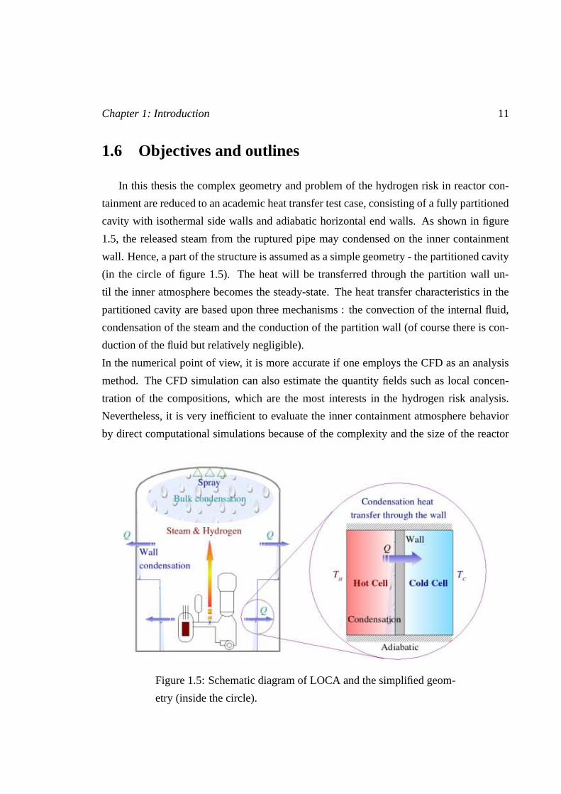
In this thesis the complex geometry and problem of the hydrogen risk in reactor con-
tainment are reduced to an academic heat transfer test case, consisting of a fully partitioned
cavity with isothermal side walls and adiabatic horizontal end walls. As shown in figure
1.5, the released steam from the ruptured pipe may condensed on the inner containment
wall. Hence, a part of the structure is assumed as a simple geometry - the partitioned cavity
(in the circle of figure 1.5). The heat will be transferred through the partition wall un-
til the inner atmosphere becomes the steady-state. The heat transfer characteristics in the
partitioned cavity are based upon three mechanisms : the convection of the internal fluid,
condensation of the steam and the conduction of the partition wall (of course there is con-
duction of the fluid but relatively negligible).
In the numerical point of view, it is more accurate if one employs the CFD as an analysis
method. The CFD simulation can also estimate the quantity fields such as local concen-
tration of the compositions, which are the most interests in the hydrogen risk analysis.
Nevertheless, it is very inefficient to evaluate the inner containment atmosphere behavior
by direct computational simulations because of the complexity and the size of the reactor
Figure 1.5: Schematic diagram of LOCA and the simplified geom-
etry (inside the circle).
12 Chapter 1: Introduction
containment (∼ 60000m3 in a typical PWR), which requires high capacity of computer
memory and CPU. Hence, if the temperature profile of the partition wall is given as a
boundary function, the computation may be economic within a framework of the simula-
tion costs.
An alternative method is then proposed in this thesis. Accordingly, a fully partitioned cavity
can be assumed as two separated cavities with a sharing boundary condition, the partition
wall. Thus, if the partition wall boundary condition is given, then it is possible to assess
the heat transfer characteristics corresponding to the partitioned cavity by using only the
’Half cavity’ simulation, which cost less than the partitioned cavity. To do this, first, a par-
titioned cavity is studied by the two-dimensional finite element code and the temperature
profile along the partition wall -so called heat transfer function- is suggested based on the
wall parameter, which is a boundary condition of the ’Half cavity’. Afterward, the the ’Half
cavity’ is also simulated in order to valid the heat transfer function.
The main parameters for the partitioned cavity natural convection heat transfer are : the
thermal conductivity ratio of the partition wall to the fluid (σ = kw/k f ), the ratio of the
partition wall thickness to the cavity length (γ = W/L) and the Rayleigh number based on
the cavity height (RaH). The range of the parameters is : 1 ≤ σ ≤ 105, 0.01 ≤ γ ≤ 0.2 and
103 ≤ RaH ≤ 107. It is noted that the values of σ of the reactor containment materials are :
∼ 850 for stainless steel 304 (∼ 17W/mK) and ∼ 50 for reinforced concrete (∼ 1W/mK)
at STP2 of air (∼ 0.02W/mK).
This thesis has three parts : Part I - Wall condensation, Part II - Natural convection heat
transfer in partitioned cavity and Part III - Conclusions and Prospects.
The outline of this thesis is :
• Chapter 2: The basic concept of the condensation is reviewed. Also two different
condensation models are reviewed : Uchida and Chilton-Colburn model.
• Chapter 3: The condensation heat transfer models are validated by the steady-state
calculation and lumped-parameter code simulation. Code CAST3M and TONUS-
0D are used for the calculation and the simulation, respectively. The reference case
study is performed by using the ’MICOCO benchmark study’, which is the simplified
2STP (Standard Temperature and Pressure) for air are 15 C (288K) and 101.3kPa(1bar) absolute,respectively.

Chapter 1: Introduction 13
test case of the MISTRA. Finally, the comparison is performed in order to valid the
resolutions.
• Chapter 4: The conclusions of the condensation heat transfer review.
• Chapter 5: The physical problem and the mathematical models for natural con-
vection heat transfer in the partitioned cavity are presented. The model is based on
the incompressible flow under Boussinesq approximation. The definition of Nusselt
number is introduced based on the thermal resistance that explains the multi-layer
region heat transfer characteristics. The code CAST3M is used in two-dimensions.
Also the governing equations are developed to SUPG finite element formulations and
to implicit scheme.
• Chapter 6: The validation and the qualification are presented on the model and
the resolutions. For the grid size convergence study, the mesh refinement method
and Richardson extrapolation method are introduced. The simulation criteria and
the iteration convergence study are discussed and a comparison with literature is
proceeded.
• Chapter 7: The results are shown and the physical phenomena of the non-partitioned
and the partitioned cavity are discussed. First, general observations of the heat trans-
fer characteristics are presented. Then, the effect of the partition wall thickness and
the conductivity ratio are discussed.
• Chapter 8: A benchmark study is proceeded by using the low Mach model. The
same numerical methods (SUPG finite element formulations and to implicit scheme)
are used and the heat transfer characteristics at large temperature difference cases are
analyzed.
• Chapter 9: The conclusions of the partitioned cavity natural convection heat transfer
study.

14 Chapter 1: Introduction

Part I
Wall condensation
15


17
Introduction
According to the scenario of the LOCA, the injected steam from the ruptured coolant
system may condense on the surfaces of the installed equipment and the inner wall of the
reactor containment. In the code CAST3M/TONUS, two different condensation models are
implemented : the Uchida and the Chilton-Colburn model. Basically, these models provide
the heat transfer coefficient in the turbulent heat transfer regime. In this part therefore the
validation of the condensation models are performed by the test case studies.
First, the basics of the thermodynamics are reviewed. Then, those models are validated by
the test case studies : the steady-state calculation by the code CAST3M and the lumped
parameter code simulation by the code TONUS-0D. The MICOCO (MIxed COnvection
and COndensation) benchmark study is applied for both calculation and simulation. This
benchmark study is focused on an air-steam steady-state study of MISTRA experiment.
The flow is classified as a turbulent since Gr∗ ∼ 1012 [11]3.
Instead of hydrogen (helium in MISTRA), MICOCO case injects high temperature steam
into the ambient temperature air filled closed geometry. The injected steam is then con-
densed on the wall remaining constant temperature during the simulation. The main goal
in this test case is to evaluate the temperature and the pressure at the steady-state in the
system to assess the inner containment behavior of the hydrogen risk. For the steady-state
confirmation, the condensation rate is monitored and assumed the steady-state when it be-
comes equal to the injection rate.
3Gr∗ is the modified Grashof number in equation (2.50)
Chapter 2
Review of the wall condensation models
Condensation is defined as the removal of heat from a system in such a manner that
vapor is converted into liquid. This may happen when vapor is cooled sufficiently below
the saturation temperature to induce the nucleation of the droplets. The nucleation may
occur homogeneously within the vapor or heterogeneously on entrained particulate matter,
for example, within the low pressure stages of a large steam turbine. The heterogeneous
nucleation may also occur on the walls of the system, particularly if these are cooled as in
the case of a surface condenser. In this latter case, there are two forms of heterogeneous
condensation, drop-wise and film-wise, corresponding to the analogous cases in evapora-
tion, of nucleate boiling and film boiling [18]. Film-wise condensation occurs on a cooled
surface which is easily wet. On the non-wet surfaces the vapor condenses in drops which
grow by further condensation and coalescence and then roll over the surface. New drops
then form to take their place.
This chapter mainly deals with two difference film-wise condensation model theories : the
Uchida and the Chilton-Colburn models, which are used in the code TONUS-0D and also
handle the turbulent heat transfer [22, 20]. For each model, condensation heat and mass
transfer rates are derived. In the Chilton-Colburn model, the convective heat transfer coef-
ficient can be calculated separately.
18

Chapter 2: Review of the wall condensation models 19
2.1 Review of thermodynamics
The thermodynamic characteristics of the gas mixture are needed and may be decided
by the volume, V , and the compositions of the mixture [67]. Suppose i is the index of the
each kind of mixture, then the mass, mi, and the density, ρi, of each composition are
mi = niMi (2.1)
where ni is the number of moles of composition i and Mi is the molar mass of composition
i. Then ρi is
ρi =mi
V. (2.2)
So, the mass of mixture, m, the number of moles, n, and the density, ρ, can be defined as
m = ∑i
mi, (2.3a)
n = ∑i
ni, (2.3b)
ρ =mV
= ∑i
ρi. (2.3c)
For each kind of mixture, the mass fraction, Yi, molar fraction, Xi, and the concentration,
Ci, can also be defined, as
Yi =mi
m=
ρi
ρ, (2.4a)
Xi =ni
n, (2.4b)
Ci =ni
V=
ρMi
. (2.4c)
Finally, the mixture molar mass, M, becomes
M = ∑i
XiMi =
(
∑i
Yi
Mi
)−1
. (2.5)
The pressure,p, temperature, T and density of a substance are related to an equation of
state. Although many substances are very complex in behavior, most gases, of engineering
20 Chapter 2: Review of the wall condensation models
interest, are well represented by the ideal gas equation of state at moderate pressure and
temperature :
p = ρRT (2.6)
where R is the gas constant of mixture. R can be written as
R =1ρ ∑
iρiRi =
Rg
M(2.7)
where Rg is the universal constant of gas. In this thesis, the value of Rg is equal to
8314J/kmoleK then R of air is equal to 287J/kmoleK.
This ideal gas equation of state is in error by less that 1% for air at room temperature for
pressures as high as 3MPa. For air at 0.1MPa, the equation is less than 1% in error for tem-
perature as low as 140K [26]. Also, if the temperature is inferior to 2000K, it is reasonable
to model the non-condensable gas by the ideal gas equation of state.
The pressure of the mixture is defined from difference between partial pressure of mixture
by the Dalton’s law :
p = ∑i
pi (2.8)
where the partial pressure, pi, is evaluated by the ideal gas equation of state (Eq. (2.6)).
The ideal gas equation of state can be described with the compressibility factor, Zi :
pi = ZiρiRiT. (2.9)
If the composition i is the ideal gas then Zi = 1 and the Dalton’s law can be written as
p = ρRT (2.10)
where the average gas constant, R, is
R =1ρ ∑
iZiρiRi. (2.11)
Consider the internal energy of a substance as e = e(v,T ) :
de =
(∂e∂T
)
vdT +
(∂e∂v
)
Tdv = CvdT +
(∂e∂v
)
Tdv (2.12)
Chapter 2: Review of the wall condensation models 21
where v = 1/ρ is the specific volume. The specific heat at constant volume is defined as
Cv ≡ (∂e/∂T )v.
Considering the ideal gas equation of state in equation (2.6), then (∂e/∂v)T = 0, and hence
e = e(T ). Consequently,
de = CvdT. (2.13)
For an ideal gas, this means that the internal energy and temperature changes may be related
to Cv. Furthermore, since e = e(T ), then Cv = Cv(T ).
The internal energy of the mixture is
e = ∑i
Yiei. (2.14)
The specific or mass enthalpy of a substance, h, is defined as
h ≡ e+pρ. (2.15)
For an ideal gas, and hence h ≡ e+RT . Since for an ideal gas, e = e(T ), then h also must
be a function of the temperature alone.
To obtain a relation between h and T , h is expressed as
h = h(p,T ). (2.16)
Then dh is
dh =
(∂h∂T
)
pdT +
(∂h∂p
)
Td p = CpdT +
(∂h∂p
)
Td p (2.17)
where the specific heat at constant pressure is defined as Cp ≡ (∂h/∂T )p. Also for an ideal
gas, (∂h/∂p)T = 0, and
dh = CpdT. (2.18)
Again, since h is a function of T alone, equation (2.18) requires that Cp be a function of T
only for an ideal gas.
For the gas mixture, the specific enthalpy can be defined as
h = ∑i
Yihi. (2.19)

22 Chapter 2: Review of the wall condensation models
Also the specific heats are defined as
Cp = ∑i
YiCpi, (2.20a)
Cv = ∑i
YiCvi. (2.20b)
The specific heats for an ideal gas have been shown to be functions of temperature only.
Their difference is a constant for each gas. Equation h = e+RT can be written as
dh = de+RdT. (2.21)
Combining this with equation (2.18), and using equation (2.13) becomes
dh = CpdT = de+RdT = CvdT +RdT. (2.22)
Then R becomes
R = Cp −Cv. (2.23)
The ratio of specific heats, γc, is defined as
γc ≡Cp
Cv. (2.24)
By using the definition of γc, equation (2.23) can be solved for either Cp or Cv in terms of
γc and R :
Cp =γcR
γc −1, (2.25a)
Cv =R
γc −1. (2.25b)
In order to derive a relationship among properties (p,v,T,s,e), the First and the Second
laws of the thermodynamics are combined, namely Gibb’s or T ds equation, where s is the
entropy, as
T ds = de+ pdv. (2.26)

Chapter 2: Review of the wall condensation models 23
This is a relationship among properties, valid for all processes between equilibrium states.
Although it is derived from the First and the Second laws, in itself it is a statement of
neither.
An alternative form of equation (2.26) can be obtained by substituting
de = d(h− pv) = dh− pdv− vd p (2.27)
to obtain
T ds = dh− vd p. (2.28)
For an ideal gas, the entropy change can be evaluated from the T ds equations :
ds =deT
+PT
dv = CvdTT
+Rdvv
, (2.29a)
ds =dhT
+vT
d p = CpdTT
−Rd pp
. (2.29b)
For special case of an isentropic process, ds = 0, and the T ds equations for an ideal gas
reduce to
CvdT + pdv = 0, (2.30a)
CpdT − vd p = 0 (2.30b)
since pv = RT . Solving for dT gives
dT =vd pCp
= − pdvCv
(2.31)
ord pp
+Cp
Cv
dvv
=d pp
+ γcdvv
= 0. (2.32)
Integrating (for γc = constant) gives
ln p+ γc lnv = lnc (2.33)
or
ln p+ lnvγc = lnc. (2.34)
Taking antilogarithms, this equation reduces to
pvγc = constant orp
ργc= constant (2.35)
Equation (2.35) is property relations for an ideal gas undergoing an isentropic process.

24 Chapter 2: Review of the wall condensation models
2.2 Uchida model
This correlation is based on the vertical plate (140mm wide, 300mm height) experiment
data of Uchida and Tagami in 1965 [30, 39, 62], which concerned the steam injection due to
the SLB LOCA scenario. In the experiments, the initial inventory of non-condensable gas
density remained constant as the steam mass fraction was increased, so that the bulk non-
condensable gas density remained constant. The correlation only works under conditions
in which the bulk non-condensable gas pressure and bulk temperature are around 1MPa
and 290K, respectively. Peterson [62] theoretically studied that the Uchida correlation may
under-predict heat removal rates for initial bulk gas pressure is above 1MPa.
The energy flux density of the system may modeled as
q′′ = hT (Tg −Tw) (2.36)
where q′′ is the energy flux density, hT is the total heat transfer coefficient, Tg is the tem-
perature of gas mixture and Tw is the temperature of wall.
The energy flux density includes the convective heat transfer coefficient and the conden-
sation heat transfer coefficient. Uchida and Tagami proposed the linear equation defining
the Uchida heat transfer coefficient, huch, in the case of condensation on a steel wall. The
empirical correlation is obtained as
hT = huch = 11.351+283.77χ (2.37)
where χ is the mass fraction of vapor, mvap to the non-condensable gas, mn−c (χ = mvap/mn−c).
It is found that the heat transfer is overestimated in the case of concrete wall since the ex-
periment of Uchida and Tagami had been held on a steel wall. In the code TONUS-0D the
Uchida heat transfer coefficient for the concrete was empirically suggested [20] :
hT = 0.4huch. (2.38)
If the mass of non-condensable gas is very small, the value of χ becomes infinite. High
value of hT may cause very small temperature difference in equation (2.36). To avoid
this situation, the value of hT is empirically limited to 5000W/m2K in the code TONUS-
0D [20]. Furthermore, hT in the Uchida correlation contains both convective and conden-
sation heat transfer coefficient :
hc ≤ hT ≤ 5000 (2.39)
Chapter 2: Review of the wall condensation models 25
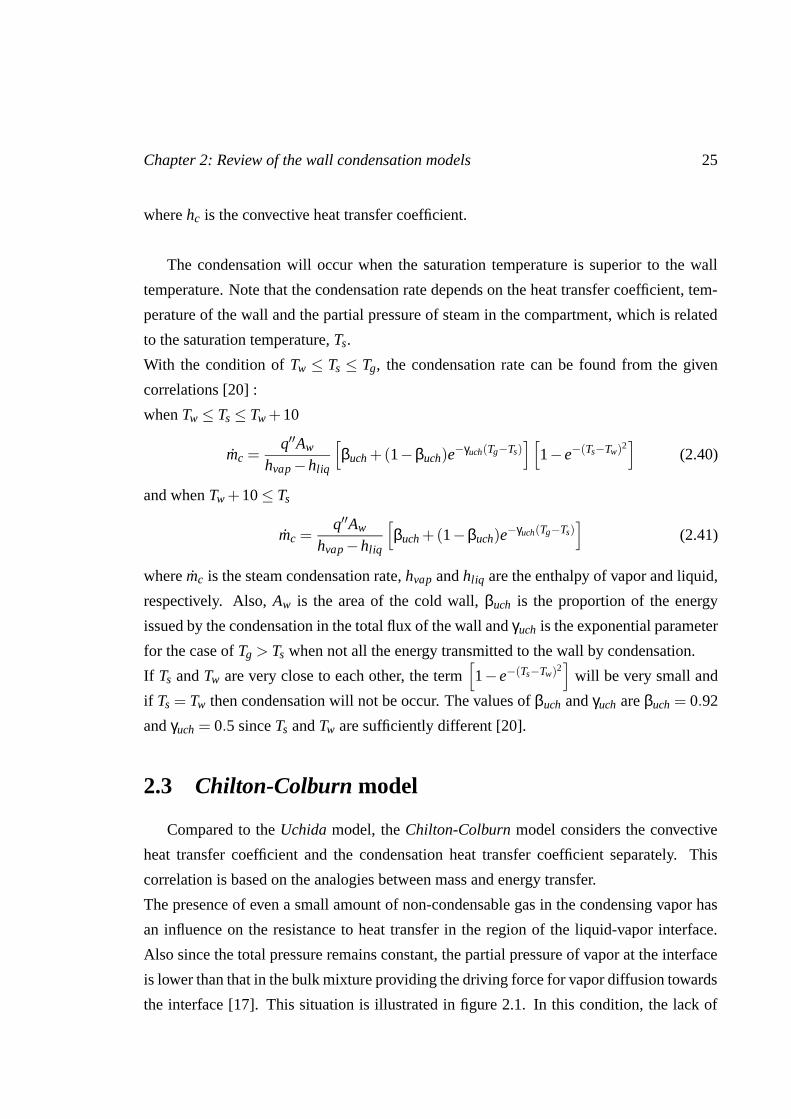
where hc is the convective heat transfer coefficient.
The condensation will occur when the saturation temperature is superior to the wall
temperature. Note that the condensation rate depends on the heat transfer coefficient, tem-
perature of the wall and the partial pressure of steam in the compartment, which is related
to the saturation temperature, Ts.
With the condition of Tw ≤ Ts ≤ Tg, the condensation rate can be found from the given
correlations [20] :
when Tw ≤ Ts ≤ Tw +10
mc =q′′Aw
hvap −hliq
[βuch +(1−βuch)e
−γuch(Tg−Ts)][
1− e−(Ts−Tw)2]
(2.40)
and when Tw +10 ≤ Ts
mc =q′′Aw
hvap −hliq
[βuch +(1−βuch)e
−γuch(Tg−Ts)]
(2.41)
where mc is the steam condensation rate, hvap and hliq are the enthalpy of vapor and liquid,
respectively. Also, Aw is the area of the cold wall, βuch is the proportion of the energy
issued by the condensation in the total flux of the wall and γuch is the exponential parameter
for the case of Tg > Ts when not all the energy transmitted to the wall by condensation.
If Ts and Tw are very close to each other, the term[1− e−(Ts−Tw)2
]will be very small and
if Ts = Tw then condensation will not be occur. The values of βuch and γuch are βuch = 0.92
and γuch = 0.5 since Ts and Tw are sufficiently different [20].
2.3 Chilton-Colburn model
Compared to the Uchida model, the Chilton-Colburn model considers the convective
heat transfer coefficient and the condensation heat transfer coefficient separately. This
correlation is based on the analogies between mass and energy transfer.
The presence of even a small amount of non-condensable gas in the condensing vapor has
an influence on the resistance to heat transfer in the region of the liquid-vapor interface.
Also since the total pressure remains constant, the partial pressure of vapor at the interface
is lower than that in the bulk mixture providing the driving force for vapor diffusion towards
the interface [17]. This situation is illustrated in figure 2.1. In this condition, the lack of

26 Chapter 2: Review of the wall condensation models
Fluid flow
Wall
x
y Mass transfer
Mixture of vapor and
Total pressure (P=Pvap+Pn−c)
Pvap
Pn−c
Tg
layer limit
liquid filmCondensed
non−condensible gas
Figure 2.1: The influence of non-condensable gas on inter-facial
resistance
vapor intends that the accumulation of non-condensable gas such as air at the interface
layer. Also these phenomena had been characterized by the Stefan velocity, Vs [30].
Let jvap and jn−c as the mass flux of vapor and non-condensable gas along the interface
at distance y :
jvap = ρvapVs −Dvapρ∂Yvap
∂y, (2.42a)
jn−c = ρn−cVs −Dvapρ∂Yn−c
∂y(2.42b)
where Dvap is the diffusion coefficient of vapor, ρ is the density of air and vapor mixture
from equation (2.3c)), ρvap and ρn−c are the density of vapor and non-condensable gas,
respectively. Also Yvap and Yn−c are the mass fraction of vapor and non-condensable gas,
respectively.
At the interface of layer, jn−c becomes zero. Then the Stefan velocity (Vs) in the i’th

Chapter 2: Review of the wall condensation models 27
component becomes
Vsi = Dvapρ
ρn−ci
(∂Yn−c
∂y
)
i= Dvap
1Yn−ci
(∂Yn−c
∂y
)
i(2.43)
where ρn−ci is the density of non-condensable gas in i’th component and Yn−ci is the mass
fraction of air in i component (Yn−ci = ρ/ρairi).
Substitute equation (2.43) into (2.42) then obtained
jvapi = − Dvapρi
1−Yvapi
(∂Yvap
∂y
)
i(2.44)
where∂Yvap
∂y+
∂Yn−c
∂y= 0 (2.45)
since Yvap +Yn−c = 1.
In the case of the analogy between the mass and energy (for Pr = Sc ≈ 1), the mass
transfer coefficient, hm, for the analogy of heat transfer coefficient (h) can be used. Hence,
the analogy between the energy and mass flux are
q′′ = −k∂T∂y
= h(T∞ −Ti), (2.46a)
jvap = −Dvapρ∂Yvap
∂y= hmρ(Yvap∞ −Yvapi) (2.46b)
where Ti is the temperature of component i, Yvapi is the mass fraction of vapor in i’th compo-
nent and T∞ and Yvap∞ are the reference (bulk) temperature and mass fraction, respectively.
Finally, the mass flux density of vapor at the interface is
jvapi = − Dvapρi
1−Yvapi
(∂Yvap
∂y
)
i=
kρi(Yvapi −Yvap∞)
1−Yvapi
. (2.47)
In the natural convection, the analogy between energy and mass transfer can be used
also when Pr ≈ Sc. The heat transfer will follow the scaling law [53] :
Nu = c ·GraH ·Prb (2.48)
where Nu is the Nusselt number (Nu = hH/k), GrH is the Grashof number based on the
height, H, in energy transfer(GrH = (gβ∆T H3)/ν2
)with ∆T = T∞ −Ti, Pr is the Prandtl

28 Chapter 2: Review of the wall condensation models
number (Pr = ν/α) and a, b and c are the constants. Where g is the acceleration due to
the gravity (9.81m/s2 in this thesis), ν is the kinematic viscosity of mixture and α is the
thermal diffusion coefficient.
Also mass transfer will follow
Sh = c ·Gr′a ·Prb (2.49)
where Sh is the Sherwood number (Sh = hmH/Dvap), Gr′ is the Grashof number in mass
transfer(Gr′ = (gβ∆Y H3)/ν2
)with ∆Y = Y∞ −Yi.
When natural convection is hybrid in certain conditions, γ(Y∞ −Yi) and β(T∞ −Ti) for ex-
ample are in same order, the Grashof number Gr and Gr′ can be arranged as the modified
Grashof number Gr∗ :
Gr∗ = [β(T∞ −Ti)+ γ(Y∞ −Yi)]gH3
ν2 =gH3
ν2
(ρi − ρ
ρ
). (2.50)
where ρi is the density of i’th component and ρ is the density of the mixture (i.e. air
and vapor). The definition of the thermal expansion coefficient, β, and mass expansion
coefficient, βM, is
β = −1ρ
(∂ρ∂T
), (2.51a)
βM = −1ρ
(∂ρ∂Y
). (2.51b)
The turbulent natural convective heat transfer coefficient may be defined from the Nus-
selt number correlation [53] :
Nu = 0.13(Gr ·Pr)1/3, 109 ≤ Gr ≤ 1012 (2.52)
and the convective heat transfer coefficient is then
hc = 0.13k
[g
(ρµ
)2(ρvap +ρn−c − ρρ
)] 13
(2.53)
where µ is the dynamic viscosity of mixture.
Note that when Tw ≤ Ts, ρvap is issued from the wall temperature (Tw) and the saturation
partial pressure at wall temperature (Psat(Tw)). Also ρn−c is issued from Tw and the partial
pressure difference (P−Psat(Tw)). When Tw > Ts, ρvap is issued from Tw and the partial

Chapter 2: Review of the wall condensation models 29
pressure of the vapor (Pvap) and ρn−c is issued from Tw and partial pressure difference
(P−Pvap).
As the analogy to the heat transfer, the mass transfer coefficient (hm) in the turbulent
may be defined from
Sh = 0.13(Gr′ ·Sc)1/3, 109 ≤ Gr′ ≤ 1012 (2.54)
and then mass transfer coefficient in natural convection, hmc, can be derived as
kc = 0.13Dvap
[(ρg
µDvap
)(ρvap +ρn−c − ρ
ρ
)] 13
=Dvap
2/3
k(
ρµ
)1/3hc. (2.55)
When Tw < Ts(Pvap), the steam condensation rate (mc) is given as
mc = kcAwρvap(Tg)−ρsat(Tw)
1−Xvap(Tw)(2.56)
where Xvap is the volume fraction of vapor.
Then the total heat transfer coefficient, hT , comprising the natural convection and the con-
densation is
hT = hc +hvap −hliq
Aw(Tg −Tw)mc. (2.57)
Finally the heat flux density becomes
q′′ = hT (Tg −Tw). (2.58)
Chapter 3
Application and simulation
Two condensation models are reviewed by the steady-state calculation and TONUS-
0D lumped-parameter code simulation. For the steady-state calculation, the code is pro-
grammed by GIBIANE computer language and the steam table from the code CAST3M
library is used. For the TONUS-0D simulation, two-dimensional axisymmetric mono-
compartment system is considered. A discussion is proceeded on the comparison of the
temperature, pressure, condensation rate and density with the literature.
As shown in figure 3.1, the MICOCO case is the simplified geometry case of the MISTRA
facility. In this case the volume is 82.7m3 and the area of the condenser surface is 71.7m2,
while those of the MISTRA are 100m3 volume and 69m2 [10]. As a scenario, 200 C of
steam injects with the rate of 0.12kg/s into the closed system, which is initially 0.5MPa and
140 C air ambient. It is assumed that the condensation will be occur only on the surface
of the cold wall with the constant temperature of 120 C, and the air is assumed as an ideal
gas. Initial and boundary conditions of MICOCO case are :
• Initial conditions
Pressure (P0) : 0.5MPa (including 0.1MPa of air at 20 C with 50% ofhumidity).Temperature (T0) : 140 C,Mass fraction of vapor (YH2O) : 0.62.
• Boundary conditions
30

Chapter 3: Application and simulation 31
1.3m
6m
3.8m
0.2m
Injector
Coldwall
4.25m
3.8m
Coldwall 6m
1.3m
0.2m
Injector
Figure 3.1: Schematic diagram of MISTRA facility (left) and MIC-
OCO case (right).
Steam injection rate (min j) : 0.12kg/s,Steam temperature (Tin j) : 200 C,Temperature of the cold wall (Tw) : 120 C.
3.1 Steady-state calculation
3.1.1 Calculation algorithm and results
The steady-state calculation is based on the energy and mass conservation equations
and steam tables. At steady-state, the energy from the injected steam, Qin j, is equal to the
energy loss due to the condensation, Qcond on the cold wall. Then the energy conservation
equation is
Qin j = Qcond . (3.1)

32 Chapter 3: Application and simulation
Table 3.1: Results of steady-state calculation.
P(MPa) Tg(C) XH2O(%) mair(kg) mvap(kg) hvap(J/kg)
Injection steam enthalpy at 0.5MPa (constant)
Uchida 3.96 131.05 66.21 97.33 118.35 2853460
Chilton 3.72 138.56 63.22 97.33 103.84 2853460
-Colburn
Above equation may rearranged as
min jhvap(Tin j)− mcondhliq(Tw) = hT Aw(Tg −Tw) (3.2)
and expresses that the latent heat of the steam (left hand side) is equal to the heat loss by
condensation (right hand side). Also considering the mass conservation between injection
and condensation flow rate :
min j = mcond (3.3)
where min j is the injection flow rate and mcond is the condensation flow rate. Then equation
(3.2) becomes
min j(hvap(Tin j)−hliq(Tw)) = hT Aw(Tg −Tw). (3.4)
Now the value of total heat transfer coefficient (hT ) is calculated by two different conden-
sation models : the Uchida and the Chilton-Colburn.
The schematic diagram of calculation algorithm for both models are shown in figure 3.2
and 3.3. The iterative method is used until ∆ρ < 10−7 is achieved and assumed the steady-
state has reached. The detail iterative methods and the equations are given in the appendix
A.
The amount of air is assumed from the density, thus, 1.1769kg/m3 at 20 C at 0.1MPa,
which are internal temperature and pressure of the MISTRA vessel before the preheating
phase [11].
The results of the calculation are shown in table 3.1. The internal mean temperature is
found as 138.56K by using the Chilton-Colburn model while it is found 131.05K by us-
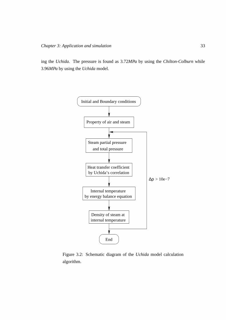
Chapter 3: Application and simulation 33
ing the Uchida. The pressure is found as 3.72MPa by using the Chilton-Colburn while
3.96MPa by using the Uchida model.
> 10e−7
Initial and Boundary conditions
Property of air and steam
and total pressure
Steam partial pressure
Heat transfer coefficientby Uchida’s correlation
by energy balance equationInternal temperature
Density of steam atinternal temperature
End
∆ρ
Figure 3.2: Schematic diagram of the Uchida model calculation
algorithm.
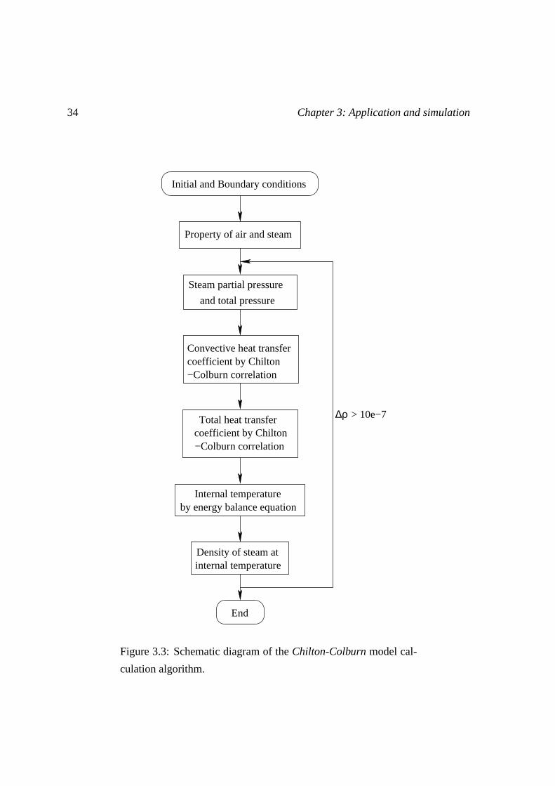
34 Chapter 3: Application and simulation
−Colburn correlationcoefficient by Chilton
by energy balance equationInternal temperature
Density of steam atinternal temperature
End
Convective heat transfer
∆ρ
Property of air and steam
and total pressure
Steam partial pressure
Initial and Boundary conditions
Total heat transfercoefficient by Chilton−Colburn correlation
> 10e−7
Figure 3.3: Schematic diagram of the Chilton-Colburn model cal-
culation algorithm.
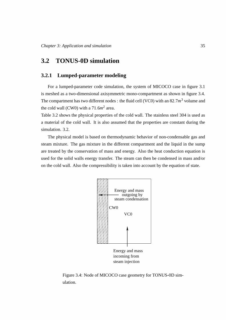
Chapter 3: Application and simulation 35
3.2 TONUS-0D simulation
3.2.1 Lumped-parameter modeling
For a lumped-parameter code simulation, the system of MICOCO case in figure 3.1
is meshed as a two-dimensional axisymmetric mono-compartment as shown in figure 3.4.
The compartment has two different nodes : the fluid cell (VC0) with an 82.7m3 volume and
the cold wall (CW0) with a 71.6m2 area.
Table 3.2 shows the physical properties of the cold wall. The stainless steel 304 is used as
a material of the cold wall. It is also assumed that the properties are constant during the
simulation. 3.2.
The physical model is based on thermodynamic behavior of non-condensable gas and
steam mixture. The gas mixture in the different compartment and the liquid in the sump
are treated by the conservation of mass and energy. Also the heat conduction equation is
used for the solid walls energy transfer. The steam can then be condensed in mass and/or
on the cold wall. Also the compressibility is taken into account by the equation of state.
VC0
CW0
steam condensation
steam injection
outgoing byEnergy and mass
Energy and massincoming from
Figure 3.4: Node of MICOCO case geometry for TONUS-0D sim-
ulation.
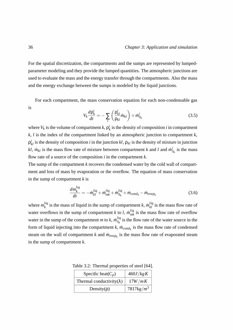
36 Chapter 3: Application and simulation
For the spatial discretization, the compartments and the sumps are represented by lumped-
parameter modeling and they provide the lumped quantities. The atmospheric junctions are
used to evaluate the mass and the energy transfer through the compartments. Also the mass
and the energy exchange between the sumps is modeled by the liquid junctions.
For each compartment, the mass conservation equation for each non-condensable gas
is
Vkdρi
k
dt= −∑
l
(ρi
kl
ρklmkl
)+ mi
Sk(3.5)
where Vk is the volume of compartment k, ρik is the density of composition i in compartment
k, l is the index of the compartment linked by an atmospheric junction to compartment k,
ρikl is the density of composition i in the junction kl, ρkl is the density of mixture in junction
kl, mkl is the mass flow rate of mixture between compartment k and l and miSk
is the mass
flow rate of a source of the composition i in the compartment k.
The sump of the compartment k recovers the condensed water by the cold wall of compart-
ment and loss of mass by evaporation or the overflow. The equation of mass conservation
in the sump of compartment k is
dmliqk
dt= −mliq
kl + mliqmk + mliq
Sk+ mcondk − mevapk
(3.6)
where mliqk is the mass of liquid in the sump of compartment k, mliq
kl is the mass flow rate of
water overflows in the sump of compartment k to l, mliqmk is the mass flow rate of overflow
water in the sump of the compartment m to k, mliqSk
is the flow rate of the water source in the
form of liquid injecting into the compartment k, mcondk is the mass flow rate of condensed
steam on the wall of compartment k and mevapkis the mass flow rate of evaporated steam
in the sump of compartment k.
Table 3.2: Thermal properties of steel [64].
Specific heat(Cp) 460J/kgK
Thermal conductivity(λ) 17W/mK
Density(ρ) 7817kg/m3

Chapter 3: Application and simulation 37
The energy conservation equation for the each compartment is
dek
dt= −∑
l
hklmkl +∑i
hSikmi
Sk+hevapk
mevapk−Awkφwk −hliq
condkmcondk (3.7)
where ek is the internal energy of gas mixture in the compartment k, hkl is the specific
enthalpy of gas mixture in the junction kl, hiSk
is the specific enthalpy of the source com-
position i injected into the compartment k, hevapkis the specific enthalpy associated to the
energy transfer by evaporation of water in the sump of compartment k, Awk is the area of
the wall in the compartment k and φwk is the thermal energy flux density change between
the compartment and the wall (by convection and condensation). If there are several walls
in the compartment, the contribution to the each wall can be considered, then, hliqcondk
is
the specific enthalpy associated to the energy transfer by condensation of the steam on the
walls of the compartment k.
The sump receives the energy produced by the condensed water on the wall and the eventual
sources such as the injector or another compartments sump. The energy loss in the sump
may caused by the evaporation or the overflow to another sump. The energy conservation
equation of the sump water is
deliqk
dt= −∑
l
hliqk mliq
kl +∑i
hliqm mliq
mk +hSliqk mliq
Sk+hliq
condkmcondk −hliq
evapkmevapk
(3.8)
where E liqk is the internal energy of water in the sump of the compartment k, hliq
k is the
specific enthalpy of water in the sump of the compartment k, mliqkl is the mass flow rate of
the water overflows from the sump of compartment k to l, hliqm is the specific enthalpy of
water in the sump of the compartment m, mliqmk is the mass flow rate of the water overflows
from the sump of compartment m to k, hSliqk is the specific enthalpy of the water as liquid
form injecting into the compartment k, hcondliqk is the specific enthalpy related to the heat
transfer by steam condensation on the wall of the compartment k.
For the structures in the compartment such as the wall, the time dependent heat con-
duction equation is used :
ρwCpw∂Tw
∂t= ∇ · (kw∇Tw) (3.9)
where ρw is the density, Cpw is the specific heat, Tw is the temperature and kw is the thermal
conductivity of the wall, respectively. In the code TONUS-0D, the structure may be mod-
eled as several layers with different thickness and physical properties.

38 Chapter 3: Application and simulation
The heat exchange between the structure and the compartments is modeled by using the
definition of heat flux, q′′, and the total heat transfer coefficient, hT , integrates the convec-
tion and the condensation :
q′′ = hT (Tg −Tw). (3.10)
The above equation is comparable to (2.36) and (2.58).
Figure 3.5 shows the calculation algorithm of TONUS-0D code. The equations from
(3.5) to (3.9) are solved by an implicit time discretization method. In lumped-parameter
approach the conservation of momentum cannot be calculated, and for this reason the at-
mospheric (or liquid) junction is used. In the atmospheric junction, the mass flow rate is
modeled by the momentum conservation equation to transport the gas mixture between the
compartment k to l via junction kl :
Lkl
Skl
dmkl
dt= (pk − pl)−
Kkl|mkl|mkl
2ρklS2kl
+ρkg(Hk −Hkl)−ρlg(Hl −Hkl) (3.11)
Mass conservation of gas & liquid(Source, Condensation, Evaporation)
Phase separation steam/liquid
Mass & energy transfer in sump(Evaporation or Condensation)
Energy conservation of gas & liquid(Source, Wall, Condensation)
Implicit time discretization
Figure 3.5: Schematic diagram of TONUS-0D calculation algo-
rithm.

Chapter 3: Application and simulation 39
Table 3.3: Results of simplified geometry case in TONUS 0D sim-
ulation.
P(MPa) Tg(C) XH2O(%) mair(kg) mvap(kg)
TONUS 0D simulation (Values at 4000s)
Uchida 4.03 131.84 66.6 97.33 121.15
Chilton 3.79 140.42 63.51 97.33 105.75
-Colburn
where Lkl is the effective length for the heat loss, Skl is the sectional area of the junction, pk
and pl are the total pressure of the compartment k and l, respectively, Kkl is the head loss
coefficient between two compartments k and l, ρkl is the density of mixture in the junction
kl and Hk, Hl and Hkl are the average height of the compartment k and l and the junction
kl, respectively.
At last, the total heat flux due to the convection and the condensation can be written as
q′′ = hc(Tg −Tw)+mcond
Aw(hvap −hliq) (3.12)
where hc is the convection heat transfer coefficient and Aw is the area of the wall. The value
of hc and mcond (and hT ) can be evaluated from both condensation models : the Uchida and
the Chilton-Colburn.
3.2.2 Results
The simulation is held until the steady-state being reached. The time steps are 0.5s
to 10s maximum and at 4000s is assumed as the steady-state. The results of simplified
geometry case TONUS-0D simulation are shown in table 3.3. The resolutions are similar
to those of the steady-state calculation in table 3.1. For example, the internal mean gas
temperature of the Chilton-Colburn model is higher then the Uchida model.

40 Chapter 3: Application and simulation
0 1000 2000 3000 4000Time (s)
0.0
0.2
0.4
0.6
0.8
Con
dens
atio
n R
ate
(kg/
s)
Chilton−ColburnUchidaInjection rate (0.12kg/s)CAST3M−3D
Figure 3.6: Evaluation of mcond and min j with time by TONUS-0D.
Figure 3.6 shows the comparison of the condensation rate (mcond). It is found that
the Uchida model under-predicts the condensation rate in the beginning of the calculation.
mcond of both models reached to the steady-state around 2000s and becomes equipoise to
the injection rate (min j). As shown in figures 3.7 and 3.8, the temperature and the pressure
of the internal gas also reached to the state-state around 2000s.
3.3 Comparison
The results of the steady-state calculations and TONUS-0D lumped-parameter simula-
tions are compared with the literature. Results of the literature are based on two [11] and
three [16] dimensional CFD simulations by the code CAST3M. The initial and boundary
conditions of both references are identical to those of the test cases in this thesis (see first
paragraph of 3). The geometry is based on the MICOCO benchmark case in figure 3.1. The
meshes in two and three dimensions are shown in figure B.1. The Navier-Stokes equations
for a multi-component gas mixture (air and steam, and hydrogen) are solved by an asymp-

Chapter 3: Application and simulation 41
0 1000 2000 3000 4000Time (s)
120
125
130
135
140
145
Gas
tem
pera
ture
(C
)
Chilton−ColburnUchidaCAST3M−3D
Figure 3.7: Evaluation of Tg with time by TONUS-0D.
0 1000 2000 3000 4000Time (s)
3.5
4.0
4.5
5.0
Pres
sure
(M
Pa)
Chilton−ColburnUhidaCAST3M−3D
Figure 3.8: Evaluation of P with time by TONUS-0D.

42 Chapter 3: Application and simulation
Table 3.4: Comparison of the results (S-S denotes the Steady-
State).
S-S TONUS-0D CAST3M-2D [11] CAST3M-3D [16]
Pressure (MPa)
Uchida 3.96 4.03 - -
Chilton 3.72 3.79 3.83 3.85
-Colburn
Temperature (C)
Uchida 131.05 131.84 - -
Chilton 138.56 140.42 128.2 138.73
-Colburn
totic low Mach number fluid flow model. The steam condensation is modeled by using the
Chilton-Colburn model. Also turbulent can be modeled by a mixing length scale model or
a standard k− ε model. The mixing length scale model is used for the CAST3M-2D and
-3D simulation.
The detail comparison is shown in table 3.4. First, the pressure by using the Uchida
model is found higher than by using the Chilton-Colburn model for both the steady-state
calculation and the code TONUS-0D simulation. As expected by the study of Peterson [62],
the Uchida model under-estimates the temperature and over-predicts the pressure. The
pressure by using the Chilton-Colburn model is found good agreement to the literature.
Also, the values of the temperature by using the Chilton-Colburn model are more compa-
rable than the Uchida model.
The temperature in case of CAST3M-2D shows relatively lower than others since the con-
vection heat transfer coefficient (hc) is assumes as 25W/m2K [11]. In the case of CAST3M-
3D, hc of 10W/m2K is used [16]. In this thesis, hc is found 10.4W/m2K when the Chilton-
Colburn model is used.
Chapter 4
Conclusion
In the study of hydrogen risk due to severe accident in PWR primary systems, the con-
densation of steam released from the broken coolant leg is an important issue for the safety
analysis. In this part the wall condensation models, the Uchida and the Chilton-Colburn
model, are reviewed in air-steam steady-state simulation by using the steady-state calcula-
tion and the lumped parameter code TONUS-0D.
The steady-state calculation is based on mass and energy conservation between injected
steam and its condensation. In TONUS-0D simulation, an axisymmetric mono-compartment
node is applied. Initial and boundary conditions are adopted from the MICOCO benchmark
study.
Comparing both condensation models, the Uchida model under-estimates the internal gas
temperature (Tg) and over-predicts the pressure (P). The reason is found that the Uchida
model is based on the experiment at the STP, and for this reason the model shows an error
when the initial pressure becomes higher than 1MPa. The results by using the Chilton-
Colburn model are found generally in good agreement with the literature.
43

44 Chapter 4: Conclusion

Part II
Natural convection heat transfer in
partitioned cavity
45


47
Introduction
Natural convection heat transfer in the (fully and center) partitioned cavity is an inter-
esting problem since the partition wall is one way to decrease the convective heat transfer
rate in various engineering applications. The heat transfer characteristics are usually com-
pare with non-partitioned cavity by an average Nusselt number, Nu.
In particular, Ho and Yih [31] have discovered the appearance of a peak in Nu when the
thermal conductivity ratio of the partition wall to the fluid, σ (= kw/k f ), increases from 1
to 105. An important feature is that the convective heat transfer reaches a maximum at the
peak value of Nu .
This phenomenon was also reported by Kangni et al,. [33, 34] and Mamou et al,. [46].
Nevertheless, the reason of the peak Nu has not yet been clearly demonstrated. In this part,
first of all, the heat transfer characteristics in the partitioned cavity are analytically and
numerically studied to understand the general phenomena and to explain the reason of the
peak.
Finally, the heat transfer function allowing the coupling between a lumped-parameter model
and a CFD is suggested based on the resolutions of the partitioned cavity. The function is
then validated by ’Half cavity’ simulation.
State of art
Tracing the history of the study, the convective heat transfer through a partition wall,
namely ’reservoir-to-reservoir’, is most concerned instead of the partitioned cavity since it
is easy to analyze theoretically.
According to the study of Lock and Ko [44], a boundary layer regime flow along the par-
tition wall is characterized within the limit of negligible thermal resistance of the partition
wall. This also means that conductivity of the partition wall is very high compare to that of
the fluid (σ = ∞). They concluded that the thermal resistance of the partition wall seems to
be negligible while the heat transfer is characterized by the boundary layer flow.
Similarly, Viskanta and Lankford [77] explained heat transfer characteristics of partitioned
cavity and suggested a method that can predict an average heat transfer coefficient (h) by
neglecting the thermal resistance of the partition wall.
Anderson and Bejan [4] analytically studied the ’reservoir-to-reservoir’ natural heat trans-

48
fer through the partition wall and concluded that the thermal resistance of the partition
wall is not negligible because the heat flux along the partition wall becomes uniform as
the thermal resistance of the partition wall is increased. This means in other words, the
thickness of the boundary layer along the partition wall becomes uniform with increasing
thermal resistance of the partition wall. They also reported that the average heat transfer
rate is relatively independent of the Prandtl number of the order 1 or higher and about 10%
difference in Nu was found between water and air.
Anderson and Bejan [5] expanded their study to the thermal stratification on the conductive
partition for the single and double partitioned cavity under negligible partition wall con-
ductivity effect and suggested a correlation concerning the number of partition walls.
An alternative approach had been tried by Duxbury (1979) in the study of Nishimura
et al,. [51]. The partitioned cavity is used instead of the ’reservoir-to-reservoir’ geometry.
An experimental study was presented on the aspect ratio of the cavity, AR (= H/L), 5/8
and 5 air filled cavity with a very thin partition inside. It is concluded that Nu decreases
from 50% compare to non-partitioned cavity case and proposed that the partitioned cavity
can be treated as two separated cavities with the cavity length of L/2 and the temperature
difference between both hot and cold walls of ∆T/2, namely, ’Half cavity’. Thus, when the
partition wall is isothermal (σ = ∞), the heat transfer characteristics of the AR = 1 parti-
tioned cavity are identical to AR ≈ 2 non-partitioned cavity at RaH/2. This is an important
feature for this thesis. Because, accordingly, the heat transfer characteristics of a ’Half cav-
ity’ are equal to those of the partitioned cavity. Thus, this fact may introduce the coupling
between lumped-parameter model and CFD by a heat transfer function. In other words, the
coupling is established by using the the heat transfer function based on a lumped-parameter
as a boundary condition of the ’Half cavity’. Hence, it is possible to obtain the same reso-
lutions compare to the partitioned cavity CFD simulation.
Within the framework of the convective heat transfer reduction, Sparrow and Parokash [68]
analytically studied a non-partitioned cavity containing heat loss by the external natural
convection boundary layer flow and Nu was found about 60% of constant temperature
boundary condition non-partitioned cavity.
Acharya and Tsang [3] considered an inclined partitioned cavity with the hot wall at upper
49
side and the cold wall at lower side and Nu was found about 45∼50% of non-partitioned
cavity.
As the conclusion of Nu reduction, Tong and Gerner [74] reported that the maximum re-
duction of Nu is shown when the partition is located in the center of the cavity.
The heat transfer mechanism in the partitioned cavity was studied by Nishimura et
al,. [51]. They found that when the thermal resistance of the partition wall becomes sig-
nificant, the thermal boundary layer thickness along the partition wall becomes uniform
because the temperature difference between the core region and the partition, thus, heat
flux is found uniform. This flow is so-called ’Uniform thermal boundary layer regime
flow’.
As an expansion of their study, for the uniform thermal boundary layer regime flow, Nu
was found identical to that of deviated partition position case [49]. The similar study was
done for multiple partition walls [50].
Similar to the study of Anderson and Bejan [4], the thermal resistance of the partition
wall becomes important if the partition thickness and the conductivity are ’finite’. As an
effect of the partition wall thickness, Meyer et al,. [47] studied the effect of partition wall
thickness and the thermal conductivity. They concluded that the partition wall becomes
thermally thin (isothermal) and the thermal resistance of the partition wall becomes neg-
ligible when the thickness of the partition wall, W , is smaller than 10% of the partition
height, H. Thus, W/H = W/L < 0.1 if AR = 1. This is a very important because it also
means that, when AR = 1, the ratio of the partition wall thickness to the cavity length, γ(= W/L), must be greater than 0.1 in order to observe the thermal resistance effect of the
partition wall.
Moreover, Kangni et al,. [33, 34] studied the effect of γ and found that Nu decreases with
increasing γ. The reason is found that the area for the convective heat transfer decreases
due to increasing γ and causes decreasing Nu.
Furthermore, Karayannis et al,. [35] found that the difference between Nu for real partition
(γ > 0.01 and σ . 102) and ideal partition (γ < 0.01 and σ & 102) is not greater than 12%
for the case of adiabatic horizontal end walls.
50
With regard to an effect of the conductivity ratio (σ), as mentioned earlier, Ho and
Yih [31] studied an air filled partitioned cavity with AR as 1, 2, 5 and 10, 103 < RaL <
5× 10⁶ and λ < 50000 where λ = σ/γ1. It was found that a peak value of Nu appears
at 100 < λ < 300 when RaL ≥ 105. After reaching a maximum, Nu decreases and finally
becomes constant at λ >∼ 104 for all RaL and AR since the conductive heat transfer across
the partition wall becomes negligible.
Kangni et al,. [33, 34] and Mamou et al,. [46] also found the peak of the Nu, which is sim-
ilar to that of Ho and Yih. Especially, Mamou et al,. used the parallel flow assumption in
high aspect ratio (AR = 4) partitioned cavity. Their study was based on an analytical and a
numerical method by using the constant heat flux boundary conditions. Nu is suggested as
a function of the partition numbers, thickness, conductivity ratio and angle for inclination
but found some discrepancy between both methods.
Now consider the fluid flow model and the geometry of the partitioned cavity study. By
the grace of its simplicity, the two-dimensional laminar steady-state incompressible flow
under the Boussinesq approximation of the Newtonian fluid with isothermal side walls and
adiabatic horizontal walls boundary condition is most considered.
According to Gray and Giorgini [27], the Boussinesq approximation can be used within the
limit of relatively small temperature difference between two isothermal walls. The Boussi-
nesq approximation may valid if ∆T ≤ 1.25 C for water (Pr = 8.1) and ∆T ≤ 28.6 C for
air (Pr = 0.72) where ∆T is the temperature difference between two isothermal side walls
(∆T = Th − Tc), when the reference temperature and pressure are 15 C and 0.1MPa, re-
spectively.
To avoid this limit, Cuckovic-Dzodzo et al,. [19] used the compressible fluid model with
temperature dependent properties. They found that the partition wall reduces convective
heat transfer from 59.1% to 63.6% in the range of the Rayleigh numbers and Prandtl num-
bers as 38000 < Ra < 369000, 2700 < Pr < 7000, γ = 0.05 and σ = 0.65.
1RaL is the cavity length based Rayleigh number. In this thesis the Rayleigh number based on the heightof the cavity, RaH , is used. The definition will be discussed later.

51
Scope of work
Compare to the non-partitioned cavity, the very high accurate multi-dimensional nu-
merical simulations for the partitioned cavity has not been yet reported and the results and
the correlations from the experiments are very restricted and insufficient.
Nevertheless, the study of non-partitioned cavity, namely, natural convection in square cav-
ity, has been studied very well by experiments and numerical methods. Especially, this
problem is reported as a benchmark study by de Vahl Davis and Jones [24].
Also de Vahl Davis and Jones [23] proposed a grid size convergence method by Richardson
extrapolation method, which may obtain the grid size independent Exact (or true) value of
the quantities. Recently, thanks to the remarkable progress of computational method, very
high accurate numerical resolutions have been obtained. Hortmann et al,. [32] presented
a numerical simulation for the non-partitioned cavity problem using 640×640 control vol-
ume cells and found results of Nu accuracy within 0.01% compare to the Exact value.
For this reason a study is performed on the ’Half cavity’ of AR ≈ 2 at RaH/2 corresponding
to the partitioned cavity as the reference of the partitioned cavity resolutions. Also, in order
to validate the resolutions of the ’Half cavity’ cases, AR = 1 non-partitioned cavity case is
simulated and their physical features are studied.
First of all, the study is presented on the laminar incompressible flow under the Boussi-
nesq approximation of the Newtonian fluid model. The temperature difference is however
large in the case of the LOCA and the incompressible-Boussinesq fluid flow model be-
comes inappropriate, and for this reason an asymptotic low Mach number model is used in
order to overcome the weakness point of the Boussinesq approximation [48]. Finally the
resolutions from both models are compared as a benchmark study.
Accordingly, the main parameters of the natural convection heat transfer in the fully
(centered) partitioned cavity are : the thermal conductivity ratio of the partition wall to the
fluid (σ), the ratio of the partition wall thickness to the cavity length (γ) and the Rayleigh
number (RaH).
The range of the parameters is : 1 ≤ σ ≤ 105, 0.01 ≤ γ ≤ 0.2 and 103 ≤ RaH ≤ 107.
The governing equations such as conservation of mass, momentum and energy for the

52
fluid and partition wall are generalized by dimensionless analysis method [8].
The governing equations are spatially discretized into the finite element method [41] with
the Streamline-Upwind/Petrov-Galerkin (SUPG) formulations [14]. This formulations are
found to be a good stability behavior at high velocity (high RaH) problems. For the mesh,
the macro-Q1 and P1-NC elements are used. This combination have found to be very
accurate and has fast convergence behavior [21]. Also the implicit scheme [60] is used to
reach the steady-state.
The simulation is proceeded by the code CAST3M in two-dimensions and the numerical
resolutions are qualified by the second-order Richardson extrapolation method [32]. Then,
the heat transfer characteristics in the non-partitioned and partitioned cavities are discussed.
Finally, the heat transfer function allowing the coupling between lumped-parameter model
and CFD, is introduced and validated by the ’Half cavity’ simulation.

Chapter 5
Problem description and mathematical
model
5.1 Fundamental principles
5.1.1 Governing equations
The governing equations are based on the conservation of mass, momentum and en-
ergy in a control volume. In particularly by using the definition of the dynamic viscosity,
µ, instead of the stress, τ, namely the constitutive relations, the momentum conservation
equation becomes the Navier-Stokes equations, which is widely used in the field of fluid
dynamics and thermal-hydraulics.
First, the differential equation of continuity for open control volume based on mass
conservation equation for closed control volume in the conservative form is
DρDt
+ρ(∇ ·~u) = 0 (5.1)
where~u is the velocity vector (u and v) in two-dimensions, t is time, ρ is density. Also ∇ is
the gradient and ∇· is the divergence.
Second, the differential equation of momentum, namely Navier-Stokes equations, in
53

54 Chapter 5: Problem description and mathematical model
conservative form is
ρD~uDt
= −∇ · (p ¯I − ¯τ)+~F = −∇p+∇ · ¯τ+~F (5.2)
where p is the pressure, ¯I is the unit tensor, ¯τ is the tensor and ~F is the body force vector.
The tensor is given as¯τ = µ(∇~u+(∇~u)T )− 2
3µ∇ ·~u ¯I (5.3)
where µ is the dynamic viscosity depending on the temperature, T . The dynamic viscosity
may determined by the Sutherland law :
µ(T )
µre f=
(T
Tre f
)3/2 Tre f +S
T +S(5.4)
where S = 110.5K for air at STP. Tre f and µre f are the reference temperature and dynamic
viscosity, respectively.
And the third, the "temperature" formulation of energy conservation equation in con-
servative form is
ρCpDTDt
= ∇ · (k∇T )−∇ ·q′′r +q′′′ +βTDpDt
+µΦ (5.5)
where Cp is the heat capacity at a constant pressure, k is the heat conductivity, q′′r is the heat
generation by radiation, q′′′ is the internal heat generation and β is the thermal expansion
coefficient at constant pressure :
β = −1ρ
(∂ρ∂T
)
p. (5.6)
Also Φ is the viscous dissipation function :
Φ = 2
[(∂u∂x
)2
+
(∂v∂y
)2]2
+
(∂u∂y
+∂v∂x
)2
(5.7)
in two-dimensions.
In this thesis the velocity and temperature are the main unknowns, hence, the non-
conservative form is used. Thus, the convective (material) derivative D/Dt is
DDt
=∂∂t
+~u ·∇. (5.8)
Chapter 5: Problem description and mathematical model 55
Mass, momentum and energy conservation equations, in non-conservative form are
∂ρ∂t
+∇ ·ρ~u = 0, (5.9a)
∂ρ~u∂t
+∇ ·ρ~u~u = −∇p+∇ · ¯τ+ρ~f , (5.9b)
ρCp
(∂T∂t
+~u ·∇T
)= ∇ · (k∇T )+βT
DpDt
(5.9c)
where it is assumed that zero radiation and internal heat generation (q′′r = 0 and q′′′ = 0)
and negligible viscous dissipation (Φ = 0). Note in equation (5.9b),
ρD~uDt
= ρ∂~u∂t
+ρ~u ·∇~u
= ρ∂~u∂t
+~u∂ρ∂t
+ρ~u ·∇~u+~u∇ ·ρ~u
=∂ρ~u∂t
+∇ ·ρ~u~u.
(5.10)
The body force term ~F in equation (5.2) becomes zero in x coordinate while ρ~f in y co-
ordinate. The force, ~f , is equal to g(−~e) where g is the acceleration due to the gravity
(g = 9.81m/s2) and ~e is the unit vector that becomes zero for x coordinate and unity for y
coordinate. Also, the fluid properties (e.g. µ and k) may be assumed to be a constant. Then
the governing equations can be rearranged as
∂ρ∂t
+∇ ·ρ~u = 0, (5.11a)
∂ρ~u∂t
+∇ ·ρ~u~u = −∇p+µ∇2~u+∇(
43
µ∇ ·~u)
+ρg(−~e), (5.11b)
ρCp
(∂T∂t
+~u ·∇T
)= k∇2T +βT
DpDt
. (5.11c)
5.1.2 Flow models and hypotheses
First of all, the conventional incompressible laminar flow under the Boussinesq approx-
imation for the viscous Newtonian fluid (µ 6= 0), air (Pr = 0.71), are used since the model
is extremely simple and convenient despite of the restrictions. Before proceeded to detailed
study, the fluid flow is classified on the basis of observable physical characteristics of flow
fields.
56 Chapter 5: Problem description and mathematical model
Laminar flow
The laminar flow is only considered in this thesis. As well known, the viscous flow
regimes are classified as laminar or turbulent on the basis of internal flow structure. In
the laminar regime, flow structure is characterized by smooth motion in laminae or lay-
ers. Contrary, the turbulent regime is characterized by random motions of fluid particles
superimposed on the mean motion [26].
Incompressible flow
Flows in which variations in density are negligible are termed incompressible while
compressible in opposite. In fact a truly constant density flow is impossible but generally
most of liquid flows are incompressible and gas flows are compressible. Of course there
are some phenomena which must consider the compressibility effects in liquid flows, water
hammer and cavitation for example.
The gas flows also may be considered incompressible if the provided flow speed is rel-
atively small than the speed of sound. Indeed, when the Mach number is less than 0.3,
the maximum density variation is less than 5% and the gas can be treated as incompress-
ible [26]. The definition of the Mach number is
Ma = v/c. (5.12)
A value of Ma = 0.3 in air at standard conditions corresponds to a speed of approximately
100m/s
Mathematically, incompressible flow represents ρ = constant, hence, dρ = 0, ∂ρ/∂t = 0
and ∇ρ = 0. For the incompressible liquid, the thermal expansion coefficient (β) becomes
zero.
Hence, for the gas flow, also for the ideal gas flow (i.e. β = 1/T ), the pressure variation
term (Dp/Dt) in energy equation (5.9c) becomes negligible since Ma → 0 [57]. In other
words, the energy term due to the thermal expansion of fluid is often small compared to the
other terms. An exception is near the front of a shock wave where Dp/Dt can be of a high
magnitude [73].

Chapter 5: Problem description and mathematical model 57
The governing equations for the incompressible flow are
∇ ·~u = 0, (5.13a)
ρ∂~u∂t
+ρ~u ·∇~u = −∇p+µ∇2~u+ρg(−~e), (5.13b)
ρCp
(∂T∂t
+~u ·∇T
)= k∇2T. (5.13c)
Boussinesq approximation
In fluid dynamics, the Boussinesq approximation is used in the field of buoyancy-driven
flow. It states that density differences are sufficiently small to be neglected, except where
they appear in terms multiplied by the acceleration due to gravity (g). The essence of the
Boussinesq approximation is that the difference in inertia is negligible (i.e. ∇ρ0 ≈ 0) but
gravity is sufficiently strong to make the specific weight appreciably different between the
two fluids.
Consider the equation of state within an ideal gas assumption is used to calculate pres-
sure term :
p = ρRT (5.14)
where R is the specific gas constant (R = Cp −Cv). Consider the boundary layer theory
along the vertical plate, the pressure is a function of longitudinal position only (i.e. ∂p∂x ≈
0) [8] :∂p∂y
=d pdy
=d p∞dy
(5.15)
where p∞ is the reference pressure. At any level of y, the densities are
ρ =p∞RT
and ρ∞ =p∞RT∞
(5.16)
where ρ∞ and T∞ are also the reference values.
Hence,
ρ−ρ∞ = ρ(
1− TT∞
). (5.17)
Above equation can be rearranged as
ρ∞ −ρρ∞
(1− ρ∞ −ρ
ρ∞
)−1
=T −T∞
T∞(5.18)

58 Chapter 5: Problem description and mathematical model
and may allow using the MacLaurin series (Taylor series expansion of function about 0).
For example, within the limit −1 < ρ∞−ρρ∞
< 1,
1
1− ρ∞−ρρ∞
= 1+ρ∞ −ρ
ρ∞+
(ρ∞ −ρ
ρ∞
)2
+ · · · . (5.19)
Hence,
ρ ' ρ∞
[1− 1
T∞(T −T∞)+ · · ·
]. (5.20)
With this equation, it is possible to say that the density is slightly decreasing below ρ∞
when the local temperature increases above the T∞. Also by using the thermal expansion
coefficient, above equation can be written as
ρ ' ρ∞ [1−β(T −T∞)+ · · · ] (5.21)
since for an ideal gas
β = −1ρ
∂ρ∂T
= −1ρ
(− P
RT 2
)=
1T
. (5.22)
The incompressible-Boussinesq fluid flow model in the closed cavity, ρ is constant
in everywhere except in the body force term of the y coordinate momentum equation
where it is replaced by ρ0[1− β(T − T0)] since the reference quantities are issued from
the initial state, T0 for temperature for example. In other words, density term in mo-
mentum equation remains constant (ρ = ρ0 in this study) except the buoyancy term, thus,
ρ = ρ0[1−β(T −T0)].
Now consider the pressure term in the momentum equation. The pressure is sum of hy-
drodynamic pressure, p′, and hydrostatic pressure, ph, as p = p′ + ph in order to avoid the
dominance of the hydrostatic pressure [57]. In deed, p′ << ph in general, hence, even the
variation of p′ exist, it is not easy to observe the pressure variation to time. Of course, in the
incompressible flow model, the pressure variation is negligible. The hydrostatic pressure
can be stated with respect to a reference level [8], thus, ph = p0 −ρ0gh.
Finally, the governing equations for the incompressible-Boussinesq fluid flow model are
∇ ·~u = 0, (5.23a)
∂~u∂t
+~u ·∇~u = − 1ρ0
∇p′ +ν∇2~u+βg(T −T0)(−~e), (5.23b)
ρCp
(∂T∂t
+~u ·∇T
)= k∇2T (5.23c)
where ν is the kinematic viscosity. Note that ∇p0 = 0.

Chapter 5: Problem description and mathematical model 59
5.2 Problem description
Consider two rectangular cavities of height, H, and width, L, with aspect ratio, AR, as
shown in figure 5.1 : non-partitioned and fully partitioned, which have a partition wall with
thickness, W . These cavities are filled with a Newtonian fluid such as air. Initially, the fluid
is isothermal and motionless everywhere in the cavity. The temperature of side walls are
constant, respectively, hot and cold wall (’Surfaces 1 and 2’ for non-partitioned cavity and
’1 and 4’ for partitioned cavity). The top and bottom walls are adiabatic. The partition
is centered, hence, size of both cells (Hot and Cold fluid cell) are identical (DH = DC)
and initially isothermal. Also the fluid in both cells are assumed to be same with constant
conductivity (k f ). The flow will be dominated by natural convection heat transfer from hot
to cold wall and through the partition wall.
5.2.1 Governing equations for non-partitioned cavity
The governing equations for non-partitioned cavity are equal to equations (5.23a),
(5.23b) and (5.23c) by using Tf instead of T where subscript f denotes the fluid1.
The initial conditions are
~u = 0, Tf = T0 at all x, y at t = 0. (5.24)
The boundary conditions are
~u = 0 on x = ±L2
and y = ±H2
at t ≥ 0, (5.25a)
∂Tf
∂y= 0 on y = ±H
2at t ≥ 0, (5.25b)
Tf = Th on x = −L2
at t ≥ 0, (5.25c)
Tf = Tc on x =L2
at t ≥ 0. (5.25d)
1The velocity and pressure are not distinguished since they are only for the fluid.

60 Chapter 5: Problem description and mathematical model
21
21
u=0,
u=0,
u=0,
u=0,
u=0,
Τ =Τ −
=0∂Τ∂y
=0∂Τ∂y
T =T +
at t=0Τ=Τ
h 0 0c
0
1 2Surface
H
g
y
x
L
=0∂Τ∂y
=0∂Τ∂y
0T=T at t=00T=T at t=0
∆Τ2
Τ =h∆Τ2
u=0,
u=0, u=0,
u=0,
u=0,
u=0,
SolidPartition
2 3 4Surface 1
Hot Cell Cold Cell(T )H (T )C
WDH DC
Τ +0 Τ −0Τ =c
(T )W
TWH TWC
yy
L
g
x H
Figure 5.1: Schematic diagram of 2-D non-partitioned and parti-
tioned rectangular cavity with isothermal side walls (right to left).

Chapter 5: Problem description and mathematical model 61
Dimensionless analysis
The governing equations for non-partitioned cavity in dimensionless form are
∇ ·~U = 0, (5.26a)
∂~U∂t∗
+~U · ∇~U = −∇P+Pr∇2~U +RaHPrθ f (−~e), (5.26b)
∂θ f
∂t∗+~U · ∇θ f = ∇2θ f (5.26c)
where ~U is the dimensionless velocity in vector, t∗ is the dimensionless time, P is the
dimensionless pressure and θ f is the dimensionless temperature of the fluid.
The definition of dimensionless parameters is
X =xH
, Y =yH
, ~U =~uHα f
, θ f =Tf −T0
∆T, P =
p′H2
ρ f 0α2f
,
t∗ =α f t
H2 ; Fourier number(Fo =k f t
ρ f 0Cp f H2 ), Pr =ν f
α f; Prandtl number,
RaH =gβ∆Tf H3
α f ν f; Rayleigh number(Ra = Gr ·Pr)
AR =HL
; Aspect ratio
(5.27)
where α f is the thermal diffusion coefficient (α f = k f /ρ fCp f ) and ∆T is the temperature
difference between hot and cold wall (∆T = Th −Tc). Also ∇ is the dimensionless form of
∇.
The initial conditions are
~U = 0, θ f = θ0 at all X , Y at t∗ = 0 (5.28)
where X and Y are dimensionless Cartesian coordinate system and the dimensionless initial
temperature θ0 = 0.
The boundary conditions are
~U = 0 on X = ± 12AR
and Y = ±12
at t∗ ≥ 0, (5.29a)
∂θ f
∂Y= 0 on Y = ±1
2at t∗ ≥ 0, (5.29b)
θ f = ±12
on X = ± 12AR
at t∗ ≥ 0. (5.29c)
Note that the height (H) is used for characteristic length of the Rayleigh number [61, 8].

62 Chapter 5: Problem description and mathematical model
5.2.2 Governing equations for partitioned cavity
The mass, momentum and energy equations for both fluid cells in figure 5.1 are same
to non-partitioned cavity case, for example equations (5.23a), (5.23b) and (5.23c). The
energy conservation equation in the partition wall is
ρwCpw∂Tw
∂t= kw∇2Tw (5.30)
where subscript w denotes the partition wall.
The initial conditions are
~u = 0, Tf = Tw = T0 at all x, y at t = 0. (5.31)
The boundary conditions are
~u = 0 on x = ±L2
and y = ±H2
at t ≥ 0, (5.32a)
∂Tf
∂y=
∂Tw
∂y= 0 on y = ±H
2at t ≥ 0, (5.32b)
Tf = Th on x = −L2
at t ≥ 0, (5.32c)
Tf = Tc on x =L2
at t ≥ 0, (5.32d)
k f∂Tf
∂x= kw
∂Tw
∂xon x = ∓W
2at t ≥ 0. (5.32e)
Note that the boundary condition (5.32e) represents the heat flux entering the partition wall
facing hot fluid cell is equal to the flux leaving from the hot fluid cell (also the heat flux
leaving the partition wall facing cold fluid cell is equal to the flux entering the cold fluid
cell).
Dimensionless analysis
Dimensionless form of equation (5.30) is
∂θw
∂t∗= ζ∇2θw (5.33)
where θw is the dimensionless temperature of the partition wall (θw = (Tw −T0)/∆T ) and
ζ is the thermal diffusivity ratio of the partition wall to the fluid (ζ = αw/α f ). The corre-
sponding initial conditions are
~U = 0, θ = θw = θ0 at all X , Y at t∗ = 0. (5.34)

Chapter 5: Problem description and mathematical model 63
The boundary conditions are
~U = 0 on X = ± 12AR
and y = ±12
at t∗ ≥ 0, (5.35a)
∂θ∂Y
= 0 on Y = ±12
at t∗ ≥ 0, (5.35b)
θ = ±12
on X = ∓ 12AR
at t∗ ≥ 0, (5.35c)
∂θ∂X
= σ∂θw
∂Xon X = ∓ γ
2at t∗ ≥ 0 (5.35d)
where γ is the ratio of the partition wall thickness to the cavity length (γ = W/L).
5.3 Heat transfer analysis
The heat transfer behavior is used to characterized by the Nusselt number, Nu. Here the
average Nusselt number, Nu, is defined as [7]
Nu =QTotal
QConduction=
QConvection +QConduction
QConduction(5.36)
For the convective heat transfer Nu > 1 and for the conductive heat transfer Nu = 1.
For the non-partitioned cavity, the total heat transfer rate at the steady-state, QTotal,NP,
in dimensional form, is
QTotal,NP =Z H
2
−H2
(k f
∂Tf
∂x−ρ fCPf vTf
)dy =
Z H2
−H2
k f∂Tf
∂x
∣∣∣∣x=±L/2
dy (5.37)
where the subscript NP denotes the non-partitioned.
The heat transfer rate by pure conduction at the steady-state, QConduction,NP, in dimensional
form, is
QConduction,NP = Hk f ∆T
L. (5.38)
Above definitions are only valid with the adiabatic horizontal end walls boundary condi-
tions (i.e. the heat is diffused from left to right side of the cavity).
The average Nusselt number of non-partitioned cavity, NuNP, becomes
NuNP =1H
Z H2
−H2
L∆T
∂Tf
∂x
∣∣∣∣x=±L/2
dy =1H
Z H2
−H2
Nuy,NPdy (5.39)

64 Chapter 5: Problem description and mathematical model
where k f is assumed as constant and Nuy,NP is the local Nusselt number of the non-
partitioned cavity :
Nuy,NP =L
∆T
∂Tf
∂x
∣∣∣∣x=±L/2
. (5.40)
In dimensionless form, Nuy,NP becomes
NuY,NP =1
AR
∂θ f
∂X
∣∣∣∣X=±1/2AR
(5.41)
and
NuNP =Z 1
2
− 12
NuY,NPdY. (5.42)
For the fully partitioned cavity (partially partitioned or aperture excluded), denoted
as P in subscript, it is not sufficient to explain the conductive heat transfer through multi-
conductive geometry by using equation (5.38). To overcome this, Lienhard and Catton [42]
proposed the Nusselt number as a function of the solid and fluid layer thicknesses and their
conductivities. They studied the Rayleigh-Bénard problem with fluid-solid-fluid layer and
conduction heat transfer through this multi-layer taken into account as sum of the thermal
resistance of each layer.
Also in the fully partitioned cavity, Meyer et al,. [47] and Mamou et al,. [46] considered
the partition thickness and the conductivity ratio in order to define the Nusselt number.
First, consider the total heat transfer rate in the partitioned cavity, QTotal,P. At the
steady-state, QTotal,P, is constant through entire domain :
QTotal,P = QHot cell = QPartition wall = QCold cell (5.43)
where QHot cell, QPartition wall and QCold cell are heat transfer rate of each part. Based on
equation (5.37), QTotal,P on the wall (i.e. x = ±L/2,±W/2) becomes
QTotal,P =Z H
2
−H2
k f∂Tf
∂x
∣∣∣∣x=±L/2,±W/2
dy. (5.44)
The heat transfer mechanism in the multi-conductive layer with the adiabatic horizontal
end walls is shown in figure 5.2 [53]. TH and TC are temperature of the hot and cold

Chapter 5: Problem description and mathematical model 65
C
TH
TC
C(k )(k )
HT
WC
RH
TH
TCC
RTWH
TWH
Solid Partition
WDH
D
Cold cell fluidHot cell fluidT
hT
c
(k )W
Q Q
TWC
RW
Figure 5.2: Schematic diagram of heat transfer between vertical
partition by thermal resistance theory [53].
cell, respectively. At the steady-state, the conductive heat transfer rate in each region,
QConduction in region, are identical :
QConduction in region =Th −TWH
RH=
TWH −TWC
Rw=
TWC −Tc
RC(5.45)
where TWH and TWC are the partition wall surface temperatures face to hot and cold cell,
respectively. Also, RH , Rw and RC are
RH =DH
Hk f, Rw =
WHkw
, RC =DC
Hk f(5.46)
where DH and DC are the length of hot and cold cell, respectively. The total conductive
heat transfer rate is equal to sum of the serials :
QTotal conduction =Σ∆Ti
ΣRi=
AR
1− γ(1−1/σ)k f ∆T (5.47)
since DH is equal to DC.
Finally, an average Nusselt number for fully partitioned cavity NuP is
NuP =1H
Z H2
−H2
L[1− γ(1−1/σ)]
∆T
∂Tf
∂x
∣∣∣∣x=±L/2,±W/2
dy =1H
Z H2
−H2
Nuy,Pdy. (5.48)

66 Chapter 5: Problem description and mathematical model
where k f is assumed as constant and Nuy,P is the local Nusselt number of the partitioned
cavity :
Nuy,P =L[1− γ(1−1/σ)]
∆T
∂Tf
∂x
∣∣∣∣x=±L/2,±W/2
. (5.49)
In dimensionless form, Nuy,P becomes
NuY,P =1− γ(1−1/σ)
AR
∂θ f
∂X
∣∣∣∣X=±1/2AR,±γ/2
. (5.50)
and
NuP =Z 1
2
− 12
NuY,PdY. (5.51)
It should be noted that the limits of above Nusselt number definition for the partitioned
cavity are 0 ≤ γ < 1 and σ ≥ 1.
Now compare both different average Nusselt number definitions in equation (5.42) and
(5.51). It is clear that NuNP is always greater than NuP because the partition wall is an
obstacle of the convective heat transfer :
NuP < NuNP (5.52)
when 0 < γ < 1 and σ > 1. In other words, the constant 1−γ(1−1/σ), the average Nusselt
number fraction, NuP/NuNP, becomes unity if γ = 0 or σ = 1.
Also as shown in figure 5.3, NuP/NuNP becomes larger with increasing γ and becomes
constant as σ is increased (γ(1−1/σ) → 1). Note that the case of γ = 0.5 is not simulated
in this thesis but applied to demonstrate the discrepancy between NuP and NuNP.
The effect of the partition wall thickness (γ) is considered in order to valid the definition
Nusselt number in equation (5.51). According to the study of Kangni et al,. [33, 34], the
average Nusselt number should be decreased with increasing γ at any values of RaH , σ and
AR since the convection area decreases with increasing γ. As shown in figure 5.4, by using
the conventional Nusselt number definitions : (5.40), (5.41) and (5.42), the value of average
Nusselt number increases at higher σ but decreases at lower σ with increasing γ. Never-
theless, by using the definition considering σ and γ : equations (5.49), (5.50) and (5.51)
the average Nusselt number decreases through the entire range of σ. As a consequence, it
is found that the constant (1− γ(1− 1/σ)) is a main factor that induces the decrement of

Chapter 5: Problem description and mathematical model 67
100
101
102
103
104
105
Conductivity ratio (σ = kw/kf)
0.4
0.5
0.6
0.7
0.8
0.9
1.0
Avg
. Nus
slet
num
ber
frac
tion
(Nu P
/ N
u NP)
γ=0.01γ=0.05γ=0.1γ=0.2γ=0.5
Figure 5.3: Fraction between different average Nusselt number def-
initions.
the average Nusselt number with increasing γ. This definition is also applicable for either
partitioned or non-partitioned (i.e. γ = 0) cavities. The physical phenomena, for example,
the effect of γ, σ and RaH , will be discussed later.
5.4 Numerical discretization
The time dependent Navier-Stokes equations are solved by a multi-dimensional code
CAST3M. The governing equations are discretized into the Stream-Upwind/Petrov-Galerkin
(SUPG) finite element formulations. Also the implicit scheme is used in order to reach the
steady-state. For the mesh, macro-Q1/P1-NC element type is used. All these algorithms
are implemented in the code CAST3M [1].
The general information of the finite element method, SUPG finite element formulations
and macro-Q1/P1-NC element type is shown in the appendix section C.1. The space and
time discretization for the governing equations are shown in the appendix section C.2.1 and
C.2.2.

68 Chapter 5: Problem description and mathematical model
100
101
102
103
104
105
Conductivity ratio (σ = kw/kf)
2.0
3.0
4.0
5.0
Avg
. Nus
selt
num
ber
γ=0.01γ=0.1γ=0.2
NuP
NuNP
Figure 5.4: The average Nusselt number comparison at RaH = 106.

Chapter 6
Validation of the code and computation -
Grid size convergence study
In this chapter, verification and validation of the code and mesh are studied in order to
ensure that the program solves the equation correctly and to test the extent to which the
model accurately represents reality. Also the qualification of the resolutions is taken into
account by the mesh convergence study. This study extrapolates the grid size independent
solutions, namely the Exact (or true) values.
To qualify and validate the resolutions, it is necessary to compare with other results (i.e.
different numerical method, experiments, analytical solutions or literature). Unfortunately,
the studies related to the natural convection in the partitioned cavity are few and very high
accurate numerical simulation has not been reported. Also the reported correlations are rel-
atively poor and restricted, hence, the qualification of the resolutions cannot be established
by recovering the literature.
According to the study of Duxbury (1979) [51] a AR = 1 partitioned cavity can be con-
sidered as two separated AR ≈ 2 of ∆T/2 (thus RaH/2) non-partitioned cavity when the
partition wall is isothermal (σ → ∞) or very thin (γ → 0). In other words, the heat trans-
fer characteristics such as Nu and temperature and velocity fields, etc, of hot or cold cell
(namely ’Half cavity’) of figure 5.1 is identical to those of the partitioned cavity.
In order to validate and qualify the partitioned cavity case resolutions, first, γ = 0.01 and
0.1 of AR = 1 partitioned cavity at RaH and σ = 105 are simulated as the representative
case study. Then compared with the cases of AR = 2.02 and 2.22 non-partitioned cavity at
69

70 Chapter 6: Validation of the code and computation - Grid size convergence study
RaH/2 with isothermal side wall boundary conditions, which correspond to the partitioned
cavity cases, respectively.
In order to validate and qualify above AR ≈ 2 cases, AR = 1 and 2 non-partitioned cavity is
also studied. Thanks to the benchmark study of de Vahl Davis [24], AR = 1 non-partitioned
cavity natural convection heat transfer case is very well studied and the reported resolutions
are in very high accuracy.
In this chapter a discussion is also presented on the mesh construction, grid size re-
finement method and iteration convergence study. Then the mesh convergence study is
performed for AR = 1, 2.02 and 2.22 non-partitioned cavity and γ = 0.01 and 0.1 of AR = 1
partitioned cavity at σ = 105. The resolutions of AR = 1 non-partitioned cavity case are
compared with the literature. Finally, γ = 0.01 and 0.1 of AR = 1 partitioned cavity cases
are validated by AR = 2.02 and 2.22 non-partitioned cavity cases.
6.1 Mesh design and simulation conditions
The mesh is constructed by the non-uniform grid size mesh, which has the smallest grid
size near walls and the largest at the center. This technique is widely used for numerical
simulations since its accuracy and fast convergence behavior [15, 32]. The sizes of the grid
are determined by using refinement method [32].
First, for the AR = 1 non-partitioned cavity for example, it is decided that the minimum
size of grid (δXmin = δX1) in the coarsest 10×10 mesh is equal to 0.05. As shown in figure
δ iXδ 3XX 1 =
=
=
=δ i−1Xη
δ 1Xi−1η
δ 2Xη
δ 1Xη 2
Xδ 1η
δ 2Xδ
Grids
=...
...
...
Figure 6.1: Schematic diagram of using the expansion ratio η.

Chapter 6: Validation of the code and computation - Grid size convergence study 71
6.1, the grid size is then increased by an expansion ratio, η. The grid size δXi is
δXi = ηδXi−1 = ηi−1δX1 (6.1)
where i is the grid size of i’th spacing. The value of η can be found by using geometric
series :N/2
∑i
δXi =N/2
∑i
ηN/2−1δX1 =δX1(1−ηN/2)
1−η=
L2
(6.2)
where N is the number of grids corresponding to the axes. Note that the half of the number
of grids (N/2) and half of the length (L/2) are used in order to construct a symmetric mesh.
Once η1 for the 10×10 mesh is found then η2 for the 20×20 mesh can be found by using
ηk =√
ηk−1 (6.3)
where k is the refinement factor and δX1 for k’th mesh can be found from equation (6.2).
In order to solve equation (6.3), the Newton-Raphson method is used since the equation
is non-linear. Thus, once decided as δX1 = 0.05 at k = 1 mesh (10 × 10 mesh for example),
equation (6.3) becomes function of η :
f (η) = 2δX1(ηN −1)−L(η−1). (6.4)
Then by the Newton-Raphson method, the value of η is
ηm = ηm−1 −f (ηm−1)
f ′(ηm−1)(6.5)
where m is the number of iterations. The convergence will be accomplished when
| f (η) f ”(η)|| f ′(η)|2 < 1. (6.6)
The iteration is conducted until residual norms between two iterations become less than
10−6 :
|ηm −ηm−1| < 10−6. (6.7)
The value of η, δXmin and the number of micro-elements for AR = 1 non-partitioned cavity
are shown in the appendix table D.1. Note that δXmin and δYmin (also ηX and ηY ) are iden-
tical since AR = 1.
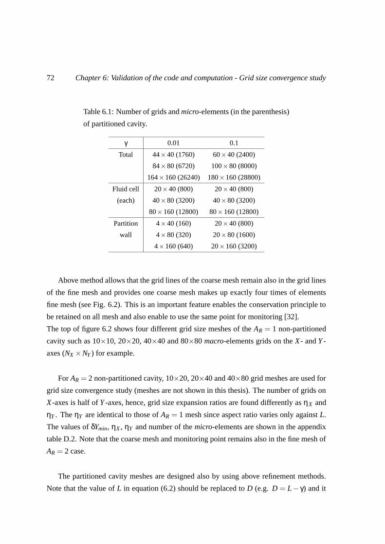
72 Chapter 6: Validation of the code and computation - Grid size convergence study
Table 6.1: Number of grids and micro-elements (in the parenthesis)
of partitioned cavity.
γ 0.01 0.1
Total 44×40 (1760) 60×40 (2400)
84×80 (6720) 100×80 (8000)
164×160 (26240) 180×160 (28800)
Fluid cell 20×40 (800) 20×40 (800)
(each) 40×80 (3200) 40×80 (3200)
80×160 (12800) 80×160 (12800)
Partition 4×40 (160) 20×40 (800)
wall 4×80 (320) 20×80 (1600)
4×160 (640) 20×160 (3200)
Above method allows that the grid lines of the coarse mesh remain also in the grid lines
of the fine mesh and provides one coarse mesh makes up exactly four times of elements
fine mesh (see Fig. 6.2). This is an important feature enables the conservation principle to
be retained on all mesh and also enable to use the same point for monitoring [32].
The top of figure 6.2 shows four different grid size meshes of the AR = 1 non-partitioned
cavity such as 10×10, 20×20, 40×40 and 80×80 macro-elements grids on the X- and Y -
axes (NX ×NY ) for example.
For AR = 2 non-partitioned cavity, 10×20, 20×40 and 40×80 grid meshes are used for
grid size convergence study (meshes are not shown in this thesis). The number of grids on
X-axes is half of Y -axes, hence, grid size expansion ratios are found differently as ηX and
ηY . The ηY are identical to those of AR = 1 mesh since aspect ratio varies only against L.
The values of δYmin, ηX , ηY and number of the micro-elements are shown in the appendix
table D.2. Note that the coarse mesh and monitoring point remains also in the fine mesh of
AR = 2 case.
The partitioned cavity meshes are designed also by using above refinement methods.
Note that the value of L in equation (6.2) should be replaced to D (e.g. D = L− γ) and it

Chapter 6: Validation of the code and computation - Grid size convergence study 73
Figure 6.2: Meshes of different grid sizes. AR = 1 non-partitioned
cavity (top, four meshes at one quarter of each clockwise) and γ =
0.1 partitioned cavity (bottom, three meshes clockwise). Symbol
"X" indicates the monitoring point.

74 Chapter 6: Validation of the code and computation - Grid size convergence study
causes δX 6= δY (also ηX 6= ηY ).
Table 6.1 shows the number of grids and micro-elements of partitioned cavity. Note that
the quadratic elements grid size of the partition wall to X-direction are differently decided
as 0.005 and 0.01 when γ are 0.01 and 0.1, respectively.
Three different type of the γ = 0.1 partitioned cavity meshes are shown in the bottom of
figure 6.2. For example, 60× 40 , 100× 80 and 180× 160 macro-elements grids on the
X- and Y -axes, respectively. The values of δXmin, δYmin, ηX , ηY and number of the micro-
elements for three different geometry cases (γ = 0.01 and 0.1) are shown in the appendix
tables D.3 and D.4.
In order to design the mesh of partition wall, both uniform and non-uniform grid size
meshes are used for X- and Y -directions, respectively. Thus, for δX = 0.01 when γ ≥ 0.1
and δX = 0.005 when γ < 0.1 are used. Note that the values of δY are identical to those of
fluid cells (see Fig. 6.2).
The time step is based on the definition of CFL number (Courant-Friedrich-Levy),
which determines how many mesh cells, a fluid element passes during a time step. Or
rather, the fraction of a time step to pass one cell. For explicit time stepping schemes, such
as Runge-Kutta, the CFL number must be less than the stability limit for the actual scheme
to converge. For implicit and semi-implicit schemes, the CFL limit does not constitute a
stability limit. On the other hand, the range of parameters in which these schemes converge
may often be characterized by the CFL number. If CFL > 1 then unstable in explicit
scheme. In this thesis the definition of CFL number is
CFL =ure f ∆t
δymin=
Ure f ∆t∗
δYmin. (6.8)
Where ure f is the reference velocity in dimensional form with
ure f =√
gβ∆T H
=
√g∆T H
T0for ideal gas.
(6.9)
Also, in dimensionless form, equation (6.9) becomes
Ure f = C ·Gr1/2 = C ·Ra1/2 ·Pr−1/2
≈C ·Ra1/2 if Pr ∼ 1(6.10)
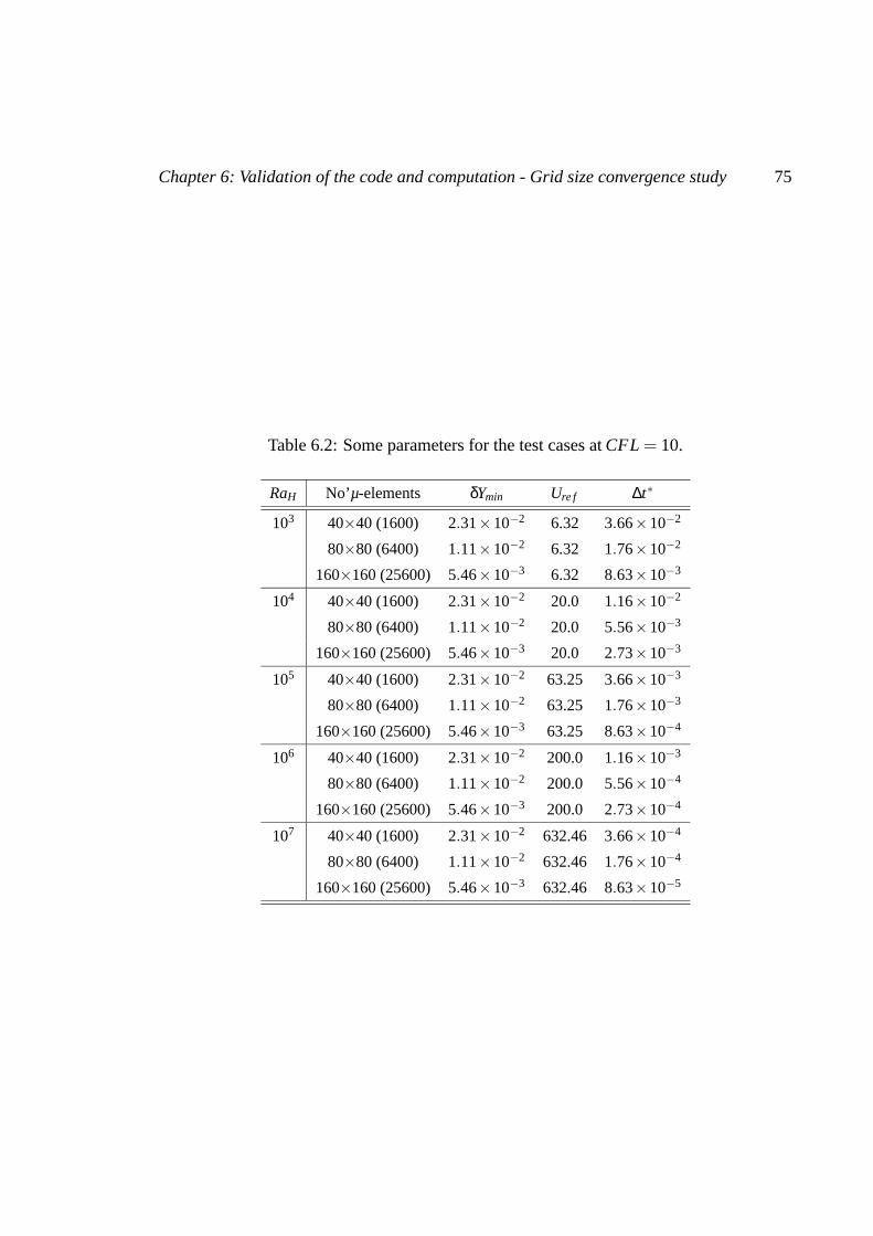
Chapter 6: Validation of the code and computation - Grid size convergence study 75
Table 6.2: Some parameters for the test cases at CFL = 10.
RaH No’µ-elements δYmin Ure f ∆t∗
103 40×40 (1600) 2.31×10⁻² 6.32 3.66×10⁻²
80×80 (6400) 1.11×10⁻² 6.32 1.76×10⁻²
160×160 (25600) 5.46×10⁻³ 6.32 8.63×10⁻³
104 40×40 (1600) 2.31×10⁻² 20.0 1.16×10⁻²
80×80 (6400) 1.11×10⁻² 20.0 5.56×10⁻³
160×160 (25600) 5.46×10⁻³ 20.0 2.73×10⁻³
105 40×40 (1600) 2.31×10⁻² 63.25 3.66×10⁻³
80×80 (6400) 1.11×10⁻² 63.25 1.76×10⁻³
160×160 (25600) 5.46×10⁻³ 63.25 8.63×10⁻⁴
106 40×40 (1600) 2.31×10⁻² 200.0 1.16×10⁻³
80×80 (6400) 1.11×10⁻² 200.0 5.56×10⁻⁴
160×160 (25600) 5.46×10⁻³ 200.0 2.73×10⁻⁴
107 40×40 (1600) 2.31×10⁻² 632.46 3.66×10⁻⁴
80×80 (6400) 1.11×10⁻² 632.46 1.76×10⁻⁴
160×160 (25600) 5.46×10⁻³ 632.46 8.63×10⁻⁵

76 Chapter 6: Validation of the code and computation - Grid size convergence study
where C is the constant. Accordingly, the value of C is found about 0.2 in the range of
103 ≤ RaH ≤ 107 [24, 15, 32, 38]. Also, equation (6.10) corresponds to the scale of the
vertical velocity (V ∼ Ra1/2H ) if Pr ∼ 1 [8]. Hence, in this thesis Ure f is calculated from
0.2Ra1/2H .
Table 6.2 shows the dimensionless time step size and other parameters for AR = 1 non-
partitioned cavity. In this thesis, CFL = 10 is used. It should be noted that the time steps
for the partitioned cavity are identical to those of the non-partitioned cavity cases since
δYmin are equal.
The simulation is conducted until maximum dimensionless temperature residual norms,
Rθ, between two time steps becomes less than 10−10 :
|θn −θn−1|max < 10−10. (6.11)
Hence, when Rθ reaches to the criteria, it is assumed that the steady-state is achieved.
6.2 Grid size convergence study
The grid size convergence is based on an extrapolation scheme, which allows obtaining
a solution of high accuracy [24]. Suppose, φ is the value of certain quantity from the mesh
with a grid size of h. By using refinement method the mesh size is refined as h1, h2 and
h3 and the values φ1, φ2 and φ3 are then computed. Note that the condition h2 = h1/2 and
h3 = h1/4 must be satisfied.
If the computed values φ1, φ2 and φ3 are monotonically varying, the Exact value φExact ,
which is the value at h → 0, can be obtained by the extrapolation, such as Richardson
method :
φExact = φk +Chnk , k = 1,2,3 (6.12)
where n is the given order of the truncation error and C is the constant, which is assumed
to be independent of h :
C =φk −φk+1
hnk+1 −hn
k=
φk −φk+1
hnk(2
−n −1)when hk+1 =
hk
2. (6.13)
Also n can be found from the extrapolation scheme :
φ1 −φ2
φ2 −φ3=
hn1 −hn
2
hn2 −hn
3(6.14)
Chapter 6: Validation of the code and computation - Grid size convergence study 77
and if h1/h2 = h2/h3 = λ :
n =lnφ1−φ2
φ2−φ3
lnλ. (6.15)
In order to qualify the proper mesh and results, following quantities are monitored and
obtained the Exact values:
• The average, maximum and minimum Nusselt number on the ’Surface 1’ of figure
5.1 (Nu, Numax and Numin).
• Dimensionless temperature, vertical and horizontal velocity on the monitoring point
(θmon, Vmon and Umon) (see Fig. 6.2).
• Maximum vertical velocity on the horizontal mid-plane (Vmax on Y = 0) and maxi-
mum horizontal velocity on the horizontal mid-plane (Umax on X = 0).
The location of monitoring point is decided as a distance from bottom left corner such as
X = −0.5+δXmin and Y = −0.45 of the coarsest mesh as shown in figure 6.2.
For the partitioned cavity cases, the position of the monitoring point is modified due to
the geometrical changes. For example, X = −0.47525 for γ = 0.01 partitioned cavity and
X = −0.4775 for γ = 0.1 partitioned cavity (see appendix Tabs. D.3 and D.4). Note that
Y = −0.45 since vertical grid sizes are constant against varying geometry. The monitoring
point also retained as mesh getting finer.
6.2.1 Non-partitioned cavity
The resolutions of grid size convergence study for AR = 1 and 2 non-partitioned cavities
are shown in the appendix tables D.1 and D.2. As shown in those tables, not all quantities
are found monotonic convergence to the number of micro-elements. For example, Umon
of RaH = 106 are found -46.5680, -46.7460 and -46.7150 at 40×40, 80×80 and 160×160
elements meshes, respectively. A second-order Richardson extrapolation (n = 2) from the
results of two finest meshes are used in order to derive a grid size independent Exact value.
Then the extrapolation equation (6.12) becomes
φExact = φk+1 +13(φk+1 −φk). (6.16)

78 Chapter 6: Validation of the code and computation - Grid size convergence study
Table 6.3: Nu of AR = 1 non-partitioned cavity at various RaH and
comparison (Percentage error between the results and those of de
Vahl Davis [23] are shown in the brackets, N/A = Not Available).
RaH
NuExact 103 104 105 106 107
This work 1.1172 2.2438 4.5196 8.8202 16.5043
[0.07%] [0.04%] [0.01%] [0.23%] N/A
de Vahl Davis [23] 1.118 2.243 4.519 8.8 N/A
Chenoweth and Paolucci [15] 1.118 2.244 4.520 8.822 16.82
[0.01%] [0.02%] [0.02%] [0.25%] N/A
Hortmann et al,. [32] N/A 2.24475 4.52164 8.82513 N/A
N/A [0.08%] [0.06%] [0.2%] N/A
Le Quere et al,. [38] 1.1178 2.245 4.522 8.825 16.52
(65×65 modes) [0.02%] [0.09%] [0.06%] [0.28%] N/A
Paillere et al,. [56] N/A N/A 4.5277 N/A N/A
(160×160 elements) N/A N/A [0.02%] N/A N/A

Chapter 6: Validation of the code and computation - Grid size convergence study 79
Table 6.4: Nu and ∆Nuerr (in the parenthesis) of AR = 1 non-
partitioned cavity.
micro-elements 1600 6400 25600 Exact
Grids 40×40 80×80 160×160
RaH Nu (∆Nuerr)
103 1.1136 (0.33%) 1.1159 (0.12%) 1.1169 (0.03%) 1.1172
104 2.2314 (0.55%) 2.2399 (0.17%) 2.2428 (0.04%) 2.2438
105 4.4811 (0.85%) 4.5087 (0.24%) 4.5169 (0.06%) 4.5196
106 8.6700 (1.70%) 8.7761 (0.50%) 8.8092 (0.13%) 8.8202
107 15.7680 ( 4.46%) 16.3270 (1.07%) 16.4600 (0.27%) 16.5043
Table 6.3 shows the Exact values of Nu, NuExact, of AR = 1 non-partitioned cavity at var-
ious RaH . Also the percentage error between those of de Vahl Davis [23] are shown in
the brackets. For RaH = 107 case, Nu is compared with the results of Chenoweth and
Paolucci [15] and Le Quere et al,. [38] and found a good agreement also. Note that the
results of Le Quere et al,. [38] and Paillere et al,. [56] are not the extrapolated Exact values
but are the finest grid sized mesh results.
Table 6.4 shows the numerical resolutions (i.e. Nu) of three different elements num-
bered meshes and the Exact value of AR = 1 non-partitioned case. The number in the
parenthesis shows the percentage error between the results and the Exact values, ∆Nuerr :
∆Nuerr(%) =
∣∣∣∣NuExact −Nu
NuExact
∣∣∣∣×100. (6.17)
It is clear that in table 6.4, the value of ∆Nuerr becomes smaller as mesh becomes finer.
Nevertheless, ∆Nuerr is showing the increasing behavior when RaH varies from 103 to 107.
The reason is found that, with increasing RaH , the vertical velocity (V ) becomes faster and
the boundary layer along the side walls becomes thinner, hence, the higher Rayleigh num-
ber needs more fine grid size in order to produce the high accurate resolutions.
As shown in table 6.5, the behavior of ∆Nuerr of the AR = 2 non-partitioned cavity
against RaH and the number of elements is identical to AR = 1 non-partitioned cavity case,

80 Chapter 6: Validation of the code and computation - Grid size convergence study
Table 6.5: Nu and ∆Nuerr (in the parenthesis) of AR = 2 non-
partitioned cavity.
micro-elements 800 3200 12800 Exact
Grids 20×40 40×80 80×160
RaH Nu (∆Nuerr)
103 1.0004 (0.33%) 1.0025 (0.12%) 1.0034 (0.03%) 1.0037
104 1.2511 (0.61%) 1.2564 (0.19%) 1.2582 (0.05%) 1.2588
105 2.4678 (1.28%) 2.4909 (0.36%) 2.4976 (0.09%) 2.4998
106 4.4606 (2.14%) 4.5316 (0.58%) 4.5514 (0.14%) 4.5580
107 7.9556 (5.05%) 8.2803 (1.18%) 8.3543 (0.29%) 8.3790
but the values of ∆Nuerr are found slightly higher then those of AR = 1 non-partitioned
cavity case.
As a conclusion of grid size convergence study for non-partitioned cavity, the resolu-
tions are found good convergence behavior. Detail resolutions at various RaH and AR are
shown in the appendix tables D.1 and D.2.
Figures 6.3 and 6.4 show the history of maximum dimensionless temperature residuals
(Rθ) variation to the number of iterations (RaH = 105 and 106 cases, for example). It is
clear that the lower Rayleigh number case requires less iterations and residuals fall more
rapid than higher for both AR = 1 and 2 cases. Also this fall becomes slower and slower
as the iteration continues. As reported in the study of Hortmann et al,. [32], this behavior
is more distinguishable as mesh becomes finer, but due to the small number of elements,
AR = 2 non-partitioned cavity case requires less iterations than AR = 1 case.
6.2.2 Partitioned cavity
As mentioned earlier, if the conductivity of the partition wall is very high, σ = 105 for
example, the partition wall becomes isothermal and the partitioned cavity is identical to
two separated cavities with isothermal side walls boundary conditions [51]. In this thesis
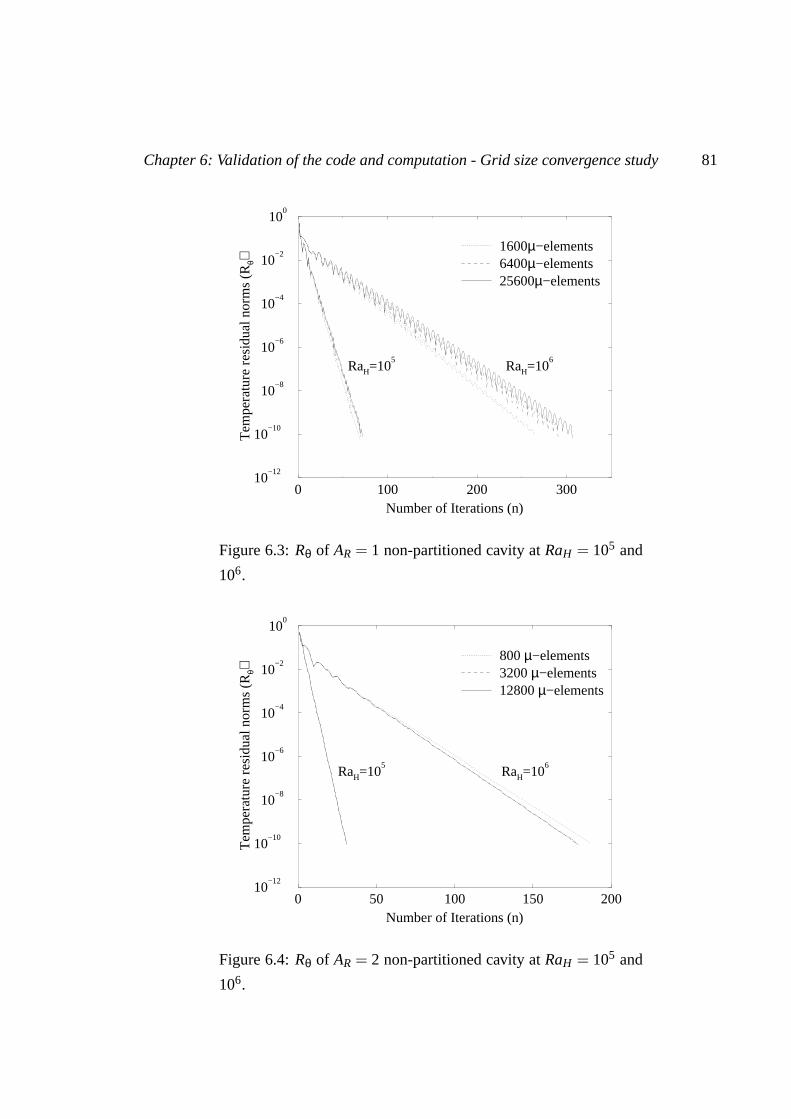
Chapter 6: Validation of the code and computation - Grid size convergence study 81
0 100 200 300Number of Iterations (n)
10−12
10−10
10−8
10−6
10−4
10−2
100
Tem
pera
ture
res
idua
l nor
ms
(Rθ)
1600µ−elements6400µ−elements25600µ−elements
RaH=105
RaH=106
Figure 6.3: Rθ of AR = 1 non-partitioned cavity at RaH = 105 and
106.
0 50 100 150 200Number of Iterations (n)
10−12
10−10
10−8
10−6
10−4
10−2
100
Tem
pera
ture
res
idua
l nor
ms
(Rθ)
800 µ−elements3200 µ−elements12800 µ−elements
RaH=105
RaH=106
Figure 6.4: Rθ of AR = 2 non-partitioned cavity at RaH = 105 and
106.

82 Chapter 6: Validation of the code and computation - Grid size convergence study
Table 6.6: Nu and ∆Nuerr (in the parenthesis) of AR = 1 and γ =
0.01 partitioned cavity at σ = 105.
micro-elements 1760 6720 26240 Exact
Grids 44×40 84×80 164×160
RaH Nu (∆Nuerr)
103 0.9973 (0.32%) 0.9993 (0.12%) 1.0002 (0.03%) 1.0005
104 1.0802 (0.43%) 1.0834 (0.14%) 1.0845 (0.03%) 1.0849
105 2.0146 (1.04%) 2.0296 (0.30%) 2.0342 (0.08%) 2.0357
106 3.7029 (1.74%) 3.7503 (0.48%) 3.7639 (0.12%) 3.7684
107 6.6559 (3.64%) 6.8452 (0.90%) 6.8920 (0.23%) 6.9076
Table 6.7: Nu and ∆Nuerr (in the parenthesis) of AR = 1 and γ = 0.1
partitioned cavity at σ = 105.
micro-elements 2400 8000 28800 Exact
Grids 60×40 100×80 180×160
RaH Nu (∆Nuerr)
103 0.9972 (0.28%) 0.9990 (0.10%) 0.9998 (0.03%) 1.0001
104 1.0442 (0.36%) 1.0466 (0.13%) 1.0476 (0.03%) 1.0479
105 1.8341 (0.90%) 1.8460 (0.26%) 1.8496 (0.06%) 1.8508
106 3.4073 (1.64%) 3.4476 (0.47%) 3.4599 (0.12%) 3.4640
107 6.0906 (3.16%) 6.2374 (0.83%) 6.2764 (0.21%) 6.2894

Chapter 6: Validation of the code and computation - Grid size convergence study 83
0 100 200 300Number of Iterations (n)
10−12
10−10
10−8
10−6
10−4
10−2
100
Tem
pera
ture
res
idua
l nor
ms
(Rθ)
1760 µ−elements6720 µ−elements26240 µ−elements
RaH=105
RaH=106
Figure 6.5: Rθ of AR = 1 and γ = 0.01 partitioned cavity at RaH =
105 and 106 and σ = 105.
two representative geometrical cases of partitioned cavity are chosen, γ = 0.01 and 0.1 at
σ = 105 in order to compare with the ’Half cavity’. Tables 6.6 and 6.7 show the numerical
resolutions and the extrapolated Exact values. Also the percentage error between Exact
value and resolutions are shown in the parenthesis.
Similar to non-partitioned cavity, the values of ∆Nuerr becomes smaller as mesh be-
comes finer but increases when RaH is raised. Nevertheless, with increasing γ from 0.01
to 0.1, ∆Nuerr is found slightly decreasing. The reason is found that the fluid cell aspect
ratio becomes higher with increasing γ and causes less convective dominated heat transfer
behavior in total domain [15].
As a conclusion, the resolutions are stable and show good convergence behavior and detail
resolutions of various RaH are shown in appendix tables D.3 and D.4.
Figures 6.5 and 6.6 show computational convergence history of partitioned cavity grid
size convergence studies. Similar to non-partitioned cavity, residual falls more rapid with

84 Chapter 6: Validation of the code and computation - Grid size convergence study
0 100 200 300Number of Iterations (n)
10−12
10−10
10−8
10−6
10−4
10−2
100
Tem
pera
ture
res
idua
l nor
ms
(Rθ)
2400 µ−elements8000 µ−elements28800 µ−elements
RaH=105
RaH=106
Figure 6.6: Rθ of AR = 1 and γ = 0.1 partitioned cavity at RaH =
105 and 106 and σ = 105.
the decreasing Rayleigh number and as mesh becomes finer. Also with increasing γ, simu-
lation require less iterations to reach criteria since the number of elements in the fluid cell
is decreased.
6.2.3 ’Half cavity’ study
The ’Half cavity’ simulation is studied in order to validate the resolutions of the par-
titioned cavity case studies. The Rayleigh number for the ’Half cavity’, RaHγ , is equal to
RaH/2 of partitioned cavity case. Because, if σ→∞, the partition wall becomes isothermal
and the temperature difference between hot and cold wall of the ’Half cavity’, ∆Tγ is equal
to ∆T/2 of partitioned cavity. Nevertheless, when σ becomes smaller, σ = 1 for example,
∆Tγ is not equal to ∆T/2. Hence it is necessary to estimate RaHγ again. This will be dis-
cussed later.
The aspect ratio of the ’Half cavity’, ARγ is equal to H/D where D is the length of fluid cell
(see Fig. 5.1). Note that the partition is centered in this problem, hence, DH = DC = D.

Chapter 6: Validation of the code and computation - Grid size convergence study 85
Then, ARγ becomes
ARγ =HD
=H
L−W2
=2AR
1− γ. (6.18)
The value of ARγ are
ARγ ≈ 2.02 for γ = 0.01partitioned cavity,
ARγ ≈ 2.22 for γ = 0.1partitioned cavity.
As a consequence, the heat transfer characteristics of AR = 1 and γ = 0.1 partitioned cavity
at σ = 105 and RaH = 106 case become identical to AR = 2.22 non-partitioned cavity at
RaHγ = 5×10⁵ case.
The mesh constructing is based on the grid size refinement method in sections 6.1 and
the Exact values are also derived by second-order Richardson extrapolation method. The
detail numerical resolutions are shown in the appendix tables D.5 and D.6. Note that the
range of RaHγ is from 5× 10³ to 5× 10⁶, which corresponds to RaH from 104 to 107 of
partitioned cavity. The case of RaHγ = 5×10², which corresponds to RaH = 103 of parti-
tioned cavity case, is not studied since it is expected that the heat transfer is characterized
by the conduction [15].
As shown in tables 6.8 and 6.9, the resolutions are stable and also the good convergence
behaviors are found1. The resolutions are in excellent agreement with corresponding parti-
tioned cavity cases as shown in figure 6.7.
The Nusselt number definition for the ’Half cavity’ cases is equal to equation (5.50) with
γ = 0 :
NuY =1− γ(1−1/σ)
AR
∂θ∂X
=1
AR
∂θ∂X
. (6.19)
Figure 6.8 shows the local Nusselt number distributions comparison between the parti-
tioned cavity and the ’Half cavity’. It is clear that the distributions are exactly same between
both cases. The insert shows the actual values of NuY from equation (5.50) and the main
shows an overlapped graph by inverting the values along the ’Surface 1’ in order to confirm
1Computational convergence histories are not shown since they are similar to AR = 2 non-partitioned case.

86 Chapter 6: Validation of the code and computation - Grid size convergence study
Table 6.8: Nu and ∆Nuerr (in the parenthesis) of ARγ = 2.02 ’Half
cavity’ (Percentage error between the Exact value and those of cor-
responding partitioned cavity case are shown in the brackets).
micro-elements 800 3200 12800 Exact
Grids 20×40 40×80 80×160
RaHγ Nu (∆Nuerr)
5×10³ 1.0804 (0.41%) 1.0833 (0.15%) 1.0845 (0.04%) 1.0849 [0%]
5×10⁴ 2.0146 (1.02%) 2.0294 (0.29%) 2.0339 (0.07%) 2.0354 [0.01%]
5×10⁵ 3.7085 (1.57%) 3.7492 (0.48%) 3.7629 (0.12%) 3.7675 [0.02%]
5×10⁶ 6.6799 (3.24%) 6.8402 (0.92%) 6.8876 (0.23%) 6.9034 [0.06%]
Table 6.9: Nu and ∆Nuerr(in the parenthesis) of ARγ = 2.22 ’Half
cavity’ (Percentage error between the Exact value and those of cor-
responding partitioned cavity case are shown in the brackets).
micro-elements 800 3200 12800 Exact
Grids 20×40 40×80 80×160
RaHγ Nu (∆Nuerr)
5×10³ 1.0442 (0.36%) 1.0466 (0.13%) 1.0476 (0.03%) 1.0479 [0%]
5×10⁴ 1.8340 (0.91%) 1.8460 (0.26%) 1.8496 (0.06%) 1.8508 [0%]
5×10⁵ 3.4073 (1.63%) 3.4475 (0.47%) 3.4598 (0.12%) 3.4639 [0.003%]
5×10⁶ 6.0789 (3.34%) 6.2370 (0.83%) 6.2761 (0.21%) 6.2891 [0.005%]

Chapter 6: Validation of the code and computation - Grid size convergence study 87
104
105
106
107
Rayleigh number (RaH)
1
10
Ave
rage
Nus
selt
num
ber
(Nu)
γ=0.01Half cavity of γ=0.01γ=0.1Half cavity of γ=0.1
Figure 6.7: Nu of the partitioned cavities at σ = 105 and the corre-
sponding ’Half cavities’.

88 Chapter 6: Validation of the code and computation - Grid size convergence study
−0.5 −0.25 0 0.25 0.5Dimensionless height (Y)
0.0
2.0
4.0
6.0
8.0
Loc
al N
usse
lt nu
mbe
r (N
u Y)
Surface 3 (Hot wall)Surface 4 (Cold wall)
−0.5 0 0.50.0
2.0
4.0
6.0
8.0
Half cavity
Partitioned cavity
Figure 6.8: NuY of γ = 0.1 partitioned cavity at σ = 105 (RaH =
106) and ARγ = 2.22 ’Half cavity’ (RaHγ = 5×10⁵).

Chapter 6: Validation of the code and computation - Grid size convergence study 89
−0.5 −0.25 0.0 0.25 0.5Dimensionless length (X)
−0.5
−0.25
0
0.25
0.5
Dim
ensi
onle
ss te
mpe
ratu
re (
θ)Partitioned cavityHalf cavity
Partition wall
Y=0.45
0.25
0.0
−0.25
−0.45
Figure 6.9: θ distributions along the horizontal planes (Y = −0.45,
-0.25, 0.0, 0.25 and 0.45) of γ = 0.1 partitioned cavity at σ = 105
(RaH = 106) and ARγ = 2.22 ’Half cavity’ (RaHγ = 5×10⁵).
a symmetric behavior of the incompressible-Boussinesq fluid flow model.
Figures 6.9 and 6.10 show the temperature and velocity distributions at different hori-
zontal planes (Y =−0.45, -0.25, 0.0, 0.25 and 0.45). The distributions between partitioned
cavity and corresponding ’Half cavity’ are matched exactly. Also demonstrates that the
’Half cavity’ case may represent the partitioned cavity case if the partition wall is isother-
mal.
As a conclusion, the heat transfer characteristics of the partitioned cavity with isother-
mal partition wall (σ = 105) are exactly identical to the corresponding ’Half cavity’ case
and the resolutions of the partitioned cavity cases are found to be valid.
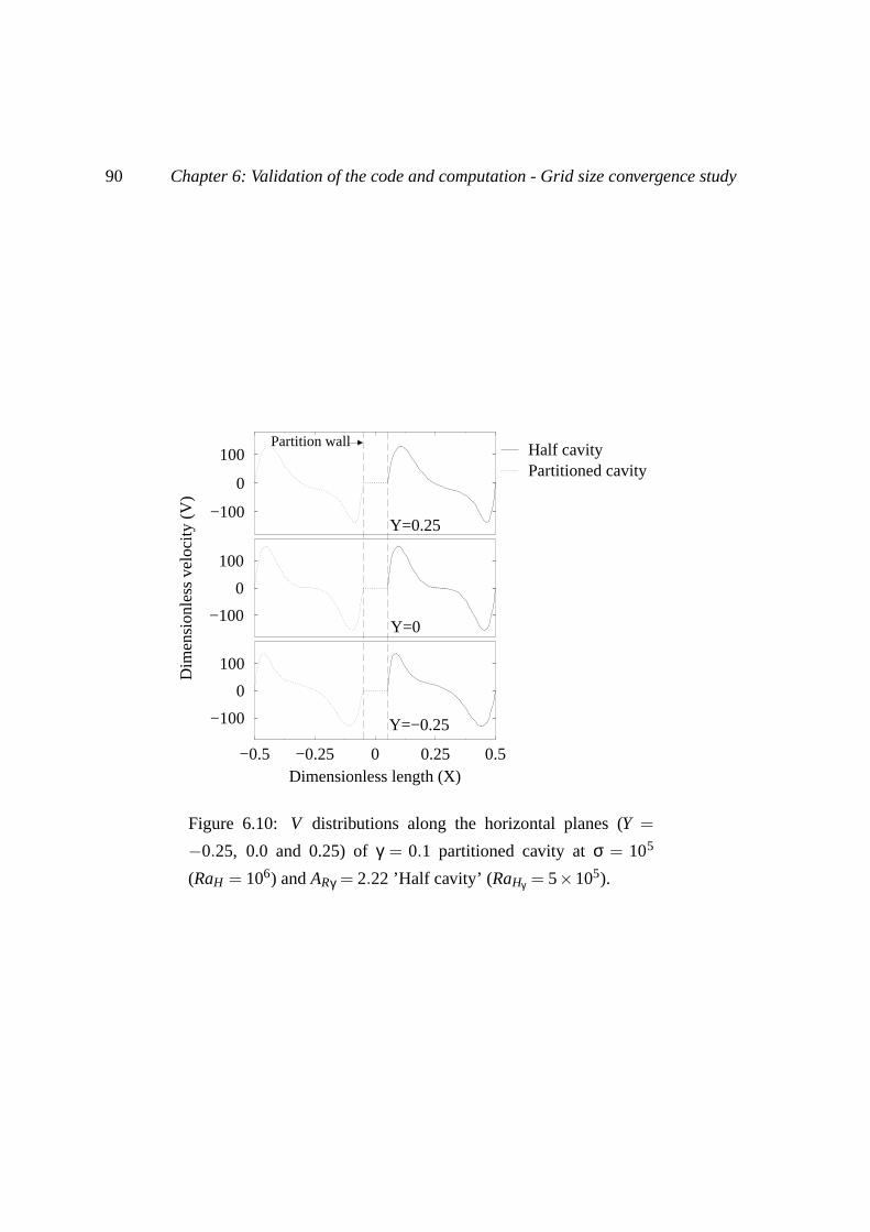
90 Chapter 6: Validation of the code and computation - Grid size convergence study
−100
0
100
Dim
ensi
onle
ss v
eloc
ity (
V)
−100
0
100 Half cavityPartitioned cavity
−100
0
100
−0.5 −0.25 0 0.25 0.5Dimensionless length (X)
Partition wall
Y=0.25
Y=0
Y=−0.25
Figure 6.10: V distributions along the horizontal planes (Y =
−0.25, 0.0 and 0.25) of γ = 0.1 partitioned cavity at σ = 105
(RaH = 106) and ARγ = 2.22 ’Half cavity’ (RaHγ = 5×10⁵).

Chapter 7
Results and discussion
In the previous chapter, a study is presented on the validation and the qualification of
the numerical resolutions by grid size convergence and benchmark. In this chapter, the
physical characteristics of the non-partitioned and partitioned cavity are discussed.
It is however true that the computation cost is very expensive to obtain the Exact values for
the entire resolutions. Indeed, the differences between those ∆Nuerr are found relatively
small compare to the simulation cost such as the CPU time1. In this chapter the results are
from the middle elements number mesh. For example, the middle element number mesh
of AR = 1 non-partitioned cavity is 6400 micro-elements (between three different sizes of
meshes, for example 1600, 6400 and 25600 micro-elements meshes). This method is also
used for the partitioned cavity.
In the previous chapter, only two representative cases (γ = 0.01 and 0.1 at σ = 105) are
studied due to the wide range of σ and γ and it is found that ∆Nuerr becomes smaller with
increasing γ. For example, comparing both middle size meshes at RaH = 107, ∆Nuerr is
equal to 0.83% at 8000 micro-elements mesh of γ = 0.1 case while ∆Nuerr is equal to 0.9%
at 6720 micro-elements mesh of γ = 0.01 case. Hence, it is possible to say that ∆Nuerr at
γ = 0.01 case is the maximum since the range of γ is from 0.01 to 0.2 and it can be expected
that ∆Nuerr of γ = 0.2 is the smallest.
1The CPU time are not compared in this thesis since the goal of the study is more focused on the physicalphenomenon rather than computational behaviors.
91

92 Chapter 7: Results and discussion
7.1 Non-partitioned cavity
The heat transfer characteristics of the natural convection in the non-partitioned cavity
had been very well studied by experiments and numerical methods. In this section, the dis-
cussion is focused on the general description of the heat transfer characteristics and their
physical features of the partitioned cavity case.
In this thesis, the flow is assumed as the boundary layer flow, which is an approxi-
mate solutions for low-viscosity fluids, such as air and water. According to the study of
Prandtl [25], the flow is divided into two regions: the thin boundary layer which develops
very close to the solid wall, in which the frictional forces are as important as the inertia
forces; and the external region, in which the flow is practically frictionless. With above cri-
teria, the Navier-Stokes equations become extremely simplified. The boundary layer flow
assumption is found to be valid not only for the laminar flow but also for the turbulent flow.
The boundary layer flow assumption is also applicable for the natural convection heat trans-
fer in the closed cavity. In the laminar flow regime, the flow is also classified into whether
boundary layer is developed or not. Namely, the pure conduction regime when boundary
layer is not developed.
According to Patterson and Imberger [61] and Bejan [8], the vertical boundary layer in the
cavity with isothermal side walls and adiabatic horizontal end walls can be distinguishable
if the final thermal boundary layer thickness, δT, f , is smaller than the cavity length (L).
From a scaling analysis of the incompressible-Boussinesq fluid flow model, the vertical
thermal and velocity boundary layer, δV, f , will be distinct when
HL
< Ra1/4H for δT, f and (7.1a)
HL
< Ra1/4H for δV, f (7.1b)
for Pr ≥ 1 fluids. It is noted that if Pr << 1, (e.g. liquid metal) the thermal boundary layer
thickness is larger than the velocity boundary layer and if Pr > 1 (e.g. water, oil) or Pr ∼ 1
(e.g. air) the velocity boundary layer is more larger then the thermal boundary layer.
The horizontal flow will be distinguishable when convective heat transfer is greater than
conductive heat transfer. From this scaling analysis, order of convective and conductive

Chapter 7: Results and discussion 93
A = RaR
−1/4
A = RaR1/4
1
Verticalboundarylayers
Shallow system
102
101
10−1
10−2
Horizontalboundarylayers
RaH1012108104
A = H/LR
IV
IITall system
High Rayleigh regime (Boundary layer regime)III
FlowConduction
I
Figure 7.1: Four heat transfer regimes for natural convection in a
two-dimensional cavity with isothermal side walls Bejan [8].
heat transfer are found ∼ k∆T (RaH ·Pr)1/4 and ∼ kL∆T/H, respectively 2. In other words,
whenHL
> Ra−1/4H , (7.2)
the horizontal streams retain their temperature identity since the horizontal end walls are
adiabatic. Finally, as shown in figure 7.1, the heat transfer at the steady-state may be
divided into four regimes as the function of RaH and AR [8]:
I. Conduction regime (when RaH < 1): Temperature variation is almost linear and the
heat transfer is conduction order but shows slow single core fluid circulation, for any
AR with very low RaH . The boundary layer is not developed and Nu shows ' 1.
II. Tall enclosure regime: RaH is relatively low since high AR cavity and boundary layer
is not developed (almost conduction dominated), and for this reason Nu shows ' 1
2∆T = Tw −T∞ for external flow and ∆T = T h −Tc for non-partitioned cavity case.

94 Chapter 7: Results and discussion
again. Nevertheless, distinct layers are observed near the adiabatic horizontal end
walls and shows clockwise circulation core pattern characteristics.
III. High-RaH boundary layer regime: The heat transfer is dominated by convection. Ver-
tical thermal boundary layers are distinguishable along the hot and cold side walls
and also along the adiabatic horizontal walls. The core of the fluid is relatively stag-
nant and thermally stratified.
IV. Shallow enclosure regime: Low AR cavity and heat transfer is dominated by the
presence of vertical thermal layers. The horizontal boundary layer seems provided
an additional insulation effect.
Consequently, it is possible to say that from equation (7.1b) and (7.2), the line of H/L =
Ra1/4H for AR > 1 and H/L = Ra−1/4
H for AR < 1 (i.e. dashed line in Fig. 7.1), are the limit
of boundary layer regime heat transfer. It should be noted that in this thesis, high-RaH
boundary layer regime (Region III. in figure 7.1) is only considered.
As a characteristic of natural convection heat transfer in the cavity, the flow can be clas-
sified into laminar and turbulent flow, and as mentioned earlier, this thesis is only focused
on laminar flow. Chenoweth and Paolucci [15] studied the natural convection heat transfer
in the cavity and suggested the range of the laminar flow as a function of the Rayleigh
number based on the length of the cavity, RaL, and the aspect ratio (AR) as shown in figure
7.2.
In this thesis, the Rayleigh number based on cavity height (H), RaH , is used. Hence, the
range for RaH in figure 7.2 is reproduced. Thus, RaH = A3RRaL and the laminar flow range
for AR = 1 is equal to 2.8×10³ < RaH < 108. Also for AR = 2 case, the range is equal to
7.84×10⁴ < RaH < 108.
When RaH is smaller than the laminar flow range, the flow becomes pure conduction. With
increasing RaH from the conduction regime, the flow is being dominated by natural convec-
tion heat transfer and the secondary flow cores in the cavity (two different flow circulation
movement in the cavity) are occurred [52]. Eventually, the flow becomes increasingly un-
steady and becomes turbulent when RaH increases significantly above the critical RaH .
The range of RaH in this thesis for non-partitioned cavity is 103,104,105,106 and 107 and
can be described by the laminar flow with development of boundary layer. Note that at

Chapter 7: Results and discussion 95
103
104
105
106
107
108
109
1010
1011
1012
1013
Rayleigh Number (RaL and RaH)
100
101
102
Asp
ect R
atio
(A
R)
RaL
RaH
RaL RaH
Critical RaH
Critical RaL
Steady core region
Figure 7.2: The range of laminar flow (filled part) of natural con-
vection heat transfer in the cavity (Reproduced from the study of
Chenoweth and Paolucci [15]).

96 Chapter 7: Results and discussion
Table 7.1: Numerical resolutions of AR = 1 non-partitioned cavity
at RaH = 105 (N/A = Not Available, ∗: Exact value).
Nu Numax Numin Vmax Umax
This work∗ 4.5196 7.7202 0.5147 68.6270 34.7353
de Vahl Davis [24]∗ 4.519 7.717 0.729 68.59 34.73
Chenoweth and Paolucci [15]∗ 4.520 N/A N/A 68.63 34.77
Hortmann et al,. [32]∗ 4.52164 7.72013 N/A 68.6396 34.7399
Le Quere et al,. (65×65 modes) [38] 4.522 7.720 0.728 68.64 34.75
Paillere et al,. (160×160 elements) [56] 4.5277 7.7198 0.7387 N/A N/A
RaH of 103 for AR = 1 as well as RaH of 103 and 104 for AR = 2, it is expected that the
conduction dominates the heat transfer (Nu ' 1).
Table 7.1 shows the results comparison between the literature of AR = 1 non-partitioned
cavity at RaH = 105. Note that the resolutions are the extrapolated grid size independent
Exact values. Compare to the literature, most of values are in good agreement except
Numin. The reason is that a steep fall of NuY at the lowest (Y =−0.5) and highest (Y = 0.5)
element of the axes as shown in figure 7.3, since the temperature field is approximated on
the node of an element.
Figure 7.3 demonstrates NuY of AR = 1 and 2 non-partitioned cavity along the ’Sur-
faces 1 and 2’ at RaH = 105. The insert shows actual values and the main shows over-
lapped graph in order to confirm a symmetric behavior of the incompressible-Boussinesq
fluid flow model.
NuY varies in the vertical direction and represents the boundary layer thickness variation
along the sidewalls. Numax appears near the starting point of the flow (i.e., Y =−0.5 of hot
wall) and Numin near the departure point (i.e., Y = 0.5 of hot wall) for both surfaces (see Fig.
7.3). Note that the values are from 6400 micro-elements (∆Nuerr = 0.24% at RaH = 105)
for AR = 1 case and 3200 micro-elements (∆Nuerr = 0.36% at RaH = 105 ) for AR = 2 case.
In general, Nu, Numax, Numin, Vmax and Umax become larger with increasing RaH (see

Chapter 7: Results and discussion 97
−0.5 −0.25 0.0 0.25 0.5Dimensionless height (Y)
0.0
2.0
4.0
6.0
8.0
10.0
Loc
al N
usse
lt nu
mbe
r (N
u Y)
Surface 1Surface 2
−0.5 0.0 0.50.0
5.0
10.0
AR = 1.0AR = 2.0
Figure 7.3: NuY distribution along the ’Surfaces 1 and 2’ of AR = 1
and 2 non-partitioned cavities at RaH = 105 (Actual values in the
insert and overlapped values in the main graph).

98 Chapter 7: Results and discussion
appendix Tabs. D.1 and D.2). This is the fact found in the scaling analysis of Pr ≥ 1 order
fluid flow [8, 61]. Accordingly, the order of the thermal boundary layer final thickness,
δT, f , V and Nu are found as
δT, f ∼ HRa−1/4H , (7.3a)
V ∼ Ra1/2H , (7.3b)
Nu =hHk f
∼ Ra1/4H . (7.3c)
From above scale analysis, it is clear that the final thickness of thermal boundary layer
(δT, f ) becomes thinner and V and Nu become larger with increasing RaH .
Consider the boundary layer thickness to the vertical direction, for example in figure 7.3, it
becomes larger as with increasing Y , in dimensional form :
δT, f ∼ y1/4. (7.4)
Also, the order of heat flux q′′ is
q′′ ∼ k f∆TδT
. (7.5)
Figures 7.4, 7.5 and 7.6 show the features of the streamlines, temperature isolines and
velocity fields of AR = 1 non-partitioned cavity at various RaH , respectively. The stream-
lines and the temperature isolines are from 6400 micro-elements mesh (∆Nu = 1.07%
at RaH = 107, for example) and the velocity fields are from 1600 micro-elements mesh
(∆Nu = 4.46% at RaH = 107, for example).
The flow characteristics are represented by the streamlines by the contour map of stream
function and velocity fields. The definition of stream function Ψ(X ,Y ) is
U = −∂Ψ∂Y
and V =∂Ψ∂Y
. (7.6)
As shown in figure 7.4, at low RaH such as 103 and 104, the flow is slow and clockwise
circulating. At RaH = 105 secondary core is appeared and shows stable, as expected in
figure 7.2. Especially at RaH = 107, the secondary core becomes inverse S-shape as shown
in figure 7.5, because the potential inflow of the discharged boundary jets along the hori-
zontal end wall [15]. As shown in figure 7.6, at lower RaH , the temperature isolines are
almost parallel to the side walls and represents that the heat transfer is dominated by the
conduction. As RaH is increased, the flow becomes more convective and the isolines near
the side walls become more dense.

Chapter 7: Results and discussion 99
Figure 7.4: Streamlines of AR = 1 non-partitioned cavity at differ-
ent RaH (103, 104, 105, 106 and 107, left to right and top to bottom).
Figure 7.5: Velocity fields of AR = 1 non-partitioned cavity at dif-
ferent RaH (103, 104, 105, 106 and 107, left to right and top to
bottom).
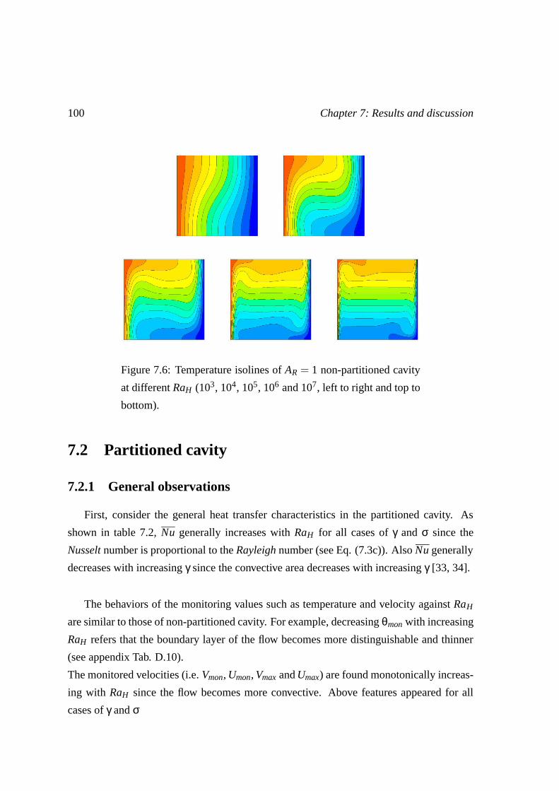
100 Chapter 7: Results and discussion
Figure 7.6: Temperature isolines of AR = 1 non-partitioned cavity
at different RaH (103, 104, 105, 106 and 107, left to right and top to
bottom).
7.2 Partitioned cavity
7.2.1 General observations
First, consider the general heat transfer characteristics in the partitioned cavity. As
shown in table 7.2, Nu generally increases with RaH for all cases of γ and σ since the
Nusselt number is proportional to the Rayleigh number (see Eq. (7.3c)). Also Nu generally
decreases with increasing γ since the convective area decreases with increasing γ [33, 34].
The behaviors of the monitoring values such as temperature and velocity against RaH
are similar to those of non-partitioned cavity. For example, decreasing θmon with increasing
RaH refers that the boundary layer of the flow becomes more distinguishable and thinner
(see appendix Tab. D.10).
The monitored velocities (i.e. Vmon, Umon, Vmax and Umax) are found monotonically increas-
ing with RaH since the flow becomes more convective. Above features appeared for all
cases of γ and σ

Chapter 7: Results and discussion 101
Table 7.2: Nu of AR = 1 partitioned cavity at RaH = 106.
γ = 0.01 γ = 0.1
RaH σ = 1 σ = 105 σ = 1 σ = 105
104 1.1323 1.0834 1.0575 1.0466
105 2.1917 2.0296 1.7455 1.8460
106 4.0078 3.7503 2.7821 3.4476
107 7.1386 6.8452 4.0418 6.2374
Precise numerical resolutions are shown in the appendix tables. The appendix tables
D.7, D.8, D.9, D.10 , D.11, D.12, D.13 and D.14 show Nu, NuMax, NuMin, θmon, Vmon, Umon,
Vmax and Umax of AR = 1 partitioned cavity with various γ, σ and RaH , respectively. Also,
the appendix tables D.15 and D.16 show the temperature difference between both sides of
the partition wall (’Surfaces 2 and 3’ of Fig. 5.1) on the horizontal mid-plane (Y = 0),
∆θW,Horizontal , and between top and bottom of ’Surface 2’ (X = −γ/2), ∆θW,Vertical , re-
spectively. It should be noted that the results are from 6720, 6720, 7200, 8000 and 6720
micro-elements mesh simulations for γ = 0.01, 0.02, 0.05, 0.1 and 0.2 partitioned cavity,
respectively.
Now consider the range of RaH for convective heat transfer in partitioned cavity. As
mentioned earlier, a fully partitioned cavity with AR can be considered as two separated
cavities with AR/2 if γ → ∞. The aspect ratio of the ’Half cavity’ are approximately 2.02,
2.04, 2.11, 2.22 and 2.5 for γ = 0.01, 0.02, 0.05, 0.1 and 0.2 partitioned cavity of AR = 1,
respectively. Based on this fact, from figure 7.2, the minimum value of RaH for the con-
vection heat transfer in partitioned cavity is 4.1×10⁴, 4.3×10⁴, 4.9×10⁴, 6.2×10⁴ and
105 at γ = 0.01, 0.02, 0.05, 0.1 and 0.2 partitioned cavity, respectively. Note again that
above ranges are based on isothermal partition wall, thus, negligible thermal resistance of
the partition wall, for example, σ = 105.
Accordingly, based on the condition of the partition wall (i.e. high or low σ), heat
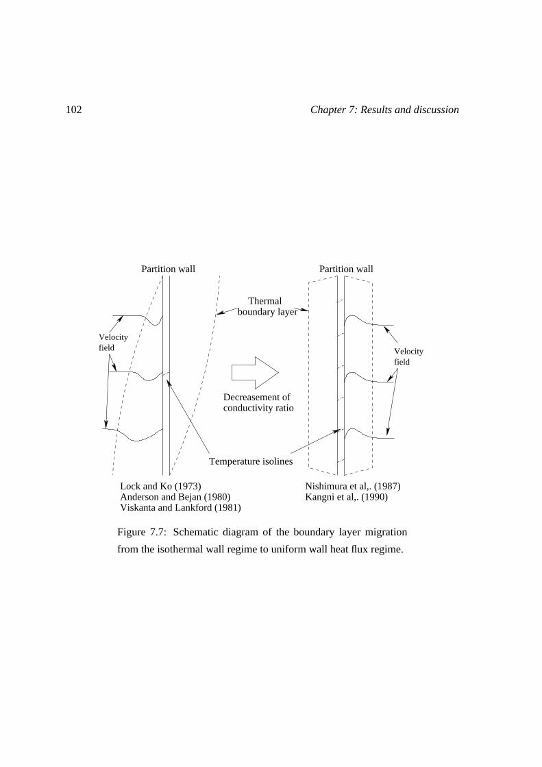
102 Chapter 7: Results and discussion
Partition wallPartition wall
Decreasement of conductivity ratio
Lock and Ko (1973)Anderson and Bejan (1980)Viskanta and Lankford (1981)
Kangni et al,. (1990)Nishimura et al,. (1987)
Temperature isolines
Thermalboundary layer
Velocityfield
Velocityfield
Figure 7.7: Schematic diagram of the boundary layer migration
from the isothermal wall regime to uniform wall heat flux regime.
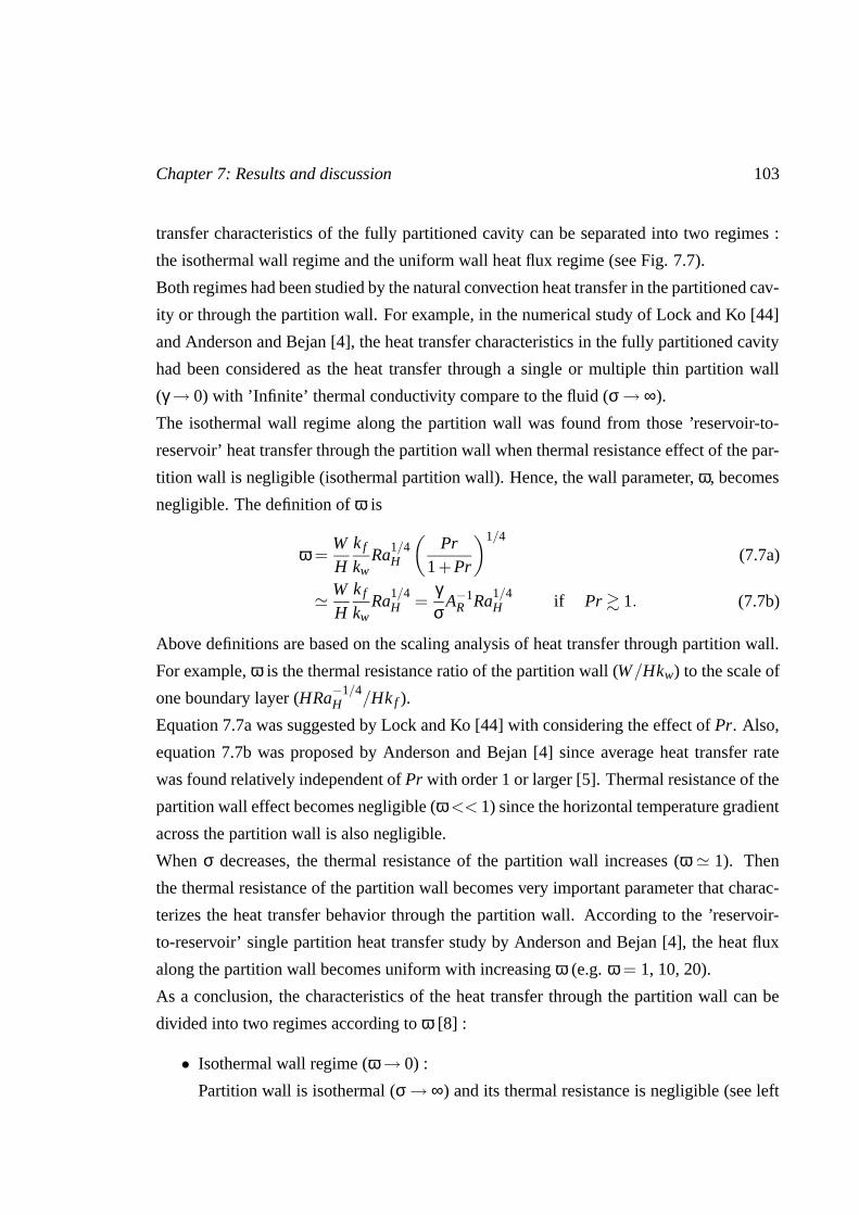
Chapter 7: Results and discussion 103
transfer characteristics of the fully partitioned cavity can be separated into two regimes :
the isothermal wall regime and the uniform wall heat flux regime (see Fig. 7.7).
Both regimes had been studied by the natural convection heat transfer in the partitioned cav-
ity or through the partition wall. For example, in the numerical study of Lock and Ko [44]
and Anderson and Bejan [4], the heat transfer characteristics in the fully partitioned cavity
had been considered as the heat transfer through a single or multiple thin partition wall
(γ → 0) with ’Infinite’ thermal conductivity compare to the fluid (σ → ∞).
The isothermal wall regime along the partition wall was found from those ’reservoir-to-
reservoir’ heat transfer through the partition wall when thermal resistance effect of the par-
tition wall is negligible (isothermal partition wall). Hence, the wall parameter, ω, becomes
negligible. The definition of ω is
ω =WH
k f
kwRa1/4
H
(Pr
1+Pr
)1/4
(7.7a)
' WH
k f
kwRa1/4
H =γσ
A−1R Ra1/4
H if Pr & 1. (7.7b)
Above definitions are based on the scaling analysis of heat transfer through partition wall.
For example, ω is the thermal resistance ratio of the partition wall (W/Hkw) to the scale of
one boundary layer (HRa−1/4H /Hk f ).
Equation 7.7a was suggested by Lock and Ko [44] with considering the effect of Pr. Also,
equation 7.7b was proposed by Anderson and Bejan [4] since average heat transfer rate
was found relatively independent of Pr with order 1 or larger [5]. Thermal resistance of the
partition wall effect becomes negligible (ω << 1) since the horizontal temperature gradient
across the partition wall is also negligible.
When σ decreases, the thermal resistance of the partition wall increases (ω ' 1). Then
the thermal resistance of the partition wall becomes very important parameter that charac-
terizes the heat transfer behavior through the partition wall. According to the ’reservoir-
to-reservoir’ single partition heat transfer study by Anderson and Bejan [4], the heat flux
along the partition wall becomes uniform with increasing ω (e.g. ω = 1, 10, 20).
As a conclusion, the characteristics of the heat transfer through the partition wall can be
divided into two regimes according to ω [8] :
• Isothermal wall regime (ω → 0) :
Partition wall is isothermal (σ → ∞) and its thermal resistance is negligible (see left

104 Chapter 7: Results and discussion
of Fig. 7.7). The boundary layers at the side walls and also at the partition wall
become thicker in the flow direction. The thermal conductivity of the partition wall
is much greater than that of the fluid (kw >> k f thus σ ∼ ∞).
In this region, the scale of boundary layer thickness and heat flux are [8]
δT, f ∼ y1/4 and q′′ ∼ y−1/4. (7.8)
In the range of Pr ≥ 1, the scale of the Nusselt number becomes
Nu ∼ HδT, f
∼ RaH1/4. (7.9)
Above scaling analysis is equal to those of non-partitioned cavity case in section 7.1.
• Uniform wall heat flux regime (ω ∼ 1):
Heat flux along the partition wall is uniform and the thermal resistance of the parti-
tion wall is important (see right figure of Fig. 7.7). Partition wall is non-isothermal.
Boundary layer thickness along the partition wall is almost uniform in the flow di-
rection. Temperature difference exists between top and bottom of the partition wall .
The scale of boundary layer thickness is [8]
δT, f ∼ HRa∗H−1/5 ∼ y1/5 (7.10)
where Ra∗H is the Rayleigh number based on q′′ :
Ra∗H =gβH4q′′
ανk f. (7.11)
In the range of Pr >> 1, the scale of the Nusselt number in this region is
Nu ∼ Ra∗H1/5. (7.12)
Indeed, based on the boundary condition between the fluid and the partition wall at the
steady-state (see Eq. (5.32e)) the heat flux leaving from hot cell (entering to cold cell), q′′f ,
is equal to the heat flux entering to partition wall (leaving from partition wall), q′′w :
q′′ = q′′f = q′′w at the steady-state. (7.13)

Chapter 7: Results and discussion 105
The definition of q′′f and q′′w is
q′′f ∼ k f∆Tf ,Horizontal
δT, f, (7.14a)
q′′w ∼ kw∆Tw,Horizontal
W(7.14b)
where ∆Tf ,Horizontal is the horizontal temperature difference between partition wall and
bulk temperature of the fluid, thus ∆Tf ,Horizontal = Tw −Tf ,∞ and ∆Tw,Horizontal is the hori-
zontal temperature difference between both sides of the partition wall, thus ∆Tw,Horizontal =
TWH −TWC.
In the isothermal wall regime, ∆Tw,Horizontal is negligible and the heat transfer is character-
ized by only q′′f . Then the heat transfer characteristics are similar to those of non-partitioned
cavity case and q′′ becomes
q′′ = q′′f ∼ k f∆Tf ,Horizontal
δT, f. (7.15)
This equation is equal to equation (7.5). This becomes true when the partition wall is very
thin. According to Meyer et al,. ∆Tw,Horizontal becomes negligible if γ < 0.01.
Nevertheless, if ∆Tw,Horizontal is not negligible, thus, for the γ > 0.01 and non-isothermal
partition wall cavity case, it is necessary to consider equation (7.13). Consequently, it is
evident that the heat transfer characteristics of the partitioned cavity are highly affected by
γ and σ. Hence, above classification of the flow regimes becomes insufficient to explain
the heat transfer characteristics in the partitioned cavity if the thermal resistance and the
thickness of the partition wall are ’finite’.
Now, a case study in performed on both flow regimes, the cases of σ = 105 for the
isothermal wall regime and of σ = 1 for the uniform wall heat flux regime. Note that the
value of γ is 0.1 in order to observe the thermal resistance effect of the partition wall [47].
First, the effect of RaH is considered. At σ = 1, the values of ω are 1 to 5.62 at RaH = 104
to 107, respectively, and may be affected by the thermal resistance effect of the partition
wall. Also at σ = 105, the values of ω are 10−5 to 5.62× 10⁻⁵ at RaH = 104 to 107, re-
spectively. They are low enough and the thermal resistance of the partition wall effect can
be negligible.
Figures 7.8, 7.9 and 7.10 show the streamlines, velocity fields and temperature isolines of
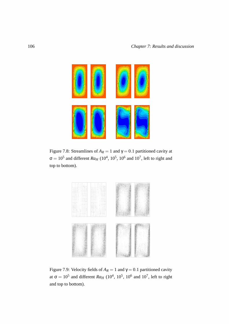
106 Chapter 7: Results and discussion
Figure 7.8: Streamlines of AR = 1 and γ = 0.1 partitioned cavity at
σ = 105 and different RaH (104, 105, 106 and 107, left to right and
top to bottom).
Figure 7.9: Velocity fields of AR = 1 and γ = 0.1 partitioned cavity
at σ = 105 and different RaH (104, 105, 106 and 107, left to right
and top to bottom).

Chapter 7: Results and discussion 107
Figure 7.10: Temperature isolines of AR = 1 and γ = 0.1 partitioned
cavity at σ = 105 and different RaH (105, 106 and 107, left to right
and top to bottom).
Figure 7.11: Streamlines of AR = 1 and γ = 0.1 partitioned cavity
at σ = 1 and different RaH (105, 106 and 107, left to right and top
to bottom).

108 Chapter 7: Results and discussion
Figure 7.12: Velocity fields of AR = 1 and γ = 0.1 partitioned cavity
at σ = 1 and different RaH (104, 105, 106 and 107, left to right and
top to bottom).
Figure 7.13: Temperature isolines of AR = 1 and γ = 0.1 partitioned
cavity at σ = 1 and different RaH (104, 105, 106 and 107, left to
right and top to bottom).

Chapter 7: Results and discussion 109
AR = 1 and γ = 0.1 partitioned cavity at σ = 105 and various RaH , respectively. Also those
of σ = 1 cases are shown in figures 7.11, 7.12 and 7.13. The streamlines and temperature
isolines are from 8000 micro-element mesh for both σ = 105 (∆Nu = 0.83% at RaH = 107,
for example) and 1 cases. The velocity fields are from 2400 micro-elements mesh for both
σ = 105 (∆Nu = 3.16% at RaH = 107, for example) and 1 cases.
As shown in figure 7.10, the partition wall is isothermal and its thermal resistance effect is
negligible at σ = 105. The characteristics of streamlines, velocity fields and temperature
isolines are similar to those of non-partitioned case as shown in figures 7.4, 7.5 and 7.6.
Because, as mentioned earlier, a partitioned cavity with σ = 105 can be considered as two
separated AR ≈ 2 non-partitioned cavities. For example, in figure 7.8, at lower RaH , the
flow is slow and clockwise circulating and secondary motion is appeared at higher RaH .
The core of the streamlines is located in the center of the cavities. Also with increasing
RaH , the secondary motion core moves toward to the cavity corners.
In figure 7.9, the existence of the boundary layer becomes more evident with increasing
RaH and the inverse S-shape cores are observed near the left top and the right bottom cor-
ners of both hot and cold cells. The temperature isolines in figure 7.10 shows that the flow
becomes more convective since the isolines shifted from parallel to side walls with increas-
ing RaH . Also the boundary layer becomes more distinguishable.
The results of σ = 1 case also show that the development of boundary layer and domina-
tion of the convective heat transfer with increasing RaH . The position of the streamline
core is found in the lower part of the hot cell and in the upper part of the hot cell. Also the
secondary core seems not stable compare to higher σ case. The boundary layer thickness
is uniform along the partition wall due to the thermal resistance of the partition wall effect
and the temperature gradients are found inside of the partition wall.
Figure 7.14 shows NuY distribution along the ’Surfaces 1, 2, 3 and 4’ of γ = 0.1 par-
titioned cavity at σ = 1 and 105 and RaH = 106. The insert shows actual values of NuY
from equation (5.50) and the main shows overlapped graph by inverting the values along
the ’Surfaces 1 and 3’ in order to confirm a symmetric behavior of the incompressible-
Boussinesq fluid flow.
First, considering the case of σ = 105. It is clear that NuY along the 4 different surfaces
vary in the vertical direction to the wall. This feature is exactly same to non-partitioned

110 Chapter 7: Results and discussion
−0.5 −0.25 0 0.25 0.5Dimensionless height (Y=y/H)
0.0
2.0
4.0
6.0
8.0
Loc
al N
usse
lt nu
mbe
r (N
u Y)
Surface 1Surface 2Surface 3Surface 4
−0.5 0 0.50.0
4.0
8.0
σ = 105
σ = 1
Figure 7.14: NuY distribution along the ’Surfaces 1, 2, 3 and 4’ of
AR = 1 and γ = 0.1 partitioned cavity at RaH = 106 (Actual values
in the insert and overlapped values in the main graph).

Chapter 7: Results and discussion 111
−0.5 −0.25 0 0.25 0.5Dimensionless length (X = x/H)
−0.5
−0.25
0
0.25
0.5
Dim
ensi
onle
ss te
mpe
ratu
re (
θ)
−0.5 0 0.5−0.5
0
0.5 Y=0.45
Partition wall
0.25
0−0.25−0.45
Figure 7.15: θ distributions along the horizontal planes (Y =
−0.45, -0.25 0.0, 0.25 and 0.45) of AR = 1 and γ = 0.1 partitioned
cavity at σ = 1 (the main) and 105 (the insert) and RaH = 106.
cavity case (see Fig. 7.3). On the other hand, in the case of σ = 1, NuY along the partition
wall surfaces (’Surface 2 and 3’) is nearly uniform. This fact represents the heat flux (and
the boundary layer) along the partition wall is uniform.
Figure 7.15 shows the temperature distributions at different horizontal planes (Y =
−0.45, -0.25 0.0, 0.25 and 0.45) of γ = 0.1 partitioned cavity at σ = 1 (the main) and
105 (the insert) and RaH = 106. This figure also clearly indicates that the existence of the
thermal boundary layers along the partition and side walls. In the case of σ = 1, the tem-
perature gradient along the ’Surfaces 1 (X = −0.5) and 4 (X = 0.5)’ varies to the vertical
direction while it is almost uniform on the ’Surfaces 2 and 3’. Thus, it is clear that the heat
transfer through the partition wall is characterized by the uniform wall heat flux region, but
in the case of σ = 105, the temperature gradient along the wall surfaces are identical and
show the isothermal wall region.
As a conclusion of the section, the heat transfer in the partitioned cavity can be char-

112 Chapter 7: Results and discussion
Table 7.3: Nu of AR = 1 partitioned cavity at RaH = 106.
γσ 0.01 0.02 0.05 0.1 0.2
1 4.0078 3.8118 3.3363 2.7821 2.1126
10 4.1497 4.0752 3.8706 3.5694 3.0570
100 4.0513 3.9434 3.7387 3.5071 3.1228
105 3.7503 3.7159 3.6149 3.4476 3.1095
acterized by two regimes when the partition wall is very thin : the isothermal wall regime
and the uniform wall heat flux regime. Also the wall parameter (ω) is presented and it is
shown that both regimes are distinguished by the value of ω.
According to the literature, the average Nusselt number (Nu) shows an interesting behavior
against increasing σ (i.e. a peak appears). Then the wall parameter becomes insufficient in
order to explain this behavior. Indeed, as shown in equations (7.7a) and (7.7b), the value of
ω is significantly affected by σ. Thus, the order of γ and Ra1/4H is relatively small compare
to σ−1 since its wide range (i.e. 1 ≤ σ ≤ 105). Note that AR is equal to unity.
Secondly, the influence of γ is higher than Ra1/4H since Ra1/4
H varies from 5.6 to 56.2 while
γ varies from 0.01 to 0.2, and consequently the effects of of γ and σ is discussed separately
in order to analyze the heat transfer characteristics in the partitioned cavity and to explain
the Nu behavior.
7.2.2 Effect of γ
According to the study of Meyer et al,. [47], the thermal resistance effect of the partition
wall is proportional to the ratio of the partition wall thickness (W ) to the height (H). Thus,
when the ratio W/H, thus γ/AR, is lower than 0.1, the temperature difference between both
sides of the partition wall (’Surfaces 2 and 3’ of figure 5.1) is very small (< 2% of total)
and the partition wall can be assumed isothermal.
First, consider the heat transfer behavior changes against γ. As shown in table 7.3,
Nu generally decreases with increasing γ. This feature is also shown in figure 7.16. The

Chapter 7: Results and discussion 113
0.01 0.1Dimensionless partition thickness (γ)
1.0
10.0
Ave
rage
Nus
selt
num
ber
(Nu)
RaH=104
RaH=105
RaH=106
RaH=107
σ=105σ=1.0
Figure 7.16: Nu of AR = 1 partitioned cavity.
main reason of this feature is : suppose σ is constant, then the convection heat transfer
(QConvection) becomes more dominant in lower γ partitioned cavity since the area of the fluid
(cold and hot cells), AConvection, is larger than higher γ cases [33, 34]. As a consequence,
the increment of partition wall thickness (γ ↑) in the fully partitioned cavity causes an
decrease in convection area (AConvection ↓). Then convection heat transfer rate decreases
(QConvection ↓) but also conduction heat transfer rate increases (QConduction ↑) through entire
domain since the conductivity of the solid partition wall is assumed to be greater than that
of the fluid in this thesis (σ ≥ 1). This mechanism can be expressed as
γ ↑∼ AConvection ↓∼ QConvection ↓∼ QConduction ↑∼ Nu ↓ . (7.16)
Nonetheless, it is observed in figure 7.16 that Nu of σ = 1 decreases more rapidly than
those of σ = 105. The reason is : according to equation (7.7a) and (7.7b), the impact of
γ to thermal resistance effect of the partition wall (ω) is relatively weak than σ since the
range of γ is 0.01 ∼ 0.1 while σ is 1 ∼ 105. In other words, at lower σ case, the effect of γis more important at lower σ case and increasing γ intends less convection dominated (Nu

114 Chapter 7: Results and discussion
−0.5 −0.25 0 0.25 0.5Dimensionless height (Y)
0.0
2.0
4.0
6.0
8.0
10.0L
ocal
Nus
selt
num
ber
(Nu Y
)
Surface 1Surface 2Surface 3Surface 4
−0.5 0 0.50.0
4.0
8.0
γ = 0.1
γ = 0.01
Figure 7.17: NuY distributions along the ’Surfaces 1, 2, 3 and 4’ of
AR = 1 partitioned cavity at σ = 1 (the main) and 105 (the insert)
and RaH = 106.
decreases more steeply).
Now consider the local Nusselt number. As shown in figure 7.17, NuY are found higher
in lower γ case. This behavior is common even the thickness of boundary layer along the
partition wall is whether uniform (σ = 1, the main graph of figure 7.17) or not (σ = 105,
the insert graph of figure 7.17). Note that the graphs are overlapped by inverting the val-
ues along the ’Surfaces 1 and 3’ to confirm a symmetric behavior of the incompressible-
Boussinesq fluid flow.
Figure 7.18 shows Nu variation with increasing RaH . It is clear that Nu are generally
low at γ = 0.1 case than those of 0.01 cases. This can be also observed at both high and
low cases of σ. The variation of Nu at σ = 105 (the insert) is found more linear than σ = 1
(the main) because the thermal resistance effect is negligible at higher σ.

Chapter 7: Results and discussion 115
104
105
106
1071
10
104
105
106
107
Rayleigh number (RaH)
1
10
Ave
rage
Nus
selt
num
ber
(Nu)
γ=0.01γ=0.1
Figure 7.18: Nu of AR = 1 partitioned cavity at σ = 1 (the main)
and 105 (the insert) cases.
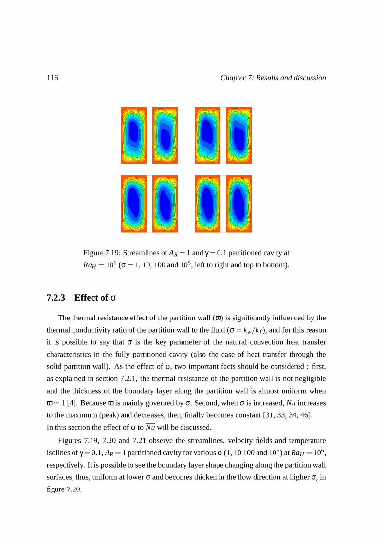
116 Chapter 7: Results and discussion
Figure 7.19: Streamlines of AR = 1 and γ = 0.1 partitioned cavity at
RaH = 106 (σ = 1, 10, 100 and 105, left to right and top to bottom).
7.2.3 Effect of σ
The thermal resistance effect of the partition wall (ω) is significantly influenced by the
thermal conductivity ratio of the partition wall to the fluid (σ = kw/k f ), and for this reason
it is possible to say that σ is the key parameter of the natural convection heat transfer
characteristics in the fully partitioned cavity (also the case of heat transfer through the
solid partition wall). As the effect of σ, two important facts should be considered : first,
as explained in section 7.2.1, the thermal resistance of the partition wall is not negligible
and the thickness of the boundary layer along the partition wall is almost uniform when
ω ' 1 [4]. Because ω is mainly governed by σ. Second, when σ is increased, Nu increases
to the maximum (peak) and decreases, then, finally becomes constant [31, 33, 34, 46].
In this section the effect of σ to Nu will be discussed.
Figures 7.19, 7.20 and 7.21 observe the streamlines, velocity fields and temperature
isolines of γ = 0.1, AR = 1 partitioned cavity for various σ (1, 10 100 and 105) at RaH = 106,
respectively. It is possible to see the boundary layer shape changing along the partition wall
surfaces, thus, uniform at lower σ and becomes thicken in the flow direction at higher σ, in
figure 7.20.

Chapter 7: Results and discussion 117
Figure 7.20: Velocity fields of AR = 1 and γ = 0.1 partitioned cav-
ity at RaH = 106 (σ = 1, 10 100 and 105, left to right and top to
bottom).
Figure 7.21: Temperature isolines of AR = 1 and γ = 0.1 partitioned
cavity at RaH = 106 (σ = 1, 10 100 and 105, left to right and top to
bottom).

118 Chapter 7: Results and discussion
−0.5 −0.25 0 0.25 0.5Dimensionless length (X)
−0.5
−0.25
0
0.25
0.5D
imen
sion
less
tem
pera
ture
(θ)
σ=1σ=10σ=10
2
Y=0.45
Partition wall
0
−0.45
Figure 7.22: θ distributions along the horizontal planes (Y = 0.45,
0 and -0.45) of AR = 1 and γ = 0.1 partitioned cavity at RaH = 106.
As shown in figure 7.19, the core of the flow in both fluid cells becomes longer to vertical
direction and the position of the core becomes more centered with increasing σ. To explain
this phenomenon, first, consider the temperature isolines in figure 7.21. At lower σ, for
example at σ = 1, the temperature distributions in hot fluid cell is more hot (also cold fluid
cell is more cold) than higher σ cases. Precisely speaking, as shown in figure 7.22, the
temperature distributions at each vertical position (Y = 0.45, 0 and -0.45) of σ = 1 case are
generally higher in hot fluid cell (lower in cold fluid cell) than others. Also, the temperature
difference between top and bottom of the fluid cell is lower than higher σ cases, and for
this reason at lower σ case the horizontal discharges along the top and bottom of each fluid
cell are slower than higher σ cases and causes the non-centered core of the streamlines.
Now consider Nu behavior showing a peak with increasing σ from 1. This feature is
shown in figure 7.23 and table 7.4. Consequently, at the maximum Nu, the convection heat
transfer through the entire domain becomes maximum 3. This feature is more evident at
3Some articles state that the heat transfer is found maximum at peak Nu, but from the definition of theNusselt number, the peak Nu, it is more reasonable that the system is more dominated by convection heat

Chapter 7: Results and discussion 119
100
101
102
103
104
105
Conductivity ratio (σ)
1.0
2.0
3.0
4.0
5.0
6.0
7.0
8.0
Ave
rage
Nus
selt
num
ber
(Nu)
γ=0.01γ=0.1
106
105
104
RaH=107
Figure 7.23: Nu of AR = 1 and γ = 0.1 and 0.01 partitioned cavity
at various σ.
Table 7.4: Nu of AR = 1 partitioned cavity at RaH = 106.
σ1 5 10 20 30 50 102 103 104 105
γ = 0.01, 6720µ-elements
Nu 4.0078 4.1411 4.1497 4.1411 4.1282 4.1029 4.0513 3.8310 3.7590 3.7503
γ = 0.1, 8000µ-elements
Nu 2.7821 3.4758 3.5694 3.5828 3.5692 3.5429 3.5071 3.4549 3.4483 3.4476

120 Chapter 7: Results and discussion
higher RaH cases. For example, at RaH = 107 of γ = 0.1 case in figure 7.23, the value of
Nu increases significantly compare to lower RaH cases in the range of σ between 1 and 30.
Also the increment of Nu at γ = 0.1 cases are more steep than that of γ = 0.01 cases, and
consequently it is possible to say that the convective heat transfer rate is greatly affected
by the increasing partition wall conductivity when thermal resistance of the partition wall
exists [31].
In order to explain the reason of the peak Nu, three different regions, which correspond to
the Nu behavior as σ changes, are introduced. Thus, with increasing σ, Nu increases until
the maximum (Thermal resistance region), then gradually decreases (Thermal transition
region) and then finally becomes constant (Isothermal wall region).
Thermal resistance region (σ ↑∼ Nu ↑)
In this region, the value of ω is relatively high and the partition wall has the temperature
differences to vertical and to horizontal directions. Also the heat flux and the boundary
layer are found uniform along the partition wall.
First, at the steady-state, the heat flux in partitioned cavity, q′′, through the entire domain
is always constant for every cases of σ and γ, thus, q′′ = q′′f = q′′w (see Eq. (7.13)) :
q′′ = k f∂Tf
∂x= kw
∂Tw
∂x= constant. (7.17)
Now, suppose increasing kw with constant k f , thus the increasing σ (kw ↑), the horizontal
temperature gradient of the partition wall decreases (∂Tw/∂x ↓) since the value of q′′ is
constant. The mean temperatures of the partition wall surfaces on both sides, T WH and
TWC, become closer (i.e. TWH ↓ and TWC ↑). This mechanism can be expressed as
kw ↑∼ ∂Tw
∂x↓∼ TWH ↓ (∼ TWC ↑). (7.18)
If kw increases until TWH = TWC, then the partition wall becomes horizontally isothermal.
In this region, the heat flux from left to right is more dominant than from bottom to top (or
top to bottom) since the adiabatic horizontal end walls boundary conditions (∂Tw/∂y = 0
on y = ±H/2, for example). Then since H >> W , the heat flux of the partition wall in
horizontal and vertical directions are
kw∂Tw
∂x>> kw
∂Tw
∂y. (7.19)
transfer.

Chapter 7: Results and discussion 121
−0.5 0.25 0 0.25 0.5Dimensionless Height (Y)
−0.2
−0.1
0
0.1
0.2
0.3
0.4
Dim
ensi
onle
ss T
empe
ratu
re (
θ) σ=1
510
203050100
103
104
105
Figure 7.24: θ distributions along the ’Surface 2’ of AR = 1 and
γ = 0.1 partitioned cavity at RaH = 106.
The variation of ∂Tw/∂y against increasing σ is negligible.
Figures 7.24 and 7.25 also demonstrate this fact. For example, in figure 7.24, it is clear
that the mean value is decreasing from σ = 1 to 20 and becomes constant. Nevertheless,
temperature difference between top (Y = 0.5) and bottom (Y = −0.5) of the partition wall
is almost constant while σ varies between 1 and 30. At γ = 0.01 partitioned cavity case in
figure 7.25, the mean value variation is relatively small since the thermal resistance effect
of the partition wall is also smaller than γ = 0.1 cases.
The scaling analysis of the heat flux is used in order to explain the relationship between
the Nusselt number and the mean surface temperatures. As shown in figure 7.26, the heat
flux of the fluid at the steady-state, q′′f , can be expressed by two different convective heat
transfer mechanism. At the steady-state :
q′′f ∼ k f∆Tf ,Horizontal
δT, f∼ k f
∆Tf ,Vertical
H(7.20)
where ∆Tf ,Vertical is the vertical temperature difference between fluid near the top and bot-
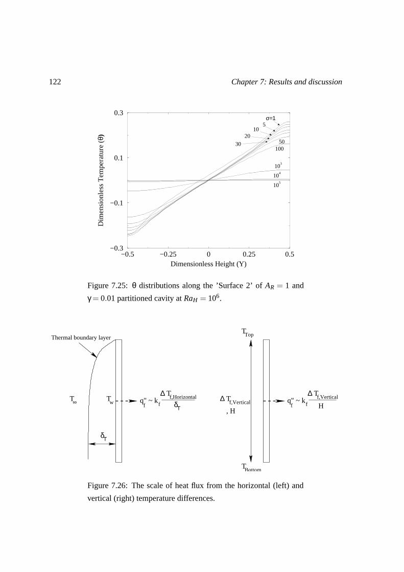
122 Chapter 7: Results and discussion
−0.5 −0.25 0 0.25 0.5Dimensionless Height (Y)
−0.3
−0.1
0.1
0.3
Dim
ensi
onle
ss T
empe
ratu
re (
θ)
σ=1
10
50100
103
104
105
5
2030
Figure 7.25: θ distributions along the ’Surface 2’ of AR = 1 and
γ = 0.01 partitioned cavity at RaH = 106.
∞T Tw
δΤ
TopT
BottomT
δΤq" ~ k f
∆ Tf,Horizontal
Thermal boundary layer
, Hf H
∆ Tf,Verticalq" ~ k f f
∆ Tf,Vertical
Figure 7.26: The scale of heat flux from the horizontal (left) and
vertical (right) temperature differences.

Chapter 7: Results and discussion 123
tom of the partition wall (∆Tf ,Vertical = Tf ,Top−Tf ,Bottom). Also as shown in equation (7.13),
at the steady-state, q′′f = q′′w, then by substituting (7.14a) and (7.14b) yields
k f∆Tf ,Horizontal
δT, f∼ kw
∆Tw,Horizontal
W. (7.21)
Note that above scaling analysis is only valid in the case of γ > 0.01 since ∆Tw,Horizontal
becomes negligible when γ < 0.01, but in the case of ’finite’ partition thickness case, the
interaction between ∆Tw,Horizontal and ∆Tf ,Horizontal exists.
According to equation (7.18), increasing kw causes a decrease in ∆Tw,Horizontal and T∞ −Tw
in figure 7.26 increases. Then in the hot fluid cell for example, the heat flux of the fluid
(q′′f ) becomes
q′′f = k fTh −TWH
DH(7.22)
and q′′f increases since TWH increases. It should be note that in equation (7.22), all values
but TWH are constant against varying σ. Indeed, q′′f of figure 7.26 is equal to convection heat
flux (of the fluid), q′′Convection. Thus, at the steady-state, as kw is increased (σ ↑), partition
wall becomes horizontally isothermal (∆Tw,Horizontal ↓) and causes an increase in convection
in the fluid cells (q′′Convection ↑). Finally, the Nusselt number of the domain increases (Nu ↑)
since the domain becomes more convection dominated with increasing σ from 1.
This mechanism can be expressed as
kw ↑∼ ∂Tw
∂x↓∼ ∆Tw,Horizontal ↓∼ q′′Convection ↑∼ Nu ↑ . (7.23)
Also, as the fluid cell becomes more convective, the thermal boundary layer thickness
becomes thinner. This feature is very well explained in figures 7.27 and 7.28. In those
figures, it is clear that the local Nusselt number distribution, which also represents the heat
flux and the boundary layer shape, varies against σ. This behavior is more evident in higher
γ case since the strong thermal resistance effect of the partition wall.
At last, as shown in figure 7.23, the increment rate of Nu with increasing σ becomes
slower and eventually reach a maximum (the peak Nu).
To explain the peak, the temperature differences between TWH and TWC, thus ∆Tw,Horizontal ,
is considered (represented by ∆θw,Horizontal which is the dimensionless form of ∆Tw,Horizontal .

124 Chapter 7: Results and discussion
−0.5 0.25 0 0.25 0.5Dimensionless Height (Y)
0.0
2.0
4.0
6.0
8.0
Loc
al N
usse
lt nu
mbe
r (N
u Y)
σ=15
1020
30
50100
103
104
105
Figure 7.27: NuY distributions along the ’Surface 2’ of AR = 1 and
γ = 0.01 partitioned cavity at RaH = 106.

Chapter 7: Results and discussion 125
−0.5 0.25 0 0.25 0.5Dimensionless Height (Y)
0.0
2.0
4.0
6.0
8.0
Loc
al N
usse
lt nu
mbe
r (N
u Y)
σ=1
510203050
100
103
104 10
5
Figure 7.28: NuY distributions along the ’Surface 2’ of AR = 1 and
γ = 0.1 partitioned cavity at RaH = 106.

126 Chapter 7: Results and discussion
100
101
102
103
104
105
Conductivity ratio (σ)
10−7
10−6
10−5
10−4
10−3
10−2
10−1
100
Tem
pera
ture
dif
fere
nce
(∆θ W
, Hor
izon
tal)
γ=0.01γ=0.1
2% of ∆θW, Horizontal
Figure 7.29: ∆θw,Horizontal along the mid-plane (Y = 0) of AR = 1
partitioned cavity at RaH = 106.
See Fig. 7.29). According to equation 7.18, the value of ∆Tw,Horizontal decreases with in-
creasing σ since TWH and TWC become closer. For example, ∆Tw,Horizontal becomes negli-
gible (< 2%) when σ = 20 at RaH = 106 of γ = 0.1 case in figure 7.29. Also at this point,
Nu becomes maximal (Nu = 3.5828, see Tab. 7.4). Thus Nu reaches to the peak when
∆TW,Horizontal becomes negligible. Note that, as mentioned earlier, the ∆TW,Horizontal of
γ = 0.01 partitioned cavity falls more rapidly since the thermal resistance effect is smaller
than γ = 0.1 case.
As a conclusion of this region, ∂Tw/∂x decreases with increasing σ (increasing kw with
constant k f ) and causes an increase in q′′Convection. Then Nu increases with increasing σ. Nu
increases until ∂Tw/∂x becomes negligible. Thus, the partition wall is horizontally isother-
mal. Finally, ∂Tw/∂x ≈ 0 and Nu reaches to the peak.

Chapter 7: Results and discussion 127
Thermal transition region (σ ↑∼ Nu ↓)
In the thermal resistance region, Nu reaches to the peak when ∂Tw/∂x and ∆TW,Horizontal
are negligible. Nevertheless, even if the partition wall becomes horizontally isothermal, it
is true that the temperature difference between top and bottom of the partition wall surface
remains still great (see Fig. 7.24 and 7.25).
In this region, due to ∂Tw/∂x ≈ 0, the heat transfer in the partition wall is characterized by
only ∂Tw/∂y. Thus, when σ is increased, the partition wall becomes vertically isothermal
and eventually Nu decreases.
The reason can be also explained by equation 7.20 and figure 7.26. Note that in this region,
∆Tf ,Horizontal ≈ 0 and equation 7.20 becomes
q′′Convection ∼ k f∆Tf ,Vertical
H= k f
∆Tw,Vertical
H. (7.24)
It should be note that the temperatures of the fluid (T f ,top and Tf ,bottom in Fig. 7.26) are
identical to the partition wall surface temperature (Tw,top and Tw,bottom). Then ∆Tf ,Vertical is
equal to ∆Tw,Vertical .
In this region, as σ is increased, the partition wall becomes vertically isothermal and
∆Tw,Vertical decreases and leads to decreases in q′′Convection. This phenomenon is clearly
shown in figure 7.30. The vertical partition wall surface temperature difference, ∆Tw,Vertical
(represented by ∆θw,Vertical in dimensionless form), at ’Surface 2’ (X = −γ/2) remains
constant from σ = 1 to 10 at the case of γ = 0.1. Then it begins decreasing steeply
when σ passes 20, which corresponds to the peak Nu. Hence, with decreasing ∆Tw,Vertical ,
q′′Convection in equation (7.24) also decreases and causes decreasing behavior of Nu.
Finally, at σ = 103, ∆Tw,Vertical becomes negligible (< 2%) and Nu becomes constant while
σ increases further. Then the partition wall eventually becomes vertically isothermal.
In figure 7.30, it is observed that ∆Tw,Vertical of γ = 0.01 is generally lower than 0.1 case.
As explained in previous section, when γ is low, the area for the fluid is larger than higher
γ and the heat transfer is more dominated by the convection, and for this reason Nu and
∆θw,Vertical are found bigger than higher γ cases [33, 34]. Consequently, at γ = 0.01 case,
decrement rate of ∆Tw,Vertical as σ increases is also slower than γ = 0.1 case.
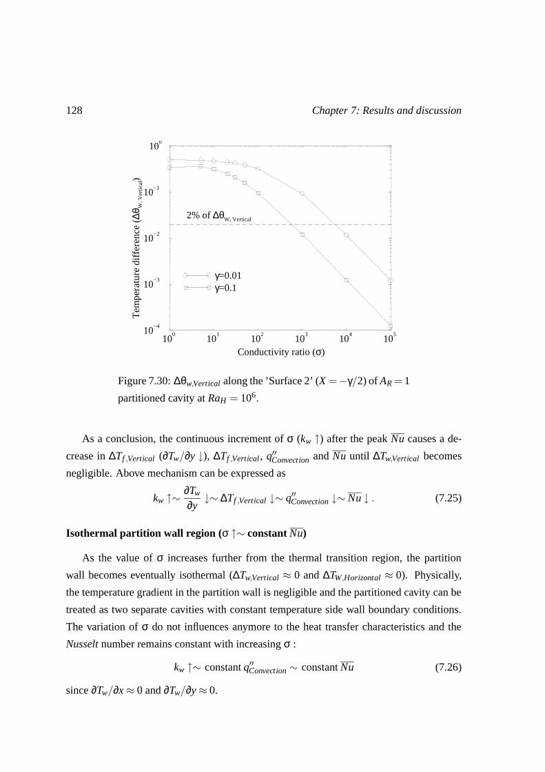
128 Chapter 7: Results and discussion
100
101
102
103
104
105
Conductivity ratio (σ)
10−4
10−3
10−2
10−1
100
Tem
pera
ture
dif
fere
nce
(∆θ W
, Ver
tical)
γ=0.01γ=0.1
2% of ∆θW, Vertical
Figure 7.30: ∆θw,Vertical along the ’Surface 2’ (X =−γ/2) of AR = 1
partitioned cavity at RaH = 106.
As a conclusion, the continuous increment of σ (kw ↑) after the peak Nu causes a de-
crease in ∆Tf ,Vertical (∂Tw/∂y ↓), ∆Tf ,Vertical , q′′Convection and Nu until ∆Tw,Vertical becomes
negligible. Above mechanism can be expressed as
kw ↑∼ ∂Tw
∂y↓∼ ∆Tf ,Vertical ↓∼ q′′Convection ↓∼ Nu ↓ . (7.25)
Isothermal partition wall region (σ ↑∼ constant Nu)
As the value of σ increases further from the thermal transition region, the partition
wall becomes eventually isothermal (∆Tw,Vertical ≈ 0 and ∆TW,Horizontal ≈ 0). Physically,
the temperature gradient in the partition wall is negligible and the partitioned cavity can be
treated as two separate cavities with constant temperature side wall boundary conditions.
The variation of σ do not influences anymore to the heat transfer characteristics and the
Nusselt number remains constant with increasing σ :
kw ↑∼ constant q′′Convection ∼ constant Nu (7.26)
since ∂Tw/∂x ≈ 0 and ∂Tw/∂y ≈ 0.

Chapter 8
Benchmark study - Low Mach number
model
At the event of LOCA, the temperature differences in the reactor containment can be
increase up to 300K [40]. Although the incompressible fluid flow model under Boussinesq
approximation is simple and has fast convergence behavior, it is inappropriate for the prob-
lem of the large temperature differences cases due to their restriction (∆T ≤ 28.6K for the
air at STP [27]). In this chapter, the partitioned cavity problem is solved by an asymptotic
low Mach number model to handle the natural convection flows with large temperature dif-
ferences [55].
The asymptotic low Mach number model is based on the compressible flow model.
As well known, the compressible flow implies appreciable variations in density through-
out a flow involving a large pressure changes. Especially for the gas flows, these pressure
changes are accompanied by significant variations in both density and temperature. Since
two additional variables are encountered in treating compressible flow, two additional equa-
tions are needed compare to incompressible flow model. Both energy equation and equa-
tion of state are necessary to solve compressible flow problems.
The compressible flow model becomes however invalid when the Mach number becomes
very small, namely low Mach number. According to Müller [48], when Mach number be-
comes zero, the flow is close to incompressible and the Navier-Stokes equations becomes
stiff and invalid. To overcome this, the pressure term in the momentum equation is split
129

130 Chapter 8: Benchmark study - Low Mach number model
into the hydrodynamic and hydrostatic pressure by the asymptotic perturbation theory in
order to give the physical meaning of the Navier-Stokes equations at low Mach number
compressible flow model. The asymptotic low Mach number model is also valid for large
global thermodynamic pressure, for small acoustic pressure and for very small incompress-
ible pressure cases [15].
In this chapter, first, the fundamental principles and mathematical model of the asymp-
totic low Mach number model is reviewed. Then the governing equations are developed in
order to solve the non-partitioned and partitioned cavity problems. Second, the governing
equations are discretized in time and space to apply for the numerical simulations. The
validation and the qualification of the resolutions are proceeded by comparing with the lit-
erature.
For the benchmark study with the incompressible fluid flow model under Boussinesq ap-
proximation, both high and low Mach number cases are considered for both non-partitioned
and partitioned cavity cases. Finally, for the partitioned cavity case, heat transfer charac-
teristics and the thermal resistance effect of the partition wall will be discussed.
8.1 Fundamental principles and mathematical model
8.1.1 Compressible flow
Recall from chapter 5, the mass, momentum and energy conservation equations for an
ideal gas, in dimensional and vector form, are
∂ρ∂t
+∇ ·ρ~u = 0, (8.1a)
∂ρ~u∂t
+∇ ·ρ~u~u = −∇p+∇ · ¯τ+ρg(−~e), (8.1b)
ρCp
(∂T∂t
+~u ·∇T
)= ∇ · (k∇T )+
d pdt
+~u ·∇p. (8.1c)

Chapter 8: Benchmark study - Low Mach number model 131
Where in equation (8.1c), the left hand side may be rearranged by using vector operator
expansion and by substituting equation (8.1a) :
ρ∂T∂t
+ρ~u ·∇T =∂ρT∂t
+∇ · (ρ~uT )−T
(∂ρ∂t
+∇ ·ρ~u)
=∂ρT∂t
+∇ · (ρ~uT ),
(8.2)
andDpDt
=d pdt
+~u ·∇p. (8.3)
Note again that β = 1/T for ideal gas and ¯τ = µ(∇~u+(∇~u)T )−2/3(µ∇ ·~u ¯I).
The impact of low Mach number can be explained by dimensionless analysis [48], thus, the
governing equations become
∂ρ∗
∂t∗u+∇ ·ρ∗~u∗ = 0, (8.4a)
∂ρ∗~u∗
∂t∗u+∇ ·ρ∗~u∗~u∗ = − 1
Ma2 ∇p∗ +
1Re∞
∇ · ¯τ∗ +1
Fr2∞
ρ∗(−~e), (8.4b)
∂ρ∗t∗u∂t∗u
+∇ · (ρ∗~u∗T ∗) =1
Pr∞Re∞∇ · (k∗∇T ∗)+
(γc −1
γc
)(d p∗
dt∗u+~u∗ ·∇p∗
). (8.4c)
The definition of dimensionless parameters is
X =xH
, Y =yH
, t∗u =tu∞H
, ρ∗ =ρ
ρ∞, p∗ =
pp∞
, ~u∗ =~uu∞
, T ∗ =TT∞
,
µ∗ =µ
µ∞, k∗ =
kk∞
, Pr∞ =Cpµ∞
k∞; Prandtl number,
Re∞ =ρ∞u∞H
µ∞; Reynolds number, Fr∞ =
u∞√gH
; Froude number.
(8.5)
The subscript ∞ denotes the reference quantities and are chosen such that the dimensionless
quantities remain of order O(1) for any low reference Mach number :
Ma∞ =u∞√
γc p∞/ρ∞. (8.6)
Thus, the reference quantity is always greater than that of measured quantities.
Also to avoid the dependence on γc :
Ma =u∞√
p∞/ρ∞=√
γcMa∞ (8.7)
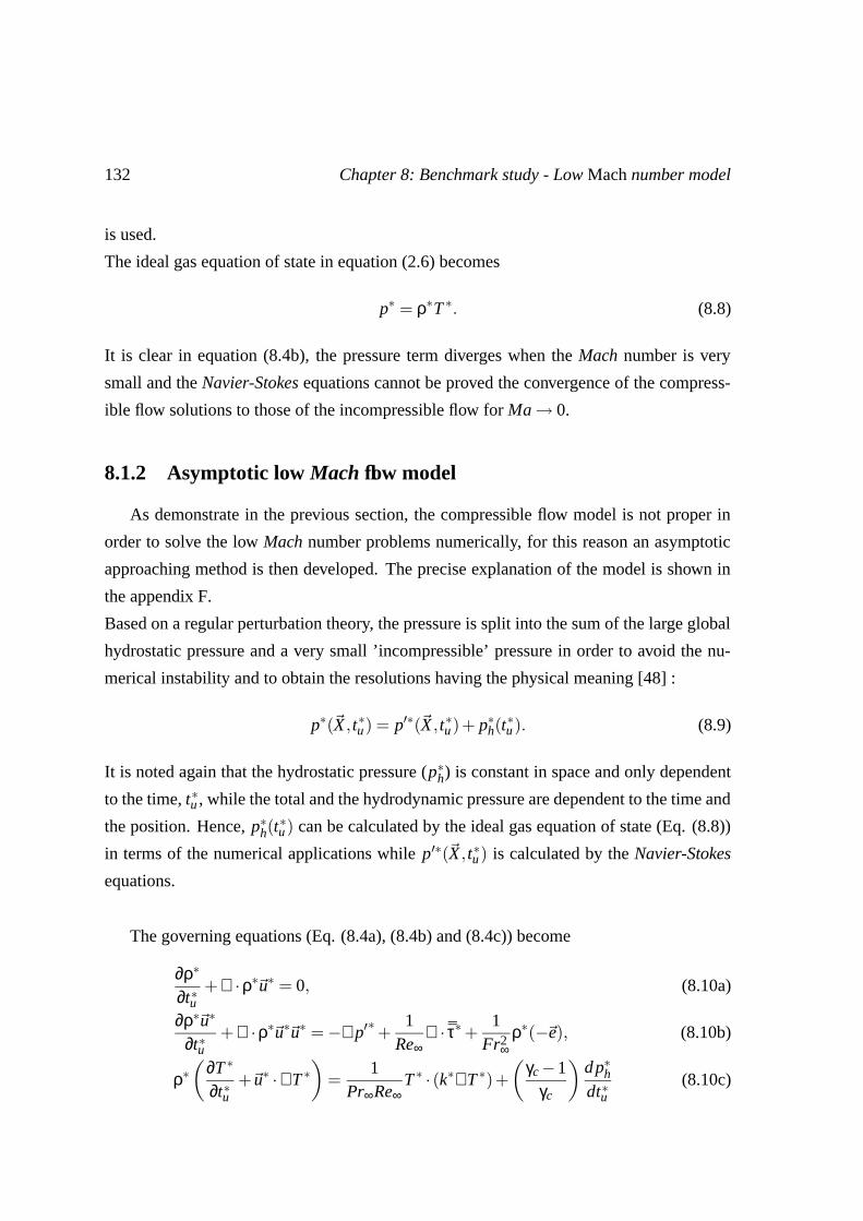
132 Chapter 8: Benchmark study - Low Mach number model
is used.
The ideal gas equation of state in equation (2.6) becomes
p∗ = ρ∗T ∗. (8.8)
It is clear in equation (8.4b), the pressure term diverges when the Mach number is very
small and the Navier-Stokes equations cannot be proved the convergence of the compress-
ible flow solutions to those of the incompressible flow for Ma → 0.
8.1.2 Asymptotic low Mach flow model
As demonstrate in the previous section, the compressible flow model is not proper in
order to solve the low Mach number problems numerically, for this reason an asymptotic
approaching method is then developed. The precise explanation of the model is shown in
the appendix F.
Based on a regular perturbation theory, the pressure is split into the sum of the large global
hydrostatic pressure and a very small ’incompressible’ pressure in order to avoid the nu-
merical instability and to obtain the resolutions having the physical meaning [48] :
p∗(~X , t∗u) = p′∗(~X , t∗u)+ p∗h(t∗u). (8.9)
It is noted again that the hydrostatic pressure (p∗h) is constant in space and only dependent
to the time, t∗u , while the total and the hydrodynamic pressure are dependent to the time and
the position. Hence, p∗h(t∗u) can be calculated by the ideal gas equation of state (Eq. (8.8))
in terms of the numerical applications while p′∗(~X , t∗u) is calculated by the Navier-Stokes
equations.
The governing equations (Eq. (8.4a), (8.4b) and (8.4c)) become
∂ρ∗
∂t∗u+∇ ·ρ∗~u∗ = 0, (8.10a)
∂ρ∗~u∗
∂t∗u+∇ ·ρ∗~u∗~u∗ = −∇p′∗ +
1Re∞
∇ · ¯τ∗ +1
Fr2∞
ρ∗(−~e), (8.10b)
ρ∗(
∂T ∗
∂t∗u+~u∗ ·∇T ∗
)=
1Pr∞Re∞
T ∗ · (k∗∇T ∗)+
(γc −1
γc
)d p∗hdt∗u
(8.10c)

Chapter 8: Benchmark study - Low Mach number model 133
where
¯τ∗ = µ∗(∇~u∗ +(∇~u∗)T )− 23
µ∗∇ ·~u∗ ¯I. (8.11)
The equation of state is then :
p∗ = ρ∗T ∗. (8.12)
8.1.3 Problem description
The geometry are equal to those of incompressible-Boussinesq fluid flow test cases in
chapter 5 as shown in figure 5.1. Air is the working fluid and initially the fluid and partition
wall are isothermal and motionless everywhere in the cavity. For the boundary conditions,
the temperature at both side walls is constant and the top and bottom walls are adiabatic.
The air is assumed as an ideal gas with R = 287J/kgK and γc = 1.4.
In low Mach model it is assumed that the fluid is to be an ideal gas, hence, the thermal
expansion coefficient is
β =1T0
(8.13)
and definition of the Rayleigh number becomes
RaH = GrH ·Pr =gρ2
0(Th −Tc)H3
T0µ20
(8.14)
where T0 = (Th +Tc)/2 and ∆T = Th−Tc. For the benchmark study, the case of RaH = 106
is only studied in this chapter. Also for the partitioned cavity, the partition thickness and
conductivity ratio are assumed as γ = 0.1 and 1 ≤ σ ≤ 105.
A dimensionless parameter, ε, is introduced in order to define the temperature differ-
ence between hot and cold side walls :
ε =Th −Tc
Th +Tc= 2
Th −Tc
T0. (8.15)
The value of ε have been used as a reference of the fluid characteristics. For example, when
ε → 0, the flow becomes incompressible. In contrary, the flow becomes compressible with
increasing ε. In this thesis, the values of ε are 0.01 and 0.6, which are generally used for
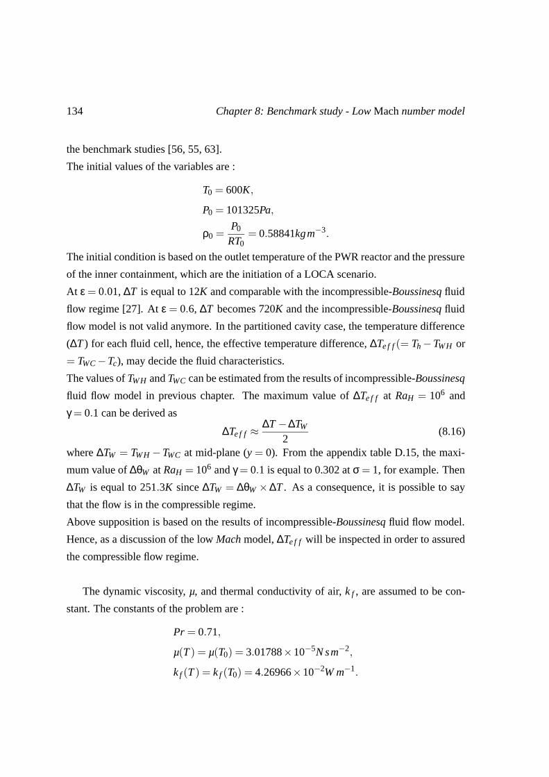
134 Chapter 8: Benchmark study - Low Mach number model
the benchmark studies [56, 55, 63].
The initial values of the variables are :
T0 = 600K,
P0 = 101325Pa,
ρ0 =P0
RT0= 0.58841kgm−3.
The initial condition is based on the outlet temperature of the PWR reactor and the pressure
of the inner containment, which are the initiation of a LOCA scenario.
At ε = 0.01, ∆T is equal to 12K and comparable with the incompressible-Boussinesq fluid
flow regime [27]. At ε = 0.6, ∆T becomes 720K and the incompressible-Boussinesq fluid
flow model is not valid anymore. In the partitioned cavity case, the temperature difference
(∆T ) for each fluid cell, hence, the effective temperature difference, ∆Te f f (= Th −TWH or
= TWC −Tc), may decide the fluid characteristics.
The values of TWH and TWC can be estimated from the results of incompressible-Boussinesq
fluid flow model in previous chapter. The maximum value of ∆Te f f at RaH = 106 and
γ = 0.1 can be derived as
∆Te f f ≈∆T −∆TW
2(8.16)
where ∆TW = TWH −TWC at mid-plane (y = 0). From the appendix table D.15, the maxi-
mum value of ∆θW at RaH = 106 and γ = 0.1 is equal to 0.302 at σ = 1, for example. Then
∆TW is equal to 251.3K since ∆TW = ∆θW ×∆T . As a consequence, it is possible to say
that the flow is in the compressible regime.
Above supposition is based on the results of incompressible-Boussinesq fluid flow model.
Hence, as a discussion of the low Mach model, ∆Te f f will be inspected in order to assured
the compressible flow regime.
The dynamic viscosity, µ, and thermal conductivity of air, k f , are assumed to be con-
stant. The constants of the problem are :
Pr = 0.71,
µ(T ) = µ(T0) = 3.01788×10⁻⁵N sm−2,
k f (T ) = k f (T0) = 4.26966×10⁻²W m−1.

Chapter 8: Benchmark study - Low Mach number model 135
The value of µ(T ) is calculated via the Sutherland law (Eq. (5.4)) with Tre f = 273K and
µre f = 1.716×10⁻⁵N sm−2. Also the value of k f is calculated via
k f (T ) =µ(T )
PrCp =
µ(T )
Prγc
γc −1R. (8.17)
The heat transfer is also characterized by the Nusselt number. Recall from chapter 5,
the definition of the Nusselt number is
Nuy =L[1− γ(1−1/σ)]
∆T∂T∂x
(8.18a)
Nu =1H
Z H2
−H2
Nuydy. (8.18b)
Note that γ = 0 for the non-partitioned cavity case.
Non-partitioned cavity
The governing equations for non-partitioned cavity in the low Mach model based on
equations (8.10a), (8.10b) and (8.10c), in dimensional form, are
∂ρ f
∂t+∇ ·ρ f~u = 0, (8.19a)
∂ρ f~u
∂t+∇ ·ρ f~u~u = −∇p′ +∇ · ¯τ+(ρ f −ρ0, f )g(−~e), (8.19b)
ρ fCp f
(∂Tf
∂t+~u ·∇Tf
)= k f ∇2Tf +
d ph
dt(8.19c)
where the subscript f denotes the fluid. It is noted that the thermal conductivity of the fluid,
k f , is assumed as constant and
¯τ = µ(∇~u+(∇~u)Tf )−
23
µ∇ ·~u ¯I. (8.20)
In order to apply to the numerical scheme, the governing equations can be rearranged as
∂ρ f
∂t+ρ f ∇ ·~u+~u ·∇ρ f = 0, (8.21a)
ρ f∂~u∂t
+ρ f~u ·∇~u = −∇p′ +∇ · ¯τ+(ρ f −ρ0, f )g(−~e), (8.21b)
ρ fCp f
∂Tf
∂t+ρ fCp f~u ·∇Tf = k f ∇2Tf +
d ph
dt. (8.21c)
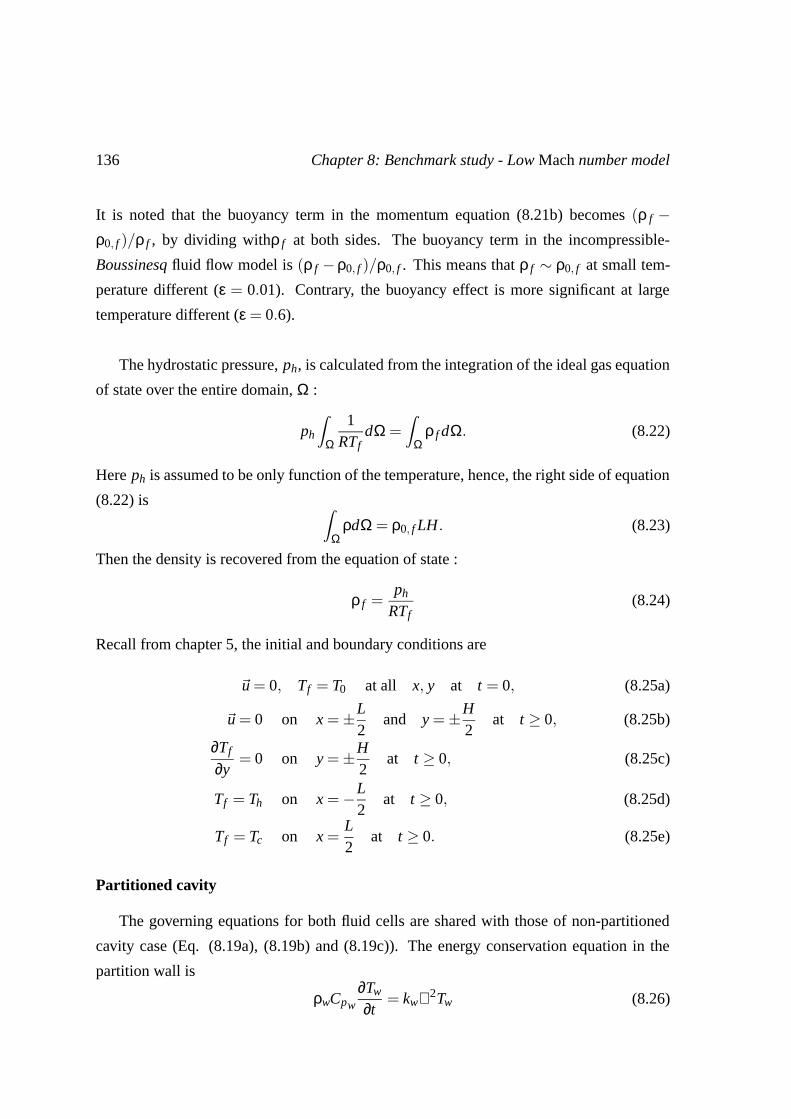
136 Chapter 8: Benchmark study - Low Mach number model
It is noted that the buoyancy term in the momentum equation (8.21b) becomes (ρ f −ρ0, f )/ρ f , by dividing withρ f at both sides. The buoyancy term in the incompressible-
Boussinesq fluid flow model is (ρ f −ρ0, f )/ρ0, f . This means that ρ f ∼ ρ0, f at small tem-
perature different (ε = 0.01). Contrary, the buoyancy effect is more significant at large
temperature different (ε = 0.6).
The hydrostatic pressure, ph, is calculated from the integration of the ideal gas equation
of state over the entire domain, Ω :
ph
Z
Ω
1RTf
dΩ =Z
Ωρ f dΩ. (8.22)
Here ph is assumed to be only function of the temperature, hence, the right side of equation
(8.22) isZ
ΩρdΩ = ρ0, f LH. (8.23)
Then the density is recovered from the equation of state :
ρ f =ph
RTf(8.24)
Recall from chapter 5, the initial and boundary conditions are
~u = 0, Tf = T0 at all x, y at t = 0, (8.25a)
~u = 0 on x = ±L2
and y = ±H2
at t ≥ 0, (8.25b)
∂Tf
∂y= 0 on y = ±H
2at t ≥ 0, (8.25c)
Tf = Th on x = −L2
at t ≥ 0, (8.25d)
Tf = Tc on x =L2
at t ≥ 0. (8.25e)
Partitioned cavity
The governing equations for both fluid cells are shared with those of non-partitioned
cavity case (Eq. (8.19a), (8.19b) and (8.19c)). The energy conservation equation in the
partition wall is
ρwCpw∂Tw
∂t= kw∇2Tw (8.26)

Chapter 8: Benchmark study - Low Mach number model 137
where subscript w denotes the partition wall and kw is assumed as the constant.
The initial and boundary conditions are
~u = 0, Tf = Tw = T0 at all x, y at t = 0, (8.27a)
~u = 0 on x = ±L2
and y = ±H2
at t ≥ 0, (8.27b)
∂Tf
∂y=
∂Tw
∂y= 0 on y = ±H
2at t ≥ 0, (8.27c)
Tf = Th on x = −L2
at t ≥ 0, (8.27d)
Tf = Tc on x =L2
at t ≥ 0, (8.27e)
k f∂Tf
∂x= kw
∂Tw
∂xon x = ∓W
2at t ≥ 0. (8.27f)
8.2 Numerical discretization
In order to benchmark with the incompressible-Boussinesq fluid flow model, macro-
Q1/P1-NC element mesh with finite element scheme with SUPG stabilization method is
also used, and shown in the appendix section C.3.1. For the time discretization, full implicit
method is also used, and shown in the appendix section C.3.2.

138 Chapter 8: Benchmark study - Low Mach number model
Table 8.1: Some parameters for the test cases at CFL = 10.
Case ε No’ µ-elements ∆T (K) H(m) δymin(m) ure f (m/s) ∆t(s)
AR = 1 non-
partitioned,
RaH = 106
40×40 (1600) 12.0 0.2663 6.16×10⁻³ 0.2286 0.2693
0.01 80×80 (6400) 12.0 0.2663 2.96×10⁻³ 0.2286 0.1296
160×160 (25600) 12.0 0.2663 1.45×10⁻³ 0.2286 0.0636
40×40 (1600) 720.0 0.068 1.57×10⁻³ 0.8948 0.0176
0.6 80×80 (6400) 720.0 0.068 7.57×10⁻⁴ 0.8948 8.45×10⁻³
160×160 (25600) 720.0 0.068 3.71×10⁻⁴ 0.8948 4.15×10⁻³
AR = 1,
γ = 0.1
partitioned,
RaH = 106
60×40 (2400) 12.0 0.2663 6.16×10⁻³ 0.2286 0.2693
0.01 100×80 (8000) 12.0 0.2663 2.96×10⁻³ 0.2286 0.1296
180×160 (28800) 12.0 0.2663 1.45×10⁻³ 0.2286 0.0636
20×40 (800) 720.0 0.068 1.57×10⁻³ 0.8948 0.0176
0.6 40×80 (3200) 720.0 0.068 7.57×10⁻⁴ 0.8948 8.45×10⁻³
80×160 (12800) 720.0 0.068 3.71×10⁻⁴ 0.8948 4.15×10⁻³
8.3 Validation of the computation
In order to valid the computation, the mesh convergence study is held for non-partitioned
and partitioned cavity cases by using low Mach flow model. The same meshes and refine-
ment methods introduced in chapter 6 are used.
Table 8.1 shows the essential parameters for the computation. Since the initial tempera-
ture and the value of ε and RaH are constants. The temperature difference between both
side walls, ∆T , and the height of the cavity, H, can be computed via the definition of εin equation (8.15) and the Rayleigh number in equation (8.14), respectively. Then ure f of
table 8.1 can be found from equation (6.9) and the proper time step size will be obtained.
Same to the incompressible-Boussinesq fluid flow case, CFL = 10 is used. Also, the values
are used both in non-partitioned and partitioned cavity cases. Note that the minimum size
of the vertical mesh, δymin, is determined by the value of δYmin in the appendix tables D.1,
D.2, D.4 and D.6 since δymin = δYmin ×H.
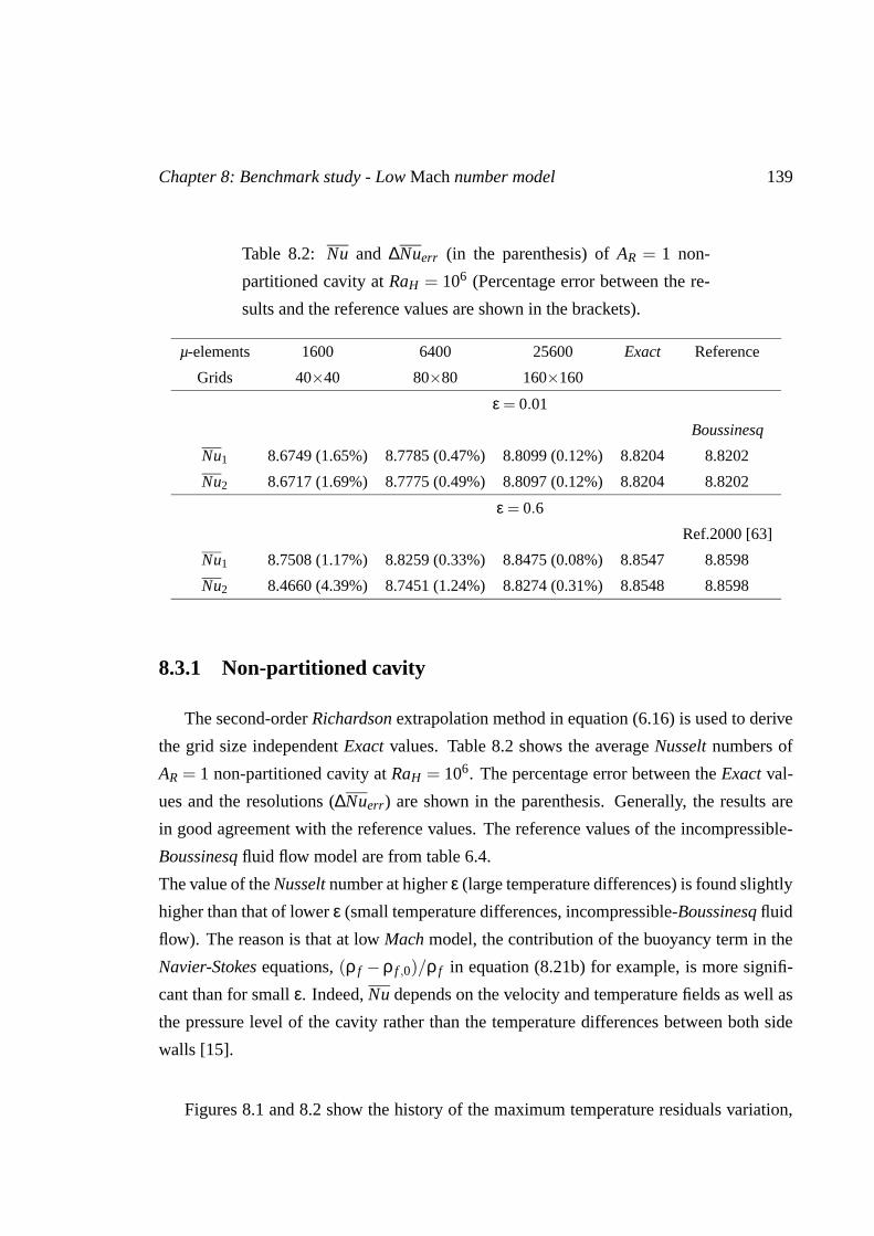
Chapter 8: Benchmark study - Low Mach number model 139
Table 8.2: Nu and ∆Nuerr (in the parenthesis) of AR = 1 non-
partitioned cavity at RaH = 106 (Percentage error between the re-
sults and the reference values are shown in the brackets).
µ-elements 1600 6400 25600 Exact Reference
Grids 40×40 80×80 160×160
ε = 0.01
Boussinesq
Nu1 8.6749 (1.65%) 8.7785 (0.47%) 8.8099 (0.12%) 8.8204 8.8202
Nu2 8.6717 (1.69%) 8.7775 (0.49%) 8.8097 (0.12%) 8.8204 8.8202
ε = 0.6
Ref.2000 [63]
Nu1 8.7508 (1.17%) 8.8259 (0.33%) 8.8475 (0.08%) 8.8547 8.8598
Nu2 8.4660 (4.39%) 8.7451 (1.24%) 8.8274 (0.31%) 8.8548 8.8598
8.3.1 Non-partitioned cavity
The second-order Richardson extrapolation method in equation (6.16) is used to derive
the grid size independent Exact values. Table 8.2 shows the average Nusselt numbers of
AR = 1 non-partitioned cavity at RaH = 106. The percentage error between the Exact val-
ues and the resolutions (∆Nuerr) are shown in the parenthesis. Generally, the results are
in good agreement with the reference values. The reference values of the incompressible-
Boussinesq fluid flow model are from table 6.4.
The value of the Nusselt number at higher ε (large temperature differences) is found slightly
higher than that of lower ε (small temperature differences, incompressible-Boussinesq fluid
flow). The reason is that at low Mach model, the contribution of the buoyancy term in the
Navier-Stokes equations, (ρ f −ρ f ,0)/ρ f in equation (8.21b) for example, is more signifi-
cant than for small ε. Indeed, Nu depends on the velocity and temperature fields as well as
the pressure level of the cavity rather than the temperature differences between both side
walls [15].
Figures 8.1 and 8.2 show the history of the maximum temperature residuals variation,

140 Chapter 8: Benchmark study - Low Mach number model
0 2000 4000 6000 8000 10000Number of Iterations (n)
10−12
10−10
10−8
10−6
10−4
10−2
100
Tem
pera
ture
res
idua
l nor
ms
(RT)
1600 µ−elements6400 µ−elements25600 µ−elements
Figure 8.1: RT of AR = 1 non-partitioned cavity at RaH = 106 and
ε = 0.01.
0 2500 5000 7500 10000 12500 15000Number of Iterations (n)
10−12
10−10
10−8
10−6
10−4
10−2
100
Tem
pera
ture
res
idua
l nor
ms
(RT)
1600 µ−elements6400 µ−elements25600 µ−elements
Figure 8.2: RT of AR = 1 non-partitioned cavity at RaH = 106 and
ε = 0.6.

Chapter 8: Benchmark study - Low Mach number model 141
Table 8.3: Nu and ∆Nuerr (in the parenthesis) of AR = 1 and γ = 0.1
partitioned cavity at RaH = 106 and σ = 105 (Percentage error be-
tween the results and the reference values are shown in the brack-
ets).
µ-elements 2400 8000 28800 Exact Ref.
Grids 60×40 100×80 180×160
ε = 0.01
Boussinesq
Nu1 3.4252 (1.12%) 3.4526 (0.33%) 3.4612 (0.08%) 3.4641 3.4640
Nu4 3.4243 (1.15%) 3.4524 (0.33%) 3.4611 (0.08%) 3.4640 3.4640
ε = 0.6
Nu1 3.4983 (0.56%) 3.5124 (0.16%) 3.5167 (0.04%) 3.5181 -
Nu4 3.4293 (2.52%) 3.4923 (0.73%) 3.5116 (0.18%) 3.5180 -
RT , to the number of iterations at ε = 0.01 and 0.6, respectively. The lower ε case requires
less iterations and residuals fall more rapid than higher.
8.3.2 Partitioned cavity
Table 8.3 shows the average Nusselt numbers of AR = 1 and γ = 0.1 partitioned cavity
at RaH = 106 and σ = 105. The percentage error between the Exact values and the res-
olutions (∆Nuerr) are shown in the parenthesis. For ε = 0.01 case, the reference values
of the incompressible-Boussinesq fluid flow model are from table 6.7 and shows excellent
agreement between the resolutions. For ε = 0.6 case, the numerical resolutions with very
high accuracy had not been reported.
Figures 8.3 and 8.4 show the history of maximum temperature residuals variation to the
number of iterations at ε = 0.01 and 0.6, respectively. The resolutions are stable and also
the good convergence is found.

142 Chapter 8: Benchmark study - Low Mach number model
0 2000 4000 6000 8000 10000Number of Iterations (n)
10−12
10−10
10−8
10−6
10−4
10−2
100
Tem
pera
ture
res
idua
l nor
ms
(RT)
2400 µ−elements8000 µ−elements28800 µ−elements
Figure 8.3: RT of AR = 1 and γ = 0.1 partitioned cavity at RaH =
106, ε = 0.01 and σ = 105.
0 5000 10000 15000Number of Iterations (n)
10−12
10−10
10−8
10−6
10−4
10−2
100
102
Tem
pera
ture
res
idua
l nor
ms
(RT)
2400 µ−elements8000 µ−elements28800 µ−elements
Figure 8.4: RT of AR = 1 and γ = 0.1 partitioned cavity at RaH =
106, ε = 0.6 and σ = 105.

Chapter 8: Benchmark study - Low Mach number model 143
Figure 8.5: Streamlines of AR = 1 non-partitioned cavity at RaH =
106 and ε = 0.01 (left) and 0.6 (right).
8.4 Benchmark of the resolutions
8.4.1 Non-partitioned cavity
At small temperature differences, for example ε = 0.01, the flow pattern is symmet-
ric and identical to the incompressible-Boussinesq fluid flow model. When the value of
ε increases, thus, the temperature differences between both side walls become larger, the
asymmetry increases and the position of the flow core shifts both towards the cold wall and
downwards the lower end of the cavity. According to Chenoweth and Paolucci [15], the
reason for this shift arises primarily from the source of vortex due to buoyancy. The tem-
perature gradient is highest on the side walls and the temperature of the fluid is lower near
the right and bottom walls than near the left and top walls. The effect of this primary source
of vortex is modified somewhat from the presence of a secondary source not presence in
the incompressible-Boussinesq fluid flow model such as the compressibility effect, thus,
the density gradient. This secondary source, in contrary to the primary one, is weakest near
the vertical walls, where the gradients of density and velocity are nearly parallel.
Above feature is very well shown in figures 8.5, 8.6 and 8.7. These figures compare
the streamlines, the velocity fields and the temperature isolines between small (ε = 0.01)
and large (ε = 0.6) temperature differences. It is clear that the core of the flow is shifted
toward to right-bottom of the cavity and asymmetry increases at ε = 0.6 while the flow
is symmetric at ε = 0.01. Note that the streamlines and the temperature isolines are from
6400 micro-elements mesh (∆Nu1 = 0.33% at ε = 0.6, for example) and the velocity fields
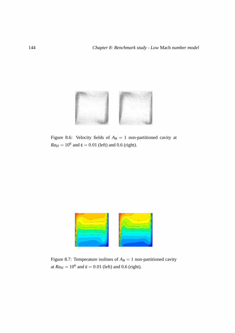
144 Chapter 8: Benchmark study - Low Mach number model
Figure 8.6: Velocity fields of AR = 1 non-partitioned cavity at
RaH = 106 and ε = 0.01 (left) and 0.6 (right).
Figure 8.7: Temperature isolines of AR = 1 non-partitioned cavity
at RaH = 106 and ε = 0.01 (left) and 0.6 (right).

Chapter 8: Benchmark study - Low Mach number model 145
−0.5 −0.25 0 0.25 0.5Dimensionless height (Y= y/H)
0
5
10
15
20
Loc
al N
usse
lt nu
mbe
r (N
u Y)
Surface 1Surface 2Boussinesq
−0.5 0 0.50
10
20
Figure 8.8: Nuy distributions along the ’Surfaces 1 and 2’ of AR = 1
non-partitioned cavity at RaH = 106 and ε = 0.01 (Actual values in
the insert and overlapped values in the main graph).
are from 1600 micro-elements mesh (∆Nu1 = 1.17% at ε = 0.6, for example).
In figures 8.8 and 8.9, the asymmetry is also observed by the distribution of the lo-
cal Nusselt number. In figure 8.8, the distributions are found exactly same to those of
the incompressible-Boussinesq fluid flow model and the distributions of both surfaces are
identical but not in figure 8.9. Note that the values are from 6400 micro-elements mesh.
8.4.2 Partitioned cavity
Similar to the non-partitioned cavity, the asymmetry increases with increasing ε. Nev-
ertheless, an impact of the increasing ε is relatively small because the magnitude of the con-
vective heat transfer of the partitioned cavity, such as the Nusselt number, is also smaller
than the non-partitioned cavity.

146 Chapter 8: Benchmark study - Low Mach number model
−0.5 −0.25 0 0.25 0.5Dimensionless height (Y= y/H)
0
5
10
15
20
Loc
al N
usse
lt nu
mbe
r (N
u Y)
Surface 1Surface 2Boussinesq
−0.5 0 0.50
10
20
Figure 8.9: Nuy distributions along the ’Surfaces 1 and 2’ of AR = 1
non-partitioned cavity at RaH = 106 and ε = 0.6 (Actual values in
the insert and overlapped values in the main graph).

Chapter 8: Benchmark study - Low Mach number model 147
Figure 8.10: Streamlines of AR = 1 and γ = 0.1 partitioned cavity
at RaH = 106 and ε = 0.01 (top) and 0.6 (bottom) (σ = 1, 100 and
105, left to right).
Figure 8.11: Velocity fields of AR = 1 and γ = 0.1 partitioned cavity
at RaH = 106 and ε = 0.01 (top) and 0.6 (bottom) (σ = 1, 100 and
105, left to right).

148 Chapter 8: Benchmark study - Low Mach number model
Figure 8.12: Temperature isolines of AR = 1 and γ = 0.1 partitioned
cavity at RaH = 106 and ε = 0.01 (top) and 0.6 (bottom) (σ = 1, 100
and 105, left to right).
Figures 8.10, 8.11 and 8.12 show the streamlines, the velocity fields and the temper-
ature isolines of AR = 1 and γ = 0.1 partitioned cavity at various ε and σ. The cores of
the flow in both fluid cells are shifted toward to right-bottom of the cells and asymmetry
increases at ε = 0.6 while the flow is symmetric at ε = 0.01. This feature can also be ob-
served at different σ cases. Note that the streamlines and the temperature isolines are from
8000 micro-elements mesh (∆Nu1 = 0.16% at ε = 0.6, for example) and the velocity fields
are from 2400 micro-elements mesh (∆Nu1 = 0.56% at ε = 0.6, for example).
Figure 8.13 represents Nuy distribution along the ’Surface 2’ of AR = 1 and γ = 0.1
partitioned cavity at σ = 1 and 105 and shows the asymmetric behavior of higher ε. Also
represents that the shape of the boundary layer change as σ increases. This feature is same
for both ε cases.
Figures 8.14 and table 8.4 show the behavior of Nu1 with increasing σ. At higher ε,
same to the incompressible-Boussinesq fluid flow model, a peak is found and decreases to

Chapter 8: Benchmark study - Low Mach number model 149
−0.5 −0.25 0 0.25 0.5Dimensionless height (Y=y/H)
0.0
2.0
4.0
6.0
8.0L
ocal
Nus
selt
num
ber
(Nu Y
)
σ = 1σ = 10
5
−0.5 0 0.50.0
4.0
8.0
BoussinesqLow Mach
Figure 8.13: Nuy distribution along the ’Surface 2’ of AR = 1 and
γ = 0.1 partitioned cavity at RaH = 106 (ε = 0.6 in the main and
ε = 0.01 in the insert graph).
Table 8.4: Nu1 of AR = 1 and γ = 0.1 partitioned cavity at RaH =
106.
σ1 5 10 20 30 50 102 103 104 105
ε = 0.01
Nu1 2.7848 3.4802 3.5743 3.5879 3.5743 3.5480 3.5122 3.4598 3.4531 3.4524
ε = 0.6
Nu1 2.8083 3.5102 3.6071 3.6232 3.6108 3.5855 3.5507 3.4996 3.4930 3.4923
Incompressible-Boussinesq
Nu1 2.7821 3.4758 3.5694 3.5828 3.5692 3.5429 3.5071 3.4549 3.4483 3.4476

150 Chapter 8: Benchmark study - Low Mach number model
100
101
102
103
104
105
Conductivity ratio (σ)
2.5
3.0
3.5
4.0
Ave
rage
Nus
selt
num
ber
(Nu)
ε=0.01ε=0.6Boussinesq
Figure 8.14: Nu1 of AR = 1 and γ = 0.1 partitioned cavity at RaH =
106.

Chapter 8: Benchmark study - Low Mach number model 151
−0.5 0.25 0 0.25 0.5Dimensionless Height (Y=y/H)
−0.2
−0.1
0
0.1
0.2
0.3
0.4
Dim
ensi
onle
ss T
empe
ratu
re (
θ)ε = 0.01ε = 0.6 σ=1
Boussinesq
σ=105
Figure 8.15: θ distributions along the ’Surface 2’ of AR = 1 and
γ = 0.1 partitioned cavity at RaH = 106.
the constant value of Nu1. These feature is also found in higher ε case. It should be noted
that the value of Nu1 at ε = 0.6 is generally higher than lower case through the entire range
of σ.
Due to the asymmetry at higher ε case, the temperature distributions along the ’Sur-
face 2’ are generally lower than those of lower ε case. As shown in figure 8.15, when the
partition wall is isothermal (σ = 105) the temperature is found lower than T0 (which corre-
sponds to 0 of θ) due to the asymmetric behavior at the large temperature difference case
(e.g. ε = 0.6).

Chapter 9
Heat transfer function
According to Nishimura et al,. [51], the temperature distribution along the partition wall
can be expressed as a linear temperature function as
θ(Y ) = CY +B (9.1)
where θ(Y ) is the dimensionless temperature as a function of height (Y ) and C and B are
the constants1. They estimated the value of C and B as ∆θ/2H and ∆θ/4, respectively. The
main assumption in their study is that the wall parameter (ω) is negligible (ω = 1.5×10⁻⁵),
thus, the partition wall is isothermal, and the thermal resistance effect was neglected.
In this thesis however the partitin wall has ’finite’ thickness (γ > 0.1) and conductiviy
(1≥ σ≥ 105), then the value of ω can be increased to 1 or higher and the thermal resistance
effect also become an important parameter. For this reason, the value of C and B are
estimated as a function of the partition wall thermal resistance, thus, the wall parameter
(ω).
The main idea of estimating the value C and B is : first, the temperature distributions along
the ’Surface 3’ (see Fig. 9.1) at different σ cases are estimated from the resolutions of the
partitioned cavity by linear fit (θ(Y ) = CY + B). Second, the values of C and B from the
linear fit (θ(Y )) are fitted as a function of a lumped-parameter ω. Finally, the function is
used as a boundary condition of the ’Half cavity’, the cold cell for example, and verified
with CAST3M simulation. It is expected that the coupling between the lumped-parameter
model and CFD can be accomplished by using the heat transfer function (θ(Y )), which is
1In dimensional form, T (y) can be used
152

Chapter 9: Heat transfer function 153
U=0,θ =θ +h 0
12
D2
U=0,
(θ )W
U=0,
U=0,
D2
U=0,θ =θ −c 0
12
U=0,θ =θ 0at t*=0
U=0,
U=0,∂Y
∂Y ∂Y
∂Y
U=0,θ =θ 0at t*=0
U=0,
2 3 41
(θ )(θ )Hot Cell Cold Cell
H C
Surface 1D
θ =θ −c 012
Solid partition
W
∂θ = 0
∂θ = 0 ∂θ = 0
∂θ = 0
Cold Cell
hθ =θ (Y)
3 4
X
Y
X
Y
L
g
H
Figure 9.1: Schematic diagram of 2-D partitioned cavity and ’Half
cavity’ with the dimensionless parameters.
based on the lumped-parameter ω. It is noted that the constant value of γ as 0.1 is used to
retain the thermal resistance effect of the partition wall and RaH of 106 and 107 are used.
9.1 Partition wall surface temperature fit
As shown in figure 9.2, the linear temperature function is fitted from the resolutions of
the partitioned cavity case with incompressible-Boussinesq fluid flow model. The function
is based upon the temperature distributions along the ’Surface 3’ for each case of σ. Nev-
ertheless, it is true that the temperature distribution along the partition wall is not exactly
linear, for this reason the linear temperature function is fitted from Y = −0.25 to 0.25 then
extended to the entire height of the partition wall. The discrepancy between the linear tem-
perature fit and the actual temperature distribution decreases with increasing σ.
Table 9.1 shows the values of C and B for different σ and RaH . The values become very
small and converge into zero as σ is increased. It should be noted that due to the symmetric
behavior of the incompressible-Boussinesq fluid flow model, equation (9.1) becomes
θ(Y ) = CY ±B. (9.2)

154
Cha
pter
9:H
eatt
rans
fer
func
tion
Table 9.1: B and C of AR = 1 and γ = 0.1 partitioned cavity.
σ1 5 10 20 30 50 102 103 104 105
RaH = 106
ω 3.16 0.63 0.32 0.16 0.11 6.32×10⁻² 3.16×10⁻² 3.16×10⁻³ 3.16×10⁻⁴ 3.16×10⁻⁵
C 0.32 0.4 0.39 0.32 0.28 0.21 0.13 1.7×10⁻² 1.7×10⁻³ 1.7×10⁻⁴
B 0.15 0.04 0.02 0.01 7.1×10⁻³ 4.1×10⁻³ 1.99×10⁻³ 1.87×10⁻⁴ 1.87×10⁻⁵ 1.87×10⁻⁶
RaH = 107
ω 5.62 1.12 0.56 0.28 0.19 0.11 5.62×10⁻² 5.62×10⁻³ 5.62×10⁻⁴ 5.62×10⁻⁵
C 0.25 0.38 0.4 0.38 0.34 0.29 0.2 0.03 3.19×10⁻³ 3.21×10⁻⁴
B 0.21 0.7 0.04 0.02 0.01 7.6×10⁻³ 3.64×10⁻³ 3.31×10⁻⁴ 3.25×10⁻⁵ 3.25×10⁻⁶
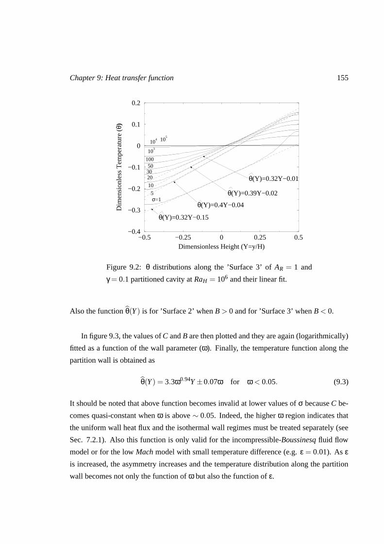
Chapter 9: Heat transfer function 155
−0.5 −0.25 0 0.25 0.5Dimensionless Height (Y=y/H)
−0.4
−0.3
−0.2
−0.1
0
0.1
0.2
Dim
ensi
onle
ss T
empe
ratu
re (
θ)
σ=15
10
203050
100
103
104 10
5
θ(Y)=0.32Y−0.15
θ(Y)=0.39Y−0.02
θ(Y)=0.4Y−0.04
θ(Y)=0.32Y−0.01
Figure 9.2: θ distributions along the ’Surface 3’ of AR = 1 and
γ = 0.1 partitioned cavity at RaH = 106 and their linear fit.
Also the function θ(Y ) is for ’Surface 2’ when B > 0 and for ’Surface 3’ when B < 0.
In figure 9.3, the values of C and B are then plotted and they are again (logarithmically)
fitted as a function of the wall parameter (ω). Finally, the temperature function along the
partition wall is obtained as
θ(Y ) = 3.3ω0.94Y ±0.07ω for ω < 0.05. (9.3)
It should be noted that above function becomes invalid at lower values of σ because C be-
comes quasi-constant when ω is above ∼ 0.05. Indeed, the higher ω region indicates that
the uniform wall heat flux and the isothermal wall regimes must be treated separately (see
Sec. 7.2.1). Also this function is only valid for the incompressible-Boussinesq fluid flow
model or for the low Mach model with small temperature difference (e.g. ε = 0.01). As εis increased, the asymmetry increases and the temperature distribution along the partition
wall becomes not only the function of ω but also the function of ε.

156 Chapter 9: Heat transfer function
10−5
10−4
10−3
10−2
10−1
100
101
ω (=γσ−1AR
−1RaH
1/4)
10−6
10−5
10−4
10−3
10−2
10−1
100
C o
r B
RaH=107
RaH=106
C=3.3ω0.94
B = 0.07ω
Figure 9.3: C and B of AR = 1 and γ = 0.1 partitioned cavity and
their linear fit.
−0.5 −0.25 0 0.25 0.5Dimensionless height (Y=y/H)
−0.15
−0.05
0.05
0.15
Dim
ensi
onle
ss te
mpe
ratu
re (
θ)
σ=50
10010
3
104
105
θ(Y)=3.3ω0.94Y−0.07ω
Figure 9.4: Comparison of θ distributions along the ’Surface 3’ of
AR = 1 and γ = 0.1 partitioned cavity at RaH = 106 and linear fit.
Chapter 9: Heat transfer function 157
Equation (9.3) is now validated by plotting together with the temperature distributions
of the numerical resolutions. As shown in figure 9.4, the equation (9.3) is valid when σ is
higher than 50.
The values of ω for the inner containment materials are : ∼ 3.2× 10⁻³ and ∼ 0.63 for
stainless steel 304 (∼ 17W/mK) and reinforced concrete (∼ 1W/mK), respectively. These
values are corresponding to σ as 103 and 50 at RaH = 106 of γ = 0.1 partitioned cavity.
9.2 Applications - ’Half cavity’
The ’Half cavity’ case is studied in order to validate the heat transfer function. As
shown in figure 9.1, the ’Half cavity’ - cold fluid cell for example - has the boundary con-
dition of θ(Y ) at the ’Surface 3’. The aspect ratio of the ’Half cavity’ (ARγ) is equal to 2.22
from equation (6.18) since γ = 0.1.
As mentioned earlier in chapter 6, when the partition wall is isothermal, the Rayleigh num-
ber for the ’Half cavity’ (RaHγ) is equal to RaH/2 of partitioned cavity since the temperature
difference between hot and cold wall of the ’Half cavity’ (∆Tγ) is equal to ∆T/2 of parti-
tioned cavity. As σ is decreased, the partition wall becomes non-isothermal and RaHγ is
not anymore equal to RaH/2. Hence, in the cases of σ = 103 and 50, it is assumed that the
temperature difference for the ’Half cavity’ (∆Tγ) is between the temperature at mid-plane
(y = H/2) of the ’Surface 3’ and the cold wall (Tc) :
∆Tγ = T (H/2)−Tc
=∆T2
(CH −2B+1).(9.4)
Note that in dimensionless form, equation (9.4) becomes
∆θγ = CH −2B+1 (9.5)
where θγ is the dimensionless temperature for the ’Half cavity’ and the definition is (T −T0)/(∆T/2). Equation (9.4) and (9.5) are for the ’Half cavity’ of cold fluid cell. For
the ’Half cavity’ of hot fluid cell, they becomes ∆Tγ = (∆T/2)(CH + 2B− 1) and ∆θγ =
CH +2B−1. Finally, RaHγ are obtained and are shown in table 9.2.

158 Chapter 9: Heat transfer function
Table 9.2: Comparison of Nu between partitioned cavity and the
’Half cavity’
σ = 50 σ = 103
Partitioned cavity
RaH 106 106
Nu 3.5429 3.4549
Cold cell with θh = θ(Y )
RaHγ 4.98×10⁵ 4.99×10⁵
Nu 3.5055 3.4493
The simulation is based on the incompressible-Boussinesq fluid flow model. The gov-
erning equations are identical to those of the non-partitioned cavity case as shown in equa-
tion (5.26a), (5.26b) and (5.26c). Also the initial conditions are same to (5.28). The bound-
ary conditions at ’Surface 3’ is
θ f = 3.3ω0.94Y −0.07ω on X = − 12ARγ
at t∗ ≥ 0. (9.6)
The mesh of the ’Half cavity’ has 3200 micro-elements, which has the accuracy of ∆Nu =
0.47% at RaH = 5×10⁵ (see Sec. 6.2.3). Also SUPG finite element method with implicit
time discretization is applied.
As a result, Nu between partitioned cavity and ’Half cavity’ are in good agreement over
the range of σ considered (see Tab. 9.2).
Figure 9.5 shows the streamlines, velocity field and temperature isolines of AR = 2.22
’Half cavity’. The features are found similar to the partitioned cavity case at lower σ such
as in figures 7.19, 7.20 and 7.21. Especially, the non-constant temperature behaviors are
found near the ’Surface 3’.
This feature is clearer in figure 9.6. The isolines of the ’Half cavity’ simulations match
exactly to those of the partitioned cavity case. In the main graph of the figure, the temper-
ature isolines near the partition wall represent the non-isothermal behavior of the partition
wall in both partitioned cavity and the ’Half cavity’ simulation. Also at σ = 103, it is clear

Chapter 9: Heat transfer function 159
Figure 9.5: Streamlines, velocity field and temperature isolines of
AR = 2.22 ’Half cavity’ corresponding to σ = 50 at RaH = 106 (left
to right).
−0.5 0.0 0.5−0.5
0
0.5
−0.5 −0.25 0.0 0.25 0.5Dimensionless length (X = x/H)
−0.5
−0.25
0
0.25
0.5
Dim
ensi
onle
ss te
mpe
ratu
re (
θ)
Partitioned cavityCold cell
Partition wall
Y=0.45
0.25
0.0
−0.25
−0.45
Figure 9.6: Comparison of the temperature isolines (σ = 50 for
main and 103 for insert).

160 Chapter 9: Heat transfer function
that partition wall is isothermal.
As a conclusion, it is possible to say that the heat transfer function for the incompressible-
Boussinesq fluid flow model is valid for the range of ω < 0.05, for this reason the further
study is needed for the range of ω > 0.05 and for the high ε cases.

Chapter 10
Conclusion
In this part, the study is presented on the heat transfer characteristics in the two-dimensional
partitioned cavity natural convection at the steady-state. The laminar flow is considered
and the time dependent Navier-Stokes equations are used. First of all, the fluid is con-
sidered through the incompressible fluid model under Boussinesq approximation. The
governing equations are discretized spatially by the finite element method with Streamline-
Upwind/Petrov-Galerkin formulation, which is stable in high velocity magnitude diffusion-
convection problems. For the time discretization, the implicit scheme is used in order to
reach the steady-state. In this study, the steady-state is defined by the maximum tempera-
ture residual norm difference between two iterations (Rθ).
The mesh is designed by using macro-Q1 and P1-NC elements to establish the shape func-
tions for velocity and temperature and pressure. Also the grid size convergence study is
proceeded by the second-order Richardson extrapolation method, which allows obtaining
the very high accurate resolutions and so-called Exact values.
The main parameters of the partitioned cavity are : the Rayleigh number (104 ≤ RaH ≤107), the thermal conductivity ratio of the partition wall to the fluid (1 ≤ σ ≤ 105), the
dimensionless partition wall thickness (0.01 ≤ γ ≤ 0.2) and the aspect ratio of the cavity
(AR = 1).
The Nusselt number is used to characterize the heat transfer. In this study the multi-layer
conductive heat transfer is considered to define the Nusselt number.
In order to valid and qualify the numerical resolutions, first, non-partitioned cavity case
161

162 Chapter 10: Conclusion
is simulated. The review is presented on the general heat transfer characteristics. The fea-
tures of the streamlines, temperature isolines and velocity fields are studied. As a result,
the resolutions are in very good agreement with the literature and it is concluded that the
computation is validated.
Second, the ’Half-cavity’ corresponding to the partitioned cavity is studied since a parti-
tioned cavity of AR can be treated as two separate AR/2 cavities when the partition wall is
isothermal (σ = 105 in this study). The comparison is proceeded between the partitioned
cavity and corresponding ’Half-cavity’, and found exact match.
For the partitioned cavity, it is found that the thermal resistance effect of the partition
wall becomes more important when the wall parameter (ω = γσ−1A−1R Ra1/4
H ) is increased.
As a consequence, as ω is increased, the heat flux becomes uniform since the partition wall
is not isothermal anymore.
In order to precise the effect of ω, the effect of γ and σ are studied separately. First, the
main characteristics of the effect of γ are:
• Convective heat transfer rate decreases with increasing γ, thus,
γ ↑∼ AConvection ↓∼ QConvection ↓∼ QConduction ↑∼ Nu ↓ .
• Nu decreases more steeply in the case of lower σ case.
• If γ < 0.01, the partition wall becomes horizontally isothermal. Thus, the temperature
difference between both sides of the partition wall is very small (<2% of total).
Second, the main characteristics of the effect of σ are:
• σ is the most important parameter for ω.
• With increasing σ, Nu first increases until the maximum and decreases to the constant
value. The reason of peak Nu is explained by each region. It should be also noted that
the convection heat flux q′′Convection is the function of ∆Tw,Horizontal and ∆Tf ,Vertical .
Thermal resistance region (σ ↑∼ Nu ↑)
As σ increased, ∂Tw/∂x decreases since the total heat transfer rate through en-
tire domain is constant. Then increasing ∆Tw,Horizontal causes an increase in

Chapter 10: Conclusion 163
∆Tf ,Horizontal . Increasing ∆Tf ,Horizontal also leads to an increase in q′′Convection of
the fluid cells : Nu increases. Nu increases until ∂Tw/∂x becomes negligible.
Thermal transition region (σ ↑∼ Nu ↓)
Since ∂Tw/∂x ≈ 0, q′′Convection is only dominated by ∂Tw/∂y and ∆Tf ,Vertical .
When σ increases, ∂Tw/∂y decreases and causes a decrease in ∆Tf ,Vertical . Con-
sequently, Nu decreases since q′′Convection is also a function of ∆Tf ,Vertical . Nu
decreases until ∂Tw/∂y becomes negligible.
Isothermal partition wall region (σ ↑∼ constant Nu)
The effect of σ is negligible since the partition wall is isothermal, thus, ∂Tw/∂x≈0 and ∂Tw/∂y ≈ 0. Then, Nu becomes independent on σ.
In order to valid the incompressible-Boussinesq fluid flow model, the asymptotic low
Mach model is also studied on the partitioned cavity. The non-partitioned and the parti-
tioned cavities are considered under the same conditions of the incompressible-Boussinesq
fluid flow model case. The resolutions are benchmarked and the very high accurate numer-
ical resolutions are obtained for small and large temperature differences (ε = 0.01 and 0.6).
At lower ε case, the heat transfer characteristics are similar to those of the incompressible-
Boussinesq fluid flow model. The asymmetry increases at higher ε case since the buoyancy
effect becomes more significant than for small temperature difference case. Hence, the
fluid core is shifted toward to right-bottom of the cavity. These features are also found
in the partitioned cavity case. It is found that the behavior of Nu versus σ retains also in
the case of the large temperature difference case. Particularly, due to this asymmetry, the
temperature of the partition wall is found lower than mean temperature (∆T/2) at higher σand higher ε.
Finally, the heat transfer function is suggested and achieved the coupling between the
lumped-parameter model and CFD. The value of ω is given as a lumped-parameter and
allows obtaining the CFD results without performing the multi-dimensional simulation for
entire system.
The function is based on the temperature distribution along the partition wall. The tem-
perature distributions are fitted as a linear function of the height (Y ) and then plotted as
a function of the wall parameter (ω). The heat transfer function for the incompressible-

164 Chapter 10: Conclusion
Boussinesq fluid flow is suggested as
θ(Y ) = 3.3ω0.94Y ±0.07ω for ω < 0.05.
Above function is validated by the ’Half cavity’ case study by using the heat transfer func-
tion as a boundary condition and the function is found to be valid. When ω increases higher
than 0.05, the thermal resistance effect also increases and it is found that the heat transfer
function becomes non-linear to ω.
Due to the asymmetry arises with increasing ε, above function is only valid in the case of
small temperature difference case (i.e. ε = 0.01).

Part III
Conclusions and prospects
165


167
According to the scenario of the PWR severe accident such as the hydrogen risk of
LOCA, the main factors that determine the risk are the temperature, the pressure of the in-
ner containment and the gas species such as air, steam and hydrogen concentrations. These
three factors are significantly affected by the condensation of the released steam on the in-
struments surface and the containment inner walls. For this reason the deep knowledge of
those factors is the most important issue in the hydrogen risk analysis, but the complexity
of the reactor containment system and the costliness militate against the analysis - not only
the experiment but also the numerical approaches.
In this thesis an alternative analysis is suggested, the coupling between the lumped-parameter
model (0D) and the computational fluid dynamics (CFD, multi-D). Thus, the complex ge-
ometry and problem of the hydrogen risk in a reactor containment are reduced to a cavity
with a fully and centered partition, so-called the partitioned cavity. In the partitioned cav-
ity, one fluid cell is separated by the partition wall from another and assumed as a large
volume of the inner reactor containment and the another fluid cell is assumed as a vacant
room. The partitioned cavity is then analyzed by the CFD in 2D and derived a temper-
ature function along the partition wall - so called ’Heat transfer function’. This function
may allow coupling between two different numerical methods - lumped-parameter model
and CFD. In other word, by using the temperature function with a boundary condition of
the non-partitioned cavity, namely the ’Half cavity’, requires less computational cost than
partitioned cavity, in which can estimate the heat transfer characteristics identical to the
partitioned cavity.
In the first part of this thesis, the brief review is presented on the wall condensation
models. Two condensation models used in the code CAST3M/TONUS are studied ; the
Uchida model based on experiments, and the Chilton-Colburn model based on the analogy
between heat and mass transfer. The models are examined by the steady-state calcula-
tion and the lumped-parameter code TONUS-0D. The reference study is performed on the
’MICOCO benchmark’ case, an air-steam steady-state simulation test case of the MIS-
TRA. The steady-state calculation is based on mass and energy conservations between the
injected steam and its condensation and coded by the GIBIANE computer language. Also
the CAST3M steam table library is used. For TONUS-0D simulation, an axisymmetric
mono-compartment node is used. The steady-state is reached after 4000s.

168
A benchmark study is conducted by comparing the internal gas temperature (Tg) and the
pressure (P) in both methods and condensation models. As a result, for example, the tem-
perature from the Chilton-Colburn model is found higher than the Uchida model. Contrary
to the temperature, the pressure from the Uchida model is found higher than from the
Chilton-Colburn model. Comparison of these results is used as often for the benchmark
studies in the literature. It is found that the Uchida model under-estimates the temperature
and over-predicts the pressure.
In the second part of the thesis, at a first step of the coupling between the lumped-
parameter model and the CFD, a study is presented on the natural convection heat transfer
(without condensation) in the partitioned cavity. Two-dimensional heat transfer is assessed
by the code CAST3M. The fluid flow model is assumed as an incompressible laminar flow
under the Boussinesq approximation of the Newtonian fluid. Also the asymptotic low Mach
model is used to handle the large temperature different case and to overcome the limit of the
incompressible-Boussinesq fluid flow model. The resolutions are compared for the bench-
mark.
Air (Pr = 0.71) is used as the working fluid. In order to apply as a numerical study,
the time dependence Navier-Stokes equations are spatially discretized into the Stream-
Upwind/Petrov-Galerkin finite element formulations, which are found to be stable in the
high velocity convection problems. Also the implicit scheme is applied to solve time de-
pendent governing equations. The macro-Q1 and P1-NC elements are used to establish
the shape functions for velocity and temperature and pressure. The mesh is based on the
non-uniform grid size mesh and designed by using the refinement method. The maxi-
mum temperature residual norm (Rθ) is used as a reference of the steady-state. The grid
size independent Exact values are derived from the resolutions by using the second-order
Richardson extrapolation method.
First of all, as a reference of the partitioned cavity, the very well reported non-partitioned
cavity is studied in order to valid the computations. In the case of the non-partitioned case,
the heat transfer characteristics are mainly dominated by the aspect ratio of the cavity (AR)
and the (cavity height based) Rayleigh number (RaH). The range of the parameters is :
1 ≥ AR ≥ 2 and 103 ≤ RaH ≤ 107. The results are compared with the literature by the aver-
age Nusselt number (Nu) to characterize the heat transfer, and are in very good agreement.

169
According to the broad investigation of the literature, it is found that the heat transfer char-
acteristics in the partitioned cavity are mainly dominated by the aspect ratio of the cavity
(AR), the Rayleigh number (RaH), the thermal conductivity ratio of the partition wall to the
fluid (σ = kw/k f ) and the dimensionless partition wall thickness (γ = W/L). The range
of the parameters is : AR = 1, 104 ≤ RaH ≤ 107, 1 ≤ σ ≤ 105 and 0.01 ≤ γ ≤ 0.2, but if
the conductivity ratio is ’infinite’ (σ = 105), a partitioned cavity can be considered as two
separated cavities (’Half cavity’) with constant temperature boundary conditions. For this
reason, the ’Half cavity’ is also simulated as a reference of the partitioned cavity and it is
concluded that the resolutions of the partitioned cavity simulations are verified.
In the framework of the partitioned cavity heat transfer behavior, the thermal resistance
effect is found to be characterized by the wall parameter (ω = γσ−1A−1R Ra1/4
H ), and plays
an important role on the boundary layer thickness along the partition wall. Thus, if ω in-
creases to order of 1 or more, the boundary layer shape becomes uniform and the thermal
resistance effect of the partition wall cannot be neglected. Nevertheless, it is found that
the wall parameter is not sufficient in order to assess the heat transfer characteristics in the
partitioned cavity, thus, Nu shows a peak while σ increases from 1.
To overcome this, the effect of γ and σ are considered separately. It is found that Nu gen-
erally decreases with increasing γ since the convective area decreases. Also, if γ < 0.01,
the partition wall becomes horizontally isothermal and the temperature difference between
both sides of the partition wall can be neglected.
When σ increases from 1 to 105, Nu also increases then reaches to the maximum and even-
tually decreases to the constant value. The reason is explained by separating the regions :
the thermal resistance region, the thermal transition region and the isothermal partition wall
region. In the thermal resistance region, the partition wall becomes horizontally isothermal
and increases the convective heat flux : Nu increases. In the thermal transition region,
the partition wall is already isothermal in the horizontal direction, then becomes vertically
isothermal and decreases the convective heat flux : Nu decreases. Finally, when the parti-
tion wall is isothermal in both vertical and horizontal directions, the convective heat flux is
independent to σ : Nu is constant.
Finally, a heat transfer function is suggested in order to couple lumped-parameter model
and CFD. The function is based on the numerical resolutions from the partitioned cavity

170
simulation. Thus, the temperature distributions along the partition wall surfaces are fitted
as a linear function of height (θ = CY ±B). Then the constants C and B are found as a
function of the lumped-parameter (ω).
The function is then validated by the ’Half cavity’ simulation by using the function as a
boundary condition of the ’Half cavity’. The aspect ratio of the ’Half cavity’ is equal to
2.22, which corresponds to γ = 0.1 partitioned cavity. From the comparison of the results,
the function is found to be valid.
When ω increases higher than 0.05, the heat transfer function becomes invalid due to the
significance of the partition wall thermal resistance effect. Furthermore, the function is
suggested only for the incompressible-Boussinesq fluid flow model. Because, it is found
that for the low Mach model - especially at higher ε -, the temperature distribution along
the partition wall becomes not only the function of ω but also the function of ε.
Bibliography
[1] CAST3M (http://www-cast3m.cea.fr). Website, 2004.
[2] J. Abedi and S. Aliabadi. Simulation of incompressible flows with heat and mass
transfer using parallel finite element method. In Proc. 5th Mississippi State Confer-
ence on Differential Equations and Computational Simulations, Electronic Journal of
Differential Equations, Oct. 10 2003.
[3] S. Acharya and C. H. Tsang. Natural convection in a fully partitioned inclined enclo-
sure. Numerical Heat Transfer, 8:407–428, 1985.
[4] R. Anderson and A. Bejan. Natural convection on both sides of a vertical wall sepa-
rating fluids at different temperatures. J. Heat Transfer, 102:630–635, 1980.
[5] R. Anderson and A. Bejan. Heat transfer through single and double vertical walls
in natural convection: Theory and experiment. Int. J. Heat Mass Transfer, 24:1611–
1620, 1981.
[6] G. G. L. Beau and T. E. Tezduyar. Finite element computation of compressible flows
with the SUPG formulation. Advances in Finite Element Analysis in Fluid Dynamics,
ASME, 123:21–27, 1991.
[7] A. Bejan. Note on Gill’s solution for free convection in a vertical enclosure. J. Fluid
Mechanics, 90:561–568, 1979.
[8] A. Bejan. Convection Heat Transfer. John Wiley & Sons, second edition, 1993.
[9] M. Bercovier and O. Pironneau. Error estimates for finite element method solution of
the Stokes problem in the primitive variables. Numerische Mathematik, 33:211–224,
1979.
171

172 Bibliography
[10] L. Blumenfeld, H. Paillère, Y. Choi, and E. Studer. CFD-calculation of mixed con-
vection and condensation in a reactor containment/ the MICOCO benchmark. In 10th
Int. Meeting on Nuclear Reactor Thermal-Hydraulics (NURETH-10), Seoul, Korea,
Oct. 5–9 2003.
[11] L. Blumenfeld, E. Studer, Y. J. Choi, J. P. Magnaud, and H. Paillère. CFD simulation
of containment thermal-hydraulic flows. QNET-CFD Network Newsletter, 1(3):8–12,
2002.
[12] J. M. Boland and R. A. Nicolaides. Stability of finite elements under divergence
constraints. J. Numerical Analysis, 20(4):722–731, 1983.
[13] F. Brezzi and J. Pitkäranta. On the stabilization of finite element approximations of
the Stokes equations. In W. Hackbusch, editor, Efficient Solutions of Elliptic Systems,
Proceedings of a GAMM-Seminar, Kiel, Jan. 27-29, 1984, pages 1–36. Friedr. Vieweg
& Sohn, 1969.
[14] A. N. Brooks and T. J. R. Hughes. Streamline Upwind/Petrov-Galerkin formula-
tions for convection dominated flows with particular emphasis on the incompressible
Navier-Stokes equations. Computer Methods in Applied Mechanics and Engineering,
32:199–259, 1982.
[15] D. R. Chenoweth and S. Paolucci. Natural convection in an enclosed vertical air
layer with large horizontal temperature differences. J. Fluid Mechanics, 169:173–
210, 1986.
[16] Y. J. Choi. Multi-dimensional simulation of air/steam tests of mistra facility using
castem code. Thesis of dea, Université de Marne-la-Vallée, Marne-la-Vallée, France,
Jun. 2002.
[17] J. G. Collier. Convective Boiling and Condensation. McGraw-Hill, second edition,
1981.
[18] J. G. Collier. Heat transfer in condensation. In Two-Phase Flow and Heat Transfer in
the Power and Process Industries, pages 330–365. Hemisphere Publishing Co., 1981.
Bibliography 173
[19] D. M. Cuckovic-Dzodzo, M. B. Dzodzo, and M. D. Pavlovic. Laminar natural con-
vection in a fully partitioned enclosure containing fluid with nonlinear thermophysical
properties. Int. J. Heat and Fluid Flow, 20:614–623, 1999.
[20] F. Dabbene. Logiciel TONUS, partie multicompartments : Modélisation physique
de la version 2.0. Internal report of DMT SEMT/LTMF/RT/98-011/B, CEA, Saclay,
France, 1998.
[21] F. Dabbene. Tutorial CAST3M pour la mécanique des fluides. Internal report of
DM2S SFME/LTMF/RT/03-035/A, CEA, Saclay, France, 2003.
[22] F. Dabbene and L. Razafindrazake. Guide utilisateur associé à la version 3.1 de
TONUS 0D. Internal report of DMT SEMT/LTMF/RT/00-003/A, CEA, Saclay,
France, 2000.
[23] G. de Vahl Davis. Natural convection of air in a square cavity: A bench mark numer-
ical solution. Int. J. Numer. Meth. Fluids, 3:249–264, 1983.
[24] G. de Vahl Davis and I. P. Jones. Natural convection in a square cavity: A comparison
exercise. Int. J. Numer. Meth. Fluids, 3:227–248, 1983.
[25] R. G. Eckert. Tribute to Ludwig Prandtl. Int. J. Heat Mass Transfer, 18:1333–1336,
1975.
[26] R. W. Fox and A. T. McDonald. Introduction to Fluid Mechanics. John Wiley &
Sons, 1985.
[27] D. D. Gray and A. Giorgini. The validity of the boussinesq approximation for liquid
and gases. Int. J. Heat Mass Transfer, 19:545–551, 1976.
[28] Group of Experts. Flame acceleration and deflagration to detonation transition in
nuclear safety. State-of-the-Art Report NEA/CSNI/R(2000)7, OECD Nuclear Energy
Agency, France, Aug 2000.
[29] M. D. Gunzburger. Finite Element Methods for Viscous Incompressible Flows. Aca-
demic Press, Inc., 1989.

174 Bibliography
[30] P. Hadida. Etude du couplage des phénomènes de condensation et de conduction dans
les code 0-D. Technical report, Quasar Informatique, Paris, France, 1997.
[31] C. J. Ho and Y. L. Yih. Conjugate natural convection heat transfer in an air-filled
rectangular cavity. Int. Comm. Heat Mass Transfer, 14:91–100, 1987.
[32] M. Hortmann, M. Peric, and G. Scheuerer. Finite volume multigrid prediction of
laminar natural convection : Benchmark solutions. Int. J. for Numerical Methods in
Fluids, 11:189–207, 1990.
[33] A. Kangni, R. Ben Yedder, and E. Bilgen. Natural convection and conduction in
enclosures with multiple vertical partitions. Int. J. Heat Mass Transfer, 34:2819–
2825, 1991.
[34] A. Kangni, P. Vasseur, and E. Bilgen. Natural convection in inclined enclosures
with multiple conducting partitions. J. Thermophysics and Heat Transfer, 9:270–277,
1995.
[35] T. G. Karayiannis, M. Ciofalo, and G. Barbaro. On natural convection in a single and
two zone rectangular enclosure. Int. J. Heat Mass Transfer, 35:1645–1657, 1992.
[36] K. Kashiyama, T. Tamai, W. Inomata, and S. Yamaguchi. A parallel finite element
method for incompressible Navier-Stokes flows based on unstructured grids. Com-
puter Methods in Applied Mechanics and Engineering, 190:333–344, 2001.
[37] N. Kechkar and D. J. Silvester. Analysis of locally stabilized mixed finite element
methods for the stokes problem. Mathematics of Computation, 58(197):1–10, 1992.
[38] P. Le Quéré and T. Alziary de Roquefort. Computation of natural convection in
two-dimensional cavities with Chebyshev polynomials. J. Computational Physics,
57:210–228, 1985.
[39] C. Leduc. Modélisation de la Condensation en Film sur les Parois d’une Enceinte de
Réacteur. Phd thesis, Université Joseph Fourier - Grenoble 1, Grenoble, France, Oct.
1995.
[40] E. E. Lewis. Nuclear Power Reactor Safety. John Wiley & Sons, 1977.

Bibliography 175
[41] R. W. Lewis, K. Morgan, H. R. Thomas, and K. N. Seetharamu. The Finite Element
Method in Heat Transfer Analysis. John Wiley & Sons, 1996.
[42] J. H. Lienhard and I. Catton. Heat transfer across a two-fluid-layer region. J. Heat
Transfer, 108:198–205, 1986.
[43] C. H. Liu and D. Y. C. Leung. Development of a finite element solution for the
unsteady Navier-Stokes equations using projection method and fractional-θ-scheme.
Computer Methods in Applied Mechanics and Engineering, 190:4301–4317, 2001.
[44] G. S. H. Lock and R. S. Ko. Coupling through a wall between two free convective
systems. Int. J. Heat Mass Transfer, 16:2087–2096, 1973.
[45] J. P. Magnaud. Discrétisation des équations de Navier-Stokes par une méthode
d’éléments finis. Lecture Note, Mar. 1996.
[46] M. Mamou, M. Hasnaoui, P. Vasseur, and E. Bilgen. Natural convection heat trans-
fer in inclined enclosures with multiple conducting solid partitions. Numerical Heat
Transfer, Part A, 25:295–315, 1994.
[47] B. A. Meyer, J. W. Mitchell, and M. M. El-Wakil. The effect of thermal wall properties
on natural convection in inclined rectangular cells. J. Heat Transfer, 104C:111–117,
1982.
[48] B. Müller. Low Mach number asymptotic of the Navier-Stokes equations and numeri-
cal implications. von Karman Institute for Fluid Dynamics, 30th computational fluid
dynamics; lecture series 1999-03 edition, Mar. 1999.
[49] T. Nishimura, M. Shiraishi, and Y. Kawamura. Natural convection heat transfer in
enclosures with an off-center partition. Int. J. Heat Mass Transfer, 30:1756–1758,
1987.
[50] T. Nishimura, M. Shiraishi, F. Nagasawa, and Y. Kawamura. Natural convection heat
transfer in enclosures with multiple vertical partitions. Int. J. Heat Mass Transfer,
31:1679–1686, 1988.
176 Bibliography
[51] T. Nishimura, Y. Shiraishi, and Y. Kawamura. Analysis of natural convection heat
transfer in enclosure divided by a vertical partition plate. In B. X. Wang, editor, Heat
Transfer Science and Technology, pages 129–136. Springer-Verlag, 1987.
[52] S. Ostrach. Natural convection heat transfer in cavities and cells. In Proc. 7th Int.
Heat Transfer Conf., volume 1, München, Fed. Rep. of Germany, Sep. 6–10 1982.
[53] M. N. Özisik. Heat Transfer - A Basic Approach. John Wiley & Sons, third edition,
1989.
[54] H. Paillère and J. P. Magnaud. A finite element elliptic flow solver for low Mach
number compressible flow. In 10th Int. Conf on Finite Elements in Fluids, Tucson,
USA, Jan. 5–8 1998.
[55] H. Paillére, P. L. Quéré, C. Weisman, J. Vierendeels, E. Dick, F. Dabbene, A. Bec-
cantitni, E. Studer, T. Kloczko, C. Corre, V. Heuveline, M. Darbandi, and S. F. Hos-
seinizadeh. Modeling of natural convection flows with large temperature differences
: A benchmark problem for low Mach number solvers. part 2. contributions to the
june 2004 conference. ESAIM : Mathematical Modeling and Numerical Analysis,
39:617–621, 2005.
[56] H. Paillère, C. Viozat, A. Kumbaro, and I. Toumi. Comparison of low Mach number
models for natural convection problems. Heat and Mass Transfer, 36:567–573, 2000.
[57] R. L. Panton. Incompressible Flow. John Wiley & Sons, 1984.
[58] C. J. Park and D. W. Sheen. p1-nonconforming quadrilateral finite element meth-
ods for second-order elliptic problems. SIAM J. Numerical Analysis, 41(2):624–640,
1996.
[59] S. V. Patankar. Numerical Heat Transfer and Fluid Flow. McGraw-Hill, 1980.
[60] S. V. Patankar and D. B. Spalding. A calculation procedure for heat, mass and mo-
mentum transfer in three-dimensional parabolic flows. Int. J. Heat Mass Transfer,
15:1787–1806, 1972.
[61] J. Patterson and J. Imberger. Unsteady natural convection in a rectangular cavity. J.
Fluid Mechanics, 100:65–86, 1980.

Bibliography 177
[62] P. F. Peterson. Theoretical basis for the Uchida correlation for condensation in reactor
containment. Nuclear Engineering and Design, 162:301–306, 1996.
[63] P. L. Quéré, C. Weisman, H. Paillére, J. Vierendeels, E. Dick, R. Becker, M. Braack,
and J. Locke. Modeling of natural convection flows with large temperature differences
: A benchmark problem for low Mach number solvers. part 1. reference solutions.
ESAIM : Mathematical Modeling and Numerical Analysis, 39:609–615, 2005.
[64] K. Raznjevic. Handbook of thermodynamic tables. Begell House, second edition,
1995.
[65] Z. M. Shapiro and T. R. Moffette. Hydrogen flammability data and application to
PWR loss of coolant accident. Technical Report WAPD-SC-545, Bettis Plant, 1957.
[66] D. J. Silvester and N. Kechkar. Stabilized bilinear-constant velocity-pressure finite el-
ements for the conjugate gradient solution of the stokes problem. Computer Methods
in Applied Mechanics and Engineering, 79:71–86, 1990.
[67] R. E. Sonntag and G. J. V. Wylen. Introduction to Thermodynamics : Classical and
Statistical. John Wiley & Sons, third edition, 1991.
[68] E. M. Sparrow and C. Prakash. Interaction between internal natural convection in an
enclosure and an external natural convection boundary-layer flow. Int. J. Heat Mass
Transfer, 24:895–907, 1981.
[69] E. Studer, F. Dabbene, J. P. Magnaud, L. Blumenfeld, J. J. Quilico, and H. Paillère.
On the use of the MISTRA coupled effect test facility for the validation of contain-
ment thermal-hydraulics codes. In 10th Int. Meeting on Nuclear Reactor Thermal-
Hydraulics (NURETH-10), Seoul, Korea, Oct. 5–9 2003.
[70] T. E. Teduyar, J. Liou, and D. K. Ganjoo. Incompressible flow computations based
on the vorticity-stream function and velocity-pressure formulations. Computers &
Structures, 35(4):445–472, 1990.
[71] T. E. Tezduyar. Stabilized finite element formulations for incompressible flows com-
putations. Advances in Applied Mechanics, 28:1–44, 1992.

178 Bibliography
[72] T. E. Tezduyar and S. Sathe. Stabilization parameters in SUPG and PSPG formula-
tions. J. Computational and Applied Mechanics, 4:71–88, 2003.
[73] N. E. Todreas and M. S. Kazimi. Nuclear Systems, volume I. Thermal Hydraulics
Fundamentals. Hemisphere Publishing Corp., 1989.
[74] T. W. Tong and F. M. Gerner. Natural convection in partitioned air-filled rectangular
enclosures. Int. Comm. Heat Mass Transfer, 13:99–108, 1986.
[75] J. Vendel, P. Cornet, J. Malet, E. Porcheron, H. Paillère, M. L. Caron-Charles,
E. Studer, K. Fischer, and H. J. Allelein. ISP47 "containment thermal-hydraulics"
computer codes expercise based on TOSQAN, MISTRA and THAI experiments.
Technical report, IRSN, 2002.
[76] C. Viozat. Calcul d’écoulments stationnaires et instationnaires à petit nombre de
mach, et en maillages étir’es. Phd thesis, Université de nice-sophia antipolis, Nice,
France, Oct. 1998.
[77] R. Viskanta and D. W. Lankford. Coupling of heat transfer between two natural
convection systems by a vertical wall. Int. J. Heat Mass Transfer, 24:1171–1177,
1981.
[78] J. S. Wong, D. L. Darmofal, and J. Peraire. The solution of the compressible Euler
equations at low Mach numbers using a stabilized finite element algorithm. Computer
Methods in Applied Mechanics and Engineering, 190:5719–5737, 2001.
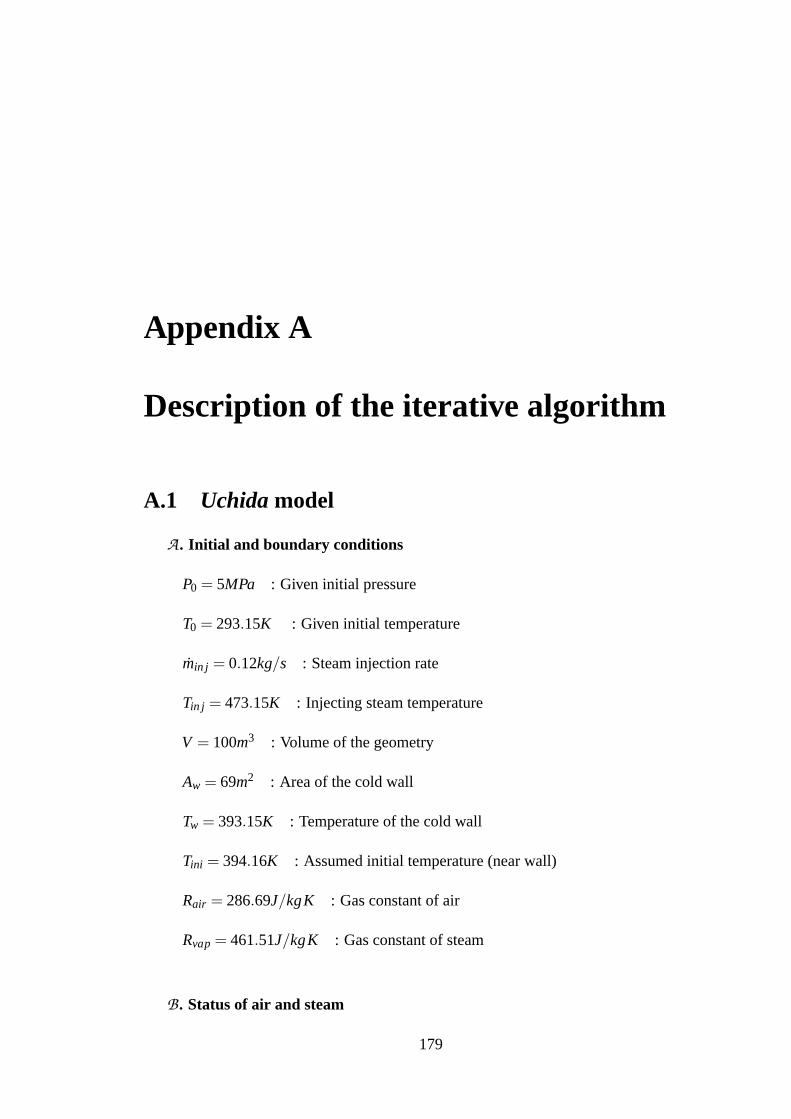
Appendix A
Description of the iterative algorithm
A.1 Uchida model
A . Initial and boundary conditions
P0 = 5MPa : Given initial pressure
T0 = 293.15K : Given initial temperature
min j = 0.12kg/s : Steam injection rate
Tin j = 473.15K : Injecting steam temperature
V = 100m3 : Volume of the geometry
Aw = 69m2 : Area of the cold wall
Tw = 393.15K : Temperature of the cold wall
Tini = 394.16K : Assumed initial temperature (near wall)
Rair = 286.69J/kgK : Gas constant of air
Rvap = 461.51J/kgK : Gas constant of steam
B . Status of air and steam
179

180 Appendix A: Description of the iterative algorithm
ρ0air = 1.1769kg/m3 : Initial air density from MISTRA pre-heating phase at STP
P0air : Initial air partial pressure from CAST3M steam table library
ρ0vap : Initial steam density from CAST3M steam table library
C . Steam partial pressure and total pressure
P0vap : Initial steam partial pressure from CAST3M steam table library
P0 = P0vap +P0air : Initial pressure
D . Heat transfer coefficient from Uchida correlation
X0 =ρ0vap
ρ0air
: Initial steam mass fraction
h0T = 11.351+(283.77X0) : Initial heat transfer coefficient
E . Internal temperature by energy balance equation
hvap : Enthalpy of steam from CAST3M steam table library
hliq : Enthalpy of condensed liquid from CAST3M steam table library
Tg = Tw +min j(hvap −hliq)
h0T Aw: Internal gas temperature
Pair =P0airTg
T0: Air partial pressure
ρair =Pair
RairTg: Air density
F . Density of steam at internal temperature
Ts : Saturation temperature from CAST3M steam table library
hT : Heat transfer coefficient from equation (2.40) or (2.41)
Appendix A: Description of the iterative algorithm 181
when Tw ≤ Ts ≤ Tw +10
hT =min j(hvap −hliq)
Aw(Tg −Tw)[βuch +(1−βuch)e−γuch(Tg−Ts)
][1− e−(Ts−Tw)2]
when Tw +10 ≤ Ts
hT =min j(hvap −hliq)
Aw(Tg −Tw)[βuch +(1−βuch)e−γuch(Tg−Ts)
]
Xvap =hT −11.351
283.77: Steam mass fraction
ρvap = Xvapρair : Steam density
G . Condition for the iteration
∆ρ =ρ0vap −ρvap
ρ0vap
: Converged when ∆ρ < 10−7
Or not
Tini = Tg : Gas temperature assumption for next iteration
P0air = Pair : Pressure assumption for next iteration
ρ0air = ρair : Air density assumption for next iteration
ρ0vap = ρvap : Steam density assumption for next iteration
Go to C .

182 Appendix A: Description of the iterative algorithm
A.2 Chilton-Colburn model
A . Initial and boundary conditions
P0 = 5MPa : Given initial pressure
T0 = 293.15K : Given initial temperature
min j = 0.12kg/s : Steam injection rate
Tin j = 473.15K : Injecting steam temperature
V = 100m3 : Volume of the geometry
Aw = 69m2 : Area of the cold wall
Tw = 393.15K : Temperature of the cold wall
Tini = 394.16K : Assumed initial temperature (near wall)
Rair = 286.69J/kgK : Gas constant of air
Rvap = 461.51J/kgK : Gas constant of steam
B . Status of air and steam
ρ0air = 1.1769kg/m3 : Initial air density from MISTRA pre-heating phase at STP
P0air : Initial air partial pressure from CAST3M steam table library
ρ0vap : Initial steam density from CAST3M steam table library
C . Steam partial pressure and total pressure
P0vap : Initial steam partial pressure from CAST3M steam table library
P0 = P0vap +P0air : Initial pressure
D . Convective heat transfer coefficient from Chilton-Colburn correlation

Appendix A: Description of the iterative algorithm 183
Ts : Saturation temperature from CAST3M steam table library
¯rho = ρ0vap +ρ0air : Density of mixture
hc = 0.13k
[g
(ρµ
)2(ρvap +ρn−c − ρρ
)] 13
: Convective heat transfer coefficient
from equation (2.53)
E . Total heat transfer coefficient from Chilton-Colburn correlation
hvap : Enthalpy of steam from CAST3M steam table library
hliq : Enthalpy of condensed liquid from CAST3M steam table library
hT = hc +hvap −hliq
Aw(Tg −Tw)min j : Total heat transfer coefficient from equation (2.57)
F . Internal temperature by energy balance equation
Tg = Tw +min j(hvap −hliq)
h0T Aw: Internal gas temperature
kc =Dvap
2/3
k(
ρµ
)1/3hc : Mass transfer coefficient from equation (2.55)
ρsat : Steam density at saturation temperature from CAST3M steam table library
Psat : Pressure at saturation temperature from CAST3M steam table library
Xvap = Psat/P0 : Steam mass fraction
ρvap =min j(1−Xvap)
kcAw+ρsat : Steam density
Pair =P0airTg
T0: Air partial pressure
ρair =Pair
RairTg: Air density

184 Appendix A: Description of the iterative algorithm
G . Condition for the iteration
∆ρ =ρ0vap −ρvap
ρ0vap
: Converged when ∆ρ < 10−7
Or not
Tini = Tg : Gas temperature assumption for next iteration
P0air = Pair : Pressure assumption for next iteration
ρ0air = ρair : Air density assumption for next iteration
ρ0vap = ρvap : Steam density assumption for next iteration
Go to C .

Appendix B
Meshes of the MICOCO benchmark
study
GIBI FECITFigure B.1: Meshes of the MICOCO benchmark study in two (left)
and three (right) dimensions.
185

Appendix C
Finite element method and numerical
discretization
C.1 Finite element method
The finite element method (FEM) is based on the variational formulation of the differ-
ential equation to treat elliptic and parabolic partial differential equations (PDE), which are
frequently no classical solution exists without appropriate hypothesis. The physical phe-
nomena such as structural deformations, heat transfer, and fluid flow can be explained with
governing equations and its boundary conditions across the solution domain. The FEM
solves those boundary values problems by using linear algebraic equations rather than PDE.
In this thesis, stabilized finite element formulation is used in order to solve buoyancy
driven flows with heat transfer. The stabilization is based on the SUPG method, which
allows solving the flow problems at high speed (i.e. high Reynolds number or Rayleigh
number) with SUPG stabilization factor τSUPG [14]. At low Rayleigh numbers for exam-
ple, the SUPG formulation is usually not necessary.
This formulation designed to prevent the potential numerical instabilities, for example,
spurious node-to-node oscillations primarily in the velocity field, for advection dominated
flows. The SUPG stabilization for incompressible flow is achieved by adding τSUPG to the
Galerkin formulation, which is the form of an integral over entire domain [71].
Precisely speaking, the standard Galerkin method was found not optimal for the convec-
186

Appendix C: Finite element method and numerical discretization 187
tion diffusion problems due to its result shows under diffused for all element Péclet number
(Pex = uhh/2αh where uh is the velocity, h is the length and αh is the thermal diffusivity.
The superscript h denotes to the element order) [41]. For SUPG method, an artificial diffu-
sion term is added to standard Galerkin model and combined with upwind scheme, which
is conditionally stable.
The implementation of the SUPG method by Brooks and Hughes [14] was based on
the Q1P0 (bi-linear velocity/constant pressure) elements and one-step time-integration of
the semi-discrete equations obtained by using such elements. According to their study, the
Navier-Stokes equations in the convection dominated problem is solved by an optimal up-
wind finite element scheme using piece-wise linear shape and test functions in conjunction
with a special quadrature. The algorithm is found simple and computationally efficient.
Nevertheless, the excessive diffusion is found in SUPG method with the Q1P0 element and
the one-step time-integration. The reason was found that the pressure function space is
too poor for the discrete formulation to benefit from the consistency property of the SUPG
stabilization [70].
For higher-order element such as Q2P1 (bi-quadratic velocity/linear pressure) and pQ2P1
(pseudo-quadratic version of Q2P1), for which pressure function space is richer, the sit-
uation improves significantly [70]. The SUPG model is successfully deployed to the un-
structured grids [36], projection method [43], etc. Also, the SUPG stabilization has been
successfully applied to not only incompressible flow but also compressible flows [6] and
low Mach number model [78].
Recently, the coupling between the SUPG method and PSPG (Pressure-Stabilizing/Petrov-
Galerkin) method is developed and improved stability and accuracy of the calculation [72,
2].
For the space and time discretization, stabilized Q1/P1-NC (stabilized bi-linear velocity/non-
conforming linear pressure) type element combination and implicit scheme are used. The
stabilized Q1 element, which is also called macro-element, has been developed by Boland
and Nicolaides [12] by using subdivided macro-elements to localize the divergence stabil-
ity condition (∇ ·~uh = 0 in a macro-element) which confirms the non-zero unique solution
is existing in Stokes problem such as incompressible flow and satisfies LBB condition.

188 Appendix C: Finite element method and numerical discretization
The Ladyzhenskaya-Babouska-Brezzi stability condition (so-called LBB condition) is the
manner of finite element stability analysis which focused on the Stokes equations and
demonstrated the need, in fluid mechanics finite element methods, for using different basis
functions for the velocity and pressure [13].
The macro-element is found to be always satisfies the divergence stability condition for
conforming finite element formulations. Combining with constant pressure (P0), Silvester
and Kechkar [66] improved locally stabilized macro-elements using spurious pressure mod-
els in the continuity equations to solve incompressible Stokes problem. The macro-Q1/P0
model was proved to be satisfied in LBB condition [37].
Even such a finite element formulation satisfies LBB condition, the discrete solution of the
velocity and pressure of the Navier-Stokes equations (~uh, ph) are not guaranteed since their
approximation behavior. For this reason, the error estimates for the discrete solution has
been developed and several combinations of velocity-pressure elements are suggested [29].
Among the combinations, the piecewise linear pressure element (P1-NC) is used in this
thesis. This element is originated from the study of Bercovier and Pironneau [9] which is
combined with Q2 velocity element with the non-conforming linear pressure shape func-
tions and found effective and stable [58].
Figure C.1 shows the schematic diagram of the macro-Q1/P1-NC element. A macro
element contains four Q1 node sub-elements (K1 to K4), also called micro-element (µ-
element) for the velocity and the temperature approximations and three pressure nodes (P1
to P3). This combination had been studied by the code CAST3M and found to be stable, fast
and precise [21]. Also considering SUPG method for the low Mach number compressible
flow, macro-element was found stable [54].
C.2 Incompressible-Boussinesq fluid flow model
C.2.1 Space discretization
The governing equations of the given problem (Eq. (5.26a), (5.26b), (5.26c) and (5.33))
for the entire domain Ω, which includes two-dimensional real (Ω ⊂ R2), is discretized by
subdividing it into element Ωe, e = 1, · · · ,nel , where nel is the number of element.
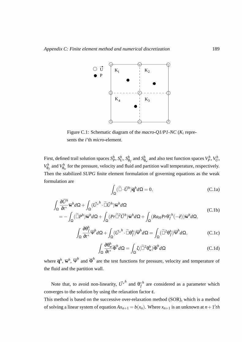
Appendix C: Finite element method and numerical discretization 189
U K1 K2
K4 K3
P
Figure C.1: Schematic diagram of the macro-Q1/P1-NC (Ki repre-
sents the i’th micro-element.
First, defined trail solution spaces ShP, Sh
U , Shθ f
and Shθw
and also test function spaces V hP , V h
U ,
V hθ f
and V hθw
for the pressure, velocity and fluid and partition wall temperature, respectively.
Then the stabilized SUPG finite element formulation of governing equations as the weak
formulation areZ
Ω(∇ ·~Uh)qhdΩ = 0, (C.1a)
Z
Ω
∂~Uh
∂t∗whdΩ+
Z
Ω( ~U∗h · ∇~Uh)whdΩ
= −Z
Ω(∇Ph)whdΩ+
Z
Ω(Pr∇2~Uh)whdΩ+
Z
Ω(RaHPrθ∗f
h(−~e))whdΩ,
(C.1b)
Z
Ω
∂θhf
∂t∗Ψh
dΩ+Z
Ω( ~U∗h · ∇θh
f )ΨhdΩ =
Z
Ω(∇2θh
f )ΨhdΩ, (C.1c)
Z
Ω
∂θhw
∂t∗Φh
dΩ =Z
Ωζ(∇2θh
w)ΦhdΩ (C.1d)
where qh, wh, Ψhand Φh
are the test functions for pressure, velocity and temperature of
the fluid and the partition wall.
Note that, to avoid non-linearity, ~U∗hand θ∗f
h are considered as a parameter which
converges to the solution by using the relaxation factor ε.
This method is based on the successive over-relaxation method (SOR), which is a method
of solving a linear system of equation Axn+1 = b(xn). Where xn+1 is an unknown at n+1′th

190 Appendix C: Finite element method and numerical discretization
time step, A is a constant and b(xn) is a value from n′th time step derived by extrapolating
the Gauss-Seidel method [60]. The extrapolation takes the form of a weighted average
between the previous iterate and the computed Gauss-Seidel iterate successively for each
component, thus, for an unknown value φ :
φn+1 = εφ∗n+1 +(1− ε)φn, 0 ≤ ε ≤ 1 (C.2)
where n is number of iteration. ε = 1 is used in this problem, thus φn+1 = φ∗n+1 from equa-
tion (C.2) and φ∗n+1 = b(φn).
Considering SUPG stabilization factor, the definition of test functions is
qh = qh + phP, (C.3a)
wh = wh + phU , (C.3b)
Ψh= Ψh + ph
θ f, (C.3c)
Φh= Φh + ph
θw(C.3d)
where qh, wh, Ψh and Φh are the continuous test functions and phP, ph
U , phθ f
and phθw
are
the discontinuous streamline upwind contributions for pressure, velocity and temperature
of the fluid and the partition wall, respectively. Both test functions and contributions are
assumed to be smooth on the element interiors [14]. The definition of the streamline upwind
contributions (which are also called perturbation parameters), is
phP =
hξ2
~Uh · ∇qh
‖~Uh‖= τSUPG~Uh · ∇qh, (C.4a)
phU =
hξ2
~Uh · ∇wh
‖~Uh‖= τSUPG~Uh · ∇wh, (C.4b)
phθ f
=hξ2
~Uh · ∇Ψh
‖~Uh‖= τSUPG~Uh · ∇Ψh, (C.4c)
phθw
=hξ2
~Uh · ∇Φh
‖~Uh‖= τSUPG~Uh · ∇Φh (C.4d)
where h is the mean length of the element and ξ is the upwind parameter. τSUPG is defined
as
τSUPG =hξ
2‖~Uh‖. (C.5)
Appendix C: Finite element method and numerical discretization 191
In the code CAST3M, the double asymptotic approximations are used for the parameter
ξ [45] :
ξ =
Pex/3 if −3 ≤ Pex ≤ 3,
sinPex if |Pex| > 3.(C.6)
To avoid the second derivative term, the diffusive term is arranged by applying the
Gauss divergence theorem :Z
Ω(∇2~Uh)whdΩ = −
Z
Ω∇wh · ∇~UhdΩ+
Z
Ω∇ · (wh∇~Uh)dΩ
= −Z
Ω∇wh · ∇~UhdΩ+
Z
Γwh(∇~Uh ·~n)dΓ
= −Z
Ω∇wh · ∇~UhdΩ+
Z
Γ1
wh(∇~Uh ·~n)dΓ1 +Z
Γ2
wh(∇~Uh ·~n)dΓ2
(C.7)
where the boundary of domain Ω denoted as Γ. Note that the velocity boundary conditions
are : Dirichlet type (~U = g1 on Γ1) and the Neumann type (∇~U ·~n = g2 on Γ2) where
g1 and g2 are constants, which are zero in this problem. The Dirichlet type boundary
condition is also called essential boundary condition since it should be satisfied explic-
itly. The Neumann type boundary condition is also called natural boundary condition since
it should be satisfied implicitly by the formulation [71]. In this problem, for example,R
Γ2wh∇~Uh ·~ndΓ2 = 0 since wh = 0 at boundary. Because ~Uh = 0 at the boundary condi-
tion.
The second derivative term of the governing equations with boundary conditions isZ
Ω(Pr∇2~Uh)whdΩ = −
Z
Ω∇wh ·Pr∇~UhdΩ, (C.8a)
Z
Ω(∇2θh
f )ΨhdΩ = −
Z
Ω∇Ψh · ∇θh
f dΩ+Z
Γ2
Ψh(∇θhf ·~n)dΓ2, (C.8b)
Z
Ω(∇2θh
w)ΦhdΩ = −Z
Ω∇Φh · ∇θh
wdΩ+Z
Γ2
Φh(∇θhw ·~n)dΓ2. (C.8c)
The pressure variation to the space term in equation (C.1b) may be arranged asZ
Ω(∇Ph)whdΩ =
Z
Ω∇ · (Phwh)dΩ−
Z
Ω(∇ ·wh)PhdΩ
=Z
Γ2
Phwh ·~ndΓ2 −Z
Ω(∇ ·wh)PhdΩ
= −Z
Ω(∇ ·wh)PhdΩ
(C.9)

192 Appendix C: Finite element method and numerical discretization
since wh = 0 at boundary.
Due to its discontinuity, streamline upwind contribution terms can not be solved by
direct integration through the domain. Then solved by using sum of integrals over the
element (∑nele=1
R
Ωe). Consider the natural boundary conditions (Eq. (C.8a), (C.8b) and
(C.8c)), equations (C.1a), (C.1b), (C.1c) and (C.1d) become
Z
Ω(∇ ·~Uh)qhdΩ+
nel
∑e=1
Z
Ωe
(τSUPG ~U∗h · ∇qh)(
∇ ·~Uh)
dΩ = 0, (C.10a)
Z
Ω
∂~Uh
∂t∗whdΩ+
Z
Ω( ~U∗h · ∇~Uh)whdΩ−
Z
Ω(∇ ·wh)PdΩ+
Z
Ω∇wh ·Pr∇~UhdΩ
−Z
Ω(RaHPrθ∗f
h(−~e))whdΩ+nel
∑e=1
Z
Ωe
(τSUPG ~U∗h · ∇wh)
(∂~Uh
∂t∗+ ~U∗h · ∇~Uh + ∇Ph −Pr∇2~Uh −RaHPrθ∗f
h(−~e)
)dΩ = 0,
(C.10b)
Z
Ω
∂θhf
∂t∗ΨhdΩ+
Z
Ω( ~U∗h · ∇θh
f )ΨhdΩ+
Z
Ω∇Ψh · ∇θh
f dΩ−Z
Γ2
Ψh(∇θhf ·~n)dΓ2
+nel
∑e=1
Z
Ωe
(τSUPG ~U∗h · ∇Ψh)
(∂θh
f
∂t∗+ ~U∗h · ∇θh
f − ∇2θhf
)dΩ = 0,
(C.10c)
Z
Ω
∂θhw
∂t∗ΦhdΩ+ζ
Z
Ω∇Φh · ∇θh
wdΩ−ζZ
Γ2
Φh(∇θhw ·~n)dΓ2
+nel
∑e=1
Z
Ωe
(τSUPG ~U∗h · ∇Φh)
(∂θh
w
∂t∗−ζ∇2θh
w
)dΩ = 0.
(C.10d)
In order to solve above weak formulation of the governing equations, the Galerkin
method is used with linearly independent shape functions.
For the velocity and temperature a macro-element is subdivided into four Q1 elements (see
Fig. C.1). At each node of a Q1 element, unknown quantities such as velocity and tempera-
ture are approximated by Lagrange interpolation polynomial, L (M), which is also called the
shape function, with M degree of freedom [41]. In Q1 element four-node square element
with the nodes located at the corners and the corresponding nodal shape functions involve
piecewise bi-linear polynomial of degree 4 (M = 4) such as 1, X , Y and XY [41]. The

Appendix C: Finite element method and numerical discretization 193
notation of the shape functions are NhU, j, Nh
θ, j and Nhθw, j for fluid velocity and temperature
and partition wall temperature, respectively, where j indicates the position of the node. The
approximated velocity and temperatures are
~Uh =M
∑j=1
~Uhj Nh
U, j, j = 1, · · · ,M, (C.11a)
θhf =
M
∑j=1
θhf , jN
hθ f , j, j = 1, · · · ,M, (C.11b)
θhw =
M
∑j=1
θhW, jN
hθw, j, j = 1, · · · ,M. (C.11c)
For the pressure, the shape function for pressure, NhP, j, involves piecewise polynomial of
degree 1 (P1 element) such as 1, X and Y . The approximated pressure is then
Ph =N
∑j=1
Phj Nh
P, j, j = 1, · · · ,N (C.12)
where the degree of freedom is N = 3.
Moreover, in the Galerkin method, test functions are selected identical to the shape func-
tions of the solution approximations :
qh = NhP,i, i = 1, · · · ,N, (C.13a)
wh = NhU,i, i = 1, · · · ,M, (C.13b)
Ψh = Nhθ f ,i, i = 1, · · · ,M, (C.13c)
Φh = Nhθw,i, i = 1, · · · ,M. (C.13d)
Considering approximated values with shape and test functions as defined above, the
continuity equation (C.10a) becomes
N
∑j=1
~Uhj
Z
Ω(∇ ·Nh
U, j)NhP,idΩ+
N
∑j=1
~Uhj
nel
∑e=1
Z
Ωe
(τSUPG ~U∗h · ∇NhP,i)(
∇ ·NhU, j
)dΩ = 0. (C.14)
Above partial differential equation can be expressed in the form of semi-discrete matrix
form in order to apply numerical calculations, thus, equation (C.14) becomes
GPU = 0. (C.15)

194 Appendix C: Finite element method and numerical discretization
The matrix is decomposed into Galerkin and Petrov-Galerkin parts :
GU = GU +GτU (C.16)
The definition of derivative matrices is
[GU ]i j =Z
Ω(∇ ·Nh
U, j)NhP,idΩ, [Gτ
P]i j =nel
∑e=1
Z
Ωe
(τSUPG ~U∗h · ∇NhP,i)(∇ ·Nh
U, j)dΩ. (C.17)
Also the definition of parametric matrices is
[U] j = ~Uh1 , · · · , ~Uh
MT , (C.18a)
[P] j = Ph1 , · · · ,Ph
NT . (C.18b)
Similarly, the momentum equation (C.10b) becomes
M
∑j=1
∂~Uhj
∂t∗
Z
ΩNh
U,iNhU, jdΩ+
M
∑j=1
~Uhj
Z
Ω( ~U∗h · ∇Nh
U, j)NhU,idΩ−
N
∑j=1
Phj
Z
Ω(∇ ·Nh
U,i)NhP, jdΩ
+PrM
∑j=1
~Uhj
Z
Ω∇Nh
U,i · ∇NhU, jdΩ−RaHPrθ∗f
h(−~e)Z
ΩNh
U,idΩ
+M
∑j=1
~Uhj
nel
∑e=1
Z
Ωe
(τSUPG ~U∗h · ∇NhU,i)
(∂Nh
U, j
∂t∗+ ~U∗h · ∇Nh
U, j −Pr∇2NhU, j
)dΩ
+N
∑j=1
Phj
nel
∑e=1
Z
Ωe
(τSUPG ~U∗h · ∇NhU,i)(
∇NhP, j
)dΩ
−nel
∑e=1
Z
Ωe
(τSUPG ~U∗h · ∇NhU,i)(
RaHPrθ∗fh(−~e)
)dΩ = 0.
(C.19)
Then, the semi-discrete matrix form is
MU U+(AU + KU)U− GU P− FU = 0 (C.20)
where the matrix M, A, K and F are derived, respectively from the time dependent, con-
vective, viscous and gravitational terms and U = ∂U/∂t∗.
Appendix C: Finite element method and numerical discretization 195
Also, all matrices are decomposed into Galerkin and Petrov-Galerkin parts :
MU = MU +MτU , (C.21a)
AU = AU +AτU , (C.21b)
KU = KU +KτU , (C.21c)
GU = GTU +Gτ
U , (C.21d)
FU = FU +FτU (C.21e)
where GTU is the transposed matrix of GU in equation (C.17).
The definition of derivative matrices is
[MU ]i j =Z
ΩNh
U, jNhU,idΩ, [Mτ
U ]i j =nel
∑e=1
Z
Ωe
(τSUPG ~U∗h · ∇NhU,i)N
hU, jdΩ,
(C.22a)
[AU ]i j =Z
Ω( ~U∗h · ∇Nh
U, j)NhU,idΩ, [Aτ
U ]i j =nel
∑e=1
Z
Ωe
(τSUPG ~U∗h · ∇NhU,i)( ~U∗h · ∇Nh
U, j)dΩ,
(C.22b)
[KU ]i j = PrZ
Ω∇Nh
U,i · ∇NhU, jdΩ, [Kτ
U ]i j = −Prnel
∑e=1
Z
Ωe
(τSUPG ~U∗h · ∇NhU,i)∇
2NhU, jdΩ,
(C.22c)
[GU ]Ti j =Z
Ω(∇ ·Nh
U,i)NhP, jdΩ, [Gτ
U ]i j = −nel
∑e=1
Z
Ωe
(τSUPG ~U∗h · ∇NhU,i)∇Nh
P, jdΩ,
(C.22d)
[FU ]i = RaHPr(−~e)Z
Ωθ∗f
hNhU,idΩ, [Fτ
U ]i = RaHPrθ∗fh(−~e)
nel
∑e=1
Z
Ωe
(τSUPG ~U∗h · ∇NhU,i)dΩ.
(C.22e)
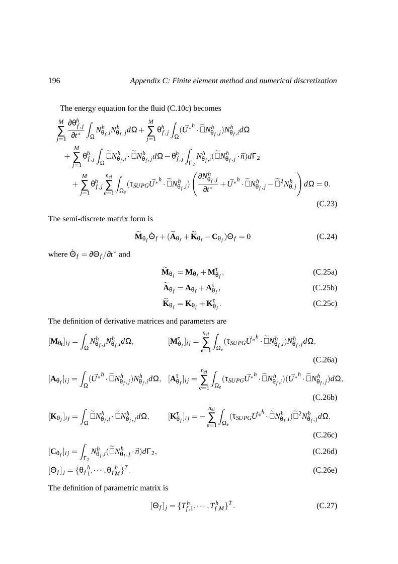
196 Appendix C: Finite element method and numerical discretization
The energy equation for the fluid (C.10c) becomes
M
∑j=1
∂θhf , j
∂t∗
Z
ΩNh
θ f ,iNhθ f , jdΩ+
M
∑j=1
θhf , j
Z
Ω( ~U∗h · ∇Nh
θ f , j)Nhθ f ,idΩ
+M
∑j=1
θhf , j
Z
Ω∇Nh
θ f ,i · ∇Nhθ f , jdΩ−θh
f , j
Z
Γ2
Nhθ f ,i(∇Nh
θ f , j ·~n)dΓ2
+M
∑j=1
θhf , j
nel
∑e=1
Z
Ωe
(τSUPG ~U∗h · ∇Nhθ f ,i)
(∂Nh
θ f , j
∂t∗+ ~U∗h · ∇Nh
θ f , j − ∇2Nhθ, j
)dΩ = 0.
(C.23)
The semi-discrete matrix form is
Mθ f Θ f +(Aθ f + Kθ f −Cθ f )Θ f = 0 (C.24)
where Θ f = ∂Θ f /∂t∗ and
Mθ f = Mθ f +Mτθ f
, (C.25a)
Aθ f = Aθ f +Aτθ f
, (C.25b)
Kθ f = Kθ f +Kτθ f
. (C.25c)
The definition of derivative matrices and parameters are
[Mθf ]i j =Z
ΩNh
θ f , jNhθ f ,idΩ, [Mτ
θ f]i j =
nel
∑e=1
Z
Ωe
(τSUPG ~U∗h · ∇Nhθ f ,i)N
hθ f , jdΩ,
(C.26a)
[Aθ f ]i j =Z
Ω( ~U∗h · ∇Nh
θ f , j)Nhθ f ,idΩ, [Aτ
θ f]i j =
nel
∑e=1
Z
Ωe
(τSUPG ~U∗h · ∇Nhθ f ,i)(
~U∗h · ∇Nhθ f , j)dΩ,
(C.26b)
[Kθ f ]i j =Z
Ω∇Nh
θ f ,i · ∇Nhθ f , jdΩ, [Kτ
θ f]i j = −
nel
∑e=1
Z
Ωe
(τSUPG ~U∗h · ∇Nhθ f ,i)∇
2Nhθ f , jdΩ,
(C.26c)
[Cθ f ]i j =Z
Γ2
Nhθ f ,i(∇Nh
θ f , j ·~n)dΓ2, (C.26d)
[Θ f ] j = θ fh1, · · · ,θ f
hMT . (C.26e)
The definition of parametric matrix is
[Θ f ] j = T hf ,1, · · · ,T h
f ,MT . (C.27)

Appendix C: Finite element method and numerical discretization 197
Also the energy equation for the partition wall (C.10d) becomes
M
∑j=1
∂θhW, j
∂t∗
Z
ΩNh
θw,iNhθw, jdΩ+ζ
M
∑j=1
θhW, j
Z
Ω∇Nh
θw,i · ∇Nhθw, jdΩ
−ζM
∑j=1
θhW, j
Z
Γ2
Nhθw,i(∇Nh
θw, j ·~n)dΓ2
+M
∑j=1
θhW, j
nel
∑e=1
Z
Ωe
(τSUPG ~U∗h · ∇Nhθw,i)
(∂Nh
θw, j
∂t∗−ζ∇2Nh
θw, j
)dΩ = 0,
(C.28)
with the semi-discrete matrix form :
MθwΘw +(Kθw −Cθw)Θw = 0 (C.29)
where Θw = ∂Θw/∂t∗ and
Mθw = Mθw +Mτθw
, (C.30a)
Kθw = Kθw +Kτθw
. (C.30b)
The definition of derivative matrices and parameters are
[Mθw]i j =Z
ΩNh
θw, jNhθw,idΩ, [Mτ
θw]i j =
nel
∑e=1
Z
Ωe
(τSUPG ~U∗h · ∇Nhθw,i)N
hθw, jdΩ,
(C.31a)
[Kθw]i j = ζZ
Ω∇Nh
θw,i · ∇Nhθw, jdΩ, [Kτ
θw]i j = −ζ
nel
∑e=1
Z
Ωe
(τSUPG ~U∗h · ∇Nhθw,i)∇
2Nhθw, jdΩ,
(C.31b)
[Cθw]i j = ζZ
Γ2
Nhθw,i(∇Nh
θw, j ·~n)dΓ2, (C.31c)
[Θw] j = θwh1, · · · ,θw
hMT . (C.31d)
The definition of parametric matrix is
[Θw] j = T hw,1, · · · ,T h
w,MT . (C.32)

198 Appendix C: Finite element method and numerical discretization
Finally the governing equations in semi-discrete matrix form are
GPU = 0, (C.33a)
MU U+(AU + KU)U− GU P− FU = 0, (C.33b)
Mθ f Θ f +(Aθ f + Kθ f −Cθ f )Θ f = 0, (C.33c)
MθwΘw +(Kθw −Cθw)Θw = 0. (C.33d)
C.2.2 Time discretization
The governing equations are discretized into a fully implicit time scheme since the
dependent variables are defined by coupled sets of equations. The matrix or iterative tech-
nique is needed to obtain the solution.
In general, an implicit method makes it attractive for the steady-state computations, because
the number of iterations required for a solution is often much smaller than the number of
time steps needed for an accurate transient that asymptotically approaches the steady con-
ditions. Especially, such scheme allows large time step sizes and unconditionally stable by
more complex to program and require more computational effort in each iteration step.
In an implicit formulation, a solution for the unknowns at level n + 1 may be obtained for
any size time step, which is reasonably decided according to physical phenomena [59].
Suppose at time t∗, the knowns are Un, Θnf , Θn
w and Pn. Then the unknowns are Un+1,
Θn+1f , Θn+1
w and Pn+1.
Although finite difference schemes are special cases of the finite element method, the
finite difference approximations are more widely used [41]. The governing equations are
discretized for the numerical application such as equation (C.20), (C.24) and (C.29). The
approximation of the time derivatives from governing equations by the backward difference
scheme is
U ≡ Un+1 −Un
∆t∗, (C.34a)
Θ f ≡Θn+1
f −Θnf
∆t∗, (C.34b)
Θw ≡ Θn+1w −Θn
w
∆t∗. (C.34c)
Finally, time discretized form of the continuity, momentum and energy equations for the

Appendix C: Finite element method and numerical discretization 199
fluid and partition wall are
GPUn+1 = 0, (C.35a)
MUUn+1 −Un
∆t∗+(AU + KU)Un+1 − GU Pn+1 − FU = 0, (C.35b)
Mθ f
Θn+1f −Θn
f
∆t∗+(Aθ f + Kθ f −Cθ f )Θ
n+1f = 0, (C.35c)
Mθw
Θn+1w −Θn
w
∆t∗+σ(Kθw −Cθw)Θn+1
w = 0. (C.35d)
C.3 Low Mach fluid flow model
C.3.1 Space discretization
The governing equations (8.19a), (8.19b), (8.19c) and (8.26) for the entire domain Ω in
two-dimensions is discretized into element Ωe, e = 1, · · · ,nel .
The trail solution spaces and the test function spaces for the density, velocity, pressure and
temperature are Shρ, Sh
u, S′hp , ShTf
and ShTw
and V hU , V h
P , V hTf
and V hθw
, respectively.
The stabilized SUPG finite element formulation of governing equations as the weak for-
mulation is
Z
Ω
∂ρh
∂tqhdΩ+
Z
Ω(ρh∇ ·~uh)qhdΩ+
Z
Ω(~uh∇ρh)qhdΩ = 0, (C.36a)
Z
Ωρh ∂~uh
∂twhdΩ+
Z
Ω(ρh~u∗
h ·∇~uh)whdΩ+Z
Ω(∇p′h)whdΩ
−Z
Ω
(∇ · ¯τh
)whdΩ−
Z
Ω(ρh −ρh
0)g(−~e)whdΩ = 0,
(C.36b)
Z
ΩρhCp
∂T hf
∂tΨh
dΩ+Z
Ω
(ρhCp~u∗
h ·∇T hf
)Ψh
dΩ
−Z
Ωk f ∇2T h
f ΨhdΩ−
Z
Ω
d phh
dtΨh
dΩ = 0,
(C.36c)
Z
ΩρhCp
∂T hw
∂tΦh
dΩ−Z
Ωkw(∇2T h
w )ΦhdΩ = 0 (C.36d)
where qh, wh, Ψhand Φh
are the test functions for the pressure, the velocity and the tem-
perature of the fluid and the partition wall and ~u∗h
is a parameter from equation (C.2) in

200 Appendix C: Finite element method and numerical discretization
order to avoid the non-linearity of the equation.
The test functions with the SUPG stabilization factor are
qh = qh + php′ , (C.37a)
wh = wh + phu, (C.37b)
Ψh= Ψh + ph
Tf, (C.37c)
Φh= Φh + ph
Tw(C.37d)
where qh, wh, Ψh and Φh are the continuous test functions and php′ , ph
u, phTf
phTw
are the
discontinuous streamline upwind contributions for the pressure, the velocity and the tem-
perature of the fluid and the partition wall, respectively.
The definition of the streamline upwind contributions is
php′ =
hξ2
~uh ·∇qh
‖~uh‖ = τSUPG~uh ·∇qh, (C.38a)
phu =
hξ2
~uh ·∇wh
‖~uh‖ = τSUPG~uh ·∇wh, (C.38b)
phTf
=hξ2
~uh ·∇Ψh
‖~uh‖ = τSUPG~uh ·∇Ψh, (C.38c)
phTw
=hξ2
~uh ·∇Φh
‖~uh‖ = τSUPG~uh ·∇Φh. (C.38d)
τSUPG is defined as
τSUPG =hξ
2‖~uh‖ . (C.39)
The value of ξ is from equation (C.6).
The diffusive term is arranged in to single derivative term as explained in section C.2.1.
Thus, in equation (C.36c) :Z
Ωk f ∇2T h
f ΨhdΩ = −Z
Ωk f ∇Ψh ·∇T h
f dΩ+Z
Γ2
k f Ψh(∇T hf ·~n)dΓ2 (C.40)
and in equation (C.36d) :Z
Ωkw(∇2T h
w )ΦhdΩ = −kw
Z
Ω∇Φh ·∇T h
w dΩ+ kw
Z
Γ2
Φh(∇T hw ·~n)dΓ2. (C.41)

Appendix C: Finite element method and numerical discretization 201
Due to the boundary condition of the problem (~uh = 0 and wh = 0) the equations become
more simple. Thus, in equation (C.36a) :Z
Ω(ρh∇ ·~uh)qhdΩ =
Z
Γ2
ρhqh(~uh ·~n)dΓ2 = 0 (C.42)
and in equation (C.36b) :Z
Ω(∇ · ¯τ)whdΩ =
Z
Γ2
wh(¯τ ·~n)dΓ2 = 0. (C.43)
The governing equations becomeZ
Ω
∂ρh
∂tqhdΩ+
Z
Ω(~uh∇ρh)qhdΩ
+nel
∑e=1
Z
Ωe
(τSUPG~u∗h ·∇qh)
(∂ρh
∂t+ρh∇ ·~uh +~uh∇ρh
)dΩ = 0,
(C.44a)
Z
Ωρh ∂~uh
∂twhdΩ+
Z
Ω(ρh~u∗
h ·∇~uh)whdΩ−Z
Ω(∇ ·wh)p′hdΩ
−Z
Ω(ρh −ρh
0)g(−~e)whdΩ+nel
∑e=1
Z
Ωe
(τSUPG~u∗h ·∇wh)
(ρh ∂~uh
∂t+ρh~u∗
h ·∇~uh +∇p′h −∇ · ¯τh − (ρh −ρh0)g(−~e)
)dΩ = 0,
(C.44b)
Z
ΩρhCp
∂T hf
∂tΨhdΩ+
Z
Ω
(ρhCp~u
h ·∇T hf
)ΨhdΩ+
Z
Ωk f ∇Ψh ·∇T h
f dΩ
−Z
Γ2
k f Ψh(∇T hf ·~n)dΓ2 −
Z
Ω
d phh
dtΨhdΩ
+nel
∑e=1
Z
Ωe
(τSUPG~u∗h ·∇Ψh)
(ρhCp
∂T hf
∂t+ρhCp~u∗
h ·∇T hf − k f ∇2T h
f −d ph
h
dt
)dΩ = 0,
(C.44c)Z
ΩρhCp
∂T hw
∂tΦhdΩ+ kw
Z
Ω∇Φh ·∇T h
w dΩ− kw
Z
Γ2
Φh(∇T hw ·~n)dΓ2
+nel
∑e=1
Z
Ωe
(τSUPG~u∗h ·∇Φh)
(ρhCp
∂T hw
∂t− kw∇2T h
w
)dΩ = 0.
(C.44d)
Also note that the pressure gradient term in equation (C.44b) isZ
Ω(∇p′h)whΩ =
Z
Ω∇ · (p′hwh)dΩ−
Z
Ω(∇ ·wh)p′hdΩ
=Z
Γ2
p′hwh ·~ndΓ2 −Z
Ω(∇ ·wh)p′hdΩ
= −Z
Ω(∇ ·wh)p′hdΩ
(C.45)

202 Appendix C: Finite element method and numerical discretization
since wh = 0 at boundary.
The approximated velocity and temperatures with corresponding shape functions are
~uh =M
∑j=1
~uhjN
hu, j, j = 1, · · · ,M, (C.46a)
T hf =
M
∑j=1
T hf , jN
hTf , j, j = 1, · · · ,M, (C.46b)
T hw =
M
∑j=1
T hw, jN
hTw, j, j = 1, · · · ,M (C.46c)
where Nhu, j, Nh
Tf , j and NhTw, j are the shape functions for fluid velocity and temperature and
partition wall temperature, respectively. The degree of freedom, M, is equal to 4 in the
corresponding nodal shape functions that involve the piecewise bi-linear polynomials.
For the pressure, the shape function (Nhp′, j) involves piecewise polynomial of degree 1 and
p′h =N
∑j=1
p′hjNhp′, j, j = 1, · · · ,N (C.47)
where the degree of freedom is N = 3.
The test functions are selected identical to the shape functions of the solution approxima-
tions in the Galerkin method :
qh = Nhp′,i, i = 1, · · · ,N, (C.48a)
wh = Nhu,i, i = 1, · · · ,M, (C.48b)
Ψh = NhTf ,i, i = 1, · · · ,M, (C.48c)
Φh = NhTw,i, i = 1, · · · ,M. (C.48d)
Consider both test and shape functions, the continuity equation (Eq. (C.44a)) becomes
∂ρh
∂t
Z
ΩNh
p′,idΩ+N
∑j=1
~uhj∇ρh
Z
ΩNh
u, jNhp′,idΩ+
nel
∑e=1
Z
Ωe
(τSUPG~u∗h ·∇Nh
p′,i)
(∂ρh
∂t
)dΩ
+N
∑j=1
~uhj
nel
∑e=1
Z
Ωe
(τSUPG~u∗h ·∇Nh
p′,i)(
ρh∇ ·Nhu, j +Nh
u, j∇ρh)
dΩ = 0.
(C.49)
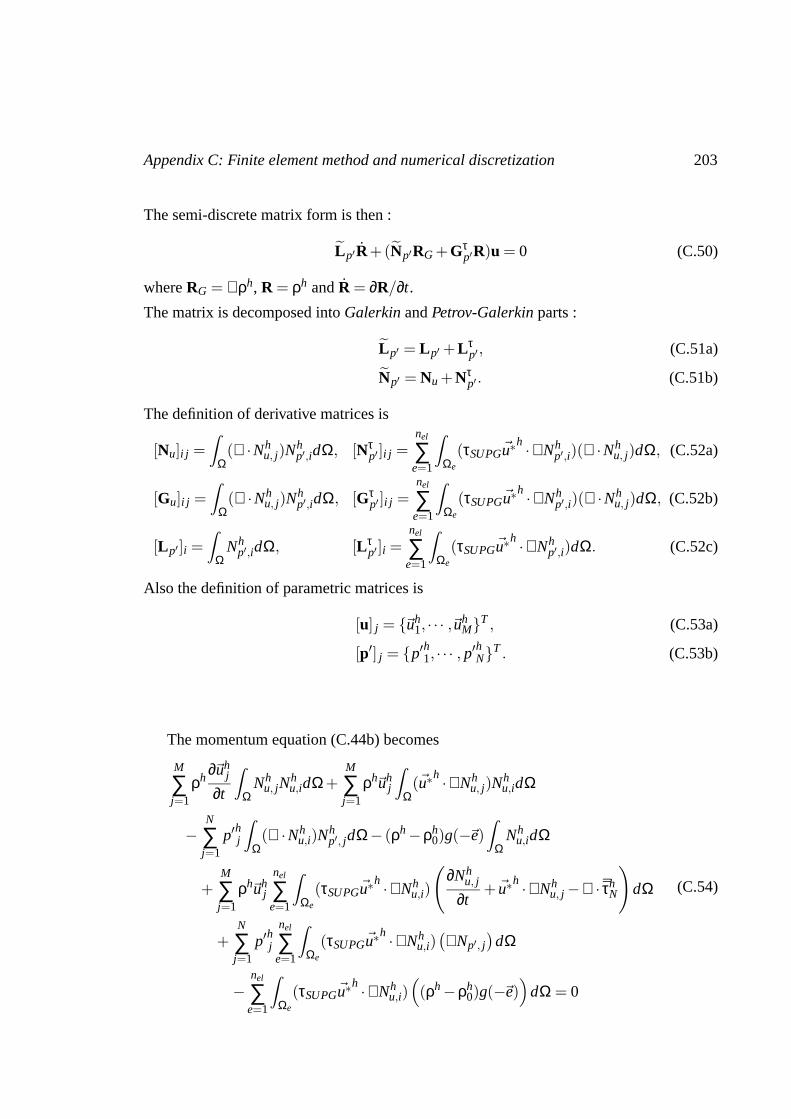
Appendix C: Finite element method and numerical discretization 203
The semi-discrete matrix form is then :
Lp′R+(Np′RG +Gτp′R)u = 0 (C.50)
where RG = ∇ρh, R = ρh and R = ∂R/∂t.
The matrix is decomposed into Galerkin and Petrov-Galerkin parts :
Lp′ = Lp′ +Lτp′ , (C.51a)
Np′ = Nu +Nτp′ . (C.51b)
The definition of derivative matrices is
[Nu]i j =Z
Ω(∇ ·Nh
u, j)Nhp′,idΩ, [Nτ
p′]i j =nel
∑e=1
Z
Ωe
(τSUPG~u∗h ·∇Nh
p′,i)(∇ ·Nhu, j)dΩ, (C.52a)
[Gu]i j =Z
Ω(∇ ·Nh
u, j)Nhp′,idΩ, [Gτ
p′ ]i j =nel
∑e=1
Z
Ωe
(τSUPG~u∗h ·∇Nh
p′,i)(∇ ·Nhu, j)dΩ, (C.52b)
[Lp′]i =Z
ΩNh
p′,idΩ, [Lτp′]i =
nel
∑e=1
Z
Ωe
(τSUPG~u∗h ·∇Nh
p′,i)dΩ. (C.52c)
Also the definition of parametric matrices is
[u] j = ~uh1, · · · ,~uh
MT , (C.53a)
[p′] j = p′h1, · · · , p′hNT . (C.53b)
The momentum equation (C.44b) becomes
M
∑j=1
ρh∂~uh
j
∂t
Z
ΩNh
u, jNhu,idΩ+
M
∑j=1
ρh~uhj
Z
Ω(~u∗
h ·∇Nhu, j)N
hu,idΩ
−N
∑j=1
p′hj
Z
Ω(∇ ·Nh
u,i)Nhp′, jdΩ− (ρh −ρh
0)g(−~e)Z
ΩNh
u,idΩ
+M
∑j=1
ρh~uhj
nel
∑e=1
Z
Ωe
(τSUPG~u∗h ·∇Nh
u,i)
(∂Nh
u, j
∂t+ ~u∗
h ·∇Nhu, j −∇ · ¯τh
N
)dΩ
+N
∑j=1
p′hjnel
∑e=1
Z
Ωe
(τSUPG~u∗h ·∇Nh
u,i)(∇Np′, j
)dΩ
−nel
∑e=1
Z
Ωe
(τSUPG~u∗h ·∇Nh
u,i)((ρh −ρh
0)g(−~e))
dΩ = 0
(C.54)
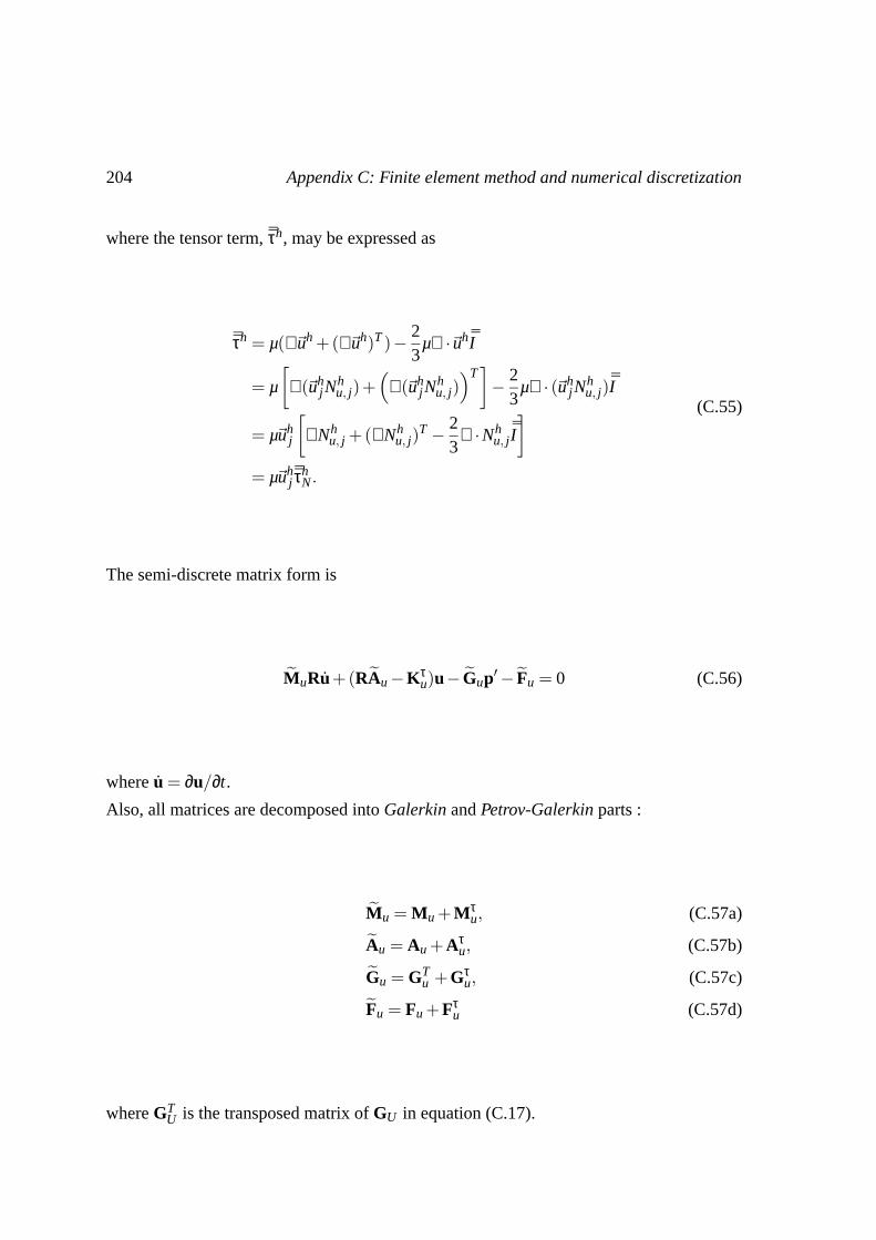
204 Appendix C: Finite element method and numerical discretization
where the tensor term, ¯τh, may be expressed as
¯τh = µ(∇~uh +(∇~uh)T )− 23
µ∇ ·~uh ¯I
= µ
[∇(~uh
jNhu, j)+
(∇(~uh
jNhu, j))T]− 2
3µ∇ · (~uh
jNhu, j)
¯I
= µ~uhj
[∇Nh
u, j +(∇Nhu, j)
T − 23
∇ ·Nhu, j
¯I
]
= µ~uhj¯τh
N .
(C.55)
The semi-discrete matrix form is
MuRu+(RAu −Kτu)u− Gup′− Fu = 0 (C.56)
where u = ∂u/∂t.
Also, all matrices are decomposed into Galerkin and Petrov-Galerkin parts :
Mu = Mu +Mτu, (C.57a)
Au = Au +Aτu, (C.57b)
Gu = GTu +Gτ
u, (C.57c)
Fu = Fu +Fτu (C.57d)
where GTU is the transposed matrix of GU in equation (C.17).
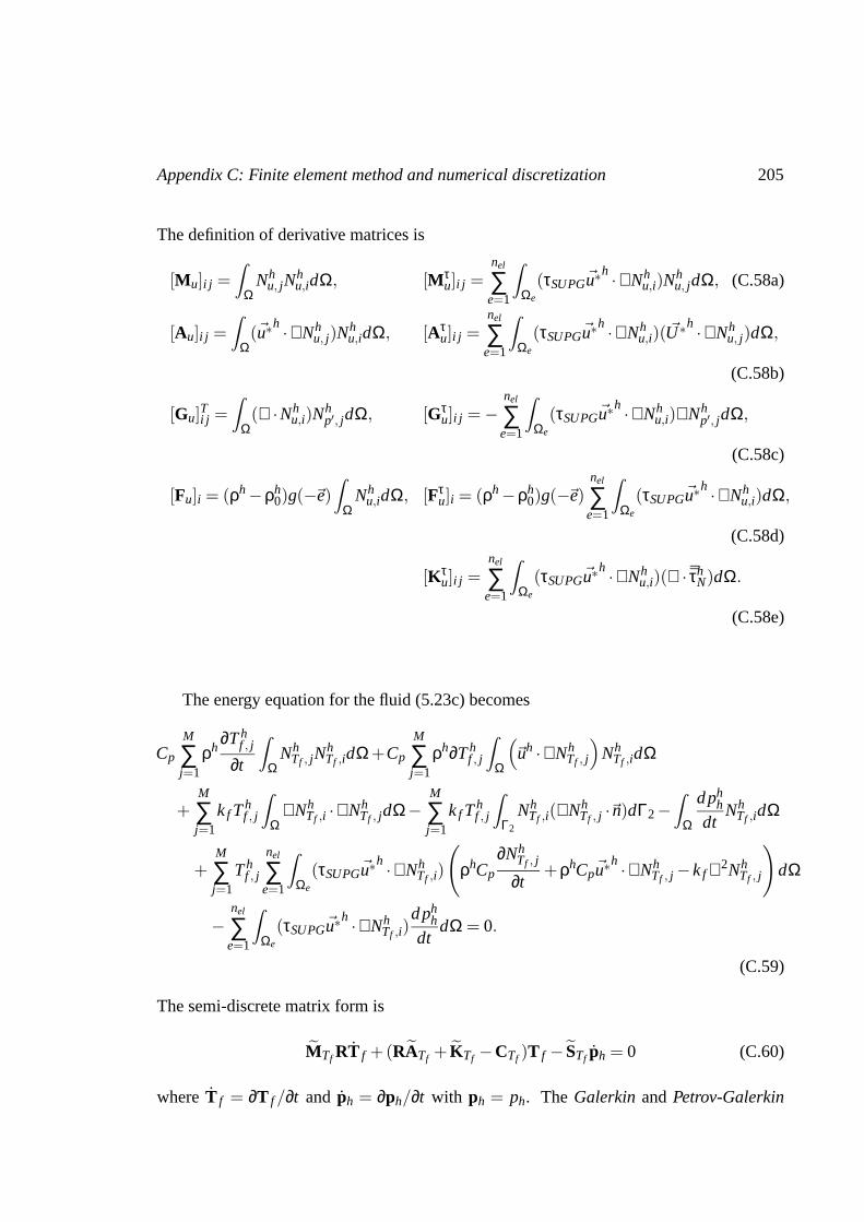
Appendix C: Finite element method and numerical discretization 205
The definition of derivative matrices is
[Mu]i j =Z
ΩNh
u, jNhu,idΩ, [Mτ
u]i j =nel
∑e=1
Z
Ωe
(τSUPG~u∗h ·∇Nh
u,i)Nhu, jdΩ, (C.58a)
[Au]i j =Z
Ω(~u∗
h ·∇Nhu, j)N
hu,idΩ, [Aτ
u]i j =nel
∑e=1
Z
Ωe
(τSUPG~u∗h ·∇Nh
u,i)( ~U∗h ·∇Nhu, j)dΩ,
(C.58b)
[Gu]Ti j =
Z
Ω(∇ ·Nh
u,i)Nhp′, jdΩ, [Gτ
u]i j = −nel
∑e=1
Z
Ωe
(τSUPG~u∗h ·∇Nh
u,i)∇Nhp′, jdΩ,
(C.58c)
[Fu]i = (ρh −ρh0)g(−~e)
Z
ΩNh
u,idΩ, [Fτu]i = (ρh −ρh
0)g(−~e)nel
∑e=1
Z
Ωe
(τSUPG~u∗h ·∇Nh
u,i)dΩ,
(C.58d)
[Kτu]i j =
nel
∑e=1
Z
Ωe
(τSUPG~u∗h ·∇Nh
u,i)(∇ · ¯τhN)dΩ.
(C.58e)
The energy equation for the fluid (5.23c) becomes
Cp
M
∑j=1
ρh∂T h
f , j
∂t
Z
ΩNh
Tf , jNhTf ,idΩ+Cp
M
∑j=1
ρh∂T hf , j
Z
Ω
(~uh ·∇Nh
Tf , j
)Nh
Tf ,idΩ
+M
∑j=1
k f T hf , j
Z
Ω∇Nh
Tf ,i ·∇NhTf , jdΩ−
M
∑j=1
k f T hf , j
Z
Γ2
NhTf ,i(∇Nh
Tf , j ·~n)dΓ2 −Z
Ω
d phh
dtNh
Tf ,idΩ
+M
∑j=1
T hf , j
nel
∑e=1
Z
Ωe
(τSUPG~u∗h ·∇Nh
Tf ,i)
(ρhCp
∂NhTf , j
∂t+ρhCp~u∗
h ·∇NhTf , j − k f ∇2Nh
Tf , j
)dΩ
−nel
∑e=1
Z
Ωe
(τSUPG~u∗h ·∇Nh
Tf ,i)d ph
h
dtdΩ = 0.
(C.59)
The semi-discrete matrix form is
MTf RT f +(RATf + KTf −CTf )T f − STf ph = 0 (C.60)
where T f = ∂T f /∂t and ph = ∂ph/∂t with ph = ph. The Galerkin and Petrov-Galerkin

206 Appendix C: Finite element method and numerical discretization
matrices are
MTf = MTf +MτTf
, (C.61a)
ATf = ATf +AτTf
, (C.61b)
KTf = KTf +KτTf
, (C.61c)
STf = STf +PτTf
. (C.61d)
The definition of derivative matrices and parameters are
[MTf]i j = Cp
Z
ΩNh
Tf , jNhTf ,idΩ, [Mτ
Tf]i j = Cp
nel
∑e=1
Z
Ωe
(τSUPG~u∗h ·∇Nh
Tf ,i)NhTf , jdΩ,
(C.62a)
[ATf ]i j = Cp
Z
Ω(~u∗
h ·∇NhTf , j)N
hTf ,idΩ, [Aτ
Tf]i j = Cp
nel
∑e=1
Z
Ωe
(τSUPG~u∗h ·∇Nh
Tf ,i)(~u∗
h ·∇NhTf , j)dΩ,
(C.62b)
[KTf ]i j = k f
Z
Ω∇Nh
Tf ,i ·∇NhTf , jdΩ, [Kτ
Tf]i j = −k f
nel
∑e=1
Z
Ωe
(τSUPG~u∗h ·∇Nh
Tf ,i)∇2Nh
Tf , jdΩ,
(C.62c)
[S]i =Z
ΩNh
Tf ,idΩ, [Sτ]i =nel
∑e=1
Z
Ωe
(τSUPG~u∗h ·∇Nh
Tf ,i)dΩ, (C.62d)
[CTf ]i j =Z
Γ2
NhTf ,i(∇Nh
Tf , j ·~n)dΓ2, (C.62e)
[Tf ] j = Tfh1, · · · ,Tf
hMT . (C.62f)
The definition of parametric matrix is
[T f ] j = T hf ,1, · · · ,T h
f ,MT . (C.63)

Appendix C: Finite element method and numerical discretization 207
Also the energy equation for the partition wall (C.44d) becomes
M
∑j=1
ρhCp∂T h
w, j
∂t
Z
ΩNh
Tw,iNhTw, jdΩ+ kw
M
∑j=1
T hw, j
Z
Ω∇Nh
Tw,i ·∇NhTw, jdΩ
− kw
M
∑j=1
T hw, j
Z
Γ2
NhTw,i(∇Nh
Tw, j ·~n)dΓ2
+M
∑j=1
ρhT hW, j
nel
∑e=1
Z
Ωe
(τSUPG ~U∗h ·∇NhTw,i)
(∂Nh
Tw, j
∂t− kw∇2Nh
Tw, j
)dΩ = 0,
(C.64)
with the semi-discrete matrix form
MTwRTw +(KTw −CTw)Tw = 0 (C.65)
where Tw = ∂Tw/∂t and
MTw = MTw +MτTw
, (C.66a)
KTw = KTw +KτTw
. (C.66b)
The definition of derivative matrices and parameters are
[Mθw]i j = Cp
Z
ΩNh
Tw, jNhTw,idΩ, [Mτ
Tw]i j = Cp
nel
∑e=1
Z
Ωe
(τSUPG~u∗h ·∇Nh
Tw,i)NhTw, jdΩ,
(C.67a)
[KTw]i j = kw
Z
Ω∇Nh
Tw,i ·∇NhTw, jdΩ, [Kτ
Tw]i j = −kw
nel
∑e=1
Z
Ωe
(τSUPG~u∗h ·∇Nh
Tw,i)∇2Nh
Tw, jdΩ,
(C.67b)
[CTw]i j = kw
Z
Γ2
NhTw,i(∇Nh
Tw, j ·~n)dΓ2, (C.67c)
[Tw] j = Twh1, · · · ,Tw
hMT . (C.67d)
The definition of parametric matrix is
[Tw] j = T hw,1, · · · ,T h
w,MT . (C.68)
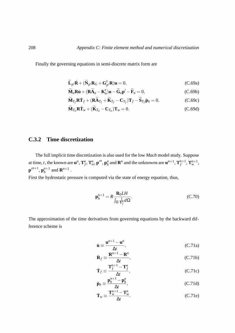
208 Appendix C: Finite element method and numerical discretization
Finally the governing equations in semi-discrete matrix form are
Lp′R+(Np′RG +Gτp′R)u = 0, (C.69a)
MuRu+(RAu −Kτu)u− Gup′− Fu = 0, (C.69b)
MTf RT f +(RATf + KTf −CTf )T f − STf ph = 0, (C.69c)
MTwRTw +(KTw −CTw)Tw = 0. (C.69d)
C.3.2 Time discretization
The full implicit time discretization is also used for the low Mach model study. Suppose
at time, t, the known are un, Tnf , Tn
w, p′n, pnh and Rn and the unknowns are un+1, Tn+1
f , Tn+1w ,
p′n+1, pn+1h and Rn+1 .
First the hydrostatic pressure is computed via the state of energy equation, thus,
pn+1h = R
R0LHR
Ω1
TnfdΩ
. (C.70)
The approximation of the time derivatives from governing equations by the backward dif-
ference scheme is
u ≡ un+1 −un
∆t, (C.71a)
R f ≡Rn+1 −Rn
∆t, (C.71b)
T f ≡Tn+1
f −Tnf
∆t, (C.71c)
ph ≡pn+1
h −pnh
∆t, (C.71d)
Tw ≡ Tn+1w −Tn
w
∆t. (C.71e)

Appendix C: Finite element method and numerical discretization 209
The time discretized form of the continuity, momentum and energy equation for the fluid
and partition wall are
Lp′Rn+1 −Rn
∆t+(Np′R
n+1G +Gτ
p′Rn+1)un+1 = 0, (C.72a)
MuR∗un+1 −un
∆t+(R∗Au −Kτ
u)un+1 − Gup′n+1 − Fu = 0, (C.72b)
MTf R∗Tn+1
f −Tnf
∆t+(R∗ATf + KTf −CTf )T
n+1f − STf
pn+1h −pn
h
∆t= 0, (C.72c)
MTwR∗Tn+1w −Tn
w
∆t+(KTw −CTw)Tn+1
w = 0 (C.72d)
,respectively, where R∗ denotes a parametric value of the density based on equation (C.2),
in order to avoid the non-linearity of the equation.
Finally the density, Rn+1, is recovered by the equation of state, as
Rn+1 =pn+1
h
RTn+1f
. (C.73)
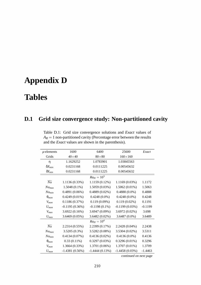
Appendix D
Tables
D.1 Grid size convergence study: Non-partitioned cavity
Table D.1: Grid size convergence solutions and Exact values ofAR = 1 non-partitioned cavity (Percentage error between the resultsand the Exact values are shown in the parenthesis).
µ-elements 1600 6400 25600 Exact
Grids 40×40 80×80 160×160
η 1.1629252 1.0783901 1.03845563
δXmin 0.0231168 0.0111225 0.00545632
δYmin 0.0231168 0.0111225 0.00545632
RaH = 103
Nu 1.1136 (0.33%) 1.1159 (0.12%) 1.1169 (0.03%) 1.1172
Numax 1.5048 (0.1%) 1.5059 (0.03%) 1.5062 (0.01%) 1.5063
Numin 0.4891 (0.06%) 0.4889 (0.02%) 0.4888 (0.0%) 0.4888
θmon 0.4249 (0.01%) 0.4248 (0.0%) 0.4248 (0.0%) 0.4248
Vmon 0.1186 (0.37%) 0.119 (0.09%) 0.119 (0.02%) 0.1191
Umon -0.1195 (0.36%) -0.1198 (0.1%) -0.1199 (0.03%) -0.1199
Vmax 3.6922 (0.16%) 3.6947 (0.09%) 3.6972 (0.02%) 3.698
Umax 3.6469 (0.05%) 3.6482 (0.02%) 3.6487 (0.0%) 3.6489
RaH = 104
Nu 2.2314 (0.55%) 2.2399 (0.17%) 2.2428 (0.04%) 2.2438
Numax 3.5205 (0.3%) 3.5282 (0.08%) 3.5304 (0.02%) 3.5311
Numin 0.4134 (0.07%) 0.4136 (0.02%) 0.4136 (0.0%) 0.4136
θmon 0.33 (0.11%) 0.3297 (0.03%) 0.3296 (0.01%) 0.3296
Vmon 1.3664 (0.33%) 1.3701 (0.06%) 1.3707 (0.01%) 1.3709
Umon -1.4381 (0.56%) -1.4444 (0.13%) -1.4458 (0.03%) -1.4463
continued on next page
210

Appendix D: Tables 211
Table D.1: (continued)
continued from previous page
µ-elements 1600 6400 25600 Exact
Grids 40×40 80×80 160×160
Vmax 19.552 (0.38%) 19.608 (0.1%) 19.622 (0.02%) 19.6267
Umax 16.096 (0.56%) 16.157 (0.18%) 16.179 (0.05%) 16.1863
RaH = 105
Nu 4.4811 (0.85%) 4.5087 (0.24%) 4.5169 (0.06%) 4.5196
Numax 7.671 (0.64%) 7.7094 (0.14%) 7.7175 (0.03%) 7.7202
Numin 0.5186 (0.75%) 0.5158 (0.2%) 0.515 (0.05%) 0.5147
θmon 0.1381 (0.99%) 0.137 (0.22%) 0.1368 (0.06%) 0.1367
Vmon 8.8299 (0.65%) 8.7932 (0.23%) 8.7781 (0.06%) 8.7731
Umon -11.163 (0.8%) -11.237 (0.14%) -11.249 (0.04%) -11.253
Vmax 68.266 (0.53%) 68.471 (0.23%) 68.588 (0.06%) 68.627
Umax 34.187 (1.58%) 34.614 (0.35%) 34.705 (0.09%) 34.735
RaH = 106
Nu 8.67 (1.7%) 8.7761 (0.5%) 8.8092 (0.13%) 8.8202
Numax 16.914 (3.58%) 17.384 (0.9%) 17.502 (0.22%) 17.5413
Numin 0.7072 (1.99%) 0.7008 (1.07%) 0.6952 (0.27%) 0.6934
θmon -0.1597 (2.41%) -0.1623 (0.8%) -0.1633 (0.2%) -0.1636
Vmon 13.974 (9.59%) 13.066 (2.47%) 12.83 (0.62%) 12.7513
Umon -46.568 (0.29%) -46.746 (0.09%) -46.715 (0.02%) -46.705
Vmax 220.07 (0.07%) 219.54 (0.17%) 219.82 (0.04%) 219.91
Umax 63.764 (1.71%) 64.628 (0.38%) 64.811 (0.09%) 64.872
RaH = 107
Nu 15.768 ( 4.46%) 16.327 (1.07%) 16.46 (0.27%) 16.504
Numax 34.517 (12.38%) 37.885 (3.83%) 39.016 (0.96%) 39.393
Numin 1.005 ( 3.39%) 0.9805 (0.87%) 0.9742 (0.22%) 0.972
θmon -0.3105 ( 1.25%) -0.3134 (0.35%) -0.3142 (0.09%) -0.3144
Vmon -31.914 (19.84%) -24.814 (6.82%) -26.177 (1.71%) -26.631
Umon -116.38 ( 1.69%) -117.37 (2.55%) -115.18 (0.64%) -114.45
Vmax 702.84 ( 0.95%) 694.43 (0.26%) 695.79 (0.07%) 696.24
Umax 143.26 ( 2.5%) 148.9 (1.33%) 147.43 (0.33%) 146.94

212 Appendix D: Tables
Table D.2: Grid size convergence solutions and Exact values ofAR = 2 non-partitioned cavity (Percentage error between the resultsand the Exact values are shown in the parenthesis).
µ-elements 800 3200 12800 Exact
Grids 20×40 40×80 80×160
ηX 1.33252621 1.15435099 1.07440727
δXmin 0.025 0.0116044 0.00559409
ηY 1.1629252 1.0783901 1.03845563
δYmin 0.0231168 0.0111225 0.00545632
RaH = 103
Nu 1.0004 (0.33%) 1.0025 (0.12%) 1.0034 (0.03%) 1.0037
Numax 1.1082 (0.1%) 1.1090 (0.02%) 1.1092 (0.01%) 1.1093
Numin 0.6117 (2.99%) 0.6231 (1.18%) 0.6287 (0.29%) 0.6306
θmon 0.4446 (-0.01%) 0.4446 (0.0%) 0.4446 (0.0%) 0.4446
Vmon 0.0909 (0.37%) 0.0913 (-0.02%) 0.0913 (-0.01%) 0.0913
Umon -0.0429 (1.43%) -0.0433 (0.37%) -0.0434 (0.09%) -0.0435
Vmax 1.9472 (0.04%) 1.9465 (0.01%) 1.9464 (0.0%) 1.9464
Umax 1.2128 (0.76%) 1.2194 (0.22%) 1.2214 (0.05%) 1.2221
RaH = 104
Nu 1.2511 (0.61%) 1.2564 (0.19%) 1.2582 (0.05%) 1.2588
Numax 2.0712 (0.5%) 2.0790 (0.13%) 2.0810 (0.03%) 2.0817
Numin 0.297 (2.87%) 0.3023 (1.15%) 0.3049 (0.29%) 0.3058
θmon 0.3976 (-0.11%) 0.3973 (-0.03%) 0.3972 (-0.01%) 0.3972
Vmon 1.217 (0.63%) 1.2232 (0.12%) 1.2243 (0.03%) 1.2247
Umon -0.5494 (2.16%) -0.5586 (0.52%) -0.5608 (0.13%) -0.5615
Vmax 17.054 (0.22%) 17.08 (0.07%) 17.089 (0.02%) 17.092
Umax 9.7705 (0.27%) 9.7896 (0.08%) 9.7952 (0.02%) 9.7971
RaH = 105
Nu 2.4678 (1.28%) 2.4909 (0.36%) 2.4976 (0.09%) 2.4998
Numax 4.5165 (0.83%) 4.547 (0.16%) 4.5525 (0.04%) 4.5543
Numin 0.2397 (3.3%) 0.2448 (1.23%) 0.2471 (0.31%) 0.2479
θmon 0.2789 (-0.4%) 0.278 (-0.08%) 0.2779 (-0.02%) 0.2778
Vmon 10.817 (-1.02%) 10.753 (-0.42%) 10.719 (-0.11%) 10.7077
Umon -4.4237 (2.9%) -4.5317 (0.53%) -4.5498 (0.13%) -4.5558
Vmax 71.871 (2.94%) 73.662 (0.52%) 73.953 (0.13%) 74.05
Umax 37.113 (2.08%) 37.666 (0.62%) 37.843 (0.16%) 37.902
RaH = 106
Nu 4.4606 (2.14%) 4.5316 (0.58%) 4.5514 (0.14%) 4.558
Numax 8.9015 (2.63%) 9.1146 (0.3%) 9.1353 (0.08%) 9.1422
continued on next page

Appendix D: Tables 213
Table D.2: (continued)
continued from previous page
µ-elements 800 3200 12800 Exact
Grids 20×40 40×80 80×160
Numin 0.3328 (2.32%) 0.3394 (0.37%) 0.3404 (0.09%) 0.3407
θmon 0.0728 (-4.31%) 0.0694 (0.59%) 0.0697 (0.15%) 0.0698
Vmon 55.28 (-6.21%) 53.1260 (-2.07%) 52.319 (-0.52%) 52.05
Umon -20.813 (5.61%) -21.961 (0.41%) -22.028 (0.1%) -22.0503
Vmax 213.54 (0.89%) 214.18 (0.59%) 215.14 (0.15%) 215.46
Umax 102.23 (0.37%) 109.38 (4.1%) 112.89 (1.03%) 114.06
RaH = 107
Nu 7.9556 (5.05%) 8.2803 (1.18%) 8.3543 (0.29%) 8.379
Numax 17.849 (14.01%) 19.952 (3.87%) 20.555 (0.97%) 20.756
Numin 0.4667 (0.25%) 0.4623 (1.18%) 0.4665 (0.3%) 0.4679
θmon -0.1953 (7.27%) -0.209 (0.75%) -0.2102 (0.19%) -0.2106
Vmon 112.97 (-20.25%) 99.886 (-6.32%) 95.432 (-1.58%) 93.947
Umon -69.632 (8.77%) -75.628 (0.92%) -76.154 (0.23%) -76.329
Vmax 697.94 (0.01%) 687.16 (1.54%) 695.2 (0.38%) 697.88
Umax 123.35 (27.1%) 144.64 (14.52%) 163.07 (3.63%) 169.21

214 Appendix D: Tables
D.2 Grid size convergence study: Partitioned cavity
Table D.3: Grid size convergence solutions and Exact values ofγ = 0.01 and AR = 1 partitioned cavity (Percentage error betweenthe results and the Exact values are shown in the parenthesis).
µ-elements 1760 6720 26240 Exact
Grids 44×40 84×80 164×160
ηX 1.33490166 1.15537945 1.07488578
δXmin 0.02475 0.0114829 0.00553423
ηY 1.1629252 1.0783901 1.03845563
δYmin 0.0231168 0.0111225 0.00545632
RaH = 103
Nu 0.9973 (0.32%) 0.9993 (0.12%) 1.0002 (0.03%) 1.0005
Numax 1.0517 (0.04%) 1.0520 (0.01%) 1.0521 (0.0%) 1.0521
Numin 0.6490 (3.03%) 0.6613 (1.19%) 0.6673 (0.3%) 0.6693
θmon 0.4737 (0.0%) 0.4737 (0.0%) 0.4737 (0.0%) 0.4737
Vmon 0.0439 (-9.9%) 0.0441 (-10.34%) 0.0410 (-2.59%) 0.0399
Umon -0.0205 (1.39%) -0.0207 (0.36%) -0.0208 (0.09%) -0.0208
Vmax 0.9581 (-0.04%) 0.9575 (0.03%) 0.9577 (0.01%) 0.9578
Umax 0.5955 (0.79%) 0.5993 (0.16%) 0.6000 (0.04%) 0.6002
RaH = 104
Nu 1.0802 (0.43%) 1.0834 (0.14%) 1.0845 (0.03%) 1.0849
Numax 1.5543 (0.42%) 1.5593 (0.1%) 1.5605 (0.03%) 1.5609
Numin 0.4204 (2.71%) 0.4302 (0.44%) 0.4316 (0.11%) 0.4321
θmon 0.4613 (-0.06%) 0.4616 (-0.12%) 0.4612 (-0.03%) 0.4610
Vmon 0.5419 (1.32%) 0.5423 (1.25%) 0.5474 (0.31%) 0.5491
Umon -0.2471 (2.81%) -0.2468 (2.94%) -0.2524 (0.74%) -0.2543
Vmax 9.1949 (0.03%) 9.1948 (0.03%) 9.1967 (0.01%) 9.1973
Umax 5.5572 (0.55%) 5.5751 (0.23%) 5.5849 (0.06%) 5.5882
RaH = 105
Nu 2.0146 (1.04%) 2.0296 (0.3%) 2.0342 (0.08%) 2.0357
Numax 3.6644 (0.73%) 3.6852 (0.16%) 3.6897 (0.04%) 3.6912
Numin 0.2155 (3.03%) 0.2209 (0.61%) 0.2219 (0.15%) 0.2222
θmon 0.4105 (-0.2%) 0.4110 (-0.32%) 0.4100 (-0.08%) 0.4097
Vmon 5.9459 (1.04%) 5.9664 (0.7%) 5.9980 (0.18%) 6.0085
Umon -2.4809 (4.11%) -2.5092 (3.02%) -2.5678 (0.75%) -2.5873
Vmax 50.515 (1.85%) 51.149 (0.62%) 51.387 (0.15%) 51.466
Umax 24.705 (-0.27%) 24.646 (-0.03%) 24.64 (-0.01%) 24.638
RaH = 106
continued on next page
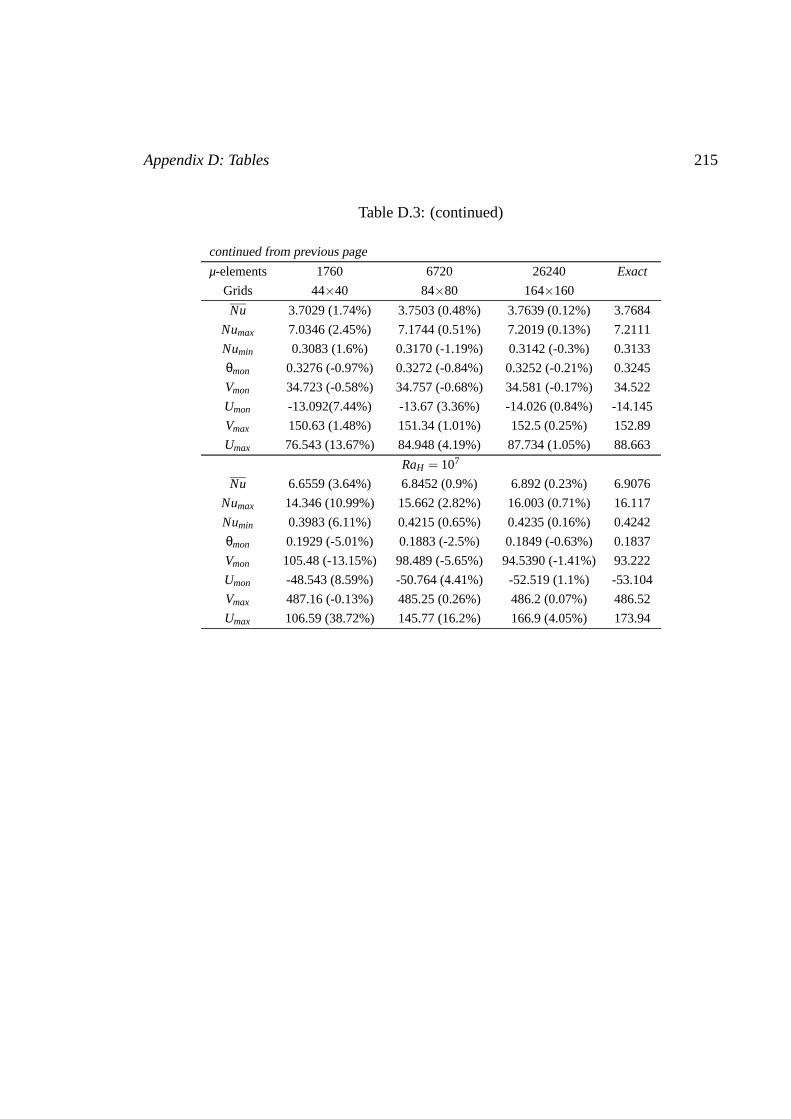
Appendix D: Tables 215
Table D.3: (continued)
continued from previous page
µ-elements 1760 6720 26240 Exact
Grids 44×40 84×80 164×160
Nu 3.7029 (1.74%) 3.7503 (0.48%) 3.7639 (0.12%) 3.7684
Numax 7.0346 (2.45%) 7.1744 (0.51%) 7.2019 (0.13%) 7.2111
Numin 0.3083 (1.6%) 0.3170 (-1.19%) 0.3142 (-0.3%) 0.3133
θmon 0.3276 (-0.97%) 0.3272 (-0.84%) 0.3252 (-0.21%) 0.3245
Vmon 34.723 (-0.58%) 34.757 (-0.68%) 34.581 (-0.17%) 34.522
Umon -13.092(7.44%) -13.67 (3.36%) -14.026 (0.84%) -14.145
Vmax 150.63 (1.48%) 151.34 (1.01%) 152.5 (0.25%) 152.89
Umax 76.543 (13.67%) 84.948 (4.19%) 87.734 (1.05%) 88.663
RaH = 107
Nu 6.6559 (3.64%) 6.8452 (0.9%) 6.892 (0.23%) 6.9076
Numax 14.346 (10.99%) 15.662 (2.82%) 16.003 (0.71%) 16.117
Numin 0.3983 (6.11%) 0.4215 (0.65%) 0.4235 (0.16%) 0.4242
θmon 0.1929 (-5.01%) 0.1883 (-2.5%) 0.1849 (-0.63%) 0.1837
Vmon 105.48 (-13.15%) 98.489 (-5.65%) 94.5390 (-1.41%) 93.222
Umon -48.543 (8.59%) -50.764 (4.41%) -52.519 (1.1%) -53.104
Vmax 487.16 (-0.13%) 485.25 (0.26%) 486.2 (0.07%) 486.52
Umax 106.59 (38.72%) 145.77 (16.2%) 166.9 (4.05%) 173.94

216 Appendix D: Tables
Table D.4: Grid size convergence solutions and Exact values ofγ = 0.1 and AR = 1 partitioned cavity (Percentage error betweenthe results and the Exact values are shown in the parenthesis).
µ-elements 2400 8000 28800 Exact
Grids 60×40 100×80 180×160
ηX 1.3568637 1.16484493 1.07927982
δXmin 0.0225 0.0103934 0.00499854
ηY 1.1629252 1.0783901 1.03845563
δYmin 0.0231168 0.0111225 0.00545632
RaH = 103
Nu 0.9972 (0.28%) 0.9990 (0.1%) 0.9998 (0.03%) 1.0001
Numax 1.0391 (0.03%) 1.0393 (0.01%) 1.0394 (0.0%) 1.0394
Numin 0.6897 (3.08%) 0.7031 (1.2%) 0.7095 (0.3%) 0.7116
θmon 0.4740 (0.0%) 0.4740 (0.0%) 0.4740 (0.0%) 0.4740
Vmon 0.0424 (0.56%) 0.0426 (0.12%) 0.0426 (0.03%) 0.0426
Umon -0.0177 (1.4%) -0.0179 (0.35%) -0.0179 (0.09%) -0.0179
Vmax 0.8062 (-0.04%) 0.8059 (-0.01%) 0.8059 (0.0%) 0.8059
Umax 0.4931 (0.5%) 0.4950 (0.13%) 0.4954 (0.03%) 0.4956
RaH = 104
Nu 1.0442 (0.36%) 1.0466 (0.13%) 1.0476 (0.03%) 1.0479
Numax 1.4202 (0.36%) 1.4240 (0.09%) 1.4250 (0.02%) 1.4253
Numin 0.4900 (2.93%) 0.4989 (1.16%) 0.5033 (0.29%) 0.5048
θmon 0.4646 (-0.03%) 0.4645 (-0.01%) 0.4645 (0.0%) 0.4645
Vmon 0.5035 (1.02%) 0.5075 (0.23%) 0.5084 (0.06%) 0.5087
Umon -0.2056 (2.07%) -0.2089 (0.5%) -0.2097 (0.13%) -0.2099
Vmax 7.8953 (0.0%) 7.8948 (0.0%) 7.8949 (0.0%) 7.8949
Umax 4.7320 (0.35%) 4.7427 (0.12%) 4.7470 (0.03%) 4.7484
RaH = 105
Nu 1.8341 (0.9%) 1.8460 (0.26%) 1.8496 (0.06%) 1.8508
Numax 3.3964 (0.75%) 3.4168 (0.16%) 3.4208 (0.04%) 3.4221
Numin 0.2071 (2.82%) 0.2106 (1.14%) 0.2125 (0.28%) 0.2131
θmon 0.4166 (-0.11%) 0.4163 (-0.03%) 0.4162 (-0.01%) 0.4162
Vmon 5.8877 (0.9%) 5.9320 (0.15%) 5.9388 (0.04%) 5.9411
Umon -2.1865 (3.23%) -2.2435 (0.71%) -2.2555 (0.18%) -2.2595
Vmax 49.396 (1.91%) 50.023 (0.67%) 50.275 (0.17%) 50.359
Umax 22.854 (-1.8%) 22.551 (-0.45%) 22.476 (-0.11%) 22.451
RaH = 106
Nu 3.4073 (1.64%) 3.4476 (0.47%) 3.4599 (0.12%) 3.4640
Numax 6.5368 (1.97%) 6.6442 (0.36%) 6.6621 (0.09%) 6.6681
continued on next page

Appendix D: Tables 217
Table D.4: (continued)
continued from previous page
µ-elements 2400 8000 28800 Exact
Grids 60×40 100×80 180×160
Numin 0.2969 (1.94%) 0.3040 (-0.41%) 0.3031 (-0.1%) 0.3027
θmon 0.3392 (-0.6%) 0.3375 (-0.11%) 0.3373 (-0.03%) 0.3372
Vmon 35.3410 (-0.28%) 35.3580 (-0.33%) 35.2720 (-0.08%) 35.2433
Umon -11.578 (6.18%) -12.199 (1.15%) -12.305 (0.29%) -12.34
Vmax 150.23 (2.56%) 153.42 (0.49%) 153.99 (0.12%) 154.18
Umax 81.673 (9.36%) 88.408 (1.89%) 89.682 (0.47%) 90.107
RaH = 107
Nu 6.0906 (3.16%) 6.2374 (0.83%) 6.2764 (0.21%) 6.2894
Numax 13.24 (9.46%) 14.2 (2.39%) 14.461 (0.6%) 14.548
Numin 0.3759 (7.89%) 0.4032 (1.2%) 0.4069 (0.3%) 0.4081
θmon 0.2124 (-3.48%) 0.2069 (-0.78%) 0.2057 (-0.19%) 0.2053
Vmon 119.01 (-9.43%) 111.22 (-2.27%) 109.37 (-0.57%) 108.75
Umon -42.632 (6.78%) -44.625 (2.42%) -45.456 (0.61%) -45.733
Vmax 481.69 (0.95% ) 479.54 (1.39%) 484.6 (0.35%) 486.2867
Umax 119.62 (41.39%) 179.12 (12.23%) 197.84 (3.06%) 204.08
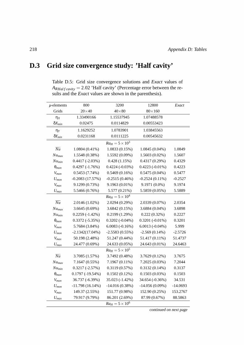
218 Appendix D: Tables
D.3 Grid size convergence study: ’Half cavity’
Table D.5: Grid size convergence solutions and Exact values ofARHal f cavity = 2.02 ’Half cavity’ (Percentage error between the re-sults and the Exact values are shown in the parenthesis).
µ-elements 800 3200 12800 Exact
Grids 20×40 40×80 80×160
ηX 1.33490166 1.15537945 1.07488578
δXmin 0.02475 0.0114829 0.00553423
ηY 1.1629252 1.0783901 1.03845563
δYmin 0.0231168 0.0111225 0.00545632
RaH = 5×10³
Nu 1.0804 (0.41%) 1.0833 (0.15%) 1.0845 (0.04%) 1.0849
Numax 1.5548 (0.38%) 1.5592 (0.09%) 1.5603 (0.02%) 1.5607
Numin 0.4417 (-2.03%) 0.428 (1.15%) 0.4317 (0.29%) 0.4329
θmon 0.4297 (-1.76%) 0.4224 (-0.03%) 0.4223 (-0.01%) 0.4223
Vmon 0.5453 (7.74%) 0.5469 (0.16%) 0.5475 (0.04%) 0.5477
Umon -0.2083 (17.57%) -0.2515 (0.46%) -0.2524 (0.11%) -0.2527
Vmax 9.1299 (0.73%) 9.1963 (0.01%) 9.1971 (0.0%) 9.1974
Umax 5.5466 (0.76%) 5.577 (0.21%) 5.5859 (0.05%) 5.5889
RaH = 5×10⁴
Nu 2.0146 (1.02%) 2.0294 (0.29%) 2.0339 (0.07%) 2.0354
Numax 3.6645 (0.69%) 3.6842 (0.15%) 3.6884 (0.04%) 3.6898
Numin 0.2259 (-1.42%) 0.2199 (1.29%) 0.222 (0.32%) 0.2227
θmon 0.3372 (-5.35%) 0.3202 (-0.04%) 0.3201 (-0.01%) 0.3201
Vmon 5.7684 (3.84%) 6.0083 (-0.16%) 6.0013 (-0.04%) 5.999
Umon -2.1342(17.04%) -2.5583 (0.55%) -2.569 (0.14%) -2.5726
Vmax 50.198 (2.48%) 51.247 (0.44%) 51.417 (0.11%) 51.4737
Umax 24.477 (0.69%) 24.633 (0.05%) 24.643 (0.01%) 24.6463
RaH = 5×10⁵
Nu 3.7085 (1.57%) 3.7492 (0.48%) 3.7629 (0.12%) 3.7675
Numax 7.1647 (0.55%) 7.1967 (0.11%) 7.2025 (0.03%) 7.2044
Numin 0.3217 (-2.57%) 0.3119 (0.57%) 0.3132 (0.14%) 0.3137
θmon 0.1797 (-19.54%) 0.1502 (0.12%) 0.1503 (0.03%) 0.1503
Vmon 36.737 (-6.39%) 35.023 (-1.42%) 34.654 (-0.36%) 34.531
Umon -11.798 (16.14%) -14.016 (0.38%) -14.056 (0.09%) -14.0693
Vmax 149.37 (2.55%) 151.77 (0.98%) 152.90 (0.25%) 153.2767
Umax 79.917 (9.79%) 86.201 (2.69%) 87.99 (0.67%) 88.5863
RaH = 5×10⁶
continued on next page
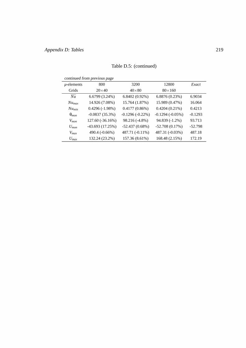
Appendix D: Tables 219
Table D.5: (continued)
continued from previous page
µ-elements 800 3200 12800 Exact
Grids 20×40 40×80 80×160
Nu 6.6799 (3.24%) 6.8402 (0.92%) 6.8876 (0.23%) 6.9034
Numax 14.926 (7.08%) 15.764 (1.87%) 15.989 (0.47%) 16.064
Numin 0.4296 (-1.98%) 0.4177 (0.86%) 0.4204 (0.21%) 0.4213
θmon -0.0837 (35.3%) -0.1296 (-0.22%) -0.1294 (-0.05%) -0.1293
Vmon 127.60 (-36.16%) 98.216 (-4.8%) 94.839 (-1.2%) 93.713
Umon -43.693 (17.25%) -52.437 (0.68%) -52.708 (0.17%) -52.798
Vmax 490.4 (-0.66%) 487.71 (-0.11%) 487.31 (-0.03%) 487.18
Umax 132.24 (23.2%) 157.36 (8.61%) 168.48 (2.15%) 172.19

220 Appendix D: Tables
Table D.6: Grid size convergence solutions and Exact values ofARHal f cavity = 2.22 ’Half cavity’ (Percentage error between the re-sults and the Exact values are shown in the parenthesis).
µ-elements 800 3200 12800 Exact
Grids 20×40 40×80 80×160
ηX 1.3568637 1.16484493 1.07927982
δXmin 0.0225 0.0103934 0.00499854
ηY 1.1629252 1.0783901 1.03845563
δYmin 0.0231168 0.0111225 0.00545632
RaH = 5×10³
Nu 1.0442 (0.36%) 1.0466 (0.13%) 1.0476 (0.03%) 1.0479
Numax 1.4209 (0.31%) 1.4242 (0.07%) 1.425 (0.02%) 1.4253
Numin 0.4903 (2.89%) 0.499 (1.16%) 0.5034 (0.29%) 0.5049
θmon 0.4291 (-3.49%) 0.429 (-3.46%) 0.4182 (-0.87%) 0.4146
Vmon 0.505 (13.21%) 0.5079 (12.71%) 0.5633 (3.18%) 0.5818
Umon -0.2061 (1.43%) -0.209 (0.06%) -0.2091 (0.01%) -0.2091
Vmax 7.8949 (0.0%) 7.8948 (0.0%) 7.8949 (0.0%) 7.8949
Umax 4.727 (0.45%) 4.7417 (0.14%) 4.7467 (0.04%) 4.7484
RaH = 5×10⁴
Nu 1.834 (0.91%) 1.846 (0.26%) 1.8496 (0.06%) 1.8508
Numax 3.4016 (0.6%) 3.4177 (0.12%) 3.4209 (0.03%) 3.422
Numin 0.2065 (3.07%) 0.2105 (1.2%) 0.2124 (0.3%) 0.213
θmon 0.331 (-10.64%) 0.3325 (-11.16%) 0.3075 (-2.79%) 0.2992
Vmon 5.9359 (7.58%) 5.9440 (7.45%) 6.3030 (1.86%) 6.4227
Umon -2.2013(27.96%) -2.2471 (26.46%) -2.8535 (6.62%) -3.0556
Vmax 49.439 (1.83%) 50.051 (0.61%) 50.283 (0.15%) 50.36
Umax 22.629 (-0.78%) 22.493 (-0.18%) 22.463 (-0.04%) 22.453
RaH = 5×10⁵
Nu 3.4073 (1.63%) 3.4475 (0.47%) 3.4598 (0.12%) 3.4639
Numax 6.5794 (1.31%) 6.6527 (0.21%) 6.6632 (0.05%) 6.6667
Numin 0.2945 (2.64%) 0.3005 (0.66%) 0.3020 (0.17%) 0.3025
θmon 0.1762 (-53.93%) 0.1747 (-52.6%) 0.1295 (-13.15%) 0.1145
Vmon 36.352 (-8.19%) 35.605 (-5.96%) 34.102 (-1.49%) 33.601
Umon -11.812 (26.96%) -12.269 (24.13%) -15.196 (6.03%) -16.172
Vmax 150.93 (2.29%) 153.97 (0.32%) 154.34 (0.08%) 154.46
Umax 84.386 (6.24%) 88.272 (1.93%) 89.572 (0.48%) 90.0
RaH = 5×10⁶
Nu 6.0789 (3.34%) 6.237 (0.83%) 6.2761 (0.21%) 6.2891
Numax 13.524 (6.9%) 14.324 (1.4%) 14.476 (0.35%) 14.527
continued on next page

Appendix D: Tables 221
Table D.6: (continued)
continued from previous page
µ-elements 800 3200 12800 Exact
Grids 20×40 40×80 80×160
Numin 0.3925 (2.9%) 0.4006 (0.9%) 0.4033 (0.23%) 0.4042
θmon -0.0806 (50.32%) -0.0891 (45.04%) -0.1439 (11.26%) -0.1622
Vmon 124.32 (-70.82%) 113.16 (-55.49%) 82.874 (-13.87%) 72.779
Umon -42.101 (26.45%) -45.347 (20.78%) -54.266 (5.19%) -57.239
Vmax 485.79 (0.18%) 481.45 (1.07%) 485.35 (0.27%) 486.65
Umax 169.65 (15.9%) 188.13 (6.74%) 198.33(1.69%) 201.73

222 Appendix D: Tables
D.4 Numerical resolutions of partitioned cavity
Table D.7: Nu of AR = 1 partitioned cavity.
σRaH 1 5 10 20 30 50 102 103 104 105
γ = 0.01, 6720µ-elements
103 1.0001 1.0001 1.0 0.9999 0.9999 0.9998 0.9997 0.9994 0.9993 0.9993
104 1.1323 1.1331 1.1306 1.126 1.1221 1.1161 1.1069 1.0872 1.0837 1.0834
105 2.1917 2.2209 2.2182 2.2078 2.1975 2.1798 2.1482 2.054 2.0321 2.0296
106 4.0078 4.1411 4.1497 4.1411 4.1282 4.1029 4.0513 3.831 3.759 3.7503
107 7.1386 7.6275 7.6837 7.6962 7.6877 7.6611 7.5939 7.147 6.8844 6.8452
γ = 0.02, 6720µ-elements
103 0.9999 0.9999 0.9998 0.9997 0.9997 0.9996 0.9995 0.9999 0.9993 0.9993
104 1.1214 1.123 1.1192 1.1126 1.1077 1.1012 1.0931 1.0805 1.0787 1.0785
105 2.1299 2.1851 2.1813 2.1651 2.1503 2.1272 2.0926 2.0226 2.0109 2.0097
106 3.8118 4.0567 4.0752 4.0635 4.0444 4.0085 3.9434 3.7596 3.7203 3.7159
107 6.5519 7.4099 7.5193 7.5488 7.5383 7.4993 7.4038 6.9545 6.7945 6.7748
γ = 0.05, 7200µ-elements
103 0.9996 0.9996 0.9995 0.9994 0.9994 0.9993 0.9992 0.9992 0.9992 0.9992
104 1.0929 1.0972 1.092 1.0849 1.0807 1.0761 1.0714 1.066 1.0654 1.0653
105 1.9658 2.083 2.0802 2.0588 2.0415 2.0187 1.9918 1.9545 1.9498 1.9493
106 3.3363 3.8218 3.8706 3.8624 3.8393 3.7987 3.7387 3.6322 3.6166 3.6149
107 5.2894 6.8189 7.0639 7.1481 7.1435 7.0961 6.983 6.6485 6.5794 6.5719
γ = 0.1, 8000µ-elements
103 0.9992 0.9993 0.9992 0.9991 0.9991 0.9991 0.9991 0.999 0.999 0.999
104 1.0575 1.0647 1.0608 1.0561 1.0537 1.0513 1.0492 1.0469 1.0467 1.0466
105 1.7455 1.9256 1.930 1.913 1.8998 1.884 1.8677 1.8485 1.8463 1.846
106 2.7821 3.4758 3.5694 3.5828 3.5692 3.5429 3.5071 3.4549 3.4483 3.4476
107 4.0418 5.9849 6.3872 6.5551 6.5751 6.5476 6.4644 6.2708 6.2405 6.2374
γ = 0.2, 6720µ-elements
103 0.9986 0.9987 0.9987 0.9987 0.9987 0.9987 0.9987 0.9987 0.9987 0.9987
104 1.0184 1.0257 1.0248 1.0234 1.0227 1.022 1.0215 1.0209 1.0209 1.0209
105 1.4278 1.6405 1.6586 1.6552 1.650 1.6436 1.6372 1.6299 1.6291 1.629
106 2.1126 2.9029 3.057 3.1171 3.1274 3.1284 3.1228 3.1112 3.1096 3.1095
107 2.778 4.6956 5.2432 5.5279 5.6002 5.6306 5.6217 5.5743 5.567 5.5662

Appendix D: Tables 223
Table D.8: NuMax along the ’Surface 1’ of AR = 1 partitioned cav-ity.
σRaH 1 5 10 20 30 50 102 103 104 105
γ = 0.01, 6720µ-elements
103 1.0733 1.0727 1.0715 1.0693 1.0677 1.0651 1.0612 1.0535 1.0522 1.0521
104 1.8358 1.8318 1.8175 1.7918 1.7704 1.7376 1.6876 1.5804 1.5613 1.5593
105 4.5877 4.6330 4.6095 4.5554 4.5057 4.4214 4.2710 3.8104 3.6980 3.6852
106 9.5851 9.8890 9.8715 9.7787 9.6829 9.5089 9.1646 7.7049 7.2314 7.1744
107 20.635 22.036 22.141 22.065 21.939 21.682 21.129 17.813 15.952 15.662
γ = 0.02, 6720µ-elements
103 1.0704 1.0694 1.0674 1.0644 1.0623 1.0595 1.0562 1.0513 1.0506 1.0506
104 1.8010 1.7945 1.7709 1.7332 1.7060 1.6696 1.6244 1.5542 1.5445 1.5434
105 4.4724 4.5583 4.5181 4.4308 4.3570 4.2442 4.0758 3.7235 3.6627 3.6561
106 9.0923 9.6504 9.6263 9.4762 9.3265 9.0712 8.6263 7.3976 7.1394 7.1111
107 18.898 21.365 21.578 21.473 21.278 20.887 20.097 16.791 15.634 15.484
γ = 0.05, 7200µ-elements
103 1.0621 1.0607 1.0579 1.0545 1.0526 1.0507 1.0487 1.0464 1.0461 1.0461
104 1.7036 1.6950 1.6599 1.6154 1.5898 1.5617 1.5339 1.5013 1.4976 1.4972
105 4.1675 4.3513 4.2836 4.1524 4.0583 3.9383 3.7977 3.5973 3.5713 3.5686
106 7.8978 8.9983 8.9820 8.7492 8.5344 8.2142 7.7792 7.0460 6.9412 6.9305
107 15.164 19.573 20.083 19.986 19.698 19.138 18.155 15.606 15.064 15.003
γ = 0.1, 8000µ-elements
103 1.0499 1.0492 1.0466 1.0440 1.0428 1.0415 1.0406 1.0394 1.0393 1.0393
104 1.5614 1.5590 1.5253 1.4904 1.4732 1.4563 1.4413 1.4258 1.4242 1.4240
105 3.7594 4.0436 3.9655 3.8272 3.7411 3.6444 3.5471 3.4315 3.4181 3.4168
106 6.5193 8.0642 8.0947 7.8579 7.6566 7.3926 7.0910 6.6967 6.6491 6.6443
107 11.478 17.072 17.953 17.968 17.676 17.115 16.234 14.507 14.229 14.2
γ = 0.2, 6720µ-elements
103 1.0310 1.0322 1.0308 1.0296 1.0291 1.0286 1.0282 1.0277 1.0277 1.0277
104 1.3415 1.3576 1.3393 1.3223 1.3148 1.3079 1.3021 1.2964 1.2958 1.2957
105 3.1453 3.4940 3.4302 3.3238 3.2643 3.2033 3.1472 3.0872 3.0806 3.0799
106 4.9422 6.6224 6.7707 6.6651 6.5568 6.4233 6.2854 6.1205 6.1014 6.0995
107 7.71 13.218 14.444 14.701 14.527 14.134 13.549 12.63 12.51 12.498

224 Appendix D: Tables
Table D.9: NuMin along the ’Surface 1’ of AR = 1 partitioned cavity.
σRaH 1 5 10 20 30 50 102 103 104 105
γ = 0.01, 6720µ-elements
103 0.652 0.6523 0.6531 0.6544 0.6554 0.657 0.6593 0.664 0.6648 0.6649
104 0.3834 0.3845 0.3871 0.3916 0.3953 0.401 0.4094 0.4268 0.4299 0.4302
105 0.1941 0.1968 0.1979 0.1995 0.2008 0.2029 0.2065 0.2176 0.2205 0.2209
106 0.2465 0.2536 0.2555 0.2582 0.2604 0.2642 0.2718 0.3045 0.3156 0.317
107 0.3068 0.3239 0.3272 0.3304 0.3327 0.3367 0.3447 0.3919 0.4176 0.4215
γ = 0.02, 6720µ-elements
103 0.6538 0.6544 0.6556 0.6574 0.6587 0.6604 0.6625 0.6655 0.6659 0.6659
104 0.3901 0.3920 0.3963 0.403 0.4078 0.4141 0.4218 0.4335 0.4351 0.4353
105 0.1898 0.1948 0.1967 0.1993 0.2012 0.2040 0.2081 0.2168 0.2183 0.2185
106 0.2375 0.2507 0.2545 0.2593 0.2630 0.2690 0.2792 0.3074 0.3136 0.3143
107 0.2861 0.3169 0.3231 0.3292 0.3334 0.3401 0.3522 0.3997 0.4156 0.4176
γ = 0.05, 7200µ-elements
103 0.6697 0.6706 0.6724 0.6745 0.6757 0.6769 0.6782 0.6796 0.6797 0.6798
104 0.4177 0.4204 0.4274 0.4361 0.4409 0.4462 0.4514 0.4575 0.4582 0.4582
105 0.1817 0.1918 0.1956 0.1998 0.2023 0.2055 0.2091 0.2142 0.2149 0.215
106 0.2178 0.246 0.2544 0.2638 0.2701 0.2785 0.2895 0.3078 0.3105 0.3108
107 0.2443 0.3026 0.3167 0.3295 0.3377 0.3491 0.3658 0.4041 0.4116 0.4124
γ = 0.1, 8000µ-elements
103 0.6961 0.6966 0.6983 0.7 0.7008 0.7016 0.7023 0.703 0.7031 0.7031
104 0.4673 0.4683 0.4762 0.4841 0.488 0.4918 0.4951 0.4985 0.4989 0.4989
105 0.1749 0.1884 0.1937 0.1987 0.2014 0.2042 0.207 0.2102 0.2106 0.2106
106 0.1931 0.2377 0.2517 0.2653 0.2729 0.2816 0.2908 0.3024 0.3038 0.304
107 0.2024 0.2817 0.3054 0.3262 0.338 0.3525 0.3701 0.3986 0.4028 0.4032
γ = 0.2, 6720µ-elements
103 0.6954 0.6946 0.6955 0.6964 0.6967 0.6971 0.6973 0.6976 0.6976 0.6976
104 0.5342 0.5275 0.5327 0.5376 0.5398 0.5417 0.5434 0.545 0.5452 0.5452
105 0.176 0.1799 0.1847 0.189 0.191 0.1929 0.1946 0.1964 0.1966 0.1966
106 0.1399 0.1983 0.2178 0.2338 0.2411 0.2483 0.2546 0.2613 0.262 0.2621
107 0.1456 0.2266 0.2587 0.2866 0.3009 0.3162 0.3318 0.3510 0.3533 0.3535

Appendix D: Tables 225
Table D.10: θmon of AR = 1 partitioned cavity.
σRaH 1 5 10 20 30 50 102 103 104 105
γ = 0.01, 6720µ-elements
103 0.4737 0.4735 0.4735 0.4736 0.4736 0.4737 0.4737 0.4739 0.474 0.474
104 0.4551 0.4548 0.4551 0.4558 0.4563 0.4571 0.4584 0.4611 0.4615 0.4616
105 0.3892 0.3872 0.3877 0.389 0.3902 0.3924 0.3961 0.4078 0.4107 0.411
106 0.2732 0.2644 0.2646 0.2666 0.2688 0.2727 0.2807 0.3147 0.3259 0.3272
107 0.1032 0.0761 0.0738 0.0748 0.0768 0.081 0.0903 0.1485 0.1829 0.1883
γ = 0.02, 6720µ-elements
103 0.4738 0.4734 0.4734 0.4734 0.4735 0.4735 0.4736 0.4737 0.4737 0.4737
104 0.4559 0.4554 0.4559 0.4568 0.4575 0.4584 0.4595 0.4613 0.4616 0.4616
105 0.3919 0.3881 0.3889 0.3911 0.3929 0.3957 0.4 0.409 0.4106 0.4108
106 0.2846 0.2681 0.2682 0.2714 0.2749 0.2808 0.2911 0.3202 0.3263 0.327
107 0.1331 0.0846 0.08 0.0812 0.0844 0.0909 0.1045 0.1642 0.1859 0.1887
γ = 0.05, 7200µ-elements
103 0.4748 0.4738 0.4737 0.4737 0.4737 0.4738 0.4738 0.4738 0.4739 0.4739
104 0.4596 0.4581 0.4588 0.4598 0.4604 0.4611 0.4618 0.4626 0.4627 0.4627
105 0.4022 0.3938 0.395 0.3981 0.4004 0.4034 0.407 0.412 0.4127 0.4128
106 0.3175 0.2843 0.2835 0.2884 0.2932 0.3006 0.3108 0.3283 0.3308 0.331
107 0.2049 0.1148 0.1038 0.1044 0.1092 0.1188 0.1365 0.184 0.1942 0.1954
γ = 0.1, 8000µ-elements
103 0.4764 0.4743 0.4741 0.474 0.474 0.474 0.474 0.474 0.474 0.474
104 0.4649 0.4619 0.4623 0.463 0.4634 0.4638 0.4641 0.4644 0.4645 0.4645
105 0.4163 0.4024 0.4033 0.4063 0.4083 0.4107 0.4130 0.4159 0.4162 0.4163
106 0.3562 0.3077 0.3049 0.3093 0.3138 0.3198 0.3269 0.3363 0.3374 0.3375
107 0.2793 0.1586 0.1391 0.137 0.1419 0.1519 0.1683 0.2011 0.2063 0.2069
γ = 0.2, 6720µ-elements
103 0.4753 0.4705 0.4698 0.4695 0.4694 0.4693 0.4692 0.4692 0.4692 0.4692
104 0.4678 0.4612 0.4608 0.4609 0.4609 0.461 0.4611 0.4612 0.4612 0.4612
105 0.4251 0.4013 0.4009 0.4029 0.4043 0.4058 0.4073 0.4089 0.4091 0.4091
106 0.3837 0.3159 0.3073 0.308 0.3103 0.3135 0.3171 0.3215 0.3221 0.3221
107 0.3393 0.1932 0.1607 0.1517 0.1542 0.1617 0.1736 0.1922 0.1945 0.1948

226 Appendix D: Tables
Table D.11: ~Vmon of AR = 1 partitioned cavity.
σRaH 1 5 10 20 30 50 102 103 104 105
γ = 0.01, 6720µ-elements
103 0.0441 0.0444 0.0444 0.0444 0.0443 0.0442 0.0441 0.0437 0.0437 0.0437
104 0.6184 0.6216 0.6180 0.6108 0.6047 0.5952 0.5806 0.5486 0.5429 0.5423
105 6.9141 6.9947 6.9734 6.9175 6.8651 6.7753 6.6144 6.1083 5.9811 5.9664
106 41.531 42.298 42.261 42.044 41.818 41.403 40.562 36.491 34.949 34.757
107 105.99 106.88 106.9 106.78 106.65 106.4 105.88 102.37 99.253 98.489
γ = 0.02, 6720µ-elements
103 0.0438 0.0445 0.0445 0.0444 0.0443 0.0442 0.0441 0.0439 0.0439 0.0439
104 0.6083 0.615 0.6092 0.5986 0.5908 0.5801 0.5666 0.5454 0.5424 0.5421
105 6.8068 6.9644 6.9294 6.8396 6.7617 6.6409 6.4575 6.065 5.9953 5.9878
106 40.458 41.924 41.876 41.518 41.155 40.521 39.364 35.701 34.841 34.745
107 104.76 106.58 106.65 106.48 106.27 105.89 105.13 101.1 98.672 98.236
γ = 0.05, 7200µ-elements
103 0.0419 0.0436 0.0437 0.0436 0.0436 0.0436 0.0435 0.0434 0.0434 0.0434
104 0.5661 0.5841 0.5763 0.5642 0.5569 0.5486 0.5403 0.5305 0.5293 0.5292
105 6.4397 6.8075 6.7554 6.6227 6.5226 6.3915 6.2344 6.0064 5.9762 5.9731
106 37.913 41.236 41.224 40.617 40.033 39.125 37.804 35.378 35.014 34.976
107 106.4 111.96 112.36 112.14 111.76 111.06 109.74 105.09 103.4 103.19
γ = 0.1, 8000µ-elements
103 0.0388 0.0421 0.0424 0.0425 0.0426 0.0426 0.0426 0.0426 0.0426 0.0426
104 0.5014 0.5392 0.534 0.5258 0.5213 0.5167 0.5125 0.508 0.5075 0.5075
105 5.9122 6.5709 6.5291 6.3947 6.303 6.1958 6.0845 5.9496 5.9336 5.932
106 34.36 40.048 40.213 39.513 38.87 37.995 36.958 35.551 35.376 35.358
107 107.43 120.17 121.5 121.37 120.8 119.7 117.84 112.56 111.35 111.22
γ = 0.2, 6720µ-elements
103 0.0378 0.0449 0.046 0.0465 0.0466 0.0468 0.0469 0.0469 0.047 0.047
104 0.4469 0.5296 0.5347 0.5344 0.5337 0.5327 0.5318 0.5308 0.5307 0.5307
105 5.499 6.6492 6.673 6.5834 6.5202 6.4501 6.3825 6.3074 6.299 6.2982
106 29.058 36.976 37.666 37.394 37.056 36.626 36.174 35.645 35.5840 35.578
107 88.138 104.67 106.37 105.91 105.0 103.44 101.04 96.601 95.976 95.912

Appendix D: Tables 227
Table D.12: ~Umon of AR = 1 partitioned cavity.
σRaH 1 5 10 20 30 50 102 103 104 105
γ = 0.01, 6720µ-elements
103 -0.0205 -0.0207 -0.0207 -0.0206 -0.0206 -0.0206 -0.0205 -0.0204 -0.0203 -0.0203
104 -0.2798 -0.2813 -0.2797 -0.2766 -0.2740 -0.2699 -0.2635 -0.2496 -0.2471 -0.2468
105 -2.8697 -2.9026 -2.8951 -2.8743 -2.8546 -2.8206 -2.7595 -2.5646 -2.5149 -2.5092
106 -16.249 -16.564 -16.551 -16.467 -16.377 -16.212 -15.878 -14.301 -13.738 -13.67
107 -58.883 -60.752 -60.92 -60.878 -60.76 -60.496 -59.875 -55.192 -51.479 -50.764
γ = 0.02, 6720µ-elements
103 -0.0204 -0.0207 -0.0207 -0.0206 -0.0206 -0.0206 -0.0205 -0.0204 -0.0204 -0.0204
104 -0.2751 -0.2782 -0.2757 -0.2711 -0.2677 -0.263 -0.2572 -0.2479 -0.2466 -0.2465
105 -2.8279 -2.8924 -2.8799 -2.8464 -2.8169 -2.7709 -2.7007 -2.5486 -2.5212 -2.5183
106 -15.814 -16.412 -16.396 -16.256 -16.113 -15.863 -15.408 -14.0220 -13.715 -13.681
107 -56.761 -60.186 -60.521 -60.464 -60.265 -59.825 -58.851 -53.5740 -50.996 -50.613
γ = 0.05, 7200µ-elements
103 -0.0188 -0.0195 -0.0195 -0.0195 -0.0195 -0.0195 -0.0195 -0.0194 -0.0194 -0.0194
104 -0.2473 -0.2551 -0.2519 -0.2468 -0.2437 -0.2403 -0.2368 -0.2326 -0.2321 -0.2321
105 -2.579 -2.7229 -2.7055 -2.6576 -2.621 -2.5727 -2.5143 -2.4287 -2.4173 -2.4161
106 -14.028 -15.278 -15.28 -15.063 -14.852 -14.526 -14.059 -13.239 -13.121 -13.109
107 -49.814 -56.471 -57.251 -57.214 -56.873 -56.139 -54.696 -49.87 -48.533 -48.375
γ = 0.1, 8000µ-elements
103 -0.0163 -0.0176 -0.0178 -0.0178 -0.0179 -0.0179 -0.0179 -0.0179 -0.0179 -0.0179
104 -0.2059 -0.2213 -0.2193 -0.2161 -0.2143 -0.2125 -0.2109 -0.2091 -0.2089 -0.2089
105 -2.2229 -2.4624 -2.4503 -2.4049 -2.3734 -2.3362 -2.2973 -2.2497 -2.244 -2.2435
106 -11.6600 -13.5520 -13.622 -13.412 -13.217 -12.9540 -12.6490 -12.252 -12.204 -12.199
107 -41.3740 -50.6920 -52.010 -52.06 -51.627 -50.7250 -49.1570 -45.404 -44.70 -44.625
γ = 0.2, 6720µ-elements
103 -0.0166 -0.0197 -0.0201 -0.0204 -0.0204 -0.0205 -0.0205 -0.0206 -0.0206 -0.0206
104 -0.1939 -0.2295 -0.2317 -0.2317 -0.2314 -0.231 -0.2306 -0.2302 -0.2302 -0.2302
105 -2.25 -2.7086 -2.7208 -2.6878 -2.6637 -2.6368 -2.6107 -2.5815 -2.5782 -2.5779
106 -11.086 -14.103 -14.427 -14.401 -14.319 -14.208 -14.088 -13.946 -13.929 -13.928
107 -37.331 -50.831 -53.167 -53.42 -52.89 -51.839 -50.268 -47.769 -47.455 -47.423

228 Appendix D: Tables
Table D.13: ~Vmax along the mid-plane of the hot cell (Y = 0) ofAR = 1 partitioned cavity.
σRaH 1 5 10 20 30 50 102 103 104 105
γ = 0.01, 6720µ-elements
103 0.9473 0.955 0.956 0.9566 0.9568 0.957 0.9572 0.9575 0.9575 0.9575
104 8.7244 8.8144 8.8429 8.8806 8.9095 8.9532 9.0199 9.1656 9.1919 9.1948
105 42.776 43.378 43.626 44.021 44.368 44.971 46.102 49.994 51.029 51.149
106 128.43 130.67 131.17 131.8 132.34 133.33 135.42 146.12 150.72 151.34
107 402.18 414.9 416.89 418.5 419.63 421.66 426.35 461.77 482.37 485.25
γ = 0.02, 6720µ-elements
103 0.9215 0.9365 0.9385 0.9395 0.9399 0.9402 0.9405 0.9408 0.9408 0.9408
104 8.5195 8.6932 8.7432 8.8005 8.8383 8.8875 8.9483 9.0428 9.056 9.0574
105 42.166 43.346 43.827 44.536 45.106 45.99 47.369 50.47 51.036 51.097
106 125.99 130.28 131.30 132.55 133.56 135.26 138.32 148.43 151.17 151.49
107 388.14 411.77 415.80 419.19 421.57 425.62 433.82 471.27 483.69 485.16
γ = 0.05, 7200µ-elements
103 0.8451 0.8804 0.8851 0.8875 0.8883 0.889 0.8895 0.89 0.89 0.89
104 7.9065 8.2977 8.3884 8.4653 8.5038 8.5438 8.5822 8.626 8.631 8.6316
105 40.302 43.077 44.1330 45.425 46.274 47.35 48.626 50.476 50.721 50.746
106 119.88 129.64 132.16 134.94 136.87 139.57 143.38 150.89 152.15 152.28
107 352.64 402.12 412.07 420.61 426.12 434.19 446.87 477.29 482.92 483.53
γ = 0.1, 8000µ-elements
103 0.7251 0.7882 0.797 0.8014 0.8029 0.8041 0.805 0.8059 0.8059 0.8059
104 6.907 7.5744 7.7 7.7815 7.8143 7.8436 7.868 7.892 7.8946 7.8948
105 37.56 42.481 44.191 45.89 46.806 47.791 48.758 49.881 50.01 50.023
106 111.55 128.48 133.15 137.69 140.36 143.59 147.30 152.64 153.35 153.42
107 318.75 386.98 404.73 420.29 429.15 440.24 454.04 476.11 479.22 479.54
γ = 0.2, 6720µ-elements
103 0.5146 0.6127 0.6276 0.6354 0.638 0.6402 0.6418 0.6432 0.6433 0.6434
104 5.0342 6.0266 6.1928 6.2837 6.3156 6.3418 6.362 6.3805 6.3823 6.3825
105 31.78 39.675 42.106 44.033 44.888 45.692 46.386 47.093 47.169 47.176
106 102.19 126.9 134.51 141.23 144.68 148.32 151.90 156.09 156.58 156.63
107 271.62 369.09 400.34 425.28 437.62 450.75 463.93 480.17 482.17 482.37

Appendix D: Tables 229
Table D.14: ~Umax along the center of the hot cell (X = −DH/2) ofAR = 1 partitioned cavity.
σRaH 1 5 10 20 30 50 102 103 104 105
γ = 0.01, 6720µ-elements
103 0.5825 0.5877 0.5889 0.5903 0.5912 0.5926 0.5946 0.5985 0.5992 0.5993
104 4.7009 4.77 4.8173 4.8933 4.9549 5.0494 5.1942 5.5109 5.5688 5.5751
105 19.565 19.854 20.042 20.351 20.614 21.049 21.797 24.035 24.583 24.646
106 61.81 62.541 63.05 63.929 64.706 66.055 68.65 80.085 84.382 84.948
107 89.795 90.111 90.878 92.307 93.567 95.732 99.982 125.57 142.99 145.77
γ = 0.02, 6720µ-elements
103 0.5655 0.5756 0.5778 0.5799 0.5811 0.5826 0.5844 0.5869 0.5873 0.5873
104 4.5988 4.7296 4.8096 4.9225 5.0021 5.1078 5.2425 5.4533 5.4828 5.4859
105 19.221 19.78 20.12 20.627 21.015 21.583 22.405 24.089 24.383 24.415
106 61.911 63.415 64.356 65.872 67.144 69.221 72.728 82.909 85.407 85.697
107 91.604 92.371 93.717 96.098 98.115 101.47 107.77 136.49 147.99 149.43
γ = 0.05, 7200µ-elements
103 0.5161 0.539 0.5433 0.5463 0.5477 0.549 0.5502 0.5515 0.5517 0.5517
104 4.2931 4.5759 4.7086 4.8515 4.9303 5.0155 5.0996 5.1976 5.2089 5.21
105 18.232 19.465 20.098 20.876 21.365 21.96 22.631 23.56 23.681 23.693
106 61.192 65.212 67.265 70.093 72.125 74.942 78.744 85.728 86.854 86.974
107 96.853 99.175 101.95 106.67 110.50 116.56 126.32 153.61 159.64 160.3
γ = 0.1, 8000µ-elements
103 0.4398 0.4797 0.4862 0.4901 0.4916 0.4929 0.4939 0.4948 0.4949 0.495
104 3.7895 4.242 4.3964 4.5249 4.5834 4.639 4.6873 4.7369 4.7422 4.7427
105 16.757 18.785 19.658 20.531 20.989 21.475 21.945 22.483 22.544 22.551
106 58.981 67.241 70.614 74.514 76.921 79.83 83.127 87.742 88.346 88.408
107 106.25 112.52 117.6 125.57 131.57 140.29 152.49 175.12 178.73 179.12
γ = 0.2, 6720µ-elements
103 0.3097 0.3698 0.3795 0.3847 0.3865 0.388 0.3892 0.3902 0.3903 0.3903
104 2.828 3.4523 3.6001 3.6962 3.7335 3.7657 3.7915 3.8161 3.8186 3.8188
105 14.281 17.317 18.373 19.224 19.60 19.952 20.253 20.559 20.592 20.595
106 46.004 61.022 66.234 71.021 73.442 75.946 78.329 81.017 81.323 81.353
107 103.44 124.82 136.28 149.68 158.14 168.5 181.12 198.53 200.78 201.01

230
App
endi
xD
:Ta
bles
Table D.15: ∆θw,Horizontal at horizontal mid-plane (Y = 0) of AR = 1 partitioned cavity.
σRaH 1 5 10 20 30 50 102 103 104 105
γ = 0.01, 6720µ-elements
103 1.00E-02 2.02E-03 1.01E-03 5.07E-04 3.38E-04 2.03E-04 1.01E-04 1.01E-05 1.01E-06 1.01E-07
104 1.28E-02 2.58E-03 1.28E-03 6.32E-04 4.16E-04 2.45E-04 1.19E-04 1.10E-05 1.09E-06 1.09E-07
105 2.73E-02 5.62E-03 2.81E-03 1.40E-03 9.22E-04 5.43E-04 2.60E-04 2.17E-05 2.05E-06 2.03E-07
106 4.61E-02 9.69E-03 4.87E-03 2.44E-03 1.62E-03 9.64E-04 4.70E-04 3.93E-05 3.61E-06 3.57E-07
107 7.83E-02 1.71E-02 8.63E-03 4.34E-03 2.89E-03 1.73E-03 8.58E-04 7.38E-05 6.47E-06 6.32E-07
γ = 0.02, 6720µ-elements
103 2.01E-02 4.08E-03 2.04E-03 1.02E-03 6.81E-04 4.09E-04 2.04E-04 2.04E-05 2.04E-06 2.04E-07
104 2.50E-02 5.10E-03 2.52E-03 1.24E-03 8.11E-04 4.76E-04 2.31E-04 2.20E-05 2.18E-06 2.18E-07
105 5.25E-02 1.11E-02 5.55E-03 2.73E-03 1.79E-03 1.04E-03 4.91E-04 4.21E-05 4.07E-06 4.06E-07
106 8.68E-02 1.91E-02 9.65E-03 4.82E-03 3.19E-03 1.88E-03 8.99E-04 7.55E-05 7.19E-06 7.14E-07
107 1.42E-01 3.34E-02 1.70E-02 8.60E-03 5.73E-03 3.42E-03 1.67E-03 1.39E-04 1.28E-05 1.26E-06
γ = 0.05, 7200µ-elements
103 5.01E-02 1.04E-02 5.25E-03 2.63E-03 1.75E-03 1.05E-03 5.27E-04 5.27E-05 5.27E-06 5.27E-07
104 5.95E-02 1.24E-02 6.13E-03 3.00E-03 1.97E-03 1.16E-03 5.70E-04 5.57E-05 5.56E-06 5.56E-07
105 1.18E-01 2.68E-02 1.33E-02 6.46E-03 4.18E-03 2.40E-03 1.13E-03 1.03E-04 1.01E-05 1.01E-06
106 1.86E-01 4.58E-02 2.33E-02 1.16E-02 7.57E-03 4.39E-03 2.08E-03 1.83E-04 1.79E-05 1.79E-06
107 2.82E-01 7.82E-02 4.11E-02 2.09E-02 1.39E-02 8.17E-03 3.91E-03 3.31E-04 3.17E-05 3.16E-06
γ = 0.1, 8000µ-elements
103 1.00E-01 2.18E-02 1.10E-02 5.53E-03 3.69E-03 2.22E-03 1.11E-03 1.11E-04 1.11E-05 1.11E-06
104 1.12E-01 2.44E-02 1.21E-02 5.97E-03 3.95E-03 2.35E-03 1.16E-03 1.15E-04 1.15E-05 1.15E-06
105 2.03E-01 5.04E-02 2.51E-02 1.20E-02 7.78E-03 4.48E-03 2.14E-03 2.02E-04 2.00E-05 2.00E-06
106 3.02E-01 8.53E-02 4.42E-02 2.18E-02 1.42E-02 8.24E-03 3.93E-03 3.63E-04 3.59E-05 3.58E-06
107 4.25E-01 1.42E-01 7.71E-02 3.96E-02 2.63E-02 1.54E-02 7.32E-03 6.48E-04 6.34E-05 6.32E-06
γ = 0.2, 6720µ-elements
103 2.00E-01 4.76E-02 2.44E-02 1.23E-02 8.27E-03 4.98E-03 2.49E-03 2.50E-04 2.50E-05 2.50E-06
104 2.07E-01 4.97E-02 2.53E-02 1.27E-02 8.47E-03 5.08E-03 2.54E-03 2.54E-04 2.54E-05 2.54E-06
105 3.16E-01 8.90E-02 4.49E-02 2.18E-02 1.42E-02 8.31E-03 4.05E-03 3.93E-04 3.91E-05 3.91E-06
106 4.48E-01 1.51E-01 8.05E-02 4.04E-02 2.66E-02 1.56E-02 7.57E-03 7.28E-04 7.24E-05 7.24E-06
107 5.76E-01 2.39E-01 1.37E-01 7.24E-02 4.83E-02 2.85E-02 1.38E-02 1.29E-03 1.27E-04 1.27E-05

Appendix
D:
Tables231
Table D.16: ∆θw,Vertical along the ’Surface 2’ (X = −γ/2) of AR = 1 partitioned cavity.
σRaH 1 5 10 20 30 50 102 103 104 105
γ = 0.01, 6720µ-elements
103 2.95E-02 2.84E-02 2.67E-02 2.38E-02 2.14E-02 1.78E-02 1.26E-02 2.00E-03 2.12E-04 2.14E-05
104 2.37E-01 2.30E-01 2.17E-01 1.96E-01 1.78E-01 1.51E-01 1.09E-01 1.83E-02 1.96E-03 1.97E-04
105 4.51E-01 4.42E-01 4.24E-01 3.94E-01 3.69E-01 3.29E-01 2.62E-01 5.84E-02 6.69E-03 6.78E-04
106 5.00E-01 4.95E-01 4.76E-01 4.45E-01 4.22E-01 3.86E-01 3.25E-01 9.40E-02 1.18E-02 1.21E-03
107 5.43E-01 5.46E-01 5.27E-01 4.98E-01 4.77E-01 4.45E-01 3.91E-01 1.50E-01 2.19E-02 2.29E-03
γ = 0.02, 6720µ-elements
103 2.79E-02 2.59E-02 2.32E-02 1.90E-02 1.61E-02 1.23E-02 7.75E-03 1.01E-03 1.04E-04 1.05E-05
104 2.27E-01 2.13E-01 1.92E-01 1.60E-01 1.38E-01 1.07E-01 6.91E-02 9.34E-03 9.68E-04 9.72E-05
105 4.37E-01 4.22E-01 3.93E-01 3.48E-01 3.13E-01 2.63E-01 1.89E-01 3.15E-02 3.38E-03 3.41E-04
106 4.74E-01 4.70E-01 4.43E-01 4.02E-01 3.71E-01 3.25E-01 2.53E-01 5.30E-02 5.99E-03 6.07E-04
107 5.01E-01 5.16E-01 4.93E-01 4.57E-01 4.31E-01 3.91E-01 3.26E-01 9.08E-02 1.12E-02 1.15E-03
γ = 0.05, 7200µ-elements
103 2.34E-02 2.01E-02 1.61E-02 1.15E-02 8.87E-03 6.11E-03 3.44E-03 3.87E-04 3.92E-05 3.93E-06
104 1.97E-01 1.72E-01 1.40E-01 1.02E-01 7.98E-02 5.57E-02 3.18E-02 3.64E-03 3.69E-04 3.70E-05
105 3.99E-01 3.75E-01 3.29E-01 2.64E-01 2.21E-01 1.67E-01 1.04E-01 1.33E-02 1.37E-03 1.38E-04
106 4.13E-01 4.17E-01 3.79E-01 3.23E-01 2.83E-01 2.28E-01 1.55E-01 2.31E-02 2.43E-03 2.45E-04
107 4.10E-01 4.55E-01 4.30E-01 3.85E-01 3.51E-01 3.01E-01 2.25E-01 4.17E-02 4.58E-03 4.62E-04
γ = 0.1, 8000µ-elements
103 1.74E-02 1.38E-02 9.99E-03 6.39E-03 4.69E-03 3.06E-03 1.64E-03 1.75E-04 1.76E-05 1.76E-06
104 1.53E-01 1.24E-01 9.14E-02 5.94E-02 4.39E-02 2.89E-02 1.56E-02 1.67E-03 1.68E-04 1.68E-05
105 3.48E-01 3.20E-01 2.62E-01 1.91E-01 1.50E-01 1.05E-01 6.00E-02 6.88E-03 6.98E-04 7.00E-05
106 3.42E-01 3.59E-01 3.15E-01 2.51E-01 2.08E-01 1.56E-01 9.56E-02 1.21E-02 1.24E-03 1.25E-04
107 3.20E-01 3.90E-01 3.67E-01 3.17E-01 2.78E-01 2.24E-01 1.51E-01 2.21E-02 2.32E-03 2.33E-04
γ = 0.2, 6720µ-elements
103 9.15E-03 7.07E-03 4.74E-03 2.82E-03 2.00E-03 1.27E-03 6.60E-04 6.86E-05 6.89E-06 6.89E-07
104 8.63E-02 6.75E-02 4.57E-02 2.74E-02 1.95E-02 1.24E-02 6.46E-03 6.73E-04 6.76E-05 6.76E-06
105 2.70E-01 2.46E-01 1.86E-01 1.23E-01 9.17E-02 6.07E-02 3.28E-02 3.55E-03 3.57E-04 3.58E-05
106 2.63E-01 2.89E-01 2.44E-01 1.79E-01 1.41E-01 9.91E-02 5.66E-02 6.50E-03 6.60E-04 6.61E-05
107 2.29E-01 3.12E-01 2.92E-01 2.40E-01 2.02E-01 1.52E-01 9.33E-02 1.17E-02 1.20E-03 1.21E-04

Appendix E
Nusselt number correlations for AR = 1
and 2 non-partitioned cavity cases
In general, the Nusselt number used to explain the heat transfer characteristics and can
be expressed as the power function of the Rayleigh numbers (i.e. Nu = c ·RaaH where c is
the slope and a is the intercept). By using least square method, both slope and intercept are
found and the correlation are
Nu = 0.1502Ra0.2933 for AR = 1, (E.1a)
Nu = 0.1043Ra0.2731 for AR = 2. (E.1b)
Considering both AR and RaH as the variables, a fitted correlation is
Nu = 0.1633A−1R Ra0.2890. (E.2)
Above correlations are valid in the range of 103 ≤ RaH ≤ 107 for AR = 1 and 104 ≤ RaH ≤107 for AR = 2. The comparison between resolutions and correlations are shown in table
E.1 and figure E.1. Note that for the AR = 2 non-partitioned cavity, RaH = 103 case is not
considered since it is in conductive heat transfer regime. Also the correlations are based on
the grid size independent Exact values (e.g. NuExact).
232

Appendix E: Nusselt number correlations for AR = 1 and 2 non-partitioned cavity cases233
Table E.1: NuExact and correlation values for AR = 1 and 2 non-
partitioned cavity at various RaH .
RaH
103 104 105 106 107
AR = 1 resolution 1.1172 2.2438 4.5196 8.8202 16.5043
Nu = 0.1502Ra0.2933 1.1391 2.2381 4.3971 8.6391 16.9734
Nu = 0.1633A−1R Ra0.2890 1.2022 2.3388 4.5497 8.8509 17.2181
AR = 2 resolution 1.0037 1.2588 2.4998 4.5580 8.379
Nu = 0.1043Ra0.2731 - 1.2903 2.4198 4.5382 8.5111
Nu = 0.1633A−1R Ra0.2890 - 1.1694 2.2749 4.4254 8.6091
103
104
105
106
107
Rayleigh number (RaH)
1
10
Ave
rage
Nus
selt
num
ber
(Nu)
AR = 1.0 resolutionNu = 0.1502Ra
0.2933
AR = 2.0 resolutionNu = 0.1043Ra
0.2731
Nu = 0.1633AR
−1Ra
0.2890
Figure E.1: NuExact and correlations for AR = 1 and 2 non-
partitioned cavity at various RaH (Figure of table E.1).

Appendix F
Development of an asymptotic low Mach
model
In the asymptotic low Mach model, the flow variables can be expanded into the power
series of Ma in low Mach asymptotic analysis. For example, the pressure, temperature,
density and velocity terms may developed as
p∗(~X , t∗,Ma) = p∗(0)(~X , t∗)+ Ma p∗(1)(~X , t∗)+ Ma2
p∗(2)(~X , t∗)+O(Ma(3)
)+ · · · ,
T ∗(~X , t∗,Ma) = T ∗(0)(~X , t∗)+ MaT ∗(1)(~X , t∗)+ Ma2
T ∗(2)(~X , t∗)+O(Ma(3)
)+ · · · ,
ρ∗(~X , t∗,Ma) = ρ∗(0)(~X , t∗)+ Maρ∗(1)(~X , t∗)+ Ma2
ρ∗(2)(~X , t∗)+O(Ma(3)
)+ · · · ,
~u∗(~X , t∗,Ma) =~u∗(0)(~X , t∗)+ Ma~u∗(1)(~X , t∗)+ Ma2~u∗(2)(~X , t∗)+O(Ma
(3))+ · · · .
(F.1)
where the superscript (0) denotes the zeroth (leading)-order, (1) and (2) denote the first and
the second-order, respectively. Also the multiplied variables such as ρ∗~u∗ may developed
as
ρ∗~u∗ =(ρ∗~u∗)(0) + Ma(ρ∗~u∗)(1) + Ma2(ρ∗~u∗)(2) +O(Ma
(3))
=[ρ∗(0) + Maρ∗(1) + Ma
2ρ∗(2) +O(Ma
(3))]+[~u∗(0) + Ma~u∗(1) + Ma
2~u∗(2) +O(Ma
(3))]
=ρ∗(0)~u∗(0) + Ma(ρ∗(0)~u∗(1) +ρ∗(1)~u∗(0))
+ Ma2(ρ∗(0)~u∗(2) +ρ∗(1)~u∗(1) +ρ∗(2)~u∗(0))+O(Ma
(3))
(F.2)
234

Appendix F: Development of an asymptotic low Mach model 235
Substituting the developed variables into equation (8.4a), the Mach number asymptotic
continuity equation becomes [76]
∂ρ∗(0)
∂t∗+∇ · (ρ∗(0)~u∗(0))
+ Ma
[∂ρ∗(1)
∂t∗+∇ · (ρ∗(0)~u∗(1) +ρ∗(1)~u∗(0))
]
+ Ma2[
∂ρ∗(2)
∂t∗+∇ · (ρ∗(0)~u∗(2) +ρ∗(1)~u∗(1) +ρ∗(2)~u∗(0))
]
+O(Ma(3)
) = 0.
(F.3)
As shown in equation (8.4b), the Mach number of order -2 (i.e. O(Ma(−2)
)) is already exist
in the pressure gradient term, 1/Ma2∇p∗. In order to obtain the pressure order of p∗(0) and
p∗(1), the Mach number asymptotic equation of order O(Ma(−2)
) and O(Ma(−1)
) must be
considered. Then equation (8.4b) becomes
1
Ma2 ∇p∗(0)
+1
Ma∇p∗(1)
+∂ρ∗(0)~u∗(0)
∂t∗+∇ ·ρ∗(0)~u∗(0)~u∗(0) +∇p∗(2)− 1
Re∞∇ · ¯τ∗(0)− 1
Fr2∞
ρ∗(0)(−~e)
+ Ma
[∂(ρ∗(0)~u∗(1) +ρ∗(1)~u∗(0))
∂t∗+∇ · (ρ∗(0)~u∗(0)~u∗(1) +ρ∗(0)~u∗(1)~u∗(0)
+ρ∗(1)~u∗(0)~u∗(0))+∇p∗(3)− 1Re∞
∇ · ¯τ∗(1)− 1Fr2
∞ρ∗(1)(−~e)+
]
+ Ma2
∂(ρ∗(0)~u∗(2) +ρ∗(1)~u∗(1) +ρ∗(2)~u∗(0))
∂t∗+∇ ·
[ρ∗(0)(~u∗(0)~u∗(2) +~u∗(1)~u∗(1)
+~u∗(2)~u∗(0))+ρ∗(1)(~u∗(0)~u∗(1) +~u∗(1)~u∗(0))+ρ∗(2)(~u∗(0)~u∗(0))]+∇p∗(4)
− 1Re∞
∇ · ¯τ∗(2)− 1Fr2
∞ρ∗(2)(−~e)
+O(Ma(3)
) = 0
(F.4)

236 Appendix F: Development of an asymptotic low Mach model
where the tensor term ¯τ∗(0) is
¯τ∗(0) = µ∗(0)(∇~u∗(0) +(∇~u∗(0))T )− 23
µ∗(0)∇ ·~u∗(0) ¯I. (F.5)
Also ¯τ∗(1) and ¯τ∗(2) terms are determined by using~u∗(1) and~u∗(2) in equation (F.5), respec-
tively.
The energy equation (Eq. (8.4c)) becomes
∂ρ∗(0)T ∗(0)
∂t∗+∇ · (ρ∗(0)~u∗(0)T ∗(0))−
(γc −1
γc
)(d p∗(0)
dt∗+~u∗(0) ·∇p∗(0)
)
− 1Pr∞Re∞
∇ · (k∗(0)∇T ∗(0))
+ Ma
[∂(ρ∗(0)T ∗(1) +ρ∗(1)T ∗(0))
∂t∗+∇ · (ρ∗(0)~u∗(0)T ∗(1) +ρ∗(0)~u∗(1)T ∗(0)
+ρ∗(1)~u∗(0)T ∗(0))−(
γc −1γc
)(d p∗(1)
dt∗+~u∗(0) ·∇p∗(1) +~u∗(1) ·∇p∗(0)
)
− 1Pr∞Re∞
∇ · (k∗(1)∇T ∗(1))
]
+ Ma2
∂(ρ∗(0)T ∗(2) +ρ∗(1)T ∗(1) +ρ∗(2)T ∗(0))
∂t∗+∇ ·
[ρ∗(0)(~u∗(0)T ∗(2)
+~u∗(1)T ∗(1) +~u∗(2)T ∗(0))+ρ∗(1)(~u∗(0)T ∗(1) +~u∗(1)T ∗(0))+ρ∗(2)~u∗(0)T ∗(0)]
−(
γc −1γc
)(d p∗(2)
dt∗+~u∗(0) ·∇p∗(2) +~u∗(1) ·∇p∗(1) +~u∗(2) ·∇p∗(0)
)
− 1Pr∞Re∞
∇ · (k∗(2)∇T ∗(2))
+O(Ma(3)
) = 0.
(F.6)
The equation of state (Eq. (8.8)) becomes
p∗(0)−ρ∗(0)T ∗(0)
+ Ma[
p∗(1)− (ρ∗(0)T ∗(1) +ρ∗(1)T ∗(0))]
+ Ma2[
p∗(2)− (ρ∗(0)T ∗(2) +ρ∗(1)T ∗(1) +ρ∗(2)T ∗(0))].
(F.7)

Appendix F: Development of an asymptotic low Mach model 237
Now consider the low Mach number as Ma → 0. Then the order of O(Ma(1)
) and
O(Ma(2)
) are relatively small than other terms and can be negligible. Hence, the gov-
erning equations only have O(Ma(0)
) terms. However, the terms of order O(Ma(−2)
) and
O(Ma(−1)
) in equation (F.4) become relatively high than other terms and the momentum
equation becomes
∇p∗(0) = 0 (F.8)
and
∇p∗(1) = 0. (F.9)
At low Mach number, the zeroth-order governing equations (Eq. (F.3), (F.4) and (F.6))
become
∂ρ∗(0)
∂t∗+∇ ·ρ∗(0)~u∗(0) = 0, (F.10a)
∂ρ∗(0)~u∗(0)
∂t∗+∇ ·ρ∗(0)~u∗(0)~u∗(0) = −∇p∗(2) +
1Re∞
∇ · ¯τ∗(0) +1
Fr2∞
ρ∗(0)(−~e), (F.10b)
∂ρ∗(0)T ∗(0)
∂t∗+∇ ·ρ∗(0)~u∗(0)T ∗(0) =
1Pr∞Re∞
T ∗(0) · (k∗(0)∇T ∗(0))+
(γc −1
γc
)d p∗(0)
dt∗
(F.10c)
where¯τ∗(0) = µ∗(0)(∇~u∗(0) +(∇~u∗(0))T )− 2
3µ∗(0)∇ ·~u∗(0) ¯I. (F.11)
Equation (8.12) becomes
p∗(0) = ρ∗(0)T ∗(0). (F.12)
In the momentum and energy equation, the pressure is then split in to two different order
terms p∗(2)) and p∗(0)) and when Ma → 0, p∗(0)) is more greater than p∗(2)). Also p∗(0))
and p∗(1)) may computed by the equation of state, hence, becomes only function of time :
p∗(~X , t∗,Ma) = p∗(0)(t∗)+ Ma p∗(1)(t∗)+ Ma2
p∗(2)(~X , t∗)+O(Ma(3)
)+ · · · . (F.13)
As a consequence, the second-order pressure (p∗(2))) is called as the hydrodynamic pres-
sure (p′∗) and the zeroth-order pressure (p∗(0))) is called as the hydrostatic pressure (ph).


![Le marquis de l'Hospital et l'Analyse des infiniment petits [résumé]](https://static.fdokumen.com/doc/165x107/6337a0a46f78ac31240eab1a/le-marquis-de-lhospital-et-lanalyse-des-infiniment-petits-resume.jpg)