
ETHIOPIA'S - Open Knowledge Repository
166
GREATRUN ETHIOPIA’S 99399 2004 2014 The Growth Acceleration and How to Pace It
-
Upload
khangminh22 -
Category
Documents
-
view
0 -
download
0
Transcript of ETHIOPIA'S - Open Knowledge Repository

GREAT RUNETHIOPIA’S
99399
2004
2014The Growth Acceleration and How to Pace It

0
Report No.: 99399-ET
Ethiopia’s Great Run
The Growth Acceleration and
How to Pace It
November 24, 2015
DRAFT

1
Contents
Abbreviations ................................................................................................................................ 2
Acknowledgements ....................................................................................................................... 3
Executive Summary ...................................................................................................................... 4
PART A: EXPLAINING GROWTH ........................................................................................ 14
Chapter 1. The Growth Acceleration ............................................................................................ 15
Chapter 2. Economic Strategy – ‘The Ethiopian Way’ ................................................................ 24
Chapter 3. Explaining Growth: Structural, External and Stabilization Factors ............................ 34
Chapter 4. Growth and Structural Change .................................................................................... 51
Chapter 5. Drivers of Agricultural Growth ................................................................................... 70
PART B: SUSTAINING GROWTH ......................................................................................... 92
Chapter 6. Managing Growth Expectations ................................................................................. 93
Chapter 7. Ethiopia’s Financing Choice: Public Infrastructure or Private Investment? ............ 107
Chapter 8. Growth and Structural Reforms ................................................................................ 127
References .................................................................................................................................. 156

2
Abbreviations
ADLI Agricultural Development Led Industrialization
AGP Agricultural Growth Program
AGSS Agricultural Sample Survey
AISE Agricultural Input Supply Enterprise
ATA Agricultural Transformation Agency
ATVET Agricultural Technical and Vocational Education and Training
CA Capital Account
CBE Commercial Bank of Ethiopia
CIMMYT International Maize and Wheat Improvement Center
CPIA Country Policy and Institutional Assessment
CSA Central Statistical Agency
DA Development Agent
DB Doing Business
DBE Development Bank of Ethiopia
DSA Debt Sustainability Analysis
EES Ethiopian Electric Service
EEU Ethiopian Electric Utility
EEU Ethiopia Economic Update
EIAR Ethiopian Institute of Agricultural Research
EPRDF Ethiopian Peoples' Revolutionary Democratic Front
ERA Ethiopia Railways Corporation
ERHS Ethiopia Rural Household Survey
ESE Ethiopian Seed Enterprise
ESLSE Ethiopian Shipping and Logistics Services Enterprise
FAOSTAT Food and Agriculture Organization Statistics
FDI Foreign Direct Investment
FtF Feed the Future
FY Fiscal Year
GCI Global Competitiveness Index
GDP Gross Domestic Product
GMM Generalized Method of Moments
GNI Gross National Income
Govt C Government Consumption
GTP Growth and Transformation Plan
GVA Gross Value Added
HDI Human Development Index
HIPC Heavily Indebted Poor Country Initiative
IFDC International Fertilizer Development Center
IFPRI International Food Policy Research Institute
IMF International Monetary Fund
LFS Labor Force Survey
LIC Low Income Country
LMIC Lower Middle Income Country
M2 Broad Money Aggregate
MDG Millennium Development Goals
MDRI Multilateral Debt Relief Initiative
MOA Ministry of Agriculture
MOFED Ministry of Finance and Economic Development
NASA National Aeronautics and Space Administration
NBE National Bank of Ethiopia (The Central Bank)
OLS Ordinary Least Squared
PASDEP Plan for Accelerated and Sustained Development to End Poverty
PIM Public Investment Management

3
Polity2 Governance variable
PPP Purchasing Power Parity
PPP Public Private Partnership
PPTs Percentage Points
PSNP Productive Safety Net Program
q/ha Quintal per hectare
REER Real Effective Exchange Rate
RER Real Exchange Rate
RuSACos Rural Saving and Credit Cooperatives
SOE State Owned Enterprise
SSA Sub-Saharan Africa
SSA5 Burkina Faso, Mozambique, Rwanda, Tanzania, Uganda
TFP Total Factor Productivity
TOT Terms of Trade
UN United Nations
UNDP United Nations Development Program
WDI World Development Indicators
WTO World Trade Organization
Acknowledgements
The World Bank greatly appreciates the close collaboration with the Government of Ethiopia (the
Ministry of Finance and Economic Cooperation, in particular) in the preparation of this report. The
report was prepared by a team led by Lars Christian Moller (Lead Economist and Program Leader,
AFCE3). It draws upon a series of background paper commissioned for the study, including:
1. Shahid Yusuf (2014): Chapters 2 and 6.
2. Lars Moller and Konstantin Wacker (2015): Chapters 3 and 6.
3. Pedro Martins (2014, 2015): Chapter 4
4. Ejaz Ghani and Stephen O’Connell (2014): Chapter 4
5. Fantu Bachewe, Guush Berhane, Bart Minten, and Alemayehu Taffesse (2015): Chapter 5
6. Maya Eden (2015ab): Chapter 7
7. Aart Kraay and Maya Eden (2014ab): Chapter 7
8. Fiseha Haile (2015): Chapter 8
9. Claire Hollweg, Esteban Rojas and Gonzalo Varela (2015): Chapter 8
Excellent research assistance was provided by Mesfin Girma (Economist, GMFDR), Eyasu Tsehaye
(Economist, GPVDR), Ashagrie Moges (Research Analyst, GMFDR), and Fiseha Haile (Consultant,
GMFDR). Helpful comments were provided by: Kevin Carey (Lead Economist, GMFDR) and Michael
Geiger (Senior Country Economist, GMFDR). The report was prepared under the overall guidance of
Albert Zeufack (Practice Manager, GMFDR), Guang Zhe Chen (Country Director, AFCE3), Pablo
Fajnzylber (Practice Manager, GPVDR) and Sajjad Shah (Country Program Coordinator, AFCE3). The
peer reviewers were: Barry Bosworth (Brookings) and Cesar Calderon (Lead Economist, AFRCE).

4
Executive Summary
This report addresses two questions: What explains Ethiopia’s growth acceleration? How can
it be sustained? In brief, we find that Ethiopia’s rapid economic growth, concentrated in
agriculture and services, was driven by substantial public infrastructure investment and supported
by a conducive external environment. To sustain high growth, three policy adjustments are
proposed, including: identifying sustainable ways of financing infrastructure, supporting private
investment through credit markets, and, tapping into the growth potential of structural reforms.
PART A: EXPLAINING GROWTH
The Growth Acceleration
1. Ethiopia’s economic growth has been remarkably rapid and stable over the past
decade. Real GDP growth averaged 10.9 percent in 2004-2014, according to official data. By
taking into consideration population growth of 2.4 percent per year, real GDP growth per capita
averaged 8.0 percent per year.1 The country moved from being the 2nd poorest in the world by
2000 to the 11th poorest in 2014, according to GNI per capita, and came closer to its goal of
reaching middle income status by 2025. This pace of growth is the fastest that the country has
ever experienced and it also exceeds what was achieved by low-income and Sub-Saharan African
countries in that period. Recent growth was also noticeably stable, as the country avoided the
volatility by spells of drought and conflict which had plagued growth in the past.
2. Accelerated economic progress started in 1992 with a shift to an even higher gear in
2004. Econometric analysis supports a story of two growth accelerations as average growth
increased from 0.5 percent in 1981-92 to 4.5 percent in 1993-2004 and to 10.9 percent in 2004-14.
The first ‘gear shift’ took place shortly after the political and economic transition of 1991 with the
downfall of the communist Derg regime and the introduction of a more market-oriented economy.
The subsequent Ethiopian People’s Revolutionary Democratic Front (EPRDF) government, in
turn, implemented a series of structural economic reforms during the 1990s which paved the way
for the second growth acceleration starting in 2004 (the subject of this report). Interestingly,
structural economic reforms have been largely absent from Ethiopia’s recent story of success,
though they offer a promising growth potential if implemented.
3. The recent growth acceleration was part of a broader and very successful
development experience. Poverty declined substantially from 55.3 percent in 2000 to 33.5
percent in 2011, according to the international poverty line of US$1.90. Despite rapid growth,
Ethiopia remained one of the most equal countries in the world with a Gini coefficient of
consumption of 0.30 in 2011. But progress went beyond monetary dimensions. Life expectancy
increased by about one year annually since 2000 and is now higher in Ethiopia than the low income
and Sub-Saharan Africa averages. In fact, Ethiopia also surpassed these peer groups in several
other key development indicators, including child and infant mortality. As a result, the country
has attained most of the Millennium Development Goals. That said, Ethiopia faces a challenge in
1 Using UN population estimates and applying them to the official national accounts data in constant factor prices.

5
promoting shared prosperity as the poorest 15 percent of the population experienced a decline in
well-being in 2005-11 mainly as a result of high food prices.
4. Growth was concentrated in services and agriculture on the supply side, and, private
consumption and investment on the demand side. While agriculture was the main economic
sector at the beginning of the take-off, the services sector gradually took over and was
complemented, in recent years, by a construction boom. Out of an average annual growth rate of
10.9 percent in 2004-14, services contributed by 5.4 percentage points followed by agriculture (3.6
percentage points) and industry with 1.7 percentage points. Private consumption contributed to
most growth on the demand side with public investment becoming increasingly important.
5. Growth decompositions reveal relatively high contributions from total factor
productivity and structural change. While capital and labor accumulation was important for
growth, Ethiopia stands out from other non-resource rich fast-growing Sub-Saharan African
countries (SSA5) by its very high total factor productivity growth of 3.4 percent per year.2
Similarly, while most labor productivity growth came from within sectors (as in other countries),
inter-sectoral labor shifts (structural change) explain a quarter of decadal of Ethiopia’s recent per
capita GDP growth (which is higher than in most other countries). Still, Ethiopia remains at an
early stage of development as reflected by continued high returns to capital.
Economic Strategy – ‘The Ethiopian Way’
6. Ethiopia stands out in many ways, including in the economic strategy that paved the
way to success. In brief, economic strategy focused on promoting agriculture and industrialization
while delivering substantial public infrastructure investment supported by heterodox macro-
financial policies. Ethiopia’s strong commitment to agricultural development is noteworthy as
reflected by high government spending and the world’s biggest contingent of agricultural
extension workers. While a strong push for infrastructure development at the early stage of
development is far from unique, the way in which Ethiopia achieved this sets it apart.
7. Heterodox financing arrangements supported one of the highest public investment
rates in the world. Even if Ethiopia generally did not follow the recommendations of the Growth
and Development Commission (2008), it did deliver the recommended impressive rates of public
investment with the purpose of crowding-in the private sector. Despite low domestic savings and
taxes, Ethiopia was able to finance high public investment in a variety of orthodox and heterodox
ways. The former include keeping government consumption low to finance budgetary public
infrastructure investment as well as tapping external concessional and non-concessional financing.
Three less conventional mechanisms stand out: First, a model of financial repression that kept
interest rates low and directed the bulk of credit towards public infrastructure. Second, an
overvalued exchange rate that cheapened public capital imports. Third, monetary expansion,
2 The IMF (2013) identifies six fast-growing Non-Resource Rich Sub-Saharan African countries, including Burkina
Faso, Ethiopia, Mozambique, Rwanda, Tanzania and Uganda. Excluding Ethiopia, we refer to this group as SSA5.
Although natural resources is becoming increasingly important in some of these countries they were not natural
resources dependent at the relevant period of analysis (1995-2010).

6
including direct Central Bank budget financing, which earned the government seignorage
revenues.
8. Ethiopia’s economic strategy was unique. Although Ethiopia gradually moved in the
direction of a market-based system, it continued to intervene in most sectors of its economy thereby
not adopting some of the key recommendation of the Growth Commission of ‘letting markets
allocate resources efficiently’. Indeed, apart from market oriented reforms implemented during
the 1990s, structural economic reforms have been absent from Ethiopia’s growth strategy in part
because of initial economic success. Although it was inspired by the East Asian development state
model and shares some common features, it is also different from these countries both in
conception and outcomes. Agriculture, for instance, features much more prominently in the
Ethiopian strategy than in East Asia. Critically, also, Ethiopia’s economic success thus far has not
been derived from the success of numerous firms drawn from the private sector as in East Asia.
Explaining Growth: The Role of Structural, External and Stabilization Factors
9. Using a cross-country regression model, we are able to distinguish between key
drivers of growth. Our approach avoids tweaked Ethiopia-specific results because we use an
existing regression model originally constructed to investigate growth elsewhere. The model is
estimated on 126 countries for the 1970-2010 period, including low income countries. Ethiopia’s
per capita real GDP growth rate is predicted using Ethiopian values of the underlying growth
determinants for three different periods: Early 2000s, Late 2000s, and Early 2010s. We distinguish
between structural, external and stabilization factors. The model predicts Ethiopia’s growth rate
quite accurately thereby underscoring its relevance as a useful analytical tool for our purposes.
10. Economic growth was driven primarily by structural improvements. When measured
at Purchasing Power Parity (PPP), the model predicts a real GDP per capita growth rate for
Ethiopia of 4.3 percent in 2000-13 compared with an observed rate of 4.8 percent. The
contribution of structural factors is estimated at 3.9 percentage points. The growth acceleration
was also supported by a conducive external environment. Exports quadrupled in nominal terms,
while volumes doubled, reflecting a substantial positive commodity price effect. Macroeconomic
imbalances in the form of exchange rate overvaluation and high inflation held back some growth.
11. Public infrastructure investment, facilitated partly by restrained government
consumption, was the key structural driver of growth. In contrast to many countries in the
region, the government deliberately emphasized capital spending over consumption within the
budget and this was key for supporting growth, according to the model. This shift was facilitated
by declining military spending following the 1998-2000 war with Eritrea giving rise to a ‘peace
dividend’. Increased openness to international trade also supported growth as did the expansion
of secondary education, though these effects were less pronounced.
12. The strong contribution of infrastructure investment arises from a substantial
physical infrastructure expansion combined with their high returns. Ethiopia stands out
during the 2000s for having registered very rapid infrastructure development. Using the data for
124 countries over four decades, the country was among the 20 percent fastest in terms of

7
infrastructure growth over the past decade. Although this is partly the result of starting from a
very low level, these infrastructure growth rates also exceed those of fast growing regional peers
with comparable income levels. As we do not know the true economic return to infrastructure
investment in Ethiopia, their average returns are estimated from the country sample. Given that
public investment was concentrated in providing basic infrastructure, such as energy, roads, and
telecom, this growth effect seems plausible.
13. Macro-financial policies held back some growth, though the effect was small. Based
on the experience of other countries, the model predicts growth to fall when credit to the private
sector declines, the exchange rate appreciates and inflation is high. Ethiopia experienced all three
trends over this period and this gives rise to an estimated negative macro-financial growth effect.
What stands out, however, is that the quantitative effect is quite small (0.44 percentage points).
This result helps explain how Ethiopia was able to achieve high economic growth in the presence
of seemingly sub-optimal macro-financial policies. In fact, it raises the question of whether growth
was able to accelerate precisely because of this heterodox policy mix, which supported growth-
inducing infrastructure investment. Although it is hard to conclude firmly either way, Ethiopia’s
experience supports the impression that ‘getting infrastructure right’ at the early stage of
development can go a long way in supporting growth.
The Role of Structural Change
14. A modest shift in labor from agriculture to services and construction can explain up
to a quarter of Ethiopia’s per capita growth in 2005-13. This result illustrates the strong
potential of structural change as a driver of economic growth as discussed in the literature (e.g.
McMillan et al. 2014). Although Ethiopia has experienced high economic growth and some
structural change in production away from agriculture towards services, the similar shift in
employment has been much more modest. Nevertheless, agricultural employment did decline
from 80 to 77 percent between 2005 and 2013 and because agricultural labor productivity is so
low, this shift gave rise to static efficiency gains as relative labor shares increased in construction
and services where the average value added of a worker is up to five times higher.
15. The nature of structural change taking place in Ethiopia differs notably from the
vision of government policy. Specifically, economic strategy in Ethiopia aims to promote the
kind of structural change first described by Sir Arthur Lewis (1954) in which workers move out
of agriculture and into manufacturing. Ethiopia has followed this ‘trodden path of development’
only partially as economic activity (output and jobs) have shifted from agriculture and into
construction and services, largely by-passing the critical phase of industrialization. In response,
the government has strengthened its institutional, legal and regulatory framework focusing on
promoting light manufacturing FDI, especially in the form of industrial parks (see World Bank
2015 for details).
16. The growth acceleration period marked the rise of the services sector in Ethiopia. Services overtook agriculture to become the largest economic sector, the biggest contributor to
economic growth, and is the second biggest employer. Within services, commerce, ‘other
services’ and the public sector were the most important contributors to output and jobs. On the

8
other hand, the Ethiopian services story is predominantly one of a rise in traditional activities,
which require face-to-face interaction, rather than modern activities such as ICT or finance.
17. Ethiopia’s growth acceleration was also supported by positive demographic effects. The economic take-off coincided with a marked increase in the share of the working-age
population giving a positive boost to labor supply. Up to thirteen percent of per capita growth in
2005-13 can be attributed to this ‘demographic dividend’ effect. A continued rise in the working
age population will support potential economic growth in the coming decades, but for the country
to fully reap these benefits it must accelerate the ongoing fertility decline and equip workers with
marketable skills to be attractive to prospective employers. Both the manufacturing and services
sectors would play an important role in absorbing this additional labor.
Drivers of Agricultural Growth
18. Ethiopia’s agricultural sector has recorded remarkable rapid growth in the last
decade and was the major driver of poverty reduction. The sector is, by far, the biggest
employer in Ethiopia, accounts for most merchandise exports and is the second largest in terms of
output. The sector also contributed to most of the employment growth over the period of analysis.
Although some labor shifted out of agriculture, substantial shifts are likely to take a long time.
Critically, agricultural growth was an important driver of poverty reduction in Ethiopia: Each
percent of agricultural growth reduced poverty by 0.9 percent compared to 0.55 percent for each
percent of overall GDP growth (World Bank, 2015). For these reasons, the report takes a deeper
look at the drivers of agricultural growth.
19. Agricultural output increases were driven by strong yield growth and increases in
area cultivated. Yield growth averaged about 7 percent per year while area cultivated increased
by 2.7 percent annually. A decomposition of yield growth reveals the importance of increased
input use as well as productivity growth. As in the Green Revolution, increased adoption of
improved seeds and fertilizer played a major role in sustaining higher yields. While starting from
a low base, these inputs more than doubled over the last decade. Total factor productivity growth
averaged 2.3 percent per year.
20. The factors associated with agricultural production growth include extension
services, remoteness and farmer’s education. A regression model was used to identify the
likelihood of adopting modern technology. Farmers that received extension visits, less remote
households and more educated farmers were more likely to adopt improved agricultural
technologies.
21. Recent agricultural growth is largely explained by high government spending on
extension services, roads, education as well as favourable price incentives. First, Ethiopia has
built up a large agricultural extension system, with one of the highest extension agent to farmer
ratios in the world. Second, there has been a significant improvement in access to markets. Third,
improved access to education led to a significant decrease in illiteracy in rural areas. Fourth, high
international prices of export products as well as improving modern input - output ratios for local
crops have led to better incentives. Other factors played a role as well, including good weather,

9
better access to micro-finance institutions in rural areas, and improved tenure security. Recent
poor rains in Ethiopia during 2014 and 2015 pose a major challenge to the country and the impact
of climate change stresses the importance of continued investment in irrigation to reduce reliance
on rain-fed production.
PART B: SUSTAINING GROWTH
Managing Growth Expectations
22. What should we expect in terms of Ethiopia’s growth rate over the next decade? Following a decade-long spell of double digit growth on the back of a strategy and performance
that seemingly emulates the East Asian developmental states, including China, one might assume
that such high growth rates can be sustained in the future on the back of the same strategy that
worked so well in the past. The second part of this report takes a deeper look at this issue on the
basis of available international and country-specific evidence.
23. We begin by highlighting the exceptional nature of the past decade performance by
drawing upon the objective statistical experience of growth accelerations elsewhere.
According to Pritchett and Summers (2014), cross-country experiences of per capita GDP growth
since the 1950s has been an average of 2 percent per year with a standard deviation of 2 percent.
Episodes of per capita growth of above 6 percent tend to be extremely short-lived with a median
duration of nine years. China’s experience from 1977 to 2010 is the only instance of a sustained
episode of per capita growth exceeding 6 percent and only two other countries come close (Taiwan
and Korea). In other words, these country experiences are statistically exceptional.
24. A country specific analysis of growth head- and tailwinds suggest a balance of factors
at play in Ethiopia. These factors were derived on the basis of the stylized facts and conceived
wisdom emanating from the most recent growth and economic development literature. The
likelihood of continued high growth in Ethiopia is buoyed by five factors: productivity-enhancing
structural change, within-sector productivity gains (including agriculture), technological catch-up,
urbanization, and FDI. The demographic transition and a large domestic market offer important
potential. These factors would need to be balanced against a number of ‘growth headwinds’
factors. Exogenous factors include geographical disadvantages and a slowdown of world trade.
Endogenous factors include: lagging agricultural productivity, low export size and diversification,
a small financial sector, low levels of human capital and poor trade logistics. Most of these
‘inhibitors’ do not pose insurmountable hurdles but collectively they could dampen Ethiopia’s
chances of maintaining its growth rate over the course of the next decade.
25. Cyclical analysis suggests that a slowdown is pending. By the very nature of having
experienced a growth acceleration, Ethiopia’s real GDP per growth rate has exceeded the potential
rate of GDP growth for the past decade. Potential GDP growth, in turn, is a function of capital,
labor and TFP growth. Investment has been exceptionally high the past years and is thus likely to
slow down. A rising working age population provides some growth impetus, but total factor
productivity growth will be hard to sustain at its current high levels. Additionally, economic
activity has been strongly supported by a construction boom in the past 3 years (2011/12-2013/14).

10
Even if government policy drives part of this boom, the private component is cyclical in nature
and will not last indefinitely.
26. Regression model simulations indicate a growth slowdown under alternative policy
scenarios. We use the abovementioned regression model to identify growth drivers and simulate
three scenarios. The first scenario assumes continued infrastructure investment that comes at the
cost of private sector crowding-out in the credit market, the buildup of inflationary pressures due
to supply constraints, and, a policy of continued real exchange rate appreciation to keep capital
imports cheap. The second scenario aims to promote accelerated private sector investment and
reduce macroeconomic imbalances. Specifically, the pace of public infrastructure investment
slows down but is partially substituted by private sector involvement. The third assumes an
acceleration public infrastructure investment at the cost of growing macroeconomic imbalances.
All three policy scenarios yield comparable annual real GDP per capita growth rates of about 4
percent in PPP terms, which is well below the rate of 6.5 percent observed in the Late 2000s.
27. Put together, alternative approaches suggest a likely range of GDP growth between
4.5 and 10.5 percent over the next decade. In per capita terms, this is equivalent to a range of
2.0 to 8.0 percent assuming a population growth rate of 2.5 percent per year. The lower bound is
given by international experience of growth accelerations and Ethiopia’s 1993-2004 growth rate.
The upper bound is given by the maximum achieved in Ethiopia and elsewhere. We note that a
decadal growth projection based on Ethiopia’s level of Hausmann-Hidalgo concept of ‘economic
complexity’ is at the lower range at 4.4 percent per year. The challenge confronting policy makers
is to make sure that growth remains at the higher end of this range.
28. To sustain high growth, three policy adjustments are proposed. This includes (1)
supporting private investment through credit markets; (2) identifying sustainable ways to finance
infrastructure, and; (3) tapping into the growth potential of structural reforms. We discuss each of
these in turn.
Supporting Private Sector Led Growth with Credit
29. While public infrastructure investment helps firms to become more productive,
Ethiopian firms appear more concerned with getting access to credit. According to six
different survey instruments, credit is mentioned as the more binding constraint for firms. This
matters, because it suggests that the government may have made progress in addressing the
infrastructure constraint and now needs to pay more attention to alleviating other constraints
important to firms. It is indicative that the marginal return to private investment may be higher
than the marginal return to public infrastructure investment. Indeed, empirical estimates of these
relative returns presented in this report support this assessment. This results arises from the fact
that Ethiopia has the third highest public investment rate in the world and the sixth lowest private
investment rate combined with the economic logic of diminishing marginal returns.
30. Arguably, the Ethiopian economy would benefit from a shift of domestic credit
towards private firms. If the aim of government policy is to enhance the productivity of private
firms, then it is important to understand what the firm-level constraints are. If firms really need

11
credit more than access to new roads or better telecommunication to grow and prosper, then
government policy would need to support the alleviation of the credit constraint at the firm level.
Since public infrastructure investment is partially financed via the same domestic savings pool, it
is clear that infrastructure financing competes directly with the financing of private investment
projects.
31. Two policy reforms could potentially address the challenge of private sector credit. The first would be to continue the existing system of financial repression, but to direct more credit
towards private firms. In that way Ethiopia’s financial system would become more similar to
Korea, where the bulk of credit was directed towards private priority sectors. A second reform
involves a gradual move towards a more liberalized interest rates that better reflect the demand
and supply for savings/credit and encourage more savings.
32. Policy reforms should be informed by two criteria: the relative returns of public and
private investment, and, the savings rate. This insights were derived from a simple theoretical
model developed for the purposes of this study. Financial repression with more private credit is
attractive in situations where the marginal return to private investment is much higher than the
marginal return to public investment. Interest rate liberalization is attractive if the saving rate of
the country is low as welfare would rise by increasing the deposit rate towards more market-
determined levels. The report presents evidence that both constraints are binding in Ethiopia.
33. Ethiopia needs to provide more access to credit to the private sector and this can be
done either within or outside the existing policy paradigm. The theoretical analysis and the
empirical evidence suggest that there are welfare enhancing effects of either option. Given
Ethiopia’s preference for financial repression, the less substantive reform would be to maintain
this system, but to follow South Korea’s footsteps and direct the bulk of domestic credit to priority
private sectors.
Identifying Alternative Infrastructure Financing Sources
34. Continued infrastructure development remains one of Ethiopia’s best strategies to
sustain growth, but the current financing model is not sustainable. Infrastructure was the most
important driver of economic growth during the growth acceleration. This is because the economic
returns to infrastructure were high and the physical infrastructure expansion in Ethiopia was
substantial. Since Ethiopia continues to have the 3rd largest infrastructure deficit in Africa, it is
not surprising that the cross-country regression model also predicts this policy to be the best going
forward. However, the past infrastructure expansion was financed via a range of mechanisms that
will begin to show their limits in the future in terms of external debt sustainability, private sector
crowding out in the credit markets and a strong exchange rate that undermines external
competitiveness. Going forward, Ethiopia needs more infrastructure, but it would need new
mechanisms to finance it.
35. There are a range of alternative financing mechanisms to continue and the report
briefly discusses their merits. Some options are consistent with current government strategy and
thinking. This includes raising tax revenues, increased private sector involvement (including

12
PPPs) and improved public investment management. Other options deviate from the existing
paradigm, including: increasing domestic savings and developing capital markets via a higher real
interest rate; greater selectivity and prioritization of investments; securitization of infrastructure
assets, and; improved pricing, including higher electricity tariffs.
The Growth Potential of Structural Reforms
36. Ethiopia lags behind Sub-Saharan African peers in most reform dimensions. This is
especially the case for domestic finance, the current account, the capital account, and services trade
restrictiveness. On the positive side, Ethiopia has done well in reducing trade tariffs and is at par
with peers here. What would be the impact on growth if Ethiopia closed the reform gap with its
peers? To address this question, we perform a benchmarking exercise using an existing regression
model that links reform with growth (Prati et al., 2013).
37. Even modest structural reforms that close gaps with peers would potentially have
considerable impact on GDP per capita growth. The results presented are only indicative and
do not constitute a comprehensive appraisal of reforms that have actually been introduced. If
Ethiopia were to catch up with the average Sub-Saharan Africa country in terms of financial
liberalization, its per capita GDP growth rate would be boosted by 1.9 percentage points per year.
These substantial effects arise because this type of reform is highly potent for growth and owing
to a substantial reform gap. Similar reforms of the current account and opening the capital account
are estimated to increase real GDP growth rates by 0.8 and 0.7 percentage points, respectively.
38. There are considerable firm level gains to be reaped from services sector
liberalization in Ethiopia, especially in credit access, energy and transport services. For
example, if the access to credit conditions of Ethiopia were to match those of Rwanda, then firm
labor productivity would increase by 4.3 percent, keeping all else equal. Similarly, if electricity
conditions were to also match those of Rwanda, the labor productivity gains would be close to a
2.2 percent. Finally, matching China’s transportation services would imply productivity gains of
4.2 percent. These results were derived using a similar benchmarking method based on an existing
regression model.
39. In terms of reform sequencing, Ethiopia has already followed international best
practice through its ‘trade-first’ approach, although it has proceeded very slowly. Economic
theory, country experience and best international practice would generally suggest the following
sequence of reforms: (1) trade liberalization; (2) financial sector liberalization, and (3) capital
account opening. That said, every country experience has been unique and reforms have to be
customized to their specific country setting. It is noteworthy that Ethiopia has so far liberalized
its merchandise trade, but not yet its services trade. The next possible step on the reform path may
be to engage in services trade and financial sector liberalization.
40. Although there are economic benefits to reforms as well as an emerging consensus
about their sequencing, policy makers are often concerned about risks. While the average
longer term net benefits seem to be positive, there is no guarantee that all countries will
automatically benefit from reforms. Ethiopia has the added advantage of being in a position to

13
learn the lessons of successful as well as painful experiences of other countries. Still, there are
important pitfalls on the reform path (e.g. regulatory frameworks need to be well developed before
liberalizing domestic finance) and these would need to be studied more carefully if Ethiopia were
to re-initiate the structural reform agenda.
Monitoring Growth Model Sustainability
41. Finally, the report propose a series of indicators that would be worth monitoring
going forward to capture the many trade-offs that are embedded in the current growth
strategy. At some point, we argue, the costs of pursuing the current policy would outweigh its
benefits. For example, the loss of external competitiveness associated with an overvalued
exchange rate may outweigh the benefits in the form of cheaper public capital imports. A
deterioration in these indicators may precede a slowdown in growth and provide early warning to
policy makers that the current growth model has run its course. Policy makers are encouraged to
be proactive and initiate reform efforts now as opposed to waiting until growth slows down.
42. With the recent launch of the Second Growth and Transformation Plan and the
recent appointment of a new economic team, the timing is right to consider the proposals of
this report. Encouragingly, the GTP2 envisions a strong increase in the tax revenue to GDP ratio
in a bid to raise domestic savings and identifying alternative and more sustainable ways to finance
infrastructure. In a similar vein, the private sector is expected to play an important role in
supporting infrastructure provisions in ways that reduced the need for public borrowing. The new
strategy also stresses the role of the private sector as the ultimate engine of growth and emphasizes
the need to maintain a competitive real exchange rate. Moreover, domestic savings are to be
mobilized by ensuring that the real interest rate remains positive. The analysis and proposals put
forward in this report are aimed to support the Government of Ethiopia in achieving these goals in
its quest towards becoming a lower middle income country by 2025.

14
PART A: EXPLAINING GROWTH
Part A is structured as follows: Chapter 1 highlights the key characteristics of the growth
acceleration. Chapter 2 describes the economic strategy that supported high growth. Chapter 3
identifies key growth determinants distinguishing between structural, external and stabilization
factors. Chapter 4 explains the take-off of the agriculture sector. Chapter 5 utilizes a structural
change framework to gain further insights about the determinants of growth.

15
Chapter 1. The Growth Acceleration
Ethiopia has experienced a growth acceleration since 2004, enabling a catch-up with the rest of
the world, as a part of a very successful broader development performance. While agriculture
was the main growth contributor at the beginning of the take-off, the services sector gradually
took over and has been complemented, in recent years, by a construction boom. Private
consumption contributed to growth on the demand side with public investment becoming
increasingly important. A Solow growth decomposition shows that growth was driven by factor
accumulation along with very high total factor productivity growth. A Shapley decomposition
reveals that most of the increase in value added per person came from higher within-sector labor
productivity supported by structural and demographic change. Still, Ethiopia remains at an early
stage of development as reflected by continued high returns to capital.
1.1 Recent Economic Growth in Perspective
1. Economic growth has been remarkably rapid and stable over the past decade. Real
GDP growth averaged 10.9 percent in 2004-2014, according to official data. By taking into
consideration population growth of 2.4 percent per year, real GDP growth per capita averaged 8.0
percent per year in this period. This substantially exceeds per capita growth rates achieved in the
first decade after the country’s transition to a market-based economy (1992-2003: 1.3 percent;
1993-2004: 4.5 percent), under the communist Derg regime (1974-91: -1.0 percent), and during
monarchy (1951-73: 1.5 percent). Droughts and conflict produced volatile growth patterns prior
to 2004, but growth has been rapid and stable since then – an impressive performance from a
historical perspective (Figure 1.1.1). Ethiopia’s growth rate also exceeded regional and low-
income averages over the past decade. Since taking off in 2004, growth has consistently exceeded
low-income and Sub-Saharan Africa averages as well as SSA5 (Figure 1.1.2).
2. As a result, Ethiopia’s real GDP has tripled since 2004 although it remains well below
regional and low-income levels. Figure 1.1.3 illustrates the dramatic rise in real GDP observed
over the past decade while Figure 1.1.4 puts this performance into perspective by comparing with
relevant peers showing that although Ethiopia is catching up with peers, its income level remains
low. Comparisons with China are also insightful (Figure 1.1.5). While China and Ethiopia had
similar levels of income in the 1980s, China is now 14 times richer than Ethiopia. Ethiopia
managed to grow ‘at Chinese rates’ for about decade, but China itself experienced a growth
acceleration that lasted for three decades. Encouragingly, Ethiopia has moved from being the 2nd
poorest to the 11th poorest country in the world since 2000, according to GNI per capita (Atlas
Method). It also moved closer to its goal of becoming a middle income country by 2025 gradually
narrowing the gap to the relevant income threshold (Figure 1.1.6). In sum, Ethiopia made a lot of
progress, but it remains a poor country.

16
Figure 1.1 Recent Economic Growth in Perspective
1. Ethiopia, Real GDP growth 2. Real GDP growth in Ethiopia, SSA and LICs
3. Real GDP in Birr (left axis) and US$ (right axis) 4. Real GDP per Capita (2005 US$)
5. GNI per Capita (Atlas Method): Ethiopia & China 6. GNI per Capita (Atlas Method)
Source: World Bank (WDI). Note: SSA5 include Burkina Faso, Mozambique, Rwanda, Tanzania and Uganda.
Famine
Drought
1st Take-Off
WarDrought
2nd Take-Off
0.5
10.6
5.6
-14-12-10
-8-6-4-202468
10121416
19
82
19
84
19
86
19
88
19
90
19
92
19
94
19
96
19
98
20
00
20
02
20
04
20
06
20
08
20
10
20
12
20
14
Ethiopia
SSA
LIC
SSA5
-4.0
-2.0
0.0
2.0
4.0
6.0
8.0
10.0
12.0
14.0
19
951
996
19
971
998
19
992
000
20
012
002
20
032
004
20
052
006
20
072
008
20
092
010
20
112
012
20
13
0
5
10
15
20
25
30
0
100
200
300
400
500
600
700
19
81
19
83
19
85
19
87
19
89
19
91
19
93
19
95
19
97
19
99
20
01
20
03
20
05
20
07
20
09
20
11
20
13
Ethiopia
Sub-Saharan
Africa (developing
only)
Low income
0
200
400
600
800
1000
1200
19
81
19
83
19
85
19
87
19
89
19
91
19
93
19
95
19
97
19
99
20
01
20
03
20
05
20
07
20
09
20
11
20
13
China
Ethiopia
0
1000
2000
3000
4000
5000
6000
70001
960
19
63
19
66
19
69
19
72
19
75
19
78
19
81
19
84
19
87
19
90
19
93
19
96
19
99
20
02
20
05
20
08
20
11
Lower Middle Income
Threshold
Gap:54%
Gap:85%
Ethiopia
0
200
400
600
800
1000
1200
1400
2000 2005 2010 2013 2014

17
1.2 Rapid growth in the Context of Development Progress
3. Ethiopia’s growth performance over the past decade was part of a broader and very
successful development experience. From 2000 to 2011 the wellbeing of Ethiopian households
improved on a number of dimensions. In 2000, Ethiopia had one of the highest poverty rates in
the world, with 55.3 percent of the population living below the international poverty line of
US$1.90 2011 PPP per day (Figure 1.2.1) and 44.2 percent of its population below the national
poverty line. By 2011, 33.5 percent lived on less than the international poverty line and 29.6
percent of the population was counted as poor by national measures. Ethiopia is one of the most
equal countries in the world and low levels of inequality have, by and large, been maintained
throughout this period of rapid economic development (Figure 1.2.2).
4. Nevertheless, Ethiopia faces a challenge in terms of promoting shared prosperity.
Promoting shared prosperity requires fostering the consumption growth of the bottom 40 percent.
Prior to 2005, Ethiopia made good progress on sharing prosperity: consumption growth of the
bottom 40 percent was higher than the top 60 percent in Ethiopia. However, this trend was
reversed in 2005 to 2011 with lower growth rates observed among the bottom 40 percent (Figure
1.2.3). As explained in more detail in World Bank (2014a), this can largely be explained by the
effect of rising food prices in 2011 which hurt the real incomes of marginal farmers and urban
dwellers.
5. The average household in Ethiopia has better health, education and living standards
today than in 2000. Life expectancy increased by about one year per year that passed since 2000
and is now higher in Ethiopia than the low income and regional averages (Figure 1.2.4).
Substantial progress was made towards the attainment of the Millennium Development Goals
(MDG), particularly on extreme poverty, undernourishment, gender parity in primary education,
infant and child mortality (Figure 1.2 .5), maternal mortality, HIV/AIDS, malaria and water access,
though progress is lagging in primary enrolment and sanitation. Women are now having fewer
births—the total fertility rate fell from 7.0 children per women in 1995 to 4.1 in 2014. At the same
time, the prevalence of stunted children was reduced from 58 percent in 2000 to 40 percent in
2014. The share of population without education was also reduced considerably from 70 percent
to less than 50 percent (Figure 1.2.6). Finally, the number of households with improved living
standards measured by electricity, piped water and water in residence doubled from 2000 to 2011.
Despite this impressive progress, the country faces deep challenges in every dimension of
development. One key challenge is to sustain rapid economic growth.

18
Figure 1.2 Ethiopia’s Development Performance 1. Share of population below international poverty line 2. Gini coefficient of consumption
3. Growth of household consumption by groups 4. Life expectancy (total, years)
5. Child and Infant Mortality in Ethiopia and SSA 6. Share of Population with no Education, by Gender
Source: 2.1-2.3 and 2.6: World Bank (2015). 2.4-2.5: World Bank (WDI).
Ethiopia
Low income
Sub-Saharan Africa
(developing only)
30
35
40
45
50
55
60
65
19
60
19
63
19
66
19
69
19
72
19
75
19
78
19
81
19
84
19
87
19
90
19
93
19
96
19
99
20
02
20
05
20
08
20
11
ETH
LIC
SSA
0
50
100
150
200
250
300
19
66
19
70
19
74
19
78
19
82
19
86
19
90
19
94
19
98
20
02
20
06
20
10

19
1.3 Proximate Growth Determinants
6. The growth acceleration was driven by services and agriculture on the supply side,
and, private consumption and investment on the demand side. More recently, there is evidence
of a boom in investment and construction activity. Figure 1.3 decomposes growth and output into
major supply and demand side components since 1980. The following trends emerge:
Growth was driven primarily by services and agriculture (Figure 1.3.1).
The services sector has overtaken agriculture as the largest in terms of output. This shift
has been ongoing for a decade, and it accelerated since 2004 (Figure 1.3.3).
Since 2004, the sectoral drivers of growth have shifted further towards services and, lately,
industry. The recent rise of industry is due to a construction boom and not because of a
rise in the manufacturing sector which remains very small at about 4 percent of GDP.
Private consumption and investment were the major demand side contributors (Figure
1.3.2).
The investment rate has increased substantially since mid-1990s with a commensurate
decline in public consumption (Figure 1.3.4).
Agriculture is no longer the major driver of growth. In 2004, about a quarter of growth
was due to agriculture. By 2014, less than a quarter of growth came from this sector.
The growth contribution of investment activity has increased in recent years (Figure 1.3.6).
7. High total factor productivity growth and factor accumulation account for most
economic growth. Growth can come from two sources: using more factors of production or inputs
(labor and capital) to increase the amount of goods and services that an economy is able to produce
or combining inputs more efficiently to produce more output for a given amount of input.
Decomposing into these two sources yields insights into the proximate causes of growth. As
illustrated in Figure 1.4.1, the growth acceleration period (in this case: 2000-10) was characterized
by substantially higher total factor productivity (TFP) growth, and, accumulations of capital and
labor compared to previous decades.3 The contribution of human capital, in comparison, was
modest and did not increase in the 2000-10 period. TFP growth was particularly high in Ethiopia
compared with fast-growing regional peers not dependent on natural resources (SSA5), as shown
in Figure 1.4.2.
3 The TFP estimates presented here are comparable to other recent estimates despite differences in decomposition
method, assumptions and time periods. The IMF (2012) estimates TFP growth at 5.2 percent for the 2006/07-2010/11
period with contributions of 2.6 percent and 3.2 percent for labor and capital, respectively. Merotto and Dogo (2014)
decompose a real GDP growth rate of 11.1 percent for the 2003/04-2011/12 period into (percentage points): TFP (4.3),
capital (4.3), labor (2.0), and education (0.4).

20
Figure 1.3 Growth Characteristics 1. Real GDP Growth (supply side), 1980/81-2013/14 2. Real GDP Growth (demand side), 1981-2013/14
3. Real GDP Shares (supply side), 1980/81-2013/14 4. Real GDP Shares (demand side), 1981-2013/14
5. Real GDP Growth (supply side), 2003/04-2013/14 6. Real GDP Growth (demand side), 2004-2013/14
Source: Staff Estimates based on data from the Ministry of Finance (National Accounts Department).
0.8 0.9
3.6
0.10.7
1.7
0.5
2.8
5.4
1.3
4.4
10.8
0.0
2.0
4.0
6.0
8.0
10.0
12.0
1980/81-1990/91 1991/92-2002/03 2003/04-2013/14
Agriculture Industry Services GDP
0.3 1.4 0.31.1
3.27.7
-0.3
2.4
4.7
0.2
-2.7 -3.0
0.2
-0.9 0.0
-0.3
1.3
1.1
-6.0
-4.0
-2.0
0.0
2.0
4.0
6.0
8.0
10.0
12.0
14.0
16.0
1980/81-1990/91 1991/92-2002/03 2003/04-2013/14
Gov. Cons Priv. Cons Total Inv.
Imports stat discre Exports
GDP Growth
64.0 Agriculture
52.3
40.2
9.5 Industry 10.9 14.3
26.6Services
36.8
45.5
0
10
20
30
40
50
60
70
80
19
80/8
1
19
82/8
3
19
84/8
5
19
86/8
7
19
88/8
9
19
90/9
1
19
92/9
3
19
94/9
5
19
96/9
7
19
98/9
9
20
00/0
1
20
02/0
3
20
04/0
5
20
06/0
7
20
08/0
9
20
10/1
1
20
12/1
3
Total Investment
Public Consumption
Private Consumption
(RHA)
0.0
10.0
20.0
30.0
40.0
50.0
60.0
70.0
80.0
0.0
5.0
10.0
15.0
20.0
25.0
30.0
35.0
40.0
45.0
19
80/8
11
982
/83
19
84/8
51
986
/87
19
88/8
91
990
/91
19
92/9
31
994
/95
19
96/9
71
998
/99
20
00/0
12
002
/03
20
04/0
52
006
/07
20
08 /
09
20
10/1
12
012
/13
8.57.1
5.8 5.03.9 3.2 2.5
4.12.2 3.1 2.3
1.3
1.0
1.11.0
1.01.0
1.1
1.5
2.1
2.82.8
2.0 4.5
4.7 5.86.3
5.9 7.0
5.7
4.4
4.0 5.3
0.0
2.0
4.0
6.0
8.0
10.0
12.0
14.0
20
03/0
4
20
04/0
5
20
05/0
6
20
06/0
7
20
07/0
8
20
08 /
09
20
09 /
10
20
10/1
1
20
11/1
2
20
12/1
3
20
13/1
4
Agriculture Industry Services GDP
2.3
14.29.2
6.0
11.66.9
10.25.4 6.3
7.64.0
10.1
-0.1
5.1
-0.8
3.3
3.6
6.1
4.18.2 2.5 8.5
-4.8 -6.0 -4.7
1.2
-2.4 -0.3-3.8
3.0
-4.5
-0.5-3.0
-10.0
-5.0
0.0
5.0
10.0
15.0
20.0
20
03/0
4
20
04/0
5
20
05/0
6
20
06/0
7
20
07/0
8
20
08/0
9
20
09/1
0
20
10/1
1
20
11/1
2
20
12/1
3
20
13/1
4
Gov. Cons Priv. Cons Total Inv.
Net Export GDP Growth

21
Figure 1.4 Growth Accounting and Decompositions 1. Ethiopia: Solow Decomposition of Real GDP 2. SSA5: Solow Decomposition of Real GDP
3. Shapley Decomposition (GVA per capita growth) 4. GVA per capita growth (%, 2005-2013)
Source: 4.1-4.2: IMF (2013). 4.3-4.4: Martins (2015).
Table 1.1 Capital Growth Rates and Estimated Returns to Capital (percent)
Full period Sub Periods
1983-2012 1983-2001 1991-2001 2002-2003 2004-2012
Real GDP Growth Rate 5.2 3.0 5.2 -2.2 10.8
Method 1: Initial-year gross fixed capital formation
Capital Growth Rate 7.1 6.0 5.1 6.4 9.2
Average Rate of Return to Capital 23.5 24.7 21.8 20.0 21.7
Method 2: ‘Rule of Thumb’ capital output ratio
Capital Growth Rate 5.0 3.2 5.3 5.3 8.4
Average Rate of Return to Capital 18.7 17.9 17.9 17.9 20.5
Source: Merotto and Dogo (2014).
1.70.7
2.4
0.8
1.0
2.10.7
0.4
0.3
-1.1
0.9
3.4
-2
0
2
4
6
8
10
1980-90 1990-2000 2000-10
TFP
Education
Adjusted Labor
Capital
1.3 1.62.5
1.2 1.1
2.1
0.2 0.2
0.3
-0.6
1.1
2.1
-2
0
2
4
6
8
10
1980-90 1990-2000 2000-10
TFP
Education
Adjusted Labor
Capital
71.656.8
76.2
17.2
8.8
24.55.1 42.5
-13.7
6.2
-8.0
13.0
-40
-20
0
20
40
60
80
100
120
140
1999-2013 1999-05 2005-13
Demographic Effect
Employment Rate
Structural change
Within sectorproductivity
-5 5 15 25 35
Finance
Transport
Utilities
Mining
Public services
Other services
Manufacturing
Construction
Structural change
Commerce
Agriculture

22
8. Rising labor productivity was a major contributor to growth with positive
contributions from structural and demographic change. Figure 1.4.3 decomposes gross value
added per person into four components: labor productivity gains within sectors, labor productivity
gains between sectors (structural change), demographic gains, and increases in the employment
rate. For the 1999-2013 period as a whole, more than seventy percent of growth is attributed to
within-sector labor productivity gains, especially in agriculture and commerce (Figure 1.4.4). The
other three components contribute to varying degrees depending on the time period. The structural
change and demographic effects are particularly pronounced in the later period (2005-13). The
employment effect, in comparison, is negative owing to a rise in the student population.
9. Despite substantial capital accumulation, the returns to capital have remained high. Table 1.1 shows estimates of the return to capital (change in output as a result of a change in
capital) using two alternative methods. The estimated return on capital ranges from 18 to 24
percent depending on the period of analysis and method. Interestingly, returns to capital increased
during the high growth period (2004-12) according to both methods, in spite of the fact that the
capital growth rate also increased.
10. This finding is consistent with the fact that Ethiopia is still in the early phases of
development as the economy continues to be capital scarce. Two theories of growth and
economic development support this observation. First, in the neoclassical growth model (Solow,
1956), starting from a low level of output per worker, saving and investment take place and the
capital-labor, and thus the output-labor ratio, rises. The economy experiences diminishing returns
to capital: the marginal product of capital, and thus the market-determined rate of profit of capital,
falls. Second, within a competitive market economy of the Lewis (1954) model, it is only when
the economy emerges from the first, labor surplus and capital scarce classical stage of development
and enters the second, labor scarce and more capital abundant neoclassical stage that real incomes
begin to rise generally.
11. When did the Ethiopian economy take-off? Interestingly, the econometric evidence is
suggestive of two recent take-offs, as discussed in Box 1.1. The first, in 1992, when there was a
change in economic and political systems. The second, in 2004, when economic growth rates
became consistently high and stable. It can therefore be argued that the economy changed to higher
gears both in 1992 and 2004. For the purposes of this study, we shall focus mainly on the period
since 2004, which is henceforth termed ‘the growth acceleration’.
12. Why has growth volatility declined since 2004? There are three main reasons for why
the standard deviation of Ethiopia’s growth rate dropped from 6.0 in 1992-2003 to 1.4 in 2004-14.
First, there was an absence of major droughts and the weather was relatively favorable. Second,
there was relative political stability and an absence of wars and conflict. Third, the Ethiopian
economy is relatively closed and external events tend to have less impact than in other countries
in the region. In particular, the trade-to-GDP ratio is quite low, the capital account is closed and
there are no foreign banks operating in Ethiopia. During the 2008/09 global financial crisis, for
instance, Ethiopia was mainly affected by a decline in exports rather than the GDP growth.
13. In summary, Ethiopia has experienced a growth acceleration since 2004 in the context
of a very successful development performance.

23
Box 1.1 When Did Ethiopia’s Economy Take Off? The concept of an economic take-off was conceptualized by Rostow (1960). He proposed a historical model of
growth whereby economies undergo five stages of growth as follows: (1) traditional society; (2) preconditions for
take-off; (3) take-off; (4) drive to maturity; and (5) age of high mass consumption. Although Rostow’s theory has
faced much criticism, the concept he introduced remains useful as it identifies a point in time in the early stages of
development where an economy starts growing at high and self-sustained rates. Subsequently developed
econometric methods help identify and analyze sustained growth take-offs (e.g. Hausmann et al. 2005)).
Two alternative years emerge as candidates for a take-off in Ethiopia: 1992 and 2004. To motivate the
discussion consider the following average annual growth rates: (1981-1992: 0.5%), (1993-2004: 4.5%) and (2004-
2014: 10.9%). This box briefly discusses the arguments in favor of either of these two interpretations and attempts
to reconcile them. We follow the definitions of Hausmann et al. (2005): (a) a growth acceleration should be
sustained for at least 8 years and the change in growth rate has to be at least 2 percentage points; (b) a country can
have more than one instance of growth acceleration as long as the dates are more than 5 years apart; (c) trend breaks
were selected at the 1% level of significance (α = 0.01) in the Autometrics options in the software package
OxMetrics 7 (Doornik et al., 2013). The test results illustrated below are sufficiently robust to changes in these
specifications.
Econometric tests reveal a break in GDP growth in 1992 when the focus is on the 1980-2014 period and
extreme observations are taken into account. This result is derived using the algorithm developed in Doornik et
al. (2013) which identifies the existence, timing and significance of breaks in mean growth rates. In the years 1998
and 2003 GDP growth witnessed sharp contractions, which coincide with the war with Eritrea and a period of
severe drought, respectively. Accounting for these two extraordinary observations, statistical tests singled out the
year 1992 as a period marking a turning point in growth performance (see Figure 1.5.1). This essentially reflects
the fact that Ethiopia’s GDP growth rate surged from 0.5% in 1981-92 to 7.7% in 1993-2014.
Figure 1.5 Ethiopia: Real GDP growth
(1) 1980-2014 (2) 1992-2014
Note: Red line: actual GDP growth rate. Blue line: fitted line derived from the statistical test. Source: Haile (2015).
Identifying 1992 as a break point is consistent with the hypothesis that the economy took off around the time
of political and economic regime change. The shift in growth performance around 1992 is associated with the
introduction of market-oriented economic reforms that ensued the demise of the socialist Derg regime (1974-1991).
In addition, the period since 1992 was preceded by political regime change and the end of a major civil war. Note,
however, that economic growth was relatively unstable in 1992-2004 compared to 2004-2014. This prompts the
need for studying the period since 1992 separately.
Econometric tests identify 2004 as the turning point in growth performance when the focus is on the 1992-
2014 period. The result, illustrated in Figure 1.5.2, unveils that that the period 1992-2014 comprises two ‘distinct’
growth regimes: 1993-2003 (when GDP growth was significantly higher than that in 1980-1992), and 2004-14
(when growth accelerated further and exhibited more stability).
In sum, it can be argued that the economy changed to higher gears in both 1992 and 2004. The year 1992
marked the shift from a command economy to a more market-oriented economy. Growth was higher, but somewhat
unstable. 2004, in turn, marked the first year of an unprecedented sustained high-growth period.

24
Chapter 2. Economic Strategy – ‘The Ethiopian Way’
Which economic strategy did the Ethiopian government pursue? In brief, economic strategy
focused on promoting agriculture and industrialization while delivering substantial public
infrastructure investment supported by heterodox macro-financial policies. Overall, there was
substantial government intervention in many aspects of the economy. Ethiopia’s economic strategy
was unique. It differed markedly from other strategies, such as the recommendations of the
Growth Commission (2008) as well as the experience of other fast growing African countries.
Although it was inspired by the East Asian development state model and shares a few common
features, economic strategy also differed from this model both in conception and outcomes.
1. Ethiopia is a unique country and its economic growth strategy is no exception. The
country prides itself of many special characteristics, including not being colonized, the use of the
Julian calendar (with 13 months), of being the cradle of mankind and origin of coffee, and having
its own worldwide known cuisine. On the economic front, there are also many unique
characteristics, including on the economic policy side. As argued in this chapter, Ethiopia’s policy
mix is an interesting hybrid of alternative economic models, but most of all it is unique.
2. The chapter is structured as follows: Section 2.1 describes the main elements of
Ethiopia’s economic strategy. Section 2.2 compares it briefly with the recommendations of the
Growth and Development Commission (2008). Section 2.3 briefly juxtaposes Ethiopia’s strategy
with that of non-resource rich, fast-growing Sub-Saharan African countries (SSA5). Finally,
Section 2.4 makes comparisons with East Asian Developmental States.
2.1 Main Elements of Economic Strategy
3. Since 1991, Ethiopia has pursued a policy of Agricultural Development Led
Industrialization (ADLI). ADLI builds on the development theories from the 1960s in which
(smallholder) agriculture needs to be developed first to facilitate demand for industrial
commodities and inputs for industrialization. The policy aims to increase agricultural productivity
to increase overall production, as well as invest in those industries with most production linkages
to rural areas. The strategy assumes that inter-sectoral linkages will reinforce the growth impetus
derived from increasing productivity in both sectors with the agricultural sector obtaining
machinery, chemicals and consumption goods from industry in exchange for food and raw
material. Since the 1990s, ADLI implementation was rather interventionist as agricultural
productivity increased and linkage development requires substantial public investment and direct
support policies, but initially it was done rather cautiously.

25
Table 2.1 Key Characteristics of the Ethiopian Economic Model Role of Government Intervention
Production The government produces some goods and services and its rationale include: (a) to encourage
competition (e.g. wholesale markets), (b) there is ‘insufficient capacity’ in the private sector (e.g.
sugar production), and (c) to meet social objectives (e.g. keeping some retail prices low).
Credit and foreign
exchange
The State channels the majority of credit and foreign exchange through state-owned banks,
mainly the Commercial Bank of Ethiopia (CBE) and Development Bank of Ethiopia (DBE).
The former largely supports public investment and the latter supports long term private
investment.
Protected sectors Key services sectors (finance, telecom, trade logistics, retail) are protected from foreign
competition on the basis of ‘infant industry’ arguments that the domestic private sector is too
underdeveloped to withstand foreign competition (e.g. retail) or the government regulator
insufficiently prepared (e.g. financial sector).
State monopoly
enterprises
Despite privatization of some SOEs, major state monopoly companies remain, including
electricity production (EET) and distribution (EES), telecoms (Ethio Telecom), railways (ERC),
sugar (Sugar Corporation), trade logistics (ESLSE), and air transport (Ethiopian Airlines).
Sometimes profits are transferred between SOEs (e.g. from telecoms to railways).
Capital account Closed. This implies that domestic residents and banks do not have access to foreign capital
markets. Moreover, repatriation of profits from Foreign Direct Investment (FDI) is difficult.
Land The Government owns all land. Land users can buy and sell lease rights.
Promoting ‘value
creation’ and
avoiding ‚rent-
seeking‘.
A key objective of government intervention is to promote ‘value creation’ and minimize ‘rent
seeking’. To illustrate, if a private investor acquires land and builds a plant that converts a raw
material (say leather) into an intermediate or final product (say shoes) and employs labor in this
process then the activity is ‘value creating’. If, on the other hand, the land is not put into
productive use and the investor sells the land use rights at a profit five years later then the
activity is termed ‘rent seeking’. An alternative term for the latter may be ‘speculation’.
Economic Development Policy
Public investment Substantial public investment is facilitated through a heterodox policy mix of: low or negative
real interest rates, credit and foreign exchange allocations, real currency appreciation, recurrent
expenditure restraint, and low international reserves.
External borrowing In addition to the concessional multilateral credits, Ethiopia is relying substantially on bilateral
non-concessional credits, especially from China. Sovereign bond financing is also used.
ADLI Agriculture Development Led Industrialization (ADLI) which emphasizes smallholder
agricultural growth to stimulate growth in other sectors of the economy, most notably industry.
Sectorial policies Emphasis is put on the development of agriculture and manufacturing. The services sector
receives less attention (except exports). Key sectors (leather, textile, metal, cut flower and agro
industry) are actively favored owing to their potential comparative advantage (labor intensive
production drawing upon domestic resources base).
Structural
transformation
The Government vision of structural transformation follows the Lewis model, whereby the
process of industrialization gradually absorbs surplus labor from the agriculture sector. This is
associated with labor productivity growth, urbanization, and reduced population growth.
Financial and Monetary Sectors
Absence of key
financial markets
Negative real interest rates imply excess demand for credit, so the credit market clears via
rationing as opposed to the price mechanism. The dollar is not depreciating fast enough
compared to the domestic-foreign price differential. As a result there is excess demand and a
black market premium. Given a fixed, low nominal interest rate, the Treasury Bill market also
does not clear via the price mechanism. There is no stock market. A very limited market exist
for corporate and subnational bonds. The recent sovereign bond market marks an exception.
Printing money and
the seignorage
Ethiopia has experienced very high levels of inflation over the past decade. The resulting
seignorage provided the Government a substantial source of finance. The federal budget
continues to be partly financed through direct advances from the central bank.
Savings The Government has raised money for a major infrastructure project (the Grand Renaissance
Dam) using bonds. A housing savings scheme, promoted by CBE, is also in place.

26
4. Starting in the mid-2000s, ADLI was gradually complemented by efforts to promote
light manufacturing to support structural transformation and exports. The 2005 PASDEP
5-year plan focused on boosting agricultural production via intensification and yield growth and
an industrial and export earnings strategy based around industries with linkages to agriculture.
Horticulture was encouraged with great success, but attempts to boost leather processing and other
industries were initially less successful. Under the Growth and Transformation Plan (2010-15),
the country’s industrialization process has been promoted by emphasizing light manufacturing in
key sectors where the country has a perceived comparative advantage (e.g. apparel, leather,
agribusiness, wood, and metal). The process is supported through industrial policy (e.g. directing
scarce credit and foreign exchange towards selected sectors).4 More recently, the government has
emphasized the importance of developing industrial zones aimed at attracting foreign investors.
Indeed, the second Growth and Transformation Plan (2015-20), is expected to put an even stronger
emphasis on structural transformation (along the lines of the ‘Lewis Model’), industrialization,
urbanization, and export promotion.
5. Massive public infrastructure investment has been at the center of economic strategy
since the mid-1990s. The public investment rate rose from about 5 percent in the early 1990s to
18.6 percent of GDP in 2011, making it the third highest in in the world (World Bank, 2013).
Starting from very low levels of infrastructure, Ethiopia has invested heavily in the energy,
transport, communications, agriculture and social sectors. Power generation capacity increased
from 473 MW in 2002 to 2,268 MW in 2014, and is projected to reach 4,138 MW in 2015. More
than 10,000 MW generation capacity will be available by 2020 once major ongoing hydro,
geothermal and wind projects have been completed. Chief amongst these is the construction of
Africa’s largest dam, the Grand Ethiopian Renaissance Dam at a cost of US$4.2 billion (8.5 percent
of GDP). The federal and regional road network increased from 26,500 km in 1997 to 60,000 km
in 2014. Railway lines connecting Addis Ababa with the Port of Djibouti as well as a Light
Railway line in the capital are near completion. The customer base of Ethio Telecom (a state
monopoly) rose from 7 to 26 million (mobile, fixed, internet) in 2011-14 and projects to upgrade
the existing networks are ongoing. Ethiopia has also invested heavily in the agriculture, education,
health, and water & sanitation infrastructure over the past decades. In spite of this impressive
growth, Ethiopia’s infrastructure deficit remains the third largest in Africa, according to the AfDB.
6. Heterodox financing arrangements to support public investment is at the heart of the
strategy. Public investment projects are implemented over the national budget and through State
Owned Enterprises (SOEs) using domestic and external sources of financing. Domestic financing
draws upon a range heterodox arrangements, including: direct lending and bond purchases by
state-owned banks to finance SOE projects, and, compulsory purchases by private banks of bonds
whose proceeds partly finance long term development lending to the private sector by DBE (the
’27 percent rule’). The dominance of state-owned banks (accounting for about two thirds of
banking system deposits) and credit rationing in the presence of negative real interest rates imply
cheap sources of financing for public projects, but also lead to the exclusion of many private
investment projects. This partly helps explain why the private investment rate in Ethiopia is the
sixth lowest worldwide. In sum, this model can be described as ‘financial repression’ (see Box
4 Rodrik (2008) describes Ethiopia’s industrial policy framework as simply consisting of: (a) a list of priority sectors
(export-oriented agribusiness, textiles and garments, processed leather, and so on); and (b) a list of incentives (cheap
land, tax incentives, technical support).

27
2.1). In addition, monetary policy has occasionally been relatively loose, contributing to higher
than necessary inflationary pressures, including through regular direct central bank financing of
the budget.
7. The role of government in the Ethiopian ‘mixed economy’ is substantial compared to
market economies. In welfare economic textbook versions of a ‘market economy’, government
intervention is justified in the context of market failure, including information asymmetry,
externalities, monopoly, and, to meet social policy objectives. Government interventions in the
Ethiopian ‘mixed economy’ model includes welfare economic justifications, but goes beyond this,
as summarized in Table 2.1.
2.2 Did Ethiopia Follow the Insights of ‘The Growth Commission’?5
8. Ethiopia has emphasized public investment, but de-emphasized the promotion of a
vibrant private sector. International experience underscores the relevance of emphasizing public
investment for growth because it expands the range of opportunities and returns on private
investment. According to the Growth and Development Commission (2008): ‘No country has
sustained rapid growth without also keeping up impressive rates of public investment—in
infrastructure, education, and health. Far from crowding out private investment, this spending
crowds it in. It paves the way for new industries to emerge and raises the return to any private
venture that benefits from healthy, educated workers, passable roads, and reliable electricity.’
However, the same report also notes that ‘Government is not the proximate cause of growth. That
role falls to the private sector, to investment and entrepreneurship responding to price signals and
market forces … Government provides the environment for growth, but it is the private sector that
invests and creates wealth for the people.’ Ethiopia followed the first part of this advice, but faces
a challenge in following the second.
9. Remarkably, Ethiopia achieved high growth despite generally not following
consensus view on how to achieve it. Aside from public infrastructure investment and a few
other polices, Ethiopia generally did not follow the recommendations of the Growth Commission.
Table 2.2 offers a systematic comparison of the common characteristics of the 13 high growth
economies studied by the Commission and the experience of Ethiopia. Of the five major
characteristics, Ethiopia’s experience coincided in terms of ‘committed, credible, and capable
government’, high investment, and relative macroeconomic stability. On the other hand, Ethiopia
did not fully exploit the world economy, let markets allocate resources, or mustered high rates of
savings. In terms of the additional ingredients of high growth experiences elsewhere listed in the
table, Ethiopia’s experience only narrowly coincides, including on labor markets and equality. On
the other hand, in most other dimensions there is limited coincidence. Differences in key
dimensions such as capital flows, financial sector development, regional development and the
quality of the public debate, stand out. Similarly, Ethiopia implemented a number of what the
Growth Report cites as suboptimal policies, such as energy subsidies, open-ended protection of
some sectors, price controls and export bans.
5 The Commission, headed by Nobel Laureate Michael Spence, based its growth recommendations on the experience
of 13 high growth economies (9 from East Asia).

28
Box 2.1. The Banking Sector in Ethiopia Ethiopia’s banking sector consists of two state-owned commercial banks, one state-owned development bank
and 16 private banks. Three public banks constitute 77 percent of total assets of the banking sector. Within this
group are the Commercial Bank of Ethiopia (CBE) and the Development Bank of Ethiopia (DBE). CBE holds 80
percent of the total outstanding loans and DBE is a large holder of treasury bills. There are no foreign-owned
banks.
On average, banks appear to be well capitalized and profitable. The system-wide capital adequacy ratio was
17.2 in June 2014 compared to the 8 percent minimum requirement. The profitability of the banking sector remains
high with return on assets and return on equity at 3.1 and 44.6 percent, respectively and well above regional
averages (2 and 17 percent, respectively). Asset quality is also good with nonperforming loans at less than 3 percent
of banks’ total loan portfolio (March 2014). The system-wide liquidity ratio, however, is only slightly above the
15 percent minimum requirement.
Ethiopia’s banking sector is characterized by ‘financial repression’. The term financial repression was initially
coined by McKinnon (1973), who defined it as government financial policies strictly regulating interest rates,
setting high reserve requirements on bank deposits, and mandatorily allocating resources. Economists are divided
as to whether financial repression is good or bad for economic growth (see Chapter 7, Box 7.1, for a discussion).
In Ethiopia, the key characteristics include: (1) below market-clearing deposit rates; (2) relatively high reserve and
liquidity requirements of banks; (3) allocation of the bulk of credit by state-owned banks, especially CBE and DBE.
Nominal interest rates are low and rigid. The minimum deposit rate, regulated by NBE, has remained constant
for the past five years at 5.0 percent. The lending rate is fully liberalized, but has been relatively unchanged over
the same period with minimum and maximum observed lending rates unchanged at 7.5 and 16.25 percent,
respectively. Moreover, the spread between the minimum deposit rate and the observed maxiumum lending rate
has been constant at around 11 percent. As a result, changes in the real interest rates have exclusively been a
product of changes in inflation (Figure 2.1.3).
Domestic credit has declined over time, as a share of the economy, as a result of low real interest rates. Figure
2.1.1 reveals a substantial reduction in domestic credit as a share of GDP over the past decade from 35.7 percent
of GDP in 2004 to 28.6 percent of GDP in 2014. This demonetization trend is mirrored in a similar decline of
broad money (M2) as a share of GDP, which declined from 38.5 percent in 2004 to 28.4 percent in 2009. The most
plausible explanatory factor for this trend has been the low real interest rate observed over this period.
Credit growth has been increasingly concentrated in public projects rather than private ones. This is
reflected in the composition of domestic credit stock (Figure 2.1.4). The share of private credit in total outstanding
credit has declined from 37 percent in 2007/08 to 28 percent in 2014/15. Conversely, the share of loans to State
Owned Enterprises increase from 21 to 62 percent over this period.
Private sector credit, as a share of GDP, has declined because of declining domestic credit and a policy
preference for financing SOEs. Put differently, the private sector has been taking a smaller share of a shrinking
cake. Private sector credit declined from about 16 to 11 percent of GDP in 2004-14, according to the NBE
definition, which counts all DBE loans as private.
In sum, Ethiopia’s credit market is characterized by financial repression with an emphasis of financing
public infrastructure projects. Figure 2.1.5 illustrates this in a simple investment-savings diagram. The savings
curve slopes upward as a higher real interest rate encourages households to save. The investment curve is
downward sloping because more investment projects are profitable at low real interest rates. In a market-based
system, the real interest rate is determined where the two curves intersect. In the case of Ethiopia, the minimum
deposit rate is effectively set by the Government (NBE) and this will have a strong bearing on the level of the real
interest rate. Since it is set below the market rate, the market clears via quantity rationing. Some agents get access
to credit at the below market rate. Other agents are completely excluded from credit access giving rise to
‘unsatisfied demand’.

29
Figure 2.1 Financial Sector Indicators 1. Domestic Credit (percent of GDP) 2. Private Sector Credit (percent of GDP)
3. Real Interest Rates 4. Composition of Domestic Credit Stock (percent)
5. Quantity Rationing in Credit Markets 6. Banking Sector Market Share (deposits)
Source: World Bank (WDI), NBE, IMF and CSA. NBE definition includes DBE. IMF definition includes DBE.
0.0
10.0
20.0
30.0
40.0
50.0
60.0
70.0
80.0
90.0
15.0
20.0
25.0
30.0
35.0
40.02
00
4
20
05
20
06
20
07
20
08
20
09
20
10
20
11
20
12
20
13
20
14
Ethiopia LIC SSA (RHA)
SSA
LIC
Ethiopia (IMF
definition)
Ethiopia (NBE
definition)
0
5
10
15
20
25
2004 2005 2006 2007 2008 2009 2010 2011 2012 2013 2014
Real minimum
deposit rate
Real maximum
lending rate
-60.0
-50.0
-40.0
-30.0
-20.0
-10.0
0.0
10.0
20.0
Jun
-02
Dec
-02
Jun
-03
Dec
-03
Jun
-04
Dec
-04
Jun
-05
Dec
-05
Jun
-06
Dec
-06
Jun
-07
Dec
-07
Jun
-08
Dec
-08
Jun
-09
Dec
-09
Jun
-10
Dec
-10
Jun
-11
Dec
-11
Jun
-12
Dec
-12
Jun
-13
Dec
-13
Jun
-14
Dec
-14
14 21 27 2941
50 58 61 6249 42 37 33
2314
9 9 8
36 37 36 39 36 36 33 31 30
0%
20%
40%
60%
80%
100%
20
06/0
7
20
07/0
8
20
08/0
9
20
09/1
0
20
10/1
1
20
11/1
2
20
12/1
3
20
13/1
4
20
14/1
5
SOEs CG credit Private credit
CBE
DB
AIB
UB
BOA
WB
NIB
CBOCBB OIB ZB Others

30
Table 2.2 Growth Commission Recommendations and Ethiopia’s Experience
Common characteristics of fast growth Ethiopia’s Strategy and Experience
1. They fully exploited the world economy Has a very low export-to-GDP ratio, is not a WTO member,
has high services restrictiveness levels and overvalued real
exchange rate.
2. They maintained macroeconomic stability Has maintained some degree of macroeconomic stability,
but has often chosen to forgo some stability in the interest
of pursuing high growth through public investment.
3. They mustered high rates of saving and investment Investment: Yes. Savings: Not until very recently.
4. They let markets allocate resources Ethiopia has a mixed economy where the markets allocate
some resources, while the Government allocates others.
5. Committed, credible, and capable governments Yes.
Ingredients
6. Technology transfer Limited. Also not taking full advantage of FDI in services
sector.
7. Competition and structural change Limited.
8. Efficient labor markets Yes
9. Export promotion and industrial policy Investment in airline services and horticulture were
successful. Other areas have been less successful.
10. Capital flows and Financial Market Openness Closed capital account.
11. Financial sector development Financial repression.
12. Urbanization and rural investment Urban infrastructure investments are implemented. Rural
investment is high.
13. Equity and equality of opportunity Very low income inequality. Strong progress on equality of
opportunity, but low levels remain.
14. Regional development There is a need to develop ‘second cities’ to complement
the capital, Addis Ababa.
15. The environment and energy use Ethiopia is a regional leader on promoting the green
economy. Energy subsidy encourages ‘over consumption’.
16. The quality of the debate Limited.
Examples of Sub-optimal growth policies Ethiopia’s Strategy and Experience
17. Subsidizing energy except for very limited
subsidies targeted at highly vulnerable sections of the
population.
Has some of the lowest tariffs in the world with across the
board subsidies benefitting primarily the better-off who
actually have access to energy.
18. Providing open-ended protection of specific
sectors, industries, firms, and jobs from competition.
Many services sectors benefit from the absence of foreign
competition.
19. Imposing price controls to stem inflation, which is
much better handled through macroeconomic policies.
Temporarily adopted in January-May 2011.
20. Banning exports for long periods of time to keep
domestic prices low for consumers at the expense of
producers.
Grains exports are currently banned.
21. Resisting urbanization and as a consequence
underinvesting in urban infrastructure.
Ethiopia has very low urbanization rates and the
Government’s interest in urbanization is relatively recent.
Source: Own elaboration based on The Growth Report (2008).

31
2.3. Fast Growing Non-resources Rich African Peers
10. Ethiopia’s growth experience stands out from a group of similar, high-performing
regional peers, analyzed by the IMF. Five other non-resource dependent African economies
experienced high growth rates, though not as high as Ethiopia: Burkina Faso, Mozambique,
Rwanda, Tanzania, and Uganda (SSA5). According to the IMF (2013a), these countries (including
Ethiopia) share several key characteristics which help explain their growth performance, such as
improved macroeconomic management, stronger institutions, increased aid, and higher investment
in human and physical capital. This leads the report authors to conclude that ‘their experience
demonstrates that improvements in macroeconomic policy combined with structural reforms and
reliable external financing, can foster productive investment and stimulate growth’ (ibid).
11. A closer inspection of the Ethiopian experience, however, reveals that it fits the IMF
narrative only partially. What sets Ethiopia markedly apart is its emphasis on a state-led model
of growth (which most peers moved away from), the strong focus on agricultural development and
uneven progress in macroeconomic management and institutions. The absence of major recent
structural reforms in Ethiopia also stands out, as discussed in Chapter 8, whereas African countries,
including SSA5, reformed substantially. Ethiopia also did not improve much on standard
quantitative measures of institutional development compared with high-performing regional peers.
Ethiopia lags considerably behind on three dimensions of the Worldwide Governance Indicators
(Kaufman et al., 2010): ‘voice and accountability’, ‘political stability and absence of
violence/terrorism’, and ‘regulatory quality’. On the other hand, foreign investors often cite
economic and political stability as a reason to locate in Ethiopia. Though there have been
improvements in ‘rule of law’, Ethiopia still scored lower than peers. Encouragingly, it was at par
with others in government effectiveness and control of corruption. Finally, Ethiopia has
consistently scored lower than SSA5 on the World Bank Country Policy and Institutional
Assessment (CPIA) index (3.4 vs. 3.8 in 2005-13).
12. However, there is something that sets Ethiopia apart institutionally that is not well
captured in most commonly used governance indices. Ethiopia has, to some extent, followed
the ‘authoritarian developmental state model’ with a mixed state-market approach with country
specific aspects. One very important aspect of such a model is that rents are managed with a view
to increasing productivity and competiveness over time, and that individual rent-seeking does not
crowd out this orientation. Ethiopia’s main strength is having institutionalized how power is
organized based on a development oriented vision, including an understanding of how
development needs to be shared among competing groups to keep the country unified. These
systems are not just heterodox from an economics point of view, they are also heterodox
institutionally – i.e. they do not conform to the Western consensus of what is a good institutional
model – and consequently don’t show up as particularly good on World Governance indicators.
The experience in Africa is different – efforts to pursue state-led development have failed where
they were tried and mostly ended in the 1980s (debt crisis/structural adjustment). The main reasons
for such failure include poor investment choices, a failure to invest in a ‘Green Revolution’ to
improve agriculture, and rent-seeking and corruption.

32
2.4. An East Asian Strategy?6
13. When Ethiopia’s economic strategy is viewed through the East Asian or Chinese
mirror, there are similarities but also important differences. Ethiopia, in its policy
pronouncements, highlights manufacturing, underscores the desirability of using exports as a lever
to raise the growth rate and relies on state owned or controlled firms to promote industrial change.
It often compares itself with China, Vietnam and Korea. There are similarities, including
substantial government leadership in the development process, high rates of investment, the
promotion of light manufacturing and structural change. However, there are a number of important
differences of economic strategy:
First, agriculture features much more prominently in Ethiopia than in the Asian
growth strategy. A sizable agricultural economy was a point of departure for Japan,
Korea, Taiwan (China) and China and in the latter case, the successful reform of the rural
economy lent impetus to and helped win political backing for the reform process. Resource
transfers from the rural sector through terms of trade effects, may have contributed
modestly at the start of the industrialization but their role diminished rapidly. It was the
transfer of workers from the agricultural sector into industrial jobs in rapidly urbanizing
economies that raised productivity and enlarged the GDP. This is the model of structural
change Ethiopia is now trying to follow, though it has yet to succeed as workers are moving
to services instead.
Second, East Asia’s performance in the last quarter of the 20th century is inseparable from
the success of numerous firms mainly drawn from the private sector, specialized in
manufacturing and the penetration of Asia’s manufactured exports into the markets of
western countries.
Third, the acceleration of growth in East Asia was followed quickly by an increase in
domestic saving (which bankrolled development) and in investment with the private sector
in the forefront because expanding opportunities and government incentives created
profitable opportunities, which companies were eager to capitalize on and not because of
a change in the business environment. Despite recent increases in savings in Ethiopia, it
still has a much larger savings-investment gap than the East Asian countries.
Fourth, infrastructure did not drive growth in East Asia although it undoubtedly
played a supporting role. All East Asian countries invested in infrastructure to
accommodate the needs of industry, trade and urbanization, but such spending followed
rather than led the development process. In Ethiopia, recent growth has been driven by
infrastructure as discussed later in Chapter 3. More recently, China has sustained its
growth at great cost, by investing lavishly in infrastructure and urban real estate for which
there is little immediate demand, but this was not the East Asian norm during its growth
heyday.
6 This sub-section draws heavily upon a background paper by Shahid Yusuf (2014) commissioned for this report.

33
Fifth, East Asian countries actively used real exchange rate undervaluation to gain
competitiveness and promote growth and exports. By contrast, Ethiopia’s real
exchange rate has remained overvalued over the past several decades.
14. Ethiopia’s strategy, while it incorporates elements of the East Asian model, diverges
significantly in terms of conception and outcomes from that of East Asian. After a decade of
growth that matches the highest rates achieved by Japan, Korea and China, the structure of the
Ethiopian economy, its low level of urbanization, its export composition (notably the large share
of unprocessed commodities and of transport services), its heavy dependence on foreign financing,
and the continuing salience of the state in economic decision-making, does not resemble that of
the East Asian “tigers” nor for that matter does the quantum of resources (including savings)
mobilized domestically, the investment by the private sector in tradable activities, the number of
Ethiopian firms active in the global marketplace and the influx of FDI.
15. In summary, more than anything, Ethiopia’s growth strategy stands out for its
uniqueness rather than its resemblance to other strategies. It is characterized by a focus on
agricultural and industrial development with a strong public infrastructure drive supported by
heterodox macro-financial policies. It has a few characteristics in common with regional fast
growers, draws selectively from East Asian policies, but bears little resemblance to the conceived
wisdom derived from the Growth Commission. Finally, it stands out for a relative absence of
structural economic policy reforms – a topic we re-visit in Chapter 8.

34
Chapter 3. Explaining Growth: Structural, External and
Stabilization Factors7
Growth was driven by public infrastructure investment and restrained government consumption
supported by a conducive external environment. Using a cross-country regression model, we are
able to distinguish between structural, external, and stabilization factors. The growth acceleration
is mainly explained by structural factors, including infrastructure and low government
consumption. Increased trade openness and the expansion of secondary education also helped,
but the effects were modest. Macroeconomic factors held back some growth, owing to declining
private credit, real currency overvaluation, and relatively high inflation.
3.1 Introduction
1. The purpose of this chapter is to classify growth determinants into structural,
external, and stabilization factors. In previous chapters we described the characteristics of the
Ethiopian growth process and the economic strategy that supported it. We found that growth was
concentrated in the services and agriculture sectors, and characterized by high total factor
productivity and substantial capital and labor accumulation. Economic strategy was characterized
by high public investment and heterodox financing arrangements, among others. This chapter
brings these pieces together by linking growth performance directly to economic policies.
2. We apply a cross-country regression model to derive insights about the determinants
of growth. In particular, we use an existing regression model developed by Brueckner (2013) and
originally constructed to investigate growth in Latin America. This approach avoids tweaked
Ethiopia-specific results and helps address the following question: Can we explain Ethiopia’s
recent growth performance by factors also observed to influence growth elsewhere?
3. The econometric method is a System Generalized Method of Moments (GMM). Internal instruments are used to avoid endogenity biases of lagged dependent and explanatory
variables. The model is estimated on 126 countries for the 1970-2010 period, including low
income countries and using 5 year averages of non-overlapping averages. We divide our period
of analysis as follows: Early 2000s, Late 2000s, and Early 2010s (see Annex A3.1 for a definition).
4. The model has three types of variables as well as a persistence effect. Structural factors
include variables such as human capital, private sector credit, trade openness, infrastructure and
government consumption. Stabilization factors include inflation, the real exchange rate and the
presence of a banking crisis. External factors are commodity prices and terms of trade. The model
also includes a persistence effect, capturing the fact that changes in the underlying variables can
also affect growth in periods after they were implemented.
5. The model accurately predicts Ethiopia’s growth over the period of analysis and is
reasonably robust. Our growth predictions are quite similar to observed rates and the model has
7 This chapter is a summary of Moller and Wacker (2015).

35
a better predictive power than similar studies on Ethiopia. Moreover, it passes a series of
robustness tests, including the choice of infrastructure variable which emerges as one of the key
explanatory factors.
6. The chapter focuses on presenting the main results of the analysis while deferring the
methodology to a technical annex. Specifically, Section 3.2 presents the main results of the
analysis. Annex A3.1 describes the methodology used to derive these results. Annex A3.2
examines model robustness. Additional details on methodology are available in Moller and
Wacker (2015).
3.2 Explaining Ethiopia’s Recent Growth Performance
7. Economic growth in 2000-13 was driven primarily by structural improvements,
according to model results. The results are illustrated in Figure 3.1, which summarizes more
detailed results contained in Table 3.1. The left panel of Figure 3.1 shows that almost all of the
(predicted) growth performance of the 2000-2013 period can be attributed to structural factors: the
model estimates these factors to have contributed 3.9 percentage points (ppts) of average annual
per capita growth rate of 4.3 percent (measured in Purchasing Power Parity, PPP). The positive
effect of the external environment was outweighed by the negative effects associated with
macroeconomic imbalances (each accounting for 0.3 ppts). The remaining growth impetus was
explained by persistence effects. Finally, the residual captures the difference between model
predicted growth and actual growth.
Figure 3.1 Regression Results: Key Growth Drivers in Ethiopia (Real GDP per Capita)
Note: A positive residual implies that actual growth was higher than predicted growth. Source: Table 3.1.
-2-1
01
23
45
67
Ann
ua
lize
d G
DP
p.c
. gro
wth
(in
%)
2000-2013
-2-1
01
23
45
67
Early 2000s
-2-1
01
23
45
67
Late 2000s
-20
24
68
Early 2010s
persistence structural stabilization
external residual (model error)

36
Table 3.1 Parameter Values, Changes and Predicted Growth Effects (real GDP per capita)
2000-13 Early 2000s Late 2000s Early 2010s
Parameter change
predicted
effect change
predicted
effect change
predicted
effect change
predicted
effect
Persistence 0.781 0.005 0.28% -0.010 -0.82% 0.039 3.07% 0.041 3.20%
Structural: 3.84% 2.52% 3.01% 1.20%
Δln(schooling) 0.018 0.064 0.20% 0.094 0.17% 0.090 0.16% 0.008 0.01%
Δln(credit/GDP) 0.074 -0.013 -0.16% 0.012 0.09% -0.009 -0.07% -0.042 -0.31%
Δln(trade/GDP) 0.082 0.020 0.28% 0.052 0.42% 0.019 0.16% -0.012 -0.10%
Δln(govt C) -0.262 -0.040 1.79% 0.009 -0.24% -0.041 1.08% -0.086 2.26%
Δln(tele lines) 0.141 0.072 1.74% 0.147 2.07% 0.119 1.68% -0.051 -0.72%
Δln(institutions) -0.003 0.000 0.00% 0.000 0.00% 0.000 0.00% -0.000 0.00%
Stabilization: -0.28% 0.09% -0.58% 0.01%
Δln(inflation) -0.011 0.052 -0.10% 0.055 -0.06% 0.285 -0.32% -0.182 0.21%
Δln(exch rate) -0.064 0.016 -0.18% -0.023 0.15% 0.040 -0.26% 0.031 -0.20%
Δln(bank crisis) -0.040 0.000 0.00% 0.000 0.00% 0.000 0.00% 0.000 0.00%
External: 0.34% -0.55% 0.95% 0.18%
Δln(TOT change) 0.118 0.016 0.32% -0.047 -0.55% 0.081 0.95% 0.014 0.16%
Δln(commodity
prices) 10.482 0.000 0.01% 0.000 0.00% 0.000 0.00% 0.000 0.02%
Predicted average
annual GDP per
capita growth rate 4.18% 1.24% 6.45% 4.53%
Source: Authors’ calculation, obtained by inserting Ethiopian values for the explanatory variables and using the
regression coefficients (parameters) of the baseline model presented in Annex Table A3.1 (column 1).
8. Public infrastructure investment and restrained government consumption were the
key structural drivers of growth. These two factors were linked as an expansion in budgetary
infrastructure investment was facilitated by reduced government consumption, arising partly as a
result of a ‘peace dividend’ effect following the end of the 1998-2000 war with Eritrea (Figure
3.2.2). As previously mentioned, public investment was also financed by extension of credit
through the domestic banking sector and foreign borrowing, and partly executed through off-
budget state owned enterprises. It also helped for growth (0.3 ppts) when Ethiopia opened more
to international trade, especially in the Early 2000s, as trade of goods and services increased its
share of GDP from 37.5 percent in 2002 to 48.7 percent in 2012 (World Bank, 2014a).8 Although
Ethiopia made substantial efforts in improving educational attainment of its population over the
past decade, the growth enhancing effects hereof have been somewhat modest (0.3 ppts), as
reflected in the regression results and the Solow decomposition results presented in Chapter 1
(Figure 1.1.5), though this may be a measurement problem as discussed by Pritchett (2001).
8 See also Chapter 2 Figure 2.2.1 on the trade policy reform side.

37
Secondary education (the explanatory variable) remains limited, even if gross enrolment improved
from 13.1 to 32.8 percent over the period of analysis.9
9. Financial disintermediation held back some growth. An expansion of credit to the
private sector enables firms to invest in productive capacity, thereby laying the foundation for a
sustainable growth path. However, Ethiopia is falling behind its peers in this area (Figure 3.2.3).
Regression results suggest a small negative growth effect of financial repression policies whereby
rationed credit is channeled through state-owned banks primarily towards public investment. It is
noteworthy that the negative quantitative effect was substantially smaller than what is generally
perceived (-0.2 ppts in 2000-13). On the other hand, the negative growth effect shows an
increasing trend (rising to -0.3 ppts in the Early 2010s), suggesting that financial repression
policies may become more costly if maintained. Indeed, this would be consistent with the
experience of China.10
10. Structural improvements were particularly important in the late 2000s supported by
a positive external environment, but held back by macro imbalances. How did growth drivers
change over time? While structural factors dominate in the Early 2000s (2.5 ppts) and Late 2000s
(3.1 ppts), they become less pronounced in the Early 2010s (1.2 ppts). The diminishing effect in
the last period, however, is affected by the choice of the infrastructure variable, as discussed in
Annex A3.2. The growth contribution of the external environment increased over the period,
shifting from a negative (-0.5 ppts) to a positive contribution (0.9 ppts) between the Early 2000s
to the Late 2000s and a weak positive effect in the Early 2010s (0.2 ppts). The deteriorating macro
environment was a drag on growth only during the late 2000s (-0.6 ppts), but not in the other two
periods. The substantial persistence effect observed in the late 2000s and early 2010s (about 3
ppts) echoes the growth drivers during the early and late 2000s, respectively. We interpret this as
the lagged effect of the structural improvements implemented in earlier periods.11
11. A conducive external environment also supported the growth acceleration. As argued
in World Bank (2014a), a strong rise in exports helped support the economic boom. Since 2003
exports quadrupled in nominal terms, while volumes doubled, reflecting a substantial positive
price effect (Figure 3.2.4). This is consistent with findings by Allaro (2012) that exports ‘Granger
caused’ growth and with Gebregziabher (2014) who finds strong causal effects from exports on
real output. The strong growth effect is somewhat surprising given that merchandise exports
account for only 7 percent of GDP – the lowest among populous developing countries (services
exports account for an additional 7 percent of GDP).
9 See World Bank (2012) for an analysis of the challenges related to secondary education in Ethiopia. There is also
evidence of a substantial mismatch between skills supply and demand, for instance in manufacturing (World Bank,
2014b). 10 See Huang and Wang (2011) for a review of the effects of financial repression policies on growth and for empirical
evidence suggesting that such policies were conducive in the early (but not later) stages of growth in China. 11 The subsistence effect should not be conflated with the unexplained residual as per Equation (2) in Annex A3.1.

38
12. The growth drag of macroeconomic imbalances sets Ethiopia apart from high
performing regional peers, though the effect was modest. Growth was held back by high
inflation and an overvalued exchange rate in the Late 2000s. The country experienced much larger
inflationary impacts of the two commodity price shocks in 2008 and 2011 than other low income
and African countries (Figure 3.2.5). This is partly explained by expansionary policies in the form
of high growth of the monetary base owing to credit expansions to state owned enterprises and
direct central bank lending to the government. Following the 2010 devaluation, the monetary
authorities also allowed the unsterilized accumulation of foreign exchange reserves arising from
the ensuing rise in exports and this contributed to additional inflation (inducing a negative growth
effect of 0.3 ppts in the Late 2000s). Most other countries in Africa achieved better monetary
control by shifting toward reliance on indirect instruments like open market operations to soak up
liquidity. Monetary policy instruments in Ethiopia, in contrast, are limited to changes in bank
reserve requirement and sales/purchases of foreign exchange reserves. In addition, the real
exchange rate was allowed to appreciate substantially since 200412, owing to insufficient nominal
depreciation in a system of foreign exchange rationing (Figure 3.2.6).13 This made the import of
expensive public infrastructure equipment relatively cheaper but undermined export
competitiveness. The net effect on growth was negative (0.3 ppts in the Late 2000s), though not
as substantial as estimated elsewhere.14 Nevertheless, what stands out from these simulations is
that the negative growth effect of some macro policies was not that substantial. High inflation and
an overvalued exchange rate cut little over half a percentage point from economic growth rates.
This helps explain why Ethiopia was able to grow fast in the presence of some sub-optimal macro
policy choices.
13. Would economic growth have been higher in the absence of heterodox
macroeconomic policies? It is hard to give a precise answer to this question. However, it should
be pointed out that financial repression, a strong real exchange rate and monetary policy induced
inflation all helped support high public infrastructure investment. By providing full access to
credit at negative real rates and foreign exchange at below market prices, the cost of public
investment was reduced substantially. Moreover, direct central bank financing of the budget
deficit and seignorage allowed more public investment to be financed, thus supporting growth. In
the presence of more orthodox macro policies, public infrastructure investment would have been
lower, which would have lowered growth. The net growth effect of these two alternatives is
difficult to estimate with precision, but it is unlikely that that public infrastructure investment could
be maintained at similar high levels on the back of orthodox macro policies.
12 The degree of real exchange rate overvaluation fluctuated over time. World Bank (2013) shows that the real
exchange rate of Ethiopia has remained overvalued throughout the 1951-2011 period. By 2011, the RER over-
valuation was 31 percent. The IMF (2014), using alternative methods and measurement, finds that the real effective
exchange rate was overvalued by 10-13 percent in 2014. 13 The de facto exchange rate arrangement is classified as a crawl-like arrangement by the IMF (2013b). The
authorities describe it as a managed float with no predetermined path for the exchange rate. The annual pace of
nominal depreciation, however, has been stable at 5 percent in recent years. The NBE continues to supply foreign
exchange to the interbank market based on plans prepared at the beginning of the fiscal year, which take into account
estimates of supply and demand. 14 The World Bank (2014a) estimates that 10 percent real exchange rate overvaluation in Ethiopia holds back the
growth rate by 2.2 percentage points. This is generally consistent with our coefficient derived from the full cross-
country data set, which implies that an immediate 0.6 percentage point decrease in the short run will cumulate to a 3
percentage point effect over the long run.

39
Figure 3.2 Trends in Key Growth Drivers 1. Infrastructure Trends 2. Public investment and consumption (% of GDP)
3. Private sector credit (% of GDP) 4. Exports: Value and Volume, 2000-2011
5. CPI Inflation (average, percent) 6. Real Effective Exchange Rate (REER)
Source: 1: Moller & Wacker (2015). 2: World Bank (2013). 3: World Bank (WDI). 4: World Bank (2014a). 5.5-5.6:
IMF (WEO).
Mobile
Road density
Telephone (Right Axis)
-0.1
0.2
0.5
0.8
1.1
1.4
0
20
40
60
80
1001
999
20
00
20
01
20
02
20
03
20
04
20
05
20
06
20
07
20
08
20
09
20
10
20
11
20
12
20
13Mobilesubscriptions (per 100 people)
Road density (km per 1,000 sq.km)
Telephone lines (per 100 people, RHS)
Public consumption
Public investment
0
2
4
6
8
10
12
14
16
18
20
1987 1989 1991 1993 1995 1997 1999 2001 2003 2005 2007 2009 2011
SSA Average
LIC Average
Ethiopia (IMF
definition)
Ethiopia (NBE
definition)
0
5
10
15
20
25
2004 2005 2006 2007 2008 2009 2010 2011 2012 2013 2014
100
200
300
400
500
600
Ex
po
rt
Gro
wth
(In
de
x f
or y
ea
r 2
00
0=
10
0)
20
00
20
01
20
02
20
03
20
04
20
05
20
06
20
07
20
08
20
09
20
10
20
11
VALUE VOLUME
Ethiopia
Ethiopia
LIC
SSA
0
5
10
15
20
25
30
35
40
45
50
2004 2005 2006 2007 2008 2009 2010 2011 2012 2013 2014
80
85
90
95
100
105
110
115
120
125
130
1995 1997 1999 2001 2003 2005 2007 2009 2011 2013

40
14. Why did infrastructure contribute so strongly to growth in Ethiopia? In brief, because
of the substantial expansion in physical infrastructure that took place over the past decade
combined with the estimated high returns to infrastructure investment (derived from 124 countries
in 1970-2010). To put Ethiopia’s infrastructure performance into perspective, we use the
underlying data set to identify decadal infrastructure growth rates for the 124 countries over 4
decades (1970s – 2000s). Figure 3.3 illustrates the results for three infrastructure variables. Each
observation represent a country and each country is represented 4 times. Ethiopia’s performance
in the 2000s is marked in red. We note that infrastructure growth (measured in log changes over
decades) is among the 20 percent fastest in all 3 cases. That infrastructure growth is high for
countries at low levels is not surprising. However, the results resonate further as SSA5 countries
are also plotted (in blue). Ethiopia outperformed these countries in infrastructure growth, which
helps explain recent economic growth.
Figure 3.3 Infrastructure Growth Rates: Ethiopia in the Global Context (1970-2010)
Source: Author’s calculation based on WDI data.
15. Our growth predictions are quite similar to observed rates and the model has a better
predictive power than similar studies on Ethiopia. Figure 3.4 compares actually observed per
capita growth with the predictions from the model. As illustrated, the model slightly under-predicts
growth in the entire period (2000-2013) while almost perfectly capturing the differing magnitude
of the slow growth period in the Early 2000s and the growth acceleration of the Late 2000s.
Predictions for the Early 2010s are the least precise, but this can be corrected by a substitution of
infrastructure variables, as discussed later. While discrepancies for country-specific results
derived from cross-country studies are not exceptional in the literature (see results for LAC
countries in Araujo et al., 2014), our residual compares very favorably to the Ethiopia results
derived from the cross-country OLS regression model reported in IMF (2013a), where the residual
effect predominates. Our residuals are quite small as depicted previously in Figure 3.1 (gray bars).

41
Figure 3.4 Prediction Performance of the Model
Note: ‘predicted’ is based on the baseline model, ‘predicted alternative infrastructure’ subtracts the effect of phone
lines from the baseline result and instead adds the average effect of roads and cell phones. Source: Authors'
calculation.
16. Our key findings are summarized as follows: Overall, the model provides good
predictions of Ethiopia’s growth performance since 2000 and our results offer plausible
quantitative explanations for key economic trends and policy developments over this period. We
find evidence that public infrastructure investment ‒ financed in part by restrained government
consumption ‒ was the key structural driver of growth. While this policy mix enjoys broad support
among mainstream macroeconomists, heterodox policies pursued by the Ethiopian government
such as financial repression, an overvalued real exchange rate, and monetary policy induced
inflation (including ‘printing money’ to finance public spending) are more controversial.
Interestingly, the empirical results show that the growth dividend of the former set of policies
outweighed the drag from the latter. This helps shed light on the question of how Ethiopia could
achieve high economic growth in the presence of seemingly growth-inhibiting macro-financial
policies.
01
23
45
67
89
2000-2013
01
23
45
67
89
Early 2000s
01
23
45
67
89
Late 2000s
01
23
45
67
89
Early 2010s
actual predicted predicted alternative infrastructure

42
Annex A3.1 Methodology
17. Our analysis is based on previous studies investigating the determinants of growth in
developing countries. We use an empirical growth model originally set up by Loayza et al. (2005)
which was improved and updated by Brueckner (2013). These cross-country growth regression
models were originally constructed to investigate growth in Latin America and the Caribbean
(Araujo et al, 2014).
18. Such cross-country growth regressions may have their limitations, but their insights
should not be neglected. We are well aware that cross-country growth regressions have their
limitations. While some strands in the literature neglect them altogether, we at least view them as
one possible approach to gain insights into the dynamics of growth (see also Durlauf, 2009),
especially in a country like Ethiopia where data coverage is relatively scarce. Furthermore, our
econometric approach tries to address the most conventional methodological issues that can arise
in cross-country growth regression exercises.
19. This approach avoids tweaked Ethiopia-specific results. Taking an existing cross-
country regression model to analyze Ethiopia’s recent growth performance potentially runs the
risk that Ethiopia-specific factors might not be well-reflected in the model. However, this is
essentially our goal as setting up a new cross-country model for our purpose will be prone to model
selection that produces the ‘best’ results for the specific case of Ethiopia. In essence, our approach
helps address the following question: can we explain Ethiopia’s recent growth performance by
factors also observed to influence growth in other countries? Or is the Ethiopian case a specific
one? Even if one remains skeptical of cross-country growth regressions, a failure of the model to
appropriately predict observed growth in Ethiopia would suggests that factors that correlate with
growth in most countries cannot explain Ethiopia’s growth acceleration. On the other hand, a good
predictive performance would imply that Ethiopia’s growth acceleration is in line with experiences
of other countries and allow us to decompose those correlates of growth in more detail.
Model and Data
20. The underlying model expresses domestic income as function of key growth drivers. Our goal is to estimate the impact of certain variables Xct on domestic income, measured as the
natural log of real PPP GDP per capita (lnyct for country c in period t). More formally, the estimated
equation can be written as the dynamic (‘steady-state’) process:
lnyct = θlnyct-1 + Γln(X)ct + ac + bt + ect (1)
where ac and bt are country and time fixed effects, respectively; and ect is an error term that remains
unexplained by the model (‘residual’, i.e. the difference between predicted and observed growth).
Note that a time period t is the average over (non-overlapping) 5-year periods to smoothen short-
run and cyclical effects.
21. These drivers of growth are grouped into the categories of structural, stabilization,
and external effects. Following the above-mentioned studies, the individual variables in the
vector Xct are assigned to those three categories. This facilitates an interpretation whether growth

43
was driven by “good policies” (structural, stabilization) or “good luck” (external). We briefly
discuss the individual variables (which are taken from the Brueckner (2013) dataset) and their
intuition below. A more detailed technical description, including the original data sources and
variable values for Ethiopia is presented in Moller and Wacker (2015).
22. Stabilization variables contain inflation, banking crises and the exchange rate. Capturing the idea that macroeconomic fluctuations can influence growth over an extended period,
we control for the number of banking crises in each period, the inflation rate, and the exchange
rate. A decrease in the latter variable is equivalent to a currency depreciation.15
23. Structural variables capture a broad set of fundamental country characteristics. This
includes secondary school enrollment as a proxy for human capital, a measure for trade openness
(trade-to-GDP ratio adjusted for population), an institutional variable (polity2), and private credit-
to-GDP as a measure of financial development. Our baseline variable for infrastructure is fixed
telephone lines per capita but given the substantial impact obtained for this variable, we also
perform alternative specifications with mobile phone and road coverage. Furthermore, our model
includes government size (government consumption to GDP). Although several government
expenditures can have a beneficial effect on income (especially in areas like health, education, or
public infrastructure), the essential idea of this variable is to capture the negative effects that an
excessive government and associated taxes can have on private activity. As our model describes
long run growth, this should not be confused with the positive stimulative effects that increased
government consumption can have during economic downturns. It should also be noted that our
model is conditional on other variables, i.e. the positive effect of government spending for
education and infrastructure, e.g., will be captured by those variables (and lagged GDP).16 Finally,
a high level of consumption (i.e. recurrent) expenditures limits fiscal space to counter cyclical
shocks. Generally welcome counter-cyclical measures can then only be financed with relatively
distortionary taxes (see also Afonso and Furceri, 2010, on the effect of expenditure volatility) or
an increased debt burden.17
24. External factors are reflected in terms of trade and commodity prices. Net barter terms
of trade and the country-specific commodity export price index of Arezki and Brueckner (2012)
are used to capture the most important effects of the global environment on growth. Furthermore,
global conditions will also be reflected in the time dummies.
25. Although our variables are not perfect, they allow for a large coverage of developing
countries. In the best case, one would have more sophisticated variables to reflect the underlying
15 As the interpretation of the exchange rate variable is somewhat difficult in the cross-country context from a policy
perspective, it should rather be seen as a control variable, i.e. controlling for the fact that an undervalued exchange
rate might boost growth temporarily. 16 See also Loayza et al. (2005: 40-41). Optimally, one would like to subtract such expenditures like health, education,
or infrastructure but this is not feasible for the wide range of countries included in the sample. Following the line of
reasoning above, one should also note that the negative effect of government size is considerably smaller when the
model is estimated unconditionally (i.e. without controlling for other variables), reflecting the fact that it then
implicitly captures the positive effects of education, infrastructure etc. (see the results in Araujo et al., 2014, especially
Tables 3 and A.3). 17 For an alternative view on the effects of government consumption on output in neoclassical growth models, see e.g.
Aiyagari et al. (1992) and the literature therein.

44
economic rationale. E.g., educational achievements might be a better proxy for human capital than
attainments. Unfortunately, data on such a level of quality is not available for a broad range of
countries. Researchers thus face a trade-off between data sophistication and country coverage.
Since data quality is especially poor in lower income countries, while our goal is to include them
in the sample to obtain most appropriate estimates for Ethiopia, we are thus limited to the
mentioned data at hand. On the upside, this leaves us with a panel of 126 countries for the 1970-
2010 period (see Moller and Wacker (2015) for country coverage).
Estimation
26. We use System GMM estimation with a limited set of internal instruments. This
method is appropriate as some of the explanatory variables, Xct, may themselves be a function of
the dependent variable and because dynamic panel estimation in the presence of country fixed
effects generally yields biased estimates for the lagged dependent variable (e.g. Nickel, 1981;
Wooldridge, 2010). Our estimator uses internal instruments to avoid endogeneity biases. More
specifically we use one first-differenced lag of the explanatory variables as instrument for those
variables in levels (see Arellano and Bover, 1995, and Blundell and Bond, 1998).18 To addresses
most conventional methodological pitfalls, our model includes country fixed effects which avoids
unobserved heterogeneity across countries, while the use of internal instruments avoids
endogeneity biases. By limiting the instrument set to one lag we avoid the well-known problems
associated with too many instruments (Roodman, 2009).19
27. Despite the limitations and concerns about System GMM, of which we address several
in robustness checks, we find it to be the most appropriate estimation method for our
purpose. System GMM can incorporate a wide range of (linear) relationships among current and
lagged values of economic variables. It also helps isolate exogenous changes in a variable from
automatic reactions of that variable to other variables in the system and is careful not to confuse
changes in a variable with a temporary shock. Furthermore, the identification strategy over time
variation makes it appropriate to assess our periods of interest for one country, as opposed to
identification strategies using cross-country variation (like the between-effects estimator) that also
potentially suffer from unobserved cross-country heterogeneity. Given the dimension of our panel
data set (especially the focus on a relatively short period) and some data gaps, we also find it
superior to cointegration methods. To address remaining concerns, we also perform several
robustness checks in addition to the battery of checks applied by Brueckner (2013), as discussed
in Annex 3.2.
18 We limit the instrument set to one lag in the baseline model in order to ensure that the number of instruments does
not grow too large in the System GMM estimation and furthermore avoid over-fitting the model by using the ‘collapse’
sub-option in the STATA xtabond2 command. Commodity prices, terms of trade and time dummies are treated as
exogenous. We also use the one-step estimator as the two-step estimator is infeasible given the dimension of our data
set. This also avoids severely downward biased standard errors associated with the two-step estimator (Blundell and
Bond, 1998). See Brueckner (2013) for further details and discussions. 19 Since the preparation of the Brueckner (2013) study, recent findings have shown that this might give rise to the
opposite problem of suspiciously weak instruments (Bazzi and Clemens, 2013; Kraay, in progress) which we briefly
address in the robustness section.

45
Calculating Growth Contributions in Ethiopia
28. Growth contributions over each time period can be calculated by first-differencing
equation (1): Δlnyct = θ(Δ lnyct-1)+ ΓΔln(X)ct + Δbt + Δect (2)
as log-changes approximate growth rates of a variable. I.e. growth can be explained by a
persistence effect (θ[Δ lnyct-1]), changes in the explanatory variables X, and a period-specific global
shock (Δbt).20 Note that the country fixed effect cancels out because it is time-invariant. To
illustrate: growth in the Late 2000s can be explained by a dynamic persistence effect from the
Early 2000s, the change in explanatory variables X in the Late 2000s, and a global time-specific
shock (relative to the previous period). In this setting, the persistence effect should be interpreted
as an ‘echo’ (or fading out) of previous improvements. Finally, the residual part Δect remains
unexplained by the model.
29. For calculating Ethiopia's drivers of growth, we extend its explanatory variables by
one 5-year period. As the original dataset contains average 5-year values across countries until
2010 only, we update the Ethiopia values using 2013 data. We treat the latter period (the ‘Early
2010s’) as if it represented a 5-year period average for 2011-2015. This can be motivated by the
consideration that the 2013 value is the mid-point for this period and most macro variables are
highly persistent. Since not all of the 2013 data were available from sources fully consistent with
the original dataset we added to the logged original series the log changes between the 2006-2010
averages and the 2013 values of those data we had available.21 Despite some caveats, this approach
allows us to also analyze the most recent period of Ethiopia’s growth performance. Furthermore,
it should be noted that this extension does not affect the model estimation results as it was
performed after estimation (and for Ethiopia only).
30. To facilitate an analysis of the growth acceleration period since 2004 with the
available data, it is useful to define time periods precisely. As illustrated in Figure A3.1, our
analyzed period 1996-2013 consists of 4 data points (t0, t1, t2 and t3), each capturing the average
values of the following time periods: 1996-2000, 2001-2005, 2006-2010, and 2011-2015 (proxied
by the 2013 value). In the remainder of the paper, we refer to ‘Early 2000s’ as the change between
the 1996-2000 and 2001-2005 averages, the ‘Late 2000s’ is defined as the performance between
the 2001-05 and 2006-10 averages, and the ‘Early 2010s’ comparing 2006-2010 averages and 2013
values.
20 Our calculation differs slightly from the one in Brueckner (2013) and Araujo et al. (2014) as we do not use the actual
lag of the growth rate for calculating the persistence effect from equation (2) but instead take the growth rate as
predicted from the model. Furthermore, we take second differences of external factors as they enter the estimated
levels equation already in first differences. To calculate effects for the 2000-2013 period, we proceed as follows to
accommodate dynamic effects: we calculate the changes over the full 15-year period and multiply them by the
respective coefficient Γ times (3+2θ+θ2)/3. This assumes that the change has been uniform over time and
accommodates their dynamic effects. Similarly, the persistence effect is calculated as (θ+ θ2+ θ3)/3 times the growth
rate in the period prior to 2000. 21 Where series were not identical (e.g. education), adding log (i.e. percentage) changes still provides a good proxy.
For the commodity price index growth, we took the 90th percentile of previous index changes in Ethiopia. This was
fairly consistent with our attempts to construct a similar index for this period. For the real exchange rate, we used IMF
data for the Real Effective Exchange Rate (using the fiscal year 2013/14 as reference) as a proxy.

46
Figure A3.1 Definition of time periods used in the study
1996 2000 2005 2010 2013
Avg. 1996-
2000
Avg. 2001-2005 Avg. 2006-2010 2013
t0 t1 t2 t3
Early 2000s Late 2000s Early 2010s
2000-2013
31. It is also instructive to recap the implications and dynamics of this empirical
neoclassical growth model. The level equation (1) implies that the (log) level of GDP changes
with the (log) level of the explanatory variables X. Any change or innovation in the (log) level of
X will thus have a permanent effect on (log) GDP and the effect is intermediated through a
temporary (transitory) effect on the growth rate. A one-time increase in human capital in the Early
2000s, for example, will thus be captured as Δln(x) > 0 in equation (2) and impact the growth rate
in the same period with parameter Γ. This growth-enhancing effect will be echoed in the Late
2000s via the lagged dependent variable effect as θ Γ < Γ (which is captured as persistence effect
in our model) and eventually fade out over time.
32. Our model is well specified and consistent with economic theory. Table A3.1
summarizes the regression model. Overall, there is no indication that the model is mis-specified
and parameters show the expected signs, except from the institutional variable Policy2 which is
statistically insignificant.22 Parameter estimates are either statistically significant or at the
borderline of significance, except for schooling which is a well-known issue in growth regressions
(e.g. Pritchett, 2001) and should not lead to neglect of education policies.
22 Institutional quality usually does not vary as much over time, so it is difficult to identify the according parameter
in this context.

47
Table A3.1 Regression Baseline Results (1) (2) (3) (4)
VARIABLES log of GDP per capita (in PPP)
Persistence 0.781*** 0.784*** 0.726*** 0.746***
(0.0569) (0.0563) (0.0491) (0.0392)
ln(exch rate) -0.0640 -0.0622 -0.0553* -0.0172
(0.0404) (0.0392) (0.0332) (0.0355)
ln(schooling) 0.0178 0.0445 0.0104 -0.0266
(0.0503) (0.0502) (0.0463) (0.0452)
ln(credit/GDP) 0.0743** 0.0542* 0.0432* 0.0238
(0.0311) (0.0304) (0.0221) (0.0245)
ln(trade/GDP) 0.0824 0.0609 0.0916*** 0.0968
(0.0502) (0.0490) (0.0350) (0.0584)
ln(govt C) -0.262*** -0.259*** -0.215*** -0.127
(0.0442) (0.0423) (0.0359) (0.0810)
ln(tele lines) 0.141*** 0.129*** 0.0769*** 0.0816***
(0.0309) (0.0297) (0.0216) (0.0261)
ln(inflation) -0.0113 -0.0145 -0.00523 -0.0128
(0.0118) (0.0110) (0.00886) (0.0112)
Δln(TOT change) 0.118*** 0.123*** 0.116*** 0.110***
(0.0286) (0.0277) (0.0264) (0.0339)
ln(bank crisis) -0.0399 -0.0430 -0.0414 -0.0461*
(0.0317) (0.0314) (0.0259) (0.0236)
Δln(commodity prices) 10.48*** 11.11*** 7.507*** 6.963
(2.686) (2.546) (2.391) (4.943)
ln(institutions) -0.00265 0.00190 -0.00549
(0.0330) (0.0247) (0.0255)
Constant 2.502*** 2.829*** 3.203*** 2.469***
(0.708) (0.465) (0.600) (0.453)
Observations 464 502 464 464
Number of countries 126 141 126 126
Estimation SysGMM SysGMM SysGMM FE
Note: Baseline w/o Polity2 lags 1-3 as
instruments
baseline
as FE
No of instruments 153 166 171
AB(1) 0.023 0.024 0.033
AB(2) 0.102 0.045 0.062
Sargan test 0.131 0.017 0.001
Note: Based on Brueckner (2013). Standard errors in parentheses. ***, **, and * indicate statistical significance on
the 1, 5, and 10 percent level, respectively. AB(1) and AB(2) is the p-value of the Arellano and Bond test for first
and second order autocorrelation, respectively. Sargan test reports p-values.

48
Annex 3.2 Model Robustness
33. Our model passed a series of robustness checks. The original model of Brueckner
(2013) also underwent a series of standard robustness checks. E.g. it was shown that main results
are robust to taking 10-year non-overlapping panel data, balanced panel data, time-varying
coefficients, or alternative specifications. Furthermore, unconditional models were estimated
variable by variable as this limits the weak-instrument problem in the case where various
instruments appear strong in isolation but are highly correlated so that they are weak when used
together (see Dollar and Kraay, 2003). Further to these results, we present three other
specifications in Table A1.1: column (2) reports the results without the Polity2 variable that had a
counter-intuitive sign in the baseline specification. The results (which also allow to include a wider
set of countries for which Polity2 is not available) are almost identical to the baseline model in
column (1). In column (3) we expand the instrument set for the explanatory variables to include
lagged differences for lags 1, 2, and 3 (as opposed to including only the first lag). While not a fully
sophisticated check for instrument robustness, this should still convince the reader of the
robustness of the results to the used instrument set and that we do not use too few instruments.
Results are again similar to the baseline, though the infrastructure parameter is (statistically
significantly) smaller but still significant and large. The results of the Sargan test also indicate that
the instrument set is not as appropriate as in the baseline model. In column (4) we also report fixed-
effect results for comparison, again with similar results to the baseline but a somewhat smaller
(but positive and significant) infrastructure parameter. The fact that the lagged dependent variable
parameter of this model is somewhat smaller than in the baseline also confirms that our baseline
model is well-specified because of the downward bias of this parameter in fixed effect estimation
(Nickell, 1981).
34. We also examine whether some variables had a significantly different effect on growth
in Ethiopia, but find no substantial Ethiopia-specific effects for growth drivers. As a
robustness check, we estimate an Ethiopia-specific coefficient – parameter by parameter. This
stepwise procedure is chosen to keep the instrument set in the GMM framework at a reasonable
size. Our results do not show any statistically significant deviation of Ethiopia’s determinants of
growth from the overall sample of countries included (See Moller and Wacker, 2015, for results).
This is consistent with the findings of Brueckner (2013) that the underlying model is largely robust
to parameter heterogeneity. We only find a strong and positive country-specific effect of Polity2
but as this variable is trending upwards in Ethiopia between 1970 and 2000, it only captures the
growth of income over time: after controlling for a country-specific time-trend, this Ethiopia-
specific variable is no longer statistically significant. Moreover, we exclude Ethiopia from the
baseline model to avoid the possibility that Ethiopia itself is driving the results, in which case the
good performance of the model to explain the country’s growth would be tautological. Although
the broad country coverage of our sample makes this unlikely, the results of Warner (2014) warrant
some caution. The results reported in column (2) of Annex Table A3.1 however, confirm that the
exclusion of Ethiopia from the sample has almost no effect.
35. Some effects differ in lower income countries but these differences are not significant. As one may argue that the overall model includes several high-income countries and is thus not
appropriate for Ethiopia, we re-estimate the model using only countries that were below the median
or mean of GDP p.c. in 1995. Detailed results are presented in Moller and Wacker (2015) and they

49
provide some weak evidence that our benchmark model somewhat overestimates the positive
impact of infrastructure (as proxied by telephone lines). We also estimated the model for
landlocked countries only but due to the small sample size (25 countries with a total of 85
observations), results were mostly insignificant and thus not very informative.
36. Overall, these results support the baseline model but suggest that the infrastructure
results may be on the higher side. As demonstrated, our model is robust to a wide range of
alternative specifications. Where results differ in magnitude, this difference is rarely statistically
significant and thus often reflects random sample effects. The only case where infrastructure is
statistically insignificant arises in a considerably reduced sample and the quantitative result is still
in line with parameter estimates from other robustness checks. In total, these robustness checks
suggest, however, that our estimate for infrastructure in the baseline model may be on the higher
side. However, we find no evidence that any of these alternative models would be more appropriate
to capture growth in Ethiopia over the recent past. Moreover, even if we assume one of the lower
parameter values (which themselves might be on the lower side), the associated contribution of
infrastructure to Ethiopia’s growth acceleration would still be substantial and in the range of one
percentage point per year.
37. The results are also robust to the choice of alternative infrastructure variables, apart
from diverging trends in Early 2010. Given the critical explanatory importance of infrastructure
and the difficulty of appropriate measurement and interpretation, we also tested whether results
are sensitive to alternative variable specification. The model results reported in Table A3.1 use
fixed telephone line coverage. We tested two alternative infrastructure variables, namely mobile
phone subscribers and road coverage and found nearly identical results up to 2010.23 We note that
all three types of infrastructure are provided exclusively by the public sector in the case of Ethiopia
giving us greater confidence in drawing inferences between public infrastructure investment and
growth. Both alternative infrastructure variables have a strong positive impact on growth in our
model, although the effect of roads is only at the borderline of statistical significance (z statistic
1.55). The results are depicted in Figure A3.3 as annualized contributions to the overall predicted
growth rate (in percentage points). The bars for telephone lines simply reproduces the results
depicted in Table A3.1 to facilitate comparison. We can further see that the effect of fixed
telephone coverage and roads for explaining growth in Ethiopia in 2000-13 is nearly identical,
despite minor differences in magnitudes and with respect to the timing across sub-periods.24
Differences only arise in the last period (the Early 2010s), which is then also reflected in the 2000-
2013 predictions. Over this period, fixed telephone lines were declining but this does not
adequately capture infrastructure developments as some substitution towards cell phones took
place and other infrastructure—such as roads—was increasing considerably as well (see Figure
3.2.1).
38. When correcting for alternative measurements, we are able to predict growth in Early
2010s with greater accuracy. To assess the impact of these alternative infrastructure measures
on the overall predicted growth rate, we subtract the effect of phone lines from our baseline
predictions and instead add the average effect of roads and cell phones, with the results depicted
23 As our original data set only covered roads data until 2007 in Ethiopia, we replaced this data using national sources. 24 For a firm-level analysis showing the positive effect of road infrastructure on firm location choice and startup size
in Ethiopia, see Shiferaw et al. (2013).

50
in the light-red bar of Figure A3.2 (‘predicted alternative infrastructure’).25 As one can see, this
corrects for this Early-2010s specific effect. Especially if one assumes an average of our baseline
prediction and the one with alternative infrastructure, our predictions come very close to the
actually observed growth rate.
39. Infrastructure improvements in the early 2010s paid off during later years as well. As one can see from Figure 3.2.1, our baseline variable of telephone lines saw a considerable
pickup (from very low levels) in the Early 2000s, stagnating in 2007. It is unlikely, that all these
improvements are captured in the GDP growth rate of the Early 2000s but they would also be
reflected in the Late 2000s (via persistence effects). During the Late 2000s, mobile phones started
to substitute for landlines, which also explains why the growth effect for landlines is considerably
smaller than for mobile phones in the Early 2010s.
Figure A3.3 Growth Impact of Infrastructure
Source: Author’s calculation.
25 Note that this calculation is possible because variables are measured in logs but it is only correct if one assumes that
the substitution of the infrastructure variables in the regression model would have no effect on the estimated
parameters of other variables.
-1%
0%
1%
2%
3%
4%
5%
6%
7%
2000-2013 Early2000s
Late 2000s Early2010s
Telephone Mobile Roads

51
Chapter 4. Growth and Structural Change26
Ethiopia has experienced growth from structural change as labor shifted from agriculture into
services and construction. About a quarter of Ethiopia’s recent economic growth can be explained
by a sectoral shift of just three percent of its worker. However, structural change in Ethiopia did
not follow the desired path of expanding the share of its small manufacturing sector and this
remains a major challenge. International and regional experience suggest that all economic
sectors are of importance at different stages of development. In Ethiopia, agriculture matters
because of poverty and size, manufacturing because it creates urban jobs, and, services because
it helps manufacturing become more competitive and absorb the rapidly growing labor force.
4.1. Introduction
1. Structural change is vital for sustaining economic growth. In simple terms, structural
change can be defined as the reallocation of labor from low-productivity sectors to more dynamic
(higher-productivity) economic activities.27 For most developing countries, this would usually
require shifting labor from subsistence agriculture to commercial agriculture, manufacturing, and
modern services. ‘The speed with which this structural change takes place is the key factor that
differentiates successful countries from unsuccessful ones’ (McMillan and Rodrik, 2011).
2. The traditional path of economic development involved processes of export-oriented
industrialization and deindustrialization. One of the oldest ideas in development economics is
that the route towards development involves structural change, following first a process of
industrialization where workers leave the agricultural sector for the higher-productivity
manufacturing sector and second one of deindustrialization where workers move into services.
This path was first taken by Western countries and replicated in recent decades by East Asia.
Farmers moved into higher-productivity manufacturing or agro-processing; economies diversified
and began to export more sophisticated goods. The share of the labor force employed in
manufacturing peaked at 25 to 45 percent in countries like the UK, U.S. and Sweden before these
countries de-industrialized. Even Korea, where the manufacturing employment share was in the
single-digit range in the 1950s, peaked at nearly 30 percent before decreasing in the 1980s.
3. Premature deindustrialization makes it harder for today’s developing countries to
follow this trodden path. Low- and middle-income countries are beginning to deindustrialize at
lower shares of industry in output and employment than their predecessors did. This stylized fact
has become known as ‘premature deindustrialization’ (Rodrik, 2015). India has been pointed out
as the paradigmatic case of a country in which the size of its manufacturing sector declines
relatively early on, after employment in the sector reached 13 percent of the total workforce. Other
examples include Brazil, where manufacturing employment peaked at 16 percent, and Mexico
where it peaked at 20 percent. This compares with early industrializers that managed to place at
least 30 percent of its labor force in manufacturing before the sector started declining.
26 This chapter draws upon background papers prepared for this report by Ghani and O’Connell (2014), Hollweg,
Rojas, and Varela (2015), and, Martins (2015). 27 Structural change can also refer to the changing composition of output. However, since shifts in production tend to
precede shifts in employment, this transformative process is arguably only under way once labor starts to relocate.

52
4. Services are now playing the role manufacturing did in the past and there is an
ongoing debate over the implications of premature deindustrialization for countries’
development. Take Africa as an example. Nearly two decades of strong growth are transforming
the structure of Africa’s economies, but not as expected. Sectoral composition of output has
shifted in favor of services, with this sector’s growth outpacing that of agriculture. Commensurate
labor shifts are taking place very slowly (World Bank, 2014).
5. On the one hand, optimists argue that services may have the potential to become the
new growth escalator for developing countries. Ghani and O’Connell (2014) show that countries
furthest away from the frontier of productivity show the fastest productivity growth in services,
converging independently of their structural characteristics (known in development economics as
‘unconditional convergence’).28 The authors do not argue that service is superior to
manufacturing, or the other way round. Rather, they make the point that the late comers to
development now have many more levers to pull. Arguably, services can also be dynamic and
contribute to growth and jobs. These arguments build on previous work by Ghani (2010) showing
how developing countries can take advantage of modern services exports where they actually have
a higher revealed comparative advantage compared to their own goods exports and compared also
to high-income countries. Although India is the most famous case of services-based growth, there
are a dozen other examples including Bangladesh, Mozambique and Rwanda.
6. On the other hand, premature deindustrialization could instead imply a movement of
labor to prospectively less dynamic sectors, thus diminishing developing countries’ growth
potential going forward. Rodrik (2014) argues that services are different from manufacturing in
two important ways, which make the sector unlikely to play the role of a growth escalator. First,
with the rise of technology, many segments of services are themselves tradable and becoming
important in global commerce. While these are high productivity, high wage, and high skill-
intensive sectors, they require highly trained workers, which are unlikely to be those exiting
agriculture in Ethiopia or other developing countries. As manufacturing worldwide has become
more capital and skill-intensive, it has diminished its potential to absorb abundant labor from rural
areas. As a result, the bulk of excess labor in low-income countries is absorbed in non-tradable
services operating at low levels of productivity. Second, because of the non-tradability of these
sectors, partial productivity gains are self-limiting as they cannot expand without inducing a
negative terms of trade shock against themselves. Put differently, since demand in these sectors is
constrained to within national borders, productivity improvements can only result in a price
reduction. In manufacturing, instead, exports provide an opportunity to avoid that outcome, since
exporters face, potentially, almost infinite demand for their products.
7. Moreover, the manufacturing sector has a strong potential to lead the growth process.
Making this case, Rodrik (2013a) develops an analytical framework identifying four distinct
channels for growth consistent with empirically observed stylized facts. The first, the
‘fundamentals’ channel is a process of convergence that accompanies the accumulation of
fundamental capabilities arising from broad-based investment in human capital and institutional
28 Rodrik has raised questions regarding the robustness of this ‘unconditional convergences in services’ result
with respect to the period of analysis (Project Syndicate, October 13, 2014). By comparison the Rodrik (2013b)
result regarding unconditional convergence in manufacturing is statistically more robust.

53
arrangements. The second channel is the forces of unconditional convergence operating within
manufacturing, which refers to the empirical fact that poorer countries achieve higher labor
productivity growth rates in manufacturing than richer countries (Rodrik, 2013b). Those two
dynamic effects are potentially augmented by two effects of reallocating labor from traditional
activities to higher-productivity manufacturing (third channel) and modern services (fourth
channel).29
8. Africa’s structural change experience has been one of realizing static gains and
dynamic losses. An analysis of Africa’s experience by Timmer et al. (2014) show that the
expansion of manufacturing activities during the early post-independence period led to a growth
enhancing reallocation of resources. This process of structural change stalled in the mid-1970s
and 80s. When growth rebounded in the 1990s, workers mainly relocated to market services which
had above-average productivity levels, but productivity growth was low and increasingly falling
behind the world frontier. This pattern of static gains but dynamic losses of reallocation since
1990 is found for many African countries. It is comparable to patterns observed in Latin America,
but different from those in Asia.
9. These considerations are highly relevant for a country such as Ethiopia, which is
experiencing structural change from agriculture directly to services. As in the rest of Africa,
output shifts have been pronounced and the employment shifts modest. Because it is a poor
country, Ethiopia’s employment structure (A: 78%; I; 7%; S:15%) resembles more that of Africa’s
poor people (A: 78%; I; 5%; S:16%) than the regional average (A: 37%; I: 24%; S: 40%) (World
Bank, 2014).
10. In line with the conventional wisdom, the Government of Ethiopia has been pursuing
a strategy of industrialization in recent years. This strategy is consistent with the
recommendations of Rodrik, as well as those of Dinh et al (2012) and Lin (2011). Hinh Dinh and
co-authors argue that Ethiopia has abundant low-cost labor, which gives it a comparative
advantage in less-skilled, labor-intensive sectors such as light manufacturing. This is held back
by constraints such as shortage of industrial land, poor trade logistics and limited access to finance.
To unleash the comparative advantage, therefore, policy should focus on addressing these sector-
specific constraints. Justin Lin (2011), in turn, argues that rising wages in China will ultimately
imply the export of millions of unskilled manufacturing jobs to low-wage countries such as
Ethiopia, as China moves up the ladder of development and specializes in more skills-intensive
manufacturing.
11. But the results of this industrialization strategy are yet to materialize, both for Africa
and Ethiopia. In addition to arguments of ‘premature deindustrialization’ and ‘the potential of
services as a growth escalator’, questions have emerged both with respect to the ability to Ethiopia
successfully pursue manufacturing-led growth and benefit from Chinese exports of low wage jobs.
29 While intuitive appealing and insightful, this framework falls somewhat short in comprehensively explaining
Ethiopia’s growth acceleration since 2004. The fundamentals channel was only partially at play in Ethiopia as
institutional improvements were modest as were human capital accumulation effects. Static efficiency gains emerged
as some agricultural labor shifted into construction and services. Although unconditional convergence in
manufacturing is an empirical regularity, Ethiopia did not experience a very high rate of labor productivity growth in
this sector. Nor were there any much sign of productivity-enhancing labor shifts into modern services.

54
Shahid Yusuf (2014) in a background paper to this report, argues that the smallness of the sector
make such prospects highly challenging and that China will fight hard not to lose even unskilled
manufacturing jobs. More recently, The Economist (2015) has argued that Asia’s dominance on
manufacturing will endure, making development harder for others, including Africa, and that ‘just
waiting for higher Chinese wages to push jobs their way is a recipe for failure’. When China loses
market share for industrial exports, it does so to countries such as Vietnam, Indonesia and
Cambodia rather than to low-wage countries in Africa.
12. With this backdrop, this chapter seeks to address the following questions: What was
the role of structural change during Ethiopia’s growth acceleration? How does Ethiopia’s
experience of structural change compare with other countries? Which sectors offer Africa and
Ethiopia the best hope of growth and transformation?
13. The remainder of the chapter is structure as follows: Section 4.2 presents an analysis
of structural change in Ethiopia in the 1999-2013 period, including changes in output, employment
and labor productivity. Section 4.3 documents the rise of the services sector. Section 4.4
summarizes the international patterns of structural change and places Ethiopia’s experience in this
context. Section 4.5 outlines the challenges faced by Africa in terms of the sectoral emphasis of
their growth paths and brings these considerations into a discussion of Ethiopia’s options.
4.2 Structural Change in Ethiopia30
14. Ethiopia’s output tripled in real terms over the past 14 years—driven primarily by
services and agriculture. Real gross value added increased from 184 billion birr in 1999 to 571
billion birr in 2013, as illustrated in Figure 4.1.1. Services contributed to half of output growth in
this period, while agriculture contributed by one third (Figure 4.1.3). Industry, which apart from
manufacturing also includes construction and utilities, contributed about 15 percent to growth.
The contribution of manufacturing was just 4 percentage points.
15. The structure of output shifted from agriculture towards services while the
corresponding employment shift was modest. The output share of agriculture declined from 57
percent in 1999 to 42 percent in 2013 (Figure 4.1.5). Services output, meanwhile, increased from
33 to 45 percent, while industry increased from 10 to 13 percent. Agriculture continued to
dominate employment, as illustrated in Figure 4.1.6, though its employment share declined from
80.2 to 77.3 percent between 2005 and 2013. Workers moved mainly into services (1.8 percentage
points) and construction (0.7 percentage points).
30 The period of analysis (1999-2013) is determined by the use of three consecutive Labor Force Surveys in 1999,
2005, and 2013.

55
Figure 4.1 Ethiopia: Output and Employment by Sector, 1999-2013. 1. Value Added (billion birr, 2010/11 prices) 2. Employment (million people)
3. Value Added Growth Contribution, 99-13 (%) 4. Employment Growth Contribution, 99-13 (%)
5. Value Added Shares (%) 6. Employment Shares (%)
Source: National Accounts Directorate, MoFED. Central Statistical Agency (CSA): LFS 1999, LFS 2005, LFS 2011.
0
100
200
300
400
500
6001
99
9
20
00
20
01
20
02
20
03
20
04
20
05
20
06
20
07
20
08
20
09
20
10
20
11
20
12
20
13
Services
Industry
Agriculture
Agriculture19.9
Agriculture25.2
Agriculture30.8
Industry1.4
Industry2.1
Industry3.0
Services3.6
Services4.1
Services6.1
0
5
10
15
20
25
30
35
40
45
1999 2005 2013
Agriculture35.2
Industry14.5
Services50.2
Agriculture73%
Industry11%
Services16%
Agriculture
Industry
Services
0%
10%
20%
30%
40%
50%
60%
70%
80%
90%
100%
19
99
20
00
20
01
20
02
20
03
20
04
20
05
20
06
20
07
20
08
20
09
20
10
20
11
20
12
20
13
Agriculture79.8
Agriculture80.2
Agriculture77.3
Industry5.5
Industry6.6
Industry7.5
Services14.7
Services13.2
Services15.2
0%
10%
20%
30%
40%
50%
60%
70%
80%
90%
100%
1999 2005 2013

56
16. Total employment increased by 15 million people since 1999 reaching 40 million in
2013 (Figure 4.1.2). Agriculture accounted for three quarters of employment growth (11 million
people). Manufacturing employment increased from 1.1 million in 1999 to 1.8 million in 2013,
but remains relatively small (about 5 percent of employment). The services sector accounted for
16 percent of total employment growth (2.4 million people), as shown in Figure 4.1.4.
17. Labor productivity levels are highest in sectors such as finance, utilities, mining, and
transport, and is lowest in agriculture and manufacturing. Output per worker per year ranges
from 126,700 birr (2010/11 prices) in finance to just 6,000 birr in agriculture and 9,200 birr in
manufacturing (Figure 4.2.1). It is useful, however, to put these figures into perspective, since
their ultimate impact on the economy greatly depends on the relative employment weight of each
sector. Figure 4.2.3 combines information on labor productivity and sectoral shares of
employment in 2013. This highlights the important role of the agriculture, manufacturing and
commerce sectors.
18. Labor productivity growth in commerce was twice as high as in manufacturing and
construction. In general, labor productivity (gross value added per worker) increased by 4.8
percent per year in 1999-2013, while accelerating over this period from 2.7 percent in 1999-2005
to 6.5 percent in 2005-13 (annual growth rates). Figure 4.1.2 shows sectoral differences of labor
productivity growth. Most sectors exhibited strong positive productivity growth, except mining,
finance and utilities all of which have small employment shares.
19. Economic growth can be understood and analyzed in terms of rising labor
productivity. Figure 4.2.4 presents a decomposition of output (value added per person), which
can increase for various reasons, including: rising labor productivity within each sector (if each
worker produces more), structural change (if workers move from low- to higher productivity
activities), demography (if the relative share of the working age population rises) and employment
(if a higher share of the working age population is employed).
20. Ethiopia has experienced strong labor productivity growth. Between 1999 and 2013,
real value added per person exhibited an average annual growth rate of 4.5 percent. Aggregate
labor productivity growth accounted for nearly 90 percent of this increase, with 72 percent due to
within-sector improvements and 17 percent due to structural change. Changes in the employment
rate and the demographic structure contributed with 5 percent and 6 percent, respectively. If labor
had not relocated across sectors, output per capita growth would have been nearly one fifth lower.
21. Structural and demographic change has accelerated since 2005. The contribution of
structural change was increasing over time – from 9 percent in 1999-2005 to 25 percent in 2005-
2013. The negative impact of the employment rate in 2005-2013 might be partly explained by
young people staying longer in education – since the working-age population includes those aged
10 and above. This might actually constitute a positive development, to the extent that young
people are acquiring relevant skills that can boost growth and structural change in the future.
Changes in the demographic structure had a negative effect on growth in 1999-2005 as a
consequence of a rising dependency ratio. In recent times, however, demographic change has been
playing a more positive role. As a youth bulge enters the labour force, it lowers the (child)
dependency ratio and potentially delivers a demographic dividend (See Box 4.1). Commerce and

57
Figure 4.2 Ethiopia: Labor Productivity, 1999-2013 1. Labor Productivity Level, 2013 (1,000 birr) 2. Labor Productivity Growth, 1999-2013 (%)
3. Labor Productivity and Labor Shares, 2013 4. Decomposing GVA Growth per Capita (99-13)
5. GVA per capita growth contribution (%, 99-13) 6. Productivity and Employment Changes, 2005-13
Source: Martins (2015) using data from National Accounts Directorate, MoFED. Central Statistical Agency (CSA):
LFS 1999, LFS 2005, LFS 2011.
6.0
60.3
9.2
78.4
29.6
22.2
64.2
126.7
33.1
35.1
0 50 100 150
Agriculture
Mining
Manufacturing
Utilities
Construction
Commerce
Transport
Finance
Public services
Other services
3.0
-6.6
4.4
-0.7
4.3
9.1
2.6
-2.0
2.6
3.8
-10 -5 0 5 10
Agriculture
Mining
Manufacturing
Utilities
Construction
Commerce
Transport
Finance
Public services
Other services
-10
10
30
50
70
90
110
Pro
du
ctiv
ity
('0
00
bir
r)
Employment Share (%)
Agriculture
Mining
Manufacturing
Utilities
Construction
Commerce
Transport
Finance
Public services
Other services
71.656.8
76.2
17.2
8.8
24.55.142.5
-13.7
6.2
-8.0
13.0
-40
-20
0
20
40
60
80
100
120
140
1999-2013 1999-05 2005-13
Demographic Effect
Employment Rate
Structural change
Within sectorproductivity
26.6
-2.4
3.5
-0.1
3.6
28.8
1.9
-0.9
3.9
6.7
17.2
-10 0 10 20 30 40
Agriculture
Mining
Manufacturing
Utilities
Construction
Commerce
Transport
Finance
Public services
Other services
Structural change
Agriculture
Mining
Manufacturing
Utilities
ConstructionCommerce
Transport
Finance
Public services
Other services
y = 0.2129x + 0.4159R² = 0.5084
-0.5
0.0
0.5
1.0
-3.5 -2.5 -1.5 -0.5 0.5 1.5
Log
of
sect
ora
l pro
du
ctiv
ity
/ to
tal p
rod
uct
ivit
y
Change in the employment share (percentage points)

58
Box 4.1. The Demographic Dividend
Ethiopia’s growth acceleration was supported by positive demographic effects. The economic take-off
coincided with a marked increase in the share of the working-age population giving a positive boost to labor supply.
Up to thirteen percent of per capita growth in 2005-13 can be attributed to this demographic effect. A continued
rise in the working age population will support potential economic growth in the coming decades.
The demographic dividend describes the interplay between changes in a population’s age structure due to
the demographic transition and rapid economic growth. Declines in child mortality, followed by declines in
fertility, produce a ‘bulge’ generation and a period when a country has a large number of working age people and
fewer dependents. Having a large number of gainfully employed workers per capita gives a boost to the economy
(World Bank, 2014). The economic benefits of a demographic dividend, however, are not automatic. For the
youthful workforce to add value they must be equipped with education and skills and the business environment
must be such as to generate jobs sufficient to productively absorb the available labor.
Ethiopia experienced rapid demographic change over the past three decades. Child and infant mortality started
declining in the mid-1980s while the total fertility rate fell rapidly a decade later in the mid-1990s, partly in response
to lower death rates. Population growth rates declined and life expectancy increased. In 1980, Ethiopia was doing
worse on these indicators than the average Sub-Saharan African country. By 2010 this situation was reversed.
Declining mortality followed by declining fertility produced a shift in the age-structure of the population as
more people were able to work. According to UN data, the share of the working-age population started increasing
in 2005 – at the same time when the economy took off. Having been constant since 1985 at about 50-51 percent,
the working age population share increased to 52.3 percent in 2010 to 55.1 percent in 2015 with a projected peak
of 67.5 percent in 2055. A similar pattern is observed for the dependency ratio which remained relatively constant
in 1990-2005 at around 97-98 percent, but then declined to 91.3 in 2010 and 81.5 in 2015.
A rising share of the working age population accounts for thirteen percent of Ethiopia’s per capita growth
in 2005-13. This result is illustrated in the decomposition of value added per person presented in Figure 4.2.4.
Changes in the demographic structure had a negative effect on growth in 1999-2005 (by 8.0 percent) as a
consequence of a rising dependency ratio. However, during the 2005-13 economic boom period, a rising working
age population can account for 13.0 percent of per capita growth. By comparison, demography accounted for 20
percent of per capita growth in the Republic of Korea in 1970-90 (Martins, 2014; 2015).
Ethiopia’s demographic transition is taking place faster than in the rest of Africa. Africa’s share of the
working age population started rising in 1990, but will not peak until ninety years later in 2080. The same process
will take only 50 years in Ethiopia (2005-55). This is the result of a more rapid decline in mortality and fertility in
Ethiopia compared to the rest of the region.
Improvements in female education had a particularly important impact on rapidly declining fertility in
Ethiopia. The 1994 education reform removed school fees, instituted school lunches in rural areas, increased the
education budget, and allowed classes to be taught in the local language rather than Amharic (World Bank, 2014).
This lead to a substantial increase in female education by 0.8 years, on average. This, in turn, reduced the
probability of teenage birth and teenage marriage (by 7 and 6 percentage points, respectively, per year of additional
schooling).
For Ethiopia to reap the benefits of the demographic dividend it must put in place policies to further
accelerate the fertility decline and for the economy to absorb a rapidly increasing labor force. Speeding up
the fertility decline require policies to reduce child mortality and improve child health, support female education
and empowerment, addressing social norms on fertility, reducing child marriage and expanding comprehensive
family planning programs. Reaping the ensuing economic benefits, in turn, require measures on the labor supply
and demand side. Workers must be endowed with marketable skills to be attractive to prospective employers and
employment of women outside the home must be encouraged. Demand for labor can be boosted by attracting
foreign direct investment through an improved business environment (Galor and Weil, 1996; World Bank, 2014).

59
agriculture provided the strongest contributions to within-sector productivity (Figure 4.2.5). This
is partly explained by their large employment shares.
22. Ethiopia experienced growth-enhancing structural change, especially since 2005.
Figure 4.2.6 plots changes in employment shares and the relative productivity of sectors – the latter
is measured by the log of the ratio between sectoral productivity and total productivity in 2013. In
a classic pattern of structural change, we would expect to find agriculture in the bottom-left
quadrant – with relatively low labour productivity and a declining labour share – and the more
dynamic economic sectors in the top-right quadrant – with relatively high labour productivity and
a rising labour share. The figures provides some evidence of growth-enhancing structural change
in Ethiopia, with the labour share declining in the sector with the lowest labour productivity (i.e.
agriculture) and increasing in more dynamic sectors – albeit slowly. On the other hand, commerce
and manufacturing observed a decline in their labour shares, while manufacturing has relatively
low productivity levels.
4.3 The Rising Services Sector
23. The services sector was one of the driving forces behind Ethiopia’s growth
acceleration. In this section, we analyze the performance of the sector in more detail, starting by
highlighting the stylized facts:
The services sector is the largest in terms of economic output accounting for 45 percent
of value added in 2013/14.
The sector accounts for about half of economic growth generated during the 2004-14
growth acceleration period.
Services are the second biggest employer in Ethiopia, accounting for 15 percent of total
employment (6.1 million people).
It helped absorb a rapidly growing labor force by creating 2.4 million new jobs between
1999 and 2013 (16 percent of all new jobs).
The services sector supported structural transformation in the form of labor shifts away
from low productivity agriculture and into services (the share of services employment
increased by 1.5 percent while the share of agriculture declined by about 3 percent).
This structural transformation produced efficiency gains because labor productivity in
services is higher than in agriculture (and manufacturing). Commerce, for instance, is five
time more productive than agriculture.
Services sector exports are as large as merchandise exports, each accounting for
roughly 7 percent of GDP (World Bank, 2014).
The contribution of services to poverty reduction has been modest. Agriculture
contributed the most to poverty reduction (World Bank, 2014).
24. Drilling down further into the Ethiopian services sector we divide it into five sub-
sectors, as follows:
Commerce: Wholesale & retail trade. Hotels & restaurants.
Transport: Transport; storage & communication.
Finance: Financial intermediation.

60
Public services: Public administration & social services. Education. Health & social work.
Other services: Real estate, renting & business. Other community social and personal
services. Activities of private households. Extraterritorial organizations and bodies.
25. Commerce, ‘other services’ and the public sector are the most important services sub-
sectors in terms of output and employment in Ethiopia. Put together, they account for 85
percent of sector value added and 92 percent of jobs. Specifically, each account for roughly a half,
a quarter and a fifth of value added and jobs in the services sector (Figures 4.3.1 and 4.3.2).31 The
remaining services sectors are transport (10 percent of services output and 6 percent of services
jobs) and finance (5 percent of services output and 2 percent of services jobs). Output shares
hardly changed over time, though the employment share of ‘other services’ and public services
have increased while commerce declined (Figures 4.3.3 and 4.3.4).
26. Labor productivity levels are highest in finance while the commerce sector saw the
strongest increase in labor productivity growth. Figures 4.3.5 illustrates services sector labor
productivity levels. Output per worker in finance is twice as high as transport and 4-5 times larger
that of the remaining services sectors. Commerce labor productivity growth was 3-4 times stronger
than other services sectors, except finance which experienced a decline.
27. The Ethiopian services story is predominantly one of a rise of traditional rather than
modern activities. Figure 4.3.6 illustrates trends in value added between 1998 and 2011 dividing
the services sector into two components. Modern activities include finance as well as
communications. The remaining sectors (commerce, transport, public services, and other services
are classified as traditional services, which typically require more face-to-face interaction.32 As
shown in the graph, traditional services rose from 31 to 42 percent of value added in 1998-2011,
while modern services increased their share from 2 to 3 percent mainly on account of finance.
4.4 Ethiopia’s Experience in the International Context
28. Services have grown much faster than other sectors in Ethiopia, just like in other low
income countries. Figure 4.3.1 compares economic growth rates by sector in Ethiopia data from
other countries (both developed and developing) during the last two decades. It shows that both
services and industry have experienced faster growth rates than agriculture. Service has
experienced the fastest growth rate in Ethiopia, as well as for other low income countries. Services
grew fast than other sectors in all country groups, except China.
29. Services have made the largest contribution to growth in Ethiopia, just like in most
other countries. Figure 4.3.2 compares the contribution of different sectors to growth in Ethiopia
with other countries. Indeed, services have made the largest contribution to growth in both
developing and developed economies. Once again, China is an exception to this trend.
31 Note the similarity in value added and employment shares of these three sectors, which is not the case for the
economy as a whole. 32 There is no internally agreed definition of modern versus traditional services (Goswani and Saez, 2014).

61
Figure 4.3 The Ethiopia Services Sector 1. Value Added (billion birr, 2010/11 prices) 2. Employment (million people)
3. Value Added Shares (%) 4. Employment Shares (%)
5. Labor Productivity Level, 2013 (1,000 birr) 6. Value added: modern and traditional services
Source: National Accounts Directorate, MoFED. Central Statistical Agency (CSA): LFS 1999, LFS 2005, LFS 2011.
27 39
110
611
26
35
14
15
26
46
15
31
64
0
50
100
150
200
250
300
1999 2005 2013
Other services
Public services
Finance
Transport
Commerce
2.3 2.42.8
0.1 0.1
0.4
0.0 0.0
0.1
0.60.7
1.2
0.60.8
1.5
0
1
2
3
4
5
6
7
1999 2005 2013
Other services
Public services
Finance
Transport
Commerce
0%
10%
20%
30%
40%
50%
60%
70%
80%
90%
100%
1999 2005 2013
Other services
Public services
Finance
Transport
Commerce
0%
10%
20%
30%
40%
50%
60%
70%
80%
90%
100%
1999 2005 2013
Other services
Public services
Finance
Transport
Commerce
22.2
64.2
126.7
33.1
35.1
0 50 100 150
Commerce
Transport
Finance
Public services
Other services Agriculture
Industry
Services -Traditional
Services -Modern 0.0
10.0
20.0
30.0
40.0
50.0
60.0
70.0
19
97/9
8
19
98/9
9
19
99/0
0
20
00/0
1
20
01/0
2
20
02/0
3
20
03/0
4
20
04/0
5
20
05/0
6
20
06/0
7
20
07/0
8
20
08/0
9
20
09/1
0
20
10/1
1

62
30. Labor productivity growth in Ethiopian services was relatively high. Figure 4.3.4 plots
growth in service labor productivity for Ethiopia and other countries on the vertical axis (from late
1990s to late 2000s), and initial service labor productivity on the horizontal axis (early 1990s). The
fitted line is a downward sloping line implying that low income countries like Ethiopia that started
with a lower level of labor productivity in services, and were further away from the global labor
productivity frontier, have experienced a much faster catch up and growth in service labor
productivity. This is good news for low income countries in Africa as they have more room to
catch-up. As discussed in more detail in Ghani and O’Connell (2014) this is suggestive evidence
of a potential phenomenon of unconditional convergence in services. Note that Ethiopia is above
the trend line, implying higher productivity growth than expected at its level of income.
31. Conversely, Ethiopian manufacturing labor productivity growth was relatively low. Figure 4.3.3 plots growth in manufacturing labor productivity on the vertical axis and initial labor
productivity on the horizontal axis. The fitted line is also downward sloping implying that late
comers to development that started with a lower level of labor productivity in manufacturing have
also experienced a faster growth in productivity. This graph is comparable to the one used by
Rodrik (2013b) to demonstrate unconditional convergence in manufacturing. Unfortunately,
Ethiopia is below the trend line, implying a much slower progress in the manufacturing sector
compared to the East Asian Tigers which are above the line.
32. As countries grow richer, their services output and job shares increase at the expense
of agriculture. Figure 4.4 plots output and employment shares for the three major sectors
(agriculture, manufacturing and services)33 against income per capita across a sample of about 100
countries. The fitted regression lines are positive for services and negative for agriculture,
implying increasing and declining shares, respectively, as income rises. The inverted U shape of
manufacturing suggest a rising contribution to output and jobs at early stages of development, but
declining shares at later stages of development where manufacturing gives way for services.
33. The global pattern has changed over time as services are now creating more jobs and
manufacturing less (premature deindustrialization). Figures 4.3.5 compares the relationship
between the share of a country’s total employment in the industrial sector against its level of
income. This relationship is shown for three different points in time, 1988 (blue), 2000 (green),
and 2010 (red). It shows that the job curves in industry have shifted downwards over time. This
means that industrial sectors are creating fewer and fewer jobs over time. Put another way, the
point at which de-industrialization begins is happening earlier in the development process.
Improvements in technology have made manufacturing much more capital-intensive. This is
happening even at the low-quality end of the spectrum (Rodrik, 2012). So the capacity of
manufacturing sector to absorb labor is shrinking over time. Figure 4.3.6 for the services sector
shows the opposite trend as service job curves have shifted upwards over time. This means that
services are creating more jobs and also at earlier stages of development.
33 Note that this presentation omits industry sectors different from manufacturing, including construction and
utilities.

63
Figure 4.3 Labor Productivity, Growth and Employment by Sector 1. GDP Growth Rate by Sector, 1990-2012 2. Growth rate contribution by Sector, 1990-2012
3. Manufacturing Sector Productivity, 1990-2010 4. Services Sector Productivity, 1990-2010
34. Industry employment share by income level 6. Services employment share by income level
Source: World Bank (WDI) reproduced from Ghani and O’Connell (2014).
0%
2%
4%
6%
8%
10%
12%
14%
LIC LMIC OECDSSA (non-oil)SSA (oil) ETH IND CHN
Agriculture Industry Services
0%
1%
2%
3%
4%
5%
6%
LIC LMIC OECD SSA
(non-oil)
SSA (oil) ETH IND CHN
Agriculture Industry Services
TanzaniaEthiopia
China
Brazil
MalaysiaIndia Thailand
-1
-0.5
0
0.5
1
1.5
2
5 7 9 11
chan
ge in
ln(m
anu
fact
uri
ng
VA
per
wo
rker
),
earl
y 1
99
0s
to la
te 2
00
0s
ln(manufacturing VA per worker), early 1990s
Tanzania
Ethiopia
China
Brazil
Malaysia
India
Thailand
-0.4
-0.2
0
0.2
0.4
0.6
0.8
1
1.2
1.4
6 8 10 12
chan
ge in
ln(s
ervi
ces
VA
per
wo
rker
), e
arly
1
99
0s
to la
te 2
00
0s
ln(services VA per worker), early 1990s
10
20
30
40
50
Industr
y E
mplo
ym
ent
Share
7 8 9 10 11ln(GDP per capita, const USD @ PPP)
1987-1990 1997-2000 2007-2010
Source: Authors' calculations using WDI. Balanced country panel formed by using latest available data from range.
Employment share regressed on ln(GDP per capita, const USD @ PPP) and its square. All definitions based on WDI.
late 80s, late 90s, late 00s
Share of employment in industry vs. GDP per capita
20
40
60
80
100
Industr
y E
mplo
ym
ent
Share
7 8 9 10 11ln(GDP per capita, const USD @ PPP)
1987-1990 1997-2000 2007-2010
Data source: WDI. Balanced country panel used.
Employment share regressed on ln(GDP per capita, const USD @ PPP) its square.
late 80s, late 90s, late 00s
Share of employment in services vs. GDP per capita

64
35. Ethiopia’s structural change pattern is consistent with these international trends,
except for manufacturing output which remained a small share of the economy. Reverting
now to Figure 4.4, note that it also compares Ethiopia’s 1992-2012 trends with those across the
world in 2012. While the services share of output and employment increased at the expense of
agriculture, the manufacturing output share did not rise as expected at this stage of development.
In fact, the predicted manufacturing output share given Ethiopia’s income per capita is about 10
percent compared to the actual one of 5 percent. The job share for manufacturing did exhibit the
expected rising trend and level. However, when combined with the output share, it is clear that
some manufacturing labor productivity growth was held back.
4.5 A Regional Perspective and Potential Implications for Ethiopia
36. Rodrik (2014) argues that Africa has four options to generate sustained, rapid growth
in the future. The first one is to revive manufacturing and put industrialization back on track, so
as to replicate as much as possible the traditional route to convergence. The second is to generate
agriculture-led growth, based on diversification into non-traditional agricultural products. The
third is to generate rapid growth in productivity in services, where most of the people will end up
in any case. The fourth is growth based on natural resources, in which many African countries are
amply endowed. Given that the natural resources sector is still in its infancy in Ethiopia (World
Bank, 2014), we dwell primarily on the first three strategies.
37. Africa’s nascent industrialization process is held back by its poor business climate
and may not overcome the global challenge associated with ‘premature de-industrialization’.
Chinese greenfield investments in manufacturing in countries such as Ethiopia, Nigeria, Ghana,
Tanzania offers hope that Africa is well poised to taking advantage of rising costs in Asia, but the
aggregate data do not yet show something like that is happening. The consensus view on what
holds African manufacturing back is a ‘poor business climate’, including costs of power, transport,
corruption, regulations, security, contract enforcement, and policy uncertainty. According to
Rodrik, an undervalued real exchange rate may be the most effective tool in overcoming these
obstacles for spurring industrialization as a real exchange rate depreciation of, say 20 percent, is
effectively a 20 percent subsidy on all tradable industries. Sustaining this, of course, would require
an appropriate monetary and fiscal framework. Yet it remains much harder for Africa to
industrialize today than previously as global demand has shifted from manufacturing to services
and because of fiercer global competition, including from Asia.
38. Since so much of Africa’s workforce is still in agriculture, it may make sense to
prioritize agricultural development as a part of a growth strategy. Without question, there are
many unexploited opportunities in African agriculture, whether in perishable non-traditional
products such as fruits and vegetables or perishable cash crops such as coffee. Agricultural
diversification is equally hampered by a ‘poor business climate’ in addition to policy challenges
associated with extension, land rights, standard setting, and input provision. Once again, the
exchange rate can be an important compensatory tool. The main counter-argument is that it is very
difficult to identify historical examples of countries that have pulled such a strategy off. In fact,
one of the strongest correlates of economic development is export diversification away from
agriculture. Moreover, even if this strategy were to succeed it would not reverse the process of
migration to urban areas, implying the need for strategies addressed towards urban job generation.

65
Figure 4.4 Output and Employment Shares across Countries, 2012
Source: World Bank (WDI) reproduced from Ghani and O’Connell (2014).
Brazil
India
KoreaRep
Malaysia
Philippines
RussianFederation
Singapore
Thailand
Ethiopia - 2012
Ethiopia - 1992
020
40
60
80
100
Share
of E
mplo
ym
ent in
Agri
culture
.5 5 10 15 20 2530 40 50GDP per capita, 000s (in constant 2005 international $ at PPP)
Data source: ILOSTAT database & World Bank World Development Indicators, 2014. Ethiopia data from Authors' calculations using labor force surveys.
2012 employment share regressed on log(2012 GDP per capita) & log(2012 GDP per capita) squared.
Ethiopia & Comparator Countries
% Employment in Agriculture vs. GDP per capita, 2012
BrazilIndia
KoreaRepMalaysia
Philippines
RussianFederation
Singapore
Thailand
Ethiopia - 2012
Ethiopia - 1992
-10
010
20
30
Share
of E
mplo
ym
ent in
Manufa
ctu
ring
.5 5 10 15 20 2530 40 50GDP per capita, 000s (in constant 2005 international $ at PPP)
Data source: ILOSTAT database & World Bank World Development Indicators, 2014. Ethiopia data from Authors' calculations using labor force surveys.
2012 employment share regressed on log(2012 GDP per capita) & log(2012 GDP per capita) squared.
Ethiopia & Comparator Countries
% Employment in Manufacturing vs. GDP per capita, 2012
Brazil
India
KoreaRep
Malaysia
Philippines
RussianFederation
Singapore
Thailand
Ethiopia - 2012
Ethiopia - 1992
020
40
60
80
100
Share
of E
mplo
ym
ent in
Serv
ices
.5 5 10 15 20 2530 40 50GDP per capita, 000s (in constant 2005 international $ at PPP)
Data source: ILOSTAT database & World Bank World Development Indicators, 2014. Ethiopia data from Authors' calculations using labor force surveys.
2012 employment share regressed on log(2012 GDP per capita) & log(2012 GDP per capita) squared.
Ethiopia & Comparator Countries
% Employment in Services vs. GDP per capita, 2012
Brazil
India
KoreaRep
Malaysia
Philippines
RussianFederation
Singapore
Thailand
Ethiopia - 2012
Ethiopia - 1992
020
40
60
Agri
culture
Valu
e A
dded S
hare
of G
DP
.5 5 10 15 20 2530 40 50GDP per capita, 000s (in constant 2005 international $ at PPP)
Data source: ILOSTAT database & World Bank World Development Indicators, 2014. Ethiopia data from national accounts.
2012 GDP share regressed on log(2012 GDP per capita) & log(2012 GDP per capita) squared.
Ethiopia & Comparator Countries
Agriculture VA % of GDP vs. GDP per capita, 2012
Brazil
India
KoreaRep
Malaysia
Philippines
RussianFederation
Singapore
Thailand
Ethiopia - 2012
Ethiopia - 1992
010
20
30
40
Manufa
ctu
ring V
alu
e A
dde
d S
hare
of G
DP
.5 5 10 15 20 2530 40 50GDP per capita, 000s (in constant 2005 international $ at PPP)
Data source: ILOSTAT database & World Bank World Development Indicators, 2014. Ethiopia data from national accounts.
2012 GDP share regressed on log(2012 GDP per capita) & log(2012 GDP per capita) squared.
Ethiopia & Comparator Countries
Manufacturing VA % of GDP vs. GDP per capita, 2012
Brazil
India
KoreaRep
Malaysia
Philippines
RussianFederation
Singapore
ThailandEthiopia - 2012
Ethiopia - 1992
20
40
60
80
100
Serv
ices V
alu
e A
dded S
hare
of G
DP
.5 5 10 15 20 2530 40 50GDP per capita, 000s (in constant 2005 international $ at PPP)
Data source: ILOSTAT database & World Bank World Development Indicators, 2014. Ethiopia data from national accounts.
2012 GDP share regressed on log(2012 GDP per capita) & log(2012 GDP per capita) squared.
Ethiopia & Comparator Countries
Services VA % of GDP vs. GDP per capita, 2012

66
39. Despite encouraging examples, competitiveness in the services sector may depend on
skills and institutions that Africa is yet to acquire. A strategy emphasizing services productivity
growth draws encouragement from success cases observed in industries such as mobile telephony
and mobile banking. Though Rodrik argues that services have not traditionally acted as a ‘growth
escalator’ like manufacturing, there are important counter-examples emerging from South Asia as
documented by Ghani (2012). One challenge for Africa is the relatively high requirement on
worker skills. The IT sector requires long years of education and institution building before farm
workers are turned into programmers or even call center operators. Contrast this with turning a
farmer into a factory worker in producing garments or shoes. So raising productivity in services
requires steady and broad-based accumulation of capabilities in human capital, institutions, and
governance. Services technologies also seem less tradable and more context-specific.
Productivity gains in narrow segments may be easily established (e.g. by letting in Walmart or
Carrefour in retailing), but productivity gains along the entire retail sector is much more
challenging. What do these regional trends imply for Ethiopia?
40. Given the large size of the agriculture sector in Ethiopia today and in the future, it is
imperative that continued efforts are made to make the sector more productive. The
agriculture sector is, by far, the biggest employer in Ethiopia, accounts for most exports and is the
second largest in terms of output. The sector also accounted for most of employment growth over
the period of analysis. Although some labor shifted out of agriculture, substantial shifts are likely
to take a long time. Moreover, agricultural growth has been an important driver of poverty
reduction in the last decade. Each percent of GDP growth reduces poverty by 0.55 percent, but
each percent of agricultural growth reduces poverty by 0.9 percent (World Bank, 2015). As a
result, further labor productivity improvements in the sector are indispensable for Ethiopia’s future
prospects.
41. Ethiopia faces considerable challenges in terms of achieving growth and structural
change through manufacturing or ‘industrialization.’ A major challenge relates to that of
scale: the manufacturing share of output is remarkably small at 4 percent and has remained at this
level since 1980. By comparison, manufacturing account for about 9 percent of output in SSA –
an already low level. Lack of manufacturing sector growth during the take-off has not been an
issue, but since the rest of the economy has grown at a similar rate of about 10-11 percent there
has been no structural change in output in favor of manufacturing. Similarly, only 5 percent of the
labor force is engaged in manufacturing – a share that has hardly changed since the mid-1990s.
The sector has the second lowest labor productivity level amongst major sectors, only twice as
high as agriculture.
42. While encouraging, the rise of the construction sector raises questions about
sustainability of recent achievements on growth and structural change. The construction
sector is, in its very nature, a sector highly dependent on the business cycle. The sector is booming
now, but this boom will not last forever, and could in a worst case scenario turn into a bust, as seen
elsewhere. Over the past three years, about a fifth of GDP growth is attributed to the construction
sector. This is substantial, as the sector has limited value added owing to high input costs.
Construction activity is driven by a combination of public and private investment which led to a
rise in employment from 1.5 to 1.9 million workers between 2005 and 2013, many migrating from
rural areas and working as day laborer. Construction has led to recent growth, jobs and contributed

67
to structural change. At some point, this impetus will fade as the business cycle turns, even as the
country continues to pursue an infrastructure-led growth strategy.
43. On the other hand, the services sector has demonstrated considerable potential for
Ethiopia, including through its contribution to structural change and in creating jobs. The
services sector is the largest in terms of economic output and is the second largest employer in the
economy. It accounts for most of the structural shifts away from agriculture in terms output and,
to a lesser extent, labor. Levels of labor productivity are relatively high and labor productivity
growth has been substantial. However, the services expansion has been into traditional and non-
tradable sectors.
44. Achieving high growth will also require acknowledging the importance of many
services sectors as growth and development escalators. The services and manufacturing sectors
in Ethiopia are more intensely linked than in most countries in the world: 63 percent of all inputs
used for Ethiopian manufacturing exports are from services. In Ethiopia, services are more
important for manufacturing value added than the manufacturing sector itself, which contrasts with
many countries in the world. This is because manufacturing is concentrated in low-value added
activities with little domestic value addition taking place, and with transport and distribution
services playing a very important role. Thus, the competitiveness of the services sector is crucial
for manufacturing to thrive (Hollweg et al., 2015).
45. Going forward, Ethiopia would need to move forward across all sectors. Agriculture
productivity improvements are indispensable, as the majority of the labor force (including the
majority of the poor) will continue to work in the sector. Manufacturing growth is essential for
structural change and it offers positive prospects for employment, exports and productivity gains.
The services sector is also of high importance given its employment generating potential which is
important to absorb the rapidly rising working age population.

68
Annex 4.1
Table A.1: Gross Value Added by Sector
Sector
GVA by sector
(constant 2010/11 birr, million)
GVA by sector
(% total GVA)
GVA by sector
(Annual compound growth, %)
1999 2005 2013 1999 2005 2013 1999-05 2005-13 1999-13
Agriculture 101,374 133,571 238,752 55.1 49.0 41.8 4.7 7.5 6.3
Mining 1,708 2,470 8,157 0.9 0.9 1.4 6.3 16.1 11.8
Manufacturing 7,988 11,048 24,798 4.3 4.1 4.3 5.6 10.6 8.4
Utilities 2,102 3,021 6,124 1.1 1.1 1.1 6.2 9.2 7.9
Construction 5,378 10,262 34,832 2.9 3.8 6.1 11.4 16.5 14.3
Commerce 26,867 39,108 110,158 14.6 14.4 19.3 6.5 13.8 10.6
Transport 5,828 11,264 25,792 3.2 4.1 4.5 11.6 10.9 11.2
Finance 2,657 5,443 13,559 1.4 2.0 2.4 12.7 12.1 12.3
Public services 15,167 25,788 45,563 8.2 9.5 8.0 9.2 7.4 8.2
Other services 14,875 30,533 63,585 8.1 11.2 11.1 12.7 9.6 10.9
TOTAL 183,944 272,508 571,320 100.0 100.0 100.0 6.8 9.7 8.4
Source: Calculated official national accounts data.
Table A.2: Employment by Sector
Sector
Employment by sector
(thousands)
Employment by sector
(% total employment)
Employment by sector
(Annual growth, %)
1999 2005 2013 1999 2005 2013 1999-05 2005-13 1999-13
Agriculture 19,869 25,208 30,821 79.8 80.2 77.3 4.0 2.5 3.2
Mining 16 82 195 0.1 0.3 0.5 31.8 11.5 19.8
Manufacturing 1,107 1,529 1,882 4.4 4.9 4.7 5.5 2.6 3.9
Utilities 28 33 90 0.1 0.1 0.2 2.7 13.4 8.7
Construction 229 446 825 0.9 1.4 2.1 11.8 8.0 9.6
Commerce 2,342 2,406 2,845 9.4 7.7 7.1 0.5 2.1 1.4
Transport 123 146 378 0.5 0.5 0.9 3.0 12.6 8.4
Finance 20 38 134 0.1 0.1 0.3 11.6 17.1 14.7
Public services 578 729 1,212 2.3 2.3 3.0 3.9 6.6 5.4
Other services 585 818 1,492 2.4 2.6 3.7 5.7 7.8 6.9
TOTAL 24,897 31,435 39,874 100.0 100.0 100.0 4.0 3.0 3.4
Source: Calculated from labour force surveys.
Table A.3: Labour Productivity by Sector
Sector
GVA per worker by sector
(constant 2010/11 birr,
thousands)
GVA per worker by sector
(Annual growth, %)
Employment
Elasticity
1999 2005 2013 1999-05 2005-13 1999-13 1999-05 2005-13 1999-13
Agriculture 5.1 5.3 7.7 0.6 4.9 3.0 0.85 0.28 0.41
Mining 109.0 30.1 41.7 -19.3 4.2 -6.6 9.50 0.60 3.04
Manufacturing 7.2 7.2 13.2 0.0 7.8 4.4 0.99 0.19 0.33
Utilities 75.0 91.9 68.2 3.4 -3.7 -0.7 0.40 1.68 1.15
Construction 23.5 23.0 42.2 -0.4 7.9 4.3 1.05 0.36 0.48
Commerce 11.5 16.3 38.7 6.0 11.5 9.1 0.06 0.10 0.07
Transport 47.4 76.9 68.2 8.4 -1.5 2.6 0.20 1.23 0.61
Finance 135.2 143.6 101.4 1.0 -4.3 -2.0 0.88 1.70 1.41
Public services 26.2 35.4 37.6 5.1 0.8 2.6 0.37 0.86 0.55
Other services 25.4 37.3 42.6 6.6 1.7 3.8 0.38 0.76 0.47
TOTAL 7.4 8.7 14.3 2.7 6.5 4.8 0.55 0.24 0.29
Source: Calculated from labour force surveys and national accounts data.

69
Table A.4: Sectoral Decomposition of GVA per capita growth (1999-2013)
Sector
Share of contribution from (%): Total
contribution
(%) Within-sector
productivity
Between-sector
shifts
Changes in
employment
Agriculture 26.6 1.4 0.5 28.5
Mining -2.4 3.5 0.6 1.8
Manufacturing 3.5 0.0 0.6 4.1
Utilities -0.1 0.9 0.2 0.9
Construction 3.6 3.2 1.7 8.5
Commerce 28.8 -4.1 -2.7 21.9
Transport 1.9 2.7 0.7 5.3
Finance -0.9 3.5 0.4 3.0
Public services 3.9 1.9 1.1 7.0
Other services 6.7 4.1 2.1 12.9
TOTAL 71.6 17.2 5.1 93.8
Note: The total does not add up to 100 because the demographic component (6.2 percent) cannot be disaggregated by sector.
Source: Calculated from labour force surveys and national accounts data.
Table A.5: Sectoral Decomposition of GVA per capita growth (2005-2013)
Sector
Share of contribution from (%): Total
contribution
(%) Within-sector
productivity
Between-sector
shifts
Changes in
employment
Agriculture 34.3 2.6 -16.7 20.1
Mining 0.8 1.0 0.4 2.2
Manufacturing 5.1 0.0 -1.0 4.2
Utilities -0.7 1.5 0.2 1.0
Construction 6.0 2.4 1.1 9.5
Commerce 29.6 -1.5 -2.1 26.0
Transport -1.1 5.2 0.9 5.0
Finance -1.7 4.2 0.4 2.9
Public services 1.1 3.2 1.1 5.4
Other services 3.0 5.8 1.9 10.7
TOTAL 76.2 24.5 -13.7 87.0
Note: The total does not add up to 100 because the demographic component (13 percent) cannot be disaggregated by sector.
Source: Calculated from labour force surveys and national accounts data.
Table A.6: Demographics and Employment Rate
1999 2005 2013
Total population 54,453 63,229 80,444
Working-age population (10+) 36,022 41,018 55,629
Working-age population (% total population) 66.2 64.9 69.2
Employment rate 69.1 76.6 71.7
Source: Calculated from labour force surveys.

70
Chapter 5. Drivers of Agricultural Growth34
Ethiopia’s agricultural sector has recorded remarkable rapid growth in the last decade. There
have been significant increases - more than a doubling - in the use of modern inputs, such as
chemical fertilizers and improved seeds, explaining part of that growth. However, there was also
significant land expansion, increased labor use, and Total Factor Productivity (TFP) growth,
estimated at 2.3 percent per year. The expansion in modern input use appears to have been driven
by high government expenditures on the agricultural sector, including agricultural extension, but
also by an improved road network, higher rural education levels, and favorable international and
local price incentives.
5.1 Introduction
1. This chapter identifies drivers of Ethiopia’s agricultural modernization process. As
in the Green Revolution, increasing adoption of improved seeds and chemical fertilizer have
played a major role in agricultural output growth. While starting from a low base, the adoption of
improved seeds and the use of chemical fertilizer more than doubled over the last decade. This
increasing adoption of modern agricultural inputs has been facilitated by large investments in the
agricultural sector and beyond, leading to improved road and communication networks, a better
educated rural population, and a large agricultural extension workforce. To further stimulate
agricultural growth in the country in the last decade, there were no major droughts, which Ethiopia
has suffered from before, there were improved incentives for agricultural intensification because
of favorable international prices for export crops and improved modern input - output price ratios
for locally consumed crops, and, more broadly, there was an end of widespread civil conflict.
2. Agriculture is the second largest economic sector in Ethiopia and cereal production
accounts for more than a quarter of GDP. Out of the 10.7 percent average annual growth in
real GDP recorded during the last decade, agriculture accounted for 3.6 percentage points. This
compares to 5.6 percent and 1.5 percent for services and industry, respectively. However, the
contribution of agriculture to overall growth has declined over the decade (from 7.1 percent in
2004/05 to 2.3 percent in 2013/14). Within agriculture the crop production subsector was most
important representing 28 percent of GDP and growing at an average annual rate of 8.8 percent.
Other agricultural activities (animal farming, hunting, and forestry) jointly accounted for nearly
12 percent of GDP and grew at 5 percent a year, on average. Owing to its predominant importance
and in light of the available data, the analysis of agricultural growth presented here focuses
primarily on the cereal production of smallholder farmers within the main season (meher).
3. The chapter is structured as follows: Section 5.2 provides evidence on growth in the
agricultural sector over the last decade and further decomposes this growth into different
components. Section 5.3 discusses the modernization of the agricultural sector and looks at the
increasing adoption of chemical fertilizer, improved seeds, and other modern and improved
34 This chapter is based on the background paper prepared by IFPRI: Bachewe, Berhane, Minten, and Taffesse (2015).
The World Bank sincerely appreciates the collaborative efforts with IFPRI in its preparation. Interested readers are
encouraged to consult the background paper for more detailed information about data sources and methodology.

71
practices. Section 5.4 identifies four major drivers that have contributed to agricultural growth in
the country, and discusses more in particular the role of extension, improved marketing, rural
education, and incentives. Section 5.5 presents evidence on these drivers. Section 5.6 concludes
and discusses further challenges for agricultural growth in the future.
5.2 The Growth of Agriculture 2004-2014
4. The total area cultivated increased by 2.7 percent per year over the past decade. In
the 2013/14 main agricultural season smallholder farmers in Ethiopia cultivated 12.9 million
hectares of land compared to 10.1 million in 2004/05 (Figure 5.1.1). This growth was mainly
driven by expansion of area covered by cereals. Grains accounted for about 96 percent of the total
cropped area during 2004/5-2013/14. In particular, nearly three-quarters of the area was covered
by the five major cereals (teff, barley, wheat, maize, and sorghum). Next in importance were pulses
and oilseeds. Area allocated to pulses, vegetables, root crops, and fruits grew relatively faster, but
from a low base.
5. Agricultural output and the number of smallholder farmers rose by 9.4 percent and
3.8 percent per year, respectively. By any standard, the growth in crop output in the last decade
has been quite rapid. According to CSA estimates, total agricultural output level during the meher
in 2013/14, estimated at 32 million metric tons, was 124 percent higher than the level in 2004/5.
This was mainly driven by growth in cereals output, which accounted for 72 percent of the total.
The number of smallholders grew from 11 million in 2004/5 to 15.3 million in 2013/14 (Figure
5.1.1).
6. Yield growth averaged about 7 percent per year. Yields in cereals averaged 21.4
quintals per hectare (q/ha) in 2013/14 and ranged from about 28 q/ha in maize to 13 q/ha in teff.
Averaged annual yield growth by crop ranged from 8.1 percent for maize to 4.8 percent for barley,
while reaching 5.2 percent for teff, 5.9 percent for wheat and 7.1 percent for sorghum. Growth in
cereal yields was faster relative to other crop groups with the exception of root crops, which had
considerably higher variation in yields.
7. The contribution of area expansion has been declining over time. Figure 5.1.2
illustrates the contributions of area expansion and yield growth to output growth for grains. While
cultivated area increased by 4 percent in the beginning of the decade, this declined to 0.8 percent
in 2013/14. Growth in yields has consistently been higher than area expansion over the decade,
but the difference has become significantly larger at the end of the decade than in the beginning.
8. A Solow decomposition of crop output growth reveals the importance of increased
input use, including labor, as well as productivity growth. Specifically, labor accounted for 31
percent followed by the expansion in cultivated area (13 percent), increased application of
chemical fertilizer (8 percent), improved seeds (11 percent), returns to scale (8 percent) and rural
roads (3 percent). The unexplained residual, or total factor productivity growth, reached 22
percent. Average annual TFP growth was 2.3 percent (Figure 5.1.3).

72
Figure 5.1 Agricultural Growth in Ethiopia, 2004-14 1. Output, area cultivated and smallholder farmers 2. Growth in area cultivated and yield of grains, %/y
3. Solow Decomposition of Crop Growth, 2004/5-2013/4 4. Yield Growth (percent per year)
5. Maize Yield: Levels (tons/ha) and Growth (%/y) 6. Wheat Yield: Levels (tons/ha) and Growth (%/y)
Source: (1) and (2) CSA annual reports. (3) Bachewe et al (2015) using CSA and NBE data. (4) Bachewe et al
(2015) using AGP, FtF, ATA and IFPRI data. (5) and (6) FAOSTAT.
Cultivated Area (million
hectares)
Smallholders (million)
Crop Output (Million
Quintals)
0
50
100
150
200
250
300
350
0
2
4
6
8
10
12
14
16
18
0
2
4
6
8
10
12
2005/06 2006/07 2007/08 2008/09 2009/10 2010/11 2011/12 2012/13 2013/14
area
yield
Labor31%
Capital1%
Land13%Fertilizer
8%
Improved seeds12%
Pesticides1%
Irrigation1%
Services0.2%
RTS 8%
Rural roads
3%
TFP22%
0
1
2
3
4
5
6
7
8
Teff Maize Barley Wheat
CSA 2005-14 Ad Hoc Surveys (2008-13) ERHS (1994-2009)
-4
-2
0
2
4
6
8
10
12
China Egypt Ethiopia Kenya USA
2004 2013 Growth
0
1
2
3
4
5
6
7
8
China Egypt Ethiopia Kenya USA
2004 2013 Growth

73
9. A cursory look at outcomes in other countries can provide a perspective. Figures 5.1.5
and 5.1.6 report on maize and wheat yield levels and growth rate during 2004-2013 for selected
countries. The impressive growth rates recorded in Ethiopia are clearly from a low base and the
country has a lot of catching up to do relative to those with the highest yield levels. For instance,
in 2004 Ethiopian maize yields were less than a quarter of those in Egypt and a fifth of those in
the USA. By 2013, the gap narrowed and Ethiopian maize yields reached 44 person of Egypt’s
and a third of the USA. Nonetheless, these gaps remain considerable.
10. The performance of Ethiopia’s agriculture is consistent with the recent recovery and
growth of agriculture in many African countries. Nin-Pratt (2015) reports that agricultural
output per worker grew by 2 percent during 2001-2012. This compares to 0.6 percent growth
during 1990s and no growth in the 1970s and 1980s. He also estimates annual average TFP growth
rate of 2.2 percent for the best performers (ranging between -1.0 and 4.2 percent) during 1995-
2012. The corresponding figure reported for Ethiopia is 2.6 percent.
11. The use of complementary sources of data reinforces the impression of significant
yield growth in the cereal sector over the past decade. We complement the data on agricultural
change from the CSA presented so far with two complementary methods, namely a comparison of
data from large ad hoc household surveys over the last 6 years (see Bachewe et al., 2015) and from
the Ethiopian Rural Household Survey (ERHS). Given that surveys were fielded in different areas
and with different methodologies, caution is required in comparing yields over time. The results
are illustrated in Figure 5.1.4. While growth rates are similar, it is to be noted that there a
differences in yield levels between these different data sources and survey methods.35
5.3 Land Intensification and Adoption of Improved Agricultural Technologies
12. Land and labor expansion have been important contributing factors to increased
agricultural production and land intensification. Cultivated land increased by 27 percent over
the last decade, according to CSA, while the number of smallholders increased by 39 percent. This
indicates smaller sizes of farms over time (the average landholding size declined annually by 1.4
percent over this period) and therefore more intensive labor use per unit of land, given relatively
little off-farm opportunities in rural areas (World Bank, 2014a). Headey et al. (2014) confirm
these stylized facts and document how already small farm sizes have been declining quite rapidly
and that young farmers cultivate substantially less land than previous generations did. They also
find that family labor use per hectare increases substantially with increasing land pressure, leading
to higher gross incomes per hectare.
13. To what extent did Ethiopia experience elements of a Green Revolution? Technological change in agriculture - such as the replacement of traditional seed varieties with
improved cultivars and the increased adoption of chemical fertilizers, often aided by better water
management through improved irrigation - has been the driver for a dramatic increase of
agricultural output in Asian countries in the 1960s and 1970s, usually referred to as the Green
Revolution (Evenson and Gollin, 2003). There has been since a significant effort to try to replicate
35 Please refer to the background paper by Bachewe et al (2015) for details.

74
this revolution in the African continent, and in Ethiopia in particular. Since early 1990s, Ethiopia
has implemented several cereal intensification programs promoting the adoption of modern
agricultural technologies. At the center of these strategies has been the push for adoption of
chemical fertilizer – improved seed packages by smallholders (Spielman et al., 2010). In this
section, we assess to what extent changes in the adoption of these improved technologies have
happened in the last decade and how they might have contributed to agricultural growth.
14. In line with Ethiopia’s intensification efforts, chemical fertilizer imports and use have
dramatically increased over the last decade. Fertilizer imports have increased by 124 percent
and fertilizer use by smallholders increased by 144 percent over the past decade (Figure 5.2.1).
The figures imply significant imported fertilizer carryovers given that imports exceeded use.
These trends are noteworthy as Ethiopia has one of most depleted soils in Africa (IFDC, 2012),
and despite the introduction of chemical fertilizers in the late 1960s, their application levels had
remained low for decades (Rashid et al, 2013).
15. Most fertilizer use has been on cereals, in part because of the attention given to cereal
production to achieve food security in Ethiopia. According to CSA, 2.1 million (46 percent)
holders growing cereals used fertilizer in 2004/05 and this number increased to 5.5 million (76
percent) holders in 2013/14 (Figure 5.4.2). Cereal area applied with fertilizer - which nearly
doubled during the same period from 2.7 million hectares in 2003/04 to 5.2 million hectares in
2013/14, or an increase from 36 percent to 53 percent of the total cereal area - accounted for at
least 91 percent of total fertilized area in all years except in 2009/10. The intensity of fertilizer
use on areas covered with fertilizer has also increased substantially from 92 kg/ha in 2003/04 to
122 kg/ha in 2013/14.
16. Fertilizer use on other crops has also shown significant increases over the same period
considered. However, fertilizer adoption is less prevalent for these crops than for cereals. For
example, the proportion of area fertilized for other crops such as pulses, oilseeds, and vegetables
has also nearly doubled in the same period (an increase from 7.9 percent to 14.5 percent for pulses,
from 5.4 percent to 11 percent for oilseeds, and from 24.9 percent to 43.1 percent for vegetables).
The proportion of area covered with root crops that was fertilized also increased from 20 percent
in 2003/04 to 31 percent in 2013/14.
17. Significantly more improved seeds have been developed and released in Ethiopia in
the last decade than in any period before. Improved variety release has been particularly
dynamic in the case of wheat and maize. These improved varieties of wheat and maize were most
often developed and released by the Ethiopian Institute of Agricultural Research (EIAR) in
collaboration with the International Maize and Wheat Improvement Center (CIMMYT). In the
case of wheat, it is estimated that 54 of the available 87 improved varieties over the last 40 years
were developed and released in the period 2001-2011 (Figure 5.2.3). This compares to 33 and 45
respectively in the case of maize. For other cereals, the number of varieties were lower, possibly
because of lower funding and less international involvement. For example, 32 improved varieties
of teff were released over the last 40 years of which 20 were released in the period after 2000
(ATA-MoA, 2014).

75
Figure 5.2 Input Use: Fertilizer, Improved Seeds, Irrigation and Pesticides. 1. Fertilizer use & imports (in 1000metric tons) 2. Fertilizer: share of holders and cereal area cover
3. Improved varieties of major cereals released (#) 4. Share of improved seed applying farm holders
5. Share of area under irrigation (%) 6. Share of pesticides applied area (%)
Source: (1): Imports: AISE for 2004/05-2011/12 and Comtrade thereafter. Use: CSA-AgSS. (2): CSA: AGSS. (3):
ATA-MoA (2014). 4: CSA-AGSS. 5 & 6: CSA Annual Reports. See details in Bachewe et al (2015).
Used
Imported
0
100
200
300
400
500
600
700
800
900
1000
46.3 47.9
Holders (%)
75.6
36.029.5
Area applied (%)
53.1
0
10
20
30
40
50
60
70
80
54
33 3427
20
33
12 79
12
0
10
20
30
40
50
60
70
80
90
100
Wheat Maize Barley Sorghum Teff
2000-2011
1970-2000
0
5
10
15
20
25
30
2004/05 2009/10 2013/14
Barley Sorghum
Teff Wheat
Maize Cereals
0
2
4
6
8
10
2004/05 2009/10 2012/13
Cereals Pulses
Oilseeds Vegetables
Root crops All crops
0
5
10
15
20
25
30
2004/05 2009/10 2012/13
Cereals Pulses
Oilseeds Vegetables
Root Crops All crops

76
18. Once improved seeds have been released, there has been a heavy reliance on the
Ethiopian Seed Enterprise (ESE) parastatal for the production and distribution of improved
seeds. In the past the ESE used to produce most of the new improved varieties on its own farms,
as well as on state farms, with large private farms playing only a minor role in production of new
varieties. However, given the consistent shortage of base seed in the system, there has been an
increasing decentralization, with other seed distributors being allowed to participate in the system
to cover base seed shortages (Alemu et al., 2010). Regional research institutes and private seed
companies have therefore become more important over time in improved seed distribution and it
is estimated that there are now more than 30 private, agricultural cooperatives, and parastatal seed
producers in Ethiopia (Benson et al., 2014). While there are still important challenges relating to
timeliness of seed delivery and the quantity and quality of seed provided (Benson et al., 2014;
Spielman and Mekonnen, 2013; Spielman et al., 2010), seed availability has improved over the
last decade, leading to higher adoption rates and higher agricultural growth.
19. The share of farmers using improved seeds in the cereal sector has increased over the
last decade. While overall adoption rates are low, the share has seen significant improvements,
with more than a doubling noted over the last decade, from 10 percent of the cereal producers in
2004/05 to 21 percent in 2013/14 (Figure 5.2.4). This was driven by the rapid increase of improved
maize seed adoption which increased from 12 to 28 percent over the decade. Large increases are
also noted in the case of teff where adoption of improved seeds increased from 1 percent to 5
percent and of wheat from 4 percent to 8 percent over that same period. While these official data
show significant improvement in adoption over time, there might however likely be significant
measurement errors in improved seed adoption in the country, as discussed in Bachewe et al.
(2015).
20. Access to irrigation is low and did not change significantly in the last decade. We
further look at two other modern agricultural practices, i.e. irrigation and pesticides, which were a
major contributor to the Green Revolution in Asia. While root crops (especially potatoes and
onions) are more likely to be grown on irrigated land, CSA numbers illustrated in Figure 5.2.5
indicate that the proportion of the area irrigated has not changed in a significant way over the last
ten years for these crops as well.36
21. Pesticides use, on the other hand, increased significantly over time. While 13 percent
of the crop area was exposed to pesticides in 2004/05 this increased to 21 percent in 2013/14
(Figure 5.2.6). Again, these trends were driven mainly by cereals which show relatively high
adoption rates and growth over this period.
22. In sum, important changes took place in the adoption of improved agricultural
technologies over the last decade. There has been more than a doubling in the use of chemical
fertilizer, improved seeds, and pesticides over this period, illustrating the increasing modernization
and intensification of agriculture in Ethiopia. The uptake of these improved agricultural
36 Other data sources on irrigation that find irrigated areas are much larger than those reported by CSA. This includes
an estimate Hagos et al. (2009) of 5 percent of total cultivated area in 2006 and by Mulat (2011) of about 5 percent in
2011. As explained in Bachewe et al (2015) this may be due to differences in seasonal coverage and the fact that
irrigation is more common in larger farms as opposed to among smallholders.
77
technologies was particularly pronounced in the second half of the decade (2009/2010-2013/14)
suggesting that land expansion and TFP growth were major contributing factors to agricultural
growth in the first half of the decade (2004/05-2009/10), but that in the latter half agricultural
growth was explained by increasing use of modern inputs.
5.4 Drivers for Change
23. What were the drivers associated with increased agricultural production in Ethiopia? To identify the drivers for the increasing adoption of improved technologies in the last decade, two
conditions have to be met. First, they need to be linked with significantly increased adoption of
improved practices. Second, they need to have shown major positive changes over the last decade.
In this section, we focus mostly on the first issue, using primary data analysis as well as a literature
review. Table 5.1 relates different associates with the adoption of improved seeds and/or chemical
fertilizer for four main cereals in the country, i.e. teff, maize, wheat, and barley. We run a Probit
model using as dependent variable the adoption of this improved technology (yes=1; no=0) for
these four crops and characteristics of the household, plot characteristics, and climatic variables as
explanatory variables. Table 5.1 presents the average marginal effects.
24. The regression results show large and significant effects for extension, remoteness,
and education on improved technology adoption. Farmers that received extension visits are
associated with higher likelihoods of adoption of improved technologies. Less remote households
and more educated households are more likely to adopt improved agricultural technologies. These
factors are significant and consistent associates of improved technology adoption and have shown
large changes over the last decade (as we will argue below) and can therefore be justified to be
main drivers for improved technology adoption in the last decade.
25. Other factors show significant association with improved technology adoption as well.
First, larger plots are associated with a higher likelihood of improved technology adoption. This
holds for the four cereals. Second, cultivator managed plots have a lower likelihood of adoption
of improved technologies. Third, access to credit of the households leads to higher likelihoods of
adoption of improved agricultural technologies. However, their effects are not significant in all
specifications or these factors have not shown large changes over the period studied. While these
results from the national agricultural sample survey illustrate that these three drivers show a
significant association with improved technology adoption, the results however do not
unambiguously show that productivity change can be attributed to these factors, because of
possible endogeneity issues. A number of authors have looked at this issue with better, but not
nationally representative, datasets. We review that literature below.

78
Table 5.1. Probit Model: Adoption of Improved Seeds or Chemical Fertilizer in Cereal Production
Barley Maize Teff Wheat
Received extension visit (1=yes) 0.3276*** 0.5605*** 0.3589*** 0.3744***
0.037 0.024 0.025 0.022
Avg. travel time to nearest city (pop. >=50000); hours -0.0153*** -0.0035 -0.0134** -0.0201***
0.004 0.004 0.004 0.005
Age of head (years) 0.0001 -0.0007** 0.0004 -0.0004
0.000 0.000 0.000 0.000
Household head is female (1=yes) 0.0323** -0.0003 0.0271* 0.0346**
0.011 0.009 0.012 0.013
Education (highest grade) 0.0103*** 0.0049*** 0.0074*** 0.0073***
0.002 0.001 0.002 0.002
Household size 0.0057** 0.0047*** 0.0010 0.0043*
0.002 0.001 0.002 0.002
Plot area in hectares 0.1357*** 0.1557*** 0.1371*** 0.2339***
0.034 0.024 0.021 0.038
All farm plots combined -0.0020 -0.0034 0.0088 -0.0003
0.004 0.004 0.006 0.005
Cultivator owns the land (1=yes) -0.0262* -0.0730*** -0.0228* -0.0361**
0.011 0.011 0.010 0.013
Cultivator used irrigation (1=yes) -0.1212*** 0.0529 -0.1896*** -0.1441*
0.023 0.048 0.049 0.057
Cultivator rotated crops (1=yes) 0.0143 -0.0289 0.0611* 0.0590*
0.023 0.019 0.027 0.027
Cultivator has access to credit (1=yes) 0.0310* 0.0465*** 0.1163*** 0.0884***
0.013 0.011 0.014 0.014
Average population density in woreda 0.0000 0.0004*** 0.0003** 0.0000
0.000 0.000 0.000 0.000
Technology adoption rate in woreda (last year); all
crops 0.5920*** 0.3177*** 0.6641*** 0.6413***
0.028 0.032 0.040 0.028
Rainfall, elevation, slope, and climate variables Included Included Included Included
Observations 18913 38390 31247 19619
Table shows (average) marginal effects. For dummy variables marginal effect is the discrete change from the base
level. Clustered standard errors (at EA level) below coefficients; * p<0.05 ** p<0.01 *** p<0.001.
Source: Bachewe et al (2015) using CSA Agricultural Sample Survey 2008/09.
26. First, a number of studies have assessed the impact of the increased coverage by
extension agents. Dercon et al (2009) have shown that extension has yielded significant impacts
on consumption growth. Others show that there is a strong association between increased use of
technologies, mainly use of improved seeds, fertilizer and pesticides, and extension services
provided (Ragasa et al., 2013; Berhane et al., forthcoming; Minten et al, 2013). Using large-scale
panel data in high-potential agricultural areas, Berhane et al. (forthcoming) illustrate that the
extension system does not increase productivity directly but that it works mostly indirectly via its
effects on input use and input use complementarities. Krishnan and Patnam (2014) further illustrate

79
that the effect of extension diminishes over time and that neighborhood effects become more
important in stimulating improved technology adoption.
27. Second, Dorosh et al. (2012) illustrate the importance of remoteness on adoption of
improved technologies for Africa as a whole. Using data from a remote area in Ethiopia, Minten
et al. (2013) show, using data from a quasi-experimental setting, that a 20 km increase in the
distance from the farm to the modern input distribution center and output market led to a 47 kg/ha
and 6 kg/ha reduction in chemical fertilizer and improved seed use, respectively. Stifel and Minten
(2015) further show a large association of remoteness with agricultural production. These results
suggest substantial impacts of remoteness on modern input use and they therefore suggest that an
improved transportation network contributes significantly to the increase in modern input use.
28. Third, Huffman (2001) shows that the dominant effect of education on agriculture is
technical change. International literature for developing countries shows that more educated
farmers are more efficient and adopt modern technologies more easily (Ogundari, 2014; Appleton
and Balihuta, 1996; Jamison and Lau, 1982). In the case of Ethiopia, several authors have
illustrated the important effect of education on fertilizer use and innovation more broadly,
especially in traditional areas in Ethiopia (Endale, 2011; Asfaw and Admassie, 2004; Knight et al.,
2003; Weir and Knight, 2004). Illiterate farmers accounted for 63 percent of the total number in
an average year during 2004/5-2013/14, according to CSA. Moreover, the proportion of farmers
with informal education was 8.5 percent while those with formal education of grades 1-3 and 4 or
higher accounted for 10.5 and 18 percent of the total. Figures 5.3.1 and 5.3.2 indicate that relative
to their share, farmers with education in Ethiopia perform superior in the adoption of modern
inputs, as shown by CSA surveys. However, out of the total number of farmers that adopted
fertilizer and improved seeds, illiterate farmers accounted for 58 percent and 54 percent,
respectively.
29. Fourth, the ratio of output over input prices has been shown to be a major incentive
for the adoption of fertilizer and other improved technologies in Africa (Morris, 2007). Spielman et al. (2012) document to what extent incentives matter in the adoption of fertilizer in
Ethiopia in particular. Minten et al. (2013) illustrate for the North of Ethiopia how distances to
input distribution centers and changes in value-costs-ratios, driven by transportation and
transaction costs, lead to significantly lower adoption rates of chemical fertilizer as well as
improved seeds. The World Bank (2014) further shows that poverty reduction in the country was
linked with improved agricultural performance, especially when prices were high, access to
markets was good, and fertilizers were used.
30. In sum, the available evidence therefore shows that four factors (extension, roads,
education and incentives) are associated with increasing adoption of improved technologies
in Ethiopia. Evidence on the changes in the last decade of these four main drivers - agricultural
extension, road infrastructure, education, and incentives - for the adoption of improved agricultural
technologies as well as other factors is discussed next.

80
5.5 Evidence on Changes in Drivers
Government Strategy
31. Cognizant of the fact that the vast majority of the Ethiopian population resides in
rural areas, mostly deriving livelihoods from agriculture, the Government of Ethiopia (GoE)
has long put agriculture at the center of its national policy priorities. An Agriculture
Development Led Industrialization (ADLI) strategy was formulated in the mid-1990s that served
as roadmap to transform smallholder agriculture in the country. The emphasis and focus given to
ADLI paved the way for rethinking overall growth pathways and served as a blueprint of the
national development agenda in the decades to come. ADLI envisioned national development
through the need for concerted efforts to transform Ethiopia’s traditional agriculture sector first,
which according to the plan, would eventually provide impetus to other sectors including
manufacturing.
32. To ensure a more efficient utilization of land and labor resources in rural areas, the
GoE invested heavily in the provision of rural public services in the late 1990s and early
2000s. Among the top priorities in the agenda were rural education and health, rural infrastructure,
extension services, and strengthening of public agricultural research. Government expenditures in
Ethiopia have over the years been guided by several plans. Since 2005, a five-year planning period
was used. The period 2005-2010 was guided by the Plan for Accelerated and Sustained
Development to End Poverty (PASDEP). The period 2010-2015 was the first phase of the Growth
and Transformation Plan (GTP). In these plans, Ethiopia has consistently advanced the agricultural
sector as one of the important sectors to invest in.
33. For example, Ethiopia signed the CAADP37 agreement in 2003 and was one of the few
countries to meet the targeted 10 percent expenditures in this area. Ethiopia was one of only
four countries that met the 10 percent target over the two periods (the three other countries are
Malawi, Zimbabwe, and Burkina Faso), as illustrated in Figures 5.3.3 and 5.3.4. Ethiopia’s
agricultural expenditures made up 17 percent of the total budget in the first period (2003 - 2008).
This declined to 10 percent for the period 2008-2013 (Benin, 2014). The sections below illustrate
the extent to which this expenditure has contributed to facilitate improved agricultural performance
and the adoption of improved agricultural technologies, likely contributing to reduce some of the
inefficiencies that have hampered improved technology adoption in the past (Jack, 2011).
37 Comprehensive Africa Agriculture Development Program (CAADP).

81
Figure 5.3 Input use by Educational Level and Government Agricultural Expenditure 1. Proportion using fertilizer 2. Proportion using improved seeds
3. Agricultural expenditures as a share of total government expenditures in Africa, 2003-2008
4. Agricultural expenditures as a share of total government expenditures in Africa, 2008-13
Source: (1) and (2): CSA Annual Reports. (3) and (4): Benin (2014).
Illiterate58%
Literate (informal)
10%
Grades 1-311%
Grades 4 and higher
21%
Illiterate54%
Literate (informal)
10%
Grades 1-312%
Grades 4 and higher
24%
1 12
42
1
3 42
3 32
4
1
54
2
54
3
6
3
6
4
2
56
4
76
54
76 6
2
9
45
2
7
18
9
12
14
2
10
6
18
10
0
5
10
15
20
25
GN
QG
NB
MA
REG
YZA
FSS
DLS
OSW
ZC
AF
CP
VM
US
DJI
BW
AC
OD
NA
MSY
CG
HA
NG
AK
EN CIV
SDN
UG
AM
OZ
DZA
AG
OST
PM
RT
BD
ITU
NTZ
AER
IC
MR
GM
BTC
DB
EN SLE
GIN
RW
ATG
OLB
RSE
NN
ERZM
BM
LIET
HC
OG
BFA
MD
GZW
EM
WI
1 1 1 2 2 2 2 2 3 3 3 3 3 3 3 3 3 3 3 3 3 4 4 4 4 4 5 5 5 6 6 6 6 6 6 6 7 7 7 78 8 8 9
101010
1516
18
0
5
10
15
20
25
GN
QG
NB
MA
REG
YZA
FSS
DLS
OSW
ZC
AF
CP
VM
US
DJI
BW
AC
OD
NA
MSY
CG
HA
NG
AK
EN CIV
SDN
UG
AM
OZ
DZA
AG
OST
PM
RT
BD
ITU
NTZ
AER
IC
MR
GM
BTC
DB
EN SLE
GIN
RW
ATG
OLB
RSE
NN
ERZM
BM
LIET
HC
OG
BFA
MD
GZW
EM
WI

82
Changes in Informational Efficiency and the Role of Agricultural Extension
34. At the core of the GoE’s investment in rural areas and agriculture has been the
provision of a public agricultural extension system which has seen unprecedented public
expenditures since 1992 (Davis et al., 2010). These expenditures largely focused on the provision
of advisory and training services through a public extension structure that spans from the federal
ministry to the regions and down to the woreda and kebeles through frontline extension agents.
35. In an effort to redress the challenges faced and to scale up best practices learned in
the earlier period, the government launched a more comprehensive large-scale extension
system in 2002. As part of the scaling up, a new wave of training of Development Agents (DAs)
was launched through Agricultural Technical and Vocational Education and Training (ATVET)
centers newly established throughout the country. The PASDEP plan outlined to assign at least
three DAs (specializing in crop production, livestock and natural resources) in each kebele. The
new DAs were trained and mandated to train farmers and carry out agricultural extension services
in each kebele. Each kebele was planned to build one Farmer Training Center where farmers would
have access to participatory demonstrations for improved technologies and new farming systems.
36. Ethiopia achieved one of highest extension agent-to-farmer ratios found in the world. By 2008 and 2009, ATVET centers established throughout the country had trained some 60,000
DAs and around 8,500 Farmer Training Centers had been built at the kebele level. As a result,
there is one DA for every 476 farmers or 21 DAs per 10,000 farmers in Ethiopia (Figure 5.4.1).
This is significantly higher than in other countries such as China, Indonesia and Tanzania, where
this ratio stood at 16, 6, and 4 respectively (Davis et al., 2010).
37. The number of holders reporting using the extension advisory service tripled with a
doubling in the use of extension packages. As illustrated in Figure 5.4.2, it increased from 3.6
million in 2004/05 to 10.9 million in 2013/14. The number of holders that participated in various
crop type extension packages more than doubled, from 2.6 million in 2004/05 to 6.6 million in
2013/14. In the same period, the planted area covered by the extension package program increased
from 1.5 million hectares in 2004/05 to 3.9 million hectares in 2013/14.
Changes in Input and Output Market Efficiency
38. Well-functioning agricultural marketing systems are important anywhere in the
world, but especially so in Ethiopia. This is because of the disastrous implications in the past
of badly functioning food markets for food security, with food stocks available in some parts of
the country and widespread famine in other parts (von Braun et al., 1998). Major reasons for
historically badly functioning food markets in Ethiopia have been linked to lack of market
information, bad road infrastructure, and high transaction costs (e.g. von Braun and Olofinbiyi,
2007). However, there have been important changes in this area in the last decade in Ethiopia
which have improved the functioning of these markets.

83
Figure 5.4 Extension Service, Transport to Markets, and Farmer’s Education. 1. Extension Agent per 10,000 Farmer Ratio 2. Extension Service Coverage
3. Share of Population Connected to a Main City 4. Farmer’s Education Level
5. Travel time to a city of at least 50,000 people (1996/97 and 2010/11)
Source: (1): Davis et al (2010). (2): CSA-AASS. (3) & (5): Kedir et al (2015). (4): CSA Annual Reports.
21
16
64
32
0
5
10
15
20
25
advisory (number of
holders)
Holders (under ext-pkg)
Hectares (under ext-
pkg)
-
2,000,000
4,000,000
6,000,000
8,000,000
10,000,000
12,000,000
0%
20%
40%
60%
80%
100%
1997/98 2006/07 2010/11
Access > 10 hours
Access 5 - 10hours
Access 3 - 5 hours
Access 1 - 3 hours
Access < 1 hour
40
45
50
55
60
65
70
75
0
2
4
6
8
10
12
14
20
04/0
5
20
05/0
6
20
06/0
7
20
07/0
8
20
08/0
9
20
09/1
0
20
10/1
1
20
11/1
2
20
12/1
3
20
13/1
4
Pro
po
rtio
n o
f ill
iter
ate
farm
ers
(%)
Pro
po
rtio
n o
f fa
rmer
s ed
uca
ted
(%
)
Illiterate Literate (informal)Grades 1-3 Grades 4-6Grades 7-8 Grades 9 and above

84
39. Most importantly, the Ethiopian government has embarked on a large road
investment program in the last two decades. The total length of all-weather surfaced roads
tripled in less than 15 years, from an estimated 32,900 km in 2000 to 99,500 km in 2013 (NBE,
2014). This type of road development has important effects on the connectivity of agricultural
markets in the country. In 1996/97, transportation infrastructure connected Addis Ababa to a
limited number of urban markets such as Mekelle, Bahr Dar, Jimma, and Dire Dawa. By 2010/11,
secondary cities linked to each other, and major corridors linking key market centers were fully
constructed (Figure 5.4.5). Whereas in 1997/98, only 15 percent of the population was within 3
hours of a city of at least 50,000 people, 47 percent was within 3 hours of such centers in 2010/11
(Figure 5.4.3). The improved road network has further led, among others, to a reduction of travel
times between wholesale markets in the country by an estimated 20 percent. However, travel costs
might have even fallen further possibly driven by more competition and a shift to bigger and
cheaper trucks (Minten et al., 2014). In this regard, the growing accessibility and expanding
transport services have been shown to have positive impacts on agricultural productivity (Li,
2011).
40. An important contribution to changes in market performance has also been
urbanization and increasing commercial surplus flowing from rural to urban areas. Urbanization has increased rapidly, but starting from a low base, and it is estimated that, compared
to the beginning of the decade, 3.7 million more people are living in urban settings in Ethiopia. As
urban people are much less likely to grow their own food, this implies that commercial surplus has
increased significantly over the last ten years. Moreover, access to urban centers leads to increasing
agricultural intensification and urbanization which can then act as an engine of agricultural
transformation (Schultz, 1951). For example, Figure 5.5.1-2 show that adoption of herbicides and
chemical fertilizer (DAP as well as UREA) for teff production was significantly higher in villages
close to Addis compared to the more remote ones. While a significant improvement is seen over
time for most farmers, intensification has however been more pronounced in villages close to cities
(see also Kedir et al., 2015).
Education
41. Ethiopia made significant strides to achieve universal primary education coverage,
particularly in rural areas. This increases the number of educated farmers as some of these
students make their livelihood afterwards in the agricultural sector. Moreover, efforts have also
been made to make adult education accessible. Growth in the proportion of farmers with higher
levels of education over the last decade is striking. Figure 5.4.4 shows that the share of illiterate
farmers declined at 1.8 percent per year over this period. Furthermore the proportion of informally
educated farmers increased at an average annual rate of 1 percent while those in grades 1-6 and 7-
8 increased at about 3 percent and 5 percent. The increase in the proportion of those with at least
grade 9 education was remarkable standing at 15 percent.
Prices and Incentives
42. Over the last decade, prices in in input and output markets have changed significantly
which have led to improved incentives for agricultural intensification. This has been the case
for the tradable and non-tradable agricultural sector. Figure 5.5.2 illustrates the ratios of output

85
prices of the five main cereals over chemical fertilizer prices were twice as high in 2012 than in
2004, leading to improved incentives for chemical fertilizer use for the production of these crops.
This changing ratio over time seems to have been linked to a number of factors, including the
fixing of margins for chemical fertilizers for the distributing cooperatives in order to keep their
prices low - sometimes leading to profitability issues for these distributing cooperatives (Rashid
et al., 2013) -, increasing exchange rate overvaluation making imports cheaper (World Bank,
2014b), a decline in international fertilizer prices since 2008 (FAO, 2012), and high output prices,
especially from 2008 until 2010.
43. International prices were significantly higher for most export crops at the end of the
decade than in the beginning. Figure 5.5.3 shows that the price of coffee was 2.5 times higher
in 2012/13 than in 2003/04 while the prices of oilseeds and pulses were twice as high. In contrast,
the price of chat stayed rather stable over this period. This general price increase for export
commodities has led to significantly higher export revenues from these export crops as well as for
increasing incentives for investments in these commodities, as for example shown in the rapid
expansion of sesame cultivation in the country over the last decade.
Other Factors
44. Over the last decade, there have been no major incidences of large-scale droughts that
have plagued Ethiopia before. Given the rain-fed character of Ethiopia’s agriculture, its
production is heavily dependent on timely and sufficient rainfall. Figure 5.5.4 shows levels of
rainfall for the four main agricultural regions, of the meher, belg, and slack seasons for the years
2004 until 2013. It illustrates, on average, the relative stability of rainfall patterns seen over the
last decade. Moreover, Ethiopia is equipped with a good early warning system for the crop and
the livestock sector as well as with a large safety net program - the Productive Safety Net
Programme (PSNP) - as to deal with the consequences of droughts. In the case that there were
droughts, government and donors have been addressing the production shortfalls adequately as
illustrated by interventions after the drought in the Horn of Africa in 2012 (Maxwell et al., 2014).
45. Other factors have contributed to improved agricultural productivity but their
importance has been more limited than the drivers mentioned above. This includes access to
credit, lower riskiness for technology adoption, land certification, mobile phone technology, and
safety nets. Each of these are discussed in turn.
46. Lack of access to credit is seemingly one of the major constraints to promoting
agricultural productivity and rural transformation overall. Following the international
microfinance revolution in the 1980’s and 1990’s, Ethiopia has seen remarkable progress in this
sector starting in the early 2000s. Over the last two decades, the number of microfinance
institutions (MFIs) in the country has grown to 32 (from one in 1994). Figures 5.6.1 and 5.6.2
indicate that the MFI industry has expanded enormously in the last decade both in terms of number
of active borrowers - from around 500 thousand in 2003 to around 3.5 million borrowers in 2014
- and an outstanding loan portfolio from a little less than 2 billion in 2003 to around 11 billion birr
(in 2011 prices) in 2014. In addition, significant amounts of government program loans were also
disbursed through Rural Saving and Credit Cooperatives (RuSACos) in the last decade. Data from
the Ministry of Agriculture indicate that in 2014 about 600 million ETB was disbursed to

86
Figure 5.5 Modern Input Adaption, Prices and Rainfall 1. Changes in adoption of chemical fertilizer in teff production by distance to Addis Ababa
2. Output – Fertilizer Price Ratio 3. Export Price Indices (2003/04=100)
4. Patterns in Total Rainfall (millimeter) During meher and belg Seasons of 2004-2013
Source: (1): Minten et al (2013). (2) & (3) Berhane et al (forthcoming). (4) NASA.
02
04
06
08
01
00
% o
f fa
rmers
0 50 100 150Transport costs to Addis (Birr/quintal)
Herbicides at survey Herbicides 10 years before
0.5
11
.52
quin
tals
/ha
0 50 100 150Transport costs to Addis (Birr/quintal)
DAP+urea at survey DAP+urea 10 years before
0.0
0.1
0.2
0.3
0.4
0.5
0.6
0.7
0.8
2003 2004 2005 2006 2007 2008 2009 2010 2011 2012
Teff
Wheat
Barley
Sorghum
Maize
Coffee
Oilseeds
Pulses
Chat
0.0
0.5
1.0
1.5
2.0
2.5
3.0
3.5
4.0
0
200
400
600
800
1000
1200
1400
1600
1800
Bel
g 2
00
4
Meh
er 2
004
Slac
k 2
00
4
Bel
g 2
00
5
Meh
er 2
005
Slac
k 2
00
5
Bel
g 2
00
6
Meh
er 2
006
Slac
k 2
00
6
Bel
g 2
00
7
Meh
er 2
007
Slac
k 2
00
7
Bel
g 2
00
8
Meh
er 2
008
Slac
k 2
00
8
Bel
g 2
00
9
Meh
er 2
009
Slac
k 2
00
9
Bel
g 2
01
0
Meh
er 2
010
Slac
k 2
01
0
Bel
g 2
01
1
Meh
er 2
011
Slac
k 2
01
1
Bel
g 2
01
2
Meh
er 2
012
Slac
k 2
01
2
Bel
g 2
01
3
Meh
er 2
013
Slac
k 2
01
3
Tigray Amhara Oromiya SNNP

87
smallholders through RuSACos (which was about 56 million ETB in 2008/09). However, while
there has been significant growth in this area, it is unclear how much of the micro-finance has been
used towards the agricultural sector. For example, the CSA data shows that the share of farmers
that used credit for agricultural purposes has not changed significantly over time (it varied between
22 percent and 28 percent over the period 2005-2013). It therefore seems that credit might have
been more readily available in rural areas, but it might not have directly impacted agricultural
activities.
47. The risk situation might also have changed in favour of higher agricultural
productivity over the last decade. Dercon and Christiaensen (2011) show that uninsured risk is
a significant constraint on technology adoption in Ethiopia, and although insurance markets may
be no different in 2014 than in 2004, it is plausible that the riskiness of technology adoption has
changed: (i) the doubling of output-input price ratios makes negative returns to fertilizer use in the
event of bad weather much less likely; (ii) there is now a functioning public safety net for many;
(iii) the run of good weather may make the salience of bad weather shocks more muted (perhaps
changing farmer’s expectations of the risk); (iv) farmers are seemingly richer, have more assets,
and are better able to self-insure; and (v) the micro-finance institutions may be easier to default on
than the government (formerly the main credit provider).
48. A large-scale land certification program was set up in the country in the 1990s as to
ensure more secure land property rights. This land certification program has been one of the
largest, cheapest, and fastest in Africa (Deininger et al., 2008) and it is estimated that about half
of the farmers in the main four regions benefited from this (Ghebru et al., 2015). While land stays
property of the state, the certificates have, however, allowed to ensure more secure property rights
as they have been found to have led to higher investments, more land rental market activity, higher
productivity, and improved food security (Holden et al., 2007; Deininger et al., 2011; Ghebru and
Holden, 2013; Melesse and Bulte, 2015). As this land certification program in most areas happened
before the period under study, it might not have directly contributed to increased productivity in
the last decade but it seems however clear that the more secure property rights have been an enabler
for the agricultural productivity increase seen in the last decade.
49. In the last decade there has been a spread of the mobile phone in urban and rural
areas in Ethiopia. This might likely have impacted agricultural trade through improved access to
information. While in the beginning of the decade, none of the agricultural traders and brokers
used mobile phones, it was ubiquitous by the end of the decade, leading to more efficient markets
(Minten et al., 2014). On the other hand, the penetration of the mobile phone with farmers in
Ethiopia is still limited, especially when compared to neighboring Kenya. The available evidence
also shows that the spread of mobile phones did not lead to major changes in agricultural pricing
for these farmers that had access to a phone (Tadesse and Bahiigwa, 2015).

88
Figure 5.6 Microfinance Activity, Fertilizer Constraints, Crop Damage and Real Wages
1. MFI: Active borrowers (million) 2. MFI: Gross Loan Portfolio (bn. birr, 2011 prices)
3. Fertilizer adoption constraints (% of hhs) 4. Share of crop area damaged (2004/05 – 2013/14)
5. Rural Real Wages (US$/day)
Source: (1) & (2): ASEMI. (3) AGP Survey (2011). (4) & (5): CSA.
0.0
0.5
1.0
1.5
2.0
2.5
3.0
3.5
4.02
00
3
20
04
20
05
20
06
20
07
20
08
20
09
20
10
20
11
20
12
20
13
20
14
0.0
2.0
4.0
6.0
8.0
10.0
12.0
20
03
20
04
20
05
20
06
20
07
20
08
20
09
20
10
20
11
20
12
20
13
20
14
0 10 20 30 40
Shortage of supply
Arrived late
High price
Lack of credit
Others
No problem/ not relevant
0 1 2 3 4 5
Crop disease
Frost or floods
Locust
Shortage of rain
Too much rain
Wild animals
Birds
Hailstone
Pests
Weeds
1
1.1
1.2
1.3
1.4
1.5
1.6

89
50. Ethiopia has started up since 2006 a large safety net program – the Productive Safety
Net Program – that covers a large area of the country and benefits more than 7 million
vulnerable people in the country. In this program, some of the participants are paid to participate
in communal works to help improve communal infrastructure such as roads, irrigation, and
terraces. Taffesse et al. (2015) show to what extent investments in these communal assets have
contributed to higher agricultural productivity. However, the area covered makes only up a small
part of the cultivated land of the country as a whole and might therefore only partly explain
agricultural growth in the last decade.
5.6 Conclusion and Further Challenges
51. There have been significant changes in Ethiopia’s agricultural and food economy in
the last decade. Agricultural output more than doubled over the last decade driven by area
expansion but more importantly by significant yield increases. The real value of agricultural GDP
increased by 7.6 percent per year and export earnings from agricultural commodities doubled over
this period. Moreover, average per capita food consumption increased by more than 20 percent
over this period and we note a relative decline of expenditures on cereals in the consumption
basket, indicative of important changes in food habits. This agricultural growth is further shown
to have been associated with significant poverty reduction in the country (World Bank, 2014).
52. The increased productivity is partly explained by a rapid uptake of a number of
improved agricultural technologies. Over the period studied, total fertilizer consumption
increased by 143 percent and the share of cereal farmers that applied chemical fertilizers increased
from 46 percent in 2004/05 to 76 percent in 2013/14. Other chemical use, such as pesticides and
herbicides, increased as well. More improved varieties for the major cereals were released in the
period 2000-2011 than in the thirty years before and while there are still problems in distribution
of improved seeds, its use - while still relatively low - doubled during this period. However, part
of the growth cannot be explained by increasing adoption of these modern inputs, and other
production factors, and we therefore also note significant growth in Total Factor Productivity
(TFP), on average 2.3 percent per year. We further note that the increasing adoption of these
modern agricultural technologies and its contribution to agricultural growth has especially
happened in the second sub-period of the last decade. In the first sub-period, agricultural growth
was relatively more driven by area expansion and TFP growth.
53. Major drivers for the increasing adoption of modern inputs seem to be multiple,
linked with significantly higher expenditures in the agricultural sector. First, Ethiopia has
built up in the last decade a large agricultural extension system, with one of the highest extension
agent to farmer ratios in the world. Second, there has been a significant improvement in access to
markets. Third, improved access to education led to a significant decrease in illiteracy in rural
areas. Fourth, high international prices of export products as well as improving modern input -
output ratios for local crops over the last decade have led to better incentives for the agricultural
sector. These factors all show a strong association with increasing adoption of improved
technologies, and consequently agricultural productivity. However, other factors played a role as
well, including good weather, better access to micro-finance institutions in rural areas, and
improved tenure security.

90
54. While the agricultural growth process in Ethiopia has been remarkable, there are a
number of challenges that should be addressed to assure that this growth process will be
continued in the future. Sustainable intensification will need to receive even more attention in
the future as land constraints have increasingly become binding (Headey et al., 2014). It seems
therefore that there will be a need for more widespread adoption of adapted modern inputs and
improved technologies, especially as there is still significant opportunity for further growth.
Chemical fertilizer use stays central to the government effort to increase agricultural productivity.
It has therefore initiated a unique soil mapping exercise in the country as to adjust fertilizer
packages to specific soil conditions. This is a promising development that might address soil
deficiencies in the country more appropriately. However, emphasis on an efficiently functioning
fertilizer distribution system is also needed as shown in the stated reasons on constraints to
adoption of fertilizer by farmers in the baseline survey of the AGP program. While the share of
farmers using fertilizer in these high potential areas was high, there were still significant issues
with the availability of fertilizer as more than 20 percent and 12 percent of the farmers citing lack
of supply and late arrival of fertilizer as a constraint to adoption respectively (Figure 5.6.3).
55. Higher adoption rates of improved and high-performing seeds are also needed. To
stimulate adoption, better supply and marketing conditions are required. On the supply side it
seems that while the public sector has an important role to play and more resources should be
channeled to the development of improved seeds in local research settings given the high return to
such investments (Alston et al., 2000), a more active role of the private sector is required as well.
Moreover, marketing, distribution and information provision on improved seeds should be
improved to generate a more vibrant seed sector in Ethiopia. To further agricultural intensification,
there will also be a need for better water management and increasing irrigation, more intensive use
of land through double cropping, and more attention to reduce important soil erosion problems in
the country. This will require an important role of the government and the private sector as to
assure that appropriate technologies are developed and are available at an affordable price. As part
of this effort, the innovation system’s link with the public extension system as well as the private
sector should be institutionalized and strengthened.
56. Climate change is expected to have a significant impact on Ethiopian agriculture in
the decades ahead. It is estimated that the shifting rainfall patterns and increasing temperatures
will lead to crop yield decreases as well as lower incomes from livestock (Robinson et al., 2013).
Moreover, the incidences of unexpected weather shocks is expected to increase. Figure 5.6.4
illustrates that weather related events were already the major source of crop damage in the last
decade. Incorporating climate change in agricultural development programs will therefore become
increasingly important. This will have to be done through adaptation to possible effects of climate
change as well as mitigation where practices are pursued that will lead to least greenhouse gas
emissions.
57. Recent poor rains during the Belg and Meher seasons illustrate the vulnerability of
Ethiopia’s rain-fed agricultural systems. At the time of writing (October 2015), Ethiopia is
experiencing severe drought following a failure of the Belg rains and very unstable rainfall pattern
of the Meher rains. It is too early to determine the potential impact of this on agricultural growth
and overall economic growth. Preliminary analysis of rainfall data and potential crop loss suggest

91
that the current situation is similar to the one experienced in 2003, but not as bad as in 2002.
Further efforts to expand the irrigated area would thus be imperative to make agriculture less
reliant on the weather.
58. While agriculture has shown high growth rates and its growth has contributed to
significant welfare improvements, there is still significant scope for improvement. One
concern is the slow change in nutritional indicators and the high level of stunting in the country,
especially in rural areas (Headey et al., 2014). More attention should therefore be paid to how
agricultural growth can have enhanced beneficial effects on food diversity and nutritional
indicators. While there are still a number of unknowns on how this nutritional transformation can
be most efficiently achieved, it seems that behavioral change communication, sanitation, improved
market access, and production diversity, especially in less connected areas, should have a major
role to play (Hirvonen and Hoddinott, 2014; Hoddinott et al., 2013; Stiefel and Minten 2015).
59. Most of the agricultural growth has happened in the cereal sector in the last decade. However, as the Ethiopian population is becoming richer and more urbanized, this will likely lead
to changing demands for foods, different consumption baskets, and a transformed agricultural
sector. For example, there will be an increasing demand for livestock products - with more cereals
being used as feed demand -, fruits and vegetables, processed and ready-to-eat products. Some of
the products require the development of new and different value chains, given lack of relevant
knowledge, seeds, and other inputs. Given the high perishability of some of these emerging
agricultural products, investments will also be needed towards new off-farm technologies, such as
cold storages and processing, that might then help to fulfil that demand.
60. Gender issues are also important in agriculture and addressing those seems needed
to improve agricultural performance, but more importantly nutritional indicators, in
Ethiopia. Empowering women in agriculture has likely pay-offs for nutritional and agricultural
outcomes. This will require policies and interventions in different areas. For example, Kumar and
Quisumbing (2015) show that reforms in law and land registration has been an important avenue
to improved gender equality in Ethiopia.
61. Mechanization in Ethiopia’s agricultural production and post-harvest activities is
currently low. However, the increasing transformation of Ethiopia’s economy is leading to higher
real wages in rural areas (Figure 5.6.5). These higher rural wages will give incentives for an
induced innovation towards labor-reducing technologies (Ruttan and Hayami, 1984). This trend
can already be seen by the increasing adoption of herbicides, a substitute of weeding labor, in
commercial agricultural areas but it will also drive the demand for more mechanization, especially
for these activities where there is a peak demand of labor, such as during planting and harvesting
periods. Making sure that the right machines, and spare parts, at affordable prices will be there to
alleviate that constraint is therefore also an important further challenge for sustained higher
agricultural productivity.

92
PART B: SUSTAINING GROWTH
Part B is structured as follows: Chapter 6 discusses how to manage our expectations to Ethiopia’s
future growth performance. Chapter 7 analyzes Ethiopia’s financing choice between public
infrastructure investment and private investment, and considers complementary financing
mechanisms for infrastructure. Chapter 8 analyzes the role of structural economic reforms in
enhancing future growth.

93
Chapter 6. Managing Growth Expectations
What should we expect in terms of Ethiopia’s growth rate over the next decade? Double digit
growth? Given its low level of income, Ethiopia has substantial potential for realizing the benefits
of catch-up growth, especially if it can avoid economic crises. At the same time, there are also
reasons for being cautious with very high growth expectations. The first reason is statistical: only
few countries have managed to sustain a growth acceleration beyond a decade. Second, country-
specific growth headwinds appear to be somewhat stronger than the tailwinds. A third reason is
cyclical: the ongoing private construction boom will not last forever. Finally, regression model
simulations suggest a growth slowdown in three alternative policy scenarios. Going forward,
growth may be expected to range between 4.5 and 10.5 percent. The objective of policy is to
maximize the changes that high growth rates can continue.
6.1 Introduction
1. What should we expect in terms of Ethiopia’s growth rate over the next decade? This
chapter will refrain from making explicit long term growth projections for Ethiopia in recognition
of the dismal record of economists in this area. What it does instead is to present a range of realistic
outcomes to form our evidence-based expectations going forward. Notably, it argues that a
continuation of the current trend, while being the policy objective under GTP2, is by no means a
certain outcome and does in fact represent an optimistic scenario.
2. We address the following questions: What can we learn from the empirical evidence on
growth accelerations across countries? What are the country-specific factors that either support or
inhibit long-term growth? To what extent is the current growth acceleration a cyclical or
permanent phenomenon? Which individual growth policies will give the ‘biggest bang for the
birr’? Which policy packages offer the best prospects for growth? How does this evidence help
form our growth expectations for Ethiopia?
3. The chapter is structured as follows: Section 6.2 reviews the international experience
with growth acceleration and derives stylized facts. Section 6.3 offers a qualitative discussion of
country-specific head-winds and tail winds expected to affect growth going forward. Section 6.4
considers cyclical factors and presents quantitative estimates. Section 6.5 uses our cross-country
regression model to benchmark the growth effect of individual policy variables. Section 6.6 uses
the same model to simulate growth outcomes under alternative policy scenarios. Section 6.7
concludes.
6.2 Growth Accelerations: The International Experience
4. What can we learn from the empirical evidence on growth accelerations? A number
of statistical facts can be derived about economic growth experiences across countries. The
stylized facts that appear particularly relevant for Ethiopia are summarized in Box 6.1. Overall,
the evidence compels us to contemplate a wider range of outcomes than are typically considered
in Ethiopia. Many of the great economic forecasting errors of the past half century came from

94
excessive extrapolation of performance in the recent past and treating a country’s growth rate as a
permanent characteristic rather than a transient condition.
Box 6.1. Stylized Facts about Growth Accelerations and their Aftermath What to expect about growth accelerations:
Cross-country experience of per capita GDP growth has been an average of 2 percent per year with a standard
deviation of 2 percent (using Penn World Tables data since the 1950s).
Episodes of per capita growth of above 6 percent are extremely short-lived with a median duration of 9 years.
China’s experience from 1977 to 2010 is the only instance of a sustained episode of per capita growth
exceeding 6 percent for more than 32 years (1977-91: 7.61 percent and 1991-2014: 8.6 percent). Only two
countries come close: Taiwan (1962-1994: 6.8 percent) and Korea (1962-1982: 6.3 percent).
The end of an episode of super-rapid growth is nearly always a growth deceleration. Of the 28 episodes of
above 6 percent per capita growth, only 2 ended with a shift to higher growth: Korea (1982) and China (1991).
Since 1950, only 24 economies have notched up a 4.5 percent per capita growth over 30 years (Rodrik, 2013).
Six non-resource rich economies have experienced decade long rates of per capita growth exceeding 7 percent:
Japan, Korea, Hong Kong, Singapore, and China (Virmani, 2012).
Six African countries experienced GDP per capita growth of more than 3 percent in 1995-2000 without that
growth being driven by the exploitation of natural resource wealth: Burkina Faso, Ethiopia, Mozambique,
Rwanda, Tanzania, and Uganda (IMF, 2013).
The Commission on Growth and Development (2008) analyzed 13 economies that had grown at an average
rate of 7 percent a year (total – not per capita!) or more for 25 years or longer since 1950.
What to expect after a growth acceleration:
The single most robust and striking statistical fact about cross-national growth rates is regression to the global
mean of 2 percent per capita growth.
Past growth is not a good predictor of future growth. The R-squared of decade-ahead predictions of decade
growth varies from 0.056 (for the recent decade) to 0.13. The best coefficient prediction is around 0.3 for
decade-ahead predictions.
The median of the growth episode that follows an episode of super-rapid growth is 2.1 percent per year.
The reason for the low growth on average of developing countries versus developed countries is not the lack
of rapid growth – it is the lack of the growth persistence and the very low growth rates during their periods of
negative growth (North, Wallis, and Weingast, 2009).
Source: Authors compilation from Pritchett and Summers (2014) unless otherwise noted.
5. How can Ethiopia’s recent growth acceleration be interpreted in light of the empirical
evidence? Between 2003/04 and 2013/14, Ethiopia achieved an average annual GDP growth rate
of 10.9 percent and 8.0 percent in per capita terms. We note that our period choice is deliberately
determined as the one which maximizes recent growth as the inclusion of earlier years would
reduce average growth. As an illustration of this statistically exceptional performance, we start by
noting that it is 3 standard deviations above the global cross-country mean growth rate of 2 percent.
6. What can be (statistically) expected of Ethiopia’s future growth performance? If we
knew nothing about the Ethiopia economy and its prospects except for the recent growth
acceleration, we could make the following assertions. In light of the stylized facts listed in Box 1,
there is a high probability that Ethiopia’s growth rate in 2015-25 would not be as high as t observed
in 2004-14. Ethiopia might join the world league of countries with exceptional growth
performance, but the associated probability is very low. The work by Pritchett and Summers
(2014) suggests that a reversion to the global mean of 2 percent per capita growth is a statistically
reasonable expectation. Even though the past is a poor predictor of the future, this would imply a
growth rate of 2.4 percent per capita for Ethiopia (using their regression coefficient of 0.3). The

95
statistical evidence also suggests that after 11 years of growth acceleration (above the median of 9
years), a growth deceleration could occur. Using the median experience across countries which
experienced a growth acceleration would yield a per capita growth rate of 2.1 percent. Finally,
and at the most pessimistic end of the range of statistical possibilities, it is not improbable that
Ethiopia could even experience negative growth rates in the future. To illustrate, among 44 low
income countries a negative growth rate has been registered 44 percent of the time and the growth
rate was negative by 5.4 percent (North, Wallis and Weingast, 2009). In fact, it is often the ability
to avoid ‘growth disasters’ in the form of economic crises that set apart countries that achieve high
long-term growth rates compared to those that do not.
7. Based on international cross-country experience it is reasonable to set a floor for our
expectations to annual per capita growth in Ethiopia in the coming decade of 2 percent. This
is not a prediction of what will happen to Ethiopia’s growth over the next decade. Rather it is a
suggestion to what might happen if Ethiopia’s future growth patterns follow well established
empirical regularities observed across countries. History teaches that abnormally rapid growth,
such as what Ethiopia has experienced since 2004, is rarely persistent. While it might be the case
that Ethiopia will continue for another decade of double digit growth this would be a statistical tail
event.
8. A glance at Ethiopia’s historical record suggests that this ‘expectations floor’ is not
unreasonable. In fact, it coincides with the 2.1 percent per capita growth rate achieved between
1992 and 2001 under EPRDF. By contrast, the 1.5 percent per capita growth achieved under
Monarchy (1951-73) or the -1.0 percent per capita under the Derg (1974-91) would not be a
relevant basis for comparison owing to the widely different economic and political regimes.
9. At the other extreme, a repeat of the growth performance of the past decade, would
represent a ceiling for growth expectations. As mentioned above, it would be unrealistic to
expect a further acceleration of growth beyond the 8 percent per capita growth rate currently
observed. After all, only 2 out of 28 growth acceleration episodes worldwide have followed this
pattern. Similarly, there are examples of countries, even if the group is small, which managed to
continue growing at very high rates for two decades. In sum, even if this is a low probability
outcome in light of the cross-country empirical evidence, it cannot be ruled out.
6.3 Growth Tailwinds and Headwinds38
10. While statistical facts from cross-country experience are insightful and critical in
forming expectations, it is equally important to consider country specific factors. Indeed, in
their analysis of the future growth prospects of China and India, Summers and Pritchett (2014)
take such an approach.
11. We identify a set of growth tailwind and headwind factors deemed relevant to a high-
growth, non-resources rich, low-income African country, such as Ethiopia. These factors
38 This section draws from the background paper prepared by Yusuf (2014) for this report. The paper is a
comprehensive review of the literature and more references can be found therein.

96
were derived on the basis of the stylized facts and conceived wisdom emanating from the most
recent growth and economic development literature.
12. The likelihood that Ethiopia’s growth acceleration could persist for a decade or more
are buoyed by five key factors:
First, there is scope for achieving substantial gains from structural change i.e. the
large scale shifting of the population into higher value adding urban-industrial and services
activities when combined with fundamental changes in institutional deepening and the
strengthening of social capabilities.39
Second, additional productivity can be squeezed out through intra-sectoral transfer
of resources from less to more productive activities. In agriculture, for instance, this
would involve the narrowing of the gap between yield per hectare on the most productive
and the average farms and an increase in the share of mechanized, commercial farming.
Third, continuing productivity gains can be derived from technological catch-up through the deepening of human capital and investment in Research and Development
across the spectrum of economic activities with agriculture leading the way during the
medium term.40
Fourth, Ethiopia can tap the growth potential inherent in large urban
agglomerations, an integrated domestic market and demand from a nascent middle class.
Fifth, there are benefits to be reaped from FDI and participation in global value
chains mediating the trade of both light manufactures such as garments and footwear and
of services.41
13. Two additional factors may also contribute to the strength of the tailwind at some
point in the future:
For the ‘demographic dividend’ to serve as a tailwind for Ethiopia, the fertility
transition needs to be accelerated, the workforce endowed with marketable skills and
businesses must invest in activities that create many more jobs.
A large domestic market offers attractive somewhat protected opportunities for local
businesses. With a population of 90 million, Ethiopia certainly has the numbers, although
its low per capita income its small urban middle class and its fractionated domestic market
currently undercut the advantages that could be bestowed by size.
39 These are the so-called advantages of backwardness first explored by Gerschenkron (1962). See also Abramovitz
(1986) and Rodrik (2013a,b). 40 See Comin and Hobijn (2010). Parente and Prescott (1999, 2003) maintain that technology gaps caused by barriers
to the adoption of technologies are the cause of income divergences and slower growth. 41 See Wacziarg and Welch (2008), Baldwin (2011), and, Baldwin and others (1998).

97
14. Offsetting the factors underpinning Ethiopia’s growth prospects are a number of
‘growth headwinds’ that would need to be overcome to sustain the growth momentum. These
can be divided into two categories: exogenous factors; and those that are endogenous and reflect
historical legacies and past policies.
The exogenous factors include:
The geographical disadvantages of being a landlocked, resource poor country in a
relatively slow growing, conflict prone neighborhood.42
Slower growth of trade partners among developed economies43 and a revival of
manufacturing in these countries that dampens the performance of middle income countries
and could restrain both South-North and South-South relations (premature de-
industrialization).
The endogenous factors are several:
Lagging agricultural productivity, traceable to illiteracy and low levels of education,
biotic factors, access to fertilizer, environmental degradation, crop diseases, shortcomings
of extension services, and infrastructure constraints.44
The size and characteristics of Ethiopia’s export sector is inhibiting its ability to
contribute to structural transformation. Ethiopia has the lowest ratio of merchandise
exports to GDP among populous countries in the world (7 percent); it has half as many of
exporting firms as Kenya (which has half the population of Ethiopia), and average exporter
size is small. Unprocessed and undifferentiated agricultural products dominate exports
with manufactures accounting for only about 10 percent.45
A relatively small financial sector offering limited access to financial services to the
vast majority of the population especially those living in the rural areas. Access to
financial services in Ethiopia is improving but remains low by world standards. Financial
access remains particularly poor in rural areas where only six percent of the adult
population is served by rural-focused institutions.
Low levels of human capital and IT use. Ethiopia is ranked 172 out of 189 countries in
the UNDP Education HDI Index (mean years of schooling were 2.4 years) and exhibit
pervasive technological backwardness (including computer use and internet access) that
impinges upon the productivity and international competitiveness of all sectors.
42 Growth of landlocked countries trailed that of coastal ones until recently however, in the past five years, landlocked
countries have outperformed coastal ones by 1.5 percent per annum (Hostland and Giugale, 2013). See also Collier
(2006), Hausman (2001), and Sachs, Mellinger and Gallup (2001). 43 There are at least four contributing factors: the lingering after effects of the financial crisis; ageing of the workforce
and its concomitant decline in many countries; higher energy prices; and the possibility that technological change
might be slowing. 44 See Reimers and Klasen (2013) for recent cross-country empirical evidence and Weir (1999) for Ethiopia. 45 World Bank (2014).

98
Weak transport infrastructure, and slow progress at trade facilitation practices and
easing foreign exchange restrictions on businesses constraints that discourage both
domestic private and foreign investment. Trade logistics is a significant hindrance because
the time to export is 44 days and costs are high, especially those related to document
preparation.
15. Most of these ‘inhibitors’ do not pose insurmountable hurdles but collectively they
may dampen Ethiopia’s chances of maintaining its growth rate over the course of the next
decade. Ethiopia can minimize the disadvantages of being landlocked through further investment
in multimodal transport solutions, by increasing the efficiency of all transport modes and raising
the quality of the logistics so as to enhance tracking and timeliness. Each of the other constraints
can be eased through the application of policies many already in effect.
6.4 Cyclical Factors
16. A key questions is the extent to which the current growth acceleration is a cyclical or
a permanent phenomenon. In this section we present three arguments suggesting that the cyclical
component is sizeable suggesting lower growth rates going forward.
17. First, projections of potential GDP growth indicate a slowdown in the medium term
on account of declining TFP growth. Figure 6.1.1 presents the historical trend and projections
for potential GDP growth since 2001. Potential GDP growth is computed as a function of changes
in the capital stock, labor force and total factor productivity along the lines of the Solow
decomposition presented in Chapter 1. Potential GDP growth increased from 6.8 percent in 2001
to 9.7 percent in 2010. It subsequently declined to 9.0 percent in 2014 and is expected to decline
further in the 2015-17 projection period. Capital growth has been exceptionally high the past years
and is thus likely to slow down. A rising working age population provides some growth impetus,
but total factor productivity growth will be hard to sustain at its current high levels. Since TFP
growth (estimated using an HP filter for 1970-2012) was exceptionally high during the growth
acceleration, this would suggest gradually declining TFP growth going forward (owing to the
assumed mean reverting process of TFP growth).
18. A specific cyclical factor relates to the ongoing construction boom. A decomposition
of recent GDP growth reveals that the contribution of construction has averaged about 20 percent
the past 3 years (2011/12-2013/14) compared to an average of just 5 percent in the eight years
prior. International experience suggest that construction booms are cyclical phenomena. As
demand for housing and office space rises, construction activity with medium term gestation
periods starts gradually rising to augment the supply. However, this process often overshoots
leading to excess supply followed by declining prices. Lower prices, in turn, puts a halt to
construction activity. A key unanswered question is what drove the unprecedented construction
boom over the past three years in Ethiopia? Of particular interest is whether it was public or
privately driven. Estimates from 2005 suggest that about half of construction value added is
private and half is public (PSD Hub, 2010). If these shares are approximately correct also today,
then the growth rate may fall by one percentage points once the private construction boom comes

99
to an end. The public part of construction will continue as long as there is a sustainable policy in
place to support public infrastructure investment.
6.5 Benchmarking
19. We return now to the cross-country regression model introduced in Chapter 3. The
model can be used as a tool to gain further insights about economic growth going forward. In this
section we analyze the impact of changing each policy variable at a time holding all other variables
constant. In the subsequent section, we vary several policies at a time.
20. Which policies would bring Ethiopia the Biggest Bang for the Birr? We address this
question by simulating alternative values for the explanatory variables in the model – one by one.
Specifically, we benchmark Ethiopia against Sub-Saharan African (SSA) and Lower-Middle
Income (LMIC) peers. We use the 90th percentile of best-performing SSA countries (in each of
the respective variables), and the 75th percentile of best-performing lower-middle income
countries. These benchmark values are depicted in Table 6.1. LMICs have a real GDP per capita
between US$981 and 4,526 (PPP) in the Late 2000s period in our data set, compared to US$599
in Ethiopia. We note that these benchmarks are ambitious, but they are chosen to better highlight
the effects of benchmarking.
21. Despite recent progress on some fronts, Ethiopia still lags behind on various aspects
that are important for growth. For example, while our analysis shows that infrastructure
improvements have been important for economic growth, this does not mean that Ethiopia’s
infrastructure level does not lag behind and would not require further improvements. In fact, as
shown in Table 6.1, the gap in infrastructure between Ethiopia and benchmark countries from Sub-
Saharan Africa and with lower-middle income status is still substantial. The same is true for
secondary education, inflation, and financial intermediation. Compared to the median of low-
middle income countries and the best performers of SSA, Ethiopia also underperforms on
institutions.
22. The most important gaps to close are not necessarily the largest ones, but the ones
that matter the most for raising the growth rate. As our econometric model implies, some
reforms will have a higher impact on growth than others. Our goal is thus to identify those gaps
which will bring Ethiopia the ‘biggest bang for the birr’ by closing them. Building on the approach
by Araujo et al. (2014), the underlying idea is that progress in areas where gaps are large is easier
to achieve and should receive relatively more policy attention, while this should be balanced
against the potential payoffs in terms of income gains. The results are depicted in Figure 6.1,
showing the (counterfactual) GDP per capita levels if Ethiopia reached variable levels of the SSA
(Figure 6.1.2) or LMIC benchmark (Figure 6.1.3) for a given explanatory variable. For
infrastructure, we take the average effect of roads, telephone lines, and mobile phone subscriptions.
We calculate the counterfactual income by the period 2021-2025 assuming that Ethiopia closed its
gap today.46
46 Note that an improvement today will not only have an impact in the same period but also in future periods via the
lagged dependent variable.

100
Table 6.1. Benchmarking Structural, Stabilization and External Factors (2006-10 data).
Variable Ethiopia Lower Middle Income Countries SSA
25% Median Average 75% 90%
Real GDP per capita (PPP), US$ 599.3 1,443.3 2,257.4 2,247.3 3,575.6 7,389.2
Real Exchange Rate 39.7 40.0 47.7 49.2 60.2 40.7
Secondary enrolment (gross, %) 32.8 42.2 55.0 54.9 82.1 86.0
Private sector credit (% of GDP) 20.1 14.1 25.9 23.6 36.7 44.5
Trade openness 0.2 -0.2 0.1 0.1 0.3 0.4
Gov. consumption (% of GDP) 9.1 7.9 11.0 12.3 19.5 6.4
CPI Inflation (annual, %) 18.4 6.0 8.8 8.7 12.0 4.3
Telephone Lines (per person) 1.1 1.3 4.0 3.4 8.8 7.0
Mobile phones (subscriptions) 3.7 30.0 44.5 40.0 57.1 78.0
Roads 0.5 1.6 2.9 2.6 4.1 6.2
Banking crisis (0=no; 1=yes) 0 0 0 0 0 0
Polity2 (governance variable) 12.0 8.0 14.5 11.1 19.0 19.0
Note that the best performing country depends on the variable in question. The 75th percentile is generally the ‘best
performer’ for LMICs, however, for some variables that have a negative impact on growth it is the 25 th percentile
(exchange rate, government consumption, banking crisis and inflation). To facilitate interpretation we have underlined
the relevant benchmark. Source: Authors’ calculation based on main data set.
23. Continued infrastructure improvements offer the single best growth prospect for
Ethiopia, according to benchmarking. This result is partly the product of a substantial existing
infrastructure gap and partly because of the high economic returns to infrastructure. The simulated
improvements imply that Ethiopia would have to achieve the same road coverage as Gabon (SSA)
or Cote d’Ivoire (LMIC) or the mobile phone coverage similar to Mauritius (SSA) or Mauritania
(LMIC). Conversely, the estimated growth effects of education and trade openness are relatively
small.
24. Increasing credit to the private sector and addressing macroeconomic imbalances
also offer important growth dividend. If Ethiopia reached the level of financial development
(private credit to GDP) as Zimbabwe (SSA) or Bolivia (LMIC), its simulated income level would
be 15.1 or 11.7 percent higher, respectively. Considering that Ethiopia also lags considerably
behind in terms of price stability (inflation), this suggests that improvements in the country’s
macro framework would potentially provide further income gains.
25. Certain caveats should be kept in mind concerning these results. The outcomes of this
exercise should not be interpreted mechanically, i.e. simply catching up with LMIC or SSA
benchmark countries in terms of infrastructure will not bring per capita income to a threefold level.
For starters, this exercise does not take into account other effects (such as external conditions).
Furthermore, the nature of our model makes it more difficult to correctly identify some parameters
compared to others. This concerns especially the relevance of governance, which is usually not
very time-varying and thus hard to estimate in fixed-effects models (which offer other advantages).
Furthermore, human capital effects are usually difficult to estimate in growth regressions. Finally,
changes in a single policy variable would have to be traded-off with changes in other variables –
a point we seek to address in the subsequent section.

101
Figure 6.1 Potential GDP Projection, Results of Benchmarking and Policy Simulations 1.Potential GDP and Components (growth)
2. Simulated Income Levels (SSA benchmark) 3. Simulated Income Levels (LMIC benchmark)
4. Policy Simulations – Major Growth Drivers 5. Policy Simulations – Structural Growth Drivers
Source: Author’s calculations.
Potential GDP
TFP
Working age population
Capital stock
0.0
2.0
4.0
6.0
8.0
10.0
12.0
14.0
16.0
18.0
20.0
050
10
015
020
0
% in
com
e c
han
ge
0
50
010
00
15
00
20
00
(Co
un
terf
actu
al)
inco
me
leve
l
actu
al
infr
astr
uctu
re
go
vt con
sum
ption
cre
dit/G
DP
op
en
ne
ss
inflatio
n
scho
olin
g
ba
nkin
g c
rises
Counterfactual income % income change
050
10
015
0
% in
com
e c
han
ge
0
50
010
00
15
00
20
00
(Co
un
terf
actu
al)
inco
me
leve
l
actu
al
infr
astr
uctu
re
go
vt con
sum
ption
cre
dit/G
DP
op
en
ne
ss
inflatio
n
scho
olin
g
ba
nkin
g c
rises
Counterfactual income % income change
-1.00%
0.00%
1.00%
2.00%
3.00%
4.00%
5.00%
6.00%
7.00%
8.00%
A B C Late2000s
External
Stabilization
Structural
Persistence
Growth
-2.00%
-1.50%
-1.00%
-0.50%
0.00%
0.50%
1.00%
1.50%
2.00%
2.50%
3.00%
3.50%
A B C Late2000s
Infrastructure
Governmentconsumption
Trade openness
Private credit
Education
Structural growthcontribution

102
6.6 Scenario Analysis
26. In this section, we use our model to gain further insights about the future of Ethiopia’s
growth. Specifically, we articulate three illustrative policy scenarios and assess their growth
implications. Compared with benchmarking, this approach has the advantage of incorporating
trade-offs involved in changing multiple policy variables simultaneously. The exercise has
important methodological limitations implying that great care must be taken when interpreting
results. Still, the simulations offer sufficiently meaningful insights about the future path of
Ethiopia’s growth and the sources of growth under alternative policies.
27. The three policy scenarios share a number of key background characteristics. We use
Early 2010s data as the base values and project one decade ahead for the Early 2020s. This is done
to facilitate an evaluation of Ethiopia’s goal of reaching middle income status by 2025. For the
external sector, we assume unchanged commodity export prices and terms of trade. Similarly, we
do not expect institutional changes or the occurrence of a banking crises. Note that these baseline
assumptions, together with the persistence effect of previous-period reforms, lead to a per capita
growth rate of 3.1 percent. The individual scenarios are described below and summarized in Table
6.2 while Table 6.3 offer detailed results. (The results are also illustrated in Figure 6.1.5-6).
28. Scenario A: ‘If it ain’t broken why fix it?’ This question is legitimate since Ethiopia’s
growth strategy has delivered an unprecedented growth acceleration over the past decade. This is
the spirit behind scenario A: ‘Business as usual’. To sketch this scenario, we assume continued
public infrastructure investments and improvements in education that are in line with
developments observed over the last decade. Public investment projects come at the cost of private
sector crowding-out in the credit market, the buildup of inflationary pressures due to supply
constraints, and, a policy of continued real exchange rate appreciation (to keep capital imports
cheap). Public consumption increases in this scenario for the purpose of (imperfectly) capturing
the growth drag of accumulating public debt to finance infrastructure investments (see Loayza et
al. 2005).
29. Scenario B: ‘The strategy of the past may not bring growth in the future’. It is equally
legitimate to ask whether the current growth strategy needs to be adjusted today to enable it to
deliver tomorrow. Scenario B simulates a reform which aims to promote accelerated private sector
investment and reduce macroeconomic imbalances. Specifically, the pace of public infrastructure
investment slows down but is partially substituted by private sector involvement, reflected in a
modest increase in infrastructure and unchanged government consumption (implying no additional
growth drag from public debt). Increased fiscal space is used to finance an expansion in secondary
education, which would then approach current average LMIC secondary enrollment rates in the
Early 2020s.47 Increased private sector development is facilitated by an increase in private credit
to GDP, which would then be slightly below the current LMIC average in the Early 2020s.
Macroeconomic stabilization leads to a decline of inflation, a realignment of the exchange rate,48
47 World Bank (2013) identifies additional resources as a key determinant of expansion of secondary education. The
assumed values for education expansion in the 3 scenarios benefitted from input from Bank education specialists. 48 We assume an unchanged exchange rate in this scenario, as the exchange rate is currently overvalued but due to a
Balassa-Samuelson effect (assumed in all scenarios), an appreciation of the exchange rate is expected in developing
economies. The scenario thus assumes that those two effects cancel each other out.

103
and more trade openness which reflects increased competitiveness from the exchange rate and
private sector development.
30. Scenario C: ‘If it worked so well the past, let’s do more of it in the future’. Scenario
C represents an accelerated public infrastructure investment scenario. While the direct growth
benefits hereof are positive, as illustrated in the benchmarking exercise, this would need to be
weighed against a number of growth-inhibiting factors, including private sector crowding-out,
more detrimental effects from elevated public consumption and higher inflation, for the above
mentioned reasons.
31. The three scenarios are highly illustrative and we do not claim a great degree of
precision in their identification. The exact numerical specification of each of the scenarios is
fraught with a number of difficulties. Chief amongst these is the lack of quantitative estimates of
the policy trade-offs. To illustrate, we do not know with precision the functional relationship
between the public infrastructure variable and the private credit-to-GDP ratio.49 As a result, we
do not claim internal consistency within each scenario nor do we pay great attention to the specific
numerical results. With those caveats in mind, we find the following results.
32. All three policy scenarios yield comparable real GDP per capita growth rates of about
4 percent per year. While there are some nuances in the projected growth rate of each scenario,
the differences are not substantial enough to merit attention. A number of insights emerge from
this exercise. First, none of the three policy scenarios stand out as superior to the others in terms
of growth outcomes, suggesting that either the model has limitations in terms of policy guidance
or that there are indeed alternative ways to reach the same outcome. Second, , the simulations
suggest that it will be challenging for Ethiopia to grow at a rate necessary to reach middle income
status by 2025. Third, projected per capita growth of about 4 percent is nonetheless a strong
performance in light of international experience. Finally, sensitivity analyses indicate a range of
per capita growth outcomes in the interval of 3 to 6 percent per year in the three illustrative
scenarios. We detail these points below.
33. All scenarios suggest that it will be challenging for Ethiopia to grow at a rate
necessary for reaching middle income status by 2025. Calculations undertaken by the World
Bank (2013) show that Ethiopia would need to grow by 10.7 percent per year until 2025 to reach
middle income status, as measured by GNI per capita (Atlas Method). This would be equivalent
to 8.0 percent real GDP per capita growth. Since the growth variable used here is log transformed,
we note that the MIC target is equivalent to 6.5 percent per capita. None of the three policy
scenarios come close to achieving this growth rate even under assumptions of a more supportive
external environment.50 The intuition behind this result is the presence of policy trade-offs in all
scenarios: positive growth effects of high public infrastructure investment are outweighed by
negative effects from public consumption increases, private credit and competitiveness.
Moreover, where growth benefitted from low government consumption in the past, all three
49 We tried estimating these using the available cross-country data, but this did not produce meaningful results. Instead,
the choice of specific numerical values were based largely on the historical values and relationships observed in
Ethiopia complemented with LMIC benchmark values. 50 For example, an annual terms of trade improvement of 1.2 percent (similar to the historical average) would add only
another 0.2 percentage points to the annual growth rate.

104
scenarios assume that this variable would have to rise (or stay constant) in the future reflecting a
higher public debt burden. In all cases, public consumption is unlikely to fall further going
forward, implying that Ethiopia cannot rely on this variable as a growth driver like in the past.
34. All scenarios, if realized, would nevertheless represent a remarkable growth
performance for Ethiopia by historical and international standards. A per capita growth rate
of 4 percent is clearly not as high as the 6.5 percent rate Ethiopia achieved in the Late 2000s. On
the other hand, it is still one standard deviation higher than the global historical average since 1950
of 2 percent calculated by Summers and Pritchett (2014). It is also higher than any of the growth
rates observed in Ethiopia in the post-WW2 period. Thus, in an international context, a slowdown
in Ethiopia’s per capita growth rate to 4 percent still represents a better-than-average long term
growth performance.
Table 6.2 Assumed Annual Growth Rates of Policy Variables by Scenario (percent)
Late 2000s Early 2020s
Base value
A. Business as
Usual
B. Private Sector
Reform
C. Accelerated
Public Investment
2000s
Δ% Level Δ% Level Δ% Level Δ% Level
Structural:
Δln(schooling) 6.4 32.8 3.3 45.4 4.5 51.1 2.0 40.0
Δln(credit/GDP) -1.3 20.1 -1.3 17.7 1.3 22.8 -2.5 15.6
Δln(trade open) 2.0 0.2 0.0 0.2 0.7 0.21 0.0 0.2
Δln(govt C) -4.0 9.1 1.0 10.1 0.0 9.1 3.0 12.2
Δln(tele lines) 7.2 1.1 7.2 2.2 3.6 1.6 14.4 4.2
Stabilization:
Δln(inflation) 5.2 18.4 0.0 18.4 -10.0 6.4 4.0 27.2
Δln(exch rate) 1.6 39.7 1.6 46.5 0.0 39.7 3.2 54.4
Note: The assumed percent changes do not imply that underlying percentage values change by the depicted
percentage points, but by the percentage. To illustrate, a 4 percent increase of an inflation rate of 10 percent
leads to an inflation rate of 10.4 percent, not 14 percent.

105
Table 6.3 Illustrative Scenarios and Growth Projections until Early 2020s
Scenario A:
Business as Usual
Scenario B:
Private Sector
Reform
Scenario C:
Accelerated Public
Investment
parameter change
predicted
effect change
predicted
effect change
predicted
effect
Persistence 0.786 0.045 3.14% 0.045 3.14% 0.045 3.14%
Structural: 1.00% 1.05% 1.49%
Δln(schooling) 0.023 0.033 0.11% 0.045 0.14% 0.020 0.06%
Δln(credit/GDP) 0.072 -0.005 -0.13% 0.013 0.13% -0.020 -0.25%
Δln(trade) 0.082 0.000 0.00% 0.007 0.08% 0.000 0.00%
Δln(govt C) -0.266 0.020 -0.37% 0.000 0.00% 0.030 -1.11%
Δln(tele lines) 0.140 0.072 1.40% 0.030 0.70% 0.120 2.79%
Δln(institutions) -0.002 0.000 0.00% 0.000 0.00% 0.000 0.00%
Stabilization: -0.14% 0.17% -0.35%
Δln(inflation) -0.012 0.040 0.00% -0.007 0.17% 0.080 -0.07%
Δln(exch rate) -0.063 0.025 -0.14% 0.000 0.00% 0.030 -0.28%
Δln(bank crisis) -0.040 0.000 0.00% 0.000 0.00% 0.000 0.00%
External: 0.00% 0.00% 0.00%
Δln(TOT change) 0.117 0.000 0.00% 0.000 0.00% 0.000 0.00%
Δln(commodity
exp prices) 10.507 0.000 0.00% 0.000 0.00% 0.000 0.00%
Predicted average annual
GDP per capita growth rate 4.00% 4.35% 4.28%
Source: Authors’ calculation.
35. Sensitivity analysis suggest that the range of projected future per capita growth rates
lie in the interval between 3 and 6 percent.51 The lower bound of this estimate is given by the
persistence effect which adds about 3 percentage points to growth. While it is feasible to design
scenarios with negative growth rates arising from set-backs in terms of banking crisis, institutions,
the external environment or economic policy mix, we do not consider such scenarios realistic. The
upper bound of about 6 percent, in turn, is derived by assuming away any policy trade-offs under
the accelerated public investment scenario C.
51 The regression model allows for fairly flexible growth outcomes for Ethiopia within reasonable intervals. For
instance, we derive a range of 0.43 to 10.6 percent per capita growth when every single variable grows at its least or
most favorable pace observed over the last three 5-year intervals, respectively. Similarly, if we take the average of the
median growth rate and the minimum or maximum over the same period, respectively, we get an interval of 3.7 to 8.8
percent for per capita growth.
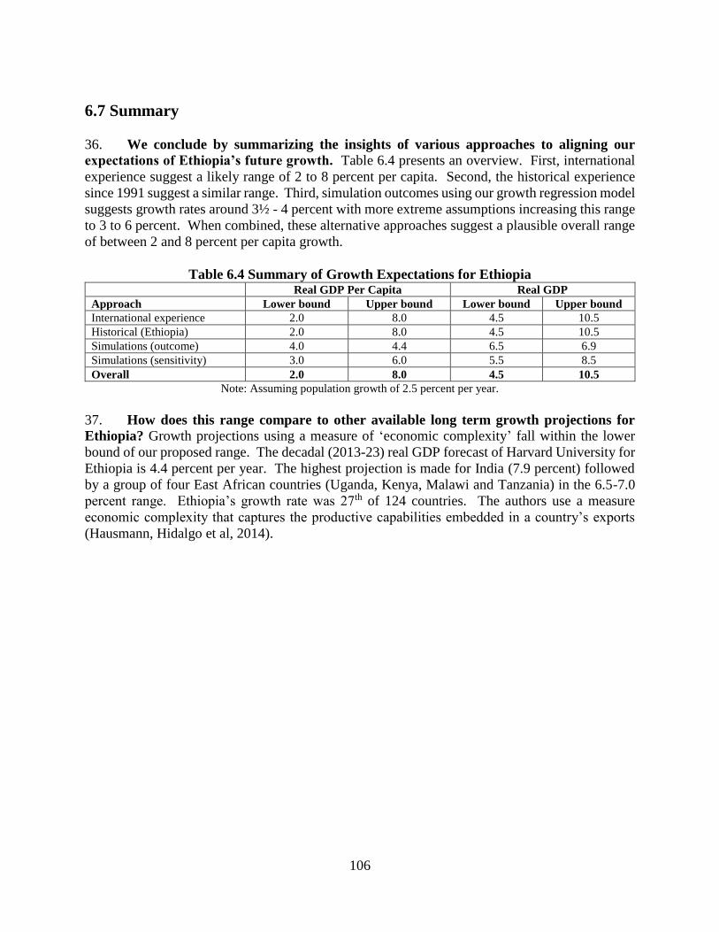
106
6.7 Summary
36. We conclude by summarizing the insights of various approaches to aligning our
expectations of Ethiopia’s future growth. Table 6.4 presents an overview. First, international
experience suggest a likely range of 2 to 8 percent per capita. Second, the historical experience
since 1991 suggest a similar range. Third, simulation outcomes using our growth regression model
suggests growth rates around 3½ - 4 percent with more extreme assumptions increasing this range
to 3 to 6 percent. When combined, these alternative approaches suggest a plausible overall range
of between 2 and 8 percent per capita growth.
Table 6.4 Summary of Growth Expectations for Ethiopia Real GDP Per Capita Real GDP
Approach Lower bound Upper bound Lower bound Upper bound
International experience 2.0 8.0 4.5 10.5
Historical (Ethiopia) 2.0 8.0 4.5 10.5
Simulations (outcome) 4.0 4.4 6.5 6.9
Simulations (sensitivity) 3.0 6.0 5.5 8.5
Overall 2.0 8.0 4.5 10.5
Note: Assuming population growth of 2.5 percent per year.
37. How does this range compare to other available long term growth projections for
Ethiopia? Growth projections using a measure of ‘economic complexity’ fall within the lower
bound of our proposed range. The decadal (2013-23) real GDP forecast of Harvard University for
Ethiopia is 4.4 percent per year. The highest projection is made for India (7.9 percent) followed
by a group of four East African countries (Uganda, Kenya, Malawi and Tanzania) in the 6.5-7.0
percent range. Ethiopia’s growth rate was 27th of 124 countries. The authors use a measure
economic complexity that captures the productive capabilities embedded in a country’s exports
(Hausmann, Hidalgo et al, 2014).

107
Chapter 7. Ethiopia’s Financing Choice: Public Infrastructure or Private
Investment?
To sustain high economic growth, Ethiopia faces a critical choice: Should it continue to direct
the bulk of domestic financing towards infrastructure or should it allocate more to support private
investment? We argue that since firms appear more constrained in credit than in infrastructure,
it may be time to focus more on alleviating credit constraints. This view is supported by empirical
estimates indicating relatively higher marginal returns to private investment in Ethiopia. A range
of policy options are considered. Within Ethiopia’s existing financial repression model, policy
makers could simply avail more credit to the private sector thereby resembling more closely the
Korean model. Another approach would be to initiate a process of interest rate liberalization,
which would enhance the overall savings pool to the benefit of both infrastructure and private
investment. Infrastructure investment is critical for growth, but it needs to be financed in a way
that reduces trade-offs with private investment, which is equally critical for growth.
7.1 Introduction
1. Few policy choices are more critical and more contested in Ethiopia than the
allocation of domestic credit to public infrastructure and private use. Ethiopia’s system of
financial repression and quantity rationing (as described in Chapter 2, Box 2.1) lends itself to a
relatively straightforward question: Suppose you had an additional unit of saving or credit and you
wished to get the highest growth return. Should you finance an infrastructure project, such as a
road, or, should you channel it to finance the expansion of capacity in a private firm? The road
project may crowd-in private sector activity if an infrastructure bottleneck is alleviated. At the
same time, it denies access to credit of another firm that is ready to expand and create jobs. Striking
the right balance is a delicate task and economic analysis can only take you so far. However, such
analysis can give help policy makers think through the opportunity costs of financing
infrastructure.
2. This chapter addresses the following questions: Is Ethiopia’s current level of public
infrastructure investment optimal vis-à-vis private investment? What are the marginal returns to
public infrastructure and private investment in Ethiopia? What is the biggest constraint for
Ethiopian firms: credit or infrastructure? What domestic finance reform options are relevant for
Ethiopia if the objective is the enhance finance to the private sector? If infrastructure remains so
important for future growth, then how else can it be financed?
3. The chapter is structured as follows: Section 7.2 estimates the marginal return to public
infrastructure and private investment. Section 7.3 examines briefly examines the constraints faced
by firms. Section 7.4 explores options for making more credit available to the private sector.
Section 7.5 explores alternative options for financing infrastructure.

108
7.2 Is Ethiopia’s Current Level of Public Infrastructure Investment Optimal?52
4. We begin by stressing the importance of infrastructure development for Ethiopia’s
growth. A key result from our regression model in Chapters 3 and 6 is that infrastructure has
driven economic growth in the past and must continue to be an important driver of growth in the
future. This is because of the high economic returns to infrastructure and the fact that Ethiopia’s
infrastructure deficit is one of the largest in the world. So when we ask the question of whether
the current level of public investment in infrastructure is optimal, this is not a question of whether
we need more infrastructure or not. Clearly, in the long run, we need much more. The problem,
however, arises when there is a financing constraint. Especially, when financing infrastructure
imposes a trade-off via domestic credit markets to private investment financing. So to phrase the
question more carefully: is Ethiopia’s current level of public infrastructure investment optimal
compared to the current level of private investment? To address this question we draw upon a
comprehensive theoretical and empirical analysis contained in the background papers prepared for
this report by Eden and Kraay (2014ab) and Eden (2015b).
5. The recent surge in public investment in Ethiopia has prompted renewed research
interest regarding the optimal scope of public investment. It gives rise to the question of
whether Ethiopia is investing too much in public capital, or whether other developing countries
investing too little. The work by Eden and Kraay (2014a) suggests that both questions can be
answered affirmatively: the vast majority of low income countries are investing too little in public
capital. However, it is likely that Ethiopia may be over-investing in public capital relative to the
optimal level, which also takes into account the marginal returns to private investment.
6. An important aspect of this debate relates to the potential spillovers from public
investment to private investment. Part of the benefits of public investment may come from
raising the productivity of private investment. However, public investment may also crowd out
private investment, either by reducing the supply of savings or by directly substituting for private
enterprises. While the relationship between public and private investment is important for
determining the optimal scope of public investment, the relationship is more nuanced than simply
crowding in vs. crowding out, which has tended to dominate policy discussions in Ethiopia.
7. Consider an example in which public and private capital are perfect substitutes. In
this case, public capital will always crowd out private capital. However, this does not necessarily
mean that public investment is undesirable, since it may be more productive than private capital
because of some comparative advantage that the government has relative to the private sector (for
example, the government may have a comparative advantage in providing security through the
police rather than private security services). Similarly, consider a case in which public investment
fully complements or crowds-in private investment. This does not necessarily mean that more
public investment is desirable, since there is an optimal level of investment (both public and
private), which depends on the cost of financing.
52 This section presents the key findings of a research paper prepared Eden and Kraay (2014a) and discusses its
application to Ethiopia. Interested readers are encouraged to consult this work for further technical details of the
underlying theoretical and empirical models.

109
8. From a policy perspective, the right question is whether the returns to public
investment exceed the costs of financing. Optimality requires that the return to public
investment is equated with the interest rate, and this is true regardless of the effect of public
investment on private investment. In Ethiopia, the supply of credit may be effectively fixed: the
economy is relatively closed and the external borrowing constraint of the government is somewhat
binding. Under a binding credit constraint, the government can be thought of as jointly choosing
the bundle of public and private investment, subject to an external credit constraint. This is because
the choice to increase public investment corresponds to a reduction in private investment through
the increased availability of credit for the private sector (i.e. the oft-cited crowding-out effect in
Ethiopia).
9. When a theoretical model is developed, it emerges that the marginal product of public
capital should equal the marginal product of private capital, in the optimum. To shed more
light on whether public investment levels are optimal in Ethiopia, we use a theoretical model for
that is adequately calibrated with data relevant for Ethiopia. The parameters of the model
presented in Annex A7.1 were calibrated using empirical estimates of (a) the extent to which public
investment increases private investment, and (b) the extent to which public investment increases
output. Estimates were derived from a sample of 39 IDA-eligible low-income countries using a
small open economy framework.53 Intuitively, the response of private investment is informative
regarding the degree of substitutability between public and private investment (𝜎): if they are more
substitutable, public investment will have a larger crowding out effect on private investment (or a
lower crowding in effect). Similarly, the higher the estimate for the relative productivity of public
investment (𝛾), the larger is the first-order effect on output. It turns out that the parameters 𝜎 and
𝛾 are jointly determined by the equilibrium responses of private investment and output.
10. To estimate the effect of public investment on private investment and output, the
exogenous variation from predetermined disbursement of loans from official creditors is
exploited. Empirically, focusing on changes in public investment induced by predetermined
disbursement of official loans is useful for establishing a causal relationship, because it abstracts
from changes in public investment that are either (a) responses to changes in private investment,
or (b) responses to changes in the economic environment that affect both public and private
investment. Using the predetermined disbursement as an instrument for public investment, two
variables are estimated: the marginal increase in private investment induced by a change in public
investment (𝛽), and, the marginal increase in output induced by a change in public investment
(𝛽𝑦). Data on predicted disbursements of loans from official creditors is taken directly from Kraay
(2013), while GDP and investment data is from the World Bank and the IMF, respectively, and
originally based on national sources.
11. Ethiopia stands out among low income countries for having a relatively high public
investment rate and a relatively low private investment rate. Figure 7.1 plots the average
investment ratios for the 1980-2012 period. Public investment rates vary widely across countries
ranging from as low as 2.5 percent of GDP in Cameroon to nearly 15 percent in Guyana. There is
53 This assumption is appropriate for most countries in the sample, although it is somewhat less appropriate in the case
of Ethiopia.

110
also a weak correlation across countries with countries with higher public investment rates also
having lower private investment rates.
Figure 7.1 Public and Private Investment in Low Income Countries (1980-2012)
Source: Eden and Kraay (2014a).
12. The empirical analysis finds general evidence of ‘crowding-in’ of public investment
among low-income countries. The main regression results derived in Eden and Kraay (2014) are
summarized in Annex 7.2. On average, an extra dollar of public investment raises private
investment by roughly two dollars and output by 1.5 dollars. These results are derived from a two-
stage least squares estimates and subjected to various sensitivity tests. The calibrations show a
strong degree of complementarity between public and private capital. However, while the
estimates are positive, the analysis produces large standard errors. The 95 percent confidence
intervals are large in both cases. For that reason, it is important to consider a wider range of the
parameter estimates in the calibration of the model beyond the point estimates.
13. The estimated marginal returns of public investment in Ethiopia are among the
lowest observed in low income countries. We define ‘the excess return’ as the marginal impact
of public investment on output less the sum of the interest rate and the rate of depreciation. In this
exercise, a 3 percent interest rate and a 10 percent depreciation rate is used. For most low income
countries in the 39 country sample, the excess returns to public investment fall in the range between
5 and 170 percent, as illustrated in Table 7.1. However, for some countries that already have high
public investment rates, the return to further investment is below the world interest rate (implying
negative excess returns). The excess return public investment in Ethiopia is estimated at -5.93
percent and the ratio of private to public investment is 0.92.
14. The empirical analysis further indicates that Ethiopia’s growth performance could
benefit from increasing its private capital stock by 12–20 percent relative to the current size
of the public capital stock. This result is derived by comparing the optimal ratio of private to
public capital of 1.18 derived in Annex A7.1.3 with alternative estimates of Ethiopia’s actual ratio
of private to public capital from two different data sources. In the first approach, World Bank data
for public and private investment is used as a proxy resulting in an actual private to public capital
ratio of 0.92 (Table 7.1). Using the formulas of the theoretical model, it can be concluded that the
public capital stock is 12 percent too high in Ethiopia. The second approach uses the Penn World
Tables (PWT) estimates of public and private capital stocks for Ethiopia and yields a private to
Pu
bli
c In
ves
tmen
t/G
DP

111
public capital ratio of 0.75, which (using the relevant formula) suggest that the stock of public
capital is 20 percent ‘too high’.
Table 7.1 Estimated Excess Returns of Public Investment
Rank Country
λ (ratio of
private and
public
investment)
Excess
returns
(%) Rank Country
λ (ratio of
private and
public
investment)
Excess
returns
(%)
1 Cameroon 7.31 1074.88
2 Sri Lanka 5.39 506.36 21 Mali 2.22 47.16 3 Armenia 5.39 505.51 22 Cambodia 1.96 31.51
4 Sudan 5.13 448.69 23 Senegal 1.87 26.78
5 Moldova 4.91 401.68 24 Benin 1.78 22.32 6 Nicaragua 4.24 277.37 25 Burkina Faso 1.77 21.83
7 Burundi 4.09 253.29 26 Togo 1.75 20.96
8 Kenya 3.85 216.11 27 Bolivia 1.73 19.79 9 Uzbekistan 3.75 202.69 28 Niger 1.68 17.61
10 Tanzania 3.70 194.92 29 Sierra Leone 1.43 7.71
11 Honduras 3.43 160.52 30 Djibouti 1.39 6.38 12 Congo 3.32 147.06 31 Côte d'Ivoire 1.38 5.83
13 Mauritania 3.32 146.60 32 Rwanda 1.35 5.00
14 Guinea 3.00 112.08 33 Madagascar 1.19 0.26 15 Uganda 2.95 107.07 34 Malawi 1.17 -0.36
16 Nepal 2.90 102.38 35 Mozambique 1.06 -3.11
17 Pakistan 2.85 97.66 36 CAR 0.99 -4.64 18 Ghana 2.70 83.42 37 Ethiopia 0.92 -5.93
19 Yemen 2.61 76.37 38 Comoros 0.88 -6.59
20 Bangladesh 2.33 54.61 39 Guyana 0.78 -8.28
Note: β =2 and βy=1.5 World Bank data for public and private investment. Source: Eden and Kraay (2014).
15. The results reflect the fact that the marginal product of private capital is substantially
higher than public capital in Ethiopia. Figure 7.2 supports the intuition behind these results.
Since the early 2000s, the public investment rate in Ethiopia has soared, while private investment
gradually declined (Figure 7.2.1). Using the estimated production function, the marginal product
of public and private capital can be computed using PWT data. The marginal product reflects the
effect on production from a one dollar increase in either form of capital expressed in percent.
Figure 7.2.2 reveals that marginal products of public and private capital were roughly equalized in
the 1987-2003 period, implying that an adequate balance was struck between public and private
investment. Starting in 2004, as the Ethiopian economy took off, the marginal product of private
capital increased substantially, while the marginal product of public capital continued to decline.
In 2011, the marginal product of private investment was 22.5 percent compared to the marginal
product of public investment of 7.5 percent.

112
Figure 7.2 Ethiopia: Public and Private Investment and their Returns 1. Public and Private Investment (% of GDP) 2. Estimated Marginal Product of Capital (%)
Note: Figure 7.2.1 uses World Bank data. Figure 7.2.1 uses PWT data. Source: Eden and Kraay (2014).
16. Similar results can be obtained from a methodology that relies only on Ethiopia data.
Eden (2015b) shows that if the rate of return on private capital is greater than 3 percent, then the
marginal return to public investment is lower than the marginal return to private investment. The
approach builds on the methodology developed in Caselli and Feyrer (2007), which decomposes
national income into labor and capital income. Given an assumption on the private rate of return
to investment, capital income can be decomposed into income attributed to private capital and
income attributed to public capital. A higher assumed rate of return on private capital implies a
lower estimated rate of return to public capital. The advantage of this approach is that it measures
the returns to public investment without relying on cross-country analysis. The disadvantage is
that the results are sensitive to assumptions regarding the labor income share, which is assumed to
be 0.67 (as in countries comparable to Ethiopia).
7.3 Firm-level Constraints: Infrastructure or Credit?
17. Firms depend on a range of high quality inputs to be competitive. Macroeconomic and
political stability together with a conducive business environment are some of the basic
ingredients. Firms also become more productive with higher quality infrastructure such as roads,
energy, telecom and water. In addition, firms rely on a range of financial services, including access
to credit, foreign exchange and insurance. They also need a range of business services (accounting,
auditing, financial advice) to thrive. At any point in time, one or several of these inputs will be
the binding constraint that prevents a firm from growing or being competitive.
18. Ethiopian firms appear to be more constrained in terms of access to credit compared
to infrastructure. Table 7.2 draws upon six different surveys which shed light on the constraints
to doing business in Ethiopia from the perspective of firms. It is noteworthy that access to credit
is mentioned as a greater concern or obstacle for doing business than infrastructure (energy and
trade logistics) across all six surveys. Additional infrastructure investment may also only address
firm needs partially. Good trade logistics outcomes is a function of ‘hardware’ (roads and rail),
but also importantly of ‘software’ (e.g. customs procedures). Reliable energy supply for firms
0
0.05
0.1
0.15
0.2
0.25
1985 1990 1995 2000 2005 2010
Public Investment Private Investment
0
0.05
0.1
0.15
0.2
0.25
0.3
0.35
0.4
0.45
0.5
1985 1990 1995 2000 2005 2010
Public Capital Private Capital

113
depends not just on total energy generation capacity, but also on investments and rehabilitation of
the existing distribution network and the establishment of dedicated power lines to industrial parks.
Table 7.2 Most Binding Constraints to Doing Business in Ethiopia, Various Rankings
Enterprise
Survey
2011
Consultations
on National
Business
Agenda 2015
Doing
Business
2015
Global
Competitiveness
Index 2014-2015
Constraints
Non-Farm
Enterprises
2013/14
Large and
Medium Scale
Manufacturing
2012/13
1. Credit Taxes Starting a
business
Government
Bureaucracy
Access to
markets
Raw materials
2. Land
Credit Credit Foreign
exchange Credit Access to
markets
3. Energy
Land Trade logistics Credit Trade logistics Credit
4. Taxes Energy Protecting
minority
investors
Corruption Taxes Energy
5. Trade logistics
Unfair
competition
Registering
property
Energy
Source: World Bank Doing Business Report (2016); Global Competitiveness Report (2014 and 2015); National
Business Agenda (2014); World Bank Enterprise Survey (2011); CSA LMSMI (2012/13); GHS (2013/14). Note:
Language has been harmonized across surveys for ease of comparability. Credit in bold. Infrastructure underlined.
19. In Ethiopia, firms that are fully credit constrained exhibit poorer performance and
productivity. According to World Bank (2014), firms in Ethiopia are more likely to be fully credit
constrained than global comparators, including SSA countries. Nearly half of firms in Ethiopia
are fully credit constrained.54 For firms, being credit constrained means poorer performance and
less productivity. In Ethiopia, a credit constrained firm has 15 percentage points lower sales
growth, 5 percentage points lower employment growth, and 11 percentage points lower labor
productivity growth than firms who are not credit constrained. Instead, investment decisions of
manufacturing and services firms in Ethiopia are heavily dependent on cash flows.
20. This is indicative that the economy would benefit from a shift of domestic credit
towards private firms. If the ultimate purpose of government policy is to enhance the
productivity of private firms, then it is important to understand what the firm level constraints are.
If firms really need credit more than access to new roads or better telecommunication to grow and
prosper, then government policy would need to support the alleviation of the credit constraint at
the firm level. Since public infrastructure investment is partially financed via the same domestic
savings pool, it is clear that infrastructure financing competes directly with the financing of private
investment projects. In addition, there may be other factors affecting firm credit constraints, such
as high collateral requirements, which the government can also seek to alleviate.
54 Fully credit constrained firms are those without external financing and which were either rejected for a loan or did
not apply even though they needed additional capital. It should be noted that credit constraints can be a function of
both lack of overall credit in the system, and, a reflection of firm characteristics (some firms are not credit worthy).

114
Box 7.1 Literature Review: Does Financial Repression Inhibit or Facilitate Economic Growth?
Economists are divided on the impact of repressive financial policies on economic growth. A large
number of studies identify possible mechanisms through which financial liberalization promotes growth,
including facilitating financial development, improving allocative efficiency, inducing technological
progress and enhancing financial stability (Shaw, 1973; Levine, Loayza and Beck, 2000). Many
empirical analyses also confirm this positive correlation (Levine, 2005; Trew, 2006). Other studies,
however, cast doubts on this relationship. Kose et al. (2009) find no clear-cut relationship between
financial globalization and economic growth in a global dataset of emerging market economies. Stiglitz
(2000) attributes increasing frequency of financial crisis during past decades to financial liberalization
in the developing world. He argues that developing countries might be more able to manage money
supply and financial stability under repressive financial policies.
While repressive financial policies would reduce economic efficiency, they might enable the
authorities to better deal with problems of market failure and financial risks. This lead some
authors to argue that this is essentially an empirical question, influenced by a list of factors such as
conditions of financial institutions, markets, regulators and the government.
Case study analysis, especially of East Asian countries tend to be supportive some financial
repression, especially at the early stages of development. In China, Huang and Wang (2011) find
empirical evidence that repressive polices helped economic growth in the 1980s and 1990s thanks to the
prudent liberalization approach. However, the effect turned negative in the 2000s as lending to the state
sector, interest rate regulation and capital account controls constrained growth. Demetriades and Luintel
(2001) develop a theoretical model which predicts a positive association between financial development
and the degree of state control over the banking system and mild repression of lending rates. They use
data from Korea to derive empirical findings that are consistent with this theoretical prediction. Ang
(2009) studies the links between financial policies and private investment. In the case of Malaysia, high
reserve and liquidity requirements exerted a positive influence on private investment. However, in the
case of India, the effect was negative.
Recent cross-country panel regression results are largely supportive of financial sector reforms. A
large body of literature suggests that a well-developed financial sector promotes economic growth (e.g.
Levine, 2005). However, relatively few studies tries to assess the impact of financial sector reforms on
economic growth. Bakaert, Havery, and Lundblad (2005) finds that foreign equity ownership increases
growth. Quinn and Toyoda (2008) document that capital account liberalization is positively associated
with growth. Prati et al. (2013) finds strong positive effects of financial sector reforms on growth.
Finally, Cristiansen et al. (2013) find that domestic financial reforms are robustly associated with growth.
Some authors argue that a time series approach is more fruitful than a cross-section approach,
though the use of instruments could potentially overcome this methodological criticism. Arestis
and Demetriades (1997) worry that the question of causality cannot be satisfactorily addressed in a cross-
section framework. Their criticism, in turn, has given rise to the series of cases studies mentioned above.
They show uni-directional causality in Germany from financial development to real GDP, but insufficient
evidence of such effects in the US, with abundant evidence of reverse causality. While modern
econometrics has developed in recent decades, the problem of causality (or more generally, endogenity)
continues to be a challenge in this sub-set of the cross-section / panel approach in this literature, which
implies that it often refers to association rather than causality between variables. The work by Prati et
al. (2013) represents an attempt to overcome this challenge as the authors use the Difference GMM
estimator which relies on internal instruments in the form of lagged dependent variables. Source: Author’s compilation.

115
7.4 Domestic Finance Reform
21. The trade-off between financing public infrastructure versus private projects arises
from the way in which the Ethiopian financial sector is designed. As explained in Chapter 2,
key characteristics include: (1) below market-clearing interest rates; (2) market dominance by a
state-owned bank, Commercial Bank of Ethiopia (CBE), which effectuates a policy of giving
public investment projects the funding priority. In the economic literature, such a system is
referred to as ‘financial repression’ (McKinnon, 1973; Shaw, 1973). The literature itself is divided
on to whether financial repression is good or bad for economic growth as discussed in Box 7.1. In
addition, it is important to note that the capital account is closed and that there are no foreign banks
operating in the Ethiopian financial sector.
22. In this section we consider two policy reforms that could help alleviate the private
sector credit constraint in Ethiopia. One policy reform would be to continue the existing system
of financial repression, but to direct more credit towards private firms at the expense of public
infrastructure projects.55 Another policy reform involves a gradual move towards a more
liberalized financial system in which interest rates reflect the demand and supply for
savings/credit. The latter approach does not necessarily imply opening up the domestic banking
sector to foreign competition nor does it require liberalization of the capital account. It is also
noted that the two policy reforms analyzed here can be considered as pure extremes on a continuum
of policies and that they can be mixed as needed. A shift towards more private sector credit within
the existing financial repression model would see public investment fall by a similar magnitude.
The deposit and lending rates of banks would remain unchanged. For simplicity of exposition it
may be helpful to think of savings as being relatively unchanged, even if reality can be more
complex.56
23. Financial repression with a strong private sector emphasis is a model that was
effectively practiced by South Korea. Like Ethiopia, the South Korean government intervened
extensively in the pricing and allocation of credit. Unlike Ethiopia, the Koreans directed the bulk
of the credit towards priority private sector activities. ‘Specifically, it ensured that priority sectors,
mainly export-oriented industry such as steel, electronics, ship-building, automobile
manufacturing etc., received preferential treatment as far as access to inexpensive bank credit was
concerned’ (Demetriades and Luntel, 2001). Private sector credit to GDP averaged around 30
percent in Korea in the 1970s compared to around 20 percent in Ethiopia today (Nguyen et al
(2015). While Ethiopia also favors some priority private sector activities, particularly in
manufacturing, the bulk of total domestic credit is currently directed towards public infrastructure
projects. To truly emulate Korea in this aspect, Ethiopia would need to shift more of credit to
priority private sectors.
55 As more domestic credit is directed towards the private sector, it is particularly important to serve the small and
medium enterprise (SME) segment. Ethiopia is characterized by a ‘missing middle’ phenomenon, whereby small
enterprises are more credit constrained than either micro or medium/large enterprises. This represents a key challenge
because typically young firms are a great source of job creation but this trend is not seen in Ethiopia, where more
established firms dominate the net job creation, suggesting that there is a lack of competitiveness and innovation in
the private sector (See World Bank, 2014, for details). 56 In the theoretical model developed later, savings may change even if the interest rate does not because future
consumption depends on the mix of public and private investment.

116
24. Introducing a more liberalized financial sector with market-determined interest rate
would be expected to induce higher savings. Through a gradual increase in the deposit interest
rate, households and firms would find it relatively more attractive to use formal deposit accounts
for their informal savings. The expected result would therefore be an increase in deposits. The
ensuing competition between banks would drive up the deposit rates and attract savings. The
magnitude of this increase depends on the elasticity of domestic savings with respect to the deposit
rate. It would no longer be possible for the government to direct credit to the public infrastructure
sector (neither via loans nor bond purchases).
25. The exact consequences of these two reforms are hard to predict with accuracy. Under
interest rate liberalization, we would expect private investment to rise. The deposit rate would
increase, attract more savings and there would be no targets for public infrastructure investment.
Higher interest rates will improve the allocation of capital within the private sector as private
projects with low returns will cease to demand credit, freeing up additional credit for more
productive projects. What would happen to public investment under a more liberal model? Given
higher borrowing cost, it is advisable to reduce public investment and finance a greater share of it
from other sources, such as higher tax revenues. Finally, it is expected that total investment would
rise given that total savings have increased. Table 7.3 summarizes the predicted effects.
Table 7.3 Predicted Effects of Financial Sector Reforms Predicted Effect (1)
Financial repression with
more private credit
(2)
Interest rate liberalization
Private investment + +
Public investment − ?
Total investment 0 +
Savings 0 +
Financial repression revenue − − −
Tax revenue from private activity + +
Rents of savers 0 +
Public debt sustainability 0 −
26. The two policy reforms would have different implications for government finances
and the surplus of savers. To begin with, it is important to realize that financial repression yields
implicit government revenues, as documented by Giovanni and de Melo (1993). In Ethiopia, the
revenue arises because government infrastructure spending can be financed at below-market
interest rates giving rise to interest payment savings. Moreover, if credit is rationed in favor of
infrastructure projects then government gets access to additional credit which it would not have
had access to in a market-based system. On the other hand, both policy reforms support a much
more dynamic private sector which would ultimately enhance the tax base and yield higher tax
revenues. Which of the two effects dominate is ultimately an empirical question. In the ‘financial
repression with more private credit’ reform, government would maintain some implicit revenue as
interest rates are unchanged. However, implicit revenues would fall as less public projects are
financed. Under the liberalization approach, government financial repression revenues would
eventually disappear as interest rates approach their market-based levels. Finally, since financial
repression involves a transfer of resources from savers to borrowers the effects differ under each
reform. Financial repression continues to involve a resource transfer from savers, but now directed

117
to private firms instead of government. Interest rate liberalization involves a transfer from
government back to savers.
27. The effects on the sustainably of public debt can be challenging under a more
liberalized system, while continued financial repression keeps this challenge at bay. It is
important to be aware that current public debt levels are deemed sustainable under the assumption
that real interest rates do not rise (IMF and World Bank, 2015). However, since interest rate
liberalization implies a rise in the real interest rates, it is clear that there would be concerns about
whether public debt can remain sustainable under a more market-based system of setting interest
rates.
28. DSA simulations suggest that an increase in the real interest rate by 7 percent would
make public debt unsustainable. The current baseline assumption of the DSA is a real interest
rate of -5.7 percent. If the real interest rate increases to a positive level of 1.3 percent then there
would be a substantial and protracted breach of the PV Debt-to-GDP ratio in the baseline scenario.
The associated increase in interest payments for the Federal Government and SOEs would be from
0.5 percent of GDP to 3.4 percent of GDP.
29. Given that each policy reform has pros and cons, neither of them is superior to the
other. Policy makers that weigh in concerns about debt sustainability and find a gradualist
approach to reform appealing would find financial repression with more private credit most
attractive. On the other hand, policy makers concerned about Ethiopia’s demonetization trends
and who want to see a strong expansion of credit to the private sector would find liberalization
more beneficial. If so, such an option would need to be combined with additional taxation of the
private sector which would help address implicit government revenue losses and the challenges of
public debt sustainability.
30. In theory, the policy choice should be informed by two criteria: the relative returns
of public and private investment, and, the savings rate. Box 7.2 summarizes a simple partial
equilibrium model developed by Eden (2015) specifically for the purposes of this study. The
model provides a useful framework within which to analyze Ethiopia’s current situation. In
particular, it becomes clear that financial repression with more private emphasis becomes attractive
in situations where the marginal return to private investment is much higher than the marginal
return to public investment. Moreover, if the saving rate of the country is quite low, then the model
suggests that welfare would enhance by increasing the deposit rate towards more market-
determined levels as in the liberalization reform. Ultimately, which of the two constraints are more
binding would be an empirical question.
31. The available empirical evidence suggests that Ethiopia has a challenge in both
dimensions, implying that both types of reform would enhance welfare. First, as shown in
Section 7.2, marginal returns to private investment appear higher than those of public investment.
Second, as shown in Chapter 2, Ethiopia has experienced a demonetization trend over the past
decade as reflected by a declining share of total credit to GDP. Given Ethiopia’s preference for
financial repression, the less radical reform may be to maintain this system, but to follow South
Korea’s footsteps and direct the bulk of the credit to the private sector.

118
Box 7.2 A Theoretical Model of Financial Repression and Interest rate liberalization57
A theoretical framework was developed to support the analysis of Ethiopia’s financial sector
reform options. This approach has the advantage of ensuring logical consistency of argument, clarifying
the underlying assumptions while also yielding additional insights that may not be immediately intuitive.
To illustrate the key ideas, we utilize the two period version of a more general model developed by Eden
(2015) for this report. The main features of the model are described below.
The model has two periods and four agents: Households, firms, government and the government bank.
Output depends positively on private capital and infrastructure (as complementary inputs) and exhibits
diminishing returns.
Private capital is produced by firms. They borrow from the government bank in the first period to
finance capital in the second period and maximize profits given the borrowing interest rate and the returns
to capital (which depend positively on infrastructure).
Supply of savings. Households receive income from firms and pay taxes. Utility is derived from
consumption in both periods and is maximized taking into account the subjective discount rate and the
deposit interest rate. In equilibrium, household savings depend positively on the deposit rate.
The government has four policy instruments: infrastructure, taxes, the policy deposit rate, and, the
lending rate. The government objective is to maximize household welfare. It collects lump sum taxes
in both periods and there is a cost associated with collecting taxes.
The model has three interest rates. The policy rate is an upper bound on the deposit rate faced by
households. The deposit rate is the return on household saving and represent the borrowing cost to the
government bank. Under financial repression, the policy rate is equal to the deposit rate. If there is no
financial repression then the policy rate can be higher than the decentralized equilibrium rate. The
borrowing rate is what firms pay to borrow and it represents a revenue for the government bank. The
spread is equal to the borrowing rate less the deposit rate and is a net revenue for government.
The optimal policy consists of some financial repression because this reduces the costs associated
with collecting taxes. The lower deposit interest rate (equal to the policy rate) associated with
government debt allows the government to economize on tax collection costs, in both periods. In
optimum, the marginal return to private capital is equal to the returns of infrastructure, net of the marginal
costs associated with raising taxes (in period 2). The model abstracts away from costs associated with
the collection of private debt. If these costs are equal to tax collection costs, then it is optimal to equalize
the returns to government and private capital, as in Eden and Kraay (2014ab). Optimality requires that
the marginal costs of taxation are also equalized across periods.
In optimum, the government sets a positive interest spread. Given the depressed deposit rate, the
government can either ration credit to the private sector or set a spread so that the market for private
credit clears. The latter alternative is superior because the spread generates revenues for the government
without further distorting private investment. This allows the government to economize on costs
associated with tax collection. Furthermore, the price mechanism guarantees that private credit is
allocated to the private projects with the highest return. Credit rationing, on the other hand, requires
some guess work regarding where are the highest-return projects: since the interest rate is depressed,
inefficient projects may find it optimal to request financing. At a higher borrowing rate, only the more
productive projects will be profitable.
57 This Box summarizes the theoretical model developed by Eden (2015) for the purposes of this study.

119
Box 7.2 (Continued) Policy Reform 1: Financial Repression with More Private Credit
Policy Scenario 1 (financial repression with more private credit) can be illustrated in the model by
simulating alternative values of the government infrastructure variable. The properties of the
theoretical model can be illustrated by assuming plausible functional forms, including Cobb Douglass
production and utility functions and a quadratic tax collection cost function. Figure 1 illustrates the effect
of alternative values of government infrastructure (kg) on other variables in the model.
There is an optimum level of government infrastructure, kg*, namely the level that maximizes welfare.
For kg < kg* there is insufficient crowding-in of infrastructure and production and consumption is too low.
For kg > kg* infrastructure crowd-out private capital via the credit markets and this lowers production and
consumption as well.
The following additional results hold: First, the future tax burden is rising in government infrastructure.
Second, any decrease in government infrastructure will be compensated by a corresponding increase in
private capital. Third, the deposit interest rate is rising in infrastructure up to the optimum, but unaffected
thereafter.
An increase in private credit would be welfare enhancing if there is currently too much government
infrastructure. In Figure 1, this situation can be illustrated by considering a situation where we are at
a point to the right of optimum and reduce the level of government infrastructure investment. As also
illustrate, this would result in an increase in private capital. As long as government infrastructure is not
reduced too much, welfare is enhanced as more private capital can be invested. At the margin, additional
private investment boosts production and consumption more than the resulting loss from lower
infrastructure investment.
Figure 7.3 Numerical Simulations with Alternative Values of Government Infrastructure

120
Box 7.2 (Continued) Policy Reform 2: Interest rate liberalization
Policy Scenario 2 (interest rate liberalization) can be illustrated in the model by simulating
alternative values of the deposit rate. Recall that the deposit rate is the return on household saving and
represent the borrowing cost to the government bank.
There is an optimum level of the deposit rate, r*, namely the level that maximizes welfare. Consider
very low levels of the deposit rate, say zero. As the policy rate increases so does the return to household
savings. This encourages households to save rather than consume and the total pool of savings increases
in the economy. However, since the government must pay the deposit rate to borrow from households,
the borrowing cost to finance government infrastructure is rising. The first effect continues to dominate
the second effect until welfare is maximized at the point indicated in the welfare graph below. Beyond
this point, the deposit rate becomes ineffective as a policy tool as further increases in the rate are matched
by additional savings which ultimately drives down the decentralized equilibrium rate, r, to its maximum
level.
The following additional results hold: First, the future tax burden is rising in the deposit rate because
higher taxes compensate for the increased borrowing cost of government. Second, private investment is
rising in the deposit rate as more savings is made available to finance it.
Interest rate liberalization will be welfare enhancing if the deposit rate is currently too low. The
larger deposit rate encourages household savings and enhances the amount of private investment that can
be financed.
However, government revenues will decline. The government bank earns a revenue from the
difference between the borrowing rate and the deposit rate. As the deposit rate rises, the spread
diminishes, and eventually disappears.
Figure 7.4 Numerical Simulations with Alternative Values of the Deposit Rate

121
7.5 Complementary Infrastructure Financing Options
32. Continued infrastructure development remains one of Ethiopia’s best strategies to
sustain growth, but the current financing model may not be sustainable. Infrastructure was
the most important driver of economic growth during the growth acceleration. This is because the
economic returns to infrastructure are high and the physical infrastructure expansion in Ethiopia
was substantial. But infrastructure expansion was financed via a range of mechanisms that will
begin to show their limits in the future.
33. Low domestic resources mobilization, including savings and tax revenue is a chief
vulnerability. To overcome it and deliver high public infrastructure investment in the past, policy
makers engaged in a series of creative financing mechanism. Going forward, inherit policy trade-
offs will eventually catch up with this strategy. Public and external indebtedness are gradually
rising as is the cost of financing and risks of debt distress. The lack of access to credit and foreign
exchange of the private sector holds back an important driver of growth. An overvalued exchange
rate hurts external competiveness. At some point one of these constraints will become binding
and limit Ethiopia’s ability to deliver public infrastructure with the current model. Going forward,
Ethiopia needs more infrastructure, but it would need new mechanisms to finance it.
34. In this section we briefly review the range of alternative infrastructure financing
options available to Ethiopian policy makers. In doing so we distinguish between policy
proposals that are broadly in line with existing government strategy and thinking and policy
options which would require a change in policy and mind set. Table 7.4 refers.
Table 7.4 Alternative Infrastructure Financing Options
Consistent with current strategy and thinking Options that would require a change in policy
1. Raising tax revenues
2. Increasing private sector financing of
infrastructure investments and maintenance
3. Improving public investment management
4. Increasing domestic savings and developing
capital markets
5. More selectivity and prioritization of
investments
6. Securitization of infrastructure assets
7. Improved pricing of infrastructure services,
such as electricity
35. Ethiopia’s tax revenue-to-GDP ratio is low compared to peers and there is substantial
scope for raising it further. At 14 percent of GDP, tax revenues in Ethiopia are on the low side.
The country urgently needs a revenue-enhancing tax reform which broadens the base and increases
the tax rates. Consistent with Ethiopia’s lagging performance in terms of reforms, the last major
tax reform can be traced back to 2002/03 when the sales tax was replaced by the Value Added
Tax. In addition to concerns about low levels of tax collection, one may add the heavy reliance on
foreign taxes, which account for almost a third of tax revenues. If Ethiopia decides to take forward
additional trade reforms, then such revenues would gradually diminish. In light of the country’s
high appetite for public infrastructure investment, it is hard to justify the current low levels of
revenues. Further analysis would be needed to identify concrete policy recommendations. That
said, a good place to start could be through an examination and evaluation of existing tax incentives
and subsidies, currently resulting in forgone tax revenues to the tune of 4 percent of GDP. Some

122
of these so-called ‘tax expenditures’ may provide good value for money, while the costs of others
may outweigh their benefits.
36. Increased involvement of the private sector in infrastructure provision and
maintenance can help reduce financing requirements of the public sector. Ethiopia has made
recent progress in this direction. The most prominent example is the 1,000MW, US$4 billion
geothermal energy project at Corbetti, where a private foreign investor consortium will sell energy
to the national grid according to a Power Purchasing Agreement (PPA). There have also been
discussions about an oil pipeline project potentially financed by Black Rhino, although agreements
are yet to be signed. Aside from direct provision of infrastructure, there are also recent examples
of private user contributions in road projects, such as the Addis-Adama Toll Express Way.
Ethiopia currently does not have a Public Private Partnership (PPP) Framework which prevents a
holistic approach to addressing the challenge.58 An important lesson from Corbetti is that ad hoc
negotiated deals are not the way to go. PPPs or pure private solutions are important alternatives
to public provision of infrastructure that must be kept in mind. If private finance is going to play
a significant role then the government needs to be proactive and systematic in its approach.
(Interested readers can consult IMF (2014) for further details).
37. Improved public investment management can help ensure that Ethiopia gets as much
infrastructure for the public money that it spends. Since weakness in public investment
management can negate the core argument that impressive rates of public investment are necessary
for a country to sustain rapid economic growth, attention to the processes that govern project
selection and management is critical. Encouragingly, Public Investment Management (PIM) in
Ethiopia is better than expected given its level of development. An international comparison of
PIM capacity across a sample of 71 poor and middle income countries conducted by the IMF and
World Bank, places Ethiopia at the median, while it is the eleventh poorest countries in the world
(Dabla-Norris et al. 2010). Of the four dimensions measured in the study, Ethiopia scores above
the median in ‘management’ and ‘appraisal’, at the median in ‘evaluation’ and below the median
in ‘selection’. On the other hand, such indices may lack precision about individual countries, and
must thus be interpreted with a great deal of caution and should not be a cause for complacency.
To illustrate, Ethiopia continues to register significant time and cost overruns in some public
infrastructure projects (see World Bank, 2013). A detailed country study of Ethiopia’s PIM
performance is currently not available. In all cases, further progress in all four dimensions of
Ethiopia’s PIM capacity would undoubtedly enhance the positive economic returns expected from
publically financed projects. (See World Bank 2015 for more details on this topic).
38. Further resources could be raised through domestic savings mobilization and the
eventual establishment of capital markets. The government has been actively aiming to raise
domestic savings, among others through bank branch expansions. As documented in the Second
Ethiopia Economic Update (World Bank, 2013), this policy has indeed had a demonstrable effect
on domestic savings in the formal banking system. However, as shown in the same analysis, a key
determinant of domestic savings is the real deposit interest rate. Since this rate is currently
negative, households have strong incentives to channel monetary savings into informal savings
mechanisms. A negative real interest rate is also a major obstacle for the development of a
58 The Government, together with the African Development Bank, is in the process of developing a PPP Framework
and a PPP Unit.

123
secondary market for treasury bills as investors would not earn a sufficient return for voluntary
purchase of such assets. On the other hand, the negative real interest rate is a part of an overall
financial repression strategy which yields other important benefits for government, including the
cheap access to finance for public infrastructure investment.
39. Selectivity and prioritization in public investments. In theory, the Government should
finance the projects with the highest expected economic return, but in practice such calculations
are seldom available. Based on the limited information available, most public investment projects
would potentially have an important positive long term impact on exports and growth. However,
not all projects (whether infrastructure or productive) have an equally compelling merit of
financing. Thus, to free overall resources for priority infrastructure investment, the government
could reduce financing of marginal projects that do not have a demonstrable strong economic
rationale.
40. Securitization of infrastructure assets is another potential source of public investment
financing. Ethiopia has a series of prominent, successful, and profitable State Owned Enterprises,
including Ethiopian Airlines, Ethio Telecom and Commercial Bank of Ethiopia. These enterprises
are currently 100 percent owned by Government. Securitization refers to a process whereby a
small share of these assets were sold to the general public. This approach has been successfully
used in countries such as China and Colombia.
41. A final proposal include the cost-based pricing of infrastructure services, such as
electricity. Households and firms currently pay energy tariffs that are below the cost of providing
such services. At the same time, Ethiopia is investing billions of dollars in new energy generation.
By charging more for energy services, consumers could help finance such energy investments.
Moreover, raising tariffs would be a progressive policy, as it is the better-off households that have
access to electricity and benefit from the implicit subsidy currently in place. (See World Bank
2015ab for more details).
42. In summary, this chapter has argued that to sustain high growth, Ethiopia needs to
explore ways of financing private investment while also finding complementary ways of
financing infrastructure. This is because both infrastructure investment and private investment
are needed, as the experience of high-growth economies show. Ethiopia’s financing choice
currently has a clear bias in favor of public infrastructure investment. Infrastructure investment
enhances the productivity of the private sector, but only when lack of infrastructure itself is
constraining growth. Ethiopian firms appear to be more constrained in credit and empirical
estimates suggest that, at the margin, credit could yield better growth returns in the private sector.
This suggests some reduction in public infrastructure financing would be beneficial for long-term
growth. To ensure continued support for infrastructure finance, this chapter presented a menu of
policy options for consideration.

124
Annex A7.1 Public and Private Investment Model: The Model Consider the following problem, in which the government takes the rental rate of capital as given and chooses
public and private capital stocks, subject to a constraint on the total capital stock:
max𝑘𝑔,𝑘𝑝
𝐹(𝑘𝑔, 𝑘𝑝) − 𝑟(𝑘𝑔 + 𝑘𝑝) 𝑠. 𝑡. 𝑘𝑔 + 𝑘𝑝 = 𝐼
Where F is a strictly positive, increasing production function, that has decreasing returns in both arguments, 𝑘𝑔 is
the per capita public capital stock, 𝑘𝑝 is the per capita private capital stock, 𝑟 is the interest rate, and 𝐼 is the
constraint on the total capital stock.
This simplified problem captures a static representation of the dynamic problem in Eden and Kraay (2014), in
which the government maximizes welfare subject to a binding aggregate credit constraint. (In the dynamic setting,
𝐼 is pinned down as the sum of depreciated capital stocks and availability of credit). Substituting in the constraint,
the optimization problem can be rewritten as:
max𝑘𝑔
𝐹(𝑘𝑔, 𝐼 − 𝑘𝑔) − 𝑟(𝑘𝑔 + 𝐼 − 𝑘𝑔) =max𝑘𝑔
𝐹(𝑘𝑔, 𝐼 − 𝑘𝑔) − 𝑟𝐼
The first order conditions of this problem yields:
𝜕𝐹
𝜕𝑘𝑔=𝜕𝐹
𝜕𝑘𝑝
In other words, the marginal product of public capital equals the marginal product of private capital and the levels
of public and private capital are determined by the aggregate credit constraint.
It is worth noting that the optimality condition does not depend on the assumption of a binding aggregate credit
constraint, as a similar optimality condition can be derived without this assumption (see Eden and Kraay (2014) for
details). The difference between the two cases is in the implications for the levels of the capital stocks: in the
constrained case, aggregate capital should equal 𝐼, and the marginal returns to investment may exceed the world
interest rate. In contrast, in the unconstrained case, the levels of investment are determined by the condition that
the marginal return to (both types of) investment is equated with the world interest rate. In both cases, the marginal
products of public and private capital should be equalized, which is the only condition used for the analysis that
follows. Consider next the following functional form (Constant Elasticity of Substitution, CES):
𝐹(𝑘𝑔, 𝑘𝑝) = 𝐴(𝛾𝑘𝑔𝜎 + (1 − 𝛾)𝑘𝑝
𝜎)∝𝜎
where 0 ≤ 𝛾 ≤ 1 and 𝜎 ≤ 1 and 𝐴 represents aggregate productivity. This functional form is quite flexible:
depending on parameters, public and private capital can be substitutes or compliments, and have different levels of
relative productivity. As special cases, this functional form nests the cases of perfect substitutes (𝜎 = 1), Cobb-
Douglas (𝜎 = 0), and perfect complements (also known as Leontief, and given by 𝜎 = −∞). This functional form
implies that the optimality condition is given by:
𝜆∗ =𝑘𝑝∗
𝑘𝑔∗= (
1 − 𝛾
𝛾)
11−𝜎
Here, 𝜆∗ is the optimal ratio of public and private capital. It depends both on the elasticity of substitution between
public and private capital, 𝜎, and on the relative productivity parameters 𝛾 and 1 − 𝛾. Thus, to determine the
optimal allocation of credit between public and private capital, a quantitative sense of 𝛾 and 𝜎 is needed. It is useful
to note that 𝜆∗ is the optimal ratio of public and private capital, regardless of the extent to which the credit constraint
is binding. However, in general, if the constraint is binding, the aggregate capital stock is too low, and there may
be positive excess returns to both types of capital (marginal output effect less the interest rate and depreciation).

125
Annex A7.2 Public and Private Investment Model: Empirical Results Table A7.2.1 The Response of Private Investment to Public Investment
Table A7.2.2 The Response of Output to Public Investment

126
Annex A7.3 Public and Private Investment Model: Calibration Table A7.3.1 presents the calibrated values of the parameters of the CES production function (𝜎 and 𝛾) as a function
of the empirical estimates of the response of private investment to public investment (𝛽) and the response of output
to public investment (𝛽𝑦). The excess returns to public investment for 𝜆=3 and 𝜆=1 implied by this calibration are
calculated using 𝑟∗+ 𝜕 = 0.13 under the assumption that credit constraints are not binding. The last two columns
present the threshold level of 𝜆∗ =𝑘𝑝∗
𝑘𝑔∗ , above which there are positive excess returns to public investment, and the
percent of countries in the sample for which 𝜆 is above the threshold. The bolded row represents the calibrated
values for the point estimates of 𝛽 =2 and 𝛽𝑦=1.5 derived from the regression model in Annex 2. What do these
results imply for the optimal level of the public capital stock in Ethiopia?
The first approach using World Bank investment data indicates that Ethiopia may benefit from reducing its
public capital stock by 12 percent. The point estimate in Table A7.3.1 suggests that optimal ratio of public and
private capital is given by 𝜆∗=1.18. By comparison, the average ratio of private and public investment in Ethiopia
is 𝜆=0.92. As a first step, it is assumed that average ratio of public and private investment roughly corresponds to
the ratio of capital stocks. The observed ratio 𝜆 = 0.92 is a little bit low compared to the estimated optimal ratio
(1.18):
𝜆 =𝑘𝑝𝑘𝑔=𝐼 − 𝑘𝑔
𝑘𝑔⇒ 𝐼 = 𝑘𝑔(1 + 𝜆) ⇒
𝐼
1 + 𝜆= 𝑘𝑔 ⇒
𝑘𝑔∗
𝑘𝑔=1 + 𝜆
1 + 𝜆∗=1 + 0.92
1 + 1.18= 0.88
Table A7.3.1 Calibration Results Empirical estimates Calibrated parameters Excess return to public investment
𝛽 𝛽𝑦 𝜎 𝛾 𝜆 = 3 𝜆 = 1 𝜆∗ Countries
(%)
Private inv. response
Output response
Degree of substitutability
Relative productivity
Optimal ratio Optimal ratio Optimal ratio Optimal ratio
1 0.5 -0.35 0.4 0.25 -0.04 1.35 82%
1.5 0.5 -1.19 0.17 0.17 -0.10 2.06 54%
1.5 1 -0.67 0.49 0.66 -0.01 1.02 90%
1.5 1.5 -0.54 0.65 1.17 0.11 0.67 100%
1.5 2 -0.48 0.73 1.7 0.22 0.51 100%
2 0.5 -3.18 0.02 0.11 -0.13 2.54 49%
2 1 -1.72 0.22 0.6 -0.09 1.59 72%
2 1.5 -1.43 0.4 1.11 -0.04 1.18 85%
2 2 -1.32 0.5 1.5 0 1.00 90%
2.5 0.5 -10.48 0.00 0.05 -0.13 2.92 38%
2.5 1 -4.96 0.007 0.54 -0.13 2.30 51%
2.5 1.5 -4.13 0.03 1.05 -0.13 1.97 54%
2.5 2 -3.8 0.06 1.56 -0.12 1.77 54%
An alternative approach using estimated capital stock indicates that public capital stock in Ethiopia should
be about 20 percent lower. One limitation of the previous approach is that 85 percent of the countries in the
sample exhibit a ratio of private and public capital which is too high relative to the optimum. The estimate based
on average investment rates is imperfect, because the ratio of capital stocks depends both on the timing on
investment and on the initial capital stocks. An alternative, and possibly more accurate, measure of the ratio of
public and private capital stocks in Ethiopia is therefore computed by complementing data on government and
private investment with estimated capital stocks from the Penn World Tables (PWT). The series are computed
using a 3 percent annual depreciation rate, which is significantly lower than the 10 percent used in Eden and Kraay
(2014). This difference is not important for the calibration of the parameters 𝜎 and 𝛾, but is important when
computing excess returns. To compute public and private capital stocks in Ethiopia, it is assumed that the initial
public capital stock in 1987 (when the investment data start) is equal to half of the aggregate capital stock reported
in PWT. Public and private capital stocks are then cumulated forward using the investment rates Figure 2.1 to
arrive at a series of public and private capital stocks. The estimated production function is then used to compute
the marginal returns to public and private capital over the past two decades. The estimates suggest that, in 2011,
Ethiopia’s ratio of private and public capital was 𝜆 = 0.75. Using the formula above, this estimate suggests that the
public capital stock should be about 20 percent lower. Given the short length of the series, the estimates of the
capital stocks may be sensitive to the specification of initial conditions. To address this concern, the analysis was
repeated under the alternative assumption that the initial public capital stock in 1987 is zero. It is noted that a lower
initial public capital stock implies higher returns to public investment. Even under this highly conservative
assumption, roughly the same gap in marginal products is derived for 2011, suggesting a fairly robust conclusion.

127
Chapter 8. Growth and Structural Reforms59
Using illustrative cross-country simulations at the macro and firm levels, this chapter shows that
even modest structural reforms may yield substantial growth pay-offs for the country. In terms of
reform sequencing, Ethiopia has already followed international best practice through its ‘trade-
first’ approach, although it has proceeded relatively slowly. Recommended next steps include the
completion of trade reforms by also opening up services followed by a liberalization of the
domestic financial sector while being cognizant of potential risks to reform efforts. Such reforms
may be important contributors to Ethiopia’s future growth given their effect of improving the
efficiency of resources allocation and enhancing productivity.
8.1 Introduction
1. Economists have long debated whether reforms promote growth. The discussion
between proponents and opponents of the Washington Consensus is a classical illustration hereof.
Because economic theory does not reach clear conclusions on the conditions that best support
income catch-up, researchers have sought to draw lessons from the experience of a broad segment
of countries using cross-country, industry, and firm level evidence.
2. There is a growing consensus that both macro- and microeconomic reforms can lead
to improvements in resource allocation, productivity, and growth. In particular, higher quality
and quantity of infrastructure and human capital, trade openness, efficient and well-developed
financial systems, appropriate tax and expenditure policies, and sound economic institutions (e.g.
strong rule of law, and avoidance of overly stringent regulation of product and labor markets) that
promote competition, facilitate entry and exit, and encourage entrepreneurship and innovation
have been variously found to increase productivity growth (Dabla-Noris et al. 2014).
3. Ethiopia’s reform effort was substantial in the 1990’s, but few reforms took place in
the 2000s. The period immediately following the overthrow of the communist Derg in 1991 was
characterized by deep and wide-ranging reforms, including trade, agriculture, exchange rate,
banking, taxation and privatization. However, reform effort slowed down towards the end 1990s
and has not picked up since. Although regulatory improvements were made to domestic
competition, investment, customs and business licensing/registration, reforms were fewer and less
deep in the 2000s. Indeed, the absence of concurrent major structural reforms is a curious
characteristic of the growth acceleration episode.
4. This experience raises an important question about what the relationship between
growth and reform is for Ethiopia. Arguably, the market-oriented reforms of the 1990s provided
a necessary foundation for the subsequent economic take-off in 2004. As documented in World
Bank (2007), the changes that occurred since 1992 constituted the first stages of a major, and
potentially, long lasting transition to institutional arrangements which were much more conducive
to the pursuit of long-term prosperity than earlier conditions. In other words, growth was not
necessarily ‘reform-less’. At the same time, continued or concurrent economic reforms could not
59 This chapter draws upon the background papers prepared by Haile (2015) and Hollweg, Rojas and Varela (2015).

128
have been a major driver of sustained growth in the 2000s precisely because the reform effort
slowed down at the same time.
5. Does this mean that Ethiopia does not need to reform to grow fast? In this chapter we
argue that it could be erroneous and complacent to reach such a conclusion. Ethiopia was able to
sustain high growth in the past because of earlier reforms and, as documented in previous chapters,
because it ‘got infrastructure right’ at the early stage of development. However, as shown in this
chapter, even for countries such as Ethiopia, there are substantial growth benefits to further
reforms. This implies that structural reforms offer a growth potential, an opportunity that Ethiopia
can tap into when needed. If growth slows down, as we have argued in Chapter 6 is a real
possibility, reigniting the structural reform agenda may well become necessary to sustain high
growth.
6. This chapter seeks to address the following questions: How has Ethiopia’s reform effort
evolved over time and how does it compare to other countries? What are the potential growth
benefits to reforming? Which reforms are most potent? How does the country’s nascent reform
sequencing compare with international best practice? What are the risks of reform? Are there
alternatives to the ‘trodden path of reform’? What would be the logical next reform step for the
country?
7. This chapter is structured as follows: Section 2 examines Ethiopia’s structural reform
status and trends, and compares with peers. Sections 3 and 4 examine the economic impact of
reforms. Section 3 evaluates its impact on economic growth using macro level data while Section
4 estimates the impact on firm productivity. Section 5 summarizes international best practice on
reform sequencing and relates it to Ethiopia’s experience. Section 6 highlights potential risks of
reform. Section 7 concludes by sketching the broad direction of future reform efforts in Ethiopia.
Finally, Section 8 sets up a framework for monitoring the sustainability of Ethiopia’s growth
model.
8.2 Trends and Status in Structural Reforms
8. Structural reform indices illustrate that Ethiopia’s reform effort accelerated since
1991 and slowed down in the late 1990s. Figure 8.1.1 illustrates this point for the real sector and
Figure 8.1.2 for the financial sector. Box 8.1 contains details on data and definitions. Prior to
1991, there were few reforms, as illustrated by relatively low levels of the reform indices. After
1991, most indices exhibit a rising trend, indicating reform progress. From the late 1990s
onwards, most indices exhibit a flat trend, suggesting that reforms came to a halt. Trade is an
important exception to this overall trend as tariffs were reduced throughout the period of analysis.
Electricity is another exception as no reforms were observed throughout the 1993-2006 period.

129
Figure 8.1 Ethiopia: Structural Reform Indices, 1973-2005. 1. Real Sector 2. Financial Sector
Note: Values cannot be compared across indices (see Box 8.1). Source: Based on data from Prati et al. (2013).
Box 8.1 Structural Reform Indices: Data and Definitions The data on structural reforms cover more than ninety developed and developing countries, and span a
fairly long period of time, namely 1973 to 2006. These data are taken from Prati et al. (2013), which are in turn
based on databases constructed by Abiad et al. (2008) and Ostry et al. (2009). The indices of structural reforms are
categorized into two groups: real sector and financial sector reforms.
The reform indicators in the real sector comprise openness to international trade and domestic product
market liberalization. Openness to international trade is measured along two dimensions: average tariff rates and
restrictions (or lack thereof) on current account transactions (including payments and receipts on exports and
imports of goods and services). The average tariff index takes the value 0 if average tariff rates are 60 percent or
higher, the value 1 if tariff rates are zero, and varies linearly for intermediate tariff rates. The degree of reforms in
the product market is captured by two different indices. The first corresponds to the agricultural sector and measures
the extent of state intervention (i.e. the presence of export marketing boards and price controls) in the market for
the country’s main agricultural export commodity. The second captures the degree of liberalization (i.e. the extent
of competition and regulatory quality) in the networks (telecommunications and electricity) sector.
Financial sector reforms are captured by two indices measuring domestic finance and capital account
liberalization. The indicator of domestic financial reform is derived as the average of six sub-indices. Five of them
involve the banking system: (i) credit controls, such as subsidized lending and direct credit; (ii) interest rate
controls, such as floors or ceilings; (iii) competition restrictions, such as entry barriers and limits on branches; (iv)
the degree of state ownership; and (v) the quality of banking supervision and regulation. The sixth sub-index focuses
on the securities markets and measures the degree of legal restrictions on the development of domestic bond and
equity markets, and the existence of independent regulators. The index of capital account liberalization measures
the intensity of restrictions on financial transactions for residents and nonresidents, as well as the use of multiple
exchange rates. We use both the aggregate indicator of capital account reforms and two sub-indices of external
capital account openness for resident and nonresident. The two sub-indices capture the degree of legal restrictions
on residents’ versus nonresidents’ ability to move capital in and out the country.
All reform indices range between 0 and 1: the higher the rating, the greater the degree of liberalization. We
note that variations in the values of each index over time and across countries reflect differences in the absolute
degree of economic liberalization within each sector. As the indices were constructed using different
methodologies, quantitative differences in the values of the indices across sectors do not provide an exact measure
of whether one sector is more liberalized than another.
Source: Prati et al. (2013).
Trade
Current account
Agriculture
Electricity
Telecom
0
0.1
0.2
0.3
0.4
0.5
0.6
0.7
0.8
0.9
11
97
3
19
75
19
77
19
79
19
81
19
83
19
85
19
87
19
89
19
91
19
93
19
95
19
97
19
99
20
01
20
03
20
05
Domestic finance
Banking
Securities
Capital account
0
0.1
0.2
0.3
0.4
0.5
0.6
0.7
0.8
0.9
1
19
73
19
75
19
77
19
79
19
81
19
83
19
85
19
87
19
89
19
91
19
93
19
95
19
97
19
99
20
01
20
03
20
05

130
Figure 8.2 Structural Reform Indices by Country and Income Groups 1. Trade Index 2. Current Account Index
3. Agriculture Index 4. Networks Index
5. Capital Account Index 6. Domestic Finance Index
Source: Based on data from Prati et al. (2013).
0
0.1
0.2
0.3
0.4
0.5
0.6
0.7
0.8
0.9
11
97
3
197
5
197
7
197
9
198
1
198
3
198
5
198
7
198
9
199
1
199
3
199
5
199
7
199
9
200
1
200
3
200
5
Ethiopia SSA LIC LMIC
0
0.1
0.2
0.3
0.4
0.5
0.6
0.7
0.8
0.9
1
197
3
197
5
197
7
197
9
198
1
198
3
198
5
198
7
198
9
199
1
199
3
199
5
199
7
199
9
200
1
200
3
200
5
Ethiopia SSA LIC LMIC
0
0.1
0.2
0.3
0.4
0.5
0.6
0.7
0.8
0.9
1
197
3
197
5
197
7
197
9
198
1
198
3
198
5
198
7
198
9
199
1
199
3
199
5
199
7
199
9
200
1
200
3
200
5
Ethiopia SSA LIC LMIC
0
0.1
0.2
0.3
0.4
0.5
0.6
0.7
0.8
0.9
1
197
3
197
5
197
7
197
9
198
1
198
3
198
5
198
7
198
9
199
1
199
3
199
5
199
7
199
9
200
1
200
3
200
5
Ethiopia SSA LIC LMIC
0
0.1
0.2
0.3
0.4
0.5
0.6
0.7
0.8
0.9
1
197
3
197
5
197
7
197
9
198
1
198
3
198
5
198
7
198
9
199
1
199
3
199
5
199
7
199
9
200
1
200
3
200
5
Ethiopia SSA LIC LMIC
0
0.1
0.2
0.3
0.4
0.5
0.6
0.7
0.8
0.9
1
197
3
197
5
197
7
197
9
198
1
198
3
198
5
198
7
198
9
199
1
199
3
199
5
199
7
199
9
200
1
200
3
200
5
Ethiopia SSA LIC LMIC

131
9. Ethiopia lags behind in most dimensions of reform, especially in domestic finance, the
current account and the capital account. Figure 8.2 compares Ethiopia’s reform experience
with the averages for Sub-Saharan Africa (SSA), Low Income Countries (LIC) and Lower Middle
Income Countries (LMIC). It draws upon the reform indices of Prati et al. (2013) described in
Box 8.1. Ethiopia has done well in reducing tariffs, implying that its trade reform index is
comparable to peers. The reform gaps in domestic finance, the current account and the capital
account are substantial. Gaps in agriculture reform and networks are less pronounced.
10. Ethiopia maintains a high level of regulatory restrictiveness towards foreign services
providers. The World Bank Services Trade Restrictions Database shows that Ethiopia exhibits
high levels of restrictiveness across all modes of supply, scoring higher than a relevant set of
comparator countries in each (Figure 8.3). Mode 3, or commercial presence, is in fact the most
restrictive form for foreign providers to supply services in Ethiopia. Ethiopia is substantially more
restrictive than its comparators in mode 1 (cross-border supply), mode 2 (consumption abroad)
and mode 3, but only slightly more restrictive than comparators in mode 4 (movement of natural
persons), traditionally the most protected mode of supply.
11. Ethiopia also exhibits high restrictiveness when considering five key services sectors
– financial, professional, retail, telecommunications and transport services. As illustrated in
Figure 8.3 Ethiopia is completely closed in retail and telecommunications, and almost entirely
closed (with a score above 75 percent) in transportation, professional, and financial services.
Figure 8.3 Services Trade Restrictiveness Index by Sector and Mode
Source: World Bank Services Trade Restrictions Database.
020
40
60
80
10
0
China Ethiopia Kenya Korea Rwanda Tanzania Uganda Vietnam Zambia
Overall Mode 1 Mode 3 Mode 4
020
40
60
80
10
0
China Ethiopia Kenya Korea Rwanda Tanzania Uganda Vietnam Zambia
Overall Financial Professinal
Retail Telecommunication Transportation

132
8.3 The Potential Growth Impact of Reforms Overview
12. What would be the potential impact on growth of structural reforms in Ethiopia? To
address this question, we perform a benchmarking exercise based on the cross-country growth
regression model in Prati et al. (2013), using the data set described in Box 8.1. Effectively, we
simulate the growth effect of closing Ethiopia’s reform gap relative to relevant peer groups,
including Sub-Saharan African, low income, and lower middle income countries. We also include
selected countries for illustrative purposes. This includes Uganda and Tanzania as examples of
structural peers, and Ghana and Sri Lanka as examples of aspirational peers. The main results are
summarized below and explained in detail subsequently. Annex 8.1 details the methodology and
Annex 8.2 summarizes the robustness checks.
13. Overall, the results indicate that even modest reforms that close gaps with Sub-
Saharan Africa peers would potentially have considerable impact on GDP per capita growth. In particular, the largest potential growth payoffs could be reaped from closing gaps in domestic
financial reforms, the current account and the capital account.
14. We acknowledge upfront that these results are only indicative. The results shed light
on the potential growth payoffs that reforms could deliver but do not constitute a comprehensive
appraisal of reforms that have actually been introduced. Among other shortcomings, the exercise
does not control for external factors that may affect the link between structural reforms and growth.
It focuses exclusively on the impact on economic growth, thereby ignoring other important
dimensions. Finally, by focusing on ‘average effects’ rather than statistical tail events the results
also tend to overlook the potential risks of reform, as discussed later the chapter.
Detailed Results and Discussion
15. Owing to the slowdown in reform effort in the late 1990s, Ethiopia’s reform gap with
peers has increased. Table 8.1 presents the average values of the structural reform indices for
Ethiopia and comparator groups and countries over the periods 1973-2006 and 2000-06. Prior to
2000, Ethiopia lagged behind all peer groups, except in trade reform. After 2000, the gap increased
because many of the comparator countries and groups, unlike Ethiopia, implemented considerable
reforms. Reform gaps for Ethiopia are most substantial in the capital account, domestic finance,
electricity, and the current account and smallest in trade. This trend is also visible in Figure 8.2.

133
Table 8.1 Average Values of Structural Reform Indices Structural reforms 2000-2006‡
Ethiopia Uganda Tanzania Sri Lanka Ghana SSA LIC LMIC
Real sectors
Trade 0.672 0.778 0.746 0.828 0.764 0.738 0.750 0.755
Current account 0.438 1.000 0.750 0.698 0.646 0.683 0.675 0.664
Agriculture 0.333 1.000 0.667 0.667 0.333 0.464 0.413 0.519
Network 0.091 0.545 0.212 0.212 0.636 0.192 0.158 0.310
Electricity 0.000 0.600 0.033 0.267 0.800 0.119 0.106 0.334
Telecommunications 0.167 0.500 0.361 0.167 0.500 0.254 0.203 0.280
Financial sectors
Domestic finance 0.370 0.685 0.815 0.713 0.537 0.671 0.606 0.581
Banking 0.333 0.756 0.867 0.722 0.511 0.709 0.636 0.594
Securities 0.556 0.333 0.556 0.667 0.667 0.483 0.461 0.519
Capital account (CA) 0.250 1.000 0.375 0.500 0.375 0.586 0.512 0.602
CA (resident) 0.250 1.000 0.250 0.250 0.250 0.551 0.461 0.552
CA (non-resident) 0.250 1.000 0.500 0.750 0.500 0.638 0.547 0.689
1973-2006†
Real sectors
Trade 0.507 0.459 0.507 0.459 0.507 0.459 0.507 0.459
Current account 0.250 0.544 0.250 0.544 0.250 0.544 0.250 0.544
Agriculture 0.146 0.364 0.146 0.364 0.146 0.364 0.146 0.364
Network 0.028 0.124 0.028 0.124 0.028 0.124 0.028 0.124
Electricity 0.000 0.127 0.000 0.127 0.000 0.127 0.000 0.127
Telecommunications 0.052 0.121 0.052 0.121 0.052 0.121 0.052 0.121
Financial sectors
Domestic finance 0.125 0.347 0.125 0.347 0.125 0.347 0.125 0.347
Banking 0.123 0.390 0.123 0.390 0.123 0.390 0.123 0.390
Securities 0.135 0.131 0.135 0.131 0.135 0.131 0.135 0.131
Capital account (CA) 0.195 0.492 0.195 0.492 0.195 0.492 0.195 0.492
CA (resident) 0.250 0.477 0.250 0.477 0.250 0.477 0.250 0.477
CA (non-resident) 0.141 0.508 0.141 0.508 0.141 0.508 0.141 0.508
Source: Staff estimates based on data from Prati et al. (2013).
16. The relationship between economic growth and reform is derived using a cross-
country growth regression model. Table 8.2 presents the results of an ordinary least squares
regression (OLS) in which real GDP per capita growth is regressed individually on the values of
real GDP (in logs) and the respective reform indicator (both lagged) using country and year fixed
effects.60 The results are similar to those presented in Prati et al. (2013), except we re-estimated
the original model by disaggregating the network index into electricity and telecommunications to
gain further insights about these sub-sectors.
17. The baseline regression results conform to our expectations. All coefficients are
positive and statistically significant at conventional critical values, except the networks index
(including electricity and telecommunications sectors). To illustrate the results, consider the
growth effect of liberalizing trade: for every unit of increase in the trade reform index, the real
GDP per capita growth rate would increase by 0.019 percentage points the subsequent year. This
is a dynamic effect, so a similar growth boost would take place the subsequent year at a diminishing
60 There are no major differences in results if the regression is estimated using a multivariate approach, i.e. considering
all reforms simultaneously. See Haile (2015) for details.

134
rate until the growth effect eventually vanishes. This cumulates into long term effect, which we
examine later.
Table 8.2 Baseline growth regressions (Dependent variable: Real GDP per capita, growth rate)
Regressions (1) (2) (3) (4) (5) (6) (7) (8) (9) (10) (11) (12)
Real sectors
Trade (𝑡 − 1)
0.019 (1.9)*
Current account (𝑡 − 1)
0.033 (4.1)***
Agriculture (𝑡 − 1)
0.018 (2.3)**
Network (𝑡 − 1)
0.004 (0.4)
Electricity (𝑡 − 1)
0.007 (1.41)
Telecom (𝑡 − 1)
0.001 (0.43)
Financial sector
Domestic finan. (𝑡 − 1)
0.064 (4.6)***
Banking (𝑡 − 1)
0.050 (4.2)***
Securities (𝑡 − 1)
0.037 (4.6)***
Capital account (𝑡 − 1)
0.021 (2.3)**
Capitalresident (𝑡 − 1)
0.015 (2.14)**
Capitalnonresident (𝑡 − 1)
0.016 (2.00)**
Log (GDP per
capita) (𝑡 − 1)
-0.048 (6.9)*
-0.051 (5.7)***
-0.036 (5.1)***
-0.045 (5.6)***
-0.042 (5.3)***
-0.041 (5.1)***
-0.047 (5.9)***
-0.051 (5.7)***
-0.049 (5.4)***
-0.051 (5.7)***
-0.045 (5.6)***
-0.044 (5.7)***
Observations 3,418 3,530 3,390 3,796 2,653 2,653 2,653 3,530 3,556 3,530 3,846 3814
R-squared 0.19 0.14 0.17 0.15 0.20 0.19 0.20 0.14 0.14 0.14 0.15 0.15
Source: Prati et al. (2013) and staff estimates.
Note: t-values (computed based on robust standard errors clustered at country level) in parentheses. All specifications are estimated by OLS
and include country and year fixed effects. The regressions include only one indicator of structural reform at a time. Annual data over 1973-
2006 when available. GDP in real terms and PPP adjusted. ***, **, * indicate statistical significance at the one, five, and ten percent.
18. The potential impact of structural reforms on GDP per capita growth is estimated
based on the reform gaps for the period 2000-2006. Because the averages for the period 1973-
2006 are likely to smooth out significant fluctuations in the reform indices over time, the discussion
focuses on the reform gaps for the more recent period, which better reflects the countries’ recent
reform trends. Although the reform gaps for the most recent period, namely 2006, would be more
relevant, in some cases we might end up capturing anomalies.
19. The results suggest that closing Ethiopia’s reform gaps would generally be associated
with significant increases in economic growth. Table 8.3 presents the results of the
benchmarking exercise. We illustrate the results by using the trade liberalization example.
Suppose Ethiopia were to close the gap with the Sub-Saharan African average in this dimension.
The reform gap is calculated as 0.738-0.672= 0.066, as per Table 8.1. The resulting growth effect,
in turn, is derived by multiplying the reform gap with the coefficient derived in Table 8.2, i.e.
0.066*0.019 = 0.13%. In other words, Ethiopia’s per capita growth rate would be 0.13 percentage

135
points higher in the first year after the reform if it could close the trade reform gap with SSA. This
growth effect would persist for a while, but gradually decline over time.
Table 8.3 Coefficient Estimates and Potential Growth Impact of Reforms Structural reforms Coefficient
estimates*
Predicted effect on Ethiopia’s real GDP
per capita, growth rate (%)
Uganda Tanzania Sri Lanka Ghana SSA LIC LMIC
Real sectors
Trade 0.019 0.20 0.14 0.30 0.17 0.13 0.15 0.16
Current account 0.033 1.86 1.03 0.86 0.69 0.81 0.78 0.75
Agriculture 0.018 1.20 0.60 0.60 0.00 0.23 0.14 0.33
Network 0.004 0.18 0.05 0.05 0.22 0.04 0.03 0.09
Electricity 0.007 0.42 0.02 0.19 0.56 0.08 0.07 0.23
Telecommunications 0.001 0.03 0.02 0.00 0.03 0.01 0.004 0.01
Financial sectors
Domestic finance 0.064 2.01 2.84 2.19 1.07 1.92 1.51 1.35
Banking 0.050 2.11 2.67 1.94 0.89 1.88 1.51 1.30
Securities 0.037 -0.82 0.00 0.41 0.41 -0.27 -0.35 -0.14
Capital account 0.021 1.58 0.26 0.53 0.26 0.71 0.55 0.74
Capital (resident) 0.015 1.13 0.00 0.00 0.00 0.45 0.32 0.45
Capital (nonresidents) 0.016 1.20 0.40 0.80 0.40 0.62 0.48 0.70
Source: Author’s computation based on data from Prati et al. (2013).
20. The most substantial growth impacts would be realized by reforming the domestic
financial sector, the current account and the capital account. Generally speaking, the growth
effects depend on two factors: First, the size of the reform gap: the larger the gap, the larger the
growth effect of closing it (Table 8.1). Second, the size of the general impact of the reform in
question with respect to growth, as reflected by the size of the estimated coefficient (Table 8.2).
We note that the first factor is country-specific, while the second factor is an average effect
estimated for all countries in the sample.61 To illustrate, additional domestic financial
liberalization in Ethiopia, up to a point where it reaches the average SSA country level, would
increase the real per capita GDP rate by 1.92 percentage points the first year after reform with
marginally declining rates in subsequent years. We defined financial liberalization broadly here
as a higher index value in the six dimensions of financial sector reform defined in Box 8.1
21. The potential long-run effects of reforms are substantial. These effects can be
estimated effectively as the cumulative sum of the gradually declining short-run effects. The
results are reported in Table 8.4. If we focus exclusively on the effect of Ethiopia catching up with
the Sub-Saharan Africa average, the results would be as follows: In the case of domestic financial
reforms, Ethiopia’s real GDP per capita would be 46 percent higher in the long run.62 Current
account reform, to the level observed for the average SSA country, would yield a real GDP per
capita for Ethiopia that is 16 percent higher. For capital account reform, the effect is 14 percent.
61 Prati et al. (2013) and Haile (2015) show how the estimated coefficients are broadly similar across income groups. 62 The long term effect is estimated over a 33 year period (1973-2006). This is potentially indicative that the long run
effect may be around thirty years.

136
Table 8.4 Coefficient estimates and potential long-run growth impact of reforms Structural reforms Long-run
multiplier*
Predicted effect on Ethiopia’s real GDP
per capita, growth rate (%)
Uganda Tanzania Sri Lanka Ghana SSA LIC LMI
Real sectors
Trade 0.396 4.20 2.91 6.18 3.64 2.61 3.06 3.28
Current account 0.647 36.40 20.22 16.85 13.48 15.85 15.35 14.66
Agriculture 0.500 33.33 16.67 16.67 0.00 6.52 4.00 9.26
Network 0.089 4.04 1.08 1.08 4.85 0.90 0.59 1.95
Electricity 0.156 9.33 0.52 4.15 12.44 1.85 1.65 5.20
Telecommunications 0.023 0.76 0.44 0.00 0.76 0.20 0.082 0.26
Financial sectors
Domestic finance 1.524 47.97 67.72 52.20 25.40 45.80 35.98 32.14
Banking 1.220 51.49 65.04 47.43 21.68 45.76 36.86 31.77
Securities 0.787 -17.49 0.00 8.75 8.75 -5.72 -7.44 -2.92
Capital account (CA) 0.412 30.88 5.15 10.29 5.15 13.84 10.77 14.51
CA(resident) 0.306 22.96 0.00 0.00 0.00 9.21 6.45 9.25
CA (nonresidents) 0.314 23.53 7.84 15.69 7.84 12.18 9.31 13.78
Source: Author’s computation based on data from Prati et al. (2013).
Note: SSA, Sub-Saharan Africa; LI, Low-income countries; LMI, Lower-middle-income countries. *Coefficient estimates obtained
through a simple manipulation of the coefficient estimates in Tables 2 and 3. The figures in the last seven columns are in percentages
and represent the growth payoffs from closing the reform gaps between Ethiopia and the respective benchmark country in the second
row. † Potential growth payoffs from getting closer to the technology frontier for the period 2000-2006.
22. In summary, we get the following results (ranked in order of importance):
Domestic financial reforms would yield the most substantial growth pay-off. This type
of reform is generally the most potent in terms of growth (coefficient: 0.064) and the reform
gap in this sector is the second largest that Ethiopia is facing. To illustrate, if Ethiopia were
to catch up with the average Sub-Saharan country in terms of financial liberalization, its
per capita growth rate could be boosted by 1.9 percentage points in the first year after the
reform. This effect pertains primarily to the banking sector.
Current account reform has the second largest growth effect. Current account reform
has the second largest growth coefficient (0.033) and Ethiopia’s gap is sizable. Catching
up with the SSA average would potentially add 0.8 percentage points to Ethiopia’s annual
per capita growth rate. Current account reform would involve a reduction of restrictions
on payments and receipts on exports and imports of goods and services. Examples on such
restrictions include rules associated with import permits.
An opening of the capital account has a growth potential comparable to that of a
current account reform. This is a reflection of the fact that Ethiopia lags substantially
behind in this area (largest gap observed) even if the growth coefficient is not particularly
large (0.021). Closing the capital account gap with the Sub-Saharan Africa average yields
an additional growth rate of 0.7 percentage points, in the short term. This would involve a
reduction of restrictions on financial transactions for residents and non-residents.
The growth payoffs from agriculture reform are modest. In agriculture, growth could
be 0.2 percentage higher by catching up with SSA as a reflection of moderate growth

137
coefficient (0.018) and reform gaps. The long term effect would be a real GDP level that
would be 6 percent higher. Agriculture reform would involve a reduction of state
interventions the market for the country’s main agricultural export commodity.
The estimated electricity and telecom reforms yield negligible growth gains (see
below). This is primarily the result of very small growth coefficients. Electricity and
telecom reforms refer to increasing the extent of competition and improving the regulatory
quality in these sectors.
23. The lack of reform data for the recent period since 2006 is not necessarily a
shortcoming for the findings as reform gaps and coefficients are unlikely to have changed
significantly: First, Ethiopia’s reform gap may arguably even have widened since 2005. Even if
we don’t have data for this period, a qualitative assessment strongly suggests that there have been
no major reforms in Ethiopia over this period. Moreover, given the historical trend for comparator
countries, it is reasonable to expect that these countries may have maintained or continued their
reform efforts and this would also be consistent with the available qualitative evidence. Second,
the coefficient estimates for reform are quite robust, implying that they are not sensitive to the
omission or inclusion of additional observations. In particular, the robustness checks shown in the
Annex show that the potential impact of reforms for the sub-periods 1973-1989 and 1990-2006
are generally consistent with each other, which might suggest that expanding the sample period
with few more observations would not have a substantial impact on the empirical estimates.
24. Growth benefits to telecom and electricity reforms may be positive for Ethiopia, even
if the results do not show this. A notable exception to the above explanation about the robustness
of coefficient estimates to new data is telecom and electricity reforms. Since such reforms are
relatively recent, it is possible that their growth effect is not accurately estimated (see Prati et al.,
2013 for details). Most likely, the growth effect would be larger than the baseline estimates
suggest. Since Ethiopia has not reformed these two sectors, it can be conjectured that closing the
reform gap with other countries could also yield growth benefits for the country.
25. The growth effect of reform generally increases as countries develop. Prati et al.
(2013) find that both real and financial sector reforms are positively associated with higher growth.
However, their results also suggest that reforms are more effective when markets and institutions
are not at their infancy but at a somewhat more advanced stage in their process of development.
A similar result is reached by Christiansen et al. (2013), who find that financial and trade reforms
are robustly associated with economic growth, but only in middle income countries.
26. To illustrate this general result, we simulate the growth impact for Ethiopia if it were
to move closer to the technology frontier. To test whether the simulated growth impacts of
reforms in Ethiopia are affected by the country’s distance to the technology frontier, the countries
in our sample are first assigned to different quartiles depending on their respective distances to the
technological frontier.63 The regression model is then estimated for each quartile. Ethiopia is
63Following Prati et al. (2013), we use the ratio of each country’s per capita GDP to that of the United States as a proxy
for its distance to the technology frontier in a given year. Note that the regression model estimated here includes a
one-year lag of the ratio of each country’s GDP per capita to that of the United States instead of per capita income
lagged one period.

138
currently in the first quartile and we estimate the hypothetical effect if it were in the second
quartile.
27. If Ethiopia were more developed, predicted growth payoffs would be even higher.
Table 8.5 presents the growth payoffs from getting closer to the technology frontier. If Ethiopia
had the same distance to the technology frontier as the countries in the second quartile, closing
gaps in current account and agriculture reforms would yield an additional 0.68 and 1.03 percentage
points increase in GDP per capita growth, respectively. Similarly, closing the gaps in domestic
finance and capital account liberalizations would increase income per capita growth rate by an
additional 2.84 and 0.80 percentage points. This is not, however, the case for openness to
international trade (as measured by average tariff rates) and reforms of the networks sector, the
growth effects of which are larger for countries in the first quartile (the farthest from the technology
frontier) than for those in the second quartile. In sum, the results suggest that additional domestic
financial liberalization would provide the largest growth gain, followed by agriculture sector
reforms, if Ethiopia moved closer to the technology frontier.
Table 8.5 Reforms, Growth, and Distance to the Technology Frontier Structural reforms Coefficient
estimates*
Reform
gap
Predicted effect on
Ethiopia’s GDP per
capita growth (%)
Growth payoff
from getting
closer to the
technology
frontier First
quartile
Second
quartile
First
quartile
Second
quartile
Real sectors
Trade 0.041 0.027 0.156 0.641 0.422 -0.219
Current account 0.028 0.054 0.260 0.729 1.406 0.677
Agriculture 0.010 0.041 0.333 0.333 1.367 1.033
Network 0.025 0.006 0.121 0.303 0.073 -0.230
Electricity 0.022 0.015 0.267 0.575 0.402 -0.173
Telecommunications 0.013 -0.008 0.000 0.000 0.000 0.000
Financial sectors
Domestic finance 0.026 0.109 0.343 0.891 3.734 2.844
Banking 0.017 0.083 0.389 0.661 3.228 2.567
Securities 0.030 0.075 0.111 0.333 0.833 0.500
Capital account 0.006 0.038 0.250 0.150 0.950 0.800
Capital (resident) 0.016 0.022 0.000 0.000 0.000 0.000
Capital (nonresidents) -0.008 0.030 0.500 -0.400 1.500 1.900
Source: Author’s computation based on data from Prati et al. (2013).
28. This simulation underscores a fundamental point: Even if growth payoffs are higher
at higher levels of development, they are sufficiently high at Ethiopia’s current level of
development. In other words, there is sufficient incentive even for low income countries, such as
Ethiopia, to initiate reform efforts at an early stage of development.

139
8.4 Productivity Impacts of Services Trade Liberalization
29. In this section, we consider the microeconomic impact of services trade reform. Section 3 made use of the cross-country structural reform data set by Prati et al. (2013) to estimate
the economic growth impact of reform at the macro level. In this section we make use of the
World Bank Enterprise Survey data to estimate the economic impact of services sector
liberalization on firm productivity.
30. Openness in the services sector is part and parcel of a comprehensive trade policy
reform package. The benefits of opening up the services and goods markets are ‘multiplicative’
or mutually reinforcing, the full potential of each not being realized without adequate openness in
the other (Duggan et al., 2013). Increased openness in the service sector not only implies increased
foreign presence, but more broadly, it implies encouraging entry and inducing increased
competition between foreign and domestic providers alike.
31. Services liberalization differs from goods trade liberalization in its effects on domestic
activity in the import-competing sector. Indeed, as pointed out by Mattoo et al. (2006), for the
case of services, liberalization implies increased scale of domestic activity in import competing
sectors because foreign factors tend to locate domestically or domestic competition increases by
more effective regulation. These dynamics of competition will lead to better and more reliable
provision of existing services, new varieties of services, and competitive pricing.
32. The benefits of a more competitive services sector typically have economy-wide
effects.64 In fact, the inefficient supply of services inputs acts as a tax on production of goods that
use these services. Firms in any industry rely on financial services, on energy, on
telecommunications, on transport, on professional services, etc. An efficient and well-regulated
financial sector is necessary to transform saving to investment efficiently, to ensure that resources
are deployed where they have the highest returns. Improved efficiency in telecoms generates
economy-wide effects as they are crucial for the dissemination of knowledge. Transport services
contribute to an efficient distribution of goods within a country and beyond. Professional
accounting services, for example, are key in reducing transaction costs – one of most significant
impediments to growth in Africa (Collier and Gunning, 1999). However, access to good quality,
reliable services varies substantially across SSA and even across regions in Ethiopia.
33. A vast literature documents the links between services sector reform and economic
performance. The existing work linking service sector reform and performance focuses on
different channels: (i) services reform and economy wide gains, (ii) services reform and services
sector performance, (iii) services reform and manufacturing export competitiveness, and (iv)
services reform and manufacturing productivity. (See Hollweg et al. 2015 for details).
34. International experience suggest that the effects of liberalizing services trade on
firms’ efficiency are sizable. Because burdensome regulations and restrictiveness to services
trade affect firms’ input choices, they are also typically associated with productivity costs for firms
64 A vast literature documents the links between services sector reform and economic performance. (See Hollweg et
al. 2015 for details).

140
in downstream sectors. A more open regime to services trade brings about increased FDI in the
services sector (currently almost negligible in Ethiopia) that increases competition and leads to
improved performance. This is backed both by systematic econometric and case-study evidence
that point to three mechanisms at work when services trade is liberalized. First, services product
variety increases. Second, quality improves. Third, services input prices fall. These mechanisms
are in turn associated with improved firms’ productivity and export competitiveness.
35. We exploit cross-country data on industrial dynamics (including Ethiopia), to gauge
the cost in terms of productivity of poor service provision. Table 8.6 summarizes the results
and Annex 7.3 details the methodology. We find that productivity performance is heterogeneous
across firms. As typically found in the literature, firms that are more integrated in the global
marketplace show productivity premia when compared to others in the same country, same sector
and same size class. For example, exporters in the sample are 12 percent more productive than
non-exporters, when looking across the 127 countries in the sample and focusing on labor
productivity (their TFP is 17.5 percent higher), and about 18.5 percent more productive when
focusing on African firms only (their TFP is 22 percent higher). Larger firms are 10 percent more
productive than medium-size firms, and this premium is homogeneous for all firms African firms.
The premium on old firms is only significant for African firms and suggests that each extra year
of experience is associated with half a percentage point extra of labor productivity.
Table 8.6 Labor Productivity Determinants Based on Perception of Services’ Performance
Regional
Average
Regional
Average
Regional
Average
Regional
Average
Regional
Average
Regional
Average
Regional
Average
Regional
Average
Dep. Var. Labor Productivity All firms All firms All firms All firms Africa Africa Africa Africa
Exporter 0.113**
* 0.113**
* 0.113**
* 0.115**
* 0.172**
* 0.169**
* 0.170**
* 0.151**
(0.017) (0.017) (0.017) (0.017) (0.058) (0.058) (0.058) (0.066)
Firm size
0.101**
*
0.102**
*
0.102**
*
0.104**
*
0.096**
*
0.101**
*
0.100**
*
0.088**
*
(0.009) (0.009) (0.009) (0.009) (0.029) (0.029) (0.029) (0.032)
Firm age -7.9e-5 -7.5e-5 -8.2e-5 -0.0002 0.004**
* 0.004**
* 0.004**
* 0.005**
*
(0.0004) (0.0004) (0.0004) (0.0004) (0.001) (0.001) (0.001) (0.001)
Finance Obstacle -0.07*** -0.165*
(0.03) (0.09)
Transportation Obstacle -0.08*** -0.03
(0.03) (0.128)
Electricity Obstacle -0.036 -0.03
(0.025) (0.09)
Telecommunications Obstacle -0.08*** -0.113
(0.024) (0.117)
Constant
1.983**
*
1.985**
*
1.934**
*
1.927**
*
2.232**
*
1.939**
*
1.971**
*
2.031**
*
(0.175) (0.174) (0.180) (0.169) (0.270) (0.308) (0.324) (0.253)
Sector dummies YES YES YES YES YES YES YES YES
Country-year dummies YES YES YES YES YES YES YES YES
Observations 41,456 41,456 41,456 39,169 6,596 6,596 6,596 5,254
R-squared 0.172 0.172 0.172 0.176 0.195 0.194 0.194 0.218
Robust standard errors in parentheses. *** p<0.01, ** p<0.05, * p<0.1 Source: Hollweg et al. (2015)

141
36. Firms’ productivity is affected by poor services provision. Evidence suggests that the
quality of financial, transport, electricity and telecommunications services provided to downstream
firms, measured through firm’s perceptions affects firm’s performance significantly, both from a
statistical point of view and from an economic point of view. The finding is relatively robust when
using alternative measures of performance (labor productivity or TFP). When focusing on African
firms only, the negative effect of poor services provision on performance is blurrier, likely due to
the smaller sample of firms, but still negative.
37. There are considerable gains to be reaped from services sector liberalization in
Ethiopia, especially in credit access, energy and transport services. The largest effects of
services provision on firms’ performance are found on these two services. Slightly below is the
estimated effects of access to finance services, while the estimated effect of electricity services is
slightly less than half the size of the average of the previous effects. For electricity, the effect is
not well-determined. To get a sense of the economic size of the effect, we combine the estimated
coefficients for each of these services with firms’ perceptions about the quality of their provision
in Ethiopia, and simulate the productivity-impact of reforms that would make firms perceive the
same level of service provided in comparator countries. For example, if Ethiopia’s access to
finance conditions were to match those of Rwanda, then firm labor productivity would increase by
4.3 percent, keeping all else equal. Similarly, if electricity conditions were to also match those of
Rwanda, the labor productivity gains would be close to a 2.2 percent. Finally, matching China’s
transportation services would imply productivity gains of 4.2 percent.65
8.5 Reform Sequencing: Best Practice and Ethiopia’s Experience
38. The analysis thus far has revealed the potentially substantial economic benefits to
liberalization, but is silent about reform sequencing. Economic benefits seem particularly large
for domestic finance, current and capital account reform (section 4) as well as reforms in
telecommunications and transport services (section 5). If policy makers were interested in
pursuing reform, what would be the best place to start? We address this question by examining
the normative guidance derived from theoretical and empirical work.
39. According to ‘interest group theory’ countries should liberalize trade and the capital
account simultaneously and prior to liberalizing the financial sector. Rajan and Zingales
(2003) argue that incumbent firms in a closed economy benefit from lack of financial development
because it denies potential new competitors the financial resources to enter the market.
Liberalizing trade and opening the capital account also disturbs the status quo by exposing
incumbents to external competition and by allowing domestic entrants to tap international capital
markets. Trade openness would expose incumbent firms to more competition and induce them to
tap domestic financial markets more to survive, leading to more financial repression. That would
be the case unless capital markets were opened simultaneously, thereby allowing incumbents to
65 These effects are calculated as the product of the change in the perception indicator needed to match the
comparator’s perception about the given service and the estimated coefficient of the effect of the perception about the
given service on firms’ performance. This is essentially similar to the benchmarking approached adopted in Section
4.

142
tap international markets. If so, liberalization of the domestic financial sector would face less
political opposition.
40. A more popular strand in the literature, the normative order of economic liberalization,
offers additional insights. McKinnon (1973, 1991) effectively argues for the following
sequencing of reforms: (1) trade liberalization, (2) domestic financial sector, (3) opening the
capital account.66 If trade liberalization preceded capital account opening then the resulting capital
inflows would undermine competitiveness through real exchange rate appreciation while also
resulting in capital flight. The domestic financial sector should also be liberalized before the
external capital account, McKinnon argues. If not, capital inflows would lead to over-borrowing
in foreign currency, which a dysfunctional domestic financial sector would misallocate, and capital
outflows could erode the domestic deposit base.
41. Empirical analyses is generally quite supportive of McKinnon’s theory. The data
shows that most countries tend to liberalize trade as their first reform step. As a second step,
countries either liberalize the domestic financial sector or the capital account in about equal
frequency with a weak statistical tendency for financial reforms to come first (Hauner and Prati,
2008). What is the impact on growth of alternative reform sequences? The trade-first sequence is
generally good for growth as a liberal trade regime is involved in both igniting growth and
sustaining it. There is also empirical support for liberalizing trade before the capital account as
this yields a more favorable growth outcome than the reverse sequence. A ‘trade first’ strategy is
also better for growth than a ‘big bang’ approach of liberalizing all sectors at once. While there
are no clear growth effects of alternative sequences, additional empirical results can be derived
with respect to macroeconomic stability: a liberalized financial sector enjoys lower
macroeconomic volatility and experience lower incidences of sudden stops. Moreover, volatility
and crisis risks in capital open economies are higher when domestic financial sector liberalization
is low, suggesting that the financial sector should be liberalized before the capital account (IMF,
2008).
42. Ethiopia’s reform sequence thus far has been consistent with international best
practice even if the country has been a slow reformer. Table 8.7 summarizes this guidance
based on alternative approaches. Accordingly, trade liberalization was the logical first step for
Ethiopia.
Table 8.7 International Best Practice Guidance on Reform Sequencing Method Political
Economy
Economic
Theory
Empirical
Analysis
Empirical
Analysis
Empirical
Analysis
Metric Reform progress Efficiency/growth Growth Macro stability As observed
Approach Normative Normative Normative Normative Positive
Step 1 Trade and Capital Trade Trade Trade
Step 2 Financial Financial Financial, Capital Financial Financial/Capital
Step 3 Capital Capital
Source Rajan & Zingales
(1993)
McKinnon (1973,
1991)
IMF (2007, 2008) IMF (2008) IMF (2008)
Note: ‘Normative’ refers to guidance as to the reform sequence countries should follow while ‘positive’ is an
analysis of what reform sequence countries actually pursue in practice. Source: Own Elaboration.
66 Note that only ‘trade liberalization first’ would be consistent with Rajan and Zingales (1993).

143
8.6 Reform Risks
43. Although there are economic benefits to reforms as well as an emerging consensus
about their sequencing, policy makers are often concerned about risks. This section briefly
discusses some of the reasons why policy makers may hesitate to pursue reforms.
44. In general, resistance to reforms can be attributed to a number of factors inherent to
the reform process itself. This includes: uncertainty about the benefits of reform; implementation
costs of reforms are usually paid upfront while benefits take time to materialize, and; some
regulations tend to create rents which are shared among the beneficiaries of the regulation. To
implement reforms, the government also needs to create consensus among the different actors of
the economy. Finally, reforms suffer from ‘collective action’ challenges as their cost is
concentrated on relatively small and well-defined interest groups, while the benefits tend to be
thinly spread over a much larger and less organized population (Olson, 1965).
45. International experience with pursuing structural economic reforms also seem to be
somewhat mixed, even if average long term net benefits are positive across countries. One
way of interpreting the empirical results presented in the previous sections is to think of them as
the average, long term effects of reform. Put differently, short term net benefits may be negative
for some countries and not all countries necessarily achieve net benefits in the long term.
Similarly, the emerging consensus around reform sequencing has developed on the basis of
country experience and the lessons from the success and failures of early reformers. To illustrate,
although financial liberalization reforms in Latin America in the 1980s were ‘particularly painful’
(Arestis and Demetriades, 1997), they eventually paved the way for robust financial institutions
that successfully intermediated savings to support growth and were sufficiently robust to withstand
the 2008/09 global financial crisis. Similarly, the 1997-99 East Asian financial crisis is often cited
as the prime example for why countries need to be careful not to liberalize the capital account
‘prematurely’ (Stiglitz, 2000). While these experiences offer benefits to latecomers of reform,
there is no guarantee that reforms will automatically bring strong positive net benefits to a country
such as Ethiopia.
46. Putting in place an effective regulatory and supervisory framework is a pre-requisite
to pursuing financial liberalization. Indeed, countries that strengthened their supervisory and
regulatory frameworks prior to the introduction of liberalization fared better than those that
liberalized first. The inadequate sequencing of reform measures had a lot to do with the
disappointing results of liberalization in some countries. In the case of Ethiopia, it is often argued
that the ability of the National Bank of Ethiopia (NBE) to regulate foreign banks and other financial
institutions is limited. NBE may not be familiar with the services and products that foreign banks
will bring with them and will therefore face difficulties in effectively supervising (partly or fully)
foreign owned financial services providers (BKP, 2007).
47. In Ethiopia, potential reforms in the services sector would have negative implications
for some SOEs and positive implications for consumers. Indeed, this is the expression of ‘costs
to a few and benefits to many’, mentioned above. The potential introduction of more foreign
competition in telecom, trade logistics or finance would reduce the market shares and profits of
Ethio Telecom, ESLSE and CBE. At the same time, there would be benefits to millions of

144
consumers in the form of lower prices and higher quality services. Government need not
necessarily lose revenue as a result. In fact, it may earn more revenues from taxation and license
fees of new entrants. Moreover, by preparing suitable regulation, Government can ensure that new
entrants contribute substantially and meaningfully to social objectives such as serving rural or
marginal customers. Similarly, there are many nuances to reform and designs can be identified
that mitigate some of the risks. For instance, rather than posing a competitive threat to the domestic
banking industry, regulation can be introduced that facilitates joint ventures between foreign and
domestic banks with benefits to both sides.
48. Further detailed, sector-by-sector analysis would be needed if the Government were
to be interested in re-initiating the reform agenda. Reforms in finance, telecom and trade
logistics share common features, but obviously have their idiosyncratic features. Moreover,
detailed studies already exist for several of these sectors, although they may need to be updated
(see BKP 2007 for an example in the financial sector). Such studies highlight the complexity and
many nuances that need to be taken into account by policy makers. While the ‘devil is in the
detail’, it is clear from their analysis that adequate reforms can be designed for a country such as
Ethiopia in a way that maximizes potential benefits and minimize costs and risks.
49. In sum, Ethiopia would need to proceed thoughtfully and strategically if it is to reap
the potential economic benefits of structural reforms. That said, the evidence and country
experience is suggestive that the benefits of reform often outweigh their costs, but this is not to say
that there are no risks involved nor that benefits are guaranteed.
8.7 Quo Vadis Ethiopia?
50. A good place to start embarking on reforms would be to complete the process of trade
liberalization by also opening the services sectors to foreign firms. The analysis presented in
Section 8.4 suggested that trade logistics and telecom reforms could be particularly beneficial to
Ethiopian manufacturing firms. Domestic financial liberalization could be a useful subsequent
step of the reform process, according to international best practice.
51. East Asian developmental states have also gradually moved towards market
liberalization, although they did so at a slower pace and at a later stage of development. As
discussed in Chapter 2, Ethiopia aims to pursue a developmental state approach inspired by the
experiences of the East Asian Tigers. This model involves considerable state intervention in the
allocation of resources. Structural reforms often, but not always, implies the introduction of
market-based mechanisms for resource allocation given that these are typically most efficient.
This raises the question, then, of how the East Asia developmental states have progressed in terms
of their structural reforms. Countries such as Korea, Malaysia and Taiwan, score quite highly in
the reform indices developed by Prati et al. (2013). As illustrated in Figure 8.4, these countries
tend to exhibit rising trends in all reform indices, reflecting increased liberalization efforts.67
China, however, does not appear to be a big reformer in this data set though this is in contrast with
received wisdom that sustained economic reforms were key to China’s double digit growth
67 The introduction of capital account restrictions in Malaysia in the mid-1990s is the only notable exception to this
trends.

145
acceleration that lasted for three decades (e.g. Knight and Ding, 2012). One potential explanation
could be that several of China’s reforms took place after the data set ends in 2006. In all cases,
the resounding impression is that all countries seem to move towards gradually more liberalized
markets, including the East Asian developmental states.
52. In light hereof, Ethiopia would eventually be expected to re-initiate its structural
reform agenda. Ethiopia has been delaying a major reform effort for years, namely the process
of joining the WTO and initiating the process of liberalizing its services sector. Our analysis of
normative reform sequencing and country experiences leads us to conclude that i is exactly the
right next step for Ethiopia to accede WTO and to make a credible services offer which is
acceptable to WTO members. In doing so, Ethiopia would follow the trodden path of reform also
followed by East Asian countries, which starts with trade liberalization and gradually embraces
financial sector liberalization.
Figure 8.4 Structural Reform Indices for East Asian Countries
1. South Korea 2. Taiwan
3. China 4. Malaysia
Source: Own calculation’s based on Prati et al. (2013).
0
0.2
0.4
0.6
0.8
1
1973
1975
1977
1979
1981
1983
1985
1987
1989
1991
1993
1995
1997
1999
2001
2003
2005
Agriculture NetworksTrade Domestic financeCapital account Current account
0
0.1
0.2
0.3
0.4
0.5
0.6
0.7
0.8
0.9
1
1973
1975
1977
1979
1981
1983
1985
1987
1989
1991
1993
1995
1997
1999
2001
2003
2005
Agriculture Networks
Trade Domestic finance
0
0.1
0.2
0.3
0.4
0.5
0.6
0.7
0.8
0.9
1
1973
1975
1977
1979
1981
1983
1985
1987
1989
1991
1993
1995
1997
1999
2001
2003
2005
Agriculture Networks
Trade Domestic finance
Capital account Current account
0
0.1
0.2
0.3
0.4
0.5
0.6
0.7
0.8
0.9
1
1973
1975
1977
1979
1981
1983
1985
1987
1989
1991
1993
1995
1997
1999
2001
2003
2005
Agriculture Networks
Trade Domestic finance
Capital account Current account

146
8.8 Growth Model Sustainability Monitoring
53. As policy makers are unlikely to initiate structural economic reforms in ‘good times’,
it may be useful to keep an eye on when ‘bad times’ may be approaching. To that effect, in
the subsequent and last section of the report, we propose a series of indicators that would be worth
monitoring going forward. These indicators were designed to capture the many trade-offs that are
embedded in the current growth strategy. At some point, we argue, the costs of pursuing the
current policy would outweigh its benefits. E.g. the loss of competitiveness associated with an
overvalued exchange rate would outweigh the benefits in the form of cheaper public capital
imports. Policy makers would do well to anticipate such developments and act in time.
54. What would be the leading indicators that the current growth model is no longer
sustainable? Even if Ethiopia has found a strong blue print to deliver economic growth, this blue
print will have to evolve over time and adjust to circumstances. Indeed, what distinguishes
successful countries from unsuccessful ones is their ability to adjust and adapt to evolving
circumstances. How would policy makers in Ethiopia know that it is time to make such an
adjustment? Ideally, adjustments would be made prior to the data showing a growth deceleration.
In other words, we need not wait for the growth deceleration to come before policy action is taken.
55. The need to monitor the performance of Ethiopia’s growth model arises from the
presence of a number of policy trade-offs. Put differently, the model has both benefits and costs.
As long as growth is promoted in a sustainable manner, the net benefits prevail. However, at some
point the costs may be higher than the benefits and then it is time to change gear. For instance,
publically financed infrastructure provision yields clear growth benefits, but has costs in terms of
rising domestic and external debt as well as financial crowding out of the private sector. We
consider each of these in turn as we propose a list of indicators to monitor (Table 8.6):
I. External Public Debt Sustainability. The annual joint IMF-World Bank Debt
Sustainability Assessment (DSA) offers insights into this indicator. Following HIPC and
MDRI debt relief, Ethiopia’s debt burden diminished considerably. To illustrate, the
external risk of debt distress rating was classified as ‘low’ in the years 2011-13. However,
in recent years, the authorities have increasingly resorted to external non-concessional
borrowing to finance infrastructure investments. At the same time export growth started
to slow down substantially. As a consequence, the risk rating was labelled ‘low on the
cusp to moderate’ in 2014, and in 2015, the risk rating was downgraded to ‘moderate’. The
rising imbalance between the level of external debt and the poor export performance is a
potential vulnerability that deserves careful monitoring, especially the Present Value (PV)
of external debt-to-exports indicator.
II. Domestic Public Debt Sustainability. The Joint IMF-Bank DSA also provides a good
overview of public debt sustainability. While public debt is currently sustainable, this
assessment is based on nominal interest rates on public sector borrowing remaining
significantly below inflation. With inflation projected to remain at a single-digit level,
under current policies interest rates on SOEs’ domestic borrowing would be at negative
real interest rate. Ethiopia’s relatively benign public sector debt outlook hinges strongly on
the continuation of these financing conditions. If the actual cost of borrowing were to rise

147
above inflation, the debt indicators would worsen or fiscal adjustment would be required
to maintain sustainability.
III. External competitiveness and the real exchange rate. As explained earlier, Ethiopia has
a policy preference for maintaining a strong real exchange rate. One important benefit
hereof is that public capital imports are cheapened. The drawback of a strong currency,
however, is that it affects export performance and the trade balance. Exports of goods and
services have performed poorly over the past 3 years (FY13-FY15) hardly registering any
growth compared with a normal annual growth rate of 20 percent. While the main culprit
is lower international commodity prices, the real exchange rate also has an important
impact on exports. Haile (2015) estimates that a 1 percent real devaluation would increase
exports by half a percentage points. The effect is higher for manufacturing 1 percentage
point than for agriculture 1/3 percentage points. Obviously, there are many other ways to
promote exports (see World Bank, 2013), but the bottom line is that exports, trade balance,
the real exchange rate, the black market premium are indicators to watch.
IV. Private sector credit and forex shortage. In light of the rationing of credit and foreign
exchange in favor of public infrastructure projects, it is clear that the private sector is
constrained. By monitoring the total outstanding credit by major sector, the government
can keep an eye on the degree of crowding out in the financial markets. The shortage of
forex is fluctuating over the year and the best two indicators would be: (a) the forex black
market premium, and; (b) evidence from firms expressing that they lack forex or credit (see
below).
V. Marginal returns to public and private investment. In an optimum, we would want to
make sure that the marginal return to private investment is equal to the marginal return to
public investment (Eden and Kray, 2014). As public infrastructure investment increases,
it is reasonable to expect that their marginal benefits decline. But how would we know this
in practice? A key problem is that two effects are conflated: (1) the short-term economic
activity effect affecting aggregate demand in any given year; (2) the long-term effect of
enhanced private sector productivity because of better infrastructure. It’s the second effect
we are interested in, but we don’t have any hard data. On the flip side we are interested in
the marginal return to private investment. Again, in the absence of hard data, we could
analyze the constraints of doing business to gauge whether credit and forex is mention as
bigger problems than public infrastructure shortages. There are four sources with
alternative frequencies: DB, CGI, national consultations, and Enterprise survey data.
VI. Marginal cost of financing. In optimum, public investment should be financed as long as
the marginal benefits equal the cost of financing (Eden and Kraay, 2014). In the absence
of reliable information about the benefits of public investment, policy makers could
monitor the external cost of financing. External non-concessional financing is arguably a
good indicator of the marginal cost of financing. Arguably, the probability that the
optimality condition holds is declining in the marginal cost of financing. In other words,
the risks that public projects receive financing when they should not have been financed
increases as the marginal financing cost increases.

148
VII. Inflation. There are several reasons to consider this indicator. From a macroeconomic
perspective, it is clear that Ethiopia’s growth model is supported by expansionary fiscal
and monetary policies. Moreover, economic activity is very high. In this environment, we
would also expect relatively high inflation rates. A model based on high public investment
may also run into challenges associated with absorptive capacity constraints. High demand
for construction services and material may drive up domestic prices and wages and hence
induce inflation. High inflation has a number of economic disadvantages and is also a
variable that directly affects the well-being of the population.
VIII. Recurrent government spending. Ethiopia benefitted from keeping government
consumption low as this created fiscal space to finance public investment. What
government needs to make sure, however, is that public employment is adequately
remunerated. While studies suggest that real civil servant salaries have declined over the
decade (World Bank, 2015d) they also suggest that public employment is a good
proposition for most urban workers (World Bank, 2015a). Still, experience from other
countries suggest that corruptive practices are associated with low public sector
remuneration. In addition, it is critical that government sets enough money aside for
operations and maintenance. O&M helps preserve the value of the initial investment and
it can become very costly if infrastructure facilities need to be re-built because they have
not been properly maintained.
IX. Domestic resources mobilization (savings and taxes). Ethiopia maintains a low deposit
real interest rate. This may explain the demonetization trend observed over the past decade
where broad money and total outstanding credit have declined substantially as a share of
GDP. In such an environment there is less money for both public and private investment.
In addition, government revenue as a share of GDP has remained at low levels, although
government has been able to finance public investment through implicit revenues arising
from seignorage and financial repression. Raising savings rates and high tax revenues are
critical to support the sustainability of the growth model.
X. Governance and corruption. Ethiopia does relatively well on indicators of corruption,
including the World Wide Governance indicators. However, since construction is an
activity which is inherently associated with corruption and Ethiopia is constructing more
than even, it is reasonable to assume that challenges of corruption are rising. Indeed, this
trend is consistent with anecdotal evidence. Corruption is a hard indicator to monitor in
practice. In addition to relying on international indices, such as Transparency International
and Mo Ibrahim indices, one would also need to rely on records of the Anti-Government
Commission as well as anecdotal and evidence.

149
Table 8.6 Ethiopia Growth Model Sustainability Indicators Main Indicator Supplementary Indicators Source
1. External Debt Sustainability External risk of debt distress
External debt to export ratio
Sovereign risk premium
Sovereign credit risk rating
IMF-WB DSA
International bond markets
Moody’s, S&P, Fitch
2. Domestic public debt sustainability Debt-to-GDP sensitivity analysis
Nominal interest rate
Inflation
IMF-WB DSA
NBE
CSA
3. External competitiveness Real effective exchange rate
Exports
Trade and services balance
Trade logistics performance
FDI
IMF
NBE
NBE
WB
NBE
4. Private sector credit/forex shortage Total outstanding private credit
Black market premium
Anecdotal evidence of shortage
NBE
NBE
5. Marginal returns to public and
private investment
Public and private investment
Firm surveys
MOFED (National Accounts)
WB Doing Business, WB
Enterprise Surveys, Global
Competitiveness Index,
National Dialogue
6. Marginal cost of financing Terms of external non-
concessional loans
MOFED (Debt Directorate)
7. Inflation Consumer prices
Producer prices
Nominal wages
CSA
CSA
CSA
8. Government recurrent spending Capital and recurrent spending
Operations and maintenance
Public wage bill (real terms)
MOFED
9. Domestic resources mobilization M2/GDP
Domestic credit to GDP
Domestic revenue to GDP
NBE
NBE
MOFED
10. Corruption Corruption perception indices
Anecdotal evidence
World Governance Indicators
Transparency International
Mo Ibrahim

150
Annex 8.1 Methodology for Estimating Growth Impact of Reforms
We use the cross-country growth regression model in Prati et al. (2013). It examines the
association between structural reforms and economic growth and takes the following form:
∆yi,t
= β0y
i,t−1+ β
1reform
i,t−1+ θXi,t−1 + η
i+ vi + εit (1)
where the subscripts 𝑖 and 𝑡 denote country and year respectively; 𝑦𝑖,𝑡 is the log of real GDP per
capita of country 𝑖 at time 𝑡, hence the difference ∆𝑦𝑖,𝑡 represents the annual growth rate of per
capita income; yi,t-1
stands for one-period lagged GDP per capita, with 𝛽0 measuring the speed of
convergence in income per capita across countries; reform𝑖,𝑡−1
represents the indicators of
structural reforms in the real and financial sectors; 𝛽1 is the key parameter of interest and captures
the effect of reforms on GDP per capita growth; 𝑋𝑖,𝑡 is a vector comprising a set of control variables
that may affect both ∆𝑦𝑖,𝑡 and reform𝑖,𝑡−1
; 𝜂𝑖 is a set of country fixed effects accounting for
unobserved country-specific and time-invariant factors (such as geographical location, historical
legacies, and legal origins) that may have significant bearing on both the introduction of reforms
and economic growth; 𝑣𝑖 is a vector of time dummies capturing universal time trends; and finally,
εit represents the error term. The analysis is based on data for more than ninety developed and
developing countries covering the period 1973-2006.
The simulated growth impact of alternative values of the reform indices corresponding to
the benchmark countries can be computed based on the following equation:
∆yi,t
bc − ∆yi,t
Eth⏟
growth payoff
= 𝛿0yi,t−1Eth + δ1 (reform
i,t−1
bc − reformi,t−1
Eth )⏟ reform gap
+ ΠXi,t−1Eth + η
i+ vi + εit (2)
where ∆𝑦𝑖,𝑡bc is the annual growth rate of GDP per capita obtained based on the average value of
the benchmark country’s reform index, with bc denoting benchmark country; ∆𝑦𝑖,𝑡Eth represents the
annual GDP per capita growth derived using the average value of the reform index for Ethiopia;
reform𝑖,𝑡−1Eth
and reform𝑖,𝑡−1bc
stand for the average values of the reform indices for Ethiopia and the
benchmark country, respectively; reform gap is thus the gap in the average levels of sectoral
reforms between the comparator country and Ethiopia; growth payoff is the change in GDP per
capita growth associated with closing the aforementioned reform gap; and the remaining variables
are as defined previously. Equation (2) shows that ceteris paribus the growth payoff from closing
the reform gaps with the benchmark country is given by the product of the reform gap and the
estimated coefficient δ̂1.

151
Annex 8.2 Robustness Checks
In this section, we run a wide array of robustness checks to test the validity of our baseline
findings. The sensitivity analysis is performed based on the original model of Prati et al. (2013),
who also conduct several econometric exercises to investigate the robustness of their main results.
We first re-estimate the baseline regressions using the GMM estimator proposed by Arellano
and Bond (1991)68. This more or less circumvents the inconsistency of fixed-effect OLS estimates
arising from the correlation between the lagged dependent variable and the lagged error term.69
The simulation results based on the GMM estimates are reported in Annex Table A.1.70 We note
that the potential growth effects of closing reform gaps are qualitatively similar to the baseline
outcomes, although the latter are in most cases quantitatively larger. This is to be expected as the
GMM regressions, unlike the baseline specifications which examine the association between
reforms and GDP per capita growth, look at the effects of reforms on GDP per capita.
Next we check that omitted variables are not biasing our results. We compute the predicted
growth effects based on a regression that includes additional set of time-varying control variables:
political institutions (proxied by the Polity IV indicator of democracy), terms of trade, and tertiary
educational attainment. Annex Table A2 shows that the results are more or less in line with our
previous findings. However, the sign of the coefficient for reforms in the networks sector (as well
as the separate indices for reforms of the electricity and telecommunications sectors) turns out to
be negative, which seems counterintuitive, albeit still statistically insignificant.
Another cause for concern is that the empirical results on the reform-growth nexus are
heterogeneous across different time periods. Thus, Annex Tables 3 and 4 report the predicted
growth effects for the periods 1973-89 and 1990-2006, which supposedly represent homogenous
periods as most of the countries in our sample implemented major structural reforms in the 1990s
and early 2000s. Overall, the main results for the full sample generally hold for the subsamples as
well.
Finally, we conduced some sensitivity tests (not reported here). These indicate that the
predicted growth impacts of reforms based on coefficient estimates from a regression that includes
only emerging and developing economies are generally consistent with our baseline findings.
Further, the main findings generally prove robust to using three- and five-year interval data instead
of employing annual data, which are often considered to be prone to measurement error.
68Note in passing, however, that the Arellano and Bond (1991) first-differenced GMM estimator may suffer from large
finite-sample biases and poor precision when the time series are persistent. In such cases, the lagged levels of the
series are weakly correlated with the lagged first differences, thereby making the instruments for the first-differenced
equations weak (Blundell and Bond, 1998). 69For fixed N, OLS estimates are consistent only for 𝑇 → ∞. Although the number of time periods in our sample is
not too small, the persistence of the lagged dependent variable can still render fixed-OLS estimates inconsistent
(Wooldridge, 2010). 70Note that Equation (1) was rearranged before applying the GMM estimator. More specifically, the baseline
specification is rewritten as a dynamic model where the lagged dependent variable appears in the right-hand-side of
the equation: yi,t
= 𝛼0yi,t−1
+ 𝛼1reformi,t−1
+ θXi,t−1 + ηi+ vi + εit, where 𝛼0 = 1 + 𝛽0.

152
Annex Table A8.1 GMM Regression: Coefficient Estimates and Growth Impact of Reforms Structural
Reforms
Coefficient
estimates*
Predicted effect on real GDP per capita,
growth rate (%)
Uganda Tanzania Sri Lanka Ghana SSA LIC LMI
Real sectors
Trade 0.031 0.33 0.23 0.48 0.29 0.26 0.20 0.24
Current account 0.054 3.04 1.69 1.41 1.13 1.22 1.32 1.28
Agriculture 0.055 3.67 1.83 1.83 0.00 1.02 0.72 0.44
Network 0.001 0.05 0.01 0.01 0.05 0.02 0.01 0.01
Electricity 0.018 1.07 0.06 0.47 1.42 0.59 0.21 0.19
Telecom -0.014 -0.48 -0.28 0.00 -0.48 -0.16 -0.13 -0.05
Financial sectors
Domestic finance 0.116 3.65 5.16 3.97 1.93 2.45 3.49 2.74
Banking 0.095 4.01 5.07 3.69 1.69 2.47 3.56 2.87
Securities 0.07 -1.56 0.00 0.78 0.78 -0.26 -0.51 -0.66
Capital account (CA) 0.037 2.78 0.46 0.93 0.46 1.30 1.24 0.97
CA (resident) 0.034 2.55 0.00 0.00 0.00 1.03 1.02 0.72
CA (nonresident) 0.024 1.80 0.60 1.20 0.60 1.05 0.93 0.71
Source: Author’s computation based on data from Prati et al. (2013).
Note: Coefficient estimates obtained from regressing GDP per capita growth on lagged GDP per capita and the reform indices one
at a time. All estimated coefficients are based on the Arellano and Bond (1991) first-differenced GMM estimator. Two and more
lags of the independent variables are used as instruments. The figures in the last seven columns are in percentage points and
represent the growth payoffs from closing the reform gaps between Ethiopia and the benchmark country in the second row.
Annex Table A8.2 Control Variable Check: Coefficient Estimates and Growth Impact Structural
Reforms
Coefficient
estimates*
Predicted effect on real GDP per capita,
growth rate (%)
Uganda Tanzania Sri Lanka Ghana SSA LI LMI
Real sectors
Trade 0.021 0.22 0.15 0.33 0.19 0.17 0.14 0.16
Current account 0.034 1.91 1.06 0.89 0.71 0.77 0.83 0.81
Agriculture 0.024 1.60 0.80 0.80 0.00 0.44 0.31 0.19
Network -0.009 -0.41 -0.11 -0.11 -0.49 -0.20 -0.09 -0.06
Electricity -0.001 -0.08 0.00 -0.04 -0.11 -0.05 -0.02 -0.02
Telecom -0.013 -0.42 -0.25 0.00 -0.42 -0.14 -0.11 -0.05
Financial sectors
Domestic finance 0.060 1.89 2.67 2.06 1.00 1.27 1.80 1.42
Banking 0.046 1.94 2.45 1.79 0.82 1.20 1.73 1.39
Securities 0.035 -0.78 0.00 0.39 0.39 -0.13 -0.25 -0.33
Capital account (CA) 0.022 1.65 0.28 0.55 0.28 0.78 0.74 0.58
CA (resident) 0.017 1.28 0.00 0.00 0.00 0.51 0.51 0.36
CA (nonresident) 0.016 1.20 0.40 0.80 0.40 0.70 0.62 0.48
Source: Author’s computation based on data from Prati et al. (2013).
*Coefficient estimates obtained from regressing GDP per capita growth on lagged GDP per capita and the reform indices one at a
time. The figures in the last seven columns are in percentage points and represent the growth payoffs from closing reform gaps
between Ethiopia and the respective benchmark countries in the second row.

153
Annex Table A8.3 Coefficient Estimates and Potential Growth Impact (1973-1989) Structural reforms Coefficient
estimates*
Predicted effect on real GDP per capita,
growth rate (%)
Uganda Tanzania Sri Lanka Ghana SSA LIC LMIC
Real sectors
Trade 0.022 0.23 0.16 0.34 0.20 0.15 0.17 0.18
Current account 0.051 2.87 1.59 1.33 1.06 1.25 1.21 1.16
Agriculture 0.002 0.13 0.07 0.07 0.00 0.03 0.02 0.04
Network 0.102 4.64 1.24 1.24 5.56 1.03 0.68 2.24
Electricity 0.065 3.91 0.22 1.74 5.22 0.78 0.69 2.18
Telecom 0.062 2.07 1.21 0.00 2.07 0.54 0.22 0.70
Financial sectors
Domestic finance 0.053 1.67 2.36 1.82 0.88 1.59 1.25 1.12
Banking 0.043 1.82 2.29 1.67 0.76 1.61 1.30 1.12
Securities 0.032 -0.71 0.00 0.36 0.36 -0.23 -0.30 -0.12
Capital acct. (CA) 0.054 4.05 0.68 1.35 0.68 1.81 1.41 1.90
CA (resident) 0.038 2.85 0.00 0.00 0.00 1.14 0.80 1.15
CA (nonresident) 0.037 2.78 0.93 1.85 0.93 1.44 1.10 1.63
Source: Author’s computation based on data from Prati et al. (2013).
Notes: SSA, Sub-Saharan Africa; LIC, Low-income countries; LMIC, Lower-middle-income countries. *Coefficient estimates
obtained from regressing GDP per capita growth on lagged GDP per capita and the reforms indices one at a time. The figures in
the last seven columns are in percentage points and represent the growth payoffs from closing the reform gaps between Ethiopia
and the respective benchmark countries in the second row.
Annex Table A8.4 Coefficient Estimates and Potential Growth Impact (1990-2006) Structural reforms Coefficient
estimates*
Predicted effect on real GDP per capita,
growth rate (%)
Uganda Tanzania Sri Lanka Ghana SSA LIC LMIC
Real sectors
Trade 0.022 0.19 0.13 0.28 0.17 0.12 0.14 0.15
Current account 0.051 2.19 1.22 1.02 0.81 0.96 0.93 0.88
Agriculture 0.002 3.13 1.57 1.57 0.00 0.61 0.38 0.87
Network 0.102 0.00 0.00 0.00 0.00 0.00 0.00 0.00
Electricity 0.065 0.39 0.02 0.17 0.52 0.08 0.07 0.22
Telecom 0.062 -0.19 -0.11 0.00 -0.19 -0.05 -0.02 -0.07
Financial sectors
Domestic finance 0.053 3.90 5.51 4.25 2.07 3.73 2.93 2.62
Banking 0.043 4.10 5.17 3.77 1.72 3.64 2.93 2.53
Securities 0.032 -1.40 0.00 0.70 0.70 -0.46 -0.60 -0.23
Capital acct. (CA) 0.054 1.28 0.21 0.43 0.21 0.57 0.44 0.60
CA (resident) 0.038 1.35 0.00 0.00 0.00 0.54 0.38 0.54
CA (nonresident) 0.037 0.15 0.05 0.10 0.05 0.08 0.06 0.09
Source: Author’s computation based on data from Prati et al. (2013).
Notes: SSA, Sub-Saharan Africa; LIC, Low-income countries; LMIC, Lower-middle-income countries. *Coefficient estimates
obtained from regressing GDP per capita growth on lagged GDP per capita and the reform indices one at a time. The figures in
the last seven columns are in percentage points and represent the growth payoffs from closing the reform gaps between Ethiopia
and the respective benchmark countries in the second row.

154
Annex 8.3 Estimating the Impact of Services Inputs Quality on Firms’ Productivity
How does access to quality services inputs affect firms’ performance? Answering this question
requires access to a dataset on the basis of which we can obtain comparable measures of quality
services input provision and of firms’ performance. Then, it is necessary to test whether a
systematic relationship exists between the two. Our approach follows that of Arnold, Mattoo and
Narciso (2006).
The dataset comes from the World Bank Enterprise Surveys. Data from these surveys are
available for a cross-section of firms from 188 country-year combinations (127 countries are
surveyed, with some countries being surveyed in more than one year, of which 42 are African
countries (including Ethiopia)). The surveys were undertaken between 2006 and 2013.
The measure of firm performance chosen is productivity. We use three alternative measures:
(i) labor productivity (the ratio of output to total labor costs), (ii) total factor productivity (TFP)
estimated in two as a residual of a Cobb-Douglas production function, with output as a function of
the capital stock, labor and intermediate inputs; and (iii) TFP estimated as a residual from a
translog specification in which output is expressed as a function of the capital stock, labor,
intermediate inputs and their squared terms, and their cross-products.
The performance of services sectors is also obtained from the Enterprise Surveys. We used
subjective measures of local services performance, which are firms’ valuations as to how much of
a constraint they consider electricity, telecommunications, transport, and access to finance for their
businesses. Firms are asked to select, on a scale from 0 to 4, whether they consider each of these
dimensions to be not an obstacle for their operations (0), a minor obstacle (1), a moderate obstacle
(2), major obstacle (3) and severe obstacle (4).
The empirical strategy consists in regressing the measure of productivity on measures of the
performance of services, controlling for factors relevant for firm performance. Factors
typically identified in the literature include firm’s export status, firm’s size, and firm’s age. In
addition, we control for country-year fixed effects, to eliminate the potential of distortions due to
changes in the relative values of the different currencies in which output, wages, intermediates and
capital stock are expressed and to eliminate the effect of country-year unobservables that may
affect both productivity and the perception of services’ quality, as well as sector fixed effects to
control for time-invariant and sector-specific unobservables.
Concerns about endogeneity arise because it is possible that poor performance affects firms’
perceptions about the obstacles that services input provision represent. This would imply a
bias upwards in the coefficient linking services performance with productivity. This makes a
specification that links firm-level perceptions of services quality with firm-level productivity
inappropriate. Our strategy, following Arnold et al (2006) consists in aggregating the individual
firm’s responses to the services-related questions on the right hand side at the regional level, within
each country. This reduces the influence that an individual firm’s performance has on the regressor.
In addition, it is likely to better summarize the quality provision of services in a given region.

155
The chosen specification is as follows:
𝜇𝑖 = 𝛼𝑐𝑡 + 𝛾𝑠 + 𝛽𝑆𝑒𝑟𝑣 𝑃𝑒𝑟𝑓𝑜𝑟𝑚𝑎𝑛𝑐𝑒𝑟 + 𝜋𝑋𝑖 + 휀𝑖 (1)
where 𝜇 is the indicator of productivity (labor productivity, residual from Cobb Douglas or residual
from translog), 𝛼 is a country-year fixed effect, 𝛾 is a sector fixed effect, ServPerformance is a
vector of perception based indicators of obstacles represented by access to finance, electricity,
transport, and telecommunications, that vary at the regional level, X is a vector of controls varying
at the firm level, and 휀 is an error term assumed orthogonal to the regressors.
We focus on the impact on domestic firms, so all regressions are estimated on a sample of
domestic-owned firms or firms with less than 10% of foreign ownership. Results are presented
for the entire cross-section of countries (188), and for the set of African countries, including
Ethiopia (42). Specific models for Ethiopia were not fitted due to the insufficient size of the
sample.

156
References
Abiad, A., Detragiache, E., Tressel, T., 2008, ‘A New Database of Financial Reforms’. IMF Working Paper 08/266.
International Monetary Fund, Washington, DC.
Abramovitz, M., 1986, ‘Catching-Up, Forging Ahead and Falling Behind, The Journal of Economic History 46(2):
385-406.
Addison, T. and A. Geda, 2001, ‘Ethiopia’s New Financial Sector and its Regulation’, WIDER Discussion Paper
2001/55.
Afonso, A. and D. Furceri, 2010, ‘Government size, volatility and economic growth.’ European Journal of Political
Economy 26(4): 517-532
Aiyagari, S.R., L.J. Christiano and M. Eichenbaum, 1992, ‘The output, employment, and interest rate effect of
government consumption.’ Journal of Monetary Economics 30: 73-86
Alemu, D., Rashid, S., Tripp, R. (2010). Seed system potential in Ethiopia: Constraints and opportunities for enhancing
the seed sector. IFPRI. Downloaded from: http://www.ata.gov.et/wp-content/uploads/Ethiopia-Seed-System-
Diagnostic-July-2010.pdf
Allaro, H. B., 2012, ‘The Effect of an Export-Led Growth Strategy on the Ethiopian Economy’, American Journal of
Economics 2(3): 50-56.
Alston, J. M., Chan-Kang, C., Marra, M. C., Pardey, P. G., & Wyatt, T. J. (2000). A meta-analysis of rates of return
to agricultural R&D: Ex pede Herculem? (Vol. 113). Intl Food Policy Res Inst.
Ang, J., 2009, ‘Private Investment and Financial Sector Policies in India and Malaysia’, World Development 37(7):
1261-73.
Appleton, S. M., & Balihuta, A. (1996). Education and agricultural productivity: evidence from Uganda. Journal of
International Development, (8), 415-444.
Araujo, J., M. Brueckner, M. Clavijo, E. Vostroknutova, and K. Wacker, 2014, ‘Benchmarking the Determinants of
Economic Growth in Latin America and the Caribbean’, World Bank, Washington DC.
Arellano, M. and O. Bover, 1995, ‘Another look at the instrumental variable estimation of error-components models.’
Journal of Econometrics 68(1): 29-51
Arestis P. and P. Demetriades, 1997, ‘Financial Development and Economic Growth: Assessing the Evidence’, The
Economic Journal 107 (May): 783-799.
Arezki, R. and M. Brueckner, 2012, ‘Commodity Windfalls, Democracy, and External Debt.’ Economic Journal 122:
848-866.
Asfaw, A., Admassie, A. (2004). The role of education on the adoption of chemical fertiliser under different
socioeconomic environments in Ethiopia. Agricultural Economics, 30(3), 215-228.
ATA-MoA (Agricultural Transformation Agency – Ministry of Agriculture) (2014). Seed system Development
Strategy, downloaded from: http://www.ata.gov.et/wp-content/uploads/20130415_Overall-seed-system-
strategy_vFINALDRAFT_Offical-Release_final.pdf
Bachewe, F., Berhane, G., Minten, B., and Taffesse, A.S. (2015). ‘Agricultural Growth in Ethiopia (2004-2014):
Evidence and Drivers’, International Food Policy Research Institute (IFRPI), Ethiopia Strategy Support Program
(ESSP), Background Paper Prepared for this Report.

157
Bakaert, G., C. Harvey, and C. Lundblad, 2005, ‘Does Financial Liberalization Spur Growth?’, Journal of Financial
Economics 77: 3-55.
Baldwin, R., 2011, ‘Trade and Industrialization after Globalization’s 2nd Unbundling: How Building and Joining a
Supply Chain are Different and Why it Matters’, NBER Working Paper 17716.
Baldwin, R., P. Martin, and G. Ottaviano, 2011, ‘Global Income Divergence, Trade and Industrialization: The
Geography of Growth Take-Offs’, NBER Working Paper 6458.
Bazzi, S. and M. Clemens, 2013, ‘Blunt Instruments: Avoiding Common Pitfalls in Identifying the Causes of
Economic Growth’, American Economic Journal: Macroeconomics 5(2): 152-186.
Benin, S. (2014). Implementation performance and progress towards core CAADP targets, presentation at the 2014
Resakks annual conference, October 8-10, Addis Ababa.
Benson, T., Spielman, D., Kasa, L. (2014). Direct seed marketing program in Ethiopia in 2013: An operational
evaluation to guide seed sector reform, IFPRI Discussion Paper 01350, Washington DC.
Berhane, G., Woldu, T.A., Taffesse, A.S., Tadesse, F. (forthcoming). “Understanding Ethiopia’s Extension System”.
ESSP Discussion Paper.
Bigsten, A., M. Gebreeysus, and M. Soderbom, 2009, ‘Gradual Trade Liberalization and Firm Performance in
Ethiopia’, Center for the Study of African Economies Working Paper 2009-21.
BKP Development and Economisti Associati Srl, 2007, ‘The Impact of WTO Accession on the Financial Services
Sector of Ethiopia – A Study Commissioned by the Ministry of Trade and Industry’.
Blundell, R., and S. Bond, 1998, ‘Initial conditions and moment restrictions in dynamic panel data models.’ Journal
of Econometrics 87: 115-43.
Brueckner, M., 2013, ‘Background Paper for Latin America and the Caribbean's Study on the Determinants of
Economic Growth: Econometric Analysis’, World Bank, Washington D.C.
Caselli, F. and J. Feyrer, 2007, ‘The Marginal Product of Capital’, The Quarterly Journal of Economics: 122(2):535-
568.
Central Statistical Agency of the Federal Democratic Republic of Ethiopia. Various years. Agricultural Sample
Survey: Volume I-Report on Area and Production of Crops (Private Peasant Holdings, Meher Season), (Central
Christiansen, L., Schindler, M., and Tressel, T., 2013, ‘Growth and Structural Reforms: A New Assessment.’ Journal
of International Economics, 89: 347-356.
Collier, P., 2006, ‘Africa and Growth’, Federal Reserve Bank of Kansas City, Fall, pages 18-21.
Comin D. and B. Hobijn, 2010, ‘Technology Diffusion and Postwar Growth’, NBER Working Paper 16378.
Commission on Growth and Development, 2008, ‘The Growth Report - Strategies for Sustained Growth and Inclusive
Development’, World Bank, Washington. D.C.
Dabla-Norris, E., J. Brumby, A. Kyobe, Z. Mills, and C. Papageorgiou, 2011, ‘Investing in Public Investment: An
Index of Public Investment Efficiency’, IMF Working Paper 11/37, Washington D.C.

158
Dabla-Noris, E., Ho, G., Kochhar, K., Kyobe, A., Tchaidze, R., 2014, ‘Anchoring Growth: The Importance of
Productivity-Enhancing Reforms in Emerging Market and Developing Economies.’ Journal of International
Commerce, Economics, and Policy 5(2).
Davis, K., Swanson, B., Amudavi, D., Mekonnen, D.A., Flohrs, A., Riese, J., Lamb, C., Zerfu, E. (2010). In-depth
Assessment of the Public Agricultural Extension System of Ethiopia and Recommendations for Improvement. IFPRI
Discussion Paper 01041.
Deininger, K., Ayalew, D., Alemu, T. (2011). Impacts of Land Certification on Tenure Security, Investment, and Land
Market Participation: Evidence from Ethiopia. Land Economics, 87(2):312–334
Deininger, K., Ayalew, D., Holden, S., Zevenbergen, J. (2008). Rural Land Certification in Ethiopia: Process, Initial
Impact, and Implications for Other African Countries. World Development, 36(10):1786–1812
Demetriades, P. and K. Luintel, 2001, ‘Financial restraints in the South Korean miracle’, Journal of Development
Economics, 64: 459–479.
Dercon, S., & Christiaensen, L. (2011). Consumption risk, technology adoption and poverty traps: Evidence from
Ethiopia. Journal of development economics, 96(2), 159-173.
Dercon, S., Gilligan, D. O., Hoddinott, J., Woldehanna, T. (2009). The impact of agricultural extension and roads on
poverty and consumption growth in fifteen Ethiopian villages. American Journal of Agricultural Economics, 91(4),
1007-1021.
Dinh H., V. Palmade, V. Chandra, and F. Cossar, 2012, ‘Light Manufacturing in Africa: Targeted Policies to Enhance
Private Investment and Create Jobs’, World Bank.
Dollar, D. and A. Kraay, 2003, ‘Institutions, trade, and growth,’ Journal of Monetary Economics 50 (1): 133-162.
Doornik, J. A., Hendry, D. F., and Pretis, F. (2013). Step-Indicator Saturation. Discussion Paper No. 658, Department
of Economics, University of Oxford.
Dorosh, P., Wang, H. G., You, L., & Schmidt, E. (2012). Road connectivity, population, and crop production in Sub‐Saharan Africa. Agricultural Economics, 43(1), 89-103.
Duggan, Victor and Rahardja, Sjamsu and Varela, Gonzalo J., Service Sector Reform and Manufacturing Productivity:
Evidence from Indonesia (2013). World Bank Policy Research Working Paper No. 6349.
Durlauf, S., 2009, ‘The rise and fall of cross-country growth regressions’, in: Boianovsky and Hoover (eds.): Robert
Solow and the development of growth economics, Duke University Press: 315-333
Easterly, B., 2002, ‘Growth in Ethiopia: Retrospect and Prospect’, unpublished manuscript prepared for the World
Bank.
Eden, M. and A. Kraay, 2014a, ‘Crowding in and the Returns to Government Investment in Low-income Countries’,
World Bank Policy Research Working Paper 6781.
Eden, M. and A. Kraay, 2014b, ‘Crowding in and the Returns to Government Investment in Low-income Countries:
Policy Implications for Ethiopia’, unpublished manuscript prepared for the World Bank.
Eden, M., 2015a, ‘Is Financial Repression Part of An Optimal Policy?’, Background note prepared for this report.
Eden, M. 2015b, ‘The Rate of Return to Government Capital in Ethiopia’, Background note prepared for this report.
Endale, K. (2011). Fertilizer Consumption and Agricultural Productivity in Ethiopia. Working Paper 003. Addis
Ababa: Ethiopia Development Research Institute.

159
EPPCF, ‘Ethiopia’s National Business Agenda’, 2014, Addis Ababa.
Evenson, R.E., Gollin, D. (2003). Assessing the impact of the Green Revolution. Science, 300:758-762.
FAO (2012). Current world fertilizer trends and outlook to 2016. Food and Agricultural Organization of the United
Nations. Rome.
Galor, O. and D. Weil, ‘The Gender Gap, Fertility and Growth’, American Economic Review 86(3): 374-87.
Gebregziabher, F. (2014). The long-run macroeconomic effects of aid and disaggregated aid in Ethiopia. Journal of
International Development, 26(4), 520-540.
Gerschenkron, A., 1962, ‘Economic Backwardness in Historical Perspective, Belknap Press of Harvard University
Press.
Ghani E. (ed.), ‘The Service Revolution in South Asia’, Oxford University Press.
Ghani, E. and S. O’Connell, 2014, ‘Can Service Be a Growth Escalator in Low Income Countries?’, World Bank
Policy Research Working Paper 6971.
Ghani, E., 2012. ‘Service with a Smile’, Economic Premise 96: 1-6, November.
Ghebru, H., Holden, S. (2013). Links between tenure security and food security: Evidence from Ethiopia: IFPRI
discussion papers 1288, International Food Policy Research Institute (IFPRI)
Ghebru, H., Koru, B., Taffesse, A.S. (2015). Further formalization or have we had enough? Land policy, agricultural
transformation and smallholder farmers in Ethiopia, ESSP Discussion paper, forthcoming.
Growth and Development Centre, Research Memorandum 149.
Hagos, F., Makombe, G., Namara, R. E., Awulachew, S. B. (2009). Importance of irrigated agriculture to the Ethiopian
economy: Capturing the direct net benefits of irrigation. Colombo, Sri Lanka: International Water Management
Institute. 37p. (IWMI Research Report 128)
Haile, F., 2015, ‘Structural Reforms and Growth in Ethiopia: A Benchmarking Exercise. Mimeo.
Hauner D. and A. Prati, 2008, ‘Openness and Domestic Financial Liberalization: Which Comes First’, On the Causes
and Consequences of Structural Reforms. Mimeo.
Hausmann, R., 2001, ‘Prisoners of Geography’, Foreign Policy 122:44.
Hausmann, R., D. Rodrik and A. Velasco, 2005, ‘Growth Diagnostics’, Working Paper.
Hausmann, R., C. Hidalgo, S. Bustos, M. Coscia, S. Chung, J. Jimenez, A. Simoes, and M. Yildrim, 2014, ‘The Atlas
of Economic Complexity: Mapping Paths to Prosperity’. Cambridge, Massachusetts: Harvard University, Center for
International Development.
Hausmann, R., L. Pritchett and D. Rodrik, 2004, ‘Growth Accelerations’, NBER Working Paper 10566.
Headey, D., Dereje, M., Taffesse, A. S. (2014). Land constraints and agricultural intensification in Ethiopia: A village-
level analysis of high-potential areas. Food Policy, 48, 129-141.
Hirvonen, K., Hoddinott, J. (2014). Agricultural production and children’s diets: Evidence from rural Ethiopia.
Ethiopia Strategy Support Program Discussion Paper 69. Addis Ababa.
Hoddinott, J., Headey, D., Dereje, M. (2013). Cows, missing milk markets and nutrition in rural Ethiopia. Ethiopia
Strategy Support Program Discussion Paper 63. Addis Ababa.

160
Holden, S., Deininger, K., Ghebru, H. (2007). Impacts of Low-Cost Land Certification on Investment and
Productivity. American Journal of Agricultural Economics, 91(2):359–373
Hollweg, C., E. Rojas, and G. Varela, 2015, ‘Integration of Services and Manufacturing in Ethiopia’, Background
Paper for this Report, World Bank.
Hostland, M. and M. Giugale, ‘Africa's Macroeconomic Story’, World Bank Policy Research Working Paper 6635.
Huang, Y. and X. Wang, 2011, ‘Does Financial Repression Inhibit or Facilitate Economic Growth? A Case Study of
Chinese Reform Experience’, Oxford Bulletin of Economics and Statistics 73(6): 833-855.
Huffman, W. E. (2001). Human capital: Education and agriculture. Handbook of agricultural economics, 1, 333-381.
IFDC (2012). “Ethiopia Fertilizer Assessment”.
International Monetary Fund, 2008, ‘Structural Reforms and Economic Performance in Advanced and Developing
Countries’, IMF Research Department. Washington D. C.
International Monetary Fund, 2013, ‘Ethiopia: 2013 Article IV Consultation’, Washington D.C.
International Monetary Fund, 2013, ‘Regional Economic Outlook – Sub-Saharan Africa: Keeping the Pace’, October,
Washington D.C.
International Monetary Fund, 2014, ‘Ethiopia: 2014 Article IV Consultation’, Washington D.C.
International Monetary Fund, 2014, World Economic Outlook, ‘Chapter 3: Is it Time for an Infrastructure Push? The
Macroeconomic Effects of Public Investment’, Washington D.C.
Jack, B.K. (2011). Constraints on the adoption of agricultural technologies in developing countries. White paper,
Agricultural Technology Adoption Initiative, J-PAL (MIT) and CEGA (UC Berkeley).
Jamison, D. T., Lau, L. J. (1982). Farmer education and farm efficiency. Johns Hopkins University Press.
Kaufmann, D., A. Kraay and M. Mastruzzi, 2010, ‘The Worldwide Governance Indicators: Methodology and
Analytical Issues.’ World Bank Policy Research Working Paper No. 5430
Kedir, M., Schmidt, E., Tilahun, H. (2015). Production Patterns and Fertilizer Use. Mimeo.
Knight, J., Weir, S., Woldehanna, T. (2003). The role of education in facilitating risk-taking and innovation in
agriculture. The Journal of Development Studies, 39(6), 1-22.
Knight, J., and S. Ding, 2012, ‘China’s Remarkable Economic Growth’, Oxford University Press.
Kose, M. A., Prasad, E., Rogoff, K. and Wei, S. J., 2009, ‘Financial globalization: a reappraisal’, IMF Staff Papers,
Vol. 56, pp. 8–62.
Kraay, A., in progress. ‘Weak Internal Instruments in Dynamic Panel Growth Regressions: A Comment on
“Redistribution, Inequality, and Growth”.’ World Bank mimeo
Krishnan, P. and Patnam, M. (2014). Neighbors and extension agents in Ethiopia: Who matters more for technology
adoption?. American Journal of Agricultural Economics, 96(1), 308-327.
Kumar, N., Quisumbing, A. R. (2015). Policy reform toward gender equality in Ethiopia: Little by little the egg begins
to walk. World Development, 67, 406-423.
Levine, R., 2005, ‘Finance and growth: theory, mechanisms and evidence’, in Aghion P. and Durlauf S. N. (eds),
Handbook of Economic Growth, Amsterdam: North-Holland.

161
Levine, R., Loayza, N. and Beck, T., 2000, ‘Financial intermediation and growth: causality and causes’, Journal of
Monetary Economics, Vol. 46, pp. 31–77.
Lewis, Arthur. 1954. “Economic Development with Unlimited Supplies of Labour.” The Manchester School. Volume
22, Issue 2, pages 139-191.
Li, J., Gorham, R., Nuru, M. (2011). Road Development, Agglomeration and Agricultural Growth in Ethiopia: an
Empirical Analysis. Manuscript.
Lin, J., 2011, ‘New Structural Economics: A Framework for Rethinking Development,’ World Bank Policy Research
Working Paper 5197.
Loayza, N., P. Fajnzylber, and C. Calderón, 2005, ‘Economic Growth in Latin America and the Caribbean: Stylized
Facts, Explanations, and Forecasts’. World Bank, Washington D.C.
Martins, P., 2014, ‘Structural change in Ethiopia – an employment perspective’, World Bank Policy Research Working
Paper 6749.
Martins, P., 2015, ‘Structural change in Ethiopia – an update using 2013 LFS data’, Background Paper prepared for
this report.
Mattoo, A., R. Rathindran, A. Subramanian (2006), ‘Measuring Services Trade Liberalization and Its Impact on
Economic Growth: An Illustration’, Journal of Economic Integration 21(1):64-98.
Maxwell, D., Majid, N., Stobaugh, H., Kim, J. J., Lauer, J., Paul, E. (2014). Lessons learned from the Somalia famine
and the greater Horn of Africa 2011-2012: Desk Review of Literature. Feinstein International Center, Tufts University:
Medford, USA.
McKinnon, R., 1973, Money and Capital in Economic Development, The Brookings Institution, Washington, D.C.
McMillan, M. and D. Rodrik, 2011, ‘Globalization, Structural Change, and Productivity Growth’, NBER Working
Paper 17143, National Bureau of Economic Research.
Melesse, M.B., Bulte, E. (2015). Does land registration and certification boost farm productivity? Evidence from
Ethiopia, Agricultural Economics, forthcoming.
Merotto, D., and H. Dogo, ‘Similar but Different: Explaining Ethiopia’s Growth Take-off – What Caused it and Is it
Sustainable?’, unpublished manuscript.
Minten, B., Koru, B., Stifel, D. (2013). The last mile(s) in modern input distribution: Pricing, profitability, and
adoption, Agricultural Economics, 44: 1-18
Minten, B., Tamiru, S., Engeda, E., Kuma, T. (2013). Ethiopia’s value chains on the move: The case of teff. ESSP II
Working Paper 52, International Food Policy Research Institute/Ethiopia Strategy Support Program II, Addis Ababa,
Ethiopia.
Minten, B., Tamiru, S., Stifel, D. (2014). Structural transformation in cereal markets in Ethiopia, Journal of
Development Studies, 50(5): 611-629
Moller, L. and K. Wacker, 2015, ‘Explaining Ethiopia’s Growth Acceleration – Insights from a Cross-Country
Regression Model’, World Bank Policy Research Working Paper 7292.
Morris, M. L. (2007). Fertilizer use in African agriculture: Lessons learned and good practice guidelines. World Bank
Publications.

162
Mulat, Y.S. (2011). The status of irrigated agriculture in Ethiopia. Research report submitted to the Ethiopian
Development Research Institute.
National Bank of Ethiopia (NBE) (2014). Annual report 2013-2014. Addis Ababa.
Nickel, 1981, ‘Biases in dynamic models with fixed effects’, Econometrica 49: 1417-1426.
Nin-Pratt, Alejandro (2015). Inputs, Productivity, and Agricultural Growth in Africa South of the Sahara. IFPRI
Discussion Paper 01432, Washington D.C.
Ngyen H., L. Ngyen and M. Geiger (2015), ‘Ethiopia and the East Asian Model’, Processed.
Ogundari, K. (2014). The paradigm of agricultural efficiency and its implications on food security in Africa: What
does meta-analysis reveal? World Development, 64: 690-702
Ostry, J., Prati, A., and Spilimbergo, A., 2009, ‘Structural Reforms and Economic Performance in Advanced and
Developing Countries.’ IMF Occasional Paper 268. International Monetary Fund, Washington, DC.
Parente, S. and E. Prescott, 1999, ‘Barriers to Riches’, Third Walras-Pareto Lecture, University of Lausanne.
(http://www.sfu.ca/~dandolfa/barrierstoriches.pdf)
Parente, S. and E. Prescott, 2003, ‘A Unified Theory of the Evolution of International Income Levels’
(http://www.minneapolisfed.org/research/prescott/papers/Unified_Theory.pdf).
Polity IV, 2012, ‘Political Regime Characteristics and Transitions.’ Online Database.
http://www.systemicpeace.org/polity/polity4.htm
Prati, A., M. Onorato, and C. Papageorgiuo, 2013, ‘Which reforms work and under what institutional environment?
Evidence from a new data set on structural reforms’, The Review of Economics and Statistics 95(3): 946-968.
Pritchett, L., 2001, ‘Where Has All the Education Gone?’ World Bank Economic Review 15(3): 367-391
Private Sector Development Hub, 2010, ‘A Study on the Determination of the Share of Private Sector in GDP’, Addis
Ababa.
Quinn, D. and A. Toyoda, 2008, ‘Does Capital Account Liberalization Lead to Growth?’, Review of Financial Studies
1403-49.
Ragasa, C., Berhane, G., Tadesse, F., Taffesse, A. S. (2013). Gender differences in access to extension services and
agricultural productivity. The Journal of Agricultural Education and Extension, 19(5), 437-468.
Rajan, R. and L. Zingales, 1998, ‘Financial Dependence and Growth’, American Economic Review 88(3): 559-86.
Rashid, S., Tefera, N., Minot, N., Ayele, G. (2013). Can modern input use be promoted without subsidies? An analysis
of fertilizer in Ethiopia. Agricultural Economics, 44(6), 595-611.
Reimers, M. and S. Klasen, 2013, ‘Revisiting the Role of Education for Agricultural Productivity’, American Journal
of Agricultural Economics 95(1): 131-152.
Reinhart, C. and K. Rogoff, 2011, ‘From Financial Crash to Debt Crisis.’ American Economic Review 101: 1676-
1706.
Robinson, S., Strzepek, K., Cervigni, R. (2013). The cost of adapting to climate change in Ethiopia: Sector-wise and
macro-economic estimates. Ethiopia Strategy Support Program II (ESSP) working Paper, 53.
Rodrik, D., 2008, ‘Notes on the Ethiopian economic situation’, Unpublished manuscript, December 22.

163
Rodrik, D., 2013a, ‘The Past, Present and Future of Economic Growth’, Global Citizen Foundation,Working Paper 1.
Rodrik, D., 2013b, ‘Structural Change Fundamentals and Growth – An overview’.
Rodrik, D., 2013c, ‘Unconditional Convergence in Manufacturing’, Quarterly Journal of Economics 128(1): 165–
204.
Rodrik, D., 2014, ‘An African Growth Miracle?’, Institute for Advanced Study, Princeton
Rodrik, D., 2015, ‘Premature Deindustrialization’ NBER Working Paper No. 20935, February 2015.
Ruttan, V. W., Hayami, Y, 1984, Toward a theory of induced institutional innovation. Journal of Development Studies,
20(4), 203-223.
Sachs, J., A. Mellinger and J. Gallup, 2001, ‘The Geography of Poverty and Wealth’, Scientific American 284(3): 70-
75
Schultz, T. W. 1951. A Framework for Land Economics. The Long View. Journal of Farm Economics, 204-215.
Shaw, A. S., 1973, Financial Deepening in Economic Development, Oxford University Press, New York.
Shiferaw, A., M. Söderbom, E. Siba and G. Alemu, 2013, ‘Road Infrastructure and Enterprise Dynamics in Ethiopia.’
College of William and Mary Working Paper 128.
Spielman, D. J., Byerlee, D., Alemu, D., Kelemework, D. (2010). Policies to promote cereal intensification in Ethiopia:
The search for appropriate public and private roles. Food Policy, 35(3), 185-194.
Spielman, D., Kelemwork, D., Alemu, D. (2012). Seed, fertilizer, and agricultural extension in Ethiopia. In In P.
Dorosh & S. Rashid (Eds.), Food and agriculture in Ethiopia: Progress and policy challenges, 132-183. Philadelphia:
IFPRI/Pennsylvania University Press.
Spielman, D., Mekonnen, D. (2013). Transforming demand assessment and supply responses in Ethiopia’s seed
system and market, mimeo.
Statistical Agency, Addis Ababa, 2004 to 2015).
Stiefel, D., Minten, B. (2015). Market access, welfare, and nutrition: Evidence from Ethiopia. ESSP Working Paper.
Stiglitz, J. E., 2000, ‘Capital market liberalization, economic growth and instability’, World Development, Vol. 28,
pp. 1075–1086
Summers, L. and L. Pritchett, 2014, ‘Asiaphoria meets Regression to the Mean’, NBER Working Paper 20573
Tadesse, G., Bahiigwa, G. (2015). Mobile phones and farmers’ marketing decisions in Ethiopia, World Development,
68:296-307.
Taffesse, A.S., Yimer, F., Dereje, M. (2015). The impact of the PSNP-created community assets on crop yield growth,
ESSP working paper, forthcoming.
The Economist, 2015, ‘Global Manufacturing: Made in China?’, March 14 (Editorial).
Timmer, M., G. de Vries and K. de Vries (2014). Patterns of Structural Change in Developing Countries. Groningen
Trew, A., 2006, ‘Finance and growth: a critical survey’, The Economic Record, Vol. 82, pp. 481–490.
USAID, 2015, ‘Finding the Binding Constraints to Sustained and Inclusive Growth in Ethiopia’, unpublished
manuscript.

164
von Braun, J., Olofinbiyi, T. (2007). Famine and food security in Ethiopia. Case study #7-4 of the program: “Food
policy for developing countries: The role of government in the global food system” 2007, edited by Pinstrup-Andersen,
P., and F. Cheng. Ithaca, NY: Cornell University.
von Braun, J., Teklu, T., Webb, P. (1998). Famine in Africa. Causes, Responses and Prevention. International Food
Policy Research Institute (IFPRI).
Wacziarg, R. and K. Welch, 2008, ‘Trade Liberalization and Growth: New Evidence’, World Bank Economic Review
22(2): 187–231.
Weir, S., 1999, ‘The Effects of Education on Farmer Productivity in Rural Ethiopia’, CSAE Working Paper 99-7.
Weir, S., Knight, J., 2004, ‘Externality effects of education: dynamics of the adoption and diffusion of an innovation
in rural Ethiopia’, Economic Development and Cultural Change 53(1): 93-113.
Wooldridge, J., 2010, ‘Econometric Analysis of Cross-Section and Panel Data’, MIT Press, Cambridge, MA.
World Bank, 2007, ‘Country Economic Memorandum: Ethiopia Accelerating Equitable Growth’, Washington D.C.
World Bank, 2011, ‘Ethiopia Enterprise Survey, 2011’, Washington, DC.
World Bank, 2012a, ‘Ethiopia Economic Update I: Overcoming Inflation, Raising Competiveness’, Washington, D.C.
World Bank, 2012b, ‘Secondary Education in Ethiopia – Supporting Growth and Transformation’, Washington D.C.
World Bank, 2013, ‘Ethiopia Economic Update II: Laying the Foundation for Achieving Middle Income Status’,
World Bank, Washington, DC.
World Bank, 2014a, ‘Ethiopia: Poverty Assessment’, World Bank, Washington D.C.
World Bank, 2014b, ‘SME Finance in Ethiopia: Addressing the Missing Middle Challenge’, World Bank,
Washington,
World Bank, 2014c, ‘3rd Ethiopian Economic Update: Strengthening Export Performance through Improved
Competitiveness’, World Bank, Washington D.C.
World Bank, 2014d, ‘Africa’s Pulse’, Volume 10 (October 2014), Office of the Chief Economist for the Africa Region.
World Bank, 2014e, ‘People-Powered Growth: The Demographic Dividend and the Future African Lions’,
Washington D.C.
World Bank, 2015a, ‘Lessons from Urban Labor Markets in Ethiopia’, World Bank, Washington, D.C.
World Bank, 2015b, ‘Doing Business 2015: Going Beyond Efficiency’, World Bank, Washington, D.C.
World Bank, 2015c, ‘The Power of Public Investment Management: Transforming Resources into Assets for Growth’,
Washington D.C.
World Bank, 2015d, ‘4th Economic Update: Overcoming Constraints in the Manufacturing Sector’, World Bank,
Washington, D.C.
World Development Indicators (WDI), 2013, Online Database. http://data.worldbank.org/indicator, World Bank.
Yusuf, S., 2014, ‘Sustaining Ethiopia’s Growth Acceleration’, Background Paper prepared for this report.