Estocástica: FINANZAS Y RIESGO

Volumen 2, número 2, julio - diciembre 2012 147

Sovereign Bond’s Credit Risk Immunization... EstocásticaFINANZAS Y RIESGO

Sovereign Bond’s Credit Risk Immunization in a Tax Income Volatility Environment: The Case of a USD Denominated Mexican Bond

Salvador Cruz Aké*

Francisco Venegas-Martínez**

Agustín Ignacio Cabrera-Llanos***

Fecha de recepción: 13 de mayo de 2012 Fecha de aceptación: 16 de julio de 2012

* Instituto Politécnico Nacional, Escuela Superior de Economía. [email protected]

** Instituto Politécnico Nacional, Escuela Superior de Economía, [email protected]

*** Instituto Politécnico Nacional, UPIBI, [email protected]

Fernando

Texto tecleado

. pp. 147-173. ISSN: 2007-5383

Fernando

Texto tecleado

Estocástica: finanzas y riesgo.

148 Volumen 2, número 2, julio - diciembre 2012

EstocásticaFINANZAS Y RIESGO

Inmunización del riesgo de crédito de un bono soberano en un ambiente de ingreso fiscal volátil: el caso de un bono mexicano denominado en dólares de Estados Unidos.

RESUMEN

En este trabajo se utiliza el modelo de Merton (1976) de valuación de op-ciones y el modelo de volatilidad estocástica Heston-Nandi (2000) cuan-do el activo subyacente sigue un proceso de difusión con saltos para cal-cular las probabilidades mensuales de incumplimiento de un bono cuyo emisor tiene ingresos inciertos con alta volatilidad en la recaudación de impuestos. En particular se ilustra el caso de un bono soberano emitido por el gobierno mexicano en dólares americanos (para asegurar la exis-tencia de riesgo de incumplimiento). La metodología propuesta incorpo-ra los conceptos de: apalancamiento previo, capacidad de generación de ingresos, gastos no recurrentes, plazo y tamaño del préstamo (tradicio-nalmente usados en el cálculo de probabilidades de incumplimiento), lo que provee una metodología alternativa para el cálculo ��de proba-bilidades de incumplimiento.

��

Palabras clave: Probabilidades de incumplimiento, inmunización credi-ticia, swaps de incumplimiento de crédito.

ABSTRACTIn this paper we use Merton’s (1976) jump diffusion model and Heston-Nandi stochastic volatility model (2000) for pricing options when the underlying asset is driven by a mixed diffusion-jump process or GARCH volatility process to compute the monthly default probabilities of a bond issuer whose income is uncertain with high volatility in tax collection. In particular, we analize the case of a sovereign bond issued by the Mexican government in United States Dollars (to ensure the existence of default risk). The proposed methodology is based on concepts such as: pre-vious leverage, income generation, non-recurring expenses, term and loan size (traditionally used in the calculation of probabilities of default), which provides an alternative methodology for computing ��de-fault probabilities.

� ��

Keywords��



Introduction

E�� !�"#�� #�$�� %�&�"�� $� '�"� '%��through debt and taxation; this being their major current concern. In or-

der to obtain the required funding, most federal governments issue debt in-struments. *&��"%#��#��+��+��$��/��&��#��3��%�&�as natural resources or government owned companies, but in some cases, they have no collateral except for the fact of being issued as sovereign debt.

As any other debtor, governments are subject to default, even if bonds are issued in its own currency, despite governmental monopoly on primary money emission due to central bank constraints1��#��"-get. This default risk is bigger when bonds are issued in a foreign currency, ��&��+��"��#�$��%��'��"��'%��&��"��"��%��-abilities. Because of this restriction, there are only two ways in which debtors �"��+��3��&��"��+��"��+��"��!�"�43��/��&��&�"�one) depending on current credit conditions; second, by using their income to pay the loan.

Regardless of whether we are dealing with a company or a government, debt payment is conditioned on debtor’s capacity to generate enough resourc-�� #�� &�� ##��#�� %�� &�#� �%�"�� %�"��and companies an easy and low cost access to debt markets, reducing thus debtor’s incentives to default, so nonpayment becomes an unusual occur-rence.

Although rare, defaults play an important role in the sovereign bond mar-$�� %�� &��"� ��5�� '�%�� #�� 3"�� "�� &�� #� /��&�negative political effects. Stulz (2010), Bernake, Lown and Friedman (1991), ��''�4�8�8<��''�"�#�"��3"��#��&��#��"��-��#��=�3��#��#�"$��&��3��$��#��"��"�%��the world; defaults also prelude major economic or legal changes on countries involved, Frankel and Schmukler (1996), Dungey, Fry, González-Hermosillo,

1 This is true in countries where the central bank is independent of the government.



and Martin (2002), and Radelet, Sachs, Cooper and Bosworth (1998) offer more details. Due to the impact of default, it is crucial for countries and lend-ers to hedge against credit risk.

Financial markets have created instruments to hedge credit risk. An ex-ample is Credit Default Swaps (CDS), which intend to deal with credit risk in a similar manner to insurance. Even though CDS were created to cover cor-porate debt, these instruments may easily be used to cover sovereign debt if �&��#��3��%�&�4�%��+��5�<��"��'��&��"��%��deposit insurance framework.2

CDS works identically to its corporate counterpart. For simplicity, suppose that a country issues a sovereign bond rated BBB by some rating agency and it is bought by a single bank, called NonRiskyBank, which may be concerned about the country's capability to pay its debt. For hedging this exposure, a NonRiskyBank may enter in a deal with a counterpart called RiskyDeals who receives a regular payment, w , until the BBB’s Bond expires or defaults. In that case, RiskyDeals is bound to pay to NonRiskyBank an amount equivalent to BBB’s bond nominal value, �, and has the right to have the defaulted bond of which it may recover a percentage, R, of the original nominal value. Shimko 4�88�<��"��@'��"��J��&�4�88K<��"�+��&�/��O�/�"$�

There are several CDS valuation methods for the above described mecha-nism. Most of them can be grouped in two competing approaches: reduced form and non arbitrage methods. Reduced form models may be considered as bond survival models; these models concede an expected value to risky bonds given a default probability,� �, and a recovery rate, ��to provide an expected fair market value on bonds default risk associated to CDS.

The reduced form CDS valuation method relies heavily on default rate probabilistic models, these include from pure structural models to pure re-duced default rate probabilistic models. Altman (1968, 2000, 2002), Altman and Sabato (2007), or Merton (1974) show examples of pure structural mod-��&��$��'�%��3"�+�+��/��&��#��$��"#V��3��-cial measurements; a good survey on these models can be found on Moraux (2001), Kijima and Suzuki (2001), and Schönbucher and Schubert (2001), try to replicate the default probability stochastic process, with a pure reduced

2 Similar to those used to hedge public deposits on private banks in most countries; an example is the Mexican Banks Savings Protection Institute (IPAB).

3 This probability may be re-evaluated on each valuation period as in Credit Risk+.



model approach. References to traditional reduced models can be found in ��!��4�XXX<��"��""�/��Y%�4�88�<��

Normality and martingale assumptions are crucial in most probabilistic CDS valuation models, in order to get a stochastic process for the default prob-ability, in all cases they give an expected value for defaultable bonds on each coupon payment date and subtract it from the risk free bond price, in order to ��!�"��!��%��'�"��&��'�%��!��""�/��*%"+%��4�XXZ<��[V\��4�88�<�� [V\�� O�&�� 4�88�<�� "� [V\�� *%"+%�� 4�88�<� �&�/�more details on CDS valuation. These assumptions are very restrictive due to heavy tails existence and non independent (across time and/or creditors) default events. These shortcomings, associated with heavy tail existence, have been overcome with the use of non Gaussian copulas, as described in Schön-+%�&�"� �� O�&%+�"�� 4�88�<� �� "^3�� +�� _�"��"�� 4�88X<�� `�-though, theoretically these models are very powerful, they have not yet been tested enough in extreme markets.

`��"+��"��33"��&��{3��+��|%��}&��4�888<��4�88�<��Blanco, Brennan and Marsh (2005), and Longstaff, Mithal and Neis (2005), and a review for this valuation method is found in Sadam (2005). The non ar-bitrage approach is based on complete markets assumption; this means that /�� /�� "�� &�� 3�"�'�� &�� "�3�� 3�� #�"$��asset. Thus, we have a unique risk free measure to value the risky asset; for a discussion on this topic see Lamberton and Lapeyre (1996) and Karatzas and Shreve (1991).

��#3��#�"$��33"��&��#3��&��#�"$��+��'��"��%-��'�%��"��"��$��+��&��'��"��+��!�"��therefore they are fully discounted by market expectations. This statement is relaxed when the existence of different credit risk levels is introduced. These levels are clearly explained as a market answer to the adverse selection prob-��#��}&��"��4�XXZ<��

[%"�#��+��&��|%��}&��O�!��%��#��"�-ing point (non arbitrage statement), and then a set of path dependent default probabilities is estimated based on Merton’s jump pricing options model (non Gaussian structural model), using as input a GARCH forecast of debtor’s fu-ture income and its volatility. Anything lying outside the 2��"-val is considered a jump and it is included in the Merton’s equation. The use of these models, considering debt payment as a strike price, transforms our model into a structural one, since debtor’s income generating capability (fu-



�%"��&��/<��"�3��+��&��#��*&��3�"��'��%"�#��&��#��be easily adapted to incorporate debtor’s intrinsic variables, like Altman and Sabato (2007) do in the corporate case.

In order to show our method’s consistency, we also calculate the default probabilities using the Heston and Nandi (2000) equation. In their model, �&��%�&�"��#��#��4 option’s probability with an ��5 dis-tribution function given by

� �*

20

1 1 ,2

iK f iiP Re d

� ��

�

��

�

where �!"��# is the characteristic probability function associated to the underlying asset and its GARCH volatility process being above the strike price, $. Due to the characteristic function, the authors used the imaginary number, i.

This probability model may be used directly, since it incorporates the �#3��'��&��%��"��`��|�3"��&��#��#��%"�-ment. As it will be explained later, the resulting probability is slightly smaller than the one obtained by our method, because we incorporate the GARCH effect on each of Merton’s probability estimation (using current data as in Heston-Nandi model), this methodology will be widely explained below.

The paper has been divided into four sections. The next section explains the possibility of modeling the default rate by means of the Merton’s jump-��''%��#��%��+��"V��#��&��/��'��"��+��as a derivative on debtor’s assets. This is a key statement since it stresses that the expected income is the main uncertainty source, avoiding the use of the complex two equation nonlinear system as in the traditional Merton debt valuation model (1974) or any related estimation based on Merton’s jump dif-'%��#��4�XK�<��*&��!��{3��+"��|%��}&��V�� O� !��%�� #�� "�� /��&� 3"�!��%�� {3��

4 This means that the option price is above zero, therefore it will be exercided. 5 A complete explanation is given in the Heston and Nandi paper. We considered it

an ad hoc model, since the characteristic distribution function, φ, changes with the GARCH process and is determined in each valuation.



probability models. Also, the role of the recovery rate calculation, R, as a non conditional expectation on debt rating will be discussed. In the third section, a hypothetical Mexican sovereign debt issuance is used to illustrate the pro-posed method. Eventually, we conclude explaining the results obtained and stating future research lines.

1. Stochastic Volatility and Jump Diffusion Income Associate Default Rates

As previously mentioned, our model provides a set of default rates based on ��+��"V��#��/�3"��'��&��!��+��"��/��equation system as in the traditional Merton’s model (1974) or in the KMV de-fault rate calculation methodology, see Dwyer and Stein (2004) for an insight. This approach is not as uncommon as it may appear, Sreedhar and Shumway 4�88�<�3"�!��&��&��\��3"�+�+��"��3"��-tors for pricing credit sensitive securities when there is a low market volatil-ity, but its predictive power does not arises from the non linear two-equation system, but from the default probability distribution.6

The predictive power associated to derivative’s distribution is directly inherited from other models like Merton’s jump diffusion (1976) or Heston-Nandi GARCH valuation model (2000), since in both methods, the “money-��3"�+�+��"��#��%"��+��&��"��'��&��"�!��!��valuation.7 Very similar results for default probabilities were obtained using both models.

Following the previous statement, we must emphasize that bankruptcy /��+��"��/&��+��"V��#��%�&��'%��##��-#��"��4�{3�"��<��/&��+��"��"��#��"�than his/her liabilities. At this point, our model resembles that of Credit Su-isse Financial Products (1997) because it only considers a default as a credit event. According to Gordy (2000), we can establish a relationship between our model and Credit Metrics. In his work, Gordy shows that Credit Risk+ and Credit Metrics may be mapped one into the other by introducing a latent vari-

6 This was proven using a naive predictor that inherits the normal distribution but does not come from any non linear system. This naive predictor behaves slightly worse than its non linear counterparts.

7 In the case of Merton’s jump diffusion model we use the N(d2), while in the Heston-Nandi model we use the P2 probability described at the beginning of the paper.



able for default probabilities estimation, and then giving some cut off values for an associated credit rating.

Therefore, the combination of Bernoulli draws and Poisson jumps frame-works that gave rise to Credit+ may be considered as a jump-diffusion Sto-�&��''�"�� %��4O� <�'�"��+��"V��&��/��/&��"��"��continuous function. This will be held as our main assumption, it also relates our work to some previous models that perform well, therefore it allows us to include their most important features into our framework. Furthermore, the same fact permits us to stress that we do not need to include a non linear equation system, because we are using income, I, rather than market prices for calculations. Therefore, we can use a jump-diffusion SDE for debtor’s in-come, as

d d d d ,t t tI t W N� � � (1.a)

}&�"��% is the instantaneous mean for income, � is its volatility and & is the expected jump size. Here, we have two sources of uncertainty, the Brow-nian motion, dWt and the Poisson jump, d�t. The Stochastic Differential For-#%�� %�� 4��<� #%�� +�� %�#�� 3"�+�+�� 3��/��&��%�#��"�� 0,

( , , , ).t T�� This construction is a simple

�^!��&��&��/��%��"�3"��%��+"%3��&��+��"V��#��4��+��"��#��+��!�"#��"��"#�<��%"��!��"�"��3�"��'�"��&��^!��&��*�$�!�4�8��<�

If the Heston-Nandi approach is used, a similar process is followed, since

it implicitly states that the underlying asset (debtor’s income) emulates an

Instant Diffusion Equation, given by

d d d ,t ttI t W� �� (1.b)

while its volatility is a mean reversion process given by

� �2 2d d dU ,tt t ta tb� ��

where a is the adjustment rate, b is the long run volatility, ' is the asset’s volatility and �(t is a Brownian motion associated to volatility. This Brow-



nian motion may or may not be correlated to the underlying asset volatili-ty; � d ,d ,t tU W obviously it is set on its own probability space given by

� � � �0,( , , , ).U U U

t T��

}��#%��"��&��3"�+�+��"��%��'"�#��&��#��/�"��calculated using current data, so results are estimated from today to a certain point in the future, all of this included in the characteristic function, ), used for each process. This may be partially demonstrated when comparing the Stochastic Differential Partial Equation generated by a jump diffusion process, hence

� �2

2 22 2

1 E2 t t t

t t t

c c c cI rI It I I ��

��

� ��

� � � E 1 , , 0,t tc I t c I t rc� ��

and those resulting from the Heston-Nandi process, given by

� �

2 22 2 2 2 2

22 22

1 0,2 t t t t t t

t t tt

c c c c cI rI a b rct I I

� ��

� � � � ��

The main difference results in a volatility change through time and the effect

�'��&��!��&��3��V��!��"��"�!��!�� 2 ,t

c��

�

this translates into

the GARCH cluster effect. This effect may be partially overcome by our model

using a different set of volatility and underlying values (drawn from the ARIMA-

GARCH forecast) for each estimation along the coupon payment calendar, this

results in the desired movements and correlations between volatility and in-

come stated on Heston-Nandi stochastic differential partial equation (SDPE).

Differences between both SDPE may be eliminated with the correct jump

tunning. In fact income jumps may be regarded as the average of volatility



clusters given by 2 ,t

c��

�� !�"��&�� %�� &�� "!�� 4XZ�� '�

probability mass if the process is a pure Brownian motion) is considered a

jump.In other words, the log normal jump diffusion probability stated in Mer-

ton’s Model (1976) using as imput some econometric ARMA-GARCH forecasts for each point of the coupon payment calendar is equivalent to a GARCH diffu-��3"��/��&��{��4�%""��<�3�"�#��"��#��'�"��&�3��&��coupon payment calendar. This explains the similarities between results on both approaches.

As postulated above, we use jump-diffusion SDE as stated in (1. a) to mod-el debtor’s income, I, in the same way as the underlying asset price is modeled in an option pricing frame. If income, *� is above the payment amount, $� on the expiration date, +, then the loan will not be defaulted.

Merton shows that this probability scenario matches the probability of �� &��#�� 3�� '�%�� 3"�+�+�� !�� +�� &�� 3"�+�+��complement. This is an important issue because we are only interested in the �3��3"�+�+�� "3"��+��%��/��are not modeling jump-option premium valuation, ,-��}��"��+�%��&��probability of getting an income above debt’s payment, $��*��&��3"�+-ability we can use Merton’s jump diffusion option formula, given by

� �� '

2,

0

', , , , , ,

!

nT t

M t BS n n nn

e T tC I T t C I T t K r v

n

� ��

�

�� (2)

where n is the number of lognormal jumps during the option lifetime,

� �' 1 k� �� is the average number of jumps, � is the expected percentage

change if the Poisson event soccurs, nnr r k

T t��

is the average for-

eign risk free rate8 per unit of time, � �ln 1 k� � is an approximation of the

change in jump size, � �� 2 2

2n

n T tv

T t� � �

��

is the average variance per unit

8 We must remember that the bond is issued in a foreign currency, so all calculations are in that currency.



of time, �. is the debtor’s income volatility, /. is the variance of the log nor-

#��"�+%�� %��4�<��,01��&��$��O�&��4�XK�<�

plain vanilla European option price for the �2th jump, such a price is given by

� � � � � �1 2 ,r T tBS tC I N d Ke N d� �� (3)

with the appropriate substitutions, it follows

and 2 1 .nd d v T t� � �

As stated previously, default probabilities estimations link our model to the Credit Metrics and Credit+, but also set some theoretical constraints that must be clearly stated. The most important constraint is the assumption that ��+��"��#��'��/��"#��#%��!�"��"�+%��/��&��3�-dent variables. This may not necessarily be true for a troubled debtor. More-over, this assumption isolates debtor’s income from other agents, complicat-ing substantially the modeling of massive defaults effects that often impact the credit markets during recession periods. Due to capital markets global integration, massive default component is important, both to corporate debt valuation and to sovereign debtors. Recent events such as the European sov-�"��+��"��"#��&��"��

*&��%"�#��3�"��!�"��#��+��&��%#3��-chastic volatility included in the income modeling.9 In Equation (2), option volatility changes when jumps are included in Merton’s formula, but this ad-justment is made only during option lifetime, +2�, since the model considers �%""��#��!��{��!�"��+��*&%��'�"��3%"��"��V��%#3�

� �2

1

ln2

,

t nn

n

I vr T t

Kd

v T t

� ��

�

9 As in all time series modeling, jump diffusion SDE modeling assumes that variable’s stochastic process will maintain its interaction with the rest of the economy, which may not be true.



Diffusion Probability Model, there is no difference whether default probabili-ties are estimated in a high or low volatility environment, but as explained above, according to the proposed methodology, it incorporates volatility clus-��"��''��'�%��3"�+�+��4�#��3"�+�+��#3��#��<��an alternative and easier method than the Heston-Nandi approach.

}��!�"��#��&��{��!��3"�+��#�+��%��`��|�#��'�"�debtor’s income forecasts, as stated in Bollerslev (1986). The income forecast leads to a non constant volatility prediction that resembles the debtor’s mac-roeconomic environment and partially incorporates the default correlation among debtors. It is possible to combine both procedures since they share the same theoretical basis, i.e. ergodic and stationary stochastic processes.

Following Brooks (2008), Cryer and Sik-Chan (2008) or Chan (2002), a GARCH model for debtor’s income, It, can be stated as one ARMA process for the mean and another ARMA related process for variance. Hence

1

1 1

2 2 20 1 1

1 1

,

,

p q

t i t i i t i t ti i

u v

t i t i ti i

I c I I

z

� �

� � � � �

� � ��

� ��

� � �

�

� �

� � (4)

}&�"��&��`��`4�,4) model for the mean considers � autoregressive pa-

"�#��"��i, and 4�#�!��!�"��3�"�#��"��i, while the ARMA for the

variance has u moving average parameters, 6i, and v autoregressive param-

eters, 7i. In this case, the uncertainty source is given by a normal stationary

stochastic process, � � 1,t t

e�

which is consistent with the Martingale frame-

work where the Merton’s model arose.10 For this reason, normal maximum

likelihood estimation is straightforward, and its results are consistent with

assumptions made on the probability estimation method. `��&�%�&� �&�� '�"�� 3�� #3"�!�� &�� ""�� /��$��

discussed before, some GARCH family methods may deliver better results for ��#��3��"��"��{�#3��"��#��%#��"� ��"%��"��!�"�#�� &�� `��|� !�� 3�� 3�%"�� &��volatility behavior better. Other special case is the TARCH model used in

10 We should remember that Brownian motion is a stationary process.



�!�"�&��{3��"��/��&��"��!��##��&��$��*&��GARCH approaches may be easily incorporated in the original proposed mod-el.11

An important remark, since default probabilities are the core in CDS esti-mation, is that they must mirror macroeconomic environment and the debt-�"V��3��'%��&��##��#��/&��#��change. This feature is the main improvement of our model compared with pure reduced or structural models. Our model captures intrinsic characteris-tics of debtor’s income forecasts, and relates them with macroeconomic envi-ronment when income’s volatility and average size jumps are included.

2. Credit Default Swap Calculations

The use of a CDS for a sovereign bond immunization is essentially an answer to the monitoring problem on this kind of bond, since there isn’t a mechanism +��/&��&��!�"��#��+��'�"��#��"��3��in order to ensure debt payment. Actually, creditor’s monitoring turns into ��'�"#��#��&��#��&��#��3��"��/��+%��%�&�mechanism could be as effective as CDS spreads, due to government’s commit-ment to be considered able to honor its debts in order to obtain new funding.

The use of the CDS spreads makes monitoring cheaper for small credit risk products investors, also allows them to diversify their portfolios with in-struments that are not usually available to them. Other CDS advantage regard-ing sovereign debt is the possibility of risk transference among a large set of investors, through standardized contracts in big enough markets.

A market, as described in this paper, may avoid traditional problems on corporate CDS such as incentives to tear down the value associated to CDS,12

since there are not sovereign nation shares to short selling. The only problem that investors may face is the systematic risk associated with the debt size. This case will be similar to buying private debt, since corporate bonds may be +�%�&��/��&�%��&��"#��&�"��

11 We consider that this methodological approach is not appropriate for Mexico’s case because of the relative macroeconomic stability in the last decade. TARCH ap-proach may be suitable for a stopping crisis scenario.

12 A person can lend some money to a company, buy a CDS for its debt and short their shares while they forget monitoring the company. If it defaults, the loan is hedged and they may have a profit from short selling.



Once explained the default probabilities estimations and its implications on the overall model, the CDS calculation method may be explained. Due to ��#3��/��{��%��"��&��|%��}&��(2000) CDS valuation methodology, which is essentially a non arbitrage mod-el, was chosen.

The proposed methodology was chosen over the Swap Market Model de-!��3�� +�� #�&�� 4�88�<� �"� ��+�"� ��"$�� !��3�� +�� "��Gatarek and Musiela (1997) because of its simplicity and the possibility of incorporating jumps to the risk neutral measure associated, with each inter-est rate along the CDS curve obtained using a Black Scholes valuation instead �'��%#3��''%��#��"��''%��`��|�3"��}��!��the Schonbucher (2000) CDS valuation model because it does not offer a risk neutral valuation default; this feature makes this methodology incompatible with the classical derivative’s valuation framework.

As the reader may notice below, our model partially resembles the one proposed by Brigo (2005) where he used an option pricing equation based on a Cox process to establish an equivalence between forward rates and default-able rates in order to value CDS with a simpler methodology.

|%��}&��O�!��%��#��#��&��'��"�3��#��&��-erates equilibrium between the present value of a risky bond expected loss (the amount received by bond holder in case of default) and a set of payments made to the insurer (the short position on CDS). This mean that CDS value is given by CDS expected payment, ,189, minus the present value of payments made to the insurer, 9:9, hence

.CDS CDSEP PVP� � (5)

{3�� %��4Z<��{3��'�"#�'�"�|%��}&��O�!��%��%�-tion is found, hence

� � � �1 1

1 ,n n

ti i ti ti ti i Ti i

CDS R g R Q v w u e Q w u��

� � � � �� (6)

}&�"��+ is CDS expiration date; ;i represents default probability on last payment, given by the sum of probabilities of each period; R is the average recovery rate given default, ut denotes the discount factor for a risky bond



from today, t=0, to default time or t if the bond is not defaulted; et represents discount factor for a risky bond from past coupon payment, t�21, to, ti; vt is the discount factor for a riskless bond from today, t=0, to any given coupon pay-ment; � is the regular payment made from CDS long to short part; <t denotes default probability on i-th payment, given by the Merton’s formula; and gt rep-resents accrued interest on the risky bond at t.

It is important to notice that on initial time, CDS value must be zero since we are on an arbitrage free environment, but when credit or interest rate con-ditions change CDS value may also change. Actually, one of the paper objec-tives is to estimate the regular payment amount, w*, given�� by

�

� 1

1

1* .

n

ti i tiin

ti ti i Ti

R g R Q vw

u e Q w u�

�

�

� ��

� �

�

� (7)

This approach assumes that there is always a portfolio that may resemble risk ��{3��"��%"��'��"%#��*&��#3��&��#3��market assumption is attained, thus there is a single risk neutral probability set that allows achieving the equilibrium condition. Lamberton and Lapeyre (1996) explain the relationship between complete markets and risk neutral probabilities. This feature is the main reason to choose this particular meth-od; it is consistent with the derivative products valuation method used pre-viously and it can be shown that is theoretically coherent with the solution of a Stochastic Optimal Control problem for a representative agent that may invest in a jump-diffusion driven risky asset, a contingent claim on this asset and a riskless bond. A riskless bond may be related with a risky one through risk neutral option pricing, as in our model. A broader explanation is given in Venegas (2001).

*&��#��"��&��&��/��"��3"�3��'�"��&��|%��}&��O�valuation method is that the recovery rate estimation, R��/&��&��{��&��#��%"�3"�3��#��&��}��3"�3��&��%��'��{3��rate estimated through transition probabilities, �ij, and their associated recov-ery rates, Ri, hence

13 Interested readers may analyze all calculations and assumptions behind this equa-tion on Hulls and White’s paper.



!

1E .

n

i ij ii

R R p R�

� � � (8)

The recovery rate allows us to partially capture the change in the recovery rate when the loan credit quality deteriorates, or when the whole transition probabilities curve changes due to major economic movements.

3. A USD denominated Mexican’s bond

}��&��&��3"�!��%��'�"��'�%��3"�+�+��#��O�!��%-ation, we are able to show the proposed method performance on a hypotheti-��O��#��{��+��%��+��&��{��!�"#��}��chose this particular case since Mexico has access to global debt markets, it has no recent default history, it faces volatility problems on tax collection.

Public information on tax collection and previously issued USD denomi-��+��!��+��*&��"��3��""��%��%"��%��&�"�tax collecting data from INEGI`s14 BIE15 database. Tax income data (1986:01 to 2011:09) was expressed on current Mexican pesos, so monthly differences /�"��#��+��8��4��<��{��3�� !��after these adjustments, a strong seasonal component, a clear trend and an intercept, were noticed in data, as shown in Graph 1.

`'��"�3�"'�"#��\JOO��"��/��%��&��&��"��-sonal differences for tax income were stationary, the resulting correlogram was examined for that stationary time series and it was concluded that the process could be modeled as driven by an ARMA (1,2,10;1,2) process. Results are shown in Table 1.

*&��#��#��+��3�"��#��%��+%��"��#��`��|��#-3��&��"��33��"��&��`��|��''��}&��&��volatility components are incorporated into the model, they correct the sec-��"��"��3��''��3"�!��/��"��%��

14 Instituto Nacional de Estadística Geografía e Informática, US Census Bureau Mexi-can’s counterpart.

15 Banco de Información Económica. http://www.inegi.org.mx/sistemas/bie/



Graph 1. Mexican Federal Government monthly income (1986:01 to 2011:09) in 2011 constant pesos.

��

��

��

��

��

��

��

��

��

��

Table 1. Regression estimates for the best ARMA model.ARMA, using 1987:01-2011:09 observations (T = 297)

Dependent variable: sd_Ingresos_TriHessian based standard deviations

� �� Standard Deviation Z P Value

Const 4078,16 1210,9 3,3679 0,00076 ***

phi_1 0,268489 0,0524338 5,1205 <0,00001 ***

phi_2 0,548326 0,0840448 6,5242 <0,00001 ***

phi_10 0,114372 0,0523673 2,1840 0,02896 **

phi_1 0,260583 0,118093 2,2066 0,02734 **

theta_2 -0,376471 0,0981241 -3,8367 0,00012 ***

theta_1 -0,635104 0,0954546 -6,6535 <0,00001 ***



*&�� `��`��`��|� #�� %�� "��V�� '�%�� 3"�+�+�� similar to that established in Equation (4). Parameter estimation is showed ��*�+��%��"��&�/��"�3&��`'��"��&��#��%��#�� "�� "��%�� /�� 3�"'�"#�� &�� "��residuals and squared standard residuals are not correlated.16

Before estimating default probability, we must emphasize that this ARMA-�`��|�#��&��{3��!��!�"��4��'��"��!��&��"��%#��#��"��&��&��%��<��&��3"��"!��&��3"�3�"-ties showed by the previous ARMA model as shown in Graph 2.

}��&��&��#��#��&��+��"V��4��{��!�"#��<��-come in MXpesos is converted to USDollars, in order to avoid the use of sei-gniorage17 to fu�� ##��#�� &��/�� %#�� {�&��rate risk, and eventhough this risk is not the core of our paper, it must be mentioned that this type of risk may be easily hedged with options or futures on USD/MXP.

Dep. Variable mean. 4255,638 Deppendent D.T. 6007,021

Innovation mean 51,44147 Innovations D.T. 4926,207

Log-likelihood -2947,998 Akaike Criterion 5911,997

Schwarz Criteron 5941,547 Hannan-Quinn Criterion 5923,827

Residuals normality test

Null Hypothesis: Normally distributed error

Test Statistic: Squared Chi (2) = 170,545

P value = 9,26234e-038

ARCH test, order 12 -

Null Hypothesis: there is no GARCH effect

Test Statistic: LM = 78,3302

P Value = P(Squared Chi (12) > 78,3302) = 8,58422e-012

16 The residuals tests for this model are not shown but are available on request. 17 This is the difference between the cost of producing Money and its value on economy.



Table 2. GARCH model parameter estimation for Mexican Tax Income.ARMA-GARCH, using 1987:01-2011:09 observations (T = 297)

Dependent variable: sd_Ingresos_TriHessian based standard deviations

Graph 2. GARCH Model actual vs fitted time series for Mexican Tax Income.

��

��

��

��

��

��

��

��

��

��

�

� ��

Const 332.545 109.509 3.0367 0.00239 ***

sd_Ingresos_1 0.368048 0.0653258 5.6340 <0.00001 ***

sd_Ingresos_2 0.333049 0.0781017 4.2643 0.00002 ***

sd_Ingreso_10 0.141471 0.0541922 2.6105 0.00904 ***

alpha(1) 0.160258 0.0616832 2.5981 0.00937 ***

alpha(2) 0.170527 0.0809477 2.1066 0.03515 **

Dep. variable Mean 4379.363 Dep. variable D.T. 6073.599

Log-likelihood -2711.740 Akaike Criterion 5443.480

Schwarz Criterion 5480.075 Hannan-Quinn Criterion 5458.147



All forthcoming calculations were made by using R Statistical Software.18 *&��{��3��{�&��#��'�"��O��K��J��O��{�&��"��/&��&�"�3"��&��'��{��{�&��"��19 at September �8th, 2010 (valuation date). Additionally, a linear interpolation for the implied interest rate on time t was estimated with zero-coupon risk free rate structure for both the United States and Mexico.20

`�&�3��&��#��&��#3�%��{��"��%3��+��%��'�"�infrastructure development was used to show the adjustment capability of the proposed method in a realistic environment. Due to the nature of the bond, historic infrastructure expenses during the last four years were con-sidered,21 assuming that they will remain the same for the next 2 years22 we estimated last 4 years average (422 millions of Mexican pesos) and doubled it '�"��&��"�#��"��!��K��888�#��!��#��&��/��+��exercised monthly for the next 2 years.

Therefore, a 140,666.6 million monthly payment in Mexican pesos is con-��"��3�"��%��'��8��8��X��XZ�8X��O��}��&��&��'�"#�-tion and an interest rate linear interpolation for USD risk free interest rates, we can calculate the default rate for each monthly payment, �(2�2) with Equa-�� 4�<�� &�� '�"�� #�� It+i, as underlying asset, the monthly payment as the exercise price for a one year option,�� the interpolated risk free rate is represented by r, the forecasted volatility �, and the outliers num-ber and average sizes of � and �, hence

� � � ��

2 , , , , , , , , ,

,10,480,696,395,1, ,0, , 2,.202032,50 .i

t i t i t i

N d f S K T r b k m

f I r

� �

�

� �

�

18 Freely available in http://www.r-project.org/ 19 Published by Mexico’s Central Bank on its web page. 20 This information was downloaded from their respective central banks. 21 Information retrieved from federal government web site http://www.infraestruc-

tura.gob.mx/index5503.html?page=requerimientos-de-inversion. 22 Assuming two years as the remaining time for current Federal Government Adminis-

tration. 23 This is for getting an annual default rate.



`��/��&�/�� %��4�<��O��3��#��"��%�"��/��%��&��#��!�"��'�[3��3��$��24 that displays the European call or put values.

This default probability estimation method incorporates the income/debt coverage ratio, as a traditional structural model variable. Also, the proposed method incorporates income forecasted volatility and interpolated credit risk free interest rate, offering a partial view on income environment. These ad-�%��#��"��&��'�3"�+�+��'�%��&�/��"�3&��

Graph 3. Forecasted default probabilities for hypothetical Mexican bond using jump diffusion – ARIMA-GARCH probabilities method.

24 Diethelm Wuertz and many others, the package can be downloaded from http://cran.r-project.org/web/packages/Options/index.html.

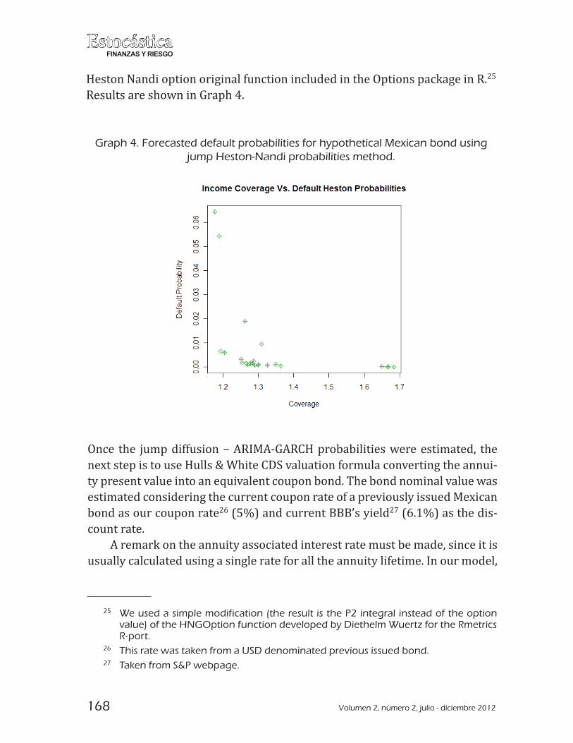
Corresponding probabilities were estimated using the Heston-Nandi frame-work in order to show their resemblance to the curve of jump diffusion prob-abilities using as input the ARIMA-GARCH forecasts, calculated with the pro-posed method. The�|��=��#��/�"��#��%��#��



Heston Nandi option original function included in the Options package in R.25 Results are shown in Graph 4.

25 We used a simple modification (the result is the P2 integral instead of the option value) of the HNGOption function developed by Diethelm Wuertz for the Rmetrics R-port.

26 This rate was taken from a USD denominated previous issued bond. 27 Taken from S&P webpage.

Graph 4. Forecasted default probabilities for hypothetical Mexican bond using jump Heston-Nandi probabilities method.

[�� &�� %#3��''%��`��`��`��|�3"�+�+��/�"��#�� &��{��3��%��|%��}&��O�!��%��'�"#%��!�"��&��%�-ty present value into an equivalent coupon bond. The bond nominal value was estimated considering the current coupon rate of a previously issued Mexican bond as our coupon rate26�4Z�<��%""��V��27�4��<��&��-count rate.

A remark on the annuity associated interest rate must be made, since it is usually calculated using a single rate for all the annuity lifetime. In our model,



28 The algorithm used for calculations are available on request.

/��%��!�"��"��"�!��'"�#��&��"3��"��%��+��#��#��%"��[+!��%��&��%��+��"��%��%+��3��-terpolation for interest rates and with them estimate the Net Present Value (NPV) for each payment. This procedure is hardly used since results are about the same but the estimation strategy is far more complex.

Also, an expected value for the recovery rate as in Equation (7) is required. �� /�� #�� +�� _�55�"�� "�� #�"�� *"%�� 4�88K<�� their paper, they made an extensive recovery rate analysis for Moody’s Inves-tor Service that is offered at no cost on the web. Based on their estimations, a "��!�"��"��'��X��/��+��*&��"��"�3"��&��!�"��"��!�"��rate for a BBB debtor taking into account the possibility of change on the as-sociated recovery rates.

}��&� �� &�� #�� &�� !��%�� O� !��%�� &�� &�-pothetical bond can be performed, resulting in a fair payment amount of 982,061,812 USD28 for the bond with an estimated nominal value of �8��X��Z�� O�� /&�� %�� jump diffusion probability. If we use the Heston Nandi probability model the payment amount is 178,444,019 USD. It may seem to be a huge amount, but it is a monthly payment that represents ��&��8��Z��'��&��#��!��%��'��'�%��#��!��%��global payment for complete credit risk insurance will be incurred into��%"��consistent with typical CDS valuations. This is the main reason why this hypo-thetical instrument must be issued in a deep money market in order to place it among several institutional investors, or within a global institution, typically a sovereign last resort lender such as the International Monetary Fund (IMF) �"��&��}�"��$�4}�<��'��&��O�3��#��, can be considered as the fair contribution that a BBB rated nation must pay to a deposit insurance system.

The payment is slightly different from the normal distribution suggested 3��#��%��&��%#3��{��&��3��#��/��#��+��!��&��3��#��/��#��+��!��-tility induced by the GARCH approximation and the interest rate interpola- by the GARCH approximation and the interest rate interpola-tion. These features have not been considered by traditional CDS valuation methods.

Conclusions

In this paper we have used the jump-diffusion risk neutral default probabili-ties models in a CDS valuation, we did this by using the complement of an ��&��#��"��V��3��3"��3"�+�+��#��/&�"��&��+��"V��



income is taken as the underlying asset and the expected payment is consid-�"��&��"�$��3"��}�� "3�"��+��"V�� #��!�� the default probabilities by using ARMA-GARCH income forecasted volatility as the underlying asset standard deviation in a jump diffusion option valu-��'"�#�/�"$��`��#��"��'�%��3"�+�+��#��-��%�%��{��+��"��&��|%��}&��O�!��%��method, result in a hybrid default probability and CDS valuation algorithm that incorporates some structural variables, as expected payment coverage, following a jump-diffusion underlying process.

Along the paper we showed that our simple jump diffusion probability series provided with ARIMA-GARCH forecasted volatilities are similar (but larger for small coverage ratios) to those obtained with the Heston-Nandi model since they arose from similar stochastic differential partial equations and the volatility process is the same, nevertheless it was calculated in differ-ent ways; outside for the jump diffusion probabilities and in the model for the Heston-Nandi ones.

The proposed method is consistent with traditional credit default prob-ability estimation methods like Credit Metrics or Credit+, and with the risk �%�"��!��%��%��|�}�#��&��3��'��&��!��&��log normal jump modeling of outliers may be improved, and perhaps it can be modeled by extreme value jump-diffusion processes. This is left as a future research as well as the use of these default probabilities in a reduced CDS valuation model or in a copula based probability model.

Bibliography

Altman, E. I. (1968). “Financial Ratios, Discriminant Analysis and the Prediction of ��"3�"��$"%3��?�� @��=��33��X��8X��

��4�888<��J"��"��'��#3��&��3��3��"��%��%��#��_��"��3�'��33��Z��

��4�88�<��!��"��O��"�� !�"�#��Credit Rating:�-�� A�� , London Risk Books.

. and G. Sabato (2007). “Modelling Credit Risk for SMEs: Evidence '"�#��&��O��"$��B��=��33��ZK�



��"�$��O��O��/��"��#��4�XX�<��*&��"��"%�&��0��2��A��9��8��B��C��, No. 2, pp. 205-247.

��$��O�&��4�XK�<��*&��J"��'�[3��"3�"��+��?�� 9� �� 8��=��33��K��Z��

��O��"��}��"�&�4�88Z<�� ̀ � #3�"��`��'��&��-�#��+��/��!��#��"��"��'�%��O/�3��+��?�� @��8��=��Z��33��ZZ��

��"��!��*��4�X��<��"��5��̀ %��"��"��!��|��"��$��?�� 8��=��33��8K��K

Brace, A., Gatarek, D. et Musiela, M. (1997). “The Market Model of Interest Rate ��#��-�� @��, 7(2), pp. 127-154.

�"�� 4�88Z<�� "$�� '�"� ��O� [3�� +�� "�� ?��.

�"��$��4�88�<��"��%��"�� #��"��'�"�� ,��2A�(��C��9��.

�"^3�� O�� +�� _�"��"�� 4�88X<�� O� /��&� ��%��"3�"�� $� �� "$�!��&��3%��/��&��'�%��^3�"��#��&^#��-ques Université d’Évry Val d’Essonne. D��A��.

�&��=��|��4�88�<��*�#��O�"��B�� @��}��O�"��J"�+�+�-lity and Statistics. USA.

Credit Suisse Financial Products (1997). CreditRisk+: A Credit Risk Management Framework, London. Credit Suisse Financial Products.-..T,

�"��"��\��&��4�88�<��*�#��O�"��`��/��&��33�� O3"��"��O`��

��!��4�88�<��'��%��'�%��;��C�@��, Vol.1, pp. ��

Dungey, M., F, R., González Hermosillo, B., Martin, V. (2002). “International Conta-�� ''��'"�#��&��%��"��&��*��=��"��3��*-@�D��A�9��.

�/��"��O��4�88�<��*��&��%#��$��!��&��V��\��

�"�$��`��O��O�&#%$��"�4�XX�<��%�"��'%��%��&��#�{��crisis of December 1994: Did local residents turn pessimistic before interna-��!��"��E��8��C��K��O%33��#��33��Z��Z��

��"��4�888<��̀ ��#3�"��!��#��'��"��"��$�#��?�� 0��2��A�F�@��, Vol. 24, No.1-2, pp. 119-149.



|��O��O��=��4�888<�� ̀ ��"#��`��|��3��%��+��C��@�� 1��=��33��K��

|%��`��}&��4�888<��%��"��'�%��O/�3��=��%��"3�"��'�%��$��?�� C��C�, Vol. 8, No. 1, pp. 29-40

�� %�� "�� '�%�� O/�3�� '�%�� ""��?�� C��C��=��33��

\�"��5��O��O&"�!��4�XX�<��"�/��O��&��%�%��Ed. Springer.

Kijima, M. and T. Suzuki (2001). “A jump diffusion model for pricing corporate debt ��%"��#3��{��3��"%��%"��;��C�@��, Vol. 1, No. 6, pp. 611-620.

��""�/��Y%�� 4�88�<�� %��"3�"��$�� &��J"��'��'�%��+��O��%"��?�� @��. Vol. 56, pp 1765-1799.

. and Turnbull (1995). “Pricing Derivatives on Financial Securities Subject to Credit

��$��?�� @��Z8�4�XXZ<��Z��Z�

��#�&��4�88�<��%��'��"��'�%��O/�3��O/�3��@��

��1��33��K��

Lamberton, D. and B. Lapeyre (1996). “Introduction to Stochastic Calculus Applied ��&�#3��|��

Longstaff, F. A., S. Mithal, and E. Neis (2005). “Corporate Yield Spreads: Default ��$��"��%��=�/� !��'"�#��&��"��'�%��O/�3��"$��+��?�� @��8��=��Z��33��Z��

�4�8�8<��*&��%+3"�#��"��"��#�"-$��?�� @�� 8��XK��=��33��Z8�

�@'��"��J��=��J��&�4�88K<��"��"��$�#��%�� {�� ̀��?��D� ��1��. USA.

��`��}&��"��4�XXZ<��"��#��*&��"�G��EH��(��C��9��.

Merton, R. C. (1974). “On the pricing of corporate debt: The risk structure of inter-��"��?�� @��. Vol. 29, No. 2, pp. 449-470.

. (1976). “Option Pricing when underlying stock returns are disconti-%�%��?�� @�� 8��33��Z��

��"�%{��4�88�<��O�"%��%"��"��$��'�"��'�%��+��O��%"��Wor2��A�9��, Université de Rennes I-IGR.

173

Superficies de volatilidad: Evidencia empirica del... EstocásticaFINANZAS Y RIESGO

O’Kane (2001). Credit Derivatives Explained, Lehman Brothers, March 2001.

��O�&�� 4�88�<�� "��*&��"��J"��-bruary 2001.

[V\��*%"+%��4�88�<��%��$��#��'��"��'�%��O/�3��J��0��

��O��O��&��=��3�"��J��/�"�&�4�XX�<��*&�� `��-��"��#��J"��3��0��A��9��8��2��B��C��

Shimko, D. (2004). “Credit Risk Modeling and Valuation: An Introduction in Credit ��$��-�� -��A��33��K�Z�Z��

Sadam, I. (2005). Alkalmazott matematikus szak, Thesis, Természettudományi Kar.

Sreedhar T. B. and T. Shumway (2008). “Forecasting default with the Merton dis-��'�%��#��C��@�� 1��=��33��X��X�

O�&@+%�&�"��J��4�888<��̀ ��+�"�#�"$��#��/��&��'�%��"��$��

. and D. Schubert (2001). “Copula-Dependent Defaults in Intensity ��`!��+��OO�=��&��3��{��"��8��X��"��8�X��

O�%�5��4�8�8<��"��'�%��O/�3��&��"��"��?�� 8��2��9��C��=��33��K��X��

*�$�!��J��4�8��<��#��/��&��!��3"��,��-��K��24��B�� 4�K��8�� 9� ��4�. Lecture Notes.

��"��5�� 4�88�<�� *�#3�"�"�� O��+��5�� `� ��&�� `��?�� 8��,�� , Vol. 25, No. 9, pp 1429-1449.

}%�"�5��et al�4�8��<��[3��J��$��'�"��&��#��"��3�"��J��

_�55�"��`��"��\�� #�"��*"%�� 4�88K<�� O�!�"��'�%��!�"��X��88��V��

Estocástica: FINANZAS Y RIESGO

Documents

Transcript of Estocástica: FINANZAS Y RIESGO