American Institute of Aeronautics and Astronautics

1

Estimation of Weather-Induced Arrival Delay Statistics

through Monte-Carlo Simulations

Monish D. Tandale* and P. K. Menon

†

Optimal Synthesis Inc., Palo Alto, CA 94303-4622

Aircraft have to be rerouted around severe weather to ensure safe operation. Consequent

changes in the flight plan often leads to arrival delays. Due to the complexity of the weather

patterns and the traffic flow structure, the uncertainties in aircraft arrival rates cannot be

predicted analytically from the uncertainties in the weather forecasts. This paper

demonstrates the use of Monte-Carlo simulation to transform the uncertainties in severe

weather prediction into uncertainties in the arrival flow rate at given airports. The aircraft

trajectories are propagated using a simulation model of the air traffic environment. A

rerouting algorithm is defined to modify the aircraft flight plans for avoiding severe weather

regions. Using the traffic data for a typical day as the baseline, 300 Monte-Carlo runs are

carried out and the variations in the aircraft arrival patterns are quantified as a function of

the weather prediction uncertainty for several airports in the continental United States.

I. Introduction

ne of the continuing challenges in the US National Airspace System (NAS) is that of improving the accuracy of

traffic flow predictions used for decision support during adverse aviation weather conditions1. Rerouting of

aircraft around severe weather, often introduces arrival delays. Such weather-related delays can be quantified using

aircraft state data in conjunction with an air traffic simulation software such as FACET2 (Future ATM Concepts

Evaluation Tool).

FACET2 is a fast-time airspace simulation environment, developed by NASA for exploring, developing and

evaluating advanced Air Traffic Management (ATM) concepts. FACET is capable of modeling system-wide

airspace operations over the United States. The software incorporates airspace models for Center/Sector boundaries,

airways, special use airspace definitions, navigation aids /fixes and airports. Weather models consisting of winds,

temperature, severe weather cells are also included. FACET models aircraft trajectories using spherical-earth

kinematic equations. The aircraft can be flown along either flight plan routes, direct routes or wind-optimal routes as

they climb, cruise and descend according to their individual aircraft-type performance models. Performance

parameters such as climb/descent rates and cruise speeds for a wide variety of aircraft are provided in the software.

For additional fidelity, the aircraft heading and airspeed dynamics are also modeled.

Although trajectories of aircraft executing their nominal flight plans can be accurately determined under given

weather conditions, there is significant uncertainty in the meteorological weather forecasts. Depending upon the

severity of the weather, the aircraft may be required to significantly deviate from their nominal flight plans,

introducing uncertainties in arrivals at various locations in the NAS. Since accurate traffic prediction is central to the

effective control of the traffic flow, methods for transforming the weather uncertainties into traffic flow

uncertainties are of interest.

However, due to the complexity of the weather patterns and the traffic flow structure, the uncertainties in the

aircraft arrivals cannot be derived analytically. Monte-Carlo simulations can be used to numerically establish the

relationship between uncertainties in the weather with the uncertainties in aircraft arrival rates. The objective of this

paper is to demonstrate the use of Monte-Carlo simulations to transform the uncertainties in severe weather

prediction into uncertainties in the aircraft arrival rates at given airports. The following sections will discuss the

formulation of Monte-Carlo simulations and sample numerical results.

This paper is organized as follows. Section II discusses how the software components are assembled for

performing the Monte-Carlo simulations. Section III will describe the modeling of the weather prediction

* Research Scientist, 868 San Antonio Road, Member AIAA.

† Chief Scientist, 868 San Antonio Road, Associate Fellow AIAA.

O

AIAA Guidance, Navigation and Control Conference and Exhibit20 - 23 August 2007, Hilton Head, South Carolina

AIAA 2007-6550

Copyright © 2007 by Optimal Synthesis Inc. Published by the American Institute of Aeronautics and Astronautics, Inc., with permission.

American Institute of Aeronautics and Astronautics

2

uncertainty. The aircraft rerouting algorithm is presented in section IV. Section V gives results of the Monte-Carlo

simulations. Conclusions are given in section VI.

II. Monte-Carlo Simulation of Traffic Flow Uncertainties

The following methodology is used to implement the Monte-Carlo simulation.

1. Generate random variations in the weather data using the knowledge of uncertainties in weather prediction.

2. Define algorithms for rerouting the aircraft around severe weather.

3. For each random variation of the weather pattern, propagate aircraft trajectory in FACET over a specified

duration including reroutes due to severe weather, and record the arrival rates at airports of interest.

4. Estimate the arrival statistics using the simulation data ensemble.

The Monte-Carlo simulation is set up by combining the FACET software with two other software components,

MATLAB®3 and CARAT#

4, 5.

MATLAB is a well-known computing platform used extensively in the scientific and engineering communities

By providing simpler access to robust numerical algorithms for linear algebra and eigensystem analysis, MATLAB

allows the user to design complex algorithms for automatic control and signal processing systems, and test them out

in the interactive environment. Availability of this software environment has spurred the development of an array of

toolboxes providing specialized functions useful in diverse fields such as image processing, automatic control,

neural networks, fuzzy logic and signal processing. In the present application, the MATLAB environment serves as

a platform for coding the Monte-Carlo simulation procedure, storing data, statistical analysis and graphical display

of the results. Trajectory propagation required for Monte-Carlo simulation runs is performed by FACET.

CARAT# (Configurable Airspace Research and Analysis Tool – Scriptable) software was developed to allow

access to the powerful capabilities of FACET from Java programs, MATLAB or Jython© 6

. This software allows

relatively inexperienced programmers to integrate other complex software packages with the capabilities of FACET.

Reference 4 and 5 discusses several such examples.

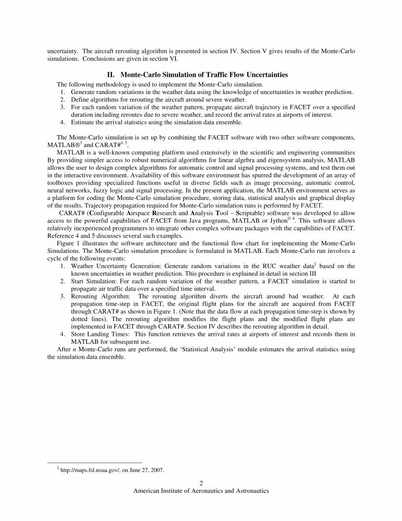
Figure 1 illustrates the software architecture and the functional flow chart for implementing the Monte-Carlo

Simulations. The Monte-Carlo simulation procedure is formulated in MATLAB. Each Monte-Carlo run involves a

cycle of the following events:

1. Weather Uncertainty Generation: Generate random variations in the RUC weather data‡ based on the

known uncertainties in weather prediction. This procedure is explained in detail in section III

2. Start Simulation: For each random variation of the weather pattern, a FACET simulation is started to

propagate air traffic data over a specified time interval.

3. Rerouting Algorithm: The rerouting algorithm diverts the aircraft around bad weather. At each

propagation time-step in FACET, the original flight plans for the aircraft are acquired from FACET

through CARAT# as shown in Figure 1. (Note that the data flow at each propagation time-step is shown by

dotted lines). The rerouting algorithm modifies the flight plans and the modified flight plans are

implemented in FACET through CARAT#. Section IV describes the rerouting algorithm in detail.

4. Store Landing Times: This function retrieves the arrival rates at airports of interest and records them in

MATLAB for subsequent use.

After n Monte-Carlo runs are performed, the ‘Statistical Analysis’ module estimates the arrival statistics using

the simulation data ensemble.

‡ http://maps.fsl.noaa.gov/, on June 27, 2007.

American Institute of Aeronautics and Astronautics

3

CARAT# SoftwareCARAT# Software

FACET Software

Trajectory

Propagation,

Predicted Landing

Rates at Airports

FACET Software

Trajectory

Propagation,

Predicted Landing

Rates at Airports

Monte Carlo Simulation

MATLAB Software

Rerouting

Algorithm

Rerouting

Algorithm

Landing Times

Statistical AnalysisStatistical Analysis

Store Landing

Times

Store Landing

Times

Weather Uncertainty

Generation

Weather Uncertainty

Generation

Start

Simulation

Start

Simulation

Repeat

n times

Repeat every

FACET

time step

Start

Simulation

Modified

Flight Plans

Original

Flight Plans

CARAT# SoftwareCARAT# Software

FACET Software

Trajectory

Propagation,

Predicted Landing

Rates at Airports

FACET Software

Trajectory

Propagation,

Predicted Landing

Rates at Airports

Monte Carlo Simulation

MATLAB Software

Rerouting

Algorithm

Rerouting

Algorithm

Landing Times

Statistical AnalysisStatistical Analysis

Store Landing

Times

Store Landing

Times

Weather Uncertainty

Generation

Weather Uncertainty

Generation

Start

Simulation

Start

Simulation

Repeat

n times

Repeat every

FACET

time step

Start

Simulation

Modified

Flight Plans

Original

Flight Plans

Figure 1. Software Architecture and Functional Flow-Chart

III. Weather Prediction Uncertainty Modeling

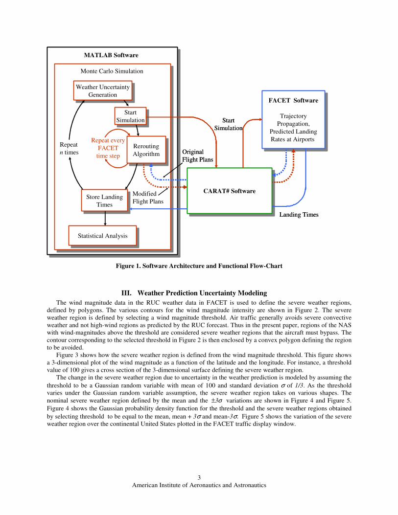
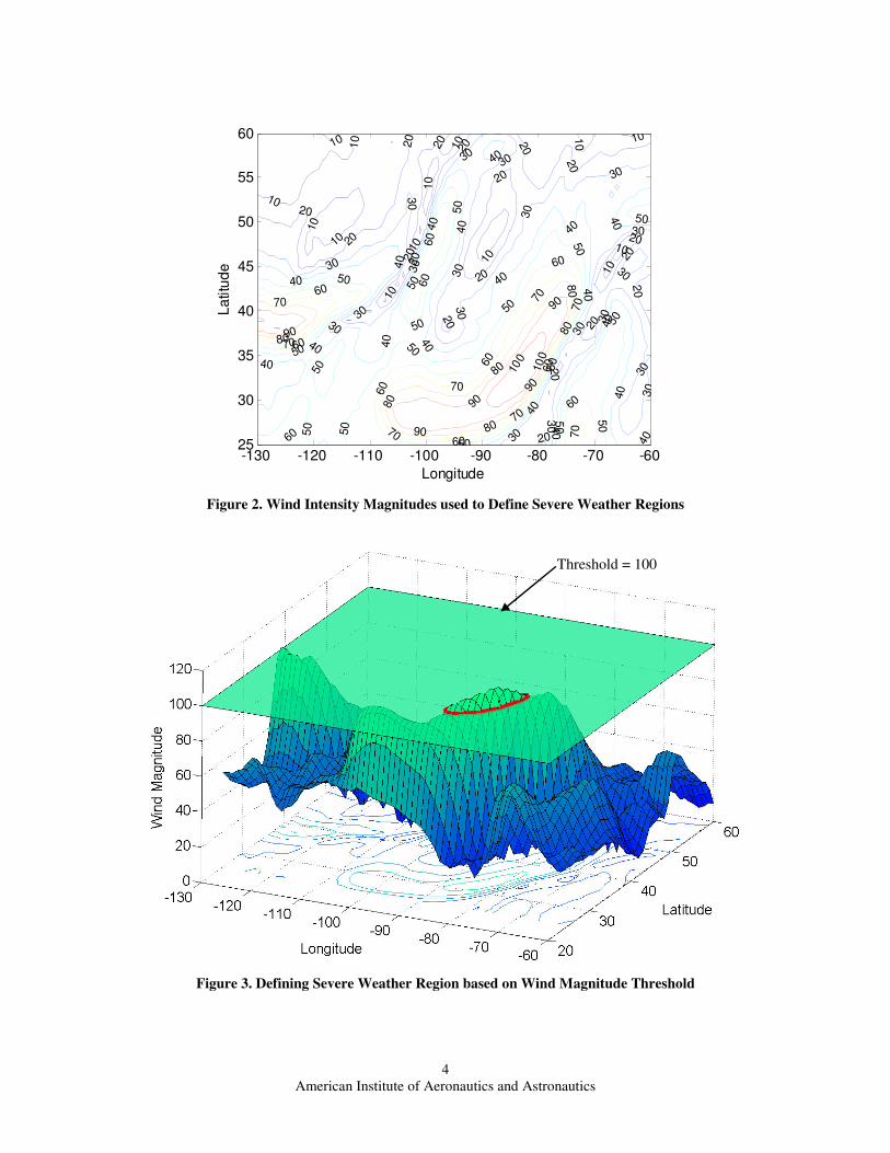
The wind magnitude data in the RUC weather data in FACET is used to define the severe weather regions,

defined by polygons. The various contours for the wind magnitude intensity are shown in Figure 2. The severe

weather region is defined by selecting a wind magnitude threshold. Air traffic generally avoids severe convective

weather and not high-wind regions as predicted by the RUC forecast. Thus in the present paper, regions of the NAS

with wind-magnitudes above the threshold are considered severe weather regions that the aircraft must bypass. The

contour corresponding to the selected threshold in Figure 2 is then enclosed by a convex polygon defining the region

to be avoided.

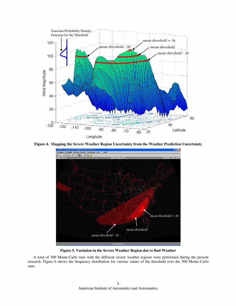
Figure 3 shows how the severe weather region is defined from the wind magnitude threshold. This figure shows

a 3-dimensional plot of the wind magnitude as a function of the latitude and the longitude. For instance, a threshold

value of 100 gives a cross section of the 3-dimensional surface defining the severe weather region.

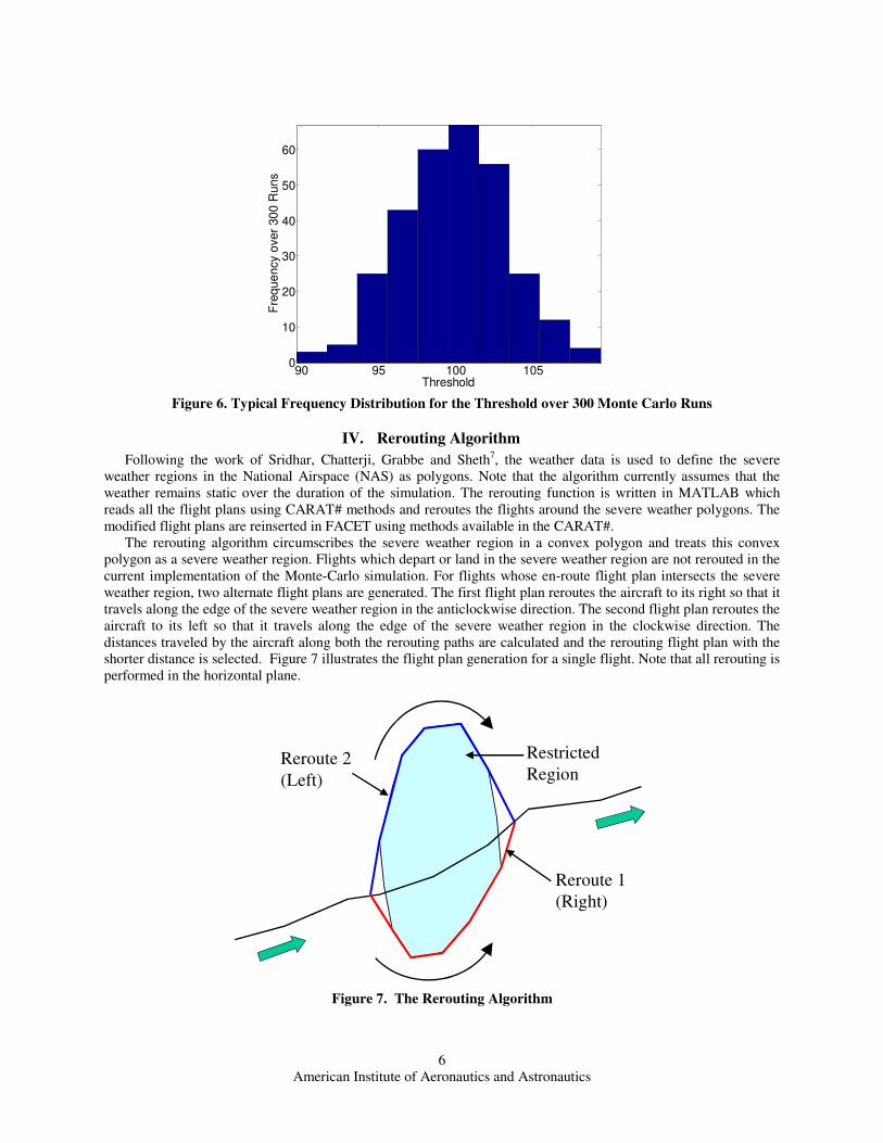
The change in the severe weather region due to uncertainty in the weather prediction is modeled by assuming the

threshold to be a Gaussian random variable with mean of 100 and standard deviation σ of 1/3. As the threshold

varies under the Gaussian random variable assumption, the severe weather region takes on various shapes. The

nominal severe weather region defined by the mean and the σ3± variations are shown in Figure 4 and Figure 5.

Figure 4 shows the Gaussian probability density function for the threshold and the severe weather regions obtained

by selecting threshold to be equal to the mean, mean + 3σ and mean-3σ. Figure 5 shows the variation of the severe

weather region over the continental United States plotted in the FACET traffic display window.

American Institute of Aeronautics and Astronautics

4

10101

010

10

10

10

10

10

10

10

10

1010

20

20

20

20

2020

2020

20

20

20

20

20

20

20

20

20

20

30

30

3030

30

30

30

30

30

30

30

30

30

30

30

30

30 30

30

40

40

40

40

40

40

40

40

404040

4040

40

4040

40

40

50

50

50

50

50

50

50

5050

50

50

50

50

50

50

50

50

60

60

60

60

60

60

60

60

60

60

60

70

70

70 70

70

70

70

70

80

80

80

80

80

80

90

90

90

90

90

10

0

100

Longitude

La

titu

de

-130 -120 -110 -100 -90 -80 -70 -6025

30

35

40

45

50

55

60

Figure 2. Wind Intensity Magnitudes used to Define Severe Weather Regions

Threshold = 100

Figure 3. Defining Severe Weather Region based on Wind Magnitude Threshold

American Institute of Aeronautics and Astronautics

5

mean - 3*sigma

mean threshold + 3σ

mean

mean - 3*sigma

Gaussian Probability Density

Function for the Threshold

mean threshold - 3σ

mean threshold + 3σ

mean threshold - 3σ

Gaussian Probability Density

Function for the Threshold

mean threshold

Figure 4. Mapping the Severe Weather Region Uncertainty from the Weather Prediction Uncertainty

mean threshold + 3σ

mean threshold - 3σ

mean threshold

Figure 5. Variation in the Severe Weather Region due to Bad Weather

A total of 300 Monte-Carlo runs with the different severe weather regions were performed during the present

research. Figure 6 shows the frequency distribution for various values of the threshold over the 300 Monte-Carlo

runs.

American Institute of Aeronautics and Astronautics

6

90 95 100 1050

10

20

30

40

50

60

Threshold

Fre

qu

en

cy o

ve

r 30

0 R

un

s

Figure 6. Typical Frequency Distribution for the Threshold over 300 Monte Carlo Runs

IV. Rerouting Algorithm

Following the work of Sridhar, Chatterji, Grabbe and Sheth7, the weather data is used to define the severe

weather regions in the National Airspace (NAS) as polygons. Note that the algorithm currently assumes that the

weather remains static over the duration of the simulation. The rerouting function is written in MATLAB which

reads all the flight plans using CARAT# methods and reroutes the flights around the severe weather polygons. The

modified flight plans are reinserted in FACET using methods available in the CARAT#.

The rerouting algorithm circumscribes the severe weather region in a convex polygon and treats this convex

polygon as a severe weather region. Flights which depart or land in the severe weather region are not rerouted in the

current implementation of the Monte-Carlo simulation. For flights whose en-route flight plan intersects the severe

weather region, two alternate flight plans are generated. The first flight plan reroutes the aircraft to its right so that it

travels along the edge of the severe weather region in the anticlockwise direction. The second flight plan reroutes the

aircraft to its left so that it travels along the edge of the severe weather region in the clockwise direction. The

distances traveled by the aircraft along both the rerouting paths are calculated and the rerouting flight plan with the

shorter distance is selected. Figure 7 illustrates the flight plan generation for a single flight. Note that all rerouting is

performed in the horizontal plane.

Reroute 1

(Right)

Reroute 2

(Left)

Restricted

Region

Figure 7. The Rerouting Algorithm

American Institute of Aeronautics and Astronautics

7

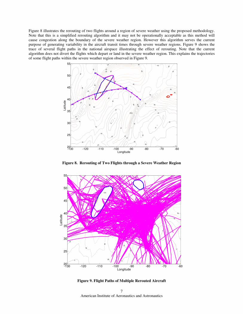
Figure 8 illustrates the rerouting of two flights around a region of severe weather using the proposed methodology.

Note that this is a simplified rerouting algorithm and it may not be operationally acceptable as this method will

cause congestion along the boundary of the severe weather region. However this algorithm serves the current

purpose of generating variability in the aircraft transit times through severe weather regions. Figure 9 shows the

trace of several flight paths in the national airspace illustrating the effect of rerouting. Note that the current

algorithm does not divert the flights which depart or land in the severe weather region. This explains the trajectories

of some flight paths within the severe weather region observed in Figure 9.

0

0

0

20

20

20

20

20

20

20

20

20

20

20

20

20

20

20

20

20

20

20

40

40

40

40

40

40

40

40

40

40

40

40

40

40

40

40

40

60

60

60

60

60

60

60

60

60

60

60

60

60

8080

80

80

80

80

10010

0 100

Longitude

La

titu

de

-130 -120 -110 -100 -90 -80 -70 -6020

25

30

35

40

45

50

55

Figure 8. Rerouting of Two Flights through a Severe Weather Region

0

0 0

0

0

0

0

0

0

40

40

40

40

40

40

40

40

40

40

4040

40

40

40

40

40

40

40

80

80

80

80

80

80

120

Longitude

La

titu

de

-130 -120 -110 -100 -90 -80 -70 -6020

25

30

35

40

45

50

55

Figure 9. Flight Paths of Multiple Rerouted Aircraft

American Institute of Aeronautics and Astronautics

8

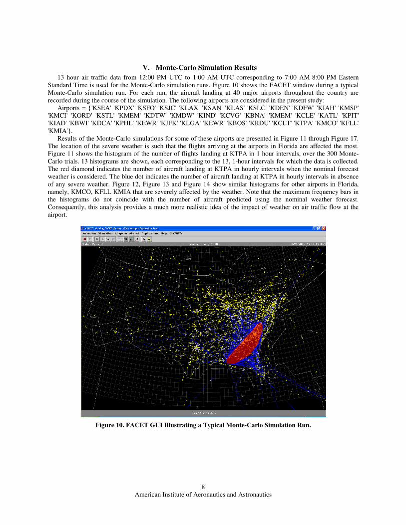
V. Monte-Carlo Simulation Results

13 hour air traffic data from 12:00 PM UTC to 1:00 AM UTC corresponding to 7:00 AM-8:00 PM Eastern

Standard Time is used for the Monte-Carlo simulation runs. Figure 10 shows the FACET window during a typical

Monte-Carlo simulation run. For each run, the aircraft landing at 40 major airports throughout the country are

recorded during the course of the simulation. The following airports are considered in the present study:

Airports = {'KSEA' 'KPDX' 'KSFO' 'KSJC' 'KLAX' 'KSAN' 'KLAS' 'KSLC' 'KDEN' 'KDFW' 'KIAH' 'KMSP'

'KMCI' 'KORD' 'KSTL' 'KMEM' 'KDTW' 'KMDW' 'KIND' 'KCVG' 'KBNA' 'KMEM' 'KCLE' 'KATL' 'KPIT'

'KIAD' 'KBWI' 'KDCA' 'KPHL' 'KEWR' 'KJFK' 'KLGA' 'KEWR' 'KBOS' 'KRDU' 'KCLT' 'KTPA' 'KMCO' 'KFLL'

'KMIA'}.

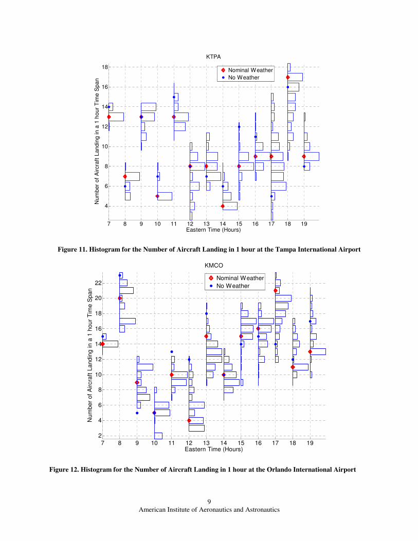
Results of the Monte-Carlo simulations for some of these airports are presented in Figure 11 through Figure 17.

The location of the severe weather is such that the flights arriving at the airports in Florida are affected the most.

Figure 11 shows the histogram of the number of flights landing at KTPA in 1 hour intervals, over the 300 Monte-

Carlo trials. 13 histograms are shown, each corresponding to the 13, 1-hour intervals for which the data is collected.

The red diamond indicates the number of aircraft landing at KTPA in hourly intervals when the nominal forecast

weather is considered. The blue dot indicates the number of aircraft landing at KTPA in hourly intervals in absence

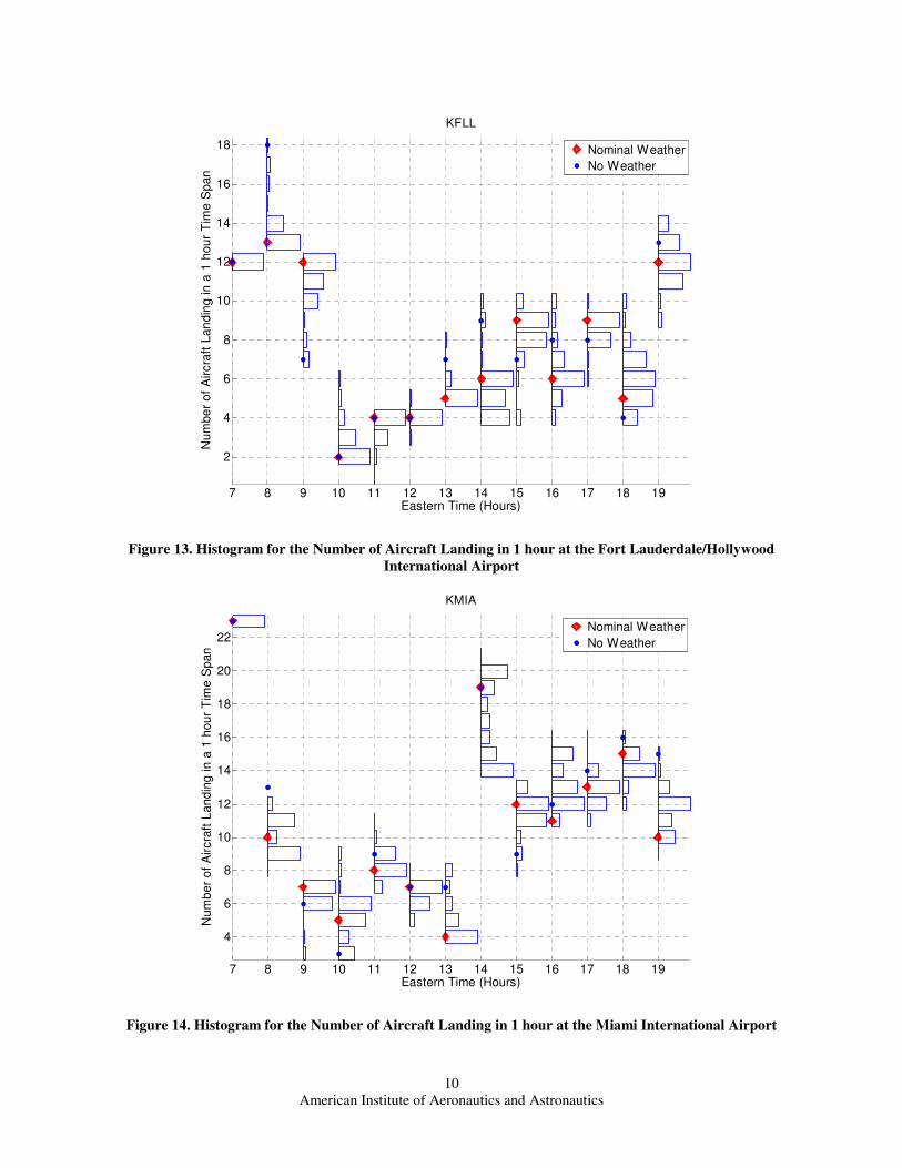
of any severe weather. Figure 12, Figure 13 and Figure 14 show similar histograms for other airports in Florida,

namely, KMCO, KFLL KMIA that are severely affected by the weather. Note that the maximum frequency bars in

the histograms do not coincide with the number of aircraft predicted using the nominal weather forecast.

Consequently, this analysis provides a much more realistic idea of the impact of weather on air traffic flow at the

airport.

Figure 10. FACET GUI Illustrating a Typical Monte-Carlo Simulation Run.

American Institute of Aeronautics and Astronautics

9

7 8 9 10 11 12 13 14 15 16 17 18 19

4

6

8

10

12

14

16

18

Eastern Time (Hours)

Num

ber

of

Air

cra

ft L

andin

g in a

1 h

our

Tim

e S

pan

KTPA

Nominal Weather

No Weather

Figure 11. Histogram for the Number of Aircraft Landing in 1 hour at the Tampa International Airport

7 8 9 10 11 12 13 14 15 16 17 18 19

2

4

6

8

10

12

14

16

18

20

22

Eastern Time (Hours)

Nu

mb

er

of

Air

cra

ft L

and

ing in

a 1

hou

r T

ime

Sp

an

KMCO

Nominal Weather

No Weather

Figure 12. Histogram for the Number of Aircraft Landing in 1 hour at the Orlando International Airport

American Institute of Aeronautics and Astronautics

10

7 8 9 10 11 12 13 14 15 16 17 18 19

2

4

6

8

10

12

14

16

18

Eastern Time (Hours)

Nu

mb

er

of

Air

cra

ft L

an

din

g in

a 1

ho

ur

Tim

e S

pa

n

KFLL

Nominal Weather

No Weather

Figure 13. Histogram for the Number of Aircraft Landing in 1 hour at the Fort Lauderdale/Hollywood

International Airport

7 8 9 10 11 12 13 14 15 16 17 18 19

4

6

8

10

12

14

16

18

20

22

Eastern Time (Hours)

Nu

mb

er

of

Air

cra

ft L

an

din

g in

a 1

ho

ur

Tim

e S

pa

n

KMIA

Nominal Weather

No Weather

Figure 14. Histogram for the Number of Aircraft Landing in 1 hour at the Miami International Airport

American Institute of Aeronautics and Astronautics

11

7 8 9 10 11 12 13 14 15 16 17 18 19

25

30

35

40

45

50

Eastern Time (Hours)

Nu

mbe

r of

Aircra

ft L

andin

g in a

1 h

our

Tim

e S

pa

n

KDFW

Nominal Weather

No Weather

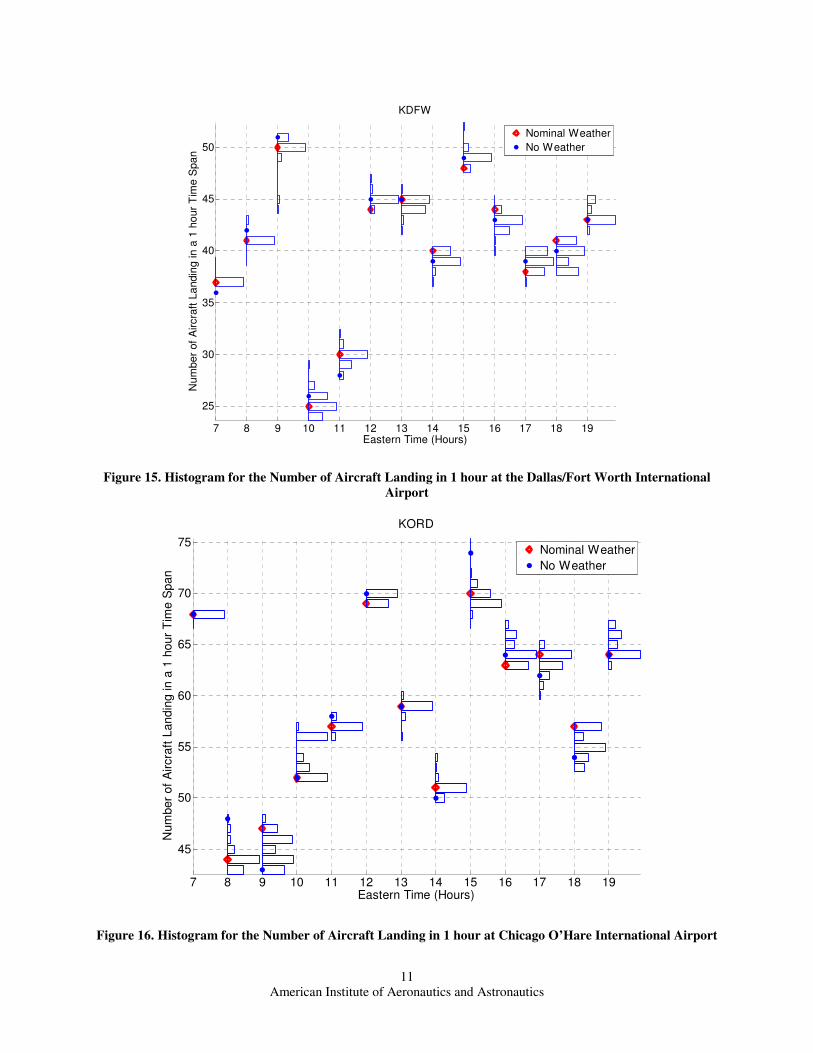
Figure 15. Histogram for the Number of Aircraft Landing in 1 hour at the Dallas/Fort Worth International

Airport

7 8 9 10 11 12 13 14 15 16 17 18 19

45

50

55

60

65

70

75

Eastern Time (Hours)

Num

ber

of

Aircra

ft L

andin

g in a

1 h

our

Tim

e S

pan

KORD

Nominal Weather

No Weather

Figure 16. Histogram for the Number of Aircraft Landing in 1 hour at Chicago O’Hare International Airport

American Institute of Aeronautics and Astronautics

12

7 8 9 10 11 12 13 14 15 16 17 18 19

5

10

15

20

25

Eastern Time (Hours)

Num

ber

of

Aircra

ft L

andin

g in a

1 h

our

Tim

e S

pa

n

KSFO

Nominal Weather

No Weather

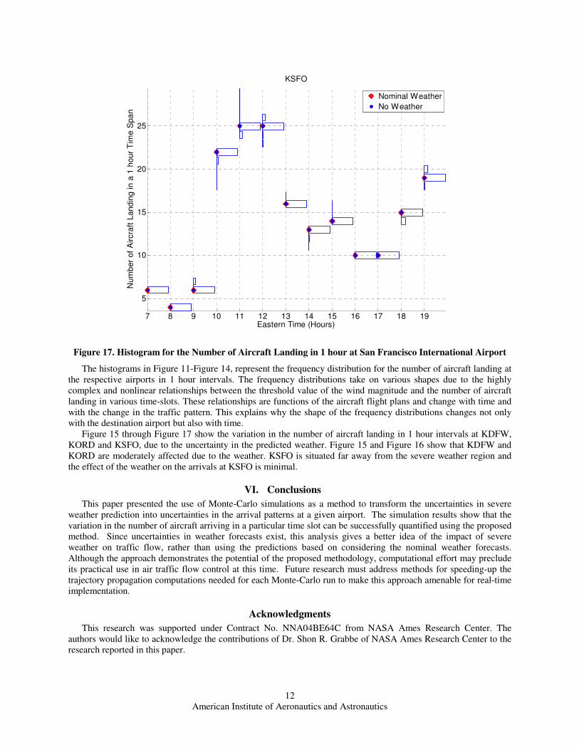
Figure 17. Histogram for the Number of Aircraft Landing in 1 hour at San Francisco International Airport

The histograms in Figure 11-Figure 14, represent the frequency distribution for the number of aircraft landing at

the respective airports in 1 hour intervals. The frequency distributions take on various shapes due to the highly

complex and nonlinear relationships between the threshold value of the wind magnitude and the number of aircraft

landing in various time-slots. These relationships are functions of the aircraft flight plans and change with time and

with the change in the traffic pattern. This explains why the shape of the frequency distributions changes not only

with the destination airport but also with time.

Figure 15 through Figure 17 show the variation in the number of aircraft landing in 1 hour intervals at KDFW,

KORD and KSFO, due to the uncertainty in the predicted weather. Figure 15 and Figure 16 show that KDFW and

KORD are moderately affected due to the weather. KSFO is situated far away from the severe weather region and

the effect of the weather on the arrivals at KSFO is minimal.

VI. Conclusions

This paper presented the use of Monte-Carlo simulations as a method to transform the uncertainties in severe

weather prediction into uncertainties in the arrival patterns at a given airport. The simulation results show that the

variation in the number of aircraft arriving in a particular time slot can be successfully quantified using the proposed

method. Since uncertainties in weather forecasts exist, this analysis gives a better idea of the impact of severe

weather on traffic flow, rather than using the predictions based on considering the nominal weather forecasts.

Although the approach demonstrates the potential of the proposed methodology, computational effort may preclude

its practical use in air traffic flow control at this time. Future research must address methods for speeding-up the

trajectory propagation computations needed for each Monte-Carlo run to make this approach amenable for real-time

implementation.

Acknowledgments

This research was supported under Contract No. NNA04BE64C from NASA Ames Research Center. The

authors would like to acknowledge the contributions of Dr. Shon R. Grabbe of NASA Ames Research Center to the

research reported in this paper.

American Institute of Aeronautics and Astronautics

13

References 1“Weather Forecasting Accuracy for FAA Traffic Flow Management: A Workshop Report,” National Research Council,

ISBN: 0-309-08731-7, 2003. 2Bilimoria, K. D., Sridhar, B., Chatterji, G. B., Sheth, G., and Grabbe, S., “FACET: Future ATM Concepts Evaluation Tool,”

3rd USA/Europe Air Traffic Management R&D Seminar, Naples, Italy, June 2000. Also in Air Traffic Control Quarterly, Vol. 9,

No. 1, March 2001, pp. 1–20. 3Anon, “MATLAB User’s Manual,” The MathWorks, Inc., Natick, MA, 2007. 4Menon, P. K., Diaz, G. M., Tandale, M. D., and Kwan, J., “CARAT# - A Rapid Prototyping Software for Developing Next-

Generation Air Traffic Management Algorithms,” Final Report Prepared under NASA Contract No. NNA05BE64C, Vol. I,

Optimal Synthesis Inc, Palo Alto, CA, November 21, 2006. 5Menon, P. K., Diaz, G. M., Vaddi, S. S., and Grabbe, S. R., “A Rapid Prototyping Environment for En Route Air Traffic

Management Research”, AIAA Guidance, Navigation and Control Conference, August 15-18 2005, San Francisco, CA. 6Pedroni, S., and Rappin, N., Jython Essentials, O’Reilley, Sebastopol, CA, 2002. 7Sridhar, B., Chatterji, G. B., Grabbe, S. and Sheth, K., “Integration of Traffic Flow Management Decisions,” AIAA

Guidance, Navigation, and Control Conference and Exhibit, Monterey, CA, August 5-8, 2002.