Munich Personal RePEc Archive

Estimation of a Supply Function

Merino Troncoso, Carlos

UNED

4 April 2021

Online at https://mpra.ub.uni-muenchen.de/106991/

MPRA Paper No. 106991, posted 06 Apr 2021 01:43 UTC

CHAPTER 2: ESTIMATION OF A SUPPLY FUNCTION

In this chapter we provide a brief introduction of the production and supply function. The theoretical neoclassical model, has limited capacity to explain data. Recent structural econometric techniques provide better estimation results and are able to explain entry, exit and investment decisions of firms. 1.- Introduction

In a similar way as in demand estimation, where we maximized utility functions, in this

chapter we estimate a production function, productivity measures and cost functions.

Technological efficiency is represented in the production function while economic

efficiency is represented in the cost function. In this chapter we will replicate the main

studies on production and cost function using standard software packages such as Excel

or R.

Productivity estimates together with demand elasticity are key components of market

structure studies. Traditionally productivity was estimated empirically using industry

panels using a theoretical production function equation. These estimates were not

consistent with data and did not explain market dynamics.

This chapter acknowledges how researchers have refined productivity estimation with

the development of a broader dynamical structural approach in a similar way as in demand

estimation. Firms decisions on investment strategies will depend on future expected

profits than invest in research and development will have a higher probability of staying

in the market while others with lower investment and lower productivity will have higher

probability of exit. Firms will invest if they have expectations on future profits based on

expectations and past achievements.

The chapter covers the dual approach of cost functions. Costs are a key component of the

benefits and as such knowledge of the costs of a company or industry and the study of

increasing returns of scale are fundamental to the analysis of competition. While the

theoretical cost functions are generally known from the introductory economics courses,

this chapter will also explain further research on increasing returns of scale and scope in

industries where competition problems are common such as telecommunication and

energy markets. The main concept here is economies of scale or the proportional increase

in cost resulting from a small proportional increase in the level of output.

We begin with the traditional production function estimation, its endogeneity problems

and further developments followed by cost function estimation developed by Viner

(1932) and Sraffa (1926). Next scale economies and multiproduct scope economies are

studied. Finally, the chapter explains other alternative methods that measure efficiency

as a mere proportion of outputs and inputs while giving up production function

determination. These methods are called frontier analysis approach and are divided into

Stochastic Frontier Analysis (SFA) and Data Envelope Analysis (DEA).

2.- Production function estimation

A production function is a mathematical function that relates the maximum quantity of

output that can be obtained with inputs for example capital and labor (2007). Productivity

is a measure of efficiency, the contribution of a particular input to the production.

Syverson (2011) documented massive differences in total factor productivity (TFP)

between industries in the US and stated that productivity is a matter of survival for

business in a market. Duration, entry and exit in a particular market will most likely be

related to a measure of efficiency or productivity of a firm. This is relevant when

discussing market structure.

There are several economic properties of a production functions, namely nonnegativity,

non-decreasing in inputs and concavity, that are generally expected and tested (for a

complete description of assumptions of production functions in Microeconomics see

Mas-Colell et al. (1995)). There are several mathematical functions that fit these

assumptions, but Cobb-Douglas, Translog and Quadratic or Cubic production functions

have been widely used in productivity analysis as we will see in this Chapter.

Classical graphs of the production function and average and marginal productivity are

shown below assuming that only one input remains variable (e.g. Labor), while the rest

are fixed. The graph represent a production function that only fulfills the general

assumptions explained above in the segment of 50 and 100 of labor input. To the left of

50 labor units, the function is convex and to the right of 100, it is decreasing in labor, so

the economically feasible region is only between 50 and 100. In the figure below average

productivity AP (or output per unit of input) and marginal productivity MP (increase in

output when input increases in one unit) are represented:

If we take into account two inputs the production function is generally represented by a

family of isoquants which are combinations of two inputs (capital and labor) that are

capable of producing an output level. There is one for each level of output and show

higher level of output the farther they are from the origin. The expected shape of the

production function implies convex isoquants with the below shape that can be easily

minimized. The cost function will be the pairs of minimal cost for each unit of production.

Unfortunately the theoretical model is too general and does not explain well specific

production and cost data. Authors have dealt with different econometrical problems that

surge when fitting easy functional forms to data.

As we mentioned, several mathematical functions that comply with minimal demanded

assumptions have been fitted to production data and tested to comply with the

abovementioned minimal assumptions.

A common function used in economics is Cobb-Douglas production function (see

Ackerberg et al. (2007)):

𝑌 = 𝐴𝐿𝛽𝐿𝐾𝛽𝐾

Where Y is output, K and L are capital and labor inputs, 𝛽 are parameters and A is total

factor productivity1. It is usually expressed as a linear equation in natural logarithms:

𝑦 = 𝛽0 + 𝛽𝑘𝑘 + 𝛽𝑙𝑙 + 𝜖

𝛽0 is the mean efficiency level while 𝜖 are unobserved sources of differences such as

managerial ability or technology differences between firms. Again, the problem if

endogeneity appears when estimating this equation using simple OLS regression (see

Econometric Appendix), as acknowledged by Marschak et al. (1944) . The problem is

that inputs K and L are not independent variables but are correlated with the unobserved

error term 𝜖. We face a problem of endogeneity if, for example, higher productivity

companies, i.e. those with the highest unobserved productivity also demand a large

number of inputs, see Davis and Garcés (2009), and a selected sample as only the most

efficient firms would appear in the panel data, as the least efficient would have exited the

market.

1 TFP - is the variation in output not explained by inputs depending on the functional approach, in this

particular case the residuals or TFP would equal 𝛽0 + 𝜖

If we do not take into account the problem of endogeneity, our estimated coefficients on

endogenous inputs would be overestimated. One possible solution is to use proxy

instrumental variables, or variables correlated with the company's demand for input but

not correlated with firm production.

Olley and Pakes (OP) (1996) suggested using investment as a proxy for productivity to

control for endogeneity. We will see that this approach takes into account the decision

process of a firm that will also be covered in chapter three, Market Structure and

Dynamics. Furthermore, Levinsohn and Petrin (2003) refined the OP work.

OP designed an algorithm to simulate the decision process of an incumbent firm. Firms

at the beginning of each period decide whether to exit or continue in the market. If they

decide to exit they will receive a liquidation value of , if they continue in the market

they will choose inputs (labor, materials and energy) and a level of investment Iit. The

sequence of decisions of a firm maximizing the expected discounted value of net future

profits is shown in the following Bellman equation2 : 𝑉(𝑘𝑗𝑡 , 𝑎𝑗𝑡 , 𝑤𝑗𝑡 , ∆𝑡 )=max{𝜙(𝑘𝑗𝑡 , 𝑎𝑗𝑡 , 𝑤𝑗𝑡 , ∆𝑡), 𝑚𝑎𝑥{𝜋(𝑘𝑗𝑡 , 𝑎𝑗𝑡 , 𝑤𝑗𝑡 , ∆𝑡) − 𝑐(𝑖𝑗𝑡 , ∆𝑡) +𝛿𝐸[𝑉(𝑘𝑗𝑡+1, 𝑎𝑗𝑡+1, 𝑤𝑗𝑡+1, ∆𝑡+1) ⋮ 𝑘𝑗𝑡 , 𝑎𝑗𝑡 , 𝑤𝑗𝑡 , ∆𝑡 , 𝑖𝑗𝑡] }

This equation describes the dynamic decision process of a firm. First, the firm decides to

exit a market if its liquidation value, 𝜙( ), exceeds the expected discounted value of net

future profits. Second, it decides on investing or not 𝑖𝑗𝑡, which is the solution to the second

maximization bracket, where 𝜋 is the profit function and C is the cost of investment, 𝛿 is

the discount function and E ( ) is the firm expectation conditional on information at t. Firms with positive productivity shocks in t will invest more in that period t. OP derive

the unobserved productivity shock as: 𝛺𝑖𝑡 = ℎ(𝑖𝑖𝑡 , 𝑘𝑖𝑡 , 𝑎𝑖𝑡)

Firms will invest in the future if there is an increase in current productivity. OP derive the

following Cobb-Douglas production function:

𝑦𝑖𝑡 = 𝛽0 + 𝛽𝑘𝑘𝑖𝑡 + 𝛽𝑙𝑙𝑖𝑡 + 𝛽𝑚𝑚𝑖𝑡 + 𝛽𝑎𝑎𝑖𝑡 + 𝑢𝑖𝑡

whereby,

𝑢𝑖𝑡 = Ω𝑖𝑡 + 𝜂𝑖𝑡

Substituting Ω𝑖𝑡 and 𝑢𝑖𝑡 in the production function, we obtain:

𝑦𝑖𝑡 = 𝛽𝑙𝑙𝑖𝑡 + 𝛽𝑚𝑚𝑖𝑡 + 𝛽𝑎𝑒𝑖𝑡 + (𝛽0 + 𝛽𝑘𝑘𝑖𝑡 + 𝛽𝑎𝑎𝑖𝑡 + ℎ(𝑖𝑖𝑡 , 𝑘𝑖𝑡 , 𝑎𝑖𝑡)) + 𝜂𝑖𝑡

Where y is output, k and l are capital and labor inputs, 𝛽 are parameters, a is age of the

firm, all in logs, Ω𝑖𝑡 is a productivity shock observed by the firm and 𝜂𝑖𝑡 unobserved

shocks. This specification takes into account the relation between inputs and Ω𝑖𝑡 and

controls for unobserved productivity, while traditional models based on OLS estimates

will be biased upwards, this specification can be estimated with OLS without bias. With

this development estimation of parameters is more accurate and a structural explanation

of entry and exit of firms in a market.

2 See appendix for an explanation of the Bellman equation.

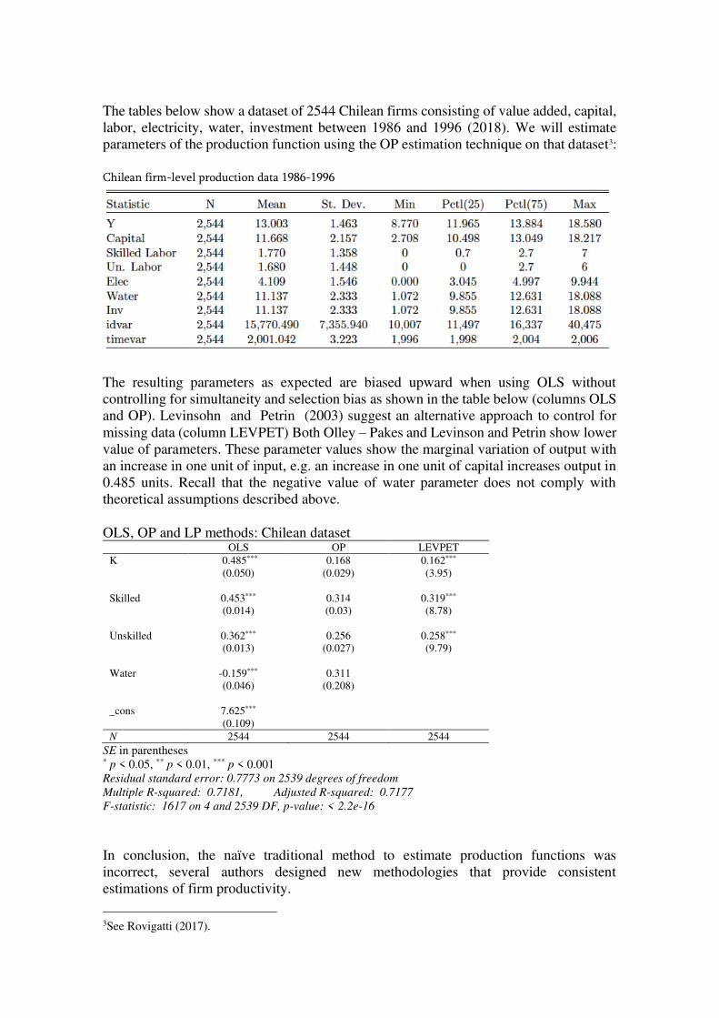
The tables below show a dataset of 2544 Chilean firms consisting of value added, capital,

labor, electricity, water, investment between 1986 and 1996 (2018). We will estimate

parameters of the production function using the OP estimation technique on that dataset3:

Chilean firm-level production data 1986-1996

The resulting parameters as expected are biased upward when using OLS without

controlling for simultaneity and selection bias as shown in the table below (columns OLS

and OP). Levinsohn and Petrin (2003) suggest an alternative approach to control for

missing data (column LEVPET) Both Olley – Pakes and Levinson and Petrin show lower

value of parameters. These parameter values show the marginal variation of output with

an increase in one unit of input, e.g. an increase in one unit of capital increases output in

0.485 units. Recall that the negative value of water parameter does not comply with

theoretical assumptions described above.

OLS, OP and LP methods: Chilean dataset OLS OP LEVPET

K 0.485*** 0.168 0.162***

(0.050) (0.029) (3.95)

Skilled 0.453*** 0.314 0.319***

(0.014) (0.03) (8.78)

Unskilled 0.362*** 0.256 0.258***

(0.013) (0.027) (9.79)

Water -0.159*** 0.311

(0.046) (0.208)

_cons 7.625***

(0.109)

N 2544 2544 2544

SE in parentheses * p < 0.05, ** p < 0.01, *** p < 0.001

Residual standard error: 0.7773 on 2539 degrees of freedom Multiple R-squared: 0.7181, Adjusted R-squared: 0.7177 F-statistic: 1617 on 4 and 2539 DF, p-value: < 2.2e-16

In conclusion, the naïve traditional method to estimate production functions was

incorrect, several authors designed new methodologies that provide consistent

estimations of firm productivity.

3See Rovigatti (2017).

3.- Cost function estimation

If we take factor prices as given and multiplying then by the quantities of production

factors a cost equation is obtained. The cost function gives the minimal cost foreach level

of production. The cost function has also general properties as the production function

such as nonnegativity, nondecreasing in factor prices, non-decreasing in output,

homogeneous and concave in input prices. Recall that through Shepard´s lemma (1953)

deriving cost function with respect to price of factors one can obtain input demand

functions and with them obtain the production function.

The graphic representation of cost functions was developed by Viner (1932). A cost

function that complies with the minimum properties is represented below (STC are short

term total cost and SVC short term variable cost). In the second graph below average and

marginal cost are represented. Short term average cost function (SAC) (and equivalently

variable cost curve SAVC) are unitary costs or total cost divided by total output and has

a U-shape following production function curvature and fixed factor prices. Average cost

decreases as output increases until the average cost is at the minimum. After this the law

of diminishing returns makes average and marginal cost to rise. Marginal cost (SMC) is

the derivative of the production function with respect to output or the infinitesimal change

in cost when production increases in one unit. When prices are given in perfect

competition, the part of marginal cost curve that is positively sloped (above min SAC)

represents the short term supply of the individual firm.

Short term means a period of time when some inputs remain fixed. Economies of scale

surge when all factors are variable and an equivalent increase in all factors generates a

more than proportionate increase in production. In the long term all factors are variable,

technological change and entry and exit can affect cost functions. The minimum average

cost is known as Minimum Efficient Scale (MES) is the optimal level of output to produce

(Greer, 2010). We will see below a classic example of economies of scale known as

natural monopoly, where average costs are always declining so efficient production is

better if it is concentrated in a single firm.

Economies of scale

The classic work on scale economies is Nerlove (1961), that studies power generation

in the US using data of 145 firms in 1955. The sample collected consisted of cost data,

fuel prices, labor and capital prices and total production of electricity for each electricity

generation plant. The summary statistics of Nerlove´s data is4 shown below:

Nerlove fitted the data to a Cobb-Douglas cost function derived from the following

production function with three inputs: capital (K), labor (L) and fuel (F):

𝑌 = 𝐴𝐿𝛽𝐿𝐾𝛽𝐾𝐹𝛽𝐹𝑢

4Table built using Hlavac, Marek (2018). stargazer: Well-Formatted Regression and Summary Statistics

Tables. R package version 5.2.2. https://CRAN.R-project.org/package=stargazer

From this production function he obtained a cost function in logs in terms of units of fuel

as follows:

𝐿𝑛 ( 𝐶𝑃𝐹) = 𝛽0 + 𝛽𝑦𝐿𝑛𝑌 + 𝛽𝐿𝐿𝑛 (𝑃𝐿𝑃𝐹) + 𝛽𝐾𝐿𝑛 (𝑃𝐾𝑃𝐹) + 𝜀

Where Y measures billion Kwatt hour of electricity produced, 𝑃𝐾 price of capital, 𝑃𝐿 price of labor (dollars per hour) and 𝑃𝐹 is the fuel price in cents of dollar per million

BTUs.

Nerlove estimated the model using traditional OLS regression using cost and input prices

for 145 companies. Results are shown in the table below were Nerlove work is replicated

using his original data:

Table: Regression results Nerlove (1963)

From the above theoretical curves it is expected that the parameter of output should be

positive as well as input price parameters (an increase in output or input price parameters

should always increase cost). Indeed, 𝛽𝑦 , 𝛽𝐿 parameters are positive and significant, the

former means that an increase in 1% in output yields a 0.72% increase in total cost,

considering all other variables to remain fixed (2010).

Nerlove rejects the hypothesis of constant returns of scale as the inverse of the log Y

parameter5 (0.72)−1 = 1.39 is greater than one. This proves that power generating plants

have increasing returns of scale (positive economies of scale). The scale parameter is

also the ratio of marginal to average cost:

𝜕𝑙𝑛𝐶𝜕𝑙𝑛𝑄 = 𝑄𝐶 𝜕𝐶𝜕𝑄 = 𝑀𝐶𝐴𝐶

5 Because 𝑟 = ∑ 𝛽𝑖𝑖 , see (2010)

This ratio is positive/negative for increasing/decreasing returns to scale. Nerlove also

divided the data in 5 groups according to the size of the firms. In the five regressions

returns to scale were lower as the size of the firm increased.

The following figure shows the Nerlove data (in log), the estimated costs based on the

output level and below the estimated residuals as a difference between the estimated and

the actual values. For the estimate to be consistent under OLS, the residuals need to have

no dependence on explanatory variables. On the contrary, the graph shows that they

depend on the output level which violates the requirement for consistent estimates. At

low and high levels of production, residuals are positive so the true cost is higher than the

estimated values. On the other hand, for output intermediate values, the true value of the

costs is better than the estimate. The graph of the residuals reflects a U-shape, see (2009)

and (2018).

Figure: Nerlove graphs on fitted Log Cost and regression residuals

This diagnosis suggests that the shape of the cost function is incorrect, high residuals at

low and high levels of output reveal an incorrect specification of the production function

which should have a U type of cost function. The plot and data prove that there are

increasing scale economies that are exhausted at a certain output level from which

declining scale economies begin. Nerlove suggests that the specification can be corrected

by expanding the function with a quadratic term. This generates a more flexible cost

function that will allow cost to vary with the output level in a way that can generate

economies of scale followed by diseconomies of scale as the level of production

increases.

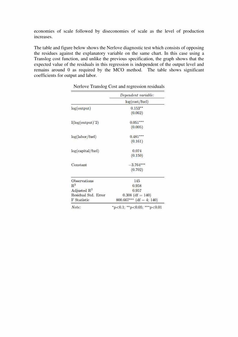
The table and figure below shows the Nerlove diagnostic test which consists of opposing

the residues against the explanatory variable on the same chart. In this case using a

Translog cost function, and unlike the previous specification, the graph shows that the

expected value of the residuals in this regression is independent of the output level and

remains around 0 as required by the MCO method. The table shows significant

coefficients for output and labor.

Nerlove Translog Cost and regression residuals

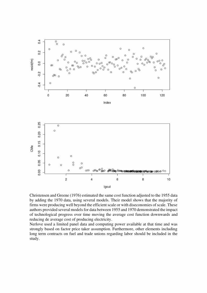
Christensen and Greene (1976) estimated the same cost function adjusted to the 1955 data

by adding the 1970 data, using several models. Their model shows that the majority of

firms were producing well beyond the efficient scale or with diseconomies of scale. These

authors provided several models for data between 1955 and 1970 demonstrated the impact

of technological progress over time moving the average cost function downwards and

reducing de average cost of producing electricity.

Nerlove used a limited panel data and computing power available at that time and was

strongly based on factor price taker assumption. Furthermore, other elements including

long term contracts on fuel and trade unions regarding labor should be included in the

study.

Multi-product firms and economies of scale

(1984) conducted an empirical estimate of AT&T's cost function and economies of scale

and scope in local and long-distance calls. this study was relevant for the decision of the

U.S. government in 1982 to break AT&T into several local firms while leaving AT&T in

the long-distance call market (2009). The allegation of AT&T against it was the

efficiencies gained from managing all telecommunications services in a single company

would be lost if it was divided by region and activities. Evans and Heckman proved

empirically that they were wrong. They used a "subaditivity" test for the cost function, a

property that implies that the cost is lower when performed by a firm that by several

firms. The failure of this test would mean that a single firm is more inefficient that several

firms.

To do this they defined a cost equation for two products:

𝐶 = 𝐶(𝑞𝐿 , 𝑞𝑇 , 𝑟, 𝑚, 𝑤, 𝑡),

Where Lq the output level of local L calls is, and Tq is the output level of long distance T

calls. Cost functions depend on the price of production factors: r is the return rate of

capital, w is the wage rate, and m is the price of the materials, t is a variable that captures

technical change.

These authors used a translog function with two products and three production factors:

log 𝐶 = 𝛼0 + ∑ 𝛼𝑖𝑖 𝑙𝑜𝑔𝑝𝑖 + ∑ 𝛽𝑖𝑖 𝑙𝑜𝑔𝑞𝑖 + 12 ∑ ∑ 𝛾𝑖𝑗𝑙𝑜𝑔𝑝𝑖𝑙𝑜𝑔𝑝𝑗𝑗𝑖 +12 ∑ ∑ 𝛿𝑘𝑗𝑙𝑜𝑔 𝑞𝑘 log 𝑞𝑗 +𝑗𝑘 ∑ ∑ 𝜌𝑖𝑘𝑙𝑜𝑔 𝑞𝑘 log 𝑝 𝑖 + ∑ 𝜆𝑖 log 𝑡𝑖𝑘𝑖 log 𝑝𝑖 + ∑ 𝜃𝑘 log 𝑡𝑘 +𝜏 log(𝑡)2 + 𝜇 log 𝑡

This cost function is much more general than that used at first by Nerlove based on a

Cobb-Douglas function. It is more flexible and can approach any cost function. Let's

define it for two inputs and two outputs.

The Translog cost function is presented in an unrestricted way but in the estimate a

number of restrictions on the cost functions suggested by the theory are imposed. Authors

impose homogeneity in input prices and symmetry on input prices. Using Shepard´s

Lemma6, one can obtain the three inputs (i=1,2,3) participation equations: 𝑠𝑖 = 𝛼𝑖 + ∑ 𝛾𝑖𝑗𝑙𝑜𝑔𝑝𝑗𝑗 + ∑ 𝜌𝑖𝑘𝑙𝑜𝑔 𝑞𝑘 ∑ 𝜆𝑖 log 𝑡 𝑖𝑘

6 The derivatives of the cost function with respect to input prices are the input demand

functions. 1 2 1 2 3( ,q , , , , )

j

j

C q p p p tI

p

¶=

¶

So the participation of input j in total costs would then be:

ln ln

ln ln

j j j

j

j j

p I p C Cs

C C p p

¶ ¶= = =

¶ ¶

By applying Shepard's lemma to the cost function we get the participation equations.

The estimate parameters of these equations are shown in the table below. A SURE

estimator (seemingly unrelated regressions) was used (2015).

Selected estimated results Translog function with 31 observations

Estimate Std. Error t value Pr(>|t|)

Constant 9.0542 0.0044524 20.335.750 < 2.2e-16 ***

Capital 0.654 0.1555707 42.075 0.0018071 **

Labour 0.354 0.1414821 51.771 0.0004148 *** Local

(output) 0.226 0.2221301 10.197 0.3319212 Toll

(Output) 0.504 0.5275837 -0.4318 0.6750634

Technology -0.201 0.0780344 -0.1255 0.9025945

---

Signif. codes: 0 ‘***’ 0.001 ‘**’ 0.01 ‘*’ 0.05 ‘.’ 0.1 ‘ ’ 1

R-squared: 0.9999439 Adjusted R-squared: 0.9998318

(Wales, 1987) proved that the function used was concave in input prices and monotonic

but fails to comply non decreasing in output.

Subaditivity Test

Heckman and Evans provided a test to prove if Bell was a natural monopoly (1984). The

traditional approach to natural monopoly was to evaluate if the company was at a level

of output where average cost was decreasing. In case of multiproduct companies like a

telephone firm (at that moment the two products were local and long call), Baumol (1977)

considered that the necessary and sufficient condition in order to identify a industry as

a natural monopoly was that the cost function must be subadditive. This test compares

the cost of producing several products separately from the cost of producing them

together. There is subbaditivity if it is cheaper to concentrate production in a firm than

dividing it in several firms, so the relevant question is whether it costs more to produce

the total output with multiple firms compared to the case where a single firm produces

everything. If it costs more to distribute production among several companies, then we

have that the firm (in this case AT&T) is a natural monopoly even though it produces

several products (1977). The test is summarized by Baumol as:

𝐶 (∑ 𝑞𝑖𝑖 ) < ∑ 𝐶(𝑞𝑖)𝑖

Graphically, scale economies in multiproduct firms are represented graphically, when

outputs increase proportionately as the gradient of the the perpendicular ray from the

origin. The degree of scale economies may be interpreted as a measure of the percentage

rate of decline or increase in ray average cost with respect to output (Baumol et al., 1982).

Evans and Heckman used a translog production function with limited dataset to test for

local subadditivity. Other authors such as Roller (1990b) contradict this Evans and

Heckman and consider that Bell was a natural monopoly before splitting, and argued that

the production function did not comply with general properties such as positive marginal

productivity of production factors and was not suitable to explain technological progress.

Frontier Analysis

Another approach to production function approach is frontier analysis, which estimates a

measure of efficiency and productivity of outcomes and has been extensively used to

assess outcomes in utilities, banks, hospitals, etc. (2012). These methods consider the

cost and production functions as "ideal" or "frontier" to be estimated.

Instead of using a mathematical function, this analysis only requires input and output data

and delivers efficiency ratios for each firm in the data, so that one can compare branches,

production units or firms. The most efficient units will form a frontier line below which

less efficient units will appear. Efficiency is measured as the ratio of the sum of outputs

produced by each unit divided by the sum of inputs spent in the production process.

Charnes et. al. (1978) estimated for the first time a production frontier technology

analysis based on a previous paper of Farrel (1957). The data consists of 70 school sites with

the following variables7:

Firm - school site number

Inputs

x1 - education level of the mother

x2- highest occupation of a family member

x3- parental visits to school

x4- time spent with children in school-related topics

x5 - the number of teachers at the site

Outputs

y1- reading score

y2- math score

y3- self–esteem score

pft =1 if in program (program follow through) and =0 if not in program

name- Site name

The basic model of one input and one output is shown below and considers the maximum

or border output that can be produced for each input level.

7 See Benckmarking Package of Rstudio

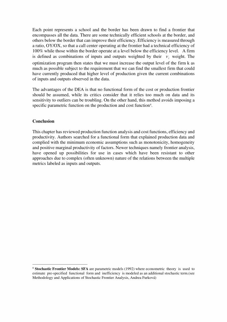
Each point represents a school and the border has been drawn to find a frontier that

encompasses all the data. There are some technically efficient schools at the border, and

others below the border that can improve their efficiency. Efficiency is measured through

a ratio, OY/OX, so that a call center operating at the frontier had a technical efficiency of

100% while those within the border operate at a level below the efficiency level. A firm

is defined as combinations of inputs and outputs weighted by their i weight. The

optimization program then states that we must increase the output level of the firm k as

much as possible subject to the requirement that we can find the smallest firm that could

have currently produced that higher level of production given the current combinations

of inputs and outputs observed in the data.

The advantages of the DEA is that no functional form of the cost or production frontier

should be assumed, while its critics consider that it relies too much on data and its

sensitivity to outliers can be troubling. On the other hand, this method avoids imposing a

specific parametric function on the production and cost function8.

Conclusion

This chapter has reviewed production function analysis and cost functions, efficiency and

productivity. Authors searched for a functional form that explained production data and

complied with the minimum economic assumptions such as monotonicity, homogeneity

and positive marginal productivity of factors. Newer techniques namely frontier analysis,

have opened up possibilities for use in cases which have been resistant to other

approaches due to complex (often unknown) nature of the relations between the multiple

metrics labeled as inputs and outputs.

8 Stochastic Frontier Models: SFA are parametric models (1992) where econometric theory is used to

estimate pre-specified functional form and inefficiency is modeled as an additional stochastic term.(see

Methodology and Applications of Stochastic Frontier Analysis, Andrea Furková)

Bibliography

A. Charnes, W. C. (1978). Measuring the efficiency of decision making units. European Journal of Operational Research, 2(6), 429-444.

Ackerberg, L. B. (2007). Econometric Tools for Analyzing Market Outcomes. In L. E.

Heckman J, The Handbook of Econometrics (Vol. 6A Chapter 63, pp. 4171-

4276). Amsterdam: North-Holland.

Battese, G. E. (1992). Frontier production functions and technical efficiency: a survey

of empirical applications in agricultural economics. Agricultural Economics, 7(3-4), 185-208.

BAUMOL, W. J. (1977). Weak invisible hand theorem on the sustainability of

multiproduct natural monopoly. American Economic Review, 60, 350 -365.

Christensen, L. R., & Greene, W. H. (1976, August). Economies of Scale in U.S.

Electric Power Generation. The Journal of Political Economy, 84(4), 655-672.

Davis, P., & Garcés, E. (2009). Quantitative Techniques for Competition and Antitrust Analysis. Princeton University Press.

Evans, D. S. (1984). Test for Subadditivity of the Cost Function with an Application to

the Bell System. The American Economic Review, 74(4), 615-623.

Farrell, M. (1957). The Measurement of Productive Efficiency. Journal of the Royal Statistical Society, 120(3), 253-290.

Greene, W. H. (2018). Econometric Analysis, 8th Edition. Stern School of Business,

New York University.

Greer, M. (2010). Electricity Cost Modelling Calculations. Academic Press.

Henningsen, A. (2015). Introduction to Econometric Production Analysis with R. Collection of Lecture Notes. Department of Food and Resource Economics, University of Copenhagen. Available at http://leanpub.com/ProdEconR/ . 2. Copenhaguen: Department of Food and Resource Economics, University of

Copenhagen. Available at http://leanpub.com/ProdEconR/ .

James Levinsohn, A. P. (2003, Abril). Estimating Production Functions Using Inputs to

Control for Unobservables. The Review of Economic Studies, 70(2), 317-341.

Marschak, J. &. (1944, Jul-Oct.). Random Simultaneous Equations and the Theory of

Production. Econometrica, 12(3/4), 143-205.

Mas-Collell, A., Whinston, M. D., & Green, J. (1995). Microeconomic Theory. Oxford

University Press.

Nerlove, M. (1961). Returns to scale in electricity supply. nstitute for mathematical

studies in the social sciences.

Olley, G. S. (1996). he Dynamics of Productivity in the Telecommunications

Equipment Industry. Econometrica, 64(6), 1263-1297.

Röller, L.-H. (1990b). Proper Quadratic Cost Functions with an Application to the Bell

System.”. The REview of Economics and Statistics, 72, 202–210.

Rovigatti, G. (2017). Retrieved from prodest: Production Function Estimation in R. R

package.: https://cran.r-project.org/web/packages/prodest/index.html

Rovigatti, G. a. (2018). Theory and practice of total-factor productivity estimation: The

control function approach using Stata. The Stata Journal, 18(3), 618-662.

Sheppard, R. W. (1953). Theory of Cost and Production Functions. Princeton

University Press.

Sraffa, P. (1926). The laws of returns under competitive conditions. The Economic Journal , 535-550.

Syverson, C. (2011). What Determines Productivity? Journal of Economic Literature, 49(2), 326-365.

Viner, J. (1932). Cost curves and supply curves. Zeitschrift für Nationalökonomie, 3(1),

23-46.

Wales, W. E. (1987). Flexible Functional Forms and Global Curvature Conditions.

Econometrica, 55, 43-68.

Worthington, A. C. (2012). A review of frontier approaches to efficiency and productivity measurement. Griffith University, Department of Accounting,

Finance and Economics, Queensland.

Annex: Alternative Fitting of Evans Heckman data in a Cubic Production Function