Estimating Test-Retest Reliability in Functional MR Imaging I: Statistical Methodology Christopher R. Genovese, Douglas C. Noll, William F. Eddy

A common problem in the analysis of functional magnetic resonance imaging (fMRI) data is quantifying the statistical reliability of an estimated activation map. While visual com- parison of the classified active regions across replications of an experiment can sometimes be informative, it is typically difficult to draw firm conclusions by inspection; noise and complex patterns in the estimated map make it easy to be misled. Here, several statistical models, of increasing com- plexity, are developed, under which “test-retest” reliability can be meaningfully defined and quantified. The method yields global measures of reliability that apply uniformly to a speci- fied set of brain voxels. The estimates of these reliability measures and their associated uncertainties under these models can be used to compare statistical methods, to set thresholds for detecting activation, and to optimize the num- ber of images that need to be acquired during an experiment. Key words: functional MRI; reliability; statistical methods; maximum likelihood.

INTRODUCTION

Every method for identifying active regions from func- tional magnetic resonance imaging (fMRI) data classifies each voxel as either active or inactive with respect to a particular contrast among experimental conditions. A method is considered reliable if it consistently identifies the same regions as active across replications of an ex- periment. However, no statistically rigorous definition of reliability has thus far emerged from this heuristic. Our goal in this paper is to put test-retest methods on firmer staiistical footing. We develop a family of statistical mod- els under which the test-retest reliability of classification can be meaningfully defined and quantified, and we present a method for estimating this reliability from fMRI data. Test-retest reliability measures consistency across replications of an experiment, and our methodology thus requires data from several replicates. However, as we will show, the results can be used to optimize reliability for later (single] runs of the same paradigm, for instance

MRM 38:497-507 (1997) From the Department of Statistics, Carnegie Mellon University (C.R.G., W.F.E.), and the Department of Radiology, University of Pittsburgh Medical Center (D.C.N.), Pittsburgh, Pennsylvania. Address correspondence to: Christopher R. Genovese, Ph.D., Department of Statistics, 132H Baker Hall, Carnegie Mellon University, Pittsburgh, PA 1521 3. Received June 20, 1996; revised January 29, 1997; accepted March 3, 1997. This work was supported by NSF Grants DMS 9505007 and IBN 9418982, The Whitaker Foundation, NIH Grant R01 -NS32756, and the Center for the Neural Basis of Cognition.

Copyright 0 1997 by Williams & Wilkins All rights of reproduction in any form resewed.

0740-31 94/97 $3.00

determining thresholds for statistical tests or the number of images to acquire.

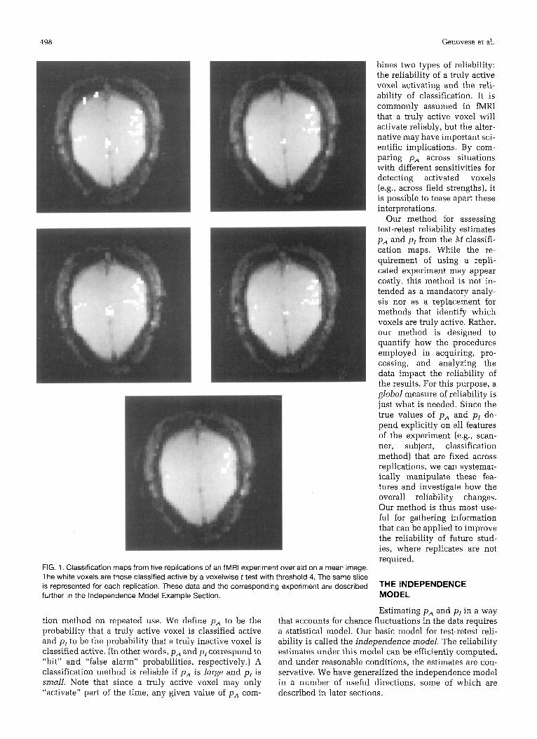
Figure 1 displays classification maps for a single slice from five replications of an fMRI experiment, overlaid on the corIesponding mean images; each white voxel has been classified active by a statistical test. While there is striking similarity in the general location of the apparent active regions, there is also substantial variation among the panels. The magnitude of this variation is difficult to assess by inspection alone, since the patterns can be sufficiently complex to mislead the eye. It is helpful here to gauge the overlap among the active sets of the different panels; the more complete the overlap, the higher the apparent reliability. To be useful for inference, however, any measure of overlap must be interpreted within the context of a model that accounts for chance fluctuations. Thus, to rigorously quantify reliability for statistical in- ference, we must distinguish among the different sources of variation in the data that affect the classification maps.

Table 1 presents a breakdown of these sources, each of which adds a distinct component to the observed vari- ability. For example, data collected across multiple ses- sions is susceptible to changes that occur between ses- sions. This is the Session entry in the table, which we can further divide into three subcomponents: differential subject position (Placement), systematic changes in the scanner state and environment (Configuration), and a residual term (Replication). The magnitudes of the Rep- lication and Block variabilities relative to the magnitude of Intrinsic variability measure the intersession and in- trasession test-retest reliability, respectively. Other sources in the table, such as differences in scanner, pulse sequence, and subject across replications, increase the observed variability but do not reflect unreliable classi- fication. To accurately assess reliability, then, i t is nec- essary to isolate the changes across block or replication from these confounding sources of variation.

We begin by replicating an fMRI experimental para- digm M times, where M ? 3. Throughout these M repli- cations, we take the scanner, acquisition scheme, statis- tical classification method, and subject to be fixed, thus eliminating several sources of variation in Table 1. We apply our chosen classification method (e.g., voxelwise t tests] artd obtain M classification maps that show how each voxel is classified in every replication. Using these maps as input, our method estimates two global mea- sures of reliability that describe the performance of clas- sification over a specified set of voxels (e.g., the whole brain].

We label each voxel in two distinct ways: (i) as either truly active or truly inactive and (ii) as either clussified active or classified inactive. Therefore, two probabilities pA and p1 characterize the performance of the classifica-

497

498 Genovese et al.

bines two types of reliability: the reliability of a truly active voxel activating and the reli- ability of classification. It is commonly assumed in fMRI that a truly active voxel will activate reliably, but the alter- native may have important sci- entific implications. By com- paring p A across situations with different sensitivities for detecting activated voxels (e.g., across field strengths), it is possible to tease apart these interpretations.

Our method for assessing test-retest reliability estimates p A and p I from the M classifi- cation maps. While the re- quirement of using a repli- cated experiment may appear costly, this method is not in- tended as a mandatory analy- sis nor as a replacement for methods that identify which voxels are truly active. Rather, our method is designed to quantify how the procedures employed in acquiring, pro- cessing, and analyzing the data impact the reliability of the results. For this purpose, a global measure of reliability is just what is needed. Since the true values of p A and p I de- pend explicitly on all features of the experiment (e.g., scan- ner, subject, classification method) that are fixed across replications, we can systemat- ically manipulate these fea- tures and investigate how the overall reliability changes. Our method is thus most use- ful for gathering information that can be applied to improve the reliability of future stud- ies, where replicates are not required.

THE “DEPENDENCE MODEL

FIG. 1. Classification maps from five replications of an fMAl experiment overlaid on a mean image. The white voxels are those classified active by a voxelwise t test with threshold 4. The same slice is represented for each replication. These data and the corresponding experiment are described further in the Independence Model Example Section.

tion method on repeated use. We define p A to be the probability that a truly active voxel is classified active and p I to be the probability that a truly inactive voxel is classified active. (In other words, pA and p,correspond to “hit” and “false alarm” probabilities, respectively.) A classification method is reliable if p A is large and pI is small. Note that since a truly active voxel may only “activate” part of the time, any given value of pA com-

Estimating p A and pI in a way that accounts for chance fluctuations in the data requires a statisiical model. Our basic model for test-retest reli- ability is called the independence model. The reliability estimates under this model can be efficiently computed, and under reasonable conditions, the estimates are con- servative. We have generalized the independence model in a number of useful directions, some of which are described in later sections.

Statistical Method for Estimating Reliability in fMRI 499

Specifying the Model

Using the classification maps for the M replications, we create what we call a raw reliability map. This map associates to each voxel v in a prespecified set V the number R, of replications out of M in which that voxel is classified active. Hence, each R, is an integer between 0 and M. The raw reliability map is the basic input to our estimation procedures. Our statistical models specify a connection between the parameters of interest ( p A and pI ) and the probability distribution of the R,’s. This connec- tion is embodied by a function called the likelihood, which is a basic tool of statistical inference (1). We will use the likelihood to construct both estimates of the parameters and standard errors of these estimates.

Under the independence model, the data are assumed statistically independent across both voxels and replica- tions, and each R, is assumed to be drawn from a mixture of two binomial distributions:

A . Binomial(M, p A ) + (1 - A) * Binomial(M, p r ) [l]

Here, BinomiallM. p ) denotes a binomial distribution (2) with M trials and event probability p . By the definitions of p A and p I and the independence assumptions of the model, the R, corresponding to an a priori truly active or a priori truly inactive voxel would have a Binomial(A4, p A ) or Binomial(M, pI ) distribution, respectively. The use of a mixture of these distributions in Eq. [I] reflects our uncertainty about which voxels are truly active. (To gen- erate a variate from the distribution in Eq. 111, one draws from either a Binomial(M, pA) or a Binomial(M, p l ) , with probabilities A and 1 - A respectively.) The parameter A thus represents the proportion of truly active voxels in V.

These model assumptions determine a likelihood func- tion for the parameters pA, pI, and A. This likelihood is constructed by combining the individual distributions in Eq. [ 11 over all voxels in V. Under the assumptions of the independence model, however, we can reduce data in the raw reliability map to a simpler form. In particular, the likelihood function, and hence all inferences about pA, pr, and A, depend only on the counts nk, for k = 0, . . ., M, where nk is the number of voxels in V that were classified active in k out of Mreplications. Consequently, for the independence model, we need only record these M i- 1 quantities to estimate the parameters.

Let n -= [no, n,, . . ., nM), and let N = xy nk be the total number of voxels in the set V, which is fixed. By the assumption of independent voxels, the likelihood func- tion is a product of the likelihoods for the individual voxels, and since all of the R,’s have the same distribu- tion of Eq. [ I ] , the terms of the product combine in a nice way. The log of the likelihood function for these data thus takes the form

+ (1 - A ) p f ( l - p p w k ’ ]

plus a constant that is independent of the parameters. Note that e is a function of the parameters; the data vector n is fixe’d at what we observe.

Table I Sources of Variation in fMRl Data across Replications of an Experiment

Computing the Estimates

We estimate the reliability parameters pA, pI, and A by the method of Maximum Likelihood (ML). This procedure chooses the values of the parameters that make the ob- served d,ata as likely as possible under the model. Specifi- cally, the estimated parameters, denoted by PA, PI, and i, are the values of pA, pr, and A, respectively, that maximize e. These are called maximum likelihood estimates.

However, estimates are only useful if accompanied by assessments of their uncertainty. Using the asymptotic theory of maximum likelihood estimators, we can com- pute approximate standard errors for PA, PI, and i. Let I be the 3 x 3 matrix containing the negative of all the second iderivatives of e with respect to the reliability parameters, evaluated at the maximum likelihood esti- mates. The diagonal elements of I-’ are approximate variances for the corresponding estimates (1, 3). The approximation gets better as the number of voxels grows and is very accurate for the typical number of voxels in fMRI dai.a.

In some applications, it is necessary or desirable to constrain the parameter A. For example, when comparing different processing methods, we compute the reliability estimates for several n vectors drawn from the same underlying set of truly active voxels. This implies the constraint that A be the same for all these data. Similarly,

Source Description Scanner Acquisition Method Statistical Method Subject Session

Placement Configuration Replication

Voxel within Session Block within Session Time within Session Intrinsic

Machine characteristics and performance Pulse sequence and imaging parameters Classification method used to identify active voxels Individual differences in physiology and response Variation across imaging session within Subject

Differential subject position State of the system, calibration, environment, etc. All remaining intersession variability

Heterogeneity among locations (voxels) in t h e brain Variation across responses to each task presentation Temporal artifacts (e.g., movement, drift, physiological) Noise and other unaccounted for variation

prior information suggests an upper bound for A less than 1. Both types of constraints can be directly incorporated into the maximization procedure; see Applications Section.

Example

To illustrate our method, we ran five replications of B func- tional MRI experiment using a simple motor task. Each trial utilized a spiral acquisition se- quence. The imaging configu- ration was as follows: four in- terleaved spirals, TR = 750

500 Genovese et al.

ms, TE = 35 ms, FA = 45, 64 X 64 matrix, 20 FOV, nine slices, 4-mm slice thickness, 0-mm spacing, 3 s per set of nine slices. Scanning was performed on a 1.5 T GE Signa scanner (GE Medical Systems, Milwaukee, WI) using two 5-inch surface coils mounted parallel to each other in a sagittal orientation on opposite sides of the head.

In each trial, a sequential finger-tapping task was alter- nated with a rest condition four times (24 s on, 24 s rest). Sixty-four images were acquired during 192 s. The data were movement and trend corrected (4, 5) during pro- cessing. Activation maps were constructed using the cor- relation coefficient (p) with a sine wave (6) that lagged the task by 6 s, calculated on a voxel-by-voxel basis. Voxels were classified active if p > T, for different thresh- old settings T.

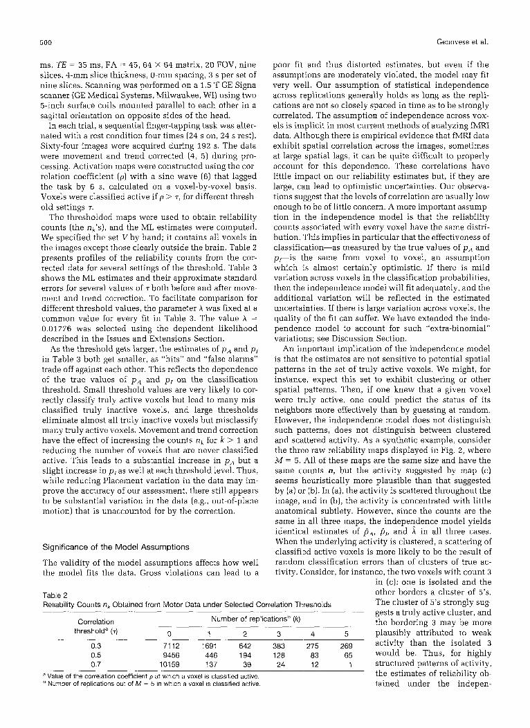
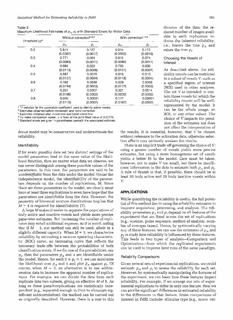
The thresholded maps were used to obtain reliability counts (the nk’s), and the ML estimates were computed. We specified the set V by hand; it contains all voxels in the images except those clearly outside the brain. Table 2 presents profiles of the reliability counts from the cor- rected data for several settings of the threshold. Table 3 shows the ML estimates and their approximate standard errors for several values of T both before and after move- ment and trend correction. To facilitate comparison for different threshold values, the parameter h was fixed at a common value for every fit in Table 3. The value h =

0.01776 was selected using the dependent likelihood described in the Issues and Extensions Section.

As the threshold gets larger, the estimates of pA and pz in Table 3 both get smaller, as “hits” and “false alarms” trade off against each other. This reflects the dependence of the true values of p A and pr on the classification threshold. Small threshold values are very likely to cor- rectly classify truly active voxels but lead to many mis- classified truly inactive voxels, and large thresholds eliminate almost all truly inactive voxels but misclassify many truly active voxels. Movement and trend correction have the effect of increasing the counts nk for k > 1 and reducing the number of voxels that are never classified active. This leads to a substantial increase in pA but a slight increase in pz as well at each threshold level. Thus, while reducing Placement variation in the data may im- prove the accuracy of our assessment, there still appears to be substantial variation in the data (e.g., out-of-plane motion) that is unaccounted for by the correction.

Significance of the Model Assumptions

The validity of the model assumptions affects how well the model fits the data. Gross violations can lead to a

Table 2

poor fit and thus distorted estimates, but even if the assumptions are moderately violated, the model may fit very well. Our assumption of statistical independence across replications generally holds as long as the repli- cations are not so closely spaced in time as to be strongly correlated. The assumption of independence across vox- els is implicit in most current methods of analyzing fMRI data. Although there is empirical evidence that fMRI data exhibit spatial correlation across the images, sometimes at large spatial lags, it can be quite difficult to properly account for this dependence. These correlations have little impact on our reliability estimates but, if they are large, c:an lead to optimistic uncertainties. Our observa- tions suggest that the levels of correlation are usually low enough to be of little concern. A more important assump- tion in the independence model is that the reliability counts associated with every voxel have the same distri- bution. This implies in particular that the effectiveness of classification-as measured by the true values of pA and pris the same from voxel to voxel, an assumption which is almost certainly optimistic. If there is mild variation across voxels in the classification probabilities, then the independence model will fit adequately, and the additional variation will be reflected in the estimated uncertainties. If there is large variation across voxels, the quality of the fit can suffer. We have extended the inde- pendence model to account for such “extra-binomial” variations; see Discussion Section.

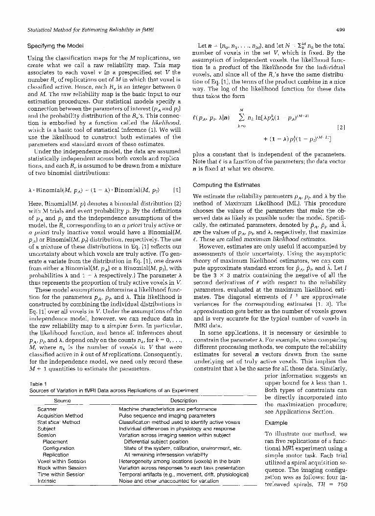
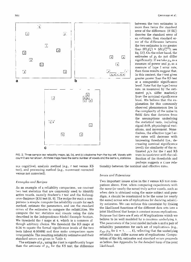
An important implication of the independence model is that the estimates are not sensitive to potential spatial patterns in the set of truly active voxels. We might, for instance, expect this set to exhibit clustering or other spatial patterns. Then, if one knew that a given voxel were ti-uly active, one could predict the status of its neighbors more effectively than by guessing at random. However, the independence model does not distinguish such patterns, does not distinguish between clustered and scattered activity. As a synthetic example, consider the three raw reliability maps displayed in Fig. 2, where M = 5. All of these maps are the same size and have the same counts R, but the activity suggested by map (c) seems heuristically more plausible than that suggested by (a) or (b). In (a), the activity is scattered throughout the image, and in (b), the activity is concentrated with little anatomical subtlety. However, since the counts are the same in all three maps, the independence model yields identical estimates of PA, PI, and in all three cases. When the underlying activity is clustered, a scattering of classified active voxels is more likely to be the result of random classification errors than of clusters of true ac- tivity. Consider, for instance, the two voxels with count 3

in (c): one is isolated and the other borders a cluster of 5’s.

Reliability Counts n, Obtained from Motor Data under Selected Correlation Thresholds

Correlation Number of replicationsb (k)

0 1 2 3 4 5 thresholda (7)

0.3 0.5 0.7

7112 1691 642 383 275 269 9456 446 194 128 83 65

101 59 137 39 24 12 1 - a M u e of the correlation coefficient p at which a voxel is classified active.

Number of replications out of M = 5 in which a voxel is classified active.

The cluster of 5’s strongly sug- gests a truly active cluster, and the bordering 3 may be more plausibly attributed to weak activity than the isolated 3 would be. Thus, for highly structured patterns of activity, the estimates of reliability ob- tained under the indepen-

Statistical Method fix Estimating Reliability in fMRI 501

Table 3 Maximum Likelihood Estimates of pa, pI with Standard Errors for Motor Data

Without correctionb,d,e With correctionc.d.e Threshold ( T ) ~

_ _ __ PA PI PA PI- 0.2 0.874

0.3 0.771

0.4 0.684

0.5 0.587

0.6 0.492

0.7 0.251

0.8 0.045

(0.0067)

(0.0083)

(0.01 13)

(0.0127)

(0.01 94)

(0.01 96)

(0.01 10)

0.127

0.054

0.022 (0.0008) 0.0078 (0.0004) 0.0038 (0.0003) 0.0007

0.00001

(0.001 7)

(0.001 1)

(0.0002)

(0.0002)

0.91 5 (0.0055) 0.81 5 (0.0080) 0.730

0.616 (0.01 18) 0.529 (0.01 72) 0.321 (0.0230) 0.1 77 (0.01 67)

(0.0101)

0.172 (0.001 6) 0.074

0.030 (0.0007) 0.01 0 (0.0004) 0.0056 (0.0003) 0.0014

0.00001

(0.001 1)

(0.0002)

(0.0002) a Thresholds for the correlation coefficient used to identify active voxels.

Estimates obtained before movement and trend correction. Estimates obtained after movement and trend correction. To make comparison easier, A is fixed at the joint-fitted value of 0.01776. Standard errors are given in parentheses beneath the associated estimate

dence model may be conservative and underestimate the reliability.

Identifiability

If for every possible data set two distinct settings of the model parameters lead to the same value of the likeli- hood function, then no matter what data we observe, we can never distinguish among these possible values of the parameters. In this case, the parameters are said to be unidentifiable from the data under the model. Under the independence model, the identifiability of the parame- ters depends on the number of replications, M. Since there are three parameters in the model, we clearly must have at least three replications to even have hope that the parameters are identifiable from the data. However, the geometry of binomial mixture distributions implies that M -5 4 is required for identifiability (7).

A large Mmakes it easier to separate the populations of truly active and inactive voxels and yields more precise parameter estimates. But increasing the number of repli- cates may entail additional expense, so it is worth noting that if M = 3 , our method can still be used, albeit in a slightly different capacity. When M = 3, we characterize reliability by estimating a receiver operating characteris- tic (ROC) curve, an increasing curve that reflects the necessary trade-offs between the probabilities of both classification errors. If we fix one of the probabilities, say p I , then the parameters p A and A are identifiable under the model. Hence, for each 0 5 p I 5 1, we can maximize the likelihood over p A and A and plot I j A against p p Of course, when M = 3, an alternative is to use within- session data to increase the apparent number of replica- tions. For example, we can divide the data from each replicate into two subsets, giving an effective M of 6. As long as these pseudoreplications are statistically inde- pendent (e.g., separated enough in time to eliminate sig- nificant autocorrelation), the method can be carried out as originally described. However, there is a cost to this

division of the data: the re- duced number of images avail- able to each replication re- duces the inherent reliability, i.e., lowers the true p A and raises the true p p

Choosing the Voxels of Interest

As described above, the reli- ability counts can be restricted to a subset of voxels V , such as a specified region of interest (ROI) used in other analyses. The set V is intended to con- tain those voxels for which the reliability counts will be well- represented by the model. It can be the whole image, an ROI, or any other subset. The choice of V impacts the preci- sion of the estimates but does not affect the interpretation of

the results. It is essential, however, that v̂ be chosen without reference to the activation data, otherwise selec- tion effects may seriously weaken the results.

There is an implicit trade-off governing the choice of V: using a greater number of voxels yields more precise estimates, but using a more homogenous set of voxels yields a better fit to the model. Care must be taken, however, not to make V too small, lest there be insuffi- cient information in the data to estimate both pn and p I . A rule of thumb is that, if possible, there should be at least 20 truly active and 20 truly inactive voxels within V.

APPLICATIONS

While quantifying the reliability is useful, the full poten- tial of this method lies in using the reliability estimates to improve acquisition, processing, and analysis. The reli- ability parameters pn and p I depend on all features of the experiment that are fixed across the set of replications (e.g., scanner, pulse sequence, method of analysis, num- ber of averages taken). Hence, by systematically varying any of these features, we can use the estimates of p A and p I to study how reliability is influenced by these features. This leads to two types of analysis-Comparison and Optimization-from which the replicated experiments can be used to improve later runs of the same paradigm.

Reliability Comparisons

Given several sets of experimental replications, we could estimate p A and p I to assess the reliability for each set. However, by systematically manipulating the features of the experiment, we can learn how these features impact reliability. For example, if we arrange our sets of exper- imental replications to differ in only one feature, then we can ascribe significant differences in estimated reliability to the differences in that feature. Some comparisons of interest in fMRI include: stimulus type (e.g., motor ver-

502 Genovese et al.

El

El

a

C

El

m

G1-V 1 5 1 2 4

Ei El

FIG. 2. Three sample raw reliability maps; (a), (b), and (c) clockwise from the top left. Voxels with count 0 are not shown. All three maps have the same number of voxels and the same nk statistics.

sus cognitive), analysis method (e.g., t test versus KS test), and processing method (e.g., movement corrected versus not corrected).

Examples and Recipes

As an example of a reliability comparison, we contrast two test statistics that are commonly used to identify active voxels, namely Student’s t test and the Kolmog- orov-Smirnov (KS) test (8, 9). The recipe for such a com- parison is simple: compute the reliability counts for each method, estimate the parameters, and use the standard errors of the estimates to compare the reliabilities. We compute the test statistics and counts using the data described in the Independence Model Example Section. We threshold the t maps at 4, which is a common al- though arbitrary choice. We threshold the KS maps at 0.54 to equate the formal significance levels of the two tests (about 0.00009) and thus make comparison more interpretable. The resulting reliability estimates and their standard errors are given in Table 4.

The estimate of p A using the t test is significantly larger than the estimate of p A for the KS test; the difference

between the two estimates is more than twice the standard error of the difference. (If SE() denotes the standard error of an estimate, then standard er- ror of the difference between the two estimates is no greater than SE(lj2)) 4 SE(I jy) l ; see Eq. [3]). On the other hand, the estimates of pr do not differ significantly. If we take pA as a measure of power and p I as a measure of type I error rate, then these results suggest that, in this context, the t test gives greater power than the KS test at a comparable significance level. Note that the type I error rate, as measured by the esti- mated p i s , differ markedly from the nominal significance level. We believe that the ex- planation for this commonly observed phenomenon lies in the complexity of the noise in fMRI data that deviates from the assumptions underlying the statistical tests, including signal drift, physiological vari- ations, and movement. None- theless, the effective type I er- ror rates will decrease with increasing threshold (i.e., de- creasing nominal significance level); the similarity of the es- timated p i s for the t and KS tests is consistent with the cal- ibration of the thresholds and perhaps suggests a close rela-

tionship between the nominal and effective rates.

lssues und Extensions

Two important issues arise in the t versus KS test com- parison above. First, when comparing experiments with the same (or nearly the same) truly active voxels, such as when data is obtained using the same subject and para- digm, A should be constrained to be the same (or nearly the same) across sets of replications for deriving reliabil- ity estimates. We can enforce this constraint by linking the likelihood functions of the different data sets into a joint likelihood that keeps h constant across replications. Suppose that there are K sets of M replications which we believe to be well-modeled by a common underlying A. The parameters of the joint model include h and a pair of reliability parameters for each set of replications (e.g., PAL, p& for k = 1, . . ., K) , reflecting that the underlying reliability may differ across sets of replications. Compu- tation of the ML estimates and standard errors proceeds as before. See Appendix for the detailed form of the joint likelihood.

Statistical Method for Estimating Reliability in jMRI 503

Table 4 ML Estimates of pa and p, with Standard Errors for t and KS Test Classifications

Statistic P A R,

t

KS

0.573 0.01 09 (0.0123) (0.0005) 0.513 0.01 13 (0.01 46) f0.0006)

Note: Standard errors are given in parentheses beneath the associated estimate.

The second issue is the statistical dependence of the counts when several reliability maps are derived from the same data. The cost of replication may make the following scenario tempting: replicate an experiment M times, analyze or process these data using several meth- ods (e.g., different voxelwise test procedures), compute the reliability estimates for each method, and compare them via the computed standard errors. The first three of these steps pose no difficulty, but the comparison in the fourth step is complicated by the statistical dependence in the different estimates that results from using the same data for each method. Specifically, if pA and pX are the parameters corresponding to two methods, then the stan- dard error of I j A - PA depends not only on the standard errors of PA and 0; but also on the correlation between the estimates.

If one ignores the dependence, the estimates them- selves are well-defined, but the difference between them can be misleading. For example, for any pair of estima- tors, the bounds

are as tight as possible without an estimate of the corre- lation between the estimators. If the dependence is ig- nored, caveat investigator.

Alternatively, we can explicitly model the depen- dence since the data at each voxel give rise to not one but several different classifications, corresponding to the different methods used. Suppose, for the purposes of discussion, that we are comparing two methods. Let pArr, (praj) denote the probability that a truly active (truly inactive] voxel is classified active by Method 1 and classified inactive by Method 2, and similarly for other combinations of a and i in the subscript. Table 5 depicts the probabilities of every possible classifica- tion by the two methods for both truly active and truly inactive voxels.

Table 5 Probabilities of Each Possible Pair of Classifications by Two Methods

Note that pA,, = 1 - pAn, - pAlu - pALla and similarly for PI,,.

These probabilities and the weight h determine a mix- ture distribution for the reliability counts; see Appendix for the detailed form of the dependent likelihood. We estimate the parameters by maximizing the likelihood function Over A, pAnnr pAnl r pAln, pIuao7 pIall and phn. We can express the original probabilities pa"'' and pirn) for method m = 1, 2 in terms of these new parameters by collapsing over the Active Voxel and Inactive Voxel sub- tables in Table 5. For instance, pz' = pAaa + pArr, and pa"'

voxel is classified active under each method. It follows that the differences we are seeking to estimate are simply

The approximate standard errors of the estimates of these quantities are obtained directly from the maximum like- lihood procedure. Meaningful comparisons can be based on these estimates and standard errors because the model accounts for the dependence in the data.

- - pAoo + pAlo give the probabilities that a truly active

pg) - P A (2) = PA*, - PA," and P?' ~ PY' = pin, -

Example Revisited

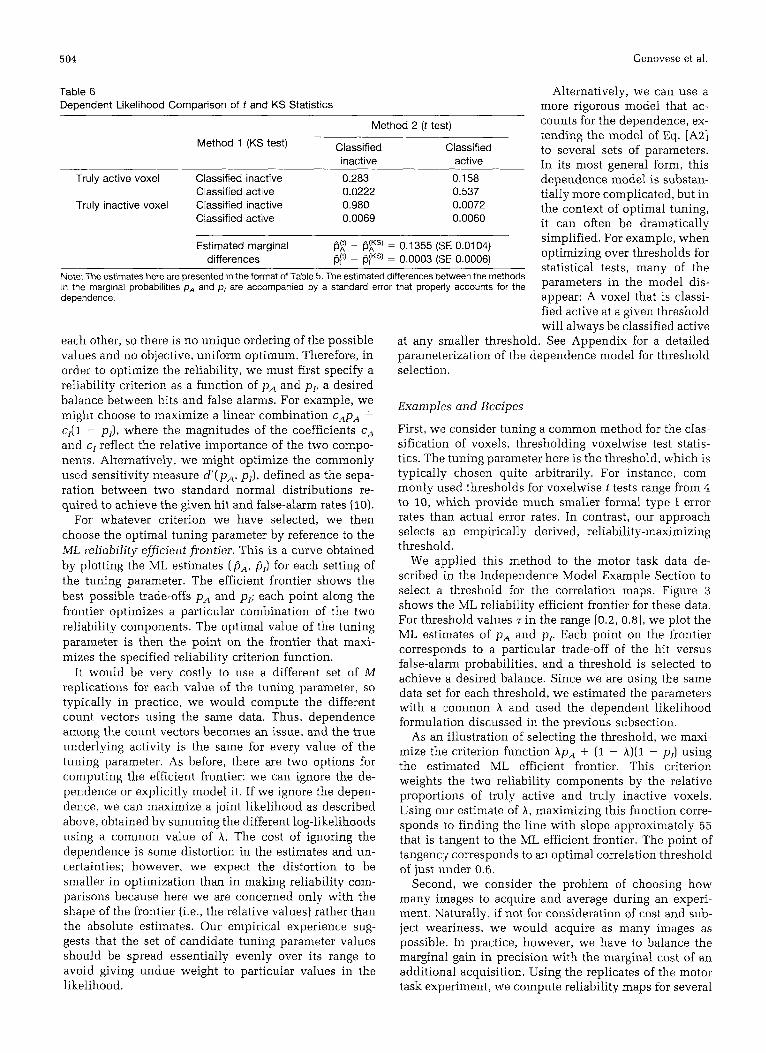
We now revisit the comparison made in the Applications Examples and Recipes Section, addressing the issues raised above. In particular, the estimates in Table 4 were based on two reliability maps derived from the same set of replications. This implies both a common h underly- ing both methods and dependence between the count vectors for t and KS. We thus apply the dependent like- lihood model. Using the correlations and the standard errors for the parameters in Table 5, we directly estimate the differences between the two methods in both pA and pI and compute the standard errors of these differences. The results are provided in Table 6. Note first that the same pattern is exhibited here as in the Applications Examples and Recipes Section: the estimates of pI for the two methods are not significantly different, but pA is significantly larger for the t test than for the KS test. However, the estimates of pA and pI for both methods are also quite different from the estimates obtained in the Applications Examples and Recipes Section. This change reflects the impact of dependence on the model; by ac- counting for dependence here, we obtain more precise estimatles and a more accurate comparison.

Reliability-Optimal Tuning

A second general application of our method is to tune acquisition, processing, and statistical analysis to maxi- mize the reliability. The data from the replicated exper-

Method 2

Classified inactive Classified active Method 1

Truly active voxel Classified inactive PA/, PA,a

Classified active PAai PAaa

Classified active Piat P/aa Truly inactive voxel Classified inactive PI,, Plia

Note: These probabilities describe the simultaneous classification by two methods, for both truly active and truly inactive voxels. The probabilities in each of the two subtables sum to 1.

iments are used to find reli- ability-optimal settings of the desired tuning parameter (e.g., the threshold for statistical maps], and the optimal set- tings are then used in later (unreplicated) runs of the same experimental paradigm.

The reliability parameters pA and pr, which represent hit and false-alarm rates respec- tively, tend to trade-off against

504 Genovese et al.

Table 6 Dependent Likelihood Comparison of t and KS Statistics

Method 2 (t test)

Classified Classified inactive active

Method 1 (KS test)

Truly active voxel Classified inactive 0.283 0.158 Classified active 0.0222 0.537

Truly inactive voxel Classified inactive 0.980 0.0072 Classified active 0.0069 0.0060

Estimated marginal fig) - fip) = 0.1355 (ISE 0.0104) #) - fiIKS) = 0.0003 (!SE 0.0006) differences

Note: The estimates here are presented in the format of Table 5. The estimated differences between the methods 1 in the marginal probabilities pn and p, are accompanied by a standard error

dependence. that properly accounts for the

each other, so there is no unique ordering of the possible values and no objective, uniform optimum. Therefore, in order to optimize the reliability, we must first specify a reliability criterion as a function of p A and pr, a desired balance between hits and false alarms. For example, we might choose to maximize a linear combination cApA + C,(I - pI ) , where the magnitudes of the coefficients c, and cI reflect the relative importance of the two compo- nents. Alternatively, we might optimize the commonly used sensitivity measure d'(p,, p I ) , defined as the sepa- ration between two standard normal distributions re- quired to achieve the given hit and false-alarm rates (10).

For whatever criterion we have selected, we then choose the optimal tuning parameter by reference to the ML reliability efficient frontier. This is a curve obtained by plotting the ML estimates ( P A , PI) for each setting of the tuning parameter. The efficient frontier shows the best possible trade-offs p A and p,; each point along the frontier optimizes a particular combination of the two reliability components. The optimal value of the tuning parameter is then the point on the frontier that maxi- mizes the specified reliability criterion function.

It would be very costly to use a different set of M replications for each value of the tuning parameter, so typically in practice, we would compute the different count vectors using the same data. Thus, dependence among the count vectors becomes an issue, and the true underlying activity is the same for every value of the tuning parameter. As before, there are two options for computing the efficient frontier: we can ignore the de- pendence or explicitly model it. If we ignore the depen- dence, we can maximize a joint likelihood as described above, obtained bv summing the different log-likelihoods using a common value of A. The cost of ignoring the dependence is some distortion in the estimates and un- certainties; however, we expect the distortion to be smaller in optimization than in making reliability com- parisons because here we are concerned only with the shape of the frontier (i.e., the relative values) rather than the absolute estimates. Our empirical experience sug- gests that the set of candidate tuning parameter values should be spread essentially evenly over its range to avoid giving undue weight to particular values in the likelihood.

Alternatively, we can use a more rigorous model that ac- counts for the dependence, ex- tending the model of Eq. [A21 to several sets of parameters. In its most general form, this dependence model is substan- tially more complicated, but in the context of optimal tuning, it can often be dramatically simplified. For example, when optimizing over thresholds for statistical tests, many of the parameters in the model dis- appear: A voxel that is classi- fied active at a given threshold will always he classified active

at any smaller threshold. See Appendix for a detailed parameterization of the dependence model for threshold selection.

Examples and Recipes

First, we consider tuning a common method for the clas- sification of voxels, thresholding voxelwise test statis- tics. The tuning parameter here is the threshold, which is typically chosen quite arbitrarily. For instance, com- monly used thresholds for voxelwise t tests range from 4 to 10, which provide much smaller formal type I error rates than actual error rates. In contrast, our approach selects an empirically derived, reliability-maximizing threshold.

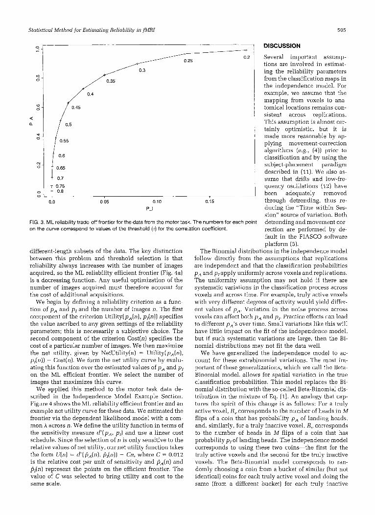
We applied this method to the motor task data de- scribed in the Independence Model Example Section to select a threshold for the correlation maps. Figure 3 shows the ML reliability efficient frontier for these data. For threshold values T in the range 0.81, we plot the ML estimates of p A and p p Each point on the frontier corresponds to a particular trade-off of the hit versus false-alarm probabilities, and a threshold is selected to achieve a desired balance. Since we are using the same data set for each threshold, we estimated the parameters with a (common A and used the dependent likolihood formulation discussed in the previous subsection.

As an illustration of selecting the threshold, we maxi- mize the criterion function Ap, + (1 - A ) ( l - p,) using the est mated ML efficient frontier. This criterion weights the two reliability components by the relative proportions of truly active and truly inactive voxels. Using our estimate of A, maximizing this function corre- sponds to finding the line with slope approximately 55 that is tangent to the ML efficient frontier. The point of tangency corresponds to an optimal correlation threshold of just under 0.6.

Second, we consider the problem of choosing how many innages to acquire and average during an experi- ment. Naturally, if not for consideration of cost and suh- ject weariness, we would acquire as many images as possible. In practice, however, we have to balance the marginal gain in precision with the marginal cost of an additional acquisition. Using the replicates of the motor task experiment, we compute reliability maps for several

Statistical Method for Estimating Reliability in fh.IR1 505

/ 0.5

0.7

0.75 0.8

0.0 0.05 0.10

p-1

0.15

FIG. 3. ML reliability trade-off frontier for the data from the motor task. The numbmers for each point on the curve correspond to values of the threshold (T) for the correlation coefficient.

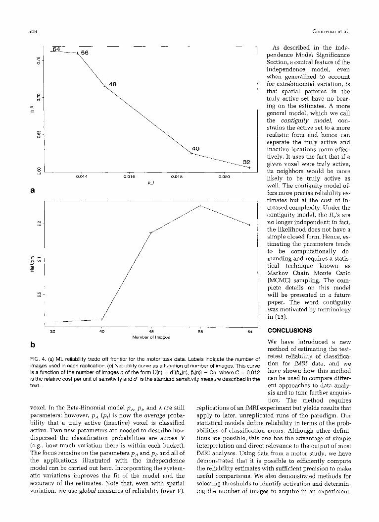
different-length subsets of the data. The key distinction between this problem and threshold selection is that reliability always increases with the number of images acquired, so the ML reliability efficient frontier (Fig. 4a) is a decreasing function. Any useful optimization of the number of images acquired must therefore account for the cost of additional acquisitions.

We begin by defining a reliability criterion as a func- tion of pA and pI and the number of images n. The first component of the criterion Utility(p,(n), pl(n)) specifies the value ascribed to any given settings of the reliability parameters; this is necessarily a subjective choice. The second component of the criterion Cost(n) specifies the cost of a particular number of images. We then maximize the net utility, given by NetUtility(n) = Utility( p,(n), pl(11)) - Cost(n). We form the net utility curve by evalu- ating this function over the estimated values of pA and pI on the ML efficient frontier. We select the number of images that maximizes this curve.

We applied this method to the motor task data de- scribed in the Independence Model Example Section. Figure 4 shows the ML reliability efficient frontier and an example net utility curve for these data. We estimated the frontier via the dependent likelihood model with a com- mon A across n. We define the utility function in terms of the sensitivity measure d‘(p,, pI) and use a linear cost schedule. Since the selection of n is only sensitive to the relative values of net utility, our net utility function takes the form U(n) = d’(PA(n), Pl(n)) - Cn, where C = 0.012 is the relative cost per unit of sensitivity and PA(n) and rjI(n) represent the points on the efficient frontier. The value of C was selected to bring utility and cost to the same scale.

DISCUSSION

Several important assump- tions are involved in estimat- ing the reliability parameters from the classification maps in the independence model. For example, we assume that the mapping from voxels to ana- tomical locations remains con- sistent across replications. This assumption is almost cer- tainly optimistic, but it is made more reasonable by ap- plying movement-correction algorithms (e.g., (4)) prior to classification and by using the subject-placement paradigm described in (11). We also as- sume that drifts and low-fre- quency oscillations (12) have been adequately removed through detrending, thus re- ducing the “Time within Ses- sion” source of variation. Both detrending and movement cor- rection are performed by de- fault in the FIASCO software platform (5).

The Binomial distributions in the independence model follow directly from the assumptions that replications are independent and that the classification probabilities pA and pIapply uniformly across voxels and replic ations. The uniformity assumption may not hold if there are systematic variations in the classification process across voxels and across time. For example, truly active voxels with veIy different degrees of activity would yield differ- ent values of p,,. Variation in the noise process across voxels can affect both pA and pp Practice effects can lead to different pA’s over time. Small variations like this will have little impact on the fit of the independence model, but if such systematic variations are large, then the Bi- nomial distributions may not fit the data well.

We have generalized the independence model to ac- count for these extrabinomial variations. The most im- portant of these generalizations, which we call the Beta- Binomial model, allows for spatial variation in the true classification probabilities. This model replaces the Bi- nomial distribution with the so-called Beta-Binomial dis- tribution in the mixture of Eq. [I]. An analogy that cap- tures the spirit of this change is as follows: For a truly active voxel, R, corresponds to the number of heads in M flips of a coin that has probability p A of landing heads, and, similarly, for a truly inactive voxel, R, corresponds to the number of heads in M flips of a coin that has probability pI of landing heads. The independence model corresponds to using these two coins-the first for the truly aciive voxels and the second for the truly inactive voxels. The Beta-Binomial model corresponds to ran- domly choosing a coin from a bucket of similar (but not identical) coins for each truly active voxel and doing the same (from a different bucket) for each truly inactive

0.014 0.016 0.018 0.020 P-1

32 40 48 56 64 Number of Images

b FIG. 4. (a) ML reliability trade-off frontier for the motor task data. Labels indicate the number of images used in each replication. (b) Net utility curve as a function of number of images. This curve is a function of the number of images n of the form U(n) = d'(fjA(n), P,(n)) - Cn. where C = 0.012 is t h e relative cost per unit of sensitivity and d' is the standard sensitivity measui'e described in the text.

voxel. In the Beta-Binomial model pA, pr, and A are still parameters; however, p A (pr) is now the average proba- bility that a truly active (inactive) voxel is classified active. Two new parameters are needed to describe how dispersed the classification probabilities are across V (e.g., how much variation there is within each bucket). The focus remains on the parameters pA and pr , and all of the applications illustrated with the independence model can be carried out here. Incorporating the system- atic variations improves the fit of the model and the accuracy of the estimates. Note that, even with spatial variation, we use global measures of reliability (over V).

Genovese et al.

As described in the Inde- pendence Model Significance Section, a central feature of the independence model, even when generalized to account for extrabinomial variation, is that spatial patterns in the truly active set have no bear- ing on the estimates. A more general model, which we call the contiguity model, con- strains the active set to a more realistic form and hence can separate the truly active and inactive locations more effec- tively. It uses the fact that if a given voxel were truly active, its neighbors would be more likely to be truly active as well. The contiguity model of- fers more precise reliability es- timates but at the cost of in- creased complexity. Under the contiguity model, the R,'s are no longer independent: in fact, the likelihood does not have a simple closed form. Hence, es- timating the parameters tends to be computationally de- manding and requires a statis- tical technique known as Markov Chain Monte Carlo (MCMC) sampling. The com- plete details on this model will be presented in a future paper. The word contiguity was motivated by terminology in (13).

CONCLUSIONS

We have introduced a new method of estimating the test- retest reliability of classifica- tion for fMRI data, and we have shown how this method can be used to compare differ- ent approaches to data analy- sis and to tune further acquisi- tion. The method requires

replications of an fMRI experiment but yields results that apply to later, unreplicated runs of the paradigm. Our statistical models define reliability in terms of the prob- abilities of classification errors. Although other defini- tions are possible, this one has the advantage of simple interpretation and direct relevance to the output of most fMRI analyses. Using data from a motor study, we have demonstrated that it is possible to efficiently compute the reliability estimates with sufficient precision to make useful comparisons. We also demonstrated methods for selecting thresholds to identify activation and determin- ing the number of images to acquire in an experiment.

Statistical Method for Estimating Reliability in f M R l 507

Our goal here is not to present data of optimal reliability; rather, we hope to demonstrate how this new tool can be used to make comparisons and design decisions that are important in most fMRI experiments.

APPENDIX

With K sets of replications, the parameters of the joint model are A, pAk. pIk for k = 1, . . ., K. The different sets of data are treated independently, except for the connec- tion through the common A. Given reliability count vec- tors R,, . . ., nK, the joint log-likelihood is of the form

e p d P A i , PIi, . . . . PAK, PIK, A h , . . ., n K )

K M

= C C nkI ln[Ap!.!.,(l- P A ~ ) ‘ ~ - J ’ + (1 - ~ d k ( 1 - pdM-”1

[ A l l

plus a constant that is independent of the parameters. Weaker constraints on A across sets can be incorporated by allowing different hk while adding a penalty term into the log-likelihood that discourages variation among the

The likelihood for the dependence model is based on modified reliability counts at each voxel that are defined by a four-vector of nonnegative integers, j = ( j l z , j l a , j a l , jaJ, that sum to M. Here, j,, is the number of replications in which the voxel was classified inactive under Method 1 and classified active under Method 2, and similarly for the other rs. Let nj denote the number of voxels with modified count vector j . Then, the dependent log-likeli- hood is

k = i j=O

hk’s.

edep(PA 9 PI , A l n ) = C nj ln[Apk,,pZiap%aipga + (1 - A) p t ~ j p t ~ o p ~ ~ i p ~ ~ o I ~

I

[A21

where the sum is overall nonnegative, integer quadruples j whose total is M.

As mentioned in the text, this reduces to a simpler form in many applications. For example, when selecting among K different thresholds arranged in increasing or- der, the parameters in Eq. [A21 reduce to A, PAk, and pIk for k = 0 , . . ., K. Here, pAk is the probability that a truly active voxel is classified active at k of the threshold levels and similarly for plk. Note that pAK and pIK are deiermined by the other parameters; that is, pAK = 1 - Z21,’ P A k and pIK = 1 - Zfzk pIk The recorded reliability counts are nt for each t = (to, . . ., tK), where nr is the

number of voxels classified active at k threshold levels t, times (out of M) for each k = 0 , . . ., K. The dependent log-likelihood then takes the form

e d e p ( P A 9 PI., Aln)

K K

= c n, M A n p% + (1 - A) n p:il [A31

The counts associated with most t vectors will tend to be zero. We then choose the threshold level that provides the optimal balance of pA and pp If the thresholds are arranged in increasing order, then for the kth threshold level, the probability of a truly active voxel being classi- fied aciive is pg’ = c:, pAI; the probability of a truly inactive voxel being classified active is pik1 = X F k pa

t k=O k = O

REFERENCES 1.

2.

3.

4

5

6

7

8

9

10

11

12

13

M. J. Schervish, “Theory of Statistics,” p. 424ff, Springer-Vwlag, New York, 1995. M. H. DeGroot, “Probability and Statistics,” 2nd Ed., Addison Wes- ley, Reading, MA, 1991. B. Efron, D. V. Hinkley, Assessing the accuracy of tho maximum likelihood estimator: observed versus expected Fisher information. Biometriku 65, 457-487 (1978). W. F. Eddy, M. Fitzgerald, D. C. Noll, Improved image registration using Fourier domain interpolation. Magn. Reson. Med. 36(6), 923- 931 (l996). W. F. Eddy, M. Fitzgerald, C. R. Genovese, A. Mockus, D. C. Noll, Functional image analysis software-computational olio. in “Pro- ceedings in Computational Statistics,” A. Prat, Ed., p ~ ) . 39-49, Physica-Verlag, Heidelberg, 1996. P. A. Bandettini, A. Jesmanowicz, E. C. Wong, J. Hyde, Processing stratqies for time-course data sets in functional MRI of the human brain. Magn. Reson. Med. 30, 161-173 (1993). B. G. Lindsay, “Mixture Models: Theory, Geometry, and Applica- tions,” (Vol. 5 of NSF-CBMS Regional Conference Series in Probabil- ity and Statistics), Institute of Mathematical Statistics, 1095. J. R. Baker, R. M. Weisskoff, C. E. Stern, D. N. Kennedy, A. Jiang, K. K. Kwong, L. B. Kolodny, T. L. Davis, J. L. Boxerman. B. R. Buchbinder, V. J. Weeden, J. W. Belliveau, B. R. Rosen, Statistical assessment of functional MRI signal change, in “Proc., SMR, 2nd Annual Meeting, San Francisco, 1994,” p. 626. E. L. Lehmann, “Nonparameterics: Statistical Methods Based on Rank:.,” Holden Day, Oakland, CA, 1975. D. W. Massaro, “Experimental Psychology: An Informatioil Process- ing Approach,” pp. 218-223, Harcourt Brace Jovanovich, New York, NY, 1989. D. C. Noll, C. R. Genovese, L. Nystrom, S. D. Forman, W. F. Eddy, J. D. Cohen, Estimating test-retest reliability in functional MR imag- ing. 11. Application to motor and cognitive activation studies. Mugn. Reson. Med. 38, 508-517 (1997). B. Biswal, F. Zerrin Yetkin, V. M. Haughton, J. S . Hyde, Functional connectivity in the motor cortex of resting human brain using echo- planar MRI. Magn. Reson. Med. 34, 537-541 (1995). S. Forman, J. C. Cohen, M. Fitzgerald, W. F. Eddy, M. A. Mintun, D. C. Noll, Improved assessment of significant change in functional fMR1 use of a cluster-size threshold. Magn. Reson. Med. 33, 636-647 (1995).