This article appeared in a journal published by Elsevier. The attachedcopy is furnished to the author for internal non-commercial researchand education use, including for instruction at the authors institution

and sharing with colleagues.

Other uses, including reproduction and distribution, or selling orlicensing copies, or posting to personal, institutional or third party

websites are prohibited.

In most cases authors are permitted to post their version of thearticle (e.g. in Word or Tex form) to their personal website orinstitutional repository. Authors requiring further information

regarding Elsevier’s archiving and manuscript policies areencouraged to visit:

http://www.elsevier.com/authorsrights

Author's personal copy

Establishing connectivity among disjoint terminals using a mixof stationary and mobile relays

Ahmad Abbas, Mohamed Younis ⇑Department of Computer Science and Electrical Engineering, University of Maryland, Baltimore County, Baltimore, MD, USA

a r t i c l e i n f o

Article history:Received 18 January 2013Received in revised form 10 June 2013Accepted 15 June 2013Available online 26 June 2013

Keywords:Repairing partitioned topologyFederating disjoint network segmentsRelay node placementMobile data carriers

a b s t r a c t

In multiple application scenarios, need arises to connect a set of disjoint nodes or segments. Examplesinclude connecting a sparsely located data sources, repairing a partitioned network topology after failure,and federating a set of standalone networks to serve an emerging event. Contemporary solutions eitherdeploy stationary relay nodes (RN) to form data paths or employ one or multiple mobile data carriers(MDCs) that pick packets from sources and transport them to destinations. In this paper we investigatethe interconnection problem when the number of available RNs is insufficient for forming a stable topol-ogy and a mix of RNs and MDCs is to be used. We present a novel algorithm for determining where theRNs are to be placed and planning optimized travel paths for the MDCs so that the data delivery latencyas well as the MDC motion overhead are minimized. The performance of the algorithm is validatedthrough simulation.

� 2013 Elsevier B.V. All rights reserved.

1. Introduction

Recent years have witnessed a massive growth in the use of net-worked devices in civil, scientific and military applications. Someapplications scenarios require networking a set of disjoint termi-nals within relatively short time duration and without extensiveinfrastructure planning. For example, wireless sensor networks(WSNs) often serve in inhospitable environments which makenodes susceptible to failure, e.g., due to detonation of explosivesin a battle field, natural calamities in forests, etc. [1]. The failuremay involve multiple nodes and cause the WSN to be divided intodisjoint segments. Restoring connectivity among these segmentswould be essential for the network to resume full operation. An-other scenario is when multiple data sources or standalone net-works are to be federated in order to aggregate their capabilitiesfor serving a certain application mission such as search and rescue,military situational awareness, criminal hunting, etc.

Interconnecting a set of disjoint terminals has lately receivedincreased attention from the research community. Published solu-tions can be classified into two categories. The first involves thedeployment of stationary relay nodes (RNs) in order to form astrongly connected inter-terminal and inter-RN topology andestablish stable communication paths between every pair for ter-minals [2–5]. Relays can be new nodes that are externally providedor existing nodes in the network that can be repositioned withoutnegatively affecting the application. To limit the cost, both in terms

of resource usage and placement overhead, the objective in such acategory of work is often to minimize the number of used RNs. Thesecond category of solutions employs one or multiple mobile datacarriers (MDCs) that tour the individual terminals to transport datafrom one terminal to another [7–10]. The motive for this solution isthe lack of sufficient RNs to form a stable inter-terminal topologyand/or the availability of mobile nodes in the network to performapplication tasks. If sufficient MDCs are available, a minimumspanning tree of all terminals may be formed and MDCs can bedesignated to serve on the individual inter-terminal links [11].

This paper considers a new variant of the federation problemwhere the available relays are fixed in count and heterogeneousin their capabilities. Specifically, the focus is on the interconnectionproblem using lS RNs and lM MDCs, whose combined count (lS + lM)is less than the number of relay nodes lRN that is necessary forforming a stable inter-terminal topology. To the best of our knowl-edge such a resource-constrained federation problem has not beeninvestigated in the literature. We propose a novel algorithm thatuses a Mix of Mobile and Stationary nodes for Inter-connecting aset of terminals (MiMSI). MiMSI employs the mobile relay asMDC to carry data among disjoint terminals and exploits the avail-ability of RNs in order to shorten the travel path for the MDCs andlower the data delivery latency. When lM > 1, the algorithm is di-vided into three phases. In the first phase a stable topology isformed assuming the availability of a sufficient RN count. The RNplacement problem is modeled as Steiner Minimum Tree with Stei-ner Points and Bounded Edge Length (SMT-MSPBEL) and one of thepublished heuristics is used for determining the least number ofRNs and their positions, i.e., the fewest Steiner Points (SPs).

0140-3664/$ - see front matter � 2013 Elsevier B.V. All rights reserved.http://dx.doi.org/10.1016/j.comcom.2013.06.004

⇑ Corresponding author.E-mail addresses: younis@umbc.edu, younis@cs.umbc.edu (M. Younis).

Computer Communications 36 (2013) 1411–1421

Contents lists available at SciVerse ScienceDirect

Computer Communications

journal homepage: www.elsevier .com/locate /comcom

Author's personal copy

In the second phase the SPs of the first phase and the terminalsare spatially grouped into lM clusters. The SPs that serve as gate-ways between the clusters, i.e., serve on the shortest path betweenpairs of clusters, are kept as part of the final solution and populatedby RNs. If fewer RNs are available than MDCs, i.e., lS < lM, MiMSI ex-tends the boundaries of some clusters in order to have some over-lapping relays to serve as gateways. Finally, the third phase isdedicated to finding the shortest MDC tour for the terminals thatare part of each cluster. The unused nodes out of the lS RNs arecarefully placed to further shorten the travel path of the individualMDCs and equalize their motion overhead. The idea is to create RN-based access points for terminals that may be connected to overmulti-hop routes. This is done by forming the convex hull for theset of the terminals and then adding the stationary relays inward.The problem is then mapped to finding the shortest path for theMDC for covering the terminals through the added stationarynodes or directly for terminals that are not connected to RNs. ForlM = 1, clustering is not needed and the first and second phases ofMiMSI are skipped. The simulation results confirm the effective-ness of MiMSI compared to recent work in the literature.

This paper is organized as follows. The Section 2 discusses therelated work. In Section 3, the proposed algorithm is described indetail. Section 4 presents the simulation results and finally Sec-tion 5 concludes the paper.

2. Related work

As pointed out in Section 1, published schemes for intercon-necting a set of disjoint terminals falls into two categories; namelyforming stable inter-terminal topology through RN placement andestablishing intermittent links by touring the terminals usingMDCs. This section discusses related work in these two categories.

2.1. Relay node placement

Careful positioning of nodes has been pursued as a means forshaping the network topology to meet certain performance objec-tives [3]. Given their cost, minimizing the number of required RNsto achieve the placement objective has been an integral goal. Whenconnectivity is the main objective, the placement problem be-comes equivalent to finding a Steiner Minimum Tree with MinimalSteiner Points and Bounded Edge-Length (SMT-MSPBEL), which isshown to be NP-Hard by Lin and Xue [6]. Therefore, heuristics havebeen pursued to find approximate or sub-optimal solutions. Pub-lished work on RN placement can be classified into three catego-ries. The first considers unconstrained setups and tries to justestablish connectivity between end points [4,5,12], or to restorelost connectivity in a partitioned network [2,13,14]. In the secondcategory either additional performance objectives are targeted[15–17], or higher degree of connectivity is to be achieved [18–20]. In the third category a constrained version of the RN place-ment problem is considered [21,22], where RNs can only be placedat a set of pre-determined spots. However, unlike MiMSI all theseapproaches employ only stationary relays and assume uncon-strained supply of relay nodes.

2.2. Mobile data collectors

Mobility has been exploited for data delivery in sparse mobilead hoc networks (MANETs), delay tolerant networks, and frag-mented sensor networks. In these networks, a mobile node playsone of two roles: a data collector that tours the sensors and carriestheir readings to user nodes, or a base-station that consumes thedata. For example, Shah et al. [23] have introduced data MULEs thatmove randomly and carry data in a sparse sensor network. Mean-

while, Shen et al. [24] use the MDCs as access points in order toconnect nodes in isolated networks through airborne units or sat-ellites. MDCs have also served in linking disjoint batches of nodes[7–9]. Almasaeid, and Kamal [7,8] focus on studying the delay ef-fect of using mobile relays. On the other hand, Message Ferries havebeen introduced in [9] to efficiently deliver data in sparse MANETsusing deterministic movement. Seah et al. [25], exploit the use ofunderwater unmanned vehicles (UUVs) to repair link breakagesdue to fading and ambient noise. UUVs also ferry the data fromthe isolated sensors when the network gets partitioned.

IDM-kMDC [11] and FeSMoR [26] are two recent approachesthat exploit the mobility of some relays to deal with the limitedRN count. In essence these two approaches have some similaritywith MiMSI and OMMSI. However, MiMSI and OMMSI tackle amore constrained version of the problem where only few nodescan move and the rest are stationary. Like MiMSI, IDM-kMDCand FeSMoR form stable inter-terminal topology and then substi-tute some of the collocated RNs to an MDC in order to cope withthe RN availability constraint. As mentioned, MiMSI is consideringa more difficult problem since the number of mobile nodes is fixed.In Section 4, we compare the performance of MiMSI to that of IDM-kMDC and FeSMoR through simulation.

3. Establishing connectivity using a mix of mobile andstationary nodes

MiMSI opts to connect a set of N terminals using a mix of lS sta-tionary relays nodes and lM mobile data collectors. As pointed outin Section 1, one way to form an inter-terminal topology is by plac-ing stationary RNs. In that case, the RN placement is modeled asSMT-MSPBEL problem to determine the least number of RNs andtheir positions. However, the fundamental assumption for MiMSIis that the combined count of the available lS RNs and lM MDCs isless than the number of relay nodes lRN that is necessary for form-ing a stable inter-terminal topology. All (lS + lM) nodes are assumedto have the same communication range R. In this section, MiMSI isexplained in detail. First, the special case of lM = 1 is handled, andthen we address the general case when lM > 1. Illustrative examplesare provided to clarify the algorithm operation.

3.1. Federation using one mobile & multiple stationary nodes

MiMSI connect the N terminals by defining a tour for the avail-able MDCs and using the ls RNs to shorten the tour length for theMDCs. To better explain the detailed operation of MiMSI, this sec-tion focuses on the case when lM = 1 and shows how the MDC touris defined and optimized using the stationary relays. The generalcase is addressed in Section 3.1.1.

3.1.1. Determining the MDC toursAn MDC tour reflects a round of data collection and is defined as

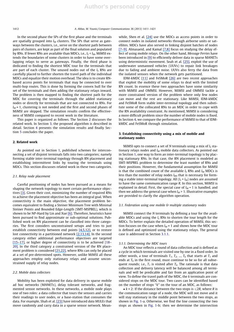
a cycle in which terminals are visited one by one in a fixed order. Inother words, a tour of terminals T1, T2, ..., Tk that starts at T1 andends at Tk in the first round, must continue to be so for all subse-quent rounds; i.e., T1 is visited after Tk. The rationale is that datacollection and delivery latency will be balanced among all termi-nals and will be predicable and fair from an application point ofview. To define the travel path of the MDC, the k terminals are con-sidered stops on the MDC tour. Two cases can be identified basedon the number of stops ‘‘k’’ on the tour of an MDC, as follows:� k = 2: If the distance between the two stops is 62R, where R is

the communication range of a node, the MDC will not move and itwill stay stationary in the middle point between the two stops, asshown in Fig. 1-a. Otherwise, we find the line connecting the twostops as shown in Fig. 1-b; then we determine the intersection

1412 A. Abbas, M. Younis / Computer Communications 36 (2013) 1411–1421

Author's personal copy

points, x and y, of this line and the two circles that represent therange of the nodes at the two stops. MiMSI uses the points, x andy, as the data collection points and the MDC will move in straightline back and forth between them.� k > 2: In this case a tour is defined so that the MDC becomes in

the range of all stops, i.e., the terminals and populated RNs in theclusters, in order to collect and deliver data. The first step is todetermine the convex hull for the k stops. Then we calculate thecenter of mass for the stops on the convex hull and identify thedata collection point for these stops by drawing a line from thecenter of mass to each stop. The data collection points are theintersections between these lines and the circles of radius R thatrepresent the communication range of each convex stop. Theformed path is considered the initial MDC tour. Fig. 2 shows anillustration. The tour can be further optimized. For a two-edge pathxy; xzf g between three stops x, y and z, if the line xz cut across the

circle of radius R that centered at y, the path xy; xzf g can be re-placed by xz. This optimization is illustrated in Fig. 3.

Next, we determine the data collection points for the non-con-vex stops. This is done by finding the nearest edge in the convexhull to each non-convex stop ‘‘i’’. Then we check whether an edge‘‘e’’ cut across the circle of radius R centered at ‘‘i’’, i.e., the MDC willbe within the communication range of ‘‘i’’ while traveling on ‘‘e’’.Fig. 4-a shows an example. If so, the stop ‘‘i’’ will be consideredas covered. Otherwise, a data collection point is define by findingthe intersection point ‘‘q’’ of the perpendicular line from ‘‘i’’ on‘‘e’’ and the circles of radius R that centered at ‘‘i’’. The edge ‘‘e’’ willbe then be replaced by two edges connecting at ‘‘q’’ as shown inFig. 4-b.

3.1.2. Minimizing the tour lengthMiMSI employs the available lS RNs for optimizing the tour of

the MDC. The optimization simply tries to place an RN so that thetravel path is shortened. One of the possible options is to place anRN on the edge between two consecutive terminals on the travelpath so that such a part does not have to be traveled. For exam-

ple, assume the tour includes traveling an edge PiPiþ1 whoselength is less than 2R (and obviously more than R since the twoterminals are not connected to start with). Placing an RN at themidpoint of PiPiþ1 will deem traveling such an edge unnecessarily.However, that will not keep the tour cyclic and in effect will nothelp the tour length without violating the data collection order onthe tour.

MiMSI applies an optimization based on the convex hull of allterminals. Basically, in order for the perimeter of a convex polygonto shrink, one of the corners obviously must be moved inward to-wards the center of the polygon. Consider for example the convexpolygon {n1, n2, n3, n4} in Fig. 2, by replacing one of the stops ni witha new inward stop nnew that is reachable to ni, nnew becomes a gate-way for accessing ni and the tour will be shortened by visiting nnew

instead of ni. Therefore, MiMSI places any available RN at an innerpoint to the tour while being in range of a convex stop so that sucha stop can be eliminated from the tour. The following analysis pro-vides guidelines for determining where an RN can be placed.

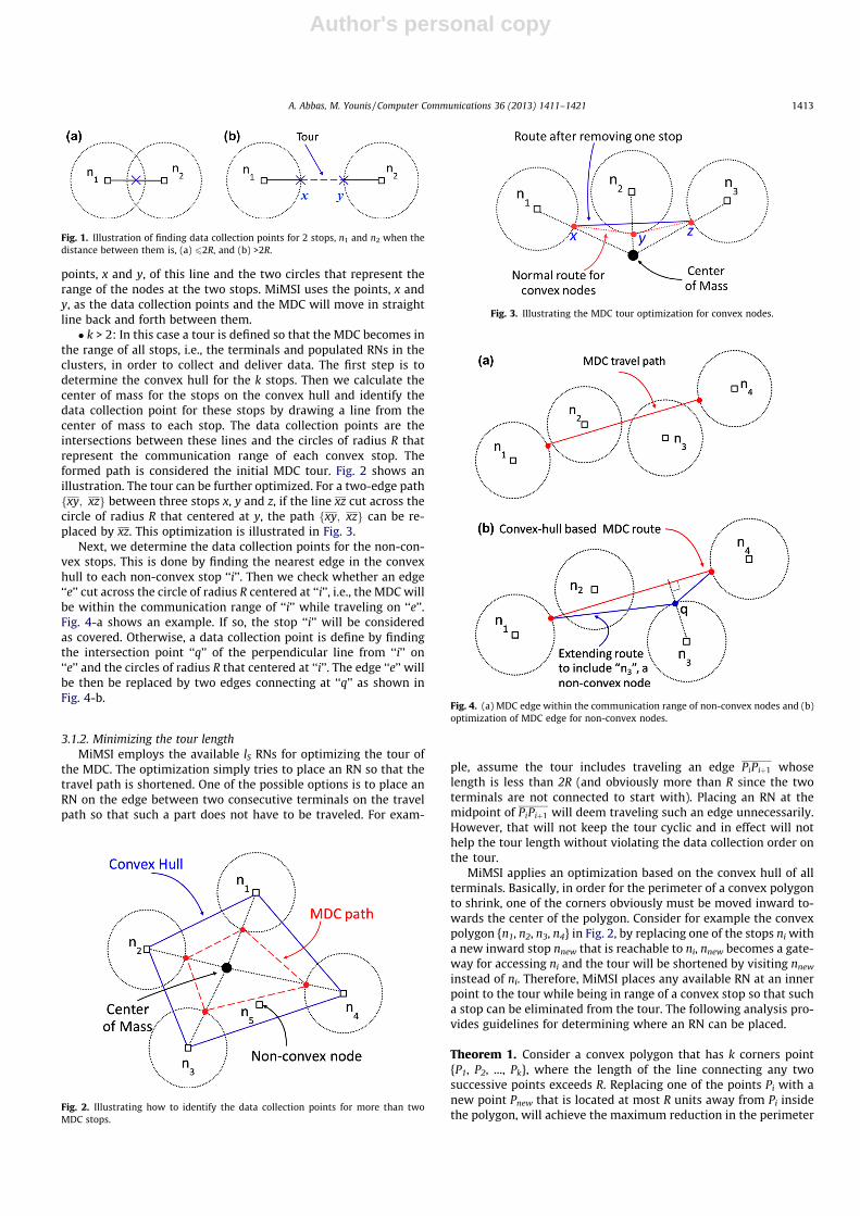
Theorem 1. Consider a convex polygon that has k corners point{P1, P2, ..., Pk}, where the length of the line connecting any twosuccessive points exceeds R. Replacing one of the points Pi with anew point Pnew that is located at most R units away from Pi insidethe polygon, will achieve the maximum reduction in the perimeter

Fig. 1. Illustration of finding data collection points for 2 stops, n1 and n2 when thedistance between them is, (a) 62R, and (b) >2R.

Fig. 2. Illustrating how to identify the data collection points for more than twoMDC stops.

Fig. 3. Illustrating the MDC tour optimization for convex nodes.

Fig. 4. (a) MDC edge within the communication range of non-convex nodes and (b)optimization of MDC edge for non-convex nodes.

A. Abbas, M. Younis / Computer Communications 36 (2013) 1411–1421 1413

Author's personal copy

of the polygon if: (1) Pi is the corner with the smallest angle hmin inthe polygon, and (2) Pnew is located on the bisector of hmin at adistance R from Pi.

Proof. Consider the illustration in Fig. 5. In order for the perimeterof the polygon to shrink, Pnew obviously must be located inside thepolygon, i.e., in an inward direction with respect to Pi. Assume thatthe angle at Pi is h and the line PiPnew divides the angle into h1 andh2. Obviously, h < 2p, and thus h1 and h2 are acute angles. Assumethat the reduction in the perimeter is Q, which corresponds tothe combined reduction in the lines PiPiþ1 and PiPi�1, as shown inFig. 5. In other words,

Q ¼ d1 þ d2

From Fig. 5, d1 � d cos h1 and d2 � d cos h2, and thus

Q � d cos h1 þ d cos h2

Q � dðcos h1 þ cos h2Þ

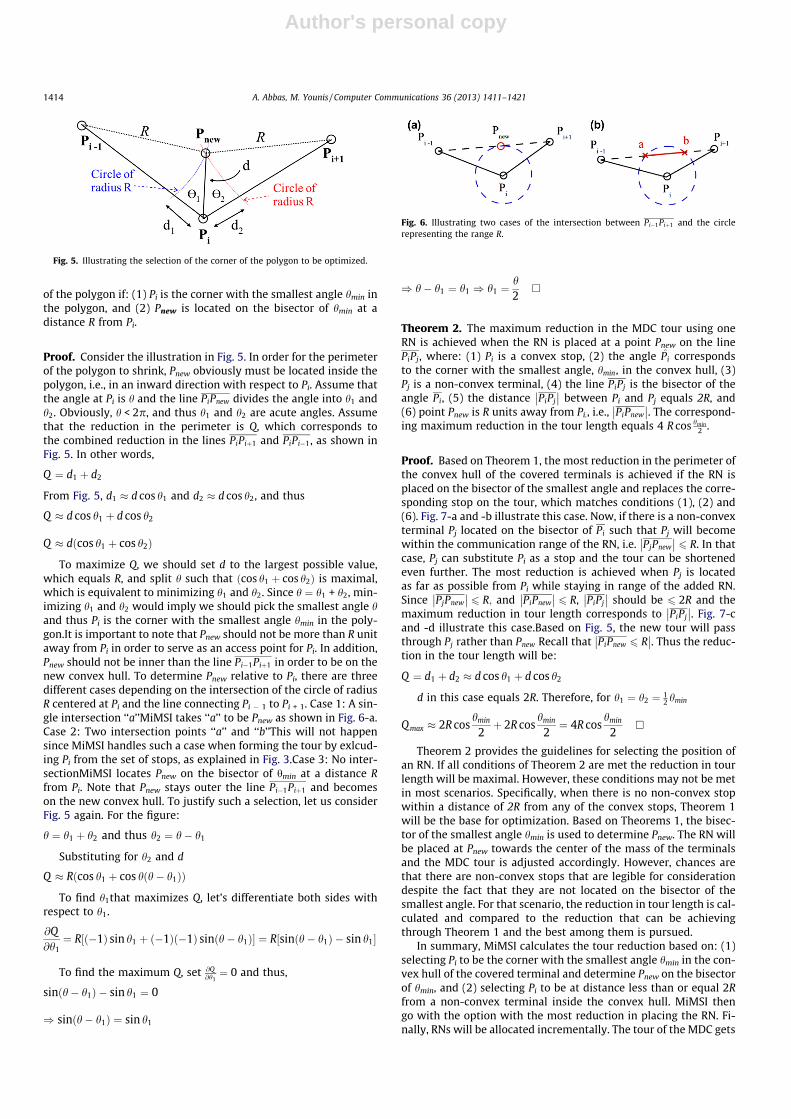
To maximize Q, we should set d to the largest possible value,which equals R, and split h such that ðcos h1 þ cos h2Þ is maximal,which is equivalent to minimizing h1 and h2. Since h ¼ h1 + h2, min-imizing h1 and h2 would imply we should pick the smallest angle hand thus Pi is the corner with the smallest angle hmin in the poly-gon.It is important to note that Pnew should not be more than R unitaway from Pi in order to serve as an access point for Pi. In addition,Pnew should not be inner than the line Pi�1Piþ1 in order to be on thenew convex hull. To determine Pnew relative to Pi, there are threedifferent cases depending on the intersection of the circle of radiusR centered at Pi and the line connecting Pi � 1 to Pi + 1. Case 1: A sin-gle intersection ‘‘a’’MiMSI takes ‘‘a’’ to be Pnew as shown in Fig. 6-a.Case 2: Two intersection points ‘‘a’’ and ‘‘b’’This will not happensince MiMSI handles such a case when forming the tour by exlcud-ing Pi from the set of stops, as explained in Fig. 3.Case 3: No inter-sectionMiMSI locates Pnew on the bisector of hmin at a distance Rfrom Pi. Note that Pnew stays outer the line Pi�1Piþ1 and becomeson the new convex hull. To justify such a selection, let us considerFig. 5 again. For the figure:

h ¼ h1 þ h2 and thus h2 ¼ h� h1

Substituting for h2 and d

Q � Rðcos h1 þ cos hðh� h1ÞÞ

To find h1that maximizes Q, let’s differentiate both sides withrespect to h1.

@Q@h1¼ R½ð�1Þ sin h1 þ ð�1Þð�1Þ sinðh� h1Þ� ¼ R½sinðh� h1Þ � sin h1�

To find the maximum Q, set @Q@h1¼ 0 and thus,

sinðh� h1Þ � sin h1 ¼ 0

) sinðh� h1Þ ¼ sin h1

) h� h1 ¼ h1 ) h1 ¼h2�

Theorem 2. The maximum reduction in the MDC tour using oneRN is achieved when the RN is placed at a point Pnew on the linePiPj, where: (1) Pi is a convex stop, (2) the angle P̂i correspondsto the corner with the smallest angle, hmin, in the convex hull, (3)Pj is a non-convex terminal, (4) the line PiPj is the bisector of theangle Pi, (5) the distance PiPj

��

�� between Pi and Pj equals 2R, and

(6) point Pnew is R units away from Pi., i.e., PiPnew

��

��. The correspond-

ing maximum reduction in the tour length equals 4 R cos hmin2 .

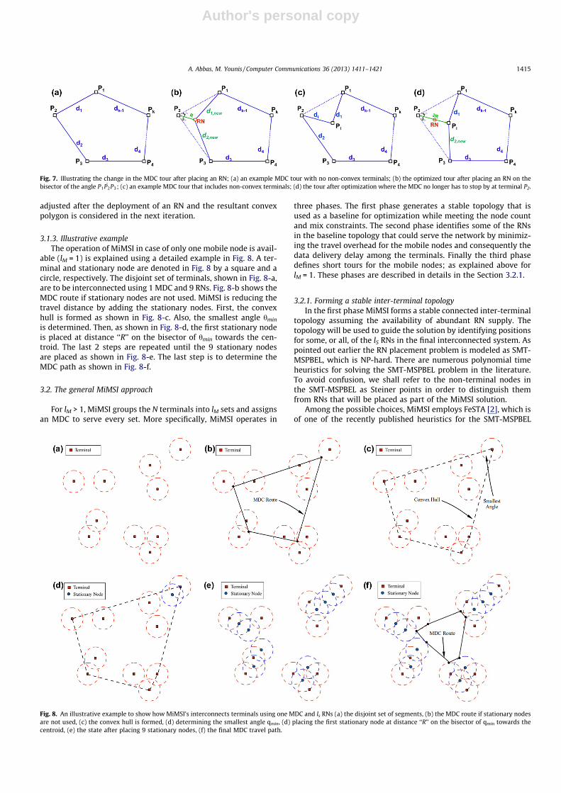
Proof. Based on Theorem 1, the most reduction in the perimeter ofthe convex hull of the covered terminals is achieved if the RN isplaced on the bisector of the smallest angle and replaces the corre-sponding stop on the tour, which matches conditions (1), (2) and(6). Fig. 7-a and -b illustrate this case. Now, if there is a non-convexterminal Pj located on the bisector of Pi such that Pj will becomewithin the communication range of the RN, i.e. PjPnew

��

�� 6 R. In that

case, Pj can substitute Pi as a stop and the tour can be shortenedeven further. The most reduction is achieved when Pj is locatedas far as possible from Pi while staying in range of the added RN.Since PjPnew

��

�� 6 R; and PiPnew

��

�� 6 R, PiPj

��

�� should be 6 2R and the

maximum reduction in tour length corresponds to PiPj

��

��. Fig. 7-c

and -d illustrate this case.Based on Fig. 5, the new tour will passthrough Pj rather than Pnew Recall that PiPnew 6 R

��

��. Thus the reduc-

tion in the tour length will be:

Q ¼ d1 þ d2 � d cos h1 þ d cos h2

d in this case equals 2R. Therefore, for h1 ¼ h2 ¼ 12 hmin

Qmax � 2R coshmin

2þ 2R cos

hmin

2¼ 4R cos

hmin

2�

Theorem 2 provides the guidelines for selecting the position ofan RN. If all conditions of Theorem 2 are met the reduction in tourlength will be maximal. However, these conditions may not be metin most scenarios. Specifically, when there is no non-convex stopwithin a distance of 2R from any of the convex stops, Theorem 1will be the base for optimization. Based on Theorems 1, the bisec-tor of the smallest angle hmin is used to determine Pnew. The RN willbe placed at Pnew towards the center of the mass of the terminalsand the MDC tour is adjusted accordingly. However, chances arethat there are non-convex stops that are legible for considerationdespite the fact that they are not located on the bisector of thesmallest angle. For that scenario, the reduction in tour length is cal-culated and compared to the reduction that can be achievingthrough Theorem 1 and the best among them is pursued.

In summary, MiMSI calculates the tour reduction based on: (1)selecting Pi to be the corner with the smallest angle hmin in the con-vex hull of the covered terminal and determine Pnew on the bisectorof hmin, and (2) selecting Pi to be at distance less than or equal 2Rfrom a non-convex terminal inside the convex hull. MiMSI thengo with the option with the most reduction in placing the RN. Fi-nally, RNs will be allocated incrementally. The tour of the MDC gets

Fig. 5. Illustrating the selection of the corner of the polygon to be optimized.

Fig. 6. Illustrating two cases of the intersection between Pi�1Piþ1 and the circlerepresenting the range R.

1414 A. Abbas, M. Younis / Computer Communications 36 (2013) 1411–1421

Author's personal copy

adjusted after the deployment of an RN and the resultant convexpolygon is considered in the next iteration.

3.1.3. Illustrative exampleThe operation of MiMSI in case of only one mobile node is avail-

able (lM = 1) is explained using a detailed example in Fig. 8. A ter-minal and stationary node are denoted in Fig. 8 by a square and acircle, respectively. The disjoint set of terminals, shown in Fig. 8-a,are to be interconnected using 1 MDC and 9 RNs. Fig. 8-b shows theMDC route if stationary nodes are not used. MiMSI is reducing thetravel distance by adding the stationary nodes. First, the convexhull is formed as shown in Fig. 8-c. Also, the smallest angle hmin

is determined. Then, as shown in Fig. 8-d, the first stationary nodeis placed at distance ‘‘R’’ on the bisector of hmin towards the cen-troid. The last 2 steps are repeated until the 9 stationary nodesare placed as shown in Fig. 8-e. The last step is to determine theMDC path as shown in Fig. 8-f.

3.2. The general MiMSI approach

For lM > 1, MiMSI groups the N terminals into lM sets and assignsan MDC to serve every set. More specifically, MiMSI operates in

three phases. The first phase generates a stable topology that isused as a baseline for optimization while meeting the node countand mix constraints. The second phase identifies some of the RNsin the baseline topology that could serve the network by minimiz-ing the travel overhead for the mobile nodes and consequently thedata delivery delay among the terminals. Finally the third phasedefines short tours for the mobile nodes; as explained above forlM = 1. These phases are described in details in the Section 3.2.1.

3.2.1. Forming a stable inter-terminal topologyIn the first phase MiMSI forms a stable connected inter-terminal

topology assuming the availability of abundant RN supply. Thetopology will be used to guide the solution by identifying positionsfor some, or all, of the lS RNs in the final interconnected system. Aspointed out earlier the RN placement problem is modeled as SMT-MSPBEL, which is NP-hard. There are numerous polynomial timeheuristics for solving the SMT-MSPBEL problem in the literature.To avoid confusion, we shall refer to the non-terminal nodes inthe SMT-MSPBEL as Steiner points in order to distinguish themfrom RNs that will be placed as part of the MiMSI solution.

Among the possible choices, MiMSI employs FeSTA [2], which isof one of the recently published heuristics for the SMT-MSPBEL

Fig. 8. An illustrative example to show how MiMSI’s interconnects terminals using one MDC and ls RNs (a) the disjoint set of segments, (b) the MDC route if stationary nodesare not used, (c) the convex hull is formed, (d) determining the smallest angle qmin, (d) placing the first stationary node at distance ‘‘R’’ on the bisector of qmin towards thecentroid, (e) the state after placing 9 stationary nodes, (f) the final MDC travel path.

Fig. 7. Illustrating the change in the MDC tour after placing an RN; (a) an example MDC tour with no non-convex terminals; (b) the optimized tour after placing an RN on thebisector of the angle ^P1P2P3; (c) an example MDC tour that includes non-convex terminals; (d) the tour after optimization where the MDC no longer has to stop by at terminal P2.

A. Abbas, M. Younis / Computer Communications 36 (2013) 1411–1421 1415

Author's personal copy

problems, and which has been shown to yield superior perfor-mance in terms of the RN count and the level of connectivity.The level of connectivity is typically measured in terms of the aver-age node degree in the formed SMT-MSPBEL. As will be later ex-plained, MiMSI groups the Steiner points and terminals in theSMT-MSPBEL into clusters based on proximity. Having high nodedegree in the SMT-MSPBEL serves MiMSI well since there will bemore gateways between the clusters which enhances the solutionachieved by MiMSI. We use FeSTA in validating MiMSI, as we ex-plain in Section 4. It should be noted that MiMSI can work otherSMT-MSPBEL heuristics as well.

3.2.2. Positioning stationary relaysThe goal of the second phase of MiMSI is to determine a set of

candidate positions for all or some of the available lS stationary re-lays and assign a subset of the terminals to each mobile node toserve. To achieve this goal, MiMSI groups the nodes (Steiner pointsand terminals) in the baseline SMT-MSPBEL, formed in the firstphase, based on proximity. The number of clusters equals the num-ber of available MDCs, lM. The rationale behind the proximity-based clustering is to group a set of terminals that are close to eachother so that an MDC can tour them with the least travel distanceoverhead. The question that is worth addressing is why the cluster-ing is not performed without forming a baseline SMT-MSPBEL. Themain advantage of the baseline SMT-MSPBEL is to point out possi-ble gateways between the clusters, something that would not beeasy to determine if the clustering is performed without knowingthe baseline SMT-MSPBEL. The Steiner points corresponding tothese gateways will be populated with RNs, if they are fewer orequal to lS, as we explain below. There are many proximity-basedclustering techniques in the literature, e.g., the k-means algorithm,which can be applied for this step.

Upon forming the clusters, MiMSI identifies the gateway nodesthat connect two or more clusters. This is done by forming a min-imum spanning tree (mst) on the set of Steiner points and termi-nals, and selecting the shortest edges that connect pairs of the lMclusters. The end points of these edges may be terminals or Steinerpoints. Unselected Steiner points in the baseline SMT-MSPBEL arenot considered any further. Depending on the relationship be-tween the number of gateway Steiner points ‘‘g’’ and lS, the avail-able RNs are assigned as follow:� g = lS: This is the simplest case for which an RN is positioned at

every selected Steiner point to serve as an inter-clustergateway.� g < lS: In this case we populate all ‘‘g’’ gateway Steiner points

with stationary relays. The remaining (g – lS) RNs will be usedfor reducing the length of the travel paths for MDCs as we ex-plain when discussing the third phase.� g > lS: This case is tricky since the number of available RNs is

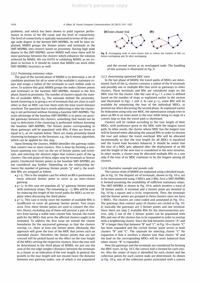
insufficient to cover all gateway Steiner points. Two issuesarise. First, these Steiner points are used to connect the clus-ters. Hence, excluding any of them will prevent a pair of clus-ters from having a stable inter-cluster link. Second, the travelpath for the MDCs that serve the affected clusters ought to beextended. To address the first issue we extend the clusterboundaries for the uncovered gateways so that the clustersoverlap, i.e., share at least one Steiner point. Obviously, thisapproach will grow the tour of the MDC that serves such anextended cluster. Therefore, the Steiner points that are notcovered will be picked based on the effect on the tour lengthof the MDCs serving the respective clusters. Since the tour willbe determined in the third phase of MiMSI, we just use thesum of the mst edge weights (distance) between the terminalsin a cluster as an indication of the tour length. In general, thegrowth in the tour length will not exceed twice the distancebetween two gateway nodes; one of which is not populated

and the second serves as an overlapped node. The handlingof this scenario is illustrated in Fig. 9.

3.2.3. Determining optimized MDC toursIn the last phase of MiMSI, the travel paths of MDCs are deter-

mined. Each of the lM clusters contains a subset of the N terminalsand possibly one or multiple RNs that serve as gateways to otherclusters. These terminals and RNs are considered stops on theMDC tour for the cluster. Like the case of lM = 1, a tour is definedbased on the number of stops as explained earlier in the sectionand illustrated in Figs. 1 and 2. In case g < lS, some RNs will beavailable for minimizing the tour of the individual MDCs, aspointed out when discussing the second phase. As explained earlierfor federation using only one MDC, the optimization simply tries toplace an RN in an inner point to the tour while being in range of aconvex stop so that the travel path is shortened.

Clusters will be ranked according to the tour length of theirMDCs, with preference given to the MDC with the longest travelpath. In other words, the cluster whose MDC has the longest tourwill be favored when allocating the unused RNs in order to shortenthe tour and reduce the travel overhead. RNs will be allocatedincrementally so that the tour length for all MDCs is equalizedand the travel load becomes balanced. It should be noted thatthe tour of a MDC gets adjusted after the deployment of an RNand the length of the new tour is considered in the next iteration.In other words, a cluster may be allocated multiple RNs in a rowonly if the tour of its MDC continues to be the longest among allclusters.

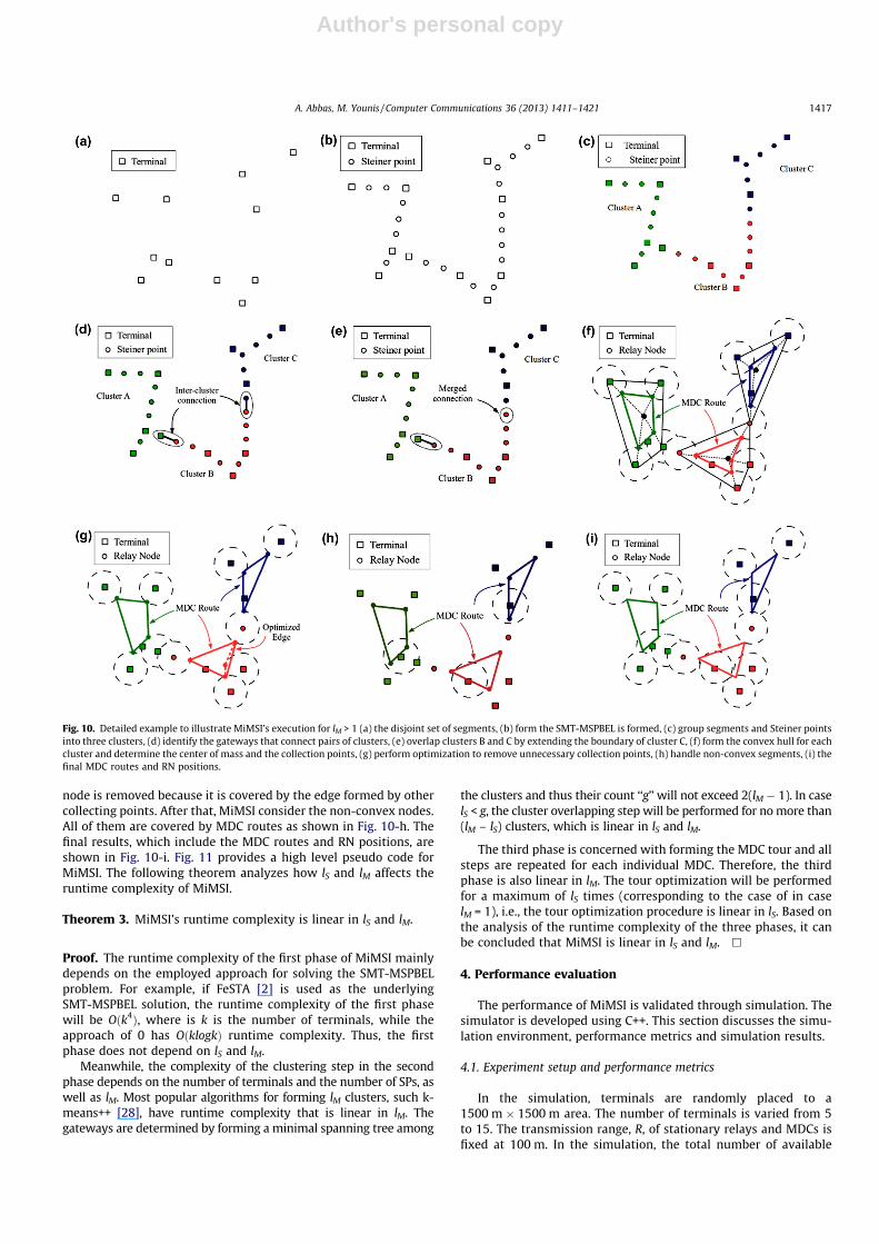
3.2.4. Illustrative example and pseudo codeThe various steps of MiMSI are explained using a detailed exam-

ple in Fig. 10. The disjoint set of terminals, shown in Fig. 10-a, areto be interconnected using 3 MDCs and 2 RNs. First a SMT-MSPBELis formed assuming the availability of sufficient stationary relays.The SMT-MSPBEL is shown in Fig. 10-b, which involves a total of18 Steiner points. A terminal and a Steiner point are denoted inFig. 10 by a square and a circle, respectively. Then, the terminalsand the Steiner points are grouped to three clusters since we have3 MDCs. The clusters are color-coded and annotated in Fig. 10-c.The gateways that connect pairs of clusters are circled in Fig. 10-d; basically the gateways are 3 Steiner points and one terminal.Since there are only 2 available RNs for the interconnection pro-cess, only 2 out of the 3 Steiner points can be populated withRNs and one of the clusters has to be expanded in order to overlapwith a neighboring cluster. Since the link between clusters ‘‘A’’ and‘‘B’’ is longer than that between ‘‘B’’ and ‘‘C’’, in Fig. 10-e cluster ‘‘C’’has been expanded and the circled Steiner point serves in bothclusters ‘‘B’’ and ‘‘C’’. The rationale for selecting cluster ‘‘C’’ forexpansion is that it involves a shorter tour than cluster ‘‘B’’ andthe load on the corresponding MDCs will be more balanced thanwhen cluster ‘‘B’’ is expanded.

Now the gateways and the terminals are considered for formingthe MDC tours. In Fig. 10-f, the convex hull is formed for each clus-ter. Also the center of mass is identified for each cluster and thecollection points for each convex node are determined. As shownin Fig. 10-g, one of the collection points associated with a convex

Fig. 9. Overlapping node in inter-cluster link to reduce the number of RNs (a)before overlapping and (b) after overlapping.

1416 A. Abbas, M. Younis / Computer Communications 36 (2013) 1411–1421

Author's personal copy

node is removed because it is covered by the edge formed by othercollecting points. After that, MiMSI consider the non-convex nodes.All of them are covered by MDC routes as shown in Fig. 10-h. Thefinal results, which include the MDC routes and RN positions, areshown in Fig. 10-i. Fig. 11 provides a high level pseudo code forMiMSI. The following theorem analyzes how lS and lM affects theruntime complexity of MiMSI.

Theorem 3. MiMSI’s runtime complexity is linear in lS and lM.

Proof. The runtime complexity of the first phase of MiMSI mainlydepends on the employed approach for solving the SMT-MSPBELproblem. For example, if FeSTA [2] is used as the underlyingSMT-MSPBEL solution, the runtime complexity of the first phasewill be Oðk4Þ, where is k is the number of terminals, while theapproach of 0 has OðklogkÞ runtime complexity. Thus, the firstphase does not depend on lS and lM.

Meanwhile, the complexity of the clustering step in the secondphase depends on the number of terminals and the number of SPs, aswell as lM. Most popular algorithms for forming lM clusters, such k-means++ [28], have runtime complexity that is linear in lM. Thegateways are determined by forming a minimal spanning tree among

the clusters and thus their count ‘‘g’’ will not exceed 2(lM� 1). In caselS < g, the cluster overlapping step will be performed for no more than(lM – lS) clusters, which is linear in lS and lM.

The third phase is concerned with forming the MDC tour and allsteps are repeated for each individual MDC. Therefore, the thirdphase is also linear in lM. The tour optimization will be performedfor a maximum of lS times (corresponding to the case of in caselM = 1), i.e., the tour optimization procedure is linear in lS. Based onthe analysis of the runtime complexity of the three phases, it canbe concluded that MiMSI is linear in lS and lM. h

4. Performance evaluation

The performance of MiMSI is validated through simulation. Thesimulator is developed using C++. This section discusses the simu-lation environment, performance metrics and simulation results.

4.1. Experiment setup and performance metrics

In the simulation, terminals are randomly placed to a1500 m � 1500 m area. The number of terminals is varied from 5to 15. The transmission range, R, of stationary relays and MDCs isfixed at 100 m. In the simulation, the total number of available

Fig. 10. Detailed example to illustrate MiMSI’s execution for lM > 1 (a) the disjoint set of segments, (b) form the SMT-MSPBEL is formed, (c) group segments and Steiner pointsinto three clusters, (d) identify the gateways that connect pairs of clusters, (e) overlap clusters B and C by extending the boundary of cluster C, (f) form the convex hull for eachcluster and determine the center of mass and the collection points, (g) perform optimization to remove unnecessary collection points, (h) handle non-convex segments, (i) thefinal MDC routes and RN positions.

A. Abbas, M. Younis / Computer Communications 36 (2013) 1411–1421 1417

Author's personal copy

nodes, RNs and MDCs, is set to the number of Steiner points toform SMT-MSPBEL multiplied by a fraction ‘‘u’’. For lM > 1, the ratioa of number of MDCs ‘‘lM’’ to RNs ‘‘lS’’ is fixed at 0.5. Separate exper-iments are runs to capture of effect of changing a on the perfor-mance of MiMSI. K-means++ [27] is used as the underlyingproximity-based clustering algorithm.

The performance under varying number of nodes, MDCs andRNs, is studied by repeating the experiment for different u val-ues. The reason is that, for different topologies the terminalscan be scattered too far or too close to each other and this affectsthe number of inserted Steiner points. Hence, varying the totalnumber of nodes will not lead us to a fair conclusion. Instead,the ratio u is varied for different topologies to handle such a con-dition. The following performance metrics are considered in thesimulation:

� Total Tour Length: This is the sum of distances traveled byall MDCs to complete one tour. This metric gauges theinflicted overhead due to mobility.

� Average Tour Length: This metric again reflects the overheaddue to mobility and factors in the number of engagedMDCs.

� Maximum Tour Length: This metric shows the longest dis-tance that an MDC has to travel in a network in a singledata collection round, which is important in analyzing themaximum delay incurred in the network. In addition, thismetric indicates the highest load that one of the MDCsmay experience, which would affect the rate of energydepletion and the node lifetime.

4.2. MiMSI performance results

We compare the performance of MiMSI to that of IDM-kMDC[11] and FeSMoR [26]. IDM-kMDC first forms a minimum spanningtree and assumes that MDCs are deployed on all edges. Tours aremerged if the number of available MDCs is less than the numberof edges, i.e., N � 1, where N is the number of terminals. Mean-while, FeSMoR opts to minimize the date delivery delay. It formsSMT-MSPBEL and replaces some of the RNs that are close to thenetwork periphery with MDCs in order to limit the effect of linkunavailability on the data delivery delay while an MDC is in mo-tion. Each simulation experiment is repeated for 50 different topol-ogies and the average is reported. It is observed that with a 95%confidence interval, our results stayed within 6–12% of the samplemean.

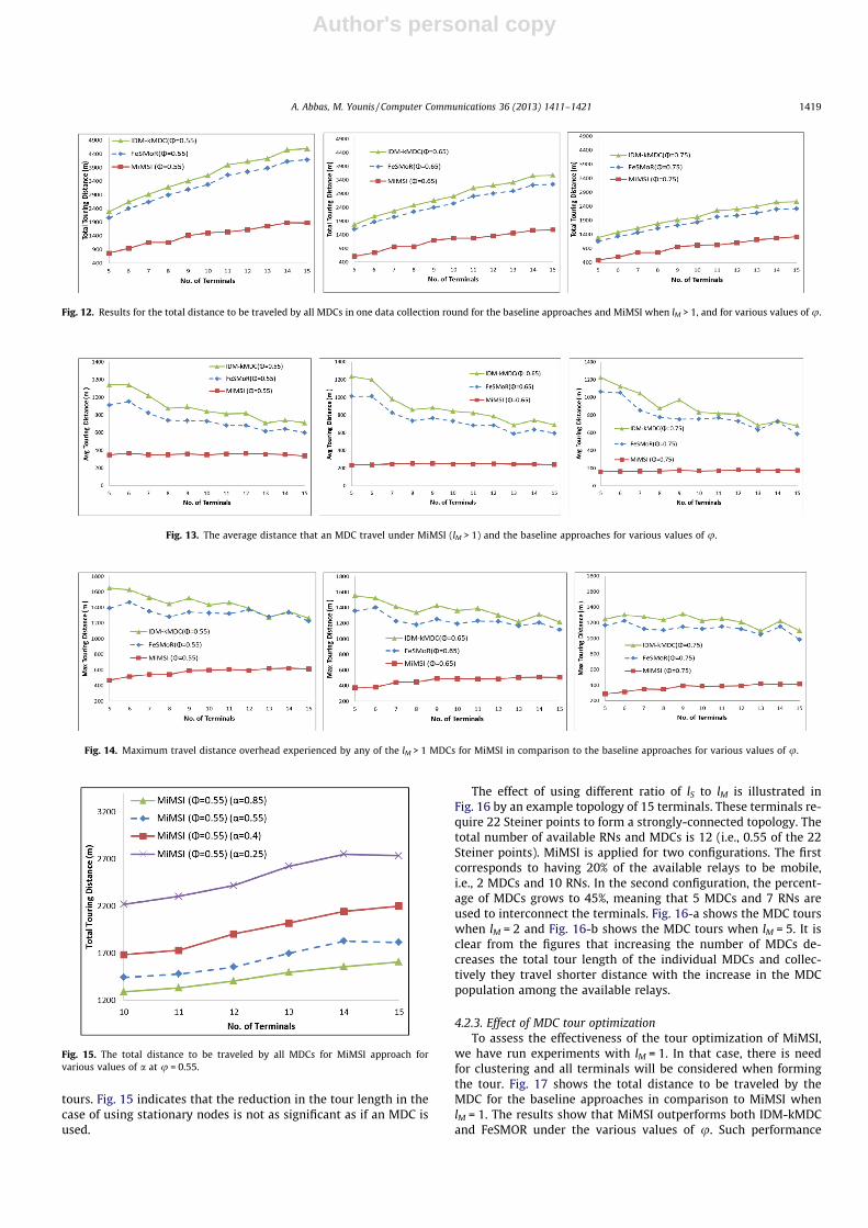
4.2.1. Simulation results for lM > 1Fig. 12 shows the observed total tour lengths results for MiMSI

and the baseline approaches. The results show that MiMSI outper-forms both IDM-kMDC and FeSMOR under the various values of u,which again reflects resources availability relative to the case offorming stable inter-terminal topology. MiMSI clusters the termi-nals based on proximity and allocates stationary relays to clustersbased on the tour length of the MDCs that serve them. All thesefeatures contribute to shortening the tour length of the individualMDCs. As u increases the performance gap diminishes since thenode count grows and fewer relays in IDM-kMDC and FeSMOR willhave to move. However, in MiMSI the impact on the travel distanceis not as significant since a is kept constant during the experimentand thus lM stays fixed. We study the effect of a later in this section.

Fig. 13 indicates that MiMSI does a good job balancing the loadamong the available MDCs by yielding superior performance interms of the average distance that an MDC has to travel. In factthe average travel overhead stays almost constant in the numberof terminals. For the same reason, Fig. 14 shows that MiMSI sus-tains its performance advantage over IDM-kMDC and FeSMoR withrespect to the maximum tour length. The maximum distancegrows very slightly with the increase in the number of terminalsdue to the proximity based clustering of the terminals. Again theeffect of increasing u is similar to the total distance performanceand is attributed to the same reasons mentioned above.

4.2.2. Effect of a on MiMSI performanceAs we mentioned before, MIMSI employs lS RNs and lM MDCs,

whose combined count (lS + lM) is less than the number of relaynodes lRN that is necessary for forming a stable inter-terminaltopology. We have studied the effect of changing the ratio a ofMDC to RN count (i.e., lM/lS). Fig. 15 shows the changes of the totaltour length of MiMSI with the changes of a. In that experiment,u = 0.55, a is changed from 0.25 to 0.85 and the number of termi-nals is varied between 10 and 15. It is clear from the Figure that asa grows, the total tour length is decreased. This is sustained for allthe different numbers of terminals.

These results provide insight that would enable effective re-source planning and trade-off. The total number of (lS + lM) is fixedand equals a fraction of lRN (equals to u. lRN). Thus, increasing thenumber of MDCs, lM, will imply a decrease in the number of sta-tionary nodes, lS. When the number of MDCs grows the numberof clusters in MiMSI will increase accordingly. Increasing the num-ber of clusters reduces the number of terminals per cluster. SinceMiMSI pursues proximity-based grouping of terminals, the re-duced cluster population shortens the tour length of the individualMDCs. On the other hand, reducing the number of MDCs will in-crease the number of available stationary nodes. As discussed be-fore, the extra stationary nodes will be used to shorten the MDC

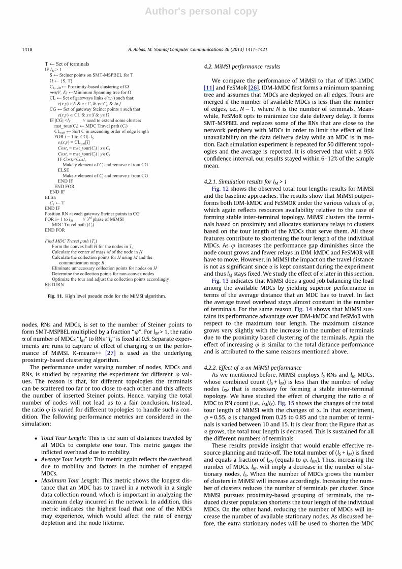
T ← Set of terminalsIF lM > 1

S ← Steiner points on SMT-MSPBEL for T Ω ← {S, T} C1,..,lM ← Proximity-based clustering of Ωmst(V, E) ←Minimum Spanning tree for ΩCL ← Set of gateways links e(x,y) such that:

e(x,y) ∈E & x∈Ci & y∈Cj, & i≠ jCG ← Set of gateway Steiner points x such that

e(x,y) ∈ CL & x∈S & y∈ΩIF |CG| <lS // need to extend some clusters

mst_tour(Ci) ← MDC Travel path (Ci)CLsort ← Sort C in ascending order of edge lengthFOR i = 1 to |CG|- lS

ei(x,y) = CLsort[i]Costx = mst_tour(Ci) | x∈CiCosty = mst_tour(Cj) | y∈CjIF Costx<Costy

Make y element of Ci and remove x from CGELSE

Make x element of Cj and remove y from CGEND IF

END FOREND IF

ELSEC1 ← T

END IFPosition RN at each gateway Steiner points in CGFOR i= 1 to lM // 3rd phase of MiMSI

MDC Travel path (Ci)END FOR

Find MDC Travel path (Tc)Form the convex hull H for the nodes in TcCalculate the center of mass M of the node in HCalculate the collection points for H using M and the

communication range REliminate unnecessary collection points for nodes on HDetermine the collection points for non-convex nodesOptimize the tour and adjust the collection points accordingly

RETURN

Fig. 11. High level pseudo code for the MiMSI algorithm.

1418 A. Abbas, M. Younis / Computer Communications 36 (2013) 1411–1421

Author's personal copy

tours. Fig. 15 indicates that the reduction in the tour length in thecase of using stationary nodes is not as significant as if an MDC isused.

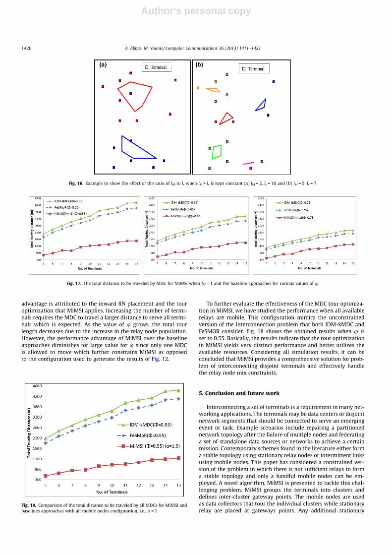
The effect of using different ratio of lS to lM is illustrated inFig. 16 by an example topology of 15 terminals. These terminals re-quire 22 Steiner points to form a strongly-connected topology. Thetotal number of available RNs and MDCs is 12 (i.e., 0.55 of the 22Steiner points). MiMSI is applied for two configurations. The firstcorresponds to having 20% of the available relays to be mobile,i.e., 2 MDCs and 10 RNs. In the second configuration, the percent-age of MDCs grows to 45%, meaning that 5 MDCs and 7 RNs areused to interconnect the terminals. Fig. 16-a shows the MDC tourswhen lM = 2 and Fig. 16-b shows the MDC tours when lM = 5. It isclear from the figures that increasing the number of MDCs de-creases the total tour length of the individual MDCs and collec-tively they travel shorter distance with the increase in the MDCpopulation among the available relays.

4.2.3. Effect of MDC tour optimizationTo assess the effectiveness of the tour optimization of MiMSI,

we have run experiments with lM = 1. In that case, there is needfor clustering and all terminals will be considered when formingthe tour. Fig. 17 shows the total distance to be traveled by theMDC for the baseline approaches in comparison to MiMSI whenlM = 1. The results show that MiMSI outperforms both IDM-kMDCand FeSMOR under the various values of u. Such performance

Fig. 12. Results for the total distance to be traveled by all MDCs in one data collection round for the baseline approaches and MiMSI when lM > 1, and for various values of u.

Fig. 13. The average distance that an MDC travel under MiMSI (lM > 1) and the baseline approaches for various values of u.

Fig. 14. Maximum travel distance overhead experienced by any of the lM > 1 MDCs for MiMSI in comparison to the baseline approaches for various values of u.

Fig. 15. The total distance to be traveled by all MDCs for MiMSI approach forvarious values of a at u = 0.55.

A. Abbas, M. Younis / Computer Communications 36 (2013) 1411–1421 1419

Author's personal copy

advantage is attributed to the inward RN placement and the touroptimization that MiMSI applies. Increasing the number of termi-nals requires the MDC to travel a larger distance to serve all termi-nals which is expected. As the value of u grows, the total tourlength decreases due to the increase in the relay node population.However, the performance advantage of MiMSI over the baselineapproaches diminishes for large value for u since only one MDCis allowed to move which further constrains MiMSI as opposedto the configuration used to generate the results of Fig. 12.

To further evaluate the effectiveness of the MDC tour optimiza-tion in MiMSI, we have studied the performance when all availablerelays are mobile. This configuration mimics the unconstrainedversion of the interconnection problem that both IDM-kMDC andFeSMOR consider. Fig. 18 shows the obtained results when u isset to 0.55. Basically, the results indicate that the tour optimizationin MiMSI yields very distinct performance and better utilizes theavailable resources. Considering all simulation results, it can beconcluded that MiMSi provides a comprehensive solution for prob-lem of interconnecting disjoint terminals and effectively handlethe relay node mix constraints.

5. Conclusion and future work

Interconnecting a set of terminals is a requirement in many net-working applications. The terminals may be data centers or disjointnetwork segments that should be connected to serve an emergingevent or task. Example scenarios include repairing a partitionednetwork topology after the failure of multiple nodes and federatinga set of standalone data sources or networks to achieve a certainmission. Contemporary schemes found in the literature either forma stable topology using stationary relay nodes or intermittent linksusing mobile nodes. This paper has considered a constrained ver-sion of the problem in which there is not sufficient relays to forma stable topology and only a handful mobile nodes can be em-ployed. A novel algorithm, MiMSI is presented to tackle this chal-lenging problem. MiMSI groups the terminals into clusters anddefines inter-cluster gateway points. The mobile nodes are usedas data collectors that tour the individual clusters while stationaryrelay are placed at gateways points. Any additional stationary

Fig. 16. Example to show the effect of the ratio of lM to ls when lM + ls is kept constant (a) lM = 2, ls = 10 and (b) lM = 5, ls = 7.

Fig. 17. The total distance to be traveled by MDC for MiMSI when lM = 1 and the baseline approaches for various values of u.

Fig. 18. Comparison of the total distance to be traveled by all MDCs for MiMSI andbaselines approaches with all mobile nodes configuration, i.e., a = 1.

1420 A. Abbas, M. Younis / Computer Communications 36 (2013) 1411–1421

Author's personal copy

nodes are used to shorten the tour of the MDCs and balance thetravel load among them.

MiMSI has been validated through simulation. The simulationresults have confirmed the performance advantage of MiMSI incomparison to competing approaches in the literature. Our futureplan includes investigating the interconnection problem whenthe connectivity is subject to quality of service requirements.

Acknowledgment

This work was supported by the National Science Foundation(NSF) awards # CNS 1018171.

References

[1] C.-Y. Chong, S.P. Kumar, Sensor networks: evolution, opportunities, andchallenges, Proceedings of the IEEE 91 (8) (2003) 1247–1256.

[2] F. Senel, M. Younis, Relay node placement in structurally damaged wirelesssensor networks via triangular steiner tree approximation, Elsevier ComputerCommunications 34 (16) (2011) 1932–1941.

[3] M. Younis, K. Akkaya, Strategies and techniques for node placement in wirelesssensor networks: a survey, Journal of Ad-Hoc Network 6 (4) (2008) 621–655.

[4] X. Cheng, D.-z. Du, L. Wang, B. Xu, Relay sensor placement in wireless sensornetworks, Wireless Networks 14 (3) (2008) 347–355.

[5] E.L. Lloyd, G. Xue, Relay node placement in wireless sensor networks, IEEETransactions on Computers 56 (1) (2007) 134–138.

[6] G. Lin, G. Xue, Steiner tree problem with minimum number of steiner pointsand bounded edge-length, Information Processing Letters 69 (2) (1999) 53–57.

[7] H. Almasaeid, A.E. Kamal, Data delivery in fragmented wireless sensornetworks using mobile agents, in: Proc. the 10th ACM/IEEE Int’l Symp. onModeling, Analysis and Simulation of Wireless and Mobile Systems (MSWiM),Chania, Greece, Oct. 2007.

[8] H. Almasaeid, A.E. Kamal, Modeling Mobility-Assisted Data Collection inWireless Sensor Networks, in: Proc. of the IEEE Global Comm. Conf.(GLOBECOM’08), New Orleans, LA, Dec. 2008.

[9] W. Zhao, M. Ammar, E. Zegura, A message ferrying approach for data deliveryin sparse mobile ad hoc networks, in: Proc. the 5th ACM internationalsymposium on Mobile ad hoc networking and computing (MobiHoc’04),Tokyo, Japan, May 2004.

[10] W. Alsalih, Selim Akl, H. Hassanein, Placement of multiple mobile base stationsin wireless sensor networks, in: Proc. of the IEEE Symp. on Signal Processingand Info. Tech. (ISSPIT), Cairo, Egypt, Dec. 2007.

[11] F. Senel, M. Younis, Optimized Interconnection of Disjoint Wireless SensorNetwork Segments Using K Mobile Data Collectors, in: Proc. of the Int’l Conf.on Comm. (ICC’12), Ottawa, Canada, Jun 2012.

[12] A. Efrat, S.P. Fekete, P.R. Gaddehosur, J.S.B. Mitchell, V. Polishchuk, J. Suomela,Improved approximation algorithms for relay placement, in: Proc. of the 16thEuropean Symposium on Algorithms, Karlsruhe, Germany, Sep. 2008.

[13] S. Lee, M. Younis, Recovery from multiple simultaneous failures in wirelesssensor networks using minimum steiner tree, Journal of Parallel andDistributed Systems 70 (2010) 525–536.

[14] F. Al-Turjman, H. Hassanein, M. Ibnkahla, Optimized relay placement tofederate wireless sensor networks in environmental applications, in: Proc. ofthe IEEE International Workshop on Federated Sensor Systems (FedSenS’11),Istanbul, Turkey, July 2011.

[15] Q. Wang, K. Xu, G. Takahara, H. Hassanein, Locally optimal relay nodeplacement in heterogeneous wireless sensor networks, in: Proc. of 48thIEEEGlobal Telecomm. Conf., St. Louis, MO, Nov. 2005.

[16] Y.T. Hou, Y. Shi, H.D. Sherali, On energy provisioning and relay node placementfor wireless sensor networks, IEEE Transactions on Wireless Communications4 (5) (2005) 2579–2590.

[17] Z. Cheng, M. Perillo, W.B. Heinzelman, General network lifetime and costmodels for evaluating sensor network deployment strategies, IEEETransactions on Mobile Computing 7 (4) (2008) 484–497.

[18] X. Han, X. Cao, E.L. Lloyd, C.-C. Shen, Fault-tolerant relay nodes placement inheterogeneous wireless sensor networks, in: Proc. of the 26th IEEE/ACM JointConf. on Computers and Comm. (INFOCOM’07), Anchorage AK, May 2007.

[19] J. Tang, B. Hao, A. Sen, Relay node placement in large scale wireless sensornetworks, Computer Communications 29 (2006) 490–501. special issue onwireless sensor networks.

[20] B. Hao, H. Tang, G. Xue, Fault-tolerant relay node placement in wireless sensornetworks: formulation and approximation, in: Proc. of the Workshop on HighPerformance Switching and Routing, Phoenix, AZ, April 2004.

[21] S. Misra, S. Dong, G. Xue, J. Tang, Constrained relay node placement in wirelesssensor networks: formulation and approximations, IEEE/ACM Transactions onNetworking 18 (2010) 434–447.

[22] D. Yang, S. Misra, X. Fang, G. Xue, J. Zhang, Two-tiered constrained relay nodeplacement in wireless sensor networks: efficient approximations, in: Proc. ofthe IEEE Conf. on Sensor, Mesh and Ad Hoc Comm. and Networks. (SECON2010), Boston, MA, June 2010.

[23] R. Shah, S. Roy, S. Jain, W. Brunette, Data MULEs: modeling a three-tierarchitecture for sparse sensor networks, in: Proc. the1st IEEE Int’l Workshopon Sensor Network Protocols and App. (SNPA’03), May 2003.

[24] C.-C. Shen, O. Koc, C. Jaikaeo, Z. Huang, Trajectory control of mobile accesspoints in MANET, in: Proc. the 48thIEEE Global Telecom. Conference(GLOBECOM ‘05), St. Louis, MO, Nov. 2005.

[25] W.K.G. Seah, H. Tan, Z. Liu, M.H. Ang, Multiple-UUV approach for enhancingconnectivity in underwater ad-hoc sensor networks, Proceedings of MTS/IEEEOCEANS 3 (2005) 2263–2268.

[26] J.L.V.M. Stanislaus, M. Younis, Delay-conscious federation of multiple wirelesssensor network segments using mobile relays, in: Proc. of the 76th IEEEVehicular Technology Conference (VTC2012-Fall), Québec City, Canada,September 2012.

[27] G. Lin, G. Xue, Steiner tree problem with minimum number of steiner pointsand bounded edge-length, Information Processing Letters 69 (1999) 53–57.

[28] D. Arthur, S. Vassilvitskii, k-means++: the advantages of careful seeding, in:Proc. of the 18th Annual ACM-SIAM Symposium on Discrete Algorithms(SODA’07), Philadelphia, PA, January 2007.

A. Abbas, M. Younis / Computer Communications 36 (2013) 1411–1421 1421