
ESSnet Big Data II
171
ESSnet Big Data II Grant Agreement Number: 847375-2018-NL-BIGDATA https://webgate.ec.europa.eu/fpfis/mwikis/essnetbigdata https://ec.europa.eu/eurostat/cros/content/essnetbigdata_en Workpackage I Mobile Network Data Deliverable I.4 (Information Techonologies) Some IT tools for the production of official statistics with mobile network data Final version, 11 November, 2020 ES LSnet co-ordinator: Workpackage Leader: David Salgado (INE, Spain) [email protected] telephone : +34 91 5813151 mobile phone : N/A Prepared by: Bogdan Oancea (INS, Romania) - Sandra Barragán (INE, Spain) - David Salgado (INE, Spain) - Luis Sanguiao (INE, Spain)
-
Upload
khangminh22 -
Category
Documents
-
view
1 -
download
0
Transcript of ESSnet Big Data II

ESSnet Big Data I I
G r a n t A g r e e m e n t N u m b e r : 8 4 7 3 7 5 - 2 0 1 8 - N L - B I G D A T A
h t t p s : / / w e b g a t e . e c . e u r o p a . e u / f p f i s / m w i k i s / e s s n e t b i g d a t a
h t t p s : / / e c . e u r o p a . e u / e u r o s t a t / c r o s / c o n t e n t / e s s n e t b i g d a t a _ e n
W o rk pa c k a ge I
Mo bi l e N e two rk D a ta
D e l i v e ra bl e I . 4 ( In fo rma t i o n T e c ho no l o g i e s )
S o me IT to o l s fo r the pro duc t i o n o f o f f i c i a l s ta t i s t i c s
wi th mo bi l e n e two rk da ta
Final version, 11 November, 2020
ES LSnet co-ordinator:
Workpackage Leader:
David Salgado (INE, Spain)
telephone : +34 91 5813151
mobile phone : N/A
Prepared by:
Bogdan Oancea (INS, Romania)
- Sandra Barragán (INE, Spain) - David Salgado (INE, Spain)
- Luis Sanguiao (INE, Spain)

Contents
1 Executive summary 1
2 Introduction 32.1. The programming languages of the IT components . . . . . . . . . . . . . . . . . 32.2. The layered structure of the IT components . . . . . . . . . . . . . . . . . . . . . . 52.3. The interfaces between layers . . . . . . . . . . . . . . . . . . . . . . . . . . . . . . 8
3 The data acquisition and preprocessing layer 173.1. MNO data . . . . . . . . . . . . . . . . . . . . . . . . . . . . . . . . . . . . . . . . . 173.2. Synthetic data . . . . . . . . . . . . . . . . . . . . . . . . . . . . . . . . . . . . . . . 18
3.2.1. The simulation software . . . . . . . . . . . . . . . . . . . . . . . . . . . . . 183.2.2. Simulation scenarios . . . . . . . . . . . . . . . . . . . . . . . . . . . . . . . 20
4 The geolocation layer 234.1. Introduction . . . . . . . . . . . . . . . . . . . . . . . . . . . . . . . . . . . . . . . . 234.2. Model construction . . . . . . . . . . . . . . . . . . . . . . . . . . . . . . . . . . . . 24
4.2.1. HMM initialization . . . . . . . . . . . . . . . . . . . . . . . . . . . . . . . . 244.2.2. Time discretization and reduction of parameters . . . . . . . . . . . . . . . 244.2.3. Construction of the emission model . . . . . . . . . . . . . . . . . . . . . . 254.2.4. Construction of the transition model . . . . . . . . . . . . . . . . . . . . . . 28
4.3. Fitting the model . . . . . . . . . . . . . . . . . . . . . . . . . . . . . . . . . . . . . 304.3.1. Parameter estimation . . . . . . . . . . . . . . . . . . . . . . . . . . . . . . . 304.3.2. Computation of the likelihood . . . . . . . . . . . . . . . . . . . . . . . . . 324.3.3. Posterior location probabilities estimation . . . . . . . . . . . . . . . . . . . 334.3.4. The initial probability distribution . . . . . . . . . . . . . . . . . . . . . . . 34
4.4. An end to end example . . . . . . . . . . . . . . . . . . . . . . . . . . . . . . . . . . 354.5. Some remarks about computational efficiency . . . . . . . . . . . . . . . . . . . . 38
4.5.1. Model construction . . . . . . . . . . . . . . . . . . . . . . . . . . . . . . . . 384.5.2. Model initialization and parametrization . . . . . . . . . . . . . . . . . . . 394.5.3. Forward-Backward algorithm . . . . . . . . . . . . . . . . . . . . . . . . . . 394.5.4. Likelihood optimization . . . . . . . . . . . . . . . . . . . . . . . . . . . . . 394.5.5. Optimization algorithm . . . . . . . . . . . . . . . . . . . . . . . . . . . . . 39
5 The deduplication layer 415.1. Introduction . . . . . . . . . . . . . . . . . . . . . . . . . . . . . . . . . . . . . . . . 41
5.1.1. Device duplicity problem . . . . . . . . . . . . . . . . . . . . . . . . . . . . 415.1.2. Bayesian approaches based on network events . . . . . . . . . . . . . . . . 42
II

Contents
5.1.3. The trajectory approach . . . . . . . . . . . . . . . . . . . . . . . . . . . . . 435.2. Syntax step by step . . . . . . . . . . . . . . . . . . . . . . . . . . . . . . . . . . . . 44
5.2.1. The Bayesian approach with network events - the one-to-one method . . 455.2.2. The Bayesian approach with network events - the pairs method . . . . . . 465.2.3. The trajectory approach . . . . . . . . . . . . . . . . . . . . . . . . . . . . . 47
5.3. Some remarks . . . . . . . . . . . . . . . . . . . . . . . . . . . . . . . . . . . . . . . 485.3.1. Basic use in the easy way . . . . . . . . . . . . . . . . . . . . . . . . . . . . 485.3.2. A note on building the HMM models . . . . . . . . . . . . . . . . . . . . . 505.3.3. Notes about computational efficiency . . . . . . . . . . . . . . . . . . . . . 50
6 The aggregation layer 516.1. Introduction . . . . . . . . . . . . . . . . . . . . . . . . . . . . . . . . . . . . . . . . 516.2. The number of detected individuals . . . . . . . . . . . . . . . . . . . . . . . . . . 52
6.2.1. Brief methodological description . . . . . . . . . . . . . . . . . . . . . . . . 526.2.2. The rNnetEvent() . . . . . . . . . . . . . . . . . . . . . . . . . . . . . . . 53
6.3. The origin destination matrix . . . . . . . . . . . . . . . . . . . . . . . . . . . . . . 566.3.1. Brief methodological description . . . . . . . . . . . . . . . . . . . . . . . . 566.3.2. The rNnetEventOD() function . . . . . . . . . . . . . . . . . . . . . . . . 56
6.4. Some remarks about computational efficiency . . . . . . . . . . . . . . . . . . . . 58
7 The inference layer 597.1. Introduction . . . . . . . . . . . . . . . . . . . . . . . . . . . . . . . . . . . . . . . . 597.2. Population at the initial time t0 . . . . . . . . . . . . . . . . . . . . . . . . . . . . . 60
7.2.1. Brief methodological description . . . . . . . . . . . . . . . . . . . . . . . . 607.2.2. Implementation step by step . . . . . . . . . . . . . . . . . . . . . . . . . . 63
7.3. The dynamical approach: population at t > t0 . . . . . . . . . . . . . . . . . . . . 667.3.1. Brief methodological description . . . . . . . . . . . . . . . . . . . . . . . . 667.3.2. Implementation step by step . . . . . . . . . . . . . . . . . . . . . . . . . . 67
7.4. Origin-destination matrices . . . . . . . . . . . . . . . . . . . . . . . . . . . . . . . 697.4.1. Brief methodological description . . . . . . . . . . . . . . . . . . . . . . . . 697.4.2. Implementation step by step . . . . . . . . . . . . . . . . . . . . . . . . . . 70
7.5. The inference REST API . . . . . . . . . . . . . . . . . . . . . . . . . . . . . . . . . 727.5.1. A conceptual overview . . . . . . . . . . . . . . . . . . . . . . . . . . . . . . 727.5.2. API example step by step . . . . . . . . . . . . . . . . . . . . . . . . . . . . 73
7.6. Some remarks about computational efficiency . . . . . . . . . . . . . . . . . . . . 80
8 Further developments 81
A Reference manual for the inference package 85
B Reference manual for the aggregation package 101
C Reference manual for the deduplication package 109
D Reference manual for the destim package 139
Bibliography 165
III


1
Executive summary
This document addresses the software implementation of the methodological frameworkdesigned to incorporate mobile phone data into the current production chain of officialstatistics. It presents an overview of the architecture of the software stack, its components,the interfaces between them and shows how they can be used.The modules of our software implementation are four R packages:
destim - it estimates the spatial distribution of the mobile devices providing thelocation probability for each device, at each time instant for each tile of the grid.
deduplication - it classifies the devices as being in 1:1 or 2:1 correspondence withits owner. This classification is probabilistic, thus, assigning each device a probabilityto belong to one of the two classes already mentioned.
aggregation - it estimates the number of individuals detected by the networkstarting from the number of devices and the duplicity probabilities. It also estimatesthe number of individuals moving from one geographical region to another, i.e. theorigin-destination matrix.
inference - combines the number of individuals provided by the previous packagewith other information like the population count from an official register and themobile operator penetration rates to provide an estimation of the target populationcount.
All R packages are freely available and they can be installed from github account of ourproject, https://github.com/MobilePhoneESSnetBigData.
1


2
Introduction
This document contains a description of the software implementation of the methodologicalframework built within the Work Package I of the ESSnet Big Data II project with the purpose ofincorporating mobile network data into the current production of official statistics. Thus, aninterested reader should be familiarized with the content of this methodological approach whichis given in Deliverable I.3 (Methodology) - A proposed production framework with mobilenetwork data (Salgado et al., 2020).
The document is divided into the following chapters. In chapter 2 we present an overallview of the architecture of the software implementation, describing the rationale behind thisarchitecture, its main components/modules, and the interfaces between them. In chapter 3we deal with the first layer in the software stack, namely the Data acquisition and preprocessinglayer. The next chapter is dedicated to the geolocation module which produces the posteriorlocation probabilities at the level of each device and (discrete) location on the map. In chapter 5we describe the implementation of the deduplication module which has the role of computingthe duplicity probability for each device detected by the network, i.e. the probability for amobile device to be in a 2-to-1 correspondence with its owner. In chapter 6 we show how thenumber of detected mobile devices, combined with the duplicity probability for each deviceand the location probabilities are transformed into the number of individuals detected by thenetwork. Chapter 7 is dedicated to the inference module that takes as inputs the numberof detected individuals and other auxiliary data sources (such as a population register) andproduces the population counts for each time instants and geographical units under consid-eration. Finally, in chapter 8 we comment on future prospects and several open issues. Thesoftware tools that we developed to implement the above mentioned methodological frame-work consists in a set o R packages that are freely available on github at the following address:https://github.com/MobilePhoneESSnetBigData
2.1. The programming languages of the IT components
We start this introductory chapter by giving some reasons for selection the programminglanguage for our software implementation. Firstly, we considered the recent trends in the devel-opment of the computing systems which shows a clear movement from the INTEL hardwareplatform to ARM (Morgan, 2020; Dipert, 2011; Blem et al., 2013). Moreover, the first supercom-puter in Top500 supercomputers in 2020 (TOP500.org, 2020), Fugaku, is powered by Fujitsu’s48-core A64FX SoC which is an ARM processor. This trend is a clear indication for us that asoftware developed now with the intention to be used in the future should be portable at the
3

2 Introduction
level of source code. In fact this is one of the main goals of software portability (Mooney, 2004a,b).
Secondly, our final goal is to produce a software for statisticians, not for computer scientists.Thus, the language of the implementation should be familiar for statisticians and easy to useby them. We decoupled in a certain degree the task of using the software from the task ofdeveloping the software. While using the software should be easy (as much as such a highlyspecialized software could be) the development could include techniques not very familiar tostatisticians and computer scientists are still needed.
Thirdly, we planned to use only open source tools like libraries, IDEs, debuggers, profilers,etc. to maintain the software development process under a strict control regarding the associatedcosts. Moreover, the programming language together with these tools should have a largecommunity of programmers and users which can be seen as a free technical support.
Fourthly, the programming language should have support for parallel and distributed com-puting. Since all the algorithms involved by our methodological approach are computationalintensive, and the size of mobile phone data could be very large, this is a mandatory requirement.
Last but not least important, the criteria of programming efficiency and resources neededto run the software even on normal desktops/laptops were considered when we selected aprogramming language.
We’ve built a pool of possible languages that fulfill the above mentioned criteria and rejectedsome of them from the beginning because they were considered of being too low level to beenough user-friendly (plain C and C++) or not widely used among official statistics community(Java, Scala or Julia) Schissler et al. (2019). Eventually, we came to the following twosoftware ecosystems: R (R Core Team, 2020) or Python (Van Rossum and Drake, 2009). Bothsystems meet our criteria and have a large community of users but while Python is generallyconsidered to be more computationally efficient (see for example Schissler et al. (2019) or theresults of the benchmarks here https://modelingguru.nasa.gov/docs/DOC-2676), Ris better suited for statistical purposes and it seems to gain ground among the official statisticscommunity (Templ and Todorov, 2016; Kowarik and van der Loo, 2018). Since our targetaudience is the official statistics community, we decided to develop our software modulesmainly by using R and write few specific functions that are computationally demanding usingC++ to fasten the execution. We list below some of the advantages of our choice:
there are around 16,500 packages available in CRAN (https://cran.r-project.org/with a wide range of them developed specially for official statistics (they can be found atthe following URL:https://github.com/SNStatComp/awesome-official-statistics-software);
R has good support for parallel and distributed processing;
R can be easily interfaced and work together with high performance languages like C++(Eddelbuettel and Francois, 2011; Eddelbuettel, 2013; Eddelbuettel and Balamuta, 2017)when the performance of plain R is not enough;
R can be interfaced with computing ecosystems used in the big data area such as Hadoop(White, 2009) or Spark (Zaharia et al., 2016). There are several packages that allow a neatinterface between R and these systems: RHadoop (which is in fact a collection of packages- rhdfs, plyrmr, rmr2, ravro), Hadoop Streaming, hive, SparkR, sparklyr (Oancea and
4

2.2 The layered structure of the IT components
Dragoescu, 2014; Rosenberg, 2012; Feinerer and Theussl, 2020; Venkataraman et al., 2016;Luraschi et al., 2020) which means that, if needed, all modules of our software stack can beintegrated with such systems for a production pipeline, with much or less programmingeffort.
We mention from the beginning that during the development of our software implementationwe used only simulated data for testing and profiling purposes but using real mobile phone datarequires no changes in the software but only a preprocessing step to bring the real data sets tothe format required by the current software. Bilateral collaborations on testing the software onreal data have been started, but data protection, data sharing restrictions, and access limitationsmake this a slow and difficult task.
If the size of real data is too big to be supported by the current implementation, all softwaremodules developed within this project can be transformed to work with Hadoop or Spark asmentioned before and ported to a cloud computing environment.
2.2. The layered structure of the IT components
Functional modularity in the statistical process is a central element when working with newdata sources that are technology dependent. In the area of mobile phone data there are alreadyspecific proposals to organize a methodological framework (Ricciato, 2018). Our methodologicalapproach is in line with this proposal (which we will call ESS Reference Methodological Framework)and is organized based on the following principles:
modularity - the division of the production process into separate parts/modules;
abstraction - the design and division of these parts/modules so that their interactiontakes place only through the interfaces making the internals of each module as muchindependent of the rest of modules;
In terms of methodology, the process steps are represented in Figure 2.1 and described indetail by Salgado et al. (2020).
Organizing the modules that made up our software implementation in such a way to min-imize their interaction is achieved by layering/stacking them in a hierarchy. Following thisidea, the software implementation uses a layered design which is one of the most commonarchitecture patterns in software design (Richards, 2015). Besides following closely the archi-tecture of the methodological framework, the layered design that we used for the softwareimplementation has other advantages too:
easy to develop and maintain;
easy to test;
changing the implementation of one layer (component) does not affect the rest of thecomponents;
We organized our stack of software modules as follows:
Data acquisition and preprocessing layer. This layer deals with capturing the network eventsand applying o series of preprocessing operations to bring them into a form that canbe statistically exploited. It is a component that is strongly dependent on the mobilenetwork technology which can vary among different MNOs and geographical regions.This component is not implemented in our software stack because we lacked access to a
5
2 Introduction
eventP
Event Model
net
locP
Loc Model
devtransP eventP
transP
Trans Model
LandUse
dupP
Dup Classif
devtransP net
f-locP f-dupP
Stat Filter
locPLandUse
dupP
nIndP nODP
Aggregation
f-dupPf-locP
indP ODP
Inference
nODPnIndP f-dupPMarket Official
MNOs
NSI
Execution
in
Process
out
MNO
Telco Reg
Public Adm
NSI
Intermediate
Data
net Network Data
dev Device Data
Official Official Data
Market Telco Market Data
Land Use Land Use Data
eventP Prob. Distr. Network
Event Variables (Emis-
sion Prob)
transP Prob. Distr. State Tran-
sition (Transition Prob)
dupP Prob. Distr. Device Du-
plicity (Duplicity Prob)
locP Prob. Distr. Location
(Location Prob)
f-locP Filtered Location Prob
f-dupP Filtered Duplicity Prob
nIndP Prob. Distr. Network In-
dividuals
nODP Prob. Distr. Net-
work Origin-Destination
Matrices
indP Prob. Distr. Individuals
ODP Prob. Distr. Origin-
Destination Matrices
Figure 2.1: Representation of the Process Steps framed in the ESS Reference MethodologicalFramework. See also Ricciato (2018).
real mobile network during the process of writing the code. Instead, we used a mobilenetwork data simulator that was described in detail by Oancea et al. (2019).
Geolocation layer. Its main purpose is to exploit the network events data and to derive theprobability of localization for each device at the level of geographical units. This is done us-ing a Hidden Markov Model and is implemented in the R package destim available fromthe following URL: https://github.com/MobilePhoneESSnetBigData/destim.It provides the location probability for each individual device as well as the joint location
6

2.2 The layered structure of the IT components
probabilities.
Deduplication layer. The purpose of this component is to classify each device d as cor-responding to an individual with only one device (1:1 correspondence between de-vices and individuals) or as corresponding to an individual with two devices (2:1 cor-respondence between devices and individuals). This classification is a probabilisticone, thus assigning a probability p
(n)d of duplicity to each device d carrying n = 1, 2
devices. The layer is implemented in the R package deduplication available here:https://github.com/MobilePhoneESSnetBigData/deduplication.
Aggregation layer. The purpose of this layer is to estimate the number of detected individualsstarting from the number of detected mobile devices and making use of the duplicity prob-ability for each device provided by the previous layer. It is implemented in the R packageaggregation available here: https://github.com/MobilePhoneESSnetBigData/aggregation.
Inference layer. The role of this layer is to compute the probability distribution for the numberof individuals in the target population conditioned on the number of individuals detectedby the network and some auxiliary information coming from telco penetration rates andpopulation registers. It is also implemented in an R package inference available here:https://github.com/MobilePhoneESSnetBigData/inference.
One can easily note that a module is missing comparing with the methodological framework.This is the statistical filtering layer. We choose not to implement it because we lack data totest such a module and it is also domain-specific. Instead, we pass the entire set of data fromthe aggregation layer to the inference layer, thus counting the entire population present in ageographical territory.
All the layers in this hierarchy communicate with theirs (direct and distance) neighbors,receiving data from the layer/layers below and passing the results to the layer/layers above.Some layers not only provide their output only to the immediate upper layer but also to otherslayers on top of them. For example, the aggregation layer receives its input from the layerimmediately below, the deduplication layer, and also from the geolocation layer and theinference layer takes its input from the aggregation, deduplication and geolocationlayers. The data that flows to an indirect upper layer practically ”tunnels” the direct upperlayer. Besides, some auxiliary data such as the sequence of time instants, the division of thegeographical area in tiles and regions, some parameters of the mobile network, etc. are availablefor all layers. Instead of passing the data as memory data objects (as it is happening in anenterprise application for example), each layer uses a secondary storage where it puts the resultsand makes them available for the next layer in the hierarchy. We opted for this approach takinginto consideration the volume of mobile phone data sets. All intermediate results are storedas using one of the widespread file formats: csv files. Thus, even if the implementation of alayer is changed in the future and the new one is using another programming language/system,these intermediate results can be easily accessed, any programming language having libraries/-facilities to read/write such files. In figure 2.2 we depict this layered structure of the softwareimplementation, showing the components (layers) and the data flow between them.
From a user perspective all our software modules provide two types of functions:
High-level functions Provide an easy way to access the main functionality of each package,hiding the complexity of implementation from the normal user.
7

2 Introduction
The core network
The data acquisition interface
Data acquisition and preprocessing layer
Geolocation layer
Deduplication layer
Aggregation layer
Inference layer
- Raw data (network event data,
other network config parameters)
- Network event data;
- Network config parameters
(RSS, SDM, …)
- Aux info (land use, transport
networks, …)
- Location probabilities
- Location probabilities
- Device multiplicity probabilities
- Device multiplicity probabilities;
- Territorial units (regions, …).
- Number of individuals
per territorial unit detected
in the network
- Number of individuals
per territorial unit detected
in the network;
- Penetration rates;
- Register based population.
Population counts,
origin-destination matrices
Se
co
nd
ary
sto
rag
e
Logical
data flow
Physical
data flow
Data flow to the
next layer
Data tunnel the
next layer and
go upper levels
Figure 2.2: The layered structure of the software implementation.
Low-level functions They are fundamental functions to execute the core methods and usuallythey are not exposed to users, but we decided to make them public and accessible forexternal users having in mind that this is only a first tentative to implement such a complexprocess and letting users access the intricacies of each computation step facilitates furtherdevelopments and improvements.
All packages have a reference manual (included in this document as annexes) and vignettes.They are intended to show the continuously evolving status of the packages. At some initialpoint this deliverable and the vignettes had a high degree of overlapping, but as we progress inour work (beyond the ESSnet Big Data II project towards the new ESS Task Force on MNO dataand national and international projects) the packages and the vignettes will evolve.
2.3. The interfaces between layers
The modules composing the software stack are entirely decoupled. One layer receives somedata as input from the layer(s) below it and provides data to the upper layer(s) as output. Settinga clear format for these data sets that flow from one layer to another make the layers independentand easy to change their implementation. The single request is to adhere to the format of the
8

2.3 The interfaces between layers
data sets passed as input and to the ones provided as the output of the layer. We define theinterface between consecutive layers as the format of the data sets flowing from one layer toanother. In the following we describe the structure of these data sets that are passed betweenconsecutive layers. For these initial versions of our R packages the name of the columns in thecsv files are fixed but there is an ongoing work to standardize the formats (column names, datatypes, accepted values, etc.) and define these standards using xsd and xml files. Then, all Rpackages from our software stack will first read the files describing the structure of the data andafter that read the files themselves.
We mention that besides these data that flow vertically, from the bottom layer to the upperone, there are other general parameters available to all layers from the secondary storage. Wedon’t deal here with the input data for the first layer Data acquisition and preprocessing since it istechnology dependent and out of the control of statisticians. We only present how the output ofthis layer should look like to be accepted as input for the geolocation layer.
Data aquisition and preprocessing layerThe outputs of this layer are a combination of data sets coming from the network after a
preprocessing stage. This preprocessing stage is necessary to eliminate all the parameters thatare dependent on a specific mobile network technology and transform the acquired data in asimple form, suitable for statistical processing.
There are three main data sets produced by this layer: the network events registered by theMNO during a period of time, a measure of the radio signal computed by the MNO in the centerof each tile of the grid and a file that define the coverage area (antenna cell) for each antennainside the geographical territory under consideration. Our methodological approach can useone of two types of radio signal value: the signal strength or the signal quality (also known assignal dominance). Both models of radio wave propagation are described in detail by Salgadoet al. (2020) and Oancea et al. (2019).
Below we give the structure of the csv files for the network events.
t, Antenna ID, Event Code, Device ID...
There are four columns in this file:
t - the time instant when the event was generated and recorded by an antenna;
Antenna ID - a unique ID of the antenna that recorded this event;
Event Code - an integer that represents the code of the network event. Currently, ourmethodology uses only the connection events, i.e. the events generated by a mobile devicewhen it connects to an antenna. We encoded this event with the value 0;
Device ID - a unique ID of the device that generated the event interacting with the antennaunder consideration. This ID uniquely identifies each mobile device in the whole data set;
The signal strength or the signal quality/dominance is a key information used to computethe location likelihood and it must be computed in the center of each tile of the grid. The valuesin this file depend on the technical parameters of the network as well as on the characteristics ofthe geographical region (open field, cities etc.) It has the following columns:
Antenna ID, Tile0, Tile1, Tile2,..., TileN-1...
9
2 Introduction
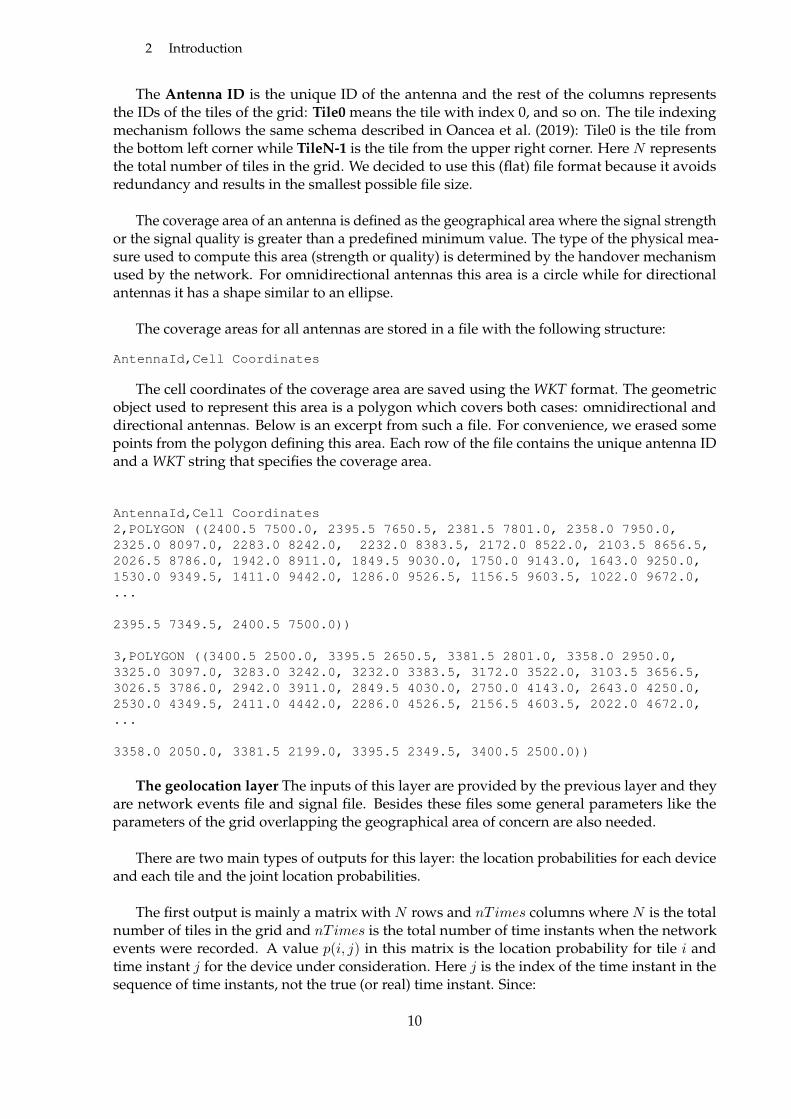
The Antenna ID is the unique ID of the antenna and the rest of the columns representsthe IDs of the tiles of the grid: Tile0 means the tile with index 0, and so on. The tile indexingmechanism follows the same schema described in Oancea et al. (2019): Tile0 is the tile fromthe bottom left corner while TileN-1 is the tile from the upper right corner. Here N representsthe total number of tiles in the grid. We decided to use this (flat) file format because it avoidsredundancy and results in the smallest possible file size.
The coverage area of an antenna is defined as the geographical area where the signal strengthor the signal quality is greater than a predefined minimum value. The type of the physical mea-sure used to compute this area (strength or quality) is determined by the handover mechanismused by the network. For omnidirectional antennas this area is a circle while for directionalantennas it has a shape similar to an ellipse.
The coverage areas for all antennas are stored in a file with the following structure:
AntennaId,Cell Coordinates
The cell coordinates of the coverage area are saved using the WKT format. The geometricobject used to represent this area is a polygon which covers both cases: omnidirectional anddirectional antennas. Below is an excerpt from such a file. For convenience, we erased somepoints from the polygon defining this area. Each row of the file contains the unique antenna IDand a WKT string that specifies the coverage area.
AntennaId,Cell Coordinates2,POLYGON ((2400.5 7500.0, 2395.5 7650.5, 2381.5 7801.0, 2358.0 7950.0,2325.0 8097.0, 2283.0 8242.0, 2232.0 8383.5, 2172.0 8522.0, 2103.5 8656.5,2026.5 8786.0, 1942.0 8911.0, 1849.5 9030.0, 1750.0 9143.0, 1643.0 9250.0,1530.0 9349.5, 1411.0 9442.0, 1286.0 9526.5, 1156.5 9603.5, 1022.0 9672.0,...
2395.5 7349.5, 2400.5 7500.0))
3,POLYGON ((3400.5 2500.0, 3395.5 2650.5, 3381.5 2801.0, 3358.0 2950.0,3325.0 3097.0, 3283.0 3242.0, 3232.0 3383.5, 3172.0 3522.0, 3103.5 3656.5,3026.5 3786.0, 2942.0 3911.0, 2849.5 4030.0, 2750.0 4143.0, 2643.0 4250.0,2530.0 4349.5, 2411.0 4442.0, 2286.0 4526.5, 2156.5 4603.5, 2022.0 4672.0,...
3358.0 2050.0, 3381.5 2199.0, 3395.5 2349.5, 3400.5 2500.0))
The geolocation layer The inputs of this layer are provided by the previous layer and theyare network events file and signal file. Besides these files some general parameters like theparameters of the grid overlapping the geographical area of concern are also needed.
There are two main types of outputs for this layer: the location probabilities for each deviceand each tile and the joint location probabilities.
The first output is mainly a matrix with N rows and nTimes columns where N is the totalnumber of tiles in the grid and nTimes is the total number of time instants when the networkevents were recorded. A value p(i, j) in this matrix is the location probability for tile i andtime instant j for the device under consideration. Here j is the index of the time instant in thesequence of time instants, not the true (or real) time instant. Since:
10

2.3 The interfaces between layers
we have a grid of such an extension that in a given time increment a device cannot reachmost of its cells, and
we have such a time and spatial resolution in the grid and the event information that adevice cannot reach most of the cells in a time increment
the matrices with location probabilities are sparse and the natural choice for storing thesematrices is to use one of the special file formats for sparse matrices. We used a format similarto the Coordinate Text File (see for example Boisvert et al. (1997) for a full description of thisfile format) to store these matrices where a row in the file contains a tuple (i, j, a[i, j]) giving thenumber of row, column, and a nonzero entry in the matrix. The single between our file formatcompared to Coordinate Text File format is that the first row specifying the total number of rows,columns and nonzeros in the matrix is missing because we already have these numbers fromother sources (for example, in case of using simulated data from the simulation configurationfil). Below we give the structure for the location probability file for a device.
tile, time, probL...
It has three columns:
tile - is the tile index (see the tile indexing system mentioned above) and it corresponds tothe row number in the matrix;
time - is the time instant for which the location probability is computed. Its index in thetime instants sequence corresponds to the column number in the matrix;
probL - is the value of the location probability. Only non-zero values are stored in this file
We mention that there is a separate file for each mobile device.The joint location probabilities files stores the probability of being in tile i at time instant
t− 1 and tile j at time instant t for all combinations of time consecutive time instants and tiles.We store again only the non-zero probabilities. The structure of this file is given below:
time_from, time_to, tile_from, tile_to , probL....
The columns in this file has the following meanings:
time from - is the initial time instant;
time to - is the final time instant;
tile from - is the initial tile;
tile to - is the destination tile;
probL - is the value of the location probability, i.e. the probability of a device to movefrom tile tile from to tile to during the time interval (time from , time to). Only non-zerovalues are stored.
We mention again that there is a separate file for each mobile device.
11

2 Introduction
The deduplication layer The inputs of this layer are the outputs of the previous layer, i.e.the two sets of files with the location probabilities and joint location probabilities for each device.Besides these two data sets, the deduplication layer also needs some files that come directlyfrom the data acquisition and preprocessing layer: the network events file and the antennas cellfile. Both files were already described in the beginning of this section. An additional input ofthis layer is an information from an external source that gives the apriori probability of a personto hold two mobile devices.
The output for the deduplication layer is a single csv file that contains the duplicity proba-bility for each device. It has two columns:
deviceID, dupP
Here deviceID is the unique Id of a device and dupP is the probability of the device to be ina 2-1 correspondence with its owner. There is one row for each device registered by the network.
The aggregation layer The inputs of this layer are:
the csv file with duplicity probabilities produced by the previous layer;
a csv file defining the geographical regions for which we want to compute the number ofindividuals detected by the network. We provide below an excerpt from such a file;
the general parameters defining the grid (number of rows and columns, the tile dimensionson OX and OY axes);
the sequence of time instants when the network events were recorded.
The file defining the geographical regions is a simple csv file where each region is definedas a collection of tiles. An example of such a file is given below:
tile,region1560,31561,31562,31563,31564,31565,31566,31567,31568,3....
We are aware that there is a certain degree of redundancy in this file, but the dimension ofsuch a file is relatively small and poses no difficulties in the process of processing it.
There are two outputs of this layer: the number of individuals in each region at each timeinstant and the number of individuals moving from one region to another. Both numbers arecomputed from a Poisson-multinomial distribution and since there is no analytical form of thePMF we generate a sequence of random numbers from this distribution which can be usedto compute a point estimation (mean, mode, median), as well as accuracy measures (credibleintervals, posterior variance).
The number of individuals for each time instant and region is saved in a csv file like in theexample below:
12

2.3 The interfaces between layers
time, region, N, iter0, 1, 10, 10, 1, 10, 20, 1, 10, 30, 1, 12, 40, 1, 13, 50, 1, 12, 6...
time represents the time instant, region is the region number and N is the number of in-dividuals. For each combination of time instant and region there are several random valuesgenerated for N and their index is given in iter column.
The number of individuals moving from a region to another is saved in a csv file with thestructure given in the following example:
time_from, time_to, region_from, region_to, Nnet, iter0, 10, 1, 1, 10, 10, 10, 2, 1, 0, 10, 10, 3, 1, 0, 10, 10, 4, 1, 1, 10, 10, 5, 1, 0, 10, 10, 6, 1, 0, 1...
The name of the columns are self-explanatory. For each distinct combination (time from,time to, region from, region to) there are several random values generated for the number ofindividuals and their index is given in iter column.
The inference layerThe inputs of this layer are:
the posterior location probabilities, one file per device (we already described the structureof these files);
a csv file with the duplicity probabilities for each device, which is the output of the(deduplication) layer (already described);
a csv file defining the geographical regions (already described);
a csv with file the general parameters defining the grid (already described);
a csv with information from a population register, giving the population count for allgeographical regions under consideration;
a csv with the penetration rate of the mobile network operator for all geographical regionsunder consideration;
a csv with the number of individuals for each time instant and region which is an outputfrom the aggregation package (already described);
a csv with the number of individuals moving from a region to another which is also anoutput from the aggregation package (already described).
The information from the population register is organized on two columns as showed below:
13

2 Introduction
region, N01, 382, 553, 654, 39...
Here, region is the region number and N0 is the population count in the correspondingregion.
The penetration rate file has a similar structure:
region, pntRate1, 0.36842112, 0.43, 0.41538464, 0.4615385...
The second column, pntRate, is the penetration rate obtained from the mobile network operator.
There are three main results of this package: the population count for each region computedat the initial time instant, the population count for each region and all time instants t > t0, andthe origin-destination matrices for all pairs of time instants. All these results are computed inthree versions: using the Beta Negative Binomial distribution, using the Negative Binomialdistribution and using the state process Negative Binomial distribution. Details about how thesedistributions are used to infer the target population are given by Oancea et al. (2019).
For the population at the initial time instant t0 the inference package generates two tables:one with a some descriptive statistics about the distribution another one with the random valuesgenerated for each region. The descriptive statistics of the population count distribution areshowed below:
region Mean Mode Median Min Max Q1 Q3 IQR SD CV CI_LOW CI_HIGH1 43 33 39 11 133 30 51 21 17.90 41.96 21.00 73.002 59 51 56 21 126 47 68 21 15.85 27.09 37.00 88.003 82 68 78 38 185 68 94 26 20.84 25.38 54.97 121.004 39 32 37 14 92 30 45 15 11.58 30.07 23.47 59.505 77 75 74 31 185 62 90 28 23.07 29.84 47.50 120.006 47 42 44 15 152 36 56 20 17.32 36.59 25.00 78.067 72 62 69 28 174 57 84 26 21.36 29.56 43.50 109.008 25 24 24 11 107 20 29 9 8.22 32.48 15.97 39.509 67 66 66 36 132 57 75 18 14.40 21.53 46.50 91.50
10 48 50 46 20 110 39 55 16 13.01 27.16 31.50 70.00
The random values generated according to the corresponding distribution are organized ina table with the following structure:
region N NPop1 11.0 53.01 9.0 35.01 13.0 56.01 12.0 46.01 12.0 33.01 12.5 65.5
...
14

2.3 The interfaces between layers
where region is the region number, N is the number of individuals detected by the networkand NPop is the target population count.
The output for the population count distribution at time instants t > t0 is organized as a listwith one element for each time instant t. An element for a time instant t is also a list with oneor two items, depending on a parameter passed to the function that perform the computations(see chapter 7 for details). The first item is a table with descriptive statistics and the second onecontains the random values generated according to the corresponding distribution. the structureof these tables are identical with the previous ones.
The third output, the origin-destination matrices for all pairs of time instants time from-time to is also a list with one element for each pair of time instants. An element for a pairtime from-time to is a list with one or two elements, as in the previous case. The first elementis a table with descriptive statistics for the origin-destination matrix with the structure as in theexample shown below:
region_from region_to Mean Mode Median Min Max Q1 Q3 IQR SD CV CI_LOW CI_HIGH1 1 34 29 33 9 93 26 41 15 11.62 33.81 19.00 54.001 2 0 0 0 0 6 0 0 0 0.84 391.64 0.00 2.211 3 0 0 0 0 0 0 0 0 0.00 NaN 0.00 0.001 4 0 0 0 0 7 0 0 0 0.69 485.36 0.00 0.001 5 0 0 0 0 0 0 0 0 0.00 NaN 0.00 0.001 6 0 0 0 0 0 0 0 0 0.00 NaN 0.00 0.001 7 0 0 0 0 0 0 0 0 0.00 NaN 0.00 0.001 8 0 0 0 0 0 0 0 0 0.00 NaN 0.00 0.001 9 0 0 0 0 0 0 0 0 0.00 NaN 0.00 0.001 10 0 0 0 0 0 0 0 0 0.00 NaN 0.00 0.002 1 1 0 0 0 11 0 0 0 1.44 211.19 0.00 3.552 2 68 73 67 28 133 58 77 19 14.67 21.47 47.60 93.002 3 1 0 0 0 12 0 3 3 2.06 150.07 0.00 5.462 4 0 0 0 0 2 0 0 0 0.15 1020.93 0.00 0.002 5 0 0 0 0 7 0 0 0 0.99 279.62 0.00 2.91
...
The second element of the list gives the random values generated for the population movingfrom one region to another and it looks like in the example below:
region_from region_to iter NPop1 1 1 401 2 1 01 3 1 01 4 1 01 5 1 01 6 1 0
...
NPop is the random value while iter represents the index of the corresponding randomvalue in the whole set.
We summarize in the following tables all the files produced by different layers in the stackand those provided from external sources. It is important to note that although the last 5 filesmentioned in table 2.2 are provided by our simulation software (the particle ”MNO1” was thegeneric name given to our hypothetical MNO), the information contained in these files can beprovided by a real MNO.
15

2 Introduction
Table 2.1: Files produced by the R packages
File name Output of: Input for: Short description
postLocDevice ID.dt.csv destim deduplication,inference
posterior location probabilities for a de-vice, for each tile and time instant
postLocJointProbDevice ID.dt.csv destim aggregation posterior joint location probabilities fora device, for each tile and time instant
duplicity.csv deduplication aggregation, infer-ence, aggregation
duplicity probability for each device
nnet.csv aggregation inference random values for number of individ-uals for each geographical region
nnetod.csv (.zip) aggregation inference random values for number of individ-uals moving from one geographical re-gion to another
Table 2.2: Files provided from external sources (simulation software, MNOs, NSOs)
File name Source Description
grid.csv NSO Defines the parameters of the grid overlapping thegeographical area considered
regions.csv NSO Defines the geographical regions as sets of tiles ofthe grid
pnt rate.csv MNOs, other national telecommunica-tion authorities
Defines the penetration rate of an MNO for each ge-ographical region
pop reg.csv NSO Gives the population count for each region, from apopulation register
AntennaCells MNO1.csv MNO Defines the mobile network cellsAntenaInfo MNO MNO1.csv MNO Gives the network events registered inside a geo-
graphical area, during a time periodSignalMeasure MNO1.csv MNO Gives the signal strength/quality emitted by each
antenna in the center of each tile of the gridantennas.xml MNO Contains technical parameters of each antennasimulation.xml NSO, MNO Gives some general parameters such as start time,
end time, time increment, etc.
16
3
The data acquisition and preprocessing layer
3.1. MNO data
Network events data ensure the operation of the network but as far as we know they areeither not currently stored in by any MNO or need some investment to be used for statisticalpurposes. So, the first step in implementing our methodological approach would be to designan acquisition system for the network events. Such a system is technology dependent (GSM,UMTS, LTE, . . . ) and can only be designed and put in place by the MNO itself. The networkevents are usually captured at the interfaces of the core network by means of installing networkprobes (Ostermayer et al., 2016). At least the following variables should be saved:
timestamp - the exact time instant when the event was captured;
deviceID - a unique identifier of the mobile device that generated the event (could be forexample IMEI);
antenna/cell ID - uniquely identifies the antenna (cell) the mobile device is currentlyconnected to;
event - a code for the captured event.
The network events data sets tend to be very large therefore it is likely that specific big datatechnologies such as a NoSQL database or the Hadoop Distributed File System should be usedto store these data (Lyko et al., 2016). There are technical solutions to interface such systemswith R to allow data processing: see for example the nodbi R package Chamberlain et al.(2019) that allows R to interact with MongoDB, Redis, CouchDB, Elasticsearch, SQLite ormore specialized packages such as mongolite Ooms (2014) package allowing an R-mongodbinterface, R4CouchDB Bock (2017) allowing R to access CouchDB, RCassandra provinding aninterfce between R and Apache Cassandra or rhdfs package that allows R to access files on aHDFS. An overview of the data acquisition process for network events can be found by Wanget al. (2017).
Once acquired, the network events should be depersonalised and preprocessed to be broughtin a usable form for our statistical needs. The term mobile network data for statistical purposesmakes reference to an abstraction which should be given a concrete substantiation within theextraordinarily complex data ecosystem associated to cellular telecommunication networks. AllMNOs tend to underline the resources needed to preprocess and prepare data for statisticalpurposes, therefore a clear win-win partnership should be put in place between NSIs and MNOs.
17

3 The data acquisition and preprocessing layer
Although there are technologies borrowed from the Privacy-Preserving Computation Tech-niques area like the Secure Multi Party Computation technique that could allow NSIs to processthe network events data remotely in a secure environment currently, we envisage that executionof almost all modules should be conducted by MNOs in their own premises.
3.2. Synthetic data
The use of synthetic data to develop the implementation of the processes and the validationof the methodology is not only a matter of the lack of real data. Synthetic data are essentialto check that every step of the process is executed as expected and to have the possibility tocompare the possible methods againts the reality. With the aim to build synthetic dataset it hasbeen crucial the usage of a simulator.
3.2.1. The simulation software
A simulator for network event data has already been developed as it is described in Oanceaet al. (2019). This tool has given the opportunity to deal with synthetic data that come fromscenarios with real characteristics. Figure 3.1 shows a schematic view of the data flow in theprocess of generating synthetic network events data.
Simulation software
persons.xml
antennas.xml
simulation.xml
probabilities.xml
Map.wkt
antennas.csv
persons.csv
Signal strength/quality
Antenna_cells.csv
Grid.csv
AntennInfo.csv
Figure 3.1: Data flow diagram
The simulation software takes as input a series of configuration files:
18

3.2 Synthetic data
a Map file - it is the map where the simulation take place. It is given as a WKT file thatcontains only the external boundary of the geographical area of concern;
a file with the general parameters of the synthetic population - named persons.xmlin Figure 3.1 which contains information like the number of persons in the syntheticpopulation, the age distribution, the share of males/females, the speed of the displacement,the share of the population starting from the same initial position in each simulation;
a file with the location and the technical parameters of the antennas needed to computethe signal strength or signal quality/dominance;
a file with parameters for the simulation process. This file define the general parametersof the simulation: the initial and the final time instant of the simulation as well as the timeincrement, information about the mobile network operators, the type of the displacementof persons, the type of the handover mechanism, the dimensions of a tile in the grid andthe name of some of the output files;
an optional file that provides information necessary to compute the location probabili-ties of the mobile devices. These probabilities were used only in the initial process ofdevelopment, now the destim package provides a more accurate estimation of them.
The software outputs the synthetic information generated during the simulation in csv files:
a grid file that contains the full description of the rectangular grid overlapped on the map,named grid.csv in Figure 3.1;
a file that stores the antennas location on the map at the initial time instant, namedantennas.csv in Figure 3.1;
a file that contains the exact position on the map and grid of each person, at each timeinstant of the simulation, named persons.csv in the same figure. The role of this file wasessential in the process of developing the methodological framework because it provides”the ground truth” allowing us to estimate the accuracy of our methods. Such informationis not available for real MNO data, therefore we emphasize again the importance of thesimulation software;
a file where the signal strength / quality is saved, depending on the handover mechanismused. The signal strength / quality is computed in the center of each tile of the grid namedSignalMeasure.csv;
a file that contains the coverage areas for each antenna, named AntennaCells_[MNOname].csvin Figure 3.1;
a file that contains the events generated by the interaction between mobile devices andantennas, together with the exact location of the mobile devices that generated the events,named AntennaInfo_MNO_[name].csv in Figure 3.1.
Some of these configuration and output files (simulation.xml, antennas.xml,AntennaInfo [MNOname].csv, AntennaCells [MNOname].csv, SignalMeasure.csv)are used by the R packages (see also table 2.2).
A full description of the simulation software was already provided by Oancea et al. (2019).The software is freely available in the form of the source code together with the makefile neces-sary to build the executable at the following address: https://github.com/MobilePhoneESSnetBigData/simulator. To facilitate the process of installing and running the program we also provide adocker image.
19

3 The data acquisition and preprocessing layer
3.2.2. Simulation scenarios
Name of the scenarios: scenario 1 2 3 4 5 6
1. number of antennas: total number of antennas in the net.
2. type connection: strength or quality.
3. tile size: in meters.
4. movement type: drift in case of random walk closed map drift or nodrift in case of ran-dom walk closed map.
5. number of persons: total number of persons in the population (with and without device).
6. speed car: in meter per second. Remember this is in mean speed, not the maximum speed.
At the time to build a good scenario there are some points to avoid:
Lack of signal: It can appear in two ways.
Useless Antennas. Many antennas are like deactivated because their signal is too lowthen there is no tile from which a device can be connected to them.
Tiles without coverage. There are some tiles inside the map where no signal is receivedfrom any antenna.
Excessive domination of one antenna. If some antenna is dominating a large part of the terri-tory, it causes problems in several steps. In the case of geolocation, in the area of coverageof this antenna the accuracy is much worse. In the case of duplicity detection, it causes anincrease in the rate of false positive. Since all devices connected to this antenna seems tobe mistakenly from the same individual.
Several scenarios have been built with the aim to study the behaviour of the developedmethodology. However, there is one scenario that has been used more deeply, scenario 1,explained below. After this scenario just a mention to other possibilities but without resultsshown in this document.
3.2.2.1. Scenario 1: scenario 70 strength 250 drift 500 16
This scenario has been built with the aim of correct the problems detected in scenario 0. Inthis case there are two types of zones but not so different. In the left upper corner there is asemi-urban area while in the right bottom corner there is a urban area.
Table 3.1: Main characteristics of the scenario 1
No. Antennas with signal 70No. Directional antennas 3Tile size (m) 250No. Tiles 1600No. Tiles without signal 0Tiles without signal inside the map no
The Figure 3.2 shows the signal strength (RSS) of each antenna in green with different in-tensity of the colour depending on the strength. Over that the coverage area of each antenna is
20

3.2 Synthetic data
70
69 6867
66
6564
63
62
61
60
59
58
57
56
55
54
53
52
51
5049
48
47
46
4544
43
42
41
40
39
38
37
36
35
34
33
32
31
30
29
28
27
2625
24
23
22
21
20
19
1817
1615
14
13
12
11
10090807
06
05
04
03
0201
0.00
0.25
0.50
0.75
1.00RSS
Figure 3.2: Antennas with signal and Tiles without signal
represented in yellow. All the antennas that give some signal to some tile are drawn in red withtheir corresponding label. The antennas without signal would be represented just with a dotpoint in black. Moreover, all the tiles without any signal from any antenna are marked with ablue dot point.
One can observe that there is no antennas deactivated and there is no tiles without coverageinside the map.
3.2.2.2. Scenario 2: scenario 20 strength 250 drift 500 16
This scenario will be built with the aim of analyse a territory with low density of antennas.Some different areas will be represented but paying attention to avoid the possible dominationof any antenna.
21

3 The data acquisition and preprocessing layer
Table 3.2: Main characteristics of the scenario 2
No. Antennas with signal 20No. Directional antennas 3Tile size (m) 250No. Tiles 1600No. Tiles without signal 0
3.2.2.3. Scenario 3: scenario 150 strength 250 drift 500 16
This scenario will be built with the aim of analyse a territory with high density of antennas.Some different areas will be represented but paying attention to avoid that some antennas areuseless due to lack of giving signal to any tile or to have the whole domination of anotherneighbour antenna.
Table 3.3: Main characteristics of the scenario 3
No. Antennas with signal 150No. Directional antennas 9Tile size (m) 250No. Tiles 1600No. Tiles without signal 0
22

4
The geolocation layer
4.1. Introduction
In this chapter, the estimation of the spatial distribution of the devices is shown by followingthe methodology explained by Salgado et al. (2020) and by using the implementation done inthe R package destim (Sanguiao et al., 2020). We illustrate the construction and adaptation of ahidden Markov model (HMM) to estimate the geolocation of a mobile device d in a referencegrid. In sections 4.2 and 4.3 we give some insights on each computational step, showing how touse destim functions step by step for each stage of the location probabilities computation andin section 4.4 we provide an end-to-end R script that starts from input data and produces thelocation probabilities.
First, some remarks about the notation of the basic elements in our model. Td(t) is a randomvariable that represents the reference grid tiles where the device d is located at time t. They arethe state (latent) variables in the HMM. The observed variables are the events in the networkdenoted as Ed(t) which are the identification of the antenna connecting to the mobile device d attime t. The target quantities will be the probability mass functions associated to each randomvariable Td(t) and the joint probability functions for two consecutive time instants t and t′. Anyauxiliary information will be denoted by Iaux.
Thus, in mathematical terms, we shall focus on:
γdti ≡ P (Tdi(t)|Ed, Iaux) = P (Td(t) = i|Ed, Iaux) (4.1a)γdtij ≡ P
(Tdi(t), Tdj(t
′)|Ed, Iaux) = P(Td(t) = i, Td(t
′) = j|Ed, Iaux) . (4.1b)
We convene in calling (4.1a) location probability for mobile device d to be in tile i at time tand calling (4.1b) joint location probability for mobile device d to be in tiles i and j in consecu-tive time instants t and t′.
The estimation of the target variables is done with the procedure explained in the followingstepwise procedure:
1. Model construction.
HMM initialization
Time discretization and reduction of parameters
Construction of the emission model
23

4 The geolocation layer
Construction of the transition model
2. Model fitting.
Computation of the likelihood
Parameter estimation (likelihood maximization)
Posterior location probabilities estimation
The initial probability distribution
4.2. Model construction
In this section, we show how to use the functions in the R package destim for the geolocationof mobile devices. We will use the simulation with 70 antennas, see the simulation scenariosdescription in chapter 3.
4.2.1. HMM initialization
The representation of the territory is done in the model by using a grid. Then, the first stepis to create a basic grid model. In our simulation scenario, we read the grid parameters from thesimulation specification file:
gridParam <- fread(’grid.csv’, sep = ’,’, header = TRUE, stringAsFactors=FALSE)ncol_grid <- gridParam[[’No Tiles Y’]]nrow_grid <- gridParam[[’No Tiles X’]]xDim_grid <- gridParam[[’X Tile Dim’]]yDim_grid <- gridParam[[’Y Tile Dim’]]
Then, we use the function HMMrectangle of the package destim to create a rectangle model.This model represents a rectangular grid with square tiles, where you can only stay in the sametile or go to a contiguous tile. This means that there are nine non zero transition probabilitiesby tile. Moreover, horizontal and vertical transitions have the same probability, and diagonaltransitions also have the same probability (but different to vertical and horizontal).
The number of transitions can be very high even for small rectangles. Let us suppose a smallrectangle of 10x10 tiles, it would have 784 transitions. Fortunatelly, we only need to fit two freeparameters as it is explained in the following. Note that the number of constraints plus thenumber of free parameters agrees with the number of transitions.
In the present example, with the simulation of 70 antennas, a rectangular grid model of40x40 tiles is created over the territory as follows:
c(nrow_grid, ncol_grid)#> [1] 40 40model <- HMMrectangle(nrow_grid, ncol_grid)
4.2.2. Time discretization and reduction of parameters
In practice, the package allows any linear constraint between the transition probabilities.There is also some support for non linear constraints.
24
4.2 Model construction
Thus, we can use constraints to reduce the number of parameters as much as wanted. Itis a good idea to keep small the number of (free) parameters: on one hand the likelihoodoptimization becomes less computationally expensive and on the other hand we get a moreparsimonious model.
Let us see how to use the time discretization to have a reduction of parameters. The idea isbased on the relation of the following three parameters, (i) the tile dimension l (we assume asquare grid for simplicity), (ii) the time increment ∆t between two consecutive instances, and(iii) an upper bound vmax for the velocity of the individuals in the population.
If we denote by NT the number of tiles, we are going to have not less than NT states, and formore complex models possibly more, so let us say we have O(NT ) states. In a hidden Markovmodel, this means that we have O(N2
T ) transition probabilities to estimate. Of course, this isnot viable, so we are going to fix all transition probabilities to non-contiguous tiles to 0. Withthis aim, we impose that in the time interval ∆t, the device d at most can displace from onetile to a contiguous tile. Under this condition, we can trivially set ∆t . l
vmax. For example, if
vmax = 150km/h ≈ 42ms−1, then ∆t . 10042 ≈ 2s.
In real data, this restriction may not be fulfilled, for example in case that in the dataset thedevice d is detected at longer time periods, e.g. once in a minute. Then we carry out time padding,i.e. the artificial introduction of some missing values between every two observed values.
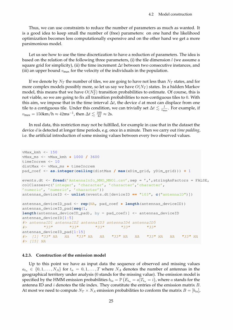
vMax_kmh <- 150vMax_ms <- vMax_kmh * 1000 / 3600timeIncrem <- 10distMax <- vMax_ms * timeIncrempad_coef <- as.integer(ceiling(distMax / max(xDim_grid, yDim_grid))) + 1
events.dt <- fread(’AntennaInfo_MNO_MNO1.csv’,sep = ’,’,stringAsFactors = FALSE,colClasses=c(’integer’, ’character’, ’character’,’character’,’numeric’, ’numeric’, ’character’))antennas_deviceID <- unlist(events.dt[deviceID == "103", c("antennaID")])
antennas_deviceID_pad <- rep(NA, pad_coef * length(antennas_deviceID))antennas_deviceID_pad[seq(1,length(antennas_deviceID_pad), by = pad_coef)] <- antennas_deviceIDantennas_deviceID[1:5]#> antennaID1 antennaID2 antennaID3 antennaID4 antennaID5#> "33" "33" "33" "33" "33"antennas_deviceID_pad[1:15]#> [1] "33" NA NA "33" NA NA "33" NA NA "33" NA NA "33" NA#> [15] NA
4.2.3. Construction of the emission model
Up to this point we have as input data the sequence of observed and missing valuesatn ∈ 0, 1, . . . , NA for tn = 0, 1, . . . , T where NA denotes the number of antennas in thegeographical territory under analysis (0 stands for the missing value). The emission model isspecified by the HMM emission probabilities bia = P
(Etn = a
∣∣Ttn = i), where a stands for the
antenna ID and i denotes the tile index. They constitute the entries of the emission matrix B.At most we need to compute NT ×NA emission probabilities to conform the matrix B = [bia],
25

4 The geolocation layer
i = 1, . . . , NT , a = 1, . . . , NA. This is done once and for all t (since we assume time homogeneity).Then, the computational cost of the emission probabilities is fixed in time.
Now, to compute bia we borrow the use of the simplified radio propagation model from thestatic analysis (see Tennekes et al., 2020) so that we can compute numerically these probabilities.Again, this is a modelling choice and several options could be possibly considered (see AppendixA of Salgado et al., 2020).
If missing values are to be used according to the preceding section, for numerical conve-nience later on the corresponding emission probabilities can be conveniently set to 1, i.e. bi0 =P(Etn = 0
∣∣Ttn = i)
= 1. This will greatly facilitate the expression of the HMM likelihood andits further optimization. Remind that this probability is not real and is completely meaningless.
Notice that having the numerical values of the emission probabilities will allow us to simplifythe computation of the likelihood for the HMMs reducing its parameter dependency only to thetransition model.
Returning to the code, the emission probabilities are also stored in a matrix. Of course, thenumber of actually observed events is expected to be much smaller than the number of possibleevents (all antennas in the network). It could happen, though, that the number of columns ofthe emissions matrix matches the number of actually observed events. This way we do not savememory with the matrix, but it allows us to do the estimations. Note that, in particular, if anypossible event corresponds to a column of the matrix of emissions, each row sums to 1. Thisdoes not happen in general, as the columns do not need to be exhaustive.
As we have not specified the emission probabilities in the HMM object created, they are setto NULL by default.
emissions(model)#> NULL
Emission probabilities are expected to be computed separately, so the model is ready todirectly insert the emissions matrix. We build the emission matrix based on the radio propaga-tion model of our choice. Let us see an example of how to build the matrix from a data.tablecontaining information about the radio propagation model.
RSS.dt <- fread(’SignalMeasure.csv’,sep = ’,’,header = TRUE, stringAsFactors = FALSE)RSS.dt#> antennaID tile RSS SDM RSS_ori SDM_ori nAntCover#> 1: 01 1560 -75.198 0.5989279 -75.198 5.989279e-01 1#> 2: 02 1560 NA NA -112.091 7.867742e-12 1#> 3: 03 1560 NA NA -109.399 3.228188e-12 1#> 4: 04 1560 NA NA -120.112 2.097113e-16 1#> 5: 05 1560 NA NA -117.471 2.504505e-14 1#> ---#> 111996: 66 39 NA NA -107.986 1.151466e-11 1#> 111997: 67 39 NA NA -105.883 7.642586e-11 1#> 111998: 68 39 NA NA -107.646 1.563671e-11 1#> 111999: 69 39 NA NA -115.541 1.283116e-14 1#> 112000: 70 39 NA NA -112.674 1.693854e-13 1
26

4.2 Model construction
#> rasterCell#> 1: 1#> 2: 1#> 3: 1#> 4: 1#> 5: 1#> ---#> 111996: 1600#> 111997: 1600#> 111998: 1600#> 111999: 1600#> 112000: 1600
This data.table named RSS.dt provides the following variables:
column antennaID: identification of the antenna for which we provide the radio propa-gation model information.column tile: identification of the tile for which we provide the radio propagation modelinformation.column RSS ori: signal strength (in dBm) from the corresponding antenna at the centerof the corresponding tile according to the RSS model.column RSS: same value as RSS ori when the strength is above the chosen threshold inthe specification files; NA otherwise.column SDM ori: signal dominance measure from the corresponding antenna at the centerof the corresponding tile according to the SDM model.column SDM: same value as SDM ori when the signal dominance measure is above thechosen threshold in the specification files; NA otherwise.column rasterCell: equivalent numbering of the tiles according to the package raster.
Then, the probabilities are obtained and the emission matrix is built as follows:
emissionProbs.dt <- RSS.dt[, watt := 10**((RSS - 30) / 10 )][
, eventLoc := watt / sum(watt, na.rm = TRUE), by = ’rasterCell’][is.na(eventLoc), eventLoc := 0][
, watt := NULL]emissionProbs.dt <- emissionProbs.dt[
, c("antennaID", "rasterCell", "eventLoc"), with = FALSE][order(antennaID, rasterCell)]
frmla <- paste0(c(’rasterCell’, ’antennaID’), collapse = ’ ˜ ’)emissionProbs.mat <- as.matrix(dcast(emissionProbs.dt, as.formula(frmla), value.var = ’eventLoc’)[
, rasterCell := NULL])
dimnames(emissionProbs.mat) <- list(as.character(unique(emissionProbs.dt[[’rasterCell’]])),as.character(unique(emissionProbs.dt[[’antennaID’]])))dim(emissionProbs.dt)#> [1] 112000 3emissionProbs.dt#> antennaID rasterCell eventLoc#> 1: 01 1 1#> 2: 01 2 1
27

4 The geolocation layer
#> 3: 01 3 1#> 4: 01 4 1#> 5: 01 5 1#> ---#> 111996: 70 1596 0#> 111997: 70 1597 0#> 111998: 70 1598 0#> 111999: 70 1599 0#> 112000: 70 1600 0
The number of rows arise from the number of different events (70 different antennas) andthe number of tiles (1600). The inclusion of missing values for the time padding is dealt withinternally during the fitting. The assignment to the model is immediate.
emissions(model) <- emissionProbs.mat
Of course, in practice, models will have many states and will be created automatically. Whilethe purpose of the package destim is estimation and not automatic modeling (at least for themoment), some functions have been added to ease the construction of example models.
A very simple function to create emissions matrices is also provided. It is called createEMand the observation events are just connections to a specific antenna. The input parameters arethe dimensions of the rectangle, the location of towers (in grid units) and the distance decayfunction of the signal strength (Tennekes et al., 2020). In this case, each tile is required to be ableto connect to at least one antenna, so no out-of-coverage tiles are allowed. Note that this is not arequirement for the model, just a limitation of the function createEM.
If the case were a network of 7 antennas, the creation of the emission matrix can be done asfollows:
tws <- matrix(c(3.2, 6.1, 2.2, 5.7, 5.9, 9.3, 5.4,4.0, 2.9, 8.6, 6.9, 6.2, 9.7, 1.3),nrow = 2, ncol = 7)S <- function(x) if (x > 5) return(0) else return(20*log(5/x))emissionProbs.mat2 <- createEM(c(nrow_grid, ncol_grid), tws, S)dim(emissionProbs.mat2)#> [1] 1600 7
4.2.4. Construction of the transition model
Now we specify a model for the transition between states (tiles in our simple rectangularmodel). Let A = [aij ] be the transition matrix, with aij = P
(Tjt∣∣Tit). In order to obtain the
elements of this matrix, we make use of our preceding imposition by which an individualcan at most reach a contiguous tile in each contiguous time. Then, to model these transitionsrectangular isotropic conditions are imposed. Let θ1 be the probability of vertical/horizontaltransition and θ2 the probability of diagonal transition, as represented in Figure˜4.1. Moreover,row-stochasticity conditions have to be fulfilled as well.
All these conditions lead to having a highly sparse transition matrix A with up to 4 termsequal to θ1 and θ2 (each) per row and diagonal entries guaranteeing row-stochasticity.
28

4.2 Model construction
1 2 3 4
5 6 7 8
9 10 11 12
13 14 15 16
Figure 4.1: Example with a regular square grid of dimensions 4× 4.
For a detailed explanation of the elements of the transition matrix (see Appendix A of Sal-gado et al., 2020).
Returning to the code, we can see that there are as many states as tiles (nrows*ncols) in thegrid and the corresponding transitions to all possible movements in the grid, consecutive tiles.
nstates(model)#> [1] 1600ntransitions(model)#> [1] 13924
The transitions with non zero probability are represented by an integer matrix with tworows, where each column is a transition. The first row is the initial state and the second the finalstate. Of course, the states are represented by an integer number. The columns of the matrix areordered first by initial state and then by final state.
transitions(model)[1:2, 1:10]#> [,1] [,2] [,3] [,4] [,5] [,6] [,7] [,8] [,9] [,10]#> [1,] 1 1 1 1 2 2 2 2 2 2#> [2,] 1 2 41 42 1 2 3 41 42 43
The constraints can be shown by using constraints(model). As we have not specifiedany constraints, one constraint by state is introduced, the sum of the transition probabilities fora given initial state has to be one (row-stochasticity of the transition matrix). Otherwise, thetransition matrix would not be stochastic. In general, the package adjusts this specific kind ofconstraints automatically.
The constraints are represented as the augmented matrix of a linear system of equations. Thetransition probabilities must fulfill the equations, with the same order as shown in transitionsfunction. So, the first coefficient in each row is for the transition probability of the transitionshown in the first row of the matrix of transitions, and so on.
Both transitions and constraints can be specified as parameters when creating the model. Itis also possible to add transitions and constraints later. Let us suposse that we add the followingtransitions:
model0 <- addtransition(model, c(1,22))model0 <- addtransition(model0, c(2,33))transitions(model0)[, 1:12]#> [,1] [,2] [,3] [,4] [,5] [,6] [,7] [,8] [,9] [,10] [,11] [,12]
29

4 The geolocation layer
#> [1,] 1 1 1 1 1 2 2 2 2 2 2 2#> [2,] 1 2 22 41 42 1 2 3 33 41 42 43
Now it becomes possible to transition from state 1 to state 22, and from state 2 to state 33.
Moreover, we can add constraints to the model. The constraints matrix is a row major sparsematrix. The function to add new constraints is addconstraint whose second argument canbe a vector or a matrix. If it is a vector, it is expected to be a set of transition probabilities indexedas in field transitions of the model. In this case the constraint added is the equality betweenthe referred probabilities of transition. The purpose of these equality constraints is to improveperformance as they might be a lot and can be treated easily.
If the second argument is a matrix, it is expected to be a system of additional linear equalitiesthat the model must fulfill. Thus, the new equations are added to the field constraints of themodel. While it is possible to use a matrix to add equality constraints, it is not recommendedbecause of performance. In any case, previous constraints of the model are preserved.
Now, an example of how an equality constraint is added. In this case the second transitionprobability is equal to the fourth one. In the matrix of transitions we can see that those transitionsrepresent: transition 2 is from state 1 to state 2 and transition 3 is from state 1 to state 22. Then,to add the equality constraint that relate these two transitions is done as follows:
dim(constraints(model0))#> [1] 13922 13927model0 <- addconstraint(model0, c(2, 3))dim(constraints(model0))#> [1] 13923 13927
Once the model is fitted, the values of the transition matrix can be obtained from the HMMobject in the element names as model$parameters$transitions. This is a vector with thevalues corresponding to each column of the matrix transitions(model).
4.3. Fitting the model
Once we have defined an appropriate model for our problem, the next step is to estimate thefree parameters. As it has been already stated, emissions are known, so there are no emissionparameters to fit. The initial state is either fixed or set to the steady state, thus the only parame-ters to fit in practice are the transition probabilities.
The method used to estimate the parameters is maximum likelihood, and the forwardalgorithm computes the (minus) log-likelihood. A constrained optimization is then done. Notethat the EM algorithm is generally not a good choice for constrained problems, so it is not usedin the package destim. Let us see in detail how the model is fitted.
4.3.1. Parameter estimation
The estimation of the unknown parameters θ = (θ1, θ2 is conducted maximizing the like-lihood. The restrictions coming from the transition model makes the optimization problemnot trivial. Notice that the EM algorithm is not useful. Instead, we provide a taylor-madesolution seeking for future generalizations with more realistic choices of transition probabilitiesincorporating land use information. Formally, the optimization problem is given by:
30

4.3 Fitting the model
max h(a)
s.t. C · a = b
a ∈ [0, 1]d,
, (4.2)
where a stands for the nonnull entries of the transition probability matrix A, the objective func-tion h(a) is derived from the likelihood L, see the following section for more detail, expressed interms of the nonnull entries of the transition matrix A, and the system C · a = b expresses thesets of restrictions from the transition model (see Appendix A of Salgado et al., 2020).
The number of restrictions nr not involving zeroes depends very sensitively on the particulartransition model chosen for the displacements. Then, we have that C ∈ Rnr×d and b ∈ Rd. Theobjective function h(a) is indeed a polynomial in the non-null entries a.
This problem can be further simplified using the QR matrix decomposition. Write C = Q ·R,where Q is an orthogonal matrix of dimensions nr × nr and R is an upper triangular matrix ofdimensions nr × d. Then we can rewrite the linear system as R · a = QT · b and we can linearlysolve variables a1, . . . , anr in terms of variables anr+1, . . . , ad:(
a1 · · · anr)T
= Cnr×(d−nr)(anr+1 · · · ad
)T.
The system (4.2) then reduces to
max h(anr+1, . . . , ad)
s.t. 0 ≤ C ·(anr+1 · · · ad
)T ≤ 1.(4.3)
The solution a∗ to problem (4.2) will be introduced in the transition probability matrix, whichwill thus be denoted by A∗.
In terms of optimization, all we have to do is a linear constrained non-linear optimization inthe same space. The linear constraints may seem to be a lot, but in practice, a good modelingwill make most of the constraints equal, as most of the transition probabilities are going to beequal.
Usually, algorithms for constrained optimization will require an initial value in the interiorof the feasible region. To get such initial value, the following algorithm is used:
1. Set transition probabilities to independent uniform (0, 1) random variables.2. Now the constraints do not hold, so the closest point in the constrained space is got
through Lagrange multipliers.3. Now some of the probabilities might be greater than one or smaller than zero. Those are
set once again to independent uniforms.4. Repeat steps 2 and 3 till all transition probabilities are between zero and one.
As already stated, the initial state is set to steady if not fixed. The steady state is calculatedas the (normalized to sum up one) solution to (A− I)x = 0, where I the identity and the lastcomponent of x is set to one divided by its dimension. This should be enough because theseMarkov chains are expected to be both irreducible and aperiodic, otherwise we would havestrange movement restrictions.
31

4 The geolocation layer
Returning to the code, the next step is to estimate the parameters of the model, by constrainedmaximum likelihood. But first, as already said, the optimizer usually requires an initial guess,so the function initparams obtains an initial random set of parameters.
model <- initparams(model)all(model$parameters$transitions < 1)#> [1] TRUEall(model$parameters$transitions > 0)#> [1] TRUErange(constraints(model) %*% c(model$parameters$transitions, -1))#> [1] 0.000000e+00 4.440892e-16
All transition probabilities are between zero and one and the constraints hold, but no ob-served data is still used.
The function minparams reduces the number of parameters of the model to the number offree parameters, as already explained. In the present example, the model has 13924 transitionsbut the number of parameters is two.
model <- minparams(model)rparams(model)#> [1] 0.33528506 0.06178254
Notice that it does not matter the size of the problem, only two parameters are really needed.It is possible to assign values with rparams, as the optimizer does, but some transition prob-ability might move outside the interval [0, 1]. The optimization process avoids this problemconstraining by linear inequalities.
Now the model is ready to be fitted. Of course, the observed events are needed. Since wehave the emissions matrix in the model, the observed events is just an integer vector, that refersto the appropriate column of the emissions matrix. The length of that vector is the number ofobserved times in a device. It is possible to introduce missing values for the observations as NA,obviously when at a time there is no event.
obs <- sapply(antennas_deviceID_pad,function(x) ifelse(!is.na(x),which (x == colnames(emissionProbs.mat)), NA))model_dev <- fit(model, obs)#> Loading required package: Rsolnprparams(model_dev)#> [1] 0.9910131 0.9820262
4.3.2. Computation of the likelihood
The likelihood is trivially computed using the numerical proviso of setting emission probabil-ities equal to 1 when there is a missing value in the observed variables. The general expression
32

4.3 Fitting the model
for the likelihood is
L(E) =
NT∑i0=1
· · ·NT∑iT=1
P (Tt0 = i0)
N∏n=1
P(Ttn = in|Ttn−1 = in−1
)P(Etn∣∣Ttn = in
)(4.4a)
=
NT∑i0=1
· · ·NT∑iT=1
P (Tt0 = i0)
N∏n=1
ain−1in(θ)binatn (4.4b)
Notice that the emission probabilities only contribute numerically providing no parameterwhatsoever to be estimated.
Returning to the code, the function to compute the likelihood for a model and a vectorof given observations of events is logLik. Despite the name, logLik returns minus the log-likelihood, so the smaller the better.
logLik(model, obs)#> [1] 26.29721logLik(model_dev, obs)#> [1] 11.57194
4.3.3. Posterior location probabilities estimation
Once the HMM has been fitted, we can readily apply the well-known forward-backward al-gorithm (Bishop, 2006) to compute the target probabilities γdti and γdtij (see equations (4.1)). Nonovel methodological content is introduced at this point. For our implementation, as suggestedby Bishop (2006), we have used the scaled version of the algorithm.
We can estimate the smooth states by means of the forward-backward algorithm. The smoothstates are the mass probability function of the states given the observed data (and the model),thus they summarize all the information available for a given time t. So one of the outputs of thepackage are the smooth states, that can be aggregated to get a space distribution of the numberof devices as explained in (section 4.2 of Salgado et al., 2020).
The other main output of the package is the posterior joint mass probability function fortwo consecutive instants t, t+ ∆t of the states. As it is a posterior probability, it is once againconditioned on all the information available, but it is more dynamic because its time reference isnow an interval. A possible analogy would be the smooth positions and speeds of a particle.The former would correspond to position and the later to speed.
These target probabilities are the main output of the geolocation estimation. Both outputsare needed to estimate the target population in next steps of the process as it is shown in thefollowing sections of this document.
Returning to the code, the function sstates returns the smooth states, i.e. the estimation ofthe posterior location probabilities. The output is given as a matrix of number of states × numberof observations (missing values included) dimensions, i.e. number of raster cells × times. So eachcolumn represents the space distribution in its corresponding time slot.
33

4 The geolocation layer
postLocP <- sstates(model_dev, obs)
dim(postLocP)#> [1] 1600 270
image(matrix(postLocP[, 4], ncol = ncol_grid))
The function scpstates returns the (smooth) joint probability mass function for consecutivestates, analogous to the usually denoted ξij probabilities in the Baum-Welch algorithm (onceconvergence is achieved). The result is a matrix with the raster cells in the rows and the rastercells per time in the columns. Then, each set of columns corresponding to the same timerepresents a space bi-variant distribution matrix. The probability of the consecutive pair of states(i, j) from time t to t+ ∆t can be found in the row i and column (t− 1) ∗NT + j. The transitionmatrix only allows transitions to contiguous points, so it is almost diagonal per blocks of times.
postJointLocP <- scpstates(model, obs)dim(postJointLocP)#> [1] 1600 430400
It is difficult to visualize these probabilities in two dimensions.
0.0 0.2 0.4 0.6 0.8 1.0
0.0
0.2
0.4
0.6
0.8
1.0
4.3.4. The initial probability distribution
The initial probability distribution P (Tt0) has not been specified yet. With abundance of data,it has very little incidence on the final results. In our implementation two options are provided:(i) the stationary state, i.e. the eigenvector of A with eigenvalue 1 and (ii) any distributionprovided by the user. The difference will be ultimately in terms of computational cost (provided
34

4.4 An end to end example
we have abundance of data).
Returning to the code, let us see in the present example how to fit the model with two differ-ent initial probability distribution: the default uniform distribution and the so-called networkdistribution (see Tennekes et al., 2020). The uniform is equivalent to the previous executionsand the network is obtained by using the information in the network about the signal strengthof the antennas.
First, we prepare the initial distribution vectors.
nTiles <- ncol_grid * nrow_gridinitialDistr_RSS_uniform.vec <- rep(1 / nTiles, nTiles)
initialDistr_RSS_network.dt <- RSS.dt[, watt := 10**( (RSS - 30) / 10 )][
, total := sum(watt, na.rm = TRUE)][, list(num = sum(watt, na.rm = TRUE), total = unique(total)),
by = ’rasterCell’][, prior_network := num / total][
order(rasterCell)]initialDistr_RSS_network.vec <- initialDistr_RSS_network.dt$prior_network
Then, we create both models and assign the corresponding initial distributions.
model_network <- modelmodel_uniform <- model
istates(model_network) <- initialDistr_RSS_network.vecistates(model_uniform) <- initialDistr_RSS_uniform.vec
4.4. An end to end example
We provide below an integrated script that exemplifies how to use this package to pro-duce the location probabilities starting from the input data. To keep the size of the scriptreasonable small we’ve made some simplifying assumptions: we considered that the emis-sion probabilities are computed using the signal strength and we used uniform prior locationprobabilities. There are also two functions that we used but we didn’t provide here their code:tileEquivalence() and transform postLoc(). The first function builds a table of equiv-alence between the numbering system used by the simulation software for tiles and the one usedby the raster package. The second one mainly transforms the dense format of the matricesstoring the location probabilities and joint location probabilities into the sparse matrix formatalready described in chapter 2. The input data used by this script are provided by the simulationsoftware. We use the same file names as described in table 2.2.
library(data.table)library(tidyr)library(destim)library(stringr)library(Matrix)library(xml2)
source(’transform_postLoc.R’)
35

4 The geolocation layer
source(’tileEquivalence.R’)
# set file namesfileGridName <- ’grid.csv’fileEventsInfoName <- ’AntennaInfo_MNO_MNO1.csv’signalFileName <- ’SignalMeasure_MNO1.csv’simulationFileName <- ’simulation.xml’
# read simulation paramssimulation.xml <- as_list(read_xml(simulationFileName))simulation.xml <- simulation.xml$simulationstart_time <- as.numeric(simulation.xml$start_time)end_time <- as.numeric(simulation.xml$end_time)time_increment <- as.numeric(simulation.xml$time_increment)times <-
seq(from = start_time,to = (end_time - time_increment),by = time_increment)
sigMin <- as.numeric(simulation.xml$conn_threshold)
# read grid paramsgridParam <- fread( ’grid.csv’, sep = ’,’, header = TRUE,
stringsAsFactors = FALSE)ncol_grid <- gridParam[[’No Tiles Y’]]nrow_grid <- gridParam[[’No Tiles X’]]tile_sizeX <- gridParam[[’X Tile Dim’]]tile_sizeY <- gridParam[[’Y Tile Dim’]]ntiles <- ncol_grid * nrow_grid
# tile-rasterCell equivalencetileEquiv.dt <- data.table(tileEquivalence(ncol_grid, nrow_grid))
# read Received Signal Strength file and compute emission probabilitiesRSS <-
fread(signalFileName, sep = ",", header = TRUE, stringsAsFactors = FALSE )setnames(RSS, c(’antennaID’, 0:(ntiles - 1)))RSS <- melt(RSS,id.vars = ’antennaID’,variable.name = ’tile’,
variable.factor = FALSE,value.name = ’RSS’)RSS[, RSS := ifelse(RSS < sigMin, NA, RSS)]
# compute event location (emission probabilities)RSS <-
RSS[, eventLoc := 10 ** RSS / sum(10 ** RSS, na.rm = TRUE), by = ’tile’]RSS <- RSS[is.na(eventLoc), eventLoc := 0]RSS[, tile := as.numeric(tile)]RSS <- RSS[tileEquiv.dt, on = ’tile’][, tile := NULL]RSS <-
dcast(RSS, rasterCell ˜ antennaID, value.var = ’eventLoc’)[, rasterCell :=NULL]
emissionProbs <- Matrix(data = as.matrix(RSS))dimnames(emissionProbs)[[1]] <-as.character(1:dim(emissionProbs)[1])
# read and process network event dataallEvents.dt <- fread( fileEventsInfoName,sep = ’,’,stringsAsFactors = FALSE,
colClasses = c(’integer’,’character’,’character’,’character’,’numeric’,’numeric’,’character’))
36

4.4 An end to end example
allEvents.dt <- allEvents.dt[!duplicated(allEvents.dt)]setnames(allEvents.dt ,c(’time’, ’antennaID’, ’eventCode’, ’device’, ’x’, ’y’, ’tile’))allEvents.dt[, obsVar := do.call(paste, c(.SD, sep = "-")),
.SDcols = c(’antennaID’, ’eventCode’)]events.dt <- allEvents.dt[eventCode %in% c(’0’, ’2’, ’3’)]events.dt_noDup <- copy(events.dt)[, list(eventCode =
as.character(min(as.numeric(eventCode)))),by = c("time", "device")]
events.dt <- merge(events.dt_noDup, events.dt,by = names(events.dt_noDup),all.x = TRUE)
events.dt <- events.dt[!duplicated(events.dt, by =c("time", "device", "eventCode"))][,.(time, device, eventCode, antennaID, obsVar)][order(time)]
# Set maximum velocity (from an external source)vMax_ms <- 16# Set time padding paramsdistMax <- vMax_ms * time_incrementpad_coef <- as.integer(ceiling(distMax / max(tile_sizeX, tile_sizeY)))pad_coef <- pad_coef + 1
# Initial state distribution (PRIOR)
# Prepare prior_network distribution (uniform prior)prior_network <- rep(1 / ntiles, ntiles)
# Initialize HMMmodel <- HMMrectangle(nrow_grid, ncol_grid)emissions(model) <- emissionProbs
model <- initparams(model) # initialize transition probmodel <- minparams(model) # parameter reduction according to restrictionsistates(model) <- prior_network
# compute posterior location probabilitiesdeviceIDs <- sort(unique(events.dt$device))
# for each devicefor (i in seq(along = deviceIDs))
devID <- deviceIDs[i]cat(paste0(’ device ’, devID,’...\n’))cat(’ Selecting network events...’)events_device.dt <- events.dt[device == devID, .(device, time, antennaID)]
[order(device, time)]
antennas_deviceID <- unlist(events_device.dt[, c("antennaID")])if (!all(is.na(antennas_deviceID))) # Fit and compute HMM modelobservedValues_pad <- rep(NA, pad_coef * length(antennas_deviceID))observedValues_pad[seq(1, length(observedValues_pad), by = pad_coef)] <-
antennas_deviceIDcolEvents <- sapply(observedValues_pad,function(x) ifelse(!is.na(x),
which(x == colnames(emissionProbs)), NA))
# Fit HMM - ML estimation of transition probabilities
37

4 The geolocation layer
fitTry <- try(model_devID <- fit(model, colEvents, init = TRUE))if (inherits(fitTry, "try-error")) stop("Fit model fails")
ssTry <- try(A <- sstates(model_devID, colEvents))if (inherits(ssTry, "try-error"))
stop("[compute_HMM] Smooth States fails")B <- scpstates(model_devID, colEvents)
# Transform output of the HMM model to sparse matrix file formattransform_output <- transform_postLoc(
postLocP = A, postLocJointP = B,observedValues = antennas_deviceID,times = times,t_increment = time_increment,ntiles = ntiles,pad_coef = pad_coef,tileEquiv.dt = tileEquiv.dt,devID = devID,sparse_postLocP = TRUE,sparse_postLocJointP = TRUE)
rm(A, B)gc()fwrite(transform_output$postLocProb[, .(tile , time, postLocProb)],
paste0(’postLocProb_’, devID,’.csv’),col.names = FALSE,row.names = FALSE,sep = ’,’)
transform_output$postLocJointProb[, time_to :=time_from + time_increment]fwrite(transform_output$postLocJointProb[, .(time_from, time_to,
tile_from, tile_to, postLocProb)],paste0(’postLocJointProb_’, devID,’.csv’), col.names =FALSE,row.names = FALSE,sep = ’,’)
4.5. Some remarks about computational efficiency
The package has some degree of optimization, as it uses Rcpp and RcppEigen (for sparselinear algebra) in some critical functions and the difference in execution speed between C++code and pure R code is well-known. We choose to use C++ for some computational intensiveoperations (based on level 3 BLAS operations) like LU factorizations or QR decompositions.For other packages in our hierarchy that also work with (sparse) matrices use the Matrix Rpackage because they only perform simple manipulations of rows or columns of these matriceswhich run fast enough.
It can handle fairly well models with around 107 states in a desktop computer (if enoughRAM is provided). Some faster sparse linear algebra library (for example Intel MKL) mightimprove a little bit the performance of such operations. Also, we are going to comment thepossibility of improve the performance using parallel computing.
4.5.1. Model construction
As has been already stated, the package is not really ready for model construction, exceptfor the function HMMrectangle, which are very basic models. While it is a rather fast function,its performance can be easily improved as it is an embarrassingly parallel algorithm. This alsoallows to use a cluster to generate the model.
38

4.5 Some remarks about computational efficiency
4.5.2. Model initialization and parametrization
The algorithm used to find an initial value for the optimizer, solves a linear system of equa-tions at each step. While the order of the system grows with the number of transitions andconstraints, in practice, most constraints state the equality between two transition probabilities.It is not difficult to get rid of one of the transitions and the constraint in those cases, so in practicethe process scales very well for parsimonious models.
Mostly all said for initialization also goes for parametrization, where the QR decompositionis the slow step.
4.5.3. Forward-Backward algorithm
This amounts mostly to multiplying sparse matrices, which relies on another library (cur-rently Eigen). Eigen is not the faster library at this moment even on a desktop computer but theperformance is not so bad. In the future Intel MKL might be a good choice, and it can also workin distributed mode.
4.5.4. Likelihood optimization
The purpose of all the previous steps is to make easier the task of the optimizer, so it shouldnot be a problem if everything else is fine. Transition probabilities are required to be betweenzero and one, what in general means O(n) inequality constraints. A well specified parsimoniousmodel, will often have a lot less constraints, as most of them are duplicated. As a reference, anHMMrectangle(20,20) has 3364 transitions and only 5 constraints are needed in practice.
Equalities between transition probabilities would generate duplicated rows in the matrix ofinequality constraints which are eliminated before calling the optimizer.
4.5.5. Optimization algorithm
Before fitting the model there is another possibility to make faster the computation. There isa parameter in the function fit, named init which is logical with FALSE as default. In thiscase, there is an assignment of the steady state in each evaluation of the optimization. If weassign the steady state to the initial state of the model with the function inisteady, and usethe argument init = TRUE in the fit of the model, there is just one assignment, so it is faster.The code is as simple as follows.
model_network <- initsteady(model_network)model_uniform <- initsteady(model_uniform)
model_devID <- fit(model_network, obs, init = TRUE)model_devID <- fit(model_uniform, obs, init = TRUE)
The optimization algorithm to be used is set in the function fit with the argument method,which is set by default to solnp from package Rsolnp. The other possible choice is constrOptimfrom package stats.
In order to avoid giving a local minimum as solution, there is another parameter that allowsthe user to execute the optimization several times. The optimizer will be launched with differentinitial parameters as many times as the number in the argument retrain. The model withhigher likelihood will be returned.
39


5
The deduplication layer
5.1. Introduction
In this chapter, it is shown how to deal with the duplicity problem about the unknownfraction of mobile subscribers carrying more than one device. It also contains a brief explanationabout the intended use of the R package deduplication (Oancea et al., 2020b) and providesa short introduction to the underlaying methodology. The goal will be to compute a device-multiplicity probability p(n)
d for each mobile device d, i.e. the probability that a device d is carriedby an individual carrying n devices. A detailed description of the methodological approachimplemented by this package is provided by Salgado et al. (2020) and Salgado et al. (2020). Tofully understand the theory behind this package it is recommended to read the above mentionedpapers.
We start by first presenting a brief theoretical introduction of the methods used to computethe duplicity probabilities (subsections )5.1.1, 5.1.2 and 5.1.3) and then we provide exampleson how to use deduplication package, step by step, in section 5.2. We also provide anexample that shows the easiest way of using this package, mainly by one single function call(computeDuplicity()) in subsection 5.3.1. All the examples provided here use some inputfiles that come from the destim package (the location probabilities for mobile devices) andfrom the simulation software (files with the networks events, the signal strength for each tile,the boundary of each cell, the grid paramaters, general simulation parameters). These files areprovided with the deduplication package but they can be replaced by users with their ownfiles. The name of the files coming from the simulation software are the same as those alreadypresented in table 2.2.
5.1.1. Device duplicity problem
The problem of device multiplicity comes from the fact that the statistical unit of analysiswith mobile network data is the individual of a target population, not a mobile device. Sincean individual can carry more than one device with him/her, this introduces the problem ofmultiple counting. For simplicity we make the simplifying assumption that each individual cancarry at most 2 devices.
The main purpose is to classify each device d in a dataset as corresponding to an individualwith only one device (1:1 correspondence between devices and individuals) or as correspondingto an individual with two devices (2:1 correspondence between devices and individuals). Thisclassification will be probabilistic, thus assigning a probability p(n)
d of duplicity to each device dcarrying n = 1, 2 devices. The generalization to more devices is just a matter of computational
41

5 The deduplication layer
complexity of this same approach.
Three methodological approaches have been developed and implemented in the deduplicationpackage, two approaches based on network events and another based on the distance betweencenters of location probabilities which compares trajectories. Let see a brief explanation beforeusing the code.
5.1.2. Bayesian approaches based on network events
5.1.2.1. The one-to-one approach
We shall follow a Bayesian hypothesis testing approach. In this case, for each device d weshall consider the disjoint set of hypotheses Hdd′d′=1,...,D meaning that the devices d and d′
are carried by the same individual. When d = d′ this reduces to mobile device d being the onlymobile device carried by its corresponding individual. We focus on computing
p(1)d = P
(Hdd
∣∣Ed1:T , Iaux) , (5.1)
where we are using the same notation as in chapter 4. Since the entire event set Ωd for device dcan be decomposed as Ωd =
⋃Dd′=1Hdd′ , we can make use of Bayes’ theorem to write:
p(1)d = 1− 1
1 +∑
d′ 6=d αdd′ · exp (`dd′ − `d)
where `d is the log-likelihood for a single device d and `dd′ for two devices d and d′ andαdd′ = 1−P1
P1, P1 is the a priori probability of 1:1 correspondence for all devices.
The log-likelihood `d for a single device d corresponds to the HMM model shown in thegeolocation chapter. The log-likelihood `dd′ for two devices d and d′ is computed according tothe HMM duplicity model represented where the emission probabilities are computed as theproduct of the original single-device emission probabilities for d and d′.
For the specification of priors the key is the available auxiliary information Iaux. For example,if some auxiliary information at the device level is available (for instance from the CustomerRelationship Management database) showing that devices d and any other d′ reside in far awaylocations, then naturally P (Hdd′ |Iaux) ≈ 0 so that p(1)
d ≈ 1, as expected.
If we denote λ(1)d = P(Ddd|Iaux)
1−P(Ddd|Iaux) the prior odds ratio which gives how much more probableis that an individual carries a priori only one device d than another device together with d,considering that apriori any other device d′ can be the second device so that P (Ddd′ |Iaux) isconstant for any other device d′ and P (Ddd|Iaux) + (ND − 1) ∗ P (Ddd′ |Iaux) = 1, where ND is thetotal number of devices, we arrive at the following formula for the probability of duplicity:
p(1)d = 1− 1
1 + exp(−`d)λd×(ND−1)
∑d′ 6=d exp (`dd′)
.
Thus, depending on the available information, if there is information at the device level thatcan be used to evaluate λd, the latter formula can be used to compute the duplicity probability,otherwise, the former formula with a single value of α for all devices is used. More detailedabout this approach is provided by Salgado et al. (2020).
42

5.1 Introduction
5.1.2.2. The pair approach
This approach is explained in detail in Salgado et al. (2020). Here there are some notes tounderstand what is computing. Denoting by Ddd′ the event which has the meaning “devices dand d′ are carried by the same individual” and by Dc
dd′ the event with the meaning “devices dand d′ are not carried by the same individual” the duplicity probability for device d is the pairduplicity probability pdd′ ≡ P(Ddd′ |E, Iaux) corresponding to device d′ more similar to d and wecan write p(2)
d = maxd′ 6=d P (Ddd′ |E, Iaux). Obviously, pdd′ = 0 for all d = d′.
We compute the pair-duplicity probabilities pdd′ for two devices d and d′ using the Bayestheorem:
P (Dcdd′ |E, Iaux) =
P(E|Dc
dd′ , Iaux)P (Dc
dd′ |Iaux)P (E|Ddd′ , Iaux)P (Ddd′ |Iaux) + P
(E|Dc
dd′Iaux)P(Dcdd′ |Iaux
) =1
1 +P(Ddd′ |Iaux)
P(Dcdd′ |I
aux)× P(E|Ddd′ ,Iaux)
P(E|Dcdd′ ,I
aux)
Here P (Ddd′ |Iaux) and P(Dcdd′ |Iaux) are the prior probabilities for the duplicity and non-
duplicity events and P (E|Ddd′ , Iaux) and P
(E|Dc
dd′ , Iaux) stands for the likelihoods under each
hypothesis Ddd′ and Dcdd′ , respectively.
After some mathematical manipulations we arrive at the following formula:
p(2)d = max
d 6=d′
(1
(1 + α ∗ exp (`dd′ − `d − `d′))
),
where α = P2P1
, P1 is the a priori probability of duplicity for a device and P2 = 1− P1.
5.1.3. The trajectory approach
This approach also follows a Bayesian philosophy, but instead of using network eventvariables E we will use properties of the trajectories derived from the HMMs, i.e. the locationprobability distributions γdt of all devices d.
Applying the Bayes theorem again we have:
P (Dcdd′ |X, Iaux) =
1
1 +P(Ddd′ |Iaux)
P(Dcdd′ |I
aux)× P(X|Ddd′ ,Iaux)
P(X|Dcdd′ ,I
aux)
,
where X is a variable related to the estimated trajectories in terms of posterior location probabil-ities.
To apply this idea we compute the probability distribution of the signed distance be-tween the x- and y-axis position of each pair of devices (we denote these random variables by∆x,dd′t = Xdt − Xd′t and ∆y,dd′t = Ydt − Yd′t) and count how many times the mode of thesedistributions are less than a predefined quantity (ξ ×max (rdt, rd′t). If a device d corresponds toan individual with two devices (2:1), there will be another device d′ such that their distance willbe significatively close to 0 along their trajectories.
We define:
pmodedd′ ≡ P (X|Ddd′ , I
aux) =#t = 1, . . . , T : |δ∗xt| ≤ ξ ·maxrddt, rdd′t, |δ∗yt| ≤ ξ ·maxrddt, rdd′t
T,
(5.2)
43

5 The deduplication layer
where δ∗xt and δ∗yt are the mode of the ∆x,dd′t and ∆y,dd′t variables. The duplicity probability willbe given by:
p(2)d = max
d6=d′
1− 1
1 + α× pmodedd′
1−pmodedd′
where α = P1
1−P1, P1 being the a priori probability of duplicity.
5.2. Syntax step by step
This section explains briefly the main functions of the package and how to use each methodof computing the duplicity probability implemented in the deduplication package. In all theexamples below we will use the data set included in this package. This data set was generatedusing the simulation software. The first step will be to set the path to the data:
library(deduplication)path_root <- ’extdata’
Then, some information which is needed whatever the duplicity method is computed. Readthe information about the territory, data from the simulation: general parameters, antennasinformation and events. Let us see the input parameters:
gridParams <-readGridParams(system.file(path_root, ’grid.csv’,package = ’deduplication’))
gridParams is a list that contains the number of rows and columns of the grid and the tiledimensions along OX and OY axes.
Since we will work with simulated data in our example, we need some parameters that wereused to generate the data set: the probability of a person to have two mobile devices (neededfor the a priori duplicity probability) and the minimum value of the signal strength/quality toallow a connection between a mobile device and an antenna. These two values are read fromthe simulation.xml file:
simParams <-readSimulationParams(system.file(path_root, ’simulation.xml’,package = ’deduplication’))
We also need to read the network events:
events <- readEvents(system.file(path_root, ’AntennaInfo_MNO_MNO1.csv’,package = ’deduplication’))
From the events table we can easily build a list of devices present in the current data setand a table with the antenna IDs where these devices are connected for every time instant:
devices <- getDeviceIDs(events)connections <- getConnections(events)
44

5.2 Syntax step by step
devices is a (sorted) list of the IDs of all devices detected by the network and connectionsis a matrix with each row corresponding to a device and the elements on the columns corre-sponding to the IDs of the antenna where the device is connected at a every time instant.
The next step will be the computation of the emission probabilities for the individual HMMmodels (for each device) and for the joint models (for pairs of devices). Since the emissionprobabilities are computed for each tile in the grid we need the number of rows and columns ofthe grid and also the file with the signal strength/quality. We also need the minimum value ofthe signal strength/quality that allows a connection between a mobile device and an antennaand we will use it to set to 0 the signal strength/quality for each tile where the actual value isbelow this threshold.
sgFileName <- system.file(path_root, ’SignalMeasure_MNO1.csv’,package = ’deduplication’)
emissionProbs <- getEmissionProbs(nrows = gridParams$nrow,ncols = gridParams$ncol,signalFileName = sgFileName,sigMin = simParams$conn_threshold)
jointEmissionProbs <- getEmissionProbsJointModel(emissionProbs)
Using the emission probablities we can build the generic HMM model (for each individualdevice) and the joint HMM model (for pairs of devices):
model <- getGenericModel(nrows = gridParams$nrow,ncols = gridParams$ncol,emissionProbs = emissionProbs)
modelJ <- getJointModel(nrows = gridParams$nrow,ncols = gridParams$ncol,jointEmissionProbs = jointEmissionProbs)
We can fit now the individual models:
ll <- fitModels(length(devices), model, connections)
fitModels calls the fit function from destim package to do this task. Being a timeconsuming operation, it builds a cluster of working nodes and spreads the computations forsubsets of devices to these nodes. The number of working nodes equals the number of logicalcores of the computer. On Windows the cluster is a SOCK one while on Unix-like operatingsystems (Linux and MacOS) it is a FORK cluster, taking advantage of its higher speed.
Now, let us see the computation of each method.
5.2.1. The Bayesian approach with network events - the one-to-one method
This method needs a complete list of pairs of devices and it also uses as an input parameterthe apriori probability for one-to-one correspondence between devices and owners.
Now, we compute the a priori probability for one-to-one correspondence and build the pairsof devices:
45
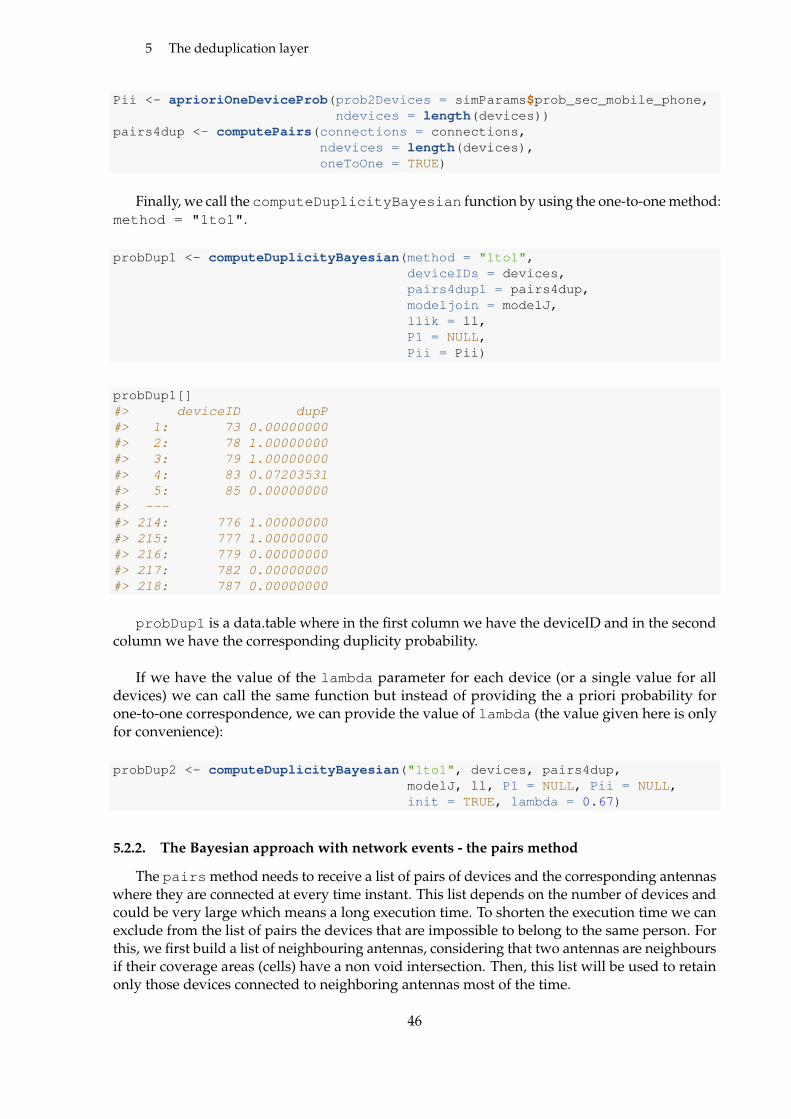
5 The deduplication layer
Pii <- aprioriOneDeviceProb(prob2Devices = simParams$prob_sec_mobile_phone,ndevices = length(devices))
pairs4dup <- computePairs(connections = connections,ndevices = length(devices),oneToOne = TRUE)
Finally, we call the computeDuplicityBayesian function by using the one-to-one method:method = "1to1".
probDup1 <- computeDuplicityBayesian(method = "1to1",deviceIDs = devices,pairs4dupl = pairs4dup,modeljoin = modelJ,llik = ll,P1 = NULL,Pii = Pii)
probDup1[]#> deviceID dupP#> 1: 73 0.00000000#> 2: 78 1.00000000#> 3: 79 1.00000000#> 4: 83 0.07203531#> 5: 85 0.00000000#> ---#> 214: 776 1.00000000#> 215: 777 1.00000000#> 216: 779 0.00000000#> 217: 782 0.00000000#> 218: 787 0.00000000
probDup1 is a data.table where in the first column we have the deviceID and in the secondcolumn we have the corresponding duplicity probability.
If we have the value of the lambda parameter for each device (or a single value for alldevices) we can call the same function but instead of providing the a priori probability forone-to-one correspondence, we can provide the value of lambda (the value given here is onlyfor convenience):
probDup2 <- computeDuplicityBayesian("1to1", devices, pairs4dup,modelJ, ll, P1 = NULL, Pii = NULL,init = TRUE, lambda = 0.67)
5.2.2. The Bayesian approach with network events - the pairs method
The pairs method needs to receive a list of pairs of devices and the corresponding antennaswhere they are connected at every time instant. This list depends on the number of devices andcould be very large which means a long execution time. To shorten the execution time we canexclude from the list of pairs the devices that are impossible to belong to the same person. Forthis, we first build a list of neighbouring antennas, considering that two antennas are neighboursif their coverage areas (cells) have a non void intersection. Then, this list will be used to retainonly those devices connected to neighboring antennas most of the time.
46
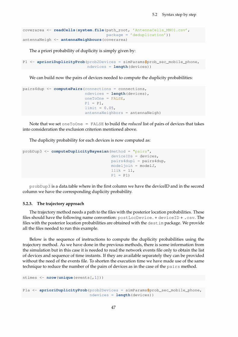
5.2 Syntax step by step
coverarea <- readCells(system.file(path_root, ’AntennaCells_MNO1.csv’,package = ’deduplication’))
antennaNeigh <- antennaNeighbours(coverarea)
The a priori probability of duplicity is simply given by:
P1 <- aprioriDuplicityProb(prob2Devices = simParams$prob_sec_mobile_phone,ndevices = length(devices))
We can build now the pairs of devices needed to compute the duplicity probabilities:
pairs4dup <- computePairs(connections = connections,ndevices = length(devices),oneToOne = FALSE,P1 = P1,limit = 0.05,antennaNeighbors = antennaNeigh)
Note that we set oneToOne = FALSE to build the reduced list of pairs of devices that takesinto consideration the exclusion criterion mentioned above.
The duplicity probability for each devices is now computed as:
probDup3 <- computeDuplicityBayesian(method = "pairs",deviceIDs = devices,pairs4dupl = pairs4dup,modeljoin = modelJ,llik = ll,P1 = P1)
probDup3 is a data.table where in the first column we have the deviceID and in the secondcolumn we have the corresponding duplicity probability.
5.2.3. The trajectory approach
The trajectory method needs a path to the files with the posterior location probabilities. Thesefiles should have the following name convention: postLocDevice + deviceID + .csv. Thefiles with the posterior location probabilities are obtained with the destim package. We provideall the files needed to run this example.
Below is the sequence of instructions to compute the duplicity probabilities using thetrajectory method. As we have done in the previous methods, there is some information fromthe simulation but in this case it is needed to read the network events file only to obtain the listof devices and sequence of time instants. If they are available separately they can be providedwithout the need of the events file. To shorten the execution time we have made use of the sametechnique to reduce the number of the pairs of devices as in the case of the pairs method.
ntimes <- nrow(unique(events[,1]))
P1a <- aprioriDuplicityProb(prob2Devices = simParams$prob_sec_mobile_phone,ndevices = length(devices))
47
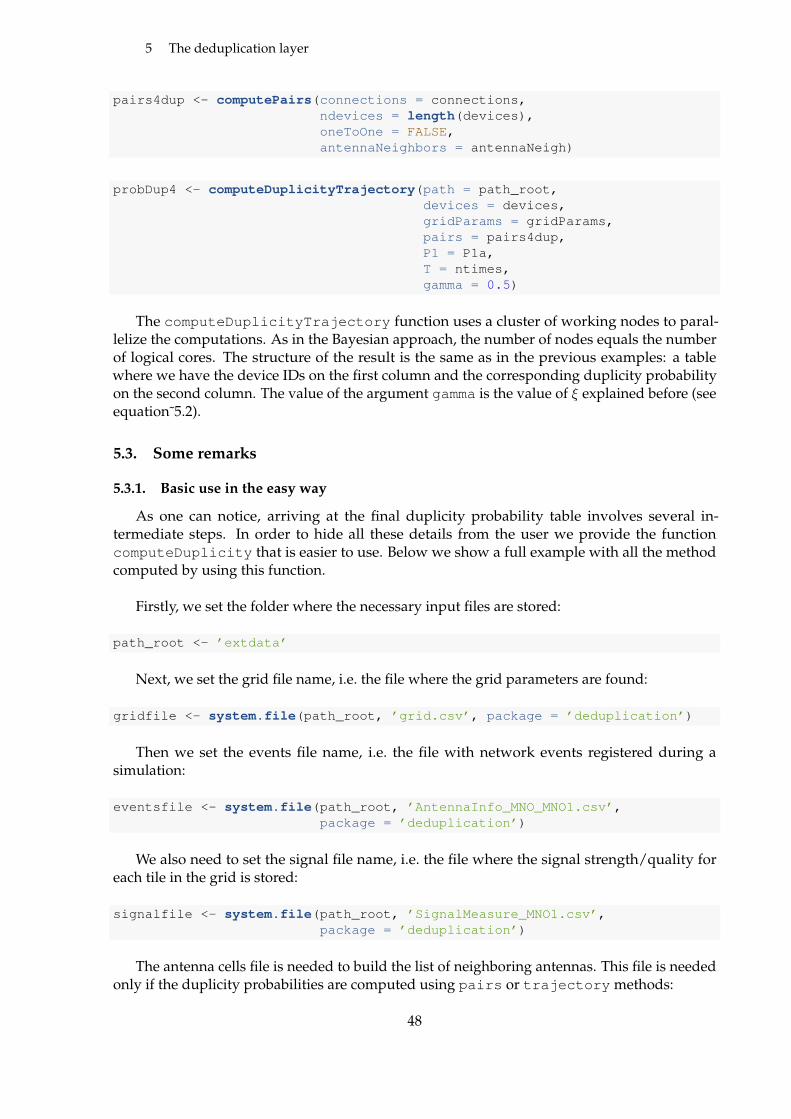
5 The deduplication layer
pairs4dup <- computePairs(connections = connections,ndevices = length(devices),oneToOne = FALSE,antennaNeighbors = antennaNeigh)
probDup4 <- computeDuplicityTrajectory(path = path_root,devices = devices,gridParams = gridParams,pairs = pairs4dup,P1 = P1a,T = ntimes,gamma = 0.5)
The computeDuplicityTrajectory function uses a cluster of working nodes to paral-lelize the computations. As in the Bayesian approach, the number of nodes equals the numberof logical cores. The structure of the result is the same as in the previous examples: a tablewhere we have the device IDs on the first column and the corresponding duplicity probabilityon the second column. The value of the argument gamma is the value of ξ explained before (seeequation˜5.2).
5.3. Some remarks
5.3.1. Basic use in the easy way
As one can notice, arriving at the final duplicity probability table involves several in-termediate steps. In order to hide all these details from the user we provide the functioncomputeDuplicity that is easier to use. Below we show a full example with all the methodcomputed by using this function.
Firstly, we set the folder where the necessary input files are stored:
path_root <- ’extdata’
Next, we set the grid file name, i.e. the file where the grid parameters are found:
gridfile <- system.file(path_root, ’grid.csv’, package = ’deduplication’)
Then we set the events file name, i.e. the file with network events registered during asimulation:
eventsfile <- system.file(path_root, ’AntennaInfo_MNO_MNO1.csv’,package = ’deduplication’)
We also need to set the signal file name, i.e. the file where the signal strength/quality foreach tile in the grid is stored:
signalfile <- system.file(path_root, ’SignalMeasure_MNO1.csv’,package = ’deduplication’)
The antenna cells file is needed to build the list of neighboring antennas. This file is neededonly if the duplicity probabilities are computed using pairs or trajectory methods:
48

5.3 Some remarks
antennacellsfile <- system.file(path_root, ’AntennaCells_MNO1.csv’,package = ’deduplication’)
Finally, we set the simulation file name, i.e. the file with the simulation parameters used toproduce the data set:
simulationfile <- system.file(path_root, ’simulation.xml’,package = ’deduplication’)
Now we can compute the duplicity probabilities using one of the three methods:
1. Using the 1to1 method:
out1 <- computeDuplicity(method = "1to1",gridFileName = gridfile,eventsFileName = eventsfile,signalFileName = signalfile,simulatedData = TRUE,simulationFileName = simulationfile)
Using the 1to1 method with lambda parameter (note that the value given here is forconvenience):
out1p <- computeDuplicity(method = "1to1",gridFileName = gridfile,eventsFileName = eventsfile,signalFileName = signalfile,simulatedData = TRUE,simulationFileName = simulationfile,lambda = 0.67)
2. Using the pairs method:
out2 <- computeDuplicity(metho = "pairs",gridFileName = gridfile,eventsFileName = eventsfile,signalFileName = signalfile,antennaCellsFileName = antennacellsfile,simulationFileName = simulationfile)
3. Using the trajectory method:
out3 <- computeDuplicity(method = "trajectory",gridFileName = gridfile,eventsFileName = eventsfile,signalFileName = signalfile,antennaCellsFileName = antennacellsfile,simulationFileName = simulationfile,path= path_root)
49
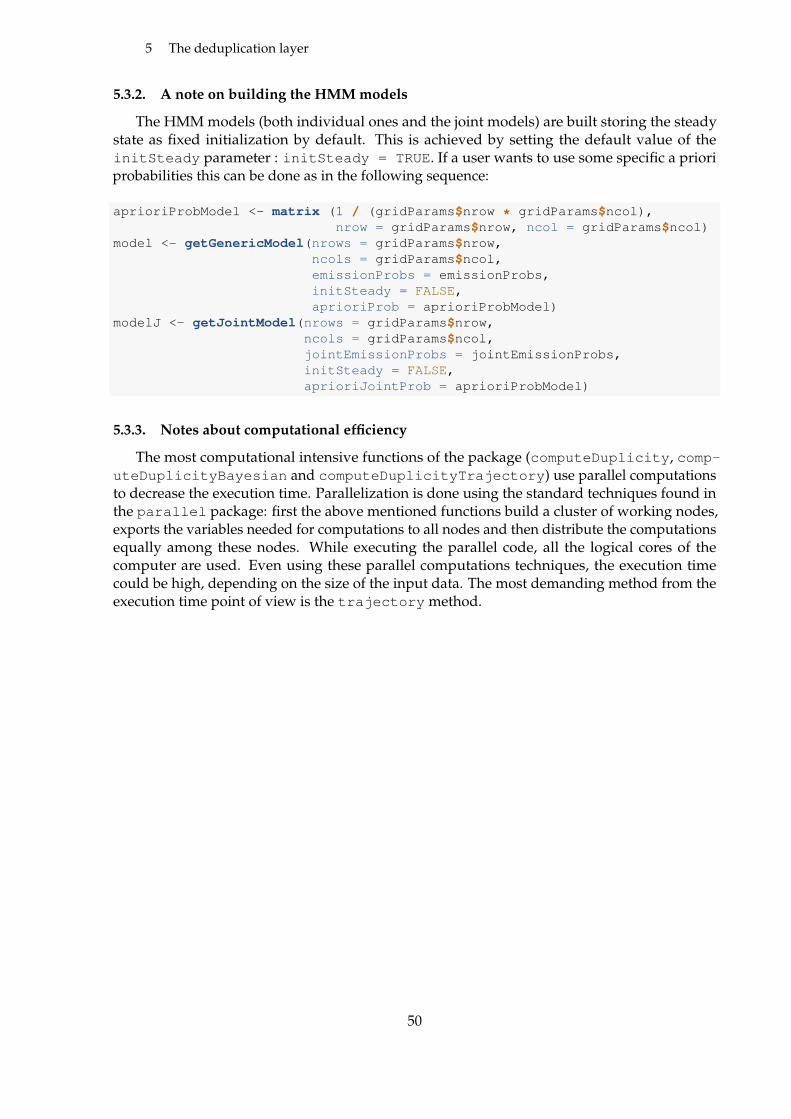
5 The deduplication layer
5.3.2. A note on building the HMM models
The HMM models (both individual ones and the joint models) are built storing the steadystate as fixed initialization by default. This is achieved by setting the default value of theinitSteady parameter : initSteady = TRUE. If a user wants to use some specific a prioriprobabilities this can be done as in the following sequence:
aprioriProbModel <- matrix (1 / (gridParams$nrow * gridParams$ncol),nrow = gridParams$nrow, ncol = gridParams$ncol)
model <- getGenericModel(nrows = gridParams$nrow,ncols = gridParams$ncol,emissionProbs = emissionProbs,initSteady = FALSE,aprioriProb = aprioriProbModel)
modelJ <- getJointModel(nrows = gridParams$nrow,ncols = gridParams$ncol,jointEmissionProbs = jointEmissionProbs,initSteady = FALSE,aprioriJointProb = aprioriProbModel)
5.3.3. Notes about computational efficiency
The most computational intensive functions of the package (computeDuplicity, comp-uteDuplicityBayesian and computeDuplicityTrajectory) use parallel computationsto decrease the execution time. Parallelization is done using the standard techniques found inthe parallel package: first the above mentioned functions build a cluster of working nodes,exports the variables needed for computations to all nodes and then distribute the computationsequally among these nodes. While executing the parallel code, all the logical cores of thecomputer are used. Even using these parallel computations techniques, the execution timecould be high, depending on the size of the input data. The most demanding method from theexecution time point of view is the trajectory method.
50

6
The aggregation layer
6.1. Introduction
In this chapter, we illustrate the aggregation process through the corresponding implementa-tion in the R package aggregation (Oancea et al., 2020a). The main purpose is to present sometechnical details of its implementation and provide examples on how to use this package. Somebasic knowledge about destim and deduplication packages would be useful to understandhow this package works (see previous chapters). A detailed description of the methodologicalapproach implemented by this package is provided by Salgado et al. (2020) and Salgado et al.(2020).
The aggregation process connects the number of devices detected by the network with thenumber of individuals in the network (the whole territory or a partition). There are two maingoals in this process:
1. The number of detected individuals.2. The origin - destination matrix.
Let us see a brief description of the underlaying methodology and the steps to solve themwith the implementation done in the aggregation package.
We are under the assumption that the goal is the whole population, so there is no need ofstatistical filtering before computing the aggregation process. In case that the target populationwould be a subset such as: domestic tourists, inbound tourists, commuters, etc., a process ofstatistical filtering must be applied before doing the aggregation. The main idea would beto identify groups of devices through their patterns of movement. We have identify severalindicators and propose some possible methods (see Salgado et al., 2020). However, we have notdeveloped a specific methodology for that process since in our simulated data there is currentlyno pattern apart from random walks (with or without drift). In fact, in the following sectionsthe example is shown through the same simulation of previous chapters.
The rest of the chapter is organized as follows. Section 6.2 presents the method of computingthe number of detected individuals. It starts with a brief introduction into the methodologicalapproach (subsection 6.2.1) and continues with an example of using the aggregation packageto compute this number (subsection 6.2.2 ) where it presents the function rNentEvent(). Thisfunction generates random variates according to a Poisson multinomial distribution which canbe used to compute a point estimation (mean, mode) of the number of individuals. Section 6.3is dedicated to the origin-destination matrix. Again, we start with a short introduction of themethodological approach and then we present an example of using function rNnetEventOD()to compute the origin-destination matrix in subsection 6.3.1.
51

6 The aggregation layer
6.2. The number of detected individuals
6.2.1. Brief methodological description
The main objective of the aggregation is to estimate the number of detected individualsstarting from the number of detecting devices and making use of the duplicity probability foreach device.
For this purpose, it uses a probabilistic approach in order to carry forward the uncertaintyalready present in the preceding stages all along the end-to-end process. The geolocation ofnetwork events is conducted with certain degree of uncertainty (due to the nature itself ofthe process – see chapter 4) and the duplicity of a given device (carried by an individual withanother device) is also probabilistic in nature (see chapter 5), therefore, a priori it is impossibleto provide a certain number of individuals in a given territorial unit.
For this reason the methodology behind this process focuses on the probability distribu-tion of the number of individuals detected by the network. Having a probability distributionamounts to having all statistical information about the random phenomenon and one can chooseany point estimation (mean, median, mode) together with uncertainty measures (coefficient ofvariation, credible intervals).
The aggregation procedure is strongly based on the results of preceding modules (geoloca-tion and duplicity) avoiding any extra hypothesis.
We define the vectors e(1)i = ei and e
(2)i = 1
2ei, where ei is the canonical unit vector in RNT(with NT the number of tiles in the reference grid).
Next, we define the random variable Tdt ∈ e(1)i , e
(2)i i=1,...,NT with probability mass function
P (Tdt|E1:D) given by
P(Tdt = e
(1)i |E1:D
)= γdti × (1− p(2)
d )
P(Tdt = e
(2)i |E1:D
)= γdti × p(2)
d ,
where p(2)d is the device duplicity probability computed with deduplication package (named
as p(2)d in chapter 5) and γdti denote the location probability of device d at time t and tile i com-
puted with destim package. It can be easily observed that this is a categorical or multinoullirandom variable.
Finally, we define the multivariate random variable Nnett providing the number of individuals
Nnetti detected by the network at each tile i = 1, . . . , NT at time instant t:
Nnett =
D∑d=1
Tdt.
The random variable N(net)t is a Poisson multinomial distributed random variable. The prop-
erties and software implementation of this distribution are not trivial and we use a Monte Carlosimulation method by convolution to generate random variates according to this distribution.
Another interesting issue is to consider the computation of the distribution of the number ofdetected individuals at a region/zone level. Let us consider a combination of tiles that we can
52

6.2 The number of detected individuals
called regions. We shall denote them as Tr =⋃i∈Ir Ti, where Ir denotes the set of tile indices
composing region r. If the independence assumption still holds (because the size of the regionis still small enough), then we can reproduce the whole derivation above just by defining thelocation probability γdtr at region r as
γdtr =∑i∈Ir
γdti. (6.1)
The subsequent elaboration to build the final Poisson-multinomial-distributed number ofdetected individuals is completely similar. Notice again that there exists a limitation in the sumof device-level distributions put by the size of the underlying region breakdown. The randomvector Nnet
t of individuals per region in terms of the deduplicated location Tdt per region wouldbe also expressed as a sum:
Nnett =
D∑d=1
Tdt. (6.2)
Notice that this decomposition allows us to write straightforwardly the mean vector andthe covariance matrix for Nnet
t . Define the deduplicated location probabilities per region as
γdedupdtr ≡ (1− p
(2)d2 ) · γdtr for all regions r = 1, . . . , R. Then
E[Nnett
]=
D∑d=1
R∑r=1
γdedupdtr er, (6.3)
V[Nnett
]=
D∑d=1
R∑r=1
γdedupdtr · (1− γdedup
dtr )Err. (6.4)
In the following, we show how to obtain in practice all these concepts.
6.2.2. The rNnetEvent()
The aggregation package provides a single function to generate random variates ac-cording to the Poisson multinomial distribution: rNnetEvent(). Thus, all the details aboutintermediate computations are hidden from the users. The input data needed by this functionare:
n: the number of the random values to be generated,dupFileName: the file with the duplicity probabilities for each device,regsFileName: the file defining the geographical regions where we intend to aggregatethe number of individuals,postLocPath: the path to the directory where the files with the posterior location proba-bilities for each device are found,prefix: the name prefix of these files (which are the output of the destim package),times: a vector with the values of time instants.
There is also an optional argument called seed, the seed needed to initialize the randomnumber generator. In the example below we use the default value of this argument.
We provide a complete set of files with example data in the extdata folder of this package.The raw data used to produce these files are given by our simulation software. If the user wantsto work with real data reading of the simulation.xml (see code below) will be skipped, and
53

6 The aggregation layer
instead a vector with all the time instants when the network events were registered should bebuild and provided.
The duplicity file is a simple .csv file which is the main result of the deduplication pack-age. It is a simple table with two columns, namely deviceID and duplicityProbability:
dupProb <- read.csv(file = system.file(’extdata/duplicity.csv’,package = ’aggregation’))
head(dupProb)#> deviceID dupP#> 1 73 0.00000000#> 2 78 1.00000000#> 3 79 1.00000000#> 4 83 0.05141439#> 5 85 0.00000000#> 6 90 0.06842542
The regions file is also a simple .csv file defined by the user. It contains two columns: the tilenumber and the region number. Normally, all tiles in the grid should be part of a region.
regions <- read.csv(file = system.file(’extdata/regions.csv’,package = ’aggregation’))
head(regions)#> tile region#> 1 1560 3#> 2 1561 3#> 3 1562 3#> 4 1563 3#> 5 1564 3#> 6 1565 3
The third parameter that should be passed to this function is the path where the files withthe posterior location probabilities are found. There should be one file for each device in thewhole set of devices. A file contains a table with the posterior location probabilities for a device.It has three columns: tile, time, probL. It contains only the entries corresponding to nonzerovalues of the posterior location probability (probL column). The file extension is .csv.
Below we show a simple example of how to use this function and its result.
# set the folder where the necessary input files are storedpath <- ’extdata’
prefix = ’postLocDevice’
# get the series of time instants from the simulation.xml file.simParamsFileName <- system.file(path, ’simulation.xml’,
package = ’aggregation’)simParams <- deduplication::readSimulationParams(simParamsFileName)time_from <- simParams$start_timetime_to <- simParams$end_timetime_incr <- simParams$time_incrementtimes <- seq(from = time_from, to = time_to-time_incr, by = time_incr)
54
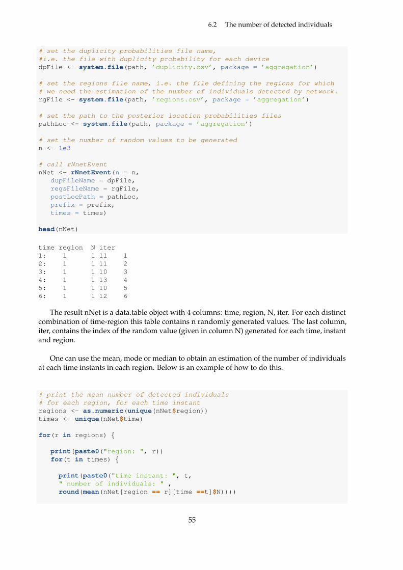
6.2 The number of detected individuals
# set the duplicity probabilities file name,#i.e. the file with duplicity probability for each devicedpFile <- system.file(path, ’duplicity.csv’, package = ’aggregation’)
# set the regions file name, i.e. the file defining the regions for which# we need the estimation of the number of individuals detected by network.rgFile <- system.file(path, ’regions.csv’, package = ’aggregation’)
# set the path to the posterior location probabilities filespathLoc <- system.file(path, package = ’aggregation’)
# set the number of random values to be generatedn <- 1e3
# call rNnetEventnNet <- rNnetEvent(n = n,
dupFileName = dpFile,regsFileName = rgFile,postLocPath = pathLoc,prefix = prefix,times = times)
head(nNet)
time region N iter1: 1 1 11 12: 1 1 11 23: 1 1 10 34: 1 1 13 45: 1 1 10 56: 1 1 12 6
The result nNet is a data.table object with 4 columns: time, region, N, iter. For each distinctcombination of time-region this table contains n randomly generated values. The last column,iter, contains the index of the random value (given in column N) generated for each time, instantand region.
One can use the mean, mode or median to obtain an estimation of the number of individualsat each time instants in each region. Below is an example of how to do this.
# print the mean number of detected individuals# for each region, for each time instantregions <- as.numeric(unique(nNet$region))times <- unique(nNet$time)
for(r in regions)
print(paste0("region: ", r))for(t in times)
print(paste0("time instant: ", t," number of individuals: " ,round(mean(nNet[region == r][time ==t]$N))))
55

6 The aggregation layer
6.3. The origin destination matrix
6.3.1. Brief methodological description
The construction of the probability distribution for the number of individuals Nnett detected
by the network can be easily generalized to the number of individuals Nnett,·· detected by the
network moving between territorial units. We begin by defining matrices E(1)rs = Ers and
E(2)rs = 1
2Ers, where Ers are the Weyl matrices of dimension R×R. Next, we define the matrixrandom variable Edt ∈ E(1)
rs , E(2)rs r,s=1...,R with probability mass function given by
P(Edt = E(1)
rs
)= γdt,sr · p(1)
d , (6.5a)
P(Edt = E(2)
rs
)= γdt,sr · p(2)
d , (6.5b)
where γdt,sr stands for the joint location probabilities computed in the geolocation moduleaggregated to the regions r, s = 1, . . . , R. Notice that, although matrix-valued, this is still acategorical or multinoulli random variable. Then, we can define the origin-destination matrixbetween regions of individuals detected by the network by
Nnett =
D∑d=1
Edt, (6.6)
which, as before, distributes according to a multinomial-Poisson distribution. Again, we shall useMonte Carlo techniques to deal with it. If we define the deduplicated joint location probabilities
γdedupdt,sr =
(1− p
(2)d2
)· γdt,sr, then the mean origin-destination matrix is given by
E[Nnett
]=
D∑d=1
R∑r,s=1
γdedupdt,sr Ers. (6.7)
Once we have posterior distributions we can also compute credible intervals for each regionand each time instant.
6.3.2. The rNnetEventOD() function
Again, the aggregation package provides a single function to generate random variatesthat can be used then to compute an estimation of the number of individuals moving from oneregion to another. The parameters of this function are:
n: the number of the random values to be generated,dupFileName: the file with the duplicity probabilities for each device,regsFileName: the file defining the geographical regions where we intend to aggregatethe number of individuals,postLocJointPath: the path to the directory where the files with the posterior jointlocation probabilities for each device are found,prefix: the name prefix of these files.
56

6.3 The origin destination matrix
There is also an optional argument, seed, the seed needed to initialize the random numbergenerator. In the example below we use the default value of this argument.
The files containing the joint probabilities are also a result of the destim package. Weprovide a complete set of files with example data in the extdata folder of this package. Theraw data used to produce these files are given by our simulation software.
# For the origin-destination matrix we proceed as follows# set the folder where the necessary input files are storedpath <- ’extdata’
postLocJointPath <- system.file(path, package = ’aggregation’)prefixJ <- ’postLocJointProbDevice’
# set the duplicity probabilities file name,# i.e. the file with duplicity probability for each devicedpFile <- system.file(path, ’duplicity.csv’, package = ’aggregation’)
# set the regions file name, i.e. the file defining the regions for which# we need the estimation of the number of individuals detected by network.rgFile <- system.file(path, ’regions.csv’, package = ’aggregation’)
# generate n random valuesn <- 1e3
nnetOD <- rNnetEventOD(n = n,dupFileName = dpFile,regsFileName = rgFile,postLocJointPath = postLocJointPath,prefix = prefixJ)
head(nnetOD)
time_from time_to region_from region_to Nnet iter1: 0 10 1 1 18.0 12: 0 10 1 1 18.5 23: 0 10 1 1 19.0 34: 0 10 1 1 18.0 45: 0 10 1 1 19.0 56: 0 10 1 1 18.0 6
For each pair(time from-time to, region from-region to) there are n random values in thelast but one column. One can use again the mean, mode or median to have an estimate of thenumber of individuals moving from one region to another at a certain time.
The following code shows how to compute the the origin-destination matrix for the timeinterval (0,10).
t_from <-0t_to <- 10
regions_from <- sort(as.numeric(unique(nnetOD$region_from)))regions_to <- sort(as.numeric(unique(nnetOD$region_to)))
57

6 The aggregation layer
ODmat <- matrix(nrow = length(regions_from), ncol = length(regions_to))for(r1 in regions_from)
for(r2 in regions_to)
aux <- nnetOD[time_from == t1][time_to == t2][region_from == r1][region_to == r2]$Nnet
ODmat[r1,r2] <- round(mean(aux))
ODmat
6.4. Some remarks about computational efficiency
The most computational intensive functions of the package (rNnetEvent, rNnetEventOD)use parallel computations to decrease the execution time. Parallelization is done using thestandard techniques found in the parallel package: firstly, the above mentioned functionsbuild a cluster of working nodes, exports the variables needed for computations to all nodesand then distribute the computations equally among these nodes. While executing the parallelcode, all the logical cores of the computer are used. Even using these parallel computationstechniques, the execution time could be high, depending on the size of the input data. Thecluster used for parallel computations is a SOCK one under the Windows operating system anda FORK one under Unix-like operating systems.
58

7
The inference layer
7.1. Introduction
In this chapter, the process on the inference layer is illustrated. The inference process con-nects the number of individuals in the network with the number of individual in the targetpopulation. The main goal is the computation of the probability distribution for the number ofindividuals in the target population conditioned on the number of individuals detected by thenetwork and some auxiliary information which is absolutely necessary to provide a meaningfulinference on the target population. The auxiliary information is provided by the penetrationrates (ratio of number of devices to number of individuals in the target population) P net
r of theMNO and the register-based population N reg
r at each region r.
We propose a two-staged modelling exercise. Firstly, we assume that there exists an initialtime instant t0 in which both the register-based target population and the actual populationcan be assimilated in terms of their physical location. We can assume, e.g., that at 6:00amall devices stay physically at the residential homes declared in the population register. Thisassumption will trigger the first stage in which we compute a probability distribution for thenumber of individuals Nt0 of the target population in all regions in terms of the number ofindividuals Nnet
0 detected by the network and the auxiliary information. Secondly, we proceedwith the dynamical part for what we assume that individuals displace over the geographicalterritory independently of the MNO, i.e. subscribers of MNO 1 will show a displacement patternsimilar to those of MNO 2. This assumption will trigger the second stage in which we provide aprobability distribution for the number of individuals Nt for later times t > t0.
Regarding the origin-destination matrix, we can use the same assumptions to infer thenumber of individuals moving from one region to another at time instant t, also providingcredible intervals as an accuracy indicator.
A detailed description of the methodological approach implemented is provided by Salgadoet al. (2020) and Salgado et al. (2020).
This chapter is divided in three main parts:
Population at the initial time t0.The dynamical approach: population at t > t0.Origin-destination matrices.
Inside each section, we show a brief methodological description that can be extended withthe material by Salgado et al. (2020) and Salgado et al. (2020) and the implementation step by
59

7 The inference layer
step that has been done in the R package inference (Oancea et al., 2020c). Thus, in section 7.2we treated the problem of estimating the population count at t0. We started by presenting a shortmethodological overwiew (subsection 7.2.1) and then we presented a detailed example on usingthe function that performs this estimation computeInitialPopulation() in subsection7.2.2. In section 7.3, we presented the estimation of the population count at successive timeinstants t > t0 in the same way: a short introduction to the methodological background isgiven in subsection 7.3.1 and an example on how to use computePopultionT() function isgiven in subsection 7.3.2. The origin-destination matrix estimation is presented in section7.4with a outline of the method used in subsection 7.4.1 and details on how to estimate thismatrix with computePopulationOD() function in subsection 7.4.2. This chapter ends withthe presentation of an add-on functionality of it, namely a REST AP, in section 7.5.
7.2. Population at the initial time t0
7.2.1. Brief methodological description
In this section we focus on the present population at the initial time t0. Then, for ease ofnotation we shall drop the time index. We shall combine the number of individuals in thenetwork per region, Nnet
r , the penetration rates per region, Pr, and the register-based populationper region N reg
r to produce the probability distribution for N = (N1, . . . , NR)T for all R regions.
We follow the approach used in the species abundance problem in Ecology by Royle and Do-razio (2009). This approach clearly distinguishes between the state and the observation process.The state process is the underlying dynamical process of the population and the observationprocess is the procedure by which we get information about the location and timestamp ofeach individual in the target population. The different available auxiliary information will beintegrated using different levels in the hierarchy of the statistical model.
7.2.1.1. Observation process
The first level makes use of the detection probability pr of individuals of a network in eachregion r. We shall concentrate first on the observation process. We model
Nnetr ' Binomial (Nr, pr) . (7.1)
This model makes the only assumption that the probability of detection pr for all individualsin region r is the same. We approximate it using the penetration rate Pr of the MNO in region r.The posterior probability distribution for Nr in terms of Nnet
r will be given by
P(Nr|Nnet
r
)=
0 if Nr < Nnet
r ,negbin
(Nr −Nnet
r ; 1− pr, Nnetr + 1
)if Nr ≥ Nnet
r ,
where negbin denotes the probability mass function of a negative binomial random variable.Once we have a distribution, we can provide a point estimators, a posterior variance, a posteriorcoefficient of variation, a credible interval, and as many indicators as possible computed fromthe distribution. In our implementation we compute the mean, mode and median as pointestimators, the standard deviation, coefficient of variation the first and third quartile, the in-terquartile range and the credible intervals.
We introduce now the second level and model the detection probability pkr per individualk in the target population as pkr = pr + noise. We propose to implement this idea modeling
60

7.2 Population at the initial time t0
pr ' Beta (αr, βr) and choosing the hyperparameters αr and βr according to the penetrationrates P net
r and the register-based population figures N regr . The penetration rate is also subjected
to the problem of device deduplication. We define:
Ω(1)r =
∑Dd=1 γdr · p
(1)d∑D
d=1 γdr, (7.2)
Ω(2)r =
∑Dd=1 γdr · p
(2)d∑D
d=1 γdr, (7.3)
with p(i)d being the duplicity probabilities (computed in chapter 6 under the same assumptions
about at most two devices per individual) and γdr the posterior location probabilities in region rfor device d. The deduplicated penetration rate is defined as:
P netr =
(Ω(1)r +
Ω(2)r
2
)· P net
r . (7.4)
Let us make the following assumptions:
On average, we assume that detection takes place with probability P netr .
Detection is undertaken over the register-based population. We assume some coherencebetween the official population count and the network population count.
The penetration rates P netr and the official population counts N reg
r come without error.Should this not be attainable or realistic, we would need to introduce a new hierarchylevel to account for this uncertainty (see below).
The deduplicated penetration rates are computed as a deterministic procedure (usinga mean point estimation), i.e. the deduplicated penetration rates are also subjected touncertainty, thus we should also introduce another hierarchy level to account for thisuncertainty.
Then, we fix the following: αr + βr = Nregr , αr
αr+βr= P net
r , which immediately implies that
αr = P netr ·N reg
r , (7.5a)
βr =(
1− P netr
)·N reg
r . (7.5b)
Now, we can readily compute the posterior distribution for Nr:
P(Nr|Nnet
r
)=
0 if Nr < Nnet
r ,betaNegBin
(Nr −Nnet
r ;Nnetr + 1, αr − 1, βr
)if Nr ≥ Nnet
r .
(7.6)
It is a displaced beta negative binomial distribution. Again, we can provide point estimatesas well as posterior variances, credible intervals, etc.
Notice that when αr, βr 1 (i.e., when min(P netr , 1 − P net
r ) · N regr 1) the beta negative
binomial distribution (7.6) reduces to the negative binomial distribution
61
7 The inference layer
P(Nr|Nnet
r
)=
0 if Nr < Nnet
r ,
negbin(Nr −Nnet
r ; βrαr+βr−1 , N
netr + 1
)if Nr ≥ Nnet
r .
Note also that βrαr+βr−1 ≈ 1 − P net
r so that in this case we do not need the register-basedpopulation (this is similar to dropping out the finite population correction factor in samplingtheory for large populations).
So far, the inference has been conducted independently in each region r. We can introduceanother layer in the hierarchy by modelling also the hyperparameters (αr, βr) so that therelationship between these parameters and the external data sources (penetration rates andregister-based population counts) is also uncertain.
7.2.1.2. State process
Finally, we can also introduce the state process. The system is a human population and wecan make a common modelling hypothesis to represent the number of individuals Nr in regionr of the target population as a Poisson-distributed random variable in terms of the populationdensity, i.e.
Nr ' Poisson (Arσr) , (7.7)
where σr stands for the population density of region r and Ar denotes the area of region r. Wechoose to model Nr in terms of the population density to make an auxiliary usage of someresults already found in the literature (see e.g. Deville et al., 2014).
Similarly to the observation process, we introduce the following hierarchy:
Nnetr ' Bin (Nr, pr) , for all r = 1, . . . , R, (7.8a)Nr ' Poisson (Arσr) , for all r = 1, . . . , R, (7.8b)pr ' Beta (αr, βr) , for all r = 1, . . . , R, (7.8c)σr ' Gamma (1 + ζr, θr) , for all r = 1, . . . , R, (7.8d)
where the hyperparameters will express the uncertainty about the register-based populationand the detection probability. The values for αr and βr are taken from (7.5). Regarding thehyperparameters θr and ζr, notice that the modes of the gamma distributions are at τr = ζr · θrand the variances are given by V (τr) = (ζr + 1) · θ2
r . We shall parameterise these gammadistributions in terms of the register-based population densities σreg
r as
ζr · θr = σregr + ∆σr,√
(ζr + 1) · θ2r = εr · σreg
r ,
where εr can be viewed as the coefficient of variation for σregr and ∆σr can be interpreted as the
bias for σregr . This parametrization implies that
62

7.2 Population at the initial time t0
θr(∆σr, εr) =σ
regr
2
(1 +
∆σr
σregr
)√√√√1 +
(2εr
1 + ∆σrσ
regr
)2
− 1
,ζr(∆σr, εr) =
2√√√√1 +
(2εr
1+ ∆σr
σregr
)2
− 1
. (7.9)
Under assumptions (7.8) and assuming αr, βr 1, as above, we get
P(N|Nnet) =
R∏r=1
negbin
(Nr −Nnet
r ;βr
αr + βr·Q(θr), N
netr + 1 + ζr
)(7.10)
where Q(θr) ≡ Arθr1+Arθr
. The interpretation of this hierarchy is also simple. It is just a Poisson-gamma model in which the gamma parameters have been chosen so that we account for theuncertainty in the register-based population figures N reg
r .
Usual point estimators are easily derived from (7.10) as well as accuracy indicators such asposterior variance or credible intervals are computed from the distribution (7.10).
Expression (7.10) contains the uncertainty of both the observation and the state processes.
7.2.2. Implementation step by step
Let us see now how to the methodology using functions from the the inference pack-age. First, the input files are read and the deduplication factors calculated as it is shown inthe following code. The input files in this stage comes from the deduplication package(duplicity.csv), destim package (the location probabilities files) and an from externalsource (the regions.csv file).
In these lines the steps are: set the folder where the location probabilities files are stored andthe prefix of these input file names, read the other input files (duplicity and regions) and thencompute the deduplication factors.
library(inference, warn.conflicts = FALSE)
path <- ’extdata’prefix <- ’postLocDevice’
postLocPath <- system.file(path, package = ’inference’)dpFileName <- system.file(path, ’duplicity.csv’, package = ’inference’)rgFileName <- system.file(path, ’regions.csv’, package = ’inference’)
omega_r <- computeDeduplicationFactors(dupFileName = dpFileName,regsFileName = rgFileName,postLocPrefix = prefix,postLocPath = postLocPath)
head(omega_r)
63

7 The inference layer
region omega1 omega21: 4 0.9786578 0.021342232: 6 0.7116936 0.288306363: 9 0.6520971 0.347902934: 3 0.7876368 0.212363175: 10 0.7199611 0.280038946: 8 0.8367990 0.16320103
Then, we can compute the parameters needed by the distribution functions used to estimatethe target population count. The computeDistrParams() function computes the parametersneeded by all three distributions presented in the previous subsection: αr, βr, θr and ζr. Thecomputations are performed under the assumption that ∆σr = 0 and εr = 10−5 unless the userspecifies other values for them. The input files needed in this step are: nnet.csv which isone of the outputs of the aggregation package containing the random variates generatedfor each region, the file with the population count for each geographical region (named herepop reg.csv) which can be taken from a population register, the penetration rates of theMNO in each of the geographical regions (named in our example pnt rates.csv) whichcan be obtained from the MNO itself or from another telecommunication authority and theparameters of the grid (grid.csv). In the code presented below we used the files included inthe inference package, but they can be replaced by the user with his/her own files easily.
nFileName <- system.file(path, ’nnet.csv’, package = ’inference’)nnet <- readNnetInitial(nFileName)pRFileName <- system.file(path, ’pop_reg.csv’, package = ’inference’)pRateFileName <- system.file(path, ’pnt_rate.csv’, package = ’inference’)grFileName <- system.file(path, ’grid.csv’, package = ’inference’)params <- computeDistrParams(omega = omega_r,
popRegFileName = pRFileName,pntRateFileName = pRateFileName,regsFileName = rgFileName,gridFileName = grFileName)
head(params)
region omega1 omega2 pntRate regionArea_km2 N0 dedupPntRate1: 1 0.6878592 0.31214077 0.3684211 10.5 38 0.31092152: 2 0.8991648 0.10083522 0.4000000 7.5 55 0.37983303: 3 0.7876368 0.21236317 0.4153846 12.0 65 0.37127844: 4 0.9786578 0.02134223 0.4615385 10.0 39 0.45661345: 5 0.6734889 0.32651114 0.3666667 10.0 60 0.30680636: 6 0.7116936 0.28830636 0.3720930 12.5 43 0.3184546
alpha beta theta zeta Q1: 11.81502 26.18498 3.619048e-10 9999999173 3.8e-092: 20.89081 34.10919 7.333334e-10 9999999173 5.5e-093: 24.13310 40.86690 5.416667e-10 9999999173 6.5e-094: 17.80792 21.19208 3.900000e-10 9999999173 3.9e-095: 18.40838 41.59162 6.000000e-10 9999999173 6.0e-096: 13.69355 29.30645 3.440000e-10 9999999173 4.3e-09
Then, the population count distribution at t0 is computed. As it has been explained before,three distributions can be used: Beta Negative Binomial, Negative Binomial or the state processNegative Binomial. The distribution used to compute the population count is specified usingthe popDistr parameter which can have three values BetaNegBin, NegBin or STNegBin.This function also needs the population count detected by the network computed using theaggregation package and read from a csv file. The result of the computeInitialPopulation
64

7.2 Population at the initial time t0
is a list object with one or two elements. If the parameter rndVal is FALSE the list will havea single element with descriptive statistics for the population count, which is a data.table ob-ject with the following columns: region, Mean, Mode, Median, Min, Max, Q1, Q3,IQR, SD, CV, CI LOW, CI HIGH. If rndVal is TRUE the list will have a second elementwhich is a data.table object containing the random values generated for each region. The nameof the two list elements giving the descriptive statistics and random values for time t are statsand rnd values.
# Beta Negative Binomial distributionn_bnb <- computeInitialPopulation(nnet = nnet,
params = params,popDistr = ’BetaNegBin’,rndVal = TRUE)
head(n_bnb$stats)
region Mean Mode Median Min Max Q1 Q3 IQR SD CV CI_LOW CI_HIGH[1,] 1 43 41 39 13 136 31 50 19 17.74 41.55 22.00 77.00[2,] 2 60 57 58 24 142 49 69 20 16.19 26.98 38.00 87.53[3,] 3 80 68 77 42 176 66 92 25 19.32 24.07 54.97 113.50[4,] 4 38 33 37 14 102 30 44 14 11.41 29.86 23.50 58.00[5,] 5 77 64 73 26 182 62 89 28 23.19 30.02 47.97 120.06[6,] 6 49 36 46 14 140 36 58 22 18.41 37.59 26.00 82.03
head(n_bnb$rnd_values)
region N NPop1: 1 11.0 46.02: 1 9.0 42.03: 1 13.0 52.04: 1 12.0 33.05: 1 12.0 35.06: 1 12.5 30.5
Here N is the population count detected by the network and NPop is the target populationcount.
# Negative Binomial distributionn_nb <- computeInitialPopulation(nnet = nnet,
params = params,popDistr = ’NegBin’,rndVal = TRUE)
head(n_nb$stats)
region Mean Mode Median Min Max Q1 Q3 IQR SD CV CI_LOW CI_HIGH[1,] 1 40 34 39 12 82 32 46 14 11.23 28.40 23.94 59.00[2,] 2 58 51 57 27 100 50 65 15 11.89 20.46 41.00 80.00[3,] 3 79 76 78 48 130 70 86 16 12.63 16.08 60.00 100.03[4,] 4 37 36 36 17 66 32 42 10 7.95 21.52 25.00 50.50[5,] 5 75 75 74 33 128 64 84 20 15.10 20.21 51.50 100.50[6,] 6 44 43 44 18 84 36 51 14 10.82 24.41 28.00 62.50
65

7 The inference layer
head(n_nb$rnd_values)
region N NPop1: 1 11.0 24.02: 1 9.0 33.03: 1 13.0 61.04: 1 12.0 32.05: 1 12.0 49.06: 1 12.5 79.5
# State process Negative Binomial distributionn_stnb <- computeInitialPopulation(nnet = nnet,
params = params,popDistr= ’STNegBin’,rndVal = TRUE)
head(n_stnb$stats)
region Mean Mode Median Min Max Q1 Q3 IQR SD CV CI_LOW CI_HIGH[1,] 1 37 36 37 22 55 34 41 8 5.45 14.71 29.00 45.53[2,] 2 55 54 54 36 73 51 59 8 6.09 11.10 45.00 64.50[3,] 3 69 68 68 49 96 64 74 9 6.72 9.74 58.00 80.00[4,] 4 37 36 37 22 56 33 40 7 5.13 13.95 29.00 45.00[5,] 5 63 62 63 42 88 58 68 9 6.89 10.91 52.00 74.50[6,] 6 42 40 42 26 60 38 46 8 5.51 13.05 33.97 51.00
head(n_stnb$rnd_values)
region N NPop1: 1 11.0 36.02: 1 9.0 33.03: 1 13.0 40.04: 1 12.0 42.05: 1 12.0 36.06: 1 12.5 36.5
7.3. The dynamical approach: population at t > t0
7.3.1. Brief methodological description
In this section we focus on the probability distributions for the number of individuals Ntr
in the target population at region r for times t > t0, then the dynamical component is takeninto consideration. Currently, we consider only closed populations, i.e. neither individuals nordevices enter into or leave the territory under analysis along the whole time period.
Our reasoning tries to introduce as less assumptions as possible. Thus, we begin by consid-ering a balance equation. Let us denote by Nt,rs the number of individuals moving from regions to region r in the time interval (t− 1, t). Then, we can write:
66

7.3 The dynamical approach: population at t > t0
Ntr = Nt−1r +
NT∑rt=1rt 6=r
Nt,rrt −Nr∑rt=1rt 6=r
Nt,rtr
=
NT∑rt=1
τt,rrt ·Nt−1rt , (7.11)
where we have defined τt,rs =Nt,rsNt−1s
(0 if Nt−1s = 0). Notice that τt,rs can be interpreted as anaggregate transition probability from region s to region r at time interval (t− 1, t) in the targetpopulation.
We make the assumption that individuals detected by the network move across regions in
the same way as individuals in the target population. Thus, we can use τnett,rs ≡
Nnett,rs
Nnett−1s
to model
τt,rs. In particular, as our first choice we shall postulate τt,rs = τnett,rs.
The probability distributions of Nnetst−1 and [Nnet
t ]sr = Nnett,rs were indeed already computed in
the aggregation layer (see chapter 6).
7.3.2. Implementation step by step
Now, we show the implementation of the dynamical procedure by computing the populationcount distribution at time instants t > t0. As it was done for the hierarchical model, we show thethree distributions: Beta Negative Binomial, Negative Binomial and the state process NegativeBinomial.
The target population distribution is computed using computePopulationT() function.As inputs, it needs the population distribution at t0 (here we will use all three previous results),the file with the population detected by the network moving from one region to another (anoutput of the aggregation package) and an optional parameter rndVal. The result of thisfunction is a list with one element for each time instant (including t0). Each element of the listis also a list with one or two elements, depending on the value of the rndVal parameter. IfrndVal is TRUE there are two elements in the list corresponding to time instant t. The firstone is a data.table object with some descriptive statistics for the population count at time t,containing the following columns:region, Mean, Mode, Median, Min, Max, Q1, Q3,IQR, SD, CV, CI LOW, CI HIGH. The second one is a data.table object with the randomvalues for population count generated for each region, with the following columns: region,iter, NPop. If rndVal is FALSE the list for time instant t contains only the first elementpreviously mentioned. The name of the list element corresponding to time instant t is t andthe name of the two list elements giving the descriptive statistics and random values are statsand rnd values.
First, we set the name of the file with the population detected by the network moving fromone region to another (output of the aggregation package (see chapter 6 and Oancea et al.(2020a)). Notice that this file is stored as a zip archive because it could be very large. Then wecall computePopulationT() function to obtain the population count estimates at t > t0.
nnetODFile <- system.file(path, ’nnetOD.zip’, package = ’inference’)
67

7 The inference layer
# Beta Negative Binomial distributionnt_bnb <- computePopulationT(nt0 = n_bnb$rnd_values,
nnetODFileName = nnetODFile,rndVal = TRUE)
To display the results we select a random time instant first and then display the results for it:
times <- names(nt_bnb)t <- sample(1:length(times), size = 1)thead(nt_bnb[[t]]$stats)
region Mean Mode Median Min Max Q1 Q3 IQR SD CV CI_LOW CI_HIGH[1,] 1 35 33 33 9 88 27 41 14 11.89 34.35 18 56[2,] 2 67 60 65 31 142 57 76 19 14.82 22.16 46 93[3,] 3 166 161 164 96 259 150 181 31 23.38 14.11 131 205[4,] 4 41 32 40 14 93 33 48 15 11.08 27.09 25 60[5,] 5 81 80 80 45 137 70 89 19 15.07 18.70 58 106[6,] 6 23 19 22 2 52 17 27 10 7.66 33.73 12 36
head(nt_bnb[[t]]$rnd_values)
region iter NPop1: 1 1 522: 2 1 573: 3 1 1844: 4 1 495: 5 1 806: 6 1 33
The iter column shows the index of the random value generated for a region. The totalnumber of random values generated for each region equals the same number used in theaggregation package that provides the input for this function.
# Negative Binomial distributionnt_nb <- computePopulationT(nt0 = n_nb$rnd_values,
nnetODFileName = nnetODFile,rndVal = TRUE)
# to display results, select a random time instanttimes <- names(nt_nb)t <- sample(1:length(times), size = 1)thead(nt_nb[[t]]$stats)
region Mean Mode Median Min Max Q1 Q3 IQR SD CV CI_LOW CI_HIGH[1,] 1 36 35 35 11 80 28 42 14 10.62 29.84 20 54.00[2,] 2 58 52 57 26 110 50 65 15 11.93 20.71 40 77.06[3,] 3 103 105 102 66 155 92 112 20 15.40 14.97 80 130.00[4,] 4 42 39 42 13 80 36 48 12 9.64 22.67 28 58.06[5,] 5 72 69 70 33 129 61 81 20 14.63 20.40 50 97.00[6,] 6 35 32 34 11 66 29 40 11 8.51 24.49 22 49.00
68

7.4 Origin-destination matrices
head(nt_nb[[t]]$rnd_values)
region iter NPop1: 1 1 382: 2 1 443: 3 1 924: 4 1 435: 5 1 646: 6 1 23
# State process Negative Binomial distributionnt_stnb <- computePopulationT(nt0 = n_stnb$rnd_values,nnetODFileName = nnetODFile,rndVal = TRUE)
# to display results, select a random time instanttimes <- names(nt_stnb)t <- sample(1:length(times), size = 1)thead(nt_stnb[[t]]$stats)
region Mean Mode Median Min Max Q1 Q3 IQR SD CV CI_LOW CI_HIGH[1,] 1 32 26 32 9 62 26 38 12 9.17 28.26 19 48[2,] 2 63 57 62 33 109 55 71 16 12.02 19.07 45 84[3,] 3 149 149 149 86 201 138 160 22 15.86 10.61 126 175[4,] 4 41 42 41 19 81 35 47 12 9.16 22.23 27 57[5,] 5 61 58 61 31 100 53 68 15 11.26 18.36 44 80[6,] 6 20 18 19 4 44 15 24 9 6.54 33.12 11 31
head(nt_stnb[[t]]$rnd_values)
region iter NPop1: 1 1 352: 2 1 533: 3 1 1524: 4 1 485: 5 1 516: 6 1 27
7.4. Origin-destination matrices
7.4.1. Brief methodological description
The inference of the origin-destination matrices for the target population is more delicatethan the present population because auxiliary information from population registers do notcontain this kind of information. Therefore, the statistical models proposed above for the presentpopulation estimation cannot be applied. As a first important conclusion we point out that, inour view, National Statistical Plans should start considering what kind of auxiliary informationis needed to make a more accurate use of Mobile Network Data and new digital data, in general.
We can provide a simple argument extending the above model to produce credible intervalsfor the origin-destination matrices. IfNtr and τt,rs denote the number of individuals of the targetpopulation at time t in region r and the aggregate transition probability from region s to region
69

7 The inference layer
r at the time interval (t − 1, t), then we can simply define Nt,rs = Nt−1s × τt,rs and triviallybuild the origin-destination matrix for each time interval (t − 1, t). Under the same generalassumption as before, if individuals are to move across the geographical territory independentlyof their mobile network operator (or even not being a subscriber or carrying two devices), wecan postulate as a first simple choice τt,rs = τnet
t,rs, as before.
7.4.2. Implementation step by step
As final step, the origin-destination matrices for all pairs of time instants time from-time toare computed. We follow the implementation in the R package inference and the three distri-butions: Beta Negative Binomial, Negative Binomial and the state process Negative Binomial.
This computation is performed by computePopulationOD() function which takes thesame input parameters as computePopulationT(). The result of this function is again a listwith one element for each pair of time from-time to. Each element of the list is also a list withone or two elements, depending on the value of the rndVal parameter. If rndVal is TRUE thereare two elements in the list corresponding to a time instant pair (time from, time to). Thefirst one is a data.table object with some descriptive statistics for the origin-destination matrix,containing the following columns: region from, region to, Mean, Mode, Median,Min, Max, Q1, Q3, IQR, SD, CV, CI LOW, CI HIGH. The second one is a data.tableobject with the random values for origin-destination matrix generated for each pair of timeinstants time from-time to and each pair of regions region from-region to, with thefollowing columns: region from, region to, iter, NPop. If rndVal is FALSE thelist for a pair of time instants time from-time to contains only the first element previ-ously mentioned. The name of the list element corresponding to a pair of time instants istime from-time to and the name of the two list elements giving the descriptive statistics andrandom values are stats and rnd values.
# Beta Negative Binomial distributionOD_bnb <- computePopulationOD(nt0 = n_bnb$rnd_values,
nnetODFileName = nnetODFile,rndVal = TRUE)
# to display results, select a random time instanttime_pairs <- names(OD_bnb)i <- sample(1:length(time_pairs), size = 1)time_pairs[i]head(OD_bnb[[i]]$stats)
region_from region_to Mean Mode Median Min Max Q1 Q3 IQR SD[1,] 1 1 34 28 33 6 95 26 41 15 11.81[2,] 1 2 1 0 0 0 12 0 0 0 1.35[3,] 1 3 0 0 0 0 0 0 0 0 0.00[4,] 1 4 0 0 0 0 5 0 0 0 0.50[5,] 1 5 0 0 0 0 0 0 0 0 0.00[6,] 1 6 0 0 0 0 0 0 0 0 0.00
CV CI_LOW CI_HIGH[1,] 34.50 17.96 56.00[2,] 259.79 0.00 3.64[3,] NaN 0.00 0.00[4,] 665.94 0.00 0.00
70

7.4 Origin-destination matrices
[5,] NaN 0.00 0.00[6,] NaN 0.00 0.00
head(OD_bnb[[i]]$rnd_values)
region_from region_to iter NPop1: 1 1 1 632: 1 2 1 03: 1 3 1 04: 1 4 1 05: 1 5 1 06: 1 6 1 0
# Negative Binomial distributionOD_nb <- computePopulationOD(nt0 = n_nb$rnd_values,
nnetODFileName = nnetODFile,rndVal = TRUE)
# to display results, select a random time instanttime_pairs <- names(OD_nb)i <- sample(1:length(time_pairs), size = 1)time_pairs[i]head(OD_nb[[i]]$stats)
region_from region_to Mean Mode Median Min Max Q1 Q3 IQR SD CV[1,] 1 1 32 30 31 5 79 25 38 13 9.99 30.85[2,] 1 2 0 0 0 0 9 0 0 0 1.25 253.77[3,] 1 3 0 0 0 0 0 0 0 0 0.00 NaN[4,] 1 4 0 0 0 0 5 0 0 0 0.49 667.92[5,] 1 5 0 0 0 0 0 0 0 0 0.00 NaN[6,] 1 6 0 0 0 0 0 0 0 0 0.00 NaN
CI_LOW CI_HIGH[1,] 18 50.00[2,] 0 3.45[3,] 0 0.00[4,] 0 0.00[5,] 0 0.00[6,] 0 0.00
head(OD_nb[[i]]$rnd_values)
region_from region_to iter NPop1: 1 1 1 312: 1 2 1 03: 1 3 1 04: 1 4 1 05: 1 5 1 06: 1 6 1 0
# State process Negative Binomial distributionOD_stnb <- computePopulationOD(nt0 = n_stnb$rnd_values,nnetODFileName = nnetODFile,rndVal = TRUE)
71

7 The inference layer
# to display results, select a random time instanttime_pairs <- names(OD_stnb)i <- sample(1:length(time_pairs), size = 1)time_pairs[i]head(OD_stnb[[i]]$stats)
region_from region_to Mean Mode Median Min Max Q1 Q3 IQR SD CV[1,] 1 1 30 32 30 8 60 24 36 12 8.83 29.17[2,] 1 2 0 0 0 0 8 0 0 0 1.17 252.68[3,] 1 3 0 0 0 0 0 0 0 0 0.00 NaN[4,] 1 4 0 0 0 0 5 0 0 0 0.44 664.15[5,] 1 5 0 0 0 0 0 0 0 0 0.00 NaN[6,] 1 6 0 0 0 0 0 0 0 0 0.00 NaN
CI_LOW CI_HIGH[1,] 17.19 45.00[2,] 0.00 3.25[3,] 0.00 0.00[4,] 0.00 0.00[5,] 0.00 0.00[6,] 0.00 0.00
head(OD_stnb[[i]]$rnd_values)
region_from region_to iter NPop1: 1 1 1 37.8461542: 1 2 1 3.1538463: 1 3 1 0.0000004: 1 4 1 0.0000005: 1 5 1 0.0000006: 1 6 1 0.000000
7.5. The inference REST API
7.5.1. A conceptual overview
The inference package can also expose its main functions as a http REST API imple-mented using the plumber package (Trestle Technology, LLC, 2018). We have to mention fromthe beginning that this feature is an add-on, i.e. inference package can be used without thisinterface as presented in the previous sections. By adding this extra-functionality we wanted toopen a new development track for future versions of our packages because it presents a series ofadvantages. Exposing the functionalities of this package as a http API has several advantages:
APIs are flexible, easy to deploy and maintain, and they are accessible by multiple clientsat the same time;
APIs can be accessed via Internet by anyone without install any R package on his/hercomputer (destim, deduplication, aggregation, inference), so, our software iseasily accessible;
a user can write not only R code to access the functions exposed by the inferencepackage, but he/she can use any language (Java, Python, etc.) capable of sending APIrequests over Internet;
72

7.5 The inference REST API
for large datasets, the functions from the inference package can take a long time tocompute their results. In this case the inference package can be installed on a powerfulcomputer that makes public its API to all the users, saving thus further investments ininfrastructure;
Using a http REST API to access the processing functions in the inference package isin line with the proposed models of mobile phone data usage: the data sets stays in the MNOpremises and the statisticians perform their data analyses calling functions from the availableAPI. Of course, the functions available through the API should be first agreed between theMNOs and statistical offices. In a real environment, more precaution should be taken, i.e. usingencrypted connections or even VPNs.
In figure 7.1 we have a representation of the interaction between a client and the inferenceAPI.
Java / Python / R
code
WEB server
(Exposes the REST API)
R running the code
send API request
returns the resultsca
lls R
fu
nctio
ns
se
nd
ba
ck th
e r
esu
lts
Client side Server side
Figure 7.1: The client-server architecture of inference.
A client that can be a script/program written in R, Python, Java or any other languagesends a request to the Web server exposing the API. In turn, the server calls the specific Rfunctions invoked by the API sending them the parameters extracted from the body of therequest. An R instance runs the function and sends back the results to the server. The serverpacks the results in a supported format (JSON for example) and sends the response to the clientwhich unpacks the body of the response to get the requested data.
7.5.2. API example step by step
We implemented this feature using the plumber R package. The code presented below isthe equivalent of the previous examples, but it uses the API to call functions of the inferencepackage. The first step is to install the inference package on the server which can be the local
73

7 The inference layer
computer (as we will use in our examples) or another true Web server accessible via Internet.
In our examples we use the same computer as client and server and we need to run twoinstances of R. In one instance we will start the http API:
library(plumber)pathPL <-’plumber’initPop_api <- plumber::plumb(system.file(pathPL, ’plumb.R’,
package = ’inference’))initPop_api$run(host = ’127.0.0.1’, port = 8000)
The address 127.0.0.1 can be changed with the address of any other server. After runningthese lines of code, if we access the localhost at port 8000 we will see the interface shown infigure 7.2.
Figure 7.2: The client-server architecture of inference.
Here we can see the names of the endpoints of our API as well as the methods that can be usedto access them (in our case GET and POST). Our API exposes the computeDeduplicationFactors(),computeDistrParams(), computeInitialPopulation(), computePopulationT() andcomputePopulationOD() as main processing functions and getPath() and readNnetInitial()needed for intermediate steps. The end points of the API have the same names as the functionsthey make public.
Now we have to switch to the other R instance which will act as a client. First we haveto set the folder where the file with duplicity probabilities (duplicity.csv, comming fromdeduplication package) and the file defining the regions (regions.csv, defined by theuser) are stored and the prefix of the posterior location probabilities files for all devices (files thatare the output of the destim package). These example files are provided in the inferencepackage but the user can change them with his/her own files.
74

7.5 The inference REST API
Please note that if you run this example using a true client-server configuration, where theclient and the server reside on different machines, in the same or different networks, the IPaddresses should be updated accordingly. The path of the files needed for computation shouldbe also updated according to their actual location.
library(httr)library(jsonlite)library(data.table)
# Set the folder where the necessary input files are stored and# the prefix of the input file names.path <- ’extData’prefix <- ’postLocDevice’dpFileName <- system.file(path, ’duplicity.csv’,
package = ’inference’)rgFileName <- system.file(path, ’regions.csv’,
package = ’inference’)
Next, we compute the deduplication factors. For this we have prepare the body of the httprequest, set the API path, set the url of the API and then send the request. In our examplewe used the POST method to send this request. The body of the http request contains theparameters needed by the R function that computes the deduplication factors. They are sentpacking them in JSON format.
# prepare the body of the http requestbody <- list(.dupFileName = dpFileName,.regsFileName = rgFileName,.postLocPrefix = prefix,.postLocPath = postLocPath
)
# set API pathpathDedup <- ’computeDeduplicationFactors’
# send POST Request to APIurl <- "http://127.0.0.1:8000"raw.result <- POST(url = url,
path = pathDedup,body = body,encode = ’json’)
Now we obtained the result. First, we check that everything went OK (we have to obtaincode 200) and then unpack it from JSON format back to an R object:
# check status coderaw.result$status_code
# transform back the results from json formatomega_r <- as.data.table(fromJSON(rawToChar(raw.result$content)))
Next, we compute the parameters of the posterior distribution of the population count usinga similar approach: prepare the input data and build the body of the http request, set the API
75

7 The inference layer
path and then send the request. After the API send back the response we check the status code(it should be 200 if all went OK) and unpack the response from JSON to an R object.
# Compute the parameters of the distribution# First reads the number of individuals detected by networknFileName <- system.file(path, ’nnet.csv’, package = ’inference’)nnet <- readNnetInitial(nFileName)
pRFileName <- system.file(path, ’pop_reg.csv’, package = ’inference’)pRateFileName <- system.file(path, ’pnt_rate.csv’, package = ’inference’)grFileName <- system.file(path, ’grid.csv’, package = ’inference’)
# prepare the body of the http requestbody <- list(.omega = omega_r,.popRegFileName = pRFileName,.pntRateFileName = pRateFileName,.regsFileName = rgFileName,.gridFileName = grFileName,.rel_bias = 0,.cv = 1e-5
)
# set API pathpathDistr <- ’computeDistrParams’
# send POST Request to APIraw.result <- POST(url = url,
path = pathDistr,body = body,encode = ’json’)
# check status coderaw.result$status_code
# transform back the results from json formatparams <- as.data.table(fromJSON(rawToChar(raw.result$content)))
We can compute now the population at initial time. In our example we will use only theBeta Negative Binomial distribution. A similar approach should be followed for the other twodistributions.
# Compute the population count distribution at t0# using the Beta Negative Binomial distribution
# prepare the body of the http requestbody <- list(.nnet = nnet,.params = params,.popDistr = ’BetaNegBin’,.rndVal = TRUE,.ciprob = 0.95,.method = ’ETI’
)
76

7.5 The inference REST API
# set API pathpathInit <- ’computeInitialPopulation’
# send POST Request to APIraw.result <- POST(url = url,
path = pathInit,body = body,encode = ’json’)
# check status coderaw.result$status_code
# transform back the results from json formatn_bnb <- fromJSON(rawToChar(raw.result$content))
# display resultsn_nb$statshead(n_nb$rnd_values)
Computing the population at time instants t > t0 is performed as follows:
# Compute the population count distribution at time instants t > t0# using the Beta Negative Binomial distribution# first set the name of the file with the population moving# from one region to another (output of the aggregation package)nnetODFile <- system.file(path, ’nnetOD.zip’, package = ’inference’)
# prepare the body of the http requestbody <- list(.nt0 = as.data.table(n_bnb$rnd_values),.nnetODFileName = nnetODFile,.zip = TRUE,.rndVal = TRUE,.ciprob = 0.95,.method = ’ETI’
)
# set API pathpathT <- ’computePopulationT’
# send POST Request to APIraw.result <- POST(url = url,
path = pathT,body = body,encode = ’json’)
# check status coderaw.result$status_code
# transform back the results from json formatnt_bnb <- fromJSON(rawToChar(raw.result$content))
# display results# first, select a random time instanttimes <- names(nt_bnb)t <- sample(1:length(times), size = 1)
77

7 The inference layer
tnt_bnb[[t]]$statshead(nt_bnb[[t]]$rnd_values)
Finally, we show how to compute the origin-destination matrix:
# Compute the Origin-Destination matrices for all pairs of time# instants time_from-time_to using the Beta Negative Binomial distribution
# prepare the body of the http requestbody <- list(.nt0 = as.data.table(n_bnb$rnd_values),.nnetODFileName = nnetODFile,.zip = TRUE,.rndVal = TRUE,.ciprob = 0.95,.method = ’ETI’
)
# set API pathpathOD <- ’computePopulationOD’
# send POST Request to APIraw.result <- POST(url = url,
path = pathOD,body = body,encode = ’json’)
# check status coderaw.result$status_code
# transform back the results from json formatOD_bnb <- fromJSON(rawToChar(raw.result$content))
# display resultstime_pairs <- names(OD_bnb)# first, select a random time instants pairi <- sample(1:length(time_pairs), size = 1)time_pairs[i]OD_bnb[[i]]$statshead(OD_bnb[[i]]$rnd_values)
The http REST API of the inference can be called from any programming language orprograms (like curl for example) capable of sending http requests. We show here a smallPython script that demonstrates how to use the R inference API from another programminglanguage. In this example we show only how to compute the population at initial time, but therest of the computations are done in a similar way. The steps are the same as in the precedingexample with two exceptions: we need to know the path where the input files are stored and wecall getPath API method and to read the number of individuals detected by the network forwhich we called getNnetInitial API method. These two intermediate API calls were notnecessary in the R example since they are available as functions of the plumber package.
1 ""import requests2 import simplejson3 import pandas as pd
78
7.5 The inference REST API
45 data = "path" : "extData"6 data_json = simplejson .dumps (data )78 session = requests .Session ( )9 session .trust_env = False
10 r = session .post ("http://127.0.0.1:8000/getPath" ,11 data = data_json )1213 path = simplejson .loads (r .content ) [ 0 ]14 prefix = ’postLocDevice’15 postLocPath = path16 dpFileName = path +"/" + "duplicity.csv"17 rgFileName = path + "/" + "regions.csv"1819 body = \20 ".dupFileName" :dpFileName ,\21 ".regsFileName" :rgFileName ,\22 ".postLocPrefix" :prefix ,\23 ".postLocPath" :path\24 2526 body_json = simplejson .dumps (body )27 r = session .post ("http://127.0.0.1:8000/computeDeduplicationFactors" ,28 data = body_json )2930 omega_r = simplejson .loads (r .content )31 omega_r_df = pd .read_json (r .content )3233 omega_r_df3435 pRFileName = path +"/" + "pop_reg.csv"36 pRateFileName = path +"/" + "pnt_rate.csv"37 grFileName = path +"/" + "grid.csv"3839 body = \40 ".omega" :omega_r , \41 ".popRegFileName" : pRFileName , \42 ".pntRateFileName" : pRateFileName , \43 ".regsFileName" : rgFileName , \44 ".gridFileName" : grFileName , \45 ".rel_bias" : 0 , \46 ".cv" : 1e−5 \47 4849 body_json = simplejson .dumps (body )50 r = session .post ("http://127.0.0.1:8000/computeDistrParams" ,51 data = body_json )5253 params = simplejson .loads (r .content )54 params_df = pd .read_json (r .content )5556 params_df5758 nnetFileName = path +"/" + "nnet.csv"59 body = ".nnetFileName" :nnetFileName60 body_json = simplejson .dumps (body )61 r = session .post ("http://127.0.0.1:8000/getNnetInitial" ,62 data = body_json )63 nnet_r = simplejson .loads (r .content )6465 body = \66 ".nnet" : nnet_r , \67 ".params" : params , \68 ".popDistr" : ’BetaNegBin’ ,\69 ".rndVal" : True ,\70 ".ciprob" : 0 . 9 5 ,\71 ".method" : ’ETI’\72 73 body_json = simplejson .dumps (body )74 r = session .post ("http://127.0.0.1:8000/computeInitialPopulation" ,
79

7 The inference layer
75 data = body_json )7677 popInitStats = simplejson .loads (r .content ) [’stats’ ]78 popInitVals = simplejson .loads (r .content ) [’rnd_values’ ]7980 stats = pd .DataFrame (popInitStats )81 vals = pd .DataFrame (popInitVals )8283 stats84 vals85 %\endverbatim
7.6. Some remarks about computational efficiency
Functions in this package make use of the processing features of the data.table packagewhich implements them very efficiently. Since population at t depends on population at t− 1,the computation of the target population distributions at different time instants is inherentlysequential. Functions that takes a longer time to execute display a progress bar to show how thecomputations advance.
In the API mode, the computational efficiency could be supported by a powerful servermachine. Moreover, parallelization of the computations is achieved on server if several clientscall in the same time different functions from API. For a real production environment a loadbalancer could be added too (available in nginx or one can use a docker-based solution ?).
80

8
Further developments
This chapter is devoted to gather some reflections and conclusions for future work whichwill be part of the national efforts of the authors of this document and of the activity of the futureESS Task Force on MNO data. The following steps can be mainly divided in two approaches:the methodological modules and the computational implementation.
In the case of the methodological part, several branches to follow have been pointed outin the section about future prospects on the deliverable of methodology (Salgado et al., 2020).In summary, the methodological framework proposed does not intend to provide closed anddefinitive methods, but to put in place a first concrete substantiation of the ESS ReferenceMethodological Framework for Mobile Network Data. Much work remains to be done in the fu-ture. Results are encouraging, since we achieve modularity and evolvability, as well as rigorousaccuracy indicators, giving a first solution to the main problem that comprise all the modules ofthe process.
Regarding the computational issues, we have developed all the implementation needed toexecute the methods of the whole process. This implementation has been done in R which is afree software environment focus on statistical computing. Then, all the code is open, availableand free to be used. Following the modularity ideas, an R package has been developed for eachmodule of the process:
Module R packageGeolocation destimDeduplication deduplicationAggregation aggregationInference inference
Regarding the future prospects about the organization of the developed software, we expectto connect all these packages with the aim to make them more user-friendly. The idea is to makeanother layer over these packages with some high level functions available to the user. Thesefunctions are devoted to obtain the final results executed in the inference layer which are thegoal of the process. Then, they will call some functions from thetextttinference package which in turn will call functions from the aggregation package whichwill call functions from the deduplication package which will call functions from the destimpackage. The results will go back to the calling functions until they will reach again the top ofthe hierarchy and the users will have the answers to their query. The user requests go from thetop of the hierarchy to the bottom and the answers go back from the bottom layer to the top.These calls will be optimized (borrowing the principle used by cache memories), for example
81

8 Further developments
if a new inference problem implies the same geolocation problem and the results are alreadyavailable, they will be not be computed again but provided from the storage. Of course, theseoptimizations will require some changes of the existing code with a considerable effort but willmake all the intermediate steps transparent to users. The current interface will still be available,though.
In terms of computational efficiency, although several improvements have been done, thereis a lot of work to upgrade the current implementation. Let see some possibilities:
Geolocation layer: There are some ideas about parallelization and a possible migration to takeadvantage of some highly optimized linear algebra libraries such as Intel Math KernelLibrary (MKL). From now on, we have given priority to the idea of being able to distributethe software fully free with GPL license. At present, the estimation is done individuallyper device, efficiency can be substantially improved if it would be done for the wholeset of the device all at once. Other high performance versions of the BLAS library canbe considered too as alternatives to Intel MKL: OpenBLAS (Qian et al., 2013), GotoBLASor GoToBLAS2 (Goto and van de Geijn, 2008), ATLAS (Whaley et al., 2001; Whaley andDongarra, 1999).
Deduplication layer: All the improvements achieved in the geolocation layer will cause animprovement in the efficiency of the Bayesian approaches to execute deduplication. Inrelation to the trajectory approach, as well as in the majority of the processes, it has beentaken into account the sparsity of the matrices of distances to speed up the executions. Onecomputational intensive step of the trajectory method consist in computing the dispersionradius which involves the calculation of the (Euclidean) distances between the rows of adata matrix. For this specific step we use the standard dist function but in the future wecan consider replacing it with rpuDist from rpud package (Yau, 2010) or gpuDist fromgputools package (Buckner et al., 2010) which uses GPU to speed-up the computations.However, the increase in the speed of execution comes with the cost of decreasing theportability of the deduplication package since both rpud and gputools requiresCUDA (Cook, 2012).
Aggregation layer: The aggregation module is base on a Poisson multinomial distributionand to increase the speed of execution the generation of random values from a Poissonmultinomial distribution should be improved. Now we use a Monte Carlo approach togenerate these values but wiser method could greatly improve the speed.
Inference layer: The computations performed in this layer are inherently serial, since the pop-ulation at t depends on population at t − 1, thus parallelization is not straightforwardhere. In case of very large data sets, some performance tests should be run to test ifparallelization of computations inside a time iteration by dividing the datasets into severalchunks and assigning them to different processors is efficient. Each processor should haveenough computations to perform in order to overcome the overhead of setting up thecluster of processors.
For all packages in our software stack the parallelization is implemented using the standardparallel package available for R. We plan to test if other parallelization techniques and Rpackages can provide higher speedups and less memory requirements. To be more specific weintend to test Rth package (Matloff and Schmidt, 2015) the provides a function to compute thedistance between rows of a matrix and has also parallel implementations for random numbergenerators. Comparing to other GPU-oriented packages mentioned before, Rth support severalparallel backends: CUDA, OpenMP or Intel TBB. So, if an NVIDIA card is not available to work
82

8 Further developments
with CUDA, Rth functions uses the multithreading capabilities offered by OpenMP or TBBlibraries. Another package that we intend to use in our performance tests is Rdsm (Matloff, 2014)which offers a shared-memory approach to parallel processing saving memory and executiontime compared with the standard parallel package, although it is available only on Unix-likeoperating systems.
At this moment, only the inference package has a WEB REST API that allow calling itsfunctions remotely. This decision was based on the fact that it is the package that providesthe highest level functions to users: population estimations for different geographical areas.We intend to add such APIs to all packages developed so far, thus letting statisticians performdifferent data analysis at various levels of the methodological stack remotely.
Moreover, all the proposed methodology is supported by the results obtained from simula-tions due to the simulator (see Oancea et al., 2019), and all the implementation done in packages.In relation to the simulations, the future work is focused on testing different scenarios andcompare the results to have a better understanding of the end-to-end process.
In conclusion, the whole methodology for the use of mobile network data in official statisticalproduction needs further research and testing. In our view, Official Statistics should avoid pasterrors and struggle for a process-oriented approach to production. Concentrating on statisticaldomains with an abuse of one-off use cases will bring the risk of growing silos again in theproduction. In our view, the construction of this process-oriented statistical process with mobilenetwork data should be made in partnerships with MNOs clearly identifying those criticalelements in the methodology (which data to access and how to process them). The process mustbe end-to-end so that the production of official statistics can be openly disseminated.
In the same way as it is said for the methodology part, the implementation has to be donefollowing the modularity of the process and with the aim to avoid developing software just forsome specific statistical domain. The main result of this work is not in the details themselves ofeach module but on the whole process as a modular structure.
83


Appendix A
Reference manual for the inference package
85

Package ‘inference’October 28, 2020
Type Package
Title R package for computing the number of individuals in the target population condi-tioned on the number of individuals detected by the MNO and auxiliary information.
Version 0.1.0
Author Bogdan Oancea <[email protected]>, David Sal-gado <[email protected]> Sandra Barra-gan <[email protected]>
Maintainer Bogdan Oancea <[email protected]>
Description R package for computing the number of individuals in the target population condi-tioned on the number of individuals detected by the mobile network and some auxiliary informa-tion
License GPL3, EUPL
Imports data.table,deduplication,Matrix,doParallel,parallel,extraDistr
Encoding UTF-8
LazyData true
RoxygenNote 7.1.1
Suggests knitr,rmarkdown
VignetteBuilder knitr
Collate 'buildCluster.R''computeDeduplicationFactors.R''computeDistrParams.R''utils.R''computeInitialPopulation.R''computeTau.R''computeStats.R''computePopulationOD.R''computePopulationT.R''computeRegionAreas.R''example.R''exampleAPI.R'
1
Appendix A Reference manual for the inference package
86

2 computeDeduplicationFactors
'inference.R''readNnetInitial.R'
R topics documented:computeDeduplicationFactors . . . . . . . . . . . . . . . . . . . . . . . . . . . . . . . 2computeDistrParams . . . . . . . . . . . . . . . . . . . . . . . . . . . . . . . . . . . . 3computeInitialPopulation . . . . . . . . . . . . . . . . . . . . . . . . . . . . . . . . . . 4computePopulationOD . . . . . . . . . . . . . . . . . . . . . . . . . . . . . . . . . . . 5computePopulationT . . . . . . . . . . . . . . . . . . . . . . . . . . . . . . . . . . . . 6example . . . . . . . . . . . . . . . . . . . . . . . . . . . . . . . . . . . . . . . . . . . 7exampleAPI . . . . . . . . . . . . . . . . . . . . . . . . . . . . . . . . . . . . . . . . . 10inference . . . . . . . . . . . . . . . . . . . . . . . . . . . . . . . . . . . . . . . . . . 13readNnetInitial . . . . . . . . . . . . . . . . . . . . . . . . . . . . . . . . . . . . . . . 14
Index 15
computeDeduplicationFactors
Computes the deduplication factors for each region.
Description
Computes the deduplication factors for each region of the map. For a complete description of thesefactors an interested reader can consult the description of the methodological framework https://webgate.ec.europa.eu/fpfis/mwikis/essnetbigdata/images/f/fb/WPI_Deliverable_I3_A_proposed_production_framework_with_mobile_network_data_2020_05_31_draft.pdf.
Usage
computeDeduplicationFactors(dupFileName,regsFileName,postLocPrefix,postLocPath
)
Arguments
dupFileName The name of the file with the duplicity probabilities. This file is the output ofthe deduplication package.
regsFileName The name of the .csv file defining the regions. It has two columns: tile,region.The first column contains the IDs of each tile in the grid while the second con-tains the number of a region. This file is defined by the user and it can be createdwith any text editor.
postLocPrefix The file name prefix of the files with posterior location probabilities for eachdevice. The whole file name is composed by a concatenation of prefixName, _and deviceID. The extension of these files is .dt.csv
postLocPath The path to the location where the posterior location probabilities are stored.
Appendix A Reference manual for the inference package
87
computeDistrParams 3
Value
A data.table object with the deduplication factors for each region.
References
https://github.com/MobilePhoneESSnetBigData
computeDistrParams Computes the parameters of the population counts distributions.
Description
Computes a series of parameters needed to build the target population counts distribution. Fora complete description of these parameters an interested reader can consult the description of themethodological framework https://webgate.ec.europa.eu/fpfis/mwikis/essnetbigdata/images/f/fb/WPI_Deliverable_I3_A_proposed_production_framework_with_mobile_network_data_2020_05_31_draft.pdf.
Usage
computeDistrParams(omega,popRegFileName,pntRateFileName,regsFileName = NULL,gridFileName = NULL,rel_bias = 0,cv = 1e-05
)
Arguments
omega The deduplication factors. They are computed by computeDeduplicationFactorsfunction and it is a data.table object with the deduplication factors for each re-gion.
popRegFileName The name of the file with the population counts for each region taken from apopulation register. It has 2 columns: region,N0.
pntRateFileName
The name of the file with the penetration rates for each region. It has 2 columns:region,pntRate.
regsFileName The name of the .csv file defining the regions. It has two columns: tile,region.The first column contains the IDs of each tile in the grid while the second con-tains the number of a region. This file is defined by the user and it can be createdwith any text editor. It is required only for the state process negative binomialdistribution.
gridFileName The name of the .csv file with the grid parameters. It is required only for thestate process negative binomial distribution.
rel_bias The value of the relative bias for the population density of each region. Thedefault value is 0.
cv The coefficient of variation for the population density of each region. The de-fault value is 0.
Appendix A Reference manual for the inference package
88

4 computeInitialPopulation
Value
A data.table object with the following columns region,omega1,omega2,pnrRate,regionArea_km2,N0,dedupPntRate,alpha,beta. If regsFileName and gridFileName are not NULL the resultwill have 3 more columns:region,omega1,omega2,pnrRate,regionArea_km2,N0,dedupPntRate,alpha,beta,theta,zeta,Q. They are needed only for the state process negative binomial distri-bution.
References
https://github.com/MobilePhoneESSnetBigData
computeInitialPopulation
Computes the distribution of the population count at initial time in-stant.
Description
Computes the distribution of the population count at initial time instant using one of the three dis-tributions: Negative Binomial, Beta Negative Binomial or State Process Negative Binomial. Fordetails of the theoretical background behind this distribution an interested reader can consult thedescription of the methodological framework https://webgate.ec.europa.eu/fpfis/mwikis/essnetbigdata/images/f/fb/WPI_Deliverable_I3_A_proposed_production_framework_with_mobile_network_data_2020_05_31_draft.pdf.
Usage
computeInitialPopulation(nnet,params,popDistr,rndVal = FALSE,ciprob = NULL,method = "ETI"
)
Arguments
nnet The random values generated with aggregation package for the number ofindividuals detected by the network.
params The parameters of the distribution. It should be a data.table object with thefollowing columns: region,omega1,omega2,pnrRate,regionArea_km2,N0,dedupPntRate,alpha,beta,theta,zeta,Q.
popDistr The distribution to be used for population count. This parameter could have oneof the following values: NegBin (negative binomial distribution), BetaNegBin(beta negative binomial distribution) or STNegBin (state process negative bino-mial distribution).
Appendix A Reference manual for the inference package
89

computePopulationOD 5
rndVal If FALSE the result return by this function will be a list with a single element, adata.table object with the following columns: region,Mean,Mode,Median,SD,Min,Max,Q1,Q3,IQR,CV,CI_LOW,CI_HIGH. If TRUE the list will have a secondelement which is a data.table object containing the random values generated foreach region.
ciprob Value of probability of the CI (between 0 and 1) to be estimated. If NULL thedefault value is 0.89.
method The method to compute credible intervals. It could have 2 values, ’ETI’ or’HDI’. The default value is ’ETI.
Value
A list object with one or two elements. If rndVal is FALSE the list will have a single elementwith descriptive statistics for the population count, which is a data.table object with the followingcolumns: region,Mean,Mode,Median,Min,Max,Q1,Q3,IQR,SD,CV,CI_LOW,CI_HIGH. If rndVal is TRUE the list will have a second element which is a data.table objectcontaining the random values generated for each region. The name of the two list elements givingthe descriptive statistics and random values for time t are ’stats’ and ’rnd_values’.
References
https://github.com/MobilePhoneESSnetBigData
computePopulationOD Computes the origin-destination matrices.
Description
Computes the origin-destination matrices for all pairs of time instants time_from-time_to. Fordetails of the theoretical background of the origin-destination matrices computation an interestedreader can consult the description of the methodological framework https://webgate.ec.europa.eu/fpfis/mwikis/essnetbigdata/images/f/fb/WPI_Deliverable_I3_A_proposed_production_framework_with_mobile_network_data_2020_05_31_draft.pdf.
Usage
computePopulationOD(nt0,nnetODFileName,zip = TRUE,rndVal = FALSE,ciprob = NULL,method = "ETI"
)
Arguments
nt0 The population at t0.
nnetODFileName the name of the file where the population moving from one region to another isstored. This is an output of the aggregation package.
Appendix A Reference manual for the inference package
90

6 computePopulationT
zip If TRUE the file where where the population moving from one region to anotheris stored is a zipped csv file, otherwise it is simple csv file.
rndVal Controls if the random values generated for each t are returned or not in theresult of this function. If TRUE, the random values generated according to thecorresponding distribution are returned in the results, if FALSE only the sum-mary statistics for each t and region are returned.
ciprob Value of probability of the CI (between 0 and 1) to be estimated. If NULL thedefault value is 0.89.
method The method to compute credible intervals. It could have 2 values, ’ETI’ or’HDI’. The default value is ’ETI.
Value
A list with one element for each pair of time_from-time_to. Each element of the list is also a listwith one or two elements, depending on the value of the rndVal parameter. If rndVal is TRUE thereare two elements in the list corresponding to time instant a pair time_from-time_to. The first one isa data.table object with some descriptive statistics for the origin-destination matrix, containing thefollowing columns:region_from,region_to,Mean,Mode,Median,Min,Max,Q1,Q3,IQR,SD,CV,CI_LOW,CI_HIGH. The second one is a data.table object with the random values for origin-destinationmatrix generated for each pair of time instants time_from-time_to and each pair of regions region_from-region_to, with the following columns: region_from,region_to,iter,NPop. If rndVal is FALSEthe list for a pair of time instants time-from-time_to contains only the first element previously men-tioned. The name of the list element corresponding to a pair of time instants is ’time_from-time_to’and the name of the two list elements giving the descriptive statistics and random values are ’stats’and ’rnd_values’.
References
https://github.com/MobilePhoneESSnetBigData
computePopulationT Computes population counts at time instants t >t0.
Description
Computes the distribution of the population counts for all times instants t > t0. For details of thetheoretical background behind this distribution an interested reader can consult the description of themethodological framework https://webgate.ec.europa.eu/fpfis/mwikis/essnetbigdata/images/f/fb/WPI_Deliverable_I3_A_proposed_production_framework_with_mobile_network_data_2020_05_31_draft.pdf.
Usage
computePopulationT(nt0,nnetODFileName,zip = TRUE,rndVal = FALSE,ciprob = NULL,method = "ETI"
)
Appendix A Reference manual for the inference package
91

example 7
Arguments
nt0 The population at t0.
nnetODFileName the name of the file where the population moving from one region to another isstored. This is an output of the aggregation package.
zip If TRUE the file where where the population moving from one region to anotheris stored is a zipped csv file, otherwise it is simple csv file.
rndVal Controls if the random values generated for each t >t0 are returned or not inthe result of this function. If TRUE, the random values generated accordingto the corresponding distribution are returned in the results, if FALSE only thesummary statistics for each t>t0 and region are returned.
ciprob Value of probability of the CI (between 0 and 1) to be estimated. If NULL thedefault value is 0.89.
method The method to compute credible intervals. It could have 2 values, ’ETI’ or’HDI’. The default value is ’ETI.
Value
A list with one element for each time instant (including t0). Each element of the list is also a listwith one or two elements, depending on the value of the rndVal parameter. If rndVal is TRUEthere are two elements in the list corresponding to time instant t. The first one is a data.tableobject with some descriptive statistics for the population count at time t, containing the followingcolumns:region,Mean,Mode,Median,Min,Max,Q1,Q3,IQR,SD,CV,CI_LOW,CI_HIGH. The secondone is a data.table object with the random values for population count generated for each region,with the following columns: region,iter,NPop. If rndVal is FALSE the list for time instant t con-tains only the first element previously mentioned. The name of the list element corresponding totime instant t is ’t’ and the name of the two list elements giving the descriptive statistics and randomvalues for time t are ’stats’ and ’rnd_values’.
References
https://github.com/MobilePhoneESSnetBigData
example Example of using the inference package
Description
This is just an example on how to use this package to generate the distribution of the populationcount.
Usage
example()
Details
This is a script that shows how to use the functions of this package to compute the distribution of theinitial target population count, the distribution of the population count at successive time instantsand the origin-destination matrix.
Appendix A Reference manual for the inference package
92

8 example
References
https://github.com/MobilePhoneESSnetBigData
Examples
# set the folder where the necessary input files are stored and the prefix of the input file names.path <- 'extData'
prefix <- 'postLocDevice'
# compute the deduplication factorsdpFileName <- system.file(path, 'duplicity.csv', package = 'inference')rgFileName <- system.file(path, 'regions.csv', package = 'inference')
omega_r <- computeDeduplicationFactors(dpFileName, rgFileName, prefix,system.file(path, package = 'inference'))
# reads the number of individuals detected by networknFileName <- system.file(path, 'nnet.csv', package = 'inference')nnet <- readNnetInitial(nFileName)
# compute the parameters of the distributionpRFileName <- system.file(path, 'pop_reg.csv', package = 'inference')pRateFileName <- system.file(path, 'pnt_rate.csv', package = 'inference')grFileName <- system.file(path, 'grid.csv', package = 'inference')params <- computeDistrParams(omega_r, pRFileName, pRateFileName, rgFileName, grFileName)
# A. Compute the population count distribution at t0# compute the population count distribution using the Beta Negative Binomial distributionn_bnb <- computeInitialPopulation(nnet, params, popDistr = 'BetaNegBin', rndVal = TRUE)
# display resultsn_bnb$statshead(n_bnb$rnd_values)
# compute the population count distribution using the Negative Binomial distributionn_nb <- computeInitialPopulation(nnet, params, popDistr = 'NegBin', rndVal = TRUE)
# display resultsn_nb$statshead(n_nb$rnd_values)
# compute the population count distribution using the state process Negative Binomial distributionn_stnb <- computeInitialPopulation(nnet, params, popDistr= 'STNegBin', rndVal = TRUE)
# display resultsn_stnb$statshead(n_stnb$rnd_values)
# B. compute the population count distribution at time instants t > t0# first set the name of the file with the population moving from one region# to another (output of the aggregation package)
Appendix A Reference manual for the inference package
93

example 9
nnetODFile <- system.file(path, 'nnetOD.zip', package = 'inference')
# 1.Using the Beta Negative Binomial distributionnt_bnb <- computePopulationT(n_bnb$rnd_values, nnetODFile, rndVal = TRUE)
# display results# first, select a random time instanttimes <- names(nt_bnb)t <- sample(1:length(times), size = 1)tnt_bnb[[t]]$statshead(nt_bnb[[t]]$rnd_values)
# 2.Using the Negative Binomial distributionnt_nb <- computePopulationT(n_nb$rnd_values, nnetODFile, rndVal = TRUE)
# display results# first, select a random time instanttimes <- names(nt_nb)t <- sample(1:length(times), size = 1)tnt_nb[[t]]$statshead(nt_nb[[t]]$rnd_values)# 3.Using the state process Negative Binomial distributionnt_stnb <- computePopulationT(n_stnb$rnd_values, nnetODFile, rndVal = TRUE)
# display results# first, select a random time instanttimes <- names(nt_stnb)t <- sample(1:length(times), size = 1)tnt_stnb[[t]]$statshead(nt_stnb[[t]]$rnd_values)
# C. compute the origin-destination matrices for all pairs of time instants time_from-time_to# first set the name of the file with the population moving from one region# to another (output of the aggregation package)nnetODFile <- system.file(path, 'nnetOD.zip', package = 'inference')
# 1.Using the Beta Negative Binomial distributionOD_bnb <- computePopulationOD(n_bnb$rnd_values, nnetODFile, rndVal = TRUE)
# display resultstime_pairs <- names(OD_bnb)# first, select a random time instants pairi <- sample(1:length(time_pairs), size = 1)time_pairs[i]OD_bnb[[i]]$statshead(OD_bnb[[i]]$rnd_values)
# 2.Using the Negative Binomial distributionOD_nb <- computePopulationOD(n_nb$rnd_values, nnetODFile, rndVal = TRUE)
# display resultstime_pairs <- names(OD_nb)
Appendix A Reference manual for the inference package
94

10 exampleAPI
# first, select a random time instants pairi <- sample(1:length(time_pairs), size = 1)time_pairs[i]OD_nb[[i]]$statshead(OD_nb[[i]]$rnd_values)
# 3.Using the state process Negative Binomial distributionOD_stnb <- computePopulationOD(n_stnb$rnd_values, nnetODFile, rndVal = TRUE)
# display resultstime_pairs <- names(OD_stnb)# first, select a random time instants pairi <- sample(1:length(time_pairs), size = 1)time_pairs[i]OD_stnb[[i]]$statshead(OD_stnb[[i]]$rnd_values)
exampleAPI Example of using the API inference
Description
This is just an example on how to use the REST API of this package to generate the distribution ofthe population count.
Usage
exampleAPI()
Details
This is a script that shows how to use the REST API of this package to compute the distributionof the initial target population count, the distribution of the population count at successive timeinstants and the origin-destination matrix.
References
https://github.com/MobilePhoneESSnetBigData
Examples
######################################### First, in a separate R console run the following instructions that start the http API# on your local computer# One can replace 127.0.0.1 with the API address of another Web serverlibrary(plumber)pathPL <-'plumber'initPop_api <- plumber::plumb(system.file(pathPL, 'plumb.R', package = 'inference'))initPop_api$run(host = '127.0.0.1', port = 8000)########################################
library(httr)
Appendix A Reference manual for the inference package
95

exampleAPI 11
library(jsonlite)library(data.table)
# set the folder where the necessary input files are stored and the prefix of the input file names.path <- 'extData'prefix <- 'postLocDevice'postLocPath <- system.file(path, package = 'inference')
# compute the deduplication factorsdpFileName <- system.file(path, 'duplicity.csv', package = 'inference')rgFileName <- system.file(path, 'regions.csv', package = 'inference')
# prepare the body of the http requestbody <- list(
.dupFileName = dpFileName,
.regsFileName = rgFileName,
.postLocPrefix = prefix,
.postLocPath = postLocPath)
# set API pathpathDedup <- 'computeDeduplicationFactors'
# send POST Request to APIurl <- "http://127.0.0.1:8000"raw.result <- POST(url = url, path = pathDedup, body = body, encode = 'json')
# check status coderaw.result$status_code
# transform back the results from json formatomega_r <- as.data.table(fromJSON(rawToChar(raw.result$content)))
# Compute the parameters of the distribution# First reads the number of individuals detected by networknFileName <- system.file(path, 'nnet.csv', package = 'inference')nnet <- readNnetInitial(nFileName)
pRFileName <- system.file(path, 'pop_reg.csv', package = 'inference')pRateFileName <- system.file(path, 'pnt_rate.csv', package = 'inference')grFileName <- system.file(path, 'grid.csv', package = 'inference')
# prepare the body of the http requestbody <- list(
.omega = omega_r,.popRegFileName = pRFileName,.pntRateFileName = pRateFileName,.regsFileName = rgFileName,.gridFileName = grFileName,.rel_bias = 0,.cv = 1e-5
)
# set API pathpathDistr <- 'computeDistrParams'
# send POST Request to API
Appendix A Reference manual for the inference package
96

12 exampleAPI
raw.result <- POST(url = url, path = pathDistr, body = body, encode = 'json')
# check status coderaw.result$status_code
# transform back the results from json formatparams <- as.data.table(fromJSON(rawToChar(raw.result$content)))
# Compute the population count distribution at t0 using the Beta Negative Binomial distribution
# prepare the body of the http requestbody <- list(
.nnet = nnet,
.params = params,
.popDistr = 'BetaNegBin',
.rndVal = TRUE,
.ciprob = 0.95,
.method = 'ETI')
# set API pathpathInit <- 'computeInitialPopulation'
# send POST Request to APIraw.result <- POST(url = url, path = pathInit, body = body, encode = 'json')
# check status coderaw.result$status_code
# transform back the results from json formatn_bnb <- fromJSON(rawToChar(raw.result$content))
# display resultsn_bnb$statshead(n_bnb$rnd_values)
# Compute the population count distribution at time instants t > t0 using the# Beta Negative Binomial distribution# first set the name of the file with the population moving from one region# to another (output of the aggregation package)nnetODFile <- system.file(path, 'nnetOD.zip', package = 'inference')
# prepare the body of the http requestbody <- list(
.nt0 = as.data.table(n_bnb$rnd_values),
.nnetODFileName = nnetODFile,
.zip = TRUE,
.rndVal = TRUE,
.ciprob = 0.95,
.method = 'ETI')
# set API pathpathT <- 'computePopulationT'
# send POST Request to APIraw.result <- POST(url = url, path = pathT, body = body, encode = 'json')
Appendix A Reference manual for the inference package
97

inference 13
# check status coderaw.result$status_code
# transform back the results from json formatnt_bnb <- fromJSON(rawToChar(raw.result$content))
# display results# first, select a random time instanttimes <- names(nt_bnb)t <- sample(1:length(times), size = 1)tnt_bnb[[t]]$statshead(nt_bnb[[t]]$rnd_values)
# Compute the Origin-Destination matrices for all pairs of time instants# time_from-time_to using the Beta Negative Binomial distribution
# prepare the body of the http requestbody <- list(
.nt0 = as.data.table(n_bnb$rnd_values),
.nnetODFileName = nnetODFile,
.zip = TRUE,
.rndVal = TRUE,
.ciprob = 0.95,
.method = 'ETI')
# set API pathpathOD <- 'computePopulationOD'
# send POST Request to APIraw.result <- POST(url = url, path = pathOD, body = body, encode = 'json')
# check status coderaw.result$status_code
# transform back the results from json formatOD_bnb <- fromJSON(rawToChar(raw.result$content))
# display resultstime_pairs <- names(OD_bnb)# first, select a random time instants pairi <- sample(1:length(time_pairs), size = 1)time_pairs[i]OD_bnb[[i]]$statshead(OD_bnb[[i]]$rnd_values)
inference inference: A package for computing the distribution of the numberof individuals in the target population conditioned on the number ofindividuals detected by MNO.
Appendix A Reference manual for the inference package
98

14 readNnetInitial
Description
This package contains functions to compute the distribution of the number of individuals in thetarget population conditioned on the number of individuals detected by MNO. For an example onhow to use this package please read example or exampleAPI.
readNnetInitial Reads the number of individuals detected by network at initial time.
Description
Reads the number of individuals detected by network at initial time instant, as they are generatedby the aggregation package.
Usage
readNnetInitial(nnetFileName)
Arguments
nnetFileName The file name of the random values generated by the aggregation package forthe number of individuals detected by network for each region and each timeinstant.
Value
A data.table object with two columns: region,N
Appendix A Reference manual for the inference package
99

Index
computeDeduplicationFactors, 2computeDistrParams, 3computeInitialPopulation, 4computePopulationOD, 5computePopulationT, 6
example, 7, 14exampleAPI, 10, 14
inference, 13
readNnetInitial, 14
15
Appendix A Reference manual for the inference package
100

Appendix B
Reference manual for the aggregation package
101

Package ‘aggregation’October 28, 2020
Type Package
Title R package for aggregation of device numbers into population number
Version 0.1.0
Author Bogdan Oancea <[email protected]>, David Sal-gado <[email protected]> Sandra Barra-gan <[email protected]>
Maintainer Bogdan Oancea <[email protected]>
Description R package for aggregation of the number of devices detected by mobile net-work into the number of individuals.
License GPL3, EUPL
Imports data.table,deduplication,Matrix,doParallel,parallel,extraDistr
Encoding UTF-8
LazyData true
RoxygenNote 7.1.1
Suggests knitr,rmarkdown
VignetteBuilder knitr
Collate 'aggregation.R''buildCluster.R''buildPostLocJointProbs.R''rNnet_Event.R''doAggr.R''example.R''nIndividuals.R''nIndividuals3.R''rNnetEvent.R''rNnetJoint_Event.R''rNnetEventOD.R'
1
Appendix B Reference manual for the aggregation package
102

2 example
R topics documented:
aggregation . . . . . . . . . . . . . . . . . . . . . . . . . . . . . . . . . . . . . . . . . 2example . . . . . . . . . . . . . . . . . . . . . . . . . . . . . . . . . . . . . . . . . . . 2rNnetEvent . . . . . . . . . . . . . . . . . . . . . . . . . . . . . . . . . . . . . . . . . 4rNnetEventOD . . . . . . . . . . . . . . . . . . . . . . . . . . . . . . . . . . . . . . . 5
Index 7
aggregation aggregation: A package for computing the number of individuals de-tected by the network.
Description
This package contains functions to compute the number of individuals detected by the network ineach geogrphical region as well as the number of individuals detected by the network moving fromone region to another at successive time instants. For an example on how to use this package pleaseread example.
example Example of using the aggregation package
Description
This is just an example on how to use this package to generate random values from a Poissonmultinomial distribution in order to obtain a point estimate of the number of individuals detectedby mobile network in a region.
Usage
example()
Details
This is a script that shows how to use the functions of this package to compute a point estimate of thenumber individuals detected by the network in each region and the number of individuals movingfrom one region to another. From the set of random values one can obtain any point estimate: mean.mode, median.
References
https://github.com/MobilePhoneESSnetBigData
Appendix B Reference manual for the aggregation package
103

example 3
Examples
# set the folder where the necessary input files are stored and the prefix of# the input file names.path <- 'extdata'
prefix='postLocDevice'
# gets the series of time instants from the simulation.xml file.simParams <-deduplication::readSimulationParams(system.file(path,'simulation.xml', package = 'aggregation'))time_from <- simParams$start_timetime_to <- simParams$end_timetime_incr <- simParams$time_incrementtimes<-seq(from=time_from, to=time_to-time_incr, by = time_incr)
# set the grid file name, i.e. the file the parameters of the gridgrFile <- system.file(path, 'grid.csv', package = 'aggregation')
# set the duplicity probabilities file name, i.e. the file with duplicity# probability for each devicedpFile<-system.file(path, 'duplicity.csv', package = 'aggregation')
# set the regions file name, i.e. the file defining the regions for which we# need the estimation of the number of individuals detected by network.rgFile<-system.file(path, 'regions.csv', package = 'aggregation')
# generate n random valuesn <- 1e3nNet <- rNnetEvent(n, grFile, dpFile, rgFile, system.file(path,package = 'aggregation'), prefix, times = times)
# print the mean number of detected individuals for each region, for each# time instantregions <- as.numeric(unique(nNet$region))times <- unique(nNet$time)
for(r in regions) print(paste0("region: ", r))for(t in times)
print(paste0("time instant: ", t, " number of individuals: " ,round(mean(nNet[region == r][time ==t]$N))))
# For the origin-destination matrix we proceed in a similar wayprefixJ <- 'postLocJointProbDevice'nnetOD <- rNnetEventOD(n, dpFile, rgFile, system.file(path,package = 'aggregation'), prefixJ)
# The origin-destination matrix can be computed now very simple# First we choose two consecutive time instantst1 <- 0t2 <- 10# The we extract the regions:
Appendix B Reference manual for the aggregation package
104
4 rNnetEvent
regions_from <- sort(as.numeric(unique(nnetOD$region_from)))regions_to <- sort(as.numeric(unique(nnetOD$region_to)))
# Now we compute the origin-destination matrix:ODmat <- matrix(nrow = length(regions_from), ncol = length(regions_to))for(r1 in regions_from)
for(r2 in regions_to) ODmat[r1,r2] <-round(mean(nnetOD[time_from==t1][time_to==t2][region_from==r1][region_to==r2]$Nnet))
ODmat
rNnetEvent Generates random values according to a Poisson multinomial proba-bility distribution.
Description
Generates random values according to a Poisson multinomial probability distribution. A point es-timation derived from this distribution (mean, mode) represents an estimation of the number ofindividuals detected by the network in a region. Regions are composed as a number of adjacenttiles. This is the only one function of this package available to users to compute an estimation of thenumber of detected individuals. For a theoretical background an interested reader can find more de-tails in the methodological framework available here: https://webgate.ec.europa.eu/fpfis/mwikis/essnetbigdata/images/f/fb/WPI_Deliverable_I3_A_proposed_production_framework_with_mobile_network_data_2020_05_31_draft.pdf
Usage
rNnetEvent(n,gridFileName,dupFileName,regsFileName,postLocPath,prefix,times,seed = 123
)
Arguments
n The number of random values to be generated.
gridFileName The name of the .csv file with the grid parameters.
dupFileName The name of the .csv file with the duplicity probability for each device. This isan output of the deduplication package.
Appendix B Reference manual for the aggregation package
105

rNnetEventOD 5
regsFileName The name of the .csv file defining the regions. It has two columns: tile,region.The first column contains the IDs of each tile in the grid while the second con-tains the number of a region. This file is defined by the user and it can be createdwith any text editor.
postLocPath The path where the files with the posterior location probabilities for each de-vice can be found. A file with the location probabilities should have the nameprefix_ID.csv where ID is replaced with the device ID and prefix is given asa parameter to this function.
prefix A prefix that is used to compose the file name with posterior location probabili-ties.
times A vector with the time instants when the events were registered.
seed The value of the random seed to be used by the random number generator.
Value
A data.table object with the following columns: time,region,N,iter. The last column containsthe index of the random value (given in column N) generated for each time instant and region.
rNnetEventOD Generates random value according to a Poisson multinomial distribu-tion needed to estimate the origin destination matrices.
Description
Generates random value according to a Poisson multinomial distribution needed to estimate theorigin destination matrices. This is a high level function, the only one to be called by users to esti-mate the number of individuals going from one region to another. For a theoretical background aninterested reader can find more details in the methodological framework available here: https://webgate.ec.europa.eu/fpfis/mwikis/essnetbigdata/images/f/fb/WPI_Deliverable_I3_A_proposed_production_framework_with_mobile_network_data_2020_05_31_draft.pdf The ac-tual omputations are performed using a parallelization (transparent to the users) which uses thewhole number of (logical) cores.
Usage
rNnetEventOD(n,dupFileName,regsFileName,postLocJointPath,prefix,seed = 123
)
Arguments
n The number of random values to be generated.
dupFileName The name of the .csv file with the duplicity probability for each device. This isan output of the deduplication package.
Appendix B Reference manual for the aggregation package
106

6 rNnetEventOD
regsFileName The name of the .csv file defining the regions. It has two columns: tile,region.The first column contains the IDs of each tile in the grid while the second con-tains the number of a region. This file is defined by the user and it can be createdwith any text editor.
postLocJointPath
The path where the files with the posterior location probabilities for each de-vice can be found. A file with the location probabilities should have the nameprefix_ID.csv where ID is replaced with the device ID and prefix is given asa parameter to this function.
prefix A prefix that is used to compose the file name with posterior location probabili-ties.
Value
A data table object with the following columns: time_from,time_to,region_from,region_to,Nnet,iter.The number of detected individuals moving from a region to another between two succesive time in-stants is given in column Nnet while the last column gives the index of the random value generatedfor this number.
Appendix B Reference manual for the aggregation package
107

Index
aggregation, 2
example, 2, 2
rNnetEvent, 4rNnetEventOD, 5
7
Appendix B Reference manual for the aggregation package
108

Appendix C
Reference manual for the deduplication package
109

Package ‘deduplication’October 30, 2020
Type Package
Title R package for computing the duplicity probility for each mobile device.
Version 0.1.0
Author Bogdan Oancea <[email protected]>, David Sal-gado <[email protected]> Sandra Barra-gan <[email protected]>
Maintainer Bogdan Oancea <[email protected]>
Description R package for computing the duplicity probility for each mobile device, i.e. the probabil-ity of a device to be in a 2-to-1 correspondence with its owner.
License GPL3, EUPL
Imports data.table,destim,Matrix,doParallel,parallel,rgeos,stringr,xml2,Rsolnp
Encoding UTF-8
LazyData true
RoxygenNote 7.1.1
Suggests knitr,rmarkdown
VignetteBuilder knitr
Collate 'antennaNeighbours.R''aprioriDuplicityProb.R''aprioriOneDevice.R''buildCentroidProbs.R''buildCentroids.R''buildCluster.R''buildDeltaProb.R''buildDeltaProb2.R''buildDuplicityTable1to1.R''buildDuplicityTablePairs.R''centerOfProbabilities.R'
1
Appendix C Reference manual for the deduplication package
110

2 R topics documented:
'checkConnections_step1.R''tileEquivalence.R''distance_coverArea.R''checkConnections_step2.R''computeDuplicity.R''computeDuplicityBayesian.R''dispersionRadius.R''readPostLocProb.R''computeDuplicityTrajectory.R''computePairs.R''deduplication.R''example1.R''example2.R''example3.R''fitModels.R''getDeviceIDs.R''getConnections.R''getEmissionProbs.R''getEmissionProbsJointModel.R''getGenericModel.R''getJointModel.R''modeDelta.R''readCells.R''readEvents.R''readGridParams.R''readSimulationParams.R''splitReverse.R'
R topics documented:antennaNeighbours . . . . . . . . . . . . . . . . . . . . . . . . . . . . . . . . . . . . . 3aprioriDuplicityProb . . . . . . . . . . . . . . . . . . . . . . . . . . . . . . . . . . . . 3aprioriOneDeviceProb . . . . . . . . . . . . . . . . . . . . . . . . . . . . . . . . . . . 4checkConnections_step1 . . . . . . . . . . . . . . . . . . . . . . . . . . . . . . . . . . 4checkConnections_step2 . . . . . . . . . . . . . . . . . . . . . . . . . . . . . . . . . . 5computeDuplicity . . . . . . . . . . . . . . . . . . . . . . . . . . . . . . . . . . . . . . 5computeDuplicityBayesian . . . . . . . . . . . . . . . . . . . . . . . . . . . . . . . . . 8computeDuplicityTrajectory . . . . . . . . . . . . . . . . . . . . . . . . . . . . . . . . 9computePairs . . . . . . . . . . . . . . . . . . . . . . . . . . . . . . . . . . . . . . . . 10deduplication . . . . . . . . . . . . . . . . . . . . . . . . . . . . . . . . . . . . . . . . 11example1 . . . . . . . . . . . . . . . . . . . . . . . . . . . . . . . . . . . . . . . . . . 12example2 . . . . . . . . . . . . . . . . . . . . . . . . . . . . . . . . . . . . . . . . . . 13example3 . . . . . . . . . . . . . . . . . . . . . . . . . . . . . . . . . . . . . . . . . . 15fitModels . . . . . . . . . . . . . . . . . . . . . . . . . . . . . . . . . . . . . . . . . . 18getConnections . . . . . . . . . . . . . . . . . . . . . . . . . . . . . . . . . . . . . . . 19getDeviceIDs . . . . . . . . . . . . . . . . . . . . . . . . . . . . . . . . . . . . . . . . 19getEmissionProbs . . . . . . . . . . . . . . . . . . . . . . . . . . . . . . . . . . . . . . 20getEmissionProbsJointModel . . . . . . . . . . . . . . . . . . . . . . . . . . . . . . . . 21getGenericModel . . . . . . . . . . . . . . . . . . . . . . . . . . . . . . . . . . . . . . 22getJointModel . . . . . . . . . . . . . . . . . . . . . . . . . . . . . . . . . . . . . . . . 23modeDelta . . . . . . . . . . . . . . . . . . . . . . . . . . . . . . . . . . . . . . . . . . 23readCells . . . . . . . . . . . . . . . . . . . . . . . . . . . . . . . . . . . . . . . . . . 24
Appendix C Reference manual for the deduplication package
111

antennaNeighbours 3
readEvents . . . . . . . . . . . . . . . . . . . . . . . . . . . . . . . . . . . . . . . . . . 24readGridParams . . . . . . . . . . . . . . . . . . . . . . . . . . . . . . . . . . . . . . . 25readPostLocProb . . . . . . . . . . . . . . . . . . . . . . . . . . . . . . . . . . . . . . 26readSimulationParams . . . . . . . . . . . . . . . . . . . . . . . . . . . . . . . . . . . 26tileEquivalence . . . . . . . . . . . . . . . . . . . . . . . . . . . . . . . . . . . . . . . 27
Index 28
antennaNeighbours Computes a list of neighbouring antennas.
Description
Computes a list of pairs antennaID1-antennaID2 with neighbouring antennas. Two antennas areconsidered neighbours if their coverage areas overlap (i.e. their intersection is not void).
Usage
antennaNeighbours(coverarea)
Arguments
coverarea a data.table object with two columns: antennaID and cell. The first columncontains the ID of each antenna while the second one contains a sp object thatrepresents the coverage area of the corresponding antenna. The coverage area isobtained by calling readCells() function.
Value
A data.table object with a single column called nei. Each element of this column is a pair of theform antennaID1-antennaID2 where the two antennas are considered neighbours.
aprioriDuplicityProb Apriori probability of duplicity.
Description
Apriori probability of duplicity, i.e. the probability of a device to be in a 2-to-1 correspondencewith the person who holds it. It is computed as 2 ∗ (Ndev − Ndev2)/(Ndev ∗ (Ndev − 1))where Ndev is the total number of devices and Ndev2 is the number of devices that are in a 1-to-1correspondence with the persons that hold them.
Usage
aprioriDuplicityProb(prob2Devices, ndevices)
Arguments
prob2Devices The probability of a person to have 2 devices. In case of using simulated data,this parameter is read from the simulation configuration file.
ndevices The number of devices detected by the network during the time horizon underconsideration.
Appendix C Reference manual for the deduplication package
112

4 checkConnections_step1
Value
Apriori probability of duplicity, i.e. the probability of a device to be in a 2-to-1 correspondencewith the person who holds it.
aprioriOneDeviceProb Apriori probability of a device to be in a 1-to-1 correspondence withits holder.
Description
Apriori probability of a device to be in a 1-to-1 correspondence with the holder. It is computedsimply as (2 ∗Ndev1−Ndev)/Ndev1 where Ndev1 is the number of devices that are in a 1-to-1correspondence with the persons that hold them and Ndev is the total number of devices.
Usage
aprioriOneDeviceProb(prob2Devices, ndevices)
Arguments
prob2Devices The probability of a person to have 2 devices. In case of using simulated data,this parameter is read from the simulation configuration file.
ndevices The number of devices detected by the network during the time horizon underconsideration.
Value
The apriori probability of a device to be in a 1-to-1 correspondence with its holder.
checkConnections_step1
Make the first step of the checks between the connections and the emis-sion model.
Description
This function obtains the results of the first step of checks for the compatibility between the con-nections observed and the emission model. It checks if each individual connection is coherent withthe probabilities in the emission matrix. In those cases when that connection is not compatible, theconnection is imputed with a missing value.
Usage
checkConnections_step1(connections, emissionProbs)
Arguments
connections A matrix with the connections, a row per device and a column per time.
emissionProbs A matrix of emission probabilities resulting from the function getEmissionProbsin deduplication package.
Appendix C Reference manual for the deduplication package
113

checkConnections_step2 5
Value
A list with two elements: one is the information about the checks and the second is the matrix ofconnections with imputation in the observations not compatible with the model in emissionProbs.
checkConnections_step2
Make the second step of the checks between the connections and theemission model.
Description
This function obtains the results of the second step of checks for the compatibility between theconnections observed and the emission model. It checks that the transitions from one connectionsto the following is coherent with the probabilities in the emission matrix. In those cases whenthe transition is not compatible, a solution to fit the model is given with the needed time paddingcoefficient.
Usage
checkConnections_step2(emissionProbs, connections, gridParams)
Arguments
emissionProbs The matrix of emission probabilities.
connections A matrix with the connections, a row per device and a column per time.
gridParams A list with the parameters of the grid:nrow,ncol,tileX,tileY.
Value
A list with two elements" one is the information about the checks with a vector containing all thetime padding coefficients and the second is the matrix of connections with the time padding doneby using the maximum coefficient.
computeDuplicity Computes the duplicity probability for each device.
Description
Computes the duplicity probability for each device using three different methods: pairs, 1-to-1 andtrajectory. The theory behind these methods is described in detail in WPI Deliverable 3 and in thepaper An end-to-end statistical process with mobile network data for Official Statistics.
Appendix C Reference manual for the deduplication package
114
6 computeDuplicity
Usage
computeDuplicity(method,gridFileName,eventsFileName,signalFileName,antennaCellsFileName = NULL,simulatedData = TRUE,simulationFileName,netParams = NULL,path = NULL,gamma = 0.5,aprioriProbModel = NULL,aprioriProbJointModel = NULL,lambda = NULL,handoverType = "strength",emissionModel = NULL,antennaFileName = NULL,prefix = NULL
)
Arguments
method The method used to compute the duplicity probability. It could have one of thefollowing values: "pairs", "1to1", "trajectory".
gridFileName The name of the file with the grid parameters. This file could be the one gener-ated by the simulation software or can be created with any text editor. The gridfile generated by the simulation software has the following columns: OriginX,Origin Y,X Tile Dim,Y Tile Dim,No Tiles X,No Tiles Y. We are interestedonly in the number of rows and columns and the tile size on OX and OY axes.Therefore, the file provided as input to this function should have at least thefollowing 4 columns: No Tiles X ,No Tiles Y, X Tile Dim and Y Tile Dim.
eventsFileName The name of the file with the network events to be used. Depending on the pa-rameter simulatedData it could be a .csv file coming from the simulation soft-ware or from a real MNO. In case the file comes from the simulation software itcontains following columns: time,antennaID,eventCode,deviceID,x,y,tileOnly the first 4 columns are used, the rest are ignored.
signalFileName The name of the .csv file that contains the signal strength/quality for each tilein the grid. Depending on the parameter simulatedData it could be a .csvfile coming from the simulation software or from a real MNO. In case the filecomes from the simulation software the data are organized as a matrix withthe number of rows equals to the number of antennas and the the followingcolumns: Antenna ID,Tile 0,Tile 1,... Tile (N-1). On the first columnthere are the antenna IDs and on the rest of the columns the corresponding signalstrength/quality for each tile in the grid.
simulatedData If TRUE the input data are provided by the simulation software, otherwise realdata is used.
simulationFileName
The name of the file used to define a simulation scenario. It is the file thatwas provided as input for the simulation software. This file is required only ifsimulatedData is TRUE.
Appendix C Reference manual for the deduplication package
115

computeDuplicity 7
netParams This parameter is required if simulatedData is FALSE, i.e. the deduplicationpackage uses real mobile network data. In this case, netParam is a list with twoelements: conn_threshold and prob_sec_mobile_phone. conn_thresholdis the minimum value of the signal strength/quality that can be used to connecta mobile device to an antenna. If the signal in a region is below this value theregion is considered out of the coverage area. prob_sec_mobile_phone is theprobability of a person to have two mobile devices.
path The path where the files with the posterior location probabilities for each deviceare to be found. This parameter is needed only if the "trajectory" method is used.
gamma This value is used only for the "trajectory" method and is the factor used in thecompariosn between the mode of Delta X and Delta Y and the dispersion radius.The default value is 0.5.
aprioriProbModel
This parameter is used to initialize the apriori probabilities for the HMM modelfor each device. The default value is NULL which means that by default themodels are initialized with the steady state.
lambda This parameter is used in combination with the "1-to-1" method. If it is NULL(which is the default value) the computations follow the description given inWPI Deliverable 3, otherwise the computations proceed as they are describedin the An end-to-end statistical process with mobile network data for OfficialStatistics paper.
handoverType The handover mechanism used by the mobile network. It could have two values:"strength" or "quality". The default value is "strength". This parameter is used tocompute the emission probabilities for the HMM models using the values fromthe signal file. If this file contains the signal strength then the handoverTypeshould be set to "strength" and if the file contains the values of the signal qualitythen the parameter should be set to "quality".
emissionModel This parameter dictates how the emission probabilities for the HMM models arecomputed. It can have two values: "RSS" and "SDM". Normally, the emissionprobabilities are computed using the signal values from the signal file assum-ing that if the handoverType is set to "strength" then the signal file containsthe strength values and if the handoverType is set to "quality" the signal filecontains the quality of the signal. For demonstrative purposes the package sup-ports unusual combinations. If handoverType is set to "strength", the signal filecontains the signal strength but the emissionModel is set to "SDM" the signalstrength values are transformed to signal quality and then the computation of theemission probabilities uses these transformed values. If handoverType is set to"quality", the signal file contains the signal quality but the emissionModel is setto "RSS", the signal quality values are transformed to signal strength and thenthe computation of the emission probablities uses these transformed values.
antennaFileName
The name of the xml file containing the technical parameters of the antennasneeded to transform the signal quality into signal strength and the other wayaround. This is an input file of the simulation software. An example file isincluded in this package. The default value is NULL because this file is onlyneeded to make unusual combinations between handoverType and the way theemission probabilities are computed.
prefix The file name prefix for the files with posterior location probabilities.
cellsFileName The name of the file where the coverage areas of antennas are to be found. It isa should be a .csv file with two values on each row: the antenna ID and a WKT
Appendix C Reference manual for the deduplication package
116

8 computeDuplicityBayesian
string representing a polygon (i.e. it should start with the word POLYGON)which is the coverage area of the corresponding antenna. This area is also calledthe antenna cell.
aprioriJointModel
This parameter is used to initialize the apriori probabilities for the joint HMMmodels for each pair of two devices. The default value is NULL which meansthat by default the models are initialized with the steady state.
Value
a data.table object with two columns: deviceID and dupP. On the first column there are deviceIDsand on the second column the corresponding duplicity probability, i.e. the probability that a deviceis in a 2-to-1 correspondence with its holder.
computeDuplicityBayesian
Computes the duplicity probabilities for each device using a Bayesianapproach.
Description
Computes the duplicity probabilities for each device using a Bayesian approach. It uses two meth-ods: "pairs" and "1to1". The "pairs" method considers the possible pairs of two compatible devices.These devices were selected by computePairs() function taking into consideration the antennaswhere the devices are connected and the coverage areas of antennas. Two devices are consideredcompatible if they are connected to the same or to neighbouring antennas. Thus, the data set withpairs of devices will be considerable smaller than all possible combinations of two devices. The"1to1" method considers all pairs of two devices when computing the duplicity probability, the timecomplexity being much greater than that of the "pairs" method. Both methods uses parallel com-putations to speed up the execution. They build a cluster of working nodes and splits the pairs ofdevices equally among these nodes.
Usage
computeDuplicityBayesian(method,deviceIDs,pairs4dupl,modeljoin,llik,P1 = NULL,Pii = NULL,init = TRUE,lambda = NULL
)
Arguments
method Selects a method to compute the duplicity probabilities. It could have one of thetwo values: "pairs" or "1to1". When selecting "pairs" method, the pairs4duplparameter contains only the compatible pairs of devices, i.e. the pairs that most
Appendix C Reference manual for the deduplication package
117

computeDuplicityTrajectory 9
of the time are connected to the same or to neighbouring antennas. "1to1"method checks all possible combinations between devices to compute the du-plicity probabilities.
deviceIDs A vector with the device IDs. It is obtained by calling the getDevices() func-tion.
pairs4dupl A data.table object with pairs of devices and pairs of antennas where these de-vices are connected. It can be obtained by calling computePairs() function.
modeljoin The joint HMM model returned by getJointModel() function.
llik A vector with the values of the log likelihoods after the individual HMM modelsfor each device were fitted. This vector can be obtained by calling fitModels()function.
P1 The apriori duplicity probability as it is returned by aprioriDuplicityProb()function. It is used when "pairs" method is selected.
Pii Apriori probability of a device to be in a 1-to-1 correspondence with the holderas it is returned by aprioriOneDeviceProb() function. This parameter is usedonly when "1to1" method is selected.
init A logical value. If TRUE, the fit() function uses the stored steady state asfixed initialization, otherwise the steady state is computed at every call of fit()function.
lambda It is used only when "1to1" method is selected and a non NULL value meanthat the computation of the duplicity probabilities is performed according to themethod described in An end-to-end statistical process with mobile network datafor Official Statistics paper.
Value
a data.table object with two columns: deviceID and dupP. On the first column there are deviceIDsand on the second column the corresponding duplicity probability, i.e. the probability that a deviceis in a 2-to-1 correspondence with the holder.
computeDuplicityTrajectory
Computes the duplicity probabilities for each device using the trajec-tory approach.
Description
Computes the duplicity probabilities for each device using the trajectory approach described in WPIDeliverable 3.
Usage
computeDuplicityTrajectory(path,prefix,devices,gridParams,pairs,P1,
Appendix C Reference manual for the deduplication package
118

10 computePairs
T,gamma
)
Arguments
path The path where the files with the posterior location probabilities for each deviceare to be found.
devices A vector with device IDs.
gridParams A list with the number of rows and columns of the grid and the tile dimensionson OX and OY axes. The items of the list are named nrow, ncol, tileX andtileY.
pairs A data.table object containing pairs with the IDs of compatible devices. It isobtained calling buildPairs() function.
P1 The apriori probability for a device to be in 1-to-1 correspondence with itsowner.
T The sequence of time instants in the data set.
gamma A coefficient needed to compute the duplicity probability. See WPI Deliverable3.
Value
a data.table object with two columns: deviceID and dupP. On the first column there are deviceIDsand on the second column the corresponding duplicity probability, i.e. the probability that a deviceis in a 2-to-1 correspondence with the holder.
computePairs Builds pairs of devices and corresponding connections.
Description
Builds a data.table object that contains pairs of antenna IDs in the form "antennaID1-antennaID2",where antennaID1 corresponds to a device while antennaID2 corresponds to another device, foreach time instant over a time period when the network events are registered. These pairs are buildfor each distinct combination "deviceID1-deviceID2" of devices. The rows of the data.table objectcorresponds to a combination of devices and the columns corresponds to different time instants.The first two columns contains the device IDs of each pair of devices and the rest of the columnscorrespond to a time instant and contains the pairs antennaID1-antennaID2 where the two devicesare connected at that time instant.
Usage
computePairs(connections,ndevices,oneToOne = TRUE,P1 = 0,limit = 0.05,antennaNeighbors = NULL
)
Appendix C Reference manual for the deduplication package
119

deduplication 11
Arguments
connections A matrix with the antenna IDs where the mobile devices are connected at ev-ery time instant. Each row corresponds to a device and each column to a timeinstant. This matrix is obtained by calling getConnections() function.
ndevices The number of devices registered by the network. A vector with device IDscan be obtained by calling getDevices() function and the number of devices issimply the lenght of this vector.
oneToOne If TRUE, the result is built to apply the method "1to1" to compute the duplicityprobability for each device. This means that the result will contain all combi-nations of devices. If FALSE, the result will consider the proximity of antennasthrough the parameter antennaNeighbors and remove all the combinations ofdevices that are impossible to belong to a single person. If most of the timeinstants two devices are connected to two antennas that are not neighbors (i.e.their cells don’t overlap) we consider that these two devices belong to differentpersons and remove this combination of devices from the result. The term "mostof the time instants" is implemented like this: we add how many times during thetime horizon two devices are connected to neighboring antennas and than keepin the final result only those combinations of devices with this number greaterthan the quantile of the sequence 0...(Number of time instants) with probability1-P1-limit. In this way we reduce the time complexity of the duplicity probabil-ity computation.
P1 The apriori probability of duplicity. It is obtained by calling aprioriDuplicityProb()function.
limit A number that stands for the error in computing apriori probability of duplicity.antennaNeighbors
A data.table object with a single column nei that contains pairs of antenna IDsthat are neighbors in the form antennaID1-antennaID2. We consider that twoantennas are neighbors if their coverage areas has a non void intersection.
Value
a data.table object. The first two columns contain the devices indices while the rest of the columnscontains pairs antennaID1-antennaID2 with antenna IDs where the devices are connected. There isone column for each time instant for the whole time horizon.
deduplication deduplication: A package for computing the duplicity probability formobile device detected by the network.
Description
This package contains functions to compute the duplicity probability for mobile device detected bythe network. It has three methods for this purpose: pairs, 1-to-1 and trajectory. The theory behindthese methods is described in detail in WPI Deliverable 3 and in the paper An end-to-end statisticalprocess with mobile network data for Official Statistics. For an example on how to use this packageplease read example1, example2 and example3.
Details
deduplication: A package for computing the duplicity probability for mobile devices.
Appendix C Reference manual for the deduplication package
120

12 example1
example1 Example of using deduplication package - the simple way
Description
This is just an example on how to compute duplicity probabilities using simulated data. All thefiles used in this example are supposed to be produced using the simulation software. The "simu-lation.xml" file is an exception and it is an input file for the simulation software. The files used inthis example are provided with the deduplication package.
Usage
example1()
Details
This is just an example on how to compute duplicity probabilities using simulated data. All thefiles used in this example are supposed to be produced using the simulation software. The "simu-lation.xml" file is an exception and it is an input file for the simulation software. The files used inthis example are provided with the deduplication package.This example showsthe simplest way ofusing this package. It reads the necessary input data and then calls computeDuplicity function.
References
https://github.com/MobilePhoneESSnetBigData
Examples
# set the folder where the necessary input files are storedpath_root <- 'extdata'
# set the grid file name, i.e. the file where the grid parameters are foundgridfile <-system.file(path_root, 'grid.csv', package = 'deduplication')
# set the events file name, i.e. the file with network events registered during# a simulationeventsfile<-system.file(path_root, 'AntennaInfo_MNO_MNO1.csv',package = 'deduplication')
# set the signal file name, i.e. the file where the signal strength/quality# for each tile in the grid is storedsignalfile<-system.file(path_root, 'SignalMeasure_MNO1.csv',package = 'deduplication')
# set the antenna cells file name, i.e. the file where the simulation software# stored the coverage area for each antenna# This file is needed only if the duplicity probabilities are computed using# "pairs" methodantennacellsfile<-system.file(path_root, 'AntennaCells_MNO1.csv',package = 'deduplication')
# set the simulation file name, i.e. the file with the simulation parameters# used to produce the data set
Appendix C Reference manual for the deduplication package
121

example2 13
simulationfile<-system.file(path_root, 'simulation.xml',package = 'deduplication')
# compute the duplicity probabilities using the "pairs" methodout1<-computeDuplicity("pairs", gridFileName = gridfile,eventsFileName = eventsfile, signalFileName = signalfile,antennaCellsFileName = antennacellsfile, simulationFileName = simulationfile)
# compute the duplicity probabilities using the "1to1" methodout2<-computeDuplicity("1to1", gridFileName = gridfile,eventsFileName = eventsfile, signalFileName = signalfile,simulatedData = TRUE, simulationFileName = simulationfile)
# compute the duplicity probabilities using the "1to1" method with lambdaout2p<-computeDuplicity("1to1", gridFileName = gridfile,eventsFileName = eventsfile, signalFileName = signalfile,simulatedData = TRUE, simulationFileName = simulationfile, lambda = 0.67)
# compute the duplicity probabilities using the "trajectory" methodprefix <- 'postLocDevice'out3<-computeDuplicity("trajectory", gridFileName = gridfile,eventsFileName = eventsfile, signalFileName = signalfile,antennaCellsFileName = antennacellsfile, simulationFileName = simulationfile,path= system.file(path_root, package='deduplication'), prefix = prefix)
example2 Example of using deduplication package - the long way
Description
This is just an example on how to compute duplicity probabilities using simulated data. All thefiles used in this example are supposed to be produced using the simulation software. The "simu-lation.xml" file is an exception and it is an input file for the simulation software. The files used inthis example are provided with the deduplication package.
Usage
example2()
Details
This is detailed example on how to compute duplicity probabilities using simulated data. All thefiles used in this example are supposed to be produced using the simulation software. The "simu-lation.xml" file is an exception and it is an input file for the simulation software. The files used inthis example are provided with the deduplication package. This example shows step by step allintermediate computations performed before calling one the functions that computes the duplicityprobabilities. All three methods are used in this example: "1-to-1", "pairs" and "trajectory".
References
https://github.com/MobilePhoneESSnetBigData
Appendix C Reference manual for the deduplication package
122

14 example2
Examples
# set the folder where the necessary input files are stored
path_root <- 'extdata'
# 0. Read simulation params
simParams <-readSimulationParams(system.file(path_root, 'simulation.xml',package = 'deduplication'))
# 1. Read grid parameters
gridParams <-readGridParams(system.file(path_root, 'grid.csv',package = 'deduplication'))
# 2.Read network events
events <- readEvents(system.file(path_root, 'AntennaInfo_MNO_MNO1.csv',package = 'deduplication'))
# 3. Get a list of detected devices
devices <- getDeviceIDs(events)
#4. Get connections for each device
connections <- getConnections(events)
#5. Emission probabilities are computed from the signal strength/quality file
emissionProbs <- getEmissionProbs(gridParams$nrow, gridParams$ncol,system.file(path_root, 'SignalMeasure_MNO1.csv', package = 'deduplication'),simParams$conn_threshold)
#6. Build joint emission probabilities
jointEmissionProbs <- getEmissionProbsJointModel(emissionProbs)
#7. Build the generic model
model <- getGenericModel(gridParams$nrow, gridParams$ncol, emissionProbs)
#8. Fit models
ll <- fitModels(length(devices), model,connections)
#9. Build the joint model
modelJ <- getJointModel(gridParams$nrow, gridParams$ncol, jointEmissionProbs)
#10. Read antenna cells and build a matrix of neighboring antennas
coverarea <- readCells(system.file(path_root, 'AntennaCells_MNO1.csv',package = 'deduplication'))
antennaNeigh <- antennaNeighbours(coverarea)
Appendix C Reference manual for the deduplication package
123

example3 15
#11. Apriori probability of duplicity
P1 <- aprioriDuplicityProb(simParams$prob_sec_mobile_phone, length(devices))
#12. Build a matrix of pairs of devices to compute duplicity probability
pairs4dupP<-computePairs(connections, length(devices), oneToOne = FALSE, P1=P1,limit = 0.05, antennaNeighbors = antennaNeigh)
#13. Compute duplicity probabilities using the "pairs" method (faster)
out1 <- computeDuplicityBayesian("pairs", devices, pairs4dupP, modelJ, ll, P1)
#14. Apriori probability of 2-to-1
Pii <- aprioriOneDeviceProb(simParams$prob_sec_mobile_phone, length(devices))
#15. Build a matrix of pairs of devices to compute duplicity probability
pairs4dupO<-computePairs(connections, length(devices), oneToOne = TRUE)
#16. Compute duplicity probabilities using "1to1" method
out2 <- computeDuplicityBayesian("1to1", devices, pairs4dupO, modelJ, ll,P1 = NULL, Pii=Pii)
#17. Compute duplicity probabilities using "trajectory method"
T<-sort(unique(events[,1][[1]]))
out3 <-computeDuplicityTrajectory(path=system.file(path_root, package = 'deduplication'),"postLocDevice", devices, gridParams, pairs4dupP, P1 = P1, T, gamma = 0.5)
example3 Example of using deduplication package - the case of incompatibility
Description
Example of using deduplication package - showing the case of incompatibility between the type ofconnection in the network and the emission model.
Usage
example3()
Details
This is an example of how to force the use of an emission model that differs from the type ofconnection done by the network. Thanks to the information from the simulator and the flexibilityof the functions of this package, it is possible to make the assumption of a kind of emission modeldifferent from the real type of connection. Obviously, this incoherence has consequences. It couldcause to type of problems. Firstly there are events to antennas without signal under the assumptionmade to build the emission probability matrix. Secondly, there are transitions between pairs of
Appendix C Reference manual for the deduplication package
124

16 example3
antennas which are not possible in consecutive times because there is some tile without signalbetween those antennas under the assumption made to build the emission probability matrix. Thesetwo problems can be detected by two functions in this package: checkConnections_step1() andcheckConnections_step2(). In the following example, one of these kinds of cases is shown.
References
https://github.com/MobilePhoneESSnetBigData
Examples
### READ DATA ####
# Set the folder where the necessary input files are stored
path_root <- 'extdata'
# 0. Read simulation params
simParams <- readSimulationParams(system.file(path_root, 'simulation.xml',package = 'deduplication'))
# 1. Read grid parameters
gridParams <- readGridParams(system.file(path_root, 'grid.csv',package = 'deduplication'))
# 2. Read network events
events <- readEvents(system.file(path_root, 'AntennaInfo_MNO_MNO1.csv',package = 'deduplication'))
# 3. Set the signal file name, i.e. the file where the signal strength/quality# for each tile in the grid is stored
signalFileName <- system.file(path_root, 'SignalMeasure_MNO1.csv')
# 4. Set the antennas file name
antennasFileName <- system.file(path_root, 'antennas.xml')
#### PREPARE DATA ####
# 5. Initial state distribution (prior)
nTiles <- gridParams$ncol * gridParams$nrowinitialDistr_RSS_uniform.vec <- initialDistr_SDM_uniform.vec <- rep(1 /nTiles, nTiles)
# 6. Get a list of detected devices
devices <- getDeviceIDs(events)
# 7. Get connections for each device
connections <- getConnections(events)
Appendix C Reference manual for the deduplication package
125

example3 17
# 8. Emission probabilities are computed from the signal strength/quality file.# In this case handoverType is strength then the emission model should be RSS.
emissionProbs_RSS <- getEmissionProbs(nrows = gridParams$nrow,ncols = gridParams$ncol, signalFileName = signalFileName,sigMin = simParams$conn_threshold, handoverType = simParams$connection_type[[1]],emissionModel = "RSS", antennaFileName = antennasFileName)
# We also try to use the emission model with the SDM assumption.
emissionProbs_SDM <- getEmissionProbs(nrows = gridParams$nrow,ncols = gridParams$ncol, signalFileName = signalFileName,sigMin = simParams$conn_threshold, handoverType = simParams$connection_type[[1]],emissionModel = "SDM", antennaFileName = antennasFileName)
# 9. Build joint emission probabilities for both options: RSS and SDM.
jointEmissionProbs_RSS <- getEmissionProbsJointModel(emissionProbs_RSS)
jointEmissionProbs_SDM <- getEmissionProbsJointModel(emissionProbs_SDM)
# 10. Build the generic model for both cases and the a priori# uniform (by default)
model_RSS_uniform <- getGenericModel( nrows = gridParams$nrow,ncols = gridParams$ncol, emissionProbs_RSS, initSteady = FALSE,aprioriProb = initialDistr_RSS_uniform.vec)
model_SDM_uniform <- getGenericModel( nrows = gridParams$nrow,ncols = gridParams$ncol, emissionProbs_SDM, initSteady = FALSE,aprioriProb = initialDistr_SDM_uniform.vec)
# 11. Fit models.
ll_RSS_uniform <- fitModels(length(devices), model_RSS_uniform, connections)
ll_SDM_uniform <- fitModels(length(devices), model_SDM_uniform, connections)
# The log likelihood is infinity for those connections that are impossible# under the model SDM (ll_SDM_uniform).
# 12. Make the checks and corresponding imputations to force the fit of SDM model.
### check1: connections incompatibles with emissionProbs are imputed as NA
check1_SDM <- checkConnections_step1(connections, emissionProbs_SDM)
check1_SDM$infoCheck_step1 connections_ImpSDM0 <-check1_SDM$connectionsImp
### check2: jumps incompatibles with emissionProbs are avoid by making time padding.
check2_SDM <- checkConnections_step2(emissionProbs = emissionProbs_SDM,connections = connections_ImpSDM0, gridParams = gridParams)
connections_ImpSDM <- check2_SDM$connections_pad
Appendix C Reference manual for the deduplication package
126

18 fitModels
# 13. Fit models.
ll_SDM_uniform <- fitModels(length(devices), model_SDM_uniform, connections_ImpSDM)
# 14. Build the joint model.
modelJ_RSS_uniform <- getJointModel( nrows = gridParams$nrow,ncols = gridParams$ncol, jointEmissionProbs = jointEmissionProbs_RSS,initSteady = FALSE, aprioriJointProb = initialDistr_RSS_uniform.vec)
modelJ_SDM_uniform <- getJointModel( nrows = gridParams$nrow,ncols = gridParams$ncol, jointEmissionProbs = jointEmissionProbs_SDM,initSteady = FALSE, aprioriJointProb = initialDistr_SDM_uniform.vec)
# 15. Apriori probability of 2-to-1
Pii <- aprioriOneDeviceProb(simParams$prob_sec_mobile_phone, length(devices))
# 16. Build a matrix of pairs of devices to compute duplicity probability
pairs4dup_RSS <- computePairs(connections, length(devices), oneToOne = TRUE)
pairs4dup_SDM <- computePairs(connections_ImpSDM, length(devices), oneToOne = TRUE)
#### COMPUTE DUPLICITY ####
# 17. Compute duplicity probabilities using "1to1" method
duplicity1to1_RSS_uniform.dt <- computeDuplicityBayesian("1to1", devices,pairs4dup_RSS, modelJ_RSS_uniform, ll_RSS_uniform, P1 = NULL, Pii=Pii)
duplicity1to1_SDM_uniform.dt <- computeDuplicityBayesian("1to1", devices,pairs4dup_SDM, modelJ_SDM_uniform, ll_SDM_uniform, P1 = NULL, Pii=Pii)
fitModels Fits the HMM model for each device.
Description
Fits the HMM model for each device using the fit() function from destim package. The compu-tations are done in parallel to reduce the running time using all the available cores. This functioncreates a cluster of working nodes, splits the devices equally among the working nodes and assignsa partition of devices to each node in the cluster. For Unix-like operating systems, this functionsuses a "FORK" cluster while for Windows it uses a "SOCK" cluster.
Usage
fitModels(ndevices, model, connections)
Appendix C Reference manual for the deduplication package
127

getConnections 19
Arguments
ndevices The number of devices.
model The HMM model returned by getGenericModel() function. This model isfitted for each device.
connections A matrix whose elements are the antenna ID where a device is connected atevery time instant. This matrix is returned by getConnections() function.
Value
A vector of log likelihoods computed using the fitted model for each device.
getConnections Builds a matrix object containing the IDs of the antennas to whichdevices are connected.
Description
Builds a matrix object containing the IDs of the antennas to which devices are connected. Thenumber of rows equals the number of devices and the number of columns equals the number oftime instants when the network events were recorded. An element [i,j] in the returned matrixequals the ID of the antenna where the mobile device with index i in the ordered list of device IDs(returned by getDeviceIDs()) is connected at the time instant with index j in the sequence of timeinstants when the network events were recorded.
Usage
getConnections(events)
Arguments
events A data.table object returned by readEvents() function.
Value
A matrix object with the antenna IDs where devices are connected for every time instants in theevents file. If a device is not connected to any antenna at a time instant, the corresponding elementin the matrix will have the value NA.
getDeviceIDs Builds a vector with the IDs of the mobile devices.
Description
Builds a vector with the IDs of the mobile devices by taking the unique values from the events dataset.
Usage
getDeviceIDs(events)
Appendix C Reference manual for the deduplication package
128
20 getEmissionProbs
Arguments
events A data.table object that contains the events generated by the mobile network. Itis returned by the readEvents() function. The device IDs are on the secondcolumn of this data.table object.
Value
A vector with the IDs of the mobile devices detected by the network.
getEmissionProbs Builds the emission probabilities for the HMM used to estimate theposterior location probabilities.
Description
Builds the emission probabilities needed for the HMM used to estimate the posterior location prob-abilities. In case of using simulated data, these probabilities are build using the signal strength orsignal quality saved by the simulation software for each tile in the grid.
Usage
getEmissionProbs(nrows,ncols,signalFileName,sigMin,handoverType = "strength",simulatedData = TRUE,emissionModel = NULL,antennaFileName = NULL
)
Arguments
signalFileName The name of the .csv file that contains the signal strength/quality for each tilein the grid. This file is one of the outputs of the data simulator. The data areorganized as a matrix with the number of rows equals to the number of antennasand the the following columns:Antenna ID,Tile 0,Tile 1,... Tile (N-1). On the first column there are theantenna IDs and on the rest of the columns the corresponding signal strength/qualityfor each tile in the grid.
sigMin The minimum value of the signal strength/quality that allow a connection be-tween a device and an antenna.
handoverType The handover mechanism used by the mobile network. It could have two values:"strength" or "quality". It should match the types of the values in the signal file,otherwise the results are impredictible.
simulatedData If TRUE, the input data provided to this function come from the simulator oth-erwise the data come from a real mobile network.
Appendix C Reference manual for the deduplication package
129

getEmissionProbsJointModel 21
emissionModel A parameter that can take two values: "RSS" or "SDM". It indicates how theemission probabilities are computed. This parameter is needed to force comput-ing the emission probabilities with a "wrong" model. For example, the signalfile contains the values of the signal strength, the handoverType parameter isset to ’strength’ but the emissionModel is set to "SDM", the values of the sig-nal strength are transformed in signal quality and the emission probabilities arecomputed using the signal quality. Such a combination should never be usedin practice but it is allowed only for demonstrative purposes: it can be use todemonstrate that if the emission probabilities are not correctly computed thenthe resulted duplicity probabilities are wrong.
antennaFileName
This parameter is needed to read the technical parameters of antennas.Theseparameters are used to transform the signal strength in signal quality and theother way around. They are needed only in the case the emission probabilitiesare computed using the signal quality when the handoverType is "strength" orwhen they are computed using signal quality when the handoverType is "qual-ity".
nrow the number of rows in the grid. It can be obtained by calling readGridParams().
ncol the number of columns in the grid. It can be obtained by calling readGridParams().
Value
Returns a Matrix object with the emission probabilities for the HMM. The number of rows equalsthe number of tiles in the grid and the number of columns equals the number of antennas. Anelement (i,j) of this matrix corresponds to the probability of a device being in tile i to be connectedto antenna j. The row names of the matrix are the tile indexes and the column names are the antennaIDs.
getEmissionProbsJointModel
Builds the emission probabilities for the joint HMM.
Description
Builds the emissions probabilities needed for the joint HMM used to estimate the posterior locationprobabilities.
Usage
getEmissionProbsJointModel(emissionProbs)
Arguments
emissionProbs the emission probabilities (the location probabilities) computed by calling getEmissionProbs()for each individual device.
Appendix C Reference manual for the deduplication package
130

22 getGenericModel
Value
Returns a matrix with the joint emission probabilities for the HMM. The number of rows equals thenumber tiles and the number of columns equals the number of combinations between antenna IDs.Before the combination between antenna IDs are build, the NA value is added to the list of antennaIDs. An element in this matrix represents the transition probability from an antenna to another,computed for each tile in the grid.
getGenericModel Builds the generic HMM model.
Description
Builds the generic HMM model using the emission probabilities given by getEmissionProbs().
Usage
getGenericModel(nrows,ncols,emissionProbs,initSteady = TRUE,aprioriProb = NULL
)
Arguments
nrows Number of rows in the grid.
ncols Number of columns in the grid.
emissionProbs A matrix with the event location probabilities. The number of rows equals thenumber of tiles in the grid and the number of columns equals the number ofantennas. This matrix is obtained by calling getEmissionProbs() function.
initSteady If TRUE the initial apriori distribution is set to the steady state of the transitionmatrix, if FALSE the apriori distribution should be given as a parameter.
aprioriProb The apriori distribution for the HMM model. It is needed only if initSteady isFALSE.
Value
Returns an HMM model with the initial apriori distribution set to the steady state of the transitionmatrix or to the value given by aprioriProb parameter.
Appendix C Reference manual for the deduplication package
131

getJointModel 23
getJointModel Builds the joint HMM model.
Description
Builds the joint HMM model using the emmission probabilities given by getEmissionProbsJointModel().
Usage
getJointModel(nrows,ncols,jointEmissionProbs,initSteady = TRUE,aprioriJointProb = NULL
)
Arguments
nrows Number of rows in the grid.
ncols Number of columns in the grid.jointEmissionProbs
A (sparse) matrix with the joint event location probabilities. The number of rowsequals the number of tiles in the grid and the number of columns equals the num-ber of antennas. This matrix is obtained by calling getEmissionProbsJointModel.
initSteady If TRUE the initial apriori distribution is set to the steady state of the transitionmatrix, if FALSE the apriori distribution should be given as a parameter.
aprioriJointProb
The apriori distribution for the HMM model. It is needed only if initSteady isFALSE.
Value
Returns an HMM model with the initial apriori distribution set to the steady state of the transitionmatrix or to the value given by aprioriJointProb parameter.
modeDelta Returns the mode of delta distribution.
Description
Returns the mode of the deltaX or deltaY distribution.
Usage
modeDelta(deltaDistribution)
Appendix C Reference manual for the deduplication package
132

24 readEvents
Arguments
deltaDistribution
A data.table object that could be Delta X or Delta Y distribution. The tablehas two columns: delta and p. It is obtainded from calling buildDeltaProb()function.
Value
Rhe mode of the delta distribution.
readCells Reads the coverage areas of antennas.
Description
Reads the coverage areas of antennas from a .csv file.
Usage
readCells(cellsFileName, simulatedData = TRUE)
Arguments
cellsFileName It is the name of the file where the coverage areas of antennas are to be found.The data have two columns, the first one is the antenna ID and the second one isa WKT string representing a polygon (i.e. it should start with the word POLY-GON) which is the coverage area of the corresponding antenna. This area is alsocalled the antenna cell.
simulatedData If TRUE it means that the file with the coverage areas is produced by the datasimulator
Value
A data.table object with 2 columns: the antenna ID and an sp geometry object which is the coveragearea of the corresponding antenna.
readEvents Reads the network events file.
Description
Reads the network events file. This file can come from the network simulator or it ca be a file withreal mobile network events provided by an MNO.
Usage
readEvents(eventsFileName, simulatedData = TRUE)
Appendix C Reference manual for the deduplication package
133

readGridParams 25
Arguments
eventsFileName The name of the file with the network events to be used. Depending on theparameter simulatedData it could be a .csv file coming from the simulationsoftware or from a real MNO. In case the file comes from the simulation soft-ware it should contain following columns:time,antennaID,eventCode,deviceID,x,y,tile. Only the first 4 columnsare used, the rest are ignored.
simulatedData If TRUE it means that the input data are simulated data, otherwise the data comefrom a real MNO.
Value
Returns a data.table object that contains the events generated by the mobile network. The number ofrows equals the number of connection events recorded by the network. The returned object has thefollowing columns: time,deviceID,eventCode,antennaID,x,y,tile,obsVar. obsVar standsfor observed variable and is a concatenation between the antenna ID and the event code.
readGridParams Reads the parameters of the grid.
Description
Reads the parameters of the grid overlapped on the geographical of interest from a .csv file.
Usage
readGridParams(gridFileName)
Arguments
gridFileName The name of the file with the grid parameters. This file could be the one gener-ated by the simulation software or can be created with any text editor. The gridfile generated by the simulation software has the following columns: OriginX,Origin Y,X Tile Dim,Y Tile Dim,No Tiles X,No Tiles Y. We are interestedonly in the number of rows and columns and the tile size on OX and OY axes.Therefore, the file provided as input to this function should have at least thefollowing 4 columns: No Tiles X ,No Tiles Y,X Tile Dim,Y Tile Dim.
Value
Returns a list with the following items: nrow - the number of rows, i.e. the number of tiles in acolumn of the grid, ncol - the number of columns, i.e. the number of tiles in a row of the grid,tileX - the dimension of a tile on OX axis, tileY - the dimension of a tile on OY axis.
Appendix C Reference manual for the deduplication package
134

26 readSimulationParams
readPostLocProb Reads a file with the posterior location probabilities.
Description
Reads a .csv file with the posterior location probabilities. Each row of the file corresponds to a tileand each column corresponds to a time instant.
Usage
readPostLocProb(path, prefixName, deviceID)
Arguments
path The path to the location where the posterior location probabilities are stored. Thefile with the location probabilities should have the name postLocDevice_ID.csvwhere ID is replaced with the device ID.
prefixName The file name prefix. The whole file name is composed by a concatenation ofprefixName, _ and deviceID.
deviceID The device ID for which the posterior location probabilities are read.
Value
A Matrix object with the posterior location probabilities for the device with ID equals to deviceID.A row corresponds to a tile and a column corresponds to a time instant.
readSimulationParams Reads the parameters of the simulation used to generate a data set.
Description
Reads the parameters of the simulation used to generate a data set from an .xml file used by the sim-ulation software. The following parameters are needed by this package: the connection thresholdwhich is the minimum signal strength/quality that can be used by a mobile device to connect to anantenna and the probability of having a two mobile devices.
Usage
readSimulationParams(simFileName)
Arguments
simFileName The name of the file used to define a simulation scenario. It is the file that wasprovided as an input for the simulation software.
Value
A list with all the parameters read from the file: start_time, end_time, time_increment, time_stay,interval_between_stays, prob_sec_mobile_phone, conn_threshold.
Appendix C Reference manual for the deduplication package
135

tileEquivalence 27
tileEquivalence Transforms the tiles indices from the notation used by the simulationsoftware to the one used by the raster package.
Description
In order to perform the population estimations, the area of interest is overlapped with a rectangulargrid of tiles. Each tile is a rectangle with predefined dimensions. This function is a utility functionwhich transform the tiles indexes from the numbering system used by the simulation software to theone used by the raster package. The simulation software uses a notation where the tile with index0 is the bottom left tile while the raster package uses another way to number the tiles, tiles beingnumbered starting with 1 for the upper left tile.
Usage
tileEquivalence(nrows, ncols)
Arguments
nrow Number of rows in the grid overlapping the area of interest.
ncol Number of columns in the grid overlapping the area of interest.
Value
Returns a data.frame object with two columns: on the first column are the tile indexes according tothe raster package numbering and on the second column are the equivalent tile indexes accordingto the simulation software numbering.
Appendix C Reference manual for the deduplication package
136

Index
antennaNeighbours, 3aprioriDuplicityProb, 3aprioriOneDeviceProb, 4
checkConnections_step1, 4checkConnections_step2, 5computeDuplicity, 5computeDuplicityBayesian, 8computeDuplicityTrajectory, 9computePairs, 10
deduplication, 11
example1, 11, 12example2, 11, 13example3, 11, 15
fitModels, 18
getConnections, 19getDeviceIDs, 19getEmissionProbs, 20getEmissionProbsJointModel, 21getGenericModel, 22getJointModel, 23
modeDelta, 23
readCells, 24readEvents, 24readGridParams, 25readPostLocProb, 26readSimulationParams, 26
tileEquivalence, 27
28
Appendix C Reference manual for the deduplication package
137


Appendix D
Reference manual for the destim package
139

Package ‘destim’October 30, 2020
Type Package
Title R package for mobile devices position estimation
Version 0.1.0
Author David Salgado <[email protected]>, Luis San-guiao Sande <[email protected]>
Maintainer Bogdan Oancea <[email protected]>
Description R package for mobile devices position estimation
License GPL3, EUPL
Imports Rcpp,Matrix,raster,RColorBrewer,ggplot2
LinkingTo Rcpp, RcppEigen
Encoding UTF-8
LazyData true
RoxygenNote 7.1.0
Suggests knitr,rmarkdown
VignetteBuilder knitr
R topics documented:addconstraint . . . . . . . . . . . . . . . . . . . . . . . . . . . . . . . . . . . . . . . . 2addtransition . . . . . . . . . . . . . . . . . . . . . . . . . . . . . . . . . . . . . . . . 3constraints . . . . . . . . . . . . . . . . . . . . . . . . . . . . . . . . . . . . . . . . . . 4createEM . . . . . . . . . . . . . . . . . . . . . . . . . . . . . . . . . . . . . . . . . . 4destim . . . . . . . . . . . . . . . . . . . . . . . . . . . . . . . . . . . . . . . . . . . . 5emissions . . . . . . . . . . . . . . . . . . . . . . . . . . . . . . . . . . . . . . . . . . 5emissions<- . . . . . . . . . . . . . . . . . . . . . . . . . . . . . . . . . . . . . . . . . 6fit . . . . . . . . . . . . . . . . . . . . . . . . . . . . . . . . . . . . . . . . . . . . . . 7fstates . . . . . . . . . . . . . . . . . . . . . . . . . . . . . . . . . . . . . . . . . . . . 8getTC . . . . . . . . . . . . . . . . . . . . . . . . . . . . . . . . . . . . . . . . . . . . 8getTM . . . . . . . . . . . . . . . . . . . . . . . . . . . . . . . . . . . . . . . . . . . . 9gettransmatrix . . . . . . . . . . . . . . . . . . . . . . . . . . . . . . . . . . . . . . . . 9
1
Appendix D Reference manual for the destim package
140

2 addconstraint
HMM . . . . . . . . . . . . . . . . . . . . . . . . . . . . . . . . . . . . . . . . . . . . 10HMMrectangle . . . . . . . . . . . . . . . . . . . . . . . . . . . . . . . . . . . . . . . 12initparams . . . . . . . . . . . . . . . . . . . . . . . . . . . . . . . . . . . . . . . . . . 12initsteady . . . . . . . . . . . . . . . . . . . . . . . . . . . . . . . . . . . . . . . . . . 13istates . . . . . . . . . . . . . . . . . . . . . . . . . . . . . . . . . . . . . . . . . . . . 14istates<- . . . . . . . . . . . . . . . . . . . . . . . . . . . . . . . . . . . . . . . . . . . 15logLik . . . . . . . . . . . . . . . . . . . . . . . . . . . . . . . . . . . . . . . . . . . . 15minparams . . . . . . . . . . . . . . . . . . . . . . . . . . . . . . . . . . . . . . . . . . 16nconstraints . . . . . . . . . . . . . . . . . . . . . . . . . . . . . . . . . . . . . . . . . 17nstates . . . . . . . . . . . . . . . . . . . . . . . . . . . . . . . . . . . . . . . . . . . . 18ntransitions . . . . . . . . . . . . . . . . . . . . . . . . . . . . . . . . . . . . . . . . . 18ptransition . . . . . . . . . . . . . . . . . . . . . . . . . . . . . . . . . . . . . . . . . . 19rparams . . . . . . . . . . . . . . . . . . . . . . . . . . . . . . . . . . . . . . . . . . . 20rparams<- . . . . . . . . . . . . . . . . . . . . . . . . . . . . . . . . . . . . . . . . . . 20scpstates . . . . . . . . . . . . . . . . . . . . . . . . . . . . . . . . . . . . . . . . . . . 21setsnames<- . . . . . . . . . . . . . . . . . . . . . . . . . . . . . . . . . . . . . . . . . 22sstates . . . . . . . . . . . . . . . . . . . . . . . . . . . . . . . . . . . . . . . . . . . . 23transitions . . . . . . . . . . . . . . . . . . . . . . . . . . . . . . . . . . . . . . . . . . 24
Index 25
addconstraint Adds constraints to the model.
Description
The specified constraints are added to the model. If parameter ct is a vector, it is expected to be aset of transition probabilities indexed as in field transitions of the model. In this case the constraintadded is the equality between the referred probabilities of transition. If parameter ct is a matrix,it is expected to be a system of additional linear equalities that the model must fulfill. Thus, thenew equations are added to the field constraints of the model. While it is possible to use a matrixto add equality constraints, it is not recommended because of performance. Previous constraints ofthe model are preserved.
Usage
addconstraint(x, ct)
Arguments
x A HMM object.
ct The additional constraints, which can be either a matrix or a vector (see details).
Value
A HMM object similar to the input but with the additional constraints.
See Also
HMM, addtransition
Appendix D Reference manual for the destim package
141

addtransition 3
Examples
model <- HMM(3)model <- addtransition(model, c(1,2))model <- addtransition(model, c(2,3))model <- addtransition(model, c(3,1))transitions(model)constraints(model)model <- addconstraint(model,c(2,4,5))constraints(model)
addtransition Adds a transition to the model.
Description
The specified transition is added to the model as a transition with non zero probability. Since thetransition probabilities from the initial state of the newly specified transition still have to sum upto one, the correspondent constraint is modified accordingly. It is not recommended to use thisfunction to define a big model, as it is much slower than specifying all transitions in advance.
Usage
addtransition(x, t)
Arguments
x A HMM object.
t The transition, as a two dimensional integer vector. The first element is thenumber of the initial state and the second one the number of the final state.
Value
A HMM object similar to the input but with the additional transition.
See Also
HMM, addconstraint
Examples
model <- HMM(3)model <- addtransition(model, c(1,2))model <- addtransition(model, c(2,3))model <- addtransition(model, c(3,1))transitions(model)constraints(model)
Appendix D Reference manual for the destim package
142

4 createEM
constraints Matrix of constraints.
Description
Returns the matrix of constraints from a HMM object.
Usage
constraints(x)
## S3 method for class 'HMM'constraints(x)
Arguments
x the HMM object.
Value
A row major sparse matrix as in HMM.
See Also
HMM, nconstraints, transitions
Examples
model <- HMMrectangle(3,3)constraints(model)nconstraints(model)nrow(constraints(model)) # should agree
createEM Creates the events matrix.
Description
Creates the events matrix for a rectangular grid according to the location of the towers and the Sfunction.
Usage
createEM(size, towers, S)
Appendix D Reference manual for the destim package
143

destim 5
Arguments
size The number of rows and columns in the grid.
towers The towers(antenna) positions. This parameter is a matrix with two rows andthe number of columns equals to the number of antennas. On the first row wehave the X coordinate of the towers and on the secnd row the Y coordinate.
S A function to compute the signal strength.
Value
The events matrix.
destim A package for mobile devices position estimation using HMM.
Description
This package contains functions to compute the posterior location probability for each device overa grid of tiles covering the geographical area under consideration. It uses Hidden Markov Models.The theory behind the method is described in detail in WPI Deliverable 3 and in the paper An end-to-end statistical process with mobile network data for Official Statistics. For an example on howto use this package please read example1 and example2.
Details
destim: A package for mobile devices position estimation.
emissions Emissions matrix
Description
Returns the matrix of emissions from a HMM object.
Usage
emissions(x)
## S3 method for class 'HMM'emissions(x)
Arguments
x the HMM object.
Value
A column major sparse matrix as in HMM.
Appendix D Reference manual for the destim package
144

6 emissions<-
See Also
HMM, emissions<-, getTM
Examples
model <- HMM(2)emissions(model)<-diag(2)emissions(model)
emissions<- Set the emissions of the model
Description
Sets the emissions of the model.
The number of rows must match the number of states. If a matrix is provided, it is converted tocolumn major sparse matrix (dgCMatrix).
Usage
emissions(x) <- value
Arguments
x A HMM model.
value A (sparse column major) matrix with the likelihoods of each emission (column)conditioned on the state (row).
Value
Changes the emissions matrix in the model.
See Also
HMM, emissions
Examples
model <- HMMrectangle(10,10)tws <- matrix(c(3.2, 6.1, 2.2, 5.7, 5.9, 9.3, 5.4,4.0, 2.9, 8.6, 6.9, 6.2, 9.7, 1.3),nrow = 2, ncol = 7)S <- function(x) if (x > 5) return(0) else return(20*log(5/x))emissions(model)<-createEM(c(10,10), tws, S)emissions(model)
Appendix D Reference manual for the destim package
145

fit 7
fit Fits a HMM model
Description
Fits the transition probabilities of the model by maximum likelihood. The transition probabilitiesare fitted by ML, subject to the linear constraints specified in the model. The argument retrain canbe used to avoid local minima. It is possible to specify additional non linear constraints, passing thesuitable arguments to the optimizer.
Usage
fit(x, e, init = FALSE, method = "solnp", retrain = 1, ...)
Arguments
x A HMM model.
e A vector with the observed events. It admits missing values.
init Logical specifying whether the initial state found in x is going to be used. De-faults to FALSE, which means that steady state initialization will be used in-stead.
method The optimization algorithm to be used. Defaults to solnp from package Rsolnp.The other possible choice is constrOptim from package stats.
retrain The times the optimizer will be launched with different initial parameters. Themodel with higher likelihood will be returned.
... Arguments to be passed to the optimizer.
Value
The fitted model.
See Also
logLik, initparams, minparams
Examples
model <- HMMrectangle(20,20)S <- function(x) if (x > 5) return(0) else return(20*log(5/x))emissions(model) <- createEM(c(20,20), towers, S)model <- initparams(model)model <- minparams(model)logLik(model,events)model <- fit(model,events)logLik(model,events)
Appendix D Reference manual for the destim package
146

8 getTC
fstates This function returns the filtered states whenever an observation ispresent and predicted states otherwise.
Description
This function returns the filtered states whenever an observation is present and predicted statesotherwise.
Usage
fstates(P, E, e)
Arguments
P Transition matrix P(will go to i | is in j)
E Event observation matrix P(detection event j | is in i)
e Sequence of observation events. Since we are taking time increase small, it isexpected to have mostly missing values. The first value is expected to have anobservation.
Value
The filtered states.
getTC Gets the column of the transition matrix.
Description
Gets the column of the transition matrix corresponding to a point from a rectangular grid accordingto the mask
Usage
getTC(point, size, mask)
Arguments
point We are setting the transition probabilities starting from this point. It correspondsto the column (point[2] - 1 ) * size[1] + point[1] of the transition matrix.
size Size of the grid. It is expected to be a 2 dimensional vector, containing thenumber of rows and columns respectively.
mask Transition probabilities to the contiguous tiles. It is expected to be a 3x3 matrixwhere the (2,2) element represents the probability of staying in the current tile.
Appendix D Reference manual for the destim package
147

getTM 9
getTM Transition matrix.
Description
Returns the transition matrix from a HMM object. The transition matrix is represented as row major.This way its transpose matrix which is used to left multiply the state is column major.
Usage
getTM(x)
## S3 method for class 'HMM'getTM(x)
Arguments
x the HMM object.
Value
A row major sparse matrix which is the transition matrix of the model.
See Also
HMM, linkemissions
Examples
model <- HMM(2)model <- addtransition(model,c(1,2))model <- initparams(model)getTM(model)
gettransmatrix Transformation matrix
Description
Returns the transformation matrix that transforms the minimal parameters into the probabilities oftransition. The transformation matrix allows obtains the probabilities of transition from the minimalset of parameters. If we append an one at the end of the vector of parameters, the product of thismatrix by such vector is the probabilities of transition vector.
Usage
gettransmatrix(x)
## S3 method for class 'HMM'gettransmatrix(x)
Appendix D Reference manual for the destim package
148

10 HMM
Arguments
x the HMM object.
Value
A matrix.
See Also
minparams, ptransition, rparams, fit
Examples
model <- HMMrectangle(3,3)model <- initparams(model)model <- minparams(model)# Should be close to zerorange(ptransition(model) - gettransmatrix(model) %*% c(rparams(model), 1))
HMM Class constructor for Hidden Markov models
Description
Creates a HMM object, as specified.
The HMM object contains five fields: states, transitions, constraints, emissions and parameters.
The field states contains a character vector with the names of the states. If the constructor is givena number S, it sets the names as follows: as.character(1:S). An additional field, called coordinatesis provided too, were in the future the geolocation of the states will be specified. Note that statedetermines geolocation, but different states might share geolocation.
The field transitions contain a matrix which is a list of the transitions with non-zero probability.It is a two row integer matrix where each column represents the transition from first row state tosecond row state. The columns of the matrix are ordered by first row and then by second row. Thisorder corresponds to a row major representation of the transition matrix. The states are referencedin the same order as they appear in field states. While (number of states)^2 transitions are possible,a much smaller number is expected. It defaults to still transitions for all states.
The field constraints is the augmented matrix of the system of linear equalities that the model mustfulfill. The variables of the system correspond to the probabilities of transition, in the same order asin field transitions. It is a row major sparse matrix. The first rows should have equalities betweenpairs of transition probabilities, which are rows with just two non zero elements. Next, we have thesum up to one conditions, which are rows with constant term equal to one. Finally, the remainingconstraints are expected to have constant term different from one (otherwise multiply the constraintby a constant). This structure, allows an efficient treatment of constraints that are equalities betweenpairs of transition probabilities.They are expected to be the most frequent constraints.
The field emissions consists in a matrix that contains the emission probabilities, where the numberof rows is the number of states and each column correspond to a possible output. EM is a columnmajor sparse matrix. Unlike usual, the emission probabilities are fixed, do not have parameters toestimate.
Appendix D Reference manual for the destim package
149

HMM 11
The field parameters contain additional information about the probabilities of transition and theinitial state of the model. Also some auxiliary information to reduce the number of parameters ofthe model. See initparams, minparams and initsteady.
Usage
HMM(...)
## S3 method for class 'integer'HMM(S, TL, CT, EM = NULL, checks = TRUE)
## S3 method for class 'numeric'HMM(S, ...)
## S3 method for class 'character'HMM(S, ...)
Arguments
S Number or names of states. It can be either a numeric or a character.
TL Matrix of integers that lists non-zero transitions. The matrix corresponds to thefield transitions of the object (see details).
CT Matrix of constraints. It corresponds to the field constraints of the object (seedetails).
EM Matrix of emissions. It corresponds to the field emissions of the object (seedetails).
Value
A HMM object.
See Also
initparams, minparams, initsteady
Examples
model1 <- HMM(5)model2 <- HMM(c("a","b","c"),
TL = matrix(c(1, 1,1, 2,2, 1,2, 2,2, 3,3, 2,3, 3), nrow = 2))
nstates(model1)ntransitions(model1)nstates(model2)ntransitions(model2)
Appendix D Reference manual for the destim package
150

12 initparams
HMMrectangle Basic HMM grid model.
Description
Creates a basic rectangular grid model as specified. This model is a rectangular grid where the onlytransitions allowed are those between contiguous tiles. Moreover, horizontal and vertical transitionprobabilities are equal for all tiles. Diagonal transition probabilities are equal between them too, butdifferent from the former. These constraints mean that there are only two parameters to estimate.The emissions field is left unassigned.
Usage
HMMrectangle(x, y)
Arguments
x length of the rectangle in tiles.
y width of the rectangle in tiles.
Value
A HMM object.
See Also
emissions, minparams
Examples
model <- HMMrectangle(3,3)nstates(model)ntransitions(model)nconstraints(model)
initparams Initializer for HMM objects
Description
Sets initial parameters for a HMM object, as specified. The field parameters of the HMM object,which includes both initial state and transition probabilities, is initialized at random.
The initial states probabilities are set to an uniform (0,1) distribution and then divided by their sum.
The initial probabilities of transition are also set to an uniform (0,1) and in this case, projected onthe constrained space. After the projection some probability might result greater than one or lessthan zero. Those probabilities are then set to uniform (0,1) again and the process is repeated untilall probabilities of transition are in (0,1) and the constraints are satisfied.
Appendix D Reference manual for the destim package
151

initsteady 13
Usage
initparams(x)
Arguments
x A HMM object.
Value
An initialized HMM object.
See Also
HMM, minparams, initsteady
Examples
model <- HMMrectangle(3,3)model <- initparams(model)range(constraints(model) %*% c(ptransition(model), -1)) # It should be close to zero
initsteady Sets the initial state to the steady state
Description
The initial a priori distribution is set to the steady state of the transition matrix.
The Markov Chain is expected to be irreducible and aperiodic. The first because otherwise thedevices would not have freedom of movement. The second because some probabilities from onestate to itself are expected to be non zero. This implies that there exists one unique steady state.
The steady state is computed by solving the sparse linear system (TM - I)x = 0, where TM isthe matrix of transitions I is identity and x the steady state. As it is an homogeneous system, andbecause of the uniqueness of the steady state, the solution is a one dimensional vector space, and thegenerator does not have any coordinate equal to zero. Then the last coordinate is set to 1 / numberof states, so the sparse linear system becomes inhomogeneous with unique solution. Finally thesolution is normalized so that the components of x sum up to 1.
Usage
initsteady(x)
Arguments
x A HMM object.
Value
The same HMM object of the input with its initial state set to steady state.
Appendix D Reference manual for the destim package
152

14 istates
See Also
HMM, initparams, minparams
Examples
model <- HMM(2)model <- addtransition(model, c(1,2))model <- addtransition(model, c(2,1))model <- initparams(model)istates(model)model <- initsteady(model)istates(model)(istates(model) %*% getTM(model))
istates Initial state probabilities.
Description
Returns the initial state probabilities from a HMM object. The object has to be initialized withinitparams, which generates a random initial state. The vector of probabilities follows the sameorder as the states, so ptransition(model)[i] is the probability of state i. Of course, the proba-bilities sum up to one.
Usage
istates(x)
## S3 method for class 'HMM'istates(x)
Arguments
x the HMM object.
Value
A numeric vector with the probabilities.
See Also
initparams, fit, nstates, initsteady
Examples
model <- HMM(2)model <- addtransition(model,c(1,2))model <- addtransition(model,c(2,1))model <- initparams(model)istates(model)sum(istates(model)) # should be one
Appendix D Reference manual for the destim package
153
istates<- 15
istates<- Set the initial states
Description
Sets the initial distribution of states.
The length must match the number of states, and the sum of the vector must be one.
Usage
istates(x) <- value
Arguments
x A HMM model.
value A numeric vector with a probability for each state that represents the initialdistribution of states.
Value
Changes the initial distribution of states in the model.
See Also
HMM, initparams, initsteady, fit
Examples
model <- HMMrectangle(3,3)model <- initparams(model)istates(model)istates(model) <- (1:9) / sum(1:9)istates(model)
logLik Minus logLikelihood
Description
Returns the minus logarithm of the likelihood given a model and a set of observations.
A slightly modified version of the forward algorithm is used to compute the likelihood, to avoidstore unneeded data. The sign is changed because it is usual to minimize instead maximize.
Usage
logLik(...)
## S3 method for class 'HMM'logLik(x, e)
Appendix D Reference manual for the destim package
154

16 minparams
Arguments
x A HMM model.
e A vector with the observed events. It admits missing values.
Value
The minus logarithm of the likelihood of the events given the model.
See Also
fit, HMM, initparams
Examples
model <- HMMrectangle(20,20)S <- function(x) if (x > 5) return(0) else return(20*log(5/x))emissions(model) <- createEM(c(20,20), towers, S)model <- initparams(model)model <- minparams(model)logLik(model,events)
minparams Reparametrizes a HMM model with a minimal set of parameters.
Description
Finds a minimal set of parameters that fully determine the probabilities of transition.
This function avoids to solve a high dimensional optimization problem with many constraints,parametrizing the probabilities of transition with as few parameters as possible: the number ofdegrees of freedom.
A pivoted QR decomposition of the constraints matrix is done, to get both the free parameters andthe matrix that transforms them back into the probabilities of transition.
Many constraints are expected to be equalities between two probabilities of transition, so the func-tion is optimized for this special kind of constraints.
Usage
minparams(x)
Arguments
x A HMM object.
Value
The same HMM object of the input with some additional fields that store the new parameters andthe matrix that transforms these parameters in the probabilities of transition.
See Also
rparams, rparams<-
Appendix D Reference manual for the destim package
155

nconstraints 17
Examples
model <- HMMrectangle(2,2)model <- initparams(model)ntransitions(model)nconstraints(model)model <- minparams(model)rparams(model)range(ptransition(model) -
gettransmatrix(model) %*% c(rparams(model), 1))
nconstraints Number of constraints.
Description
Returns the number of constraints from a HMM object.
Usage
nconstraints(x)
## S3 method for class 'HMM'nconstraints(x)
Arguments
x the HMM object.
Value
An integer with the number of constraints of the model.
See Also
constraints, nstates, ntransitions
Examples
model <- HMM(5)nconstraints(model)model <- HMMrectangle(3, 3)nconstraints(model)
Appendix D Reference manual for the destim package
156

18 ntransitions
nstates Number of states.
Description
Returns the number of states from a HMM object.
Usage
nstates(x)
## S3 method for class 'HMM'nstates(x)
Arguments
x the HMM object.
Value
An integer with the number of states of the model.
See Also
ntransitions, nconstraints
Examples
model <- HMM(5)nstates(model)
ntransitions Number of transitions.
Description
Returns the number of possible transitions from a HMM object.
Usage
ntransitions(x)
## S3 method for class 'HMM'ntransitions(x)
Arguments
x the HMM object.
Appendix D Reference manual for the destim package
157

ptransition 19
Value
An integer with the number of possible transitions of the model.
See Also
transitions, nstates, nconstraints
Examples
model <- HMM(5)ntransitions(model)model <- addtransition(model, c(1,2))ntransitions(model)
ptransition Probabilities of transition.
Description
Returns the probabilities of transition from a HMM object. The object has to be initialized withinitparams, otherwise it will return numeric(0). The order is row major.
Usage
ptransition(x)
## S3 method for class 'HMM'ptransition(x)
Arguments
x the HMM object.
Value
A numeric vector with the probabilities of transition.
See Also
HMM, initparams, transitions, ntransitions
Examples
model <- HMM(2)model <- addtransition(model,c(1,2))model <- addtransition(model,c(2,1))model <- initparams(model)ptransition(model)
Appendix D Reference manual for the destim package
158

20 rparams<-
rparams Reduced parameters.
Description
Returns the values of the minimal set of parameters. The minimal set of parameters are selected byminparams. They are a few probabilities of transition that determine the remaining ones because ofthe constraints. They are used to fit the model.
Usage
rparams(x)
## S3 method for class 'HMM'rparams(x)
Arguments
x the HMM object.
Value
A numeric vector with the values of the parameters.
See Also
minparams, ptransition, gettransmatrix, fit
Examples
model <- HMMrectangle(3,3)model <- initparams(model)model <- minparams(model)rparams(model)ntransitions(model)length(rparams(model)) # A much smaller parameter space!
rparams<- Set reduced parameters
Description
Sets the parameters selected by minparams function.
The function minparams selects a minimal set of parameters, that fully determine the transitionprobabilities. This function sets those parameters and recalculates all transition probabilities fromthem.
The model is initialized with initparams and minparams when required.
Appendix D Reference manual for the destim package
159

scpstates 21
Usage
rparams(x) <- value
Arguments
x A HMM model.
value A numeric vector with the new parameters.
Value
Changes parameters$reducedparams$params and parameters$transitions in the object x.
See Also
minparams, rparams, initparams
Examples
model <- HMMrectangle(3,3)rparams(model)<-c(0.3, 0.03)ptransition(model)
scpstates Returns ξ like in the Baum-Welch algorithm.
Description
Returns the smooth joint probability mass function for consecutive states, which is usually calledξ in the Baum-Welch algorithm. Smooth states are marginal but as they are far to be independentit is convenient to have some information about their dependence. This function returns the jointprobability mass function for two time consecutive states, conditional on the observations. Thisagrees with the so called ξ from the Baum-Welch algorithm.
It is returned as a matrix, so that the said joint probability for time instants i - 1 and i are the columnsfrom i - 1 times the number of states plus one, to i times the number of states.
Usage
scpstates(...)
## S3 method for class 'HMM'scpstates(x, e)
Arguments
x A HMM model.
e A vector with the observed events. It admits missing values.
Appendix D Reference manual for the destim package
160

22 setsnames<-
Value
A sparse matrix. The number of rows is the number of states, and the number of columns is thenumber of states times the number of observed events minus one. Each full row square slice of theoutput matrix corresponds to a joint probability mass function, so it sums up to one.
See Also
HMM, sstates, backward
Examples
model <- HMMrectangle(10,10)tws <- matrix(c(3.2, 6.1, 2.2, 5.7, 5.9, 9.3, 5.4,4.0, 2.9, 8.6, 6.9, 6.2, 9.7, 1.3),nrow = 2, ncol = 7)S <- function(x) if (x > 5) return(0) else return(20*log(5/x))emissions(model)<-createEM(c(10,10), tws, S)obs <- c(1,2,NA,NA,NA,NA,7,7)model <- fit(model, obs)scpstates(model, obs)
setsnames<- Set the names of the states.
Description
Sets the names of the states.
The length of the character vector must match the number of states of the model.
Usage
setsnames(x) <- value
Arguments
x A HMM model.
value A character vector with the names.
Value
Changes states names in the object x.
See Also
HMM
Examples
model <- HMM(3)setsnames(model) <- c("a","b","c")model$states$names
Appendix D Reference manual for the destim package
161

sstates 23
sstates Smooth states
Description
Returns the smooth states from the forward-backward algorithm.
Smooth states are the marginal of the state conditional on the observations, for each time. Thisagrees with the so called γ from the Baum-Welch algorithm.
It is returned as a matrix, so that the smooth state for time instant i is the column i of the matrix.
Usage
sstates(...)
## S3 method for class 'HMM'sstates(x, e)
Arguments
x A HMM model.
e A vector with the observed events. It admits missing values.
Value
A sparse matrix. The number of rows is the number of states, and the number of columns is thenumber of observed events. Each column of the output matrix corresponds to the probability massfunction for the state, so it sums up to one.
See Also
HMM, scpstates, backward
Examples
model <- HMMrectangle(10,10)tws <- matrix(c(3.2, 6.1, 2.2, 5.7, 5.9, 9.3, 5.4,4.0, 2.9, 8.6, 6.9, 6.2, 9.7, 1.3),nrow = 2, ncol = 7)S <- function(x) if (x > 5) return(0) else return(20*log(5/x))emissions(model)<-createEM(c(10,10), tws, S)obs <- c(1,2,NA,NA,NA,NA,7,7)model <- fit(model, obs)sstates(model, obs)
Appendix D Reference manual for the destim package
162

24 transitions
transitions Transitions.
Description
Returns the list of possible transitions from a HMM object. Each column represents a transition,the first row is the initial state and the second row is the final state. The transitions are ordered, firston the initial state and then on the final state. Any transition not listed in the matrix is supposed tobe not possible (zero probability).
Usage
transitions(x)
## S3 method for class 'HMM'transitions(x)
Arguments
x the HMM object.
Value
An integer matrix with two rows as in HMM.
See Also
HMM, ntransitions, constraints, ptransition
Examples
model <- HMM(2)transitions(model)model <- addtransition(model,c(1,2))model <- addtransition(model,c(2,1))transitions(model)
Appendix D Reference manual for the destim package
163

Index
addconstraint, 2, 3addtransition, 2, 3
backward, 22, 23
constraints, 4, 17, 24createEM, 4
destim, 5
emissions, 5, 6, 12emissions<-, 6, 6example1, 5example2, 5
fit, 7, 10, 14–16, 20fstates, 8
getTC, 8getTM, 6, 9gettransmatrix, 9, 20
HMM, 2–6, 9, 10, 13–16, 19, 22–24HMMrectangle, 12
initparams, 7, 11, 12, 14–16, 19, 21initsteady, 11, 13, 13, 14, 15istates, 14istates<-, 15
logLik, 7, 15
minparams, 7, 10–14, 16, 20, 21
nconstraints, 4, 17, 18, 19nstates, 14, 17, 18, 19ntransitions, 17, 18, 18, 19, 24
ptransition, 10, 19, 20, 24
rparams, 10, 16, 20, 21rparams<-, 16, 20
scpstates, 21, 23setsnames<-, 22sstates, 22, 23
transitions, 4, 19, 24
25
Appendix D Reference manual for the destim package
164

Bibliography
Bishop, C. M. (2006). Pattern recognition and machine learning. Springer.
Blem, E., J. Menon, and K. Sankaralingam (2013). Power struggles: Revisiting the RISC vs.CISC debate on contemporary ARM and x86 architectures. In 2013 IEEE 19th InternationalSymposium on High Performance Computer Architecture (HPCA), pp. 1–12.
Bock, T. (2017). R4CouchDB: A R Convenience Layer for CouchDB 2.0. R package version 0.7.5.
Boisvert, R. F., R. Pozo, K. Remington, R. F. Barrett, and J. J. Dongarra (1997). Matrix Market: aweb resource for test matrix collections, pp. 125–137. Boston, MA: Springer US.
Buckner, J., J. Wilson, M. Seligman, B. Athey, S. Watson, and F. Meng (2010). The gputoolspackage enables gpu computing in r. Bioinformatics 26(1), 134–135.
Chamberlain, S., R. FitzJohn, J. Ooms, and R. Herold (2019). nodbi: ’NoSQL’ Database Connector.R package version 0.4.0.
Cook, S. (2012). CUDA Programming: A Developer’s Guide to Parallel Computing with GPUs (1sted.). San Francisco, CA, USA: Morgan Kaufmann Publishers Inc.
Deville, P., C. Linard, S. Martin, M. Gilbert, F. Stevens, A. Gaughan, V. Blondel, and A. Tatem(2014). Dynamic population mapping using mobile phone data. Proceedings of the NationalAcademy of Sciences (USA) 111, 15888– 15893.
Dipert, B. (2011). ARM versus Intel: A successful stratagem for RISC or grist for CISC’s tricks?EDN 56(7), 25–35.
Eddelbuettel, D. (2013). Seamless R and C++ Integration with Rcpp. New York: Springer. ISBN978-1-4614-6867-7.
Eddelbuettel, D. and J. J. Balamuta (2017, aug). Extending R with C++: A Brief Introduction toRcpp. PeerJ Preprints 5, e3188v1.
Eddelbuettel, D. and R. Francois (2011). Rcpp: Seamless R and C++ integration. Journal ofStatistical Software 40(8), 1–18.
Feinerer, I. and S. Theussl (2020). hive: Hadoop InteractiVE. R package version 0.2-2.
Goto, K. and R. van de Geijn (2008). High-performance implementation of the level 3 blas. ACMTrans. Math. Softw. 35(1), 1–14.
Kowarik, A. and M. van der Loo (2018). Using R in the Statistical Office: the experiences ofStatistics Netherlands and Statistics Austria. Romanian Statistical Review (1), 15–29.
165
Bibliography
Luraschi, J., K. Kuo, K. Ushey, J. Allaire, H. Falaki, L. Wang, A. Zhang, Y. Li, and The ApacheSoftware Foundation (2020). sparklyr: R Interface to Apache Spark. R package version 1.4.0.
Lyko, K., M. Nitzschke, and A.-C. N. Ngomo (2016). Big Data Acquisition, pp. 39–61. SpringerInternational Publishing.
Matloff, N. (2014). Rdsm: Threads Environment for R. R package version 2.1.1.
Matloff, N. and D. Schmidt (2015). Rth: Parallel R through Thrust. R package version 0.1-0.
Mooney, J. (2004a). Developing portable software. EDN 56(7), 25–35.
Mooney, J. (2004b). Developing portable software. In R. Reis (Ed.), Information Technology,Volume IFIP International Federation for Information Processing, 157. Springer, Boston, MA.
Morgan, T. P. (2020). Stacking Up ARM Server Chips Against X86.
Oancea, B., S. Barragan, and D. Salgado (2020a). aggregation: An R package to produce probabilitydistributions of aggregate number of mobile devices. R package version 0.1.0.
Oancea, B., S. Barragan, and D. Salgado (2020b). deduplication: An R package for deduplicatingmobile device counts into population individual counts. R package version 0.1.0.
Oancea, B., S. Barragan, and D. Salgado (2020c). inference: R package for computing the probabilitydistribution of the number of individuals in the target population. R package version 0.1.0.
Oancea, B. and R. Dragoescu (2014). Integrating R and Hadoop for Big Data analysis. RomanianStatistical Review (2), 83–94.
Oancea, B., M. Necula, D. Salgado, and L. Sanguiao (2019). WPIDeliverableI.2. Data Simulator -A simulator for network event data.
Ooms, J. (2014). The jsonlite package: A practical and consistent mapping between json dataand r objects. arXiv:1403.2805 [stat.CO].
Ostermayer, G., C. Kieslich, and M. Lindorfer (2016). Trajectory estimation based on mobilenetwork operator data for cellular network simulations. EURASIP Journal on Wireless Commu-nications and Networking volume (242).
Qian, W., Z. Xianyi, Z. Yunquan, and Q. Yi (2013). Augem: Automatically generate highperformance dense linear algebra kernels on x86 cpus. In International Conference for HighPerformance Computing, Networking, Storage and Analysis (SC’13), Denver CO.
R Core Team (2020). R: A Language and Environment for Statistical Computing. Vienna, Austria: RFoundation for Statistical Computing.
Ricciato, F. (2018). Towards a Reference Methodological Framework for processing MNO datafor Official Statistics.
Richards, M. (2015). Software Architecture Patterns. O’Reilly Media, Inc.
Rosenberg, D. S. (2012). HadoopStreaming: Utilities for using R scripts in Hadoop streaming. Rpackage version 0.2.
Royle, A. and R. Dorazio (2009). Hierarchical modelling and inference in Ecology. New York:Elsevier.
166

Bibliography
Salgado, D., L. Sanguiao, S. Barragan, B. Oancea, and M. Suarez-Castillo (2020). WPI Deliver-ableI.3. Methodology - A proposed production framework with mobile network data.
Salgado, D., L. Sanguiao, B. Oancea, S. Barragan, and M. Necula (2020). An end-to-end statisticalprocess with mobile network data for official statistics. In Big Data Meets Survey Science(BigSurv20), November 2020. Submitted to EPJ Data Science.
Sanguiao, L., S. Barragan, and D. Salgado (2020). destim: An R package for mobile devices positionestimation. R package version 0.1.0.
Schissler, A. G., H. Nguyen, T. Nguyen, J. Petereit, and V. Gardeux (2019). Statistical Software, pp.1–11. American Cancer Society.
Templ, M. and V. Todorov (2016, Feb). The Software Environment R for Official Statistics andSurvey Methodology. Austrian Journal of Official Statistics 45(1), 97–124.
Tennekes, M., Y. A. Gootzen, and S. H. Shah (2020, May). A Bayesian approach to location esti-mation of mobile devices from mobile network operator data. resreport, Statistics Netherlands(CBS).
TOP500.org (2020, June). Top 500 - The list.
Trestle Technology, LLC (2018). plumber: An API Generator for R. R package version 0.4.6.
Van Rossum, G. and F. L. Drake (2009). Python 3 Reference Manual. Scotts Valley, CA: CreateSpace.
Venkataraman, S., Z. Yang, D. Liu, E. Liang, H. Falaki, X. Meng, R. Xin, A. Ghodsi, M. Franklin,I. Stoica, and M. Zaharia (2016). SparkR: Scaling R Programs with Spark. In Proceedings of the2016 International Conference on Management of Data, SIGMOD ’16, New York, NY, USA, pp.1099–1104. Association for Computing Machinery.
Wang, Z., G. Wei, Y. Zhan, and Y. Sun (2017, Sept.). Big data in telecommunication operators:data, platform and practices. Journal of Communications and Information Networks 2(3), 78091.
Whaley, R. C. and J. Dongarra (1999). Automatically Tuned Linear Algebra Software. In NinthSIAM Conference on Parallel Processing for Scientific Computing. CD-ROM Proceedings.
Whaley, R. C., A. Petitet, and J. J. Dongarra (2001). Automated empirical optimiza-tion of software and the ATLAS project. Parallel Computing 27(1–2), 3–35. Alsoavailable as University of Tennessee LAPACK Working Note #147, UT-CS-00-448, 2000(www.netlib.org/lapack/lawns/lawn147.ps).
White, T. (2009). Hadoop: The Definitive Guide (1st ed.). O’Reilly Media, Inc.
Yau, C. (2010). rpud: R functions for computation on GPU. R package version 0.0.2.
Zaharia, M., R. S. Xin, P. Wendell, T. Das, M. Armbrust, A. Dave, X. Meng, J. Rosen, S. Venkatara-man, M. J. Franklin, A. Ghodsi, J. Gonzalez, S. Shenker, and I. Stoica (2016, oct). Apache Spark:A Unified Engine for Big Data Processing. Commun. ACM 59(11), 56–65.
167