University of Massachusetts Amherst University of Massachusetts Amherst

ScholarWorks@UMass Amherst ScholarWorks@UMass Amherst

Doctoral Dissertations Dissertations and Theses

July 2018

Essays on the Term Structure of Volatility and Option Returns Essays on the Term Structure of Volatility and Option Returns

Vincent Campasano University of Massachusetts Amherst

Follow this and additional works at: https://scholarworks.umass.edu/dissertations_2

Part of the Finance and Financial Management Commons

Recommended Citation Recommended Citation Campasano, Vincent, "Essays on the Term Structure of Volatility and Option Returns" (2018). Doctoral Dissertations. 1220. https://doi.org/10.7275/11875864.0 https://scholarworks.umass.edu/dissertations_2/1220

This Open Access Dissertation is brought to you for free and open access by the Dissertations and Theses at ScholarWorks@UMass Amherst. It has been accepted for inclusion in Doctoral Dissertations by an authorized administrator of ScholarWorks@UMass Amherst. For more information, please contact scholarworks@library.umass.edu.

ESSAYS ON THE TERM STRUCTUREOF VOLATILITY AND OPTION RETURNS

A Dissertation Presented

by

VINCENT CAMPASANO

Submitted to the Graduate School of the

University of Massachusetts Amherst in partial fulfillment

of the requirements for the degree of

DOCTOR OF PHILOSOPHY

May 2018

Management

c©Copyright by Vincent Campasano 2018

All Rights Reserved

ESSAYS ON THE TERM STRUCTUREOF VOLATILITY AND OPTION RETURNS

A Dissertation Presented

by

VINCENT CAMPASANO

Approved as to style and content by:

Hossein B. Kazemi, Co-Chair

Matthew Linn, Co-Chair

Nikunj Kapadia, Member

Eric Sommers, Member

George Milne, Ph.D. Program DirectorManagement

ACKNOWLEDGEMENTS

I would like to thank my co-chairs, Professors Hossein Kazemi and Matthew Linn,

for their guidance, support, and advice. Their input was essential in the com-

pletion of this dissertation. I also would like to thank my committee members,

Professors Nikunj Kapadia and Eric Sommers, for their helpful comments and

suggestions, and the faculty members and students of the Finance Department for

their mentoring and support. Most importantly, I thank my wife Christine, my

parents and children for their unwavering support, understanding and encourage-

ment during these years.

iv

ABSTRACT

ESSAYS ON THE TERM STRUCTURE

OF VOLATILITY AND OPTION RETURNS

MAY 2018

VINCENT CAMPASANO

B.A., HARVARD UNIVERSITY

J.D., VANDERBILT UNIVERSITY

Ph.D., UNIVERSITY OF MASSACHUSETTS AMHERST

Directed by: Professors Hossein B. Kazemi and Matthew Linn

The first essay studies the dynamics of equity option implied volatility and

shows that they depend both upon the option’s time to maturity (horizon) and

slope of the implied volatility term structure for the underlying asset (term struc-

ture). We propose a simple, illustrative framework which intuitively captures

these dynamics. Guided by our framework, we examine a number of volatility

trading strategies across horizon, and the extent to which profitability of trading

strategies is due to an interaction between term structure and realized volatility.

While profitable trading strategies based upon term structure exist for both long

and short horizon options, this interaction requires that positions in long horizon

options be very different than those required for short horizon options.

Equity option returns depend upon both term structure and horizon, but for

index options, implied volatility term structure slope negatively predicts returns.

While the carry trade has been applied profitably across asset classes and to index

volatility, given this difference in index and equity implied volatility dynamics, I

examine the carry trade in the equity volatility market in the second essay. I show

that the carry trade in equity volatility produces significant returns, and unlike

the returns to carry in other asset classes, is not exposed to liquidity or volatility

v

risks and negatively loads on market risk. A long volatility carry portfolio, after

transactions costs, remains significantly profitable and negatively loads on market

risks, challenging traditional asset pricing theories.

Overwriting an index position with call options creates a portfolio with fixed

exposures to market and volatility risk premia. I allow for time-varying allocations

to volatility and the market by conditioning on the slope of the implied volatility

term structure. I show that a three asset portfolio holding a VIX futures position,

the S&P 500 Index and cash triples the returns of the index and more than doubles

the risk-adjusted returns of the covered call while maintaining a return volatility

roughly equal to that of the S&P 500 Index.

vi

CONTENTS

Page

ACKNOWLEDGEMENTS . . . . . . . . . . . . . . . . . . . . . . . . . . . iv

ABSTRACT . . . . . . . . . . . . . . . . . . . . . . . . . . . . . . . . . . . v

LIST OF TABLES . . . . . . . . . . . . . . . . . . . . . . . . . . . . . . . . ix

LIST OF FIGURES . . . . . . . . . . . . . . . . . . . . . . . . . . . . . . . xi

CHAPTER

1 UNDERSTANDING AND TRADING THE TERM STRUCTURE OF

VOLATILITY . . . . . . . . . . . . . . . . . . . . . . . . . . . . . . . . . 1

1.1 Introduction . . . . . . . . . . . . . . . . . . . . . . . . . . . . . . . . 1

1.2 Data and Methodology . . . . . . . . . . . . . . . . . . . . . . . . . . 5

1.3 Term Structure Dynamics . . . . . . . . . . . . . . . . . . . . . . . . . 7

1.4 Framework . . . . . . . . . . . . . . . . . . . . . . . . . . . . . . . . . 21

1.5 Trading . . . . . . . . . . . . . . . . . . . . . . . . . . . . . . . . . . . 23

1.6 Robustness Checks . . . . . . . . . . . . . . . . . . . . . . . . . . . . 34

1.7 Conclusion . . . . . . . . . . . . . . . . . . . . . . . . . . . . . . . . . 37

2 VOLATILITY CARRY . . . . . . . . . . . . . . . . . . . . . . . . . . . . 39

2.1 Introduction . . . . . . . . . . . . . . . . . . . . . . . . . . . . . . . . 39

2.2 Volatility Carry . . . . . . . . . . . . . . . . . . . . . . . . . . . . . . 42

2.3 Data and Methodology . . . . . . . . . . . . . . . . . . . . . . . . . . 45

2.4 Returns to Volatility Carry . . . . . . . . . . . . . . . . . . . . . . . . 47

2.4.1 Carry: Forward Variance Swaps . . . . . . . . . . . . . . . . . . 47

2.4.2 Carry: Calendar Spreads . . . . . . . . . . . . . . . . . . . . . . 50

vii

2.5 Examination of Carry Returns . . . . . . . . . . . . . . . . . . . . . . 55

2.5.1 Earnings Releases . . . . . . . . . . . . . . . . . . . . . . . . . . 55

2.5.2 Equity Volume . . . . . . . . . . . . . . . . . . . . . . . . . . . 56

2.5.3 Returns to Deferred Carry Portfolios . . . . . . . . . . . . . . . 57

2.6 Equity Volatility Carry Exposures . . . . . . . . . . . . . . . . . . . . 58

2.7 Conclusion . . . . . . . . . . . . . . . . . . . . . . . . . . . . . . . . . 59

3 BEATING THE S&P 500 INDEX . . . . . . . . . . . . . . . . . . . . . . 60

3.1 Introduction . . . . . . . . . . . . . . . . . . . . . . . . . . . . . . . . 60

3.2 Covered Calls . . . . . . . . . . . . . . . . . . . . . . . . . . . . . . . 65

3.3 VIX Products . . . . . . . . . . . . . . . . . . . . . . . . . . . . . . . 66

3.4 Time-Varying Allocations . . . . . . . . . . . . . . . . . . . . . . . . . 70

3.5 Conclusion . . . . . . . . . . . . . . . . . . . . . . . . . . . . . . . . . 74

APPENDIX . . . . . . . . . . . . . . . . . . . . . . . . . . . . . . . . . . . . 129

BIBLIOGRAPHY . . . . . . . . . . . . . . . . . . . . . . . . . . . . . . . . 131

viii

LIST OF TABLES

Table Page

1. Volatility Risk Premia for Portfolios . . . . . . . . . . . . . . . . . . . . 75

2. Summary Statistics of Implied Volatility by Decile and Maturity . . . . 76

3. Movements of One Month Implied Volatility vs. Six Month Implied

Volatility . . . . . . . . . . . . . . . . . . . . . . . . . . . . . . . . . . . 78

4. Explanatory Power of Realized Volatility on Implied Volatility . . . . . . 79

5. Impact of Realized Volatility on Term Structure . . . . . . . . . . . . . 81

6. Reaction of Implied Volatility to Short Term Implied Volatility . . . . . 82

7. Straddle Returns Sorted by Term Structure . . . . . . . . . . . . . . . . 84

8. Straddle Returns Sorted on Change in Realized Volatility . . . . . . . . 86

9. Summary Statistics and Correlations: Overreaction Measures . . . . . . 87

10. Returns Regressed on “Underreaction”, “Overreaction” Portfolios . . . . 88

11. Market Capitalization and Average Option Volume Traded . . . . . . . 90

12. Option Bid-Ask Spread by Decile and Maturity . . . . . . . . . . . . . . 90

13. Returns Sorted by Option Bid-Ask Spread: Effect of Transactions Costs 91

14. Delta hedged Straddle Returns Sorted by Term Structure . . . . . . . . 92

15. Straddle Returns Separated by Upcoming Earnings Release, Sorted by

Term Structure . . . . . . . . . . . . . . . . . . . . . . . . . . . . . . . . 94

16. Variance Swaps: Summary Statistics . . . . . . . . . . . . . . . . . . . . 96

17. Variance Swaps: Predictive Regressions . . . . . . . . . . . . . . . . . . 97

18. Returns of Variance Swaps . . . . . . . . . . . . . . . . . . . . . . . . . 98

19. Summary Statistics of Calendar Spreads . . . . . . . . . . . . . . . . . . 99

20. Returns of Calendar Spreads . . . . . . . . . . . . . . . . . . . . . . . . 100

ix

21. Calendar Spreads: Returns with Transactions Costs . . . . . . . . . . . 101

22. Calendar Spreads: Earnings Announcements . . . . . . . . . . . . . . . 102

23. Calendar Spreads: Returns Conditioned on Equity Volume . . . . . . . . 103

24. Calendar Spreads: Returns Conditioned on Market Capitalization . . . 104

25. Returns of Deferred Calendar Spreads . . . . . . . . . . . . . . . . . . . 105

26. Carry: Summary Statistics and Correlations Across Assets . . . . . . . . 106

27. Exposures of Long-Short Equity Volatility Carry Portfolio . . . . . . . . 107

28. Exposures of Equity Long Volatility Carry Portfolio . . . . . . . . . . . 108

29. Covered Call Summary Statistics: Monthly Returns, 1996 - 2015 . . . . 109

30. Decomposition of Covered Call Strategies: 1996 - 2015 . . . . . . . . . . 110

31. Summary Statistics of Volatility Exposures: 2007 - 2015 . . . . . . . . . 111

32. Conditional Returns: Volatility Exposures, 2007 - 2015 . . . . . . . . . . 111

33. Volatility/Equity Portfolio Returns . . . . . . . . . . . . . . . . . . . . . 112

34. Volatility/Equity Portfolios: Fixed Allocations . . . . . . . . . . . . . . 113

35. Volatility/Equity Portfolios: Variable Allocations . . . . . . . . . . . . . 114

A1. Volatility/Equity Portfolios: Returns 2016 to February 2018 . . . . . . . 130

x

LIST OF FIGURES

Figure Page

1. Term Structure of Volatility Risk Premia . . . . . . . . . . . . . . . . . 115

2. Time Series of Implied Volatilities . . . . . . . . . . . . . . . . . . . . . 116

3. Time Series of Monthly Returns . . . . . . . . . . . . . . . . . . . . . . 117

4. Variance Swap and Forward Variance Swap Levels by Decile . . . . . . . 118

5. Current, Future Variance Swap and Forward Variance Swap Levels by

Decile . . . . . . . . . . . . . . . . . . . . . . . . . . . . . . . . . . . . . 119

6. Returns to Equity Volatility Carry Trades . . . . . . . . . . . . . . . . . 120

7. Returns to Long Volatility Carry Trade . . . . . . . . . . . . . . . . . . 121

8. Composition of Term Structure Slope Portfolios . . . . . . . . . . . . . . 122

9. Returns to Carry Trades . . . . . . . . . . . . . . . . . . . . . . . . . . . 123

10. Returns to Long Volatility Carry Trade . . . . . . . . . . . . . . . . . . 124

11. VIX Futures Beta with respect to VIX Index . . . . . . . . . . . . . . . 125

12. VIX Futures Allocation, Fully Allocated Portfolio . . . . . . . . . . . . . 126

13. Allocations, Volatility Targeted Optimized Portfolio . . . . . . . . . . . 127

14. Equity Curves, 2007-2015 . . . . . . . . . . . . . . . . . . . . . . . . . . 128

xi

CHAPTER 1

UNDERSTANDING AND TRADING THE TERM

STRUCTURE OF VOLATILITY

1.1 Introduction

We study the behavior of volatility embedded in equity option prices across dif-

ferent maturities. Our focus is on how the dynamics of option implied volatility

is related to the term structure of volatility in the cross-section of equity options.

We show that volatility dynamics depend both upon time to maturity (horizon) of

options and slope of the implied volatility term structure for the underlying asset

(term structure). Furthermore, the dynamics crucially depend upon an interac-

tion between horizon and term structure: for stocks with similar term structure,

dynamics are strongly dependent upon horizon. For options with a given horizon,

the dynamics of volatility depend upon term structure. In addition, we show that

the relationship between implied volatility and realized volatility of the underly-

ing stock depends upon horizon and term structure. This relationship between

realized and implied volatility has implications for the volatility risk premia of

individual stocks.

We contribute to a rapidly growing literature seeking to understand the term

structure of risk prices. Van Binsbergen, Brandt, and Koijen (2012) and Van Bins-

bergen, Hueskes, Koijen, and Vrugt (2013) study the prices of market risk as mea-

sured by the Sharpe Ratios of claims to dividends on the market index at different

horizons. These papers sparked a large interest in the idea that even though eq-

1

uity is a claim on cash flows over an infinite horizon, the risks associated with

different horizons could be priced differently.1 Shortly thereafter, Dew-Becker,

Giglio, Le, and Rodriguez (2015), Aıt-Sahalia, Karaman, and Mancini (2014) and

Johnson (2016) extended the idea of studying the term structure of prices of risk,

examining market volatility prices at different horizons.2 These recent papers all

document a consistent finding across asset classes: for unconditional prices of risk

associated with market expected returns and volatility, the longer the horizon over

which the risk is measured, the smaller the magnitude of that risk’s price. The

consistency of findings across asset classes and types of risk (market and volatil-

ity) suggests something fundamental about investors’ risk preferences over varying

time horizons. However, most theoretical asset pricing models fail to explain these

findings.3

While the majority of volatility and equity term structure papers focus on

the unconditional properties of risk prices, little is known about the dynamics

of implied volatility and its term structure. A small number of papers have ex-

amined trading strategies based upon the slope of the volatility term structure:

Johnson (2016) shows that the slope of the VIX term structure predicts future

returns to variance assets. Specifically, he finds that slope negatively predicts

returns: An upward-sloping curve results in negative returns on variance assets;

a downward-sloping curve produces relatively higher, and in some cases positive,

returns.4 Vasquez (2015) and Jones and Wang (2012) both examine the cross-

sectional returns of short-term equity options straddles, conditioned on the slopes

of each stock’s volatility curve. They independently find that variations in slope

predict returns for short maturity straddles. Interestingly, their findings suggest

the relation between term structure and future straddle returns of individual op-

tions has the opposite sign as the relation shown by Johnson (2016) who uses index

1See Rietz (1988), Campbell and Cochrane (1999), Croce, Lettau, and Ludvigson (2008),Bansal and Yaron (2004), and Barro (2006). See Han, Subrahmanyam, and Zhou (2015) for anexamination of the term structure of credit risk premia.

2See also Cheng (2016).3Barro (2006), Rietz (1988), and Gabaix (2008) are consistent with these findings.4See also Simon and Campasano (2014).

2

options: In the cross-section of equity options, term structure positively predicts

returns of short-maturity straddles. An upward-sloping curve results in relatively

high returns, and an inverted curve produces low returns. This difference between

conditional returns to index and equity option straddles highlights the importance

of separately studying equity and index options.

In order to examine the relation between the dynamics of volatility and term

structure slope, we require a large cross-section of assets. For this reason, we

use the cross-section of options on individual names in our study. While not

as liquid as index options in general, the market for individual options is large

and relatively liquid. The large cross-section provides a nice setting for our study

because it allows us to examine the joint dynamics of short and long term volatility

conditional on a firm’s term structure slope. At any point in time, we can examine

the dynamics among firms with a wide array of term structure slopes. This helps

give us a better sense of how term structure affects implied volatility dynamics.

By examining the movement of equity option prices using both at the money

(ATM) implied volatility and ATM straddle returns with one through six month

maturities, we document the term structure behavior. We find that the term

structure inverts (becomes downward sloping) due largely to an increase in one

month implied volatility as opposed to an increase in volatility of the underlying

asset. Thus we find a strong relationship between slope of volatility term structure

and volatility risk premia in short maturity options. Accordingly, we find that as

the term structure inverts, the impact of realized volatility on the slope diminishes.

Whereas the risk premia in one month options increase as term structure becomes

inverted, the volatility risk premium for longer maturity options reverses as the

curve steepens: we find a decrease in the risk premium for 6 month volatility

as the term structure slope decreases (becomes more inverted). Surprisingly, the

average volatility risk premia for 6 month options becomes negative for equities

whose term structure curve has the lowest slope (is more inverted).

We propose a simple framework for understanding the dynamics which encap-

3

sulate our empirical findings. Based upon these insights, we then examine the

returns to trading strategies using ATM straddles with maturities of one to six

months. Consistent with prior research, we find economically and statistically sig-

nificant negative returns, a loss of 11.85% per month, for short-maturity straddles

when the slope is most negative. As the slope increases, we find the returns of the

one month straddles monotonically increase. When examining the returns of two

month straddles, the pattern, although weaker, persists. This pattern disappears

in the three and four month maturity options. As we look at longer maturity

options we again find a monotonic relation between returns and slope. However,

in the longer maturity straddles we find a significant decrease in returns as slope

increases. A six month portfolio with the most negative slope returns an average

of 3.42% per month.

Our study contributes to three strands of recent literature. First, we contribute

to the literature which examines the pricing of volatility in options.5 Second, we

contribute to a growing literature seeking to understand the cross-sectional pricing

of individual options returns.6 Finally, our study extends the literature on the

term structure of risk premia by improving our understanding of the dynamics of

volatility across the term structure.

We differ from previous literature on returns in the cross-section of options

in that we study returns across a range of maturities.7 Specifically we study

how option (straddle) returns depend upon volatility term structure in the cross-

section and across maturities. We show that the relation between volatility term

structure and future returns varies across maturities of the options we examine.

While short maturity options exhibit a positive relation between term structure

slope and subsequent returns, the longer maturity straddles exhibit a negative

5Seminal studies include Coval and Shumway (2001), Bakshi and Kapadia (2003a), Bakshi,Kapadia, and Madan (2003), and Jackwerth and Rubinstein (1996)

6See Goyal and Saretto (2009), Carr and Wu (2009), Driessen, Maenhout, and Vilkov (2009),Bakshi and Kapadia (2003b), Cao and Han (2013), Vasquez (2015), Boyer and Vorkink (2014),and Bali and Murray (2013).

7See e.g. Bakshi and Kapadia (2003b), Boyer and Vorkink (2014), Bali and Murray (2013),Cao and Han (2013), and Goyal and Saretto (2009).

4

relation. This pattern is closely related to the implied volatility dynamics we

uncover in the first part of our study.

Our study proceeds as follows. Section 1.2 describes the data and methodology

for forming the portfolios. Section 1.3 examines the term structure dynamics,

and in Section 1.4 we describe a framework based on our analysis and propose a

number of trading strategies. Section 1.5 reviews the returns of these strategies

which verify our analysis. Section 1.6 performs robustness checks. Section 1.7

concludes the first chapter.

1.2 Data and Methodology

The OptionMetrics Ivy Database is our source for all equity options prices, the

prices of the underlying equities, and risk-free rates. The Database also supplies

realized volatility data and implied volatility surfaces which we use as a robust-

ness check for our calculations of annualized realized volatility and slope of the

volatility term structure, respectively. Our dataset includes all U.S. equity op-

tions from January, 1996 through August, 2015. We follow the Goyal and Saretto

(2009) procedures in forming portfolios. The day following the standard monthly

options expiration on the third Friday of each month, typically a Monday, we form

portfolios of options straddles. On this date, we deem all options ineligible from

inclusion in portfolios if they violate arbitrage conditions or the underlying equity

price is less than $10. We then identify the put and call option for each equity, for

each expiration from one to six months, which is closest to at-the-money (ATM),

as long as the delta is between 0.35 (-0.35) and 0.65 (-0.65) for the call (put).8

If, for each equity, for each expiration, both a put and call option exists which

meets the above conditions, then a straddle for that equity for that expiration will

be included in a portfolio. Since the procedure for the listing of equity options is

not consistent in the cross-section or over time, the number of straddles included

8The deltas are also taken from the OptionsMetrics Database. Option deltas are calculatedin OptionsMetrics using a proprietary algorithm based on the Cox-Ross-Rubinstein binomialmodel.

5

across maturities will vary for each firm and over time, as will the number of

straddles in each portfolio. While we include statistics for portfolios of options

with maturities of one through six months, our study focuses on the performance

of portfolios holding one month and six month options. Even though individual

equity options are more thinly traded than index options, we only look at ATM

options and by taking portfolio averages, we hope to mitigate issues which may

arise due to illiquidity and noisy prices.

After identifying the ATM straddles eligible for inclusion, we form portfolios

based on the slope of the implied volatility term structure. For all options, we use

the implied volatilities provided by OptionMetrics.9 We define the slope of the

term structure as follows. On each formation date, the day following the standard

options expiration, we identify for each equity the ATM straddle with the shortest

maturity between six months and one year. We use the implied volatility of

this straddle, defined as the average of the implied volatilities of the put and

call, as the six month implied volatility. We use this measure, and the implied

volatility of the one month straddle, to calculate the slope as determined by the

percentage difference between the implied volatilities of the straddle, 1mIV6mIV

− 1.

When determining the slope of the term structure, we allow for the flexibility

of maturity in the six month measure due to the fact that for each month, an

equity may not have six month options due to the calendar listing cycle to which

an equity is assigned. The options of each equity are assigned to one of three

sequential cycles: January, February, and March. Regardless of the cycle, options

are listed for the first two monthly expirations.10 Beyond the front two months, the

expirations listed vary. For example, on the first trading day of the year, January

and February options are listed for all equities. The next expirations listed for

options of the January cycle are April and July, the first month of the following

quarters; for the February cycle, the next listings are May and August, the second

9As with the option deltas, the implied volatilities are determined in OptionsMetrics using aproprietary algorithm based on the Cox-Ross-Rubinstein binomial model.

10In addition, equities with the most heavily traded options may list additional expirations.

6

month of the following quarters. Those equities in the March cycle find March

and June options listed. Thus, in any one month, roughly 33% of equities list a

six month option, with the remainder listing a seven or eight month option. In

calculating the slope, we use the shortest maturity six months or longer, and so the

slopes for any month actually include one month - six month, one month - seven

month, and one month - eight month slopes. Using this measure each month for

an equity, we place all eligible straddles for that equity into a decile and maturity

bucket. Decile 1 holds straddles with the most upward-sloping term structure, or

positive slope; Decile 10 contains those with the most inverted, downward sloping,

or negative slope. We view the returns of the portfolios across both decile and

maturity to examine the interaction of the two. Consistent with Goyal and Saretto

(2009), these portfolios are created the day following expiration; opening prices

for the options, the midpoint between the closing bid and ask, are taken the day

following portfolio formation. Typically, then, opening trades for the portfolios are

executed on the close the Tuesday after expiration. For one month straddles held

to expiration, closing prices are calculated as the absolute value of the difference

between the strike price and the stock price on expiration. For one month options

held for two weeks, the exit prices of the straddles used are the midpoint of the

closing bid and ask prices two weeks from the prior expiration. For the two through

six month straddles, the exit prices of the straddles are the midpoint of the bid

and ask of the closing prices on the following expiration day. Over the period

of January, 1996 through August, 2015, our analysis includes 924,952 straddles

across all maturities, representing 7,076 equities. Using the implied volatilities of

these straddles, we examine the dynamics of the term structure of equity options.

1.3 Term Structure Dynamics

Figure 1 and Table 1 are the starting points of our analysis. The volatility risk

premiums for all portfolios are reported in Table 1. Each month on the formation

date, ATM straddles are sorted into portfolios on the basis of volatility term

7

structure. For each straddle, the V RP = IV−RVRV

, where the realized volatility

of the underlying is determined ex ante using daily returns over a period equal

to the straddle horizon. This measure differs slightly from that typically used

to quantify VRP in that we examine the ratio of option-implied volatility (IV)

to realized volatility (RV). This measure removes biases that can arise due to

underlying assets tending to have widely disparate volatilities in the cross-section.

This normalization of the risk premium of course is not necessary when studying

volatility risk premia in the index because the underlying asset has a stable, mean

reverting volatility process. In the cross-section of stocks however, there is wide

variation in volatility of the underlying. This necessitates such a normalization in

order to avoid single firms contributing disproportionately to a portfolio’s average

implied volatility. Portfolio VRP is defined as the average VRPs of the equities

within a portfolio. Figure 1 plots unconditional index and equity VRP, and VRP

for each conditioned on term structure. While most of our analysis sorts equity

options into ten portfolios cross-sectionally, we sort into five portfolios here to

be consistent with our index sort. In order to conserve space within the figure,

we plot only the two extreme quintiles’ average volatility risk premia. For more

detailed results, Table 1 reports monthly time series averages within all portfolios

sorted into deciles based upon term structure.

Figure 1 depicts the VRPs over different maturities. The first figure plots

the average index and equity portfolio VRPs. For all maturities, the VRPs for

both index and equity are positive; the equity portfolio VRPs are positive for one

through five month maturities, dipping slightly negative for the six month maturity

(-0.02). This is consistent with a negative price of volatility and a positive volatility

risk premium. It is well known that the volatility risk premium implied by index

options is large and positive on average, while the premia for equities is smaller.

This is seen as well: the equity portfolio VRP is less than that of the index. Unlike

the index, the equity portfolio VRP is downward sloping: longer maturities carry

a lower premium.

8

Figure 1 shows that the differences in the premia also depend upon the slope

of the implied volatility term structure, similar to the analysis of Johnson (2016).

When the index term structure is upward sloping (Quintile 1), the volatility risk

premia is large across all maturities. When the term structure is inverted, the

volatility risk premia inherent in the index is significantly smaller. For equities,

however, the patterns are strikingly dissimilar to those found in the index. While

the risk premia is large when the curve is upward sloping in the index, the portfolio

measure is lower across all maturities for the equity portfolio. The largest premia

for the individual equities is in the one month options with the most inverted term

structure. This contrasts with the premia in the index where the inverted term

structure corresponds to the smallest premia among the one month options. In

Quintile 5, in the individual options, the average volatility risk premia are steeply

decreasing in maturity. Surprisingly, the six month options with the most inverted

term structure actually have a negative volatility risk premium on average. This

of course contrasts with the commonly held assertion that investors are willing to

pay a premium to avoid exposure to volatility risk. Figure 1 also shows that the

individual and index volatility premia differ in that index premia tend to decrease

as the term structure becomes more inverted, regardless of maturity. For the

individual options, we see increasing premia as the term structure increases for

the shorter maturity options and the pattern slowly reverses as maturity increases.

For the five and six month options, the premia decrease as term structure becomes

more inverted. The remainder of the paper aims to improve our understanding of

the patterns depicted in Figure 1.

Differences between implied volatility and realized volatility are approximate

risk premia. Table 1 shows a nearly monotonic relationship across deciles for the

one and six month maturities. All one month options portfolios exhibit large

VRP. This is in line with the notion that investors are averse to bearing volatility

and require a premium for bearing it. In the one month options, VRP is strongly

increasing in term structure inversion. As the maturity increases, we see a gradual

9

shift in the VRP pattern, as average VRP is virtually flat between Deciles 1 and

10 for the three and four month options. In the five and six month options, the

VRPs decrease in term structure inversion, and the six month implied volatilities

of the equities with most inverted term structures (Decile 10) actually exhibit a

negative risk premium: −3.30%. A negative VRP corresponds to realized volatility

exceeding implied volatility on average. This implies a positive price of volatility

which is difficult to reconcile with economic theory and recent empirical work of

Ang, Hodrick, Xing, and Zhang (2006), Rosenberg and Engle (2002) and Chang,

Christoffersen, and Jacobs (2013).

While Figure 1 and Table 1 describe unconditional averages, our analysis fo-

cuses on the dynamics of term structure. In order to get a sense of how the term

structure evolves, Figure 2 depicts the time series of average implied volatilities

used in the construction of our measures of term structure slope. In order to

conserve space, we only show the implied volatilities from the two extreme slope

deciles: the average one month and six month implied volatilities for at-the-money

options on stocks within the top and bottom 10 percent each month, as defined

by 1mIV6mIV

. In the first panel, we see that the one month implied volatility is al-

ways higher in the most inverted decile (10) than in the least inverted decile (1).

Furthermore, the difference is significant over most of the sample. The second

panel shows the time series of six month implied volatilities in Deciles 1 and 10.

While the six month implied volatility in Decile 10 exceeds that of Decile 1 on

average, the two do not exhibit much of a spread through most of the sample.

This suggests that most of the variation in term structure is driven by variation

in the short maturity implied volatility. Both series exhibit spikes around the

dot com crash of 2000 and the financial crisis of 2008. The last panel shows the

slope of volatility term structure measured each month in the sample, for the two

extreme deciles, and the slope of the S&P 500 Index. The Index term structure

more closely follows that of Decile 1 over the entire period, but during spikes will

approach the measure of Decile 10. The average implied volatility term structure

10

slope does not exhibit the same pattern, suggesting that average volatility term

structure is not simply a measure of market volatility.

To understand how the distributional properties of implied volatility depend

upon term structure and time to maturity, Table 2 reports the means, standard

deviations, and skewness of the implied volatilities of the portfolios formed using

the procedure described above. Each month, the day after the standard monthly

expiration, ATM straddles are sorted into portfolios by maturity and the slope of

the term structure. Decile 1 holds ATM straddles with the most upward sloping

term structure; Decile 10 holds straddles with the most inverted, or downward

sloping term structure. Table 2 uses the average implied volatility each month

of the ATM straddles to calculate these summary statistics. Thus, Panel A re-

ports the average implied volatilities over time of the portfolio’s average implied

volatilities calculated each month; Panels B and C hold the standard deviation

and skewness, respectively, over time of the portfolio’s average implied volatilities

calculated each month.

By separately measuring average means, standard deviations and skewness

of each portfolios’ implied volatility and by examining the measures for options

of different maturities, we are able to get a clear picture of the strong patterns

that exist in the term structure of implied volatilities. The far right column in

each panel shows summary statistics when we aggregate all deciles. Similarly,

the bottom row reports summary statistics for each decile of term structure slope

when aggregated across all times to maturity.

In Panel A, if we look only at the column that aggregates across all deciles, we

see that average implied volatility is monotonically decreasing in time to matu-

rity. However, this column shows a relatively small spread in the average implied

volatilities of about 2.6 percentage points. If we look across the decile portfolios

however, we observe that the monotonic pattern is strongest in Decile 10, the

most negatively sloped term structure. The spread between the six month and

one month average implied volatilities in the tenth decile is more than 12 percent-

11

age points, nearly five times the spread we see when we aggregate across deciles.

Notice that in the extreme upward sloping decile, the spread is much smaller than

in the extreme inverted decile. By construction Decile 1 has higher six month

average implied volatility than the one month. This pattern is also monotonic in

time to maturity which is not a tautology.

Similarly, if average implied volatility is aggregated across all maturities, we see

that portfolios of options with the most negatively sloped volatility term structure

have higher implied volatilities on average. The difference is roughly 10.5 percent-

age points. However, by looking at the top row, it becomes clear that the spread

is driven by the shorter maturity options. The spread in the one month options

is approximately twice that of the aggregated spread we see in the bottom row.

Furthermore, the spread is monotonically decreasing in maturity. This suggests

that when we see inverted term structure, it tends to be driven by large increases

in short term volatility as opposed to decreasing six month implied volatility. In-

terestingly, the six month average implied volatilities also increase as the term

structure becomes inverted. Of course the increase is much larger for the one

month options than for the six month options.

Panel B of Table 2 shows that time series standard deviations of annualized

implied volatilities tend to be larger the more negative the slope. Furthermore,

while average time series standard deviations tend to increase monotonically as

time to maturity decreases, the spread between standard deviations of Decile 10

and Decile 1 is most exaggerated in the one month options. As in Panel A, this

suggests that the driver of term structure is due to movement in the short term

implied volatility. Importantly for trading strategies we will investigate in Section

1.5, the distribution of implied volatility tends to be positively skewed for all deciles

and for all times to maturity. The skewness is largest for the most inverted term

structures. Furthermore, the spread between skewness in Decile 10 (inverted) and

Decile 1 (upward sloping) tends to be larger for short term options. The skewness

patterns we’ve shown will be explicitly incorporated into our framework in Section

12

1.4 as they are central to understanding how one can implement trading strategies

that exploit dynamics in the term structure curve.

From the summary statistics, a picture begins to emerge as to how the term

structure changes. Given the spread between Deciles 1 and 10 in the one month

mean and standard deviation of implied volatility, the short end drives the term

structure. Table 3 shows the time series relationship between percent changes

in short term (one month) implied volatility and long term (six month) implied

volatility. The changes in one month and six month volatilities are calculated

for each firm, and then the changes are averaged within each portfolio. Table 3

reports the results of regressing the change in one month volatility on the change

in six month volatility for each portfolio and for the entire sample:

IV 1mi,t

IV 1mi,t−1

− 1 = consi + b6mIV,t

(IV 6m

i,t

IV 6mi,t−1

− 1

)+ εi,t. (1.1)

Across all deciles, we see highly significant loadings, b6mIV,t. The loadings

are all positive and in excess of one meaning that changes in six month implied

volatility are associated with larger changes in one month implied volatility. We

can think of one month implied volatility as exhibiting dynamics similar to a

levered version of the six month implied volatility. There is a monotonic pattern

to the relation between term structure inversion and regression coefficient b6mIV,t,

suggesting that the magnification of movements from six month implied volatility

to one month implied volatility is increasing in term structure inversion. For the

most inverted (tenth) decile, a one percent change in six month implied volatility is

associated with a 1.734 percent change in one month implied volatility on average.

While the two are highly correlated, we see much larger swings in implied volatility

of one month options than in six month options. This is especially true in the

decile of options with the most inverted term structures. Since we know from

Table 2, the distributions of implied volatilities are positively skewed, this means

that we tend to see small increases in six month implied volatilities and these are

associated with larger increases in one month implied volatilities.

13

We see that the movements of one month implied volatility act as the driver

of the volatility spread. We then examine the average realized volatility of each

portfolio for the period leading up to the formation date, as compared to the av-

erage implied volatility, to get a snapshot of the relationship between realized and

implied volatility. While Table 1 measures the relationship between realized and

implied volatility averaged over time, Table 4 examines the relationship between

realized and implied volatility. In order to conserve space, we report the results

for only the shortest (one month) and longest (six month) maturities in our sam-

ple. Each month, within each decile, the implied volatilities of the ATM straddles

are regressed on the realized volatilities of the underlying, calculated using past

daily closes over a fixed horizon. Each of the resulting monthly cross-sectional

regression coefficients are then averaged over the entire time series.

We examine past horizons of one month and one year to determine the effects

of long term and short term measures of past realized volatility on current implied

volatility. For each firm, at each date we run the following regressions for short

and long term realized volatility respectively:

IVi,t = consi + bi,RVRVi,t−1 + εi,t, (1.2)

IVi,t = consi + bi,RVRVi,t−12 + εi,t, (1.3)

where IVi,t and RVi,t denote implied and realized volatility of firm i at month

t respectively. Table 4 averages the coefficients, standard errors, and R2s of these

regressions over the sample period within each decile. The regression coefficients

from Equation (1.2) are positive and highly significant across all deciles, for both

measures of realized volatility and for both maturities.

For one month implied volatility, Panel A shows that there isn’t much variation

in slope coefficients when we regress one month implied volatility on the previous

month’s realized volatility. While the slope coefficient generally decreases as the

14

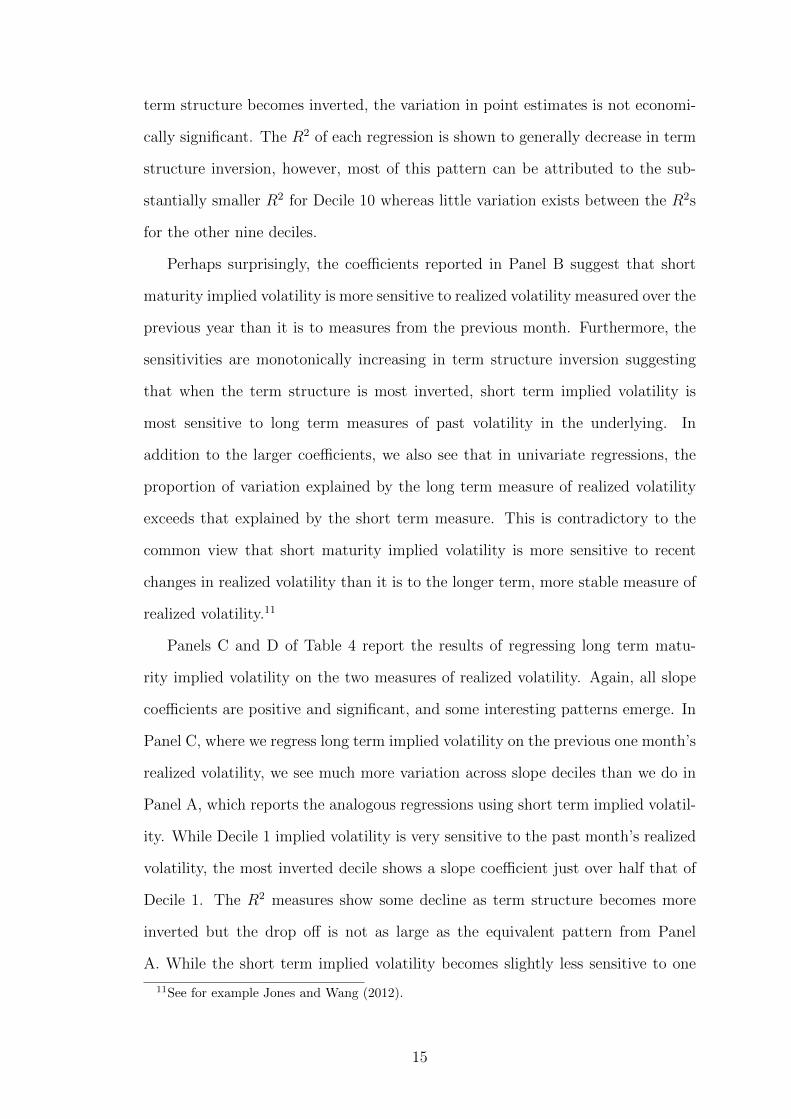
term structure becomes inverted, the variation in point estimates is not economi-

cally significant. The R2 of each regression is shown to generally decrease in term

structure inversion, however, most of this pattern can be attributed to the sub-

stantially smaller R2 for Decile 10 whereas little variation exists between the R2s

for the other nine deciles.

Perhaps surprisingly, the coefficients reported in Panel B suggest that short

maturity implied volatility is more sensitive to realized volatility measured over the

previous year than it is to measures from the previous month. Furthermore, the

sensitivities are monotonically increasing in term structure inversion suggesting

that when the term structure is most inverted, short term implied volatility is

most sensitive to long term measures of past volatility in the underlying. In

addition to the larger coefficients, we also see that in univariate regressions, the

proportion of variation explained by the long term measure of realized volatility

exceeds that explained by the short term measure. This is contradictory to the

common view that short maturity implied volatility is more sensitive to recent

changes in realized volatility than it is to the longer term, more stable measure of

realized volatility.11

Panels C and D of Table 4 report the results of regressing long term matu-

rity implied volatility on the two measures of realized volatility. Again, all slope

coefficients are positive and significant, and some interesting patterns emerge. In

Panel C, where we regress long term implied volatility on the previous one month’s

realized volatility, we see much more variation across slope deciles than we do in

Panel A, which reports the analogous regressions using short term implied volatil-

ity. While Decile 1 implied volatility is very sensitive to the past month’s realized

volatility, the most inverted decile shows a slope coefficient just over half that of

Decile 1. The R2 measures show some decline as term structure becomes more

inverted but the drop off is not as large as the equivalent pattern from Panel

A. While the short term implied volatility becomes slightly less sensitive to one

11See for example Jones and Wang (2012).

15

month previous realized volatility when the curve becomes inverted, the long term

implied volatility becomes much less sensitive. However, when the curve is least

inverted, the long term implied volatility is more sensitive to the previous one

month’s volatility than is the short term implied volatility.

In Panel D where we examine the relation between the previous year’s realized

volatility and long term maturity implied volatility we see higher slope coefficients

as compared with Panel C. This is consistent with the finding for the one month

implied volatility in Panels A and B. However, here we see a weak decreasing

pattern in the slope coefficients as the term structure becomes more inverted.

While this contrasts with the increasing pattern seen in Panel B, it is more in line

with the general intuition that as the term structure becomes inverted, long term

maturity implied volatility is less sensitive to previous realized volatility measured

over long horizons.

We extend our analysis of the impact of realized volatility to include the term

structure itself. Table 5 reports the results of cross-sectional regressions similar

to those in Table 4 except with term structure slope as the dependent variable.

Each month, within each decile, term structure slopes are regressed on the real-

ized volatilities of the underlying, calculated using past daily returns over a fixed

horizon. Each of the resulting monthly cross-sectional regression coefficients are

then averaged over the entire time series.

Panel A reports the results for regressions with realized volatility calculated

using the returns of the underlying over the previous month. Panel B reports the

results from similar regressions where realized volatility is measured over the pre-

vious year’s daily returns. Recall that our term structure measure is a percentage

difference between long and short term maturity implied volatility so that we are

essentially controlling for the level of implied volatility. In both regressions we

see a monotonic decline in both slope coefficients and R2s as we move from least

inverted to most inverted term structure. This suggests that as the term structure

becomes more inverted, the slope is less determined by past realized volatility. If

16

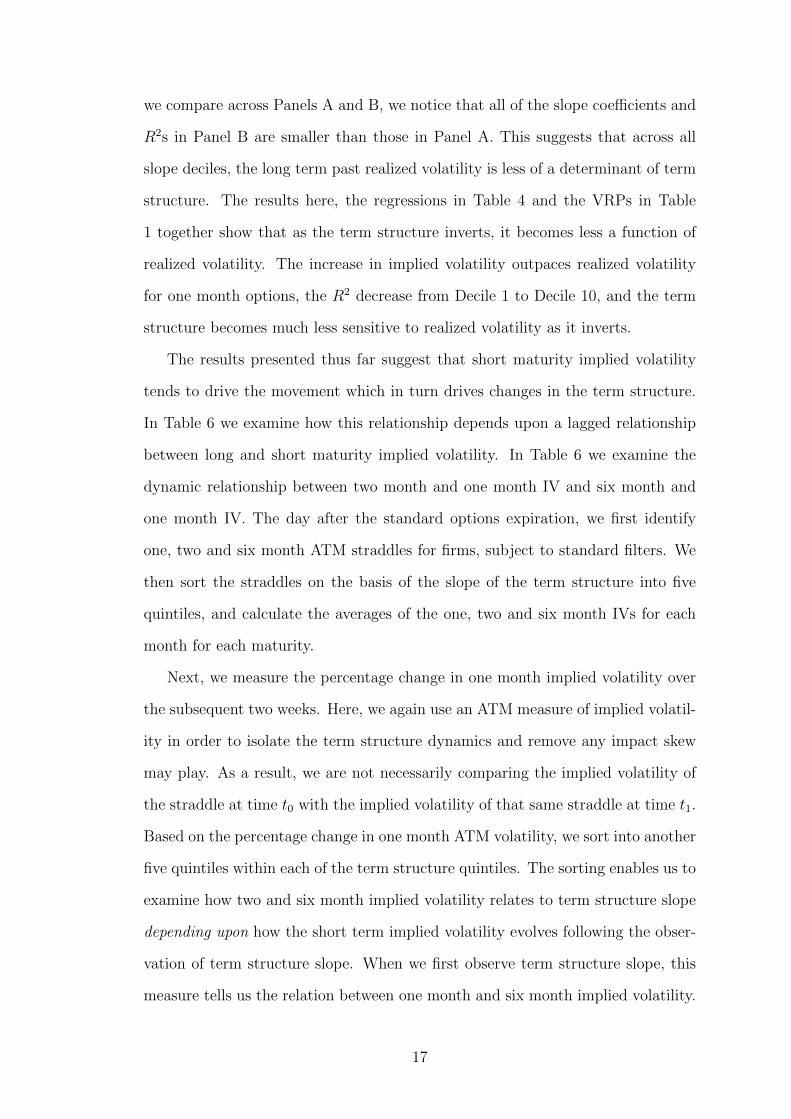
we compare across Panels A and B, we notice that all of the slope coefficients and

R2s in Panel B are smaller than those in Panel A. This suggests that across all

slope deciles, the long term past realized volatility is less of a determinant of term

structure. The results here, the regressions in Table 4 and the VRPs in Table

1 together show that as the term structure inverts, it becomes less a function of

realized volatility. The increase in implied volatility outpaces realized volatility

for one month options, the R2 decrease from Decile 1 to Decile 10, and the term

structure becomes much less sensitive to realized volatility as it inverts.

The results presented thus far suggest that short maturity implied volatility

tends to drive the movement which in turn drives changes in the term structure.

In Table 6 we examine how this relationship depends upon a lagged relationship

between long and short maturity implied volatility. In Table 6 we examine the

dynamic relationship between two month and one month IV and six month and

one month IV. The day after the standard options expiration, we first identify

one, two and six month ATM straddles for firms, subject to standard filters. We

then sort the straddles on the basis of the slope of the term structure into five

quintiles, and calculate the averages of the one, two and six month IVs for each

month for each maturity.

Next, we measure the percentage change in one month implied volatility over

the subsequent two weeks. Here, we again use an ATM measure of implied volatil-

ity in order to isolate the term structure dynamics and remove any impact skew

may play. As a result, we are not necessarily comparing the implied volatility of

the straddle at time t0 with the implied volatility of that same straddle at time t1.

Based on the percentage change in one month ATM volatility, we sort into another

five quintiles within each of the term structure quintiles. The sorting enables us to

examine how two and six month implied volatility relates to term structure slope

depending upon how the short term implied volatility evolves following the obser-

vation of term structure slope. When we first observe term structure slope, this

measure tells us the relation between one month and six month implied volatility.

17

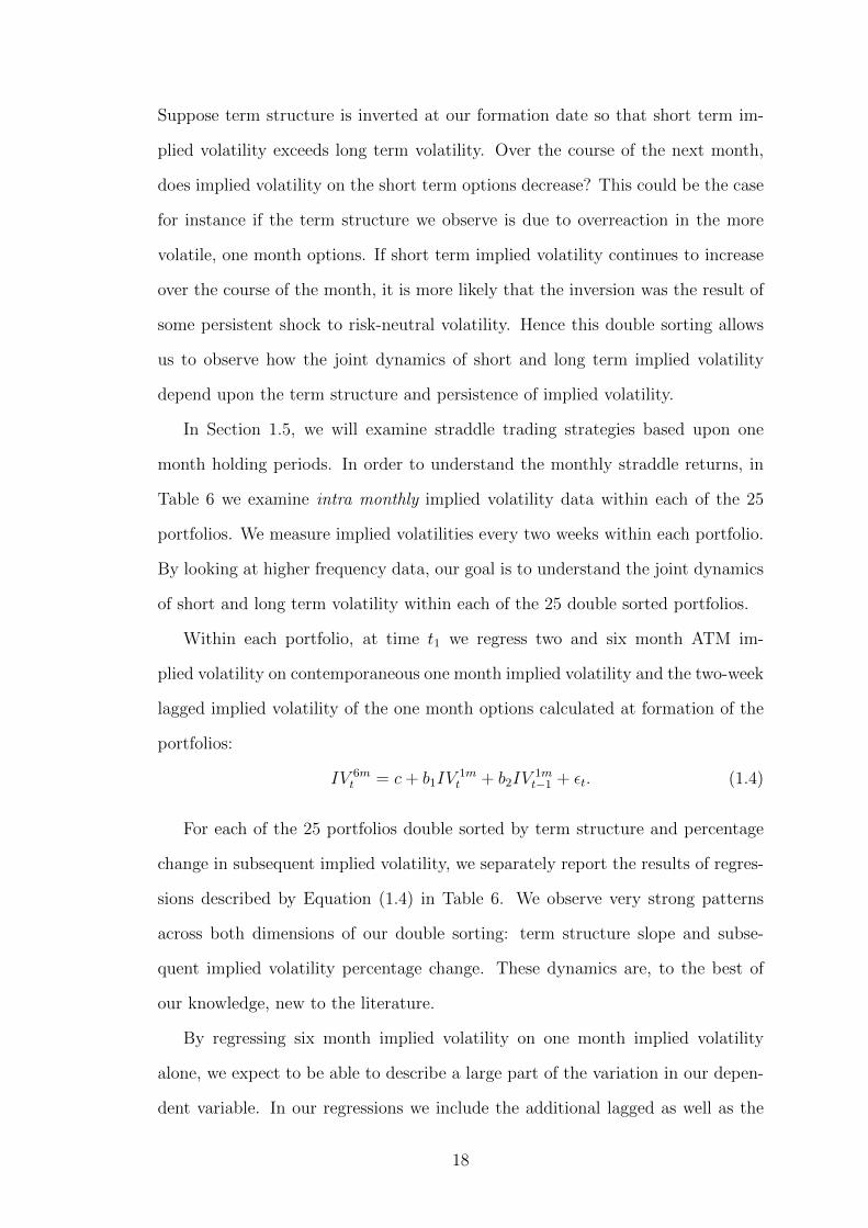
Suppose term structure is inverted at our formation date so that short term im-

plied volatility exceeds long term volatility. Over the course of the next month,

does implied volatility on the short term options decrease? This could be the case

for instance if the term structure we observe is due to overreaction in the more

volatile, one month options. If short term implied volatility continues to increase

over the course of the month, it is more likely that the inversion was the result of

some persistent shock to risk-neutral volatility. Hence this double sorting allows

us to observe how the joint dynamics of short and long term implied volatility

depend upon the term structure and persistence of implied volatility.

In Section 1.5, we will examine straddle trading strategies based upon one

month holding periods. In order to understand the monthly straddle returns, in

Table 6 we examine intra monthly implied volatility data within each of the 25

portfolios. We measure implied volatilities every two weeks within each portfolio.

By looking at higher frequency data, our goal is to understand the joint dynamics

of short and long term volatility within each of the 25 double sorted portfolios.

Within each portfolio, at time t1 we regress two and six month ATM im-

plied volatility on contemporaneous one month implied volatility and the two-week

lagged implied volatility of the one month options calculated at formation of the

portfolios:

IV 6mt = c+ b1IV

1mt + b2IV

1mt−1 + εt. (1.4)

For each of the 25 portfolios double sorted by term structure and percentage

change in subsequent implied volatility, we separately report the results of regres-

sions described by Equation (1.4) in Table 6. We observe very strong patterns

across both dimensions of our double sorting: term structure slope and subse-

quent implied volatility percentage change. These dynamics are, to the best of

our knowledge, new to the literature.

By regressing six month implied volatility on one month implied volatility

alone, we expect to be able to describe a large part of the variation in our depen-

dent variable. In our regressions we include the additional lagged as well as the

18

contemporaneous 1 month implied volatility. Across all but one of the 25 portfo-

lios, the regression R2s exceed 92%. The portfolio with the steepest upward sloped

term structure and the lowest subsequent percentage change in implied volatility

(Portfolio (1,1)) has an R2 of only 82.2%. In each of the portfolios, the parameters

of the regression equations are estimated with a high degree of precision.

We observe several novel results within Table 6. The patterns relating dy-

namics across portfolios are important for informing the trading strategies we will

describe in Section 1.5. First, we find that regardless of the percentage change

in implied volatility, the sensitivity of six month implied volatility to contempo-

raneous one month implied volatility monotonically decreases in term structure

inversion. On the other hand, the sensitivity of six month to the (two week)

lagged one month implied volatility is monotonically increasing in term structure

inversion regardless of subsequent changes in implied volatility. That is, within

each implied volatility change quintile, six month implied volatility’s sensitivity to

contemporaneous short term volatility decreases in term structure inversion while

the sensitivity to lagged short term inversion increases in term structure inversion.

More succinctly, the more inverted the term structure is, the more six month im-

plied volatility lags behind one month implied volatility. Within each of the five

quintiles sorted on implied volatility we have strict monotonicity. This combined

with the fact that the regression coefficients are estimated with strong precision

suggests that the relationship is very robust.

In addition to the patterns across term structure inversion, we also look across

the portfolios sorted on implied volatility changes. Interestingly, the pattern de-

scribed in the previous paragraph is stronger for portfolios with the larger change

in subsequent one month implied volatility. The relationship is monotonic in the

following sense: within each term structure portfolio, the sensitivity of long term

implied volatility to contemporaneous short term implied volatility is decreasing

in subsequent short term implied volatility change. On the other hand the sensi-

tivity to the lagged short term implied volatility is increasing as we move down

19

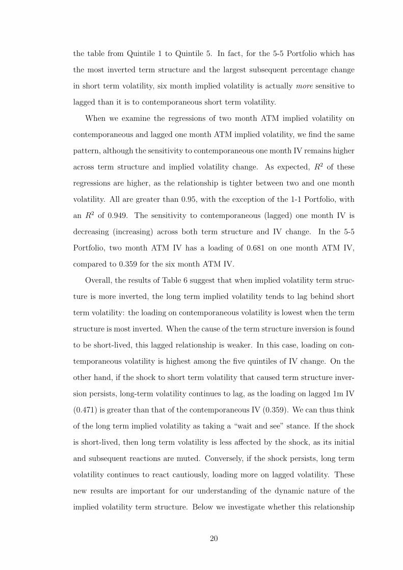
the table from Quintile 1 to Quintile 5. In fact, for the 5-5 Portfolio which has

the most inverted term structure and the largest subsequent percentage change

in short term volatility, six month implied volatility is actually more sensitive to

lagged than it is to contemporaneous short term volatility.

When we examine the regressions of two month ATM implied volatility on

contemporaneous and lagged one month ATM implied volatility, we find the same

pattern, although the sensitivity to contemporaneous one month IV remains higher

across term structure and implied volatility change. As expected, R2 of these

regressions are higher, as the relationship is tighter between two and one month

volatility. All are greater than 0.95, with the exception of the 1-1 Portfolio, with

an R2 of 0.949. The sensitivity to contemporaneous (lagged) one month IV is

decreasing (increasing) across both term structure and IV change. In the 5-5

Portfolio, two month ATM IV has a loading of 0.681 on one month ATM IV,

compared to 0.359 for the six month ATM IV.

Overall, the results of Table 6 suggest that when implied volatility term struc-

ture is more inverted, the long term implied volatility tends to lag behind short

term volatility: the loading on contemporaneous volatility is lowest when the term

structure is most inverted. When the cause of the term structure inversion is found

to be short-lived, this lagged relationship is weaker. In this case, loading on con-

temporaneous volatility is highest among the five quintiles of IV change. On the

other hand, if the shock to short term volatility that caused term structure inver-

sion persists, long-term volatility continues to lag, as the loading on lagged 1m IV

(0.471) is greater than that of the contemporaneous IV (0.359). We can thus think

of the long term implied volatility as taking a “wait and see” stance. If the shock

is short-lived, then long term volatility is less affected by the shock, as its initial

and subsequent reactions are muted. Conversely, if the shock persists, long term

volatility continues to react cautiously, loading more on lagged volatility. These

new results are important for our understanding of the dynamic nature of the

implied volatility term structure. Below we investigate whether this relationship

20

can be exploited in a profitable trading strategy.

1.4 Framework

In this section we encapsulate the basic properties of long and short term implied

volatility uncovered above. In Section 1.5, we examine trading strategies as a

verification of our findings. While we take the information presented in Tables 2

through 6 as the basis for our framework, we use only the most salient features.

As a result, the framework we describe below is intentionally very simple in order

to plainly show where potential for profitable trading strategies emerge.

Here, we assume that when we see the term structure invert, there has been

some sort of positive shock to implied volatility in the pricing of short term (one

month) options. Of course it is a simplification to assume that the inverted term

structure is due only to a positive shock to implied volatility of short term options.

However, the summary statistics in Table 2 show that the majority of movement

in implied volatility resulting in inverted term structure is due to the short term

options. To see this, note that for the one month options, the difference between

the average IV for the least inverted and most inverted volatility term structure

is more than 20% versus a difference of less than 5% in the long term options.

The fact that Table 2b shows time series standard deviations of average implied

volatilities are much larger for the one month options than for the six month

options further informs our simplifying assumption that term structure inversion

is due solely to movement in implied volatilities to one month options.

In Panel C of Table 2, we see that average implied volatility has a positively

skewed distribution for all bins and the skewness is greatest among the most

inverted (Decile 10). For this reason, when we model shocks to implied volatility

of firms with inverted term structure, we will only look at positive shocks to

volatility. As a result our simplified distributions will have only two levels: a

baseline and high level of implied volatility. This is the simplest way for us to

model a positively skewed distribution, where the baseline volatility has a larger

21

probability mass than that of the high level. Let V sB denote the baseline volatility

and let V sH denote the high level volatility of short term options, where V s

B < V sH .

We will further assume that returns to straddles are exactly replicated by buying

and selling the level of implied volatility. So, if we buy a short term straddle at

time t and sell it at time t+1, then our straddle returns are given by (V st+1−V s

t )/V st ,

where V st denotes short term (1 month) implied volatility at time t.

Here, an inverted term structure is driven by a shock to only short term volatil-

ity. We further assume that if the shock ultimately persists, then the long term

implied volatility will adjust accordingly, after it is determined that the shock was

not noise. Importantly, this revelation takes place sometime after we first observe

the inverted term structure but before the end of the holding period in which

we trade. This is a simplification of the results presented in Table 6 where we

show that when the term structure becomes inverted and we witness a persistent

shock to short term implied volatility, six month implied volatility tends to load

more heavily on lagged short term implied volatility. On the other hand, when

term structure is inverted but the shock turns out not to be persistent, six month

implied volatility tends to load less heavily on lagged short term implied volatility.

Assume that we observe a shock to short term volatility, or equivalently, an

inverted term structure of volatility. Given the inverted term structure curve, the

probability that the shock causing the inversion is fundamental (as opposed to just

noise) we denote by pf . The probability of the shock being pure noise is 1 − pf .

The trading strategies we describe are based upon first observing that a shock has

occurred, and then buying and selling option straddles accordingly.

If we observe an inverted term structure today, then at the end of our holding

period, we either realize that the shock was just noise, in which case one month

implied volatility reverts to its baseline level V sB, or, if the shock turns out to

be fundamental, then the volatility remains at the high level, V sH . Similarly, six

month implied volatility has a skewed distribution (see Table 2) and we assume

that it has a baseline and high level V LB < V L

H , where V LB denotes the baseline and

22

V LH denotes the high level for long term options.

There are two trading strategies we examine once we observe an inverted term

structure. Strategy 1 buys short term straddles. Strategy 2 buys long term strad-

dles. Strategy 1 realizes negative returns when the shock we observe turns out to

be noise. Strategy 2 makes money when the shock persists.

The expected returns to Strategy 1 are:

E(R1) = 0 · pf + (1− pf )(V s

B − V sH)

V sH

< 0.

The expected returns to Strategy 2 are given by:

E(R2) = pf(V L

H − V LB )

V LB

+ 0 · (1− pf ) > 0.

In terms of comparative statics, both strategies will see a larger return when the

spread between VH and VB is higher. Also, if the probability of a shock turning out

to be fundamental (pf ) is large, then Strategy 2 has a higher (positive) expected

return. On the other hand the returns to Strategy 1 are most negative when if

the probability of a shock being fundamental (pf ) is low.

1.5 Trading

Given the joint dynamics we’ve shown for short and long term implied volatility,

we next investigate whether these translate to profitable trading strategies using

option straddles. Based upon our framework from Section 1.4 for understanding

the patterns observed in the implied volatility data, we propose trading strategies

which we show bear out the predictions of our framework.

Table 7 reports the returns and standard errors for straddle portfolios of dif-

ferent maturities and the long/short portfolio which owns Portfolio 10 and shorts

Portfolio 1. Sharpe Ratios are included for the one and six month options portfo-

lios and the calendar spread portfolios. The holding period for all is one month,

with the exception of the first stanza, which shows the returns of portfolios of

23

one month straddles held for two weeks. The returns for both versions of the

one month portfolios echo the findings of Vasquez (2015): the returns on strad-

dle positions decrease as the term structure becomes more inverted. Holding the

Decile 10 portfolio to expiry costs 11.85% monthly, while owning Decile 1 port-

folio returns 2.55% per month. A portfolio which buys Decile 1, and sells Decile

10 returns 14.41% monthly, posting a Sharpe Ratio of 2.723. While the returns

of Decile 1 are not statistically significant, those of Decile 10 and the long/short

position are highly significant. As discussed above, as term structure becomes

more inverted, the change in implied volatility outpaces that of realized volatility;

one interpretation is the implied volatility is overreacting to the movement of the

underlying.

The returns for the two month options generally follow the pattern seen in

the one month options. While not monotonic, the returns decrease moving from

Decile 1 to 10. The Decile 1 portfolio returns 2.46%, while Decile 10 loses 45 bps

per month. A portfolio that is long Decile 1 and short Decile 10 returns 2.91%

monthly, and is highly significant. Throughout the paper, we include two month

option portfolios as a short term strategy alternative to the one month straddles.

We do this to ameliorate any concerns that the abnormally large returns in the one

month options are the result of biases arising around the time of option expirations.

For the three to five month portfolios, a change in sign of the 10-1 Portfolios is

seen. For the long/short portfolios with one and two month maturities, a positive

return is generated if we buy Portfolio 1 and sell Portfolio 10. For spread portfolios

with maturities of four and five months, the opposite position is needed to post

a positive return. The 10-1, four month Portfolio (long Decile 10, short Decile 1)

earns 0.58% per month and is statistically significant at the 10% level; the 10-1,

five month Portfolio posts a significant 2.14% monthly return. In addition, the five

month returns increase monotonically across deciles, with the exception of Decile

9.

Recall from Table 2 that for portfolios of six month maturity options, implied

24

volatilities increase as the term structure becomes more inverted. From Table 1,

however, we know that the difference in implied volatilities across deciles of six

month options is smaller than the average difference in realized volatility across

deciles. The returns for long maturity straddle portfolios mirrors this pattern

insofar as straddle returns mirror percentage changes in implied volatility and we

see higher returns in Decile 10 than in Decile 1. In contrast to the findings of

Vasquez (2015) for the short maturity straddles, the long maturity returns are

strongly monotone and increase from Decile 1 to 10. Buying Portfolio 10 earns

3.42% month, is statistically significant and posts a Sharpe Ratio of 1.391. As this

is a long volatility portfolio, the returns are negatively correlated to the S&P 500

Index (-0.416). The 10-1 Portfolio, while earning less than Decile 10 since Decile

1 also has positive returns, posts a higher Sharpe Ratio, 1.697, due to the lower

volatility of the spread portfolio.

In practice, a common options strategy is the calendar, or time spread, whereby

options with the same strike but different maturities on the same underlying are

bought and sold. The bottom panel in Table 7 holds the returns of calendar

spreads in aggregate. For each decile, the returns represent a trade where the

six month options portfolio is bought and the one month portfolio is sold. Given

the dynamics seen in both the one and six month options portfolios, it is perhaps

unsurprising that we see increasing monotonicity in the returns. Decile 1 loses

1.56% monthly, while the Decile 10 spread earns a significant 15.35% per month,

with a Sharpe Ratio of 3.123. Finally, a calendar spread spread: a position which

buys the calendar spread of Decile 10 and sells that of Decile 1 (buying six month,

Decile 10, selling one month, Decile 10; selling six month, Decile 1, buying one

month, Decile 1) returns 16.90%, with a Sharpe Ratio of 3.312.

Figure 3 shows the monthly returns to the one, two, and six month long/short

straddle portfolios based upon term structure slope. The return spikes seen for

the one month portfolio coincide with market deciles. The portfolio formed after

the August 2001 expiration posts the largest monthly loss, 94.5%, for the sample.

25

Other spikes occur during the financial crisis, the European debt crisis, and the

mini-flash crash in August, 2015. During volatility spikes, then, the losses from

shorting the undervalued options in Decile 1 outpace the gains from owning the

overvalued options in Decile 10. The returns of the two month portfolio are highly

correlated (0.82) to those of the one month portfolio, as in both cases Decile 1 is

bought and Decile 10 is sold, and as shown above the dynamics of the two are

similar. In contrast, the correlation of the six month returns to the one month is

-0.28.

Returning to our framework, we expect the returns of the one month straddles

to be most negative when the term structure is inverted and the volatility shock

turns out to be transitory. And, if the shock persists, the returns seen are muted,

as implied volatility already is elevated. In contrast, if the volatility shock has no

follow through, we expect the losses on the six month straddles to be mollified as

there was an underreaction relative to the front part of the curve. We test our

model by performing an ex post double sort on returns. The day after the standard

options expiration, we identify one, two and six month ATM straddles for firms,

subject to standard filters. We then sort the straddles on the basis of the slope

of the term structure into five quintiles, and hold the positions for one month.

After one month, we sort the portfolios into three buckets, based on the average

percentage change in realized volatility for the underlying firms over the course

of the month-long holding period. Portfolio sorting exercises are typically used as

a model free way to test whether a premium is earned via a trading strategy as

a result of bearing risk. The sorting we do in Table 8 is obviously not meant to

analyze a trading strategy as the second sort is done ex post. We include the ex

post sorting procedure as a way to further analyze the predictions of our simple

model of the dynamics of implied volatility. Table 8 helps us understand from

where the returns described in Table 7 come.

The columns of Table 8 represent quintile portfolios based upon the term struc-

ture slope: column one represents least inverted while column five represents most

26

inverted. The last column contains the returns of a 5-1 Portfolio, which is long

Portfolio 5 and shorts Portfolio 1. The three rows within each panel represent

the ex post sorting by percentage change in realized volatility of the underlying

stock: within the five deciles, the first row represents the averages of those stocks

whose percentage change in realized volatility is smallest while the third row rep-

resents those with the largest percentage change in realized volatility. Finally, the

intersection of the right-most column with the final row measures the return of

a portfolio which is long the 5-1 Portfolio of ∆ RV Bucket 3 and short the 5-1

Portfolio of ∆ RV Bucket 1, where ∆ RV denotes the percentage change in realized

volatility. This portfolio buys the high minus low portfolio in the highest ∆ RV

tercile and shorts the high minus low portfolio in the lowest ∆ RV tercile.

We can think of the double sorted portfolios as a model free way of examining

how returns vary across straddles when we vary both term structure slope and

percentage changes in subsequent realized volatility. The 5-1 Portfolios represent

differences in returns due to differences in term structure slope, controlling for

∆RV terciles. Similarly, differences along the ∆RV columns show how straddle

returns vary within quintiles defined by term structure slope. The bottom row,

right most column which reports the difference in the long short portfolios across

∆ RV tercile can be interpreted as a nonparametric measure of the interaction

between term structure slope and ∆ RV: it measures how variation in returns

across term structure slope will vary as ∆ RV varies. The analogous regression

would regress straddle returns on term structure slope, ∆RV and an interaction

term:

rs = a+ β1TS + β2∆RV + β3TS ·∆RV + ε, (1.5)

where rs denotes straddle returns and TS denotes term structure slope. In all

three Panels of Table 8 we see large and significant spreads across all ∆RV and

term structure portfolios. This is akin to significant point estimates of β1 and

β2. The bottom right entry in each panel is akin to the point estimate of β3. The

27

advantage of the double sorts as opposed to the regression equation is that the

sorting does not rely on any parametric assumption. The regression equation in

(1.5) on the other hand assumes a very specific linear relationship between straddle

returns, the two explanatory variables and the interaction term.

Table 8 is similar to Table 6 in that we look at portfolios which are first

sorted on volatility term structure and then, within each slope portfolio, sorted

by subsequent ex post changes in volatility. Whereas the second sort in Table 6 is

based upon one month option implied volatility, the second sort in Table 8 is based

upon changes in realized volatility in the underlying. Table 6 is informative for

understanding the dynamic relationship between short term and long term implied

volatility. However, in order to compare the returns of one month, two month and

six month straddles in Table 8 we measure subsequent volatility using realized

volatility of the underlying asset rather than one month implied volatility so that

there is less of a mechanical relation between returns and changes in subsequent

volatility.

As we show in Table 8, the behavior of long term implied volatility depends

upon whether or not volatility persists after the portfolio formation date. When

our variable of interest is straddle returns, we sort on subsequent changes in real-

ized volatility as our measure. If term structure is inverted on the sort date and

realized volatility of the underlying asset grows over the subsequent month, we

consider this a fundamental change in volatility that was captured by the inverted

term structure. Our framework of volatility term structure dynamics suggests

that if term structure becomes inverted and volatility persists then the long term

straddle will see positive returns. Furthermore, if the long term straddle returns

are largely reliant on a positive relation to fundamental volatility of the underlying

asset, then we expect to see larger returns to the long term 5-1 strategy when ∆ RV

is large rather than small. This is exactly what we see in Table 8. Consistent with

Table 7 the 5-1 strategy for long term volatility earns positive returns in all three

∆ RV terciles, and the returns for the high minus low strategy are increasing in

28

∆ RV terciles. As the last column, final row shows, the difference between the 5-1

returns in the largest and smallest ∆ RV deciles is both statistically and econom-

ically significant at 2.73% per month, suggesting a significant interaction between

term structure slope and subsequent volatility. This is consistent with the results

of Table 6 where we see that the dynamics of six month implied volatility depend

upon the slope of the term structure and the contemporaneous volatility (mea-

sured by one month implied volatility). Here our sorts illustrate in nonparametric

fashion an interaction effect between term structure slope and realized volatility.

Panels A and B of Table 8 report the returns for the one month and two month

straddles respectively. We discuss these two panels together as the short maturity

straddle returns. In both cases, the high minus low term structure portfolios

earn negative returns in all three ∆ RV terciles, consistent with Table 7. In

neither panel is the difference between the high minus low strategy siginificantly

different between the highest and lowest ∆ RV terciles. We can however see a

large spread between returns in ∆ RV Terciles 3 and 1 within each of the term

structure quintiles. This suggests that both the term structure and changes in

realized volatility over the holding period are significant determinants of straddle

returns. However, unlike the returns of the long maturity straddles, it does not

appear that there is as significant an interaction effect between the term structure

and subsequent volatility sorts. It is important to remember that the sorts used

for Panels A, B and C are all exactly the same since they are based upon the

underlying as opposed to the options. So the fact that we see an interaction for

the six month options but not a strong interaction effect for the short term options

is not due to differences in break points for the sorts. Rather this difference is due

to differences in the pricing of short and long maturity options.

Surprisingly, for the one month straddles in Panel A, the high minus low port-

folio returns are fairly consistent across ∆ RV terciles and the point estimate are

not monotonic. While there are very large spreads across ∆ RV terciles, within

each of the term structure quintiles, there does not seem to be any sign of an inter-

29

action between the term structure and realized volatility in determining straddle

returns. For the two month straddle returns of Panel B, just as in Panel A, the

spread in returns across the ∆ RV terciles is significant for each of the five term

structure portfolios. For the two month straddle returns however, there is a weak

monotonic relation in the 5-1 column but the difference between the high ∆ RV

and low ∆ RV terciles is not significant in this column. Since the sorting in all

three panels of Table 8 is the same, we can confidently say that the interaction

effect is stronger for the long term options than it is for the short term options.

Overall, the results presented in Table 8 suggest that the spread we observe in

straddle returns based upon term structure sorts in the longer maturity options

is to a large extent due to interaction between the term structure and changes

in volatility of the underlying. There is a positive relationship between the term

structure-based, long maturity trading strategy described in Table 7 and changes

in the underlying volatility. The reason for the positive interaction is also alluded

to in Table 6. There we show that the way six month implied volatility reacts to

changes in short term implied volatility differs across portfolios formed on term

structure slope. The way it varies across term structure portfolios actually de-

pends upon subsequent changes in short term implied volatility. We see another

manifestation of the interaction effect in Panel C of Table 8 where difference in

long short portfolio returns across ∆RV terciles is significant.

Various measures have been proposed in the literature to examine whether

options markets overreact. The measures of which we are aware do not necessar-

ily consider specific events with respect to which we observe a reaction. Rather,

short term implied volatility is compared with a longer term measure of volatility.

Movements away from this long term measure have been deemed to be overreac-

tions. The summary statistics described in Table 2 show that short term options

show higher implied volatility as well as more volatile and skewed distributions of

average implied volatilities. Furthermore, the dichotomy between implied volatil-

ity of short term and long term options is magnified when we look at the most

30

inverted term structure portfolio. As a result, we examine the relation between

overreaction of short term options and the implied volatility term structure.

While we witness an interaction between term structure and realized volatility

in the long term options, we fail to see the same in the short-term options. We

posit that the movement in the short-term options may be an overreaction to an

expectation of future volatility, and so, in our model, the returns may be muted

from any persistence in volatility. We examine three measures of overreaction

in the short term options. The first, 1mIV12mRV

− 1, compares one month IV to

twelve month RV (Goyal and Saretto (2009)); the second is the VRP, measured as

1mIV1mRV

−1; and the third, 1mIVIVave

−1, compares one month IV to a six month average

of one month IV. For measures one and two, realized volatility is calculated based

on the daily closes of the underlying. After firms are sorted into ten portfolios

according to term structure, the averages of these three measures and the term

structure are calculated for each firm and then averaged for each portfolio each

month. Table 9 reports the time series correlations of the three measures with

that of IV term structure.

Panel A reports the average of each overreaction measure for each decile over

the entire sample. All three of the measures are increasing in term structure in-

version deciles. This suggests that as term structure becomes more inverted so

that the one month implied volatility exceeds six month implied volatility, the

overreaction measures monotonically increase. This is intuitive since the overre-

action measures depend on an increase as current one month implied volatility

increases, and the same is true of term structure inversion. Of course each of the

overreaction measures has a different volatility measure with which to compare

current one month implied volatility. In this sense, the volatility term structure

can be thought of as a measure of overreaction in that it compares short term

implied volatility to six month IV, a more stable measure.

Panel B describes the time series correlation between our measure of volatility

term structure and each overreaction measure within each portfolio. All three

31

of the overreaction measures are positively correlated with the volatility term

structure and we see an increasing pattern in the correlations as we move from

Decile 1 to Decile 10. This suggests that the inverted term structure is more

correlated with measures of overreaction in short term implied volatility, and is

explored in Vasquez (2015). To test whether the movement in short-term volatility

may be an overreaction, we take the monthly portfolio returns summarized in

Table 7, and regress them on the returns of an “under” and “over” portfolio. The

“under” and “over” portfolios are formed by sorting eligible straddles according to

the overreaction measure 1mIV12mRV

− 1 from Goyal and Saretto (2009). The “under”

portfolio consists of firms in Decile 1: underreaction. The “over” portfolio consists

of firms in Decile 10: overreaction. The “overunder” factor used to examine the

10-1 returns is a long-short portfolio which owns the “over” and shorts the “under”

portfolios. Table 10 examines the possibility that overreaction or underreaction is

driving the results presented in Section 1.5. Vasquez (2015) finds limited evidence

suggesting that overreaction can explain some of the returns to a trading strategy

involving one month straddles held for a week long period.

We examine the ability of our overreaction measure to account for returns

to the straddle portfolio strategy described in Table 7. We focus only on the

short term and long maturity straddle portfolios since these are where we see

the largest and most significant returns. For the long maturity straddles, we use

only the six month straddles. For the short maturity straddles we examine both

one month and two month straddle portfolios. We look at both because the one

month straddle portfolios potentially could be adulterated by events around option

expiration. Since the two month straddles are sold with one month remaining on

the straddles, this avoids any noise that could be attributed to erratic movements

around expiration.

Panel A of Table 10 reports the results for one month options held to expiration.

The coefficients on the underreaction as well as the overreaction factor returns are

significant at the 1% level for most of the ten portfolios. We observe a trend

32

in each of the coefficients across deciles. As one would expect, the loading on

“underreaction” tends to be higher for the lower deciles and lower for the higher

deciles. Conversely, there is a monotonic pattern in the “overreaction” coefficient.

Loadings on the overreaction factor are increasing as we move from least inverted

(Decile 1) to most inverted (Decile 10). In the final column of Panel A, we regress

the 10-1 portfolio on the “overunder” factor. The alpha is significantly different

from zero however, at -5.03%, its magnitude is about one third of the 10-1 straddle

return of -14.41% reported in Table 7. This means that the traded “overunder”

measure captures about two thirds of the returns associated with the one month

straddle strategy based upon term structure slope.

In Panel B, we further investigate the relation between short maturity straddle

returns and the overreaction measure, using two month options. Recall that the

10-1 returns for two month options described in Table 7 shows highly significant

negative returns. The mean returns to the two month straddles are only 2.91%

per month, not nearly as large as the one month straddle returns. In Panel B

of Table 10, we see the same general pattern as described in Panel A. The most

important difference however is that when we control for the “overunder” factor,

the returns to the 10-1 portfolio are no longer statistically significant for the two

month straddles. The intercept or the point estimate for unexplained returns are

actually positive but insignificant at 0.21% per month. This further suggests that

a large part of the returns we described in Table 7 for the short maturity options

can be attributed to the measure of overreaction.

Panel C of Table 10 shows the results when portfolios of our six month straddles

are regressed on the over and underreaction factors and the long-short portfolio is

regressed on the overreaction minus underreaction factor. Although the loadings

on each of these factors are not monotonic across the deciles, there is a general

pattern of increasing sensitivity to the overreaction measure and a decreasing

sensitivity to the underreaction factor as term structure becomes more inverted.

When we regress the long-short portfolio on the “overunder” factor, the intercept

33

remains highly significant and the magnitude actually increases from the returns

reported in Table 7: from 2.62% to 3.37% per month.

The results of Table 10 suggest that a large portion of the returns to the

short maturity straddle portfolio strategy based upon term structure slope can be

attributed to a measure of overreaction documented by Goyal and Saretto (2009).

For the one month straddles, about two thirds of the returns to the 10-1 Portfolio

can be attributed to the overreaction factor but the unexplained returns are still

significant. When we use two month straddles as our short maturity options

in order to avoid calculating returns near expiration, we find that the returns

unexplained by the overreaction factor are no longer significant. On the other

hand, when we examine the long maturity straddles held for the same one month

holding period, the overreaction factor cannot explain the returns shown in Table

7.

1.6 Robustness Checks

The analysis above supports the framework presented in Section 1.4. Here we ex-

amine the extent to which transactions costs, delta hedging, and upcoming earn-

ings announcements affect our findings. Table 11 holds the time series average of

the portfolio averages of firm size and the notional value of the firm’s options con-

tracts traded. The average size across term structure deciles is roughly constant,

and the notional average option volume traded exhibits no pattern across deciles,

but Decile 1 has the highest notional average dollar volume and Decile 10, the

portfolio which produces the largest return differential across the term structure,

has the lowest. In our calculations, the tables above have calculated returns using

the midpoint of the bid-ask spreads for all options. Since Decile 10 is comprised

of firms whose options are lightly traded, it is possible that transactions costs can

explain the returns. In addition to being lightly traded, Table 12, which contains

the options spreads sorted by maturity and decile, show that the options held in

Decile 10 have relatively wide bid-ask spreads.

34

Table 13 examines the impact of transactions costs on Decile 10 returns. The

one and six month Decile 10 portfolios, and the six month - one month calendar

spread, are sorted into three buckets based on the bid-ask spread. Bucket 1 (3)

holds options with a narrow (wide) spread. Since transactions costs are incorpo-

rated, the returns presented are consistent with the framework above: the one

month portfolio holds short options positions and the six month portfolio holds

long options. The six month-one month calendar spread holds long six month

options and short one month options. The first column displays returns as if they

were executed at the midpoint of the bid-ask spread. In this respect, the returns

are calculated as they are in Section 1.5, and all returns are positive and signifi-

cant, although they increase from Bucket 1 to 3. Columns two and three impose

transactions costs. The returns in column two assume a 50% effective spread;12

column three imposes a 100% effective spread where the full bid-ask spread is

crossed. The narrowest spread bucket produces positive significant returns for

the short one month options and the calendar spreads. Imposing a 50% (100%)

calendar spread produces 9.66% (7.78%) monthly and a 1.47 (0.80) Sharpe Ratio.

The second spread bucket manages to produce significant one month returns for

the 50% effective spread, generating a significant 4.99% monthly return and a 0.75

Sharpe Ratio. The portfolios with the widest bid-ask spreads find that returns

deteriorate when incorporating transactions costs as the calendar spread returns

are negative. The return dynamics persist when incorporating bid-ask spreads if

options with relatively narrow bid-ask spreads are held. However, since Decile

10 holds options with lower trading volume, limits may exist to capturing these

return differentials.

In explaining the interaction between term structure and volatility dynamics,

our framework centers on a term structure inversion witnessed in Decile 10, as the

short term implied volatility elevates in anticipation of an impending shock. Until

here, returns have been calculated by entering options positions and exiting them

12As an example, if the spread is $1.00 at $2.00, a 50% effective spread is $1.25 at $1.75. Thepurchase price here would be $1.75.

35

once the holding period ends. Table 14 examines whether the shock is manifested

in daily price movements in the underlying equity by delta hedging the options

daily. Return calculations follow the procedures set forth in Frazzini and Pedersen

(2012). At trade inception, straddles worth $1 worth are held, V0 = 1. Each day,

the value of the portfolio is computed iteratively as follows:

Vt = Vt−1 + x(Ft − Ft−1)− x∆t−1rSt St−1 + rft (Vt−1 − xFt−1 + x∆t−1St−1) (1.6)

where x = 1/F0, the number of options contracts; F is the option price; rs is

the daily stock return; rf is the daily risk free rate; and ∆ is the option’s delta.

The second term above represents the dollar return from the change in option

price, the profit or loss from the delta hedge is computed in the third term. The

final term calculates the financing cost of the position. The return to the position,

RT , is

RT = VT − V0 = VT − 1 (1.7)

The return patterns when delta hedging the options position mirror those from

Table 7. For one month options, the returns drop monotonically from 3.68% to

-7.30% from Decile 1 to Decile 10. The same occurs for the two month returns,

although the difference is smaller in magnitude. The 10-1 Portfolio, which owns

Decile 10 and shorts Decile 1, turns positive with three month options here, one

month earlier seen in Table 7, and is significantly positive for four through six

month options. Incorporating daily price movements do not materially impact

the return dynamics of options portfolios across the term structure.

Finally, it is possible that the returns from term structure inversions are driven

by known upcoming events. Table 15 holds the one, two, and six month option

returns, separated by whether the firm has an earnings release scheduled in the

next options expiration cycle. Interestingly, in the subsample where earnings

36

releases are upcoming, the returns for one month options, those with the highest

exposure to moves in the underlying stock, are higher than when there is no

upcoming earnings release. For Deciles 1 through 3, the returns are positive and

significant, from 18.44% to 9.52%, compared to 1.07% to -2.65% for the sample

without an upcoming earnings release. In either subsample, the patterns persist:

returns decrease from Decile 1 to Decile 10 for the one and two month options,

increase for the six month options, and the 10-1 Portfolio returns are significant.

Either sample supports our framework.

1.7 Conclusion

We examine the term structure of volatility in the cross-section of equity options

to reveal several novel facts. We show that term structure of volatility among

individual stocks behaves differently from that of the index. In the cross-section

we find that movements in the term structure are driven by changes in short term

volatility, and unlike in the index, the premia associated with volatility is strongly

dependent upon both horizon and slope of the volatility term structure. We show

that long term implied volatility is slow to react to these shocks in short term im-

plied volatility. Furthermore, the speed with which long term volatility reacts to

shocks depends upon the slope of the implied volatility curve. We propose a simpli-

fied framework for understanding our empirical findings. Based upon our analysis

and proposed framework, we propose strategies for trading ATM option straddles

across maturities. The returns to these trading strategies perform consistent with

the volatility term structure dynamics and the predictions of our framework. We

find that the profitability of our strategies in long maturity straddles are driven

by an interaction between the term structure and realized volatility. On the other

hand, short maturity straddle returns appear not to be be driven by this type of

interaction.

While the literature studying index options is much larger than that of options

on individual equities, the number of studies empirically examining the cross-

37

section of individual equity options has rapidly grown in recent years. The vast

majority of papers studying the cross-section of individual options examine only

those options with a fixed, single month to maturity. A number of option pricing

anomalies have been uncovered in the cross-section of these options. Often, these

anomalies are not existent in index options. This highlights the need for empirical

research in the cross-section of individual options in addition to the empirical

work studying index options. Our results provide a new and important way of

understanding option prices in the cross-section. We contribute to the literature

by studying the dynamics of options prices across maturities and term structure.

This allows us to uncover new empirical facts about the relative pricing of options

across maturities, a dimension that has until now been unexplored in the literature.

38

CHAPTER 2

VOLATILITY CARRY

2.1 Introduction

Asset managers have employed the carry trade for decades in foreign exchange.

The strategy, in which investors buy (sell) currency pairs forward when the for-

ward rate is at a discount (premium) to the current spot rate, has consistently

produced significant risk-adjusted returns.1 Carry owes its returns to the viola-

tion of the uncovered interest parity (UIP) hypothesis; Hansen and Hodrick (1980)

and Fama (1984) showed that forward foreign exchange rates are biased indica-

tors of future spot levels.2 The strategy has been studied extensively and has

been found to be positively exposed to crash risk, liquidity risk, volatility risk,

and peso problems.3 Across asset classes, the term structure of prices is central

to the analysis of carry, as the trade centers on the difference between spot and

forward price,4 and carry has been applied more generally to show that the returns

to carry permeate across assets: forward asset prices are poor predictors of future

spot asset prices, significant returns to carry exist, and as in foreign exchange,

the returns across asset classes generally are exposed to liquidity, volatility, and

1See, for example, Jurek (2014).2Also see Meese and Rogoff (1983) for an early examination of carry in the foreign exchange

market.3See Farhi and Gabaix (2015) for crash risk; Brunnermeier, Nagel, and Pedersen (2008)

for liquidity risk; Burnside, Eichenbaum, Kleshchelski, and Rebelo (2010) for peso problems;Menkhoff, Sarno, Schmeling, and Schrimpf (2012) and Lustig, Roussanov, and Verdelhan (2011)for volatility risk.

4Related studies to carry in other asset classes center on the basis in commodities, see Gorton,Hayashi, and Rouwenhorst (2013) and Yang (2013); and slope in bonds, see Fama and Bliss(1987) and Campbell and Shiller (1991).

39

macroeconomic factors.5 This analysis of term structure has been applied to index

options and volatility: Simon and Campasano (2014) and Johnson (2016) show

that the slope of the implied volatility term structure predicts returns, and VIX

futures prices are biased indicators of future spot levels of the VIX Index. Simon

and Campasano (2014) show that a VIX futures trading strategy centered on the

VIX basis produces positive returns, and Johnson (2016) shows that slope predicts

the returns to index variance assets generally. Koijen, Moskowitz, Pedersen, and

Vrugt (2013) find significantly positive returns when applying the concept to in-

dex option put and call prices. While these studies show that term structure slope

informs returns and profitable carry strategies in index options and index implied

volatility exist, Vasquez (2015) and Campasano and Linn (2017) show that the

index and equity option volatility dynamics conditional on term structure differ.

Index term structure slope is negatively related to variance returns across the term

structure; however, Campasano and Linn (2017) demonstrate that equity option

returns depend on an interaction between the slope of the term structure and the

horizon of the options: for short-dated options, term structure slope has a positive

relationship with equity option returns, for long-dated options, slope negatively

impacts returns. Due to these differences, I investigate the concept of carry in

the equity volatility market. I find that the strategy produces positive significant

returns, as forward volatility is not predictive of future spot volatility. Unlike the

returns to carry in other assets, however, I find that the equity implied volatility

carry trade is not exposed to volatility or liquidity factors and loads negatively

on the market. After accounting for transactions costs, a long volatility carry

portfolio produces significantly positive returns and is negatively exposed to the

market, challenging traditional theories of asset pricing.

Koijen, Moskowitz, Pedersen, and Vrugt (2013) broadly define carry as the

returns to any futures or forward asset if the spot price remains the same, and

examine the returns to carry in global equities and bonds, treasuries, commodities,

5See Koijen, Moskowitz, Pedersen, and Vrugt (2013).

40

credit, and index options. Their application to index options centers on the option

prices, and is affected by the impact of time decay and the path of the underlying.

My analysis is more closely related to Simon and Campasano (2014) and Johnson

(2016) and the Della Corte, Sarno, and Tsiakas (2011) and Della Corte, Kozhan,

and Neuberger (2016) studies. Della Corte, Sarno, and Tsiakas (2011) use forward

volatility agreements (FVA), an over-the-counter swap, to show that a volatility

carry strategy in foreign exchange produces significant returns by buying (selling)

FVAs when the level is lower (higher) than the current spot implied volatility.

In the equity options market, while FVAs and forward variance swaps rarely are

traded, they can be replicated from equity option prices by following Britten-Jones

and Neuberger (2000). Since variance swaps are more commonly traded in the

index market, I choose to synthesize forward variance swap rates. By comparing

the forward and spot variance rates, I form portfolios each month. I show that

the forward variance rate is a biased predictor of the future spot variance rate

when the current and forward variance rates diverge, and find that a long/short

portfolio which buys (sells) forward variance when less (greater) than the current

spot produces significant returns. While variance swaps and forward variance

swaps are replicated using the prices of listed equity options, the rates calculated

are hypothetical and do not represent the rates of swaps actually traded. I examine

an investable version of the carry trade by employing an options structure known

as a calendar, or time spread, and find that a long/short portfolio also produce

significant returns. I then examine the extent to which stock liquidity, upcoming

earnings releases, and maturity impact the returns to equity volatility carry. I find

that, although exposed to both stock liquidity and maturity, neither completely

account for the returns. These findings, along with the absence of or negative

loading on market factors, are supportive of the Campasano and Linn (2017)

framework and the Garleanu, Pedersen, and Poteshman (2009) model of demand-

based pricing and help inform the difference between the returns to equity volatility

carry and other assets, including index volatility. The Campasano and Linn (2017)

41

framework illustrates how positive returns to a long equity volatility carry would

arise; similarly, the demand based options pricing theory of Garleanu, Pedersen,

and Poteshman (2009) is consistent with these returns to carry. The theory holds

that price sensitivity is proportional to the unhedgeable risk of that asset. One

measure of unhedgeability cited by Garleanu, Pedersen, and Poteshman (2009)

is the gamma, or the change of an option’s delta with respect to the underlying.

Since gamma and horizon are negatively related, it directly affects the pricing of

short maturity forward variance and calendar spreads. This is consistent with my

findings that higher returns to carry are found in shorter maturities and in less

liquid stocks.

The following section describes how I apply the concept to the equity volatil-

ity market. Section 2.3 discusses the data and methodology employed. Section

2.4 reviews the implementation of the carry strategy. Section 2.5 examines the

exposure to state variables and the returns to carry in other assets; Section 2.6

concludes this chapter.

2.2 Volatility Carry

In applying carry to the equity volatility market, the definition, construction, and

execution differs somewhat from other markets. I discuss how it is implemented

here as well as the issues which arise peculiar to the options market.

Koijen, Moskowitz, Pedersen, and Vrugt (2013) define carry generally as a “fu-

tures (or synthetic futures if none exist) return assuming prices stay the same.”

Thus, the carry is the difference between the futures or forward price and the

spot price for any asset. In the foreign currency market, carry trades are con-

structed where currency pairs are bought (sold) forward when the forward rate is

less (greater) than the current spot rate. In the foreign exchange implied volatility

market, the carry trade may be effected through the use of an over-the-counter

swap known as a forward volatility agreement (FVA). Della Corte, Sarno, and Tsi-

akas (2011) and Della Corte, Kozhan, and Neuberger (2016) show that the foreign

42

exchange volatility carry trade produces significant returns by buying (selling)

forward implied volatility when the forward level is less (greater) than the current

spot level of implied volatility, and these returns strategy cannot be explained by

foreign exchange carry trade returns.

In the equity index volatility market, forward variance swaps (FV) are more

commonly traded than FVAs, and in individual equities, neither are commonly

traded. While FVA prices can be synthesized, I choose to synthesize forward

variance swaps since they are more commonly traded in the equity markets. As

with FVAs, the maturities and forward periods can be varied. Assuming that the

period in question begins at τ1 and ends at τ2, then the buyer of FV (τ1, τ2 − τ1)

exchanges the τ2 − τ1 month variance swap at τ1 at a level agreed upon today for

the τ2 − τ1 variance swap (VS) determined at τ1, V Sτ1(τ2 − τ1). The payoff to

owning this forward variance swap equals

(V Sτ1(τ2 − τ1)− FV (τ1, τ2)) ∗ V (2.1)

where V is the notional implied variance traded. In effecting a carry trade

in equity volatility, then, the forward implied variance level is compared to the

current spot implied variance level. If the forward implied variance level is less

(greater) than the current spot implied variance rate, the forward variance swap

is bought (sold).

In order to synthesize the forward variance levels, I first calculate two variance

swap rates: V St(τ2 − τ0) and V St(τ1 − τ0) by following the procedure from Carr

and Wu (2009).6 With the two variance swap levels, I then calculate the forward

variance swap rate. Since variance is additive,

V Sτ0(τ2 − τ0) = V Sτ0(τ1 − τ0) + V Sτ1(τ2 − τ1). (2.2)

6Carr and Wu (2009) synthesizes equity variance swaps following Carr and Madan (1998) andBritten-Jones and Neuberger (2000), who show that under certain assumptions the model-freeimplied variance can be calculated from a set of options prices. Jiang and Tian (2005) relaxesthese assumptions to allow for jumps in the underlying.

43

Substituting FV (t1, t2) for V Sτ1(τ2 − τ1), simple manipulation of equation 2.2

yields:

FV (t1, t2) = V S(τ2 − τ0)− V S(τ1 − τ0). (2.3)

From Equation 2.3, I synthesize forward variance swaps using the two variance

swap rates by subtracting the short maturity swap, V S(τ1 − τ0) from the long

maturity swap V S(τ2 − τ0). Revisiting Equation 2.1, the payoff to the swap

equals the difference between the forward and future spot variance levels, and

the returns to the forward variance swap can be determined as a function of the

forward variance swap level:

rFV =V Sτ1(τ2 − τ1)

FV (t1, t2)− 1. (2.4)

The following serves as an example of the calculation of the forward variance

swap rate and return. On April 20, 2015, the one and two month variance swap

levels for Chipotle Mexican Grill (CMG) are 1352.58 and 778.74, and the days

until expiration for each are 25 and 60 days, respectively. The FV(1,1) level is

calculated by subtracting the one month level from the two month level, after

adjusting for the number of days until expiration:

FV (1, 1) =(778.74 ∗ 60)− (1532.58 ∗ 25)

60− 25= 368.86

At the one month expiration date, May 15, 2015, the one month variance swap

level is 292.55, and the return to the forward variance swap is 292.55368.86

−1 = −20.69%.

Note that the returns to a forward variance swap are derived from implied variance

levels only, while the returns to a variance swap are determined using the implied

variance level and the variance realized by the underlying over the period identified.

Thus, the analysis here differs from option studies which examine the difference

between the volatility realized by the underlying and the option implied volatility,

or the difference between the value of options at entry and expiration, which

44

incorporate the movement of the underlying.7

Since the levels are synthesized and do not represent the rates from actual

swaps, I also examine an investable version of the carry trade. Forward variance

swap prices are determined by incorporating the prices of all valid options from

the short and long maturities, and is calculated by subtracting a short maturity

variance swap level from a long maturity variance swap level. The investable ver-

sion takes the form of a calendar spread, with equal notional sizes of ATM short

and long maturity straddles where one buys a long maturity ATM straddle and

sells a short maturity ATM straddle.8 This position has zero delta and no direc-

tional exposure at inception, but path dependency when employing vanilla options

is unavoidable, and the returns of calendar spreads will suffer if the price of the

underlying moves away from the strike. As this may negatively impact returns, it

serves to understate the returns relative to those of the forward variance structure.

2.3 Data and Methodology

The OptionMetrics Ivy Database is the source for all equity options prices, equity

prices, and risk-free rates. In addition, I use the deltas and implied volatilities

(IVs) supplied by OptionMetrics in forming the portfolios, following the literature.

The dataset includes U.S. equity options from January, 1996, through August,

2015 with one and two month maturities. I apply the standard filters and discard

any options which have no bid price or violate arbitrage conditions. I also require

the underlying equity price to be greater than $10. When constructing variance

swaps, I require a minimum of two valid OTM put and call options for both

one and two month maturities, following the procedure set forth in Carr and Wu

(2009).9 The day following each standard monthly expiration, I calculate variance

7For example, see Coval and Shumway (2001), Bakshi and Kapadia (2003a), Bakshi andKapadia (2003b), Carr and Wu (2009), Goyal and Saretto (2009), Cao and Han (2013), amongothers.

8Unpublished alternative implementations yield similar results.9I relax the requirement in Carr and Wu (2009) here from three options to two to be more

inclusive, as Carr and Wu (2009) uses 35 equities with the most liquid options.

45

and forward variance swap prices and form portfolios.10 Using the IVs of eligible

options, I create a grid of 1000 option prices between moneyness levels of 0.01% to

300%, and interpolate the implied volatilities for the options using a cubic spline.

For the moneyness levels outside the lowest and highest strikes observed, I flatten

the surface based on the implied volatilities of the lowest and highest observed

strikes. I calculate OTM option prices for the 1000 options using the implied

volatilities and then the variance swap rate, again following Carr and Wu (2009).

Specifically,

V (t , τ) ≈∫ ∞S(t)

2

K 2C (t , τ,K )dK +

∫ S(t)

0

2

K 2P(t , τ,K )dK (2.5)

where V represents the implied variance; C and P the call and put prices;

and K the strike price.11 Once I have the one and two month variance swap

levels, I calculate the FV (1, 1) rate using one and two month variance swap levels,

and then sort into ten portfolios based on the percentage difference between the

forward and current spot variance level, with Portfolio 1 (10) holding positions

where the forward level is highest (lowest) relative to the spot level. The sample

period includes 56,932 variance swaps and 2,977 equities.

Variance swaps avoid the path dependency issues inherent in vanilla options

strategies, and index variance swaps have been examined recently by Aıt-Sahalia,

Karaman, and Mancini (2014) and Dew-Becker, Giglio, Le, and Rodriguez (2015).

However, they are rarely traded on all but the most liquid equities, and so I use

ATM equity options to examine investable strategies. Instead of using two and one

month variance swap levels to determine the forward variance level, the structure,

a calendar spread, consists of a long two month, short one month ATM strad-

dle, held in notionally equal amounts. Since a straddle consists of one put and

call option, I relax the filter above to require only one valid OTM put and call

10Standard procedure in the literature, and that which I follow when calculating the returnsof investable portfolios, forms portfolios on the day following expiration, and the entry pricesthe day after that. I calculate opening prices and form portfolios on the same day because whenI delay the determination of entry prices, my sample size drops by approximately 25%.

11In the calculation, I include the approximation error for jumps in the underlying process.

46

option for each expiry. Portfolio formation and construction for calendar spreads

follow procedure set forth by Goyal and Saretto (2009). The day following the

standard monthly expiration, typically a Monday, eligible options are identified,

structures are created, and portfolios sorted on the difference between forward and

spot volatility. While portfolios are formed the day following expiration (Monday),

the opening prices used when calculating options returns are taken the following

day (Tuesday), in order to avoid any microstructure issues which may arise from

forming and trading the portfolios on the same day. The positions are held until

the one month options expire, where at that time the two month options are sold.

For both entry and exit prices, the midpoint between the bid and ask prices is

used. The returns to the structure equal CSt+1

CSt− 1, where CSt equals the price

of the two month minus the one month ATM straddles; CSt+1 equals the price of

the two month straddle on the following expiration minus the expiration value of

the one month ATM straddles. The relaxed data filters here yield a larger sample

than for the forward variance swaps: 284,984 spreads on 6,799 equities.

2.4 Returns to Volatility Carry

2.4.1 Carry: Forward Variance Swaps

To begin I sort each month on the percentage difference between the spot and

forward variance rates and form ten portfolios. This comparison of spot and

forward variance is directly analogous to the implementation of carry in foreign

exchange and other markets. Table 16 contains the time series averages and first

differences of the one and two month variance swap levels, V S(1) and V S(2),

and the one month forward one month variance swap level, FV (1, 1) for the ten

portfolios and the entire sample. While variance swaps are more commonly traded

than volatility swaps, I also include the time series averages for model free implied

volatility (MFIV).12 Since traded variance and volatility swaps are expressed in

12MFIV =√V or√FV , from equations 1 and 3, respectively.

47

volatility or variance“points”, I do so here. The first row shows the deviation of

forward from spot variance, and is the measure on which portfolios are formed;

Decile 1 (10) contains firms whose spot variance is lower (higher) than forward.

From Equation 2.3, the forward variance level is equal to the difference between the

longer and shorter dated variance swap, adjusted for the maturities of each, and so

is directly dependent on the slope of the term structure of implied volatility. The

one and two month variance swap levels across portfolios illustrate how shifts in the

term structure are driven by the one month maturity. While the V S(2) level stays

fairly constant across portfolios, the V S(1) rate is monotonically increasing from

Decile 1 to 10. As V S(1) increases from 2753.84 to 4818.16 and V S(2) remains

constant, the forward rate drops. In Decile 1, FV (1, 1), at 4049.92, sits above

the V (1) rate of 2753.84. In Decile 10, the V (1) is almost double the FV (1, 1)

level (4848.16 vs. 2763.87). Figure 4 graphically depicts the relationship between

current one month variance swap and FV(1,1) levels.

The first differences listed in Table 16 confirm that the short maturity implied

volatility drives changes in the term structure, and thus changes in the forward

variance level. Each month when portfolios are formed I compute the one and

two month implied variances for each equity for the month prior, and average

them. The first differences for V S(1) and V S(2) are the time series averages of

these cross-sectional means. While the two month variance swap level for Decile

1 increases by more than the one month level decreases, 14.23% vs. -10.96%,

the changes in Decile 9 and 10 show that the volatility term structure from the

preceding month has steepened. The two month levels increase by 1.48 and 8.10%

while the one month VS rates increase by 14.56 and 40.63% respectively. Term

structure inversion and the difference between spot and forward variance is driven

by the relative increase of the short term rate.

Two landmark studies of the carry trade, Bilson (1981) and Fama (1984),

begin with an examination of an expectations hypothesis, or ”speculative efficiency

hypothesis”, which holds that forward rates are unbiased predictors of future spot

48

rates. To test the hypothesis here, I run the analogue of the Bilson (1981) and

Fama (1984) predictive regressions. Using the time series averages of the ten

portfolios created, I regress the one month implied variance of period t+1 on the

current forward volatility:

V St+1(1) = α + β ∗ FV (1, 1) + εt+1 (2.6)

If the speculative efficiency hypothesis holds, then α = 0 and β = 1. Table

17 holds the results to these regressions. In eight of the ten portfolios, α is not

statistically different from 0. The estimates of β increase monotonically from

Deciles 1 to 10. For the first two deciles, the hypothesis β = 1 is violated at the

1% level as the estimates are 0.8612 and 0.8861. For Deciles 8 through 10, the

estimates for β are significantly greater than one, violating the null at the 1% level.

An estimate of β less (greater) than one indicates that the forward variance level

overstates (understates) the future spot variance rate. As portfolios are created

by sorting on the difference between current spot variance and forward variance,

when the two diverge in Deciles 1, 2, 8, 9 and 10, the volatility analogue of the

speculative efficiency hypothesis is violated. When the forward variance level is

greater than the spot rate in Deciles 1 and 2, the forward rate serves to overstate

future spot variance; when the forward variance level is less than the spot rate

in Deciles 8 through 10, the forward rate understates future spot variance. At

the extremes, however, the forward variance level appears to predict changes in

variance swap levels: Figure 5 displays the FV(1,1) levels along with the current

and t+1 one month variance swap levels.

If the forward variance rate is a biased predictor of future spot rates, then a

trading strategy can be crafted to exploit this bias. Table 18 directly examines

the implied volatility carry trade, holding the return statistics for the ten equally

weighted portfolios of forward variance swaps, where returns are calculated as

V St+1(1)FV (1,1)

−1. The returns here increase monotonically from Decile 1 to 10. The first

portfolio yields losses significantly different than zero, losing 5.557% per month.

49

From Deciles 4 through 10, the returns are positive and statistically significant,

reaching 19.67 and 49.68% in Deciles 9 and 10 respectively. The return volatility

remains fairly constant from Deciles 1 to 8, ranging from 27.54% to 36.84%, before

rising to 41.68% and 114.33 % in the last two portfolios. The 10-1 long/short

portfolio, earning 55.25% each month with a volatility of 103.33%, produces an

annualized Sharpe Ratio of 1.85.

2.4.2 Carry: Calendar Spreads

Since the variance swap rates are hypothetical, I look at an investable version of

carry using ATM straddles. Recall from Equation 2.3 that the forward variance

swap levels are determined by subtracting the one month from the two month

VS level, adjusted for the relative maturities. From Britten-Jones and Neuberger

(2000), the variance swap levels are derived from a set of options prices for each

expiration date. The investable trade structure, a calendar spread, requires only

one ATM put and call for the one and two month maturities, and buys the two

month ATM straddle and sells the one month ATM straddle. By requiring an equal

number of options at each maturity, the structure has a pre-defined maximum loss,

similar to both a long option position and the forward variance swap. Since two

ATM straddles are used, the position will have no delta at inception, but the

payoff of this structure is dependent on the path of the underlying, unlike that

of the variance swap. This dynamic, however, will serve to lower returns if the

underlying moves from the strike price, and so will cause returns from the calendar

spread to be lower than that of the variance swap if the underlying price moves

away from the strike prices. The following comparison serves as an example of the

impact of the underlying movement. On April 21, 2015, with the stock price of

Chipotle Mexican Grill at $692.52, the two month 690 straddle price is $64.50, the

one month 690 straddle price is $56.20, and the one month - two month calendar

spread costs $8.30. On May 15, 2015, the one month straddle expires with the

stock price at $632.37. The value of the one month straddle at expiration, the

50

absolute difference between the strike and the stock price, is $57.63. The value

of the long-dated straddle (now a one month straddle), is $58.875, and thus the

closing price of the calendar spread is $1.245, resulting in a loss of 85.06%. By

comparison, the hypothetical one month forward one month variance swap rate

for Chipotle Mexican Grill in April, 2015, is 3680, and the closing price, the one

month variance swap rate in May, is 2930, resulting in a loss of 20.69%.

The day after each standard monthly expiration, I identify eligible equities and

sort into portfolios based on the implied volatility of the one month ATM straddle

and the one month ATM volatility level one month forward, as calculated above.13

This sort is directly analogous to the portfolio sorting method in Table 16. Table

19 holds the summary statistics for the calendar spreads. The first row, 1mIVFV (1,1)

−1,

holds the difference between the spot and forward ATM implied volatility. The

extreme portfolios’ volatility differential is comparable to that of the variance

swaps. The one month IV stands 20.38% less than the one month forward IV for

Decile 1, compared to 18.78% for the variance swaps; for Decile 10, the one month

IV stands 41.57% higher, while the difference is 35.24% for that of the variance

swap portfolio. As with the variance swaps, the two month ATM implied volatility

is fairly constant, varying less than three percentage points, while the one month

implied volatility ranges from 0.3928 to 0.5289. The straddles are closest to at the

money, but have some residual data: Table 19 shows that the average deltas are

less than 1% (from 0.30% to 0.76%).

Table 20 holds the returns of the one and two month straddle returns and

the calendar spread returns. The calendar spread returns, as with those of the

forward variance swaps, increase monotonically from Decile 1 to 10. Similar to

the forward variance swap, all portfolios post significantly positive returns (for the

forward variance swaps, nine of the ten portfolio returns are positive). Consistent

with the volatility dynamics from Tables 16 and 19, the two month straddle returns

13While classifying this as forward volatility is an abuse of notation, it remains consistent withthe forward variance swap analysis. And, since the forward level is calculated from the one andtwo month straddles, a sort on one and two month IV differential is equivalent.

51

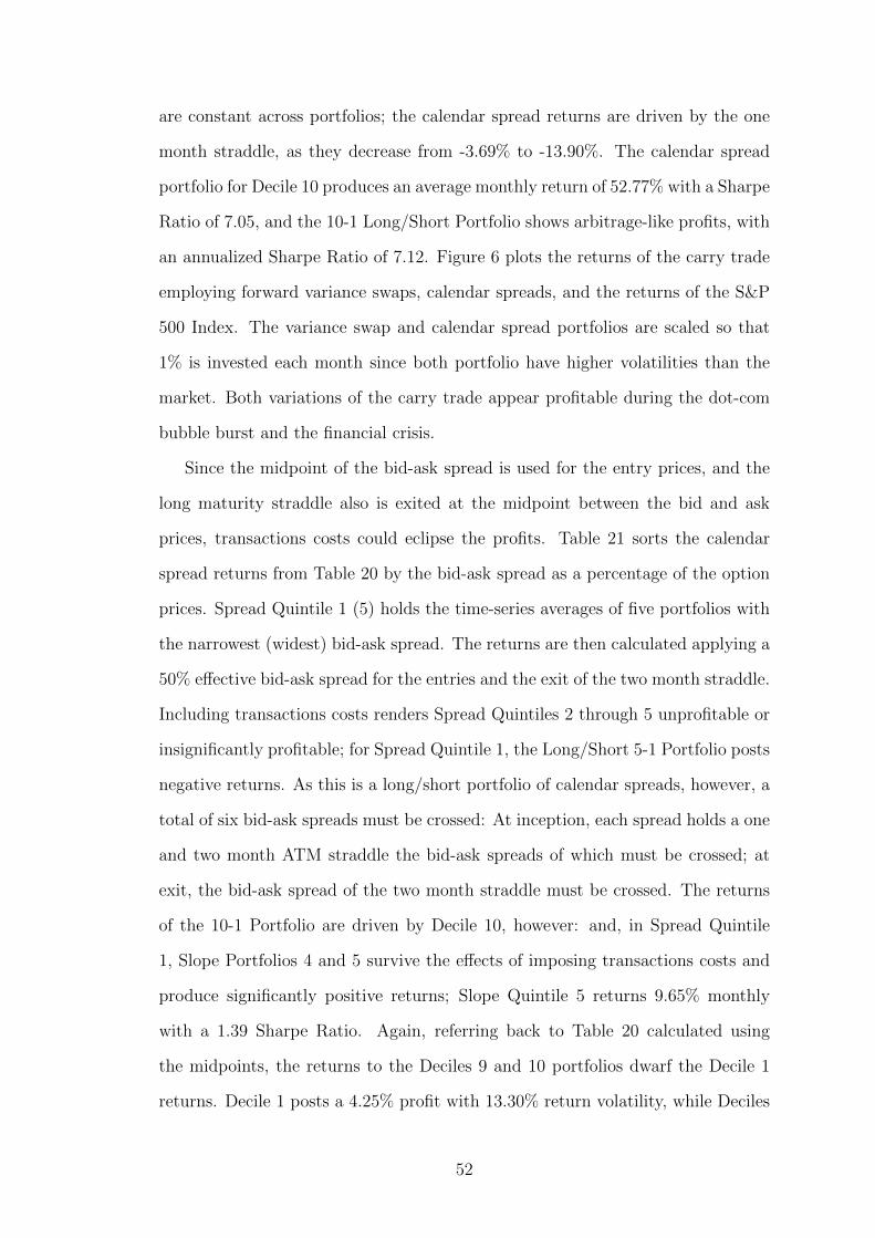
are constant across portfolios; the calendar spread returns are driven by the one

month straddle, as they decrease from -3.69% to -13.90%. The calendar spread

portfolio for Decile 10 produces an average monthly return of 52.77% with a Sharpe

Ratio of 7.05, and the 10-1 Long/Short Portfolio shows arbitrage-like profits, with

an annualized Sharpe Ratio of 7.12. Figure 6 plots the returns of the carry trade

employing forward variance swaps, calendar spreads, and the returns of the S&P

500 Index. The variance swap and calendar spread portfolios are scaled so that

1% is invested each month since both portfolio have higher volatilities than the

market. Both variations of the carry trade appear profitable during the dot-com

bubble burst and the financial crisis.

Since the midpoint of the bid-ask spread is used for the entry prices, and the

long maturity straddle also is exited at the midpoint between the bid and ask

prices, transactions costs could eclipse the profits. Table 21 sorts the calendar

spread returns from Table 20 by the bid-ask spread as a percentage of the option

prices. Spread Quintile 1 (5) holds the time-series averages of five portfolios with

the narrowest (widest) bid-ask spread. The returns are then calculated applying a

50% effective bid-ask spread for the entries and the exit of the two month straddle.

Including transactions costs renders Spread Quintiles 2 through 5 unprofitable or

insignificantly profitable; for Spread Quintile 1, the Long/Short 5-1 Portfolio posts

negative returns. As this is a long/short portfolio of calendar spreads, however, a

total of six bid-ask spreads must be crossed: At inception, each spread holds a one

and two month ATM straddle the bid-ask spreads of which must be crossed; at

exit, the bid-ask spread of the two month straddle must be crossed. The returns

of the 10-1 Portfolio are driven by Decile 10, however: and, in Spread Quintile

1, Slope Portfolios 4 and 5 survive the effects of imposing transactions costs and

produce significantly positive returns; Slope Quintile 5 returns 9.65% monthly

with a 1.39 Sharpe Ratio. Again, referring back to Table 20 calculated using

the midpoints, the returns to the Deciles 9 and 10 portfolios dwarf the Decile 1

returns. Decile 1 posts a 4.25% profit with 13.30% return volatility, while Deciles

52

9 and 10 produce returns of 31.35% and 52.77% with return volatilities less than

double that of Decile 1. The Sharpe Ratios of Deciles 9 and 10, 5.13 and 7.05,

illustrate that the returns to equity volatility carry are driven by inverted volatility

term structure: buying variance forward, or buying the calendar spreads, produce

large returns when the curve is most inverted; when applying transactions costs,

these returns survive. Figure 7 plots the returns of the Spread Quintile 1, Slope

Quintile 5 Portfolio and the S&P 500 Index. As with the long-short variance swap

and calendar spread portfolios, the Decile 10 returns increase during the financial

crisis and the post-Internet bubble period.

The summary statistics of both the forward variance swaps and the calendar

spreads are right skewed. The current variance swap rate for Decile 1 is roughly

33% lower than the forward rate, while for Decile 10 the current rate is almost

double that of the forward variance swap rate. In sympathy, the one month implied

volatility of the ATM straddle is 20% less than that of the one month implied

volatility one month forward, while the one month implied volatility for Decile

10 is more than 40% higher than the forward ATM IV. Since forward volatility

is a function of the relationship between the one and two month IV, and the two

month IVs are fairly constant across deciles, a relatively elevated one month IV

produces the comparatively low forward volatilities for Deciles 8 through 10. As

the forward implied volatility level is driven by the one month maturity, so are

the returns: the two month straddle and variance swap returns in Tables 18 and

20 are roughly constant, and the one month returns decrease from Deciles 1 to 10.

Since the forward variance swap and calendar spread returns can be decomposed

into a long two month, short one month position, the significant returns for Slope

Quintiles 4 and 5 in Table 21 are a function of the relatively low returns of the

one month positions.

Vasquez (2015) shows that term structure and short maturity option returns

have a negative relationship, and Campasano and Linn (2017) show that the return

dynamics for short maturity equity and index options differ when conditioning on

53

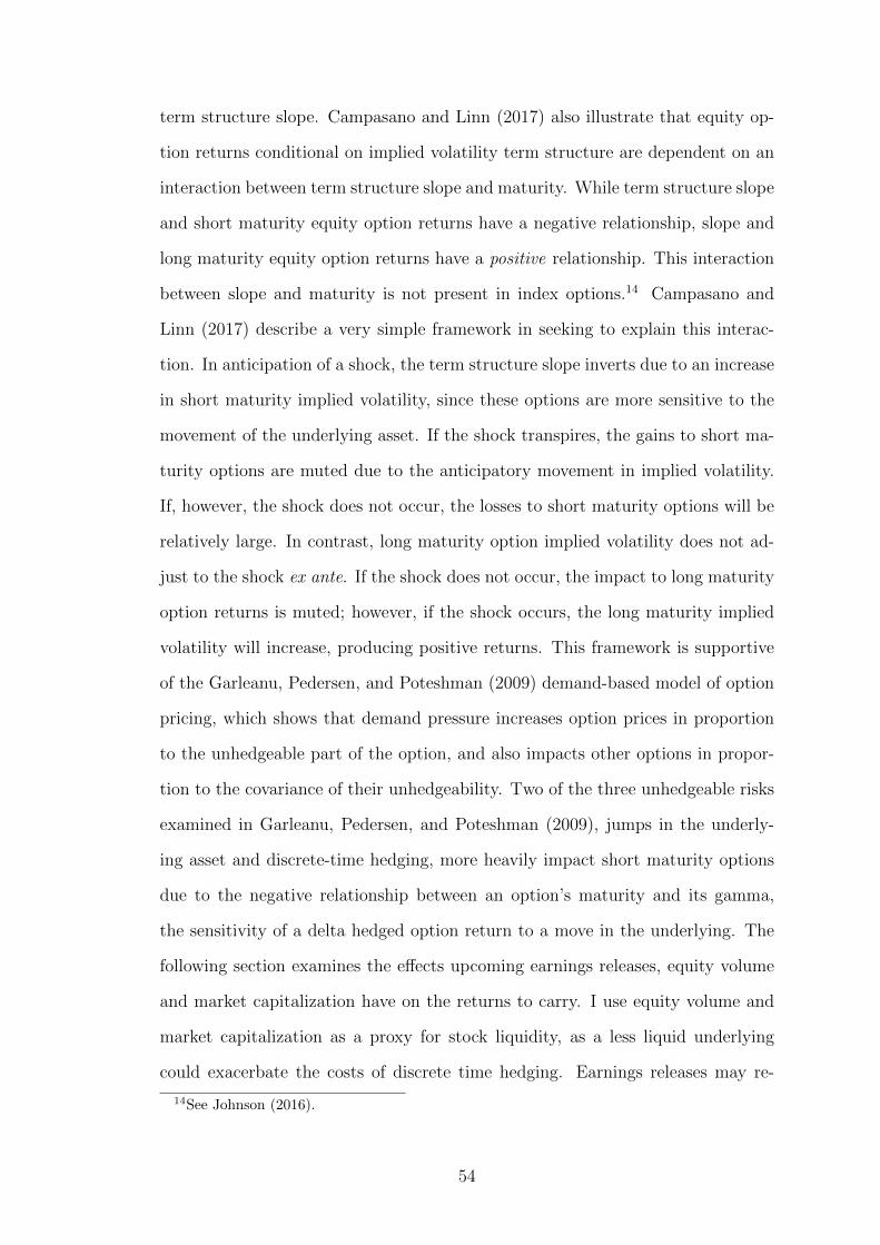
term structure slope. Campasano and Linn (2017) also illustrate that equity op-

tion returns conditional on implied volatility term structure are dependent on an

interaction between term structure slope and maturity. While term structure slope

and short maturity equity option returns have a negative relationship, slope and

long maturity equity option returns have a positive relationship. This interaction

between slope and maturity is not present in index options.14 Campasano and

Linn (2017) describe a very simple framework in seeking to explain this interac-

tion. In anticipation of a shock, the term structure slope inverts due to an increase

in short maturity implied volatility, since these options are more sensitive to the

movement of the underlying asset. If the shock transpires, the gains to short ma-

turity options are muted due to the anticipatory movement in implied volatility.

If, however, the shock does not occur, the losses to short maturity options will be

relatively large. In contrast, long maturity option implied volatility does not ad-

just to the shock ex ante. If the shock does not occur, the impact to long maturity

option returns is muted; however, if the shock occurs, the long maturity implied

volatility will increase, producing positive returns. This framework is supportive

of the Garleanu, Pedersen, and Poteshman (2009) demand-based model of option

pricing, which shows that demand pressure increases option prices in proportion

to the unhedgeable part of the option, and also impacts other options in propor-

tion to the covariance of their unhedgeability. Two of the three unhedgeable risks

examined in Garleanu, Pedersen, and Poteshman (2009), jumps in the underly-

ing asset and discrete-time hedging, more heavily impact short maturity options

due to the negative relationship between an option’s maturity and its gamma,

the sensitivity of a delta hedged option return to a move in the underlying. The

following section examines the effects upcoming earnings releases, equity volume

and market capitalization have on the returns to carry. I use equity volume and

market capitalization as a proxy for stock liquidity, as a less liquid underlying

could exacerbate the costs of discrete time hedging. Earnings releases may re-

14See Johnson (2016).

54

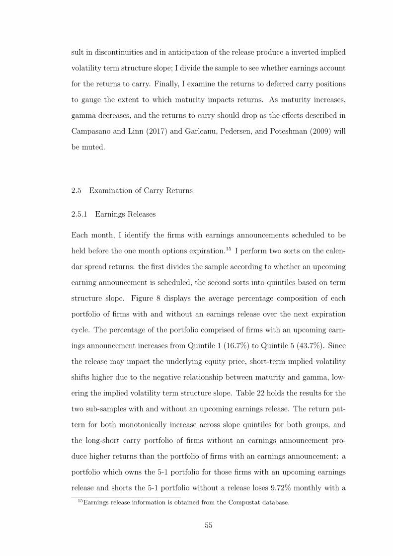
sult in discontinuities and in anticipation of the release produce a inverted implied

volatility term structure slope; I divide the sample to see whether earnings account

for the returns to carry. Finally, I examine the returns to deferred carry positions

to gauge the extent to which maturity impacts returns. As maturity increases,

gamma decreases, and the returns to carry should drop as the effects described in

Campasano and Linn (2017) and Garleanu, Pedersen, and Poteshman (2009) will

be muted.

2.5 Examination of Carry Returns

2.5.1 Earnings Releases

Each month, I identify the firms with earnings announcements scheduled to be

held before the one month options expiration.15 I perform two sorts on the calen-

dar spread returns: the first divides the sample according to whether an upcoming

earning announcement is scheduled, the second sorts into quintiles based on term

structure slope. Figure 8 displays the average percentage composition of each

portfolio of firms with and without an earnings release over the next expiration

cycle. The percentage of the portfolio comprised of firms with an upcoming earn-

ings announcement increases from Quintile 1 (16.7%) to Quintile 5 (43.7%). Since

the release may impact the underlying equity price, short-term implied volatility

shifts higher due to the negative relationship between maturity and gamma, low-

ering the implied volatility term structure slope. Table 22 holds the results for the

two sub-samples with and without an upcoming earnings release. The return pat-

tern for both monotonically increase across slope quintiles for both groups, and

the long-short carry portfolio of firms without an earnings announcement pro-

duce higher returns than the portfolio of firms with an earnings announcement: a

portfolio which owns the 5-1 portfolio for those firms with an upcoming earnings

release and shorts the 5-1 portfolio without a release loses 9.72% monthly with a

15Earnings release information is obtained from the Compustat database.

55

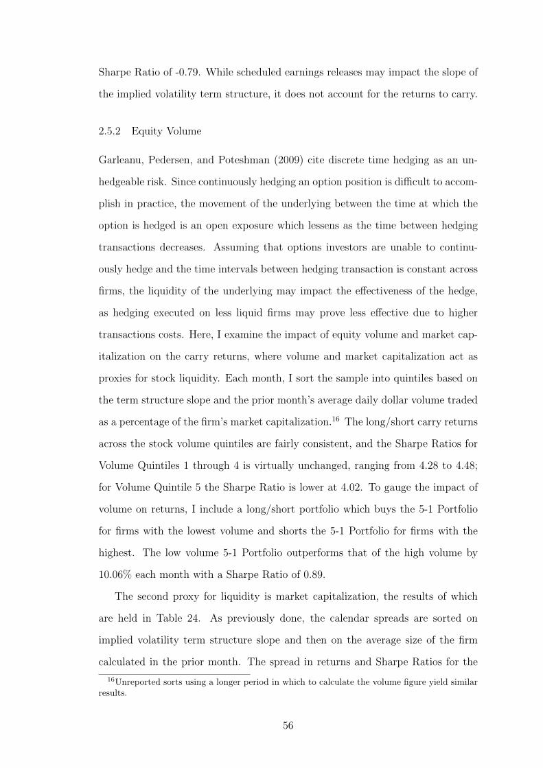
Sharpe Ratio of -0.79. While scheduled earnings releases may impact the slope of

the implied volatility term structure, it does not account for the returns to carry.

2.5.2 Equity Volume

Garleanu, Pedersen, and Poteshman (2009) cite discrete time hedging as an un-

hedgeable risk. Since continuously hedging an option position is difficult to accom-

plish in practice, the movement of the underlying between the time at which the

option is hedged is an open exposure which lessens as the time between hedging

transactions decreases. Assuming that options investors are unable to continu-

ously hedge and the time intervals between hedging transaction is constant across

firms, the liquidity of the underlying may impact the effectiveness of the hedge,

as hedging executed on less liquid firms may prove less effective due to higher

transactions costs. Here, I examine the impact of equity volume and market cap-

italization on the carry returns, where volume and market capitalization act as

proxies for stock liquidity. Each month, I sort the sample into quintiles based on

the term structure slope and the prior month’s average daily dollar volume traded

as a percentage of the firm’s market capitalization.16 The long/short carry returns

across the stock volume quintiles are fairly consistent, and the Sharpe Ratios for

Volume Quintiles 1 through 4 is virtually unchanged, ranging from 4.28 to 4.48;

for Volume Quintile 5 the Sharpe Ratio is lower at 4.02. To gauge the impact of

volume on returns, I include a long/short portfolio which buys the 5-1 Portfolio

for firms with the lowest volume and shorts the 5-1 Portfolio for firms with the

highest. The low volume 5-1 Portfolio outperforms that of the high volume by

10.06% each month with a Sharpe Ratio of 0.89.

The second proxy for liquidity is market capitalization, the results of which

are held in Table 24. As previously done, the calendar spreads are sorted on

implied volatility term structure slope and then on the average size of the firm

calculated in the prior month. The spread in returns and Sharpe Ratios for the

16Unreported sorts using a longer period in which to calculate the volume figure yield similarresults.

56

5-1 portfolios across market capitalization is wider than that seen in the double

sort on stock volume and slope in table 23. The Sharpe Ratio drops from 5.09 to

2.73 from Size Quintile 1 to 5; by comparison, the drop from Volume Quintile 1

to 5 is 4.48 to 4.02. A portfolio which owns the 5-1 Portfolio for small firms and

sells the 5-1 Portfolio for large firms earns 14.57% monthly, with a 1.20 Sharpe

Ratio. While the 5-1 returns are significant across firm size and market volume,

a return differential exists between low and high volume and small and large firms.

2.5.3 Returns to Deferred Carry Portfolios

Until this point, the carry trades consist of one and two month positions. I next

examine the returns to two month-four month and three month-six month cal-

endar spreads.17 Increasing both the forward period and maturity will decrease

exposure to the effects of discrete time hedging and also mute the dynamics of

the Campasano and Linn (2017) framework. Table 25 holds the returns of both

deferred carry trades, sorted into term structure slope deciles. As with the one

month-two month calendar spreads, returns increase monotonically for both from

Decile 1 to 10, and returns are significant across deciles. However, the Sharpe Ra-

tios of the long-short portfolios decrease as maturities increase. Recall from Table

20 the Sharpe Ratio of 7.12 for the one month-two month calendar spread. The

ratio more than halves, to 3.16, for the two month-four month calendar spread,

and decreases further to 2.65 for the three month-six month calendar spread. As

with volume and size, the deferred carry positions remain profitable; however, the

risk-adjusted returns decline.

17Given the equity option listing conventions, the number of observations for both deferredspreads are lower. For a more detailed explanation of listing conventions, see Campasano andLinn (2017).

57

2.6 Equity Volatility Carry Exposures

Koijen, Moskowitz, Pedersen, and Vrugt (2013) examine carry across global equi-

ties, fixed income, foreign exchange, commodities, treasuries, credit, equity index

call options and put options. Table 26 holds the summary statistics of carry on

the nine assets along with the correlation matrix including the long-short equity

volatility carry portfolio from Table 20 from 1996 through September, 2012.18

While the long/short equity volatility carry portfolio posts a much higher Sharpe

Ratio (7.12), the after transactions costs long carry portfolio’s Sharpe Ratio, 1.39,

is within the range seen here: from 0.19 for global equities to 1.52 for equity index

option puts. The equity volatility correlations range from 0.025 with one version

of the global bond carry to -0.175 for the credit portfolio.19 The correlations for

the equity volatility portfolio with the index call and put options are both negative

(-0.171 and -0.133).

By volatility-weighting the nine different strategies, a diversified carry portfolio

produces a Sharpe Ratio of 1.18, higher than that of the traditional foreign ex-

change portfolio, 0.66.20 The diversified carry portfolio, however, remains exposed

to liquidity and volatility.21 Table 27 examines the exposure of the volatility carry

portfolio to excess market returns, the small minus big (SMB) and high minus

low (HML) returns of Fama and French (1992); momentum portfolio returns of

Carhart (1997); traded liquidity portfolio (Liq) returns of Pastor and Stambaugh

(2003); Coval and Shumway (2001) zero beta straddle (zbr) returns; and the di-

versified carry portfolio of Koijen, Moskowitz, Pedersen, and Vrugt (2013). The

zbr and Liq portfolios proxy for market volatility and liquidity, respectively. The

volatility carry portfolio loadings on all factors are insignificant with the exception

of the HML portfolio at the 10% level and the excess market returns at the 0.1%

18The data used here is obtained from the website of Lasse H. Pedersen.19Koijen, Moskowitz, Pedersen, and Vrugt (2013) decomposes bond carry into the bond’s yield

spread to the risk free rate (slope), and the price roll down the yield curve (level).20Koijen, Moskowitz, Pedersen, and Vrugt (2013) follow the volatility-weighting procedures of

Asness, Moskowitz, and Pedersen (2013) by normalizing each strategy to a 10% annual volatility.21Koijen, Moskowitz, Pedersen, and Vrugt (2013).

58

level; both coefficients, however, are negative. Constants for the four regressions

are significantly positive, at roughly 50%. Since it is shown that transactions

costs have a significant impact on returns, the loadings of the after transactions

cost long volatility carry portfolio on the above factors is examined in Table 28.

The portfolio similarly loads significantly negatively on the market, and while it

loads negatively on the aggregate volatility factor, zbr, the magnitude, -0.10, is

economically insignificant. The constants for the four regressions are positive and

significant, ranging from 10.5% to 12.0%. Figures 9 and 10 graphically illustrate

the differences in returns by displaying the equity graphs of investments in the

equity volatility carry portfolios and the diversified carry portfolio. Unlike a di-

versified carry portfolio, the returns to equity volatility carry are not exposed to

market, liquidity, or volatility factors.

2.7 Conclusion

The carry trade has been shown to exist across asset classes. In index options

and volatility, the trade has been shown to produce significant positive returns, as

forward volatility poorly predicts future spot volatility. As the index and equity

volatility term structure dynamics differ, I examine whether the carry trade exists

in the equity volatility market by first synthesizing forward variance swaps. I

find that forward variance poorly predicts future spot variance, and a carry trade

effected on these hypothetical swaps would prove profitable. I then turn to an

investable version of the carry trade by employing calendar spreads. The returns

to carry here are arbitrage-like; after incorporating transactions costs, I find that

the long volatility carry trade produces significantly positive returns which are

negatively exposed to both market and volatility risks. After further examination,

I find that size, liquidity and trade tenor impact returns, although none completely

explain the performance. The findings are supportive of the Campasano and Linn

(2017) volatility framework and demand based options pricing model of Garleanu,

Pedersen, and Poteshman (2009).

59

CHAPTER 3

BEATING THE S&P 500 INDEX

3.1 Introduction

The covered call is perhaps the most basic options strategy: a call option is sold

against a long position in an asset. The premium collected on the option softens

any losses should the asset price decline; in exchange, the asset may be called

away if the price of the asset exceeds the strike price at expiration. The strategy

can be performed using any asset in a cash account, as long as options can be

written on it. Asset managers often engage in this strategy against core equity

and/or equity index positions; a suite of covered call indexes are published by

the Chicago Board Options Exchange (CBOE). When executed on a broad-based

index, the strategy typically outperforms the underlying on a risk-adjusted basis.

Kapadia and Szado (2007) and Israelov and Nielsen (2014), among others, show

that this outperformance is borne from the risk premium inherent in the short

call.1 While systematically writing options against a long index position has been

shown to outperform the underlying, the allocation to the two risk premia, market

and volatility, is fixed: the portfolio invests fully in the index and call options are

written against the position. In this study I allow the allocations to volatility

and the market to vary over time. Instead of expressing the volatility exposure

through short options, I pair an index position with VIX futures due to its inde-

pendence to path and time. This two asset portfolio created outperforms that of

the index on both a risk adjusted and absolute basis. When accounting for the

1See also Hill, Balasubramanian, Gregory, and Tierens (2006).

60

expected returns to volatility conditional on term structure slope, a naive portfolio

produces a Sharpe Ratio 25% higher than that of the index, and bests covered call

strategies. A portfolio optimized ex ante triples index performance with similar

return volatility and more than doubles the risk-adjusted performance of covered

call strategies.

The Chicago Board Options Exchange introduced its Buy Write Monthly Index

(BXM) in 2002. The Index consists of two components: a long position in the S&P

500 Index and a short at the money (ATM) one month call written on the Index.

The strategy is implemented systematically: a one month, ATM call is written

on the index and the call is cash settled at expiration, at which time another one

month ATM call is sold. In examining the historical performance of the BXM

from June, 1988 through 2001, Whaley (2002) finds that the strategy posts an

average monthly return of 1.106% vs. the S&P 500 Index’s 1.187%, with volatility

roughly two-thirds that of the S&P 500. In addition to a higher Sharpe Ratio,

the strategy also posts a positive Jensen’s alpha (0.23%). In concluding, Whaley

posits that, in an efficient market, the risk adjusted returns of the two should

not differ, and perhaps demand pressure on S&P 500 Index options produces the

outperformance.

Kapadia and Szado (2007) study the returns of the covered call strategy exe-

cuted on the Russell 2000 Index from 1996-2006. Similar to Whaley, the covered

call strategy on the Russell 2000 Index outperforms the index on a risk-adjusted

basis. While the absolute returns approximately match that of the index itself,

the standard deviation is lower by roughly one-third. In dissecting their sample

period, they also find that the strategy outperforms the index from 2003 to 2006,

a relatively unfavorable period for the strategy due to the combination of persis-

tently high index returns and low volatility. By decomposing the returns to the

short call position, it is shown that the implied volatility of the call option sold

is higher on average than the volatility realized over the life of the option, and if

the implied volatility of the call option equaled the volatility subsequently realized

61

by the index, the short calls would have generated a significant loss. This echoes

earlier studies by Bakshi and Kapadia (2003a), Coval and Shumway (2001), and

Carr and Wu (2009) which show that a volatility risk premium exists: selling index

options produce significant returns.

Since a covered call strategy typically is implemented passively by selling call

options systematically and then exiting the position at the option’s expiration, the

path of the underlying can influence the degree to which the strategy outperforms

the index. During a prolonged rally, the returns will look relatively poor as the

call sales act to cap the gains on the underlying index, and as the market falls, the

protection is limited to the premium collected. Israelov and Nielsen (2014) further

decompose the strategy to isolate the risk premium and the impact of the path of

the underlying. At inception, an ATM covered call position can be viewed as two

separate positions: A long position in the underlying equal to one half of the index

position, and a short volatility exposure where the other half of the index position

acts to delta hedge the short call. The hedge needed is not static, however, as the

call delta changes with the index level. The returns of the covered call, then, can

be parsed into three exposures:

• Passive Equity, equal to the Equity ∗ (1- Initial Call Delta);

• Short Volatility, equal to - (Call - Current Delta ∗ Equity); and

• Dynamic Equity, equal to Equity ∗ (Initial Call Delta - Current Call Delta).

To illustrate with an example, assume the price of the index is 100, as is the

strike of the call sold. The call delta is 0.50, and the price of the option is $4.00.

$1,000,000 of the index is purchased, and so $40,000 in premium is collected. The

exposures are:

• Passive Equity: (1− 0.50) ∗ $1, 000, 000 = $500, 000 Equity

• Short Volatility: −(Call − 0.50 ∗ $1, 000, 000) = −Call + $500, 000 Equity

• Dynamic Equity: (0.50− 0.50) ∗ $1, 000, 000 = $0.

62

If the index rises to 102, and the call delta increases to 0.70, then the three

exposures become:

• Passive Equity: (1− 0.50) ∗ $1, 020, 000 = $510, 000 Equity

• Short Volatility: −(Call − 0.70 ∗ $1, 020, 000) = −Call + $714, 000 Equity

• Dynamic Equity: (0.50− 0.70) ∗ $1, 020, 000 = −$204, 000.

The first two components provide exposure to the equity and volatility risk

premia. The passive equity component increases by 2% as the index rallies 2%.

The short volatility position necessitates a larger index position in order to hedge

the option, as the delta has increased from 0.50 to 0.70. Since a larger index

position is needed to hedge the short option, the dynamic equity factor falls. As-

suming a positive market risk premium, the expected return of the dynamic equity

factor is at best zero. Israelov and Nielsen (2015) show that actively managing

the covered call to mute this exposure improves the risk-adjusted returns. The

resulting portfolio produces superior risk-adjusted returns to both the traditional

covered call strategy and the index, and eliminates the return asymmetry in up

and down markets present in the traditional covered call strategy. The absolute

returns, however, lag the index, the position requires active management, and

unlike the traditional covered call strategy, the rehedging of the option requires a

margin account.

Israelov and Nielsen (2015) neutralize the dynamic equity component of the

traditional covered call to produce a structure capturing market and volatility

risk premia. As documented by Bakshi and Kapadia (2003a), among others, the

volatility risk premia is larger and distinct from the market premia, and as Kapa-

dia and Szado (2007) illustrates, it drives the outperformance of the covered call

strategy. Here I show that substituting a short VIX futures exposure for short op-

tions produce a portfolio with similar risks and returns of the hedged covered call

strategy. As understanding of the volatility risk premia has evolved, studies have

shown that the term structure slope is a powerful predictor of returns to volatility

63

assets: Simon and Campasano (2014) show that, for VIX futures, the volatility

expectations hypothesis fails to hold, and the VIX futures basis holds predictive

power over VIX futures returns. Johnson (2016) shows that term structure slope

predicts excess returns for S&P 500 Index variance swaps and delta hedged option

positions in addition to VIX futures. The fact that the expectations hypothesis

fails presents a puzzle, as an inverted term structure cheapens the cost of volatility

as market risk is increasing. Cheng (2016) shows this is not a function of mismea-

surement, and finds that demand for VIX futures drops during these episodes of

increasing risk.

While the covered call strategy holds fixed the allocation to both market and

volatility premia, I incorporate the findings of the term structure studies, allowing

the allocations between market and volatility to vary over time. Using VIX futures

instead of S&P 500 Index options to express the volatility view enable investors

to gain volatility exposure more easily given the independence to the path of the

underlying for VIX futures. Following the procedure in Simon and Campasano

(2014) and Cheng (2016), I first condition the volatility investment on the sign

of the slope of the VIX term structure using the weightings of a covered call;

the resulting portfolio bests the hedged covered call strategy. I then optimize ex

ante using a long-term historical measure of market returns, and the VIX futures

basis, the forward-looking measure of the difference between the VIX futures and

the VIX Index. The portfolio holding VIX futures, the S&P 500 Index, and cash

triples the returns of the index and more than doubles the risk-adjusted returns

of covered call strategies.

In the next section, I review the characteristics of covered call strategies; in

Section 3.3 I discuss VIX futures and volatility risk premia. Section 3.4 describes

the time varying allocation optimization process and results. Section 3.5 concludes

this chapter.

64

3.2 Covered Calls

Table 29 provides summary statistics for the S&P 500 Index, the covered call

strategy executed on the S&P 500 Index, and the hedged covered call strategy

following the Israelov and Nielsen (2015) process from 1996 through 2015. Monthly

statistics are calculated over the standard option expirations. On each expiration

day, the lowest strike call option out of the money is sold and the option expiring

is cash settled. Over the life of the option, the hedged covered call strategy adjusts

the index position daily such that the entire position’s delta remains at 0.50.

The monthly returns for both covered call strategies are approximately 10

basis points lower than the index returns, but the covered call monthly standard

deviation is 30% lower (0.0339 vs. 0.0493), and the standard deviation for the

hedged covered call is 42% lower (0.0284). As a result, the Sharpe Ratios of the

covered call, 0.47, and hedged covered call, 0.57, are higher than that of the index,

0.39. Due to the asymmetry of the covered call, the strategy is more negatively

skewed, and its downside beta, 0.87, is higher than both its beta, 0.60, and upside

beta, 0.39. The hedged strategy addresses this asymmetry. The three measures of

beta are approximately equal (0.56, 0.55, and 0.58 for its beta, upside beta, and

downside beta, respectively) and its skewness is less negative (-1.32 vs. -1.99).

Finally, the extreme variation of the hedged covered call is less than that of the

covered call and the index. The lowest returns for the three strategies, occurring

during the October, 2008 expiration, are 21.38%, 18.82%, and 13.80% for the

index, covered call, and hedged covered call strategies, respectively; the highest

returns occur two months later (17.73%, 14.55%, and 10.05%).

Table 30 decomposes the returns of both versions of the covered call strategies

into two components. Panel A parses the returns of the covered call into the index

and short call option. Panel B splits the returns into an index position equal to

50% of the entire position, and the short call, delta hedged daily with a target

delta of 0.50 to maintain the index exposure at inception. It is unsurprising that

65

the returns to the short ATM call are negative, losing ten basis points on average.

The resulting portfolio, however, posts higher risk-adjusted returns. Kapadia

and Szado (2007) showed that the implied volatility at which the call is sold

was consistently higher than the volatility subsequently realized by the index,

producing the higher risk-adjusted returns. This is seen more directly in Panel

B of Table 30. Here the hedged covered call position is separated into the delta

hedged call and the index. The delta hedged call produces a high Sharpe Ratio,

1.55, with virtually no beta, and the strategy produces higher risk-adjusted returns

and lower downside risk over the covered call and the index.

3.3 VIX Products

Variance swaps allow sellers to gain short volatility exposure independent of the

path of the underlying where the payoff is determined by the difference between

the variance implied by option prices and that realized by the index. However,

these products are only available over-the-counter.2 VIX futures provide exposure

to future levels of the VIX Index. The Index itself is a measure of 30 day volatility,

and is derived using the prices of options, as follows:

σ2 = 2T

∑i

∆KiK2 e

RTQ(Ki)− 1T

[ FK0− 1]2

where:

• σ = V IX100

,

• T=time to expiration,

• F = forward index level,

• K0 is the first strike below the forward index level,

2The Chicago Board Options Exchange lists a product similar to a variance swap but it isnot actively traded.

66

• Ki is the strike price of an OTM option (calls where the strike price is greater

than the forward price, puts where the strike price is less than the forward

price),

• ∆Ki is the interval between strike prices,

• R is the interest rate, and

• Q(Ki) is the midpoint between the bid and the ask of the option price.

While it is theoretically possible to construct a position in the VIX Index,

the daily rebalancing costs would prove prohibitive. VIX futures, however, allow

investors to express a view on index volatility. The resulting exposure is not

identical to that of delta hedged options, as the underlying volatility does not

enter directly into the returns to VIX futures, but the correlation of VIX futures

and delta hedged call returns is fairly high at 0.69. Table 31 contains the returns

of the delta hedged call and a constant maturity one month VIX future over 2007

through 2015. The sample period is shortened here as prior to 2007 VIX futures

were thinly traded and not listed monthly. The constant maturity one month VIX

futures position is calculated by rolling daily, in equal amounts, a position from

the front month contract to the second month contract in order to maintain the

one month maturity, following the methodology which determines the S&P 500

VIX Short-Term Futures Index.3 The daily returns are then calculated according

to the position held each day. A constant maturity VIX future is used in order to

maintain a constant exposure, as the beta of the VIX future with respect to the

VIX index increases as it approaches expiration: Figure 11 plots the beta of the

front month VIX futures with respect to the VIX Index according to the days until

expiry. As the front month VIX future approaches expiry, its beta with respect

to the VIX index increases driving higher its volatility.

3See http://us.spindices.com/indices/strategy/sp-500-vix-short-term-index-mcap for a de-tailed description of the index. Exchange traded products such as VXX and VIXY offer exposureto the VIX short-term futures index.

67

Since each portfolio is fully invested in the short volatility instrument, the

returns and volatility are higher than the returns attributed to the short volatility

in Table 30. The delta hedged call option returns are calculated following the

methodology in Frazzini and Pedersen (2012). At trade inception, I start with $1

worth of calls, V0 = 1. Each day, the value of the portfolio is computed iteratively

as follows:

Vt = Vt−1 + x(Ft − Ft−1)− x∆t−1rSt St−1 + rft (Vt−1 − xFt−1 + x∆t−1St−1) (3.1)

where x = 1/F0, the number of options contracts; F is the option price; rs is

the daily stock return; rf is the daily risk free rate; and ∆ is the option’s delta.

The second term above represents the dollar return from the change in option

price, the profit or loss from the delta hedge is computed in the third term. The

final term calculates the financing cost of the position. The return to the position,

RT , is

RT = VT − V0 = VT − 1 (3.2)

The constant maturity VIX future produces a lower Sharpe Ratio, 0.51, than

the short delta hedged call, 0.68. Examination of the betas listed reveal that the

upside beta of the delta hedged ATM call, 1.05, is much lower than the beta, 2.43,

and downside beta, 2.58. The difference in betas for the VIX future is greater,

with the downside beta, 3.83, and beta, 2.38, standing higher than the upside

beta, 0.29. Another notable difference is the returns of the delta hedged call in

Table 30 and 31. Over the entire sample from 1996 through 2015, the returns

to delta hedged calls decrease from the first half to the second; the fact that the

financial crisis lies in the second half of the sample does not account solely for this

difference.

While the returns from short VIX futures fall short of delta hedged option

68

returns, the constant maturity VIX futures are used in the study for their path

and time independency and ease in varying exposures. Studies have shown that

a significant predictor of volatility returns is term structure slope. Simon and

Campasano (2014) first document that VIX futures levels are poor predictors of

the VIX Index, and the basis, the difference between the VIX futures and the

Index, predicts VIX futures returns: selling VIX futures when the term structure

is upward sloping and buying VIX futures when the term structure is downward

sloping produce significant returns. Given this, in Table 32, I examine the short

volatility exposures conditional on the sign of the VIX futures term structure

slope, where:

Slope =ConstantOneMonthV IXFuture

V IXIndex− 1 (3.3)

Each day, the slope is examined. If positive, the position is held; if negative, the

position is closed.4 Over the entire sample, the slope is positive 76.6% of the time.

The returns for the delta hedged call drop when conditioning on term structure

slope, but in keeping with the covered call strategy, the option originally sold at

the beginning of each expiration period is the option traded over the life of that

expiration cycle. Term structure inversion typically occurs after a market decline,

and so exiting the short call position results in closing a low delta call with little

optionality remaining. As VIX futures are path independent, conditioning on the

sign of the term structure slope boosts absolute returns of the constant maturity

VIX futures from 2.93% to 4.28%, with the Sharpe Ratio increasing from 0.51 to

1.16. The minimum return rises from -96.74% to -33.21%, as the term structure

slope is negative for much of the latter part of 2008 during the financial crisis.

4Simon and Campasano (2014) and Cheng (2016) show that the costs to owning volatilitymay turn positive when the term structure slope inverts. Given that a covered call is essentiallya long market, short volatility portfolio, the volatility positions held here are either short or flat.

69

3.4 Time-Varying Allocations

A covered call and the hedged covered call allocate between market and volatility

premia. The covered call invests fully in the market and overwrites the position

with an ATM call; the hedged covered call can be viewed as investing 50% of

assets in the market and holding a short delta hedged ATM call with a notional

value equal to the entire portfolio. Options investors typically express the size of

volatility positions in terms of the vega, the sensitivity of the option price with

respect to a one percentage point change in the option’s implied volatility. While

vega is positively related to the implied volatility of the option, the vega of the

one month ATM option will remain roughly consistent. Table 33 examines the

market/VIX futures portfolio where 50% of assets are invested in the market and

the VIX futures component is set such that the sensitivity of the position with

respect to volatility equals the vega of the short option. Included for comparison

purposes are the S&P 500 Index, the covered call, and hedged covered call strat-

egy. While both versions of the covered call are fully invested, and the hedged

covered call will use leverage to delta hedge the option, the portfolio holding VIX

futures allocates 2.47% on average to VIX futures, with a maximum allocation

of 7.22%; greater than 40% of the position remains in cash. Panel A holds the

unconditional returns of the strategies. While the covered call strategy has been

shown to outperform the index on a risk-adjusted basis, during this sample period

the covered call actually underperforms the index, posting a 0.39 Sharpe Ratio as

compared to 0.42 for the index. The average returns across the three strategies are

roughly consistent, ranging between 41 and 47 basis points monthly. The portfo-

lio holding VIX futures underperforms the hedged covered call strategy, posting a

Sharpe Ratio of 0.45 vs. 0.50, while having an exposure to the underlying index

similar to that of the hedged covered call. Panel B holds the returns conditioned

on the sign of the VIX futures slope. Each day, the VIX futures slope is calcu-

lated. If the slope is negative, the position is exited; if the slope is positive, the

70

position remains on or is entered if no position exists.5 Here, the VIX portfolio

outperforms, posting a 0.54 Sharpe Ratio with similar skewness to the index and

hedged covered call and a minimum return of 10.69% compared to 21.37% and

11.04% for the index and hedged covered call respectively. Conditioning on term

structure slope sign produces a portfolio with a Sharpe Ratio 10% higher than the

hedged covered call and 28% higher than the S&P 500 Index.

Since the portfolio holding VIX futures is not fully invested, as the relatively

modest allocation to VIX futures averages 2.47%, Table 34 increases the fixed al-

location to VIX futures. As with Table 33, Panel A includes unconditional returns

and Panel B holds the returns conditional on term structure slope sign. Three

allocations, 2, 5, and 10% are included, with a 2% allocation matching roughly

the portfolio from Table 33. In Panel A, the monthly returns and Sharpe Ratios

increase as the VIX futures exposure increases. Betas become more asymmetrical

as well; at a 10% allocation the downside beta, 0.88, is greater than the beta

0.74, and upside beta, 0.53. These patterns persist in Table B, except for the

beta asymmetry; conditioning on term structure slope sign mutes the differential

between up and down beta. The portfolio allocating 10% has a 0.75 Sharpe Ratio,

posting returns 13% higher with volatility 38% lower than the index. The results

here in Table 34 illustrate that the composition of a covered call is suboptimal

when viewed from the standpoint of a portfolio allocating to market and volatility

premia.

Until now the study has conditioned on the sign of the term structure slope;

when the futures slope is negative, the allocation to volatility is closed. Cheng

(2016) showed that the magnitude of the ex ante premium, however, predicts

returns with a coefficient close to one. In order to incorporate the magnitude of

the VIX basis, I create an optimal portfolio using the VIX basis as the expected

return of the VIX futures position. A ten year historical average return of the

S&P 500 Index is used as the expected return of the index to obtain a measure of

5For the hedged covered calls, the option sold at the beginning of the expiration cycle is theoption resold if the position was exited previously.

71

market risk premia.6 The daily returns of the past one month are used to calculate

expected return variance. Each day, the S&P 500 Index and short VIX futures

weightings are determined by maximizing the Sharpe Ratio.7 Specifically,

maxwV IX ,wMKT

wV IX ∗ E(RV IX) + wMKT ∗ E(RMKT )−Rrf√w2V IX ∗ σ2

V IX + w2MKT ∗ σ2

MKT + 2 ∗ wV IX ∗ wMKT ∗ σ2V IX,MKT

(3.4)

subject to:

0 ≤ wV IX ≤ 1,

0 ≤ wMKT ≤ 1,

wV IX + wMKT = 1

where:

• wV IX is the allocation to the constant maturity VIX futures;

• wMKT is the allocation to the S&P 500 Index;

• E(RMKT ) is the expected return of the S&P 500 Index using a long-term

average;

• E(RV IX) is the expected return of the VIX futures position using VIX fu-

tures basis;

• Rrf is the risk-free rate;

• σ2MKT is the expected variance of index returns using the prior month’s daily

returns;

• σ2V IX is the expected variance of VIX futures returns using the prior month’s

daily returns; and

6Unreported examinations using shorter time periods produce substantially similar results.7Calculating the portfolio weightings and then adjusting the portfolio the following day pro-

duce substantially similar results.

72

• σ2V IX,MKT is the expected covariance of the VIX futures and S&P 500 Index

using the prior month’s daily returns.

The Optimized Portfolio in Table 35 is produced by maximizing Equation 3.4.

Figure 12 displays a histogram of the allocation to VIX futures. The portfolio

returns 5% monthly, with a 1.23 Sharpe Ratio, but as it invests entirely in a

short VIX futures position over 60% of the time, the return volatility, 14%, is

more than double that of the index and more than four times larger than that of

the hedged covered call. Due to this relatively high volatility, I also include the

Volatility Targeted Optimized Portfolio, which is designed to produce a return

volatility similar to that of the S&P 500 Index. Each day, the positions are

scaled so that the expected portfolio volatility equals the expected volatility of the

market. As the Optimized Portfolio holds the portfolio with the highest expected

Sharpe Ratio, the Volatility Targeted Optimized Portfolio is the portfolio on the

Security Market Line which allocates to the Optimized Portfolio and cash in an

effort to target the return volatility of the S&P 500 Index. The Volatility Targeted

Optimized Portfolio returns 2.02% on average each month, triple that of the index,

with a monthly return volatility of 5.95%, slightly higher than the S&P 500 Index

volatility (5.56%). In contrast to portfolios examined earlier, the upside beta, 1.06,

is higher than the beta, 0.95, and downside beta, 0.89, while the skewness, -1.15,

is close to that of the Index, -1.07. Figure 13 holds the allocations to VIX Futures,

the S&P 500 Index, and cash for the Volatility Targeted Optimized Portfolio. The

portfolio invests on average less than half of assets, with the average cash holding

equal to 51.8%; an average index weight of 33.1% and average VIX futures weight

of 23.4%. The allocation to the market over time resembles a barbell, with no

position held roughly 60% of the time and a fully invested index portfolio about

30% of the sample. An investment in VIX futures greater than 50% occurs 7% of

the time, during the market rebound in 2009, when the VIX was elevated and the

VIX futures term structure slope was positive.

Figure 14 plots the equity curves of the index, the covered call, the hedged

73

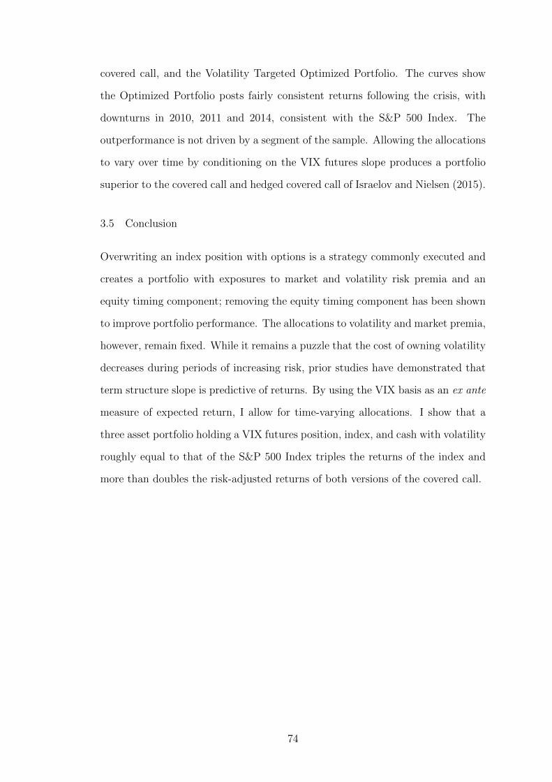
covered call, and the Volatility Targeted Optimized Portfolio. The curves show

the Optimized Portfolio posts fairly consistent returns following the crisis, with

downturns in 2010, 2011 and 2014, consistent with the S&P 500 Index. The

outperformance is not driven by a segment of the sample. Allowing the allocations

to vary over time by conditioning on the VIX futures slope produces a portfolio

superior to the covered call and hedged covered call of Israelov and Nielsen (2015).

3.5 Conclusion

Overwriting an index position with options is a strategy commonly executed and

creates a portfolio with exposures to market and volatility risk premia and an

equity timing component; removing the equity timing component has been shown

to improve portfolio performance. The allocations to volatility and market premia,

however, remain fixed. While it remains a puzzle that the cost of owning volatility

decreases during periods of increasing risk, prior studies have demonstrated that

term structure slope is predictive of returns. By using the VIX basis as an ex ante

measure of expected return, I allow for time-varying allocations. I show that a

three asset portfolio holding a VIX futures position, index, and cash with volatility

roughly equal to that of the S&P 500 Index triples the returns of the index and

more than doubles the risk-adjusted returns of both versions of the covered call.

74

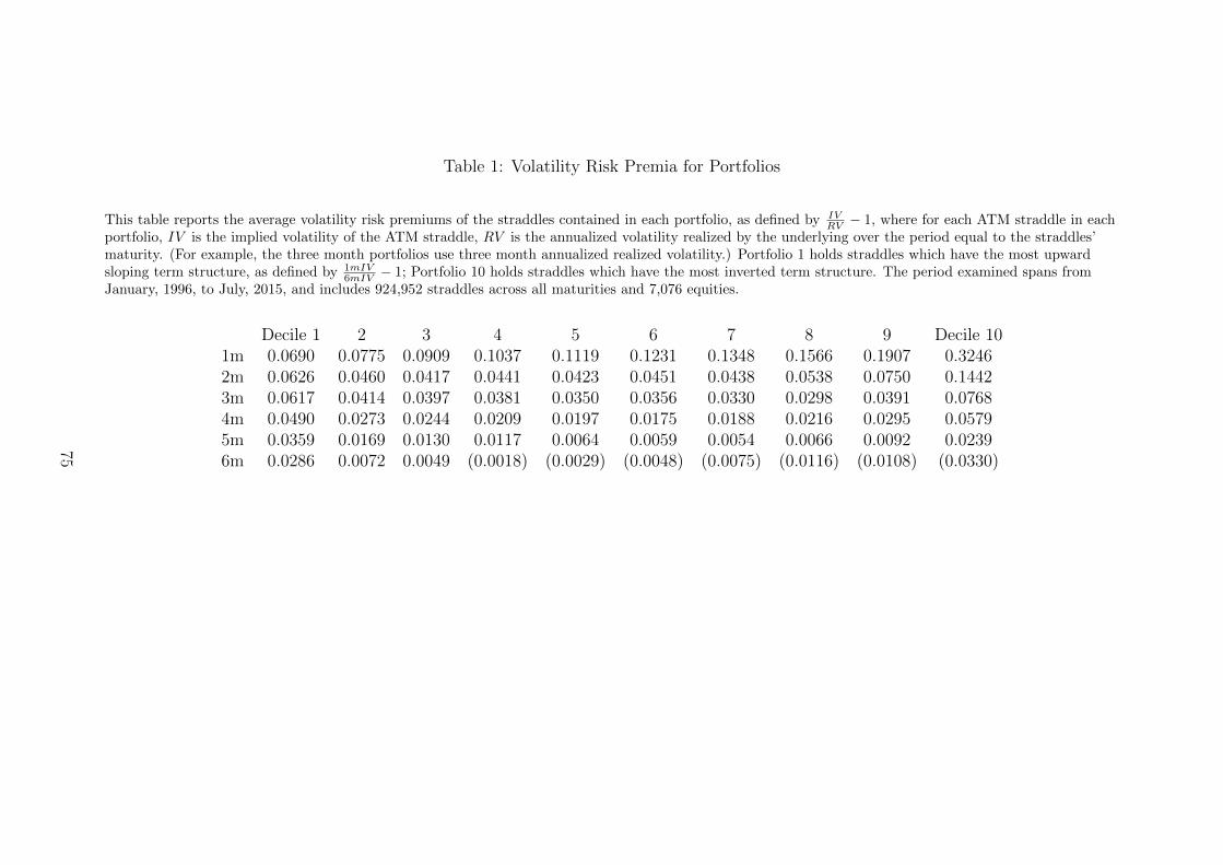
Table 1: Volatility Risk Premia for Portfolios

This table reports the average volatility risk premiums of the straddles contained in each portfolio, as defined by IVRV − 1, where for each ATM straddle in each

portfolio, IV is the implied volatility of the ATM straddle, RV is the annualized volatility realized by the underlying over the period equal to the straddles’maturity. (For example, the three month portfolios use three month annualized realized volatility.) Portfolio 1 holds straddles which have the most upwardsloping term structure, as defined by 1mIV

6mIV − 1; Portfolio 10 holds straddles which have the most inverted term structure. The period examined spans fromJanuary, 1996, to July, 2015, and includes 924,952 straddles across all maturities and 7,076 equities.

Decile 1 2 3 4 5 6 7 8 9 Decile 101m 0.0690 0.0775 0.0909 0.1037 0.1119 0.1231 0.1348 0.1566 0.1907 0.32462m 0.0626 0.0460 0.0417 0.0441 0.0423 0.0451 0.0438 0.0538 0.0750 0.14423m 0.0617 0.0414 0.0397 0.0381 0.0350 0.0356 0.0330 0.0298 0.0391 0.07684m 0.0490 0.0273 0.0244 0.0209 0.0197 0.0175 0.0188 0.0216 0.0295 0.05795m 0.0359 0.0169 0.0130 0.0117 0.0064 0.0059 0.0054 0.0066 0.0092 0.02396m 0.0286 0.0072 0.0049 (0.0018) (0.0029) (0.0048) (0.0075) (0.0116) (0.0108) (0.0330)

75

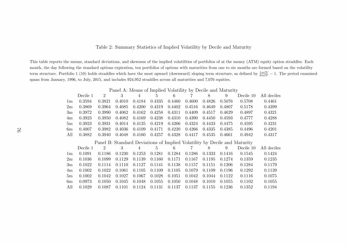
Table 2: Summary Statistics of Implied Volatility by Decile and Maturity

This table reports the means, standard deviations, and skewness of the implied volatilities of portfolios of at the money (ATM) equity option straddles. Each

month, the day following the standard options expiration, ten portfolios of options with maturities from one to six months are formed based on the volatility

term structure. Portfolio 1 (10) holds straddles which have the most upward (downward) sloping term structure, as defined by 1mIV6mIV − 1. The period examined

spans from January, 1996, to July, 2015, and includes 924,952 straddles across all maturities and 7,076 equities.

Panel A: Means of Implied Volatility by Decile and MaturityDecile 1 2 3 4 5 6 7 8 9 Decile 10 All deciles

1m 0.3594 0.3821 0.4010 0.4184 0.4335 0.4460 0.4600 0.4826 0.5076 0.5708 0.44612m 0.3869 0.3964 0.4085 0.4200 0.4319 0.4402 0.4516 0.4649 0.4807 0.5178 0.43993m 0.3972 0.3990 0.4062 0.4162 0.4258 0.4311 0.4409 0.4517 0.4629 0.4897 0.43214m 0.3923 0.3950 0.4082 0.4169 0.4238 0.4310 0.4390 0.4450 0.4593 0.4777 0.42885m 0.3923 0.3931 0.4014 0.4135 0.4219 0.4266 0.4324 0.4433 0.4475 0.4595 0.42316m 0.4007 0.3982 0.4036 0.4109 0.4171 0.4220 0.4266 0.4335 0.4385 0.4496 0.4201All 0.3882 0.3940 0.4048 0.4160 0.4257 0.4328 0.4417 0.4535 0.4661 0.4942 0.4317

Panel B: Standard Deviations of Implied Volatility by Decile and MaturityDecile 1 2 3 4 5 6 7 8 9 Decile 10 All deciles

1m 0.1091 0.1186 0.1230 0.1253 0.1281 0.1284 0.1286 0.1333 0.1416 0.1545 0.14242m 0.1036 0.1099 0.1129 0.1139 0.1160 0.1171 0.1167 0.1195 0.1274 0.1359 0.12353m 0.1022 0.1114 0.1110 0.1127 0.1141 0.1138 0.1157 0.1151 0.1206 0.1284 0.11794m 0.1002 0.1022 0.1061 0.1105 0.1109 0.1105 0.1079 0.1109 0.1196 0.1292 0.11395m 0.1002 0.1042 0.1027 0.1067 0.1028 0.1051 0.1042 0.1044 0.1122 0.1116 0.10756m 0.0973 0.1050 0.1045 0.1048 0.1055 0.1050 0.1048 0.1010 0.1055 0.1102 0.1055All 0.1029 0.1087 0.1101 0.1124 0.1131 0.1137 0.1137 0.1155 0.1236 0.1352 0.1194

76

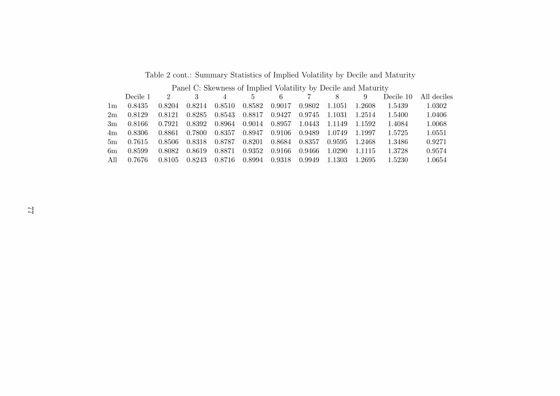
Table 2 cont.: Summary Statistics of Implied Volatility by Decile and Maturity

Panel C: Skewness of Implied Volatility by Decile and MaturityDecile 1 2 3 4 5 6 7 8 9 Decile 10 All deciles

1m 0.8435 0.8204 0.8214 0.8510 0.8582 0.9017 0.9802 1.1051 1.2608 1.5439 1.03022m 0.8129 0.8121 0.8285 0.8543 0.8817 0.9427 0.9745 1.1031 1.2514 1.5400 1.04063m 0.8166 0.7921 0.8392 0.8964 0.9014 0.8957 1.0443 1.1149 1.1592 1.4084 1.00684m 0.8306 0.8861 0.7800 0.8357 0.8947 0.9106 0.9489 1.0749 1.1997 1.5725 1.05515m 0.7615 0.8506 0.8318 0.8787 0.8201 0.8684 0.8357 0.9595 1.2468 1.3486 0.92716m 0.8599 0.8082 0.8619 0.8871 0.9352 0.9166 0.9466 1.0290 1.1115 1.3728 0.9574All 0.7676 0.8105 0.8243 0.8716 0.8994 0.9318 0.9949 1.1303 1.2695 1.5230 1.0654

77

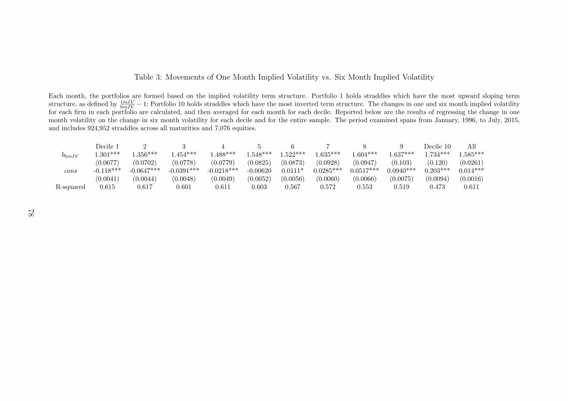
Table 3: Movements of One Month Implied Volatility vs. Six Month Implied Volatility

Each month, the portfolios are formed based on the implied volatility term structure. Portfolio 1 holds straddles which have the most upward sloping termstructure, as defined by 1mIV

6mIV − 1; Portfolio 10 holds straddles which have the most inverted term structure. The changes in one and six month implied volatilityfor each firm in each portfolio are calculated, and then averaged for each month for each decile. Reported below are the results of regressing the change in onemonth volatility on the change in six month volatility for each decile and for the entire sample. The period examined spans from January, 1996, to July, 2015,and includes 924,952 straddles across all maturities and 7,076 equities.

Decile 1 2 3 4 5 6 7 8 9 Decile 10 Allb6mIV 1.301*** 1.356*** 1.454*** 1.488*** 1.548*** 1.522*** 1.635*** 1.604*** 1.637*** 1.734*** 1.585***

(0.0677) (0.0702) (0.0778) (0.0779) (0.0825) (0.0873) (0.0928) (0.0947) (0.103) (0.120) (0.0261)cons -0.118*** -0.0647*** -0.0391*** -0.0218*** -0.00620 0.0111* 0.0285*** 0.0517*** 0.0940*** 0.203*** 0.014***

(0.0041) (0.0044) (0.0048) (0.0049) (0.0052) (0.0056) (0.0060) (0.0066) (0.0075) (0.0094) (0.0016)R-squared 0.615 0.617 0.601 0.611 0.603 0.567 0.572 0.553 0.519 0.473 0.611

78

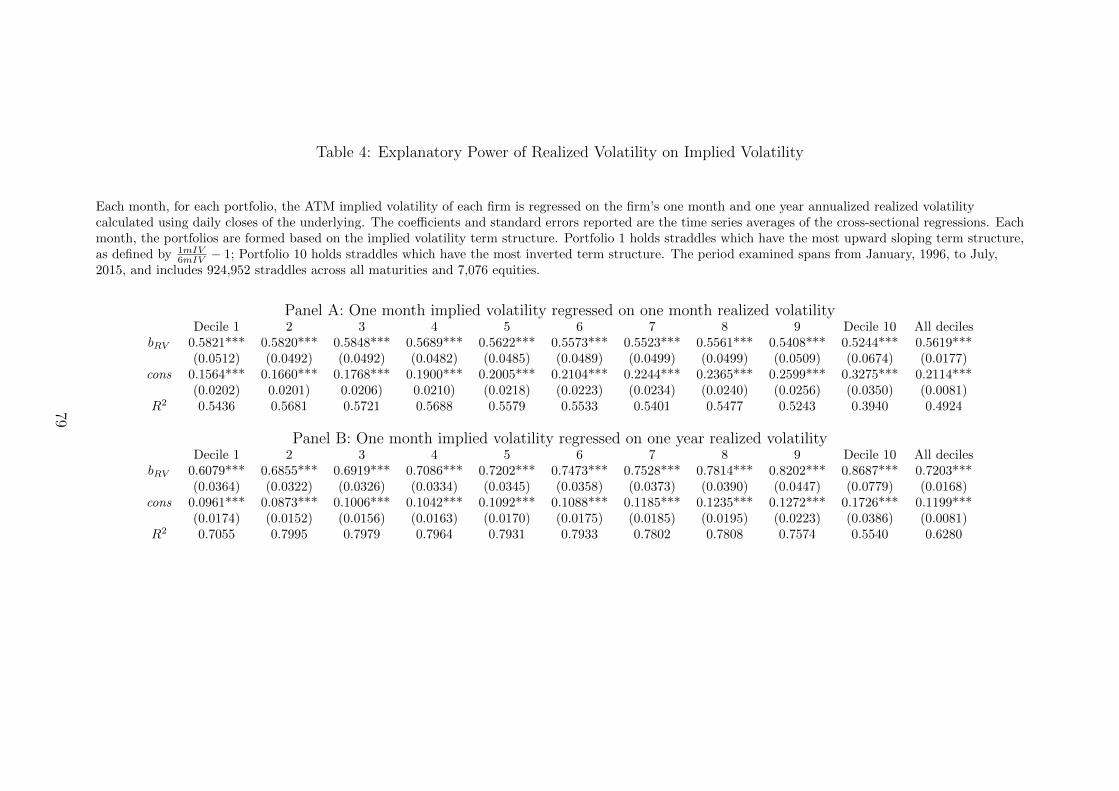
Table 4: Explanatory Power of Realized Volatility on Implied Volatility

Each month, for each portfolio, the ATM implied volatility of each firm is regressed on the firm’s one month and one year annualized realized volatilitycalculated using daily closes of the underlying. The coefficients and standard errors reported are the time series averages of the cross-sectional regressions. Eachmonth, the portfolios are formed based on the implied volatility term structure. Portfolio 1 holds straddles which have the most upward sloping term structure,as defined by 1mIV

6mIV − 1; Portfolio 10 holds straddles which have the most inverted term structure. The period examined spans from January, 1996, to July,2015, and includes 924,952 straddles across all maturities and 7,076 equities.

Panel A: One month implied volatility regressed on one month realized volatilityDecile 1 2 3 4 5 6 7 8 9 Decile 10 All deciles

bRV 0.5821*** 0.5820*** 0.5848*** 0.5689*** 0.5622*** 0.5573*** 0.5523*** 0.5561*** 0.5408*** 0.5244*** 0.5619***(0.0512) (0.0492) (0.0492) (0.0482) (0.0485) (0.0489) (0.0499) (0.0499) (0.0509) (0.0674) (0.0177)

cons 0.1564*** 0.1660*** 0.1768*** 0.1900*** 0.2005*** 0.2104*** 0.2244*** 0.2365*** 0.2599*** 0.3275*** 0.2114***(0.0202) 0.0201) 0.0206) 0.0210) (0.0218) (0.0223) (0.0234) (0.0240) (0.0256) (0.0350) (0.0081)

R2 0.5436 0.5681 0.5721 0.5688 0.5579 0.5533 0.5401 0.5477 0.5243 0.3940 0.4924

Panel B: One month implied volatility regressed on one year realized volatilityDecile 1 2 3 4 5 6 7 8 9 Decile 10 All deciles

bRV 0.6079*** 0.6855*** 0.6919*** 0.7086*** 0.7202*** 0.7473*** 0.7528*** 0.7814*** 0.8202*** 0.8687*** 0.7203***(0.0364) (0.0322) (0.0326) (0.0334) (0.0345) (0.0358) (0.0373) (0.0390) (0.0447) (0.0779) (0.0168)

cons 0.0961*** 0.0873*** 0.1006*** 0.1042*** 0.1092*** 0.1088*** 0.1185*** 0.1235*** 0.1272*** 0.1726*** 0.1199***(0.0174) (0.0152) (0.0156) (0.0163) (0.0170) (0.0175) (0.0185) (0.0195) (0.0223) (0.0386) (0.0081)

R2 0.7055 0.7995 0.7979 0.7964 0.7931 0.7933 0.7802 0.7808 0.7574 0.5540 0.6280

79

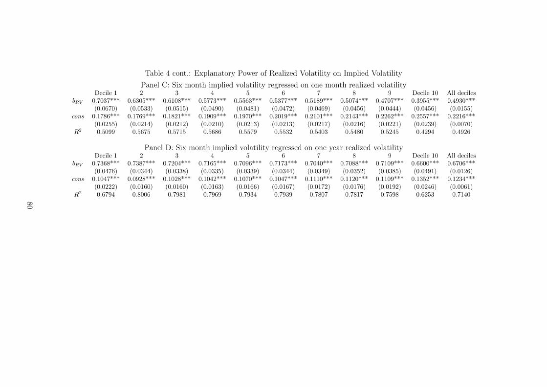
Table 4 cont.: Explanatory Power of Realized Volatility on Implied Volatility

Panel C: Six month implied volatility regressed on one month realized volatilityDecile 1 2 3 4 5 6 7 8 9 Decile 10 All deciles

bRV 0.7037*** 0.6305*** 0.6108*** 0.5773*** 0.5563*** 0.5377*** 0.5189*** 0.5074*** 0.4707*** 0.3955*** 0.4930***(0.0670) (0.0533) (0.0515) (0.0490) (0.0481) (0.0472) (0.0469) (0.0456) (0.0444) (0.0456) (0.0155)

cons 0.1786*** 0.1769*** 0.1821*** 0.1909*** 0.1970*** 0.2019*** 0.2101*** 0.2143*** 0.2262*** 0.2557*** 0.2216***(0.0255) (0.0214) (0.0212) (0.0210) (0.0213) (0.0213) (0.0217) (0.0216) (0.0221) (0.0239) (0.0070)

R2 0.5099 0.5675 0.5715 0.5686 0.5579 0.5532 0.5403 0.5480 0.5245 0.4294 0.4926

Panel D: Six month implied volatility regressed on one year realized volatilityDecile 1 2 3 4 5 6 7 8 9 Decile 10 All deciles

bRV 0.7368*** 0.7387*** 0.7204*** 0.7165*** 0.7096*** 0.7173*** 0.7040*** 0.7088*** 0.7109*** 0.6600*** 0.6706***(0.0476) (0.0344) (0.0338) (0.0335) (0.0339) (0.0344) (0.0349) (0.0352) (0.0385) (0.0491) (0.0126)

cons 0.1047*** 0.0928*** 0.1028*** 0.1042*** 0.1070*** 0.1047*** 0.1110*** 0.1120*** 0.1109*** 0.1352*** 0.1234***(0.0222) (0.0160) (0.0160) (0.0163) (0.0166) (0.0167) (0.0172) (0.0176) (0.0192) (0.0246) (0.0061)

R2 0.6794 0.8006 0.7981 0.7969 0.7934 0.7939 0.7807 0.7817 0.7598 0.6253 0.7140

80

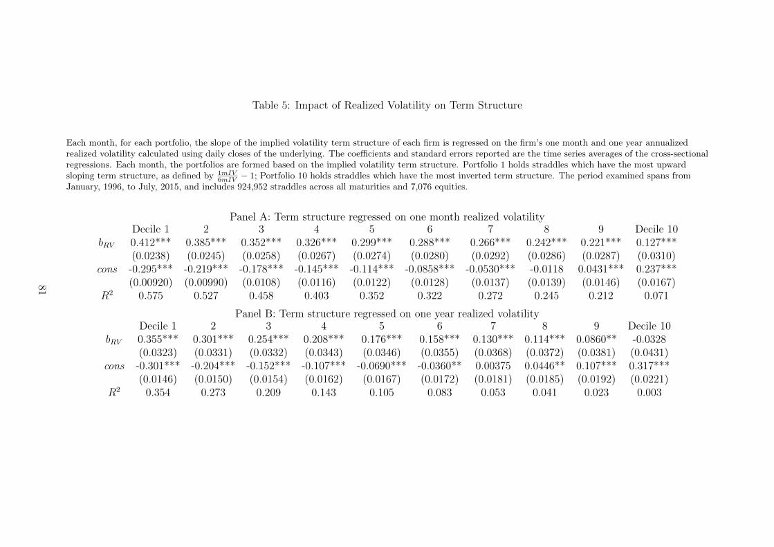
Table 5: Impact of Realized Volatility on Term Structure

Each month, for each portfolio, the slope of the implied volatility term structure of each firm is regressed on the firm’s one month and one year annualizedrealized volatility calculated using daily closes of the underlying. The coefficients and standard errors reported are the time series averages of the cross-sectionalregressions. Each month, the portfolios are formed based on the implied volatility term structure. Portfolio 1 holds straddles which have the most upwardsloping term structure, as defined by 1mIV

6mIV − 1; Portfolio 10 holds straddles which have the most inverted term structure. The period examined spans fromJanuary, 1996, to July, 2015, and includes 924,952 straddles across all maturities and 7,076 equities.

Panel A: Term structure regressed on one month realized volatilityDecile 1 2 3 4 5 6 7 8 9 Decile 10

bRV 0.412*** 0.385*** 0.352*** 0.326*** 0.299*** 0.288*** 0.266*** 0.242*** 0.221*** 0.127***(0.0238) (0.0245) (0.0258) (0.0267) (0.0274) (0.0280) (0.0292) (0.0286) (0.0287) (0.0310)

cons -0.295*** -0.219*** -0.178*** -0.145*** -0.114*** -0.0858*** -0.0530*** -0.0118 0.0431*** 0.237***(0.00920) (0.00990) (0.0108) (0.0116) (0.0122) (0.0128) (0.0137) (0.0139) (0.0146) (0.0167)

R2 0.575 0.527 0.458 0.403 0.352 0.322 0.272 0.245 0.212 0.071

Panel B: Term structure regressed on one year realized volatilityDecile 1 2 3 4 5 6 7 8 9 Decile 10

bRV 0.355*** 0.301*** 0.254*** 0.208*** 0.176*** 0.158*** 0.130*** 0.114*** 0.0860** -0.0328(0.0323) (0.0331) (0.0332) (0.0343) (0.0346) (0.0355) (0.0368) (0.0372) (0.0381) (0.0431)

cons -0.301*** -0.204*** -0.152*** -0.107*** -0.0690*** -0.0360** 0.00375 0.0446** 0.107*** 0.317***(0.0146) (0.0150) (0.0154) (0.0162) (0.0167) (0.0172) (0.0181) (0.0185) (0.0192) (0.0221)

R2 0.354 0.273 0.209 0.143 0.105 0.083 0.053 0.041 0.023 0.003

81

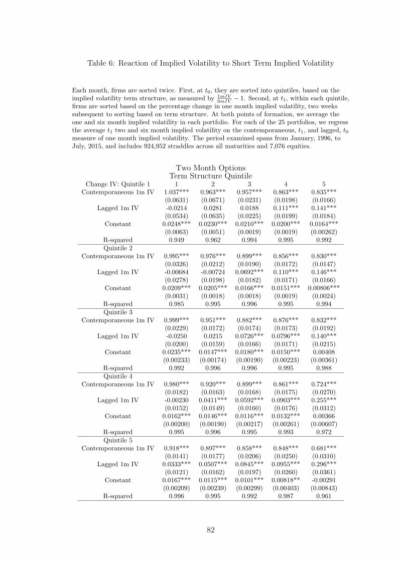
Table 6: Reaction of Implied Volatility to Short Term Implied Volatility

Each month, firms are sorted twice. First, at t0, they are sorted into quintiles, based on theimplied volatility term structure, as measured by 1mIV

6mIV − 1. Second, at t1, within each quintile,firms are sorted based on the percentage change in one month implied volatility, two weekssubsequent to sorting based on term structure. At both points of formation, we average theone and six month implied volatility in each portfolio. For each of the 25 portfolios, we regressthe average t1 two and six month implied volatility on the contemporaneous, t1, and lagged, t0measure of one month implied volatility. The period examined spans from January, 1996, toJuly, 2015, and includes 924,952 straddles across all maturities and 7,076 equities.

Two Month OptionsTerm Structure Quintile

Change IV: Quintile 1 1 2 3 4 5Contemporaneous 1m IV 1.037*** 0.963*** 0.957*** 0.863*** 0.835***

(0.0631) (0.0671) (0.0231) (0.0198) (0.0166)Lagged 1m IV -0.0214 0.0281 0.0188 0.111*** 0.141***

(0.0534) (0.0635) (0.0225) (0.0199) (0.0184)Constant 0.0248*** 0.0230*** 0.0210*** 0.0200*** 0.0164***

(0.0063) (0.0051) (0.0019) (0.0019) (0.00262)R-squared 0.949 0.962 0.994 0.995 0.992Quintile 2

Contemporaneous 1m IV 0.995*** 0.976*** 0.899*** 0.856*** 0.830***(0.0326) (0.0212) (0.0190) (0.0172) (0.0147)

Lagged 1m IV -0.00684 -0.00724 0.0692*** 0.110*** 0.146***(0.0278) (0.0198) (0.0182) (0.0171) (0.0166)

Constant 0.0209*** 0.0205*** 0.0166*** 0.0151*** 0.00806***(0.0031) (0.0018) (0.0018) (0.0019) (0.0024)

R-squared 0.985 0.995 0.996 0.995 0.994Quintile 3

Contemporaneous 1m IV 0.999*** 0.951*** 0.882*** 0.876*** 0.832***(0.0229) (0.0172) (0.0174) (0.0173) (0.0192)

Lagged 1m IV -0.0250 0.0215 0.0726*** 0.0796*** 0.140***(0.0200) (0.0159) (0.0166) (0.0171) (0.0215)

Constant 0.0235*** 0.0147*** 0.0180*** 0.0150*** 0.00408(0.00233) (0.00174) (0.00190) (0.00223) (0.00361)

R-squared 0.992 0.996 0.996 0.995 0.988Quintile 4

Contemporaneous 1m IV 0.980*** 0.920*** 0.899*** 0.861*** 0.724***(0.0182) (0.0163) (0.0168) (0.0175) (0.0270)

Lagged 1m IV -0.00230 0.0411*** 0.0592*** 0.0903*** 0.255***(0.0152) (0.0149) (0.0160) (0.0176) (0.0312)

Constant 0.0162*** 0.0146*** 0.0116*** 0.0132*** 0.00366(0.00200) (0.00190) (0.00217) (0.00261) (0.00607)

R-squared 0.995 0.996 0.995 0.993 0.972Quintile 5

Contemporaneous 1m IV 0.918*** 0.897*** 0.858*** 0.848*** 0.681***(0.0141) (0.0177) (0.0206) (0.0250) (0.0310)

Lagged 1m IV 0.0333*** 0.0507*** 0.0845*** 0.0955*** 0.296***(0.0121) (0.0162) (0.0197) (0.0260) (0.0361)

Constant 0.0167*** 0.0115*** 0.0101*** 0.00818** -0.00291(0.00209) (0.00239) (0.00299) (0.00403) (0.00843)

R-squared 0.996 0.995 0.992 0.987 0.961

82

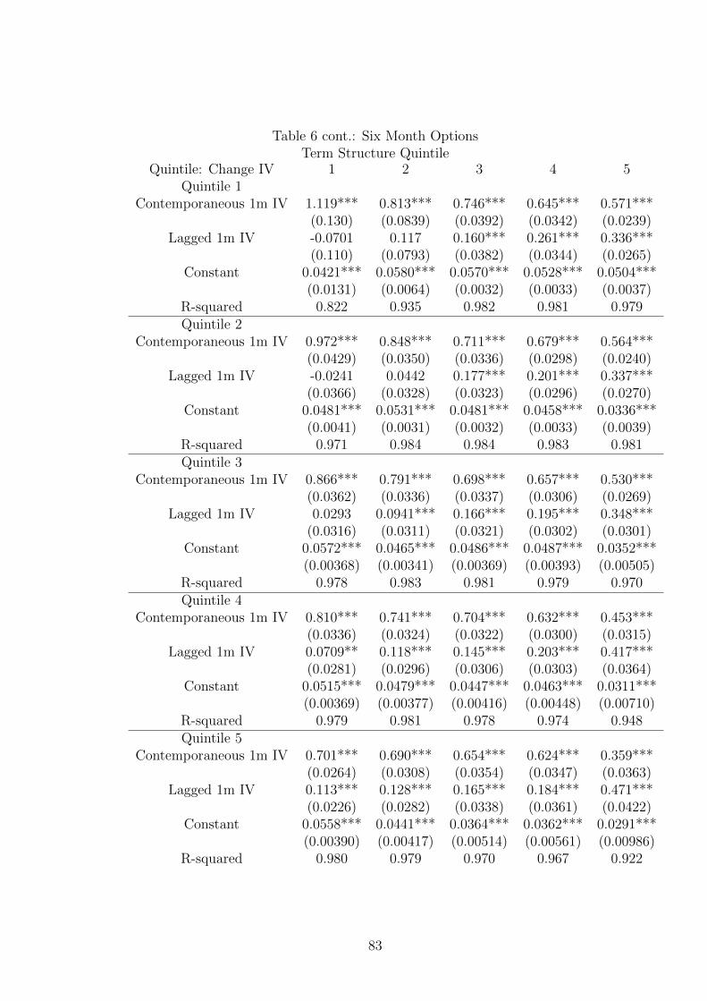
Table 6 cont.: Six Month OptionsTerm Structure Quintile

Quintile: Change IV 1 2 3 4 5Quintile 1

Contemporaneous 1m IV 1.119*** 0.813*** 0.746*** 0.645*** 0.571***(0.130) (0.0839) (0.0392) (0.0342) (0.0239)

Lagged 1m IV -0.0701 0.117 0.160*** 0.261*** 0.336***(0.110) (0.0793) (0.0382) (0.0344) (0.0265)

Constant 0.0421*** 0.0580*** 0.0570*** 0.0528*** 0.0504***(0.0131) (0.0064) (0.0032) (0.0033) (0.0037)

R-squared 0.822 0.935 0.982 0.981 0.979Quintile 2

Contemporaneous 1m IV 0.972*** 0.848*** 0.711*** 0.679*** 0.564***(0.0429) (0.0350) (0.0336) (0.0298) (0.0240)

Lagged 1m IV -0.0241 0.0442 0.177*** 0.201*** 0.337***(0.0366) (0.0328) (0.0323) (0.0296) (0.0270)

Constant 0.0481*** 0.0531*** 0.0481*** 0.0458*** 0.0336***(0.0041) (0.0031) (0.0032) (0.0033) (0.0039)

R-squared 0.971 0.984 0.984 0.983 0.981Quintile 3

Contemporaneous 1m IV 0.866*** 0.791*** 0.698*** 0.657*** 0.530***(0.0362) (0.0336) (0.0337) (0.0306) (0.0269)

Lagged 1m IV 0.0293 0.0941*** 0.166*** 0.195*** 0.348***(0.0316) (0.0311) (0.0321) (0.0302) (0.0301)

Constant 0.0572*** 0.0465*** 0.0486*** 0.0487*** 0.0352***(0.00368) (0.00341) (0.00369) (0.00393) (0.00505)

R-squared 0.978 0.983 0.981 0.979 0.970Quintile 4

Contemporaneous 1m IV 0.810*** 0.741*** 0.704*** 0.632*** 0.453***(0.0336) (0.0324) (0.0322) (0.0300) (0.0315)

Lagged 1m IV 0.0709** 0.118*** 0.145*** 0.203*** 0.417***(0.0281) (0.0296) (0.0306) (0.0303) (0.0364)

Constant 0.0515*** 0.0479*** 0.0447*** 0.0463*** 0.0311***(0.00369) (0.00377) (0.00416) (0.00448) (0.00710)

R-squared 0.979 0.981 0.978 0.974 0.948Quintile 5

Contemporaneous 1m IV 0.701*** 0.690*** 0.654*** 0.624*** 0.359***(0.0264) (0.0308) (0.0354) (0.0347) (0.0363)

Lagged 1m IV 0.113*** 0.128*** 0.165*** 0.184*** 0.471***(0.0226) (0.0282) (0.0338) (0.0361) (0.0422)

Constant 0.0558*** 0.0441*** 0.0364*** 0.0362*** 0.0291***(0.00390) (0.00417) (0.00514) (0.00561) (0.00986)

R-squared 0.980 0.979 0.970 0.967 0.922

83

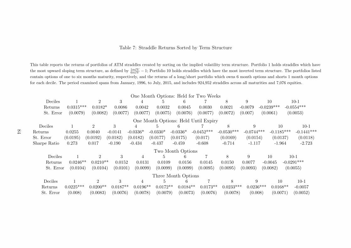
Table 7: Straddle Returns Sorted by Term Structure

This table reports the returns of portfolios of ATM straddles created by sorting on the implied volatility term structure. Portfolio 1 holds straddles which have

the most upward sloping term structure, as defined by 1mIV6mIV − 1; Portfolio 10 holds straddles which have the most inverted term structure. The portfolios listed

contain options of one to six months maturity, respectively, and the returns of a long/short portfolio which owns 6 month options and shorts 1 month options

for each decile. The period examined spans from January, 1996, to July, 2015, and includes 924,952 straddles across all maturities and 7,076 equities.

One Month Options: Held for Two WeeksDeciles 1 2 3 4 5 6 7 8 9 10 10-1

Returns 0.0315*** 0.0182* 0.0086 0.0042 0.0032 0.0045 0.0030 0.0021 -0.0079 -0.0239*** -0.0554***St. Error (0.0079) (0.0082) (0.0077) (0.0077) (0.0075) (0.0076) (0.0077) (0.0072) (0.007) (0.0061) (0.0053)

One Month Options: Held Until ExpiryDeciles 1 2 3 4 5 6 7 8 9 10 10-1

Returns 0.0255 0.0040 -0.0141 -0.0336* -0.0330* -0.0336* -0.0452*** -0.0530*** -0.0744*** -0.1185*** -0.1441***St. Error (0.0195) (0.0192) (0.0182) (0.0182) (0.0177) (0.0175) (0.017) (0.0169) (0.0154) (0.0137) (0.0118)Sharpe Ratio 0.273 0.017 -0.190 -0.434 -0.437 -0.459 -0.608 -0.714 -1.117 -1.964 -2.723

Two Month OptionsDeciles 1 2 3 4 5 6 7 8 9 10 10-1

Returns 0.0246** 0.0210** 0.0152 0.0131 0.0109 0.0156 0.0145 0.0150 0.0077 -0.0045 -0.0291***St. Error (0.0104) (0.0104) (0.0101) (0.0099) (0.0099) (0.0099) (0.0095) (0.0095) (0.0093) (0.0082) (0.0055)

Three Month OptionsDeciles 1 2 3 4 5 6 7 8 9 10 10-1

Returns 0.0225*** 0.0200** 0.0187** 0.0196** 0.0172** 0.0184** 0.0173** 0.0233*** 0.0236*** 0.0168** -0.0057St. Error (0.008) (0.0083) (0.0076) (0.0078) (0.0079) (0.0073) (0.0076) (0.0078) (0.008) (0.0071) (0.0052)

84

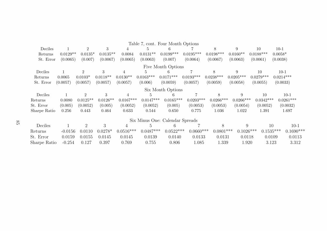
Table 7, cont. Four Month OptionsDeciles 1 2 3 4 5 6 7 8 9 10 10-1

Returns 0.0129** 0.0135* 0.0135** 0.0084 0.0131** 0.0199*** 0.0195*** 0.0198*** 0.0160** 0.0188*** 0.0058*St. Error (0.0065) (0.007) (0.0067) (0.0065) (0.0063) (0.007) (0.0064) (0.0067) (0.0063) (0.0061) (0.0038)

Five Month OptionsDeciles 1 2 3 4 5 6 7 8 9 10 10-1

Returns 0.0065 0.0103* 0.0118** 0.0130** 0.0163*** 0.0171*** 0.0193*** 0.0238*** 0.0205*** 0.0279*** 0.0214***St. Error (0.0057) (0.0057) (0.0057) (0.0057) (0.006) (0.0059) (0.0057) (0.0059) (0.0058) (0.0055) (0.0033)

Six Month OptionsDeciles 1 2 3 4 5 6 7 8 9 10 10-1

Returns 0.0080 0.0125** 0.0126** 0.0167*** 0.0147*** 0.0165*** 0.0203*** 0.0266*** 0.0266*** 0.0342*** 0.0261***St. Error (0.005) (0.0052) (0.005) (0.0052) (0.0052) (0.005) (0.0053) (0.0053) (0.0054) (0.0052) (0.0032)Sharpe Ratio 0.256 0.443 0.464 0.633 0.544 0.650 0.775 1.036 1.022 1.391 1.697

Six Minus One: Calendar SpreadsDeciles 1 2 3 4 5 6 7 8 9 10 10-1

Returns -0.0156 0.0110 0.0278* 0.0516*** 0.0487*** 0.0522*** 0.0660*** 0.0801*** 0.1026*** 0.1535*** 0.1690***St. Error 0.0159 0.0155 0.0145 0.0145 0.0139 0.0140 0.0133 0.0131 0.0118 0.0109 0.0113Sharpe Ratio -0.254 0.127 0.397 0.769 0.755 0.806 1.085 1.339 1.920 3.123 3.312

85

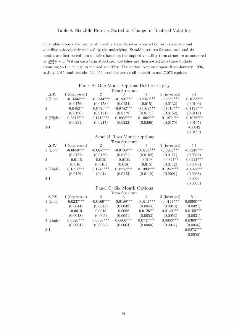
Table 8: Straddle Returns Sorted on Change in Realized Volatility

This table reports the results of monthly straddle returns sorted on term structure and

volatility subsequently realized by the underlying. Straddle returns for one, two, and six

months are first sorted into quintiles based on the implied volatility term structure as measured

by 1mIV6mIV − 1. Within each term structure, portfolios are then sorted into three buckets

according to the change in realized volatility. The period examined spans from January, 1996,

to July, 2015, and includes 924,952 straddles across all maturities and 7,076 equities.

Panel A: One Month Options Held to ExpiryTerm Structure

∆RV 1 (depressed) 2 3 4 5 (inverted) 5-11 (Low) -0.1556*** -0.1734*** -0.1807*** -0.2040*** -0.2589*** -0.1033***

(0.0176) (0.0158) (0.0154) (0.015) (0.0132) (0.0103)2 -0.0482** -0.0751*** -0.0782*** -0.1082*** -0.1613*** -0.1131***

(0.0190) (0.0191) (0.0179) (0.0171) (0.0159) (0.0114)3 (High) 0.2347*** 0.1712*** 0.1608*** 0.1668*** 0.1271*** -0.1075***

(0.0231) (0.0217) (0.0222) (0.0206) (0.0179) (0.0165)3-1 -0.0042

(0.0159)

Panel B: Two Month OptionsTerm Structure

∆RV 1 (depressed) 2 3 4 5 (inverted) 5-11 (Low) -0.0658*** -0.0657*** -0.0705*** -0.0734*** -0.0908*** -0.0249***

(0.0177) (0.0189) (0.0171) (0.0182) (0.0171) (0.0046)2 -0.0115 -0.0151 -0.0103 -0.0193 -0.0327** -0.0212***

(0.016) (0.016) (0.018) (0.015) (0.0142) (0.0048)3 (High) 0.1397*** 0.1245*** 0.1225*** 0.1394*** 0.1242*** -0.0155**

(0.0129) (0.01) (0.0123) (0.0112) (0.0091) (0.0068)3-1 0.0094

(0.0065)

Panel C: Six Month OptionsTerm Structure

∆ RV 1 (depressed) 2 3 4 5 (inverted) 5-11 (Low) -0.0237*** -0.0169*** -0.0189*** -0.0147*** -0.0147*** 0.0090***

(0.0044) (0.0043) (0.0042) (0.0044) (0.0043) (0.0027)2 -0.0010 0.0018 0.0058 0.0126** 0.0149*** 0.0159***

(0.0048) (0.005) (0.0051) (0.0052) (0.0053) (0.0031)3 (High) 0.0520*** 0.0586*** 0.0606*** 0.0747*** 0.0883*** 0.0363***

(0.0064) (0.0065) (0.0064) (0.0068) (0.0071) (0.0046)3-1 0.0273***

(0.0050)

86

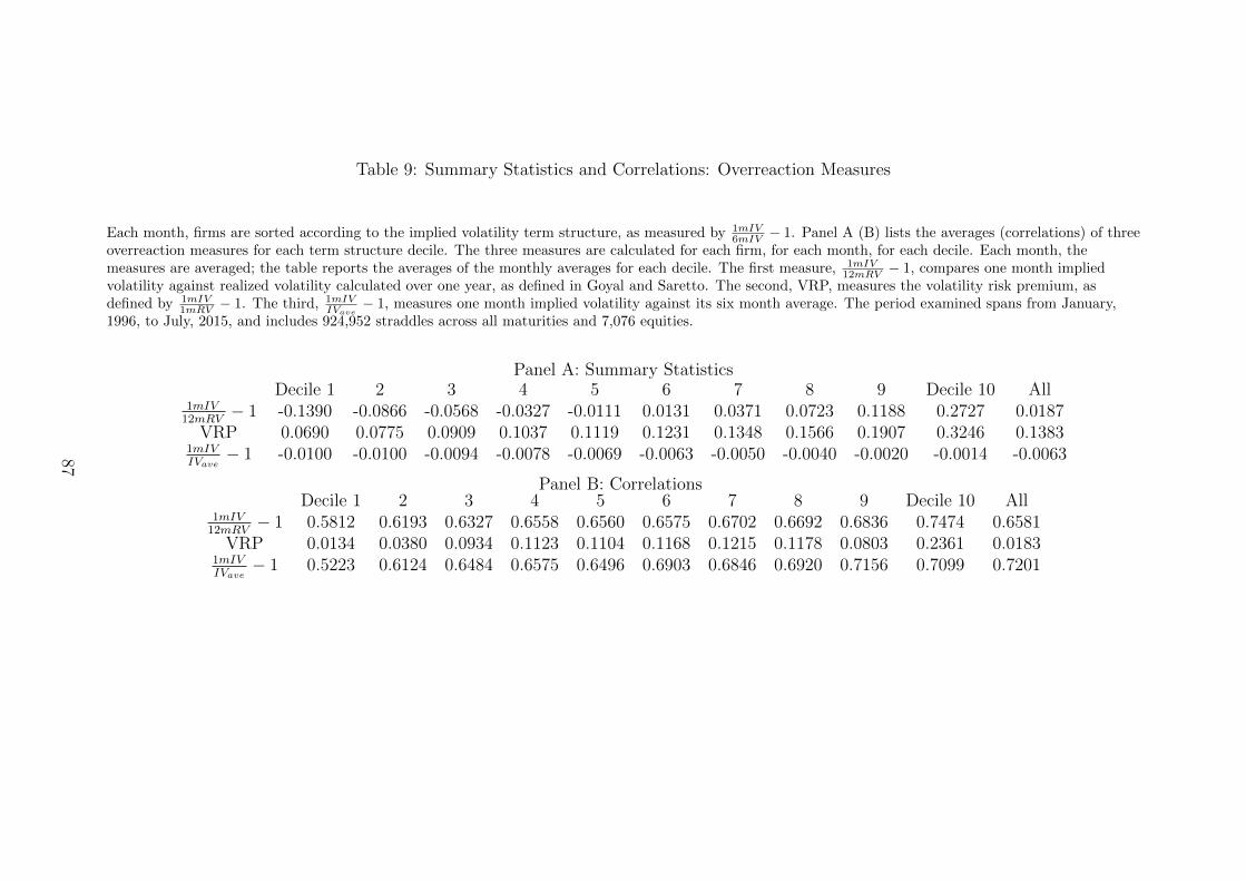
Table 9: Summary Statistics and Correlations: Overreaction Measures

Each month, firms are sorted according to the implied volatility term structure, as measured by 1mIV6mIV − 1. Panel A (B) lists the averages (correlations) of three

overreaction measures for each term structure decile. The three measures are calculated for each firm, for each month, for each decile. Each month, themeasures are averaged; the table reports the averages of the monthly averages for each decile. The first measure, 1mIV

12mRV − 1, compares one month impliedvolatility against realized volatility calculated over one year, as defined in Goyal and Saretto. The second, VRP, measures the volatility risk premium, asdefined by 1mIV

1mRV − 1. The third, 1mIVIVave

− 1, measures one month implied volatility against its six month average. The period examined spans from January,1996, to July, 2015, and includes 924,952 straddles across all maturities and 7,076 equities.

Panel A: Summary StatisticsDecile 1 2 3 4 5 6 7 8 9 Decile 10 All

1mIV12mRV

− 1 -0.1390 -0.0866 -0.0568 -0.0327 -0.0111 0.0131 0.0371 0.0723 0.1188 0.2727 0.0187VRP 0.0690 0.0775 0.0909 0.1037 0.1119 0.1231 0.1348 0.1566 0.1907 0.3246 0.1383

1mIVIVave

− 1 -0.0100 -0.0100 -0.0094 -0.0078 -0.0069 -0.0063 -0.0050 -0.0040 -0.0020 -0.0014 -0.0063

Panel B: CorrelationsDecile 1 2 3 4 5 6 7 8 9 Decile 10 All

1mIV12mRV

− 1 0.5812 0.6193 0.6327 0.6558 0.6560 0.6575 0.6702 0.6692 0.6836 0.7474 0.6581VRP 0.0134 0.0380 0.0934 0.1123 0.1104 0.1168 0.1215 0.1178 0.0803 0.2361 0.0183

1mIVIVave

− 1 0.5223 0.6124 0.6484 0.6575 0.6496 0.6903 0.6846 0.6920 0.7156 0.7099 0.7201

87

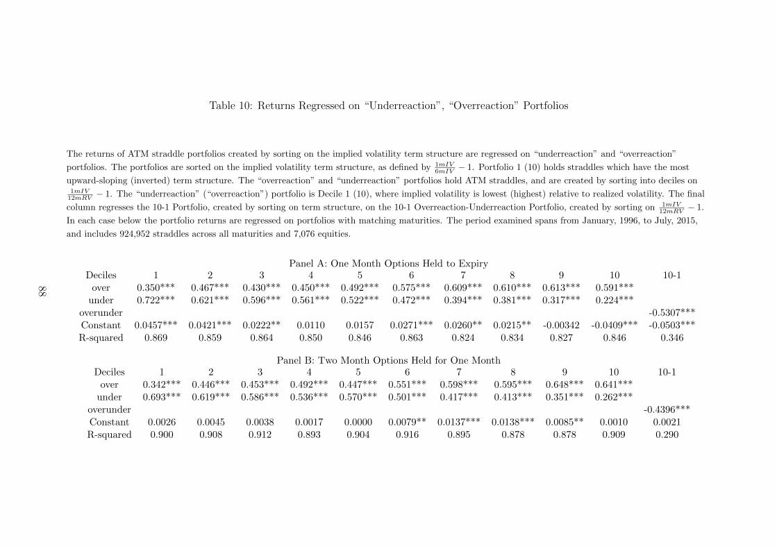
Table 10: Returns Regressed on “Underreaction”, “Overreaction” Portfolios

The returns of ATM straddle portfolios created by sorting on the implied volatility term structure are regressed on “underreaction” and “overreaction”

portfolios. The portfolios are sorted on the implied volatility term structure, as defined by 1mIV6mIV − 1. Portfolio 1 (10) holds straddles which have the most

upward-sloping (inverted) term structure. The “overreaction” and “underreaction” portfolios hold ATM straddles, and are created by sorting into deciles on1mIV12mRV − 1. The “underreaction” (“overreaction”) portfolio is Decile 1 (10), where implied volatility is lowest (highest) relative to realized volatility. The final

column regresses the 10-1 Portfolio, created by sorting on term structure, on the 10-1 Overreaction-Underreaction Portfolio, created by sorting on 1mIV12mRV − 1.

In each case below the portfolio returns are regressed on portfolios with matching maturities. The period examined spans from January, 1996, to July, 2015,

and includes 924,952 straddles across all maturities and 7,076 equities.

Panel A: One Month Options Held to ExpiryDeciles 1 2 3 4 5 6 7 8 9 10 10-1

over 0.350*** 0.467*** 0.430*** 0.450*** 0.492*** 0.575*** 0.609*** 0.610*** 0.613*** 0.591***under 0.722*** 0.621*** 0.596*** 0.561*** 0.522*** 0.472*** 0.394*** 0.381*** 0.317*** 0.224***

overunder -0.5307***Constant 0.0457*** 0.0421*** 0.0222** 0.0110 0.0157 0.0271*** 0.0260** 0.0215** -0.00342 -0.0409*** -0.0503***R-squared 0.869 0.859 0.864 0.850 0.846 0.863 0.824 0.834 0.827 0.846 0.346

Panel B: Two Month Options Held for One MonthDeciles 1 2 3 4 5 6 7 8 9 10 10-1

over 0.342*** 0.446*** 0.453*** 0.492*** 0.447*** 0.551*** 0.598*** 0.595*** 0.648*** 0.641***under 0.693*** 0.619*** 0.586*** 0.536*** 0.570*** 0.501*** 0.417*** 0.413*** 0.351*** 0.262***

overunder -0.4396***Constant 0.0026 0.0045 0.0038 0.0017 0.0000 0.0079** 0.0137*** 0.0138*** 0.0085** 0.0010 0.0021R-squared 0.900 0.908 0.912 0.893 0.904 0.916 0.895 0.878 0.878 0.909 0.290

88

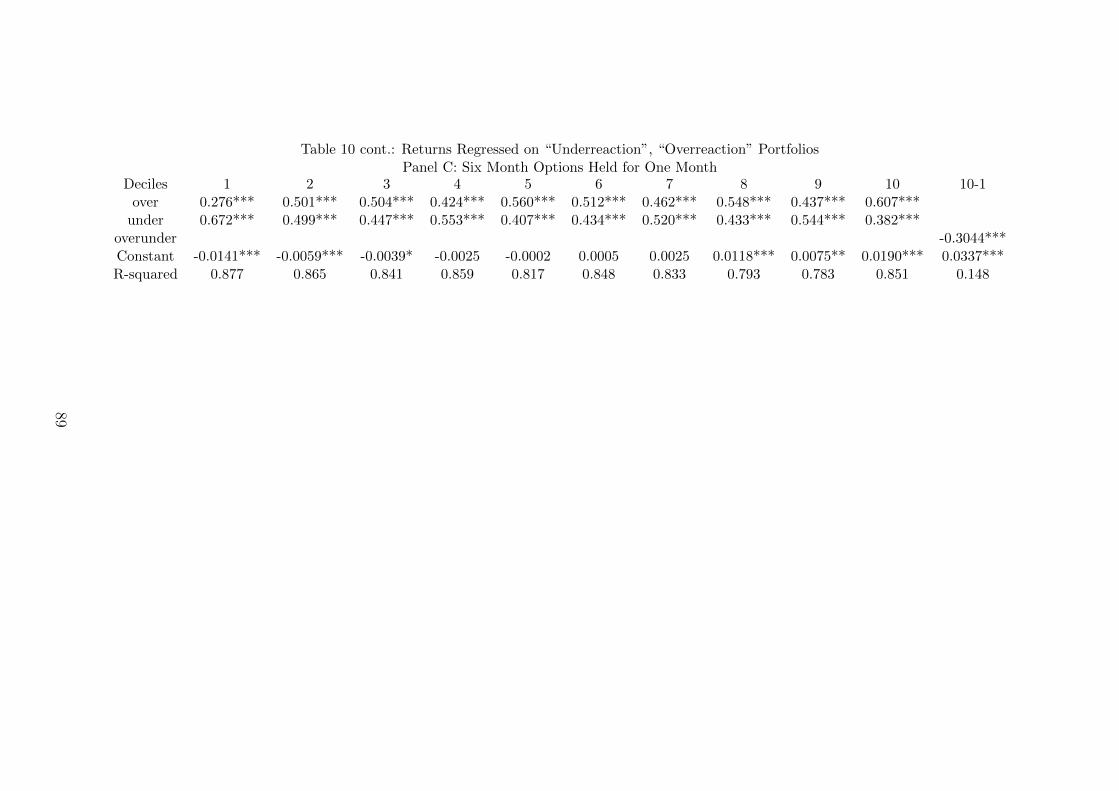
Table 10 cont.: Returns Regressed on “Underreaction”, “Overreaction” PortfoliosPanel C: Six Month Options Held for One Month

Deciles 1 2 3 4 5 6 7 8 9 10 10-1over 0.276*** 0.501*** 0.504*** 0.424*** 0.560*** 0.512*** 0.462*** 0.548*** 0.437*** 0.607***

under 0.672*** 0.499*** 0.447*** 0.553*** 0.407*** 0.434*** 0.520*** 0.433*** 0.544*** 0.382***overunder -0.3044***Constant -0.0141*** -0.0059*** -0.0039* -0.0025 -0.0002 0.0005 0.0025 0.0118*** 0.0075** 0.0190*** 0.0337***R-squared 0.877 0.865 0.841 0.859 0.817 0.848 0.833 0.793 0.783 0.851 0.148

89

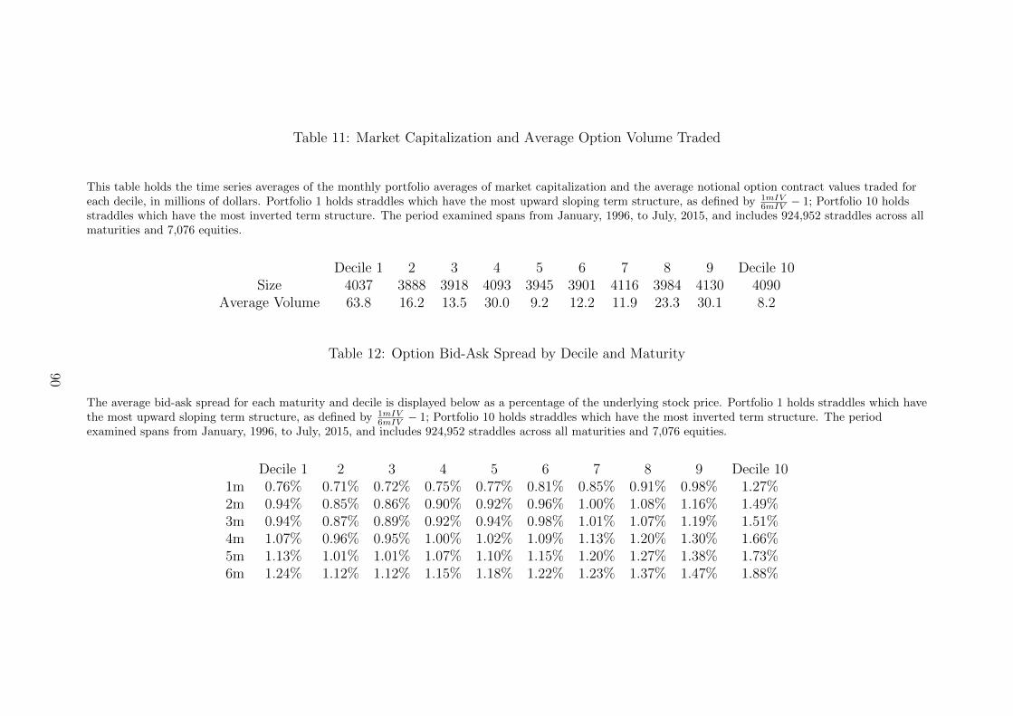
Table 11: Market Capitalization and Average Option Volume Traded

This table holds the time series averages of the monthly portfolio averages of market capitalization and the average notional option contract values traded foreach decile, in millions of dollars. Portfolio 1 holds straddles which have the most upward sloping term structure, as defined by 1mIV

6mIV − 1; Portfolio 10 holdsstraddles which have the most inverted term structure. The period examined spans from January, 1996, to July, 2015, and includes 924,952 straddles across allmaturities and 7,076 equities.

Decile 1 2 3 4 5 6 7 8 9 Decile 10Size 4037 3888 3918 4093 3945 3901 4116 3984 4130 4090

Average Volume 63.8 16.2 13.5 30.0 9.2 12.2 11.9 23.3 30.1 8.2

Table 12: Option Bid-Ask Spread by Decile and Maturity

The average bid-ask spread for each maturity and decile is displayed below as a percentage of the underlying stock price. Portfolio 1 holds straddles which havethe most upward sloping term structure, as defined by 1mIV

6mIV − 1; Portfolio 10 holds straddles which have the most inverted term structure. The periodexamined spans from January, 1996, to July, 2015, and includes 924,952 straddles across all maturities and 7,076 equities.

Decile 1 2 3 4 5 6 7 8 9 Decile 101m 0.76% 0.71% 0.72% 0.75% 0.77% 0.81% 0.85% 0.91% 0.98% 1.27%2m 0.94% 0.85% 0.86% 0.90% 0.92% 0.96% 1.00% 1.08% 1.16% 1.49%3m 0.94% 0.87% 0.89% 0.92% 0.94% 0.98% 1.01% 1.07% 1.19% 1.51%4m 1.07% 0.96% 0.95% 1.00% 1.02% 1.09% 1.13% 1.20% 1.30% 1.66%5m 1.13% 1.01% 1.01% 1.07% 1.10% 1.15% 1.20% 1.27% 1.38% 1.73%6m 1.24% 1.12% 1.12% 1.15% 1.18% 1.22% 1.23% 1.37% 1.47% 1.88%

90

Table 13: Returns Sorted by Option Bid-Ask Spread: Effect of Transactions Costs

This table examines the impact of transactions costs on Decile 10 by presenting returns using a0%, 50%, and 100% effective bid-ask spread. Reported below are the results of the short onemonth, long six month, and the one-six month calendar spread portfolio returns of Decile 10sorted into quintiles by options bid-ask spread as a percentage of stock price: Quintile 1 hasthe smallest spread; Quintile 5 has the largest. The first column holds returns where the optiontrades are executed at the midpoint. The second column executes trades assuming the bid-askspread is 50% as wide as the prices posted. The last column buys (sells) options on the ask(bid). The period examined spans from January, 1996, to July, 2015, and includes 924,952straddles across all maturities and 7,076 equities.

Effective Spread 0% 50% 100%1 1M 0.1077*** 0.0923*** -0.0778***(Narrow) 6M 0.0354*** 0.0059 -0.0226

6M - 1M 0.1415*** 0.0966*** 0.0534***Sharpe Ratio 2.17 1.47 0.80

2 1M 0.1003*** 0.0729*** 0.0477***6M 0.0267*** -0.0261 -0.0754

6M - 1M 0.1270*** 0.0499*** -0.0244Sharpe Ratio 2.10 0.75 -0.35

3 1M 0.1351*** 0.0703*** 0.0194(Wide) 6M 0.0401*** -0.0836 -0.1835

6M - 1M 0.1739*** -0.0146 -0.1655Sharpe Ratio 2.95 -0.21 -2.02

91

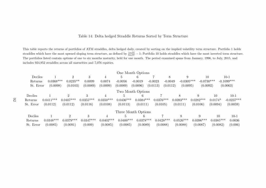
Table 14: Delta hedged Straddle Returns Sorted by Term Structure

This table reports the returns of portfolios of ATM straddles, delta hedged daily, created by sorting on the implied volatility term structure. Portfolio 1 holds

straddles which have the most upward sloping term structure, as defined by 1mIV6mIV − 1; Portfolio 10 holds straddles which have the most inverted term structure.

The portfolios listed contain options of one to six months maturity, held for one month. The period examined spans from January, 1996, to July, 2015, and

includes 924,952 straddles across all maturities and 7,076 equities.

One Month OptionsDeciles 1 2 3 4 5 6 7 8 9 10 10-1

Returns 0.0368*** 0.0235** 0.0099 0.0074 -0.0056 -0.0019 -0.0023 -0.0049 -0.0305*** -0.0730*** -0.1099***St. Error (0.0098) (0.0103) (0.0089) (0.0099) (0.0089) (0.0096) (0.0113) (0.0112) (0.0095) (0.0092) (0.0063)

Two Month OptionsDeciles 1 2 3 4 5 6 7 8 9 10 10-1

Returns 0.0411*** 0.0407*** 0.0355*** 0.0350*** 0.0436*** 0.0384*** 0.0376*** 0.0393*** 0.0282*** 0.0174* -0.0237***St. Error (0.0112) (0.0112) (0.0116) (0.0108) (0.0113) (0.0111) (0.0105) (0.0111) (0.0106) (0.0094) (0.0059)

Three Month OptionsDeciles 1 2 3 4 5 6 7 8 9 10 10-1

Returns 0.0348*** 0.0379*** 0.0347*** 0.0402*** 0.0400*** 0.0378*** 0.0428*** 0.0526*** 0.0396*** 0.0385*** 0.0036St. Error (0.0085) (0.0091) (0.009) (0.0085) (0.0085) (0.0089) (0.0088) (0.0088) (0.0087) (0.0082) (0.006)

92

Table 14 cont.: Delta hedged Straddle Returns Sorted by Term StructureFour Month Options

Deciles 1 2 3 4 5 6 7 8 9 10 10-1Returns 0.0371*** 0.0386*** 0.0349*** 0.0411*** 0.0388*** 0.0481*** 0.0478*** 0.0557*** 0.0556*** 0.0514*** 0.0143**St. Error (0.0092) (0.0099) (0.0096) (0.0094) (0.0098) (0.0098) (0.0092) (0.0097) (0.0093) (0.0092) (0.0073)

Five Month OptionsDeciles 1 2 3 4 5 6 7 8 9 10 10-1

Returns 0.0236*** 0.0258*** 0.0409*** 0.0444*** 0.0538*** 0.0491*** 0.0581*** 0.0649*** 0.0611*** 0.0713*** 0.0476***St. Error (0.0093) (0.0094) (0.0095) (0.0108) (0.0101) (0.0093) (0.0105) (0.0099) (0.0092) (0.0096) (0.0079)

Six Month OptionsDeciles 1 2 3 4 5 6 7 8 9 10 10-1

Returns 0.0250*** 0.0348*** 0.0373*** 0.0486*** 0.0355*** 0.0459*** 0.0368*** 0.0533*** 0.0507*** 0.0659*** 0.0410***St. Error (0.0086) (0.009) (0.0086) (0.0087) (0.0085) (0.0084) (0.0086) (0.0079) (0.009) (0.0087) (0.0076)93

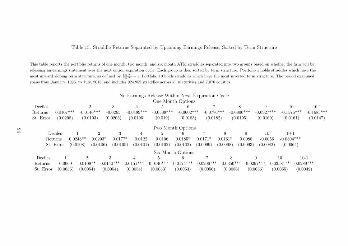
Table 15: Straddle Returns Separated by Upcoming Earnings Release, Sorted by Term Structure

This table reports the portfolio returns of one month, two month, and six month ATM straddles separated into two groups based on whether the firm will be

releasing an earnings statement over the next option expiration cycle. Each group is then sorted by term structure. Portfolio 1 holds straddles which have the

most upward sloping term structure, as defined by 1mIV6mIV − 1; Portfolio 10 holds straddles which have the most inverted term structure. The period examined

spans from January, 1996, to July, 2015, and includes 924,952 straddles across all maturities and 7,076 equities.

No Earnings Release Within Next Expiration CycleOne Month Options

Deciles 1 2 3 4 5 6 7 8 9 10 10-1Returns 0.0107*** -0.0146*** -0.0265 -0.0489*** -0.0589*** -0.0602*** -0.0776*** -0.0800*** -0.0927*** -0.1576*** -0.1683***St. Error (0.0208) (0.0193) (0.0203) (0.0196) (0.019) (0.0183) (0.0182) (0.0195) (0.0169) (0.0161) (0.0147)

Two Month OptionsDeciles 1 2 3 4 5 6 7 8 9 10 10-1

Returns 0.0248** 0.0203* 0.0177* 0.0122 0.0106 0.0185* 0.0171* 0.0161* 0.0080 -0.0056 -0.0304***St. Error (0.0108) (0.0106) (0.0105) (0.0101) (0.0102) (0.0102) (0.0099) (0.0098) (0.0093) (0.0082) (0.0064)

Six Month OptionsDeciles 1 2 3 4 5 6 7 8 9 10 10-1

Returns 0.0069 0.0109** 0.0140*** 0.0151*** 0.0140*** 0.0174*** 0.0206*** 0.0350*** 0.0297*** 0.0358*** 0.0289***St. Error (0.0055) (0.0054) (0.0054) (0.0054) (0.0053) (0.0053) (0.0056) (0.0086) (0.0056) (0.0055) (0.0042)

94

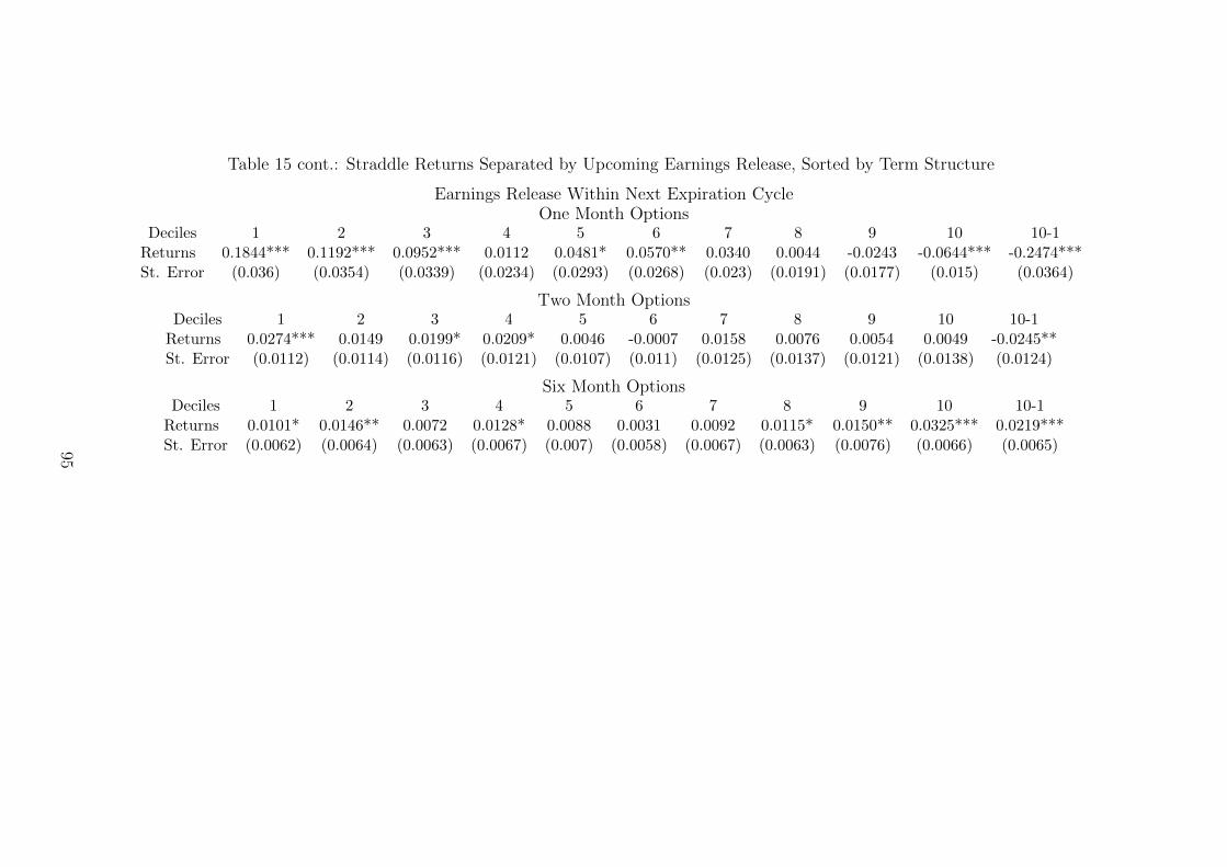
Table 15 cont.: Straddle Returns Separated by Upcoming Earnings Release, Sorted by Term Structure

Earnings Release Within Next Expiration CycleOne Month Options

Deciles 1 2 3 4 5 6 7 8 9 10 10-1Returns 0.1844*** 0.1192*** 0.0952*** 0.0112 0.0481* 0.0570** 0.0340 0.0044 -0.0243 -0.0644*** -0.2474***St. Error (0.036) (0.0354) (0.0339) (0.0234) (0.0293) (0.0268) (0.023) (0.0191) (0.0177) (0.015) (0.0364)

Two Month OptionsDeciles 1 2 3 4 5 6 7 8 9 10 10-1

Returns 0.0274*** 0.0149 0.0199* 0.0209* 0.0046 -0.0007 0.0158 0.0076 0.0054 0.0049 -0.0245**St. Error (0.0112) (0.0114) (0.0116) (0.0121) (0.0107) (0.011) (0.0125) (0.0137) (0.0121) (0.0138) (0.0124)

Six Month OptionsDeciles 1 2 3 4 5 6 7 8 9 10 10-1

Returns 0.0101* 0.0146** 0.0072 0.0128* 0.0088 0.0031 0.0092 0.0115* 0.0150** 0.0325*** 0.0219***St. Error (0.0062) (0.0064) (0.0063) (0.0067) (0.007) (0.0058) (0.0067) (0.0063) (0.0076) (0.0066) (0.0065)95

Table 16: Variance Swaps: Summary Statistics

Each month, equally weighted portfolios of hypothetical variance swaps (VS) are formed based on the difference between the one month variance swap rate and

the one month variance swap rate one month forward, defined as V S(1)FV (1,1) − 1. Portfolio 1 (10) holds VS whose current one month variance swap rate is lowest

(highest) relative to the one month VS one month forward, FV(1,1). The first stanza of the table holds the current/forward differential, V S(1)FV (1,1) − 1; one and

two month VS rates, V S(1) and V S(2); and the first differences of each expressed as a percentage, ∆V X(1) and ∆V X(2); the one month VS one monthforward, FV (1, 1); and the t+1 one month VS rate, V St+1(1). The second stanza holds the equivalent levels for volatility swaps for ease of analysis. Allvolatility and variance measures are represented in volatility and variance “points”, as defined by V olatility ∗ 100 and V ariance ∗ 10000. The period examinedspans from January, 1996, to July, 2015, and includes 56,932 straddles and 2,977 equities.

Decile 1 2 3 4 5 6 7 8 9 Decile 10 AllV S(1)

FV (1,1) − 1 -0.3296 -0.1945 -0.1224 -0.0623 -0.0085 0.0480 0.1152 0.2048 0.3559 0.9688 0.0975

V S(1) 2753.84 2806.23 2809.55 3058.26 3042.15 3354.34 3438.89 3564.35 3982.79 4818.16 3362.86∆V X(1) -0.1096 -0.0696 -0.0710 -0.0076 -0.0257 0.0608 0.0955 0.0637 0.1456 0.4063 0.0488V S(2) 3422.11 3085.11 2958.57 3107.03 3011.00 3231.93 3222.61 3240.28 3435.82 3743.04 3245.75∆V X(2) 0.1423 0.0602 0.0120 0.0468 0.0113 0.0660 0.0634 0.0028 0.0148 0.0810 0.0501FV (1, 1) 4049.92 3358.43 3106.45 3163.26 2991.95 3129.85 3033.03 2949.12 2944.09 2763.87 3149.00V St+1(1) 3642.89 3282.32 3125.34 3256.40 3153.62 3273.49 3330.87 3323.39 3458.12 3636.85 3348.33

Volatility Swaps

Decile 1 2 3 4 5 6 7 8 9 Decile 10 All1mV olSwap

FV (1,1) − 1 -0.1878 -0.1064 -0.0669 -0.0354 -0.0081 0.0197 0.0517 0.0926 0.1580 0.3524 0.0270

1m Vol Swap 47.34 47.66 47.97 49.77 49.96 52.22 53.03 54.38 57.63 63.92 52.392m Vol Swap 53.23 50.41 49.57 50.51 50.01 51.55 51.59 52.02 53.70 56.43 51.901m Vol Swap 1m fwd 58.06 52.85 51.02 51.20 50.05 50.92 50.22 49.72 49.78 48.30 51.211m Vol Swap, t+1 54.83 51.75 50.60 51.41 50.73 51.63 52.01 52.04 53.16 54.42 52.26N 5583 5705 5733 5702 5683 5747 5730 5705 5733 5611 56932

96

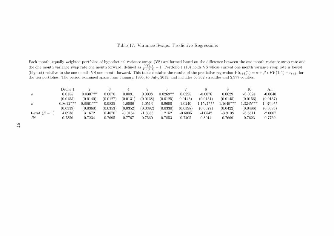
Table 17: Variance Swaps: Predictive Regressions

Each month, equally weighted portfolios of hypothetical variance swaps (VS) are formed based on the difference between the one month variance swap rate and

the one month variance swap rate one month forward, defined as V S(1)FV (1,1) − 1. Portfolio 1 (10) holds VS whose current one month variance swap rate is lowest

(highest) relative to the one month VS one month forward. This table contains the results of the predictive regression V St+1(1) = α+ β ∗ FV (1, 1) + εt+1, forthe ten portfolios. The period examined spans from January, 1996, to July, 2015, and includes 56,932 straddles and 2,977 equities.

Decile 1 2 3 4 5 6 7 8 9 10 Allα 0.0155 0.0307** 0.0070 0.0091 0.0008 0.0269** 0.0225 -0.0076 0.0029 -0.0024 -0.0040

(0.0155) (0.0140) (0.0127) (0.0131) (0.0138) (0.0125) 0.0143) (0.0131) (0.0145) (0.0156) (0.0137)β 0.8612*** 0.8861*** 0.9835 1.0006 1.0513 0.9600 1.0240 1.1527*** 1.1649*** 1.3245*** 1.0769**

(0.0339) (0.0360) (0.0353) (0.0352) (0.0392) (0.0330) (0.0398) (0.0377) (0.0422) (0.0486) (0.0383)t-stat (β = 1) 4.0938 3.1672 0.4670 -0.0164 -1.3085 1.2152 -0.6035 -4.0542 -3.9108 -6.6811 -2.0067R2 0.7356 0.7234 0.7695 0.7767 0.7560 0.7853 0.7405 0.8014 0.7669 0.7623 0.7730

97

Table 18: Returns of Variance Swaps

Each month, equally weighted portfolios of hypothetical variance swaps (VS) are formed based on the difference between the one month variance swap rate and

the one month variance swap rate one month forward, defined as V S(1)FV (1,1) − 1. Portfolio 1 (10) holds VS whose current one month variance swap rate is lowest

(highest) relative to the one month VS one month forward. This table contains the time series average portfolio returns, standard deviations, (t)-statistics forportfolios 1 through 10, and the Long/Short 10-1 portfolio. In addition, the annualized Sharpe Ratio is included for the 10-1 portfolio. The period examinedspans from January, 1996, to July, 2015, and includes 56,932 straddles and 2,977 equities.

Decile 1 2 3 4 5 6 7 8 9 Decile 10 10-1Return -0.0557 0.0032 0.0217 0.0532 0.0686 0.0756 0.1185 0.1343 0.1967 0.4968 0.5525St. Error (0.0180) (0.0219) (0.0216) (0.0230) (0.0239) (0.0232) (0.0241) (0.0238) (0.0272) (0.0747) (0.0675)t-stat -3.09 0.14 1.00 2.31 2.87 3.26 4.92 5.63 7.22 6.65 8.18Sharpe Ratio 1.85

98

Table 19: Summary Statistics of Calendar Spreads

Each month, portfolios of calendar spreads are formed based on the implied volatility differential between the two legs, as defined by 1mIVFV (1,1) − 1. The calendar

spreads consist of a long two month ATM equity option straddle and a short one month ATM equity option straddle. Portfolio 1 (10) holds calendar spreadswhose implied volatility curves have steepest upward (downward) slope. The period examined spans from January, 1996, to July, 2015, and includes 284,984calendar spreads and 6,799 equities.

Decile 1 2 3 4 5 6 7 8 9 10 All1mIV

FV (1,1) − 1 -0.2038 -0.1083 -0.0665 -0.0346 -0.0058 0.0230 0.0558 0.0974 0.1630 0.4157 0.0417

1m IV 0.3928 0.4038 0.4168 0.4259 0.4364 0.4441 0.4570 0.4681 0.4863 0.5289 0.44252m IV 0.4488 0.4280 0.4307 0.4325 0.4366 0.4382 0.4441 0.4469 0.4525 0.4594 0.4374FV(1,1) 0.4942 0.4494 0.4433 0.4385 0.4368 0.4325 0.4318 0.4261 0.4185 0.3853 0.4305Delta 0.0050 0.0030 0.0046 0.0056 0.0067 0.0064 0.0070 0.0076 0.0071 0.0064 0.0035N 28387 28519 28527 28516 28482 28560 28527 28516 28530 28420 284984

99

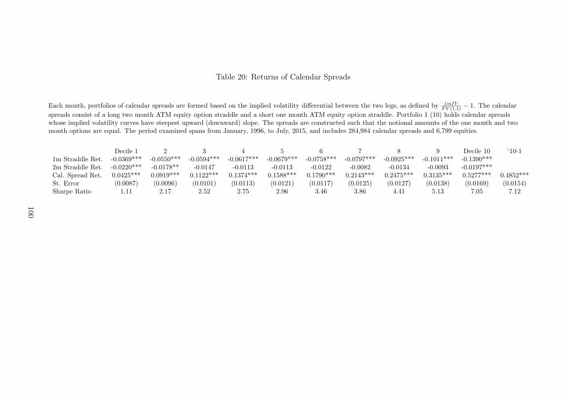
Table 20: Returns of Calendar Spreads

Each month, portfolios of calendar spreads are formed based on the implied volatility differential between the two legs, as defined by 1mIVFV (1,1) − 1. The calendar

spreads consist of a long two month ATM equity option straddle and a short one month ATM equity option straddle. Portfolio 1 (10) holds calendar spreadswhose implied volatility curves have steepest upward (downward) slope. The spreads are constructed such that the notional amounts of the one month and twomonth options are equal. The period examined spans from January, 1996, to July, 2015, and includes 284,984 calendar spreads and 6,799 equities.

Decile 1 2 3 4 5 6 7 8 9 Decile 10 ‘10-11m Straddle Ret. -0.0369*** -0.0550*** -0.0594*** -0.0617*** -0.0679*** -0.0758*** -0.0797*** -0.0925*** -0.1011*** -0.1390***2m Straddle Ret. -0.0220*** -0.0178** -0.0147 -0.0113 -0.0113 -0.0122 -0.0082 -0.0134 -0.0093 -0.0197***Cal. Spread Ret. 0.0425*** 0.0919*** 0.1122*** 0.1374*** 0.1588*** 0.1790*** 0.2143*** 0.2475*** 0.3135*** 0.5277*** 0.4852***St. Error (0.0087) (0.0096) (0.0101) (0.0113) (0.0121) (0.0117) (0.0125) (0.0127) (0.0138) (0.0169) (0.0154)Sharpe Ratio 1.11 2.17 2.52 2.75 2.96 3.46 3.86 4.41 5.13 7.05 7.12

100

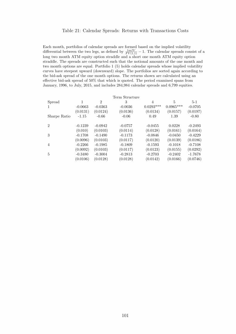
Table 21: Calendar Spreads: Returns with Transactions Costs

Each month, portfolios of calendar spreads are formed based on the implied volatilitydifferential between the two legs, as defined by 1mIV

FV (1,1) − 1. The calendar spreads consist of a

long two month ATM equity option straddle and a short one month ATM equity optionstraddle. The spreads are constructed such that the notional amounts of the one month andtwo month options are equal. Portfolio 1 (5) holds calendar spreads whose implied volatilitycurves have steepest upward (downward) slope. The portfolios are sorted again according tothe bid-ask spread of the one month options. The returns shown are calculated using aneffective bid-ask spread of 50% that which is quoted. The period examined spans fromJanuary, 1996, to July, 2015, and includes 284,984 calendar spreads and 6,799 equities.

Term StructureSpread 1 2 3 4 5 5-11 -0.0663 -0.0363 -0.0036 0.0293*** 0.0965*** -0.0705

(0.0131) (0.0124) (0.0136) (0.0134) (0.0157) (0.0197)Sharpe Ratio -1.15 -0.66 -0.06 0.49 1.39 -0.80

2 -0.1239 -0.0942 -0.0757 -0.0455 0.0228 -0.2493(0.010) (0.0103) (0.0114) (0.0128) (0.0161) (0.0164)

3 -0.1708 -0.1490 -0.1173 -0.0846 -0.0450 -0.4229(0.0096) (0.0103) (0.0117) (0.0120) (0.0139) (0.0186)

4 -0.2266 -0.1985 -0.1809 -0.1593 -0.1018 -0.7108(0.0092) (0.0103) (0.0117) (0.0123) (0.0155) (0.0292)

5 -0.3480 -0.3004 -0.2813 -0.2703 -0.2402 -1.7678(0.0106) (0.0128) (0.0128) (0.0142) (0.0166) (0.0746)

101

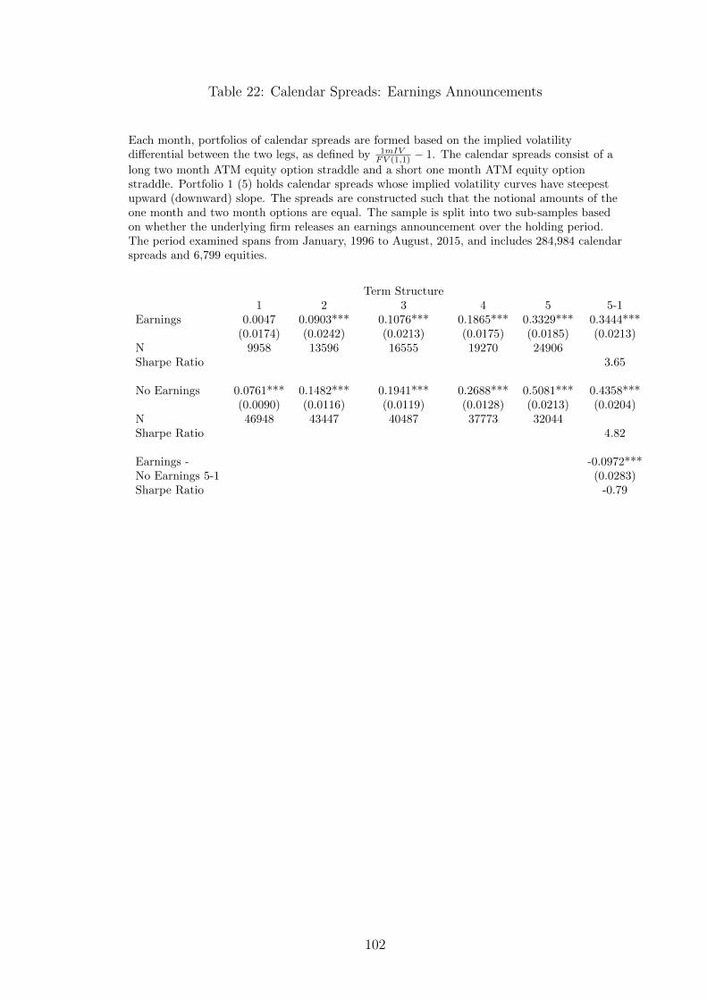
Table 22: Calendar Spreads: Earnings Announcements

Each month, portfolios of calendar spreads are formed based on the implied volatilitydifferential between the two legs, as defined by 1mIV

FV (1,1) − 1. The calendar spreads consist of a

long two month ATM equity option straddle and a short one month ATM equity optionstraddle. Portfolio 1 (5) holds calendar spreads whose implied volatility curves have steepestupward (downward) slope. The spreads are constructed such that the notional amounts of theone month and two month options are equal. The sample is split into two sub-samples basedon whether the underlying firm releases an earnings announcement over the holding period.The period examined spans from January, 1996 to August, 2015, and includes 284,984 calendarspreads and 6,799 equities.

Term Structure1 2 3 4 5 5-1

Earnings 0.0047 0.0903*** 0.1076*** 0.1865*** 0.3329*** 0.3444***(0.0174) (0.0242) (0.0213) (0.0175) (0.0185) (0.0213)

N 9958 13596 16555 19270 24906Sharpe Ratio 3.65

No Earnings 0.0761*** 0.1482*** 0.1941*** 0.2688*** 0.5081*** 0.4358***(0.0090) (0.0116) (0.0119) (0.0128) (0.0213) (0.0204)

N 46948 43447 40487 37773 32044Sharpe Ratio 4.82

Earnings - -0.0972***No Earnings 5-1 (0.0283)Sharpe Ratio -0.79

102

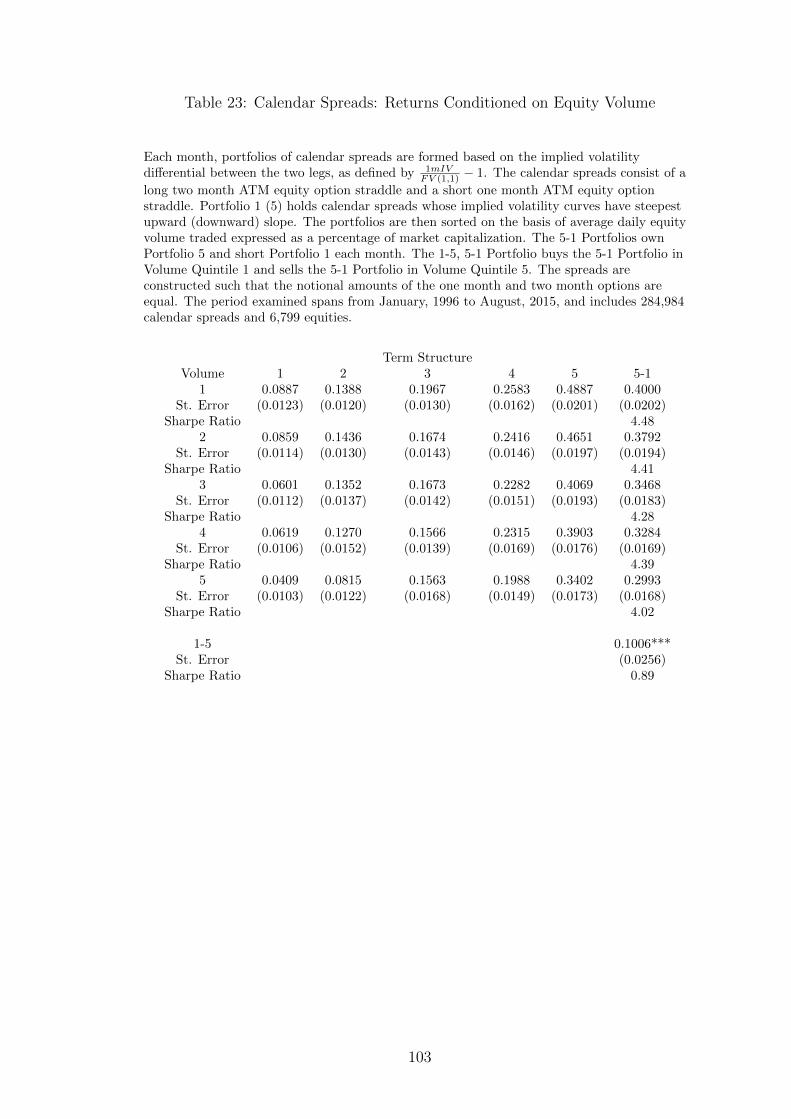
Table 23: Calendar Spreads: Returns Conditioned on Equity Volume

Each month, portfolios of calendar spreads are formed based on the implied volatilitydifferential between the two legs, as defined by 1mIV

FV (1,1) − 1. The calendar spreads consist of a

long two month ATM equity option straddle and a short one month ATM equity optionstraddle. Portfolio 1 (5) holds calendar spreads whose implied volatility curves have steepestupward (downward) slope. The portfolios are then sorted on the basis of average daily equityvolume traded expressed as a percentage of market capitalization. The 5-1 Portfolios ownPortfolio 5 and short Portfolio 1 each month. The 1-5, 5-1 Portfolio buys the 5-1 Portfolio inVolume Quintile 1 and sells the 5-1 Portfolio in Volume Quintile 5. The spreads areconstructed such that the notional amounts of the one month and two month options areequal. The period examined spans from January, 1996 to August, 2015, and includes 284,984calendar spreads and 6,799 equities.

Term StructureVolume 1 2 3 4 5 5-1

1 0.0887 0.1388 0.1967 0.2583 0.4887 0.4000St. Error (0.0123) (0.0120) (0.0130) (0.0162) (0.0201) (0.0202)

Sharpe Ratio 4.482 0.0859 0.1436 0.1674 0.2416 0.4651 0.3792

St. Error (0.0114) (0.0130) (0.0143) (0.0146) (0.0197) (0.0194)Sharpe Ratio 4.41

3 0.0601 0.1352 0.1673 0.2282 0.4069 0.3468St. Error (0.0112) (0.0137) (0.0142) (0.0151) (0.0193) (0.0183)

Sharpe Ratio 4.284 0.0619 0.1270 0.1566 0.2315 0.3903 0.3284

St. Error (0.0106) (0.0152) (0.0139) (0.0169) (0.0176) (0.0169)Sharpe Ratio 4.39

5 0.0409 0.0815 0.1563 0.1988 0.3402 0.2993St. Error (0.0103) (0.0122) (0.0168) (0.0149) (0.0173) (0.0168)

Sharpe Ratio 4.02

1-5 0.1006***St. Error (0.0256)

Sharpe Ratio 0.89

103

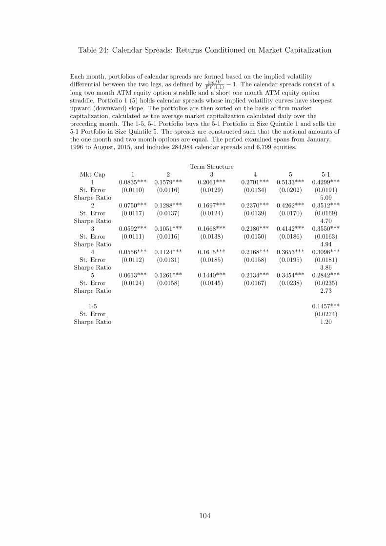
Table 24: Calendar Spreads: Returns Conditioned on Market Capitalization

Each month, portfolios of calendar spreads are formed based on the implied volatilitydifferential between the two legs, as defined by 1mIV

FV (1,1) − 1. The calendar spreads consist of a

long two month ATM equity option straddle and a short one month ATM equity optionstraddle. Portfolio 1 (5) holds calendar spreads whose implied volatility curves have steepestupward (downward) slope. The portfolios are then sorted on the basis of firm marketcapitalization, calculated as the average market capitalization calculated daily over thepreceding month. The 1-5, 5-1 Portfolio buys the 5-1 Portfolio in Size Quintile 1 and sells the5-1 Portfolio in Size Quintile 5. The spreads are constructed such that the notional amounts ofthe one month and two month options are equal. The period examined spans from January,1996 to August, 2015, and includes 284,984 calendar spreads and 6,799 equities.

Term StructureMkt Cap 1 2 3 4 5 5-1

1 0.0835*** 0.1579*** 0.2061*** 0.2701*** 0.5133*** 0.4299***St. Error (0.0110) (0.0116) (0.0129) (0.0134) (0.0202) (0.0191)

Sharpe Ratio 5.092 0.0750*** 0.1288*** 0.1697*** 0.2370*** 0.4262*** 0.3512***

St. Error (0.0117) (0.0137) (0.0124) (0.0139) (0.0170) (0.0169)Sharpe Ratio 4.70

3 0.0592*** 0.1051*** 0.1668*** 0.2180*** 0.4142*** 0.3550***St. Error (0.0111) (0.0116) (0.0138) (0.0150) (0.0186) (0.0163)

Sharpe Ratio 4.944 0.0556*** 0.1124*** 0.1615*** 0.2168*** 0.3653*** 0.3096***

St. Error (0.0112) (0.0131) (0.0185) (0.0158) (0.0195) (0.0181)Sharpe Ratio 3.86

5 0.0613*** 0.1261*** 0.1440*** 0.2134*** 0.3454*** 0.2842***St. Error (0.0124) (0.0158) (0.0145) (0.0167) (0.0238) (0.0235)

Sharpe Ratio 2.73

1-5 0.1457***St. Error (0.0274)

Sharpe Ratio 1.20

104

Table 25: Returns of Deferred Calendar Spreads

Each month, portfolios of calendar spreads are formed based on the implied volatility differential between the two legs. The two calendar spreads examined area two month four month calendar spread (2m-4m return) and a three month six month calendar spread (3m-6m return). Portfolio 1 (10) holds calendar spreadswhose implied volatility curves have steepest upward (downward) slope. The spreads are constructed such that the notional amounts of the short and long termoptions are equal. The period examined spans from January, 1996, to July, 2015. The two month four month calendar spread sample includes 129,779 calendarspreads and 6,912 equities; the three month six month calendar spread includes 138,064 calendar spreads and 7,022 equities.

Decile 1 2 3 4 5 6 7 8 9 Decile 10 10-12m-4m Return 0.0759*** 0.1024*** 0.1196*** 0.1250*** 0.1553*** 0.1844*** 0.1907*** 0.2112*** 0.2668*** 0.4556*** 0.3733***St. Error (0.0049) (0.0067) (0.0078) (0.0082) (0.0101) (0.0120) (0.0124) (0.0138) (0.0174) (0.0297) (0.0244)Sharpe Ratio 3.16

3m-6m Return 0.0790*** 0.1175*** 0.1600*** 0.1565*** 0.1841*** 0.2018*** 0.2237*** 0.2535*** 0.3140*** 0.5045*** 0.4254***St. Error (0.0052) (0.0077) (0.0104) (0.0102) (0.0120) (0.0132) (0.0146) (0.0165) (0.0205) (0.0329) (0.0278)Sharpe Ratio 2.65

105

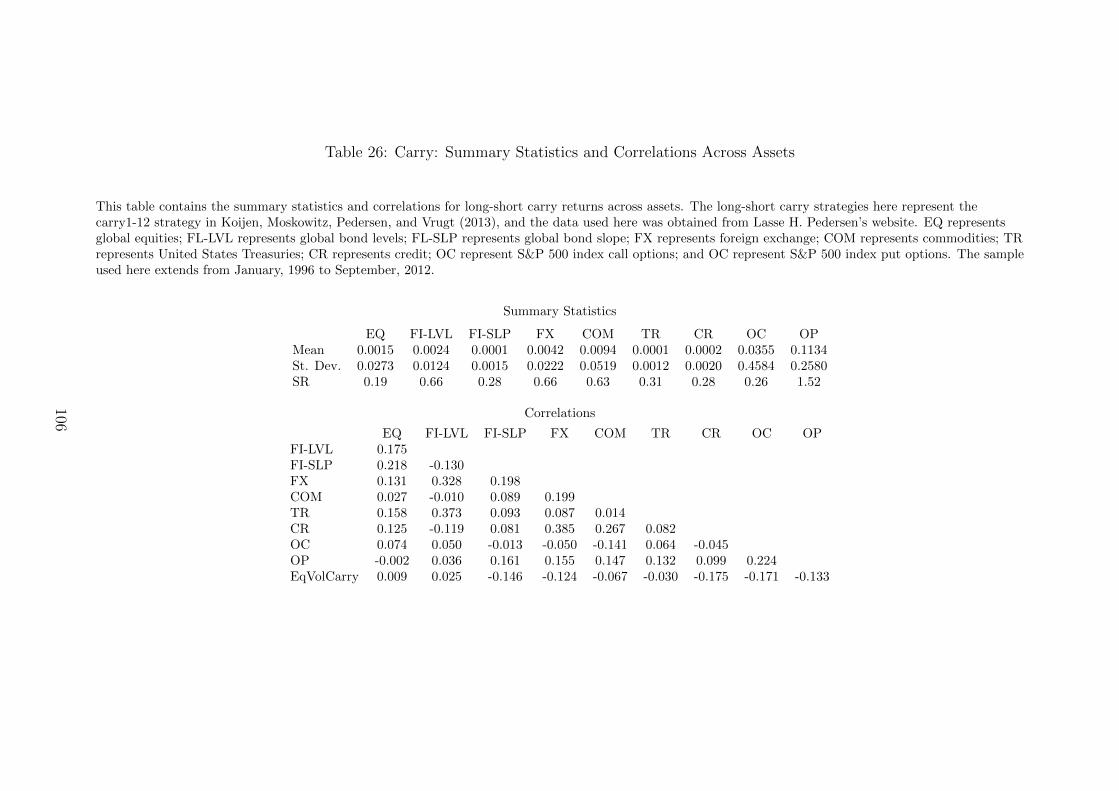
Table 26: Carry: Summary Statistics and Correlations Across Assets

This table contains the summary statistics and correlations for long-short carry returns across assets. The long-short carry strategies here represent thecarry1-12 strategy in Koijen, Moskowitz, Pedersen, and Vrugt (2013), and the data used here was obtained from Lasse H. Pedersen’s website. EQ representsglobal equities; FL-LVL represents global bond levels; FL-SLP represents global bond slope; FX represents foreign exchange; COM represents commodities; TRrepresents United States Treasuries; CR represents credit; OC represent S&P 500 index call options; and OC represent S&P 500 index put options. The sampleused here extends from January, 1996 to September, 2012.

Summary Statistics

EQ FI-LVL FI-SLP FX COM TR CR OC OPMean 0.0015 0.0024 0.0001 0.0042 0.0094 0.0001 0.0002 0.0355 0.1134St. Dev. 0.0273 0.0124 0.0015 0.0222 0.0519 0.0012 0.0020 0.4584 0.2580SR 0.19 0.66 0.28 0.66 0.63 0.31 0.28 0.26 1.52

Correlations

EQ FI-LVL FI-SLP FX COM TR CR OC OPFI-LVL 0.175FI-SLP 0.218 -0.130FX 0.131 0.328 0.198COM 0.027 -0.010 0.089 0.199TR 0.158 0.373 0.093 0.087 0.014CR 0.125 -0.119 0.081 0.385 0.267 0.082OC 0.074 0.050 -0.013 -0.050 -0.141 0.064 -0.045OP -0.002 0.036 0.161 0.155 0.147 0.132 0.099 0.224EqVolCarry 0.009 0.025 -0.146 -0.124 -0.067 -0.030 -0.175 -0.171 -0.133

106

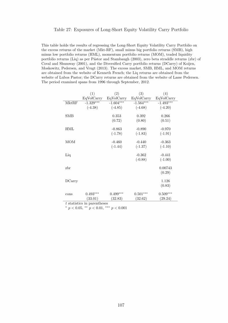
Table 27: Exposures of Long-Short Equity Volatility Carry Portfolio

This table holds the results of regressing the Long-Short Equity Volatility Carry Portfolio onthe excess returns of the market (Mkt-RF), small minus big portfolio returns (SMB), highminus low portfolio returns (HML), momentum portfolio returns (MOM), traded liquidityportfolio returns (Liq) as per Pastor and Stambaugh (2003), zero beta straddle returns (zbr) ofCoval and Shumway (2001), and the Diversified Carry portfolio returns (DCarry) of Koijen,Moskowitz, Pedersen, and Vrugt (2013). The excess market, SMB, HML, and MOM returnsare obtained from the website of Kenneth French; the Liq returns are obtained from thewebsite of Lubos Pastor; the DCarry returns are obtained from the website of Lasse Pedersen.The period examined spans from 1996 through September, 2012.

(1) (2) (3) (4)EqVolCarry EqVolCarry EqVolCarry EqVolCarry

MktRF -1.329∗∗∗ -1.604∗∗∗ -1.564∗∗∗ -1.493∗∗∗

(-4.38) (-4.85) (-4.68) (-4.20)

SMB 0.353 0.392 0.266(0.72) (0.80) (0.51)

HML -0.863 -0.890 -0.970(-1.78) (-1.83) (-1.91)

MOM -0.460 -0.440 -0.363(-1.44) (-1.37) (-1.10)

Liq -0.362 -0.441(-0.88) (-1.00)

zbr 0.00743(0.29)

DCarry 1.126(0.83)

cons 0.493∗∗∗ 0.499∗∗∗ 0.501∗∗∗ 0.509∗∗∗

(33.01) (32.83) (32.62) (29.24)t statistics in parentheses∗ p < 0.05, ∗∗ p < 0.01, ∗∗∗ p < 0.001

107

Table 28: Exposures of Equity Long Volatility Carry Portfolio

This table holds the results of regressing the Equity Long Volatility Carry Portfolio, afteraccounting for transactions costs, on the excess returns of the market (Mkt-RF), small minusbig portfolio returns (SMB), high minus low portfolio returns (HML), momentum portfolioreturns (MOM), traded liquidity portfolio returns (Liq) as per Pastor and Stambaugh (2003),zero beta straddle returns (zbr) of Coval and Shumway (2001), and the Diversified Carryportfolio returns (DCarry) of Koijen, Moskowitz, Pedersen, and Vrugt (2013). The excessmarket, SMB, HML, and MOM returns are obtained from the website of Kenneth French; theLiq returns are obtained from the website of Lubos Pastor; the DCarry returns are obtainedfrom the website of Lasse Pedersen. The period examined spans from 1996 through September,2012.

(1) (2) (3) (4)LongCarry LongCarry LongCarry LongCarry

MktRF -1.666∗∗∗ -1.909∗∗∗ -1.987∗∗∗ -2.061∗∗∗

(-5.55) (-5.82) (-6.02) (-6.10)

SMB 0.265 0.190 -0.337(0.55) (0.39) (-0.68)

HML -0.406 -0.355 -0.726(-0.85) (-0.74) (-1.51)

MOM -0.577 -0.615 -0.419(-1.82) (-1.94) (-1.33)

Liq 0.694 0.0272(1.71) (0.06)

zbr -0.108∗∗∗

(-4.52)

DCarry 0.966(0.75)

cons 0.105∗∗∗ 0.110∗∗∗ 0.107∗∗∗ 0.120∗∗∗

(7.10) (7.31) (7.04) (7.27)t statistics in parentheses∗ p < 0.05, ∗∗ p < 0.01, ∗∗∗ p < 0.001

108

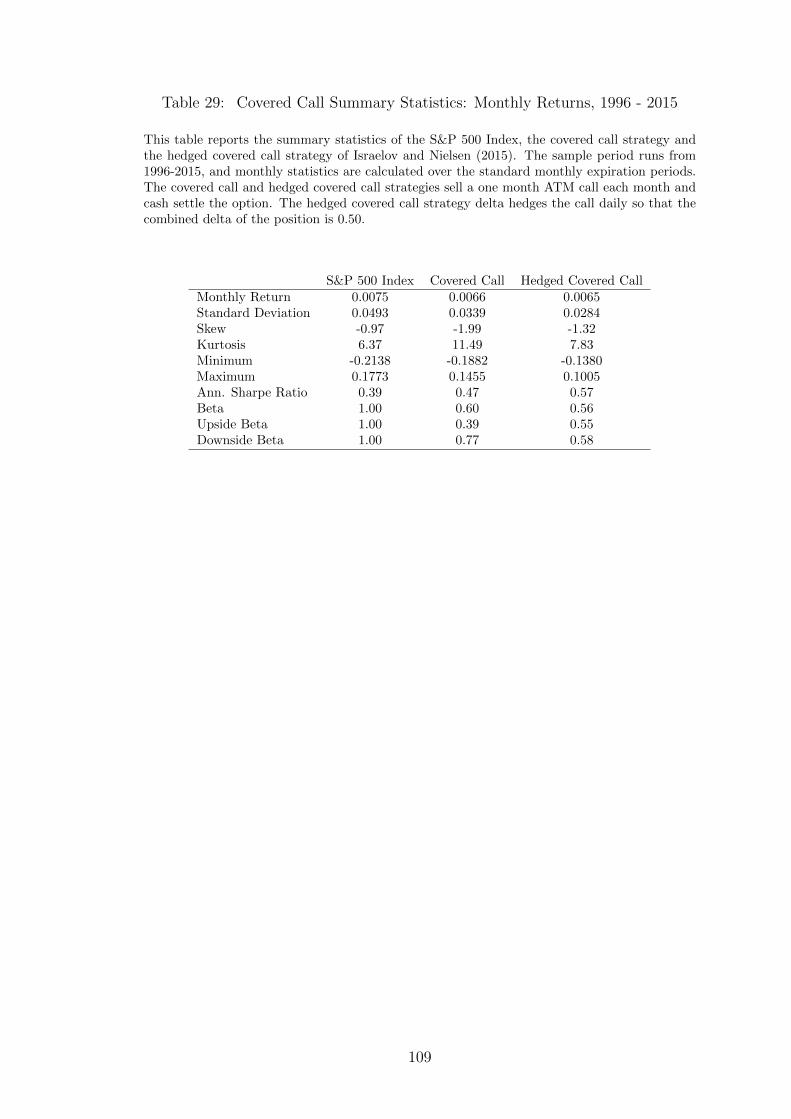
Table 29: Covered Call Summary Statistics: Monthly Returns, 1996 - 2015

This table reports the summary statistics of the S&P 500 Index, the covered call strategy andthe hedged covered call strategy of Israelov and Nielsen (2015). The sample period runs from1996-2015, and monthly statistics are calculated over the standard monthly expiration periods.The covered call and hedged covered call strategies sell a one month ATM call each month andcash settle the option. The hedged covered call strategy delta hedges the call daily so that thecombined delta of the position is 0.50.

S&P 500 Index Covered Call Hedged Covered CallMonthly Return 0.0075 0.0066 0.0065Standard Deviation 0.0493 0.0339 0.0284Skew -0.97 -1.99 -1.32Kurtosis 6.37 11.49 7.83Minimum -0.2138 -0.1882 -0.1380Maximum 0.1773 0.1455 0.1005Ann. Sharpe Ratio 0.39 0.47 0.57Beta 1.00 0.60 0.56Upside Beta 1.00 0.39 0.55Downside Beta 1.00 0.77 0.58

109

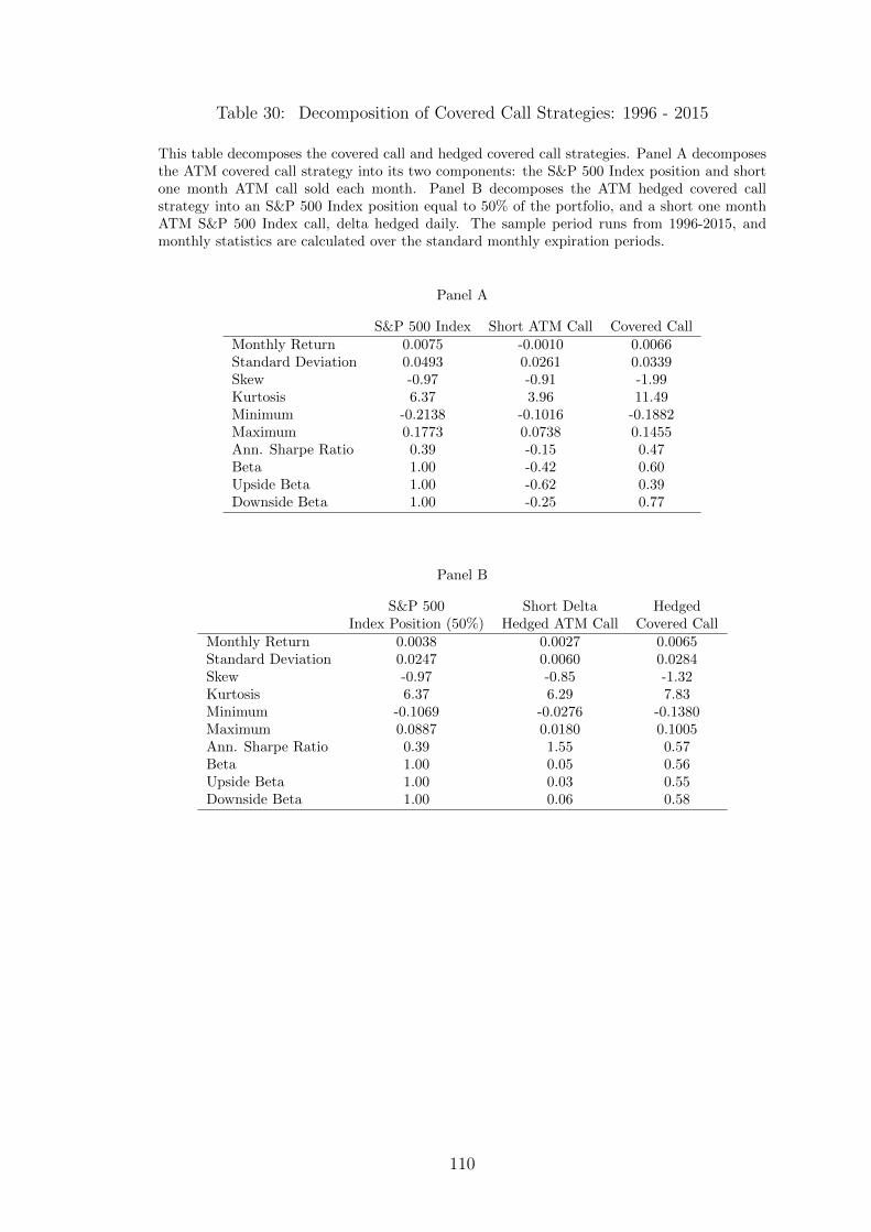
Table 30: Decomposition of Covered Call Strategies: 1996 - 2015

This table decomposes the covered call and hedged covered call strategies. Panel A decomposesthe ATM covered call strategy into its two components: the S&P 500 Index position and shortone month ATM call sold each month. Panel B decomposes the ATM hedged covered callstrategy into an S&P 500 Index position equal to 50% of the portfolio, and a short one monthATM S&P 500 Index call, delta hedged daily. The sample period runs from 1996-2015, andmonthly statistics are calculated over the standard monthly expiration periods.

Panel A

S&P 500 Index Short ATM Call Covered CallMonthly Return 0.0075 -0.0010 0.0066Standard Deviation 0.0493 0.0261 0.0339Skew -0.97 -0.91 -1.99Kurtosis 6.37 3.96 11.49Minimum -0.2138 -0.1016 -0.1882Maximum 0.1773 0.0738 0.1455Ann. Sharpe Ratio 0.39 -0.15 0.47Beta 1.00 -0.42 0.60Upside Beta 1.00 -0.62 0.39Downside Beta 1.00 -0.25 0.77

Panel B

S&P 500 Short Delta HedgedIndex Position (50%) Hedged ATM Call Covered Call

Monthly Return 0.0038 0.0027 0.0065Standard Deviation 0.0247 0.0060 0.0284Skew -0.97 -0.85 -1.32Kurtosis 6.37 6.29 7.83Minimum -0.1069 -0.0276 -0.1380Maximum 0.0887 0.0180 0.1005Ann. Sharpe Ratio 0.39 1.55 0.57Beta 1.00 0.05 0.56Upside Beta 1.00 0.03 0.55Downside Beta 1.00 0.06 0.58

110

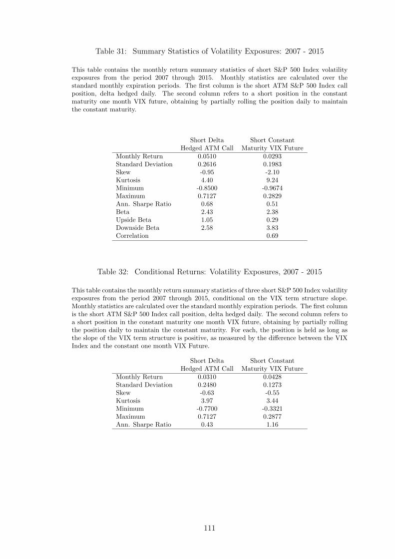
Table 31: Summary Statistics of Volatility Exposures: 2007 - 2015

This table contains the monthly return summary statistics of short S&P 500 Index volatilityexposures from the period 2007 through 2015. Monthly statistics are calculated over thestandard monthly expiration periods. The first column is the short ATM S&P 500 Index callposition, delta hedged daily. The second column refers to a short position in the constantmaturity one month VIX future, obtaining by partially rolling the position daily to maintainthe constant maturity.

Short Delta Short ConstantHedged ATM Call Maturity VIX Future

Monthly Return 0.0510 0.0293Standard Deviation 0.2616 0.1983Skew -0.95 -2.10Kurtosis 4.40 9.24Minimum -0.8500 -0.9674Maximum 0.7127 0.2829Ann. Sharpe Ratio 0.68 0.51Beta 2.43 2.38Upside Beta 1.05 0.29Downside Beta 2.58 3.83Correlation 0.69

Table 32: Conditional Returns: Volatility Exposures, 2007 - 2015

This table contains the monthly return summary statistics of three short S&P 500 Index volatilityexposures from the period 2007 through 2015, conditional on the VIX term structure slope.Monthly statistics are calculated over the standard monthly expiration periods. The first columnis the short ATM S&P 500 Index call position, delta hedged daily. The second column refers toa short position in the constant maturity one month VIX future, obtaining by partially rollingthe position daily to maintain the constant maturity. For each, the position is held as long asthe slope of the VIX term structure is positive, as measured by the difference between the VIXIndex and the constant one month VIX Future.

Short Delta Short ConstantHedged ATM Call Maturity VIX Future

Monthly Return 0.0310 0.0428Standard Deviation 0.2480 0.1273Skew -0.63 -0.55Kurtosis 3.97 3.44Minimum -0.7700 -0.3321Maximum 0.7127 0.2877Ann. Sharpe Ratio 0.43 1.16

111

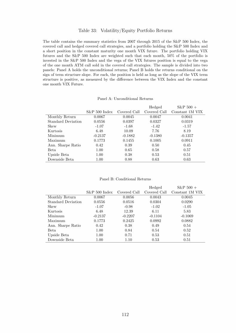
Table 33: Volatility/Equity Portfolio Returns

The table contains the summary statistics from 2007 through 2015 of the S&P 500 Index, thecovered call and hedged covered call strategies, and a portfolio holding the S&P 500 Index anda short position in the constant maturity one month VIX future. The portfolio holding VIXfutures and the S&P 500 Index are weighted such that each month, 50% of the portfolio isinvested in the S&P 500 Index and the vega of the VIX futures position is equal to the vegaof the one month ATM call sold in the covered call strategies. The sample is divided into twopanels: Panel A holds the unconditional returns; Panel B holds the returns conditional on thesign of term structure slope. For each, the position is held as long as the slope of the VIX termstructure is positive, as measured by the difference between the VIX Index and the constantone month VIX Future.

Panel A: Unconditional Returns

Hedged S&P 500 +S&P 500 Index Covered Call Covered Call Constant 1M VIX

Monthly Return 0.0067 0.0045 0.0047 0.0041Standard Deviation 0.0556 0.0397 0.0327 0.0319Skew -1.07 -1.68 -1.42 -1.57Kurtosis 6.48 10.09 7.76 8.19Minimum -0.2137 -0.1882 -0.1380 -0.1357Maximum 0.1773 0.1455 0.1005 0.0911Ann. Sharpe Ratio 0.42 0.39 0.50 0.45Beta 1.00 0.65 0.58 0.57Upside Beta 1.00 0.38 0.53 0.51Downside Beta 1.00 0.88 0.63 0.63

Panel B: Conditional Returns

Hedged S&P 500 +S&P 500 Index Covered Call Covered Call Constant 1M VIX

Monthly Return 0.0067 0.0056 0.0043 0.0045Standard Deviation 0.0556 0.0516 0.0304 0.0290Skew -1.07 -0.98 -1.02 -1.05Kurtosis 6.48 12.39 6.11 5.83Minimum -0.2137 -0.2207 -0.1104 -0.1069Maximum 0.1773 0.2425 0.0992 0.0882Ann. Sharpe Ratio 0.42 0.38 0.49 0.54Beta 1.00 0.84 0.54 0.52Upside Beta 1.00 0.71 0.53 0.51Downside Beta 1.00 1.10 0.53 0.51

112

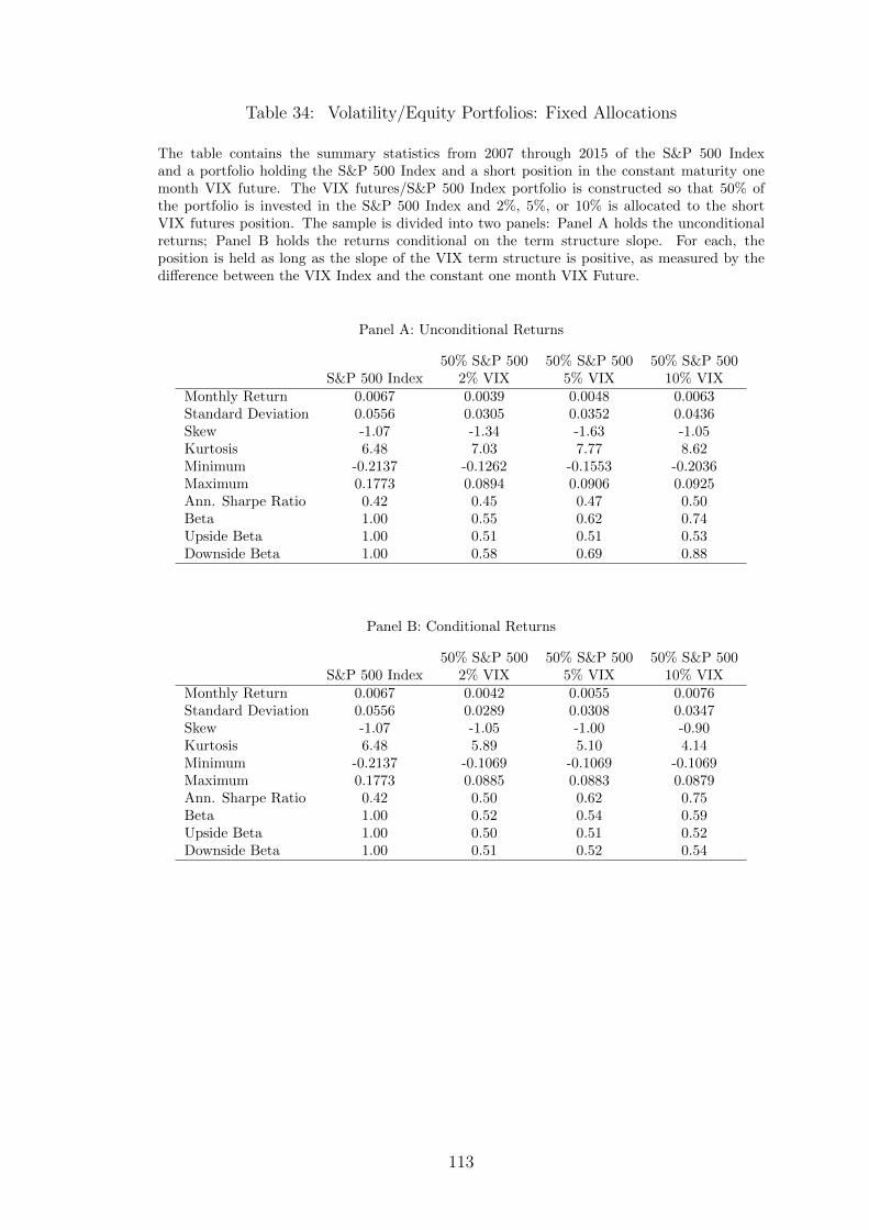
Table 34: Volatility/Equity Portfolios: Fixed Allocations

The table contains the summary statistics from 2007 through 2015 of the S&P 500 Indexand a portfolio holding the S&P 500 Index and a short position in the constant maturity onemonth VIX future. The VIX futures/S&P 500 Index portfolio is constructed so that 50% ofthe portfolio is invested in the S&P 500 Index and 2%, 5%, or 10% is allocated to the shortVIX futures position. The sample is divided into two panels: Panel A holds the unconditionalreturns; Panel B holds the returns conditional on the term structure slope. For each, theposition is held as long as the slope of the VIX term structure is positive, as measured by thedifference between the VIX Index and the constant one month VIX Future.

Panel A: Unconditional Returns

50% S&P 500 50% S&P 500 50% S&P 500S&P 500 Index 2% VIX 5% VIX 10% VIX

Monthly Return 0.0067 0.0039 0.0048 0.0063Standard Deviation 0.0556 0.0305 0.0352 0.0436Skew -1.07 -1.34 -1.63 -1.05Kurtosis 6.48 7.03 7.77 8.62Minimum -0.2137 -0.1262 -0.1553 -0.2036Maximum 0.1773 0.0894 0.0906 0.0925Ann. Sharpe Ratio 0.42 0.45 0.47 0.50Beta 1.00 0.55 0.62 0.74Upside Beta 1.00 0.51 0.51 0.53Downside Beta 1.00 0.58 0.69 0.88

Panel B: Conditional Returns

50% S&P 500 50% S&P 500 50% S&P 500S&P 500 Index 2% VIX 5% VIX 10% VIX

Monthly Return 0.0067 0.0042 0.0055 0.0076Standard Deviation 0.0556 0.0289 0.0308 0.0347Skew -1.07 -1.05 -1.00 -0.90Kurtosis 6.48 5.89 5.10 4.14Minimum -0.2137 -0.1069 -0.1069 -0.1069Maximum 0.1773 0.0885 0.0883 0.0879Ann. Sharpe Ratio 0.42 0.50 0.62 0.75Beta 1.00 0.52 0.54 0.59Upside Beta 1.00 0.50 0.51 0.52Downside Beta 1.00 0.51 0.52 0.54

113

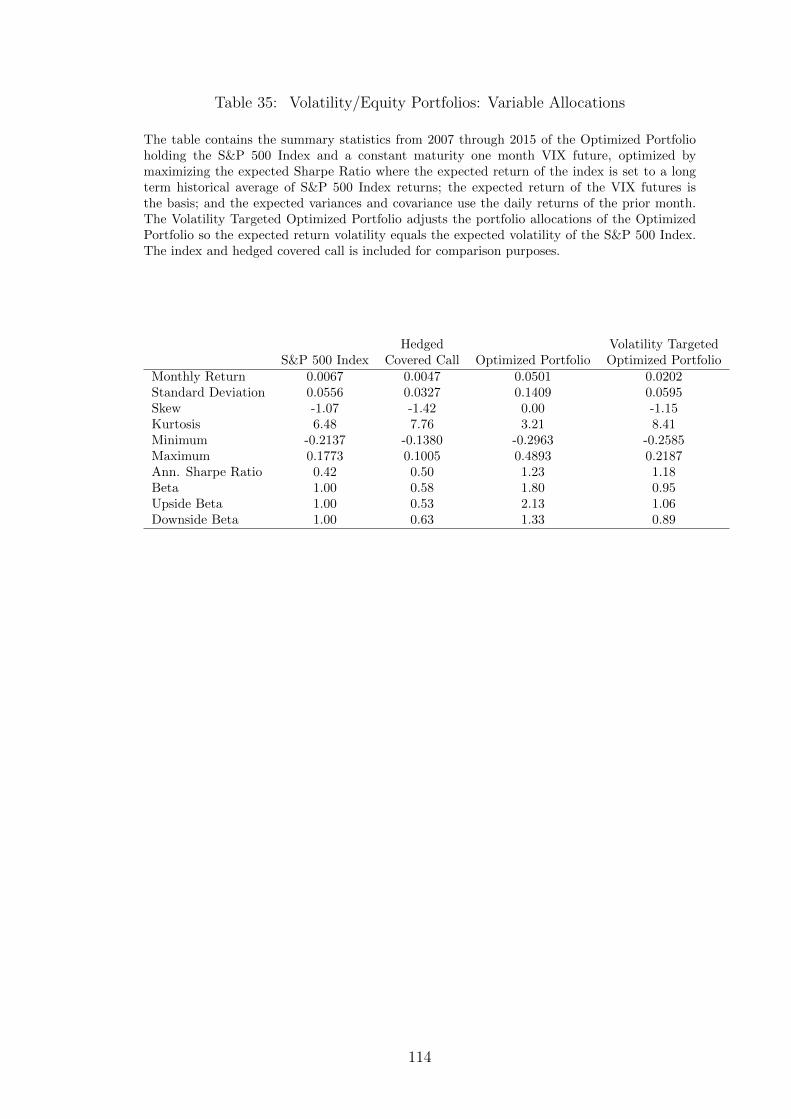
Table 35: Volatility/Equity Portfolios: Variable Allocations

The table contains the summary statistics from 2007 through 2015 of the Optimized Portfolioholding the S&P 500 Index and a constant maturity one month VIX future, optimized bymaximizing the expected Sharpe Ratio where the expected return of the index is set to a longterm historical average of S&P 500 Index returns; the expected return of the VIX futures isthe basis; and the expected variances and covariance use the daily returns of the prior month.The Volatility Targeted Optimized Portfolio adjusts the portfolio allocations of the OptimizedPortfolio so the expected return volatility equals the expected volatility of the S&P 500 Index.The index and hedged covered call is included for comparison purposes.

Hedged Volatility TargetedS&P 500 Index Covered Call Optimized Portfolio Optimized Portfolio

Monthly Return 0.0067 0.0047 0.0501 0.0202Standard Deviation 0.0556 0.0327 0.1409 0.0595Skew -1.07 -1.42 0.00 -1.15Kurtosis 6.48 7.76 3.21 8.41Minimum -0.2137 -0.1380 -0.2963 -0.2585Maximum 0.1773 0.1005 0.4893 0.2187Ann. Sharpe Ratio 0.42 0.50 1.23 1.18Beta 1.00 0.58 1.80 0.95Upside Beta 1.00 0.53 2.13 1.06Downside Beta 1.00 0.63 1.33 0.89

114

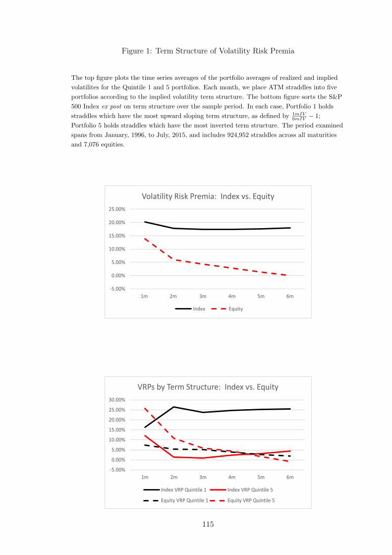
Figure 1: Term Structure of Volatility Risk Premia

The top figure plots the time series averages of the portfolio averages of realized and implied

volatilites for the Quintile 1 and 5 portfolios. Each month, we place ATM straddles into five

portfolios according to the implied volatility term structure. The bottom figure sorts the S&P

500 Index ex post on term structure over the sample period. In each case, Portfolio 1 holds

straddles which have the most upward sloping term structure, as defined by 1mIV6mIV − 1;

Portfolio 5 holds straddles which have the most inverted term structure. The period examined

spans from January, 1996, to July, 2015, and includes 924,952 straddles across all maturities

and 7,076 equities.

-5.00%

0.00%

5.00%

10.00%

15.00%

20.00%

25.00%

1m 2m 3m 4m 5m 6m

Volatility Risk Premia: Index vs. Equity

Index Equity

-5.00%

0.00%

5.00%

10.00%

15.00%

20.00%

25.00%

30.00%

1m 2m 3m 4m 5m 6m

VRPs by Term Structure: Index vs. Equity

Index VRP Quintile 1 Index VRP Quintile 5

Equity VRP Quintile 1 Equity VRP Quintile 5

115

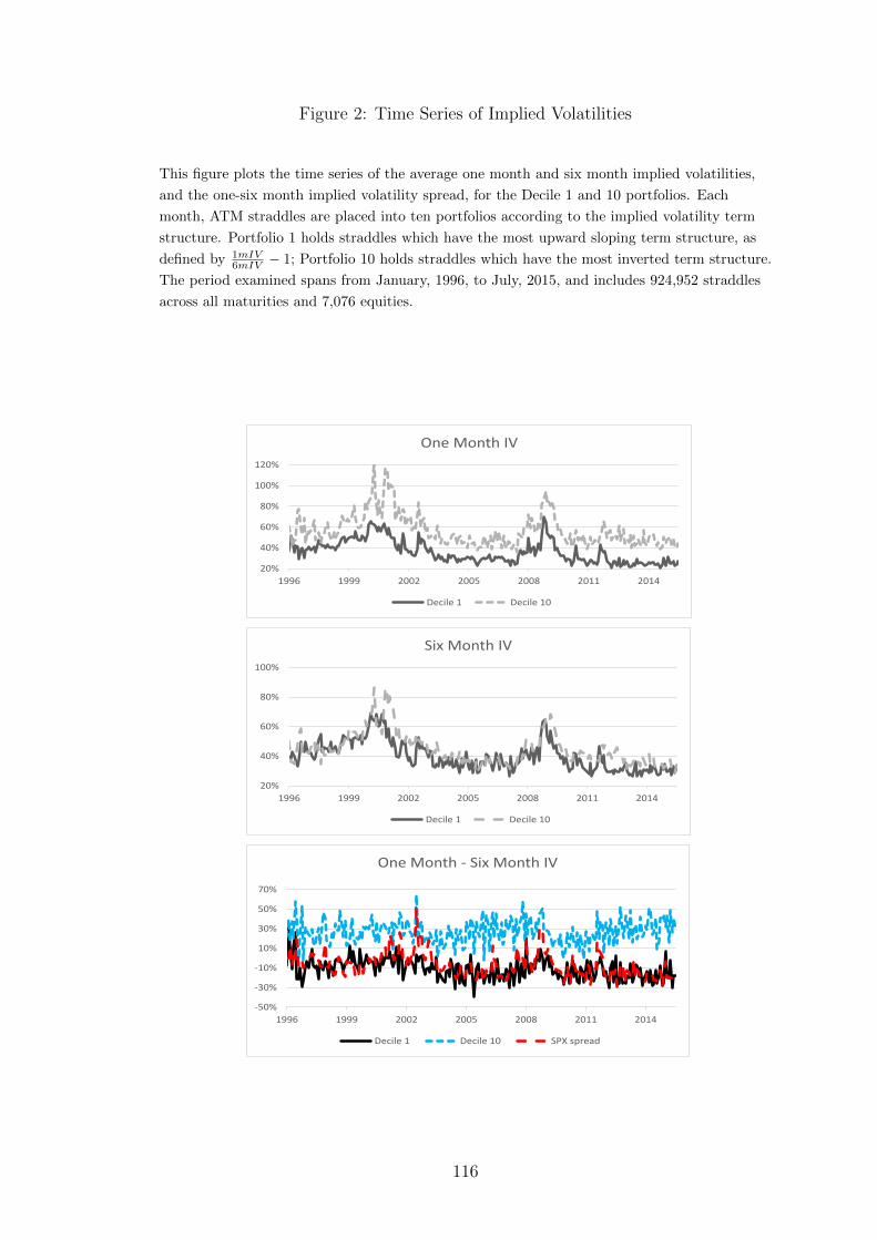
Figure 2: Time Series of Implied Volatilities

This figure plots the time series of the average one month and six month implied volatilities,

and the one-six month implied volatility spread, for the Decile 1 and 10 portfolios. Each

month, ATM straddles are placed into ten portfolios according to the implied volatility term

structure. Portfolio 1 holds straddles which have the most upward sloping term structure, as

defined by 1mIV6mIV − 1; Portfolio 10 holds straddles which have the most inverted term structure.

The period examined spans from January, 1996, to July, 2015, and includes 924,952 straddles

across all maturities and 7,076 equities.

20%

40%

60%

80%

100%

120%

1996 1999 2002 2005 2008 2011 2014

One Month IV

Decile 1 Decile 10

20%

40%

60%

80%

100%

1996 1999 2002 2005 2008 2011 2014

Six Month IV

Decile 1 Decile 10

-50%

-30%

-10%

10%

30%

50%

70%

1996 1999 2002 2005 2008 2011 2014

One Month - Six Month IV

Decile 1 Decile 10 SPX spread

116

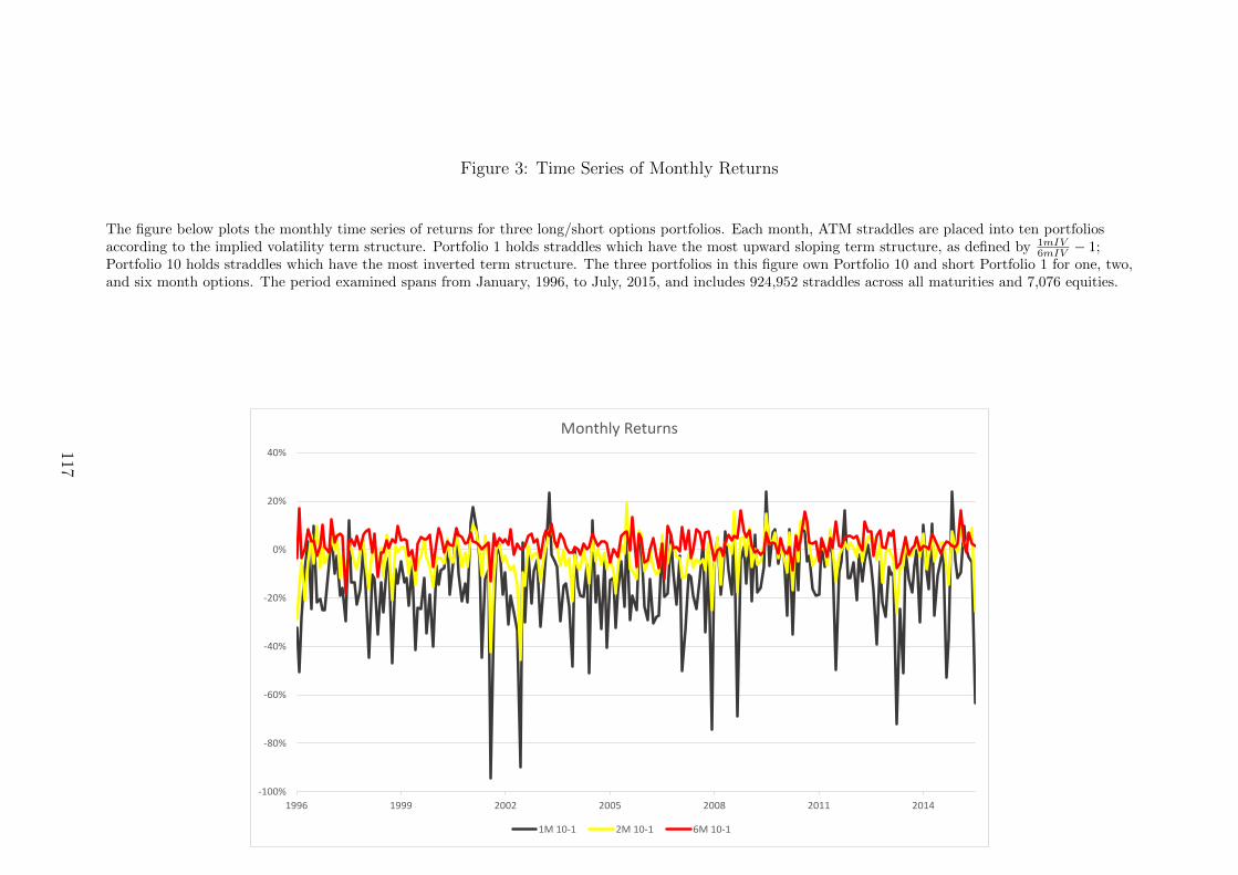
Figure 3: Time Series of Monthly Returns

The figure below plots the monthly time series of returns for three long/short options portfolios. Each month, ATM straddles are placed into ten portfoliosaccording to the implied volatility term structure. Portfolio 1 holds straddles which have the most upward sloping term structure, as defined by 1mIV

6mIV − 1;Portfolio 10 holds straddles which have the most inverted term structure. The three portfolios in this figure own Portfolio 10 and short Portfolio 1 for one, two,and six month options. The period examined spans from January, 1996, to July, 2015, and includes 924,952 straddles across all maturities and 7,076 equities.

-100%

-80%

-60%

-40%

-20%

0%

20%

40%

1996 1999 2002 2005 2008 2011 2014

Monthly Returns

1M 10-1 2M 10-1 6M 10-1

117

Figure 4: Variance Swap and Forward Variance Swap Levels by Decile

This figure plots the time series average of the one month variance swap and FV(1,1) levels for the ten portfolios created each month by sorting on V S(1)FV (1,1) − 1.

The period examined spans from January, 1996, to July, 2015, and includes 2,977 equities and 56,932 variance swaps.

0.00

1000.00

2000.00

3000.00

4000.00

5000.00

6000.00

1 2 3 4 5 6 7 8 9 10

Forward and Spot Variance by Decile

FV(1,1) VS(1)

118

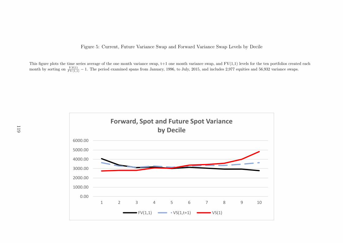
Figure 5: Current, Future Variance Swap and Forward Variance Swap Levels by Decile

This figure plots the time series average of the one month variance swap, t+1 one month variance swap, and FV(1,1) levels for the ten portfolios created each

month by sorting on V S(1)FV (1,1) − 1. The period examined spans from January, 1996, to July, 2015, and includes 2,977 equities and 56,932 variance swaps.

0.00

1000.00

2000.00

3000.00

4000.00

5000.00

6000.00

1 2 3 4 5 6 7 8 9 10

Forward, Spot and Future Spot Varianceby Decile

FV(1,1) VS(1,t+1) VS(1)

119

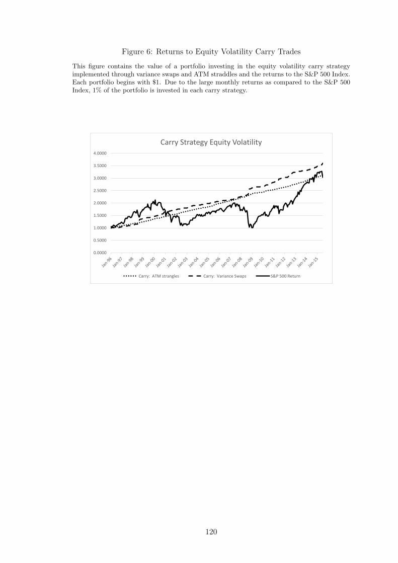
Figure 6: Returns to Equity Volatility Carry Trades

This figure contains the value of a portfolio investing in the equity volatility carry strategyimplemented through variance swaps and ATM straddles and the returns to the S&P 500 Index.Each portfolio begins with $1. Due to the large monthly returns as compared to the S&P 500Index, 1% of the portfolio is invested in each carry strategy.

0.0000

0.5000

1.0000

1.5000

2.0000

2.5000

3.0000

3.5000

4.0000

Carry Strategy Equity Volatility

Carry: ATM strangles Carry: Variance Swaps S&P 500 Return

120

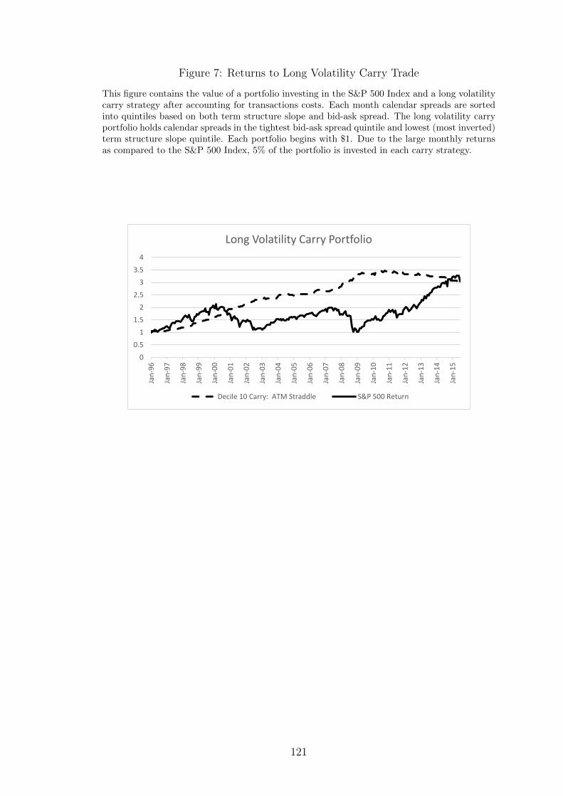
Figure 7: Returns to Long Volatility Carry Trade

This figure contains the value of a portfolio investing in the S&P 500 Index and a long volatilitycarry strategy after accounting for transactions costs. Each month calendar spreads are sortedinto quintiles based on both term structure slope and bid-ask spread. The long volatility carryportfolio holds calendar spreads in the tightest bid-ask spread quintile and lowest (most inverted)term structure slope quintile. Each portfolio begins with $1. Due to the large monthly returnsas compared to the S&P 500 Index, 5% of the portfolio is invested in each carry strategy.

0

0.5

1

1.5

2

2.5

3

3.5

4

Jan

-96

Jan

-97

Jan

-98

Jan

-99

Jan

-00

Jan

-01

Jan

-02

Jan

-03

Jan

-04

Jan

-05

Jan

-06

Jan

-07

Jan

-08

Jan

-09

Jan

-10

Jan

-11

Jan

-12

Jan

-13

Jan

-14

Jan

-15

Long Volatility Carry Portfolio

Decile 10 Carry: ATM Straddle S&P 500 Return

121

Figure 8: Composition of Term Structure Slope Portfolios

Each month, portfolios of calendar spreads are formed based on the implied volatility differentialbetween the two legs, as defined by 1mIV

FV (1,1) − 1. Portfolio 1 (5) holds variance swaps whose

implied volatility curves have steepest upward (downward) slope. This figure shows the averagepercentage composition of each portfolio for firms with and without an upcoming earnings release.The period examined spans from January, 1996, to August, 2015, and includes 284,984 calendarspreads and 6,799 equities.

0%

20%

40%

60%

80%

100%

1 2 3 4 5

Composition of term structure slope quintile: Earnings Releases

Earnings Release No Earnings Release

122

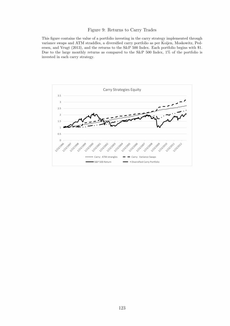
Figure 9: Returns to Carry Trades

This figure contains the value of a portfolio investing in the carry strategy implemented throughvariance swaps and ATM straddles, a diversified carry portfolio as per Koijen, Moskowitz, Ped-ersen, and Vrugt (2013), and the returns to the S&P 500 Index. Each portfolio begins with $1.Due to the large monthly returns as compared to the S&P 500 Index, 1% of the portfolio isinvested in each carry strategy.

0

0.5

1

1.5

2

2.5

3

3.5

Carry Strategies Equity

Carry: ATM strangles Carry: Variance Swaps

S&P 500 Return Diversified Carry Portfolio

123

Figure 10: Returns to Long Volatility Carry Trade

This figure contains the value of a portfolio investing in the Quintile 5 Slope/Quintile 1 Spreadcarry strategy implemented using ATM straddles after accounting for transactions costs, a di-versified carry portfolio as per Koijen, Moskowitz, Pedersen, and Vrugt (2013), and the returnsto the S&P 500 Index. Each portfolio begins with $1. Due to the large monthly returns ascompared to the S&P 500 Index, 5% of the portfolio is invested in each carry strategy.

0

0.5

1

1.5

2

2.5

3

3.5

4

Jan

-96

Jan

-97

Jan

-98

Jan

-99

Jan

-00

Jan

-01

Jan

-02

Jan

-03

Jan

-04

Jan

-05

Jan

-06

Jan

-07

Jan

-08

Jan

-09

Jan

-10

Jan

-11

Jan

-12

Jan

-13

Jan

-14

Jan

-15

Quintile 5-Spread 1 Carry Portfolio

Decile 10 Carry: ATM Straddle S&P 500 Return

124

Figure 11: VIX Futures Beta with respect to VIX Index

This figure plots the beta of the front month VIX futures contract with respect to the VIX Index

as a function of the days until expiration. The period examined spans from 2007 through 2015.

0

0.1

0.2

0.3

0.4

0.5

0.6

0.7

0.8

0.9

0 2 4 6 8 10 12 14 16 18 20

Bet

a

Days Until Expiration

VIX Futures Beta

125

Figure 12: VIX Futures Allocation, Fully Allocated Portfolio

This figure plots the VIX Futures allocation of the Optimized Portfolio created by maximizing

the expected Sharpe Ratio where the expected return of the index is set to a long term historical

average of S&P 500 Index returns; the expected return of the VIX futures is the basis; and

the expected variances and covariance use the daily returns of the prior month. The period

examined spans from 2007 through 2015.

70% 80% 90% 100% More

Frequency

0.00%

10.00%

20.00%

30.00%

40.00%

50.00%

60.00%

70.00%

0% 20% 40% 60% 80% 100%

VIX Futures Allocation, Fully Invested Portfolio

126

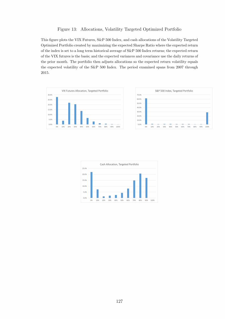
Figure 13: Allocations, Volatility Targeted Optimized Portfolio

This figure plots the VIX Futures, S&P 500 Index, and cash allocations of the Volatility Targeted

Optimized Portfolio created by maximizing the expected Sharpe Ratio where the expected return

of the index is set to a long term historical average of S&P 500 Index returns; the expected return

of the VIX futures is the basis; and the expected variances and covariance use the daily returns of

the prior month. The portfolio then adjusts allocations so the expected return volatility equals

the expected volatility of the S&P 500 Index. The period examined spans from 2007 through

2015.

0.0%

5.0%

10.0%

15.0%

20.0%

25.0%

30.0%

0% 10% 20% 30% 40% 50% 60% 70% 80% 90% 100%

VIX Futures Allocation, Targeted Portfolio

0.0%

10.0%

20.0%

30.0%

40.0%

50.0%

60.0%

70.0%

0% 10% 20% 30% 40% 50% 60% 70% 80% 90% 100%

S&P 500 Index, Targeted Portfolio

0.0%

5.0%

10.0%

15.0%

20.0%

25.0%

0% 10% 20% 30% 40% 50% 60% 70% 80% 90% 100%

Cash Allocation, Targeted Portfolio

127

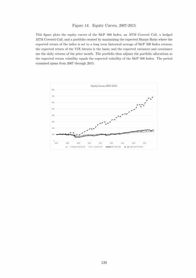
Figure 14: Equity Curves, 2007-2015

This figure plots the equity curves of the S&P 500 Index, an ATM Covered Call, a hedged

ATM Covered Call, and a portfolio created by maximizing the expected Sharpe Ratio where the

expected return of the index is set to a long term historical average of S&P 500 Index returns;

the expected return of the VIX futures is the basis; and the expected variances and covariance

use the daily returns of the prior month. The portfolio then adjusts the portfolio allocations so

the expected return volatility equals the expected volatility of the S&P 500 Index. The period

examined spans from 2007 through 2015.

0

100

200

300

400

500

600

700

800

2007 2008 2009 2010 2011 2012 2013 2014 2015

Equity Curves 2007-2015

Hedged Covered Call Covered Call S&P 500 Index Optimized Portfolio

128

APPENDIX

RECENT RETURNS TO OPTIMIZED PORTFOLIO

On February 6, 2018, XIV, an exchange traded note that tracks the inverse of the

constant maturity VIX futures, opened more than 90% lower than the previous

close. Credit Suisse, the issuer of the product, subsequently liquidated the note

on February 21st. The episode received widespread media coverage, as volatility

products were cited as the trigger for the broader market sell-off.8 Table A1 holds

the returns of the Optimized Portfolio and the Volatility Targeted Optimized Port-

folio from 2016 through February 13, 2018. The Optimized Portfolio allocates to

the constant maturity VIX future and S&P 500 Index, optimized ex ante using

historical measures of return volatility, index returns, and the VIX futures basis.

The Volatility Targeted Optimized Portfolio allocates to the Optimized Portfolio

and cash in order to target the return volatility of the S&P 500 Index. Over the

period, the index saw steady positive returns which produced a Sharpe Ratio of

1.58. The Volatility Targeted Optimized Portfolio posted a substantially similar

return, volatility and Sharpe Ratio to the S&P 500 Index. From December, 2017

through 2018, the S&P 500 Index returned approximately 1.2%, while the Volatil-

ity Targeted Optimized Portfolio returned 0.4%. During the volatility spike in

early February, the Volatility Targeted Optimized Portfolio allocated entirely to

the index, as the expected returns to the VIX futures position were negative.

8See for example, Reklaitis (2018): https://www.marketwatch.com/story/credit-suisse-ceo-defends-enabling-bets-against-volatility-with-xiv-it-worked-well-for-a-long-time-until-it-didnt-2018-02-14.

129

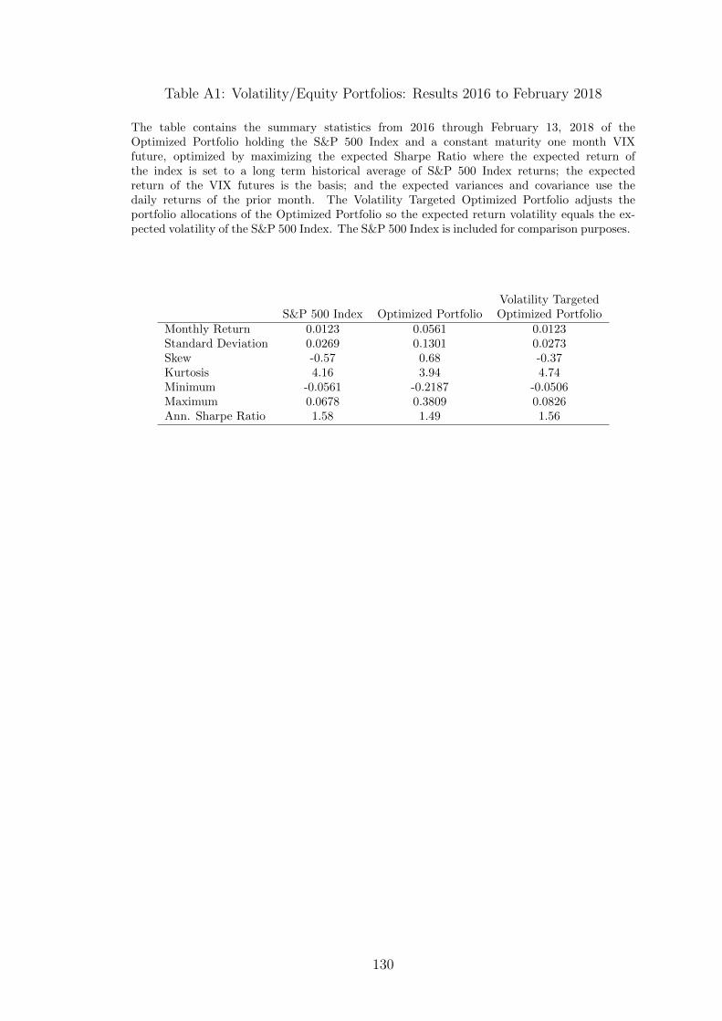
Table A1: Volatility/Equity Portfolios: Results 2016 to February 2018

The table contains the summary statistics from 2016 through February 13, 2018 of theOptimized Portfolio holding the S&P 500 Index and a constant maturity one month VIXfuture, optimized by maximizing the expected Sharpe Ratio where the expected return ofthe index is set to a long term historical average of S&P 500 Index returns; the expectedreturn of the VIX futures is the basis; and the expected variances and covariance use thedaily returns of the prior month. The Volatility Targeted Optimized Portfolio adjusts theportfolio allocations of the Optimized Portfolio so the expected return volatility equals the ex-pected volatility of the S&P 500 Index. The S&P 500 Index is included for comparison purposes.

Volatility TargetedS&P 500 Index Optimized Portfolio Optimized Portfolio

Monthly Return 0.0123 0.0561 0.0123Standard Deviation 0.0269 0.1301 0.0273Skew -0.57 0.68 -0.37Kurtosis 4.16 3.94 4.74Minimum -0.0561 -0.2187 -0.0506Maximum 0.0678 0.3809 0.0826Ann. Sharpe Ratio 1.58 1.49 1.56

130

BIBLIOGRAPHY

Aıt-Sahalia, Yacine, Mustafa Karaman, and Loriano Mancini, 2014, The termstructure of variance swaps and risk premia, Unpublished working paper, Prince-ton University, University of Zurich, EPFL and Swiss Finance Institute.

Ang, Andrew, Robert J Hodrick, Yuhang Xing, and Xiaoyan Zhang, 2006, Thecross-section of volatility and expected returns, The Journal of Finance 61,259–299.

Asness, Clifford S, Tobias J Moskowitz, and Lasse Heje Pedersen, 2013, Value andmomentum everywhere, The Journal of Finance 68, 929–985.

Bakshi, Gurdip, and Nikunj Kapadia, 2003a, Delta-hedged gains and the negativemarket volatility risk premium, Review of Financial Studies 16, 527–566.

, 2003b, Volatility risk premiums embedded in individual equity options:Some new insights, The Journal of Derivatives 11, 45–54.

, and Dilip Madan, 2003, Stock return characteristics, skew laws, and thedifferential pricing of individual equity options, The Review of Financial Studies16, 101–143.

Bali, Turan G, and Scott Murray, 2013, Does risk-neutral skewness predict thecross-section of equity option portfolio returns?, Journal of Financial and Quan-titative Analysis 48, 1145–1171.

Bansal, Ravi, and Amir Yaron, 2004, Risks for the long run: A potential resolutionof asset pricing puzzles, The Journal of Finance 59, 1481–1509.

Barro, Robert J, 2006, Rare disasters and asset markets in the twentieth century,The Quarterly Journal of Economics pp. 823–866.

Bilson, J.F.O., 1981, The ”speculative efficiency” hypothesis, the Journal of Busi-ness 54, 435–451.

Boyer, Brian H, and Keith Vorkink, 2014, Stock options as lotteries, The Journalof Finance 69, 1485–1527.

Britten-Jones, Mark, and Anthony Neuberger, 2000, Option prices, implied priceprocesses, and stochastic volatility, The Journal of Finance 55, 839–866.

Brunnermeier, Markus K, Stefan Nagel, and Lasse H Pedersen, 2008, Carry tradesand currency crashes, NBER macroeconomics annual 23, 313–348.

131

Burnside, Craig, Martin Eichenbaum, Isaac Kleshchelski, and Sergio Rebelo, 2010,Do peso problems explain the returns to the carry trade?, The Review of Fi-nancial Studies 24, 853–891.

Campasano, Jim, and Matthew Linn, 2017, Understanding and trading the termstructure of volatility, Available at SSRN 2871616.

Campbell, John Y., and John H. Cochrane, 1999, By force of habit: Aconsumption-based explanation of aggregate stock market behavior, Journalof Political Economy 107, 205–251.

Campbell, John Y, and Robert J Shiller, 1991, Yield spreads and interest ratemovements: A bird’s eye view, The Review of Economic Studies 58, 495–514.

Cao, Jie, and Bing Han, 2013, Cross section of option returns and idiosyncraticstock volatility, Journal of Financial Economics 108, 231–249.

Carhart, Mark M, 1997, On persistence in mutual fund performance, The Journalof finance 52, 57–82.

Carr, Peter, and Dilip Madan, 1998, Towards a theory of volatility trading, Volatil-ity: New estimation techniques for pricing derivatives pp. 417–427.

Carr, Peter, and Liuren Wu, 2009, Variance risk premiums, Review of FinancialStudies 22, 1311–1341.

Chang, Bo Young, Peter Christoffersen, and Kris Jacobs, 2013, Market skewnessrisk and the cross section of stock returns, Journal of Financial Economics 107,46–68.

Cheng, Ing-Haw, 2016, The vix premium, Available at SSRN 2495414.

Coval, Joshua D, and Tyler Shumway, 2001, Expected option returns, The journalof Finance 56, 983–1009.

Croce, Mariano Massimiliano, Martin Lettau, and Sydney C Ludvigson, 2008,Investor information, long-run risk, and the duration of risky cash flows, inAFA 2008 New Orleans Meetings.

Della Corte, Pasquale, Roman Kozhan, and Anthony Neuberger, 2016, The cross-section of currency volatility premia, .

Della Corte, Pasquale, Lucio Sarno, and Ilias Tsiakas, 2011, Spot and forwardvolatility in foreign exchange, Journal of Financial Economics 100, 496–513.

Dew-Becker, Ian, Stefano Giglio, Anh Le, and Marius Rodriguez, 2015, The priceof variance risk, Discussion paper, National Bureau of Economic Research.

Driessen, Joost, Pascal J Maenhout, and Grigory Vilkov, 2009, The price of cor-relation risk: Evidence from equity options, The Journal of Finance 64, 1377–1406.

Fama, Eugene F, 1984, Forward and spot exchange rates, Journal of monetaryeconomics 14, 319–338.

132

, and Robert R Bliss, 1987, The information in long-maturity forwardrates, The American Economic Review pp. 680–692.

Fama, Eugene F, and Kenneth R French, 1992, The cross-section of expected stockreturns, the Journal of Finance 47, 427–465.

Farhi, Emmanuel, and Xavier Gabaix, 2015, Rare disasters and exchange rates,The Quarterly Journal of Economics 131, 1–52.

Frazzini, Andrea, and Lasse H Pedersen, 2012, Embedded leverage, Discussionpaper, National Bureau of Economic Research.

Gabaix, Xavier, 2008, Variable rare disasters: An exactly solved framework forten puzzles in macro-finance, Discussion paper, National Bureau of EconomicResearch.

Garleanu, Nicolae, Lasse Heje Pedersen, and Allen M Poteshman, 2009, Demand-based option pricing, Review of Financial Studies 22, 4259–4299.

Gorton, Gary B, Fumio Hayashi, and K Geert Rouwenhorst, 2013, The funda-mentals of commodity futures returns, Review of Finance pp. 35–105.

Goyal, Amit, and Alessio Saretto, 2009, Cross-section of option returns and volatil-ity, Journal of Financial Economics 94, 310–326.

Han, Bing, Avanidhar Subrahmanyam, and Yi Zhou, 2015, The term structure ofcredit spreads and the cross-section of stock returns, .

Hansen, Lars Peter, and Robert J Hodrick, 1980, Forward exchange rates as opti-mal predictors of future spot rates: An econometric analysis, journal of PoliticalEconomy 88, 829–853.

Hill, Joanne M, Venkatesh Balasubramanian, Krag Gregory, and Ingrid Tierens,2006, Finding alpha via covered index writing, Financial Analysts Journal 62,29–46.

Israelov, Roni, and Lars N Nielsen, 2014, Covered call strategies: One fact andeight myths, Financial Analysts Journal 70, 23–31.

, 2015, Covered calls uncovered, Financial Analysts Journal 71, 44–57.

Jackwerth, Jens Carsten, and Mark Rubinstein, 1996, Recovering probability dis-tributions from option prices, The Journal of Finance 51, 1611–1631.

Jiang, George J, and Yisong S Tian, 2005, The model-free implied volatility andits information content, Review of Financial Studies 18, 1305–1342.

Johnson, Travis L, 2016, Risk premia and the vix term structure, Available atSSRN 2548050.

Jones, Chris, and Tong Wang, 2012, The term structure of equity option impliedvolatility, Unpublished working paper, University of Southern California.

133

Jurek, Jakub W, 2014, Crash-neutral currency carry trades, Journal of FinancialEconomics 113, 325–347.

Kapadia, Nikunj, and Edward Szado, 2007, The risk and return characteristicsof the buy-write strategy on the russell 2000 index, The Journal of AlternativeInvestments 9, 39–56.

Koijen, Ralph SJ, Tobias J Moskowitz, Lasse Heje Pedersen, and Evert B Vrugt,2013, Carry, Discussion paper, National Bureau of Economic Research.

Lustig, Hanno, Nikolai Roussanov, and Adrien Verdelhan, 2011, Common riskfactors in currency markets, The Review of Financial Studies 24, 3731–3777.

Meese, Richard A, and Kenneth Rogoff, 1983, Empirical exchange rate models ofthe seventies: Do they fit out of sample?, Journal of international economics14, 3–24.

Menkhoff, Lukas, Lucio Sarno, Maik Schmeling, and Andreas Schrimpf, 2012,Currency momentum strategies, Journal of Financial Economics 106, 660–684.

Pastor, L’ubos, and Robert F Stambaugh, 2003, Liquidity risk and expected stockreturns, Journal of Political economy 111, 642–685.

Reklaitis, Victor, 2018, Credit Suisse CEO defends enablingvolatility bets with XIV: ’It worked well . . . until it didn’t,https://www.marketwatch.com/story/credit-suisse-ceo-defends-enabling-bets-against-volatility-with-xiv-it-worked-well-for-a-long-time-until-it-didnt-2018-02-14.

Rietz, Thomas A, 1988, The equity risk premium a solution, Journal of monetaryEconomics 22, 117–131.

Rosenberg, Joshua V, and Robert F Engle, 2002, Empirical pricing kernels, Jour-nal of Financial Economics 64, 341–372.

Simon, David P, and Jim Campasano, 2014, The vix futures basis: Evidence andtrading strategies, The Journal of Derivatives 21, 54–69.

Van Binsbergen, Jules, Michael Brandt, and Ralph Koijen, 2012, On the timingand pricing of dividends, The American Economic Review 102, 1596–1618.

Van Binsbergen, Jules, Wouter Hueskes, Ralph Koijen, and Evert Vrugt, 2013,Equity yields, Journal of Financial Economics 110, 503–519.

Vasquez, Aurelio, 2015, Equity volatility term structures and the cross-section ofoption returns, Available at SSRN 1944298.

Whaley, Robert E, 2002, Return and risk of CBOE buy write monthly index, TheJournal of Derivatives 10, 35–42.

Yang, Fan, 2013, Investment shocks and the commodity basis spread, Journal ofFinancial Economics 110, 164–184.

134