ABSTRACT

Title of dissertation: ESSAYS ON EDUCATIONIN DEVELOPING COUNTRIES

Andrew Brudevold-NewmanDoctor of Philosophy, 2017

Dissertation directed by: Professor Pamela JakielaDepartment of Agricultural and Resource Economics

Almost all countries subsidize education. These subsidies are generally de-

signed to account for positive social returns to education and a recognition of edu-

cation as a basic human right. Without subsidies, credit constraints may preclude

children from attending school. While the availability of low-cost private schooling

is increasing, it is likely that governments, through these subsidy programs, will be

responsible for ensuring access to a quality education for all children.

The first two papers of my dissertation examine government implemented for-

mal education policies in Kenya designed to improve access to secondary schooling

and the quality of selected secondary schools, respectively. My first paper exploits

the introduction of a free secondary education program to examine the demand re-

sponse to a supply side government program to improve access as well as measure

the impacts of secondary schooling on demographic and labor market outcomes.

My second paper evaluates a school upgrade program designed to improve school

quality at selected secondary schools.

In many developing countries formal education is often insufficient, however,

to ensure that individuals are able to enter the formal labor market. With this

in mind, in my third paper, I examine a multifaceted labor market intervention

implemented by an international NGO that was designed to improve labor market

outcomes for young women who have already completed or dropped out of formal

schooling.

ESSAYS ON EDUCATION IN DEVELOPING COUNTRIES

by

Andrew Brudevold-Newman

Dissertation submitted to the Faculty of the Graduate School of theUniversity of Maryland, College Park in partial fulfillment

of the requirements for the degree ofDoctor of Philosophy

2017

Advisory Committee:Professor Pamela Jakiela, Chair/AdvisorDr. Owen Ozier, Co-AdvisorProfessor Kenneth LeonardProfessor Snaebjorn GunnsteinssonProfessor Sergio Urzua

c© Copyright byAndrew Brudevold-Newman

2017

Acknowledgments

Thank you to everyone who provided support, encouragement, and feedback through-

out my writing of this dissertation.

A special thank you to Pamela Jakiela and Owen Ozier who provided patient

and invaluable guidance throughout the process and who also got me into “the field”

ensuring I gained an understanding of the setting and behaviors I was studying.

Thank you also to Kenneth Leonard for his consistent reminder to highlight why we

care and to focus on questions that matter. Finally, this dissertation also benefited

from a number of conversations with both Snaebjorn Gunnsteinsson and Sergio

Urzua.

The first chapter of my dissertation benefited from conversations with Pamela

Jakiela, Snaebjorn Gunnsteinsson, Kenneth Leonard, and Owen Ozier. Also, for

their comments and suggestions, I thank Anna Alberini and Todd Pugatch. All

errors are my own.

The second chapter was funded by the Gardner Dissertation Enhancement

Award (2015). I am grateful to Snaebjorn Gunnsteinsson, Pamela Jakiela, Ken

Leonard, and Owen Ozier, as well as conference participants at NEUDC 2015 for

helpful comments and suggestions.

For my third chapter, which is coauthored with Maddalena Honorati, Pamela

Jakiela, and Owen Ozier, we are grateful to Sarah Baird, Maya Eden, David Evans,

Deon Filmer, Jessica Goldberg, Markus Goldstein, Joan Hamory Hicks, David Lam,

Isaac Mbiti, David McKenzie, Patrick Premand, seminar participants at Duke, USC,

ii

and the University of Oklahoma, as well as numerous conference attendees for help-

ful comments. Rohit Chhabra, Emily Cook-Lundgren, Gerald Ipapa, and Laura

Kincaide provided excellent research assistance. The research was funded by the

IZA/DFID Growth and Labour Markets in Low Income Countries Programme, the

CEPR/DFID Private Enterprise Development in Low-Income Countries Research

Initiative, the ILO’s Youth Employment Network, the National Science Foundation

(award number 1357332), and the World Bank (SRP, RSB, i2i, Gender Innova-

tion Lab). The study was registered at the AEA RCT registry under ID number

AEARCTR-0000459. We are indebted to staff at the International Rescue Commit-

tee (the implementing organization) and Innovations for Poverty Action for their

help and support. The findings, interpretations and conclusions expressed in this

paper are entirely those of the authors, and do not necessarily represent the views of

the World Bank, its Executive Directors, or the governments of the countries they

represent.

iii

Table of Contents

List of Tables vii

List of Figures ix

1 Introduction 11.1 Introduction . . . . . . . . . . . . . . . . . . . . . . . . . . . . . . . . 1

2 The Impacts of Free Secondary Education: Evidence from Kenya 42.1 Introduction . . . . . . . . . . . . . . . . . . . . . . . . . . . . . . . . 42.2 School Attainment, Credit, Ability, and Fertility . . . . . . . . . . . . 13

2.2.1 Basic model . . . . . . . . . . . . . . . . . . . . . . . . . . . . 132.2.2 Credit Constraints . . . . . . . . . . . . . . . . . . . . . . . . 162.2.3 A caveat on capacity constraints . . . . . . . . . . . . . . . . . 182.2.4 Child bearing . . . . . . . . . . . . . . . . . . . . . . . . . . . 192.2.5 Model predictions and implications for analysis . . . . . . . . 22

2.3 Kenya’s Education System and Free Secondary Schooling . . . . . . . 222.4 Data . . . . . . . . . . . . . . . . . . . . . . . . . . . . . . . . . . . . 25

2.4.1 Demographic and Health Survey . . . . . . . . . . . . . . . . . 252.4.2 Administrative Test Scores . . . . . . . . . . . . . . . . . . . . 272.4.3 Defining Treatment . . . . . . . . . . . . . . . . . . . . . . . . 28

2.5 FSE and educational attainment . . . . . . . . . . . . . . . . . . . . . 312.5.1 Identification strategy . . . . . . . . . . . . . . . . . . . . . . 312.5.2 FSE and educational attainment results . . . . . . . . . . . . 37

2.6 Education, fertility, and occupational choice . . . . . . . . . . . . . . 402.6.1 Identification strategy . . . . . . . . . . . . . . . . . . . . . . 402.6.2 Impacts of education on fertility . . . . . . . . . . . . . . . . . 432.6.3 Impacts of education on occupational choice . . . . . . . . . . 46

2.7 FSE and student achievement . . . . . . . . . . . . . . . . . . . . . . 482.7.1 Identification strategy . . . . . . . . . . . . . . . . . . . . . . 482.7.2 FSE and student achievement results . . . . . . . . . . . . . . 52

2.8 Conclusion . . . . . . . . . . . . . . . . . . . . . . . . . . . . . . . . . 54

iv

Appendices 752.A Additional Tables and Figures . . . . . . . . . . . . . . . . . . . . . . 752.B Robustness samples . . . . . . . . . . . . . . . . . . . . . . . . . . . . 89

2.B.1 Drop Nairobi/Mombasa . . . . . . . . . . . . . . . . . . . . . 892.B.2 Drop smallest population counties . . . . . . . . . . . . . . . . 912.B.3 Unrestricted DHS sample (1983-1996) . . . . . . . . . . . . . . 932.B.4 Alternative treatment definition . . . . . . . . . . . . . . . . . 95

2.B.4.1 Defining treatment . . . . . . . . . . . . . . . . . . . 952.C Simulation . . . . . . . . . . . . . . . . . . . . . . . . . . . . . . . . . 98

2.C.1 Simulation adding lower quality students . . . . . . . . . . . . 98

3 Can Government School Upgrades Up Grades? Evidence from Kenyan Sec-ondary Schools 993.1 Introduction . . . . . . . . . . . . . . . . . . . . . . . . . . . . . . . . 993.2 Kenya’s Education System and the School Upgrade Program . . . . . 1043.3 Data . . . . . . . . . . . . . . . . . . . . . . . . . . . . . . . . . . . . 107

3.1 KCSE and Secondary School Data . . . . . . . . . . . . . . . 1083.2 KCPE and School Preference Data . . . . . . . . . . . . . . . 109

3.4 Identification Strategy . . . . . . . . . . . . . . . . . . . . . . . . . . 1103.1 Main specification . . . . . . . . . . . . . . . . . . . . . . . . . 1103.2 Changes-in-changes . . . . . . . . . . . . . . . . . . . . . . . . 114

3.5 Student Achievement Results . . . . . . . . . . . . . . . . . . . . . . 1163.6 Student Composition and Preference Changes . . . . . . . . . . . . . 1203.7 Conclusion . . . . . . . . . . . . . . . . . . . . . . . . . . . . . . . . . 122

Appendices 1393.A Additional Tables and Figures . . . . . . . . . . . . . . . . . . . . . . 139

4 A Firm of One’s Own: Experimental Evidence on Credit Constraints andOccupational Choice 1424.1 Introduction . . . . . . . . . . . . . . . . . . . . . . . . . . . . . . . . 1424.2 Conceptual Framework . . . . . . . . . . . . . . . . . . . . . . . . . . 1494.3 Research Design and Procedures . . . . . . . . . . . . . . . . . . . . . 157

4.1 Two Labor Market Interventions . . . . . . . . . . . . . . . . 1584.1.1 The Franchise Treatment . . . . . . . . . . . . . . . 1584.1.2 The Grant Treatment . . . . . . . . . . . . . . . . . 161

4.2 Data Collection . . . . . . . . . . . . . . . . . . . . . . . . . . 1614.3 Sample Characteristics . . . . . . . . . . . . . . . . . . . . . . 1624.4 Compliance with Treatment . . . . . . . . . . . . . . . . . . . 163

4.4 Analysis . . . . . . . . . . . . . . . . . . . . . . . . . . . . . . . . . . 1644.1 Estimation Strategy . . . . . . . . . . . . . . . . . . . . . . . 1664.2 Labor Market Outcomes 7–10 Months after Treatment . . . . 1684.3 Labor Market Outcomes 14–22 Months after Treatment . . . . 1714.4 Impacts of Treatment on Firm Structure . . . . . . . . . . . . 1734.5 Impacts on Other Outcomes . . . . . . . . . . . . . . . . . . . 174

v

4.6 Comparing Implementation Costs . . . . . . . . . . . . . . . . 1764.5 Participant Evaluations . . . . . . . . . . . . . . . . . . . . . . . . . . 180

4.1 Empirical Approach and Practical Considerations . . . . . . . 1804.2 Framework for Interpreting Empirics . . . . . . . . . . . . . . 1844.3 Results . . . . . . . . . . . . . . . . . . . . . . . . . . . . . . . 188

4.6 Conclusion . . . . . . . . . . . . . . . . . . . . . . . . . . . . . . . . . 190

Appendices 2024.A Proof and extension of Proposition 1 . . . . . . . . . . . . . . . . . . 202

4.1 Proof of Part (1) . . . . . . . . . . . . . . . . . . . . . . . . . 2024.2 Proof of Part (2) . . . . . . . . . . . . . . . . . . . . . . . . . 2024.3 Proof of Part (3) . . . . . . . . . . . . . . . . . . . . . . . . . 2024.4 Extension of Proposition 1: constant wage . . . . . . . . . . . 204

4.B Additional Tables and Figures . . . . . . . . . . . . . . . . . . . . . . 205

vi

List of Tables

2.1 DHS sample characteristics . . . . . . . . . . . . . . . . . . . . . . . . 642.2 Secondary school completion examination summary statistics . . . . . 652.3 Difference-in-differences estimates: primary schooling . . . . . . . . . 662.4 Binary treatment intensity difference-in-differences estimates: sec-

ondary education . . . . . . . . . . . . . . . . . . . . . . . . . . . . . 672.5 Difference-in-differences estimates: secondary education . . . . . . . . 682.6 Falsification test difference-in-differences estimates: secondary edu-

cation . . . . . . . . . . . . . . . . . . . . . . . . . . . . . . . . . . . 692.7 Instrumental variables estimates: fertility behaviors . . . . . . . . . . 702.8 Instrumental variables estimates: contraceptive use . . . . . . . . . . 712.9 Instrumental variables estimates: desired fertility . . . . . . . . . . . 712.10 Instrumental variables estimates: sector of work . . . . . . . . . . . . 722.11 County expansion at secondary school completion . . . . . . . . . . . 732.12 Student achievement . . . . . . . . . . . . . . . . . . . . . . . . . . . 742.13 Estimates from a changes-in-changes model . . . . . . . . . . . . . . . 742.A.1DHS sample characteristics . . . . . . . . . . . . . . . . . . . . . . . . 802.A.2Binary intensity measure difference-in-differences estimates: primary

schooling . . . . . . . . . . . . . . . . . . . . . . . . . . . . . . . . . . 812.A.3Binary treatment intensity difference-in-differences estimates: sec-

ondary education . . . . . . . . . . . . . . . . . . . . . . . . . . . . . 822.A.4Binary treatment diff-in-diffs excluding transition cohorts: secondary

education . . . . . . . . . . . . . . . . . . . . . . . . . . . . . . . . . 832.A.5OLS estimates: fertility behaviors . . . . . . . . . . . . . . . . . . . . 842.A.6Instrumental variables estimates: fertility behaviors . . . . . . . . . . 852.A.7Instrumental variables estimates: contraceptive use . . . . . . . . . . 862.A.8Instrumental variables estimates: desired fertility . . . . . . . . . . . 862.A.9Instrumental variables estimates: sector of work . . . . . . . . . . . . 872.A.10School openings (by type) . . . . . . . . . . . . . . . . . . . . . . . . 882.A.11Class size changes expansion . . . . . . . . . . . . . . . . . . . . . . . 882.B.1Difference-in-differences estimates: education - no cities . . . . . . . . 902.B.2Difference-in-differences estimates: education - no small counties . . . 922.B.3Difference-in-differences estimates: secondary education . . . . . . . . 94

vii

2.B.4Student achievement: alternative treatment intensity . . . . . . . . . 972.C.1Simulated impact on student achievement (under no credit constraints) 98

3.1 KCSE Summary Statistics . . . . . . . . . . . . . . . . . . . . . . . . 1283.2 School Summary Statistics . . . . . . . . . . . . . . . . . . . . . . . . 1293.3 Common Trends Regressions . . . . . . . . . . . . . . . . . . . . . . . 1303.4 Impact of Treatment on School Cohort Size . . . . . . . . . . . . . . 1313.5 Estimated Treatment Coefficients . . . . . . . . . . . . . . . . . . . . 1323.6 Upgrade Treatment Effect by Percentile . . . . . . . . . . . . . . . . . 1333.7 Estimated Impact on Standard Deviation . . . . . . . . . . . . . . . . 1343.8 Estimated Treatment Coefficients by Relative Grant Size . . . . . . . 1353.9 Impact of Treatment on Subject Selection . . . . . . . . . . . . . . . 1363.10 Grant Spending Correlates of Treatment Effects . . . . . . . . . . . . 1373.11 Impact of Treatment on Test Scores of Incoming Students . . . . . . 1383.A.1Pooled Regressions . . . . . . . . . . . . . . . . . . . . . . . . . . . . 1393.A.2Estimated Treatment Coefficients by Relative Grant Size . . . . . . . 1393.A.3Estimated Treatment Coefficients - Closest School . . . . . . . . . . . 1403.A.4Complete Counties Estimated Treatment Coefficients . . . . . . . . . 1403.A.5Estimated Treatment Coefficients: School Level . . . . . . . . . . . . 141

4.1 Sample Characteristics at Baseline . . . . . . . . . . . . . . . . . . . 1954.2 Compliance with Treatment . . . . . . . . . . . . . . . . . . . . . . . 1964.3 Intent to Treat Estimates: Labor Market Outcomes after 7–10 Months1974.4 Intent to Treat Estimates: Labor Market Outcomes after 14–22 Months1984.5 Firm Structure and Business Practices after 14–22 Months . . . . . . 1994.B.1Baseline Covariates, by Treatment Status . . . . . . . . . . . . . . . . 2054.B.2Attrition from the Sample . . . . . . . . . . . . . . . . . . . . . . . . 2064.B.5Intent to Treat Estimates: Occupational Sector and Other Outcomes

after 14–22 Months . . . . . . . . . . . . . . . . . . . . . . . . . . . . 2084.B.3Treatment on the Treated: Labor Market Outcomes after 7–10 Months2124.B.4Intent to Treat Estimates: Occupational Sectors after 7–10 Months . 213

viii

List of Figures

2.1 Secondary school admissions 2000-2013 . . . . . . . . . . . . . . . . . 572.2 Cohort exposure . . . . . . . . . . . . . . . . . . . . . . . . . . . . . . 582.3 Common pre-program trends . . . . . . . . . . . . . . . . . . . . . . . 592.4 Pre-program primary to secondary transition rate histogram . . . . . 602.5 Pre-program primary to secondary transition rates by county . . . . . 602.6 Kaplan-Meier survival estimates . . . . . . . . . . . . . . . . . . . . . 612.7 Interaction coefficients . . . . . . . . . . . . . . . . . . . . . . . . . . 622.8 Fertility behavior coefficients . . . . . . . . . . . . . . . . . . . . . . . 632.A.1Age distribution of KCPE test takers . . . . . . . . . . . . . . . . . . 752.A.2Mean KCSE scores (Public/Private) . . . . . . . . . . . . . . . . . . 762.A.3Secondary school time to completion . . . . . . . . . . . . . . . . . . 772.A.4Falsification test: Pre-FSE sample . . . . . . . . . . . . . . . . . . . . 782.A.5Probability of secondary school completion by KCPE score . . . . . . 792.B.1No cities . . . . . . . . . . . . . . . . . . . . . . . . . . . . . . . . . . 892.B.2No small counties . . . . . . . . . . . . . . . . . . . . . . . . . . . . . 912.B.3Full DHS sample . . . . . . . . . . . . . . . . . . . . . . . . . . . . . 932.B.4Treatment intensity multiplier . . . . . . . . . . . . . . . . . . . . . . 96

3.1 Reported Grant Spending Categories . . . . . . . . . . . . . . . . . . 1243.2 Sample Schools . . . . . . . . . . . . . . . . . . . . . . . . . . . . . . 1253.3 Mean KCSE grades of Upgraded and Eligible Schools (2006-2011) . . 1263.4 Mean KCSE grades of Phase 1/2 Schools and Phase 3 Schools (2006-

2011) . . . . . . . . . . . . . . . . . . . . . . . . . . . . . . . . . . . . 1273.5 Percent of Student Preferences for Original National Schools and Up-

graded National Schools . . . . . . . . . . . . . . . . . . . . . . . . . 127

4.1 Shape of the Production Function, F∗(Kt) . . . . . . . . . . . . . . . 1534.2 Examples of Production Functions . . . . . . . . . . . . . . . . . . . 1544.1 Participants’ Beliefs about Impacts of Treatments . . . . . . . . . . . 2004.2 Participants’ Beliefs about Impacts of Treatments . . . . . . . . . . . 201

ix

Chapter 1: Introduction

1.1 Introduction

Investments in human capital and the associated development of cognitive skills have

a demonstrated relationship with economic growth (Hanushek and Woßmann, 2008).

However, while improving, many developing countries still lag behind developed

countries in access to education and have students that substantially underachieve

relative to their counterparts in developed countries (Pritchett, 2013). With the

potential growth benefits in mind, ensuring and increasing access to high-quality

education has become a key development goal.

Policies designed to ensure access to a quality education must address a number

of questions: are supply-side policies to increase access to education sufficient to spur

demand? If the policies do increase demand, is there an access-quality tradeoff where

a rapid influx of students decreases the education quality? Is increasing educational

attainment sufficient to improve labor market outcomes or are there other binding

constraints? Finally, in many developing countries, the transition into the labor

market is slow and youth underemployment is high for individuals of all education

levels; if formal education is insufficient to secure a position in the labor market, can

policies that promote self-employment and entrepreneurship speed up this transition

1

and help young adults earn an income?

In this dissertation, I address these questions using a combination of govern-

ment policy changes in Kenya and a randomized evaluation of a non-governmental

organization’s labor market intervention implemented in Nairobi, Kenya.

In my first paper, I examine the Kenyan government’s 2008 abolition of tuition

for public secondary schools, showing that it dramatically increased the proportion

of students continuing from primary to secondary school, particularly from areas

with low initial primary to secondary transition rates. Using this regional varia-

tion in exposure to the program together with birth-cohort variation, I show that

post-primary education in Kenya delays childbirth and related behaviors, and shifts

employment away from agriculture towards skilled work. Despite concerns over the

quality impact of this rapid expansion of schooling, there is little evidence that sec-

ondary school completion examination grades deteriorated in regions more impacted

by the program.

In the second chapter, I focus on a Kenyan government program that upgraded

selected secondary schools to a higher-quality national tier and examine whether

the program improved student educational outcomes, as measured by student sec-

ondary school completion examination results. The program impact is identified by

comparing student outcomes at upgraded schools to student outcomes at schools

that met the government’s upgrade eligibility criteria, but were not selected for the

upgrade program. To avoid potential composition changes resulting from the pro-

gram, I examine only cohorts already enrolled in the schools prior to the upgrade

announcements. Using this difference-in-differences approach, I find evidence of het-

2

erogeneous program impact: while the program had no measurable impact for girls,

the program improved overall examination scores for boys. The improved scores for

boys appear to be driven by shifting up the lower tail of the test score distribution.

Finally, recognizing that in many developing countries, education is often not

sufficient to ensure that individuals are able to enter the formal labor market, in my

third paper which is co-authored with Maddalena Honorati, Pamela Jakiela, and

Owen Ozier, I focus on a non-governmental organization’s approach to addressing

high youth underemployment in a developing country context by examining the

impacts of a multifaceted labor market intervention implemented in Nairobi, Kenya.

We benchmark the program impact against a cash grant of comparable value to the

program and find that both programs increase self-employment and income in the

short run but that these impacts do not persist into the second year of the program.

3

Chapter 2: The Impacts of Free Secondary Education: Evidence

from Kenya

2.1 Introduction

Over the past 15 years, countries throughout sub-Saharan Africa have abolished

school fees for primary education (UNESCO, 2015). These policies have been shown

to increase educational attainment across a variety of contexts and among the most

vulnerable populations.1 Free primary education programs also coincided with the

rapid increase in the region’s net primary enrollment rate from 59% in 1999 to 79% in

2012 (UNESCO, 2015).2 A small number of countries have recently expanded their

free education systems to include secondary school.3 Whether these supply side

policies are sufficient to increase educational attainment at the secondary school

level remains to be seen.

There are a number of reasons why we might expect a more muted demand

1See, for example the analysis of programs in Kenya (Lucas and Mbiti, 2012a), Malawi (Al-Samarrai and Zaman, 2007), Tanzania (Hoogeveen and Rossi, 2013), and Uganda (Deininger, 2003;Grogan, 2009; Nishimura, Yamano, and Sasaoka, 2008).

2For a broad review of interventions targeting schooling access and quality, including easingfinancial constraints, see Murnane and Ganimian (2014) and Petrosino, Morgan, Fronius, Tanner-Smith, and Boruch (2012). The global net enrollment rate rose from 84% to 91% between 1999and 2012.

3Secondary school fees were eliminated in Uganda (2007), Rwanda (2007, 2012), Tanzania(2016), for girls in The Gambia (2001-2004), and selectively for schools in relatively poorer areasin South Africa (2007).

4

response to free secondary education programs than has been observed for free

primary education programs. First, the opportunity cost of schooling is likely to

increase with child age, so that the opportunity costs of attending secondary school

will typically exceed those of attending primary school.4 Second, these opportu-

nity costs may be particularly important in settings with low returns to secondary

education, where it may be optimal for individuals to forgo secondary schooling

entirely: in contexts where secondary schooling does not increase cognitive skills,

the returns to education are likely to be low, and the demand response to a free

secondary education policy is likely to be small.5 Even in contexts where secondary

schooling does increase cognitive skills, it may still be optimal to forgo schooling if

the expected demand for secondary school graduates is low. Third, parents may be

responsible for selecting the schooling level of the child but may not have incentives

fully aligned with the child’s long-term earnings potential (Baland and Robinson,

2000). In this case, parents may be less responsive to a free secondary education

policy, opting instead to enter the child into the labor market. Finally, individuals

or parents may underinvest in secondary schooling if they are misinformed about the

returns to further schooling (Jensen, 2010).6 This may be particularly important at

the secondary school level in areas with low educational attainment, and where the

4All countries in sub-Saharan Africa, except Liberia and Somalia, have ratified the InternationalLabour Organization’s Minimum Age Convention (1973) mandating minimum ages of labor marketparticipation between 14 and 16.

5While it is generally the development of cognitive skills, and not schooling attainment, thatis important for individual earnings (Hanushek and Woßmann, 2008), recent evidence has foundrelatively low returns to additional schooling when credentials are held constant, implying a largesignaling benefit (Eble and Hu, 2016).

6There are a number of behavioral reasons one might underinvest in education, such as presentbias, overemphasis on routine, and projection bias (Lavecchia, Liu, and Oreopoulos, 2015).

5

community perception of the value of secondary education may be low. If access

to free secondary education does increase educational attainment, then we might

expect such a policy to impact a range of demographic and economic outcomes.

Increased educational attainment is likely to have broad demographic impacts;

Schultz (1993) describes the negative relationship between parental education and

fertility as “one of the most important discoveries in research on nonmarket returns

to women’s education.” There are three main mechanisms through which education

is likely to impact fertility (Ferre, 2009). First, secondary school students may learn

about contraceptive methods leading to lower rates of unintended pregnancies. If

women are getting pregnant earlier than they would like, this knowledge could help

them delay pregnancy until they are ready. Second, education may shift preferences

towards fewer, higher quality children (Grossman, 2006). Third, if having a child

precludes the mother from continued schooling, young women may delay sexual

activity to ensure that they can finish their schooling. Regardless of the mechanism,

delaying age of first birth and lowering desired fertility could have long term benefits

for the mother and child. Childbearing at a young age and high total fertility have

been linked to deleterious impacts on both the mother and child, including higher

morbidity and mortality, lower educational attainment, and lower family income

(Ferre, 2009; Schultz, 2008).7

Additional education is also likely to impact labor market outcomes (Hanushek

7The longer terms impacts of women delaying marriage is more nuanced. Delaying marriagewithout an accompanying increase in educational attainment has been shown to lead individualsto partner with lower cognitive ability spouses. In contrast, individuals who delayed marriagewhile also increasing their schooling attainment have been shown to partner with more educatedhusbands (Baird, McIntosh, and Ozler, 2016).

6

and Woßmann, 2008; Heckman, Lochner, and Todd, 2006; Goldberg and Smith,

2008). Potential impacts of education on occupational choice may be particularly

important as labor flows from low-productivity sectors to high-productivity sectors

have been shown to be a key driver of development (McMillan and Rodrik, 2011;

McMillan, Rodrik, and Verduzco-Gallo, 2014). Free secondary education policies

may stimulate economic growth if they provide the cognitive skills required for

occupations in higher productivity sectors.

An important caveat is that lowering the cost of education may adversely im-

pact student learning. A rapid influx of students together with an inelastic supply

of education inputs may dilute per-student resources.8 If these inputs enter posi-

tively into an education production function, a dilution is likely to decrease student

achievement.9 Additionally, lowering the cost of schooling may induce lower-ability

students to attend secondary school, decreasing average peer quality. In the presence

of positive peer effects, this would lower student learning. An impact on academic

achievement, as measured by test scores, combines a deterioration of per-student

resources with a change in the composition of the student body. An increase in test

scores indicates that the price decrease enabled high performing, credit-constrained

individuals to attend secondary school, overcoming the negative impact of a dilution

8Teacher supply has been shown to be a constraint at the primary school level in developingcountries where there are relatively few secondary school graduates to teach future students (An-drabi, Das, and Khwaja, 2013). Teacher supply at the secondary school level may be particularlyinelastic as a result of small tertiary education systems; countries in sub-Saharan Africa have anaverage tertiary education gross enrollment rate of 6% (UNESCO, 2010).

9The distribution of a fixed supply of teachers within a national school system contrasts withsome of the U.S. research on exogenous increases in the number of students. For example, an influx‘Katrina children’ had little impact on per-student resources due to displaced teachers entering thesame school systems as displaced students leading to no impact on non-evacuee students’ learning(Imberman, Kugler, and Sacerdote, 2012).

7

of resources.

This paper examines the impacts of a national free secondary education (FSE)

program in Kenya on educational attainment and achievement, and uses the pro-

gram as an instrument to examine the impact of education on fertility behaviors

and labor market outcomes. There are three primary contributions of this paper.

First, I present the first evaluation of a national secondary school fee elimination

program implemented without gender or socioeconomic eligibility restrictions. Sec-

ond, I present new evidence on the impact of secondary education on both labor

and non-labor market outcomes. Finally, I compile and use new data on educational

achievement at the individual level for all students who completed secondary school

to evaluate the impact of the policy on academic performance.

My identification of causal impacts exploits region and cohort-specific vari-

ation in the treatment intensity of individuals exposed to the program. Regional

variation in treatment intensity stems from heterogeneous pre-program primary to

secondary school transition rates across Kenya: regions with low pre-FSE primary to

secondary transition rates experienced larger increases in secondary schooling rates

as a result of the program.10 The cohort variation arises from the timing of the

program: individuals above secondary schooling age at the time of the program’s

implementation in 2008 would have had to return to school to take advantage of

FSE rather than simply continue their schooling from primary to secondary school.

I use these sources of variation to measure the impact of FSE on educational attain-

10The transition rate is unrelated to overall county educational attainment. Rather, it measuresthe proportion of students who progress to start secondary school after finishing primary school.Thus, high transition rates can arise in counties where only a small fraction of a cohort completesprimary school but where most of the completers then subsequently start secondary school.

8

ment using a difference-in-differences framework. There are two main assumptions

underlying this approach. First, variation in pre-program primary to secondary

transition rates should be attributable to unchanging characteristics of the counties

and second, the pre-FSE time trends across high and low transition rate counties

should be the same. Under these assumptions, the identification strategy differ-

ences out the structural region and cohort differences yielding a consistent measure

of program impact. I present evidence indicating that these assumptions are likely

to be satisfied in this setting. I demonstrate that the pre-program treatment in-

tensity measures are highly correlated across time indicating that differences across

counties in primary to secondary transition rates are due to structural rather than

transitory factors. I also show long term pre-program common trends across high

and low treatment intensity regions and, as a robustness test, explicitly control for

potentially confounding region specific trends.

As my analysis exploits variation in primary to secondary transition rates

rather than the proportion of the population with any secondary schooling, I re-

quire a further assumption that FSE did not differentially change the composi-

tion of primary school completers across treatment intensities. I present analogous

difference-in-difference estimates to demonstrate that FSE intensity is uncorrelated

with changes in the probability of completing primary school.11

My difference-in-difference estimates indicate that FSE increased educational

11Using the primary to secondary transition rate and focusing on the sample of primary schoolcompleters should provide additional power as it restricts attention to individuals who are likelyto be affected by the program; that is, students who do not attend primary school are unlikely tochange their behavior as a result of the program. I confirm that the results are robust to definingthe intensity based on the proportion of the population with any secondary schooling.

9

attainment and, contrary to concerns expressed in the local media, had no significant

detrimental impacts on the academic achievement of students. At the mean county

intensity, the program is estimated to have increased schooling by 0.8 years of edu-

cation, with similar results by gender, indicating that the program was successful at

inducing students to continue to secondary school. There is also suggestive evidence

that the program increased the proportion of students completing secondary school,

although this result is not significant across all specifications.12

Building on the demonstrated impact of FSE on educational attainment, I

then use exposure to the FSE program as an instrumental variable to measure the

impact of education on a variety of fertility behaviors. This instrumental variables

approach is most closely related to that of Keats (2014) and Osili and Long (2008)

who examine the impact of free primary education on similar variables in Uganda

and Nigeria respectively. My results suggest education causes large delays for age

of first intercourse (10-20% at each age), age of first marriage (50% at each age),

and age of first birth (30-50%) for each age between 16 and 20. Despite impacts on

probability of first birth, I find no evidence that education decreased women’s desired

fertility or increased contraceptive use. This suggests that the primary mechanism

through which education acted on fertility behaviors is through a confinement effect

whereby women delay intercourse to ensure that they can continue their schooling.

Using the same instrumental variables approach, I also use exposure to the FSE

program to examine impacts of education on labor market outcomes. My estimates

12I run a falsification test where I assume that the program was implemented five years beforeits actual implementation and demonstrate that, as expected, the hypothetical program had nosignificant impacts on educational attainment.

10

show that post-primary education shifts young women into more productive sectors:

decreasing the probability of agricultural work and increasing the probability of

skilled labor while potentially delaying entry into the labor force.

This paper contributes to several literatures. First, it connects with the grow-

ing literature on the impact of education on non-market outcomes. While recent

empirical work in both the United States and Cambodia found little evidence that

education increased the age of first birth (McCrary and Royer, 2011; Filmer and

Schady, 2014), empirical work from developing countries in East Africa has found

that secondary schooling has significant impacts on child bearing decisions (Baird,

Chirwa, McIntosh, and Ozler, 2010; Ferre, 2009; Ozier, Forthcoming). These diver-

gent findings suggest that impacts may be conditional on high fertility levels.13

My results also contribute to the literature examining the impacts of formal

education on labor market sector.14 Earlier studies, focusing on outcomes for men,

have found that education increases the probability of wage work (Duflo, 2004)

and decreases the probability of self-employment (Ozier, Forthcoming). My results

for women compliment this earlier work: while I find no impact on wage work or

self-employment, I find that education shifts women across sectors, decreasing the

likelihood of working in agriculture and increasing the probability of skilled work.

I also provide new evidence on the impact of a free secondary education pro-

13An ongoing randomized evaluation of secondary school scholarships in Ghana will examinethe impacts on incomes, health, and fertility outcomes as described in Duflo, Dupas, and Kremer(2012). Preliminary data from the evaluation has been used to examine the impact of schoolmanagement on academic outcomes Dupas and Johnston (2015).

14A related but distinct literature examines the impact of vocational education programs on labormarket outcomes (Attanasio, Kugler, and Meghir, 2011; Bandiera, Buehren, Burgess, Goldstein,Gulesci, Rasul, and Sulaiman, 2014b; Card, Ibarraran, Regalia, Rosas-Shady, and Soares, 2011).

11

grams on academic attainment, building on recent studies in a range of contexts

(Gajigo, 2012; Garlick, 2013; Barrera-Osorio, Linden, and Urquiola, 2007).15 These

studies have found that the programs are successful at enrolling additional students

although the magnitude of estimated effects has varied widely with larger impacts

typically stemming from lower income countries. To date, the literature has not

examined a national FSE program that was offered unconditional on gender or so-

cioeconomic status. Examining a policy that targeted both males and females might

be particularly important if the price elasticity of demand varies across gender.

Finally, my results also contribute to the related but smaller literature ex-

amining the causal impacts of free education policies on educational achievement.

This recent empirical work suggests an optimistic ability of countries to rapidly ex-

pand access through free education programs without negative achievement impacts.

Evaluations of large scale primary education programs have been able to rule out

broad negative impacts (Lucas and Mbiti, 2012a; Valente, 2015), while a smaller sec-

ondary school program in The Gambia was shown to increase achievement (Blimpo,

Gajigo, and Pugatch, 2015). The literature has yet to examine the impact of a

secondary school program at the scale of the Kenya FSE, or one that impacted the

cost of schooling for both males and females. The absolute size of the secondary

school system may be important; there were over 1.3 million students in the Kenyan

secondary school system at FSE implementation, potentially limiting the ability of

policy makers to target attention or resources towards mitigating quality declines.

15There is a related literature demonstrating the sensitivity of schooling behaviors to programsthat lower either basic household costs, such as school feeding programs (Kremer and Vermeersch,2005), or ancillary education costs, such as school uniform subsidies (Duflo, Dupas, and Kremer,2015; Evans, Kremer, and Ngatia, 2012).

12

Subsequent sections of this paper detail a model of schooling, credit con-

straints, and fertility (section 2.2), provide a background of Kenya’s education sys-

tem (section 3.2), describe the data (section 2.4), examine the impact of FSE on

educational attainment (section 2.5), examine the impact of FSE on fertility and

occupational choice (section 2.6), present reduced form results examining the impact

of FSE on student achievement (section 2.7), and conclude (section 2.8).

2.2 School Attainment, Credit, Ability, and Fertility

I motivate the analysis using a stylized model of human capital investment and

child-bearing adapted from Lochner and Monge-Naranjo (2011) and Duflo, Dupas,

and Kremer (2015). The model presents conditions under which the expanded access

resulting from free secondary education leads to changes in academic performance,

depending on credit constraints and the ability level of the students induced by

the program to enroll in secondary school. Incorporating child-bearing, I illustrate

that free secondary education should lead to decreased levels of risky behaviors that

preclude attaining further education.

2.2.1 Basic model

Consider a two-period model where a primary school graduate can either enter the

labor force in period 0, or continue to secondary school and delay entry into the

13

labor force until period 1. Preferences are over consumption in the two periods:

U = u (c0) + δu (c1) (2.1)

where u (·) is the period utility function with u′ (·) > 0, u′′ (·) < 0, ct is period t

consumption, and δ is a discount factor. Individuals inelastically supply one unit of

labor in each period and utility is maximized by choosing to either work or attend

school in the initial period. Individuals who have not gone to school can provide

unskilled labor in either period and earn a wage which is normalized to 1. Skilled

labor results from attending school and earns a premium on the accumulated human

capital, h (a), which is increasing in individual ability, a, which itself is drawn from a

distribution F (·) with domain A = [amin, amax]. Attending school in the first period

costs p = pt+pf which is the sum of tuition, pt, and other fees such as uniforms, pf ,

and which can be borrowed at gross interest rate R > 1. The utility that students

obtain from attending school/working are:

Us (a) = u (c0) + δu (c1) = δu (h (a)−R · p) (2.2)

Uw = u (c0) + δu (c1) = u (1) + δu (1) (2.3)

where initial period consumption for students is normalized to zero. Individuals

compare the utility from working, Uw, against attending school, Us, and attend

school if:

Us (a) ≥ Uw (2.4)

14

Let a?p be the ability level such that individuals are indifferent, at price p, between

attending school and working in the initial period so that all students with a > a?p

attain greater utility from attending school than from working in the initial period.

The mean ability of students attending school in this baseline scenario is:

Ap =

∫ amax

a?paf (a) da∫ amax

a?pf (a) da

(2.5)

Eliminating tuition in this scenario lowers the price from p to pf . A lower price

of schooling increases the utility of attending school at any ability level and serves

to lower a∗ so that a∗pf < a∗p. Thus, in addition to those students who would

attend at the full price (for whom a ≥ a∗p), tuition-free schooling also induces lower-

ability students (for whom a∗pf ≤ a < a∗p) to attend school. As the only change is

that lower ability students now attend secondary school, it follows that eliminating

tuition necessarily lowers the mean ability of students attending secondary school:

Apf =

∫ amax

a?pfaf (a) da∫ amax

a?pff (a) da

< Ap (2.6)

I summarize the findings of this section in the following prediction:

Prediction 1. The introduction of free secondary education will increase educa-

tional attainment and lower the average ability of students who continue through to

secondary school.

15

2.2.2 Credit Constraints

I now extend the model of the prior section to introduce the possibility that some

students are credit constrained. Suppose that there is a mass 1 of individuals split

between a fraction, w, who come from wealthy families, while the remainder, 1−w,

come from poor families.16 Suppose also that individuals from poor families are

restricted to borrowing an amount p (a), which is increasing in ability and is such

that the original price of schooling precludes poor students from attending school;

that is, ∀a ∈ A, p (a) < p.17 This credit constraint has no impact on students from

wealthy households who attend school subject to the same ability cutoff level as the

basic model. For students from poor families, the borrowing limit serves to preclude

continued schooling. The mean ability level at p depends only on the ability of

wealthy students attending school and is the same as the basic model.18

Lowering the price of schooling from p to pf increases access and has an am-

biguous impact on average ability. As in the basic model, a decrease in price allows

lower-ability students from wealthy families to attend school. For students from poor

families, the price decrease lowers the cost of schooling so that, with a sufficient price

drop, the cost of schooling for high-ability students falls below their borrowing con-

straint. This increases attendance from students who were, at the original price,

16This setup yields the same Prediction 1 in the absence of credit constraints. Students fromboth wealthy and poor families would attend subject to the same ability cutoff as above: a?p =a?p,W = a?p,P. A decrease in price lowers the requisite ability level for both types of students inthe same fashion and Prediction 1 would follow.

17The idea that the borrowing limit is increasing in ability relates to the increased return toeducation that high-ability students receive which, in turn, makes creditors willing to lend more.

18While the mean ability level is the same, access is lower as students from poor families withability levels above the cutoff are not attending school.

16

precluded from schooling by the credit constraints. The mean student quality after

the price drop is:

Ap =w ·∫ amax

a?pfaf (a) da+ (1− w) ·

∫ amax

a?ccaf (a) da

w ·∫ amax

a?pff (a) da+ (1− w) ·

∫ amax

a?ccf (a) da

(2.7)

where a?cc is the lowest ability level such that poor individuals both want to, and

are able to, attend secondary school.19 The mean student ability could be lower

than the original cohort if, for example, either no students from poor families are

induced to go to secondary school (a∗cc > amax) or students from poor families attend

subject to the same ability threshold as those from wealthy families (a∗cc = a∗pf ). In

either of these cases, the impact on the mean ability of wealthy students attending

secondary school indicates what will happen to the overall mean ability. In the case

where no students from poor families attend secondary school, then only students

from wealthy families attend school and the new, lower ability wealthy students

cause a drop in the mean ability. In the case where the lower price completely

eases the credit constraints and poor students attend subject to the same ability

cutoff as wealthy students, then average ability among the new poor students is the

same as the average ability among the wealthy students and mean ability decreases.

However, as the borrowing constraint is increasing in ability, in between these two

extremes cases, average ability could increase. This could happen if, for example, the

price drop only eases the credit constraint for particularly high achieving students

from poor families, (when a∗pf < a∗cc < amax), and if the poor are a sufficiently large

19This corresponds to satisfying both p (a?cc) = pf and Us (a?cc) ≥ Uw.

17

proportion of the population.20

I summarize this credit-constrained model in the following prediction:

Prediction 2. In the presence of credit constraints, the introduction of free sec-

ondary education will increase educational attainment and lead to an ambiguous

change in the average ability of students who continue through to secondary school.

2.2.3 A caveat on capacity constraints

If the education system can accommodate only a certain number of students and the

highest-ability students who are willing to pay are admitted, the above predictions

change only slightly. Without credit constraints, lowering the price of schooling

serves to lower the threshold ability level for students from all families. These new

students attempting to attend school are lower ability than those already in school

and, with capacity constraints, will be excluded. Thus, in this case, a price decrease

yields no change in average ability.

In the presence of credit constraints, however, all individuals from poor families

are initially precluded from further schooling. When the price drops, high-ability

students from poor families will attend school, displacing low-ability students from

wealthy families. In this case, the mean ability of students increases.

20While I use one density, f , for students from wealthy and poor families in expression 2.7, thesame argument holds if the densities differ. That is, without loss of generality, I could instead allowthe ability density to differ across the populations with fW for students from wealthy families anda different fP for students from poor families.

18

2.2.4 Child bearing

I next incorporate childbirth and sexual activity into the above credit constrained

framework by assuming that children arrive as a probabilistic outcome of unpro-

tected sex.21 Utility now depends on both consumption and the quantity of un-

protected sex which yields a benefit, absent a pregnancy, of µ (s) and is additively

separable from the utility of consumption. I assume that utility is increasing in

unprotected sex to a certain level, s, above which utility is decreasing in s: that is,

µ′ (·) > 0 for s < s, µ′ (·) < 0 for s ≥ s, and µ′′ (·) < 0. I assume that pregnancy it-

self yields a utility benefit, B > 0, and occurs with a probability v (si) which satisfies

v′ (·) > 0 and v′′ (·) < 0. Individuals who have a child are unable to continue their

schooling, so they earn the unskilled labor wage in both periods. The timing is such

that individuals select a level of initial period unprotected sex, realize the pregnancy

outcome, and then in the absence of a birth, select initial period schooling or labor.

Individuals choose a level of unprotected sex to maximize expected utility.

As in the baseline case, there is a threshold ability level, a?, such that individ-

uals from both poor and wealthy families with ability below this threshold prefer to

work in the initial period rather than go to school. For these individuals, the po-

tential arrival of a child does not change the optimal decision as they can still work

in unskilled labor in the second period. As such, for these low ability individuals,

21This addition is an adaptation of the model of education and sexual activity in Duflo, Dupas,and Kremer (2015).

19

there is no expected utility cost of unprotected sex. These individuals maximize:

U = maxs

µ (s) + u (1) + v (s) [B + δu (1)] + (1− v (s)) [δu (1)] (2.8)

which yields the following first order condition:

µ′ (s) = −v′ (s)B (2.9)

which, as both v′ (·) and B are positive, implies that these low ability individuals

choose a sufficiently high level of s, denoted sl, so that sl > s and the marginal

utility of unprotected sex is negative. These individuals set the marginal disutility

of unprotected sex equal to the expected marginal utility gain from having a child.

For individuals with ability a > a?, it is optimal to attend school in the first

period. These individuals maximize:

U = maxs

µ (s) + v (s) [B + u (1) + δu (1)] + (1− v (s)) [δu (h (a)−Rp)] (2.10)

which yields the first order condition that equates marginal costs and benefits of

unprotected sex:

µ′ (s) + v′ (s) [B + u (1) + δu (1)] = v′ (s) [δu (h (a)−Rp)] (2.11)

20

which can be rearranged to:

µ′ (s) = −v′ (s)B + v′ (s) [δu (h (a)−Rp)− u (1)− δu (1)] (2.12)

where I denote sh as the level of unprotected sex that satisfies this condition. Equa-

tion 2.12 is similar to the optimality condition of equation 2.9 with the addition of

the second term on the right. From equation 2.4, this second term is positive for

high ability individuals for whom, in the absence of childbearing, schooling is the

optimal decision. This indicates that µ′ (sh) > µ′ (sl) so that the marginal utility of

unprotected sex is less negative for high ability individuals than low ability individ-

uals. As µ′′ (·) < 0, this finding implies that sh < sl; high ability individuals select

a lower level of unprotected sex than low ability individuals.

For credit constrained high ability individuals from poor families, attending

secondary school is not an option. Rather, these individuals maximize utility by

acting as low ability individuals and selecting a high level of unprotected sex. Low-

ering the cost of schooling from p to pf allows individuals from poor families to

attend school and changes their optimal behavior to incorporate the possibility of

lost income resulting from a potential pregnancy. Thus, lowering the price of school-

ing is expected to lower the incidence of unprotected sex and decrease the rate of

pregnancy by decreasing the rates for high ability individuals from poor families.

This yields the following prediction:

Prediction 3. The introduction of free secondary education will decrease risky be-

haviors that preclude additional schooling.

21

2.2.5 Model predictions and implications for analysis

I now summarize the predictions of the above model. The introduction of free sec-

ondary education will increase educational attainment and decrease risky behaviors.

It will also have an ambiguous effect on average student ability depending on the

presence of credit constraints. Without credit constraints, the average ability will

decrease. With credit constraints, the average ability can increase, decrease, or stay

the same.

Free education is likely to impact both average ability, as modeled above, and

the quality of educational resources. Without a large accompanying program to

increase resource quantity or quality, free education is likely to dilute educational

resources. As a result, the impact on student achievement is a combination of this

negative impact on resource quality, together with an unknown impact on mean

ability. A positive or null effect on mean achievement implies an increase in mean

ability sufficient to overcome any negative impact of diluted resource quality and is

indicative of the presence of credit constraints. I take these predictions to the data

in Sections 2.5-2.6.

2.3 Kenya’s Education System and Free Secondary Schooling

In 2003, the Kenyan government implemented a free primary education policy cov-

ering the 8 first years of schooling.22 This was followed up by the passage of a

22Lucas and Mbiti (2012a) describes the introduction of the free primary education program intheir evaluation of the short term impacts of the program.

22

free, 4 year, secondary education (FSE) policy in January 2008. The FSE program

covered basic tuition expenses of KSh10,265 (∼USD100) annually and was aimed

at increasing access to secondary schools. In conjunction with the FSE policy, the

Kenyan government also implemented policies designed to increase the capacity of

public secondary schools. The government sought to increase class sizes from 40

to 45 students and increase the standard number of classes per grade per school

to a minimum of three (Ministry of Education, 2008a). The introduction of the

FSE program coincided with a rapid expansion in the number of students attend-

ing secondary school. Figure 2.1 shows the number of students entering secondary

school in each year and demonstrates the rapid growth in admissions which started

following the introduction of FSE and which has continued in recent years.

FSE was implemented as a capitation grant disbursed directly to schools from

the central government in three payments each year. The capitation grant was not

designed to cover all costs of attendance and students were still responsible for costs

of school uniforms as well as infrastructure and boarding fees.23 The capitation

grant was not available to students attending private schools which, as Figure 2.A.2

shows, are generally lower performing than public schools. Using data from the

2005 Kenya Integrated Household Budget Survey, Glennerster, Kremer, Mbiti, and

Takavarasha (2011) estimate that households spent an average of KSh25,000 per

secondary school student with approximately KSh10,000 going towards non-tuition

expenditures. These calculations suggest that the capitation grant covered approx-

23Ministry of Education, Science and Technology (2014b) notes that infrastructure fees arecapped at KSh2000 (∼USD25) per year. Approximately 10% of students attend premium tierpublic schools where the FSE policy did not completely defray the higher tuition these institutionsare allowed to charge.

23

imately 40% of the household cost of a secondary school student.24

At the conclusion of both primary school and secondary school, students take

a set of standardized exams: the Kenya Certificate of Primary Education (KCPE)

is used to determine admission into secondary school while the Kenya Certificate of

Secondary Education (KCSE) determines admission and funding for higher educa-

tion and is also used as a credential on the labor market. The exams are conducted

by a national testing organization and are centrally developed and graded. Ad-

mission to public secondary schools is obtained through a central mechanism that

allocates students based on KCPE scores and student submitted preferences over

schools.25 The Kenyan school year follows the calendar year so that students in the

first FSE cohort took the KCPE in November 2007 and decided whether or not to

continue to secondary school in February 2008.

Within the context of the model presented in the prior section, without credit

constraints, this expansion in access would open up additional slots for lower per-

forming students, decreasing the average ability of students attending secondary

school. Alternatively, with credit constraints, the policy would potentially allow

both high and low ability, credit constrained individuals to attend school, yielding

an ambiguous change in the average ability of students.

24In the 2016/2017 budget, FSE was allocated 1.9% of the total national budget (∼USD320million).

25Students list separate preferences over schools in each of the three public school tiers: national,county, and district.

24

2.4 Data

This paper uses two main datasets: the 2014 Kenya Demographic and Health Survey

(DHS) and an administrative dataset of secondary school completion examination

results.

2.4.1 Demographic and Health Survey

The 2014 Kenya DHS comprises two survey instruments which were administered

to slightly different samples: a short module was administered in all sample house-

holds and is representative of females aged 15-49 at the county level while a full

module was administered to males and females in every other sample household.

The short module includes questions on education, health, and child-bearing his-

tories. The additional modules include questions on income-generating activities,

spousal education and employment, desired fertility, and contraceptive usage.

To focus on individuals who were both near the first FSE cohort as well as

those likely to have completed schooling by the time of the survey, I restrict attention

to DHS respondents born between 1983 and 1996 and who are at least 18 years old

at the time of the survey.26 In my analysis of the impact of FSE, I focus on the

13,605 individuals who have completed primary school.27

26In Section 2.4.3, I use administrative registration data to show that students born after 1990likely made their secondary education decision in the free secondary education regime.

27Focusing on individuals who completed primary school introduces the potential for selectionbias if the free secondary education policy changes whether individuals choose to complete primaryschool. I discuss the validity of this approach and evaluate the robustness of my results to relaxingthis restriction in Section 2.5.1 and Appendix 2.B.3.

25

Summary statistics are presented in Table 2.1.28 As the DHS disproportion-

ately targeted women, the sample is 71% female. The average individual has slightly

more than 10.5 years of education, 65% have some secondary schooling and 42% have

completed secondary school.29 Within the sample, the average ages of first inter-

course, marriage, and birth for women are all between 17 and 19. This contrasts

with men, for whom there is a 6 year gap between age of first intercourse and age

of first marriage. A little over one quarter of the sample reports not working. Of

those who are working, the majority are in unskilled work while an equal amount

report either agricultural or skilled work.

Panel B restricts the sample to individuals who have completed secondary

school demonstrating, in the cross section, the later fertility behavior ages. Relative

to the full sample, women are over 1 year older at age of first intercourse, and 1.75

years older at age of first birth and age of first marriage. Smaller delays are seen for

men who complete secondary school among whom age of first intercourse is about 0.5

years later and age of first marriage is 0.8 years later. For employment outcomes,

individuals completing secondary school are slightly less likely to report no work

than the full sample. There is, however, a noticeable shift across sectors: secondary

school completers are about 35% less likely to report working in agriculture relative

to primary school completers and almost 60% more likely to report skilled work.

28Summary statistics for the full DHS are presented in Appendix Table 2.A.1.29The high disparity between any secondary schooling and the secondary school completion rates

may be due to younger members of the sample still being in school; while the survey does not askwhether individuals are still in school, 58% of the sample aged 20 or under have some secondaryschooling but have not completed secondary school while the number drops to 25% for those overage 20. If individuals initially have a noisy signal about their own ability and can gain informationby attending secondary school, FSE may lead to more students trying and quitting secondaryschool, as it lowers the cost of gaining more information for marginal students.

26

There is no change in likelihood of unskilled labor.

2.4.2 Administrative Test Scores

This paper also uses an administrative dataset of all students who took the KCSE

between 2006-2015 with the exception of the 2012 cohort.30 The KCSE is a national

test administered at the conclusion of secondary school and is used as a credential

in the labor market as well as for admissions decisions into tertiary education. Each

student must take a minimum of 7 exams across four subject categories: three

compulsory subjects (English, Kiswahili, and math), 2 sciences, 1 humanities, and 1

practical subject.31 Each subject is graded on a 12(A)-1(F) scale with a maximum

total score of 84 points.32 Each student is assigned an aggregate grade between

A and E based on their composite score.33 Detailed subject grades are available

from 2009 to 2015 while only the overall letter grades are available prior to 2009. I

standardize grades within each year to account for small differences across years in

the grade distributions.34 As my identification strategy exploits variation in county

level exposure, I exclude national tier schools that draw students from around the

30The test data are a combination of publicly available data from 2006-2010 together with datascraped from the national examination council’s website for 2011 and 2013-2015. The nationalexamination council web site did not have the 2012 results publicly available.

31Science options include biology, chemistry, and physics. Humanities options are his-tory/government and geography. Practical subjects include Christian religious education, Islamicreligious education, Hindu religious education, home science, art and design, agriculture, wood-work, metalwork, building construction, power mechanics, electricity, drawing and design, aviationtechnology, computer studies, French, German, Arabic, Kenyan sign language, music, and businessstudies.

32The grading scheme has plus and minus and decreases by one point for each grade type sothat 12 is equivalent to A, 11 is equivalent to A-, and so on.

33Overall KCSE grades are assigned as follows: a score between 84 and 81 is an A, 80 to 74 isan A-, 73 to 67 is a B+, 66 to 60 is a B, 59 to 53 is a B-, 52 to 46 is a C+, 45 to 39 is a C, 38 to32 is a C-, 31 to 25 is a D+, 24 to 18 is a D, 17 to 12 is a D- and below 12 is an E.

34Similar results are obtained with the raw test data.

27

country, restricting attention to schools that primarily cater to the local county

population.35

Each student record within the dataset is identified by a 9-digit student num-

ber that is unique within each year. The first three digits of the student number

indicate the student’s district, the second three identify the school within a dis-

trict, while the last three denote the student within the school. Additional data on

school characteristics come from the Ministry of Education’s Kenyan Schools Map-

ping Project conducted in 2007, the National Examination Council’s testing center

public/private categorization for 2015, and an individual level examination results

panel for a single cohort who took the KCPE in 2010 and the KCSE in 2014. Table

2.2 presents selected summary statistics for the examination data.

2.4.3 Defining Treatment

Each of the two datasets contains different information about individual exposure

to FSE and requires slightly different treatment definitions. The DHS includes year

and month of birth so exposure can be defined based on birth cohort.36 Conversely,

the administrative examination data do not include comprehensive year of birth

data and require a treatment definition based on examination cohort.

I first consider how to define treatment based on the birth cohort available

in the DHS data. The first cohort able to make their secondary schooling decision

after FSE was implemented completed primary school in 2007. The Kenya National

35There were 18 national tier schools in 2011.36The DHS does not include comprehensive schooling histories which would indicate who com-

pleted primary school in the FSE period, and clearly delineate treatment.

28

Examinations Council (KNEC) calls for students to take the primary school com-

pletion examination between ages 13 and 14 suggesting that the first cohort was

born in 1993 and 1994.37 However, rates of grade repetition are high for primary

school students in Kenya: registration data for the 2014 primary school completion

examination indicates that only 40% of the students who took this exam were in

the 13-14 age range, while over 40% were aged 15-16 years old, and 16% were aged

17 or older.

Figure 2.2 examines the implications of the observed age distribution for cohort

level exposure to FSE. The histogram in the figure plots the age distribution of

the first cohort impacted by FSE, where I assume that the age distribution of the

students who complete primary school in 2007 follows that of the 2014 cohort.38 The

scatter plot depicts the fraction of each cohort exposed to FSE assuming the same

distribution of cohort exposure in subsequent exam years. For example, the oldest

students in the first FSE cohort were aged 19 and were the last of their cohort

to complete primary school. Therefore, the remainder of their cohort completed

primary school before FSE and these 19 year olds are the only ones from their cohort

37The official entrance age to primary school is 6. The KNEC age range assumes that studentsstart primary school at age 6 and continue through the 8 years of primary school with no graderepetition. This yields a November exam cohort of 13-14 year-olds.

38Ideally, I would use a pre-period cohort to examine the age distribution but I do not havethe necessary data. I do, however, have data from 2008 for 15 of the 47 counties which togetheraccount for approximately 37% of the population. While this is in the FSE period, there are anumber of reasons to expect that the distribution is indicative of a pre-FSE cohort. First, studentsretaking the exam are given identifiable registration numbers so that I can focus only on first timetest takers. Second, as students take the exam after completing primary school, only students whoeither dropped out after 7th grade or who completed primary school but did not take the KCPEcould be endogenous first time takers in 2008 in response to the program. I expect these groupsto be small as there are likely frictions to returning to school and because the KCPE results areused as a credential on the market, most students who reach the exam are likely to take it. Withthis in mind, Appendix Figure 2.A.1 compares the age distribution of first time test takers in theseregions in 2008 and 2014. There are not substantive differences in the age distributions suggestingthat the 2014 cohort provides a valid indication of cohort FSE exposure.

29

exposed to FSE. Conversely, the youngest students in the first FSE cohort were aged

12. These students were the first in their cohort to complete primary school and were

in the FSE regime, so that all other students in their cohort were also in the FSE

regime. For cohorts of students between ages 12 and 19, some students completed

primary school before FSE while others completed primary school after FSE was

introduced. The figure suggests three general treatment intensity periods based on

student age in 2007: almost all students aged 14 or under in 2007 had access to

FSE and I consider these cohorts treated (born in 1993 or after). Around half of the

students aged 15 or 16 (born in 1991 or 1992) were exposed to FSE and I consider

these cohorts treated in most specifications, although this may reduce power. Only

a small fraction of students who were aged 17 or older (born in 1990 or before) were

exposed to FSE, and I consider these students untreated.39

In my analysis of the impact of FSE on student achievement, I consider treat-

ment based on examination cohort as the administrative examination data does not

have the year of birth for all individuals. FSE was first available for students who en-

tered secondary school in 2008 who would, without grade repetition, take the KCSE

in 2011. Grade repetition is a potential threat to identification using this definition

of treatment. If students entered secondary school in the pre-FSE 2007 cohort but

then took five years to complete secondary school, I would consider them treated.

Grade repetition within secondary school is, however, relatively low; KCSE regis-

tration data show that almost 80% of students proceed through secondary school in

39Appendix Table 2.A.4 presents a robustness check of the results where the transition cohortsare excluded.

30

4 years.40 As such, I consider students who take the secondary school completion

examination in 2011 or later as treated and those who take the exam in 2010 or

earlier as untreated.41 This analytical choice, in the worst case, should only slightly

bias my results towards zero.

2.5 FSE and educational attainment

2.5.1 Identification strategy

I measure the impact of FSE on educational attainment by exploiting cohort-region

variation in exposure to the program using a difference-in-differences approach. Co-

hort variation arises from the timing of the program: individuals above secondary

schooling age at the time of the program’s implementation in 2008 would have had to

return to school to take advantage of FSE rather than simply continue their school-

ing from primary to secondary school. Regional variation stems from heterogeneous

pre-program primary to secondary transition rates across Kenya’s 47 counties. In

counties with high pre-FSE primary to secondary transition rates, there were rela-

tively few students who could be induced by the program to continue to secondary

school. In contrast, in counties with low pre-FSE primary to secondary transition

rates, there was a relatively large number of primary school graduates who could be

40Appendix Figure 2.A.3 presents a histogram of the number of years between primary schooland secondary school completion examinations for students in the 2014 KCSE cohort.

41Students who take the exam between 2008 and 2010 are marginally exposed to FSE in thattheir school fees were removed which may lead to higher persistence in secondary school. I focuson treatment as inducing students to change their secondary schooling decision so I consider theseyears untreated as students in these cohorts entered secondary school in the pre-FSE regime.

31

induced by the program to continue to secondary school.42

Based on the program cohort exposure described in Section 2.4.3, I use the

DHS data to calculate the pre-program primary to secondary transition rate for

each county. The rate is calculated as the fraction of primary school completers

who attend some secondary school for cohorts born in the two closest pre-FSE

periods.43 Figure 2.3 shows how the transition rates have evolved over time for

counties with high/low pre-FSE transition rates. While areas with high and low

pre-program transition rates moved similarly before the introduction of FSE, with

a noticeable gap between the two, the rates converged following the introduction of

FSE.

Figure 2.4 presents a histogram of the pre-program primary to secondary tran-

sition rates across counties showing that the rate ranges from 0.34 (Kitui county)

to 0.94 (Mandera county) with a median of 0.659. Figure 2.5 maps the transition

rates. The one obvious pattern in the figure is the high transition rate band across

the North and North-Eastern portion of the country.44 In Appendix 2.B.1-2.B.2,

I confirm robustness of the results to excluding the smallest population counties,

42Using the primary to secondary transition rate and focusing on a sample of primary schoolcompleters should provide additional power relative to an alternative definition based on the pro-portion of each cohort with any secondary schooling. However, using the transition rate approachimposes an additional assumption on the difference-in-differences estimates: that FSE did notdifferentially induce students to complete primary school. This assumption ensures that there isno selection bias introduced by a changing composition of the secondary school student body. Iconsider the validity of this assumption later in this section.

43I consider the average over two years to ensure that I am not calculating the transition ratefrom a small number of observations. 13 counties have fewer than 10 observations in the closestpre-program birth cohort. The intensity for county k is calculated as Frack =

mk,1989+mk,1990

nk,1989+nk,1990

where nkj represents the number of individuals completing primary school in cohort j and mkj isthe number of individuals who have attended some secondary schooling.

44The transition rate measures the proportion who progress to start secondary school afterfinishing primary school and is not related to overall educational attainment.

32

which includes these high-transition rate counties and also to excluding the two

major cities: Nairobi and Mombasa.45

To motivate my approach, I first consider the impact of FSE on educational

attainment within a binary treatment difference-in-differences framework. To satisfy

the difference-in-differences setup, I define a binary treatment equal to one for high

intensity counties, where pre-program primary to secondary transition rates are

below the median level, and equal to zero for low intensity counties, with transition

rates above the median level. I then consider the change in outcomes in treated

regions following the introduction of FSE relative to the change in untreated regions.

This identifies the program impact under the assumption that absent the program,

the outcomes of treated regions would have followed the same trajectory of low

intensity regions. This corresponds to a regression of the form:

Sijk = α0 + β1 (Highk ∗ FSEj) + ηk + γj + εijk (2.13)

where Sijk reflects the schooling of individual i in cohort j in county k, Highk is an

indicator variable equal to 1 if county k has a pre-program primary to secondary

transition rate below the median, FSEj is a dummy variable equal to one for in-

dividuals born in cohorts impacted by FSE, and ηk and γj represent county and

45I rerun the analysis without Kenya’s two main cities, Nairobi and Mombasa, to ensure that theresults are not being driven by these cities and the potential noise arising from internal migration.In the second set, I rerun the analysis without the smallest counties where the estimation ofthe primary to secondary transition rates are calculated based on a particularly small sample.The small counties excluded in the robustness check are Garissa, Mandera, Marsabit, Samburu,Turkana, and Wajir. A third set of robustness results employs an alternative definition of treatmentintensity that varies over years allowing for earlier cohorts to be impacted by larger younger cohorts.

33

cohort fixed effects, respectively.46 The interaction coefficient, β1 is the estimate of

the effect of FSE on education.

There are two main assumptions underlying this difference-in-differences ap-

proach. First, selection bias (treatment intensity) should be attributable to un-

changing characteristics of the counties and second, the pre-FSE time trends across

high and low transition rate counties should be the same. In assessing the first

assumption, it is notable that if capacity constraints at the secondary school level

are binding, then the ratio of primary school graduates to secondary school spots

determines the transition rate. Without large changes in either the number of pri-

mary school graduates or secondary school capacity, the transition rate is likely to

be serially correlated over time. Indeed, the data suggest that the first assumption

is likely to hold: the correlation between the treatment intensity calculated using

the 2 years prior to treatment and 10 years prior to treatment is 0.8. For the second

assumption, Figure 2.3 demonstrates common trends going back 8 years, suggest-

ing that differences across counties in primary to secondary transition rates are due

to structural rather than transitory factors. If the assumptions are satisfied, the

identification strategy differences out these structural county and cohort differences

yielding a consistent measure of treatment impact.

Even under the above assumptions, another threat to my identification is that

the estimated impact may be due to other programs which are correlated with my

treatment intensity measure. With this in mind, I follow Lucas and Mbiti (2012a)

46The usual formulation of a difference-in-differences with two periods includes two dummyvariables in addition to the interaction: one for the treated group and one for the post period. Inthe present formulation, these are subsumed by the county and year fixed effects.

34

and control for county development funding levels, pre-program unemployment lev-

els, and county specific linear trends.47 The constituency development funding levels

were calculated based on the poverty incidence in 2003 and are reported annually

at the sub-county level which I aggregate to the county level.48 If areas with higher

treatment intensity also received greater development funding, I may conflate the

impact of FSE with the differential funding. To address this concern, I interact the

development funding with cohort dummies. Similarly, I include unemployment levels

interacted with cohort dummies to account for programs that potentially targeted

areas with higher unemployment. I cluster errors at the county level to account for

possible serial correlation within school markets over time.

Forming a binary high intensity variable from the continuous primary to sec-

ondary transition rate entails a loss of information. To use the relative magnitudes

of the transition rates across counties, I define a continuous treatment intensity

measure based on the transition rate as Ik = (1− transition rate) which reflects the

maximum potential increase in the transition rate.49 Thus, the intensity is higher

for counties with low pre-program transition rates where there is greater ability for

FSE to induce students to attend secondary school. I use this treatment intensity in

an analysis analogous to equation 2.13 where the binary treatment intensity variable

47The basic difference-in-differences approach relies on common trends across treated and com-parison groups. In the above specification with heterogeneous treatment intensities, I can not testfor common trends across the counties but instead include county-specific linear trends as a controlto directly account for potentially confounding trends.

48Constituency development fund allocation data are posted on http://www.cdf.go.ke.49An alternative analysis that defined treatment intensity as 1/(transition rate) yielded similar

results.

35

is replaced with the continuous measure:

Sijk = α0 + β1 (Ik ∗ FSEj) + ηk + γj + εijk (2.14)

where Ik is the treatment intensity for county k. The coefficient β1 is the estimate of

the impact of FSE on education. This regression uses all of the primary to secondary

transition rate information and its estimates should be more precise. I include the

same controls in this continuous intensity analysis as in the binary treatment analysis

described above.

In examining the impact on educational attainment, I focus on the sample of

primary school completers as they are the group most likely induced by free sec-

ondary education to continue their schooling.50 Identification in this framework

requires that FSE did not differentially induce students to complete primary school,

thereby avoiding any potential selection bias introduced by a changing composition

of the secondary school student body. Table 2.3 presents coefficients from regressions

represented by equation 2.14 with primary school completion as the dependent vari-

able. All estimated coefficients are small with two of the 15 coefficients marginally

significant.51 The coefficients for the male only sample are slightly larger in mag-

nitude. Overall, the regressions provide little evidence in support of differential

increases in the likelihood of completing primary school.

I also run a falsification test that examines the impact of a hypothetical pro-

gram introduced for the 1987 birth cohort: five years before the program was actually

50Appendix 2.B.3 presents results relaxing the restriction on primary school completers.51Appendix Table 2.A.2 presents analogous results for the binary treatment analysis.

36

implemented. For this analysis, I use the primary to secondary transition rate in

1985-1986 to identify high/low intensity counties and calculate the continuous treat-

ment intensity measure. This generates estimates for the impact of a hypothetical

program on education levels.52

2.5.2 FSE and educational attainment results

Table 2.4 column 1 presents the standard difference-in-differences estimates repre-

sented by equation 2.13, where each coefficient represents the marginal impact of

being in a high intensity county in the FSE period. Results are presented for both

years of education (Panel 1) and completed secondary school (Panel 2). Column 2

controls for funding made available to counties by the central government through

the constituency development fund mechanism and examines whether changes in

schooling were related to differential funding levels by interacting the levels with co-

hort dummy variables. Similarly, column 3 interacts unemployment levels with birth

cohorts to account for endogenous schooling expansion in response to unemployment

levels. Column 4 adds a county specific linear trend to control for potentially het-

erogeneous pre-program trends. Column 5 controls for both county funding and

unemployment as well as the county specific linear trends. The difference in pri-

mary to secondary transition rates between the high and low intensity regions is

0.21. The results suggest that moving from the low intensity average to the high

intensity average led to an average increase of 0.3-0.4 years of education. The esti-

52In Appendix Table 2.A.3, I also run falsification tests using the basic above/below medianintensity difference-in-differences framework for each of the six years 1981-1986.

37

mated coefficients across both genders are similar for the first 3 columns. Including

county trends reveals a potential divergence where the gains in years of education

for males becomes insignificant. This suggests that the earlier estimated impact for

men is explained by pre-program trends. In contrast, controlling for county trends

increases the estimated impact on women’s education. Despite increasing average

education, there is no estimated impact on the likelihood of completing secondary

school across either gender. While these estimates are informative and guide the

interpretation of the results, my preferred specification exploits the full variation in

primary to secondary transition rates by using the continuous intensity measure.

Table 2.5 presents the difference-in-differences estimates represented by equa-

tion 2.14 for years of education (Panel 1) and completed secondary schooling (Panel

2). Results are presented for the entire sample as well as for males and females

separately.53 The consistently positive and significant coefficients across the ta-

ble illustrate that free secondary education induced students in counties with low

pre-program primary to secondary transition rates to continue to secondary school.

While the coefficients are much larger than those presented in Table 2.4, the in-

tensity variable has a different interpretation. While the binary intensity measure

presents the impact from going from a low treatment intensity county to a high

treatment intensity county, the continuous variable presents the expected gain at

a given intensity level. At the mean treatment intensity value of 0.34, the average

years of education are estimated to increase by about 0.8 years which is slightly

53Appendix 2.B.1-2.B.3 presents a series of robustness results that exclude either main cities(Nairobi and Mombasa), the smallest counties, or including individuals who have not completedprimary school. The results are similar in magnitude and significance to those presented below.

38

larger than an estimate based on a comparable increase in the binary treatment

specification. Assuming that all students complete their secondary schooling, this

corresponds to inducing about 57% of students not-transitioning prior to the pro-

gram to transition. The estimated coefficients are similar across all specifications.

Notably, and in contrast with the simple binary treatment specification, the results

for men are significant and similar in magnitude to those of the women only sample.

Panel 2 examines whether greater exposure to FSE is associated with a greater

likelihood of completing secondary school. Both pooled gender and female only

specifications yield coefficients around 0.15-0.25. At the average intensity of 0.34,

this corresponds to a decrease in the drop-out rate at primary school completion of

approximately 20%. Estimates across columns 2-5 remain similarly significant and

with similar estimated coefficients with the controls added.

The gains of around 0.8 years of education at the mean intensity estimated

here are considerably lower than the 1 and 1.5 years of education increase estimated

by Keats (2014) for free primary education (FPE) in Uganda and by Osili and Long

(2008) for FPE in Nigeria, respectively. While smaller than the estimated impacts

for primary school programs, the impacts estimated for FSE in Kenya are slightly

larger than those estimated for a secondary school program in The Gambia. Gajigo

(2012) estimates that the girls’ scholarship program led to an increase of about

0.3-0.4 years of education for female students. The smaller coefficients obtained for

secondary schooling programs relative to primary schooling may reflect the higher

opportunity cost of schooling at the secondary level.

I next examine the results of the falsification test examining the impact of a

39

hypothetical program introduced for the 1986 birth cohort. Appendix Figure 2.A.4

splits the sample based on the calculated treatment intensity, suggesting reasonable

common trends across the bifurcated sample. The two rates continue to share the

same trend after the introduction of the hypothetical program. Table 2.6 presents

the regression estimates analogous to Table 2.5 using the falsification sample and

treatment intensity. The coefficients are small and insignificant reflecting the fact

that the pre-FSE transition rates are not correlated with pre-FSE schooling changes.

These results together suggest that FSE led to large and significant gains in

schooling. I next use exposure to FSE as an instrument to examine the impact of

secondary schooling on the fertility behaviors of young women.

2.6 Education, fertility, and occupational choice

2.6.1 Identification strategy

In this section, I use the relationship between FSE and increased educational at-

tainment established in Section 2.5 as the first stage of an instrumental variables

approach to examine the impact of educational attainment on various demographic

and occupational choice variables.

Figure 2.6 presents Kaplan-Meier estimates of the distribution of age of first

intercourse, age at first birth, and age at first marriage, highlighting the drastically

different age of first incidence among those who attend secondary school relative

to those who do not.54 By age 18 over 28% of women who had not attended sec-

54Kaplan-Meier figures illustrate the probability of survival across different intervals when dataare censored (Kaplan and Meier, 1958). Age at first birth and marriage are reported to the nearest

40

ondary school had given birth compared to just 12% for those who had attended

some secondary school, while by age 20, the rates were 56% and 26% for the same

groups. For age of first marriage: by age 18 almost 33% of women who had not

attended secondary school were married compared to just 11% for those who had

some secondary schooling. Results from OLS regressions examining the age of first

incidence for these behaviors are reported in Appendix Table 2.A.5 with large esti-

mated impacts.55 However, relating education to these variables directly is fraught

with endogeneity.56 Using the demonstrated relationship between FSE and increased

educational attainment developed in the prior section, I use exposure to the FSE

program as an instrument for education in regressions examining the impact of ed-

ucation on women’s fertility decisions. This corresponds to estimating equations of

the form:

Sijk = α1 + f (Iijk) + β1Xijk + η1k + γ1j + εijk (2.15)

Pijk = α2 + ξ2Sijk + β2Xijk + η2k + γ2j + υijk (2.16)

where the endogenous level of schooling Sijk is instrumented using the exposure to

FSE, f (Iijk), which depends on county and year of birth. In running this analysis,

only the interaction instruments of the first stage are excluded from the second stage.

I include religion and tribe demographic variables as covariates. The identifying

month while age at first intercourse is reported at the year level.55Similarly, summary statistics presented in Section 2.4.1 illustrate large differences across edu-

cational attainment in labor market sector.56Omitted variables such as ability and discount rates are likely to be correlated with both

education and childbearing decisions introducing bias into OLS estimates.

41

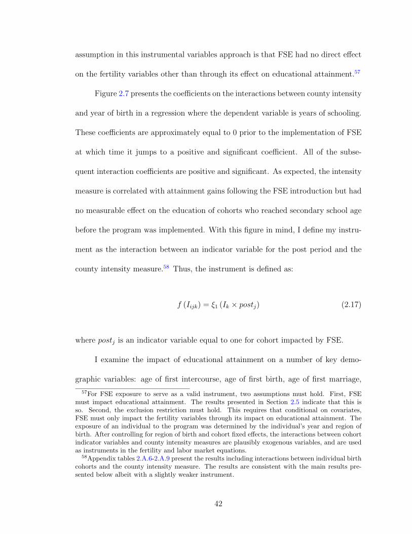
assumption in this instrumental variables approach is that FSE had no direct effect

on the fertility variables other than through its effect on educational attainment.57

Figure 2.7 presents the coefficients on the interactions between county intensity

and year of birth in a regression where the dependent variable is years of schooling.

These coefficients are approximately equal to 0 prior to the implementation of FSE

at which time it jumps to a positive and significant coefficient. All of the subse-

quent interaction coefficients are positive and significant. As expected, the intensity

measure is correlated with attainment gains following the FSE introduction but had

no measurable effect on the education of cohorts who reached secondary school age

before the program was implemented. With this figure in mind, I define my instru-

ment as the interaction between an indicator variable for the post period and the

county intensity measure.58 Thus, the instrument is defined as:

f (Iijk) = ξ1 (Ik × postj) (2.17)

where postj is an indicator variable equal to one for cohort impacted by FSE.

I examine the impact of educational attainment on a number of key demo-

graphic variables: age of first intercourse, age of first birth, age of first marriage,

57For FSE exposure to serve as a valid instrument, two assumptions must hold. First, FSEmust impact educational attainment. The results presented in Section 2.5 indicate that this isso. Second, the exclusion restriction must hold. This requires that conditional on covariates,FSE must only impact the fertility variables through its impact on educational attainment. Theexposure of an individual to the program was determined by the individual’s year and region ofbirth. After controlling for region of birth and cohort fixed effects, the interactions between cohortindicator variables and county intensity measures are plausibly exogenous variables, and are usedas instruments in the fertility and labor market equations.

58Appendix tables 2.A.6-2.A.9 present the results including interactions between individual birthcohorts and the county intensity measure. The results are consistent with the main results pre-sented below albeit with a slightly weaker instrument.

42

desired fertility, and contraceptive use. For each of the age variables, I examine

the impact of schooling on the probability of doing each of these activities before

ages 16, 17, 18, 19, and 20. I report results for both genders pooled and for women

only.59

I use the same approach to examine the impact of education on labor market

outcomes including whether individuals are working and the sector of work. As my

sample includes individuals as young as 18, it is likely that some younger members

of the sample have not yet entered the labor market. This would increase the

proportion reporting no work and potentially underestimate the impact on working

in the professional sector. With this in mind, I progressively restrict the sample to

older and older cohorts to try and focus on individuals who are unlikely to still be

in school. This yields three sets of results; one for individuals aged 18 and over,

another for individuals 19 and over, and a final set for those aged 20 and over.

2.6.2 Impacts of education on fertility

Figure 2.8 and Table 2.7 present the coefficients from the instrumental variable

estimates for the probability of first intercourse, birth, and marriage before each

teenage age. The coefficients for first intercourse are all negative with the magnitude

of the estimated coefficients increasing as the age cutoff increases. Each additional

year of education is estimated to decrease the probability of having first intercourse

at age 16 by around 3 percentage points, rising to almost 8 percentage points by age

59For the male only sample, which is smaller, the instrument fails to satisfy the Staiger andStock (1997) recommendation that the F-statistic exceed 10.

43

18 and 18 percentage points by age 20 on base rates of 23%, 46% and 70% suggesting

a decrease of between 10-25% at each age. The results appear to be driven by large

effects for women as the coefficients for the pooled sample where men are included

are lower than the women’s only sample. Larger impacts are estimated for age of

first marriage. The coefficients for women indicate a decrease of about 59% in the

likelihood of being married before age 18 and of 47% for being married before age 20.

The results for age of first birth are also consistent across ages with the estimated

coefficients indicate a decreased likelihood of having a first child by age 16-20 of

30-50%.60

Taken together, the estimated coefficients suggest large and significant impacts

of education on delaying these fertility behaviors. The estimated impacts on age of

first birth are slightly larger in magnitude than those estimated by Ferre (2009) who,

in her analysis of adding an additional year of primary schooling in Kenya, concludes

that an additional year of education decreases the probability of teenage childbearing

by 24-29%. In his analysis of the secondary school admissions discontinuity in

Kenya, Ozier (Forthcoming) estimates that secondary schooling almost completely

eliminates teen pregnancy. While my instrument is too weak to examine the impact

of completing secondary school on teenage pregnancy, the estimated coefficient on

each additional year of education suggests that a similar elimination of teenage

pregnancy would arise from a full four years of secondary education. Using the

introduction of free primary education in Uganda, Keats (2014) obtains slightly

60Appendix Table 2.A.5 presents coefficients from OLS estimates of the impact of education onage of first intercourse, age of first birth, and age of first marriage. The IV estimates are univer-sally larger than the OLS estimates suggesting downward omitted variable bias due to negativecorrelation between family variables, such as income, and fertility behaviors.

44

smaller estimates: each additional year of education decreases the probability of first

birth at each age between 16 and 20 by between 5-20%. By contrast, while I estimate

large and significant negative impacts of education on age of first intercourse, Keats

(2014) finds evidence that an additional year of education increased the likelihood

of intercourse by age 18, and estimates insignificant coefficients for other ages. The

apparent incongruity of the Uganda and Kenya results may be due to the different

policies examined and the different ages at which they keep students in school: free

primary education is likely to induce students to remain in school through their

middle teenage years while free secondary education is likely to induce students to

remain through their late teenage years.

Ferre (2009) details three main mechanisms through which education may

delay child bearing: a “knowledge” effect where more educated individuals are better

informed about contraception, an “autonomy” or empowerment effect where women

shift their preferences towards fewer, higher quality children, and an “incarceration”

effect whereby students either spend time in school and therefore have less time to

get pregnant or they may delay childbearing to finish their schooling.61 All of these

effects are potential avenues through which education could also impact age of first

intercourse and age of first birth. If an incarceration effect is the primary mechanism

through which education delays childbearing then the different impact patterns on

age of first birth estimated in this paper and Keats (2014) could be due to the

differing sources of variation: primary education may only impact behaviors around

61Students who get pregnant in Kenya are often asked to leave school. While Ministry ofEducation guidelines stipulate that students can remain in school while pregnant and return toschool post-pregnancy this does not always occur in practice.

45

the primary age range and impacts decreasing in the late teenage years. In Tables

2.8-2.9, I investigate whether educational attainment changed behaviors or beliefs

corresponding with the first and second of the three mechanisms.

Table 2.8 examines the impact of education on reported contraceptive usage

finding no evidence of increased contraceptive use or access. Table 2.9 examines the

impact of education on desired fertility which is marginally significant for the pooled

sample and negative and insignificant for the female sample. The pooled estimate

of -0.2 desired children is similar to that estimated by Keats (2014), who found

evidence of a large (-0.3) and significant impact. The lack of significant impacts for

women on proxies for both the knowledge and autonomy effects suggests that the

incarceration effect may be the dominant mechanism of behavior change. As FSE

primarily impacted day schools where students return home in the evenings and over

weekends, it seems likely that the measured impacts are not attributable to a direct

confinement effect associated with being separated from individuals of the opposite

gender, but rather to individuals choosing to delay intercourse to ensure that they

can continue their schooling.

2.6.3 Impacts of education on occupational choice

Table 2.10, Panel A presents analogous instrumental variables estimates examining

the impacts of education on women’s sector of work. The results indicate an in-

creased likelihood of skilled work and a decreased likelihood of agricultural work.

The estimates of decreased agricultural work may be attributable to a delayed tran-

46

sition to the labor market as many of the younger women in the sample might still

be in school, which would potentially inflate the proportion reporting no work. If

individuals exit secondary school and enter agricultural work, the presented coeffi-

cients overestimate the negative impact on agricultural work. Panel B and Panel C

restrict the sample to slightly older populations to try and decrease the proportion

reporting no work due to continued schooling. As expected, the older samples are

less likely to report no work. While the estimated impact of education on agricul-

tural work decreases slightly in the older samples, the estimated coefficient remains

large in magnitude and significant with no corresponding decrease in impact on

skilled work. This suggests that individuals are less likely to work in agriculture

and more likely to have skilled work. These findings for women complement those

of Ozier (Forthcoming), who found that secondary schooling for men decreased low-

skill self-employment and may have increased formal employment.

While the positive impact I find on skilled work is likely a lower bound, as it

may grow stronger as the sample ages, this shift towards skilled work might not yield

the growth benefits if it comes as a result of signaling rather than an increased stock

of cognitive ability (Hanushek and Woßmann, 2008). However, Ozier (Forthcoming)

presents evidence that secondary schooling in Kenya increases human capital. His

estimates are valid for the inframarginal students that may be impacted by FSE,

suggesting that the sectoral shifts are likely not purely the result of signaling, but

also of increased human capital.

47

2.7 FSE and student achievement

2.7.1 Identification strategy

I next examine the impact that FSE had on student achievement by exploiting

the differential exposure to FSE, and the associated differential expansion, across

counties. As modeled in Section 2.2.1, a decrease in the cost of schooling will lead

to a decrease in student achievement unless high-performing students are credit

constrained prior to the program. With this in mind, my analysis of the impact of

FSE on student achievement is a test of credit constraints: an increase in student

achievement indicates that credit constraints precluded high-ability students from

further schooling.

As described in Section 2.4.3, I consider cohorts of students who made the

secondary school entrance decision after the program was announced as treated – the

first cohort entered secondary school in 2008 and subsequently took the secondary

school completion examination in 2011. With this in mind, I set the treatment

intensity to zero for cohorts prior to 2011.62 I first examine the impact of FSE

on overall student achievement by running a regression analogous to equation 2.14

examining student performance on the secondary school completion examination:

Tijk = α0 + β1 (Ik ∗ FSEj) + ηk + γj + εijk (2.18)

62Appendix 2.B.4 presents the results of an alternative analysis where I assume that older cohortsare impacted by larger younger FSE cohorts and the early FSE cohorts are less impacted due tosmaller cohorts ahead of them.

48

where Tijk is the normalized test score of individual i in cohort j in county k. As

described in the model, this regression will conflate a dilution of resource quality

with a changing composition of the student body. If the estimated coefficient of β1

is zero, then counties that expanded their secondary schooling levels more saw no

change in their average performance. With a dilution of existing school resources,

this implies that the average student ability increased which indicates that students

were credit constrained.63 A negative coefficient on average achievement confounds a

dilution of school resources with new student quality and I am unable to determine

the impact of FSE on average student ability. The results from this test, shown

below in Section 2.7.2, are able to rule out large negative impacts.

I then follow Lucas and Mbiti (2012a) and Valente (2015) and examine the

impact of the program on students who likely would have continued through to sec-

ondary school even in the absence of the program. For these students, there is no

change in the composition of the student body so that any measured impact on aca-

demic achievement should be restricted to arise only from the dilution of resources.64

While the preceding analysis suggests that FSE eased credit constraints allowing

both high and low performing students to continue their schooling, for this analysis,

63Redistributing existing resources, such as teachers, across counties would mitigate the dilutionof resources and bias my estimates down. If the program targeted a select population or region,additional resources could be diverted and offset the dilution with only limited impact on theresources available to the non-treated population. FSE was implemented at a national level andthus the estimates are appropriate in incorporating any intentional redistribution of resourcesacross counties. Empirically, data from Ministry of Education (2008b) and Ministry of Education,Science and Technology (2014a) do not provide evidence of a redistribution of teachers: the growthin number of teachers at the regional level is negatively correlated (-0.5) with the mean regionalintensity and only weakly positively correlated (0.1) when excluding three North-Eastern Kenyacounties which experienced a large relative increase in teachers (Garissa, Mandera, and Wajir).

64Lucas and Mbiti (2012a) and Valente (2015) both assume that additional students are lowerperforming and use the changes-in-changes approach of Athey and Imbens (2006) to measure theimpact across the upper-half of the distribution.

49

I assume that the highest performers would have been able to attend secondary

school even in the absence of the program by raising funds through family or vil-

lage networks.65 The analysis requires that I identify a sufficiently high-performing

sample, based on KCSE score, for whom the introduction of FSE was unlikely to

change their schooling decisions. I use the one cohort of primary school graduates

for whom I have both KCPE and KCSE data to examine the relationship between

primary school and secondary school completion examination results. Figure 2.A.5

shows the proportion of students who completed secondary school in either 2014

or 2015 broken down by their score on the 2010 KCPE. In this period, 90% of the

students who score over 290 points (out of 500) complete secondary school within 5

years suggesting that the remaining uniform, book, and facilities fees are deterring,

at most, 10% of students from continuing to secondary school. I define my sample

so that no more than 5% of students are expected to have KCPE results below this

value; 95% of students who scored 64 or above on the KCSE also scored above 290

on the KCPE and constitute a little less than 10% of the test taking body. I there-

fore restrict attention to the highest performing 10% across counties and assume

that these students are sufficiently high performing that they would have been able

to raise the requisite funds for schooling in the absence of FSE.66 The identification

65Ideally, I would like to examine the likelihood, by primary school completion examinationgrade, that students who completed primary school in 2007 continued on to secondary school. Ifalmost all students who scored above some mark proceeded to secondary school then I could exam-ine the impact of FSE on the relative performance of students who scored above the mark withoutcomposition effects of additional students induced to attend secondary school. Unfortunately, I donot have matched primary and secondary school completion examination results for all years andcan only examine the likelihood of completing secondary school for those who sat for the primaryschool examination in 2010. This is in the post-FSE period which will inflate the likelihood thatstudents of any score proceed to secondary school but which I assume is indicative of the pre-FSEperiod.

66The cutoff for funded admission to universities, which varies year-to-year, has historically been

50

assumption to examine the impact of resource dilution on academic outcomes within

the sample is that the schooling decisions of students who scored in the top 10%

of their county were unaffected by the FSE program.67 While I can also examine

the impact at lower performance levels, these estimates are more likely to conflate

resource dilution together with potential composition changes.

I also examine the impact on the top 10% of the distribution using the changes-

in-changes (CiC) approach of Athey and Imbens (2006). The CiC model is a gener-

alization of the difference-in-differences estimator that estimates the entire counter-

factual distribution of a treated group which is identified under the assumption that

the changes in the distribution of the treated and comparison groups would, absent

treatment, be the same. The standard estimator considers the impact of a binary

treatment across two time periods. I consider the pre- and post-FSE periods and

compare students in counties exposed to a treatment intensity above the median to

those in counties below the median intensity level. The treatment effect at quantile

q is calculated as:

τCiCq = F−1Y 1,11 (q)− F−1

Y N ,11(q) = F−1

Y 1,11 (q)− F−1Y,01

(FY,00

(F−1Y,10 (q)

))(2.19)

where FY 1,gt is the cumulative distribution function of group g in time t. The

CiC model imposes three main assumptions.68 First, the potential test scores of

around 64 points.67I am currently seeking an analogous probability of reaching the KCSE by KCPE score for the

pre-FSE period.68These are laid out in Athey and Imbens (2006) Assumption 3.1-3.3. An additional common

support assumption (Athey and Imbens (2006) assumption 3.4) requires that outcomes of thetreated group in any period be a subset of the untreated outcomes.

51

untreated individuals(KCSEi

N)

should satisfy:

KCSEiN = h (Ai, Ti) (2.20)

where Ai is an underlying unobserved ability and Ti is the time period in which

the test was taken. Second, CiC imposes a strict monotonicity framework that

the test score production function h (Ai, Ti) be strictly increasing in A. Third, the

underlying ability distribution within a group can not vary over time:

Ai⊥Ti|Gi (2.21)

Focusing on the entire sample of students who sat for the KCSE exam in

the post-FSE period would violate this assumption as FSE would likely have in-

duced not only the credit constrained students to continue their schooling but also

lower-ability students for whom FSE changes their optimal schooling decision. As

described above, I try to satisfy the requirement that the underlying ability dis-

tribution within a group not vary over time by restricting my focus to the highest

performing students. I control for county fixed effects and county linear trends

following the parametric approach suggested by Athey and Imbens (2006).

2.7.2 FSE and student achievement results

In examining the impact of FSE on student achievement, I first confirm that the

growth in secondary school students is evident in the secondary school completion

52

examination results. Table 2.11 presents the estimates of the regression represented

by equation 2.18 where the dependent variable is the number of students who sat for

the secondary school completion examination relative to pre-FSE levels. The results

show that more intensely treated counties saw larger increases in the number of test

takers. The gains in test takers are robust to controlling for potentially confounding

programs and funding levels. The estimated impacts are similar gains for males

and females, and are also similar in magnitude to the statistically insignificant gains

estimated above using the DHS data.

Confirming that the FSE growth is evident in the test data, I next consider

the impact on average test scores. Table 2.12 Panel A presents results examining

whether average test scores decreased in areas that more intensely treated. The

pooled results presented in columns 1-2 indicate small impacts as the estimated

coefficients of -0.007 and 0.07 standard deviations suggest that at the average in-

tensity of 0.34 the estimated impact is about 0.02 standard deviations. To put this

coefficient into perspective, I run a simulation to estimate the effect of the program

without credit constraints where I assume that the program induced lower-ability

students to continue their schooling. This simulation yields an estimated impact of

about -0.3 standard deviations.69 This null result is indicative of credit constraints,

as the negative impact of a dilution in educational resources requires an increase in

average ability to yield no overall impact.

With the near zero estimated coefficients providing evidence in support of

69Appendix C describes the simulation and Appendix Table 2.C.1 presents the estimated treat-ment coefficients.

53

the presence of credit constraints, I next consider the impact of the program on

the scores of students at the very upper end who may have taken the exam in the

absence of FSE. Panel B of Table 2.12 presents the results associated with equation

2.18 where the sample is restricted to individuals who scored above 64 on the KCSE.

The results rule out large negative impacts and are suggestive of positive impacts.

Finally, Table 2.13 uses the changes-in-changes methodology to examine whether

FSE differentially impacted students across the top of the score or ability distribu-

tion. One of the nine coefficients is significant at the 10% level with all estimated

coefficients relatively small. The estimated impacts here and above together suggest

limited impacts of school access expansion on academic achievement. This finding

is in line with that of Lucas and Mbiti (2012a) who find evidence of, at most, small

impacts of free primary education in Kenya. While I can not fully rule out pos-

itive impacts, the non-negative impacts are in line with those of Blimpo, Gajigo,

and Pugatch (2015) who find that free secondary education for girls in The Gambia

increased test scores.

2.8 Conclusion

In early 2008, the Kenyan government implemented a free secondary education pro-

gram. The program increased educational attainment for primary school completers

by approximately 0.8 years. This paper uses differential exposure to the program,

in an instrumental variables framework, to present new evidence on the impact of

education on a range of demographic and labor market outcomes.

54

I find that secondary schooling has broad impacts on fertility behaviors. Sec-

ondary schooling decreases the probability of first intercourse at all ages between

16 and 20 by around 25%, decreases the probability of first marriage at all ages

between 16 and 20 by around 50%, and decreases the probability of teenage child-

bearing by 37%. Despite these impacts, I find no evidence that secondary schooling

decreases desired fertility or increases modern contraceptive use. This suggests that

free education decreases risky behaviors that could potentially preclude continued

schooling. These demographic impacts suggest a potentially large additional benefit

of the program, as delayed fertility behaviors are associated with significant benefits

for both the mother and child (Ferre, 2009; Schultz, 2008).

I also find that post-primary schooling shifts young women across labor market

sectors. Education increases the likelihood of work in skilled labor by 28% and

decreases the likelihood of working in agriculture by almost 80%. These findings

for women complement similar existing findings for men (Ozier, Forthcoming). This

shift towards more productive sectors is suggestive of potential growth consequences

of the program.

Finally, I use new individual examination results data to demonstrate that the

rapid increases in educational attainment associated with the free secondary educa-

tion policy did not lead to a corresponding decrease in the educational achievement

of students. Impact estimates which combine both composition changes and re-

source dilution are small and insignificant. With a decrease in resource quality, this

implies an increase in mean student ability. I present a model showing that an

offsetting increase in mean student ability is consistent with credit constraints pre-

55

cluding poor students from attending secondary schooling. The results on student

achievement suggest that concerns over rapid expansions of schooling systems may

be overstated and that countries are able to adjust to additional students without

negative consequences to the quality of education.

The methodology used here could be employed with future survey data, in

which individuals exposed to the program are older, to examine longer term fertility

and labor market outcomes. Further, using future data may also provide evidence

on the impact of education on spousal quality: if assortative matching is taking

place, we may expect the education gains to have intergenerational impacts.

56

Figure 2.1: Secondary school admissions 2000-2013

2008 FSE

010

020

030

040

050

060

070

0S

ec. s

choo

l adm

issi

ons

(tho

usan

ds)

-6 -4 -2 0 2 4 6Year

Actual admissions Trend line for Pre-FSE period

Source: Kenya Economic Surveys (2000-2013).

57

Figure 2.2: Cohort exposure

0.2

.4.6

.81

Den

sity

of e

xam

coh

ort

020

4060

8010

0P

erce

nt c

ohor

t tre

ated

8 10 12 14 16 18 20 22Age at time of FSE

Age distribution of primary school completion exam cohortImplied percent of cohort exposed to FSE

Source: 2014 KCPE registration data.Notes: The age distribution for the first FSE cohort (2007 primary school completers) is assumedto have been the same as that observed in the 2014 cohort. The implied cumulative distributionassumes that age distribution of test takers is stable across time.

based on the age distribution of primary school completersPercent of each cohort exposed to FSE

58

Figure 2.3: Common pre-program trends

.4.6

.8P

rimar

y-se

cond

ary

tran

sitio

n ra

te

-6 -4 -2 0 2 4 6Cohort

High pre-program access Low pre-program accessPre-program linear trend Pre-program linear trend

Source: 2014 Kenya DHS.Notes: High/low pre-program access defined as whether county average pri-sec transition ratebetween 1989 and 1990 was above/below the average transition rate. Pri-sec transition ratedefined as share of primary school graduates with at least some secondary schooling. Freesecondary education introduced in early 2008 for the 2007 KCPE cohort. 70% of KCPE students in 2014 were 14-16 years old suggesting program first impacted students born between 1991 and 1993.

and by high/low pre-FSE program transition ratesPrimary to secondary transition rates by birth cohort

59

Figure 2.4: Pre-program primary to secondary transition rate histogram

02

46

810

Fre

quen

cy

.2 .4 .6 .8 1Primary to secondary transition rate

Source: 2014 Kenya DHS.Notes: Transition rate measured as students with any secondary schooling as a fraction ofprimary school graduates. Dashed line indicates mean county transition rate.

Pre-FSE county transition rates

Figure 2.5: Pre-program primary to secondary transition rates by county

60

Figure 2.6: Kaplan-Meier survival estimates

Panel A: Age of first intercourse:

0.00

0.25

0.50

0.75

1.00

10 15 20 25 30Age

No secondary school Any secondary school

Panel B: Age at first birth:

0.00

0.25

0.50

0.75

1.00

10 15 20 25 30Age

No secondary school Any secondary school

Panel C: Age of first marriage:

0.00

0.25

0.50

0.75

1.00

10 15 20 25 30Age

No secondary school Any secondary school

Lines depict the probability of still being in a (a) nointercourse, (b) no birth, or (c) no marriage state byschooling level. Sample restricted to women. In thiscontext, survival refers to remaining in the initial state.

61

Figure 2.7: Interaction coefficients

-2-1

01

23

45

6In

tera

ctio

n co

effic

ient

-6 -4 -2 0 2 4 6Cohort

in the years of education regressionInteraction between year of birth and treatment intensity

Note: Coefficients are on the interaction between county FSE intensity and birthcohort. A joint F-test of pre-program values does not reject that all values are

equal to zero.

62

Figure 2.8: Fertility behavior coefficients

-.3

-.2

-.1

0E

stim

ated

impa

ct

16 17 18 19 20Age

First intercourse First marriage First birth

Each point represents the coefficient on years of education from separate regressions wherethe dependent variables are binary indicators for whether individuals participated in each behaviorbefore age X. Years of education is instrumented with cohort * county level exposure. The barsdenote the corresponding 95% confidence intervals, with standard errors clustered by county. TheF-statistics for first intercourse and first marriage are 10.46, 10.46, 10.46, 12.43, and 14.38 forage 16, 17, 18, 19, and 20, respectively. First birth F-statistics are 18.08, 18.08, 18.08,22.76, and 13.34.

before selected agesEstimated impact of secondary education on behaviors

63

Table 2.1: DHS sample characteristics

Obs. Mean S.D. Median Min. Max.

A. Primary School Completers

Female 13605 0.71 0.46 1 0 1

Age 13605 23.97 3.90 24 18 31

Years of education 13605 10.49 2.35 10 8 19

Completed primary school 13605 1.00 0.00 1 1 1

Attended some secondary school 13605 0.65 0.48 1 0 1

Completed secondary school 13605 0.42 0.49 0 0 1

Female fertility behaviors:

Age at first intercourse 8298 17.72 2.85 18 5 30

Age at first birth 6432 19.54 3.08 19 11 31

Age at first marriage/cohabitation 6097 19.47 3.23 19 10 31

Male fertility behaviors:

Age at first intercourse 3446 16.45 3.38 16 5 30

Age at first marriage/cohabitation 1454 22.46 3.13 23 13 30

Employment sector:

Not working 8499 0.28 0.45 0 0 1

Agricultural work 8499 0.17 0.38 0 0 1

Unskilled work 8499 0.37 0.48 0 0 1

Skilled work 8499 0.18 0.38 0 0 1

Intensity (1-transition rate) 13605 0.35 0.12 0.34 0.05 0.66

B. Secondary School Completers

Female 5704 0.69 0.46 1 0 1

Age 5704 24.32 3.64 24 18 31

Female fertility behaviors:

Age at first intercourse 3389 18.95 2.81 19 8 29

Age at first birth 2231 21.24 3.10 21 11 31

Age at first marriage/cohabitation 2166 21.21 2.94 21 10 30

Male fertility behaviors:

Age at first intercourse 1575 16.93 3.41 17 5 30

Age at first marriage/cohabitation 603 23.30 2.90 23 13 30

Employment sector:

Not working 3615 0.24 0.43 0 0 1

Agricultural work 3615 0.11 0.32 0 0 1

Unskilled work 3615 0.35 0.48 0 0 1

Skilled work 3615 0.30 0.46 0 0 1

Source: 2014 Kenya DHSNote: Sample restricted to individuals born between 1983 and 1996 and who are atleast 18 years old at the time of the survey. Employment questions were only includedin the full survey which was asked of approximately half the sample. Unskilled workcomprises unskilled manual work, household work, and services work. Skilled workcomprises skilled manual work or professional work.

64

Table 2.2: Secondary school completion examination summary statistics

Pre-FSE Post-FSE(2008-2010) (2011-2015)

(1) (2)

Number of schools: 5141 7445Public schools: 4346 6213Private schools: 795 1232

Number of test takers per year: 300355 437049Public schools: 262995 384756Private schools: 37360 52294

Number of test takers per school: 88.94 92.32Public schools: 90.23 94.76Private schools: 79.89 74.38

Standardized KCSE score: -0.051 -0.066Public schools: -0.022 -0.050Private schools: -0.254 -0.205

Note: Counts calculated as annual averages over stated period.2012 data are not available. A small number of national schools thatdraw high performing students from across Kenya are excluded.

65

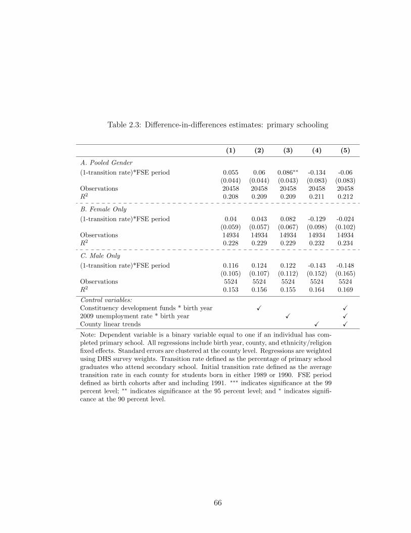
Table 2.3: Difference-in-differences estimates: primary schooling

(1) (2) (3) (4) (5)

A. Pooled Gender

(1-transition rate)*FSE period 0.055 0.06 0.086∗∗ -0.134 -0.06(0.044) (0.044) (0.043) (0.083) (0.083)

Observations 20458 20458 20458 20458 20458R2 0.208 0.209 0.209 0.211 0.212

B. Female Only

(1-transition rate)*FSE period 0.04 0.043 0.082 -0.129 -0.024(0.059) (0.057) (0.067) (0.098) (0.102)

Observations 14934 14934 14934 14934 14934R2 0.228 0.229 0.229 0.232 0.234

C. Male Only

(1-transition rate)*FSE period 0.116 0.124 0.122 -0.143 -0.148(0.105) (0.107) (0.112) (0.152) (0.165)

Observations 5524 5524 5524 5524 5524R2 0.153 0.156 0.155 0.164 0.169

Control variables:Constituency development funds * birth year X X2009 unemployment rate * birth year X XCounty linear trends X X

Note: Dependent variable is a binary variable equal to one if an individual has com-pleted primary school. All regressions include birth year, county, and ethnicity/religionfixed effects. Standard errors are clustered at the county level. Regressions are weightedusing DHS survey weights. Transition rate defined as the percentage of primary schoolgraduates who attend secondary school. Initial transition rate defined as the averagetransition rate in each county for students born in either 1989 or 1990. FSE perioddefined as birth cohorts after and including 1991. ∗∗∗ indicates significance at the 99percent level; ∗∗ indicates significance at the 95 percent level; and ∗ indicates signifi-cance at the 90 percent level.

66

Table 2.4: Binary treatment intensity difference-in-differences estimates: secondaryeducation

(1) (2) (3) (4) (5)

Panel 1: years of education

A. Pooled Gender

High Intensity*FSE period 0.348∗∗∗ 0.344∗∗∗ 0.283∗∗ 0.382∗∗ 0.387∗

(0.133) (0.129) (0.135) (0.168) (0.198)Observations 13605 13605 13605 13605 13605R2 0.093 0.095 0.094 0.1 0.102

B. Female Only

High Intensity*FSE period 0.346∗∗∗ 0.357∗∗∗ 0.279∗∗ 0.479∗∗ 0.564∗∗

(0.132) (0.13) (0.139) (0.199) (0.221)Observations 9596 9596 9596 9596 9596R2 0.089 0.091 0.09 0.096 0.099

C. Male Only

High Intensity*FSE period 0.367∗ 0.348∗ 0.328 0.138 0.024(0.199) (0.192) (0.205) (0.337) (0.39)

Observations 4009 4009 4009 4009 4009R2 0.124 0.128 0.127 0.139 0.146

Panel 2: completed secondary school

A. Pooled Gender

High Intensity*FSE period 0.001 0.005 -0.004 0.013 0.024(0.021) (0.021) (0.023) (0.039) (0.038)

Observations 13605 13605 13605 13605 13605R2 0.1 0.101 0.101 0.103 0.105

B. Female Only

High Intensity*FSE period -0.008 -0.002 -0.012 0.033 0.063(0.023) (0.023) (0.026) (0.049) (0.048)

Observations 9596 9596 9596 9596 9596R2 0.098 0.1 0.099 0.102 0.105

C. Male Only

High Intensity*FSE period 0.014 0.017 0.009 -0.044 -0.062(0.035) (0.035) (0.04) (0.072) (0.078)

Observations 4009 4009 4009 4009 4009R2 0.129 0.134 0.135 0.14 0.151

Control variables:Constituency development funds * birth year X X2009 unemployment rate * birth year X XCounty linear trend X X

Note: Reported coefficients are the estimated interaction coefficient between a dummyvariable for high treatment intensity counties and an FSE indicator variable equal to one forall individuals born in 1991 or later. Sample restricted to individuals who have completed atleast primary school. All regressions include birth year, county, and ethnicity/religion fixedeffects. Standard errors are clustered at the county level. Regressions are weighted usingDHS survey weights. Transition rate defined as the percentage of primary school graduateswho attend secondary school. Initial transition rate defined as the average transition ratein each county for students born in either 1989 or 1990. ∗∗∗ indicates significance at the 99percent level; ∗∗ indicates significance at the 95 percent level; and ∗ indicates significanceat the 90 percent level.

67

Table 2.5: Difference-in-differences estimates: secondary education

(1) (2) (3) (4) (5)

Panel 1: years of education

A. Pooled Gender

(1-transition rate)*FSE period 2.255∗∗∗ 2.256∗∗∗ 2.060∗∗∗ 2.059∗∗∗ 2.134∗∗∗

(0.31) (0.311) (0.356) (0.718) (0.677)Observations 13605 13605 13605 13605 13605R2 0.099 0.101 0.1 0.104 0.106

B. Female Only

(1-transition rate)*FSE period 2.409∗∗∗ 2.449∗∗∗ 2.221∗∗∗ 2.058∗∗ 2.336∗∗∗

(0.277) (0.268) (0.336) (0.897) (0.709)Observations 9596 9596 9596 9596 9596R2 0.091 0.093 0.092 0.096 0.099

C. Male Only

(1-transition rate)*FSE period 2.047∗∗∗ 2.035∗∗∗ 1.942∗∗∗ 2.374∗∗ 2.075(0.673) (0.616) (0.686) (1.090) (1.309)

Observations 4009 4009 4009 4009 4009R2 0.125 0.129 0.128 0.14 0.147

Panel 2: completed secondary school

A. Pooled Gender

(1-transition rate)*FSE period 0.129∗ 0.145∗∗ 0.116 0.158 0.201(0.071) (0.066) (0.087) (0.135) (0.126)

Observations 13605 13605 13605 13605 13605R2 0.104 0.105 0.105 0.107 0.109

B. Female Only

(1-transition rate)*FSE period 0.143∗ 0.164∗∗ 0.146 0.213 0.321∗∗

(0.081) (0.069) (0.091) (0.156) (0.13)Observations 9596 9596 9596 9596 9596R2 0.099 0.1 0.099 0.102 0.105

C. Male Only

(1-transition rate)*FSE period 0.085 0.107 0.064 0.046 -0.05(0.111) (0.108) (0.129) (0.231) (0.267)

Observations 4009 4009 4009 4009 4009R2 0.129 0.134 0.135 0.14 0.151

Control variables:Constituency development funds * birth year X X2009 unemployment rate * birth year X XCounty linear trend X X

Note: Sample restricted to individuals who have completed at least primary school. Allregressions include birth year, county, and ethnicity/religion fixed effects. Standard errorsare clustered at the county level. Regressions are weighted using DHS survey weights.Transition rate defined as the percentage of primary school graduates who attend secondaryschool. Initial transition rate defined as the average transition rate in each county forstudents born in either 1989 or 1990. FSE period defined as birth cohorts after and including1991. ∗∗∗ indicates significance at the 99 percent level; ∗∗ indicates significance at the 95percent level; and ∗ indicates significance at the 90 percent level.

68

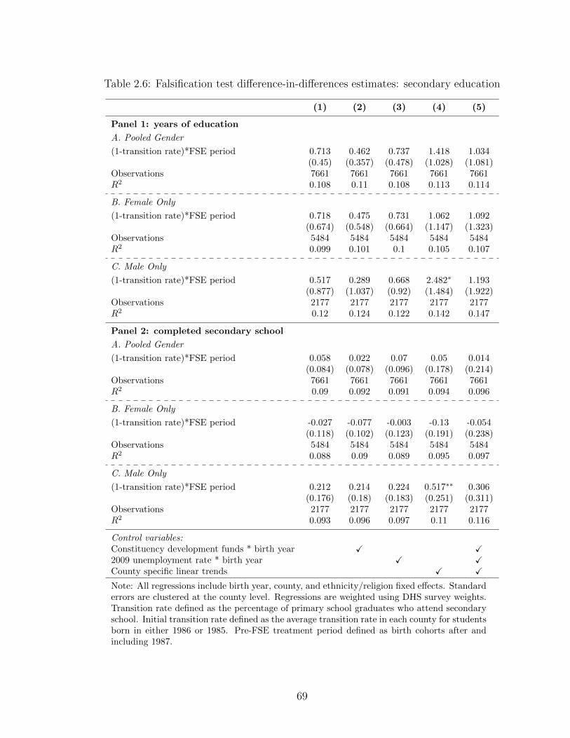
Table 2.6: Falsification test difference-in-differences estimates: secondary education

(1) (2) (3) (4) (5)

Panel 1: years of education

A. Pooled Gender

(1-transition rate)*FSE period 0.713 0.462 0.737 1.418 1.034(0.45) (0.357) (0.478) (1.028) (1.081)

Observations 7661 7661 7661 7661 7661R2 0.108 0.11 0.108 0.113 0.114

B. Female Only

(1-transition rate)*FSE period 0.718 0.475 0.731 1.062 1.092(0.674) (0.548) (0.664) (1.147) (1.323)

Observations 5484 5484 5484 5484 5484R2 0.099 0.101 0.1 0.105 0.107

C. Male Only

(1-transition rate)*FSE period 0.517 0.289 0.668 2.482∗ 1.193(0.877) (1.037) (0.92) (1.484) (1.922)

Observations 2177 2177 2177 2177 2177R2 0.12 0.124 0.122 0.142 0.147

Panel 2: completed secondary school

A. Pooled Gender

(1-transition rate)*FSE period 0.058 0.022 0.07 0.05 0.014(0.084) (0.078) (0.096) (0.178) (0.214)

Observations 7661 7661 7661 7661 7661R2 0.09 0.092 0.091 0.094 0.096

B. Female Only

(1-transition rate)*FSE period -0.027 -0.077 -0.003 -0.13 -0.054(0.118) (0.102) (0.123) (0.191) (0.238)

Observations 5484 5484 5484 5484 5484R2 0.088 0.09 0.089 0.095 0.097

C. Male Only

(1-transition rate)*FSE period 0.212 0.214 0.224 0.517∗∗ 0.306(0.176) (0.18) (0.183) (0.251) (0.311)

Observations 2177 2177 2177 2177 2177R2 0.093 0.096 0.097 0.11 0.116

Control variables:Constituency development funds * birth year X X2009 unemployment rate * birth year X XCounty specific linear trends X X

Note: All regressions include birth year, county, and ethnicity/religion fixed effects. Standarderrors are clustered at the county level. Regressions are weighted using DHS survey weights.Transition rate defined as the percentage of primary school graduates who attend secondaryschool. Initial transition rate defined as the average transition rate in each county for studentsborn in either 1986 or 1985. Pre-FSE treatment period defined as birth cohorts after andincluding 1987.

69

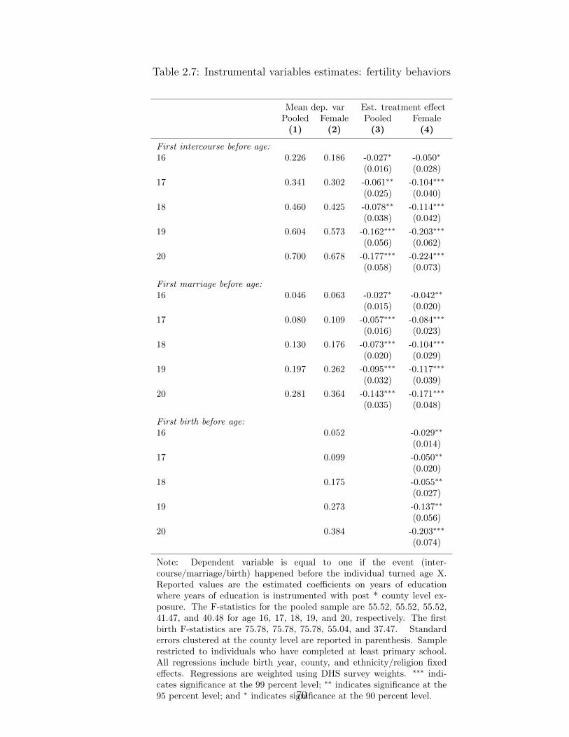
Table 2.7: Instrumental variables estimates: fertility behaviors

Mean dep. var Est. treatment effectPooled Female Pooled Female

(1) (2) (3) (4)

First intercourse before age:16 0.226 0.186 -0.027∗ -0.050∗

(0.016) (0.028)

17 0.341 0.302 -0.061∗∗ -0.104∗∗∗

(0.025) (0.040)

18 0.460 0.425 -0.078∗∗ -0.114∗∗∗

(0.038) (0.042)

19 0.604 0.573 -0.162∗∗∗ -0.203∗∗∗

(0.056) (0.062)

20 0.700 0.678 -0.177∗∗∗ -0.224∗∗∗

(0.058) (0.073)

First marriage before age:16 0.046 0.063 -0.027∗ -0.042∗∗

(0.015) (0.020)

17 0.080 0.109 -0.057∗∗∗ -0.084∗∗∗

(0.016) (0.023)

18 0.130 0.176 -0.073∗∗∗ -0.104∗∗∗

(0.020) (0.029)

19 0.197 0.262 -0.095∗∗∗ -0.117∗∗∗

(0.032) (0.039)

20 0.281 0.364 -0.143∗∗∗ -0.171∗∗∗

(0.035) (0.048)

First birth before age:16 0.052 -0.029∗∗

(0.014)

17 0.099 -0.050∗∗

(0.020)

18 0.175 -0.055∗∗

(0.027)

19 0.273 -0.137∗∗

(0.056)

20 0.384 -0.203∗∗∗

(0.074)

Note: Dependent variable is equal to one if the event (inter-course/marriage/birth) happened before the individual turned age X.Reported values are the estimated coefficients on years of educationwhere years of education is instrumented with post * county level ex-posure. The F-statistics for the pooled sample are 55.52, 55.52, 55.52,41.47, and 40.48 for age 16, 17, 18, 19, and 20, respectively. The firstbirth F-statistics are 75.78, 75.78, 75.78, 55.04, and 37.47. Standarderrors clustered at the county level are reported in parenthesis. Samplerestricted to individuals who have completed at least primary school.All regressions include birth year, county, and ethnicity/religion fixedeffects. Regressions are weighted using DHS survey weights. ∗∗∗ indi-cates significance at the 99 percent level; ∗∗ indicates significance at the95 percent level; and ∗ indicates significance at the 90 percent level.70

Table 2.8: Instrumental variables estimates: contraceptive use

Uses any Uses modern Uses Can getcontraceptive method condoms condoms

(1) (2) (3) (4)

Years of education -0.017 -0.043 0.022 0.032(0.052) (0.042) (0.03) (0.049)

Constant 0.675 0.83∗∗ -0.14 0.203(0.492) (0.399) (0.282) (0.496)

Observations 8298 8298 8298 3868First stage F-stat: 30.311 30.311 30.311 10.419

Note: Years of education instrumented with post * county level exposure.Standard errors clustered at the county level are reported in parenthesis.Sample restricted to individuals who have completed at least primary schooland have had intercourse. All regressions include birth year, county, andethnicity/religion fixed effects. Regressions are weighted using DHS surveyweights. ∗∗∗ indicates significance at the 99 percent level; ∗∗ indicates signif-icance at the 95 percent level; and ∗ indicates significance at the 90 percentlevel.

Table 2.9: Instrumental variables estimates: desired fertility

Pooled Female(1) (2)

Years of education -0.228∗ -0.133(0.133) (0.153)

Constant 5.001∗∗∗ 4.849∗∗∗

(1.214) (1.536)Observations 8465 4502First stage F-stat: 30.622 15.031

Note: Dependent variable is the respondent’s idealnumber of children. Years of education instrumentedwith post * county level exposure. Standard errorsclustered at the county level are reported in paren-thesis. Sample restricted to individuals who havecompleted at least primary school. All regressions in-clude birth year, county, and ethnicity/religion fixedeffects. Standard errors are clustered at the countylevel. Regressions are weighted using DHS surveyweights. ∗∗∗ indicates significance at the 99 percentlevel; ∗∗ indicates significance at the 95 percent level;and ∗ indicates significance at the 90 percent level.

71

Table 2.10: Instrumental variables estimates: sector of work

Skilled Unskilled Agricultural NoWork Work Work Work

(1) (2) (3) (4)

Panel 1. Age 18 and over

Years of education 0.069∗∗∗ -0.06 -0.18∗∗∗ 0.171∗∗

(0.022) (0.064) (0.039) (0.079)Observations 4525 4525 4525 4525First stage F-stat: 22.909 22.909 22.909 22.909

Panel 2. Age 19 and over

Years of education 0.074∗∗∗ -0.047 -0.169∗∗∗ 0.142∗∗

(0.023) (0.059) (0.037) (0.07)Observations 4295 4295 4295 4295First stage F-stat: 24.347 24.347 24.347 24.347

Panel 3. Age 20 and over

Years of education 0.082∗∗∗ -0.037 -0.137∗∗∗ 0.092(0.025) (0.057) (0.033) (0.067)

Observations 3935 3935 3935 3935First stage F-stat: 16.226 16.226 16.226 16.226

Note: Dependent variable is a binary variable equal to one if respondent worksin sector X. Years of education instrumented with post * county level exposure.Unskilled labor aggregates household/domestic work, service jobs, and unskilledmanual labor. Skilled labor aggregates professional/technical/managerial/clericaland skilled manual labor. Standard errors clustered at the county level are re-ported in parenthesis. Sample restricted to women who have completed at leastprimary school. All regressions include birth year, county, and ethnicity/religionfixed effects. Regressions are weighted using DHS survey weights. ∗∗∗ indicatessignificance at the 99 percent level; ∗∗ indicates significance at the 95 percentlevel; and ∗ indicates significance at the 90 percent level.

72

Table 2.11: County expansion at secondary school completion

(1) (2) (3) (4)

A. Pooled Gender

(1-transition rate)*FSE period 0.192∗∗ 0.196∗ 0.245∗∗∗ 0.246∗∗∗

(0.097) (0.104) (0.09) (0.093)Observations 423 423 423 423R2 0.969 0.971 0.977 0.977

B. Female Only

(1-transition rate)*FSE period 0.763∗∗ 0.751∗∗ 0.405∗∗ 0.413∗∗

(0.297) (0.295) (0.16) (0.162)Observations 423 423 423 423R2 0.942 0.944 0.966 0.966

C. Male Only

(1-transition rate)*FSE period 0.557∗∗∗ 0.542∗∗∗ 0.488∗∗∗ 0.483∗∗∗

(0.126) (0.129) (0.126) (0.128)Observations 423 423 423 423R2 0.948 0.953 0.962 0.964

Control variables:Constituency development funds * birth year X X2009 unemployment rate * birth year X X

Note: Regressions are run at the county-year level. Dependent variable is the countycohort KCSE registration divided by the 2010 cohort KCSE registration. Standarderrors clustered at the county level are reported in parenthesis. All columns includeyear fixed effects as well as county linear trends. ∗∗∗ indicates significance at the99 percent level; ∗∗ indicates significance at the 95 percent level; and ∗ indicatessignificance at the 90 percent level.

73

Table 2.12: Student achievement

(1) (2) (3) (4)

A. Full sample

(1-transition rate)*FSE period -0.007 0.074 . .(0.02) (0.047)

(1-transition rate)*FSE period*Female . . -0.019 0.055(0.02) (0.054)

(1-transition rate)*FSE period*Male . . 0.012 0.112∗

(0.024) (0.06)Observations 3321504 3321504 3321504 3321504R2 0.039 0.221 0.049 0.238

B. High performers

(1-transition rate)*FSE period 0.131 0.122∗ . .(0.197) (0.074)

(1-transition rate)*FSE period*Female . . 0.147 0.01(0.215) (0.1)

(1-transition rate)*FSE period*Male . . 0.121 0.173∗∗

(0.197) (0.082)Observations 269436 269436 269436 269436R2 0.357 0.409 0.361 0.418

Control variables:Constituency development funds * birth year X X2009 unemployment rate * birth year X X

Note: Dependent variable is standardized KCSE score. Standard errors clusteredat the county level are reported in parenthesis. All columns include county fixedeffects and county linear trends while Panel B also includes year fixed effects.Columns 2 and 4 also include dummies for public schools, single gender schools,and district level schools. Controls are interacted with gender for columns 3 and4. ∗∗∗ indicates significance at the 99 percent level; ∗∗ indicates significance at the95 percent level; and ∗ indicates significance at the 90 percent level.

Table 2.13: Estimates from a changes-in-changes model

Percentile Overall Female Male

0.8 0.037 0.063∗ -0.0050.9 0.015 0.026 -0.0180.95 0.022 0.010 -0.021

Note: Estimates are from a changes-in-changes model. Standard errors clusteredat the county level. County fixed effectsand linear trends are included as describedin the text above. ∗∗∗ indicates significanceat the 99 percent level; ∗∗ indicates signif-icance at the 95 percent level; and ∗ indi-cates significance at the 90 percent level.

74

Appendix

2.A Additional Tables and Figures

Figure 2.A.1: Age distribution of KCPE test takers

010

2030

40D

ensi

ty o

f exa

m c

ohor

t

10 12 14 16 18 20Age

2008 cohort 2014 cohort

Source: 2008 and 2014 KCPE data.Notes: 2008 data are only available for Central, Nyanza, and Western provinces. The 2014 dataare restricted to the same provinces. Data restricted to first time test takers.

for Central, Nyanza, and Western provincesAge distribution of 2008 and 2014 exam cohorts

75

Figure 2.A.2: Mean KCSE scores (Public/Private)

-.3

-.2

-.1

0.1

Sta

ndar

dize

d ex

am s

core

2006 2008 2010 2012 2014 2016Year

Public schools Private schools

Notes: Mean scores calculated from KCSE data. Each year approximately 12% of test takersattend private schools.

76

Figure 2.A.3: Secondary school time to completion

020

4060

80P

erce

nt

4 5 6 7 8 9Years since primary school completion

Source: 2014 KCSE Registration DataNote: Fewer than 2% of test takers complete secondary school more than 7 years after primaryschool.

Time between primary and secondary school completion

77

Figure 2.A.4: Falsification test: Pre-FSE sample

.4.6

.8P

rimar

y-se

cond

ary

tran

sitio

n ra

te

-4 -2 0 2 4Cohort

High pre-program access Low pre-program accessPre-program linear trend Pre-program linear trend

Notes: High/low pre-program access defined as whether county average pri-sec transition ratebetween 1985 and 1986 was above/below the average transition rate. Pri-sec transition ratedefined as share of primary school graduates with at least some secondary schooling.Source: 2014 Kenya DHS.

and by high/low pre-free secondary education program transition ratesPrimary to secondary transition rates by birth cohort

78

Figure 2.A.5: Probability of secondary school completion by KCPE score

0.2

.4.6

.81

Pro

port

ion

com

plet

ing

seco

ndar

y sc

hool

0 100 200 300 400 500Primary School Completion Examination Score

Source: KCPE results data and KCSE registration data.Note: The graph shows, by primary school completion examination score, the proportion of 2010primary school completers who registered for the secondary school completion examination ineither 2014 or 2015.

79

Table 2.A.1: DHS sample characteristics

Obs. Mean S.D. Median Min. Max.

DHS Sample

Female 20458 0.73 0.44 1 0 1

Age 20458 24.24 3.97 24 18 31

Christian 20458 0.84 0.37 1 0 1

Muslim 20458 0.13 0.34 0 0 1

Kalenjin 20458 0.15 0.36 0 0 1

Kikuya 20458 0.15 0.35 0 0 1

Luhya 20458 0.12 0.33 0 0 1

Luo 20458 0.10 0.30 0 0 1

Other ethnicity 20458 0.22 0.41 0 0 1

Urban household 20458 0.41 0.49 0 0 1

Years of education 20458 8.21 4.11 8 0 19

Completed primary school 20458 0.67 0.47 1 0 1

Attended some secondary school 20458 0.43 0.50 0 0 1

Completed secondary school 20458 0.28 0.45 0 0 1

Female fertility behaviors:

Age at first intercourse 13287 17.00 2.95 17 5 30

Age at first birth 11104 18.75 3.10 18 10 31

Age at first marriage/cohabitation 10718 18.37 3.41 18 9 31

Male fertility behaviors:

Age at first intercourse 4734 16.31 3.38 16 5 30

Age at first marriage/cohabitation 2204 21.95 3.25 22 13 30

Intensity (1-transition rate) 20458 0.34 0.12 0.34 0.05 0.66

Source: 2014 Kenya DHSNote: Sample restricted to individuals born between 1983 and 1996.

80

Table 2.A.2: Binary intensity measure difference-in-differences estimates: primaryschooling

(1) (2) (3) (4) (5)

A. Pooled Gender

High Intensity*FSE period -0.0005 0.00002 0.007 -0.059∗∗∗ -0.044∗

(0.013) (0.013) (0.014) (0.023) (0.023)Observations 20458 20458 20458 20458 20458R2 0.201 0.201 0.201 0.204 0.205

B. Female Only

High Intensity*FSE period 0.006 0.005 0.014 -0.054∗ -0.032(0.015) (0.015) (0.015) (0.028) (0.028)

Observations 14934 14934 14934 14934 14934R2 0.228 0.229 0.229 0.232 0.234

C. Male Only

High Intensity*FSE period -0.011 -0.006 -0.015 -0.057 -0.066(0.026) (0.026) (0.027) (0.038) (0.04)

Observations 5524 5524 5524 5524 5524R2 0.153 0.155 0.155 0.164 0.17

Control variables:Constituency development funds * birth year X X2009 unemployment rate * birth year X XCounty linear trends X X

Note: Dependent variable is a binary variable equal to one if an individual has com-pleted primary school. All regressions include birth year, county, and ethnicity/religionfixed effects. Standard errors are clustered at the county level. Regressions are weightedusing DHS survey weights. Transition rate defined as the percentage of primary schoolgraduates who attend secondary school. Initial transition rate defined as the averagetransition rate in each county for students born in either 1989 or 1990. FSE perioddefined as birth cohorts after and including 1991. ∗∗∗ indicates significance at the 99percent level; ∗∗ indicates significance at the 95 percent level; and ∗ indicates signifi-cance at the 90 percent level.

81

Table 2.A.3: Binary treatment intensity difference-in-differences estimates: sec-ondary education

(1) (2) (3) (4) (5)

A. Falsification for program introduced in 1986

High Intensity*FSE period 0.198∗ 0.139 0.224∗ 0.229 0.162(0.119) (0.094) (0.126) (0.2) (0.214)

Observations 10324 10324 10324 10324 10324R2 0.112 0.115 0.112 0.117 0.12

A. Falsification for program introduced in 1985

High Intensity*FSE period 0.184 0.126 0.222 0.152 0.121(0.13) (0.114) (0.14) (0.214) (0.204)

Observations 11142 11142 11142 11142 11142R2 0.111 0.114 0.111 0.117 0.12

B. Falsification for program introduced in 1984

High Intensity*FSE period 0.095 0.044 0.104 -0.047 -0.157(0.104) (0.086) (0.1) (0.203) (0.21)

Observations 10643 10643 10643 10643 10643R2 0.111 0.114 0.111 0.116 0.119

C. Falsification for program introduced in 1983

High Intensity*FSE period 0.062 0.002 0.082 -0.03 -0.06(0.116) (0.12) (0.111) (0.246) (0.231)

Observations 10264 10264 10264 10264 10264R2 0.113 0.117 0.114 0.118 0.121

D. Falsification for program introduced in 1982

High Intensity*FSE period 0.04 0.07 0.085 0.385∗ 0.504∗∗

(0.133) (0.145) (0.125) (0.207) (0.232)Observations 9760 9760 9760 9760 9760R2 0.113 0.115 0.114 0.118 0.121

E. Falsification for program introduced in 1981

High Intensity*FSE period -0.158 -0.075 -0.133 0.19 0.476∗∗

(0.174) (0.176) (0.168) (0.247) (0.233)Observations 9353 9353 9353 9353 9353R2 0.111 0.114 0.112 0.117 0.12

Control variables:Constituency development funds * birth year X X2009 unemployment rate * birth year X XCounty linear trend X X

Note: Reported coefficients are the estimated interaction coefficient between a dummyvariable for high treatment intensity counties and an FSE indicator variable equal to onefor all individuals born after the introduction of the falsified program. Sample restricted toindividuals who have completed at least primary school. All regressions include birth year,county, and ethnicity/religion fixed effects. Standard errors are clustered at the countylevel. Regressions are weighted using DHS survey weights. Transition rate defined as thepercentage of primary school graduates who attend secondary school. Initial transition ratedefined as the average transition rate in each county for students born in either 1989 or1990. ∗∗∗ indicates significance at the 99 percent level; ∗∗ indicates significance at the 95percent level; and ∗ indicates significance at the 90 percent level.

82

Table 2.A.4: Binary treatment diff-in-diffs excluding transition cohorts: secondaryeducation

(1) (2) (3) (4) (5)

Panel 1: years of education

A. Pooled Gender

High Intensity*FSE period 0.346∗∗ 0.39∗∗∗ 0.332∗∗ 0.578∗∗∗ 0.605∗∗∗

(0.146) (0.147) (0.153) (0.192) (0.186)Observations 11684 11684 11684 11684 11684R2 0.093 0.101 0.1 0.106 0.109

B. Female Only

High Intensity*FSE period 0.356∗∗ 0.416∗∗∗ 0.319∗∗ 0.725∗∗∗ 0.852∗∗∗

(0.15) (0.147) (0.155) (0.234) (0.204)Observations 8246 8246 8246 8246 8246R2 0.089 0.095 0.095 0.102 0.104

C. Male Only

High Intensity*FSE period 0.322∗ 0.389∗∗ 0.407∗ 0.274 0.151(0.194) (0.188) (0.208) (0.459) (0.473)

Observations 3438 3438 3438 3438 3438R2 0.117 0.136 0.135 0.147 0.155

Panel 2: completed secondary school

A. Pooled Gender

High Intensity*FSE period -0.014 0.005 0.002 0.03 0.052(0.025) (0.024) (0.027) (0.05) (0.048)

Observations 11684 11684 11684 11684 11684R2 0.09 0.108 0.107 0.11 0.112

B. Female Only

High Intensity*FSE period -0.026 -0.005 -0.015 0.042 0.085(0.029) (0.025) (0.03) (0.072) (0.065)

Observations 8246 8246 8246 8246 8246R2 0.091 0.106 0.105 0.109 0.112

C. Male Only

High Intensity*FSE period 0.002 0.029 0.04 -4.09e-06 -0.011(0.037) (0.033) (0.039) (0.081) (0.09)

Observations 3438 3438 3438 3438 3438R2 0.106 0.145 0.145 0.151 0.162

Control variables:Constituency development funds * birth year X X2009 unemployment rate * birth year X XCounty linear trend X X

Note: Reported coefficients are the estimated interaction coefficient between a dummyvariable for high treatment intensity counties and a post period dummy equal to one forall individuals born in 1991 or later. Sample restricted to individuals who have completedat least primary school and excludes the partially impacted cohorts born in 1991 and 1992.All regressions include birth year, county, and ethnicity/religion fixed effects. Standarderrors are clustered at the county level. Regressions are weighted using DHS survey weights.Transition rate defined as the percentage of primary school graduates who attend secondaryschool. Initial transition rate defined as the average transition rate in each county forstudents born in either 1989 or 1990. FSE period defined as birth cohorts after and including1991. ∗∗∗ indicates significance at the 99 percent level; ∗∗ indicates significance at the 95percent level; and ∗ indicates significance at the 90 percent level.83

Table 2.A.5: OLS estimates: fertility behaviors

Mean dep. var Est. treatment effectPooled Female Pooled Female

(1) (2) (3) (4)

First intercourse before age:16 0.226 0.186 -0.033∗∗∗ -0.037∗∗∗

(0.002) (0.002)

17 0.341 0.302 -0.045∗∗∗ -0.055∗∗∗

(0.003) (0.003)

18 0.460 0.425 -0.053∗∗∗ -0.067∗∗∗

(0.003) (0.003)

19 0.604 0.573 -0.052∗∗∗ -0.066∗∗∗

(0.002) (0.003)

20 0.700 0.678 -0.047∗∗∗ -0.060∗∗∗

(0.002) (0.003)

First marriage before age:16 0.046 0.063 -0.013∗∗∗ -0.017∗∗∗

(0.001) (0.002)

17 0.080 0.109 -0.023∗∗∗ -0.031∗∗∗

(0.001) (0.002)

18 0.130 0.176 -0.034∗∗∗ -0.046∗∗∗

(0.002) (0.002)

19 0.197 0.262 -0.047∗∗∗ -0.062∗∗∗

(0.002) (0.002)

20 0.281 0.364 -0.055∗∗∗ -0.071∗∗∗

(0.002) (0.002)

First birth before age:16 0.052 -0.011∗∗∗

(0.001)

17 0.099 -0.022∗∗∗

(0.002)

18 0.175 -0.043∗∗∗

(0.002)

19 0.273 -0.061∗∗∗

(0.002)

20 0.384 -0.077∗∗∗

(0.003)

Note: Dependent variable is equal to one if the event (inter-course/marriage/birth) happened before the individual turned age X.Reported values are the estimated coefficients on years of education.Standard errors clustered at the county level are reported in parenthe-sis. Sample restricted to individuals who have completed at least primaryschool. All regressions include birth year, county, and ethnicity/religionfixed effects. Regressions are weighted using DHS survey weights. ∗∗∗

indicates significance at the 99 percent level; ∗∗ indicates significance atthe 95 percent level; and ∗ indicates significance at the 90 percent level.

84

Table 2.A.6: Instrumental variables estimates: fertility behaviors

Mean dep. var Est. treatment effectPooled Female Pooled Female

(1) (2) (3) (4)

First intercourse before age:16 0.226 0.186 -0.020 -0.046∗

(0.016) (0.024)

17 0.341 0.302 -0.055∗∗ -0.095∗∗∗

(0.024) (0.033)

18 0.460 0.425 -0.071∗∗ -0.098∗∗∗

(0.034) (0.035)

19 0.604 0.573 -0.157∗∗∗ -0.181∗∗∗

(0.049) (0.052)

20 0.700 0.678 -0.161∗∗∗ -0.205∗∗∗

(0.055) (0.068)

First marriage before age:16 0.046 0.063 -0.024∗ -0.038∗∗

(0.013) (0.018)

17 0.080 0.109 -0.050∗∗∗ -0.076∗∗∗

(0.014) (0.019)

18 0.130 0.176 -0.067∗∗∗ -0.096∗∗∗

(0.018) (0.024)

19 0.197 0.262 -0.090∗∗∗ -0.109∗∗∗

(0.028) (0.029)

20 0.281 0.364 -0.133∗∗∗ -0.157∗∗∗

(0.033) (0.044)

First birth before age:16 0.052 -0.023

(0.014)

17 0.099 -0.035∗

(0.019)

18 0.175 -0.034(0.026)

19 0.273 -0.096∗∗∗

(0.037)

20 0.384 -0.149∗∗∗

(0.053)

Note: Dependent variable is equal to one if the event (inter-course/marriage/birth) happened before the individual turned age X.Reported values are the estimated coefficients on years of educationwhere years of education is instrumented with cohort * county levelexposure. The F-statistics for the pooled sample are 10.46, 10.46, 10.46,12.43, and 14.38 for age 16, 17, 18, 19, and 20, respectively. The firstbirth F-statistics are 18.08, 18.08, 18.08, 22.76, and 13.34. Standarderrors clustered at the county level are reported in parenthesis. Samplerestricted to individuals who have completed at least primary school.All regressions include birth year, county, and ethnicity/religion fixedeffects. Regressions are weighted using DHS survey weights. ∗∗∗ indi-cates significance at the 99 percent level; ∗∗ indicates significance at the95 percent level; and ∗ indicates significance at the 90 percent level.85

Table 2.A.7: Instrumental variables estimates: contraceptive use

Uses any Uses modern Uses Can getcontraceptive method condoms condoms

(1) (2) (3) (4)

Years of education 0.017 -0.005 0.013 0.035(0.048) (0.034) (0.025) (0.033)

Constant 0.358 0.473 -0.062 0.181(0.438) (0.312) (0.239) (0.347)

Observations 8298 8298 8298 3868First stage F-stat: 15.365 15.365 15.365 7.122

Note: Years of education instrumented with cohort * county level exposure.Standard errors clustered at the county level are reported in parenthesis.Sample restricted to individuals who have completed at least primary schooland have had intercourse. All regressions include birth year, county, andethnicity/religion fixed effects. Regressions are weighted using DHS surveyweights. ∗∗∗ indicates significance at the 99 percent level; ∗∗ indicates signif-icance at the 95 percent level; and ∗ indicates significance at the 90 percentlevel.

Table 2.A.8: Instrumental variables estimates: desired fertility

Pooled Female(1) (2)

Years of education -0.148 -0.056(0.117) (0.108)

Constant 4.307∗∗∗ 4.079∗∗∗

(1.072) (1.088)Observations 8465 4502First stage F-stat: 9.145 8.655

Note: Dependent variable is the respondent’s idealnumber of children. Years of education instrumentedwith cohort * county level exposure. Standard errorsclustered at the county level are reported in paren-thesis. Sample restricted to individuals who havecompleted at least primary school. All regressions in-clude birth year, county, and ethnicity/religion fixedeffects. Standard errors are clustered at the countylevel. Regressions are weighted using DHS surveyweights. ∗∗∗ indicates significance at the 99 percentlevel; ∗∗ indicates significance at the 95 percent level;and ∗ indicates significance at the 90 percent level.

86

Table 2.A.9: Instrumental variables estimates: sector of work

Skilled Unskilled Agricultural NoWork Work Work Work

(1) (2) (3) (4)

Panel 1. Age 18 and over

Years of education 0.069∗∗∗ -0.06 -0.18∗∗∗ 0.171∗∗

(0.022) (0.064) (0.039) (0.079)Observations 4525 4525 4525 4525First stage F-stat: 22.909 22.909 22.909 22.909

Panel 2. Age 19 and over

Years of education 0.074∗∗∗ -0.047 -0.169∗∗∗ 0.142∗∗

(0.023) (0.059) (0.037) (0.07)Observations 4295 4295 4295 4295First stage F-stat: 24.347 24.347 24.347 24.347

Panel 3. Age 20 and over

Years of education 0.082∗∗∗ -0.037 -0.137∗∗∗ 0.092(0.025) (0.057) (0.033) (0.067)

Observations 3935 3935 3935 3935First stage F-stat: 16.226 16.226 16.226 16.226

Note: Dependent variable is a binary variable equal to one if respondent works insector X. Years of education instrumented with cohort * county level exposure.Unskilled labor aggregates household/domestic work, service jobs, and unskilledmanual labor. Skilled labor aggregates professional/technical/managerial/clericaland skilled manual labor. Standard errors clustered at the county level are re-ported in parenthesis. Sample restricted to women who have completed at leastprimary school. All regressions include birth year, county, and ethnicity/religionfixed effects. Regressions are weighted using DHS survey weights. ∗∗∗ indicatessignificance at the 99 percent level; ∗∗ indicates significance at the 95 percentlevel; and ∗ indicates significance at the 90 percent level.

87

Table 2.A.10: School openings (by type)

(1) (2) (3) (4)

(1-transition rate)*FSE period 0.136 0.13 0.176∗∗ 0.171∗∗

(0.099) (0.105) (0.081) (0.083)(1-transition rate)*FSE period*Public . . . .

(1-transition rate)*FSE period*Private . . . .

Observations 423 423 423 423R2 0.968 0.97 0.975 0.976

Control variables:

Constituency development funds * birth year X X2009 unemployment rate * birth year X X

Note: Regressions are run at the county-year level. Dependent variable is the changein number of schools from 2006 levels. Standard errors clustered at the county levelare reported in parenthesis. All columns include year and county fixed effects as wellas county linear trends. ∗∗∗ indicates significance at the 99 percent level; ∗∗ indicatessignificance at the 95 percent level; and ∗ indicates significance at the 90 percent level.

Table 2.A.11: Class size changes expansion

(1) (2) (3) (4)

(1-transition rate)*FSE period 4.279 4.991 . .(3.695) (3.901)

(1-transition rate)*FSE period*Public . . 0.418 0.334(4.235) (3.934)

(1-transition rate)*FSE period*Private . . 10.616 14.892∗

(7.314) (8.009)Observations 52797 52797 52797 52797R2 0.283 0.283 0.301 0.301

Control variables:

Constituency development funds * birth year X X2009 unemployment rate * birth year X XCounty linear trend X X

Note: Dependent variable is number of students in school cohort and the regressionsare run at the school-year level. Standard errors clustered at the county level arereported in parenthesis. All columns include year and county fixed effects. ∗∗∗

indicates significance at the 99 percent level; ∗∗ indicates significance at the 95percent level; and ∗ indicates significance at the 90 percent level.

88

2.B Robustness samples

2.B.1 Drop Nairobi/Mombasa

The Kenya DHS does not include information on where individuals received their schoolingor their county of birth. As my identification exploits geographic variation in exposureto FSE, internal migration poses a potential threat. In this section, I repeat the maineducational attainment analysis excluding Kenya’s two largest cities and main migrationdestinations: Nairobi and Mombasa. Figure 2.B.1 depicts a similar shape to the inter-actions coefficient figure suggesting that the intensity measure is unrelated educationalgains prior to the program and correlated with gains following the program. Similarly,table 2.B.1 presents the difference-in-differences estimates illustrating similar impacts oneducation as the full sample.

Figure 2.B.1: No cities

-2-1

01

23

45

6In

tera

ctio

n co

effic

ient

-6 -4 -2 0 2 4 6Cohort

in the years of education regressionInteraction between year of birth and treatment intensity

89

Table 2.B.1: Difference-in-differences estimates: education - no cities

(1) (2) (3) (4) (5)

Panel 1: years of schooling

(1-transition rate)*FSE period 2.086∗∗∗ 2.064∗∗∗ 2.024∗∗∗ 2.760∗∗∗ 2.560∗∗

(0.438) (0.442) (0.45) (1.039) (1.028)Observations 12485 12485 12485 12485 12485R2 0.092 0.094 0.093 0.098 0.102

Panel 2: completed secondary school

(1-transition rate)*FSE period 0.153 0.15 0.151 0.188 0.163(0.109) (0.106) (0.112) (0.252) (0.226)

Observations 12485 12485 12485 12485 12485R2 0.102 0.104 0.104 0.106 0.109

Control variables:Constituency development funds * birth year X X2009 unemployment rate * birth year X XCounty specific linear trends X X

Note: All regressions include birth year, county, and ethnicity/religion fixed effects. Standarderrors are clustered at the county level. Regressions are weighted using DHS survey weights.Transition rate defined as the percentage of primary school graduates who attend secondaryschool. Initial transition rate defined as the average transition rate in each county for studentsborn in either 1989 or 1990. FSE period defined as birth cohorts after and including 1991.

90

2.B.2 Drop smallest population counties

As described in Section 2.5.1, I define my primary to secondary transition rates usingindividuals in the 1989 and 1990 cohorts. In this section, I repeat the analysis excludingthe smallest population counties for whom the transition rate is calculated based on asmall number of observations and thus may be particularly susceptible to measurementerror: Garissa, Mandera, Marsabit, Samburu, Turkana, and Wajir. Figure 2.B.2 depicts asimilar shape to the interactions coefficient figure suggesting that the intensity measure isunrelated educational gains prior to the program and correlated with gains following theprogram. Similarly, table 2.B.2 presents the difference-in-differences estimates illustratingsimilar impacts on education as the full sample

Figure 2.B.2: No small counties

-2-1

01

23

45

6In

tera

ctio

n co

effic

ient

-6 -4 -2 0 2 4 6Cohort

in the years of education regressionInteraction between year of birth and treatment intensity

91

Table 2.B.2: Difference-in-differences estimates: education - no small counties

(1) (2) (3) (4) (5)

Panel 1: years of schooling

(1-transition rate)*FSE period 2.252∗∗∗ 2.255∗∗∗ 1.970∗∗∗ 2.029∗∗∗ 2.176∗∗∗

(0.316) (0.318) (0.369) (0.731) (0.688)Observations 12970 12970 12970 12970 12970R2 0.099 0.101 0.1 0.104 0.106

Panel 2: completed secondary school

(1-transition rate)*FSE period 0.124∗ 0.143∗∗ 0.092 0.157 0.182(0.073) (0.068) (0.094) (0.139) (0.13)

Observations 12970 12970 12970 12970 12970R2 0.104 0.105 0.104 0.107 0.109

Control variables:Constituency development funds * birth year X X2009 unemployment rate * birth year X XCounty specific linear trends X X

Note: All regressions include birth year, county, and ethnicity/religion fixed effects. Standarderrors are clustered at the county level. Regressions are weighted using DHS survey weights.Transition rate defined as the percentage of primary school graduates who attend secondaryschool. Initial transition rate defined as the average transition rate in each county for studentsborn in either 1989 or 1990. FSE period defined as birth cohorts after and including 1991.

92

2.B.3 Unrestricted DHS sample (1983-1996)

The main analysis restricts attention to a sample of primary school completers for whomthe program could change their decision to attend secondary school. This section relaxesthat focus and examines the impacts in the full DHS sample born between 1983 and 1996.

Figure 2.B.3: Full DHS sample-2

-10

12

34

56

Inte

ract

ion

coef

ficie

nt

-6 -4 -2 0 2 4 6Cohort

in the years of education regressionInteraction between year of birth and treatment intensity

93

Table 2.B.3: Difference-in-differences estimates: secondary education

(1) (2) (3) (4) (5)

Panel 1: years of education

A. Pooled Gender

(1-transition rate)*FSE period 1.750∗∗ 1.727∗∗ 2.328∗∗∗ 1.426 2.073∗∗

(0.79) (0.693) (0.692) (0.87) (0.886)Observations 20458 20458 20458 20458 20458R2 0.291 0.292 0.293 0.298 0.299

Panel 2: completed secondary school

A. Pooled Gender

(1-transition rate)*FSE period 0.081 0.092∗ 0.099∗ 0.066 0.129(0.051) (0.05) (0.057) (0.114) (0.112)

Observations 20458 20458 20458 20458 20458R2 0.149 0.15 0.149 0.151 0.152

Control variables:Constituency development funds * birth year X X2009 unemployment rate * birth year X XCounty linear trend X X

Note: All regressions include birth year, county, and ethnicity/religion fixed effects. Standard errors areclustered at the county level. Regressions are weighted using DHS survey weights. Transition rate definedas the percentage of primary school graduates who attend secondary school. Initial transition rate definedas the average transition rate in each county for students born in either 1989 or 1990. FSE period definedas birth cohorts after and including 1991. ∗∗∗ indicates significance at the 99 percent level; ∗∗ indicatessignificance at the 95 percent level; and ∗ indicates significance at the 90 percent level.

94

2.B.4 Alternative treatment definition

The main student achievement results above assumes that individuals in cohorts prior to2011 are not impacted by FSE. While students in the pre-2011 cohorts were not inducedby the program to attend secondary school, there may be resource dilution effects wherethe quality of the schooling provided to these students is lower due to larger cohorts in thegrades below. In this section, I rerun the analysis with an alternative definition of treat-ment that accounts for the potential impacts of these larger cohorts on the achievementof the pre-FSE cohorts.

2.B.4.1 Defining treatment

Consider a student in the cohort that completed secondary school in 2008. This studentcompleted the first three years of secondary school before FSE was announced and wasonly impacted by FSE by having a larger cohort in form 1 while this student was in form 4.Therefore, for three years, the student was not impacted and in the final year, the studentwas impacted only by having a larger cohort in one of the younger grades. Therefore,of the 16 cohorts that were in school while this student attended secondary school, onlyone was admitted under FSE. Similarly, for a student who completed secondary school in2009, three of the 16 cohorts were FSE cohorts. With this in mind, I define an alternativeintensity measure for county j and cohort k, Ijk as the county intensity measure, Ijk,multiplied by the fraction of the overlapping cohorts that were admitted under the FSEregime. Compared to the original treatment intensity multiplier which switches from 0 to1 in 2011, this alternative measure ramps up as shown in figure 2.B.4.

This alternative approach is not valid for the analysis of education attainment butmay be more representative of the impact of FSE on educational achievement. With thatin mind, I present the results analogous to regression 2.18 and table 2.12.

95

Figure 2.B.4: Treatment intensity multiplier

Intensity multiplier Alternative intensity multiplier

2006 0.000 0.0002007 0.000 0.0002008 0.000 0.0632009 0.000 0.1882010 0.000 0.3752011 1.000 0.6252012 1.000 0.8132013 1.000 0.9382014 1.000 1.0002015 1.000 1.000

Note: Alternative intensity multiplier calculated as the fraction of cohorts that were admitted under FSE during the four years leading up to the KCSE examination. Using the 2010 cohort as an example, when they entered secondary school in 2007, none of the cohorts were FSE cohorts. In form 2, one of the four cohorts were FSE cohorts. In form 3, two of the four cohorts were FSE cohorts. In form 4, three of the four cohorts were FSE cohorts. This generates an average FSE cohort fraction of (0+1+2+3)/16 = 6/16.

96

Table 2.B.4: Student achievement: alternative treatment intensity

(1) (2) (3) (4)

A. Full sample

Alternative treatment intensity -0.023 0.251 . .(0.068) (0.175)

Alternative treatment intensity*Female . . -0.059 0.141(0.069) (0.188)

Alternative treatment intensity*Male . . 0.024 0.372∗∗

(0.076) (0.184)Observations 3321504 3321504 3321504 3321504R2 0.039 0.221 0.049 0.238

B. High performers

Alternative treatment intensity 0.151 0.419 . .(0.259) (0.334)

Alternative treatment intensity*Female . . 0.188 -0.211(0.287) (0.378)

Alternative treatment intensity*Male . . . 0.751∗∗

(0.328)Observations 269436 269436 269436 269436R2 0.357 0.409 0.361 0.418

Control variables:Constituency development funds * birth year X X2009 unemployment rate * birth year X X

Note: Dependent variable is standardized KCSE score. Standard errors clusteredat the county level are reported in parenthesis. All columns include county fixedeffects and county linear trends while Panel B also includes year fixed effects.Columns 2 and 4 also include dummies for public schools, single gender schools,and district level schools. Controls are interacted with gender for columns 3 and4. ∗∗∗ indicates significance at the 99 percent level; ∗∗ indicates significance at the95 percent level; and ∗ indicates significance at the 90 percent level.

97

2.C Simulation

2.C.1 Simulation adding lower quality students

This section details a simulation designed to measure the impact of a hypothetical policythat only adds lower quality students. In the pre-FSE period, I keep all students andtheir grades. For the post-FSE period, I first keep the highest performing students ineach county where the number of students kept is equal to the 2010 county cohort size.This yields a sample of individuals, in each county and for each year, that is equal insize to the 2010 cohort. I then add any students observed in the exam but not includedin this sample to the sample with an assigned score of 0. For all post-FSE individualsI then randomly draw a value from a uniform [0,1] distribution which is added to theirscore. I then rescale the post-FSE grades to match the empirical pre-FSE distribution.As desired, this process yields a sample where any additional students added after theintroduction of FSE are assumed to be lower performing than the existing student body:the high performing students are of the same size and distribution across counties as thelast pre-FSE cohort and all new students are assigned random grades and across countiesin proportion to actual student body growth. I bootstrap this process 1,000 times.

Table 2.C.1: Simulated impact on student achievement (under no credit constraints)

(1) (2)

(1-transition rate)*FSE period -0.303∗∗∗ -0.335∗∗∗

(0.001) (0.001)Observations 3326790 3073281R2 0.019 0.213

Control variables:Constituency development funds * birth year X2009 unemployment rate * birth year XCounty linear trend X

Note: Dependent variable is adjusted standardized KCSE score.Scores in post-FSE period simulated assuming all additional studentsin a county beyond 2010 county registration are the lowest performingstudents in the county. Scores were randomly generated for these stu-dents and then normalized to match the 2010 score distribution. Allcolumns include county fixed effects. Estimates obtained from boot-strapped simulation. R2 from single run. ∗∗∗ indicates significance atthe 99 percent level; ∗∗ indicates significance at the 95 percent level;and ∗ indicates significance at the 90 percent level.

98

Chapter 3: Can Government School Upgrades Up Grades? Evidence

from Kenyan Secondary Schools

3.1 Introduction

Over the past 20 years, countries throughout sub-Saharan Africa have dramatically

increased education access. Between 1999 and 2012, the region’s net primary enroll-

ment rate increased from 59% to 79% (UNESCO, 2015).1 Student learning, how-

ever, remains low as students from developing countries consistently and substan-

tially underperform relative to their counterparts in developed countries (Pritchett,

2013). Given the demonstrated relationship between human capital development

and growth, and the recognition that human capital is better captured by cog-

nitive skills than schooling attainment, low quality schooling may lower economic

growth (Hanushek and Woßmann, 2007). This may be particularly true at the post-

primary level as secondary education has been shown to decrease the probability of

self-employment and increase the probability of skilled work (Ozier, Forthcoming;

Brudevold-Newman, 2016) and labor flows from low-productivity sectors to high-

productivity sectors have been shown to be a key driver of development (McMillan

1UNESCO Institute for Statistics estimates that the region’s net secondary enrollment rateincreased from 20% to 33% over the same period.

99

and Rodrik, 2011; McMillan, Rodrik, and Verduzco-Gallo, 2014).

This paper evaluates the impact of a government funded school promotion

program for high-performing public secondary schools. The promotion from a mid-

level tier to the top-level tier afforded the selected schools flexibility to charge higher

fees, granted higher priority in teacher assignment, and came with a USD300,000

grant to improve school facilities. There are three main contributions of this paper.

First, it estimates the impact on academic outcomes of a government implemented

program specifically targeting school quality. While the number of low-cost private

schools is growing, public schools remain the dominant source of education for many,

suggesting that any meaningful improvements in school quality will likely depend

on government programs improving quality at public institutions. Second, I provide

estimates of the impact of a particularly large block grant issued directly to schools,

and use detailed descriptions of how the schools spent their additional funding to

identify correlates of increased academic performance. Finally, I measure the im-

pact of the program on the composition of the student body, illustrating how the

implementation of the national central student assignment mechanism likely caused

a decrease in the quality of students attending the upgraded schools following the

program.

My identification of causal impacts exploits the school eligibility criteria used

in the implementation of the program. I use a difference-in-differences approach

to compare the outcomes of students at schools selected for the program against

students at schools that met the upgrade program eligibility criteria but were not

selected for the program. This methodology relies on two main assumptions. First,

100

the selection of the upgraded schools from the pool of eligible schools needs to

be attributable to fixed characteristics, so that any selection bias is absorbed by

school fixed effects. I demonstrate that the highest scoring eligible schools were

often upgraded suggesting that pre-program average examination results were the

primary driver of school selection. The second assumption is common trends across

the treated and comparison schools. I use pre-treatment data to demonstrate that,

despite a difference in performance levels, the trends in test performance of stu-

dents at upgraded schools tracked closely with the performance of students at the

comparison schools.

As the program raised the prestige of upgraded institutions, one threat to

identification is the possibility that students responded to the program by differen-

tially seeking enrollment at treated schools, changing their composition relative to

comparison schools. With this in mind, I use cohorts of students who enrolled in

the sample schools before the program was announced; thus, the sample students

all enrolled in medium-tier schools, some of which were subsequently upgraded to

national-tier schools. I also demonstrate that within these cohorts, upgraded schools

did not experience differential cohort growth.

My difference-in-differences estimates suggest heterogeneous program impact:

while the program had no measurable impact for girls, the program improved overall

examination scores for boys by 0.12 standard deviations with larger gains estimated

for English and Swahili scores. The improved scores for boys appear to be driven

by shifting up the lower tail of the test score distribution. I also demonstrate that

among the upgraded schools, improvements in test scores are correlated with having

101

spent program funds on basic furniture for students such as desks and tables.

This paper contributes to several literatures. First, it contributes to the wide

variety of interventions attempting to improve school quality that have been im-

plemented and evaluated, and which have led to an extensive set of systematic

reviews (Glewwe, Hanushek, Humpage, and Ravina, 2011; Kremer, Brannen, and

Glennerster, 2013; Murnane and Ganimian, 2014; McEwan, 2014). These reviews

consistently recommend three classes of interventions: programs that tailor teaching

to student skills (such as streaming or certain ICT interventions), repeated teacher

training, and improving teacher accountability (Evans and Popova, 2015). Two of

the reviews also suggest that interventions which change the students’ daily learning

experiences may also be particularly effective (Glewwe, Hanushek, Humpage, and

Ravina, 2011; Murnane and Ganimian, 2014). The reviews are consistent in finding

no positive impact of increased monetary resources on academic achievement.

Despite discouraging results from the existing literature, the fact that it was

high-performing secondary schools that were impacted by the upgrade program,

combined with the research examining elite-oriented curricula may help account for

the positive impacts found here.2 The majority of the existing evidence on the

efficacy of additional funding on student outcomes stems from studies conducted

at the primary school level. The lack of demonstrated impact at this level may

be attributable to other binding constraints such as a lack of accountability that

2While tracking and repeated teacher training have been shown to improve academic outcomesthere is no evidence to suggest either was implemented as a result of the program. Also, whilelarger systems changes such as local contract teachers or enhanced parental involvement in parent-teacher associations have been successful, these policies are unlikely to be affected by the programgiven the national nature of the schools.

102

are not eased by additional resources; secondary schools may face a different set of

constraints and may be able to benefit from additional funding. Earlier research has

highlighted that the Kenyan curriculum is set at a level appropriate for students in

elite schools and may be inappropriate for the majority of students attending schools

frequently burdened by barriers such as high teacher absence (Glewwe, Kremer, and

Moulin, 2009; Kremer, 2003). This elite-focused system may explain the lack of

demonstrated impact among earlier interventions if they targeted lower-performing

schools and were not designed to overcome this curriculum-based barrier to learning.

On the other hand, high-performing schools with high quality students, as is the

case in this program, may be better equipped to benefit from additional resources.

My results also complement earlier research examining the marginal impact of

elite-tier secondary schools on student outcomes. Using a regression discontinuity

approach, Lucas and Mbiti (2014) find no evidence of value-added from the Kenyan

national-tier schools suggesting that observed differences in outcomes across school

quality tiers are the result of student selection rather than differential learning. The

authors also reject heterogeneous treatment effects for students of different quality

within the top tier schools which consists of students admitted to county schools.

As they focus on students just above and below the national school cutoffs, their

sample likely aligns with the upper end of my sample. In line with their results, I

find no evidence of an impact on the upper end of the sample student distribution

for either boys or girls. My finding that the upgrade program shifted the lower end

of the distribution to the right for students at the upgraded boys’ schools suggests

that lower ability students may benefit from the additional resources afforded to the

103

higher tier schools.

Finally, my results also contribute to the literature focusing on school choice

and student preferences in centralized allocation systems. Recent empirical work has

exploited individual-level preferences to demonstrate the potential for the mecha-

nisms to stratify students by socioeconomic status in both the U.S. and Ghana

(Hastings and Weinstein, 2008; Ajayi, 2013), measure efficiency gains associated

with eliciting more preferences (Ajayi and Sidibe, 2015), explore gender differences

in submitted preferences (Ajayi and Buessing, 2015), and examine patterns in pref-

erence submission errors (Lucas and Mbiti, 2012b). I highlight that a decrease in

admitted student quality is likely attributable to the specific structure of the pref-

erence submission mechanism.

The remainder of the paper is structured as follows: Section 3.2 provides a

background of Kenya’s education system and the school upgrade program, Section

3.3 describes the data, Section 3.4 describes my difference-in-differences and changes-

in-changes identification strategy, Section 3.5 presents the impacts of the upgrade

program on student achievement, Section 3.6 examines the impacts of the program

on the composition of the student body, and I conclude in Section 3.7.

3.2 Kenya’s Education System and the School Upgrade Program

Kenya’s education system consists of 8 years of primary school, 4 years of secondary

school, and 4 years of university. Standardized tests are administered at the conclu-

sion of both primary school and secondary school: the Kenya Certificate of Primary

104

Education (KCPE) is used to determine admission into secondary school while the

Kenya Certificate of Secondary Education (KCSE) determines admission and fund-

ing for higher education and is also used as a credential on the labor market. The

exams are conducted by a national testing organization - the Kenya National Ex-

aminations Council - and are centrally developed and graded. The public secondary

education system is tiered with schools categorized as either national, county, or dis-

trict schools.3 Admission to public secondary schools is obtained through a central

mechanism that allocates students based on KCPE scores and student submitted

preferences over schools. Students submit ranked lists over schools in each of the

three public school tiers, submitting four national school choices, three county school

choices, and a district school choice. The student preferences are submitted at the

time of registration for the KCPE examination, approximately 9 months before the

exam. Students are assigned via a student-proposing deferred acceptance algorithm

similar to that of Gale and Shapley (1962). In general, this mechanism assigns the

top performers from each county to schools in the national tier, high performers to

schools in the county tier, and the remaining students to either the district or are

left unassigned due to capacity constraints.4 Because students can only list four

national schools, they will be assigned to either a county or district school if all

of the national schools they listed are full, even if there is capacity remaining at a

3Of the 8,228 secondary schools that administered the secondary school completion examinationin 2014, 94 were national schools, 1,222 were county schools, 5,444 were district schools, while 1,468were private schools. All national schools are single gender while 75% of county schools and 10%of district schools are single gender.

4Of the 2014 secondary school graduates, only 11% were assigned to either national or countytier secondary schools when they joined secondary school in 2010. Ozier (Forthcoming) detailshow the KCPE score is used to determine eligibility for secondary school admission.

105

national school that they did not list and which they may prefer over their assigned

school.

In addition to receiving preferential assignment of students, national schools

also have better educated staff with more experience and more extensive facilities,

such as computer labs and classroom space (Lucas and Mbiti, 2014).5 The numerous

advantages afforded to the national schools bear out in their performance on the

KCSE: the average grade of a student in a national school in 2010 was 67 (B+/B)

while that for county and district schools was 39 (C/C-) and 28.95 (D+) respec-

tively.6 This paper evaluates a government program to upgrade selected schools

from county-level schools to national-level schools.

Between 2011 and 2014, the Kenyan government upgraded 76 county schools

to national schools with the explicit goal of ensuring that each county had two na-

tional schools: one for boys and one for girls. The upgrade eligibility criteria were

established by the Ministry of Education and based on school KCSE performance

over the prior 5 years, existing physical infrastructure, geographic equity, and com-

munity support (Kenya National Assembly Official Records, 2011).7 To meet the

performance criteria, each school had to have a mean KCSE grade of C+ or higher

5In contrast to Kenyan primary schools, overall attrition at the secondary school level is quitelow with secondary school survival rates of around 92% (Ministry of Education, 2008b). Similarly,repetition rates at the secondary school level are low: KCSE registration data show that almost 80%of students proceed through secondary school in 4 years. Both repetition and dropout are likelyto be lower for students attending the national and county schools where students are generallythe children of the elite or middle class and where credit constraints or the price of schooling areless likely to influence schooling decisions.

6A full description of the KCSE examination is provided in Section 3.3.7Although not explicitly listed by the Ministry of Education as an eligibility requirement, all

upgraded schools were public. Ministry of Education officials confirmed that two schools wereselected for the upgrade program but declined: Kapropita Girls in Baringo county and ChebisassBoys in Uasin Gishu county. These schools are excluded from the analysis.

106

over the 2006-2010 period. For counties that did not have any schools that met the

grade eligibility criteria, lower KCSE thresholds of C and C- were used for boys’

and girls’ schools, respectively. The infrastructure criteria required that each school

be single gender and have existing boarding facilities. The geographic criteria were

inherent in the program’s design; two eligible schools were upgraded in each county,

one girls’ school and one boys’ school.

Each selected school was allocated KSh25 million (USD300,000) for improve-

ments. While the Ministry of Education was explicit that the funding had to be

spent on school infrastructure, the specific purchases were left to the schools with

ministry audits confirming the expenditures. The first group of 30 upgraded schools

was announced in 2011 and began admitting students as a national school in 2012.

The second group of 30 upgraded schools was announced in 2012 and began admit-

ting students as a national school in 2013. The last group of 16 upgraded schools

was announced in 2013 and began admitting students as a national school in 2014.

3.3 Data

This paper makes use of two administrative datasets: the first comprises the KCSE

examination results of all students who took the exam between 2006 and 2014 with

the exception of the 2012 cohort while the second contains KCPE scores, submitted

secondary school preferences, and assigned secondary schools for students assigned

to either national or county schools between 2010 and 2014.8

8The test data are a combination of publicly available data from 2006-2008 together with datascraped from the national examination council’s website for 2009-2011 and 2013-2014. The nationalexamination council web site did not have the 2012 KCSE results publicly available.

107

3.1 KCSE and Secondary School Data

The KCSE consists of a minimum of 7 exams across four subject categories: three

compulsory subjects (English, Kiswahili, and math), 2 science subjects, 1 humanities

subject, and 1 practical subject.9 Each subject is graded on a 12(A)-1(E) scale

with a maximum total score of 84 points. Each student is assigned an aggregate

grade between A and E based on their composite score.10 Detailed subject grades

are available from 2009 to 2014, while only the overall letter grades are available

prior to 2009. The data prior to 2009 is used to identify schools that met the

upgrade program eligibility criteria while the primary analysis uses the detailed

results available from 2009 to 2014. Summary statistics for all students for each

exam between 2009 and 2014 are presented in Table 3.1. Column 2 details the

average grades of students from the national schools in 2009 and illustrates the

stronger performance of the national school students who average between a 10

(B+) and 8 (B-) for each subject while the overall average is generally between a 6

(C) and 3 (D).11

9Science options include biology, chemistry, and physics. Humanities options are his-tory/government and geography. Practical subjects include Christian religious education, Islamicreligious education, Hindu religious education, home science, art and design, agriculture, wood-work, metalwork, building construction, power mechanics, electricity, drawing and design, aviationtechnology, computer studies, French, German, Arabic, Kenyan sign language, music, and businessstudies.

10Overall KCSE grades are assigned as follows: a score between 84 and 81 is an A, 80 to 74 isan A-, 73 to 67 is a B+, 66 to 60 is a B, 59 to 53 is a B-, 52 to 46 is a C+, 45 to 39 is a C, 38 to32 is a C-, 31 to 25 is a D+, 24 to 18 is a D, 17 to 12 is a D- and below 12 is an E.

11The differences between the summary statistics of the national schools and all schools alsohighlights the difficulty inherent in measuring education intervention effect sizes in standard de-viations. The standard deviation of overall test scores for students in national schools is about25% less than the overall test taking population. In an intervention designed to improve high-performing schools, it is not clear which of the standard deviations is a more relevant benchmark.As such, I report raw grade impacts and reference the standard deviation of the overall studentbody in 2009.

108

Each student record within the dataset is identified by a 9-digit student number

that is unique within each year. The first six digits of the student number indicate

the school at which the test was administered while the last three denote the student

within the school. Each upgraded school received a new school code at the time it

was promoted. The new national school codes are mapped back to the county school

codes using the school name and county. Additional data on school characteristics

come from the Ministry of Education’s Kenyan Schools Mapping Project conducted

in 2007. I supplement my analysis with information from the Ministry of Education

detailing how each school reported spending their upgrade grant. While the dataset

includes spending type, it does not include the amount spent on each category.

Figure 3.1 illustrates the spending categories selected by upgraded schools.

3.2 KCPE and School Preference Data

The KCPE consists of five subject tests - English, Swahili, math, science, and social

studies/religious education - each of which is graded out of 100 points. An overall

KCPE test score is assigned as the sum of the five subject grades and is out of 500

points. This paper makes use of an administrative dataset of individual-level KCPE

examination results between 2010 and 2014. I combine the examination results

together with individual-level data on the submitted preferences over secondary

schools and their assigned school. The preference and assignment data were available

only for students assigned through the central mechanism and covers approximately

the top 20% of the student body in each year.

109

3.4 Identification Strategy

3.1 Main specification

I identify the effect of school upgrading on student achievement by comparing the

KCSE results of students who were admitted to county schools that were then up-

graded (“upgraded schools”) to students admitted to other county schools that met

the government’s eligibility criteria but which were not selected to be upgraded (“el-

igible schools”). For this difference-in-differences approach, the primary regression

is of the form:

yijt = β0 + β1T + β2Xjt + λt + γj + εijt (3.1)

where yijt is the KCSE score of student i in school j in year t. The school upgrade

program is represented by T , which is an indicator variable equal to one for upgraded

schools once they have been upgraded. I include annual fixed effects, λt, to account

for any differences in test difficulty and a vector of school characteristics that change

over time, Xjt, which will include the number of students registered for the exam

at school j in year t. Had the upgrade program been randomly assigned to eligible

schools, a regression of yijt on T for all eligible schools would consistently estimate

the impact of the upgrade program. I also include school fixed effects, γj, to capture

school specific characteristics and ensure that any school specific attributes that led

to upgrading are not relegated to an unobservable correlated with treatment.

As the upgrade program was implemented with the goal of introducing two

national schools in each county, one for boys and one for girls, each upgraded school

110

represents a county-gender pair. While some counties had a number of schools that

met the eligibility criteria, other counties had only a single school that met the

criteria so that there are no natural comparison schools.12 In cases where only one

school was eligible and upgraded, the school is excluded from the analysis. The

eligibility criteria identify 104 eligible, but not upgraded, schools that pair with 49

of the 76 upgraded schools.13

Table 3.2 presents summary statistics for the upgraded and eligible schools.

The upgraded schools are slightly higher performing, closer to cities and main roads,

and also have more teachers and acreage although the differences are insignificant

for all variables except acreage. The comparison of upgraded and eligible schools

across genders are similar although upgraded schools are closer to cities and roads

for the boys’ schools and further for the girls’ schools. Figure 3.2 maps the sample

schools which are mainly concentrated in the former Central, Eastern, Rift Valley,

and Western provinces of Kenya.

To avoid student selection issues, I focus only on students attending and ad-

mitted to the sample schools prior to their upgrade to national status. The analysis

makes use of the fact that the students at the upgraded schools, like the students

at the comparison schools, were originally admitted to middle-tier schools. The

12In the regressions, eligible schools are weighted based on the number of eligible schools inthe county so results are not biased by specific counties with a large number of eligible schools.Appendix Table 3.A.3 presents an alternative analysis that includes only one comparison schoolper county. The comparison school is chosen as the school with the closest mean KCSE score overthe prior five years. There are no substantive changes in the results.

13In line with the implementation of the program, I consider public status as an additionaleligibility criteria of the program. The sample approximately splits by gender with female schoolscomprising 27 of the 49 upgraded schools and 53 of the 103 comparison schools. Appendix Table3.A.4 presents an alternative analysis that includes only counties where both the boys’ and girls’schools have eligible comparison schools.

111

students at the upgraded schools differ in that they subsequently received one or

more years of education at a national-tier institution. As the first set of students

admitted to the newly upgraded schools enrolled in 2011, they took the KCSE in

2015; my data includes KCSE results through 2014 which should mitigate the pos-

sibility that individuals selected into treated schools as the sample students were

all initially admitted to schools of the same tier quality. Further, I test for differ-

ential cohort size growth at treatment schools. The main identifying assumption of

this difference-in-differences fixed effects approach is that the two groups of schools

(upgraded and eligible) follow common trends prior to the intervention.

Figure 3.3a uses the 2006-2011 data on aggregate KCSE score to evaluate the

comparability of the upgraded and upgrade-eligible schools prior to the implemen-

tation of the program. The trend lines of the upgraded and eligible schools suggest

that it is unlikely that the program was randomly assigned among all eligible schools

as the upgraded schools outperformed other eligible schools not selected. However,

once we account for the differences in levels, the trends of the two groups follow very

closely supporting the inclusion of fixed effects in the above regression. Figures 3.3b

and 3.3c present equivalent figures for the split sample of boys’ schools and girls’

schools. Evident in Figures 2 and 3 - and Figure 1 to a lesser extent - are small

deviations from common trends in 2007 and 2008.14 Given these deviations and the

greater detail test score results, I restrict attention in the analysis to the post 2008

period where the figures suggest that the common trends hold.

14These small deviations could be the result of the Kenyan election and subsequent post-electionviolence in late 2007 into 2008.

112

I examine the validity of the common trends assumption more formally by

looking at whether the grades of students in upgraded schools changed differentially

between 2006 and 2010 relative to the grades of students in the eligible schools.15

This is equivalent to running a regression of the form:

yijt = δ0 + δ1τ + δ2T ∗ τ + γj + εijt (3.2)

where yijt are individual test scores of student i at school j in time t, τ is a time

trend, T is a dummy variable equal to one for the eventually upgraded schools, and

γj are school fixed effects.

Another threat to identification in the above model could be that students

respond to the new national schools by transferring to the upgraded schools which

would result in potential composition effects. I can test for differential cohort growth

across the new national schools by running regressions of the form:

njt = α0 + α1T + λt + γj + εijt (3.3)

where njt is the KCSE cohort size of school j in time t. α1 captures the impact

that the national school upgrade has on the number of students taking the KCSE.

A significant coefficient for α1 could indicate that students are transferring to the

school or that there is a compositional effect whereby the school is registering a

15As subject specific data are available only from 2009 onwards, I examine the common trendsbetween 2009 and 2010. I restrict attention prior to 2011 to avoid any contamination from schoolsthat may have received some benefit from the upgrade program between when it was announcedin 2011 and when it admitted students as a national school in 2012.

113

greater or fewer number of students to take the KCSE exam in the year. Results

from this regression are presented in table 3.4. Upgraded schools did not see a

significant change in the number of students registering for the exam following their

promotion to the national tier.

Another possible identification strategy would exploit the phased-in nature

of the upgrade program and compare the outcomes of schools that were upgraded

early to those that were phased in later. Without the 2012 cohort, this amounts

to comparing the outcomes of students at schools upgraded in 2012/2013 to those

upgraded in 2014. Figures 3.4a and 3.4b again use the 2006-2011 data on aggregate

KCSE score to evaluate the comparability of the schools phased in first to those

upgraded later. The very different trends in test scores suggest that the two groups

are not comparable and that this alternative identification strategy is not valid.

I examine the impact on the composition of the incoming student body using

regressions of the form represented by equation 3.1. In this analysis, I use the KCPE

scores of incoming students to test whether the composition of the incoming cohorts

are different than those entering before the upgrade program.

3.2 Changes-in-changes

The upgrade program could also alter the distribution of KCSE results if the benefits

of the program accrued to students at a certain point in the test score distribution. I

employ the changes-in-changes (CiC) model of Athey and Imbens (2006) to examine

the impact on the entire distribution of test scores. The CiC model is a generaliza-

114

tion of the difference-in-differences estimator that estimates the entire counterfactual

distribution of a treated group which is identified under the assumption that the

changes in the distribution of the treated and comparison groups would, absent

treatment, be the same. The standard estimator considers the impact of a binary

treatment across two time periods. I consider the pre- and post-upgrade periods

and compare the upgraded schools to the eligible but not upgraded schools. The

treatment effect at quantile q is calculated as:

τCiCq = F−1Y 1,11 (q)− F−1

Y N ,11(q) = F−1

Y 1,11 (q)− F−1Y,01

(FY,00

(F−1Y,10 (q)

))(3.4)

where FY 1,gt is the cumulative distribution function of group g in time t. The

CiC model imposes three main assumptions.16 First, the potential test scores of

untreated individuals(KCSEi

N)

should satisfy:

KCSEiN = h (Ui, Ti) (3.5)

where Ui is an underlying unobserved ability and Ti is the time period in which the

test was taken. Second, CiC imposes a strict monotonicity framework that the test

score production function h (Ui, Ti) be strictly increasing in u. Third, the underlying

ability distribution within a group can not vary over time:

Ui⊥Ti|Gi (3.6)

16These are laid out in Athey and Imbens (2006) Assumption 3.1-3.3. An additional commonsupport assumption (Athey and Imbens (2006) assumption 3.4) requires that outcomes of thetreated group in any period be a subset of the untreated outcomes.

115

I consider students who were all admitted to the schools prior to the upgrade pro-

gram, when the upgraded schools were all known as high performing county schools.

As such, it seems likely that the students are of consistently high ability.17 I control

for the school cohort size following the parametric approach suggested by Athey and

Imbens (2006) and which is both employed and described in a similar context by

Lucas and Mbiti (2012a).

3.5 Student Achievement Results

Table 3.5 presents the difference-in-differences estimates represented by equation 3.1

for the core KCSE subjects, where each coefficient represents the impact of attending

an upgraded school. Column 1 shows that there is a positive but insignificant

effect of upgrading across all schools. Overall, the program is estimated to have

marginally significantly increased only English scores. Columns 2 and 3 split the

sample to examine the impact of the upgrade program separately for the sample

of boys’ schools and girls’ schools. Column 2 shows that the program is estimated

to have significantly increased examination scores at upgraded boys’ schools by

0.35 points (0.16 standard deviations) where a one point increase represents a one

letter point increase (e.g C to C+) in each subject.18 Conversely, column 3 shows

17Lucas and Mbiti (2012a) employ the CiC framework to examine the impact of free primaryeducation in Kenya. To satisfy the requirement that the underlying ability distribution within agroup not vary over time, they restrict their focus to the top half of the distribution where freeprimary education was less likely to have impacted their schooling decisions but would have stillimpacted their schooling inputs. The current context avoids the composition changes by focusingon students already enrolled in the sample schools prior to the announcement of the upgradeprogram.

18The impact reported in standard deviations is relative to the overall examination standarddeviation. The sample standard deviation is much smaller so that the 0.36 point increase representsa 0.40 standard deviation increase.

116

that the program is estimated to have had a negative but insignificant effect on

the academic achievement of students at upgraded girls’ schools. The second row

examines the impact on the percentage of students who qualify for preferential

university admission and funding, which requires scoring above a threshold score.19

Male students at upgraded schools were 8% more likely to qualify for the preferential

admission and funding. Across the two columns, the coefficients show that the

overall significant coefficient for English is entirely driven by the large (0.16 standard

deviations) and highly significant impact on boys English scores as the coefficient

for girls is negative and insignificant. The program is also estimated to have had a

positive and significant impact on boys Swahili scores of 0.29 standard deviations

and a weakly negative impact on girls Swahili scores. Treatment appears to have

had no impact on any test scores for students at the upgraded girls’ schools.20

Table 3.6 presents the changes-in-changes estimates across the score distribu-

tions for the boys’ schools and girls’ schools.21 For the boys’ schools, the estimated

impact is significant across the lower end of the distribution, a trend also evident

in the Swahili and math results. Importantly, these gains did not appear to come

at the expense of students at the upper end of the distribution where there is no

evidence of negative impacts. The results also indicate that the upgrade program

improved English scores across the whole distribution, including at the upper end.

19The threshold score for males was 63 in 2009-2011 and 60 in 2013-2014. The requisite scorefor females was 2 points lower (61 and 58).

20Appendix Table 3.A.1 shows that the difference between the estimated coefficients for boysand girls in pooled gender regressions is at least weakly significant across all subjects.

21Appendix Table 3.A.5 similarly explores whether the upgrade program had heterogeneouseffects at different achievement levels within the schools by showing school-level regressions exam-ining the impact of the upgrade program on the 25th, 50th, 75th percentile scores.

117

In contrast, the upgrade program is not estimated to impacted test scores for stu-

dents attending the upgraded girls’ schools at any point in the distribution and on

any of the exams.

Table 3.7 examines whether the upgrade program impacted the standard de-

viation of the scores of the treatment schools. As suggested by Table 3.6 where

the gains are larger for the lower end of the distribution, the estimated impact of

treatment on the standard deviation is negative. This is true for the overall score,

Swahili score, and math score for all schools, as well as the Swahili and overall KCSE

scores for the boys’ schools.

Taken together, Tables 3.6 and 3.7 suggest an upward shift and compression

of the test score distribution for the test scores of boys’ schools and no change

for the distribution of test scores of girls’ schools. While the upward shift of the

boys’ scores are observed in the overall KCSE scores, the compression of the test

score distribution arises from greater gains for lower performing students relative to

higher performing students and is confirmed by smaller school test score standard

deviations. This suggests that the upgrade program conveyed the greatest benefits

to students at the lower end of the test score distribution.

Table 3.8 examines the impact of receiving a larger relative grant by exploiting

the fact that upgraded schools were of different sizes so that the grants, which were

of constant dollar amount, were of different value in terms of dollars per student.

I split the sample in half based on their 2011 cohort size to create two different

dummy variables. The first dummy variable equals one in post-upgrade periods

for the smaller upgraded schools (more dollars per student) and the second dummy

118

variable equals one in post-upgrade periods for the larger schools (fewer dollars

per student).22 Using 2011 cohort numbers, the high dollars per student category

received about 40% more per student than the low dollar per student category. In

spite of the greater relative funds, I am unable to reject equal impact on overall test

scores.23

One mechanism that could lead the upgraded schools to improve grades with-

out improving human capital would be to encourage students to take easier elective

subjects. Table 3.1 shows that students taking government/history score between

0.5-1 point higher than students taking geography, a subject that meets the same

curriculum requirement. Similarly, of the sciences, both biology and physics con-

sistently award higher grades than chemistry. Table 3.9 presents regression results

looking at whether the upgrade program changed the subjects students choose. The

table shows coefficients from a series of linear probability model regressions for

each of the optional subjects from the science and humanities categories.24 The

table suggests that there was shifting of students towards geography and away from

government/history which would be expected to lower overall performance. The

coefficients in the last line of the table indicate an insignificant increase at both the

boys and girls schools in the number exams taken by each student.

Table 3.10 examines the correlates of improved test performance by running

regressions with the estimated impact on school test scores as the dependent variable

22As the upgraded girls’ schools are larger on average, the sample is split by gender beforesplitting again by school size so that the indicator variables are balanced by gender.

23Appendix Table 3.A.2 presents the results separately for the core subjects with similar findings.24English, Swahili, and math are compulsory for all students and so are not affected by the

upgrade program.

119

and binary variables for grant spending as the independent variables. Unfortunately,

the small sample provides little insight into positive spending: overall only spending

on student furniture which included student desks, tables, and beds, is associated

with improved outcomes. This finding is consistent with earlier literature reviews

which found that interventions that provide additional resources which change the

daily learning environment have the most impact.

3.6 Student Composition and Preference Changes

As described in Section 3.2, students are centrally allocated to secondary school

based on their primary school completion examination score and listed preferences.

In this section, I use incoming student preference and assignment data to demon-

strate that the composition of the new national-tier schools’ student body changed

following the introduction of the national school designation.

Figure 3.5 shows the proportion of the total national-tier preference slots as-

signed to each national-school type from 2010 to 2014.25 As expected, in 2010 and

2011 almost all of the students list the original national schools in their four national

school slots.26 The 2012 introduction of 30 new national school options appears to

have been known and have opened up desirable schools as slightly less than half of

the preferences submitted in 2012 were for the new schools. This contrasts with the

46 schools upgraded in 2013 and 2014 which account for less than 20% of the listed

25Recall that while the number of national schools increased between 2010 and 2014, studentsremained constrained to providing a ranked list of only four national schools.

26Lucas and Mbiti (2012b) detail the causes and consequences of errors made in the listing ofsecondary school preferences. These errors could account for the listing of non-original nationalschools.

120

preferences in 2014.

The limited interest in some of the new national schools together with the

higher number of national schools relative to national school preference slots suggests

an ambiguous impact on incoming student quality. If a district is allocated a slot

in a national school, the allocation mechanism will run through all students in that

district in descending score order until it finds a student who listed that school

among his/her preferences. With an additional 76 schools to list and the number of

slots held constant at four, the probability that a lower performing student is the

first to list a certain national school increases, which could serve to decrease the

quality of students entering the new national schools.

Table 3.11 presents the results of regressions represented by equation 3.1 where

the dependent variable is the primary school completion examination (KCPE) scores

of incoming students. Overall, the quality of the admitted students in the upgraded

schools decreased following their promotion to national school status. This result

could be attributable to the larger number of national schools and the fact that

the allocation mechanism needed to go further down the student list before finding

a student from each district who listed each national school as one of the four

national school preferences.27 This decrease in incoming student quality suggests

that a simple before-and-after analysis of student performance at upgraded schools

that made use of students admitted after the upgrade program was implemented

27In 2016, the National Examinations Council and the Ministry of Education changed the pref-erence submission structure. Instead of listing any of the national schools in each of the nationalschool slots, students were required to select schools only from a list for each of the slots. Byplacing the traditional national schools in a single category, students were unable to consistentlylist the same schools making it less likely that low-ability students would be the first to list acertain national school.

121

would be inappropriate. Also, if peer effects across grades are particularly strong,

it is possible that the relatively lower quality of incoming students in the girls’

schools could bias downwards the impact of the upgrade program on students already

enrolled.

3.7 Conclusion

Between 2011 and 2013, the Kenyan government upgraded selected high-performing

secondary schools. I identify the impact of the program by comparing students

already in the selected schools to students in other schools that were eligible but

not selected for the program. The program had a heterogeneous impact on aca-

demic achievement of students at the impacted schools. The program improved

examination scores for students at upgraded boys’ schools but had no impact on

upgraded girls’ schools. Boys’ mean overall grades at upgraded schools increased by

0.16 standard deviations. Boys’ English and Swahili examination scores increased

by 0.16 and 0.23 standard deviations respectively. In addition to the increase in ex-

amination scores, the program led to a rightward shift and compression of the test

score distribution resulting from benefits that accrued to lower-performing students

at the upgraded schools. While the overall test score gains are small relative to

the resources allocated to the program, it does represent a government implemented

school improvement program that successfully increased academic outcomes.

There are a number of possible explanations for the fact that the program

improved achievement at boys’ schools but not girls’ schools. First, average per-

122

formance was higher at the upgraded boys’ schools; it is possible that the school

inputs affected by the program are not the binding constraint facing the slightly

lower achievement girls’ schools.

In addition to demonstrating impact on student achievement, I also demon-

strate that the program decreased the composition of students admitted to the

upgraded schools. I attribute this counterintuitive result to the structure of the

central student assignment mechanism and detail why common preference for the

original national schools could lead to a decrease in the average ability of incoming

students. A new policy, attempting to address low-ability students being admit-

ted to national-tier schools, was introduced in 2016 and changed the way students

are required to list their preferences. The ad-hoc nature of these policies provides

interesting experiments that could, in future research, provide insights into the un-

derlying preferences of students over schools. The new policy in particular imposes

restrictions on the listing of schools and presents interesting opportunities to exam-

ine the welfare changes.

123

Figure 3.1: Reported Grant Spending Categories

Dormitories Classrooms

Toilet facilities Administration/staff buildings

Science/language labs Student furniture

Dining hall Library

Security

Note: Schools could spend on multiple categories. 125 categories reported across 49 upgraded schools.School grant spending was audited.

124

Figure 3.2: Sample Schools

100 0 100 200 300 400 km Comparison SchoolsUpgraded Schools

125

Figure 3.3: Mean KCSE grades of Upgraded and Eligible Schools (2006-2011)

67

89

10M

ean

KC

SE

Sco

re

2006 2007 2008 2009 2010 2011Year

Upgraded Schools Upgrade Eligible Schools

a) Both Boys' and Girls' Schools

67

89

10M

ean

KC

SE

Sco

re

2006 2007 2008 2009 2010 2011Year

Upgraded Schools Upgrade Eligible Schools

b) Boys' Schools

67

89

10M

ean

KC

SE

Sco

re

2006 2007 2008 2009 2010 2011Year

Upgraded Schools Upgrade Eligible Schools

c) Girls' Schools

126

Figure 3.4: Mean KCSE grades of Phase 1/2 Schools and Phase 3 Schools (2006-2011)

67

89

10M

ean

KC

SE

Sco

re

2006 2007 2008 2009 2010 2011Year

Phase 1/2 Schools Phase 3 Schools

a)

Figure 3.5: Percent of Student Preferences for Original National Schools and Up-graded National Schools

020

4060

8010

0P

erce

nt o

f nat

iona

l pre

fere

nces

2010 2011 2012 2013 2014

to each of the school classifications by yearPercent of national school preferences slots allocated

Original National Schools Upgraded Phase 1Upgraded Phase 2 Upgraded Phase 3

127

Table 3.1: KCSE Summary Statistics

2009 2010 2011 2013 2014All Nat All All All All(1) (2) (3) (4) (5) (6)

Students 337387 15472 357447 413510 449214 486430

Overall Score 4.94 9.60 5.15 5.25 5.12 5.38(2.32) (1.74) (2.42) (2.47) (2.49) (2.47)

Core Subjects

English 5.36 9.94 5.52 5.38 4.90 5.59(2.48) (1.35) (2.55) (2.51) (2.43) (2.42)

Swahili 5.05 9.42 5.43 5.72 5.40 5.65(2.43) (1.88) (2.50) (2.61) (2.70) (2.65)

Math 3.40 9.01 3.54 3.67 3.92 3.64(2.92) (2.99) (3.05) (3.22) (3.38) (3.19)

Humanities

Gov’t/History 5.93 10.15 6.05 5.79 5.87 6.15(2.60) (1.69) (2.77) (2.66) (2.70) (2.69)

Geography 4.98 9.24 4.91 5.51 5.56 5.53(2.62) (2.08) (2.59) (2.85) (2.87) (2.93)

Sciences

Biology 4.70 9.70 4.86 5.09 4.93 4.99(2.68) (1.99) (2.80) (2.79) (2.84) (2.87)

Physics 4.82 9.04 5.19 5.33 5.51 5.40(2.89) (2.65) (3.04) (3.12) (3.16) (3.10)

Chemistry 3.68 8.39 3.97 3.91 3.96 4.41(2.31) (2.76) (2.60) (2.71) (2.70) (2.73)

Note: Standard deviation reported in parenthesis. Overall score is themean score across the three core subjects, 1 subject from the humanities,2 subjects from the sciences, as well as one additional practical subjectfrom the list presented in footnote 8.

128

Table 3.2: School Summary Statistics

Sample Schools Upgraded Schools Eligible SchoolsAll Boys’ Girls’ All Boys’ Girls’ All Boys’ Girls’

Schools 153 75 78 49 22 27 104 53 51

Overall Score 8.11 8.28 7.95 8.46 8.76 8.21 7.95 8.08 7.81(0.90) (0.80) (0.96) (0.95) (0.88) (0.96) (0.83) (0.69) (0.95)

Cohort Size (2010) 198.05 204.60 191.74 222.08 238.50 208.70 186.72 190.53 182.76(69.72) (68.21) (71.01) (68.90) (82.54) (53.36) (67.51) (56.41) (77.76)

TSC Teachers 26.07 26.43 25.73 27.94 28.50 27.48 25.19 25.57 24.80(13.00) (14.83) (11.05) (14.72) (18.20) (11.49) (12.08) (13.29) (10.81)

Total Teaching Staff 30.49 31.75 29.28 32.61 34.41 31.15 29.49 30.64 28.29(13.67) (15.65) (11.43) (15.31) (18.36) (12.46) (12.79) (14.42) (10.84)

Distance to City 17.46 18.86 16.12 15.22 11.78 18.01 18.52 21.80 15.11(12.66) (13.55) (11.68) (12.02) (11.62) (11.81) (12.88) (13.29) (11.61)

Distance to Road 9.76 11.17 8.41 8.05 9.34 6.99 10.57 11.93 9.16(10.99) (12.62) (9.04) (11.49) (14.96) (7.77) (10.71) (11.58) (9.64)

Religious Sponsor 0.63 0.60 0.65 0.61 0.50 0.70 0.63 0.64 0.63(0.49) (0.49) (0.48) (0.49) (0.51) (0.47) (0.48) (0.48) (0.49)

Government Sponsor 0.35 0.37 0.33 0.39 0.50 0.30 0.34 0.32 0.35(0.48) (0.49) (0.47) (0.49) (0.51) (0.47) (0.47) (0.47) (0.48)

Acreage 29.30 36.56 22.24 37.88 52.77 25.85 25.39 30.14 20.36(32.16) (41.67) (16.17) (46.71) (65.05) (17.12) (21.85) (25.73) (15.50)

Note: Standard deviation reported in parenthesis. Sample schools include all upgraded andeligible schools. Upgraded schools were selected for upgrade to the national tier in either2011, 2012, or 2013. Eligible schools met the upgrade criteria but were not selected to beupgraded. Overall score reflects the school mean overall KCSE performance. TSC teachersrefers to the number of government certified teachers.

129

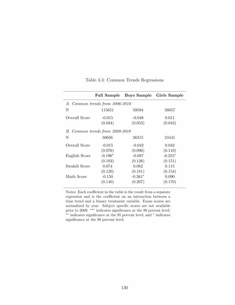
Table 3.3: Common Trends Regressions

Full Sample Boys Sample Girls Sample

A. Common trends from 2006-2010

N 115651 59594 56057

Overall Score -0.015 -0.048 0.011(0.034) (0.053) (0.043)

B. Common trends from 2009-2010

N 50656 26215 24441

Overall Score -0.015 -0.042 0.042(0.076) (0.096) (0.110)

English Score -0.196∗ -0.087 -0.255∗

(0.103) (0.126) (0.151)Swahili Score 0.074 0.082 0.115

(0.120) (0.181) (0.154)Math Score -0.150 -0.361∗ 0.090

(0.140) (0.207) (0.170)

Notes: Each coefficient in the table is the result from a separateregression and is the coefficient on an interaction between atime trend and a binary treatment variable. Exam scores arenormalized by year. Subject specific scores are not availableprior to 2009. ∗∗∗ indicates significance at the 99 percent level;∗∗ indicates significance at the 95 percent level; and ∗ indicatessignificance at the 90 percent level.

130

Table 3.4: Impact of Treatment on School Cohort Size

All Schools Boys’ Schools Girls’ Schools(1) (2) (3)

Upgraded Schools 5.720 6.646 5.048(9.072) (13.156) (12.505)

Constant 265.684∗∗∗ 265.342∗∗∗ 174.157∗∗∗

(3.395) (5.888) (4.671)Observations 763 375 388R2 0.834 0.849 0.814

Note: Dependent variable is school cohort size and the regression isrun at the school-year level. Five school-year pairs are excluded be-cause the exam results were nullified. All regressions include year andschool fixed effects. Standard errors are clustered at the school level.Upgraded School is a binary variable equal to one once the school hasreceived its national school designation. ∗∗∗ indicates significance atthe 99 percent level; ∗∗ indicates significance at the 95 percent level;and ∗ indicates significance at the 90 percent level.

131

Table 3.5: Estimated Treatment Coefficients

Full Boys Girls(1) (2) (3)

N 134966 69398 65568

Examination Outcomes

Overall Score 0.055 0.359∗∗ -0.208(0.122) (0.174) (0.160)

Higher Ed. Funding Cutoff 0.016 0.085∗∗ -0.044(0.029) (0.041) (0.038)

Core Subject Scores

English Score 0.192∗ 0.397∗∗ -0.021(0.099) (0.155) (0.116)

Swahili Score 0.067 0.560∗∗ -0.368∗

(0.153) (0.212) (0.194)Math Score -0.016 0.314 -0.284

(0.157) (0.212) (0.202)

Note: Each coefficient in the table is a result from a sepa-rate regression. All regressions include school and year fixedeffects. Standard errors are clustered at the school level.Treatment is a binary variable equal to one once the schoolreceived its national school designation. ∗∗∗ indicates sig-nificance at the 99 percent level; ∗∗ indicates significance atthe 95 percent level; and ∗ indicates significance at the 90percent level.

132

Table 3.6: Upgrade Treatment Effect by Percentile

Boys GirlsPercentile Overall English Swahili Math Overall English Swahili Math

(1) (2) (3) (4) (5) (6) (7) (8)

0.10 0.371 0.677∗∗∗ 0.780∗∗ 0.651∗∗ -0.064 -0.013 -0.369 -0.1690.240 0.209 0.332 0.296 0.187 0.223 0.280 0.233

0.20 0.539∗∗ 0.442∗∗ 0.775∗∗ 0.599∗ -0.050 -0.072 -0.208 -0.0930.268 0.186 0.303 0.329 0.182 0.140 0.304 0.281

0.25 0.417∗ 0.564∗∗ 0.861∗∗∗ 0.841∗∗∗ -0.041 -0.130 -0.283 -0.2050.243 0.220 0.291 0.262 0.188 0.215 0.230 0.231

0.30 0.474∗∗ 0.221 0.865∗∗∗ 0.273 -0.069 -0.125 -0.228 -0.3680.237 0.263 0.330 0.326 0.256 0.150 0.239 0.335

0.40 0.481∗∗ 0.340∗ 0.647∗∗ 0.447 -0.050 -0.032 -0.424 -0.3340.230 0.205 0.276 0.304 0.170 0.171 0.260 0.351

0.50 0.347 0.488∗∗ 0.549∗ 0.411 -0.088 -0.049 -0.252 -0.3340.217 0.207 0.285 0.299 0.196 0.102 0.202 0.332

0.60 0.333 0.211 0.526∗ 0.390∗ -0.285 0.000 -0.103 -0.2450.220 0.203 0.306 0.221 0.237 0.164 0.235 0.289

0.70 0.202 0.177 0.347 0.070 -0.049 -0.141 -0.087 -0.2370.189 0.161 0.270 0.127 0.156 0.177 0.192 0.284

0.75 0.254 0.363∗ 0.227 0.042 0.000 -0.050 -0.146 -0.2840.196 0.190 0.221 0.127 0.166 0.107 0.193 0.256

0.80 0.210 0.516∗∗ 0.154 0.081 -0.017 0.043 -0.023 -0.2250.221 0.218 0.257 0.230 0.197 0.094 0.171 0.231

0.90 0.070 0.263 0.045 0.223 0.041 0.019 -0.201 -0.0850.149 0.173 0.208 0.195 0.101 0.152 0.152 0.156

0.95 0.112 0.558∗∗ 0.000 0.000 -0.017 0.075 -0.217 -0.3460.221 0.231 0.152 0.173 0.181 0.111 0.153 0.291

Note: Standard errors clustered at the school level. Estimates are from a changes-in-changesmodel. ∗∗∗ indicates significance at the 99 percent level; ∗∗ indicates significance at the 95percent level; and ∗ indicates significance at the 90 percent level.

133

Table 3.7: Estimated Impact on Standard Deviation

Overall Male Female(1) (2) (3)

N 755 358 397

Examination Outcomes

Overall Score -0.082∗ -0.123∗ -0.042(0.042) (0.067) (0.043)

Core Subjects

English Score -0.029 -0.079 0.013(0.033) (0.048) (0.044)

Swahili Score -0.128∗∗ -0.221∗∗ -0.050(0.054) (0.088) (0.062)

Math Score -0.105∗ -0.110 -0.092(0.062) (0.097) (0.072)

Note: Dependent variable is the standard deviation ofscores in each school in each year. The regression is runat the school-year level where five school-year pairs are ex-cluded because the exam results were nullified. Each coef-ficient in the table is a result from a separate regression.All regressions include school and year fixed effects. Stan-dard errors are clustered at the school level. Treatment is abinary variable equal to one once the school received its na-tional school designation. ∗∗∗ indicates significance at the99 percent level; ∗∗ indicates significance at the 95 percentlevel; and ∗ indicates significance at the 90 percent level.

134

Table 3.8: Estimated Treatment Coefficients by Relative Grant Size

Overall Male Female

High dollar per student 0.024 0.352 -0.284(0.163) (0.261) (0.187)

Low dollar per student 0.077 0.364∗ -0.152(0.153) (0.208) (0.22)

Constant 9.674∗∗∗ 9.891∗∗∗ 7.868∗∗∗

(0.314) (0.259) (0.256)Observations 134966 69398 65568R2 0.28 0.257 0.286F-test: high=low (p-value) 0.791 0.968 0.621

Note: All regressions include cohort size as an additional in-dependent variable as well as year and school fixed effects.Standard errors are clustered at the school level. High (low)dollar per student is a binary variable equal to one for schoolswith a student body less (more) than the median student bodyonce the school received its national school designation. Thesample includes the set of students at schools that were up-graded as well as students at schools that were eligible but notupgraded. ∗∗∗ indicates significance at the 99 percent level; ∗∗

indicates significance at the 95 percent level; and ∗ indicatessignificance at the 90 percent level.

135

Table 3.9: Impact of Treatment on Subject Selection

Overall Male Female(1) (2) (3)

A: Linear Probability ModelGov’t/History Score -0.020 -0.070∗ 0.023

(0.024) (0.037) (0.032)Geography Score 0.044∗ 0.047 0.040

(0.024) (0.043) (0.025)Biology 0.013 0.016 0.010∗

(0.009) (0.018) (0.006)Physics 0.009 0.015 0.006

(0.022) (0.037) (0.026)Chemistry 0.002 0.003 0.000

(0.002) (0.005) (0.001)B: OLSNumber of Subjects 0.061∗∗ 0.072 0.048

(0.028) (0.047) (0.033)

Note: All regressions include year and school fixedeffects as well as cohort size. Standard errors areclustered at the school level. Treatment is a binaryvariable equal to one once the school received its na-tional school designation. ∗∗∗ indicates significanceat the 99 percent level; ∗∗ indicates significance atthe 95 percent level; and ∗ indicates significance atthe 90 percent level.

136

Table 3.10: Grant Spending Correlates of Treatment Effects

Overall Male Female(1) (2) (3)

Dormitories 0.166 0.476 0.111(0.22) (0.342) (0.307)

Classrooms -0.387∗ -0.404 -0.318(0.226) (0.78) (0.296)

Science/language labs 0.436 0.484 0.432(0.281) (0.683) (0.361)

Library 0.241 -0.05 0.191(0.235) (0.688) (0.303)

Toilet facilities 0.345 0.216 0.603∗∗

(0.278) (0.845) (0.282)Administration/staff buildings -0.221 0.568 -0.596

(0.244) (0.482) (0.426)Dining hall 0.175 0.979 0.211

(0.269) (0.734) (0.408)Security 0.351 1.041 -0.126

(0.402) (0.668) (0.314)Student furniture 0.707∗∗ 0.768 0.929∗

(0.289) (0.527) (0.553)Constant -0.237 -0.524∗ -0.327

(0.219) (0.302) (0.309)Observations 49 22 27R2 0.342 0.411 0.459

Note: All spending is categorized and represented by a dummyvariable equal to one if the school spent funds on the category. ∗∗∗

indicates significance at the 99 percent level; ∗∗ indicates signifi-cance at the 95 percent level; and ∗ indicates significance at the90 percent level.

137

Table 3.11: Impact of Treatment on Test Scores of Incoming Students

Incoming Student KCPE ScoresOverall Male Female

(1) (2) (3)

Upgraded Schools -9.107∗∗∗ -7.696∗∗∗ -10.226∗∗∗

(1.787) (2.637) (2.431)Constant 353.244∗∗∗ 356.067∗∗∗ 350.614∗∗∗

(0.883) (1.248) (1.242)Observations 140585 72680 67905R2 0.279 0.29 0.262

Note: All regressions include year and school fixed effects.Standard errors are clustered at the school level. UpgradedSchool is a binary variable equal to one once the schoolhas received its national school designation. ∗∗∗ indicatessignificance at the 99 percent level; ∗∗ indicates significanceat the 95 percent level; and ∗ indicates significance at the90 percent level.

138

Appendix

3.A Additional Tables and Figures

Table 3.A.1: Pooled Regressions

Mean KCSE Grade English Swahili Math(1) (2) (3) (4)

Upgraded Male Schools 0.35∗∗ 0.421∗∗∗ 0.559∗∗∗ 0.302(0.17) (0.158) (0.209) (0.209)

Upgraded Female Schools -0.211 -0.013 -0.369∗ -0.288(0.162) (0.116) (0.194) (0.205)

Constant 8.251∗∗∗ 9.265∗∗∗ 8.363∗∗∗ 7.105∗∗∗

(0.303) (0.159) (0.317) (0.549)Observations 134966 134866 134898 134966R2 0.282 0.306 0.271 0.201p-value (male = female): 0.017 0.028 0.001 0.042

Note: All regressions include year and school fixed effects. Standard errors are clusteredat the school level. Upgraded Male School and Upgraded Female School are binaryvariables equal to one once the school has received its national school designation.

Table 3.A.2: Estimated Treatment Coefficients by Relative Grant Size

English Swahili MathOverall Male Female Overall Male Female Overall Male Female

High dollar per student 0.191 0.458∗ -0.013 -0.079 0.371 -0.47∗∗ -0.1 0.34 -0.515∗∗

(0.144) (0.24) (0.147) (0.202) (0.317) (0.236) (0.193) (0.276) (0.261)Low dollar per student 0.193∗ 0.354∗∗ -0.027 0.17 0.695∗∗∗ -0.294 0.043 0.296 -0.115

(0.117) (0.167) (0.157) (0.188) (0.249) (0.261) (0.195) (0.275) (0.253)Constant 10.126∗∗∗ 9.602∗∗∗ 9.351∗∗∗ 9.569∗∗∗ 9.652∗∗∗ 7.919∗∗∗ 9.178∗∗∗ 9.658∗∗∗ 6.052∗∗∗

(0.168) (0.283) (0.093) (0.354) (0.316) (0.314) (0.626) (0.321) (0.506)Observations 134866 69350 65516 134898 69361 65537 134966 69397 65569

R2 0.304 0.293 0.314 0.267 0.274 0.268 0.2 0.146 0.219F-test: high=low (p-value) 0.989 0.692 0.946 0.310 0.389 0.588 0.539 0.903 0.226

Note: All regressions include cohort size as an additional independent variable as well as year and school fixed effects. Standard errors areclustered at the school level. High (low) dollar per student is a binary variable equal to one for schools with a student body less (more) thanthe median student body once the school received its national school designation. The sample includes the set of students at schools that wereupgraded as well as students at schools that were eligible but not upgraded. ∗∗∗ indicates significance at the 99 percent level; ∗∗ indicatessignificance at the 95 percent level; and ∗ indicates significance at the 90 percent level.

139

Table 3.A.3: Estimated Treatment Coefficients - Closest School

Full Boys Girls(1) (2) (3)

N 87687 41657 46030

Overall Score 0.012 0.439∗∗ -0.311∗

(0.140) (0.217) (0.168)Higher Ed. Funding Cutoff 0.003 0.098∗ -0.069∗

(0.033) (0.052) (0.040)Core SubjectsEnglish Score 0.162 0.368∗ -0.034

(0.113) (0.198) (0.124)Swahili Score 0.055 0.774∗∗∗ -0.482∗∗

(0.178) (0.246) (0.200)Math Score -0.056 0.389 -0.341

(0.185) (0.266) (0.226)

Note: Each coefficient in the table is a result from a sepa-rate regression. All regressions include school and year fixedeffects. Standard errors are clustered at the school level.Treatment is a binary variable equal to one once the schoolreceived its national school designation.

Table 3.A.4: Complete Counties Estimated Treatment Coefficients

Full Boys Girls(1) (2) (3)

N 105021 58651 46370

Overall Score 0.105 0.303 -0.087(0.142) (0.191) (0.206)

Higher Ed. Funding Cutoff 0.029 0.080∗ -0.023(0.033) (0.046) (0.047)

Core SubjectsEnglish Score 0.177 0.392∗∗ -0.030

(0.121) (0.174) (0.156)Swahili Score 0.071 0.532∗∗ -0.374

(0.171) (0.216) (0.238)Math Score 0.011 0.137 -0.056

(0.164) (0.222) (0.224)

Note: Each coefficient in the table is a result from a sepa-rate regression. All regressions include school and year fixedeffects. Standard errors are clustered at the school level.Treatment is a binary variable equal to one once the schoolreceived its national school designation.

140

Table 3.A.5: Estimated Treatment Coefficients: School Level

A: Overall B: Male C: Female25th 50th 75th 25th 50th 75th 25th 50th 75th(1) (2) (3) (4) (5) (6) (7) (8) (9)

Overall Score 0.183 0.054 -0.015 0.421 0.242 0.336∗ -0.020 -0.106 -0.298(0.170) (0.150) (0.135) (0.253) (0.213) (0.191) (0.224) (0.210) (0.179)

Core SubjectsEnglish Score 0.170 0.126 0.106 0.382 0.403∗∗ 0.244 -0.008 -0.108 -0.008

(0.148) (0.130) (0.112) (0.238) (0.197) (0.177) (0.187) (0.160) (0.143)Swahili Score 0.207 0.008 -0.070 0.739∗∗ 0.521∗∗ 0.330 -0.218 -0.397 -0.386∗

(0.207) (0.188) (0.157) (0.330) (0.258) (0.208) (0.239) (0.253) (0.215)Math Score 0.256 -0.036 -0.182 0.558∗ 0.268 0.035 0.000 -0.283 -0.341

(0.221) (0.246) (0.226) (0.315) (0.336) (0.300) (0.312) (0.347) (0.307)

Note: Each coefficient in the table is a result from a separate regression. All regressions includeschool and year fixed effects. Standard errors are clustered at the school level. Treatment is abinary variable equal to one once the school received its national school designation.

141

Chapter 4: A Firm of One’s Own: Experimental Evidence on Credit

Constraints and Occupational Choice

Joint with Maddalena Honorati, Pamela Jakiela, and Owen Ozier

4.1 Introduction

Youth underemployment is a major challenge facing developing nations, particularly

in Africa Filmer and Fox (2014). Young people are more likely to be unemployed

than older adults (Kluve et al. 2016). In low-income countries, unemployment figures

also typically underestimate the proportion of youths who cannot find productive

jobs Fares, Montenegro, and Orazem (2006). After leaving school, it often takes

young adults in low-income countries several years to find gainful employment or

launch a viable household enterprise; during that transition from school to the labor

market, many youth are forced to rely on family members for support between stints

of work in irregular, informal positions World Bank (2006). Demographics make the

problem of youth underemployment particularly acute in Sub-Saharan Africa, where

more than half the population is under 25. Filmer and Fox (2014) estimate that,

over the next ten years, only a quarter of the African youth entering the labor

market will be able to find paid employment.

142

Since formal sector jobs are scarce in low-income settings, many policymakers

have advocated entrepreneurship promotion programs intended to help unemployed

youth generate an income through self-employment United Nations Development

Programme (2013); Franz (2014). The simplest entrepreneurship promotion pro-

grams are credit market interventions such as loans or one-off grants of money or

physical capital. Economic theory suggests that such interventions can help po-

tential entrepreneurs who have limited opportunities to save or borrow to start or

expand profitable businesses, and one recent study suggests that cash grants can

help unemployed youth launch businesses and increase their incomes Blattman, Fi-

ala, and Martinez (2014). However, a growing body of evidence on the the returns

to capital among entrepreneurs suggests that credit constraints may not be the main

obstacle limiting the growth of female-owned microenterprises: evaluations to date

have found that, in most cases, cash grants to female entrepreneurs do not lead to

sustained increases in business profits or income (De Mel, McKenzie, and Woodruff

2008, De Mel, McKenzie, and Woodruff 2009, Fafchamps, McKenzie, Quinn, and

Woodruff 2011, Fiala 2014, Karlan, Knight, and Udry 2015, Blattman et al. 2016).1

Taken together, these results suggest that many women who operate small busi-

nesses are “subsistence entrepreneurs” Schoar (2010) who lack either the ability or

the inclination to expand their enterprises; if this is true, access to capital (alone)

is unlikely to have major impacts.

1Recent evaluations also suggest that microfinance loans, the canonical credit market interven-tion intended to help subsistence entrepreneurs, do not lead to significant increases in income or,in most cases, microenterprise profits (Angelucci, Karlan, and Zinman 2015, Attanasio et al. 2015,Augsburg, De Haas, Harmgart, and Meghir 2015, Banerjee, Duflo, Glennerster, and Kinnan 2015,Crepon, Devoto, Duflo, and Parient 2015, Tarozzi, Desai, and Johnson 2015).

143

In fact, though capital drop interventions are becoming increasingly common,

many youth entrepreneurship programs offer more than just capital, for example,

start-up capital together with skills training or ongoing business mentoring (Kluve

et al. 2016). The theory of change underlying such multifaceted approaches is that

young entrepreneurs face many different obstacles and constraints that need to be

addressed simultaneously in order to launch a successful microenterprise. For exam-

ple, they may lack the vocational skills needed to attract customers in competitive

markets, they may not have access to the start-up capital needed to launch a busi-

ness, and they may not know how to manage an enterprise successfully after it is

launched. Several recent studies suggest that multifaceted programs that combine

vocational education and start-up capital with life skills training may improve the

income prospects of young women, in particular (cf. Adoho et al. 2014, Bandiera et

al. 2014).2

We evaluate one such multifaceted entrepreneurship intervention: a “microfran-

chising” program that offered young women in some of Nairobi’s poorest neighbor-

hoods a combination of vocational and life skills training together with start-up

capital and ongoing business mentoring. Like many entrepreneurship programs, the

microfranchising model is premised on the idea that many youth do not have the

skills and experience necessary to be competitive in the labor market, and also lack

the financial and human capital needed to start a successful enterprise (for example,

2There is also evidence that multifaceted programs which combine skills training and assettransfers can improve the income-generating capacity of vulnerable adults (not just youth andnot just women). Banerjee et al. (2015) demonstrate that one such multipronged approach, theultrapoor Graduation Program implemented by the NGO BRAC, led to large increases in income,food security, and rates of savings. A recent meta-analysis also highlights the relative effectivenessof multifaceted entrepreneurship promotion programs Cho and Honorati (2014).

144

the ability to conduct market research and develop a business plan). The franchise

treatment that we study attempts to overcome these barriers by providing moti-

vated young women with an established business model and the specific capital and

supply chain linkages needed to operate the business. The franchise treatment was

designed and implemented by the International Rescue Committee (the IRC) in

cooperation with local community-based organizations.3

We estimate the impacts of this franchise treatment on applicants via a ran-

domized trial. We not only measure the program’s impacts in relation to a control

group, but also compare those impacts to the effects of a simpler cash grant inter-

vention that relaxed the credit constraint without providing any additional training

or support. We interpret our findings through the lens of a simple model of invest-

ment decisions when individuals differ in terms of their labor productivity. High

productivity types who have limited opportunities to save or borrow may be unable

to launch profitable businesses because they cannot accumulate the required capital.

In such cases, credit market imperfections may create a poverty trap, and one-off

transfers of money or capital, such as those in our study, can lead to permanent in-

creases in income. One of the key insights from the model is that credit constraints

are only an obstacle to productive entrepreneurship for a subset of individual types;

less productive types are unable to sustain a business in any steady state. Nonethe-

less, savings constraints can also affect the investment decisions and occupational

choices of lower productivity types who receive one-off infusions of funding or cap-

3See International Rescue Committee (2016b) for an overview of the IRC’s economic develop-ment programs.

145

ital; though these individuals cannot sustain businesses, they may invest in capital

and launch unproductive firms because enterprise capital is a technology for saving,

albeit at a negative interest rate. Thus, short-term impacts of one-off transfers on

entrepreneurship should not be taken as evidence that a program relieved a credit

constraint or addressed a poverty trap; the critical issue is whether impacts on

income persist over the longer-term.

We find that both the franchise treatment and the grant treatment led to

substantial increases in income in the year after the interventions. Point estimates

suggest impacts that are both economically and statistically significant: the fran-

chise treatment increased weekly income by 30 percent, up 1.6 US dollars from a

mean of 5.5 dollars in the control group (p-value 0.035); the grant treatment in-

creased weekly income by 3.2 dollars (p-value 0.008) or 56 percent. As expected,

these impacts appear to be driven by a shift from paid work to self-employment;

women assigned to either the franchise or the grant treatment are approximately 10

percentage points more likely to be self-employed than those in the control group.

Women assigned to the grant treatment also increased their labor supply (hours

worked) substantially.

Though both interventions increased income in the relatively short-run, data

from endline surveys conducted between 14 and 22 months after treatment indicate

that the observed impacts on income disappeared in the second year after the pro-

gram(s). At endline, women assigned to either the franchise treatment or the grant

treatment are more likely to be self-employed than women in the control group,

but the treatments are not associated with increases in income or labor supply.

146

In addition, we find no impacts of treatment on food security, expenditures, liv-

ing conditions, or empowerment at endline. Seen through the lens of our model,

these findings are consistent with the existence of savings constraints; large impacts

on income and occupational choice that disappear relatively quickly make sense if

enterprise capital is one of the few viable savings technologies available to young

women in a poor urban area. However, our findings do not suggest that credit con-

straints had been preventing productive entrepreneurs from launching profitable,

sustainable businesses.

This paper makes several contributions. First, we measure the impact of

an active labor market program on young women in an urban area in a developing

country. Here, we contribute to an active literature on active labor market programs

and youth unemployment.4 Our work is most closely related to Bandiera et al. (2014)

and Adoho et al. (2014), who also evaluate multifaceted labor market interventions

for young women in Sub-Saharan Africa.

We compare the impacts of a multifaceted entrepreneurship promotion inter-

vention to those of a one-off cash grant; this provides a natural cost-effectiveness

benchmark without any of the contextual caveats that would accompany a more

traditional cost-benefit analysis. Though evaluations of cash grants are becoming

more common Haushofer and Shapiro (2016)cf., the use of cash as a benchmark

within program evaluation is still relatively uncommon. Our results, like those of

Karlan, Knight, and Udry (2015), suggest that unrestricted cash grant treatments

can provide an extremely useful alternative to the traditional control group (that

4See Kluve et al. (2016) for a recent survey.

147

receives no treatment).5

We measure both interventions’ impacts over time, expanding our understand-

ing of the dynamics of the estimated impacts. In addition, we present a model,

building on previous work (cf. Fafchamps et al. 2011, Blattman, Fiala, and Mar-

tinez 2014, Blattman et al. 2016), that yields a straightforward interpretation of the

estimated program impacts in relation to credit and savings constraints. Our model

suggests that the patterns of impacts that we observe are more likely to be explained

by savings constraints than by credit-constraint-based poverty traps. This conclu-

sion resonates with other recent evidence that the poor, particularly poor women,

have a very limited menu of savings technologies Dupas and Robinson (2013a,b).

Finally, we capitalize on the program evaluation setting to test whether par-

ticipants hold accurate beliefs about program impacts; in so doing, we provide a

framework for comparing methods of belief elicitation. Our work builds directly on

the contributions of Smith, Whalley, and Wilcox (2011) and Smith, Whalley, and

Wilcox (2012). Like McKenzie (2016a), we find the program participants do a poor

job of estimating their own counterfactual (probabilistic) outcomes. However, we

extend the existing set of best practices by demonstrating that participants are quite

good at estimating average treatment impacts on the population once behavioral

biases are taken into account.

The remainder of this paper is organized as follows. Section 4.2 outlines our

theoretical model. Section 4.3 describes our research design and the specific fran-

5Supporting this argument, Ozler (2016) has also remarked that “the interesting comparison isnot against ‘no support’ ... it’s against cost-equivalent alternative efforts.”

148

chise and grant treatments that we evaluate. Section 4.4 presents our main results.

Section 4.5 characterizes participants’ beliefs about the impacts of the program.

Section 4.6 concludes.

4.2 Conceptual Framework

To understand the impacts of capital infusions and other credit market interventions,

we require a framework for interpreting individual responses to these interventions.

We propose a simple model of labor supply decisions in the presence of credit mar-

ket imperfections, when individuals may face credit constraints and may also be

unable to save. We show that high productivity individuals who are are unable to

save or borrow may find themselves in a poverty trap in which they never launch a

business, even though their enterprises would be profitable once launched. In this

constrained environment, a large capital transfer enables these individuals to start

lasting businesses. In contrast, low productivity individuals are unable to sustain an

enterprise in any steady state; because these individuals cannot sustain a profitable

enterprise, the fact that they are not accessing loans does not indicate a market

failure. However, in a savings-constrained environment, low productivity types may

open businesses after receiving a large capital transfer, using enterprise capital as

a savings vehicle when other savings technologies are unavailable. These businesses

are temporary (because low productivity individuals cannot sustain businesses in

the steady state), and are eventually closed after the initial capital investment de-

preciates.

149

We begin by considering a simple model in which production in each period de-

pends on labor and capital. Labor is allocated between two activities: own-enterprise

production, characterized by production function f e(K,Le), and wage labor, char-

acterized by production function fw(Lw). Individuals allocate their labor across

sectors subject to the constraint: Le + Lw ≤ 1. Importantly, we follow other re-

cent work Blattman, Fiala, and Martinez (2014)cf. in assuming that own-enterprise

production requires a capital investment that exceeds some minimum scale; thus,

potential entrepreneurs who are credit-constrained and unable to save cannot launch

arbitrarily small businesses that could then grow over time. This minimum scale

requirement creates the potential for a poverty trap. Both production functions are

characterized by diminishing returns with respect to individual inputs; we assume

that the enterprise production function, f e(K,Le), is homogeneous of degree one

above the minimum scale.

We make the following specific assumptions about the own-enterprise produc-

150

tion function, f e(K,Le):

f e(K,Le) ≡ 0 ∀K ≤ Kmin (minimum scale) (A1)

δ2

δK2f e(K,Le) < 0 <

δ

δKf e(K,Le) ∀K ≥ Kmin (diminishing returns) (A2)

δ2

δL2f e(K,Le) < 0 <

δ

δLf e(K,Le) ∀K ≥ Kmin (diminishing returns) (A3)

δ2

δLδKf e(K,Le) > 0 ∀K ≥ Kmin (inputs are complements) (A4)

limL→0

δ

δLf e(K,Le) = +∞ ∀K ≥ Kmin (Inada) (A5)

limK→Kmin

δ

δKf e(K,Le) = +∞ (Inada) (A6)

limK→+∞

δ

δKf e(K,Le) = 0 (Inada) (A7)

With respect to the wage labor production function, fw(Lw), we assume that stan-

dard Inada conditions hold.6 In other words, we assume

fw(0) = 0 (A8)

δ

δLfw(Lw) > 0 (A9)

δ2

δL2fw(Lw) < 0 (A10)

limL→0

δ

δLfw(Lw) = +∞ (A11)

In each period t, the agent has capital Kt and one unit of labor to divide

between activities such that Le + Lw ≤ 1. The agent produces using whatever

allocation of labor she chooses, yielding F(Kt, Lw) = fw(Lw) + f e(Kt, 1−Lw). The

6In the Online Appendix, we show that the same argument can be extended for a constant wagerate.

151

maximum level of production in a given period results from the optimal allocation

of labor between the two possible sectors:

F∗(Kt) = max

0≤Lw≤1F(Kt, L

w) (1)

Proposition 1 characterizes the properties of F∗(Kt). Because of the minimum level

of capital required to produce output in the own-enterprise sector, the function

F∗(Kt) has a characteristic shape, which is shown in Figure 4.1. The characteristic

shape of F∗(Kt) drives the predictions of our model.

Proposition 1. F∗(Kt), the total production function conditional on the optimal

allocation of labor across the wage labor and own enterprise sectors, has the following

properties:

1. For all Kt ≤ Kmin, F∗(Kt) = fw(1); hence, the first and second derivatives of

F∗(Kt) are equal to 0 for all Kt ≤ Kmin.

2. For all Kt > Kmin, F∗(Kt) has a positive first derivative.

3. For all Kt > Kmin, F∗(Kt) has a negative second derivative.

Proof: see Online Appendix.

Intuitively, F∗(Kt) is flat for Kt ≤ Kmin. Levels of capital below the minimum

level required to operate a business, Kmin, do not contribute to total output and

simply depreciate; hence, for individuals who have access to a range of savings

technologies, there is no reason to invest K < Kmin in the own-enterprise sector. At

152

levels of capital exceeding Kmin, F∗(Kt) inherits the properties of the production

function in the own enterprise sector; it is always optimal to allocate one’s capital

and some of one’s labor to the own enterprise sector and operate a business at some

scale because the marginal product of capital approaches infinity as Kt → K+min.

Figure 4.1: Shape of the Production Function, F∗(Kt)

F* (K

)

Kmin K

After production, the previous period’s capital depreciates, so that it becomes

Kt(1− δ). The agent also chooses a level of consumption, ct, in period t. Capital in

the next period is thus given by:

Kt+1 = F∗(Kt)− ct +Kt(1− δ) (2)

A steady state is characterized by a level of capital, Kss, and a level of consumption,

css, that satisfy the following condition:

Kss = F∗(Kss)− css +Kss(1− δ) (3)

153

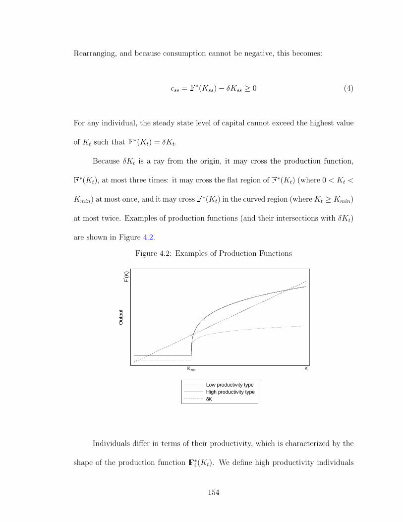
Rearranging, and because consumption cannot be negative, this becomes:

css = F∗(Kss)− δKss ≥ 0 (4)

For any individual, the steady state level of capital cannot exceed the highest value

of Kt such that F∗(Kt) = δKt.

Because δKt is a ray from the origin, it may cross the production function,

F∗(Kt), at most three times: it may cross the flat region of F∗(Kt) (where 0 < Kt <

Kmin) at most once, and it may cross F∗(Kt) in the curved region (where Kt ≥ Kmin)

at most twice. Examples of production functions (and their intersections with δKt)

are shown in Figure 4.2.

Figure 4.2: Examples of Production Functions

F* (K

)O

utpu

t

Kmin K

Low productivity typeHigh productivity typedK

Individuals differ in terms of their productivity, which is characterized by the

shape of the production function F∗i (Kt). We define high productivity individuals

154

as those that can sustain a self-employment activity in any steady state.

Definition 1. Individual i is a high productivity type if she is able to sustain

a business in any steady state, i.e. if there exists Kt such that F∗i (Kt) > δKt and

Kt > Kmin. A latent entrepreneur is a high productivity type with at least one

steady state that satisfies the condition F∗i (Kss) > fw(1).

Being a high productivity type is a necessary condition for successful entrepreneur-

ship: individuals who are not high productivity types are unable to sustain an

enterprise in any steady state.7 If high productivity individuals are sufficiently pa-

tient and they are able to save at a sufficiently non-negative interest rate, then those

who prefer operating their own businesses to working (exclusively) in the wage sec-

tor will do so — they will save up the funds needed to make the initial profitable

capital investment of Kss > Kmin and launch their own businesses. Alternatively,

high productivity types who face sufficiently low borrowing costs can borrow the

funds needed to launch their businesses. However, when opportunities for saving

and borrowing are limited, high productivity types who wish to launch their own

enterprises may not be able to do so — creating a poverty trap.

Savings constraints also shape individual responses to cash grant interventions.

When individuals are able to save, investing a transfer in enterprise capital (or in

any other illiquid asset) is only attractive if the return on the investment exceeds the

return on saving. However, when saving is impossible, investing in business capital

7Whether a high productivity type prefers entrepreneurship to wage labor will depend on theirpreferences. For many preferences specifications, opening a business is attractive when fw(1) ≤maxKss

F∗i (Kss). However, the predictions of the model do not depend on specific assumptions

about the utility function.

155

and launching a small-scale enterprise may be one of the only ways to smooth

positive income shocks across periods. We assume that capital stock is carried

forward (minus depreciation) as long as an individual allocates at least ε > 0 units

of labor to the own-enterprise sector; we allow ε to be arbitrarily small.

The first key prediction of the model is that a one-off transfer to a latent

entrepreneur can lead to a permanent increase in income. Individuals who have

access to a zero-interest savings technology will invest enough in their businesses to

transition to their preferred steady-state level of capital. In this case, income will

immediately rise from fw(1) to F∗i (Kss), and will remain there indefinitely. Con-

sumption may also be directly impacted if individuals save and consume transferred

funds without investing them in microenterprises (though these direct impacts on

consumption should not be associated with changes in occupational choice).

When latent entrepreneurs are unable to save, they will invest any transfers

received in their businesses.8 If the amount of the transfer exceeds the lowest possible

steady state capital stock, income rises from fw(1) to F∗i (Ktransfer) and then settles

toward the individual’s optimal steady state value of F∗i (Kss) > fw(1) over time.

Thus, the short-term impacts of capital infusions on income may be larger than the

long-term impacts, but the long-term impacts on income are positive.

In contrast, for lower productivity individuals — those for whom δKt only

crosses F∗i (Kt) once, in the flat region where Kt < Kmin — a capital transfer does

not have permanent impacts. These individuals cannot operate their own enterprises

8Transfer recipients may choose to consume of the transferred funds upon receipt; this does notimpact the predictions of our model. Ktransfer should then be interpreted as the amount that isnot immediately consumed.

156

in a steady state. Even when they are able to save at a non-negative interest rate,

saving money to invest in the own-enterprise sector is not an attractive proposition.

Even when they are able to borrow at low interest rates, borrowing the funds to

launch a business is unattractive (if one is required to eventually repay the loan).

However, when individuals who cannot sustain a profitable enterprise receive

a large transfer, they may choose to invest the money in a business if they are

savings constrained. Intuitively, enterprise capital is a means of saving at a negative

interest rate ofF

∗i (Kt)

Kt− δ. For large infusions of capital, launching a business,

consuming the business income, and allowing the business to shrink over time as the

capital depreciates will sometimes be preferable to immediately consuming all of the

capital received. Operating that business, even if depreciation exceeds production,

is still better than letting the capital depreciate without production. Thus, savings-

constrained individuals who are not productive enough to sustain enterprises may

operate temporary businesses if given a cash infusion. The key distinction between

latent entrepreneurs and lower productivity types is that one-off infusions of capital

can permanently increase the incomes of latent entrepreneurs, while such infusions

of capital have impacts on lower productivity types that disappear over time.

4.3 Research Design and Procedures

We conducted a randomized evaluation of two labor market interventions targeted

to young women aged 18 to 19 in three of Nairobi’s poorest neighborhoods, Baba

157

Dogo, Dandora, and Lunga Lunga.9 Applicants to the program were stratified

by neighborhood and application date and then randomly assigned to one of three

treatment arms: a franchise treatment, a cash grant treatment, and a control group.

This design allows us to estimate the impact of the franchise and grant treatments

on those invited to the program, and to compare the impacts of the cash grant

treatment — which relaxes the credit constraint but provides no other training or

support — to a multifaceted program designed to address many of the obstacles to

youth entrepreneurship simultaneously.

4.1 Two Labor Market Interventions

4.1.1 The Franchise Treatment

Credit constraints may prevent potential entrepreneurs from launching profitable

businesses. However, credit constraints may not be the only obstacle to entrepreneurial

success; potential entrepreneurs — particularly young people — may also lack the

market intelligence and business training needed to launch a successful enterprise

Berge, Bjorvatn, and Tungodden (2014). We evaluate a multifaceted “microfranchis-

ing” program that provided eligible applicants with an established business model

and the specific training, capital, and business linkages (for example, with whole-

sale suppliers) needed to make the business operational. Microfranchisees supply

9Applications were solicited from women between the ages of 16 and 19; in practice, relativelyfew of the applicants (only 14.6 percent) were below 18 years of age when they applied. Onlythose women who had attained the age of legal majority were eligible to receive cash grants, soour analysis focuses on those who were in the two oldest age cohorts (randomization to treatmentwas stratified by age). The cash grant treatment was not announced in advance; women appliedfor a business training program and were then randomized into one of the three treatment arms.

158

their labor, and are free to expand their microenterprises as they see fit. Thus,

a microfranchise has features in common with both a formal sector job and self-

employment: while microfranchisees do not need to devise business models, they

work with very little managerial supervision and considerable latitude for creativ-

ity — managing their own time and entrepreneurial effort. Thus, microfranchising

strikes a middle ground between entrepreneurship and wage employment.

We evaluate a microfranchising intervention geared toward young women in

Nairobi’s poorest neighborhoods. The program helped young women launch branded

franchise businesses, either salons or mobile food carts. The intervention combined

a number of distinct elements: business skills training, franchise-specific vocational

training, start-up capital (in the form of the specific physical capital required to

start the franchise), and ongoing business mentoring. Several of the intervention’s

components are common to many entrepreneurship promotion and job skills pro-

grams; what distinguishes microfranchise programs from other interventions is the

focus on a small number of specific franchise business models that are tailored to

the skills and constraints of program participants (i.e. poor young women in urban

Nairobi) and to local market conditions. In this case, the implementing organization

(the IRC) partnered with two Kenyan businesses looking to expand their presence

in slum neighborhoods — a maker of hair extensions and a poultry producer known

for its fast food restaurants. The franchise partners are both relatively well-known

firms (within Kenya), and their reputations added value to the franchise package

that program participants received.

The first component of the franchise program was a two-week training course.

159

In addition to a standard curriculum of business and life skills training topics, the

training included modules about the two specific franchise business models. At the

end of the course, participants indicated their ranking of the two franchise partners

and were then matched with one of them (almost always their first choice).

After the business skills course, program participants received training from

the franchise business partner with whom they had been matched. Women assigned

to the salon franchise received six weeks of classroom training and then completed

a two-week internship with a local salon. At the end of the internship, participants

organized themselves into small groups and received their business start-up kits

(which included branded aprons, a hair washing sink, a hair dryer, and a variety of

hair cutting and styling products).

For women assigned to the food cart franchise, the franchise-specific training

was a one-day session where franchisees were introduced to the brand, available

products, and appropriate preparation methods. Following the franchise training,

program participants organized themselves into small groups and received business

start-up kits that included a mobile cart, an apron or t-shirt displaying the company

logo, and an initial stock of smoked chicken sausages.

Each franchise business launched through the program was assigned a mentor

who visited the business every few weeks. Mentors helped the young women in

the program get their businesses off the ground — for example, by coordinating

additional training with the franchise partners, helping the businesses set up bank

accounts, or assisting with financial management and record keeping.

160

4.1.2 The Grant Treatment

Applicants assigned to the cash grant treatment were offered an unrestricted transfer

of 20,000 Kenyan shillings (or 239 US dollars at the prevailing exchange rate of 83.8

shillings to the dollar).10 Individuals assigned to the grant arm were contacted by

phone and invited to meet privately with a member of the disbursement team to

discuss the grant. During the meeting, individuals were told that there were no

restrictions on how the grant could be used and that the grant did not need to be

paid back. Disbursements to the grant recipients were timed to coincide with the

launch of the microfranchise businesses.

4.2 Data Collection

Our analysis draws on three main sources of data. First, we administered a brief

baseline survey to all eligible applicants prior to randomization. We also conducted

a midline survey 7 to 10 months after the end of the intervention.11 The midline

surveys were conducted via phone. The midline included detailed questions about

income-generating activities, but did not ask about a broader range of outcomes

(this was not feasible in a short phone survey). We conducted a more comprehensive

endline survey 14–22 months after the end of the intervention.

10Though the US dollar value of the shilling has since declined, the exchange range was fairlyconstant during the grant disbursement period (from November 1, 2013 to January 13, 2014). Thevalue of the grant was selected to make it roughly comparable to the value of the microfranchisingpackage of training and capital; the 20,000 shilling amount is also identical to the grant size inanother study of cash grants for Kenyan youth Hicks, Kremer, Mbiti, and Miguel (2016).

11We also conducted an extremely brief phone survey 2 to 5 months after the intervention, butwe did not ask about income-generating activities at that time. The goal of that survey was tocollect better contact information than had been gathered at baseline.

161

Attrition rates are extremely low in both the midline and the endline surveys:

we successfully surveyed 94.0 percent of the baseline sample at midline and 92.5

percent of the baseline sample at endline. Regressions testing for differential attri-

tion across treatment arms are reported in the Online Appendix. Attrition is not

associated with either treatment.

4.3 Sample Characteristics

Table 4.1 describes the baseline characteristics of the young women in our sample.

As expected, there is little variation in age: 94.6 percent of the young women in the

sample were 18, 19, or 20 years of age at baseline. 11.6 percent of women in our

sample did not have a living parent at the time of the baseline survey. 16.5 percent

were married or cohabitating, and 40.9 percent had given birth. The median number

of years of schooling in the sample is 10; 92.4 percent of baseline respondents finished

primary school, while only 41.1 percent finished secondary school.12 34.5 percent

had done some form of vocational training prior to the program.

Only 14.6 percent of the sample was engaged in an income-generating activity

(IGA) at the time of the baseline survey, but 54.6 percent had been involved in an

IGA at some point in the past. 23.2 percent had been self-employed at some point

in the past. The young women in the sample spent a considerable amount of time

doing unpaid work at home: the median number of hours of unpaid housework (in

12The average level of education among women aged 18-20 in Nairobi is 10.6 years; 28 percentare currently married or living with a partner, and 26 percent have had a child (Kenya DHS 2014).Thus, relative to the general population of comparably-age women in Nairobi, our sample is slightlyless educated, less likely to be married or cohabitating, and more likely to have had a child. Thesedifferences likely reflect the program’s focus on Nairobi’s poorest neighborhoods.

162

the week prior to the baseline) was 21. Only 8.8 percent of women in the sample had

a bank account at baseline, and only a third had any savings in money or jewelry.

Among those with savings, the median amount of savings was (equivalent to) 8.91

US dollars.

Balance checks (i.e. tests of the hypothesis that observable characteristics

are balanced across treatments) are reported in the Online Appendix. Observable

characteristics were relatively balanced prior to the program. Out of 75 hypothesis

tests, we find 3 differences across treatments that are significant at greater than 95

percent statistical confidence.13

4.4 Compliance with Treatment

As is typical in training programs (McKenzie and Woodruff, 2014), not all the

women assigned to the program participated in it, and not all those who started

the business training completed the program. Table 4.2 reports the proportion of

women in the treatment and control groups who completed each stage of the pro-

gram.14 61 percent of those assigned to the franchise treatment attended the initial

two-week business training course at least once; 39 percent of those assigned to the

franchise treatment completed the franchise-specific business training and launched

a microfranchise. Though these modest take-up rates are not out of line with those

13Women assigned to the control group come from slightly larger households, and are somewhatmore likely to have given birth prior to the program. Women assigned to the cash grant treatmenthad, on average, about half a year less schooling than those assigned to the franchise treatmentand the control group. Controls for those variables that are not balanced across treatments areincluded in our main specifications (though results are nearly identical when controls are omitted).

14The table is based on administrative data from the implementing NGO and the franchisepartners, though self-reports line up with administrative records.

163

observed in comparable training programs McKenzie and Woodruff (2014), they

have important ramifications for the interpretation of intent-to-treat estimates of

program impacts (a point we return to below). Unsurprisingly, the take-up rate is

extremely high in the cash grant treatment: 95 percent of those assigned to the

grant treatment accepted and received the grant. We also find very little evidence

of imperfect compliance with the evaluation design on the part of the implement-

ing organization: no women assigned to the control group attended the business

training, and only 1 percent were involved in starting a microfranchise.

4.4 Analysis

Our theoretical model predicts that infusions of funding will increase self-employment

and income over the relatively short-term if individuals are unable to save through

channels other than enterprise capital. For relatively unproductive individuals, these

increases in income are temporary; they disappear as capital depreciates. Thus, im-

pacts on entrepreneurship and income over the short-term do not indicate that cap-

ital infusions relieved a credit constraint or helped potential entrepreneurs to escape

a poverty trap. In the presence of savings constraints, the key distinction between

latent entrepreneurs and less productive individuals is that latent entrepreneurs can

transform one-off infusions of capital into permanent increases in income. A compar-

ison of shorter-term versus longer-term impacts indicates whether capital transfers

are likely to have alleviated a poverty trap.

The cash grant intervention is exactly the type of unrestricted financial trans-

164

fer described by our model. If the cash grant impacts occupational choice and

income in the relatively short-term, analysis of longer-term impacts allows us to

assess the extent to which the capital infusion relieved a poverty trap. Of course,

if low productivity individuals are not savings constrained, there is little reason for

them to knowingly launch an unproductive enterprise. In that case, an infusion of

capital could increase consumption, savings, or assets (though possibly only over

the relatively short-term), but would not impact occupational choice.

We model the impact of an infusion of capital, but our analysis compares two

distinct interventions. An important question is whether an equivalently-valued

intervention that offers enterprise capital in a more restricted form (including some

in the form of human capital) has comparable impacts. Women assigned to the

franchise treatment who did not wish to start a business and were not savings-

constrained had the option of selling the physical capital that they received through

the program, though we would expect the market value of, for example, a mobile

food cart to be well below the cost of providing the entire microfranchise package

of training and mentoring plus capital. Thus, if low productivity individuals who

are not savings constrained participated in the program, we would not expect them

to launch businesses, and the impacts on (e.g.) consumption might be relatively

small. Alternatively, if credit and savings constraints are the main obstacles to

successful entrepreneurship (and business training and mentoring add little value),

we might expect the impacts of the franchise treatment to be smaller than the

impacts of the grant treatment (because much of the program spending paid for

training that, by assumption, would not be the relevant barrier to entrepreneurship

165

for these individuals). On the other hand, the training and mentoring provided

through the franchise program might impact participants’ productivity, increasing

the fraction of high productivity types. If this were the case, we would expect the

impacts of the franchise treatment to be more persistent than those of the grant

treatment — though they might initially be smaller in magnitude, depending on

the initial mix of types in the population and the value of the capital transferred to

franchise program participants.

We test these predictions using data from two rounds of surveys: midline

surveys that were conducted between 7 and 10 months after the interventions and

endline surveys that were conducted 14 to 22 months after the interventions. Both

the midline and endline surveys contain detailed data on involvement in income-

generating activities. The endline survey also includes a range of measures of con-

sumption, expenditure, and well-being — which might be impacted by treatment

if participants saved or consumed the value of the capital they received without

launching a small business.

4.1 Estimation Strategy

In our main analysis, we report intent-to-treat (ITT) estimates of the impacts of

the franchise treatment and the cash grant treatment on women assigned to each

treatment group. Treatment assignment was random within strata, so the impacts

of the interventions on any outcome Yi can be estimated via the OLS regression

166

specification:

Yi = α+β ·Franchisei +γ ·Granti + δstratum +φenumerator + ζmonth + η ·Xi + εi (5)

where Franchisei and Granti are indicators for, respectively, random assignment to

the franchise treatment or the grant treatment, δstratum is a randomization stratum

fixed effect, φenumerator is a survey enumerator fixed effect, ζmonth is a fixed effect for

the month the survey was administered, Xi is a vector of individual controls, and

εi is a conditionally-mean-zero error term.15,16

We also report treatment-on-the-treated (TOT) estimates that instrument for

take-up (specifically, indicators for starting the business training portion of the

franchise program and receiving the cash grant). Since take-up is almost universal

among those assigned to the grant treatment, ITT and TOT estimates are nearly

identical. However, the TOT estimates give us a better sense of how the franchise

program impacted those who chose to participate (subject, of course, to additional

assumptions).

15In our main specifications, we include controls for baseline household size, education level, andindicators for having given birth, having received any vocational training, or having any paid workexperience prior to the baseline survey. Results are similar in magnitude and significance whenthese controls are omitted.

16We do not correct for the false discovery rate in our analysis of medium-term labor marketoutcomes: we consider a relatively small set of outcomes (because the midline survey did not collectdata on a broader range of outcomes), none of which can be treated as statistically independent.As will become apparent in the subsequent discussion, most of these outcomes are impacted by thetreatments over the medium-term; so the overall pattern of findings is unlikely to be explained bymultiple testing. In our analysis of longer-term impacts, we look at a broad range of outcomes; asalmost none are impacted by either treatment, there is little need to correct for the false discoveryrate. However, we implement the multiple test correction procedure proposed by Benjamini andHochberg (1995), following the procedures suggested by Anderson (2008). Results are discussedbelow.

167

4.2 Labor Market Outcomes 7–10 Months after Treatment

We summarize the (relatively) short-term impacts of the franchise and grant in-

terventions on labor market outcomes in Table 4.3. Both the franchise treatment

and the grant treatment had a positive and significant effect on the likelihood of

self-employment, though they did not increase the likelihood of involvement in any

income-generating activity. Women assigned to both treatments used the capital

that they received to launch businesses. Point estimates suggest an extremely large

effect: 24.5 percent of women assigned to the control group were self-employed at

midline; the franchise and grant treatments both increased the likelihood of self-

employment by approximately 10 percentage points. Coefficient estimates suggest

that both interventions also reduced the likelihood of paid work for others, though

the coefficients are not statistically significant at conventional levels.17 As expected,

the franchise treatment increased the likelihood of operating a microfranchise, while

the grant treatment did not (Table 4.3, Panel B).

Though the grant and franchise treatments had similar impacts on the like-

lihood of self-employment and paid work, they had distinctly different impacts on

labor supply (as shown in Table 4.3, Panel C). The grant treatment had a large

positive impact on hours worked (over the week prior to the survey). The coefficient

estimate indicates that women assigned to the grant treatment worked 6.8 more

hours (p-value 0.019), which represents a 38 percent increase in hours worked. In

17The coefficient estimate on the franchise treatment suggests a marginally significant impacton the likelihood of paid work (p-value 0.061). The coefficient on the grant treatment is not evenmarginally significant (p-value 0.116).

168

contrast, the franchise treatment did not have a significant impact on the total num-

ber of hours worked (p-value 0.607), and we can reject the hypothesis that the two

treatments had comparable impacts on hours worked (p-value 0.046). As expected,

both treatments increased self-employment hours substantially; these increases are

partially offset by modest (and insignificant) declines in the number of hours of paid

work for others. The increases in self-employment hours are both large in magnitude

and statistically significant. Assignment to the franchise treatment is associated

with 4.1 additional self-employment hours per week (p-value 0.002), which repre-

sents an 87 percent increase in self-employment hours. Assignment to the grant

treatment is associated with 7.6 additional hours of work in self-employment per

week (p-value < 0.001), or a 162 percent increase in self-employment hours. Thus,

both treatments are associated with substantial increases in both the likelihood of

self-employment and the number of hours devoted to entrepreneurial activities.

Panel D of Table 4.3 summarizes the impacts of the treatment on income

(excluding transfers). Neither treatment impacts the overall likelihood of reporting

an income, but both the franchise treatment and the grant treatment had positive

and significant impacts on income. The franchise treatment increased weekly income

by 1.6 dollars (p-value 0.035); this represents about a 30 percent increase over the

mean income in the control group of 5.5 dollars per week. The grant treatment

increased income by 3.2 dollars a week (p-value 0.008), or 56 percent relative to

the control group mean. Though the coefficient on the grant treatment is larger

in magnitude than the coefficient on the franchise treatment, we cannot reject the

hypothesis that the two treatments had statistically indistinguishable impacts on

169

income (p-value 0.208). Results are similar if we focus on log transformations of

income. As expected, the impacts on income are driven by extremely large (and

statistically significant) increases in self-employment income that are not offset by

any statistically significant changes in income from paid work. Thus, our results

provide clear evidence that both the franchise treatment and the grant treatment

encouraged young women to become self-employed; this shift into self employment

was associated with large increases in income over the year after the interventions.

In the Online Appendix, we report instrumental variables estimates of the

impact of the franchise and grant treatments on compliers (i.e. treatment-on-the-

treated estimates). As expected, ITT and TOT estimates are nearly identical for the

grant treatment, since 95 percent of those assigned to treatment received the grant.

We can never reject the hypothesis that the TOT impacts of the franchise and grant

treatments are identical. Thus, the evidence does not support the hypothesis that

the franchise treatment had larger impacts on compliers than the grant treatment.

The one important difference between our ITT and our TOT results is that we

can no longer reject the hypothesis that the two treatments had different impacts

on hours worked (p-value 0.140), though the point estimate suggests a much larger

TOT effect for the grant treatment (7.1 additional hours versus 1.9 additional hours).

Both the ITT and TOT effects of the treatments on income and occupational choice

are statistically indistinguishable.

170

4.3 Labor Market Outcomes 14–22 Months after Treatment

In Table 4.4, we examine labor market outcomes 14 to 22 months after treatment.

Looking across the range of outcomes related to occupational choice (Panels A and

B), hours worked (Panel C), and income (Panel D), a clear pattern emerges: the

impacts on hours and income that we observed at midline disappeared completely

by the time of the endline survey. Looking at income, we see that neither treatment

is associated with a significant increase in income at endline, and the point estimates

for both treatments are negative. Moreover, the lack of significance is not simply the

result of noise. The 95 percent confidence interval for the impact of grant treatment

is [−2.4, 2.3]; this range does not include the point estimate (of 3.153) for the impact

of the grant treatment after 7 to 10 months.18 There is also no evidence that either

treatment had a significant impact on hours worked (in the last week) 14 to 22

months after treatment. The coefficients on both the franchise treatment and the

grant treatment are small and not statistically significant. Moreover, once again we

find that the point estimate for the impact of the grant treatment on hours worked

at midline is outside the 95 percent confidence interval for the impact at endline:

the 95 percent confidence interval for the impact of the grant treatment on hours

worked at endline is [−3.7, 6.1]; the point estimate for the impact on hours worked

at midline was 6.8.19

18Similarly, the point estimate for the impact of the franchise treatment at midline, 1.6, is nearthe extreme end of the 95 percent confidence interval for the impact of the franchise treatment onincomes at endline. The 95 percent confidence interval is is [−2.2, 1.7].

19The franchise treatment did not have a significant impact on hours worked at midline — so, ofcourse, we cannot reject the hypothesis that the non-effects at midline and endline are identical.

171

Looking across the range of labor market outcomes, the clear pattern that

emerges is that, by the time of the endline survey, impacts on hours and income had

disappeared; however, impacts on occupational choice persisted. Both the franchise

and the grant treatments increased the likelihood of self-employment at endline.

The franchise treatment caused an 11.8 percentage point increase in the likelihood

of self-employment (p-value 0.001) while the grant treatment led to a 12.9 percentage

point increase in the likelihood of self-employment (p-value 0.003). Both effects are

large in magnitude relative to the rate of self-employment in the comparison group,

which is 24.3 percent. Both the franchise treatment and the grant treatment are

also associated with large increases in self-employment hours and, to some extent,

increases in income from self-employment (we observe significant impacts on log

self-employment income, but not on the level of self-employment income).

Thus, the overall picture at endline is that the impacts of both the franchise

treatment and the grant treatment are confined to the domain of occupational choice.

Both treatments shift young women into self-employment, but have no overall im-

pact on income or labor supply. One somewhat anomalous finding is that assignment

to the franchise treatment is associated with a significant increase in the likelihood

of reporting any income-generating activity. Though the increase is relatively large

in magnitude (the coefficient estimate suggests a 7.6 percentage point increase in the

likelihood of involvement in any IGA), it is difficult to interpret since the franchise

treatment does not lead to increases in the total number of hours worked or the

likelihood of reporting any income over the seven days prior to the survey.

In the Online Appendix, we show that the franchise treatment increased the

172

likelihood of working in the salon or beauty sector at endline; otherwise, neither the

franchise treatment nor the grant treatment had a significant impact on occupational

sector at endline.20 We also find no evidence of impacts on labor market churning:

women assigned to treatment are not more likely to have either started or closed a

business between midline and endline, nor are they more likely to have left a job or

started a new job.

4.4 Impacts of Treatment on Firm Structure

In Table 4.5, we examine the impacts of the two labor market interventions on the

characteristics of microenterprises. As always, we estimate Equation 5 in the full

sample of women who completed the endline survey, but we also report the results of

analogous specifications in a restricted sample of self-employed women. These latter

specifications help to test the hypothesis that the interventions led to the creation

of enterprises that differed in structure from those started by women in the control

group.21 As one would expect, we see that the franchise treatment increased the

likelihood that a woman operates an enterprise that is directly linked to vocational

training that she has received.22,23 The grant treatment leads to significant increases

20The impact of the franchise treatment on the probability of working in the salon or beautysector is robust to the multiple hypothesis testing procedure proposed by Benjamini and Hochberg(1995) (corrected q-value 0.010).

21In other words, the restricted sample helps us to distinguish between impacts that occurbecause the interventions increased the likelihood of self-employment, but without changing thecharacter of self-employment, and impacts that are not the direct result of the overall increase inthe self-employment rate among women assigned to treatment.

22This variable is equal to one if a woman who has received salon skills training operates a salonor beauty business, if a woman who has received tailoring training works as a self-employed tailor,or if a woman who has received culinary training operates a prepared food business.

23In the Online Appendix, we show that the franchise and grant treatments had significantimpacts on the industrial sector in which women worked (in either self-employment or paid workfor others) at midline, but that these effects had largely disappeared by the time of the endline

173

in the amount invested to start a business and the likelihood that a business was

started with NGO funding; moreover, the businesses launched by women assigned to

the grant treatment are significantly larger (in terms of the amount invested in them

when they were launched) than the business operated by women assigned to either

the control group or the franchise treatment. More interestingly, businesses launched

by women in the grant treatment are also significantly more likely to employ others.

The point estimate suggests that women assigned to the grant treatment are 5.8

percentage points more likely to run a business that employs anyone than women

assigned to the control group (p-value 0.007), while businesses operated by women

assigned to the grant treatment are 13.3 percentage points more likely to have

employees than businesses operated by women in the control group (p-value 0.029).

Thus, though the treatment effects on participant incomes disappear in the second

year after treatment, positive spillovers on employees may persist.

4.5 Impacts on Other Outcomes

Though the impacts of the labor market interventions we evaluate dissipated over

time, an important question is whether the treatments might have had longer-term

impacts on other outcomes. As discussed above, women who are not savings con-

strained and are not productive entrepreneurs might save the funds that they re-

ceived through the cash grant intervention; thus, the grants might increase con-

survey. At midline, both treatments were associated with a decrease in the likelihood of doingjanitorial or trash collection work and an increase in the likelihood of working in the retail sector.The franchise treatment was also associated with an increase in the probability of working in thesalon sector, while the grant treatment was associated with a decline in the probability of workingin the salon sector. Only the impact of the franchise treatment on the likelihood of work in thesalon sector persisted at endline.

174

sumption or expenditure without impacting income (except at the moment that the

grant is disbursed) or occupational status. Alternatively, women might use grant

money or resulting temporary increases in income to purchase durable assets that

would improve their living conditions or quality of life over the relatively long-term.

A third possibility is that the experience of receiving training and/or launching a

business impacted self-confidence or empowerment. In any of these cases, we might

expect the labor market interventions to have persistent impacts on overall welfare,

even if labor market impacts are temporary.

In the Online Appendix, we estimate the impacts of the franchise and grant

treatments on a range of outcomes: household assets, food security, expenditures,

living arrangements and conditions, savings, time use, self-esteem, and empower-

ment. We find almost no evidence that the treatments had long-run impacts on any

of these outcomes.24 There is no evidence that the treatments improved women’s

living conditions or food security or increased their expenditures, nor is their any

evidence of improvements in self-esteem or empowerment.25 Thus, the evidence does

not provide any meaningful support for the hypothesis that the interventions had

temporary impacts on income but impacted overall welfare in a more permanent

manner.

24In the Online Appendix, we report the estimated impacts of the franchise and grant treatmentson 81 different outcomes. The estimated impacts of the franchise treatment on the likelihood ofworking in the salon sector or having done any vocational training are significant at the 99 percentlevel after implementing the multiple hypothesis testing correction proposed by Benjamini andHochberg (1995). Those assigned to the grant treatment are also more likely to have paid schoolfees for someone else’s child in the year after receiving the grant (Benjamini-Hochberg q-value 0.01).No other outcomes are significantly related to either treatment with adjusted q-values below 0.05.

25We use a range of measures including the Rosenberg self-esteem, the Ladder of Life, and Gritscales, plus the entire range of empowerment measures used by Bandiera et al. (2014) and Adohoet al. (2014).

175

4.6 Comparing Implementation Costs

The two treatment arms of our study allow for natural cost comparisons, comple-

menting our overall estimates of each program’s impacts. Costs in the cash grant

arm are relatively straightforward. The cash grant itself was worth 239 US dollars.

Because compliance was slightly below 100 percent, the average disbursement per

respondent in the cash grant arm was 228 dollars. Besides simply transferring the

money, administrative tasks supporting this arm included having field team mem-

bers meet participants twice (once to explain the no-strings-attached grant, once

for the actual transfer); confirming, via fingerprint reader, that the individuals our

team met with were indeed the intended recipients; and data, accounting, and other

indirect costs. These administrative tasks cost a total of roughly 82 dollars per in-

tended recipient. Thus, the total cost of the cash grant arm, per intended recipient,

was roughly 310 dollars.

Costs in the microfranchising intervention are more complicated. We begin

with all costs that the IRC incurred implementing the program over three fiscal

years. This study evaluates only the final calendar year of the program, but other

participants were involved in the prior calendar year, and setup costs were required

beforehand to make the program possible. Once we arrive at a total cost figure (the

numerator), we divide by the total number of participants across all program years

(the denominator). We face a number of decisions in both arriving at a total cost

figure and in arriving at the number of participants, so we report upper and lower

176

bounds on our cost estimates.26

One of the smallest cost items in the IRC budget is international staff support

costs. We exclude this for simplicity. A larger cost is internationally hired staff in

Kenya, including portions of the country director’s time. Our upper bound includes

these costs; our lower bound excludes them on the basis that they are needed most

intensely for the startup phase of a project. The rest of the costs (national staff

time, business support, trainings, office expenses, etc.) are concentrated in the two

fiscal years in which the program trained most participants, but there are some

costs from the first fiscal year in which the program began and in which the first

participants started training. Our upper bound includes these costs; our lower

bound includes only half of the first fiscal year’s costs, on the basis that continued

program operation or operation at larger scale would involve lower startup costs.

The upper bound figure for the total cost of the program is roughly 763,000 dollars;

the lower bound is 637,000 dollars. Either way, half of the costs come from providing

trainings, including the (substantial) costs of providing refreshments for hundreds

of participants each day.

These total cost estimates translate into a cost of between 616 dollars and 809

dollars per participant in the microfranchising arm.27 However, this figure is the

26In order to determine cost per activity, each project expense was allocated, completely or par-tially, to either entrepreneurship activities, cash dispersements, or other non-treatment activities,and summed to determine total cost per activity. Total values were then divided by number ofclients served to get an average cost per client. See International Rescue Committee (2016a) for adetailed discussion of the costing methodology.

27The number of participants in the microfranchising program was carefully recorded by the localpartner organizations that helped run the training sessions. Over the duration of the program,there were 898 participants in these sessions: 297 in the first program year, and 601 in the second.Women launching businesses were encouraged to involve others in their enterprises, but in the firstyear, records only indicated 45 additional participants of this type. This leads to the lower boundfigure of 898 + 45 = 943 participants. We were unable to obtain detailed records of any others

177

cost associated with the treatment on the treated — not the cost for the intention

to treat. This distinction matters because while 95 percent of those assigned to

the grant treatment received a grant, only 61 percent of those assigned to the mi-

crofranchising treatment actually started the training. The intervention costs per

individual assigned to the relevant treatment are thus roughly 286 dollars for the

grant arm, and between 376 dollars and 494 dollars for the microfranchising arm.

The point estimates in Tables 4.3 and 4.4 for impacts of the cash grant are

generally larger than (though not statistically distinguishable from) the point esti-

mates for the microfranchising intervention; this suggests that they are comparable

in effectiveness, though the point estimates suggest that the cash grant is slightly

more effective. The somewhat higher costs of the microfranchising treatment do

not substantially change this picture, though they tilt it further in favor of the cash

grant: point estimates for the cash grant suggest it is more cost-effective than mi-

crofranchising across a range of outcomes and follow-up durations. The difference

is statistically significant at the 10 percent level for 7–10 month effects on income,

but otherwise is generally not statistically significant.

A full cost-benefit analysis involves measuring the extent of the benefits that

accrued to participants over time. We only measure the benefits at two points in

time: 7–10 months after treatment, and 14–22 months after treatment. The effects

we find are statistically significant at the first of these follow-ups, but not at the

second. We arrive at a lower bound on the benefits by multiplying the shorter-term

involved in new enterprises in the second year, but we can extrapolate that it is proportional tothe number of participants, so roughly twice the number in the second year as in the first. Thisleads us to an upper bound estimate of 898 + 45 + 91 = 1034 participants overall.

178

impacts on income by the period between the start of the program and the survey,

assuming that the impacts disappeared immediately after the 7–10 month follow-

up; this is, in essence, the area of a rectangle 7–10 months wide and as tall as the

impact estimate. A reasonable upper bound extends these impacts (the width of the

rectangle) until just before the 14–22 month follow-up.28 Using these approaches,

and the coefficients on income in Table 4.3, the microfranchising intervention had

total income benefits of between 60 dollars and 116 dollars; the cash grant had total

income benefits of between 128 dollars and 247 dollars.

Neither intervention shows signs of the benefits exceeding the costs. However,

the amount of the grant (239 dollars) falls between the upper and lower bounds of

the estimated impacts on income over the year after the intervention. This sug-

gests that grant recipients do a relatively efficient job of smoothing their income

by investing grants in enterprise capital. If such one-off grants could be distributed

with minimal overhead costs (as in larger programs like GiveDirectly), or the distri-

butional benefits of making transfers to vulnerable populations justified a modest

level of transaction costs, cash transfers could be socially desirable. The franchise

treatment that we study achieves lower (temporary) income gains at higher cost; it

is therefore reasonable to conclude that cash grants are a more efficient approach to

achieving the same level of redistribution.

28A nearly-equivalent approach to the upper bound calculation assumes a downward ramp shape:large impacts at first, tapering linearly to zero at the 14–22 month follow-up, and with a heightthat is only measured at the 7–10 month follow-up. The area of the resulting triangle is justslightly larger than that of the upper bound rectangle, since the follow-up when the “height” ismeasured is just under halfway along the “base” of the triangle. This approach generates similarestimates of the total program impacts on income.

179

4.5 Participant Evaluations

Given the tremendous lengths one must go to in order to produce credible estimates

of a program’s impacts, an important question is whether participants themselves

understand the effects of the programs in which they participate. It is not un-

common for labor market programs to survey participants ex post ; however, Smith,

Whalley, and Wilcox (2012) find that such ex post assessments of a program’s impact

are not highly correlated with objective measures of program effects. Understand-

ing participants’ beliefs about program impacts is important for two reasons. Most

obviously, if — through their participation — participants obtain reasonable esti-

mates of program impacts, this information may be a feasible, low-cost alternative

to formal impact evaluation. On the other hand, if program participants do not

understand a program’s impacts, even after they have participated in the program,

it is hard to imagine that they are making optimal decisions about whether or not

to participate.

4.1 Empirical Approach and Practical Considerations

As Smith, Whalley, and Wilcox (2012) point out, one reason participant evalua-

tions of programs may differ from rigorous estimates of program impacts is that

participant evaluation questions are often quite open-ended. For example, partici-

pants in the National Job Training Partnership Act program were asked “Do you

think that the training or other assistance that you got from the program helped

you get a job or perform better on the job?” (Smith, Whalley, and Wilcox, 2011,

180

p. 9). This question is obviously problematic because it is not at all clear whether

better on-the-job performance should be linked to any measurable outcome (e.g. in-

come); moreover, the link between the fraction of participants who believe that the

program had a positive impact and the estimated treatment effect of the program

is unclear, making it difficult to test whether participants’ subjective evaluations

are accurate. Smith, Whalley, and Wilcox (2012) suggest replacing such subjective

evaluation questions with alternatives that (i) clearly specify the outcomes and time

periods of interest, (ii) ask for continuous (as opposed to binary) responses that can

be directly compared to ITT estimates, and (iii) make the counterfactual nature of

the question transparent.

We follow the recommendations of Smith, Whalley, and Wilcox (2012) and

ask participants in the franchise and grant treatments to estimate the counterfac-

tual probabilities of self-employment and paid work for a reference group of women

similar to themselves. Specifically, we ask women in each of the two treatment arms

the question: “I would like you to imagine 100 women from [your neighborhood]

who applied to the [name of treatment arm] program but who were not admitted

into it. In other words, please think about 100 women similar to yourself who were

not selected to the [name of treatment arm] program. Out of 100 women, how many

do you think are currently running or operating their own business?” We also ask

an analogous question about involvement in paid work for others. Smith, Whalley,

and Wilcox (2012) suggest using this question to construct a perceived counter-

factual, which can then be compared with the average outcome in the treatment

group. We take a different approach, asking each participant to estimate how many

181

of 100 women similar to themselves who “applied for and were admitted into” the

program were (at the time of the survey) operating their own business (and, in a

subsequent question, we ask how many were doing paid work for others). We cal-

culate each participant’s belief about the treatment effect of the program (on, for

example, self-employment) by taking the difference between the perceived frequency

of self-employment among women invited to participate in the program and the per-

ceived frequency of self-employment among similar women who were not invited to

participate.

We also test a second method proposed by Smith, Whalley, and Wilcox (2012):

asking participants about the probability that they would be self-employed (or doing

paid work for others) in the absence of the program. These individual-level beliefs

about one’s own counterfactual can then be combined with data on actual outcomes

to construct estimates of perceived treatment effects. However, as Smith, Whalley,

and Wilcox (2012) emphasize, there are several drawbacks to this approach. First,

program participants may find it inherently difficult to imagine what their lives

would have been like in the absence of the program. For example, psychological

studies of “hindsight bias” suggest that people have a difficult time remembering the

beliefs they held in the past and tend to assume that realized outcomes were always

foreseeable Fischhoff (1975); Madarasz (2012). In our context, we might expect that

those who have received vocational training and gained self-employment experience

might have a difficult time remembering that they had not always known how to

operate a business; thus, hindsight bias might inflate participants’ estimates of their

own counterfactual, particularly among successful microentrepreneurs. Estimates of

182

one’s own counterfactual may also be biased by the tendency to attribute one’s own

success to individual agency as opposed to external factors Miller and Ross (1975).

This would lead those who have benefited from business or vocational training to

overstate the likelihood that they would have started a successful business in the

absence of the program.

In the context of our evaluation, a third problem with questions designed

to elicit beliefs about one’s own counterfactual probability of self-employment (or

paid work) is that they are unlikely to work well when respondents have low levels of

numeracy. Though almost 92 percent of the women in our sample completed primary

school, a relatively large number are not familiar with the concept of percentages.

Roughly one in four cannot (correctly) answer the question: “If there is a 75 percent

chance of rain and a 25 percent chance of sun, which type of weather is more likely?”

While it is possible to elicit probabilistic expectations from subjects with no prior

knowledge of probability, it is costly and time-consuming to do so. Instead, we

asked every subject categorical questions about their counterfactual probabilities of

self-employment and paid work, and collected more specific data on counterfactual

probabilities from those who successfully answered the screening question described

above.29

29We worded the categorical question to make responses directly comparable to probabilityestimates. Respondents chose one of the following options: (1) In the absence of the program,I would definitely be self-employed, (2) In the absence of the program, I would probably be self-employed but it is not certain, (3) In the absence of the program, the chances of me being self-employed or not self-employed are equal, (4) In the absence of the program, I would probably notbe self-employed but it is not certain, or (5) In the absence of the program, I would definitely notbe self-employed.

183

4.2 Framework for Interpreting Empirics

To facilitate comparisons between different approaches to belief elicitation, we intro-

duce a simple conceptual framework that formalizes the measurement issues high-

lighted above. First, consider an outcome, y, and a program whose causal effect on

that outcome is to increase its expected value by β > 0. Let γ denote the expected

value of y in the absence of the program: E[yj|Tj = 0] = γ.

We wish to know whether program participants hold accurate beliefs about β.

Let

βi = β + φi (6)

denote participant i’s belief about the impact of the program, and let

E[yj|Tj = 0] = γ + νi (7)

be participant i’s belief about the expected value of the outcome of interest for

an untreated individual j who is outwardly similar to her. β is the average belief

about the impact of the program, and γ is the average belief about the outcome

of interest in the eligible population in the absence of the program. φi is the id-

iosyncratic component of beliefs about the impact of the program; without loss of

generality, we assume that the distribution of φi is mean zero, and we let σφ denote

its variance. νi can be decomposed into a mean-zero error term and a term which

reflects the perceived difference between the population average of y and one’s own

184

counterfactual:

νi = αi · 1(j = i) + εi. (8)

As discussed above, asking participants about their own counterfactuals may be

problematic (for example, because of hindsight bias), and the population mean of

these αi values, α = E[αi] may not be equal to 0.30 Combining and generalizing

these expressions, respondents report:

E[yj|Tj] = β · Tj + γ + αi · 1(j = i) + φi · Tj + εi (9)

Specifically, when asked to report the rate of self-employment among 100 poten-

tial program participants who were not invited to participate in the program, a

respondent in our study reports:

E[yj|Tj = 0] = γ + εi. (10)

When asked to report the rate of self-employment among 100 potential program

participants who were invited to participate in the program, she reports:

E[yj|Tj = 1] = β + γ + φi + εi. (11)

Finally, when asked to report her own counterfactual probability of self-employment,

30This may be thought of as a “Lake Wobegon” effect.

185

a participant reports:

E[yi|Ti = 0] = γ + αi + εi. (12)

The framework presented above helps to clarify the distinctions between the

different approaches to estimating participant beliefs. First, consider an estimate of

participant beliefs constructed by taking the average belief about one’s own coun-

terfactual (in our context, the counterfactual probability of self-employment) and

subtracting this from the observed outcome in the treatment group. The expected

value of this estimator is:

E[yj|Tj = 1]− E[E[yi|Ti = 0]] = β + γ − (γ + α + E[εi])

= β + (γ − γ)− α(13)

since E[εi] = 0. Thus, this estimator will be biased if participants hold inaccurate

beliefs about the counterfactual probability of self-employment, and it will be biased

when psychological factors such as hindsight bias lead participants to overstate their

own counterfactual probability of self-employment. The second estimator proposed

by Smith, Whalley, and Wilcox (2012) is constructed by subtracting the mean rate

of self-employment in a reference group of untreated women from the observed rate

of self-employment in the treatment group. The expected value of this estimator is

given by:

E[yj|Tj = 1]− E[E[yj|Tj = 0]] = β + γ − (γ + E[εi])

= β + (γ − γ)

(14)

186

This estimator overcomes the behavioral issues inherent in estimating one’s own

counterfactual. However, when estimates of participant beliefs constructed in this

manner diverge from actual program impacts, it is impossible to determine whether

participants hold inaccurate beliefs about the impact of the program or inaccurate

beliefs about the counterfactual.

The outcomes of interest in impact evaluations are often difficult to mea-

sure, and considerable effort goes into the design and pre-testing of questionnaires.

Nonetheless, there is no guarantee that outcome measures derived from survey ques-

tions (for example, about labor market participation) and participant responses to

belief-elicitation questions will line up, particularly in low-income settings where

formal, full-time employment is relatively uncommon (and there is continuous vari-

ation in the number of hours worked, and labor supply varies substantially from

week to week).31 Impact evaluation questions designed to measure beliefs about the

counterfactual may reveal systematic deviations between participants’ beliefs about

outcome levels and actual outcome levels; however, such measurement error is only

problematic if it cannot be separated from the quantity of interest. To address

this issue, we propose an estimate of participant beliefs that is calculated by taking

the difference between beliefs about the mean outcome of interest in a reference

31Smith, Whalley, and Wilcox (2012) are aware of this issue and recommend asking extremelyspecific questions: for example, what fraction of participants meet a well-specified criterion foremployment — for example, working more than 35 hours per week — which can then be used toconstruct the empirical estimate of the programs impact. However, such precisely worded questionsare not always feasible. In our context, we worried that any question of the form “Out of 100women, how many spend at least X hours operating their own business?” would be substantiallymore difficult to answer than a less specific question because few people work full-time and thereis no obvious break in the distribution of hours worked at any point.

187

population of treatment versus control individuals:

E[E[yj|Tj = 0]]− E[E[yj|Tj = 0]]

= β + γ + E[φi] + E[εi]− (γ + E[εi])

= β

(15)

Such an estimator allows for a direct test of the hypothesis that participants hold

accurate beliefs about program impacts; moreover, collection of the relevant data

necessarily also allows researchers to assess the related issue of whether partici-

pants can estimate the counterfactual — allowing for a comparison of the different

approaches of belief estimation.

4.3 Results

Our results, which are summarized in Figure 4.1, suggest that participants hold

remarkably accurate beliefs about program impacts. The figure compares ITT es-

timates of program impacts to estimates of participant beliefs about program im-

pacts calculated by taking the difference in reference group probabilities for the

treatment and control groups.32 For example, the ITT estimates suggest that the

franchise treatment increased the likelihood of self-employment by 11.9 percentage

points; those assigned to the program believe that it increased the likelihood of self-

employment by 12.3 percentage points. Similarly, those assigned to the cash grant

32In other words, beliefs were estimated by asking women assigned to each treatment group toestimate reference group probabilities (frequencies) for both the treatment and comparison groups.Women assigned to the control group were not asked to estimate a reference group probabilityfor those assigned to the treatment groups since they were not familiar with the details of eachtreatment.

188

treatment believe that it increased the likelihood of self-employment by 10.6 per-

centage points; the ITT estimates suggest a 12.9 percentage point increase. Those

assigned to the franchise treatment also have remarkably accurate beliefs about the

program’s impact on the likelihood of paid employment. Those assigned to the

cash grant treatment have less accurate beliefs about the program’s impact on paid

employment, though they are appropriately signed and well within the confidence

interval of the estimated treatment effect. Thus, our results suggest that partici-

pants’ do a reasonably good job of estimating the impact of programs that they have

participated in. For the outcome most directly impacted by the treatments (self-

employment), participants do a remarkably good job of estimating the program’s

impacts.

Figure 4.2 compares beliefs about the probability of self-employment and paid

work to levels observed in the treatment and control groups, and compares beliefs

about one’s own counterfactual to beliefs about a reference population of untreated

women. Several patterns are apparent. First, women in the franchise treatment

group underestimate the probability of paid work in both the treatment and the

control group. Consequently, an estimate of the impact of the franchise program on

the probability of paid work that compared counterfactual beliefs to observed levels

in the treatment group would perform very poorly. Women in both the franchise

and grant treatments hold more accurate beliefs about the level of self-employment

(in both the treatment and control groups); however, women in both treatment

arms seem to overestimate the frequency of self-employment and underestimate

the frequency of paid work in both the treatment and the control groups. Thus,

189

differences between observed outcome levels and participant beliefs appear to be

systematic, suggesting that it will typically be better to estimate program beliefs

by comparing beliefs about the control group to beliefs about the treatment group

(rather than the observed outcome levels in the treatment group).

The figure also demonstrates that concerns that estimates of one’s own coun-

terfactual might be biased appear well-founded: the average of own counterfactual

estimates is consistently higher than the estimated outcome for a reference popula-

tion of untreated women. This pattern is particularly pronounced for the franchise

treatment, most dramatically when participants are asked to report their own coun-

terfactual probability of self-employment. Though participants hold accurate beliefs

about the level of self-employment in both the treatment and control groups, own

counterfactual estimates are so inflated that they suggest a negative impact of the

program on self-employment. Thus, our evidence clearly supports the view that

own counterfactual estimates are of little use in estimating treatment effects. This

finding is consistent with recent work by McKenzie (2016a); he finds that program

participants (business owners) do a very poor job of estimating the counterfactual.

Our results support his conclusion, but suggest that an alternative approach to

eliciting participants’ beliefs performs substantially better.

4.6 Conclusion

We report the results of an impact evaluation comparing two labor market interven-

tions that were offered to young, unemployed women in some of Nairobi’s poorest

190

neighborhoods. The multifaceted franchise program we evaluate provided partic-

ipants with business and life skills training, vocational training, business-specific

capital and supply chain linkages, and ongoing mentoring. This program was meant

to simultaneously address both credit constraints and other obstacles to youth en-

trepreneurship. The cash grant program was a simple intervention that provided

participants with an unrestricted grant of 20,000 Kenyan shillings (equivalent to 239

US dollars in 2013). Both treatments were randomly assigned (offered) to eligible

applicants to the franchise program; our randomized design allows us to compare

the two programs, and to compare both programs to a control group.

We find that both programs increased the likelihood of self-employment among

eligible participants. In addition, both the franchise treatment and the grant treat-

ment had large and statistically significant impacts on income in the year after the

program. However, the impacts on income did not persist. By the second year after

treatment, women assigned to both the franchise and grant treatments looked simi-

lar to the control group in terms of income, labor supply, food security, expenditures,

living conditions, and empowerment.

Seen through the lens of a simple theoretical model, our findings suggest that

individuals in our sample are savings-constrained; they launch unsustainable busi-

nesses to stretch out the capital infusions provided by the interventions. Our findings

suggest that the training component of the franchise intervention did not increase

individual productivity sufficiently to create enduring, profitable entrepreneurship.

Our findings are also not consistent with the existence of a credit-constraint-based

poverty trap. Of course, our results should not be taken as evidence that credit

191

constraints never generate poverty traps. Recent studies by Blattman, Fiala, and

Martinez (2014) and Blattman et al. (2016) suggest that credit constraints may

well be preventing latent entrepreneurs from launching successful businesses in re-

cently conflict-affected regions of northern Uganda. However, our findings resonate

with a number of recent studies of cash grants and other credit market interven-

tions. Studies of the return to capital among microenterprises operated by women

in developing countries have consistently failed to find positive impacts on business

profits, though cash grants do help men expand their businesses in some contexts

(cf. De Mel, McKenzie, and Woodruff 2008, De Mel, McKenzie, and Woodruff 2009,

Fafchamps, McKenzie, Quinn, and Woodruff 2011, Fiala 2014, Karlan, Knight, and

Udry 2015). Recent randomized evaluations of microfinance also suggest that access

to credit has, at best, a limited impact on enterprise profits (cf. Angelucci, Karlan,

and Zinman 2015, Attanasio et al. 2015, Augsburg, De Haas, Harmgart, and Meghir

2015, Banerjee, Duflo, Glennerster, and Kinnan 2015, Crepon, Devoto, Duflo, and

Pariente 2015, Tarozzi, Desai, and Johnson 2015). Our findings also coincide with

the estimated (short-term) impact of the cash grant program offered by the NGO

GiveDirectly: Haushofer and Shapiro (2016) find that grants led to increased rev-

enues from farm and non-farm enterprises, but not increased profits (see Haushofer

and Shapiro 2016, Online Appendix Table 77). Taken together, these studies suggest

that credit constraints are not the main obstacle preventing the poor — particularly

poor women — from launching and expanding profitable, sustainable businesses.

Yet, even when they don’t lead to permanent increases in income, cash grants

may have important impacts. Haushofer and Shapiro (2016) find that cash transfers

192

improved psychological wellbeing. Our results show that grants lead to economi-

cally large and statistically significant impacts on income for almost a year after

treatment; it is reasonable to conclude that these increases in income were also as-

sociated with improved wellbeing within that time frame. Moreover, as in other

studies of cash transfers, we see no sign of excessive spending on temptation goods

Evans and Popova (2016). Also as in other studies of cash transfers, we see that if

anything, cash grants temporarily induced an increase in labor force participation,

with no evidence of a decrease in either the short or long term Banerjee, Hanna,

Kreindler, and Olken (2015). Thus, our results are consistent with the view that

one-off cash transfers are a simple, direct way of improving the wellbeing of the poor

and vulnerable. Because grants were used to launch small-scale businesses, impacts

persisted for some time, though they were not permanent.

Point estimates suggest that the cash grant was more cost effective than the

franchise treatment. Other populations or subgroups could, of course, experience

different benefits. Within our sample, the impacts of the franchise treatment were

probably greatest among the 39 percent who actually launched businesses, relative to

the 22 percent who only did some of the training but never launched businesses or the

remainder of those assigned to the franchise treatment, who chose not to participate

in the program. Better targeting could potentially improve impacts.33 However, our

protocol did include a reasonably high degree of screening based on non-monetary

33Several recent studies find positive impacts of cash grants on potential entrepreneurs whowere required to submit detailed business plans Blattman, Fiala, and Martinez (2014); McKenzie(2016b)cf.. However, the interventions we study were intended to assist poor young women withvery limited work experience, many of whom might not have been able to produce detailed businessplans prior to the program.

193

effort costs Dupas, Hoffmann, Kremer, and Zwane (2016): everyone in our sample

first filled out an application form and then visited the implementing organization’s

office to complete a baseline survey. Moreover, a lengthier application process would

also come with its own implementation costs. Thus, given the observed pattern of

impacts, the cash grant intervention appears both simpler and more cost-effective.

Our results emphasize the importance of examining relatively long-run out-

comes and collecting multiple rounds of post-treatment data whenever possible.

We show that while participants in our study may face credit constraints, these

constraints are not acting as a poverty trap; savings constraints provide a better

explanation for the patterns of outcomes that we observe. Though transforming

unemployed young women into profitable entrepreneurs is a laudable policy goal,

our results suggest that it may be difficult to achieve in urban contexts, where mar-

kets are active and potentially quite competitive. However, one-off cash transfers

can work as a relatively cost-effective means of income support for vulnerable young

women; helping these vulnerable individuals may be a sufficient policy goal in and

of itself.

194

Table 4.1: Sample Characteristics at Baseline

Obs. Mean S.D. Median Min. Max.

Panel A. Demographics and Household Composition

Age 905 18.780 0.787 19 17 20

At least one parent alive 903 0.884 0.321 1 0 1

Household size 905 4.882 2.168 5 1 13

Married or cohabitating 905 0.165 0.371 0 0 1

Has given birth 905 0.409 0.492 0 0 1

Panel B. Educational Background

Father’s education, if known 554 9.773 2.990 11 0 16

Mother’s education, if known 714 9.036 2.868 8 0 16

Years of education 905 9.894 2.055 10 0 12

Any vocational training 905 0.345 0.476 0 0 1

Panel C. Involvement in Income-Generating Activities

Any (paid) work experience 905 0.546 0.498 1 0 1

Engaged in any income-generating activities 905 0.146 0.353 0 0 1

Any self-employment activity 905 0.052 0.232 0 0 2

Any paid work for someone else 905 0.099 0.303 0 0 2

Hours of housework in last week 884 26.072 15.295 21 4 84

Panel D. Assets, Saving, and Living Conditions

Food insecurity index 904 0.259 0.175 0.250 0 0.929

Has a personal bank account 901 0.088 0.283 0 0 1

Has any savings (including jewelry) 904 0.330 0.470 0 0 1

Value of savings (in USD) 905 4.938 14.774 0 0 104.886

Value of savings, if any (in USD) 248 18.022 23.709 8.911 0.593 104.886

Owns a personal mobile phone 905 0.734 0.442 1 0 1

Household has electricty 905 0.750 0.433 1 0 1

Household has piped water 905 0.490 0.500 0 0 1

Household owns a television 905 0.568 0.496 1 0 1

Household owns a radio 905 0.685 0.465 1 0 1

Household asset index 905 -0.000 1.000 -0.080 -1.670 3.933

The food insecurity access scale is an adaptation of the measure proposed by the Food and Nutrition TechnicalAssistance (FANTA) Project; the measure used at baseline is based on 7 questions, and is rescaled to range from0 (no food insecurity) to 1 (the maximum level of food insecurity). Savings balances are first deflated usingCPI data from the Kenya National Bureau of Statistics to reflect prevailing prices in July 2013, when the firstbaseline surveys were conducted; balances are then converted to US dollars using the average exchange rate fromJuly 2013 (84.04 Kenyan shillings to the dollar). The top 1 percent of values of the Value of savings variableare trimmed. The household asset index is calculated by taking the first principal component of the indicatorsfor whether a respondent’s household or dwelling has power, piped water, a radio, a television, a gas or electricstove, a refrigerator, a motorcycle, a bicycle, a DVD player, and a computer; the first principal component isthen normalized to be mean-zero and have a standard deviation of one.

195

Table 4.2: Compliance with Treatment

Franchise GrantControl Treatment Treatment

(1) (2) (3)

Completed baseline survey 1.00 1.00 1.00

Attended business training 0.00 0.61 0.01

Helped to start a microfranchise 0.01 0.39 0.01

Received a cash grant 0.00 0.00 0.95

Observations 363 360 182

Compliance rates for the franchise treatment are calculated using administrativerecords (attendance sign-in sheets) from the implementing organization and itslocal partners. Compliance rates for the cash grant treatment are calculated fromthe disbursement records of the research organization. Estimates of compliancebased on self-reports of program participation (recorded during the first MidlineSurvey) yield nearly identical compliance rates.

196

Table 4.3: Intent to Treat Estimates: Labor Market Outcomes after 7–10 Months

Treatment Effects

Control Franchise Grant p-value:

Obs. Mean Treatment Treatment F = G

(1) (2) (3) (4) (5)

Panel A. Involvement in Income-Generating Activities (Previous Month)

Engaged in any income-generating activities 851 0.586 0.019 0.024 0.918(0.038) (0.046)

Any self-employment activity 851 0.245 0.098∗∗∗ 0.101∗∗ 0.940(0.035) (0.043)

Paid work for someone else 851 0.382 -0.069∗ -0.070 0.973(0.037) (0.045)

Panel B. Likelihood of Operating a Microfranchise (Previous Month)

Operates a microfranchise 851 0.000 0.085∗∗∗ -0.001 0.000(0.015) (0.004)

Operates a salon microfranchise 851 0.000 0.050∗∗∗ -0.003 0.000(0.012) (0.003)

Operates a food cart microfranchise 851 0.000 0.036∗∗∗ 0.001 0.001(0.010) (0.003)

Panel C. Labor Supply (Previous 7 Days)

Hours worked in last week 851 17.945 1.097 6.831∗∗ 0.046(2.131) (2.903)

Self-employment hours 851 4.723 4.127∗∗∗ 7.634∗∗∗ 0.104(1.353) (2.012)

Hours of paid work for someone else 851 13.017 -2.880 -0.871 0.365(1.787) (2.342)

Panel D. Income Excluding Transfers (Previous 7 Days)

Reports any labor income 851 0.466 0.056 0.060 0.939(0.038) (0.047)

Income excluding transfers (in USD) 851 5.476 1.637∗∗ 3.153∗∗∗ 0.208(0.775) (1.179)

Log income (in USD) 851 -1.436 0.508∗∗ 0.560∗ 0.870(0.253) (0.317)

Self-employment income (in USD) 851 2.617 1.305∗∗ 2.306∗∗ 0.314(0.615) (1.001)

Log of self-employment income (in USD) 851 -3.158 0.633∗∗∗ 0.705∗∗ 0.802(0.215) (0.277)

Income from paid work for someone else (in USD) 851 2.901 0.092 0.489 0.557(0.480) (0.650)

Log of income from paid work (in USD) 851 -2.595 -0.087 -0.063 0.931(0.222) (0.273)

Robust standard errors in parentheses. ∗, ∗∗, and ∗∗∗ indicate significance at the 90, 95, and 99percent confidence levels, respectively. OLS regressions reported. All specifications include controlsfor baseline household size, education level, and indicators for having given birth, having received anyvocational training, or having any paid work experience prior to the baseline survey, in addition tosurvey enumerator and survey month fixed effects. Incomes are deflated to July 2013 levels using CPIdata from the Kenya National Bureau of Statistics, then converted to US dollars using the averageexchange rate from July 2013 (84.04 Kenyan shillings to the dollar). The top 1 percent of values of allhours and income variables are trimmed.

197

Table 4.4: Intent to Treat Estimates: Labor Market Outcomes after 14–22 MonthsTreatment Effects

Control Franchise Grant p-value:

Obs. Mean Treatment Treatment F = G

(1) (2) (3) (4) (5)

Panel A. Involvement in Income-Generating Activities (Previous Month)

Engaged in any income-generating activities 837 0.657 0.076∗∗ 0.057 0.655(0.035) (0.043)

Any self-employment activity 837 0.243 0.118∗∗∗ 0.129∗∗∗ 0.798(0.035) (0.043)

Works for someone else 837 0.497 -0.040 -0.063 0.635(0.040) (0.048)

Panel B. Likelihood of Operating a Microfranchise

Operates a microfranchise 837 0.000 0.038∗∗∗ -0.002 0.001(0.011) (0.003)

Operates a salon microfranchise 837 0.000 0.028∗∗∗ -0.002 0.003(0.009) (0.003)

Operates a food cart microfranchise 837 0.000 0.009∗ -0.000 0.087(0.005) (0.002)

Panel C. Labor Supply (Previous 7 Days)

Hours worked in last week 837 19.130 1.490 1.223 0.919(2.103) (2.520)

Self-employment hours 837 3.509 3.094∗∗∗ 4.406∗∗∗ 0.427(1.141) (1.441)

Hours of paid work for someone else 837 15.559 -1.758 -3.180 0.538(1.961) (2.267)

Hours of unpaid work in the last week 837 23.364 -0.952 -0.995 0.975(1.278) (1.459)

Panel D. Income Excluding Transfers (Previous 7 Days)

Reports any labor income 837 0.556 0.036 0.062 0.584(0.039) (0.047)

Income excluding transfers (in USD) 837 9.106 -0.239 -0.038 0.858(1.013) (1.198)

Log income (in USD) 837 -0.655 0.252 0.435 0.577(0.270) (0.326)

Income from self-employment (in USD) 837 2.849 1.022 1.373 0.679(0.715) (0.863)

Log of income from self-employment (in USD) 837 -3.276 0.575∗∗∗ 0.988∗∗∗ 0.184(0.221) (0.292)

Income from paid work for someone else (in USD) 837 6.060 -1.107 -0.958 0.862(0.765) (0.883)

Log of income from paid work (in USD) 837 -1.331 -0.304 -0.514 0.552(0.302) (0.351)

Robust standard errors in parentheses. ∗, ∗∗, and ∗∗∗ indicate significance at the 90, 95, and 99 percentconfidence levels, respectively. OLS regressions reported. All specifications include controls for baselinehousehold size, education level, and indicators for having given birth, having received any vocationaltraining, or having any paid work experience prior to the baseline survey, in addition to survey enumer-ator and survey month fixed effects. Incomes are deflated to July 2013 levels using CPI data from theKenya National Bureau of Statistics, then converted to US dollars using the average exchange rate fromJuly 2013 (84.04 Kenyan shillings to the dollar). The top 1 percent of values of all hours and incomevariables are trimmed.

198

Tab

le4.

5:F

irm

Str

uct

ure

and

Busi

nes

sP

ract

ices

afte

r14

–22

Mon

ths

Not

Con

dit

ion

al

on

Self

-Em

plo

ym

ent

Con

dit

ion

al

on

Self

-Em

plo

ym

ent

Tre

atm

ent

Eff

ects

“T

reatm

ent”

Eff

ects

Contr

ol

Fra

nch

ise

Gra

nt

p-v

alu

e:

Contr

ol

Fra

nch

ise

Gra

nt

p-v

alu

e:

Mean

Tre

atm

ent

Tre

atm

ent

F=

GM

ean

Tre

atm

ent

Tre

atm

ent

F=

G

(1)

(2)

(3)

(4)

(5)

(6)

(7)

(8)

Rec

eive

dIG

A-r

elev

ant

bu

sin

ess

orsk

ills

trai

nin

g0.0

62

0.1

62∗∗∗

0.0

63∗

0.0

09

0.2

56

0.3

37∗∗∗

0.1

03

0.0

14

(0.0

28)

(0.0

32)

(0.0

72)

(0.0

97)

Am

ount

inve

sted

tost

art

bu

sin

ess

(in

US

D)

5.8

77

1.6

50

13.2

73∗∗∗

0.0

03

24.2

23

-10.2

96

20.9

77∗

0.0

01

(2.3

23)

(3.8

42)

(7.9

11)

(10.9

13)

Use

db

ank

orM

FI

loan

tost

art

bu

sin

ess

0.0

00

0.0

00

0.0

00

.0.0

00

0.0

00

0.0

00

.(.

)(.

)(.

)(.

)

Use

dfu

nd

ing

from

NG

Oto

star

tb

usi

nes

s0.0

00

0.0

13∗

0.0

70∗∗∗

0.0

08

0.0

00

0.0

41

0.1

89∗∗∗

0.0

06

(0.0

07)

(0.0

20)

(0.0

25)

(0.0

53)

On

lyu

sed

own

savin

gsto

star

tb

usi

nes

s0.0

83

0.0

23

-0.0

03

0.3

49

0.3

41

-0.1

06

-0.1

73∗∗

0.3

77

(0.0

23)

(0.0

27)

(0.0

74)

(0.0

82)

Isco

-ow

ner

ofa

bu

sin

ess

0.0

38

0.0

21

0.0

45∗

0.3

62

0.1

59

-0.0

11

0.0

55

0.3

03

(0.0

17)

(0.0

23)

(0.0

59)

(0.0

64)

Em

plo

ys

oth

ers

0.0

15

0.0

30∗∗

0.0

58∗∗∗

0.2

22

0.0

61

0.0

42

0.1

33∗∗

0.1

33

(0.0

14)

(0.0

22)

(0.0

52)

(0.0

61)

Kee

ps

IGA

acco

unts

separ

ate

from

per

son

alfu

nd

s0.1

01

0.1

07∗∗∗

0.0

90∗∗

0.6

54

0.4

15

0.1

16

0.0

44

0.3

78

(0.0

28)

(0.0

35)

(0.0

83)

(0.0

93)

Wor

ks

ina

con

cret

eb

uil

din

g0.3

46

-0.0

43

-0.0

42

0.9

97

0.4

27

-0.1

66∗

-0.1

42

0.8

23

(0.0

43)

(0.0

51)

(0.1

00)

(0.1

17)

Rob

ust

stan

dar

der

rors

inp

aren

thes

es.∗ ,∗∗

,an

d∗∗∗

ind

icate

sign

ifica

nce

at

the

90,

95,

an

d99

per

cent

con

fid

ence

leve

ls,

resp

ecti

vely

.O

LS

regre

ssio

ns

rep

orte

d.

All

spec

ifica

tion

sin

clu

de

contr

ols

for

base

lin

eh

ou

seh

old

size

,ed

uca

tion

level

,an

din

dic

ato

rsfo

rh

avin

ggiv

enb

irth

,h

avin

gre

ceiv

edany

voca

tion

altr

ain

ing,

orh

avin

gan

yp

aid

wor

kex

per

ien

cep

rior

toth

eb

ase

lin

esu

rvey

,in

ad

dit

ion

tosu

rvey

enu

mer

ato

ran

dsu

rvey

month

fixed

effec

ts.

Mon

eyam

ounts

are

defl

ated

toJu

ly20

13le

vels

usi

ng

CP

Id

ata

from

the

Ken

yaN

ati

onal

Bu

reau

of

Sta

tist

ics,

then

conve

rted

toU

Sd

oll

ars

usi

ng

the

aver

age

exch

ange

rate

from

Ju

ly20

13(8

4.04

Ken

yan

shil

lin

gs

toth

ed

oll

ar)

.T

he

top

1p

erce

nt

of

valu

esof

all

hou

rsan

din

com

eva

riab

les

are

trim

med

.

199

Figure 4.1: Participants’ Beliefs about Impacts of Treatments

Panel A: Beliefs about Impact of Franchise Treatment

-.1

0.1

.2

Self-Employment Paid Work for Others

Estimated ITT impact of franchise treatment on self-employment

Participants' belief about impact of franchise treatment on self-employment

Estimated ITT impact of franchise treatment on paid work for others

Participants' belief about impact of franchise treatment on paid work for others

Panel B: Beliefs about Impact of Grant Treatment

-.1

0.1

.2

Self-Employment Paid Work for Others

Estimated ITT impact of grant treatment on self-employment

Participants' belief about impact of grant treatment on self-employment

Estimated ITT impact of grant treatment on paid work for others

Participants' belief about impact of grant treatment on paid work for others

ITT estimates of treatment are estimated via OLS, controlling for stratum fixed effects (we omitother controls included in our main specifications to make ITT estimates as comparable toself-reported beliefs as possible, though these controls have minimal impacts on estimated

coefficients). Beliefs are estimated using estimates of the frequency of outcomes in a referenceclass of young women similar to oneself. For example, the estimate of the impact of the franchise

treatment on the probability of self-employment is constructed using average responses to twoquestions: (1) “I would like you to imagine 100 women from [your neighborhood] who applied to

the [name of treatment arm] program and were admitted into it, just as you were. In otherwords, please think about 100 women similar to yourself. Out of 100 women, how many do youthink are currently running or operating their own business?” and (2) “Now I would like you to

imagine 100 women from [your neighborhood] who applied to the [name of treatment arm]program and but who were not admitted into it. In other words, please think about 100 womensimilar to yourself who were not selected to the [name of treatment arm] program. Out of 100women, how many do you think are currently running or operating their own business?” The

difference in responses to these two questions (divided by 100) is the individual-level estimate ofthe average treatment effect of the program on self-employment.

200

Fig

ure

4.2:

Par

tici

pan

ts’

Bel

iefs

abou

tIm

pac

tsof

Tre

atm

ents

Pan

elA

:F

ran

chis

eT

reatm

ent

Gro

up

:P

an

elB

:F

ran

chis

eT

reatm

ent

Gro

up

:B

elie

fsab

out

Sel

f-E

mp

loym

ent

Bel

iefs

ab

ou

tP

aid

Work

for

Oth

ers

0.1.2.3.4.5.6

Out

com

es v

s. B

elie

fs:

Fra

nchi

se T

reat

men

t Gro

upO

utco

mes

vs.

Bel

iefs

:C

ontr

ol G

roup

Bel

iefs

:O

wn

Cou

nter

fact

ual

Act

ual p

roba

bilit

y of

sel

f-em

ploy

men

t in

fran

chis

e tr

eatm

ent g

roup

Par

ticip

ants

' bel

ief a

bout

pro

babi

lity

of s

elf-

empl

oym

ent

Act

ual p

roba

bilit

y of

sel

f-em

ploy

men

t in

cont

rol g

roup

Par

ticip

ants

' bel

ief a

bout

pro

babi

lity

of s

elf-

empl

oym

ent

Pro

babi

lity

resp

onde

nt s

elf-

empl

oyed

if n

o tr

eatm

ent

Pro

babi

lity

resp

onde

nt s

elf-

empl

oyed

if n

o tr

eatm

ent (

no q

ualit

ativ

e re

spon

ses)

0.1.2.3.4.5.6

Out

com

es v

s. B

elie

fs:

Fra

nchi

se T

reat

men

t Gro

upO

utco

mes

vs.

Bel

iefs

:C

ontr

ol G

roup

Bel

iefs

:O

wn

Cou

nter

fact

ual

Act

ual p

roba

bilit

y of

pai

d w

ork

in fr

anch

ise

trea

tmen

t gro

up

Par

ticip

ants

' bel

ief a

bout

pro

babi

lity

of p

aid

wor

k

Act

ual p

roba

bilit

y of

pai

d w

ork

in c

ontr

ol g

roup

Par

ticip

ants

' bel

ief a

bout

pro

babi

lity

of p

aid

wor

k

Pro

babi

lity

resp

onde

nt d

oing

pai

d w

ork

if no

trea

tmen

t

Pro

babi

lity

resp

onde

nt d

oing

pai

d w

ork

if no

trea

tmen

t (no

qua

litat

ive

resp

onse

s)

Pan

elC

:G

rant

Tre

atm

ent

Gro

up

:P

an

elD

:G

rant

Tre

atm

ent

Gro

up

:B

elie

fsab

out

Sel

f-E

mp

loym

ent

Bel

iefs

ab

ou

tP

aid

Work

for

Oth

ers

0.1.2.3.4.5.6

Out

com

es v

s. B

elie

fs:

Gra

nt T

reat

men

t Gro

upO

utco

mes

vs.

Bel

iefs

:C

ontr

ol G

roup

Bel

iefs

:O

wn

Cou

nter

fact

ual

Act

ual p

roba

bilit

y of

sel

f-em

ploy

men

t in

gran

t tre

atm

ent g

roup

Par

ticip

ants

' bel

ief a

bout

pro

babi

lity

of s

elf-

empl

oym

ent

Act

ual p

roba

bilit

y of

sel

f-em

ploy

men

t in

cont

rol g

roup

Par

ticip

ants

' bel

ief a

bout

pro

babi

lity

of s

elf-

empl

oym

ent

Pro

babi

lity

resp

onde

nt s

elf-

empl

oyed

if n

o tr

eatm

ent

Pro

babi

lity

resp

onde

nt s

elf-

empl

oyed

if n

o tr

eatm

ent (

no q

ualit

ativ

e re

spon

ses)

0.1.2.3.4.5.6

Out

com

es v

s. B

elie

fs:

Gra

nt T

reat

men

t Gro

upO

utco

mes

vs.

Bel

iefs

:C

ontr

ol G

roup

Bel

iefs

:O

wn

Cou

nter

fact

ual

Act

ual p

roba

bilit

y of

pai

d w

ork

in g

rant

trea

tmen

t gro

up

Par

ticip

ants

' bel

ief a

bout

pro

babi

lity

of p

aid

wor

k

Act

ual p

roba

bilit

y of

pai

d w

ork

in c

ontr

ol g

roup

Par

ticip

ants

' bel

ief a

bout

pro

babi

lity

of p

aid

wor

k

Pro

babi

lity

resp

onde

nt d

oing

pai

d w

ork

if no

trea

tmen

t

Pro

babi

lity

resp

onde

nt d

oing

pai

d w

ork

if no

trea

tmen

t (no

qua

litat

ive

resp

onse

s)

Th

efi

gu

reco

mpare

sob

serv

edle

vel

sof

self

-em

plo

ym

ent

an

dp

aid

work

inth

etr

eatm

ent

gro

up

san

dth

eco

ntr

olgro

up

tob

elie

fsab

ou

tle

vel

sh

eld

by

wom

enass

ign

edto

the

fran

chis

ean

dgra

nt

trea

tmen

tarm

s.S

eeF

igu

re4.1

for

ad

escr

ipti

on

of

the

bel

ief

elic

itati

on

qu

esti

on

s.T

he

pro

bab

ilit

yth

at

are

spon

den

tw

ou

ldb

ed

oin

gp

aid

work

or

inse

lf-e

mp

loym

ent

inth

eab

sen

ceof

trea

tmen

tis

the

aver

age

resp

on

seto

aqu

esti

on

ab

ou

tth

eco

unte

rfact

ual

likel

ihood

of

involv

emen

tin

the

lab

or

mark

et.

201

Appendix

4.A Proof and extension of Proposition 1

4.1 Proof of Part (1)

To show Part (1) of Proposition 1, that for all K ≤ Kmin, F∗(Kt) = fw(1), it isstraightforward to proceed by contradiction. If any labor is allocated to the enterprisesector, the resulting production in the enterprise sector is zero, following Assumption A1.Thus, for any choice of the quantity of wage labor, Lw, the total output, F(Kt, L

w),is equal to fw(Lw). Because this is an increasing function of Lw by Assumption A9,F(Kt, L

w) < F (Kt, 1) ∀Lw < 1. Therefore, for all K ≤ Kmin, Lw cannot be less than 1.Thus, for all K ≤ Kmin, no labor is allocated to the enterprise sector, all labor is allocatedto the wage sector, and F∗(Kt) = fw(1). In other words, F∗(Kt) is flat for K ≤ Kmin.

4.2 Proof of Part (2)

To show Part (2) of Proposition 1, that for Kt ≥ Kmin, the function F∗(Kt) has a positivefirst derivative, we reason as follows. Consider Kt ≥ Kmin, and K ′t ≥ Kt. Recall thatF∗(Kt) maximizes, over Lw, the value of F(Kt, L

w) = fw(Lw) + fe(Kt, 1− Lw). BecauseKt ≥ Kmin, and K ′t ≥ Kt, we apply Assumption A2 (fek > 0) implies that fe(K ′t, 1−Lw) >fe(Kt, 1− Lw). Thus, F(K ′t, L

w) > F(Kt, Lw). Because F∗(Kt) maximizes, over Lw, the

value of F(Kt, Lw), it must be the case that F∗(Kt) is weakly greater than F(K ′t, L

w)(which is achieved without adjusting the allocation of labor between activities). Thus,F(K ′t, L

w) > F(Kt, Lw), so F∗(Kt) has a positive first derivative.34

4.3 Proof of Part (3)

To show Part (3) of Proposition 1, that the function, F∗(Kt) has a negative second deriva-tive for Kt ≥ Kmin, it is useful to provide first a lemma, then a diagram.

Lemma 1. The derivative of F∗(Kt) is equal to the partial derivative of fe(Kt, Le) with

respect to capital at the optimum value of Le.

34Because of Assumption A5, the optimal allocation of labor across sectors is an interior solutionin Le for all Kt > Kmin. This remains true for arbitrarily large Kt because of Assumption A11.Intuitively, the interior nature of the solution follows immediately from the fact that the marginalproduct of labor approaches infinity as labor goes to zero in either sector. If the marginal productof labor in the wage labor sector were constant, the optimal allocation of labor across sectors couldinvolve no wage labor at some values of Kt > Kmin.

202

Proof. Though this can be shown as a direct applicaton of the envelope theorem, it canalso be argued succinctly as follows:

F∗(Kt) = fw(Lw) + fe(Kt, L

e)

d

dKtF∗(Kt) =

dfw

dLwdLw

dKt+δfe

δKt+δfe

δLedLe

dKt

But because dfw

dLw = dfe

dLe (marginal products are equated) at the optimum, and becausedLw

dKt= − dLe

dKtat the constraint (since Le+Lw = 1, so any movement in one is accompanied

by an opposite movement in the other), this becomes:

d

dKtF∗(Kt) = − df

e

dLedLe

dKt+δfe

δKt+δfe

δLedLe

dKt

The first and last terms cancel, proving that:

d

dKtF∗(Kt) =

δfe

δKt

Next, we provide a diagram for reference. The graph below shows (on the verticalaxis) the marginal products of labor in the two sectors, as labor (LW , on the horizontalaxis) shifts between them. At the left side of the diagram, LW = 0; at the right, LW = 1.

L1LC

L2

LW

MPLW MPLE MPLE2 constMPL

The two curves showing the marginal product of labor in each sector, MPLw and MPLe,are given their shapes by Assumptions A3 and A10. Where the marginal products areequated, the curves cross at the optimal allocation of labor, L1.

With reference to this diagram, Part (3) of Proposition 1 concerns changes in K.If K increases, the change in the allocation of labor depends on the shape of fw. ByAssumption A4, that inputs are complements, an increase in K increases the entire MPLe

curve so that it becomes MPLe2, shown in dashes. As a benchmark, we now consider if,instead of a diminishing returns fw, we instead had a constant returns fw = bL for someconstant b. The graph shows how it too could intersect MPLe at the point L1. If thewage sector were constant returns, then when the MPLe curve shifts to become MPLe2,the new optimal allocation would be at LC, and the optimal marginal product of laborwould remain unchanged. But with the actual fw, the new optimum is at L2, which is asmaller shift in labor allocation: it must be the case that LC < L2 < L1. But because

203

fe is homogeneous of degree one above the minimum scale, we know that the marginalproducts of capital and labor in the enterprise sector are functions only of the capital-labor ratio. Thus, if the marginal product of labor is higher at the new equilibrium, it isbecause labor did not adjust enough to preserve the capital-labor ratio. The new marginalproduct of capital in the enterprise sector is thus lower at L2 than at L1: the value of δfe

δKt

is declining in Kt at the optimum. Application of Lemma 1 now implies that ddKtF∗(Kt)

is also declining in Kt, so F∗(Kt) has a negative second derivative.

4.4 Extension of Proposition 1: constant wage

If, instead of Assumption A10 (that δ2

δL2 fw(Lw) < 0), the wage labor sector is characterized

by a constant wage δ2

δL2 fw(Lw) = 0, then Part 3 of Proposition 1 changes to: “For all

Kt > Kmin, F∗(Kt) has a weakly negative second derivative. Specifically, there exists Ksuch that for all Kt above Kmin but below K, F∗(Kt) has a second derivative equal tozero; and for all Kt above k, F∗(Kt) has a negative second derivative.”

The proof is straightforward. By Assumtion A5, above Kmin, the marginal productof labor in the enterprise sector crosses the fixed wage in the enterprise sector at some point(L1 in the diagram above) where a nonzero fraction of labor is allocate to the enterprisesector (LW > 0). Any increase in capital shifts the MPLe curve upward, moving theoptimum allocation to LC in the diagram above. Because the marginal product of labordid not change, and because fe is homogeneous of degree one above the minimum scale,the capital-labor ratio did not change. Thus, as long as the MPLe curve intersects thefixed wage line, for every increase in capital, there is an exactly proportionate shift inlabor from the wage to the enterprise sector. Because fe is homogeneous of degree one,this produces a proportionate shift in output. The change in output at the optimumis thus linear in capital, as long as the MPLe curve intersects the fixed wage line. Atsome level of capital, K, the MPLe curve rises entirely above the fixed wage line in thediagram above. After this point, the optimum allocation of labor is a corner solutionsetting LW = 0. At this point, the shape of F∗(Kt) is necessarily the shape of fe, whichby diminishing returns (Assumption A2) means it has a negative second derivative. Thisslight variation on the characteristic shape of F∗(Kt) yields the same possible numbers ofcrossings as before, so the definitions of latent entrepreneurial types that are used in thepaper still hold.

204

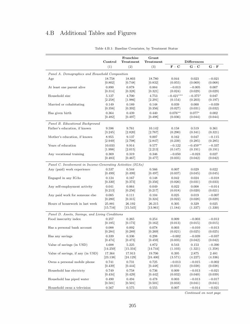
4.B Additional Tables and Figures

Table 4.B.1: Baseline Covariates, by Treatment Status

Franchise GrantControl Treatment Treatment Differences

(1) (2) (3) F – C G – C G – F

Panel A. Demographics and Household Composition

Age 18.758 18.803 18.780 0.044 0.023 −0.021[0.802] [0.748] [0.832] (0.055) (0.069) (0.068)

At least one parent alive 0.890 0.878 0.884 −0.013 −0.005 0.007[0.314] [0.328] [0.321] (0.024) (0.029) (0.029)

Household size 5.127 4.700 4.753 −0.421∗∗∗ −0.375∗ 0.047[2.258] [1.986] [2.291] (0.154) (0.203) (0.197)

Married or cohabitating 0.149 0.189 0.148 0.039 0.000 −0.039[0.356] [0.392] [0.356] (0.027) (0.031) (0.032)

Has given birth 0.364 0.439 0.440 0.076∗∗ 0.077∗ 0.002[0.482] [0.497] [0.498] (0.036) (0.044) (0.044)

Panel B. Educational Background

Father’s education, if known 9.596 9.761 10.142 0.158 0.519 0.361[3.245] [2.820] [2.767] (0.290) (0.341) (0.321)

Mother’s education, if known 8.955 9.137 9.007 0.162 0.047 −0.115[2.949] [2.798] [2.847] (0.239) (0.285) (0.285)

Years of education 10.033 9.914 9.577 −0.122 −0.459∗∗ −0.337[1.998] [2.015] [2.213] (0.147) (0.191) (0.191)

Any vocational training 0.369 0.319 0.346 −0.050 −0.023 0.027[0.483] [0.467] [0.477] (0.035) (0.042) (0.042)

Panel C. Involvement in Income-Generating Activities (IGAs)

Any (paid) work experience 0.537 0.544 0.566 0.007 0.029 0.022[0.499] [0.499] [0.497] (0.037) (0.045) (0.045)

Engaged in any IGAs 0.124 0.167 0.148 0.042 0.024 −0.018[0.330] [0.373] [0.356] (0.026) (0.031) (0.033)

Any self-employment activity 0.041 0.064 0.049 0.022 0.008 −0.014[0.213] [0.256] [0.217] (0.018) (0.020) (0.021)

Any paid work for someone else 0.085 0.111 0.104 0.025 0.019 −0.007[0.280] [0.315] [0.324] (0.022) (0.028) (0.029)

Hours of housework in last week 25.881 26.192 26.215 0.305 0.329 0.025[15.716] [15.545] [13.961] (1.184) (1.337) (1.330)

Panel D. Assets, Savings, and Living Conditions

Food insecurity index 0.257 0.265 0.254 0.009 −0.003 −0.012[0.185] [0.173] [0.162] (0.013) (0.015) (0.015)

Has a personal bank account 0.088 0.092 0.078 0.003 −0.010 −0.013[0.284] [0.289] [0.269] (0.021) (0.025) (0.025)

Has any savings 0.339 0.336 0.298 −0.002 −0.039 −0.037[0.474] [0.473] [0.459] (0.035) (0.042) (0.042)

Value of savings (in USD) 4.688 5.225 4.872 0.543 0.153 −0.390[14.250] [15.334] [14.744] (1.103) (1.321) (1.358)

Value of savings, if any (in USD) 17.364 17.913 19.706 0.395 2.875 2.481[23.138] [24.129] [24.400] (3.571) (4.227) (4.336)

Owns a personal mobile phone 0.741 0.731 0.725 −0.013 −0.015 −0.002[0.439] [0.444] [0.448] (0.031) (0.038) (0.038)

Household has electricty 0.749 0.758 0.736 0.009 −0.013 −0.021[0.434] [0.429] [0.442] (0.032) (0.040) (0.039)

Household has piped water 0.490 0.494 0.478 0.003 −0.013 −0.017[0.501] [0.501] [0.501] (0.033) (0.041) (0.041)

Household owns a television 0.567 0.575 0.555 0.007 −0.014 −0.021

Continued on next page

205

Table 4.B.1 – Continued from previous page

Franchise GrantControl Treatment Treatment Differences

(1) (2) (3) F – C G – C G – F

[0.496] [0.495] [0.498] (0.036) (0.044) (0.045)

Household owns a radio 0.716 0.664 0.665 −0.053 −0.054 −0.001[0.451] [0.473] [0.473] (0.034) (0.042) (0.043)

Household asset index -0.003 0.013 -0.020 0.012 −0.021 −0.034[0.971] [1.024] [1.013] (0.073) (0.089) (0.091)

Observations 363 360 182

Standard deviation in brackets, robust standard errors in parentheses. Columns 4 through 6report differences in means across treatments, with significance levels estimated controlling forstrata fixed effects (as in our main specifications). ∗, ∗∗, and ∗∗∗ indicate significance at the 90,95, and 99 percent confidence levels, respectively. Asset PCA is the first principal component ofthe set of indicators for: whether the household has electricity, whether the household has pipedwater, and whether anyone in the household owns or has a television, a refrigerator, a stove, acomputer, a DVD player, a motorcycle, a bicycle, or a lamp.

Table 4.B.2: Attrition from the Sample

OLS OLS OLS(1) (2) (3)

Franchise treatment 0.009 0.017 -0.379(0.02) (0.028) (0.73)

Grant treatment 0.014 0.018 -0.662(0.024) (0.034) (0.857)

Age . 0.019 0.003(0.016) (0.026)

At least one parent alive . 0.057 0.076(0.046) (0.086)

Household size . -0.01 -0.004(0.006) (0.01)

Married or cohabitating . -0.019 -0.004(0.043) (0.07)

Has given birth . -0.003 0.023(0.033) (0.058)

Father’s education, if known . -0.009∗ -0.0007(0.005) (0.008)

Mother’s education, if known . 0.011∗∗ 0.008(0.005) (0.009)

Years of education . -0.003 -0.005(0.008) (0.014)

Any vocational training . 0.033 0.04(0.028) (0.043)

Any (paid) work experience . -0.015 0.008(0.028) (0.044)

Engaged in any IGAs . -0.065 0.026(0.042) (0.073)

Hours of housework in last week . 0.00007 0.00003(0.0008) (0.001)

Food insecurity index . -0.017 -0.142(0.081) (0.125)

Has a personal bank account . 0.01 0.032(0.046) (0.074)

Has any savings . 0.023 0.044(0.028) (0.045)

Household asset index . -0.013 -0.029(0.015) (0.024)

Age x franchise treatment . . 0.027Continued on next page

206

Table 4.B.2 – Continued from previous page

OLS OLS OLS(1) (2) (3)

(0.039)At least one parent alive x franchise treatment . . 0.003

(0.113)Household size x franchise treatment . . -0.0006

(0.015)Married or cohabitating x franchise treatment . . -0.037

(0.098)Has given birth x franchise treatment . . -0.041

(0.079)Father’s education, if known x franchise treatment . . -0.024∗∗

(0.011)Mother’s education, if known x franchise treatment . . 0.002

(0.013)Years of education x franchise treatment . . 0.011

(0.019)Any vocational training x franchise treatment . . 0.034

(0.064)Any (paid) work experience x franchise treatment . . -0.052

(0.064)Engaged in any IGAs x franchise treatment . . -0.129

(0.099)Hours of housework in last week x franchise treatment . . -0.001

(0.002)Food insecurity index x franchise treatment . . 0.381∗∗

(0.186)Has a personal bank account x franchise treatment . . 0.007

(0.104)Has any savings x franchise treatment . . -0.056

(0.063)Household asset index x franchise treatment . . 0.044

(0.035)Age x grant treatment . . 0.046

(0.044)At least one parent alive x grant treatment . . -0.058

(0.128)Household size x grant treatment . . -0.025

(0.017)Married or cohabitating x grant treatment . . 0.038

(0.122)Has given birth x grant treatment . . -0.032

(0.093)Father’s education, if known x grant treatment . . 0.012

(0.015)Mother’s education, if known x grant treatment . . -0.008

(0.016)Years of education x grant treatment . . -0.009

(0.022)Any vocational training x grant treatment . . -0.086

(0.079)Any (paid) work experience x grant treatment . . 0.008

(0.077)Engaged in any IGAs x grant treatment . . -0.119

(0.124)Hours of housework in last week x grant treatment . . 0.003

(0.002)Food insecurity index x grant treatment . . -0.0003

(0.231)Has a personal bank account x grant treatment . . -0.113

(0.134)Has any savings x grant treatment . . 0.011

(0.078)Household asset index x grant treatment . . 0.032

(0.041)Constant 0.069∗∗∗ -0.271 -0.05

Continued on next page

207

Table 4.B.2 – Continued from previous page

OLS OLS OLS(1) (2) (3)

(0.014) (0.314) (0.489)Observations 905 499 499R2 0.0004 0.036 0.097F-Test: observables (p-value) 0.371 0.959F-Test: treatment-observables interactions (p-value) 0.545

Robust standard errors in parentheses. ∗, ∗∗, and ∗∗∗ indicate significance at the 90,95, and 99 percent confidence levels, respectively. OLS regressions reported. Thedependent variable in all specifications is an indicator for attrition from the sample(between baseline and endline). The last two rows of the table report p-valuesfrom associated F-tests of whether the observable characteristics and observablecharacteristics interacted with treatment are jointly significant in the attritionregressions in columns 2 and 3.

Table 4.B.5: Intent to Treat Estimates: Occupational Sector and Other Outcomes after 14–22 Months

Treatment Effects

Control Franchise Grant p-value:

Obs. Mean Treatment Treatment F = G

(1) (2) (3) (4) (5)

Panel A. Occupational Sectors

Domestic services 837 0.198 -0.021 0.014 0.374(0.031) (0.039)

Salon and beauty 837 0.166 0.114∗∗∗ -0.002 0.002(0.031) (0.035)

Retail and hawking 837 0.121 0.009 0.048 0.274(0.026) (0.034)

Food service and catering 837 0.056 0.022 -0.013 0.116(0.020) (0.021)

Sells prepared food or cooked snacks 837 0.053 0.013 -0.000 0.560(0.019) (0.022)

White collar or professional 837 0.047 -0.022 -0.005 0.272(0.014) (0.019)

Janitorial work and trash collection 837 0.041 -0.008 -0.003 0.741(0.015) (0.018)

Sells uncooked fruits and vegetables 837 0.027 0.013 0.016 0.894(0.014) (0.018)

Works in light industry (factory work) 837 0.024 0.002 0.010 0.690(0.013) (0.017)

Wholesale and distribution 837 0.024 -0.003 -0.005 0.853(0.011) (0.014)

Tailoring, sewing, and arts and crafts 837 0.021 0.001 0.026 0.177(0.011) (0.018)

Entertainment or professional sport 837 0.012 -0.003 -0.013∗ 0.120(0.009) (0.007)

Construction, security, and manual labor 837 0.009 -0.003 0.001 0.548(0.005) (0.007)

Farming or agricultural labor 837 0.000 0.012∗ 0.018∗ 0.624(0.006) (0.010)

Sex worker 837 0.000 0.002 -0.000 0.329(0.002) (0.001)

Panel B. Labor Market Churning

Closed a business between midline and endline 812 0.183 0.010 0.024 0.715Continued on next page

208

Table 4.B.5 – Continued from previous page

Treatment Effects

Control Franchise Grant p-value:

Obs. Mean Treatment Treatment F = G

(1) (2) (3) (4) (5)

(0.032) (0.040)

Left a paid job between midline and endline 812 0.241 -0.051 -0.056 0.894(0.033) (0.040)

Started a business between midline and endline 812 0.177 0.039 0.047 0.850(0.031) (0.037)

Started a new paid job between midline and endline 812 0.387 -0.055 -0.058 0.941(0.039) (0.047)

Panel C. Occupational Sector

Years of education 837 10.198 -0.032 -0.083 0.605(0.092) (0.092)

Curently enrolled in school 837 0.101 -0.014 -0.016 0.934(0.022) (0.026)

Has done any vocational training 837 0.568 0.292∗∗∗ 0.035 0.000(0.033) (0.045)

Has done business skills training 837 0.098 0.149∗∗∗ 0.001 0.000(0.028) (0.029)

Business skills score (scaled 0 to 5) 837 1.036 0.129 -0.103 0.037(0.095) (0.109)

Has done salon skills training 837 0.213 0.289∗∗∗ 0.003 0.000(0.034) (0.039)

Salon skills score (scaled 0 to 9) 837 4.580 0.136 -0.485∗∗∗ 0.000(0.128) (0.159)

Has done tailoring training 837 0.062 0.003 0.018 0.564(0.019) (0.026)

Tailoring skills score (scaled 0 to 8) 837 1.325 -0.021 0.035 0.610(0.092) (0.112)

Has done computer training 837 0.237 -0.069∗∗ 0.003 0.032(0.027) (0.034)

Seconds required to complete typing test 835 100.935 5.298 13.055∗∗ 0.145(4.385) (5.285)

Panel D. Household Composition and Living Arrangements

Household size 837 4.716 -0.082 0.133 0.289(0.169) (0.205)

Married or cohabitating 837 0.269 0.012 -0.040 0.208(0.034) (0.041)

Had an additional child (after program) 837 0.145 0.061∗∗ 0.045 0.663(0.030) (0.037)

Lives with own child 837 0.453 0.071∗∗ 0.091∗∗ 0.624(0.032) (0.040)

Lives in Nairobi 837 0.891 -0.023 -0.049 0.416(0.024) (0.031)

Panel E. Household Assets and Living Conditions

Household has electricity 837 0.849 -0.023 -0.041 0.645(0.028) (0.037)

Household has piped water 837 0.470 0.039 0.068 0.488(0.035) (0.043)

Household has flush toilet 837 0.388 0.056 0.076∗ 0.618(0.034) (0.041)

Household owns a TV 837 0.598 -0.042 -0.020 0.631(0.039) (0.046)

Household owns computer 837 0.080 -0.051∗∗∗ -0.040∗∗ 0.486(0.017) (0.019)

Owns a personal mobile phone 837 0.891 -0.011 -0.062∗ 0.134(0.025) (0.034)

Continued on next page

209

Table 4.B.5 – Continued from previous page

Treatment Effects

Control Franchise Grant p-value:

Obs. Mean Treatment Treatment F = G

(1) (2) (3) (4) (5)

Owns a personal SIM card 837 0.950 -0.011 -0.010 0.984(0.019) (0.023)

Panel F. Consumption, Expenditures, and Savings

Food Insecurity Access Scale (out of 27) 837 9.571 -0.224 0.903 0.072(0.512) (0.621)

Women’s Dietary Diversity Score (scaled 0 to 9) 805 4.745 0.156 0.049 0.484(0.122) (0.145)

Expenditures on self and children (in USD) 837 7.837 0.050 -0.528 0.477(0.735) (0.845)

Log of expenditures on self and children (in USD) 837 1.266 0.172 0.045 0.365(0.114) (0.143)

Spent money on tea, soda, or sweets in past week 837 0.663 0.020 0.017 0.956(0.036) (0.043)

Spent money on alcohol in past week 837 0.059 -0.036∗∗ -0.025 0.514(0.016) (0.019)

Transfers (in USD) 837 2.725 -0.006 0.286 0.524(0.367) (0.470)

Log of transfers (in USD) 837 -0.859 0.216 0.168 0.849(0.200) (0.251)

Savings (in USD) 837 49.211 -9.496 2.118 0.199(7.967) (9.783)

Change in savings relative to last year 837 -0.139 -0.169∗∗ -0.156∗ 0.875(0.072) (0.084)

Paid school fees for self or own child in 2014 837 0.107 -0.003 0.019 0.469(0.024) (0.030)

Paid school fees for someone else’s child in 2014 837 0.071 0.009 0.124∗∗∗ 0.001(0.021) (0.034)

Panel G. Time Use on Week Day Prior to Survey

Hours of income-generating activities 837 2.746 0.283 0.498 0.623(0.356) (0.420)

Self-employment hours 837 0.364 0.287∗ 0.431∗∗ 0.534(0.163) (0.201)

Hours of paid work for others 837 2.382 -0.004 0.067 0.862(0.341) (0.398)

Hours of unpaid household work 837 5.544 0.142 -0.055 0.512(0.258) (0.299)

Hours of unpaid work in a business 837 0.393 -0.085 0.023 0.421(0.121) (0.141)

Hours of job search 837 0.086 -0.007 0.026 0.670(0.055) (0.074)

Hours commuting or in transit 837 0.166 -0.062 0.265∗ 0.029(0.050) (0.155)

Hours of leisure 837 10.260 -0.431 -0.722∗∗ 0.362(0.276) (0.314)

Hours of education or training 837 0.595 0.071 -0.037 0.571(0.167) (0.181)

Hours of religious observance, visiting the sick 837 0.154 0.089 0.022 0.481(0.096) (0.092)

Panel H. Indices Capturing Empowerment, Self-Esteem, etc.

Rosenberg self-esteem scale (0 to 30) 837 19.130 0.363 -0.348 0.056(0.310) (0.370)

Ladder of Life wellbeing scale (scaled from 0 to 10) 837 6.491 0.139 -0.000 0.280(0.110) (0.126)

Grit (scaled from 1 to 5) 837 2.006 -0.004 0.006 0.737Continued on next page

210

Table 4.B.5 – Continued from previous page

Treatment Effects

Control Franchise Grant p-value:

Obs. Mean Treatment Treatment F = G

(1) (2) (3) (4) (5)

(0.022) (0.029)

Panel I. Empowerment Measures Used in Bandiera et al (2015)

Gender Empowerment Index (scaled 0 to 100) 837 48.352 -0.740 2.171 0.171(1.749) (2.096)

Business Confidence Index (scaled 0 to 100) 837 71.915 0.589 -2.267∗ 0.015(0.942) (1.175)

Suitable age for a woman to marry 837 24.828 -0.357∗ -0.205 0.530(0.207) (0.230)

Suitable age for a man to marry 837 28.281 -0.328 0.085 0.182(0.263) (0.281)

Desired age of marriage for daughter 788 26.101 -0.226 -0.300 0.759(0.206) (0.238)

Desired age of marriage for son 813 28.856 -0.283 0.073 0.209(0.242) (0.280)

Suitable age for a woman to have a child 837 24.891 -0.294 -0.161 0.672(0.251) (0.291)

Number of children desired 837 2.757 0.039 0.057 0.824(0.069) (0.084)

Number of boys desired 835 1.494 -0.061 0.044 0.086(0.054) (0.065)

Desired proportion of male children 835 0.537 -0.030∗∗ 0.021 0.003(0.014) (0.018)

Panel J. Empowerment Measures Used in Adoho et al (2014)

Self Confidence Index (scaled from 1 to 6) 837 4.257 0.066 -0.094 0.133(0.087) (0.106)

Respondent has her own money 837 0.805 0.081∗∗∗ 0.066∗ 0.660(0.028) (0.036)

Controls money she earns from IGAs 644 0.956 0.012 0.013 0.963(0.017) (0.022)

Needs permission to spend earnings 837 0.050 0.009 0.006 0.912(0.018) (0.022)

Robust standard errors in parentheses. ∗, ∗∗, and ∗∗∗ indicate significance at the 90, 95, and99 percent confidence levels, respectively. OLS regressions reported. All specifications includecontrols for baseline household size, education level, and indicators for having given birth, havingreceived any vocational training, or having any paid work experience prior to the baseline survey,in addition to survey enumerator and survey month fixed effects. Money amounts are deflated toJuly 2013 levels using CPI data from the Kenya National Bureau of Statistics, then converted toUS dollars using the average exchange rate from July 2013 (84.04 Kenyan shillings to the dollar).The top 1 percent of values of all hours and income variables are trimmed. The estimatedimpacts of the franchise treatment on the likelihood of working in the salon sector (see Panel A)or having done any vocational training (see Panel C) are significant at the 99 percent level afterimplementing the multiple hypothesis testing correction proposed by Benjamini and Hochberg(1995). Those assigned to the grant treatment are also more likely to have paid school fees forsomeone else’s child in the year after receiving the grant (Benjamini-Hochberg q-value 0.01; seePanel F). No other outcomes are significantly related to either treatment with adjusted q-valuesbelow 0.05.

211

Table 4.B.3: Treatment on the Treated: Labor Market Outcomes after 7–10 Months

TOT Estimates

Started

Control Franchise Received p-value:

Obs. Mean Program Grant F = G

(1) (2) (3) (4) (5)

Panel A. Involvement in Income-Generating Activities (Previous Month)

Engaged in any income-generating activities 851 0.586 0.032 0.025 0.908(0.061) (0.047)

Any self-employment activity 851 0.245 0.163∗∗∗ 0.105∗∗ 0.307(0.055) (0.044)

Paid work for someone else 851 0.382 -0.114∗ -0.073 0.473(0.059) (0.046)

Panel B. Labor Supply (Previous 7 Days)

Hours worked in last week 851 17.945 1.853 7.105∗∗ 0.140(3.442) (2.953)

Self-employment hours 851 4.723 6.856∗∗∗ 7.938∗∗∗ 0.680(2.180) (2.047)

Hours of paid work for someone else 851 13.017 -4.756 -0.903 0.167(2.893) (2.383)

Panel C. Income Excluding Transfers (Previous 7 Days)

Reports any labor income 851 0.466 0.093 0.062 0.607(0.061) (0.048)

Income excluding transfers (in USD) 851 5.476 2.720∗∗ 3.278∗∗∗ 0.699(1.250) (1.198)

Log income (in USD) 851 -1.436 0.842∗∗ 0.582∗ 0.525(0.407) (0.323)

Self-employment income (in USD) 851 2.617 2.167∗∗ 2.397∗∗ 0.843(0.988) (1.018)

Log of self-employment income (in USD) 851 -3.158 1.049∗∗∗ 0.733∗∗∗ 0.382(0.345) (0.282)

Income from paid work for someone else (in USD) 851 2.901 0.154 0.508 0.675(0.776) (0.661)

Log of income from paid work (in USD) 851 -2.595 -0.143 -0.066 0.825(0.359) (0.278)

Panel D. First-Stage F-Statistics on Excluded Instruments

Franchise treatment 277.723

Grant treatment 2440.035

Robust standard errors in parentheses. ∗, ∗∗, and ∗∗∗ indicate significance at the 90, 95, and99 percent confidence levels, respectively. OLS regressions reported. All specifications includecontrols for baseline household size, education level, and indicators for having given birth, havingreceived any vocational training, or having any paid work experience prior to the baseline survey,in addition to survey enumerator and survey month fixed effects. Money amounts are deflated toJuly 2013 levels using CPI data from the Kenya National Bureau of Statistics, then converted toUS dollars using the average exchange rate from July 2013 (84.04 Kenyan shillings to the dollar).The top 1 percent of values of all hours and income variables are trimmed.

212

Table 4.B.4: Intent to Treat Estimates: Occupational Sectors after 7–10 Months

Treatment Effects

Control Franchise Grant p-value:

Obs. Mean Treatment Treatment F = G

(1) (2) (3) (4) (5)

Panel A. Occupational Sectors

Domestic services 851 0.143 -0.045∗ -0.049 0.904(0.025) (0.030)

Salon and beauty 851 0.146 0.088∗∗∗ -0.073∗∗ 0.000(0.029) (0.030)

Retail and hawking 851 0.090 0.043∗ 0.112∗∗∗ 0.055(0.024) (0.035)

Food service and catering 851 0.026 -0.007 0.006 0.434(0.013) (0.016)

Sells prepared food or cooked snacks 851 0.061 0.037∗ 0.034 0.916(0.020) (0.025)

White collar or professional 851 0.020 0.002 0.016 0.373(0.011) (0.016)

Janitorial work and trash collection 851 0.026 -0.020∗ -0.028∗∗∗ 0.196(0.011) (0.009)

Sells uncooked fruits and vegetables 851 0.038 -0.021 0.031 0.010(0.014) (0.022)

Works in light industry (factory work) 851 0.035 -0.009 0.005 0.409(0.014) (0.019)

Wholesale and distribution 851 0.006 0.018∗ 0.010 0.450(0.009) (0.009)

Tailoring, sewing, and arts and crafts 851 0.015 -0.000 -0.005 0.667(0.010) (0.011)

Entertainment or professional sport 851 0.017 -0.015∗∗ -0.009 0.353(0.007) (0.010)

Construction, security, and manual labor 851 0.009 -0.005 0.004 0.246(0.006) (0.007)

Farming or agricultural labor 851 0.015 -0.013∗∗ -0.004 0.257(0.006) (0.011)

Sex worker 851 0.000 0.002 -0.000 0.325(0.002) (0.001)

Robust standard errors in parentheses. ∗, ∗∗, and ∗∗∗ indicate significance at the 90, 95,and 99 percent confidence levels, respectively. OLS regressions reported. All specificationsinclude controls for baseline household size, education level, and indicators for having givenbirth, having received any vocational training, or having any paid work experience prior tothe baseline survey, in addition to survey enumerator and survey month fixed effects..

213

Bibliography

Adoho, F., S. Chakravarty, D. T. Korkoyah Jr., M. Lundberg, and A. Tas-neem (2014): “The Impact of an Adolescent Girls Employment Program: The EPAGProject in Liberia,” World Bank Policy Research Working Paper 6832.

Ajayi, K. (2013): “School choice and education mobility: lessons from secondary schoolapplications in Ghana,” Working Paper.

Ajayi, K., and M. Sidibe (2015): “An empirical analysis of School choice under Unc-etainty,” Working Paper.

Ajayi, K. F., and M. Buessing (2015): “Gender Parity and Schooling Choices,” TheJournal of Development Studies, 51(5), 503–522.

Al-Samarrai, S., and H. Zaman (2007): “Abolishing School Fees in Malawi: TheImpact on Education Access and Equity,” Education Economics, 15(3), 359–75.

Anderson, M. L. (2008): “Multiple Inference and Gender Differences in the Effects ofEarly Intervention: A Reevaluation of the Abecedarian, Perry Preschool, and EarlyTraining Projects,” Journal of the American Statistical Association, 103(484), 1481–1495.

Andrabi, T., J. Das, and A. I. Khwaja (2013): “Students today, teachers tomorrow:Identifying constraints on the provision of education,” Journal of Public Economics,100, 1–14.

Angelucci, M., D. Karlan, and J. Zinman (2015): “Microcredit Impacts: Evi-dence from a Randomized Microcredit Program Placement Experiment by Comparta-mos Banco,” American Economic Journal: Applied Economics, 7(1), 151–82.

Athey, S., and G. W. Imbens (2006): “Identification and Inference in nonlineardifference-in-difference models,” Econometrica, 74(2), 431–497.

Attanasio, O., B. Augsburg, R. De Haas, E. Fitzsimons, and H. Harmgart(2015): “The Impacts of Microfinance: Evidence from Joint-Liability Lending in Mon-golia,” American Economic Journal: Applied Economics, 7(1).

214

Attanasio, O., A. Kugler, and C. Meghir (2011): “Subsidizing Vocational Trainingfor Disadvantaged Youth in Colombia: Evidence from a Randomized Trial,” AmericanEconomic Journal: Applied Economics, 3(3), 188–220.

Augsburg, B., R. De Haas, H. Harmgart, and C. Meghir (2015): “The Impactsof Microcredit: Evidence from Bosnia and Herzegovina,” American Economic Journal:Applied Economics, 7(1), 183–203.

Baird, S., E. Chirwa, C. McIntosh, and B. Ozler (2010): “The short-term im-pacts of a schooling conditional cash transfer program on the sexual behavior of youngwomen,” Health Economics, 19(S1), 55–68.

Baird, S., C. McIntosh, and B. Ozler (2016): “When the money runs out: Evaluat-ing the Longer-Term Impacts of a Two year Cash Transfer Program,” Working Paper.

Baland, J.-M., and J. A. Robinson (2000): “Is child labor inefficient?,” Journal ofPolitical Economy, 108(4), 663–679.

Bandiera, O., N. Buehren, R. Burgess, M. Goldstein, S. Gulesci, I. Rasul,and M. Sulaiman (2014a): “Women’s Empowerment in Action: Evidence from aRandomized Control Trial in Africa,” working paper.

Bandiera, O., O. Buehren, R. Burgess, M. Goldstein, S. Gulesci, I. Rasul,and M. Sulaiman (2014b): “Womens Empowerment in Action: Evidence from aRandomized Control Trial in Africa,” Working Paper.

Banerjee, A., E. Duflo, R. Glennerster, and C. Kinnan (2015): “The Miracle ofMicrofinance? Evidence from a Randomized Evaluation,” American Economic Journal:Applied Economics, 7(1), 22–53.

Banerjee, A., E. Duflo, N. Goldberg, D. Karlan, R. Osei, W. Pariente,J. Shapiro, B. Thuysbaert, and C. Udry (2015): “A Multifaceted Program CausesLasting Progress for the Very Poor: Evidence from Six Countries,” Science, 348(6236).

Banerjee, A., R. Hanna, G. Kreindler, and B. A. Olken (2015): “Debunkingthe Stereotype of the Lazy Welfare Recipient: Evidence from Cash Transfer ProgramsWorldwide,” mimeo (available online at http://economics.mit.edu/files/10861, ac-cessed 8 February 2017).

Barrera-Osorio, F., L. L. Linden, and M. Urquiola (2007): “The Effects of UserFee Reductions on Enrollment: Evidence from a Quasi-Experiment,” Working Paper.

Benjamini, Y., and Y. Hochberg (1995): “Controlling the False Discovery Rate: aPractical and Powerful Approach to Multiple Testing,” Journal of the Royal StatisticalSociety. Series B (Methodological), 57(1), 289–300.

Berge, L. I. O., K. Bjorvatn, and B. Tungodden (2014): “Human and financialcapital for microenterprise development: Evidence from a field and lab experiment,”Management Science, 61(4), 707–722.

215

Blattman, C., N. Fiala, and S. Martinez (2014): “Generating Skilled Self-Employment in Developing Countries: Experimental Evidence from Uganda,” QuarterlyJournal of Economics, 129(2), 697–752.

Blattman, C., E. P. Green, J. Jamison, M. C. Lehmann, and J. Annan (2016):“The Returns to Microenterprise Support among the Ultrapoor: A Field Experimentin Postwar Uganda,” American Economic Journal: Applied Economics, 8(2), 35–64.

Blimpo, M. P., O. Gajigo, and T. Pugatch (2015): “Financial Constraints andGirls’ Secondary Education: Evidence from School Fee Elimination in the Gambia,”IZA Discussion Paper, (No. 9129).

Brudevold-Newman, A. (2016): “The Impacts of Free Secondary Education: Evidencefrom Kenya,” Working Paper.

Card, D., P. Ibarraran, F. Regalia, D. Rosas-Shady, and Y. Soares (2011):“The Labor Market Impacts of Youth Training in the Dominican Republic,” Journal ofLabor Economics, 29(2), 267–300.

Cho, Y., and M. Honorati (2014): “Entrepreneurship Programs in Developing Coun-tries: A Meta Regression Analysis,” Labour Economics, 28, 110–130.

Crepon, B., F. Devoto, E. Duflo, and W. Pariente (2015): “Estimating theImpact of Microcredit on Those Who Take It Up: Evidence from a Randomized Exper-iment in Morocco,” American Economic Journal: Applied Economics, 7(1), 123–50.

De Mel, S., D. McKenzie, and C. Woodruff (2008): “Returns to Capital in Mi-croenterprises: Evidence from a Field Experiment,” Quarterly Journal of Economics,123(4), 1329–1372.

(2009): “Are Women More Credit Constrained? Experimental Evidence on Gen-der and Microenterprise Returns,” American Economic Journal: Applied Economics,1(3), 1–32.

Deininger, K. (2003): “Does cost of schooling affect enrollment by the poor? Universalprimary education in Uganda,” Economics of Education Review, 22(3), 291–305.

DHS (2014): Kenya Demographic and Health Survey. ICF Macro, Calverton, Maryland.

Duflo, E. (2004): “Schooling and Labor Market Consequences of School Construction InIndonesia: Evidence from an unusual policy experiement,” American Economic Review,91(4).

Duflo, E., P. Dupas, and M. Kremer (2012): “Estimating the Benefit to SecondarySchool in Africa: Experimental Evidence from Ghana,” The International Growth Cen-ter Policy Brief, 2020.

(2015): “Education, HIV, and Early Fertility: Experimental Evidence fromKenya,” American Economic Review, 105(9), 2757–97.

216

Dupas, P., V. Hoffmann, M. Kremer, and A. P. Zwane (2016): “Targeting HealthSubsidies through a Nonprice Mechanism: A Randomized Controlled Trial in Kenya,”Science, 353(6302), 889–895.

Dupas, P., and J. Johnston (2015): “Returns to secondary education: unpacking thedelivery of senior secondary schooling in Ghana,” Working Paper.

Dupas, P., and J. Robinson (2013a): “Savings Constraints and Microenterprise Devel-opment: Evidence from a Field Experiment in Kenya,” American Economic Journal:Applied Economics, 5(1), 163–192.

(2013b): “Why Don’t the Poor Save More? Evidence from Health SavingsExperiments,” The American Economic Review, 103(4), 1138–1171.

Eble, A., and F. Hu (2016): “The Importance of Educational Credentials: SchoolingDecisions and Returns in Modern China,” Working Paper.

Evans, D. K., M. Kremer, and M. Ngatia (2012): “The Impact of DistributingSchool Uniforms on Childrens Education in Kenya,” Working Paper.

Evans, D. K., and A. Popova (2015): “What Really Works to Improve Learning inDeveloping Countries?,” Policy Research Working Paper, (7203).

(2016): “Cash Transfers and Temptation Goods,” Economic Development andCultural Change, 65, 189–221.

Fafchamps, M., D. McKenzie, S. Quinn, and C. Woodruff (2011): “Microenter-prise Growth and the Flypaper Effect: Evidence from a Randomized Experiment inGhana,” Journal of Development Economics, 106, 211–226.

Fares, J., C. E. Montenegro, and P. F. Orazem (2006): “How are Youth Faringin the Labor Market? Evidence from Around the World,” World Bank Policy ResearchWorking Paper 4071.

Ferre, C. (2009): “Age at First Child: Does Education Delay Fertility Timing? TheCase of Kenya,” Policy Research Working Paper 4833.

Fiala, N. (2014): “Stimulating Microenterprise Growth: Results from a Loans, Grantsand Training Experiment in Uganda,” working paper.

Filmer, D., and L. Fox (2014): “Youth Employment in Sub-Saharan Africa: Overview,”Washington, DC: World Bank.

Filmer, D., and N. Schady (2014): “The Medium-Term Effects of Scholarships in aLow Income Country,” Journal of Human Resources, 49(3), 663–94.

Fischhoff, B. (1975): “Hindsight Is Not Equal to Foresight: The Effect of OutcomeKnowledge on Judgment Under Uncertainty.,” Journal of Experimental Psychology:Human Perception and Performance, 1(3), 288.

217

Franz, J. (2014): “Youth Employment Initiatives in Kenya,” Report of a ReviewCommissioned by the World Bank and Kenya Vision 2030 (available online at www.

vision2030.go.ke/lib.php?f=wb-youth-employment-initiatives-report-13515,accessed 18 November 2016).

Gajigo, O. (2012): “Closing the Education Gender Gap: Estimating the Impact ofGirls Scholarship Program in The Gambia,” African Development Bank Group WorkingPaper 164.

Gale, D., and L. S. Shapley (1962): “College admissions and the stability of marriage,”The American Mathematical Monthly, 69(1), 9–15.

Garlick, R. (2013): “How Price Sensitive is Primary and Secondary School Enrollment?Evidence from Nationwide Tuition Fee Reforms in South Africa,” Working Paper.

Glennerster, R., M. Kremer, I. Mbiti, and K. Takavarasha (2011): Access andQuality in the Kenyan Education System: A Review of the Progress, Challenges andPotential Solutions. The Abdul Latif Poverty Action Lab.

Glewwe, P., M. Kremer, and S. Moulin (2009): “Many children left behind? Text-books and test scores in Kenya,” American Economic Journal: Applied Economics,1(1), 112–135.

Glewwe, P. W., E. A. Hanushek, S. D. Humpage, and R. Ravina (2011): “Schoolresources and educational outcomes in developing countries: a review of the literaturefrom 1990 to 2010,” in Education Policy in Developing Countries, ed. by P. W. Glewwe.University of Chicago Press.

Goldberg, J., and J. Smith (2008): “The Effects of Education on Labour MarketOutcomes,” in Handbook of Research in Education, Finance, and Policy, ed. by E. Fiske,and H. Ladd, chap. 38. Routledge.

Grogan, L. (2009): “Universal Primary Education and School Entry in Uganda,” Journalof African Economies, 18(2), 183–211.

Grossman, M. (2006): “Education and Nonmarket Outcomes,” in Handbook of the Eco-nomics of Education, Volume 1, ed. by E. A. Hanushek, and F. Welch, chap. 10, pp.578–628. North Holland.

Hanushek, E., and L. Woßmann (2007): “The Role of School Improvement in Eco-nomic Development,” NBER Working Paper, (No. 12832).

(2008): “The Role of Cognitive Skills in Economic Development,” Journal ofEconomic Literature, 46(3).

Hastings, J. S., and J. M. Weinstein (2008): “Information, School Choice, andAcademic Achievement: Evidence from Two Experiments,” Quarterly Journal of Eco-nomics, 123(4), 1373–414.

Haushofer, J., and J. Shapiro (2016): “The Short-Term Impact of UnconditionalCash Transfers to the Poor: Experimental Evidence from Kenya,” Quarterly Journalof Economics, 131(4), 1973–2042.

218

Heckman, J., L. Lochner, and P. Todd (2006): “Earnings functions, rates of re-turn and treatment effects: The Mincer equation and beyond.,” in Handbook of theEconomics of Education, ed. by E. Hanushek, and F. Welch. Elsevier.

Hicks, J. H., M. Kremer, I. Mbiti, and E. Miguel (2016): “Start-up Capital forYouth,” AEA RCT Registry.

Hoogeveen, J., and M. Rossi (2013): “Enrolment and Grade Attainment following theIntroduction of Free Primary Education in Tanzania,” Journal of African Economies,22(3), 375–93.

Imberman, S., A. Kugler, and B. Sacerdote (2012): “Katrina’s children: evidenceon the structure of peer effects from hurricane evacuees,” American Economic Review,102(5), 2048–82.

International Rescue Committee (2016a): “Cost Analysis Method-ology at the IRC,” available online at https://rescue.box.com/s/

co7xgj2vvohgzir3ejnr2e5mwbmqhvp7, accessed 9 January 2017.

(2016b): “Economic Recovery and Development at the International RescueCommittee,” available online at https://www.rescue.org/sites/default/files/

document/1048/irceconomicrecoveryanddevelopmentoverviewinfo0816.pdf, ac-cessed 9 January 2017.

Jensen, R. (2010): “The (Perceived) Returns to Education and the Demand for School-ing,” Quarterly Journal of Economics, 125(2), 515–48.

Kaplan, E. L., and P. Meier (1958): “Nonparametric Estimation from IncompleteObservations,” Journal of the American Statistical Association, 53(282), 457–81.

Karlan, D., R. Knight, and C. Udry (2015): “Consulting and Capital Experimentswith Microenterprise Tailors in Ghana,” Journal of Economic Behavior & Organization,118, 281–302.

Keats, A. (2014): “Women’s Schooling, Fertility, and Child Health Outcomes: Evidencefrom Uganda’s Free Primary Education Program,” Working Paper.

Kenya National Assembly Official Records (2011): pp. 30–41.

Kenya National Bureau of Statistics (2000-2014): Kenya Economic Survey.

Kluve, J., S. Puerto, D. Robalino, J. M. Romero, F. Rother, J. Stoterau,F. Weidenkaff, and M. Witte (2016): “Do Youth Employment Programs ImproveLabor Market Outcomes? A Systematic Review,” IZA Discussion Paper No. 10263.

Kremer, M. (2003): “Randomized Evaluations of Educational Programs in DevelopingCountries: Some Lessons,” The American Economic Review, 93(2), 102–106.

Kremer, M., C. Brannen, and R. Glennerster (2013): “The Challenge of Educationand Learning in the Developing World,” Science, 340(6130), 297–300.

219

Kremer, M., and C. Vermeersch (2005): “School Meals, Educational Achievement,and School Competition: Evidence from a Randomized Evaluation,” Policy ResearchWorking Paper.

Lavecchia, A. M., H. Liu, and P. Oreopoulos (2015): “Behavioral Economics ofEducation: Progress and Possibilities,” IZA Discussion Paper, 8853.

Lochner, L. J., and A. Monge-Naranjo (2011): “The Nature of Credit Constraintsand Human Capital,” American Economic Review, 101, 2487–529.

Lucas, A. M., and I. M. Mbiti (2012a): “Access, Sorting, and Achievement: the shortrun effects of free primary education in Kenya,” American Economic Journal: AppliedEconomics, 4(4), 226–53.

(2012b): “The Determinants and Consequences of School Choice Errors inKenya,” American Economic Review, Papers and Proceedings, 102(3), 283–88.

(2014): “Effects of school quality on student achievement: Discontinuity evidencefrom Kenya,” American Economic Journal: Applied Economics, 6(3), 234–63.

Madarasz, K. (2012): “Information Projection: Model and Applications,” The Reviewof Economic Studies, 79(3), 961–985.

McCrary, J., and H. Royer (2011): “The effect of Female education on fertility andinfant health: evidence from school entry policies using exact date of birth,” AmericanEconomic Review, 101(1), 158–195.

McEwan, P. J. (2014): “Improving Learning in Primary Schools of Developing CountriesA Meta-Analysis of Randomized Experiments,” Review of Educational Research.

McKenzie, D. (2016a): “Can Business Owners Form Accurate Counterfactuals? Elicit-ing Treatment and Control Beliefs about Their Outcomes in the Alternative TreatmentStatus,” World Bank Policy Research Working Paper 7768.

(2016b): “Identifying and Spurring High-Growth Entrepreneurship: Experimen-tal Evidence from a Business Plan Competition,” BREAD Working Paper No. 462.

McKenzie, D., and C. Woodruff (2014): “What Are We Learning from BusinessTraining and Entrepreneurship Evaluations around the Developing World?,” WorldBank Research Observer, 29(1), 48–82.

McMillan, M., and D. Rodrik (2011): “Globalization, Structural Change and Pro-ductivity Growth,” in Making Globalization Socially Sustainable, ed. by M. Bachetta,and M. Jansen. International Labour Organization.

McMillan, M., D. Rodrik, and I. n. Verduzco-Gallo (2014): “Globalization,Structural Change and Productivity Growth, with an Update on Africa,” World Devel-opment, 63, 11–32.

Miller, D. T., and M. Ross (1975): “Self-Serving Biases in the Attribution of Causal-ity: Fact or Fiction?,” Psychological Bulletin, 82(2), 213.

220

Ministry of Education (2008a): “The development of education: National report ofKenya,” Report presented at The International Conference on Education, November2008.

(2008b): “Education Statistical Booklet 2003 - 2007,” Education ManagementInformation System Kenya Report.

Ministry of Education, Science and Technology (2014a): “2014 Basic EducationStatistical Booklet,” UNICEF.

(2014b): “Education for All, The 2015 National Review,” Submitted by the StateDepartment of Education for the World Education Forum 2015.

Murnane, R. J., and A. J. Ganimian (2014): “Improving Educational Outcomes inDeveloping Countries: Lessons from Rigorous Evaluations,” NBER Working Paper No.20284.

Nishimura, M., T. Yamano, and Y. Sasaoka (2008): “Impacts of the Universal Pri-mary Education Policy on Educational Attainment and Private Costs in Rural Uganda,”International Journal of Educational Development, 28(2), 161–75.

Osili, U. O., and B. T. Long (2008): “Does female schooling reduce fertility? Evidencefrom Nigeria,” Journal of Development Economics, 87, 5775.

Ozier, O. (Forthcoming): “The Impact of Secondary Schooling in Kenya: A RegressionDiscontinuity Analysis,” Journal of Human Resources.ΩOzler

Ozler, B. (2016): “GiveDirectly just announced a basic incomegrant experiment. Here is how to make it better.,” blog post (avail-able online at http://blogs.worldbank.org/impactevaluations/

givedirectly-just-announced-basic-income-grant-experiment-here-how-make-it-better,accessed 20 February 2017).

Petrosino, A., C. Morgan, T. A. Fronius, E. E. Tanner-Smith, and R. F.Boruch (2012): “Interventions in Developing Nations for Improving Primary and Sec-ondary School Enrollment of Children: A Systematic Review,” Campbell SystematicReviews.

Pritchett, L. (2013): The Rebirth of Education: Schooling Ain’t Learning. Center forGlobal Development, Washington, D.C.

Schoar, A. (2010): “The Divide between Subsistence and Transformational En-trepreneurship,” Innovation Policy and the Economy, 10(1), 57–81.

Schultz, T. P. (1993): “Returns to women’s education,” in Womens Education in De-veloping Countries: Barriers, Benefits, and Policies, ed. by E. King, and M. Hill, pp.51–99. Johns Hopkins University Press.

(2008): “Population policies, fertility, women’s human capital, and child quality,”in Handbook of Development Economics, Volume Four, ed. by T. Schultz, and J. Strauss.Elsevier Science B.V.

221

Smith, J., A. Whalley, and N. Wilcox (2011): “Are Program Participants GoodEvaluators?,” working paper.

(2012): “Are Participants Good Evaluators?,” working paper.

Staiger, D., and J. H. Stock (1997): “Instrumental variables regression with weakinstruments,” Econometrica, 65(3).

Tarozzi, A., J. Desai, and K. Johnson (2015): “The Impacts of Microcredit: Evidencefrom Ethiopia,” American Economic Journal: Applied Economics, 7(1), 54–89.

UNESCO (2010): “Trends in Tertiary Education: sub-Saharan Africa,” Institute forStatistics Fact Sheet.

(2015): “Education for All 2000-2015: Achievements and Challanges,” Educationfor All Global Monitoring Report.

United Nations Development Programme (2013): “Kenya’s Youth UnemploymentChallenge,” Discussion Paper (available online at http://www.undp.org/content/

dam/undp/library/Poverty%20Reduction/Inclusive%20development/Kenya_YEC_

web(jan13).pdf, accessed 18 November 2016).

Valente, C. (2015): “Primary Education Expansion and Quality of Schooling: Evidencefrom Tanzania,” IZA Discussion Paper Series, 9208.

World Bank (2006): World Development Report 2007: Development and the Next Gen-eration. World Bank: the International Bank for Reconstruction and Development.

222