ERDC/CERL TR-16-15 "Assessing Socioeconomic Impacts of ...
130
ERDC/CERL TR-16-15 Human-Infrastructure System Assessment for Military Operations Assessing Socioeconomic Impacts of Cascading Infrastructure Disruptions Using the Capability Approach Construction Engineering Research Laboratory Yi (Victor) Wang, Armin Tabandeh, Paolo Gardoni, Tina M. Hurt, Ellen R. Hartman, and Natalie R. Myers August 2016 Approved for public release; distribution is unlimited.
-
Upload
khangminh22 -
Category
Documents
-
view
1 -
download
0
Transcript of ERDC/CERL TR-16-15 "Assessing Socioeconomic Impacts of ...
ERD
C/CE
RL T
R-16
-15
Human-Infrastructure System Assessment for Military Operations
Assessing Socioeconomic Impacts of Cascading Infrastructure Disruptions Using the Capability Approach
Cons
truc
tion
Engi
neer
ing
Res
earc
h La
bora
tory
Yi (Victor) Wang, Armin Tabandeh, Paolo Gardoni, Tina M. Hurt, Ellen R. Hartman, and Natalie R. Myers
August 2016
Approved for public release; distribution is unlimited.

The U.S. Army Engineer Research and Development Center (ERDC) solves the nation’s toughest engineering and environmental challenges. ERDC develops innovative solutions in civil and military engineering, geospatial sciences, water resources, and environmental sciences for the Army, the Department of Defense, civilian agencies, and our nation’s public good. Find out more at www.erdc.usace.army.mil.
To search for other technical reports published by ERDC, visit the ERDC online library at http://acwc.sdp.sirsi.net/client/default.
Cover Photo: Lagos, Nigeria at night (source: http://www.blog.kpmgafrica.com/wp-content/up-
loads/2013/05/megacities1.jpg).
Human-Infrastructure System Assessment for Military Operations
ERDC/CERL TR-16-15 August 2016
Assessing Socioeconomic Impacts of Cascading Infrastructure Disruptions Using the Capability Approach
Tina M. Hurt, Ellen R. Hartman, Natalie R. Myers Construction Engineering Research Laboratory U.S. Army Engineer Research and Development Center 2902 Newmark Drive Champaign, IL 61822
Yi (Victor) Wang, Armin Tabandeh, Paolo Gardoni University of Illinois at Urbana-Champaign Department of Civil and Environmental Engineering 205 N Mathews Ave. Urbana IL 61801-2352
Final report
Approved for public release; distribution is unlimited.
Prepared for Assistant Secretary of the Army for Acquisition, Logistics, and Technology 103 Army Pentagon Washington, DC 20314-1000
Under Project No. 405479, “Human Infrastructure System Assessment for Military Operations”

ERDC/CERL TR-16-15 ii
Abstract
U.S. Army doctrine requires that commanders understand, visualize, and de-scribe the infrastructure component of the Joint Operating Environment to accomplish the Army’s missions of protecting, restoring, and developing in-frastructure. The functionality of modern cities relies heavily on interdepend-ent infrastructure systems such as those for water, power, and transportation. Disruptions often propagate within and across physical infrastructure net-works and result in catastrophic consequences. The reaction of communities to disasters may further transfer and aggravate the burden and facilitate cas-cading secondary disruptions. Hence, a holistic analysis framework that inte-grates infrastructure interdependencies and community behaviors is needed to evaluate vulnerability to disruptions and to assess the impact of a disaster. The research for Human-Infrastructure System Assessment (HISA) for Military Operations adopts the Capability Approach (CA) to measure and predict the impact of potential infrastructural interdictions on the City of Maiduguri, Borno State, Nigeria. With the CA, 10 capabilities are identi-fied to describe the well-being levels of Maiduguri. To quantify these 10 ca-pabilities, 16 indicators were chosen to represent them. These indicator justifications provide the rationale for choosing the indicators for the cor-responding capabilities and predictive modeling. Developing probabilistic predictive models of the indicators (or their indices) allows analysis of so-cial well-being in relationship to cascading infrastructure failure.
DISCLAIMER: The contents of this report are not to be used for advertising, publication, or promotional purposes. Ci-tation of trade names does not constitute an official endorsement or approval of the use of such commercial products. All product names and trademarks cited are the property of their respective owners. The findings of this report are not to be construed as an official Department of the Army position unless so designated by other authorized documents.
DESTROY THIS REPORT WHEN NO LONGER NEEDED. DO NOT RETURN IT TO THE ORIGINATOR.

ERDC/CERL TR-16-15 iii
Contents Abstract .................................................................................................................................... ii
Figures and Tables ................................................................................................................... v
Abbreviations ........................................................................................................................... vi
Preface ...................................................................................................................................viii
1 Introduction ...................................................................................................................... 1 1.1 Background ........................................................................................................ 1 1.2 Human-Infrastructure Systems Assessment (HISA) ........................................ 2
1.2.1 Maiduguri case study .................................................................................................. 3 1.3 Objective............................................................................................................. 3 1.4 Approach ............................................................................................................ 3 1.5 Scope .................................................................................................................. 4
2 The Capability Approach to Societal Impact of Disruptions ....................................... 5 2.1 Selecting capabilities ........................................................................................ 8 2.2 Selecting indicators and regressors ...............................................................11 2.3 Review of the capability identification and indicator selection process ...................................................................................................................... 13
3 Extending the Capability Approach for Predictive Analysis...................................... 16 3.1 Reliability-based capability approach ............................................................. 16
3.1.1 Scaling indicators ...................................................................................................... 16 3.1.2 Indicator predictive models ...................................................................................... 17 3.1.3 Aggregate indicators ................................................................................................. 17
3.2 Methods for predictive model framework ..................................................... 18 3.2.1 Formulation of the probabilistic predictive models ................................................. 18 3.1.1 Bayesian updating and model selection .................................................................. 20 3.2.2 Formulation of the reliability problem ...................................................................... 23
3.3 Aggregation process ....................................................................................... 26 3.4 Probability distribution ................................................................................... 28
3.4.1 Capability: “Meeting the Physiological Needs” ........................................................ 28 3.4.2 Capability: “Being Physically Safe” ........................................................................... 29 3.4.3 Capability: “Being Sheltered” ................................................................................... 30 3.4.4 Capability: “Having Access to Energy” ..................................................................... 30 3.4.5 Capability: “Earning Income” .................................................................................... 31 3.4.6 Capability: “Owning Property” ................................................................................... 31 3.4.7 Capability: “Being Mobile” ........................................................................................ 32 3.4.8 Capability: “Being Educated” .................................................................................... 32 3.4.9 Capability: “Having Access to Medical Services” .................................................... 33 3.4.10 Capability: “Being Socially Connected” .................................................................... 34 3.4.11 Overall capability ....................................................................................................... 35

ERDC/CERL TR-16-15 iv
4 Conclusion ...................................................................................................................... 37 4.1 Summary of efforts.......................................................................................... 37 4.2 Results............................................................................................................. 38 4.3 Scenario .......................................................................................................... 39
Appendix A: Capability and Indicator Descriptions .......................................................... 47
Appendix B: Probabilistic Predictive Models of Indicator Indices ................................. 68
Appendix C: Figures .............................................................................................................. 98
References .......................................................................................................................... 111

ERDC/CERL TR-16-15 v
Figures and Tables
Figures
Figure 1. Capability of accessing potable water (source:: Water Scarcity, Daily Post Nigeria, Ugwuanyi, 20 January 2015). ............................................................................... 7 Figure 2. Capability of being mobile (source: Bella Africana.com). ........................................ 7 Figure 3. Capability of having access to electricity (source: www.news24.com). ................ 8 Figure 4. Data question collection sequence. ........................................................................ 11 Figure 5. A fault-tree analysis of the intolerable state of a series system of capability indicators (University of Illinois). ............................................................................... 25 Figure 6. Fault tree before disruption (University of Illinois). ................................................. 27 Figure 7. Fault tree after disruption (University of Illinois). ..................................................... 28 Figure 8. Example of infrastructure nodes before disruption and level of access to the node (initial source of water) (ERDC-CERL). .................................................................. 40 Figure 9. Example of infrastructure nodes after disruption and the cascading effect of the impacts to social well-being (final source of water) (ERDC-CERL). ................. 41 Figure 10. Example of infrastructure nodes before disruption and level of access to the node (initial source of water) (ERDC-CERL). .................................................................. 42 Figure 11. Example of infrastructure nodes after disruption and the cascading effect of the impacts to social well-being (final source of water) (ERDC-CERL). ................. 43 Figure 12. Example of infrastructure nodes before disruption and level of access to the node (initial time to food) (ERDC-CERL). ........................................................................44 Figure 13. Example of infrastructure nodes after disruption, and the cascading effect of the impacts to social well-being (final time to food) (ERDC-CERL). ....................... 45
Tables
Table 1. Matrix of the 10 capabilities and the 16 supporting indicators. ........................... 12

ERDC/CERL TR-16-15 vi
Abbreviations
Term Meaning ASAALT Assistant Secretary of the Army for Acquisition, Logistics, and Technology BH Boko Haram CA Capability Approach CDC Centers for Disease Control and Prevention (U.S.) CERL Construction Engineering Research Laboratory CIA Central Intelligence Agency (U.S.) EFInA Enhancing Financial Innovation and Access, Nigeria ERDC Engineering Research and Development Center FAO Food and Agriculture Organization of the United Nations FME Federal Ministry of Education of Nigeria FMH Federal Ministry of Health of Nigeria FORM First-Order Reliability Method GDP gross domestic product GNI gross national income HDI Human Development Index HDR Human Development Report HISA Human-Infrastructure System Assessment (for Military Operations) IDP internally displaced person IPUMS Integrated Public Use Microdata Series JMP Joint Monitoring Programme of the World Health Organization/United
Nations Children’s Emergency Fund LGA local government area MCMC Markov Chain Monte Carlo (simulation) MPC Minnesota Population Center NBS National Bureau of Statistics, Nigeria NEPA National Electric Power Authority (Nigeria) OED Oxford English Dictionary PDF probability density function PROSAB Promoting Sustainable Agriculture project in southern Borno State (Nigeria) SMART specific, measurable, attainable, relevant, and timely SORM Second-Order Reliability Method UBE Universal Basic Education (Nigeria) UBEC Universal Basic Education Commission (Nigeria) UNDP United Nations Development Programme UNESCO United Nations Educational, Scientific and Cultural Organization UNGA United Nations General Assembly

ERDC/CERL TR-16-15 vii
Term Meaning UNICEF United Nations Children’s Emergency Fund UPE Universal Primary Education, Nigeria USACE United States Army Corps of Engineers WHO World Health Organization

ERDC/CERL TR-16-15 viii
Preface
This study was conducted for the Assistant Secretary of the Army for Acqui-sition, Logistics, and Technology (ASAALT) under Project No. 405479, “Hu-man Infrastructure System Assessment for Military Operations.” The technical monitor was Mr. Ritchie L. Rodebaugh of the U.S. Army Engineer Research and Development Center’s Geospatial Research Engineering Of-fice of Technical Director (CEERD-TZ-T).
The work was performed by the Ecological Processes Branch (CNN) of the Installation Division (CN), U.S. Army Engineer Research and Development Center, Construction Engineering Research Laboratory (ERDC-CERL). At the time of publication, Dr. Chris C. Rewerts was Chief, CEERD-CNN; Ms. Michelle Hanson was Chief, CEERD-CN; and Mr. Ritchie L. Rodebaugh, was the Technical Director for Geospatial Research and Engineering (CEERD-TZ-T). The Deputy Director of ERDC-CERL was Dr. Kirankumar Topudurti, and the Director was Dr. Ilker Adiguzel.
COL Bryan Green was the Commander of ERDC, and Dr. Jeffery P. Holland was the Director.

ERDC/CERL TR-16-15 1
1 Introduction
1.1 Background
Modern cities are comprised of complex infrastructure networks, such as those for power, water, and transportation, which interact with one an-other and jointly function to provide resources and services to city resi-dents. As cities continue to expand and prosper, the ever-growing population imposes pressing challenges to the urban infrastructure sys-tems in every aspect. Even for properly designed infrastructures that sat-isfy people’s needs in normal-functioning scenarios, infrastructure performance is often vulnerable to unexpected disruptions due to factors such as natural disasters or hostile human activities. In such situations, the performance of the city and the well-being of the society can be signifi-cantly impacted, resulting in social disruptions related to economic loss, humanitarian crisis, and demographic loss.
Urban infrastructure failures are likely to stimulate strong reactions from the population. A direct consequence of most system failure is difficulty for residents to access life-supporting resources. For example, people may have to line up at gas stations to purchase overpriced fuel, travel a longer distance to access water, or turn to diesel generators when the power grid is disrupted.
In reality, infrastructure failure and community reactions are mutually de-pendent, which further complicates the problem. For example, people may have to travel through the transportation network to deliver or retrieve re-sources, while some infrastructural interdependencies are realized by de-livering commodities from one facility to another via transportation. When congestion increases due to people’s response to system failure, the fluid-ity of commodity flow may be compromised and the cascading effect could be further exacerbated. Therefore, instead of allowing only one-directional impacts from system failure to population response, the impacts of human activities on physical system performances should also be considered.

ERDC/CERL TR-16-15 2
1.2 Human-Infrastructure Systems Assessment (HISA)
The HISA research project is sponsored by the U.S. Army Corps of Engi-neers – Engineer Research Development Center (USACE-ERDC). This re-search evaluates the effects of infrastructure disruptions on the well-being of civilian populations. Critical infrastructure systems (e.g., communica-tion, electricity, food security, transportation, and water) provide vital ser-vices that support and enable societal functions. Consequently, their loss due to disasters, terrorism, population migrations, or military operations can potentially result in widespread, catastrophic disruptions. Of particu-lar concern are the interdependencies between infrastructures—failures in one system can rapidly lead to failures in other systems, in a chain reaction that greatly exacerbates the situation. Given the physical placement and interconnections of the various components of the infrastructure net-works, HISA performs three calculations:
• HISA estimates the cascading physical damage on infrastructure com-ponents (e.g. generators, storage tanks, and bridges)
• HISA translates that damage estimate into a change in available infra-structure services.
• HISA utilizes societal traits to compute changes in safety, health, shel-ter, and income.
For example, the failure of a critical water pump may shut down the power plant due to the need for cooling. This failure translates into a restricted loss of water services, but a widespread loss of electricity. The significance, or effect, of these failures is dependent on how communities use the ser-vices. Households unconnected to the electrical grid will not be impacted by electrical failure. On the other hand, commercial vendors dependent on the electrical grid to refrigerate food supplies could potentially affect re-gional health conditions. Utilizing societal traits enables agencies to plan for the potential effects of the loss of infrastructure services, focus efforts towards rehabilitation, and/or create additional services.
The goal of HISA is to build a model that represents combined human-in-frastructure systems so that the potential impacts of infrastructure changes on social well-being in Army-relevant contexts can be explored. This model will be designed to provide possible policy insights into how best to protect crucial infrastructures, reserve emergency supplies, and avoid humanitarian disasters.

ERDC/CERL TR-16-15 3
1.2.1 Maiduguri case study
Maiduguri is the capital city of Borno State in northeastern Nigeria (11o51'N, 13o05'E), with an estimated total population of 1.2 million. Con-current with rapid urban growth, the local government has been facing ad-ditional severe challenges. Challenges include natural hazards such as drought and floods that cause significant adverse effects (Odihi 1996), both active military events and terrorist attacks that threaten people’s daily life and the security of urban infrastructure (Ibeh 2015), and large numbers of internally displaced persons (IDPs) fleeing into Maiduguri af-ter terrorist attacks, which exhaust the resources in the city, resulting in further pressure on the system (Haruna 2015). From this angle, the model aims to better understand and interpret these pressing social concerns, providing possible policy insights into how best to protect crucial infra-structures, reserve emergency supplies, and avoid humanitarian disasters.
The HISA pilot study, Maiduguri, Nigeria, is a beta application of the HISA process for a 12-square-mile region in northeastern Nigeria that includes the municipal jurisdiction of Maiduguri. Maiduguri is located in the heart of the rebel activity of Boko Haram and experiences frequent attacks on its infrastructure. The Alau Reservoir is the primary source of water for Mai-duguri residents. The shrinking of Lake Chad has also caused several con-flicts to emerge as sources for water, food, and livelihoods disappear. The pilot study illustrates the value of the HISA capability and validates results by using scenarios that mimic past events.
1.3 Objective
The objective of this research is to develop and test a network interde-pendency model that provides quantitative geospatial representations of socioeconomic impacts of changes to or failures within an infrastructure system, while considering that population reactions to infrastructure fail-ures may change demand patterns, which in turn, may affect the entire system.
1.4 Approach
This report provides a review of the reliability-based capability approach, discusses the proposed framework, discusses the selection of capabilities and their indicators and regressors, develops probabilistic predictive mod-

ERDC/CERL TR-16-15 4
els of the indicators (or their indices), presents the requirements of the ca-pability assessment, and presents an illustrative example that describes the proposed framework.
Significant work remained on operationalizing the reliability-based capa-bility approach and transforming the methodology into practical tools. In particular, different steps of operationalizing the capability approach are explained through a case study example. Furthermore, probabilistic pre-dictive models are developed for the selected capability indicators and then the models were calibrated using the observed data available for Mai-duguri, Nigeria. The predictive models relate the capabilities of individuals to the three influencing resources (i.e., internal, external, and social and material structure of the society). The developed predictive models were used to formulate a system reliability problem. In the reliability problem, which combinations of indicator indices can lead to different capabilities states are explained. Specifically, this report illustrates how to define and estimate the probability of achieving different capabilities states that are in principle acceptable, tolerable, and intolerable. An important considera-tion in defining the thresholds between different capabilities states is hu-man rights that specify the minimum moral thresholds that all individuals are entitled by virtue of their humanity. The final product, summarizing the results of the reliability analyses, is a series of maps that show the spa-tial distribution of each capability dimension over the given region as well as their aggregation.
1.5 Scope
Preceding technical reports on this subject include:
Hart, Steven D., J. Ledie Klosky, Scott Katalenich, Berndt Spittka, and Erik Wright. (2014). Infrastructure and the Operational Art: A Handbook for Understanding, Visualizing, and Describing Infrastructure Systems. ERDC/CERL TR-14-14. Champaign, IL: ERDC-CERL.
Myers, Natalie R., Angela M. Rhodes, Jeanne M. Roningen, Thomas A. Bozada, Lucy A. Whalley, Susan I. Enscore, Tina M. Hurt, David A. Krooks, Ghassan K. Al-Chaar, George W. Calfas, and Dawn A. Morrison. 2016. Understanding the Effects of Infrastructure Changes on Sub-Populations. ERDC TR-16-3. Champaign, IL: ERDC-CERL.
Xin Wang, Liqun Lu, , Zhaodong Wang, Yanfeng Ouyang, Jeanne Roningen, Scott Tweddale, Patrick Edwards, and Natalie Myers. 2016. Assessing Socioeconomic Impacts of Cascading Infrastructure Disruptions in a Dynamic Human-Infrastructure Network. ERDC TR-16-11. Champaign, IL: ERDC-CERL.

ERDC/CERL TR-16-15 5
2 The Capability Approach to Societal Impact of Disruptions
In order to quantify the effects the infrastructural interdictions have on so-ciety and local populations of Maiduguri, the Capability Approach (CA) was adopted. The CA was pioneered by the Nobel prize-winning economist Amartya Sen and philosopher Martha Nussbaum (Murphy and Gardoni 2006, 1074; Nussbaum 2000; 2007; Robeyns 2006, 351; Sen 1989; 1999a). It has been widely used as the appropriate methodology to meas-ure human development. Based on the CA, the United Nations Develop-ment Programme (UNDP) has, since 1990, annually published the Human Development Report (HDR) with Human Development Indices (HDIs) in-dicating the human development status of countries throughout the world (see e.g., UNDP 1990, 2000, 2010, 2015). Within the field of risk and haz-ard research, Dr. Paolo Gardoni and Dr. Colleen Murphy have further de-veloped the CA and introduced it to risk and hazard impact analysis (see e.g., Gardoni and Murphy 2008, 2009, 2010, 2014; Murphy and Gardoni 2006, 2007, 2008, 2010a, 2010b, 2012a, 2012b).
The core concepts of the CA are an individual’s functionings and capabili-ties. An individual’s functionings are “what an individual does or becomes in [her or his] life that is of value” (Murphy and Gardoni 2006, 1074). Ex-amples of functionings include “Being Physically Safe,” “Being Sheltered,” Being Mobile, and “Having Access to Medical Services.” Meanwhile, capa-bilities are the “constitutive dimensions of individual well-being and re-flect what individuals have a genuine opportunity to do” (Gardoni and Murphy 2014, 1210). The implementation of the CA can effectively capture the societal impacts that resulted from the infrastructural interdictions of interest. First, the CA avoids the narrow identification of easily-quantifia-ble consequences, such as fatalities, injuries, damaged structures, and di-rect economic losses. Second, the CA provides an accurate, uniform, and consistent metric for quantifying societal impacts. Third, the CA is based on an objective methodology, with transparent value judgments to deter-mine the level of acceptable and tolerable risks instead of resorting to indi-viduals’ preferences (Murphy and Gardoni 2006, 1077-1080).
In the context of risk analysis, Drs. Murphy and Gardoni developed a ca-pabilities-based risk analysis to quantify the consequences of hazardous scenarios. In this approach, the potential societal impact of disruptions is

ERDC/CERL TR-16-15 6
evaluated in terms of individuals’ capabilities as constitutive elements of well-being. The capabilities of individuals refer to their genuine oppor-tunity to become or achieve things they have reason to value. Examples in-clude being adequately nourished, having shelter, being mobile, and becoming educated. Such doings and beings are called functionings. The capabilities of individuals are influenced by:
• their internal resources, • their external resources, and • the social and material structure of the society within which they act.
Internal resources refer to personal skills, talents, and psychological well-being. Examples of external resources include income and wealth. Cus-toms and traditions, laws, physical infrastructures, and language are all examples of the social and material structures that are salient for deter-mining the capabilities.
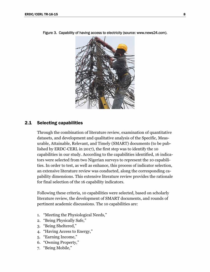
In order to implement the CA, two steps needed to be taken. The first step is to identify the appropriate capabilities (e.g., Figure 1, Figure 2, and Fig-ure 3), and the second step is to select the pertinent indicators to represent these capabilities. The first step required the researchers to follow three criteria, as listed below (Gardoni and Murphy 2010, 623):
• The selected capabilities need to be relevant and important. • The minimum number of possible capabilities needs to be specified. • Each of the selected capabilities needs to provide information that can-
not be ascertained from the other capabilities.
The CA process is accomplished by the steps listed below:
• Selection of capabilities. Identify capabilities that provide an accu-rate picture of the societal impacts.
• Selection of indicators. Pick appropriate indicators that track the societal impacts on the capabilities of interest.
• Scaling indicators. Scale the salient capability indicators to generate the corresponding capability indicator indices.
• Development of predictive models for indicator indices. De-velop regression models that can effectively forecast the changes in the values of capability indicator indices due to societal impacts of disrup-tions to civil infrastructure.

ERDC/CERL TR-16-15 7
• Development of an aggregated measure of capabilities. De-velop composite measure that summarizes the changes in capability in-dicator indices due to disruptions to civil infrastructure.
Figure 1. Capability of accessing potable water (source:: Water Scarcity, Daily Post Nigeria, Ugwuanyi, 20 January 2015).
Figure 2. Capability of being mobile (source: Bella Africana.com).
ERDC/CERL TR-16-15 8
Figure 3. Capability of having access to electricity (source: www.news24.com).
2.1 Selecting capabilities
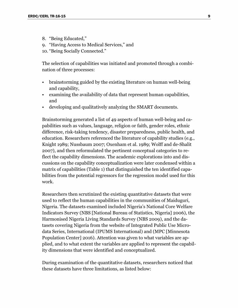
Through the combination of literature review, examination of quantitative datasets, and development and qualitative analysis of the Specific, Meas-urable, Attainable, Relevant, and Timely (SMART) documents (to be pub-lished by ERDC-CERL in 2017), the first step was to identify the 10 capabilities in our study. According to the capabilities identified, 16 indica-tors were selected from two Nigerian surveys to represent the 10 capabili-ties. In order to test, as well as enhance, this process of indicator selection, an extensive literature review was conducted, along the corresponding ca-pability dimensions. This extensive literature review provides the rationale for final selection of the 16 capability indicators.
Following these criteria, 10 capabilities were selected, based on scholarly literature review, the development of SMART documents, and rounds of pertinent academic discussions. The 10 capabilities are:
1. “Meeting the Physiological Needs,” 2. “Being Physically Safe,” 3. “Being Sheltered,” 4. “Having Access to Energy,” 5. “Earning Income,” 6. “Owning Property,” 7. “Being Mobile,”
ERDC/CERL TR-16-15 9
8. “Being Educated,” 9. “Having Access to Medical Services,” and 10. “Being Socially Connected.”
The selection of capabilities was initiated and promoted through a combi-nation of three processes:
• brainstorming guided by the existing literature on human well-being and capability,
• examining the availability of data that represent human capabilities, and
• developing and qualitatively analyzing the SMART documents.
Brainstorming generated a list of 49 aspects of human well-being and ca-pabilities such as values, language, religion or faith, gender roles, ethnic difference, risk-taking tendency, disaster preparedness, public health, and education. Researchers referenced the literature of capability studies (e.g., Knight 1989; Nussbaum 2007; Oxenham et al. 1989; Wolff and de-Shalit 2007), and then reformulated the pertinent conceptual categories to re-flect the capability dimensions. The academic explorations into and dis-cussions on the capability conceptualization were later condensed within a matrix of capabilities (Table 1) that distinguished the ten identified capa-bilities from the potential regressors for the regression model used for this work.
Researchers then scrutinized the existing quantitative datasets that were used to reflect the human capabilities in the communities of Maiduguri, Nigeria. The datasets examined included Nigeria’s National Core Welfare Indicators Survey (NBS [National Bureau of Statistics, Nigeria] 2006), the Harmonised Nigeria Living Standards Survey (NBS 2009), and the da-tasets covering Nigeria from the website of Integrated Public Use Micro-data Series, International (IPUMS International) and (MPC [Minnesota Population Center] 2016). Attention was given to what variables are ap-plied, and to what extent the variables are applied to represent the capabil-ity dimensions that were identified and conceptualized.
During examination of the quantitative datasets, researchers noticed that these datasets have three limitations, as listed below:

ERDC/CERL TR-16-15 10
• There is a lack of highly pertinent variables of interest, such as crime rate in a community to manifest the capability of “Being Physically Safe” and the annual household income to reflect the capability of “Earning Income.”
• A number of highly relevant variables of interest are present in sepa-rate datasets, while the regression model used here requires them to be in one single dataset.
• The data collected within the datasets were examined, but they had a relatively coarse granularity, as the database of IPUMS International only has data at the nation-state level, and the two Nigerian surveys have data at a maximum of local government area (LGA) level, which is lacking neighborhood, community, or household level of information.
Despite these limitations, examination of the dataset confirmed that con-ceptualization of capability dimensions through developing a matrix of ca-pabilities is meaningful and can be operationalized.
ERDC-CERL (Construction Engineering Research Laboratory) then devel-oped the SMART documents in the format of questionnaires to gain in-sight into the societal characteristics of communities (Figure 4 illustrates the data question sequence format). The SMART documents were de-signed to characterize five layers of infrastructure (i.e., communication, electricity, food security, transportation, and water). Through analysis, re-searchers confirmed strong connections between the major themes of the SMART documents and the capability dimensions conceptualized within the matrix of capabilities (see Table 1).
Assessing infrastructure’s impact with SMART documents follows the gen-eral sequence shown in Figure 4, and allows for:
• Defined Socio-Cultural Data Needs – understand how society uses infrastructure and the impact of disruptions.
• Standardized Data – standardized responses support an area-wide understanding of the human-infrastructure environment.
• Data Guides – guides analysts in interpreting and understanding data.
• Field Guides – instructions for observers and data collectors. • Shareable Reports & Dashboards – visualization tools to display
and communicate data and assessments.

ERDC/CERL TR-16-15 11
Figure 4. Data question collection sequence.
2.2 Selecting indicators and regressors
The second step of implementing the CA was selecting the pertinent indi-cators representing the appropriate capabilities. This process required the researchers to meet two criteria. The selected indicator needed to be repre-sentative of the corresponding capability and the chosen indicator needed to be intuitively plausible (Gardoni and Murphy 2010, 624–626). In order to ensure the representativity and plausibility of the indicators reflecting the appropriate capabilities, 16 indicator justifications were developed with respect to each of the selected 16 capability indicators. These 16 capa-bility indicators correspond to the 10 capabilities that were identified (see Table 1). Theoretically, an indicator is a “statistic of direct normative inter-est which facilitates concise, comprehensive and balanced judgments about the condition of major aspects of a society” (Land 1975, 15). A good indicator needs to have high construct validity, or “the degree to which a measure of a concept actually reflects the concept” (Stinchcombe and Wendt 1975, 58). The indicators selected to reflect the capability dimen-sions need to be unidimensional, occupying a single causal locus in the corresponding theoretical domain (Stinchcombe and Wendt 1975, 60). In addition, the indicators need to have good reliability, which refers to the quality of being replicable when used at different times (Stinchcombe and Wendt 1975, 60).
Based on the 10 capabilities identified and conceptualized, the 16 indica-tors represent and measure the capabilities. These indicators differ from the regressors. A regressor is a variable from a quantitative dataset used and determined by the regression model as being pertinent to predicting

ERDC/CERL TR-16-15 12
the value of a capability indicator of interest. Within the study, both indi-cators and regressors are based on the variables from the quantitative da-tasets that were investigated. Each indicator provides a schematic of the capability dimension it represents, and each can be derived from the varia-bles from the same quantitative dataset to which the indicator belongs. Any variable that is not the indicator within the dataset becomes a poten-tial regressor for the regression model to determine. Once examined by the regression model, a potential regressor will be either discarded from the model or contained as a regressor for deriving the capability indicator.
Based on these understandings, the appropriate indicators representing capability dimensions were identified from the two Nigerian surveys (NBS 2006; 2009), since these surveys provide the finest granularity among the datasets available. Concurrently, existing literature was referenced for evi-dence to support or disagree with the rationale for selecting capability in-dicators. This literature evidence is also reflected within Appendix A of this report, “Capability and Indicator Descriptions.” Bounded within the theoretical framework delineated by the reviewed literature, 16 indicators were selected from the two Nigerian surveys to represent the 10 identified capabilities (Table 1). These indicators were selected based on relevancy and the availability of data.
Table 1. Matrix of the 10 capabilities and the 16 supporting indicators.
Capability Indicator
Meeting physiological needs Main source of drinking water
Frequency of problems with supply of drinking water
Frequency of problems satisfying food needs
Being physically safe Do members feel safe walking on the street at night?
Being sheltered Frequency of problems paying house rent
Having access to energy Source of electricity
Number of hours without electricity in previous 24 hours
Earning income Household financial situation
Owning property Number of household durables
Dwelling ownership
Being mobile Time to nearest food market
Being educated Time to nearest primary school
Frequency of problems paying school fees

ERDC/CERL TR-16-15 13
Capability Indicator
Having access to medical services
Time to nearest hospital
Frequency of problems paying for healthcare
Being socially connected Can household depend on religious association during difficult period?
2.3 Review of the capability identification and indicator selection process
Based on the capability identification and indicator selection with the CA, a corresponding model was developed that measures the pre-interdiction capability level of the study area, and a logistic regression model was de-veloped that provides the prediction of the post-interdiction capability level of the study area—Maiduguri, Nigeria. Through comparing the pre-interdiction and post-interdiction capability levels of the study area, the ef-fects to the society and local populations resulting from the infrastructural interdictions of interest were successfully quantified.
The 16 capability indicator justifications provide the rationale for the deci-sions of selecting the pertinent indicators to represent the corresponding 10 capabilities. For each indicator, researchers present the capability that the indicator represents, display the survey question and the correspond-ing answers for deriving the values of the indicator, detail the pertinent in-formation, elaborate on the logic for choosing the indicator, and identify whether the indicator is replicable.
The societal impact is obtained by predicting the individual capability level as influenced by the physical damage, its cascading effects, and the pro-pensity of the society impact (i.e., the social vulnerability), which is influ-enced by its socioeconomic characteristics.
Including the population into this analysis embraces the challenges of rep-resenting the community and the day-to-day life of individuals within that community. The analysis looks at indicators and regressors that affect a given individual’s capability. The 10 capabilities analyze the well-being of society. Each capability has an indicator or multiple indicators, based on the determining factors, to identify the capability and the availability of data to substantiate the determination.

ERDC/CERL TR-16-15 14
Tabandeh et al. (2016) extended the capabilities-based risk analysis to pre-dict the capabilities of individuals by using a system reliability approach. The overall capability of individuals is treated as a system of intercon-nected components. Indicator indices, as proxies of specific capabilities, are the components of the system. To determine the overall capability of individuals, both the values of indicator indices and how those values col-lectively determine the overall capability must be known. It is proposed to develop empirical probabilistic predictive models for each indicator index that relates the values of the indicator indices to a set of influencing fac-tors. The developed probabilistic models, along with the configuration of indicator indices in the system, can be used to formulate a system reliabil-ity problem and predict the capabilities of individuals, for example, in the aftermath of a disruption. Comparing the predicted values in the post-dis-ruption condition with those measured/predicted in the pre-disruption situation can give an estimate of the extent of the societal impact.
Concurrent with the growth of urban population and the increased rate of development, the susceptibility of human communities to potentially dev-astating consequences of hazards is increasing. Consequences of past dis-asters have shown that such events can adversely impact people and communities in which they live and result in significant loss of lives, busi-ness interruption, direct and indirect economic loss, and various other so-cietal impacts. Examples of such disasters over the past decade include 2005 Hurricane Katerina in the United States, 2008 Sichuan earthquake in China, and 2011 Tohoku earthquake and tsunami in Japan. The conse-quences of such events can simply go beyond the geographic boundaries of the region that has been physically impacted. Also, the impact could be at multiple scales affecting governments, institutions, economic sectors, live-lihoods, and people. These past events have highlighted the significance of accounting for the far-reaching societal impacts, which is crucial both for the pre-event effective mitigation planning and the post-event optimal re-source allocation.
Similar hazards in different communities can result in dramatically differ-ent consequences. Furthermore, it is increasingly becoming clear that peo-ple and groups are impacted, react, adjust, and recover in different ways when a disruption occurs. Such differences are rooted in the societal char-acteristics of the communities. The ultimate impact of disruptive events is the product of dynamic interactions between the built environment (e.g., civil infrastructures) and the societal characteristics of the community.

ERDC/CERL TR-16-15 15
Due to the interdependencies of the infrastructure networks, the damage to the components of each network can propagate through different layers and result in cascading failures. The damage to the urban infrastructure would stimulate strong reactions from the population. The extent of such reactions and the subsequent chaos is related to the level of the realized damage and the societal characteristics of the communities. The important challenges in assessing the societal impact are to:
• determine what consequences are contributing and should be consid-ered,
• develop a mathematical formulation to quantify the overall conse-quences both in the immediate aftermath of the disruption and over time, and
• define the acceptable and tolerable levels of the perceived conse-quences.
The particular focus is to quantify the societal impact of disruptions to civil infrastructure systems. To this end, researchers identified the dimensions of well-being which are the testbed in order to quantify, compare, and ag-gregate the ultimate impact of various disruptive events.

ERDC/CERL TR-16-15 16
3 Extending the Capability Approach for Predictive Analysis
3.1 Reliability-based capability approach
The reliability-based capability approach augments the indicators and ca-pabilities by scaling the indicators to create indicator indices, developing probabilistic predictive models of the indicator indices, and developing an aggregate measure of the indicator indices. Here, the theoretical back-ground and the requirements of each step are briefly explained.
In selecting the capabilities, the main focus is on the underlying values of the problem, based on which capabilities might become important and the others trivial (capabilities relevance/significance). Among the set of all pertinent and significant capabilities, the particular interest is to select the smallest subset of capabilities that can provide all the required infor-mation (i.e., cover all the important dimensions of well-being in relation to the problem under study). This property is called the capability parsi-mony. Furthermore, it is desirable that each of the selected capabilities provides information that cannot be ascertained from the other ones. This property is called the capabilities orthogonality. The orthogonality prop-erty demands to avoid redundant information (i.e., selecting similar capa-bilities) that leads to overemphasizing a subset of well-being dimensions in a sense causing double counting.
Because capabilities are not directly measurable, indicators are selected as proxies for each capability. More precisely, the indicators are quantifying the achieved functionings. Hence, the selected indicators should be repre-sentative of the corresponding capability. Furthermore, the availability of data is an integral part of selecting the indicators. Typically, an ideal list of indicators is initially developed and justified using the best of knowledge available in the literature that is also supported by personal explanations. The ideal list might then be tailored/adjusted based upon the availability of data. The ideal list, however, could still be used as a guidance of the fu-ture work to collect the required data.
3.1.1 Scaling indicators
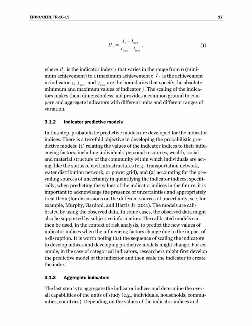
Before developing the aggregate measure, the indicators are scaled to cre-ate the indicator indices as follows in Equation (1):
ERDC/CERL TR-16-15 17
min
max min
: ,−
=−
jj
I III
I I (1)
where jII is the indicator index j that varies in the range from 0 (mini-mum achievement) to 1 (maximum achievement); jI is the achievement in indicator j ; minI , and maxI are the boundaries that specify the absolute minimum and maximum values of indicator j . The scaling of the indica-tors makes them dimensionless and provides a common ground to com-pare and aggregate indicators with different units and different ranges of variation.
3.1.2 Indicator predictive models
In this step, probabilistic predictive models are developed for the indicator indices. There is a two-fold objective in developing the probabilistic pre-dictive models: (1) relating the values of the indicator indices to their influ-encing factors, including individuals' personal resources, wealth, social and material structure of the community within which individuals are act-ing, like the status of civil infrastructures (e.g., transportation network, water distribution network, or power grid), and (2) accounting for the pre-vailing sources of uncertainty in quantifying the indicator indices; specifi-cally, when predicting the values of the indicator indices in the future, it is important to acknowledge the presence of uncertainties and appropriately treat them (for discussions on the different sources of uncertainty, see, for example, Murphy, Gardoni, and Harris Jr. 2011). The models are cali-brated by using the observed data. In some cases, the observed data might also be supported by subjective information. The calibrated models can then be used, in the context of risk analysis, to predict the new values of indicator indices when the influencing factors change due to the impact of a disruption. It is worth noting that the sequence of scaling the indicators to develop indices and developing predictive models might change. For ex-ample, in the case of categorical indicators, researchers might first develop the predictive model of the indicator and then scale the indicator to create the index.
3.1.3 Aggregate indicators
The last step is to aggregate the indicator indices and determine the over-all capabilities of the units of study (e.g., individuals, households, commu-nities, countries). Depending on the values of the indicator indices and

ERDC/CERL TR-16-15 18
their combination, the capabilities state of each unit is one of the follow-ing:
• acceptable • tolerable • intolerable
A system reliability problem can be formulated and analyzed to determine the capabilities state of each unit, accounting for the uncertainties in the values/categories of the indicator indices. The first step in the system reli-ability formulation is to define the states of the indicator indices (i.e., a map from the values/categories of the indicator indices to a set of prede-fined states). The second step is to describe what combinations of the indi-cator indices, in terms of their states, give rise to each of the three capabilities states. In the last step, a reliability analysis is performed for each unit, using the developed combination schemes and the probabilistic models of the indicator indices. The result of the reliability analysis for each unit is the probability distribution of its capabilities states.
3.2 Methods for predictive model framework
This section explains the proposed probabilistic formulation of indicator indices and how a Bayesian approach calibrates the models, using both the objective and the subjective information. The objective information refers to the observed data, and the subjective information refers to the experts’ knowledge. Finally, an explanation is given about how to formulate the re-liability problem and develop an aggregate measure of the indicator indi-ces that summarizes the overall impact.
3.2.1 Formulation of the probabilistic predictive models
An empirical probabilistic models were developed to predict the val-ues/categories of the indicator indices as functions of their influencing fac-tors. The general form of the proposed probabilistic predictive models is as follows in Equation (2):
( )1
, ,θ σ ε=
= + ∑x Θln
l l l lj lj l lj
g II x (2)

ERDC/CERL TR-16-15 19
where [ ( , )] : ln{ ( , ) / [1 ( , )]}l l l l l l l l lg II II II= −x Θ x Θ x Θ ; ( , )l l lII x Θ is the pre-dicted value of the thl indicator index; 1: ( ,..., )
ll l lnx x=x is the set of regres-sors (i.e., influencing factors); : ( , )l l lσ=Θ θ is the set of unknown model parameters that should be estimated, in which 1: ( ,..., )
ll l lnθ θ=θ ; and l lσ ε is the model error term, in which lσ is the standard deviation of the model error and is assumed to be independent of lx (homoscedasticity assump-tion) and lε is a standard normal random variable (normality assump-tion). The accuracy of the model prediction depends on different factors, including the form of the model, the quality of regressors in a sense that having strong relation with the corresponding indicator index, and the size of the database used for model calibration (i.e., estimating lΘ ).
The predictive model in Equation (2) works well for integer- or real-valued indicators and, thus, their indices. However, in practice, there are indica-tors that are categorical and take values only from a finite set. For such in-dicators, the predictive model in Equation (2) does not apply; hence, multinomial logit model was developed to predict the outcomes of the cat-egorical indicators. The general form of the model is as follows Equation (3):
( )
( )( ) { }
( ) { }
1
1
1 1
1
1 1
exp, 1, , 1 ,
1 exp,
1 , ,1 exp
l
l l
l l
nlkj ljj
lK nlkj ljk j
l l l
lK nlkj ljk j
xk K
xI k
k Kx
θ
θ
θ
=
−
= =
−
= =
∈ − += =
∈+
∑∑ ∑
∑ ∑
P x Θ
(3)
where [ ( , ) ]l l lI k=P x Θ is the probability that the indicator l , ( , )l l lI x Θ , has the label {1,..., }lk K∈ ; 1: ( ,..., )
ll l lnx x=x is a set of regressors; and 1 1: ( ,..., )
ll l lK −=Θ θ θ is the set of unknown model parameters that should be estimated, in which 1: ( ,..., )
llk lk lknθ θ=θ . It is useful to note that {1,..., }lK is an ordered set where the assigned numbers (i.e., {1,..., }lk K∈ ) are simply la-bels and do not show the actual gap between different k ’s. Indices (i.e.,
( , )l l lII x Θ ) can then by created by mapping the predicted indicators into numbers in the interval [0,1] .

ERDC/CERL TR-16-15 20
3.1.1 Bayesian updating and model selection
To estimate the unknown model parameters in Equations (2) and (3), a Bayesian updating rule (Box and Tiao 2011) was used, as follows in Equa-tion (4):
( ) ( ) ( ): ,κ=Θ Θ Θl l lf L p (4)
where ( )lf Θ is the posterior probability density function (PDF), repre-senting the updated information about lΘ ; ( )lL Θ is the likelihood function that contains the objective information about lΘ , gained from the ob-served values of indicator (indices) and the regressors; ( )lp Θ is the prior PDF of lΘ , representing the previous information about lΘ , based on, for example, a similar past experiment or experts knowledge; and
1: [ ( ) ( ) ]l l lL p dκ −= ∫ Θ Θ Θ is a normalizing constant. A significant challenge in the Bayesian inference is computing κ . Typically, the integral
( ) ( )l l lL p d∫ Θ Θ Θ is not analytically tractable, and its exact calculation is not feasible; however, the Monte Carlo simulation methods can be used (e.g., Gelman et al. 2014) to make approximate inference. Specifically, the Markov chain Monte Carlo (MCMC) simulation method (Haario et al. 2006) was used to estimate the posterior statistics of the unknown model parameters.
The likelihood function is proportional to the conditional probability of the observed indicator (indices) given a value of lΘ . Because the predictive models for the integer-/real-valued indicators (see Equation (2)) and the categorical indicators (see, Equation (3)) are different, their likelihood functions would be different as well. Specifically, the likelihood function of the model in Equation (2) can be written as Equation (5):
( ) ( )1
1 ,φσ σ=
∝
∏
θΘ
nli l
li l l
rL (5)
where 1
: ( ) lnli li lj ljij
r g II xθ=
= −∑ is the prediction's residual for the thi obser-
vation (e.g., individual or household). Likewise, the likelihood function of the model in Equation (3) can be written as Equation (6):
ERDC/CERL TR-16-15 21
( ) ( ) { }
1 1
, ,=
= =
∝ = ∏∏1
Θ P x Θl
I kli
Kn
l l li li k
L I k (6)
where lix and liI are the regressors and the label of the indicator lI for the thi observation; { }liI k=1 is an indicator function and defined such that
{ } 1liI k= =1 when liI k= and { } 0
liI k= =1 , otherwise.
If there is no prior information, a noninformative prior PDF can be used such that it has no or minimal influence on the posterior PDF. Hence, the Bayesian inference is unaffected by information external to the observa-tions. However, in practice, there might be external information beyond that provided by the observed data. For instance, in the case of a similar past experiment, the estimated posterior PDF could be used in that experi-ment as a prior PDF in the current calibration. Likewise, the expert knowledge could be incorporated to create a subjective prior PDF.
In general, it is possible to use more than just one database for calibrating the predictive models. In this way, both the number of observations (i.e., n in Equations (5) and (6)) and the number of variables (i.e., candidate x ’s in Equations (2) and (3)) can be extended. Enriching the database has sev-eral advantages, including that it: (1) increases the possibility to find varia-bles analogous to the ideal indicators; (2) increases the flexibility in selecting informative regressors that can sufficiently describe the variabil-ity in the corresponding indicators (i.e., increases the model accuracy); and (3) reduces the statistical uncertainty arises from the scarcity of data (i.e., the sampled data would sufficiently represent the actual situation of the population). However, in practice, there are difficulties to using such potentials. Typically, different databases do not have similar variables or observations; hence, the databases cannot simply be merged to create a larger database. Furthermore, the resolution of different databases might not be the same. There might be databases that give information at the in-dividual level, whereas others might only provide a summary of the statis-tics at the local community level. If the same set of variables (i.e., jI s and x s) are available in different databases, collected at different resolution or time periods, the updating rule of the Bayesian statistics will benefit in the following ways. First, the predictive models are calibrated, using one of the available databases to write ( )lL Θ along with a noninformative ( )lp Θ and estimate ( )lf Θ . Next, the calibration process is repeated with a new set of

ERDC/CERL TR-16-15 22
observations, but this time, with an informative ( )lp Θ that is the esti-mated posterior distribution from the previous run. This process can be repeated sequentially until all available databases are used.
Model selection is an integral part of developing the predictive models. First a pool of candidate regressors is created. Similar to the selection of the indicators, a list of ideal candidate regressors is developed that are be-lieved to have impacts on the corresponding indicators. The ideal list in-cludes different resources and constraints, listed earlier, that can influence the capabilities of individuals and, thus, the corresponding indicators. The ideal list might then be tailored based on the availability of the data. For practical prediction purposes, it is important to select regressors that are easily measurable/predictable at different locations and over time (e.g., over the region of interest in the aftermath of a disruption). Furthermore, it is desirable to eliminate the regressors that are not statistically signifi-cant in predicting the indicator (indices). For this purpose, a stepwise de-letion process was used to successively eliminate one regressor, ljx , at a time, based on the posterior statistics of the coefficient, ljθ . After each elimination, the model is recalibrated with the remaining regressors. The process is recursive up to the point that the elimination of one more re-gressor leads to a relatively significant increase in jσ in Equation (2) or a measure of the model error in Equation (3). The decision about the signifi-cance of the increase in the model error or where to stop the process is subjective, and it depends on the desired level of accuracy and the number of regressors left in the model.
The predictive models in Equations (2) and (3) are typically calibrated by using the data representing a stabilized situation of the society. When these models are used to predict the values/categories of the indicator in-dices in a chaos situation (e.g., in the aftermath of a disruption), care should be taken about changing the values of the regressors. To explain this point, attention is drawn to the relation between the indicator indices and their regressors. This relation can be of two kinds: (1) causal relation, in which a regressor is a sufficient cause to realize the indicator index, and (2) noncausal relation, in which there is only a pattern between the meas-ured/predicted regressor and the corresponding indicator index. When the relation is causal, a change in the value of the regressor means a change in the value/category of the indicator index, both in the stabilized and the chaos situations. However, in the case of the noncausal relation, a change

ERDC/CERL TR-16-15 23
in the value of the regressor happens in a condition different from the cali-bration one, and such a change can lead to a change in the value/category of the indicator (index) that might not replicate the reality. Hence, in this case, it might be reasonable not to change the values of such regressors.
3.2.2 Formulation of the reliability problem
The three capability states are defined in terms of the states of the indica-tor indices and their combinations. Murphy and Gardoni (2008) defined three states for the indicator indices with the same labeling as the capabil-ity states (i.e., acceptable, tolerable, intolerable). The principles of human rights (e.g., dignity, fairness, equality, and autonomy) can guide the de-scription of what conditions constitute each of the acceptable, tolerable, and intolerable states of the indicator indices. Human rights represent moral standards that individuals in a society should not fall below (e.g., human right to life, health, and subsistence; Caney 2010). According to Murphy and Gardoni (2008), the values/categories of the indicator indices that correspond to the intolerable state are so low that no individual should ever experience that state, regardless of its duration. To determine the states of the indicator indices, with reference to the previous discus-sion, first partition the values/categories of each indicator index into its acceptable, tolerable, and intolerable states. This partitioning can be used to determine the state of indicator indices and eventually, the capabilities states in the immediate aftermath of a disruption. To determine the state of the indicator indices and, thus, capabilities states over time, the effect of recovery is accounted for. For example, the tolerable state of the indicator indices would become intolerable if the required recovery time to improve to the acceptable state exceeds a reference duration.
Mathematically, the indicator indices are modeled as discrete random var-iables with three possible states. The probability of each state can be writ-ten as Equation (7):
( ) ( )( ) ( )( ) { }( )
,acc
,acc ,tol , ,
,tol ,acc ,tol , ,
Acceptable ,
Tolerable , , ,
Intolerable , , ,
= = ≥ = = < ≥ ≤
= = < < ≥ >
P P
P P
P P
j j j
j j j j j R j R j
j j j j j j j R j R j
II ii
II ii II ii T t
II ii II ii II ii T t
(7)

ERDC/CERL TR-16-15 24
where :[0,1] {Acceptable,Tolerable,Intolerable}j +× →R is the mapping func-tion from the values of the indicator indices and the recovery time to their states; jII is the random indicator index j modeled by Equation (2) or (3);
,acc (0,1)jii ∈ is the acceptable threshold that delimits the acceptable and tol-erable states of the indicator index j ; ,tol ,acc(0, )j jii ii∈ is the tolerable threshold that delimits the tolerable and intolerable states of the indicator index j ; ,R jT is the random recovery time to improve the state of the indi-cator index j from the tolerable state to the acceptable one; and ,R jt is the reference recovery duration beyond which the tolerable state transforms into the intolerable one. It is useful to note that not all the indicator indi-ces necessarily realize all the three states. There might be indicator indices for which only two states are defined (e.g., acceptable and intolerable).
The indicator indices can be viewed as the components of a system that are interacting with each other to satisfy a desired objective which in this case is the well-being of individuals. A fault-tree analysis is used to explore the conditions that can cause an unfavorable state of the system (i.e., tolerable or intolerable capabilities state). A fault tree is a deductive technique which starts with the unfavorable state of the system, called the top event, and then considers what can cause the occurrence of this state. The imme-diate causal events are identified and connected to the top event through a logic gate (i.e., an OR-gate or AND-gate). This deductive process then con-tinues from each of the immediate causal events until a certain level of de-tail is reached, called the basic events. A fault tree schematically illustrates how the occurrence of the basic events collectively give rise to the top event. A collection of the basic events, whose joint occurrence ensures re-alizing the top event, is called a cut-set. A cut-set is said to be minimal if there is no redundant basic event in the collection. In other words, a mini-mal cut-set is no longer a cut-set if any of the basic events is removed from the collection. The occurrence of at least one minimal cut-set is sufficient to realize the top event. Subsequently, the probability of the top event comes down to the calculation of the probability of occurrence of at least one minimal cut-set from all the potential ones.
Figure 5 shows an example fault-tree where the top event is the intolerable state of the capabilities. The immediate causal events, 1,intol 2,intol ,intol, ,..., mC C C are the intolerable states of each capability, connected to the top event through an OR-gate. This structure implies that the top event occurs when at least one capability is in its intolerable state. The justification is that be-

ERDC/CERL TR-16-15 25
cause capabilities are selected to be equally important and capture differ-ent aspects of well-being, failing to satisfy the acceptable state in each di-mension leads to the unacceptable state (i.e., intolerable state in this example) of the entire system. In the next step, the intolerable state of each capability is determined in terms of the corresponding indicator indi-ces. For instance, the causal event 1,intolC occurs when at least one of the in-dicator indices 1II , 2II , or 3II is in its intolerable state. Assuming a similar situation for all the other capabilities, the overall capabilities can be mod-eled as a series system of jII s, such that the intolerable state of any jII leads to the intolerable state of the overall capabilities. Accordingly, the probability of the top event can be written as Equation (8):
( ) ( )1
Intolerable Intolerable ,=
= = =
P P
J
jj
(8)
where 1:{ } {Acceptable,Tolerable,Intolerable}J× × → is a mapping function from the states of the indicator indices to the capabilities state. For the purposes of calculation, reliability methods can be used to solve Equation (8). Examples of such methods include the First-Order Reliabil-ity Method (FORM), the Second-Order Reliability Method (SORM), or dif-ferent simulation methods.
Figure 5. A fault-tree analysis of the intolerable state of a series system of capability indicators (University of Illinois).

ERDC/CERL TR-16-15 26
3.3 Aggregation process
To evaluate the capabilities of individuals, first the states of each indicator are determined. Fault-trees are created that explain the topology of the system. Subsequently, for each community, system reliability problems are formulated, and the probability distribution of the states of each capability are calculated as well as the probability distribution of the overall capabil-ity states.
Figures C1 through C10 (see Appendix C) show the relation between the categories/values of the capability indicators and their states. The color-codes of the acceptable, tolerable, and intolerable states of indicators are green, yellow, and red, respectively. For a subset of indicators, only two states may be defined. Examples include the indicators “Main Source of Drinking Water” and “Source of Electricity.” For the indicator “Main Source of Drinking Water,” there are three possible categories; however, because the first two categories are not significantly different, it was de-cided to label both as an acceptable state and to label the last category as a tolerable state. For the indicator “Source of Electricity,” however, there are only two possible categories defined; hence, having defined two states, in-stead of three, is due to the constraint of the possible categories.
Using the probabilistic predictive models developed in the previous sec-tion, three-state random variables can be created, representing the three states of indicators. Figure 6 and Figure 7 show the fault-tree developed for the tolerable and intolerable states, which represent the relation be-tween the states of the indicators and capabilities. Using the topology in the fault-tree, the probability distribution of the states of each capability as well as the overall capabilities can be calculated.
To illustrate the proposed formulation, system reliability analyses were performed for a household randomly selected from the database. The dia-grams in Figure 6 and Figure 7 show the capability fault-tree analyses for pre- and post-disruption situations of the selected household. To create the diagrams, the probability distributions of each indicator was first ob-tained by using the developed probabilistic predictive models along with the definitions of the state based on the values/categories. In the next step, the developed formulation of the system reliability problem for each capa-bility was used to obtain the corresponding probability distribution of the states. Finally, the expressions in Equations (28) through (30) were used

ERDC/CERL TR-16-15 27
to calculate the probability distribution of the states of the overall capabil-ity.
The developed fault-trees demonstrate a series system such that failure of each indicator in meeting the desired objective leads to the failure of the entire system. For example, the post-disruption fault-tree shows that intol-erable state of the indicator “Time to the Nearest Hospital” gives rise to the intolerable state of the overall capability. The graphical feature of the fault-tree allows one to see the root causes of different outcomes and guide where to invest resources in order to improve the system performance. Further, it provides an understandable basis to debate the topology of the system and how different indicators can contribute to the overall capabil-ity.
Figure 6. Fault tree before disruption (University of Illinois).

ERDC/CERL TR-16-15 28
Figure 7. Fault tree after disruption (University of Illinois).
3.4 Probability distribution
In the following subsections, the expressions for the probability distribu-tion of the states of each capability are derived.
3.4.1 Capability: “Meeting the Physiological Needs”
The expression for the probability of the acceptable state can be written as Equation (9):
( ) ( ){ }
( ) ( ) ( )
{ } ( ) ( )1
1 1,2,3
1 2 1 3 2
2 2
2 1 3 21 1
Acc. Acc.
Acc. Acc. Acc. Acc. Acc.
1 1 ,
jj
I jk j
I I j I k I
∈
== =
= = = = = = = = =
= = = = =∑∑
P P
P P P
1 P P
(9)
where 1{ }I j=1 is the probability that 1I j= ; because {1,2}j∈ ,
1{ }I j=1 is the probability of the acceptable state; 2 1( 1| )I I j= =P is the probability of the acceptable state of 2I , given that 1I j= ; and 3 2( | 1)I k I= =P is the proba-bility that 3I k= when 2 1I = is known, because {1,2}k∈ , 3 2( | 1)I k I= =P is the probability of the acceptable state given that 2 1I = . The category of the indicator 1I is predicted using the infrastructure network analysis; the

ERDC/CERL TR-16-15 29
probability of the predicted category is one, and the other states are zero. To obtain 2 1( 1| )I I j= =P for a household (or a community), Equation (31) is used, along with the values of the regressors for the household (or com-munity) and set 1I j= . Similarly, to obtain 3 2( | 1)I k I= =P , Equation (32)1 is used, along with the values of the regressors for the same household (or community) and set 2 1I = .
The probability of the intolerable state can be obtained as Equation (10):
( ) ( ){ }
( ){ }
( ) ( ) ( ){ } ( ) ( )
1
1 1,2,3
1,2,3
1 2 1 3 2
3 2 3
2 1 3 21 1 1
Intol. Intol.
1 Intol.
1 Intol. Intol. Intol. Intol. Intol.
1 ,
jj
jj
I jl k j
I k I j I l I k
∈
∈
== = =
= = = = − =
= − = = = = =
= − = = = =∑∑∑
P P
P
P P P
1 P P
(10)
where Intol. is the complement of the intolerable state which includes the acceptable and tolerable states. The calculation of the probability terms is similar to the terms in Equation (9). Accordingly, the probability of the tol-erable state can be found as Equation (11):
( ) ( ) ( )1 1 1Tolerable 1 Acceptable Intolerable .= = − = − =P P P (11)
3.4.2 Capability: “Being Physically Safe”
The achieved functioning in this capability is quantified by only one indi-cator. Hence, the calculation of the probability distribution of the capabil-ity’s states comes down to use of the developed predictive model, along with the designated states of the indicator Equation (12):
1 Equations 31–42 are shown in Appendix B.

ERDC/CERL TR-16-15 30
( ) ( ) ( )( ) ( ) ( )( ) ( ) ( )
2 4 4
2 4 4
2 4 4
Acceptable Acceptable 1 ,
Tolerable Tolerable 2 ,
Intolerable Intolerable 3 ,
I
I
I
= = = = =
= = = = = = = = = =
P P P
P P P
P P P
(12)
where the values of the regressors of the households (or community) in Equation (33) are used to obtain the corresponding probabilities.
3.4.3 Capability: “Being Sheltered”
Similar to the previous capability, this one is also quantified by means of only one indicator. Accordingly, the probability distribution of the capabil-ity’s states is obtained in Equation (13):
( ) ( ) ( )( ) ( ) ( )( ) ( ) ( )
23 5 51
3 5 5
3 5 5
Acceptable Acceptable ,
Tolerable Tolerable 3 ,
Intolerable Intolerable 4 ,
kI k
I
I
= = = = = = = = = = = = = = = =
∑P P P
P P P
P P P
(13)
where Equation (34) is used to obtain 5 5( 1), , ( 4)I I= =P P .
3.4.4 Capability: “Having Access to Energy”
The probability distribution of Equation (14):
( ) ( ){ }
( ) ( )
( ) ( )
( ) ( ) ( )
4 6,7
6 7
4
6 5 51
4 3
7 2 5 2 51 1
Acceptable Acceptable
Acceptable Acceptable
1
1 , ,
jj
l
l k
I I l I l
I I k I l I k I l
∈
=
= =
= = = = = =
= = = =
× = = = = =
∑
∑∑
P P
P P
P P
P P P
(14)
where Equation (35) was used to calculate 6 5( 1| )I I l= =P , in which 5I l= is set; use Equation (34) to obtain 5( )I l=P ; use Equation (36) to obtain
7 2 5( 1| , )I I k I l= = =P , in which 2I k= and 5I l= are set; and use Equation (31) to obtain 2( )I k=P .
ERDC/CERL TR-16-15 31
Next, the probability of the intolerable state is calculated as Equation (15):
( ) ( ){ }
( ){ }
( ) ( )( ) ( )
( ) ( ) ( )
4 6,7
6,7
6 7
4
6 5 51
4 3 2
7 2 5 2 51 1 1
Intolerable Intolerable
1 Intolerable
1 Intolerable Intolerable
1 1
, .
jj
jj
l
l k j
I I l I l
I j I k I l I k I l
∈
∈
=
= = =
= = = = − =
= − = =
= − = = =
× = = = = =
∑
∑∑∑
P P
P
P P
P P
P P P
(15)
Finally, the probability of the tolerable state can be written as Equation (16):
( ) ( ) ( )4 4 4Tolerable 1 Acceptable Intolerable .= = − = − =P P P (16)
3.4.5 Capability: “Earning Income”
Because the capability is quantified by only one indicator, the probability distribution of the capability can be simply obtained as Equation (17):
( ) ( ) ( )( ) ( ) ( )( ) ( ) ( )
45 8 83
5 8 8
5 8 8
Acceptable Acceptable ,
Tolerable Tolerable 2 ,
Intolerable Intolerable 1 ,
kI k
I
I
= = = = = = = = = = = = = = = =
∑P P P
P P P
P P P
(17)
where Equation (37) is used to calculate 8 8( 1), , ( 4)I I= =P P .
3.4.6 Capability: “Owning Property”
The joint distribution of the two capability indicators determines the prob-ability distribution of the capability. First, the probability of the acceptable state is obtained as Equation (18):

ERDC/CERL TR-16-15 32
( ) ( ){ }
( ) ( )
( ) ( )
6 9,10
9 10
6
9 104
Acceptable Acceptable
Acceptable Acceptable
1 ,
jj
kI k I
∈
=
= = = = = =
= = × =∑
P P
P P
P P
(18)
where Equations (38) and (39) are used to obtain 9( )I k=P and 10( 1)I =P . Because for both indicators the intolerable state is not defined, the associ-ated probability would be uniformly 0 (i.e., 6( Intolerable) 0= =P ). Ac-cordingly, the probability of the tolerable state can be written as Equation (19):
( ) ( )6 6Tolerable 1 Acceptable .= = − =P P (19)
3.4.7 Capability: “Being Mobile”
There is only one indicator to quantify this capability, and it is predicted by using the infrastructure network analysis. Thus, the probability distri-bution can be simply written as Equation (20):
( ) ( ) { }
( ) ( ) { }
( ) ( ) { }
11
11
11
37 11 1
7 11 4
7 11 5
Acceptable Acceptable ,
Tolerable Tolerable ,
Intolerable Intolerable .
I kk
I
I
==
=
=
= = = = = = = =
= = = =
∑P P 1
P P 1
P P 1
(20)
3.4.8 Capability: “Being Educated”
The two capability indicators are combined to obtain the probability distri-bution of the capability’s states. First, the probability of the acceptable state is written as Equation (21):
ERDC/CERL TR-16-15 33
( ) ( ){ }
( ) ( )
{ } ( )12
8 12,13
12 13
3 2
131 1
Acceptable Acceptable
Acceptable Acceptable
jj
I kk k
I k
∈
== =
= = = = = =
= × =∑ ∑
P P
P P
1 P
(21)
where 12I is obtained from the infrastructure network analysis and 13I is predicted using Equation(40). Next, the probability of the intolerable state is obtained as Equation (22):
( ) ( ){ }
( ){ }
( ) ( )
{ } ( )12
8 12,13
12,13
12 13
4 3
131 1
Intolerable Intolerable
1 Intolerable
1 Intolerable Intolerable
1 1 .
jj
jj
I kk k
I k
∈
∈
== =
= = = = − =
= − = =
= − × =∑ ∑
P P
P
P P
P
(22)
Subsequently, the probability of the tolerable state can be written as Equa-tion (23):
( ) ( ) ( )8 8 8Tolerable 1 Acceptable Intolerable .= = − = − =P P P (23)
3.4.9 Capability: “Having Access to Medical Services”
Similar to the previous capability, this one is consisting of two indicators. The probability of the acceptable state of the capability can be written as Equation (24):

ERDC/CERL TR-16-15 34
( ) ( ){ }
( ) ( )
{ } ( )14
9 14,15
14 15
3 2
151 1
Acceptable Acceptable
Acceptable Acceptable
,
jj
I kk k
I k
∈
== =
= = = = = =
= × =∑ ∑
P P
P P
1 P
(24)
where 14I is obtained from the infrastructure network analysis and 15I is predicted by using Equation(41). Next, the probability of the intolerable state is obtained from Equation (25):
( ) ( ){ }
( ){ }
( ) ( )
{ } ( )14
9 14,15
14,15
14 15
4 3
151 1
Intolerable Intolerable
1 Intolerable
1 Intolerable Intolerable
1 1 .
jj
jj
I kk k
I k
∈
∈
== =
= = = = − =
= − = =
= − × =∑ ∑
P P
P
P P
P
(25)
Finally, the probability of the tolerable state can be written as Equation (26):
( ) ( ) ( )9 9 9Tolerable 1 Acceptable Intolerable .= = − = − =P P P (26)
3.4.10 Capability: “Being Socially Connected”
The achieved functioning, this capability is quantified by means of a binary indicator. Thus, the capability has only two states, which are the accepta-ble and tolerable states. The corresponding probabilities can be obtained as Equation (27):
( ) ( ) ( )( ) ( ) ( )
10 16 16
10 16 16
Acceptable Acceptable 1 ,
Tolerable Tolerable 2 ,
I
I
= = = = =
= = = = =
P P P
P P P
(27)
where Equation (42) is used to calculate 16( 1)I =P and 16( 2)I =P .

ERDC/CERL TR-16-15 35
3.4.11 Overall capability
In the next step, the probability distribution of different capabilities is combined according to the fault-tree topology to obtain the probability distribution of the overall capability. The overall capability is modeled as a series system, such that the probability distribution of the states can be written as Equation (28):
( ) ( )
( ) ( )
( ) ( ) ( )
10
1
10
1
Acceptable Acceptable ,
Intolerable Intolerable ,
Tolerable 1 Acceptable Intolerable .
rr
rr
=
=
= = = = = =
= = − = − =
P P P
P P P
P P P
(28)
First, the probability of the acceptable state is calculated. The calculation involves a 16-fold summation of the joint probability distribution of the in-dicators. However, the statistical independence of a subset of indicators is of benefit. The final expression for the probability of the acceptable state can be written as Equation (29):
( ) ( )
{ } ( ) ( ) ( )
( ) { } ( ) ( )
( ) ( ) ( )
1
11
1
10 16
1 1
6 2 2
2 1 9 1 10 12 1 1
2 3 2 2
13 1 3 2 11 5 111 1 1 1
6 5 7 2 5 15 11
Acceptable Acceptable
1 1
1,
2 1 1,
r jr j
I jl k j
I lm l k j
I
I I j I l I j I I j
I k I j I j I I l I k I l
I I k I I I k I m I l
= =
== = =
== = = =
= = =
= = = = = = =
= = × = = = = =
= = = = = = =
×
∑∑∑
∑∑∑∑
P P P P
1 P P P
P 1 P P
P P P
1
{ } ( ) { } ( ) ( )2 14
3 3 4
4 12 8 14 16 141 1 3
1 1 .j I kj k j
I I j I j I k I I k= == = =
= = × = = = =∑ ∑∑P 1 P P
(29)
The probability of the intolerable state can be written as Equation (30):
ERDC/CERL TR-16-15 36
( ) ( )( )
{ } ( ) ( ) ( )
( ) ( ) ( )
{ }
11
12
10 10
1 1
16
1
3 4 2 3 3 2
2 3 2 11 5 111 1 1 1 1 1
6 5 7 2 5 15 11
4
Intolerable 1 Intolerable
1 Intolerable
1 ,
2 ,
r rr j
jj
I no n m l k j
I k
I j I k I j I n I l I n
I I l I m I j I l I o I n
I j I
= =
=
== = = = = =
=
= = − = = − =
= − = = = = = =
= = = = = = =
× =
∑∑∑∑∑∑
P P P P
P P
1 P P P
P P P
1 P
( ) { } ( ) ( )14
4 2 4 4 3
12 8 14 131 1 1 2 1
.I kk j k j j
k I j I k I j== = = = =
= × = = × =∑∑ ∑∑ ∑1 P P
(30)
The derived expressions for the probabilities of the acceptable and intoler-able states can be used in Equation (28) to obtain the probability of the tolerable state.
See Appendix B, Probabilistic Predictive Models of Indicator Indices, for an explanation of the probabilistic predictive models (Equations 31–42) that were developed for the indicator indices of the selected capabilities.

ERDC/CERL TR-16-15 37
4 Conclusion
4.1 Summary of efforts
This research used a capability approach to quantify the societal impact of disruptions to civil infrastructure. A set of 10 pertinent capabilities was se-lected to capture specific social, cultural, and economic aspects of individ-uals’ well-being. This list includes the following capabilities:
1. Meeting the physiological needs. 2. Being physically safe. 3. Being sheltered. 4. Having access to energy. 5. Earning income. 6. Owning property. 7. Being mobile. 8. Being educated. 9. Having access to medical services. 10. Being socially connected.
Because these capabilities are not directly measurable, a set of 16 indica-tors was selected to quantify the corresponding capabilities (See Table 1). For example, to quantify the achieved functionings of the capability of “Meeting the Physiological Needs,” three indicators were selected:
1. “Main Source of Drinking Water,” 2. “Frequency of Problems with Supply of Drinking Water,” and 3. “Frequency of Problems Satisfying Food Needs.”
The rationale behind selecting each indicator was discussed, and their sig-nificance and relevance were justified based on an extensive literature re-view and statistical analyses of different datasets. The third step involves scaling the indicators to create indices. The indicator indices vary in the range [0,1] , where 0 is the minimum achievement and 1 is the maximum. The values/categories of the indicators (or their indices) for each individ-ual/household depend on the status of the infrastructure systems to de-liver vital needs like potable water, the wealth to satisfy basic needs, and the social structure of communities. In order to quantitatively explore such relations, in the fourth step, probabilistic predictive models of the indica-tor (indices) were developed. An important consideration in developing

ERDC/CERL TR-16-15 38
the predictive models is to account for various sources of uncertainty sur-round the quantification of the indicator (indices). For example, there is uncertainty in predicting the value/category of indicator (indices) in the future. The values/categories of different indicators collectively determine the state of the corresponding capability, which could be in principle ac-ceptable, tolerable, or intolerable. In the last step, a system of capability indicators was created, and the methods of system reliability analysis were used to obtain the probability distribution of the capability states.
As an application of the proposed formulation, the capabilities of house-holds living in the urban areas of Maiduguri, Nigeria, was quantified. The disruptive event scenario used includes the failure of a fuel depot, which in turn cascades to a water treatment plant. To predict the values/categories of different indicator (indices), results of infrastructure network analysis were used along with the available census data in the predictive models. To determine the topology of the system of capability indicators, a fault-tree analysis was used (see Figure 6 and Figure 7). Given an unfavorable state of the system as a top event, the fault-tree systematically explores the root causes of observing the top event. The analytical expressions derived for the probability distribution of each capability were solved for each ca-pability.
4.2 Results
The results are summarized as a series of maps that show the average achievements of the households in Maiduguri in terms of each of the 10 ca-pabilities as well as their overall aggregated capability (see Appendix C, Figures C11–C21).
Future research could be conducted in a number of areas incorporating the SMART documents in information and data gathering either at a sur-vey level or observation level. Data Guides and Field Guides (forthcoming from ERDC-CERL in 20017) have been developed to assist SMART docu-ment users to capture relevant individual and societal detailed information based on the access, availability, and use of the five infrastructure nodes within this study (communication, electricity, food security, transporta-tion, and water).

ERDC/CERL TR-16-15 39
4.3 Scenario
The proposed framework is used, along with the collected data for the households in the urban area of Maiduguri, to calculate the spatial distri-bution of well-being in terms of each capability and overall capabilities. The predictive models developed for indicators are calibrated using the data for the households. However, the information about the location of the households, used for calibration, is available only at the LGA level. The result of the infrastructure network analysis, required to predict a subset of indicators and regressors, is available at the community level, where communities are smaller units within each LGA. To be consistent in the prediction of capabilities, the community was set as the target unit of anal-ysis. The averaged values of the regressors at the LGA level would apply to all communities within the LGA, unless the value of the regressors from the infrastructure network analysis that gives the values at the community level can be obtained. Furthermore, the network analysis is calibrated with the predicted quantities (i.e., regressors/indicators) at the LGA level, be-fore the occurrence of any disruptive events, being similar to those from the database.
A scenario was developed wherein a disruption impacts the fuel depot and the southeast water treatment plant and the failure propagation and social impacts were investigated. The fuel depot power substation is a critical node that supports a variety of other infrastructure nodes, including trans-portation, electricity, and water. The water treatment plant provides pota-ble water to a large portion of the city. After applying the model, the before and after disruption results were identified for the capability of “Meeting Physiological Needs.” Figure 8 shows the infrastructure nodes before dis-ruption and the level of access to that node and Figure 9 shows the infra-structure nodes after disruption and the cascading effect of the impacts to social well-being in terms of access to water and access to food.

ERDC/CERL TR-16-15 40
Figure 8. Example of infrastructure nodes before disruption and level of access to the node (initial source of water) (ERDC-CERL).

ERDC/CERL TR-16-15 41
Figure 9. Example of infrastructure nodes after disruption and the cascading effect of the impacts to social well-being (final source of water) (ERDC-CERL).
The impacts are that all electricity transformers are shut down, the elec-tricity network is disabled, while only local electrical generators can work based on fuel, providing very limited (and expensive) power supply to nearby communities. Furthermore, the water network is also disrupted, while only local water vendors can pump water from wells.
In terms of meeting physiological needs, the indicators represented in-clude access to water and access to food (see Figure 10–Figure 13). The water distribution system is impacted by requiring individuals to go to an alternative source to obtain water. Access cost therefore increases making it more difficult to meet physiological needs. Depending on the area, ac-cess to food is compromised—restaurants do not have power, markets can’t keep food fresh, and agriculture suffers from lack of water source. The transportation network is ultimately effected, and access to food and water is compromised. Three indicators were selected to address physio-logical needs:

ERDC/CERL TR-16-15 42
1. “Main Source of Drinking Water,” 2. “Frequency of Problems with Supply of Drinking Water,” and 3. “Frequency of Problems Satisfying Food Needs.”
Figure 10. Example of infrastructure nodes before disruption and level of access to the node (initial source of water) (ERDC-CERL).

ERDC/CERL TR-16-15 43
Figure 11. Example of infrastructure nodes after disruption and the cascading effect of the impacts to social well-being (final source of water) (ERDC-CERL).

ERDC/CERL TR-16-15 44
Figure 12. Example of infrastructure nodes before disruption and level of access to the node (initial time to food) (ERDC-CERL).

ERDC/CERL TR-16-15 45
Figure 13. Example of infrastructure nodes after disruption, and the cascading effect of the impacts to social well-being (final time to food) (ERDC-CERL).
The capabilities of households in different communities are evaluated in an average sense. For this purpose, the three capability states were scored as {0,0.5,1}, respectively, for intolerable, tolerable, and acceptable states. Combining the scored state with the corresponding calculated probabili-ties will estimate the averaged values. Based on these calculations, a series of maps was created (see Appendix C, Figures C11–C23) that show the av-eraged capabilities before and after the disruption. The post-disruption ca-pabilities represent the immediate aftermath condition. To predict the long-term effects, further information is required about the restoration process and how fast the states of capabilities would be improved. From the obtained results, it can be observed that there are only three capabili-ties that are changed with respect to the pre-disruption situation. How-ever, when evaluating the impact of a disruption, it is important to account for all the defined capabilities and not to focus only on those whose values have changed. The impact of a disruption in two communities subject to the same change in a subset of capabilities, but being noticeably different in terms of other capabilities, would not be similar. Furthermore, when the capabilities are statistically dependent, the improvement in one capability can affect the others as well. Hence, the decision about where to invest the

ERDC/CERL TR-16-15 46
limited resources would be different whether or not the state of unchanged capabilities were accounted for.

ERDC/CERL TR-16-15 47
Appendix A: Capability and Indicator Descriptions
Capability: “Meeting the Physiological Needs”
This capability represents one of the two facets within the concept of meet-ing physiological needs. In this study, two physiological needs were con-sidered: the need for potable water and the need for food (as identified in Table A1). These two needs are fundamental for survival.
Table A1. Capability of “Meeting the Physiological Needs” (NBS 2006).
Indicator NBS Question Answer Main Source of Drinking Water What is the main source
of drinking water? Pipe-borne water, treated. Pipe-borne water, untreated. Bore hole or hand pump. Protected well. Unprotected well. Rain water. River, lake, or pond. Vendor, truck. Other.
Frequency of Problems with Supply of Drinking Water
Are there any problems with supply of drinking water?
No. Yes, during dry season. Yes, frequently.
Frequency of Problems Satisfying Food Needs
Are there any problems with satisfying food needs?
Never. Seldom. Sometimes. Often. Always.
Indicator: “Main Source of Drinking Water”
As outlined by Table A1, the first indicator of the capability of “Meeting the Physiological Needs” is “Main Source of Drinking Water.” This indicator is used to refer to the aspect of access to potable water.
Every human being needs clean drinking water to sustain her/his life, bod-ily health, and other central human capabilities (Nussbaum 2007, 23). The
ERDC/CERL TR-16-15 48
quality of drinking water source defines the level of an individual’s capa-bility to meet physiological needs, especially in Sub-Saharan Africa (Akali et al. 2014). According to the World Health Organization (WHO)/United Nations Children’s Emergency Fund (UNICEF) Joint Monitoring Pro-gramme (JMP), drinking water sources can be categorized into four groups, as given below:
1. Piped water on premises. 2. Other improved sources, including public tap or standpipe, tubewell or
borehole, protected spring, protected dug well, and rainwater collec-tion.
3. Unimproved sources, including unprotected dug well, unprotected spring, cart with small tank or drum, tanker truck, and bottled water.
4. Surface water (UNICEF and WHO 2012, 33; 2015, 50).
Here, the rationale for the JMP’s classifying bottled water as an “unim-proved” drinking water source is due to the observation that “bottled water alone does not provide [an] affordable supply of water for all domestic needs” (UNICEF and WHO 2011, 45).
In Nigeria, the borehole and the treated utility piped water are the most reliable drinking water sources, while water from vehicle tankers and pro-tected dug wells is also decent but of lower quality (Ince et al. 2010, 40). The operational practices of the vehicle tankers might affect the water quality, while “protected dug wells are normally managed by individual households”, and their quality relies on the hygiene conditions of the man-aging households (Ince et al. 2010, 40).
Based on these universal and local conditions, a protocol was developed to determine the scale that represents the corresponding levels of quality of drinking water sources identified within the dataset (NBS 2006). Based on the UNICEF/WHO JMP’s taxonomy of drinking water sources (UNICEF and WHO 2012, 33; 2015, 50), the sources were ranked from 1 to 4, re-spectively. Following the local assessment of drinking-water quality in Ni-geria (Ince et al. 2010, 40), borehole and treated utility piped water were coded 1, vehicle tanker and protected dug well were coded 2, and the other drinking water sources in Maiduguri were coded 3. Through summing up these two sets of integer scores, a scale of drinking water sources was de-rived, as listed below in Table A2.

ERDC/CERL TR-16-15 49
Table A2. Drinking water source priority protocol (ERDC-CERL).
Group Source UNICEF/WHO JMP Score
Local Assessment Score
Final Score
Very Good
Pipe-borne water, treated 1 1 2
Good Bore hole or hand pump 2 1 3
Decent
Protected well 2 2 4
Vendor, truck 3 2 5
Rain water 2 3 5
Poor Pipe-borne water, untreated 3 3 6
Unprotected well 3 3 6
Very Poor
River, lake, or pond 4 3 7
Other 4 3 7
Disruptions in water supply/infrastructure will possibly negatively impact drinking water sources. The value of the indicator “Main Source of Drink-ing Water” is likely to shift toward the less desirable after a disruption oc-curs. However, for the residents whose drinking water sources are already poor, the relief drinking water supply, such as sachet and bottled water provided immediately to the affected areas, might temporarily increase those residents’ level of well-being by having access to a more desirable source of potable water, reflected by the indicator “Main Source of Drink-ing Water.”
Indicator: “Frequency of Problems with the Supply of Drinking Water”
The second indicator manifesting the capability of “Meeting the Physiolog-ical Needs” is “Frequency of Problems with the Supply of Drinking Water”, as illustrated in Table A1.
During a disruption or in a disaster situation, such as after an earthquake (Mileti 1999, 91), tsunami (CDC [Centers for Disease Control] 2014), hur-ricane (EPA 2005), flood (EPA 2015), massive explosion (Colon and Ford 2015), or terror event (Gleick 2006), the drinking water sources within the impact area are likely to be damaged or polluted, so the affected locals might face a shortage of drinking water after the disruption. In Maiduguri, one of the main water sources is the Alau Reservoir, which is located 14 km

ERDC/CERL TR-16-15 50
southeast of the city. The Alau Reservoir, along with a treatment plant about 100 m from University of Maiduguri Gate II, has become one of the main sources of drinking water for the city of Maiduguri (World Bank 1996; Dammo and Sangodoyin 2014, 387).
However, a drinking water shortage could still occur if the Alau Reservoir were to dry up during the dry season from January to July (e.g., World Bank 1996, 4). Moreover, recent local studies show that beyond-tolerance-levels for lead and pesticide concentrations have been detected in the tis-sues of fish samples from the Alau Reservoir (Dimari et al. 2008; Akan et al. 2013). Also, researchers have detected high concentrations of nitrate, phosphate, and Escherichia coli in the Alau Reservoir (Dammo and Sangodoyin 2014). Thus, it is anticipated that when a severe disruption oc-curs to the local community, the impact will negatively affect the existing issues with the supply of drinking water in the city of Maiduguri. The im-pact could immediately increase the frequency of problems with the supply of drinking water that a local household would face. If one household’s fre-quency of problems with supply of drinking water is already high, it is an-ticipated that a disruption could exacerbate this situation.
Indicator: “Frequency of Problems Satisfying Food Needs”
As displayed in Table A1, the third indicator of the capability of “Meeting the Physiological Needs” is “Frequency of Problems Satisfying Food Needs.” This indicator represents the availability of food, access to food, and local food security.
Food security is characterized as a “situation that exists when all people, at all times, have physical, social, and economic access to sufficient, safe, and nutritious food that meets their dietary needs and food preferences for an active and healthy life” (FAO [Food and Agriculture Organization of the United Nations] 1996; FAO 2001, 49). Food security is not only related to the supply of food or food availability, but also it is dependent on the enti-tlement of the household that could guarantee the food to be accessible to the household (Sen 1981; FAO 2003, 28).
When a disruption occurs, the impact could damage livestock, crops, and farming facilities (Alexander 1993, 329; Tobin and Montz 1997, 245; Mileti 1999, 91). It could also lead to household income loss due to destruction of workplaces (Mileti 1999, 98), thus disrupting the entitlements of the local residents and subsequently the local food consumption.
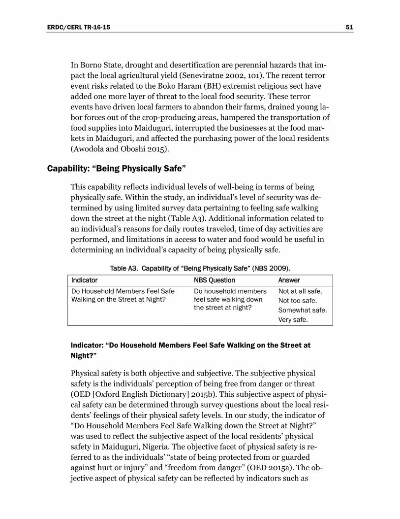
ERDC/CERL TR-16-15 51
In Borno State, drought and desertification are perennial hazards that im-pact the local agricultural yield (Seneviratne 2002, 101). The recent terror event risks related to the Boko Haram (BH) extremist religious sect have added one more layer of threat to the local food security. These terror events have driven local farmers to abandon their farms, drained young la-bor forces out of the crop-producing areas, hampered the transportation of food supplies into Maiduguri, interrupted the businesses at the food mar-kets in Maiduguri, and affected the purchasing power of the local residents (Awodola and Oboshi 2015).
Capability: “Being Physically Safe”
This capability reflects individual levels of well-being in terms of being physically safe. Within the study, an individual’s level of security was de-termined by using limited survey data pertaining to feeling safe walking down the street at the night (Table A3). Additional information related to an individual’s reasons for daily routes traveled, time of day activities are performed, and limitations in access to water and food would be useful in determining an individual’s capacity of being physically safe.
Table A3. Capability of “Being Physically Safe” (NBS 2009).
Indicator NBS Question Answer Do Household Members Feel Safe Walking on the Street at Night?
Do household members feel safe walking down the street at night?
Not at all safe. Not too safe. Somewhat safe. Very safe.
Indicator: “Do Household Members Feel Safe Walking on the Street at Night?”
Physical safety is both objective and subjective. The subjective physical safety is the individuals’ perception of being free from danger or threat (OED [Oxford English Dictionary] 2015b). This subjective aspect of physi-cal safety can be determined through survey questions about the local resi-dents’ feelings of their physical safety levels. In our study, the indicator of “Do Household Members Feel Safe Walking down the Street at Night?” was used to reflect the subjective aspect of the local residents’ physical safety in Maiduguri, Nigeria. The objective facet of physical safety is re-ferred to as the individuals’ “state of being protected from or guarded against hurt or injury” and “freedom from danger” (OED 2015a). The ob-jective aspect of physical safety can be reflected by indicators such as

ERDC/CERL TR-16-15 52
crime rate of the local community, and the per capita number of injuries or deaths caused by violent events in the local community. Researchers have not yet found satisfactory indicators reflecting the objective aspect of phys-ical safety for our purpose. It is recognized that the identification of these indicators would increase the accuracy of this study’s model results.
In the northern states of Nigeria, especially in Borno State, religious vio-lence committed by the BH religious sect has posed great threat to the well-being of the local residents. In Maiduguri, the BH extremists attack police stations, mosques and churches, and food markets (Onuoha 2010, 60; Awodola and Oboshi 2015, 14). With the rise of such terrorist events, it is also observed that local gunshot injuries have become rampant in Mai-duguri (Abba et al. 2012, 19).
Given the existing poor physical safety situation in and around Maiduguri, it is helpful to identify how the local residents perceive their physical safety levels.
Capability: “Being Sheltered”
An individual’s housing situation was determined based on limited survey data pertaining to problems paying rent (see Table A4). Additional infor-mation related to an individual’s access to housing, living conditions, in-come status, and family dynamics would enhance the understanding of an individual’s capacity of being sheltered.
Table A4. Capability of “Being Sheltered” (NBS 2006).
Indicator NBS Question Answer Frequency of Problems Paying House Rent
How often in the last year did you have problems satisfying the house rent of the household?
Never. Seldom. Sometimes. Often. Always.
Indicator: “Frequency of Problems Paying House Rent”
According to the United Nation’s “Universal Declaration of Human Rights,” an adequate level of housing is one of the major elements that constitute an adequate standard of living, which has been defined as a uni-versal right of all human beings (UNGA [United Nations General Assem-bly] 1948, 76). For some researchers, housing is one of the best indicators

ERDC/CERL TR-16-15 53
of a person’s standard of living and her/his place in the society (Festus and Amos 2015, 53).
In Nigeria, with the rapid rate of urbanization, there has been a great shortage of adequate housing facilities in urban areas (Abiodun 1976, 339). A phenomenal increase of housing needs resulting from such short-ages in housing units is common, especially in the urban centers (Olotuah and Taiwo 2013, 2).
In order to reflect the local residents’ well-being level in terms of the capa-bility of “Being Sheltered,” the indicator “Frequency of Problems Paying House Rent” was used. It is assumed that those households in Maiduguri who are having more frequent problems paying house rent tend to have a lower level of quality of life in terms of being sheltered.
Restoring housing is always one of the most important aspects of commu-nity recovery (Zhang and Peacock 2010, 5). However, such a housing re-covery process is not the same for all affected individuals. Residents with lower socioeconomic status tend to experience disproportionately higher levels of damage (Peacock et al. 2014, 357). The more socially vulnerable population is more prone to experiencing a deterioration of housing condi-tion, even after a disaster recovery process.
Capability: “Having Access to Energy”
This capability reflects the well-being level of individuals living in the study area in terms of having access to the electrical grid (or an alternative power source), and what energy source is actually used and reliable.
Since there are relatively very few respondents who gave the other three answers (shown in Table A5), the answers of “None” and “NEPA (National Electric Power Authority) only” are the only ones taken into account within this study’s regression model.
Table A5. Capability of “Having Access to Energy” (NBS 2006).
Indicator NBS Question Answer Source of Electricity What is the main source of
electricity? None. NEPA only. Rural electrification only. Private generator only. Rural electricity plant or generator.

ERDC/CERL TR-16-15 54
Indicator NBS Question Answer Number of Hours without Electricity in Previous 24 Hours
How many hours have you experienced without electricity during the previous 24 hours?
0-24
Indicator: “Source of Electricity”
Energy is the most important element in the economic development, pov-erty eradication, and security of any nation state in the modern world. Its consumption is directly related to the standard of living of the individual residents (Oyedepo 2012, 2).
Although Nigeria has an abundance of energy resources, the country has been experiencing an energy crisis for two decades (Oyedepo 2012, 2-3). In 2009, only about 40% of households in Nigeria were connected to the national grid (Sambo 2009, 15). According to the Nigerian Energy Policy report from 2003, even those connected to the national grid system were short of power supply over 60% of the time (Obadote 2009, 2).
According to the 2006 survey, NEPA was the sole monopoly of power gen-eration, transmission, and distribution in Nigeria since 1972 (Olukoju 2004, 53–54). Rural residents in Nigeria still use biomass energy such as firewood, agricultural residue, animal wastes, municipal solid wastes, saw-dust, and wood wastes, as main sources of energy (Sambo 2009, 16–17). Nonetheless, NEPA’s electricity service had been increasingly intolerable according to the local residents (Olukoju 2004, 54). When a community disruption occurs, the local neighborhoods in the affected area will experi-ence a loss of access to electricity (Mileti 1999, 91–92).
Indicator: “Number of Hours without Electricity in the Previous 24 Hours”
This indicator represents the individuals’ capability of having access to a reliable source of electricity, and how the individual’s daily routines are shaped by this access to electricity.
In terms of using the indicator “Number of Hours without Electricity in Previous 24 Hours,” the rationale is that this indicator reflects the quality of electricity service that one household in Nigeria is enjoying. However, when using this indicator, there is a need to be aware that only less than 45% of the respondents provided meaningful answers to this survey ques-

ERDC/CERL TR-16-15 55
tion. Although this percentage is consistent with the percentage of popula-tion that has access to the national grid system, such a small percentage of meaningful answers might pose difficulties to the operations of running this study’s regression model.
In spite of these facts, literature shows that when a large scale of disrup-tion occurs to a community, the local residents’ access to electricity could be severely impacted (Mileti 1999, 91–92). Thus, it is anticipated that if a local household is already experiencing a large number of hours without electricity in a 24-hour period, a disruption could decrease availability of electricity to a greater extent.
Capability: “Earning Income”
This capability reflects the well-being of individuals living in the study area in terms of income and financial status (see Table A6). It characterizes the household’s financial well-being.
Table A6. Capability of “Earning Income” (NBS 2009).
Indicator NBS Question Answer Household Financial Situation What is your household
financial situation? Very poor. Poor. Moderate. Fairly rich. Rich.
Indicator: “Household Financial Situation”
Adequate income is one of the fundamental aspects that determine the well-being level of an individual (Sen 1993, 41–42; Burchardt 2010). An individual’s income level is also highly correlated with her/his other well-being dimensions such as being literate and being healthy (Sen 1999a, 19).
Since 2014, Nigeria has emerged as Africa’s largest economy (CIA [Central Intelligence Agency] 2015). Its gross domestic product (GDP) at market prices was US$568.5 billion in 2014 (World Bank 2016). However, af-fected by its total population of 177.5 million, Nigeria’s GDP per capita was a mere US$3,203, ranking Nigeria 119 among a total of 184 countries with the available data around the world (World Bank 2016). Also, Nigeria has a gross national income (GNI) per capita of US$2,970, only the 114th high-est among the 171 national entities with available data in the world (World
ERDC/CERL TR-16-15 56
Bank 2016). Additionally, Nigeria’s inflation rate of 8.1% in 2014, as meas-ured by the consumer price index, was the 17th highest among 173 coun-tries in the world (World Bank 2016). The unemployment rate of Nigeria was at 7.5% in 2014, ranking it 76 among 174 countries in the world (World Bank 2016). However, Nigeria’s Gini index is relatively large, at 43.0 in 2009, ranking it 22 among the 75 countries with the available data (World Bank 2016). Therefore, the overall income level of an average household in Nigeria is medium low, compared to other countries in the world.
A household’s financial situation reflects the level of the household’s capa-bility of “Earning Income.” Thus, in order to represent the local residents’ well-being level in terms of earning income in Maiduguri, “Household Fi-nancial Situation” was chosen as an appropriate indicator.
Literature suggests a large scale disruption to a community could severely affect the local residents’ assets and livelihoods, both of which could con-tribute to a change of income to the population in the affected area (Mileti 1999, 98; Wisner et al. 2003, 222). However, such a disruption might une-qually affect the local residents’ financial situation. The redistribution of income after a community disruption is determined to a large extent by the socioeconomic factors of the local neighborhoods (Wisner et al. 2004, 222).
Capability: “Owning Property”
This capability characterizes the levels of well-being in terms of owning or renting a home and owning household items or durables, as identified in Table A7. In Table A7, the answers “Rents the dwelling,” “Pays nominal or subsidized rent,” “Uses without paying rent,” and “Nomadic or temporary dwelling” were grouped together and then tagged with “Does not own the dwelling.” As for owning durables, the potential items that individuals may possess are listed.

ERDC/CERL TR-16-15 57
Table A7. Capability of “Owning Property” (NBS 2006).
Indicator NBS Question Answer Number of Household Durables
Does your household own an electric iron? Does your household own a charcoal iron? Does your household own a refrigerator? Does your household own a television? Does your household own a personal computer? Does your household own a fixed line telephone? Does your household own a mobile phone? Does your household own a mattress or bed? Does your household own a radio? Does your household own a watch or clock? Does your household own a sewing machine? Does your household own a modern stove? Does your household own gas cooker? Does your household own a generator? Does your household own a bicycle? Does your household own a motorcycle? Does your household own a vehicle? Does your household own a fan? Does your household own a canoe? Does your household own a mat? Does your household own a VCR (videocassette recorder)? Does your household own a donkey? Does your household own a camel? Does your household own furniture?
Yes No
Dwelling Ownership What is the occupancy status of the dwelling used?
Owns the dwelling. Rents the dwelling. Pays nominal or subsidized rent. Uses without paying rent. Nomadic or temporary dwelling.
Indicator: “Number of Household Durables”
The household durables indicator is a composite index. It is constructed to represent individuals’ capability of “Owning Property” with respect to du-rable goods. Being able to hold property in the form of durable goods and having the pertinent property rights on an equal basis with others is one of the major aspects of an individual’s central capability of control over their material environment (Nussbaum 2011, 34). Also, the characteristics of
ERDC/CERL TR-16-15 58
commodities or goods possessed by an individual provide the basic infor-mation for deriving that individual’s capability (Sen 1999b, 6–7).
In Maiduguri, Nigeria, scholars have utilized ownership of the individual assets as an indicator to demonstrate the positive result of local develop-ment program, such as the Promoting Sustainable Agriculture project in southern Borno State (PROSAB [Promoting Sustainable Agriculture Pro-ject in Southern Borno State, Nigeria] in Manza and Atala 2014). However, by combining all the variables of durable ownership together, a more vivid picture is captured that manifests the well-being levels of the local house-holds.
When a community disruption occurs, residents living in the affected area are likely to experience losses due to damage to their personal belongings, such as their durable properties (Tobin and Montz 1997, 250; Mileti 1999, 66). It is anticipated that a disruption could reduce the number of dura-bles possessed by one household living in the affected area.
Indicator: “Dwelling Ownership”
Home ownership is traditionally regarded as a major indicator of eco-nomic well-being at the household level (Megbolugbe and Linneman 1993, 659). Conventional urban studies researchers note that home ownership increases local residents’ opportunity level through enhancing personal wealth, improving local residents’ psychological and physical health, sup-porting youth behaviors that facilitate social advancement, promoting neighborhood stability, and encouraging participation in voluntary activi-ties (Rohe et al. 2002, 53). Although the causal relationship between home ownership and the perceived benefits associated with home ownership still is not well understood (Schwartz 2010, 292), home ownership is corre-lated with those benefits, and especially noticeably for this study’s pur-pose, home ownership is correlated with personal wealth that facilitates the possession of properties.
In Nigeria, home ownership is one of the highest priorities of most house-holds (Udechukwu 2008, 182). For those who own a house in Nigeria, home ownership “represents their largest singular investment accounting for about 60 percent of household income” (Udechukwu 2008, 182). Home ownership in Nigeria brings substantial social benefits, as it posi-tively affects “educational achievement, civil participation, health benefits, public assistance, [and] property maintenance and improvement” (Halid

ERDC/CERL TR-16-15 59
and Akinnitire 2013, 41). Home ownership in Nigeria also provides “pride of ownership, freedom of control, privacy, strong credit base, financial sta-bility, [and appreciation] of asset” (Halid and Akinnitire 2013, 41).
Home ownership in Nigeria is to a large extent determined by income level of the household (Halid and Akinnitire 2013; Nwakanma and Nnamdi 2013). However, as has been indicated by the 8th indicator “Household Fi-nancial Situation,” most of the Nigerian residents have a moderate, poor, or very poor level of income. Consequently, Nigeria’s urban owner-occu-pancy rate was merely 52% in 2008 (EFInA [Enhancing Financial Innova-tion and Access] 2010, 30). Concomitant to the low income level of local residents, other barriers to home ownership in Nigeria include problems with land accessibility in terms of poor land availability and difficulty in land transaction, a poor mortgage finance system, a high inflation rate, the high cost of building materials, and poor quality of construction (Halid and Akinnitire 2013, 42; Udechukwu 2008, 185–191; Udoekanem et al. 2014, 186).
Capability: “Being Mobile”
This capability characterizes daily routines, destinations, and available modes of transportation of individuals (see Table A8).
Indicator: “Time to Nearest Food Market”
The level of mobility depends on both internal physical ability of an indi-vidual to move and the external environmental factors such as availability and accessibility of transportation facilities.
Since its establishment as a regional capital city, Maiduguri has become a commercial center that attracts people from all other Nigerian states and nearby countries (Kyari 2002, 7–8; Awodola and Oboshi 2015, 13). Conse-quently, transportation issues are always problematic, both between Mai-duguri and other cities in Nigeria and within the city of Maiduguri (Oladejo and Tamber 2014, 448; Mukhtar et al. 2015, 14). In order to cap-ture both the internal and external factors that determine an individual’s travel capability in the city of Maiduguri, using “Time to Nearest Food Market” was proposed as the appropriate indicator.

ERDC/CERL TR-16-15 60
Table A8. Capability of “Being Mobile” (NBS 2006).
Indicator NBS Question Answer Time to Nearest Food Market How long does it take you
to the nearest food market?
0-14 minutes. 15-29 minutes. 30-44 minutes. 45-59 minutes. 60+ minutes.
In Maiduguri, among others there are three major food markets: (1) Gom-boru market for perishable products, (2) the Baga fish market for fish and seafood, and (3) the Monday Market for food distribution and supply in-side and outside Nigeria (Awodola and Oboshi 2015, 13). Given that the food markets are located across the city of Maiduguri, “Time to Nearest Food Market” was used as the proxy measure of an individual’s capability of “Being Mobile.”
When a community experiences a severe disruption, the local transporta-tion systems could be severely impacted (Stallings 1995, 117; Mileti 1999, 91). Local residents living in the affected area may find it more difficult to move around. Thus, it is anticipated that after a disruption, the average time that local residents travel to the nearest food market will be in-creased.
Capability: “Being Educated”
This capability identifies education availability, access, location, and af-fordability (see Table A9).
Table A9. Capability of “Being Educated” (NBS 2006).
Indicator NBS Question Answer Time to the Nearest Primary School How long in minutes
does it take you from here to reach the nearest primary school?
0-14 minutes. 15-29 minutes. 30-44 minutes. 45-59 minutes. 60+ minutes.
Frequency of Problems Paying School Fees
How often in the last year did you have problems satisfying the school fees needs of the household?
Never. Seldom. Sometimes. Often. Always.

ERDC/CERL TR-16-15 61
Indicator: “Time to the Nearest Primary School”
In a modern human society, education is a necessity of life (Dewey 1916, 1). According to the United Nations Universal Declaration of Human Rights, everyone “has the right to education” (UNGA 1948, 76). Since 1990, the UNDP has been weighting knowledge and education as one of the pivotal aspects in its HDRs and HDIs for each country (see, e.g., UNDP 1990; 2000; 2010; 2015). Within its HDRs and HDIs, the UNDP uses indi-cators such as literacy rate, expected years of schooling, and mean years of schooling, without referring to indicators about access to educational in-frastructure. However, in our study, the condition of “access to educational infrastructure” also reflects the level of an individual’s well-being in terms of her/his capability of “Being Educated.”
In Nigeria, one of the specific goals of education is to ensure “and sustain unfettered access and equity to education for the total development of the individual” (FME [Federal Ministry of Education] 2013, 2). According to the FME of Nigeria’s annual report for 2013, access to both basic and sec-ondary education in Nigeria continues to improve nationwide recently (FME 2014, 22–23). With the support of the federal government through the Universal Basic Education Commission (UBEC), billions of naira (1 naria is currently equivalent to .0034100 U.S. dollars) have been allo-cated to enhance the educational infrastructure in Nigeria, in terms of school facilities and staff accommodation, so as to increase and improve equitable access to quality basic education (FME 2014, 23).
In spite of the Federal government’s efforts to provide equitable educa-tional opportunities for all citizens in Nigeria, the rate of women’s partici-pation in education is still low, especially in Maiduguri. According to the local scholarship, the main factors of this gender inequality in access to ed-ucational infrastructure include: attitude of parents, traditional practices, socioeconomic status of parents, and the general illiteracy rate in Maidu-guri (Okafor 2010). In addition to those factors, the religious extremist movement of the BH has also been posing a threat to access to educational facilities, considering that the group’s name literally means “Western edu-cation is forbidden” (Chothia 2012). Given these factors and the fact that, in general, there are more primary schools available than secondary schools, the indicator of “Time to the Nearest Primary School” was se-lected to reflect the level of access to the local educational infrastructure.

ERDC/CERL TR-16-15 62
When a disruption occurs to a local community’s educational infrastruc-ture, although it is expected that there will be no impact to an individual’s well-being level and capability of “Being Educated,” it is anticipated that access to educational facilities will be affected.
Indicator: “Frequency of Problems Paying School Fees”
This indicator characterizes the ability to afford schooling when education facilities are available and they are accessible. A high quality of education has the power to: reduce poverty, boost job opportunities, drive economic growth, increase people’s chances of leading a healthy life, deepen demo-cratic institutions, protect the environment, assist community to adapt to climate change, and enhance gender equity (UNESCO [United National Educational, Scientific, and Cultural Organization] 2014, 143). In order to “unlock the wider benefits of education, all children need access to both primary and lower secondary education of good quality” (142). One of the key factors that affects the quality of the universal primary and lower sec-ondary education is school fees (UNESCO 2015, 77).
In 1976, the federal government of Nigeria initiated the Universal Primary Education (UPE) scheme, which was abandoned midway (Aluede 2006, 97). The most recent effort for promoting primary education is the Univer-sal Basic Education (UBE) program, which was launched by President Olusegun Obasanjo’s administration in 1999 (97). The UBE program in-tends to provide a nine-year universal, free, and compulsory education for children, with six years of primary schooling plus three years of junior sec-ondary school education (Tsafe 2013, 24–25).
Educational funding “to meet maintenance or running costs, or to obtain supplies of instructional materials and other educational inputs” used to be a problem for educational provision in Nigeria (World Bank 1998, xiii). But since the initiation of the UBE program, access to basic education in Nigeria has been greatly improved. These improvements include: enrol-ment in primary schools, gender parity, retention and completion in pri-mary schools, and transition from primary schools to secondary schools (FME 2014, 22). In 2013, the total amount allocated to basic education in Nigeria was 38.5 billion naira ($131.29 million U.S. dollars); the average amount between 2005 and 2013 was 27.6 billion naira (FME 2014, 65).
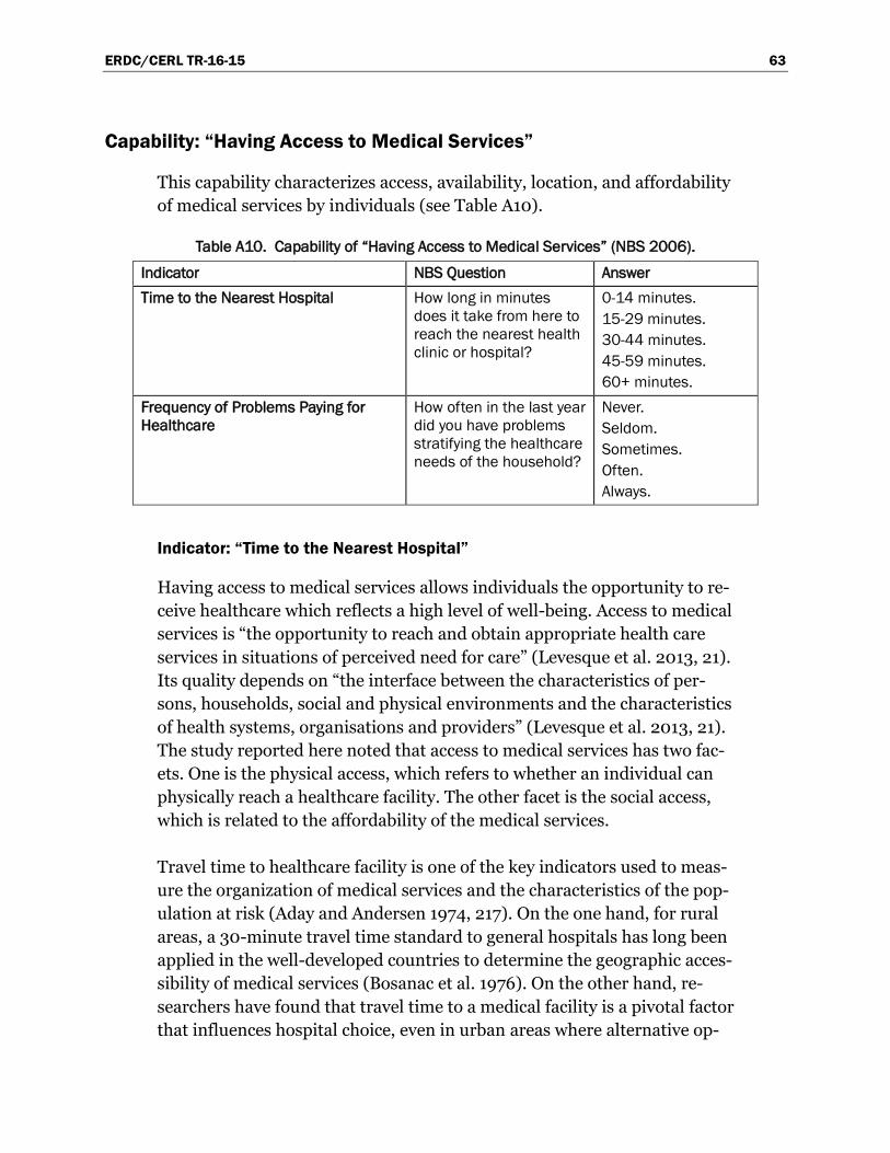
ERDC/CERL TR-16-15 63
Capability: “Having Access to Medical Services”
This capability characterizes access, availability, location, and affordability of medical services by individuals (see Table A10).
Table A10. Capability of “Having Access to Medical Services” (NBS 2006).
Indicator NBS Question Answer Time to the Nearest Hospital How long in minutes
does it take from here to reach the nearest health clinic or hospital?
0-14 minutes. 15-29 minutes. 30-44 minutes. 45-59 minutes. 60+ minutes.
Frequency of Problems Paying for Healthcare
How often in the last year did you have problems stratifying the healthcare needs of the household?
Never. Seldom. Sometimes. Often. Always.
Indicator: “Time to the Nearest Hospital”
Having access to medical services allows individuals the opportunity to re-ceive healthcare which reflects a high level of well-being. Access to medical services is “the opportunity to reach and obtain appropriate health care services in situations of perceived need for care” (Levesque et al. 2013, 21). Its quality depends on “the interface between the characteristics of per-sons, households, social and physical environments and the characteristics of health systems, organisations and providers” (Levesque et al. 2013, 21). The study reported here noted that access to medical services has two fac-ets. One is the physical access, which refers to whether an individual can physically reach a healthcare facility. The other facet is the social access, which is related to the affordability of the medical services.
Travel time to healthcare facility is one of the key indicators used to meas-ure the organization of medical services and the characteristics of the pop-ulation at risk (Aday and Andersen 1974, 217). On the one hand, for rural areas, a 30-minute travel time standard to general hospitals has long been applied in the well-developed countries to determine the geographic acces-sibility of medical services (Bosanac et al. 1976). On the other hand, re-searchers have found that travel time to a medical facility is a pivotal factor that influences hospital choice, even in urban areas where alternative op-

ERDC/CERL TR-16-15 64
tions are widely available (McGuirk and Porell 1984). More recently, re-searchers also used travel time to a health care facility to define rational hospital catchment areas (Schuurman et al. 2006) and to reflect the effect of centralization of health care services (Kobayashi et al. 2015).
Although the healthcare system in Nigeria is generally weak in delivering medical services (FMH [Federal Ministry of Health] 2010, 32), there are a number of medical facilities that provide medical and health services to the local residents in Maiduguri. The major medical clinics and hospitals in Maiduguri include: the University of Maiduguri Teaching Hospital, the State Specialist Hospital, the New Foundation Hospital, the Federal Neuro-Psychiatric Hospital, the Sunni Hospital, the Kanem Hospital, the Avon Healthcare Nakowa Specialist Hospital, the Old Maiduguri Clinic, the Maiduguri Clinic, the Clinic, the Muhammad Buba Marwa House, the Bulabulin Dispensary, the Deribe Hospital, the Alheri Hospital, the Ab-baganaram Clinic, and others (Hospitalby 2016). These medical facilities are located across the urban area that is north of the Ngadda and Gambole Rivers.
When a large-scale disruption occurs, it could severely damage the local transportation systems (Mileti 1999, 91). Especially when bridges are no longer functional and the road network is compromised, traveling to the hospital becomes problematic.
Indicator: “Frequency of Problems Paying for Healthcare”
Having access to medical services encompasses the availability, access, and affordability of healthcare. The indicator “Frequency of Problems Pay-ing for Health Care” is used to determine the level of care received.
Health care, or medical service, is one of the major social services that a society can provide to enhance individuals’ capabilities (Ariana and Naveed 2009, 233). However, there can be several barriers to the utiliza-tion of health care services. Among these barriers, price and cost factors are the most prevalent–on both the demand and the supply sides. These price and cost factors include: (1) indirect consumer costs such as distance cost and opportunity cost; (2) price and availability of substitute health products and services; (3) direct price of service of a given level of health service quality, including informal payment; and (4) price of drugs and other consumables (Ensor and Cooper 2004, 70). Given the importance of the price and cost factors in determining the capability level of “Having

ERDC/CERL TR-16-15 65
Access to Medical Services,” “Frequency of Problems Paying for Health Care” was selected as the appropriate indicator reflecting the capability of “Having Access to Medical Services.”
In Nigeria, the public health condition is poor. Its overall health system performance was ranked only 187th among the 191 member states of the WHO in 2000. Nigeria’s maternal mortality rate is one of the highest in the world (FMH 2006a, 3). According to the FMH of Nigeria, despite “con-siderable investment in the health sector over the years, available evidence suggests that health services throughout Nigeria are delivered through a weak health care system” (FMH 2010, 32). Nigeria’s “health care system is unable to provide basic, cost-effective services for the prevention and management of common health problems especially at the LGA and Ward levels” (FMH 2010, 33). In addition, the majority of Nigerians (90.2%) who live below the income level of $2 a day are unable to afford and obtain medication in Nigeria (FMH 2006b, 5).
When a severe disruption occurs, it could cause fatalities and injuries as well as psychological impacts to the local population (Lindell and Prater 2003, 177–178). Given the existing poor condition of public health service in Nigeria, it is anticipated that a massive disruption in Maiduguri will se-verely increase the demand for local medical service. Such a sharp increase in demand for medical service will lead to greater barriers to the local ac-cess to medical service.
Capability: “Being Socially Connected”
An individual’s level of social connectivity was only able to be determined by using limited survey data pertaining to religious association (see Table A11). Additional information pertaining to an individual’s daily routines, practices, form of communication, access to information, family dynamics, and living conditions would be useful in characterizing an individual’s ca-pability of social connectivity.
Table A11. Capability of “Being Socially Connected” (NBS 2009).
Indicator NBS Question Answer Can Household Depend on Religious Association during Difficult Period?
Can household depend on religious association during difficult period?
Yes. No.

ERDC/CERL TR-16-15 66
Indicator: “Can Household Depend on Religious Association during Difficult Period?”
Being socially connected is equivalent to the central human capability of affiliation, which means an individual is “able to live with and toward oth-ers, to recognize and show concern for other human beings, to engage in various forms of social interaction, [and] to be able to imagine the situa-tion of another” (Nussbaum 2007, 23). Being socially connected also means the possession of social capital, which refers to the “connections among individuals—social networks and the norms of reciprocity and trustworthiness that arise from them” (Putnam 2000, 19). Social capital is virtually most powerful when it is “embedded in a dense network of recip-rocal social relations” (Putnam 2000, 19). From the perspective of disaster management, social capital is the “potential resources in goods, labor, and other forms of assistance, that are embedded in local-level social networks of family and neighbors, and other groups formed through place-based, work-based, and common interest-based bonds of interaction, trust, reci-procity, and support, that people can mobilize individually and collectively to use for community resilience in the face of disasters” (LaLone 2012, 211).
According to political scientist Daniel Aldrich, high levels of social capital serve as the core engine of disaster recovery (2012, 15). In general, strong social capital provides information, knowledge, and access to members of the network; strong social ties create trust among network members; and social capital builds new norms about compliance and participation (Al-drich 2012, 46). As has also been pointed out by Aldrich, however, social capital can be a double-edged sword in a disaster situation. When overlaid with prejudice and discrimination, “strong social relationships across cer-tain groups can slow down the recovery of out-groups” (Aldrich 2012, 14). Further, “peripheral or marginalized groups within society that hold less social capital benefit little and often are harmed by the groups holding stronger social capital after a disaster” (Aldrich 2012, 14). Those who hold the power always have a tendency to relentlessly “search for scapegoats to blame for destruction and loss of life” (Drabeck and Quarantelli 1968, 12; see Farley 2000, 25 for scapegoating and projection).
Within social capital, religious involvement is one of the principal compo-nents of civic engagement (Putnam 2000, 69). According to political scien-tist Robert Putnam, “[regular] worshipers and people who say that religion is very important to them are much more likely than other people to visit

ERDC/CERL TR-16-15 67
friends, to entertain at home, to attend club meetings, and to belong to sports groups; professional and academic societies; school service groups; youth groups; service clubs; hobby or garden clubs; literary, art, discus-sion, and study groups; school fraternities and sororities; farm organiza-tions; political clubs; nationality groups; and other miscellaneous groups” (Putnam 2000, 66–67). Religious involvement is also a strong predictor of volunteerism and philanthropy (Putnam 2000, 66–67).

ERDC/CERL TR-16-15 68
Appendix B: Probabilistic Predictive Models of Indicator Indices
After selecting the capability indicators, the proposed formulation in Chapter 3 was used to develop probabilistic predictive models of the indi-cator indices. To calibrate the predictive models and estimate their un-known model parameters, the available survey database was used for Maiduguri, Nigeria.
Capability: “Meeting the Physiological Needs”
The capability of “Meeting the Physiological Needs” consists of three indi-cators to quantify the achieved functionings. The selected indicators are: (1) “Main Source of Drinking Water;” (2) “Frequency of Problems with Supply of Drinking Water;” and (3) “Frequency of Problems with Satisfy-ing Food Needs.” The first indicator is tracked in the aftermath of the dis-ruptive event by means the infrastructure network analysis. To predict the categories of the other two indicators, probabilistic predictive models were developed, as explained in Chapter 3.
Table B1 shows the codebook of the three possible outcomes of the indica-tor “Frequency of Problems with Supply of Drinking Water.” Because the indicator is of the categorical type, Equation (3) is used to develop the pre-dictive model. For this purpose, a list of candidate regressors is first se-lected that can influence the possible outcome of the indicator. Table B2 summarizes the list of candidate regressors considered for developing the predictive model. The stepwise deletion process was used to assess the sta-tistical significance of the candidate regressors. After the elimination of statistically insignificant terms, the deletion process is stopped and two re-gressors, 2,6x and 2,9x , are left in the model. The final form of the predic-
tive model is shown in Equation (31):

ERDC/CERL TR-16-15 69
( )
{ }( ){ }( ) { }
{ }( ) { }
2, , 2,6,9
22, , 2,1 6,9
2 2 2
22, , 2,1 6,9
exp, 1, 2 ,
1 exp,
1 , 3 .1 exp
k j jj
k j jk j
k j jk j
xk
xI k
kx
θ
θ
θ
∈
= ∈
= ∈
∈ += =
∈+
∑∑ ∑
∑ ∑
P x Θ (31)
Table B1. Codebook of the indicator 2 :I = “Frequency of Problems with Supply of Drinking Water.”
Category Codebook Percentage of Population
No 1 54.4
Dry season 2 43.7
Frequently 3 1.9
Table B2. List of candidate regressors for the predictive model of 2I .
Regressor
2,1 :x = Constant
2,2 :x = Age of the household head
2,3 :x = Household size
2,4 :x =Occupational group of the household head
2,5 :x = Educational status of the household head
2,6 :x =Road construction projects in the last 5 years
2,7 :x = Time to the nearest food market
2,8 :x = Time to the nearest hospital
2,9 :x =Main source of drinking water
2,10 :x = Provider of drinking water

ERDC/CERL TR-16-15 70
Table B3 summarizes the posterior statistics of the parameters. The rela-tion between the indicator and both of the selected regressors is of the causal kind. The regressors, 2,6x and 2,9x , are explaining the two common
causes of problem with the supply of drinking water. The regressor 2,6x
implies that the ease of access to the source of drinking water could be a cause of a problem with the supply of drinking water. Specifically, when the main source of drinking water is “pipe borne” or “vendor, truck” a de-cisive factor is the ease of transportation, which depends on the existence of the paved roads among other factors. Furthermore, the “Main Source Of Drinking Water,” captured by 2,9x , is another cause of the problem. The
source of drinking water influences both its quality and availability. For in-stance, “pipe borne” and “vendor, truck” are considered to be better sources with respect to pond or river water, in terms of both quality and availability, particularly during the dry season.
Table B3. Posterior statistics of the parameters in the predictive model of 2I .
Parameter Mean Standard Deviation
2,1,6θ 5.32 1.31
2,1,9θ −2.90 0.82
2,2,6θ 2.36 1.24
2,2,9θ −0.06 0.68
Next, similar steps were followed to develop a probabilistic predictive model for the indicator “Frequency of Problems with Supply of Drinking Water.” Table B4 shows the corresponding codebook. This indicator is also of the categorical type; hence, Equation (3) was used to develop the pre-dictive model. Table B5 summarizes the candidate regressors. Using the stepwise deletion process arrives at a parsimonious, yet accurate form of the model, shown as Equation (32):

ERDC/CERL TR-16-15 71
( )
{ }( ){ }( ) { }
{ }( ) { }
3, , 3,10,11,13
33, , 3,1 10,11,13
3 3 3
33, , 3,1 10,11,13
exp, 1,2,3 ,
1 exp,
1 , 4 .1 exp
k j jj
k j jk j
k j jk j
xk
xI k
kx
θ
θ
θ
∈
= ∈
= ∈
∈ += =
∈+
∑∑ ∑
∑ ∑
P x Θ (32)
Table B4. Codebook of the indicator 3 :I = “Frequency of
Problems Satisfying Food Needs.”
Category Codebook Percentage of Population
Never 1 17.2
Seldom 2 18.5
Sometimes 3 44.4
Often 4 19.9
Table B5. List of candidate regressors for the predictive model of 3I .
Regressor
3,1 :x = Constant
3,2 :x = Age of the household head
3,3 :x = Household size
3,4 :x =Marital status of the household head
3,5 :x = Occupational group of the household head
3,6 :x = Educational status of the household head
3,7 :x = Number of members contributing to income
3,8 :x = Road construction projects in the last 5 years
3,9 :x = Time to the nearest school
3,10 :x = Time to the nearest food market
3,11 :x = Welfare quintile
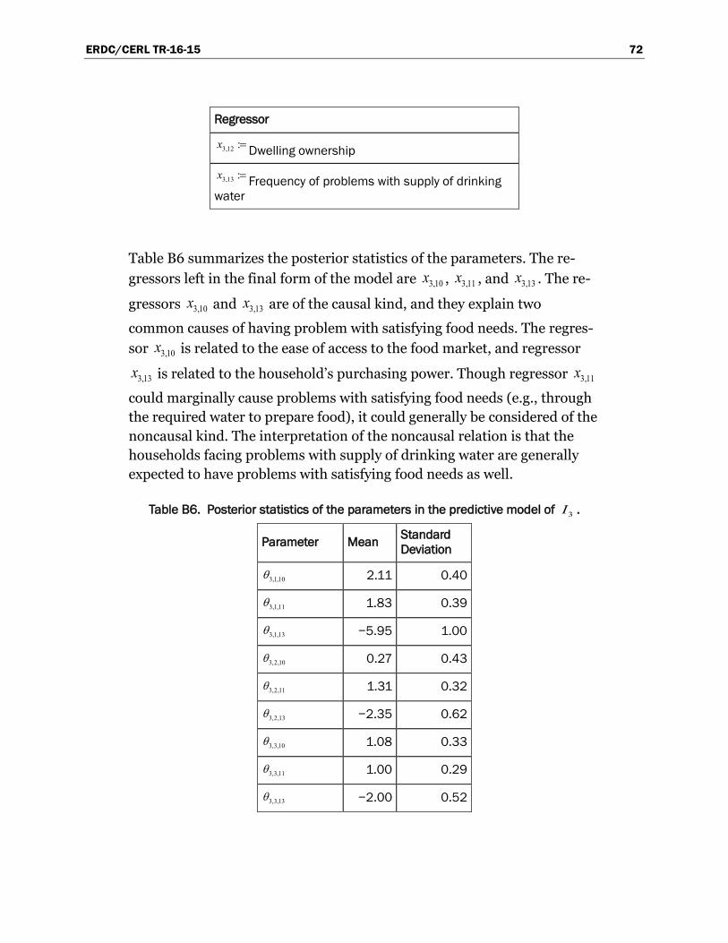
ERDC/CERL TR-16-15 72
Regressor
3,12 :x =Dwelling ownership
3,13 :x = Frequency of problems with supply of drinking water
Table B6 summarizes the posterior statistics of the parameters. The re-gressors left in the final form of the model are 3,10x , 3,11x , and 3,13x . The re-
gressors 3,10x and 3,13x are of the causal kind, and they explain two
common causes of having problem with satisfying food needs. The regres-sor 3,10x is related to the ease of access to the food market, and regressor
3,13x is related to the household’s purchasing power. Though regressor 3,11x
could marginally cause problems with satisfying food needs (e.g., through the required water to prepare food), it could generally be considered of the noncausal kind. The interpretation of the noncausal relation is that the households facing problems with supply of drinking water are generally expected to have problems with satisfying food needs as well.
Table B6. Posterior statistics of the parameters in the predictive model of 3I .
Parameter Mean Standard Deviation
3,1,10θ 2.11 0.40
3,1,11θ 1.83 0.39
3,1,13θ −5.95 1.00
3,2,10θ 0.27 0.43
3,2,11θ 1.31 0.32
3,2,13θ −2.35 0.62
3,3,10θ 1.08 0.33
3,3,11θ 1.00 0.29
3,3,13θ −2.00 0.52

ERDC/CERL TR-16-15 73
Capability: “Being Physically Safe”
To quantify the achieved functioning in the capability of “Being Physically Safe,” the subjective indicator “Do Members Feel Safe Walking on the Street at Night?” was used as the sole indicator. Ideally, it would be desira-ble to have an objective indicator (besides the subjective one) that shows the number of crime-like robberies committed in the community. How-ever, the objective indicators in the survey database lack enough variation to be quantified by means of the predictive models (i.e., more than 97% of the interviewed individuals reported they have never been subjected to any crime). Regarding this capability, it is important to know how safe individ-uals feel in their communities, beyond the actual collected data of the com-mitted crime. Such subjective information is particularly relevant when evaluating the capabilities of individuals who have not been significantly impacted by a disruptive event, but are living among others who are suf-fering from low capabilities.
Table B7 shows the codebook of the indicator. Because the indicator is of the categorical type, Equation (3) was used to develop the predictive model.
Table B8 shows the list of selected candidate regressors to develop the pre-dictive model. Using a stepwise deletion process and eliminating statisti-cally insignificant terms, the final form of the model is shown as Equation (33):
( )
{ }( ){ }( ) { }
{ }( ) { }
4, , 4,1,9,10,13
24, , 4,1 1,9,10,13
4 4 4
24, , 4,1 1,9,10,13
exp, 1,2 ,
1 exp,
1 , 3 .1 exp
k j jj
k j jk j
k j jk j
xk
xI k
kx
θ
θ
θ
∈
= ∈
= ∈
∈ += =
∈+
∑∑ ∑
∑ ∑
P x Θ (33)
Table B7. Codebook of the indicator 4 :I = “Do Members Feel Safe Walking on the Street at Night?”
Category Codebook Percentage of Population
Very safe 1 47.5
Somewhat safe 2 29.4

ERDC/CERL TR-16-15 74
Category Codebook Percentage of Population
Not too safe 3 23.1
Table B8. List of candidate regressors for the predictive model of 4I .
Regressor
4,1 :x = Constant
4,2 :x =Sex
4,3 :x = Age
4,4 :x =Marital status
4,5 :x = Radio, frequency of use
4,6 :x =Daily newspaper, frequency of use
4,7 :x =Highest grade completed
4,8 :x = Standards of living with respect to others in the community
4,9 :x =Welfare quintile
4,10 :x = Time to the nearest school
4,11 :x = Time to the nearest hospital
4,12 :x = Time to the nearest food market
4,13 :x =Neighborhood watching in the community
Table B9 summarizes the posterior statistics of the model parameters. The remaining regressors in the model are 4,1x , 4,9x , 4,10x , and 4,13x . The regres-sor 4,1x is a constant, 4,9x and 4,10x are generally of the noncausal kind, and
4,13x is of the causal kind. The noncausal regressors are showing a relation that is typically valid under the calibration condition. For instance, living close to or far away from the nearest school might not necessarily cause a person to feel that a community is safe or unsafe. However, the collected information from the respondents in the survey shows that the feeling of safety and the time to the nearest school are related. Furthermore, the causal regressor,
4,13x , shows that community members generally feel safe

ERDC/CERL TR-16-15 75
when they know there is a neighborhood watching that can protect them. It is worth noting that there is a hidden fact in the previous conclusion that conditions the causal relation to the degree of trust in authority.
Table B9. Posterior statistics of the parameters in the predictive model of 4I .
Parameter Mean Standard Deviation
4,1,1θ −5.23 0.74
4,1,9θ 0.76 0.21
4,1,10θ 1.12 0.24
4,1,13θ 1.63 0.28
4,2,1θ −2.89 0.67
4,2,9θ −0.19 0.20
4,2,10θ 1.31 0.24
4,2,13θ 1.19 0.28
Capability: “Being Sheltered”
The achieved functioning in this capability is quantified by means of the indicator “Frequency of Problems with Paying Rent.” In addition to this indicator, three other indicators were considered that are related to the type of material used in the roof, walls, and floor of the dwellings. These indicators were intended to quantify the quality of the dwellings. However, the recorded data in the survey showed there is not enough variation to be quantified by the predictive models. For example, the roof of 94% of dwell-ings in the database is made of iron sheet. A similar observation also ap-plies to the other two indicators.
Table B10 shows the codebook of the selected indicator. Because the indi-cator is categorical, Equation (3) was used to develop the predictive model. Similar to the previous predictive models, a list of candidate regressors was selected that can influence the possible category of the indicator. Ta-ble B11 summarizes the list of selected candidate regressors, along with their possible values/categories. After performing the stepwise deletion process and eliminating the statistically insignificant terms, the final form of the model was obtained as Equation (34):

ERDC/CERL TR-16-15 76
( )
{ }( ){ }( ) { }
{ }( ) { }
5, , 5,2,3,5,6,9,11
35, , 5,1 2,3,5,6,9,11
5 5 5
35, , 5,1 2,3,5,6,9,11
exp, 1,2,3 ,
1 exp,
1 , 4 .1 exp
k j jj
k j jk j
k j jk j
xk
xI k
kx
θ
θ
θ
∈
= ∈
= ∈
∈ += =
∈+
∑∑ ∑
∑ ∑
P x Θ (34)
Table B10. Codebook of the indicator 5 :I = “Frequency of Problems Paying House Rent.”
Category Codebook Percentage of Population
Never 1 60.3
Seldom 2 12.6
Sometimes 3 19.9
Often 4 7.3
Table B11. List of candidate regressors for the predictive model of 5I .
Regressor
5,1 :x = Constant
5,2 :x = Age of the household head
5,3 :x = Household size
5,4 :x =Marital status of the household head
5,5 :x = Occupational group of the household head
5,6 :x = Education level of the household head
5,7 :x =Number of members contributing to income
5,8 :x = Road construction project in the last 5 years
5,9 :x = Time to the nearest food market
5,10 :x =Main source of drinking water
5,11 :x = Welfare quintile

ERDC/CERL TR-16-15 77
Table B12 shows the estimated posterior statistics of the model parame-ters. The regressors remained in the final form of the model are
5,2x , 5,3x ,
5,5x , 5,6x ,
5,9x , and 5,11x . The higher number of regressors left in the model
implies that the selected candidate regressors are not as efficient as in the case of other predictive models in describing the variability in the indica-tor over the population. More informative regressors might be thought of to improve the model; however, important constraints in developing such predicative models is the availability of the data to calibrate the model and also the ability to measure/predict the values of the regressors at different locations and over time. In this model, the relation of all the regressors can be considered causal, in some sense; however, in general, they do not im-mediately impact the possible outcome of the indicator. All the regressors, in some sense, are capturing the financial aspect of the problem to pay the rent. For example, the age of the household head and his/her ability to produce wealth are related. Likewise, when the size of the household is large and there is only one or two members contributing to the income, this could be a cause to have a problem with paying the rent. In contrast, when all the members are contributing, this could be seen as a positive ef-fect. The education and occupation of the household head are also contrib-uting to the problem of paying the rent. Specifically, when the occupation is looked at as a binary variable (i.e., employed or unemployed), its causal relation would be more tangible. Among the regressors in Equation (32), distinguishing the causal relation of
5,11x is easier, as it is directly related to the economic situation of the household.
Table B12. Posterior statistics of the parameters in the predictive model of 5I .
Parameter Mean Standard Deviation
5,1,2θ 0.14 0.05
5,1,3θ 0.11 0.31
5,1,5θ −0.70 0.23
5,1,6θ −0.94 0.26
5,1,9θ −0.04 0.47
5,1,11θ 1.15 0.61
5,2,2θ 0.10 0.06
5,2,3θ 0.09 0.32

ERDC/CERL TR-16-15 78
Parameter Mean Standard Deviation
5,2,5θ −0.44 0.25
5,2,6θ −0.66 0.26
5,2,9θ −0.81 0.62
5,2,11θ 0.92 0.64
5,3,2θ 0.03 0.06
5,3,3θ 0.76 0.33
5,3,5θ −0.05 0.27
5,3,6θ −0.57 0.27
5,3,9θ 0.74 0.48
5,3,11θ −0.94 0.71
Capability: “Having Access to Energy”
Two indicators were used to quantify the achieved functioning in this ca-pability. The selected indicators are the “Source of Electricity” and the “Number of Hours without Electricity in the Past 24 Hours.” The first indi-cator determines whether or not households are having access to electric-ity. The second indicator quantifies the quality of access.
Table B13 shows the codebook of the two possible outcomes of the indica-tor “Source of Electricity.” NEPA is the main source of electricity in the ur-ban area of Maiduguri, which is the focus of this study. However, in the rural areas, households are using other sources such as private generators or rural electricity plants. Because the indicator is of the categorical type, with two possible outcomes, Equation (3) was used to develop the predic-tive model. Table B14 summarizes the list of candidate regressors to de-velop the predictive model. Using the stepwise deletion process, the statistically significant terms were eliminated. The final form of the model consists of regressors
6,6x , 6,12x , and
6,14x , as shown in Equation (35):

ERDC/CERL TR-16-15 79
( )
{ }( ){ }( ) { }
{ }( ) { }
6, , 6,6,12,14
6, , 6,6,12,146 6 6
6, , 6,6,12,14
exp, 1 ,
1 exp,
1 , 2 .1 exp
θ
θ
θ
∈
∈
∈
∈ += =
∈+
∑∑
∑
P x Θ
k j jj
k j jj
k j jj
xk
xI k
kx
(35)
Table B13. Codebook of the indicator 6 :I = “Source of Electricity.”
Category Codebook Percentage of Population
None 1 12.5
NEPA 2 87.5
Table B14. List of candidate regressors for the predictive model of 6I .
Regressor
6,1 :x = Constant
6,2 :x =Gender of the household head
6,3 :x = Age of the household head
6,4 :x =Household size
6,5 :x = Marital status of the household head
6,6 :x =Occupational group of the household head
6,7 :x = Education level of the household head
6,8 :x = Does the household own a vehicle
6,9 :x = Time to the nearest school
6,10 :x = Time to the nearest hospital
6,11 :x = Time to the nearest food market
6,12 :x = Welfare quintile

ERDC/CERL TR-16-15 80
Regressor
6,13 :x = Frequency of problems with supply of drinking water
6,14 :x = Frequency of problems paying house rent
Table B15 summarizes the posterior statistics of the model parameters. The regressors that remained in the final form of the model are trying to capture the financial aspect of the problem (i.e., whether or not the house-holds can pay the utility bills). Beyond being able or not to pay the bills, the regressors collectively might describe a situation that there is no NEPA coverage in the community. Under both circumstances, the relation of all the regressors could be considered causal but not with immediate impact. Generally speaking, it becomes a matter of time to see the actual impact on the possible outcome of the indicator.
Table B15. Posterior statistics of the parameters in the predictive model of 6I .
Parameter Mean Standard Deviation
6,1,6θ 0.64 0.21
6,1,12θ −1.56 0.36
6,1,14θ −1.12 0.46
Next, a probabilistic predictive model was developed for the indicator “Number of Hours without Electricity in the Past 24 Hours.” The possible values are in the interval [0, 24] , and Table B16 gives a summary of the dis-tribution of the indicator over the considered households for the purpose of calibration. This indicator is of the integer/real-value type; hence, Equa-tion (2) was used to develop the predictive model.
Table B17 summarizes the candidate regressors used to develop the model. The statistically insignificant terms were eliminated from the model, using the stepwise deletion process. The obtained final form of the model is shown as Equation (36):
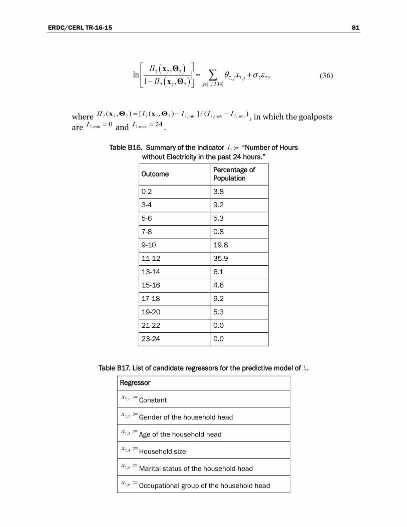
ERDC/CERL TR-16-15 81
( )( ) { }
7 7 77, 7, 7 7
1,13,147 7 7
,ln ,
1 ,θ σ ε
∈
= + − ∑
x Θx Θ j j
j
IIx
II (36)
where 7 7 7 7 7 7 7,min 7,max 7,min( , ) [ ( , ) ] / ( )= − −x Θ x ΘII I I I I , in which the goalposts are 7,min 0=I and 7,max 24=I .
Table B16. Summary of the indicator 7 :=I “Number of Hours without Electricity in the past 24 hours.”
Outcome Percentage of Population
0-2 3.8
3-4 9.2
5-6 5.3
7-8 0.8
9-10 19.8
11-12 35.9
13-14 6.1
15-16 4.6
17-18 9.2
19-20 5.3
21-22 0.0
23-24 0.0
Table B17. List of candidate regressors for the predictive model of 7I .
Regressor
7,1 :=x Constant
7,2 :=x Gender of the household head
7,3 :=x Age of the household head
7,4 :=x Household size
7,5 :=x Marital status of the household head
7,6 :=x Occupational group of the household head
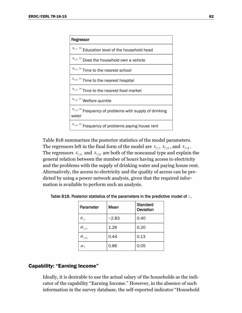
ERDC/CERL TR-16-15 82
Regressor
7,7 :=x Education level of the household head
7,8 :=x Does the household own a vehicle
7,9 :=x Time to the nearest school
7,10 :=x Time to the nearest hospital
7,11 :=x Time to the nearest food market
7,12 :=x Welfare quintile
7,13 :=x Frequency of problems with supply of drinking water
7,14 :=x Frequency of problems paying house rent
Table B18 summarizes the posterior statistics of the model parameters. The regressors left in the final form of the model are 7,1x , 7,13x , and 7,14x . The regressors 7,13x and 7,14x are both of the noncausal type and explain the general relation between the number of hours having access to electricity and the problems with the supply of drinking water and paying house rent. Alternatively, the access to electricity and the quality of access can be pre-dicted by using a power network analysis, given that the required infor-mation is available to perform such an analysis.
Table B18. Posterior statistics of the parameters in the predictive model of 7I .
Parameter Mean Standard Deviation
7,1θ −2.83 0.40
7,13θ 1.26 0.20
7,14θ 0.44 0.13
7σ 0.86 0.05
Capability: “Earning Income”
Ideally, it is desirable to use the actual salary of the households as the indi-cator of the capability “Earning Income.” However, in the absence of such information in the survey database, the self-reported indicator “Household

ERDC/CERL TR-16-15 83
Financial Situation” was used. Though there might be bias in the self-re-ported income status, it would expected that the predictive model would not be adversely affected given that the unknown subset of biased observa-tions is not dominating in the database.
Table B19 shows the codebook of the indicator along with the percentage of population within each category. Because the indicator is categorical, Equation (3) was used to develop the predictive model.
Table B20 lists the set of selected candidate regressors to develop the pre-dictive model. Starting with the complete model (i.e., all candidate regres-sors), the stepwise deletion process was used to eliminate one term at a time until arriving at a parsimonious form of the model. After elimination of statistically insignificant terms, the final form of the model is obtained as Equation (37):
( )
{ }( ){ }( ) { }
{ }( ) { }
8, , 8,1,3,5
38, , 8,1 1,3,5
8 8 8
38, , 8,1 1,3,5
exp, 1,2,3 ,
1 exp,
1 , 4 .1 exp
k j jj
k j jk j
k j jk j
xk
xI k
kx
θ
θ
θ
∈
= ∈
= ∈
∈ += =
∈+
∑∑ ∑
∑ ∑
P x Θ (37)
Table B19. Codebook of the indicator 8 :=I ”Household Financial Situation.”
Category Codebook Percentage of Population
Very poor 1 11.6
Poor 2 29.1
Moderate 3 53.3
Fairly rich 4 6.1
Table B20. List of candidate regressors for the predictive model of 8I .
Regressor
8,1 :=x Constant
8,2 :=x Time to the nearest school

ERDC/CERL TR-16-15 84
Regressor
8,3 :=x Time to the nearest hospital
8,4 :=x Time to the nearest food market
8,5 :=x Does a household member belong to a religious association
8,6 :=x Minimum needed per month to satisfy basic needs
Table B21 summarizes the estimated posterior statistics of the model pa-rameters. All the regressors in the final form of the model, 5,1x , 5,3x , and 5,5x , are of the noncausal type. Hence, it is suggested to not change the values of the regressors when predicting the capabilities of households in the im-mediate aftermath of a disruption.
Table B21. Posterior statistics of the parameters in the predictive model of 8I .
Parameter Mean Standard Deviation
8,1,1θ 1.93 1.47
8,1,3θ 0.51 0.20
8,1,5θ −1.43 0.75
8,2,1θ 5.79 1.38
8,2,3θ 0.30 0.20
8,2,5θ −2.93 0.70
8,3,1θ 6.53 1.36
8,3,3θ 0.23 0.19
8,3,5θ −2.89 0.69
Capability: “Owning Property”
The achieved functioning in this capability is quantified in terms of two in-dicators. The selected indicators are the “Number of Household Durables” and “Dwelling Ownership.” In selecting the indicators, care should be taken to consider the population under study. Because what constitutes properties for households in rural areas might not be applicable for people

ERDC/CERL TR-16-15 85
living in urban areas, and vice versa. For example, the area of land, or the number of animals like sheep, goats, and cows are considered to be prop-erties for households living in rural areas, which is not the case for people in urban areas.
Table B22 shows the codebook of the possible outcomes of the indicator “Number of Household Durables.” The table also shows the items consid-ered as properties for households in the urban area of Maiduguri, as the focus of this study. Because the indicator is categorical, Equation (3) was used to develop the predictive model.
Table B23 lists the set of candidate regressors for developing the predictive model. A stepwise deletion process was used to eliminate the statistically insignificant terms. The final form of the model is shown in Equation (38):
( )
{ }( ){ }( ) { }
{ }( ) { }
9, , 9,1,2,11,12
49, , 9,1 1,2,11,12
9 9 9
49, , 9,1 1,2,11,12
exp, 1, , 4 ,
1 exp,
1 , 5 .1 exp
k j jj
k j jk j
k j jk j
xk
xI k
kx
θ
θ
θ
∈
= ∈
= ∈
∈ += =
∈+
∑∑ ∑
∑ ∑
P x Θ
(38)
Table B22. Summary of the indicator 9 :=I “Number of Household Durables” (including refrigerator, television, personal computer, fixed-line telephone, mobile
phone, modern stove, gas cooker, generator, bicycle, motorcycle, vehicle).
Outcome Percentage of Population
0 25.5
1 21.7
2 18.0
3 11.2
4 7.5
5 8.1
6 7.5

ERDC/CERL TR-16-15 86
Table B23. List of candidate regressors for the predictive model of 9I .
Regressor
9,1 :=x Constant
9,2 :=x Age of the household head
9,3 :=x Household size
9,4 :=x Marital status of the household head
9,5 :=x Occupational group of the household head
9,6 :=x Education level of the household head
9,7 :=x Number of members contributing to household income
9,8 :=x Road construction project in the last five years
9,9 :=x Time to the nearest hospital
9,10 :=x Time to the nearest food market
9,11 :=x Main source of drinking water
9,12 :=x Welfare quintile
Table B24 summarizes the posterior statistics of the model parameters. The regressors that remained in the final form of the model— 9,1x
, 9,2x,
9,11x, and 9,12x
—are generally of noncausal type. Only 9,12x might be consid-
ered as causal. The regressors partially explain the reasoning behind hav-ing the selected durables, given that such an opportunity is available. Hence, it is suggested not to update the categories of regressors, such as the “Main Source of Drinking Water,” when predicting the outcome of the indicator in the immediate aftermath of a disruption.
Next, a probabilistic predictive model was developed for the indicator “Dwelling Ownership.” The possible values are either owning or renting a house. Table B25 shows the codebook of the indicator, along with the per-centage of considered households within each group. Because the indica-tor is categorical, Equation (3) was used to develop the predictive model.

ERDC/CERL TR-16-15 87
Table B26 summarizes the candidate regressors used to develop the model. The statistically insignificant terms are eliminated from the model, using the stepwise deletion process. The final form of the model is shown as Equation (39):
( )
{ }( ){ }( ) { }
{ }( ) { }
10, , 10,5,9,13,14
10, , 10,5,9,13,1410 10 10
10, , 10,5,9,13,14
exp, 1 ,
1 exp,
1 , 2 .1 exp
k j jj
k j jj
k j jj
xk
xI k
kx
θ
θ
θ
∈
∈
∈
∈ += =
∈+
∑∑
∑
P x Θ (39)
Table B24. Posterior statistics of the parameters in the predictive model of 9I .
Parameter Mean Standard Deviation
9,1,1θ 23.73 4.36
9,1,2θ 0.02 0.05
9,1,11θ −2.14 1.01
9,1,12θ −6.89 1.05
9,2,1θ 25.17 4.26
9,2,2θ −0.08 0.05
9,2,11θ −2.08 0.97
9,2,12θ −5.43 0.96
9,3,1θ 20.46 4.15
9,3,2θ −0.11 0.05
9,3,11θ −0.77 0.92
9,3,12θ −4.09 0.88
9,4,1θ 15.80 4.21
9,4,2θ −0.10 0.05
9,4,11θ 0.62 0.99
9,4,12θ −3.71 0.90

ERDC/CERL TR-16-15 88
Parameter Mean Standard Deviation
9,5,1θ 10.72 3.85
9,5,2θ −0.01 0.04
9,5,11θ −0.34 0.91
9,5,12θ −2.57 0.80
9,6,1θ 4.73 3.50
9,6,2θ −0.09 0.04
9,6,11θ 0.59 0.83
9,6,12θ −0.56 0.69
Table B25. Codebook of the indicator 10 :=I “Dwelling Ownership.”
Category Codebook Percentage of Population
Owns the dwelling 1 48.2
Rents the dwelling 2 51.8
Table B26. List of candidate regressors for the predictive model of 10I .
Regressor
10,1 :=x Constant
10,2 :=x Gender of the household head
10,3 :=x Age of the household head
10,4 :=x Household size
10,5 :=x Marital status of the household head
10,6 :=x Occupational group of the household head
10,7 :=x Education level of the household head
10,8 :=x Number of members contributing to household income

ERDC/CERL TR-16-15 89
Regressor
10,9 :=x Road construction project in last five years
10,10 :=x Time to the nearest school
10,11 :=x Time to the nearest hospital
10,12 :=x Time to the nearest food market
10,13 :=x Main source of drinking water
10,14 :=x Welfare quintile
Table B27 summarizes the posterior statistics of the model parameters. The regressors in the final form of the model are generally noncausal. In evaluating the capabilities of households in the aftermath of a disruption, the ownership status does not change; however, there might be damage (from slight to complete collapse) to the property. This latter possibility can be evaluated by performing structural analysis of individual buildings or more generally, by predicting the level of damage to buildings of certain types, due to a particular hazard, by means of physical loss assessments.
Table B27. Posterior statistics of the parameters in the predictive model of 10I .
Parameter Mean Standard Deviation
10,5θ 0.93 0.19
10,9θ −2.37 0.40
10,13θ −0.13 0.27
10,14θ 0.93 0.22
Capability: “Being Mobile”
Ideally, it is desirable to have an indicator that truly captures the achieved functioning in the capability of “Being Mobile.” For example, the number of travels per day that individuals undertake could be a suitable choice. The capability of “Being Mobile" is related to the availability of paved roads, availability of vehicle for travel, and social norms that may prevent someone from traveling. The number of travels that individuals can make accounts for such factors. In the absence of such an ideal choice, however,

ERDC/CERL TR-16-15 90
the indicator “Time to the Nearest Food Market” was selected to quantify the achieved functioning. This indicator set the purpose of travel as a ge-neric one that individuals generally may choose to do. The time of travel can capture the availability of the vehicle or paved roads. However, care should be taken in interpreting the results because if the time to the near-est food market being changed, this does not necessarily lead to a change in this capability, given that everything else remains the same. For predic-tion purposes, the network analysis of infrastructure systems is used to ob-tain the likely outcome in the aftermath of a disruption.
Capability: “Being Educated”
Disruptive events can adversely impact the capability of “Being Educated” by causing damage to the building or stopping the building from function-ing due to, for example, loss of power. The influence of such impacts gen-erally becomes a matter of time and how long they last. Not being able to go to school for a week or a month might not be too critical. However, not being able to educate in general is a big issue. Though this capability might not be significantly impacted by a disruptive event, when quantifying the overall capabilities of individuals, it can make a difference to account for it.
To quantify the achieved functioning in this capability, two indicators were used, which are “Time to the Nearest School” and “Frequency of Problems Paying School Fees.” To predict the value of the first indicator in the after-math of a disruption, the network analysis of infrastructure systems is used. Regarding the second indicator, Equation (3) was used to develop a probabilistic predictive model.
Table B28 shows the codebook of the indicator “Frequency of Problems Paying School Fees” along with the percentage of the considered house-holds within each category. Table B29 lists the set of all candidate regres-sors considered for developing the predictive model. After eliminating the statistically insignificant terms, the final form of the model is shown as Equation (40):

ERDC/CERL TR-16-15 91
( )
{ }( ){ }( ) { }
{ }( ) { }
13, , 13,1,6,11
313, , 13,1 1,6,11
13 13 13
313, , 13,1 1,6,11
exp, 1,2,3 ,
1 exp,
1 , 4 .1 exp
k j jj
k j jk j
k j jk j
xk
xI k
kx
θ
θ
θ
∈
= ∈
= ∈
∈ += =
∈+
∑∑ ∑
∑ ∑
P x Θ (40)
Table B28. Codebook of the indicator 13 :=I “Frequency of Problems Paying School Fees.
Category Codebook Percentage of Population
Never 1 75.2
Seldom 2 10.6
Sometimes 3 8.7
Often/Always 4 5.6
Table B29. List of candidate regressors for the predictive model of 13I .
Regressor
13,1 :=x Constant
13,2 :=x Age of the household head
13,3 :=x Household size
13,4 :=x Marital status of the household head
13,5 :=x Occupational group of the household head
13,6 :=x Education level of the household head
13,7 :=x Number of members contributing to household income
13,8 :=x Road construction project in last five years
13,9 :=x Time to the nearest school
13,10 :=x Time to the nearest food market

ERDC/CERL TR-16-15 92
Regressor
13,11 :=x Main source of drinking water
13,12 :=x Welfare quintile
13,13 :=x Dwelling ownership
Table B30 summarizes the estimate posterior statistics of the model pa-rameters. As discussed earlier, the capability in general, and the category of the indicator in particular, might not change over a short-term period. However, it is still important to account for such capability in assessing the well-being of individuals. Hence, the regressors are of noncausal type, and they show a general relation between the category of the indicator and the regressors. Specifically, the education of the household head is intuitively connected to the category of the indicator. However, the relation between the source of drinking water and the category of indicator is less tangible, and it might refer to social status of the household and whether or not they can afford the school fees.
Table B30. Posterior statistics of the parameters in the predictive model of 13I .
Parameter Mean Standard Deviation
13,1,1θ 6.10 1.89
13,1,6θ −0.72 0.21
13,1,11θ −0.88 0.82
13,2,1θ −1.44 2.30
13,2,6θ −0.22 0.23
13,2,11θ 1.36 0.94
13,3,1θ −4.80 2.64
13,3,6θ 0.04 0.26
13,3,11θ 2.32 1.01
Capability: “Having Access to Medical Services”
A disruptive event may hinder the ability to access hospitals or make medi-cal services unavailable. When a disruptive event endangers the life of indi-viduals or causes injuries, the capability of “Having Access To Medical

ERDC/CERL TR-16-15 93
Services” becomes of utmost significance. To quantify the achieved func-tioning in this capability, two indicators were considered: “Time to the Nearest Hospital” and “Frequency of Problems Paying for Healthcare.” The selected indicators are supposed to collectively capture the ease to access to medical services. Access to medical services in general can be influenced by proximity of medical services, availability of resources such as the doctor-to-patient ratio, facilities of the hospitals and healthcare centers, and the costs. Regarding the first indicator, the infrastructure network analysis was used to predict the likely value of the indicator in the aftermath of a disrup-tion. This indicator plays a major role in evaluating the capabilities of indi-viduals during any emergencies that arise in the aftermath of a disruption. In contrast, the second indicator is more pertinent for evaluating the level access to medical services during the stable condition of the society. To pre-dict the likely category of this indicator, Equation (3) was used to develop a probabilistic predictive model.
Table B31 shows the codebook and the percentage of the considered house-hold in each category. Table B32 lists the set of all candidate regressors con-sidered for developing the predictive model. As before, the stepwise deletion process was used to eliminate the statistically insignificant terms. The final form of the model after the deletion process is shown in Equation (41):
( )
{ }( ){ }( ) { }
{ }( ) { }
15, , 15,11,13
415, , 15,1 11,13
15 15 15
415, , 15,1 11,13
exp, 1, , 4 ,
1 exp,
1 , 5 .1 exp
k j jj
k j jk j
k j jk j
xk
xI k
kx
θ
θ
θ
∈
= ∈
= ∈
∈ += =
∈+
∑∑ ∑
∑ ∑
P x Θ
(41)
Table B31. Codebook of the indicator 15 :=I “Frequency of Problems Paying for Healthcare.”
Category Codebook Percentage of Population
Never 1 35.2
Seldom 2 2.5
Sometimes 3 57.4

ERDC/CERL TR-16-15 94
Category Codebook Percentage of Population
Often 4 3.1
Always 5 1.9
Table B32. List of candidate regressors for the predictive model of 15I .
Regressor
15,1 :=x Constant
15,2 :=x Gender of the household head
15,3 :=x Age of the household head
15,4 :=x Household size
15,5 :=x Occupational group of the household head
15,6 :=x Education level of the household head
15,7 :=x Number of members contributing to household income
15,8 :=x Road construction project in last five years
15,9 :=x Time to the nearest school
15,10 :=x Time to the nearest hospital
15,11 :=x Time to the nearest food market
15,12 :=x Main source of drinking water
15,13 :=x Welfare quintile
Table B33 summarizes the estimated posterior statistics of the model pa-rameters. There are two regressors that remain in the model. The regres-sor
15,11x is of noncausal type, and the regressor 15,13x is causal (that explains
whether a household can afford the expenses of medical services).

ERDC/CERL TR-16-15 95
Table B33. Posterior statistics of the parameters in the predictive model of 15I .
Parameter Mean Standard Deviation
15,1,11θ −0.60 0.68
15,1,13θ 1.68 0.53
15,2,11θ 0.19 0.71
15,2,13θ 0.23 0.61
15,3,11θ 1.07 0.61
15,3,13θ 0.91 0.51
15,4,11θ −0.12 0.82
15,4,13θ 0.37 0.64
Capability: “Being Socially Connected”
The capability of “Being Socially Connected” refers to the aspect of well-being that humans, as social creatures, live together, not only because liv-ing together is instrumentally beneficial, but also because humans have a sense of belonging to or being affiliated with a group, association, commu-nity, or region. From the instrumental perspective, “Being Socially Con-nected” acts more like a mean to achieve a higher level of acceptance; hence, it can be interpreted more like a regressor than a capability. How-ever, from the capability point of view, it is an independent aspect of well-being which is intrinsically important. To quantify the achieved function-ing in this capability, the binary indicator “Can Household Depend on Re-ligious Association during Difficult Period?” was selected.
Table B34 shows the codebook of the indicator, along with the percentage of the considered individuals in each category. Table B35 lists the set of candidate regressors considered for developing the predictive model. As usual, the stepwise deletion process is used to eliminate the statistically in-significant terms and arrive at a parsimonious form of the model, repre-sented as Equation (42):
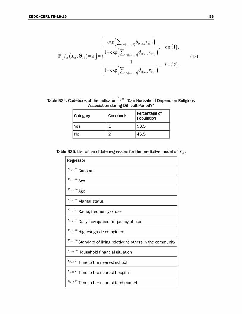
ERDC/CERL TR-16-15 96
( )
{ }( ){ }( ) { }
{ }( ) { }
16, , 16,1,11,13
16, , 16,1,11,1316 16 16
16, , 16,1,11,13
exp, 1 ,
1 exp,
1 , 2 .1 exp
k j jj
k j jj
k j jj
xk
xI k
kx
θ
θ
θ
∈
∈
∈
∈ += =
∈+
∑∑
∑
P x Θ (42)
Table B34. Codebook of the indicator 16 :=I “Can Household Depend on Religious Association during Difficult Period?”
Category Codebook Percentage of Population
Yes 1 53.5
No 2 46.5
Table B35. List of candidate regressors for the predictive model of 16I .
Regressor
16,1 :=x Constant
16,2 :=x Sex
16,3 :=x Age
16,4 :=x Marital status
16,5 :=x Radio, frequency of use
16,6 :=x Daily newspaper, frequency of use
16,7 :=x Highest grade completed
16,8 :=x Standard of living relative to others in the community
16,9 :=x Household financial situation
16,10 :=x Time to the nearest school
16,11 :=x Time to the nearest hospital
16,12 :=x Time to the nearest food market

ERDC/CERL TR-16-15 97
Regressor
16,13 :=x Does household belong to a family association
16,14 :=x Can read a simple letter in what Nigerian language
Table B36 summarizes the estimate posterior statistics of the model pa-rameters. The regressors in the final form of the model are noncausal; thus, as before, it would be suggested not to the change the category of the indicator for the purpose of predicting the capability of households in the immediate aftermath of a disruption.
Table B36. Posterior statistics of the parameters in the predictive model of 16I .
Parameter Mean Standard Deviation
16,1,1θ 12.11 1.43
16,1,11θ −1.44 0.30
16,1,13θ −6.95 0.77

ERDC/CERL TR-16-15 98
Appendix C: Figures
Figures C1-C10 show the relation between the values/categories of the in-dicators and their states. In general, each capability indicator can have three states: (1) the acceptable state (green), (2) the tolerable state (yel-low), and (3) the intolerable state (red). However, note that not all the in-dicators necessarily have the three states. This is because either the number of possible categories/values is less than 3 like the indicator "source of electricity" or the nature of the indicator is such that not all the three states are realizable, like the indicator “number of household dura-bles.”
Figure C1. The states of the indicators quantifying the capability of “Meeting the Physiological Needs” (University of Illinois).
Figure C2. The states of the indicator quantifying the capability of “Being Physically Safe” (University of Illinois).
Figure C3. The states of the indicator quantifying the capability of “Being Sheltered” (University of Illinois).
Figure C4. The states of the indicator quantifying the capability of “Having Access to Energy” (University of Illinois).

ERDC/CERL TR-16-15 99
Figure C5. The states of the indicator quantifying the capability of “Earning Income” (University of Illinois).
Figure C6. The states of the indicators quantifying the capability of “Owning Property” (University of Illinois).
Figure C7. The states of the indicator quantifying the capability of “Being Mobile” (University of Illinois).
Figure C8. The states of the indicators quantifying the capability of “Being Educated” (University of Illinois).
Figure C9. The states of the indicators quantifying the capability of “Having Access to Medical Services” (University of Illinois).
Figure C10. The states of the indicators quantifying the capability of “Being Socially Connected” (University of Illinois).
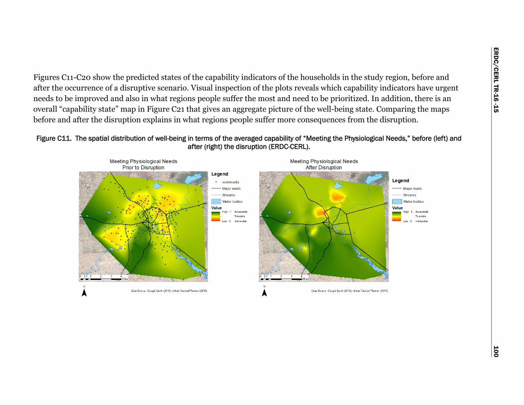
ERD
C/CER
L TR-16 -15
100
Figures C11-C20 show the predicted states of the capability indicators of the households in the study region, before and after the occurrence of a disruptive scenario. Visual inspection of the plots reveals which capability indicators have urgent needs to be improved and also in what regions people suffer the most and need to be prioritized. In addition, there is an overall “capability state” map in Figure C21 that gives an aggregate picture of the well-being state. Comparing the maps before and after the disruption explains in what regions people suffer more consequences from the disruption.
Figure C11. The spatial distribution of well-being in terms of the averaged capability of “Meeting the Physiological Needs,” before (left) and after (right) the disruption (ERDC-CERL).

ERD
C/CER
L TR-16 -15
101
Figure C12. The spatial distribution of well-being in terms of the averaged capability of “Being Physically Safe,” before (left) and after (right) the disruption (ERDC-CERL).

ERD
C/CER
L TR-16 -15
102
Figure C13. The spatial distribution of well-being in terms of the averaged capability of “Being Sheltered,” before (left) and after (right) the disruption (ERDC-CERL).

ERD
C/CER
L TR-16 -15
103
Figure C14. The spatial distribution of well-being in terms of the averaged capability of “Having Access to Energy,” before (left) and after (right) the disruption (ERDC-CERL).

ERD
C/CER
L TR-16 -15
104
Figure C15. The spatial distribution of well-being in terms of the averaged capability of “Earning Income,” before (left) and after (right) the disruption (ERDC-CERL).

ERD
C/CER
L TR-16 -15
105
Figure C16. The spatial distribution of well-being in terms of the averaged capability of “Owning Property,” before (left) and after (right) the disruption (ERDC-CERL).

ERD
C/CER
L TR-16 -15
106
Figure C17. The spatial distribution of well-being in terms of the averaged capability of “Being Mobile,” before (left) and after (right) the disruption (ERDC-CERL).

ERD
C/CER
L TR-16 -15
107
Figure C18. The spatial distribution of well-being in terms of the averaged capability of “Being Educated,” before (left) and after (right) the disruption (ERDC-CERL).

ERD
C/CER
L TR-16 -15
108
Figure C19. The spatial distribution of well-being in terms of the averaged capability of “Having Access to Medical Services,” before (left) and after (right) the disruption (ERDC-CERL).

ERD
C/CER
L TR-16 -15
109
Figure C20. The spatial distribution of well-being in terms of the averaged capability of “Being Socially Connected,” before (left) and after (right) the disruption (ERDC-CERL).

ERD
C/CER
L TR-16 -15
110
Figure C21. The spatial distribution of well-being in terms of the averaged overall capability, before (left) and after (right) the disruption (ERDC-CERL).

ERDC/CERL TR-16-15 111
References Abba, A., A. Abbas, and A. Bakari. 2012. “Epidemiology of Armed Robbery-Related
Gunshot Injuries in Maiduguri, Nigeria.” Nigerian Journal of Clinical Practice 15(1): 19.
Abiodun, J. O. 1976. “Housing Problems in Nigerian Cities.” The Town Planning Review 47(4): 339–347.
Aday, L. A., and R. Andersen. 1974. “A Framework for the Study of Access to Medical Care.” Health Services Research 9(3): 208–220.
Akali, D. M., O. T. Iorhemen, J.A. Otun, and M. I. Alfa 2014. “Provision of Sustainable Water Supply System in Nigeria: A Case Study of Wannune-Benue State.” World Journal of Environmental Engineering 2(1): 1–5.
Akan, J. C., Z. Mohammed, L. Jafiya, and S.I. Audu. 2013. “Organophosphorus Pesticide Residues in Different Tissues of Fish Samples from Alau Dam, Borno State, Nigeria.” World Journal of Fish and Marine Sciences 5(5): 519–526.
Aldrich, D. P. 2012. Building Resilience: Social Capital in Post-Disaster Recovery. Chicago, IL: The University of Chicago Press.
Alexander, D. E. 1993. Natural Disasters. New York, NY: Chapman & Hall.
Aluede, R. O. A. 2006. “Universal Basic Education in Nigeria: Matters Arising.” Journal of Human Ecology 20(2): 97–101.
Ariana, P., and A. Naveed. 2009. “Health.” Chapter 10 in An Introduction to the Human Development and Capability Approach: Freedom and Agency, edited by S. Deneulin and L. Shahani, 228–245. London, UK: Earthscan.
Awodola, B., and A. Oboshi. 2015. “Terrorism in Northern Nigeria: A Threat to Food Security in Maiduguri.” Mediterranean Journal of Social Sciences 6(3/S2): 11–17.
Bosanac, E. M., R.C. Parkinson, and D.S. Hall. 1976. “Geographic Access to Hospital Care: A 30-Minute Travel Time Standard.” Medical Care 14(7): 616–624.
Box, George E. P., and George C. Tiao. 2011. Bayesian Inference in Statistical Analysis. Wiley Online Library. doi: 10.1002/9781118033197.
Burchardt, T. 2010. “Time, Income and Substantive Freedom: A Capability Approach.” Time and Society 19(3): 318–344.
Caney, S. 2010. “Climate Change, Human Rights, and Moral Thresholds.” Climate Ethics: Essential Readings, 163-177.

ERDC/CERL TR-16-15 112
CDC (U.S. Centers for Disease Control and Prevention). 2014. Emergency Preparedness and Response—Tsunamis: Water Quality. Atlanta, GA: Centers for Disease Control and Prevention. Accessed 27 August 2015. http://emergency.cdc.gov/disasters/tsunamis/waterquality.asp.
Chothia, F. 2012. “Who Are Nigeria’s Boko Haram Islamists?” BBC News of 11 January, 2012. Accessed 6 March 2016. http://cfec.typepad.com/files/article---boko-haram-background---1-11-12---bbc.pdf.
CIA (U.S. Central Intelligence Agency). 2015. The World Factbook: Africa: Nigeria. Fairfax, VA: Central Intelligence Agency. Accessed 6 September 2015. https://www.cia.gov/library/publications/the-world-factbook/geos/ni.html.
Conlon, K., and D. Ford. 2015. “Explosion and Oil Spill after Train Derails in West Virginia.” Atlanta, GA: Cable News Network. Accessed 27 August 2015. http://www.cnn.com/2015/02/16/us/west-virginia-train-derailment/.
Dammo, M. N., and A.Y. Sangodoyin. 2014. “Socioeconomic Activities around Alau Dam and the Quality of Raw Water Supply to Maiduguri Treatment Plant, Nigeria.” Water Practice & Technology 9(3): 386–391.
Dewey, J. 1916. Democracy and Education: An Introduction to the Philosophy of Education. New York, NY: The Macmillan Company.
Dike, V. N., T.C. Chineke, O.K. Nwofor, and U.K. Okoro. 2012. “Optimal Angles for Harvesting Solar Electricity in Some African Cities.” Renewable Energy 39(1): 433–439.
Dimari, G. A., F.L. Abdulrahman, J.C. Akan, and S.T. Garba. 2008. “Metals Concentrations in Tissues of Tilapia gallier, Crarias lazera and Osteoglossidae Caught from Alau Dam, Maiduguri, Borno State, Nigeria.” American Journal of Environmental Sciences 4(4): 373-379.
Drabeck, Thomas E., and Enrico L. Quarantelli. 1968. “Scapegoats, Villains, and Disasters: The Need to Blame Someone for a Catastrophe Can Hamper the Search for What Caused It.” Transaction 4(4): 12–17.
EFInA (Enhancing Financial Innovation and Access). 2010. Overview of the Housing Finance Sector in Nigeria. Ikoyi, Lagos State, Nigeria: EFInA.
Ensor, T., and S. Cooper. 2004. “Overcoming Barriers to Health Service Access: Influencing the Demand Side.” Health Policy and Planning 19(2): 69–79.
EPA (U.S. Environmental Protection Agency). 2005. “EPA and HHS Urge Caution in Areas Exposed to Contaminated Flood Water.” Washington, DC: U.S. Environmental Protection Agency. Accessed 27 August 2015. http://yosemite.epa.gov/opa/admpress.nsf/d9bf8d9315e942578525701c005e573c/42d070b72d7b833b85257074006ccff2!OpenDocument.
______. 2015. “Hurricane Sandy Response: Drinking Water.” Washington, DC: U. S. Environmental Protection Agency,. Accessed 27 August 2015. https://archive.epa.gov/region02/sndy/web/htiml/disinfectdrinkingwater.html.

ERDC/CERL TR-16-15 113
FAO (Food and Agriculture Organization of the United Nations). 1996. Rome Declaration on World Food Security. World Food Summit, 13-17 November 1996 in Rome, Italy. Accessed 3 September 2015. http://www.fao.org/docrep/003/w3613e/w3613e00.HTM.
______. 2001. The State of Food Insecurity in the World 2001. Rome, Italy: Food and Agriculture Organization of the United Nations. Accessed 3 September 2015. http://www.fao.org/docrep/003/y1500e/y1500e00.htm.
______. 2003. Trade Reforms and Food Security: Conceptualizing the Linkages. Rome, Italy: Food and Agriculture Organization of the United Nations.
Farley, J. E. 2000. Majority-Minority Relations, 4th edition. Upper Saddle River, NJ: Prentice Hall.
Festus, I. A., and I.O. Amos. 2015. “Housing Policy in Nigeria: An Overview.” American International Journal of Contemporary Research 5(2): 53–59.
FME (Federal Ministry of Education of Nigeria). 2006a. National Health Promotion Policy. Abuja, Nigeria: Federal Ministry of Health of Nigeria.
______. 2006b. Medicine Prices in Nigeria: Prices People Pay for Medicines. Abuja, Nigeria: Federal Ministry of Health of Nigeria.
______. 2010. National Strategic Health Development Plan (NSHDP) 2010-2015. Abuja, Nigeria: Federal Ministry of Health of Nigeria.
______. 2013. National Policy on Education. Abuja, Nigeria: Federal Ministry of Education of Nigeria.
______. 2014. Sustaining the Transformation in the Education Sector: FME Annual Report 2013. Abuja, Nigeria: Federal Ministry of Education of Nigeria.
Gardoni, P., and C. Murphy. 2008. “Recovery from Natural and Man-Made Disasters as Capabilities Restoration and Enhancement.” International Journal of Sustainable Development and Planning 3(4): 317-333.
______. 2009. “Capabilities-Based Approach to Measuring the Societal Impacts of Natural and Man-Made Hazards in Risk Analysis.” Natural Hazards Review 10(2): 29–37.
______. 2010. “Gauging the Societal Impacts of Natural Disasters Using a Capability Approach.” Disasters 34(3): 619–636.
______. 2014. “A Scale of Risk.” Risk Analysis 34(7): 1208–1227.
Gelman, A., J. B. Carlin, H. S. Stern, and D. B. Rubin. 2014. Bayesian Data Analysis. New York: Chapman & Hall/CRC.
Gleick, P. H. 2006. “Water and Terrorism.” Water Policy 8: 481–503. doi: 10.2166/wp.2006.035.
Haario, H. , M. Laine, A. Mira, and E. Saksman. 2006. “DRAM: Efficient Adaptive MCMC.” Statistics and Computing 16(4): 339–354.

ERDC/CERL TR-16-15 114
Halid, O. Y., and F. I. Akinnitire. 2013. “A Logit Regression Analysis of Homeowners in Nigeria.” Global Journal of Science Frontier Research 13(3,Version 1): 41–45.
Hospitalby. 2016. “Maiduguri Hospital.” Accessed 27 April 2016. http://www.hospitalby.com/nigeria-hospital/maiduguri-hospital/.
Ince, M., D Bashir, O. O. O. Oni, E. O. Awe, V. Ogbechie, K. Korve, M. A. Adeyinka, A. A. Olufolabo, F. Ofordu, and M. Kehinde. 2010. Rapid Assessment of Drinking-Water Quality in the Federal Republic of Nigeria: Country Report of the Pilot Project Implementation in 2004-2005. Geneva, Switzerland: World Health Organization.
Knight, J. 1989. “Educational Policy Issues in a Period of Stabilization and Structural Adjustment.” Journal of Development Planning: Human Development in the 1980s and Beyond 19: 59–72.
Kobayashi, D., T. Otsubo, and Y. Imanaka. 2015. “The Effect of Centralization of Health Care Services on Travel Time and Its Equality.” Health Policy 119(3): 298–306. doi: 10.1016/j.healthpol.2014.11.008.
Kyari, M. 2002. “The Growth of Maiduguri as an Urban Centre in Late Twentieth Century.” In State, City and Society: Processes of Urbanisation, edited by A. Garba, 7–11. Maiduguri, Borno, Nigeria: Centre for Trans-Sahara Studies.
LaLone, M. B. 2012. “Neighbors Helping Neighbors: An Examination of the Social Capital Mobilization Process for Community Resilience to Environmental Disasters.” Journal of Applied Social Science 6(2): 209–237.
Land, K. C. 1975. “Social Indicator Models: An Overview.” Chapter 2 in Social Indicator Models, edited by K.C. Land and S. Spilerman, 5–36. New York, NY: Russell Sage Foundation.
Levesque, J.-F., M. F. Harris, and G. Russell. 2013. “Patient-Centred Access to Health Care: Conceptualising Access at the Interface of Health Systems and Populations.” International Journal for Equity in Health 12: 18–26. doi: 10.1186/1475-9276-12-18.
Lindell, M. K., and C. S. Prater. 2003. “Assessing Community Impacts of Natural Disasters.” Natural Hazards Review 4(4): 176–185.
Manza, E. A. G., and T. K. Atala. 2014. “Socioeconomic Characteristics of Farming Households and Asset Ownership of Households in the PROSAB and Non PROSAB Project Areas in Southern Borno State, Nigeria.” Research Journal of Agriculture and Environmental Management 3(3): 175–183.
McGuirk, M. A., and F. W. Porell. 1984. “Spatial Patterns of Hospital Utilization: The Impact of Distance and Time.” Inquiry 21(1): 84–95.
Megbolugbe, I. F., and P. D. Linneman. 1993. “Home Ownership.” Urban Studies 30(4/5): 659–682.
Mileti, D. S. 1999. Disasters by Design: A Reassessment of Natural Hazards in the United States. Washington, DC: Joseph Henry Press.

ERDC/CERL TR-16-15 115
MPC (Minnesota Population Center). 2016. Integrated Public Use Microdata Series, International. Minneapolis, MN: University of Minnesota. Accessed 13 June 2016. https://international.ipums.org/international/.
Mukhtar, A., M. Waziri, B. Abdulsalam, and I. M. Dankani. 2015. “Assessment of Tricycle as a Tool of Poverty Alleviation in Maiduguri, Borno State, Northeast Nigeria.” IOSR Journal of Humanities and Social Science 20(8): 14–18.
Murphy, C., and P. Gardoni. 2006. “The Role of Society in Engineering Risk Analysis: A Capabilities-Based Approach.” Risk Analysis 26(4): 1073–1083.
______. 2007. “Determining Public Policy and Resource Allocation Priorities for Mitigating Natural Hazards: A Capabilities-Based Approach.” Science and Engineering Ethics 13(4): 489–504.
______. 2008. “The Acceptability and the Tolerability of Societal Risks: A Capabilities-Based Approach.” Science and Engineering Ethics 14(1): 77–92.
______. 2010a. “Assessing Capability instead of Achieved Functionings in Risk Analysis.” Journal of Risk Research 13(2): 137–147.
______. 2010b. “Evaluating the Source of the Risks Associated with Natural Events.” Res Publica 17(2): 125–140.
______. 2012a. “Design, Risk and Capabilities.” Chapter 10 in The Capability Approach, Technology and Design, edited by I. Oosterlaken, and J. van den Hoven. Dordrecht, Netherlands: Springer Science+Business Media B.V., 173–188.
______. 2012b. “The Capability Approach in Risk Analysis.” Chapter 39 in Handbook of Risk Theory: Epistemology, Decision Theory, Ethics, and Social Implications of Risk, edited by S. Roeser, R. Hillerbrand, P. Sandin, and M. Peterson. Dordrecht, Netherlands: Springer Science+Business Media B.V., 980–997.
Murphy, C., P. Gardoni, and C. E. Harris Jr. 2011. “Classification and Moral Evaluation of Uncertainties in Engineering Modeling.” Science and Engineering Ethics 17(3): 553–570.
Myers, Natalie. 2015. “Geospatial Research and Engineering FY15 in Progress Review: Human Infrastructure System Assessment for Military Operations Work Package (FY14-16).” Presentation to ERDC on 1 April 2015. Champaign, IL: U.S. Army Corps of Engineers, Engineering Research and Development Center-Construction Engineering Research Laboratory.
NBS (National Bureau of Statistics, Nigeria). 2006. Nigeria – National Core Welfare Indicators Survey, 2006, Third Edition. Abuja, Nigeria: National Bureau of Statistics, Federal Government of Nigeria. Accessed 15 March 2016. http://www.nigerianstat.gov.ng/nada/index.php/catalog/30.
______. 2009. Nigeria – Harmonised Nigeria Living Standards Survey 2009, First Round: Education Housing and Subjective Poverty. Abuja, Nigeria: National Bureau of Statistics, Federal Government of Nigeria. Accessed 17 Feb 2016: http://nigerianstat.gov.ng/nada/index.php/catalog/38/study-description.
ERDC/CERL TR-16-15 116
Nussbaum, M. C. 2000. Women and Human Development: The Capabilities Approach. Cambridge, UK: Cambridge University Press.
______. 2007. “Human Rights and Human Capabilities.” Harvard Human Rights Journal 20: 21–24.
______. 2011. Creating Capabilities: The Human Development Approach. Cambridge, MA: The Belknap Press of Harvard University Press.
Nwakanma, P. C., and K. C. Nnamdi. 2013. “Income Status and Homeownership: Micro-Econometric Evidence on Nigerian Households.” West African Journal of Industrial and Academic Research 8(1): 182–191.
Obadote, D. J. 2009. Energy Crisis in Nigeria: Technical Issues and Solutions. Presented at Power Sector Conference in Abuja, Nigeria, 25–27 June 2009.
OED (Oxford English Dictionary). 2015a. Safety. Oxford, UK: Oxford University Press. Accessed 3 July 2015. http://www.oed.com/view/Entry/169687?result=1&rskey=CZat0v&.
______. 2015b. Security. Oxford University Press, Oxford, UK. Accessed 3 July 2015. http://www.oed.com/view/Entry/174661?redirectedFrom=security&.
Okafor, Grace O. 2010. “Factors Affecting Women Education in Maiduguri, Borno State.” Knowledge Review 21(4): 61–68.
Oladejo, M. O., and J. A. Tamber, J. 2014. “Optimal Transportation Network Using Challenges as Catalytic Factors on Insurgent-Activities-Characterized Routes to Maiduguri.” Asian Journal of Science and Technology 5(8): 448–474.
Olotuah, A. O., and A.A. Taiwo. 2013. “Housing the Urban Poor in Nigeria through Low-Cost Housing Schemes.” International Journal of Physical and Human Geography 1(3): 1–8.
Olukoju, A. 2004. “‘Never Expect Power Always’: Electricity Consumers’ Response to Monopoly, Corruption and Inefficient Services in Nigeria.” African Affairs 103(410): 51–71.
Onuoha, Freedom C. 2010. “The Islamist Challenge: Nigeria’s Boko Haram Crisis Explained.” African Security Review 19(2): 54–67. doi: 10.1080/10246029.2010.503061.
Oyedepo, S. O. 2012. “Energy and Sustainable Development in Nigeria: The Way Forward.” Energy, Sustainability and Society 2(Article 15): 1–17.
Oxenham, J., J. DeJong, and S. Treagust. 1989. “Improving the Quality of Education in Developing Countries.” Journal of Development Planning: Human Development in the 1980s and Beyond 19: 101–127.
Peacock, W. G., S. Van Zandt, Y. Zhang, and W. E. Highfield. 2014. “Inequities in Long-Term Housing Recovery after Disasters.” Journal of the American Planning Association 80(4): 356–371.
Putnam, R. D. 2000. Bowling Alone: The Collapse and Revival of American Community. New York, NY: Simon & Schuster Paperbacks.

ERDC/CERL TR-16-15 117
Robeyns, I. 2006. “The Capability Approach in Practice.” The Journal of Political Philosophy 14(3): 351–376.
Rohe, W. M., S. van Zandt, and G. McCarthy. 2002. “Home Ownership and Access to Opportunity.” Housing Studies 17(1): 51–61.
Sambo, A. S. 2009. “Strategic Developments in Renewable Energy in Nigeria.” International Association for Energy Economics 16(3): 15–19.
Schuurman, N., R. S. Fiedler, S. C. W. Grzybowski, and D. Grund. 2006. “Defining Rational Hospital Catchments for Non-Urban Areas Based on Travel-Time.” International Journal of Health Geographics 5(1): 43.
Schwartz, A. F. 2010. Housing Policy in the United States (second edition). New York, NY: Routledge.
Sen, Amartya K. 1981. Poverty and Famines: An Essay on Entitlement and Deprivation. New York, NY: Oxford University Press.
______. 1989. “Development as Capability Expansion.” Journal of Development Planning. No. 19: Human Development in the 1980s and Beyond, 41–58.
______. 1993. Capability and Well-Being. In The Quality of Life, edited by M.C. Nussbaum, and A. K.Sen. Oxford, UK: Oxford University Press, 30–53.
______. 1999a. Development as Freedom. New York, NY: Anchor Books.
______. 1999b. Commodities and Capabilities. Delhi, India: Oxford University Press.
Seneviratne, H. M. M. B. 2002. “Natural Hazards, Human Adjustment System and Resource Base in Borno: A Frontier Region.” In State, City and Society: Processes of Urbanisation, edited by A. Garba. Maiduguri, Borno, Nigeria: Centre for Trans-Sahara Studies, 100–106.
Stallings, Robert. A. 1995. Promoting Risk: Constructing the Earthquake Threat. Hawthorne, NY: Aldine de Gruyter.
Stinchcombe, A. L., and J. C. Wendt. 1975. “Theoretical Domains and Measurement in Social Indicator Analysis.” Chapter 3 in Social Indicator Models edited by K.C. Land, and S. Spilerman. New York, NY: Russell Sage Foundation, 37–73.
Tabandeh, A., P. Gardoni, C. Murphy. 2016. “A Reliability-based Capability Approach to Societal Risk Assessment,” Risk Analysis (under review).
Tobin, G. A., and B. E. Montz. 1997. Natural Hazards: Explanation and Integration. New York, NY: The Guilford Press.
Tsafe, A. K. 2013. “A Critical Analysis of Universal Basic Education on Its Implementation So Far.” Scientific Journal of Pure and Applied Sciences 2(1): 23–34.
Udechukwu, C. E. 2008. “Obstacles to Individual Home Ownership in Nigeria.” International Journal of Housing Markets and Analysis 1(2): 182–194.

ERDC/CERL TR-16-15 118
Udoekanem, N. B., D. O. Adoga, , and V. O. Onwumere. 2014. “Land Ownership in Nigeria: Historical Development, Current Issues and Future Expectations.” Journal of Environment and Earth Science 4(21): 182–188.
UNDP (United Nations Development Programme). 1990. Human Development Report 1990. New York, NY: Oxford University Press.
______. 2000. Human Development Report 2000: Human Rights and Human Development. New York, NY: Oxford University Press.
______. 2010. Human Development Report 2010 (20th Anniversary Edition), The Real Wealth of Nations: Pathways to Human Development. Basingstoke, Hampshire, UK: Palgrave Macmillan.
______. 2015. Human Development Report 2015: Work for Human Development. New York, NY: United Nations Development Programme.
UNESCO (United Nations Educational, Scientific and Cultural Organization). 2014. EFA Global Monitoring Report 2013/4—Teaching and Learning: Achieving Quality for All. Paris, France: United Nations Educational, Scientific and Cultural Organization.
______. 2015. EFA Global Monitoring Report 2015—Education for All 2000-2015: Achievements and Challenges. Paris, France: United Nations Educational, Scientific and Cultural Organization.
UNGA (United Nations General Assembly). 1948. General Assembly Resolution 217 A (III) International Bill of Human Rights. New York, NY: United Nations General Assembly, 71–79.
UNICEF (United Nations Children’s Emergency Fund), and WHO (World Health Organization). 2011. Drinking Water: Equity, Safety and Sustainability. New York, NY: UNICEF.
______. 2012. Progress on Drinking Water and Sanitation: 2012 Update. New York, NY: UNICEF.
______. 2015. 25 Years Progress on Sanitation and Drinking Water: 2015 Update and MDG Assessment. Geneva, Switzerland: World Health Organization.
Wisner, Ben, Piers Blaikie, Terry Cannon, and Ian Davis,.2003. At Risk: Natural Hazards, People’s Vulnerability and Disasters. 2nd Ed. London, UK: Routledge.
Wolff, J., and A. de-Shalit. 2007. Disadvantage. Oxford, UK: Oxford University Press.
World Bank. 1996. Implementation Completion Report: Federal Republic of Nigeria Borno State Water Supply Project (Loan No. 2528-UNI). Washington, DC: The World Bank.
______. 1998. Hard Lessons: Primary Schools, Community, and Social Capital in Nigeria. World Bank Technical Paper No. 420: Africa Region Series. Washington, DC: The World Bank.

ERDC/CERL TR-16-15 119
______. 2016. Data. Washington, DC: World Bank. Accessed 28 April 2016: http://data.worldbank.org/.
Zhang, Y., and W. G. Peacock. 2010. “Planning for Housing Recovery? Lessons Learned from Hurricane Andrew.” Journal of the American Planning Association 76(1): 5–24.
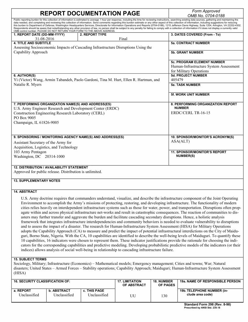
REPORT DOCUMENTATION PAGE Form Approved OMB No. 0704-0188
Public reporting burden for this collection of information is estimated to average 1 hour per response, including the time for reviewing instructions, searching existing data sources, gathering and maintaining the data needed, and completing and reviewing this collection of information. Send comments regarding this burden estimate or any other aspect of this collection of information, including suggestions for reducing this burden to Department of Defense, Washington Headquarters Services, Directorate for Information Operations and Reports (0704-0188), 1215 Jefferson Davis Highway, Suite 1204, Arlington, VA 22202-4302. Respondents should be aware that notwithstanding any other provision of law, no person shall be subject to any penalty for failing to comply with a collection of information if it does not display a currently valid OMB control number. PLEASE DO NOT RETURN YOUR FORM TO THE ABOVE ADDRESS. 1. REPORT DATE (DD-MM-YYYY)
31-08-2016
2. REPORT TYPE Final
3. DATES COVERED (From - To) 4. TITLE AND SUBTITLE
Assessing Socioeconomic Impacts of Cascading Infrastructure Disruptions Using the Capability Approach
5a. CONTRACT NUMBER 5b. GRANT NUMBER 5c. PROGRAM ELEMENT NUMBER Human-Infrastructure System Assessment for Military Operations
6. AUTHOR(S) Yi (Victor) Wang, Armin Tabandeh, Paolo Gardoni, Tina M. Hurt, Ellen R. Hartman, and Natalie R. Myers
5d. PROJECT NUMBER 405479 5e. TASK NUMBER 5f. WORK UNIT NUMBER
7. PERFORMING ORGANIZATION NAME(S) AND ADDRESS(ES) U.S. Army Engineer Research and Development Center (ERDC) Construction Engineering Research Laboratory (CERL) PO Box 9005 Champaign, IL 61826-9005
8. PERFORMING ORGANIZATION REPORT NUMBER
ERDC/CERL TR-16-15
9. SPONSORING / MONITORING AGENCY NAME(S) AND ADDRESS(ES) 10. SPONSOR/MONITOR’S ACRONYM(S) ASA(ALT) Assistant Secretary of the Army for
Acquisition, Logistics, and Technology 103 Army Pentagon Washington, DC 20314-1000
11. SPONSOR/MONITOR’S REPORT NUMBER(S)
12. DISTRIBUTION / AVAILABILITY STATEMENT Approved for public release. Distribution is unlimited.
13. SUPPLEMENTARY NOTES 14. ABSTRACT
U.S. Army doctrine requires that commanders understand, visualize, and describe the infrastructure component of the Joint Operating Environment to accomplish the Army’s missions of protecting, restoring, and developing infrastructure. The functionality of modern cities relies heavily on interdependent infrastructure systems such as those for water, power, and transportation. Disruptions often prop-agate within and across physical infrastructure net-works and result in catastrophic consequences. The reaction of communities to dis-asters may further transfer and aggravate the burden and facilitate cascading secondary disruptions. Hence, a holistic analysis framework that integrates infrastructure interdependencies and community behaviors is needed to evaluate vulnerability to disruptions and to assess the impact of a disaster. The research for Human-Infrastructure System Assessment (HISA) for Military Operations adopts the Capability Approach (CA) to measure and predict the impact of potential infrastructural interdictions on the City of Maidu-guri, Borno State, Nigeria. With the CA, 10 capabilities are identified to describe the well-being levels of Maiduguri. To quantify these 10 capabilities, 16 indicators were chosen to represent them. These indicator justifications provide the rationale for choosing the indi-cators for the corresponding capabilities and predictive modeling. Developing probabilistic predictive models of the indicators (or their indices) allows analysis of social well-being in relationship to cascading infrastructure failure.
15. SUBJECT TERMS Sociology, Military; Infrastructure (Economics) – Mathematical models; Emergency management; Cities and towns; War; Natural disasters; United States – Armed Forces – Stability operations; Capability Approach; Maiduguri; Human-Infrastructure System Assessment (HISA)
16. SECURITY CLASSIFICATION OF: 17. LIMITATION OF ABSTRACT
18. NUMBER OF PAGES
19a. NAME OF RESPONSIBLE PERSON
a. REPORT Unclassified
b. ABSTRACT Unclassified
c. THIS PAGE Unclassified
UU
130
19b. TELEPHONE NUMBER (in-clude area code)
Standard Form 298 (Rev. 8-98) Prescribed by ANSI Std. 239.18