Entropy and Complexity Analyses in Alzheimer's Disease: An MEG Study
13
The Open Biomedical Engineering Journal, 2010, 4, 223-235 223 1874-1207/10 2010 Bentham Open Open Access Entropy and Complexity Analyses in Alzheimer’s Disease: An MEG Study Carlos Gómez* and Roberto Hornero Biomedical Engineering Group, E.T.S. Ingenieros de Telecomunicación, University of Valladolid, Spain Abstract: Alzheimer’s disease (AD) is one of the most frequent disorders among elderly population and it is considered the main cause of dementia in western countries. This irreversible brain disorder is characterized by neural loss and the appearance of neurofibrillary tangles and senile plaques. The aim of the present study was the analysis of the magnetoencephalogram (MEG) background activity from AD patients and elderly control subjects. MEG recordings from 36 AD patients and 26 controls were analyzed by means of six entropy and complexity measures: Shannon spectral entropy (SSE), approximate entropy (ApEn), sample entropy (SampEn), Higuchi’s fractal dimension (HFD), Maragos and Sun’s fractal dimension (MSFD), and Lempel-Ziv complexity (LZC). SSE is an irregularity estimator in terms of the flatness of the spectrum, whereas ApEn and SampEn are embbeding entropies that quantify the signal regularity. The complexity measures HFD and MSFD were applied to MEG signals to estimate their fractal dimension. Finally, LZC measures the number of different substrings and the rate of their recurrence along the original time series. Our results show that MEG recordings are less complex and more regular in AD patients than in control subjects. Significant differences between both groups were found in several brain regions using all these methods, with the exception of MSFD (p-value < 0.05, Welch’s t-test with Bonferroni’s correction). Using receiver operating characteristic curves with a leave- one-out cross-validation procedure, the highest accuracy was achieved with SSE: 77.42%. We conclude that entropy and complexity analyses from MEG background activity could be useful to help in AD diagnosis. Keywords: Signal processing, entropy, complexity, Alzheimer’s disease, magnetoencephalogram. 1. INTRODUCTION Magnetoencephalography (MEG) is a non-invasive technique that allows recording the magnetic fields produced by brain activity. It provides an excellent temporal resolution, orders of magnitude better than other methods for measuring cerebral activity, as magnetic resonance imaging, single-photon-emission computed tomography or positron- emission tomography [1]. A good spatial resolution can also be achieved due to the large number of sensors. Moreover, the activity in different parts of the brain can be monitored simultaneously with whole-head equipments, such as the magnetometer used in the present study [1]. The use of MEG recordings to study the brain background activity also offers some advantages over electroencephalography (EEG) signals. Firstly, electrical activity is more affected than magnetic oscillations by skull and extracerebral brain tissues [1, 2]. Moreover, EEG acquisition can be significantly influenced by technical and methodological issues, like distance between electrodes and the sensor placement. In addition to this, MEG provides reference-free recordings. On the other hand, the magnetic signals generated by the human brain are extremely weak. Thus, large arrays of superconducting quantum interference devices (SQUIDs), immersed in liquid helium at 4.2 K, are necessary to detect them. In addition, MEG signals must be recorded in a magnetically shielded room to reduce the environmental noise [1]. Therefore, MEG is characterized by limited availability and high equipment cost. *Address correspondence to this author at the Biomedical Engineering Group, E.T.S. Ingenieros de Telecomunicación, University of Valladolid, Paseo Belén, 15, 47011 - Valladolid, Spain; Tel: +34 983423000 ext. 3703; Fax: +34 983423667; E-mail: [email protected] Alzheimer’s disease (AD) is a progressive and irreversible brain disorder of unknown aetiology. It is the main cause of dementia in western countries, accounting for 50-60% of all cases [3]. AD affects 1% of population aged 60-64 years, but the prevalence increases exponentially with age, so around 30% of people over 85 years suffer from this disease [4]. Additionally, due to the fact that life expectancy has significantly improved in western countries in the last decades, it is expected that the number of people with dementia increase up to 81 million in 2040 [4]. AD is characterized by the presence of neuritic plaques and neurofibrillary tangles, accompanied by the loss of cortical neurons and synapses [5]. Clinically, this disease manifests as a slowly progressive impairment of mental functions whose course lasts several years prior to death [5]. Usually, AD starts by destroying neurons in parts of the patient’s brain that are responsible for storing and retrieving information. Then, it affects the brain areas involved in language and reasoning. Eventually, many other brain regions are atrophied. Thus, AD patients may wander, be unable to engage in conversation, appear non-responsive, become helpless and need complete care and attention [6]. Although a definite AD diagnosis is only possible by necropsy, a differential diagnosis with other types of dementia and with major depression should be attempted. The differential diagnosis includes medical history studies, physical and neurological evaluation, mental status tests, and neuroimaging techniques. The electromagnetic brain activity in AD has been researched in the last decades by means of several complexity and entropy techniques. The most widely used methods to characterize the complexity of a system are the first positive Lyapunov exponent (L1) and the correlation
-
Upload
independent -
Category
Documents
-
view
5 -
download
0
Transcript of Entropy and Complexity Analyses in Alzheimer's Disease: An MEG Study
The Open Biomedical Engineering Journal, 2010, 4, 223-235 223
1874-1207/10 2010 Bentham Open
Open Access
Entropy and Complexity Analyses in Alzheimer’s Disease: An MEG Study
Carlos Gómez* and Roberto Hornero
Biomedical Engineering Group, E.T.S. Ingenieros de Telecomunicación, University of Valladolid, Spain
Abstract: Alzheimer’s disease (AD) is one of the most frequent disorders among elderly population and it is considered the main cause of dementia in western countries. This irreversible brain disorder is characterized by neural loss and the appearance of neurofibrillary tangles and senile plaques. The aim of the present study was the analysis of the magnetoencephalogram (MEG) background activity from AD patients and elderly control subjects. MEG recordings from 36 AD patients and 26 controls were analyzed by means of six entropy and complexity measures: Shannon spectral entropy (SSE), approximate entropy (ApEn), sample entropy (SampEn), Higuchi’s fractal dimension (HFD), Maragos and Sun’s fractal dimension (MSFD), and Lempel-Ziv complexity (LZC). SSE is an irregularity estimator in terms of the flatness of the spectrum, whereas ApEn and SampEn are embbeding entropies that quantify the signal regularity. The complexity measures HFD and MSFD were applied to MEG signals to estimate their fractal dimension. Finally, LZC measures the number of different substrings and the rate of their recurrence along the original time series. Our results show that MEG recordings are less complex and more regular in AD patients than in control subjects. Significant differences between both groups were found in several brain regions using all these methods, with the exception of MSFD (p-value < 0.05, Welch’s t-test with Bonferroni’s correction). Using receiver operating characteristic curves with a leave-one-out cross-validation procedure, the highest accuracy was achieved with SSE: 77.42%. We conclude that entropy and complexity analyses from MEG background activity could be useful to help in AD diagnosis.
Keywords: Signal processing, entropy, complexity, Alzheimer’s disease, magnetoencephalogram.
1. INTRODUCTION
Magnetoencephalography (MEG) is a non-invasive technique that allows recording the magnetic fields produced by brain activity. It provides an excellent temporal resolution, orders of magnitude better than other methods for measuring cerebral activity, as magnetic resonance imaging, single-photon-emission computed tomography or positron-emission tomography [1]. A good spatial resolution can also be achieved due to the large number of sensors. Moreover, the activity in different parts of the brain can be monitored simultaneously with whole-head equipments, such as the magnetometer used in the present study [1]. The use of MEG recordings to study the brain background activity also offers some advantages over electroencephalography (EEG) signals. Firstly, electrical activity is more affected than magnetic oscillations by skull and extracerebral brain tissues [1, 2]. Moreover, EEG acquisition can be significantly influenced by technical and methodological issues, like distance between electrodes and the sensor placement. In addition to this, MEG provides reference-free recordings. On the other hand, the magnetic signals generated by the human brain are extremely weak. Thus, large arrays of superconducting quantum interference devices (SQUIDs), immersed in liquid helium at 4.2 K, are necessary to detect them. In addition, MEG signals must be recorded in a magnetically shielded room to reduce the environmental noise [1]. Therefore, MEG is characterized by limited availability and high equipment cost.
*Address correspondence to this author at the Biomedical Engineering Group, E.T.S. Ingenieros de Telecomunicación, University of Valladolid, Paseo Belén, 15, 47011 - Valladolid, Spain; Tel: +34 983423000 ext. 3703; Fax: +34 983423667; E-mail: [email protected]
Alzheimer’s disease (AD) is a progressive and irreversible brain disorder of unknown aetiology. It is the main cause of dementia in western countries, accounting for 50-60% of all cases [3]. AD affects 1% of population aged 60-64 years, but the prevalence increases exponentially with age, so around 30% of people over 85 years suffer from this disease [4]. Additionally, due to the fact that life expectancy has significantly improved in western countries in the last decades, it is expected that the number of people with dementia increase up to 81 million in 2040 [4]. AD is characterized by the presence of neuritic plaques and neurofibrillary tangles, accompanied by the loss of cortical neurons and synapses [5]. Clinically, this disease manifests as a slowly progressive impairment of mental functions whose course lasts several years prior to death [5]. Usually, AD starts by destroying neurons in parts of the patient’s brain that are responsible for storing and retrieving information. Then, it affects the brain areas involved in language and reasoning. Eventually, many other brain regions are atrophied. Thus, AD patients may wander, be unable to engage in conversation, appear non-responsive, become helpless and need complete care and attention [6]. Although a definite AD diagnosis is only possible by necropsy, a differential diagnosis with other types of dementia and with major depression should be attempted. The differential diagnosis includes medical history studies, physical and neurological evaluation, mental status tests, and neuroimaging techniques.
The electromagnetic brain activity in AD has been researched in the last decades by means of several complexity and entropy techniques. The most widely used methods to characterize the complexity of a system are the first positive Lyapunov exponent (L1) and the correlation
224 The Open Biomedical Engineering Journal, 2010, Volume 4 Gómez and Hornero
dimension (D2). L1 is a dynamic complexity measure that describes the divergence of trajectories starting at nearby initial states [7], while D2 computes the geometric complexity of the reconstructed attractor [8]. For instance, Jeong et al. [7] showed that AD patients exhibit significantly lower D2 and L1 values than controls in many EEG channels. In a MEG study [9], this complexity loss was reported only in the high frequency bands. Nevertheless, these classical measures for estimating the non-linear dynamic complexity have some drawbacks. Reliable estimation of L1 and D2 requires a large quantity of data and stationary and noise free time series [10, 11]. Since these assumptions cannot be achieved for physiological data, other complexity measures are necessary for the analysis of brain time series. The dimensional complexity of a signal can also be estimated directly in the time domain using the fractal dimension (FD) without reconstructing the attractor in the phase space. In the last decades, the number of algorithms to estimate the FD has increased rapidly: Higuchi’s fractal dimension (HFD) [12], Maragos and Sun’s fractal dimension (MSFD) [13] or Katz’s algorithm [14]. Some of them have been successfully applied to EEG/MEG recordings in dementia [15, 16]. Finally, other non-linear complexity measures, as Lempel-Ziv complexity (LZC) or multiscale entropy, have also been used to characterize the brain activity in AD [17-20].
Entropy is a concept addressing randomness and predictability, with greater entropy often associated with more randomness and less system order [21]. Mainly, there are two families of entropy estimators: spectral entropies and embedding entropies [22]. Spectral entropies extract information from the amplitude component of the frequency spectrum. On the other hand, embedding entropies are calculated directly using the time series. This entropies family provides information about how the signal fluctuates with time by comparing the time series with a delayed version of itself [22]. Both spectral and embedding entropies have demonstrated their usefulness in the analysis of EEG/MEG background activity in AD. An increase of entropy values has been found using approximate entropy (ApEn) [20, 21], sample entropy (SampEn) [18, 23], Shannon spectral entropy (SSE), Rényi spectral entropy and Tsallis spectral entropy [24].
In this study, we have examined the MEG background activity in 36 patients with probable AD and 26 elderly control subjects using six entropy and complexity measures: SSE, ApEn, SampEn, HFD, MSFD and LZC. Some of these methods have been already used to characterize the MEG activity in AD [15, 17, 18, 20, 24]. Nevertheless, it should be noted that previously published studies were based on slightly different databases, thus making a direct comparison of the results impossible. However, in this paper, all complexity and entropy techniques were applied to the same MEG database. Our purpose is to test the hypothesis that the neuronal dysfunction in AD is associated with differences in the dynamical processes underlying the MEG recording.
2. MATERIALS
2.1. Subjects
In this study, MEG signals were recorded from 62 subjects: 36 AD patients and 26 elderly control subjects.
Clinical diagnosis was ascertained by means of exhaustive general medical, neurological, and psychiatric examinations. All patients and controls underwent a neuropsychological evaluation including the Spanish versions of the following scales and batteries: Wechsler Memory Scale 3rd Edition (WMS-III), Boston Naming Test (BNT), Stroop Test, Wisconsin Card Shorting Test (WCST), Silhouettes Test of the Visual Object and Space Battery (VOSP), and tests for constructive and ideatory apraxia. Additionally, cognitive status was screened in both groups with the Spanish version [25] of the Mini Mental State Examination (MMSE) of Folstein et al. [26], whereas functional status was evaluated by means of the Global Deterioration Scale/Functional Assessment Staging (GDS/FAST) system [27].
MEGs were obtained from 36 patients (12 men and 24 women; age = 74.06 ± 6.95 years, mean ± standard deviation, SD) fulfilling the criteria of probable AD. They were recruited from the “Asociación de Familiares de Enfermos de Alzheimer” in Spain. Diagnosis for all patients was made according to the National Institute of Neurological and Communicative Disorders and Stroke and Alzheimer’s Disease and Related Disorders Association (NINCDS–ADRDA) criteria [28]. The MMSE and GDS/FAST scores for these patients were 18.06 ± 3.36 and 4.17 ± 0.45 (mean ± SD), respectively. Patients were free of other significant medical, neurological and psychiatric diseases than AD and they were not taking drugs which could affect MEG activity.
The control group consisted of 26 elderly control subjects without past or present neurological disorders (9 men and 17 women; age = 71.77 ± 6.38 years, MMSE score = 28.88 ± 1.18 points, GDA/FAST score = 1.73 ± 0.45 points; mean ± SD). The difference in age between both populations was not statistically significant (p-value = 0.1911 > 0.05). All control subjects and patients’ caregivers signed an informed consent for the participation in this research work. The local Ethics Committee approved this study.
2.2. MEG Recording
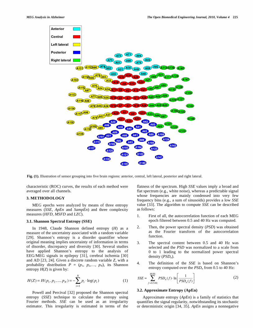
MEGs were acquired with a 148-channel whole-head magnetometer (MAGNES 2500 WH, 4D Neuroimaging) placed in a magnetically shielded room at “Centro de Magnetoencefalografía Dr. Pérez-Modrego” (Spain). The subjects lay on a patient bed, in a relaxed state and with their eyes closed. For each subject, five minutes of recording were acquired at a sampling frequency of 678.17 Hz, using a hardware band-pass filter from 0.1 to 200 Hz. Then, the equipment decimated each 5 minutes data set. This process consisted of filtering the data to satisfy the Nyquist criterion, following by a down-sampling by a factor of 4, thus obtaining a sampling rate of 169.549 Hz. Finally, artifact-free epochs of 5 seconds were processed using a band-pass filter with a Hamming window and cut-off frequencies at 0.5 and 40 Hz. For LZC, the epoch length was 20 seconds, as previous studies suggested that LZC values become stable for MEG signals longer than 3000 samples [17]. For the statistical analysis, the channels were grouped in five brain areas (anterior, central, left lateral, posterior and right lateral), which are included as default sensor groups in the 4D-Neuroimaging source analysis software, as Fig. (1) shows. For classification purposes with receiver operating
MEG Analysis in Alzheimer The Open Biomedical Engineering Journal, 2010, Volume 4 225
characteristic (ROC) curves, the results of each method were averaged over all channels.
3. METHODOLOGY
MEG epochs were analyzed by means of three entropy measures (SSE, ApEn and SampEn) and three complexity measures (HFD, MSFD and LZC).
3.1. Shannon Spectral Entropy (SSE)
In 1948, Claude Shannon defined entropy (H) as a measure of the uncertainty associated with a random variable [29]. Shannon’s entropy is a disorder quantifier whose original meaning implies uncertainty of information in terms of disorder, discrepancy and diversity [30]. Several studies have applied Shannon’s entropy to the analysis of EEG/MEG signals in epilepsy [31], cerebral ischemia [30] and AD [23, 24]. Given a discrete random variable Z, with a probability distribution P = (p1, p2,…, pN), its Shannon entropy H(Z) is given by:
H (Z ) = H (p1, p2 , ..., pN ) = pi log(pi )i=1
N
(1)
Powell and Percival [32] proposed the Shannon spectral entropy (SSE) technique to calculate the entropy using Fourier methods. SSE can be used as an irregularity estimator. This irregularity is estimated in terms of the
flatness of the spectrum. High SSE values imply a broad and flat spectrum (e.g., white noise), whereas a predictable signal whose frequencies are mainly condensed into very few frequency bins (e.g., a sum of sinusoids) provides a low SSE value [33]. The algorithm to compute SSE can be described as follows:
1. First of all, the autocorrelation function of each MEG epoch filtered between 0.5 and 40 Hz was computed.
2. Then, the power spectral density (PSD) was obtained as the Fourier transform of the autocorrelation function.
3. The spectral content between 0.5 and 40 Hz was selected and the PSD was normalized to a scale from 0 to 1 leading to the normalized power spectral density (PSDn).
4. The definition of the SSE is based on Shannon’s entropy computed over the PSDn from 0.5 to 40 Hz:
SSE = PSDn ( f ) ln1
PSDn ( f )f =0.5Hz
40Hz
(2)
3.2. Approximate Entropy (ApEn)
Approximate entropy (ApEn) is a family of statistics that quantifies the signal regularity, notwithstanding its stochastic or deterministic origin [34, 35]. ApEn assigns a nonnegative
Fig. (1). Illustration of sensor grouping into five brain regions: anterior, central, left lateral, posterior and right lateral.
226 The Open Biomedical Engineering Journal, 2010, Volume 4 Gómez and Hornero
number to a sequence, with larger values corresponding to greater apparent process randomness or serial irregularity, and smaller values corresponding to more instances of recognizable features or patterns in the data [36]. To compute ApEn, two input parameters must be specified: a run length m and a tolerance window r. The dimensionless parameter m represents a window length of the number of contiguous time-series points that are compared with one another in forming the ApEn calculation. Briefly, ApEn measures the logarithmic likelihood that runs of patterns that are close (within r) for m contiguous observations remain close (within the same tolerance width r) on next incremental comparisons [36, 37]. Comparisons between data sequences must be made with the same values of m, r and N, where N is the number of points of the MEG epoch [37]. Pincus has suggested parameter values of m = 1 or m = 2, and with r a fixed value between 0.1 to 0.25 times the SD of the original time series [37]. The parameter r is normalized to give ApEn a translation and scale invariance. In this study, ApEn was computed with the established parameters of m = 1 and r = 0.25 times the SD of the analyzed signal [36]. These parameters provide good statistical reproducibility for sequences longer than N = 60, as considered herein [34, 35]. As ApEn can be applied to short and relatively noisy time series, it has been widely used to extract potentially useful information from biomedical time series such as electrocardiogram [38], EEG [23], concentration time series [39] and respiratory recordings [40], among others.
The algorithm used to compute the entropy of a signal X = (x1, x2,..., xN) is as follows [34]:
1. Form a set of vectors X1,…, XN–m+1 defined by X
i = (xi, xi+1,…, xi+m–1), i = 1,…, N – m + 1. These vectors represent m consecutive values of X, starting with the i-th point.
2. Define the distance between Xi and Xj, d[Xi, Xj] as the
maximum absolute difference between their respective scalar components:
d[Xi , X j ] = maxk=0,...,m 1
| xi+ k x j+ k | (3)
3. For a given Xi, let N
m(i) denote the number of j (j = 1,…, N – m + 1) so that d[Xi, X
j] r. Thus, for i = 1,…, N – m + 1:
Crm (i) =
Nm (i)
N m +1 (4)
Crm(i) measure, within a tolerance r, the regularity or
frequency of patterns similar to a given one of window length m.
4. Compute the natural logarithm of each Crm(i) and
average it over i:
m (r) =1
N m +1lnCr
m (i)i=1
N m+1
(5)
5. Increase the dimension to m + 1 and repeat the previous steps to obtain Cr
m+1(i) and m+1(r).
6. Finally, ApEn is defined as:
ApEn(m, r) = lim[N
m (r) m+1(r)] (6)
7. As the signal length N is finite, ApEn is estimated by the statistic:
ApEn(m, r,N ) = m (r) m+1(r) (7)
3.3. Sample Entropy (SampEn)
Sample entropy (SampEn) is an embedding entropy that quantifies the signal irregularity: more irregularity in the data produces larger SampEn values [41]. This metric solves some problems associated with ApEn. The ApEn algorithm counts each sequence as matching itself to avoid the occurrence of ln(0) in the calculations and this has led to discussion of the bias of ApEn [41]. To reduce this bias, Richman and Moorman have developed the so called SampEn. SampEn is largely independent of the signal length and displays relative consistency under circumstances where ApEn does not. Additionally, the algorithm used to compute the SampEn is simpler than the ApEn one [41]. Despite its advantages over ApEn, the use of SampEn is not widespread. This measure has been used to study some biological signals, such as heart rate time series [42, 43], EEG data [23, 44] and MEG recordings [18]. SampEn has two input parameters: a run length m and a tolerance window r. SampEn is the negative natural logarithm of the conditional probability that two sequences similar for m points remain similar at the next point [41]. For this study, SampEn was calculated with parameter values m = 1 and r = 0.25 times the SD of the original data sequence.
To calculate the SampEn(m, r, N) from a time series, X = (x1, x2,..., xN), one should follow these steps [41]:
1. Form a set of vectors Xm1,…, Xm
N–m+1 defined by Xmi =
(xi, xi+1,…, xi+m–1), i = 1,…, N – m + 1.
2. The distance between Xmi and Xm
j, d[Xmi, Xm
j], is the maximum absolute difference between their respective scalar components:
d[Xmi , Xm
j ] = maxk=0,...,m 1
| xi+ k x j+ k | (8)
3. For a given Xmi, count the number of j (1 j N – m,
j i), denoted as Bi, such that d[Xmi, Xm
j] r. Then, for 1 i N – m,
Bim (r) =
1
N m 1Bi (9)
4. Define Bm (r) as:
Bm (r) =1
N mBim (r)
i=1
N m
(10)
5. Similarly, calculate Aim (r) as 1/(N – m + 1) times the
number of j (1 j N – m, j i), such that the distance between Xm+1
j and Xm+1i is less than or equal
to r. Set Am (r) as:
Am (r) =1
N mAim (r)
i=1
N m
(11)
MEG Analysis in Alzheimer The Open Biomedical Engineering Journal, 2010, Volume 4 227
Thus, Bm (r) is the probability that two sequences will match
for m points, whereas Am (r) is the probability that two sequences will match for m + 1 points.
6. Finally, define:
SampEn(m, r) = limN
lnAm (r)
Bm (r) (12)
which is estimated by the statistic:
SampEn(m, r,N ) = lnAm (r)
Bm (r) (13)
3.4. Higuchi’s Fractal Dimension (HFD)
The term FD was introduced by Mandelbrot to study temporal or spatial continuous phenomena that show correlation into a range of scales [45]. Applied to brain recordings, FD quantifies the complexity and self-similarity of these signals [46]. Many algorithms are available to compute FD, like those proposed by Higuchi [12], Maragos and Sun [13], and Katz [14]. Higuchi’s fractal dimension (HFD) is an appropriate method for analysing biomedical signals [46], as MEG recordings, due to the fact that it provides more accurate estimation of FD than other methods. Higuchi’s algorithm calculates the FD directly from time series. As the reconstruction of the attractor phase space is not necessary, this algorithm is simpler and faster than D2 and other classical measures derived from chaos theory. On the other hand, Higuchi’s algorithm is more sensitive to the noise level than other measures, producing a sensible, slightly distorted, translation towards higher FD values [46, 47]. HFD has already been used to analyse the complexity of EEG signals [46, 48] and MEG recordings [15].
The detailed algorithm for the computation of HFD is as follows [12]:
1. Given a time series X = (x1, x2,..., xN), form k new
time series m
kX :
Xkm= xm , xm+ k , ..., x
m+ intN m
kk
(14)
where k is an integer that indicates the discrete time interval between points and m, also integer, denotes the initial time value. Lastly, int(a) represents the integer part of a.
2. The length of each new time series can be defined by:
L m, k( ) =
xm+ ik xm+ i 1( ) ki=1
intN m
k
R
k (15)
where R = N 1( ) intN m
kk is a normalization
factor.
3. The length of the curve for the time interval k is defined as the average of the lengths L(m,k), for m =
1, 2, …, k:
L k( ) =1
kL m, k( )
m=1
k
(16)
4. Finally, HFD is defined as the slope of the line that
fits the pairs ln L k( ) , ln 1 / k( ){ } , for k = 1, 2,...,
kmax, in a least-squares sense. In order to choose an appropriate value of the parameter kmax, the criterion proposed by Doyle et al. [49] was used. HFD values were plotted against a range of kmax. The point at which the FD plateaus is considered a saturation point and that kmax value should be selected. Using this criterion, a value of kmax = 56 was chosen in our study.
3.5. Maragos and Sun’s Fractal Dimension (MSFD)
The method proposed by Petros Maragos and Fang-Kuo Sun is other way to measure the FD of a signal [13]. The FD of time series is calculated by using morphological erosion and dilation function operations to create covers around a signal graph at multiple scales. This method has some computational advantages. Its computational complexity is linear with respect to both the signal length and the maximum scale [13]. Moreover, Maragos and Sun’s fractal dimension (MSFD) gives a good approximation for a very small number of points [46]. Additionally, the results achieved with synthetic signals showed average estimation errors of about 2-4% [13]. Accardo et al. [46] confirmed these results. MSFD has been used for the characterization of the Spanish fricatives sounds [50] and for the analysis of sea surface images [51]. In other study, the method was compared with Higuchi’s algorithm for the analysis of EEG signals [46].
Given N points from a time series X = (x1, x2,..., xN), the algorithm to estimate MSFD is the following [13, 46]:
1. Select a structuring element B. There are three possibilities for the selection of B: a 3 x 3 pixel square, a 5-pixel rhombus, and a 3-pixel horizontal segment. In this work, we have used the last one, with the following associated function g [13]:
gj = 0 j = –1, 0, 1
gj = – j –1, 0, 1 (17)
2. The function g is used to recursively perform the support-limited dilations and erosions of the time series X by g
d at different scales. In our case, the dilation operation (for erosions, the expressions are analogous) corresponds to:
X S gd( )
n= max xn 1, xn , xn+1{ } d = 1
X S gd+1( )
n= max X S g
d( )n 1, X S g
d( )n+1{ } d 2 (18)
3. Then, the cover areas are computed for different scales d = 1, 2,…, dmax:
228 The Open Biomedical Engineering Journal, 2010, Volume 4 Gómez and Hornero
A d[ ] = X S gd( )
nX S g
d )n(
n=1
N
d = 1, 2,…, dmax (19)
4. Finally, MSFD is defined as the slope of the line that
fits the pairs ln A d[ ] D2( ), ln 1 / D( ){ } in a least-
squares sense, where D = 2 d / N. In order to select an appropriate value of the parameter dmax, the heuristic rule proposed by Maragos and Sun [13] was used.
3.6. Lempel-Ziv Complexity (LZC)
The LZC algorithm was proposed by Lempel and Ziv to evaluate the randomness of finite sequences [52]. It is a nonparametric and simple-to-compute measure of complexity for one-dimensional signals that does not require long data segments to be calculated [53]. Larger LZC values correspond to more complex data. Previous studies have shown that LZC mainly depends on the bandwidth of the signal spectrum, although a slight dependence on the sequence probability density function was also found [48, 54]. Additionally, LZC could be interpreted as a harmonic variability metric [54]. LZC has been used to study the relationship between brain activity patterns and depth of anesthesia [53], to characterize the complexity of DNA sequences [55], and to quantify the complexity in uterine electromyography [56]. Due to the fact that LZC analyzes a finite symbol sequence, the given signal must first be coarse-grained [53]. In this study, a binary (zeros and ones) conversion was used, since previous studies found that this kind of conversion may keep enough signal information [53, 54]. The data points were compared to a threshold, Td. We fixed Td to the median of the analyzed signal, as partitioning about this value is robust to outliers [56]. By comparison with Td, the original data X = (x1, x2,..., xN) are converted into a 0-1 sequence P = (s1, s2,..., sN), with si defined by [53]:
si =0 if xi < Td1 if xi Td
(20)
The string P is scanned from left to right and a complexity counter c(N) is increased by one unit every time a new subsequence of consecutive characters is encountered in the scanning process. The detailed algorithm for the measure of LZC is as follows [53, 56, 57]:
1. Let S and Q denote two subsequences of the original sequence P. SQ is the concatenation of S and Q, while SQ is a string derived from SQ after its last character is deleted ( means the operation to delete the last character). Let v(SQ ) denote the vocabulary of all different substrings of SQ .
2. At the beginning, the complexity counter c(N) = 1, S = s1, Q = s2, SQ = s1, s2 and SQ = s1.
3. For generalization, suppose that S = s1, s2,…, sr, Q = sr+1 and, therefore, SQ = s1, s2,…, sr. If Q v(SQ ), then Q is a subsequence of SQ , not a new sequence.
4. S does not change and renew Q to be sr+1, sr+2, then judge if Q belongs to v(SQ ) or not.
5. The previous steps are repeated until Q does not belong to v(SQ ). Now Q = sr+1, sr+2,…, sr+i is not a subsequence of SQ = s1, s2,…, sr+i–1, so increase the counter by one.
6. Thereafter, S and Q are combined and renewed to be s1, s2,…, sr, sr+1,…, sr+i, and sr+i+1, respectively.
7. Repeat the previous steps until Q is the last character. At this time, the number of different substrings is c(N), the measure of complexity.
In order to obtain a complexity measure independent of the sequence length, c(N) should be normalized. If the length of the sequence is N and is the number of different symbols, it has been proved that the upper bound of c(N) is given by [52]:
c(N ) <N
1 N( ) log (N ) (21)
where N is a small quantity and N 0 (N ). In general, N/log (N) is the upper limit of c(N), i.e.
limN
c(N ) = b(N )N
log (N ) (22)
For a binary conversion = 2, b(N) N/log2(N) and c(N) can be normalized via b(N):
C(N ) =c(N )
b(N ) (23)
C(N) reflects the arising rate of new patterns along with the sequence.
4. RESULTS AND DISCUSSION
SSE, ApEn, SampEn, HFD, MSFD and LZC were estimated for the 148 MEG channels. The results were averaged based on all the artefact-free epochs within the five-minute period of recording. In order to reduce the dimension of the results, the MEG channels were grouped in five brain areas (anterior, central, left lateral, posterior and right lateral). Normality of distribution was assessed with Kolmogorov-Smirnov test, whereas homoscedasticity was analyzed with Levene’s test. As the entropy and complexity results did not meet homoscedasticity assumption, Welch t-test with Bonferroni’s correction was used for the statistical comparison between AD patients and control subjects.
In this study, we have used the SSE to quantify the distribution of spectral power in MEG time-series of 848 samples. For SSE computation, it is not necessary to set any parameters. The average SSE value for the control group was 5.00 ± 0.34 (mean ± SD), whereas it reached 4.73 ± 0.33 for the AD patients. Fig. (2) summarizes the average SSE values estimated for the patients with AD and the control subjects, for all the MEG channels. This figure and the following ones have been plotted using scripts developed with the software package MATLAB (version 7.0; Mathworks, Natick, MA). These results suggest an irregularity decrease, in terms of the flatness of the power spectrum, for AD patients. Additionally, differences between AD patients and elderly control subjects were statistically significant in anterior, central and both lateral regions (p < 0.05; Welch t-test with Bonferroni’s correction). Previous studies have shown an
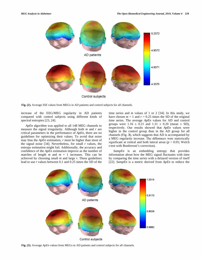
MEG Analysis in Alzheimer The Open Biomedical Engineering Journal, 2010, Volume 4 229
increase of the EEG/MEG regularity in AD patients compared with control subjects using different kinds of spectral entropies [23, 24].
ApEn algorithm was applied to all 148 MEG channels to measure the signal irregularity. Although both m and r are critical parameters in the performance of ApEn, there are no guidelines for optimizing their values. To avoid that noise may bias the ApEn estimation, r must be higher than most of the signal noise [34]. Nevertheless, for small r values, the entropy estimation might fail. Additionally, the accuracy and confidence of the ApEn estimation improve as the number of matches of length m and m + 1 increases. This can be achieved by choosing small m and large r. These guidelines lead to use r values between 0.1 and 0.25 times the SD of the
time series and m values of 1 or 2 [34]. In this study, we have chosen m = 1 and r = 0.25 times the SD of the original time series. The average ApEn values for AD and control groups were 1.16 ± 0.21 and 1.31 ± 0.20 (mean ± SD), respectively. Our results showed that ApEn values were higher in the control group than in the AD group for all channels (Fig. 3), which suggests that AD is accompanied by a MEG regularity increase. The differences were statistically significant at central and both lateral areas (p < 0.05; Welch t-test with Bonferroni’s correction).
SampEn is an embedding entropy that provides information about how the MEG signal fluctuates with time by comparing the time series with a delayed version of itself [22]. SampEn is a metric derived from ApEn to reduce the
Fig. (2). Average SSE values from MEGs in AD patients and control subjects for all channels.
Fig. (3). Average ApEn values from MEGs in AD patients and control subjects for all channels.
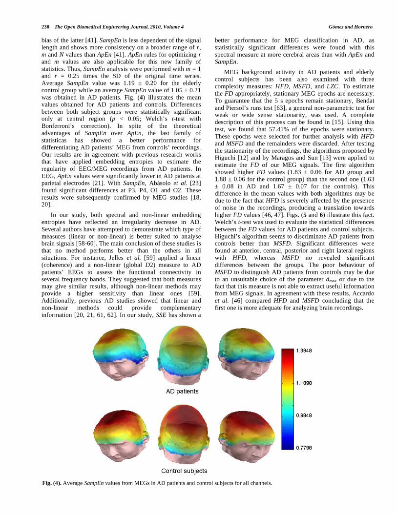
230 The Open Biomedical Engineering Journal, 2010, Volume 4 Gómez and Hornero
bias of the latter [41]. SampEn is less dependent of the signal length and shows more consistency on a broader range of r, m and N values than ApEn [41]. ApEn rules for optimizing r and m values are also applicable for this new family of statistics. Thus, SampEn analysis were performed with m = 1 and r = 0.25 times the SD of the original time series. Average SampEn value was 1.19 ± 0.20 for the elderly control group while an average SampEn value of 1.05 ± 0.21 was obtained in AD patients. Fig. (4) illustrates the mean values obtained for AD patients and controls. Differences between both subject groups were statistically significant only at central region (p < 0.05; Welch’s t-test with Bonferroni’s correction). In spite of the theoretical advantages of SampEn over ApEn, the last family of statisticas has showed a better performance for differentiating AD patients’ MEG from controls’ recordings. Our results are in agreement with previous research works that have applied embedding entropies to estimate the regularity of EEG/MEG recordings from AD patients. In EEG, ApEn values were significantly lower in AD patients at parietal electrodes [21]. With SampEn, Abásolo et al. [23] found significant differences at P3, P4, O1 and O2. These results were subsequently confirmed by MEG studies [18, 20].
In our study, both spectral and non-linear embedding entropies have reflected an irregularity decrease in AD. Several authors have attempted to demonstrate which type of measures (linear or non-linear) is better suited to analyse brain signals [58-60]. The main conclusion of these studies is that no method performs better than the others in all situations. For instance, Jelles et al. [59] applied a linear (coherence) and a non-linear (global D2) measure to AD patients’ EEGs to assess the functional connectivity in several frequency bands. They suggested that both measures may give similar results, although non-linear methods may provide a higher sensitivity than linear ones [59]. Additionally, previous AD studies showed that linear and non-linear methods could provide complementary information [20, 21, 61, 62]. In our study, SSE has shown a
better performance for MEG classification in AD, as statistically significant differences were found with this spectral measure at more cerebral areas than with ApEn and SampEn.
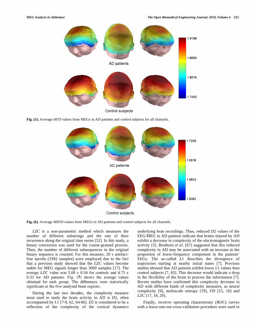
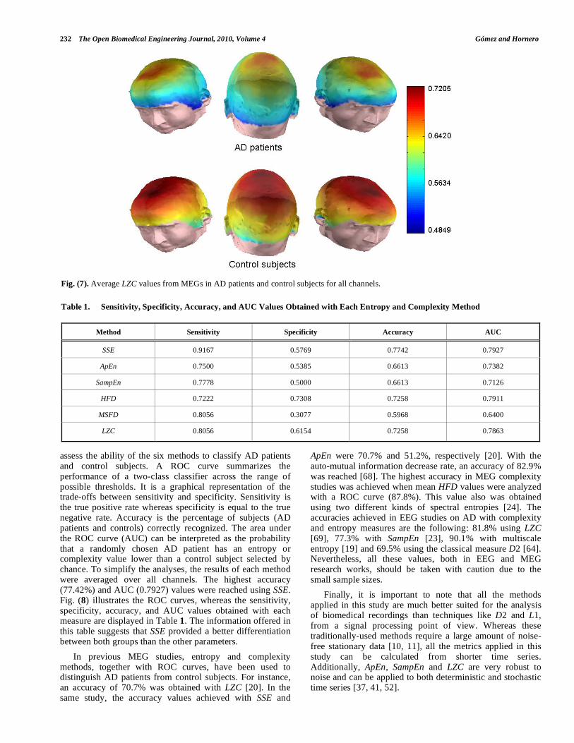
MEG background activity in AD patients and elderly control subjects has been also examined with three complexity measures: HFD, MSFD, and LZC. To estimate the FD appropriately, stationary MEG epochs are necessary. To guarantee that the 5 s epochs remain stationary, Bendat and Piersol’s runs test [63], a general non-parametric test for weak or wide sense stationarity, was used. A complete description of this process can be found in [15]. Using this test, we found that 57.41% of the epochs were stationary. These epochs were selected for further analysis with HFD and MSFD and the remainders were discarded. After testing the stationarity of the recordings, the algorithms proposed by Higuchi [12] and by Maragos and Sun [13] were applied to estimate the FD of our MEG signals. The first algorithm showed higher FD values (1.83 ± 0.06 for AD group and 1.88 ± 0.06 for the control group) than the second one (1.63 ± 0.08 in AD and 1.67 ± 0.07 for the controls). This difference in the mean values with both algorithms may be due to the fact that HFD is severely affected by the presence of noise in the recordings, producing a translation towards higher FD values [46, 47]. Figs. (5 and 6) illustrate this fact. Welch’s t-test was used to evaluate the statistical differences between the FD values for AD patients and control subjects. Higuchi’s algorithm seems to discriminate AD patients from controls better than MSFD. Significant differences were found at anterior, central, posterior and right lateral regions with HFD, whereas MSFD no revealed significant differences between the groups. The poor behaviour of MSFD to distinguish AD patients from controls may be due to an unsuitable choice of the parameter dmax or due to the fact that this measure is not able to extract useful information from MEG signals. In agreement with these results, Accardo et al. [46] compared HFD and MSFD concluding that the first one is more adequate for analyzing brain recordings.
Fig. (4). Average SampEn values from MEGs in AD patients and control subjects for all channels.
MEG Analysis in Alzheimer The Open Biomedical Engineering Journal, 2010, Volume 4 231
Fig. (5). Average HFD values from MEGs in AD patients and control subjects for all channels.
Fig. (6). Average MSFD values from MEGs in AD patients and control subjects for all channels.
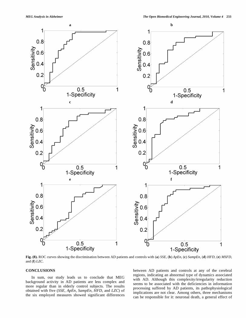
LZC is a non-parametric method which measures the number of different substrings and the rate of their recurrence along the original time series [52]. In this study, a binary conversion was used for the coarse-grained process. Then, the number of different subsequences in the original binary sequence is counted. For this measure, 20 s artefact-free epochs (3392 samples) were employed due to the fact that a previous study showed that the LZC values become stable for MEG signals longer than 3000 samples [17]. The average LZC value was 5.00 ± 0.34 for controls and 4.73 ± 0.33 for AD patients. Fig. (7) shows the average values obtained for each group. The differences were statistically significant at the five analyzed brain regions.
During the last two decades, the complexity measure most used to study the brain activity in AD is D2, often accompanied by L1 [7-9, 62, 64-66]. D2 is considered to be a reflection of the complexity of the cortical dynamics
underlying bran recordings. Thus, reduced D2 values of the EEG/MEG in AD patients indicate that brains injured by AD exhibit a decrease in complexity of the electromagnetic brain activity [5]. Besthorn et al. [67] suggested that this reduced complexity in AD may be associated with an increase in the proportion of lower-frequency component in the patients’ EEGs. The so-called L1 describes the divergence of trajectories starting at nearby initial states [7]. Previous studies showed that AD patients exhibit lower L1 values than control subjects [7, 65]. This decrease would indicate a drop in the flexibility of the brain to process the information [7]. Recent studies have confirmed this complexity decrease in AD with different kinds of complexity measures, as neural complexity [9], multiscale entropy [19], FD [15, 16] and LZC [17, 18, 20].
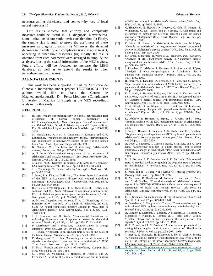
Finally, receiver operating characteristic (ROC) curves with a leave-one-out cross-validation procedure were used to
232 The Open Biomedical Engineering Journal, 2010, Volume 4 Gómez and Hornero
assess the ability of the six methods to classify AD patients and control subjects. A ROC curve summarizes the performance of a two-class classifier across the range of possible thresholds. It is a graphical representation of the trade-offs between sensitivity and specificity. Sensitivity is the true positive rate whereas specificity is equal to the true negative rate. Accuracy is the percentage of subjects (AD patients and controls) correctly recognized. The area under the ROC curve (AUC) can be interpreted as the probability that a randomly chosen AD patient has an entropy or complexity value lower than a control subject selected by chance. To simplify the analyses, the results of each method were averaged over all channels. The highest accuracy (77.42%) and AUC (0.7927) values were reached using SSE. Fig. (8) illustrates the ROC curves, whereas the sensitivity, specificity, accuracy, and AUC values obtained with each measure are displayed in Table 1. The information offered in this table suggests that SSE provided a better differentiation between both groups than the other parameters.
In previous MEG studies, entropy and complexity methods, together with ROC curves, have been used to distinguish AD patients from control subjects. For instance, an accuracy of 70.7% was obtained with LZC [20]. In the same study, the accuracy values achieved with SSE and
ApEn were 70.7% and 51.2%, respectively [20]. With the auto-mutual information decrease rate, an accuracy of 82.9% was reached [68]. The highest accuracy in MEG complexity studies was achieved when mean HFD values were analyzed with a ROC curve (87.8%). This value also was obtained using two different kinds of spectral entropies [24]. The accuracies achieved in EEG studies on AD with complexity and entropy measures are the following: 81.8% using LZC [69], 77.3% with SampEn [23], 90.1% with multiscale entropy [19] and 69.5% using the classical measure D2 [64]. Nevertheless, all these values, both in EEG and MEG research works, should be taken with caution due to the small sample sizes.
Finally, it is important to note that all the methods applied in this study are much better suited for the analysis of biomedical recordings than techniques like D2 and L1, from a signal processing point of view. Whereas these traditionally-used methods require a large amount of noise-free stationary data [10, 11], all the metrics applied in this study can be calculated from shorter time series. Additionally, ApEn, SampEn and LZC are very robust to noise and can be applied to both deterministic and stochastic time series [37, 41, 52].
Fig. (7). Average LZC values from MEGs in AD patients and control subjects for all channels.
Table 1. Sensitivity, Specificity, Accuracy, and AUC Values Obtained with Each Entropy and Complexity Method
Method Sensitivity Specificity Accuracy AUC
SSE 0.9167 0.5769 0.7742 0.7927
ApEn 0.7500 0.5385 0.6613 0.7382
SampEn 0.7778 0.5000 0.6613 0.7126
HFD 0.7222 0.7308 0.7258 0.7911
MSFD 0.8056 0.3077 0.5968 0.6400
LZC 0.8056 0.6154 0.7258 0.7863
MEG Analysis in Alzheimer The Open Biomedical Engineering Journal, 2010, Volume 4 233
a b
c d
e f
Fig. (8). ROC curves showing the discrimination between AD patients and controls with (a) SSE, (b) ApEn, (c) SampEn, (d) HFD, (e) MSFD, and (f) LZC.
CONCLUSIONS
In sum, our study leads us to conclude that MEG background activity in AD patients are less complex and more regular than in elderly control subjects. The results obtained with five (SSE, ApEn, SampEn, HFD, and LZC) of the six employed measures showed significant differences
between AD patients and controls at any of the cerebral regions, indicating an abnormal type of dynamics associated with AD. Although this complexity/irregularity reduction seems to be associated with the deficiencies in information processing suffered by AD patients, its pathophysiological implications are not clear. Among others, three mechanisms can be responsible for it: neuronal death, a general effect of
234 The Open Biomedical Engineering Journal, 2010, Volume 4 Gómez and Hornero
neurotransmitter deficiency, and connectivity loss of local neural networks [5].
Our results indicate that entropy and complexity measures could be useful in AD diagnosis. Nevertheless, some limitations of our study merit consideration. (i) Firstly, the sample size is small to prove the usefulness of these measures as diagnostic tools. (ii) Moreover, the detected decrease in irregularity and complexity is not specific to AD, appearing in other brain disorders. (iii) Finally, the results obtained from each parameter were averaged to simplify the analyses, loosing the spatial information of the MEG signals. Future efforts will be focussed to increase the MEG database, as well as to extend the results to other neurodegenerative diseases.
ACKNOWLEDGEMENTS
This work has been supported in part by Ministerio de Ciencia e Innovación under project TEC2008-02241. The authors would like to thank the Centro de Magnetoencefalografía Dr. Pérez-Modrego (Complutense University of Madrid) for supplying the MEG recordings analyzed in this study.
REFERENCES
[1] R. Hari, “Magnetoencephalography in clinical neurophysiological assessment of human cortical functions,” in Electroencephalography: Basic Principles, Clinical Applications,
and Related Fields, 5th ed., E. Niedermeyer and F. Lopes da Silva, Eds. Philadelphia: Lippincontt Williams & Wilkins, pp. 1165-1197, 2005.
[2] M. Hämäläinen, R. Hari, R. Ilmoniemi, J. Knuutila, and O.V. Lounasmaa, “Magnetoencephalography: theory, instrumentation, and applications to noninvasive studies of the working human brain,” Rev. Mod. Phys., vol. 65, pp. 413-97, 1993.
[3] K. Blennow, M. J. de Leon, and H. Zetterberg, “Alzheimer’s disease,” Lancet, vol. 368, pp. 387-403, 2006.
[4] A. F. Jorm, “Cross-national comparisons of the occurrence of Alzheimer’s and vascular dementias,” Eur. Arch. Psychiatry Clin. Neurosci., vol. 240, pp. 218-222, 1991.
[5] J. Jeong, “EEG dynamics in patients with Alzheimer’s disease,” Clin. Neurophysiol., vol. 115, no. 7, pp. 1490-1505, Jul. 2004.
[6] J. L. Cummings, “Alzheimer’s disease,” N. Engl. J. Med., vol. 351, pp. 56-67, 2004.
[7] J. Jeong, S. Y. Kim, and S. H. Han, “Non-linear dynamical analysis of the EEG in Alzheimer’s disease with optimal embedding dimension,” Electroenceph. Clin. Neurophysiol., vol. 106, no. 3, pp. 220-228, Mar. 1998.
[8] B. Jelles, J. H. van Birgelen, J. P. J. Slaets, R. E. M. Hekster, E. J. Jonkman, and C. J. Stam, “Decrease of non-linear structure in the EEG of Alzheimer patients compared to healthy controls,” Clin. Neurophysiol., vol. 110, pp. 1159-1167, 1999.
[9] A. M. van Cappellen van Walsum, Y. A. L. Pijnenburg, H. W. Berendse, B. W. van Dijk, D. L. Knol, Ph. Scheltens, and C. J. Stam, “A neural complexity measure applied to MEG data in Alzheimer’s disease,” Clin. Neurophysiol., vol. 114, pp. 1034-1040, 2003.
[10] J. P. Eckmann, and D. Ruelle, “Fundamental limitations for estimating dimensions and Lyapunov exponents in dynamical systems,” Physica D, vol. 56, no. 2-3, pp. 185-187, May 1992.
[11] P. Grassberger, and I. Procaccia, “Characterization of strange attractors,” Phys. Rev. Lett., vol. 50, pp. 346-349, 1983.
[12] T. Higuchi, “Approach to an irregular time series on the basis of the fractal theory,” Physica D, vol. 31, pp. 277-283, 1988.
[13] P. Maragos, and F. K. Sun, “Measuring the fractal dimension of signals: morphological covers and iterative optimization,” IEEE
Trans. Signal. Proc., vol. 41, pp. 108-121, 1983. [14] M. Katz, “Fractals and the analysis of waveforms,” Comput. Biol.
Med., vol. 18, pp. 145-156, 1988. [15] C. Gómez, A. Mediavilla, R. Hornero, D. Abásolo, and A.
Fernández, “Use of the Higuchi’s fractal dimension for the analysis
of MEG recordings from Alzheimer’s disease patients,” Med. Eng.
Phys., vol. 31, pp. 306-313, 2009. [16] G. Henderson, E. Ifeachor, N. Hudson, C. Goh, N. Outram, S.
Wimalartna, C. Del Percio, and F. Vecchio, “Development and assessment of methods for detecting dementia using the human electroencephalogram,” IEEE Trans. Biomed. Eng., vol. 53, pp. 1557-1568, 2006.
[17] C. Gómez, R. Hornero, D. Abásolo, A. Fernández, and M. López, “Complexity analysis of the magnetoencephalogram background activity in Alzheimer’s disease patients,” Med. Eng. Phys., vol. 28, no. 9, pp. 851-859, Nov. 2006.
[18] C. Gómez, R. Hornero, D. Abásolo, A. Fernández, and J. Escudero, “Analysis of MEG background activity in Alzheimer’s disease using non-linear methods and ANFIS,” Ann. Biomed. Eng., vol. 37, pp. 586-594, 2009.
[19] J. Escudero, D. Abásolo, R. Hornero, P. Espino, and M. López, “Analysis of electroencephalograms in Alzheimer’s disease patients with multiscale entropy,” Physiol. Meas., vol. 27, pp. 1091-1106, 2006.
[20] R. Hornero, J. Escudero, A. Fernández, J. Poza, and C. Gómez, “Spectral and non-linear analyses of MEG background activity in patients with Alzheimer’s disease,” IEEE Trans. Biomed. Eng., vol. 55, pp. 1658-1665, 2008.
[21] D. Abásolo, R. Hornero, P. Espino, J. Poza, C. I. Sánchez, and R. de la Rosa, “Analysis of regularity in the EEG background activity of Alzheimer’s disease patients with approximate entropy,” Clin. Neurophysiol., vol. 116, no. 8, pp. 1826-1834, Aug. 2005.
[22] J. W. Sleigh, D. A. Steyn-Ross, C. Grant, and G. Ludbrook, “Cortical entropy changes with general anaesthesia: theory and experiment,” Physiol. Meas., vol. 25, no. 4, pp. 921-934, Aug. 2004.
[23] D. Abásolo, R. Hornero, P. Espino, D. Álvarez, and J. Poza, “Entropy analysis of the EEG background activity in Alzheimer’s disease patients,” Physiol. Meas., vol. 27, no. 3, pp 241-253, Mar. 2006.
[24] J. Poza, R. Hornero, J. Escudero, A. Fernández, and C. I. Sánchez, “Regional analysis of spontaneous MEG rhythms in patients with Alzheimer’s disease using spectral entropies,” Ann. Biomed. Eng., vol. 36, pp. 141-152, 2008.
[25] A. Lobo, J. Ezquerra, F. Gómez Burgada, J. M. Sala, and A. Seva Díaz, “Cognocitive mini-test (a simple practical test to detect intellectual changes in medical patients),” Actas Luso-Españolas de Neurología Psiquiatría y Ciencias Afines, vol. 7, pp. 189-202, 1979.
[26] M. F. Folstein, S. E. Folstein, and P. R. McHugh, “Mini-mental state. A practical method for grading the cognitive state of patients for the clinician,” J. Psychiatr. Res., vol. 12, no. 3, pp. 189-198, Nov. 1975.
[27] S. Auer, and B. Reisberg, “The GDS/FAST staging system,” Int.
Psychogeriatr., vol. 9, pp. 167-171, 1997. [28] G. McKhann, D. Drachman, M. Folstein, R. Katzman, D. Price,
and E. M. Stadlan, “Clinical diagnosis of Alzheimer's disease: report of the NINCDS-ADRDA Work Group under the auspices of Department of Health and Human Services Task Force on Alzheimer's Disease,” Neurology, vol. 34, no. 7, pp. 939-944, Jul. 1984.
[29] C. E. Shannon, “A mathematical theory of communication,” Bell
Syst. Tech. J., vol. 27, pp. 379-423, 1948. [30] A. Bezerianos, S. Tong, and N. Thakor, “Time-dependent entropy
estimation of EEG rhythm changes following brain ischemia,” Ann. Biomed. Eng., vol. 31, pp. 221-232, 2003.
[31] A. Capurro, L. Diambra, D. Lorenzo, O. Macadar, M. T. Martin, C. Mostaccio, A. Plastino, E. Rofman, M. E. Torres, and J. Velluti, “Tsallis entropy and cortical dynamics: the analysis of EEG signals,” Phys. A, vol. 257, pp. 149-155, 1998.
[32] G. E. Powell, and I. C. Percival, “A spectral entropy method for distinguishing regular and irregular motion of Hamiltonian systems,” J. Phys. A, vol. 12, pp. 2053-2071, 1979.
[33] T. Inouye, K. Shinosaki, H. Sakamoto, S. Toi, S. Ukai, A. Iyama, Y. Katsuda, and M. Hirano, “Quantification of EEG irregularity by use of the entropy of the power spectrum,” Electroencephalogr.
Clin. Neurophysiol., vol. 79, no. 3, pp. 204-210, Sep. 1991. [34] S. M. Pincus, “Approximate entropy as a measure of system
complexity,” Proc. Natl. Acad. Sci. USA, vol. 88, no. 6, pp. 2297-2301, Mar. 1991.
MEG Analysis in Alzheimer The Open Biomedical Engineering Journal, 2010, Volume 4 235
[35] S. Pincus, “Approximate entropy as a measure of irregularity for psychiatric serial metrics,” Bipolar Disord., vol. 8, no. 5 pt 1, pp. 430-440, Oct. 2006.
[36] S. M. Pincus, M. L. Hartman, F. Roelfsema, M. O. Thorner, and J. D. Veldhuis, “Hormone pulsatility discrimination via coarse and short time sampling,” Am. J. Physiol. Endocrinol. Metab., vol. 277, pp. E948-E957, 1999.
[37] S. M. Pincus, “Assesing serial irregularity and its implications for health,” Ann. N. Y. Acad. Sci., vol. 954, pp. 245-267, 2001.
[38] V. K. Yeragani, E. Sobolewski, V. C. Jampala, J. Kay, S. Yeragani, and G. Igel, “Fractal dimension and approximate entropy of heart period and heart rate: awake versus sleep differences and methodological issues,” Clin. Sci., vol. 95, pp. 295-301, 1998.
[39] O. Schmitz, C. B. Juhl, M. Hollingdal, J. D. Veldhuis, N. Porksen, and S. M. Pincus, “Irregular circulating insulin concentrations in type 2 diabetes mellitus: An inverse relationship between circulating free fatty acid and the disorderliness of an insulin time series in diabetic and healthy individuals,” Metabolism, vol. 50, pp. 41-46, 2001.
[40] A. Rezek, and S. J. Roberts, “Stochastic complexity measures for physiological signal analysis,” IEEE Trans. Biomed. Eng., vol. 45, pp. 1186-1191, 1998.
[41] J. S. Richmann, and J. R. Moorman, “Physiological time-series analysis using approximate entropy and sample entropy,” Am. J. Physiol. Heart Circ. Physiol., vol. 278, pp. H2039-H2049, 2000.
[42] W. S. Kim, Y. Z. Yoon, J. H. Bae, and K. S. Soh, “Nonlinear characteristics of heart rate time series: influence of three recumbent positions in patients with mild or severe coronary artery disease,” Physiol. Meas., vol. 26, pp. 517-529, 2005.
[43] D. E. Lake, J. S. Richman, M. P. Griffin, and J. R. Moorman, “Sample entropy analysis of neonatal heart rate variability,” Am. J.
Physiol. Regul. Integr. Comp. Physiol., vol. 283, pp. R789-R797, 2002.
[44] P. Ramanand, V. P. Nampoori, and R. Sreenivasan, “Complexity quantification of dense array EEG using sample entropy analysis,” J. Integr. Neurosci., vol. 3, no. 3, pp. 343-358, 2004.
[45] B. Mandelbrot, Fractals: Form, Chance, and Dimension. San Francisco: Freeman, 1977.
[46] A. Accardo, M. Affinito, M. Carrozzi, and F. Bouquet, “Use of the fractal dimension for the analysis of electroencephalographic time series,” Biol. Cybern., vol. 77, pp. 339-350, 1997.
[47] R. Esteller, G. Vachtsevanos, J. Echauz, and B. Litt, “A comparison of waveform fractal dimension algorithms,” IEEE
Trans. Circuits Syst., vol. 48, pp. 177-183, 2001. [48] R. Ferenets, T. Lipping, A. Anier, V. Jäntti, S. Melto, and S.
Hovilehto, “Comparison of entropy and complexity measures for the assessment of depth of sedation,” IEEE Trans. Biomed. Eng., vol. 53, no. 6, pp. 1067-1077, Jun. 2006.
[49] T. L. A. Doyle, E. L. Dugan, B. Humphries, and R. U. Newton, ‘Discriminating between elderly and young using a fractal dimension analysis of centre of pressure,” Int. J. Med. Sci., vol. 1, pp. 11-20, 2004.
[50] S. Fernández, S. Feijóo, and R. Balsa, “Fractal characterization of Spanish fricatives,” in XIV International Congress of Phonetic Sciences, pp. 2145-2148, 1999.
[51] F. Berizzi, P. Gamba, A. Garzelli, G. Bertini, and F. Dell'Acqua, “Fractal behavior of sea SAR ERS1 images,” in Proc. IEEE Int.
Geosci. Remote Sens. Symp., pp. 1114-1116, 2002. [52] A. Lempel, and J. Ziv, “On the complexity of finite sequences,”
IEEE Trans. Inf. Theory, vol. IT-22, pp. 75-81, 1976. [53] X. S. Zhang, R. J. Roy, and E. W. Jensen, “EEG complexity as a
measure of depth of anesthesia for patients,” IEEE Trans. Biomed. Eng., vol. 48, pp. 1424-1433, 2001.
[54] M. Aboy, R. Hornero, D. Abásolo, and D. Álvarez, “Interpretation of the Lempel-Ziv complexity measure in the context of biomedical signal analysis,” IEEE Trans. Biomed. Eng., vol. 53, pp. 2282-2288, 2006.
[55] V. D. Gusev, L. A. Nemytikova, and N. A. Chuzhanova, “On the complexity measures of genetic sequences,” Bioinformatics, vol. 15, pp. 994-999, 1999.
[56] R. Nagarajan, “Quantifying physiological data with Lempel-Ziv complexity - certain issues,” IEEE Trans. Biomed. Eng., vol. 49, no. 11, pp. 1371-1373, Nov. 2002.
[57] X. S. Zhang, and R. J. Roy, “Derived fuzzy knowledge model for estimating the depth of anesthesia,” IEEE Trans. Biomed. Eng., vol. 48, pp 312-323, 2001.
[58] K. Ansari-Asl, L. Senhadji, J. J. Bellanger, and F. Wendling, “Quantitative evaluation of linear and nonlinear methods characterizing interdependencies between brain signals,” Phys. Rev. E, vol. 74, p. 031916, 2006.
[59] B. Jelles, Ph. Scheltens, W. M. van der Flier, E. J. Jonkman, F. H. Loopes da Silva, and C. J. Stam, “Global dynamical analysis of the EEG in Alzheimer’s disease: Frequency-specific changes of functional interactions,” Clin. Neurophysiol., vol. 119, pp. 837-841, 2008.
[60] R. Quian Quiroga, J. Arnhold, K. Lehnertz, and P. Grassberger, “Kulback-Leibler and renormalized entropies: applications to electroencephalograms of epilepsy patients,” Phys. Rev. E, vol. 62, pp. 8380-8386, 2000.
[61] B. Czigler, D. Csikós, Z. Hidasi, Z. A. Gaál, E. Csibri, E. Kiss, P. Salacz, M. Molnár, “Quantitative EEG in early Alzheimer's disease patients - Power spectrum and complexity features,” Int. J.
Psychophysiol., vol. 68, pp. 75-80, 2008. [62] W. S. Pritchard, D. W. Duke, K. L. Coburn, N. C. Moore, K. A.
Tucker, M. W. Jann, and R. M. Hostetler, “EEG-based, neural-net predictive classification of Alzheimer’s disease versus control subjects is augmented by nonlinear EEG measures,” Electroencephalogr. Clin. Neurophysiol., vol. 91, pp. 118-130, 1994.
[63] J. Bendat, and A. Piersol, Random Data Analysis and Measurement
Procedures. New York: Wiley, 2000. [64] C. Besthorn, R. Zerfass, C. Geiger-Kabisch, H. Sattel, S. Daniel, U.
Schreiter-Gasser, and H. Förstl, “Discrimination of Alzheimer’s disease and normal aging by EEG data,” Electroenceph. Clin.
Neurophysiol, vol. 103, pp. 241-248, 1997. [65] J. Jeong, J. H. Chae, S. Y. Kim, and S. H. Han, “Nonlinear
dynamic analysis of the EEG in patients with Alzheimer’s disease and vascular dementia,” J. Clin. Neurophysiol., vol. 18, pp. 58-67, 2001.
[66] C. J. Stam, B. Jelles, H. A. M. Achtereekte, S. A. R. B. Rombouts, J. P. J. Slaets, and R. W. M. Keunen, “Investigation of EEG nonlinearity in dementia and Parkinson’s disease,” Electroenceph.
Clin. Neurophysiol., vol. 95, pp. 309-317, 1995. [67] C. Besthorn, H. Sattel, C. Geiger-Kabisch, R. Zerfass, and H,
Förstl, “Parameters of EEG dimensional complexity in Alzheimer’s disease,” Electroenceph. Clin. Neurophysiol., vol. 95, pp. 84-89, 1995.
[68] C. Gómez, R. Hornero, D. Abásolo, A. Fernández, and J. Escudero, “Analysis of the magnetoencephalogram background activity in Alzheimer’s disease patients with auto-mutual information,” Comput. Meth. Programs Biomed., vol. 87, pp. 239-247, 2007.
[69] D. Abásolo, R. Hornero, C. Gómez, M. García, and M. López, “Analysis of EEG background activity in Alzheimer’s disease patients with Lempel-Ziv complexity and Central Tendency Measure,” Med. Eng. Phys., vol. 28, pp. 315-322, 2006.
Received: February 27, 2010 Revised: July 27, 2010 Accepted: July 29, 2010
© Gómez and Hornero; Licensee Bentham Open.
This is an open access article licensed under the terms of the Creative Commons Attribution Non-Commercial License
(http://creativecommons.org/licenses/by-nc/3.0/) which permits unrestricted, non-commercial use, distribution and reproduction in any medium, provided the
work is properly cited.