NET Institute*

www.NETinst.org

Working Paper #10-08

September 2010

Entrepreneurial Finance and the Flat-World Hypothesis: Evidence from Crowd-Funding Entrepreneurs in the Arts

Ajay Agrawal, Christian Catalini, Avi Goldfarb

University of Toronto

* The Networks, Electronic Commerce, and Telecommunications (“NET”) Institute, http://www.NETinst.org, is a non-profit institution devoted to research on network industries, electronic commerce, telecommunications, the Internet, “virtual networks” comprised of computers that share the same technical standard or operating system, and on network issues in general.

Entrepreneurial Finance and the Flat-World Hypothesis:

Evidence from Crowd-Funding Entrepreneurs in the Arts∗

Ajay Agrawal, Christian Catalini, Avi GoldfarbUniversity of Toronto

September 30, 2010

Abstract

We examine the geography of early stage entrepreneurial finance in the context of an internetmarketplace for funding new musical artist-entrepreneurs. A large body of research documentsthat investors in early-stage projects are disproportionately co-located with the entrepreneur.Theory predicts this will be particularly true of artist-entrepreneurs with preliminary-stageprojects, difficult-to-contract-for effort, difficult-to-observe creativity, negligible tangible assets,and limited reputations. At the same time, however, observers of the spatial effects of the in-ternet and related technologies report that many economic activities have become much lessgeographically dependent. At an aggregate level, the internet marketplace we examine doesindeed demonstrate a spatial transformation of the entrepreneurial finance process: the aver-age distance between investors and artist-entrepreneurs is 4,831 km. However, geography stillmatters; investors are disproportionately likely to be local and, conditional on investing, localinvestors invest more. This apparent role for proximity is strongest before entrepreneurs visiblyaccumulate capital. Within a single round of financing, local investors are more likely to en-gage earlier in the funding cycle. However, this difference in the timing of investment is almostentirely explained by a particular type of investor, whom we characterize as “family, friends,and fans.” We conjecture that these individuals, who are disproportionately co-located with theentrepreneur, have offline information about the entrepreneur and therefore derive less new in-formation from observing the aggregate financing raised. We speculate that the path-dependentrole of this offline network in conveying information to the online community limits the “flatworld” potential of these communication technologies.

JEL Classifications: R12, Z1, L17, G21, G24Keywords: Entrepreneurial finance, crowd-funding, internet, family and friends, local bias,social networks.

∗ We thank Iain Cockburn, Richard Florida, Jeff Furman, Tim Simcoe, and seminar participants at BostonUniversity, the Martin Prosperity Institute, the MIT Open Innovation Conference, and the University of Torontofor comments. We also thank Johan Vosmeijer and Dagmar Heijmans, co-founders of Sellaband, for their industryinsights and overall cooperation with this study. This research was funded by the Martin Prosperity Institute, theNET Institute (www.netinst.org), and the Social Sciences and Humanities Research Council of Canada. Errors remainour own.

1 Introduction

One of the most salient effects of the communications revolution brought about by the commercial-

ization of the internet is the variety of long-distance interactions made possible and economically

feasible. Popular examples include international retail transactions, off-shoring semi-complex ser-

vices such as reading medical x-rays, and the cross-border co-production of software. The essence of

this phenomenon, eliminating or greatly reducing the role of distance resulting in a spatial transfor-

mation of particular economic activities, has been widely documented (Cairncross 1997, Choi and

Bell 2010, Brynjolfsson, Hu, and Rahman 2009, Forman, Ghose, and Goldfarb 2009, Goldfarb and

Tucker 2010) and was famously characterized by Friedman (2005) as the Flat-World Hypothesis.

Yet, many scholars report empirical evidence suggesting significant limitations to this hypoth-

esis. First, direct interaction facilitated by co-location enhances the transfer of tacit knowledge

(Jaffe, Trajtenberg, and Henderson 1993, Zucker, Darby, and Brewer 1998), the delivery of services

(Partridge, Rickman, Ali, and Olfert 2008), and the enforcement of contracts (Hortacsu, Martinez-

Jerez, and Douglas 2009). Second, tastes are spatially correlated (Blum and Goldfarb 2006). And

third, social networks are local (Wellman 2001).

Using data from a “crowd-funding” website that facilitates small investments in early-stage

musicians seeking financing for the production of an album, we examine the role of geography

in the context of a traditionally localized market that is made accessible online.1 Specifically,

we examine early stage entrepreneurial finance, a setting that is widely recognized to be localized

(Tribus 1970, Florida and Kenney 1988, Florida and Smith 1993, Sorenson and Stuart 2001, Powell,

Koput, Bowie, and Smith-Doerr 2002, Zook 2002, Mason 2007). Within entrepreneurial finance we

focus on funding musical artists, a setting that theory predicts to be particularly localized because

of difficult-to-contract-for effort, difficult-to-observe creative ability, negligible tangible assets, and1As we detail below, the musicians on this website are unsigned artists (i.e., early-stage and without a contract

with a record label) with little income from music. They joined the website in order to raise funds to produce analbum, the revenues from which would be shared with investors. To attract investors artists record and distributesample music and video, post information about the vision for their project, communicate generally with the investorcommunity, communicate directly with actual or potential investors, develop a business plan that details how theywill spend their $50,000 on the production of their album as well as their plans to subsequently promote their product.In other words, these artists engage in a variety of entrepreneurial activities with a community of investors and thusthroughout the paper we refer to these artists as entrepreneurs.

1

limited reputations. In other words, we explore a type of transaction that one might reasonably

expect to remain localized, even in an online setting.

At the same time, however, we focus our attention on an online community platform specifically

designed to reduce the transaction costs that are the basis for deterring distant investment. This

market platform enables small investment increments as well as small revenue sharing payouts, and

provides standardized contracts, centralized monitoring of expenses, and a variety of mechanisms

for sharing information.

Our aggregate data suggest that the crowd-funding’ mechanism used to finance these early-

stage entrepreneurs does indeed transform the traditional spatial characteristics of entrepreneurial

finance: on average, more than three-quarters of financing comes from investors who are more than

50 km away. In fact, the average distance between the entrepreneur and investor is 4,831 km.

However, upon closer inspection, we find that despite the transformational effect of this technology,

it does not eliminate the role of distance. For example, conditional on investing, investors who are

co-located with the entrepreneur invest more than double their distant counterparts, on average.

We focus our analysis on how local and distant investors respond to a prominant piece of

information revealed about the entrepreneur in real time: the amount of financing raised to date.

The system requires entrepreneurs to raise $50,000 before they are able to access any capital,

Examining the timing of investments, we find that the probability of a distant investor investing in

a given week increases significantly as the amount raised increases, whereas local investors do not

increase their propensity to invest upon receiving this information.

We next explore the source of this apparent role for proximity on the timing of investment.

The entrepreneurial finance literature makes frequent reference to “family, friends, and fools” as

an important source of very early-stage capital, preceding angel investment, venture capital, and

other private equity. Cumming and Johan (2009, p. 10) note that “Apart from the founding

entrepreneur’s savings, family, friends, and fools are a common source of capital for earliest-stage

entrepreneurial firms. An entrepreneur without a track record typically has an easier time raising

this type of capital because these investors will have known the entrepreneur for a long time. In

other words, information asymmetries faced by the 3 Fs are lower than those faced by other sources

2

of capital.”

Thus, we code each investor-entrepreneur pair with an indicator variable for “family, friends,

and fans” (FFF) based on particular behavioral traits they exhibit on the site (and check robustness

using information from two artists who specifically identified their friends and family among their

investors).2 While FFF are disproportionately local, there is also a substantial number who are

distant. We find that, within a single round of financing, FFF investors tend to invest early,

whether they are local or distant and non-FFF investors tend to invest late, whether they are local

or distant. In other words, conditional on this proxy of offline relationships, there is no difference

between local and distant investing.

We interpret these results as providing nuanced support for the Flat-World Hypothesis. Using

new communications technologies entrepreneurs are able to, and do, access capital globally for

financing early-stage projects; in aggregate, distant investors account for the majority of investment

in our sample. In addition, the online platform appears to virtually eliminate the difference between

local and distant investors who do not have a personal relationship with the entrepreneurs, at least

in terms of their timing of investments. Yet, offline information about the entrepreneur does

mediate investors’ responsiveness to financing information. Furthermore, offline relations tend to

be local, preventing a complete spatial transformation. Of the various limitations to the Flat World

hypothesis, our results suggest that a key difference between local and distant investors is explained

by spatial correlation of social networks. This is consistent with Nanda and Khanna (2010), who

find that cross-border social networks play a key role in entrepreneurial finance when access to

capital is particularly difficult.

Moreover, we speculate that there may be an important path dependency in the ability of en-

trepreneurs to access distant investors, even under conditions of significantly lowered transaction

costs. To the extent that our results show that distant investors disproportionately rely on infor-

mation revealed in the prior investment decisions of others, investors with offline information about

the entrepreneur might play an important role in making the early investments that generate that2Despite the acknowledged importance of FFF, there are surprisingly few empirical studies focussed on this form

of investment, likely owing to a paucity of data. However, as Cumming and Johan note, “Recent efforts spurred bythe Kaufmann Foundation have begun to fill this gap, but there is significant work to be done in gathering systematicdata.”

3

information. If true, this would imply an important limitation to the Flat-World Hypothesis. Al-

though communications technologies enable entrepreneurs from anywhere to access capital globally,

in reality only those entrepreneurs with a sufficient base of offline support may be able to do so.

2 Empirical Setting

2.1 Sellaband

Sellaband is an Amsterdam-based crowd-funding platform that enables unsigned musicians to raise

financing to produce an album. Launched on August 15, 2006, it was one of the first mainstream

websites of its kind and has been referred to as the “granddaddy” of crowd-funding (Kappel 2009).

At the time of our data, the Sellaband website worked as follows: 3

Musical artists set up a profile page on Sellaband, at no charge, where they include a photo,

bio, links, blog postings, and up to three demo songs.4 Investors search the website, learn about

artists, listen to their demos and, if they choose, buy one or more shares in an artist’s future album

at $10 per share. Investors see information posted by the artist as well as how much financing the

artist has raised to date. Figure 1 provides a picture of a typical artist profile. Funds raised are

held in escrow and may not be accessed until the artist has sold 5,000 shares (raising $50,000).

Upon raising $50,000, the artist may spend those funds according to a plan they develop that is

approved by Sellaband to record their album. As they incur expenses, they send vendor invoices

to Sellaband for payment. Investors also receive a CD. After the album is completed, the revenues

from album sales are split equally three ways between the artist, investors, and Sellaband. During

our period of observation, approximately three years, 34 artists raised the full $50,000.

The individuals and groups on Sellaband are typically early-stage artists who have never signed

a contract with a record label, recorded a professional album, or performed live outside of local pubs

or cafes. At this stage of their careers, their income from live shows and music sales is negligible.3The website has changed substantially since September 2009, reducing the focus on early-stage artists, limiting

the ability to receive a monetary return for the investments, and allowing much more flexibility to artists in amountraised and how the money is used.

4A “demo,” short for demonstration recording,” is an informal recording made solely for the purpose of pitchinga song rather than for release. It is a way for musicians to approximate their ideas and convey them to record labels,producers, or other artists (Passman 2009).

4

In other words, these individuals face many of the same financing challenges and constraints as

entrepreneurs in many other settings. Artists on Sellaband are there to raise capital to finance the

recording of an album. They market themselves, develop a budget, create a plan for promoting

their product, and raise financing. Sellaband therefore provides a platform for artists to engage in

entrepreneurial activities with a community of investors.

2.2 Data

Our data contain every investment made on the Sellaband website from its launch in August 2006

until September 2009. Over this period, there were 4,712 artists on Sellaband who received at least

one $10 investment. Of these, 34 raised the $50,000 required to access their capital to finance the

making of their album. Investments are highly skewed: these 34 artists raised 73% of the $2,322,750

invested on the website by a total of 15,517 investors.

To explore the role of geography in the crowd-funding of early-stage entrepreneurial projects,

we cleaned and standardized geographic information disclosed by entrepreneurs and investors on

Sellaband. For entrepreneurs, location was cross-checked with their official artist website, MySpace,

and Facebook profiles. We used the Google Maps APIs5 to retrieve latitude and longitude for each

location6 and to standardize city names. We then manually checked locations and in the case of

multiple or ambiguous matches either cleaned further or coded as missing. Finally, we calculated

geodesic distances between artists and investors using a method developed by Thaddeus Vincenty

and implemented by Austin Nichols (Nichols 2003). In our focal sample, we have distance measures

for 90% of entrepreneur-investor pairs.

The other data we use in our main specifications is the cumulative investment raised by the

entrepreneur from all investors as of the previous week. We also use song and video uploads that

entrepreneurs post on the website and investor proximity to concert locations (and the dates of

those concerts).

We focus our analysis on investments in the 34 entrepreneurs who raised $50,000, examining5See http://code.google.com/apis/maps/ (accessed 13-04-2010)6According to the data available, we used country, region, city name, and zipcode or country-region-city triads or

country-city pairs.

5

the timing of investment and types of investors. We show robustness of our core results to using

the full sample of all entrepreneurs and to other subsamples. We focus on these 34 for several

reasons. First, they are more comparable with each other in terms of their performance on the

site since they have each successfully gone through the full funding cycle. Second, we eliminate

concerns about right truncation of the data by focusing on artists who complete the funding cycle.

Third, we have geographic location information for the vast majority of the investors in these 34

entrepreneurs because investors must give their location in order to receive their CD. Finally, since

these 34 entrepreneurs account for nearly three-quarters of all funds raised on Sellaband, we argue

that little information is lost by focusing on them (and our robustness checks confirm this).

The main sample is therefore constructed by taking the 34 entrepreneurs who reach $50,000

during our observation period. Entrepreneurs enter the sample when they receive their first invest-

ment and exit when they reach the target. The resulting panel is unbalanced. We identify every

investor who invested at least once in one of these 34 entrepreneurs. Investors enter the sample

when they make their first investment on Sellaband (in any entrepreneur) because their profile is

visible to entrepreneurs and other investors at that time. Investors never exit the sample.

Our main ($50k) sample of entrepreneur-investor pairs is the Cartesian product of the 34 suc-

cessful entrepreneurs and all investors who invest at least once in one of them. Each pair appears

during each week in which both the entrepreneur and the investor are in the sample.7 Because

we use entrepreneur-investor pair fixed effects in our regression analysis, pairs with no investments

are dropped. There are 18,827 entrepreneur-investor pairs with at least one investment from the

investor in the entrepreneur and 709,471 entrepreneur-investor-week observations.

We present descriptive statistics for the $50K sample in Table 1a. Of these successful en-

trepreneurs, the average takes approximately one year (53 weeks) to reach $50,000, although there

is considerable variation around the mean from as short as two months to as long as two years.

The source of financing is widely distributed; on average entrepreneurs raise their financing from

609 different investors. However, these investors are not necessarily the same across entrepreneurs.7For example, if Entrepreneur 1 receives her first investment in week 10 and reaches $50K in week 20, then she

will appear in the sample from weeks 10 through 20. If Investor 2 made his first investment in week 5, then he ispaired with Entrepreneur 1 for weeks 10 through 20. If Investor 3 made his first investment in Week 18, then he ispaired with Entrepreneur 1 for weeks 18 through 20.

6

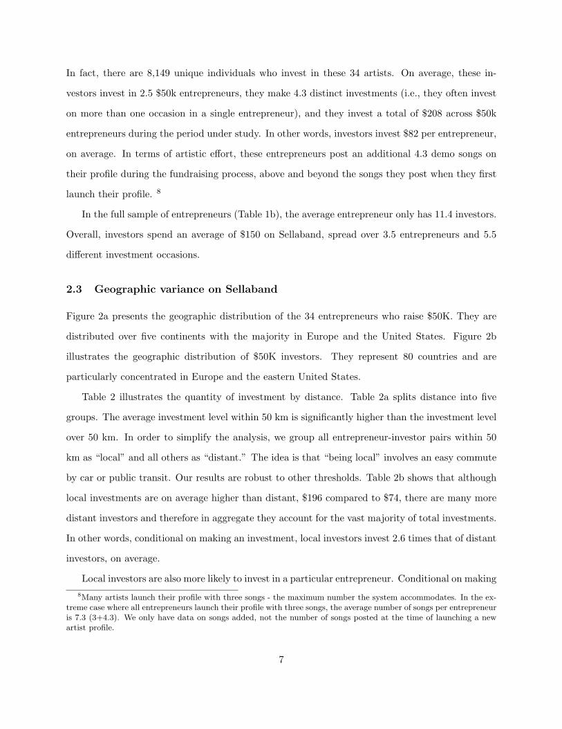
In fact, there are 8,149 unique individuals who invest in these 34 artists. On average, these in-

vestors invest in 2.5 $50k entrepreneurs, they make 4.3 distinct investments (i.e., they often invest

on more than one occasion in a single entrepreneur), and they invest a total of $208 across $50k

entrepreneurs during the period under study. In other words, investors invest $82 per entrepreneur,

on average. In terms of artistic effort, these entrepreneurs post an additional 4.3 demo songs on

their profile during the fundraising process, above and beyond the songs they post when they first

launch their profile. 8

In the full sample of entrepreneurs (Table 1b), the average entrepreneur only has 11.4 investors.

Overall, investors spend an average of $150 on Sellaband, spread over 3.5 entrepreneurs and 5.5

different investment occasions.

2.3 Geographic variance on Sellaband

Figure 2a presents the geographic distribution of the 34 entrepreneurs who raise $50K. They are

distributed over five continents with the majority in Europe and the United States. Figure 2b

illustrates the geographic distribution of $50K investors. They represent 80 countries and are

particularly concentrated in Europe and the eastern United States.

Table 2 illustrates the quantity of investment by distance. Table 2a splits distance into five

groups. The average investment level within 50 km is significantly higher than the investment level

over 50 km. In order to simplify the analysis, we group all entrepreneur-investor pairs within 50

km as “local” and all others as “distant.” The idea is that “being local” involves an easy commute

by car or public transit. Our results are robust to other thresholds. Table 2b shows that although

local investments are on average higher than distant, $196 compared to $74, there are many more

distant investors and therefore in aggregate they account for the vast majority of total investments.

In other words, conditional on making an investment, local investors invest 2.6 times that of distant

investors, on average.

Local investors are also more likely to invest in a particular entrepreneur. Conditional on making8Many artists launch their profile with three songs - the maximum number the system accommodates. In the ex-

treme case where all entrepreneurs launch their profile with three songs, the average number of songs per entrepreneuris 7.3 (3+4.3). We only have data on songs added, not the number of songs posted at the time of launching a newartist profile.

7

at least one investment in any entrepreneur on Sellaband, 11.4% of individuals who are local to an

entrepreneur invest. In contrast, only 1.5% of distant individuals invest. In this way, investors are

disproportionately local.

3 Empirical Strategy

Our econometric analysis is a straightforward difference-in-difference framework at the entrepreneur-

investor-week level. Investor i will invest in entrepreneur e in week t if the expected value from

investment is positive:

veit = β1CumulativeInvtet−1 + β2Distanceei × CumulativeInvtet−1 + γXeit + µei + ψt + εeit

where veit is the value of investing in entrepreneur e at time t by investor i. The value from

investment includes both the monetary expected return of investment as well as any consumption

utility derived from investing in that entrepreneur. β1 is the perceived marginal value of cumulative

investment as of the previous week. For example, a higher cumulative investment may indicate that

more investors perceive the entrepreneur to be of high quality and therefore a better investment.

Alternatively, investors may derive more consumption utility from investing in entrepreneurs who

are closer to the $50K threshold. β2 measures how the marginal value of cumulative investment

changes with distance, γ is the perceived marginal value of the controls (Xeit), µei is an entrepreneur-

investor fixed effect to control for overall tastes of the investor, ψt is a week fixed effect to control

for changes in the Sellaband environment over time, and εeit is an idiosyncratic error term. The

main effect of distance will drop out due to collinearity with the entrepreneur-investor fixed effects.

However, since veit is a latent variable, we instead examine the decision to invest. Therefore, to

understand the value to the investor in investing in entrepreneur e at time t we use the following

discrete choice specification:

1(Investeit) = β1CumulativeInvtet−1 +β2Distanceei×CumulativeInvtet−1 +γXeit +µei +ψt +εeit

8

Consistent with the suggestions of Angrist and Pischke (2009), we estimate this using a linear

probability model although we show robustness to alternative specifications. Likely because our

covariates are binary, the predicted probabilities of our estimates all lie between zero and one.

Therefore the potential bias of the linear probability model is not an issue in our estimation (Horrace

and Oaxaca 2006). The fixed effects mean that our analysis examines the timing of investment for

entrepreneur-investor pairs where we observe at least one investment. The fixed effects completely

capture the entrepreneur-investor pairs in which we never see investment, and these pairs can

therefore be removed from the analysis without any empirical consequences. Standard errors are

clustered at the entrepreneur-investor pair level.

With this empirical approach we examine when investment occurs, conditional on at least one

investment by that investor in that entrepreneur. We assume that the timing of investment is

driven by the change in cumulative investment rather than by a change that is specific to the

entrepreneur-investor pair. We also assume that the entrepreneur-investor and week fixed effects

control for omitted variables. Our main results hold as long as there is not an omitted variable

that drives lagged cumulative investment, an increase in the value of distant investing, and a si-

multaneous decrease in the value of local investing. One plausible variable that might fit such a

description is concert touring. As an entrepreneur gains visibility, they may be more able to tour

to more distant locations. We therefore show that our results are robust to controls for touring.

4 Results

We build our results in three steps. First, we document that investors’ propensity to invest in a

given week increases as the entrepreneur visibly accumulates capital on the site. Second, we show

that local investors do not follow this pattern. Instead they are most likely to invest early in the

cycle, before an entrepreneur has raised $10,000. Finally, we show that this difference between local

and distant investors is entirely explained by the group of investors we label Friends, Family, and

Fans (FFF). The results are robust to numerous specifications, some of which appear in the paper

9

and some in the appendix.9

4.1 Investment propensity increases with funds raised

In Table 3 we show that investment propensity increases as an entrepreneur accumulates investment.

Column (1) reports the main results using the $50K sample. This is our primary sample and all

subsequent results are based on this sample unless otherwise noted. The use of the $50K sample

ensures this is not a simple selection story where only the better artists appear in the sample with

higher cumulative investment. Relative to an entrepreneur with less than $10,000 in investment, a

given investor is 2.1 percentage points more likely to invest in a given week if the entrepreneur has

$10,000-$20,000 and 8.4 percentage points more likely to invest if they have more than $40,000.

These increases are large relative to a base rate of 4.1% on the first $10,000. We illustrate the

estimates of the increase in propensity to invest in a given week over different capital levels in

Figure 3.

Column (2) shows that the qualitative result is robust to using the full sample of all en-

trepreneurs. Column (3) shows robustness to a fixed-effects linear regression using quantity invested

as the dependent variable rather than a dummy for whether an investment occurred. Column (4)

shows robustness to including controls for artistic effort including posting videos and songs to the

website and giving live performances in the investor’s locale. Videos and concerts are positively

related to investments but their inclusion does not affect the relationship between cumulative in-

vestment and propensity to invest.10

9In the main tables we focus on a core specification and a handful of key robustness checks. In the appendix weverify that our results are robust to numerous alternative specifications of the sample chosen, covariates used, andfunctional form.

10For this table, as well as tables 4 and 6, we show robustness to several more specifications in the appendix. TableA1 repeats the main results of the paper to facilitate comparison. In terms of the sample, we show robustness tothe full sample (Table A2), the sample of entrepreneurs who reach $1000 in investments (Table A3), the sample ofentrepreneurs who reach $5,000 in investments (Table A4), the sample constructed by dropping entrepreneurs fromthe Netherlands (the home country of the website) (Table A5), and the sample constructed by dropping entrepreneursfrom the music hubs of New York City, Los Angeles, Nashville, London, and Paris (Tables A6 and A7). In terms ofcovariates, we show robustness to defining cumulative investment as appearing on the Sellaband “charts” as one ofthe 25 artists closest to raising $50,000 (Table A8), to including just video and song uploads (Table A9), to includingjust whether the entrepreneur performed in the investor’s locale (Table A10), and to including videos, songs, andperformances (Table A11). In terms of the functional form, we show robustness to fixed-effects logit (Table A12),fixed-effects poisson regression on the total parts invested (Table A13), and linear regression on the total parts investedand (when applicable) disinvested (Table A14). The appendix also shows robustness of Tables 4 and 6 to alternativemeasures of ”local” (Tables A15 and A16), treating missing geographic information as distant (Table A17), combining

10

Overall, Table 3 shows that investment accelerates as an entrepreneur gets closer to $50,000.

This is suggestive evidence of path dependency: past investment may increase the propensity to

invest. It is only suggestive because, in the absence of a truly exogenous shock to investment, we

cannot reject the possibility that some other activity may cause the acceleration in investment.

Nevertheless, to the extent that the fixed effects and the covariates on entrepreneurial effort control

such activities, the underlying pattern in the data, combined with the prominent placement of

cumulative investment information on the website, suggest that high levels of cumulative investment

may cause an increase the rate at which new investment arrives.

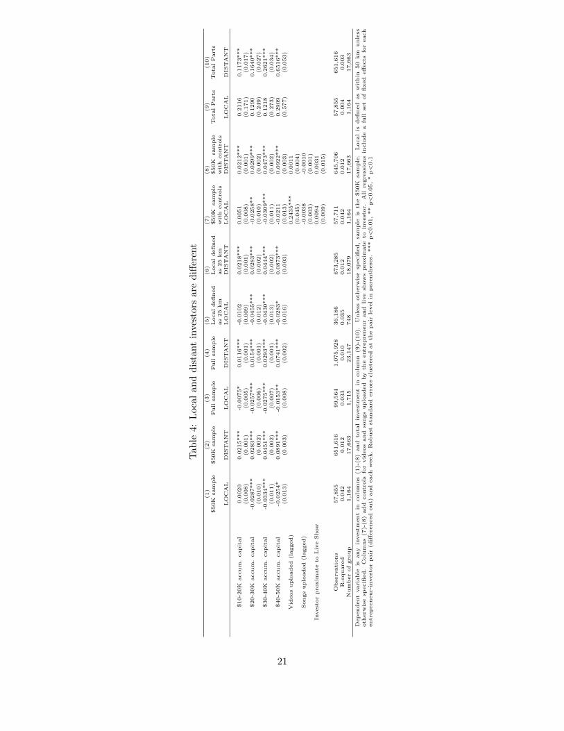
4.2 Local and distant investors are different

In Table 4 we stratify the data between local and distant investors. Local investors are more likely

to invest over the first $20,000 than later. In contrast, the results for distant investors resemble the

overall results shown in Table 3. Columns (1) and (2) show our main specification. Columns (3)

and (4) show robustness to the full set of entrepreneurs and columns (5) and (6) show robustness

to defining local as 25 rather than 50 km.

As mentioned above, our interpretation of these results holds as long as there is not an omitted

variable that drives lagged cumulative investment, an increase in the value of distant investing,

and a decrease in the value of local investing. In columns (7) and (8) we address the possibility

that entrepreneurs increase their effort to attract distant investors as they become more successful.

They might perform concerts further from home or they might post more material on their web-

site. Specifically, we show robustness to whether the entrepreneur performs within 50 km of the

investor and whether the entrepreneur posted a new song or video to their website. The qualitative

differences between local and distant investment patterns remain.

Columns (9) and (10) show robustness to using parts rather than discretizing the dependent

variable. The parts results show a flat relationship between investment propensity and cumulative

investment for local investors largely because the local investments are highly skewed with a very

distant and local in the same regression and using interactions (Table A18), and to alternative definitions of FFF(Table A19).

11

small number of large investments (over $5,000) driving the results. Still, distant investors increase

their propensity to invest as the entrepreneur accumulates capital whereas local investors do not.

In Figure 4 we provide a graphical representation of the propensity to invest at different stages

in the investment cycle. Local and distant investors clearly display opposite patterns; distant

investors’ propensity to invest rises as the entrepreneur accumulates capital, whereas local investors’

propensity does not.

4.3 Friends, Family, and Fans

In this section we show that a particular type of investor, whom we label as “Friends, Family, and

Fans” (FFF) of a particular entrepreneur, explains the observed difference between local and distant

investors. These individuals likely joined this market-making platform to fund that particular

entrepreneur. We define FFF by the following three characteristics:

1. The FFF investor invested in the focal entrepreneur before investing in any other (i.e. the

investor is likely to have joined the system for the focal entrepreneur)

2. The FFF investor’s investment in the focal entrepreneur is their largest investment

3. The investor invests in no more than three other entrepreneurs (i.e. the focal entrepreneur

remains a key reason for being on the site)

To confirm the validity of our measure, we asked two successful entrepreneurs on Sellaband to

identify investors they knew independently of Sellaband. Specifically, we asked them to identify

from their list of investors all family members, friends, and fans that they knew prior to joining

Sellaband. Our measure captured all investors that these two entrepreneurs identified, as well as a

number of investors that the entrepreneurs did not know personally.

In Table 5 we provide descriptive statistics for the FFF sample. Using investor-level measures

of the use of the website’s communications tools (emails sent through the website and comments

on webpages), in Table 5a we show that they use Sellaband less intensively than other investors.

Specifically, they send approximately 34 times fewer emails, post 29 times fewer comments, receive

five times fewer emails, and receive 16 times fewer comments than non-FFF investors, on average.

12

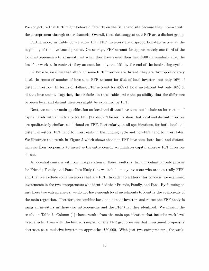
We conjecture that FFF might behave differently on the Sellaband site because they interact with

the entrepreneur through other channels. Overall, these data suggest that FFF are a distinct group.

Furthermore, in Table 5b we show that FFF investors are disproportionately active at the

beginning of the investment process. On average, FFF account for approximately one third of the

focal entrepreneur’s total investment when they have raised their first $500 (or similarly after the

first four weeks). In contrast, they account for only one fifth by the end of the fundraising cycle.

In Table 5c we show that although some FFF investors are distant, they are disproportionately

local. In terms of number of investors, FFF account for 63% of local investors but only 16% of

distant investors. In terms of dollars, FFF account for 43% of local investment but only 16% of

distant investment. Together, the statistics in these tables raise the possibility that the difference

between local and distant investors might be explained by FFF.

Next, we run our main specification on local and distant investors, but include an interaction of

capital levels with an indicator for FFF (Table 6). The results show that local and distant investors

are qualitatively similar, conditional on FFF. Particularly, in all specifications, for both local and

distant investors, FFF tend to invest early in the funding cycle and non-FFF tend to invest later.

We illustrate this result in Figure 5 which shows that non-FFF investors, both local and distant,

increase their propensity to invest as the entrepreneur accumulates capital whereas FFF investors

do not.

A potential concern with our interpretation of these results is that our definition only proxies

for Friends, Family, and Fans. It is likely that we include many investors who are not really FFF,

and that we exclude some investors that are FFF. In order to address this concern, we examined

investments in the two entrepreneurs who identified their Friends, Family, and Fans. By focusing on

just these two entrepreneurs, we do not have enough local investments to identify the coefficients of

the main regression. Therefore, we combine local and distant investors and re-run the FFF analysis

using all investors in these two entrepreneurs and the FFF that they identified. We present the

results in Table 7. Column (1) shows results from the main specification that includes week-level

fixed effects. Even with the limited sample, for the FFF group we see that investment propensity

decreases as cumulative investment approaches $50,000. With just two entrepreneurs, the week-

13

level fixed effects mean that there is little variation in the data to identify the main effect of the

level of cumulated investment. For this reason, in column (2) we estimate the same regression

without the week fixed effects and in column (3) we show results with no fixed effects but add

controls for changes in artistic effort over time. Overall, Table 7 shows that the results of Table 6

are robust to this survey-based definition of FFF. We interpret this result as providing validity for

our definition of FFF.

In summary, our results suggest that there is no systematic difference between local and distant

investors, except to the extent that social networks (as measured by FFF) are disproportionately

local.

5 Conclusion

We examine the role of geography in an online crowd-funding platform for early stage musical

artists. Because these artists engage in entrepreneurial activities with a community of investors,

we use this setting to understand how online mechanisms interact with the financing of early stage

entrepreneurial ventures. We find that the propensity to invest is independent of geographic dis-

tance between entrepreneur and investor in a setting where investment is facilitated by an online

crowd-funding market platform and conditioned on the entrepreneur’s offline network. This result

contrasts with the existing literature on early-stage entrepreneurial finance that emphasizes the

importance of local interactions. Instead, our result suggests that online mechanisms can reduce

many of the challenges associated with investing in early-stage projects over long distances. Only

the spatial correlation of pre-existing social networks is not resolved. Furthermore, our result em-

phasizes the important role that friends, family, (and fans) may play online and offline in generating

early investment in entrepreneurial ventures. Speculatively, this early investment may serve as a

signal to later investors and increase the likelihood of further funding by way of access to distant

sources of capital.

14

References

Angrist, J. D., and J.-S. Pischke (2009): Mostly Harmless Econometrics: An Empiricist’sCompanion. Princeton University Press: Princeton NJ.

Blum, B., and A. Goldfarb (2006): “Does the internet defy the law of gravity?,” Journal ofInternational Economics, 70(2), 384–405.

Brynjolfsson, E., Y. J. Hu, and M. S. Rahman (2009): “Battle of the Retail Channels: HowProduct Selection and Geography Drive Cross-Channel Competition,” Management Science, 55(11), 1755–1765.

Cairncross, F. (1997): The Death of Distance. Harvard University Press. Cambridge, MA.

Choi, J., and D. Bell (2010): “Preference Minorities and the Internet,” Working paper, Wharton.

Florida, R., and D. Smith (1993): “Venture capital formation, investment and regional Indus-trialization,” Annals of the Association of American Geographers, 83(3), 434–5.

Florida, R. L., and M. Kenney (1988): “Venture Capital, High Technology and RegionalDevelopment,” Regional Studies, 22, 33–48.

Forman, C., A. Ghose, and A. Goldfarb (2009): “Competition Between Local and ElectronicMarkets: How the Benefit of Buying Online Depends on Where You Live,” Management Science,55 (1), 47–57.

Friedman, T. (2005): The World is Flat: A Brief History of the Twenty-First Century. NewYork: Farrar, Straus, and Giroux.

Goldfarb, A., and C. Tucker (2010): “Advertising Bans and the Substitutability of Onlineand Offline Advertising,” Journal of Marketing Research, (forthcoming).

Horrace, W. C., and R. L. Oaxaca (2006): “Results on the bias and inconsistency of ordinaryleast squares for the linear probability model,” Economic Letters, 90, 321–327.

Hortacsu, A., F. A. Martinez-Jerez, and J. Douglas (2009): “The Geography of Tradein Online Transactions: Evidence from eBay and MercadoLibre.,” American Economic Journal:Microeconomics, 1(1), 53–74.

Jaffe, A., M. Trajtenberg, and R. Henderson (1993): “Geographic Localization of Knowl-edge Spillovers as Evidenced by Patent Citations,” The Quarterly Journal of Economics, 108(3),577–598.

Kappel, T. (2009): “Ex ante crowdfunding and the recording industry: a model for the U.S.?,”LLAE Law Review, 29, 375–385.

Mason, C. (2007): “Venture capital: a geographical perspective,” in H Landstrm (ed) Handbookof Research on Venture Capital, Edward Elgar, Cheltenham, pp. 86–112.

Nanda, R., and T. Khanna (2010): “Diasporas and Domestic Entrepreneurs: Evidence from theIndian Software Industry,” Journal of Economics and Management Strategy, (forthcoming).

15

Nichols, A. (2003): “Vincenty: Stata module to calculate distances on the Earth’s surface,”Statistical Software Components.

Partridge, M. D., D. S. Rickman, K. Ali, and M. R. Olfert (2008): “Employment Growthin the American Urban Hierarchy: Long Live Distance,” The B.E. Journal of Macroeconomics,Vol. 8 : Iss. 1 (Contributions), Article 10.

Passman, D. (2009): All you need to know about the music business. Free Press, New York.

Powell, W. W., K. W. Koput, J. I. Bowie, and L. Smith-Doerr (2002): “The SpatialClustering of Science and Capital: Accounting for Biotech Firm-Venture Capital Relationships,”Regional Studies, 36(3), 291–305.

Simcoe, T. (2007): “XTPQML: Stata module to estimate Fixed-effects Poisson (Quasi-ML) regres-sion with robust standard errors,” Statistical Software Components, Boston College Departmentof Economics.

Sorenson, O., and T. Stuart (2001): “Syndication Networks and the Spatial Distribution ofVenture Capital Investments,” American Journal of Sociology, 106(6), 1546–1588.

Tribus, M. (1970): “Panel on government and new business proceedings,” Venture Capital andManagement, Management Seminar, Boston College, Boston, MA, May 28.

Wellman, B. (2001): “Computer Networks As Social Networks,” Science, 29, 2031–2034.

Zook, M. A. (2002): “Grounded capital: venture financing and the geography of the Internetindustry, 19942000,” Journal of Economic Geography, 2(2), 151–177.

Zucker, L. G., M. R. Darby, and M. B. Brewer (1998): “Intellectual Human Capital andthe Birth of U.S. Biotechnology Enterprises,” American Economic Review, 88(1), 290–306.

16

Table 1a: Descriptive stats - $50K (main) Sample

Obs. Mean Std. Dev. Min Max

Entrepreneur LevelInvestors at $50K 34 608.8 220.9 316 1,338Weeks to $50K 34 53.1 34.6 8 124Songs uploaded† 34 4.29 8.02 0 32Videos uploaded 34 0.68 0.47 0 1Investor levelNumber of 50K entrepreneurs invested in 8,149 2.54 4.23 1 34Number of distinct investments 8,149 4.33 12.78 1 330Total amount invested across 50K entrepreneurs ($) 8,149 208 1,083.9 0 33,430Entrepreneur-Investor levelInvestment amount ($) 18,827 82 379.8 0 23,500Geographic distance (km) 18,827 5,118 5,658 0.003 19,827Number of investments in same entrepreneur 18,827 1.7 2.3 1 72Position in funding cycle at first investment ($) 18,827 12,099 13,361 0 49,990Entrepreneur-Investor-Week levelInvestment amount ($) 709,471 2.378 40.82 0 15,000Live show proximate to investor 709,471 0.002 0.046 0 1

†Entrepreneurs may upload 1 to 3 songs when registering on the website. Since we do not haveaccess to this data, the initial songs are not included in this count.

17

Table 1b: Descriptive stats - Full Sample

Obs. Mean Std. Dev. Min Max

Entrepreneur LevelInvestors 4,712 11.4 60.5 1 1,338Total Investment 4,712 49.3 437.5 0 5,000Songs uploaded† 4,712 1.82 2.686 0 59Videos uploaded 4,712 0.11 0.378 0 8Investor levelNumber of entrepreneurs invested in 15,517 3.46 21.1 1 1,835Number of distinct investments 15,517 5.52 34.3.1 1 2,155Total amount invested across all entrepreneurs ($) 15,517 149.7 991.9 0 38,440Entrepreneur-Investor levelInvestment amount ($) 24,862 42.69 253.61 0 23,500Geographic distance (km) 24,862 4,831.5 5,523.6 .003 19,863Number of investments in same entrepreneur 24,862 1.79 2.52 1 72Position in funding cycle at first investment ($) 24,862 9,998 12,464 0 49,990Entrepreneur-Investor-Week levelInvestment amount ($) 1,175,492 1.83 33.71 0 15,000

†Entrepreneurs may upload 1 to 3 songs when registering on the website. Since we do not haveaccess to this data, the initial songs are not included in this count.

18

Table 2a: Local versus Distant - $50K Sample

Distance Obs. Mean Investment Total Investment % of Total

0-5 km 191 255.76 48,850 2.9%5-50 km 973 184.62 179,640 10.6%50-500 km 4,403 67.67 297,970 17.5%500-3,000 km 4,232 79.56 336,680 19.8%> 3,000 km 9,028 75.15 678,410 39.9%Not Available 1,999 79.26 158,450 9.3%

Table 2b: Local versus Distant, consolidated - $50K Sample

Obs. Mean Investment Total Investment % of Total

Local (under 50 km) 1,164 196 228,490 13.4%Distant (over 50 km) 17,663 74 1,313,060 77.2%Not Available 1,999 79 158,450 9.3%

19

Table 3: Investment propensity increases over time

(1) (2) (3) (4)$50K sample Full sample Total Parts Additional covariates

$10-20K accum. capital 0.0213*** 0.0109*** 0.1216*** 0.0211***(0.001) (0.001) (0.018) (0.001)

$20-30K accum. capital 0.0261*** 0.0134*** 0.1654*** 0.0277***(0.002) (0.001) (0.028) (0.002)

$30-40K accum. capital 0.0420*** 0.0266*** 0.2575*** 0.0442***(0.002) (0.001) (0.035) (0.002)

$40-50K accum. capital 0.0840*** 0.0691*** 0.6279*** 0.0871***(0.003) (0.002) (0.056) (0.003)

Videos uploaded (lagged) 0.0084*(0.004)

Songs uploaded (lagged) -0.0011(0.001)

Investor proximate to Live Show 0.0098*(0.006)

Observations 709,471 1,175,492 709,471 703,417R-squared 0.012 0.010 0.002 0.011Number of group 18,827 24,862 18,827 18,827

Dependent variable is any investment in columns (1)-(2)-(4) and total investment in column (3).Unless otherwise specified, sample is the $50K sample. Column (4) adds controls for videos and songsuploaded by the entrepreneur, and live shows proximate to investor. All regressions include a full setof fixed effects for each entrepreneur-investor pair (differenced out) and each week. Robust standarderrors clustered at the pair level in parentheses.*** p<0.01, ** p<0.05, * p<0.1

20

Tab

le4:

Loc

alan

ddi

stan

tin

vest

ors

are

diffe

rent

(1)

(2)

(3)

(4)

(5)

(6)

(7)

(8)

(9)

(10)

$50K

sam

ple

$50K

sam

ple

Full

sam

ple

Full

sam

ple

Local

defi

ned

as

25

km

Local

defi

ned

as

25

km

$50K

sam

ple

wit

hcontr

ols

$50K

sam

ple

wit

hcontr

ols

Tota

lP

art

sT

ota

lP

art

s

LO

CA

LD

IST

AN

TL

OC

AL

DIS

TA

NT

LO

CA

LD

IST

AN

TL

OC

AL

DIS

TA

NT

LO

CA

LD

IST

AN

T

$10-2

0K

accum

.capit

al

0.0

020

0.0

215***

-0.0

075*

0.0

116***

-0.0

102

0.0

218***

0.0

051

0.0

212***

0.2

116

0.1

173***

(0.0

08)

(0.0

01)

(0.0

05)

(0.0

01)

(0.0

09)

(0.0

01)

(0.0

08)

(0.0

01)

(0.1

71)

(0.0

17)

$20-3

0K

accum

.capit

al

-0.0

287***

0.0

283***

-0.0

257***

0.0

154***

-0.0

455***

0.0

283***

-0.0

258**

0.0

299***

0.1

290

0.1

640***

(0.0

10)

(0.0

02)

(0.0

06)

(0.0

01)

(0.0

12)

(0.0

02)

(0.0

10)

(0.0

02)

(0.2

49)

(0.0

27)

$30-4

0K

accum

.capit

al

-0.0

334***

0.0

451***

-0.0

275***

0.0

293***

-0.0

430***

0.0

444***

-0.0

309***

0.0

473***

0.1

218

0.2

621***

(0.0

11)

(0.0

02)

(0.0

07)

(0.0

01)

(0.0

13)

(0.0

02)

(0.0

11)

(0.0

02)

(0.2

73)

(0.0

34)

$40-5

0K

accum

.capit

al

-0.0

254*

0.0

891***

-0.0

153**

0.0

741***

-0.0

283*

0.0

873***

-0.0

211

0.0

922***

0.2

909

0.6

516***

(0.0

13)

(0.0

03)

(0.0

08)

(0.0

02)

(0.0

16)

(0.0

03)

(0.0

13)

(0.0

03)

(0.5

77)

(0.0

53)

Vid

eos

uplo

aded

(lagged)

0.2

435***

0.0

011

(0.0

45)

(0.0

04)

Songs

uplo

aded

(lagged)

-0.0

038

-0.0

010

(0.0

03)

(0.0

01)

Invest

or

pro

xim

ate

toL

ive

Show

0.0

094

0.0

031

(0.0

09)

(0.0

15)

Obse

rvati

ons

57,8

55

651,6

16

99,5

64

1,0

75,9

28

36,1

86

673,2

85

57,7

11

645,7

06

57,8

55

651,6

16

R-s

quare

d0.0

42

0.0

12

0.0

33

0.0

10

0.0

35

0.0

12

0.0

42

0.0

12

0.0

04

0.0

03

Num

ber

of

gro

up

1,1

64

17,6

63

1,7

15

23,1

47

748

18,0

79

1,1

64

17,6

63

1,1

64

17,6

63

Dep

endent

vari

able

isany

invest

ment

incolu

mns

(1)-

(8)

and

tota

lin

vest

ment

incolu

mn

(9)-

(10).

Unle

ssoth

erw

ise

specifi

ed,

sam

ple

isth

e$50K

sam

ple

.L

ocal

isdefi

ned

as

wit

hin

50

km

unle

ssoth

erw

ise

specifi

ed.

Colu

mns

(7)-

(8)

add

contr

ols

for

vid

eos

and

songs

uplo

aded

by

the

entr

epre

neur

and

live

show

spro

xim

ate

toin

vest

or.

All

regre

ssio

ns

inclu

de

afu

llse

tof

fixed

eff

ects

for

each

entr

epre

neur-

invest

or

pair

(diff

ere

nced

out)

and

each

week.

Robust

standard

err

ors

clu

stere

dat

the

pair

level

inpare

nth

ese

s.***

p<

0.0

1,

**

p<

0.0

5,

*p

<0.1

21

Table 5a: FFF use the website differently

FFF Not FFF

Average # of emails sent to entrepreneurs 0.24 8.25Average # of comments sent to entrepreneurs 0.44 12.74Average # of emails received from entrepreneurs 13.19 68.97Average # of comments received from entrepreneurs 1.14 18.77

Table 5b: FFF are disproportionately active at the beginning

First $500 First 4 weeks Full $50k

FFF 34% 37% 22%Not FFF 66% 63% 78%

Table 5c: FFF are disproportionately local

Pairs Local 25 km Distant Local 50 km Distant Local 100 km Distant

FFF 65% 18% 63% 16% 55% 16%Not FFF 35% 82% 37% 84% 45% 84%

Dollars Local 25 km Distant Local 50 km Distant Local 100 km Distant

FFF 36% 18% 43% 16% 43% 15%Not FFF 64% 82% 57% 84% 57% 85%

22

Tab

le6:

Loc

alan

ddi

stan

tin

vest

ors

are

sim

ilar,

cond

itio

nal

onF

FF

(1)

(2)

(3)

(4)

(5)

(6)

(7)

(8)

(9)

(10)

$50K

sam

ple

$50K

sam

ple

Full

Sam

ple

Full

Sam

ple

Local

defi

ned

as

25

km

Local

defi

ned

as

25

km

$50K

sam

ple

wit

hcontr

ols

$50K

sam

ple

wit

hcontr

ols

Tota

lP

art

sT

ota

lP

art

s

LO

CA

LD

IST

AN

TL

OC

AL

DIS

TA

NT

LO

CA

LD

IST

AN

TL

OC

AL

DIS

TA

NT

LO

CA

LD

IST

AN

T

$10-2

0K

accum

.capit

al

0.0

322***

0.0

233***

0.0

173***

0.0

140***

0.0

194*

0.0

232***

0.0

324***

0.0

229***

0.5

943***

0.1

268***

(0.0

09)

(0.0

01)

(0.0

06)

(0.0

01)

(0.0

11)

(0.0

01)

(0.0

09)

(0.0

01)

(0.2

12)

(0.0

17)

$20-3

0K

accum

.capit

al

0.0

276**

0.0

329***

0.0

218***

0.0

208***

0.0

057

0.0

327***

0.0

277**

0.0

343***

0.7

685**

0.1

787***

(0.0

12)

(0.0

02)

(0.0

07)

(0.0

01)

(0.0

14)

(0.0

02)

(0.0

12)

(0.0

02)

(0.3

08)

(0.0

27)

$30-4

0K

accum

.capit

al

0.0

337**

0.0

517***

0.0

357***

0.0

376***

0.0

178

0.0

503***

0.0

335**

0.0

536***

0.7

840***

0.2

878***

(0.0

14)

(0.0

02)

(0.0

11)

(0.0

02)

(0.0

17)

(0.0

02)

(0.0

14)

(0.0

02)

(0.3

00)

(0.0

35)

$40-5

0K

accum

.capit

al

0.0

521***

0.1

086***

0.0

590***

0.0

952***

0.0

448**

0.1

068***

0.0

539***

0.1

115***

1.4

283

0.7

572***

(0.0

17)

(0.0

03)

(0.0

15)

(0.0

02)

(0.0

21)

(0.0

03)

(0.0

17)

(0.0

03)

(0.9

80)

(0.0

57)

$10-2

0K

accum

.capit

al

*F

FF

-0.0

803***

-0.0

909***

-0.0

551***

-0.0

753***

-0.0

759***

-0.0

943***

-0.0

738***

-0.0

854***

-0.9

861***

-0.4

108***

(0.0

12)

(0.0

06)

(0.0

08)

(0.0

04)

(0.0

14)

(0.0

06)

(0.0

12)

(0.0

06)

(0.2

76)

(0.0

53)

$20-3

0K

accum

.capit

al

*F

FF

-0.1

184***

-0.1

377***

-0.0

905***

-0.1

150***

-0.1

098***

-0.1

356***

-0.1

121***

-0.1

305***

-1.3

505***

-0.5

489***

(0.0

13)

(0.0

07)

(0.0

09)

(0.0

05)

(0.0

15)

(0.0

07)

(0.0

13)

(0.0

07)

(0.2

94)

(0.0

62)

$30-4

0K

accum

.capit

al

*F

FF

-0.1

397***

-0.1

644***

-0.1

146***

-0.1

477***

-0.1

288***

-0.1

638***

-0.1

337***

-0.1

565***

-1.4

375***

-0.6

860***

(0.0

15)

(0.0

07)

(0.0

13)

(0.0

05)

(0.0

17)

(0.0

07)

(0.0

15)

(0.0

07)

(0.2

93)

(0.0

71)

$40-5

0K

accum

.capit

al

*F

FF

-0.1

590***

-0.2

521***

-0.1

281***

-0.2

338***

-0.1

514***

-0.2

463***

-0.1

531***

-0.2

444***

-2.1

922***

-1.2

360***

(0.0

18)

(0.0

08)

(0.0

16)

(0.0

06)

(0.0

22)

(0.0

07)

(0.0

18)

(0.0

08)

(0.7

82)

(0.0

81)

Vid

eos

uplo

aded

(lagged)

0.2

444***

0.0

034

(0.0

44)

(0.0

04)

Songs

uplo

aded

(lagged)

-0.0

035

-0.0

018*

(0.0

03)

(0.0

01)

Invest

or

pro

xim

ate

toL

ive

Show

0.0

090

0.0

043

(0.0

09)

(0.0

15)

Obse

rvati

ons

57,8

55

651,6

16

99,5

64

1,0

75,9

28

36,1

86

673,2

85

57,7

11

645,7

06

57,8

55

651,6

16

R-s

quare

d0.0

50

0.0

19

0.0

37

0.0

15

0.0

43

0.0

19

0.0

50

0.0

18

0.0

05

0.0

04

Num

ber

of

gro

up

1,1

64

17,6

63

1,7

15

23,1

47

748

18,0

79

1,1

64

17,6

63

1,1

64

17,6

63

Dep

endent

vari

able

isany

invest

ment

incolu

mns

(1)-

(8)

and

tota

lin

vest

ment

incolu

mn

(9)-

(10).

Unle

ssoth

erw

ise

specifi

ed,

sam

ple

isth

e$50K

sam

ple

.L

ocal

isdefi

ned

as

wit

hin

50

km

unle

ssoth

erw

ise

specifi

ed.

Colu

mns

(7)-

(8)

add

contr

ols

for

vid

eos

and

songs

uplo

aded

by

the

entr

epre

neur

and

live

show

spro

xim

ate

toin

vest

or.

All

regre

ssio

ns

inclu

de

afu

llse

tof

fixed

eff

ects

for

each

entr

epre

neur-

invest

or

pair

(diff

ere

nced

out)

and

each

week.

Robust

standard

err

ors

clu

stere

dat

the

pair

level

inpare

nth

ese

s.***

p<

0.0

1,

**

p<

0.0

5,

*p

<0.1

23

Table 7: FFF definition based on interviews with two entrepreneurs

(1) (2) (3)VARIABLES With Week FEs Without Week FEs Without Week FEs

$10-20K accum. capital 0.0256 0.0202*** 0.0203***(0.020) (0.004) (0.005)

$20-30K accum. capital -0.0174 0.0321*** 0.0420***(0.019) (0.006) (0.006)

$30-40K accum. capital -0.0582*** 0.0070 0.0191**(0.019) (0.008) (0.008)

$40-50K accum. capital 0.0081 0.0964*** 0.1083***(0.026) (0.011) (0.012)

$10-20K accum. capital * FFF -0.1147 -0.1189 0.0167(0.116) (0.115) (0.087)

$20-30K accum. capital * FFF -0.1750 -0.1803 -0.0206(0.120) (0.126) (0.088)

$30-40K accum. capital * FFF -0.1513 -0.1443 0.0223(0.125) (0.133) (0.090)

$40-50K accum. capital * FFF -0.3652*** -0.3685*** -0.2122**(0.134) (0.141) (0.099)

Videos uploaded (lagged) 0.0861***(0.015)

Songs uploaded (lagged) -0.0124(0.010)

Investor proximate to Live Show -0.0478(0.030)

Observations 25,521 25,521 24,895R-squared 0.026 0.009 0.012Number of group 1,128 1,128 1,128

Dependent variable is any investment. Sample is the $50K sample. All regressions includea full set of fixed effects for each entrepreneur-investor pair (differenced out). Column 1has week fixed effects and column 2 and 3 do not. Column 3 adds controls for songs andvideos uploaded by the entrepreneur and live shows proximate to the investor. Local anddistant combined for sample size reasons. Robust standard errors clustered at the pair levelin parentheses. *** p<0.01, ** p<0.05, * p<0.1

24

Figure 1: Sellaband screenshot

Figure 2a: Map of $50K entrepreneurs locations

25

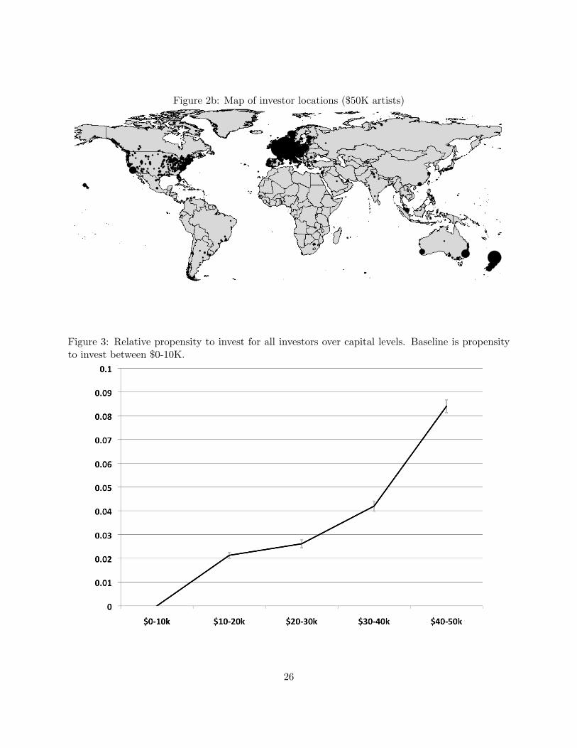
Figure 2b: Map of investor locations ($50K artists)

Figure 3: Relative propensity to invest for all investors over capital levels. Baseline is propensityto invest between $0-10K.

26

Figure 4: Relative propensity to invest over capital levels for local versus distant investors. Baselineis propensity to invest between $0-10K within each group.

27

Figure 5: Relative propensity to invest over capital levels for FFF versus not-FFF investors (bothlocal and distant). Baseline is propensity to invest between $0-10K within each group.

28

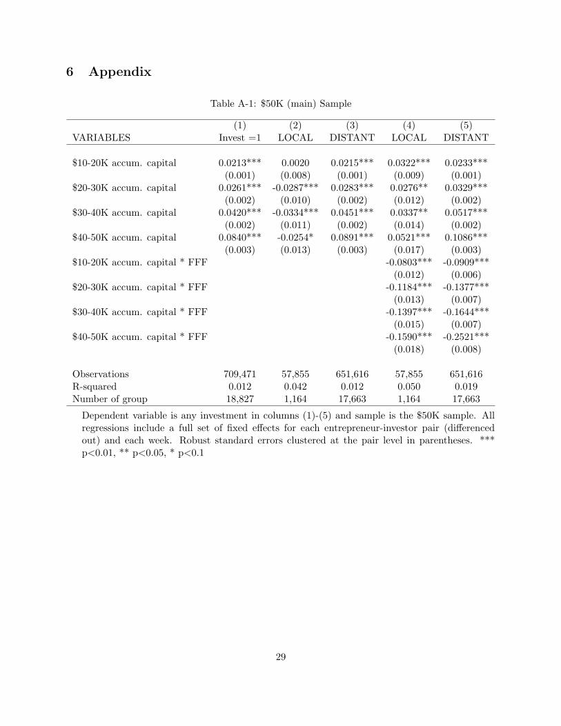
6 Appendix

Table A-1: $50K (main) Sample

(1) (2) (3) (4) (5)VARIABLES Invest =1 LOCAL DISTANT LOCAL DISTANT

$10-20K accum. capital 0.0213*** 0.0020 0.0215*** 0.0322*** 0.0233***(0.001) (0.008) (0.001) (0.009) (0.001)

$20-30K accum. capital 0.0261*** -0.0287*** 0.0283*** 0.0276** 0.0329***(0.002) (0.010) (0.002) (0.012) (0.002)

$30-40K accum. capital 0.0420*** -0.0334*** 0.0451*** 0.0337** 0.0517***(0.002) (0.011) (0.002) (0.014) (0.002)

$40-50K accum. capital 0.0840*** -0.0254* 0.0891*** 0.0521*** 0.1086***(0.003) (0.013) (0.003) (0.017) (0.003)

$10-20K accum. capital * FFF -0.0803*** -0.0909***(0.012) (0.006)

$20-30K accum. capital * FFF -0.1184*** -0.1377***(0.013) (0.007)

$30-40K accum. capital * FFF -0.1397*** -0.1644***(0.015) (0.007)

$40-50K accum. capital * FFF -0.1590*** -0.2521***(0.018) (0.008)

Observations 709,471 57,855 651,616 57,855 651,616R-squared 0.012 0.042 0.012 0.050 0.019Number of group 18,827 1,164 17,663 1,164 17,663

Dependent variable is any investment in columns (1)-(5) and sample is the $50K sample. Allregressions include a full set of fixed effects for each entrepreneur-investor pair (differencedout) and each week. Robust standard errors clustered at the pair level in parentheses. ***p<0.01, ** p<0.05, * p<0.1

29

Table A-2: Full Sample

(1) (2) (3) (4) (5)Full Sample Full Sample Full Sample Full Sample Full Sample

VARIABLES Invest=1 LOCAL DISTANT LOCAL DISTANT

$10-20K accum. capital 0.0109*** -0.0075* 0.0116*** 0.0173*** 0.0140***(0.001) (0.005) (0.001) (0.006) (0.001)

$20-30K accum. capital 0.0134*** -0.0257*** 0.0154*** 0.0218*** 0.0208***(0.001) (0.006) (0.001) (0.007) (0.001)

$30-40K accum. capital 0.0266*** -0.0275*** 0.0293*** 0.0357*** 0.0376***(0.001) (0.007) (0.001) (0.011) (0.002)

$40-50K accum. capital 0.0691*** -0.0153** 0.0741*** 0.0590*** 0.0952***(0.002) (0.008) (0.002) (0.015) (0.002)

$10-20K accum. capital * FFF -0.0551*** -0.0753***(0.008) (0.004)

$20-30K accum. capital * FFF -0.0905*** -0.1150***(0.009) (0.005)

$30-40K accum. capital * FFF -0.1146*** -0.1477***(0.013) (0.005)

$40-50K accum. capital * FFF -0.1281*** -0.2338***(0.016) (0.006)

Observations 1,175,492 99,564 1,075,928 99,564 1,075,928R-squared 0.010 0.033 0.010 0.037 0.015Number of group 24,862 1,715 23,147 1,715 23,147

Dependent variable is any investment in columns (1)-(5) and sample is the full sample. All regres-sions include a full set of fixed effects for each entrepreneur-investor pair (differenced out) and eachweek. Robust standard errors clustered at the pair level in parentheses. *** p<0.01, ** p<0.05, * p<0.1

30

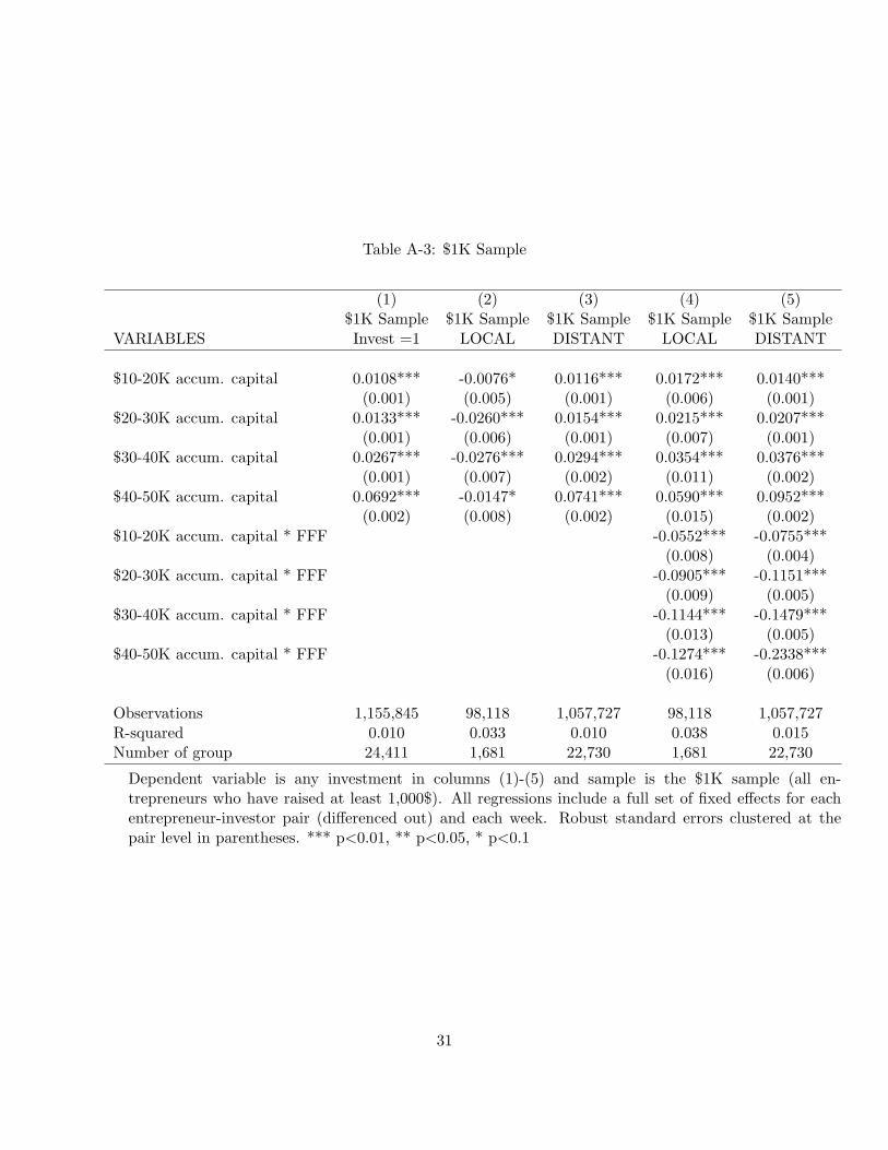
Table A-3: $1K Sample

(1) (2) (3) (4) (5)$1K Sample $1K Sample $1K Sample $1K Sample $1K Sample

VARIABLES Invest =1 LOCAL DISTANT LOCAL DISTANT

$10-20K accum. capital 0.0108*** -0.0076* 0.0116*** 0.0172*** 0.0140***(0.001) (0.005) (0.001) (0.006) (0.001)

$20-30K accum. capital 0.0133*** -0.0260*** 0.0154*** 0.0215*** 0.0207***(0.001) (0.006) (0.001) (0.007) (0.001)

$30-40K accum. capital 0.0267*** -0.0276*** 0.0294*** 0.0354*** 0.0376***(0.001) (0.007) (0.002) (0.011) (0.002)

$40-50K accum. capital 0.0692*** -0.0147* 0.0741*** 0.0590*** 0.0952***(0.002) (0.008) (0.002) (0.015) (0.002)

$10-20K accum. capital * FFF -0.0552*** -0.0755***(0.008) (0.004)

$20-30K accum. capital * FFF -0.0905*** -0.1151***(0.009) (0.005)

$30-40K accum. capital * FFF -0.1144*** -0.1479***(0.013) (0.005)

$40-50K accum. capital * FFF -0.1274*** -0.2338***(0.016) (0.006)

Observations 1,155,845 98,118 1,057,727 98,118 1,057,727R-squared 0.010 0.033 0.010 0.038 0.015Number of group 24,411 1,681 22,730 1,681 22,730

Dependent variable is any investment in columns (1)-(5) and sample is the $1K sample (all en-trepreneurs who have raised at least 1,000$). All regressions include a full set of fixed effects for eachentrepreneur-investor pair (differenced out) and each week. Robust standard errors clustered at thepair level in parentheses. *** p<0.01, ** p<0.05, * p<0.1

31

Table A-4: $5K Sample

(1) (2) (3) (4) (5)$5K Sample $5K Sample $5K Sample $5K Sample $5K Sample

VARIABLES Invest =1 LOCAL DISTANT LOCAL DISTANT

$10-20K accum. capital 0.0114*** -0.0087* 0.0121*** 0.0160*** 0.0144***(0.001) (0.005) (0.001) (0.006) (0.001)

$20-30K accum. capital 0.0141*** -0.0286*** 0.0162*** 0.0190** 0.0214***(0.001) (0.006) (0.001) (0.007) (0.001)

$30-40K accum. capital 0.0279*** -0.0302*** 0.0307*** 0.0328*** 0.0387***(0.002) (0.007) (0.002) (0.011) (0.002)

$40-50K accum. capital 0.0705*** -0.0171** 0.0755*** 0.0561*** 0.0963***(0.002) (0.008) (0.002) (0.015) (0.002)

$10-20K accum. capital * FFF -0.0551*** -0.0756***(0.008) (0.005)

$20-30K accum. capital * FFF -0.0909*** -0.1150***(0.009) (0.005)

$30-40K accum. capital * FFF -0.1148*** -0.1477***(0.013) (0.005)

$40-50K accum. capital * FFF -0.1276*** -0.2338***(0.016) (0.006)

Observations 1,070,501 89,276 981,225 89,276 981,225R-squared 0.011 0.035 0.011 0.040 0.016Number of group 23,269 1,544 21,725 1,544 21,725

Dependent variable is any investment in columns (1)-(5) and sample is the $5K sample (all en-trepreneurs who have raised at least 5,000$). All regressions include a full set of fixed effects for eachentrepreneur-investor pair (differenced out) and each week. Robust standard errors clustered at thepair level in parentheses. *** p<0.01, ** p<0.05, * p<0.1

32

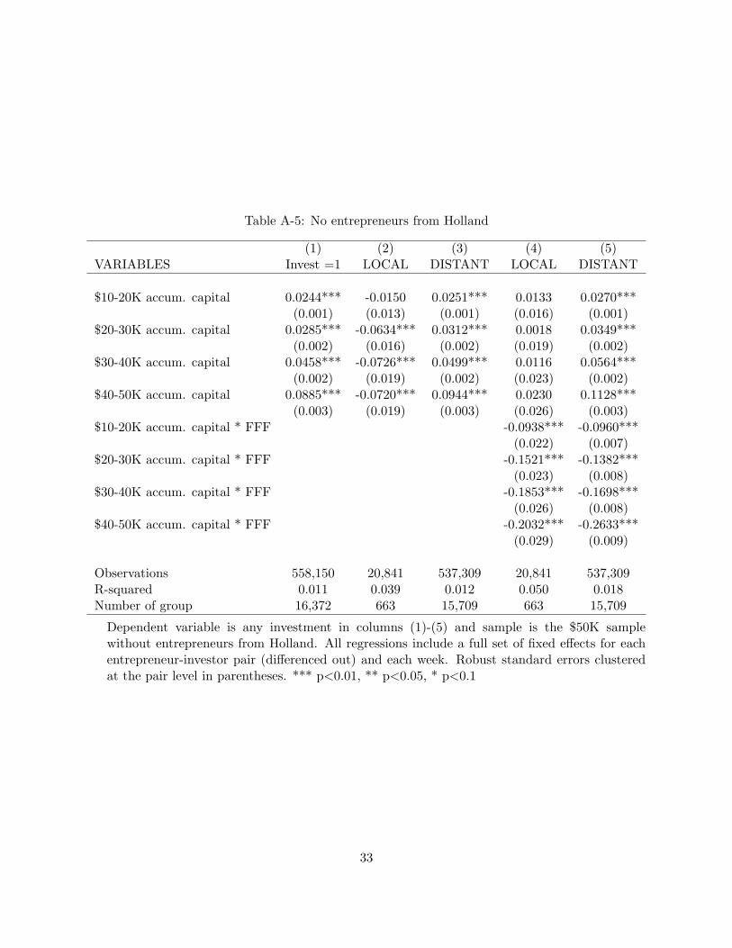
Table A-5: No entrepreneurs from Holland

(1) (2) (3) (4) (5)VARIABLES Invest =1 LOCAL DISTANT LOCAL DISTANT

$10-20K accum. capital 0.0244*** -0.0150 0.0251*** 0.0133 0.0270***(0.001) (0.013) (0.001) (0.016) (0.001)

$20-30K accum. capital 0.0285*** -0.0634*** 0.0312*** 0.0018 0.0349***(0.002) (0.016) (0.002) (0.019) (0.002)

$30-40K accum. capital 0.0458*** -0.0726*** 0.0499*** 0.0116 0.0564***(0.002) (0.019) (0.002) (0.023) (0.002)

$40-50K accum. capital 0.0885*** -0.0720*** 0.0944*** 0.0230 0.1128***(0.003) (0.019) (0.003) (0.026) (0.003)

$10-20K accum. capital * FFF -0.0938*** -0.0960***(0.022) (0.007)

$20-30K accum. capital * FFF -0.1521*** -0.1382***(0.023) (0.008)

$30-40K accum. capital * FFF -0.1853*** -0.1698***(0.026) (0.008)

$40-50K accum. capital * FFF -0.2032*** -0.2633***(0.029) (0.009)

Observations 558,150 20,841 537,309 20,841 537,309R-squared 0.011 0.039 0.012 0.050 0.018Number of group 16,372 663 15,709 663 15,709

Dependent variable is any investment in columns (1)-(5) and sample is the $50K samplewithout entrepreneurs from Holland. All regressions include a full set of fixed effects for eachentrepreneur-investor pair (differenced out) and each week. Robust standard errors clusteredat the pair level in parentheses. *** p<0.01, ** p<0.05, * p<0.1

33

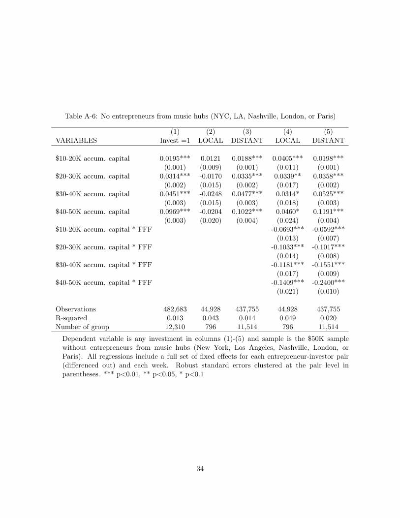
Table A-6: No entrepreneurs from music hubs (NYC, LA, Nashville, London, or Paris)

(1) (2) (3) (4) (5)VARIABLES Invest =1 LOCAL DISTANT LOCAL DISTANT

$10-20K accum. capital 0.0195*** 0.0121 0.0188*** 0.0405*** 0.0198***(0.001) (0.009) (0.001) (0.011) (0.001)

$20-30K accum. capital 0.0314*** -0.0170 0.0335*** 0.0339** 0.0358***(0.002) (0.015) (0.002) (0.017) (0.002)

$30-40K accum. capital 0.0451*** -0.0248 0.0477*** 0.0314* 0.0525***(0.003) (0.015) (0.003) (0.018) (0.003)

$40-50K accum. capital 0.0969*** -0.0204 0.1022*** 0.0460* 0.1191***(0.003) (0.020) (0.004) (0.024) (0.004)

$10-20K accum. capital * FFF -0.0693*** -0.0592***(0.013) (0.007)

$20-30K accum. capital * FFF -0.1033*** -0.1017***(0.014) (0.008)

$30-40K accum. capital * FFF -0.1181*** -0.1551***(0.017) (0.009)

$40-50K accum. capital * FFF -0.1409*** -0.2400***(0.021) (0.010)

Observations 482,683 44,928 437,755 44,928 437,755R-squared 0.013 0.043 0.014 0.049 0.020Number of group 12,310 796 11,514 796 11,514

Dependent variable is any investment in columns (1)-(5) and sample is the $50K samplewithout entrepreneurs from music hubs (New York, Los Angeles, Nashville, London, orParis). All regressions include a full set of fixed effects for each entrepreneur-investor pair(differenced out) and each week. Robust standard errors clustered at the pair level inparentheses. *** p<0.01, ** p<0.05, * p<0.1

34

Table A-7: No entrepreneurs from music hubs (NYC, LA, Nashville, London, or Paris) and con-trolling for live shows

(1) (2) (3) (4) (5)VARIABLES Invest =1 LOCAL DISTANT LOCAL DISTANT

$10-20K accum. capital 0.0183*** 0.0123 0.0175*** 0.0371*** 0.0184***(0.001) (0.009) (0.001) (0.011) (0.001)

$20-30K accum. capital 0.0334*** -0.0188 0.0355*** 0.0287* 0.0374***(0.002) (0.015) (0.002) (0.017) (0.002)

$30-40K accum. capital 0.0475*** -0.0274* 0.0501*** 0.0252 0.0544***(0.003) (0.015) (0.003) (0.018) (0.003)

$40-50K accum. capital 0.1006*** -0.0222 0.1060*** 0.0404* 0.1223***(0.003) (0.020) (0.004) (0.024) (0.004)

$10-20K accum. capital * FFF -0.0618*** -0.0553***(0.013) (0.007)

$20-30K accum. capital * FFF -0.0966*** -0.0931***(0.014) (0.008)

$30-40K accum. capital * FFF -0.1116*** -0.1450***(0.017) (0.009)

$40-50K accum. capital * FFF -0.1335*** -0.2307***(0.021) (0.010)

Videos uploaded (lagged) 0.0019 0.1633*** -0.0029 0.1670*** -0.0021(0.005) (0.059) (0.005) (0.058) (0.005)

Songs uploaded (lagged) -0.0009 -0.0020 -0.0008 -0.0013 -0.0013(0.001) (0.003) (0.001) (0.003) (0.001)

Investor proximate to Live Show 0.0124* 0.0365*** -0.0052 0.0378*** -0.0027(0.007) (0.014) (0.020) (0.014) (0.020)

Observations 478,251 44,815 433,436 44,815 433,436R-squared 0.012 0.040 0.013 0.046 0.018Number of group 12,310 796 11,514 796 11,514

Dependent variable is any investment in columns (1)-(5) and sample is the $50K sample withoutentrepreneurs from music hubs (New York, Los Angeles, Nashville, London, or Paris). Controlsfor videos and songs uploaded by the entrepreneurs, as well as live shows proximate to theinvestor are included. All regressions include a full set of fixed effects for each entrepreneur-investor pair (differenced out) and each week. Robust standard errors clustered at the pair levelin parentheses. *** p<0.01, ** p<0.05, * p<0.1

35

Table A-8: Overall charts rather than cumulative investment

(1) (2) (3) (4) (5)VARIABLES Invest =1 LOCAL DISTANT LOCAL DISTANT

Entrepreneur in overall charts (lagged) 0.0161*** -0.0161*** 0.0180*** -0.0009 0.0210***(0.001) (0.004) (0.001) (0.007) (0.001)

Entrepreneur in overall charts * FFF -0.0260*** -0.0321***(0.007) (0.003)

Observations 703,417 57,711 645,706 57,711 645,706R-squared 0.007 0.038 0.007 0.038 0.007Number of group 18,827 1,164 17,663 1,164 17,663

Dependent variable is any investment in columns (1)-(5) and sample is the $50K sample. Instead ofcumulative investment, the regressions introduce a dummy for the presence of the entrepreneurs on theoverall charts (Top 25). All regressions include a full set of fixed effects for each entrepreneur-investorpair (differenced out) and each week. Robust standard errors clustered at the pair level in parentheses.*** p<0.01, ** p<0.05, * p<0.1

36

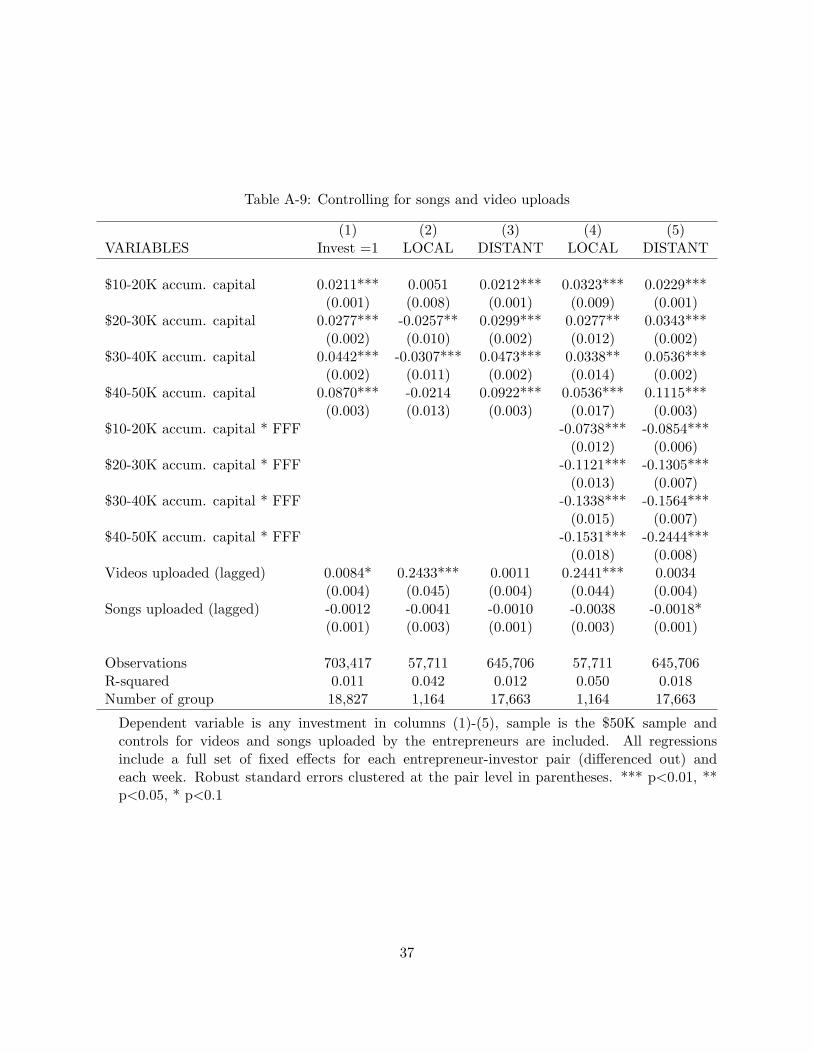
Table A-9: Controlling for songs and video uploads

(1) (2) (3) (4) (5)VARIABLES Invest =1 LOCAL DISTANT LOCAL DISTANT

$10-20K accum. capital 0.0211*** 0.0051 0.0212*** 0.0323*** 0.0229***(0.001) (0.008) (0.001) (0.009) (0.001)

$20-30K accum. capital 0.0277*** -0.0257** 0.0299*** 0.0277** 0.0343***(0.002) (0.010) (0.002) (0.012) (0.002)

$30-40K accum. capital 0.0442*** -0.0307*** 0.0473*** 0.0338** 0.0536***(0.002) (0.011) (0.002) (0.014) (0.002)

$40-50K accum. capital 0.0870*** -0.0214 0.0922*** 0.0536*** 0.1115***(0.003) (0.013) (0.003) (0.017) (0.003)

$10-20K accum. capital * FFF -0.0738*** -0.0854***(0.012) (0.006)

$20-30K accum. capital * FFF -0.1121*** -0.1305***(0.013) (0.007)

$30-40K accum. capital * FFF -0.1338*** -0.1564***(0.015) (0.007)

$40-50K accum. capital * FFF -0.1531*** -0.2444***(0.018) (0.008)

Videos uploaded (lagged) 0.0084* 0.2433*** 0.0011 0.2441*** 0.0034(0.004) (0.045) (0.004) (0.044) (0.004)

Songs uploaded (lagged) -0.0012 -0.0041 -0.0010 -0.0038 -0.0018*(0.001) (0.003) (0.001) (0.003) (0.001)

Observations 703,417 57,711 645,706 57,711 645,706R-squared 0.011 0.042 0.012 0.050 0.018Number of group 18,827 1,164 17,663 1,164 17,663

Dependent variable is any investment in columns (1)-(5), sample is the $50K sample andcontrols for videos and songs uploaded by the entrepreneurs are included. All regressionsinclude a full set of fixed effects for each entrepreneur-investor pair (differenced out) andeach week. Robust standard errors clustered at the pair level in parentheses. *** p<0.01, **p<0.05, * p<0.1

37

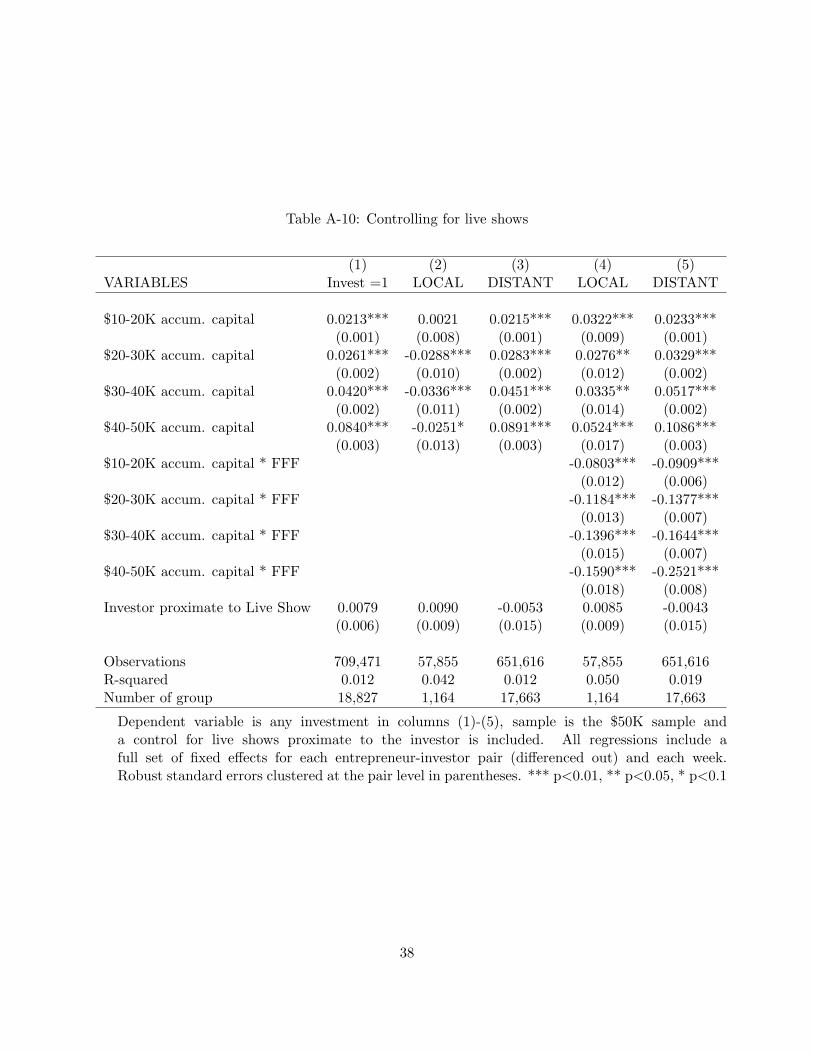
Table A-10: Controlling for live shows

(1) (2) (3) (4) (5)VARIABLES Invest =1 LOCAL DISTANT LOCAL DISTANT

$10-20K accum. capital 0.0213*** 0.0021 0.0215*** 0.0322*** 0.0233***(0.001) (0.008) (0.001) (0.009) (0.001)

$20-30K accum. capital 0.0261*** -0.0288*** 0.0283*** 0.0276** 0.0329***(0.002) (0.010) (0.002) (0.012) (0.002)

$30-40K accum. capital 0.0420*** -0.0336*** 0.0451*** 0.0335** 0.0517***(0.002) (0.011) (0.002) (0.014) (0.002)

$40-50K accum. capital 0.0840*** -0.0251* 0.0891*** 0.0524*** 0.1086***(0.003) (0.013) (0.003) (0.017) (0.003)

$10-20K accum. capital * FFF -0.0803*** -0.0909***(0.012) (0.006)

$20-30K accum. capital * FFF -0.1184*** -0.1377***(0.013) (0.007)

$30-40K accum. capital * FFF -0.1396*** -0.1644***(0.015) (0.007)

$40-50K accum. capital * FFF -0.1590*** -0.2521***(0.018) (0.008)

Investor proximate to Live Show 0.0079 0.0090 -0.0053 0.0085 -0.0043(0.006) (0.009) (0.015) (0.009) (0.015)

Observations 709,471 57,855 651,616 57,855 651,616R-squared 0.012 0.042 0.012 0.050 0.019Number of group 18,827 1,164 17,663 1,164 17,663

Dependent variable is any investment in columns (1)-(5), sample is the $50K sample anda control for live shows proximate to the investor is included. All regressions include afull set of fixed effects for each entrepreneur-investor pair (differenced out) and each week.Robust standard errors clustered at the pair level in parentheses. *** p<0.01, ** p<0.05, * p<0.1

38

Table A-11: Controlling for live shows, songs, and video uploads

(1) (2) (3) (4) (5)VARIABLES Invest =1 LOCAL DISTANT LOCAL DISTANT

$10-20K accum. capital 0.0211*** 0.0051 0.0212*** 0.0324*** 0.0229***(0.001) (0.008) (0.001) (0.009) (0.001)

$20-30K accum. capital 0.0277*** -0.0258** 0.0299*** 0.0277** 0.0343***(0.002) (0.010) (0.002) (0.012) (0.002)

$30-40K accum. capital 0.0442*** -0.0309*** 0.0473*** 0.0335** 0.0536***(0.002) (0.011) (0.002) (0.014) (0.002)

$40-50K accum. capital 0.0871*** -0.0211 0.0922*** 0.0539*** 0.1115***(0.003) (0.013) (0.003) (0.017) (0.003)

$10-20K accum. capital * FFF -0.0738*** -0.0854***(0.012) (0.006)

$20-30K accum. capital * FFF -0.1121*** -0.1305***(0.013) (0.007)

$30-40K accum. capital * FFF -0.1337*** -0.1565***(0.015) (0.007)

$40-50K accum. capital * FFF -0.1531*** -0.2444***(0.018) (0.008)

Videos uploaded (lagged) 0.0084* 0.2435*** 0.0011 0.2444*** 0.0034(0.004) (0.045) (0.004) (0.044) (0.004)

Songs uploaded (lagged) -0.0011 -0.0038 -0.0010 -0.0035 -0.0018*(0.001) (0.003) (0.001) (0.003) (0.001)

Investor proximate to Live Show 0.0098* 0.0094 0.0031 0.0090 0.0043(0.006) (0.009) (0.015) (0.009) (0.015)

Observations 703,417 57,711 645,706 57,711 645,706R-squared 0.011 0.042 0.012 0.050 0.018Number of group 18,827 1,164 17,663 1,164 17,663

Dependent variable is any investment in columns (1)-(5), sample is the $50K sample and controlsfor videos and songs uploaded by the entrepreneurs as well as live shows proximate to investorare included. All regressions include a full set of fixed effects for each entrepreneur-investorpair (differenced out) and each week. Robust standard errors clustered at the pair level inparentheses. *** p<0.01, ** p<0.05, * p<0.1

39

Table A-12: Logit

(1) (2) (3) (4) (5)VARIABLES Invest =1 LOCAL DISTANT LOCAL DISTANT

$10-20K accum. capital 0.5156*** 0.2256** 0.5138*** 0.7930*** 0.6178***(0.024) (0.093) (0.026) (0.124) (0.027)

$20-30K accum. capital 0.5873*** -0.4573*** 0.6319*** 1.1096*** 0.8655***(0.031) (0.129) (0.032) (0.159) (0.033)

$30-40K accum. capital 1.0305*** -0.2008 1.0652*** 1.6613*** 1.3640***(0.036) (0.152) (0.037) (0.190) (0.039)

$40-50K accum. capital 1.5759*** -0.1075 1.6240*** 1.7933*** 2.0462***(0.037) (0.168) (0.038) (0.207) (0.040)

$10-20K accum. capital * FFF -1.4185*** -1.9948***(0.151) (0.078)

$20-30K accum. capital * FFF -3.1988*** -3.7121***(0.179) (0.095)

$30-40K accum. capital * FFF -4.1826*** -4.9322***(0.236) (0.114)

$40-50K accum. capital * FFF -4.3448*** -6.3427***(0.268) (0.129)

Observations 708,745 57,814 650,931 57,814 650,931Number of group 18,234 1,127 17,107 1,127 17,107Log Likelihood -85886 -5617 -79640 -5356 -77703

Dependent variable is any investment in columns (1)-(5) and sample is the $50K sample. AllLogit regressions include a full set of fixed effects for each entrepreneur-investor pair (differencedout) and each week. Robust standard errors clustered at the pair level in parentheses. ***p<0.01, ** p<0.05, * p<0.1

40

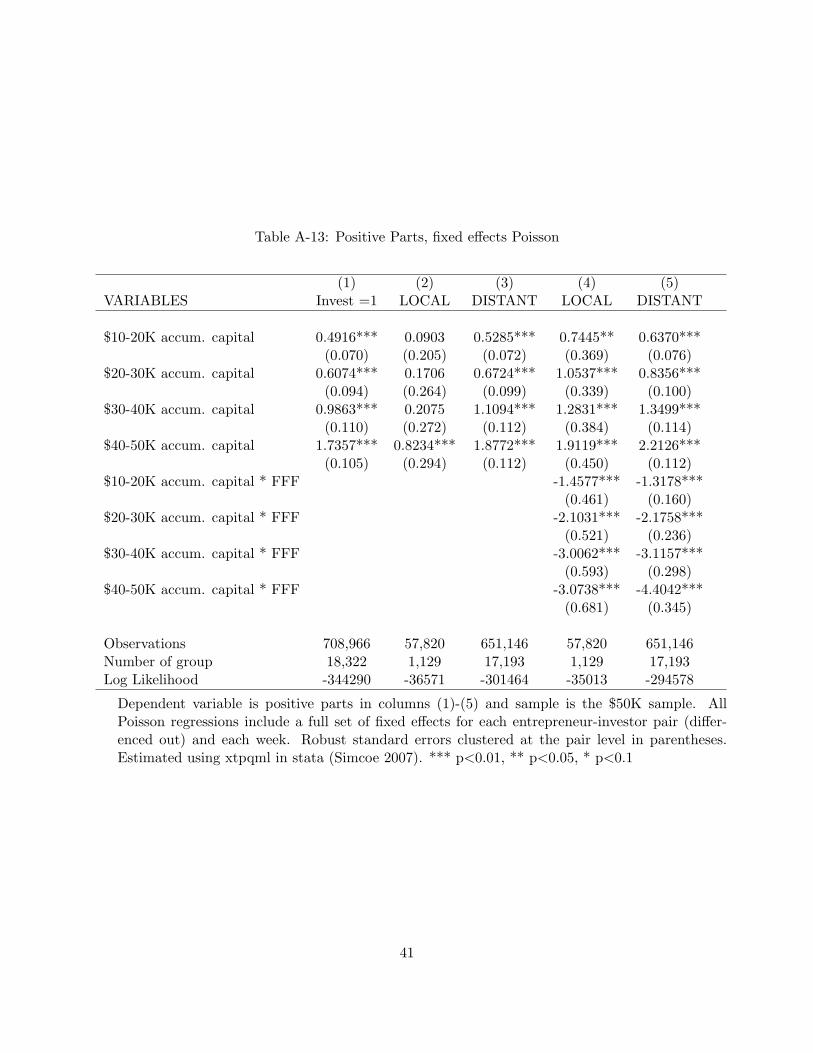
Table A-13: Positive Parts, fixed effects Poisson

(1) (2) (3) (4) (5)VARIABLES Invest =1 LOCAL DISTANT LOCAL DISTANT

$10-20K accum. capital 0.4916*** 0.0903 0.5285*** 0.7445** 0.6370***(0.070) (0.205) (0.072) (0.369) (0.076)

$20-30K accum. capital 0.6074*** 0.1706 0.6724*** 1.0537*** 0.8356***(0.094) (0.264) (0.099) (0.339) (0.100)

$30-40K accum. capital 0.9863*** 0.2075 1.1094*** 1.2831*** 1.3499***(0.110) (0.272) (0.112) (0.384) (0.114)

$40-50K accum. capital 1.7357*** 0.8234*** 1.8772*** 1.9119*** 2.2126***(0.105) (0.294) (0.112) (0.450) (0.112)

$10-20K accum. capital * FFF -1.4577*** -1.3178***(0.461) (0.160)

$20-30K accum. capital * FFF -2.1031*** -2.1758***(0.521) (0.236)

$30-40K accum. capital * FFF -3.0062*** -3.1157***(0.593) (0.298)

$40-50K accum. capital * FFF -3.0738*** -4.4042***(0.681) (0.345)

Observations 708,966 57,820 651,146 57,820 651,146Number of group 18,322 1,129 17,193 1,129 17,193Log Likelihood -344290 -36571 -301464 -35013 -294578

Dependent variable is positive parts in columns (1)-(5) and sample is the $50K sample. AllPoisson regressions include a full set of fixed effects for each entrepreneur-investor pair (differ-enced out) and each week. Robust standard errors clustered at the pair level in parentheses.Estimated using xtpqml in stata (Simcoe 2007). *** p<0.01, ** p<0.05, * p<0.1

41

Table A-14: Total Parts, OLS

(1) (2) (3) (4) (5)VARIABLES Invest =1 LOCAL DISTANT LOCAL DISTANT

$10-20K accum. capital 0.1216*** 0.2116 0.1173*** 0.5943*** 0.1268***(0.018) (0.171) (0.017) (0.212) (0.017)

$20-30K accum. capital 0.1654*** 0.1290 0.1640*** 0.7685** 0.1787***(0.028) (0.249) (0.027) (0.308) (0.027)

$30-40K accum. capital 0.2575*** 0.1218 0.2621*** 0.7840*** 0.2878***(0.035) (0.273) (0.034) (0.300) (0.035)

$40-50K accum. capital 0.6279*** 0.2909 0.6516*** 1.4283 0.7572***(0.056) (0.577) (0.053) (0.980) (0.057)

$10-20K accum. capital * FFF -0.9861*** -0.4108***(0.276) (0.053)

$20-30K accum. capital * FFF -1.3505*** -0.5489***(0.294) (0.062)

$30-40K accum. capital * FFF -1.4375*** -0.6860***(0.293) (0.071)

$40-50K accum. capital * FFF -2.1922*** -1.2360***(0.782) (0.081)

Observations 709,471 57,855 651,616 57,855 651,616R-squared 0.002 0.004 0.003 0.005 0.004Number of group 18,827 1,164 17,663 1,164 17,663

Dependent variable is total parts in columns (1)-(5) and sample is the $50K sample. Totalparts includes a small number of disinvestments where investors withdraw money from anentrepreneur. Therefore, the analysis is done with OLS rather than fixed effects poisson. Allregressions include a full set of fixed effects for each entrepreneur-investor pair (differencedout) and each week. Robust standard errors clustered at the pair level in parentheses. ***p<0.01, ** p<0.05, * p<0.1

42

Table A-15: Local defined as within 25 km

(1) (2) (3) (4)VARIABLES LOCAL 25 km DISTANT LOCAL 25 km DISTANT

$10-20K accum. capital -0.0102 0.0218*** 0.0194* 0.0232***(0.009) (0.001) (0.011) (0.001)

$20-30K accum. capital -0.0455*** 0.0283*** 0.0057 0.0327***(0.012) (0.002) (0.014) (0.002)

$30-40K accum. capital -0.0430*** 0.0444*** 0.0178 0.0503***(0.013) (0.002) (0.017) (0.002)

$40-50K accum. capital -0.0283* 0.0873*** 0.0448** 0.1068***(0.016) (0.003) (0.021) (0.003)

$10-20K accum. capital * FFF -0.0759*** -0.0943***(0.014) (0.006)

$20-30K accum. capital * FFF -0.1098*** -0.1356***(0.015) (0.007)

$30-40K accum. capital * FFF -0.1288*** -0.1638***(0.017) (0.007)

$40-50K accum. capital * FFF -0.1514*** -0.2463***(0.022) (0.007)

Observations 36,186 673,285 36,186 673,285R-squared 0.035 0.012 0.043 0.019Number of group 748 18,079 748 18,079

Dependent variable is any investment in columns (1)-(4) and sample is the $50K sample.All investors within 25 km from the entrepreneurs are here coded as local investors. Allregressions include a full set of fixed effects for each entrepreneur-investor pair (differencedout) and each week. Robust standard errors clustered at the pair level in parentheses. ***p<0.01, ** p<0.05, * p<0.1

43

Table A-16: Local defined as within 100 km

(1) (2) (3) (4)VARIABLES LOCAL 100 km DISTANT LOCAL 100 km DISTANT

$10-20K accum. capital 0.0082 0.0216*** 0.0340*** 0.0236***(0.006) (0.001) (0.007) (0.001)

$20-30K accum. capital -0.0225*** 0.0290*** 0.0307*** 0.0336***(0.008) (0.002) (0.009) (0.002)

$30-40K accum. capital -0.0254*** 0.0458*** 0.0379*** 0.0527***(0.009) (0.002) (0.011) (0.002)

$40-50K accum. capital -0.0140 0.0902*** 0.0637*** 0.1099***(0.011) (0.003) (0.014) (0.003)

$10-20K accum. capital * FFF -0.0898*** -0.0876***(0.010) (0.007)

$20-30K accum. capital * FFF -0.1301*** -0.1346***(0.011) (0.007)

$30-40K accum. capital * FFF -0.1508*** -0.1657***(0.013) (0.008)

$40-50K accum. capital * FFF -0.1813*** -0.2533***(0.015) (0.008)

Observations 78,897 630,574 78,897 630,574R-squared 0.039 0.012 0.049 0.018Number of group 1,572 17,255 1,572 17,255

Dependent variable is any investment in columns (1)-(4) and sample is the $50K sample.All investors within 100 km from the entrepreneurs are here coded as local investors. Allregressions include a full set of fixed effects for each entrepreneur-investor pair (differencedout) and each week. Robust standard errors clustered at the pair level in parentheses. ***p<0.01, ** p<0.05, * p<0.1

44

Tab

leA

-17:

Ifge

ogra

phic

info

rmat

ion

ism

issi

ng,

code

das

dist

ant

(1)

(2)

(3)

(4)

(5)

VA

RIA

BL

ES

Inve

st=

1w

ith

NA

sL

OC

AL

DIS

TA

NT

orN

As

LO

CA

LD

IST

AN

Tor

NA

s

$10-

20K

accu

m.

capi

tal

0.01

80**

*0.

0020

0.01

81**

*0.

0322

***

0.02

30**

*(0

.001

)(0

.008

)(0

.001

)(0

.009

)(0

.001

)$2

0-30

Kac

cum

.ca

pita

l0.

0216

***

-0.0

287*

**0.

0235

***

0.02

76**

0.03

13**

*(0

.002

)(0

.010

)(0

.002

)(0

.012

)(0

.002

)$3

0-40

Kac

cum

.ca

pita

l0.

0357

***

-0.0

334*

**0.

0382

***

0.03

37**

0.04

87**

*(0

.002

)(0

.011

)(0

.002

)(0

.014

)(0

.002

)$4

0-50

Kac

cum

.ca

pita

l0.

0731

***

-0.0

254*

0.07

72**

*0.

0521

***

0.10

49**

*(0

.003

)(0

.013

)(0

.003

)(0

.017

)(0

.003

)$1

0-20

Kac

cum

.ca

pita

l*

FF

F-0

.080

3***

-0.1

118*

**(0

.012

)(0

.005

)$2

0-30

Kac

cum

.ca

pita

l*

FF

F-0

.118

4***

-0.1

474*

**(0

.013

)(0

.005

)$3

0-40

Kac

cum

.ca

pita

l*

FF

F-0

.139

7***

-0.1

703*

**(0

.015

)(0

.006

)$4

0-50

Kac

cum

.ca

pita

l*

FF

F-0

.159

0***

-0.2

436*

**(0

.018

)(0

.006

)

Obs

erva

tion

s78

3,37

257

,855

725,

517

57,8

5572

5,51

7R

-squ

ared

0.01

20.

042

0.01

10.

050

0.02

1N

umbe

rof

grou

p20

,826

1,16

419

,662

1,16

419

,662

Dep

ende

ntva

riab

leis

any

inve

stm

ent

inco

lum

ns(1

)-(5

)an

dsa

mpl

eis

the

$50K

sam

ple.

Ifge

ogra

phic

info

rmat

ion

onth

ein

vest

oris

mis

sing

,th

ein

vest

oris

code

das

adi

stan

tin

vest

or.

All

regr

essi

ons

incl

ude

afu

llse

tof

fixed

effec

tsfo

rea

chen

trep

rene

ur-i

nves

tor

pair

(diff

eren

ced

out)

and

each

wee

k.R

obus

tst

anda

rder

rors

clus

tere

dat

the

pair

leve

lin

pare

nthe

ses.

***

p<0.

01,

**p<

0.05

,*

p<0.

1

45

Table A-18: Distant and local in same regression

(1) (2)VARIABLES Invest=1 Invest=1

$10-20K accum. capital -0.0228*** 0.0045(0.006) (0.007)

$20-30K accum. capital -0.0376*** 0.0119(0.006) (0.009)

$30-40K accum. capital -0.0369*** 0.0230*(0.007) (0.012)

$40-50K accum. capital -0.0276*** 0.0449***(0.008) (0.015)

$10-20K accum. capital * FFF -0.0791***(0.012)

$20-30K accum. capital * FFF -0.1111***(0.013)

$30-40K accum. capital * FFF -0.1296***(0.015)

$40-50K accum. capital * FFF -0.1476***(0.018)

$10-20K accum. capital * Distant 0.0447*** 0.0192***(0.006) (0.007)

$20-30K accum. capital * Distant 0.0653*** 0.0206**(0.006) (0.009)

$30-40K accum. capital * Distant 0.0804*** 0.0269**(0.007) (0.012)

$40-50K accum. capital * Distant 0.1149*** 0.0619***(0.008) (0.015)

$10-20K accum. capital * Distant * FFF -0.0119(0.013)

$20-30K accum. capital * Distant * FFF -0.0265*(0.014)

$30-40K accum. capital * Distant * FFF -0.0350**(0.017)

$40-50K accum. capital * Distant * FFF -0.1043***(0.019)

Observations 709,471 709,471R-squared 0.013 0.019Number of group 18,827 18,827

Dependent variable is any investment in columns (1)-(2) andsample is the $50K sample. Distant and local are presentedhere in same regression (i.e. interaction term). All regressionsinclude a full set of fixed effects for each entrepreneur-investor pair(differenced out) and each week. Robust standard errors clusteredat the pair level in parentheses. *** p<0.01, ** p<0.05, * p<0.1

46

Tab

leA

-19:

Alt

erna

tive

spec

ifica

tion

sfo

rF

FF

(1)

(2)

(3)

(4)

(5)

(6)

(7)

(8)

(9)

(10)

Fir

stIn

vt

Fir

stIn

vt

Fir

stIn

vt

Fir

stIn

vt

Fir

stIn

vt

Fir

stIn

vt

Fir

stIn

vt

Fir

stIn

vt

Larg

est

invt

Larg

est

invt

Larg

est

Invt

Larg

est

Invt

Most

3oth

ers

Most

3oth

ers

Larg

est

invt

Larg

est

invt

No

more

No

more

No

Oth

er

No

Oth

er

than

3oth

ers

than

3oth

ers

VA

RIA

BL

ES

LO

CA

LD

IST

AN

TL

OC

AL

DIS

TA

NT

LO

CA

LD

IST

AN

TL

OC

AL

DIS

TA

NT

LO

CA

LD

IST

AN

T

$10-2

0K

accum

.capit

al

0.0

400***

0.0

242***

0.0

271***

0.0

229***

0.0

345***

0.0

236***

0.0

345***

0.0

236***

0.0

311***

0.0

236***

(0.0

10)

(0.0

01)

(0.0

09)

(0.0

01)

(0.0

09)

(0.0

01)

(0.0

09)

(0.0

01)

(0.0

09)

(0.0

01)

$20-3

0K

accum

.capit

al

0.0

367***

0.0

360***

0.0

171

0.0

324***

0.0

320***

0.0

344***

0.0

277**

0.0

336***

0.0

259**

0.0

334***

(0.0

13)

(0.0

02)

(0.0

12)

(0.0

02)

(0.0

12)

(0.0

02)

(0.0

12)

(0.0

02)

(0.0

12)

(0.0

02)

$30-4

0K

accum

.capit

al

0.0

430***

0.0

566***

0.0

164

0.0

508***

0.0

397***

0.0

539***

0.0

333**

0.0

525***

0.0

368**

0.0

524***

(0.0

15)

(0.0

02)

(0.0

14)

(0.0

02)

(0.0

15)

(0.0

02)

(0.0

14)

(0.0

02)

(0.0

14)

(0.0

02)

$40-5

0K

accum

.capit

al

0.0

707***

0.1

208***

0.0

331*

0.1

065***

0.0

558***

0.1

147***

0.0

620***

0.1

099***

0.0

557***

0.1

090***

(0.0

19)

(0.0

03)

(0.0

17)

(0.0

03)

(0.0

18)

(0.0

03)

(0.0

18)

(0.0

03)

(0.0

18)

(0.0

03)

$10-2

0K

accum

.capit

al

*F

FF

-0.0

797***

-0.0

805***

-0.0

784***

-0.0

962***

-0.0

803***

-0.0

870***

-0.0

751***

-0.0

895***

-0.0

782***

-0.0

755***

(0.0

12)

(0.0

05)

(0.0

12)

(0.0

07)

(0.0

12)

(0.0

06)

(0.0

12)

(0.0

06)

(0.0

12)

(0.0

06)

$20-3

0K

accum

.capit

al

*F

FF

-0.1

148***

-0.1

292***

-0.1

115***

-0.1

455***

-0.1

203***

-0.1

367***

-0.1

075***

-0.1

365***

-0.1

153***

-0.1

175***

(0.0

13)

(0.0

06)

(0.0

13)

(0.0

08)

(0.0

13)

(0.0

06)

(0.0

13)

(0.0

07)

(0.0

13)

(0.0

06)

$30-4

0K

accum

.capit

al

*F

FF

-0.1

329***

-0.1

560***

-0.1

240***

-0.1

714***

-0.1

431***

-0.1

627***

-0.1

257***

-0.1

628***

-0.1

436***

-0.1

429***

(0.0

16)

(0.0

06)

(0.0

15)

(0.0

08)

(0.0

16)

(0.0

06)

(0.0

15)

(0.0

07)

(0.0

16)

(0.0

06)

$40-5

0K

accum

.capit

al

*F

FF

-0.1

599***

-0.2

498***

-0.1

414***

-0.2

597***

-0.1

576***

-0.2

567***

-0.1

566***

-0.2

485***

-0.1

634***

-0.2

225***

(0.0

18)

(0.0

06)

(0.0

18)

(0.0

09)

(0.0

19)

(0.0

07)

(0.0

18)

(0.0

08)

(0.0

18)

(0.0

07)

Obse

rvati

ons

57,8

55

651,6

16

57,8

55

651,6

16

57,8

55

651,6

16

57,8

55

651,6

16

57,8

55

651,6

16

R-s

quare

d0.0

49

0.0

21

0.0

48

0.0

18

0.0

50

0.0

20

0.0

48

0.0

19

0.0

50

0.0

18

Num

ber

of

gro

up

1,1

64

17,6

63

1,1

64

17,6

63

1,1

64

17,6

63

1,1

64

17,6

63

1,1

64

17,6

63

Dep

endent

vari

able

isany

invest

ment

incolu

mns

(1)-

(10)

and

sam

ple

isth

e$50K

sam

ple

.In

colu

mns

(1)-

(2),

an

invest

or

isdefi

ned

as

FF

Fif

she

invest

ed

inth

at

entr

epre

neur

befo

rein

vest

ing

inany

oth

er.

Incolu

mns

(3)-

(4),

an

invest

or

isdefi

ned

as

FF

Fif

she

invest

ed

inth

at

entr

epre

neur

befo

rein

vest

ing

inany

oth

er,

her

invest

ment

inth

efo

cal

entr

epre

neur

isher

larg

est

invest

ment

and

she

invest

sin

no

oth

er

entr

epre

neurs

.In

colu

mns

(5)-

(6),

an

invest

or

isdefi

ned

as

FF

Fif

she

invest

ed

inth

at

entr

epre

neur

befo

rein

vest

ing

inany

oth

er

and

she

did

not

invest

inm

ore

than

thre

eoth

er

entr

epre

neurs

.In

colu

mns

(7)-

(8),

an

invest

or

isdefi

ned

as

FF

Fif

she

invest

ed

inth

at

entr

epre

neur

befo

rein

vest

ing

inany

oth

er

and

her

invest

ment

inth

efo

cal

entr

epre

neur

isher

larg

est

invest

ment.

Incolu

mns

(9)-

(10),

an

invest

or

isdefi

ned

as

FF

Fif

her

invest

ment

inth

efo

cal

entr

epre

neur

isher

larg

est

invest

ment

and

she

did

not

invest

sin

more

than

thre

eoth

er

entr

epre

neurs

.A

llre

gre

ssio

ns

inclu

de

afu

llse

tof

fixed

eff

ects

for

each

entr

epre

neur-

invest

or

pair

(diff

ere

nced

out)

and

each

week.

Robust

standard

err

ors

clu

stere

dat

the

pair

level

inpare

nth

ese

s.***

p<

0.0

1,

**

p<

0.0

5,

*p

<0.1

47