ARTICLE IN PRESSISA Transactions ( ) –

Contents lists available at ScienceDirect

ISA Transactions

journal homepage: www.elsevier.com/locate/isatrans

Enhanced disturbance rejection for open-loop unstable process with time delayM. Shamsuzzoha, Moonyong Lee ∗School of Chemical Engineering and Technology, Yeungnam University, Kyongsan 712–749, South Korea

a r t i c l e i n f o

Article history:Received 26 May 2008Received in revised form4 September 2008Accepted 29 October 2008Available online xxxx

Keywords:PID cascaded with a lead–lag filterUnstable processTwo-degree-of-freedom controlDisturbance rejectionTime delay process

a b s t r a c t

The present study suggests a disturbance estimator designmethod for application to a recently published,two-degree-of-freedom, control scheme for open-loop, unstable processes with time delay. A simple PIDcontroller cascaded with a lead–lag filter replaces the high-order disturbance estimator for enhancedperformance. A new analytical method on the basis of the IMC design principle, featuring only one user-defined tuning parameter, is developed for the design of the disturbance estimator. Several illustrativeexamples taken from previous works are included to demonstrate the superiority of the proposeddisturbance estimator. The results confirm the superior performance of the proposed disturbanceestimator in both nominal and robust cases. The proposed method also offers several importantadvantages for industrial process engineers: it covers several classes of unstable process with time delayin a unified manner, and is simple and easy to design and tune.

© 2008 ISA. Published by Elsevier Ltd. All rights reserved.

1. Introduction

Time-delayed unstable processes are commonly encounteredin process industries and are difficult to control due to right-halfplane (RHP) poles. A time delay is introduced into the transferfunction description of such system due to themeasurement delayor an actuator delay or by the approximation of higher dynamicsof the system by that of a lower order plus delay systems.The design area of the control of an unstable delay system has

recently attracted much research attention [1–6]. Proportional-Integrative-Derivative (PID) controllers are the most common andsuccessful type found in industrial control applications due totheir simple structure and meaning of the corresponding threeparameters, which simplifies the understanding of the PID controlcompared to most other advanced control techniques. In addition,the PID controller usually exhibits satisfactory performance inmany situations. The widespread use of PID controllers raises theimportance of designing a simple but efficient method for tuningthe controller.The distinguishable framework for control system design and

implementation of the internal model control (IMC) (Morari andZafiriou, [1]; Lee et al., [2]; Yang et al., [5]; Shamsuzzoha andLee, [6]) has directed much research attention on exploiting theIMC principle for the design of equivalent feedback controllersfor unstable processes. The principle has attracted the attentionof industrial users because there is only one user-defined tuning

∗ Corresponding author. Fax: +82 53 811 3262.E-mail address:mynlee@yu.ac.kr (M. Lee).

parameter, which is directly related to the closed-loop timeconstant.Due to its internal instability, the IMC design principle cannot

be directly applied for the design of the unstable processes. Theseveralmodified, IMC-based control strategies have therefore beendeveloped for controlling unstable processes with time delayand are freely available in the literature [2,5–8]. Furthermore,two-degree-of-freedom (2DOF) control methods based on theSmith–Predictor (SP) were proposed (Kwak et al. [9]; Majhi andAtherton [10]; Zhang et al. [11]) to achieve a smooth nominalsetpoint response without overshoot for first-order unstableprocesseswith timedelay. Kwak et al. [9] have proposed amodifiedSP for unstable processes, which predicts the dynamics of theactual process from the process model. However, the methodis sensitive to uncertainties in the process parameters. Majhiand Atherton [10] have modified the original SP for unstabletime delay process, proposed a PD controller for stabilizing theunstable process and obtained improved performance with theadded advantage of decoupling the disturbance rejection responsefrom the setpoint tracking. Zhang et al. [11] have also suggested amodified SP structure for unstable, first-order, time delay process.They modified the structure proposed by Kwak et al. [9] anddesigned a PID controller to stabilize the unstable process andreject the disturbance based on the desired closed-loop response.It is important to note that in the several design methods

based on either the modified IMC or the modified SP methods, thenominal setpoint response tends to be faster without overshootfor unstable processes. In fact, the design methods based onthe modified IMC and SP methods employ the nominal processmodel in their control structures, which accounts for their goodperformance. However, many existing 2DOF control methods are

0019-0578/$ – see front matter© 2008 ISA. Published by Elsevier Ltd. All rights reserved.doi:10.1016/j.isatra.2008.10.010

Please cite this article in press as: Shamsuzzoha M, Lee M. Enhanced disturbance rejection for open-loop unstable process with time delay. ISA Transactions (2008),doi:10.1016/j.isatra.2008.10.010

ARTICLE IN PRESS2 M. Shamsuzzoha, M. Lee / ISA Transactions ( ) –

restricted to the unstable processes in the form of a first-orderrational part plus time delay, which cannot, in fact, represent avariety of industrial and chemical unstable processes well enough.Besides, the usual presence of unmodeled dynamics inevitablytends to deteriorate the control system performance.Recently Liu et al. [8] proposed a novel, 2DOF control scheme

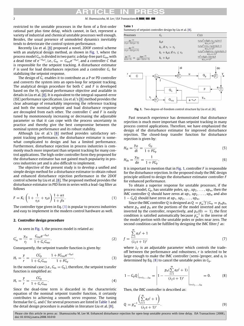
with an analytical design method, as shown in Fig. 1, where theprocessmodelGm is divided in twoparts: a delay-free partGmowitha dead time of e−θms, i.e., Gm = Gmoe−θms, and a controller C thatis responsible for the setpoint tracking. A disturbance estimatorF is used for load disturbances rejection and a controller Gc forstabilizing the setpoint response.The design of Gc enables it to contribute as a P or PD controller

and converts the system into an open-loop for setpoint tracking.The analytical design procedure for both C and F is developedbased on the H2 optimal performance objective and available indetails in Liu et al. [8]. It is equivalent to the integral-squared-error(ISE) performance specification. Liu et al.’s [8]method provides theclear advantage of remarkably improving the reference trackingand both the nominal setpoint and load disturbance responseare decoupled from each other. The controller C and F is easilytuned by monotonously increasing or decreasing the adjustableparameter so that it can cope with the process uncertainty inpractice and thereby give the best compromise between thenominal system performance and its robust stability.Although Liu et al.’s [8] method provides satisfactory set-

point tracking performance, the disturbance estimator is some-what complicated to design and has a limited performance.Furthermore, disturbance rejection in process industries is com-monly muchmore important than setpoint tracking for many con-trol applications. The high-order controller form they proposed forthe disturbance estimator has not gained much popularity in pro-cess industries yet and is also difficult to implement.The objective of the present study is to develop a unified and

simple design method for a disturbance estimator to obtain robustand enhanced disturbance rejection performance in the 2DOFcontrol scheme by Liu et al. [8]. The proposedmethod provides thedisturbance estimator in PID form in series with a lead–lag filter asfollows

F = KC

(1+

1τIs+ τDs

)1+ αs1+ βs

. (1)

The controller type given in Eq. (1) is popular to process industriesand easy to implement in the modern control hardware as well.

2. Controller design procedure

As seen in Fig. 1, the process model is related as:

G′m =ymrf=Gmoe−θms

1+ GcGmo. (2)

Consequently, the setpoint transfer function is given by:

Hr =yr=

CGp1+ GcGmo

·1+ FGmoe−θms

1+ FGp. (3)

In the nominal case (i.e., Gm = Gp), therefore, the setpoint transferfunction is simplified as:

Hr =yr=

CGp1+ GcGmo

. (4)

Since the dead-time term is discarded in the characteristicequation of the nominal setpoint transfer function, it certainlycontributes to achieving a smooth servo response. The tuningformulae for Gc and C for several processes are listed in Table 1 andthe detail design procedure is available in literature Liu et al. [8].

Table 1Summary of setpoint controller design by Liu et al. [8].

Processes Gc C(s)

ke−θs(τ1s−1)(τ2s−1)

kdsτ1τ2s2+(kdk−τ1−τ2)s+1

k(λc s+1)2

ke−θs(τ1s−1)(τ2s+1)

kc , if τ1 > τ2τ1τ2s2+(τ1−τ2)s+kc k−1

k(λc s+1)2

kc + kds, if τ1 ≤ τ2τ1τ2s2+(kdk+τ1−τ2)s+kc k−1

k(λc s+1)2

ke−θss(τ s−1) =

kφe−θs

(φs−1)(τ s−1) kc + kdsτ s2+(kdk−1)s+kc k

k(λc s+1)2

Fig. 1. Two-degree-of-freedom control structure by Liu et al. [8].

Past research experience has demonstrated that disturbancerejection is much more important than setpoint tracking in manyprocess control applications. Therefore, we have emphasized thedesign of the disturbance estimator for improved disturbancerejection. The closed-loop transfer function for disturbancerejection is given by:

Hdi =ydidi=

Gp1+ FGp

(5)

Hdo =ydodo=

11+ FGp

. (6)

It is important to mention that in Fig. 1, controller F is responsiblefor the disturbance rejection. In the proposed study the IMC designprinciple utilized to design the disturbance estimator controller Ffor enhanced performance.To obtain a superior response for unstable processes, if the

process model, Gp, has unstable poles, up1, up2, . . . , upm, then theIMC controller Q should have zeros at up1, up2, . . . , upm and also1− GpQ should have zeros at up1, up2, . . . , upm.Since the IMC controllerQ is designed asQ = p−1m f (Gm = pmpA,

where pm and pA are the portions of the model inverted and notinverted by the controller, respectively, and pA(0) = 1), the firstcondition is satisfied automatically because p−1m is the inverse ofthe model portion with the unstable poles or poles near zero. Thesecond condition can be fulfilled by designing the IMC filter f as:

f =

m∑i=1aisi + 1

(λf s+ 1)r(7)

where λf is an adjustable parameter which controls the trade-off between the performance and robustness, r is selected to belarge enough to make the IMC controller (semi-)proper, and ai isdetermined by Eq. (8) to cancel the unstable poles in Gp.

1− GpQ∣∣s=z1,...zm

=

∣∣∣∣∣∣∣∣1−pA(

m∑i=1aisi + 1)

(λf s+ 1)r

∣∣∣∣∣∣∣∣s=z1,...,zm

= 0. (8)

Then, the IMC controller is described as:

Q = p−1m

(m∑i=1aisi + 1

)(λf s+ 1)r

. (9)

Please cite this article in press as: Shamsuzzoha M, Lee M. Enhanced disturbance rejection for open-loop unstable process with time delay. ISA Transactions (2008),doi:10.1016/j.isatra.2008.10.010

ARTICLE IN PRESSM. Shamsuzzoha, M. Lee / ISA Transactions ( ) – 3

From the above design procedure, a stable, closed-loop responsecan be achieved by using the IMC controller. The ideal feedbackcontroller that is equivalent to the IMC controller can be expressedin terms of the internal model Gm and the IMC controller Q :

Fim (s) =Q

1− GmQ. (10)

Substituting the value of the process model Gm and the IMCcontroller Q into Eq. (10) gives the ideal feedback controller:

Fim (s) =p−1m

(m∑i=1aisi+1

)(λf s+1)r

1−pA

(m∑i=1aisi+1

)(λf s+1)

r

. (11)

Let us consider the design of the following unstable process withtwo RHP poles as a representative model:

Gp =ke−θs

(τ1s− 1) (τ2s− 1)(12)

where k is the gain, τ1 and τ2 are the time constants, and θ is thetime delay. The IMC filter structure is chosen as

f =

(a2s2 + a1s+ 1

)(λf s+ 1

)4 . (13)

The IMC filter form in Eq. (13) was also utilized by severalresearchers [2,12] to design the IMC–PID controller. The resultingIMC controller becomes

Q =(τ1s− 1) (τ2s− 1)

(a2s2 + a1s+ 1

)K(λf s+ 1

)4 . (14)

Therefore, the ideal desired disturbance estimator obtained as:

Fim (s) =(τ1s− 1) (τ2s− 1)

(a2s2 + a1s+ 1

)k[(λf s+ 1

)4− e−θs

(a2s2 + a1s+ 1

)] . (15)

This ideal disturbance estimator can be approximated to a simplePID cascaded with a lead–lag filter. The dead time e−θs in Eq. (15)is approximated by 1/1 Pade expansion,

e−θs =(1− θs/2)(1+ θs/2)

(16)

which results in Fim(s) given in Box I.Box I reveals that the resulting disturbance estimator has the

form of a PID controller cascaded with a high-order filter. Theanalytical PID formula can be obtained by rearranging the equationin Box I as below:

KC =a1

k(4λf + θ − a1

) ; τI = a1; τD =a2a1. (17)

Furthermore, it is obvious from Eq. (8) that the remaining part ofthe denominator in Box I contains the factor of the process poles,(τ1s− 1) (τ2s− 1). Therefore, the parameter β can be obtainedby taking the first derivative of the equation given in Box II andsubstituting s = 0 as:

β =

(a1θ/2− a2 + 2λf θ + 6λ2f

)(θ + 4λf − a1

) + (τ1 + τ2) . (18)

The filter parameter α can be easily obtained from Box I:

α = 0.5θ. (19)

Since the high-order γ s2 term has little impact on the overallcontrol performance in the control relevant frequency range,the remaining part of the fraction in Box II can be successfullyapproximated to a simple first-order, lead–lag filter, as (1 +αs)/(1+ βs).The values of a1 and a2 are selected to cancel out the poles

at 1/τ1 and 1/τ2. This requires[1− GpQ

]∣∣s=1/τ1 ,1/τ2

= 0 and

thus[1−

(a2s2 + a1s+ 1

)e−θs/

(λf s+ 1

)4]∣∣∣s=1/τ1 ,1/τ2

= 0. The

values of a1 and a2 are obtained after simplification and givenbelow.

a1 =τ 21

(λfτ1+ 1

)4eθ/τ1 − τ 22

(λfτ2+ 1

)4eθ/τ2 +

(τ 22 − τ

21

)(τ1 − τ2)

(20)

a2 = τ 21

[(λf

τ1+ 1

)4eθ/τ1 − 1

]− a1τ1. (21)

Table 2 summarizes the proposed disturbance estimator design.The proposedmethod can also be applied to other types of second-order unstable process by simply transforming it into the standardform of Eq. (12). For example, the integrating first-order unstableprocess is approximated with a second-order unstable process asfollows:

Gp =ke−θs

s (τ s− 1)=

kφe−θs

(φs− 1) (τ s− 1)(22)

where φ is an arbitrary constant with a sufficiently large value.

Remark 1. For a second-order unstable process without any zero,it is observed that the designed value of β is too large toprovide robust performance when the parametric uncertaintiesare large. On the basis of extensive simulation study conductedon different second-order unstable processes, the use of 0.1βinstead of β ensures robust control performance. It is importantto mention that recently Shamsuzzoha et al. [12] and Rao andChidambaram [13] also recognized the above finding for gettingthe robust performance for second-order unstable processes.

It is worthwhile to mention that all the IMC approachesutilize some kind of model reduction techniques to convert theideal feedback controller to the low order PID controller, anapproximation error necessarily occurs. The performance of theresulting controller is determined by many design factors such asthe type of IMC filter, the order and structure of the low ordercontroller, and the model reduction technique applied. A properlydesigned PID controller only can mitigate the conversion errorremarkably and provide a satisfactory performance enhancement.

3. Robust stability for closed-loop system

The robustness of the proposed controller design can beanalyzed theoretically by utilizing the robust stability theorem [1].It is of significance in the proposed tuning rule to establishthe relationship with a multiplicative uncertainty bound and anadjustable parameter λf . In the proposed tuning rule, λf can beadjusted for the uncertainties in the process and for the loaddisturbance.Robust Stability Theorem (Morari and Zafirou, [1]): Let us

assume that all plants Gp in the family∏

∏=

{Gp :

∣∣∣∣Gp (iω)− Gm (iω)Gm (iω)

∣∣∣∣ < ¯̀m (ω)} (23)

have the same number of RHP poles and that a particular controllerF stabilizes the nominal plant Gm. Then, the system is robustly

Please cite this article in press as: Shamsuzzoha M, Lee M. Enhanced disturbance rejection for open-loop unstable process with time delay. ISA Transactions (2008),doi:10.1016/j.isatra.2008.10.010

ARTICLE IN PRESS4 M. Shamsuzzoha, M. Lee / ISA Transactions ( ) –

Fim (s) =[(τ1s− 1) (τ2s− 1)]

(a2s2 + a1s+ 1

)(1+ θs/2)

k(θ + 4λf − a1

)s[1+

(a1θ/2−a2+2λf θ+6λ2f

)(θ+4λf−a1)

s+

(a2θ2/2+3λ2f θ+4λ

3f

)(θ+4λf−a1)

s2 +

(2λ3f θ+λ

4f

)(θ+4λf−a1)

s3 +λ4f θ

2/2

(θ+4λf−a1)s4]

Box I.

(γ s2 + βs+ 1

)=

[1+

(a1θ/2−a2+2λf θ+6λ2f

)(θ+4λf−a1)

s+

(a2θ2/2+3λ2f θ+4λ

3f

)(θ+4λf−a1)

s2 +

(2λ3f θ+λ

4f

)(θ+4λf−a1)

s3 +λ4f θ

2/2

(θ+4λf−a1)s4]

(τ1s− 1) (τ2s− 1)

Box II.

Table 2Summary of the proposed disturbance estimator design.

Process Disturbance estimator parameters a1 and a2

ke−θs(τ1s−1)(τ2s−1)

KC =a1

k(4λf +θ−a1); τI = a1; τD =

a2a1

a1 =τ21

(λfτ1+1)4eθ/τ1−τ22

(λfτ2+1)4eθ/τ2+

(τ22−τ

21

)(τ1−τ2)

α = 0.5θ

β =

(a1θ/2−a2+2λf θ+6λ2f

)(θ+4λf −a1)

+ (τ1 + τ2) a2 = τ 21

[(λfτ1+ 1

)4eθ/τ1 − 1

]− a1τ1

stable with the controller F if and only if the complementarysensitivity function η̃ for the nominal plant Gm satisfies thefollowing bound:∥∥η̃ ¯̀m∥∥∞ = supω ∣∣η̃ ¯̀m (ω)∣∣ < 1. (24)

Since η̃ = GmQ = Gmp−1m f for the IMC controller, the resultingEq. (24) becomes:∣∣Gmp−1m f ¯̀m (ω)∣∣ < 1 ∀ ω. (25)

Thus, the above theorem can be interpreted as∣∣ ¯̀m∣∣ <

1/ |η̃| = 1/∣∣Gmp−1m f ∣∣, which guarantees robust stability when the

multiplicative model error is bounded by |∆m (s)| ≤ ¯̀m.

‖η̃ (s)∆m (s)‖∞ < 1 (26)

where∆m (s) defines the processmultiplicative uncertainty boundas follows

∆m (s) =(Gp − Gm

)/Gm. (27)

This uncertainty bound can be utilized to represent the modelreduction error, process input actuator uncertainty, and processoutput sensor uncertainty, etc., which are very frequent in actualprocess plants.For the process with two unstable poles, the complementary

sensitivity function η̃(s) can be obtained as

η̃ (s) =

(a2s2 + a1s+ 1

)e−θs(

λf s+ 1)4 . (28)

Substituting Eqs. (20), (21), (27) and (28) into Eq. (26) yieldsthe robust stability constraint required for tuning the adjustableparameters λf as given in Box III.Suppose the process represented by Eq. (12) has uncertainty in

different process parameters, i.e., θ, τ , and k.Consequently, we have to consider the uncertainty in the

different parameters separately. Let us consider the process withtwo unstable poles having the uncertainty in all three parametersas

Gp =(k+∆k)e−(θ+∆θ)s

(τ1s− 1)(τ2s− 1)(∆τ s+ 1)(29)

where ∆ is the uncertainty on each process parameter, with thepossibility of assuming negative or positive values. It is most

common practice that a low order model is approximated froma high order process in the real process plant. Therefore, it isassumed for the uncertainty in the time constant that a smalltime constant ∆τ is neglected/missing in developing the nominalmodel as considered in Eq. (29). Then the process multiplicativeuncertainty bound becomes

∆m(s) =

(1+ ∆k

k

)e−∆θs

(∆τ s+ 1)− 1. (30)

Substituting s = iω into Box III and the uncertainty bound given inEq. (30) results in the equation given in Box IV.The robust stability constraint in Box IV is very useful to adjust

λf where there is uncertainty in the process parameters. It can alsobe useful for the determination of the maximum allowable valuesof uncertainty in±∆k,±∆θ and±∆τ or various combinations ofthem for which robust stability can be guaranteed. For an example,a plot of

∣∣η̃ (ω) ¯̀m (ω)∣∣ vs. ω can be constructed for a small valueof any parametric uncertainty and/or combination of differentuncertainties.It is important to describe that the closed-loop system is

robustly stable and has robust performance for load disturbancerejection if and only if the following constraint has to bemet [1], i.e.

|∆mη̃| +∣∣W1 [1− η̃]∣∣ < 1. (31)

For the IMC controller, Eq. (31) becomes:∣∣∆mGmp−1m f ∣∣+ ∣∣W1 [1− Gmp−1m f ]∣∣ < 1 (32)

where W1 is a weight function of the closed-loop sensitivityfunction, which is given by (1− η̃) and usually can be chosen as1/s for the step change of the load disturbance.The similar stability and robustness analysis can be carried

out for the remaining unstable process with one stable pole andintegrating and unstable process with dead time.

4. Simulation results

4.1. Maximum sensitivity (Ms) to modeling error

To evaluate the robustness of a control system, the maximumsensitivity, Ms, defined as Ms = max

∣∣1/[1+ GpGc(iω)]∣∣, is used.Since Ms is the inverse of the shortest distance from the Nyquistcurve of the loop transfer function to the critical point (−1, 0),

Please cite this article in press as: Shamsuzzoha M, Lee M. Enhanced disturbance rejection for open-loop unstable process with time delay. ISA Transactions (2008),doi:10.1016/j.isatra.2008.10.010

ARTICLE IN PRESSM. Shamsuzzoha, M. Lee / ISA Transactions ( ) – 5

∥∥∥∥∥∥∥∥∥∥∥∥

[τ 21

[(λfτ1+ 1

)4eθ/τ1 − 1

]− a1τ1

]s2 +

τ21

(λfτ1+1)4eθ/τ1−τ22

(λfτ2+1)4eθ/τ2+

(τ22−τ

21

)(τ1−τ2)

s+ 1(λf s+ 1

)4∥∥∥∥∥∥∥∥∥∥∥∥∞

<1

‖∆m(s)‖∞

Box III.

√√√√√[τ 21 [( λfτ1 + 1)4 eθ/τ1 − 1]− a1τ1

]2ω2 +

1− τ21

(λfτ1+1)4eθ/τ1−τ22

(λfτ2+1)4eθ/τ2+

(τ22−τ

21

)(τ1−τ2)

ω22

(λ2f ω

2 + 1)2 <

1∣∣∣∣(1+∆kk

)e−∆θ iω

(∆τ iω+1) − 1∣∣∣∣

∀ ω > 0

Box IV.

a small Ms value indicates that the control system has a largestability margin. Ms is a well-known robustness measure thathas been used by many researchers (Shamsuzzoha and Lee, [6];Skogestad, [14]).

4.2. Total variation (TV)

To evaluate the manipulated input usage, we compute thetotal variation (TV ) of the input u(t) which is the sum of allits moves up and down. If we discretize the input signal as thesequence [u1, u2, u3, . . . , ui, . . .], then TV =

∑∞

i=1 |ui+1 − ui|should be minimized. TV is a good measure of the control effort(Shamsuzzoha and Lee, [6]; Skogestad, [14]).

Example 1 (Process with Two Unstable Poles). Consider the processwith twounstable poles, as studied by Liu et al. [8] and Tan et al. [7].

Gp =2e−0.3s

(3s− 1) (1s− 1). (33)

Liu et al. [8] have already explained the advantage of their methodover that of Tan et al. [7]. In this study, the setpoint trackingcontroller is designed as kd = 3, λc = 1.7θ = 0.51. Theresulting C(s) =

(1.5s2 + s+ 0.5

)/ (0.51s+ 1)2, according to Liu

et al.’s [8] method. The disturbance estimator F , by Liu et al.’s [8]method, is provided as KC = 1.7638, τI = 1.8679, τD = 2.3042(i.e. λf = 1.7θ = 0.51) in the form of PID controller. The third-order controller by Liu et al. [8] for λf = 1.5θ = 0.45 is given as:

F3/3 (s) =32.82s3 + 439.41s2 + 232.64s+ 129.79

0.56s3 + 0.8s2 + 100s. (34)

The disturbance estimator by the proposed method in the form ofPID with a lead–lag filter is given by:

KC = 3.5671, τI = 1.491, τD = 1.3364, α = 0.15,and β = 0.0058 for λf = 0.35.

For performance comparison, a unit step change to the setpointinput at t = 0 and an inverse unit step change of load disturbanceto the process input at t = 10 are added.

In order to evaluate the robustness of each controller,Ms valueshave been calculated and are given as Ms = 3.14, 3.85 and7.69 for the proposed, Liu et al.’s high order and PID controllers,respectively.

Fig. 2. Response for Example 1 (nominal).

The simulation results are shown in Fig. 2. The proposeddisturbance estimator has a faster settling time and smaller peakthan either the high order or PID controller by Liu et al. [8]. ThePID controller by Liu et al. [8] shows the longest settling time withoscillation. The control effort has been also estimated in termsof TV value. The results are TV = 4.50, 5.41 and 9.73 for eachcontroller, consecutively.Fig. 3 shows the responses for a simultaneous perturbation of

5% in each process parameter towards the worst case model mis-match,which is given asGp = 2.1e−0.315s/ (2.85s− 1) (0.95s− 1).Since Liu et al.’s [8] disturbance estimator in the PID form providesa completely unstable response, it is not shown in the figure. Asseen from the figures and their Ms and TV values, the proposedmethod gives better performance than both the third-order andPID controllers by Liu et al. [8].

Example 2 (Unstable Process with Large Time Delay). The followingunstable process with comparatively large time delay is studied byLiu et al. [8] and Yang et al. [5].

Gp =e−1.2s

(1s− 1) (0.5s+ 1). (35)

The above unstable process is transformed into the form of Eq. (12)and the process parameters for the controller design are obtainedas: k = −1, τ1 = 1, τ2 = −0.5, and θ = 1.2.

Please cite this article in press as: Shamsuzzoha M, Lee M. Enhanced disturbance rejection for open-loop unstable process with time delay. ISA Transactions (2008),doi:10.1016/j.isatra.2008.10.010

ARTICLE IN PRESS6 M. Shamsuzzoha, M. Lee / ISA Transactions ( ) –

Fig. 3. Response for Example 1 (model mismatch).

Two previous studies Tan et al. [7] and Majhi and Atherton [10]emphasized the extreme difficulty in using a PID type controllerto control the large time delay process mentioned above. AsLiu et al. [8] mentioned, the methods of Tan et al. [7] andMajhi and Atherton [10] are unable to damp down a stepload disturbance with magnitude of 0.05. The modified IMC–PIDapproach suggested by Yang et al. [5] shows a severe oscillation.To obtain a smooth and fast response, they proposed a high-ordercontroller numerically derived by using the RLS algorithm. Liuet al. [8] have recently explained the advantage of their methodover several other well-known design methods.The setpoint tracking controller is designed as kc = 2 and λc =

3.6 and C(s) =(0.5s2 + 0.5s+ 1

)/ (3.6s+ 1)2 according to Liu

et al.’s [8]method. The PIDparameters of the disturbance estimatorby Liu et al.’s [8] method are KC = 1.05, τI = 245.8901, τD =0.881 for λf = 3.2 and their fifth-order controller is given belowfor λf = 2.2.

F5/5 (s)

=36.12s5 + 337.86s4 + 1168.12s3 + 1331.04s2 + 120.05s+ 1

s(2.08s4 + 122.32s3 + 9.84s2 + 1131.54s+ 100

) . (36)

The controller parameters by the proposed method are KC =1.1165, τI = 61.3412, τD = 0.4983, α = 0.6, and β = 0.0145 forλf = 1.3. A unit step change is made to the setpoint input at t = 0and an inverse step change of load disturbance with magnitude of0.05 to the process input at t = 50. Fig. 4 presents the simulationresults to compare the proposed controller with Liu et al.’s [8]PID and fifth-order controller. The proposedmethod clearly showsthe significant advantage of load disturbance performance. Thedisturbance estimator of Liu et al.’s [8] method in the form of PIDgives a long peak and significant oscillation, while their fifth-ordercontroller has a smooth response.

The TV values have been also calculated as TV = 0.86, 1.30 and2.67 for the proposed, Liu et al.’s fifth-order and PID controllers,respectively.The robust performance of the controller has been investi-

gated for model mismatch by simultaneously inserting a per-turbation uncertainty of 5% in each parameter towards theworst direction and assuming the actual process as Gp =

1.05e−1.26s/ (0.95s− 1) (0.475s+ 1). Fig. 5 shows the perturbedresponse of the proposed controller and Liu et al.’s [8] fifth-ordercontroller. Liu et al.’s [8] fifth-order disturbance estimator gave anunstable oscillatory response and their PID controller showed afully unstable response (data not shown in Fig. 5). The proposed

Fig. 4. Response for Example 2 (nominal).

Fig. 5. Response for Example 2 (model mismatch).

method shows better performance with less control effort in nom-inal response. For the model mismatch, both the servo and regula-tory response was stable and satisfactory.

Example 3 (Integrating andUnstable Process). The unstable processwith an integrator, previously studied by Liu et al. [8] and Leeet al. [2], is considered.

Gp =e−0.2s

s (1s− 1). (37)

To use the proposed method the above process is modified to thefollowing second-order unstable process:

Gp =100e−0.2s

(100s− 1) (1s− 1). (38)

The controller parameters for the proposed disturbance estimatorare KC = 3.0241, τI = 1.7941, τD = 1.058, α = 0.10 andβ = 0.0087 for λf = 0.40. The proposed disturbance estimatoris compared with Liu et al.’s [8] one with KC = 1.4738, τI =2.5712, τD = 1.683 (i.e. λc = λf = 3θ = 0.6). For theservo response in both the proposed and Liu et al.’s [8] methods,kc = 1 and kd = 2 are selected to stabilize the setpointresponse and C(s) =

(s2 + s+ 1

)/ (0.6s+ 1)2. On the basis

of the PID parameters setting above, the Ms and TV values of

Please cite this article in press as: Shamsuzzoha M, Lee M. Enhanced disturbance rejection for open-loop unstable process with time delay. ISA Transactions (2008),doi:10.1016/j.isatra.2008.10.010

ARTICLE IN PRESSM. Shamsuzzoha, M. Lee / ISA Transactions ( ) – 7

Fig. 6. Response for Example 3 (nominal).

Fig. 7. Response for Example 3 (model mismatch).

both the proposed and Liu et al.’s method have been calculated:the proposed method Ms = 1.83, TV = 2.96; the Liu et al.Ms = 2.33, TV = 3.75. A unit step change is added to thesetpoint input at t = 0 and an inverse unit step change of loaddisturbance is added to the process input at t = 15. The simulationresults are provided in Fig. 6, which clearly demonstrates thesuperior enhancement provided by the proposed controller for theregulatory problem with small overshoot and fast settling time, incomparison with Liu et al. [8]. The resultingMs and TV values alsovalidate superiority of the proposed method.

In the case of a 25% error in estimating the process pa-rameters towards the worst case model mismatch, i.e., Gp =1.25e−0.25s/s (0.75s− 1), the perturbed system responses areshown in Fig. 7. The result demonstrates that the proposedmethodfacilitates better robust stability for both the servo and regula-tory problem than does Liu et al.’s [8] method. These results con-firm the noteworthy performance improvement of the proposedmethod for both the nominal case and that with severe processuncertainty.A comparison has been performed for checking the stability

region of the perturbation in the time delay, the time constant,and the process gain by utilizing the Kharitonov’s theorem [15]. Itstates that the Hurwitz stability of the real (or complex) intervalpolynomial family can be guaranteed by the Hurwitz stabilityof four prescribed critical vertex polynomials in this family. The

number of critical vertex polynomials to be checked is independentof the order of the polynomial family. The result is important sinceit significantly reduces the stability evaluation for infinitely manypolynomials.Every polynomial in the familyχ(s) is Hurwitz stable if and only

if the following four extreme polynomials are Hurwitz stable:

k1 (s) = χ0 + χ̄1s+ χ̄2s2+ χ

3s3 + χ

4s4 + χ̄5s5 + χ̄6s6 . . . (39a)

k2 (s) = χ0 + χ1s+ χ̄2s2+ χ̄3s3 + χ4s

4+ χ

5s5 + χ̄6s6 . . . (39b)

k3 (s) = χ̄0 + χ1s+ χ2s2+ χ̄3s3 + χ̄4s4 + χ5s

5+ χ

6s6 . . . (39c)

k4 (s) = χ̄0 + χ̄1s+ χ2s2+ χ

3s3 + χ̄4s4 + χ̄5s5 + χ6s

6 . . . . (39d)

The stability of the above four equations formed from Kharitonovpolynomials is to be checked. For the fixed values of gain k and timeconstant τ , a perturbation in time delay θ , i.e., (θ −∆θ) ≤ θ ≤(θ +∆θ), is substituted in the above coefficients and Kharitonov’sfour equations are checked for stability using the Routh–Hurwitzmethod. Similar perturbation analysis can also be performed fork, i.e., (k−∆k) ≤ k ≤ (k+∆k) (for fixed τ and θ ), and τ ,i.e., (τ −∆τ) ≤ τ ≤ (τ +∆τ) (for fixed k and θ ).The characteristic equation for the closed-loop system is 1 +

GOL = 0. By substitution of GOL and approximating the deadtime term by a Pade approximation, the general form of thecharacteristic equation 1+GOL = 0 for the integrating andunstableprocess can be extracted as:

χ (s) = χ0 + χ1s+ χ2s2 + χ3s3 + χ4s4 + χ5s5 (40)

χi≤ χi ≤ χ̄i, (i = 0, 1, 2, 3, 4, 5) where χ i and χ̄i are the lower

and the upper bound for χi, respectively.Consider the control system design of the integrating and

unstable process by the PID with a lead–lag filter controller formin Eq. (1). The characteristic equation is given as:

1+Kck

(1+ τIs+ τIτDs2

)(1+ αs) e−θs

τIs2 (τ s− 1) (1+ βs)= 0. (41)

The time delay term in Eq. (41) has been approximated by usingEq. (16) and the coefficient of the characteristic equation is givenbelow:

χ0 = Kck (42a)χ1 = −0.5Kckθ + Kckα + KckτI (42b)χ2 = −0.5θ (Kckα + KckτI)+ KckτIα + KckτIτD − τI (42c)

χ3 = −0.5θ (KckτIα + KckτIτD)+ KckτIτDα− 0.5τIθ + τIτ − τIβ (42d)

χ4 = 0.5θ (τIτ − τIβ)+ τIβτ − 0.5KckτIτDαθ (42e)χ5 = 0.5τIβτθ. (42f)

Eq. (42) is the coefficient of the characteristic equation in Eq. (40).Uncertainty in the process parameters can be checked for thestability of all four Kharitonov polynomials in Eq. (39).On the basis of Kharitonov’s theorem described above, the

parametric uncertainties for the proposed and the Liu et al.’smethodhas been computed and given as: for the proposedmethod,k = ±0.48, τ = ±0.545, θ = ±0.186 and for the Liuet al.’s method k = ±0.39, τ = ±0.535, θ = ±0.17. Thelarger uncertainty boundaries for robust stability indicate that thecontroller designed by the proposed method found more robustthan Liu et al. [8].

Remark 2 (λ Guideline). In the proposed method, λc and λf arethe user-defined parameters to adjust performance and robustnessof the set-point and disturbance rejection, respectively. It is

Please cite this article in press as: Shamsuzzoha M, Lee M. Enhanced disturbance rejection for open-loop unstable process with time delay. ISA Transactions (2008),doi:10.1016/j.isatra.2008.10.010

ARTICLE IN PRESS8 M. Shamsuzzoha, M. Lee / ISA Transactions ( ) –

Table 3Tuning parameters for a perturbed process in Example 3.

λc and λf C(s) PID parameters Stability region

(λc = 0.8, λf = 0.4) (s2 + s+ 1)/(0.8s+ 1)2 KC = 3.0241, τI = 1.7941, τD = 1.058, α = 0.10, β = 0.0087 k = ±0.48, τ = ±0.545, θ = ±0.186(λc = 0.8, λf = 0.6

) (s2 + s+ 1

)/ (0.8s+ 1)2 KC = 1.476, τI = 2.582, τD = 1.712, α = 0.10, β = 0.0129 k = ±0.43, τ = ±0.6366, θ = ±0.265(

λc = 0.6, λf = 0.6) (

s2 + s+ 1)/ (0.6s+ 1)2 KC = 1.476, τI = 2.582, τD = 1.712, α = 0.10, β = 0.0129 k = ±0.43, τ = ±0.6366, θ = ±0.265(

λc = 0.6, λf = 0.4) (

s2 + s+ 1)/ (0.6s+ 1)2 KC = 3.0241, τI = 1.7941, τD = 1.058, α = 0.10, β = 0.0087 k = ±0.48, τ = ±0.545, θ = ±0.186

Stability region for Liu et al. [8] k = ±0.39, τ = ±0.535, θ = ±0.17.

Fig. 8. Response for perturbed system with different set of λc and λf .

important to note that both the servo response and disturbancerejection are decoupled in the proposed method and can beadjusted independently. The tuning parameters λc is responsiblefor the servo response and it can be adjusted online for the desiredset-point response. The recommended value for initial adjustmentis in the range of 2θ < λc < 3θ .

For the disturbance estimator, λf is the only user-definedparameter and is directly related to the performance androbustness of the system. Therefore,λf guidelines are also essentialfor achieving fast and robust response. A small value of λf isfavored for a small peak and fast response while a large valueof λf for robust and stable response. The starting value of λfis recommended to be set as the process time delay for robustresponse. λc and λf then can be independently adjusted on-line until the desired trade-off between the nominal and robustperformance is achieved.It is important to understand the effect of λc and λf

on the closed-loop performance of a perturbed process. Forillustration, a perturbed case of integrating and unstable process(Gp = 1.25e−0.25s/s (0.75s− 1)

)is selected for simulation study.

The tuning parameters on the basis of the nominal process forExample 3 have been calculated for different set of λc and λf andgiven in Table 3.Fig. 8 shows the response for the perturbed systems with

a different set of λc and λf . It clearly demonstrates that as λfincreases, the disturbance response becomes more smooth androbust but it sacrifices the speed of response and leads to a longersettling time. As far as the same λf value is used, the disturbancerejection response is not changed, as seen from the figure. Notethatλf determines the closed-loop stability in the proposed controlsystem while λc affects the servo performance only. Based on theKharitonov’s theorem [15], the stability margin is calculated foreach set of λc and λf and also given in Table 3.

5. Conclusions

A newly designed method for a disturbance estimator has beenproposed for enhanced disturbance rejection in the 2DOF controlscheme developed by Liu et al. [8]. The proposed disturbanceestimator uses a simple and practical structure such as thePID cascaded with a lead–lag filter. Furthermore, the developedtuning formula for the proposed disturbance estimator is verysimple, easy to memorize, and also applicable to several classes ofunstable process with time delay in a unique manner. It containsonly one user-defined parameter, λf , which is directly related tothe disturbance rejection characteristics. Comparisons with theprevious method by Liu et al. [8] demonstrate a clear advantageof the proposed method in both nominal and robust performancesin disturbance rejection. It is also observed that in the modelmismatch case the proposed disturbance estimator provides betterservo performance as well as regulatory performance.

Acknowledgements

This research was supported by Yeungnam University researchgrants in 2008.

References

[1] Morari M, Zafiriou E. Robust process control. Englewood Cliffs, New York:Prentice Hall; 1989.

[2] Lee Y, Lee J, Park S. PID controller tuning for integrating and unstable processeswith time delay. Chem Eng Sci 2000;55:3481–93.

[3] Park JH, Sung SW, Lee IB. An enhanced PID control strategy for unstableprocesses. Automatica 1998;34:751–6.

[4] Wang YG, Cai WJ. Advanced proportional-integral-derivative tuning forintegrating and unstable processes with gain and phasemargin specifications.Ind Eng Chem Res 2002;41:2910–4.

[5] Yang XP, Wang QG, Hang CC, Lin C. IMC-based control system design forunstable processes. Ind Eng Chem Res 2002;41:4288–94.

[6] Shamsuzzoha M, Lee M. IMC–PID controller design for improved disturbancerejection of time-delayed processes. Ind Eng Chem Res 2007;46:2077–91.

[7] Tan W, Marquez HJ, Chen T. IMC design for unstable processes with timedelays. J Process Control 2003;13:203–13.

[8] Liu T, Zhang W, Gu D. Analytical design of two-degree-of-freedom controlscheme for open-loop unstable process with time delay. J Process Control2005;15:559–72.

[9] Kwak HJ, Sung SW, Lee IB, Park JY. Modified Smith predictor with a newstructure for unstable processes. Ind Eng Chem Res 1999;38:405–11.

[10] Majhi S, Atherton DP. Obtaining controller parameters for a new Smithpredictor using autotuning. Automatica 2000;36:1651–8.

[11] Zhang WD, Gu D, Wang W, Xu X. Quantitative performance design of amodified Smith predictor for unstable processes with time delay. Ind EngChem Res 2004;43(2004):56–62.

[12] Shamsuzzoha M, Jeon J, Lee M. Improved analytical PID controller design forthe second-order unstable processwith time delay. In: Valentin Plesu and PaulSerban Agachi, editors. 17th European symposium on computer aided processengineering. 2007. p. 901–6.

[13] Rao S, Chidambaram M. Enhanced two-degrees-of-freedom control strategyfor second-order unstable processes with time delay. Ind Eng Chem Res 2006;45:3604–14.

[14] Skogestad S. Simple analytic rules for model reduction and PID controllertuning. J Process Control 2003;13:291–309.

[15] Bhattacharyya SP, Chapellat H, Keel LH. Robust control: The parametricapproach. NJ: Prentice-Hall: Information and System Sciences; 1995.

Please cite this article in press as: Shamsuzzoha M, Lee M. Enhanced disturbance rejection for open-loop unstable process with time delay. ISA Transactions (2008),doi:10.1016/j.isatra.2008.10.010