AFRL-IF-RS-TR-1999-53 Final Technical Report March 1999

A KNOWLEDGE-BASED INTERFERENCE REJECTION SCHEME FOR DIRECT-SEQUENCE SPREAD-SPECTRUM SYSTEMS

Syracuse University

P. K. Varshney, D. D. Weiner, S. Hamid Nawab, I. Demirkiran, V. N. S. Samarasooriya, and Ramamurthy Mani

APPROVED FOR PUBLIC RELEASE; DISTRIBUTION UNLIMITED.

AIR FORCE RESEARCH LABORATORY INFORMATION DIRECTORATE

ROME RESEARCH SITE ROME, NEW YORK

^W^mPEcrmyt

This report has been reviewed by the Air Force Research Laboratory, Information Directorate, Public Affairs Office (IFOIPA) and is releasable to the National Technical Information Service (NTIS). At NTIS it will be releasable to the general public, including foreign nations.

AFRL-IF-RS-TR-1999-53 has been reviewed and is approved for publication.

APPROVED: ^ I j STEPHEN C. TYLER Project Engineer

FOR THE DIRECTOR: WARREN H. DEB ANY, JR., Technical Advisor Information Grid Division Information Directorate

If your address has changed or if you wish to be removed from the Air Force Research Laboratory Rome Research Site mailing list, or if the addressee is no longer employed by your organization, please notify AFRL/IFGC, 525 Brooks Road, Rome, NY 13441-4505. This will assist us in maintaining a current mailing list.

Do not return copies of this report unless contractual obligations or notices on a specific document require that it be returned.

REPORT DOCUMENTATION PAGE rütm Appromd OMB No. 0704-0188

it» mm mt I tawpvn «»•mm «tu imimrt|d»>WinMmTmBBin.nta.il

—t Itmru. »15 .Mt»» mi» H«n. t«ul204. Ä>HW. »A SOT-OOZ. Ml u da Otto •< Hi ~" "* " ■"" —>■■"■» •« ««eng Ott MM. U »iMal«! Huanvun Sncai. Dncmi I« M I timnm* «iMiiiu Pnpcl I070U1UI. •■«■««. DC 20503

1. AGENCY USE ONLY tlmtUmkl 2. REPORT DATE

March 199 4. TITLE AMD SUBTITLE

A KNOWLEDGE-BASED INTERFERENCE REJECTION SCHEME FOR DIRECT-SEQUENCE SPREAD-SPECTRUM SYSTEMS

3. REPORT TYPE AND DATES COVERED

Final Jun95 - Mar 98

I. AUTHOR«)

Syracuse University: P. K. Varshney, D. D. Weiner, I. Kemirkiran, andV. N. S. Samarasooriya Boston University: S. Hamid Nawab, and Ramamurthy Mani ?. PERFORMING ORGANIZATION NAME») AND ADDRESSIES)

Prime Contractor: Syracuse University Department of Electrical Engineering and Computer Sciences Svracmc NY 1TM4 B. SPONSORING/MONITORING AGENCY NAMEIS) AND ADDRESSIES)

Air Force Research Laboratory/IFGC 525 Brooks Road Rome NY 13441-4505

Subcontractor: Boston University Department of Electrical and Computer Engineering Boston MA 02215

It. SUPPLEMENTARY NOTES

S. FUNDING NUMBERS

C - F30602-95-C-0204 PE - 62702F PR - 4519 TA - 42 WU - 90

I. PERFORMING ORGANIZATION REPORT NUMBER

N/A

10. SPONSORINGMONITORING AGENCY REPORT NUMBER

AFRL-JF-RS-TR-1999-53

Air Force Research Laboratory Project Engineer: Stephen C. Tyter/IFGC/(315) 330-3618

IZi. DISTRIBUTION AVAILABILITY STATEMENT

Approved for public release; distribution unlimited.

12k DISTRIBUTION CODE

13. ABSTRACT MUM 200 mrntV'

Spread-spectrum signals are used widely in military and commercial communication systems due to their interference rejection capability and their lower probability of interception. In military applications the effects of intentional interference (jamming) are mitigated by the processing gain of me spread-spectrum system. In many spread-spectrum systems, processing gain alone is not sufficient to achieve satisfactory system performance and additional interference rejection techniques need to be employed. The interference suppression circuit is placed prior to the spectrum despreader with the goal of reducing the jammer/interferer energy to an adequately low level that can be handled by the system processing gain.

We have presented a novel knowledge-based interference cancellation scheme for direct sequence spread-spectrum systems. This innovative approach utilizes:

* IPUS, an expert system for the Integrated processing and Understanding of signals, to monitor the communication signal environment in order to determine the parameters of interferiruj signals withm a pre-specified accuracy, and

* Expert system rules to select from a library of preselected techniques, suitable interference rejection schemes based upon the knowledge obtained from monitoring the signal environment.

The effectiveness of this novel interference rejection capability is demonstrated by considering a number of interference scenarios and using the software package SPW®, a time-domain Signal Processing Worksystem.

14. SUBJECT TERMS

Communications, Spread Spectrum

15. NUMBER OF PAGES

104 IB. PRICE CODE

17. SECURITY CLASSIFICATION OF REPORT

UNCLASSIFIED

18. SECURITY CLASSIFICATION OF THIS PAGE

UNCLASSIFIED

IB. SECURITY CLASSIFICATION OF ABSTRACT

UNCLASSIFIED

iö. LIMITATION OF ABSTRACT

UL

UWM> M»| Mam tn. «MUM. Oct M

Executive Summary

With the ever increasing signal density of the available electro-magnetic spectrum, the

desired signal of one channel or system becomes the undesired signal or interference of

another. When the number and nature of interference signals, including their frequency

spectra or waveforms, are not known a priori, communications becomes quite difficult.

In military communication environments, the interference that affects the communication

could also be intentional and hostile. Another problem is that transmitted information may

be intercepted by unintentional users. Therefore, additional signal processing techniques are

required in communication systems both to mitigate the effects of intentional interference

and to lower the probability of interception. Advanced modulation schemes employing

spread-spectrum and coding techniques are commonly used in communication systems to

decrease their vulnerability to interference and to lower their probability of interception.

In this study we focus on interference suppression in spread-spectrum communication

systems. An effective technique used in spread-spectrum systems to minimize the effects

of jamming is to pseudo-randomly distribute the information to be transmitted over a

range of parameters (time, frequency and phase). Jamming protection is achieved because

the jammer does not know the pseudo-random pattern and must distribute its limited

resources (power) over many alternatives. This pseudo-random distribution of information

also serves to conceal the information and thus prevents it from being intercepted. The

inherent interference immunity displayed by a spread-spectrum system is not sufficient to

combat all types of interference encountered in a communication environment. Additional

interference mitigation techniques are, therefore, needed to ensure effective and secure

information transfer.

A significant number of interference cancellation schemes have been introduced in the

literature. While these schemes are able to provide effective cancellation for specific types of

interference, no single scheme is able to suppress all types of interference that is encountered

by the spread-spectrum system. We present a novel knowledge-based interference cancella-

tion scheme for direct-sequence spread-spectrum systems. This innovative approach utilizes

• IPUS, an expert system for the Integrated Processing and Understanding of Sig-

nals, to monitor the communication signal environment in order to determine the

parameters of interfering signals within a pre-specified accuracy, and

• Expert system rules to select from a library of preselected techniques, suitable inter-

ference rejection schemes based upon the knowledge obtained from monitoring the

signal environment.

The effectiveness of this novel interference rejection capability is demonstrated by

computer-aided modeling and simulation using the software package SPW®, a time-

domain Signal Processing Worksystem.

11

Contents

1 Introduction 1

2 Spread-Spectrum Communication Systems 3

2.1 Direct-Sequence Spread-Spectrum Systems 4

2.2 Jamming Signals • 8

3 Interference Rejection in Spread-Spectrum Systems 13

3.1 Adaptive Transversal Filtering 14

3.2 Transform Domain Processing 18

3.3 Nonlinear Cancellation Techniques !9

3.4 CW Jammer Cancellation Using Phase-Locked-loop (PLL) . 21

3.5 Limitations of Existing Interference Cancellation Techniques 26

4 Knowledge-Based Interference Rejection Framework 28

5 IPUS-Based Interference Isolation 32

5.1 Elaboration of Approach to Interference Isolation 32

5.1.1 Delineating Isolated MNBI Tones 33

5.1.2 Adjusted Filterbank Analysis of MNBI Tones with FM 34

5.2 Supporting System Architecture 36

5.2.1 IPUS Model . 36

5.2.2 Appropriateness of IPUS Model 39

111

5.3 IPUS Mechanisms for TF Approach 42

5.3.1 Data Representations 42

5.3.2 Prediction 43

5.3.3 Adjusted STFT Processing 45

5.3.4 Discrepancy Detection 46

5.3.5 Reprocessing Planning and Reprocessing 48

5.4 Implementation 48

6 Some Prototype Development Issues

6.1 Signal Processing Worksystem SPW® 51

6.2 Custom Coded Blocks 52

6.3 Integration of SPW with IPUS 54

7 System Models and Experimentation 59

7.1 System Models in SPW 59

7.1.1 Transmitter 59

7.1.2 Receiver 62

7.1.3 Channel and Interference Signals 63

7.1.4 Linear FM (LFM) signal 63

7.1.5 CW jammer 66

7.1.6 Random ON/OFF Jammer 68

7.2 PLL Approach for Interference Cancellation 69

7.3 Transform Domain Excisor 73

7.4 Knowledge-Based Interference Cancellation 77

8 Simulation Results 80

8.1 Scenario 1: . . 80

8.2 Scenario 2: 81

8.3 Scenario 3: 83

IV

9 SUMMARY AND DISCUSSION 86

9.1 Summary . 86

9.2 Discussion and Suggestions for Future Work 87

List of Figures

2.1 Base-band Spread-Spectrum System

2.2 Effect of Spreading and Despreading on Signal and Interference Spectra . . 5

2.3 Spread Spectrum Signaling 6

2.4 Maximal Length Linear Feedback Shift Register PN Code Generator ... 7

2.5 Autocorrelation Function of a Maximal Length PN Sequence 8

2.6 Instantaneous Frequency of a LFM Jamming Signal 10

2.7 Frequency Domain Representation of Single and Multi-tone CW, Narrow-

band, and Broad-band Jammers. 12

3.1 (a): Two-sided Transversal Filter (b): Single-Sided Transversal Filter ... 16

3.2 The Adaptive Transversal Filter Used as a Notch Filter or Whitening Filter. 17

3.3 Block Diagram of an Adaptive Transform Domain Processing Receiver . . 19

3.4 Nonlinear Adaptive predictor 20

3.5 CW Interference Rejection System Based on a PLL 22

4.1 Block Diagram of the Knowledge-Based Interference Cancellation System.. . . 31

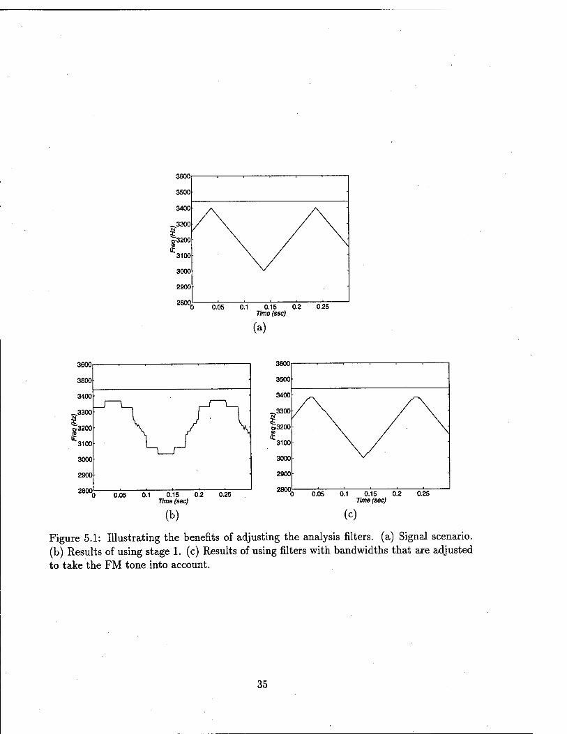
5.1 Illustrating the benefits of adjusting the analysis filters, (a) Signal scenario,

(b) Results of using stage 1. (c) Results of using filters with bandwidths

that are adjusted to take the FM tone into account 35

5.2 IPUS model. . 38

VI

5.3 Depiction of the mapping between various aspects of our MNBI isolation

approach and IPUS mechanisms 4°

5.4 Procedure for tracking the time-frequency trajectories of tones on the basis

of spectral peaks extracted from the signal 44

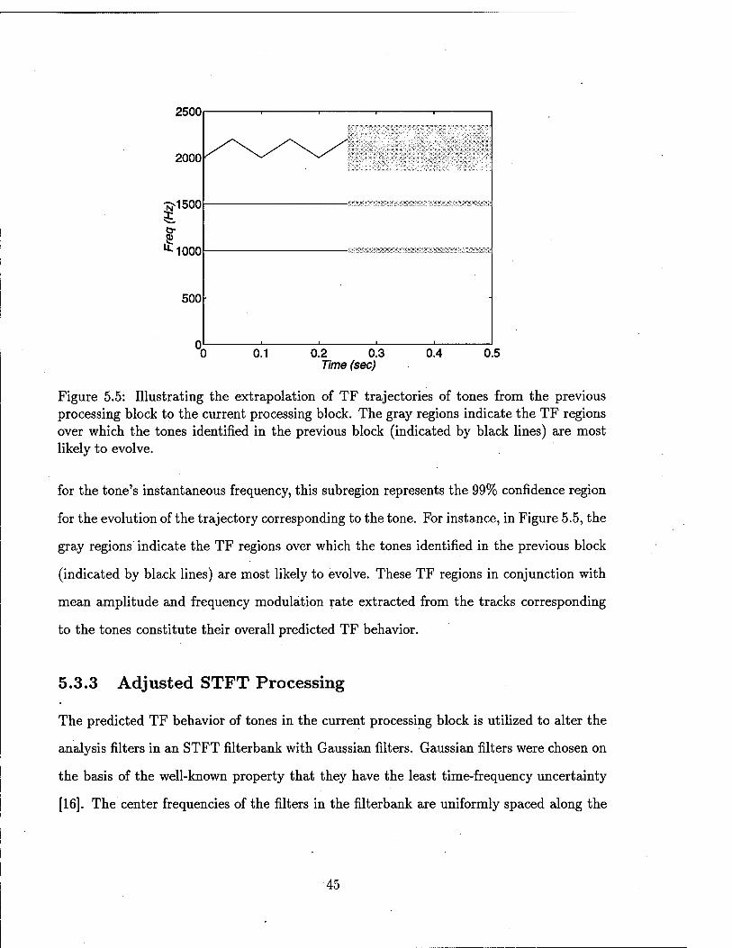
5.5 Illustrating the extrapolation of TF trajectories of tones from the previous

processing block to the current processing block. The gray regions indi-

cate the TF regions over which the tones identified in the previous block

(indicated by black lines) are most likely to evolve 45

5.6 Diagram of a portion of the goal/plan/subgoal hierarchy from our testbed. 50

6.1 Integration Circuits Located at the Transmitter . 57

6.2 Integration Circuits Located at the Receiver 58

7.1 Detailed Model of the Transmitter in SPW . . . 60

7.2 Transmitter Parameters

7.3 Spectra of the Transmitted Signal and the Input Message 61

7.4 Detailed Model of the Receiver in SPW 62

7.5 Receiver Parameters 62

7.6 Channel Model 63

7.7 Detailed LFM Jammer Model in SPW . 64

7.8 Spectra of the Transmitted Signal Plus LFM Jammer 65

7.9 Detailed SPW Model of the CW Jammer 66

7.10 Spectrum of DSSS Signal Plus a CW Jammer 67

7.11 Detailed SPW Model of ON/OFF Jammer 68

7.12 Detailed SPW Model of the PLL Interference Canceller 70

7.13 Performance of the PLL-based CW Canceller When a Good Estimate of the

CW Jamming Frequency is Used at the Second PLL Input 71

7.14 Performance of the PLL-based CW Canceller When a Poor Estimate of the

CW Jamming Frequency is Used at the Second PLL Input. . 72

vii

7.15 Detailed Excisor Model in SPW . . . 74

7.16 Insertion of a Zero at the Jamming Frequency Using an Excisor 75

7.17 System Input and Output when an Excisor is Employed 76

7.18 Interference Cancellation Engine Implementation 79

8.1 Actual Time-Frequency Distribution of the Four CW Jamming Signals in

Scenario-1 • • 81

8.2 Estimated Time-Frequency Distribution of Four CW Jamming Signals Gen-

erated by IPUS for Scenario-1 • 82

8.3 Performance Comparison for Scenario-1 82

8.4 Actual Time-Frequency Track of Two ON/OFF and Two CW Jamming

Signals in Scenario-2 83

8.5 Estimated Time-Frequency Track of Two ON/OFF and Two CW Jamming

Signals generated by IPUS for Scenario-2 8^

8.6 Performance Comparison for Scenario-2 8^

8.7 Actual and Estimated Time-Frequency Track of One LFM Jammer for Scenario-

3 85

8.8 Performance Comparison for Scenario-3 85

Vlll

Chapter 1

Introduction

Spread-spectrum signals are used widely in military and commercial communication sys-

tems due to their interference rejection capability and their lower probability of interception.

In military applications the effects of intentional interference (jamming) are mitigated by

the processing gain of the spread-spectrum system. In commercial systems code division

multiple access (CDMA) systems rely heavily on this interference rejection ability to oper-

ate satisfactorily in the presence of multiuser interference.

Interference rejection in spread spectrum systems is achieved by pseudo-randomly dis-

tributing the information to be transmitted over a range of parameters ( time, frequency

and phase). This gives rise to what is known as the processing gain of the system. In many

spread-spectrum systems, processing gain alone is not sufficient to achieve satisfactory sys-

tem performance and additional interference rejection techniques need to be employed. The

interference suppression circuit is placed prior to the spectrum despreader with the^goal of

reducing the jammer/interferer. energy to an adequately low level that can be handled by

the system processing gain.

The problem of interference rejection has been investigated quite extensively. A variety

of interference suppression techniques have been presented in the literature [1, 2, 3, 4, 5].

These techniques can be broadly categorized into two classes:

• Time-domain adaptive filter cancellation

• Transform domain excisors.

While these schemes are able to provide effective cancellation for specific types of interfer-

ence, no single scheme is able to suppress all types of interference that is encountered by

the spread-spectrum system. We present a novel knowledge-based interference cancellation

scheme for direct-sequence spread-spectrum systems. This innovative approach utilizes :

• I PUS, an expert system for the Integrated Processing and Understanding of Sig-

nals, to monitor the communication signal environment in order to determine the

parameters of interfering signals within a pre-specified accuracy, and

• Expert system rules to select from a library of preselected techniques, suitable inter-

ference rejection schemes based upon the knowledge obtained from monitoring the

signal environment.

The effectiveness of this novel interference rejection capability is demonstrated by con-

sidering a number of interference scenarios and using the software package SPW®, a

time-domain Signal Processing Worksystem.

In Chapter 2 we provide a brief tutorial on spread-spectrum signals and jammers. A

brief review of existing interference cancellation algorithms is presented in Chapter 3. The

overall framework of our knowledge-based cancellation approach is introduced in Chapter

4. Details of IPUS and how it isolates different interference signals are given in Chapter

5. Some architectural issues related to prototype development are discussed in Chapter 6.

SPW models used in our system development are given in Chapter 7. Simulation results

for three interference scenarios are presented in Chapter 8. Concluding remarks as well as

recommendations for future work are given in Chapter 9.

Chapter 2

Spread-Spectrum Communication

Systems

In all communication systems the bandwidth occupied by the modulated waveform is de-

pendent upon the modulation method used and the data that is being transmitted. In a

spread-spectrum system, the transmitted signal has a bandwidth that is much larger than

the original message waveform bandwidth. The spreading of the message bandwidth over a

wide frequency band limits the ability of an interfering signal to cause a significant distor-

tion to the transmitted information. The flat noise-like spectrum of the spread-spectrum

signal also hinders unwarranted interception of the signal. The use of a transmission band-

width which is much larger than that required by the message data rate is responsible for

the improved interference rejection capability. The following are three salient features of a

spread-spectrum communication system [1, 2]:

• The bandwidth of the spread-spectrum signal is much larger than the bandwidth of

the original information-bearing signal.

• Spreading is accomplished through the use of a spreading code that is independent

of the data itself.

• Reception is accomplished by cross correlation of the received wide-band signal with

a signal employing a synchronously generated replica of the spreading code.

Some of the popular techniques employed in spread spectrum communication systems

are [2, 3]:

• Direct sequence

• Frequency hopping

• Time hopping

• Chirp

• Hybrid methods.

In this research effort we have concentrated on interference cancellation schemes for

Direct-Sequence Spread-Spectrum (DSSS) systems.

2.1 Direct-Sequence Spread-Spectrum Systems

In direct-sequence spread-spectrum systems a pseudo-random noise (PN) code is used for

spectrum spreading. The code sequence has a much higher rate than the original digital

data rate which greatly expands the bandwidth beyond that of the original information

bandwidth. This PN code, c(i), takes values +1 and -1 and is known both to the trans-

mitter and its dedicated receiver. As a result of multiplication by the PN code c(t), the

bandwidth of the information signal d(t) is spread over a wider frequency band. The spread

signal s(t) = d(t)c(t) is transmitted after modulation and received in the presence of white

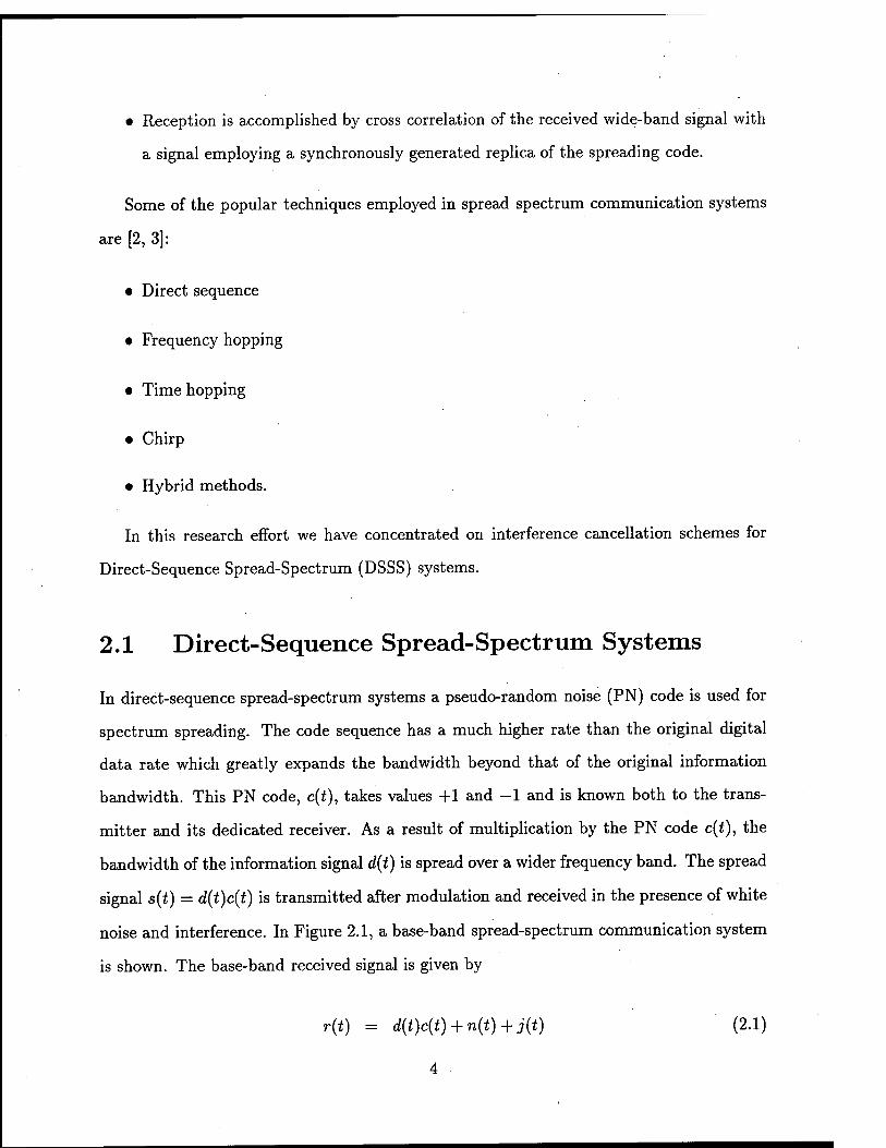
noise and interference. In Figure 2.1, a base-band spread-spectrum communication system

is shown. The base-band received signal is given by

r(t) = d(t)c(t) + n{t)+j{t) (2.1)

where n(t) and j(t) denote the equivalent base-band white noise and interference, respec-

tively. The received signal is despread at the receiver by multiplying with a locally gener-

ated replica of c(t). After multiplication by c(t), the resulting signal y(t) can be written as

follows:

y(t) = c2(t)d(t) + c(t)(n(t)+j(t))

= d(t) + c(t)n(t) + c{t)j{t). (2.2)

j(t) + n(t)

r(0 y(0 ,

c(t)

PNCode Generator

Baseband (low-pass)

filter

Output

TRANSMITTER ', CHANNEL ', RECEIVER

Figure 2.1: Base-band Spread-Spectrum System

Interference

Signal

Signal

-f

nterference

►f

Before Despreading After Despreading

Figure 2.2: Effect of Spreading and Despreading on Signal and Interference Spectra

As shown in Figure 2.2, the desired signal component of y(t) has a bandwidth that

has been reduced back to the original data bandwidth and the interference bandwidth

is increased to at least the spread bandwidth. When y(t) is passed through a low-pass

filter with bandwidth equal to that of d(t), most of the noise and interference energy

in {n(t) + j(t))c(t) is removed by filtering. This gives rise to what is referred to as the

processing gain advantage over the interference. The effective jammer power is reduced at

the output of the low-pass filter, since all jammer components outside of the data bandwidth

are rejected.

Time domain Frequency domain

DATA

1/TK

X *

PN-CODE

Ul CODED-DATA _\ 7^f

Figure 2.3: Spread Spectrum Signaling

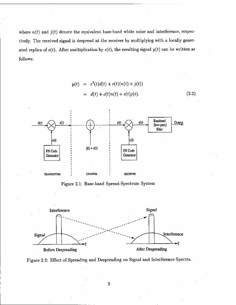
As shown in Figure 2.3, the square pulse with duration Tb represents part of the binary

information signal. Its Fourier transform is a Sine function with zero values spaced at

1/Tb. The spread-spectrum signal is formed by multiplying the information signal with a

PN sequence consisting of narrow pulses of time duration Tc. Multiplication in the time

domain is equivalent to convolution of the spectra in the frequency domain. Because the

bandwidth of the PN sequence spectrum is 1/TC, the spread-spectrum signal has a much

larger bandwidth than that of the transmitted message whenever Tc<g.Tb. The basic pulse

width in the PN sequence is Tc and is referred to as the chip duration. We define the

multiplicity factor, or the processing gain of the system as G = Tb/Tc. Pseudo-noise codes

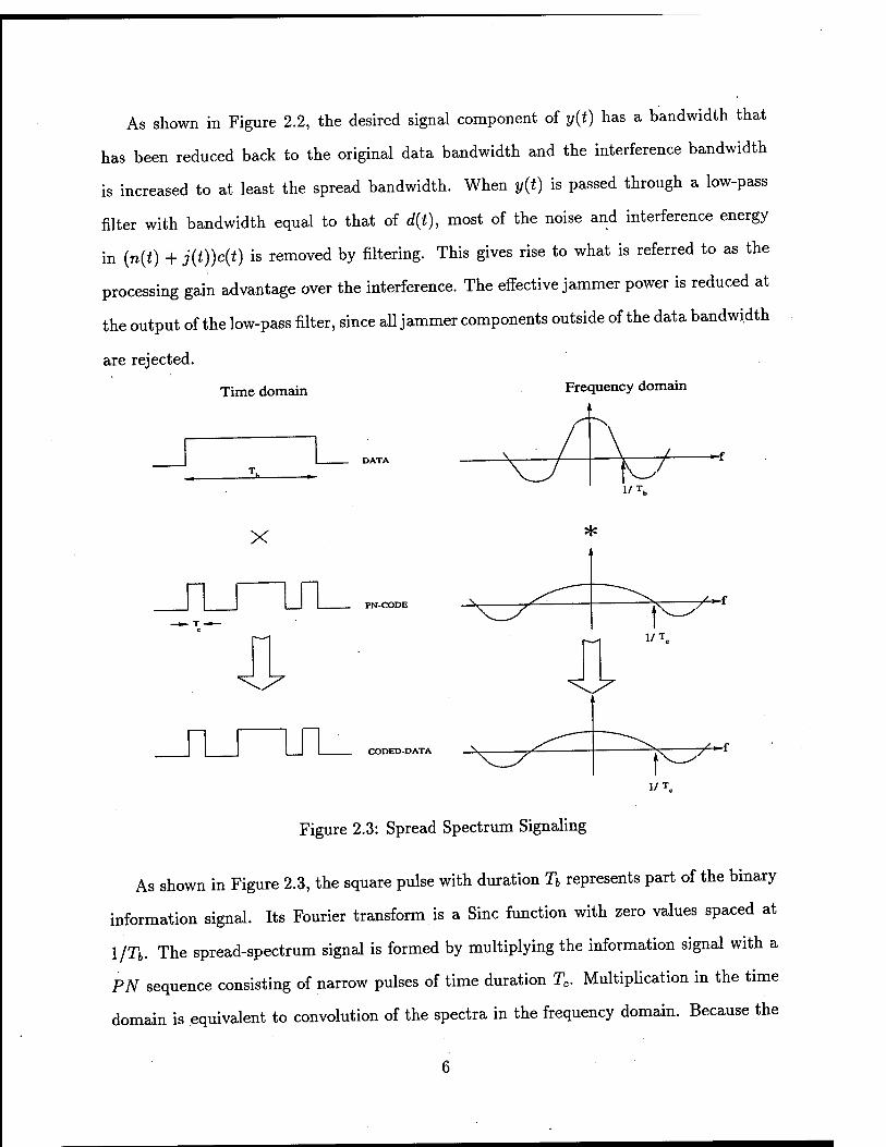
are periodic in that the produced sequence repeats itself after a certain period of time. A

maximal length linear feedback shift register PN code generator [2] is shown in Figure 2.4

where Ck equals either 0 or 1 for k=l, 2, 3, ...,n.

&■ >®—«e—•©

n-2 n-1 ►OUTPUT

Figure 2.4: Maximal Length Linear Feedback Shift Register PN Code Generator

The PN code used in a spread-spectrum system should be designed such that the PN

code is statistically independent of the message signal. In the case of a maximal length

linear feedback shift register PN code generator, the period L [2] is equal to 2"-l, where n is

the number of stages in the code generator. An important reason for using maximal length

PN sequences to modulate a message signal is the small correlation between successive

chips as demonstrated by the autocorrelation function shown in Figure 2.5. It takes the

value unity when the displacement r = 0, =p£Tc, ^2LTC,.., and is equal to -1/L [2] for all

other values of r. The period I of a PN sequence can be made large by employing a large

number of stages in the shift register. In turn, the correlation between successive chips can

be made as small as needed.

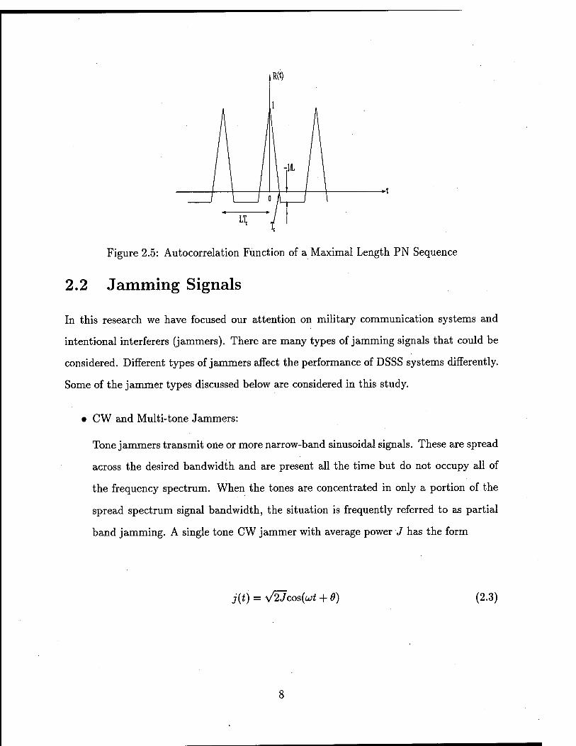
Figure 2.5: Autocorrelation Function of a Maximal Length PN Sequence

2.2 Jamming Signals

In this research we have focused our attention on military communication systems and

intentional interferers (jammers). There are many types of jamming signals that could be

considered. Different types of jammers affect the performance of DSSS systems differently.

Some of the jammer types discussed below are considered in this study.

• CW and Multi-tone Jammers:

Tone jammers transmit one or more narrow-band sinusoidal signals. These are spread

across the desired bandwidth and are present all the time but do not occupy all of

the frequency spectrum. When the tones are concentrated in only a portion of the

spread spectrum signal bandwidth, the situation is frequently referred to as partial

band jamming. A single tone CW jammer with average power J has the form

j(t) = V%Jcos(u;t + 9) (2.3)

while multi-tone jammers using Nt equal power tones can be described by

Nt IU m = T/(\hr^°<u;'t + 9') (2-4) 1=1 V Mt

where all phases are assumed to be independent and uniformly distributed over [0,2n]

and J denotes the average power of j(t). The performance of direct-sequence spread-

spectrum systems in the presence of a single-tone or multi-tone CW jammer is rela-

tively easy to obtain. For example, the average probability of error for the multi-tone

CW jammer case using BPSK is approximately given by [1, 3];

f- = W*.+stw-.> (2'5)

where Eb is the bit energy, N0 is the white noise power spectral density, Tc is the

chip duration, m is the number of jammer tones, Jn is the average power of the nth

jamming signal and erfc is the complement error function and given by

2 fx

erfc(x) — —=. / exp(—z2)dz. y/TTJO

• Pulse (ON/OFF) Jammer :

A pulse jammer with average power J refers to a jammer which transmits a peak

power given by

T J / x Jpeak = — (2.6) P

for a fraction of time, p, and nothing for the remaining fraction of the time, 1 - p.

The received signal can be viewed as consisting of jammer plus thermal noise with

probability, p, and thermal noise alone with probability, I — p.

A direct-sequence spread-spectrum system that does not employ error-correction cod-

ing may be quite vulnerable to pulses that are longer than a message bit. The pulse

jammer transmits short, high-intensity pulses, at either a regular or an irregular rate.

A large duration pulse will completely destroy the message information contained in

a given bit and, if these pulses occur with sufficient frequency, the resulting bit-error

rate will be greater than an acceptable level. The net result of strong enough pulse

jamming is that the probability of error increases and errors tend to cluster together.

The jamming pulses are usually several message bits in length. The probability of

error due to strong enough pulse jamming is given by

„ 1 e 2^ (2.7)

where p is the pulse duty factor. A duty cycle of 50% is frequently used, because it

represents a suitable compromise between peak power, average power, and probability

of error from the jammer's point of view.

• Narrow-band Interference:

Interference signals whose spectral bandwidth is much smaller than the spectral band-

width of the transmitted spread spectrum signal are classified as narrow-band inter-

ference signals.

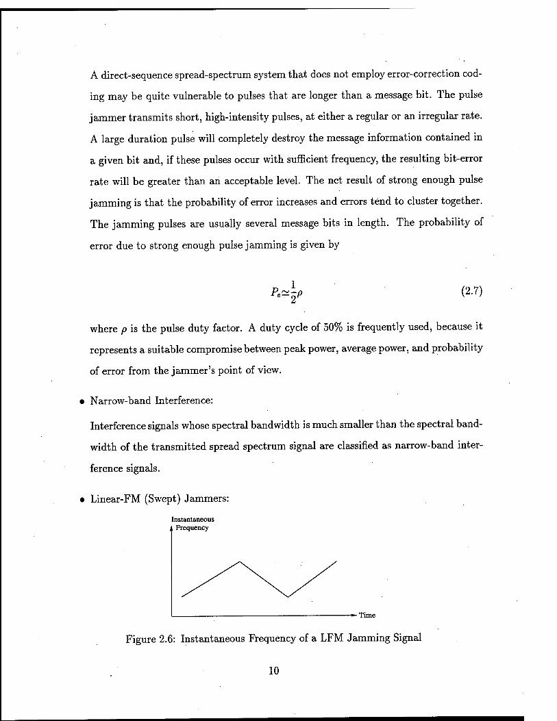
• Linear-FM (Swept) Jammers:

Instantaneous Frequency

-Time

Figure 2.6: Instantaneous Frequency of a LFM Jamming Signal

10

This type of jammer is very effective in disturbing a direct-sequence spread-spectrum

receiver. The instantaneous frequency of the jamming signal varies in a linear fashion

with time. Depending on the rate of frequency change, these jammers could be

classified further as fast linear-FM or slow linear-FM jammers. The range over which

the jammer frequency is swept may include the entire spread-spectrum bandwidth or

only a portion of this range. The instantaneous frequency is time variant (as shown

in Figure 2.6) and the jamming signal with average power J may be expressed as

j(t) = -s/2Jcos( / U(T)<IT + 9). (2.8) •/o

where u>(t) denotes the instantaneous frequency of the jammer.

• Broad-band Noise Jammer:

A broadband noise jammer spreads noise of average power J evenly over the total

frequency range of the spread bandwidth, wss. This results in the equivalent single-

sided noise power spectral density given by

Nj = -L. (2.9)

The broadband noise jammer is a brute force jammer that does not exploit any

knowledge of the characteristics of the communication system except its transmission

bandwidth, uss. The resulting bit error probability is the same as that with additive

white Gaussian noise of one-sided power spectral density equal to Nj.

Figure 2.7 illustrates different types of jammers. In the next chapter we discuss some

of the existing interference cancellation techniques for DSSS systems.

11

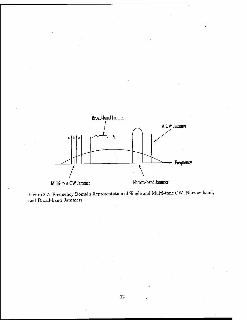
Broad-band Jammer

A CW Jammer

Frequency

Multi-tone CW Jammer Narrow-band Jammer

Figure 2.7: Frequency Domain Representation of Single and Multi-tone CW, Narrow-band, and Broad-band Jammers.

12

Chapter 3

Interference Rejection in

Spread-Spectrum Systems

In a spread-spectrum communication system the effect of interference on system perfor-

mance is reduced because of the inherent processing gain of the spread-spectrum system.

To be able to achieve an even greater resistance to interference, the system processing gain

( or spread-spectrum signal bandwidth ) must be increased. In many practical applications

this may not be possible due to bandwidth restrictions. Therefore, in many situations, espe-

cially in the presence of jammers, additional interference cancellation techniques need to be

employed in order to attain satisfactory communication system performance. This problem

has been investigated quite extensively. A variety of interference suppression techniques

have been presented in the literature [4, 5]. These techniques can be broadly categorized

into two classes:

• Time-domain adaptive filter cancellation

• Transform domain excisors.

The interference suppression circuit is placed prior to the spectrum despreader with

the goal of reducing the jammer/interferer energy to an adequately low level that can

13

be handled by the system processing gain. These techniques introduce minor distortions

in the received spread-spectrum signal. However, the performance improvement obtained

by attenuating the interfering signals far outweighs such minor distortions caused by the

canceller.

Interference rejection schemes for spread-spectrum systems often need to be adaptive

because of the dynamic or changing nature of the interference and the channel. The design

of optimum cancellation schemes requires a priori information about the statistical char-

acteristics of the interference. We also need knowledge regarding the 'ON' times of the

interference during which it is affecting communication performance. Perfect interference

cancellation could be accomplished with the availability of accurate time-frequency charac-

teristics of the interference. Adaptive cancellation techniques are used since such complete

and accurate knowledge is generally not available. An adaptive technique is self-adjusting

in nature and relies on a recursive algorithm to converge to a cancellation process that is

optimum in some statistical sense. In the following sections, we discuss some of the existing

interference cancellation techniques for DSSS systems.

3.1 Adaptive Transversal Filtering

There are many ways to implement adaptive filters to achieve narrow-band interference

suppression. The most popular one is to use an estimator/subtracter method. The basic

operation of this type of implementation involves subtracting an estimate of the interference

from the received signal. This results in the received signal being whitened. An important

problem faced in this approach is formation of the estimate. This is accomplished by em-

ploying the predictability of the interference. The spread-spectrum signal has an almost

fiat spectrum. Therefore, the spread-spectrum signal is unpredictable without the knowl-

edge of the pseudo-random sequence used in spreading the spectrum. Since the interferer

is narrow-band, a large portion of its energy is concentrated within a small bandwidth.

Therefore, successive samples of the narrow-band interferer are strongly correlated and can

14

be closely predicted. Effective interference cancellation is then achieved by predicting the

interference from the received signal and subtracting the predicted value from the received

data samples. A transversal filter is often used as a predictor of the narrow-band inter-

ference signals. This adaptive transversal filter could have either a one-sided or two-sided

filter structure as shown Figure 3.1, where Tc is the sampling interval which equals the chip

duration.

If narrow band interference is present in the received signal, the weights of the transver-

sal filter should be updated in order to predict the narrow-band interference in such a way

that the resulting mean-squared error is minimized. Minimization can be done by using

an algorithm such as the least-mean-squared (LMS) estimation algorithm which can be

expressed as follows [4, 5]:

• 1) The filter output: yk = wj^Xk

• 2) the error : ek = dk - yk

• 3) The tap weight adaptation: Wk+i = Wk + ßXkt*k

where k denotes the discrete time index, yk is the scalar output of the transversal filter, w^

is the tap-weight vector, x_k is the tap-input vector, H indicates Hermitian transposition,

Ck is the estimation error, dk is the desired response, \i is the step-size parameter and the

asterisk denotes conjugation. In practice, several different design criteria are used to set

the tap weights for the filter, as we discuss below.

Criterion 1 corresponds to whitening the received signal. It is based on predicting the

narrow band interference and subtracting the estimate from the received signal. Since the

transmitted spread spectrum signal and the white noise are wide-band processes, there is

little correlation between their sample values. For this reason, it is impossible to predict

future values of white noise and the transmitted spread-spectrum signal. However, there

is always correlation between sample values of any narrow-band process. Hence, it is pos-

sible to predict with acceptable errors future values of the narrow-band interference from

15

Lk+N Lk+1 Lk-1 "■k-N

±*S ' ' ' ^0 ^... ^

"* X

(a)

* x (b)

Figure 3.1: (a): Two-sided Transversal Filter (b): Single-Sided Transversal Filter

16

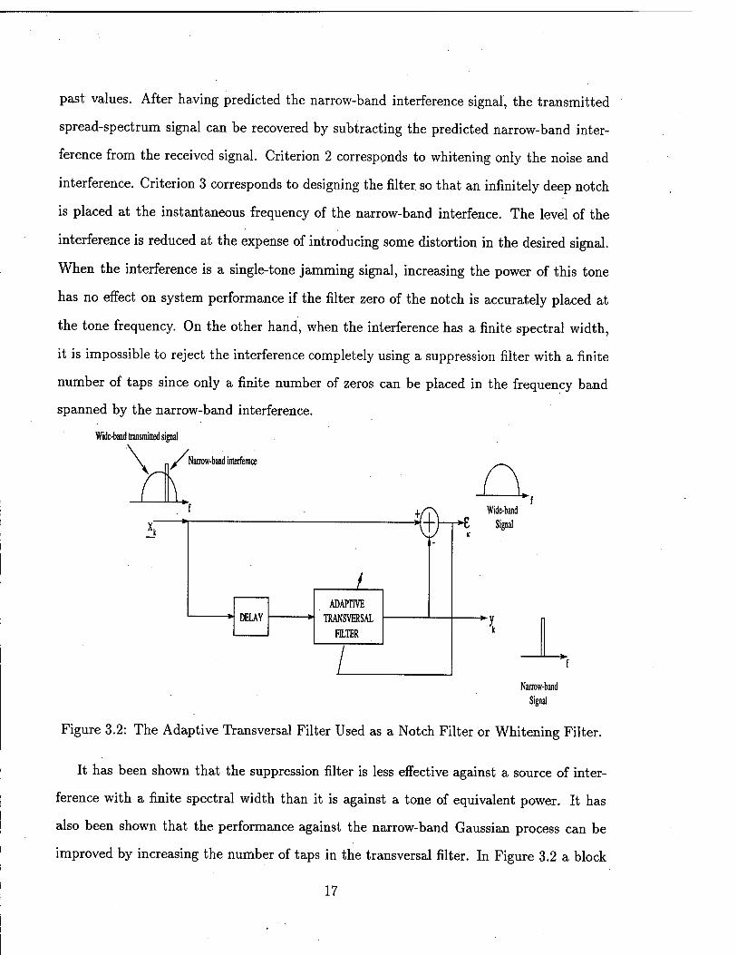
past values. After having predicted the narrow-band interference signal, the transmitted

spread-spectrum signal can be recovered by subtracting the predicted narrow-band inter-

ference from the received signal. Criterion 2 corresponds to whitening only the noise and

interference. Criterion 3 corresponds to designing the filter, so that an infinitely deep notch

is placed at the instantaneous frequency of the narrow-band interfence. The level of the

interference is reduced at the expense of introducing some distortion in the desired signal.

When the interference is a single-tone jamming signal, increasing the power of this tone

has no effect on system performance if the filter zero of the notch is accurately placed at

the tone frequency. On the other hand, when the interference has a finite spectral width,

it is impossible to reject the interference completely using a suppression filter with a finite

number of taps since only a finite number of zeros can be placed in the frequency band

spanned by the narrow-band interference.

Wide-band transmitted signal

\ -S Narrow-band interfemce

f if ̂ 1

h '

/

\ ) ■

K

DELAY ADAPTIVE

TRANSVERSAL FILTER

/

Wide-band Signal

*f

Narrow-band

Figure 3.2: The Adaptive Transversal Filter Used as a Notch Filter or Whitening Filter.

It has been shown that the suppression filter is less effective against a source of inter-

ference with a finite spectral width than it is against a tone of equivalent power. It has

also been shown that the performance against the narrow-band Gaussian process can be

improved by increasing the number of taps in the transversal filter. In Figure 3.2 a block

17

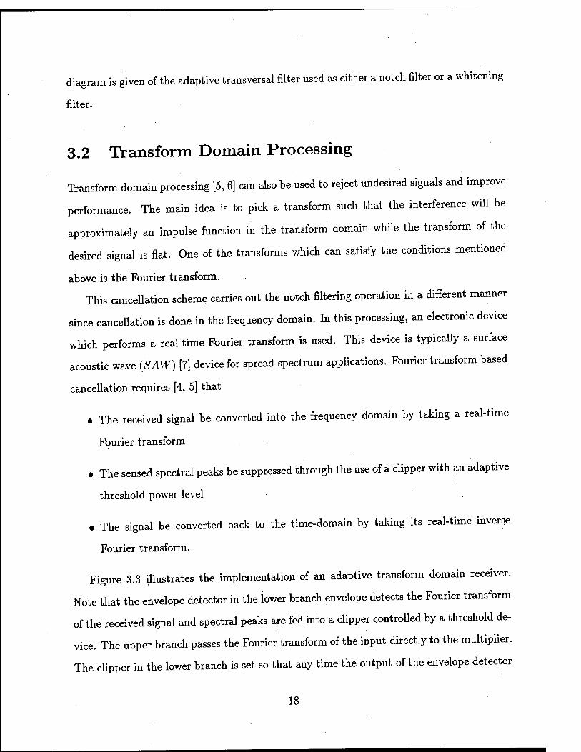
diagram is given of the adaptive transversal filter used as either a notch filter or a whitening

filter.

3.2 Transform Domain Processing

Transform domain processing [5, 6] can also be used to reject undesired signals and improve

performance. The main idea is to pick a transform such that the interference will be

approximately an impulse function in the transform domain while the transform of the

desired signal is flat. One of the transforms which can satisfy the conditions mentioned

above is the Fourier transform.

This cancellation scheme carries out the notch filtering operation in a different manner

since cancellation is done in the frequency domain. In this processing, an electronic device

which performs a real-time Fourier transform is used. This device is typically a surface

acoustic wave (SAW) [7] device for spread-spectrum applications. Fourier transform based

cancellation requires [4, 5] that

• The received signal be converted into the frequency domain by taking a real-time

Fourier transform

• The sensed spectral peaks be suppressed through the use of a clipper with an adaptive

threshold power level

• The signal be converted back to the time-domain by taking its real-time inverse

Fourier transform.

Figure 3.3 illustrates the implementation of an adaptive transform domain receiver.

Note that the envelope detector in the lower branch envelope detects the Fourier transform

of the received signal and spectral peaks are fed into a clipper controlled by a threshold de-

vice. The upper branch passes the Fourier transform of the input directly to the multiplier.

The clipper in the lower branch is set so that any time the output of the envelope detector

18

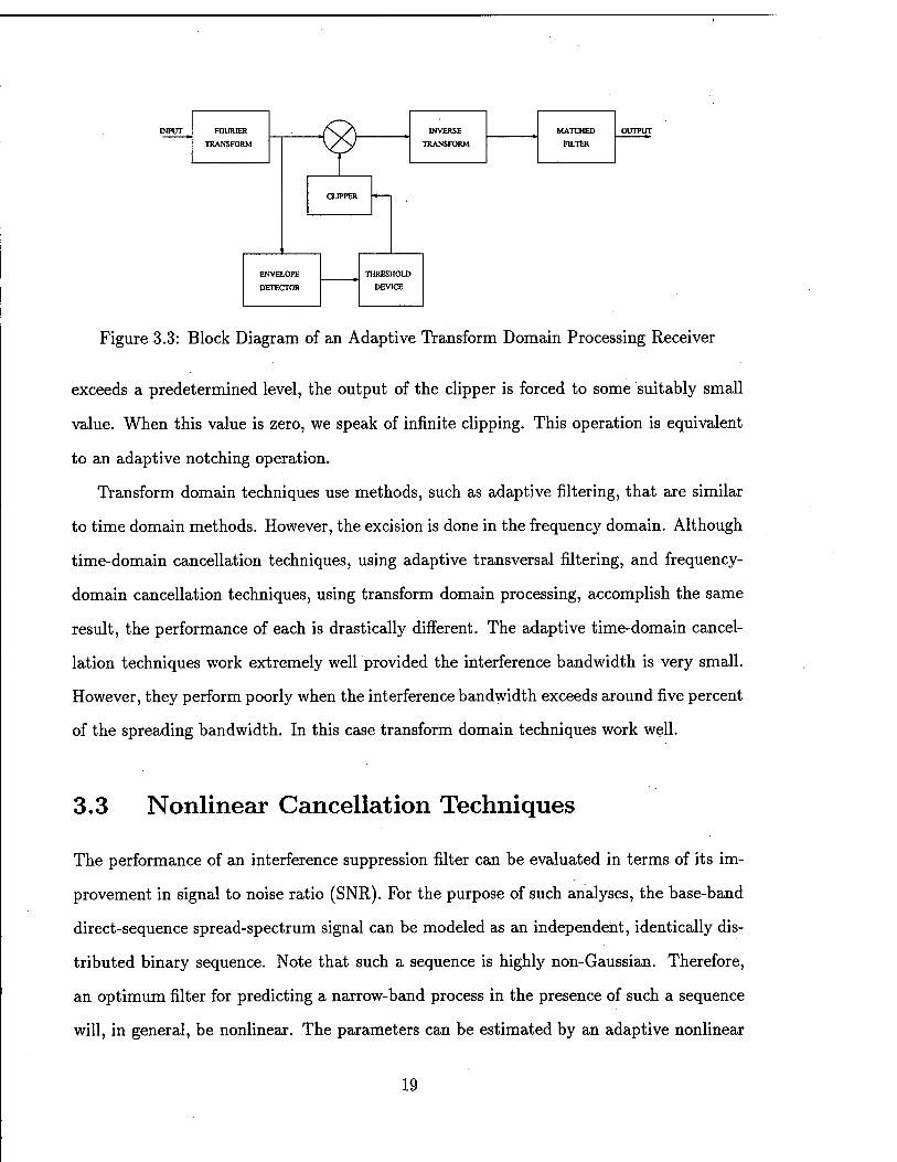
Figure 3.3: Block Diagram of an Adaptive Transform Domain Processing Receiver

exceeds a predetermined level, the output of the clipper is forced to some suitably small

value. When this value is zero, we speak of infinite clipping. This operation is equivalent

to an adaptive notching operation.

Transform domain techniques use methods, such as adaptive filtering, that are similar

to time domain methods. However, the excision is done in the frequency domain. Although

time-domain cancellation techniques, using adaptive transversal filtering, and frequency-

domain cancellation techniques, using transform domain processing, accomplish the same

result, the performance of each is drastically different. The adaptive time-domain cancel-

lation techniques work extremely well provided the interference bandwidth is very small.

However, they perform poorly when the interference bandwidth exceeds around five percent

of the spreading bandwidth. In this case transform domain techniques work well.

3.3 Nonlinear Cancellation Techniques

The performance of an interference suppression filter can be evaluated in terms of its im-

provement in signal to noise ratio (SNR). For the purpose of such analyses, the base-band

direct-sequence spread-spectrum signal can be modeled as an independent, identically dis-

tributed binary sequence. Note that such a sequence is highly non-Gaussian. Therefore,

an optimum filter for predicting a narrow-band process in the presence of such a sequence

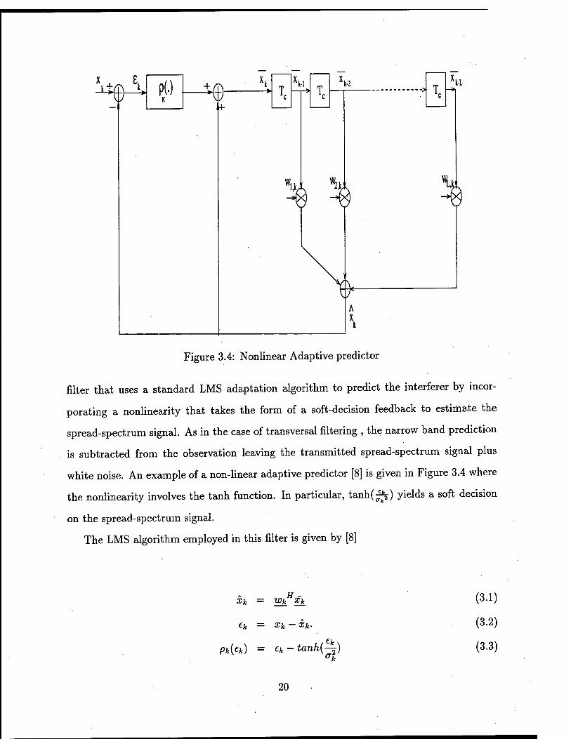
will, in general, be nonlinear. The parameters can be estimated by an adaptive nonlinear

19

x + E, ^0

—,. *®

vk-l \-l Vk-L

\

Figure 3.4: Nonlinear Adaptive predictor

filter that uses a standard LMS adaptation algorithm to predict the interferer by incor-

porating a nonlinearity that takes the form of a soft-decision feedback to estimate the

spread-spectrum signal. As in the case of transversal filtering , the narrow band prediction

is subtracted from the observation leaving the transmitted spread-spectrum signal plus

white noise. An example of a non-linear adaptive predictor [8] is given in Figure 3.4 where

the nonlinearity involves the tanh function. In particular, tanh(^) yields a soft decision

on the spread-spectrum signal.

The LMS algorithm employed in this filter is given by [8]

Xk

Pk(tk)

wkHxk

= Xk — Xk.

tk - tanh(-)

(3.1)

(3.2)

(3.3)

20

xk - xk-tanh(—-)

= xk + Pk(ek). (3.4)

where xk is the input signal, pk(ek) is an estimate of the noise, xk is an estimate of the

interference signal, xk is the observation less the soft decision on the spread-spectrum signal,

ek represents the observation less the interference estimate, Tc is the delay equal to the chip

duration, and L is the number of taps used in the transversal filter.

It has been shown that linear prediction techniques are suboptimal for prediction of a

narrow-band interferer in the presence of non-Gaussian noise. Non-linear techniques have

been shown to yield better performance.

3.4 CW Jammer Cancellation Using Phase-Locked-

loop (PLL)

In this section we assume that the interference corrupting the transmitted spread-spectrum

signal consists only of a CW jammer. In such a situation a PLL-based approach can be

utilized to perform interference cancellation. Some theoretical background for the use of

a PLL-based interference cancellation approach is given. For a spread-spectrum system

operating in a CW interference environment, the received signal can be written as

ri(t) = S„{t) + AiOOB{u>ii + 0i) (3.5)

where Sss(t) is the received spread-spectrum signal with average power SR and bandwidth A2

u>ss and AiCos((jJit + 0.) is the received CW interference with average power IR= -f.

21

CW JAMMER

+m r*(t). SPREAD SPECTRUM RECEIVER TRANSMITTER —<])

•6

FFT

COS(K),t+e,)

/ XjCosCtDit+Sj)

PHASE LOCKED LOOP

/ p

3((t)

\

TIMES2

AMPLIFIER

1 LOW-PASS

FILTER —yy—

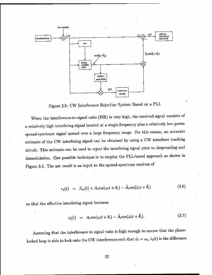
Figure 3.5: CW Interference Rejection System Based on a PLL

When the interference-to-signal ratio (ISR) is very high, the received signal consists of

a relatively high interfering signal located at a single frequency plus a relatively low power

spread-spectrum signal spread over a large frequency range. For this reason, an accurate

estimate of the CW interfering signal can be obtained by using a CW interferer tracking

circuit. This estimate can be used to reject the interfering signal prior to despreading and

demodulation. One possible technique is to employ the PLL-based approach as shown in

Figure 3.5. The net result is an input to the spread-spectrum receiver of

r2(t) = Sss(t) + AiCos{u>it + 0i) - ÄiCos{u)it + 0,-) (3.6)

so that the effective interfering signal becomes

i2(t) = Aicosfat + Oi) - ÄiCos(u>it + 0i). (3.7)

Assuming that the interference to signal ratio is high enough to ensure that the phase-

locked loop is able to lock onto the CW interference such that c5t- = uu «'2CO is the difference

22

of two sinusoids of the same frequency which can be combined by the trigonometric identity

Acos(ut + a) + Bcos(u>t + ß) = Ccos(ut + 7) (3.8)

where

C = ^A2 + B2 + 2ABcos(a-ß). (3.9)

Therefore,

»2(0 = y/A2 + Ä2-2AiÄicos{ei - 0,-) cos(wrf + 7). (3.10)

The effectiveness of this interference rejection scheme is measured by the amplitude of

i2(t) which is given by

Air = \fA2 + Ä2-2AiÄicos(9i- §i). (3.11)

Observe that the average power of ^(i) is

h = 4^- (3.12)

The amplitude estimate, A,-, is generated at the output of the low pass filter (LPF) with

input yi(t) where

yi(i) = rMpcoBfat + Oi)]. (3.13)

23

Substituting for n(t) from (3.5), (3.13) becomes

yi (t) = 2Sss{t)cos{uit + ei) + AicoS(<f>e) + Aicos{2uit + 6i + 6i) (3.14)

where <f>e = .0t- - 0,-. The response of the LPF to yi(t) provides the amplitude estimate of

the CW interference and is

Äi = AiCoS(<l>e) + Ea(t) (3-15)

where Ea(t) is the LPF response to [2S„(t)cos(uit + *)]. With <j>e small, a good estimate

of Ai can be obtained. Ea(t) represents the noise in the amplitude estimate. The mean-

squared value of Ea(t) is given by

EW) = 2ß0(^) I3"16)

where Ba is the bandwidth of the LPF. Substituting (3.11) into (3.15) and assuming that

4>e « 1, Air is given by

Air = sJAUl + El (3-17)

The interfering signal power at the spread-spectrum receiver input is thus

Al I2 = *c (3-18) 2

= ^ + § (3-19) 2 Ve 2

24

rp2

= IR^ + Y- (3-20)

For the case of interest here the PLL input is composed of At- cos(u>;t + 0,-) plus the

wide-band spread-spectrum signal of average power SR and bandwidth uss which, to the

narrow-band PLL, looks like white noise of spectral density SR/USS. Therefore, the phase

error variance is given by

al 2SRB<j> (321)

A]u)ss

= ^^ (3.22) Uss IR

where Bj, is the bandwidth of the PLL. If the phase estimate is unbiased, <j>e can be

approximated by a\t. Thus,

4>e\ = *J. (3-23)

(3.24) Bf SR

wss IR

By using (3.24), (3.15), and (3.16) the interference-to-signal ratio, ISR, at the spread-

spectrum receiver input can be expressed as

OR WSS

We conclude that when there is a single-tone jammer with a large average power which

is contaminating the transmitted spread-spectrum signal, the PLL can achieve phase-lock

and can generate an accurate estimate of the CW interferes After cancellation, the resid-

ual interference due to incomplete interference rejection can readily be handled by the

25

processing gain (PG) provided by the spread-spectrum system.

3.5 Limitations of Existing Interference Cancellation

Techniques

Interference cancellation schemes using adaptive transversal filters suffer from the drawback

that they do not perform very well in the presence of multiple narrow-band interference sig-

nals and in situations where the instantaneous frequency of the interference varies rapidly

over a large frequency range. Although these drawbacks may be partially overcome by

increasing the order of the filter employed, this imposes additional problems in the form

of filter transient times and receiver design complexity. Alternative approaches to narrow-

band interference rejection involving time-frequency analysis performed using filter-banks

have been proposed to handle scenarios with narrow-band interference with significant

frequency modulation rates. While these solutions are suitable for suppressing a few in-

terfere» with slowly varying frequency modulations, they generally fail when applied to

signals with several interfere» with rapidly varying modulations. The primary cause for

failure is the fixed tradeoff between time and frequency resolution at any given point in

the time-frequency plane. When the interference has a finite spectral width, it cannot be

completely rejected by suppression filters with a finite number of taps, since only a finite

number of zeros can be placed in the frequency band spanned by the interference.

In transfer domain processing the primary consideration in the overall system design is

the shape of the window used to view the received waveform. In the Fast Fourier transform

(FFT) operation, rectangular windows are the ones most widely used. But it is also known

that rectangular windows create very large side-lobes that severely degrade the interference

cancellation performance [6]. Although these side-lobes can be reduced by proper weighting

functions [6], they distort the input signal itself.

Nonlinear cancellation techniques have the same drawbacks as adaptive cancellation

26

techniques. In addition to this, it usually involves a very complex design. The main

idea in nonlinear cancellation techniques is to optimize the detection process dynamically,

in the presence of interference, by estimating the non-Gaussian statistics and using this

information to derive a nonlinear transformation to apply to the corrupted signal. That is

the reason why these cancellation schemes are quite complex.

In the next chapter we introduce our novel knowledge-based interference cancellation

framework that is quite robust and is able to remove different types of interference signals.

27

Chapter 4

Knowledge-Based Interference

Rejection Framework

As indicated in the previous chapter, a great deal of effort has gone into the development of

interference cancellation schemes for spread-spectrum systems. These schemes are able to

handle specific classes of interference. There is no single interference cancellation scheme

that is able to effectively suppress all types of interference. Accurate knowledge of the time-

frequency characteristics of the interference embedded in the received spread-spectrum

signal is required in order to apply suitable cancellation techniques. In this chapter we

introduce our innovative knowledge-based approach for interference cancellation in spread-

spectrum systems. This approach utilizes

• I PUS, an expert system for the Integrated Processing and Understanding of Signals,

to monitor the signal environment in order to correctly determine the interfering sig-

nals within a pre-specified accuracy

and

28

• Expert system rules to select from a library of preselected techniques suitable in-

terference rejection schemes based upon knowledge obtained from monitoring the

environment.

The approach has been found to be quite effective. Its effectiveness is demonstrated by

computer-aided modeling and simulation using the software package SPW later in this

report.

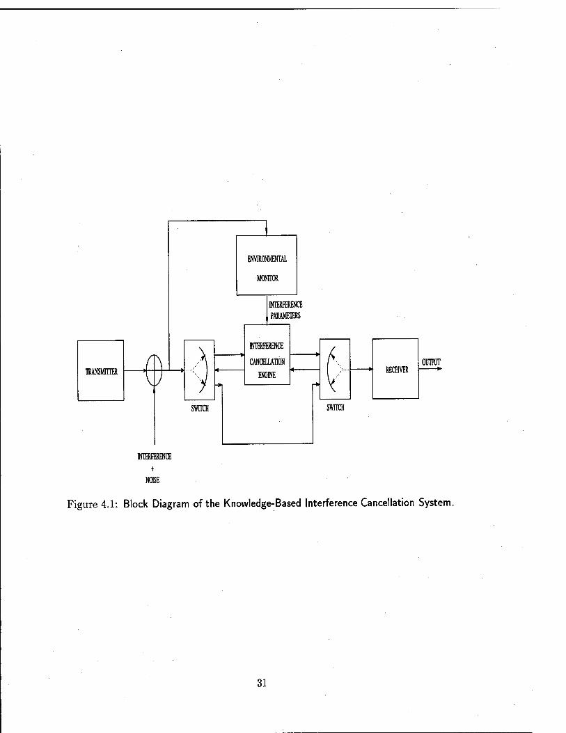
The overall knowledge-based framework for interference rejection is shown in Figure

4.1. The transmitted spread-spectrum signal is assumed to be corrupted by additive ther-

mal noise and a number of interference signals prior to its reception at the receiver. The

received signal is processed by the expert system called IPUS which carries out the en-

vironmental monitoring function. It determines the types of interference signals (from a

specified list of interference types) present in the received signal along with their parame-

ters. If an interference type is not on the specified list, IPUS can be extended to include

new interference types. Details on the version of IPUS included in our prototype will be

provided in Chapter 5. Based on the information generated by IPUS ( time-frequency

locations of the isolated interferers ), the most appropriate interference cancellation filters

from a library of available filters is employed to eliminate interference from the received

signal. This selection is based on a set of rules that have been developed and described in

Chapter 7. Additional rules can always be added when needed. Two switches are included

to allow for either selection of an appropriate interference cancellation filter from the filter

bank or for bypassing the interference cancellation stage when IPUS determines that no

interference is present. Finally, the spread-spectrum receiver demodulates its input and

recovers the transmitted information.

The problem of interference cancellation in spread-spectrum systems may be formally

described by considering received signals of the form:

r(t) = s(t) + JTjk(t). (4.1)

29

where s(t) is the information-bearing spread spectrum signal and jk(t), k-1,2,..., are dif-

ferent types of jamming signals that may be simultaneously present on the channel. They

have the form jk(t) = akcos[ß uk(r)dr + <f>k]. Our objective is to sufficiently attenuate all

the interferes jk(t) such that the original spread-spectrum signal s(t) can be successfully

demodulated due to the inherent processing gain of the system. In the prototype that we

have developed to demonstrate the proof of concept for our knowledge-based approach, we

have restricted the types of interferers to be:

(1) Multiple tone interferers operating in a continuous wave (CW) mode,

(2) Linear-FM ( or chirp) interfering signals,

(3) Multiple CW tones operating in an ON/OFF mode with or without frequency

hopping.

Different interference cancellation schemes are required to mitigate these different types

of interferers. Also, for linear FM interferers, changes in the parameters of the cancellation

filter are required as a function of time. For situations where one or more of these types of

interferers are present, the IPUS-bzsed interference cancellation approach is expected to

show improved performance over that achieved with a single fixed interference canceller.

For example, the instantaneous frequency information of linear FM interference available

from I PUS will suggest the use of a moving notch filter for interference cancellation.

Details on different aspects of our methodology are provided in the rest of the chapters.

Chapter 5 describes the approach used in IPUS. In Chapter 6 we briefly describe the

computer-aided design and simulation tool SPW. Integration of IPUS and SPW is also

discussed. Chapter 7 contains a description of communication system models used for

simulation purposes. We also present some experimental work leading to the set of rules

for interference cancellation filter selection. Several simulation examples to demonstrate

the superior performance of our knowledge-based approach are presented in Chapter 8.

Conclusions and recommendations for future work are provided in Chapter 9.

30

TRANSMITTER

SWITCH

INTERFERENCE +

NOISE

ENVIRONMENTAL

MONITOR

INTERFERENCE PARAMETERS

INTERFERENCE

CANCELLATION

ENGINE

Figure 4.1: Block Diagram of the Knowledge-Based Interference Cancellation System.

31

Chapter 5

IPUS-Based Interference Isolation

In this chapter we provide a detailed treatment of our approach to isolating each modulated

narrow-band interference (MNBI) tone from a contaminated spread-spectrum signal. In

particular, we describe how we can efficiently search for a time-frequency (TF) representa-

tion of the signal that separately resolves the spectral contributions from each MNBI tone.

Furthermore, we discuss the appropriateness of the I PUS framework [9] as the supporting

system architecture for this type of search process. We also provide details on how we have

incorporated our TF analysis approach into an I PUS framework. Finally, we describe a

software system we have implemented and used to experimentally validate this approach

to interference isolation.

5.1 Elaboration of Approach to Interference Isolation

Let us now consider the details of our approach for isolating MNBI tones from a contam-

inated spread spectrum signal. The process of such isolation may be alternatively viewed

as the resolution of each MNBI tone from its nearest neighbor in a TF representation of

the signal. Our overall strategy for accomplishing our isolation objective may be viewed as

consisting of two main stages. In the first stage, we compute a TF representation using the

32

short-time Fourier transform (STFT) [10] in order to identify TF trajectories1 that corre-

spond to MNBI tones. The analysis filters of the STFT have sufficiently small bandwidths

to ensure isolation of components that are as close as 16 Hz. For MNBI tones with signifi-

cant frequency modulation (FM) such TF analysis leads to TF trajectories that are smooth

versions of the original TF trajectories. During the second stage the TF trajectory of each

MNBI tone with FM is refined by re-processing the signal using an adjusted filterbank.

The filters in this filterbank are modified in a manner such that they optimize the time

resolution of MNBI tones with FM while resolving them separately from their neighbors.

5.1.1 Delineating Isolated MNBI Tones

In the first stage we find time-frequency-amplitude trajectories for all MNBI tones present

in the signal. To find such trajectories, we process the signal using an STFT filterbank

whose analysis filters have impulse responses of the form

hc(t) = h0(t)e>u°* (5.1)

where u>c is the center frequency of the filter and h0(t) is a Gaussian waveform that controls

the bandwidth of the filter. The bandwidth of each filter is assumed to be less than 32

Hz because we expect MNBI tones to be no closer than 16 Hz. The output of the STFT

filterbank separately resolves each MNBI tone from its nearest neighbor. Spectral peak

picking and tracking algorithms determine the time-frequency-amplitude trajectories of

MNBI tones from the output of the STFT.

1For the purpose of this discussion, we assume the availability of algorithms that can detect and track peaks in the TF representation in order to form time-frequency-amplitude trajectories for the various tones present in the signal.

33

5.1.2 Adjusted Filterbank Analysis of MNBI Tones with FM

During the second stage we refine the TF trajectories of MNBI tones with FM. The nar-

row bandwidth filters utilized in the first stage provide inaccurate estimates for the TF

trajectories of such tones. The process of refining these trajectories involves adjusting the

analysis filters in the vicinity of each FM tone to have optimal time resolution and sufficient

frequency resolution to separate the tone from its nearest neighbor.

To carry out such filtering in the vicinity of MNBI tones with FM we adopt an iterative

procedure for adjusting the filters. For a candidate MNBI tone we first determine the

frequency separation A/(t) from its nearest neighbor using the TF trajectories obtained

in the first stage. Furthermore, we also use the time-amplitude trajectories of the MNBI

tones found in the first stage to determine the relative amplitude ar(t) of the candidate

tone with respect to its nearest neighbor. The time-varying functions Af(t) and ar(t) are

utilized to determine the bandwidth of the analysis filters centered around the candidate

tone for each time. This bandwidth is such that it allows only 2% of the candidate tone's

energy to be contributed by the nearest neighbor. To obtain the filters with the desired

bandwidth, the variance of the Gaussian h0(t) for the corresponding filter should be chosen

to be I—— 2.14^(0 (5 2)

'W " 2irA/(t) ' ^

These adjusted analysis filters are applied to the signal and a refined time-frequency-

amplitude trajectory of the FM tone is formed. If the average percentage change between

the previous TF trajectory and the refined TF trajectory is less than 5%, we assume

that the filters have succeeded in refining the trajectory of the candidate tone. For larger

changes, we repeat the process described above but with the refined estimate for the time-

amplitude and time-frequency trajectories. At the end of the iterative process, an accurate

TF trajectory of the candidate tone is obtained.

We illustrate the benefits of adjusting the analysis filters through an example. The

signal scenario depicted in Figure 5.1(a) consists of two closely spaced tones: one with no

34

0.1 0.15 0.2 Time (sec)

(a)

3600

3500

3400

_3300

1 O-3200

3100

3000

2900

2800 0.05 0.1 0.15 0.2

Time (sec) 0.25

3600 ._._... , .,, ., 1 1 1

■

3500 ■

3400

_3300

&3200

1 3100

\-

3000 • ■

2900

2800

•

) 0.05 0.1 0.15 0.2 Time (sec)

0.25

0>) (c)

Figure 5.1: Illustrating the benefits of adjusting the analysis filters, (a) Signal scenario, (b) Results of using stage 1. (c) Results of using filters with bandwidths that are adjusted to take the FM tone into account.

35

modulation and having a frequency of 3440 Hz and the other with FM and centered around

3200 Hz. The TF trajectories from the first stage of processing are shown in Figure 5.1(b).

We see that the trajectory of the FM tone is inaccurate. We now use the results of Figure

5.1(b) to estimate the frequency separation and relative amplitude of the two tones. Based

upon these estimates, we obtain a modified set of analysis filters and re-process the signal.

The results of this processing are shown in Figure 5.1(c). The TF trajectory of the FM

tone is now similar to the original FM tone TF trajectory.

5.2 Supporting System Architecture

We now examine our reasons for selecting the I PUS framework as the supporting system

architecture for our approach to interference isolation. Because of its blackboard archi-

tecture, the IPUS framework allows constraint matching and signal re-processing to be

carried out on data at multiple levels of abstraction. This is suitable for a system realization

of our approach which requires the application of constraints on TF trajectories of MNBI

tones. Furthermore, the blackboard paradigm emphasizes modularity that is conducive

to incremental system development. Finally, a distinguishing feature that sets the IPUS

framework apart from other blackboard architectures is a central mechanism called the

re-processing loop. This mechanism allows convenient system realization of our two-stage

approach to TF analysis described in the previous section.

In the next sections, we discuss the basics of the IPUS model's re-processing loop and

the description of how this re-processing loop supports various aspects of our two-stage

approach is provided.

5.2.1 IPUS Model

Central to the IPUS model is a reprocessing loop which detects and eliminates inconsis-

tencies between signal processing results and constraints on permissible signal behaviors.

36

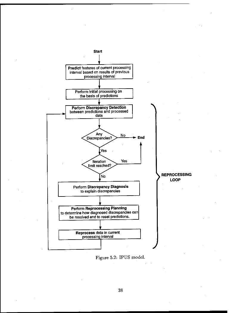
The reprocessing loop is iterative because the elimination of inconsistencies generally re-

quires a search over various plausible remedial actions. During each iteration processing

is carried out on signal representations that are stored at various levels of abstraction in

a blackboard database. Algorithms for constraint matching and signal reprocessing, which

are called knowledge sources (KSs), operate on these data abstractions. The KSs utilized

in the reprocessing loop are of four types: discrepancy detection, discrepancy diagnosis,

reprocessing planning, and reprocessing. In Figure 5.2, we show how these KSs are invoked

during the reprocessing loop.

The discrepancy detection KS identifies "distortions" in the signal features extracted

from the results of signal processing. Such distortions correspond to features that are

incompatible with constraints from the application domain. Alternatively, distortions also

arise when signal features are inconsistent with expected signal features. A prediction KS

is invoked prior to the reprocessing loop to generate the expected features on the basis of

signal features found in earlier temporal intervals of the signal data.

Distortions identified during discrepancy detection are analyzed by a discrepancy diag-

nosis KS. This KS generates plausible explanations for the cause of each distortion. The

generation of these explanations may be viewed as the process of using one or more "dis-

tortion operators" to map expected signal features to the signal features detected in the

processing interval. We illustrate such mapping through an example. Consider a signal in

the spread spectrum domain for which expected features indicate the presence of two tones,

while signal features detected from signal processing outputs show the presence of a single

tone. Diagnosis would then use a frequency resolution type of distortion operator to map

the two tones to a single tone. To facilitate such mapping the diagnosis KS generally has

an intimate knowledge of domain constraints as well as the properties of signal processing

algorithms used in the application. It should also be noted that there may not be a unique

sequence of distortion operators to explain a distortion. Consequently, the diagnosis KS is

not guaranteed to produce the "correct" explanation in the first attempt. Multiple itera-

37

Start

Predict features of current processing interval based on results of previous

processing interval

Perform initial processing on the basis of predictions

Perform Discrepancy Detection between predictions and processed

data

\

No -►End

,1

Yes

Perform Discrepancy Diagnosis to explain discrepancies

\ REPROCESSING / LOOP

Perform Reprocessing Planning to determine how diagnosed discrepancies can

be resolved and to reset predictions.

Reprocess data in current processing.interval

J Figure 5.2: IPUS model.

38

tions of the reprocessing loop need to be performed to sift through the explanations and

converge on the correct one.

Following diagnosis, a reprocessing planning KS utilizes the distortion operators to hy-

pothesize remedial reprocessing KSs that could be applied to the data. This requires that

the reprocessing planning KS have an accurate knowledge of the behaviors of various signal

processing algorithms. We illustrate reprocessing planning using the example considered

in the description of discrepancy diagnosis. In this example, a low frequency resolution

distortion operator was identified to explain the distortion of two tones into a single tone.

When the reprocessing planning KS finds such an operator, it hypothesizes that the signal

should be reprocessed with filters having smaller bandwidths. The new set of filters are

then designed on the basis of the relative amplitudes of the tones. In certain situations,

reprocessing planning cannot arrive at the best reprocessing KS in the first iteration of

the reprocessing loop. Multiple iterations of the reprocessing loop are again necessary to

ensure that the correct strategy is identified.

Reprocessing KSs are finally applied to the signal data to try and remove the distortions.

Once reprocessing has been performed, the reprocessing loop is repeated to identify and

resolve distortions that may still persist. Persistant distortions result from incorrect diag-

nosis or the reprocessing planning failing to specify proper remedial actions. Repetitions

of the loop are carried out until all distortions are removed or an iteration limit is reached.

5.2.2 Appropriateness of IPUS Model

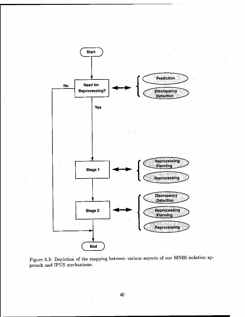
We now examine how the various mechanisms of the IPUS framework's reprocessing loop

are utilized to obtain a system realization of our two-stage TF analysis approach. In Figure

5.3 we depict the specific mapping that we have performed between each of the two stages

and the IPUS mechanisms of prediction, discrepancy detection, reprocessing planning, and

reprocessing. Let us examine this mapping in greater detail.

We begin by using the prediction and discrepancy detection mechanisms to obtain an

39

C Start )

'

No Need for Reprocessing?

<

Yes

Stage 1

\ r

Stage 2

'

{

{

Prediction

Discrepancy Detection

Reprocessing Planning

Reprocessing

Discrepancy Detection

Reprocessing Planning

Reprocessing

C End ) Figure 5.3: Depiction of the mapping between various aspects of our MNBI isolation ap- proach and IPUS mechanisms.

40

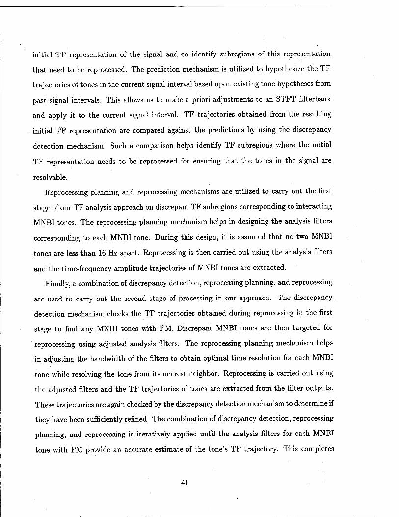
initial TF representation of the signal and to identify subregions of this representation

that need to be reprocessed. The prediction mechanism is utilized to hypothesize the TF

trajectories of tones in the current signal interval based upon existing tone hypotheses from

past signal intervals. This allows us to make a priori adjustments to an STFT filterbank

and apply it to the current signal interval. TF trajectories obtained from the resulting

initial TF representation are compared against the predictions by using the discrepancy

detection mechanism. Such a comparison helps identify TF subregions where the initial

TF representation needs to be reprocessed for ensuring that the tones in the signal are

resolvable.

Reprocessing planning and reprocessing mechanisms are utilized to carry out the first

stage of our TF analysis approach on discrepant TF subregions corresponding to interacting

MNBI tones. The reprocessing planning mechanism helps in designing the analysis filters

corresponding to each MNBI tone. During this design, it is assumed that no two MNBI

tones are less than 16 Hz apart. Reprocessing is then carried out using the analysis filters

and the time-frequency-amplitude trajectories of MNBI tones are extracted.

Finally, a combination of discrepancy detection, reprocessing planning, and reprocessing

are used to carry out the second stage of processing in our approach. The discrepancy

detection mechanism checks the TF trajectories obtained during reprocessing in the first

stage to find any MNBI tones with FM. Discrepant MNBI tones are then targeted for

reprocessing using adjusted analysis filters. The reprocessing planning mechanism helps

in adjusting the bandwidth of the filters to obtain optimal time resolution for each MNBI

tone while resolving the tone from its nearest neighbor. Reprocessing is carried out using

the adjusted filters and the TF trajectories of tones are extracted from the filter outputs.

These trajectories are again checked by the discrepancy detection mechanism to determine if

they have been sufficiently refined. The combination of discrepancy detection, reprocessing

planning, and reprocessing is iteratively applied until the analysis filters for each MNBI

tone with FM provide an accurate estimate of the tone's TF trajectory. This completes

41

the IPUS-b&sed TF analysis of the signal interval.

5.3 IPUS Mechanisms for TF Approach

In this section we describe the specific details on how the IPUS framework was used to sup-

port our approach to TF analysis. We begin with a description of the data representations

used in the various mechanisms of the reprocessing loop. Later we describe the prediction,

signal processing, discrepancy detection, reprocessing planning, and reprocessing KSs that

we have developed.

5.3.1 Data Representations

For facilitating prediction, discrepancy detection, diagnosis, and reprocessing, we need to

represent the signal data in terms of modulated tones. Such tone representations may

be obtained through the application of spectral peak picking and tone tracking to a TF

representation of the signal. TF analysis first separately resolves spectral contributions

from each tone in the TF plane. Significant spectral peaks are identified in the filterbank

outputs using Klassner's peak picker [11]. The peaks are then used to form time-frequency-

amplitude trajectories of the modulated tones present in the signal.

The tracking of trajectories of modulated tones may be viewed as a problem of multi-

target tracking [12]. A solution to this problem involves modeling the time-frequency-

amplitude evolution of a tone by means of state equations and then utilizing multi-hypothesis

target tracking [13] to form state trajectories for each modulated tone. The state equations

that we utilize are based upon those introduced for maneuvering targets [14] and are given

by

x(t) = Fx(t) + Gv(t)

z(t) = Hx(t) + w{t) (5.3)

42

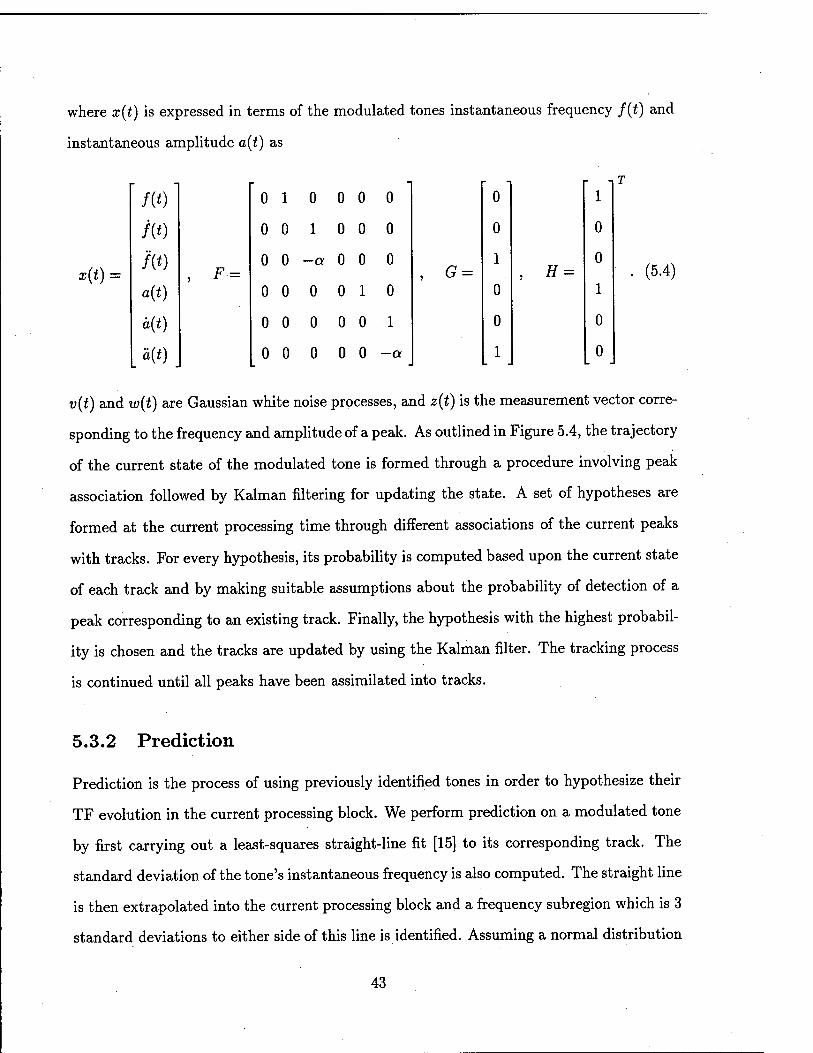
where x(t) is expressed in terms of the modulated tones instantaneous frequency /(i) and

instantaneous amplitude a(t) as

x (t) =

f(t)

/(*)

a(t)

a{t)

o(t)

F =

0 10 0 0 0

0 0 10 0 0

0 0 -a 0 0 0

0 0 0 0 1 0

0 0 0 0 0 1

0 0 0 0 0 -a

0 1

0 0

, G = 1

, H = 0

0 1

0 0

1 0

-|T

(5.4)

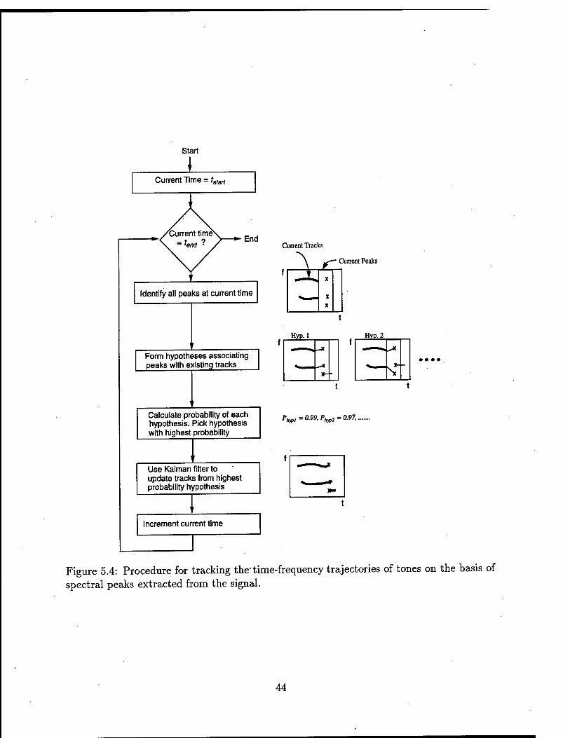
v(t) and w(t) are Gaussian white noise processes, and z(t) is the measurement vector corre-

sponding to the frequency and amplitude of a peak. As outlined in Figure 5.4, the trajectory

of the current state of the modulated tone is formed through a procedure involving peak

association followed by Kaiman filtering for updating the state. A set of hypotheses are

formed at the current processing time through different associations of the current peaks

with tracks. For every hypothesis, its probability is computed based upon the current state

of each track and by making suitable assumptions about the probability of detection of a

peak corresponding to an existing track. Finally, the hypothesis with the highest probabil-

ity is chosen and the tracks are updated by using the Kaiman filter. The tracking process

is continued until all peaks have been assimilated into tracks.

5.3.2 Prediction

Prediction is the process of using previously identified tones in order to hypothesize their

TF evolution in the current processing block. We perform prediction on a modulated tone

by first carrying out a least-squares straight-line fit [15] to its corresponding track. The

standard deviation of the tone's instantaneous frequency is also computed. The straight line

is then extrapolated into the current processing block and a frequency subregion which is 3

standard deviations to either side of this line is identified. Assuming a normal distribution

43

Start

I Current Time = fsfart

End

Identify all peaks at current time

Form hypotheses associating peaks with existing tracks

Calculate probability of each hypothesis. Pick hypothesis with highest probability

Use Kaiman filter to update tracks from highest probability hypothesis

Increment current time

Current Tracks

^b £1 Current Peaks

Hyp-i Hyp. 2

Phyp,= 0.99, Phyp2 = 0.97,.

Figure 5.4: Procedure for tracking the-time-frequency trajectories of tones on the basis of spectral peaks extracted from the signal.

44

2500

2000

1^1500

o-

^1000

500-

0.1 0.2 0.3 Time (sec)

0.4 0.5

Figure 5.5: Illustrating the extrapolation of TF trajectories of tones from the previous processing block to the current processing block. The gray regions indicate the TF regions over which the tones identified in the previous block (indicated by black lines) are most likely to evolve.

for the tone's instantaneous frequency, this subregion represents the 99% confidence region

for the evolution of the trajectory corresponding to the tone. For instance, in Figure 5.5, the

gray regions indicate the TF regions over which the tones identified in the previous block

(indicated by black lines) are most likely to evolve. These TF regions in conjunction with

mean amplitude and frequency modulation rate extracted from the tracks corresponding

to the tones constitute their overall predicted TF behavior.

5.3.3 Adjusted STFT Processing

The predicted TF behavior of tones in the current processing block is utilized to alter the

analysis filters in an STFT filterbank with Gaussian filters. Gaussian filters were chosen on

the basis of the well-known property that they have the least time-frequency uncertainty

[16]. The center frequencies of the filters in the filterbank are uniformly spaced along the

45

frequency axis and the impulse response of the i-th filter is given by

hi[n] — Aexp{-cm2}exv{j^n}, \n\ < m

0, M > «t

Here /,• is the center frequency of the filter, fs is the sampling rate, n; is the time index

before which the magnitude of the impulse response decays to a small value e, A is a scaling

factor which ensures that the filter has unit energy, and a is a parameter that controls the

bandwidth of the filter. To ensure that the filters have bandwidths with adequate frequency

resolution to separately resolve two adjacent tones, we have to pick an appropriate value

of a for filters in the vicinity of the two tones. Through an analysis of the Gaussian

filter's frequency response, we have shown that this may be achieved by ensuring that the

a parameter corresponding to these filters is at most

a=^J^C (5-6) ln(e) (3A2 - Ax)2/;

where A\ and A2 are the average amplitudes of the two predicted tones such that A2 > A\

and /i and f2 are the frequencies of the two predicted tones.

5.3.4 Discrepancy Detection

Two different discrepancy detection mechanisms are specified for use before stage 1 and

during stage 2 of our approach, respectively. The first mechanism is targeted at finding

discrepancies between the predictions and the results of initial STFT processing. The

second discrepancy detection mechanism is used in adjusting the analysis filters for MNBI

tones with FM in stage 2.

Discrepancy Detection before Stage 1:

Discrepancy detection is the process of identifying mismatches between the predictions

and the results of adjusted STFT processing. In order to facilitate discrepancy detec-

46

tion, the results of initial STFT processing are used to compute temporal and spectral

energy profiles of the current analysis interval. The temporal profile corresponds to inte-

grating the magnitude-squared of the output of the STFT over the entire time range of

the current analysis interval. Similarly, the spectral energy profile corresponds to integrat-

ing the magnitude-squared of the output of the STFT over all frequencies. These profiles

are matched against the predictions to determine if they bear out the assumption that

all tones found in the previous analysis interval continue unchanged through the current

analysis interval.

Discontinuities are identified in the temporal profile to find possible locations where

MNBI tones may have terminated or started. These discontinuities are discrepancies with

respect to the predictions which assume that the tones continue unchanged from the pre-

vious block to the current one. The time locations of discontinuities are found through a

chi-squared test [15].

In the case of the spectral energy profile, discrepancies are found by identifying each

spectral region that has significant energy even in the absence of any predicted MNBI tones

in that region. Such regions correspond to possible starts of new MNBI tones in the signal.

The process of finding such discrepant regions involves first picking peaks in the spectral

profile. If any peaks are found in frequency regions that do not overlap with the predicted

MNBI tones, then such peaks mark the locations of discrepancies.

Discrepancy Detection in Stage 2:

This mechanism is used to determine whether the TF trajectory of an MNBI tone with

FM has been sufficiently refined. The discrepancy detection process compares the TF

trajectory obtained using the adjusted analysis filters against the TF trajectory obtained

in the previous iteration of the second stage. If the average change between the two

trajectories is more than 5% over the entire duration of the MNBI tone, then a discrepancy

is declared.

47

5.3.5 Reprocessing Planning and Reprocessing

The reprocessing planning and reprocessing mechanisms also have two different versions.

During Stage 1 the first version is invoked to reprocess TF regions where predictions do

not match the tone TF trajectories found in the results of initial STFT processing. The

analysis niters are chosen to have sufficient frequency resolution to separate tones that

are at least 16 Hz apart. In Stage 2 the second version of .the reprocessing planning and

reprocessing mechanisms is used to reprocess MNBI tones with FM. In particular, these

mechanisms help choose a set of analysis filters that result in accurate TF trajectories for

MNBI tones with FM.

5.4 Implementation

We have implemented a C++ software testbed based on our approach to tone separation.

This testbed is built on top of the recently introduced I PUS C++ Platform (ICP) [17].

In implementing our testbed ICP was used to develop, compile, debug, and test all the

components required by the IPUS-based framework described in a later section . Using

ICP's library of base C++ classes, we derived a version of the blackboard database that

is suitable for our spread spectrum application. Functional blocks for the various I PUS

mechanisms were developed, compiled and tested by taking advantage of the inherent

support that ICP provides for C++ software development. Furthermore, we also utilized

ICP's libraries to instantiate a RESUN control planner for runtime scheduling of IPUS

mechanisms. Although a large portion of RESUN's capabilities are not exercised by our

application, we used it to provide modularity to the testbed as well as to allow future

system upgrades.

Our 4-level blackboard database was derived from ICP's base classes that have a rich set

of default behaviors. The different levels of the database are: waveform, spectrum, peaks,

and tracks. For each level, the base classes were also used to customize the behaviors of

48

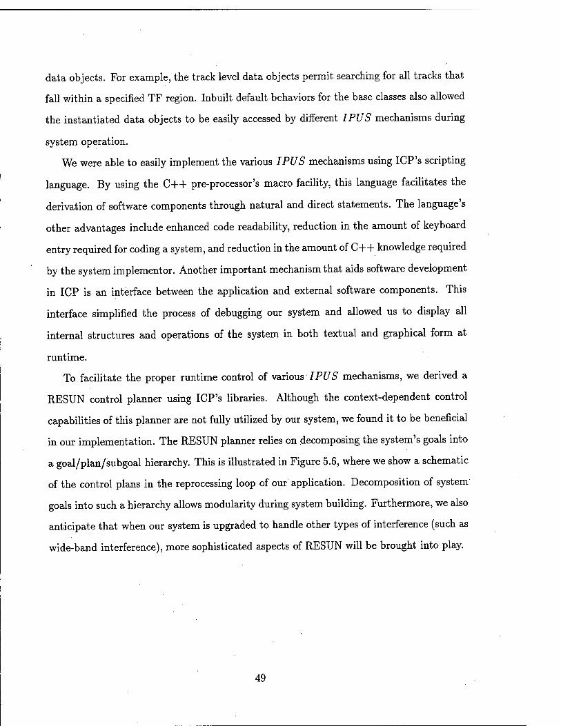
data objects. For example, the track level data objects permit searching for all tracks that

fall within a specified TF region. Inbuilt default behaviors for the base classes also allowed

the instantiated data objects to be easily accessed by different IPUS mechanisms during

system operation.

We were able to easily implement the various IPUS mechanisms using ICP's scripting

language. By using the C++ pre-processor's macro facility, this language facilitates the

derivation of software components through natural and direct statements. The language's

other advantages include enhanced code readability, reduction in the amount of keyboard

entry required for coding a system, and reduction in the amount of C++ knowledge required

by the system implementor. Another important mechanism that aids software development

in ICP is an interface between the application and external software components. This

interface simplified the process of debugging our system and allowed us to display all

internal structures and operations of the system in both textual and graphical form at

runtime.

To facilitate the proper runtime control of various IPUS mechanisms, we derived a

RESUN control planner using ICP's libraries. Although the context-dependent control

capabilities of this planner are not fully utilized by our system, we found it to be beneficial

in our implementation. The RESUN planner relies on decomposing the system's goals into

a goal/plan/subgoal hierarchy. This is illustrated in Figure 5.6, where we show a schematic

of the control plans in the reprocessing loop of our application. Decomposition of system

goals into such a hierarchy allows modularity during system building. Furthermore, we also

anticipate that when our system is upgraded to handle other types of interference (such as

wide-band interference), more sophisticated aspects of RESUN will be brought into play.

49

Have Reprocessing Loop

Have Track

Clusters

Form Track Clusters

Perform Reprocessing Loop

Have Discrepancy Detection

Perform Discrepancy Detection

Have Discrepancy;

Diagnosis j

; Have Reprocessing | ! Planning !

Perform Discrepancy Diagnosis

Perform leprocessinc Planning

Reprocessinc Planl

Reprocessint Planl

Key: I I Plan Schema \ Subgoal Primitive Action

Figure 5.6: Diagram of a portion of the goal/plan/subgoal hierarchy from our testbed.

50

Chapter 6

Some Prototype Development Issues

An analytical performance evaluation of rule-based systems that rely on knowledge extrac-

tion is generally not feasible. In these cases, one needs to employ computer-aided modeling

and simulation for system evaluation. In our case, the complexity of the communication

system along with knowledge-based interference cancellation makes an analytical perfor-

mance evaluation extremely difficult. For this reason we employ computer-aided modeling

and simulation in order to demonstrate the effectiveness of our approach. To this end we

use a signal processing software tool for time-domain modeling and simulation of communi-

cation systems called Signal Processing Worksystem (SPW©) from Cadence Corp. In this

chapter we briefly describe this tool. Another key issue was to establish communication

between I PUS and SPW. We also describe our solution to this problem.

6.1 Signal Processing Worksystem SPW©

In the signal processing software package SPW systems are completely characterized in the

time domain. The spread-spectrum system is modeled in terms of functional blocks such

as mixers, amplifiers and detectors. Transmitted signals are generated in the time domain

as are the responses of the receiver functional blocks to the received spread-spectrum signal

and the interference. This enables us to realistically evaluate system degradation due to

51

interference and the effectiveness of the proposed rejection scheme.

The signal processing software tool used in this research for the time-domain modeling

and simulation of communication systems is the Signal Processing Worksystem (SPW).

SPW is an integrated software package for designing signal processing systems. Its vast

communication systems and digital signal processing library, graphical design methodol-

ogy, fast simulator, test and analysis facility, and implementation options make SPW an

excellent choice for concept to prototype design. SPW can be used to model and simulate

a system, then debug, revise and re-simulate the system until optimal results are obtained.

SPW consists of several modules. The Designer/Block Diagram Editor module is used

to graphically represent a system as a set of functional blocks connected by wires. Each

block is a symbol that represents an operation and the interconnecting wires symbolize the

flow of signals between blocks. The Signal Calculator module is used to create input signals

and analyze output signals from the modeled system. It can also perform signal operations

such as filtering, convolution, fast Fourier transforms, and cross correlation. The Signal

Flow Simulator module is used to convert block diagrams created in the Designer/Block

Diagram Editor module into simulation programs. It processes input signals created by

the Signal Calculator module and then executes the simulation.

6.2 Custom Coded Blocks

Although SPW comes with a large number of blocks, it is sometimes necessary to create a

block which is not provided in the SPW libraries. In this project we needed a few blocks

that are necessary to provide a communication capability between SPW and I PUS. These

blocks are nothing but C codes which carry out certain tasks. Creating a custom coded

block can be divided into seven sub-processes.

• Create and Save Symbol: Any block can be created by drawing and labeling the

appropriate inputs and outputs. The ports are added to the created blocks in order

52

to pass data in and out of the blocks.

• Create and Save Parameter Model:

A parameter screen model is created in order to let the user specify the parameter

values. It is created using lines, boxes, and the add parameter command.

• Link Symbol and Parameter Model:

The created block and its parameter screen file must be linked. By doing so, the

block is able to access its assigned parameter values.

• Generate Source Code:

In the block design window (BDW) there is a command to prepare blocks. When

we execute this command, ".c"(C code file) and ".h" (Header file) are generated. The

code we write must be put into ".c".

• Insert Code:

The ".h" file contains all C code structure definitions. It contains all of the procedure

call declarations which need to be written.

• Compile Code:

After having edited the code, it must be compiled. If an error occurs, the appropriate

changes are made and the code is recompiled.

• Add New Block to Block-list:

Before the newly created block is used in any simulation, it must be added to its pool

of available blocks.

The following are the functions of some of the important CGS blocks that we have developed

mSPW:

• LTRIG-CG : After a block of N samples are stored, this block writes '1' into a certain

flag file. This triggers the I PUS system to process the stored samples.

53

• TRIG-4 : After having processed a certain number of samples, The block activates

the cancellation engine.

• JAMMERJNFO : This block reads the information about parameters of jamming

signals from IPUS system. It send this information to the cancellation engine.

• CW : This block reads information about the time-frequency tracks from IPUS and

sends this information to the cancellation engine.

6.3 Integration of SPW with IPUS

Performance evaluation of the knowledge-based interference cancellation scheme presented

in this report involves simulating the spread-spectrum system using SPW in conjunction

with the IPUS C++ platform. The collaboration of the SPW signal flow simulator and

IPUS during the simulation process is an important issue. This can be further explained

as follows. The simulation process can be viewed as consisting of three consecutive stages,

each one depending on the successful completion of the preceding stage. The first stage

consists of the spread-spectrum transmitter and the channel. The transmitter generates

the direct-sequence spread-spectrum signal. Disturbances such as AWGN and interference,

are introduced in the transmitted signal during the passage through the channel. The in-

terferes are selected from the list of interferers discussed in a previous chapter. A graphical

user interface is provided that allows the user to select any combination of interferers from

a preselected menu by clicking on the appropriate switch. The spread-spectrum bandwidth

is divided into four sub-bands and, in each sub-band, the user is given a choice of selecting

an interferer from the menu. This graphical interface could be easily modified to include

many more interferers in each sub-band and also to allow for the overlapping in frequency

of interferers.

The received signal consists of the transmitted spread-spectrum signal and the inter-

ference. The second stage of the simulation consists of processing the received signal by

54

I PUS. In the third stage interference cancellation is carried out based on the information

on the interference extracted by I PUS.

The IPUS C++ platform has to be integrated with both the SPW simulation system

that performs the signal and interference generation tasks and the functional stages that

perform the interference cancellation and demodulation tasks. This issue is complicated

due to the fact that the IPUS C++ platform cannot be directly incorporated as an SPW

custom-coded block since the current version available at the time of development, version

3.5 of the Signal Processing Worksystem, did not support a C++ compiler. An alternative

approach is therefore, required to pass the received data to IPUS for processing and to

collect the information extracted by IPUS regarding the interference that is disrupting

the received spread-spectrum signal. As described earlier in this chapter, SPW runs the

simulation in the time-domain. The SPW scheduler controls the progress of the simulator

by passing tokens from one or more blocks that concurrently perform their signal process-

ing tasks to the succeeding block or blocks. Multirate blocks like up-samplers and down

samplers are also handled using this token-passing approach. SPW facilitates the control

of the execution of a particular functional block by means of a 'hold' control signal. The

'hold' signal, when set high, suspends the execution of the block. This feature is used in our

simulation in generating data arriving at the spread-spectrum receiver ( stage 1 ), process-

ing of the received data by IPUS, and performing the subsequent interference cancellation

operations based on the information provided by IPUS. We pass data in a block-wise

fashion from one stage to the succeeding stage. The length of the block of data is sele'cted

such that IPUS receives adequate data samples in the block to perform its interference

isolation task efficiently without introducing excessive delays due to block-wise processing

of data.

The following procedure is adopted for the combined SPW-IPUS simulation.

(1) The transmitter generates the DSSS signal and interference is introduced during

transmission through the channel. A block of N received signal samples are written to a

55

data file. IPUS is currently in an idle state, and is polling a flag for the signal to start

processing the received data. Stage 3 blocks, comprised of the interference cancellation

stage and the SS demodulator, are also currently disabled by means of hold-control. As

soon as stage 1 has written N data samples to the file, the flag is set to trigger the next

stage (I PUS) to start processing data. Once I PUS is triggered, stage 1 goes into the idle-

state and waits until the succeeding stages have completed processing the current block of

N data samples. Enabling and disabling the blocks in stage 1 is achieved by setting the

hold signal to either a low or high value, respectively.

(2) The I PUS data processing cycle is triggered by the flag. I PUS resets the IPUS-

trigger flag and starts processing the received data. The information transfer from I PUS

to stage 3 is also done through the Unix system interface. I PUS generates time-frequency

tracks for each identified jammer and writes the information in file(s). Stage 3 is still in

the idle state and is polling the 'stage-3 trigger' flag to determine when to start reading the

processed information from I PUS. Once I PUS has completed processing the block of N

received data samples, the stage-3 trigger flag is set and I PUS goes back to the idle state

and keeps polling the IPUS-trigger flag to determine when to start reading the next block

of samples.

(3) Stage 3 is triggered by I PUS by setting the stage-3 trigger flag. Once triggered,

stage 3 resets the stage-3 trigger flag and proceeds to read the jammer information written

in data files by IPUS. The stage 3 processing cycle continues until the current N data

samples have been processed. The stage 3 signals to stage 1 by setting the flag that enables

the hold-signal for stage 1 blocks. Upon detecting the flag, Stage 1 resets the flag and

starts generating the next block of N data samples at the receiver.

A control block is developed in stage 1 for the purpose of generating the control signals

that trigger the next stage, and the hold signal for stage 1. A custom-coded block is

designed for the purpose of polling and resetting the flag set by stage 3. Figures 6.1 and

6.2 show the circuits that generates the trigger signals for IPUS.

56

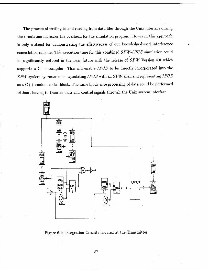
The process of writing to and reading from data files through the Unix interface during

the simulation increases the overhead for the simulation program. However, this approach

is only utilized for demonstrating the effectiveness of our knowledge-based interference

cancellation scheme. The execution time for this combined SPW-IPUS simulation could

be significantly reduced in the near future with the release of SPW Version 4.0 which

supports a C++ compiler. This will enable IPUS to be directly incorporated into the

SPW system by means of encapsulating IPUS with an SPW shell and representing IPUS

as a C++ custom coded block. The same block-wise processing of data could be performed

without having to transfer data and control signals through the Unix system interface.

UIHDOU

UIHDOU

UIHDOU

TOGGLE BUTTOttH4

QOTF

-8S

UIHDOU

H

T0G6LE BUTT0H}->

-9*

U>» SIMPLE

COUNTER

OIMfl UUE IS] -S5

3 DO

, >=KEfltJ->4

SIfFLE c

COUNTER

IT —)□ >*U +~>-

@4

I.TRIG.C9

UIHDOU

HULTI ASM

Figure 6.1: Integration Circuits Located at the Transmitter

57

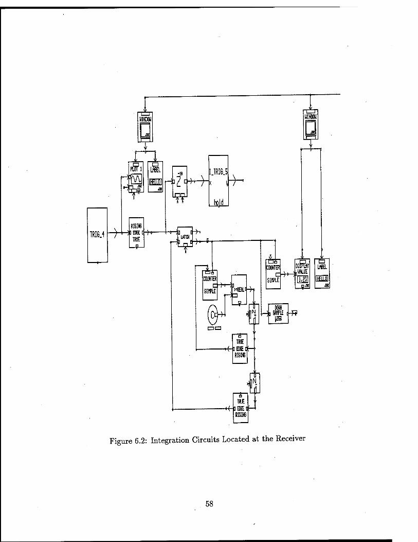
MfflOU

Hl

TR36.4

UINDOH

pffl

f5 □

LABEL

HOD

RISING

TRUE

W

^

IJRI6.5

hold

-)-

WTO) HP n'H*-4-

ra COUNTER

q)« )|D SIlfLE

(r J>=REW.lH-c

Ho

4]

-* TRUE

OEDEtft-' RISING

4]

TRUE -t-f-fa EDE *■

RISING

$ , US

ICOUKTER £=B~H&

SIMPLE

\r >1>

oisra WOE

□ LABEL

MM ■*£

DOUN MoSflHPLE Hfl

Figure 6.2: Integration Circuits Located at the Receiver

58

Chapter 7

System Models and Experimentation

7.1 System Models in SPW

The main focus of this chapter is to present models for communication system blocks

that have been created in SPW to demonstrate the effectiveness of our knowledge-based

interference cancellation approach. We also include some discussion on the development of

rules for the selection of interference cancellers from the library of filters.

7.1.1 Transmitter

The model for the spread-spectrum transmitter is shown in Figure 7.1. The random data

generator generates 0 and l's with equal probability and provides the information bits for

the BPSK modulator.. The spreading signal is generated by the PN sequence generator

whose values of 0 and 1 are transformed to -1 and +1, respectively, by the block designated

as binary to numeric. The bit rate of the PN codes is 32 times that of the information

bit rate. This provides the spread-spectrum system with a processing gain of 32 or 15 dB.

The spread information bit stream is modulated by a carrier prior to transmission over the

channel. The parameter values for the transmitter are listed in Figure 7.2. Typical spectra

of the input message and transmitter output are shown in Figure 7.3.

59

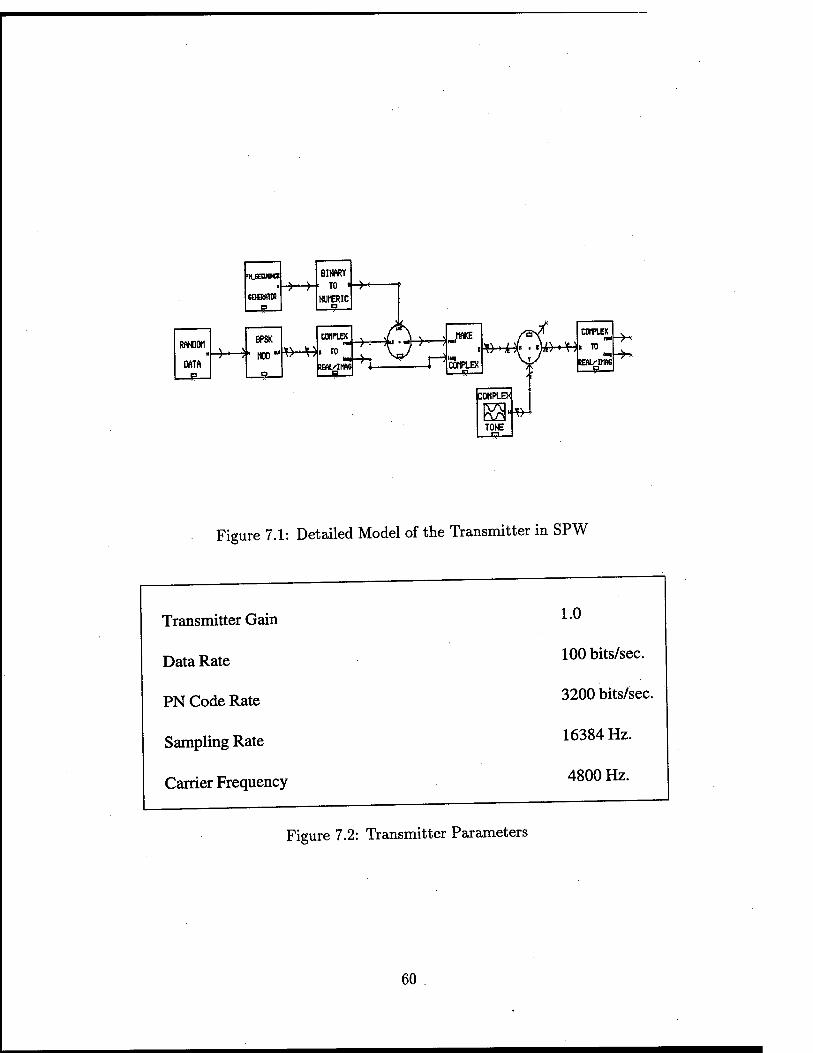
tLEEOJEME i

KHBSTO •*—*■

BIKARY . TO > NUMERIC

RANDOM 1

DATA o

-H_> BPSK

MOD' *»-+* CtJIFLEX

i 70 --H-

iEAL'IIIM V

,MAKE i

r"^ COMPLEX

*KM» -«to-^H

POMPLEXI

TONE *}-

CDTFLEX m

« TO feEM/THUG

Figure 7.1: Detailed Model of the Transmitter in SPW

Transmitter Gain

Data Rate

PN Code Rate

Sampling Rate

Carrier Frequency

1.0

100 bits/sec.

3200 bits/sec.

16384 Hz.

4800 Hz.

Figure 7.2: Transmitter Parameters

60

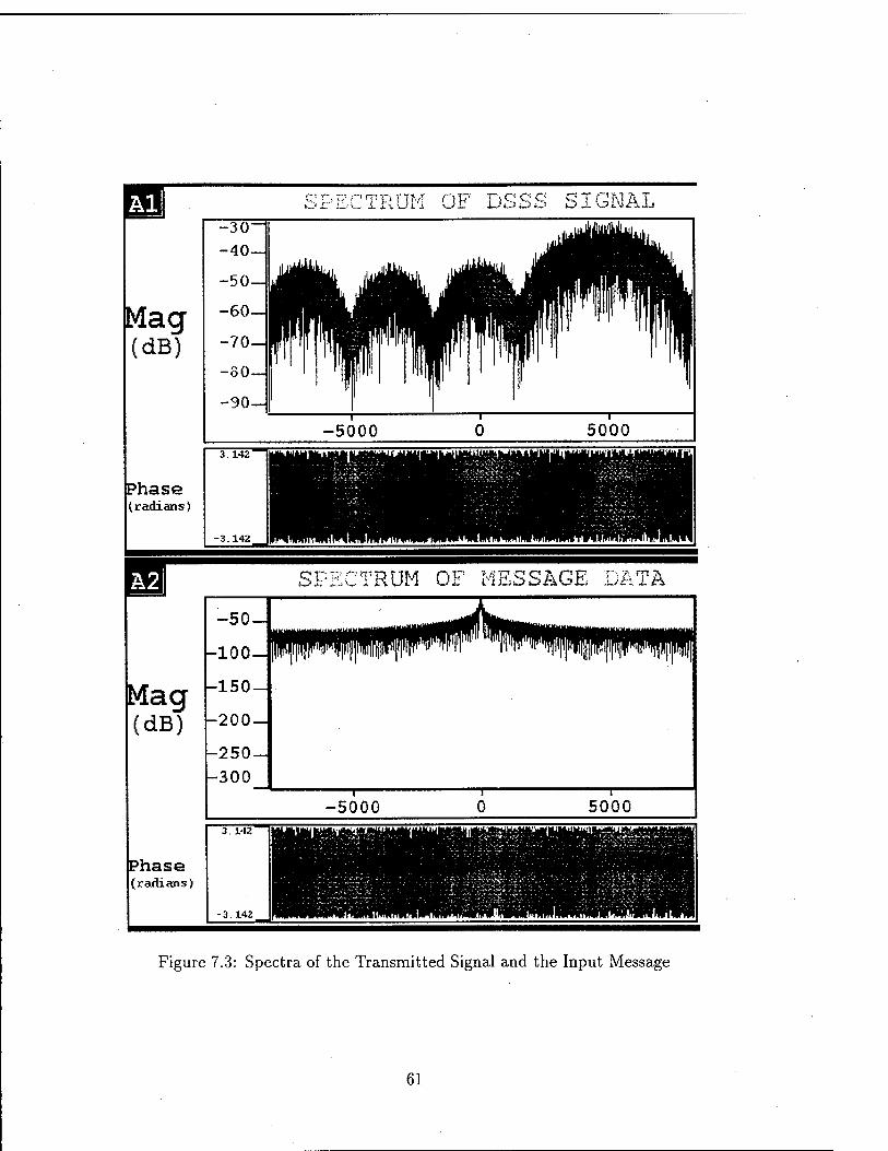
SPECTRUM OF DSSS SIGNAL

Mag (dB)

Phase (radians)

M SPECTRUM OF MESSAGE DATA

-50J Ji^ 1

-100-

Mag (dB)

-150-

-200-

-250- -300

-5000 0 5000 3.142 IIIIM/BI^^

Phase (radians) HHH H

-3.142 ^mmmmtmmslmSmmmi^mi

Figure 7.3: Spectra of the Transmitted Signal and the Input Message

61

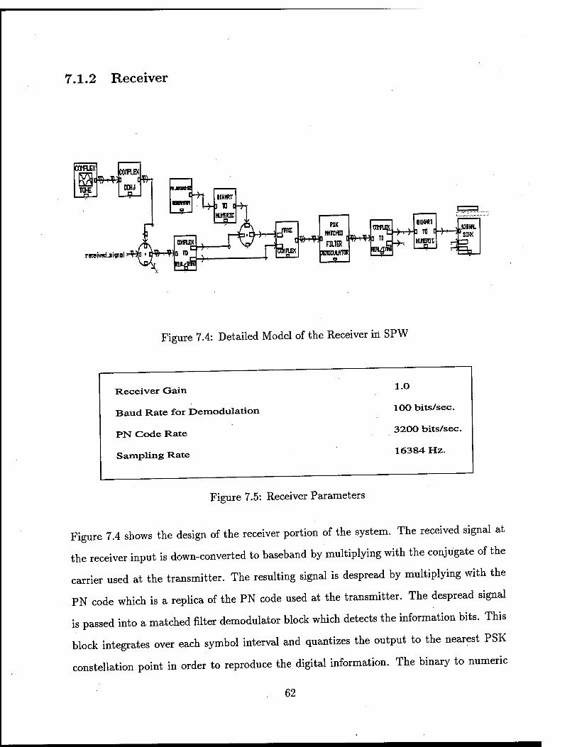
7.1.2 Receiver

TONE

ICOfLEX

ESiflW*"" i|W-r COrFLBi

ECHO -B-

rwiYBd-sigial

[ ~H IIH«r H-] TO d-h

Sfl! iS

NltlERIC -■B I jk I 1

P^cfttPLBK t'JMH]

PSK micra FILTER

jEranjifflCF 3.

Hb-W,

BMttT ] TO [

HireRic —n—

fHf 31BHFL SI*

Figure 7.4: Detailed Model of the Receiver in SPW

Receiver Gain

Baud Rate for Demodulation

PN Code Rate

Sampling Rate

1.0

100 bits/sec.

3200 bits/sec.

16384 Hz.

Figure 7.5: Receiver Parameters

Figure 7.4 shows the design of the receiver portion of the system. The received signal at

the receiver input is down-converted to baseband by multiplying with the conjugate of the

carrier used at the transmitter. The resulting signal is despread by multiplying with the

PN code which is a replica of the PN code used at the transmitter. The despread signal

is passed into a matched filter demodulator block which detects the information bits. This

block integrates over each symbol interval and quantizes the output to the nearest PSK

constellation point in order to reproduce the digital information. The binary to numeric

62

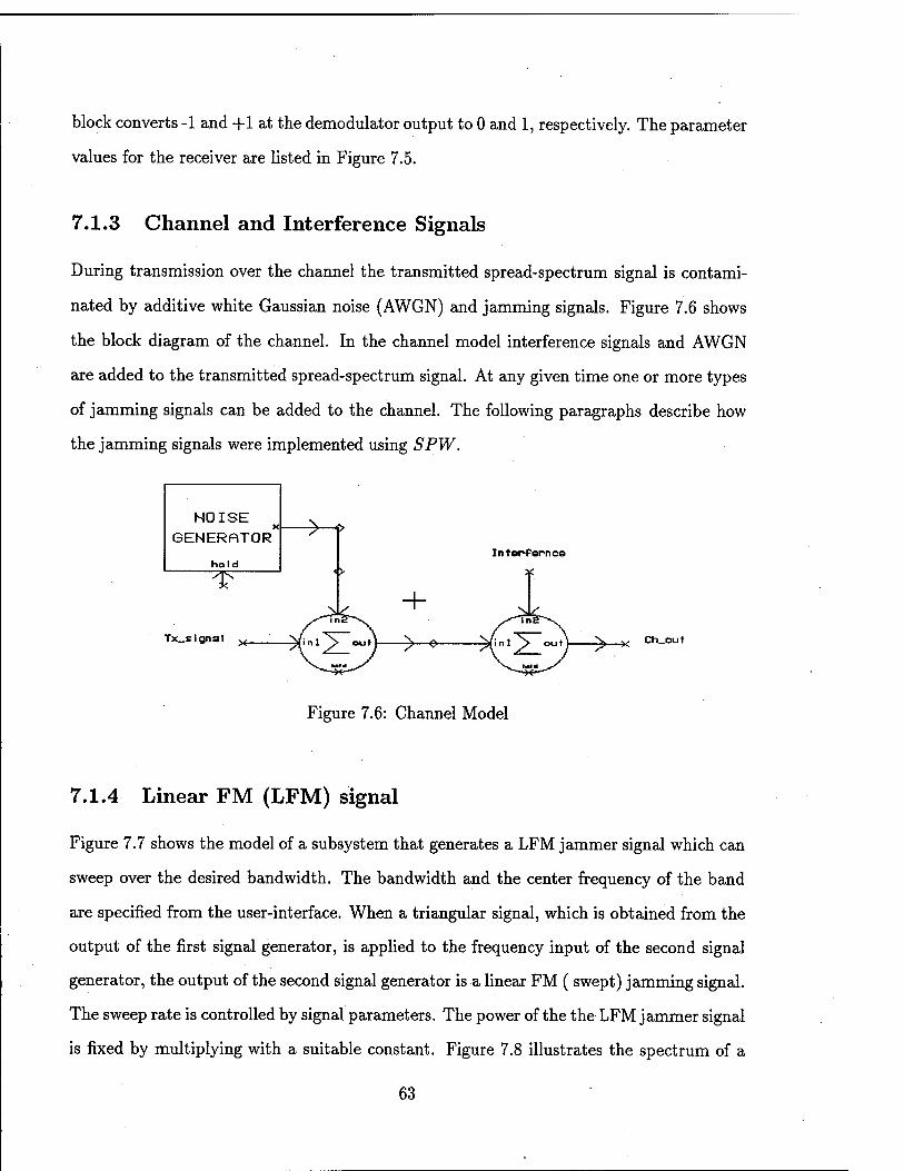
block converts -1 and +1 at the demodulator output to 0 and 1, respectively. The parameter

values for the receiver are listed in Figure 7.5.

7.1.3 Channel and Interference Signals

During transmission over the channel the transmitted spread-spectrum signal is contami-

nated by additive white Gaussian noise (AWGN) and jamming signals. Figure 7.6 shows

the block diagram of the channel. In the channel model interference signals and AWGN

are added to the transmitted spread-spectrum signal. At any given time one or more types

of jamming signals can be added to the channel. The following paragraphs describe how

the jamming signals were implemented using SPW.

NOISE GENERATOR'

hold

Tx_signal

>-r Interfernes

+ ^ Ch_out

Figure 7.6: Channel Model

7.1.4 Linear FM (LFM) signal

Figure 7.7 shows the model of a subsystem that generates a LFM jammer signal which can

sweep over the desired bandwidth. The bandwidth and the center frequency of the band

are specified from the user-interface. When a triangular signal, which is obtained from the

output of the first signal generator, is applied to the frequency input of the second signal

generator, the output of the second signal generator is a linear FM ( swept) jamming signal.

The sweep rate is controlled by signal parameters. The power of the the LFM jammer signal

is fixed by multiplying with a suitable constant. Figure 7.8 illustrates the spectrum of a

63

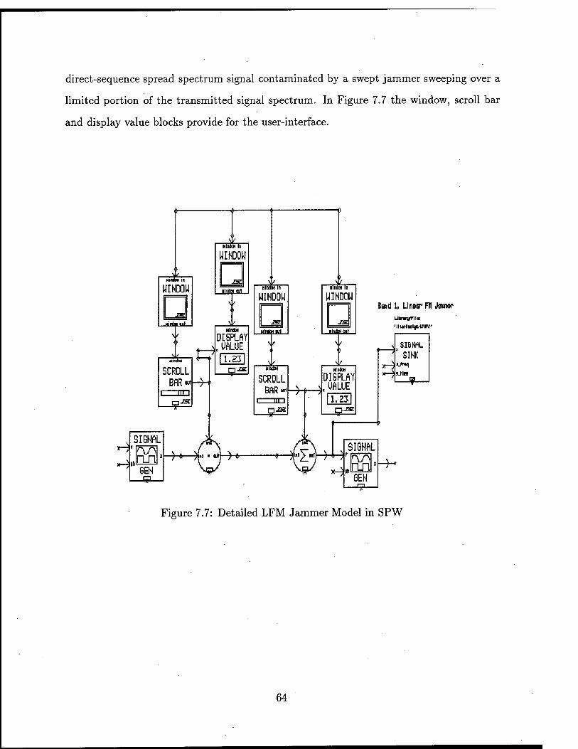
direct-sequence spread spectrum signal contaminated by a swept jammer sweeping over a

limited portion of the transmitted signal spectrum. In Figure 7.7 the window, scroll bar

and display value blocks provide for the user-interface.

Band 1, Linear FH Javier

Figure 7.7: Detailed LFM Jammer Model in SPW

64

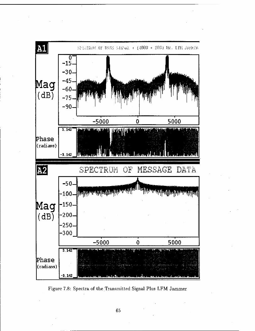
m SPL;;IRIM OF DSSS SIGNAL * (4000 + 2001 Hz. LFM J«H>

Phase (radians)

SPECTRUM OF MESSAGE DATA

Phase (radians)

Figure 7.8: Spectra of the Transmitted Signal Plus LFM Jammer

65

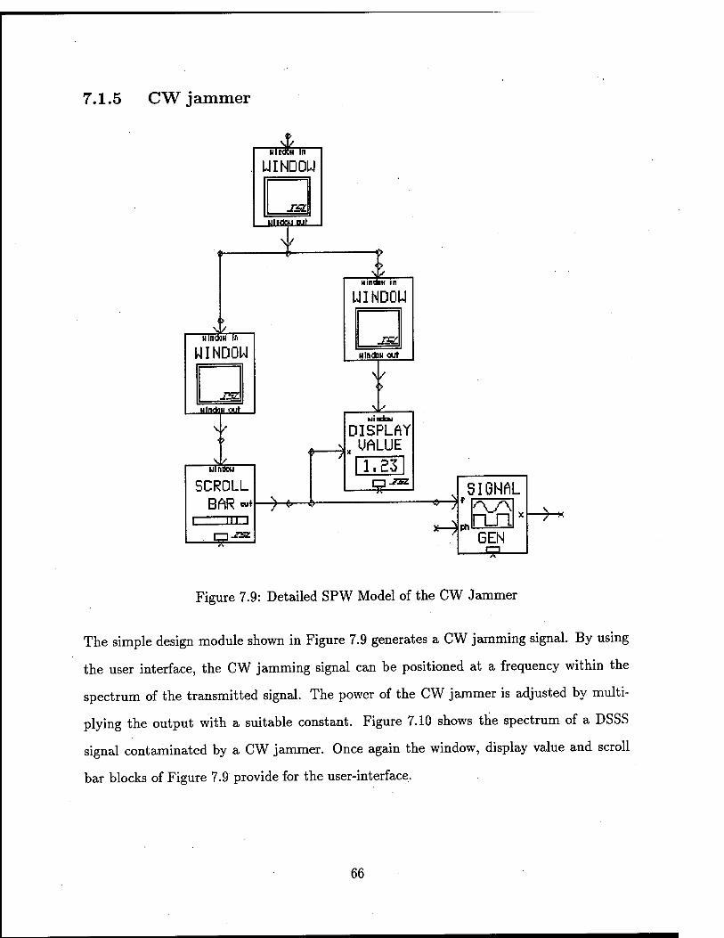
7.1.5 C W j ammer

(noofif HlndaH in

WINDON

J3L ulndau cut

MIMHM

SCROLL BAR »♦

' HI i —_S^i

HiidoH in

UINDDU

ISL HliOaj wr

\f

->-*-

UINDOU

JSL HlnddM out

_\iL

DISPLAY „ UALUE

1.23 M JSZ

Figure 7.9: Detailed SPW Model of the CW Jammer

The simple design module shown in Figure 7.9 generates a CW jamming signal. By using

the user interface, the CW jamming signal can be positioned at a frequency within the

spectrum of the transmitted signal. The power of the CW jammer is adjusted by multi-

plying the output with a suitable constant. Figure 7.10 shows the spectrum of a DSSS

signal contaminated by a CW jammer. Once again the window, display value and scroll

bar blocks of Figure 7.9 provide for the user-interface.

66

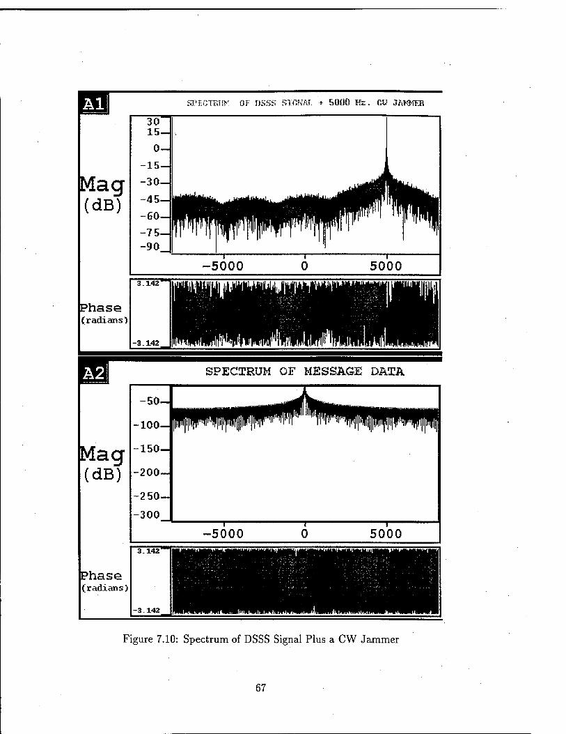
M SPECTRliK OF nSSS SIGNAL + 5000 Hz. C¥ JAMMER

Mag (dB)

Phase (radians)

Mag (dB)

Phase (radians)

SPECTRUM OF MESSAGE DATA

Figure 7.10: Spectrum of DSSS Signal Plus a CW Jammer

67

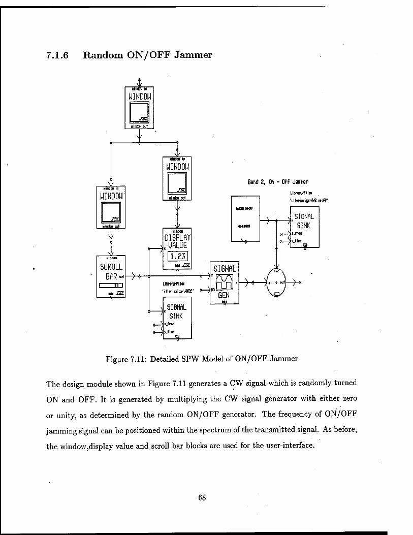
7.1.6 Random ON/OFF Jammer

HindoH in

WINDOW

JSL »■dm put

NindoK in

WINDOW

ISL HJlllfcM Out

SCROLL BAR«"

nn mISt.

-*

-H-

->

v

_&_ Hindoo

DISPLAY . UALUE

1.23 MO J2SZ

-x

Band 2, On - Off Janrer

Librarv'Fi IK

'illsriasigs'JOJ.oioff'

LlDravFlle:

'iHwissiBS-JOfEe' X—)ph

Figure 7.11: Detailed SPW Model of ON/OFF Jammer

The design module shown in Figure 7.11 generates a CW signal which is randomly turned

ON and OFF. It is generated by multiplying the CW signal generator with either zero

or unity, as determined by the random ON/OFF generator. The frequency of ON/OFF

jamming signal can be positioned within the spectrum of the transmitted signal. As before,

the window,display value and scroll bar blocks are used for the user-interface.

68

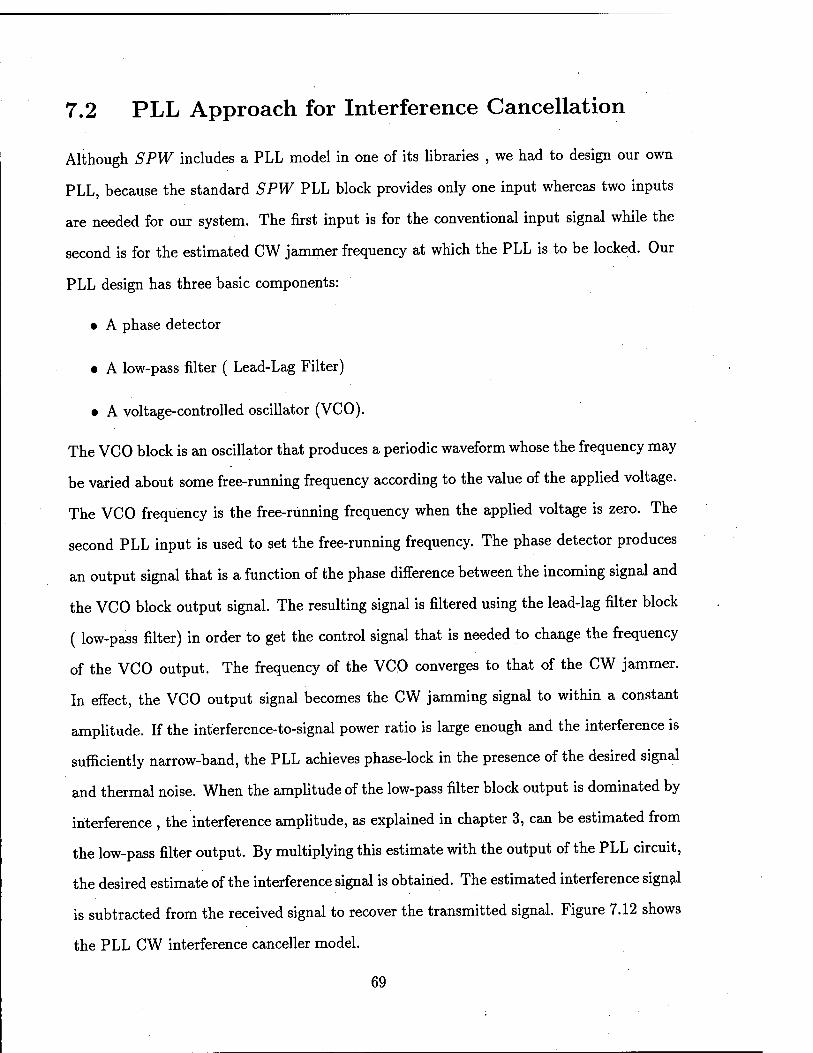
7.2 PLL Approach for Interference Cancellation

Although SPW includes a PLL model in one of its libraries , we had to design our own

PLL, because the standard SPW PLL block provides only one input whereas two inputs

are needed for our system. The first input is for the conventional input signal while the

second is for the estimated CW jammer frequency at which the PLL is to be locked. Our

PLL design has three basic components:

• A phase detector

• A low-pass filter ( Lead-Lag Filter)

• A voltage-controlled oscillator (VCO).

The VCO block is an oscillator that produces a periodic waveform whose the frequency may

be varied about some free-running frequency according to the value of the applied voltage.

The VCO frequency is the free-running frequency when the applied voltage is zero. The

second PLL input is used to set the free-running frequency. The phase detector produces

an output signal that is a function of the phase difference between the incoming signal and

the VCO block output signal. The resulting signal is filtered using the lead-lag filter block

( low-pass filter) in order to get the control signal that is needed to change the frequency

of the VCO output. The frequency of the VCO converges to that of the CW jammer.

In effect, the VCO output signal becomes the CW jamming signal to within a constant

amplitude. If the interference-to-signal power ratio is large enough and the interference is

sufficiently narrow-band, the PLL achieves phase-lock in the presence of the desired signal

and thermal noise. When the amplitude of the low-pass filter block output is dominated by

interference , the interference amplitude, as explained in chapter 3, can be estimated from

the low-pass filter output. By multiplying this estimate with the output of the PLL circuit,

the desired estimate of the interference signal is obtained. The estimated interference signal

is subtracted from the received signal to recover the transmitted signal. Figure 7.12 shows

the PLL CW interference canceller model.

69

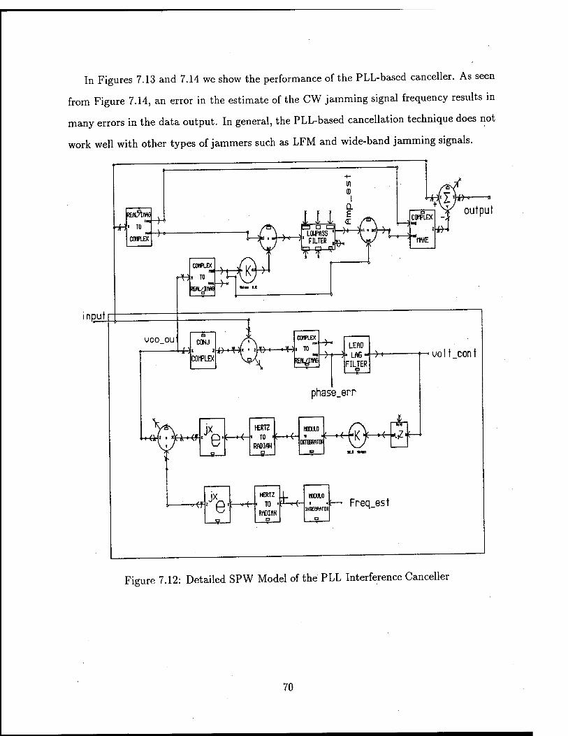
In Figures 7.13 and 7.14 we show the performance of the PLL-based canceller. As seen

from Figure 7.14, an error in the estimate of the CW jamming signal frequency results in

many errors in the data output. In general, the PLL-based cancellation technique does not

work well with other types of jammers such as LFM and wide-band jamming signals.

COIfLEX ~ ) »

■ -H-

rtt

input

vco ou

COMPLEX

x TO

REN./IM«

-w- ■+*

LOUPftSS ' FILTER ,$,

j&*—■ Sj/ output

*TB

CONJ

COMPLEX &+*i*' im ■ ' n

COTLEX m

I TO LEfiO * LAG-

FILTER -H-

phase.err

:« ■ «Hr^f

1-

J* {-**

HERTZ

TO *—+*

RADIfW —8—

HOOUU)

IKTEGRflTB <—4 &

-f 4r -,Z<^

uolt con t

*& Jx, e- HERTZ

TO '

RftDIflN F*-e

I10DULO

UflEOMTOt Freq_est

Figure 7.12: Detailed SPW Model of the PLL Interference Canceller

70

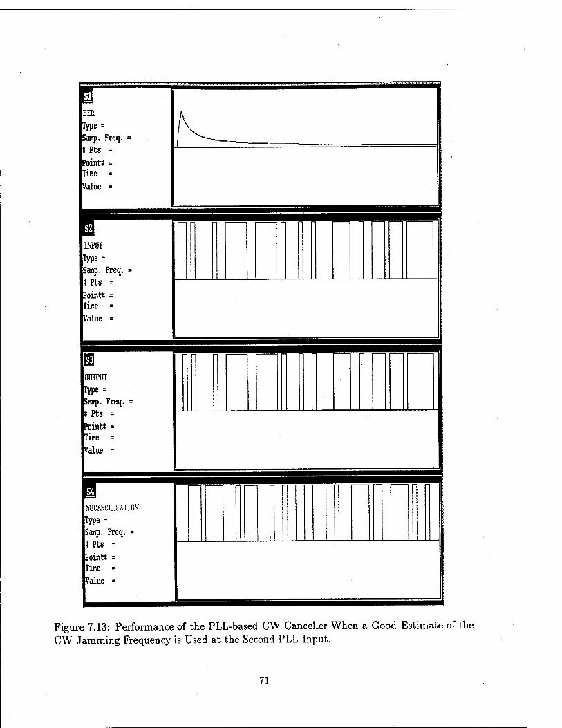
BER K Type = f\ Samp. Freq. = j ft Pts = ' PointI = Time = Value =

1 ffl DJPOI Type = Samp. Freq. = ft Pts = Point! = lime = Value =

1

E n OUTPUT Type* Samp. Freq. = ft Pts = PointI = lime = Value =

I 7 NOCANCEIinON Type = Samp. Freq. = 1 Pts * PointI = Tiae = Value =

Figure 7.13: Performance of the PLL-based CW Canceller When a Good Estimate of the CW Jamming Frequency is Used at the Second PLL Input.

71

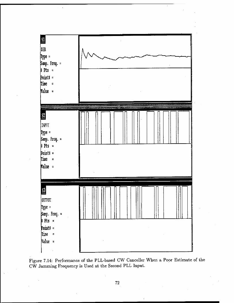
I Iype = Sasp. Freq.

Pts =

iPoint« =

Value

MIT

Type = Saup, Freq.

Pts =

Point« = Iiise =

Value =

OUTPUT Iype = Sawp. Freq,

Pts =

Point« = liie =

Value =

Figure 7.14: Performance of the PLL-based CW Canceller When a Poor Estimate of the CW Jamming Frequency is Used at the Second PLL Input.

72

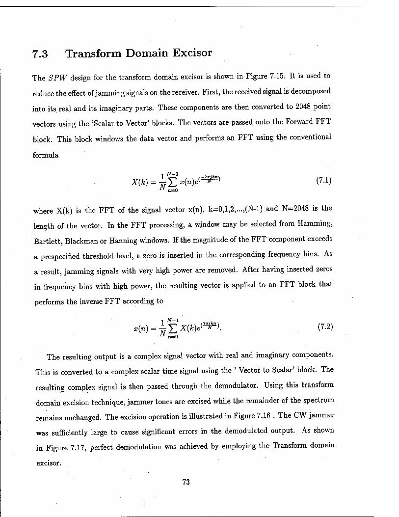
7.3 Transform Domain Excisor

The SPW design for the transform domain excisor is shown in Figure 7.15. It is used to

reduce the effect of jamming signals on the receiver. First, the received signal is decomposed

into its real and its imaginary parts. These components are then converted to 2048 point

vectors using the 'Scalar to Vector' blocks. The vectors are passed onto the Forward FFT

block. This block windows the data vector and performs an FFT using the conventional

formula

" n=0

where X(k) is the FFT of the signal vector x(n), k=0,l,2,...,(N-l) and N=2048 is the

length of the vector. In the FFT processing, a window may be selected from Hamming,

Bartlett, Blackman or Hanning windows. If the magnitude of the FFT component exceeds

a prespecified threshold level, a zero is inserted in the corresponding frequency bins. As

a result, jamming signals with very high power are removed. After having inserted zeros

in frequency bins with high power, the resulting vector is applied to an FFT block that

performs the inverse FFT according to

«(») = TjT.X{k)P&. (7.2) iV n=0

The resulting output is a complex signal vector with real and imaginary components.

This is converted to a complex scalar time signal using the ' Vector to Scalar' block. The

resulting complex signal is then passed through the demodulator. Using this transform

domain excision technique, jammer tones are excised while the remainder of the spectrum

remains unchanged. The excision operation is illustrated in Figure 7.16 . The CW jammer

was sufficiently large to cause significant errors in the demodulated output. As shown

in Figure 7.17, perfect demodulation was achieved by employing the Transform domain

excisor.

73

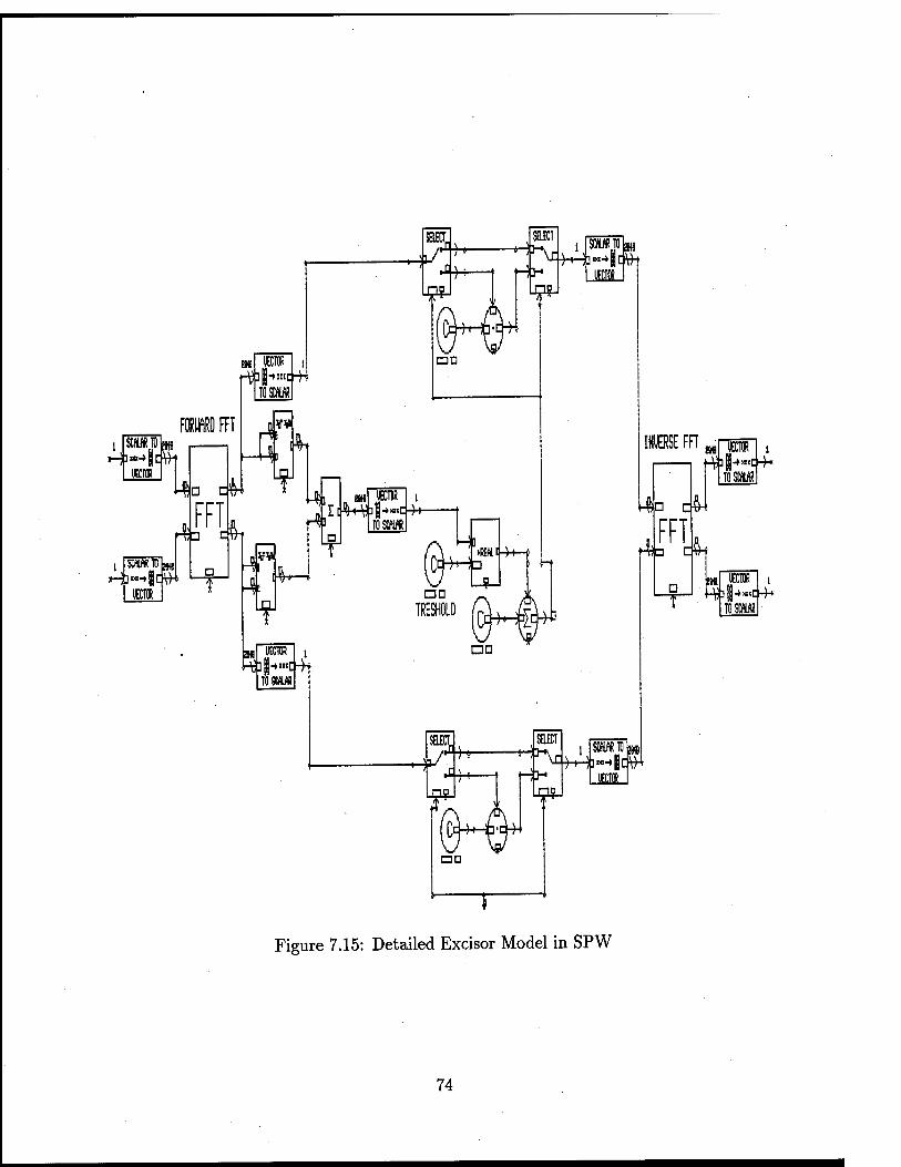
-H* SELECT. /4

►i

W-

SELICT

H^ m-

©Mr FFI

i $«->S#t

uccnx D C

SCfWRUäw Hb»-»|t:\H

MI

SfflWRTO m EfH]»-»Si:!!h

■H*

SELECT

►£

J*

SELKT ■H>v HJ-

□ D

T

INVERSE FFT «I

u

SOI/MM )-Hh-»8$H

n d4 FFk n D

TO SIM

M -\j]|-»H»c4*

Toscfiua

Figure 7.15: Detailed Excisor Model in SPW

74

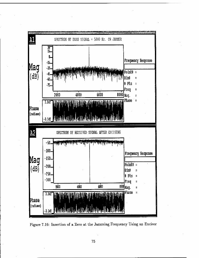
51

SPECTRUM OF DSSS SIQfflL + 5000 Hz. CII JfiHHER

Frequency Response

Point* = Bint = tPts = Freq = Mag. = Phase =

Phase radians)

SPECTRUM OF RECEIVED SIGNAL AFTER EXCISING

Figure 7.16: Insertion of a Zero at the Jamming Frequency Using an Excisor

75

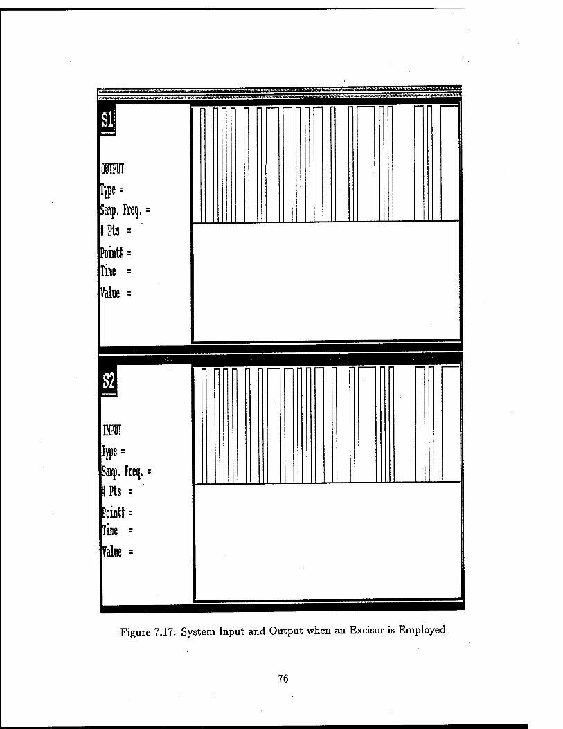
IHM

lype = Sip, Frei},

Pts =

■Point« =

ran !jpe = Saf. Freq. =

Pts =

löiBtf =

Um =

Figure 7.17: System Input and Output when an Excisor is Employed

76

7.4 Knowledge-Based Interference Cancellation

As indicated earlier, our knowledge-based interference cancellation approach relies heavily

on the expert system I PUS. This system processes the received signal to extract knowledge

such as the presence/absence of interferers, number and types of interferers, their param-

eters, etc. Based on this information, a set of rules are used to select the most suitable

interference cancellation schemes from the library of cancellation algorithms.

In our proof-of-concept demonstration we have limited attention to linear FM (or chirp)

jammers and/or single or multiple tone jammers that may or may not operate in an

ON/OFF mode. Moreover, we assumed ideal operating conditions in the sense that no

other uncertainties exist, e.g. lack of synchronization. The types of jammers considered

are completely characterized by their instantaneous frequencies and the times at which they

turn ON and OFF. IPUS is able to provide this information quite accurately in terms of

time-instantaneous frequency tracks. With this limited set of jammers and the information

provided by IPUS, it was discovered that simple notch filters are capable of reducing the

amplitudes of the jamming signals to acceptable levels. However, the type of notch filter

depends upon the type of interference. This considerably simplified the rules needed for

selecting the appropriate cancellation scheme. In a more different diverse environment it is

expected that other cancellation schemes will be needed and additional rules will need to

be developed.

The approach used in the current version of the knowledge-based interference cancel-

lation system prototype is to have the notch of a band-stop filter track the estimated

instantaneous frequency of the jammer. The residual interference from the moving notch

filter was found to be small enough so that it was readily handled by the processing gain of

the spread-spectrum system. The filter coefficients of the notch filter are set to center the

notch on the estimated instantaneous jammer frequency. Information provided by IPUS

in terms of time-instantaneous frequency tracks was found to be adequate for designing the

desired moving notch filter.

77

Although moving notch filters exhibited very good cancellation performance, they did

introduce transients that degraded performance. For this reason, it was decided to use the

notch filter only when needed. Based on the ON/OFF information provided by the time-

frequency tracks received from I PUS, notch filter was inserted only when a jamming signal

was present in the received signal. Otherwise, the filter was bypassed. This is implemented

by means of switches.

The cancellation scheme uses two types of band-stop filters. They are Chebychev Type

2 and the elliptic type band-stop filters. One of the major reasons this filter was chosen

for interference cancellation is that it makes the transition between the. passband and the

stopband very quickly. This feature makes this type of filter an excellent choice, when

we receive the transmitted spread-spectrum signal in the presence of slow swept (LFM)

jammer.

An elliptic band-stop filter was also used. This filter has an equiripple passband atten-

uation and the stopband attenuation oscillates between total stoppage and the attenuation

at the stopband edge. The smallest attenuation in the stopband is not specified directly

but is determined by the other filter parameters. Both the passband and stopband fre-

quencies are specified. The attenuation in the passband oscillates between 0 dB and the

value specified at the passband edge. The stopband attenuation is always greater than or

equal to its value at the stopband edge.

Based upon the information obtained from IPUS, the Chebychev Type 2 filter was

chosen to handle CW or a swept (LFM) jammers. However, the elliptic band-stop filter

was selected to combat ON/OFF CW jammers. A diagram of the interference cancellation

engine is shown in Figure 7.18. The effectiveness of this approach is demonstrated in the

next chapter.

78

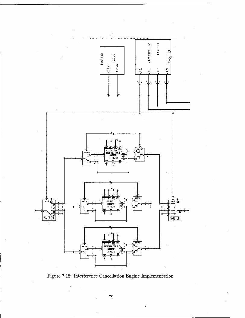
^, r-v-

SWITCH

-7-t>

-H

-%-

central

-K-

»'-£-?

I lf( \l/ W W

f "f If«-*"' mtm FIFE 2"

BMETÜP ItR FILTH

TT *

v . owtrol

Jsld_

X ■^H

\l/ W M/

BJJPIIC MCSTH> •

I» HUB |

TT

v Mfral

i )a _/-i~H

BBifrvl v v

**\.

w vl/ \b

«nflWITTTf t WWW

> )*_!

IKFILTDI tfHt )ti~l

t-r" /-i ■»+-

**- 4-

/ouF —»/ SWITCH

Figure 7.18: Interference Cancellation Engine Implementation

79

Chapter 8

Simulation Results

This chapter presents the results of simulations for three different scenarios to demonstrate

the performance improvement achieved by our knowledge-based interference cancellation

scheme over that of the adaptive transversal filter. Performance is characterized in terms of

the bit error rate (BER). The BER curves were obtained assuming perfect synchronization.

Different combinations of jamming signals are used in the three scenarios where the power

of each jammer is' of a magnitude sufficiently large to over ride the processing gain of the

spread-spectrum system so as to result in significant errors at the demodulator output.

8.1 Scenario 1:

This scenario has four simultaneous CW jamming signals contaminating the transmitted

spread-spectrum signal. The frequency of each CW jamming signal falls within the spec-

trum of the transmitted signal. Figure 8.1 illustrates the time-instantaneous frequency

track of these jamming signals. The power of each CW jamming signal is greater than 15

dB above the power of the transmitted signal. Upon analyzing the interference corrupted

received waveform, the IPUS-based interference isolation stage indicated the presence of

four CW jamming signals and provided time-frequency tracks for each of the interfering

signals. In Figure 8.2 we show the estimated time-instantaneous frequency tracks. The

80

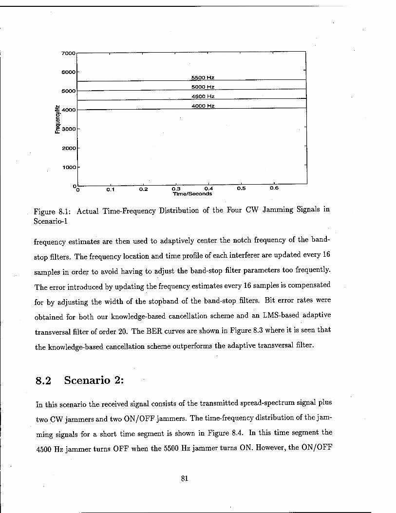
7000

6000

5000

4000

.1^3000

2000

1000

5500 Hz

5000 Hz

4500 Hz

4000 Hz

0.1 0.2 0.3 0.4 Time/Secorids

0.5 0.6

Figure 8.1: Actual Time-Frequency Distribution of the Four CW Jamming Signals in Scenario-1

frequency estimates are then used to adaptively center the notch frequency of the band-

stop filters. The frequency location and time profile of each interferer are updated every 16

samples in order to avoid having to adjust the band-stop filter parameters too frequently.

The error introduced by updating the frequency estimates every 16 samples is compensated

for by adjusting the width of the stopband of the band-stop filters. Bit error rates were

obtained for both our knowledge-based cancellation scheme and an LMS-based adaptive

transversal filter of order 20. The BER curves are shown in Figure 8.3 where it is seen that

the knowledge-based cancellation scheme outperforms the adaptive transversal filter.

8.2 Scenario 2:

In this scenario the received signal consists of the transmitted spread-spectrum signal plus

two CW jammers and two ON/OFF jammers. The time-frequency distribution of the jam-

ming signals for a short time segment is shown in Figure 8.4. In this time segment the

4500 Hz jammer turns OFF when the 5500 Hz jammer turns ON. However, the ON/OFF

81

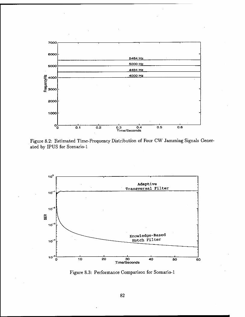
7000

6000

1 1 1 1 ■ i

5484 Hz -

5000 5000 Hz

4484 Hz

5 4000 c 3

4000 Hz

JT3000 ~

2000 -

1000

i i i i 1 « 0.1 0.2 0.3 0.4

Time/Seconds 0.5 0.6

Figure 8.2: Estimated Time-Frequency Distribution of Four CW Jamming Signals Gener- ated by IP US for Scenario-1

10

10-1 f

io

10

10

Adaptive Transversal Filter

Knowledge-Based Notch Filter

10 20 30 40 Time/Seconds

50 60

Figure 8.3: Performance Comparison for Scenario-1

82

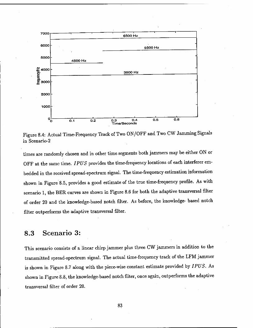
7000

6000

5000

3E 4000 B" c

JT3000

2000

1000

6500 Hz

5500 Hz

4500 Hz

3500 Hz

0.1 0.2 0.3 0.4 Time/Seconds

0.5 0.6

Figure 8.4: Actual Time-Frequency Track of Two ON/OFF and Two CW Jamming Signals in Scenario-2

times are randomly chosen and in other time segments both jammers may be either ON or

OFF at the same time. I PUS provides the time-frequency locations of each interferer em-

bedded in the received spread-spectrum signal. The time-frequency estimation information

shown in Figure 8.5, provides a good estimate of the true time-frequency profile. As with

scenario 1, the BER curves are shown in Figure 8.6 for both the adaptive transversal filter

of order 20 and the knowledge-based notch filter. As before, the knowledge- based notch

filter outperforms the adaptive transversal filter.

8.3 Scenario 3:

This scenario consists of a linear chirp jammer plus three CW jammers in addition to the

transmitted spread-spectrum signal. The actual time-frequency track of the LFM jammer

is shown in Figure 8.7 along with the piece-wise constant estimate provided by I PUS. As

shown in Figure 8.8, the knowledge-based notch filter, once again, outperforms the adaptive

transversal filter of order 20.

83

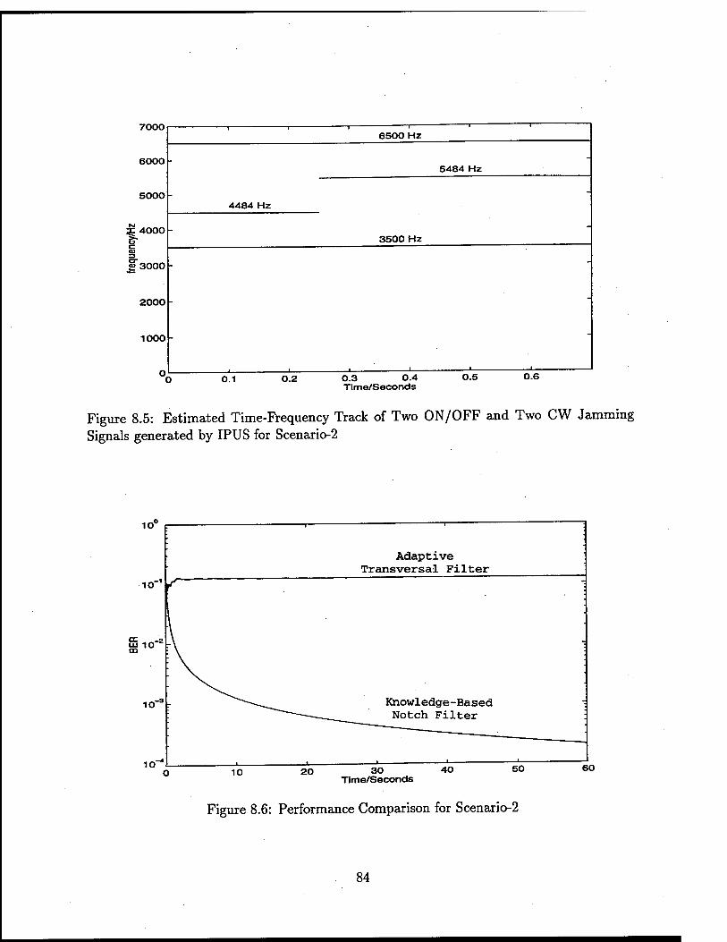
7000

6000

5000

5 4000 B* to

£3000

2000

1000

4484 Hz

0.1 0.2

6500 Hz

5484 Hz

3500 Hz

0.3 0.4 Time/Seconds

0.5 0.6

Figure 8.5: Estimated Time-Frequency Track of Two ON/OFF and Two CW Jamming Signals generated by IPUS for Scenario-2

io s-

10"

IO

Adaptive Transversal Filter

Knowledge-Based Notch Filter

10 20 30 40 Time/Seconds

50 60

Figure 8.6: Performance Comparison for Scenario-2

84

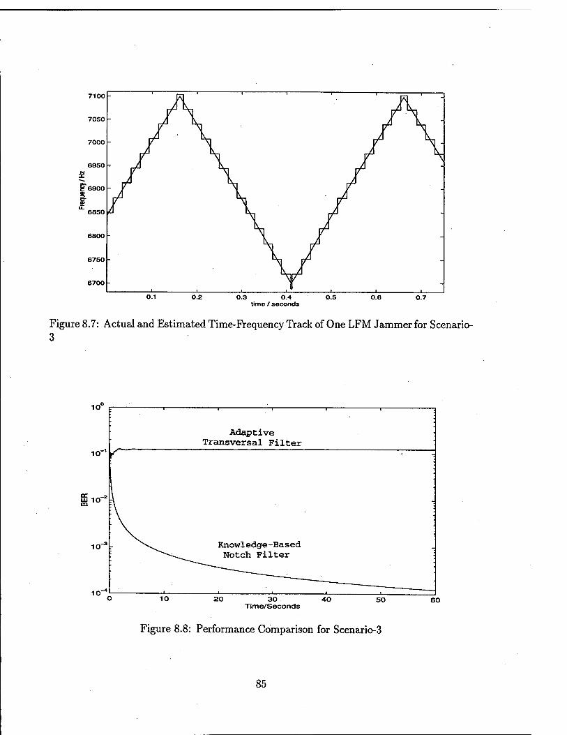
7100 i _ i 1 i -i 1 ——i -

7050 rA \-i

7000 y \i y \" 6950

£ §"6900 a>

¥ /

"~ 6850 i/

6800 y

6750 \ V

6700 1 1 ,, i ■ i i i

0.1 0.2 0.3 0.4 time / seconds

0.5 0.6 0.7

Figure 8.7: Actual and Estimated Time-Frequency Track of One LFM Jammer for Scenario- 3

10"

io-1 <"

Adaptive Transversal Filter

20 30 40 Time/Seconds

Figure 8.8: Performance Comparison for Scenario-3

85

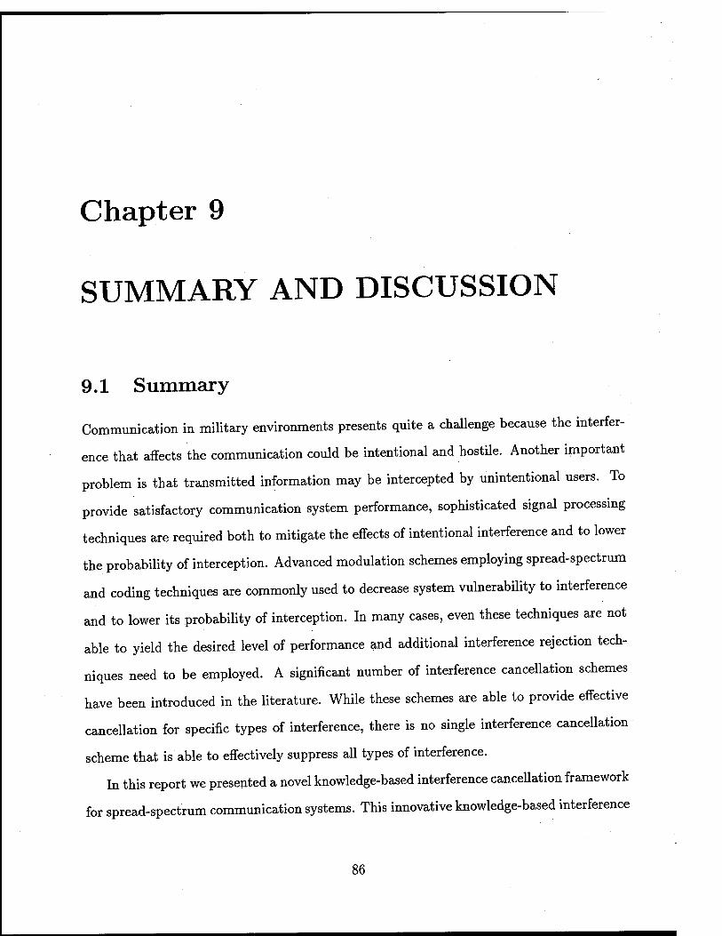
Chapter 9

SUMMARY AND DISCUSSION

9.1 Summary

Communication in military environments presents quite a challenge because the interfer-

ence that affects the communication could be intentional and hostile. Another important

problem is that transmitted information may be intercepted by unintentional users. To

provide satisfactory communication system performance, sophisticated signal processing

techniques are required both to mitigate the effects of intentional interference and to lower

the probability of interception. Advanced modulation schemes employing spread-spectrum

and coding techniques are commonly used to decrease system vulnerability to interference

and to lower its probability of interception. In many cases, even these techniques are not

able to yield the desired level of performance and additional interference rejection tech-

niques need to be employed. A significant number of interference cancellation schemes

have been introduced in the literature. While these schemes are able to provide effective

cancellation for specific types of interference, there is no single interference cancellation

scheme that is able to effectively suppress all types of interference.

In this report we presented a novel knowledge-based interference cancellation framework

for spread-spectrum communication systems. This innovative knowledge-based interference

86

cancellation technique utilizes IPUS, an expert system for the Integrated Processing and

Understanding of Signals, to monitor the communication signal environment in order to

determine the parameters of interfering signals within a prespecified accuracy. After hav-

ing monitored the environment, the knowledge- based interference cancellation technique

selects the most suitable cancellation filter from a library of cancellation filter banks in

order to eliminate the interference signal from the received signal.

In this effort we limited our attention to direct-sequence spread-spectrum communi-

cation systems and to the set of jammers consisting of continuous wave, linear FM and

ON/OFF jammers. We evaluated the performance of our schemes using computer-aided

modeling and simulation techniques.

In addition, extensive experimentation was carried out in the development of rules for

selection of the most suitable interference cancellation schemes. A number of interfer-

ence scenarios were investigated and results demonstrated the superior performance of our

knowledge-based interference cancellation schemes.

9.2 Discussion and Suggestions for Future Work

The goal of this research project was to provide a proof-of-concept demonstration for our

knowledge-based interference cancellation framework. Only a limited set of interferers were

considered in this first phase of the research project. In the next phase, we shall introduce

additional jammers to our set of allowable jammers such as broad-band jammers, hopping

jammers and intelligent jammers. This will require extension of IPUS capabilities to be

able to handle new classes of jammers, development of filter section rules, and inclusion of

additional interference cancellation schemes to the library of interference cancellers.

During our protype development, ideal conditions were assumed, For example, perfect

synchronization between the transmitter and the receiver was assumed. Also, no fading

or multipath on the communication channel was assumed. In the next phase of the effort,

we shall introduce these and other sources of uncertainty. Performance of our knowledge-

87

based scheme in the presence of non-ideal conditions will be investigated and compared

with other interference cancellation algorithms. Thus, robustness of our schemes will be

examined and methods for improving robustness will be determined.

Another interesting problem is the development of knowledge-based adaptive filtering

for interference cancellation. One can investigate the development of reduced order adap-

tive transversal filters based on the interference characteristics available from IPUS. It

is expected that such filters will be much simpler to implement while maintaining their

adaptive behavior in case the information available from IPUS is not accurate enough.

Our research in the first phase concentrated on knowledge-based interference cancel-

lation in the time-domain. Knowledge-based interference cancellation utilizing transform-

domain processing remains to be investigated. The interesting problem then arises of how

to utilize the information available from IPUS most effectively with regard to both time-

domain and in Transform-domain processing.

Thus far, the research has emphasized a knowledge-based approach to interference can-

cellation. However, such propagation characteristics of the transmission medium, as fad-

ing, multipath and additive/multiplicative disturbances should be taken into account in

the operation of a reliable communications link. In addition to the signal processing at

the receiver, these factors can influence transmitter choices dealing with modulation type,

data rate, and transmitted power. It remains to explore how IPUS can be used to char-

acterize the transmission channel and how this information can be employed by both the

transmitter and receiver to improve communications performance.

Finally, with the newer version of SPW, it would be possible to embed IPUS within

SPW. It remains to be investigated whether it would be an effective architecture or the

two should be on different machines to allow for distributed computing.

88

Bibliography

[1] S. Haykin, Digital Communications, Wiley, 1988.

[2] R. C. Dixon, Spread Spectrum Systems, Wiley-Interscience, 1976.

[3] R. L. Pickholtz, D. L. Schilling, and L. B. Milstein, "Theory of Spread-Spectrum

Communications," IEEE Trans, on Commun., vol. COM-30, pp. 885-884, May 1982.

[4] L. B. Milstein, " Interference Rejection Techniques in Spread-Spectrum Communica-

tions," Proceedings of The IEEE, vol. 76, no. 6, pp. 657-671 June 1988.

[5] J. D. Laster, and J. H. Reed, "Interference Rejection in Digital Wireless Communica-

tion," IEEE Signal Processing Magazine, pp.37-62, May 1997.

[6] L. B. Milstein, and P. Das, "An Analysis of a Real-Time Transform Domain Filtering

Digital Communication System, Part 1: Narrowband Interference Rejection," IEEE

Trans. Commun., Vol. COM-28, pp. 816-824, June 1980.

[7] L. B. Milstein, and P. Das, "Spread-Spectrum Receiver Using Acoustic Surface Wave

Technology'" IEEE Trans, on Commun., vol. COM-25, No. 8, pp. 841-847, Aug. 1977.

[8] H. V. Poor, and L. A. Rusch, " Narrowband Interference Suppression in Spread-

Spectrum CDMA," IEEE Personal Communications Magazine, pp. 14-27, Third Quar-

ter 1994.

89

[9] V. R. Lesser, S. H. Nawab, and F. I. Klassner, "IPUS 1 : An Architecture for the

Integrated Processing and Understanding of Signals," Artificial Intelligence, vol. 77,

pp 129-171, 1995.

[10] S. H. Nawab and T. F. Quatieri, "Short-Time Fourier Transform," in Advanced Topics

in Signal Processing Edited by Jae S-Lim and A.V.Oppenheim, Prentice Hall, Engle-

wood Cliffs, N.J., 1988.

[11] F. Klassner, "Data Reprocessing in Signal Understanding Systems," Doctoral disser-

tation, University of Massachusetts, Amherst, September 1996.

[12] Y. Bar-Shalom, and T. E. Fortmann, Tracking and Data Association, Academic Press,

1988.

[13] D. B. Reid, "An Algorithm for Tracking Multiple Targets," IEEE Trans, on Automatic

Control, vol. AC-24, no. 6, pp. 843-54, 1979.

[14] R. A. Singer, "Estimating Optimal Tracking Filter Performance for Manned Maneu-

vering Targets," IEEE Trans, on Aerospace and Electronic Systems, vol. AES-6, no.

4, pp. 473-83, 1970.

[15] E. Kreyszig, Advanced Engineering Mathematics, Seventh Edition, Wiley, 1993.

[16] F. J. Harris, "On the Use of Windows for Harmonic Analysis with the Discrete-Fourier

Transform," Proceedings of the IEEE, vol. 66, no. 1, pp. 51-83, 1995.

[17] J. M. Winograd and S. H. Nawab, "A C++ Software Environment for the Development

of Embedded Signal Processing Systems," Proc. ICASSP 1995, vol. 4, pp. 2715-19,

Detroit, May 1995.

^0 «U.S. GOVERNMENT PRINTING OFFICE: 1999-610-130-81110

MISSION OF

AFRL/INFORMATIONDIRECTORATE (IF)

The advancement and application of information systems science and

technology for aerospace command and control and its transition to air,

space, and ground systems to meet customer needs in the areas of Global

Awareness, Dynamic Planning and Execution, and Global Information

Exchange is the focus of this AFRL organization. The directorate's areas

of investigation include a broad spectrum of information and fusion,

communication, collaborative environment and modeling and simulation,

defensive information warfare, and intelligent information systems

technologies.