ENERGY-EFFICIENT CONTROL OF COMMERCIAL BUILDING HVAC SYSTEMS ANDANALYSIS FOR GRID SUPPORT

By

NAREN SRIVATHS RAMAN

A DISSERTATION PRESENTED TO THE GRADUATE SCHOOLOF THE UNIVERSITY OF FLORIDA IN PARTIAL FULFILLMENT

OF THE REQUIREMENTS FOR THE DEGREE OFDOCTOR OF PHILOSOPHY

UNIVERSITY OF FLORIDA

2021

© 2021 Naren Srivaths Raman

To my parents

ACKNOWLEDGMENTS

I thank my advisor, Dr. Prabir Barooah, for understanding my strengths and weaknesses

right from the beginning and guiding me accordingly throughout my Ph.D. program. He taught

me to communicate scientific ideas in a clear and concise manner. He gave me an opportunity

to work on a variety of projects, always believed in my abilities, and constantly pushed me to

expand my boundaries. I am very grateful for his continuous support.

I would like to thank Dr. Herbert Ingley, as my first exposure to commercial heating,

ventilation, and air conditioning (HVAC) systems was through his course during my master’s

program in the fall of 2011. He has always been very kind, supportive, and has patiently shared

his expertise in HVAC systems.

I thank Dr. Oscar Crisalle and Dr. Matthew Hale for being in my committee, and giving

feedback to improve the quality and presentation of this work. Dr. Oscar Crisalle’s feedback

after my oral proposal has helped in making me a confident speaker.

I am very thankful to Dr. Sean Meyn for providing my first exposure to reinforcement

learning (RL) and several helpful discussions on using RL for various applications and controls

in general. I also thank Dr. Timothy Middelkoop for teaching me to manage the information

technology (IT) infrastructure used to communicate with the energy management system at

the Innovation Hub building.

My special thanks to Skip Rockwell and others from the University of Florida Physical

Plant Division for various helpful discussions and their help with experiments at the Innovation

Hub building. I also thank David Brooks for taking the time to share his expertise in HVAC

systems.

I thank Dr. Jonathan Brooks, Dr. Adithya Devraj, Vignesh Subramaniam, Dr. Surya

Chandan Dhulipala, Karthikeya Devaprasad, Bo Chen, Rahul Umashankar Chaturvedi, Zhong

Guo, Srivattsan Sridharan, my lab-mates, friends, teachers, co-authors of the various papers

I have written, and all others who supported me in any respect during the completion of this

work.

4

I thank my parents and my family for their constant love and support. I dedicate this

dissertation to my parents.

The research reported here was partially supported by the National Science Foundation

through grants 1646229 (CPS/ECCS) and 1934322 (CMMI), the State of Florida through a

REET (Renewable Energy and Energy Efficient Technologies) grant, and the Department of

Energy through GMLC program (Virtual Batteries).

5

TABLE OF CONTENTSpage

ACKNOWLEDGMENTS . . . . . . . . . . . . . . . . . . . . . . . . . . . . . . . . . . . 4

LIST OF TABLES . . . . . . . . . . . . . . . . . . . . . . . . . . . . . . . . . . . . . . 8

LIST OF FIGURES . . . . . . . . . . . . . . . . . . . . . . . . . . . . . . . . . . . . . 9

ABSTRACT . . . . . . . . . . . . . . . . . . . . . . . . . . . . . . . . . . . . . . . . . 12

CHAPTER

1 INTRODUCTION . . . . . . . . . . . . . . . . . . . . . . . . . . . . . . . . . . . 15

2 MPC FOR ENERGY-EFFICIENT HVAC OPERATION WITH HUMIDITY ANDLATENT HEAT CONSIDERATIONS . . . . . . . . . . . . . . . . . . . . . . . . . 18

2.1 Overview . . . . . . . . . . . . . . . . . . . . . . . . . . . . . . . . . . . . . 182.2 Review of Prior Work . . . . . . . . . . . . . . . . . . . . . . . . . . . . . . 212.3 System Description and Models . . . . . . . . . . . . . . . . . . . . . . . . . 25

2.3.1 Hygro-Thermal Dynamics Model . . . . . . . . . . . . . . . . . . . . 272.3.2 Cooling and Dehumidifying Coil Model . . . . . . . . . . . . . . . . . 272.3.3 Power Consumption Models . . . . . . . . . . . . . . . . . . . . . . . 30

2.4 Control Algorithms . . . . . . . . . . . . . . . . . . . . . . . . . . . . . . . . 312.4.1 Proposed Controller: SL-MPC . . . . . . . . . . . . . . . . . . . . . . 312.4.2 Model Predictive Control Incorporating Only Sensible Heat (S-MPC) . 352.4.3 Baseline Control (BL) . . . . . . . . . . . . . . . . . . . . . . . . . . 362.4.4 Information Requirement for Implementation . . . . . . . . . . . . . . 37

2.5 Simulation Setup . . . . . . . . . . . . . . . . . . . . . . . . . . . . . . . . 382.5.1 Plant Parameters and Thermal Comfort Envelope . . . . . . . . . . . 392.5.2 Controller Parameters . . . . . . . . . . . . . . . . . . . . . . . . . . 402.5.3 Performance Metrics . . . . . . . . . . . . . . . . . . . . . . . . . . . 41

2.6 Results and Discussions . . . . . . . . . . . . . . . . . . . . . . . . . . . . . 422.6.1 Results for the Different Outdoor Weather Conditions . . . . . . . . . 42

2.6.1.1 Hot-humid day . . . . . . . . . . . . . . . . . . . . . . . . 422.6.1.2 Mild day . . . . . . . . . . . . . . . . . . . . . . . . . . . . 442.6.1.3 Cold day . . . . . . . . . . . . . . . . . . . . . . . . . . . . 46

2.6.2 Comparison among Controllers . . . . . . . . . . . . . . . . . . . . . 462.7 Summary . . . . . . . . . . . . . . . . . . . . . . . . . . . . . . . . . . . . . 48

3 MPC-BASED HIERARCHICAL CONTROL OF A MULTI-ZONE COMMERCIALHVAC SYSTEM . . . . . . . . . . . . . . . . . . . . . . . . . . . . . . . . . . . . 50

3.1 Overview . . . . . . . . . . . . . . . . . . . . . . . . . . . . . . . . . . . . . 503.2 Comparison with Literature on Multi-Zone MPC . . . . . . . . . . . . . . . . 533.3 System and Problem Description, and Plant Simulator . . . . . . . . . . . . . 543.4 Proposed Multi-Zone Hierarchical Control (MZHC) . . . . . . . . . . . . . . 59

6

3.4.1 MPC-Based High-Level Controller (HLC) . . . . . . . . . . . . . . . . 603.4.2 Projection-Based Low-Level Controller (LLC) . . . . . . . . . . . . . . 65

3.5 Baseline Control (BL) . . . . . . . . . . . . . . . . . . . . . . . . . . . . . . 683.6 Simulation Setup . . . . . . . . . . . . . . . . . . . . . . . . . . . . . . . . 693.7 Results and Discussions . . . . . . . . . . . . . . . . . . . . . . . . . . . . . 74

3.7.1 Hot-Humid Week . . . . . . . . . . . . . . . . . . . . . . . . . . . . 753.7.2 Mild Week . . . . . . . . . . . . . . . . . . . . . . . . . . . . . . . . 773.7.3 Cold Week . . . . . . . . . . . . . . . . . . . . . . . . . . . . . . . . 79

3.8 Summary . . . . . . . . . . . . . . . . . . . . . . . . . . . . . . . . . . . . . 79

4 ANALYSIS OF ROUND-TRIP EFFICIENCY OF AN HVAC-BASED VIRTUAL BATTERY 82

4.1 Overview . . . . . . . . . . . . . . . . . . . . . . . . . . . . . . . . . . . . . 824.2 Definitions and Other Preliminaries . . . . . . . . . . . . . . . . . . . . . . . 85

4.2.1 Round-Trip Efficiency of an Electrochemical Battery . . . . . . . . . . 854.2.2 Round-Trip Efficiency of an HVAC-Based VES System . . . . . . . . . 864.2.3 Charging vs. Change in SoC . . . . . . . . . . . . . . . . . . . . . . . 87

4.3 Model of an HVAC-Based VES System . . . . . . . . . . . . . . . . . . . . . 884.3.1 Thermal Dynamics of HVAC-Based VES . . . . . . . . . . . . . . . . 894.3.2 HVAC Power Consumption Model . . . . . . . . . . . . . . . . . . . . 904.3.3 VES System Dynamics and Power Consumption . . . . . . . . . . . . 92

4.4 RTE with Zero-Mean Square-Wave Power Consumption . . . . . . . . . . . . 934.4.1 A Single Period of Square-Wave Power Consumption . . . . . . . . . . 944.4.2 Multiple Periods of Square-Wave Power Consumption . . . . . . . . . 984.4.3 Numerical Verification . . . . . . . . . . . . . . . . . . . . . . . . . . 100

4.5 RTE with Nonzero-Mean Square-Wave Power Consumption . . . . . . . . . . 1024.5.1 Nonzero-Mean Power Deviation to Ensure Zero-Mean Temperature

Deviation . . . . . . . . . . . . . . . . . . . . . . . . . . . . . . . . . 1024.5.2 Effect of Various Parameters on η∞rt . . . . . . . . . . . . . . . . . . . 105

4.5.2.1 Building size . . . . . . . . . . . . . . . . . . . . . . . . . . 1064.5.2.2 Time period of the power deviation . . . . . . . . . . . . . . 107

4.6 Summary . . . . . . . . . . . . . . . . . . . . . . . . . . . . . . . . . . . . . 108

5 CONCLUSION . . . . . . . . . . . . . . . . . . . . . . . . . . . . . . . . . . . . . 109

APPENDIX

A PROOFS . . . . . . . . . . . . . . . . . . . . . . . . . . . . . . . . . . . . . . . . 111

B EXPRESSIONS FOR ∆P AND TO . . . . . . . . . . . . . . . . . . . . . . . . . . 118

REFERENCES . . . . . . . . . . . . . . . . . . . . . . . . . . . . . . . . . . . . . . . . 121

BIOGRAPHICAL SKETCH . . . . . . . . . . . . . . . . . . . . . . . . . . . . . . . . . 129

7

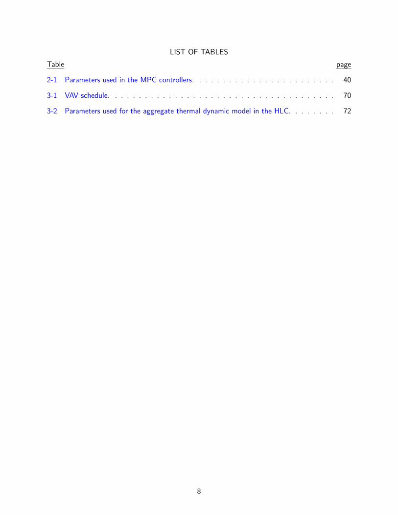
LIST OF TABLESTable page

2-1 Parameters used in the MPC controllers. . . . . . . . . . . . . . . . . . . . . . . . 40

3-1 VAV schedule. . . . . . . . . . . . . . . . . . . . . . . . . . . . . . . . . . . . . . 70

3-2 Parameters used for the aggregate thermal dynamic model in the HLC. . . . . . . . 72

8

LIST OF FIGURESFigure page

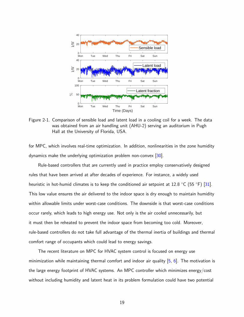
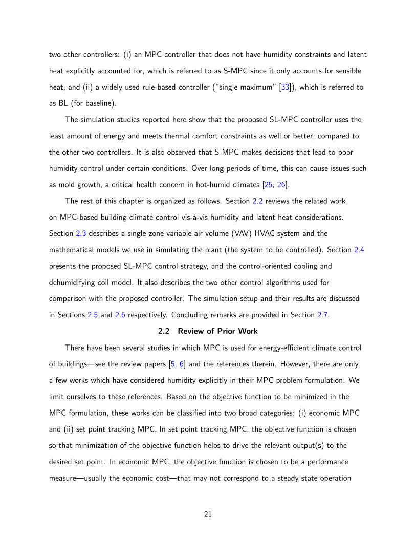
2-1 Comparison of sensible load and latent load in a cooling coil for a week. The datawas obtained from an air handling unit (AHU-2) serving an auditorium in Pugh Hallat the University of Florida, USA. . . . . . . . . . . . . . . . . . . . . . . . . . . . 19

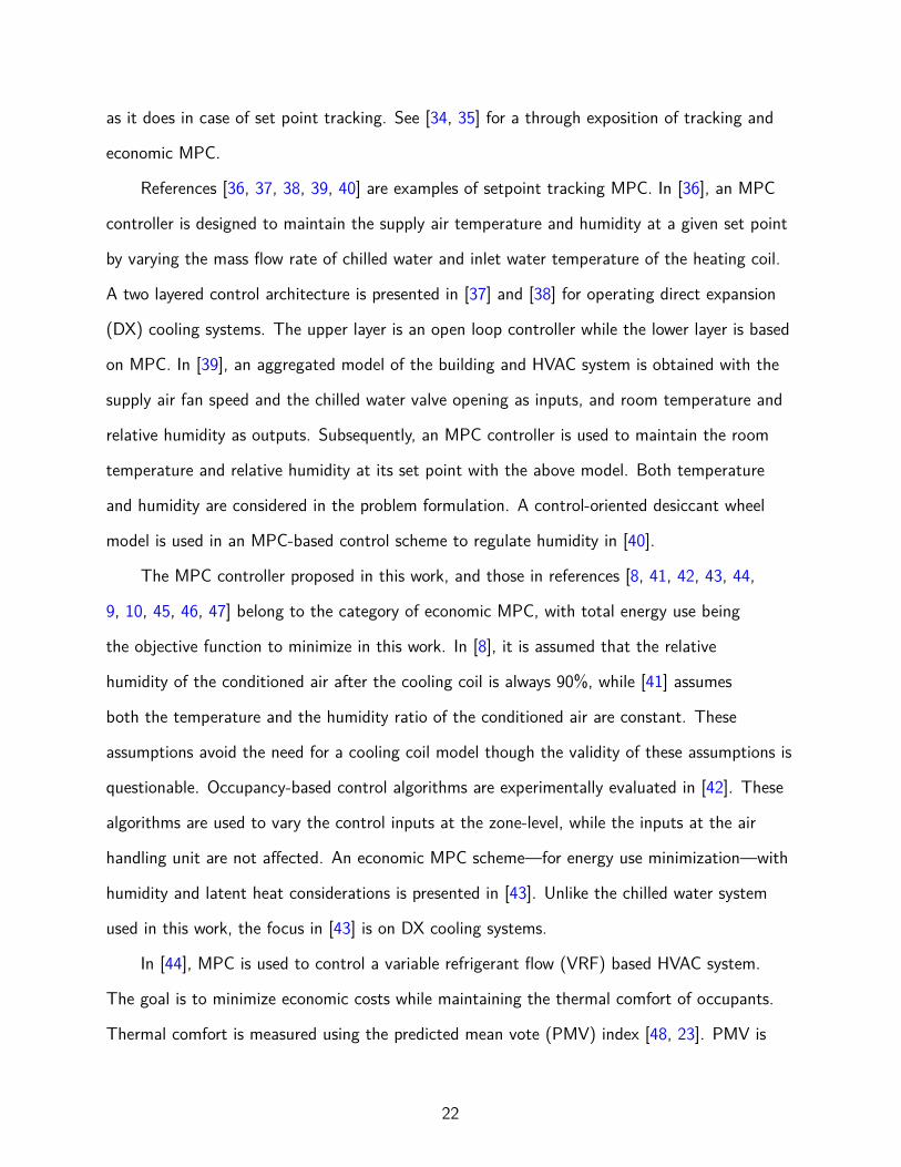
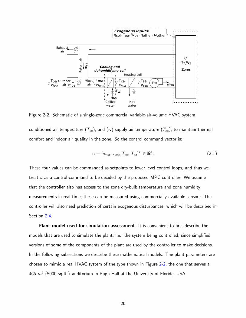
2-2 Schematic of a single-zone commercial variable-air-volume HVAC system. . . . . . . 26

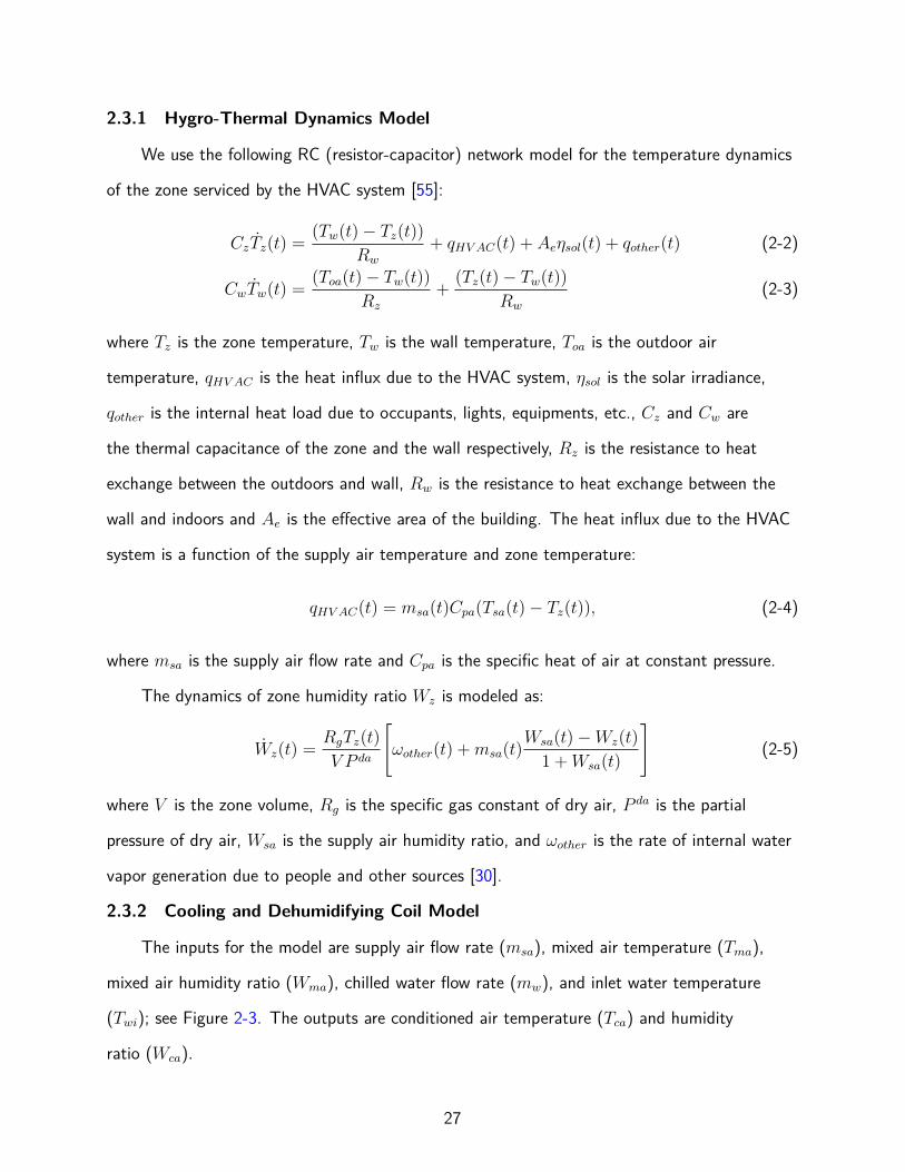
2-3 A cooling and dehumidifying coil, and relevant variables (model inputs in rectangles,outputs in circles). . . . . . . . . . . . . . . . . . . . . . . . . . . . . . . . . . . . 28

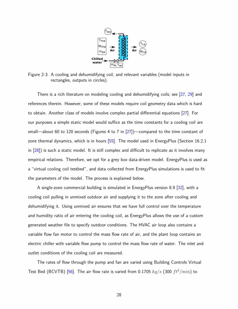
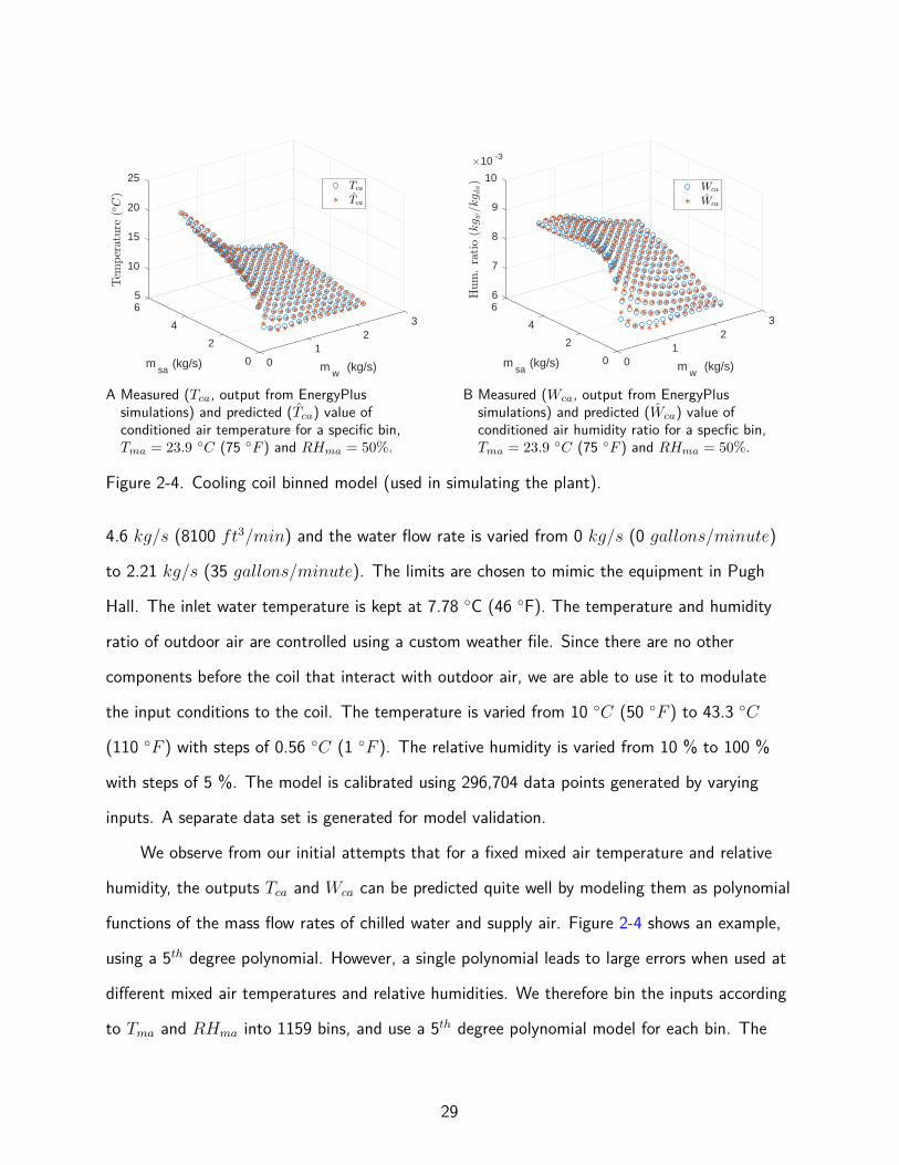
2-4 Cooling coil binned model (used in simulating the plant). . . . . . . . . . . . . . . 29

2-5 Proposed SL-MPC control architecture. . . . . . . . . . . . . . . . . . . . . . . . . 31

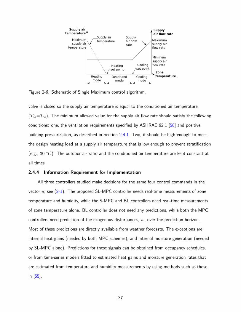
2-6 Schematic of Single Maximum control algorithm. . . . . . . . . . . . . . . . . . . . 37

2-7 Thermal comfort envelope from [1] shown as the hatched areas. Comfort envelopechosen in this work shown as the shaded area during scheduled hours of occupancyand the unshaded area enclosed by dashed line during unoccupied hours. . . . . . . 39

2-8 Comparison of the three controllers for a hot-humid day (August/06/2016, Gainesville,Florida, USA). The scheduled hours of occupancy are shown as the gray shaded area. 42

2-9 Comparison of the three controllers for a mild day (March/25/2016, Gainesville,Florida, USA). The scheduled hours of occupancy are shown as the gray shaded area. 45

2-10 Comparison of controllers’ performance. . . . . . . . . . . . . . . . . . . . . . . . 47

3-1 Schematic of a multi-zone—specifically, a two zone—commercial variable-air-volumeHVAC system. In this figure, oa: outdoor air, ra: return air, ma: mixed air, ca: conditionedair, and sa: supply air. . . . . . . . . . . . . . . . . . . . . . . . . . . . . . . . . . 51

3-2 Innovation Hub building located at the University of Florida campus. . . . . . . . . 56

3-3 Floor plans of the southern half of phase-1 which is serviced by AHU-2. . . . . . . . 56

3-4 Floor 1 of the virtual building created in Dymola using components from the IDEASlibrary [2]. . . . . . . . . . . . . . . . . . . . . . . . . . . . . . . . . . . . . . . . 57

3-5 Structure of the proposed multi-zone hierarchical controller (MZHC). We denoteestimates as • and forecasts as ˆ•. Variables with a subscript i are for the individualzones, while the variables with a subscript f represent the aggregate quantities foreach floor/meta-zone. In this figure, Tz,f , Wz,f , qac,f , Tz,f , Tw,f , ˆqint,f , ˆωint,f , andTHLCz,f are ∀f ∈ F; msa,i and Tz,i are for i ∈ If , ∀f ∈ F; Tsa,i is for i ∈ Irh,f , ∀f ∈ F. 60

3-6 Schematic of the Dual Maximum control algorithm. . . . . . . . . . . . . . . . . . 68

9

3-7 Thermal comfort envelope from [1] shown as the hatched areas. Comfort envelopechosen in this chapter shown as the green shaded area. . . . . . . . . . . . . . . . 71

3-8 Out of sample aggregate zone temperature (Tz,f ) prediction results using the estimatedaggregate RC network model. . . . . . . . . . . . . . . . . . . . . . . . . . . . . . 73

3-9 Comparison of the total energy consumed for a week when using the baseline (BL)and proposed (MZHC) controllers for different outdoor weather conditions. . . . . . 74

3-10 Comparison of the two controllers for a hot-humid week (Jul/06 to Jul/13, Gainesville,Florida, USA). . . . . . . . . . . . . . . . . . . . . . . . . . . . . . . . . . . . . . 76

3-11 Individual zone conditions (temperatures and relative humidities) when using MZHCand BL for a hot-humid week. The black dashed lines are the thermal comfort limits. 77

3-12 Comparison of the two controllers for a mild week (Feb/19 to Feb/26, Gainesville,Florida, USA). . . . . . . . . . . . . . . . . . . . . . . . . . . . . . . . . . . . . . 78

4-1 Simplified schematic of a commercial variable-air-volume HVAC system. . . . . . . . 88

4-2 VES system; we assume that the VES controller provides perfect tracking so thatP (t) tracks P r(t). . . . . . . . . . . . . . . . . . . . . . . . . . . . . . . . . . . . 89

4-3 Up/down scenario, possibility 1: since T (2tp) > 0 additional charging is neededto bring back T to its initial value(=0). Possibility 2: since T (2tp) < 0 additionaldischarging is needed to bring back T to its initial value(=0). . . . . . . . . . . . . 94

4-4 Down/up scenario, possibility 1: since T (2tp) > 0 additional charging is needed tobring back T to its initial value (=0). Possibility 2: since T (2tp) < 0 additionaldischarging is needed to bring back T to its initial value (=0). . . . . . . . . . . . . 95

4-5 ηrt vs. tp, for roa = 1 and roa = 0.5; ∆P = 0.2P(b)hvac. The vertical line shown is t∗p

(≈12 minutes) computed from (4-24) for roa = 1. . . . . . . . . . . . . . . . . . . 97

4-6 Fan power vs. airflow rate; measurements from AHU-2 of Pugh Hall at UF (circles),and predictions from the best fit model (4-9) to the measurements (curve). . . . . . 97

4-7 Additional charging or discharging needed to bring T to its initial value (=0) aftern periods of down/up cycle. . . . . . . . . . . . . . . . . . . . . . . . . . . . . . . 98

4-8 Robustness to modeling assumptions. . . . . . . . . . . . . . . . . . . . . . . . . . 101

4-9 Zero-mean power deviation leads to a nonzero-mean temperature deviation at steadystate (plot shown on the bottom right corner). The values used were: ∆P = 0.3P (b)

hvac= 2917.7 W, roa = 0.5, and 2tp = 3600 seconds. . . . . . . . . . . . . . . . . . . . 103

10

4-10 Nonzero-mean power deviation used to ensure that the temperature deviation atsteady state is zero-mean (plot shown on the bottom right corner). The value of∆P used was 168.6 W, for P (b)

hvac = 9725.6 W and ∆P = 0.3P(b)hvac = 2917.7 W,

computed from (B-1). Also roa = 0.5 and 2tp = 3600 seconds. . . . . . . . . . . . 103

4-11 Nonzero-mean power deviation to ensure zero-mean temperature deviation (at steadystate). As before, the time trecov is the time needed to bring the temperature deviationto 0 after n periods of the square-wave power deviation. To is the maximum valueof T after the building reaches steady state. . . . . . . . . . . . . . . . . . . . . . 104

4-12 ηrt vs n, when the virtual battery tracks a nonzero-mean square-wave power consumptionso that the average steady state temperature deviation is zero. η∞rt = 0.8907 for∆P = 0.3P

(b)hvac = 2917.7 W, roa = 0.5, and 2tp = 3600 seconds. . . . . . . . . . . 105

4-13 η∞rt (left axis) and RC (right axis) vs. building size; for roa = 0.5. Case (i): Same∆P (1945.1 W) irrespective of building size. Case (ii): ∆P increasing with buildingsize. . . . . . . . . . . . . . . . . . . . . . . . . . . . . . . . . . . . . . . . . . . 106

4-14 η∞rt vs. time period (2tp); for roa = 0.5 and ∆P = 0.2P(b)hvac = 1945.1 W. . . . . . . 107

11

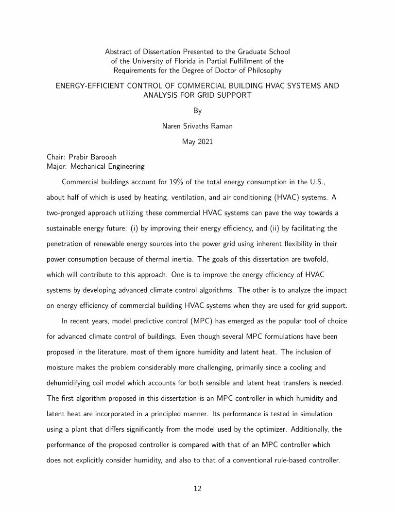
Abstract of Dissertation Presented to the Graduate Schoolof the University of Florida in Partial Fulfillment of theRequirements for the Degree of Doctor of Philosophy

ENERGY-EFFICIENT CONTROL OF COMMERCIAL BUILDING HVAC SYSTEMS ANDANALYSIS FOR GRID SUPPORT

By

Naren Srivaths Raman

May 2021

Chair: Prabir BarooahMajor: Mechanical Engineering

Commercial buildings account for 19% of the total energy consumption in the U.S.,

about half of which is used by heating, ventilation, and air conditioning (HVAC) systems. A

two-pronged approach utilizing these commercial HVAC systems can pave the way towards a

sustainable energy future: (i) by improving their energy efficiency, and (ii) by facilitating the

penetration of renewable energy sources into the power grid using inherent flexibility in their

power consumption because of thermal inertia. The goals of this dissertation are twofold,

which will contribute to this approach. One is to improve the energy efficiency of HVAC

systems by developing advanced climate control algorithms. The other is to analyze the impact

on energy efficiency of commercial building HVAC systems when they are used for grid support.

In recent years, model predictive control (MPC) has emerged as the popular tool of choice

for advanced climate control of buildings. Even though several MPC formulations have been

proposed in the literature, most of them ignore humidity and latent heat. The inclusion of

moisture makes the problem considerably more challenging, primarily since a cooling and

dehumidifying coil model which accounts for both sensible and latent heat transfers is needed.

The first algorithm proposed in this dissertation is an MPC controller in which humidity and

latent heat are incorporated in a principled manner. Its performance is tested in simulation

using a plant that differs significantly from the model used by the optimizer. Additionally, the

performance of the proposed controller is compared with that of an MPC controller which

does not explicitly consider humidity, and also to that of a conventional rule-based controller.

12

Simulations show that the proposed MPC controller outperforms the other two consistently. It

is also observed that under certain conditions, the MPC formulation which does not consider

humidity leads to poor humidity control, or higher energy usage as it is unaware of the latent

load on the cooling coil.

The controller proposed above is primarily for single-zone buildings. Several of the

MPC formulations proposed in the literature are also for buildings with one zone or a small

number of zones. A direct extension of such formulations for large multi-zone buildings

has two main challenges: (i) the optimization problem in MPC is computationally complex

because of the large number of decision variables, and (ii) it requires a high-resolution model

of the thermal dynamics of the multi-zone building. To overcome these challenges, a novel

MPC-based hierarchical architecture is proposed. Unlike prior works we do not assume the

availability of a high-resolution multi-zone building model. Instead, the architecture uses a

low-resolution model of the building which is divided into a small number of “meta-zones”

that can be easily identified using existing data-driven modeling techniques. At the higher

level, an MPC controller uses the low-resolution model to make decisions for the air handling

unit (AHU) and the meta-zones. Since the meta-zones are fictitious, a lower level controller

converts the high-level MPC decisions into commands for the individual zones by solving

a projection problem that strikes a trade-off between two potentially conflicting goals: the

AHU-level decisions made by the MPC are respected while the climate of the individual

zones is maintained within the comfort bounds. The performance of the proposed controller

is assessed via simulations in a high-fidelity simulation testbed and compared to that of a

rule-based controller that is used in practice. Simulations in multiple weather conditions show

the effectiveness of the proposed controller in terms of energy savings, climate control, and

computational tractability.

In the second part of this work, the impact on the energy efficiency of commercial building

HVAC systems when they are used for grid support is analyzed. Flexible loads, especially

HVAC systems can be used to provide a battery-like service to the power grid by varying their

13

demand up and down over a baseline. Recent work has reported that providing virtual energy

storage with HVAC systems leads to a net loss of energy, akin to a low round-trip efficiency

(RTE) of a battery. In this work, we rigorously analyze the RTE of a virtual battery through a

simplified physics-based model. We show that the low RTEs reported in recent experimental

and simulation work are an artifact of the experimental/simulation setup. When the HVAC

system is repeatedly used as a virtual battery, the asymptotic RTE is 1. Robustness of the

result to assumptions made in the analysis is illustrated through a simulation case study. We

also show that when an additional constraint is imposed—that the mean temperature of the

building must remain the same—the asymptotic RTE can be lower than 1. Dependence on

parameter values is explored numerically.

14

CHAPTER 1INTRODUCTION

Commercial buildings account for 19% of the total energy consumption in the U.S. [3], of

which about 44% is used by heating, ventilation, and air conditioning (HVAC) systems [4].

The vision for a sustainable energy future is to reduce greenhouse gas emissions and

increase the utilization of renewable energy sources. A two-pronged approach using HVAC

systems in commercial buildings—which have such a large energy footprint—can pave the

way towards this vision: (i) by improving their energy efficiency, and (ii) by facilitating the

penetration of renewable energy sources into the grid using inherent flexibility in their power

consumption because of thermal inertia.

A cost-effective way to improve the energy efficiency of HVAC systems is by using

advanced climate control algorithms. This is especially so in commercial buildings, as most

modern-day commercial buildings are already equipped with the required sensors, actuators,

and communication infrastructure, and have a significant amount of data available [5].

Moreover, currently used control algorithms are rule-based and utilize conservatively designed

set points, which do not make full use of the available resources.

In the first part of this work, advanced climate control algorithms are developed

to improve the energy efficiency of HVAC systems. In recent years, model predictive

control (MPC) has emerged as the popular tool of choice for advanced climate control of

buildings [5, 6]. A main reason for this is that MPC can satisfy conflicting goals such as

keeping energy use small while maintaining thermal comfort and indoor air quality. In MPC,

control commands for a planning horizon are decided at every decision instant by solving an

optimization problem, implementing only the first segment of the plan, and then repeating the

process ad infinitum. Because of its use of numerical optimization, MPC can handle various

constraints that are otherwise challenging to ensure, which has led to the success of MPC in

many applications [7]. Therefore, we focus on MPC-based control algorithms in this study.

15

Several MPC formulations have been proposed in the literature for energy-efficient climate

control of buildings [5, 6]; however, most of them ignore humidity and latent heat. An MPC

controller which minimizes energy/cost without including humidity and latent heat in its

problem formulation could have two potential issues particularly in hot-humid climates. One,

it may lead to poor humidity control. Two, since the latent component of cooling—energy

required to dehumidify air—is not accounted for in the objective function, the predicted energy

use by the controller may be far from the actual energy use when the controller is used in

practice. The first contribution of this dissertation is the development of an MPC controller

in which humidity and latent heat are incorporated in a principled manner. This controller is

presented in Chapter 2.

The controller presented in Chapter 2 is primarily for single-zone buildings. Many of

the MPC formulations proposed in the literature are also for buildings with one zone [8, 9,

10] or a small number of zones [11, 12]. A direct extension of such formulations for large

multi-zone buildings has two main challenges: (i) the underlying optimization problem in

MPC is computationally complex because of the large number of decision variables, and (ii) it

requires a high-resolution model of the thermal dynamics a multi-zone building, which is much

more difficult to obtain when compared to a single-zone building model. To overcome these

challenges, a novel hierarchical architecture is proposed for MPC-based energy-efficient control

of HVAC systems in multi-zone buildings. This is the second contribution of the dissertation

and is presented in Chapter 3.

In the second part of this work, the impact on energy-efficiency of commercial building

HVAC systems when they are used for grid support is analyzed. The power grid is a complex

network of generators and loads. For a reliable operation of the power grid, generation should

be equal to the load [13]. With greater penetration of renewable energy sources, especially

solar and wind, maintaining this balance has become challenging as these sources are volatile

and uncontrollable. Fossil-fuel based generators cannot provide the rapid ramping needed to

offset the volatility of such renewable sources due to their operating constraints. Large-scale

16

electrical energy storage is an option, but it is expensive [14]. In recent years, it has been

recognized that the power demand of certain electric loads is flexible, allowing it to be varied

above and below a baseline, and can be used to provide a battery-like service to the power

grid. Thus, such a load, or collection of loads, can be called virtual batteries (VB) or virtual

energy storage (VES) systems [15]. HVAC systems in commercial buildings are a great resource

for this as they consume a significant amount of power, have huge thermal inertia, and are

equipped with the necessary control and communication infrastructure [16].

Consumers’ quality of service (QoS) must be maintained by these virtual batteries. When

HVAC systems are used for VES, a key QoS measure is indoor temperature. Another important

QoS measure is the total energy consumption. Continuously varying the power consumption

of loads around a baseline may lead to a net reduction in the efficiency of energy use, causing

the load to consume more energy in the long run. If so, that will be analogous to the virtual

battery having a round-trip efficiency (RTE) less than unity. Electrochemical batteries also

have a less-than-unity round-trip efficiency due to various losses [17]. The aim of Chapter 4 is

to analyze the RTE of a VES system comprised of HVAC equipment in commercial buildings.

This is the third contribution of the dissertation.

This document is organized as follows. The MPC controller primarily for single-zone

buildings is presented in Chapter 2, which is available in [18, 19]. The MPC-based hierarchical

controller for multi-zone buildings is presented in Chapter 3. This work has been submitted

to a journal and is currently under review; it is available in [20]. In Chapter 4, the effects

of providing grid support on energy efficiency are analyzed. These results are published

in [21, 22]. Chapter 5 concludes this dissertation and discusses topics for future work.

17

CHAPTER 2MPC FOR ENERGY-EFFICIENT HVAC OPERATION WITH HUMIDITY AND LATENT

HEAT CONSIDERATIONS

2.1 Overview

In this chapter, an MPC formulation for energy-efficient climate control of a commercial

building in which humidity and latent heat are taken into account in a principled manner is

presented.

As explained in Chapter 1, a main reason for the popularity of using MPC for building

climate control is that it can satisfy conflicting goals such as keeping energy use small while

maintaining thermal comfort and indoor air quality. Thermal comfort of occupants is influenced

by several factors such as space temperature, humidity, air speed, clothing, metabolic rate,

etc. [23]. Space temperature and humidity are especially important factors in determining

comfort and health [24, 25, 26]. Despite the importance of humidity and latent heat in

building climate control, it is ignored in most existing MPC formulations.

The principal challenge in including humidity and latent heat is that variables that

determine the building’s temperature and humidity—humidity and temperature of the

conditioned air—are a complex function of control commands, and cannot be independently

chosen. The control commands that can be independently chosen are inlet conditions of the

cooling coil that cools and dehumidifies the air supplied to the indoor space. Incorporating

humidity into MPC requires a model of the cooling and dehumidifying coil that accounts for

both sensible and latent heat transfers, and predicts how control commands (conditions at the

coil inlet) determines the temperature and humidity of the conditioned air. Such models are

usually highly complex. Some are partial differential equations (PDEs) with a large number

of parameters and several sub-models based on the condition of the cooling coil such as

completely dry, completely wet, and partly wet [27]. Some are ordinary differential equations or

even static models consisting of a large number of empirical relations that vary depending on

coil geometry, configuration, and manufacturer [28, 29]. Such complex models are not suitable

18

Mon Tue Wed Thu Fri Sat Sun0

20

40

Sensible load

Mon Tue Wed Thu Fri Sat Sun0

20

40

Latent load

Mon Tue Wed Thu Fri Sat Sun

Time (Days)

0

50

100

Latent fraction

Figure 2-1. Comparison of sensible load and latent load in a cooling coil for a week. The datawas obtained from an air handling unit (AHU-2) serving an auditorium in PughHall at the University of Florida, USA.

for MPC, which involves real-time optimization. In addition, nonlinearities in the zone humidity

dynamics make the underlying optimization problem non-convex [30].

Rule-based controllers that are currently used in practice employ conservatively designed

rules that have been arrived at after decades of experience. For instance, a widely used

heuristic in hot-humid climates is to keep the conditioned air setpoint at 12.8 ◦C (55 ◦F) [31].

This low value ensures the air delivered to the indoor space is dry enough to maintain humidity

within allowable limits under worst-case conditions. The downside is that worst-case conditions

occur rarely, which leads to high energy use. Not only is the air cooled unnecessarily, but

it must then be reheated to prevent the indoor space from becoming too cold. Moreover,

rule-based controllers do not take full advantage of the thermal inertia of buildings and thermal

comfort range of occupants which could lead to energy savings.

The recent literature on MPC for HVAC system control is focused on energy use

minimization while maintaining thermal comfort and indoor air quality [5, 6]. The motivation is

the large energy footprint of HVAC systems. An MPC controller which minimizes energy/cost

without including humidity and latent heat in its problem formulation could have two potential

19

issues. One, it may lead to poor humidity control. Two, since the latent component of

cooling—energy required to dehumidify air—is not accounted for in the objective function,

the predicted energy use by the controller may be far from the actual energy use when the

controller is used in practice. Figure 2-1 shows the sensible load, latent load, and the latent

fraction (ratio of latent load to the total load) in a cooling coil for a week which was obtained

from an air handling unit (AHU-2) serving an auditorium in Pugh Hall at the University of

Florida, USA. It can be seen that the latent load is not negligible and constitutes about 41% of

the total cooling load.

In this chapter, we propose an MPC formulation for energy-efficient climate control of a

commercial building in which humidity and latent heat are taken into account in a principled

manner. The proposed controller is hereafter referred to as SL-MPC, because it accounts

for both sensible and latent components of cooling. We specifically focus on a single-zone

variable-air-volume (VAV) HVAC system that uses chilled water to cool and dehumidify, i.e.,

condition the air supplied to the building. Figure 2-2 shows the schematic of a VAV HVAC

system.

As mentioned earlier, one of the main challenges of including humidity and latent heat

is the need for a cooling and dehumidifying coil model that is simple enough to be used in

real-time optimization and yet accurate enough to lead to useful results. To address this

challenge we develop a data-driven low order model that predicts temperature and humidity of

the conditioned air (outputs) as a function of the inputs: the temperature, humidity and flow

rate of air incident on the coil, and temperature and flow rate of chilled water entering the coil.

This model is used in the optimizer used by the MPC controller. We also develop a slightly

more complex, but much higher accuracy, data-driven model that is used to simulate the plant.

Both models are identified from data, which can come from experiments or from software such

as EnergyPlus [32].

Apart from the proposed MPC controller and the data-driven cooling coil models, a third

contribution of this work is a comparison of the performance of the proposed controller with

20

two other controllers: (i) an MPC controller that does not have humidity constraints and latent

heat explicitly accounted for, which is referred to as S-MPC since it only accounts for sensible

heat, and (ii) a widely used rule-based controller (“single maximum” [33]), which is referred to

as BL (for baseline).

The simulation studies reported here show that the proposed SL-MPC controller uses the

least amount of energy and meets thermal comfort constraints as well or better, compared to

the other two controllers. It is also observed that S-MPC makes decisions that lead to poor

humidity control under certain conditions. Over long periods of time, this can cause issues such

as mold growth, a critical health concern in hot-humid climates [25, 26].

The rest of this chapter is organized as follows. Section 2.2 reviews the related work

on MPC-based building climate control vis-à-vis humidity and latent heat considerations.

Section 2.3 describes a single-zone variable air volume (VAV) HVAC system and the

mathematical models we use in simulating the plant (the system to be controlled). Section 2.4

presents the proposed SL-MPC control strategy, and the control-oriented cooling and

dehumidifying coil model. It also describes the two other control algorithms used for

comparison with the proposed controller. The simulation setup and their results are discussed

in Sections 2.5 and 2.6 respectively. Concluding remarks are provided in Section 2.7.

2.2 Review of Prior Work

There have been several studies in which MPC is used for energy-efficient climate control

of buildings—see the review papers [5, 6] and the references therein. However, there are only

a few works which have considered humidity explicitly in their MPC problem formulation. We

limit ourselves to these references. Based on the objective function to be minimized in the

MPC formulation, these works can be classified into two broad categories: (i) economic MPC

and (ii) set point tracking MPC. In set point tracking MPC, the objective function is chosen

so that minimization of the objective function helps to drive the relevant output(s) to the

desired set point. In economic MPC, the objective function is chosen to be a performance

measure—usually the economic cost—that may not correspond to a steady state operation

21

as it does in case of set point tracking. See [34, 35] for a through exposition of tracking and

economic MPC.

References [36, 37, 38, 39, 40] are examples of setpoint tracking MPC. In [36], an MPC

controller is designed to maintain the supply air temperature and humidity at a given set point

by varying the mass flow rate of chilled water and inlet water temperature of the heating coil.

A two layered control architecture is presented in [37] and [38] for operating direct expansion

(DX) cooling systems. The upper layer is an open loop controller while the lower layer is based

on MPC. In [39], an aggregated model of the building and HVAC system is obtained with the

supply air fan speed and the chilled water valve opening as inputs, and room temperature and

relative humidity as outputs. Subsequently, an MPC controller is used to maintain the room

temperature and relative humidity at its set point with the above model. Both temperature

and humidity are considered in the problem formulation. A control-oriented desiccant wheel

model is used in an MPC-based control scheme to regulate humidity in [40].

The MPC controller proposed in this work, and those in references [8, 41, 42, 43, 44,

9, 10, 45, 46, 47] belong to the category of economic MPC, with total energy use being

the objective function to minimize in this work. In [8], it is assumed that the relative

humidity of the conditioned air after the cooling coil is always 90%, while [41] assumes

both the temperature and the humidity ratio of the conditioned air are constant. These

assumptions avoid the need for a cooling coil model though the validity of these assumptions is

questionable. Occupancy-based control algorithms are experimentally evaluated in [42]. These

algorithms are used to vary the control inputs at the zone-level, while the inputs at the air

handling unit are not affected. An economic MPC scheme—for energy use minimization—with

humidity and latent heat considerations is presented in [43]. Unlike the chilled water system

used in this work, the focus in [43] is on DX cooling systems.

In [44], MPC is used to control a variable refrigerant flow (VRF) based HVAC system.

The goal is to minimize economic costs while maintaining the thermal comfort of occupants.

Thermal comfort is measured using the predicted mean vote (PMV) index [48, 23]. PMV is

22

dependent on several variables one of which is humidity. Even though humidity is explicitly

considered in this work, unlike the chilled water system used in our work, the focus is on a VRF

system.

A framework which concurrently optimizes thermal and electric storage in buildings is

presented in [47]. The goal of the optimizer is to reduce the operating cost and demand

peaks under time-of-use tariffs by varying the temperature setpoints of the zones in a building

and battery dispatch. In [9], MPC is used to optimize the performance of a hydronic radiant

floor system in an office building. However, the humidity in the building is controlled using a

proportional-integral (PI) controller, and is not considered in the MPC formulation.

In [10], MPC is used to control an environmental chamber located at the Pennsylvania

State University campus. Humidity is indirectly considered through a data-driven thermal

comfort model (dynamic thermal sensation model) developed by the authors. However, latent

heat is ignored in the MPC formulation. In [46], a token based scheduling algorithm is used

to minimize the energy consumption for a building located at the Nanyang Technological

University, Singapore campus. It is based on a distributed control algorithm presented in [49],

and is used to vary the supply air flow rate to the zones. Humidity is indirectly maintained

through the thermal sensation model used but latent heat is ignored.

Ref. [45] provides a comprehensive MPC framework which uses real-time building energy

management system data. An enthalpy control algorithm is used to regulate the amount of

outdoor air supplied to a building.

There are also a few papers in which the terms in the objective function consist of both

energy use and deviation from set points, so these can be thought of as a hybrid between

tracking and economic MPC—[50, 51, 52]. Multiple MPC strategies are compared for an air

handling unit serving a single-zone in [50]. It is assumed that the temperature and humidity

ratio after the cooling coil can be chosen independently, thereby not requiring the use of a

cooling coil model. This assumption will not hold in physical systems, as the only variables that

can be independently chosen are the inlet conditions to the coil. Unlike the cooling-based air

23

dehumidification considered in this work, reference [51] uses a liquid desiccant air conditioning

(LDAC) system. The inlet desiccant solution flow rate and temperature are varied to maintain

the temperature and humidity ratio of the outlet air.

Ref. [52] is the most relevant to our work; they use a cooling coil model in their

optimization in which temperature and humidity of the conditioned air is modeled correctly

to be thermodynamically coupled. The supply air flow rate is not a control command, while

in our formulation it is. The controller in [52] will be unaware of disturbances in the longer

time scales, since a short prediction horizon of 10 minutes is used. In contrast, we use a

prediction horizon of 24 hours. Moreover, there are multiple elements included in the objective

function: energy use, thermal comfort, indoor air quality, etc., which needs careful tuning of

weights. In our formulation, energy use is the objective to be minimized, with thermal comfort

and indoor air quality being constraints to be met. Lastly, a nondeterministic optimization

algorithm (genetic algorithm) is used to perform the minimization which is challenging to use

for real-time control. In contrast, we use a deterministic search method through a nonlinear

programming (NLP) solver.

Although the papers on HVAC control that do not consider humidity and latent heat are

outside the scope of this review, a subset of those works report experimental evaluations in

real buildings. These deserve special attention: if an MPC controller that does not consider

humidity and latent heat can still provide good performance in real buildings that are affected

by humidity and latent heat, then incorporating these features into the controller—which

necessarily increase complexity—is perhaps not necessary. In particular, refs. [53, 54, 12]

describe experimental demonstrations that have been carried out with MPC-based controllers

on real buildings. The problem formulations in these references do not consider latent

heat/room humidity dynamics. It is not clear from the reported assessment if the controllers

were able to maintain humidity, since humidity measurements were not reported.

In [53], an MPC based controller was implemented in a Swiss office building. They used

thermally activated building systems, an air handling unit, and blinds, for actuation. Majority

24

of the experiments were done when the weather was cold and dry in which humidity and

latent cooling loads were unlikely to be of concern. However, one set of experiments was

done between May-August when it was hot and humid. Space humidity was not reported in

the evaluations. The MPC demonstration reported in [54] controlled the heating system of a

building in Prague during winter when humidity is not a concern for that climate.

The work [12] describes an MPC-based controller that was implemented in a mid-size

(650m2) commercial building in Champaign, Illinois, which is hot and humid during the

summer. Two sets of tests were conducted. One was during the transition season in October

and the other was during cold season (February). It is not clear from published results whether

humidity was maintained within acceptable limits, since only zone temperature and CO2 levels

were reported, not humidity.

In summary, it is not possible to say from the published literature if an MPC controller

that does not consider humidity and latent heat is able to provide good performance—in terms

of humidity control and energy savings. Our results—reported later in the chapter—indicate

it is unlikely in hot and humid climates, thus motivating a need for an MPC formulation that

includes these features.

2.3 System Description and Models

Our focus is a single-zone variable-air-volume HVAC system used in commercial buildings.

The schematic of a typical configuration used is shown in Figure 2-2. In such a system, part

of the air exhausted from the zone is recirculated and mixed with outdoor air. Then the

mixed air is sent through a cooling coil where it is cooled and dehumidified to conditioned

air temperature (Tca) and humidity ratio (Wca). This air is then passed through a reheat coil

where the air is heated to supply air temperature (Tsa) before being supplied to the zone.

There is no water vapor phase change across the heating coil, so the humidity ratio of supply

air and conditioned air is the same: Wsa = Wca. The role of the climate control system is to

vary the following control commands: (i) supply air flow rate (msa), (ii) outdoor air ratio (roa,

which is the ratio of outdoor air flow rate to supply air flow rate, roa = moa

msa= moa

moa+mra), (iii)

25

Retu

rn a

ir

Exhaustair

Outdoor air

Mixedair

Zone

Cooling and

dehumidifying coil

Tca

Chilledwater

msaTma

FanToa

Tz,Wz

WcaWmaWoa

Twi

mw

Heating coil

Hotwater

TsaWsa

Exogenous inputs:

mra

moa

ηsol, Toa, Woa, qother, ωother

Figure 2-2. Schematic of a single-zone commercial variable-air-volume HVAC system.

conditioned air temperature (Tca), and (iv) supply air temperature (Tsa), to maintain thermal

comfort and indoor air quality in the zone. So the control command vector is:

u = [msa, roa, Tca, Tsa]T ∈ ℜ4. (2-1)

These four values can be commanded as setpoints to lower level control loops, and thus we

treat u as a control command to be decided by the proposed MPC controller. We assume

that the controller also has access to the zone dry-bulb temperature and zone humidity

measurements in real time; these can be measured using commercially available sensors. The

controller will also need prediction of certain exogenous disturbances, which will be described in

Section 2.4.

Plant model used for simulation assessment. It is convenient to first describe the

models that are used to simulate the plant, i.e., the system being controlled, since simplified

versions of some of the components of the plant are used by the controller to make decisions.

In the following subsections we describe these mathematical models. The plant parameters are

chosen to mimic a real HVAC system of the type shown in Figure 2-2, the one that serves a

465 m2 (5000 sq.ft.) auditorium in Pugh Hall at the University of Florida, USA.

26

2.3.1 Hygro-Thermal Dynamics Model

We use the following RC (resistor-capacitor) network model for the temperature dynamics

of the zone serviced by the HVAC system [55]:

CzTz(t) =(Tw(t)− Tz(t))

Rw

+ qHV AC(t) + Aeηsol(t) + qother(t) (2-2)

CwTw(t) =(Toa(t)− Tw(t))

Rz

+(Tz(t)− Tw(t))

Rw

(2-3)

where Tz is the zone temperature, Tw is the wall temperature, Toa is the outdoor air

temperature, qHV AC is the heat influx due to the HVAC system, ηsol is the solar irradiance,

qother is the internal heat load due to occupants, lights, equipments, etc., Cz and Cw are

the thermal capacitance of the zone and the wall respectively, Rz is the resistance to heat

exchange between the outdoors and wall, Rw is the resistance to heat exchange between the

wall and indoors and Ae is the effective area of the building. The heat influx due to the HVAC

system is a function of the supply air temperature and zone temperature:

qHV AC(t) = msa(t)Cpa(Tsa(t)− Tz(t)), (2-4)

where msa is the supply air flow rate and Cpa is the specific heat of air at constant pressure.

The dynamics of zone humidity ratio Wz is modeled as:

Wz(t) =RgTz(t)

V P da

[ωother(t) +msa(t)

Wsa(t)−Wz(t)

1 +Wsa(t)

](2-5)

where V is the zone volume, Rg is the specific gas constant of dry air, P da is the partial

pressure of dry air, Wsa is the supply air humidity ratio, and ωother is the rate of internal water

vapor generation due to people and other sources [30].

2.3.2 Cooling and Dehumidifying Coil Model

The inputs for the model are supply air flow rate (msa), mixed air temperature (Tma),

mixed air humidity ratio (Wma), chilled water flow rate (mw), and inlet water temperature

(Twi); see Figure 2-3. The outputs are conditioned air temperature (Tca) and humidity

ratio (Wca).

27

Tma

Wma

msa

Twimw,

Tca

WcaAir Air

Two

Chilledwater

Figure 2-3. A cooling and dehumidifying coil, and relevant variables (model inputs inrectangles, outputs in circles).

There is a rich literature on modeling cooling and dehumidifying coils; see [27, 29] and

references therein. However, some of these models require coil geometry data which is hard

to obtain. Another class of models involve complex partial differential equations [27]. For

our purposes a simple static model would suffice as the time constants for a cooling coil are

small—about 60 to 120 seconds (Figures 4 to 7 in [27])—compared to the time constant of

zone thermal dynamics, which is in hours [55]. The model used in EnergyPlus (Section 16.2.1

in [28]) is such a static model. It is still complex and difficult to replicate as it involves many

empirical relations. Therefore, we opt for a grey box data-driven model. EnergyPlus is used as

a “virtual cooling coil testbed”, and data collected from EnergyPlus simulations is used to fit

the parameters of the model. The process is explained below.

A single-zone commercial building is simulated in EnergyPlus version 8.9 [32], with a

cooling coil pulling in unmixed outdoor air and supplying it to the zone after cooling and

dehumidifying it. Using unmixed air ensures that we have full control over the temperature

and humidity ratio of air entering the cooling coil, as EnergyPlus allows the use of a custom

generated weather file to specify outdoor conditions. The HVAC air loop also contains a

variable flow fan motor to control the mass flow rate of air, and the plant loop contains an

electric chiller with variable flow pump to control the mass flow rate of water. The inlet and

outlet conditions of the cooling coil are measured.

The rates of flow through the pump and fan are varied using Building Controls Virtual

Test Bed (BCVTB) [56]. The air flow rate is varied from 0.1705 kg/s (300 ft3/min) to

28

56

10

3

15

4

20

msa

(kg/s)

2

mw

(kg/s)

25

2 10 0

A Measured (Tca, output from EnergyPlussimulations) and predicted (Tca) value ofconditioned air temperature for a specific bin,Tma = 23.9 ◦C (75 ◦F ) and RHma = 50%.

66

7

3

8

10 -3

4

9

msa

(kg/s)

2

mw

(kg/s)

10

2 10 0

B Measured (Wca, output from EnergyPlussimulations) and predicted (Wca) value ofconditioned air humidity ratio for a specfic bin,Tma = 23.9 ◦C (75 ◦F ) and RHma = 50%.

Figure 2-4. Cooling coil binned model (used in simulating the plant).

4.6 kg/s (8100 ft3/min) and the water flow rate is varied from 0 kg/s (0 gallons/minute)

to 2.21 kg/s (35 gallons/minute). The limits are chosen to mimic the equipment in Pugh

Hall. The inlet water temperature is kept at 7.78 ◦C (46 ◦F). The temperature and humidity

ratio of outdoor air are controlled using a custom weather file. Since there are no other

components before the coil that interact with outdoor air, we are able to use it to modulate

the input conditions to the coil. The temperature is varied from 10 ◦C (50 ◦F ) to 43.3 ◦C

(110 ◦F ) with steps of 0.56 ◦C (1 ◦F ). The relative humidity is varied from 10 % to 100 %

with steps of 5 %. The model is calibrated using 296,704 data points generated by varying

inputs. A separate data set is generated for model validation.

We observe from our initial attempts that for a fixed mixed air temperature and relative

humidity, the outputs Tca and Wca can be predicted quite well by modeling them as polynomial

functions of the mass flow rates of chilled water and supply air. Figure 2-4 shows an example,

using a 5th degree polynomial. However, a single polynomial leads to large errors when used at

different mixed air temperatures and relative humidities. We therefore bin the inputs according

to Tma and RHma into 1159 bins, and use a 5th degree polynomial model for each bin. The

29

resulting model is called a “binned model”. The root mean square error for the validation data

is less than 0.28 ◦C (0.5 ◦F , 1%) for Tca and 0.3× 10−4 kgw/kgda (1%) for Wca.

2.3.3 Power Consumption Models

We assume that the power consumed by components such as dampers is negligible; the

only power consuming components are the air supply fan, the reheat coil, and the cooling coil.

The fan power is usually modeled as a quadratic function of the supply air flow rate [57]:

Pfan(t) = αfmsa(t)2. (2-6)

The power consumed by the cooling and dehumidifying coil is modeled as being proportional to

the heat it extracts from the mixed air stream as follows:

Pcc(t) =msa(t)

[hma(t)− hca(t)

]ηccCOPc

, (2-7)

where hma(t) and hca(t) are the specific enthalpies of the mixed and supply air respectively, ηcc

is the cooling coil efficiency, and COPc is the chiller coefficient of performance. Since a part of

the return air is mixed with the outside air, the specific enthalpy of the mixed air is:

hma(t) = roa(t)hoa(t) + (1− roa(t))hz(t), (2-8)

where hoa(t) and hz(t) are the specific enthalpies of the outdoor and zone air respectively,

and roa(t) is the outside air ratio: roa(t) := moa(t)msa(t)

. The specific enthalpy of moist air with

temperature T and humidity ratio W is given by [1]: h(T,W ) = CpaT + W (gH20 + CpwT ),

where gH20 is the heat of evaporation of water at 0 ◦C, and Cpa, Cpw are specific heat of air

and water at constant pressure.

The power consumed by the reheat coil is modeled as being proportional to the heat

added to the conditioned air stream by the coil. Since the humidity ratio does not change

across the reheat coil (Wsa = Wca), the power consumption has the form

Preheat(t) =msa(t)Cpa

[Tsa(t)− Tca(t)

]ηreheatCOPh

, (2-9)

30

where ηreheat is the reheat coil efficiency, and COPh is the boiler coefficient of performance.

2.4 Control Algorithms

2.4.1 Proposed Controller: SL-MPC

Figure 2-5 shows the control architecture for the proposed SL-MPC controller. Control

decisions are computed in discrete time indices k = 0, 1, . . . , with ∆t being the sampling

interval.

The control inputs for N time steps are obtained by solving a constrained optimization

problem of minimizing the energy consumption subject to thermal comfort, indoor air quality,

and actuator constraints. Then the control inputs obtained for the first time step are applied to

the plant. The optimization problem is solved again for the next N time steps with the initial

state of the model obtained from plant measurements. This process is repeated at the next

time instant. To describe the optimization problem, first we define the state vector x(k) and

the vector of control commands and internal variables v(k) as:

x(k) := [Tz(k), Wz(k)]T ∈ ℜ2,

v(k) := [u(k)T , mw(k), Wca(k)]T ∈ ℜ6,

where u(k) is the control command vector defined in (2-1). The exogenous input vector is:

w(k) := [ηsol(k), Toa(k), Woa(k), qother(k), ωother(k)]T ∈ ℜ5. (2-10)

PlantSL-MPC

u = [msa, roa, Tca, Tsa]

w

x = [Tz, Wz]

w = [ηsol, Toa, Woa, qother, ωother]

Figure 2-5. Proposed SL-MPC control architecture.

31

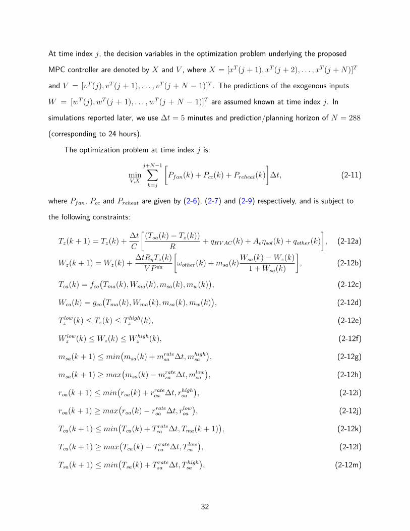
At time index j, the decision variables in the optimization problem underlying the proposed

MPC controller are denoted by X and V , where X = [xT (j + 1), xT (j + 2), . . . , xT (j + N)]T

and V = [vT (j), vT (j + 1), . . . , vT (j + N − 1)]T . The predictions of the exogenous inputs

W = [wT (j), wT (j + 1), . . . , wT (j + N − 1)]T are assumed known at time index j. In

simulations reported later, we use ∆t = 5 minutes and prediction/planning horizon of N = 288

(corresponding to 24 hours).

The optimization problem at time index j is:

minV,X

j+N−1∑k=j

[Pfan(k) + Pcc(k) + Preheat(k)

]∆t, (2-11)

where Pfan, Pcc and Preheat are given by (2-6), (2-7) and (2-9) respectively, and is subject to

the following constraints:

Tz(k + 1) = Tz(k) +∆t

C

[(Toa(k)− Tz(k))

R+ qHV AC(k) + Aeηsol(k) + qother(k)

], (2-12a)

Wz(k + 1) = Wz(k) +∆tRgTz(k)

V P da

[ωother(k) +msa(k)

Wsa(k)−Wz(k)

1 +Wsa(k)

], (2-12b)

Tca(k) = fco(Tma(k),Wma(k),msa(k),mw(k)

), (2-12c)

Wca(k) = gco(Tma(k),Wma(k),msa(k),mw(k)

), (2-12d)

T lowz (k) ≤ Tz(k) ≤ T high

z (k), (2-12e)

W lowz (k) ≤ Wz(k) ≤ W high

z (k), (2-12f)

msa(k + 1) ≤ min(msa(k) +mrate

sa ∆t,mhighsa

), (2-12g)

msa(k + 1) ≥ max(msa(k)−mrate

sa ∆t,mlowsa

), (2-12h)

roa(k + 1) ≤ min(roa(k) + rrateoa ∆t, rhighoa

), (2-12i)

roa(k + 1) ≥ max(roa(k)− rrateoa ∆t, rlowoa

), (2-12j)

Tca(k + 1) ≤ min(Tca(k) + T rate

ca ∆t, Tma(k + 1)), (2-12k)

Tca(k + 1) ≥ max(Tca(k)− T rate

ca ∆t, T lowca

), (2-12l)

Tsa(k + 1) ≤ min(Tsa(k) + T rate

sa ∆t, T highsa

), (2-12m)

32

Tsa(k + 1) ≥ max(Tsa(k)− T rate

sa ∆t, Tca(k + 1)), (2-12n)

Wca(k) ≤ Wma(k), (2-12o)

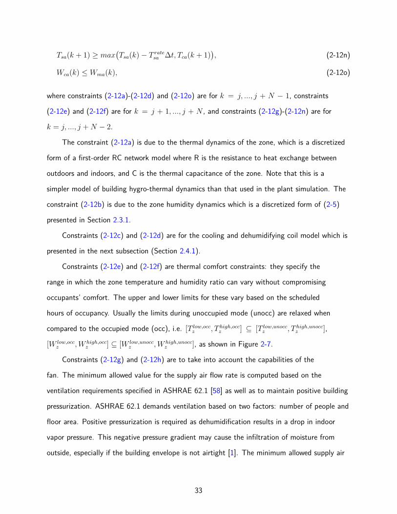
where constraints (2-12a)-(2-12d) and (2-12o) are for k = j, ..., j + N − 1, constraints

(2-12e) and (2-12f) are for k = j + 1, ..., j + N , and constraints (2-12g)-(2-12n) are for

k = j, ..., j +N − 2.

The constraint (2-12a) is due to the thermal dynamics of the zone, which is a discretized

form of a first-order RC network model where R is the resistance to heat exchange between

outdoors and indoors, and C is the thermal capacitance of the zone. Note that this is a

simpler model of building hygro-thermal dynamics than that used in the plant simulation. The

constraint (2-12b) is due to the zone humidity dynamics which is a discretized form of (2-5)

presented in Section 2.3.1.

Constraints (2-12c) and (2-12d) are for the cooling and dehumidifying coil model which is

presented in the next subsection (Section 2.4.1).

Constraints (2-12e) and (2-12f) are thermal comfort constraints: they specify the

range in which the zone temperature and humidity ratio can vary without compromising

occupants’ comfort. The upper and lower limits for these vary based on the scheduled

hours of occupancy. Usually the limits during unoccupied mode (unocc) are relaxed when

compared to the occupied mode (occ), i.e. [T low,occz , T high,occ

z ] ⊆ [T low,unoccz , T high,unocc

z ],

[W low,occz ,W high,occ

z ] ⊆ [W low,unoccz ,W high,unocc

z ], as shown in Figure 2-7.

Constraints (2-12g) and (2-12h) are to take into account the capabilities of the

fan. The minimum allowed value for the supply air flow rate is computed based on the

ventilation requirements specified in ASHRAE 62.1 [58] as well as to maintain positive building

pressurization. ASHRAE 62.1 demands ventilation based on two factors: number of people and

floor area. Positive pressurization is required as dehumidification results in a drop in indoor

vapor pressure. This negative pressure gradient may cause the infiltration of moisture from

outside, especially if the building envelope is not airtight [1]. The minimum allowed supply air

33

flow rate is:

mlowsa = max

((mp

oanp +mAoaA)/roa, mbp

oa/roa), (2-13)

where mpoa is the outdoor air rate required per person, np is the number of people, mA

oa is the

outdoor air required per zone area, A is the zone area, mbpoa is the outdoor air rate required to

maintain positive building pressurization, and roa is the outdoor air ratio.

Constraints (2-12i)-(2-12n) are to take into account the capabilities of the damper

actuators, cooling and reheat coils. In constraints (2-12k) and (2-12o) the inequalities

Tca(k + 1) ≤ Tma(k + 1) and Wca(k) ≤ Wma(k) ensure that the cooling coil can only cool

and dehumidify the mixed air stream; it cannot add heat or moisture. Similarly, in constraint

(2-12n) the inequality Tsa(k + 1) ≥ Tca(k + 1) ensures that the reheat coil can only add heat;

it cannot cool.

Cooling and dehumidifying coil model used in SL-MPC. Even though the binned

model of cooling and dehumidifying coil presented in Section 2.3.2 is quite accurate, it

cannot be used in the optimizer as doing so makes the optimization a mixed integer nonlinear

programming (MINLP) problem which is quite challenging to solve. Therefore, we develop a

control-oriented cooling and dehumidifying coil model which makes the optimization problem a

nonlinear program (NLP). It is a static model with the outputs being a polynomial function of

the inputs. Note that when the chilled water flow rate is zero, no cooling or dehumidifying of

the air can occur so that the conditioned air temperature and humidity ratio must be equal to

the mixed air temperature and humidity ratio: Tca = Tma and Wca = Wma, when mw = 0. To

make the model have this behavior, the following functional form is chosen:

Tca = Tma +mw f(Tma,Wma,msa,mw) (2-14)

Wca = Wma +mw g(Tma,Wma,msa,mw) (2-15)

34

For the functions f and g, we use a quadratic form as higher degree polynomials did not show

substantial gain in accuracy. The final form of the model is:

Tca = fco(Tma,Wma,msa,mw) (2-16)

= Tma +mw

[α1Tma + α2Wma + α3msa + α4mw + α5+

α6T2ma + α7W

2ma + α8m

2sa + α9m

2w+

α10TmaWma + α11Wmamsa + α12msamw + α13mwTma + α14Tmamsa + α15Wmamw

]Wca = gco(Tma,Wma,msa,mw) (2-17)

= Wma +mw

[β1Tma + β2Wma + β3msa + β4mw + β5+

β6T2ma + β7W

2ma + β8m

2sa + β9m

2w+

β10TmaWma + β11Wmamsa + β12msamw + β13mwTma + β14Tmamsa + β15Wmamw

],

where the αi’s and βj’s are the model parameters to be determined. For the numerical results

shown next, data obtained from EnergyPlus simulations—as explained in Section 2.3.2—

are used to fit these parameters. In practice, measurements can be used to fit them. For

the validation data set, the maximum prediction errors observed are 1.61 ◦C (3 ◦F ) and

1.1 × 10−3 kgw/kgda for Tca and Wca, respectively. This is twice the maximum error observed

when using the binned cooling and dehumidifying coil model presented in Section 2.3.2.

2.4.2 Model Predictive Control Incorporating Only Sensible Heat (S-MPC)

This controller is similar to the one described in Section 2.4.1, with the main difference

being that the moisture and latent heat of the air are not considered. The optimization

problem formulation is similar to the one presented in [59].

For this controller, the vectors x(k) and v(k) are defined as follows: x(k) := Tz(k) ∈ ℜ1

and v(k) := u(k) ∈ ℜ4, where u(k) is the control command vector defined in (2-1). The

optimization problem at time index j is:

minV,X

j+N−1∑k=j

[Pfan(k) + P S

cc(k) + Preheat(k)

]∆t, (2-18)

35

subject to the constraints: (2-12a),(2-12e), (2-12g)-(2-12n), where Pfan and Preheat are given

by (2-6) and (2-9), and

P Scc(k) =

msa(k)Cpa

[Tma(k)− Tca(k)

]ηccCOPc

, (2-19)

where Tma(t) and Tca(t) are the dry bulb temperatures of the mixed and conditioned air. The

exogenous disturbance needed to compute the constraints in the optimizer are:

w(k) := [ηsol(k), Toa(k), qother(k)]T ∈ ℜ3. (2-20)

Notice the difference with SL-MPC: since this controller does not consider humidity and

latent heat, the constraints placed on the humidity ratio at various locations in the air loop as

well as the zone—(2-12b), (2-12f), and (2-12o)—are no longer used. The constraints placed

on the system due to the cooling and dehumidifying coil model—(2-12c) and (2-12d)—are also

not present. The cooling power term in the objective function is based only on the sensible

heat; latent heat is ignored.

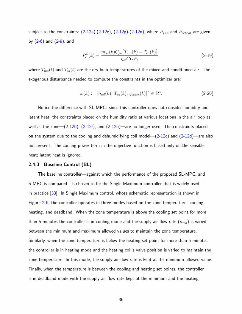
2.4.3 Baseline Control (BL)

The baseline controller—against which the performance of the proposed SL-MPC, and

S-MPC is compared—is chosen to be the Single Maximum controller that is widely used

in practice [33]. In Single Maximum control, whose schematic representation is shown in

Figure 2-6, the controller operates in three modes based on the zone temperature: cooling,

heating, and deadband. When the zone temperature is above the cooling set point for more

than 5 minutes the controller is in cooling mode and the supply air flow rate (msa) is varied

between the minimum and maximum allowed values to maintain the zone temperature.

Similarly, when the zone temperature is below the heating set point for more than 5 minutes

the controller is in heating mode and the heating coil’s valve position is varied to maintain the

zone temperature. In this mode, the supply air flow rate is kept at the minimum allowed value.

Finally, when the temperature is between the cooling and heating set points, the controller

is in deadband mode with the supply air flow rate kept at the minimum and the heating

36

Maximum supply air

temperature

Supply airtemperature Maximum

supply air flow rate

Supply air flow rate

Deadband mode

Cooling mode

Heating mode

Zonetemperature

Supply air flow rate

Minimumsupply airflow rate

Supply airtemperature

Heatingset point

Cooling set point

Figure 2-6. Schematic of Single Maximum control algorithm.

valve is closed so the supply air temperature is equal to the conditioned air temperature

(Tsa=Tca). The minimum allowed value for the supply air flow rate should satisfy the following

conditions: one, the ventilation requirements specified by ASHRAE 62.1 [58] and positive

building pressurization, as described in Section 2.4.1. Two, it should be high enough to meet

the design heating load at a supply air temperature that is low enough to prevent stratification

(e.g., 30 ◦C). The outdoor air ratio and the conditioned air temperature are kept constant at

all times.

2.4.4 Information Requirement for Implementation

All three controllers studied make decisions for the same four control commands in the

vector u; see (2-1). The proposed SL-MPC controller needs real-time measurements of zone

temperature and humidity, while the S-MPC and BL controllers need real-time measurements

of zone temperature alone. BL controller does not need any predictions, while both the MPC

controllers need prediction of the exogenous disturbances, w, over the prediction horizon.

Most of these predictions are directly available from weather forecasts. The exceptions are

internal heat gains (needed by both MPC schemes), and internal moisture generation (needed

by SL-MPC alone). Predictions for these signals can be obtained from occupancy schedules,

or from time-series models fitted to estimated heat gains and moisture generation rates that

are estimated from temperature and humidity measurements by using methods such as those

in [55].

37

The BL controller does not need any models while both the MPC controllers do. These

models are learned off-line. Both the MPC controllers need models of the thermal dynamics

of the zone; its parameters can be identified off-line by one of several existing methods. The

parameters used in this work are fitted to Pugh Hall data by using the method in [55]. The

SL-MPC requires a humidity dynamic model of the zone and a cooling coil model while the

S-MPC does not. The humidity dynamic model used in this work is a physics-based model;

volume of the zone is the only parameter and was obtained from the mechanical drawings

for the Pugh Hall building. The cooling coil model parameters can be fitted by a regression

technique, to data collected from an actual HVAC system or a high fidelity simulation.

The parameters used in this work are fitted using least squares to data collected from an

EnergyPlus model of an AHU. The EnergyPlus model was created using manufacturer provided

data about the Pugh Hall equipment; see Section 2.3.2.

2.5 Simulation Setup

The plant is simulated in SIMULINK. The optimization problem is solved using CasADi

[60] and IPOPT [61], a nonlinear programming (NLP) solver, on a Desktop Linux computer

with 16GB RAM and a 3.60 GHz × 8 CPU. On an average it takes 2 seconds for SL-MPC

and 0.6 seconds for S-MPC to solve their respective optimization problems. The higher

computation time for SL-MPC is attributed to the larger number of decision variables. Both

the NLPs are non-convex, and the NLP solver indicates that it is able to find a local minimum

successfully 100% of the time. In cases where they may not be feasible, the controllers are

programmed to use the control command computed at the previous time step.

Three types of outdoor weather conditions are tested: hot-humid (Aug/06/2016), mild

(Mar/25/2016), and cold (Dec/20/2016), all for Gainesville, FL, USA. The weather data is

obtained from Weather Underground [62] and National Solar Radiation Database [63]. The

simulations are run for 24 hours starting at 8:00 AM.

38

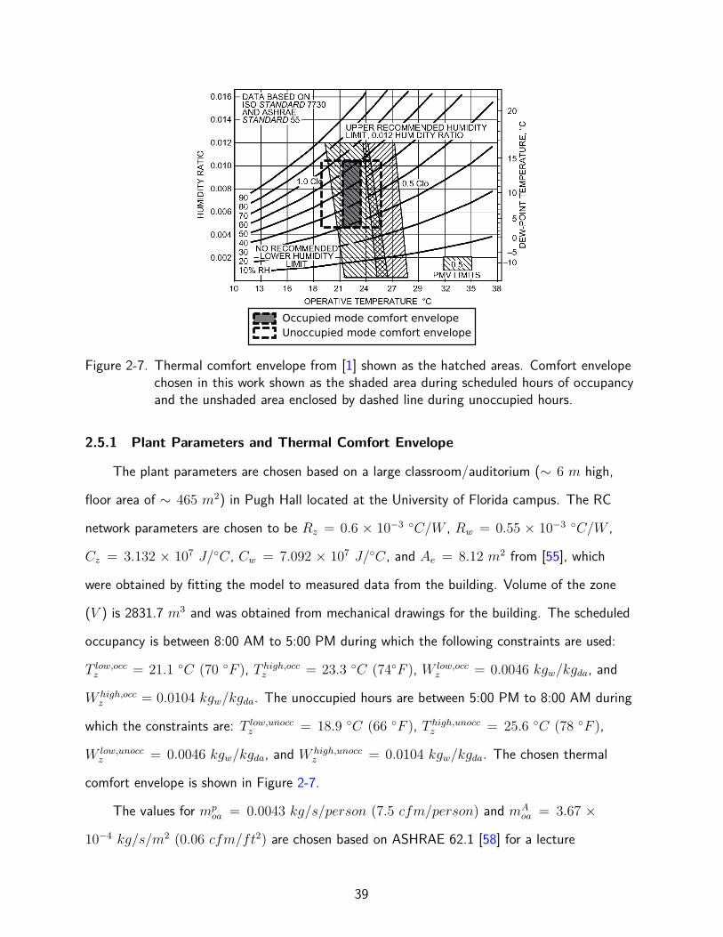
Occupied mode comfort envelopeUnoccupied mode comfort envelope

Figure 2-7. Thermal comfort envelope from [1] shown as the hatched areas. Comfort envelopechosen in this work shown as the shaded area during scheduled hours of occupancyand the unshaded area enclosed by dashed line during unoccupied hours.

2.5.1 Plant Parameters and Thermal Comfort Envelope

The plant parameters are chosen based on a large classroom/auditorium (∼ 6 m high,

floor area of ∼ 465 m2) in Pugh Hall located at the University of Florida campus. The RC

network parameters are chosen to be Rz = 0.6 × 10−3 ◦C/W , Rw = 0.55 × 10−3 ◦C/W ,

Cz = 3.132 × 107 J/◦C, Cw = 7.092 × 107 J/◦C, and Ae = 8.12 m2 from [55], which

were obtained by fitting the model to measured data from the building. Volume of the zone

(V ) is 2831.7 m3 and was obtained from mechanical drawings for the building. The scheduled

occupancy is between 8:00 AM to 5:00 PM during which the following constraints are used:

T low,occz = 21.1 ◦C (70 ◦F ), T high,occ

z = 23.3 ◦C (74◦F ), W low,occz = 0.0046 kgw/kgda, and

W high,occz = 0.0104 kgw/kgda. The unoccupied hours are between 5:00 PM to 8:00 AM during

which the constraints are: T low,unoccz = 18.9 ◦C (66 ◦F ), T high,unocc

z = 25.6 ◦C (78 ◦F ),

W low,unoccz = 0.0046 kgw/kgda, and W high,unocc

z = 0.0104 kgw/kgda. The chosen thermal

comfort envelope is shown in Figure 2-7.

The values for mpoa = 0.0043 kg/s/person (7.5 cfm/person) and mA

oa = 3.67 ×

10−4 kg/s/m2 (0.06 cfm/ft2) are chosen based on ASHRAE 62.1 [58] for a lecture

39

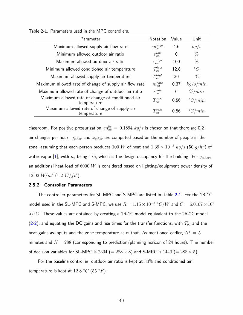
Table 2-1. Parameters used in the MPC controllers.Parameter Notation Value Unit

Maximum allowed supply air flow rate mhighsa 4.6 kg/s

Minimum allowed outdoor air ratio rlowoa 0 %

Maximum allowed outdoor air ratio rhighoa 100 %

Minimum allowed conditioned air temperature T lowca 12.8 ◦C

Maximum allowed supply air temperature T highsa 30 ◦C

Maximum allowed rate of change of supply air flow rate mratesa 0.37 kg/s/min

Maximum allowed rate of change of outdoor air ratio rrateoa 6 %/min

Maximum allowed rate of change of conditioned airtemperature T rate

ca 0.56 ◦C/min

Maximum allowed rate of change of supply airtemperature T rate

sa 0.56 ◦C/min

classroom. For positive pressurization, mbpoa = 0.1894 kg/s is chosen so that there are 0.2

air changes per hour. qother and ωother are computed based on the number of people in the

zone, assuming that each person produces 100 W of heat and 1.39 × 10−5 kg/s (50 g/hr) of

water vapor [1], with np being 175, which is the design occupancy for the building. For qother,

an additional heat load of 6000 W is considered based on lighting/equipment power density of

12.92 W/m2 (1.2 W/ft2).

2.5.2 Controller Parameters

The controller parameters for SL-MPC and S-MPC are listed in Table 2-1. For the 1R-1C

model used in the SL-MPC and S-MPC, we use R = 1.15× 10−3 ◦C/W and C = 6.0167× 107

J/◦C. These values are obtained by creating a 1R-1C model equivalent to the 2R-2C model

(2-2), and equating the DC gains and rise times for the transfer functions, with Toa and the

heat gains as inputs and the zone temperature as output. As mentioned earlier, ∆t = 5

minutes and N = 288 (corresponding to prediction/planning horizon of 24 hours). The number

of decision variables for SL-MPC is 2304 (= 288× 8) and S-MPC is 1440 (= 288× 5).

For the baseline controller, outdoor air ratio is kept at 30% and conditioned air

temperature is kept at 12.8 ◦C (55 ◦F ).

40

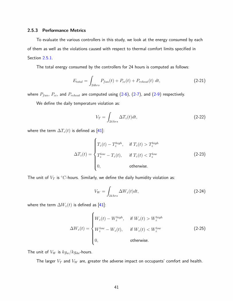
2.5.3 Performance Metrics

To evaluate the various controllers in this study, we look at the energy consumed by each

of them as well as the violations caused with respect to thermal comfort limits specified in

Section 2.5.1.

The total energy consumed by the controllers for 24 hours is computed as follows:

Etotal =

∫24hrs

Pfan(t) + Pcc(t) + Preheat(t) dt, (2-21)

where Pfan, Pcc, and Preheat are computed using (2-6), (2-7), and (2-9) respectively.

We define the daily temperature violation as:

VT =

∫24hrs

∆Tz(t)dt, (2-22)

where the term ∆Tz(t) is defined as [41]:

∆Tz(t) =

Tz(t)− T high

z , if Tz(t) > T highz

T lowz − Tz(t), if Tz(t) < T low

z

0, otherwise.

(2-23)

The unit of VT is ◦C-hours. Similarly, we define the daily humidity violation as:

VW =

∫24hrs

∆Wz(t)dt, (2-24)

where the term ∆Wz(t) is defined as [41]:

∆Wz(t) =

Wz(t)−W high

z , if Wz(t) > W highz

W lowz −Wz(t), if Wz(t) < W low

z

0, otherwise.

(2-25)

The unit of VW is kgw/kgda-hours.

The larger VT and VW are, greater the adverse impact on occupants’ comfort and health.

41

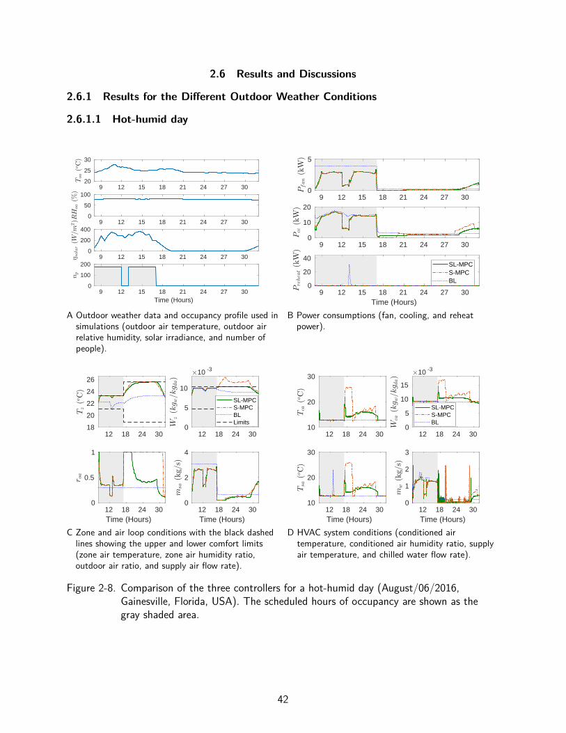
2.6 Results and Discussions

2.6.1 Results for the Different Outdoor Weather Conditions

2.6.1.1 Hot-humid day

9 12 15 18 21 24 27 3020

25

30

9 12 15 18 21 24 27 300

50

100

9 12 15 18 21 24 27 300

200

400

9 12 15 18 21 24 27 30Time (Hours)

0

100

200

A Outdoor weather data and occupancy profile used insimulations (outdoor air temperature, outdoor airrelative humidity, solar irradiance, and number ofpeople).

9 12 15 18 21 24 27 300

5

9 12 15 18 21 24 27 300

10

20

9 12 15 18 21 24 27 30Time (Hours)

0

20

40SL-MPCS-MPCBL

B Power consumptions (fan, cooling, and reheatpower).

12 18 24 3018

20

22

24

26

12 18 24 300

5

10

10 -3

SL-MPCS-MPCBLLimits

12 18 24 30Time (Hours)

0

0.5

1

12 18 24 30Time (Hours)

0

2

4

C Zone and air loop conditions with the black dashedlines showing the upper and lower comfort limits(zone air temperature, zone air humidity ratio,outdoor air ratio, and supply air flow rate).

12 18 24 3010

20

30

12 18 24 300

5

10

15

10 -3

SL-MPCS-MPCBL

12 18 24 30Time (Hours)

10

20

30

12 18 24 30Time (Hours)

0

1

2

3

D HVAC system conditions (conditioned airtemperature, conditioned air humidity ratio, supplyair temperature, and chilled water flow rate).

Figure 2-8. Comparison of the three controllers for a hot-humid day (August/06/2016,Gainesville, Florida, USA). The scheduled hours of occupancy are shown as thegray shaded area.

42

Figure 2-8 shows the simulation results for a hot-humid day. It is found that SL-MPC

consumes the least amount of energy when compared to S-MPC and BL, as presented in

Figure 2-10. There are large violations in humidity limits by S-MPC, specifically during the

unoccupied hours, as shown in Figures 2-10 and 2-8C.

All three controllers are able to maintain thermal comfort limits during scheduled hours

of occupancy almost all the time; see 08:00-17:00 hours in Figure 2-8C. The BL ensures that

dry air is supplied to the zone and hence the humidity limit is not violated since it keeps the

conditioned air temperature at a constant value of 12.8 ◦C (55◦F ). In the case of S-MPC,

the optimal control decisions made by it are observed to be similar to those made by SL-MPC.

This can be attributed to the high internal heat load and hot outdoor air temperature.

Specifically, S-MPC decides to keep the conditioned air temperature low enough (at 12.8 ◦C)

to meet the heat load which has the unintended, but good, side effect of maintaining zone

humidity within the comfort limits.

Both the MPC controllers consume lesser energy when compared to BL during occupied

hours; see 08:00-17:00 hours in Figure 2-8B. The reason for this is that the outdoor air ratio is

kept constant for BL and it also assumes full occupancy from 08:00 to 17:00 hours. Therefore,

the air flow rate has to be kept high enough so that the ventilation requirements specified

in ASHRAE 62.1 [58] are met. This high air flow rate, combined with the low conditioned

air temperature, is highly suboptimal, especially when there is a reduction in occupancy: not

only is the air cooled unnecessarily, but reheating must also be performed to prevent the

zone from becoming too cold. This phenomenon can be seen between 12:00-13:00 hours in

Figures 2-8B and 2-8C. The MPC controllers in contrast vary the outdoor air ratio and air flow

rate as occupancy varies, leading to a lower fan and cooling energy consumption. It should be

noted that this reduction in energy use by the MPC controllers requires accurate prediction of

occupancy.

From Figure 2-8C it can be seen that S-MPC violates the humidity limits during

unoccupied hours while SL-MPC and BL do not. This is because S-MPC decides to bring

43

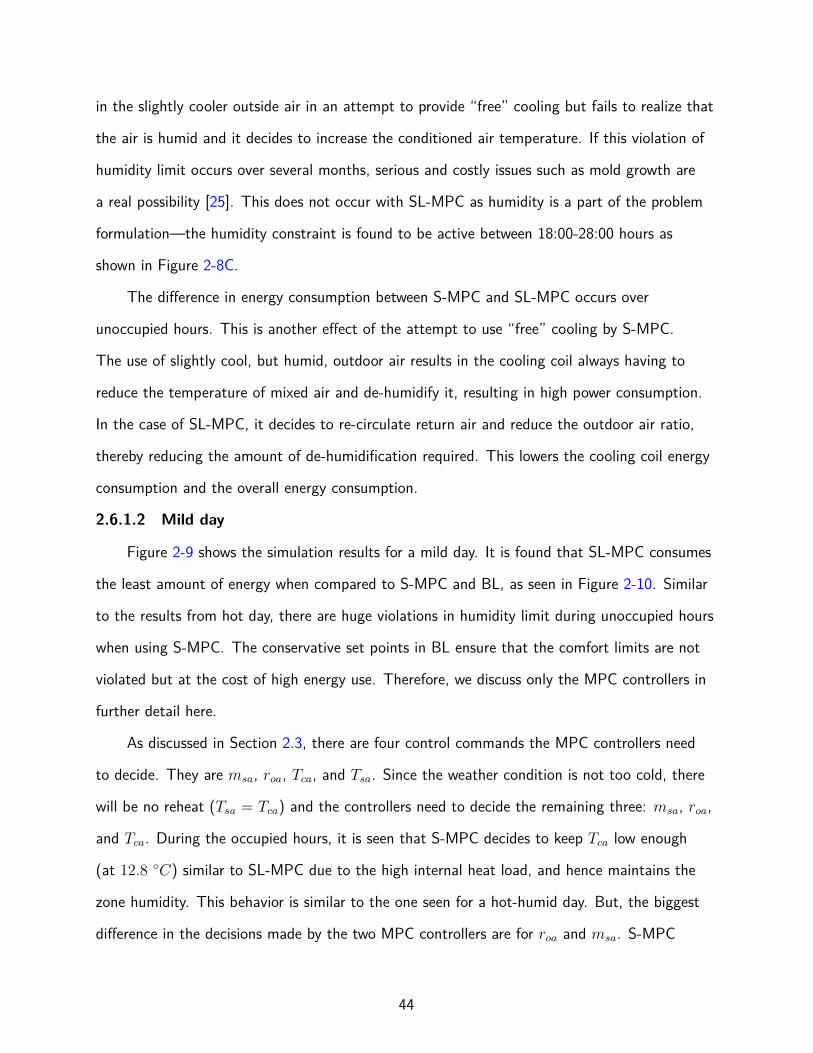
in the slightly cooler outside air in an attempt to provide “free” cooling but fails to realize that

the air is humid and it decides to increase the conditioned air temperature. If this violation of

humidity limit occurs over several months, serious and costly issues such as mold growth are

a real possibility [25]. This does not occur with SL-MPC as humidity is a part of the problem

formulation—the humidity constraint is found to be active between 18:00-28:00 hours as

shown in Figure 2-8C.

The difference in energy consumption between S-MPC and SL-MPC occurs over

unoccupied hours. This is another effect of the attempt to use “free” cooling by S-MPC.

The use of slightly cool, but humid, outdoor air results in the cooling coil always having to

reduce the temperature of mixed air and de-humidify it, resulting in high power consumption.

In the case of SL-MPC, it decides to re-circulate return air and reduce the outdoor air ratio,

thereby reducing the amount of de-humidification required. This lowers the cooling coil energy

consumption and the overall energy consumption.

2.6.1.2 Mild day

Figure 2-9 shows the simulation results for a mild day. It is found that SL-MPC consumes

the least amount of energy when compared to S-MPC and BL, as seen in Figure 2-10. Similar

to the results from hot day, there are huge violations in humidity limit during unoccupied hours

when using S-MPC. The conservative set points in BL ensure that the comfort limits are not

violated but at the cost of high energy use. Therefore, we discuss only the MPC controllers in

further detail here.

As discussed in Section 2.3, there are four control commands the MPC controllers need

to decide. They are msa, roa, Tca, and Tsa. Since the weather condition is not too cold, there

will be no reheat (Tsa = Tca) and the controllers need to decide the remaining three: msa, roa,

and Tca. During the occupied hours, it is seen that S-MPC decides to keep Tca low enough

(at 12.8 ◦C) similar to SL-MPC due to the high internal heat load, and hence maintains the

zone humidity. This behavior is similar to the one seen for a hot-humid day. But, the biggest

difference in the decisions made by the two MPC controllers are for roa and msa. S-MPC

44

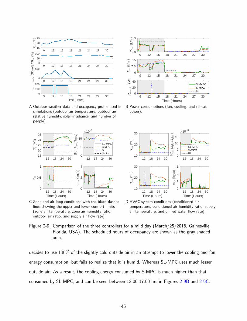
9 12 15 18 21 24 27 3015

20

25

9 12 15 18 21 24 27 300

50

100

9 12 15 18 21 24 27 300

500

9 12 15 18 21 24 27 30Time (Hours)

0

100

200

A Outdoor weather data and occupancy profile used insimulations (outdoor air temperature, outdoor airrelative humidity, solar irradiance, and number ofpeople).

9 12 15 18 21 24 27 300

5

9 12 15 18 21 24 27 300

7.5

15

9 12 15 18 21 24 27 30Time (Hours)

0

20

40SL-MPCS-MPCBL

B Power consumptions (fan, cooling, and reheatpower).

12 18 24 3018

20

22

24

26

12 18 24 300

5

10

10 -3

SL-MPCS-MPCBLLimits

12 18 24 30Time (Hours)

0

0.5

1

12 18 24 30Time (Hours)

0

2

4

C Zone and air loop conditions with the black dashedlines showing the upper and lower comfort limits(zone air temperature, zone air humidity ratio,outdoor air ratio, and supply air flow rate).

12 18 24 3010

20

30

12 18 24 300

5

10

15

10 -3

SL-MPCS-MPCBL

12 18 24 30Time (Hours)

10

20

30

12 18 24 30Time (Hours)

0

1

2

3

D HVAC system conditions (conditioned airtemperature, conditioned air humidity ratio, supplyair temperature, and chilled water flow rate).

Figure 2-9. Comparison of the three controllers for a mild day (March/25/2016, Gainesville,Florida, USA). The scheduled hours of occupancy are shown as the gray shadedarea.

decides to use 100% of the slightly cold outside air in an attempt to lower the cooling and fan

energy consumption, but fails to realize that it is humid. Whereas SL-MPC uses much lesser

outside air. As a result, the cooling energy consumed by S-MPC is much higher than that

consumed by SL-MPC, and can be seen between 12:00-17:00 hrs in Figures 2-9B and 2-9C.

45

During unoccupied hours both the MPC controllers decide to bring in 100% outside air,

but SL-MPC decides to keep Tca lower than the one decided by S-MPC to ensure that the air

is dehumidified enough before being supplied to the zone.

2.6.1.3 Cold day

Since the outdoor weather is dry, no matter what decisions are made by a controller, it

is unlikely to violate humidity constraints in the building. The energy consumed by the two

MPC controllers is almost the same, which is much smaller than that by BL (Figure 2-10).

BL performs simultaneous heating and cooling in a pronounced manner leading to high energy

consumption: the fixed outdoor air ratio combined with the 12.8 ◦C (55 ◦F ) conditioned air

requires usage of cooling energy, additionally reheating is required to keep the building warm

enough because of the cold weather. The MPC controllers choose to use as much outdoor air

as possible, since the cold outdoor conditions provide free cooling without having to use chilled

water.

2.6.2 Comparison among Controllers

The performance metrics discussed in Section 2.5.3 are computed from simulation data for

each of the three controllers, and are shown in Figure 2-10. The temperature violation VT was

observed to be minimal for all three controllers, and is therefore not shown in the figure. We

see from the figure that space humidity is a concern only during hot-humid and mild weather

conditions.

Figure 2-10 shows that SL-MPC outperforms the other two controllers: it consumes the

least amount of energy under various outdoor weather conditions with negligible violation in

thermal comfort constraints.

The simulation results discussed in the previous section show that S-MPC makes decisions

that either leads to thermal comfort violations, or higher energy use when compared to

SL-MPC, under the following conditions.

1. Mild internal heat load but high outdoor humidity (e.g. spring/summer night): In such

a condition, S-MPC decides that slightly cooler outside air can provide free cooling and

46

Hot-humid day Mild day Cold day0

50

100

150

200

E tot

al fo

r a d

ay (k

Wh)

SL-MPCS-MPCBL

A Comparison of total energy consumed over 24hours by SL-MPC, S-MPC, and BL for differentoutdoor weather conditions.

Hot-humid day Mild day Cold day0.000

0.002

0.004

0.006

0.008

0.010

0.012

0.014

V W (k

g w/k

g da-h

ours

)

SL-MPCS-MPCBL2.5% Violation

B Comparison of humidity violation over 24 hours bySL-MPC, S-MPC, and BL for different outdoorweather conditions. The black line indicates thevalue of VW when there is a 2.5% violation overthe upper limit of humidity ratio at every instant.

Figure 2-10. Comparison of controllers’ performance.

it also decides to increase the conditioned air temperature, but the high humidity of the

outside air combined with humid air supplied to the zone causes high indoor humidity;

see Figures 2-10B, 2-8C, and 2-9C. Thus, S-MPC makes decisions in the interest of

reducing energy/cost that leads to violation of humidity constraints.

2. During occupied hours on a mild weather day: In this case, the S-MPC decides to meet

the air flow requirement with a larger fraction of outdoor air due to its small sensible

heat, failing to recognize its high latent heat. Because of the high internal sensible load

during occupied hours, it uses a low conditioned air setpoint which incidentally reduces

humidity of the air supplied, so fortunately no space humidity violations occur. However,

the decision is energy inefficient compared to the proposed SL-MPC controller.

Interestingly, S-MPC makes decisions similar to the proposed SL-MPC controller either

when (i) the internal heat load is high and outdoor weather is hot and humid, or (ii) the

outdoor weather is cold and dry. In the latter case, the cold outdoor is used to provide free

(sensible) cooling, and since it is dry there is no risk of space humidity becoming large. In

the former scenario, S-MPC recognizes that the conditioned air temperature must be low

47

enough to maintain the indoor temperature within allowable limits. That decision has an

unintended, but good, side effect of maintaining space humidity even though the controller has

no knowledge of humidity.

BL uses conservative set points which ensures that there are no violations in humidity and

temperature constraints almost all the time, but leads to higher energy use when compared to

the two MPC controllers.

These observations provide a basis for a cost-benefit trade-off analysis of the three

controllers. One should first note that the proposed SL-MPC requires more sophisticated

modeling and additional humidity sensors compared to an MPC controller that ignores

humidity/latent heat, and thus is more expensive to use in practice. The additional energy cost

savings due to the proposed MPC controller over the naive MPC controller S-MPC is small,

about 5%; see Figure 2-10A. The larger difference is space humidity. As discussed previously, in

mild outdoor weather conditions such as spring/summer nights, the proposed MPC controller is

able to maintain space humidity constraints while the naive MPC controller leads to poor space

humidity. Since this large space humidity occurs over many hours in a night (Figures 2-8C

and 2-9C), and this behavior is likely to repeat every night over the entire season, it may lead

to mold growth which can seriously affect occupant health. In fact, additional simulations

that are not reported here due to space constraints, show that with larger internal moisture

generation, poor space humidity occurs even during occupied hours. Therefore, the benefit of

incorporating humidity/latent heat in MPC control of HVAC—or conversely the cost of not

doing so—maybe more about occupant health and comfort, and less about energy savings.

Additionally, since these benefits (conversely, costs) manifest only over long time periods,

experimental evaluations conducted over a short time period, say, less than a few months, may

not be adequate to provide a complete assessment.

2.7 Summary

An MPC-based controller which incorporates humidity and latent heat in a principled

manner is presented. Simulations show that the proposed MPC controller outperforms both a

48

naive MPC controller (that does not consider humidity/latent heat) and a baseline rule-based

controller, despite large plant-model mismatch. A thorough comparison for several weather

conditions indicate the key advantage of the proposed controller over the naive MPC is not

energy savings but humidity control. The naive controller may lead to poor humidity control,

especially during mild outdoor weather conditions such as spring or summer nights. Such

violations in humidity over long periods can cause mold growth and can affect occupant health

and comfort.

This study is a first step; there are several avenues for further exploration. A natural

extension is to multi-zone buildings, which is presented in Chapter 3. A thorough numerical

investigation for various climate zones and HVAC systems is also needed. It may be possible

to reformulate the underlying optimization problem in the proposed controller to guarantee

feasibility and convexity. Theoretical properties of the controller need to be investigated

as well. Another avenue for future work is extension to supply side applications, such as

development of humidity- and latent heat-aware HVAC control to provide ancillary services to

power grid.

49

CHAPTER 3MPC-BASED HIERARCHICAL CONTROL OF A MULTI-ZONE COMMERCIAL HVAC

SYSTEM

3.1 Overview

In this chapter, a novel hierarchical architecture for MPC-based indoor climate control of

multi-zone buildings to provide energy-efficiency is proposed.

Several of the MPC formulations proposed in the literature are for buildings with one

zone [8, 9, 10] or a small number of zones [11, 12]. The algorithm presented in Chapter 2

is also primarily for single-zone buildings. A direct extension of such formulations for large

multi-zone buildings has two main challenges. First, solving the underlying optimization

problem in MPC for a building with a large number of zones is computationally complex

because of the large number of decision variables. To reduce the computational complexity,

several distributed and hierarchical approaches have been proposed [49, 46, 59, 64, 65, 66,

67]. The second challenge, which has attracted far less attention, is that MPC requires a

“high-resolution” model of the thermal dynamics of a multi-zone building. High-resolution

means that the temperature of every zone in the building is a state in the model and the

control commands for every zone are inputs in the model. One way of obtaining such a

multi-zone model is by first constructing a “white box” model, such as by using a building

energy modeling software, and then simplifying it to make it suitable for MPC, e.g., [68]. But

constructing a white box model is expensive; it requires significant effort [69]. Moreover, the

resulting model may not reflect the building as is. Another way of obtaining a high-resolution

multi-zone model is by utilizing data-driven techniques, which use input-output measurements.

Getting reliable estimates using data-driven modeling is challenging even for a single-zone

building, as a building’s thermal dynamics is affected by a non-trivial and unmeasurable

disturbance, the heat gain from occupants and their use of equipment, that strongly affects

quality of the identified model [70]. In the case of multi-zone model identification, it becomes

intractable since the model has too many degrees of freedom: as many unknown disturbance

signals as there are number of zones. To the best of our knowledge, there are no works on

50

Return airExhaustair

Outdoor air

Mixedair

Cooling and

dehumidifying coil

Tca

Chilledwater

msaTma Fan

ToaWcaWmaWoa

Twi

mwTsa,1

mra

moa

Zone 2

Zone 1

VAVW/REHEAT

msa,1

Tsa,2msa,2

VAVW/REHEAT

Tz,1 Wz,1

Tz,2 Wz,2

pduct

Air Handling Unit

TraWra

Wsa,1

Wsa,2

Figure 3-1. Schematic of a multi-zone—specifically, a two zone—commercialvariable-air-volume HVAC system. In this figure, oa: outdoor air, ra: return air,ma: mixed air, ca: conditioned air, and sa: supply air.

reliable identification of multi-zone building models without making assumptions on the nature

of the disturbance affecting individual zones [71].

In addition to the challenges mentioned above, most of the prior works—whether

on single-zone or on multi-zone buildings—ignore humidity and latent heat in their MPC

formulations, as explained in Chapter 2.

In this chapter, a humidity- and latent heat-aware MPC formulation for a multi-zone

building with a variable air volume (VAV) HVAC system is proposed. Figure 3-1 shows the

schematic of such a system.

To overcome the challenges mentioned above, we propose a two-level control architecture.

The high-level controller (HLC) decides on the AHU-level control commands. The HLC is an

MPC controller that uses a “low-resolution” model of the building with a small number of

“meta-zones”, with each meta-zone being a single-zone equivalent of a part of the building

consisting of several zones. In the case study presented here, a 33 zone three-floor building

is aggregated to a 3 meta-zone model, with each meta-zone corresponding to a floor. The

advantage of such an approach is that a high-resolution multi-zone model is not needed as a

starting point. Rather, a single-zone equivalent model of each meta zone, in which disturbance

in all the zones are aggregated into one signal, can be directly identified from measurements

collected from the building. The identification problem of such a single-zone equivalent model

51

is more tractable [72]. In this chapter, we use the system identification method from [72],

though other identification methods can also be used. Since the HLC uses a low-resolution

model with a much smaller number of meta-zones than that in the building, its computational

complexity is low. However, this reduction of computational complexity creates a different

challenge. Since the decision variables of the optimization problem in the HLC correspond

to the meta-zones (air flow rate, temperature, etc.), they do not correspond to those for the

actual zones of the building. The low-level controller (LLC) is now used to compute the control

commands for individual zones. It does so by solving a projection problem that appropriately

distributes aggregate quantities computed by the HLC to individual zones. The LLC uses

feedback from each zone to assess their needs and ensures indoor climate of each zone is

maintained.

The proposed controller—that includes the HLC and LLC—is hereafter referred to as

MZHC which stands for multi-zone hierarchical controller. Its performance is assessed through

simulations on a “virtual building” plant. The plant is representative of a section of the

Innovation Hub building comprising of 33 zones and is located at the University of Florida

campus. The plant is constructed using Modelica [73]. The performance of the proposed

controller is compared with that of Dual Maximum controller as a baseline [33]. The Dual

Maximum controller—which is referred to as BL (for baseline)—is a rule-based controller, and

is one of the more energy efficient controllers among those used in practice [33]. Simulation

results show that using the proposed controller provides significant energy savings when

compared to BL while maintaining indoor climate.

Compared to the literature on MPC design for multi-zone building HVAC systems, our

work makes four principal contributions, with details discussed in Section 3.2. (i) The first

contribution is that the proposed method does not assume availability of a high-resolution

model of the multi-zone building which is difficult to obtain. Instead, it can utilize existing

data-driven methods that can quickly identify a low-resolution model of the multi-zone building

from measurements. (ii) Since the MPC part of the proposed controller uses a low-resolution

52

model with a small number of meta-zones, the method is scalable to buildings with a large

number of zones. Although distributed iterative computation has been proposed in the

literature as an alternate approach to reducing computational complexity, ours can be solved

in a centralized setting. (iii) The third contribution is the incorporation of humidity and latent

heat in our multi-zone MPC formulation, which has been largely ignored in the literature

on MPC for buildings, and especially so in the literature on multi-zone building MPC. Our

simulations show that when using MZHC, the indoor humidity constraint is active, especially

during hot-humid weather. Without humidity being explicitly considered, the controller would

have caused high space humidity in an effort to reduce energy use. (iv) The fourth contribution

is a realistic evaluation of the proposed controller in a high-fidelity simulation platform that

introduces a large plant-model mismatch. In many prior works on multi-zone MPC, the model

used by the controller is the same as that used in simulating the plant. In contrast, the only

information provided to the proposed controller about the building is sensor measurements

(past data for model identification and real-time data during control) and design parameters

such as expected occupancy, minimum design airflow rates for each VAV box, etc.

The rest of this chapter is organized as follows. Section 3.2 discusses our work in relation

to the literature on multi-zone MPC. Section 3.3 describes a multi-zone building equipped

with a VAV HVAC system and the models we use in simulating the plant (the system to be

controlled). Section 3.4 presents the proposed MPC-based hierarchical controller. Section 3.5

describes a rule-based baseline controller with which the performance of the proposed controller

is compared. The simulation setup is described in Section 3.6. Simulation results are presented

and discussed in Section 3.7. Finally, the main conclusions are provided in Section 3.8.

3.2 Comparison with Literature on Multi-Zone MPC

Several distributed and hierarchical approaches have been proposed to reduce the

computational complexity of MPC for multi-zone buildings [49, 46, 59, 64, 65, 66, 67]. In [49],

a hierarchical distributed algorithm called token-based scheduling is proposed to vary the supply

airflow rate to the zones. A modified version of this algorithm is used in [46] to minimize the

53

energy consumption of a multi-zone building located at the Nanyang Technological University,

Singapore campus.

In [64], a two-layered control architecture is proposed for operating a VAV HVAC system.

The upper layer is an open loop controller, while the lower layer is based on MPC and it varies

the supply airflow rates to the zones. Similar to [49], [46], and [64], the works [66, 65, 67]

consider varying only the zone-level control inputs such as the supply airflow rates and

zone temperature set points. These works exclude the AHU-level control inputs such as the

conditioned air temperature and outside airflow rate. Unlike the works mentioned above, the

work [74] uses MPC to vary only the AHU-level control inputs; the zone-level control inputs are

excluded in this formulation.

One of the few works similar to ours is [59], as they consider both the zone-level and

AHU-level control inputs in their formulation. But their algorithm requires a high-resolution

multi-zone model, and they do not consider humidity and latent heat in their formulation.

3.3 System and Problem Description, and Plant Simulator

Our focus is a multi-zone building equipped with a variable-air-volume (VAV) HVAC

system, whose schematic is shown in Figure 3-1. In such a system, part of the air exhausted

from the zones is recirculated and mixed with outdoor air. This mixed air is sent through the

cooling coil where the air is cooled and dehumidified to the conditioned air temperature (Tca)

and humidity ratio (Wca). This conditioned air is then sent through the supply ducts to the

VAV boxes, which have a damper to control airflow, and finally supplied to the zones. Some

VAV boxes have reheat coils; they can change temperature of supply air but not humidity, i.e.,

Tsa,i ≥ Tca and Wsa,i = Wca, where Tsa,i and Wsa,i are the temperature and humidity ratio of

supply air to the ith zone. If a VAV box is not equipped with a reheat coil (cooling only), then

the temperature of air supplied by it to its zone will be at the conditioned air temperature, i.e.,

Tsa,i = Tca.

54

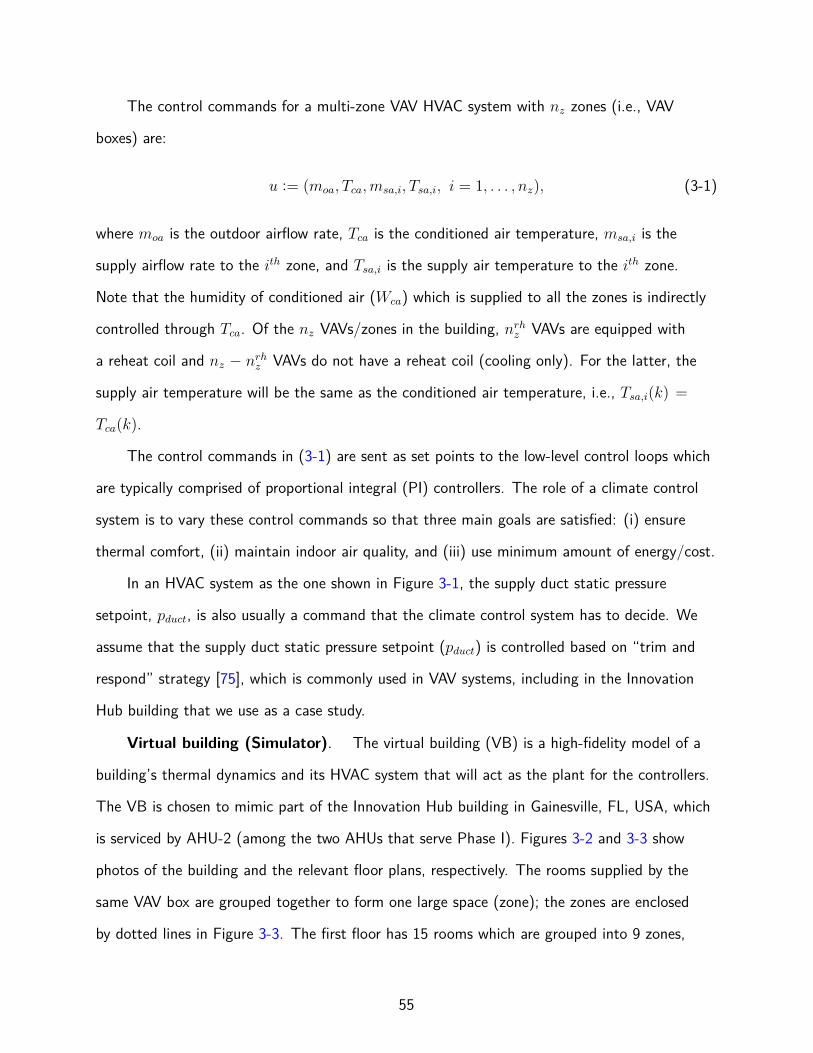
The control commands for a multi-zone VAV HVAC system with nz zones (i.e., VAV

boxes) are:

u := (moa, Tca,msa,i, Tsa,i, i = 1, . . . , nz), (3-1)

where moa is the outdoor airflow rate, Tca is the conditioned air temperature, msa,i is the

supply airflow rate to the ith zone, and Tsa,i is the supply air temperature to the ith zone.

Note that the humidity of conditioned air (Wca) which is supplied to all the zones is indirectly

controlled through Tca. Of the nz VAVs/zones in the building, nrhz VAVs are equipped with

a reheat coil and nz − nrhz VAVs do not have a reheat coil (cooling only). For the latter, the

supply air temperature will be the same as the conditioned air temperature, i.e., Tsa,i(k) =

Tca(k).

The control commands in (3-1) are sent as set points to the low-level control loops which

are typically comprised of proportional integral (PI) controllers. The role of a climate control

system is to vary these control commands so that three main goals are satisfied: (i) ensure

thermal comfort, (ii) maintain indoor air quality, and (iii) use minimum amount of energy/cost.

In an HVAC system as the one shown in Figure 3-1, the supply duct static pressure

setpoint, pduct, is also usually a command that the climate control system has to decide. We

assume that the supply duct static pressure setpoint (pduct) is controlled based on “trim and

respond” strategy [75], which is commonly used in VAV systems, including in the Innovation

Hub building that we use as a case study.

Virtual building (Simulator). The virtual building (VB) is a high-fidelity model of a

building’s thermal dynamics and its HVAC system that will act as the plant for the controllers.

The VB is chosen to mimic part of the Innovation Hub building in Gainesville, FL, USA, which

is serviced by AHU-2 (among the two AHUs that serve Phase I). Figures 3-2 and 3-3 show

photos of the building and the relevant floor plans, respectively. The rooms supplied by the

same VAV box are grouped together to form one large space (zone); the zones are enclosed

by dotted lines in Figure 3-3. The first floor has 15 rooms which are grouped into 9 zones,

55

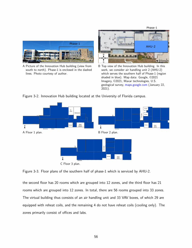
Phase-1

A Picture of the Innovation Hub building (view fromsouth to north). Phase-1 is enclosed in the dashedlines. Photo courtesy of author.

Phase-1

AHU-2

c Google

N

S

EW

B Top view of the Innovation Hub building. In thiswork, we consider air handling unit 2 (AHU-2)which serves the southern half of Phase-1 (regionshaded in blue). Map data: Google, ©2021Imagery, ©2021, Maxar technologies, U.S.geological survey, maps.google.com (January 22,2021).

Figure 3-2. Innovation Hub building located at the University of Florida campus.

Lunch & Vending

roomConference Conference

Copy/

Mailroom Men Women Storage

ITroom

Mechanical

StorageTelecom

Electrical

Client room

IToffice

Recycling/DumpstersMechElevator

Stair

Corridor

Corridor

Corridor

DoorWindow

N

VAV-104 VAV-105

VAV-101

VAV-102

VAV-103

VAV-108

VAV-106VAV-107

VAV-109

A Floor 1 plan.

Lab Lab

Lab

Lab

LabLab

Office Office Office Office Office Office Office Office

Office Office

Storage

Telecom Electrical

Storage

Shared hood room

StorageElevator Stair

Door

Window

Corridor

Corridor

Corridor Corridor

N

VAV-201

VAV-202 VAV-203

VAV-204

VAV-206

VAV-207

VAV-208

VAV-205

SV-209VAV-210 VAV-212

VAV-211

B Floor 2 plan.

Office Office Office Office Office Office

Office Office

Office Office

Lab Lab Lab Autoclave Lab Lab

Telecom Electrical

Elevator Storage

Shared Equipment

Stair

Corridor Corridor

Corridor

Corridor

Door

Window

N

VAV-301

VAV-304

VAV-302 SV-303 VAV-306

VAV-305

VAV-307

VAV-312

VAV-309

SV-310 VAV-311VAV-308

C Floor 3 plan.

Figure 3-3. Floor plans of the southern half of phase-1 which is serviced by AHU-2.

the second floor has 20 rooms which are grouped into 12 zones, and the third floor has 21

rooms which are grouped into 12 zones. In total, there are 56 rooms grouped into 33 zones.

The virtual building thus consists of an air handling unit and 33 VAV boxes, of which 29 are

equipped with reheat coils, and the remaining 4 do not have reheat coils (cooling only). The

zones primarily consist of offices and labs.

56

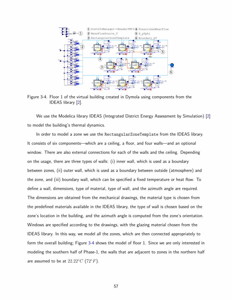
v108Flo

B

C

D

Cei

A

Flo

B

C

D

Cei

A

v107Flo

B

C

D

Cei

A

Flo

B

C

D

Cei

A

v106Flo

B

C

D

Cei

A

Flo

B

C

D

Cei

A

v105Flo

B

C

D

Cei

A

Flo

B

C

D

Cei

A

v104Flo

B

C

D

Cei

A

Flo

B

C

D

Cei

A

v102Flo

B

C

D

Cei

A

Flo

B

C

D

Cei

A

v101Flo

B

C

D

Cei

A

Flo

B

C

D

Cei

A

prescribedHeatFlow prescribedHeatFlow1

prescribedHeatFlow2 prescribedHeatFlow3 prescribedHeatFlow4

prescribedHeatFlow7

prescribedHeatFlow8

sinWat

i

Xi

C

m_flow

T m

s101

Xi

C

m_flow

T m

s108

Xi

C

m_flow

T m

s107

Xi

C

m_flow

T m

s106

Xi

C

m_flow

T m

s105

Xi

C

m_flow

T m

s104

Xi

C

m_flow

T m

s102

Xi

C

m_flow

T m

s109

v109Flo

B

C

D

Cei

A

Flo

B

C

D

Cei

A

prescribedHeatFlow5

x_pTphi

TphiX_steam

x_pTphi1

TphiX_steam

x_pTphi2

TphiX_steam

x_pTphi3

TphiX_steam

x_pTphi4

TphiX_steam

x_pTphi5

TphiX_steam

x_pTphi6

TphiX_steam

x_pTphi7

TphiX_steam

T_sa_108

T_sa_107

m_sa_108

m_sa_107

W_z_108T_z_108

T_z_107W_z_107

m_sa_106

T_sa_106

m_sa_105

T_sa_105

T_sa_104

m_sa_104

T_sa_102

m_sa_102

T_sa_101

T_z_101W_z_101 W_z_102

T_z_102

T_z_104W_z_104 W_z_105

T_z_105 T_z_106W_z_106

q_other_101

co2_z_106

co2_z_108co2_z_102co2_z_101

co2_z_105

co2_z_104

co2_z_107

q_other_102

q_other_104 q_other_105 q_other_106

q_other_108

q_other_107

n_101 n_108

n_106n_105

n_107

n_104

n_102

W_sa

E

T_dry

RH

wind_speedT_dew

T_sky

DNI

GHI

m_sa_109

T_sa_109

n_109

T_z_109

co2_z_109

W_z_109

q_other_109

co2

m_sa_101

1

2

3

4

5

1 SimInfoManager->ReaderTMY3

2 MassFlowSource_T

3 RectangularZoneTemplate

4 PrescribedHeatFlow

5 X_pTphi

6

6 Boundary_pT

Figure 3-4. Floor 1 of the virtual building created in Dymola using components from theIDEAS library [2].

We use the Modelica library IDEAS (Integrated District Energy Assessment by Simulation) [2]

to model the building’s thermal dynamics.

In order to model a zone we use the RectangularZoneTemplate from the IDEAS library.

It consists of six components—which are a ceiling, a floor, and four walls—and an optional

window. There are also external connections for each of the walls and the ceiling. Depending

on the usage, there are three types of walls: (i) inner wall, which is used as a boundary

between zones, (ii) outer wall, which is used as a boundary between outside (atmosphere) and

the zone, and (iii) boundary wall, which can be specified a fixed temperature or heat flow. To

define a wall, dimensions, type of material, type of wall, and the azimuth angle are required.

The dimensions are obtained from the mechanical drawings, the material type is chosen from

the predefined materials available in the IDEAS library, the type of wall is chosen based on the

zone’s location in the building, and the azimuth angle is computed from the zone’s orientation.

Windows are specified according to the drawings, with the glazing material chosen from the

IDEAS library. In this way, we model all the zones, which are then connected appropriately to

form the overall building; Figure 3-4 shows the model of floor 1. Since we are only interested in

modeling the southern half of Phase-1, the walls that are adjacent to zones in the northern half

are assumed to be at 22.22◦C (72◦F ).

57

Inputs to the building thermal dynamics portion of the VB are supply airflow rate (msa,i),

supply air temperature (Tsa,i), and supply air humidity ratio (Wsa,i) for all the zones. These

are implemented using the MassFlowSource_T block from the IDEAS library; an ideal flow

source that produces a specified mass flow with specified temperature, composition, and trace

substances. Outputs of the simulator are temperature (Tz,i) and humidity ratio (Wz,i) of all

the zones. The zone temperature and humidity are also influenced by several exogenous inputs:

(i) outdoor weather conditions such as solar irradiation (ηsol), outdoor air temperature (Toa),

etc. which are provided using the ReaderTMY3 block from the IDEAS library, (ii) internal

sensible and latent heat loads due to occupants, which are computed based on the number

of occupants provided to the zone block, and (iii) internal heat load due to lighting and

equipment which is given using the PrescribedHeatFlow from the Modelica standard library.

Cooling and dehumidifying coil model: The cooling coil model has five inputs and two

outputs. The inputs are supply airflow rate (msa), mixed air temperature (Tma) and humidity

ratio (Wma), chilled water flow rate (mw), and chilled water inlet temperature (Twi). The

outputs are conditioned air temperature (Tca) and humidity ratio (Wca). We use the gray box

data-driven model presented in Chapter 2.

Power consumption models: For the HVAC system configuration presented in

Figure 3-1, there are three main components which consume power. They are supply fan,

cooling and dehumidifying coil, and reheating coils. The fan power consumption is modeled as:

Pfan(k) = αfanmsa(k)3, (3-2)

where msa(k) is the total supply airflow rate at the AHU [76].

The cooling and dehumidifying coil power consumption is modeled to be proportional to

the heat it extracts from the mixed air stream:

Pcc(k) =msa(k)

[hma(k)− hca(k)

]ηccCOPc

, (3-3)

58

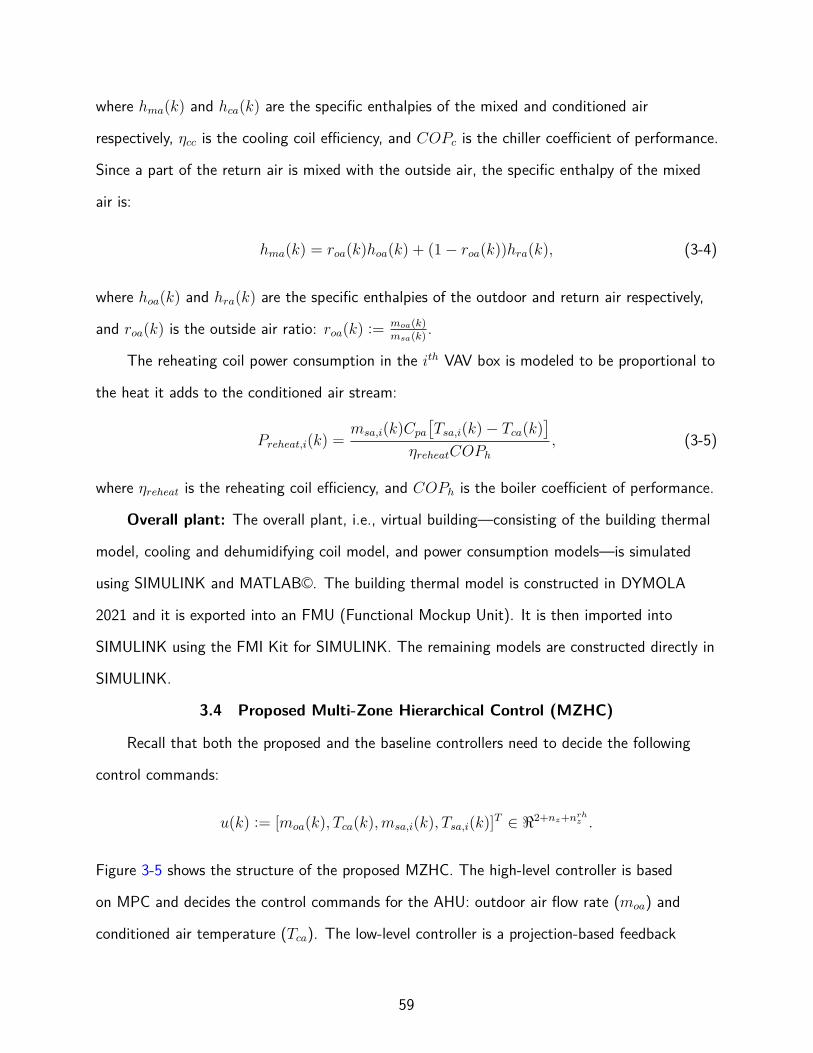
where hma(k) and hca(k) are the specific enthalpies of the mixed and conditioned air

respectively, ηcc is the cooling coil efficiency, and COPc is the chiller coefficient of performance.

Since a part of the return air is mixed with the outside air, the specific enthalpy of the mixed

air is:

hma(k) = roa(k)hoa(k) + (1− roa(k))hra(k), (3-4)

where hoa(k) and hra(k) are the specific enthalpies of the outdoor and return air respectively,

and roa(k) is the outside air ratio: roa(k) :=moa(k)msa(k)

.

The reheating coil power consumption in the ith VAV box is modeled to be proportional to

the heat it adds to the conditioned air stream:

Preheat,i(k) =msa,i(k)Cpa

[Tsa,i(k)− Tca(k)

]ηreheatCOPh

, (3-5)

where ηreheat is the reheating coil efficiency, and COPh is the boiler coefficient of performance.

Overall plant: The overall plant, i.e., virtual building—consisting of the building thermal

model, cooling and dehumidifying coil model, and power consumption models—is simulated

using SIMULINK and MATLAB©. The building thermal model is constructed in DYMOLA

2021 and it is exported into an FMU (Functional Mockup Unit). It is then imported into

SIMULINK using the FMI Kit for SIMULINK. The remaining models are constructed directly in

SIMULINK.

3.4 Proposed Multi-Zone Hierarchical Control (MZHC)

Recall that both the proposed and the baseline controllers need to decide the following

control commands:

u(k) := [moa(k), Tca(k),msa,i(k), Tsa,i(k)]T ∈ ℜ2+nz+nrh

z .

Figure 3-5 shows the structure of the proposed MZHC. The high-level controller is based

on MPC and decides the control commands for the AHU: outdoor air flow rate (moa) and

conditioned air temperature (Tca). The low-level controller is a projection-based feedback

59

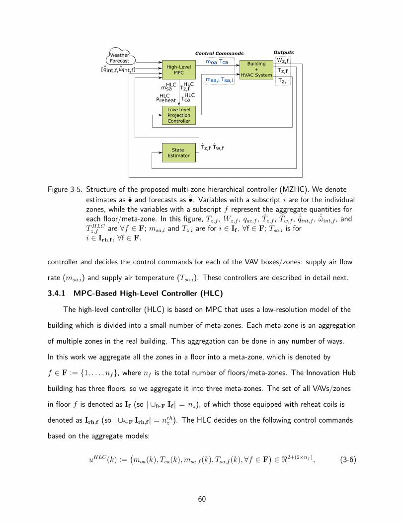
Tcamoa

Tz,fBuilding

+HVAC System

High-LevelMPC

Low-LevelProjectionController

State Estimator

Tsa,imsa,imsa

Preheat

Wz,f

Tz,i

Tz,f Tw,f

[qint,f,ωint,f]

Tz,fHLC

WeatherForecast

HLC

HLC

OutputsControl Commands

TcaHLC

Figure 3-5. Structure of the proposed multi-zone hierarchical controller (MZHC). We denoteestimates as • and forecasts as ˆ•. Variables with a subscript i are for the individualzones, while the variables with a subscript f represent the aggregate quantities foreach floor/meta-zone. In this figure, Tz,f , Wz,f , qac,f , Tz,f , Tw,f , ˆqint,f , ˆωint,f , andTHLCz,f are ∀f ∈ F; msa,i and Tz,i are for i ∈ If , ∀f ∈ F; Tsa,i is for

i ∈ Irh,f , ∀f ∈ F.

controller and decides the control commands for each of the VAV boxes/zones: supply air flow

rate (msa,i) and supply air temperature (Tsa,i). These controllers are described in detail next.

3.4.1 MPC-Based High-Level Controller (HLC)

The high-level controller (HLC) is based on MPC that uses a low-resolution model of the

building which is divided into a small number of meta-zones. Each meta-zone is an aggregation

of multiple zones in the real building. This aggregation can be done in any number of ways.

In this work we aggregate all the zones in a floor into a meta-zone, which is denoted by

f ∈ F := {1, . . . , nf}, where nf is the total number of floors/meta-zones. The Innovation Hub

building has three floors, so we aggregate it into three meta-zones. The set of all VAVs/zones

in floor f is denoted as If (so | ∪f∈F If | = nz), of which those equipped with reheat coils is

denoted as Irh,f (so | ∪f∈F Irh,f | = nrhz ). The HLC decides on the following control commands

based on the aggregate models:

uHLC(k) :=(moa(k), Tca(k),msa,f (k), Tsa,f (k),∀f ∈ F

)∈ ℜ2+(2×nf ), (3-6)

60

where msa,f (k) :=∑i∈If

msa,i(k) is the aggregate (total) supply airflow rate to all the zones

in floor/meta-zone f and Tsa,f (k) is the aggregate supply air temperature. Of the control

commands computed in (3-6), moa(k) and Tca(k) can be directly sent to the plant. The

remaining information computed by the HLC including msa,f (k) and Tsa,f (k) are used by the

low-level controller (LLC), described in Section 3.4.2, to decide on the supply airflow rate

(msa,i(k)) and supply air temperature (Tsa,i(k)) for the individual zones/VAV boxes in each

floor.

A comment on notation: all variables with a subscript i are for the individual zones, while

the variables with a subscript f represent the aggregate quantities for each meta-zone.

For MPC formulation, we use a model interval of ∆t = 5 minutes, a control interval

of ∆T = 15 minutes, and a prediction/planning interval of T = 24 hours. So we have

T = N∆T and ∆T = M∆t, where N = 96 (planning horizon) and M = 3. The control

inputs for N time steps are obtained by solving an optimization problem of minimizing the

energy consumption subject to thermal comfort, indoor air quality, and actuator constraints.

Then the control commands obtained for the first time step are sent to the plant and the LLC.

The optimization problem is solved again for the next N time steps with the initial states of

the model obtained from a state estimator, which uses measurements from the plant. This

process is repeated at the next control time step, i.e., after an interval of ∆T [77].

To describe the optimization problem, first we define the state vector x(k) and the vector

of control commands and internal variables v(k) as:

x(k) :=(Tz,f (k), Tw,f (k),Wz,f (k), ∀f ∈ F

)∈ ℜ3×nf , (3-7)

v(k) :=(uHLC(k),mw(k),Wca(k)

)∈ ℜ2+(2×nf )+2, (3-8)

where Tz,f (k), Tw,f (k), and Wz,f (k) are the aggregate zone temperature, wall temperature,

and humidity ratio of floor/meta-zone f , respectively; uHLC(k) is the control command vector

defined in (3-6) and mw(k) is the chilled water flow rate into the cooling coil. The exogenous

61

input vector is:

w(k) :=(ηsol(k), Toa(k),Woa(k), qint,f (k), ωint,f (k), ∀f ∈ F

)∈ ℜ3+(2×nf ), (3-9)

where ηsol(k) is the solar irradiance, Toa(k) is the outdoor air temperature, Woa(k) is the

outdoor air humidity ratio, qint,f (k) is the aggregate internal heat load in floor/meta-zone f

due to occupants, lights, equipment, etc., and ωint,f (k) is the aggregate rate of water vapor

generation in floor/meta-zone f due to occupants and other sources. We denote the forecast

of these exogenous inputs as ˆw; in Section 3.6, we discuss how these forecasts are obtained.

The vector of nonnegative slack variables ζ(k) :=(ζ lowT,f (k), ζ

highT,f (k), ζ lowW,f (k), ζ

highW,f (k), ∀f ∈

F)∈ ℜ4×nf , is introduced for feasibility of the optimization problem.

The optimization problem at time index j is:

minV,X,Z

j+NM−1∑k=j

[Pfan(k) + Pcc(k) +

∑f∈F

Preheat,f (k)

]∆t+ Pslack(k), (3-10a)

where Pfan(k) is given by (3-2), Pcc(k) is given by (3-3), Preheat,f (k) :=msa,f (k)Cpa

[Tsa,f (k)−Tca(k)

]ηreheatCOPh

,

V := [vT (j), vT (j+1), . . . , vT (j+NM −1)]T , X := [xT (j+1), xT (j+2), . . . , xT (j+NM)]T ,

and Z := [ζT (j + 1), ζT (j + 2), . . . ζT (j + NM)]T . The last term, Pslack, penalizes the

aggregate zone temperature and humidity slack variables:

Pslack(k) :=∑f∈F

[λlowT ζ lowT,f (k + 1) + λhigh

T ζhighT,f (k + 1) + λlowW ζ lowW,f (k + 1) + λhigh

W ζhighW,f (k + 1)

],

where the λs are penalty parameters. The total supply airflow rate msa(k) used in Pfan(k) and

Pcc(k), is given by msa(k) =∑f∈F

msa,f (k) =∑f∈F

∑i∈If

msa,i(k). The optimal control commands

are obtained by solving the optimization problem (3-10a) subject to the following constraints:

Tz,f (k + 1) = Tz,f (k) + ∆t

[Toa(k)− Tz,f (k)

τza,f+

Tw,f (k)− Tz,f (k)

τzw,f

+ Az,fηsol(k)+

qint,f (k) + qac,f (k)

Cz,f

](3-10b)

Tw,f (k + 1) = Tw,f (k) + ∆t

[Toa(k)− Tw,f (k)

τwa,f

+Tz,f (k)− Tw,f (k)

τwz,f

+ Aw,fηsol(k)

](3-10c)

62

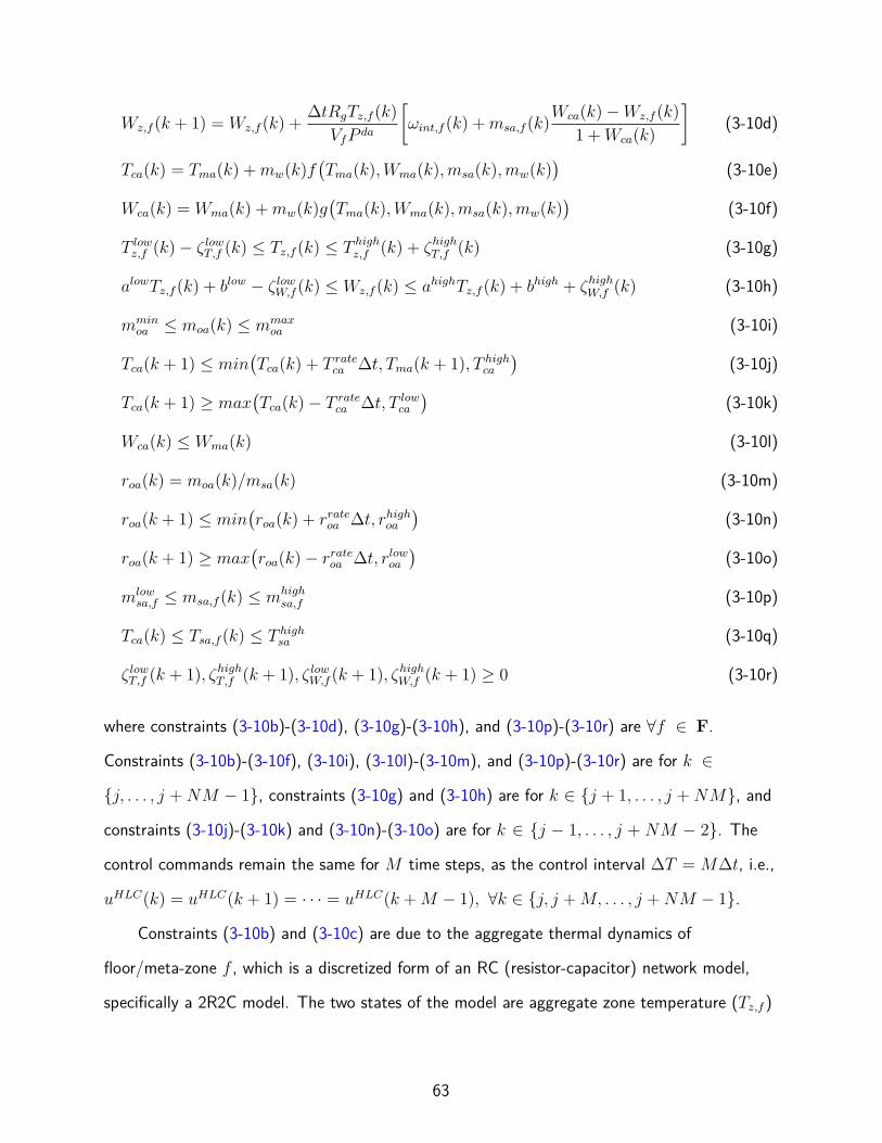
Wz,f (k + 1) = Wz,f (k) +∆tRgTz,f (k)

VfP da

[ωint,f (k) +msa,f (k)

Wca(k)−Wz,f (k)

1 +Wca(k)

](3-10d)

Tca(k) = Tma(k) +mw(k)f(Tma(k),Wma(k),msa(k),mw(k)

)(3-10e)

Wca(k) = Wma(k) +mw(k)g(Tma(k),Wma(k),msa(k),mw(k)

)(3-10f)

T lowz,f (k)− ζ lowT,f (k) ≤ Tz,f (k) ≤ T high

z,f (k) + ζhighT,f (k) (3-10g)

alowTz,f (k) + blow − ζ lowW,f (k) ≤ Wz,f (k) ≤ ahighTz,f (k) + bhigh + ζhighW,f (k) (3-10h)

mminoa ≤ moa(k) ≤ mmax

oa (3-10i)

Tca(k + 1) ≤ min(Tca(k) + T rate

ca ∆t, Tma(k + 1), T highca

)(3-10j)

Tca(k + 1) ≥ max(Tca(k)− T rate

ca ∆t, T lowca

)(3-10k)

Wca(k) ≤ Wma(k) (3-10l)

roa(k) = moa(k)/msa(k) (3-10m)

roa(k + 1) ≤ min(roa(k) + rrateoa ∆t, rhighoa

)(3-10n)

roa(k + 1) ≥ max(roa(k)− rrateoa ∆t, rlowoa

)(3-10o)

mlowsa,f ≤ msa,f (k) ≤ mhigh

sa,f (3-10p)

Tca(k) ≤ Tsa,f (k) ≤ T highsa (3-10q)

ζ lowT,f (k + 1), ζhighT,f (k + 1), ζ lowW,f (k + 1), ζhighW,f (k + 1) ≥ 0 (3-10r)

where constraints (3-10b)-(3-10d), (3-10g)-(3-10h), and (3-10p)-(3-10r) are ∀f ∈ F.

Constraints (3-10b)-(3-10f), (3-10i), (3-10l)-(3-10m), and (3-10p)-(3-10r) are for k ∈

{j, . . . , j +NM − 1}, constraints (3-10g) and (3-10h) are for k ∈ {j + 1, . . . , j +NM}, and

constraints (3-10j)-(3-10k) and (3-10n)-(3-10o) are for k ∈ {j − 1, . . . , j + NM − 2}. The

control commands remain the same for M time steps, as the control interval ∆T = M∆t, i.e.,

uHLC(k) = uHLC(k + 1) = · · · = uHLC(k +M − 1), ∀k ∈ {j, j +M, . . . , j +NM − 1}.

Constraints (3-10b) and (3-10c) are due to the aggregate thermal dynamics of

floor/meta-zone f , which is a discretized form of an RC (resistor-capacitor) network model,

specifically a 2R2C model. The two states of the model are aggregate zone temperature (Tz,f )

63

and wall temperature (Tw,f , a fictitious state). In constraint (3-10b), qac,f (k) is the heat

influx due to the HVAC system and is given by qac,f (k) := msa,f (k)Cpa(Tsa,f (k) − Tz,f (k)).

The model has seven parameters {Cz,f , τzw,f , τza,f , Az,f , τwz,f , τwa,f , Aw,f}. In the evaluation

study, they are estimated using the algorithm presented in [72] and will be discussed later in

Section 3.6.

The constraint (3-10d) is for the aggregate humidity dynamics of floor/meta-zone f ,

where Wz,f is the aggregate zone humidity ratio, Vf is the volume of meta-zone f , Rg is

the specific gas constant of dry air, P da is the partial pressure of dry air, and Wca is the

conditioned air humidity ratio [30].

Constraints (3-10e) and (3-10f) are for the control-oriented cooling and dehumidifying coil

model, which was developed in Chapter 2. The specific functional form in (3-10e) and (3-10f)

is chosen so that when the chilled water flow rate is zero, no cooling or dehumidification of the

air occurs, so the conditioned air temperature and humidity ratio are equal to the mixed air

temperature and humidity ratio: Tca = Tma and Wca = Wma, when mw = 0.

Constraints (3-10g) and (3-10h) are box constraints to maintain the temperature and

humidity of the meta-zones within the allowed comfort limits. The constraints are softened

using slack variables ζ lowT,f (k), ζhighT,f (k), ζ lowW,f (k), and ζhighW,f (k); constraint (3-10r) ensures that

these slack variables are nonnegative. Imposing constraints directly on the relative humidity

of zones (RHz) is difficult, as relative humidity is a highly nonlinear function of dry bulb

temperature and humidity ratio [1, Chapter 1]. So we linearize this function which gives us

alow, blow, ahigh, and bhigh in (3-10h), and helps in converting the constraints on relative

humidity to humidity ratio (Wz).

Constraint (3-10i) is for the outdoor airflow rate, where the minimum allowed value

(mminoa ) is computed based on the ventilation requirements specified in ASHRAE 62.1 [58] and

to maintain positive building pressurization.

Constraints (3-10j)-(3-10k) and (3-10n)-(3-10o) are to take into account the capabilities

of the cooling coil and damper actuators. In constraints (3-10j) and (3-10l), the inequalities

64

Tca(k + 1) ≤ Tma(k + 1) and Wca(k) ≤ Wma(k) ensure that the cooling coil can only

cool and dehumidify the mixed air stream; it cannot add heat or moisture. Similarly, in

constraint (3-10q) the inequality Tsa,f (k) ≥ Tca(k) ensures that the reheat coils can only add

heat; it cannot cool.

Constraint (3-10p) is to take into account the capabilities of the fan and aggregate

capabilities of the VAV boxes. The limits mlowsa,f and mhigh

sa,f are computed using the VAV

schedule from the mechanical drawings of a building as follows: mlowsa,f :=

∑i∈If

mlowsa,i and

mhighsa,f :=

∑i∈If

mhighsa,i .

Note that of the states x(k) defined in (3-7), Tw,f is a fictitious state that cannot be

measured, while the other two states aggregate zone temperature (Tz,f ) and aggregate zone

humidity ratio (Wz,f ) are measured. So we estimate the current state x(k) using a Kalman

filter.

3.4.2 Projection-Based Low-Level Controller (LLC)

The role of the low-level controller (LLC) is to appropriately distribute the aggregate

quantities—such as the total supply airflow rate and reheat power consumption—computed

by the HLC to individual zones/VAVs. The LLC needs to do so by capturing two important

properties: (i) it should consider the needs of individual zones and distribute accordingly, and

(ii) it should act in coherence with the HLC, so that there is minimal mismatch for the MPC

optimization.

The LLC is a projection-based feedback controller that decides on the supply airflow rate

and supply air temperature for each VAV box/zone. That is, the control command vector that

the LLC needs to decide is:

uLLC(k) := [msa,i(k), Tsa,i(k)]T ∈ ℜnz+nrh

z ,

where for msa,i, i ∈ If , ∀f ∈ F, and for Tsa,i, i ∈ Irh,f , ∀f ∈ F. It decides these control

commands by using the following information from the HLC: (i) total allowed supply airflow

rate to all the zones msa(k) =∑f∈F

msa,f (k), (ii) total allowed reheat power consumption

65

Preheat(k) =∑f∈F

Preheat,f (k), (iii) the temperature at which the zones in each meta-zone

should be maintained at Tz,f (k + 1), and (iv) the conditioned air temperature Tca(k). Here on

in this section, we will be using the superscript HLC (•HLC) for these variables to make it clear

that these are obtained from the high-level controller.

First the needs of each zone are assessed based on the current measured temperature

Tz,i(k) and the range it should be in [T htgz,i (k), T

clgz,i (k)] and are translated into the desired

supply airflow rate mdsa,i(k) and supply air temperature T d

sa,i(k). Then these desired values

along with the information obtained from the HLC are used to solve a projection problem to

compute the control commands for all the zones, uLLC(k).

The procedure used to compute the desired values mdsa,i(k) and T d

sa,i(k) is explained

below. This is similar to the Dual Maximum control logic presented in Section 3.5; a schematic

representation of it is shown in Figure 3-6.

• First the temperature range [T htgz,i (k), T

clgz,i (k)] in which each zone should be is computed

as follows: T htgz,i (k) = max

(THLCz,f (k + 1) − T db

z /2, T lowz,f

)∀i ∈ If and T clg

z,i (k) =

min(THLCz,f (k + 1) + T db

z /2, T highz,f

)∀i ∈ If , where THLC

z,f (k + 1) is obtained from theHLC, T db

z is a deadband, and T lowz,f and T high

z,f are the limits used in constraint (3-10g).

• If the zone temperature is between the cooling and heating setpoints (Tz,i(k) ∈[T htg

z,i (k), Tclgz,i (k)]), then the controller is in deadband mode. The supply airflow rate

is desired to be at its minimum and no heating is required, i.e., mdsa,i(k) = mlow

sa,i andT dsa,i(k) = THLC

ca (k).

• If the zone temperature is warmer than the cooling setpoint (Tz,i(k) > T clgz,i (k)), then

the controller is in cooling mode. The supply airflow rate is desired to be increasedas needed and no heating is required, i.e., md

sa,i(k) = min(mlow

sa,i + Kclgm,i(Tz,i(k) −

T clgz,i (k)), m

highsa,i

)and T d

sa,i(k) = THLCca (k).

• If the zone temperature is cooler than the heating setpoint (Tz,i(k) < T htgz,i (k)),

then the controller is in heating mode. Heating is required, and the supply airflowrate is desired to be increased only if additional heating is needed, i.e., T d

sa,i(k) =

min(THLCca (k) + Khtg

T,i (Thtgz,i (k) − Tz,i(k)), T

highsa

); if T d

sa,i(k) = T highsa , then md

sa,i(k) =

min(mlow

sa,i +Khtgm,i(T

htgz,i (k)− Tz,i(k)), m

high,reheatsa,i

), otherwise md

sa,i(k) = mlowsa,i.

66

• Finally, we impose the following rate constraints:

msa,i(k −M)−mratesa,i∆T ≤ md

sa,i(k) ≤ msa,i(k −M) +mratesa,i∆T,

Tsa,i(k −M)− T ratesa,i ∆T ≤ T d

sa,i(k) ≤ Tsa,i(k −M) + T ratesa,i ∆T,

where msa,i(k − M) and Tsa,i(k − M) are the supply airflow rate and supply airtemperature from the previous control time step.

These desired values—mdsa,i(k) and T d

sa,i(k)—along with information from the HLC are

used to solve the following projection problem to obtain the control commands for all the

zones, uLLC(k):

minuLLC(k)

∑f∈F

∑i∈If

λm,i(msa,i(k)−mdsa,i(k))

2 +∑f∈F

∑i∈Irh,f

λT,i(Tsa,i(k)− T dsa,i(k))

2 (3-11a)

subject to the following constraints:

∑f∈F

∑i∈If

msa,i(k) ≤ mHLCsa (k) (3-11b)

∑f∈F

∑i∈Irh,f

msa,i(k)Cpa

(Tsa,i(k)− THLC

ca (k))

ηreheatCOPh

≤ PHLCreheat(k) (3-11c)

mlowsa,i ≤ msa,i(k) ≤ mhigh

sa,i , ∀i ∈ If , ∀f ∈ F (3-11d)

THLCca (k) ≤ Tsa,i(k) ≤ T high

sa , ∀i ∈ Irh,f , ∀f ∈ F (3-11e)

where the sets If and Irh,f are defined at the beginning of this section, λs are weights,

mHLCsa (k) =

∑f∈F

mHLCsa,f (k), and PHLC

reheat(k) =∑f∈F

PHLCreheat,f (k).

Constraints (3-11b) and (3-11c) are to ensure that the total supply airflow rate and

reheat power consumption do not exceed the limits computed by the HLC. Constraints (3-11d)

and (3-11e) are to take in to account the capabilities of the VAV boxes and reheat coils. In

constraint (3-11e), the inequality Tsa,i(k) ≥ Tca(k) ensures that the reheat coils can only add

heat to the conditioned air and cannot cool. The upper limit on supply air temperature (T highsa )

in constraint (3-11e) is to prevent thermal stratification [33].

67

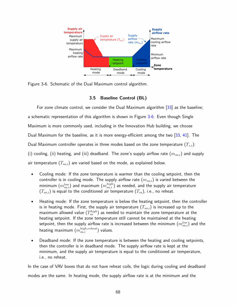
Maximum supply air

temperature

Supply airtemperature (Tsa,i) Maximum

cooling airflow rate

Supply airflow rate (msa,i)

Deadband mode

Cooling mode

Heating mode

Zonetemperature

Supply airflow rate

Minimumairflow rate

Supply airtemperature

Heatingsetpoint

Cooling setpoint

Maximum heating

airflow rate

Figure 3-6. Schematic of the Dual Maximum control algorithm.

3.5 Baseline Control (BL)

For zone climate control, we consider the Dual Maximum algorithm [33] as the baseline;

a schematic representation of this algorithm is shown in Figure 3-6. Even though Single

Maximum is more commonly used, including in the Innovation Hub building, we choose

Dual Maximum for the baseline, as it is more energy-efficient among the two [33, 41]. The

Dual Maximum controller operates in three modes based on the zone temperature (Tz,i):

(i) cooling, (ii) heating, and (iii) deadband. The zone’s supply airflow rate (msa,i) and supply

air temperature (Tsa,i) are varied based on the mode, as explained below.

• Cooling mode: If the zone temperature is warmer than the cooling setpoint, then thecontroller is in cooling mode. The supply airflow rate (msa,i) is varied between theminimum (mlow

sa,i) and maximum (mhighsa,i ) as needed, and the supply air temperature

(Tsa,i) is equal to the conditioned air temperature (Tca), i.e., no reheat.

• Heating mode: If the zone temperature is below the heating setpoint, then the controlleris in heating mode. First, the supply air temperature (Tsa,i) is increased up to themaximum allowed value (T high

sa ) as needed to maintain the zone temperature at theheating setpoint. If the zone temperature still cannot be maintained at the heatingsetpoint, then the supply airflow rate is increased between the minimum (mlow

sa,i) and theheating maximum (mhigh,reheat

sa,i ) values.

• Deadband mode: If the zone temperature is between the heating and cooling setpoints,then the controller is in deadband mode. The supply airflow rate is kept at theminimum, and the supply air temperature is equal to the conditioned air temperature,i.e., no reheat.

In the case of VAV boxes that do not have reheat coils, the logic during cooling and deadband

modes are the same. In heating mode, the supply airflow rate is at the minimum and the

68

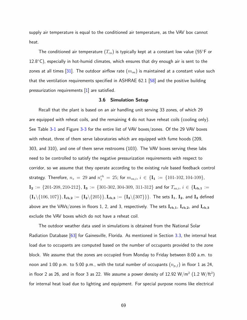
supply air temperature is equal to the conditioned air temperature, as the VAV box cannot

heat.

The conditioned air temperature (Tca) is typically kept at a constant low value (55◦F or

12.8◦C), especially in hot-humid climates, which ensures that dry enough air is sent to the

zones at all times [31]. The outdoor airflow rate (moa) is maintained at a constant value such

that the ventilation requirements specified in ASHRAE 62.1 [58] and the positive building

pressurization requirements [1] are satisfied.

3.6 Simulation Setup

Recall that the plant is based on an air handling unit serving 33 zones, of which 29

are equipped with reheat coils, and the remaining 4 do not have reheat coils (cooling only).

See Table 3-1 and Figure 3-3 for the entire list of VAV boxes/zones. Of the 29 VAV boxes

with reheat, three of them serve laboratories which are equipped with fume hoods (209,

303, and 310), and one of them serve restrooms (103). The VAV boxes serving these labs

need to be controlled to satisfy the negative pressurization requirements with respect to

corridor, so we assume that they operate according to the existing rule based feedback control

strategy. Therefore, nz = 29 and nrhz = 25; for msa,i, i ∈ {I1 := {101-102, 104-109},

I2 := {201-208, 210-212}, I3 := {301-302, 304-309, 311-312} and for Tsa,i, i ∈ {Irh,1 :=

{I1\{106, 107}}, Irh,2 := {I2\{205}}, Irh,3 := {I3\{307}}}. The sets I1, I2, and I3 defined

above are the VAVs/zones in floors 1, 2, and 3, respectively. The sets Irh,1, Irh,2, and Irh,3

exclude the VAV boxes which do not have a reheat coil.

The outdoor weather data used in simulations is obtained from the National Solar

Radiation Database [63] for Gainesville, Florida. As mentioned in Section 3.3, the internal heat

load due to occupants are computed based on the number of occupants provided to the zone

block. We assume that the zones are occupied from Monday to Friday between 8:00 a.m. to

noon and 1:00 p.m. to 5:00 p.m., with the total number of occupants (np,f ) in floor 1 as 24,

in floor 2 as 26, and in floor 3 as 22. We assume a power density of 12.92 W/m2 (1.2 W/ft2)

for internal heat load due to lighting and equipment. For special purpose rooms like electrical

69

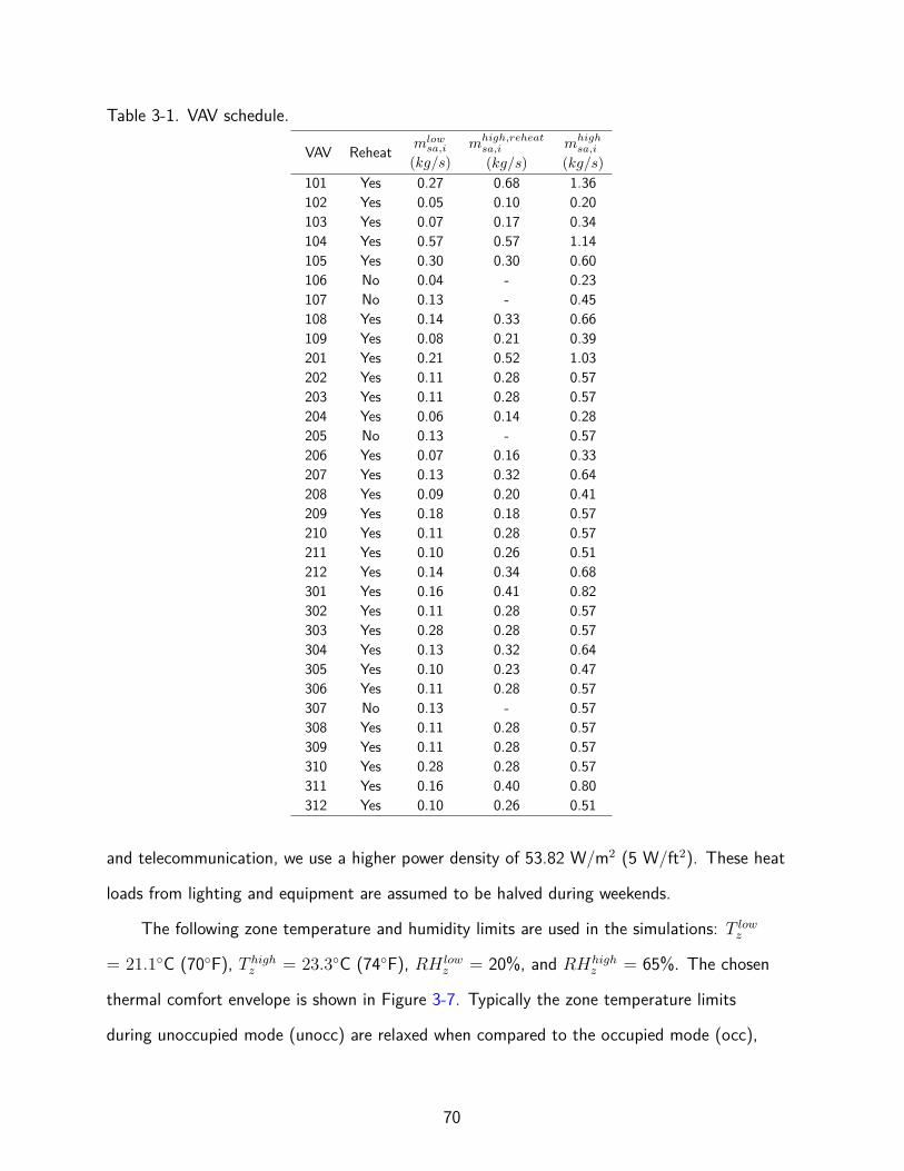
Table 3-1. VAV schedule.

VAV Reheat mlowsa,i

(kg/s)

mhigh,reheatsa,i

(kg/s)

mhighsa,i

(kg/s)

101 Yes 0.27 0.68 1.36102 Yes 0.05 0.10 0.20103 Yes 0.07 0.17 0.34104 Yes 0.57 0.57 1.14105 Yes 0.30 0.30 0.60106 No 0.04 - 0.23107 No 0.13 - 0.45108 Yes 0.14 0.33 0.66109 Yes 0.08 0.21 0.39201 Yes 0.21 0.52 1.03202 Yes 0.11 0.28 0.57203 Yes 0.11 0.28 0.57204 Yes 0.06 0.14 0.28205 No 0.13 - 0.57206 Yes 0.07 0.16 0.33207 Yes 0.13 0.32 0.64208 Yes 0.09 0.20 0.41209 Yes 0.18 0.18 0.57210 Yes 0.11 0.28 0.57211 Yes 0.10 0.26 0.51212 Yes 0.14 0.34 0.68301 Yes 0.16 0.41 0.82302 Yes 0.11 0.28 0.57303 Yes 0.28 0.28 0.57304 Yes 0.13 0.32 0.64305 Yes 0.10 0.23 0.47306 Yes 0.11 0.28 0.57307 No 0.13 - 0.57308 Yes 0.11 0.28 0.57309 Yes 0.11 0.28 0.57310 Yes 0.28 0.28 0.57311 Yes 0.16 0.40 0.80312 Yes 0.10 0.26 0.51

and telecommunication, we use a higher power density of 53.82 W/m2 (5 W/ft2). These heat

loads from lighting and equipment are assumed to be halved during weekends.

The following zone temperature and humidity limits are used in the simulations: T lowz

= 21.1◦C (70◦F), T highz = 23.3◦C (74◦F), RH low

z = 20%, and RHhighz = 65%. The chosen

thermal comfort envelope is shown in Figure 3-7. Typically the zone temperature limits

during unoccupied mode (unocc) are relaxed when compared to the occupied mode (occ),

70

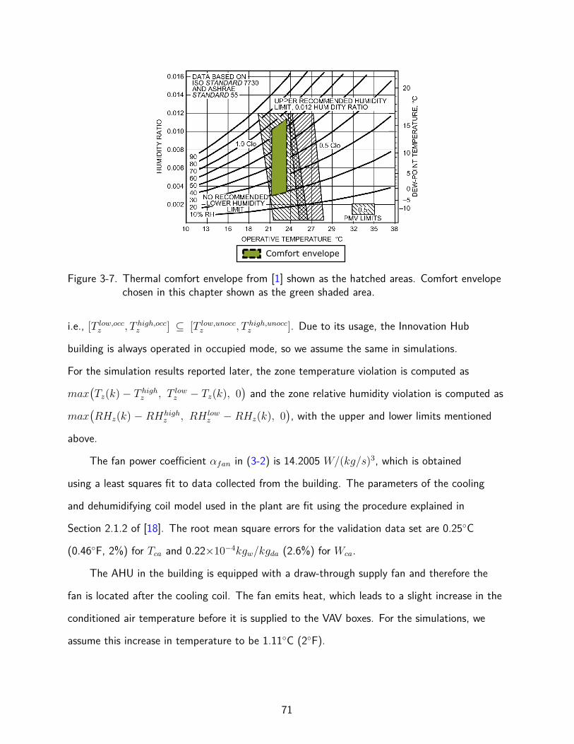
Comfort envelope

Figure 3-7. Thermal comfort envelope from [1] shown as the hatched areas. Comfort envelopechosen in this chapter shown as the green shaded area.

i.e., [T low,occz , T high,occ

z ] ⊆ [T low,unoccz , T high,unocc

z ]. Due to its usage, the Innovation Hub

building is always operated in occupied mode, so we assume the same in simulations.

For the simulation results reported later, the zone temperature violation is computed as

max(Tz(k)− T high

z , T lowz − Tz(k), 0

)and the zone relative humidity violation is computed as

max(RHz(k) − RHhigh

z , RH lowz − RHz(k), 0

), with the upper and lower limits mentioned

above.

The fan power coefficient αfan in (3-2) is 14.2005 W/(kg/s)3, which is obtained

using a least squares fit to data collected from the building. The parameters of the cooling

and dehumidifying coil model used in the plant are fit using the procedure explained in

Section 2.1.2 of [18]. The root mean square errors for the validation data set are 0.25◦C

(0.46◦F, 2%) for Tca and 0.22×10−4kgw/kgda (2.6%) for Wca.

The AHU in the building is equipped with a draw-through supply fan and therefore the

fan is located after the cooling coil. The fan emits heat, which leads to a slight increase in the

conditioned air temperature before it is supplied to the VAV boxes. For the simulations, we

assume this increase in temperature to be 1.11◦C (2◦F).

71

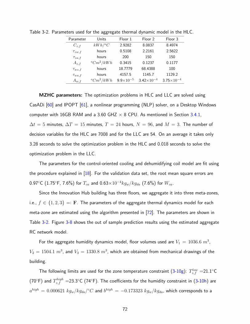
Table 3-2. Parameters used for the aggregate thermal dynamic model in the HLC.Parameter Units Floor 1 Floor 2 Floor 3

Cz,f kWh/oC 2.9282 8.0837 8.4974τzw,f hours 0.5108 2.2161 2.5622τza,f hours 200 150 150Az,f

oCm2/kWh 0.3415 0.1237 0.1177τwz,f hours 18.7779 68.4388 100τwa,f hours 4157.5 1145.7 1129.2Aw,f

oCm2/kWh 9.9×10−5 3.42×10−4 3.75×10−4

MZHC parameters: The optimization problems in HLC and LLC are solved using

CasADi [60] and IPOPT [61], a nonlinear programming (NLP) solver, on a Desktop Windows

computer with 16GB RAM and a 3.60 GHZ × 8 CPU. As mentioned in Section 3.4.1,

∆t = 5 minutes, ∆T = 15 minutes, T = 24 hours, N = 96, and M = 3. The number of

decision variables for the HLC are 7008 and for the LLC are 54. On an average it takes only

3.28 seconds to solve the optimization problem in the HLC and 0.018 seconds to solve the

optimization problem in the LLC.

The parameters for the control-oriented cooling and dehumidifying coil model are fit using

the procedure explained in [18]. For the validation data set, the root mean square errors are

0.97◦C (1.75◦F, 7.6%) for Tca and 0.63×10−4kgw/kgda (7.6%) for Wca.

Since the Innovation Hub building has three floors, we aggregate it into three meta-zones,

i.e., f ∈ {1, 2, 3} =: F. The parameters of the aggregate thermal dynamics model for each

meta-zone are estimated using the algorithm presented in [72]. The parameters are shown in

Table 3-2. Figure 3-8 shows the out of sample prediction results using the estimated aggregate

RC network model.

For the aggregate humidity dynamics model, floor volumes used are V1 = 1036.6 m3,

V2 = 1504.1 m3, and V3 = 1330.8 m3, which are obtained from mechanical drawings of the

building.

The following limits are used for the zone temperature constraint (3-10g): T lowz,f =21.1◦C

(70◦F) and T highz,f =23.3◦C (74◦F). The coefficients for the humidity constraint in (3-10h) are

ahigh = 0.000621 kgw/kgda/◦C and bhigh = −0.173323 kgw/kgda, which corresponds to a

72

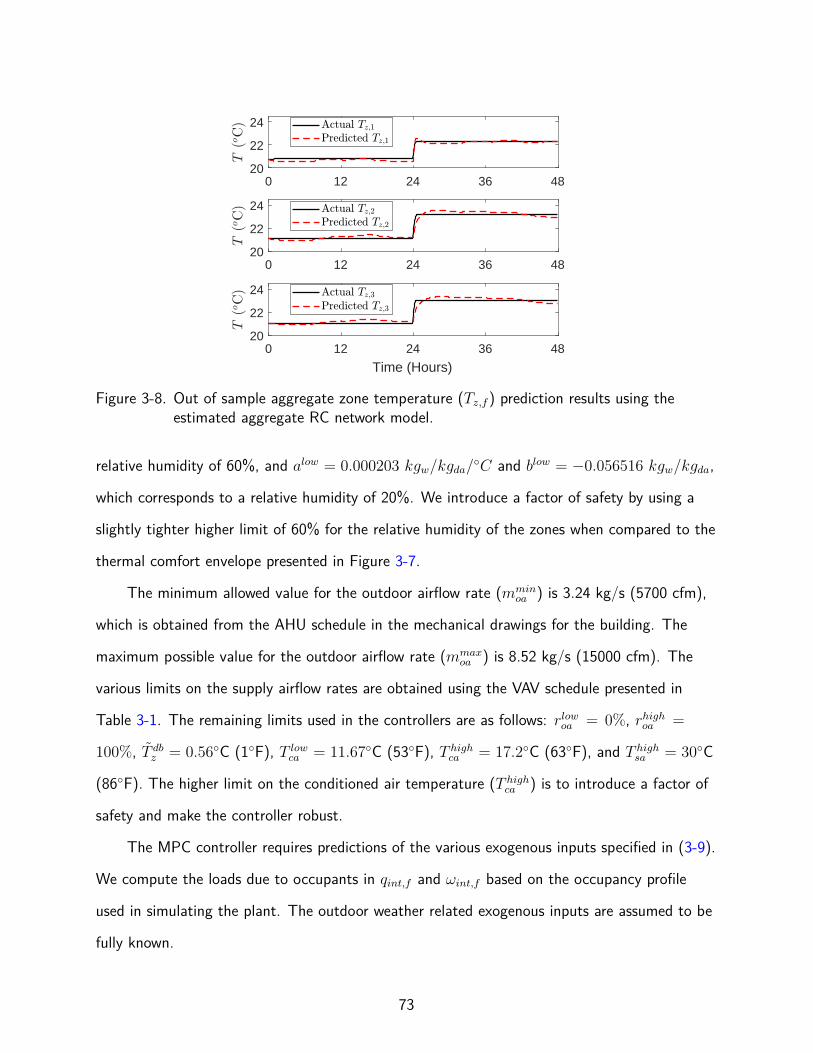
0 12 24 36 4820

22

24

0 12 24 36 4820

22

24

0 12 24 36 48

Time (Hours)

20

22

24

Figure 3-8. Out of sample aggregate zone temperature (Tz,f ) prediction results using theestimated aggregate RC network model.

relative humidity of 60%, and alow = 0.000203 kgw/kgda/◦C and blow = −0.056516 kgw/kgda,

which corresponds to a relative humidity of 20%. We introduce a factor of safety by using a

slightly tighter higher limit of 60% for the relative humidity of the zones when compared to the

thermal comfort envelope presented in Figure 3-7.

The minimum allowed value for the outdoor airflow rate (mminoa ) is 3.24 kg/s (5700 cfm),

which is obtained from the AHU schedule in the mechanical drawings for the building. The

maximum possible value for the outdoor airflow rate (mmaxoa ) is 8.52 kg/s (15000 cfm). The

various limits on the supply airflow rates are obtained using the VAV schedule presented in

Table 3-1. The remaining limits used in the controllers are as follows: rlowoa = 0%, rhighoa =

100%, T dbz = 0.56◦C (1◦F), T low

ca = 11.67◦C (53◦F), T highca = 17.2◦C (63◦F), and T high

sa = 30◦C

(86◦F). The higher limit on the conditioned air temperature (T highca ) is to introduce a factor of

safety and make the controller robust.

The MPC controller requires predictions of the various exogenous inputs specified in (3-9).

We compute the loads due to occupants in qint,f and ωint,f based on the occupancy profile

used in simulating the plant. The outdoor weather related exogenous inputs are assumed to be

fully known.

73

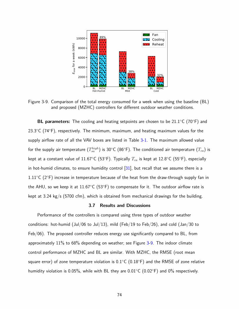
BL Hot-Humid

MZHC BL Mild

MZHC BL Cold

MZHC0

2000

4000

6000

8000

10000

E tot

al fo

r a w

eek

(kW

h)

89%

38%32%

FanCoolingReheat

Figure 3-9. Comparison of the total energy consumed for a week when using the baseline (BL)and proposed (MZHC) controllers for different outdoor weather conditions.

BL parameters: The cooling and heating setpoints are chosen to be 21.1◦C (70◦F) and

23.3◦C (74◦F), respectively. The minimum, maximum, and heating maximum values for the

supply airflow rate of all the VAV boxes are listed in Table 3-1. The maximum allowed value

for the supply air temperature (T highsa ) is 30◦C (86◦F). The conditioned air temperature (Tca) is

kept at a constant value of 11.67◦C (53◦F). Typically Tca is kept at 12.8◦C (55◦F), especially

in hot-humid climates, to ensure humidity control [31], but recall that we assume there is a

1.11◦C (2◦F) increase in temperature because of the heat from the draw-through supply fan in

the AHU, so we keep it at 11.67◦C (53◦F) to compensate for it. The outdoor airflow rate is

kept at 3.24 kg/s (5700 cfm), which is obtained from mechanical drawings for the building.

3.7 Results and Discussions

Performance of the controllers is compared using three types of outdoor weather

conditions: hot-humid (Jul/06 to Jul/13), mild (Feb/19 to Feb/26), and cold (Jan/30 to

Feb/06). The proposed controller reduces energy use significantly compared to BL, from

approximately 11% to 68% depending on weather; see Figure 3-9. The indoor climate

control performance of MZHC and BL are similar. With MZHC, the RMSE (root mean

square error) of zone temperature violation is 0.1◦C (0.18◦F) and the RMSE of zone relative

humidity violation is 0.05%, while with BL they are 0.01◦C (0.02◦F) and 0% respectively.

74

The computational cost of the proposed MZHC is small, just a few seconds are needed to

compute decisions at every control update. On an average it takes 3.28 seconds to solve the

optimization problem in the HLC and 0.018 seconds to solve the optimization problem in the

LLC.

Simulation results for the different weather conditions are discussed in detail next.

3.7.1 Hot-Humid Week

Figure 3-10 shows the simulation time traces for a hot-humid week. It is found that

using the proposed MZHC leads to 11% energy savings when compared to BL, as presented in

Figure 3-9.

Both controllers lead to negligible violations of aggregate zone temperature (Tz,f )

and relative humidity (RHz,f ) constraints. Data for the three meta-zones are shown in

Figure 3-10C, and for three individual zones, one from each floor, are shown in Figure 3-11. BL

ensures that dry enough air is supplied to the zones at all times by keeping the conditioned air

temperature (Tca) at a constant low value of 11.67◦C (53◦F), and hence the humidity limit is

not violated. In the case of MZHC, the humidity constraint is found to be active always. This

can be seen in Figure 3-10C; recall that we use a tighter constraint of 60% instead of 65%

to introduce a factor of safety. This active constraint limits the increase in Tca, which can be

seen in Figure 3-10D. One of the reasons reheating is required even during such a hot week

(the outdoor air temperature is as high as 32.2◦C/90◦F) is because of this active humidity

constraint, which requires dry, and thus, cold air to be supplied to the zones. This could also

be one of the reasons MZHC decides to maintain the zone temperatures at the lower limit

(Figure 3-10C). Keeping the zones at a higher temperature will require an increase in reheating

energy.

The above observations indicate the need to incorporate humidity and latent heat in

MPC formulations. In an effort to reduce energy/cost, MPC controllers that ignore humidity

are likely to make decisions during these hot-humid conditions which will lead to poor indoor

humidity, as they are unaware of the factors mentioned above.

75

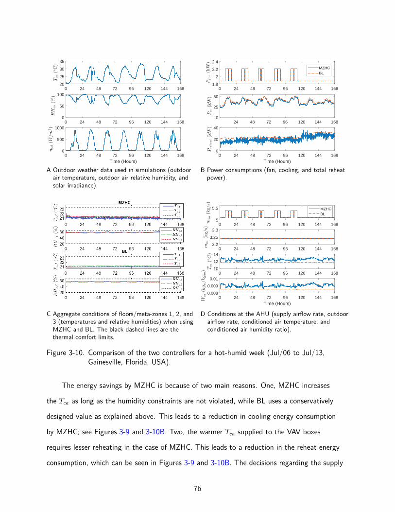
0 24 48 72 96 120 144 16820

25

30

35

0 24 48 72 96 120 144 1680

50

100

0 24 48 72 96 120 144 168

Time (Hours)

0

500

1000

A Outdoor weather data used in simulations (outdoorair temperature, outdoor air relative humidity, andsolar irradiance).

0 24 48 72 96 120 144 1681.8

2

2.2

2.4MZHCBL

24 48 72 96 120 144 1680

25

50

0 24 48 72 96 120 144 168

Time (Hours)

0

20

40

B Power consumptions (fan, cooling, and total reheatpower).

C Aggregate conditions of floors/meta-zones 1, 2, and3 (temperatures and relative humidities) when usingMZHC and BL. The black dashed lines are thethermal comfort limits.

0 24 48 72 96 120 144 1685

5.5 MZHCBL

0 24 48 72 96 120 144 1683.2

3.25

3.3

0 24 48 72 96 120 144 16810

12

14

0 24 48 72 96 120 144 168

Time (Hours)

0.008

0.009

0.01

D Conditions at the AHU (supply airflow rate, outdoorairflow rate, conditioned air temperature, andconditioned air humidity ratio).

Figure 3-10. Comparison of the two controllers for a hot-humid week (Jul/06 to Jul/13,Gainesville, Florida, USA).

The energy savings by MZHC is because of two main reasons. One, MZHC increases

the Tca as long as the humidity constraints are not violated, while BL uses a conservatively

designed value as explained above. This leads to a reduction in cooling energy consumption

by MZHC; see Figures 3-9 and 3-10B. Two, the warmer Tca supplied to the VAV boxes

requires lesser reheating in the case of MZHC. This leads to a reduction in the reheat energy

consumption, which can be seen in Figures 3-9 and 3-10B. The decisions regarding the supply

76

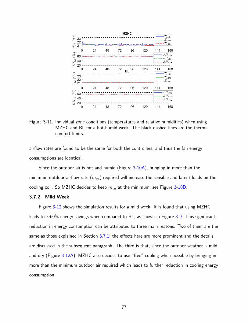
Figure 3-11. Individual zone conditions (temperatures and relative humidities) when usingMZHC and BL for a hot-humid week. The black dashed lines are the thermalcomfort limits.

airflow rates are found to be the same for both the controllers, and thus the fan energy

consumptions are identical.

Since the outdoor air is hot and humid (Figure 3-10A), bringing in more than the

minimum outdoor airflow rate (moa) required will increase the sensible and latent loads on the

cooling coil. So MZHC decides to keep moa at the minimum; see Figure 3-10D.

3.7.2 Mild Week

Figure 3-12 shows the simulation results for a mild week. It is found that using MZHC

leads to ∼60% energy savings when compared to BL, as shown in Figure 3-9. This significant

reduction in energy consumption can be attributed to three main reasons. Two of them are the

same as those explained in Section 3.7.1; the effects here are more prominent and the details

are discussed in the subsequent paragraph. The third is that, since the outdoor weather is mild

and dry (Figure 3-12A), MZHC also decides to use “free” cooling when possible by bringing in

more than the minimum outdoor air required which leads to further reduction in cooling energy

consumption.

77

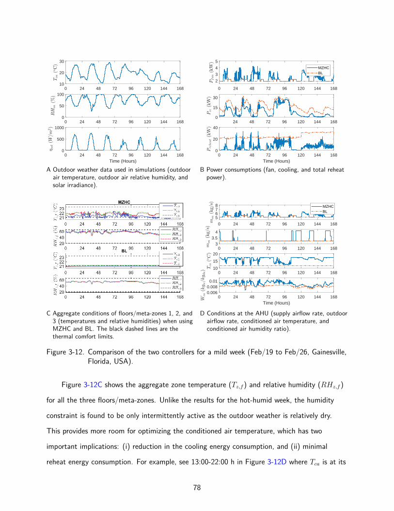
0 24 48 72 96 120 144 16810

20

30

0 24 48 72 96 120 144 1680

50

100

0 24 48 72 96 120 144 168

Time (Hours)

0

500

1000

A Outdoor weather data used in simulations (outdoorair temperature, outdoor air relative humidity, andsolar irradiance).

0 24 48 72 96 120 144 168

2

3

4

5

MZHCBL

24 48 72 96 120 144 1680

15

30

0 24 48 72 96 120 144 168

Time (Hours)

0

20

40

B Power consumptions (fan, cooling, and total reheatpower).

C Aggregate conditions of floors/meta-zones 1, 2, and3 (temperatures and relative humidities) when usingMZHC and BL. The black dashed lines are thethermal comfort limits.

0 24 48 72 96 120 144 168

5678 MZHC

BL

0 24 48 72 96 120 144 1683

3.54

0 24 48 72 96 120 144 16810

15

20

0 24 48 72 96 120 144 168

Time (Hours)

0.0060.008

0.01

D Conditions at the AHU (supply airflow rate, outdoorairflow rate, conditioned air temperature, andconditioned air humidity ratio).

Figure 3-12. Comparison of the two controllers for a mild week (Feb/19 to Feb/26, Gainesville,Florida, USA).

Figure 3-12C shows the aggregate zone temperature (Tz,f ) and relative humidity (RHz,f )

for all the three floors/meta-zones. Unlike the results for the hot-humid week, the humidity

constraint is found to be only intermittently active as the outdoor weather is relatively dry.

This provides more room for optimizing the conditioned air temperature, which has two

important implications: (i) reduction in the cooling energy consumption, and (ii) minimal

reheat energy consumption. For example, see 13:00-22:00 h in Figure 3-12D where Tca is at its

78

higher limit, and also see Figure 3-12B where Pcc is significantly reduced and Preheat is almost

zero.

3.7.3 Cold Week

The energy savings when using MZHC is found to be significant as can be seen in

Figure 3-9. Since the outdoor weather is cold and dry, there is a lot of room for optimizing the

control commands. The reasons for energy reduction when using MZHC are the same as those

explained in Section 3.7.2, therefore we do not discuss them in detail here.

Comment 3.1. Recall that as mentioned in Section 3.5, the Innovation Hub building uses

Single Maximum algorithm for zone climate control as opposed to the Dual Maximum

algorithm presented here [33]. In the case of Single Maximum algorithm, the minimum allowed

value for the supply airflow rate has to be high enough so that the heating load can be met

with low enough supply air temperature to prevent thermal stratification [33]. While in the

case of Dual Maximum algorithm, the airflow rate is varied during the heating mode, thus the

minimum allowed airflow rate is not limited by stratification. Therefore using Single Maximum

algorithm leads to higher fan, cooling, and reheating energy consumptions. This also implies

that the energy savings by the proposed controller will be even higher.

3.8 Summary

The proposed control architecture is designed to address a number of limitations in the

existing literature on multi-zone building control using MPC. The main one is the reliance

on a high-resolution multi-zone model, which can be challenging to obtain. A low-resolution

model of the building is more convenient since such a model can be identified in a tractable

manner from measurements. The challenge then is to convert the MPC decisions, which are

computed for the fictitious zones in the model, to the commands for the VAV boxes of the

actual building. The proposed architecture does that by posing this conversion as a projection

problem that uses not only what the MPC computes but also feedback from zones. The result

is a principled method of computing VAV box commands that are consistent with the optimal

decisions made by the MPC without needing dynamic models of individual zones. At the same

79

time, the use of feedback from the zones ensures that zone climate states are also close to the

aggregate climate states computed by the MPC.

The positive simulation results provide confidence on the effectiveness of the proposed

controller especially because of the large plant model mismatch. The simulation testbed

mimics a real building closely, including the heterogeneous nature of the zones in the building.

Another observation from the simulations that should be emphasized is the need to incorporate

humidity and latent heat. The indoor humidity constraint is seen to be active when using the

proposed controller, especially during hot-humid weather. Without humidity being explicitly

considered, the controller is likely to have caused high space humidity in an effort to reduce

energy use.

Recall that as mentioned in Chapter 1, the energy savings reported in this chapter and

in Chapter 2 will lead to a corresponding reduction in greenhouse gas emissions. The fan and

cooling energy savings will translate to a reduction in electricity usage and the heating energy

savings will translate to a reduction in the usage of gas, as heating in commercial buildings

is typically provided using gas-fired boilers. An approximate estimate of the corresponding

reduction in greenhouse gas emissions can be computed using the greenhouse gas equivalencies

calculator proposed by the United States Environmental Protection Agency (EPA) [78].

Using this calculator, the energy savings reported in this chapter correspond to a reduction

in greenhouse gas emissions by 0.419 to 1.508 metric tons of carbon dioxide equivalent per

week depending on the weather. Note that this estimate is only an approximation, obtaining

an accurate estimate will require considering several factors such as: (i) energy sources,

(ii) location, (iii) time of usage, etc. This is a topic for future work.

Another positive effect of the energy savings on the environment could be a reduction

in cooling tower make-up water usage and a reduction in the emission of water vapor, a

greenhouse gas [79], from cooling towers. Several factors need to be considered in estimating

this, such as: (i) reduction at the site (building) because of chiller cooling load reduction,

80

(ii) reduction at the source (power plant) because of electricity usage reduction, etc. This is

another topic for future work.

81

CHAPTER 4ANALYSIS OF ROUND-TRIP EFFICIENCY OF AN HVAC-BASED VIRTUAL BATTERY

4.1 Overview

In this chapter, the impact on energy efficiency of commercial building HVAC systems

when they are used for grid support is analyzed. There is a growing recognition that the

power demand of most electric loads is flexible, and this flexibility can be exploited to provide

ancillary services to the grid by varying the demand up and down over a baseline [80, 81].

To the grid they appear to be providing the same service as a battery [82]. Such a load, or

collection of loads, can therefore be called Virtual Energy Storage (VES) systems or virtual

batteries.

Consumers’ quality of service (QoS) must be maintained by these virtual batteries. When

HVAC systems are used for VES, a key QoS measure is indoor temperature. Another important

QoS measure is the total energy consumption. Continuously varying the power consumption

of loads around a baseline may lead to a net reduction in the efficiency of energy use, causing

the load to consume more energy in the long run. If so, that will be analogous to the virtual

battery having a round-trip efficiency (RTE) less than unity. Electrochemical batteries also

have a less-than-unity round-trip efficiency due to various losses [17].

The aim of this chapter is to analyze the RTE of VES system comprised of HVAC

equipment in commercial buildings. The inspiration for this work comes from [16] and its

follow-on work [83]. To the best of our knowledge, the article [16] is the first to provide

experimental data on the round-trip efficiency of buildings providing virtual energy storage

from an experiment carried out at a building in the Los Alamos National Laboratory (LANL)

campus. The average RTE (over many tests) reported in [16] was less than 0.5. These values

are quite low compared to that for electrochemical batteries, which vary from 0.75 to 0.97

depending on the electrochemistry [17]. If the RTE estimates in [16] are representative, that

bodes ill for the use of building HVAC systems to be virtual batteries.

82

This chapter provides an analysis of the RTE of an HVAC based VES system using a

simple physics-based model. We establish that the RTE in fact approaches 1 when the HVAC

system is repeatedly used as a virtual battery for many cycles. The low RTE values seen in the

LANL experiments was due to the fact that the experiment was run for one cycle.

Literature review and statement of contribution. In the experiments reported in

[16], fan power was varied in an approximately square wave fashion with a time period of 30

minutes in a ∼ 30, 000 m2 building in the LANL campus. After one cycle of the square wave,

the climate control system was re-activated to bring the building temperature back to its

baseline value. It was observed that the control system had to expend a considerable amount

of additional energy in the recovery phase in almost all the tests performed. This loss was

expressed as a round-trip efficiency less than unity. In a small number of tests, the RTE was

observed to be greater than unity. The mean RTE observed from all the tests was in the order

of 0.5.

In the experiments reported in the article [81], fan power in a ∼ 3700 m2 building at the

University of Florida (UF) campus was varied to track Pennsylvania-New Jersey-Maryland’s

(PJM) RegD signal [84]. When the VES controller was turned off at the end of the

experiment, no large transient was observed in either power or temperature; see Figure 8

of [85]. A more recent paper that also presented results from experiments in a test building

at Lawrence Berkeley National Laboratory (LBNL) in which HVAC fan power was varied to

track RegD, observed similar behavior [86]. In fact [86] reported a slight decrease in energy

use compared to the baseline. Unlike the LANL experiments, the UF and LBNL experiments

involved higher frequency variation in the HVAC power, of time scales shorter than 10 minutes.

The paper [83] attempted to explain the experimental observations in [16] by conducting

simulations. They also examined the effect of several model parameters and sources of

experimental uncertainty such as imprecise knowledge of baseline power consumption. They

were able to replicate several trends observed in the LANL experiments, but there were also

significant differences.

83

The purpose of this work is to rigorously analyze the RTE of a VES system that is based

on commercial-building HVAC equipment and to determine factors that affect the RTE. In

that sense, our goal is similar to that of [83]. In contrast to [83], which explored the effect of

many factors on the RTE by simulation alone, we focus on deriving results for a limited set of

conditions for which provable results can be provided. Following [83], we also use a simplified

physics-based model of a building’s temperature dynamics and power consumption instead of

using a simulation software so that rigorous analysis is possible.

This work makes three main contributions to the nascent literature on the RTE of

HVAC-based virtual batteries. The first contribution is to show that the RTE values much

smaller than unity that were reported in prior work were an artifact of the experimental/simulation

set up. In particular, the HVAC system underwent only “one demand-response event” in [16],

i.e., one period of a square-wave power variation. The simulation study [83] also focused on

that situation and observed similar values of the RTE. It did explore multiple demand-response

events, in which the RTE was found to be close to 1. These events, however, were chosen in

a particular manner that are unlikely to occur in practice. We focus on a general case in which

an HVAC-based virtual battery undergoes n repeated cycles of a square-wave power variation.

We show through rigorous analysis that the RTE approaches 1 as n → ∞. When n is small,

especially when n = 1, we show that the RTE can indeed be larger or smaller than 1 depending

on the time period of the reference signal.

Second, we show that if an additional constraint is imposed—that the mean steady state

temperature of the building must not be changed by the VES service—then additional energy

consumption may be needed, which reduces the asymptotic RTE to a value strictly below

1. We then examine how this RTE varies with various model parameters such as building

size and time period of power deviation. The trends observed are valuable in choosing design

parameters, such as whether a smaller or larger building is better suited to provide VES service.

Third, we explicitly define terms and concepts that are standard for electrochemical

batteries, such as “state of charge”, but not yet for HVAC-based virtual batteries. Some of

84

these terms were used—even implicitly defined—in prior work [16, 83]. We believe future

studies on RTE of virtual batteries will benefit from the definitions proposed here.

The rest of this chapter is organized as follows. Section 4.2 describes the terminology and

definitions needed for the sequel. Section 4.3 describes the HVAC system model used. Section

4.4 and 4.5 provides analysis of RTE, with and without the “zero-mean temperature deviation”

constraint, respectively. Section 4.6 summarizes the conclusions.

4.2 Definitions and Other Preliminaries

4.2.1 Round-Trip Efficiency of an Electrochemical Battery

The state of charge (SoC) of a battery, which we denote by SB(t), is defined as [87]

SB(t) = SB(0) +1

Q0

∫ t

0

IB(t)dt, (4-1)

where IB(t) is the current drawn by the battery (positive during charging and negative

during discharging) and Q0 is its maximum charge (in Coulomb). The SoC is a number

between 0 and 1. It is more convenient to use power drawn (or discharged) instead of current

in (4-1). For simplicity, we assume the voltage across the battery is constant, V0, so the

power drawn by the battery from the grid is PB(t) := V0IB(t). Eq. (4-1) then becomes

SB(t) = SB(0) +1

Q0V0

∫ t

0PB(t)dt. Differentiating, we get

C0SB(t) = PB(t) (4-2)

where C0 = Q0V0.

Definition 4.1 (Complete charge-discharge). We say a battery has undergone a complete

charge-discharge during a time interval [ti, tf ] if SoC(ti) = SoC(tf ). The time interval [ti, tf ]

is called a complete charge-discharge interval.

The qualifier “complete” does not mean the SoC reaches 1 or 0. It only means the SoC

comes back to where it started from.

Definition 4.2 (RTE). Suppose a battery undergoes a complete charge-discharge over a time

interval [0, tcd]. Let tc be the length of time during which the battery is charging and td be the

85

length of time during which the battery is discharging so that tc + td = tcd. The round-trip

efficiency (RTE) of the battery, denoted by ηrt, during this interval is

ηrt , Ed

Ec

=−∫tdPB(t)dt∫

tcPB(t)dt

, (4-3)

where Ed is the energy released by the battery to the grid during discharging, Ec is the energy

consumed by the battery from the grid during charging, and∫tc

(resp.,∫td

) denotes integration

performed over the charging times (resp., discharging times).

Notice that by convention PB(t) < 0 means the battery is releasing power to the grid at

time instant t. In general, the RTE depend on many factors including how a particular SoC

was achieved [88]. For simplicity, we ignore those effects and use (4-3) to define the RTE of

the battery.

4.2.2 Round-Trip Efficiency of an HVAC-Based VES System

We now consider an HVAC system whose power demand is artificially varied from its

baseline demand to provide virtual energy storage. The power consumption of the virtual

battery, P , is defined as the deviation of the electrical power consumption of the HVAC system

from the baseline power consumption:

P (t) := Phvac(t)− P(b)hvac(t), (4-4)

where P(b)hvac is the baseline power consumption of the HVAC system, defined as the power the

HVAC system needs to consume to maintain a baseline indoor temperature T (b).

To make a connection between a real battery and a virtual battery, consider the simple

dynamic model of a building’s temperature:

CT (t) = q(t), (4-5)

where C is the heat capacity of the building (J/K) and q is the net heat influx rate (J/s),

which is the combined effect of heat gain of the building from solar, outdoor weather,

occupants, and the HVAC system. Comparing (4-5) and (4-2), we see that indoor temperature,

86

T (t), and the SoC of an electrochemical battery, SB, are analogous. Just as the SoC of a real

battery must be kept between 0 and 1, the temperature of a building must be kept between a

minimum value, denoted by TL (low), and a maximum value, denoted by TH (high), to ensure

QoS. We therefore define the SoC of an HVAC-based virtual battery as follows, which is similar

to the one used in [89] for water heaters.

Definition 4.3 (SoC of a VES system). The SoC of an HVAC-based VES system with

indoor temperature T is the ratio TH − T

TH − TL

where [TL, TH ] is the allowable range of indoor

temperature.

The definition of a complete charge-discharge interval of a virtual battery is the

same as that for a battery: Definition 4.1, with SoC as defined in Definition 4.3. The

round-trip efficiency of the virtual battery, denoted as ηrt, is also the same as that of a

battery (Definition 4.2), with power consumption of the battery, PB(t), replaced by power

consumption of the virtual battery, P (t). Thus,

ηrt =−∫tdP (t)dt∫

tcP (t)dt

=−∫td(Phvac(t)− P

(b)hvac(t))dt∫

tc(Phvac(t)− P

(b)hvac(t))dt

(4-6)

4.2.3 Charging vs. Change in SoC

A comment on the implication of Definition 4.3 is in order. Whether an increase in SoC is

accompanied by an increase in the VES system’s power consumption depends on the baseline

condition. Imagine the scenario when the HVAC system provides net cooling. When the VES

system charges, i.e., P > 0, additional cooling is provided to the building (Equation (4-4)),

and the temperature decreases over baseline, thereby increasing the SoC according to the

definition above. Similarly, when it discharges, i.e., P < 0, less cooling is provided and

temperature increases over baseline, thereby lowering the SoC. If the HVAC system is in the

heating mode, the opposite occurs. Charging (P > 0) means more heating, increase in

temperature and therefore lowering of the SoC, and vice versa for discharging. Although that

may appear contrary to intuition based on electrochemical batteries, we believe it is sensible

since charging (resp., discharging) of a battery, real or virtual, should correspond to positive

87

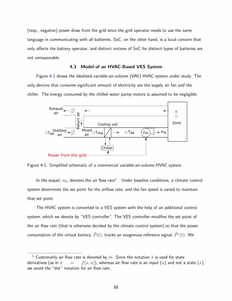
(resp., negative) power draw from the grid since the grid operator needs to use the same

language in communicating with all batteries. SoC, on the other hand, is a local concern that

only affects the battery operator, and distinct notions of SoC for distinct types of batteries are

not unreasonable.

4.3 Model of an HVAC-Based VES System

Figure 4-1 shows the idealized variable-air-volume (VAV) HVAC system under study. The

only devices that consume significant amount of electricity are the supply air fan and the

chiller. The energy consumed by the chilled water pump motors is assumed to be negligible.

Ret

urn

air

Exhaustair

Outdoor air

Mixedair

Zone

T

Cooling coil

Tsa

Chiller

Power from the grid

maTma FanToa

Figure 4-1. Simplified schematic of a commercial variable-air-volume HVAC system.

In the sequel, ma denotes the air flow rate1 . Under baseline conditions, a climate control

system determines the set point for the airflow rate, and the fan speed is varied to maintain

that set point.

The HVAC system is converted to a VES system with the help of an additional control

system, which we denote by “VES controller”. The VES controller modifies the set point of

the air flow rate (that is otherwise decided by the climate control system) so that the power

consumption of the virtual battery, P (t), tracks an exogenous reference signal, P r(t). We

1 Customarily air flow rate is denoted by m. Since the notation x is used for statederivatives (as in x = f(x, u)), whereas air flow rate is an input (u) and not a state (x),we avoid the “dot” notation for air flow rate.

88

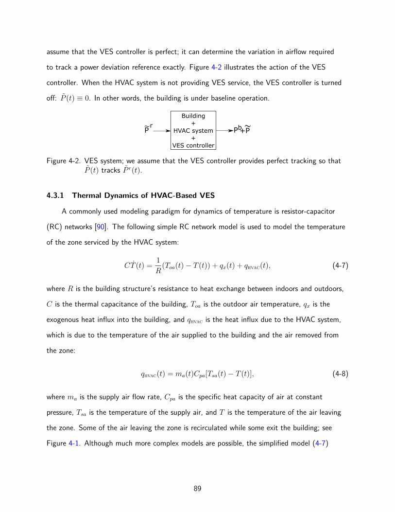
assume that the VES controller is perfect; it can determine the variation in airflow required

to track a power deviation reference exactly. Figure 4-2 illustrates the action of the VES

controller. When the HVAC system is not providing VES service, the VES controller is turned

off: P (t) ≡ 0. In other words, the building is under baseline operation.

Building+

HVAC system+

VES controller

P Pb+Pr ∼∼

Figure 4-2. VES system; we assume that the VES controller provides perfect tracking so thatP (t) tracks P r(t).

4.3.1 Thermal Dynamics of HVAC-Based VES

A commonly used modeling paradigm for dynamics of temperature is resistor-capacitor

(RC) networks [90]. The following simple RC network model is used to model the temperature

of the zone serviced by the HVAC system:

CT (t) =1

R(Toa(t)− T (t)) + qx(t) + qhvac(t), (4-7)

where R is the building structure’s resistance to heat exchange between indoors and outdoors,

C is the thermal capacitance of the building, Toa is the outdoor air temperature, qx is the

exogenous heat influx into the building, and qhvac is the heat influx due to the HVAC system,

which is due to the temperature of the air supplied to the building and the air removed from

the zone:

qhvac(t) = ma(t)Cpa[Tsa(t)− T (t)], (4-8)

where ma is the supply air flow rate, Cpa is the specific heat capacity of air at constant

pressure, Tsa is the temperature of the supply air, and T is the temperature of the air leaving

the zone. Some of the air leaving the zone is recirculated while some exit the building; see

Figure 4-1. Although much more complex models are possible, the simplified model (4-7)

89

aids analysis. Furthermore, it is argued in [91] that a first-order RC network model—such as

(4-7)—is adequate for prediction up to a few days.

4.3.2 HVAC Power Consumption Model

The power consumption of the HVAC system is a sum of the fan power and chiller power:

Phvac(t) = Pf (t) + Pch(t).

We model the fan power consumption as:

Pf (t) = α1fm2a(t) + α2fma(t), (4-9)

where α1f (> 0) and α2f are coefficients that depend on the fan. Variable speed air supply fan

power models reported in the literature are typically cubic [76]. We use a quadratic model for

two main reasons. One is ease of analysis, which will be utilized in Section 4.4. The other is

that a quadratic model is adequate to fit measured data, which we will show in Section 4.4.1.

Note that α2f is allowed to be negative to better fit measurements, though Pf is always

non-negative for the range of airflows in which we consider the VES system to be operating.

Electrical power consumption by the chiller, Pch, is modeled as being proportional to the

heat it extracts from the mixed air stream that passes through the evaporator (or the cooling

coil in a chilled water system):

Pch(t) =ma(t)[hma(t)− hsa(t)]

COP, (4-10)

where COP is the coefficient of performance of the chiller, h(·) is specific enthalpy of air, and

the subscripts ma and sa stand for “mixed air” and “supply air”; see Figure 4-1. Since a part

of the return air is mixed with the outside air, the specific enthalpy of the mixed air is:

hma(t) = roa(t)hoa(t) + (1− roa(t))h(t), (4-11)

where roa is the so-called outside air ratio: roa := moa

ma, hoa is the specific enthalpy of outdoor

air, and h is the specific enthalpy of the air leaving the zone. The specific enthalpy of moist air

with temperature T and humidity ratio W is given by: h(T,W ) = CpaT +W (gH20 + CpwT ),

90

where gH20 is the heat of evaporation of water at 0◦C, and Cpa, Cpw are specific heat of air and

water at constant pressure. We assume the following throughout this chapter to simplify the

analysis:

Assumption 4.1. (i) The ambient temperature (Toa), the exogenous heat gain (qx), and the

coefficient of performance of the chiller (COP) are constants. (ii) The ambient is warmer than

the maximum allowable indoor temperature: Toa > TH , so the HVAC system only provides

cooling. (iii) Effect of humidity change is ignored so that the specific enthalpy of an air stream,

h, with (dry-bulb) temperature T is h = CpaT , where Cpa is the specific heat capacity of dry

air. (iv) The supply air temperature, Tsa, is constant, and Tsa < T (b).

The first three are taken for the ease of analysis. The fourth usually holds in practice

because the cooling coil control loop maintains Tsa at a constant set point, which is lower than

indoor temperature in cooling applications.

With Assumption 4.1, (4-9), (4-10), and (4-11) yield

Phvac(ma, T ) = α1f (ma)2 + α2fma +

maCpa[roaToa + (1− roa)T − Tsa]

COP. (4-12)

Similarly, the temperature dynamics (4-7) and (4-8) become

T =1

RC(Toa − T ) +

1

Cqx +

1

CmaCpa(Tsa − T ). (4-13)

Definition 4.4 (Baseline). Baseline corresponds to an equilibrium condition in which zone

temperature and air flow rate are held at constant values, denoted by T (b) and m(b)a .

It follows from Definition 4.4 and (4-13) that the baseline variables T (b) and m(b)a must

satisfy

0 =1

R(Toa − T (b)) + qx +m(b)

a Cpa(Tsa − T (b)). (4-14)

The baseline power consumption, P (b)hvac, is obtained by plugging in T (b) and m

(b)a into the

expression for Phvac in (4-12).

91

The baseline temperature is best thought of as the setpoint that the climate controller

uses, and can be any temperature that is strictly inside the allowable interval, meaning

TL < T (b) < TH . Since some variation of the temperature around the setpoint is inevitable

due to imperfect reference tracking by a climate controller, the setpoint is always chosen to be

inside the allowable limits. The requirement TL < T (b) < TH is consistent with this practice.

4.3.3 VES System Dynamics and Power Consumption

Now we will derive the expressions for the VES system dynamics and power consumption

which will be used in the subsequent analysis presented in Section 4.4. Let ma(t) be the

airflow rate deviation (from the baseline) commanded by the VES controller. Note that

ma(t) = m(b)a + ma(t). Let the resulting deviation in the zone temperature be

T (t) := T (t)− T (b). (4-15)

The power consumption by the virtual battery is:

P (t) :=Phvac(ma(t), T (t))− P(b)hvac(m

(b)a , T (b)), (4-16)

where Phvac(·, ·) is given by (4-12).

By expanding (4-16), we obtain:

P = ama + bT + cmaT + dm2a, (4-17)

where the constants a, b, c, and d are:

a := 2α1fm(b)a + α2f +

Cpa[roaToa + (1− roa)T(b) − Tsa]

COP, (4-18)

b :=Cpam

(b)a (1− roa)

COP, c :=

Cpa(1− roa)

COP, d := α1f . (4-19)

Differentiating (4-15), and using (4-13) and (4-14) we obtain:

˙T = −αT − βma − γT ma, (4-20)

where α :=RCpam

(b)a + 1

RC, β :=

Cpa(T(b) − Tsa)

C, γ :=

Cpa

C. (4-21)

92

The dynamics of the temperature deviation (and therefore of the SoC of the virtual battery, cf.

Definition 4.3) are thus a differential algebraic equation (DAE): ˙T = f(T , ma) , P = g(T , ma),

where the first (differential) equation is given by (4-20) and the second (algebraic) equation is

given by (4-17).

4.4 RTE with Zero-Mean Square-Wave Power Consumption

In this work we restrict the power consumption of the virtual battery to a square-wave

signal. There are three reasons for this choice. One, it enables comparison with prior

work [16, 83]. Two, it aids the analysis of temperature dynamics. Three, an arbitrary

square-integrable signal can be approximated by a combination of square waves using the

Haar wavelet transform [92].

Let the amplitude of the power consumption P (t) be ∆P and the half-period be tp

(so that the period is 2tp). For half of the period, P (t) = ∆P , and for the other half,

P (t) = −∆P . Consider a complete charge-discharge interval of the VES system, [0, τ ], so that

SoC(0) = SoC(τ); cf. Definition 4.1. Let tc be the total length of the time intervals during

which the VES was charging, i.e., the value of P (t) is ∆P at any t in those intervals. Similarly,

let td be the total length of the time intervals during which the VES was discharging, i.e., the

value of P (t) is −∆P at any t in those intervals. Note that tc + td = τ . It follows from (4-6)

that

ηrt =−∫td[−∆P ]dt∫

tc[∆P ]dt

=tdtc. (4-22)

The RTE will therefore be either larger or smaller than one depending on whether td ≥ tc or

vice versa. The formula (4-22) will be used in the subsequent analysis.

Since [16] reported differences in observed RTE depending on whether the power

consumption is first increased and then decreased from the baseline (“up/down” scenario),

or vice versa (“down/up” scenario), we treat them separately.

93

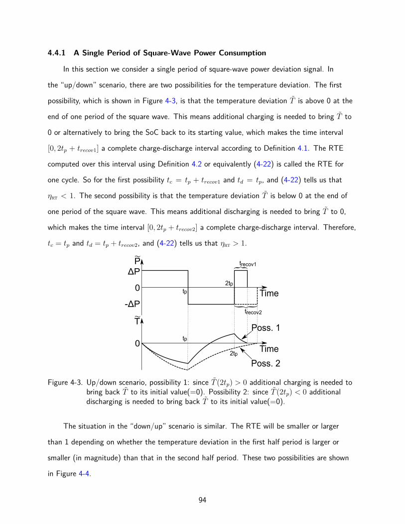
4.4.1 A Single Period of Square-Wave Power Consumption

In this section we consider a single period of square-wave power deviation signal. In

the “up/down” scenario, there are two possibilities for the temperature deviation. The first

possibility, which is shown in Figure 4-3, is that the temperature deviation T is above 0 at the

end of one period of the square wave. This means additional charging is needed to bring T to

0 or alternatively to bring the SoC back to its starting value, which makes the time interval

[0, 2tp + trecov1] a complete charge-discharge interval according to Definition 4.1. The RTE

computed over this interval using Definition 4.2 or equivalently (4-22) is called the RTE for

one cycle. So for the first possibility tc = tp + trecov1 and td = tp, and (4-22) tells us that

ηrt < 1. The second possibility is that the temperature deviation T is below 0 at the end of

one period of the square wave. This means additional discharging is needed to bring T to 0,

which makes the time interval [0, 2tp + trecov2] a complete charge-discharge interval. Therefore,

tc = tp and td = tp + trecov2, and (4-22) tells us that ηrt > 1.

P∼ΔP

-ΔPTime

02tp

T∼

Time0

} trecov1

2tp

tp

tp

}

trecov2

Poss. 1

Poss. 2

Figure 4-3. Up/down scenario, possibility 1: since T (2tp) > 0 additional charging is needed tobring back T to its initial value(=0). Possibility 2: since T (2tp) < 0 additionaldischarging is needed to bring back T to its initial value(=0).

The situation in the “down/up” scenario is similar. The RTE will be smaller or larger

than 1 depending on whether the temperature deviation in the first half period is larger or

smaller (in magnitude) than that in the second half period. These two possibilities are shown

in Figure 4-4.

94

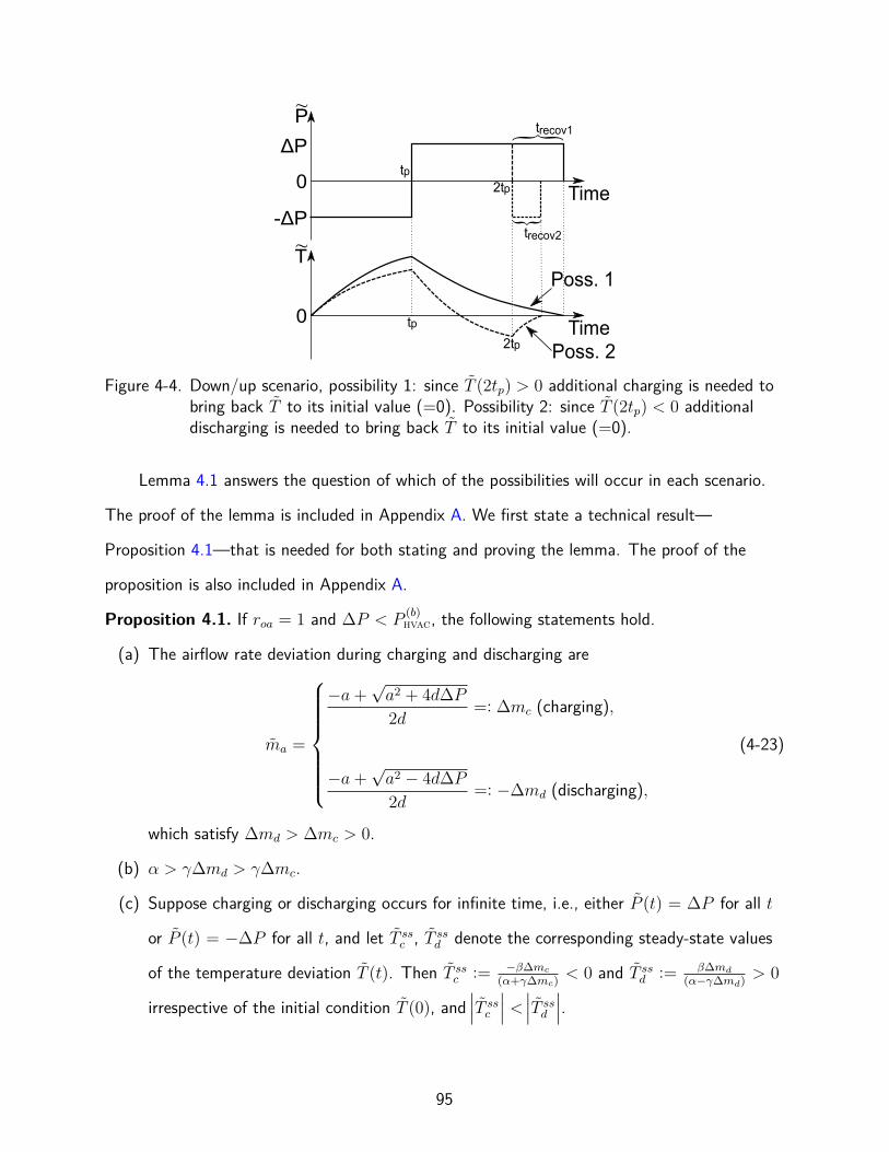
P∼

ΔP

-ΔPTime

0 2tp

T∼

Time0

}

trecov2

2tp

tp

tp

} trecov1

Poss. 1

Poss. 2

Figure 4-4. Down/up scenario, possibility 1: since T (2tp) > 0 additional charging is needed tobring back T to its initial value (=0). Possibility 2: since T (2tp) < 0 additionaldischarging is needed to bring back T to its initial value (=0).

Lemma 4.1 answers the question of which of the possibilities will occur in each scenario.

The proof of the lemma is included in Appendix A. We first state a technical result—

Proposition 4.1—that is needed for both stating and proving the lemma. The proof of the

proposition is also included in Appendix A.

Proposition 4.1. If roa = 1 and ∆P < P(b)hvac, the following statements hold.

(a) The airflow rate deviation during charging and discharging are

ma =

−a+√a2 + 4d∆P

2d=: ∆mc (charging),

−a+√a2 − 4d∆P

2d=: −∆md (discharging),

(4-23)

which satisfy ∆md > ∆mc > 0.

(b) α > γ∆md > γ∆mc.

(c) Suppose charging or discharging occurs for infinite time, i.e., either P (t) = ∆P for all t

or P (t) = −∆P for all t, and let T ssc , T ss

d denote the corresponding steady-state values

of the temperature deviation T (t). Then T ssc := −β∆mc

(α+γ∆mc)< 0 and T ss

d := β∆md

(α−γ∆md)> 0

irrespective of the initial condition T (0), and∣∣∣T ss

c

∣∣∣ < ∣∣∣T ssd

∣∣∣.

95

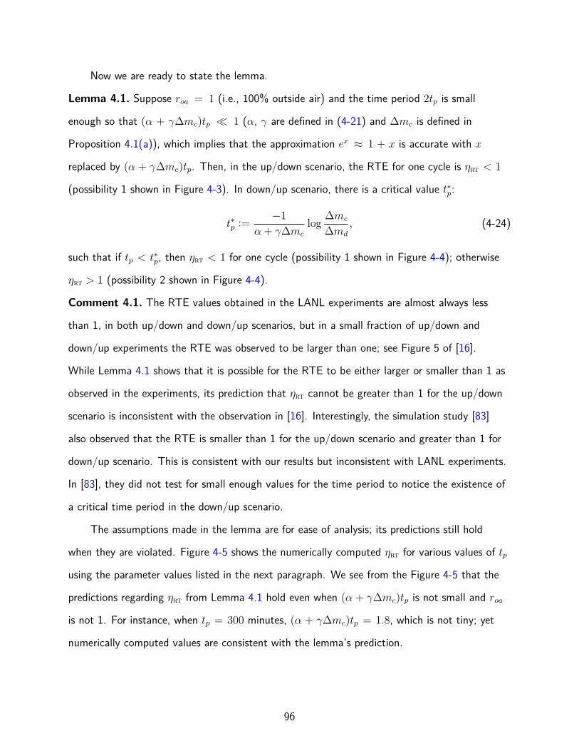
Now we are ready to state the lemma.

Lemma 4.1. Suppose roa = 1 (i.e., 100% outside air) and the time period 2tp is small

enough so that (α + γ∆mc)tp ≪ 1 (α, γ are defined in (4-21) and ∆mc is defined in

Proposition 4.1(a)), which implies that the approximation ex ≈ 1 + x is accurate with x

replaced by (α + γ∆mc)tp. Then, in the up/down scenario, the RTE for one cycle is ηrt < 1

(possibility 1 shown in Figure 4-3). In down/up scenario, there is a critical value t∗p:

t∗p :=−1

α + γ∆mc

log∆mc

∆md

, (4-24)

such that if tp < t∗p, then ηrt < 1 for one cycle (possibility 1 shown in Figure 4-4); otherwise

ηrt > 1 (possibility 2 shown in Figure 4-4).

Comment 4.1. The RTE values obtained in the LANL experiments are almost always less

than 1, in both up/down and down/up scenarios, but in a small fraction of up/down and

down/up experiments the RTE was observed to be larger than one; see Figure 5 of [16].

While Lemma 4.1 shows that it is possible for the RTE to be either larger or smaller than 1 as

observed in the experiments, its prediction that ηrt cannot be greater than 1 for the up/down

scenario is inconsistent with the observation in [16]. Interestingly, the simulation study [83]

also observed that the RTE is smaller than 1 for the up/down scenario and greater than 1 for

down/up scenario. This is consistent with our results but inconsistent with LANL experiments.

In [83], they did not test for small enough values for the time period to notice the existence of

a critical time period in the down/up scenario.

The assumptions made in the lemma are for ease of analysis; its predictions still hold

when they are violated. Figure 4-5 shows the numerically computed ηrt for various values of tp

using the parameter values listed in the next paragraph. We see from the Figure 4-5 that the

predictions regarding ηrt from Lemma 4.1 hold even when (α + γ∆mc)tp is not small and roa

is not 1. For instance, when tp = 300 minutes, (α + γ∆mc)tp = 1.8, which is not tiny; yet

numerically computed values are consistent with the lemma’s prediction.

96

1 5 10 15 30 60 120 180 300

tp (minutes)

0.7

0.8

0.9

1

1.1

1.2

1.3

RT

Up/down cycle: roa

=1

Up/down cycle: roa

=0.5

Down/up cycle: roa

=1

Down/up cycle: roa

=0.5

Figure 4-5. ηrt vs. tp, for roa = 1 and roa = 0.5; ∆P = 0.2P(b)hvac. The vertical line shown is t∗p

(≈12 minutes) computed from (4-24) for roa = 1.

1.8 2 2.2 2.4 2.6 2.8 3

Supply air flow rate (kg/s)

500

1000

1500

2000

2500

3000

3500

4000

4500

5000

Fan

pow

er (

W)

Figure 4-6. Fan power vs. airflow rate; measurements from AHU-2 of Pugh Hall at UF(circles), and predictions from the best fit model (4-9) to the measurements(curve).

The following parameters were chosen for the numerical computations: Tsa = 55◦F,

T (b) = 72◦F, TL = 70◦F, and TH = 74◦F. The building in this chapter is based on a large

auditorium (∼ 6 m high, floor area of ∼ 465 m2) in Pugh Hall located in the University of

Florida campus, which is served by a dedicated air handling unit. We choose m(b)a = 2.27

kg/s since that is representative of the airflow rate to this zone. We choose the following

parameters, guided by [93]: C = 3.4 × 107 J/K and R = 1.3 × 10−3 K/W. We also choose

97

P∼

ΔP

-ΔPTime

0 2tp

∼ ∼

(n-1)2tp n2tp

T∼

Time0

∼ ∼

}t (n) recov1

}

t (n)recov2

4tp

2tp

(n-1)2tp

n2tp

4tp

Poss. 1

Poss. 2

Figure 4-7. Additional charging or discharging needed to bring T to its initial value (=0) aftern periods of down/up cycle.

Toa = 80◦F and COP = 3.5, somewhat arbitrarily. The fan power coefficients were chosen to

be α1f = 662 W/(kg/s)2 and α2f = −576 W/(kg/s), based on fitting a quadratic model to

measured fan power from the zone in question; see Figure 4-6.

4.4.2 Multiple Periods of Square-Wave Power Consumption

We now consider n periods of the square-wave, n > 1. At the end of n periods, the

temperature deviation may not be exactly 0 (i.e., T (n2tp) = 0), even though its initial value

was 0 (i.e., T (0) = 0). Charging or discharging might be needed for an additional amount of

time trecov to bring the temperature deviation back to 0. Whether recovery to the initial SoC

requires additional charging or additional discharging depends on whether T (n2tp) is positive

or negative. In either case, since T (0) = T (n2tp + trecov) = 0, according to Definition 4.1, the

time interval [0, n2tp + trecov] constitutes a complete charge-discharge interval of the virtual

battery. The RTE computed over this interval using Definition 4.2 or equivalently (4-22) is

called the RTE for n cycles or ηrt(n).

Figure 4-7 shows an illustration of the two possible scenarios for the possible values

of T (n2tp). For the sake of concreteness, we have assumed the VES service starts with a

down/up cycle in the figure. In the first possibility, denoted by the solid lines, T (n2tp) ≥ 0,

and therefore additional charging is performed for trecov1 ≥ 0 amount of time in order to

bring the temperature deviation to 0. If this possibility were to occur, within the complete

98

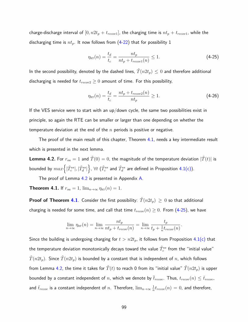
charge-discharge interval of [0, n2tp + trecov1], the charging time is ntp + trecov1, while the

discharging time is ntp. It now follows from (4-22) that for possibility 1

ηrt(n) =tdtc

=ntp

ntp + trecov1(n)≤ 1. (4-25)

In the second possibility, denoted by the dashed lines, T (n2tp) ≤ 0 and therefore additional

discharging is needed for trecov2 ≥ 0 amount of time. For this possibility,

ηrt(n) =tdtc

=ntp + trecov2(n)

ntp≥ 1. (4-26)

If the VES service were to start with an up/down cycle, the same two possibilities exist in

principle, so again the RTE can be smaller or larger than one depending on whether the

temperature deviation at the end of the n periods is positive or negative.

The proof of the main result of this chapter, Theorem 4.1, needs a key intermediate result

which is presented in the next lemma.

Lemma 4.2. For roa = 1 and T (0) = 0, the magnitude of the temperature deviation |T (t)| is

bounded by max{|T ss

c |, |T ssd |

}, ∀t (T ss

c and T ssd are defined in Proposition 4.1(c)).

The proof of Lemma 4.2 is presented in Appendix A.

Theorem 4.1. If roa = 1, limn→∞ ηrt(n) = 1.

Proof of Theorem 4.1. Consider the first possibility: T (n2tp) ≥ 0 so that additional

charging is needed for some time, and call that time trecov(n) ≥ 0. From (4-25), we have

limn→∞

ηrt(n) = limn→∞

ntpntp + trecov(n)

= limn→∞

tptp +

1ntrecov(n)

.

Since the building is undergoing charging for t > n2tp, it follows from Proposition 4.1(c) that

the temperature deviation monotonically decays toward the value T ssc from the “initial value”

T (n2tp). Since T (n2tp) is bounded by a constant that is independent of n, which follows

from Lemma 4.2, the time it takes for T (t) to reach 0 from its “initial value” T (n2tp) is upper

bounded by a constant independent of n, which we denote by trecov. Thus, trecov(n) ≤ trecov,

and trecov is a constant independent of n. Therefore, limn→∞1ntrecov(n) = 0, and therefore,

99

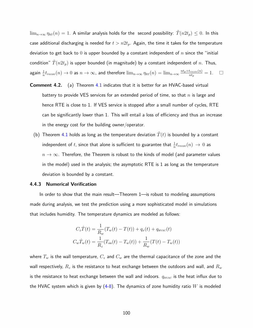
limn→∞ ηrt(n) = 1. A similar analysis holds for the second possibility: T (n2tp) ≤ 0. In this

case additional discharging is needed for t > n2tp. Again, the time it takes for the temperature

deviation to get back to 0 is upper bounded by a constant independent of n since the “initial

condition” T (n2tp) is upper bounded (in magnitude) by a constant independent of n. Thus,

again 1ntrecov(n) → 0 as n → ∞, and therefore limn→∞ ηrt(n) = limn→∞

ntp+trecov(n)

ntp= 1.

Comment 4.2. (a) Theorem 4.1 indicates that it is better for an HVAC-based virtual

battery to provide VES services for an extended period of time, so that n is large and

hence RTE is close to 1. If VES service is stopped after a small number of cycles, RTE

can be significantly lower than 1. This will entail a loss of efficiency and thus an increase

in the energy cost for the building owner/operator.

(b) Theorem 4.1 holds as long as the temperature deviation T (t) is bounded by a constant

independent of t, since that alone is sufficient to guarantee that 1ntrecov(n) → 0 as

n → ∞. Therefore, the Theorem is robust to the kinds of model (and parameter values

in the model) used in the analysis; the asymptotic RTE is 1 as long as the temperature

deviation is bounded by a constant.

4.4.3 Numerical Verification

In order to show that the main result—Theorem 1—is robust to modeling assumptions

made during analysis, we test the prediction using a more sophisticated model in simulations

that includes humidity. The temperature dynamics are modeled as follows:

CzT (t) =1

Rw

(Tw(t)− T (t)) + qx(t) + qhvac(t)

CwTw(t) =1

Rz

(Toa(t)− Tw(t)) +1

Rw

(T (t)− Tw(t))

where Tw is the wall temperature, Cz and Cw are the thermal capacitance of the zone and the

wall respectively, Rz is the resistance to heat exchange between the outdoors and wall, and Rw

is the resistance to heat exchange between the wall and indoors. qhvac is the heat influx due to

the HVAC system which is given by (4-8). The dynamics of zone humidity ratio W is modeled

100

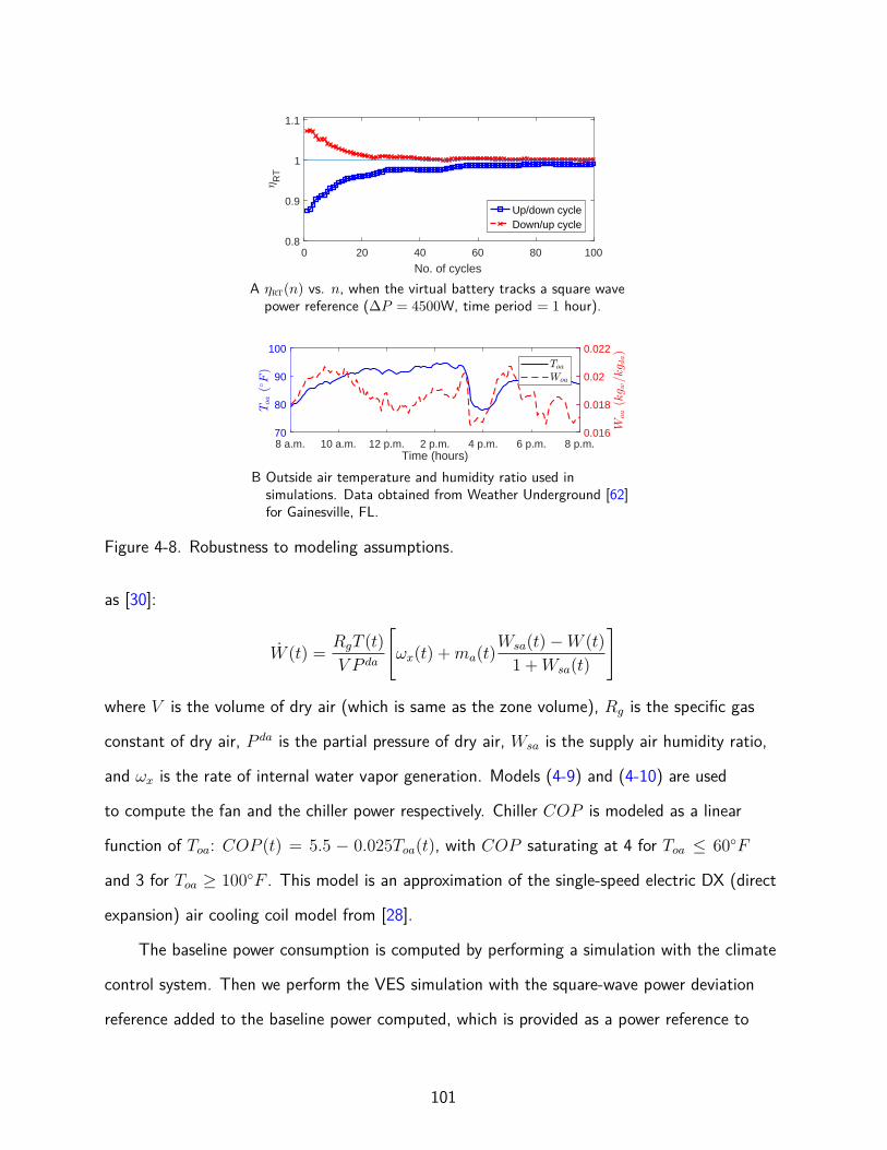
0 20 40 60 80 100

No. of cycles

0.8

0.9

1

1.1

RT

Up/down cycleDown/up cycle

A ηrt(n) vs. n, when the virtual battery tracks a square wavepower reference (∆P = 4500W, time period = 1 hour).

8 a.m. 10 a.m. 12 p.m. 2 p.m. 4 p.m. 6 p.m. 8 p.m.Time (hours)

70

80

90

100

0.016

0.018

0.02

0.022

B Outside air temperature and humidity ratio used insimulations. Data obtained from Weather Underground [62]for Gainesville, FL.

Figure 4-8. Robustness to modeling assumptions.

as [30]:

W (t) =RgT (t)

V P da

[ωx(t) +ma(t)

Wsa(t)−W (t)

1 +Wsa(t)

]

where V is the volume of dry air (which is same as the zone volume), Rg is the specific gas

constant of dry air, P da is the partial pressure of dry air, Wsa is the supply air humidity ratio,

and ωx is the rate of internal water vapor generation. Models (4-9) and (4-10) are used

to compute the fan and the chiller power respectively. Chiller COP is modeled as a linear

function of Toa: COP (t) = 5.5 − 0.025Toa(t), with COP saturating at 4 for Toa ≤ 60◦F

and 3 for Toa ≥ 100◦F . This model is an approximation of the single-speed electric DX (direct

expansion) air cooling coil model from [28].

The baseline power consumption is computed by performing a simulation with the climate

control system. Then we perform the VES simulation with the square-wave power deviation

reference added to the baseline power computed, which is provided as a power reference to

101

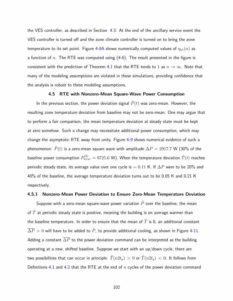
the VES controller, as described in Section 4.3. At the end of the ancillary service event the

VES controller is turned off and the zone climate controller is turned on to bring the zone

temperature to its set point. Figure 4-8A shows numerically computed values of ηrt(n) as

a function of n. The RTE was computed using (4-6). The result presented in the figure is

consistent with the prediction of Theorem 4.1 that the RTE tends to 1 as n → ∞. Note that

many of the modeling assumptions are violated in these simulations, providing confidence that

the analysis is robust to these modeling assumptions.

4.5 RTE with Nonzero-Mean Square-Wave Power Consumption

In the previous section, the power deviation signal P (t) was zero-mean. However, the

resulting zone temperature deviation from baseline may not be zero-mean. One may argue that

to perform a fair comparison, the mean temperature deviation at steady state must be kept

at zero somehow. Such a change may necessitate additional power consumption, which may

change the asymptotic RTE away from unity. Figure 4-9 shows numerical evidence of such a

phenomenon: P (t) is a zero-mean square wave with amplitude ∆P = 2917.7 W (30% of the

baseline power consumption P(b)hvac = 9725.6 W). When the temperature deviation T (t) reaches

periodic steady state, its average value over one cycle is ∼ 0.11 K. If ∆P were to be 20% and

40% of the baseline, the average temperature deviation turns out to be 0.05 K and 0.21 K

respectively.

4.5.1 Nonzero-Mean Power Deviation to Ensure Zero-Mean Temperature Deviation

Suppose with a zero-mean square-wave power variation P over the baseline, the mean

of T at periodic steady state is positive, meaning the building is on average warmer than

the baseline temperature. In order to ensure that the mean of T is 0, an additional constant

∆P > 0 will have to be added to P , to provide additional cooling, as shown in Figure 4-11.

Adding a constant ∆P to the power deviation command can be interpreted as the building

operating at a new, shifted baseline. Suppose we start with an up/down cycle, there are

two possibilities that can occur in principle: T (n2tp) > 0 or T (n2tp) < 0. It follows from

Definitions 4.1 and 4.2 that the RTE at the end of n cycles of the power deviation command

102

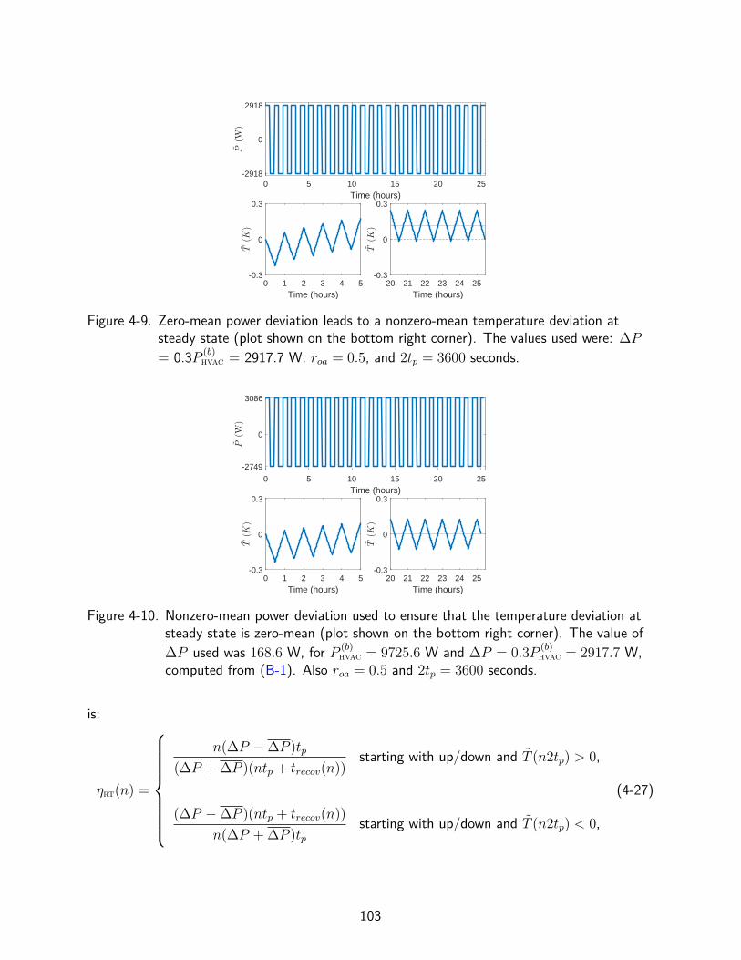
0 5 10 15 20 25Time (hours)

-2918

0

2918

0 1 2 3 4 5Time (hours)

-0.3

0

0.3

20 21 22 23 24 25Time (hours)

-0.3

0

0.3

Figure 4-9. Zero-mean power deviation leads to a nonzero-mean temperature deviation atsteady state (plot shown on the bottom right corner). The values used were: ∆P

= 0.3P (b)hvac = 2917.7 W, roa = 0.5, and 2tp = 3600 seconds.

0 5 10 15 20 25Time (hours)

-2749

0

3086

0 1 2 3 4 5Time (hours)

-0.3

0

0.3

20 21 22 23 24 25Time (hours)

-0.3

0

0.3

Figure 4-10. Nonzero-mean power deviation used to ensure that the temperature deviation atsteady state is zero-mean (plot shown on the bottom right corner). The value of∆P used was 168.6 W, for P (b)

hvac = 9725.6 W and ∆P = 0.3P(b)hvac = 2917.7 W,

computed from (B-1). Also roa = 0.5 and 2tp = 3600 seconds.

is:

ηrt(n) =

n(∆P −∆P )tp

(∆P +∆P )(ntp + trecov(n))starting with up/down and T (n2tp) > 0,

(∆P −∆P )(ntp + trecov(n))

n(∆P +∆P )tpstarting with up/down and T (n2tp) < 0,

(4-27)

103

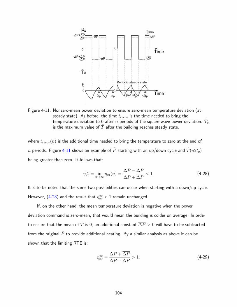
P∼

ΔP

-ΔP

Time0

∼ ∼

T∼

Time0

∼ ∼

trecov

2tp n2tp4tp

To

∼

(n-1)2tp

}}ΔP

}ΔP

}ΔP

ΔP+ΔP

-ΔP+ΔP }ΔP

Periodic steady state

Figure 4-11. Nonzero-mean power deviation to ensure zero-mean temperature deviation (atsteady state). As before, the time trecov is the time needed to bring thetemperature deviation to 0 after n periods of the square-wave power deviation. To

is the maximum value of T after the building reaches steady state.

where trecov(n) is the additional time needed to bring the temperature to zero at the end of

n periods. Figure 4-11 shows an example of P starting with an up/down cycle and T (n2tp)

being greater than zero. It follows that:

η∞rt = limn→∞

ηrt(n) =∆P −∆P

∆P +∆P< 1. (4-28)

It is to be noted that the same two possibilities can occur when starting with a down/up cycle.

However, (4-28) and the result that η∞rt < 1 remain unchanged.

If, on the other hand, the mean temperature deviation is negative when the power

deviation command is zero-mean, that would mean the building is colder on average. In order

to ensure that the mean of T is 0, an additional constant ∆P > 0 will have to be subtracted

from the original P to provide additional heating. By a similar analysis as above it can be

shown that the limiting RTE is:

η∞rt =∆P +∆P

∆P −∆P> 1. (4-29)

104

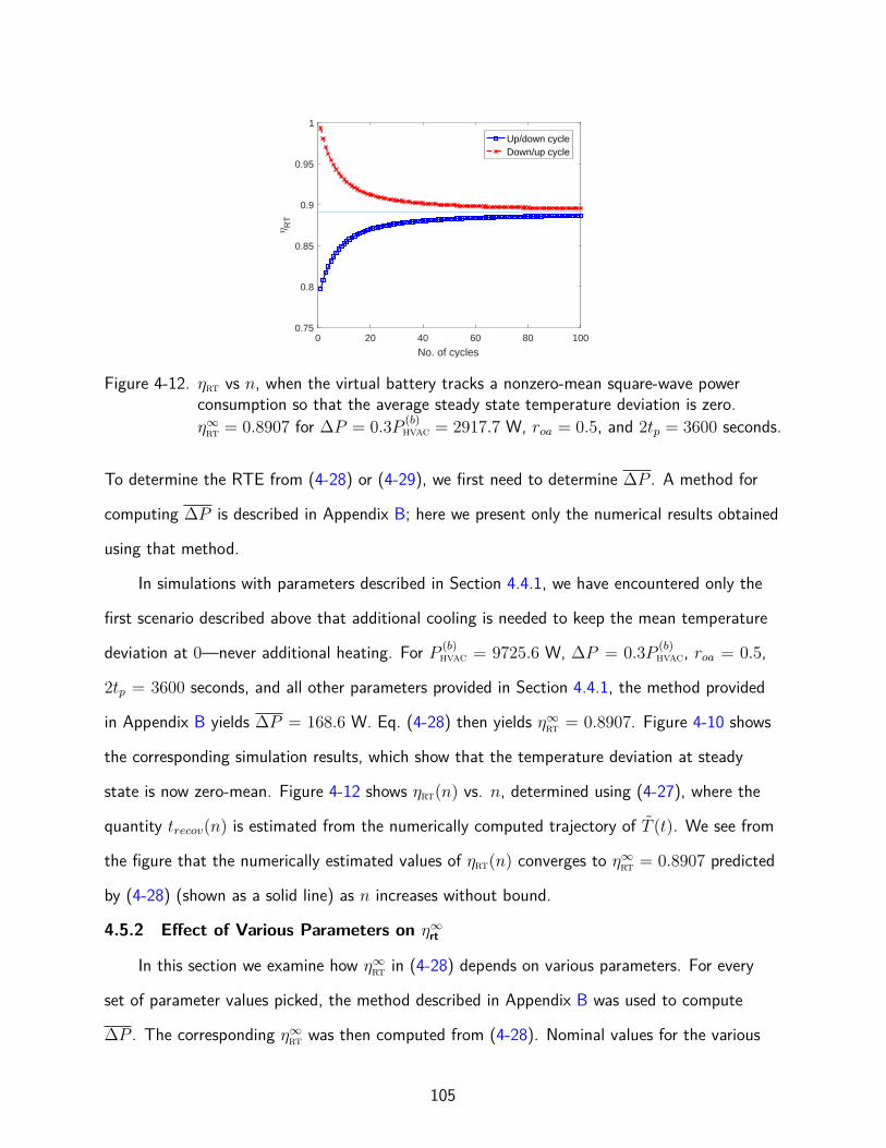
0 20 40 60 80 100

No. of cycles

0.75

0.8

0.85

0.9

0.95

1

RT

Up/down cycleDown/up cycle

Figure 4-12. ηrt vs n, when the virtual battery tracks a nonzero-mean square-wave powerconsumption so that the average steady state temperature deviation is zero.η∞rt = 0.8907 for ∆P = 0.3P

(b)hvac = 2917.7 W, roa = 0.5, and 2tp = 3600 seconds.

To determine the RTE from (4-28) or (4-29), we first need to determine ∆P . A method for

computing ∆P is described in Appendix B; here we present only the numerical results obtained

using that method.

In simulations with parameters described in Section 4.4.1, we have encountered only the

first scenario described above that additional cooling is needed to keep the mean temperature

deviation at 0—never additional heating. For P (b)hvac = 9725.6 W, ∆P = 0.3P

(b)hvac, roa = 0.5,

2tp = 3600 seconds, and all other parameters provided in Section 4.4.1, the method provided

in Appendix B yields ∆P = 168.6 W. Eq. (4-28) then yields η∞rt = 0.8907. Figure 4-10 shows

the corresponding simulation results, which show that the temperature deviation at steady

state is now zero-mean. Figure 4-12 shows ηrt(n) vs. n, determined using (4-27), where the

quantity trecov(n) is estimated from the numerically computed trajectory of T (t). We see from

the figure that the numerically estimated values of ηrt(n) converges to η∞rt = 0.8907 predicted

by (4-28) (shown as a solid line) as n increases without bound.

4.5.2 Effect of Various Parameters on η∞rt

In this section we examine how η∞rt in (4-28) depends on various parameters. For every

set of parameter values picked, the method described in Appendix B was used to compute

∆P . The corresponding η∞rt was then computed from (4-28). Nominal values for the various

105

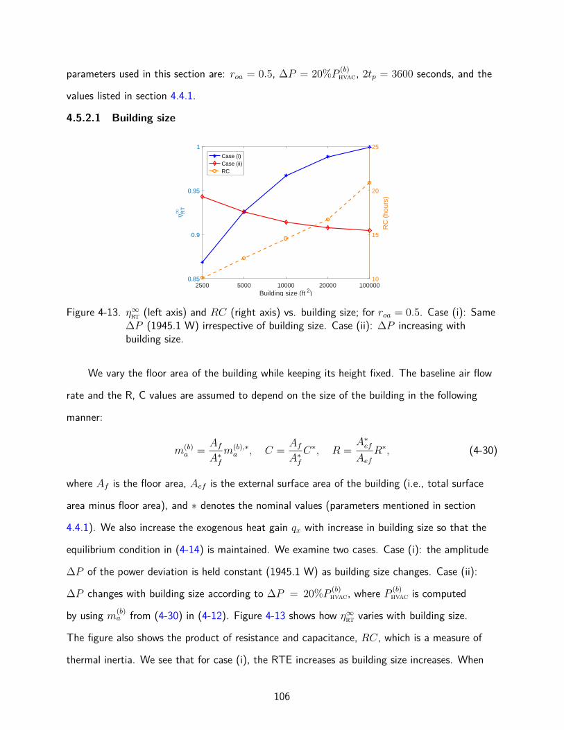
parameters used in this section are: roa = 0.5, ∆P = 20%P(b)hvac, 2tp = 3600 seconds, and the

values listed in section 4.4.1.

4.5.2.1 Building size

2500 5000 10000 20000 100000Building size (ft 2)

0.85

0.9

0.95

1

RT

10

15

20

25

RC

(ho

urs)

Case (i)Case (ii)RC

Figure 4-13. η∞rt (left axis) and RC (right axis) vs. building size; for roa = 0.5. Case (i): Same∆P (1945.1 W) irrespective of building size. Case (ii): ∆P increasing withbuilding size.

We vary the floor area of the building while keeping its height fixed. The baseline air flow

rate and the R, C values are assumed to depend on the size of the building in the following

manner:

m(b)a =

Af

A∗f

m(b),∗a , C =

Af

A∗f

C∗, R =A∗

ef

Aef

R∗, (4-30)

where Af is the floor area, Aef is the external surface area of the building (i.e., total surface

area minus floor area), and ∗ denotes the nominal values (parameters mentioned in section

4.4.1). We also increase the exogenous heat gain qx with increase in building size so that the

equilibrium condition in (4-14) is maintained. We examine two cases. Case (i): the amplitude

∆P of the power deviation is held constant (1945.1 W) as building size changes. Case (ii):

∆P changes with building size according to ∆P = 20%P(b)hvac, where P

(b)hvac is computed

by using m(b)a from (4-30) in (4-12). Figure 4-13 shows how η∞rt varies with building size.

The figure also shows the product of resistance and capacitance, RC, which is a measure of

thermal inertia. We see that for case (i), the RTE increases as building size increases. When

106

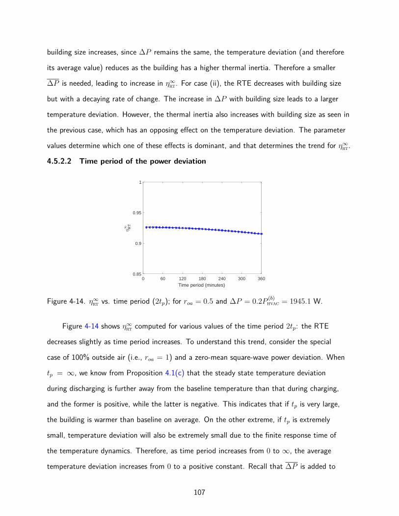
building size increases, since ∆P remains the same, the temperature deviation (and therefore

its average value) reduces as the building has a higher thermal inertia. Therefore a smaller

∆P is needed, leading to increase in η∞rt. For case (ii), the RTE decreases with building size

but with a decaying rate of change. The increase in ∆P with building size leads to a larger

temperature deviation. However, the thermal inertia also increases with building size as seen in

the previous case, which has an opposing effect on the temperature deviation. The parameter

values determine which one of these effects is dominant, and that determines the trend for η∞rt.

4.5.2.2 Time period of the power deviation

0 60 120 180 240 300 360

Time period (minutes)

0.85

0.9

0.95

1

RT

Figure 4-14. η∞rt vs. time period (2tp); for roa = 0.5 and ∆P = 0.2P(b)hvac = 1945.1 W.

Figure 4-14 shows η∞rt computed for various values of the time period 2tp: the RTE

decreases slightly as time period increases. To understand this trend, consider the special

case of 100% outside air (i.e., roa = 1) and a zero-mean square-wave power deviation. When

tp = ∞, we know from Proposition 4.1(c) that the steady state temperature deviation

during discharging is further away from the baseline temperature than that during charging,

and the former is positive, while the latter is negative. This indicates that if tp is very large,

the building is warmer than baseline on average. On the other extreme, if tp is extremely

small, temperature deviation will also be extremely small due to the finite response time of

the temperature dynamics. Therefore, as time period increases from 0 to ∞, the average

temperature deviation increases from 0 to a positive constant. Recall that ∆P is added to

107

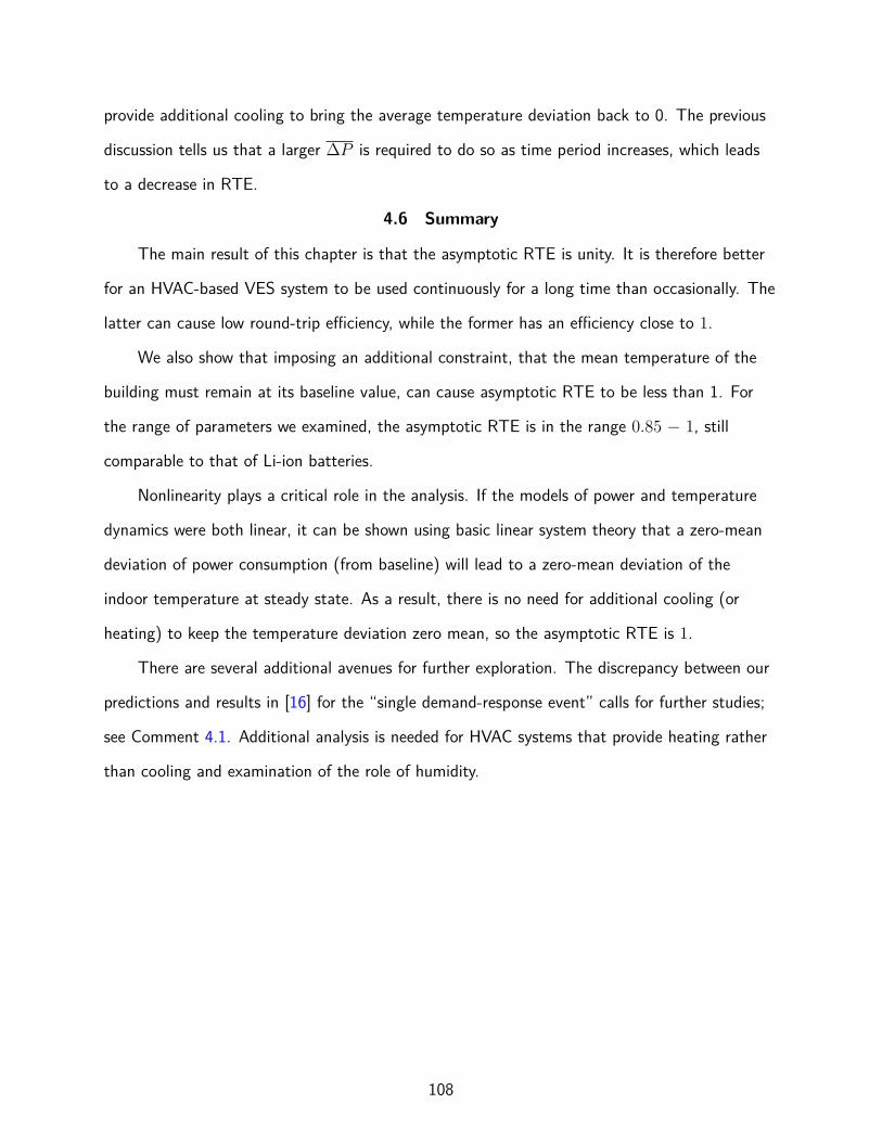
provide additional cooling to bring the average temperature deviation back to 0. The previous

discussion tells us that a larger ∆P is required to do so as time period increases, which leads

to a decrease in RTE.

4.6 Summary

The main result of this chapter is that the asymptotic RTE is unity. It is therefore better

for an HVAC-based VES system to be used continuously for a long time than occasionally. The

latter can cause low round-trip efficiency, while the former has an efficiency close to 1.

We also show that imposing an additional constraint, that the mean temperature of the

building must remain at its baseline value, can cause asymptotic RTE to be less than 1. For

the range of parameters we examined, the asymptotic RTE is in the range 0.85 − 1, still

comparable to that of Li-ion batteries.

Nonlinearity plays a critical role in the analysis. If the models of power and temperature

dynamics were both linear, it can be shown using basic linear system theory that a zero-mean

deviation of power consumption (from baseline) will lead to a zero-mean deviation of the

indoor temperature at steady state. As a result, there is no need for additional cooling (or

heating) to keep the temperature deviation zero mean, so the asymptotic RTE is 1.

There are several additional avenues for further exploration. The discrepancy between our

predictions and results in [16] for the “single demand-response event” calls for further studies;

see Comment 4.1. Additional analysis is needed for HVAC systems that provide heating rather

than cooling and examination of the role of humidity.

108

CHAPTER 5CONCLUSION

In this dissertation, two MPC-based algorithms for energy-efficient control of HVAC

systems in commercial buildings are developed and tested through simulations. In addition, the

RTE when HVAC systems in commercial buildings are used for grid-support as a virtual battery

is rigorously analyzed.

In Chapter 2, an MPC controller which incorporates humidity and latent heat in a

principled manner is presented; this controller is primarily for single-zone buildings. Simulations

show that the proposed controller outperforms both an MPC controller which does not

consider humidity/latent heat and a baseline rule-based controller. Simulations also indicate

that under certain conditions, using the MPC controller which ignores humidity/latent heat

can lead to two issues. One, it may lead to poor humidity control. Two, it may lead to higher

energy usage as it is unaware of the latent load on the cooling coil. Since our proposed

controller explicitly considers these factors, it is able to perform well under various weather

conditions.

In Chapter 3, an MPC-based hierarchical controller for multi-zone buildings is presented.

The proposed control architecture is designed to address a number of limitations in the existing

literature on multi-zone buildings. The main one is the reliance on a high-resolution multi-zone

model, which can be challenging to obtain. Instead, we use a low-resolution model of the

building, which can be identified in a tractable manner from measurements. The challenge then

is to convert the MPC decisions, which are computed for the fictitious zones in the model, to

the commands for the VAV boxes of the actual building. The proposed architecture does that

by posing this conversion as a projection problem that uses not only what the MPC computes

but also feedback from zones. The result is a principled method of computing VAV box

commands that are consistent with the optimal decisions made by the MPC without needing

dynamic models of individual zones. At the same time, the use of feedback from the zones

ensures that zone climate states are also close to the aggregate climate states computed by the

109

MPC. The positive simulation results provide confidence on the effectiveness of the proposed

controller especially because of the large plant model mismatch.

In Chapter 4, the RTE of an HVAC-based virtual battery is rigorously analyzed. The

main result is that the asymptotic RTE is unity. It is therefore better for an HVAC-based VES

system to be used continuously for a long time than occasionally. The latter can cause low

round-trip efficiency, while the former has an efficiency close to 1. We also show that imposing

an additional constraint, that the mean temperature of the building must remain at its baseline

value, can cause asymptotic RTE to be less than 1. For the range of parameters we examined,

the asymptotic RTE is in the range 0.85− 1, still comparable to that of Li-ion batteries.

This dissertation is only a first step, there are several avenues for further exploration.

(i) Experimentally verifying the performance of the two proposed MPC-based controllers.

(ii) Modifying the MPC formulations to minimize cost instead of energy and to include demand

charges. (iii) Improving methods to forecast disturbances that are used in the controllers.

(iv) Experimentally verifying the results on RTE. Inspired by this work, some experiments

were performed by researchers from the University of Michigan and North Carolina State

University to investigate the impact on energy efficiency caused by successive load shifting, and

preliminary results are reported in [94].

110

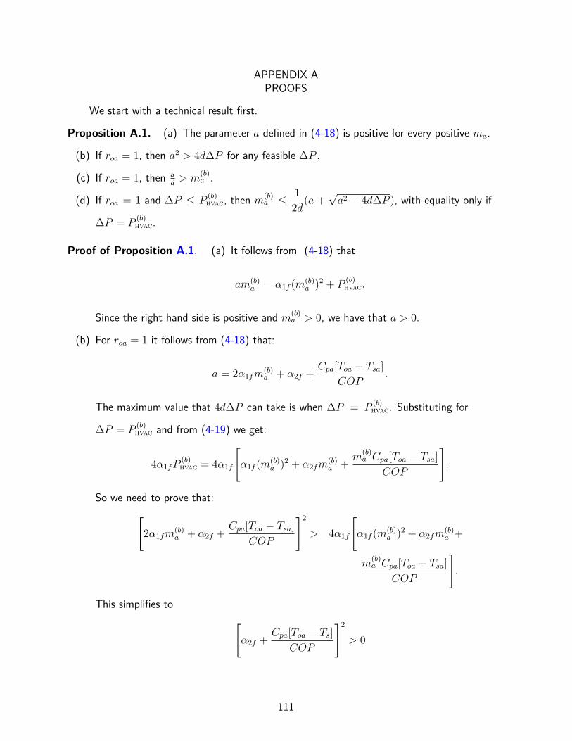
APPENDIX APROOFS

We start with a technical result first.

Proposition A.1. (a) The parameter a defined in (4-18) is positive for every positive ma.

(b) If roa = 1, then a2 > 4d∆P for any feasible ∆P .

(c) If roa = 1, then ad> m

(b)a .

(d) If roa = 1 and ∆P ≤ P(b)hvac, then m

(b)a ≤ 1

2d(a +

√a2 − 4d∆P ), with equality only if

∆P = P(b)hvac.

Proof of Proposition A.1. (a) It follows from (4-18) that

am(b)a = α1f (m

(b)a )2 + P

(b)hvac.

Since the right hand side is positive and m(b)a > 0, we have that a > 0.

(b) For roa = 1 it follows from (4-18) that:

a = 2α1fm(b)a + α2f +

Cpa[Toa − Tsa]

COP.

The maximum value that 4d∆P can take is when ∆P = P(b)hvac. Substituting for

∆P = P(b)hvac and from (4-19) we get:

4α1fP(b)hvac = 4α1f

[α1f (m

(b)a )2 + α2fm

(b)a +

m(b)a Cpa[Toa − Tsa]

COP

].

So we need to prove that:[2α1fm

(b)a + α2f +

Cpa[Toa − Tsa]

COP

]2

> 4α1f

[α1f (m

(b)a )2 + α2fm

(b)a +

m(b)a Cpa[Toa − Tsa]

COP

].

This simplifies to [α2f +

Cpa[Toa − Ts]

COP

]2

> 0

111

which is always true, and therefore a2 > 4d∆P .

(c) It follows from (4-18) and (4-19) that when roa = 1

a

d=

2α1fm(b)a + α2f +

Cpa[Toa−Tsa]

COP

α1f

.

With further algebraic manipulation it reduces to m(b)a + P

(b)hvac/(α1fm

(b)a ). Since α1f ,

m(b)a , and P

(b)hvac are positive, we have a/d > m

(b)a .

(d) Let us look at the following expression:

a+√a2 − 4d∆P

2d. (A-1)

Substituting for ∆P = P(b)hvac in the above expression and using the expressions for a and

d from (4-18) and (4-19) respectively, we get:

2α1fm(b)a + α2f +

Cpa[Toa−Tsa]

COP+∣∣∣α2f +

Cpa[Toa−Tsa]

COP

∣∣∣2α1f

. (A-2)

If α2f +Cpa[Toa−Tsa]

COP> 0 then (A-2) becomes:

m(b)a +

α2f +Cpa[Toa−Tsa]

COP

α1f

,

which is greater than m(b)a since α1f > 0. If α2f +

Cpa[Toa−Tsa]

COP< 0, then (A-2) becomes

equal to m(b)a . In (A-1) for any ∆P < P

(b)hvac the value of (A-1) increases and therefore is

greater than m(b)a . This completes the proof.

Proof of Proposition 4.1. (a) Since roa = 1 from (4-19), b = 0 and c = 0. Therefore the

solution for ma as a function of P from (4-17) reduces to:

ma =−a±

√a2 + 4dP

2d.

During charging P = ∆P , so the the two roots in the equation above are −a+√a2+4d∆P2d

and −a−√a2+4d∆P2d

. The second root is not possible, since it is negative with a minimum

112

magnitude +a+√a2

2d= a

d, which is larger than m

(b)a by Proposition A.1(c), making the

total airflow rate negative. Therefore during charging, the airflow rate is −a+√a2+4d∆P2d

.

This proves the first statement, regarding ∆mc. During discharging, P = −∆P , so the

two possible roots are −a+√a2−4d∆P2d

and −a−√a2−4d∆P2d

. The second root is not possible,

since it is negative with a minimum magnitude larger than m(b)a for ∆P < P

(b)hvac from

Proposition A.1(d), which will make the total air flow rate negative. Therefore during

charging, the airflow rate is −a+√a2−4d∆P2d

. This proves the second statement, regarding

∆md.

To prove the inequality ∆md > ∆mc, let ν , 4d∆P for simplifying the notation. The

inequality ∆md > ∆mc is equivalent to:

−a+√a2 + ν

2d<

a−√a2 − ν

2d

⇒ −a+√a2 + ν < a−

√a2 − ν, as d > 0.

Further algebraic manipulation gives,

√a2 + ν −

√a2 − ν >

ν

a. (A-3)

Since a2 > ν from Proposition A.1(b), let us define a2 = ν + ϵ where ϵ > 0. Therefore,

(A-3) becomes:

√2ν + ϵ−

√ϵ >

ν√ν + ϵ

⇒√

(2ν + ϵ)(ν + ϵ) > ν +√

ϵ(ν + ϵ).

Squaring on both sides yields:

⇒ ν2 + 2νϵ > 2ν√

ϵ(ν + ϵ),

squaring again on both sides and simplifying, we get: ν4 > 0, which is true, and

therefore ∆mc < ∆md.

113

(b) Note that the maximum value that ∆md can take is m(b)a ; otherwise, the total airflow

rate will be negative. For that value of ∆md, γ∆md = Cpam(b)a

C(as γ = Cpa/C).

Substituting for α from (4-21) and since R,C > 0, we have Cpam(b)a

C+ 1

RC> Cpam

(b)a

C

so that α > γ∆md. For the second inequality, note that from Proposition4.1(a)

∆mc < ∆md. Since γ is positive, γ∆mc < γ∆md. Therefore, α > γ∆md > γ∆mc.

(c) We have already proved above that, ma(t) ≡ ∆mc when charging and ma(t) ≡ −∆md

when discharging. It follows from (4-20) that the temperature dynamics reduce in the

charging scenario to

˙T (t) = −(α + γ∆mc)T − β∆mc, (A-4)

and in the discharging scenario to

˙T (t) = −(α− γ∆md)T + β∆md. (A-5)

Both of these are linear time invariant systems driven by constant inputs that are

asymptotically stable; stability follows from α > γ∆md, which was proved above and

α, γ, and ∆mc being positive. It follows from elementary linear systems analysis [95]

that T (t) converges to a constant steady-state value irrespective of the initial condition,

which is, in the charging scenario: T ssc = β∆mc

−(α+γ∆mc), and in the discharging scenario:

T ssd = β∆md

(α−γ∆md). Since α, β, γ, ∆mc and ∆md are all positive, T ss

c < 0, and the fact

that T ssd > 0 follows from Proposition 4.1(b), proved above.

For the second part of the statement, we need to prove that

β∆mc

(α + γ∆mc)<

β∆md

(α− γ∆md). (A-6)

It follows from Proposition 4.1(b) that α + γ∆mc > α − γ∆mc > 0. Therefore, and

since all relevant parameters are positive,

β∆mc

α + γ∆mc

<β∆mc

α− γ∆mc

. (A-7)

114

Again from Proposition 4.1(b), we get

β∆mc

α + γ∆mc

<β∆mc

α− γ∆mc

<β∆md

α− γ∆md

, (A-8)

where the second inequality follows from ∆mc < ∆md. Thus from (A-8) we get the

desired inequality (A-6), which proves the second statement.

Now we are ready to prove Lemma 4.1.

Proof of Lemma 4.1. Since roa = 1, recall that we established in the proof of Proposition 4.1(c)

that T (t) is governed by two asymptotically stable linear time invariant systems, with step

inputs, (A-4) and (A-5), during the charging and discharging half-periods respectively. Consider

first the up/down scenario, with initial condition T (0) = 0. By solving the two differential

equations (A-4)-(A-5), we obtain the temperature deviation at the end of one period of the

square wave:

T (2tp) =−β∆mce

−(α−γ∆md)tp(1− e−(α+γ∆mc)tp)

α + γ∆mc

+β∆md(1− e−(α−γ∆md)tp)

α− γ∆md

.

By hypothesis, (α − γ∆md)tp < (α + γ∆mc)tp ≪ 1, so we can use a first order Taylor

expansion to get the following approximation:

T (2tp) ≈ tpβ(∆md −∆mce

−(α−γ∆md)tp). (A-9)

Since ∆mc < ∆md and (α − γ∆md) > 0, we get T (2tp) > 0. This is possibility 1 shown

in Figure 4-3: td = tp, while tc = tp + trecov for some trecov > 0. It follows from (4-22)

that ηrt < 1. Consider second the down/up scenario, with initial condition T (0) = 0. The

corresponding expression becomes:

T (2tp) =β∆mde

−(α+γ∆mc)tp(1− e−(α−γ∆md)tp)

α− γ∆md

− β∆mc(1− e−(α+γ∆mc)tp)

α + γ∆mc

.

115

A similar approximation gives:

T (2tp) ≈ tpβ(e−(α+γ∆mc)tp∆md −∆mc

). (A-10)

As long as tp > t∗p, we have e−(α+γ∆mc)tp < ∆mc/∆md, and thus T (2tp) < 0. This is

possibility 2 shown in Figure 4-4: tc = tp, while td = tp + trecov for some trecov > 0. It now

follows from (4-22) that ηrt > 1. However, if tp < t∗p, then e−(α+γ∆mc)tp > ∆mc/∆md, and we

have T (2tp) > 0. This is possibility 1 shown in Figure 4-4: td = tp, while tc = tp + trecov for

some trecov > 0, and it follows from (4-22) that ηrt < 1.

Proof of Lemma 4.2. Recall that we established in the proof of Proposition 4.1(c) that

T (t) is governed by two asymptotically stable, linear, time invariant systems, with step inputs,

(A-4) and (A-5), during the charging and discharging half-periods respectively. It follows

from elementary linear systems theory that the step response of a stable first-order LTI

system monotonically increases (or decreases, depending on the initial condition) towards the

steady-state value. Therefore, in the time interval [0, tp], the maximum value of |T (t)| will be

(depending on whether the system is charging or discharging)

|T (t)| ≤ max{|T (0)|, |T ss

c |, |T ssd |

}, ∀t ∈ [0, tp]. (A-11)

The value of T (tp) will serve as the initial condition to the LTI dynamics that govern T (t)

during the interval [tp, 2tp], which is either (A-4) or (A-5). Using the same argument, we see

that the maximum value of |T (t)| in this time interval will satisfy

|T (t)| ≤ max{|T (tp)|, |T ss

c |, |T ssd |

}, ∀t ∈ [tp, 2tp],

≤ max{|T (0)|, |T ss

c |, |T ssd |

}, ∀t ∈ [0, tp],

where the second inequality follows from combining the first inequality with (A-11). Since

T (2tp) serves as the initial condition for the second period [2tp, 4tp] and so on, we can repeat

this argument ad infinitum, and arrive at the conclusion that |T (t)|, for any t ≥ 0, is bounded

by the constants |T (0)|, |T ssc |, and |T ss

d |. Since T (0) = 0, max{|T (0)|, |T ss

c |, |T ssd |

}=

116

max{|T ss

c |, |T ssd |

}. Therefore, |T (t)|, for any t ≥ 0, is bounded by the constants |T ss

c |, |T ssd |,

which proves the statement.

117

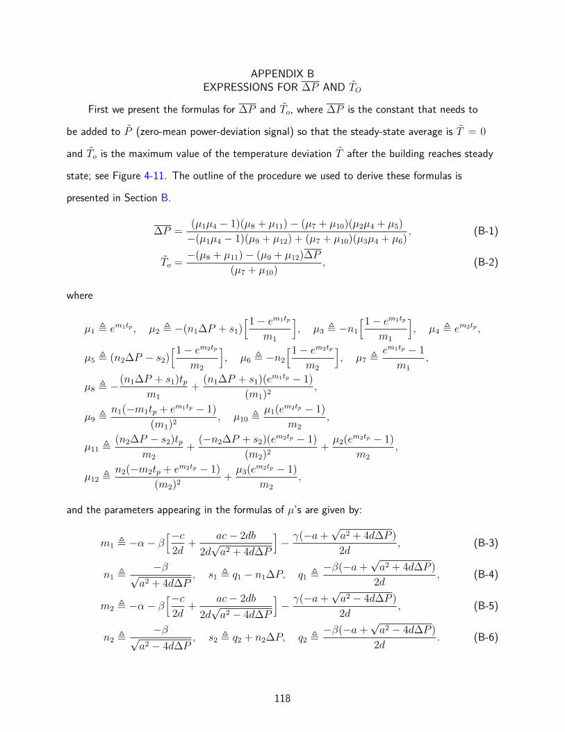
APPENDIX BEXPRESSIONS FOR ∆P AND TO

First we present the formulas for ∆P and To, where ∆P is the constant that needs to

be added to P (zero-mean power-deviation signal) so that the steady-state average is T = 0

and To is the maximum value of the temperature deviation T after the building reaches steady

state; see Figure 4-11. The outline of the procedure we used to derive these formulas is

presented in Section B.

∆P =(µ1µ4 − 1)(µ8 + µ11)− (µ7 + µ10)(µ2µ4 + µ5)

−(µ1µ4 − 1)(µ9 + µ12) + (µ7 + µ10)(µ3µ4 + µ6), (B-1)

To =−(µ8 + µ11)− (µ9 + µ12)∆P

(µ7 + µ10), (B-2)

where

µ1 , em1tp , µ2 , −(n1∆P + s1)[1− em1tp

m1

], µ3 , −n1

[1− em1tp

m1

], µ4 , em2tp ,

µ5 , (n2∆P − s2)[1− em2tp

m2

], µ6 , −n2

[1− em2tp

m2

], µ7 ,

em1tp − 1

m1

,

µ8 , −(n1∆P + s1)tpm1

+(n1∆P + s1)(e

m1tp − 1)

(m1)2,

µ9 ,n1(−m1tp + em1tp − 1)

(m1)2, µ10 ,

µ1(em2tp − 1)

m2

,

µ11 ,(n2∆P − s2)tp

m2

+(−n2∆P + s2)(e

m2tp − 1)

(m2)2+

µ2(em2tp − 1)

m2

,

µ12 ,n2(−m2tp + em2tp − 1)

(m2)2+

µ3(em2tp − 1)

m2

,

and the parameters appearing in the formulas of µ’s are given by:

m1 , −α− β[−c

2d+

ac− 2db

2d√a2 + 4d∆P

]− γ(−a+

√a2 + 4d∆P )

2d, (B-3)

n1 ,−β√

a2 + 4d∆P, s1 , q1 − n1∆P, q1 ,

−β(−a+√a2 + 4d∆P )

2d, (B-4)

m2 , −α− β[−c

2d+

ac− 2db

2d√a2 − 4d∆P

]− γ(−a+

√a2 − 4d∆P )

2d, (B-5)

n2 ,−β√

a2 − 4d∆P, s2 , q2 + n2∆P, q2 ,

−β(−a+√a2 − 4d∆P )

2d. (B-6)

118

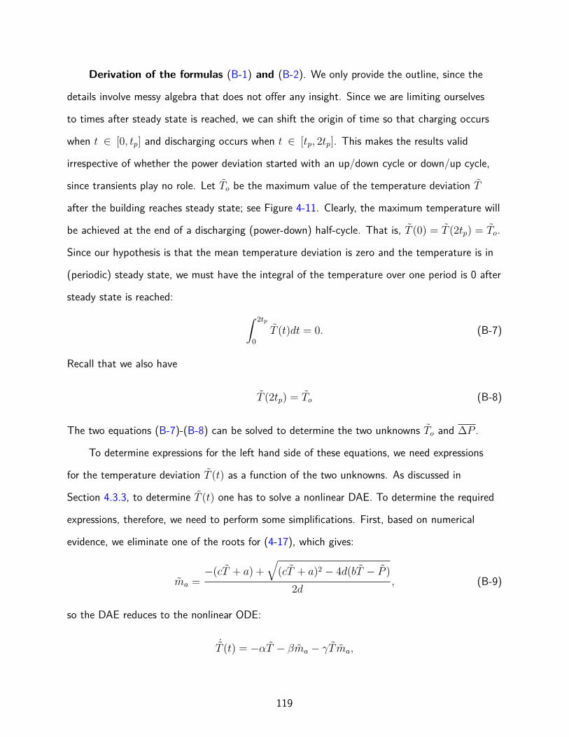
Derivation of the formulas (B-1) and (B-2). We only provide the outline, since the

details involve messy algebra that does not offer any insight. Since we are limiting ourselves

to times after steady state is reached, we can shift the origin of time so that charging occurs

when t ∈ [0, tp] and discharging occurs when t ∈ [tp, 2tp]. This makes the results valid

irrespective of whether the power deviation started with an up/down cycle or down/up cycle,

since transients play no role. Let To be the maximum value of the temperature deviation T

after the building reaches steady state; see Figure 4-11. Clearly, the maximum temperature will

be achieved at the end of a discharging (power-down) half-cycle. That is, T (0) = T (2tp) = To.

Since our hypothesis is that the mean temperature deviation is zero and the temperature is in

(periodic) steady state, we must have the integral of the temperature over one period is 0 after

steady state is reached: ∫ 2tp

0

T (t)dt = 0. (B-7)

Recall that we also have

T (2tp) = To (B-8)

The two equations (B-7)-(B-8) can be solved to determine the two unknowns To and ∆P .

To determine expressions for the left hand side of these equations, we need expressions

for the temperature deviation T (t) as a function of the two unknowns. As discussed in

Section 4.3.3, to determine T (t) one has to solve a nonlinear DAE. To determine the required

expressions, therefore, we need to perform some simplifications. First, based on numerical

evidence, we eliminate one of the roots for (4-17), which gives:

ma =−(cT + a) +

√(cT + a)2 − 4d(bT − P )

2d, (B-9)

so the DAE reduces to the nonlinear ODE:

˙T (t) = −αT − βma − γT ma,

119

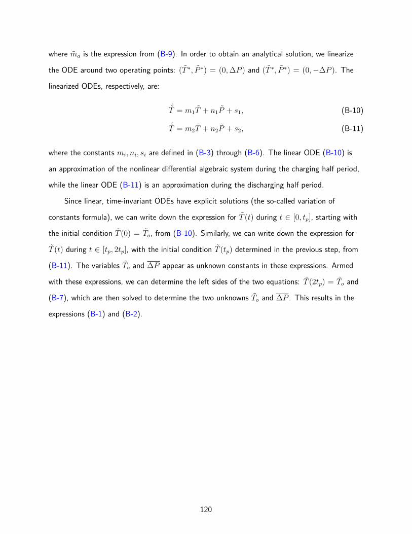
where ma is the expression from (B-9). In order to obtain an analytical solution, we linearize

the ODE around two operating points: (T ∗, P ∗) = (0,∆P ) and (T ∗, P ∗) = (0,−∆P ). The

linearized ODEs, respectively, are:

˙T = m1T + n1P + s1, (B-10)˙T = m2T + n2P + s2, (B-11)

where the constants mi, ni, si are defined in (B-3) through (B-6). The linear ODE (B-10) is

an approximation of the nonlinear differential algebraic system during the charging half period,

while the linear ODE (B-11) is an approximation during the discharging half period.

Since linear, time-invariant ODEs have explicit solutions (the so-called variation of

constants formula), we can write down the expression for T (t) during t ∈ [0, tp], starting with

the initial condition T (0) = To, from (B-10). Similarly, we can write down the expression for

T (t) during t ∈ [tp, 2tp], with the initial condition T (tp) determined in the previous step, from

(B-11). The variables To and ∆P appear as unknown constants in these expressions. Armed

with these expressions, we can determine the left sides of the two equations: T (2tp) = To and

(B-7), which are then solved to determine the two unknowns To and ∆P . This results in the

expressions (B-1) and (B-2).

120

REFERENCES

[1] ASHRAE, “The ASHRAE handbook fundamentals (SI Edition),” 2017.

[2] F. Jorissen, G. Reynders, R. Baetens, D. Picard, D. Saelens, and L. Helsen,“Implementation and Verification of the IDEAS Building Energy Simulation Library,”Journal of Building Performance Simulation, vol. 11, pp. 669–688, 2018.

[3] U.S. DoE, “Buildings energy data book,” Energy Efficiency & Renewable Energy Depart-ment, 2011.

[4] “Commercial buildings energy consumption survey (CBECS): Overview ofcommercial buildings, 2012,” Energy information administration, Departmentof Energy, U.S. Govt., Tech. Rep., December 2012. [Online]. Available:https://www.eia.gov/consumption/commercial/reports/2012/energyusage/

[5] G. Serale, M. Fiorentini, A. Capozzoli, D. Bernardini, and A. Bemporad, “Model predictivecontrol (MPC) for enhancing building and HVAC system energy efficiency: Problemformulation, applications and opportunities,” Energies, vol. 11, no. 3, p. 631, 2018.

[6] P. H. Shaikh, N. B. M. Nor, P. Nallagownden, I. Elamvazuthi, and T. Ibrahim, “A reviewon optimized control systems for building energy and comfort management of smartsustainable buildings,” Renewable and Sustainable Energy Reviews, vol. 34, pp. 409 – 429,2014.

[7] S. Qin and T. A. Badgwell, “A survey of industrial model predictive control technology,”Control Engineering Practice, vol. 11, no. 7, pp. 733 – 764, 2003.

[8] S. Goyal and P. Barooah, “Energy-efficient control of an air handling unit for a single-zoneVAV system,” in IEEE Conference on Decision and Control, 2013, pp. 4796 – 4801.

[9] J. Joe and P. Karava, “A model predictive control strategy to optimize the performance ofradiant floor heating and cooling systems in office buildings,” Applied Energy, vol. 245, pp.65 – 77, 2019.

[10] X. Chen, Q. Wang, and J. Srebric, “Occupant feedback based model predictive control forthermal comfort and energy optimization: A chamber experimental evaluation,” AppliedEnergy, vol. 164, pp. 341 – 351, 2016.

[11] J. Ma, J. Qin, T. Salsbury, and P. Xu, “Demand reduction in building energy systems basedon economic model predictive control,” Chemical Engineering Science, vol. 67, no. 1, pp.92 – 100, 2012, dynamics, Control and Optimization of Energy Systems.

[12] S. C. Bengea, A. D. Kelman, F. Borrelli, R. Taylor, and S. Narayanan, “Implementation ofmodel predictive control for an HVAC system in a mid-size commercial building,” HVAC&RResearch, vol. 20, pp. 121–135, 2013.

121

[13] B. Kirby, “Ancillary services: Technical and commercial insights,” Oak Ridge NationalLaboratory, Oak Ridge, Tennessee, USA, Tech. Rep., 2007, prepared for Wärtsilä NorthAmerica Inc.

[14] N. J. Cammardella, R. W. Moye, Y. Chen, and S. P. Meyn, “An energy storage costcomparison: Li-ion batteries vs Distributed load control,” in 2018 Clemson UniversityPower Systems Conference (PSC), Sep. 2018, pp. 1–6.

[15] P. Barooah, A. Bušić, and S. Meyn, “Spectral decomposition of demand side flexibilityfor reliable ancillary service in a smart grid,” in 48th Hawaii International Conference onSystems Science (HICSS), January 2015, pp. 2700–2709, invited paper.

[16] I. Beil, I. A. Hiskens, and S. Backhaus, “Round-trip efficiency of fast demand response in alarge commercial air conditioner,” Energy and Buildings, vol. 97, pp. 47 – 55, 2015.

[17] X. Luo, J. Wang, M. Dooner, and J. Clarke, “Overview of current development in electricalenergy storage technologies and the application potential in power system operation,”Applied Energy, vol. 137, pp. 511 – 536, 2015.

[18] N. S. Raman, K. Devaprasad, B. Chen, H. A. Ingley, and P. Barooah, “Modelpredictive control for energy-efficient HVAC operation with humidity and latent heatconsiderations,” Applied Energy, vol. 279, p. 115765, December 2020. [Online]. Available:https://doi.org/10.1016/j.apenergy.2020.115765

[19] N. S. Raman, K. Devaprasad, and P. Barooah, “MPC-based building climate controllerincorporating humidity,” in American Control Conference, July 2019, pp. 253–260.[Online]. Available: https://doi.org/10.23919/ACC.2019.8814615

[20] N. S. Raman, R. U. Chaturvedi, Z. Guo, and P. Barooah, “MPC-Based Hierarchical Controlof a Multi-Zone Commercial HVAC System,” arXiv preprint:2102.02914, 2021.

[21] © 2020 IEEE. Reprinted, with permission, from, N. S. Raman, and P. Barooah,“On the round-trip efficiency of an HVAC-based virtual battery,” IEEE Transactionson Smart Grid, vol. 11, no. 1, pp. 403–410, Jan 2020. [Online]. Available:https://doi.org/10.1109/TSG.2019.2923588

[22] N. S. Raman and P. Barooah, “Analysis of round-trip efficiency of an HVAC-based virtualbattery,” in 5th International Conference on High Performance Buildings, July 2018, pp.1–10.

[23] American Society of Heating, Refrigerating and Air-Conditioning Engineers,“ANSI/ASHRAE standard 55-2017, Thermal environmental conditions for humanoccupancy,” 2017.

[24] W. S. Duda, “Pitfalls of single-fan dual-duct systems in humid climates,” ASHRAE Journal,vol. 60, no. 9, pp. 60–66, 2018.

122

[25] A. Baughman and E. A. Arens, “Indoor humidity and human health–Part I: Literaturereview of health effects of humidity-influenced indoor pollutants,” ASHRAE Transactions,vol. 102 Part1, pp. 192–211, 1996.

[26] J. C. Fischer and C. W. Bayer, “Humidity control in school facilities,” Energy, vol. 30,no. 35, pp. 606–613, 2003.

[27] X. Zhou and J. E. Braun, “A simplified dynamic model for chilled-water cooling anddehumidifying coils—Part 1: Development (RP-1194),” HVAC&R Research, vol. 13, no. 5,pp. 785–804, 2007.

[28] U.S. DOE, “EnergyPlus engineering reference: The reference to EnergyPlus calculations,”Lawrence Berkeley National Laboratory, pp. 1–1704, 2018.

[29] S. Klein, W. Beckman, J. Mitchell, J. Duffie, N. Duffie, T. Freeman et al., “Trnsys 17: Atransient system simulation program: Mathematical reference,” University of Wisconsin:Madison, WI, USA, pp. 1–486, 2009.

[30] S. Goyal and P. Barooah, “A method for model-reduction of non-linear thermal dynamicsof multi-zone buildings,” Energy and Buildings, vol. 47, pp. 332–340, April 2012.

[31] J. Williams, “Why is the supply air temperature 55F?” http://8760engineeringblog.blogspot.com/2013/02/why-is-supply-air-temperature-55f.html, 2013, last accessed: Aug,03, 2020.

[32] D. B. Crawley, L. K. Lawrie, F. C. Winkelmann, W. F. Buhl, Y. J. Huang, C. O. Pedersenet al., “EnergyPlus: creating a new-generation building energy simulation program,” Energyand buildings, vol. 33, no. 4, pp. 319–331, 2001.

[33] ASHRAE, “The ASHRAE handbook : HVAC applications (SI Edition),” 2011.

[34] J. B. Rawlings, D. Q. Mayne, and M. Diehl, Model Predictive Control: Theory,Computation, and Design. Nob Hill, 2017.

[35] J. B. Rawlings, D. Angeli, and C. N. Bates, “Fundamentals of economic model predictivecontrol,” in 51st IEEE Conference on Decision and Control (CDC), Dec 2012, pp.3851–3861.

[36] D. Schwingshackl, J. Rehrl, and M. Horn, “LoLiMoT based MPC for air handling units inHVAC systems,” Building and Environment, vol. 96, pp. 250 – 259, 2016.

[37] J. Mei, X. Xia, and M. Song, “An autonomous hierarchical control for improving indoorcomfort and energy efficiency of a direct expansion air conditioning system,” AppliedEnergy, vol. 221, pp. 450 – 463, 2018.

[38] J. Mei and X. Xia, “Energy-efficient predictive control of indoor thermal comfort and airquality in a direct expansion air conditioning system,” Applied Energy, vol. 195, pp. 439 –452, 2017.

123

[39] X.-C. Xi, A.-N. Poo, and S.-K. Chou, “Support vector regression model predictive controlon a HVAC plant,” Control Engineering Practice, vol. 15, no. 8, pp. 897–908, 2007.

[40] N. Wang, J. Zhang, and X. Xia, “Desiccant wheel thermal performance modeling for indoorhumidity optimal control,” Applied Energy, vol. 112, pp. 999–1005, 2013.

[41] S. Goyal, H. Ingley, and P. Barooah, “Occupancy-based zone climate control for energyefficient buildings: Complexity vs. performance,” Applied Energy, vol. 106, pp. 209–221,June 2013.

[42] S. Goyal, P. Barooah, and T. Middelkoop, “Experimental study of occupancy-based controlof HVAC zones,” Applied Energy, vol. 140, pp. 75–84, February 2015.

[43] M. Kumar and I. N. Kar, “Design of model-based optimizing control scheme for anair-conditioning system,” HVAC&R Research, vol. 16, no. 5, pp. 565–597, 2010.

[44] A. E. Ruano, S. Pesteh, S. Silva, H. Duarte, G. Mestre, P. M. Ferreira et al., “The IMBPCHVAC system: A complete MBPC solution for existing HVAC systems,” Energy andBuildings, vol. 120, pp. 145–158, 2016.

[45] Y. Kwak, J.-H. Huh, and C. Jang, “Development of a model predictive control frameworkthrough real-time building energy management system data,” Applied Energy, vol. 155, pp.1 – 13, 2015.

[46] E. Png, S. Srinivasan, K. Bekiroglu, J. Chaoyang, R. Su, and K. Poolla, “An internet ofthings upgrade for smart and scalable heating, ventilation and air-conditioning control incommercial buildings,” Applied Energy, vol. 239, pp. 408 – 424, 2019.

[47] C. J. Meinrenken and A. Mehmani, “Concurrent optimization of thermal and electricstorage in commercial buildings to reduce operating cost and demand peaks undertime-of-use tariffs,” Applied Energy, vol. 254, p. 113630, 2019.

[48] P. Fanger, Thermal comfort: Analysis and applications in environmental engineering.McGraw-Hill, 1970.

[49] N. Radhakrishnan, Y. Su, R. Su, and K. Poolla, “Token based scheduling for energymanagement in building HVAC systems,” Applied Energy, vol. 173, pp. 67 – 79, 2016.

[50] V. M. Zavala, “Real-time optimization strategies for building systems,” Industrial &Engineering Chemistry Research, vol. 52, no. 9, pp. 3137–3150, 2012.

[51] Y. Jiang, X. Wang, H. Zhao, L. Wang, X. Yin, and L. Jia, “Dynamic modeling andeconomic model predictive control of a liquid desiccant air conditioning,” Applied Energy,vol. 259, p. 114174, 2020.

[52] S. Wang and X. Jin, “Model-based optimal control of VAV air-conditioning system usinggenetic algorithm,” Building and Environment, vol. 35, no. 6, pp. 471–487, 2000.

124

[53] D. Sturzenegger, D. Gyalistras, M. Morari, and R. S. Smith, “Model predictive climatecontrol of a Swiss office building: Implementation, results, and cost-benefit analysis,” IEEETransactions on Control Systems Technology, vol. 24, no. 1, pp. 1–12, Jan 2016.

[54] J. Široký, F. Oldewurtel, J. Cigler, and S. Privara, “Experimental analysis of modelpredictive control for an energy efficient building heating system,” Applied Energy, vol. 88,no. 9, pp. 3079–3087, September 2011.

[55] A. Coffman and P. Barooah, “Simultaneous identification of dynamic model andoccupant-induced disturbance for commercial buildings,” Building and Environment, vol.128, pp. 153–160, 2018.

[56] M. Wetter and P. Haves, “A modular building controls virtual test bed for the integrationof heterogeneous systems,” Proceedings of SimBuild, vol. 3, no. 1, pp. 69–76, 2008.

[57] N. S. Raman and P. Barooah, “On the round-trip efficiency of an HVAC-based virtualbattery,” ArXiv e-prints, 2018, ArXiv:1803.02883 (2018).

[58] ASHRAE, “ANSI/ASHRAE standard 62.1-2016, ventilation for acceptable air quality,”2016.

[59] Y. Ma, S. Richter, and F. Borrelli, “Chapter 14: Distributed model predictive control forbuilding temperature regulation,” In Control and Optimization with Differential-AlgebraicConstraints, vol. 22, pp. 293–314, March 2012.

[60] J. A. E. Andersson, J. Gillis, G. Horn, J. B. Rawlings, and M. Diehl, “Casadi: a softwareframework for nonlinear optimization and optimal control,” Mathematical ProgrammingComputation, vol. 11, no. 1, pp. 1–36, Mar 2019.

[61] A. Wächter and L. T. Biegler, “On the implementation of an interior-point filter line-searchalgorithm for large-scale nonlinear programming,” Mathematical Programming, vol. 106,no. 1, pp. 25–57, Mar 2006.

[62] “Weather Underground,” https://www.wunderground.com.

[63] “National Solar Radiation Database (NSRDB),” https://nsrdb.nrel.gov.

[64] J. Mei and X. Xia, “Multi-zone building temperature control and energy efficiency usingautonomous hierarchical control strategy,” in 2018 IEEE 14th International Conference onControl and Automation (ICCA), 2018, pp. 884–889.

[65] N. R. Patel, M. J. Risbeck, J. B. Rawlings, M. J. Wenzel, and R. D. Turney, “Distributedeconomic model predictive control for large-scale building temperature regulation,” in 2016American Control Conference (ACC), July 2016, pp. 895–900.

[66] Y. Yang, G. Hu, and C. J. Spanos, “HVAC energy cost optimization for a multizone buildingvia a decentralized approach,” IEEE Transactions on Automation Science and Engineering,vol. 17, no. 4, pp. 1950–1960, 2020.

125

[67] Yushen Long, Shuai Liu, Lihua Xie, and K. H. Johansson, “A hierarchical distributed MPCfor HVAC systems,” in 2016 American Control Conference (ACC), 2016, pp. 2385–2390.

[68] F. Jorissen and L. Helsen, “Towards an automated tool chain for MPC in multi-zonebuildings,” in 4th International Conference on High Performance Buildings, July 2016, pp.1–10.

[69] X. Li and J. Wen, “Review of building energy modeling for control and operation,”Renewable and Sustainable Energy Review, vol. 37, p. 517–537, 2014.

[70] D. Kim, J. Cai, K. B. Ariyur, and J. E. Braun, “System identification for building thermalsystems under the presence of unmeasured disturbances in closed loop operation: Lumpeddisturbance modeling approach,” Building and Environment, vol. 107, pp. 169 – 180, 2016.

[71] T. Zeng and P. Barooah, “Identification of network dynamics and disturbance for amulti-zone building,” IEEE Transactions on Control Systems Technology, vol. 28, pp. 2061– 2068, August 2020.

[72] Z. Guo, A. R. Coffman, J. Munk, P. Im, T. Kuruganti, and P. Barooah, “Aggregation anddata driven identification of building thermal dynamic model and unmeasured disturbance,”Energy and Buildings, September 2020, in press, available online Sept 2020.

[73] P. Fritzson and V. Engelson, “Modelica — A unified object-oriented language for systemmodeling and simulation,” in ECOOP’98 — Object-Oriented Programming, E. Jul, Ed.Berlin, Heidelberg: Springer Berlin Heidelberg, 1998, pp. 67–90.

[74] W. Liang, R. Quinte, X. Jia, and J.-Q. Sun, “MPC control for improving energy efficiencyof a building air handler for multi-zone VAVs,” Building and Environment, vol. 92, pp. 256– 268, 2015.

[75] S. T. Taylor, “VAV system static pressure setpoint reset,” ASHRAE journal, vol. 6, 2007.

[76] C.-A. Roulet, F. Heidt, F. Foradini, and M.-C. Pibiri, “Real heat recovery with air handlingunits,” Energy and Buildings, vol. 33, no. 5, pp. 495 – 502, 2001.

[77] S. Huang, Y. Lin, V. Chinde, X. Ma, and J. Lian, “Simulation-based performance evaluationof model predictive control for building energy systems,” Applied Energy, vol. 281, p.116027, 2021.

[78] United States Environmental Protection Agency, “Greenhouse gas equivalencies calculator,”https://www.epa.gov/energy/greenhouse-gas-equivalencies-calculator, 2019.

[79] ——, “Climate change indicators: Atmospheric concentrationsof greenhouse gases,” https://www.epa.gov/climate-indicators/climate-change-indicators-atmospheric-concentrations-greenhouse-gases.

[80] Y. V. Makarov, J. Ma, S. Lu, and T. B. Nguyen, “Assessing the value of regulation resourcesbased on their time response characteristics,” Pacific Northwest National Laboratory, June2008.

126

[81] Y. Lin, P. Barooah, S. Meyn, and T. Middelkoop, “Experimental evaluation of frequencyregulation from commercial building HVAC systems,” IEEE Transactions on Smart Grid,vol. 6, no. 2, pp. 776 – 783, 2015.

[82] M. Cheng, S. S. Sami, and J. Wu, “Benefits of using virtual energy storage system forpower system frequency response,” Applied Energy, vol. 194, no. Supplement C, pp. 376 –385, 2017.

[83] Y. Lin, J. L. Mathieu, J. X. Johnson, I. A. Hiskens, and S. Backhaus, “Explaininginefficiencies in commercial buildings providing power system ancillary services,” Energyand Buildings, vol. 152, pp. 216 – 226, 2017.

[84] PJM, “PJM manual 12: Balancing operations, rev. 27,” December 2012.

[85] Y. Lin, P. Barooah, S. Meyn, and T. Middelkoop, “Demand side frequency regulationfrom commercial building HVAC systems: An experimental study,” in American ControlConference, 2015, pp. 3019 – 3024.

[86] E. Vrettos, E. C. Kara, J. MacDonald, G. Andersson, and D. S. Callaway, “Experimentaldemonstration of frequency regulation by commercial buildings—Part II: Results andperformance evaluation,” IEEE Transactions on Smart Grid, vol. 9, no. 4, pp. 3224–3234,Jul. 2018.

[87] K. S. Ng, C.-S. Moo, Y.-P. Chen, and Y.-C. Hsieh, “Enhanced coulomb counting methodfor estimating state-of-charge and state-of-health of lithium-ion batteries,” Applied Energy,vol. 86, no. 9, pp. 1506 – 1511, Sep. 2009.

[88] V. Sprenkle, D. Choi, A. Crawford, and V. Viswanathan, “(Invited) Life-cycle comparison ofEV Li-ion battery chemistries under grid duty cycles,” Meeting Abstracts, vol. MA2017-02,no. 4, p. 218, 2017.

[89] K. Vanthournout, R. D’hulst, D. Geysen, and G. Jacobs, “A smart domestic hot waterbuffer,” IEEE Transactions on Smart Grid, vol. 3, no. 4, pp. 2121–2127, Dec. 2012.

[90] R. Kramer, J. van Schijndel, and H. Schellen, “Simplified thermal and hygric buildingmodels: A literature review,” Frontiers of Architectural Research, vol. 1, no. 4, pp. 318 –325, 2012.

[91] S. F. Fux, A. Ashouri, M. J. Benz, and L. Guzzella, “EKF based self-adaptive thermalmodel for a passive house,” Energy and Buildings, vol. 68, Part C, pp. 811 – 817, 2014.

[92] S. Mallat, A wavelet tour of signal processing: The sparse way. Academic press, 2008.

[93] Y. Lin, “Control of commercial building HVAC systems for power grid ancillary services,”Ph.D. dissertation, University of Florida, August 2014.

[94] A. Keskar, S. Lei, T. Webb, S. Nagy, H. Lee, I. A. Hiskens, J. L. Mathieu, and J. X.Johnson, “Stay cool and be flexible: Energy-efficient grid services using commercial

127

buildings HVAC systems,” in ACEEE Summer Study on Energy Efficiency in Buildings,2020.

[95] H. Kwakernaak and R. Sivan, Linear Optimal Control Systems. Wiley-Interscience, 1972.

128

BIOGRAPHICAL SKETCH

Naren Srivaths Raman was born in Tamil Nadu, India in 1990. He received his Bachelor of

Engineering degree in mechanical engineering from Anna University, India in 2011 and Master

of Science in mechanical engineering from the University of Florida in 2013. After completing

his master’s program, he worked as an application engineer designing, programming, and

implementing energy management systems for commercial buildings. He also had his own

heating, ventilation, and air conditioning (HVAC) controls consulting firm. Working in the

HVAC industry helped him understand the current practices and the potential for improvement,

specifically in terms of controls. He joined the Ph.D. program under the supervision of

Dr. Prabir Barooah in 2016. He received his Ph.D. degree in mechanical engineering from

the University of Florida in 2021. He has given talks at various international conferences

and was invited to be the chair for a session on Smart Grids at the 4th IEEE conference on

control technology and applications (CCTA), 2020. He has also published several papers in

international conferences and journals. His research focus is on control of building HVAC

systems for energy efficiency and grid support.

129