Energy-based predictions in Lorenz system by a unified formalism and neural network modelling

Nonlin. Processes Geophys., 17, 809–815, 2010www.nonlin-processes-geophys.net/17/809/2010/doi:10.5194/npg-17-809-2010© Author(s) 2010. CC Attribution 3.0 License.

Nonlinear Processesin Geophysics

Energy-based predictions in Lorenz system by a unified formalismand neural network modelling

A. Pasini1, R. Langone2, F. Maimone3, and V. Pelino3

1CNR, Institute of Atmospheric Pollution Research, Rome, Italy2Katholieke Universiteit Leuven, Department ESAT/SISTA, Leuven, Belgium3Italian Air Force, CNMCA, Pratica di Mare (Rome), Italy

Received: 23 September 2010 – Accepted: 6 December 2010 – Published: 23 December 2010

Abstract. In the framework of a unified formalism forKolmogorov-Lorenz systems, predictions of times of regimetransitions in the classical Lorenz model can be successfullyachieved by considering orbits characterised by energy orCasimir maxima. However, little uncertainties in the startingenergy usually lead to high uncertainties in the return energy,so precluding the chance of accurate multi-step forecasts.In this paper, the problem of obtaining good forecasts ofmaximum return energy is faced by means of a neuralnetwork model. The results of its application show promisingresults.

1 Introduction

In the past few decades basic concepts of dynamical systemstheory have been applied to a wide variety of real systems.One of the most important applications, for its impact onevery-day life and society, has been in the field of numericalweather forecasts (Palmer and Hagedorn, 2006).

On the one hand the detailed study of several low-order chaotic systems has shed much light on their strangeand unexpected behaviour, like the well-known fact thata small initial uncertainty can propagate in the course oftime evolution even exponentially, making deterministicpredictions about the final state possibly meaningless.

On the other hand the much more complex models likethose used in operational meteorology gave no chance atall for a complete characterisation of their solutions, due to

Correspondence to:A. Pasini([email protected])

the impressively large number of variables and parametersinvolved. Such a characterisation would represent, in fact, atask well beyond the current state of computer technology.

Nevertheless, although questionable in principle, someof the concepts developed in the framework of low-orderchaotic systems have been empirically transferred to thelatter models, and have largely shown their usefulness forpractical purposes.

Apart from operational meteorology, also climatology hasbenefited from elementary concepts of dynamical systemstheory, such as that of “climate attractor” (see, e.g., Corti etal., 1999), whose existence for real climate system is a matterof philosophical controversy, and that of “climatic regimes‘”(see Stephenson et al., 2004, for a critical discussion on theirdefinition and existence).

Motivated by new results obtained within the class of theso called Kolmogorov-Lorenz low-order models (Pasini andPelino, 2000; Pelino and Pasini, 2001), which includes thefamous Lorenz-63 model and a symmetric version of Lorenz-84 model, in a recent paper (Pelino and Maimone, 2007) ithas been proposed a possibly useful predictor, namely theintrinsic energy maximum, as a natural candidate to be usedin forecasting various system’s occurrences, such as regimeschanges, mean lasting times in a given regime, and even,to some extent, the sequence of mean lasting times in thedifferent regimes.

Multiple regimes and chaotic transition among them seem,in fact, to be a very common feature of dynamical systems,including fluid-dynamical ones, and the possible existence ofapproximate long-term predictors can be a desirable featurein many circumstances.

Published by Copernicus Publications on behalf of the European Geosciences Union and the American Geophysical Union.

http://creativecommons.org/licenses/by/3.0/

810 A. Pasini et al.: Energy-based predictions in Lorenz system

A first necessary step in view of a possible empiricalapplication of the energetic argument to real systems,particularly within low-frequency variability of atmosphericpatterns, in the same spirit of Kondrashov et al. (2004) –where a Lorenz model is also used as a test case – andDeloncle et al. (2007), is to check whether a given statisticaltool working solely on the solutions of the model (i.e.,ignoring dynamical laws) is able to capture the relationbetween predictors and predictands in the system itself.

Aim of the present paper is to show that this is indeedpossible using a neural network based technique.

2 A unified formalism for Kolmogorov-Lorenz modelsand the role of maximum energy

Let us start with a brief summary on Kolmogorov-Lorenzmodels. These models possess three degrees of freedomand their describing equations can be written as the sumof the Lie-Poisson brackets of the algebra of SO(3) spatialrotation group, and of dissipation and forcing terms (Einsteinsummation convention is used):

xi = {xi,H }−3ijxj +f i, (i = 1,2,3) (1)

assuming the following gyrostat-like Hamiltonian

H =1

2�ikxixk +hkxk , (2)

and the Lie-Poisson bracket structure

{F,G} = Jik∂iF∂kG, with Jik = εijkxj , (3)

where εijk is the Levi-Civita symbol representing theconstants of structure of the algebrag= so(3), andF,G ∈

C∞(g∗) (Pasini and Pelino, 2000; Pelino and Pasini, 2001).The main point on the above formalism is precisely the

possibility to clearly separate dynamics into a Hamiltonian,a dissipation and a forcing contribution.

To be more specific, let us consider Lorenz-63 case, whichis analysed in Pelino and Maimone (2007): the reader canrefer to this paper for further details. In this particular case,Kolmogorov-Lorenz parameters become� = diag(2, 1, 1)andh = (0,0,−σ) for the Hamiltonian part,3 = diag(σ,1,β)

for the dissipation term andf = (0,0,−β(ρ +σ)) for theforcing term. In the dynamical integrations we will performhere, the standard valuesσ = 10,ρ = 28 andβ = 8/3 will beconsidered.

The main peculiarity of the model’s dynamics consistsin the following: for a suitable choice of the parameters, achaotic macro-dynamics can be identified, which consists ofsudden and unpredictable transitions between two separateregions in phase-space, which will be referred to as theleft (9L) and right (9R) regions covering the attractor9 =

9L ∪9R.

Fig. 1. Ellipsoid of Casimir extremes intersecting the attractor infour regions: the two stripes in the semi-spacex2 < 0 represent theset of maxima and the remaining two (x2 > 0) the minima. Figurefrom Pelino and Maimone (2007), copyright American PhysicalSociety.

The intrinsic energyE: 12�ikxixk +hkxk = H defines a

foliation of the phase-space into ellipsoid surfaces, whileextreme values we are interested in are accomplished by theconditionH = 0. By means of Eq. (1) one can see that thiscondition turns out in a geometric condition on the phasespace, defining a new (fixed) ellipsoid.

This ellipsoid intersects9 in four separate regions, whichpossess a natural fractal structure. Two of these regionscorrespond to minimum values of intrinsic energy and arelocated, by symmetry, each on a lobe of the attractor, whilethe other two ones represent the maximum values (as inFig. 1).

A remarkable property of maximum energies, as opposedto the minimum ones, is that they have a natural orderwith respect to the distance from the fixed points incorrespondence with each lobe. We can then consider thereturn map connecting points on a given region of maximumenergies.

Another notable property of maximum energy regions isthat they can be divided into ordered shells, each of whichis associated with a given range of return time, and to aprecise number of turns of the system’s representative pointon the opposite lobe. Moreover, it turns out that return timeshave a natural band structure, with the bands separated bya common distance of the order ofτ0 ≈ 0.66 (for the givenparameters).

On the other side, the knowledge of the starting shellof energy does not turn into a precise knowledge of thereturn shell, by which one could be allowed to re-iterate theforecast of the subsequent number of turns. However, shellsthemselves could be divided into sub-shells, each sub-shell

Nonlin. Processes Geophys., 17, 809–815, 2010 www.nonlin-processes-geophys.net/17/809/2010/

A. Pasini et al.: Energy-based predictions in Lorenz system 811

corresponding to the number of turns that the representativepoint will perform after the second passage from the initialregime to the other one, and so on.

It is also worthwhile to note that what we have said forenergy is also valid for Casimir functionC, defined as thekernels of bracket (3), i.e.{C,G} = 0,∀G ∈ C∞(g∗). In thepresent case it is easy to check thatC = xkxk. In Fig. 1the maximum regions lying on the intersection between themaximum Casimir ellipsoid and the attractor are shown.

In summary, once known the energy of a starting point ona Casimir maximum at a certain lobe, the number of turns thesystem experiences in the other lobe is precisely determined.But, unfortunately, a little uncertainty in this starting energyis generally associated with a large uncertainty in the energymaximum on the first lobe when the trajectory is back: thisfact does not allow us to perform a forecast for the nextnumber of turns on the second lobe and achieve a multi-stepforecast.

In the next section we will show that a learning algorithmis able to efficiently analyse the couples maximum energies– return times and to achieve just a reliable forecast of theenergy maximum on the first lobe when the trajectory is back.

Dynamical integrations are performed via a 4th-orderRunge-Kutta scheme with time step1t = 0.01, while forneural runs we use the model that will be sketched in thenext section.

3 A neural network model for empirical forecastof the return maximum energy

During the last decades, neural networks (NNs) have showntheir increasing usefulness in analysing many nonlinearsystems, especially as far as the search for robust and reliablenonlinear relations between system variables (predictors andpredictands) is concerned, even in presence of uncertaintiesand chaotic behaviours.

At present, many applications can be found in the realm ofgeophysical and environmental sciences: for recent reviews,see, for instance, Krasnopolsky (2007), Hsieh (2009) andsome specific papers in Haupt et al. (2009). Furthermore,even several properties of the Lorenz-63 model have beenanalysed by means of NNs: see, for instance, de Oliveiraet al. (2000), Boudjema and Cazelles (2001), Roebber andTsonis (2005) and Pasini (2008). In this last recent paper,in particular, the difficulty of forecasting Lorenz variables inone-step by NN models is discussed, also through examples(see also references therein).

In this framework, the discovery of the particular roleof maximum energy (inside the formalism sketched in theprevious section) leads us to analyse if information about itand the return time allows a NN to establish a reliable relationwith the return maximum energy. This could be the first steptowards an extension of the prediction time-horizon on theLorenz attractor.

Up to now, many kinds of NNs, endowed with distinctarchitectures and learning algorithms, have been developed.Here, for our investigation we adopt multi-layer perceptrons(MLPs) with a backpropagation training scheme.

General surveys of these networks can be found in Hertzet al. (1991), Bishop (1995) and Hsieh (2009), while thespecific tool used in the present investigation has beenworked out some years ago for diagnostic characterisationand forecast activity in complex systems (Pasini and Potesta,1995; Pasini et al., 2001). Since its development, this toolhas been applied to diagnostic and prognostic problems in theatmospheric boundary layer (Pasini and Potesta, 1995; Pasiniet al., 2001, 2003; Pasini and Ameli, 2003), to attributionand impact analyses in the climate system (Pasini et al.,2006, 2009; Pasini and Langone, 2010) and to analyses ofpredictability in unforced and forced Lorenz models (Pasini,2008).

The kernel of this tool consists in feed-forward networkswith one hidden layer, characterised by nonlinear transferfunctions (sigmoids) – calculated at hidden and outputneurons – and a backpropagation training method withupdating rules for weights including gradient descent andmomentum terms. At each iteration stept , these rules readas follows:

Wij (t +1) = Wij (t)−η∂Eµ

∂Wij (t)+m

[Wij (t)−Wij (t −1)

]= Wij (t)+ηg′

i

(h

µi

)(T

µi −O

µi

)V

µj

+ m[Wij (t)−Wij (t −1)

](4)

and

wjk (t+1) = wjk (t)−η∂Eµ

∂wjk (t)+m

[wjk (t)−wjk (t −1)

]= wjk (t)+ηg′

j

(h

µj

)∑i

Wij g′

i

(h

µi

)(T

µi −O

µi

)I

µk

+ m[wjk (t)−wjk (t −1)

](5)

Here, referring to Eqs. (4)–(5) and Fig. 2,Wij andwjk arethe weights associated to the “synapses” connecting hiddento output layer and input to hidden layer, respectively,µ isthe number of a specific pattern of inputs-target couples,I

µi

are the input data about predictors,Tµi are the targets, i.e.

the real values of predictand data to be reconstructed/forecastby the NN, O

µi are the outputs, i.e. the results of the

NN in reconstructing/forecasting the targets,hµj andh

µi are

the weighted sums converging to the neurons of the hiddenand output layers, respectively,gj andgi are the sigmoidscalculated at hidden and output neurons,V

µj represent what

exits from the hidden neurons after the calculation of theirnonlinear transfer functions,g′ are the sigmoid derivatives,η

is the learning rate, directly associated with the minimizationof the total error (a quadratic cost function ofT

µi andO

µi ) on

www.nonlin-processes-geophys.net/17/809/2010/ Nonlin. Processes Geophys., 17, 809–815, 2010


Fig. 2. A feed-forward neural network.

the training set via gradient descent, and the termm is the so-called momentum term, useful for avoiding large oscillationsin the learning process. A good combination ofη and m

permits to escape from relative minima of the cost functionand to reach a deeper minimum.

Once fixed the weights at the end of the iterative training(on a training set), the network is nothing but a functionthat maps input values to output ones. If this map showsits validity also for data which are unknown to the network(i.e. on validation/test sets), we have found a fully nonlinearregressive law linking input and output data (predictors andpredictands). Of course, methods are to be used in order toprevent overfitting: here, early stopping is adopted.

Together with these quite common features of NNmodels, our tool provides also many training/validation/testprocedures and facilities which are very useful for handlingdata from complex systems.

4 NN runs and results

By performing dynamical integrations of the Lorenzsystem, 66 000 points characterised by maximum energiesare obtained on the attractor. Then we calculate return timeand maximum return energy for trajectories starting fromthese points. Thus every point can be labelled by a triplet-pattern (maximum starting energy, return time, maximumreturn energy). We consider the first 44 000 patterns astraining set, the following 11 000 as validation set and thelast 11 000 as test set for our NN runs.

As cited above, the main scope of using NNs in thisframework is to analyse if information about maximumstarting energies (Est) on a lobe and return times permits toforecast the values of maximum return energy (Eret) on thislobe of the attractor when the trajectory is back. However, asa preliminary test of neural performance, it is interesting toanalyse if NNs are able to predict the correct values of returntime, starting from data aboutEst.

Fig. 3. Return times as a function of Casimir. Figure from Pelinoand Maimone (2007), copyright American Physical Society.

Table 1. Performance of linear and NN predictions on the test setssummarised in terms of the linear correlation coefficientR betweentargets and outputs.

Input Target Linear Neuralvariables regression networks

Est Return time 0.920 0.991±0.006Est Eret 0.367 0.559±0.037Return time Eret 0.109 0.702±0.026Est + Return time Eret 0.679 0.960±0.019

From Pelino and Maimone (2007) it is known that thesereturn times are quite precisely determined by the knowledgeof Est (or Casimir) and this is substantially due to a sortof “quantisation” of their values, as shown in Fig. 3: the“band structure” of the return times is well described in thesame paper, too. As a matter of fact, a network endowedwith Est as input, return time as target and 10 neurons ina single hidden layer is able to catch this relationships asshown, for instance, by the performance in predicting thevalues of return time on the test set, summarised in the firstrow of Table 1. In this table the error bars associated withNN forecasts are derived by ensemble runs of the modelperformed for networks with the same topology but endowedwith different initial random weights, so that the networksthemselves are able to widely explore the landscape of thecost function. The interval indicates±2 standard deviations.

After this preliminary test, the main task of predicting thetarget values of maximum return energy is tackled. Someattempts are performed by considering just one predictor(Est or return time) at once. Even if the performance ofthese networks is much better than linear regressions (seeTable 1), these results are not accurate enough and do notsupply us with a satisfying forecast of the return energy



300

400

500

600

700

800

900

1000

1100

1200

300 400 500 600 700 800 900 1000 1100 1200

Target

Out

put

Fig. 4. Results of NN forecasts: outputs (Eret predictions) vs.targets (Eret real values) on the test set.

values. Thus, a new network characterised by topology 2-20-1 is now trained for this task. Here,Est and return timeare the inputs (predictors) andEret is the target (predictand).Empirical tests show that an amount of 20 neurons in a singlehidden layer is enough to correctly capture the underlyingfunction linking the data and not so high to lead us to fallinto overfitting problems.

If Table 1 supplies us with an index of clear increase inperformance, an analysis of Figs. 4–7 permits to achieve adeeper insight of the neural results.

In Fig. 4 the scatter plot of NN outputs (Eret predictions)vs. targets (Eret real values) is shown on the test set. Dueto the high correlation coefficient shown in Table 1, oneforesees a cloud of points quite closed to the bisecting lineand somewhat homogeneous. As a matter of fact, the pointsare closed enough to the bisecting line, if we exclude thepoorer performance for high energies, but, in any case, thegraph seems quite strange: the cloud is not homogeneousand several preferred lines are visible. May we supposethis is due to the structure of our data, in particular to the“quantised” band structure of return times?

In order to test this hypothesis, the results ofEretpredictions are divided into classes, one for each band ofreturn times: in Fig. 5 the results for the first eight classes(# 1, . . . , # 8) are shown. It is now clear that each preferredline visible in Fig. 4 is associated with a different band ofreturn times.

From Figs. 4–5 a decrease in performance for highenergies, especially for high bands of return times, is alsoevident. The reason for this lack of performance can betwofold. First of all, in these regions we find just a fewpoints and we have a poor statistics for the training of NNs.Secondly, the dynamics of the Lorenz system implies thatat high starting energies a little change (error) inEst leadsto a big change (error) inEret. Look at Fig. 6, where theblue squares show the dynamical law linkingEst andEret:the blue curves become more and more vertical as startingenergy increases.

# 1

200

400

600

800

1000

1200

200 400 600 800 1000 1200

Target

Out

put

# 3

200

400

600

800

1000

1200

200 400 600 800 1000 1200

TargetO

utpu

t

# 5

200

400

600

800

1000

1200

200 400 600 800 1000 1200

Target

Out

put

# 7

200

400

600

800

1000

1200

200 400 600 800 1000 1200Target

Out

put

# 2

200

400

600

800

1000

1200

200 400 600 800 1000 1200Target

Out

put

# 4

200

400

600

800

1000

1200

200 400 600 800 1000 1200

Target

Out

put

# 6

200

400

600

800

1000

1200

200 400 600 800 1000 1200

Target

Out

put

# 8

200

400

600

800

1000

1200

200 400 600 800 1000 1200

Target

Out

put

# 1

200

400

600

800

1000

1200

200 400 600 800 1000 1200

Target

Out

put

# 3

200

400

600

800

1000

1200

200 400 600 800 1000 1200

Target

Out

put

# 5

200

400

600

800

1000

1200

200 400 600 800 1000 1200

Target

Out

put

# 7

200

400

600

800

1000

1200

200 400 600 800 1000 1200Target

Out

put

# 2

200

400

600

800

1000

1200

200 400 600 800 1000 1200Target

Out

put

# 4

200

400

600

800

1000

1200

200 400 600 800 1000 1200

Target

Out

put

# 6

200

400

600

800

1000

1200

200 400 600 800 1000 1200

Target

Out

put

# 8

200

400

600

800

1000

1200

200 400 600 800 1000 1200

Target

Out

put

# 1

200

400

600

800

1000

1200

200 400 600 800 1000 1200

Target

Out

put

# 3

200

400

600

800

1000

1200

200 400 600 800 1000 1200

Target

Out

put

# 5

200

400

600

800

1000

1200

200 400 600 800 1000 1200

Target

Out

put

# 7

200

400

600

800

1000

1200

200 400 600 800 1000 1200Target

Out

put

# 2

200

400

600

800

1000

1200

200 400 600 800 1000 1200Target

Out

put

# 4

200

400

600

800

1000

1200

200 400 600 800 1000 1200

Target

Out

put

# 6

200

400

600

800

1000

1200

200 400 600 800 1000 1200

TargetO

utpu

t

# 8

200

400

600

800

1000

1200

200 400 600 800 1000 1200

Target

Out

put

# 1

200

400

600

800

1000

1200

200 400 600 800 1000 1200

Target

Out

put

# 3

200

400

600

800

1000

1200

200 400 600 800 1000 1200

Target

Out

put

# 5

200

400

600

800

1000

1200

200 400 600 800 1000 1200

Target

Out

put

# 7

200

400

600

800

1000

1200

200 400 600 800 1000 1200Target

Out

put

# 2

200

400

600

800

1000

1200

200 400 600 800 1000 1200Target

Out

put

# 4

200

400

600

800

1000

1200

200 400 600 800 1000 1200

Target

Out

put

# 6

200

400

600

800

1000

1200

200 400 600 800 1000 1200

Target

Out

put

# 8

200

400

600

800

1000

1200

200 400 600 800 1000 1200

Target

Out

put

# 1

200

400

600

800

1000

1200

200 400 600 800 1000 1200

Target

Out

put

# 3

200

400

600

800

1000

1200

200 400 600 800 1000 1200

Target

Out

put

# 5

200

400

600

800

1000

1200

200 400 600 800 1000 1200

Target

Out

put

# 7

200

400

600

800

1000

1200

200 400 600 800 1000 1200Target

Out

put

# 2

200

400

600

800

1000

1200

200 400 600 800 1000 1200Target

Out

put

# 4

200

400

600

800

1000

1200

200 400 600 800 1000 1200

Target

Out

put

# 6

200

400

600

800

1000

1200

200 400 600 800 1000 1200

Target

Out

put

# 8

200

400

600

800

1000

1200

200 400 600 800 1000 1200

Target

Out

put

Fig. 5. Results of NN forecasts: outputs (Eret predictions) vs.targets (Eret real values) on the test set for the first eight classesof return-time bands.



# 1

200

400

600

800

1000

1200

200 400 600 800 1000 1200

Target

Out

put

# 3

200

400

600

800

1000

1200

200 400 600 800 1000 1200

Target

Out

put

# 5

200

400

600

800

1000

1200

200 400 600 800 1000 1200

Target

Out

put

# 7

200

400

600

800

1000

1200

200 400 600 800 1000 1200Target

Out

put

# 2

200

400

600

800

1000

1200

200 400 600 800 1000 1200Target

Out

put

# 4

200

400

600

800

1000

1200

200 400 600 800 1000 1200

Target

Out

put

# 6

200

400

600

800

1000

1200

200 400 600 800 1000 1200

Target

Out

put

# 8

200

400

600

800

1000

1200

200 400 600 800 1000 1200

Target

Out

put

# 1

200

400

600

800

1000

1200

200 400 600 800 1000 1200

Target

Out

put

# 3

200

400

600

800

1000

1200

200 400 600 800 1000 1200

Target

Out

put

# 5

200

400

600

800

1000

1200

200 400 600 800 1000 1200

Target

Out

put

# 7

200

400

600

800

1000

1200

200 400 600 800 1000 1200Target

Out

put

# 2

200

400

600

800

1000

1200

200 400 600 800 1000 1200Target

Out

put

# 4

200

400

600

800

1000

1200

200 400 600 800 1000 1200

Target

Out

put

# 6

200

400

600

800

1000

1200

200 400 600 800 1000 1200

Target

Out

put

# 8

200

400

600

800

1000

1200

200 400 600 800 1000 1200

TargetO

utpu

t

# 1

200

400

600

800

1000

1200

200 400 600 800 1000 1200

Target

Out

put

# 3

200

400

600

800

1000

1200

200 400 600 800 1000 1200

Target

Out

put

# 5

200

400

600

800

1000

1200

200 400 600 800 1000 1200

Target

Out

put

# 7

200

400

600

800

1000

1200

200 400 600 800 1000 1200Target

Out

put

# 2

200

400

600

800

1000

1200

200 400 600 800 1000 1200Target

Out

put

# 4

200

400

600

800

1000

1200

200 400 600 800 1000 1200

Target

Out

put

# 6

200

400

600

800

1000

1200

200 400 600 800 1000 1200

Target

Out

put

# 8

200

400

600

800

1000

1200

200 400 600 800 1000 1200

Target

Out

put

Fig. 5. Continued.

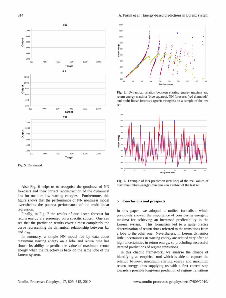
Also Fig. 6 helps us to recognise the goodness of NNforecasts and their correct reconstruction of the dynamicallaw for medium-low starting energies. Furthermore, thisfigure shows that the performance of NN nonlinear modeloverwhelms the poorest performance of the multi-linearregression.

Finally, in Fig. 7 the results of our 1-step forecast forreturn energy are presented on a specific subset. One cansee that the prediction results cover almost completely thecurve representing the dynamical relationship betweenEstandEret.

In summary, a simple NN model fed by data aboutmaximum starting energy on a lobe and return time hasshown its ability to predict the value of maximum returnenergy when the trajectory is back on the same lobe of theLorenz system.

300

400

500

600

700

800

900

1000

1100

1200

300 400 500 600 700 800 900 1000 1100 1200

Starting energy

Ret

urn

ener

gy y

Fig. 6. Dynamical relation between starting energy maxima andreturn energy maxima (blue squares), NN forecasts (red diamonds)and multi-linear forecasts (green triangles) on a sample of the testset.

300

400

500

600

700

800

900

1000

1100

1200

1 25 49 73 97 121 145 169 193

Integration step

Ret

urn

ener

gy

Fig. 7. Example of NN prediction (red line) of the real values ofmaximum return energy (blue line) on a subset of the test set.

5 Conclusions and prospects

In this paper, we adopted a unified formalism whichpreviously showed the importance of considering energeticmaxima for achieving an increased predictability in theLorenz system. This formalism led to a quite precisedetermination of return times referred to the transitions froma lobe to the other one. Nevertheless, in Lorenz dynamicslittle uncertainties in starting energy are related very often tohigh uncertainties in return energy, so precluding successfuliterated predictions of regime transitions.

In this chaotic framework, we analyse the chance ofidentifying an empirical tool which is able to capture therelation between maximum starting energy and maximumreturn energy, thus supplying us with a first correct steptowards a possible long-term prediction of regime transitions



on the Lorenz attractor. A NN model has shown good resultsin predicting return energy once fed by data about startingenergy and return time.

Here, simple multi-layer perceptrons are applied andprediction is limited to 1-step forecasts. As prospects offurther research, application of improved NN models isplanned and multi-step forecasts are envisaged.

Furthermore, the formalism adopted here can be appliedalso in the case of more general and realistic N-dimensionalfluid-dynamical systems, such as those discussed in Pelinoand Maimone (2007). Thus, we are confident that ourdynamical and NN approach can be pursued to catchsome features of dynamics and predictability of the realatmosphere, too.

Acknowledgements.Two of us (F.M. and V.P.) were partiallysupported by PEPS Mathematical Methods of Climate Models.

Edited by: W. HsiehReviewed by: two anonymous referees

References

Bishop, C. M.: Neural networks for pattern recognition, OxfordUniversity Press, New York, USA, 1995.

Boudjema, G. and Cazelles, B.: Extraction of nonlinear dynamicsfrom short and noisy time series, Chaos Soliton. Fract., 12, 2051–2069, doi:10.1016/S0960-0779(00)00163-6, 2001.

Corti, S., Molteni, F., and Palmer, T. N.: Signature of recent climatechange in frequencies of natural atmospheric circulation, Nature,398, 799–802, doi:10.1038/19745, 1999.

de Oliveira, K. A., Vannucci, A., and da Silva, E. C.: Using artificialneural networks to forecast chaotic time series, Physica A, 284,393–404, doi:10.1016/S0378-4371(00)00215-6, 2000.

Deloncle, A., Berk, R., D’Andrea, F., and Ghil, M.: Weather regimeprediction using statistical learning, J. Atmos. Sci., 64, 1619–1635, 2007.

Haupt, S. E., Pasini, A., and Marzban, C. (Eds.): Artificialintelligence methods in the environmental sciences, Springer,New York, USA, 2009.

Hertz, J., Krogh, A., and Palmer, R. G.: Introduction to the theory ofneural computation, Addison-Wesley-Longman, Reading, MA,USA, 1999.

Hsieh, W. W.: Machine learning methods in the environmentalsciences: Neural networks and kernels, Cambridge UniversityPress, Cambridge, UK, 2009.

Kondrashov, D., Ide, K., and Ghil, M.: Weather regimes andpreferred transition paths in a three-level quasi-geostrophicmodel, J. Atmos. Sci., 61, 568–587, 2004.

Krasnopolsky, V. M.: Neural network emulations for complexmultidimensional geophysical mappings: Applications of neuralnetwork techniques to atmospheric and oceanic satellite re-trievals and numerical modeling, Rev. Geophys., 45, RG3009,doi:10.1029/2006RG000200, 2007.

Palmer, T. and Hagedorn, R.: Predictability of Weather and Climate,Cambridge University Press, Cambridge, UK, 2006.

Pasini, A.: External forcings and predictability in Lorenz model:An analysis via neural network modelling, Nuovo Cimento C,31, 357–370, 2008.

Pasini, A. and Ameli, F.: Radon short range forecastingthrough time series preprocessing and neural network modelling,Geophys. Res. Lett., 30(7), 1386, doi:10.1029/2002GL016726,2003.

Pasini, A. and Langone, R.: Attribution of precipitation changeson a regional scale by neural network modeling: A case study,Water, 2, 321–332, doi:10.3390/w2030321, 2010.

Pasini, A. and Pelino, V.: A unified view of Kolmogorov and Lorenzsystems, Phys. Lett. A, 275, 435–446, doi:10.1016/S0375-9601(00)00620-4, 2000.

Pasini, A. and Potesta, S.: Short-range visibility forecast by meansof neural-network modelling: A case study, Nuovo Cimento C,18, 505–516, doi:10.1007/BF02506781, 1995.

Pasini, A., Pelino, V., and Potesta, S.: A neural network modelingfor visibility nowcasting from surface observations: Results andsensitivity to physical input variables, J. Geophys. Res., 106,14951–14959, doi:10.1029/2001JD900134, 2001.

Pasini, A., Perrino, C., andZujic, A.: Non-linear atmosphericstability indices by neural network modelling, Nuovo CimentoC, 26, 633–638, doi:10.1393/ncc/i2004-10001-7, 2003.

Pasini, A., Lore, M., and Ameli, F.: Neural network modelling forthe analysis of forcings/temperatures relationships at differentscales in the climate system, Ecol. Model., 191, 58–67,doi:10.1016/j.ecolmodel.2005.08.012, 2006.

Pasini, A., Szpunar, G., Amori, G., Langone, R., and Cristaldi,M.: Assessing climatic influences on rodent density: A neuralnetwork modelling approach and a case study in Central Italy,Asia-Pac. J. Atmos. Sci., 45, 319–330, 2009.

Pelino, V. and Maimone, F.: Energetics, skeletal dynamics, andlong-term predictions on Kolmogorov-Lorenz systems, Phys.Rev. E, 76, 046214, doi:10.1103/PhysRevE.76.046214, 2007.

Pelino, V. and Pasini, A.: Dissipation in Lie-Poisson systemsand the Lorenz-84 model, Phys. Lett. A, 291, 389–396,doi:10.1016/S0375-9601(01)00764-2, 2001.

Roebber, P. J. and Tsonis, A. A.: A method to improve predictionof atmospheric flow transitions, J. Atmos. Sci, 62, 3818–3824,doi:10.1175/JAS3572.1, 2005.

Stephenson, D. B., Hannachi, A., and O’Neill, A.: On the existenceof multiple climate regimes, Q. J. Roy. Meteor. Soc., 130, 583–605, doi:10.1256/qj.02.146, 2004.


Energy-based predictions in Lorenz system by a unified formalism and neural network modelling

Documents

Transcript of Energy-based predictions in Lorenz system by a unified formalism and neural network modelling