Empirical investigation of simplied step-size

control in metaheuristics with a view to theory

Jens Jägersküpper⋆ & Mike Preuss

Technische Universität Dortmund, Fakultät für Informatik,44221 Dortmund, Germany

Abstract. Randomized direct-search methods for the optimization of afunction f : Rn

→ R given by a black box for f -evaluations are inves-tigated. We consider the cumulative step-size adaptation (CSA) for thevariance of multivariate zero-mean normal distributions. Those are com-monly used to sample new candidate solutions within metaheuristics,in particular within the CMA Evolution Strategy (CMA-ES), a state-of-the-art direct-search method. Though the CMA-ES is very successfulin practical optimization, its theoretical foundations are very limited be-cause of the complex stochastic process it induces. To forward the theoryon this successful method, we propose two simplications of the CSAused within CMA-ES for step-size control. We show by experimentaland statistical evaluation that they perform suciently similarly to theoriginal CSA (in the considered scenario), so that a further theoreticalanalysis is in fact reasonable. Furthermore, we outline in detail a proba-bilistic/theoretical runtime analysis for one of the two CSA-derivatives.

1 Introduction

The driving force of this paper is the desire for a theoretical runtime analy-sis of a sophisticated stochastic optimization algorithm, namely the covariancematrix adaptation evolution strategy (CMA-ES). As this algorithm is very hardto analyze theoretically because of the complex stochastic process it induces,we follow an unorthodox approach: We decompose it into its main algorithmiccomponents: the covariance matrix adaptation (CMA), and the cumulative step-size adaptation (CSA). While the CMA is, in some sense, supposed to handleill-conditionedness in the optimization problems, it is the duty of the CSA tocope with a challenge that every algorithm for real-valued black-box optimiza-tion faces: step-size control, i.e. the adaptation of step-sizes when approachingan optimum. The idea behind this decomposition is to substitute one of thecomponents by an alternative mechanism that is more amenable to a theoret-ical analysis. While doing so, we rely on experimentation to assess how far wedepart from the original algorithm. Here simpler mechanisms for step-size con-trol are substituted for CSA. The desired outcome of this process is a modied

⋆ supported by the German Research Foundation (DFG) through the collaborativeresearch center Computational Intelligence (SFB 531)

C.C. McGeoch (Ed.): WEA 2008, LNCS 5038, pp. 263--274, 2008.Copyright Springer-Verlag Berlin Heidelberg 2008

algorithm that is both: tractable by theoretical analysis techniques, and, testedempirically, still working reasonably similar to the original one. At the same timewe aim at better understanding the core-mechanisms of the original algorithm.(A simplied algorithm may also be interesting for practitioners, as simple meth-ods often spread much faster than their complicated counterparts, even if thelatter have slight performance advantages.) The full theoretical analysis itself,however, is not part of this work, but is still pending. Rather we discuss whya theoretical analysis seems feasible and outline in detail how it could be ac-complished. Note that proving (global) convergence is not the subject of thetheoretical investigations. The subject is a probabilistic analysis of the randomvariable corresponding to the number of steps necessary to obtain a predenedreduction of the approximation error. For such an analysis to make sense, theclass of objective functions covered by the analysis must necessarily be ratherrestricted and simple. This paper provides evidence by experimental and statis-tical evaluation that a theoretical analysis for the simplied algorithm does makesense to yield more insight into CSA, the step-size control within the CMA-ES.

In a sense, our approach can be seen as algorithm re-engineering, a viewpointwhich is to our knowledge uncommon in the eld of metaheuristics. Therefore,we also strive for making a methodological contribution that will hopefully in-spires other researchers to follow a similar path. To this end, it is not necessaryto be familiar with the latest scientic work on metaheuristics to understandthe concepts applied herein. It is one of the intrinsic properties of stochastic al-gorithms in general that even simple methods may display surprising behaviorsthat are not at all easy to understand and analyze. We explicitly focus on prac-tically relevant dimensions. As it may be debatable what relevant is, we give a3-fold categorization used in the following: Problems with up to 7 dimensionsare seen as small, whereas medium sized ones from 8 to 63 dimensions are toour knowledge of the highest practical importance. Problems with 64 dimensionsand beyond are termed large.

In the following section the original CSA is described in detail. The twonew simplied CSA-derivatives are presented in Section 3, and their technicaldetails and dierences as well as some related work are discussed in Section 4.Furthermore, a detailed outline of a theoretical runtime analysis is given. Theexperimental comparison (including statistical evaluation) of the three CSA-variants is presented in Section 5. Finally, we conclude in Section 6.

2 Cumulative step-size adaptation (CSA)

The CMA-ES of Hansen and Ostermeier [1] is regarded as one of the most e-cient modern stochastic direct-search methods for numerical black-box optimiza-tion, cf. the list of over 100 references to applications of CMA-ES compiled byHansen [2]. Originally, CSA was designed for so-called (1,λ) Evolution Strate-gies, in which 1 candidate solution is iteratively evolved. In each iteration, λnew search points are sampled, each independently in the same way, namely byadding a zero-mean multivariate normal distribution to the current candidate

264

solution. When CMA is not used, like here, each of the λ samples is generatedby independently adding a zero-mean normal distribution with variance σ2 toeach of its n components. The best of the λ samples becomes the next candidatesolutionirrespective of whether this best of λ amounts to an improvement ornot (so-called comma selection; CSA does not work well for so-called elitist se-lection where the best sample becomes the next candidate solution only if it is atleast as good as the current one). The idea behind CSA is as follows: Consecutivesteps of an iterative direct-search method should be orthogonal. Therefore, onemay recall that steps of steepest descent (a gradient method) with perfect linesearch (i.e., the truly best point on the line in gradient direction is chosen) areindeed orthogonal when a positive denite quadratic form is minimized. WithinCSA the observation of mainly positively [negatively] correlated steps is taken asan indicator that the step-size is too small [resp. too large]. As a consequence, thestandard deviation σ of the multivariate normal distribution is increased [resp.decreased]. Since the steps' directions are random, considering just the last twosteps does not enable a smooth σ-adaptation because of the large variation of therandom angle between two steps. Thus, in each iteration the so-called evolutionpath is considered, namely its length is compared with the length that wouldbe expected when the steps were orthogonal. Essentially, the evolution path isa recent part of the trajectory of candidate solutions. Considering the completetrajectory is not the most appropriate choice, though. Rather, a certain amountof the recent history of the search is considered. In the original CSA as proposedby Hansen and Ostermeier, σ is adapted continuously, i.e. after each iteration.The deterministic update of the evolution path p ∈ R

n after the ith iterationworks as follows:

p[i+1] := (1 − cσ) · p[i] +√

cσ · (2 − cσ) · m[i]/σ[i] (1)

where m[i] ∈ Rn denotes the displacement (vector) of the ith step, and the xed

parameter cσ ∈ (0, 1) determines the weighting between the recent history ofthe optimization and its past within the evolution path. We use cσ := 1/

√n

as suggested by Hansen and Ostermeier [1]. Note that m[i] is one of λ vectorseach of which was independently chosen according to a zero-mean multivariatenormal distribution with standard deviation σ[i]. The length of such a vectorfollows a scaled (by σ[i]) χ-distribution. Initially, p[0] is chosen as the all-zerovector. The σ-update is done deterministically as follows:

σ[i+1] := σ[i] · exp

(cσ

dσ·( |p[i+1]|

χ− 1

))(2)

where the xed parameter dσ is called damping factor, and χ denotes the ex-pectation of the χ-distribution. Note that σ is kept unchanged if the length ofthe evolution path equals χ. We used dσ := 0.5 because this leads to a betterperformance than dσ ∈ 0.25, 1 for the considered function scenario. Naturally,there is interdependence between dσ and cσ, and moreover, an optimal choicedepends (among others) on the function to be optimized, of course.

265

3 Two simplied CSA-Derivatives

In this section we introduce two simplications of the original CSA, created bysubsequently departing further from the dening Equations (1) and (2). The rstsimplication (common to both CSA-derivatives) will be to partition the courseof the optimization into phases of a xed length in which σ is not changed. Sucha partitioning of the process has turned out useful in former theoretical analyses,cf. [3,4] for instance. Thus, both variants use phases of a xed length, after eachof which σ is adaptedsolely depending on what happened during that phase,respectively. Therefore, recall that cσ = 1/

√n in the path update, cf. Eqn. (1).

Since (1 − 1/√

n)i = 0.5 for i ≍ √n · ln 2 (as n grows), the half-live of a step

within the evolution path is roughly 0.5√

n iterations for small dimensions androughly 0.7

√n for large n. For this reason we choose the phase length k as ⌈√n ⌉

a priori for the simplied versions to be described in the following. The secondsimplication to be introduced is as follows: Rather than comparing the length ofthe displacement of a phase with the expected length that would be observed ifthe steps in the phase were completely orthogonal, the actual correlations of thesteps of a phase in terms of orthogonality are considered directly and aggregatedinto a criterion that we call correlation balance.

pCSA. The p stands for phased. The run of the ES is partitioned into phaseslasting k := ⌈√n⌉ steps, respectively. After each phase, the vector correspond-ing to the total movement (in the search space) in this phase is considered. Thelength of this displacement is compared to ℓ :=

√k · σ · χ, where χ is the expec-

tation of the χ-distribution with n degrees of freedom. Note that ℓ equals thelength of the diagonal of a k-dimensional cube with edges of length σ · χ, andthat σ · χ equals the expected step-length in the phase. Thus, if all k steps of aphase had the expected length, and if they were completely orthogonal, then thelength of the displacement vector in such a phase would just equal ℓ. Dependingon whether the displacement's actual length is larger [or smaller] than ℓ, σ isconsidered as too small (because of positive correlation) [resp. as too large (be-cause of negative correlation)]. Then σ is scaled up [resp. down] by a predenedscaling factor larger than one [resp. by the reciprocal of this factor].

CBA. CBA stands for correlation-balance adaptation. The optimization isagain partitioned into phases each of which lasts k := ⌈√n⌉ steps. After eachphase, the k vectors that correspond to the k movements in the phase are con-sidered. For each pair of these k vectors the correlation is calculated, so that weobtain

(k2

)= k(k − 1)/2 correlation values. If the majority of these values are

positive [negative], then the σ used in the respective phase is considered as toosmall [resp. as too large]. Hence, σ is scaled up [resp. down] after the phase bysome predened factor larger than one [resp. by the reciprocal of this factor].

4 Related work, discussion, and a view to theory

Evolutionary algorithms for numerical optimization usually try to learn goodstep-sizes, which may be implemented by self-adaptation or success-based rules,

266

the most prominent of which may be the 1/5-rule to increase [decrease] step sizesif more [less] than 1/5 of the samples result in an improvement. This simple deter-ministic adaptation mechanism, which is due to Rechenberg [5] and Schwefel [6],has already been the subject of a probabilistic analysis of the (random) numberof steps necessary to reduce the approximation error in the search space. The rstresults from this viewpoint of analyzing ES like usual randomized algorithmswere obtained in [7] for the simplest quadratic function, namely x 7→

∑ni=1 x2

i ,which is commonly called Sphere. This analysis has been extended in [8] toquadratic forms with bounded condition number as well as to a certain classof ill-conditioned quadratic forms (parameterized in the dimensionality of thesearch space) for which the condition number grows as the dimensionality of thesearch space increases. The main result of the latter work is that the runtime(to halve the approximation error) increases proportionally with the conditionnumber. This drawback has already been noticed before in practice, of course. Asa remedy, the CMA was proposed which, in some sense, learns and continuouslyadjusts a preconditioner by adapting the covariance matrix of the multivariatenormal distribution used to sample new candidate solutions. As noted above,within the CMA-ES the CSA is applied for step-size control, which is neithera self-adaptive mechanism nor based on a success rule. In the present work, weexclusively deal with this CSA mechanism. Therefore, we consider a sphericallysymmetric problem, so that the CMA mechanism is dispensable. We demandthat the simplied CSA-derivatives perform suciently well on this elementarytype of problem at least. If they did not, they would be unable to ensure localconvergence at a reasonable speed, so that eorts on a theoretical analysis wouldseem questionable.

CSA, pCSA, and CBA are basically (1, λ) ES, and results obtained followinga dynamical-system approach indicate that the expected spatial gain towards theoptimum in an iteration is bounded above by O(ln(λ) ·d/n), where d denotes thedistance from the optimum, cf. [9, Sec. 3.2.3, Eqn. (3.115)]. As this result wasobtained using simplifying equations to describe the dynamical system inducedby the ES, however, it cannot be used as a basis for proving theorems on theruntime of (1, λ)ES. Nevertheless, this is a strong indicator that a (1, λ) ES con-verges, if at all, at best linearly at an expected rate 1 − O(ln(λ)/n). From this,we can conjecture that the expected number of iterations necessary to halve theapproximation error is bounded below by Ω(n/ lnλ). This lower bound has infact been rigorously proved in [10, Thm. 1] for a framework of iterative methodsthat covers pCSA as well as CBA. (Unfortunately, CSA is not covered since thefactor for the σ-update in Eqn. (2) depends on the course of the optimization,namely on the length of the evolution path.) Actually, it is proved that less than0.64n/ ln(1+3λ) iterations suce to halve the approximation error only with anexponentially small probability e−Ω(n) (implying the Ω(n/ lnλ)-bound on theexpected number of steps). Moreover, [10, Thm. 4] provides a rigorous proofthat a (1, λ) ES using a simple σ-adaptation mechanism (based on the relativefrequency of improving steps) to minimize Sphere needs with very high prob-ability at most O(n/

√lnλ) iterations to halve the approximation error. This

267

upper bound is larger than the lower bound by a factor of order√

lnλ, whichis actually due to the σ-adaptation: It adapts σ such that it is of order Θ(d/n),whereas σ = Θ(

√lnλ · d/n) seems necessary. For the original CSA minimizing

Sphere, a result obtained in [11, Eqn. (20)] (using the dynamical-system ap-proach again) indicates that the expected spatial gain in an iteration tends to(√

2 − 1) · (c1,λ)2 · d/n = Θ(ln(λ) · d/n) as the dimensionality n goes to innity,

where c1,λ = Θ(√

lnλ) is the so-called (1,λ)-progress coecient (obtained foroptimal σ, cf. [9, Eqn. (3.114)]); σ is reported to tend to

√2 · c1,λ · d/n as the

dimensionality n goes to innity, which is indeed Θ(√

lnλ · d/n) [11, Eqn. (19)].

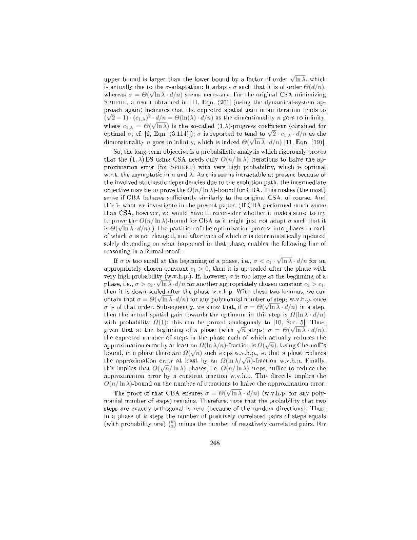
So, the long-term objective is a probabilistic analysis which rigorously provesthat the (1, λ) ES using CSA needs only O(n/ lnλ) iterations to halve the ap-proximation error (for Sphere) with very high probability, which is optimalw.r.t. the asymptotic in n and λ. As this seems intractable at present because ofthe involved stochastic dependencies due to the evolution path, the intermediateobjective may be to prove the O(n/ lnλ)-bound for CBA. This makes (the most)sense if CBA behaves suciently similarly to the original CSA, of course. Andthis is what we investigate in the present paper. (If CBA performed much worsethan CSA, however, we would have to reconsider whether it makes sense to tryto prove the O(n/ lnλ)-bound for CBA as it might just not adapt σ such that itis Θ(

√lnλ · d/n).) The partition of the optimization process into phases in each

of which σ is not changed, and after each of which σ is deterministically updatedsolely depending on what happened in that phase, enables the following line ofreasoning in a formal proof:

If σ is too small at the beginning of a phase, i.e., σ < c1 ·√

lnλ · d/n for anappropriately chosen constant c1 > 0, then it is up-scaled after the phase withvery high probability (w.v.h.p.). If, however, σ is too large at the beginning of aphase, i.e., σ > c2 ·

√lnλ ·d/n for another appropriately chosen constant c2 > c1,

then it is down-scaled after the phase w.v.h.p. With these two lemmas, we canobtain that σ = Θ(

√lnλ ·d/n) for any polynomial number of steps w.v.h.p. once

σ is of that order. Subsequently, we show that, if σ = Θ(√

lnλ · d/n) in a step,then the actual spatial gain towards the optimum in this step is Ω(lnλ · d/n)with probability Ω(1); this can be proved analogously to [10, Sec. 5]. Thus,given that at the beginning of a phase (with

√n steps) σ = Θ(

√lnλ · d/n),

the expected number of steps in the phase each of which actually reduces theapproximation error by at least an Ω(lnλ/n)-fraction is Ω(

√n). Using Cherno's

bound, in a phase there are Ω(√

n) such steps w.v.h.p., so that a phase reducesthe approximation error at least by an Ω(lnλ/

√n)-fraction w.v.h.p. Finally,

this implies that O(√

n/ lnλ) phases, i.e. O(n/ lnλ) steps, suce to reduce theapproximation error by a constant fraction w.v.h.p. This directly implies theO(n/ lnλ)-bound on the number of iterations to halve the approximation error.

The proof of that CBA ensures σ = Θ(√

lnλ · d/n) (w.v.h.p. for any poly-nomial number of steps) remains. Therefore, note that the probability that twosteps are exactly orthogonal is zero (because of the random directions). Thus,in a phase of k steps the number of positively correlated pairs of steps equals(with probability one)

(k2

)minus the number of negatively correlated pairs. For

268

a theoretical analysis of CBA, for each phase(k2

)0-1-variables can be dened.

Each of these indicator variables tells us whether the respective pair of steps ispositively correlated (1) or not (0). (Recall that in CBA the decision whetherto up- or down-scale σ is based on whether the sum of these indicator variablesis larger than

(k2

)/2 or smaller.) There are strong bounds on the deviation of

the actual sum of 0-1-variables from the expected sum, in particular when thevariables are independentwhich is not the case for CBA. This can be overcomeby stochastic dominance arguments, so that we deal with independent Bernoullitrials, rather than with dependent Poisson trials. We merely need to know howthe success probability of a Bernoulli trial depends on σ.

All in all, CBA is a candidate for a theoretical runtime analysis of an ESusing this simplied CSA-variant. It was an open question, whether CBA worksat all and, if so, how well it performs compared to the original CSA (and pCSA).Thus, we decided for an experimental comparison with statistical evaluation.

5 Experimental investigation of the CSA-variants

Since the underlying assumption in theory on black-box optimization is thatthe evaluation of the function f to be optimized is by far the most expensiveoperation, the number of f -evaluations (λ times the iterations) is the sole per-formance measure in the following comparison of the three CSA-variants. Tond out the potentials of the σ-adaptation mechanisms described above, we fo-cus on the simplest unimodal function scenario, namely the minimization of thedistance from a xed point. This is equivalent (here) to the minimization of aperfectly (pre)conditioned positive denite quadratic form. One of these func-tions, namely x 7→

∑ni=1 xi

2, is the commonly investigated Sphere (level sets ofsuch functions form hyper-spheres). We decided for a (1,5) Evolution Strategy,i.e. λ := 5. The reason for this choice is that, according to Beyer [9, p. 73], vesamples are most eective for comma selection, i.e. allow maximum progressper function evaluation. Thus, dierences in the adaptations' abilities (to chooseσ as close to optimal as possible) should be most noticeable for this choice.

Experiment: Do the CSA-derivatives perform similar to the original CSA?

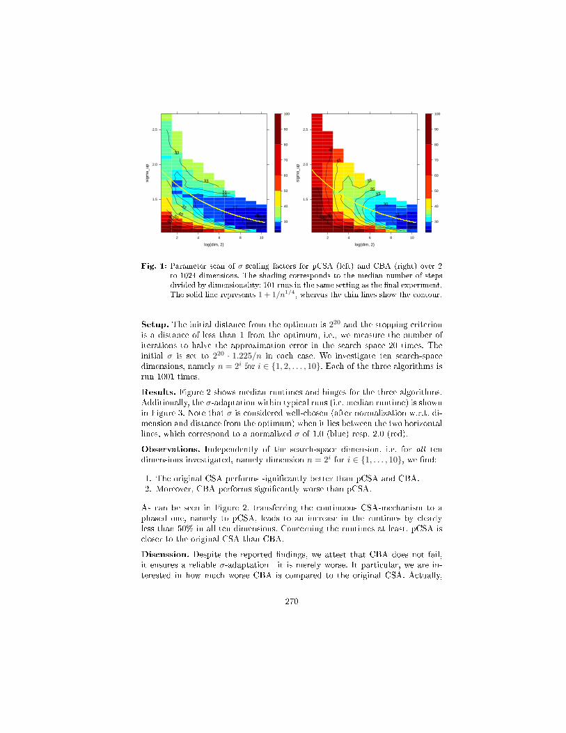
Pre-experimental planning. In addition to the adaptation rule and the phaselength, the scaling factor by which σ is increased or decreased after a phase hadto be xed for pCSA and CBA. For both CSA-derivatives, the σ-scaling factorwas determined by parameter scans, cf. Figure 1, whereas the phase length kwas chosen a priori as ⌈√n ⌉ (for the reason given above). Interestingly, theparameter scans show that the σ-scaling factor should be chosen identically as1 + 1/n1/4 for pCSA as well as for CBA.

Task. The hypothesis is that the three CSA-variants perform equally well interms of number of iterations. As the data can not be supposed to be normallydistributed, we compare two variants, namely their runtimes (i.e. number ofiterations), by the Wilcoxon rank-sum test (as implemented by wilcox.test inR), where a p-value of 0.05 or less indicates a signicant dierence.

269

log(dim, 2)

sigm

a_up

1.5

2.0

2.5

2 4 6 8 10

25

27

3031

33

33

33

40506080 30

40

50

60

70

80

90

100

log(dim, 2)

sigm

a_up

1.5

2.0

2.5

2 4 6 8 10

27

30

3335

38

45

60

8010030

40

50

60

70

80

90

100

Fig. 1: Parameter scan of σ-scaling factors for pCSA (left) and CBA (right) over 2to 1024 dimensions. The shading corresponds to the median number of stepsdivided by dimensionality; 101 runs in the same setting as the nal experiment.The solid line represents 1 + 1/n1/4, whereas the thin lines show the contour.

Setup. The initial distance from the optimum is 220 and the stopping criterionis a distance of less than 1 from the optimum, i.e., we measure the number ofiterations to halve the approximation error in the search space 20 times. Theinitial σ is set to 220 · 1.225/n in each case. We investigate ten search-spacedimensions, namely n = 2i for i ∈ 1, 2, . . . , 10. Each of the three algorithms isrun 1001 times.

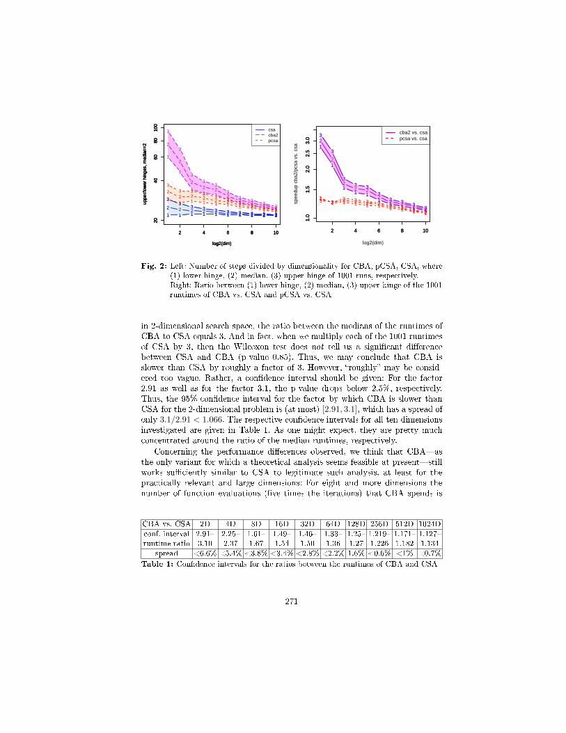
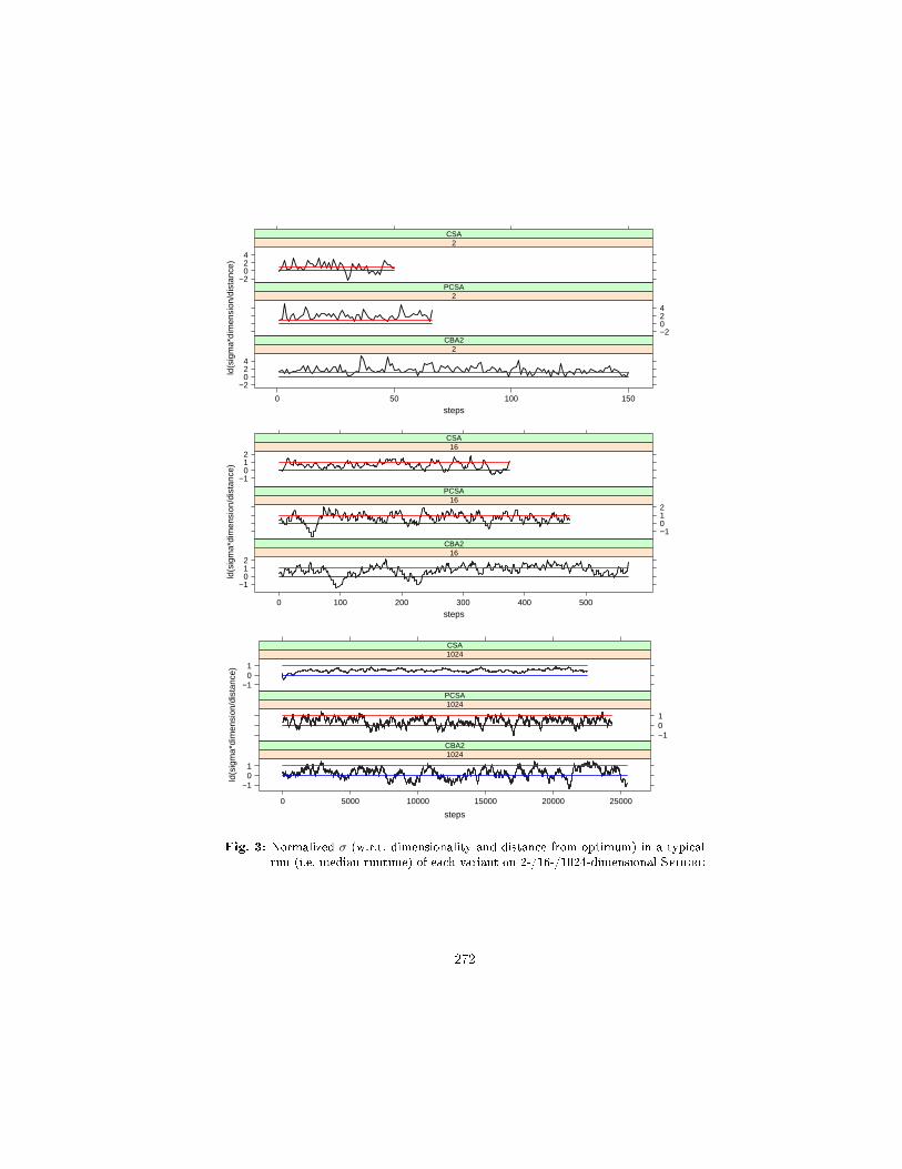
Results. Figure 2 shows median runtimes and hinges for the three algorithms.Additionally, the σ-adaptation within typical runs (i.e. median runtime) is shownin Figure 3. Note that σ is considered well-chosen (after normalization w.r.t. di-mension and distance from the optimum) when it lies between the two horizontallines, which correspond to a normalized σ of 1.0 (blue) resp. 2.0 (red).

Observations. Independently of the search-space dimension, i.e. for all tendimensions investigated, namely dimension n = 2i for i ∈ 1, . . . , 10, we nd:

1. The original CSA performs signicantly better than pCSA and CBA.2. Moreover, CBA performs signicantly worse than pCSA.

As can be seen in Figure 2, transferring the continuous CSA-mechanism to aphased one, namely to pCSA, leads to an increase in the runtimes by clearlyless than 50% in all ten dimensions. Concerning the runtimes at least, pCSA iscloser to the original CSA than CBA.

Discussion. Despite the reported ndings, we attest that CBA does not fail,it ensures a reliable σ-adaptationit is merely worse. It particular, we are in-terested in how much worse CBA is compared to the original CSA. Actually,

270

1 1 1 1 1 1 1 1 1 1

2 4 6 8 10

2040

6080

100

log2(dim)

uppe

r/lo

wer

hin

ges,

med

ian=

2

2 2 2 2 2 2 2 2 2 2

33

3 3 3 3 3 3 3 31 1 1 1 1 1 1 1 1 1

2 4 6 8 10

2040

6080

100

log2(dim)

uppe

r/lo

wer

hin

ges,

med

ian=

2

2 2 2 2 2 2 2 2 2 2

33

3 3 3 3 3 3 3 3

1

1

11 1

11 1 1 1

2 4 6 8 10

2040

6080

100

log2(dim)

uppe

r/lo

wer

hin

ges,

med

ian=

2 2

2

22 2

22 2 2 2

3

3

3

33

33

33

3

11 1 1 1 1 1 1 1 1

2 4 6 8 10

2040

6080

100

log2(dim)

uppe

r/lo

wer

hin

ges,

med

ian=

2

22 2 2 2 2

2 2 2 2

33 3

33 3

3 33 3

csacba2pcsa

1

1

11 1

11 1 1 1

2 4 6 8 10

1.0

1.5

2.0

2.5

3.0

log2(dim)

spee

dup

cba2

/pcs

a vs

. csa

2

2

22 2

22 2 2 2

3

3

33 3

33 3 3

3

1

1

11 1

11 1 1 1

2 4 6 8 10

1.0

1.5

2.0

2.5

3.0 2

2

22 2

22 2 2 2

3

3

33 3

33 3 3

3

11 1 1 1 1 1 1 1 1

2 4 6 8 10

1.0

1.5

2.0

2.5

3.0

22 2 2 2 2

2 2 2 2

3 33 3 3 3 3 3 3 3

cba2 vs. csapcsa vs. csa

Fig. 2: Left: Number of steps divided by dimensionality for CBA, pCSA, CSA, where(1) lower hinge, (2) median, (3) upper hinge of 1001 runs, respectively.Right: Ratio between (1) lower hinge, (2) median, (3) upper hinge of the 1001runtimes of CBA vs. CSA and pCSA vs. CSA

in 2-dimensional search space, the ratio between the medians of the runtimes ofCBA to CSA equals 3. And in fact, when we multiply each of the 1001 runtimesof CSA by 3, then the Wilcoxon test does not tell us a signicant dierencebetween CSA and CBA (p-value 0.85). Thus, we may conclude that CBA isslower than CSA by roughly a factor of 3. However, roughly may be consid-ered too vague. Rather, a condence interval should be given: For the factor2.91 as well as for the factor 3.1, the p-value drops below 2.5%, respectively.Thus, the 95%-condence interval for the factor by which CBA is slower thanCSA for the 2-dimensional problem is (at most) [2.91, 3.1], which has a spread ofonly 3.1/2.91 < 1.066. The respective condence intervals for all ten dimensionsinvestigated are given in Table 1. As one might expect, they are pretty muchconcentrated around the ratio of the median runtimes, respectively.

Concerning the performance dierences observed, we think that CBAasthe only variant for which a theoretical analysis seems feasible at presentstillworks suciently similar to CSA to legitimate such analysis, at least for thepractically relevant and large dimensions: For eight and more dimensions thenumber of function evaluations (ve times the iterations) that CBA spends is

CBA vs. CSA 2D 4D 8D 16D 32D 64D 128D 256D 512D 1024D

conf. interval 2.91 2.25 1.61 1.49 1.46 1.33 1.25 1.219 1.171 1.127runtime ratio 3.10 2.37 1.67 1.54 1.50 1.36 1.27 1.226 1.182 1.134

spread <6.6% <5.4% <3.8% <3.4% <2.8% <2.2% 1.6% <0.6% <1% <0.7%

Table 1: Condence intervals for the ratios between the runtimes of CBA and CSA

271

steps

ld(s

igm

a*di

men

sion

/dis

tanc

e)

−2024

0 50 100 150

2CBA2

−2024

2PCSA

−2024

2CSA

steps

ld(s

igm

a*di

men

sion

/dis

tanc

e)

−1012

0 100 200 300 400 500

16CBA2

−1012

16PCSA

−1012

16CSA

steps

ld(s

igm

a*di

men

sion

/dis

tanc

e)

−101

0 5000 10000 15000 20000 25000

1024CBA2

−101

1024PCSA

−101

1024CSA

Fig. 3: Normalized σ (w.r.t. dimensionality and distance from optimum) in a typicalrun (i.e. median runtime) of each variant on 2-/16-/1024-dimensional Sphere

272

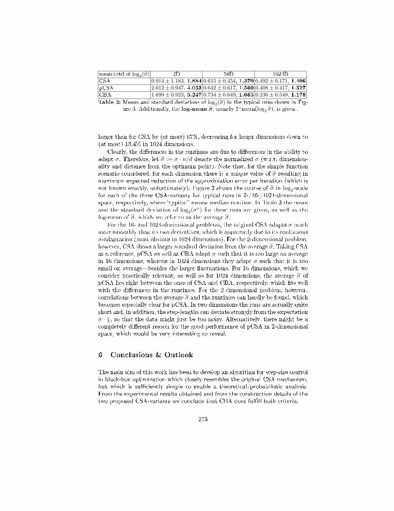
mean±std of log2(bσ) 2D 16D 1024D

CSA 0.914 ± 1.183, 1.884 0.615 ± 0.454, 1.370 0.492 ± 0.171, 1.406

pCSA 2.012 ± 0.947, 4.033 0.642 ± 0.617, 1.560 0.408 ± 0.417, 1.327

CBA 1.699 ± 0.923, 3.247 0.734 ± 0.649, 1.663 0.236 ± 0.549, 1.178

Table 2: Means and standard deviations of log2(bσ) in the typical runs shown in Fig-ure 3. Additionally, the log-mean bσ, namely 2^mean(log2 bσ), is given.

larger than for CSA by (at most) 67%, decreasing for larger dimensions down to(at most) 13.4% in 1024 dimensions.

Clearly, the dierences in the runtimes are due to dierences in the ability toadapt σ. Therefore, let σ := σ · n/d denote the normalized σ (w.r.t. dimension-ality and distance from the optimum point). Note that, for the simple functionscenario considered, for each dimension there is a unique value of σ resulting inmaximum expected reduction of the approximation error per iteration (which isnot known exactly, unfortunately). Figure 3 shows the course of σ in log2-scalefor each of the three CSA-variants for typical runs in 2-/16-/1024-dimensionalspace, respectively, where typical means median runtime. In Table 2 the meanand the standard deviation of log2(σ

∗) for these runs are given, as well as thelog-mean of σ, which we refer to as the average σ.

For the 16- and 1024-dimensional problems, the original CSA adapts σ muchmore smoothly than its two derivatives, which is apparently due to its continuousσ-adaptation (most obvious in 1024 dimensions). For the 2-dimensional problem,however, CSA shows a larger standard deviation from the average σ. Taking CSAas a reference, pCSA as well as CBA adapt σ such that it is too large on averagein 16 dimensions, whereas in 1024 dimensions they adapt σ such that it is toosmall on averagebesides the larger uctuations. For 16 dimensions, which weconsider practically relevant, as well as for 1024 dimensions, the average σ ofpCSA lies right between the ones of CSA and CBA, respectively, which ts wellwith the dierences in the runtimes. For the 2-dimensional problem, however,correlations between the average σ and the runtimes can hardly be found, whichbecomes especially clear for pCSA. In two dimensions the runs are actually quiteshort and, in addition, the step-lengths can deviate strongly from the expectationσ · χ, so that the data might just be too noisy. Alternatively, there might be acompletely dierent reason for the good performance of pCSA in 2-dimensionalspace, which would be very interesting to reveal.

6 Conclusions & Outlook

The main aim of this work has been to develop an algorithm for step-size controlin black-box optimization which closely resembles the original CSA mechanism,but which is suciently simple to enable a theoretical/probabilistic analysis.From the experimental results obtained and from the construction details of thetwo proposed CSA-variants we conclude that CBA does fulll both criteria.

273

Additionally, some interesting facts have been unveiled. One of these aectsthe change from continuous σ-update to phases in which σ is kept constant.Contrary to what we expected, this modication does not explain the largeruntime dierences in small dimensions. Those may rather be due to the largeuctuations observed in the step-sizes adjusted by the two CSA-derivatives; CSAstep-size curves are obviously much smoother in higher dimensions. Furthermore,it has been found that an appropriate σ-scaling factor for both CSA-derivativesseems to follow a double square root (namely 1 + 1/n1/4) rather than a singlesquare root function (like 1 + 1/

√n) as one might expect.

Currently, we work on the details of a theoretical/probabilistic analysis ofCBA following the approach outlined in Section 4. Furthermore, we are goingto experimentally review the performance of the two CSA-derivatives on morecomplexactually, less trivialfunctions in comparison to the original CSA(also and in a particular in combination with CMA), but also to classical direct-search methods like the ones reviewed in [12].

Acknowledgment. We thank Thomas Stützle for helping us improve the paper.

References

1. Hansen, N., Ostermeier, A.: Adapting arbitrary normal mutation distributionsin evolution strategies: The covariance matrix adaptation. In: Proc. IEEE Int'lConference on Evolutionary Computation (ICEC). (1996) 312317

2. Hansen, N.: List of references to various applications of CMA-ES (2008)http://www.bionik.tu-berlin.de/user/niko/cmaapplications.pdf.

3. Droste, S., Jansen, T., Wegener, I.: On the analysis of the (1+1) EvolutionaryAlgorithm. Theoretical Computer Science 276 (2002) 5182

4. Jägersküpper, J.: Algorithmic analysis of a basic evolutionary algorithm for con-tinuous optimization. Theoretical Computer Science 379 (2007) 329347

5. Rechenberg, I.: Cybernetic solution path of an experimental problem. Royal Air-craft Establishment (1965)

6. Schwefel, H.P.: Numerical Optimization of Computer Models. Wiley, New York(1981)

7. Jägersküpper, J.: Analysis of a simple evolutionary algorithm for minimization inEuclidean spaces. In: Proc. 30th Int'l Colloquium on Automata, Languages andProgramming (ICALP). Volume 2719 of LNCS., Springer (2003) 106879

8. Jägersküpper, J.: How the (1+1)ES using isotropic mutations minimizes positivedenite quadratic forms. Theoretical Computer Science 361 (2005) 3856

9. Beyer, H.G.: The Theory of Evolution Strategies. Springer (2001)10. Jägersküpper, J.: Probabilistic runtime analysis of (1+, λ)ES using isotropic muta-

tions. In: Proc. 2006 Genetic and Evolutionary Computation Conference (GECCo),ACM Press (2006) 461468

11. Beyer, H.G., Arnold, D.V.: Performance analysis of evolutionary optimizationwith cumulative step-length adaptation. IEEE Transactions on Automatic Control(2004) 617622

12. Kolda, T.G., Lewis, R.M., Torczon, V.: Optimization by direct search: New per-spectives on some classical and modern methods. SIAM Review 45 (2004) 385482

274