Empirical and Theoretical Comparisons of Selected Criterion Functions for Document Clustering

Machine Learning, 55, 311–331, 2004c© 2004 Kluwer Academic Publishers. Manufactured in The Netherlands.

Empirical and Theoretical Comparisons of SelectedCriterion Functions for Document Clustering∗

YING ZHAO [email protected] KARYPIS [email protected] of Minnesota, Department of Computer Science Minneapolis, MN 55455, USA

Editor: Douglas Fisher

Abstract. This paper evaluates the performance of different criterion functions in the context of partitionalclustering algorithms for document datasets. Our study involves a total of seven different criterion functions, threeof which are introduced in this paper and four that have been proposed in the past. We present a comprehensiveexperimental evaluation involving 15 different datasets, as well as an analysis of the characteristics of the variouscriterion functions and their effect on the clusters they produce. Our experimental results show that there are a setof criterion functions that consistently outperform the rest, and that some of the newly proposed criterion functionslead to the best overall results. Our theoretical analysis shows that the relative performance of the criterion functionsdepends on (i) the degree to which they can correctly operate when the clusters are of different tightness, and (ii)the degree to which they can lead to reasonably balanced clusters.

Keywords: partitional clustering, criterion function, data mining, information retrieval

1. Introduction

The topic of clustering has been extensively studied in many scientific disciplines and avariety of different algorithms have been developed (MacQueen, 1967; King, 1967; Zahn,1971; Sneath & Sokal, 1973; Dempster, Laird, & Rubin, 1977; Jackson, 1991; Ng & Han,1994; Berry, Dumais, & O’Brien, 1995; Cheeseman & Stutz, 1996; Ester et al., 1996; Guha,Rastogi, & Shim, 1998; Boley, 1998; Guha, Rastogi, & Shim, 1999; Karypis, Han, & Kumar,1999a; Strehl & Ghosh, 2000; Ding et al., 2001). Two recent surveys on the topics (Jain,Murty, & Flynn, 1999; Han, Kamber, & Tung, 2001) offer a comprehensive summaryof the different applications and algorithms. These algorithms can be categorized alongdifferent dimensions based either on the underlying methodology of the algorithm, leadingto agglomerative or partitional approaches, or on the structure of the final solution, leadingto hierarchical or non-hierarchical solutions.

In recent years, various researchers have recognized that partitional clustering algorithmsare well-suited for clustering large document datasets due to their relatively low compu-tational requirements (Cutting et al., 1992; Larsen & Aone, 1999; Steinbach, Karypis, &

∗This work was supported by NSF ACI-0133464, CCR-9972519, EIA-9986042, ACI-9982274, and by ArmyHPC Research Center contract number DAAH04-95-C-0008.

312 Y. ZHAO AND G. KARYPIS

Kumar, 2000). A key characteristic of many partitional clustering algorithms is that they usea global criterion function whose optimization drives the entire clustering process. For someof these algorithms the criterion function is implicit (e.g., PDDP (Boley, 1998)), whereasfor other algorithms (e.g, K -means (MacQueen, 1967), Cobweb (Fisher, 1987), and Auto-class (Cheeseman & Stutz, 1996)) the criterion function is explicit and can be easily stated.This latter class of algorithms can be thought of as consisting of two key components.First is the criterion function that the clustering solution optimizes, and second is the actualalgorithm that achieves this optimization.

The focus of this paper is to study the suitability of different criterion functions tothe problem of clustering document datasets. In particular, we evaluate a total of sevencriterion functions that measure various aspects of intra-cluster similarity, inter-clusterdissimilarity, and their combinations. These criterion functions utilize different views ofthe underlying collection by either modeling the documents as vectors in a high dimen-sional space or by modeling the collection as a graph. We experimentally evaluated theperformance of these criterion functions using 15 different datasets obtained from varioussources. Our experiments show that different criterion functions do lead to substantially dif-ferent results and that there are a set of criterion functions that produce the best clusteringsolutions.

Our analysis of the different criterion functions shows that their overall performancedepends on the degree to which they can correctly operate when the dataset contains clustersof different tightness (i.e., they contain documents whose average pairwise similarities aredifferent) and the degree to which they can produce balanced clusters. Moreover, our analysisalso shows that the sensitivity to the difference in the cluster tightness can also explain anoutcome of our study (that was also observed in earlier results reported in Steinbach,Karypis, and Kumar (2000)), that for some clustering algorithms the solution obtained byperforming a sequence of repeated bisections is better (and for some criterion functionsby a considerable amount) than the solution obtained by computing the clustering directly.When the solution is computed via repeated bisections, the tightness difference betweenthe two clusters that are discovered is in general smaller than the tightness differencesbetween all the clusters. As a result, criterion functions that cannot handle well variation incluster tightness tend to perform substantially better when used to compute the clusteringvia repeated bisections.

The rest this paper is organized as follows. Section 2 provides some information on thedocument representation and similarity measure used in our study. Section 3 describes thedifferent criterion functions and the algorithms used to optimize them. Section 4 providesthe detailed experimental evaluation of the various criterion functions. Section 5 analyzesthe different criterion functions and explains their performance. Finally, Section 6 providessome concluding remarks.

2. Preliminaries

Document representation. The various clustering algorithms described in this paper rep-resent each document using the well-known term frequency-inverse document frequency(tf-idf) vector-space model (Salton, 1989). In this model, each document d is considered to

SELECTED CRITERION FUNCTIONS FOR DOCUMENT CLUSTERING 313

be a vector in the term-space and is represented by the vector

dtfidf = (tf1 log(n/df1), tf2 log(n/df2), . . . , tfm log(n/dfm)),

where tfi is the frequency of the i th term (i.e., term frequency), n is the total number ofdocuments, and dfi is the number of documents that contain the i th term (i.e., documentfrequency). To account for documents of different lengths, the length of each documentvector is normalized so that it is of unit length. In the rest of the paper, we will assume thatthe vector representation for each document has been weighted using tf-idf and normalizedso that it is of unit length.

Similarity measures. Two prominent ways have been proposed to compute the similaritybetween two documents di and d j . The first method is based on the commonly-used (Salton,1989) cosine function

cos(di , d j ) = dit d j/(‖di‖‖d j‖),

and since the document vectors are of unit length, it simplifies to dit d j . The second method

computes the similarity between the documents using the Euclidean distance dis(di , d j ) =‖di − d j‖. Note that besides the fact that one measures similarity and the other measuresdistance, these measures are quite similar to each other because the document vectors areof unit length.

Definitions. Throughout this paper we will use the symbols n, m, and k to denote thenumber of documents, the number of terms, and the number of clusters, respectively. Wewill use the symbol S to denote the set of n documents to be clustered, S1, S2, . . . , Sk todenote each one of the k clusters, and n1, n2, . . . , nk to denote their respective sizes. Given aset A of documents and their corresponding vector representations, we define the compositevector DA to be DA = ∑

d∈A d , and the centroid vector CA to be CA = DA/|A|.

3. Document clustering

At a high-level the problem of clustering is defined as follows. Given a set S of n documents,we would like to partition them into a pre-determined number of k subsets S1, S2, . . . , Sk ,such that the documents assigned to each subset are more similar to each other than thedocuments assigned to different subsets.

As discussed in the introduction, our focus is to study the suitability of various clusteringcriterion functions in the context of partitional document clustering algorithms. Conse-quently, given a particular clustering criterion function C, the clustering problem is tocompute a k-way clustering solution such that the value of C is optimized. In the rest of thissection we first present a number of different criterion functions that can be used to bothevaluate and drive the clustering process, followed by a description of the algorithms thatwere used to perform their optimization.


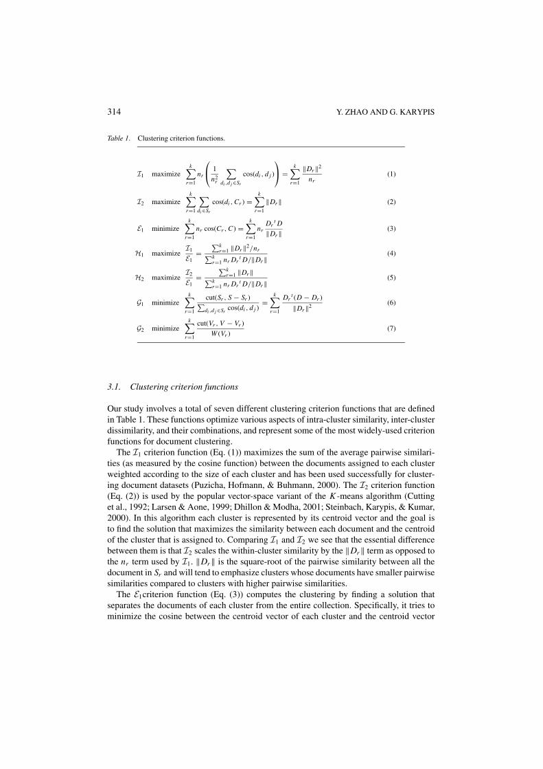
Table 1. Clustering criterion functions.

I1 maximizek∑

r=1

nr

1

n2r

∑di ,d j ∈Sr

cos(di , d j )

=

k∑r=1

‖Dr ‖2

nr(1)

I2 maximizek∑

r=1

∑di ∈Sr

cos(di , Cr ) =k∑

r=1

‖Dr ‖ (2)

E1 minimizek∑

r=1

nr cos(Cr , C) =k∑

r=1

nrDr

t D

‖Dr ‖ (3)

H1 maximizeI1

E1=

∑kr=1 ‖Dr ‖2/nr∑k

r=1 nr Drt D/‖Dr ‖

(4)

H2 maximizeI2

E1=

∑kr=1 ‖Dr ‖∑k

r=1 nr Drt D/‖Dr ‖

(5)

G1 minimizek∑

r=1

cut(Sr , S − Sr )∑di ,d j ∈Sr

cos(di , d j )=

k∑r=1

Drt (D − Dr )

‖Dr ‖2 (6)

G2 minimizek∑

r=1

cut(Vr , V − Vr )

W (Vr )(7)

3.1. Clustering criterion functions

Our study involves a total of seven different clustering criterion functions that are definedin Table 1. These functions optimize various aspects of intra-cluster similarity, inter-clusterdissimilarity, and their combinations, and represent some of the most widely-used criterionfunctions for document clustering.

The I1 criterion function (Eq. (1)) maximizes the sum of the average pairwise similari-ties (as measured by the cosine function) between the documents assigned to each clusterweighted according to the size of each cluster and has been used successfully for cluster-ing document datasets (Puzicha, Hofmann, & Buhmann, 2000). The I2 criterion function(Eq. (2)) is used by the popular vector-space variant of the K -means algorithm (Cuttinget al., 1992; Larsen & Aone, 1999; Dhillon & Modha, 2001; Steinbach, Karypis, & Kumar,2000). In this algorithm each cluster is represented by its centroid vector and the goal isto find the solution that maximizes the similarity between each document and the centroidof the cluster that is assigned to. Comparing I1 and I2 we see that the essential differencebetween them is that I2 scales the within-cluster similarity by the ‖Dr‖ term as opposed tothe nr term used by I1. ‖Dr‖ is the square-root of the pairwise similarity between all thedocument in Sr and will tend to emphasize clusters whose documents have smaller pairwisesimilarities compared to clusters with higher pairwise similarities.

The E1criterion function (Eq. (3)) computes the clustering by finding a solution thatseparates the documents of each cluster from the entire collection. Specifically, it tries tominimize the cosine between the centroid vector of each cluster and the centroid vector


of the entire collection. The contribution of each cluster is weighted proportionally to itssize so that larger clusters will be weighted higher in the overall clustering solution. E1wasmotivated by multiple discriminant analysis and is similar to minimizing the trace of thebetween-cluster scatter matrix (Duda, Hart, & Stork, 2001).

The H1 and H2 criterion functions (Eqs. (4) and (5)) are obtained by combining criterionI1 with E1, and I2 with E1, respectively. Since E1 is minimized, both H1 and H2 need to bemaximized as they are inversely related to E1.

The criterion functions that we described so far, view each document as a multidimen-sional vector. An alternate way of modeling the relations between documents is to use graphs.Two types of graphs are commonly-used in the context of clustering. The first correspondsto the document-to-document similarity graph Gs and the second to the document-to-termbipartite graph Gb (Beeferman & Berger, 2000; Zha et al., 2001a; Dhillon, 2001). Gs isobtained by treating the pairwise similarity matrix of the dataset as the adjacency matrixof Gs , whereas Gb is obtained by viewing the documents and the terms as the two sets ofvertices (Vd and Vt ) of a bipartite graph. In this bipartite graph, if the i th document containsthe j th term, then there is an edge connecting the corresponding i th vertex of Vd to the j thvertex of Vt . The weights of these edges are set using the tf-idf model discussed in Section 2.

Viewing the documents in this fashion, a number of edge-cut-based criterion functionscan be used to cluster document datasets (Cheng & Wei, 1991; Hagen & Kahng, 1991; Shi& Malik, 2000; Ding et al., 2001; Zha et al., 2001a; Dhillon, 2001). G1 and G2 (Eqs. (6) and(7)) are two such criterion functions that are defined on the similarity and bipartite graphs,respectively. The G1 function (Ding et al., 2001) views the clustering process as that of par-titioning the documents into groups that minimize the edge-cut of each partition. However,because this edge-cut-based criterion function may have trivial solutions the edge-cut ofeach cluster is scaled by the sum of the cluster’s internal edges (Ding et al., 2001). Notethat cut (Sr , S − Sr ) in Eq. (6) is the edge-cut between the vertices in Sr and the rest ofthe vertices S − Sr , and can be re-written as Dr

t (D − Dr ) since the similarity betweendocuments is measured using the cosine function. The G2 criterion function (Zha et al.,2001a; Dhillon, 2001) views the clustering problem as a simultaneous partitioning of thedocuments and the terms so that it minimizes the normalized edge-cut (Shi & Malik, 2000)of the partitioning. Note that Vr is the set of vertices assigned to the r th cluster and W (Vr )is the sum of the weights of the adjacency lists of the vertices assigned to the r th cluster.

3.2. Criterion function optimization

There are many techniques that can be used to optimize the criterion functions describedin the previous section. They include relatively simple greedy schemes, iterative schemeswith varying degree of hill-climbing capabilities, and powerful but computationally ex-pensive spectral-based optimizers (MacQueen, 1967; Cheeseman & Stutz, 1996; Fisher,1996; Meila & Heckerman, 2001; Karypis, Han, & Kumar, 1999b; Boley, 1998; Zha et al.,2001b; Zha et al., 2001a; Dhillon, 2001). Despite this wide-range of choices, in our study,the various criterion functions were optimized using a simple and obvious greedy strategy.This was primarily motivated by our experience with document datasets (and similar resultspresented in Savaresi and Boley (2001)), which showed that greedy-based schemes (when


run multiple times) produce comparable results to those produced by more sophisticatedoptimization algorithms for the range of the number of clusters that we used in our experi-ments. Nevertheless, the choice of the optimization methodology can potentially impact therelative performance of the various criterion functions, since that performance may dependon the optimizer (Fisher, 1996). However, as we will see later in Section 5, our analysisof the criterion functions correlates well with our experimental results, suggesting that thechoice of the optimizer does not appear to be biasing the experimental comparisons.

Our greedy optimizer computes the clustering solution by first obtaining an initial k-wayclustering and then applying an iterative refinement algorithm to further improve it. Duringinitial clustering, k documents are randomly selected to form the seeds of the clustersand each document is assigned to the cluster corresponding to its most similar seed. Thisapproach leads to an initial clustering solution for all but the G2 criterion function as itdoes not produce an initial partitioning for the vertices corresponding to the terms (Vt ). Theinitial partitioning of Vt is obtained by assigning each term v to the partition that is mostconnected with. The iterative refinement strategy that we used is based on the incrementalrefinement scheme described in Duda, Hart, and Stork (2001). During each iteration, thedocuments are visited in a random order and each document is moved to the cluster thatleads to the highest improvement in the value of the criterion function. If no such clusterexists, then the document does not move. The refinement phase ends, as soon as an iterationis performed in which no documents were moved between clusters. Note that in the caseof G2, the refinement algorithm alternates between document-vertices and term-vertices(Kolda & Hendrickson, 2000).

The algorithms used during the refinement phase are greedy in nature, they are notguaranteed to converge to a global optimum, and the local optimum solution they obtaindepends on the particular set of seed documents that were selected to obtain the initialclustering. To eliminate some of this sensitivity, the overall process is repeated a number oftimes. That is, we compute N different clustering solutions (i.e., initial clustering followedby cluster refinement), and the one that achieves the best value for the particular criterionfunction is kept. In all of our experiments, we used N = 10. For the rest of this discussionwhen we refer to a clustering solution we will mean the solution that was obtained byselecting the best (with respect to the value of the respective criterion function) out of theseN potentially different solutions.

4. Experimental results

We experimentally evaluated the performance of the different clustering criterion functionson a number of different datasets. In the rest of this section we first describe the variousdatasets and our experimental methodology, followed by a description of the experimentalresults.

4.1. Document collections

In our experiments, we used a total of 15 datasets (http://www.cs.umn.edu/˜karypis/cluto/files /datasets.tar.gz.) whose general characteristics and sources are summarized in Table 2.


Table 2. Summary of datasets used to evaluate the various clustering criterion functions.

No. of No. of No. ofData Source documents terms classes

classic CACM/CISI/CRANFIELD/MEDLINE 7089 12009 4(ftp://ftp.cs.cornell.edu/pub/smart)

fbis FBIS (TREC-5 (TREC, 1999)) 2463 12674 17

hitech San Jose Mercury (TREC, TIPSTER Vol. 3) 2301 13170 6

reviews San Jose Mercury (TREC, TIPSTER Vol. 3) 4069 23220 5

sports San Jose Mercury (TREC, TIPSTER Vol. 3) 8580 18324 7

la12 LA Times (TREC-5 (TREC, 1999)) 6279 21604 6

new3 TREC-5 & TREC-6 (TREC, 1999) 9558 36306 44

tr31 TREC-5 & TREC-6 (TREC, 1999) 927 10128 7

tr41 TREC-5 & TREC-6 (TREC, 1999) 878 7454 10

ohscal OHSUMED-233445 (Hersh et al., 1994) 11162 11465 10

re0 Reuters-21578 (Lewis, 1999) 1504 2886 13

re1 Reuters-21578 (Lewis, 1999) 1657 3758 25

k1a WebACE (Han et al., 1998) 2340 13879 20

k1b WebACE (Han et al., 1998) 2340 13879 6

wap WebACE (Han et al., 1998) 1560 8460 20

The smallest of these datasets contained 878 documents and the largest contained 11,162documents. To ensure diversity in the datasets, we obtained them from different sources.For all datasets we used a stop-list to remove common words and the words were stemmedusing Porter’s suffix-stripping algorithm (Porter, 1980). Moreover, any term that occurs infewer than two documents was eliminated.

4.2. Experimental methodology and metrics

For each one of the different datasets we obtained a 5-, 10-, 15-, and 20-way clusteringsolution that optimized the various clustering criterion functions shown in Table 1. Thequality of a clustering solution was evaluated using the entropy measure that is based onhow the various classes of documents are distributed within each cluster. Given a particularcluster Sr of size nr , the entropy of this cluster is defined to be

E(Sr ) = − 1

log q

q∑i=1

nir

nrlog

nir

nr,

where q is the number of classes in the dataset and nir is the number of documents of the

i th class that were assigned to the r th cluster. The entropy of the entire solution is defined


to be the sum of the individual cluster entropies weighted according to the cluster size, i.e.,

Entropy =k∑

r=1

nr

nE(Sr ).

A perfect clustering solution will be the one that leads to clusters that contain documentsfrom only a single class, in which case the entropy will be zero. In general, the smaller theentropy values, the better the clustering solution is.

To eliminate any instances that a particular clustering solution for a particular criterionfunction got trapped into a bad local optimum, in all of our experiments we found tendifferent clustering solutions. As discussed in Section 3.2 each of these ten clusteringsolutions correspond to the best solution (in terms of the respective criterion function) outof ten different initial partitioning and refinement phases. As a result, for each particularvalue of k and criterion function we generated 100 different clustering solutions. The overallnumber of experiments that we performed was 3 ∗ 100 ∗ 4 ∗ 8 ∗ 15 = 144,000, that werecompleted in about 8 days on a Pentium III@600MHz workstation.

One of the problems associated with such large-scale experimental evaluation is that ofsummarizing the results in a meaningful and unbiased fashion. Our summarization is doneas follows. For each dataset and value of k, we divided the entropy obtained by a particularcriterion function by the smallest entropy obtained for that particular dataset and value of kover the different criterion functions. These ratios represent the degree to which a particularcriterion function performed worse than the best criterion function for that dataset and valueof k. These ratios are less sensitive to the actual entropy values and the particular value of k.We will refer to these ratios as relative entropies. Now, for each criterion function and valueof k we averaged these relative entropies over the various datasets. A criterion function thathas an average relative entropy close to 1.0 indicates that this function did the best formost of the datasets. On the other hand, if the average relative entropy is high, then thiscriterion function performed poorly. In addition to these numerical averages, we evaluatedthe statistical significance of the relative performance of the criterion functions using apaired-t test (Devore & Peck, 1997) based on the original entropies for each dataset. Theoriginal entropy values for all the experiments presented in this paper can be found in Zhaoand Karypis (2001).

4.3. Evaluation of direct k-way clustering

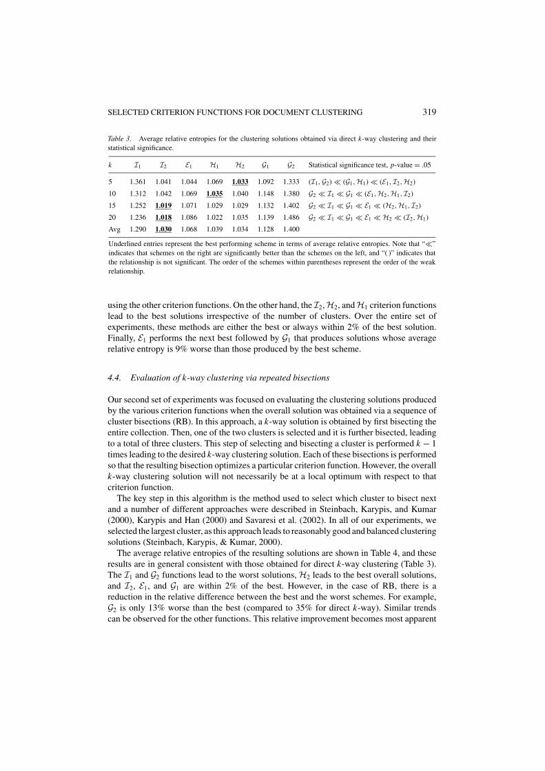
Our first set of experiments was focused on evaluating the quality of the clustering so-lutions produced by the various criterion functions when they were used to compute ak-way clustering solution directly. The values for the average relative entropies for the5-, 10-, 15-, and 20-way clustering solutions are shown in Table 3. The row labeled“Avg” contains the average of these averages over the four sets of solutions. Furthermore,the last column shows the relative ordering of the different schemes using the paired-ttest.

From these results we can see that the I1 and the G2 criterion functions lead to clusteringsolutions that are consistently worse (in the range of 19–35%) than the solutions obtained


Table 3. Average relative entropies for the clustering solutions obtained via direct k-way clustering and theirstatistical significance.

k I1 I2 E1 H1 H2 G1 G2 Statistical significance test, p-value = .05

5 1.361 1.041 1.044 1.069 1.033 1.092 1.333 (I1,G2) � (G1,H1) � (E1, I2,H2)

10 1.312 1.042 1.069 1.035 1.040 1.148 1.380 G2 � I1 � G1 � (E1,H2,H1, I2)

15 1.252 1.019 1.071 1.029 1.029 1.132 1.402 G2 � I1 � G1 � E1 � (H2,H1, I2)

20 1.236 1.018 1.086 1.022 1.035 1.139 1.486 G2 � I1 � G1 � E1 � H2 � (I2,H1)

Avg 1.290 1.030 1.068 1.039 1.034 1.128 1.400

Underlined entries represent the best performing scheme in terms of average relative entropies. Note that “�”indicates that schemes on the right are significantly better than the schemes on the left, and “( )” indicates thatthe relationship is not significant. The order of the schemes within parentheses represent the order of the weakrelationship.

using the other criterion functions. On the other hand, the I2,H2, andH1 criterion functionslead to the best solutions irrespective of the number of clusters. Over the entire set ofexperiments, these methods are either the best or always within 2% of the best solution.Finally, E1 performs the next best followed by G1 that produces solutions whose averagerelative entropy is 9% worse than those produced by the best scheme.

4.4. Evaluation of k-way clustering via repeated bisections

Our second set of experiments was focused on evaluating the clustering solutions producedby the various criterion functions when the overall solution was obtained via a sequence ofcluster bisections (RB). In this approach, a k-way solution is obtained by first bisecting theentire collection. Then, one of the two clusters is selected and it is further bisected, leadingto a total of three clusters. This step of selecting and bisecting a cluster is performed k − 1times leading to the desired k-way clustering solution. Each of these bisections is performedso that the resulting bisection optimizes a particular criterion function. However, the overallk-way clustering solution will not necessarily be at a local optimum with respect to thatcriterion function.

The key step in this algorithm is the method used to select which cluster to bisect nextand a number of different approaches were described in Steinbach, Karypis, and Kumar(2000), Karypis and Han (2000) and Savaresi et al. (2002). In all of our experiments, weselected the largest cluster, as this approach leads to reasonably good and balanced clusteringsolutions (Steinbach, Karypis, & Kumar, 2000).

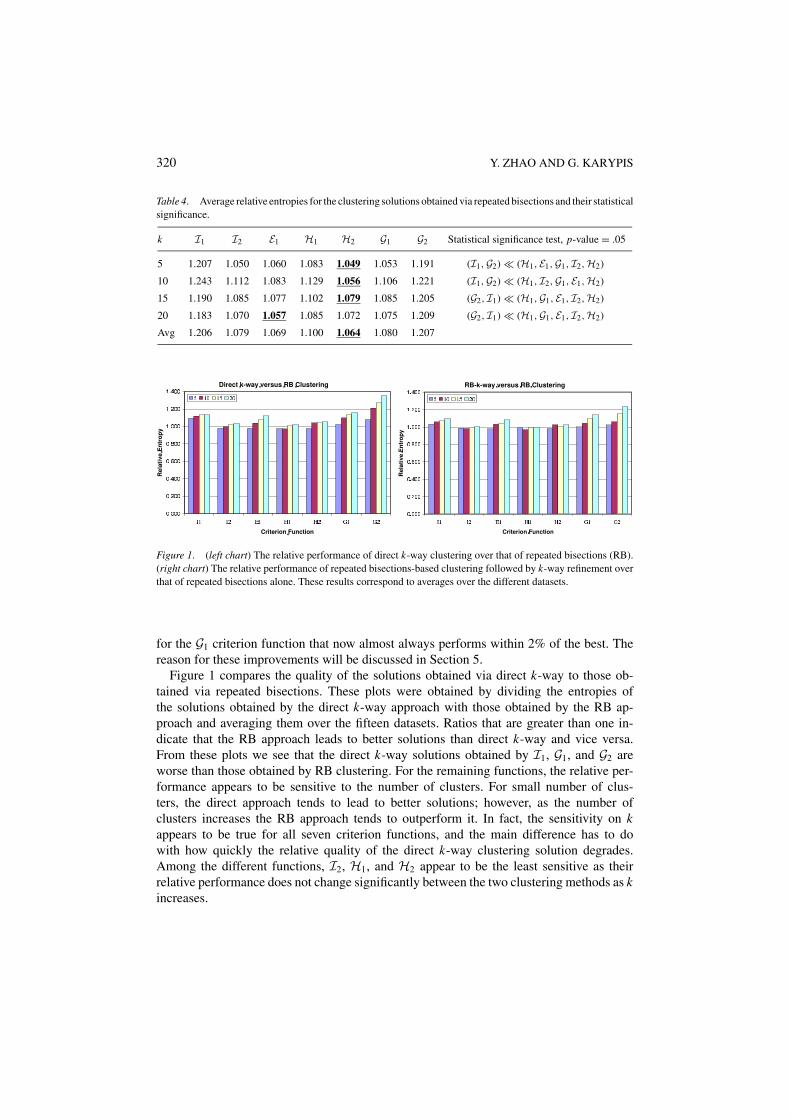
The average relative entropies of the resulting solutions are shown in Table 4, and theseresults are in general consistent with those obtained for direct k-way clustering (Table 3).The I1 and G2 functions lead to the worst solutions, H2 leads to the best overall solutions,and I2, E1, and G1 are within 2% of the best. However, in the case of RB, there is areduction in the relative difference between the best and the worst schemes. For example,G2 is only 13% worse than the best (compared to 35% for direct k-way). Similar trendscan be observed for the other functions. This relative improvement becomes most apparent


Table 4. Average relative entropies for the clustering solutions obtained via repeated bisections and their statisticalsignificance.


5 1.207 1.050 1.060 1.083 1.049 1.053 1.191 (I1,G2) � (H1, E1,G1, I2,H2)

10 1.243 1.112 1.083 1.129 1.056 1.106 1.221 (I1,G2) � (H1, I2,G1, E1,H2)

15 1.190 1.085 1.077 1.102 1.079 1.085 1.205 (G2, I1) � (H1,G1, E1, I2,H2)

20 1.183 1.070 1.057 1.085 1.072 1.075 1.209 (G2, I1) � (H1,G1, E1, I2,H2)

Avg 1.206 1.079 1.069 1.100 1.064 1.080 1.207

Figure 1. (left chart) The relative performance of direct k-way clustering over that of repeated bisections (RB).(right chart) The relative performance of repeated bisections-based clustering followed by k-way refinement overthat of repeated bisections alone. These results correspond to averages over the different datasets.

for the G1 criterion function that now almost always performs within 2% of the best. Thereason for these improvements will be discussed in Section 5.

Figure 1 compares the quality of the solutions obtained via direct k-way to those ob-tained via repeated bisections. These plots were obtained by dividing the entropies ofthe solutions obtained by the direct k-way approach with those obtained by the RB ap-proach and averaging them over the fifteen datasets. Ratios that are greater than one in-dicate that the RB approach leads to better solutions than direct k-way and vice versa.From these plots we see that the direct k-way solutions obtained by I1, G1, and G2 areworse than those obtained by RB clustering. For the remaining functions, the relative per-formance appears to be sensitive to the number of clusters. For small number of clus-ters, the direct approach tends to lead to better solutions; however, as the number ofclusters increases the RB approach tends to outperform it. In fact, the sensitivity on kappears to be true for all seven criterion functions, and the main difference has to dowith how quickly the relative quality of the direct k-way clustering solution degrades.Among the different functions, I2, H1, and H2 appear to be the least sensitive as theirrelative performance does not change significantly between the two clustering methods as kincreases.


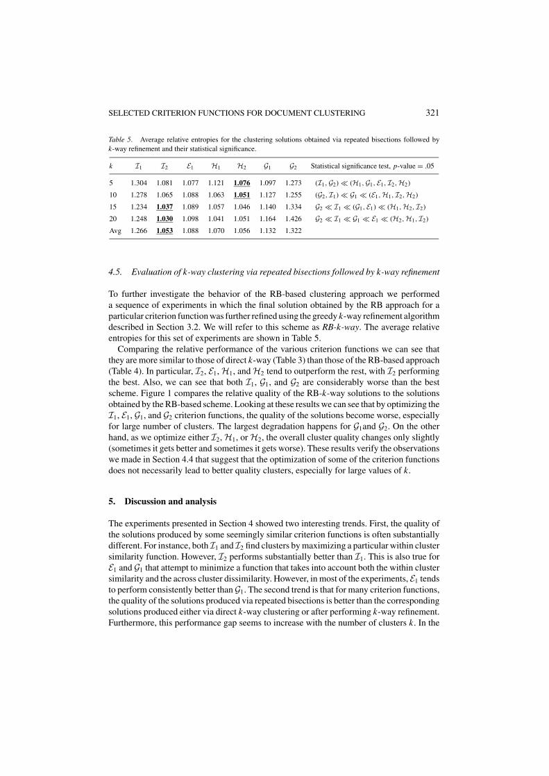
Table 5. Average relative entropies for the clustering solutions obtained via repeated bisections followed byk-way refinement and their statistical significance.


5 1.304 1.081 1.077 1.121 1.076 1.097 1.273 (I1,G2) � (H1,G1, E1, I2,H2)

10 1.278 1.065 1.088 1.063 1.051 1.127 1.255 (G2, I1) � G1 � (E1,H1, I2,H2)

15 1.234 1.037 1.089 1.057 1.046 1.140 1.334 G2 � I1 � (G1, E1) � (H1,H2, I2)

20 1.248 1.030 1.098 1.041 1.051 1.164 1.426 G2 � I1 � G1 � E1 � (H2,H1, I2)

Avg 1.266 1.053 1.088 1.070 1.056 1.132 1.322

4.5. Evaluation of k-way clustering via repeated bisections followed by k-way refinement

To further investigate the behavior of the RB-based clustering approach we performeda sequence of experiments in which the final solution obtained by the RB approach for aparticular criterion function was further refined using the greedy k-way refinement algorithmdescribed in Section 3.2. We will refer to this scheme as RB-k-way. The average relativeentropies for this set of experiments are shown in Table 5.

Comparing the relative performance of the various criterion functions we can see thatthey are more similar to those of direct k-way (Table 3) than those of the RB-based approach(Table 4). In particular, I2, E1, H1, and H2 tend to outperform the rest, with I2 performingthe best. Also, we can see that both I1, G1, and G2 are considerably worse than the bestscheme. Figure 1 compares the relative quality of the RB-k-way solutions to the solutionsobtained by the RB-based scheme. Looking at these results we can see that by optimizing theI1, E1, G1, and G2 criterion functions, the quality of the solutions become worse, especiallyfor large number of clusters. The largest degradation happens for G1and G2. On the otherhand, as we optimize either I2, H1, or H2, the overall cluster quality changes only slightly(sometimes it gets better and sometimes it gets worse). These results verify the observationswe made in Section 4.4 that suggest that the optimization of some of the criterion functionsdoes not necessarily lead to better quality clusters, especially for large values of k.

5. Discussion and analysis

The experiments presented in Section 4 showed two interesting trends. First, the quality ofthe solutions produced by some seemingly similar criterion functions is often substantiallydifferent. For instance, both I1 and I2 find clusters by maximizing a particular within clustersimilarity function. However, I2 performs substantially better than I1. This is also true forE1 and G1 that attempt to minimize a function that takes into account both the within clustersimilarity and the across cluster dissimilarity. However, in most of the experiments, E1 tendsto perform consistently better than G1. The second trend is that for many criterion functions,the quality of the solutions produced via repeated bisections is better than the correspondingsolutions produced either via direct k-way clustering or after performing k-way refinement.Furthermore, this performance gap seems to increase with the number of clusters k. In the


cid Size Sim base

ball

bask

etba

ll

foot

ball

hock

ey

boxi

ng

bicy

clin

g

golfi

ng

1 475 0.087 97 35 143 8 112 64 162 384 0.129 1 1 381 13 1508 0.032 310 58 1055 11 5 59 104 844 0.094 1 1 841 15 400 0.163 1 3996 835 0.097 829 67 1492 0.067 1489 1 28 756 0.099 2 752 1 19 621 0.108 618 1 210 1265 0.036 65 560 296 9 5 22 308

I2 Criterion Function (Entropy=0.240)

cid Size Sim base

ball

bask

etba

ll

foot

ball

hock

ey

boxi

ng

bicy

clin

g

golfi

ng

1 1035 0.098 1034 12 594 0.125 1 592 13 322 0.191 321 14 653 0.127 1 6525 413 0.163 4136 1041 0.058 10417 465 0.166 464 18 296 0.172 2969 3634 0.020 1393 789 694 157 121 145 33510 127 0.268 108 1 17 1

I1 Criterion Function (Entropy=0.357)

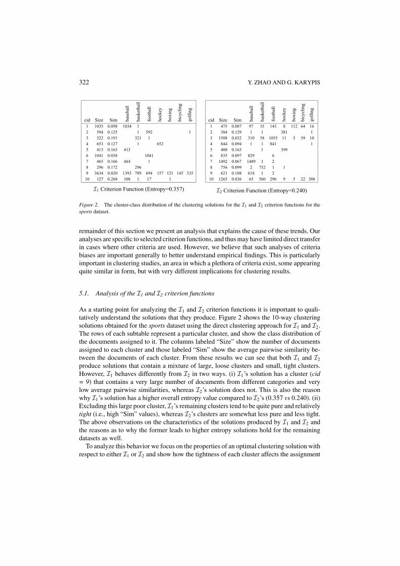
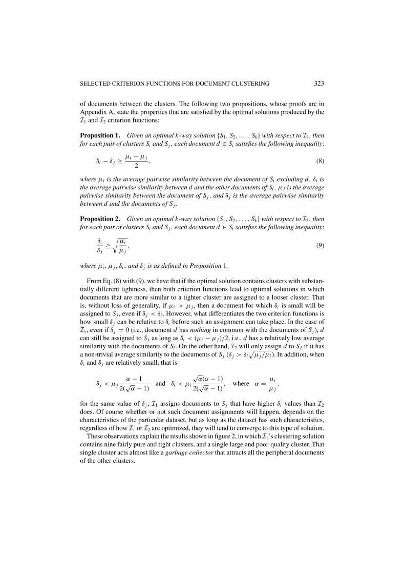
Figure 2. The cluster-class distribution of the clustering solutions for the I1 and I2 criterion functions for thesports dataset.

remainder of this section we present an analysis that explains the cause of these trends. Ouranalyses are specific to selected criterion functions, and thus may have limited direct transferin cases where other criteria are used. However, we believe that such analyses of criteriabiases are important generally to better understand empirical findings. This is particularlyimportant in clustering studies, an area in which a plethora of criteria exist, some appearingquite similar in form, but with very different implications for clustering results.

5.1. Analysis of the I1 and I2 criterion functions

As a starting point for analyzing the I1 and I2 criterion functions it is important to quali-tatively understand the solutions that they produce. Figure 2 shows the 10-way clusteringsolutions obtained for the sports dataset using the direct clustering approach for I1 and I2.The rows of each subtable represent a particular cluster, and show the class distribution ofthe documents assigned to it. The columns labeled “Size” show the number of documentsassigned to each cluster and those labeled “Sim” show the average pairwise similarity be-tween the documents of each cluster. From these results we can see that both I1 and I2

produce solutions that contain a mixture of large, loose clusters and small, tight clusters.However, I1 behaves differently from I2 in two ways. (i) I1’s solution has a cluster (cid= 9) that contains a very large number of documents from different categories and verylow average pairwise similarities, whereas I2’s solution does not. This is also the reasonwhy I1’s solution has a higher overall entropy value compared to I2’s (0.357 vs 0.240). (ii)Excluding this large poor cluster, I1’s remaining clusters tend to be quite pure and relativelytight (i.e., high “Sim” values), whereas I2’s clusters are somewhat less pure and less tight.The above observations on the characteristics of the solutions produced by I1 and I2 andthe reasons as to why the former leads to higher entropy solutions hold for the remainingdatasets as well.

To analyze this behavior we focus on the properties of an optimal clustering solution withrespect to either I1 or I2 and show how the tightness of each cluster affects the assignment


of documents between the clusters. The following two propositions, whose proofs are inAppendix A, state the properties that are satisfied by the optimal solutions produced by theI1 and I2 criterion functions:

Proposition 1. Given an optimal k-way solution {S1, S2, . . . , Sk} with respect to I1, thenfor each pair of clusters Si and Sj , each document d ∈ Si satisfies the following inequality:

δi − δ j ≥ µi − µ j

2, (8)

where µi is the average pairwise similarity between the document of Si excluding d, δi isthe average pairwise similarity between d and the other documents of Si , µ j is the averagepairwise similarity between the document of S j , and δ j is the average pairwise similaritybetween d and the documents of S j .

Proposition 2. Given an optimal k-way solution {S1, S2, . . . , Sk} with respect to I2, thenfor each pair of clusters Si and Sj , each document d ∈ Si satisfies the following inequality:

δi

δ j≥

√µi

µ j, (9)

where µi , µ j , δi , and δ j is as defined in Proposition 1.

From Eq. (8) with (9), we have that if the optimal solution contains clusters with substan-tially different tightness, then both criterion functions lead to optimal solutions in whichdocuments that are more similar to a tighter cluster are assigned to a looser cluster. Thatis, without loss of generality, if µi > µ j , then a document for which δi is small will beassigned to Sj , even if δ j < δi . However, what differentiates the two criterion functions ishow small δ j can be relative to δi before such an assignment can take place. In the case ofI1, even if δ j = 0 (i.e., document d has nothing in common with the documents of Sj ), dcan still be assigned to Sj as long as δi < (µi − µ j )/2, i.e., d has a relatively low averagesimilarity with the documents of Si . On the other hand, I2 will only assign d to Sj if it hasa non-trivial average similarity to the documents of Sj (δ j > δi

√µ j/µi ). In addition, when

δi and δ j are relatively small, that is

δ j < µ jα − 1

2(√

α − 1)and δi < µi

√α(α − 1)

2(√

α − 1), where α = µi

µ j,

for the same value of δ j , I1 assigns documents to Sj that have higher δi values than I2

does. Of course whether or not such document assignments will happen, depends on thecharacteristics of the particular dataset, but as long as the dataset has such characteristics,regardless of how I1 or I2 are optimized, they will tend to converge to this type of solution.

These observations explain the results shown in figure 2, in which I1’s clustering solutioncontains nine fairly pure and tight clusters, and a single large and poor-quality cluster. Thatsingle cluster acts almost like a garbage collector that attracts all the peripheral documentsof the other clusters.


cid Size Sim base

ball

bask

etba

ll

foot

ball

hock

ey

boxi

ng

bicy

clin

g

golfi

ng

1 1330 0.076 1327 2 12 975 0.080 3 5 966 13 742 0.072 15 703 244 922 0.079 84 8 32 797 15 768 0.078 760 1 6 16 897 0.054 6 2 8897 861 0.091 845 0 15 18 565 0.079 24 525 13 1 29 878 0.034 93 128 114 4 97 121 32110 642 0.068 255 36 286 7 24 24 10

E1 Criterion Function (Entropy=0.203)

cid Size Sim base

ball

bask

etba

ll

foot

ball

hock

ey

boxi

ng

bicy

clin

g

golfi

ng

1 519 0.146 516 32 597 0.118 1 595 13 1436 0.033 53 580 357 13 100 20 3134 720 0.105 718 1 15 1664 0.032 1387 73 77 49 7 63 86 871 0.101 8717 1178 0.049 6 5 11678 728 0.111 1 7279 499 0.133 498 110 368 0.122 80 33 145 19 15 62 14

G1 Criterion (Entropy=0.239)

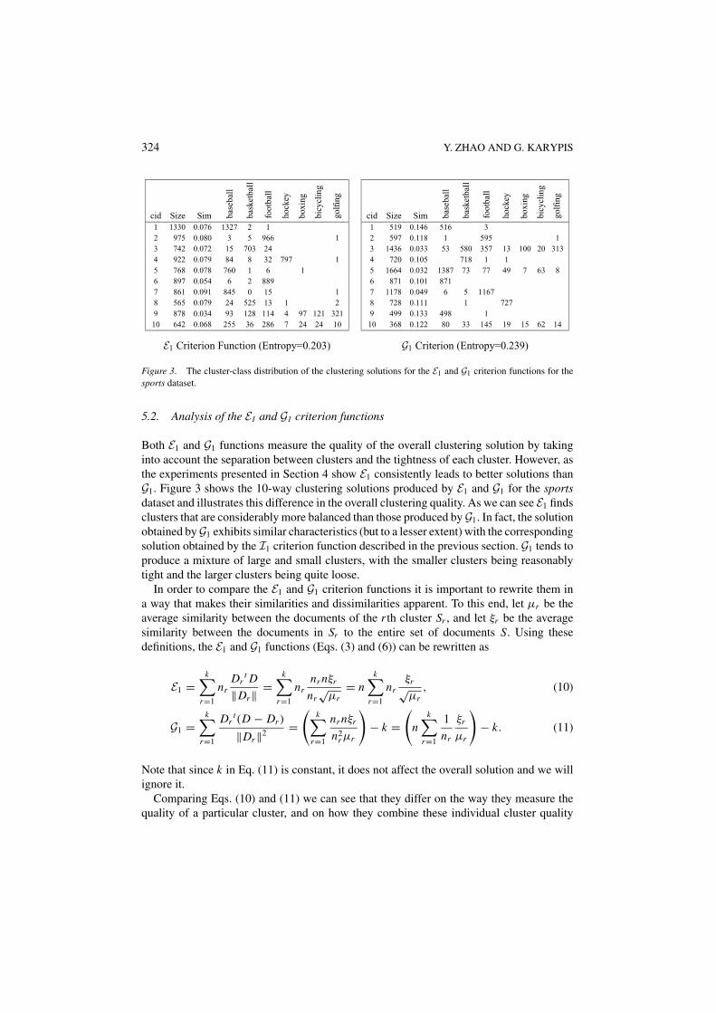
Figure 3. The cluster-class distribution of the clustering solutions for the E1 and G1 criterion functions for thesports dataset.

5.2. Analysis of the E1 and G1 criterion functions

Both E1 and G1 functions measure the quality of the overall clustering solution by takinginto account the separation between clusters and the tightness of each cluster. However, asthe experiments presented in Section 4 show E1 consistently leads to better solutions thanG1. Figure 3 shows the 10-way clustering solutions produced by E1 and G1 for the sportsdataset and illustrates this difference in the overall clustering quality. As we can see E1 findsclusters that are considerably more balanced than those produced by G1. In fact, the solutionobtained by G1 exhibits similar characteristics (but to a lesser extent) with the correspondingsolution obtained by the I1 criterion function described in the previous section. G1 tends toproduce a mixture of large and small clusters, with the smaller clusters being reasonablytight and the larger clusters being quite loose.

In order to compare the E1 and G1 criterion functions it is important to rewrite them ina way that makes their similarities and dissimilarities apparent. To this end, let µr be theaverage similarity between the documents of the r th cluster Sr , and let ξr be the averagesimilarity between the documents in Sr to the entire set of documents S. Using thesedefinitions, the E1 and G1 functions (Eqs. (3) and (6)) can be rewritten as

E1 =k∑

r=1

nrDr

t D

‖Dr‖ =k∑

r=1

nrnr nξr

nr√

µr= n

k∑r=1

nrξr√µr

, (10)

G1 =k∑

r=1

Drt (D − Dr )

‖Dr‖2 =(

k∑r=1

nr nξr

n2r µr

)− k =

(n

k∑r=1

1

nr

ξr

µr

)− k. (11)

Note that since k in Eq. (11) is constant, it does not affect the overall solution and we willignore it.

Comparing Eqs. (10) and (11) we can see that they differ on the way they measure thequality of a particular cluster, and on how they combine these individual cluster quality


measures to derive the overall quality of the clustering solution. In the case of E1, thequality of the r th cluster is measured as ξr/

√µr , whereas in the case of G1 it is measured

as ξr/µr . Since the quality of each cluster is inversely related to either µr or√

µr , bothmeasures will prefer solutions in which there are no clusters that are extremely loose.Because large clusters tend to have small µr values, both of the cluster quality measureswill tend to produce solutions that contain reasonably balanced clusters. Furthermore, thesensitivity of G1’s cluster quality measure on clusters with small µr values is higher than thecorresponding sensitivity of E1 (µr ≤ √

µr because µr ≤ 1). Consequently, we would haveexpected G1 to lead to more balanced solutions than E1, which as the results in figure 3 showdoes not happen, suggesting that the second difference between E1 and G1 is the reason forthe unbalanced clusters.

The E1 criterion function sums the individual cluster qualities weighting them propor-tionally to the size of each cluster. G1 performs a similar summation but each cluster qualityis weighted proportionally to the inverse of the size of the cluster. This weighting schemeis similar to that used in the ratio-cut objective for graph partitioning (Cheng & Wei,1991; Hagen & Kahng, 1991). Recall from our previous discussion that since the qualitymeasure of each cluster is inversely related to µr , the quality measure of large clusters willhave large values, as these clusters will tend to be loose (i.e., µr will be small). Now, inthe case of E1, by multiplying the quality measure of a cluster by its size, it ensures thatthese large loose clusters contribute a lot to the overall value of E1’s criterion function. Asa result, E1 will tend to be optimized when there are no large loose clusters. On the otherhand, in the case of G1, by dividing the quality measure of a large loose cluster by its size,it has the net effect of decreasing the contribution of this cluster to the overall value of G1’scriterion function. As a result, G1 can be optimized at a point in which there exist somelarge and loose clusters.

5.3. Analysis of the G2 criterion function

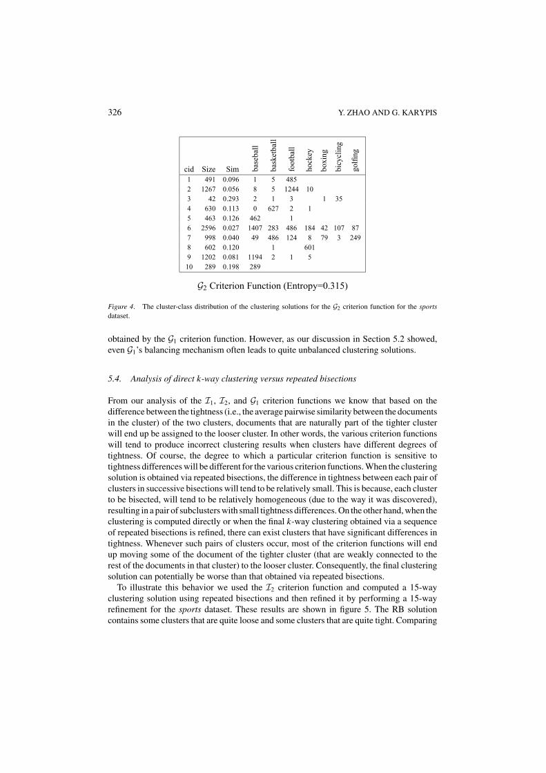
The various experiments presented in Section 4 showed that theG2 criterion function consis-tently led to clustering solutions that were among the worst over the solutions produced bythe other criterion functions. To illustrate how G2 fails, figure 4 shows the 10-way clusteringsolution that it produced via direct k-way clustering on the sports dataset. As we can see, G2

produces solutions that are highly unbalanced. For example, the sixth cluster contains over2500 documents from many different categories, whereas the third cluster contains only42 documents that are primarily from a single category. Note that, the clustering solutionproduced by G2 is very similar to that produced by the I1 criterion function (figure 2).In fact, for most of the clusters we can find a good one-to-one mapping between the twoschemes.

The nature of G2’s criterion function makes it extremely hard to analyze it. However, onereason that can potentially explain the unbalanced clusters produced by G2 is the fact that ituses a normalized-cut inspired approach to combine the separation between the clusters (asmeasured by the cut) versus the size of the respective clusters. It has been shown in Dinget al. (2001) that when the normalized-cut approach is used in the context of traditionalgraph partitioning, it leads to a solution that is considerably more unbalanced than that


cid Size Sim base

ball

bask

etba

ll

foot

ball

hock

ey

boxi

ng

bicy

clin

g

golfi

ng

1 491 0.096 1 5 4852 1267 0.056 8 5 1244 103 42 0.293 2 1 3 1 354 630 0.113 0 627 2 15 463 0.126 462 16 2596 0.027 1407 283 486 184 42 107 877 998 0.040 49 486 124 8 79 3 2498 602 0.120 1 6019 1202 0.081 1194 2 1 510 289 0.198 289

G2 Criterion Function (Entropy=0.315)

Figure 4. The cluster-class distribution of the clustering solutions for the G2 criterion function for the sportsdataset.

obtained by the G1 criterion function. However, as our discussion in Section 5.2 showed,even G1’s balancing mechanism often leads to quite unbalanced clustering solutions.

5.4. Analysis of direct k-way clustering versus repeated bisections

From our analysis of the I1, I2, and G1 criterion functions we know that based on thedifference between the tightness (i.e., the average pairwise similarity between the documentsin the cluster) of the two clusters, documents that are naturally part of the tighter clusterwill end up be assigned to the looser cluster. In other words, the various criterion functionswill tend to produce incorrect clustering results when clusters have different degrees oftightness. Of course, the degree to which a particular criterion function is sensitive totightness differences will be different for the various criterion functions. When the clusteringsolution is obtained via repeated bisections, the difference in tightness between each pair ofclusters in successive bisections will tend to be relatively small. This is because, each clusterto be bisected, will tend to be relatively homogeneous (due to the way it was discovered),resulting in a pair of subclusters with small tightness differences. On the other hand, when theclustering is computed directly or when the final k-way clustering obtained via a sequenceof repeated bisections is refined, there can exist clusters that have significant differences intightness. Whenever such pairs of clusters occur, most of the criterion functions will endup moving some of the document of the tighter cluster (that are weakly connected to therest of the documents in that cluster) to the looser cluster. Consequently, the final clusteringsolution can potentially be worse than that obtained via repeated bisections.

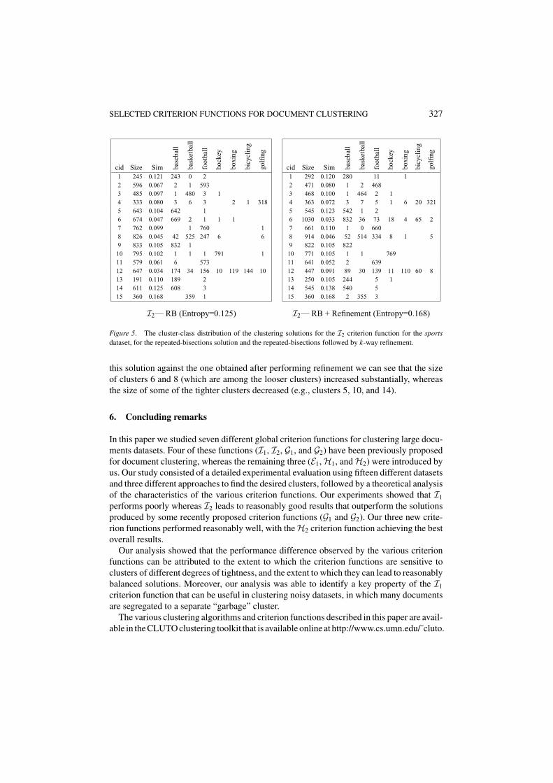
To illustrate this behavior we used the I2 criterion function and computed a 15-wayclustering solution using repeated bisections and then refined it by performing a 15-wayrefinement for the sports dataset. These results are shown in figure 5. The RB solutioncontains some clusters that are quite loose and some clusters that are quite tight. Comparing


cid Size Sim base

ball

bask

etba

ll

foot

ball

hock

ey

boxi

ng

bicy

clin

g

golfi

ng

1 245 0.121 243 0 22 596 0.067 2 1 5933 485 0.097 1 480 3 14 333 0.080 3 6 3 2 1 3185 643 0.104 642 16 674 0.047 669 2 1 1 17 762 0.099 1 760 18 826 0.045 42 525 247 6 69 833 0.105 832 110 795 0.102 1 1 1 791 111 579 0.061 6 57312 647 0.034 174 34 156 10 119 144 1013 191 0.110 189 214 611 0.125 608 315 360 0.168 359 1

I2— RB (Entropy=0.125)

cid Size Sim base

ball

bask

etba

ll

foot

ball

hock

ey

boxi

ng

bicy

clin

g

golfi

ng

1 292 0.120 280 11 12 471 0.080 1 2 4683 468 0.100 1 464 2 14 363 0.072 3 7 5 1 6 20 3215 545 0.123 542 1 26 1030 0.033 832 36 73 18 4 65 27 661 0.110 1 0 6608 914 0.046 52 514 334 8 1 59 822 0.105 82210 771 0.105 1 1 76911 641 0.052 2 63912 447 0.091 89 30 139 11 110 60 813 250 0.105 244 5 114 545 0.138 540 515 360 0.168 2 355 3

I2— RB + Refinement (Entropy=0.168)

Figure 5. The cluster-class distribution of the clustering solutions for the I2 criterion function for the sportsdataset, for the repeated-bisections solution and the repeated-bisections followed by k-way refinement.

this solution against the one obtained after performing refinement we can see that the sizeof clusters 6 and 8 (which are among the looser clusters) increased substantially, whereasthe size of some of the tighter clusters decreased (e.g., clusters 5, 10, and 14).

6. Concluding remarks

In this paper we studied seven different global criterion functions for clustering large docu-ments datasets. Four of these functions (I1, I2, G1, and G2) have been previously proposedfor document clustering, whereas the remaining three (E1, H1, and H2) were introduced byus. Our study consisted of a detailed experimental evaluation using fifteen different datasetsand three different approaches to find the desired clusters, followed by a theoretical analysisof the characteristics of the various criterion functions. Our experiments showed that I1

performs poorly whereas I2 leads to reasonably good results that outperform the solutionsproduced by some recently proposed criterion functions (G1 and G2). Our three new crite-rion functions performed reasonably well, with the H2 criterion function achieving the bestoverall results.

Our analysis showed that the performance difference observed by the various criterionfunctions can be attributed to the extent to which the criterion functions are sensitive toclusters of different degrees of tightness, and the extent to which they can lead to reasonablybalanced solutions. Moreover, our analysis was able to identify a key property of the I1

criterion function that can be useful in clustering noisy datasets, in which many documentsare segregated to a separate “garbage” cluster.

The various clustering algorithms and criterion functions described in this paper are avail-able in the CLUTO clustering toolkit that is available online at http://www.cs.umn.edu/˜cluto.


Acknowledgments

We would like to thank the anonymous reviewers and Douglas H. Fisher for their valuablecomments and suggestions on the presentation of this paper.

Appendix A: Proofs of I1’s and I2’s optimal solution properties

Proof (Proposition 1): For contradiction, let Aopt = {S1, S2, . . . , Sk} be an optimal so-lution and assume that there exists a document d and clusters Si and Sj such that d ∈ Si

and δi − δ j < (µi − µ j )/2. Consider the clustering solution A′ = {S1, S2, . . . , {Si −d}, . . . , {Sj + d}, . . . , Sk}. Let Di , Ci , and D j , C j be the composite and centroid vectorsof cluster Si − d and Sj , respectively. Then,

I1(Aopt ) − I1(A′) = ‖Di + d‖2

ni + 1+ ‖D j‖2

n j−

(‖Di‖2

ni+ ‖D j + d‖2

n j + 1

)

=(‖Di + d‖2

ni + 1− ‖Di‖2

ni

)−

(‖D j + d‖2

n j + 1− ‖D j‖2

n j

)

=(

2ni dt Di + ni − Dit Di

ni (ni + 1)

)−

(2n j dt D j + n j − D j

t D j

n j (n j + 1)

)

=(

2niδi

ni + 1+ 1

ni + 1− niµi

ni + 1

)

−(

2n jδ j

n j + 1+ 1

n j + 1− n jµ j

n j + 1

)≈ (2δi − 2δ j ) − (µi − µ j ),

when ni and n j are sufficiently large. Since δi − δ j < (µi − µ j )/2, we have I1(Aopt ) −I1(A′) < 0, a contradiction.

Proof (Proposition 2): For contradiction, let Aopt = {S1, S2, . . . , Sk} be an optimal solu-tion and assume that there exists a document d and clusters Si and Sj such that d ∈ Si andδi/δ j <

√µi/µ j . Consider the clustering solution A′ = {S1, S2, . . . , {Si − d}, . . . , {Sj +

d}, . . . , Sk}. Let Di , Ci , and D j , C j be the composite and centroid vectors of cluster Si − dand Sj , respectively. Then,

I2(Aopt ) − I2(A′) = ‖Di + d‖ + ‖D j‖ − (‖Di‖ + ‖D j + d‖)

= (√Di

t Di + 1 + 2dt Di −√

Dit Di

)− (√

D jt D j + 1 + 2dt D j −

√D j

t D j). (12)

Now, if ni and n j are sufficiently large we have that Dit Di + 2dt Di 1, and thus

Dit Di + 1 + 2dt Di ≈ Di

t Di + 2dt Di . (13)


Furthermore, we have that

(√Di

t Di + dt Di√Di

t Di

)2

= Dit Di + (dt Di )2

Dit Di

+ 2dt Di ≈ Dit Di + 2dt Di , (14)

as long as δ2i /µi = o(1). This condition is fairly mild as it essentially requires that µi is

sufficiently large relative to δ2i , which is always true for sets of documents that form clusters.

Now, using Eqs. (13) and (14) for both clusters, Eq. (12) can be rewritten as

I2(Aopt ) − I2(A′) = dt Di√Di

t Di

− dt D j√D j

t D j

= δi√µi

− δ j√µ j

.

Since δi/δ j <√

µi/µ j , we have I2(Aopt ) − I2(A′) < 0, a contradiction.

References

Available at http://www.cs.umn.edu/˜karypis/cluto/files/datasets.tar.gz.Available from ftp://ftp.cs.cornell.edu/pub/smart.Beeferman, D., & Berger, A. (2000). Agglomerative clustering of a search engine query log. In Proc. of the Sixth

ACM SIGKDD Int’l Conference on Knowledge Discovery and Data Mining (pp. 407–416).Berry, M., Dumais, S., & O’Brien, G. (1995). Using linear algebra for intelligent information retrieval. SIAM

Review, 37, 573–595.Boley, D. (1998). Principal direction divisive partitioning. Data Mining and Knowledge Discovery, 2:4.Cheeseman, P., & Stutz, J. (1996). Baysian classification (AutoClass): Theory and results. In U. Fayyad, G.

Piatetsky-Shapiro, P. Smith, & R. Uthurusamy (Eds.), Advances in Knowledge Discovery and Data Mining (pp.153–180). AAAI/MIT Press.

Cheng, C.-K., & Wei, Y.-C. A. (1991). An improved two-way partitioning algorithm with stable performance.IEEE Transactions on Computer Aided Design, 10:12, 1502–1511.

Cutting, D., Pedersen, J., Karger, D., & Tukey, J. (1992). Scatter/gather: A cluster-based approach to browsinglarge document collections. In Proceedings of the ACM SIGIR. (pp. 318–329). Copenhagen.

Dempster, A. P., Laird, N. M., & Rubin, D. B. (1977). Maximum likelihood from incomplete data via the EMalgorithm. Journal of the Royal Statistical Society, 39.

Devore, J., & Peck, R. (1997). Statistics: The exploration and analysis of data. Belmont, CA: Duxbury Press.Dhillon, I. S. (2001). Co-clustering documents and words using bipartite spectral graph partitioning. In Knowledge

Discovery and Data Mining (pp. 269–274).Dhillon, I. S., & Modha, D. S. (2001). Concept decompositions for large sparse text data using clustering. Machine

Learning, 42:1/2, 143–175.Ding, C., He, X., Zha, H., Gu, M., & Simon, H. (2001). Spectral min-max cut for graph partitioning and data

clustering. Technical Report TR-2001-XX, Lawrence Berkeley National Laboratory, University of California,Berkeley, CA.

Duda, R., Hart, P., & Stork, D. (2001). Pattern classification. John Wiley & Sons.Ester, M., Kriegel, H.-P., Sander, J., & Xu, X. (1996). A density-based algorithm for discovering clusters in large

spatial databases with noise. In Proc. of the Second Int’l Conference on Knowledge Discovery and Data Mining.Portland: OR.

Fisher, D. (1987). Knowledge acquisition via incremental conceptual clustering. Machine Learning, 2, 139–172.Fisher, D. (1996). Iterative optimization and simplification of hierarchical clusterings. Journal of Artificial Intel-

ligence Research, 4, 147–180.Guha, S., Rastogi, R., & Shim, K. (1998). CURE: An efficient clustering algorithm for large databases. In Proc.

of 1998 ACM-SIGMOD Int. Conf. on Management of Data.


Guha, S., Rastogi, R., & Shim, K. (1999). ROCK: A robust clustering algorithm for categorical attributes. In Proc.of the 15th Int’l Conf. on Data Eng.

Hagen, L., & Kahng, A. (1991). Fast spectral methods for ratio cut partitioning and clustering. In Proceedings ofIEEE International Conference on Computer Aided Design (pp. 10–13).

Han, E., Boley, D., Gini, M., Gross, R., Hastings, K., Karypis, G., Kumar, V., Mobasher, B., & Moore, J. (1998).WebACE: A web agent for document categorization and exploartion. In Proc. of the 2nd International Confer-ence on Autonomous Agents.

Han, J., Kamber, M., & Tung, A. K. H. (2001). Spatial clustering methods in data mining: A survey. In H. Miller,& J. Han (Eds.), Geographic data mining and knowledge discovery. Taylor and Francis.

Hersh, W., Buckley, C., Leone, T., & Hickam, D. (1994). OHSUMED: An interactive retrieval evaluation and newlarge test collection for research. In SIGIR-94 (pp. 192–201).

Jackson, J. E. (1991). A User’s guide to principal components. John Wiley & Sons.Jain, A. K., Murty, M. N., & Flynn, P. J. (1999). Data clustering: A review. ACM Computing Surveys, 31:3,

264–323.Karypis, G., & Han, E. (2000). Concept indexing: A fast dimensionality reduction algorithm with applications to

document retrieval & categorization. Technical Report TR-00-016, Department of Computer Science, Universityof Minnesota, Minneapolis. Available on the WWW at URL http://www.cs.umn.edu/˜karypis.

Karypis, G., Han, E., & Kumar, V. (1999a). Chameleon: A hierarchical clustering algorithm using dynamicmodeling. IEEE Computer, 32:8, 68–75.

Karypis, G., Han, E., & Kumar, V. (1999b). Multilevel refinement for hierarchical clustering. Technical ReportTR-99-020, Department of Computer Science, University of Minnesota, Minneapolis.

King, B. (1967). Step-wise clustering procedures. Journal of the American Statistical Association, 69, 86–101.Kolda, T., & Hendrickson, B. (2000). Partitioning sparse rectangular and structurally nonsymmetric matrices for

parallel computation. SIAM Journal on Scientific Computing, 21:6, 2048–2072.Larsen, B., & Aone, C. (1999). Fast and effective text mining using linear-time document clustering. In Proc. of

the Fifth ACM SIGKDD Int’l Conference on Knowledge Discovery and Data Mining (pp. 16–22).Lewis, D. D. (1999). Reuters-21578 text categorization test collection Distribution 1.0. http://www.research.

att.com/∼lewis.MacQueen, J. (1967). Some methods for classification and analysis of multivariate observations. In Proc. 5th

Symp. Math. Statist, Prob (pp. 281–297).Meila, M., & Heckerman, D. (2001). An experimental comparison of model-based clustering methods. Machine

Learning, 42, 9–29.Ng, R., & Han, J. (1994). Efficient and effective clustering method for spatial data mining. In Proc. of the 20th

VLDB Conference (pp. 144–155). Santiago, Chile.Porter, M. F. (1980). An algorithm for suffix stripping. Program, 14:3, 130–137.Puzicha, J., Hofmann, T., & Buhmann, J. M. (2000). A theory of proximity based clustering: Structure detection

by optimization. PATREC: Pattern Recognition. Pergamon Press. (vol. 33, pp. 617–634).Salton, G. (1989). Automatic text processing: The transformation, analysis, & retrieval of information by computer.

Addison-Wesley.Savaresi, S., & Boley, D. (2001). On the performance of bisecting K-means and PDDP. In First SIAM International

Conference on Data Mining (SDM’2001).Savaresi, S., Boley, D., Bittanti, S., & Gazzaniga, G. (2002) Choosing the cluster to split in bisecting divisive

clustering algorithms. In Second SIAM International Conference on Data Mining (SDM’2002).Shi, J., & Malik, J. (2000). Normalized cuts and image segmentation. IEEE Transactions on Pattern Analysis and

Machine Intelligence, 22:8, 888–905.Sneath, P. H., & Sokal, R. R. (1973). Numerical taxonomy. London, UK: Freeman.Steinbach, M., Karypis, G., & Kumar, V. (2000). A comparison of document clustering techniques. KDD Workshop

on Text Mining.Strehl, A., & Ghosh, J. (2000). Scalable approach to balanced, high-dimensional clustering of market-baskets. In

Proceedings of HiPC.TREC (1999). Text REtrieval conference. http://trec.nist.gov.Zahn, K. (1971). Graph-theoretical methods for detecting and describing gestalt clusters. IEEE Transactions on

Computers, C-20, 68–86.


Zha, H., He, X., Ding, C., Simon, H., & Gu, M. (2001a). Bipartite graph partitioning and data clustering. CIKM.Zha, H., He, X., Ding, C., Simon, H., & Gu, M. (2001b). Spectral relaxation for K-means clustering. Technical

Report TR-2001-XX, Pennsylvania State University, University Park, PA.Zhao, Y., & Karypis, G. (2001). Criterion functions for document clustering: Experiments and analysis. Technical

Report TR #01–40, Department of Computer Science, University of Minnesota, Minneapolis, MN. Availableon the WWW at http://cs.umn.edu/˜karypis/publications.

Received February 21, 2002Revised May 7, 2003Accepted May 7, 2003Final manuscript July 1, 2003

Empirical and Theoretical Comparisons of Selected Criterion Functions for Document Clustering

Documents

Transcript of Empirical and Theoretical Comparisons of Selected Criterion Functions for Document Clustering