EMMI User’s Manual - 5.3 LSO-MAN-ESO-40100-0001/5.3

EUROPEAN SOUTHERN OBSERVATORY

Organisation Europeenne pour des Recherches Astronomiques dans l’Hemisphere Austral

Europaische Organisation fur astronomische Forschung in der sudlichen Hemisphare

LA SILLA OBSERVATORY

EMMIThe ESO Multi-Mode Instrument

User’s Manual

Doc. No. LSO-MAN-ESO-40100-0001/5.3

Issue 5.3

15/7/2006

Jean-Francois GONZALEZ 1998-aug-21Prepared . . . . . . . . . . . . . . . . . . . . . . . . . . . . . . . . . . . . . . . . . .Name Date Signature

Stephane Brillant 2000-August-31Revised . . . . . . . . . . . . . . . . . . . . . . . . . . . . . . . . . . . . . . . . . . .Name Date Signature

Emanuela Pompei 2006-July-15Revised . . . . . . . . . . . . . . . . . . . . . . . . . . . . . . . . . . . . . . . . . . .

Name Date Signature

Michael Sterzik 2006-July-15Approved . . . . . . . . . . . . . . . . . . . . . . . . . . . . . . . . . . . . . . . . . . .Name Date Signature

Michael Sterzik 2006-July-15Released . . . . . . . . . . . . . . . . . . . . . . . . . . . . . . . . . . . . . . . . . . .Name Date Signature

ii

Change Record

Issue/Rev. Date Section/Parag. affected Reason/Initiation/Documents/Remarks

4.0 23/07/1998 All First preparation

4.1 21/09/1998 All Comments included and new figures added

4.2 31/03/2000 All upgrade some parts and new figures added.S. Brillant et O. Hainaut

4.3 31/03/2000 All some minors modifications and new figures.S. Brillant and O. Hainaut

4.5 31/08/2002 All new red CCD. Modifications following the upgrade.E. Pompei, O. Hainaut, C. Foellmi, J. Willis

4.6 7/11/2003 RILD, REMD MOS appendix and new efficiencies for RILD,REMD;New wavelength atlas for RILD, REMD and echelle;Update efficiencies for echelle and interorder gaps.

Appendix B New system efficiency curvesE. Pompei, C. Foellmi & T. Dall (echelle mode)renamed to 5.0 for ISO9001 compliance

5.1 9/15/2004 All Update for P74, E. Pompei

5.2 4/15/2006 All Update for P77, E. Pompei

5.3 7/15/2006 All Update for P78, new dual portreadout mode, update to the blueand red filter tables. E. Pompei

iii

iv

Contents

1 Introduction 1

1.1 Purpose . . . . . . . . . . . . . . . . . . . . . . . . . . . . . . . . . . . . . . . . . . . . 11.2 Scope . . . . . . . . . . . . . . . . . . . . . . . . . . . . . . . . . . . . . . . . . . . . . 21.3 Applicable documents . . . . . . . . . . . . . . . . . . . . . . . . . . . . . . . . . . . . 21.4 Reference Documents . . . . . . . . . . . . . . . . . . . . . . . . . . . . . . . . . . . . 21.5 Abbreviations and Acronyms . . . . . . . . . . . . . . . . . . . . . . . . . . . . . . . . 31.6 Acknowledgements . . . . . . . . . . . . . . . . . . . . . . . . . . . . . . . . . . . . . . 4

2 Instrument Overview 5

2.1 Optical Design . . . . . . . . . . . . . . . . . . . . . . . . . . . . . . . . . . . . . . . . 52.2 What mode for what observations? . . . . . . . . . . . . . . . . . . . . . . . . . . . . . 62.3 Optical components . . . . . . . . . . . . . . . . . . . . . . . . . . . . . . . . . . . . . 6

2.3.1 Filters . . . . . . . . . . . . . . . . . . . . . . . . . . . . . . . . . . . . . . . . . 82.3.2 Grisms . . . . . . . . . . . . . . . . . . . . . . . . . . . . . . . . . . . . . . . . . 82.3.3 Gratings . . . . . . . . . . . . . . . . . . . . . . . . . . . . . . . . . . . . . . . . 82.3.4 Starplates . . . . . . . . . . . . . . . . . . . . . . . . . . . . . . . . . . . . . . . 82.3.5 Medium-dispersion slit . . . . . . . . . . . . . . . . . . . . . . . . . . . . . . . . 92.3.6 Echelle mask . . . . . . . . . . . . . . . . . . . . . . . . . . . . . . . . . . . . . 92.3.7 Atmospheric Dispersion Corrector . . . . . . . . . . . . . . . . . . . . . . . . . 9

3 EMMI characteristics 11

3.1 Detectors . . . . . . . . . . . . . . . . . . . . . . . . . . . . . . . . . . . . . . . . . . . 113.2 Imaging . . . . . . . . . . . . . . . . . . . . . . . . . . . . . . . . . . . . . . . . . . . . 14

3.2.1 Filters . . . . . . . . . . . . . . . . . . . . . . . . . . . . . . . . . . . . . . . . . 153.2.2 Coronography . . . . . . . . . . . . . . . . . . . . . . . . . . . . . . . . . . . . . 163.2.3 Performance . . . . . . . . . . . . . . . . . . . . . . . . . . . . . . . . . . . . . 16

3.3 Low-Dispersion Spectroscopy . . . . . . . . . . . . . . . . . . . . . . . . . . . . . . . . 203.3.1 Grisms, slits and filters . . . . . . . . . . . . . . . . . . . . . . . . . . . . . . . 203.3.2 Multi-object spectroscopy (MOS) . . . . . . . . . . . . . . . . . . . . . . . . . . 213.3.3 Performance . . . . . . . . . . . . . . . . . . . . . . . . . . . . . . . . . . . . . 22

3.4 Medium-Dispersion Spectroscopy . . . . . . . . . . . . . . . . . . . . . . . . . . . . . . 223.4.1 Slit and gratings . . . . . . . . . . . . . . . . . . . . . . . . . . . . . . . . . . . 243.4.2 Performance . . . . . . . . . . . . . . . . . . . . . . . . . . . . . . . . . . . . . 25

3.5 Echelle Spectroscopy . . . . . . . . . . . . . . . . . . . . . . . . . . . . . . . . . . . . . 253.5.1 Echelle gratings . . . . . . . . . . . . . . . . . . . . . . . . . . . . . . . . . . . . 253.5.2 Performance . . . . . . . . . . . . . . . . . . . . . . . . . . . . . . . . . . . . . 28

4 Observing with EMMI 29

4.1 The VLT environment . . . . . . . . . . . . . . . . . . . . . . . . . . . . . . . . . . . . 294.2 Preparation of the observations: P2PP . . . . . . . . . . . . . . . . . . . . . . . . . . . 294.3 At the telescope . . . . . . . . . . . . . . . . . . . . . . . . . . . . . . . . . . . . . . . 304.4 Execution of the observations: BOB . . . . . . . . . . . . . . . . . . . . . . . . . . . . 32

v

4.5 Achieving a good image quality . . . . . . . . . . . . . . . . . . . . . . . . . . . . . . . 324.5.1 The active optics system . . . . . . . . . . . . . . . . . . . . . . . . . . . . . . . 334.5.2 Focusing . . . . . . . . . . . . . . . . . . . . . . . . . . . . . . . . . . . . . . . . 344.5.3 The seeing monitor . . . . . . . . . . . . . . . . . . . . . . . . . . . . . . . . . . 35

4.6 Target acquisition . . . . . . . . . . . . . . . . . . . . . . . . . . . . . . . . . . . . . . 354.6.1 Imaging . . . . . . . . . . . . . . . . . . . . . . . . . . . . . . . . . . . . . . . . 364.6.2 Spectroscopy - Low dispersion and MOS. . . . . . . . . . . . . . . . . . . . . . 364.6.3 Medium Dispersion and Echelle spectroscopy . . . . . . . . . . . . . . . . . . . 37

4.7 Tracking, autoguiding and pointing . . . . . . . . . . . . . . . . . . . . . . . . . . . . . 374.8 The Real-Time Display . . . . . . . . . . . . . . . . . . . . . . . . . . . . . . . . . . . 384.9 Estimating the overheads . . . . . . . . . . . . . . . . . . . . . . . . . . . . . . . . . . 394.10 The data-flow system . . . . . . . . . . . . . . . . . . . . . . . . . . . . . . . . . . . . . 404.11 Data Reduction . . . . . . . . . . . . . . . . . . . . . . . . . . . . . . . . . . . . . . . . 40

5 Calibration 43

5.1 Calibration unit . . . . . . . . . . . . . . . . . . . . . . . . . . . . . . . . . . . . . . . . 435.2 Bias and dark current . . . . . . . . . . . . . . . . . . . . . . . . . . . . . . . . . . . . 435.3 Flat fields . . . . . . . . . . . . . . . . . . . . . . . . . . . . . . . . . . . . . . . . . . . 445.4 Wavelength Calibration . . . . . . . . . . . . . . . . . . . . . . . . . . . . . . . . . . . 455.5 Fringing . . . . . . . . . . . . . . . . . . . . . . . . . . . . . . . . . . . . . . . . . . . . 475.6 Photometric Calibration . . . . . . . . . . . . . . . . . . . . . . . . . . . . . . . . . . . 485.7 Spectrophotometric Calibration . . . . . . . . . . . . . . . . . . . . . . . . . . . . . . . 485.8 The Calibration Plan . . . . . . . . . . . . . . . . . . . . . . . . . . . . . . . . . . . . . 48

A A sample FITS header 50

B EMMI Efficiencies 54

C Wavelength calibration spectra 66

C.1 Low-dispersion grisms . . . . . . . . . . . . . . . . . . . . . . . . . . . . . . . . . . . . 66C.2 Red medium-dispersion gratings . . . . . . . . . . . . . . . . . . . . . . . . . . . . . . 70C.3 Blue medium-dispersion gratings . . . . . . . . . . . . . . . . . . . . . . . . . . . . . . 83C.4 Echelle gratings . . . . . . . . . . . . . . . . . . . . . . . . . . . . . . . . . . . . . . . . 95

D Punching MOS plates 96

D.1 Preparing the mask . . . . . . . . . . . . . . . . . . . . . . . . . . . . . . . . . . . . . . 96D.1.1 Interactive mask creation . . . . . . . . . . . . . . . . . . . . . . . . . . . . . . 98D.1.2 Automatic mask creation . . . . . . . . . . . . . . . . . . . . . . . . . . . . . . 100D.1.3 Mask creation from a target file . . . . . . . . . . . . . . . . . . . . . . . . . . . 100D.1.4 Preparation of the target acquisition . . . . . . . . . . . . . . . . . . . . . . . . 100

D.2 Punching the plate . . . . . . . . . . . . . . . . . . . . . . . . . . . . . . . . . . . . . . 100

E Differential Refraction 102

F EMMI setup request form 104

vi

Chapter 1

Introduction

1.1 Purpose

This manual describes the ESO Multi-Mode Instrument (EMMI) and its operation at the NewTechnology Telescope (NTT) on the La Silla observatory. It is intended to be read by visitingastronomers to help them prepare their application for observing time as well as their observing run.EMMI is a versatile intrument, allowing a wide range of observations: imaging and spectroscopy,from low to high-dispersion, including long-slit and multi-object spectroscopy. It is permanentlymounted on an adaptor-rotator at the Nasmyth B focus of the NTT. EMMI was designed to makeuse of the high image quality foreseen for the NTT and to minimize instrument change-overs. Theconcept which was adopted is that of a dual-beam instrument, fully dioptric, and based on the whitepupil principle. The main advantages of this type of design are the efficiency in both channels andthe easy and fast change from imaging to grism and grating spectroscopy.The present version of this manual gives the status of EMMI after the 2002 red arm CCD upgrade,done in May. The detector is now completely characterized, and the most important points can besummarized as follows:

• a): The new camera is a mosaic of two 2k by 4k MIT/LL thinned CCDs and has a FIERAcontroller, which permits a very fast readout (∼ 20s). The efficiency is ∼35% higher withrespect to the old tektronics chip.

• b): The files are delivered as Multi Extension Fits (MEF) files, with a main header and 2 fitsextensions, each of them corresponding to 2 of the 4 amplifiers which read out the CCDs. Ascript to read correctly the files with MIDAS can be downloaded from EMMI web page.

• c): The center of the spectra will always fall on the region read by amplifier #B on the masterchip. The amplifiers are named A, B, C, D from right to the left of the mosaic.

• d): Due to the larger dimensions of the detector, some second order overlap in the spectramight occur close to the edge of the chip. In doubt ask for the insertion of an order separatingfilter. Second order contamination is important for gratings #8 and #13 (see technical reporton EMMI web page).

• e): Starting P78 we will officially offer dual-port readout mode, reading the master and theslave chip with one amplifier each. The readout time is 10% higher than the four port readoutmodes.

• f): Offsets along the slit are available for all EMMI spectroscopic modes since P75.

• h): The dichroic mode is not offered anymore starting from P70, hence all the relatedinformation has been eliminated from the manual.

1

The telescope configuration is the one familiarly known as post Big-Bang, a major telescope upgradecarried on during 1996-1997. Only a few of its optical elements have been repaired or replaced,but the instrument control software and, more important for the observer, the user interfaces arecompletely different from what it was before the Big Bang. The reader will find updated informationon the SciOps WWW page (http://www.ls.eso.org/lasilla/sciops/ntt/) or in The Messenger,which is published every three months.The last information on test made on the instrument and technical news can be found in the latestnews web page, linked from the EMMI web page:(http://www.ls.eso.org/lasilla/sciops/ntt/emmi/emmiNews.html/)

1.2 Scope

This manual describes the capabilities of the instrument (Chap.2) and gives detailed characteristicsfor each observing modes (Chap.3). It also gives an overview of the observing procedures in thepost-Big Bang era of the NTT (Chap.4), as well as information about calibration data and pipe-linereduction (Chap.5).This document does not cover the telescope control software, nor the active optics system, althoughsome information is given, in order for the visitor to get a better understanding of the system andtune up his observations.

1.3 Applicable documents

The following documents, of the exact issue shown, form a part of this document to the extentspecified herein. In the event of conflict between the documents referenced herein and the contentsof this document, the contents of this document shall be considered as a superseding specification.

[1] VLT-MAN-ESO-19200-1644/2.4, 18/07/2002 — P2PP Users’ Manual, David Silva

[2] LSO-MAN-ESO-40110-0001/1.1 01/10/2001 — SUSI/EMMI Template Signature File Parame-ters Reference Guide, Paul Le Saux

[3] N-PLA-ESO-109-076 NTT Upgrade - EMMI Commissioning Plan, Martin

[4] LSO-TRE-ESO-40200-1036 — Test and Technical Time Report: Period 36, Oct.22-24, 1999,Hainaut

[5] LSO-PLA-ESO-40400-0001/0.93 — EMMI Red CCD Upgrade Plan, Hainaut and d’Odorico.

[6] VLT-INS-96-0142, Repair of EMMI Red Camera: image quality, Dekker and Buzzoni

1.4 Reference Documents

The following documents are referenced in this document.

[3] LSO-MAN-ESO-40100-1001/1.0 — The NTT Active Optics System Users Manual, PhilippeGitton

[4] VLT-MAN-ESO-17240-0866/2.5, 28/07/1997 — Real-Time Display User Manual, A. Brighton

[5] LSO-LIS-ESO-40500-0001/1.0, 15/09/1998 — A List of Observation Blocks for PhotometricStandard Stars to be used with EMMI, Fernando Comeron

2

[6] LSO-LIS-ESO-40500-0002/2.0, 14/09/1999 — A List of Observation Blocks for Spectropho-tometric Standard Stars to be used with EMMI in Low Dispersion Spectroscopy, FernandoComeron, Benoit Joguet

[7] LSO-PLA-ESO-40400-0001/0.4, 26/09/1997 — NTT Imaging Calibration Plan, David Silva &Gautier Mathys

[8] LSO-PLA-ESO-40401-0001/0.2, 02/06/1997 — NTT EMMI Spectroscopy Calibration Plan,David Silva & Gautier Mathys

[9] LSO-PLA-ESO-40400-0001/0.5, 28/05/1998 — EMMI and SUSI2 calibration plan, FernandoComeron

[10] Andersen M. I., Feryhammer L., Storm J., 1995, Gain Calibration of Array Detectors by Shiftedand Rotated Exposures, in ESO STSci Calibration Workshop 1995

[11] Dekker H., Delabre B., D’Odorico S., 1986, SPIE 627, 339

[12] Filippenko A., 1982, PASP 94, 715

[13] Dekker H., D’Odorico S., Fontana A., 1994, The Messenger 76, 16

[14] D’Odorico S., Ghigo M., Ponz D., 1987, An atlas of the Thorium-Argon Spectrum for CASPECin the 3400–9000A region, ESO Scientific Report No. 6

[15] Hamuy M., Walker A. R., Suntzeff N. B., Gigoux P., Heathcote S. R., Phillips M. M., 1992,PASP 104, 533

[16] Hamuy M., Suntzeff N. B., Heathcote S. R., Walker A. R., Gigoux P., Phillips M. M., 1994,PASP 106, 566

[17] Landolt A. U., 1992, AJ 104, 340

[18] Osterbrock, D.E.; Fulbright, Jon P.; Martel, Andre R.; Keane, Michael J.; Trager, Scott C;Basri, G., 1996, PASP 106 277

[19] Osterbrock, D.E.; Fullbright, J.P.; Bida, T.A., 1997, PASP 109, 614

[20] Pasquini et al., 1994, The Messenger 77, 5

[21] Pompei, E., et al, 2004, The Messenger 116, 16

[22] Tyson N. D., Gal R. R., 1993, AJ 105, 1206

[23] Wilson R. N., Franza F., Noethe L., Andreoni G., 1991, Journal of Modern Optics 38, 219

1.5 Abbreviations and Acronyms

The following abbreviations and acronyms are used in this document:

ADC Atmospheric Dispersion Corrector unitADU Analogue to digital unitsAOS Active Optics SystemBIMG Blue IMaGing mode of EMMIBLMD BLue Medium-Dispersion mode of EMMICCD Charged-Coupled DeviceDAT Digital Audio TapeDIMM Differential Image Motion Monitor (seeing monitor)

3

DIMD DIchroic Medium-Dispersion mode of EMMIDVD Digital Video DiscEFOSC ESO Faint Object Spectrograph CameraEMMI ESO MultiMode InstrumentESO European Southern ObservatoryFITS Flexible Image Transport Systemftp file transfer protocolgain conversion factor (e− per ADU)GUI Graphical User InterfaceHW HardwareIA Image AnalysisICS Instrument Control SoftwareIRAF Image Reduction and Analysis FacilityLCU Local Control UnitMIDAS Munich Image Data Analysis SystemMOS MultiObject SpectroscopyNTT New Technology TelescopePA Position AnglePSF Point-Spread FunctionREMD REd Medium-Dispersion mode of EMMIRILD Red Imaging and Low-Dispersion mode of EMMIRON read-out noiseRTD Real-Time DisplaySUSI SUperb Seeing ImagerTCS Telescope Control SoftwareVCS VLT Control SoftwareVLT Very Large TelescopeWS Work StationWWW World-Wide Web

1.6 Acknowledgements

The present version of the EMMI manual is an updated version of the 4.2 written by J.F Gonzalesand updated by S. Brillant.The present version of the EMMI manual uses parts of the previous version (3.0) written by A.Zijlstra, E. Giraud, J. Melnick, H. Dekker, and S. D’Odorico.Many thanks to Gautier Mathys, Olivier Hainaut and all La Silla SciOps team for their suggestionsand comments and to Cedric Foellmi for the updates on the echelle part.

4

Chapter 2

Instrument Overview

2.1 Optical Design

EMMI is divided in two “arms” defined by optical elements coated for high efficiency from 300 to500 nm for the “blue arm” and from 400 to 1000 nm for the “red arm” and with separate detectors.Each arm has two possible light paths: one for imaging and one for grating spectroscopy. In the redarm only, the imaging mode also supports low-resolution spectroscopy using grisms. Each of the fourpossible light paths (two per arm) is called an “Observing Mode”. They are called:

RILD: Red Imaging and Low-Dispersion spectroscopy (includes multi-object spectroscopy)

REMD: REd Medium Dispersion spectroscopy (includes echelle spectroscopy)

BIMG: Blue IMaGing

BLMD: BLue Medium Dispersion spectroscopy

Figure 2.1 shows the optical layout and identifies the main components of EMMI. A detailed descrip-tion can be found in [11].

Blue CCDController

Red CCDController

NIM Crate CAMAC Crate

Shutter control

Junction box

1 29

BLUE RED

Grating unit Grating unit

Camera Camera

Filter wheel

Mirror unit

Filter Wheel

CCD/cryostatCCD/cryostatTransfer collimator

MD slit

Grism wheel

Collimator Prism wheel

Starplate wheel(LD slit)

Collimator

Below-slit filter wheels

Slit-viewing camera

Stray-light maskField lens

Field lens

Figure 2.1: Schematic layout of EMMI showing locations of the main components.

5

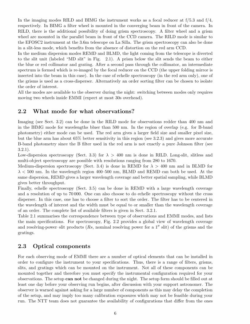
In the imaging modes RILD and BIMG the instrument works as a focal reducer at f/5.3 and f/4,respectively. In BIMG a filter wheel is mounted in the converging beam in front of the camera. InRILD, there is the additional possibility of doing grism spectroscopy. A filter wheel and a grismwheel are mounted in the parallel beam in front of the CCD camera. The RILD mode is similar tothe EFOSC2 instrument at the 3.6m telescope on La Silla. The grism spectroscopy can also be donein a slit-less mode, which benefits from the absence of distortion on the red arm CCD.In the medium dispersion modes REMD and BLMD, the light coming from the telescope is divertedto the slit unit (labeled “MD slit” in Fig. 2.1). A prism below the slit sends the beam to eitherthe blue or red collimator and grating. After a second pass through the collimator, an intermediatespectrum is formed which is re-imaged by the focal reducer on the CCD (the upper folding mirror isinserted into the beam in this case). In the case of echelle spectroscopy (in the red arm only), one ofthe grisms is used as a cross-disperser. Alternatively an order sorting filter can be chosen to isolatethe order of interest.All the modes are available to the observer during the night: switching between modes only requiresmoving two wheels inside EMMI (expect at most 30s overhead).

2.2 What mode for what observations?

Imaging (see Sect. 3.2) can be done in the RILD mode for observations redder than 400 nm andin the BIMG mode for wavelengths bluer than 500 nm. In the region of overlap (e.g. for B-bandphotometry) either mode can be used. The red arm gives a larger field size and smaller pixel size,but the blue arm has about 65% better sensitivity in this region (see 3.2.3) and gives more accurateB-band photometry since the B filter used in the red arm is not exactly a pure Johnson filter (see3.2.1).Low-dispersion spectroscopy (Sect. 3.3) for λ > 400 nm is done in RILD. Long-slit, slitless andmulti-object spectroscopy are possible with resolutions ranging from 280 to 1670.Medium-dispersion spectroscopy (Sect. 3.4) is done in REMD for λ > 400 nm and in BLMD forλ < 500 nm. In the wavelength region 400–500 nm, BLMD and REMD can both be used. At thesame dispersion, REMD gives a larger wavelength coverage and better spatial sampling, while BLMDgives better throughput.Finally, echelle spectroscopy (Sect. 3.5) can be done in REMD with a large wavelength coverageand a resolution of up to 70 000. One can also choose to do echelle spectroscopy without the crossdisperser. In this case, one has to choose a filter to sort the order. The filter has to be centered inthe wavelength of interest and the width must be equal to or smaller than the wavelength coverageof an order. The complete list of available filters is given in Sect. 3.2.1.Table 2.1 summarises the correspondence between type of observations and EMMI modes, and liststhe main specifications. For spectroscopy, Fig. 2.2 provides a global view of wavelength coverageand resolving-power–slit products (Rs, nominal resolving power for a 1′′ slit) of the grisms and thegratings.

2.3 Optical components

For each observing mode of EMMI there are a number of optical elements that can be installed inorder to configure the instrument to your specifications. Thus, there is a range of filters, grisms,slits, and gratings which can be mounted on the instrument. Not all of these components can bemounted together and therefore you must specify the instrumental configuration required for yourobservations. The setup can not be changed during the night. The setup form should be filled out atleast one day before your observing run begins, after discussion with your support astronomer. Theobserver is warned against asking for a large number of components as this may delay the completionof the setup, and may imply too many calibration exposures which may not be feasible during yourrun. The NTT team does not guarantee the availability of configurations that differ from the ones

6

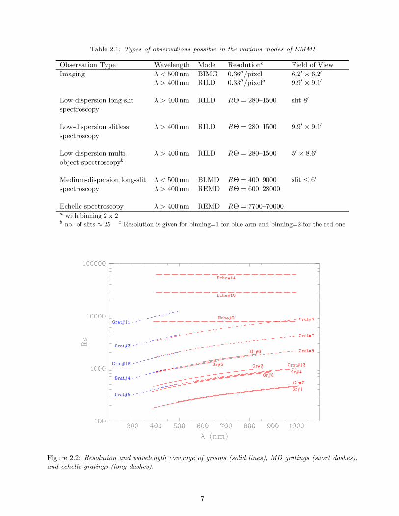
Table 2.1: Types of observations possible in the various modes of EMMI

Observation Type Wavelength Mode Resolutionc Field of View

Imaging λ < 500 nm BIMG 0.36′′/pixel 6.2′ × 6.2′

λ > 400 nm RILD 0.33′′/pixela 9.9′ × 9.1′

Low-dispersion long-slit λ > 400 nm RILD RΘ = 280–1500 slit 8′

spectroscopy

Low-dispersion slitless λ > 400 nm RILD RΘ = 280–1500 9.9′ × 9.1′

spectroscopy

Low-dispersion multi- λ > 400 nm RILD RΘ = 280–1500 5′ × 8.6′

object spectroscopyb

Medium-dispersion long-slit λ < 500 nm BLMD RΘ = 400–9000 slit ≤ 6′

spectroscopy λ > 400 nm REMD RΘ = 600–28000

Echelle spectroscopy λ > 400 nm REMD RΘ = 7700–70000a with binning 2 x 2b no. of slits ≈ 25 c Resolution is given for binning=1 for blue arm and binning=2 for the red one

Figure 2.2: Resolution and wavelength coverage of grisms (solid lines), MD gratings (short dashes),and echelle gratings (long dashes).

7

mentioned in your Phase I proposal. An example of the setup form is shown in Appendix F. Therequest is now done through the web, at:(http://www.ls.eso.org/lasilla/sciops/ntt/emmi/)

2.3.1 Filters

EMMI has four filter wheels: the blue and red imaging filter wheels, and the blue and the red below-slit wheels. The last two are only used for grating spectroscopy and usually contain neutral-densityfilters only, to attenuate the calibration lamps or for very bright targets. They are seldom used as thelamps are not very bright and dome flat-fields are preferable. Each of the two imaging filter wheelshas 9 positions of which 8 are available for mounting filters and one is kept free. Order-sorting filtersare also placed into these filter wheels. Both red and blue filters have a free circular diameter of80 mm and an outside diameter of 85 mm. The filter thickness is 10mm. All filters are permanentlymounted in special cells which make replacement very easy. Adapters are available for filters of otherinstruments (e.g. EFOSC2) but use of smaller filters will produce vignetted images in BIMG, onlyuseful in the centre of the CCD and are not suitable for photometry. In RILD, filters are mounted inthe parallel beam, and the use of smaller filters reduces the aperture. Adapters have to be requesteda few weeks in advance. More information about EMMI filters is given in Sect. 3.2.1.The usage of non standard filters must be mentioned in the Phase I proposal. It is strongly recom-mended that you contact us (lasilla@eso.org) before submitting your proposal.

2.3.2 Grisms

EMMI has a grism wheel in the red arm only. It has nine positions of which one is kept free fordirect imaging and one is used for the focus wedge. Two of the remaining positions are rotated by90◦ to be used as cross-dispersers for the echelle gratings. Thus, for low-resolution spectroscopy, fivegrisms can be mounted for a single night. Changing the grisms during the night is not possible. Alist of available grisms is given in Sect. 3.3.1.

2.3.3 Gratings

EMMI contains two grating units, one in each arm, which are used for (long-slit) medium-resolutionspectroscopy. The gratings are mounted in special housings, and one such housing can be installedon each arm of EMMI. The housings can contain two gratings back to back; the allocation of gratingsto a given housing is permanent. Eight housings, five for the red arm and three for the blue, arepresently available (see Sect. 3.4.1). The housings cannot be exchanged during the night.There are three echelle gratings available for the red arm (see Sect. 3.5.1). Two of these, #10 and#14 (the ones with the highest resolution) each have a special housing containing only one grating.Mounting one of these housings takes extra effort and cannot be done on short notice. Exchangingbetween these two gratings or the other housings in an observing run is normally not possible, unlessrequested in the Phase I proposal.

2.3.4 Starplates

EMMI has a slit unit mounted in the red arm and used for grism spectroscopy; it contains a wheelwhich has 5 positions. In four of the five positions, a so-called starplate can be inserted. The fifthposition is kept free for direct imaging. A starplate, in the EMMI language, is a dismountable platecontaining a slit. Thus, up to 4 slits can be mounted at any given time. There are six fixed slitsavailable, with widths of 0.5′′ to 10′′, and each with a length of 8′ (see Sect. 3.3.1).It is also possible to make your own starplate, to get an off-centre slit (which will be of lesser qualitythan the pre-existing slits) or slitlets for multi-object spectroscopy (Sect. 3.3.2). For this purpose,a punching machine is available in the control room. Up to four of the regular long-slit plates canbe replaced by starplate blanks. Four punch heads are available, but only one can be mounted in

8

a given run. During the night it is not possible to change the starplates unless a special waiver hasbeen granted by ls-emmi@eso.orgA coronographic glass (see Sect. 3.2.2) plate can also be installed in the starplate wheel. It can beused in conjunction with a filter and/or a grism (either imaging or slitless spectroscopy is possible),but not with a long slit. The plate contains 6 black dots of sizes ranging from 1′′ to 5′′.

2.3.5 Medium-dispersion slit

EMMI contains a slit unit used for grating spectroscopy (see Sect. 3.4.1). It is mounted in front ofthe beam splitter so that the same slit is used for both arms. The slit length can be adjusted between3′′ and 330′′ and its width between 0.4′′ and 8.5′′. A technical CCD camera provides images of thecentral field of view of the telescope as reflected off the slit jaws in grating spectroscopy.It should be noted that the two slit units are rotated over 90◦ with respect to each other.The grating slit unit is oriented North–South, whereas the starplate slits (RILD) are oriented East–West. This often causes confusion because on the CCD the spectra are always oriented the sameway, the dispersion direction being parallel to the Y-axis and the spatial direction parallel to theX-axis. EMMI can be rotated as a whole to align the slit with any particular angle on the sky, butthis rotation angle differs by 90◦ between the two modes.

2.3.6 Echelle mask

For echelle spectroscopy only, a mask can be mounted which limits the field of view to about 30′′ inthe slit direction. The mask reduces the inter-order scattered light by 30%. It has to be installed inthe afternoon and cannot be taken out during the night. This mask is used for Echelle 10 and 14but not for Echelle 9.

2.3.7 Atmospheric Dispersion Corrector

EMMI has an Atmospheric Dispersion Corrector (ADC) unit located in front of the mode selectionunit. Although all parts of the ADC unit are present in EMMI, the control software for this unit hasnever been implemented, so the ADC unit is normally put in position “free” and disabled during theobservations.

9

10

Chapter 3

EMMI characteristics

3.1 Detectors

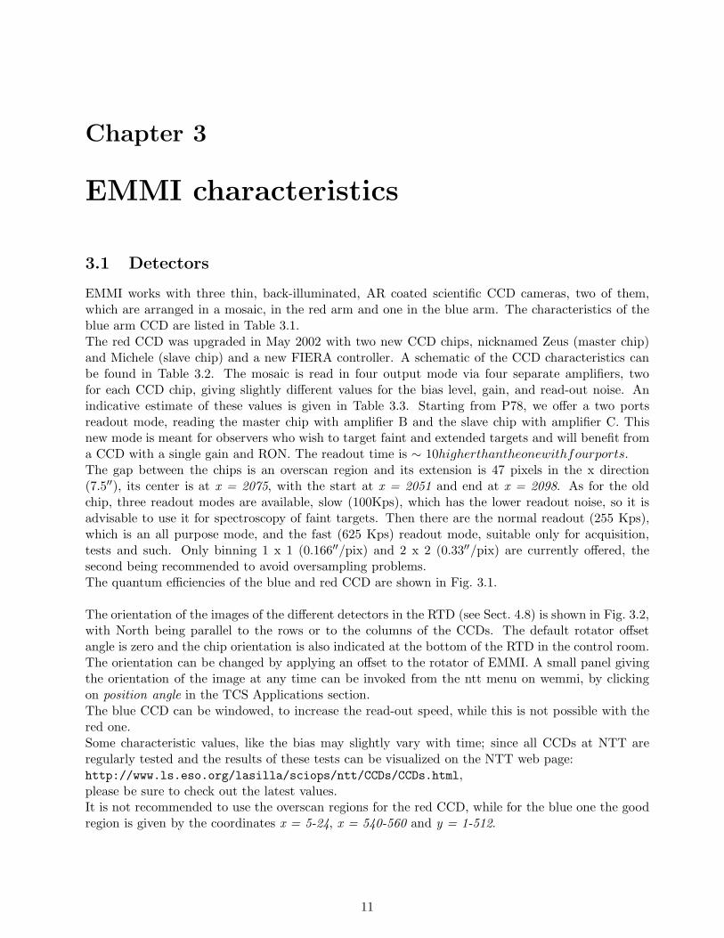
EMMI works with three thin, back-illuminated, AR coated scientific CCD cameras, two of them,which are arranged in a mosaic, in the red arm and one in the blue arm. The characteristics of theblue arm CCD are listed in Table 3.1.The red CCD was upgraded in May 2002 with two new CCD chips, nicknamed Zeus (master chip)and Michele (slave chip) and a new FIERA controller. A schematic of the CCD characteristics canbe found in Table 3.2. The mosaic is read in four output mode via four separate amplifiers, twofor each CCD chip, giving slightly different values for the bias level, gain, and read-out noise. Anindicative estimate of these values is given in Table 3.3. Starting from P78, we offer a two portsreadout mode, reading the master chip with amplifier B and the slave chip with amplifier C. Thisnew mode is meant for observers who wish to target faint and extended targets and will benefit froma CCD with a single gain and RON. The readout time is ∼ 10higherthantheonewithfourports.

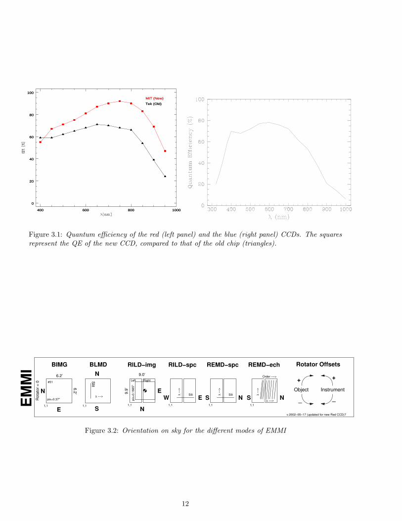
The gap between the chips is an overscan region and its extension is 47 pixels in the x direction(7.5′′), its center is at x = 2075, with the start at x = 2051 and end at x = 2098. As for the oldchip, three readout modes are available, slow (100Kps), which has the lower readout noise, so it isadvisable to use it for spectroscopy of faint targets. Then there are the normal readout (255 Kps),which is an all purpose mode, and the fast (625 Kps) readout mode, suitable only for acquisition,tests and such. Only binning 1 x 1 (0.166′′/pix) and 2 x 2 (0.33′′/pix) are currently offered, thesecond being recommended to avoid oversampling problems.The quantum efficiencies of the blue and red CCD are shown in Fig. 3.1.

The orientation of the images of the different detectors in the RTD (see Sect. 4.8) is shown in Fig. 3.2,with North being parallel to the rows or to the columns of the CCDs. The default rotator offsetangle is zero and the chip orientation is also indicated at the bottom of the RTD in the control room.The orientation can be changed by applying an offset to the rotator of EMMI. A small panel givingthe orientation of the image at any time can be invoked from the ntt menu on wemmi, by clickingon position angle in the TCS Applications section.The blue CCD can be windowed, to increase the read-out speed, while this is not possible with thered one.Some characteristic values, like the bias may slightly vary with time; since all CCDs at NTT areregularly tested and the results of these tests can be visualized on the NTT web page:http://www.ls.eso.org/lasilla/sciops/ntt/CCDs/CCDs.html,please be sure to check out the latest values.It is not recommended to use the overscan regions for the red CCD, while for the blue one the goodregion is given by the coordinates x = 5-24, x = 540-560 and y = 1-512.

11

400 600 800 1000

0

20

40

60

80

100

MIT (New)

Tek (Old)

400 600 800 1000

0

20

40

60

80

100

MIT (New)

Tek (Old)

Figure 3.1: Quantum efficiency of the red (left panel) and the blue (right panel) CCDs. The squaresrepresent the QE of the new CCD, compared to that of the old chip (triangles).

E1,1

#31

N

6.2’

6.2

’

pix=0.37"

BIMG

1,1

E

N

pix

=0

.16

65

"

RightLeft

9.9

’

9.0’

RILD−img

Slit

1,1

RILD−spc

λ −−

>

W E1,1

λ −−

>

REMD−spc

S NSlit

1,1

REMD−ech

S N

λ −−

>

λ −−>

Order −−>

1,1

BLMD

Slit

λ −−>

N

S

Rotator Offsets

Object Instrument

++

_ _Rota

tor

= 0

EM

MI

v.2002−05−17 (updated for new Red CCD)7

Figure 3.2: Orientation on sky for the different modes of EMMI

12

FILR GRIS

RILDSTAPCCD RED

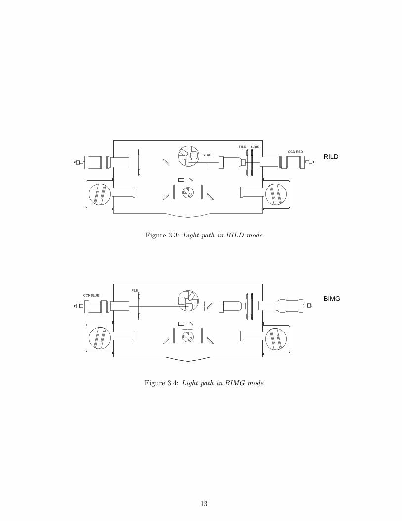
Figure 3.3: Light path in RILD mode

BIMGFILB

CCD BLUE

Figure 3.4: Light path in BIMG mode

13

3.2 Imaging

Imaging with EMMI can be done with both the RILD and the BIMG mode, respectively for red(λ > 400 nm) and blue (λ < 500 nm) observations. Figures 3.3 and 3.4 show the light path in eachmode.To avoid that the main object falls in the inter-chip gap, the mosaic has been slightly shifted in thedewar so that the target will fall in the area of the master chip (right hand side of the mosaic).Other effects to keep in mind are CCD translation, rotation and astrometry.Translation: The slave chip is translated with respect to the master (note: the master chip is Zeus):x(master) - x(slave) = 27.0 pixels = 4.5′′

y(master) - y(slave) = -2.6 pixels = 0.43′′

This effect is corrected by software, adjusting the number of pre-scan column on each chip. Joiningthe 4 sub-images will produce an image geometrically correct within 1 pixel in the central region (y∼ 2000). The geometric error goes up to 2 pixels at the top and the bottom of the gap.Rotation: A small rotation of one chip with respect to the other has been measured:∆X = 0.90 pixels over 4000 pixels∆Y = 0.35 pixels over 4000 pixelsThese values correspond to a rotation of 0.22 mrad and it’s a physical rotation of the CCD, so nocorrection is possible.Astrometry: An estimate of the astrometric transformation has been determined for both chips:Master chip (right hand side one):d(α) = cost + 0.046274x + 0.000144y + 0.000002xy + 0.000024x2 - 0.000014y2

d(δ) = cost - 0.000029x - 0.046179y - 0.000044xy + 0.000039x2 - 0.000019y2

Slave chip (left hand side one):d(α) = cost + 0.046489x + 0.000139y + 0.000000xy - 0.000018x2 - 0.000005y2

d(δ) = cost - 0.000050x - 0.046299y - 0.000009xy + 0.000004x2 - 0.000003y2

where d(α) and d(δ) are in degrees and x and y are in un-binned pixels.EMMI files have no WCS information in the header; if you need to obtain a good astrometry for yourtargets, we recommend that you re-calculate the astrometric solution, either with Gaia or with thecommand koords within the Karma visualization package (http://www.atnf.csiro.au/computing/software/karma/).

Table 3.1: Blue arm CCD characteristics

Blue #31Model Tektronix TK1034 AB Grade 1Pixel size (µm) 24 × 24Image size (pixels) 1024 × 1024Controler ACELinearity (% < 65535 ADU) 0.4Dark current (e−/pix/h) 6.9Shutter delay (s) 0.12

Slow Normal FastBias (ADU) 572 564 610Gain (e−/ADU) 1.42 2.85 2.75Read-Out Noise (e−) 5.2 6.9 9.2Read-Out Time (s) 50 40 33

Camera f/4Pixel scale (”/pixel) 0.362Field size (’) 6.2 × 6.2

14

3.2.1 Filters

Red-arm filters, which are inserted in a parallel beam, are mounted at an angle in their cells, to avoidreflections between the CCD and the filter. Most are mounted at 5◦ inclination, the remainder aremounted at 2.5◦ or 7.5◦. Blue arm filters, used in the converging beam in front of the blue camera,do not suffer from reflection with the CCD and hence are mounted with no inclination. Using ared-arm filter in the blue will result in a slight change of the central wavelength (only critical fornarrow-band filters) and will cause some astigmatism. If a blue filter is used in the red arm, everyobject in the field produces a reflection ghost, which is about 5 magnitudes fainter than the originalobject. Thus, although it is possible to use blue filters in the red and vice-versa (one might want todo this in the overlap region, 400 to 500 nm), filters should normally be used in the wheel they areintended for.Filters with very narrow bandwidths are not well suited for the red arm. Because the filters aremounted in the parallel beam, and tilted, the central wavelength will change across the field. Inextreme cases, the central wavelength may be outside the edge of the filter sensitivity response nearthe edge of the field of view. The tabulated wavelength corresponds to the centre of the CCD. Asa guide line, avoid filters with ∆λ < 5 nm for red imaging. The wavelength change also affectswide-field photometry if using narrow-band filters. In the blue arm, since the filter wheel is mountedin the converging beam, it it possible to use narrow-band filters. The effective wavelength staysconstant across the field.Table 3.4 gives a list of standard EMMI filters to be used on the red arm, while Table 3.5 gives thefilters to be used on the blue arm. Filters marked with a star symbol on both tables can be used onboth arms, provided the limitations discussed above. The full list of ESO filters and transmission

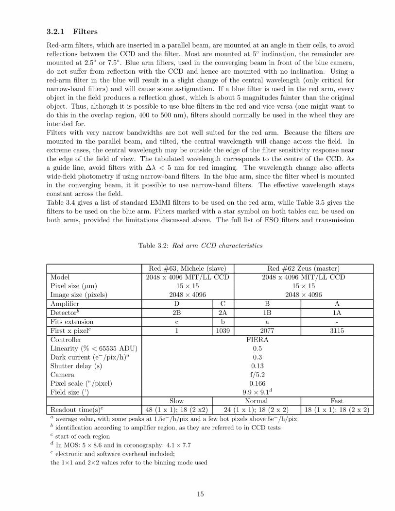
Table 3.2: Red arm CCD characteristics

Red #63, Michele (slave) Red #62 Zeus (master)Model 2048 x 4096 MIT/LL CCD 2048 x 4096 MIT/LL CCDPixel size (µm) 15 × 15 15 × 15Image size (pixels) 2048 × 4096 2048 × 4096

Amplifier D C B A

Detectorb 2B 2A 1B 1A

Fits extension c b a -

First x pixelc 1 1039 2077 3115

Controller FIERALinearity (% < 65535 ADU) 0.5Dark current (e−/pix/h)a 0.3Shutter delay (s) 0.13Camera f/5.2Pixel scale (”/pixel) 0.166Field size (’) 9.9 × 9.1d

Slow Normal FastReadout time(s)e 48 (1 x 1); 18 (2 x2) 24 (1 x 1); 18 (2 x 2) 18 (1 x 1); 18 (2 x 2)a average value, with some peaks at 1.5e−/h/pix and a few hot pixels above 5e−/h/pixb identification according to amplifier region, as they are referred to in CCD testsc start of each regiond In MOS: 5 × 8.6 and in coronography: 4.1 × 7.7e electronic and software overhead included;

the 1×1 and 2×2 values refer to the binning mode used

15

curves can be viewed using the MIDAS graphical user interface (GUI) FILTERS. The most recentversion is always (and only) available on the workstation kila in La Silla. Approximate transmissioncurves for EMMI filters can be found in the La Silla WWW pages:http://filters.ls.eso.org/efs.The B-band filter used in the red arm (Bb filter) shows scatter in the colour terms of > 0.10m. It isopen towards the UV so its effective colour equation depends on EMMI and camera transmissionsand the CCD QE at ∼ 400 nm. The red optics have a sharp cut-off at 390 nm due to the coating,which causes the total response curve to resemble that of the true B-filter, but accurate B-bandphotometry should normally be done in the blue arm. The blue arm is also more sensitive at 400 nm(See Sect. 3.2.3).

3.2.2 Coronography

Coronography is possible in the red arm by mounting a coronographic plate in the starplate wheel.The coronograph consists of a transparent glass plate which has 6 circular dots of size ranging from1′′ to 5′′. It is useful for allowing longer exposures in the presence of a bright star, without stronglyoverexposing the CCD. The telescope is pointed such that the star falls one one of these dots. Notethat the peak of the PSF is blocked out, but not the wings, nor the spider diffraction pattern. NoLyot mask is available.The approximate positions of the dots on the CCD, together with the size in arcseconds, is shown inTable 3.6. The positions can vary a little with the alignment of the plate, and the precise positionshould be calibrated during the setup.The plate does not cover the entire field: the mounting reduces the field size to 4.1′ × 7.7′. Pleasenote that the 4.9′′ and the 1.9′′ dots are quite close to the mosaic gap in EMMI default orientation.The field can be aligned with a preferred direction on the sky by rotating EMMI.Another option which might be considered is to place the bright star in the gap between the twoCCDs (7.5 arcsec wide), avoiding in this way the field limitation discussed above. The coordinatesof the center of the gap are X = 2075, Y = 2079.

3.2.3 Performance

The count rates of the instruments are monitored and scaled to a 15mag star at unit airmass. Mostrecent measurement from observations taken during May 2002 commissioning are given in Table 3.7

Table 3.3: Red arm CCD paramaters

CCD subchip c Michele b Michele a Zeus - ZeusBinning 1 x 1 2 x 2 1 x 1 2 x 2 1 x 1 2 x 2 1 x 1 2 x 2

Slow=100Kps Bias 303 313 286 299 305 310 299 307Gain (e−/ADU) 1.34 1.27 1.32 1.22 1.38 1.22 1.35 1.26

RON 3.55 3.47 4.27 3.27 3.71 3.24 3.56 3.41

Normal=225Kps Bias 295 346 269 345 285 359 281 359Gain (e−/ADU) 1.34 1.27 1.32 1.24 1.39 1.27 1.35 1.27

RON 5.70 5.46 5.48 5.09 6.24 5.45 5.93 5.16

Fast=625Kps Bias 677 378 649 346 613 357 590 355Gain (e−/ADU) 1.35 1.36 1.38 1.34 1.43 1.38 1.40 1.37

RON 21.17 14.05 21.66 13.67 24.49 16.55 23.17 15.52

16

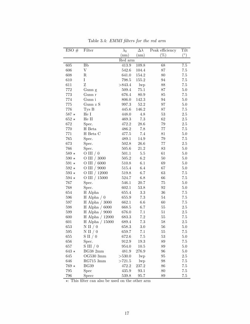
Table 3.4: EMMI filters for the red arm

ESO # Filter λ0 ∆λ Peak efficiency Tilt(nm) (nm) (%) (◦)Red arm

605 Bb 413.9 109.8 68 7.5606 V 542.6 104.4 87 7.5608 R 641.0 154.2 80 7.5610 I 798.5 155.2 94 7.5611 Z >843.4 lwp 88 7.5772 Gunn g 509.4 75.1 87 5.0773 Gunn r 676.4 80.9 85 7.5774 Gunn i 806.0 142.3 94 5.0775 Gunn z S 997.3 52.2 97 5.0776 Tys B 445.6 146.2 87 7.5587 ? He I 448.0 4.8 53 2.5652 ? He II 469.3 7.3 62 2.5672 Spec. 472.2 28.6 79 2.5770 H Beta 486.2 7.8 77 7.5771 H Beta C 477.5 7.4 81 5.0765 Spec. 489.1 14.9 79 7.5673 Spec. 502.8 26.6 77 2.5766 Spec. 505.6 21.2 83 5.0589 ? O III / 0 501.1 5.5 61 5.0590 ? O III / 3000 505.2 6.2 50 5.0591 ? O III / 6000 510.8 6.1 69 5.0592 ? O III / 9000 515.4 6.4 67 5.0593 ? O III / 12000 519.8 6.7 63 7.5594 ? O III / 15000 524.7 6.8 66 7.5767 Spec. 546.1 20.7 75 5.0768 Spec. 602.1 53.8 92 5.0654 H Alpha 655.4 3.3 36 7.5596 H Alpha / 0 655.9 7.3 54 7.5597 H Alpha / 3000 662.1 6.6 60 7.5598 H Alpha / 6000 668.5 6.7 55 2.5599 H Alpha / 9000 676.0 7.1 51 2.5600 H Alpha / 12000 683.3 7.2 55 7.5601 H Alpha / 15000 689.4 7.3 58 2.5653 N II / 0 658.3 3.0 56 5.0595 N II / 0 659.7 7.1 55 7.5655 S II / 0 672.6 7.5 53 5.0656 Spec. 912.9 19.3 89 7.5657 S III / 0 954.0 10.5 89 5.0643 ? BG38 2mm 481.9 276.9 96 5.0645 OG530 3mm >530.0 lwp 95 2.5646 RG715 3mm >721.5 lwp 98 7.5769 ? BG39 472.2 237.2 86 7.5795 Spec 435.9 93.1 80 7.5796 Specc 539.8 95.7 89 7.5?: This filter can also be used on the other arm

17

Table 3.5: EMMI filters for the blue arm

ESO # Filter λ0 ∆λ Peak efficiency Tilt(nm) (nm) (%) (◦)Blue arm

602 U 354.2 54.2 67 0603 B 422.3 94.1 66 0604 B 422.0 94.6 65 0658 EUV (UG11/5) <366.1 swp 70 0647 Ne V 342.2 8.3 39 0648 O II / 0 372.5 6.9 35 0649 O II / 5000 379.5 6.7 44 0650 O II / 10000 385.3 7.0 43 0651 O II / 15000 392.7 7.8 41 0671 ? He II 468.0 15.2 57 0588 ? He II 469.0 6.6 71 0723 Spec. 394.9 3.5 44 0644 ? GG375 3mm >369.2 lwp 99 7.5?: This filter can also be used on the other arm

Table 3.6: Coronographic plate

Dot Size (”) Approx. position on CCD

1 4.9 2025,17332 3.8 2347,17373 2.7 2667,17414 1.9 2021,22475 1.3 2343,22516 0.9 2663,2253

18

and updated values can be found on the “EMMI Latest News” web page.An exposure time calculator for the imaging modes is available in the EMMI WWW pages.Approximate colour equations for the BVRI filters used in RILD and for the UB filters used in BIMGhave been derived from observations done during technical time: they are given in Table 3.8. In thistable, lower case refers to instrumental magnitudes in e−/s and upper case refers to actual magnitudes.These equations are meant to be a guideline and should not be relied upon for accurate photometry.To obtain photometry to better than 0.1m, the colour terms should be measured. Alternatively, onecould also choose the calibration stars to be of similar colour to the program stars.A MIDAS tool to derive the zero points (hereafter ZP) during the night is available on the off-linemachine; for more details see Sect. 4.10.

Table 3.7: Imaging throuhput for a 15th mag A star at airmass=0

Red arm Blue armFilter Count rate Filter Count rate

(e− / s) (e− / s)

Bb 13439 U 2450V 25712 B 19290R 31185I 17915

Table 3.8: Colour equations

Red arm Blue arm

B − b = (0.018±0.079)×(B-V)+25.27±0.03-0.214×Z U − u = 0.06×(U-B)+24.03V − v = (-0.009±0.022)×(V-R)+25.98±0.01-0.125×Z B − b = 0.142×(B-V)+25.92R − r = (-0.041±0.040)×(V-R)+26.21±0.02-0.091×ZI − i = (-0.024±0.082)×(R-I)+25.57±0.03-0.051×Z

An update of the ZP, color terms and extinction is available at:http://www.ls.eso.org/lasilla/sciops/ntt/emmi/emmiImagingPerformance.html

19

3.3 Low-Dispersion Spectroscopy

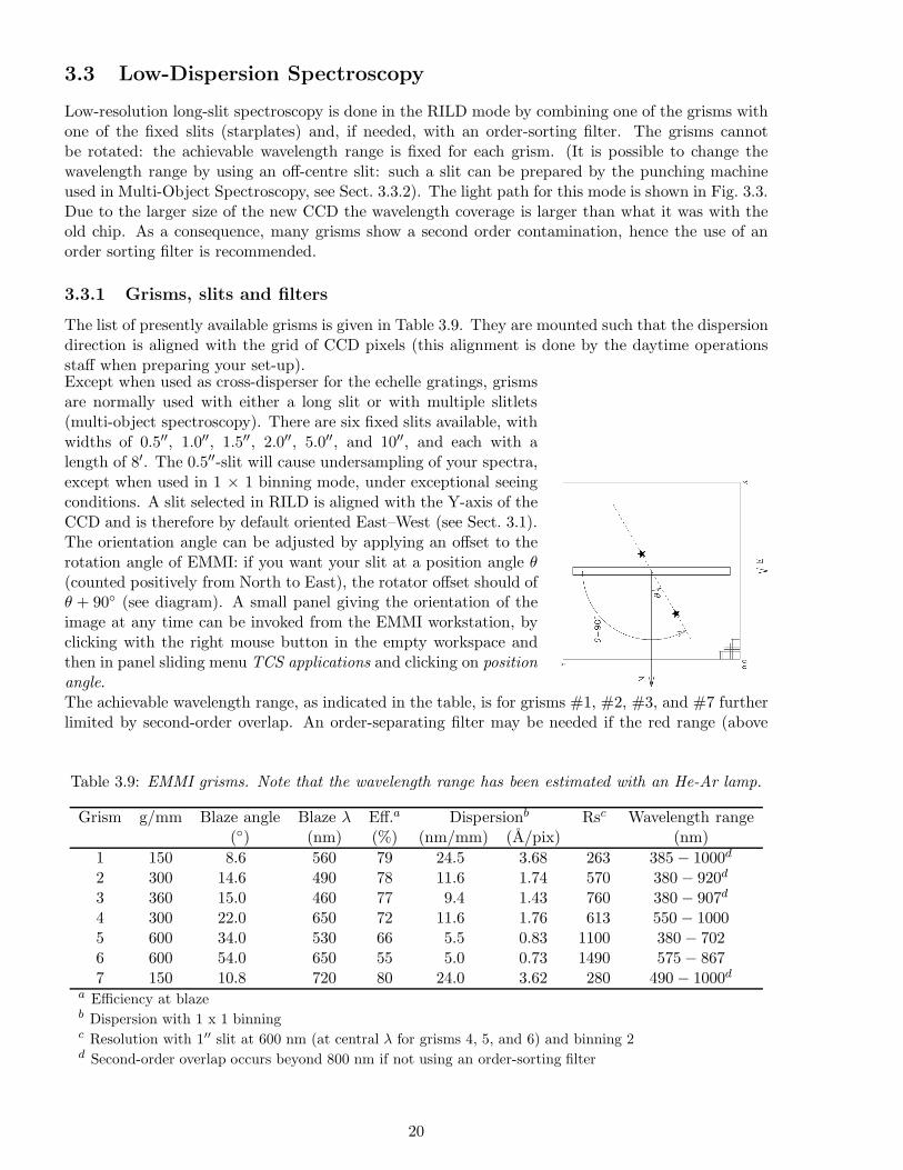
Low-resolution long-slit spectroscopy is done in the RILD mode by combining one of the grisms withone of the fixed slits (starplates) and, if needed, with an order-sorting filter. The grisms cannotbe rotated: the achievable wavelength range is fixed for each grism. (It is possible to change thewavelength range by using an off-centre slit: such a slit can be prepared by the punching machineused in Multi-Object Spectroscopy, see Sect. 3.3.2). The light path for this mode is shown in Fig. 3.3.Due to the larger size of the new CCD the wavelength coverage is larger than what it was with theold chip. As a consequence, many grisms show a second order contamination, hence the use of anorder sorting filter is recommended.

3.3.1 Grisms, slits and filters

The list of presently available grisms is given in Table 3.9. They are mounted such that the dispersiondirection is aligned with the grid of CCD pixels (this alignment is done by the daytime operationsstaff when preparing your set-up).Except when used as cross-disperser for the echelle gratings, grismsare normally used with either a long slit or with multiple slitlets(multi-object spectroscopy). There are six fixed slits available, withwidths of 0.5′′, 1.0′′, 1.5′′, 2.0′′, 5.0′′, and 10′′, and each with alength of 8′. The 0.5′′-slit will cause undersampling of your spectra,except when used in 1 × 1 binning mode, under exceptional seeingconditions. A slit selected in RILD is aligned with the Y-axis of theCCD and is therefore by default oriented East–West (see Sect. 3.1).The orientation angle can be adjusted by applying an offset to therotation angle of EMMI: if you want your slit at a position angle θ

(counted positively from North to East), the rotator offset should ofθ + 90◦ (see diagram). A small panel giving the orientation of theimage at any time can be invoked from the EMMI workstation, byclicking with the right mouse button in the empty workspace andthen in panel sliding menu TCS applications and clicking on positionangle.The achievable wavelength range, as indicated in the table, is for grisms #1, #2, #3, and #7 furtherlimited by second-order overlap. An order-separating filter may be needed if the red range (above

Table 3.9: EMMI grisms. Note that the wavelength range has been estimated with an He-Ar lamp.

Grism g/mm Blaze angle Blaze λ Eff.a Dispersionb Rsc Wavelength range(◦) (nm) (%) (nm/mm) (A/pix) (nm)

1 150 8.6 560 79 24.5 3.68 263 385 − 1000d

2 300 14.6 490 78 11.6 1.74 570 380 − 920d

3 360 15.0 460 77 9.4 1.43 760 380 − 907d

4 300 22.0 650 72 11.6 1.76 613 550 − 10005 600 34.0 530 66 5.5 0.83 1100 380 − 7026 600 54.0 650 55 5.0 0.73 1490 575 − 8677 150 10.8 720 80 24.0 3.62 280 490 − 1000d

a Efficiency at blazeb Dispersion with 1 x 1 binningc Resolution with 1′′ slit at 600 nm (at central λ for grisms 4, 5, and 6) and binning 2d Second-order overlap occurs beyond 800 nm if not using an order-sorting filter

20

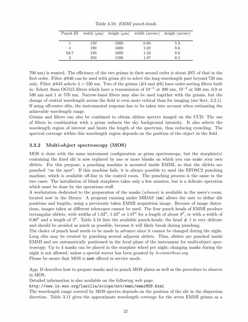
Table 3.10: EMMI punch-heads

Punch ID width (µm) height (µm) width (arcsec) height (arcsec)

1 150 1000 0.80 5.34 190 1600 1.02 8.6

6&7 249 1600 1.34 8.63 350 1590 1.87 8.5

700 nm) is wanted. The efficiency of the two grisms in their second order is about 20% of that in thefirst order. Filter #646 can be used with grism #1 to select the long-wavelength part beyond 720 nmonly. Filter #645 selects λ > 530 nm. Two of the grisms (#4 and #6) have order-sorting filters builtin: Schott 3mm OG515 filters which have a transmission of 10−5 at 490 nm, 10−2 at 500 nm, 0.9 at530 nm and 1 at 570 nm. Narrow-band filters may also be used together with the grisms, but thechange of central wavelength across the field is even more critical than for imaging (see Sect. 3.2.1).If using off-centre slits, the instrumental response has to be taken into account when estimating theachievable wavelength range.Grisms and filters can also be combined to obtain slitless spectra imaged on the CCD. The useof filters in combination with a grism reduces the sky background intensity. It also selects thewavelength region of interest and limits the length of the spectrum, thus reducing crowding. Thespectral coverage within this wavelength region depends on the position of the object in the field.

3.3.2 Multi-object spectroscopy (MOS)

MOS is done with the same instrument configuration as grism spectroscopy, but the starplate(s)containing the fixed slit is now replaced by one or more blanks on which you can make your ownslitlets. For this purpose, a punching machine is mounted inside EMMI, so that the slitlets arepunched “on the spot”. If this machine fails, it is always possible to used the EFOSC2 punchingmachine, which is available off-line in the control room. The punching process is the same in thetwo cases. The installation of blank starplates takes only a few minutes, but is a delicate operationwhich must be done by the operations staff.A workstation dedicated to the preparation of the masks (wlsmos) is available in the users’s room,located now in the library. A program running under MIDAS (xm) allows the user to define slitpositions and lengths, using a previously taken EMMI acquisition image. Because of image distor-tions, images taken at different telescopes cannot be used. The four punch heads of EMMI producerectangular slitlets, with widths of 1.02′′, 1.34′′ or 1.87′′ for a length of about 8′′, or with a width of0.80′′ and a length of 5′′. Table 3.10 lists the available punch-heads; the head # 1 is very delicateand should be avoided as much as possible, because it will likely break during punching.The choice of punch head needs to be made in advance since it cannot be changed during the night.Long slits may be created by punching several adjacent slitlets. Thus, slitlets are punched insideEMMI and are automatically positioned in the focal plane of the instrument for multi-object spec-troscopy. Up to 4 masks can be placed in the starplate wheel per night; changing masks during thenight is not allowed, unless a special waiver has been granted by ls-emmi@eso.org.Please be aware that MOS is not offered in service mode.

App. D describes how to prepare masks and to punch MOS plates as well as the procedure to observein MOS.Detailed information is also available on the following web page:http://www.ls.eso.org/lasilla/sciops/ntt/emmi/emmiMOS.html

The wavelength range covered by MOS spectra depends on the position of the slit in the dispersiondirection. Table 3.11 gives the approximate wavelength coverage for the seven EMMI grisms as a

21

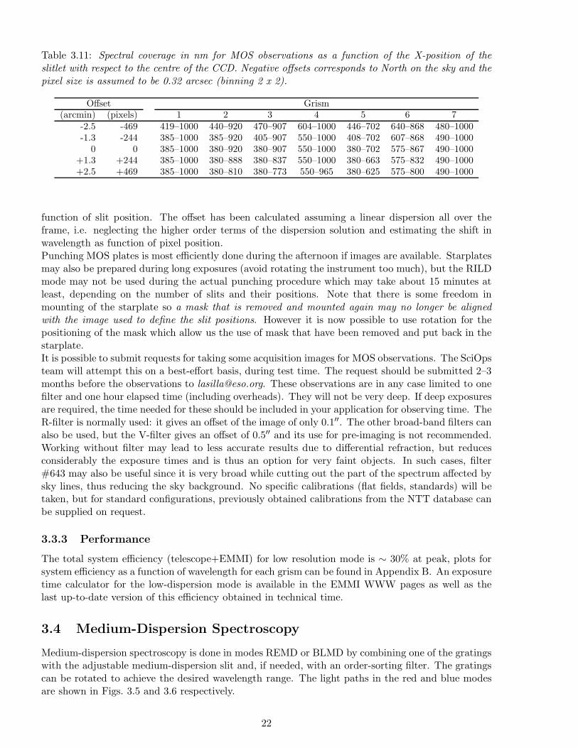
Table 3.11: Spectral coverage in nm for MOS observations as a function of the X-position of theslitlet with respect to the centre of the CCD. Negative offsets corresponds to North on the sky and thepixel size is assumed to be 0.32 arcsec (binning 2 x 2).

Offset Grism(arcmin) (pixels) 1 2 3 4 5 6 7

-2.5 -469 419–1000 440–920 470–907 604–1000 446–702 640–868 480–1000-1.3 -244 385–1000 385–920 405–907 550–1000 408–702 607–868 490–1000

0 0 385–1000 380–920 380–907 550–1000 380–702 575–867 490–1000+1.3 +244 385–1000 380–888 380–837 550–1000 380–663 575–832 490–1000+2.5 +469 385–1000 380–810 380–773 550–965 380–625 575–800 490–1000

function of slit position. The offset has been calculated assuming a linear dispersion all over theframe, i.e. neglecting the higher order terms of the dispersion solution and estimating the shift inwavelength as function of pixel position.Punching MOS plates is most efficiently done during the afternoon if images are available. Starplatesmay also be prepared during long exposures (avoid rotating the instrument too much), but the RILDmode may not be used during the actual punching procedure which may take about 15 minutes atleast, depending on the number of slits and their positions. Note that there is some freedom inmounting of the starplate so a mask that is removed and mounted again may no longer be alignedwith the image used to define the slit positions. However it is now possible to use rotation for thepositioning of the mask which allow us the use of mask that have been removed and put back in thestarplate.It is possible to submit requests for taking some acquisition images for MOS observations. The SciOpsteam will attempt this on a best-effort basis, during test time. The request should be submitted 2–3months before the observations to lasilla@eso.org. These observations are in any case limited to onefilter and one hour elapsed time (including overheads). They will not be very deep. If deep exposuresare required, the time needed for these should be included in your application for observing time. TheR-filter is normally used: it gives an offset of the image of only 0.1′′. The other broad-band filters canalso be used, but the V-filter gives an offset of 0.5′′ and its use for pre-imaging is not recommended.Working without filter may lead to less accurate results due to differential refraction, but reducesconsiderably the exposure times and is thus an option for very faint objects. In such cases, filter#643 may also be useful since it is very broad while cutting out the part of the spectrum affected bysky lines, thus reducing the sky background. No specific calibrations (flat fields, standards) will betaken, but for standard configurations, previously obtained calibrations from the NTT database canbe supplied on request.

3.3.3 Performance

The total system efficiency (telescope+EMMI) for low resolution mode is ∼ 30% at peak, plots forsystem efficiency as a function of wavelength for each grism can be found in Appendix B. An exposuretime calculator for the low-dispersion mode is available in the EMMI WWW pages as well as thelast up-to-date version of this efficiency obtained in technical time.

3.4 Medium-Dispersion Spectroscopy

Medium-dispersion spectroscopy is done in modes REMD or BLMD by combining one of the gratingswith the adjustable medium-dispersion slit and, if needed, with an order-sorting filter. The gratingscan be rotated to achieve the desired wavelength range. The light paths in the red and blue modesare shown in Figs. 3.5 and 3.6 respectively.

22

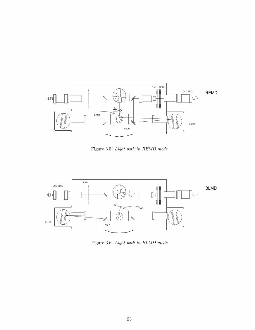
FILR GRIS

REMD

TV

BSLR

GRTR

CCD RED

LONS

Figure 3.5: Light path in REMD mode

BLMDCCD BLUE

FILB

BSLB

GRTB

LONS

TV

Figure 3.6: Light path in BLMD mode

23

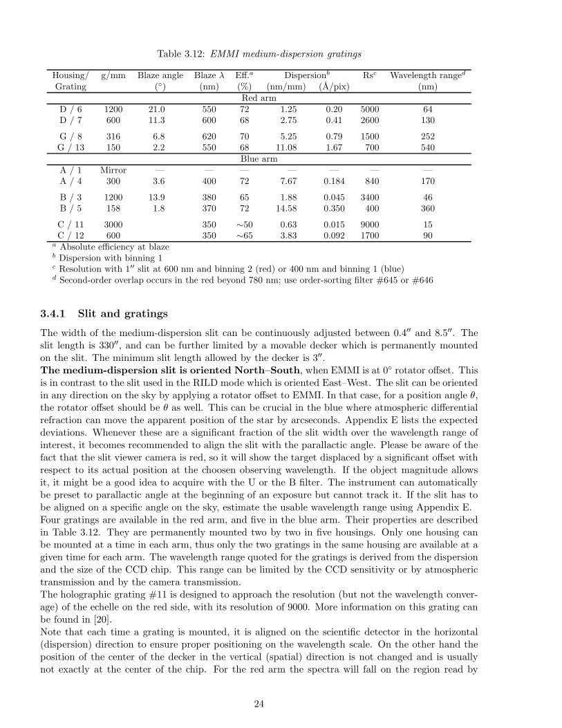
Table 3.12: EMMI medium-dispersion gratings

Housing/ g/mm Blaze angle Blaze λ Eff.a Dispersionb Rsc Wavelength ranged

Grating (◦) (nm) (%) (nm/mm) (A/pix) (nm)Red arm

D / 6 1200 21.0 550 72 1.25 0.20 5000 64D / 7 600 11.3 600 68 2.75 0.41 2600 130

G / 8 316 6.8 620 70 5.25 0.79 1500 252G / 13 150 2.2 550 68 11.08 1.67 700 540

Blue armA / 1 Mirror — — — — — — —A / 4 300 3.6 400 72 7.67 0.184 840 170

B / 3 1200 13.9 380 65 1.88 0.045 3400 46B / 5 158 1.8 370 72 14.58 0.350 400 360

C / 11 3000 350 ∼50 0.63 0.015 9000 15C / 12 600 350 ∼65 3.83 0.092 1700 90

a Absolute efficiency at blazeb Dispersion with binning 1c Resolution with 1′′ slit at 600 nm and binning 2 (red) or 400 nm and binning 1 (blue)d Second-order overlap occurs in the red beyond 780 nm; use order-sorting filter #645 or #646

3.4.1 Slit and gratings

The width of the medium-dispersion slit can be continuously adjusted between 0.4′′ and 8.5′′. Theslit length is 330′′, and can be further limited by a movable decker which is permanently mountedon the slit. The minimum slit length allowed by the decker is 3′′.The medium-dispersion slit is oriented North–South, when EMMI is at 0◦ rotator offset. Thisis in contrast to the slit used in the RILD mode which is oriented East–West. The slit can be orientedin any direction on the sky by applying a rotator offset to EMMI. In that case, for a position angle θ,the rotator offset should be θ as well. This can be crucial in the blue where atmospheric differentialrefraction can move the apparent position of the star by arcseconds. Appendix E lists the expecteddeviations. Whenever these are a significant fraction of the slit width over the wavelength range ofinterest, it becomes recommended to align the slit with the parallactic angle. Please be aware of thefact that the slit viewer camera is red, so it will show the target displaced by a significant offset withrespect to its actual position at the choosen observing wavelength. If the object magnitude allowsit, it might be a good idea to acquire with the U or the B filter. The instrument can automaticallybe preset to parallactic angle at the beginning of an exposure but cannot track it. If the slit has tobe aligned on a specific angle on the sky, estimate the usable wavelength range using Appendix E.Four gratings are available in the red arm, and five in the blue arm. Their properties are describedin Table 3.12. They are permanently mounted two by two in five housings. Only one housing canbe mounted at a time in each arm, thus only the two gratings in the same housing are available at agiven time for each arm. The wavelength range quoted for the gratings is derived from the dispersionand the size of the CCD chip. This range can be limited by the CCD sensitivity or by atmospherictransmission and by the camera transmission.The holographic grating #11 is designed to approach the resolution (but not the wavelength conver-age) of the echelle on the red side, with its resolution of 9000. More information on this grating canbe found in [20].Note that each time a grating is mounted, it is aligned on the scientific detector in the horizontal(dispersion) direction to ensure proper positioning on the wavelength scale. On the other hand theposition of the center of the decker in the vertical (spatial) direction is not changed and is usuallynot exactly at the center of the chip. For the red arm the spectra will fall on the region read by

24

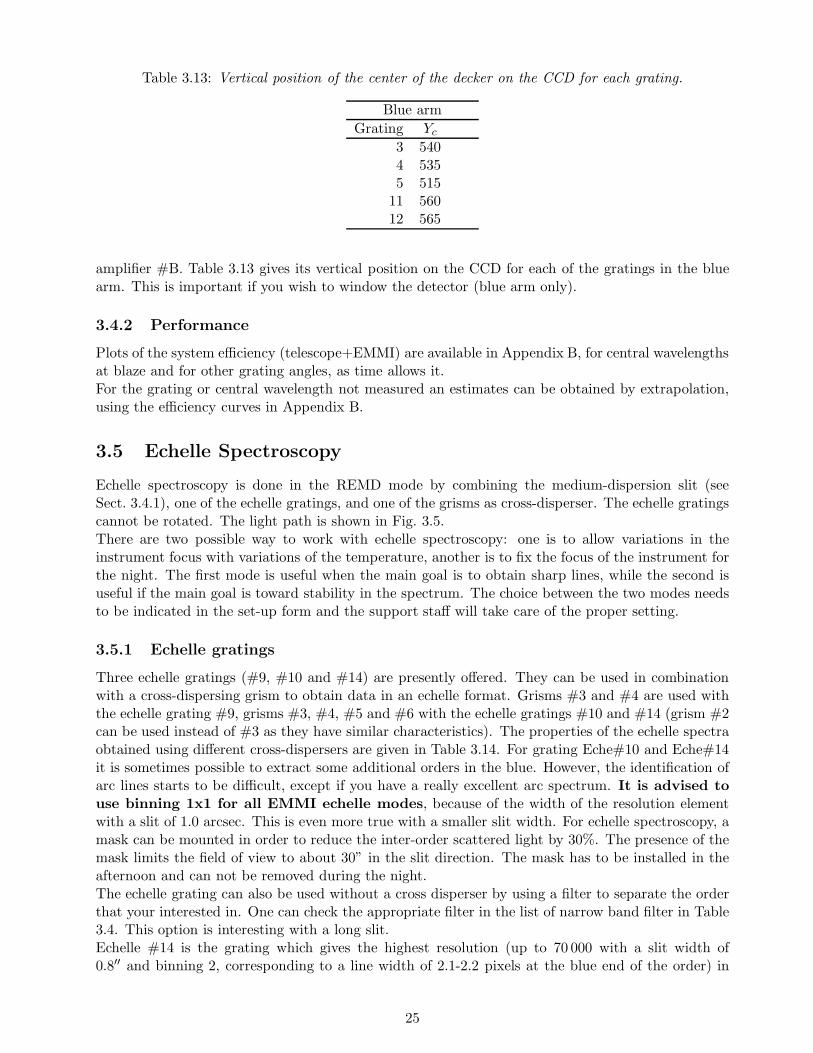
Table 3.13: Vertical position of the center of the decker on the CCD for each grating.

Blue arm

Grating Yc

3 5404 5355 515

11 56012 565

amplifier #B. Table 3.13 gives its vertical position on the CCD for each of the gratings in the bluearm. This is important if you wish to window the detector (blue arm only).

3.4.2 Performance

Plots of the system efficiency (telescope+EMMI) are available in Appendix B, for central wavelengthsat blaze and for other grating angles, as time allows it.For the grating or central wavelength not measured an estimates can be obtained by extrapolation,using the efficiency curves in Appendix B.

3.5 Echelle Spectroscopy

Echelle spectroscopy is done in the REMD mode by combining the medium-dispersion slit (seeSect. 3.4.1), one of the echelle gratings, and one of the grisms as cross-disperser. The echelle gratingscannot be rotated. The light path is shown in Fig. 3.5.There are two possible way to work with echelle spectroscopy: one is to allow variations in theinstrument focus with variations of the temperature, another is to fix the focus of the instrument forthe night. The first mode is useful when the main goal is to obtain sharp lines, while the second isuseful if the main goal is toward stability in the spectrum. The choice between the two modes needsto be indicated in the set-up form and the support staff will take care of the proper setting.

3.5.1 Echelle gratings

Three echelle gratings (#9, #10 and #14) are presently offered. They can be used in combinationwith a cross-dispersing grism to obtain data in an echelle format. Grisms #3 and #4 are used withthe echelle grating #9, grisms #3, #4, #5 and #6 with the echelle gratings #10 and #14 (grism #2can be used instead of #3 as they have similar characteristics). The properties of the echelle spectraobtained using different cross-dispersers are given in Table 3.14. For grating Eche#10 and Eche#14it is sometimes possible to extract some additional orders in the blue. However, the identification ofarc lines starts to be difficult, except if you have a really excellent arc spectrum. It is advised to

use binning 1x1 for all EMMI echelle modes, because of the width of the resolution elementwith a slit of 1.0 arcsec. This is even more true with a smaller slit width. For echelle spectroscopy, amask can be mounted in order to reduce the inter-order scattered light by 30%. The presence of themask limits the field of view to about 30” in the slit direction. The mask has to be installed in theafternoon and can not be removed during the night.The echelle grating can also be used without a cross disperser by using a filter to separate the orderthat your interested in. One can check the appropriate filter in the list of narrow band filter in Table3.4. This option is interesting with a long slit.Echelle #14 is the grating which gives the highest resolution (up to 70 000 with a slit width of0.8′′ and binning 2, corresponding to a line width of 2.1-2.2 pixels at the blue end of the order) in

25

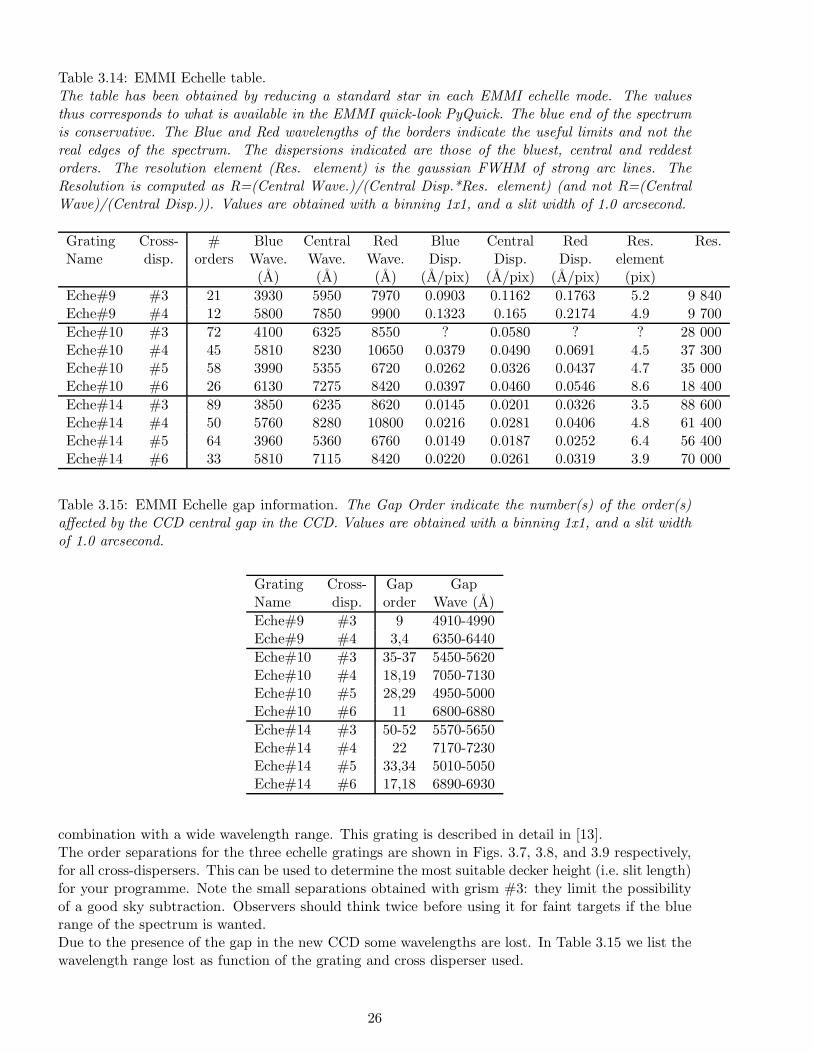
Table 3.14: EMMI Echelle table.The table has been obtained by reducing a standard star in each EMMI echelle mode. The valuesthus corresponds to what is available in the EMMI quick-look PyQuick. The blue end of the spectrumis conservative. The Blue and Red wavelengths of the borders indicate the useful limits and not thereal edges of the spectrum. The dispersions indicated are those of the bluest, central and reddestorders. The resolution element (Res. element) is the gaussian FWHM of strong arc lines. TheResolution is computed as R=(Central Wave.)/(Central Disp.*Res. element) (and not R=(CentralWave)/(Central Disp.)). Values are obtained with a binning 1x1, and a slit width of 1.0 arcsecond.

Grating Cross- # Blue Central Red Blue Central Red Res. Res.Name disp. orders Wave. Wave. Wave. Disp. Disp. Disp. element

(A) (A) (A) (A/pix) (A/pix) (A/pix) (pix)

Eche#9 #3 21 3930 5950 7970 0.0903 0.1162 0.1763 5.2 9 840Eche#9 #4 12 5800 7850 9900 0.1323 0.165 0.2174 4.9 9 700

Eche#10 #3 72 4100 6325 8550 ? 0.0580 ? ? 28 000Eche#10 #4 45 5810 8230 10650 0.0379 0.0490 0.0691 4.5 37 300Eche#10 #5 58 3990 5355 6720 0.0262 0.0326 0.0437 4.7 35 000Eche#10 #6 26 6130 7275 8420 0.0397 0.0460 0.0546 8.6 18 400

Eche#14 #3 89 3850 6235 8620 0.0145 0.0201 0.0326 3.5 88 600Eche#14 #4 50 5760 8280 10800 0.0216 0.0281 0.0406 4.8 61 400Eche#14 #5 64 3960 5360 6760 0.0149 0.0187 0.0252 6.4 56 400Eche#14 #6 33 5810 7115 8420 0.0220 0.0261 0.0319 3.9 70 000

Table 3.15: EMMI Echelle gap information. The Gap Order indicate the number(s) of the order(s)affected by the CCD central gap in the CCD. Values are obtained with a binning 1x1, and a slit widthof 1.0 arcsecond.

Grating Cross- Gap GapName disp. order Wave (A)

Eche#9 #3 9 4910-4990Eche#9 #4 3,4 6350-6440

Eche#10 #3 35-37 5450-5620Eche#10 #4 18,19 7050-7130Eche#10 #5 28,29 4950-5000Eche#10 #6 11 6800-6880

Eche#14 #3 50-52 5570-5650Eche#14 #4 22 7170-7230Eche#14 #5 33,34 5010-5050Eche#14 #6 17,18 6890-6930

combination with a wide wavelength range. This grating is described in detail in [13].The order separations for the three echelle gratings are shown in Figs. 3.7, 3.8, and 3.9 respectively,for all cross-dispersers. This can be used to determine the most suitable decker height (i.e. slit length)for your programme. Note the small separations obtained with grism #3: they limit the possibilityof a good sky subtraction. Observers should think twice before using it for faint targets if the bluerange of the spectrum is wanted.Due to the presence of the gap in the new CCD some wavelengths are lost. In Table 3.15 we list thewavelength range lost as function of the grating and cross disperser used.

26

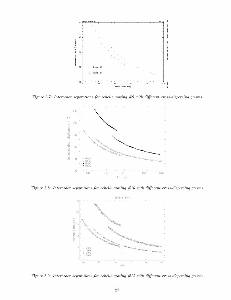
Figure 3.7: Interorder separations for echelle grating #9 with different cross-dispersing grisms

Figure 3.8: Interorder separations for echelle grating #10 with different cross-dispersing grisms

Figure 3.9: Interorder separations for echelle grating #14 with different cross-dispersing grisms

27

3.5.2 Performance

The latest news concerning the performance can be found in the “EMMI Latest News” web page.Plots of the total efficiencies as a function of wavelength can be found in Appendix B.

28

Chapter 4

Observing with EMMI

4.1 The VLT environment

During the Big Bang, the NTT control system was changed to make it compliant with VLT standard.Everything except the low-level electronics has been replaced. The new control system is now identicalto the one that is used on the Unit Telescopes (UTs) of the VLT. The biggest change concerningEMMI apart the CCD upgrade is thus the observing procedure and philosophy.Observations are described in so-called Observations Blocks (OB) containing all the necessary infor-mation to perform a single (science or calibration) observation. An OB contains a Target Package(TP), which tells the telescope where to go, an Acquisition Template (AT), which tells the systemhow to go, and an Observation Description (OD), which tells the system what to do once in position.The OD in turn may contain several templates, the true unit of observation. In service mode, OBscontain also a Constraint Set (CS).OBs are executed by BOB, the Broker for Observation Blocks. It sends commands to the ObservationSoftware (OS), which then redistributes them to the instrument (ICS), detector (DCS), and telescope(TCS) control sofware. This forms the VLT Control Software (VCS).

4.2 Preparation of the observations: P2PP

Advance preparation of your OBs can optimize the use of the telescope by minimizing overheads.Investigators asking for service observing will have to submit a set of fully defined OBs to be executedunder certain conditions, whereas “classical observers” can prepare a few typical OBs, and will havemore flexibility at the telescope to modify and adapt them to their immediate needs. OBs are createdand edited with the P2PP (Phase 2 Proposal Preparation) tool at La Silla a few days before your run,or at the telescope while observing. Observers with a previous experience of P2PP may also startcreating their OBs at their home institute. The Instrument Package describing the templates for thethree instruments of the NTT will be updated regularly and the latest version will be automaticallydownloaded by P2PP when you log-in with your username and password.Users should be aware that only registered users can use P2PP: username and password are sent to theP.I. of each observing program and to La Silla Observatory by USD in Garching (usd-help@eso.org).Should the observer be different from the P.I. it will be his/her responsibility to contact the P.I toobtain the necessary information.Service observers will use the service mode of P2PP, which allows to save defined OBs to a databasecalled the ESO repository, from which a schedule is created. The NTT staff then uses the ObservingTool to select OBs from this schedule and pass them to BOB for execution. Full instructions forservice mode observations are available from:

http://www.ls.eso.org/lasilla/sciops/observing/service.html

Classical observers will use P2PP in visitor mode, on a WS which talks directly to BOB. In this case,

29

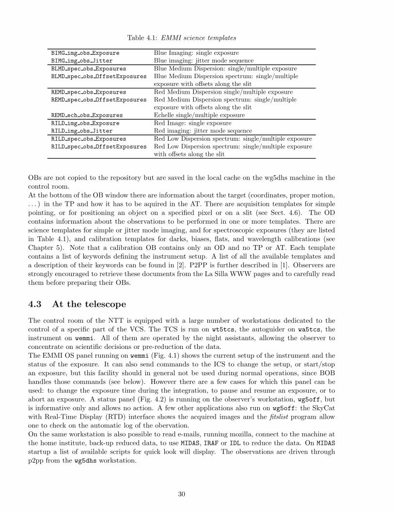
Table 4.1: EMMI science templates

BIMG img obs Exposure Blue Imaging: single exposureBIMG img obs Jitter Blue imaging: jitter mode sequenceBLMD spec obs Exposures Blue Medium Dispersion: single/multiple exposureBLMD spec obs OffsetExposures Blue Medium Dispersion spectrum: single/multiple

exposure with offsets along the slitREMD spec obs Exposures Red Medium Dispersion single/multiple exposureREMD spec obs OffsetExposures Red Medium Dispersion spectrum: single/multiple

exposure with offsets along the slitREMD ech obs Exposures Echelle single/multiple exposureRILD img obs Exposure Red Image: single exposureRILD img obs Jitter Red imaging: jitter mode sequenceRILD spec obs Exposures Red Low Dispersion spectrum: single/multiple exposureRILD spec obs OffsetExposures Red Low Dispersion spectrum: single/multiple exposure

with offsets along the slit

OBs are not copied to the repository but are saved in the local cache on the wg5dhs machine in thecontrol room.At the bottom of the OB window there are information about the target (coordinates, proper motion,. . . ) in the TP and how it has to be aquired in the AT. There are acquisition templates for simplepointing, or for positioning an object on a specified pixel or on a slit (see Sect. 4.6). The ODcontains information about the observations to be performed in one or more templates. There arescience templates for simple or jitter mode imaging, and for spectroscopic exposures (they are listedin Table 4.1), and calibration templates for darks, biases, flats, and wavelength calibrations (seeChapter 5). Note that a calibration OB contains only an OD and no TP or AT. Each templatecontains a list of keywords defining the instrument setup. A list of all the available templates anda description of their keywords can be found in [2]. P2PP is further described in [1]. Observers arestrongly encouraged to retrieve these documents from the La Silla WWW pages and to carefully readthem before preparing their OBs.

4.3 At the telescope

The control room of the NTT is equipped with a large number of workstations dedicated to thecontrol of a specific part of the VCS. The TCS is run on wt5tcs, the autoguider on wa5tcs, theinstrument on wemmi. All of them are operated by the night assistants, allowing the observer toconcentrate on scientific decisions or pre-reduction of the data.The EMMI OS panel running on wemmi (Fig. 4.1) shows the current setup of the instrument and thestatus of the exposure. It can also send commands to the ICS to change the setup, or start/stopan exposure, but this facility should in general not be used during normal operations, since BOBhandles those commands (see below). However there are a few cases for which this panel can beused: to change the exposure time during the integration, to pause and resume an exposure, or toabort an exposure. A status panel (Fig. 4.2) is running on the observer’s workstation, wg5off, butis informative only and allows no action. A few other applications also run on wg5off: the SkyCatwith Real-Time Display (RTD) interface shows the acquired images and the fitslist program allowone to check on the automatic log of the obervation.On the same workstation is also possible to read e-mails, running mozilla, connect to the machine atthe home institute, back-up reduced data, to use MIDAS, IRAF or IDL to reduce the data. On MIDAS

startup a list of available scripts for quick look will display. The observations are driven throughp2pp from the wg5dhs workstation.

30

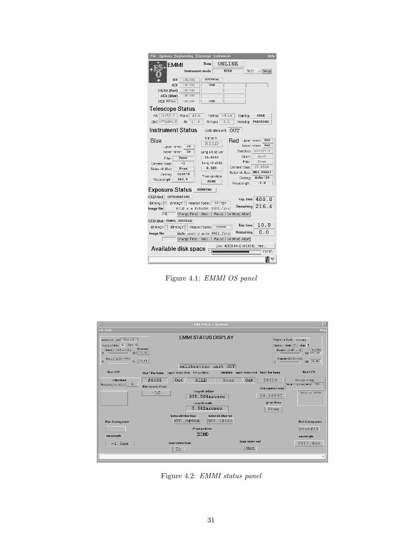
Figure 4.1: EMMI OS panel

Figure 4.2: EMMI status panel

31

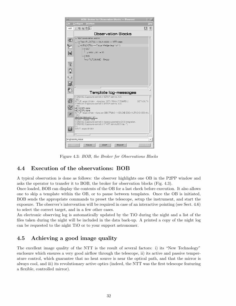
Figure 4.3: BOB, the Broker for Observations Blocks

4.4 Execution of the observations: BOB

A typical observation is done as follows: the observer highlights one OB in the P2PP window andasks the operator to transfer it to BOB, the broker for observation blocks (Fig. 4.3).Once loaded, BOB can display the contents of the OB for a last check before execution. It also allowsone to skip a template within the OB, or to pause between templates. Once the OB is initiated,BOB sends the appropriate commands to preset the telescope, setup the instrument, and start theexposure. The observer’s intervention will be required in case of an interactive pointing (see Sect. 4.6)to select the correct target, and in a few other cases.An electronic observing log is automatically updated by the TiO during the night and a list of thefiles taken during the night will be included in the data back-up. A printed a copy of the night logcan be requested to the night TiO or to your support astronomer.

4.5 Achieving a good image quality

The excellent image quality of the NTT is the result of several factors: i) its “New Technology”enclosure which ensures a very good airflow through the telescope, ii) its active and passive temper-ature control, which guarantee that no heat source is near the optical path, and that the mirror isalways cool, and iii) its revolutionary active optics (indeed, the NTT was the first telescope featuringa flexible, controlled mirror).

32

4.5.1 The active optics system

The good image quality of the NTT is in part due to the active control of the primary and thesecondary mirror. The primary (M1) mirror is supported by 75 actuators and three fixed points,corresponding to actuators #7, #29 and #50. The force applied to each of the 75 actuators canbe adjusted and thus the shape of M1 can be modified. The secondary mirror (M2) can be movedin X,Y,Z, where the X,Y motion of M2 is used to correct for decentring coma and the motion in Zcontrols the focus. The active supports are used to compensate for various deformation effects in thetelescope structure and the mirrors, and for effects due to inhomogeneities of the air temperaturein the dome. Some of these effects are elastic and can be empirically calibrated for each position.Others have inelastic components and are more difficult to predict.Confusion is sometimes found about the difference between active optics and adaptive optics. Adap-tive optics can correct for turbulence in the atmosphere by means of very fast corrections to theoptics, whereas active optics only corrects for much slower variations. Thus, whereas adaptive opticscan reach the diffraction limit of the telescope, active optics (as on the NTT) only allows the telescopeto reach the ambient seeing.There are two different procedures to set the NTT Active Optics System (AOS). The first is to usea default setting correcting for gravitationally induced deformations, using predefined look-up tablesat different values of the telescope altitude. These tables include corrections for astigmatism anddefocus, but not for higher-order effects. The second method is to do a full wavefront analysis, theso-called image analysis, and to calculate the mirror settings from this. This method can be usedeither in open or in closed loop.The image-analysis systems (there is one at each Nasmyth station, located inside the instrumentadapter/rotators) consist of a Shack-Hartmann grid and a CCD to record the image. The pupilimage corresponding to a particular star is transformed by the grid into a regular pattern of dots.The position of each dot has been calibrated with an internal light source. The wavefront distor-tions can be obtained from the displacement of each dot from its calibrated position. From this, asoftware determines the telescope aberrations[23]: it solves for defocus [r2], spherical aberration [r4],coma [r3 cos(ϕ)], astigmatism [r2 cos(2ϕ)], triangular coma [r3 cos(3ϕ)] and quadratic astigmatism[r4 cos(4ϕ)], where r is the radial and ϕ the azimuth mirror coordinate. A low-order Zernike poly-nomial is fitted to the map of the displacement vectors. The accuracy or validity of the solution isestimated from the rms residual deviations with respect to this polynomial. If the rms is poor, thecorrections are normally not applied to the mirror. The bad rms is usually caused by very bad seeing(in this case it’s not really worth to perform the image analysis).The image-analysis system can be used in parallel mode, during the science exposures. In this mode,a dichroic is inserted in front of the guide probe which deflects most of the light of the guide starto the Shack-Hartmann grid. The corrections are calculated and applied between one exposure andthe next one. The parallel mode requires a guide star brighter than 13th magnitude, which is notalways available, and no jitter between one science exposure and the next. More information aboutthe AOS can be found in [3]

Practical considerations

The AOS is initialized every afternoon by the night assistant. A full image analysis will be done atthe beginning of the night, when it has become sufficiently dark. This will generally be immediatelyafter the taking of twilight sky flat fields and takes around 10 minutes. This analysis is done notonly to improve your images, but also to monitor the telescope and detect possible problems. Theobservers may decide to shift these measurements to later in the night if they conflict with urgentobservations, but the night assistants are instructed to do this test every night.During the night it is usualy advisable to repeat the image analysis procedure. If the conditionsimprove noticeably, the mirror settings from the initial analysis are likely insufficiently accurateto make full use of this. A significant change may also be seen when moving to a different field,

33

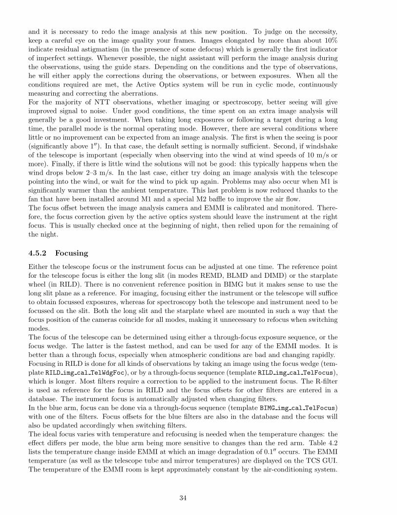
and it is necessary to redo the image analysis at this new position. To judge on the necessity,keep a careful eye on the image quality your frames. Images elongated by more than about 10%indicate residual astigmatism (in the presence of some defocus) which is generally the first indicatorof imperfect settings. Whenever possible, the night assistant will perform the image analysis duringthe observations, using the guide stars. Depending on the conditions and the type of observations,he will either apply the corrections during the observations, or between exposures. When all theconditions required are met, the Active Optics system will be run in cyclic mode, continuouslymeasuring and correcting the aberrations.For the majority of NTT observations, whether imaging or spectroscopy, better seeing will giveimproved signal to noise. Under good conditions, the time spent on an extra image analysis willgenerally be a good investment. When taking long exposures or following a target during a longtime, the parallel mode is the normal operating mode. However, there are several conditions wherelittle or no improvement can be expected from an image analysis. The first is when the seeing is poor(significantly above 1′′). In that case, the default setting is normally sufficient. Second, if windshakeof the telescope is important (especially when observing into the wind at wind speeds of 10 m/s ormore). Finally, if there is little wind the solutions will not be good: this typically happens when thewind drops below 2–3 m/s. In the last case, either try doing an image analysis with the telescopepointing into the wind, or wait for the wind to pick up again. Problems may also occur when M1 issignificantly warmer than the ambient temperature. This last problem is now reduced thanks to thefan that have been installed around M1 and a special M2 baffle to improve the air flow.The focus offset between the image analysis camera and EMMI is calibrated and monitored. There-fore, the focus correction given by the active optics system should leave the instrument at the rightfocus. This is usually checked once at the beginning of night, then relied upon for the remaining ofthe night.

4.5.2 Focusing

Either the telescope focus or the instrument focus can be adjusted at one time. The reference pointfor the telescope focus is either the long slit (in modes REMD, BLMD and DIMD) or the starplatewheel (in RILD). There is no convenient reference position in BIMG but it makes sense to use thelong slit plane as a reference. For imaging, focusing either the instrument or the telescope will sufficeto obtain focussed exposures, whereas for spectroscopy both the telescope and instrument need to befocussed on the slit. Both the long slit and the starplate wheel are mounted in such a way that thefocus position of the cameras coincide for all modes, making it unnecessary to refocus when switchingmodes.The focus of the telescope can be determined using either a through-focus exposure sequence, or thefocus wedge. The latter is the fastest method, and can be used for any of the EMMI modes. It isbetter than a through focus, especially when atmospheric conditions are bad and changing rapidly.Focusing in RILD is done for all kinds of observations by taking an image using the focus wedge (tem-plate RILD img cal TelWdgFoc), or by a through-focus sequence (template RILD img cal TelFocus),which is longer. Most filters require a correction to be applied to the instrument focus. The R-filteris used as reference for the focus in RILD and the focus offsets for other filters are entered in adatabase. The instrument focus is automatically adjusted when changing filters.In the blue arm, focus can be done via a through-focus sequence (template BIMG img cal TelFocus)with one of the filters. Focus offsets for the blue filters are also in the database and the focus willalso be updated accordingly when switching filters.The ideal focus varies with temperature and refocusing is needed when the temperature changes: theeffect differs per mode, the blue arm being more sensitive to changes than the red arm. Table 4.2lists the temperature change inside EMMI at which an image degradation of 0.1′′ occurs. The EMMItemperature (as well as the telescope tube and mirror temperatures) are displayed on the TCS GUI.The temperature of the EMMI room is kept approximately constant by the air-conditioning system.

34

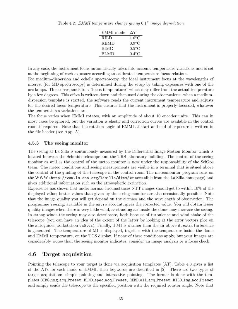
Table 4.2: EMMI temperature change giving 0.1′′ image degradation

EMMI mode ∆T

RILD 1.6◦CREMD 0.9◦CBIMG 0.5◦CBLMD 0.4◦C

In any case, the instrument focus automatically takes into account temperature variations and is setat the beginning of each exposure according to calibrated temperature-focus relations.For medium-dispersion and echelle spectroscopy, the ideal instrument focus at the wavelengths ofinterest (for MD spectroscopy) is determined during the setup by taking exposures with one of thearc lamps. This corresponds to a “focus temperature” which may differ from the actual temperatureby a few degrees. This offset is written down and then used during the observations: when a medium-dispersion template is started, the software reads the current instrument temperature and adjustsfor the desired focus temperature. This ensures that the instrument is properly focussed, whateverthe temperatures variations are.The focus varies when EMMI rotates, with an amplitude of about 10 encoder units. This can inmost cases be ignored, but the variation is elastic and correction curves are available in the controlroom if required. Note that the rotation angle of EMMI at start and end of exposure is written inthe file header (see App. A).

4.5.3 The seeing monitor

The seeing at La Silla is continuously measured by the Differential Image Motion Monitor which islocated between the Schmidt telescope and the TRS laboratory building. The control of the seeingmonitor as well as the control of the meteo monitor is now under the responsability of the SciOpsteam. The meteo conditions and seeing measurements are visible in a terminal that is situed abovethe control of the guiding of the telescope in the control room The meteomonitor program runs onthe WWW (http://www.ls.eso.org/lasilla/dimm/ or accessible from the La Silla homepage) andgives additional information such as the atmospheric extinction.Experience has shown that under normal circumstances NTT images should get to within 10% of thedisplayed value; better values than given by the seeing monitor are also occasionally possible. Notethat the image quality you will get depend on the airmass and the wavelength of observation. Theprogramme seeing, available in the astro account, gives the corrected value. You will obtain lesserquality images when there is very little wind, as standing air inside the dome may increase the seeing.In strong winds the seeing may also deteriorate, both because of turbulence and wind shake of thetelescope (you can have an idea of the extent of the latter by looking at the error vectors plot onthe autoguider workstation wa5tcs). Finally, if M1 is warmer than the air above it, extra turbulenceis generated. The temperature of M1 is displayed, together with the temperature inside the domeand EMMI temperature, on the TCS display. If none of these conditions apply, but your images areconsiderably worse than the seeing monitor indicates, consider an image analysis or a focus check.

4.6 Target acquisition

Pointing the telescope to your target is done via acquisition templates (AT). Table 4.3 gives a listof the ATs for each mode of EMMI, their keywords are described in [2]. There are two types oftarget acquisition: simple pointing and interactive pointing. The former is done with the tem-plates BIMG img acq Preset, BLMD spec acq Preset, REMD all acq Preset, RILD img acq Preset

and simply sends the telescope to the specified position with the required rotator angle. Note that

35

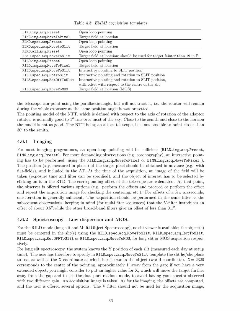
Table 4.3: EMMI acquisition templates

BIMG img acq Preset Open loop pointingBIMG img acq MoveToPixel Target field at locationBLMD spec acq Preset Open loop pointingBLMD spec acq MovetoSlit Target field at locationREMD all acq Preset Open loop pointingREMD spec acq MoveToSlit Target field at location; should be used for target fainter than 19 in RRILD img acq Preset Open loop pointingRILD img acq MoveToPixel Target field at locationRILD spec acq MoveToSlit Interactive pointing to SLIT positionRILD spec acq RotToSlit Interactive pointing and rotation to SLIT positionRILS spec acq RotOffToSlit Interactive pointing and rotation to SLIT position,

with offset with respect to the centre of the slitRILD spec acq MoveToMOS Target field at location (MOS)

the telescope can point using the parallactic angle, but will not track it, i.e. the rotator will remainduring the whole exposure at the same position angle it was presetted.The pointing model of the NTT, which is defined with respect to the axis of rotation of the adaptorrotator, is normally good to 1′′ rms over most of the sky. Close to the zenith and close to the horizonthe model is not as good. The NTT being an alt–az telescope, it is not possible to point closer than30′ to the zenith.

4.6.1 Imaging

For most imaging programmes, an open loop pointing will be sufficient (RILD img acq Preset,BIMG img acq Preset). For more demanding observations (e.g. coronography), an interactive point-ing has to be performed, using the RILD img acq MoveToPixel or BIMG img acq MoveToPixel ).The position (x,y, measured in pixels) of the target pixel should be obtained in advance (e.g. withflat-fields), and included in the AT. At the time of the acquisition, an image of the field will betaken (exposure time and filter can be specified), and the object of interest has to be selected byclicking on it in the RTD. The corresponding offset of the telescope are calculated. At that point,the observer is offered various options (e.g. perform the offsets and proceed or perform the offsetand repeat the acquisition image for checking the centering, etc.). For offsets of a few arcseconds,one iteration is generally sufficient. The acquisition should be performed in the same filter as thesubsequent observations, keeping in mind (for multi fiter sequences) that the V-filter introduces anoffset of about 0.5′′,while the other broad-band filters give an offset of less than 0.1′′.

4.6.2 Spectroscopy - Low dispersion and MOS.

For the RILD mode (long slit and Multi Object Spectroscopy), no slit viewer is available; the object(s)must be centered in the slit(s) using the RILD spec acq MoveToSlit, RILD spec acq RotToSlit,RILD spec acq RotOFFToSlit or RILD spec acq MoveToMOS, for long slit or MOS acqusition respec-tively.For long slit spectroscopy, the system knows the Y position of each slit (measured each day at setuptime). The user has therefore to specify in RILD spec acq MoveToSlit template the slit he/she plansto use, as well as the X coordinate at which he/she wants the object (world coordinate). X= 2320corresponds to the center of the pointing, approximately 1’ away from the gap; if you have a veryextended object, you might consider to put an higher value for X, which will move the target furtheraway from the gap and to use the dual port readout mode, to avoid having your spectra observedwith two different gain. An acquisition image is taken. As for the imaging, the offsets are computed,and the user is offered several options. The V filter should not be used for the acquisition image,

36

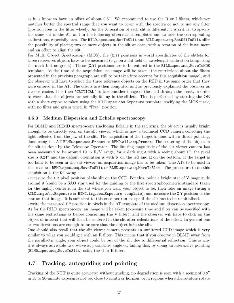
as it is know to have an offset of about 0.5′′. We recommend to use the R or I filters, whichevermatches better the spectral range that you want to cover with the spectra or not to use any filter(position free in the filter wheel). As the X position of each slit is different, it is critical to specifythe same slit in the AT and in the following observation templates and to take the correspondingcalibrations, especially arcs. The RILD spec acq RotToSlit and RILD spec acq RotOffToSlit offerthe possibility of placing two or more objects in the slit at once, with a rotation of the instrumentand an offset to align the slit.For Multi Object Spectroscopy (MOS), the (X,Y) positions in world coordinates of the slitlets forthree references objects have to be measured (e.g. on a flat field or wavelenght calibration lamp usingthe mask but no grism). These (X,Y) positions are to be entered in the RILD spec acq MoveToMOS

template. At the time of the acquisition, an image will be taken (the restrictions about the filterspresented in the previous paragraph are still to be taken into account for this acquisition image), andthe observer will have to select the three reference objects on the RTD in the same order that theywere entered in the AT. The offsets are then computed and as previously explained the observer asvarious choice. It is then *CRITICAL* to take another image of the field through the mask, in orderto check that the objects are actually falling in the slitlets. This is performed by starting the OBwith a short exposure taken using the RILD spec obs Exposure template, spcifying the MOS mask,with no filter and grism wheel in “Free” position.

4.6.3 Medium Dispersion and Echelle spectroscopy

For BLMD and REMD spectroscopy (including Echelle in the red arm), the object is usually brightenough to be directly seen on the slit viewer, which is now a technical CCD camera collecting thelight reflected from the jaw of the slit. The acquisition of the target is done with a direct pointing,done using the AT BLMD spec acq Preset or REMD all acq Preset. The centering of the object inthe slit us done by the Telescope Operator. The limiting magnitude of the slit viewer camera hasbeen measured to be around 19 in R/V range, for a dark night with a seeing about 1′′; the pixelsize is 0.24” and the default orientation is with N on the left and E on the bottom. If the target istoo faint to be seen in the slit viewer, an acquisition image has to be taken. The ATs to be used inthis case are REMD spec acq MoveToSlit or BLMD spec acq MoveToSlit. The procedure to do thisacquisition is the following :- measure the X Y pixel position of the slit on the CCD. For this, point a bright star of V magnitudearound 9 (could be a SAO star used for the guiding or the first spectrophotometric standard takenfor the night), center it in the slit where you want your object to be, then take an image (using aRILD img obs Exposure or BIMG img obs Exposure template), and measure the X Y position of thestar on that image. It is sufficient to this once per run except if the slit has to be reinitialised.- write the measured X Y position in pixels in the AT template of the medium dispersion spectroscopy.As for the RILD spectroscopy, an image will be taken (exposure time and filter can be specified withthe same restrictions as before concerning the V filter), and the observer will have to click on theobject of interest that will then be centered in the slit after calculations of the offset. In general oneor two iterations are enough to be sure that the object is in the slit.One should also recall that the slit viewer camera presents an unfiltered CCD image which is verysimilar to what you would get with an R filter. This means that if you observe in BLMD away fromthe parallactic angle, your object could be out of the slit due to differential refraction. This is whyit is always advisable to observe at parallactic angle or, failing this, by doing an interactive pointing(BLMD spec acq MoveToSlit) using the U or B filter.

4.7 Tracking, autoguiding and pointing

Tracking of the NTT is quite accurate: without guiding, no degradation is seen with a seeing of 0.8′′

in 15 to 20-minute exposures not too close to zenith or horizon, or in regions where the rotators rotate

37

rapidly (these positions are available in the control room). Because the pointing model corrects foratmospheric refraction which is wavelength dependent, the central wavelength used in the scientificexposures can be set in the TCS to achieve a very high precision. However, for most observations,using the default value of 650 nm is sufficient.Guiding the telescope during an exposure is usually done by setting one of the two guide probeslocated in the rotator/adapter on a star and using the autoguider. After each telescope preset, a listof suitable guide stars is displayed on the autoguider panel. The night assistant selects one of themand starts the guiding. The acquisition is done by a technical CCD, upgraded in November 2005,which default orientation is North on the top and East to the left, with a field of view of 1.7′×1.7′, anda scale of 0.2′′/pix. The resolution of the guide probes is 0.05′′. As the autoguider only corrects thealtitude and azimuth motions, tracking inaccuracies of the rotator may induce image displacements.Note that in case of poor seeing or strong wind, autoguiding may make the images worse since thecorrections always lag behind actual conditions. In such conditions, it is better to lower the frequencyof the corrections to average the effects.It is also possible to observe moving targets with the NTT, but this is not implemented in the auto-guider. Presently the best way is to use the tracking model, and to supply differential tracking rates,in arcsec/sec. The expected accuracy is the same as for simple tracking since the telescope is alt-azimutal, it doesn’t care if the tracking is sidereal or not. For grating spectroscopy, the slit-viewercan be used for sufficiently bright targets to check they stay in the slit. For all other cases, careshould be taken in re-acquiring the moving object in the slit on average each 10m, depending on thetelescope position and on the target speed.The NTT has an Altitude-Azimutal mounting and, as a consequence, the singularity is in the Zenithand not in the pole. When observing very close to the Zenith, the telescope building and the rotatorhave to rotate very fast in order to track the object. The result will be a poor image quality, lessaccurate pointing and problems with the positioning of the object in the slit for spectrocopy. In theworst case scenario, if we point too close to the Zenith, the system can crash. A software interlock

will trigger at telescope elevations of 89◦ and 10◦ respectively, while an hardware interlock willtrigger at telescope elevations of 90◦ and 8.9◦ respectively. Users should be aware of the fact that,once the hardware interlock has been activated, a considerable amount of time will be neeeded torecover the telescope.In order to avoid such problem, it is advisable to respect the following limitations.

• Never, ever point within 5 degrees from Zenith (-32<dec<-26, HA < 00:10:00)

• Never, ever observe within 5 degrees from Zenith (-32<dec<-26, HA < 00:10:00)

• In the -32 to -27 range do NOT observe within 15 minute from the meridian.

• In the -50 to -10 range be aware that you may get bad surprises within 15 degrees from themeridian.

In all cases, AO should not be attempted at elevation < 40◦ and optics adjustment must be done atelevation below 20◦, not even M2 focus adjustment for temperature variations.

4.8 The Real-Time Display

The RTD (Fig. 4.4) is a very complete tool. It is essentially a FITS viewer, but with much morecapability: not only can it display previously acquired images, but it may be connected to any ofthe scientific or technical CCDs and display images as they are read-out. Several RTDs are usuallyrunning in the control room: one for the autoguider, one for the slit viewer when observing with oneof the medium-dispersion modes, and two for each of the scientific CCDs in use. One of the latterruns on wemmi and is used to specify the right target in an interactive pointing.

38

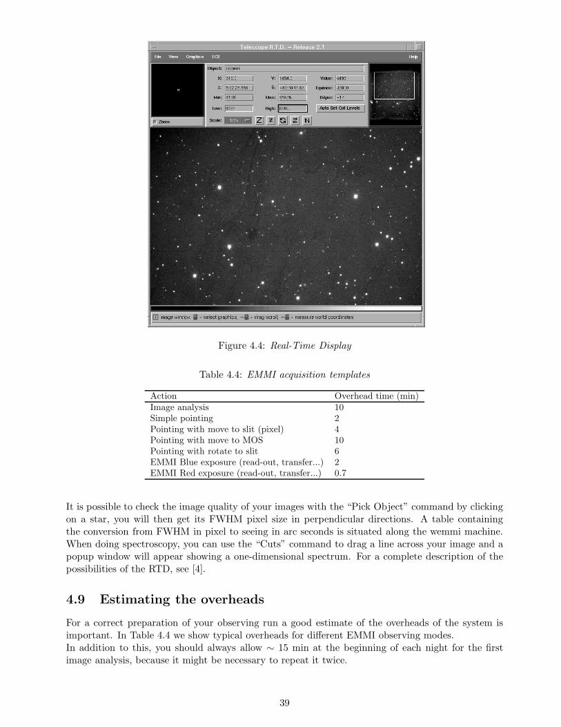
Figure 4.4: Real-Time Display

Table 4.4: EMMI acquisition templates

Action Overhead time (min)Image analysis 10Simple pointing 2Pointing with move to slit (pixel) 4Pointing with move to MOS 10Pointing with rotate to slit 6EMMI Blue exposure (read-out, transfer...) 2EMMI Red exposure (read-out, transfer...) 0.7

It is possible to check the image quality of your images with the “Pick Object” command by clickingon a star, you will then get its FWHM pixel size in perpendicular directions. A table containingthe conversion from FWHM in pixel to seeing in arc seconds is situated along the wemmi machine.When doing spectroscopy, you can use the “Cuts” command to drag a line across your image and apopup window will appear showing a one-dimensional spectrum. For a complete description of thepossibilities of the RTD, see [4].

4.9 Estimating the overheads

For a correct preparation of your observing run a good estimate of the overheads of the system isimportant. In Table 4.4 we show typical overheads for different EMMI observing modes.In addition to this, you should always allow ∼ 15 min at the beginning of each night for the firstimage analysis, because it might be necessary to repeat it twice.

39

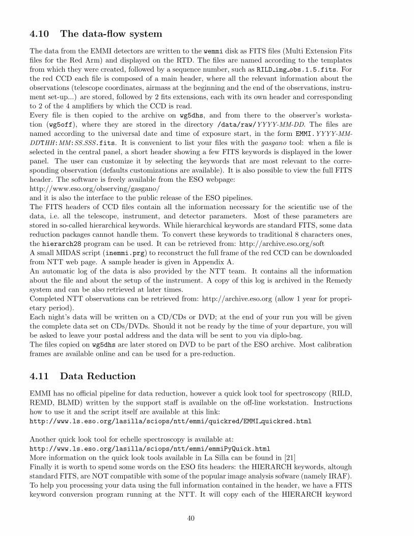
4.10 The data-flow system

The data from the EMMI detectors are written to the wemmi disk as FITS files (Multi Extension Fitsfiles for the Red Arm) and displayed on the RTD. The files are named according to the templatesfrom which they were created, followed by a sequence number, such as RILD img obs.1.5.fits. Forthe red CCD each file is composed of a main header, where all the relevant information about theobservations (telescope coordinates, airmass at the beginning and the end of the observations, instru-ment set-up...) are stored, followed by 2 fits extensions, each with its own header and correspondingto 2 of the 4 amplifiers by which the CCD is read.Every file is then copied to the archive on wg5dhs, and from there to the observer’s worksta-tion (wg5off), where they are stored in the directory /data/raw/YYYY-MM-DD. The files arenamed according to the universal date and time of exposure start, in the form EMMI.YYYY-MM-

DDTHH:MM:SS.SSS.fits. It is convenient to list your files with the gasgano tool: when a file isselected in the central panel, a short header showing a few FITS keywords is displayed in the lowerpanel. The user can customize it by selecting the keywords that are most relevant to the corre-sponding observation (defaults customizations are available). It is also possible to view the full FITSheader. The software is freely available from the ESO webpage:http://www.eso.org/observing/gasgano/and it is also the interface to the public release of the ESO pipelines.The FITS headers of CCD files contain all the information necessary for the scientific use of thedata, i.e. all the telescope, instrument, and detector parameters. Most of these parameters arestored in so-called hierarchical keywords. While hierarchical keywords are standard FITS, some datareduction packages cannot handle them. To convert these keywords to traditional 8 characters ones,the hierarch28 program can be used. It can be retrieved from: http://archive.eso.org/softA small MIDAS script (inemmi.prg) to reconstruct the full frame of the red CCD can be downloadedfrom NTT web page. A sample header is given in Appendix A.An automatic log of the data is also provided by the NTT team. It contains all the informationabout the file and about the setup of the instrument. A copy of this log is archived in the Remedysystem and can be also retrieved at later times.Completed NTT observations can be retrieved from: http://archive.eso.org (allow 1 year for propri-etary period).Each night’s data will be written on a CD/CDs or DVD; at the end of your run you will be giventhe complete data set on CDs/DVDs. Should it not be ready by the time of your departure, you willbe asked to leave your postal address and the data will be sent to you via diplo-bag.The files copied on wg5dhs are later stored on DVD to be part of the ESO archive. Most calibrationframes are available online and can be used for a pre-reduction.

4.11 Data Reduction

EMMI has no official pipeline for data reduction, however a quick look tool for spectroscopy (RILD,REMD, BLMD) written by the support staff is available on the off-line workstation. Instructionshow to use it and the script itself are available at this link:http://www.ls.eso.org/lasilla/sciops/ntt/emmi/quickred/EMMI quickred.html

Another quick look tool for echelle spectroscopy is available at:http://www.ls.eso.org/lasilla/sciops/ntt/emmi/emmiPyQuick.html

More information on the quick look tools available in La Silla can be found in [21]Finally it is worth to spend some words on the ESO fits headers: the HIERARCH keywords, altoughstandard FITS, are NOT compatible with some of the popular image analysis sofware (namely IRAF).To help you processing your data using the full information contained in the header, we have a FITSkeyword conversion program running at the NTT. It will copy each of the HIERARCH keyword

40

into another keyword whose name is on word of 8 or less characters (i.e. IRAF compatible), withthe price, however, of slightly more cryptic names like IFIL3NM for HIERARCH ESO INS FILT3NAME. To run this program, type corrfitsIraf filename to convert one file, or corrfits EMMI*fitsto convert all the images from your directory.corrfitsIraf only run on the ESO machines and cannot be exported; alternatively you can try theFTU, short for Fits Transform Utility, which can be downloaded together with a collection of otherFITS tools from: http://archive.eso.org/soft.Users of Eclipse and scisoft packages should be aware that these tools are already included in thedistribution of the software.

41

42

Chapter 5

Calibration

Numerous calibration templates exist for EMMI, to acquire biases or darks, dome or twilight flatfields, or wavelength calibration exposures. They are listed in Table 5.1 and a complete descriptionof their keywords can be found in [2]. An automatic script, called CalObBuild, is now available: thisscript will check the header of the frames taken during the night and automatically create an OBwhich includes all the calibration templates needed. The OB is then run by the day crew. SinceCalObBuild will produce only the minimum amount of calibrations required by EMMI calibrationplan, the observers are strongly encouraged to take their own calibrations in the afternoon.

5.1 Calibration unit

There exists a system of calibration lamps associated with the adapter/rotators at the NTT whichcan be used for most of the wavelength calibrations required for EMMI data. The main componentof the calibration system is an integrating sphere mounted on the side of the adapter. Light fromthe output aperture of the integrating sphere passes through a lens and it is reflected onto the centerof the focal plane by a 45◦ mirror which is moved into the optical axis. On the integrating sphereHe, Ar, and ThAr lamps are mounted, while the light from flatfield or other spectral lamps that aremounted in a rack on the floor which is fed to the sphere through an optical fibre. The fiber inducessome broad absorption features around 724µm and 880µm. The angular size, location, and shape(including central obscuration) of the NTT exit pupil are approximately simulated. The illuminationis homogeneous and unvignetted in a 3′ × 6′ field and is still usable in a field of 5′ × 8′ which is themaximum field size for MOS.For imaging programs, especially those using narrow band filters it is recommeded to use sky flats,taking also into account the bigger size of the new chip. We also recommend to take at least onesky flat for all the spectroscopic programs targeting extended objects, in order to derive the slitillumination function.

5.2 Bias and dark current

To measure the bias level introduced by the detector electronics, a set of 5–10 bias frames are sufficientfor most purposes, unless the programme is limited by read noise, in which case it is recommended totake about 25 frames. They should always be taken with the same CCD parameters (readout mode,windowing, binning) as your science data.The very low dark current of the EMMI CCDs makes it hardly necessary to measure it. Observersinsisting on taking dark frames should take exposures at least as long as the longest science frame.However, due to the large amount of time such frames will take on the daytime operations, observersare encouraged to use dark frames taken by the staff during the periodic CCD tests (see Sect. 5.8).Both types of frames can be taken using the templates BIMG img cal Darks, BLMD spec cal Darks,REMD all cal Darks, or RILD all cal Darks. The selection between bias and dark frames is done

43

Table 5.1: EMMI calibration templates

BIMG img cal Darks Blue CCD biases or darksBIMG img cal DomeFF Blue Imaging: Dome Flat FieldBIMG img cal SkyFF Blue Imaging: Twilight Sky Flat FieldBIMG img cal TelFocus Blue Imaging: Thru Focus SequenceBLMD spec cal Darks Blue CCD biases or darksBLMD spec cal Flats Blue Medium Dispersion: Dome Flat FieldBLMD spec cal Arcs Blue Medium Dispersion Wavelength calibrationREMD all cal Darks Red CCD biases or darksREMD spec cal Flats Red Medium Dispersion: Dome Flat FieldREMD spec cal Arcs Red Medium Dispersion Wavelength calibrationREMD ech cal Flats Echelle: Dome Flat FieldREMD ech cal Arcs Echelle Wavelength calibrationRILD all cal Darks Red CCD biases or darksRILD img cal DomeFF Red Imaging: Dome Flat FieldRILD img cal IntFF Red Imaging: Internal Lamp Flat FieldRILD img cal SkyFF Red Imaging: Twilight Sky Flat FieldRILD img cal TelFocus Red Imaging: Thru Focus SequenceRILD img cal TelWdgFoc Red Imaging: Focus wedgeRILD spec cal Flats Red Low Dispersion spectrum: Internal Lamp or Dome Flat FieldRILD spec cal SkyFF Red Low Dispersion spectrum: Sky Flat FieldRILD spec cal Arcs Red Low Dispersion Wavelength calibration

by setting the exposure time to zero or to a non-zero value, respectively.

5.3 Flat fields

Flat fields can be obtained from internal lamps, dome flats, twilight flats and night-sky flats. Theymust be obtained in the same readout mode and binning as the science exposures. The use of internallamps is not encouraged, except for RILD mode, because they are weak and because of the absorptionbands caused by the optical fiber (see Sect. 5.1).Dome flats are obtained by pointing the telescope at a white screen inside the dome, which can beilluminated by slightly opening the dome flaps or by a halogen lamp. For demanding applications(mainly echelle spectroscopy and spectroscopy at short wavelengths), up to 8400W of power areavailable. Internal lamp and dome flat fields can be taken with the templates BIMG img cal DomeFF,BLMD spec cal Flats, REMD spec cal Flats, REMD ech cal Flats, RILD img cal DomeFF,RILD spec cal Flats, or RILD spec cal IntFF. The user has to enter the desired count level, andthe template will take a short test frame to determine the suitable exposure time and the amount oflight illumination in the dome to reach the desired level, then it will continue automatically.Twilight flats can be taken on the sky during morning and evening twilight; sky flats with narrowband filters however are possible only during the afternoon. For imaging with broad-band filters, thisis possible for about 30 minutes around −12◦ twilight; for imaging with narrow-band filters and forspectroscopy, exposures should be done close to sunrise and sunset. They are obtained by using thetemplates BIMG img cal SkyFF, RILD img cal SkyFF, or RILD spec cal SkyFF. No sky flat templateis available for the medium dispersion modes, but a sky flat can nevertheless be obtained by usingthe BLMD spec cal Flats, REMD spec cal Flats templates and setting the number of exposures to1. The user enters the desired count level, and the template takes a short test frame and uses theTyson & Gal [22] algorithm to calculate the appropriate sequence of exposure times accounting forthe dimming or brightening of the sky. A list of sparsely populated (“empty”) fields which are nor-mally used for twilight flats and sky flats is available as a catalog in the TCS and can also be viewed at:http://www.ls.eso.org/lasilla/Telescopes/2p2T/D1p5M/misc/EmptyFields.html. The night assistant

44

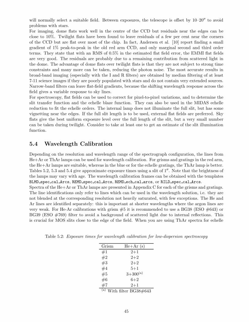
will normally select a suitable field. Between exposures, the telescope is offset by 10–20′′ to avoidproblems with stars.For imaging, dome flats work well in the centre of the CCD but residuals near the edges can beclose to 10%. Twilight flats have been found to leave residuals of a few per cent near the cornersof the CCD but are flat over most of the chip. In fact, Andersen et al. [10] report finding a smallgradient of 1% peak-to-peak in the old red arm CCD, and only marginal second and third orderterms. They state that with an RMS of 0.5% in the estimated flat field error, the EMMI flat fieldsare very good. The residuals are probably due to a remaining contribution from scattered light inthe dome. The advantage of dome flats over twilight flats is that they are not subject to strong timeconstraints and many more can be taken, reducing the photon noise. The most accurate results inbroad-band imaging (especially with the I and R filters) are obtained by median filtering of at least7-11 science images if they are poorly populated with stars and do not contain very extended sources.Narrow-band filters can leave flat-field gradients, because the shifting wavelength response across thefield gives a variable response to sky lines.For spectroscopy, flat fields can be used to correct for pixel-to-pixel variations, and to determine theslit transfer function and the echelle blaze function. They can also be used in the MIDAS echellereduction to fit the echelle orders. The internal lamp does not illuminate the full slit, but has somevignetting near the edges. If the full slit length is to be used, external flat fields are preferred. Skyflats give the best uniform exposure level over the full length of the slit, but a very small numbercan be taken during twilight. Consider to take at least one to get an estimate of the slit illuminationfunction.

5.4 Wavelength Calibration

Depending on the resolution and wavelength range of the spectrograph configuration, the lines fromHe+Ar or ThAr lamps can be used for wavelength calibration. For grisms and gratings in the red arm,the He+Ar lamps are suitable, whereas in the blue or for the echelle gratings, the ThAr lamp is better.Tables 5.2, 5.3 and 5.4 give approximate exposure times using a slit of 1′′. Note that the brightness ofthe lamps may vary with age. The wavelength calibration frames can be obtained with the templatesBLMD spec cal Arcs, REMD spec cal Arcs, REMD ech cal arcs, or RILD spec cal Arcs.Spectra of the He+Ar or ThAr lamps are presented in Appendix C for each of the grisms and gratings.The line identifications only refer to lines which can be used in the wavelength solution, i.e. they arenot blended at the corresponding resolution not heavily saturated, with few exceptions. The He andAr lines are identified separately: this is important at shorter wavelengths where the argon lines arevery weak. For He-Ar calibrations with grism #5 it is recommended to use a BG38 (ESO #643) orBG39 (ESO #769) filter to avoid a background of scattered light due to internal reflections. Thisis crucial for MOS slits close to the edge of the field. When you are using ThAr spectra for echelle

Table 5.2: Exposure times for wavelength calibration for low-dispersion spectroscopy

Grism He+Ar (s)

#1 2+1#2 2+2#3 2+2#4 5+1

#5 3+300(a)

#6 6+2#7 2+1(a) With filter BG38#643

45

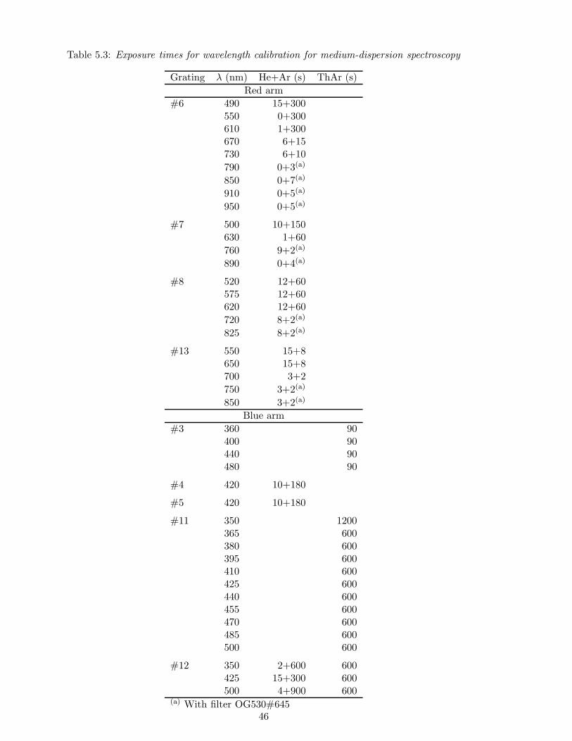
Table 5.3: Exposure times for wavelength calibration for medium-dispersion spectroscopy

Grating λ (nm) He+Ar (s) ThAr (s)

Red arm

#6 490 15+300550 0+300610 1+300670 6+15730 6+10

790 0+3(a)

850 0+7(a)

910 0+5(a)

950 0+5(a)

#7 500 10+150630 1+60

760 9+2(a)

890 0+4(a)

#8 520 12+60575 12+60620 12+60

720 8+2(a)

825 8+2(a)

#13 550 15+8650 15+8700 3+2

750 3+2(a)

850 3+2(a)

Blue arm

#3 360 90400 90440 90480 90

#4 420 10+180

#5 420 10+180

#11 350 1200365 600380 600395 600410 600425 600440 600455 600470 600485 600500 600

#12 350 2+600 600425 15+300 600500 4+900 600

(a) With filter OG530#64546

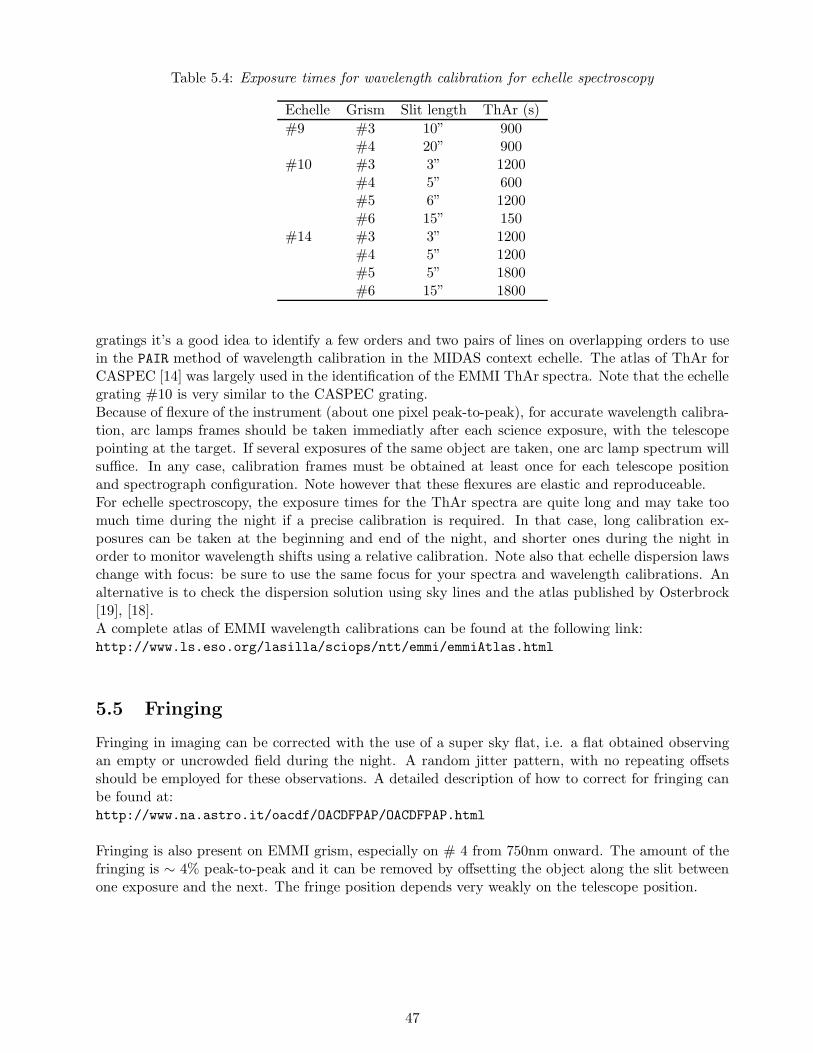
Table 5.4: Exposure times for wavelength calibration for echelle spectroscopy

Echelle Grism Slit length ThAr (s)

#9 #3 10” 900#4 20” 900

#10 #3 3” 1200#4 5” 600#5 6” 1200#6 15” 150

#14 #3 3” 1200#4 5” 1200#5 5” 1800#6 15” 1800

gratings it’s a good idea to identify a few orders and two pairs of lines on overlapping orders to usein the PAIR method of wavelength calibration in the MIDAS context echelle. The atlas of ThAr forCASPEC [14] was largely used in the identification of the EMMI ThAr spectra. Note that the echellegrating #10 is very similar to the CASPEC grating.Because of flexure of the instrument (about one pixel peak-to-peak), for accurate wavelength calibra-tion, arc lamps frames should be taken immediatly after each science exposure, with the telescopepointing at the target. If several exposures of the same object are taken, one arc lamp spectrum willsuffice. In any case, calibration frames must be obtained at least once for each telescope positionand spectrograph configuration. Note however that these flexures are elastic and reproduceable.For echelle spectroscopy, the exposure times for the ThAr spectra are quite long and may take toomuch time during the night if a precise calibration is required. In that case, long calibration ex-posures can be taken at the beginning and end of the night, and shorter ones during the night inorder to monitor wavelength shifts using a relative calibration. Note also that echelle dispersion lawschange with focus: be sure to use the same focus for your spectra and wavelength calibrations. Analternative is to check the dispersion solution using sky lines and the atlas published by Osterbrock[19], [18].A complete atlas of EMMI wavelength calibrations can be found at the following link:http://www.ls.eso.org/lasilla/sciops/ntt/emmi/emmiAtlas.html

5.5 Fringing

Fringing in imaging can be corrected with the use of a super sky flat, i.e. a flat obtained observingan empty or uncrowded field during the night. A random jitter pattern, with no repeating offsetsshould be employed for these observations. A detailed description of how to correct for fringing canbe found at:http://www.na.astro.it/oacdf/OACDFPAP/OACDFPAP.html

Fringing is also present on EMMI grism, especially on # 4 from 750nm onward. The amount of thefringing is ∼ 4% peak-to-peak and it can be removed by offsetting the object along the slit betweenone exposure and the next. The fringe position depends very weakly on the telescope position.

47

5.6 Photometric Calibration

The transformation from instrumental magnitudes to “standard” magnitudes, the extinction coeffi-cients, and the colour terms are obtained by the observation of photometric standard stars. A setof predefined OBs to observe a sample of Landolt [17] standard fields in the most commonly usedbroad-band filters and for each readout mode has been created and is available to the observers. Thefields are close to the celestial equator and cover the whole right ascenscion range. A document [5]describes these OBs, gives finding charts, and lists magnitudes and colours of the standard stars.The OBs are available in the NTT local repository and can be imported into P2PP at the beginningof the night or during the observations.A nice MIDAS tool to get a full photometric solution can be found at:http://www.sc.eso.org/ ohainaut/bin/tmag.cgi

otherwise you can use the package photcal in IRAF.

5.7 Spectrophotometric Calibration

An absolute flux calibration of your spectra can be obtained by observing spectrophotometric stan-dard stars through a wide (≥ 5′′) slit. If the atmospheric extinction curve is important, it can bedetermined by the observation of three standard stars at airmasses close to 1.0, 1.5 and 2.0.A set of predefined OBs to observe a sample of Hamuy et al. [15, 16] spectrophotometric standardstars for each grism and echelle grating with a slit of 1′′ or 5′′ and for each readout mode hasbeen created and is available to the observers. A document [6] describes these OBs, and givesfinding charts and flux plots for the standard stars. Alternatively this information can be found at:http://www.eso.org/observing/standards/spectra/These OBs can be imported from the disk by the observer to be executed in the telescope. Nopredefined OBs exist for narrow band imaging or for medium dispersion gratings. In the last casethis is because of the large number of possible central wavelengths, but the information given in [6],together with a list of exposure times, can be used to create OBs.

5.8 The Calibration Plan

The upgrade to the VLT data flow system and the implementation of service observing at the NTTmakes it necessary to define the minimal set of calibration data required for each observation andto ensure that this set is available to service observers and archive users. Visiting astronomers areencouraged to adhere to this calibration plan, as this will allow the building of a calibration databasefrom which they will benefit, and which will be used for quick look of data at the telescope, butalso to take all the calibrations they see fit for their science program. We stress once more that thevisitors must take their own calibrations. The database contains bias frames, dark frames, dome andtwilight flats fields, images of photometric standards and spectra of spectrophotometric standards, aswell as hot pixel, dark pixel, and trap masks for both CCDs. Only the most commonly used modesof EMMI and one CCD configuration are or will be supported.The calibration plan requires that biases and flat fields corresponding to the observations done duringa given night, with the same CCD parameters, be taken during the afternoon by the day operatorand the visitor, or, if some problem occcurs, the following morning, by executing the CalObBuildscript. At night, the observer is expected to take the relevant photometric and spectrophotometricstandards and wavelength calibration exposures. For more specific needs, the observer can takeadditional calibrations at night, or request them from the day operator as long as the total timespent on daytime calibrations does not exceed two hours. In case of observing mode requiringlong calibration (echelle for example) this time can be exceeded after discussion with the supportastronomer, but it is always preferred that the observer takes his/her own calibrations during theafternoon.

48

More information about the calibration plan can be found inhttp://www.ls.eso.org/lasilla/sciops/observing/service.html.

49

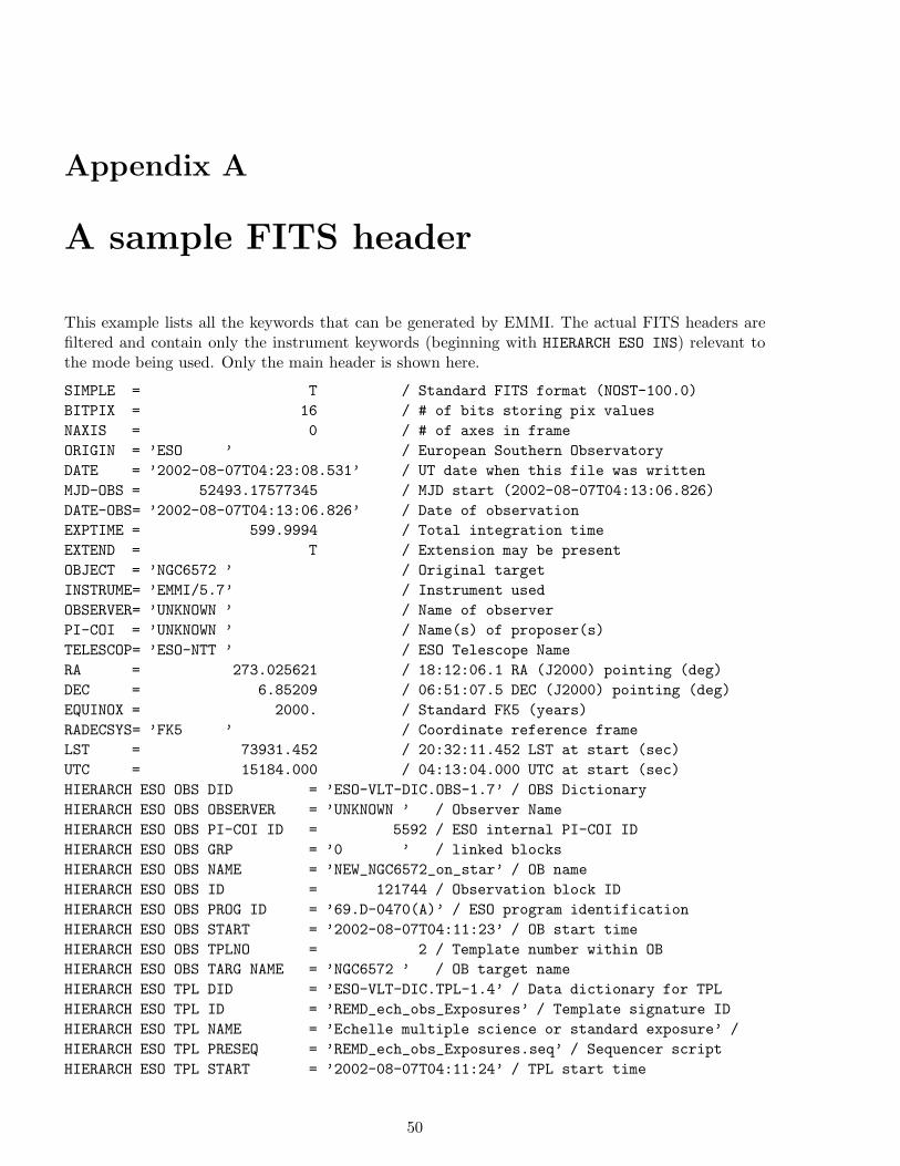
Appendix A

A sample FITS header

This example lists all the keywords that can be generated by EMMI. The actual FITS headers arefiltered and contain only the instrument keywords (beginning with HIERARCH ESO INS) relevant tothe mode being used. Only the main header is shown here.

SIMPLE = T / Standard FITS format (NOST-100.0)

BITPIX = 16 / # of bits storing pix values

NAXIS = 0 / # of axes in frame

ORIGIN = ’ESO ’ / European Southern Observatory

DATE = ’2002-08-07T04:23:08.531’ / UT date when this file was written

MJD-OBS = 52493.17577345 / MJD start (2002-08-07T04:13:06.826)

DATE-OBS= ’2002-08-07T04:13:06.826’ / Date of observation

EXPTIME = 599.9994 / Total integration time

EXTEND = T / Extension may be present

OBJECT = ’NGC6572 ’ / Original target

INSTRUME= ’EMMI/5.7’ / Instrument used

OBSERVER= ’UNKNOWN ’ / Name of observer

PI-COI = ’UNKNOWN ’ / Name(s) of proposer(s)

TELESCOP= ’ESO-NTT ’ / ESO Telescope Name

RA = 273.025621 / 18:12:06.1 RA (J2000) pointing (deg)

DEC = 6.85209 / 06:51:07.5 DEC (J2000) pointing (deg)

EQUINOX = 2000. / Standard FK5 (years)

RADECSYS= ’FK5 ’ / Coordinate reference frame

LST = 73931.452 / 20:32:11.452 LST at start (sec)

UTC = 15184.000 / 04:13:04.000 UTC at start (sec)

HIERARCH ESO OBS DID = ’ESO-VLT-DIC.OBS-1.7’ / OBS Dictionary

HIERARCH ESO OBS OBSERVER = ’UNKNOWN ’ / Observer Name

HIERARCH ESO OBS PI-COI ID = 5592 / ESO internal PI-COI ID

HIERARCH ESO OBS GRP = ’0 ’ / linked blocks

HIERARCH ESO OBS NAME = ’NEW_NGC6572_on_star’ / OB name

HIERARCH ESO OBS ID = 121744 / Observation block ID

HIERARCH ESO OBS PROG ID = ’69.D-0470(A)’ / ESO program identification

HIERARCH ESO OBS START = ’2002-08-07T04:11:23’ / OB start time

HIERARCH ESO OBS TPLNO = 2 / Template number within OB

HIERARCH ESO OBS TARG NAME = ’NGC6572 ’ / OB target name

HIERARCH ESO TPL DID = ’ESO-VLT-DIC.TPL-1.4’ / Data dictionary for TPL

HIERARCH ESO TPL ID = ’REMD_ech_obs_Exposures’ / Template signature ID

HIERARCH ESO TPL NAME = ’Echelle multiple science or standard exposure’ /

HIERARCH ESO TPL PRESEQ = ’REMD_ech_obs_Exposures.seq’ / Sequencer script

HIERARCH ESO TPL START = ’2002-08-07T04:11:24’ / TPL start time

50

HIERARCH ESO TPL VERSION = ’1.0 ’ / Version of the template

HIERARCH ESO TPL NEXP = 1 / Number of exposures within template

HIERARCH ESO TPL EXPNO = 1 / Exposure number within template

HIERARCH ESO DPR CATG = ’SCIENCE ’ / Observation category

HIERARCH ESO DPR TECH = ’ECHELLE ’ / Observation technique

HIERARCH ESO TEL DID = ’ESO-VLT-DIC.TCS’ / Data dictionary for TEL

HIERARCH ESO TEL ID = ’v 5.0 ’ / TCS version number

HIERARCH ESO TEL DATE = ’not set ’ / TCS installation date

HIERARCH ESO TEL ALT = 40.654 / Alt angle at start (deg)

HIERARCH ESO TEL AZ = 131.385 / Az angle at start (deg) S=0,W=90

HIERARCH ESO TEL GEOELEV = 2377. / Elevation above sea level (m)

HIERARCH ESO TEL GEOLAT = -29.2584 / Tel geo latitute (+=North) (deg)

HIERARCH ESO TEL GEOLON = -70.7345 / Tel geo longitute (+=East) (deg)

HIERARCH ESO TEL OPER = ’NTT TIO ’ / Telescope Operator

HIERARCH ESO TEL FOCU ID = ’NB ’ / Telescope focus station ID

HIERARCH ESO TEL FOCU LEN = 120.000 / Focal length (m)

HIERARCH ESO TEL FOCU SCALE = 1.718 / Focal scale (arcsec/mm)

HIERARCH ESO TEL FOCU VALUE = -3.854 / M2 setting (mm)

HIERARCH ESO TEL PARANG START= 138.753 / Parallactic angle at start (deg)

HIERARCH ESO TEL AIRM START = 1.533 / Airmass at start

HIERARCH ESO TEL AMBI WINDSP = 3.75 / Observatory ambient wind speed query

HIERARCH ESO TEL AMBI WINDDIR= 358. / Observatory ambient wind direction

HIERARCH ESO TEL AMBI RHUM = 39. / Observatory ambient relative humidity

HIERARCH ESO TEL AMBI TEMP = 8.95 / Observatory ambient temperature query

HIERARCH ESO TEL MOON RA = 74129.683026 / ~~:~~:~~.~ RA (J2000) (deg)

HIERARCH ESO TEL MOON DEC = 243453.47151 / ~~:~~:~~.~ DEC (J2000) (deg)

HIERARCH ESO TEL TRAK STATUS = ’NORMAL ’ / Tracking status

HIERARCH ESO TEL DOME STATUS = ’FULLY-OPEN’ / Dome status

HIERARCH ESO TEL CHOP ST = F / True when chopping is active

HIERARCH ESO TEL PARANG END = 136.864 / Parallactic angle at end (deg)

HIERARCH ESO TEL AIRM END = 1.589 / Airmass at end

HIERARCH ESO ADA ABSROT START= 138.19991 / Abs rot angle at exp start (deg)

HIERARCH ESO ADA POSANG = 140.36500 / Position angle at start

HIERARCH ESO ADA GUID STATUS = ’ON ’ / Status of autoguider

HIERARCH ESO ADA ABSROT END = 141.81224 / Abs rot angle at exp end (deg)

HIERARCH ESO ADA GUID RA = 272.872190 / 18:11:29.3 Guide star RA J2000

HIERARCH ESO ADA GUID DEC = 7.00370 / 07:00:13.3 Guide star DEC J2000

HIERARCH ESO INS MODE = ’REMD ’ / Instrument mode used

HIERARCH ESO INS PATH = ’RED ’ / Optical path used

HIERARCH ESO INS DATE = ’YYYY-MM-DDTh’ / Instrument release date (YYYY-MM

HIERARCH ESO INS ID = ’EMMI/5.7’ / Instrument ID

HIERARCH ESO INS MIRR4 ID = ’REMD ’ / MIRR4 unique ID

HIERARCH ESO INS MIRR4 NAME = ’REMD ’ / MIRR4 name

HIERARCH ESO INS MIRR4 NO = 3 / MIRR4 slot number

HIERARCH ESO INS MIRR4 TYPE = ’Mirror ’ / MIRR4 element

HIERARCH ESO INS SLIT1 WID = 1.2 / width of the slit

HIERARCH ESO INS SLIT1 LEN = 4.0 / length of the slit

HIERARCH ESO INS PRSM1 ID = ’REMD ’ / PRSM1 unique ID

HIERARCH ESO INS PRSM1 NAME = ’REMD ’ / PRSM1 name

HIERARCH ESO INS PRSM1 NO = 1 / PRSM1 slot number

HIERARCH ESO INS PRSM1 TYPE = ’Prism ’ / PRSM1 element

51

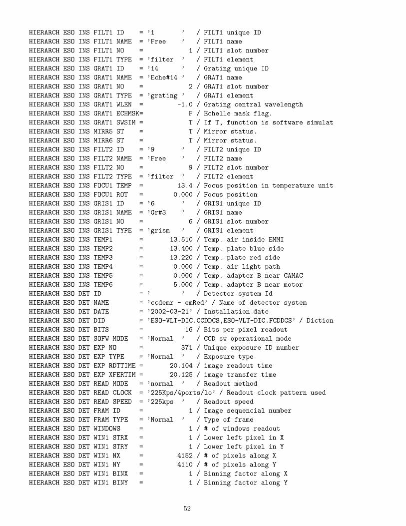
HIERARCH ESO INS FILT1 ID = ’1 ’ / FILT1 unique ID

HIERARCH ESO INS FILT1 NAME = ’Free ’ / FILT1 name

HIERARCH ESO INS FILT1 NO = 1 / FILT1 slot number

HIERARCH ESO INS FILT1 TYPE = ’filter ’ / FILT1 element

HIERARCH ESO INS GRAT1 ID = ’14 ’ / Grating unique ID

HIERARCH ESO INS GRAT1 NAME = ’Eche#14 ’ / GRAT1 name

HIERARCH ESO INS GRAT1 NO = 2 / GRAT1 slot number

HIERARCH ESO INS GRAT1 TYPE = ’grating ’ / GRAT1 element

HIERARCH ESO INS GRAT1 WLEN = -1.0 / Grating central wavelength

HIERARCH ESO INS GRAT1 ECHMSK= F / Echelle mask flag.

HIERARCH ESO INS GRAT1 SWSIM = T / If T, function is software simulat

HIERARCH ESO INS MIRR5 ST = T / Mirror status.

HIERARCH ESO INS MIRR6 ST = T / Mirror status.

HIERARCH ESO INS FILT2 ID = ’9 ’ / FILT2 unique ID

HIERARCH ESO INS FILT2 NAME = ’Free ’ / FILT2 name

HIERARCH ESO INS FILT2 NO = 9 / FILT2 slot number

HIERARCH ESO INS FILT2 TYPE = ’filter ’ / FILT2 element

HIERARCH ESO INS FOCU1 TEMP = 13.4 / Focus position in temperature unit

HIERARCH ESO INS FOCU1 ROT = 0.000 / Focus position

HIERARCH ESO INS GRIS1 ID = ’6 ’ / GRIS1 unique ID

HIERARCH ESO INS GRIS1 NAME = ’Gr#3 ’ / GRIS1 name

HIERARCH ESO INS GRIS1 NO = 6 / GRIS1 slot number

HIERARCH ESO INS GRIS1 TYPE = ’grism ’ / GRIS1 element

HIERARCH ESO INS TEMP1 = 13.510 / Temp. air inside EMMI

HIERARCH ESO INS TEMP2 = 13.400 / Temp. plate blue side

HIERARCH ESO INS TEMP3 = 13.220 / Temp. plate red side

HIERARCH ESO INS TEMP4 = 0.000 / Temp. air light path

HIERARCH ESO INS TEMP5 = 0.000 / Temp. adapter B near CAMAC

HIERARCH ESO INS TEMP6 = 5.000 / Temp. adapter B near motor

HIERARCH ESO DET ID = ’ ’ / Detector system Id

HIERARCH ESO DET NAME = ’ccdemr - emRed’ / Name of detector system

HIERARCH ESO DET DATE = ’2002-03-21’ / Installation date

HIERARCH ESO DET DID = ’ESO-VLT-DIC.CCDDCS,ESO-VLT-DIC.FCDDCS’ / Diction

HIERARCH ESO DET BITS = 16 / Bits per pixel readout

HIERARCH ESO DET SOFW MODE = ’Normal ’ / CCD sw operational mode

HIERARCH ESO DET EXP NO = 371 / Unique exposure ID number

HIERARCH ESO DET EXP TYPE = ’Normal ’ / Exposure type

HIERARCH ESO DET EXP RDTTIME = 20.104 / image readout time

HIERARCH ESO DET EXP XFERTIM = 20.125 / image transfer time

HIERARCH ESO DET READ MODE = ’normal ’ / Readout method

HIERARCH ESO DET READ CLOCK = ’225Kps/4ports/lo’ / Readout clock pattern used

HIERARCH ESO DET READ SPEED = ’225kps ’ / Readout speed

HIERARCH ESO DET FRAM ID = 1 / Image sequencial number

HIERARCH ESO DET FRAM TYPE = ’Normal ’ / Type of frame

HIERARCH ESO DET WINDOWS = 1 / # of windows readout

HIERARCH ESO DET WIN1 STRX = 1 / Lower left pixel in X

HIERARCH ESO DET WIN1 STRY = 1 / Lower left pixel in Y

HIERARCH ESO DET WIN1 NX = 4152 / # of pixels along X

HIERARCH ESO DET WIN1 NY = 4110 / # of pixels along Y

HIERARCH ESO DET WIN1 BINX = 1 / Binning factor along X

HIERARCH ESO DET WIN1 BINY = 1 / Binning factor along Y

52

HIERARCH ESO DET WIN1 NDIT = 1 / # of subintegrations

HIERARCH ESO DET WIN1 UIT1 = 600.000000 / user defined subintegration time

HIERARCH ESO DET WIN1 DIT1 = 599.999361 / actual subintegration time

HIERARCH ESO DET WIN1 DKTM = 600.2250 / Dark current time

HIERARCH ESO DET RA = 0.00000000 / Apparent 00:00:00.0 RA at start

HIERARCH ESO DET DEC = 0.00000000 / Apparent 00:00:00.0 DEC at start

HIERARCH ESO DET CHIPS = 2 / # of chips in detector array

HIERARCH ESO DET OUTPUTS = 4 / # of outputs

HIERARCH ESO DET OUTREF = 0 / reference output

HIERARCH ESO DET WIN1 ST = T / If T, window enabled

HIERARCH ESO DET READ NFRAM = 1 / Number of readouts buffered in sin

HIERARCH ESO DET SHUT TYPE = ’Iris ’ / type of shutter

HIERARCH ESO DET SHUT ID = ’Emmi Red shutterCCD Sensor1’ / Shutter unique id

HIERARCH ESO DET SHUT TMOPEN = 0.414 / Time taken to open shutter

HIERARCH ESO DET SHUT TMCLOS = 0.412 / Time taken to close shutter

ORIGFILE= ’REMD_e_o_Exposures.fits’ / Original File Name

ARCFILE = ’ONTT.2002-08-07T04:13:06.826.fits’ / Archive File Name

CHECKSUM= ’9gaFHdY99daCEdY9’ / ASCII 1’s complement checksum

53

Appendix B

EMMI Efficiencies

The efficiencies of the individual EMMI components are given in the following figures. These includethe transmission of EMMI optics, the transmission curves of grisms, the absolute reflectivities ofgratings used in the red and the blue arms, and the throughput for a 15th AB magnitude stars forsome grisms and gratings.

54

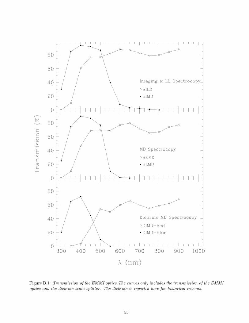
Figure B.1: Transmission of the EMMI optics.The curves only includes the transmission of the EMMIoptics and the dichroic beam splitter. The dichroic is reported here for historical reasons.

55

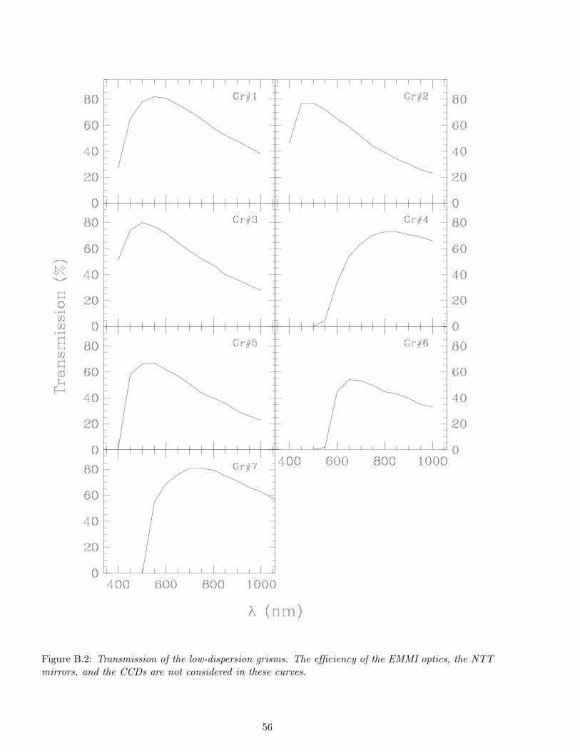
Figure B.2: Transmission of the low-dispersion grisms. The efficiency of the EMMI optics, the NTTmirrors, and the CCDs are not considered in these curves.

56

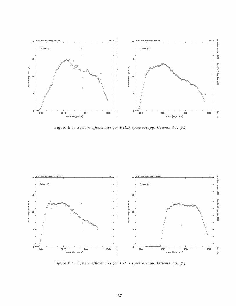
Figure B.3: System efficiencies for RILD spectroscopy, Grisms #1, #2

Figure B.4: System efficiencies for RILD spectroscopy, Grisms #3, #4

57

Figure B.5: System efficiencies for RILD spectroscopy, Grisms #5, #6

Figure B.6: System efficiencies for RILD spectroscopy, Grism #7

58

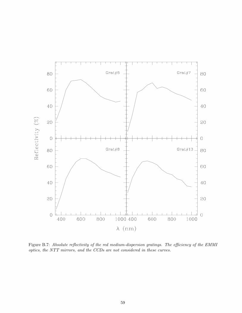
Figure B.7: Absolute reflectivity of the red medium-dispersion gratings. The efficiency of the EMMIoptics, the NTT mirrors, and the CCDs are not considered in these curves.

59

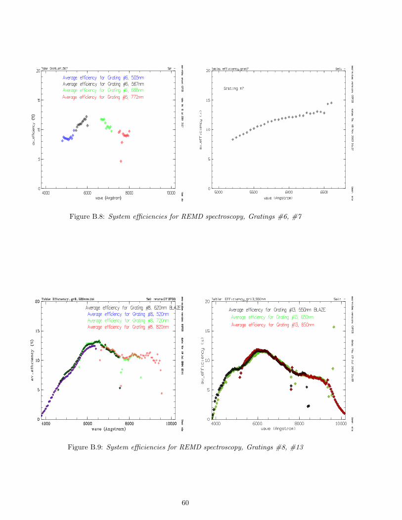
Figure B.8: System efficiencies for REMD spectroscopy, Gratings #6, #7

Figure B.9: System efficiencies for REMD spectroscopy, Gratings #8, #13

60

Figure B.10: Absolute reflectivity of the blue medium-dispersion gratings. The efficiency of the EMMIoptics, the NTT mirrors, and the CCDs are not considered in these curves.

61

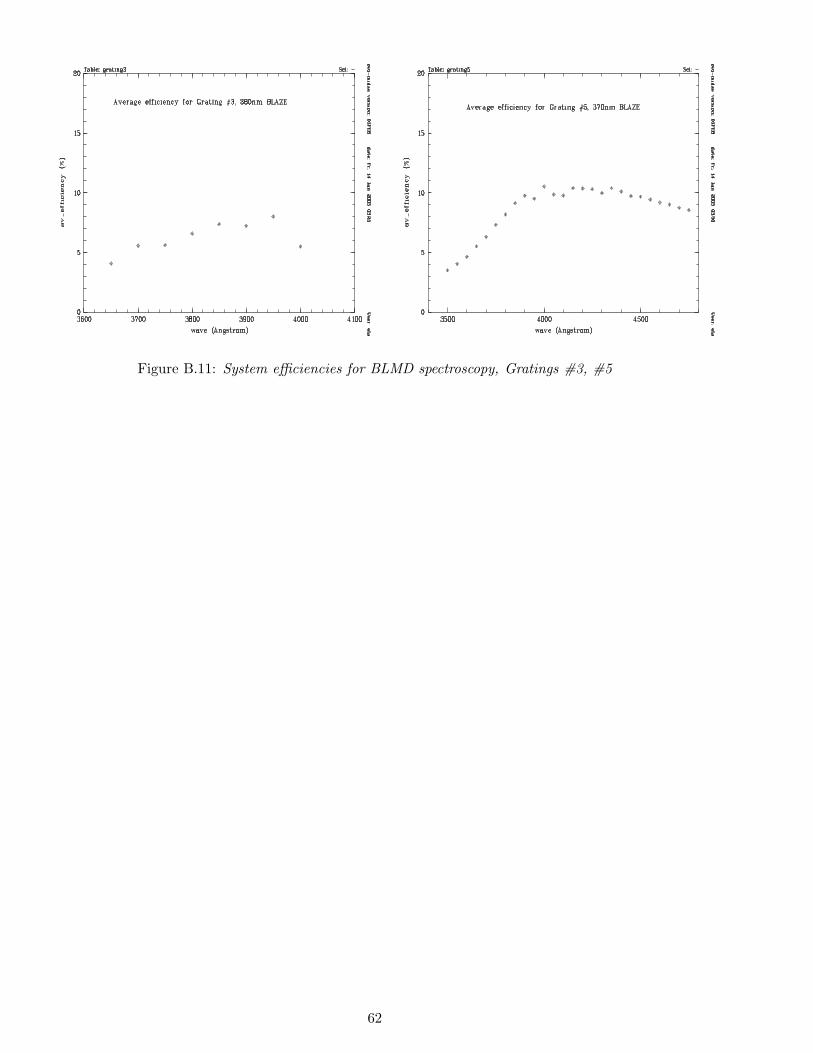
Figure B.11: System efficiencies for BLMD spectroscopy, Gratings #3, #5

62

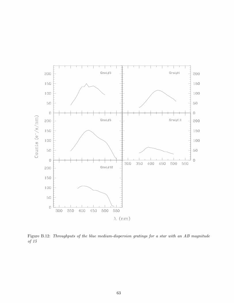
Figure B.12: Throughputs of the blue medium-dispersion gratings for a star with an AB magnitudeof 15

63

Figure B.13: Absolute reflectivity of the echelle gratings. The efficiency of the EMMI optics, theNTT mirrors, and the CCDs are not considered in these curves.

64

Figure B.14: Total efficiencies of the echelle gratings used in combination with different cross-dispersing grisms

65

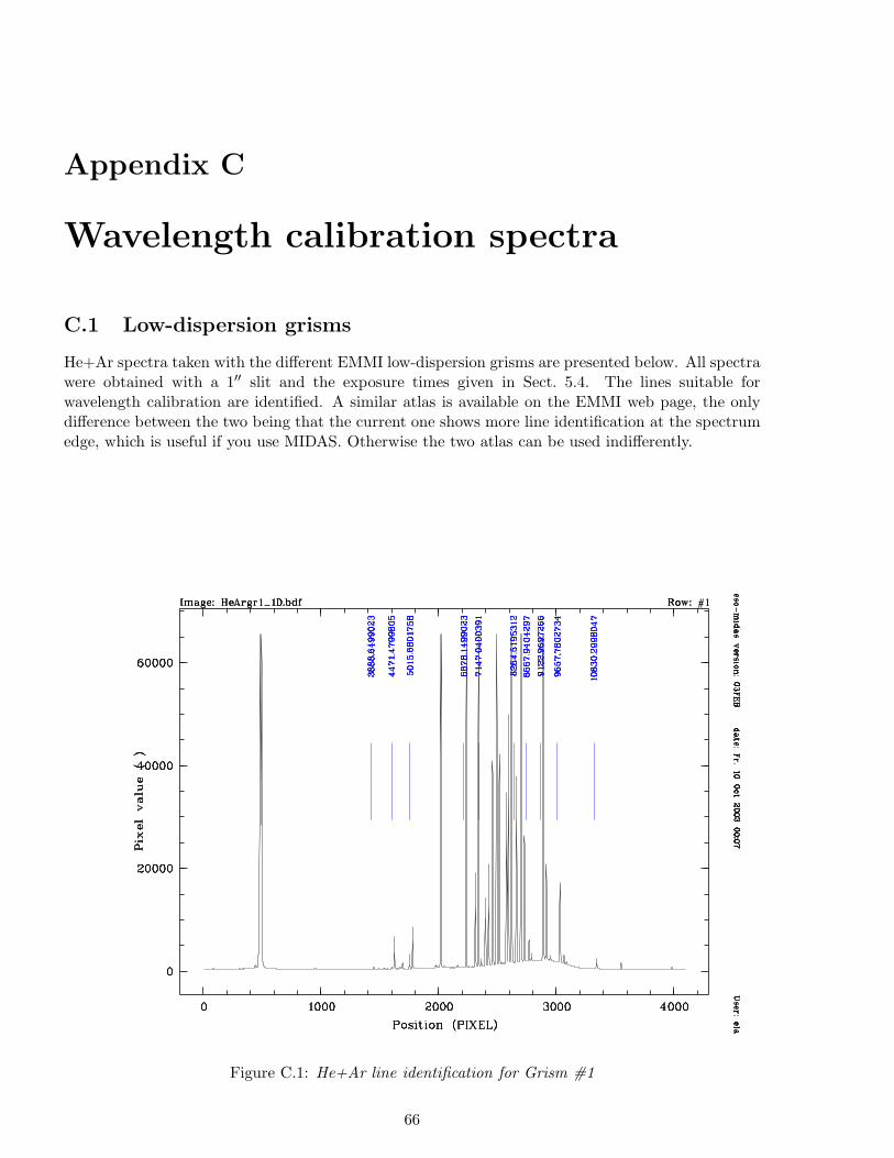
Appendix C

Wavelength calibration spectra

C.1 Low-dispersion grisms

He+Ar spectra taken with the different EMMI low-dispersion grisms are presented below. All spectrawere obtained with a 1′′ slit and the exposure times given in Sect. 5.4. The lines suitable forwavelength calibration are identified. A similar atlas is available on the EMMI web page, the onlydifference between the two being that the current one shows more line identification at the spectrumedge, which is useful if you use MIDAS. Otherwise the two atlas can be used indifferently.

Figure C.1: He+Ar line identification for Grism #1

66

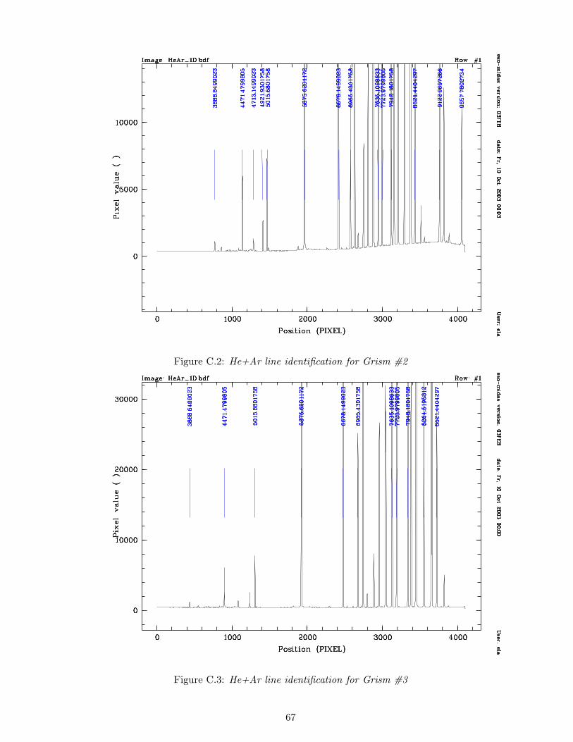
Figure C.2: He+Ar line identification for Grism #2

Figure C.3: He+Ar line identification for Grism #3

67

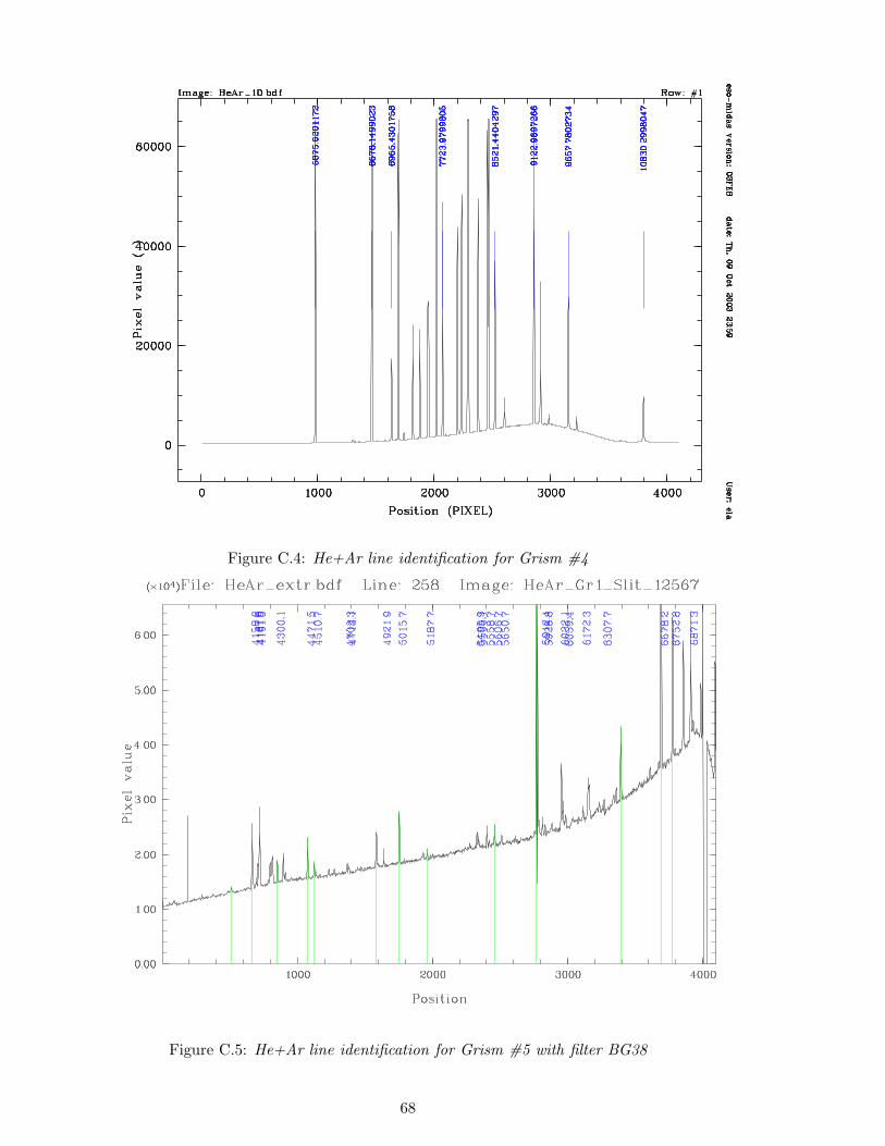
Figure C.4: He+Ar line identification for Grism #4

Figure C.5: He+Ar line identification for Grism #5 with filter BG38

68

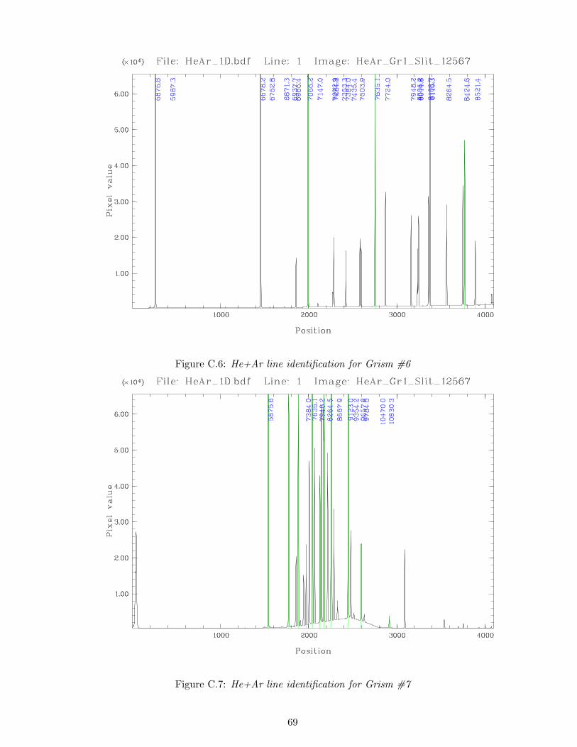
Figure C.6: He+Ar line identification for Grism #6

Figure C.7: He+Ar line identification for Grism #7

69

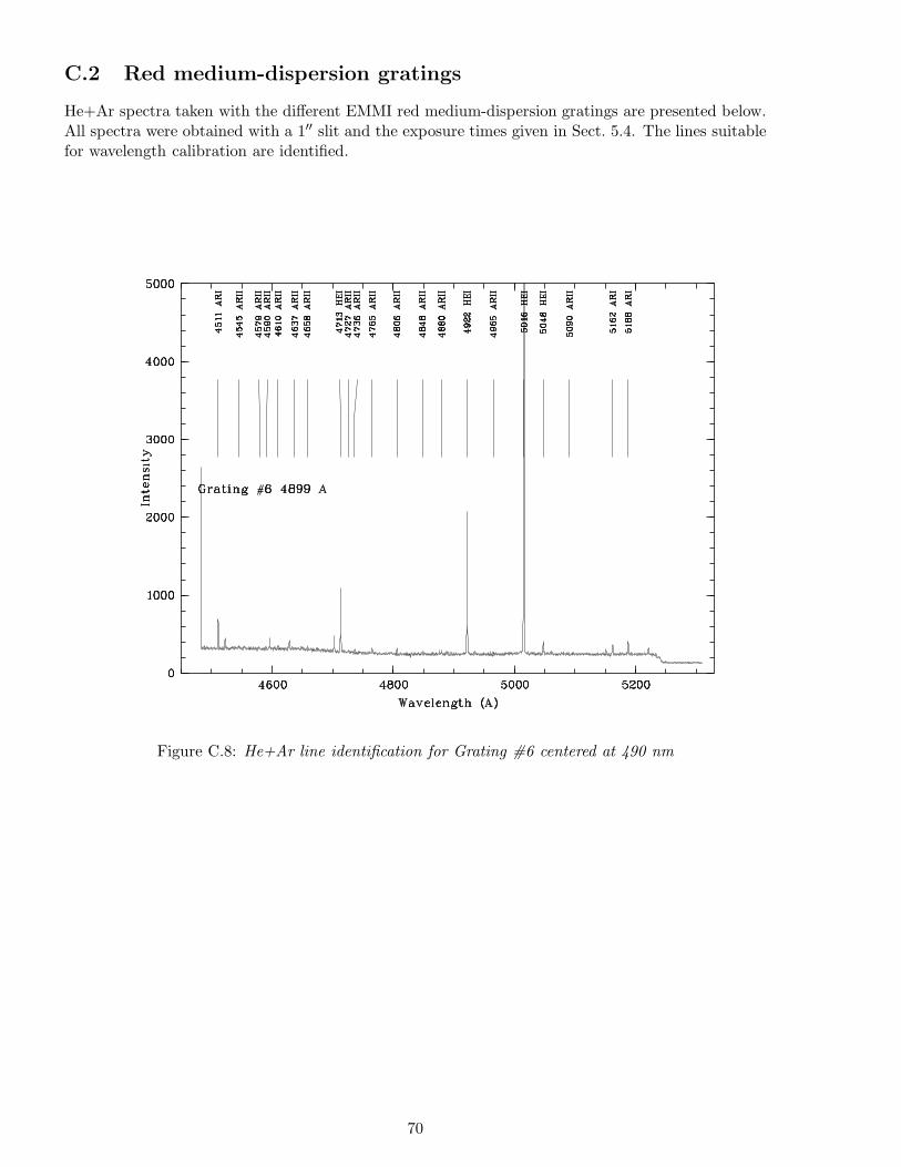
C.2 Red medium-dispersion gratings

He+Ar spectra taken with the different EMMI red medium-dispersion gratings are presented below.All spectra were obtained with a 1′′ slit and the exposure times given in Sect. 5.4. The lines suitablefor wavelength calibration are identified.

Figure C.8: He+Ar line identification for Grating #6 centered at 490 nm

70

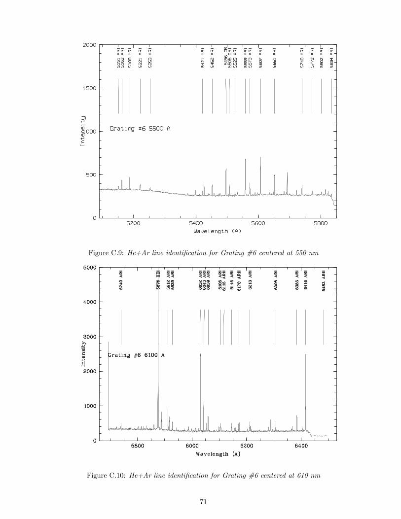
Figure C.9: He+Ar line identification for Grating #6 centered at 550 nm

Figure C.10: He+Ar line identification for Grating #6 centered at 610 nm

71

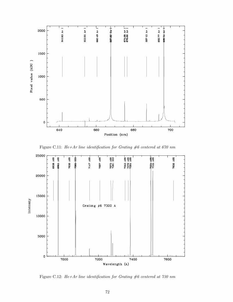
Figure C.11: He+Ar line identification for Grating #6 centered at 670 nm

Figure C.12: He+Ar line identification for Grating #6 centered at 730 nm

72

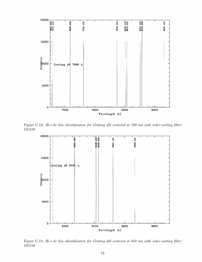
Figure C.13: He+Ar line identification for Grating #6 centered at 790 nm with order-sorting filterOG530

Figure C.14: He+Ar line identification for Grating #6 centered at 850 nm with order-sorting filterOG530

73

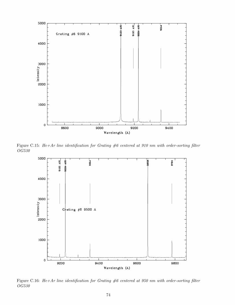
Figure C.15: He+Ar line identification for Grating #6 centered at 910 nm with order-sorting filterOG530

Figure C.16: He+Ar line identification for Grating #6 centered at 950 nm with order-sorting filterOG530

74

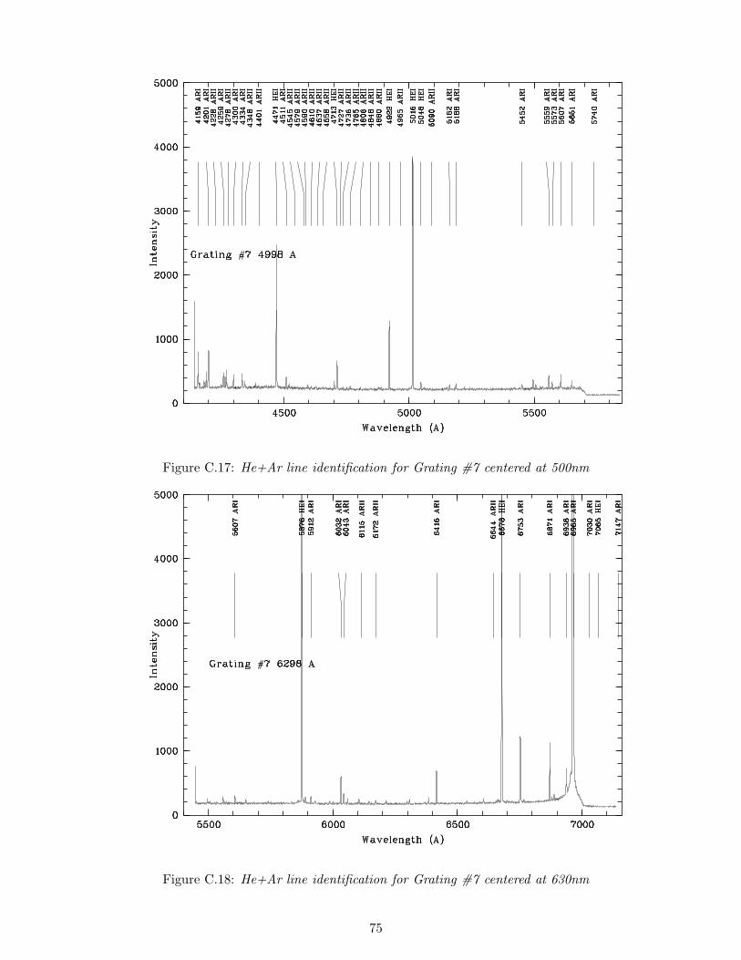
Figure C.17: He+Ar line identification for Grating #7 centered at 500nm

Figure C.18: He+Ar line identification for Grating #7 centered at 630nm

75

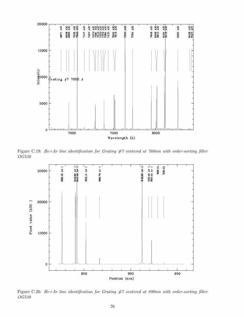
Figure C.19: He+Ar line identification for Grating #7 centered at 760nm with order-sorting filterOG530

Figure C.20: He+Ar line identification for Grating #7 centered at 890nm with order-sorting filterOG530

76

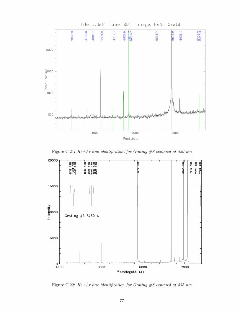
Figure C.21: He+Ar line identification for Grating #8 centered at 520 nm

Figure C.22: He+Ar line identification for Grating #8 centered at 575 nm

77

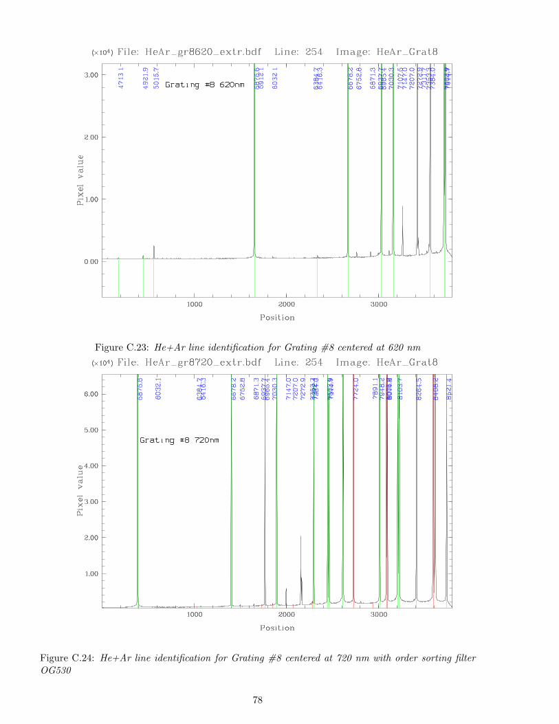
Figure C.23: He+Ar line identification for Grating #8 centered at 620 nm

Figure C.24: He+Ar line identification for Grating #8 centered at 720 nm with order sorting filterOG530

78

Figure C.25: He+Ar line identification for Grating #8 centered at 820 nm with order sorting filterOG530

79

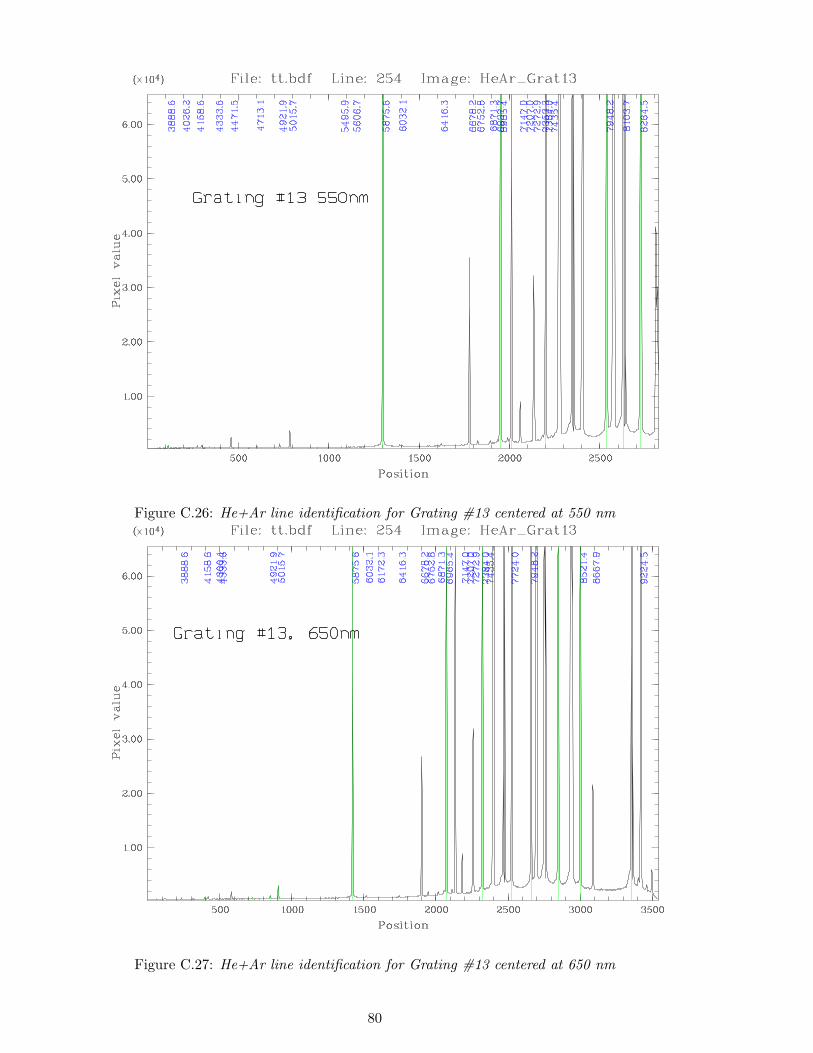
Figure C.26: He+Ar line identification for Grating #13 centered at 550 nm

Figure C.27: He+Ar line identification for Grating #13 centered at 650 nm

80

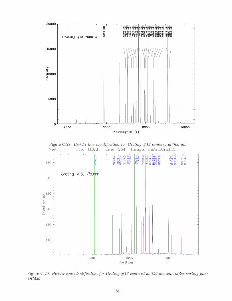
Figure C.28: He+Ar line identification for Grating #13 centered at 700 nm

Figure C.29: He+Ar line identification for Grating #13 centered at 750 nm with order sorting filterOG530

81

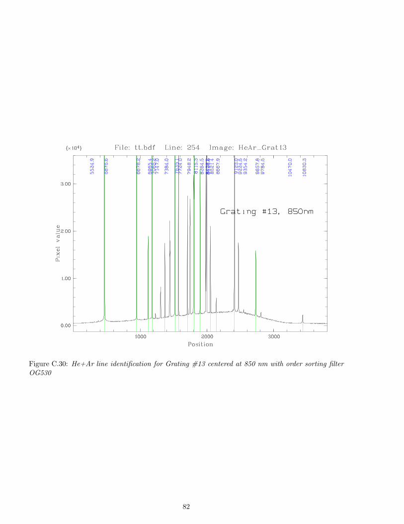
Figure C.30: He+Ar line identification for Grating #13 centered at 850 nm with order sorting filterOG530

82

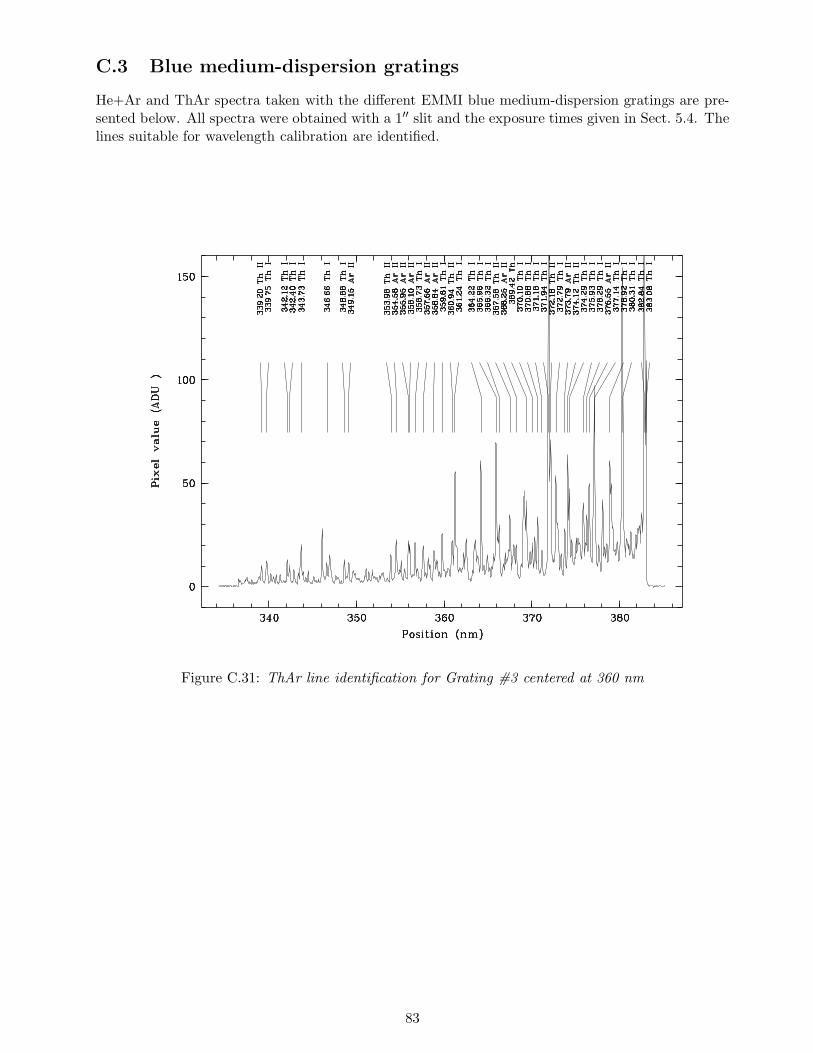
C.3 Blue medium-dispersion gratings

He+Ar and ThAr spectra taken with the different EMMI blue medium-dispersion gratings are pre-sented below. All spectra were obtained with a 1′′ slit and the exposure times given in Sect. 5.4. Thelines suitable for wavelength calibration are identified.

Figure C.31: ThAr line identification for Grating #3 centered at 360 nm

83

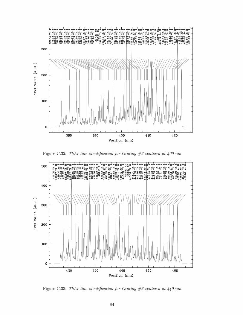
Figure C.32: ThAr line identification for Grating #3 centered at 400 nm

Figure C.33: ThAr line identification for Grating #3 centered at 440 nm

84

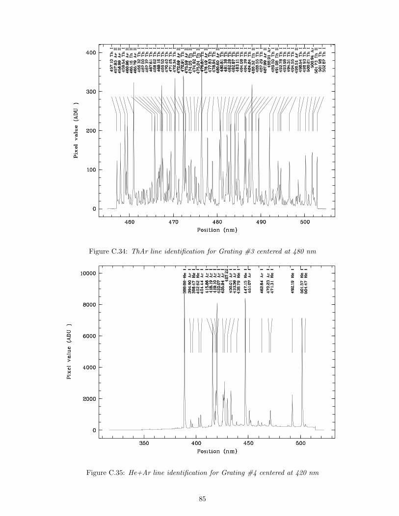
Figure C.34: ThAr line identification for Grating #3 centered at 480 nm

Figure C.35: He+Ar line identification for Grating #4 centered at 420 nm

85

Figure C.36: He+Ar line identification for Grating #5 centered at 420 nm

Figure C.37: ThAr line identification for Grating #11 centered at 350 nm

86

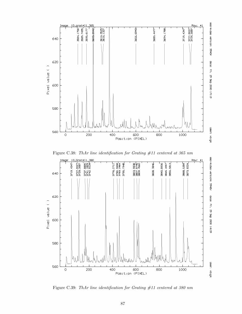
Figure C.38: ThAr line identification for Grating #11 centered at 365 nm

Figure C.39: ThAr line identification for Grating #11 centered at 380 nm

87

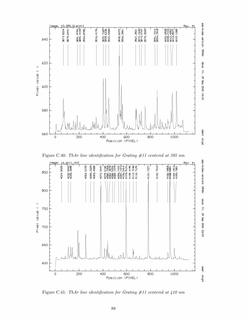
Figure C.40: ThAr line identification for Grating #11 centered at 395 nm

Figure C.41: ThAr line identification for Grating #11 centered at 410 nm

88

Figure C.42: ThAr line identification for Grating #11 centered at 425 nm

Figure C.43: ThAr line identification for Grating #11 centered at 440 nm

89

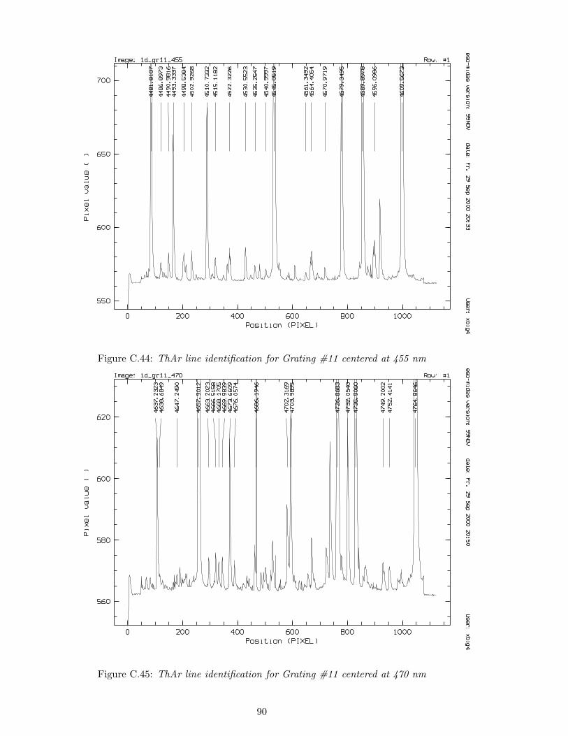
Figure C.44: ThAr line identification for Grating #11 centered at 455 nm

Figure C.45: ThAr line identification for Grating #11 centered at 470 nm

90

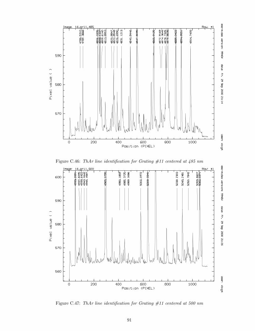
Figure C.46: ThAr line identification for Grating #11 centered at 485 nm

Figure C.47: ThAr line identification for Grating #11 centered at 500 nm

91

Figure C.48: He+Ar line identification for Grating #12 centered at 350 nm

Figure C.49: He+Ar line identification for Grating #12 centered at 425 nm

92

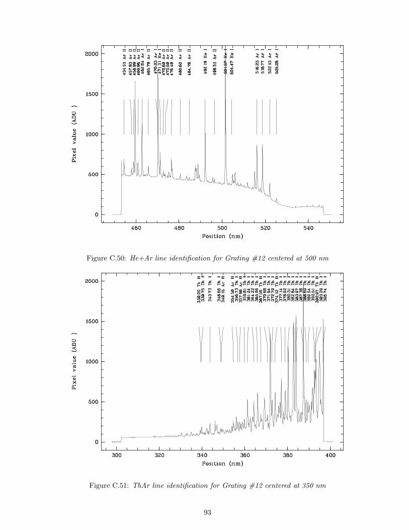
Figure C.50: He+Ar line identification for Grating #12 centered at 500 nm

Figure C.51: ThAr line identification for Grating #12 centered at 350 nm

93

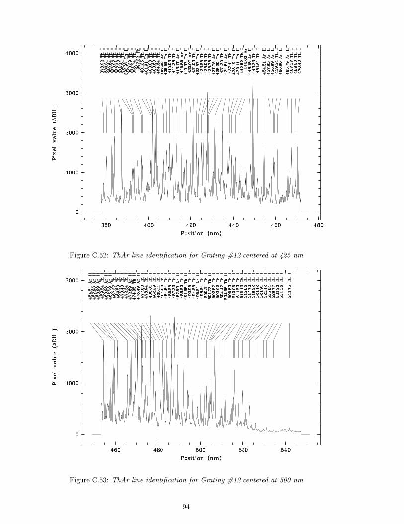
Figure C.52: ThAr line identification for Grating #12 centered at 425 nm

Figure C.53: ThAr line identification for Grating #12 centered at 500 nm

94

C.4 Echelle gratings

Spectra of the ThAr lamp taken with the echelle gratings are available at the following link:

http://www.ls.eso.org/lasilla/sciops/ntt/emmi/emmiAtlas.html

95

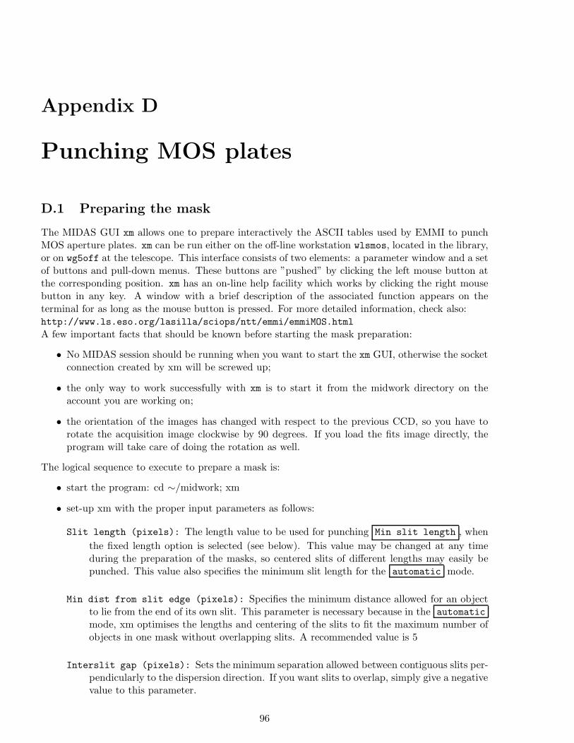
Appendix D

Punching MOS plates

D.1 Preparing the mask

The MIDAS GUI xm allows one to prepare interactively the ASCII tables used by EMMI to punchMOS aperture plates. xm can be run either on the off-line workstation wlsmos, located in the library,or on wg5off at the telescope. This interface consists of two elements: a parameter window and a setof buttons and pull-down menus. These buttons are ”pushed” by clicking the left mouse button atthe corresponding position. xm has an on-line help facility which works by clicking the right mousebutton in any key. A window with a brief description of the associated function appears on theterminal for as long as the mouse button is pressed. For more detailed information, check also:http://www.ls.eso.org/lasilla/sciops/ntt/emmi/emmiMOS.html

A few important facts that should be known before starting the mask preparation:

• No MIDAS session should be running when you want to start the xm GUI, otherwise the socketconnection created by xm will be screwed up;

• the only way to work successfully with xm is to start it from the midwork directory on theaccount you are working on;

• the orientation of the images has changed with respect to the previous CCD, so you have torotate the acquisition image clockwise by 90 degrees. If you load the fits image directly, theprogram will take care of doing the rotation as well.

The logical sequence to execute to prepare a mask is:

• start the program: cd ∼/midwork; xm

• set-up xm with the proper input parameters as follows:

Slit length (pixels): The length value to be used for punching Min slit length , when

the fixed length option is selected (see below). This value may be changed at any timeduring the preparation of the masks, so centered slits of different lengths may easily bepunched. This value also specifies the minimum slit length for the automatic mode.

Min dist from slit edge (pixels): Specifies the minimum distance allowed for an objectto lie from the end of its own slit. This parameter is necessary because in the automatic

mode, xm optimises the lengths and centering of the slits to fit the maximum number ofobjects in one mask without overlapping slits. A recommended value is 5

Interslit gap (pixels): Sets the minimum separation allowed between contiguous slits per-pendicularly to the dispersion direction. If you want slits to overlap, simply give a negativevalue to this parameter.

96

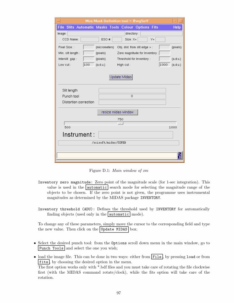
Figure D.1: Main window of xm

Inventory zero magnitude: Zero point of the magnitude scale (for 1-sec integration). Thisvalue is used in the automatic search mode for selecting the magnitude range of theobjects to be chosen. If the zero point is not given, the programme uses instrumentalmagnitudes as determined by the MIDAS package INVENTORY.

Inventory threshold (ADU): Defines the threshold used by INVENTORY for automaticallyfinding objects (used only in the automatic mode).

To change any of these parameters, simply move the cursor to the corresponding field and typethe new value. Then click on the Update MIDAS box.

• Select the desired punch tool: from the Options scroll down menu in the main window, go toPunch Tools and select the one you wish;

• load the image file. This can be done in two ways: either from File , by pressing load or fromfits , by choosing the desired option in the menu.The first option works only with *.bdf files and you must take care of rotating the file clockwisefirst (with the MIDAS command rotate/clock), while the fits option will take care of therotation.

97

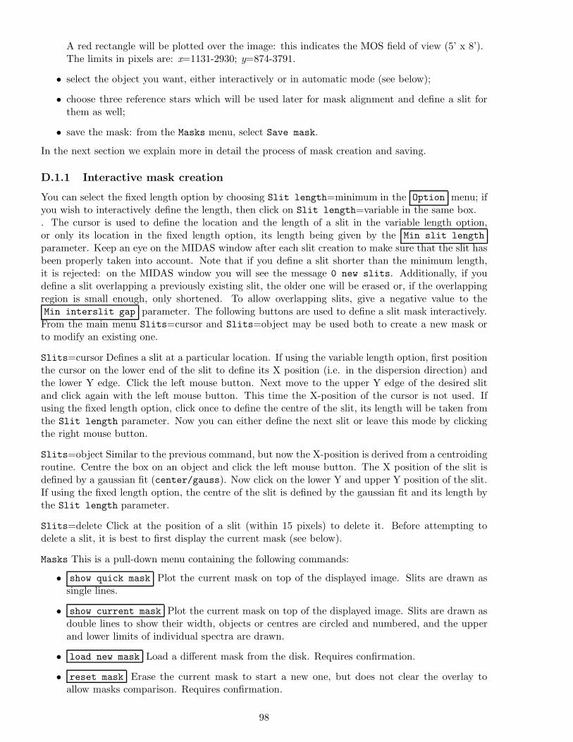
A red rectangle will be plotted over the image: this indicates the MOS field of view (5’ x 8’).The limits in pixels are: x=1131-2930; y=874-3791.

• select the object you want, either interactively or in automatic mode (see below);

• choose three reference stars which will be used later for mask alignment and define a slit forthem as well;

• save the mask: from the Masks menu, select Save mask.

In the next section we explain more in detail the process of mask creation and saving.

D.1.1 Interactive mask creation

You can select the fixed length option by choosing Slit length=minimum in the Option menu; ifyou wish to interactively define the length, then click on Slit length=variable in the same box.. The cursor is used to define the location and the length of a slit in the variable length option,or only its location in the fixed length option, its length being given by the Min slit length

parameter. Keep an eye on the MIDAS window after each slit creation to make sure that the slit hasbeen properly taken into account. Note that if you define a slit shorter than the minimum length,it is rejected: on the MIDAS window you will see the message 0 new slits. Additionally, if youdefine a slit overlapping a previously existing slit, the older one will be erased or, if the overlappingregion is small enough, only shortened. To allow overlapping slits, give a negative value to theMin interslit gap parameter. The following buttons are used to define a slit mask interactively.From the main menu Slits=cursor and Slits=object may be used both to create a new mask orto modify an existing one.

Slits=cursor Defines a slit at a particular location. If using the variable length option, first positionthe cursor on the lower end of the slit to define its X position (i.e. in the dispersion direction) andthe lower Y edge. Click the left mouse button. Next move to the upper Y edge of the desired slitand click again with the left mouse button. This time the X-position of the cursor is not used. Ifusing the fixed length option, click once to define the centre of the slit, its length will be taken fromthe Slit length parameter. Now you can either define the next slit or leave this mode by clickingthe right mouse button.

Slits=object Similar to the previous command, but now the X-position is derived from a centroidingroutine. Centre the box on an object and click the left mouse button. The X position of the slit isdefined by a gaussian fit (center/gauss). Now click on the lower Y and upper Y position of the slit.If using the fixed length option, the centre of the slit is defined by the gaussian fit and its length bythe Slit length parameter.

Slits=delete Click at the position of a slit (within 15 pixels) to delete it. Before attempting todelete a slit, it is best to first display the current mask (see below).

Masks This is a pull-down menu containing the following commands:

• show quick mask Plot the current mask on top of the displayed image. Slits are drawn assingle lines.

• show current mask Plot the current mask on top of the displayed image. Slits are drawn asdouble lines to show their width, objects or centres are circled and numbered, and the upperand lower limits of individual spectra are drawn.

• load new mask Load a different mask from the disk. Requires confirmation.

• reset mask Erase the current mask to start a new one, but does not clear the overlay toallow masks comparison. Requires confirmation.

98

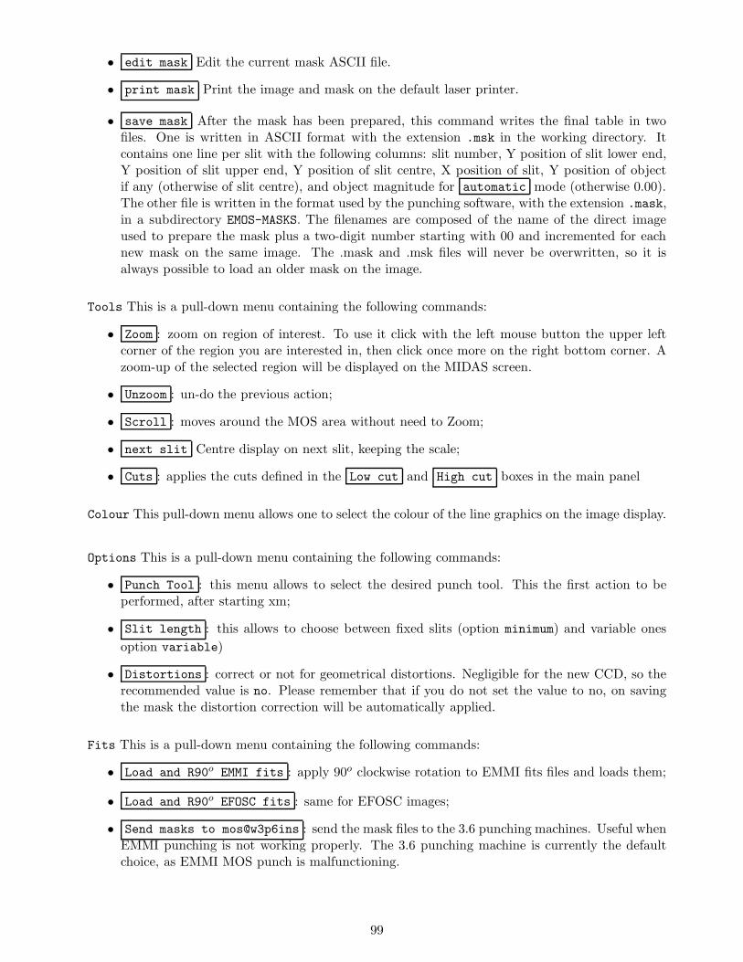
• edit mask Edit the current mask ASCII file.

• print mask Print the image and mask on the default laser printer.

• save mask After the mask has been prepared, this command writes the final table in twofiles. One is written in ASCII format with the extension .msk in the working directory. Itcontains one line per slit with the following columns: slit number, Y position of slit lower end,Y position of slit upper end, Y position of slit centre, X position of slit, Y position of objectif any (otherwise of slit centre), and object magnitude for automatic mode (otherwise 0.00).The other file is written in the format used by the punching software, with the extension .mask,in a subdirectory EMOS-MASKS. The filenames are composed of the name of the direct imageused to prepare the mask plus a two-digit number starting with 00 and incremented for eachnew mask on the same image. The .mask and .msk files will never be overwritten, so it isalways possible to load an older mask on the image.

Tools This is a pull-down menu containing the following commands:

• Zoom : zoom on region of interest. To use it click with the left mouse button the upper leftcorner of the region you are interested in, then click once more on the right bottom corner. Azoom-up of the selected region will be displayed on the MIDAS screen.

• Unzoom : un-do the previous action;

• Scroll : moves around the MOS area without need to Zoom;

• next slit Centre display on next slit, keeping the scale;

• Cuts : applies the cuts defined in the Low cut and High cut boxes in the main panel

Colour This pull-down menu allows one to select the colour of the line graphics on the image display.

Options This is a pull-down menu containing the following commands:

• Punch Tool : this menu allows to select the desired punch tool. This the first action to beperformed, after starting xm;

• Slit length : this allows to choose between fixed slits (option minimum) and variable ones

option variable)

• Distortions : correct or not for geometrical distortions. Negligible for the new CCD, so therecommended value is no. Please remember that if you do not set the value to no, on savingthe mask the distortion correction will be automatically applied.

Fits This is a pull-down menu containing the following commands:

• Load and R90o EMMI fits : apply 90o clockwise rotation to EMMI fits files and loads them;

• Load and R90o EFOSC fits : same for EFOSC images;

• Send masks to mos@w3p6ins : send the mask files to the 3.6 punching machines. Useful whenEMMI punching is not working properly. The 3.6 punching machine is currently the defaultchoice, as EMMI MOS punch is malfunctioning.

99

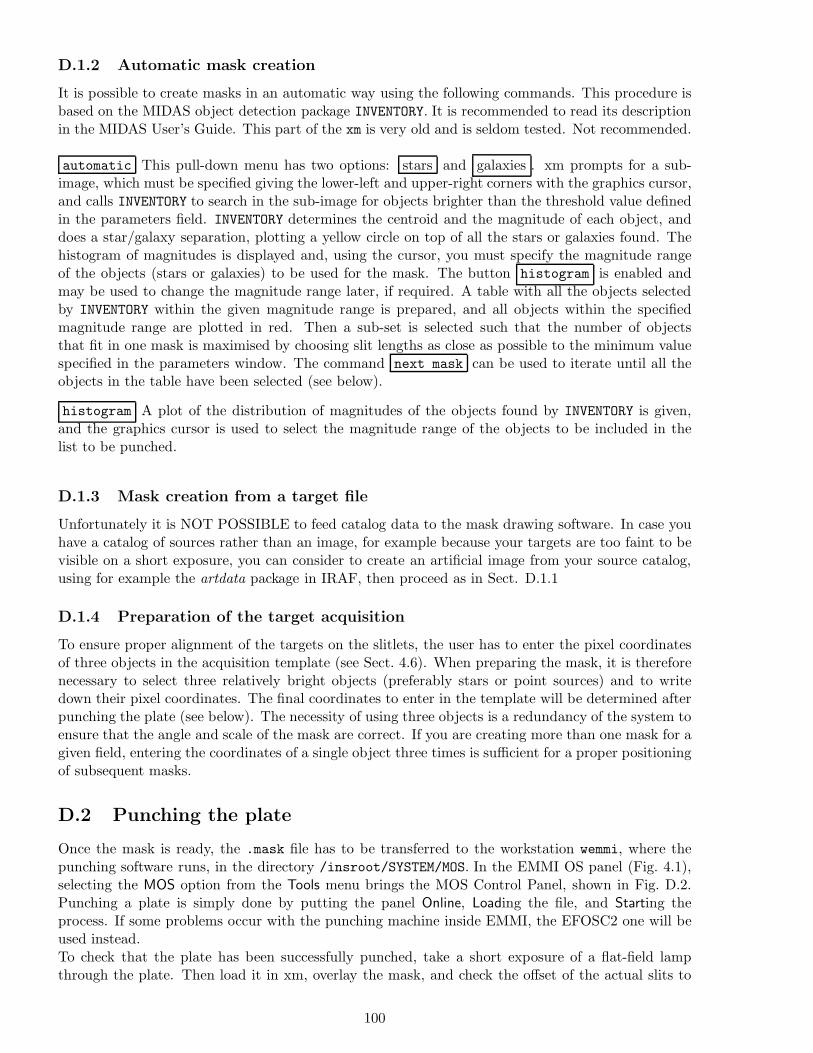
D.1.2 Automatic mask creation

It is possible to create masks in an automatic way using the following commands. This procedure isbased on the MIDAS object detection package INVENTORY. It is recommended to read its descriptionin the MIDAS User’s Guide. This part of the xm is very old and is seldom tested. Not recommended.

automatic This pull-down menu has two options: stars and galaxies . xm prompts for a sub-image, which must be specified giving the lower-left and upper-right corners with the graphics cursor,and calls INVENTORY to search in the sub-image for objects brighter than the threshold value definedin the parameters field. INVENTORY determines the centroid and the magnitude of each object, anddoes a star/galaxy separation, plotting a yellow circle on top of all the stars or galaxies found. Thehistogram of magnitudes is displayed and, using the cursor, you must specify the magnitude rangeof the objects (stars or galaxies) to be used for the mask. The button histogram is enabled andmay be used to change the magnitude range later, if required. A table with all the objects selectedby INVENTORY within the given magnitude range is prepared, and all objects within the specifiedmagnitude range are plotted in red. Then a sub-set is selected such that the number of objectsthat fit in one mask is maximised by choosing slit lengths as close as possible to the minimum valuespecified in the parameters window. The command next mask can be used to iterate until all theobjects in the table have been selected (see below).

histogram A plot of the distribution of magnitudes of the objects found by INVENTORY is given,and the graphics cursor is used to select the magnitude range of the objects to be included in thelist to be punched.

D.1.3 Mask creation from a target file

Unfortunately it is NOT POSSIBLE to feed catalog data to the mask drawing software. In case youhave a catalog of sources rather than an image, for example because your targets are too faint to bevisible on a short exposure, you can consider to create an artificial image from your source catalog,using for example the artdata package in IRAF, then proceed as in Sect. D.1.1

D.1.4 Preparation of the target acquisition

To ensure proper alignment of the targets on the slitlets, the user has to enter the pixel coordinatesof three objects in the acquisition template (see Sect. 4.6). When preparing the mask, it is thereforenecessary to select three relatively bright objects (preferably stars or point sources) and to writedown their pixel coordinates. The final coordinates to enter in the template will be determined afterpunching the plate (see below). The necessity of using three objects is a redundancy of the system toensure that the angle and scale of the mask are correct. If you are creating more than one mask for agiven field, entering the coordinates of a single object three times is sufficient for a proper positioningof subsequent masks.

D.2 Punching the plate

Once the mask is ready, the .mask file has to be transferred to the workstation wemmi, where thepunching software runs, in the directory /insroot/SYSTEM/MOS. In the EMMI OS panel (Fig. 4.1),selecting the MOS option from the Tools menu brings the MOS Control Panel, shown in Fig. D.2.Punching a plate is simply done by putting the panel Online, Loading the file, and Starting theprocess. If some problems occur with the punching machine inside EMMI, the EFOSC2 one will beused instead.To check that the plate has been successfully punched, take a short exposure of a flat-field lampthrough the plate. Then load it in xm, overlay the mask, and check the offset of the actual slits to

100

Figure D.2: The MOS Control Panel

the defined ones. Finally, write down the pixel coordinates of the punched slits corresponding to thethree previously selected objects. Those coordinates are the ones that will have to be entered in theacquisition template. To determine these pixel coordinates accurately, one can use a center/gauss

command with a wide rectangle as the searching box for the X position. To obtain the Y position,zoom in on the slit and measure the positions of the edges with a get/cursor command.

101

Appendix E

Differential Refraction

Differential atmospheric refraction can be an important effect for some spectroscopic observations.The following table is taken from the the Boller and Chivens manual (ESO operating manual No. 9)and gives an indication how far the stellar image at a particular wavelength will be displaced fromthe image at a reference wavelength. If the difference over the wavelength range of your spectrum isa significant fraction of the slit width, it is recommended to align the slit with the parallactic angleto reduce the wavelength-dependent slit losses.For detailed information, you can check the paper by Filippenko [12].

102

Table E.1: Atmospheric differential refraction at an altitude of 2 km in arcseconds with respect to awavelength of 500 nm

λ (nm)sec z 300 350 400 450 500 550 600 650 700 750 800 850 900 950 10001.00 0.00 0.00 0.00 0.00 0.00 0.00 0.00 0.00 0.00 0.00 0.00 0.00 0.00 0.00 0.001.05 0.68 0.38 0.20 0.08 0.00 −0.06 −0.11 −0.14 −0.17 −0.19 −0.21 −0.23 −0.24 −0.25 −0.261.10 0.97 0.55 0.29 0.12 0.00 −0.09 −0.15 −0.20 −0.24 −0.28 −0.30 −0.32 −0.34 −0.36 −0.371.15 1.20 0.68 0.36 0.15 0.00 −0.11 −0.19 −0.25 −0.30 −0.34 −0.38 −0.40 −0.42 −0.44 −0.461.20 1.40 0.80 0.42 0.17 0.00 −0.13 −0.22 −0.30 −0.35 −0.40 −0.44 −0.47 −0.50 −0.52 −0.541.25 1.59 0.90 0.48 0.20 0.00 −0.14 −0.25 −0.33 −0.40 −0.45 −0.50 −0.53 −0.56 −0.59 −0.611.30 1.76 1.00 0.53 0.22 0.00 −0.16 −0.28 −0.37 −0.44 −0.50 −0.55 −0.59 −0.62 −0.65 −0.671.35 1.92 1.09 0.58 0.24 0.00 −0.17 −0.30 −0.40 −0.48 −0.55 −0.60 −0.64 −0.68 −0.71 −0.731.40 2.07 1.18 0.62 0.26 0.00 −0.19 −0.33 −0.44 −0.52 −0.59 −0.65 −0.69 −0.73 −0.77 −0.791.45 0.22 1.26 0.67 0.28 0.00 −0.20 −0.35 −0.47 −0.56 −0.63 −0.69 −0.74 −0.79 −0.82 −0.85

1.50 2.37 1.34 0.71 0.29 0.00 −0.21 −0.37 −0.50 −0.60 −0.68 −0.74 −0.79 −0.84 −0.87 −0.911.55 2.51 1.42 0.75 0.31 0.00 −0.23 −0.40 −0.53 −0.63 −0.72 −0.78 −0.84 −0.89 −0.93 −0.961.60 2.64 1.50 0.80 0.33 0.00 −0.24 −0.42 −0.56 −0.67 −0.75 −0.83 −0.88 −0.93 −0.98 −1.011.65 2.78 1.58 0.84 0.34 0.00 −0.25 −0.44 −0.59 −0.70 −0.79 −0.87 −0.93 −0.98 −1.03 −1.061.70 2.91 1.65 0.88 0.36 0.00 −0.26 −0.46 −0.61 −0.73 −0.83 −0.91 −0.97 −1.03 −1.07 −1.111.75 3.04 1.73 0.92 0.38 0.00 −0.27 −0.48 −0.64 −0.77 −0.87 −0.95 −1.02 −1.07 −1.12 −1.161.80 3.17 1.80 0.95 0.39 0.00 −0.29 −0.50 −0.67 −0.80 −0.90 −0.99 −1.06 −1.12 −1.17 −1.211.85 3.29 1.87 0.99 0.41 0.00 −0.30 −0.52 −0.69 −0.83 −0.94 −1.03 −1.10 −1.16 −1.22 −1.261.90 3.42 1.94 1.03 0.42 0.00 −0.31 −0.54 −0.72 −0.86 −0.98 −1.07 −1.14 −1.21 −1.26 −1.311.95 3.54 2.01 1.07 0.44 0.00 −0.32 −0.56 −0.75 −0.89 −1.01 −1.11 −1.19 −1.25 −1.31 −1.36

2.00 3.67 2.08 1.10 0.45 0.00 −0.33 −0.58 −0.77 −0.92 −1.05 −1.15 −1.23 −1.30 −1.35 −1.402.10 3.91 2.22 1.18 0.48 0.00 −0.35 −0.62 −0.82 −0.99 −1.12 −1.22 −1.31 −1.38 −1.44 −1.502.20 4.15 2.36 1.25 0.51 0.00 −0.37 −0.66 −0.87 −1.05 −1.18 −1.30 −1.39 −1.47 −1.53 −1.592.30 4.38 2.49 1.32 0.54 0.00 −0.40 −0.69 −0.92 −1.11 −1.25 −1.37 −1.47 −1.55 −.162 −1.682.40 4.62 2.62 1.39 0.57 0.00 −0.42 −0.73 −0.97 −1.16 −1.32 −1.44 −1.55 −1.63 −1.70 −1.772.50 4.85 2.75 1.46 0.60 0.00 −0.44 −0.77 −1.02 −1.22 −1.38 −1.52 −1.62 −1.71 −1.79 −1.862.60 5.08 2.88 1.53 0.63 0.00 −0.46 −0.80 −1.07 −1.28 −1.45 −1.59 −1.70 −1.80 −1.88 −1.942.70 5.31 3.01 1.60 0.66 0.00 −0.48 −0.84 −1.12 −1.34 −1.51 −1.66 −1.78 −1.88 −1.96 −2.032.80 5.54 3.14 1.67 0.69 0.00 −0.50 −0.88 −1.17 −1.40 −1.58 −1.73 −1.85 −1.96 −2.04 −2.122.90 5.76 3.27 1.74 0.71 0.00 −0.52 −0.91 −1.21 −1.45 −1.64 −1.80 −1.93 −2.04 −2.13 −2.20

3.00 5.99 3.40 1.80 0.74 0.00 −0.54 −0.95 −1.26 −1.51 −1.71 −1.87 −2.00 −2.12 −2.21 −2.293.10 6.21 3.53 1.87 0.77 0.00 −0.56 −0.98 −1.31 −1.57 −1.77 −1.94 −2.08 −2.19 −2.29 −2.383.20 6.44 3.65 1.94 0.80 0.00 −0.58 −1.02 −1.36 −1.62 −1.84 −2.01 −2.15 −2.27 −2.38 −2.463.30 6.66 3.78 2.00 0.83 0.00 −0.60 −1.05 −1.40 −1.68 −1.90 −2.08 −2.23 −2.35 −2.46 −2.553.40 6.88 3.91 2.07 0.85 0.00 −0.62 −1.09 −1.45 −1.73 −1.96 −2.15 −2.30 −2.43 −2.54 −2.633.50 7.10 4.03 2.14 0.88 0.00 −0.64 −1.12 −1.50 −1.79 −2.03 −2.22 −2.38 −2.51 −2.62 −2.723.60 7.32 4.16 2.20 0.91 0.00 −0.66 −1.16 −1.54 −1.85 −2.09 −2.29 −2.45 −2.59 −2.70 −2.803.70 7.54 4.28 2.27 0.94 0.00 −0.68 −1.19 −1.59 −1.90 −2.15 −2.36 −2.52 −2.66 −2.78 −2.883.80 7.76 4.41 2.34 0.96 0.00 −0.70 −1.23 −1.64 −1.96 −2.21 −2.42 −2.60 −2.74 −2.86 −2.973.90 7.98 4.53 2.40 0.99 0.00 −0.72 −1.26 −1.68 −2.01 −2.28 −2.49 −2.67 −2.82 −2.95 −3.05

4.00 8.20 4.66 2.47 1.02 0.00 −0.74 −1.30 −1.73 −2.07 −2.34 −2.56 −2.74 −2.90 −3.03 −3.144.10 8.42 4.78 2.53 1.04 0.00 −0.76 −1.33 −1.77 −2.12 −2.40 −2.63 −2.82 −2.97 −3.11 −3.224.20 8.64 4.90 2.60 1.07 0.00 −0.78 −1.37 −1.82 −2.18 −2.46 −2.70 −2.89 −3.05 −3.19 −3.304.30 8.85 5.03 2.67 1.10 0.00 −0.80 −1.40 −1.87 −2.23 −2.53 −2.77 −2.96 −3.13 −3.27 −3.394.40 9.07 5.15 2.73 1.12 0.00 −0.82 −1.44 −1.91 −2.29 −2.59 −2.83 −3.04 −3.21 −3.35 −3.474.50 9.29 5.27 2.80 1.15 0.00 −0.84 −1.47 −1.96 −2.34 −2.65 −2.90 −3.11 −3.28 −3.43 −3.554.60 9.51 5.40 2.86 1.18 0.00 −0.86 −1.51 −2.00 −2.40 −2.71 −2.97 −3.18 −3.36 −3.51 −3.644.70 9.72 5.52 2.93 1.21 0.00 −0.88 −1.54 −2.05 −2.45 −2.77 −3.04 −3.25 −3.44 −3.59 −3.724.80 9.94 5.64 2.99 1.23 0.00 −0.90 −1.57 −2.09 −2.51 −2.84 −3.10 −3.33 −3.51 −3.67 −3.804.90 10.15 5.77 3.06 1.26 0.00 −0.92 −1.61 −2.14 −2.56 −2.90 −3.17 −3.40 −3.59 −3.75 −3.88

103

Appendix F

EMMI setup request form

The set-up form has to filled after discussion with your support astronomer and MUST be filled inbefore 7am of the day in which you begin your observing run.The web form is available on EMMI webpage

oOo

104

� � � � �� � � � �� � � � �

� � � � �� � � � �� � � � �

� � �� � �� � �

� � �� � �� � �

(nm)# g/mm nm/pix

#4 300 0.173

#1 test mirror

#3 1200 0.042

#5 158 0.360

#11 3000 0.015

#12 600 0.091

or

or

λ c (nm)# g/mm nm/pix

#6 1200 0.032

#7 600 0.065

#8 316 0.125

#13 150 0.265

or

#10 31.6 0.0058or

or #14 31.6 0.0040

Date of Setup:

for mode RILD (see overleaf)

Select cross disperser in setup form

Free1

2

3

Free1

2

3

Below slit filter wheel

Nota: Slit width and height are continuously adjustable and computer controlled

Neutral densities available: 0.3, 0.5, 1.0, 2.0, 3.0, 4.0

Red arm (400 - 1100 nm)

Comments on Obs. Strategy:

DIMDBlue arm (300 - 500 nm)

λ c

EMMI SETUP REQUEST FORM

LSO-FOR-ESO-40600-0001/1.44, 11/20/1999

Medium dispersion and echelle modes (BLMD, REMD, DIMD)

Standard grating housings Standard grating housings

(only #10 and #14)

Long Slit Echelle ?

I do NOT need theEchelle mask!

or Echelle grating units

or#2 test mirror

#9 60 0.021

PLEASE DO NOT OVERFILL...!!!!!For Imaging and low dispersion modes

please turn over ->

Set up discussed and approved by Support Astronomer:

Supp.Astro.Name: Date: Supp.Astro.Signature:

Name: Prog. ID:

105

� � � � �� � � � �� � � � �

� � � �� � � �� � � �

� � � �� � � �� � � �

� � �� � �� � �

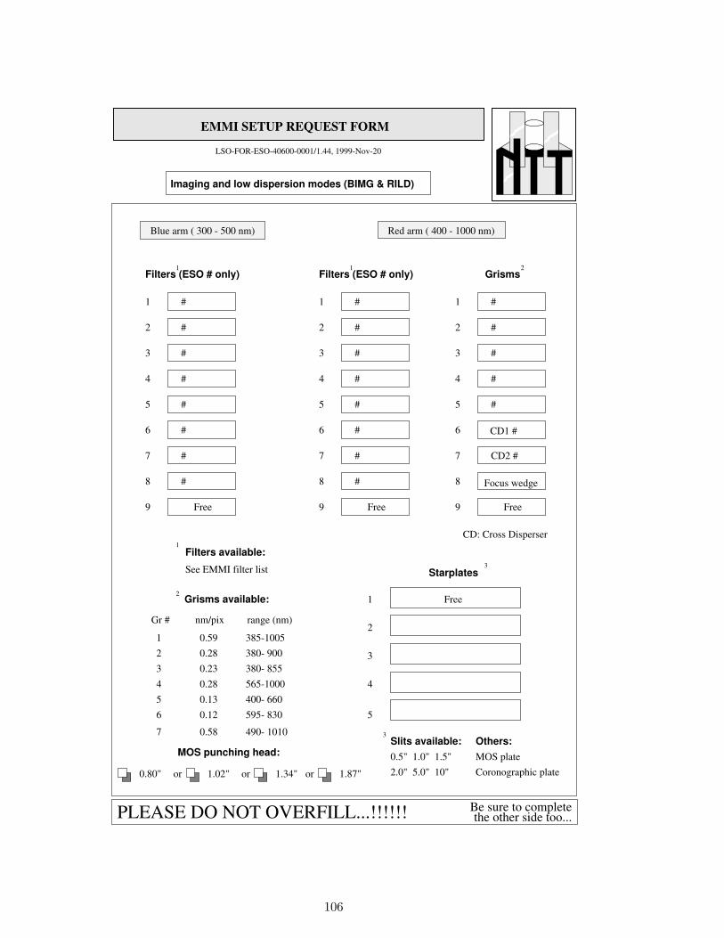
Slits available:

or or 1.87"or1.34"1.02"0.80"

Filters (ESO # only)1

Filters (ESO # only)1

Grisms2

0.5" 1.0" 1.5"

2.0" 5.0" 10"

5

1

2

3

4

#

#

#

#

#

#

See EMMI filter list

#

LSO-FOR-ESO-40600-0001/1.44, 1999-Nov-20

#

1

2

3

4

5

6

7

8

9

CD: Cross Disperser

#

#

#

#

#

1

2

3

4

5

6

7

8

9

Grisms available:

Blue arm ( 300 - 500 nm)

CD1 #

CD2 #

2

3Others:

MOS plateMOS punching head:

1 0.59 385-1005

2 0.28 380- 900

4 0.28 565-1000

7 0.58 490- 1010

3 0.23 380- 855

5 0.13 400- 660

6 0.12 595- 830

Gr # nm/pix range (nm)

Coronographic plate

Free

Free

Focus wedge

Red arm ( 400 - 1000 nm)

Filters available:1

Starplates3

Free

#

#

#

#

#

#

#

#

1

2

3

4

5

6

7

8

9 Free

EMMI SETUP REQUEST FORM

Imaging and low dispersion modes (BIMG & RILD)

PLEASE DO NOT OVERFILL...!!!!!! the other side too...Be sure to complete

106