Emissions Trends and Labour Productivity Dynamics Sector Analyses of De-coupling/Recoupling on a 1990-2005 Namea

NOTA DILAVORO50.2009

Giovanni Marin, University of FerraraMassimiliano Mazzanti, University of Ferrara, University of Bologna and Ceris CNR National Research Council

The opinions expressed in this paper do not necessarily reflect the position of Fondazione Eni Enrico Mattei

Corso Magenta, 63, 20123 Milano (I), web site: www.feem.it, e-mail: working.papers@feem.it

SUSTAINABLE DEVELOPMENT Series Editor: Carlo Carraro Emissions Trends and Labour Productivity Dynamics Sector Analyses of De-coupling/Recoupling on a 1990-2005 Namea By Giovanni Marin, University of Ferrara Massimiliano Mazzanti, University of Ferrara, University of Bologna and Ceris CNR National Research Council Summary This paper provides new empirical evidence on Environmental Kuznets Curves (EKC) for greenhouse gases (GHGs) and air pollutants at sector level. A panel dataset based on the Italian NAMEA over 1990-2005 is analysed, focusing on both emission efficiency (EKC model) and total emissions (IPAT model). Results show that looking at sector evidence, both decoupling and also eventually re-coupling trends could emerge along the path of economic development. CH4 is moderately decreasing in recent years, but being a minor gas compared to CO2, the overall performance on GHGs is not compliant with Kyoto targets, which do not appear to have generated a structural break in the dynamics at least for GHGs. SOx and NOx show decreasing patterns, though the shape is affected by some outlier sectors with regard to joint emission-productivity dynamics, and for SOx exogenous innovation and policy related factors may be the main driving force behind observed reductions. Services tend to present stronger delinking patterns across emissions. Trade expansion validates the pollution haven in some cases, but also show negative signs when only EU15 trade is considered: this may due to technology spillovers and a positive ‘race to the top’ rather than the bottom among EU15 trade partners (Italy and Germany as the main exporters and trade partner in the EU). Finally, general R&D expenditure show weak correlation with emissions efficiency. EKC and IPAT derived models provide similar conclusions overall; the emission-labour elasticity estimated in the latter is generally different from 1, suggesting that in most cases, and for both services and industry, a scenario characterised by emissions saving technological dynamics. Further research should be directed towards deeper investigation of trade relationship at sector level, increased research into and efforts to produce specific sectoral data on ‘environmental innovations’, and to verifying the value of heterogeneous panel models capturing sector heterogeneity. Keywords: Greenhouse Gases, Air Pollutants, NAMEA, Trade Openness, Labour Productivity, EKC, STIRPAT, Delinking JEL Classification: C23, O4, Q55, Q56 We thank Cesare Costantino, Angelica Tudini and all ISTAT Environmental Accounting Unit in Rome for the excellent work of providing yearly updated NAMEA matrixes and for valuable comments. Address for correspondence: Giovanni Marin University of Ferrara Department of Economics Institutions and Territory Via Voltapaletto 11 44100 Ferrara Italy E-mail: giovanni.marin@student.unife.it

EMISSIONS TRENDS AND LABOUR PRODUCTIVITY DYNAMICS SECTOR ANALYSES OF DE-COUPLING/RECOUPLING ON A 1990-2005 NAMEA♣

Giovanni Marin♦ & Massimiliano Mazzanti♠

Abstract

This paper provides new empirical evidence on Environmental Kuznets Curves (EKC) for greenhouse gases (GHGs) and air pollutants at sector level. A panel dataset based on the Italian NAMEA over 1990-2005 is analysed, focusing on both emission efficiency (EKC model) and total emissions (IPAT model). Results show that looking at sector evidence, both decoupling and also eventually re-coupling trends could emerge along the path of economic development. CH4 is moderately decreasing in recent years, but being a minor gas compared to CO2, the overall performance on GHGs is not compliant with Kyoto targets, which do not appear to have generated a structural break in the dynamics at least for GHGs. SOx and NOx show decreasing patterns, though the shape is affected by some outlier sectors with regard to joint emission-productivity dynamics, and for SOx exogenous innovation and policy related factors may be the main driving force behind observed reductions. Services tend to present stronger delinking patterns across emissions. Trade expansion validates the pollution haven in some cases, but also show negative signs when only EU15 trade is considered: this may due to technology spillovers and a positive ‘race to the top’ rather than the bottom among EU15 trade partners (Italy and Germany as the main exporters and trade partner in the EU). Finally, general R&D expenditure show weak correlation with emissions efficiency. EKC and IPAT derived models provide similar conclusions overall; the emission-labour elasticity estimated in the latter is generally different from 1, suggesting that in most cases, and for both services and industry, a scenario characterised by emissions saving technological dynamics. Further research should be directed towards deeper investigation of trade relationship at sector level, increased research into and efforts to produce specific sectoral data on ‘environmental innovations’, and to verifying the value of heterogeneous panel models capturing sector heterogeneity. JEL: C23, O4, Q55, Q56 Keywords: Greenhouse gases, air pollutants, NAMEA, trade openness, labour productivity, EKC, STIRPAT, delinking

♣ We thank Cesare Costantino, Angelica Tudini and all ISTAT Environmental Accounting Unit in Rome for the excellent work of providing yearly updated NAMEA matrixes and for valuable comments. ♦ Corresponding author. University of Ferrara, Italy. E-mail: giovanni.marin@student.unife.it ♠ (1) University of Ferrara, Italy, (2), University of Bologna, Italy, (3) Ceris CNR National Research Council, Milan, Italy.

1

1. Introduction Indicators of ‘delinking’ or ‘decoupling’, that is improvements of environmental/resource indicators with respect to economic indicators, are increasingly used to evaluate progress in the use of natural and environmental resources. Delinking trends for industrial materials and energy in advanced countries have been under scrutiny for decades. In the 1990s, research on delinking was extended to air pollutants and greenhouse gases (GHGs, henceforth) emissions. ‘Stylised facts’ were proposed on the relationship between pollution and economic growth which came to be known as the ‘Environmental Kuznets Curve’ (EKC, henceforth), which was based on general reasoning around relative or absolute delinking in income-environment dynamics relationships. The value of this mainly empirical paper is manifold. First, its originality lies in the very rich NAMEA sector based economic-environmental merged dataset for 1990-2005 (29 branches), which is further merged with data on trade openness for the EU15 and extra-EU15 dimensions, and research and development (R&D) sector data. The quite long dynamics and the high sector heterogeneity of these data allow robust inference on various hypotheses related to the ‘driving forces’ of delinking trends. In this paper, we investigate CO2, CH4, SOx and NOx. In addition to core evidence on the EKC shape, we test the following hypotheses: (a) whether services and industry have moved along different directions; (b) whether the increasing trends associated with trade openness among the EU15 and non-EU15 countries affect emissions dynamics, following the ‘pollution haven’ debate (Cole 2003, 2004; Cole and Elliott, 2002; Copeland and Taylor, 2004); (c) whether pre-Kyoto and post-Kyoto dynamics show different empirical structures; (d) whether sector R&D plays a role in explaining emissions efficiency. As empirical reference models we use a standard EKC model that measures emissions in relation to employees as an indication of environmental technical efficiency, and a STIRPAT/IPAT model, which uses emissions as the dependent variable, and relaxes the assumptions about unitary elasticity with respect to labour (population), which enters as a driver. The policy relevance of this work lies in: (1) the temporal structural break in pre-Kyoto and post-Kyoto dynamics; and (2) the macro sector (services, industry) level evidence it provides which could help to shape EU policies such as refinements to existing Emission Trading Scheme (ETS), or a new carbon tax for non-industry sectors or small businesses. The use of NAMEA accounting, which is a panel (that consists of a time series of cross-sections) of observations for air pollutants, value added, trade, R&D and employment matched for the same productive branches of the economy (Femia and Panfili, 2005), is a novelty of our study, compared to other international studies on EKC. We use a disaggregation at 29 productive branches and 4 air polluting emissions. The paper is structured as follows. Section 2 presents the EKC framework and outlines the main methodological and empirical issues. Some of the more recent studies are reviewed in order to define the state of the art and identify areas where value added may be provided. Section 3 presents and discusses our dataset and methodology. Section 4 presents the main findings for GHGs and other air polluting emissions. Section 5 concludes. 2. Economic growth, environmental efficiency and delinking analyses Our discussion of some of the approaches to studying delinking begins within a simple IPAT model framework. The IPAT model defines environmental impact (I, i.e. atmospheric emissions or waste production) as the (multiplicative) result of the impacts of population level (P), ‘affluence’ (A) measured as GDP per capita, and the impact per unit of economic activity (i.e. I/GDP) representing the ‘technology’ of the system (T), thus I=P•A•T. This is an accounting identity suited to decomposition

2

exercises aimed at identifying the relative role of P, A and T for an observed change in I over time and/or across countries. For example, it implies that to stabilise or reduce environmental impact (I) as population (P) and affluence (A) increase, technology (T) needs to change. While the meaning of P and A as drivers of I is clear, T is an indicator of ‘intensity’ and measures how many units of Impact (natural resource consumption) are required by an economic system to ‘produce’ one unit ($1) of GDP. As a technical coefficient representing the ‘resource-use efficiency’ of the system (or if the reciprocal GDP/I is considered, ‘resource productivity’ in terms of GDP), T is an indicator of the average ‘state of the technology’ in terms of the Impact variable. Changes in T, for a given GDP, reflect a combination of shifts towards sectors with different resource intensities (e.g. from manufacturing to services) and the adoption/diffusion in a given economic structure of techniques with different resource requirements (e.g. inter-fuel substitution in manufacturing). If T decreases over time, there is a gain in environmental efficiency or resource productivity, and T can be directly examined in the delinking analysis. P•A, which is conceptually equivalent to consumption (Nansai et al., 2007), and T are the main ‘control variables’ in the system. Within an IPAT framework, three aspects of ‘delinking analysis’ and ‘EKC analysis’ emerge. First, delinking analysis or the separate observation of T may produce ambiguous results. Decreases in the variable I over time are commonly defined as ‘absolute decoupling’, but might not reflect a delinking process as they say nothing about the role of economic drivers. An environmental Impact growing more slowly than the economic drivers, i.e. a decrease in T, is generally described as ‘relative delinking’. Thus, ‘relative delinking’ could be strong, while ‘absolute delinking’ might not occur (i.e. if I is stable or increasing) if the increasing efficiency is not sufficient to compensate for the ‘scale effect’ of other drivers, i.e. population and per capita income. Second, a delinking process, i.e. a decreasing T, suggests that the economy is more efficient, but offers no explanation of what is driving this process. In its basic accounting formulation, the IPAT framework implicitly assumes that the drivers are all independent variables. This does not of course apply to a dynamic setting. The theory and evidence suggests, that, in general, if T refers to a key resource such as energy, then T can depend on GDP or GDP/P, and vice versa. In a dynamic setting, I can be a driver of T as the natural resource/environmental scarcity stimulates invention, innovation and diffusion of more efficient technologies through market mechanisms (changes in relative prices) and policy actions, including price- and quantity-based ‘economic instruments’ (Zoboli, 1996). But, improvements in T for a specific I can also stem from general techno-economic changes, e.g. ‘dematerialisation’ associated with ICT diffusion, which are not captured by resource-specific ‘induced innovation’ mechanisms (through the re-discovery of the Hicksian ‘induced innovation’ hypothesis in the environmental field), and can vary widely for given levels of GDP/P depending on the different innovativeness of similar countries. Then, a decrease in T can be related to micro and macro non-deterministic processes that also involve dynamic feedbacks, for which economics proposes a set of open interpretations. Third, EKC analysis addresses some of the above relationships, i.e. between I and GDP or between T and GDP/P, by looking at the direct/indirect ‘benefits’ and ‘costs’ of growth in terms of environmental Impact. Even though it may highlight empirical regularities that are of heuristic value, it does not directly provide economic explanations. Here, we do not address the different meanings of the various formulations of the EKC hypothesis, which range from a relationship between I and GDP to a relationship between T (or I/GDP) and GDP/P. We note only that if the relationship is between I and GDP, the EKC provides the same information as analysis of T. Furthermore, if I and GDP show

3

an EKC relationship, then there should also be one evident between T and GDP because, with some exceptions, both P and GDP are increasing over the long run, and delinking must have occurred at some level of GDP. However, in the case of an EKC for T and GDP or GDP/P, it does not necessarily follow that this will also apply to I and GDP, because GDP and P might have pushed I more than the ‘relative decoupling’, i.e. decreasing T, was able to compensate for. This is what occurs in the case of global CO2 emissions over the very long run. When relying on GDP or GDP/P as the only explanatory variable, EKC suffers an additional risk. The existence of an EKC could deterministically be misleading in suggesting that rapid growth towards high levels of GDP/P automatically produces greater environmental efficiency, i.e. ‘absolute’ or ‘relative’ delinking, and thus growth can be the ‘best policy strategy’ to reduce environmental Impact. We now provide a short assessment of some recent contributions in the delinking, structural decomposition and EKC analyses fields. Though our work relies mainly on an EKC-like framework, insights from other fields, such as decomposition analysis, are of interest given our specific and intrinsic sector based flavour. Empirical evidence supporting an EKC dynamics, or delinking between emissions and income growth, was initially more limited and less robust for CO2, compared to local emissions and water pollutants (Cole et al., 1997; Bruvoll and Medin, 2003). Decoupling of income growth and CO2 emissions is not (yet) apparent for many important countries (Vollebergh and Kemfert, 2005) and, where delinking is observed, is mostly ‘relative’ rather than ‘absolute’ (Fischer Kowalski and Amann, 2001). The exploitation of geographical and sector disaggregated data, in our opinion, is one of the research lines that may provide major advancements in EKC research, since it goes deeper into the (within-country) dynamics of emissions and economic drivers. An increasingly important research field is the integration of EKC, international trade and technological dynamics associated with the so called ‘pollution heaven’ hypothesis. Among the recent work in this area, we refer to Copeland and Taylor (2004) for a general overview on all such integrated issues, and to Cole (2003, 2005), Muradian et al., (2002), Cole et al. (2006) for empirical evidence based on the use of aggregated and disaggregated industry datasets. Structural decomposition analysis (SDA) is another correlated technique for analysing delinking trends and focuses on the sector heterogeneity deriving from extensive use of input-output data. Decomposition analysis is one of the most effective and widely applied tools for investigating the mechanisms influencing energy consumption and emissions and their environmental side-effects. Despite some limitations, decomposition has several strengths one of which is that it provides an aggregate measure that captures energy or emissions efficiency trends. SDA has been applied to a wide range of topics, including demand for energy (e.g. Jacobsen, 2000; Kagawa and Inamura, 2004, 2001) and pollutant emissions (e.g. Casler and Rose, 1998; Wier, 1998). Among the methodologies employed for decomposing energy and emissions trends, the more prominent are index decomposition analyses (IDA) or techniques, input-output structural decomposition analysis (I-O SDA) and related methods such as growth accounting and shift-share analyses. We comment on some work of interest as general background to our paper. Jacobsen (2000) performs an I-O SDA for Denmark based on trade factors, for the period 1966-1992. He decomposes the changes in Danish energy consumption for 117 industries into six components and finds that structural factors matter less than final demand and intensity of energy, with the exception of trade factors which show a relevant effect. In fact, structural change in foreign trade patterns can

4

increase domestic energy demand. In the period observed, the effect of strongly increasing exports relative to imports results in dominance of the export effect and an increase in energy demand. Wier (1998) explores the anatomy of Danish energy consumption and emissions of CO2, SO2 and NOx emissions. Changes in energy-related emissions between 1966 and 1988 (a 22-year period) are investigated using I-O SDA. The study includes emissions from 117 production sectors and the household sector. Increasing final demand (economic growth) is shown to be the main determinant of changes in emissions (CO2 emissions increased proportional to energy consumption, NOx emissions increased relatively more, while SO2 emissions declined considerably in the period). The decrease in SO2 emissions was the result of changes in the fuel mix. de Haan (2001) using I-O analysis calculates that the main causes of reductions in pollution can be categorised as eco-efficiency, changes in the production structure, changes in the demand structure, changes in demand volume. He finds that scale effects are not compensated for by eco efficiency gains, and the reductions resulting from the other two factors are negligible, which resulted in a 20% net increase in CO2 emissions in the Netherlands for 1987-1998. This study confirms the complementarity and increased value in terms of the information to be derived from decomposition analysis compared to delinking studies, which calculate the income-environment dynamic elasticity and the drivers of delinking using NAMEA data (Mazzanti et al., 2008a,b). Kagawa and Inamura (2001) applied an I-O SDA model to identify the sources of changes in the energy demand structure, the non-energy input structure, the non-energy product mix and the non-energy final demand of embodied energy requirements in Japan, for 1985 to 1990. The authors used a hybrid rectangular I-O model (HRIO) expressed in both monetary and physical terms. The results show that total energy requirements increased mainly because of changes in the non-energy final demand, while product mix changes had the effect of energy saving. We conclude this section with some policy-oriented reasoning. Taking account of national dynamics is highly relevant when reasoning around the underlying dynamics of emissions and related policy implementation and policy effectiveness. The value of country based delinking evidence is high, and NAMEA structured studies could provide great value added for the policy arena as well as contributing to the EKC economic debate (List and Gallet, 1999). Some stylised facts might help. Concerning GHGs, mainly CO2, and other air polluting emissions, the empirical literature discussed above and the general evidence (EEA, 2004a) indicate the emergence of at least a relative but also an absolute decoupling at EU level. Acidifying pollutants, ozone precursors, fine particulates and particulate precursors all decrease; however, despite this partially positive evidence, reductions are largely heterogeneous by country and sectors/economic activities. We thus argue that specific in depth country evidence would be helpful to inform both national policies and, e.g. the core Clean Air For Europe (CAFE) programme, and the implementation of the EU ETS and its modification. 3. Empirical model and data sources 3.1 Models and research hypotheses 3.1.1 EKC oriented specifications We test two kinds of models: the first uses the EKC framework as a reference (Mazzanti et al., 2008a,b for a similar formulation); the second is a modified STIRPAT model.1 We reformulate the EKC relationship to exploit the sector-level disaggregation of the NAMEA matrix. This framework means we lose standard demographic and income information, but allows us to take 1 STIRPAT is ‘Stochastic Impacts by Regressions on Population, Affluence and Technology’.

5

advantage of insights on economic and environmental efficiencies in the production process. Equation (1) shows the EKC based empirical model: (1) ititititititititit ε+)]L(VA[β)]L(VA[β+)L(VAβKyotoβ+β=)L(E 3

42

321,010i /ln/ln/ln/ln ++

In equation (1) environmental technical efficiency2 (emissions/full-time equivalent jobs) is a function of a third order polynomial equation of labour productivity (in terms of value added per full-time equivalent job), individual (sector) dummy variables (β0i) and a temporal structural break called Kyoto, coded 0 for 1990-1997 and 1 for 1998-2005. Logarithmic forms of the dependent and explanatory variables enables the estimated coefficients to be interpreted as elasticity. We test equation (1) on the whole dataset (29 branches) and then on the separate industry (C, D, E and F) and services (G to O) macro-sectors in order to check whether the average picture differs from that provided by the sub-sample results. Third order polynomial form allows us to test for non-linearity (normal/inverted U or N shaped curves) in the relationship between E/L and VA/L. A significant cubic specification results in N (or inverted N) shaped curves, while a quadratic one signals U (or inverted U) curve. The choice of polynomial order in the EKC literature is still somewhat controversial. First, an N shaped curve indicates that absolute delinking is followed by a return to a monotonic joint trend of environmental pressures and economic growth (re-coupling) determined by a strong scale effect. Second, many authors (e.g. Stern, 1998) point out that both forms allow environmental pressure tending to an infinite plus or minus, both physically impossible outcomes. Finally, N (or inverted N) shaped curve in a medium-short period perspective may indicate a rather volatile relationship. We believe it is relevant to assess these non-linear shapes in our framework, given that we analyse dynamic relationships across different sectors and pollutants. In addition, even in the presence of pollutants already showing evidence of absolute delinking, the re-coupling hypothesis is worth investigating as a possible (new) state of the world. Individual effects (β0i) capture the specific features of the branch in terms of average emissions intensity. We estimate these individual effects using a fixed effects model (FEM) (dummy variable regressions) following Wooldridge (2005).3 In addition to the core specification, we design a sort of ‘Kyoto’ structural break by means of a dummy variable that takes the value 1 for the years after 1997, to try to capture the direct or indirect effects of Kyoto Protocol: the direct effects should be GHG emissions reductions in response to policies introduced to meet the Kyoto target; the indirect effects will be related to the anticipatory strategies for future policies on GHGs and, for pollutants, from the ancillary benefits from GHG emissions reductions.4 We can state, therefore, in addition to specific Kyoto-related effects, this dummy variable captures temporal variations in emissions linked to various policy effects in the EU and Italian environment, and other temporal changes common to all the branches. The antilog of β1 can be viewed as the average level of emissions ceteris paribus in 1998-2005, with average emissions levels in 1990-1997 equal to 1.

2 Intended as emissions on labour (Mazzanti and Zoboli, 2009). 3 “When we cannot consider the observations to be random draws from a large population — for example, if we have data on states or provinces — it often makes sense to think of the β0i as parameters to estimate, in which case we use fixed effects methods” (Wooldridge, 2005, p. 452) 4 See EEA (2004b), Markandya and Rübbelke (2003), Pearce (1992, 2000) and Barker and Rosendahl (2000) for in depth analyses of such ancillary benefits.

6

We first extend the base model by adding two trade openness indexes, one for the EU15 and one for the extra-EU15 area. Because of the high level of correlation between the two ‘openness indexes’ (0.796) we analyse them separately to overcome potential collinearity problems. We can then refer to (2) and (3):

(2) ititEUitit

itititititit

ε+)(TOβ+)]L(VA[β+

)]L(VA[β+)L(VAβKyotoβ+β=)L(E

1553

4

2321,010i

ln/ln

/ln/ln/ln ++

(3) ititEUEXTRAitit

itititititit

ε+)(TOβ+)]L(VA[β+

)]L(VA[β+)L(VAβKyotoβ+β=)L(E

15_53

4

2321,010i

ln/ln

/ln/ln/ln ++

For a review of the theoretical reasoning behind the link between trade openness and emissions growth, we refer among others to Zugravu et al. (2008), Frankel and Rose (2005), Cole (2003, 2004, 2005), Cole and Elliott (2002), Dietzenbacher and Mukhopadhay (2006) and Mazzanti et al. (2008a,b). The sign of the relationship depends on two potentially conflicting forces: the delocalisation of polluting industries in less developed areas with lax regulation (pollution haven effect); and the country specialisation in capital intensive and energy intensive industrial sectors (factor endowment effect). The originality of our empirical exercise is that we are able to disentangle two trade openness dynamics, within EU15 and extra-EU15. We can state here that EU15 openness is not expected to be associated to pollution haven effects on the basis of the growing homogeneity of European environmental policies: we can expect then either a not significant or a negative effect on emissions. EU environmental policies explicitly take account of and correct for potential intra-EU unwanted and harmful to the environment displacement of polluting productions in search of lax environmental policies. Such homogeneity, linked to the growing stringency in EU-wide environmental regulations, could result in a high correlation between EU15 openness and the stringency of domestic environmental regulation, with a potential beneficial effect (race-to-the-top) on environmental efficiency. In the contingent case of Italy, the main trade relationship with Germany, a leader in (environmental) technology and standards in the EU, is a relevant anecdotal fact. Communitarian openness, apart from race-to-the-top effects, is related to intra-sector specialisation in response to relative abundance/scarcity of factors (linked to particular environmental pressures) endowment and the spread of environmental efficient technologies. Extra-EU15 openness instead captures the balance between the factor endowment and pollution haven effects: Italy is expected to have a comparative advantage in capital (and then pollution) intensive productions and more stringent environmental regulation relative to the average extra-EU15 trade partners; even relying on the empirical evidence on the issue of environmental effects of trade openness, we can state that no a priori expectation about the sign of the relationship between extra-EU15 openness and environmental efficiency is possible. Finally, we test the effect of R&D/VA, in order to evaluate whether the innovative efforts of enterprises could have a beneficial or negative effect on environmental efficiency. Generally, the adoption of process/product innovations occurs with a delay as a consequence of R&D investments. We use a contemporary R&D/VA ratio because if we use lags we lose too many observations.5 If we add R&D, equation (4) becomes the estimation basis. 5 The merging of R&D and NAMEA data sources is a worthwhile value added exercise. We are aware that both R&D expenditures are somewhat endogenous with respect to value added in a dynamic scenario. Two stages analysis might be an alternative possibility. R&D is also the input stage of innovation dynamics: data on real innovation adoptions could be more

7

(4) ititititit

itititititit

ε+)currVAD(Rβ+)]L(VA[β+

)]L(VA[β+)L(VAβKyotoβ+β=)L(E

_/&ln/ln

/ln/ln/ln

53

4

2321,010i ++

3.1.2. STIRPAT based specifications The second category of models is an adaptation of a single-country sector disaggregation of the STIRPAT framework (Dietz and Rosa, 1994; York et al., 2003). The stochastic reformulation of the IPAT formula relaxes the constraint of unitary elasticity between emissions and population, implicit in EKC studies where the dependent variable is the logarithm of per capita pressures on the environment (Martinez-Zarzoso et al. 2007, Cole and Neumayer 2004). This model allows us to investigate explicitly the role of demographic factors in determining environmental pressures and to use a non-relative measure of this pressure as the dependent variable. We start from a revised IPAT identity,6 as described in equations 5-8 below, where the emissions (E) for each branch are the multiplicative result of employment (L), labour productivity (VA/L) and emission intensity of value added (E/VA). (5) )/(*)/( VAELVAL=E ∗ (6) it

βitit

βitit

βit0iit eVAELVA)(Lβ=E 21 *)/(*)/(** 3

(7) )ln()/ln()/Lln(VAlnln 3 ititititit2it10iit eVAEββ+)(Lβ+β=)(E ++ (8) ititit2it10iit β+)(Lβ+β=)(E ε+)/Lln(VAlnln

(9) ititit

ititititititit

ε+)(Lβ)(Lβ

)]L(VA[β+)]L(VA[β+)L(VAβKyotoβ+β=)(E2

65

34

2321,010i

lnln

/ln/ln/lnln

++

++

The above stochastic reformulation of equation (5) has some interesting features: it allows separate investigation of the relationship between environmental pressures and employment and uses absolute pressures, which are related more to sustainability issues than relative ones, as the dependent variable. We should stress that in our analysis the focus is on labour not population. This opens the window to complex theory and empirical assessment of labour dynamics associated with technological development, and then with emissions dynamics. For the sake of brevity, we just touch on this issue referring the reader to other streams of the literature. To sum up, the relationship between emissions and employment recalls and is strictly connected to both the (dynamic) relationship between physical capital and labour and the relationship between emissions and physical capital.7 This relationship can identify particular effects associated with technological change: emission saving effect, labour saving effect and neutral effect.

effective at an empirical level. More relevant, eco-innovations and environmental R&D should be the focus in this framework. Currently, there are no data from official sources that are at a sufficient disaggregated level; only microeconomic data and evidence on environmental innovation processes are available. 6 See Mazzanti et al. (2008a,b). 7 We refer to Mazzanti and Zoboli (2009), Stern (2004b), Berndt and Wood (1979); Koetse et al. (2008);

8

We maintain the third order polynomial form for labour productivity and add the squared term of employment to test for non-linearities. Individual effects, the Kyoto structural break and labour productivity are interpreted similar to the EKC models, the difference being that they now refer to total, not per employee, measures of environmental pressures, which may be more relevant for effective sustainability assessment and provided that policy targets are defined in total terms. The interpretation of the coefficients of employment varies depending on an increasing or decreasing level of labour In the presence of increasing employment, we observe an emissions saving effect when emissions increase less than proportionally to employment (or even decrease) (elasticity <1), whereas an increase more than proportional of emissions in comparison with employment shows a labour saving effect (elasticity >1). When employment is decreasing the effect linked to each range of elasticity values is inverted. Similar to the EKC equation, we test the STIRPAT based model on the whole dataset (29 branches) and on the separate industry and services macro-sectors. We add trade openness indexes and the R&D/VA ratio (equations not shown for brevity): the explanatory role of these variables in the model is the same as in the EKC framework. 3.2 The data The contribution of our empirical analysis is as follows. Firstly, we assess EKC shapes for four of the GHG8 and air pollutant emissions included in NAMEA for Italy, using panel data disaggregated at sector level. We argue that using sector disaggregated panel data improves understanding of the income–environment relationship because it provides rich heterogeneity. Secondly, we analyse the EKC shapes for total industry and services separately, in order to check whether the average picture differs from the sub-sample results. The sub-sample analysis is suggested by the conceptual perspective of NAMEA (Femia and Panfili, 2005).9 In the current work, we are specifically interested in exploring whether the income-environment EKC dynamics of the decreasing (in GDP share) manufacturing sector (more emissions-intensive), and the increasing (in GDP share) services sector (less emissions-intensive), differ. Additional drivers of emissions intensity are then included in order to control the robustness of main specifications and investigate further theoretical hypotheses. The main factors we investigate are trade openness, R&D and some policy-oriented proxies. We use NAMEA tables for Italy for the period 1990-2005, allowing branch disaggregation at the 2-digit Nace (Ateco) classification level. In the NAMEA tables environmental pressures (for Italian NAMEA air emissions and virgin material withdrawal) and economic data (output, value added,10 final consumption expenditures and full-time equivalent job) are assigned to the economic branches of resident units or to the household consumption categories directly responsible for environmental and economic phenomena.11 We use only data on economic branches, excluding household consumption

8 The main externalities, such as CO2 and CH4 for GHGs; SOx and NOx for air pollutants. Estimates for PM (particulate matter smaller than 10 microns) are not shown but are available upon request. 9 See works by Ike (1999), Vaze (1999), de Haan and Keuning (1996) and Keuning et al. (1999), among others, which provide descriptive and methodological insights on NAMEA for some of the major countries. Steenge (1999) provides an analysis of NAMEA with reference to environmental policy issues, while Nakamura (1999) exploits Dutch NAMEA data for a study of waste and recycling along with input-output reasoning. We claim that exploiting NAMEA using quantitative methods may, currently and in the future, provide a major contribution to advancements in EKC and policy effectiveness analyses. 10 Output and value added are both in current prices and in Laspeyres-indexed prices. 11 For an exhaustive overview of environmental accounting system see the so-called ‘SEEA 2003’ (UN et al., 2003).

9

expenditure and respective environmental pressures, with a disaggregation of 29 branches (2 for the agricultural sector, 18 for industry and 9 for the services sector). The added value of using environmental accounting data comes from the definitional internal coherence and consistency between economic and environmental modules and the possibility of extending the scope of analysis, but still maintaining this coherence and consistence. We exploit the possibility of extending the basic NAMEA matrix by the addition of foreign trade data: for each branch, import and export of the items directly related to the output of the branch are included (CPAteco classification). Exports correspond to the part of the output of each linked Nace branch sold to non-resident units; imports are CPAteco domestically produced items bought by resident units (including households final and intermediate consumption) supplied by non-resident units. Data on national accounting for foreign trade are available from supply (import) and use (export) tables at the 2-digit CPAteco classification level (51 items) for the period 1995-2004. Istat also produces COEWEB, a very detailed database on Italian foreign trade: time series 1991-2005 of external trade are available at the level of the 4-digit CPAteco classification for A to E capital letters (agricultural sector and industry except F), with a disaggregation for the area (EU15, EU25, EU27 or extra-EU15) of the partner. Unfortunately, we cannot exploit this database consistently because, for privacy protection reasons, Istat do not publish data for branches with less than three units: data related to such branches are also not included in the 4-digit disaggregation or the less detailed disaggregations. However, we use these distinctions between EU15 – extra-EU15 trade as a weighting to split national accounting data. Hereafter, we construct trade openness indicators dividing the sum of imports and exports of every CPAteco category by the value added12 of the corresponding Nace branch: (10) (11) where X is export, M is import,13 VA_curr is value added at current prices, i is the branch (Nace) or the product (CPAteco) and t is the year between 1995 and 2004, the period of reference for the estimates using these covariates. We also merge NAMEA tables with ANBERD14 OECD Database containing R&D expenditures of enterprises for 19 OECD countries, covering the period 1987-2003 (for Italy only 1991-2003, thus the period of reference in below regressions). Enterprises’ expenditures are disaggregated according to the ISIC Rev. 3 standard,15 which is not perfectly compatible with Nace classification because it excludes units belonging to institutional sectors different from private enterprises. We retain only the industrial branches (excluding CA and CB) and exclude services. We use the R&D/VA ratio to derive information on the relative measure of innovative effort of the different branches and to get an index in constant prices. Because of the limited compatibility with national and environmental accounts, the ratio per se has a limited meaning but its variations may highlight changes in the relative innovative 12 Both trade (import and export) and value added are at current prices, giving a inflation-corrected index of openness. 13 Import, export and trade openness respectively, with partners inside and outside the EU15 area. 14 ANBERD is Analytical Business Enterprise Expenditure on Research and Development. 15 International Standard Industrial Classification (http://unstats.un.org/unsd/class/family/family2.asp?Cl=2).

it

itEUitEUitEU currVA

MXTO_

)()()( 151515

+=

it

itEUEXTRAitEUEXTRAitEUEXTRA currVA

MXTO

_)()(

)( 15_15_15_

+=

10

efforts of the enterprises in each industry branch. Figures 1-5 depict the observed dynamics on which we focus. 4. Empirical evidence We comment on main results of the various empirical analyses focusing first on the two investigated GHGs, and then on regional pollutants such as SOx and NOx. Though we do not provide results for PM , we include some comments where necessary. 4.1 Greenhouse gases 4.1.1 EKC specifications The evidence for CO2 and CH4 signals a relative delinking in the cases of the aggregate economy and industry: the elasticity of emissions efficiency with regard to labour productivity in fact is around 0.47-0.49 for CO2 and 0.77 for CH4.

16 This outcome is as expected given that Italy is still lagging behind the Kyoto target.17 Tables 4-5 present the main regressions related to the comments in the text. For services, estimates show a recoupling trend for CO2, with a ‘low’ turning point occurring within the range of observed values. This case highlights the relevance of relying on and studying sector based data. In fact, the recoupling vanishes, becoming an (expected) absolute delinking (negative linear relationship with elasticity -0.61) when we omit sector18 K (real estate, renting and business activities),19 a sort of ‘outlier’ in this20 and other cases which we comment on below. The evidence for CH4 is similar; the overall evidence is an N shape curve that turns into a bell shape if we exclude K and J. Focusing on the Kyoto structural break, the two GHGs present quite opposite evidence. If the dummy presents a positive sign for CO2 driven by industry dynamics, all the other estimated coefficients (for services and methane in industry) are negative. It seems, therefore, that neither the Kyoto emergence nor the 2003 Italian ratification has had significant effects on emissions performances by the main emitters, industrial sectors (76.28% in 200521). Industry has neither massively ‘adapted’ to the new climate change policy scenario, and even the environmental Italian policy as a whole has somewhat lagged behind other leading countries in terms pf policy efforts.22 Future assessments, e.g. of the EU ETS scheme operative since 2005 in the EU (Alberola et al. 2008, 2009; Smith and Swierzbinski, 2007) would provide subjects for further research.23 The evidence is nevertheless as expected and, in part (in

16 CH4 for industry shows an EKC shape with an outside range turning point as shown in Table 5. 17 Italy is (among EU15) third for total GHGs, 12th for GHGs per capita and 10th for GHGs per GDP and is responsible of 11% of GHGs in the EU27. Current GHGs emissions are 10% higher than the Kyoto target (-6.5% for Italy), and are estimated to be +7.5% to -4.6% in 2010 depending on the measures adopted. German Watch’s Climate change performance index places Italy 44th in the list of 57 States with major CO2 emissions, producing 90% of global GHGs. 18 Actually branch. Hereafter we use the term ‘sector’ when commenting on a branch sub-sector within a macro sector. 19 The main fact is that K shows decreasing labour productivity, due to the high growth of employment in services and in some sectors such as K. Employment growth is then higher than value added growth; given that emission efficiency increases, the result is a positive sign captured by panel estimates. Heterogeneous panel models may circumvent this estimation output. This example shows the importance of investigating latent sector dynamics, and the relevance of analysing the driving forces of decoupling and recoupling trends. 20 See Fig. 6 for a graphic representation of the role of K as an outlier in the services macro-sector. 21 In this kind of econometric analysis each branch is assigned the same weight, regardless of the contribution to total environmental pressure. Thus, the general figure could derive from the behaviour of branches with low emissions. In order to account for this risk we tested the base models to reduce the datasets to include only branches whose contribution to total emissions was over 5% in 2005. In general, the evidence from these estimates confirms the aggregate results in the specific range of VA/L. 22 The Italian carbon tax proposal of 1999 was never implemented. 23 In the recent debate over the implementation of ETS in Europe, the Italian government claimed that the end (even if gradual) of the ‘grandfathering’ system (the assignment of permits with no paying) would damage the competitiveness of

11

addition to the main sources of private transport and household emissions), a reason for the lack of absolute delinking regarding GHGs in the Italian economy so far.24 Moving on to the results for trade openness and R&D (all estimated regressions omit services), we note that neither trade openness dynamics emerge as significant. This may be due to the compensating and opposite effects (pollution haven and capital abundance) of trade on emissions, an explanation proposed by several authors who also found not (very) significant relationships.25 R&D26 overall is not relevant: a 10% statistical significance emerges only for carbon, with a positive partially counterintuitive sign, which may reflect the weak eco-innovation content of and low environmental expenditure on process innovation dynamics in Italian industries, on average. Economic significance is also low, and the coefficient is negligible. We refer to what we said above about the need for further investigation of the relationship using specific environmental innovation data at sector level. 4.1.2 STIRPAT specifications In this type of analysis we refer to effects on emissions per se, not emissions technical efficiency, as stated. Tables 6-7 sum up the main regressions related to comments in the text. We stress that although similar, we would not expect the EKC and STIRPAT evidence to be very different just because on the first focuses on emissions efficiency and the second on emission levels. First, we can see that relative delinking is confirmed for carbon. For CH4, the evidence signals an N shape which depends on CA and DF, two sectors that are to the right of the second TP. There is another sector specific element that emerges from the aggregate figure. We have highlighted that the recoupling is possibly explained by initially increasing emissions and labour productivity trends, then (after 1997-1998) a decreasing emissions and productivity figure. Thus, it can be seen that the Italian situation is rather idiosyncratic and characterised by productivity slowdown, especially during 2001-2006, a period when aggregate labour productivity decreased by 0.1%27, the only case in the EU, and many sectors witnessed a significant decrease. This new and contingent stylised fact has implications for our reasoning in terms of the income-environment relationship. On the one hand a positive sign of the relationship and a potential recoupling, may depend on a decrease in both emissions and productivity;28 on the other hand, a slowdown may have negative implications for environmental efficiency, by lowering investments in more efficient technology, renewables and other energy saving and emissions saving strategies that need initial investment and are the basis of complementarities rather than trade offs between labour and environmental productivities (Mazzanti and Zoboli, 2009). Further, the economic slowdown in association with higher than (historically)

EU (and particularly Italian) manufacturing sectors. In the preliminary negotiation it obtained exemption from payment of emissions quotas for industrial sectors producing paper (DA), pottery, glass (DI) and steel (DJ). The testing of the EKC model separately for those branches highlights the bad performance of paper (elasticity above unity), a smaller delinking in comparison with the industry for pottery and glass (elasticity < 1 but > 0.5) and a robust absolute delinking for steel. According to this evidence, while an exemption would seem appropriate for paper, its justification for pottery, glass and especially steel is less clear. 24 The slight reduction of CH4 is more than compensated for by carbon emissions increases. 25 Regarding CH4, we find a negative sign for TO extra-EU15: the relative weaker role of capital intensity for this gas may be an explanation supporting ‘pollution haven’ evidence. CH4 is nevertheless highly sector specific, with sector A being responsible for 41%. 26 The correlation between R&D/VA and VA/L is low: 0.0764. We find that a significant and positive relationship between economic productivity (VA/L) and innovative efforts (R&D/VA) only after the third lag (in years) of the R&D/VA ratio. 27 Using the NAMEA data we observe a reduction from 1999 to 2003 (-4.8%), then an increase from 2003 to 2004 and finally a further decrease in 2005. 28 A sort of potential ‘hot air’ scenario such as occurred in eastern EU countries in the 1990s.

12

average oil prices may have created incentives for a re-balancing at the beginning of the century towards coal, as happened in the late seventies in most EU countries. Looking at the evidence for industry and services, relative and absolute delinking respectively are generally confirmed by the STIRPAT models. The main evidence from the STIRPAT framework relates to the ‘emissions-labour relationship’, which is implicitly defined in the EKC model. We note first that, on average at least, the employment trend, as in other countries, is decreasing for industry and increasing for services over the period considered. We focus on the specific figures for industry and services which we believe are more relevant than aggregate estimates. For industry, the elasticity is positive (0.5 for carbon and 0.7 for CH4). For services the evidence is more mixed, although : though observing bell shapes and a, carbon-labour curve are typical presents a majority of most ‘positive’ values,29, and CH4 for two thirds he methane one 2/3 of ‘negative’ ones. On the basis of the empirical evidence, in the period considered we can propose a ‘labour-saving’ interpretation: emissions decrease less than employment in industry, which has ‘destroyed’ labour. On the other hand, the employment increases in services tend to be associated with ‘emissions saving’ dynamics. This evidence should hold also for the future when we would expect similar trends, although probably mitigated in terms of its relative size. Finally, trade openness (coverage 1995-2004) is negatively related to emissions for both GHGs (though the size is negligible for CO2, and for both EU15 and extra-EU15 trade dynamics). This can be interpreted as the pollution haven effect, which is generally driven by trade openness, being more significant if we focus on emissions rather than emissions efficiency.30 This suggests an area for future research. Given that trade openness in the extra-EU15 has increased since 1999, the higher elasticity we estimate has some serious implications for future scenarios. R&D is again positively but negligibly driving carbon emissions, while for CH4 the sign of the link is negative, but still economically negligible. All Kyoto-related evidence is confirmed as in para 4.1.1. 4.2 Air pollutants 4.2.1 EKC specifications For NOx and SOx, which both show sharp decreases since 1990, the EKC related evidence suggests non-linear cubic relationships which are worthy of careful investigation. Tables 8-9 present the main regressions in relation to comments in the text. For NOx, similar to the case of CH4, the features of sectors CA and DF explain the final increasing part of the curve:31 Productivity slowdown reasoning is the main phenomenon here. In addition, an EKC shape emerges from the econometric analysis. The estimated SOx inverted N leaves at the right of the second TP a bunch of few units. A U shape then becomes plausible. The coherence of this evidence with the very sharp decrease in emissions over the last 20 years can be found in the statistically and economically very significant ‘Kyoto break’ factor.32 For example, this seems to capture all the statistical explanatory power in the SOx industry regression. In other words, we can say that for SOx 29 The elasticity of the linear relationship is 0.77-0.8. 30 This is not true evidently for the EU. We comment on this evidence (negative sign linking EU15 trade openness and emissions) below for air pollutants. 31 See Fig. 7 for a graphic representation of the role of CA and DF as outlier aggregate estimations for NOx. 32 Very significant for both pollutants, but larger for SOx. We note that, in line with the work cited in the first part of the paper, GHGs and pollutant reductions are often integrated. Climate change related actions lead to ancillary benefits in terms of local pollutant reductions. The more we shift from end of pipe solutions to integrated process and product environmental innovations, the higher the potential for complementary dividends.

13

the role played by income dynamics is less relevant for explaining environmental pressures relative to more exogenous factors that are only partly captured here. These include the many regulatory interventions on air pollution by the EU since the early 1980s (e.g. Directive 1980/779/EC substituted by the 1999/30/EC, the Directive 1999/32/EC, the new CAFE (Clean Air for Europe) programme from 2005), and the adoption of end of pipe technologies which are currently the main tool for addressing pollution. For services, both pollutants show U curves mainly depending on the J and K outlier dynamics, already commented on above for CO2 and CH4. In addition, services shows the expected negative linear income-environment dynamics, well beyond the EKC turning point. It remains relevant to assess the extent to which stagnation periods may affect, more or less substantially, the structural trend depicted by the EKC hypothesis. Trade openness shows negative and significant coefficients that are larger for SOx. If on the one hand the extra-EU15 related evidence suggests a stronger weight of the ‘pollution haven’ factor relative to endowments, on the side of EU15 trade the motivations may include a number of perspectives. First, increasing trade openness (38% and 65% from 1994 to 2004 respectively for the EU15 and extra-EU15) is associated with a stricter integration in terms of environmental policy, which may explain the good and converging performance of eastern newcomers since the late 1990s (Zurgavu et al., 2008). We can confirm that Italy is a ‘follower’ and a convergent country in terms of environmental policy implementation in the EU context, thus this hypothesis has robust roots. Such convergence may also (have) occur(ed) along pure market dynamics though technological spillovers and increasing technological and organisational environmental standards in order to compete with European leaders. Second, along the path of increasing openness, intra-branch specialisations over time may be favouring more efficient technologies and production processes. This would support increasing Italian specialisation in more environmentally benign sectors and production processes. It is obvious that a structural decomposition analysis would be the best tool for assessing the relevance of these driving forces captured here, at a lower level of sector detail, using econometric techniques that result in more ‘average trends and statistical regularities’. Finally, it should be noted that SOx is the only case where R&D emerges as being associated with a statistically negative and economically significant coefficient.33 4.2.2 STIRPAT specifications As far as the evidence of emissions-labour productivity is concerned, the results confirm the EKC analyses. For NOx in the aggregate and industry, and SOx in the aggregate, the same comments on CA and DF apply as above; for services we note again the need for an investigation of sector specificity: sector I explains the N shape, which is transformed into a linear negative dynamics when the sector is omitted and shows a weaker delinking with respect to other sectors. As NOx emissions are highly dependent on I, the role of this sector emerges as crucial. Tables 10-11 sum up the main regressions with reference to the comments in the text.

33 If this perhaps seems to conflict with what was said above about end of pipe exogenous effects associated with technological expenditures external to the firm (acquisition of equipment, thus not core R&D), in house or external R&D may be better and primarily targeted towards externalities such as SOx, embodying some element of privateness in terms of rent appropriability, compared to pure public goods such as GHGs. It remains true that the movement towards integrated process innovations away from end of pipe solutions entails an higher degree of complementarity between GHGs and pollutant reductions.

14

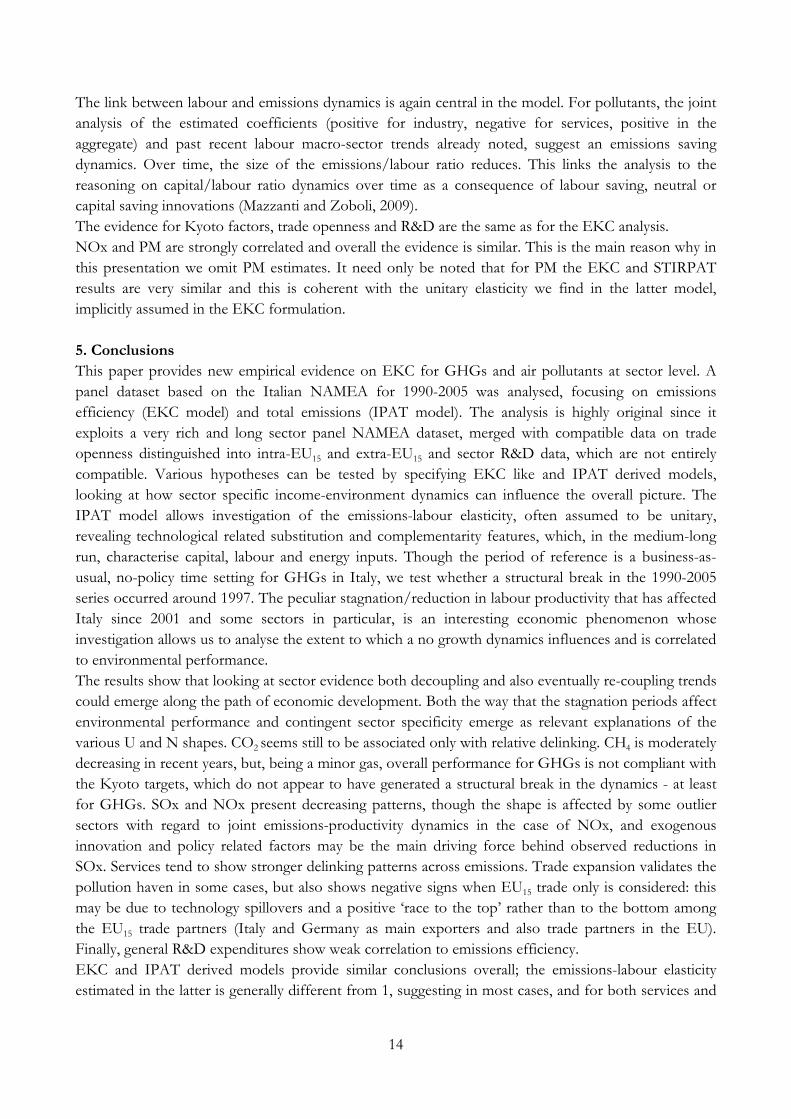
The link between labour and emissions dynamics is again central in the model. For pollutants, the joint analysis of the estimated coefficients (positive for industry, negative for services, positive in the aggregate) and past recent labour macro-sector trends already noted, suggest an emissions saving dynamics. Over time, the size of the emissions/labour ratio reduces. This links the analysis to the reasoning on capital/labour ratio dynamics over time as a consequence of labour saving, neutral or capital saving innovations (Mazzanti and Zoboli, 2009). The evidence for Kyoto factors, trade openness and R&D are the same as for the EKC analysis. NOx and PM are strongly correlated and overall the evidence is similar. This is the main reason why in this presentation we omit PM estimates. It need only be noted that for PM the EKC and STIRPAT results are very similar and this is coherent with the unitary elasticity we find in the latter model, implicitly assumed in the EKC formulation. 5. Conclusions This paper provides new empirical evidence on EKC for GHGs and air pollutants at sector level. A panel dataset based on the Italian NAMEA for 1990-2005 was analysed, focusing on emissions efficiency (EKC model) and total emissions (IPAT model). The analysis is highly original since it exploits a very rich and long sector panel NAMEA dataset, merged with compatible data on trade openness distinguished into intra-EU15 and extra-EU15 and sector R&D data, which are not entirely compatible. Various hypotheses can be tested by specifying EKC like and IPAT derived models, looking at how sector specific income-environment dynamics can influence the overall picture. The IPAT model allows investigation of the emissions-labour elasticity, often assumed to be unitary, revealing technological related substitution and complementarity features, which, in the medium-long run, characterise capital, labour and energy inputs. Though the period of reference is a business-as-usual, no-policy time setting for GHGs in Italy, we test whether a structural break in the 1990-2005 series occurred around 1997. The peculiar stagnation/reduction in labour productivity that has affected Italy since 2001 and some sectors in particular, is an interesting economic phenomenon whose investigation allows us to analyse the extent to which a no growth dynamics influences and is correlated to environmental performance. The results show that looking at sector evidence both decoupling and also eventually re-coupling trends could emerge along the path of economic development. Both the way that the stagnation periods affect environmental performance and contingent sector specificity emerge as relevant explanations of the various U and N shapes. CO2 seems still to be associated only with relative delinking. CH4 is moderately decreasing in recent years, but, being a minor gas, overall performance for GHGs is not compliant with the Kyoto targets, which do not appear to have generated a structural break in the dynamics - at least for GHGs. SOx and NOx present decreasing patterns, though the shape is affected by some outlier sectors with regard to joint emissions-productivity dynamics in the case of NOx, and exogenous innovation and policy related factors may be the main driving force behind observed reductions in SOx. Services tend to show stronger delinking patterns across emissions. Trade expansion validates the pollution haven in some cases, but also shows negative signs when EU15 trade only is considered: this may be due to technology spillovers and a positive ‘race to the top’ rather than to the bottom among the EU15 trade partners (Italy and Germany as main exporters and also trade partners in the EU). Finally, general R&D expenditures show weak correlation to emissions efficiency. EKC and IPAT derived models provide similar conclusions overall; the emissions-labour elasticity estimated in the latter is generally different from 1, suggesting in most cases, and for both services and

15

industry, a scenario characterised by emissions saving technological dynamics (as well as labour saving in relation to GHGs in industry). The application of heterogeneous panel estimators is a direction for future applied research to assess the extent to which U and N shapes emerge from ‘average’ trends. Both sector based and country based analyses would benefit from a comparison of homogenous and heterogeneous panel estimations. From a data construction point of view, future research should aim at using environmental R&D and innovation data at sector level; a final and challenging research direction would be to set up trade factors in terms of inter-sector and intra-sector datasets, by exploiting I-O tables and NAMEA or other compatible sources related to trading partners.

16

References Alberola E., Chevallier J.,Chèze B., 2008, Price drivers and structural breaks in European carbon prices

2005-2007, Energy Policy, 36 (2), pp. 787-797

― 2009, The EU Emissions Trading Scheme: Country-Specific Perspectives of the Impacts of Industrial Production on Carbon Prices, Journal of Policy Modelling, forthcoming

Barker T., Rosendahl K. E., 2000, Ancillary Benefits of GHG Mitigation in Europe: SO2, NOx and PM10 reductions from policies to meet Kyoto targets using the E3ME model and EXTERNE valuations, Ancillary Benefits and Costs of Greenhouse Gas Mitigation, Proceedings of an IPCC Co-Sponsored Workshop, March, OECD, Paris

Berndt E. R., Wood D. O., 1979, Engineering and Econometric Interpretations of Energy-Capital Complementarity, The American Economic Review, Vol. 69, No. 3, pp. 342-354

Bruvoll A., Medin H., 2003, Factors behind the environmental Kuznets curve. A decomposition of the changes in air pollution, Environmental and Resource Economics, Vol. 24, pp. 27-48

Casler S. D., Rose A., 1998, Carbon Dioxide Emissions in the U.S. Economy, Environmental and Resource Economics, 11 (3-4), pp. 349-363

Cole M. A., 2003, Development, Trade and the Environment: How Robust is the Environmental Kuznets Curve? Environment and Development Economics, Vol. 8, pp. 557-80

― 2004, Trade, the pollution haven hypothesis and the environmental Kuznets curve: examining the linkages, Ecological Economics, Vol. 48, No. 1, pp. 71-81

― 2005, Re-examining the pollution-income relationship: a random coefficients approach, Economics Bulletin, Vol. 14, pp. 1-7

Cole M. A., Elliott R., 2002, Determining the trade-environment composition effect: the role of capital, labor and environmental regulation, Journal of Environmental Economics and Management, No. 46, pp. 363-383

Cole M. A., Elliott R., Shimamoto K., 2006, Why the grass is not always greener: the competing effects of environmental regulations and factor intensities on US specialization, Ecological Economics, Vol. 54, pp. 95-109.

Cole M. A., Neumayer E., 2004, Examining the Impact of Demographic Factors on Air Pollution, Population & environment, 26 (1), pp. 5-21

Cole M. A., Rayner A., Bates J., 1997, The EKC: an empirical analysis, Environment and Development Economics, 2, pp. 401-16

Copeland B. R., Taylor M. S., 2004, Trade, growth and the environment, Journal of Economic Literature, Vol. 42, pp. 7-71

de Haan M., 2001, A Structural Decomposition Analysis of Pollution in the Netherlands, Economic System Research, Vol. 13, No. 2, pp. 181-196

de Haan M. Keuning S.J., 1996, Taking the environment into account: the NAMEA approach, The Review of Income and Wealth, Vol. 42, pp. 131-48

17

Dietz T., Rosa E. A., 1994, Rethinking the Environmental Impacts of Population, Affluence and Technology, Human Ecology Review, No. 1, pp. 277-300

Dietzenbacher E., Mukhopadhay K., 2006, An empirical examination of the pollution haven hypothesis for India: towards a green Leontief paradox?, Environmental & Resource Economics, Vol. 36, pp. 427-49

EEA, 2004a, Air Emissions in Europe, 1990-2000, Copenhagen, European Environment Agency

― 2004b, Air Pollution and Climate Change Policies in Europe: Exploring Linkages and the Added Value of an Integrated Approach, EEA Technical report No. 5/2004, Copenhagen, European Environment Agency

Femia A., Panfili P., 2005, Analytical applications of the NAMEA, Paper presented at the annual meeting of the Italian Statistics society, Rome

Fischer Kowalski M., Amann C., 2001, Beyond IPAT and Kuznets Curves: globalization as a vital factor in analyzing the environmental impact of socio economic metabolism. Population and the Environment, Vol. 23

Frankel J., Rose A., 2005, Is trade good or bad for the environment? The Review of Economics and Statistics, Vol. 87, No. 1, pp. 85-91

Ike T., 1999, A Japanese NAMEA, Structural change and economic dynamics, Vol. 10, pp. 122-149.

Kagawa S., Inamura H., 2001, A Structural Decomposition of Energy Consumption Based on a Hybrid Rectangular Input-Output Framework: Japan’s Case, Economic Systems Research, Vol. 13, No. 4, pp. 339-363

― 2004, A Spatial Structural Decomposition Analysis of Chinese and Japanese Energy Demand: 1985-1990, Economic Systems Research, Vol. 16, No. 3, pp. 279-299

Keuning S., van Dalen J., de Haan M., 1999, The Netherlands’ NAMEA; presentation, usage and future extensions, Structural change and economic dynamics, Vol. 10, pp. 15-37

Koetse M. J., de Groot H. L. F., Florax R. J. G. M., 2008, Capital-energy substitution and shifts in factor demand: A meta analysis, Energy Economics, Vol. 30, pp. 2236-2251

Jacobsen H. K., 2000, Energy Demand, Structural Change and Trade: A Decomposition Analysis of the Danish Manufacturing Industry, Economic Systems Research, Vol. 12, No. 3, pp. 319-343

List J. A., Gallet C. A., 1999, Does one size fits all?, Ecological Economics, Vol. 31, pp. 409-424

Markandya A., Rübbelke D. T. G., 2003, Ancillary Benefits of Climate Policy, Nota di lavoro No. 105, Milan, FEEM

18

Martinez-Zarzoso I., Bengochea-Morancho A., Morales-Lage R., 2007, The impact of population on CO2 emissions: evidence from European countries, Environmental and Resource Economics, Vol. 38, pp. 497-512

Mazzanti M. Zoboli R., 2009, Environmental efficiency and labour productivity: trade-off or joint dynamics?, Ecological Economics, forthcoming

Mazzanti M. Montini A. Zoboli R., 2008a, Environmental Kuznets curve for air pollutant emissions in Italy: evidence from environmental accounts NAMEA panel data, Economic System Research, Vol. 20, No. 3, pp. 279-305

― 2008b, Environmental Kuznets Curves and Greenhouse gas emissions. Evidence from NAMEA and provincial data, International journal of global environmental issues, Vol. 8, No. 4, pp. 392-424

Muradian R., O’Connor M., Martinez-Alier J., 2002, Embodied pollution in trade: estimating the environmental load displacement of industrialised countries, Ecological Economics, Vol. 41, pp. 51-67

Nakamura S., 1999, An inter-industry approach to analyzing economic and environmental effects of the recycling of waste, Ecological economics, Vol. 28, pp. 133-145

Nansai K., Kagawa S., Moriguchi Y., 2007, Proposal of a simple indicator for sustainable consumption: classifying goods and services into three types focusing on their optimal consumption levels, Journal of Cleaner Production, Vol. 15, Issue 10, pp. 879-885

Pearce D., 1992, Secondary Benefits of Greenhouse Gas Control, CSERGE Working Paper 92-12 (London)

Pearce D., 2000, Policy Framework for the Ancillary Benefits of Climate Change Policies, Paper Presented at the IPCC Workshop on Assessing the Ancillary Benefits and Costs of Greenhouse Gas Mitigation Strategies (Washington DC)

Smith S., Swierzbinski J., 2007, Assessing the performance of the UK Emission Trading Scheme, Environmental and Resource Economics, Vol. 37, pp. 131-158

Steenge A., 1999, Input-output theory and institutional aspects of environmental policy, Structural change and economic dynamics, Vol. 10, pp. 161-76

Stern D., 1998, Progress on the environmental Kuznets curve? Environment and Development Economics Vol. 3, pp. 173–196.

― 2004a, The rise and fall of the Environmental Kuznets curve, World Development, Vol. 32, No. 8, pp. 1419-38

― 2004b, Elasticities of Substitution and Complementarity, Rensselaer Working Papers in Economics, No. 20/2004

UN, Eurostat, IMF, OECD, World Bank, 2003, Integrated Environmental and Economic Accounting 2003 – Handbook of National Accounting, Final Draft circulated for information prior to official editing, http://unstats.un.org/UNSD/envaccounting

Vaze P., 1999, A NAMEA for the UK, Structural change and economic dynamics, Vol. 10, pp. 99-121

19

Vollebergh H., Kemfert C., 2005, The role of technological change for a sustainable development. Ecological Economics, Vol. 54, pp. 133-147

Wier M., 1998, Sources of Changes in Emissions from Energy: A Structural Decomposition Analysis, Economic system research, Vol. 10, No. 2, pp. 99-112

Wooldridge J., 2005, Introductory Econometrics – A Modern Approach, Mason (Ohio), Thomson South-Western, 2nd edition

York R., Rosa E. A., Dietz T., 2003, STIRPAT, IPAT and ImPACT: analytic tools for unpacking the driving forces of environmental impacts, Ecological Economics, No. 46, pp. 351-365

Zoboli R., 1996, Technology and Changing Population Structure: Environmental Implications for the Advanced Countries, Dynamis-Quaderni, 6/96, Milan, IDSE-CNR, www.idse.mi.cnr.it

Zugravu N., Millock K., Duchene G., 2008, The Factors Behind CO2 Emission Reduction in Transition Economies, Nota di lavoro No. 58, Milan, FEEM

20

90

100

110

120

130

140

150

160

170

1990

1991

1992

1993

1994

1995

1996

1997

1998

1999

2000

2001

2002

2003

2004

2005

VA VA/L L TO (EU 15) TO (extra EU 15)

Fig. 1: VA, VA/L, L, TO aggregate (1990=100 for VA, VA/L and L and 1995=100 for TO)

80

85

90

95

100

105

110

115

120

1990

1991

1992

1993

1994

1995

1996

1997

1998

1999

2000

2001

2002

2003

2004

2005

VA VA/L L

Fig. 2: VA, VA/L, L industry (1990=100)

90

95

100

105

110

115

120

125

130

1990

1991

1992

1993

1994

1995

1996

1997

1998

1999

2000

2001

2002

2003

2004

2005

VA VA/L L

Fig. 3: VA, VA/L, L services (1990=100)

21

20

30

40

50

60

70

80

90

100

110

120

1990

1991

1992

1993

1994

1995

1996

1997

1998

1999

2000

2001

2002

2003

2004

2005

CO2/L CH4/L NOx/L SOx/L

Fig. 4: Emission/L trends (aggregate; 1990=100)

20

30

40

50

60

70

80

90

100

110

120

1990

1991

1992

1993

1994

1995

1996

1997

1998

1999

2000

2001

2002

2003

2004

2005

CO2 CH4 NOx SOx

Fig. 5: Emission trends (aggregate; 1990=100)

22

J

K

67

89

10ln

(CO

2/L)

3 3.5 4 4.5 5ln(VA/L)

ln(CO2/L) Fitted (U-shape with K)Fitted (linear without K)

Fig. 6: Outlier K in EKC estimations for CO2 (services macro-sector)

DF

CA

02

46

8ln

(NO

x/L)

2 3 4 5 6ln(VA/L)

ln(NOx/L) Fitted (N-shape with CA and DF)Fitted (Inverted-U-shape without CA and DF)

Fig. 7: Outliers CA and DF in EKC estimations for NOx (aggregate)

23

Table 1: Nace branches classification

Nace (Sub-section) Sector Description

A Agriculture B Fishery

CA Extraction of energy minerals CB Extraction of non energy minerals DA Food and beverages DB Textile DC Leather textile DD Wood DE Paper and cardboard DF Coke, oil refinery, nuclear disposal DG chemical DH Plastic and rubber DI Non metallurgic minerals DJ Metallurgic DK Machinery DL Electronic and optical machinery DM Transport vehicles production DN Other manufacturing industries E Energy production (electricity, water, gas)

Ind

ust

ry

F Construction G Commerce H Hotels and restaurants I Transport J Finance and insurance K Other market services (real estate, ICT, R&D) L Public administration M Education N Health

Serv

ices

O Other public services

Table 2: Correlation matrix

ln(VA/L) ln(L) ln(TOEU15) ln(TOextraEU15) ln(R&D/VA) ln(CO2) 0.0887 0.0971 -0.1386* -0.1465* 0.1036** ln(CH4) 0.0134 -0.19 -0.2138* -0.2829* -0.0138** ln(NOx) 0.2905 0.2157 -0.3233* -0.5185* 0.0101** ln(SOx) -0.3218 0.132 -0.3641* -0.5216* -0.2157** ln(CO2/L) 0.4161 -0.5348 -0.1485* -0.0358* 0.1259** ln(CH4/L) 0.167 -0.4415 -0.2129* -0.2132* 0.0148** ln(NOx/L) -0.0798 -0.1418 -0.352* -0.4745* 0.0429** ln(SOx/L) -0.2481 -0.046 -0.3766* -0.5034* -0.2039** ln(VA/L) 1 -0.5003 -0.3698* -0.1868* 0.0764** ln(L) -0.5003 1 0.0282* -0.1351* -0.0837** ln(TOEU15)* -0.3698* 0.0282* 1* 0.7964* - ln(TOextraEU15)* -0.1868* -0.1351* 0.7964* 1* - ln(R&D/VA)**

0.0764** -0.0837** - - 1**

* Only for branches A, B, C, D and E ** Only for branches D, E and F Correlation between panel variables is equal to corr(xit, yit)=(β1*β2)1/2, with β1 and β2 given by REM estimates of equations yit=α+ β1xit+ν2it and xit=α+ β2yit+ν2it

24

Table 3: Descriptive statistics

VARIABLE MIN MAX MEAN (overall)

MEDIAN (overall)

WHOLE NAMEA [29 BRANCHES] (1990-2005)

VA/L 11.51 (A 1990)

528.5 (CA 2000) 62.83 41.51

L 6 (CA 2000, CA 2001)

3660 (G 1991) 780.64 479.5

INDUSTRY [C, D, E, F] (1990-2005)

VA/L 22.44 (DD 1990)

528.5 (CA 2000) 74.81 45.22

L 6 (CA 2000, CA 2001)

1898 (F 2005) 379.07 266

SERVICES [G, H, I, J, K, L, M, N, O] (1990-2005)

VA/L 27.11 (H 2004)

111.53 (K 1990) 48.83 39.07

L 588 (J 2000)

3660 (G 1991) 1575.58 1450

TRADE OPENNESS [A, B, C, D, E] (1995-2004)

VA/L 15.63 (A 1995)

528.5 (CA 2000) 74.69 46.07

L 6 (CA 2000, CA 2001)

1640 (A 1995) 348.62 253

TO EU15 0.0241 (E 1999)

4.8922 (DF 2003) 1.0334 0.7805

TO extra EU15 0.0442 (E 1997)

12.796 (DF 2002) 1.3614 0.7368

RESERACH & DEVELOPMENT [D, E, F] (1991-2003)

VA/L 23.76 (DD 1991)

321.8 (DF 1995) 59.67 44.79

L 24 (DF 2002, DF 2003)

1794 (F 2003) 421.1 279

R&D/VA 0.0408 (F 1992)

179.7654 (DM 1993) 20.999 3.2635

25

Notes (Tables 4 to 11): Coefficients are shown in cells: *10% significance, **5%, ***1%. For each column we present the

best fitting specification (linear, quadratic, cubic) in terms of overall and coefficient significance. All specifications are

estimated using FE model; individual fixed effects coefficients are not shown for brevity. Below Kyoto coefficient, between

brackets, average emissions in 1998-2005 given 1990-1997 average equal to 100% are shown. F test is the joint test of

significance on all coefficients whereas F test fixed effect is the test of significance on individual fixed effects. TP both for

VA/L (two for cubic and one for quadratic specifications) and L are shown: between brackets there is the percentile of

each TP. Underlined TP are outside the range of the observations of VA/L or L Table 4: EKC models for CO2

EKC 1 [aggr]

EKC 2 [ind]

EKC 3 [serv]

EKC 5 [R&D/VA]

ln(CO2/L) ln(CO2/L) ln(CO2/L) ln(CO2/L) ln(VA/L) 0.4727*** 0.4965*** -7.4279*** 0.4726*** ln(VA/L)2 0.9458*** ln(VA/L)3 ln(TOEU15) ln(TOextraEU15) ln(R&D/VA) 0.0261* Kyoto 0.0416***

(104.25%) 0.1098*** (111.6%)

-0.0583** (94.34%)

0.0818*** (108.52%)

Constant 7.4618*** 7.9769*** 22.4173*** 8.0405*** R2 (overall) 0.2935 0.449 0.036 0.6309 F test 57.12*** 97.32*** 15.81*** 29.08*** F test fixed effects 1904.22*** 1863.46*** 1079*** 1018.55*** N*T 464 288 144 208 Period 1990-2005 1990-2005 1990-2005 1991-2003 Turning point(s) - - 50.7433***

(74) -

Shape (VA/L) Linear relationship

Linear relationship

U shape Linear relationship

Table 5: EKC models for CH4

EKC 1

[aggr] EKC 2 [ind]

EKC 3 [serv]

EKC 4a [TOEU15]

EKC 4b [TOextraEU15]

ln(CH4/L) ln(CH4/L) ln(CH4/L) ln(CH4/L) ln(CH4/L) ln(VA/L) 0.7745*** 1.8288*** 80.2449* TO non sign -1.7028*** ln(VA/L)2 -0.1085** -21.585* 0.2078*** ln(VA/L)3 1.9153* ln(TOEU15) ln(TOextraEU15) -0.2408*** ln(R&D/VA) Kyoto -0.2623***

(76.93%) -0.0465* (95.46%)

-0.7155*** (48.89%)

0.0654** (106.75%)

Constant -1.4227*** -3.5908*** -98.0505 5.514*** R2 (overall) 0.2274 0.6716 0.0309 0.0843 F test 39.37*** 29.72*** 58.21*** 10.09*** F test fixed effects 1156.84*** 1565.26*** 1011.3*** 1570.47*** N*T 464 288 144 190 Period 1990-2005 1990-2005 1990-2005 1995-2004 1995-2004 Turning point(s) - 4586.943 29.1941***

(6) 62.7539*** (78)

60.1708*** (76)

Shape (VA/L) Linear relationship

Inverted-U shape

N shape U shape

26

Table 6: STIRPAT models for CO2

STIRPAT 1

[aggr] STIRPAT 2 [ind]

STIRPAT 3 [serv]

STIRPAT 4a [TOEU15]

STIRPAT 4b [TOextraEU15]

STIRPAT 5 [R&D/VA]

ln(CO2) ln(CO2) ln(CO2) ln(CO2) ln(CO2) ln(CO2) ln(VA/L) 0.1555** 0.3236*** -44.28546** -3.7014** -3.665** 0.3106*** ln(VA/L)2 10.8242** 0.9108** 0.9052** ln(VA/L)3 -0.8807** -0.0674** -0.0671** ln(L) 0.2742*** 0.5042*** 19.9504*** 0.4131*** 0.3848*** 0.3914*** ln(L)2 -1.3123*** ln(TOEU15) -0.0801** ln(TOextraEU15) -0.0857** ln(R&D/VA) 0.0219* Kyoto 0.0536***

(105.51%) 0.0985*** (110.35%)

-0.055* (94.65%)

0.0491*** (105.03%)

0.055*** (105.65%)

0.0759*** (107.89%)

Constant 13.0296*** 11.3477*** 0.1075 17.6752*** 17.7354*** 12.1557*** R2 (overall) 0.0938 0.1471 0.0812 0.3513 0.3669 0.0151 F test 13.77*** 30.31*** 13.40*** 7.76*** 7.79*** 12.98*** F test fixed effects 1797.36*** 2056.23*** 1243.94*** 1162.54*** 1093.39*** 1071.92*** N*T 464 288 144 190 190 208 Period 1990-2005 1990-2005 1990-2005 1995-2004 1995-2004 1991-2003 TP (VA/L) - - 51.6548***

(74) 70.052*** (79)

22.1*** (9) 369.7534*** (97)

21.6562*** (8) 373.719*** (97)

-

TP (L) - - 2000.333*** (84)

- - -

Shape (VA/L) Linear relationship

Linear relationship

Inverted-N shape

Inverted-N shape

Inverted-N shape

Linear relationship

Table 7: STIRPAT models for CH4

STIRPAT 1 [aggr]

STIRPAT 2 [ind]

STIRPAT 3 [serv]

STIRPAT 4a [TOEU15]

STIRPAT 4b [TOextraEU15]

STIRPAT 5 [R&D/VA]

ln(CH4) ln(CH4) ln(CH4) ln(CH4) ln(CH4) ln(CH4) ln(VA/L) -5.5736** 0.6978*** -1.4912*** -9.175*** -7.8076*** 2.0434*** ln(VA/L)2 1.3107** 1.9984*** 1.6898** -0.1405* ln(VA/L)3 -0.099** -0.1376*** -0.1164** ln(L) -1.0067*** 1.5866*** 37.7562*** 5.9565*** ln(L)2 -0.0926** -2.6445*** -0.4585*** ln(TOEU15) -0.1519** ln(TOextraEU15) -0.335*** ln(R&D/VA) -0.039* Kyoto -0.2329***

(79.22%) -0.5473***

(57.85%) 0.059**

(106.07%)

Constant 21.2267*** -1.20098 -120.8714*** 20.9491*** 18.9406*** -17.1251*** R2 (overall) 0.001 0.0042 0.0181 0.3225 0.1325 0.0019 F test 20.88*** 15.37*** 76.57*** 6.33*** 8.28*** 8.65*** F test fixed effects 1055.47*** 1545.28*** 1371.51*** 2138.17*** 2290.87*** 1218.49*** N*T 464 288 144 190 190 208 Period 1990-2005 1990-2005 1990-2005 1995-2004 1995-2004 1991-2003 TP (VA/L) 35.6373***

(36) 190.5869*** (95)

- - 42.1155*** (33) 381.101*** (97)

45.2407*** (45) 352.0945*** (96)

1440.685

TP (L) - 5233.27 1259.677*** (33)

- - 661.8836*** (84)

Shape (VA/L) Inverted-N shape

Linear relationship

Linear relationship

Inverted-N shape

Inverted-N shape

Inverted-U shape

27

Table 8: EKC models for NOx

EKC 1 [aggr]

EKC 2 [ind]

EKC 3 [serv]

EKC 4a [TOEU15]

EKC 4b [TOextraEU15]

EKC 5 [R&D/VA]

ln(NOx/L) ln(NOx/L) ln(NOx/L) ln(NOx/L) ln(NOx/L) ln(NOx/L) ln(VA/L) 10.0681*** 11.5742*** -5.6082*** 5.9872** 7.1212*** -0.4047*** ln(VA/L)2 -2.3925*** -2.7614*** 0.7409*** -1.5026** -1.7495*** ln(VA/L)3 0.1829*** 0.2104*** 0.1195** 0.1361*** ln(TOEU15) -0.177** ln(TOextraEU15) -0.3179*** ln(R&D/VA) 0.0449* Kyoto -0.3102***

(73.33%) -0.2657*** (76.67%)

-0.4442*** (64.13%)

-0.1344*** (87.42%)

-0.0986*** (90.61%)

-0.2628*** (76.89%)

Constant -10.0073*** -11.6318** 13.4133*** -3.644 5.3821 5.4869*** R2 (overall) 0.0664 0.2302 0.0219 0.0069 0 0.4027 F test 77.55*** 41.29*** 84.97*** 14.81*** 18.48*** 38.33*** F test fixed effects 687.13*** 490.77*** 801.01*** 438.63*** 460.54*** 261.86*** N*T 464 288 144 190 190 208 Period 1990-2005 1990-2005 1990-2005 1995-2004 1995-2004 1991-2003 Turning point(s) 34.6481***

(34) 176.9981*** (94)

32.4444*** (17) 194.3337*** (91)

44.0287*** (67)

26.0667*** (11) 167.59*** (90)

27.873*** (12) 188.734*** (92)

-

Shape (VA/L) N shape N shape U shape N shape N shape Linear relationship

Table 9: EKC models for SOx

EKC 1

[aggr] EKC 2 [ind]

EKC 3 [serv]

EKC 4a [TOEU15]

EKC 4b [TOextraEU15]

EKC 5 [R&D/VA]

ln(SOx/L) ln(SOx/L) ln(SOx/L) ln(SOx/L) ln(SOx/L) ln(SOx/L) ln(VA/L) -11.1397*** -19.8059*** -0.4014* ln(VA/L)2 2.4244*** 2.5326*** ln(VA/L)3 -0.1691*** ln(TOEU15) -0.5588*** ln(TOextraEU15) -0.6415*** ln(R&D/VA) -0.1427*** Kyoto -1.224***

(29.41%) -1.2114*** (29.78%)

-1.0875*** (33.71%)

-0.9168*** (39.98%)

-0.864*** (42.15%)

-0.9923*** (37.07%)

Constant 19.2953*** 3.7807*** 39.3315*** 3.2841*** 3.1642*** 5.6374*** R2 (overall) 0.0745 0.0589 0.0291 0.0355 0.0204 0.0174 F test 218.81*** 704.57*** 64.84*** 209.14*** 213.68*** 223.3*** F test fixed effects 342.92*** 646.16*** 127.48*** 633.84*** 647.78*** 248.36*** N*T 464 288 144 190 190 208 Period 1990-2005 1990-2005 1990-2005 1995-2004 1995-2004 1991-2003 Turning point(s) 46.5812***

(65) 303.8811*** (98)

- 49.908*** (74)

- - -

Shape (VA/L) Inverted-N shape

No significant relationship

U shape No significant relationship

No significant relationship

Linear relationship

28

Table 10: STIRPAT models for NOx

STIRPAT 1 [aggr]

STIRPAT 2 [ind]

STIRPAT 3 [serv]

STIRPAT 4a [TOEU15]

STIRPAT 4b [TOextraEU15]

ln(NOx) ln(NOx) ln(NOx) ln(NOx) ln(NOx) ln(VA/L) 8.5468*** 14.7747*** -101.1291*** 6.2669** 6.5561** ln(VA/L)2 -2.0815*** -3.4499*** 25.5436*** -1.5721** -1.6129** ln(VA/L)3 0.16*** 0.2607*** -2.1457*** 0.1253** 0.1253** ln(L) 0.566*** 1.4859*** 13.3198** 1.0819*** 0.8761*** ln(L)2 -0.9414*** ln(TOEU15) -0.172** ln(TOextraEU15) -0.331*** ln(R&D/VA) Kyoto -0.3033***

(73.84%) -0.2572*** (77.32%)

-0.3537** (70.21%)

-0.1331*** (87.54%)

-0.099*** (90.58%)

Constant -4.8665* -19.2495*** 96.383** -4.4553 -3.9644 R2 (overall) 0.174 0.1618 0.1043 0.2226 0.2707 F test 70.24*** 57.88*** 35.55*** 15.08*** 18.39*** F test fixed effects 614.9*** 496.92*** 859.59*** 412.89*** 424.82*** N*T 464 288 144 190 190 Period 1990-2005 1990-2005 1990-2005 1995-2004 1995-2004 TP (VA/L) 28.1356***

(11) 207.6904*** (95)

38.8578*** (32) 174.2916*** (90)

43.742*** (63) 63.9451*** (78)

26.468*** (11) 162.3941*** (90)

27.3207*** (12) 194.6497*** (92)

TP (L) - - 1181.589*** (28)

- -

Shape (VA/L) N shape N shape Inverted-N shape

N shape N shape

Table 11: STIRPAT models for SOx

STIRPAT 1 [aggr]

STIRPAT 2 [ind]

STIRPAT 3 [serv]

STIRPAT 4a [TOEU15]

STIRPAT 4b [TOextraEU15]

STIRPAT 5 [R&D/VA]

ln(SOx) ln(SOx) ln(SOx) ln(SOx) ln(SOx) ln(SOx) ln(VA/L) -2.2639*** -2.1298*** 3.8154*** 4.0174*** -0.6676*** ln(VA/L)2 0.2273** -0.4424*** -0.4591*** ln(VA/L)3 ln(L) 0.7889*** 0.9916*** -2.8852*** -3.6036*** -3.8822*** ln(L)2 0.5108*** 0.5093*** ln(TOEU15) -0.7244*** ln(TOextraEU15) -0.8058*** ln(R&D/VA) -0.1497*** Kyoto -1.2064***

(29.93%) -1.2123*** (29.75%)

-0.7356*** (47.92%)

-0.914*** (40.09%)

-0.8565*** (42.46%)

-1.0019*** (36.72%)

Constant 9.3382*** 3.8264** 37.121*** 4.5337 5.3881 12.3995*** R2 (overall) 0.0457 0.1329 0.05 0.0445 0.0747 0.0167 F test 225.23*** 386.51*** 64.67*** 83.29*** 85.13*** 242.5*** F test fixed effects 319.81*** 609.69*** 165.01*** 415.78*** 422.36*** 244.51*** N*T 464 288 144 190 190 208 Period 1990-2005 1990-2005 1990-2005 1995-2004 1995-2004 1991-2003 TP (VA/L) 145.5714*

(92) - - 74.5703***

(79) 79.4935*** (82)

-

TP (L) - - - 34.0425** (14)

45.2139*** (16)

-

Shape (VA/L) U shape No significant relationship

Linear relationship

Inverted-U shape

Inverted-U shape

Linear relationship

NOTE DI LAVORO DELLA FONDAZIONE ENI ENRICO MATTEI

Fondazione Eni Enrico Mattei Working Paper Series

Our Note di Lavoro are available on the Internet at the following addresses: http://www.feem.it/Feem/Pub/Publications/WPapers/default.htm

http://www.ssrn.com/link/feem.html http://www.repec.org

http://agecon.lib.umn.edu http://www.bepress.com/feem/

NOTE DI LAVORO PUBLISHED IN 2009 SD 1.2009 Michael Hoel: Bush Meets Hotelling: Effects of Improved Renewable Energy Technology on Greenhouse Gas

Emissions SD 2.2009 Abay Mulatu, Reyer Gerlagh, Dan Rigby and Ada Wossink: Environmental Regulation and Industry LocationSD 3.2009 Anna Alberini, Stefania Tonin and Margherita Turvani: Rates of Time Preferences for Saving Lives in the

Hazardous Waste Site Context SD 4.2009 Elena Ojea, Paulo A.L.D. Nunes and Maria Loureiro: Mapping of Forest Biodiversity Values: A Plural

Perspective SD 5.2009 Xavier Pautrel : Macroeconomic Implications of Demography for the Environment: A Life-Cycle Perspective IM 6.2009 Andrew Ellul, Marco Pagano and Fausto Panunzi: Inheritance Law and Investment in Family Firms IM 7.2009 Luigi Zingales: The Future of Securities Regulation SD 8.2009 Carlo Carraro, Emanuele Massetti and Lea Nicita: How Does Climate Policy Affect Technical Change? An

Analysis of the Direction and Pace of Technical Progress in a Climate-Economy Model SD 9.2009 William K. Jaeger: The Welfare Effects of Environmental Taxation SD 10.2009 Aude Pommeret and Fabien Prieur: Double Irreversibility and Environmental Policy Design SD 11.2009 Massimiliano Mazzanti and Anna Montini: Regional and Sector Environmental Efficiency Empirical Evidence

from Structural Shift-share Analysis of NAMEA data SD 12.2009 A. Chiabai, C. M. Travisi, H. Ding, A. Markandya and P.A.L.D Nunes: Economic Valuation of Forest

Ecosystem Services: Methodology and Monetary Estimates SD 13.2009 Andrea Bigano, Mariaester Cassinelli, Fabio Sferra, Lisa Guarrera, Sohbet Karbuz, Manfred Hafner, Anil

Markandya and Ståle Navrud: The External Cost of European Crude Oil Imports SD 14.2009 Valentina Bosetti, Carlo Carraro, Romain Duval, Alessandra Sgobbi and Massimo Tavoni: The Role of R&D

and Technology Diffusion in Climate Change Mitigation: New Perspectives Using the Witch Model IM 15.2009 Andrea Beltratti, Marianna Caccavaio and Bernardo Bortolotti: Stock Prices in a Speculative Market: The

Chinese Split-Share Reform GC 16.2009 Angelo Antoci, Fabio Sabatini and Mauro Sodini: The Fragility of Social Capital SD 17.2009 Alexander Golub, Sabine Fuss, Jana Szolgayova and Michael Obersteiner: Effects of Low-cost Offsets on

Energy Investment – New Perspectives on REDD – SD 18.2009 Enrica De Cian: Factor-Augmenting Technical Change: An Empirical Assessment SD 19.2009 Irene Valsecchi: Non-Uniqueness of Equilibria in One-Shot Games of Strategic Communication SD 20.2009 Dimitra Vouvaki and Anastasios Xeapapadeas: Total Factor Productivity Growth when Factors of Production

Generate Environmental Externalities SD 21.2009 Giulia Macagno, Maria Loureiro, Paulo A.L.D. Nunes and Richard Tol: Assessing the Impact of Biodiversity

on Tourism Flows: A model for Tourist Behaviour and its Policy Implications IM 22.2009 Bernardo Bortolotti, Veljko Fotak, William Megginson and William Miracky: Sovereign Wealth Fund

Investment Patterns and Performance IM 23.2009 Cesare Dosi and Michele Moretto: Auctioning Monopoly Franchises: Award Criteria and Service Launch

Requirements SD 24.2009 Andrea Bastianin: Modelling Asymmetric Dependence Using Copula Functions: An application to Value-at-

Risk in the Energy Sector IM 25.2009 Shai Bernstein, Josh Lerner and Antoinette Schoar: The Investment Strategies of Sovereign Wealth Funds SD 26.2009 Marc Germain, Henry Tulkens and Alphonse Magnus: Dynamic Core-Theoretic Cooperation in a Two-

Dimensional International Environmental Model IM 27.2009 Frank Partnoy: Overdependence on Credit Ratings Was a Primary Cause of the Crisis SD 28.2009 Frank H. Page Jr and Myrna H. Wooders (lxxxv): Endogenous Network Dynamics SD 29.2009 Caterina Calsamiglia, Guillaume Haeringer and Flip Klijnb (lxxxv): Constrained School Choice: An

Experimental Study SD 30.2009 Gilles Grandjean, Ana Mauleon and Vincent Vannetelbosch (lxxxv): Connections Among Farsighted Agents SD 31.2009 Antonio Nicoló and Carmelo Rodríguez Álvarez (lxxxv): Feasibility Constraints and Protective Behavior in

Efficient Kidney Exchange SD 32.2009 Rahmi İlkiliç (lxxxv): Cournot Competition on a Network of Markets and Firms SD 33.2009 Luca Dall'Asta, Paolo Pin and Abolfazl Ramezanpour (lxxxv): Optimal Equilibria of the Best Shot Game SD 34.2009 Edoardo Gallo (lxxxv): Small World Networks with Segregation Patterns and Brokers SD 35.2009 Benjamin Golub and Matthew O. Jackson (lxxxv): How Homophily Affects Learning and Diffusion in

Networks

SD 36.2009 Markus Kinateder (lxxxv): Team Formation in a Network SD 37.2009 Constanza Fosco and Friederike Mengel (lxxxv): Cooperation through Imitation and Exclusion in Networks SD 38.2009 Berno Buechel and Tim Hellmann (lxxxv): Under-connected and Over-connected Networks SD 39.2009 Alexey Kushnir (lxxxv): Matching Markets with Signals SD 40.2009 Alessandro Tavoni (lxxxv): Incorporating Fairness Motives into the Impulse Balance Equilibrium and Quantal

Response Equilibrium Concepts: An Application to 2x2 Games SD 41.2009 Steven J. Brams and D. Marc Kilgour (lxxxv): Kingmakers and Leaders in Coalition Formation SD SD GC SD SD SD GC SD SD

42.2009 43.2009 44.2009 45.2009 46.2009 47.2009 48.2009 49.2009 50.2009

Dotan Persitz (lxxxv): Power in the Heterogeneous Connections Model: The Emergence of Core-Periphery Networks Fabio Eboli, Ramiro Parrado, Roberto Roson, Climate Change Feedback on Economic Growth: Explorations with a Dynamic General Equilibrium Mode Fabio Sabatini, Does Social Capital Create Trust? Evidence from a Community of Entrepreneurs ZhongXiang Zhang, Is it Fair to Treat China as a Christmas Tree to Hang Everybody’s Complaints? Putting its Own Energy Saving into Perspective Eftichios S. Sartzetakis, Anastasios Xepapadeas and Emmanuel Petrakis, The Role of Information Provision as a Policy Instrument to Supplement Environmental Taxes: Empowering Consumers to Choose Optimally Jean-François Caulier, Ana Mauleon and Vincent Vannetelbosch, Contractually Stable Networks Massimiliano Mazzanti, Susanna Mancinelli, Giovanni Ponti and Nora Piva, Education, Reputation or Network? Evidence from Italy on Migrant Workers Employability William Brock and Anastasios Xepapadeas, General Pattern Formation in Recursive Dynamical Systems Models in Economics Giovanni Marin and Massimiliano Mazzanti, Emissions Trends and Labour Productivity Dynamics Sector Analyses of De-coupling/Recoupling On A 1990-2005 Namea

(lxxxv) This paper has been presented at the 14th Coalition Theory Network Workshop held in Maastricht, The Netherlands, on 23-24 January 2009 and organised by the Maastricht University CTN group (Department of Economics, http://www.feem-web.it/ctn/12d_maa.php).

NOTE DI LAVORO DELLA FONDAZIONE ENI ENRICO MATTEI

Fondazione Eni Enrico Mattei Working Paper Series

Our Note di Lavoro are available on the Internet at the following addresses: http://www.feem.it/Feem/Pub/Publications/WPapers/default.htm

http://www.ssrn.com/link/feem.html http://www.repec.org

http://agecon.lib.umn.edu http://www.bepress.com/feem/

NOTE DI LAVORO PUBLISHED IN 2009 SD 1.2009 Michael Hoel: Bush Meets Hotelling: Effects of Improved Renewable Energy Technology on Greenhouse Gas

Emissions SD 2.2009 Abay Mulatu, Reyer Gerlagh, Dan Rigby and Ada Wossink: Environmental Regulation and Industry LocationSD 3.2009 Anna Alberini, Stefania Tonin and Margherita Turvani: Rates of Time Preferences for Saving Lives in the

Hazardous Waste Site Context SD 4.2009 Elena Ojea, Paulo A.L.D. Nunes and Maria Loureiro: Mapping of Forest Biodiversity Values: A Plural

Perspective SD 5.2009 Xavier Pautrel : Macroeconomic Implications of Demography for the Environment: A Life-Cycle Perspective IM 6.2009 Andrew Ellul, Marco Pagano and Fausto Panunzi: Inheritance Law and Investment in Family Firms IM 7.2009 Luigi Zingales: The Future of Securities Regulation SD 8.2009 Carlo Carraro, Emanuele Massetti and Lea Nicita: How Does Climate Policy Affect Technical Change? An

Analysis of the Direction and Pace of Technical Progress in a Climate-Economy Model SD 9.2009 William K. Jaeger: The Welfare Effects of Environmental Taxation SD 10.2009 Aude Pommeret and Fabien Prieur: Double Irreversibility and Environmental Policy Design SD 11.2009 Massimiliano Mazzanti and Anna Montini: Regional and Sector Environmental Efficiency Empirical Evidence

from Structural Shift-share Analysis of NAMEA data SD 12.2009 A. Chiabai, C. M. Travisi, H. Ding, A. Markandya and P.A.L.D Nunes: Economic Valuation of Forest

Ecosystem Services: Methodology and Monetary Estimates SD 13.2009 Andrea Bigano, Mariaester Cassinelli, Fabio Sferra, Lisa Guarrera, Sohbet Karbuz, Manfred Hafner, Anil

Markandya and Ståle Navrud: The External Cost of European Crude Oil Imports SD 14.2009 Valentina Bosetti, Carlo Carraro, Romain Duval, Alessandra Sgobbi and Massimo Tavoni: The Role of R&D

and Technology Diffusion in Climate Change Mitigation: New Perspectives Using the Witch Model IM 15.2009 Andrea Beltratti, Marianna Caccavaio and Bernardo Bortolotti: Stock Prices in a Speculative Market: The

Chinese Split-Share Reform GC 16.2009 Angelo Antoci, Fabio Sabatini and Mauro Sodini: The Fragility of Social Capital SD 17.2009 Alexander Golub, Sabine Fuss, Jana Szolgayova and Michael Obersteiner: Effects of Low-cost Offsets on

Energy Investment – New Perspectives on REDD – SD 18.2009 Enrica De Cian: Factor-Augmenting Technical Change: An Empirical Assessment SD 19.2009 Irene Valsecchi: Non-Uniqueness of Equilibria in One-Shot Games of Strategic Communication SD 20.2009 Dimitra Vouvaki and Anastasios Xeapapadeas: Total Factor Productivity Growth when Factors of Production

Generate Environmental Externalities SD 21.2009 Giulia Macagno, Maria Loureiro, Paulo A.L.D. Nunes and Richard Tol: Assessing the Impact of Biodiversity

on Tourism Flows: A model for Tourist Behaviour and its Policy Implications IM 22.2009 Bernardo Bortolotti, Veljko Fotak, William Megginson and William Miracky: Sovereign Wealth Fund

Investment Patterns and Performance IM 23.2009 Cesare Dosi and Michele Moretto: Auctioning Monopoly Franchises: Award Criteria and Service Launch

Requirements SD 24.2009 Andrea Bastianin: Modelling Asymmetric Dependence Using Copula Functions: An application to Value-at-

Risk in the Energy Sector IM 25.2009 Shai Bernstein, Josh Lerner and Antoinette Schoar: The Investment Strategies of Sovereign Wealth Funds SD 26.2009 Marc Germain, Henry Tulkens and Alphonse Magnus: Dynamic Core-Theoretic Cooperation in a Two-

Dimensional International Environmental Model IM 27.2009 Frank Partnoy: Overdependence on Credit Ratings Was a Primary Cause of the Crisis SD 28.2009 Frank H. Page Jr and Myrna H. Wooders (lxxxv): Endogenous Network Dynamics SD 29.2009 Caterina Calsamiglia, Guillaume Haeringer and Flip Klijnb (lxxxv): Constrained School Choice: An

Experimental Study SD 30.2009 Gilles Grandjean, Ana Mauleon and Vincent Vannetelbosch (lxxxv): Connections Among Farsighted Agents SD 31.2009 Antonio Nicoló and Carmelo Rodríguez Álvarez (lxxxv): Feasibility Constraints and Protective Behavior in

Efficient Kidney Exchange SD 32.2009 Rahmi İlkiliç (lxxxv): Cournot Competition on a Network of Markets and Firms SD 33.2009 Luca Dall'Asta, Paolo Pin and Abolfazl Ramezanpour (lxxxv): Optimal Equilibria of the Best Shot Game SD 34.2009 Edoardo Gallo (lxxxv): Small World Networks with Segregation Patterns and Brokers SD 35.2009 Benjamin Golub and Matthew O. Jackson (lxxxv): How Homophily Affects Learning and Diffusion in

Networks

SD 36.2009 Markus Kinateder (lxxxv): Team Formation in a Network SD 37.2009 Constanza Fosco and Friederike Mengel (lxxxv): Cooperation through Imitation and Exclusion in Networks SD 38.2009 Berno Buechel and Tim Hellmann (lxxxv): Under-connected and Over-connected Networks SD 39.2009 Alexey Kushnir (lxxxv): Matching Markets with Signals SD 40.2009 Alessandro Tavoni (lxxxv): Incorporating Fairness Motives into the Impulse Balance Equilibrium and Quantal

Response Equilibrium Concepts: An Application to 2x2 Games SD 41.2009 Steven J. Brams and D. Marc Kilgour (lxxxv): Kingmakers and Leaders in Coalition Formation SD 42.2009 Dotan Persitz (lxxxv): Power in the Heterogeneous Connections Model: The Emergence of Core-Periphery

Networks SD 43.2009 Fabio Eboli, Ramiro Parrado, Roberto Roson: Climate Change Feedback on Economic Growth: Explorations

with a Dynamic General Equilibrium Mode GC 44.2009 Fabio Sabatini: Does Social Capital Create Trust? Evidence from a Community of Entrepreneurs SD 45.2009 ZhongXiang Zhang: Is it Fair to Treat China as a Christmas Tree to Hang Everybody’s Complaints? Putting

its Own Energy Saving into Perspective SD 46.2009 Eftichios S. Sartzetakis, Anastasios Xepapadeas and Emmanuel Petrakis: The Role of Information Provision

as a Policy Instrument to Supplement Environmental Taxes: Empowering Consumers to Choose Optimally SD 47.2009 Jean-François Caulier, Ana Mauleon and Vincent Vannetelbosch: Contractually Stable Networks GC 48.2009 Massimiliano Mazzanti, Susanna Mancinelli, Giovanni Ponti and Nora Piva: Education, Reputation or

Network? Evidence from Italy on Migrant Workers Employability SD 49.2009 William Brock and Anastasios Xepapadeas: General Pattern Formation in Recursive Dynamical Systems

Models in Economics SD 50.2009 Giovanni Marin and Massimiliano Mazzanti: Emissions Trends and Labour Productivity Dynamics Sector

Analyses of De-coupling/Recoupling on a 1990-2005 Namea

(lxxxv) This paper has been presented at the 14th Coalition Theory Network Workshop held in Maastricht, The Netherlands, on 23-24 January 2009 and organised by the Maastricht University CTN group (Department of Economics, http://www.feem-web.it/ctn/12d_maa.php).