Elimination of high-amplitude noise during passive monitoring of hydrocarbon deposits by the...

1002

ISSN 1069-3513, Izvestiya, Physics of the Solid Earth, 2008, Vol. 44, No. 12, pp. 1002–1017. © Pleiades Publishing, Ltd., 2008.Original Russian Text © I.Ya. Chebotareva, A.F. Kushnir, M.V. Rozhkov, 2008, published in Fizika Zemli, 2008, No. 12, pp. 65–82.

INTRODUCTION

Emission tomography has been widely used in seis-mology for reconstruction of the distribution of localheterogeneities and monitoring of seismic activity[Nikolaev et al., 1986; Aleksandrov and Rykunov,1992; Arnason and Flovenz, 1992; Furumoto et al.,1992; Shubik and Ermakov, 1997; Tchebotareva andNikolaev, 1998; Chouet et al., 1999; Tchebotarevaet al., 2000; Kugaenko et al., 2004]. Emission tomogra-phy has also been applied in oil pool development formonitoring of induced seismicity (localization of weakand microearthquake sources) and diagnostic imagingof formation hydrofractures with the help of deep bore-hole observations [Aleksandrov and Mirzoev, 1997;Aleksandrov et al., 2005].

Weakened crustal volumes, such as fault zones,large fractures, interfaces of blocks, and porous andfractured reservoirs, radiate seismic noise during theirformation and subsequent development under the influ-ence of variations of tectonic and tidal stresses. Thisnoise is generated by growth of cracks and friction offault walls on different scales of a fractured structure.These factors cause constant coherent seismic emissioncharacterized by a noiselike waveform whose powerspectrum is controlled by processes in a weakened

zone. This radiation as recorded on the surface is com-parable in intensity with background microseismicvibrations generally possessing an incoherent structure.

In development of oil and gas fields, strong varia-tions in of the stress state of the medium associatedwith hydraulic fracturing and stress relaxation in thefracture formation also lead to seismic coherent emis-sive radiation from zones of structural defects andstress concentration. A coherent seismic emission isalso generated in the process of fluid migration throughpercolation channels and pulsations of related gas accu-mulations.

Seismic tomography, applied to localization of deepsources of coherent seismic emission, is an effectiveand practically convenient tool for monitoring of thedynamic state of the medium and detection of deeplocal structures. Using this method, a 3-D image ofsources of weak seismic radiation can be reconstructedin the form of a “cloud” filling the radiating region ofthe medium and the intensity and spectral compositionof the radiation can be estimated.

Seismic emission tomography is effective for local-izing not only active sources of a coherent seismic sig-nal, such as local earthquakes, natural and anthropo-genic surface sources, and deep sources of seismic

Elimination of High-Amplitude Noise during Passive Monitoring of Hydrocarbon Deposits by the Emission Tomography Method

I. Ya. Chebotareva

a

, A. F. Kushnir

b

, and M. V. Rozhkov

c

a

Institute of Oil and Gas Problems, Russian Academy of Sciences, ul. Gubkina 3, Moscow, 117701 Russia

b

International Institute of Earthquake Prediction Theory and Mathematical Geophysics, Russian Academy of Sciences, Varshavskoe sh. 79, korp. 2, Moscow, 113556 Russia

c

SYNAPSE Science Center (SSC), pr. Vernadskogo 101/1, Suite 303, Moscow, 119526 Russia

Received November 12, 2007

Abstract

—Emission tomography used in passive seismic monitoring of hydrocarbon deposits enables regularinspection of development of hydraulic fracturing and relaxation processes in volumes of fracturing, tracing offluid migration paths, redistribution of stresses due to field development accompanied by seismic emission fromvolumes of structural defects and stress concentration, and localization of fractured and faulted structures fromemission and scattering data. Intensive man-made seismic noise in the areas of oil field development producesa strong screening effect in identification of weak deep seismic sources. On the basis of experiments with sim-ulated and real data of surface seismic arrays in regions of oil deposits in Western Siberia (carried out in theframework of the passive monitoring program of the SYNAPSE Science Center), it is shown that the use ofalgorithms of adaptive optimal and rejection spatial filtering with the estimation of the spectral density matrixof multichannel observations in the framework of multivariate autoregressive-moving average modeling iseffective for eliminating the influence of anthropogenic noise and revealing (in oil production areas) both deepseismic sources supposedly active in scattering regions of the lower part of the sedimentary cover and the crys-talline basement. The projection of the scattering regions onto the horizontal plane correlates well with the posi-tion of faults in the area of in situ observations.

PACS numbers: 91.30.Jk

DOI:

10.1134/S1069351308120033

IZVESTIYA, PHYSICS OF THE SOLID EARTH

Vol. 44

No. 12

2008

ELIMINATION OF HIGH-AMPLITUDE NOISE 1003

emission from the regions of structural defects andstress concentration (passive monitoring), but alsozones of intense scattering of seismic signals propagat-ing from earthquakes and explosions and related tocontrasting velocity inhomogeneities and ruptures ofthe medium (diffraction emission tomography). Seis-mic noise records obtained by a 1-D (profile), 2-D, or3-D array of stations are used as initial data in passivemonitoring, and coda records of signals from explo-sions or earthquakes are used as input information indiffraction emission tomography.

Implementation of the emission tomographymethod implies that, at each sampling point of a 3-Dgrid, delay times of a noiselike waveform of seismicemission are calculated according to the acceptedvelocity structure and, using these results, the geophonearray is tuned for amplification of the signal from thesampling point. Then with the help of algorithmsimplementing emission tomography in the time domain[Nikolaev et al., 1986; Tchebotareva et al., 2000], theenergy of seismic records of the geophone array isaccumulated over channels and with time. A 3-D sub-surface image was calculated in terms of a coherentquadratic measure. If diffuse seismic noise is recorded,the reconstructed image of the medium has a uniformbrightness distribution. In the presence of a localizedseismic emission source, a bright spot appears in theimage, whose position points to the source location inthe medium. Given a weak signal, the numerical valueof the coherent quadratic measure at the source local-ization point is, accurate to an additive constant, theproduct of the number of channels and the signal/noiseenergy ratio at the surface [Tchebotareva et al., 2000].In the presence of additive diffuse seismic noise, thefluctuation value of the coherent quadratic measure atpoints outside the source decreases with an increase inthe accumulation time of the signal [Tchebotarevaet al., 2000]; i.e., an increase in the accumulation timemakes the method more sensitive.

The seismic wave field recorded in areas of com-mercial hydrocarbon deposits contains strong coherentnoise caused by surface anthropogenic sources. In thecase of borehole observations with deeply mountedrecording instruments, the influence of this surfacenoise can be substantially reduced. However, if record-ing instruments are installed on the surface or at smalldepth (up to 10 m), anthropogenic noise can have astrong detrimental effect on the results, masking a weakendogenous seismic signal, and even an increase in theaccumulation time of such a signal does not improvethe situation because the noise is coherent but not dif-fuse. On the other hand, deep (drilling tools) and pow-erful surface anthropogenic sources create a seismic“illumination” effect that can be used for identificationof velocity inhomogeneities, fractures, and faults fromdata on the scattered wave field generated by thesesources.

The analysis of seismic signals recorded in oil prov-inces of Western Siberia by geophones at shallowdepths or on the surface shows that wave fields in suchareas have a very complex wave structure including alow velocity component in addition to longitudinal andtransverse waves. If a wave field is a mixture of severalwave modes, imaging of the medium with a given wavemode implies that the remaining wave modes arenoises. If three-component records are used, suchnoises can be suppressed rather efficiently with the helpof emission tomography algorithms, after which thegeophone array can be tuned to the polarization of theselected wave mode. This is impossible if only verticalinstruments are used. In this case, reconstructed imagesof real sources of the chosen wave mode will be super-imposed by false defocused and biased images ofsources of the remaining wave modes. Depending onrelations between velocities and intensities of seismicemission of different wave modes and parameters of therecording array, the image distortion can be so strongthat the desired sources of endogenous emission will beunrecognizable against the background of intensenoise-related “trails.”

The presently existing seismic three-componentgeophones are very sensitive to installation conditionsor are extremely expensive, which impedes their utili-zation in mobile recording systems. Therefore, in prac-tice one has to use recording systems with vertical geo-phones. In order to ensure a successful analysis of fielddata for the purpose of monitoring of weak endogenousseismic emission, efficient methods should be devel-oped and used in order to eliminate the influence ofintense surface or deep sources of coherent noises.

ADAPTIVE OPTIMAL AND REJECTION SPATIAL FILTERING

In seismology, for seismic signals that are maskedby strong coherent noises, methods of statistical analy-sis of multivariate stationary time series have beendeveloped to synthesize statistically optimal algorithmsof adaptive and band-elimination multichannel (spatial)filtering and adaptive spatial spectral analysis [Kushnirand Mostovoi, 1990]. On the basis of experiments withthe model and real data of small aperture seismic arrays[Kushnir and Lapshin, 1997], it was shown that theapplication of the aforementioned statistically optimaladaptive algorithms to analysis of records of remoteearthquakes and nuclear explosions ensures accuratedetermination of the time function of the signal seismicwave and the direction of its arrival to the array with anappreciably smaller signal/noise ratio compared to tra-ditionally used algorithms.

This paper presents results of application of the opti-mal methods of rejection and adaptive spatial filteringand spatial spectral analysis to elimination of the strongcoherent noise influence in seismic emission tomogra-phy. When applied to emission tomography, computa-tional algorithms had to be modified and additionally

1004

IZVESTIYA, PHYSICS OF THE SOLID EARTH

Vol. 44

No. 12

2008

CHEBOTAREVA et al.

tested. This was caused not only by a large number ofseismic channels and transition to a 3-D dense scanninggrid (which influenced the algorithm stability and com-putation accuracy) but also by the fact that some resultsobtained for plane waves were found to be invalid forthe case of signals from near sources. For example, aswas shown in [Kushnir and Lapshin, 1997], the highresolution spatial spectral analysis [Capon, 1969] ofplane waves yields sharper peaks for signal arrivaldirections and weak spurious maximums as comparedwith the low resolution spectral analysis; i.e., the highresolution method is undoubtedly preferable. However,it was found that, in the case of real records containingsignals from near surface sources, the high resolutionmethod actually gives localized high amplitude peaksfor surface sources but, at a depth, it brings about abrighter trail masking weak deep sources more inten-sively compared to the low resolution method. Thus, inreconstructing 3-D seismic emission images, the tradi-tional methods of high resolution spatial spectral anal-ysis cannot be considered as preferable, particularlybecause they give ratios of peak values at seismicsource localization points that do not coincide withratios of signal intensities and can be very strongly dis-torted depending on the geometry of the seismic arrayand configuration of sources. The latter effect is relatedto the fact that functionals used in high resolution meth-ods are not consistent estimates of the spatial spectraldensity.

If intense coherent noise is present in seismicrecords and the source position and the noise propaga-tion velocity are known, it is appropriate to use a reject-ing spatial filter. A spatial filter

r

(

f

) = (

r

1

(

f

), …,

r

m

(

f

))

is a multichannel filter transforming

m

input traces

x

(

f

) = (

x

1

(

f

), …,

x

m

(

f

))

T

(

T

is the transposition sign)that are Fourier transforms of observations at a arrayof geophones into the scalar trace

y

(

f

)

using the rela-tion

y

(

f

)=

r

*(

f

)

x

(

f

), (1)

where

f

is the frequency and

*

is the sign of Hermitianconjugation.

The rejection spatial filter is a filter that suppressescoherent noises generated by localized sources whosepositions are known and extracts the useful coherentsignal generated by the source at the focusing point ofthe array. Theoretically, the filter suppresses com-pletely such noises if their number is less than the num-ber

m

of array geophones and diffuse noise is absent inobservations. A vector frequency characteristic of therejection spatial filter that ensures the maximum outputsignal/noise ratio (in the presence of diffuse noise) canbe written as

(2)

where

h

s

(

f

) = (exp{–

i

2

π

f

τ

k

(

r

s

)}

,

k

= 1, …,

m

, is the col-umn vector of the phase delays determined by the timedelays

τ

k

(

r

s

)

acquired between the first and

k

th geo-

rr f( ) hs* f( )B f( )[ ]/ hs* f( )B f( )hs f( )[ ]1/2,=

phones by the seismic signal propagating from the arrayfocusing point with the coordinates

r

s

= (

x

s

,

y

s

,

z

s

)

T

and

B

(

f

)

is the complex frequency-dependent matrix of therejection spatial filter. In the case of a single source ofcoherent noise, the matrix takes the form

(3)

where

I

is the unit matrix and

h

n

(

f

) = (exp{–

i

2

π

f

τ

k

(

r

n

)},

k

= 1, …,

m

)

is determined by the time delays

τ

k

(

r

n

)

ofthe coherent noise generated by the source with theknown coordinates

r

n

while propagating between thefirst and the

k

th geophone of the array.The formula for the frequency-dependent matrix of

the rejection spatial filter that suppresses coherentnoises generated by several active sources has a morecomplex form and is not presented here but can befound in [Kushnir and Mostovoi, 1990].

If information on the source coordinates of coherentnoises is absent or the noise is generated by numeroussources of coherent noises and diffuse seismic noise, itis appropriate to apply an adaptive optimal spatial filterensuring a maximum output signal/noise ratio (andwhitening of the residual noise):

(4)

where is the estimate of the inverse complexmatrix of the noise spectral density.

As is shown in [Kushnir and Mostovoi, 1990], if

in (4) coincides with the actual inverse matrix

of the array noise spectral density , the numberof coherent noise sources is less than

m

, and the inten-sity of diffuse noise tends to zero, then the efficiency ofsuppression of coherent noises by adaptive multichan-nel filter (4) approaches the efficiency of their suppres-sion by rejection spatial filter (3).

The vector frequency characteristic of the simplest(beamforming) spatial filter is

(5)

where

m

is the number of geophones in the array.The latter type of filter is basic in the algorithm of

traditional low resolution spatial spectral analysis: the

estimate of the signal source coordinates corre-sponds to the maximum of the functional

(6)

where

D

x

(

f) = x(f)x*(f) is the matrix periodogram, thatis, the simplest (nonsmoothed) estimate of the spectral

B f( ) I hn f( )hn* f( )– hn* f( )hn f( )⁄[ ],=

ra f( ) hs* f( )Fn1– f( )[ ]/ hs* f( )Fn

1–f( )hs f( )[ ]

1/2,=

Fn1–

f( )

Fn1–

f( )Fn

1– f( )

rb f( ) hs* f( )/ hs* f( )hs f( )( ) hs* f( )/m,= =

rs+

Pb r( ) r* f r,( )x f( ) 2

f min

f max

∑=

= hs* f r,( )Dx f( )hs f r,( ),f min

f max

∑

IZVESTIYA, PHYSICS OF THE SOLID EARTH Vol. 44 No. 12 2008


density matrix of the multichannel signal x(t) at the out-put of a group, where x(t) is the discrete Fourier trans-formation from x(t).

It is easy to show, using the Parseval theorem, thatfunctional (6) is equivalent (up to a normalizing factor)to the Semblance functional, used for implementationof the emission tomography algorithms for a single-component seismic array in the time domain:

(7)

where xi(tj) is the value of the signal recorded by the ithgeophone at the time moment tj and τi(r) is the timedelay of the signal arriving at the ith geophone from thesampled point with the coordinates r. Consequently,calculating the functionals Pb(r) and S(r) from recordsof a 3-D spatial sampling network in the framework ofa known velocity structure, we should obtain identicalseismic emission images in which brightness maxi-mums (maximums of the functionals Pb(r) and S(r))correspond to the position of seismic sources.

As is shown in [Kushnir, 1997], the statistically

optimal estimate of the source coordinates of a seis-mic signal (with a completely unknown waveform)recorded by a array of vertical geophones and maskedby random stationary seismic noise with the complexmatrix of the spectral density Fn(f) corresponds to themaximum of the functional

(8)

where h(f, r) = (exp{–i2πfτk(r)}, k = 1, …, m) is the col-umn vector of phase delays determined by the timedelays τk(r) acquired between the first and kth geo-phones by the seismic signal propagating from thearray focusing point with the coordinates rs. Compari-son of expressions (4) and (8) shows that the functionalPa(r) is equal to the intensity of the output signal of theadaptive optimal spatial filter tuned for the extraction ofa signal that propagates from the point with the coordi-nates r. This means that the adaptive optimal spatial fil-ter is the basic spatial filter for the construction of func-tional (8).

Using rejection spatial (2) as the basic filter in con-structing the functional for estimation of the source

coordinates of a coherent signal against the back-

S r( )

xi t j τi r( )–( )i 1=

K

∑⎝ ⎠⎜ ⎟⎛ ⎞

2

j 1=

T

∑

xi2 t j τi r( )–( )

i 1=

K

∑j 1=

T

∑-------------------------------------------------------,=

rs

Pa r( ) h* f r,( )Fn1–

f( )x f( )2

h* f r,( )Fn1–

f( )h f r,( )---------------------------------------------------------,

f min

f max

∑=

rs

ground of coherent noise, we obtain that the estimate of

is provided by the maximum of the functional

(9)

Adaptive optimal and rejection spatial filtering (inthe form of functionals (8) and (9)) is well suited forlocalizing weak deep seismic sources from data of sur-face seismic arrays in the presence of intense coherentnoises. However, the reconstruction of 3-D seismicemission images of the medium with the use of formu-las (8) and (9) requires a computation time that is morethan one order of magnitude larger compared to imagesreconstructed without filtering by formula (7) with therealization in the time domain. Functionals (8) and (9)can be applied in practice only with the use of multipro-cessor computers or simplified calculation schemes.

We used a simplified calculation scheme describedbelow. Formula (8) can be rewritten in an equivalentform:

(10)

Assume that the frequency range under consideration(fmax, fmin) is so narrow that variations in the functions

h(f, r) and (f) in this range can be neglected. Then,formula (10) can be rewritten in the form

(11)

where f0 is the central frequency of the frequency range(fmax, fmin) analyzed. The expression in the brackets isthe matrix periodogram of the recorded multichanneldata of the array summed over frequencies of thisrange. It can be replaced with the statistically more sub-

stantiated value (fmax – fmin) , where is asmoothed estimate of the matrix power spectrum den-sity of the array multichannel data x(t) (under theassumption that this estimate varies weakly within thefrequency range analyzed). In this case, we obtain thefollowing approximation for functional (8):

(12)

ρ

Pr r( ) h* f r,( )B f( )x f( ) 2

h* f r,( )B f( )h f r,( )-----------------------------------------------------.

f min

f max

∑=

Pa r( )

= h* f r,( )Fn

1–f( )x f( )x* f( )Fn

1–f( )h f r,( )

h* f r,( )Fn1–

f( )h f r,( )---------------------------------------------------------------------------------------------.

f min

f max

∑

Fn1–

Pa r( )

=

h* f 0 r,( )Fn1–

f 0( ) x f( )x* f( )f min

f max

∑ Fn1–

f 0( )h f 0 r,( )

h* f 0 r,( )Fn1–

f 0( )h f 0 r,( )-------------------------------------------------------------------------------------------------------------------,

Fx f 0( ) Fx f( )

Pa r( )h* f 0 r,( )Fn

1–f 0( )Fx f 0( )Fn

1–f 0( )h f 0 r,( )

h* f 0 r,( )Fn1–

f 0( )h f 0 r,( )----------------------------------------------------------------------------------------------≈

× f max f min–( ).

1006


CHEBOTAREVA et al.

Analogously, the approximation formula obtainedfor functional (9) by applying band-elimination multi-channel filter (2) is

(13)

and, using the simplest spatial filter (5), functional (6)can be approximated by the formula

. (14)

In broadband analysis, formulas (12), (13), and (14)are used for calculation of a set of narrowband sourceimages to be summed. Algorithms implementing theseapproximation formulas reduce the computation timeby more than two orders of magnitude with an insig-nificant distortion of source images, and this is illus-trated below in the discussion of results of real dataprocessing.

A statistically reliable and computationally efficientestimate of the spectral density matrix of array multi-channel data can be obtained on the basis of the multi-variate autoregressive-moving average (ARMA) model[Kushnir and Mostovoi, 1990]. The ARMA model of avector time series x(t) = (x1(t), …, xM(t))T, t ∈ Z, is anew time series y(t) = (y1(t), …, yM(t))T satisfying thedifference equation

(15)

where Z is a set of whole numbers; e(t) = (e1(t), …,em(t))T, ek(t), k = 1, …, m, are random variables that areindependent for all k and t and have zero means and unitvariances; and A(l), l = 1, …, p, and B(l), l = 0, …, q,are m × m matrix parameters of autoregression andmoving average, respectively, whose first p + q + 1 val-ues of the matrix covariance function are the same asthose in time series x(t). The inverse spectral densitymatrix of the ARMA model y(t) has the form

F–1(f) = P(f)Q–1(f)P*(f), (16)

where P(f) = , Q(f) =

exp(–i2πkf/fs), A(0) = I is the unit matrix,and fs is the sampling frequency of the initial time seriesx(t).

Estimates of the inverse spectral densitymatrix of noises at geophone outputs that were used inexperiments with model and real data of 2-D arraysdescribed below had structure (16), i.e., corresponded toARMA models of multichannel observations x(t), t = 1, …,

N. The autoregression coefficients (k), k = 1, …, m,

Pr r( )h* f 0 r,( )B f 0( )Fx f 0( )B f 0( )h f 0 r,( )

h* f 0 r,( )B f 0( )h f 0 r,( )--------------------------------------------------------------------------------------≈

× f max f min–( ),

Pb r( ) h* f 0 r,( )Fx f 0( )h f 0r( )≈

y t( ) A l( )y t l–( ) B l( )e t l–( ),l 0=

q

∑+l 1=

p

∑=

t Z,∈

A k( ) i2πkf / f s–( )expk 0=p∑

B k( )k 0=q∑

Fn1–

f( )

A

were estimated from the first p values of the samplingmatrix correlation function of observations x(t), t = 1, …,N, with the help of the computationally efficient multi-dimensional Levinson–Durbin procedure [Kushnir andMostovoi, 1990], and estimates of the moving average

coefficients (k), k = 0, …, m, were set equal to B(k) =Cz(k)w(k), where Cz(k) are the sampling matrix auto-correlations of the preliminarily whitened time series

z(t) = x(t – k), (0) = I, and w(k) = w(–k),w(k) = 1 – k/(q – 1) q > k > 0 are the coefficients of theBartlett time window.

The choice of the frequency step for calculatingfunctionals (12), (13), and (14) in the broadband analy-sis of the array data

x(t), t = 1, …, N, was determined by the orders p andq of the corresponding ARMA model, which were usedfor the estimation of the spectral density matrix ofobservations x(t).

The pseudo-bending method proposed in [Um andThurber, 1987] implemented in our work as a computerprogram was used for seismic ray tracing and calcula-tion of time delays. In this approach, a preset firstapproximation of a ray trace connecting source andreceiver points is iteratively perturbed in such a way asto satisfy the Fermat principle. For gradient velocitystructures, this method is very efficient, enabling 3-Dseismic ray tracing.

NUMERICAL MODELING

In this section, we present results of numerical mod-eling illustrating the efficiency of the use of rejectionand adaptive optimal spatial filtering in emissiontomography algorithms. The modeling used a realgeometry of a seismic geophone array (Fig. 5). Themodel wave velocities also had real values, and a fre-quency range of 10–30 Hz is used.

Results obtained by the method of rejection spatialfiltering are shown in Fig. 1. The wave field generatedin the model is a result of the superposition of weak ran-dom noise uncorrelated between channels and signalsfrom four seismic sources with the coordinates in kilo-meters (1, 1), (–1, –1), (–1, 1), and (1, –1). The timefunctions of signals represent an uncorrelated randomprocess. The emission intensities are chosen in such away that the image brightness values at the sourcepoints coincide. Figure 1a displays the seismic emis-sion image of the model wave field calculated with thehelp of functional (14) with the summation over a set offrequencies within a range of 10–30 Hz. The (1, 1) sourceis farther from the center of the geophone array com-pared to the three other sources. As a result, a trail oflarger values is observed near the source, in the vicinityof a sharp peak. In Fig. 1a, this source is the third fromthe right. Evidently, brightness maximums with suchintense and extended trails are more difficult to elimi-nate compared to well localized maximums. Neverthe-

B

A k( )k 0=p∑ A



less, as seen from Fig. 1b, the rejection spatial filtering(formula (13)) removes completely the maximum withthe intense trail.

Figure 1c illustrates successful suppression of the(1, 1) and (–1, –1) sources with the help of the rejectionspatial filtering.

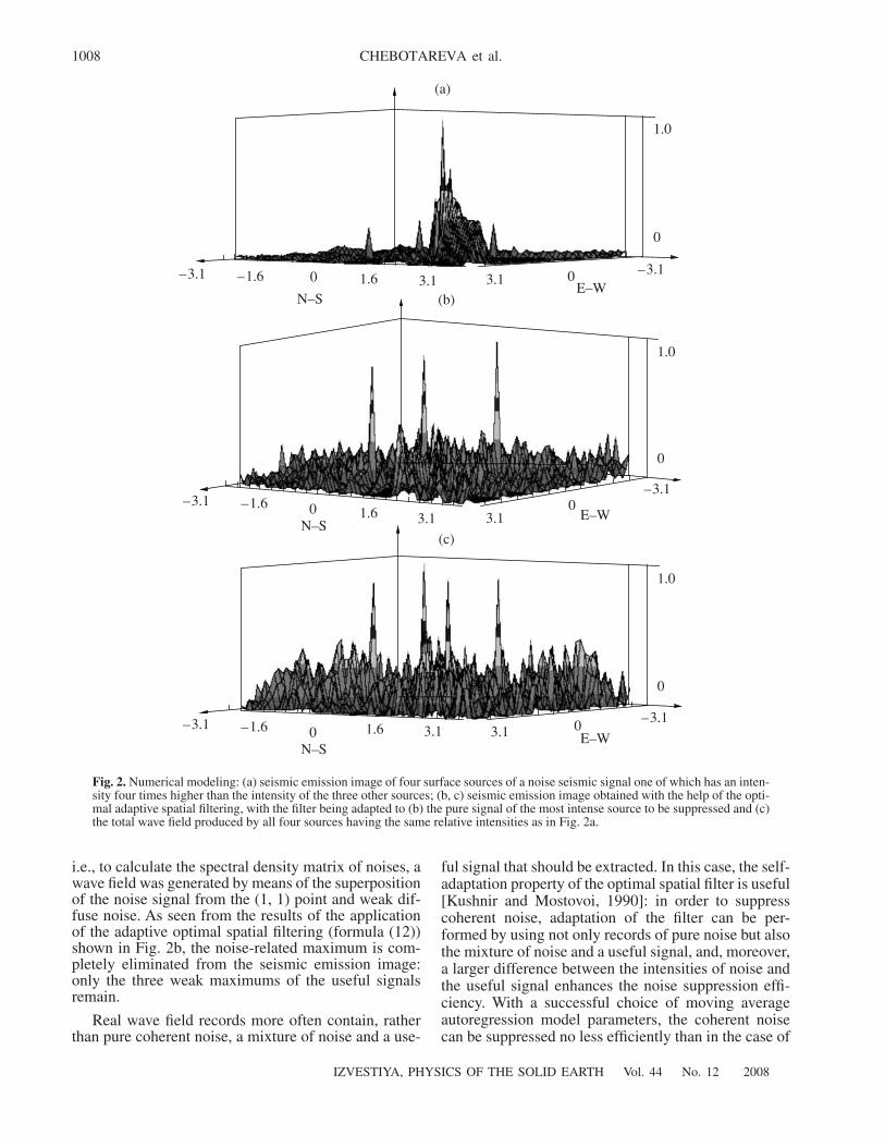
Results of application of the adaptive optimal spatialfiltering are shown in Fig. 2. The input data wereobtained, as before, by superposition of the arrayrecords from four noise sources with the coordinates in

kilometers (1, 1), (–1, –1), (–1, 1), (1, –1) and from dif-fuse noise. Emission intensities of three sources aresuch that the values of the corresponding maximumsare identical, while the fourth, (1, 1) source modelingcoherent noise is stronger and its maximum four timeslarger compared to the other three sources. A seismicemission image of the model wave field calculated withthe help of functional (14) and the summation over fre-quencies in the range 10–30 Hz is shown in Fig. 2a. Totune the adaptive optimal spatial filter to “pure noise,”

–3.1 –1.6 0 1.6 3.1 3.10

–3.1

0

1.0

N–S E–W

(a)

–3.1 –1.6 0 1.6 3.1 3.10

–3.1

0

1.0

N–SE–W

(b)

–3.1 –1.6 0 1.6 3.1 3.10

–3.1

0

1.0

N–SE–W

(c)

Fig. 1. Numerical modeling: (a) seismic emission image of four surface sources of a seismic noise signal having the same intensity;(b) seismic emission image obtained with the help of rejection spatial filtering suppressing one of the sources; (c) seismic emissionimage obtained with the help of rejection filtering simultaneously suppressing two sources.

1008


CHEBOTAREVA et al.

i.e., to calculate the spectral density matrix of noises, awave field was generated by means of the superpositionof the noise signal from the (1, 1) point and weak dif-fuse noise. As seen from the results of the applicationof the adaptive optimal spatial filtering (formula (12))shown in Fig. 2b, the noise-related maximum is com-pletely eliminated from the seismic emission image:only the three weak maximums of the useful signalsremain.

Real wave field records more often contain, ratherthan pure coherent noise, a mixture of noise and a use-

ful signal that should be extracted. In this case, the self-adaptation property of the optimal spatial filter is useful[Kushnir and Mostovoi, 1990]: in order to suppresscoherent noise, adaptation of the filter can be per-formed by using not only records of pure noise but alsothe mixture of noise and a useful signal, and, moreover,a larger difference between the intensities of noise andthe useful signal enhances the noise suppression effi-ciency. With a successful choice of moving averageautoregression model parameters, the coherent noisecan be suppressed no less efficiently than in the case of

–3.1 –1.6 0 1.6 3.1 3.10

–3.1

0

1.0

N–SE–W

(b)

–3.1 –1.6 0 1.6 3.1 3.1 0–3.1

0

1.0

N–SE–W

(c)

–3.1 –1.6 0 1.6 3.1 3.1 0 –3.1

0

1.0

N–SE–W

(a)

Fig. 2. Numerical modeling: (a) seismic emission image of four surface sources of a noise seismic signal one of which has an inten-sity four times higher than the intensity of the three other sources; (b, c) seismic emission image obtained with the help of the opti-mal adaptive spatial filtering, with the filter being adapted to (b) the pure signal of the most intense source to be suppressed and (c)the total wave field produced by all four sources having the same relative intensities as in Fig. 2a.



tuning to pure noise. Figure 2c displays a result of theadaptive spatial filtering application, with the filtertuned to the input wave field whose seismic emissionimage is shown in Fig. 2a. As is readily seen, the peakcorresponding to intense noise is strongly weakened,and all four peaks are of nearly the same height.

RESULTS OF REAL DATA TREATMENT

We used experimental data obtained in the frame-work of joint projects of the SSC and the UgraResearch Institute of Information Technologies(URIIT), Khanty-Mansiisk, on passive monitoring ofhydrocarbon deposits.

We performed a few in situ tests in order to makesure that the quality of the observation systems in use,numerical algorithms of data processing, recordingtechnology, and analysis of seismic data provideauthentic images of in situ seismic signal sources andbrightness maximums. We used seismic recordsobtained in a well drilled in an oil field of WesternSiberia. Seismic emission was recorded by a seismicarray consisting of 20 vertical geophones located ata shallow depth and distributed almost uniformlyover a 1 × 1-km2 area.

Seismic emission image of the wellhead. A well-head is a seismic source in the territory of oil and gasfield development that is easily located on the surface,and the well is directed vertically downward from it. Adifficulty involved in the localization of this surfacesource by means of passive monitoring is that a largenumber of other anthropogenic sources are located onthe surface and are generally more intense than the seis-mic signal from the wellhead. Numerous surface

sources produce a spatial imagery background maskingthe wellhead image. A good quality of the wellheadimage obtained with P and S waves can be attained withthe additional seismic “illumination” associated withthe pulling out of the drill string. A 3-D image of thewellhead and adjacent noisy upper section of the well(the upper edge of the cube is the free surface) is shownin Fig. 3. For the reconstruction of the seismic emissionimage, functional (7) was used to perform calculationsin the time domain with the preliminary filtering ofmultichannel data of the array within a range of 10–30 Hz. The noisy well section visible in the figure isabout 500 m long. The image position of the wellheadcoincides with its GPS coordinates accurate to the 25-mspacing of the sampling grid. An additional bright spotis seen at the base of the cube near its frontal face. Itsorigin was not examined in detail, but it may be due tothe reflection of the anthropogenic signal from deepstructures.

Seismic emission image of the drilling tool. Thesecond test was the reconstruction of the seismic emis-sion image of a drilling tool in a horizontal well at adepth of 2 km. Results of this test are shown in Fig. 4.The wave field recording system described above wasused. A distinct image of the working drill was obtainedin a range of 10–20 Hz in its operation time intervals.At higher frequencies of emission, image reconstruc-tion results are not so stable and their quality is poorer.Numerical modeling showed this is mainly due toinsufficient determination accuracy of geophone coor-dinates. An increase in the accuracy of localization ofrecording instruments can radically change the result,which can be achieved with the use of modern methodsand existing high-precision instruments, e.g., Trimble

Fig. 3. Image of a wellhead and the adjacent noisy sectionof the well in the process of drill string pulling out. The sizeof the cubic frame is 1.2 km.

Fig. 4. Image of a drill tool during horizontal drilling at adepth of 2 km. The size of the cubic frame is 1.2 km.

1010


CHEBOTAREVA et al.

instruments with measurements in accordance with thedifferential GPS technology in the rapid static regime.Numerical experiments demonstrated that the locationaccuracy of recording instruments should amount 1–2 min a range of 10–30 Hz and no worse than 0.5 m in arange of 30–80 Hz.

According to results of in situ tests, emissiontomography provides images of weak seismic sourcesat depths of a few kilometers. The spatial location accu-racy of images is a more complex problem. The degreeof adequacy of the velocity structure, i.e., its confor-mity to the real 3-D velocity distribution, influences theposition of a seismic source image in the seismic emis-sion imagery. A homogeneous velocity structure wasused for the surface image reconstruction of the well-head. The velocity value at the surface was chosen insuch a way as to ensure maximal focusing of the surfacesource (a minimum spot size and maximum peakheight). The real velocity distribution at the surface isvery irregular but, because the distribution of geo-phones around the source was rather isotropic, theinfluence of velocity inhomogeneities did not lead tosignificant displacements of the image, so that its coor-dinates coincided with the real wellhead coordinatesaccurate to sampling grid spacing.

In the case of drill tool localization, all geophones ofthe array were located on one side of the seismic emis-sion source. The exact velocity distribution under theobservation area was not known. We used a constantgradient velocity structure. The surface velocity waschosen in accordance with the previous test, and thegradient value was taken in such a way that the depth ofthe drill tool image coincided with the depth of the drill

tool obtained from inclinometer data. Under such con-ditions, the coordinates of drill tool images in differenttime intervals had a small random scatter but a signifi-cant horizontal displacement with respect to inclinom-eter data. The horizontal displacement could be com-pensated by introducing a horizontal gradient or anisot-ropy into the velocity structure.

The dependence of the coordinates of a deep sourceimage on parameters of the velocity structure can beused for estimating these parameters. For example, inthe case of observation systems with the orthogonalarrival direction of rays from the source, the velocityanisotropy of the medium can be assessed.

Passive monitoring. To elaborate the methodologyof removal of coherent noise in passive monitoring, weused records of continuous observations on the Lebyazh’ecommercial deposit in Western Siberia. We had recordsof two daily observation intervals separated by 10 days.A few wells were located in and near the area of obser-vations and tapping of the oil bearing bed by two ofthem stimulated an intense oil inflow. An analysis of thetemporal variability of reconstructed deep sourceimages and their relation to the field development pro-cess are beyond the scope of the present paper, and weplan to present its results in future papers. Here we areconcerned only with problems related to methods suit-able for removing the effect of intense coherent noise inorder to improve the quality of seismic emission imag-ery of deep sources.

A schematic of the position of vertical geophones inthe observation area is shown in Fig. 5. The total numberof the geophones amounted to 60. They were mounted inwells of 5–7 m. Seismic signals was recorded continu-ously at a sampling frequency of 500 Hz. Records ofabout one-third of geophones proved unsuitable andwere not used in the analysis. As a result, we analyzedrecords obtained with a array consisting of about40 vertical geophones. The receiving channels were notpreliminarily calibrated during field work. We calibratedthem with the help of vertically incident waves of astrong event recorded on the second day of observations.

As seen from Fig. 5, the receiving array consists oftwo subgroups and is ~1.5 km long in the NE directionand ~4 km long in the NW direction. The square framebounding in Fig. 5 the area of observations is a horizontalcross section of the volume in which sources of signalswere reconstructed by the method of seismic emissiontomography imagery. The center of the area with thecoordinates (0, 0) coincides in position with the north-ernmost geophone of the southern subgroup. Structure-controlling faults are shown in Fig. 5 in accordance withthe map of comparing landforms, the synthetic strainfield of the horizon G, and the fault system of the Leb-yazh’e area given in [Glukhmanchuk, 2004]. The faultswere delineated in conformity with two lakes and a riverbed observable in a satellite photograph.

Signal source images were constructed at depths from0 to 6 km with a step of 0.125 km in a 6 × 6-km2 area on

3

2

1

0

–1

–2

–3

3210–1–2–3

123

45

67

8

Fig. 5. Schematic layout of the field observation area. Thehorizontal and vertical axes strike W–E and N–S, respec-tively. The triangles are geophones of the areal seismicarray, the circles are wells, the solid lines are structure-con-trolling faults according to [Glukhmanchuk, 2004], and thenumbers designate the wells.



a grid with a spacing of 0.0625 km. In some cases, theimages were calculated in a larger, 12.5 × 12.5-km2 areawith a grid spacing of 0.125 km.

The velocity structure in the region of field workwas unknown, but we had at our disposal a layeredvelocity structure of a similar deposit up to a depth of3.1 km, and we chose it as a reference structure. Thestructure had too many layers (45) with velocitiesslowly varying with depth. To enhance the efficiency ofcomputational algorithms, we replaced the layeredstructure with a constant gradient structure. The chosensurface velocity had a value ensuring maximum focus-ing to surface sources (a minimum spot size and a max-imum peak height), while the velocity at a depth of3.1 km was set equal to the value assigned in the lay-ered structure to the last layer, and these velocitiesdetermined the value of the gradient.

The seismic records were subjected to preliminary10–30-Hz bandpass filtering. The lower bandpass fre-quency was selected under the condition that diffusenoise is uncorrelated between the nearest geophones,i.e., the wavelength of P waves does not exceed mini-mum distances between geophones. The upper bandfrequency is determined by the estimation accuracy ofrecording point coordinates.

Seismic records of the first day of observations arecomplicated by intense noise in the form of periodicallyrecurrent phases with a fixed position of sources and asmall apparent velocity (Fig. 6). Local maximums ofamplitude of one of the phases recur with a period ofabout 20 s and their values sometimes strongly vary.This anthropogenic noise has a low frequency, its spec-trum rapidly decays with a frequency increase, and itsmaximum lies beyond the lower bandpass of therecording instrument, i.e., below 4 Hz. We selected anoptimal velocity of the phase at which the seismic emis-sion surface source is best focused. This velocity is verylow, about 0.2–0.3 km/s. The reconstruction of surfaceseismic emission images in a range of 10–30 Hz revealsa distinct peak in the area of wells marked in Fig. 5 bynumbers 1 and 2. To the east of the main maximum, anadditional broad maximum observed in the figure isaccompanied by a trail of smaller peaks (Fig. 7a). Achange in the velocity within 0.2–0.3 km/s does notaffect the position of the noisy area on the surface(Figs. 7b, 7c), and only relative amplitudes of the peaksvary. With a further increase in the velocity, images ofthe low velocity sources disappear. Numerical model-ing showed that the noisy area to the east of the mainmaximum is not a spatial trail from sources pin-

0 s10 20 30 40 50 60 70 80 90 100 110 120

1234567

98

1011121314151617181920212223242526272829303132333435363738394041

Fig. 6. Examples of seismic records with intense coherent noise.

1012


CHEBOTAREVA et al.

3.1

0.94

3.1

–0.27

–0.27

0–3.1–6.2–6.2

0

S–N, km

E–W, km

0.94

0–3.1–6.1 6.2E–W, km

S–N, km

3.1

–0.27

0.94

0–3.1–6.1E–W, km

S–N, km6.2

(a)

(b)

(c)

Fig. 7. Seismic emission image of a seismic wave field with focusing to the Earth’s surface. (a, b) Reconstruction is carried out fora velocity of 0.3 km/s: (a) 3-D isometric representation with the vertical axis showing a coherent estimate used for calculating thebrightness distribution in the image; (b) representation in the projection onto the southern vertical plane. (c) Southern vertical planeprojection of the image reconstructed with a velocity of 0.25 km/s.



pointed by peak values and is likely to be a distrib-uted source.

The low velocity phase has a strong screening effectin the S wave reconstruction of the medium because ofthe closeness of their velocities (the S wave velocitynear the surface is approximately 0.5–0.6 km/s). Thelow velocity phase and P wave surface sources producesuch a strong disturbing effect that S wave sources onthe surface cannot be located because the relative val-ues of velocities and emission intensities of wave fieldcomponents are such that they give rise to a system ofintense artifacts masking real S wave sources. We used

a complex 3-D image of the wave field artifacts arisingduring the S wave reconstruction of a seismic emissionimage in order to gain a clear idea of the degree of sim-ilarity between results obtained by algorithms in thetime and frequency domains implementing exact andapproximate formulas (6), (7) and (14), respectively. Asseen from Fig. 8, the main features of images remaingenerally unchanged, i.e., the use of approximate for-mulas (12)–(14) does not distort significantly resultsobtained with the help of exact formulas but reduces thecomputational time of data processing by hundreds oftimes.

(a)

X = 51

(b)

X = 51

(c)

X = 51

Fig. 8. Seismic emission images obtained from an initial S wave field by different algorithms of emission tomography: (a) timedomain, formula (7); (b) frequency domain, formula (6); (c) frequency domain approximate formula (14).

–3.1

0.49

–1.6 0 1.6 3.1 3.10

–3.1

1.00

(a)

E–W

N–S

–3.1

0.24

–1.6 0 1.6 3.1 3.10

–3.1

1.00

(b)

E–WN–S

Fig. 9. Illustration of real data processing with the help of rejection spatial filtering (P waves). The top panels show 3-D isometricrepresentations of the surface image intensity distribution. A coherent estimate used for calculating the image brightness distributionis plotted on the vertical axis. The bottom panels show 3-D images of sources of surface coherent noise and a spatial trail producedby them; the black zones are regions of maximum coherent estimates. (a) Seismic emission image obtained from the initial wavefield. (b) Results of application of the rejection spatial array filtering.

1014


CHEBOTAREVA et al.

The P wave tomography reveals a few centralintense sources located west and south of the observa-tion area center (Fig. 9a). We used the rejection filteringin our attempts at reducing the effect of this surfacenoise. Numerical modeling showed that the rejectionfiltering is extremely efficient and does not introducesignificant distortions into the image if the position of asource to be eliminated and the signal velocity are wellknown. If at least one of the parameters is known, thesecond can be determined, for example, by the emis-sion tomography technique. In our case, we knew nei-ther the position of sources nor the velocity structure.The surface velocity was chosen under the condition ofmaximum focusing of the visible source images (a min-imal bright spot size and the strongest intensity maxi-mum). To estimate the source coordinates, we chose theposition of observed local maximums in the image. Theresulting system of five sources of P waves made it pos-sible to almost completely remove surface noise(Fig. 9b). The remaining strongly localized peak couldnot be removed by means of the suppression of P wavesradiating from the area of the peak position. This meansthat the peak is not produced by the P wave signal prop-

agating from this point. Although the screening effectof the residual noise is still significant, we did not gointo the details inherent in the simultaneous estimationof coordinates of noise sources and velocities. In ourcase, this problem is a rather difficult problem. Takinginto account that no information is available on param-eters of possible noise sources, we thought it moreappropriate to test the method of adaptive filtering.

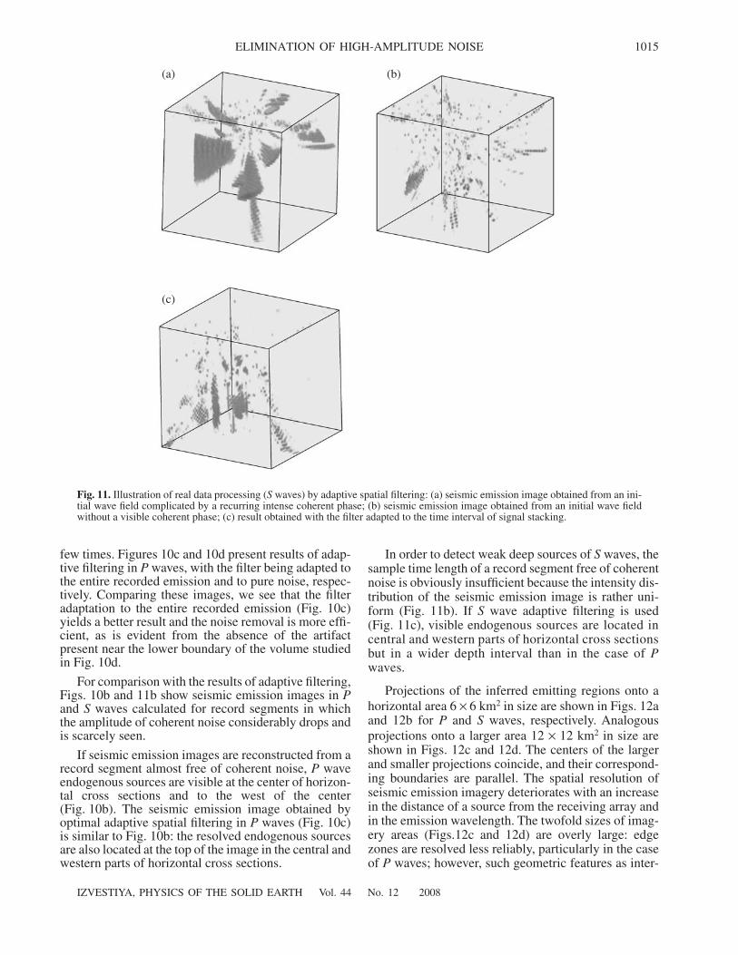
Results of the optimal adaptive spatial filtering of Pand S waves are shown, respectively, in Figs. 10 and 11.The respective reconstructions of seismic emissionimages from the initial wave field with a stacking timeof 100 s are shown in Figs. 10a and 11a. The strongestsurface sources are clearly visible in P waves, while asystem of intense artifacts prevails in the 3-D bright-ness distribution of the seismic emission imageobtained in S waves. As mentioned above, adaptive fil-tering enables tuning of the adaptive filter to pure noiseor a mixture of a signal and noise. We tested and com-pared both variants. To specify pure noise, we chose asmall time interval beyond the time interval used for theimage reconstruction applied to a record with the high-est noise amplitude, exceeding its usual maximum by a

(a) (b)

(c) (d)

Fig. 10. Illustration of real data processing (P waves) with the help of adaptive spatial filtering: (a) seismic emission image obtainedfrom an initial wave field complicated by a recurring intense coherent phase; (b) seismic emission image obtained from an initialwave field without a visible coherent phase; (c, d) results of the application of adaptive spatial filtering with the filter adapted to thetime interval of signal stacking (c) and pure noise (d).



few times. Figures 10c and 10d present results of adap-tive filtering in P waves, with the filter being adapted tothe entire recorded emission and to pure noise, respec-tively. Comparing these images, we see that the filteradaptation to the entire recorded emission (Fig. 10c)yields a better result and the noise removal is more effi-cient, as is evident from the absence of the artifactpresent near the lower boundary of the volume studiedin Fig. 10d.

For comparison with the results of adaptive filtering,Figs. 10b and 11b show seismic emission images in Pand S waves calculated for record segments in whichthe amplitude of coherent noise considerably drops andis scarcely seen.

If seismic emission images are reconstructed from arecord segment almost free of coherent noise, P waveendogenous sources are visible at the center of horizon-tal cross sections and to the west of the center(Fig. 10b). The seismic emission image obtained byoptimal adaptive spatial filtering in P waves (Fig. 10c)is similar to Fig. 10b: the resolved endogenous sourcesare also located at the top of the image in the central andwestern parts of horizontal cross sections.

In order to detect weak deep sources of S waves, thesample time length of a record segment free of coherentnoise is obviously insufficient because the intensity dis-tribution of the seismic emission image is rather uni-form (Fig. 11b). If S wave adaptive filtering is used(Fig. 11c), visible endogenous sources are located incentral and western parts of horizontal cross sectionsbut in a wider depth interval than in the case of Pwaves.

Projections of the inferred emitting regions onto ahorizontal area 6 × 6 km2 in size are shown in Figs. 12aand 12b for P and S waves, respectively. Analogousprojections onto a larger area 12 × 12 km2 in size areshown in Figs. 12c and 12d. The centers of the largerand smaller projections coincide, and their correspond-ing boundaries are parallel. The spatial resolution ofseismic emission imagery deteriorates with an increasein the distance of a source from the receiving array andin the emission wavelength. The twofold sizes of imag-ery areas (Figs.12c and 12d) are overly large: edgezones are resolved less reliably, particularly in the caseof P waves; however, such geometric features as inter-

(a) (b)

(c)

Fig. 11. Illustration of real data processing (S waves) by adaptive spatial filtering: (a) seismic emission image obtained from an ini-tial wave field complicated by a recurring intense coherent phase; (b) seismic emission image obtained from an initial wave fieldwithout a visible coherent phase; (c) result obtained with the filter adapted to the time interval of signal stacking.

1016


CHEBOTAREVA et al.

sections of noisy zones generally extending E–W andN–S are better resolved.

The structure of the fractured reservoir in the regionof seismological observations is also characterized by asystem of ruptures and faults trending E–W and N–S[Glukhmanchuk, 2004]. Maps of fault systems wereobtained in [Glukhmanchuk, 2004] from seismic sur-vey results on the basis of a detailed analysis of thestrain field structures. Major structure-controllingfaults in the area of seismological observations areshown schematically in Fig. 5. The figure displays ageometric similarity between the distribution of deepsources of the noise seismic signal projected onto thehorizontal plane (Fig. 12) and the configuration offaults in the area of observations (Fig. 5). Taking intoaccount that the thickness of the sedimentary cover inthe Middle Ob oil and gas bearing province, includingthe area studied, is 2900–3700 m [Sharifullina, 2004],we may suggest that seismic emission images in Swaves obtained with adaptive spatial filtering give anidea of details of the fault–fracture structure under thebasement top and in the adjacent lower part of the sed-imentary cover. As is known, scattering of both P and Swaves by heterogeneities either longitudinal or trans-verse results in predominant remission into S waves[Sato and Fehler, 1998]. As a consequence, powerfulanthropogenic sources create “seismic illumination,”which reveals zones of intense scattering of seismicemission just with the help of S waves. This can also

explain why focusing of deep sources in S waves disap-pears with the elimination of intense anthropogenicnoise (Fig. 11b). In the case of P waves, endogenoussources are distinguishable in the part of section corre-sponding to the middle and lower parts of the sedimen-tary cover. Noisy areas are visible both in the presenceand in the absence of the most intense anthropogenicnoise, which means that they are apparently activesources, rather than zones of seismic wave scatteringalone.

CONCLUSIONS

Results of real data processing and numerical mod-eling showed that the rejection and optimal adaptivespatial filtering methods reduce the effect of intensecoherent noise in passive seismic monitoring withrecording at the Earth’s surface. Implementation ofthese methods with in terms of approximate formulasdoes not introduce significant distortions in the finalresult but decreases the time of computations by a fewhundreds of times, enabling real-time use of coherentnoise filtering techniques.

Results of localization of deep sources revealedafter removal of intense anthropogenic noise are pre-liminary. The use of P waves resolves noisy regions inthe sedimentary cover in central and western parts ofthe volume studied, while S waves locate sources in thecrystalline basement and sedimentary cover. Projec-tions of the noisy regions onto the horizontal plane cor-relate with the position of major faults in the area ofobservations inferred by independent studies.

The method of emission tomography was effec-tively applied to the localization of a drilling tool at adepth of 2 km from data of a surface recording network.The required time of computations is small enough torealize real-time monitoring of the drilling process.

The determination accuracy of location of a drill andother deep sources is controlled by the accuracy of theaccepted velocity structure. If the position of a sourceis known, emission tomography can be used to updateparameters of the velocity structure using deviations ofimage coordinates from the actual position of thesource. If the position of a deep source is unknown, theutilization of a recording system with the orthogonaldirection of wave arrivals provides the possibility toassess the velocity anisotropy of the medium.

The use of high frequencies imposes stronger con-straints on the accuracy of the receiving array coordi-nate determination and the accepted velocity model; theaccuracy of the latter can be estimated with the help ofnumerical modeling. If the accuracy requirements arenot satisfied, reconstructed seismic emission imagescan be completely defocused.

(c) (d)

(a) (b)

Fig. 12. Projection of noisy regions onto the horizontalplane (the center of the projection coincides with the originof coordinates in the area of observations shown in Fig. 5):(a, b) the square side size is 6 km; (c, d) the square side sizeis 12 km; (a, c) reconstruction using P wave velocities;(b, d) reconstruction using S wave velocities.



ACKNOWLEDGMENTSThis work used experimental data obtained in the

framework of the project “Development of a FieldFirmware Complex and Research Methods for SeismicMonitoring of Oil Bearing Deposits” and other jointprojects of the SSC and URIIT. We are grateful toP.B. Bortnikov and G.N. Erokhin, who provided uswith a velocity structure typical of Western Siberia, aswell as other geophysical data that were necessary forour work. The figures were prepared using theSeisCube5D-View system of 3-D visualization devel-oped by A.Yu. Bezhaev (URIIT), who kindly affordedit to us; the SNDA (Seismic Network Data Analysis,SSC) and GMT (Generic Mapping Tool, University ofHawaii, United States) software packages were alsoused.

REFERENCES1. S. I. Aleksandrov and L. N. Rykunov, “Noise Monitoring

in Southern Iceland,” Dokl. Akad. Nauk 326 (5), 808–810 (1992).

2. S. I. Aleksandrov and K. M. Mirzoev, “Monitoring ofEndogenous Microseismic Radiation in the RomashkinoOil Deposit Are,” in Problems of Geomorphology, Ed. byA. V. Nikolaev (Nauka, Moscow, 1997), pp. 176–188 [inRussian].

3. S. I. Aleksandrov, G. N. Gogonenkov, and V. A. Mishin,“Application of Passive Seismic Observations to Moni-toring of Formation Hydrofracture Parameters,” Neft.Khoz., No. 5 (2005).

4. K. Arnason and O. G. Flovenz, “Evaluation of PhysicalMethods in Geothermal Exploration of Rifted VolcanicCrust,” Geotherm. Res. Counc. 16, 207–214 (1992).

5. J. Capon, “High-Resolution Spatiotemporal SpectralAnalysis,” Proc. IEEE 57 (8), 69–79 (1969).

6. B. Chouet, G. Saccorotti, P. Dawson, et al., “BroadbandMeasurements of the Sources of Explosions at StromboliVolcano, Italy,” Geophys. Res. Lett. 26 (13), 1937–1940(1999).

7. M. Furumoto, T. Kunitomo, H. Inoue, and K. Yamaoka,“Seismic Image of the Volcanic Tremor Source at theIzu-Jshima Volcano, Japan,” in The Volcanic Seismology,Ed. by P. Gasparini, R. Scarpa, and K. Aki. (Springer,New York, 1992), pp. 201–211.

8. E. D. Glukhmanchuk, “Detection, Mapping, and Classi-fication of Fractured Reservoirs and Active Faults in a

Sedimentary Sequence from Seismic and Other Geo-physical Data” (2004), pp. 1-4 (httr://www.uriit.ru/ver-sion/ru/content/page_571_0_353.html).

9. Yu. A. Kugaenko, V. A. Saltykov, V. I. Sinitsyn, andV. N. Chebrov, “Emission Tomography Application tothe Localization of Seismic Noise Sources Associatedwith Hydrothermal Activity,” Fiz. Zemli, No. 2, 66–81(2004) [Izvestiya, Phys. Solid Earth 40, 149–162(2004)].

10. A. F. Kushnir, “Estimation of the Plane Wave ApparentSlowness Vector from Three-Component Seismic ArrayData: A Statistical Problem with Noisy Parameters,” inComputational Seismology (1997) Vol. 29, 215–233 [inRussian].

11. A. F. Kushnir and S. V. Mostovoi, Statistical Analysis ofGeophysical Fields (Naukova Dumka, Kiev, 1990) [inRussian].

12. A. F. Kushnir and V. M. Lapshin, “Recognition and Iden-tification of a Signal Waveform in Coda profile a StrongInterfering Event,” Computational Seismology (1997)Vol. 29, 197–214 (1997).

13. A. V. Nikolaev, P. A. Troitskii, and I. Ya. Tchebotareva,“Seismic Noise Application to the Study of the Lithosphere,”Dokl. Akad. Nauk SSSR 282 (9), 586–591 (1986).

14. H. Sato and M. C. Fehler, Seismic Wave Propagationand Scattering in the Heterogeneous Earth (Springer,New York, 1998).

15. E. A. Sharifullina, Analysis of Development of LicensedAreas in the Middle Ob Oil-and-Gas Province underConditions of the Contemporary Use of MineralResources, Extended Abstract of Cand. Sci. (Geol.–Miner.) Dissertation, TyumGNGU, Tyumen, 2004,p. 20.

16. B. M. Shubik and A. B. Ermakov, “Automatic Determi-nation of Coordinates and Occurrence Times of SeismicEvents Based on the Principles of Emission Tomogra-phy,” in Problems of Geothomography, Ed. byA. V. Nikolaev (Nauka, Moscow, 1997) [in Russian].

17. I. I. Tchebotareva and A. V. Nikolaev, “Exploration ofCrustal Heterogeneities Using Earthquake Codas,”Dokl. Akad. Nauk 364 (6), 816–820 (1998).

18. I. I. Tchebotareva, A. V. Nikolaev, and H. Sato, “SeismicEmission Activity of Earth’s Crust in Northern Kanto,Japan,” Phys Earth Planet. Inter. 120 (3), 167–182(2000).

19. J. Um and C. Thurber, “A Fast Algorithm for Two-PointSeismic Ray Tracing,” Bull. Seismol. Soc. Am. 77 (3),972–986 (1987).

Elimination of high-amplitude noise during passive monitoring of hydrocarbon deposits by the...

Documents

Transcript of Elimination of high-amplitude noise during passive monitoring of hydrocarbon deposits by the...