Co t uous C aModule 04: Electric Fields and Module 04: Electric Fields and

Continuous Chargege Distributions

1

=

VV

( ) ?P =Er

( )

Continuous Charge DistributionsgBreak distribution into parts:

Q = Δqi i

∑ → dq V ∫∫∫

i

E field at P due to Δq

V

2 ˆE re

qk ΔΔ = r

q

2 ˆE re

dqd k→ = r

2e r Superposition:

2e r

E E= Δ∑r r

Ed→ ∫ r

2

E EΔ∑ Ed→ ∫

Continuous Sources: Charge Density

R V l V R2LdVdQ ρ=

ρ = QVL

Volume = V = π R2L

L

dAdQ σ=

σ = QA

w Area = A = wL

Q

AL

QLength L= dLdQ λ=

3

λ =QL

L

Examples of Continuous Sources: Line of chargeLine of charge

Length L= dLdQ λ=

L Q=λ

g

L L

Link to applet

4

Examples of Continuous Sources: Line of chargeLine of charge

Length L= dLdQ λ=

L Q=λ

g

L L

Link to applet

5

Examples of Continuous Sources: Ring of ChargeRing of Charge

QλdLdQ λ 2

Q R

λ π

=dLdQ λ=

Link to applet

6

Examples of Continuous Sources: Ring of ChargeRing of Charge

QλdLdQ λ 2

Q R

λ π

=dLdQ λ=

Link to applet

7

Example: Ring of Charge

P on axis of ring of charge, x from centerg g , Radius a, charge density λ.

8

Find E at P

= =

Ring of Charge 1) Think about it

Symmetry!E⊥ = 0

2) D fi V i bl 2) Define Variables

dq = λ dl = λ a dϕ( )dq λ dl 22

λ a dϕ( )

9

22 xar +=

Ring of Charge 3) Write Equation dq = λa dϕ

2

ˆE e

rd k dq= r

22 xar +=

3e rk dq= r

2e q r 3e q

r

dE x = k edq x r3 r

10

∫ ∫

Ring of Charge 4) Integrate dq = λa dϕ

E x = dE x∫ = k e dq x 3∫

22 xar += x x∫ e r3∫

= k e

x 3 dq∫e r3 q∫

Very special case: everything except dq is constant

∫ 2π 2π

= λ ⋅ a2πdq∫ = λa dϕ 0

2π

∫ = λa dϕ 0

2π

∫ 11

Q=

Ring of Charge5) Clean Up

Ex = keQxr3 r

Ex = keQx

( )3/ 2

x eQ

a2 + x2( )3/ 2

6) Ch k Li it 0ˆE ixk Q=

r6) Check Limit a → 0

( )3/22 2E iek Q

a x+ Ex → keQx

2( )3/ 2 =keQx2

12

x2( ) x

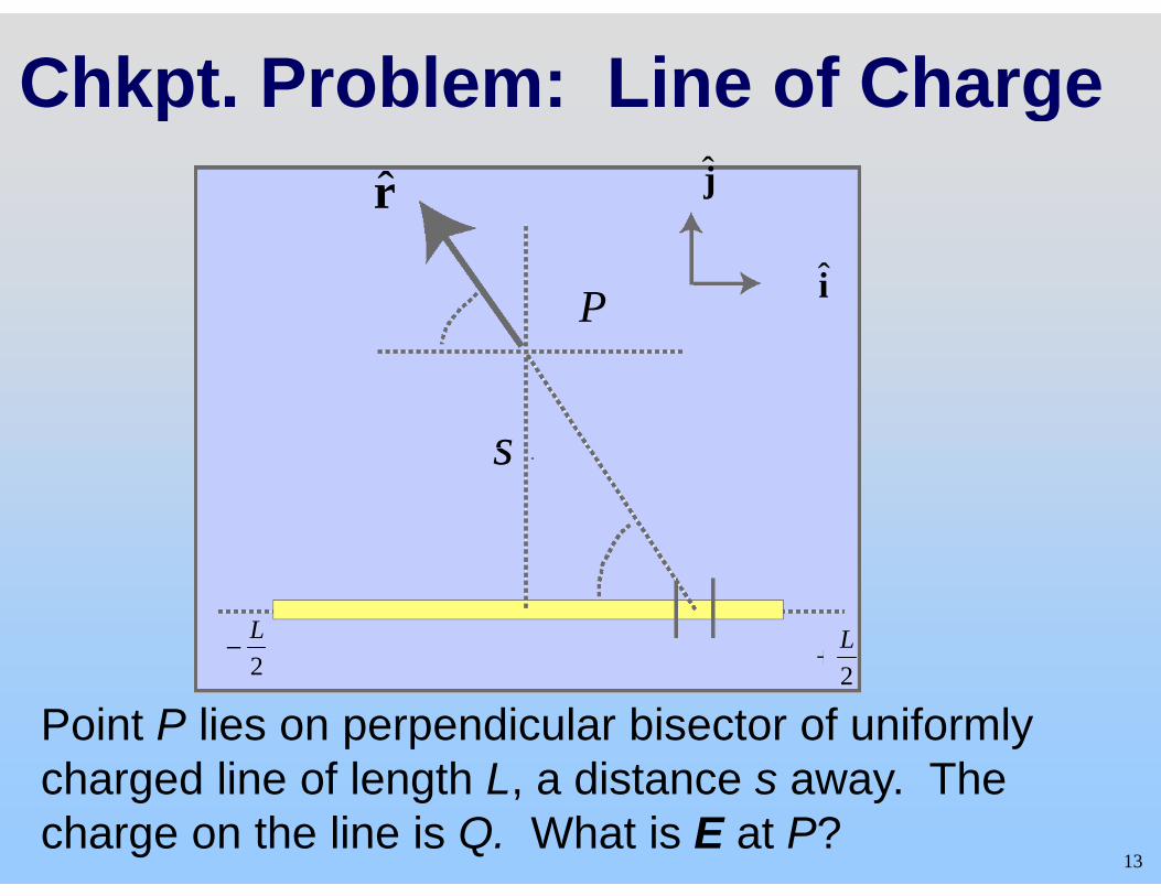
Chkpt. Problem: Line of Charge r j

P i

ss

2 L− L+ 2 2

Point P lies on perpendicular bisector of uniformly charged line of length L a distance s away The

13

charged line of length L, a distance s away. The charge on the line is Q. What is E at P?

Hint: Line of Charge r j

g

θ P i

22 xsr ′+=

P

θ d ′ xddq ′= λ

s

θ

L L

xd ′

′ 2−

2 L+x

Typically give the integration variable (x’) a “primed”

14

variable name. ALSO: Difficult integral (trig. sub.)

E Field from Line of Chargeg

ˆQr2 2 1/2( / 4)

E jeQk

s s L=

+( / 4)s s L+Limits:Limits:

ˆlim E jQk→r

Point charge2lim E je

s Lk

s>>→

Q λ

g

ˆ ˆ2 2lim E j je es L

Qk kLs s

λ<<

→ =r

Infinite charged line

15

In-Class: Uniformly Charged Disky g

( x > 0 )

P on axis of disk of charge x from center P on axis of disk of charge, x from center Radius R, charge density σ.

16 Find E at P

Disk: Two Important Limitsp

xσ ⎡ ⎤⎢ ⎥

( )1/22 2ˆ1

2E idisk

o

x

x R

σε

⎢ ⎥= −⎢ ⎥+⎣ ⎦

r

( )o x R+⎣ ⎦

Li it1 ˆE iQr

Limits:

P i t h2

1lim 4

E idiskx R o

Qxπε>>

→ Point charge

ˆlim 2E idisk

σ→r

Infinite charged plane

17

lim 2diskx R oε<<

Scaling: E for Plane is Constantg

1) Dipole: E falls off like 1/r3 ) p 2) Point charge: E falls off like 1/r2

3) Line of charge:E falls off like 1/r 4) Plane of charge: E constant 4) Plane of charge: E constant

18

MIT OpenCourseWarehttp://ocw.mit.edu

8.02SC Physics II: Electricity and Magnetism Fall 2010

For information about citing these materials or our Terms of Use, visit: http://ocw.mit.edu/terms.