Computer Physics Communications 134 (2001) 291–306www.elsevier.nl/locate/cpc

Eigenstate expansion method for simulations ofnon-perturbative multiphoton processes

M. Nurhudaa, F.H.M. Faisalb, U. Schwengelbeckb,∗a Physics Department, Brawijaya University, Malang 65144, Indonesia

b Fakultät für Physik, Universität Bielefeld, Postfach 100131, D-33501 Bielefeld, Germany

Received 30 May 2000; received in revised form 19 July 2000

Abstract

A method to solve the time-dependent Schrödinger equation of the hydrogen atom and hydrogen-like ions in intense laserpulses, based on an expansion of the total wavefunction in boundand continuum eigenstates of the unperturbed system, ispresented. The problem arising from the well-known singular continuum–continuum dipole matrix elements is fully analyzedand resolved by a combination of analytical integration of the singular contribution and a numerical integration of thesingularity-free difference contribution. Unlike in usual finite-difference methods using a spatial grid, in the present approach,probability amplitudes of bound–bound, bound–free and free–free transitions are obtained without additional calculations. Theefficacy and accuracy of the present method is demonstrated by calculating above-threshold ionization spectra (ATI) and highharmonic generation spectra (HHG) for different values of laser parameters. Finally, the results obtained by using the presentmethod are compared with that of a finite-difference method involving a spatial grid. The present method proves to be an efficientalternative to the usual spatial grid methods for the solution of the time-dependent Schrödinger equation and the estimation ofATI and HHG spectra in case of intense laser pulses. 2001 Elsevier Science B.V. All rights reserved.

PACS: 32.80.Rm; 31.15.-p

Keywords: Eigenstate expansion method; One-electron atoms; Intense laser fields; Above-threshold-ionization; High harmonic generation;Free–free matrix elements

1. Introduction

Non-perturbative theoretical investigations of atomic systems interacting with intense laser fields generally re-quire the time-dependent solution of the corresponding three-dimensional (3D) Schrödinger equation. The mostfrequently used numerical methods for obtaining the system wavefunction are based on some approximant of theshort-time propagator of the system [1–6], discretizing the radial coordinate on a grid. In contrast to the usual split-ting of the total Hamiltonian in the short-time propagator into an unperturbed and an interaction term, a numericalmethod to solve the time-dependent Schrödinger equation has been introduced recently, where the propagator isbased on the total system Hamiltonian [6]. It has been shown that this method could be successfully used even incircumstances where the so-called split-operator algorithm becomes inefficient and/or inaccurate.

* Corresponding author.E-mail address: uschweng@physik.uni-bielefeld.de (U. Schwengelbeck).

0010-4655/01/$ – see front matter 2001 Elsevier Science B.V. All rights reserved.PII: S0010-4655(00)00207-1

292 M. Nurhuda et al. / Computer Physics Communications 134 (2001) 291–306

The perhaps most natural approach to solve the time-dependent Schrödinger equation is to expand thewavefunction in a basis set of the unperturbed atomic eigenfunctions. In principle, this requires only a (numerical)integration of the resulting coupled set of first-order (ordinary) differential equations for the time-dependentprobability amplitudes. In case of Coulombic systems however, there appears the difficulty of carrying out thisstep in a straightforward way, due to presence of the well-known singularity of the dipole coupling matrix elementsbetween two degenerate continuum eigenfunctions of different parity [7,8].

The significance of the singularity occurring in connection with free–free transition matrix elements and theelectric dipole approximation has been recently discussed by van Enk et al. [9] and Mercouris et al. [10]. It hasbeen pointed out in Ref. [9], that the assumption of neglecting the spatial dependence of the transverse vector fieldis responsible for the occurrence of the divergence. On the other hand, in Ref. [10], the numerical significance ofthe free–free singularity in high-order multiphoton processes, in particular in case of intense laser fields, has beenpointed out.

In this work we first analyze the entire singular matrix elements and then construct a singularity-free systemof differential equations. This is achieved by writing the matrix element as the sum of the singular term anda singularity free difference term. Then, the coupling with the singular part is treated analytically, while thatof the (singularity-free) difference part is treated numerically. The resulting algorithm allows an efficient andaccurate computation of physical properties of laser-driven systems, such as above-threshold ionization (ATI)and high-harmonic generation (HHG). The obtained spectra are compared with those obtained by using a spatialgrid method [6]. It is worth noting that, unlike in finite-difference methods based on a spatial grid, the presentapproach already includes all probability amplitudes of bound–bound,bound–free and free–free transitions withoutadditional computations.

2. Theory

The Schrödinger equation describing the laser atom interaction can be written [12] (unless explicitly statedotherwise, atomic units are used:e=m= h= 1, c= 137.036)

i∂

∂tΨ (r, t) = (H0 +Hint)Ψ (r, t), (1)

where

H0 = p2

2− Z

r(2)

is the unperturbed atomic Hamiltonian withp = −i∇, the nuclear chargeZ, and

Hint =

1cA(t) · p (in velocity gauge),

E(t) · r (in length gauge)(3)

is the interaction Hamiltonian, whereA(t) = ezA(t) denotes the vector potential andE(t) = ezE(t) is thecorresponding electric field of the laser pulse with a polarization along thez-direction.

The total quantum wavepacket, evolving from a given initial state att = 0, can be expanded (as usual) in a set ofeigenstates of the unperturbed HamiltonianH0, provided both the discrete set of states{nlm} and continuum states{Eklm} of the atom are incorporated:

Ψ (r, t) =∑nlm

anlm(t)Rnl(r)Ylm(θ,ϑ)

+∑lm

∞∫0

dEk bEklm(t)REkl(r)Ylm(θ,ϑ), (4)

M. Nurhuda et al. / Computer Physics Communications 134 (2001) 291–306 293

whereanlm(t) and bEklm(t) are the amplitudes for the respective discrete and continuum states at timet , andEk = k2/2 denotes the kinetic energy of the electron. For numerical simulations, the integral over the continuumis replaced by a summation over small intervals of the kinetic energy, running from zero up to a given maximumvalueEmax, beyond which contributions to the final results become negligible. To be specific, we normalize theradial eigenfunctions as follows:

∞∫0

dr r2Rn′l (r)Rn′l = δnn′ ,

∞∫0

dr r2REkl(r)REk′ l = δ(Ek −Ek′). (5)

On substituting Eq. (4) into the Schrödinger equation (1) and projecting onto the orthogonal spherical harmonicsY ∗lm, one obtains an infinite set of coupled ordinary differential equations for the amplitudes,

i anlm(t) = Enanlm(t)+∑n′l′m′

Vnlm;n′l′m′an′l′m′(t)+∑l′m′

∞∫0

dEkVnlm,Ekl′m′bEkl′m′(t),

i bEklm(t) = EkbEklm(t)+∑n′l′m′

VEklm,n′l′m′an′l′m′(t)+∑l′m′

∞∫0

dEk′VEklm,Ek′ l′m′bEk′ l′m′(t), (6)

whereVEklm,Ek′ l′m′ are the matrix elements of the laser-atom interaction Hamiltonian (3) between two arbitrarycontinuum eigenstates. Similarly, the otherV ’s stand for the bound–bound and bound–continuum matrix elements.For the atom–laser interaction (3), given in length gauge, the coupling matrix elements can be separated into aproduct of an angular part, denoted byClm,l′m′ , and a radial part, denoted bydEl,E′l′ , where the energyE is givenby

E =− Z2

2n2 (in case of bound states),

k2

2 =Ek (in case of continuum states).(7)

Thus, the transition matrix elements take the form

VElm,E′ l′m′ =E(t)Clml′m′dEl,E′l′ , (8)

where

Clml′m′ = ⟨l,m|cosθ |l′m′⟩

=√(l + 1−m)(l + 1+m)(2l + 3)(2l+ 1)

δl′,l+1δm,m′ +√

(l2 −m2)

(2l + 1)(2l− 1)δl′,l−1δm,m′ . (9)

The matrix element for the radial part,dEl,E′l′ , had been studied for the first time by Gordon [11]. Gordon’sexpression for the radial matrix elements for the transitions (bound–bound, bound–continuum and continuum–continuum) from an initial state with angular momentuml to a final state with angular momentuml − 1 can bewritten in a generalized form (for both positive and negative energiesE):

dEl;E′l−1 =∞∫

0

r3drREl(r)RE′l−1(r)

294 M. Nurhuda et al. / Computer Physics Communications 134 (2001) 291–306

= 1

16N(λ, l)N(λ′, l − 1)2l(2l+ 1)(2l− 1)!v

2+2l

ux

×uλ(−u)λ′{

2F1

(−λ,−λ′,2l,1− 1

u2

)− u2

2F1(−λ− 2,−λ′,2l,1− 1

u2

)}, (10)

where the variablesx, x ′, u, v, λ andλ′ are defined by

x =√

2|E| (for bound states),

−ik (for continuum states),

x ′ =√

2|E′| (for bound states),

−ik′ (for continuum states),

v = 2

x + x ′ , u= x ′ − xx + x ′ ,

λ = 1

a0x− l − 1, λ′ = 1

a0x ′ − l, a0 = 1

Z, (11)

whereλ = n andλ′ = n′ are the principle quantum numbers of the bound states. The normalization constants inEq. (10) are given by

N(λ, l)=

( 1a0

)3/2 2n2(2l+1)!

√(n+l)!(n−l−1)!

( 1na0

)l (for bound states),

1(2l+1)!

√√√√∏lj=1(j

2 + 1k2a2

0)

sinh( πka0)

( 2a0

)1/2eπ/(2ka0)kl (for continuum states).

For the transition froml to l + 1, one can use the propertydEl;E′l+1 = d∗E′l+1,El = dE′l+1,El and replaceE, l, E′

andl − 1 in Eq. (10) byE′, l + 1,E andl, respectively.The continuum–continuum matrix elements cannot be evaluated directly from the expressions given by

Gordon [11] in the case of degenerate initial and final states due to the presence of a singularity. We will thereforere-examine the associated matrix element in order to obtain an appropriate expression that can be used in numericalcalculations.

2.1. Singular radial matrix element

The radial matrix element (10) in the case of continuum–continuum transitions reduces to (see Appendix A)

dEkl;Ek′ l−1 = i

16N(λ, l)N(λ′, l − 1)(2l + 1)!v

2+2l

uk× uλ(−u)λ′

2F1

(−λ,−λ′,2l,1− 1

u2

)+ c.c., (12)

where c.c. stands for the complex conjugate of the previous term. In connection with the radial matrix elements(12), we first make the following transformations of the hypergeometric functions, depending on a parameterη, defined byη = 0.24e−0.025(l+1). Then, on definingy = (1 − 1/u2) in case ofu2 < η, one may express thehypergeometric function in Eq. (12) as follows:

2F1(a, b, c, y) = Γ (c)Γ (b− a)Γ (c− a)Γ (b)(1− y)−a 2F1

(a, c− b, a + 1− b, 1

1− y)

+ Γ (c)Γ (a − b)Γ (c− b)Γ (a)(1− y)−b 2F1

(b, c− a, b+ 1− a, 1

1− y). (13)

M. Nurhuda et al. / Computer Physics Communications 134 (2001) 291–306 295

Foru2> η andy > 1− u2 one may consequently write

2F1(a, b, c, y)= (1− y)−a 2F1

(a, c− b, c, y

y − 1

). (14)

On using the previously specified value of parameterη, the above given equations can be used convenientlyto calculate the radial dipole matrix elements for all non-singular continuum–continuum transitions with highnumerical accuracy, even for very low energies (e.g.,∼10−5 eV) and high angular momenta (e.g.,l′ = 75).

On the other hand, the above matrix elements are still singular in the case of degenerate initial and finalcontinuum states withEk = Ek′ . In the following, we first analyse the singularity and derive the full asymptoticexpression, extracting all singular terms of the continuum–continuum dipole (CCD) radial matrix elements in thevicinity of the singularity.

An exact treatment of the singular CCD matrix elements was attempted by Madajczyk and Trippenbach [7]by means of an analytical regularization. They showed that the singular part of the CCD matrix elements maybe expressed in terms of a delta function and its first derivative in the energy difference. Véniard and Piraux [8]extended the analysis to the next order by including the linear terms. To obtain the full asymptotic expression weshall use Eq. (12). To this end, we expand each individual function in a Taylor series aroundk− k′ = 0 and identifyall the singular terms in the vicinity of the singularity. Details of the analysis are given in Appendix B; here wequote only the final result:

d∞Ekl;Ek′ l±1 = C±

0 (lm, k)

k

{1

(k′ − k)2 + i

a0k2(k′ − k)(ln(−i(k′ − k))

+C1(lm, k))−

((ln |k′ − k|

2a20k

4

(ln |k′ − k| −

(l2 + 1

a20k

2

))

+ ln(−i(k′ − k))a2

0k4

(C1(lm, k)+ ia0k)

)(1+ π |k′ − k|

2a0k2

))+ i π ln(|k′ − k|)

2a0k2

}+ c.c., (15)

where

lm = max(l, l ± 1),

C±0 (lm, k)= ± i

2π

(lm ∓ ia0k)√

l2m + 1a2

0k2

,

C1(lm, k)= γ + 1

2

(ψ

(lm + i

a0k+ θ

)+ψ

(lm − i

a0k+ θ

))− ln(2k)+ i

a0k

2,

θ = 0 if l′ = l − 1,

1 if l′ = l′ + 1,(16)

withψ(x)= d ln(Γ (x))dx denoting the digamma function [13] andγ = 0.5772156 the Euler number. It should be noted

that the leading order terms of Eq. (15) are exactly the same as those obtained by Madajczyk and Trippenbach [7]and Véniard and Piraux [8]. Note, that in the above expression, the terms containing ln|k′ − k|/(k − k′) andln |k′ − k| are also divergent atk = k′ and ought to be included in the singular part.

It is now most convenient to separate the exact CCD matrix element into two parts asd = d∞ + (d−d∞) wherethe difference matrix elementf = (d − d∞) is completely non-singular and can be evaluated numerically withoutdifficulty for all values ofEk andEk′ (including also cases whereEk =Ek′ ). From Eqs. (15) and (12), we identifythe singular partd∞ = d∞

Ekl;Ek′ l±1 and the non-singular part

f = fEkl;Ek′ l±1 = dEkl;Ek′ l±1 − d∞Ekl;Ek′ l±1. (17)

296 M. Nurhuda et al. / Computer Physics Communications 134 (2001) 291–306

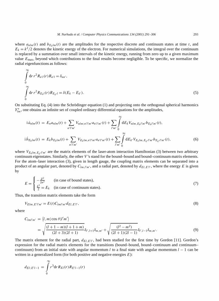
Fig. 1. Radial dipole difference function (see Eq. (17) for various values of energyEk and angular momental andl′ : (a)Ek = 0.551 (15 eV),l = 1, l′ = 0; (b)Ek = 0.551 (15 eV),l = 0, l′ = 1; (c)Ek = 0.551 (15 eV),l = 75, l′ = 74; (d)Ek = 1.837× 10−6 (5× 10−5 eV), l = 20,l′ = 21.

In Fig. 1 we show typical values of the difference matrix elementf for various values ofEk andEk′ , as well asl andl′. As can be seen, the graphs show no singularity atEk = Ek′ , indicating that all terms contributing to thesingularity in Eq. (12) have in fact been extracted in Eq. (15). It is worthwhile noting that the caseEk = Ek′ leadsonly to a finite change of the slope of the difference functionf in Fig. 1.

2.2. Analysis of the singular radial velocity matrix element

So far, we have considered the electron-field interaction described in length gauge. For a numerical simulationof the time-dependent Schrödinger equation (TDSE), however, it is usually more convenient to work in the velocitygauge and this is in particular so in the present context since the continuum–continuum matrix elements are lessdivergent in the velocity gauge than in the length gauge. In order to derive the corresponding matrix elements, werecall the well-known commutative relation betweenz andH0 (e.g., [14]),

iz= [H0, z] =H0z− zH0. (18)

The corresponding matrix elements of the velocity operator between the eigenfunctions of arbitrary energyE andE′ are given by (cf. Eq. (8))

izmm′

ll′ = (E −E′)〈Rl |r|Rl′ 〉Clml′m′ . (19)

The radial velocity matrix elements for all transitions of interest consequently take the form

idEl;E′l−1 = (E −E′)dEl;E′l−1

={(E −E′)

16N(λ, l)N(λ′, l − 1)(2l+ 1)!v

2+2l

u xuλ(−u)λ′

× 2F1

(−λ,−λ′,2l,1− 1

u2

)+ c.c.

}. (20)

M. Nurhuda et al. / Computer Physics Communications 134 (2001) 291–306 297

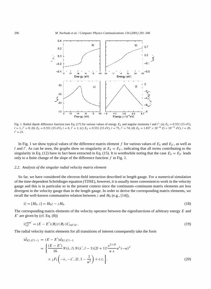
Fig. 2. Same as Fig. 1 but for the radial velocity difference functiong.

Therefore, the asymptotic expression of the continuum–continuum matrix elements in the vicinity of thesingularity for the radial velocity operator can be found from that of the radial operator analysed above. Thus,on writing (Ek −Ek′)= (k − k′)(k + k′)/2 and then multiplying with expression (15), one finds

id∞Ekl;Ek′ l±1 = −C±

0 (lm, k)

{k

(k′ − k) + i

a0kln(−i(k′ − k))

}+ c.c., (21)

whereC±0 (lm, k) is given by Eq. (16). Note that in Eq. (21) only the terms contributing to the singularity have been

retained. Using the same procedures as applied in the case of radial matrix elements in length gauge, the exactmatrix element can be separated into a singular term and a non-singular difference termg = i(d − d∞).

Fig. 2 shows a set of graphs forg, calculated from the difference of the exact matrix element and the asymptoticexpression equation (21). As expected, one observes that the difference functions do not contain a singularity andshow only a change of the slope with a cusp at the pointEk =Ek′ .

Returning to the coupled set of equations for the amplitudes, (6), we may now rewrite the continuum–continuumcoupling terms on the right hand side of Eq. (5) as follows:

I± =Emax∫0

dEk′ VEkl;Ek′ l±1bEk′ l±1m′(t)

�Ek−3Ek/2∑

0

3Ek′VEkl;Ek′ l±1bEk′ l±1m′(t)+Ek+3Ek/2∫Ek−3Ek/2

dEk′ VEkl;Ek′ l±1bEk′ l±1m′(t)

+Ekmax∑

Ek+3Ek/23Ek′VEkl;Ek′ l±1bEk′ l±1m′(t). (22)

The first and the third term are non-singular and can therefore be treated numerically without problem, whereas thesecond term, containing the singularity, can be analysed analytically. The second (integral) term becomes

298 M. Nurhuda et al. / Computer Physics Communications 134 (2001) 291–306

I±2 =

Ek+3Ek/2∫Ek−3Ek/2

dEk′ VEkl;Ek′ l±1bEk′ l±1m′(t)

≈ −i

cA(t)bEkl±1m′(t)

(i

Ek+3Ek/2∫Ek−3Ek/2

dEk′ d∞Ekl;Ek′ l±1 +

Ek+3Ek/2∫Ek−3Ek/2

dEk′ gEkl;Ek′ l±1

)

= −i

cA(t)bEkl±1m′(t)(I±

s + I±ns). (23)

This integral involving the non-singular difference functiong in Eq. (23) can be evaluated numerically withoutproblem, because this term is free from any singularity. Moreover, the singular term can now be integratedanalytically employing the replacementk→ k+ iε in the limit ε→ 0 (corresponding to the ingoing wave boundarycondition) in Eq. (21),

id∞Ekl;Ek′ l±1 → −C±

0 (lm, k)

{k

(k′ − k − iε)+ i

a0kln(−i(k′ − k))

}+ c.c. (24)

On using the identity [15]

1

(k − k′ − iε)= P

(1

(k − k′)

)+ iπδ(k′ − k),

(25)

whereP denotes the principle value, and writing dEk′ = k′dk′ with k′ = k + ξ , such that dk′ = dξ , one finds

I±s = −C±

0 (lm, k)

{k

(J1 + i

a0k2J2

)+(J3 + i

a0k2J4

)}+ c.c., (26)

where

J1 = ln(|ξ |)∣∣k2−k

k1−k−iπ

k2∫k1

δ(k′ − k)dk′,

J2 = (ξ ln(−iξ)− ξ)∣∣(k2−k)

(k1−k),J3 = (k2 − k1),

J4 = ξ2

2ln(−iξ)− ξ2

4

∣∣∣∣(k2−k)

(k1−k)(27)

with k2 = √2Ek +3Ek andk1 = √

2Ek −3Ek.2.3. Solution of the coupled TDSE

On using Eqs. (6), (19) and (26), the final system of singularity-free differential equations for the quantumprobability amplitudes can be written

i anlm(t) = Enanlm(t)+A(t)∑n′l′m′

Clml′m′ dnl;n′l′an′l′m′(t)

+A(t)∑3kl′m′

3EkClml′m′ dnlm,Ekl′m′bEkl′m′(t),

M. Nurhuda et al. / Computer Physics Communications 134 (2001) 291–306 299

i bEklm(t) = EkbEklm(t)+A(t)∑n′l′m′

Clml′m′ dEk lm,n′l′m′an′l′m′ (t)

+A(t)∑l′m′Clml′m′

{Ek−3Ek/2∑

0

3Ek′ dEkl;Ek′ l′bEk′ l′m′(t)

− i(I±s + I±

ns )bEkl′m′(t)+Emax∑

Ek+3Ek/23Ek′ dEkl;Ek′ l′bEk′ l′m′(t)

}. (28)

The numerical time-propagation of the above system can then be carried out step-by-step, using any suitablealgorithm for solving first order coupled differential equations, e.g., the standard Runge–Kutta methods [16] orthe well-known Adams–Bashforth–Moulton predictor–corrector method (e.g., [17]).

3. Results and discussions

We have computed both above-threshold-ionization (ATI) spectra and high-harmonic generation (HHG) spectrain simulations of the time-dependent wave packets evolving from the ground state hydrogen atom at both lowand high laser frequencies and intensities. The absolute ATI spectra can be computed directly from the solutions,corresponding to the continuum occupation amplitudes:

dP(Ek)

dEk=∑lm

|bEklm|2. (29)

Fig. 3. Comparison of the ATI spectra obtained with two different values of3Ek , an intensityI0 = 1014 W/cm2, the frequencyω = 0.0735(2 eV) and a total pulse duration of 24 optical cycles (50 fs). In both simulations, the maximum angular momentum is given bylmax= 10.

300 M. Nurhuda et al. / Computer Physics Communications 134 (2001) 291–306

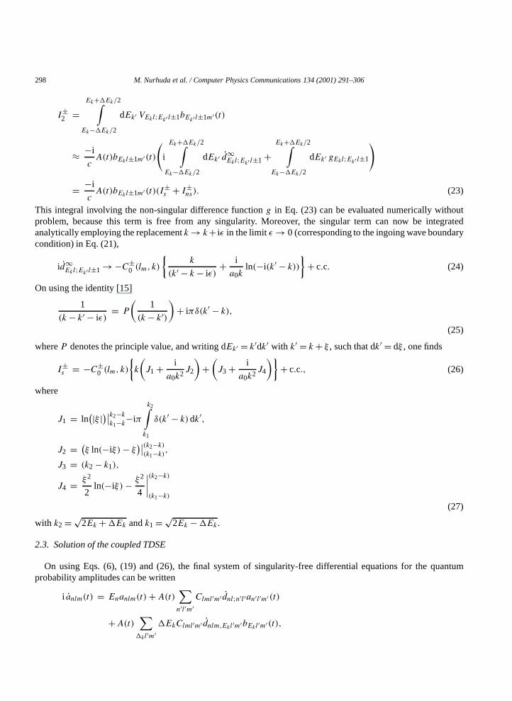
Fig. 4. Comparison of the ATI spectra obtained with three different values ofEmax. The physical parameters are the same as that used in Fig. 3.

The convergence of the final spectra is tested by varying the simulation parameters: the width of the energy spacing3Ek, the maximum continuum energyEmax and the maximum angular momentumlmax.

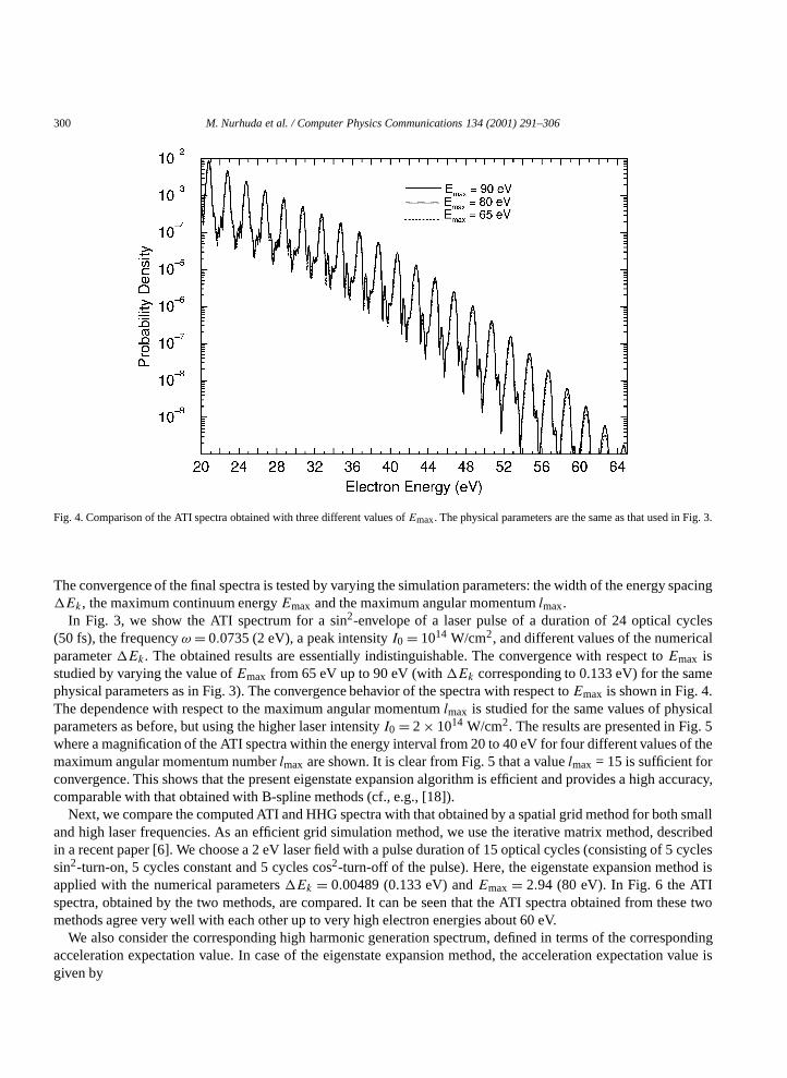
In Fig. 3, we show the ATI spectrum for a sin2-envelope of a laser pulse of a duration of 24 optical cycles(50 fs), the frequencyω = 0.0735 (2 eV), a peak intensityI0 = 1014 W/cm2, and different values of the numericalparameter3Ek. The obtained results are essentially indistinguishable. The convergence with respect toEmax isstudied by varying the value ofEmax from 65 eV up to 90 eV (with3Ek corresponding to 0.133 eV) for the samephysical parameters as in Fig. 3). The convergence behavior of the spectra with respect toEmax is shown in Fig. 4.The dependence with respect to the maximum angular momentumlmax is studied for the same values of physicalparameters as before, but using the higher laser intensityI0 = 2× 1014 W/cm2. The results are presented in Fig. 5where a magnification of the ATI spectra within the energy interval from 20 to 40 eV for four different values of themaximum angular momentum numberlmax are shown. It is clear from Fig. 5 that a valuelmax = 15 is sufficient forconvergence. This shows that the present eigenstate expansion algorithm is efficient and provides a high accuracy,comparable with that obtained with B-spline methods (cf., e.g., [18]).

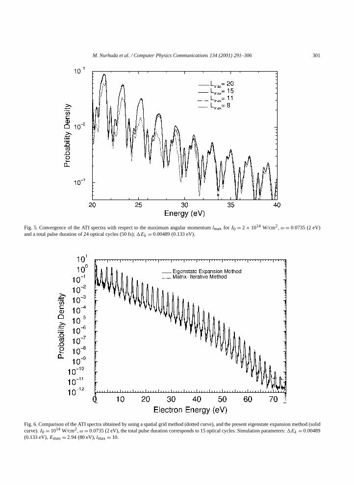
Next, we compare the computed ATI and HHG spectra with that obtained by a spatial grid method for both smalland high laser frequencies. As an efficient grid simulation method, we use the iterative matrix method, describedin a recent paper [6]. We choose a 2 eV laser field with a pulse duration of 15 optical cycles (consisting of 5 cyclessin2-turn-on, 5 cycles constant and 5 cycles cos2-turn-off of the pulse). Here, the eigenstate expansion method isapplied with the numerical parameters3Ek = 0.00489 (0.133 eV) andEmax = 2.94 (80 eV). In Fig. 6 the ATIspectra, obtained by the two methods, are compared. It can be seen that the ATI spectra obtained from these twomethods agree very well with each other up to very high electron energies about 60 eV.

We also consider the corresponding high harmonic generation spectrum, defined in terms of the correspondingacceleration expectation value. In case of the eigenstate expansion method, the acceleration expectation value isgiven by

M. Nurhuda et al. / Computer Physics Communications 134 (2001) 291–306 301

Fig. 5. Convergence of the ATI spectra with respect to the maximum angular momentumlmax for I0 = 2× 1014 W/cm2, ω = 0.0735 (2 eV)and a total pulse duration of 24 optical cycles (50 fs);3Ek = 0.00489 (0.133 eV).

Fig. 6. Comparison of the ATI spectra obtained by using a spatial grid method (dotted curve), and the present eigenstate expansion method (solidcurve).I0 = 1014 W/cm2, ω= 0.0735 (2 eV), the total pulse duration corresponds to 15 optical cycles. Simulation parameters:3Ek = 0.00489(0.133 eV),Emax= 2.94 (80 eV),lmax= 10.

302 M. Nurhuda et al. / Computer Physics Communications 134 (2001) 291–306

Fig. 7. Comparison of the HHG spectra obtained by using a spatial grid method (dotted curve) and the present eigenstate expansion method(solid curve). The laser parameters are the same as that used in Fig. 6.

〈z(t)〉 = −∑

Elm;E′l′m′Clml′m′(E −E′)idEl;E′l′hElm(t)hE′ l′m′(t), (30)

whereE andE′ are given by Eq. (7) andh = anlm(t) corresponds to bound states, whereash = bEklm(t)3Ekcorresponds to continuum states. The corresponding power spectrum is then given by (cf. [16])

S(ω)=∣∣∣∣T∫

0

〈z(t)〉eiωt dt

∣∣∣∣2

, (31)

whereT denotes the duration of the laser pulse. The computational results are shown in Fig. 7. It can be seenthat the HHG spectrum is in good agreement with the spectrum obtained by a finite difference method, basedon a spatial grid. We finally compute ATI spectra in case of high laser frequencies, using the present eigenstateexpansion method, and compare the results with that obtained using the matrix iterative method [6]. To this end,we choose a VUV laser field withω = 1 (27.2116 eV), an intensityI0 = 3.5×1016 W/cm2 and a pulse durationof 15 optical cycles. A comparison of the calculated ATI spectrum at this laser frequency, obtained by the twodifferent methods is shown in Fig. 8, which again reveals a very good agreement between the results up to highestelectron energies about 200 eV.

4. Summary

We have developed a singularity-free method for simulations of non-perturbative multiphoton processes of (3D)hydrogenic atoms interacting with intense laser pulses, based on the expansion of the system wavefunction interms of the eigenstates (bound and continuum) of the unperturbed Hamiltonian. The well-known singularity of the

M. Nurhuda et al. / Computer Physics Communications 134 (2001) 291–306 303

Fig. 8. Same as Fig. 6, but forI0 = 3.5 × 1016 W/cm2, ω = 1 (27.2116 eV) and a pulse duration of 15 cycles. Simulation parameters:3Ek = 0.01837 (0.5 eV),Emax= 11.0247 (300 eV),lmax= 6.

continuum–continuum dipole matrix elements at the same energy is isolated completely. A non-singular methodis developed by integrating the full singularity analytically and treating the non-singular difference between thetotal and the singular part numerically. The efficacy of the resulting algorithm is demonstrated by computing ATIspectra at both optical and VUV laser frequencies. The convergence of the corresponding algorithm in terms ofphysical quantities is studied by a calculation of ATI spectra on the basis of different values of the numericalparameters3Ek,Emax andlmax. The present eigenstate expansion method can also be very effectively used for thecomputation of high-harmonic generation spectra of atoms in intense laser fields.

Appendix A. Singular radial matrix element

To prove Eq. (12), we transform the associated hypergeometric functions as follows (cf. [13]):

2F1(a, b, c, z) = Γ (c)Γ (b− a)Γ (c− a)Γ (b)(1− z)−a2F1

(a, c− b, a + 1− b, z

1− z)

+ Γ (c)Γ (a − b)Γ (c− b)Γ (a) (1− z)−b2F1

(b, c− a, b+ 1− a, z

1− z). (A.1)

On using (A.1) in Eq. (10), we get

dEl;E′l−1 = i

16N(λ, l)N(λ′, l − 1)2l(2l+ 1)(2l− 1)!

× v2+2l

ukuλ(−u)λ′

{(u−2λ Γ (2l)Γ (λ− λ′)

Γ (−λ′)Γ (2l + λ) 2F1(−λ,2l + λ′, λ′ − λ+ 1, u2)

304 M. Nurhuda et al. / Computer Physics Communications 134 (2001) 291–306

+u−2λ′ Γ (2l)

Γ (−λ)Γ (λ′ − λ)Γ (2l + λ′) 2F1

(−λ′,2l + λ,λ− λ′ + 1, u2))

−(u2u−2(λ+2) Γ (2l)Γ (λ+ 2− λ′)

Γ (−λ′)Γ (2l + λ+ 2)2F1

(−λ− 2,2l + λ′, λ′ − λ− 1, u2)+u2u−2λ′ Γ (2l)Γ (λ′ − λ− 2)

Γ (−λ− 2)Γ (2l + λ′) 2F1(−λ,2l + λ′, λ′ − λ+ 1, u2))}. (A.2)

With λ= i/a0k − l − 1 andλ′ = i/a0k′ − l, it can be shown directly that the following relations hold:

Γ (λ− λ′)∗ = Γ (λ′ − λ− 2),

Γ (λ′ − λ)∗ = Γ (λ+ 2− λ′),Γ (−λ− 2)∗ = Γ (2l + λ),Γ (−λ′)∗ = Γ (2l + λ′),Γ (−λ)∗ = Γ (2l + λ+ 2),

2F1(−λ,2l + λ′, λ′ − λ+ 1, u2)∗ = 2F1

(−λ,2l + λ′, λ′ − λ+ 1, u2),2F1

(−λ′,2l + λ,λ− λ′ + 1, u2)∗ = 2F1(−λ− 2,2l+ λ′, λ′ − λ− 1, u2), (A.3)

where∗ indicates the complex conjugation of the respective function. On inserting (A.3) in the curly brackets ofthe expression (A.2) and multiplying withuλ(−u)λ′

, one obtains the expression{(uλ(−u)λ′

u−2λ Γ (2l)Γ (λ− λ′)Γ (−λ′)Γ (2l + λ) 2F1

(−λ,2l + λ′, λ′ − λ+ 1, u2)+ uλ(−u)λ′

u−2λ′ Γ (2l)

Γ (−λ)Γ (λ′ − λ)Γ (2l+ λ′) 2F1

(−λ′,2l + λ,λ− λ′ + 1, u2))

−(uλ(−u)λ′

u2u−2(λ+2) Γ (2l)Γ (λ′ − λ)∗

Γ (2l + λ′)∗Γ (−λ)∗(2F1

(−λ′,2l + λ,λ′ − λ+ 1, u2))∗+ uλ(−u)λ′

u2u−2λ′ Γ (2l)Γ (λ− λ′)∗

Γ (2l+ λ)∗Γ (−λ′)∗(

2F1(−λ,2l + λ′, λ′ − λ+ 1, u2))∗)}. (A.4)

Since(uλ(−u)λ′

u−2λ)∗ = ((−1)λ

′uλ

′−λ)∗ = (−1)λ′uλ−λ′+2,(

uλ(−u)λ′u−2λ′)∗ = (

(−1)λ′uλ−λ′)∗ = (−1)λ

′uλ

′−λ−2, (A.5)

one can see that the terms within the second big brackets( )

in (A.4) are the complex conjugate of the terms withinthe first big brackets. Therefore, the expression (A.4) can be rewritten as{(

uλ(−u)λ′u−2λ Γ (2l)Γ (λ− λ′)

Γ (−λ′)Γ (2l + λ) 2F1(−λ,2l + λ′, λ′ − λ+ 1, u2)

+ uλ(−u)λ′u−2λ′ Γ (2l)

Γ (−λ)Γ (λ′ − λ)Γ (2l+ λ′) 2F1

(−λ′,2l + λ,λ− λ′ + 1, u2))− c.c.

}. (A.6)

On multiplying (A.6) with the pure imaginary factor

i

16N(λ, l)N(λ′, l − 1)2l(2l+ 1)(2l − 1)!v

2+2l

uk

and using Eq. (A.1), one finds the relation stated in Eq. (12).

M. Nurhuda et al. / Computer Physics Communications 134 (2001) 291–306 305

Appendix B. Derivation of the asymptotic expression of the CCD matrix elements

To derive the asymptotic form of the CCD matrix elements in Eq. (15), we use again the transformation (A.1),because in case ofk → k′, the argument of the corresponding hypergeometric function becomes singular. Usingthe transformation (A.1), the dipole matrix elements in (12) become

dEl;E′l−1 = i

16N(λ, l)N(λ′, l − 1)2l(2l+ 1)(2l− 1)!v

2+2l

ukuλ(−u)λ′

×{Γ (2l)Γ (−1+ i

a0k− ia0k

′ )

Γ (l − 1+ ia0k)Γ (l − i

a0k′ )

(k′ − kk + k′

)2(l+1− ia0k)

×2F1

(l + 1− i

a0k,2− l − i

a0k,2− i

a0k+ i

a0k′ ,−(k′ − kk′ + k

))2

+ Γ (2l)Γ (1+ ia0k

′ − ia0k)

Γ (l + 1− ia0k)Γ (l + i

a0k′ )

(k′ − kk + k′

)2(l−i/(a0k′))

× 2F1

(l − i

a0k′ ,1− l − i

a0k′ ,−i

a0k′ + i

a0k,−(k′ − kk + k′

)2)}+ c.c.,

(B.1)

where in the case of continuum states,λ = i/a0k − l − 1 andλ′ = i/a0k′ − l (see Eq. (11)). It can now be seen

that, as(k′ → k), the argument of the first hypergeometric function in Eq. (B.1) vanishes and the limiting value isequal to unity, while the second hypergeometric function is of first order in(k′ − k). The normalization constant,expressed in terms of the gamma function, reads

N(λ, l)= 1

(2l + 1)!∣∣∣∣Γ(l + 1+ i

a0k

)∣∣∣∣(

2k

π

)1/2

eπ/(2ka0)kl . (B.2)

On usingΓ (z)Γ (−z)= −π/(z sin(πz)), it is clear that

limk→k′

Γ

(−1+ i

a0k′ − i

a0k

)=(

i

a0k− i

a0k′

)−1

. (B.3)

On writing k′ = k + (k′ − k) and performing the respective limit of the functions in Eq. (B.1),

limk′→k

1

k + k′ = 1

2k− k′ − k

4k2 ,

limk′→k

Γ

(l + i

a0k′

)= limk′→k

Γ

(l + i

a0k− i(k′ − k)

a0k2

)

= Γ(l + i

a0k

)(1− i(k′ − k)

a0k2 ψ(l + i

a0k)

)

limk′→k

|k′ − k|−i(k′−k) = 1− i(k′ − k) ln(|k′ − k|)− 12(k

′ − k)2 ln2(|k′ − k|)limk′→k

ek′−k = 1+ (k′ − k) (B.4)

one obtains, after extracting the terms which are singular atk = k′, the explicit expression given in Eq. (15).

306 M. Nurhuda et al. / Computer Physics Communications 134 (2001) 291–306

References

[1] K.C. Kulander, B.W. Shore, Phys. Rev. Lett. 62 (1989) 524.[2] K.J. LaGattuta, Phys. Rev. A 41 (1990) 5110.[3] L. Roso-Franco, A. Sampera, M. Pons, L. Plaja, Phys. Rev. A 44 (1991) 4652.[4] P.L. De Vries, Comput. Phys. Commun. 63 (1991) 95.[5] J.L. Krause, K.J. Schafer, K.C. Kulander, Phys. Rev. A 45 (1992) 4998.[6] M. Nurhuda, F.H.M. Faisal, Phys. Rev. A 60 (1999) 3125.[7] J.L. Madajczyk, M. Trippenbach, J. Phys. A 22 (1989) 2369.[8] V. Véniard, B. Piraux, Phys. Rev. A 41 (1990) 4019.[9] S.J. van Enk, Jian Zhang, P. Lambropoulos, J. Phys. B 30 (1997) L17.

[10] Th. Mercouris, Y. Komninos, S. Dionissopoulou, C.A. Nicolaides, J. Phys. B 30 (1997) 2133.[11] W. Gordon, Ann. Phys. (Leipzig) 2 (1929) 1031.[12] F.H.M. Faisal, Theory of Multiphoton Processes, Plenum, New York, 1987.[13] M. Abramowitz, I.A. Stegun, Handbook of Mathematical Functions, Dover, New York, 1968.[14] L.I. Schiff, Quantum Mechanics, McGraw-Hill, New York, 1981.[15] G. Arfken, Mathematical Methods for Physicists, Academic Press, San Diego, 1985.[16] W.H. Press, S.A. Teukolsky, W.T. Vetterling, B.P. Flannery, Numerical Recipes in Fortran, Cambridge University Press, Cambridge, 1992.[17] L.F. Shampine, M.K. Gordon, Computer Solution of Ordinary Differential Equations, Prentice-Hall, Englewood Cliffs, NJ, 1975.[18] E. Cormier, P. Lambropoulos, J. Phys. B 30 (1997) 77.