Efficacy of cleaning method for removal of exogenous welding ...

Purdue UniversityPurdue e-Pubs

Open Access Theses Theses and Dissertations

Summer 2014

Efficacy of cleaning method for removal ofexogenous welding fume contamination from nailtissue prior to use as a biomarker for welding fumemanganese exposureJeffrey Corral BainterPurdue University

Follow this and additional works at: https://docs.lib.purdue.edu/open_access_theses

Part of the Biochemistry Commons, Occupational Health and Industrial Hygiene Commons,and the Toxicology Commons

This document has been made available through Purdue e-Pubs, a service of the Purdue University Libraries. Please contact [email protected] foradditional information.

Recommended CitationBainter, Jeffrey Corral, "Efficacy of cleaning method for removal of exogenous welding fume contamination from nail tissue prior touse as a biomarker for welding fume manganese exposure" (2014). Open Access Theses. 720.https://docs.lib.purdue.edu/open_access_theses/720

https://docs.lib.purdue.edu?utm_source=docs.lib.purdue.edu%2Fopen_access_theses%2F720&utm_medium=PDF&utm_campaign=PDFCoverPages

https://docs.lib.purdue.edu/open_access_theses?utm_source=docs.lib.purdue.edu%2Fopen_access_theses%2F720&utm_medium=PDF&utm_campaign=PDFCoverPages

https://docs.lib.purdue.edu/etd?utm_source=docs.lib.purdue.edu%2Fopen_access_theses%2F720&utm_medium=PDF&utm_campaign=PDFCoverPages

https://docs.lib.purdue.edu/open_access_theses?utm_source=docs.lib.purdue.edu%2Fopen_access_theses%2F720&utm_medium=PDF&utm_campaign=PDFCoverPages

http://network.bepress.com/hgg/discipline/2?utm_source=docs.lib.purdue.edu%2Fopen_access_theses%2F720&utm_medium=PDF&utm_campaign=PDFCoverPages



https://docs.lib.purdue.edu/open_access_theses/720?utm_source=docs.lib.purdue.edu%2Fopen_access_theses%2F720&utm_medium=PDF&utm_campaign=PDFCoverPages

01 14

PURDUE UNIVERSITY GRADUATE SCHOOL

Thesis/Dissertation Acceptance

Thesis/Dissertation Agreement.Publication Delay, and Certification/Disclaimer (Graduate School Form 32)adheres to the provisions of

Department

Jeffrey Corral Bainter

EFFICACY OF CLEANING METHOD FOR REMOVAL OF EXOGENOUS WELDINGFUME CONTAMINATION FROM NAIL TISSUE PRIOR TO USE AS A BIOMARKER FORWELDING FUME MANGANESE EXPOSURE

Master of Science

Ulrike Dydak

Frank Rosenthal

Neil Zimmerman

Huiling (Linda) Nie

Ulrike Dydak

Keith Stantz 07/18/2014

i

EFFICACY OF CLEANING METHOD FOR REMOVAL OF EXOGENOUS WELDING FUME CONTAMINATION FROM NAIL TISSUE PRIOR TO USE AS A

BIOMARKER FOR WELDING FUME MANGANESE EXPOSURE

A Thesis

Submitted to the Faculty

of

Purdue University

by

Jeffrey Corral Bainter

In Partial Fulfillment of the

Requirements for the Degree

of

Master of Science

August 2014

Purdue University

West Lafayette, Indiana

ii

I dedicate this work to the peoples of this Earth, may they finally find liberation from the

oppressions which besiege them physically, mentally and spiritually. May they soon find

a freer and more just society in which we can all seek together the betterment of mankind

and the protection of our one and only home in this vast universe.

iii

ACKNOWLEDGEMENTS

First and foremost, I wish to express my love and gratitude to my beloved Naime, whose

beauty, kindness, sincerity, and warmth never cease to amaze me. Without her support, I

certainly would not have persevered through the labyrinth of pain, stress and confusion

which befell me over the past year.

I would like to thank Dr. Neil Zimmerman for inspiring me to continue onward toward a

PhD in Occupational Health and Safety and ultimately toward a career in teaching. I

certainly have some large footstep to follow. I am overjoyed to have been able to study

under your tutelage at Purdue during your final year of teaching. Thank you for hanging

in there until I arrived to Purdue.

I also want to thank Dr. Ulrike Dydak for having an enormous amount of patience and

helping to keep me calm through the rough seas I faced during my final year at Purdue.

You have my deepest gratitude. Though I may be leaving, I hope to continue my work

on welding exposures and someday we may collaborate again. I wish you and all The

Wabash Study members the greatest success.

iv

To Dr. Frank Rosenthal, I express my thankfulness and appreciation for the advice and

guidance he provided along the way and for taking the chance on me to bring me into the

program in the beginning. I wish you continued success in all your endeavors, be them

academic or personal in nature.

To Dr. Huiling (Linda) Nie, thanks for your support and for your willingness to cross

over into the IH world in order to sit on my thesis committee. I feel fortunate to have had

the opportunity to study radiation safety in your class while at Purdue, it was a

challenging yet rewarding experience.

I want to recognize the National Institutes for Health for their support through their

Research Project Grant Program (R01 grant R01 ES020529, Dydak) and for the NIOSH

training grant program, both of which funded the majority of this study.

I would also like to thank the Zheng lab for allowing me to utilize critical lab equipment

necessary to achieve the goals of this work and the HSCI office personnel, Yvonne Nash,

Karen Walker, Helen Terrell, and Jennifer Franklin from the School of Nursing and

Health Sciences. Their concern and dedication has been greatly appreciated.

Lastly, but certainly not the least, I want to thank Karl Wood and Arlene Rothwell of the

Purdue Campus-Wide Mass Spectrometry Center. Without their diligent attention to

detail and analytical chemistry skills, this work would be but a fragment of what it is.

v

TABLE OF CONTENTS

Page

LIST OF TABLES ........................................................................................................... viii

LIST OF FIGURES ............................................................................................................ x

ABSTRACT ................................................................................................................ xii

CHAPTER 1. INTRODUCTION ................................................................................... 1

1.1 Introduction ............................................................................................................... 1

1.2 Body Fluids As Biomarkers of Metal Exposure ........................................................... 4

1.3 Keratin Tissue As Biomarker of Metal Exposure ......................................................... 5

1.4 Use of Nail Tissue As Biomarker of Welding Fume Mn Exposure ............................. 7

1.5 Toenail Tissue As Biomarker for The Wabash Study ................................................ 10

CHAPTER 2. SPECIFIC AIM, HYPOTHESES, AND OBJECTIVES ....................... 12

2.1 Specific Aim ............................................................................................................. 12

2.2 Primary Objectives And Central Hypotheses ............................................................ 15

2.2.1 Objective 1: Exogenous Mn contamination to welder fingernail ...............15

2.2.2 Objective 2: Verification of contamination method ....................................16

2.2.3 Objective 3: Nail cleaning method validity testing .....................................16

CHAPTER 3. METHODOLOGY ................................................................................ 18

3.1 GMAW Welding Fume As Mn Contaminant ............................................................. 18

3.2 Containment Vessel Design ........................................................................................ 20

3.3 Welding Equipment .................................................................................................... 21

3.4 Experimental Design ................................................................................................... 22

3.4.1 Welder Fingernail Analysis .........................................................................23

3.4.2 Cleaning Protocol ........................................................................................25

3.4.3 Experiment Round 1 Design .......................................................................25

vi

Page

3.4.3.1 Estimating required mass of GMAW WF for initial contamination ....26

3.4.3.2 Determining the required GMAW arc time for initial contamination..30

3.4.3.3 Prediction of C / Cmax based on steady-state build up ..........................30

3.4.4 Round 1 ICP-MS preparations and estimated Mn concentrations ..............32



3.5 ICP-MS Analysis ........................................................................................................ 40

3.6 Statistical Analysis ...................................................................................................... 42

CHAPTER 4. RESULTS .............................................................................................. 45

4.1 Round 1 Results .......................................................................................................... 45

4.2 Round 2 Results .......................................................................................................... 49

4.3 Estimation of Required Sample Size .......................................................................... 52

4.4 Round 3 Results .......................................................................................................... 55

CHAPTER 5. ANALYSIS ............................................................................................ 59

5.1 Normality Testing ....................................................................................................... 61

5.1.1 Normality testing – P-P and Q-Q plots .......................................................61

5.1.2 Normality testing – Box plots .....................................................................62

5.1.3 Normality testing – Skewness and Kurtosis ................................................69

5.1.4 Normality testing – Chi-Square Test ...........................................................72

5.1.5 Normality testing – Shapiro-Wilk Test .......................................................73

5.1.6 Normality testing – Anderson-Darling Test ................................................75

5.1.7 Normality testing – Synopsis ......................................................................76

5.2 Statistical Testing of Hypothesis 1 ............................................................................. 76



5.5 Cleaning Method Effectiveness .................................................................................. 90

CHAPTER 6. DISCUSSION ........................................................................................ 92

6.1 Primary Findings ......................................................................................................... 92

6.1.1 Occupational Exogenous WF Contamination to Fingernail Tissue ............92

vii

Page

6.1.2 Effectiveness of Design for GMAW Contamination of Nail Tissue ..........94

6.1.3 Efficacy of Nail Tissue Cleaning Method for GMAW WF Mn .................94

6.1.4 Residual WF Mn and...................................................................................96

6.2 Limitations of this study ............................................................................................. 98

6.2.1 Single control subject ..................................................................................98

6.2.2 Limited sample sizes ...................................................................................98

6.2.3 Artificial Method of Exposure ....................................................................98

6.2.4 Fingernails vs. Toenails. ..............................................................................99

6.2.5 Unable to determine leaching effect ..........................................................100

6.3 Lack of literature ....................................................................................................... 100

6.4 Potential future work ................................................................................................. 102

6.4.1 Effects of sonication ..................................................................................103

6.4.2 Alternative Cleaning Procedures ...............................................................103

6.4.3 Nature of binding of residual exogenous Mn ............................................104

6.4.4 Cleaning for other metals (Pb, As, Cr, Cu, Zn, etc.) .................................104

6.4.5 Relation between personal nail growth variability, clipping depth, and

chronological window of exposure depicted by nail sample ................................. 105

6.4.6 Within-Subject Welder Design to Ascertain Exogenous WF Contamination

Level .................................................................................................................. 105

CHAPTER 7. CONCLUSION .................................................................................... 106

LIST OF REFERENCES ................................................................................................ 107

APPENDICES

Appendix A Nail Digestion and ICP-MS Sample Protocol ................................... 110

Appendix B Images of Welding Fume Contamination Process ............................ 116

VITA .............................................................................................................. 120

PUBLICATIONS ............................................................................................................ 121

viii

LIST OF TABLES

Table .............................................................................................................................. Page

Table 3-1 Demographics and toenail Mn concentration for selected welders subjects .... 24

Table 4-1 Round 1 ICP-MS Data...................................................................................... 46

Table 4-2 Round 1 ICP-MS Spike Data .......................................................................... 46

Table 4-3 Round 2 ICP-MS Data..................................................................................... 50


Table 4-5 Round 1 & 2 pooled data .................................................................................. 53

Table 4-6 Descriptive statistics & CI for Round 1 & 2 pooled data ................................ 54

Table 4-7 Round 3 ICP-MS Data..................................................................................... 57


Table 5-1 Groups W-EU and W-EC Pooled Data – All Rounds ..................................... 59

Table 5-2 Groups UU and EU Pooled Data – All Rounds .............................................. 60

Table 5-3 Groups UC and EC Pooled Data – All Rounds ............................................... 60

Table 5-4 Descriptive Statistics For All Pooled Group Data – All Rounds .................... 61

Table 5-5 Skewness and kurtosis by treatment group ..................................................... 72

Table 5-6 Results of Chi-Square Test for normality ........................................................ 73

Table 5-7 Results of Shapiro-Wilk Test for normality .................................................... 74

Table 5-8 Results of the Anderson-Darling Test for normality ....................................... 75

Table 5-9 Two-Sample t-test results W-EC vs. W-EU .................................................... 79

ix

Table .............................................................................................................................. Page

Table 5-10 Folded F results for W-EC vs. W-EU t-test .................................................. 79

Table 5-11 Results of Wilcoxon and Kruskal-Wallis Tests for W-EC and W-EU ......... 80

Table 5-12 Two-Sample t-test results EU vs. UU ........................................................... 83

Table 5-13 Folded F results for EU vs. UU t-test ............................................................ 83

Table 5-14 Results of Wilcoxon and Kruskal-Wallis Tests for EU vs. UU .................... 84

Table 5-15 Two-Sample t-test results EC vs. UC ............................................................ 87

Table 5-16 Folded F results for EC vs. UC t-test ............................................................ 87

Table 5-17 Results of Wilcoxon and Kruskal-Wallis Tests for EC vs. UC ..................... 88

Table 5-18 Confidence Interval for the Difference Between Two Means for EU–UU

(WF Contamination) and EC-UC (WF Residual) for Within Subject Paired Samples

Only................................................................................................................................... 91

Table 5-19 Effectiveness of the Cleaning Method by WF Residual Percent of WF

contamination .................................................................................................................... 91

x

LIST OF FIGURES

Figure ............................................................................................................................. Page

Figure 2-1 Hypothesis flow diagram ............................................................................... 13

Figure 3-1 Welding Fume Containment Vessel Design ................................................... 21

Figure 3-2 Flow diagram of the statistical methods......................................................... 44

Figure 4-1 Round 1 ICP-MS Calibration Curve ............................................................... 47

Figure 4-2 GMAW arc time vs. nail Mn concentration .................................................... 49

Figure 4-3 Round 2 ICP-MS Calibration Curve .............................................................. 51

Figure 4-4 Round 3 ICP-MS Calibration Curve .............................................................. 58

Figure 5-1 P-P plot for normality for treatment group W-EU ......................................... 63

Figure 5-2 Q-Q plot for normality for treatment group W-EU ........................................ 63

Figure 5-3 P-P plot for normality for treatment group W-EC ......................................... 64

Figure 5-4 Q-Q plot for normality for treatment group W-EC ........................................ 64

Figure 5-5 P-P plot for normality for treatment group UU .............................................. 65

Figure 5-6 Q-Q plot for normality for treatment group UU ............................................ 65

Figure 5-7 P-P plot for normality for treatment group EU .............................................. 66

Figure 5-8 Q-Q plot for normality for treatment group EU ............................................. 66

Figure 5-9 P-P plot for normality for treatment group UC .............................................. 67

Figure 5-10 Q-Q plot for normality for treatment group UC ........................................... 67

Figure 5-11 P-P plot for normality for treatment group EC ............................................ 68

xi

Figure ............................................................................................................................. Page

Figure 5-12 Q-Q plot for normality for treatment group EC ........................................... 68

Figure 5-13 Box plot of W-EU & W-EC distributions .................................................... 69

Figure 5-14 Box plot of UU & EU distributions ............................................................. 70

Figure 5-15 Box plot of UC & EC distributions .............................................................. 71

Figure 5-16 Box plot mean with confidence intervals W-EU vs. W-EC ......................... 77

Figure 5-17 Distributions of Toenail Mn (µg/g) for groups W-EC and W-EU ............... 81

Figure 5-18 Distribution of Wilcoxon Scores groups W-EC and W-EU ........................ 81

Figure 5-19 Box plot mean with confidence intervals UU vs. EU .................................. 83

Figure 5-20 Distributions of Toenail Mn (µg/g) for groups EU and UU ........................ 85

Figure 5-21 Distribution of Wilcoxon Scores groups EU and UU .................................. 85

Figure 5-22 Box plot mean with confidence intervals UC vs. EC................................... 86

Figure 5-23 Distributions of Toenail Mn (µg/g) for groups EC and UC ......................... 89

Figure 5-24 Distribution of Wilcoxon Scores groups EC and UC .................................. 90

xii

ABSTRACT

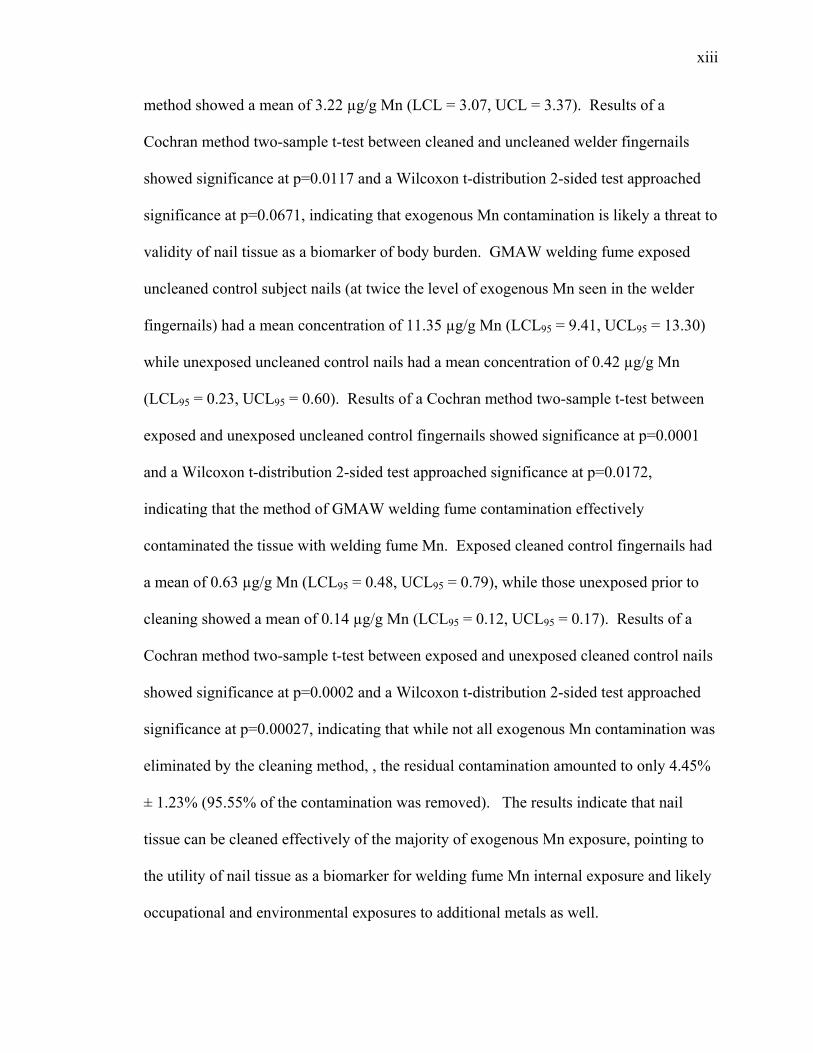
Bainter, Jeffrey C. M.S., Purdue University, August 2014. Efficacy of Cleaning Method for Removal of Exogenous Welding Fume Contamination from Nail Tissue Prior to Use as a Biomarker for Welding Fume Manganese Exposure. Major Professors: Ulrike Dydak and Frank Rosenthal. Nail tissue has been proposed as a biomarker for body burden of occupational exposure

to manganese from welding fumes. Though recent studies have shown correlation

between manganese exposure and both nail tissue concentration as well as concentrations

in dopaminergic regions of the brain, concerns of the validity of nail tissue as a biomarker

have arisen due to the potential for exogenous contamination of Mn to undermine the

quantization of endogenous Mn in nail. Previous studies have used a cleaning method of

1% Triton X-100 surfactant plus sonication in order to attempt to remove exogenous

welding fume contamination. Determination of the potential level of exogenous Mn from

welding fume on welder nail tissue was investigated. In addition, an intentional welding

fume contamination methodology was developed in order to deposit welding fume Mn

onto control nail samples in a within-subject design in order to test the efficacy of the

prior nail tissue cleaning method. Paired sample fingernails from welders exposed to gas

metal arc welding (GMAW) welding fume were digested and analyzed by inductively

coupled plasma-mass spectrometry (ICP-MS). Uncleaned welder fingernails had a mean

of 8.78 µg/g Mn (LCL = 5.58, UCL = 11.99) while those cleaned via the prior cleaning

xiii

method showed a mean of 3.22 µg/g Mn (LCL = 3.07, UCL = 3.37). Results of a

Cochran method two-sample t-test between cleaned and uncleaned welder fingernails

showed significance at p=0.0117 and a Wilcoxon t-distribution 2-sided test approached

significance at p=0.0671, indicating that exogenous Mn contamination is likely a threat to

validity of nail tissue as a biomarker of body burden. GMAW welding fume exposed

uncleaned control subject nails (at twice the level of exogenous Mn seen in the welder

fingernails) had a mean concentration of 11.35 µg/g Mn (LCL95 = 9.41, UCL95 = 13.30)

while unexposed uncleaned control nails had a mean concentration of 0.42 µg/g Mn

(LCL95 = 0.23, UCL95 = 0.60). Results of a Cochran method two-sample t-test between

exposed and unexposed uncleaned control fingernails showed significance at p=0.0001

and a Wilcoxon t-distribution 2-sided test approached significance at p=0.0172,

indicating that the method of GMAW welding fume contamination effectively

contaminated the tissue with welding fume Mn. Exposed cleaned control fingernails had

a mean of 0.63 µg/g Mn (LCL95 = 0.48, UCL95 = 0.79), while those unexposed prior to

cleaning showed a mean of 0.14 µg/g Mn (LCL95 = 0.12, UCL95 = 0.17). Results of a

Cochran method two-sample t-test between exposed and unexposed cleaned control nails

showed significance at p=0.0002 and a Wilcoxon t-distribution 2-sided test approached

significance at p=0.00027, indicating that while not all exogenous Mn contamination was

eliminated by the cleaning method, , the residual contamination amounted to only 4.45%

± 1.23% (95.55% of the contamination was removed). The results indicate that nail

tissue can be cleaned effectively of the majority of exogenous Mn exposure, pointing to

the utility of nail tissue as a biomarker for welding fume Mn internal exposure and likely

occupational and environmental exposures to additional metals as well.

1

CHAPTER 1. INTRODUCTION

1.1 Introduction

Occupational exposure to welding fume is a well-documented workplace hazard in

facilities implementing the use of welding techniques for metal fabrication. Though

worker exposure assessments can lead to insight of the potential exposure a worker may

experience, they are at best an indirect measure of exposure with somewhat limited

reliability. Exposure assessments for welding fume often involve work history and

dietary questionnaires, personal breathing zone (PBZ) and work area air monitoring,

work logs and data, type of welding and welding materials, use and type of respirators

and other PPE as well as local and general exhaust ventilation. The goal is to determine

the exposure to the various hazardous constituents contained in welding fume, chiefly

manganese, iron, lead, and copper in typical mild steel alloy welding wire and chrome

and zinc respectively when the welding work involve stainless steel or galvanized metal.

Obviously it would be very beneficial for industrial hygiene and occupational health

workers to be able to quantize workers exposure to these welding fume components via

more direct methods. Having a direct measurement of the distinct metals, associated with

neurologic effects, from welding fume exposure would offer key insight to the overall

exposure of workers to welding fumes. The uptake of metals in welding fumes are

2

typically from aerosol states of the various metals which are quickly oxidized after

condensation in the air. Unlike many organic contaminants, metals are persistent in the

body as they cannot be broken down into smaller organic molecules, but can only

undergo changes in oxidation state and potentially bind or chelate to large biomolecules.

Although metabolic excretion pathways such as urine, feces, sweat, and exhaled air do

account for large percentages of metal exposure to be excreted from the body,

metabolism does not actually eliminate metal intake entirely. For most metals a

significant fraction will persist in one state or another which if still present in bodily fluid

or tissue, can be used as a biomarker of the metal exposure.1

Adroit use of legitimately accurate biomarkers for assessment of worker welding fume

exposure helps researchers strengthen the internal validity of their study by having a

second measure of exposure in addition to the typical exposure assessment methods such

as air sampling and work history data collection. This will help ensure there is less

likelihood of measurement bias as the exposure assessment and biological tissue

assessment should be related and any indication of inconsistencies could alert an astute

researcher of potential problems in protocol, methodology, equipment or reagents.

According to Eastman2, it is important to identify adequate biomarkers of exposure for

metal exposures because they most likely reveal the “integration of the internalized dose

over time”. In essence, the true goal of exposure assessment is to demonstrate an

exposure-effect relationship and researchers should strive to identify the measure that

most effectively and accurately demonstrates this effect. The belief is that external

assessments of exposure (e.g. personal breathing zone air monitoring, etc.) will always

3

leave some doubt as to whether they are true representations of the internalized dose,

whereas biomarkers which can be shown to directly reflect the physically incorporated

toxicant (body burden). For example, there should be better prediction of actual risk by

an effective chronologically integrated biomarker such as Mn in keratin rather than

exogenic references such as air concentrations or indirect measures such as work histories

or hour welding.2

Even if, however, the a biomarker is shown to be a valid, objective, precise, and reliable

measurement of exposure with less bias than other alternatives, there are certain

limitations involved as with biomarkers as well. Laboratory errors are possible, though

this is no different to lab errors possible in the analysis of air sampling filters and quite

akin to transcription and analysis errors in the use of questionnaire and historical data.

Timing can be a factor as well. As will be discussed in more detail, different types of

metals have varying half-lives in various biological tissues. The desired time-window of

exposure which is to be measured must parallel the biomarkers chronological expression

of the metal exposure in a fashion which will allow meaningful observations. Time can

be another factor as well. The proper allowable storage time of samples in various states

throughout the process of collection, preparation, and final analysis, must be determined.

The samples must not be allowed to degenerate, lose concentration, or suffer integrity

loss such that they are no longer valid. Expense may also play a negative role as

analysis of some biomarkers may be more costly than other exposure assessment methods.

Finally there is also the question of acceptability. There may be ethical questions related

to the use of particular biomarkers, such as cerebral-spinal fluid used with children. The

4

subjects of the biomarker analysis must be made aware of the overall risks and benefits

and must deem the intrusion of the biomarker sampling to be acceptable.26

1.2 Body Fluids As Biomarkers of Metal Exposure

Techniques for analysis of body fluids such as blood and urine as biomarkers of metal

exposure have been available to researchers for a long time. Higher blood serum and

urine concentrations of typical welding fume related metals such as Mn have been found

in welders exposed to welding fume compared to control subjects, however these fluids

may only be useful for testing relatively recent (acute) exposures.3 Excessive blood

serum and urine concentrations of many metals such as Mn, quickly diminish to

homeostatic levels due to hepatic and renal metabolism pathways. Unfortunately this

leads to limited utility of these fluids as a biomarker of metal exposures, their value being

primarily that of comparing acute exposures in short time frame models to validate very

recent personal and area exposure air monitoring.

Santamaria reviewed a great deal of research regarding various attempts to correlate

blood and urine, as biological measures of Mn exposure, with measures of neurological

dysfunction (e.g. measures of memory, word recall, hand-eye coordination, etc.) and

found little consensus on the use of these fluids as biomarkers of exposure related to

adverse health effects of Mn.4 Lees-Haley performed a meta-analysis of 20 separate

research studies performed between 1997 and 2002 which looked at occupational

exposure to Mn. The analysis concluded that urine and blood did not show correlation

with air monitoring assessments or total years of exposure to the worker.5

5

Laohaudomchok also showed that Mn exposure over work shift was not correlated to

blood of urine. His study used both apprentice and professional welders attending

boilermaker welding school. Laohaudomchok used analysis of Mn exposure over work

shifts and cumulative exposure assessments in an attempt to determine if Mn

concentrations in certain human biological tissues were correlated to these measures and

thus could be considered effective biomarkers of Mn exposure. The study determined that

both blood and urine were not effective measures of Mn exposure.6

1.3 Keratin Tissue As Biomarker of Metal Exposure

In light of limited utility of blood and urine as biomarkers due to the short retention

period of the metals in those fluids, keratin based tissue such as nail and hair material has

been proposed as an alternative. Many studies have looked at the potential for nail and

hair, keratin based tissues, to be used as biomarkers of various metal exposures.

Longnecker demonstrated that selenium in toenails represented an integrated exposure

over the typical growth window of toenail (7-12 month timeframe).7 Garland showed

that long-term reproducibility of selenium mercury and arsenic concentrations in toenail

correlated to dietary intake.8 Palmeri discussed the advantages which keratin based

tissues have over body fluids as biomarkers. Palmeri’s primary concern was the

incorporation of drug metabolites into the keratin matrix, but the same mechanisms come

into play in the deposition of trace metals into the nail or hair tissue as well. Palmeri

states that there are three basic reasons why keratin tissue may prove much more useful

as a biomarker of metal exposure in long-term exposure scenarios. As a biological

material, keratin has a strong chemical and physical integrity, a natural affinity for metals

6

as it grows, and a relatively slow growth rate which can assist more long-term modeling

of exposure.9

Robust nail and hair keratin proteins are able to bear substantial physical and chemical

attack without incurring significant damage. Nail and hair keratin contains high levels of

cysteine, an amino acid containing sulfhydryl-bonded thiol side chains which leads to

strong covalent disulfide bonds through coupling of thiol groups from adjacent molecules.

This is one reason keratin based hair and nail tissue is so strong and resilient.9

Closely linked to the nature of keratin stability and strength is the tissue’s distinctive

affinity for metals of interest such as Mn. It has been shown that the high levels of thiol

groups (from cysteine) in nail and hair keratin are responsible for the high affinity of

metals to the forming keratin tissue.9

The lengthy time scale for growth of both nail tissue (typically 1.6 mm/month 10

corresponding to 6-12 months 7, 11, 12 for an average full big toe growth length of 20mm

and roughly half that for fingernails 10,13) and hair tissue (typically 250 µm/day growth

rate2, 14) can also allow these tissue to be used to give a rough chronological distribution

of the workers exposure if analyzed segmentally. Such data can be plotted against the

personal or area exposure in a timeline to validate and correlate the relationship between

biomarker and air exposure as well as to measurements of neurologic degeneration.11

While the variation associated in human toenail growth does, could be a potential

confounder of nail as a biomarker for metal exposure, Grashow proposes that any growth

7

rate variation would not correlate to exposure measures, such as welding hours or air

concentrations, and would thus not harm the internal validity of studies tying nail

concentrations to such measures.11

Once a thorough understanding of the use of nail and hair as biomarkers for metal

exposures exists, future uses of this type of analysis could be implemented. Beyond the

research realm, new uses could include medical screening for metals exposures during

typical medical surveillance before job placement (to get worker-specific baseline data),

periodically during the term of employment (to help assess on-site exposure), and at time

of termination or job transfer (to verify the workers exposure upon leaving the company).

1.4 Use of Nail Tissue As Biomarker of Welding Fume Mn Exposure

Sriram demonstrated that Mn accumulation in nail clippings is strongly correlated with

brain tissue concentration of Mn. In his study, he intratracheally dosed rats with

dissolved suspended fume from gas metal arc welding (GMAW) and MMAW (manual

metal arc welding) to ensure the absolute intake of Mn. Sriram reported that Mn in the

striatum (R2 = 0.9386; P<0.0001) and the midbrain (R2 = 0.9332; P<0.0001) were highly

correlated to Mn concentration in toenail tissue. He was also able to demonstrate that

dopaminergic abnormalities such as changes in mitochondrial function and expression of

proteins (Th, Park5, Park7), which are associated with neurodegeneration in Parkinson’s

Disease and Parkinsonism, were linked to Mn concentrations in these same brain regions.

Thus his study showed direct correlations between Mn exposure markers, both brain

tissue concentration and nail tissue concentration, and neurological degeneration. He

8

concluded that Mn in keratin tissue is a better predictor of Mn accumulation and exposure

than blood and urine. All of these facts help validate the use of Mn in nail tissue as a

good biomarker of neurotoxicological effect from Mn in welding fume exposure.15

Laohaudomchok, in a previously study, tested toenail for its correlation to Mn exposure

measures. After adjusting his data for potentially confounding variables such as age and

diet, significant correlation was found between various ranges of cumulative exposure

between the 7 and 12 month time windows prior to nail sampling, corresponding

approximately to the time frame of the sample clippings actual growth at the cuticle.

Laohaudomchok likewise concluded that while blood and urine were poor indicators of

cumulative Mn exposure, toenail tissue did seem to be a valid biomarker of Mn

exposure.6

Grashow used the same cohort which Laohaudomchok had studied but focused on using

a far simpler measure of external exposure, total weld hours. Toenail clippings were

acquired from welders and analyzed via dynamic reaction cell-inductively coupled

plasma-mass spectrometry (DRC-ICP-MS) after cleaning and digestion. To remove the

suspect exogenous welding fume contamination Grashow sonicated the tissue samples in

a surfactant solution (1% Triton X-100) for 20 minutes followed by repeated rinses with

Milli-Q water. Results indicated that cumulative lifetime years of welding work were not

related to hours welded in past year which Grashow accepted as evidence that years

working as a welder is not a confounding variable in relation to toenail as a biomarker of

9

welding fume Mn exposure from the past year. This is significant because of the

inclusion of both professional and apprentice welders in the cohort.11

Since the toenail Mn concentrations were not normally distributed, Grashow compared

log-transformed toenail concentration, adjusted for BMI, smoking status, age, and

respirator use, with weld hours. Toenail Mn levels had a positive associatation only with

weld hours from the previous 7-9 month yearly quarter (β = 0.0032, p < 0.001). Age,

BMI and smoking status did not appear to have significant correlation to toenail Mn in

any of the models tested. Respirator use hours, however, was negatively associated to

toenail Mn levels in the fourth quarter (10-12 months prior to clipping; β = -0.1877, p =

0.02).11 Overall median Mn concentration in toenail for the cohort11 was 0.81 µg/g

similar to the 0.8 µg/g seen in the same cohort in the Laohaudomchok study6 but

significantly lower than other studies, notably a Portuguese miner study which found a

mean toenail concentration of 2.5 µg/g.16 The cohort used in the Grashow and

Laohaudomchok studies were welders involved in a boilermaker welding school in which

welders worked in large, temperature controlled workstations that were equipped with

local exhaust ventilation (LEV).6 It is assumed that welders in less clean environments

and without the benefit of LEV and respirator use are much more likely to exhibit

significantly higher nail concentrations of Mn relative to a greater airborne exposure of

welding fume particulate matter.

10

1.5 Toenail Tissue As Biomarker for The Wabash Study

For an ongoing exposure assessment of welders and controls through a research study

(The Wabash Study) conducted at Purdue University under the guidance of Drs. Ulrike

Dydak and Frank Rosenthal, direct measurements of cumulative exposure to Mn relative

to known periods of exposure were compared to the welders’ current and past exposure

status. Toenail tissue was selected as a biomarker of Mn internal exposure due to its

distinct affinity for metals such as Mn during its growth and the fact that toenail Mn

concentration level is currently among the most promising biomarkers for Mn intake as

shown in recent studies.6, 15

As The Wabash Study aims to related welding fume manganese exposures to overall

neurological deficit, external exposure assessment (such as air sampling), and brain

deposition of manganese (determined by MRI analysis), it is imperative that any

biomarker for manganese should consistently reflect actual exposure intake of the

individual subject for a distinct time window. It may be determined that the Mn

accumulation in nail tissue is actually representative of a fraction of the true total intake

(due to possible alternative exposure routes such as olfactory nerve route), however as

long nail tissue Mn concentration is found to represent a constant fraction of the total

body burden, nail tissue will likely be a useful biomarker. As mentioned above, at least

some evidence to this effect is seen in Sriram’s work.

Toenail tissue is being used preferentially over fingernail in The Wabash Study in order

to minimize the effect of exogenous contamination of welding fume particulate matter to

11

the nail tissue as workers’ feet are typically somewhat protected in the work environment,

in contrast to fingernails. Analysis of nail tissue was also a favorable alternative to blood

and urine as it is minimally invasive to the test subjects and can be used to analyze other

cumulative metal levels as well, such as Cu, Fe, Zi, Pb and CrIII.7, 8, 11, 12

Nail clippings are collected from test subjects throughout The Wabash Study. Before

analysis clippings are cleaned thoroughly by using a specific cleaning protocol (similar to

the one used by Grashow’s group) and then chemically digested via a specific digestion

protocol (see Appendix A). This is followed by sample preparation and dilution prior to

analysis via ICP-MS in order to determine the metal concentration levels of the toenail

tissue. Due to the nature of toenail growth, the Mn concentration of the actual tissue

sample (coming from the tip, representing the oldest toenail growth) corresponds to nail

growth during the time window of exposure approximately 7-12 months prior to the nail

clipping. Mn nail concentration is obtained for each subject which is then compared to air

sampling and exposure modeling. The Wabash Study has found that toenail Mn

concentration (in µg/g) is highly correlated to the 7-12 months exposure window

assessment (in mg/yr-m3) (p = 0.0027)29.

12

CHAPTER 2. SPECIFIC AIM, HYPOTHESES, AND OBJECTIVES

2.1 Specific Aim

The principal goal of this thesis research is to determine the efficacy of the nail tissue

cleaning method utilized previously in The Wabash Study. A significant degree of

concern has arisen in the research community that significant exogenous contamination

of welding fume particulates remains on welder subject nail tissue after collection. Thus

there is concern that this external contamination, containing various welding fume related

metals, is not entirely removed via the ultrasonic/surfactant based cleaning and purified

water rinse method employed in The Wabash Study. As this tissue cleaning method is

also one commonly used by researchers studying the use of nail tissue as a biomarker for

welding fume related manganese exposure the present experiment will shed light on the

validity of previous studies’ results.11

The various objectives of this study all revolve around this central goal of determining

the validity of the general nail cleaning methodology. For the sake of simplification due

to time and logistic concerns, manganese will be the sole element of concern throughout

this study. To assist comprehension of the nature of the hypotheses relevant to the

experimental design, a schematic hypothesis flow diagram is shown in

13

Figure 2-1 which depicts the flow from nail tissue samples, through the experimental

stage, toward analysis and hypothesis testing.

Figure 2-1 Hypothesis flow diagram

14

While the relationship of Hypothesis 1 to the difference between the W-EU and W-EC

groups is fairly straightforward, it will be helpful to clarify the relationship of Hypotheses

2 and 3,listed below, relevant to the difference of means between treatment groups UU

& EU and UC and EC respectively. To do this a set of variables is set up as follows:

ENV = Environmental Mn on control nail BIO = Endogenous bio-metabolized Mn incorporated in the nail tissue WF = Intentional GMAW WF Mn contamination WF_Residual = Residual GMAW WF Mn remaining on nail after cleaning

Using these variables the constituents of the total Mn level for each group can be

depicted as:

UC = BIO UU = BIO + ENV EU = WF + ENV + BIO EC = WF_Residual + BIO

Therefore, the comparison of EU to UU should determine if significant contamination is

being achieved by the WF contamination method to be employed in this study, as will be

utilized in Hypothesis 2.

Also, the comparison of EC and UC should determine if significant contamination

remains on the nail tissue after the cleaning protocol has been employed, allowing the

analysis of Hypothesis 3.

In addition, the relative cleaning efficiency can be determined by comparing the total

welding fume contamination level to the welding fume residual level. These values can

be can derive by;

15

EU - UU = (WF + ENV + BIO) - (BIO + ENV) = WF

and

EC - UC = (WF_Residual + BIO) - (BIO) = WF_Residual

From there it is a simple progression to determining the welding fume concentration

removed divided by the total welding fume contamination (WF - WF_RESIDUAL / WF)

to get the removal efficiency.

(EU - UU) - (EC - UC ) / (EU - UU) = removal efficiency

2.2 Primary Objectives And Central Hypotheses

2.2.1 Objective 1: Exogenous Mn contamination to welder fingernail

The initial objective of this study is to determine the level of exogenous Mn exposure on

welder fingernail tissue collected from a selection of The Wabash Study’s welder

subjects to get an idea of upper level of potential exogenous Mn exposure which welder

subject nail samples may exhibit. Knowledge of a reasonably approximate upper level of

exogenous welding fume Mn contamination will allow an attempt to set the intentional

welding fume Mn contamination of fingernail tissue at a realistic level to provide

significant contamination without unreasonably overwhelming the cleaning method’s

ability to remove exogenous Mn. The presence of significant exogenous Mn

contamination to nail tissue, if determined, will be evidence of the necessity of an

efficacious and reliable tissue cleaning method.

Hypothesis 1: Welder subject nail tissue, prior to cleaning, contains a significant quantity

of exogenous manganese from welding fume exposure.

16

2.2.2 Objective 2: Verification of contamination method

After the determination is made as to a reasonable value of exogenous Mn contamination

from welding fume from Objective 1, the necessary apparatus and methodology for

application of Mn welding fume contaminant deposition must be designed and tested to

ensure nail tissue Mn contamination at an appropriate level necessary for further analysis

of the effectiveness of the nail tissue cleaning method. Additionally, lab sample

preparation methods must be designed in order to identify proper nail digestion sample

dilution protocols to ensure proper analysis and analytical equipment safeguarding. For a

detailed explanation of the serial dilution steps performed see Appendix A: Nail

Digestion and ICP-MS sample Protocol.

Hypothesis 2: Intentional exposure to GMAW welding fume, within the set experimental

design, will result in significantly higher external contamination levels of

Mn on the Exposed/Uncleaned fingernails when compared to

Unexposed/Uncleaned fingernails.

2.2.3 Objective 3: Nail cleaning method validity testing

Once the proper exposure level and sample dilution levels are determined, the heart of

this study will be addressed. Comparison of nail tissue samples from the control subject

with exogenous exposure of GMAW welding fume and unexposed nail tissue from the

control subject, will have the current cleaning protocol performed on them prior to

digestion and analysis for total nail tissue Mn concentration. The exposed cleaned nail

tissue is presumed to incorporate the residual welding fume contamination after the

17

cleaning plus the endogenous nail Mn. The unexposed cleaned nail tissue is presumed to

only reflect the endogenous nail Mn. The data will be analyzed to determine if there is

statistical difference between the means of these two treatment groups. Rejection of

Hypothesis 3 indicates that some residual welding fume Mn remains after cleaning.

If residual welding fume Mn contamination remains the data will be analyzed to

determine the fraction of the original contamination level which the residual represents,

thus the level of effectiveness of the cleaning method to remove exogenous welding fume

Mn contamination. If it is possible to show that significantly high levels of external Mn

contamination can be satisfactorily removed prior to nail tissue digestion and analysis,

then the use of nail tissue as a viable biomarker will be supported and validated for

welding fume exposure studies as well as for other settings such as child and

environmental exposure epidemiological studies.

Hypothesis 3: There is no difference between population means of nail tissue Mn

concentration after the current cleaning protocol for nail tissue

significantly contaminated with GMAW welding fume and untreated nail

tissue cleaned by the same process.

18

CHAPTER 3. METHODOLOGY

3.1 GMAW Welding Fume As Mn Contaminant

Actual welding fume was chosen as the contaminant for this study in order to provide

significant and realistic Mn external exposure to nail tissue. Other options considered

were suspended solutions of precipitated welding fume particulates and manganese

chloride solutions. These alternatives were rejected due to the fact that they are not true

representations of the actual exposure to which welding workers’ nail tissue are exposed.

Manganese (II) chloride is not in the same oxidative state and chemical species as

manganese in GMAW welding fume, primarily Manganese (II, III) Oxide 17 (Mn3O4

sometimes written MnO.Mn2O3), a compound formed when manganese is heated in air

above 1000 °C 18 well below the 6000-8000 °C temperatures of a typical GMAW weld

arc.19 Precipitated welding fume, like many typical sub-micron particulates, tend to

agglomerate and aggregate over time and any later suspension of this material would not

be likely to form deposition on nail tissue as true welding fume does. Chung, in his

experiments on welding fume air sampling, showed that penetration of welding fume

through porous foam samplers dropped off as much as 55% after just 4 minutes of

welding fume aging, an indication that considerable aggregation was taking place over

time and that aged fume is likely to change significantly in respect to its chemical and

physical properties.20 It is therefore felt that the extraneous variables introduced by

19

the use of either of the proposed alternatives would be of substantial detriment to the

internal validity of this study.

Consequently, with the decision to utilize actual welding fume for this study, it became

necessary to design a welding fume contamination vessel and develop a contamination

method that is as uniform and as repeatable as possible. The welding used for

contamination purposes in this study, GMAW, employs a similar welding technique and

material as The Wabash Study’s worker cohort which predominantly uses GMAW

welding processes. GMAW, sometimes referred to as Metal Inert Gas (MIG), utilizes an

electric arc with mild steel solid core wire and an inert shielding gas, thus avoiding the

use of flux core wires. This typically results in superior welds and eliminates the need

for flux on the substrate or in the wire which characteristically involves greater exposure

to the welder from Mn fume.21

Upon completion of the GMAW containment vessel design and construction, an initial

exposure test was performed to determine the duration of weld arc time required to

provide a significant and realistic level of Mn deposition on the baseline control nails that

would be similar to the amount of exogenous Mn determined to be on the welder subjects’

uncleaned fingernail tissue. Serial dilutions of the digested nail samples were performed

on all welding fume exposed uncleaned nail tissue samples in this step in order to

determine proper dilution levels which would allow proper analysis without endangering

the sensitive ICP-MS equipment from excessively high Mn concentrations.

20

3.2 Containment Vessel Design

For this study, a welding fume containment vessel was prepared in order to capture

generated welding fume and force its precipitation on the cross sectional area of the

vessel thus allowing sufficient prediction of fume to area deposition onto the exposed nail

tissue samples. The vessel consisted of a glass aquarium with glass spatter shield and

several glass plates to enclose the top of the vessel in order to contain the welding fume.

The ground clip of the welder unit was run into the vessel and held the carbon steel (mild

steel) work piece substrate in place facing upward making it easier to weld on while

allowing minimal open area for the arc gun to enter. The top of the work piece was kept

approximately 4 inches below the top glass containment plate, however, in order to

minimize risk of the excessive heat generated during welding to weaken and crack the

glass plate.

Multiple glass containment plates were placed on either side of a vertically placed glass

spatter shield in order to seal the top portion of the vessel. The spatter shield eliminated

the possibility that welding spatter would excessively contaminate the nail tissue samples

beyond the level required and which could pose a threat to the analytical equipment later

on. Once the set arc time was completed and the fume had been produced in the arc side

of the vessel, the arc gun was removed and the opening was closed. At this time the

spatter shield was carefully pulled up from between the top glass covers and as it was

removed the covers were slid together and the glass seam was covered with another plate

of glass, effectively capturing the fume and allowing it to disperse uniformly throughout

the vessel. The fume was allowed to precipitate uniformly and undisturbed for a period

21

of two hours prior to the tissue samples being removed and carefully sealed in plastic

containers for further sample preparation. The vessel dimensions are 10”W x 20”L x

11”H and the volume is 1.273 ft3. Figure 3-1 below depicts the design elements of the

welding fume containment device. Photographs of the device and actual application of

the welding fume contamination process are found in Appendix B.

Figure 3-1 Welding Fume Containment Vessel Design

3.3 Welding Equipment

The welding device used in the study was a Century 100 Wire Feed Welder Model 117-

050 (120V, 30-100A range). The rated DC output of that model is 85A and 18V and the

duty cycle is 20%. For this study the Wire Feed speed selector was set to 4 and the Heat

selector set to 4. The approximate wire speed was 12 fpm or about 61 mm/s.

22

The welding wire used was solid core Lincoln Superarc L-56 MIG (GMAW) wire with a

wire diameter of 0.025”. This is a copper coated (for tip protection) wire similar to the

wires used by welder subjects in The Wabash Study. The AWS ER70S-6 Mn

requirements for this wire are 1.40 – 1.85 % Mn and the typical range provided by the

manufacturer is 1.42 – 1.65% Mn. As GMAW requires shielding gas, argon/CO2 inert

shielding was supplied via the arc gun to the arc point at a rate of 15 cfh. Shielding gas

for this study was acquired from Praxair, Lafayette, IN.

3.4 Experimental Design

With the exception of the welder subject nail tissue which was analyzed to test

Hypothesis 1 under Objective 1, the rest of this study was a within subject design as all

the nails for treatment groups UU, EU, UC, and EC came from a single control subject..

This was chosen to increase the sensitivity of the experimental design, making it more

likely that small differences in the treatment conditions would be detected. Left and right

fingernail sample pairs from the same subject were used as a paired units for comparison

of the independent variables. Additionally, while the welder nail Mn concentrations may

have a non-normal distribution, due to unknown fluctuations in their occupational

exposure levels, it is fairly reasonable to assume that the nail tissue Mn concentrations of

the single control subject, used for the rest of the study, have a normal distribution,

allowing easier and more reliable statistical analysis of the small data sample sizes. This

assumption relies on the facts that the control subject had not obvious occupational or

environmental Mn exposure, lived and worked in the same locations throughout the

growth periods of the tissue collected, and did not significantly alter his diet throughout

23

the study. There is no known reason why the control subjects nails would skew in either

direction from the mean Mn concentration over the course of tissue collection and nail

growth relevant to this study.

This study’s single control subject was a non-smoking white male, age 43, with no Mn

associated health problems and no previous history of welding or any Mn exposure

associated occupation. The nail samples from the control subject were acquired between

November 6, 2013 and May 12, 2014.

3.4.1 Welder Fingernail Analysis

One reason for using fingernail tissue for Objective 1 was that all the toenail samples so

far collected during The Wabash Study had already been cleaned and digested for

analysis to collect data for The Wabash Study. Another reason was that while welders’

toenails are somewhat protected from welding fumes, being inside socks and boots

during the exposure period, fingernails are much less protected and typically in closer

proximity to the welding arc. While welders typically wear protective gloves during the

act of welding, they routinely remove the gloves throughout the work shift, exposing the

fingernail tissue to the ambient Mn from welding fume mixed into the work area air. Not

all welder subjects were able to provide fingernail tissue samples, but of the welding

subjects that supplied ample fingernail tissue for analysis, the welding subjects that

previously showed the highest toenail Mn concentration were selected in order to

determine the exogenous Mn contamination from welding fume which represents the

higher end of the exogenous exposure range.

24

Welder subjects WW-10, WW-13, WW-15 and WW-17 were chosen for this analysis.

Demographics and toenail Mn concentration for the selected welders are shown in Table

3-1 below. For the purpose of this study the welder fingernails were considered as an

exposed treatment group due to their occupational exposure to welding fume. Half of

each pair of fingernail sample was left uncleaned prior to digestion (Exposed/Uncleaned

or EU) and the other half was cleaned via the current cleaning method (Exposed/Cleaned

or EC). Samples were digested according to current protocol and ICP-MS analysis was

run on sample dilutions concurrent with standard spike additions for concentration

calibration and blanks to subtract instrument background noise. WW-13 and WW-15

samples were run during the Round 1 samples group while WW-10 and WW-17 samples

were run during the Round 3 samples group.

Table 3-1 Demographics and toenail Mn concentration for selected welders subjects

Subject Clip Date Race Gender Age Years

Welding Smoker

Toenail Mn

(µg/g) WW10 4/6/2013 white Male 42 12.25 no 9.18

WW13 7/27/2013 white Male 53 23 no 12.86

WW15 8/10/2013 Hispanic Male 44 15 no 11.02

WW17 10/13/2013 African American Male 29 3.5 no 13.90

Nail tissue sample Mn concentrations were determined and the difference between the

welder EU and the welder EC results are the level of exogenous Mn from GMAW

welding fume present on the welder subjects’ fingernail tissue.

25

3.4.2 Cleaning Protocol

The Wabash Study cleaning protocol subsists of a surfactant solution assisted by

ultrasonic cleaning. Ultrasonic assisted cleaning works via cavitation action at substrate-

cleaning solution interface. For a detailed description of the cleaning protocol see

Appendix A section 1. All DDI water used for cleaning and sample/standard/spike

preparations had a conductivity of between 13.4 – 13.8 µΩ. Below is a brief synopsis of

the cleaning protocol.

• Toenail sample immersed in 10 mL of 1% Triton X-100 solution • Samples placed in Branson Sonifier ultrasonic cleaner (400W - 27000Hz) for 15

minutes at 50% power • After ultrasonic cleaning, sample rinsed 5 times with Distilled De-Ionized water

(DDI)

3.4.3 Experiment Round 1 Design

This round was designed to test the equipment design, determine proper arc time of

exposure, and begin obtaining data for Objectives 1 through 3. During this step, four

pairs of the control subject’s fingernails were prepared and analyzed. Two pairs were

split into Unexposed/Uncleaned (UU) and Exposed/Uncleaned (EU) treatment groups.

The other two pairs were split into Unexposed/Cleaned (UC) and Exposed/Uncleaned

(EU) treatment groups. The exposed samples were exposed incrementally to

successively higher levels of welding fume by running progressively longer periods of

arc time within the containment vessel for each exposed sample, producing more fume

26

which deposited on the nail tissue sample. The first half of the welder subject nails

previously discussed were analyzed as part of Round 1 as well.

3.4.3.1 Estimating required mass of GMAW WF for initial contamination

As this step was run concurrent with the first objective step, due to time constraints, an

estimated contamination rate needed to be determined as a starting point of exposure.

Once the estimated preferential arc time was determined arc times of 0.1x, 1x, 10x, and

20x were run as the exposures in order to increase the likelihood of finding the

appropriate exposure window which would allow significant and realistic exposure.

It has previously been determined that welding fume particulate is predominantly

generated from the welding wire and not the substrate (due to the positive charge polarity

at the wire) thus the wire itself was of concern in determining the estimated arc time for

proper contamination.17 Carpenter, et al., determined that GMAW welding fume consists

of 8.3 % Mn3O4 ; 91.7% Fe3O4 with trace levels of Si and other elements.17 This analysis

of GMAW fume will be used for the purposes of this study.

Quimby, et al., using similar GMAW methods as this study and a solid core mild steel

wire with diameter width of 0.045”, predicted for low voltage and amperage similar to

this study that a GMAW fume formation rate is in the range of approximately 0.2 – 0.4

g/min).22

27

The starting point to determine an appropriate contamination level was the determination

of theoretical amount of Mn in a fingernail sample. It was determined that the average

Mn concentration in The Wabash Study welder subjects toenail tissue was 8.25 µg/g Mn

however the highest concentration found in a welder subject toenail tissue (24.9 µg/g Mn)

will be used as a worst case estimate. The average weight of toenail samples was 93.2

mg. The expected typical weight of fingernail sample is half of that weight (46.6 mg).

Though fingernails typically grow about twice as fast as toenails and thus typically have

about half the concentration of Mn, the 24.9 µg/g Mn estimate will be used as a liberal

estimate. Thus the estimated amount of Mn in a welder subject fingernail sample is 24.9

µg/g X 46.6 mg = 1.16 µg.

In order to determine the deposition on a fingernail sample from the generated welding

fume, the ratio of fingernail surface area relative to the cross section area of the floor of

the containment vessel was required. An estimation of the surface area of a fingernail

sample was made based on the measurements found in Table 3-2 taken from a typical

sample of fingernail tissue from the study’s control subject.

The combined surface area of one hand’s fingernail sample is 179 mm2. For a liberal

estimate of the deposition of welding fume to the nail sample it was assumed that

gravitational and electrostatic deposition would occur across all but the one down side

which rests on the floor of the vessel. The orientation of the nails in on the floor of the

containment vessel was such that the smallest were never actually the down side. The

remaining four sides were averaged and the average was subtracted from the total surface

28

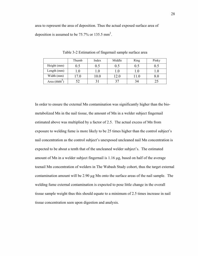
area to represent the area of deposition. Thus the actual exposed surface area of

deposition is assumed to be 75.7% or 135.5 mm2.

Table 3-2 Estimation of fingernail sample surface area

Thumb Index Middle Ring Pinky

Height (mm) 0.5 0.5 0.5 0.5 0.5 Length (mm) 1.0 1.0 1.0 1.0 1.0 Width (mm) 17.0 10.0 12.0 11.0 8.0 Area (mm2) 52 31 37 34 25

In order to ensure the external Mn contamination was significantly higher than the bio-

metabolized Mn in the nail tissue, the amount of Mn in a welder subject fingernail

estimated above was multiplied by a factor of 2.5. The actual excess of Mn from

exposure to welding fume is more likely to be 25 times higher than the control subject’s

nail concentration as the control subject’s unexposed uncleaned nail Mn concentration is

expected to be about a tenth that of the uncleaned welder subject’s. The estimated

amount of Mn in a welder subject fingernail is 1.16 µg, based on half of the average

toenail Mn concentration of welders in The Wabash Study cohort, thus the target external

contamination amount will be 2.90 µg Mn onto the surface areas of the nail sample. The

welding fume external contamination is expected to pose little change in the overall

tissue sample weight thus this should equate to a minimum of 2.5 times increase in nail

tissue concentration seen upon digestion and analysis.

29

Based on the estimated deposition area of the nail sample and the target contamination

concentration amount the target mass of deposition per unit area was:

2.90 µg Mn / 135.5 mm2 = 0.0214 µg/mm2 Mn

The assumption was made that all generated welding fume precipitate deposits equally

upon the settling area of the chamber (254mm * 508mm = 129,032 mm2), thus the total

fume generation required was:

129,032 mm2 * 0.0214 µg/mm2 Mn = 2761.3 µg = 2.76 mg Mn

The chief constituent of Mn in GMAW WF, Mn3O4, is 72% Mn, thus the required mass

of Mn3O4 was:

2.76 mg Mn / .72 Mn = 3.833 mg Mn3O4

Based on Carpenters work17, assuming GMAW WF is 8.3 % Mn3O4, the required mass of

GMAW WF would be:

3.833 mg Mn3O4 / 0.083 Mn3O4/WF = 46.18 mg GMAW WF

30

3.4.3.2 Determining the required GMAW arc time for initial contamination

According to research performed by Quimby7, GMAW WF generation rate, for similar

voltage, amperage as this study, range approximately around 0.2 - 0.4 g/min arc time.

However Quimby was using 0.045" diameter wire. The wire used in this study was

0.025" diameter which is approximately 26.4% of the cross-sectional area of the wire

used in Quimby’s study. Therefore it was estimated that the GMAW WF generation rate

for this study’s setup and wire was likely in the range of 0.05 - 0.10 g/min arc time.

Thus in order to achieve the target amount of welding fume particulate to be contained

and precipitated in the vessel, the total arc time needed was:

0.0462 g GMAW WF / 0.075 g/min arc time = 0.616 minutes arc time (~ 37 sec.)

In order to expand the window of concentration for the welding fume exposure range

finding test, exposure runs were made at approximately the target arc time, one tenth

target time, ten times target time and 20 times target time (4, 40, 400, and 800 seconds

arc time).

3.4.3.3 Prediction of C / Cmax based on steady-state build up

As the welding performed in this experiment was GMAW, which requires shielding gas

flowing to the arc tip, and the welding fume containment vessel was of small, finite

volume, it was necessary to determine whether the arc times listed above would approach

the steady state system caused by the forced gas flow to the vessel. The volume of the

31

vessel (V) was 1.27 ft3 and the flow (Q) of shielding gas was 15 ft3/hr = 0.25 cfm at

constant arc. The residence time (τ) = V/Q = 5.08 min. The rate constant (k) therefore

was 1/τ = 0.197 min-1.

According to the exponential growth equation, relevant to build-up phase, one can

determine the proportion of the steady state concentration (Cmax) achieved at each of the

arc dwell times previously listed as follows:

C / Cmax = (1 – e-kt)

Thus the following levels of C / Cmax were determined for each of the assigned arc dwell

times;

For 4 seconds (0.067 min) C / Cmax = 0.013 (1.3% of Cmax)




Based on these calculations a nearly 10 fold increase in exposure should exist between

the 4 and 40 second arc time exposures while the jump to 400 seconds and 800 seconds

would only be 6 times and 1.25 times the previous arc time exposure respectively. It was

unlikely that an arc time of more than 800 seconds will significantly increase the

exposure level.

32

An assumption was made based on the C / Cmax calculations above, to estimate that the 4

and 40 second arc times would be relatively close to the estimated target contamination

levels but that the 400 and 800 arc times would lead to 6 and 7.5 times the 40 sec arc time

level respectively.

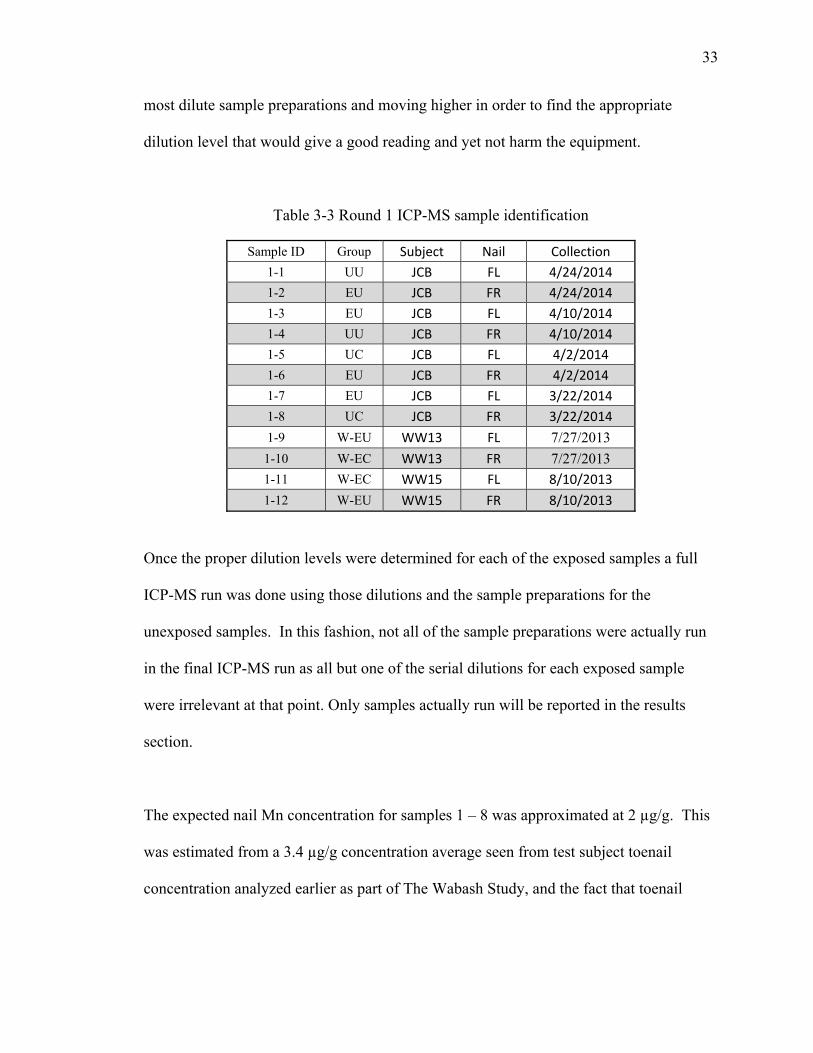
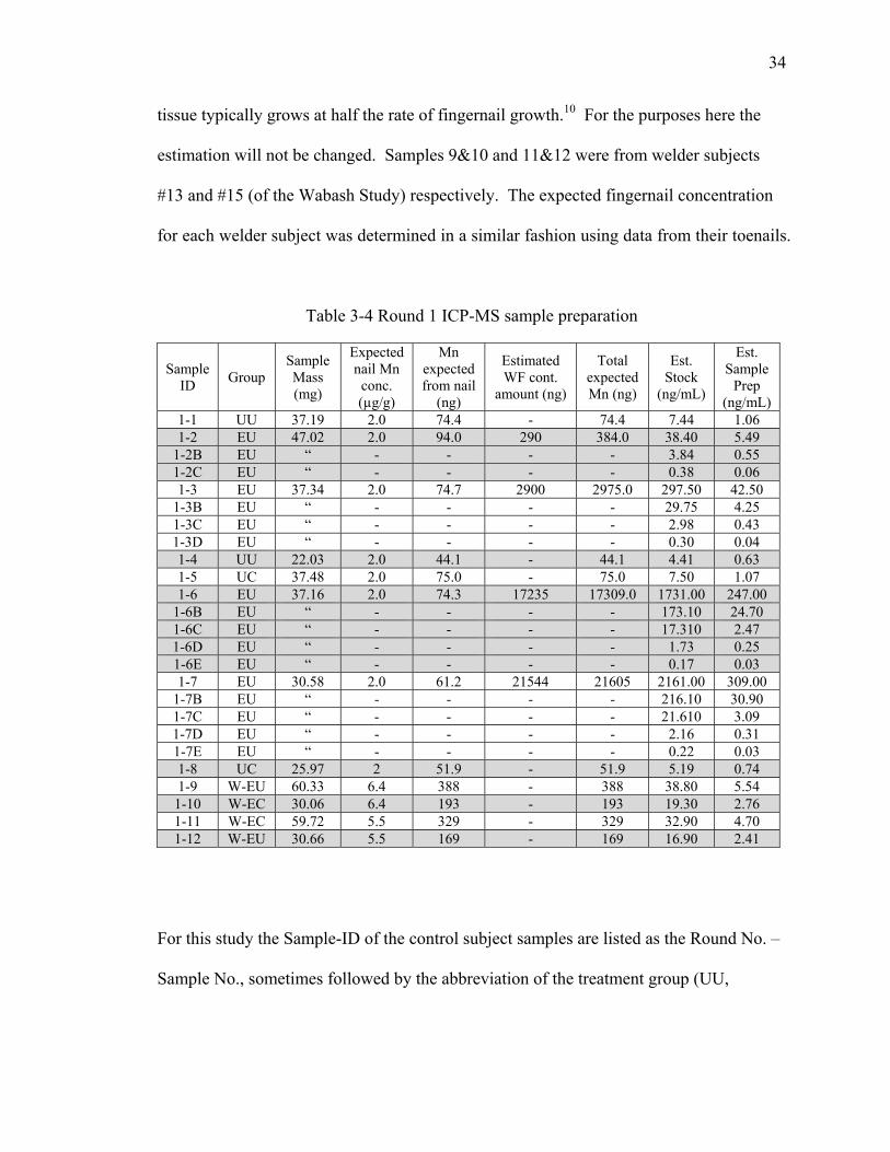
3.4.4 Round 1 ICP-MS preparations and estimated Mn concentrations

Table 3-3 and Table 3-4 below describe the Round 1 sample identification and sample

preparations for ICP-MS analysis respectively, which include both Objective 1 and

Objective 2 samples. In order to protect the ICP-MS equipment serial dilutions were

made of the welding fume exposed sample preparations. For each subsequent order of

magnitude serial dilution the initial stock solution was diluted to one tenth of the previous

stock solution. These serial diluted stock solutions were then used to prepare sample

preparations. For example, the sample 1-2 stock solution was diluted to 0.1 concentration

and labeled as the 0.1 dilution stock solution for sample 1-2 and the sample 1-2B ICP-MS

sample preparation was prepared from that stock solution. The 0.1 dilution stock solution

for sample 1-2 was then diluted to one tenth (0.01 concentration of the original stock

solution) and the sample 1-2C ICP-MS sample preparation was prepared from that stock

solution and so on. The serial dilutions were annotated with a letter suffix attached to the

sample number B being prepared from a 0.1 dilution stock solution, C from a 0.01 stock

solution, etc.

Analytical chemists were instructed as to the nature of the estimated Mn ppb levels and

the serial dilution order so they could do a pre-run ICP-MS analysis starting with the

33

most dilute sample preparations and moving higher in order to find the appropriate

dilution level that would give a good reading and yet not harm the equipment.

Table 3-3 Round 1 ICP-MS sample identification

Sample ID Group Subject Nail Collection

1-1 UU JCB FL 4/24/2014

1-2 EU JCB FR 4/24/2014

1-3 EU JCB FL 4/10/2014

1-4 UU JCB FR 4/10/2014

1-5 UC JCB FL 4/2/2014

1-6 EU JCB FR 4/2/2014

1-7 EU JCB FL 3/22/2014

1-8 UC JCB FR 3/22/2014

1-9 W-EU WW13 FL 7/27/2013

1-10 W-EC WW13 FR 7/27/2013 1-11 W-EC WW15 FL 8/10/2013

1-12 W-EU WW15 FR 8/10/2013

Once the proper dilution levels were determined for each of the exposed samples a full

ICP-MS run was done using those dilutions and the sample preparations for the

unexposed samples. In this fashion, not all of the sample preparations were actually run

in the final ICP-MS run as all but one of the serial dilutions for each exposed sample

were irrelevant at that point. Only samples actually run will be reported in the results

section.

The expected nail Mn concentration for samples 1 – 8 was approximated at 2 µg/g. This

was estimated from a 3.4 µg/g concentration average seen from test subject toenail

concentration analyzed earlier as part of The Wabash Study, and the fact that toenail

34

tissue typically grows at half the rate of fingernail growth.10 For the purposes here the

estimation will not be changed. Samples 9&10 and 11&12 were from welder subjects

#13 and #15 (of the Wabash Study) respectively. The expected fingernail concentration

for each welder subject was determined in a similar fashion using data from their toenails.

Table 3-4 Round 1 ICP-MS sample preparation

Sample ID

Group Sample Mass (mg)

Expected nail Mn

conc. (µg/g)

Mn expected from nail

(ng)

Estimated WF cont.

amount (ng)

Total expected Mn (ng)

Est. Stock

(ng/mL)

Est. Sample

Prep (ng/mL)

1-1 UU 37.19 2.0 74.4 - 74.4 7.44 1.06 1-2 EU 47.02 2.0 94.0 290 384.0 38.40 5.49

1-2B EU “ - - - - 3.84 0.55 1-2C EU “ - - - - 0.38 0.06 1-3 EU 37.34 2.0 74.7 2900 2975.0 297.50 42.50

1-3B EU “ - - - - 29.75 4.25 1-3C EU “ - - - - 2.98 0.43 1-3D EU “ - - - - 0.30 0.04 1-4 UU 22.03 2.0 44.1 - 44.1 4.41 0.63 1-5 UC 37.48 2.0 75.0 - 75.0 7.50 1.07 1-6 EU 37.16 2.0 74.3 17235 17309.0 1731.00 247.00

1-6B EU “ - - - - 173.10 24.70 1-6C EU “ - - - - 17.310 2.47 1-6D EU “ - - - - 1.73 0.25 1-6E EU “ - - - - 0.17 0.03 1-7 EU 30.58 2.0 61.2 21544 21605 2161.00 309.00

1-7B EU “ - - - - 216.10 30.90 1-7C EU “ - - - - 21.610 3.09 1-7D EU “ - - - - 2.16 0.31 1-7E EU “ - - - - 0.22 0.03 1-8 UC 25.97 2 51.9 - 51.9 5.19 0.74 1-9 W-EU 60.33 6.4 388 - 388 38.80 5.54

1-10 W-EC 30.06 6.4 193 - 193 19.30 2.76 1-11 W-EC 59.72 5.5 329 - 329 32.90 4.70 1-12 W-EU 30.66 5.5 169 - 169 16.90 2.41

For this study the Sample-ID of the control subject samples are listed as the Round No. –

Sample No., sometimes followed by the abbreviation of the treatment group (UU,

35

UC..etc.) for clarity. The GMAW welding fume exposed samples were Sample 1-2 (4

sec. arc time WF generation exposure), Sample 1-3 (40 sec.), Sample 1-6 (400 sec.), and

Sample 1-7 (800 sec.). The welder subject nail samples were also considered exposed,

for the purpose of this study, but were not intentionally exposed to additional welding

fume during this study.

It must be noted that upon finishing the 800 second arc time run and removing the spatter

shield, the seal was broken on the top of the vessel and some fume escaped before it

could be resealed. This was expected to result in a contamination level for that sample

significantly less than expected. Also the expected concentrations for the uncleaned

welder subject fingernails do not take into account any external Mn contamination. It is

assumed there is contamination but at the time of analysis there was no way of predicting

the level.

Standard spike additions were made using the sample 5 stock in order to preserve the

matrix effects of nail keratin constituents, present in all other sample preparations, along

with the standard addition preparations for use in determining a calibration curve from

the ICP-MS analysis data. Additions were prepared from Exaxol multi-element standard

which resulted in standards spikes of sample 5 sample preparations at +1.43 ppb, + 4.29

ppb, + 7.15 ppb, + 14.3 ppb, and + 28.6 ppb Mn. Blank sample preparations were also

prepared to be run during the ICP-MS run and all sample preparations including the serial

dilution sample preparations were maintained at 2% nitric concentration using ultrapure

trace element analysis grade nitric acid.

36

ICP-MS data was collected from the Round 1 analytical run and used to help determine

the results of Objective 1 and 2 and to determine the exposure level for further rounds of

welding fume contamination samples for evaluation of Objectives 2 and 3.

It was predicted that since this subject was a control (at the time of tissue collection) that

the UU and UC tissue Mn concentrations would be significantly similar and that all EU

samples regardless of arc time of exposure, would have significantly higher Mn

concentration resulting from the uncleaned external welding fume exposure.


Once the Round 1 samples were analyzed, a contamination per arc time curve was

prepared (see figure 4-2) in order to attempt to match a specific arc time exposure to a

reasonable contamination level based on the exogenous Mn level seen on the welders nail

tissue. At that point, once the proper exposure level is determined, Round 2 was initiated

to continue deriving data for Objective 2 as well as to begin obtaining data for Objective

3. Within-subject and within-group pairs of the control subject’s fingernails (left and

right samples maintained separately) were split into separate treatment groups. Half of

each pair was exposed and cleaned using The Wabash Study cleaning protocol and the

other half unexposed and cleaned via the same method. In this manner the efficacy of the

cleaning method will be tested. Once the four pairs of the EC/UC combinations from

Round 2 were run and analyzed, statistical tests were performed in order to determine the

number of additional samples needed to be run in the same fashion (during Round 3) in

37

order to define with statistic validity whether the exogenous contamination is being fully

removed by the cleaning method. (Objective 3)

Additional sets of fingernails were run with half of the pair exposed to GMAW fume and

left uncleaned (EU) to be compared to the unexposed and uncleaned half of the pair (UU)

in order to validate the actual exposure level of the particular round of exposure. This

was necessary due to the marginal control over the actual welding fume exposure

generation available with the welding device, and the need to assure each round of

exposures received an adequate and reasonable level of contamination.

Samples were analyzed via ICP-MS in a similar fashion as in Round 1. To be sure that

the Exposed/Uncleaned (EU) sample preparations would not damage ICP-MS equipment,

serial dilutions were again run on Round 2 samples. Additionally in order to be sure that

failure of the cleaning method does not result in Exposed/Cleaned (EC) samples

remaining at too high a concentration for the ICP-MS equipment, one set of serial

dilutions for a particular Exposed/Cleaned (EC) sample was also be prepared and

analytical chemists were instructed on the nature of all samples.


preparations for ICP-MS analysis respectively, which include both Objective 2 and

Objective 3 samples. The same digestion and sample preparation protocol along with

spikes, blanks, and necessary serial dilutions were performed as in Round 1. Only

samples actually run will be reported in the results section.

38

The estimation of the control subject’s nail tissue concentration was adjusted to 0.2 µg/g

Mn after analysis of Round 1 data indicated the error in the initial estimate. The

estimated deposition mass of WF Mn contamination to the exposed Round 2 samples was

derived from the estimated WF Mn concentration for the arc time used in Round 2 based

on the analysis of the concentration range by arc time analysis performed on the Round 1

data (see Figure 4-2). For a detailed explanation of how the estimation was derived as

well as why the particular arc time was chosen for Round 2 exposure, see section 4.1.


Sample ID Group Subject Nail Collection

2-1 UU JCB FL 3/10/2014

2-2 EU JCB FR 3/10/2014

2-3 EU JCB FL 2/28/2014

2-4 UU JCB FR 2/28/2014

2-5 UC JCB FL 2/16/2014

2-6 EC JCB FR 2/16/2014

2-7 EC JCB FL 2/2/2014

2-8 UC JCB FR 2/2/2014

2-9 UC JCB FL 1/26/2014

2-10 EC JCB FR 1/26/2014

2-11 EC JCB FL 1/13/2014

2-12 UC JCB FR 1/13/2014


Once the Round 2 samples were analyzed and descriptive statistics and confidence

intervals were identified for the treatment group comparisons associated to Hypotheses 2

and 3, Round 3 samples were prepared and run based on the estimations of required

sample sizes needed based on the pooled data from Round 1 and Round 2. Again, similar

UU/EU samples were prepared to determine the absolute contamination level of the

39

Round 3 contamination and similar ICP-MS analysis was performed with serial dilutions

as mentioned above.


Sample ID


Expected nail Mn

conc. (µg/g)

Mn expected from nail

(ng)

Estimated WF cont.

amount (ng)


Est. Stock

(ng/mL)

Est. Sample

Prep (ng/mL)

2-1 UU 33.38 0.20 6.68 - 6.68 0.67 0.10

2-2 EU 32.52 0.20 6.50 1300.80 1307.30 130.73 18.68

2-2B EU " - - - - 13.07 1.87

2-2C EU " - - - - 1.31 0.19

2-3 EU 31.92 0.20 6.38 1276.80 1283.18 128.32 18.33

2-3B EU " - - - - 12.83 1.83

2-3C EU " - - - - 1.28 0.18

2-4 UU 38.37 0.20 7.67 - 7.67 0.77 0.11

2-5 UC 34.25 0.20 6.85 - 6.85 0.69 0.10

2-6 EC 37.82 0.20 7.56 - 7.56 0.76 0.11

2-6B EC " - - - - 0.08 0.01

2-7 EC 29.08 0.20 5.82 - 5.82 0.58 0.08

2-7B EC " - - - - 0.06 0.01

2-8 UC 26.63 0.20 5.33 - 5.33 0.53 0.08

2-9 UC 31.35 0.20 6.27 - 6.27 0.63 0.09

2-10 EC 36.56 0.20 7.31 - 7.31 0.73 0.10

2-10B EC " - - - - 0.07 0.01

2-11 EC 33.03 0.20 6.61 - 6.61 0.66 0.09

2-11B EC " - - - - 0.07 0.01

2-12 UC 37.22 0.20 7.44 - 7.44 0.74 0.11


preparations for ICP-MS analysis respectively, which include samples to obtain data for

Objectives 1 through 3. Only samples actually run will be reported in the results section.

For an explanation of how the estimated deposition mass of WF Mn contamination to the

exposed Round 3 samples was derived, see section 4.2.

40


Sample ID Group Subject Nail Collection 3-1 EU JCB FL 5/12/2014 3-2 EU JCB FR 5/12/2014 3-3 EU JCB FL 1/2/2014 3-4 UU JCB FR 1/2/2014 3-5 UU JCB FL 12/24/2013 3-6 EU JCB FR 12/24/2013 3-7 EC JCB FL 12/11/2013 3-8 UC JCB FR 12/11/2013 3-9 UC JCB FL 11/30/2013 3-10 EC JCB FR 11/30/2013 3-11 EC JCB FL 11/19/2013 3-12 UC JCB FR 11/19/2013 3-13 UC JCB FL 11/6/2013

3-14 EC JCB FR 11/6/2013

3-15 W-EC WW10 FL 4/6/2013 3-16 W-EU WW10 FR 4/6/2013 3-17 W-EU WW17 FL 10/13/2013 3-18 W-EC WW17 FR 10/13/2013

3.5 ICP-MS Analysis

For this study 55Mn ICPMS results were obtained using an ELEMENT-2

(ThermoFinnigan, Bremen, Germany) mass spectrometer in the medium resolution mode.

An Aridus desolvating system with a T1H nebulizer (Cetac Technologies, Omaha NE)

was used to introduce the sample preparations into the plasma which enhances sensitivity

and reduces oxide and hydride interferences. Argon sweep gas and nitrogen of the Aridus

were adjusted for maximum peak height and stability using 7Li, 115In and 238U peaks

obtained from a Merck multi-element standard (1ng/ml, Merck & Co.). The nebulized

sample introduced into the high temperature argon plasma (on the order of 10,000°K)

rapidly desolvates, vaporizes and atomizes. Mn atoms quickly ionize (near 100% yield)

as singly charged ions which are detected and analyzed via mass spectrometry. A

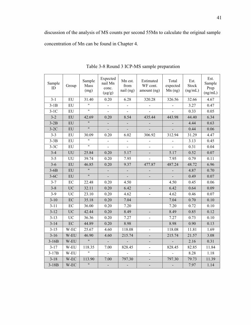
41

discussion of the analysis of MS counts per second 55Mn to calculate the original sample

concentration of Mn can be found in Chapter 4.


Sample ID


Expected nail Mn

conc. (µg/g)

Mn est. from

nail (ng)

Estimated WF cont.

amount (ng)


Est. Stock

(ng/mL)

Est. Sample

Prep (ng/mL)

3-1 EU 31.40 0.20 6.28 320.28 326.56 32.66 4.67

3-1B EU " - - - - 3.27 0.47

3-1C EU " - - - - 0.33 0.05

3-2 EU 42.69 0.20 8.54 435.44 443.98 44.40 6.34

3-2B EU " - - - - 4.44 0.63

3-2C EU " - - - - 0.44 0.06

3-3 EU 30.09 0.20 6.02 306.92 312.94 31.29 4.47

3-3B EU " - - - - 3.13 0.45

3-3C EU " - - - - 0.31 0.04

3-4 UU 25.84 0.20 5.17 - 5.17 0.52 0.07

3-5 UU 39.74 0.20 7.95 - 7.95 0.79 0.11

3-6 EU 46.85 0.20 9.37 477.87 487.24 48.72 6.96

3-6B EU " - - - - 4.87 0.70

3-6C EU " - - - - 0.49 0.07

3-7 EC 22.48 0.20 4.50 4.50 0.45 0.06

3-8 UC 32.11 0.20 6.42 - 6.42 0.64 0.09

3-9 UC 23.10 0.20 4.62 - 4.62 0.46 0.07

3-10 EC 35.18 0.20 7.04 7.04 0.70 0.10

3-11 EC 36.00 0.20 7.20 7.20 0.72 0.10

3-12 UC 42.44 0.20 8.49 - 8.49 0.85 0.12

3-13 UC 36.36 0.20 7.27 - 7.27 0.73 0.10

3-14 EC 44.89 0.20 8.98 8.98 0.90 0.13

3-15 W-EC 25.67 4.60 118.08 - 118.08 11.81 1.69

3-16 W-EU 46.90 4.60 215.74 - 215.74 21.57 3.08

3-16B W-EU " - - - - 2.16 0.31

3-17 W-EU 118.35 7.00 828.45 - 828.45 82.85 11.84

3-17B W-EU " - - - - 8.28 1.18

3-18 W-EC 113.90 7.00 797.30 - 797.30 79.73 11.39

3-18B W-EC " - - - - 7.97 1.14

42

3.6 Statistical Analysis

For all nail tissue concentration data collected it was important to establish whether data

showed a significant deviation from normality. Various statistical methods were

employed for this purpose. Typically determination of dataset normality is performed

using numeric or graphical methods which can be either descriptive-based or theory-

based (hypothesis-based). Due to the very small sample size of this study’s treatment

groups, the methods chosen were P-P and Q-Q plots (Theoretical-Graphical), box plot

(Descriptive-Graphical), skewness and kurtosis (Descriptive-Numerical), and three

Hypothesis-driven numerical methods, the Shapiro-Wilk, Chi-Square and Anderson-

Darling normality tests.

The Shapiro-Wilk Normality Test was given the most weight in decision making because

it is appropriate for distribution analysis of groups with small sample sizes like the ones

in this study and is likely a more truthful representation of the normality of such small

sample size data than descriptive-based methods listed. The National Institute of Health

recommends the use of the Shapiro-Wilk Normality Test for sample size of less than 50.

NIH recommends that one of the most popular normality tests, the Kolmogorov-Smirnov

Test should no longer be used because of its low power in general, especially for sample

sizes below 50.23 Additional reasoning for the use of particular methods lies in research

performed by Razali, in which he detailed a comparison of the hypothesis-based

numerical methods, Shapiro–Wilk, Anderson-Darling, Kolmogorov–Smirnov, and

Lilliefors. Razali found that for a given significance level the Shapiro-Wilk Test had the

43

most statistical power. He found the Anderson-Darling Test to be a close second in the

running.24 The Chi-Square test for normality, although not a very powerful method, is

quite useful for very low sample sizes.

If data was found to be normal, 95% confidence limits about the mean for the two groups

were calculated as well as a Two-group t-test of the difference of means for small sample

size used to test the hypothesis that the two population means are significantly different.

For data found to be non-normally distributed, the determination was made that the small

sample sizes would not enable a clear depiction of the population distributions. Thus any

attempt to discern another standard type of distribution would likely yield similar limited

conclusions do to low statistical power. It was determined not to normalized the data but

to instead rely upon non-parametric methods, specifically the Wilcoxon Ranked Sum

Test and Kruskal-Wallis Test. The non-parametric tests are a more conservative approach

when dealing with datasets of unknown and differing distribution types. It was assumed

at the onset of the study that by the nature of the within-subject design for Objectives 2

and 3, the data acquired from the single control subject nail samples would likely be

normally distributed. A schematic flow diagram of the statistical methods used in this

study is presented in Figure 3-2.

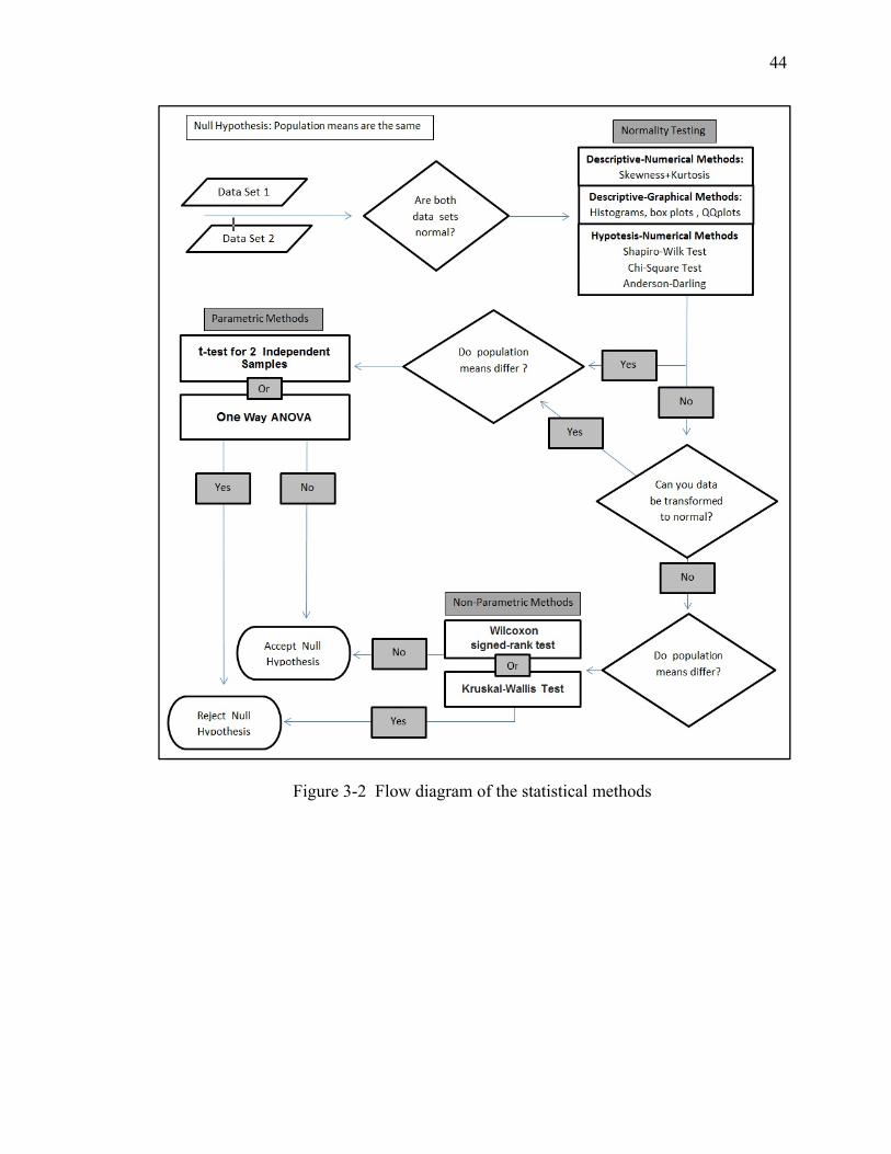
44

Figure 3-2 Flow diagram of the statistical methods

45

CHAPTER 4. RESULTS

4.1 Round 1 Results

Table 4-1 displays the results of the Round 1 ICP-MS analysis for Mn in the prepared

samples. The Round 1 blank preparations had an average Mn counts per second (cps) of

296.4 and this cps value is deducted from the actual cps for each sample in order to

eliminate the signal noise of the instrument. It should be noted that, as mentioned in the

methodology section, the analytical chemists ran serial dilution samples ahead of the

actual Round 1 ICP-MS run to determine the appropriate serial dilution level to use. All

samples chosen for the main run were prepared from the initial stock solution with the

exception of samples 1-6B and 1-7B which were prepared from 0.1x dilution stock

solution. The dilution factor is taken into account before the calculation of the nail tissue

Mn concentration level.

A calibration curve was prepared based on the ICP-MS cps data from sample 1-5 and the

four standard addition spikes made with that sample’s stock solution. Data from the

spiked samples is seen in Table 4-2 and the Round 1 calibration curve is shown in Figure

4-1. The 55Mn (cps) data in Table 4-1 and Table 4-2 already have the average blank cps

deducted. Figure 4-1 also shows the line equation for the calibration curve. The slope of

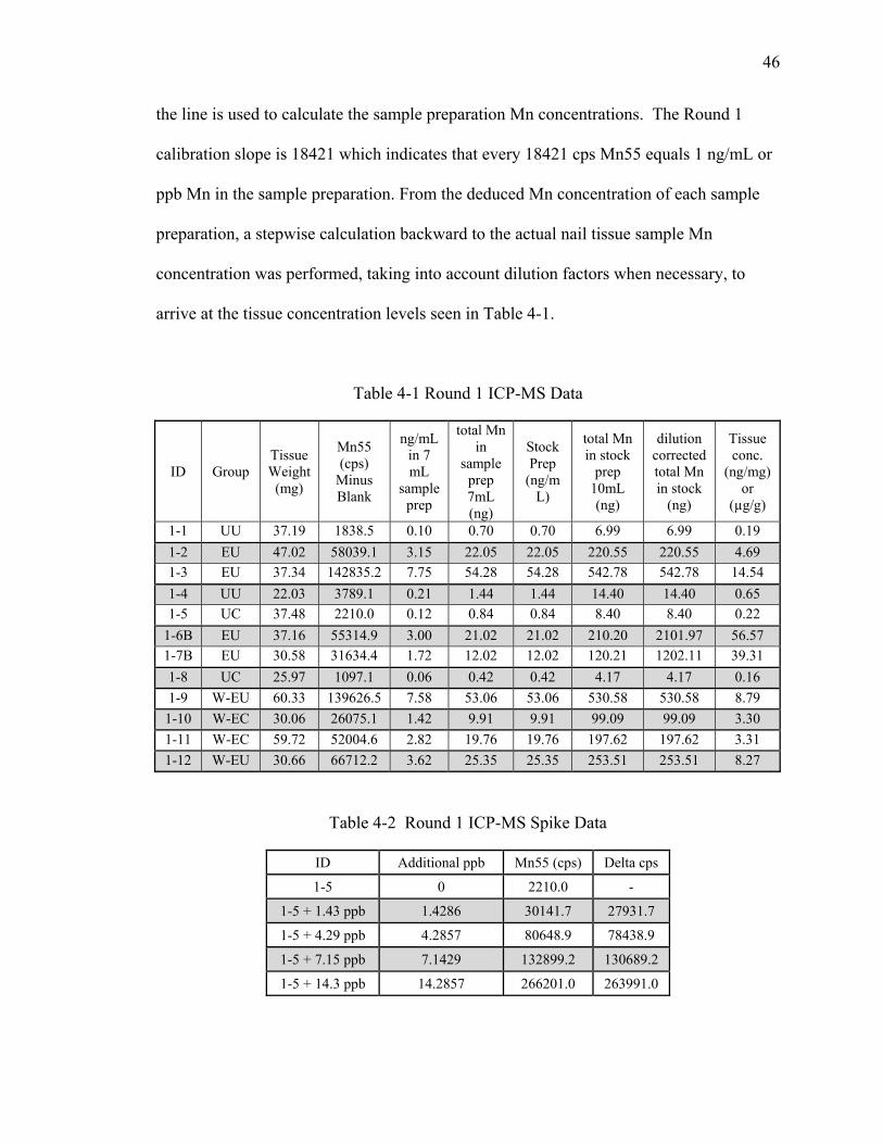
46

the line is used to calculate the sample preparation Mn concentrations. The Round 1

calibration slope is 18421 which indicates that every 18421 cps Mn55 equals 1 ng/mL or

ppb Mn in the sample preparation. From the deduced Mn concentration of each sample

preparation, a stepwise calculation backward to the actual nail tissue sample Mn

concentration was performed, taking into account dilution factors when necessary, to

arrive at the tissue concentration levels seen in Table 4-1.

Table 4-1 Round 1 ICP-MS Data

ID Group Tissue Weight (mg)

Mn55 (cps)

Minus Blank

ng/mL in 7 mL

sample prep

total Mn in

sample prep 7mL (ng)

Stock Prep

(ng/mL)

total Mn in stock

prep 10mL (ng)

dilution corrected total Mn in stock

(ng)

Tissue conc.

(ng/mg) or

(µg/g)

1-1 UU 37.19 1838.5 0.10 0.70 0.70 6.99 6.99 0.19

1-2 EU 47.02 58039.1 3.15 22.05 22.05 220.55 220.55 4.69

1-3 EU 37.34 142835.2 7.75 54.28 54.28 542.78 542.78 14.54

1-4 UU 22.03 3789.1 0.21 1.44 1.44 14.40 14.40 0.65

1-5 UC 37.48 2210.0 0.12 0.84 0.84 8.40 8.40 0.22

1-6B EU 37.16 55314.9 3.00 21.02 21.02 210.20 2101.97 56.57

1-7B EU 30.58 31634.4 1.72 12.02 12.02 120.21 1202.11 39.31

1-8 UC 25.97 1097.1 0.06 0.42 0.42 4.17 4.17 0.16

1-9 W-EU 60.33 139626.5 7.58 53.06 53.06 530.58 530.58 8.79

1-10 W-EC 30.06 26075.1 1.42 9.91 9.91 99.09 99.09 3.30

1-11 W-EC 59.72 52004.6 2.82 19.76 19.76 197.62 197.62 3.31

1-12 W-EU 30.66 66712.2 3.62 25.35 25.35 253.51 253.51 8.27

Table 4-2 Round 1 ICP-MS Spike Data

ID Additional ppb Mn55 (cps) Delta cps

1-5 0 2210.0 -

1-5 + 1.43 ppb 1.4286 30141.7 27931.7

1-5 + 4.29 ppb 4.2857 80648.9 78438.9

1-5 + 7.15 ppb 7.1429 132899.2 130689.2

1-5 + 14.3 ppb 14.2857 266201.0 263991.0

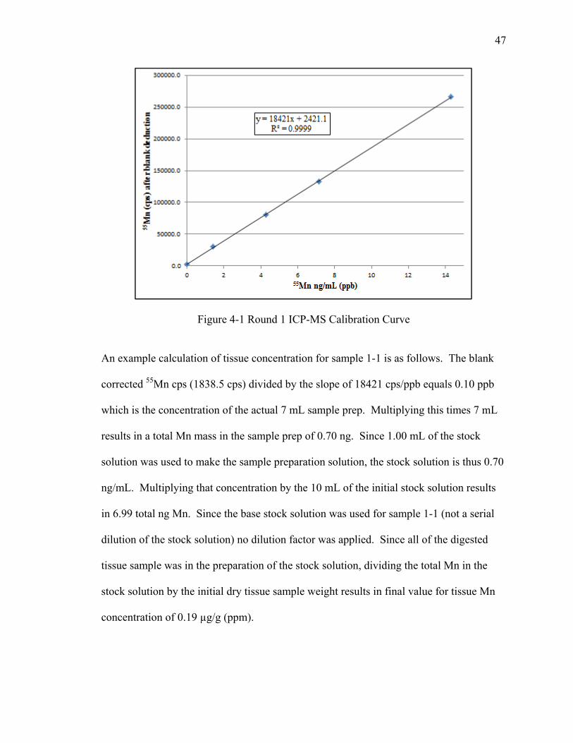
47

Figure 4-1 Round 1 ICP-MS Calibration Curve

An example calculation of tissue concentration for sample 1-1 is as follows. The blank

corrected 55Mn cps (1838.5 cps) divided by the slope of 18421 cps/ppb equals 0.10 ppb

which is the concentration of the actual 7 mL sample prep. Multiplying this times 7 mL

results in a total Mn mass in the sample prep of 0.70 ng. Since 1.00 mL of the stock

solution was used to make the sample preparation solution, the stock solution is thus 0.70

ng/mL. Multiplying that concentration by the 10 mL of the initial stock solution results

in 6.99 total ng Mn. Since the base stock solution was used for sample 1-1 (not a serial

dilution of the stock solution) no dilution factor was applied. Since all of the digested

tissue sample was in the preparation of the stock solution, dividing the total Mn in the

stock solution by the initial dry tissue sample weight results in final value for tissue Mn

concentration of 0.19 µg/g (ppm).

48

Figure 4-2 shows a graphical representation of the first three Exposed/Uncleaned samples

used to test the increase in tissue nail concentration increase with increasing arc time in

the welding fume containment vessel (arc times 4s, 40s, and 400s). A steady state build

up curve is fitted to the data points and shown in Figure 4-2. The fourth

Exposed/Uncleaned sample was not used. As noted early the 800s arc time exposure was

deemed unusable due to an error in sealing the containment vessel after the welding fume

was generated, allowing a significant portion of the fume to escape before it could

precipitate onto the nail tissue. As predicted the increase of nail Mn concentration from

the contamination follows a steady-state build up curve due to the flow of shielding gas

into the containment vessel.

The welder subject fingernail tissue, analyzed in Round 1, exhibited an average of

approximately 5.25 µg/g Mn, as exogenous Mn contamination. This was presumed to be

from their occupational welding fume exposure. To be certain that the contamination of

the control subject nail tissue in Rounds 2 and 3, for the Exposed treatment groups, was

contaminated with at least double that level and yet not so high as to overwhelm the

cleaning protocol, a choice was made to target a nail tissue contamination level of 40

µg/g Mn as exogenous Mn contamination. The choice was skewed to the high side as the

contamination method had an as of yet unproven repeatability and many inputs effect the

overall generation of welding fume, such as wire speed, proper containment, shielding

gas flow, etc. On the GMAW arc time vs. nail Mn concentration chart the arc time which

corresponds to the 40 µg/g Mn concentration level is approximately 180 seconds.

Therefore, a 180s arc time was chosen as the exposure level for Round 2.

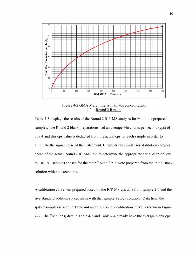
49

Figure 4-2 GMAW arc time vs. nail Mn concentration 4.2 Round 2 Results




eliminate the signal noise of the instrument. Chemists ran similar serial dilution samples

ahead of the actual Round 2 ICP-MS run to determine the appropriate serial dilution level

to use. All samples chosen for the main Round 2 run were prepared from the initial stock

solution with no exceptions.


five standard addition spikes made with that sample’s stock solution. Data from the



50

deducted. Figure 4-3 also shows the line equation for the Round 2 calibration curve. The

slope of the line is used to calculate the sample preparation Mn concentrations. The

Round 2 calibration slope is 13324 which indicates that every 13324 cps Mn55 equals 1

ng/mL or ppb Mn in the sample preparation. From the deduced Mn concentration of each

sample preparation, a stepwise calculation backward to the actual nail tissue sample Mn

concentration was performed to arrive at the tissue concentration levels seen in Table 4-3.

Dilution factors were not necessary for analysis of Round 2 data as none of the serial

dilution samples were used in the main run.


ID Group Tissue Weight (mg)

Mn55 (cps)

Minus Blank

ng/mL in 7 mL

sample prep

total Mn in sample prep

7mL (ng)

Stock Prep (ng/mL)

total Mn in stock prep 10mL (ng)

Tissue conc.

(ng/mg) or (µg/g)

2-1 UU 33.38 2802.9 0.21 1.47 1.47 14.73 0.44

2-2 EU 32.52 52173.2 3.92 27.41 27.41 274.10 8.43

2-3 EU 31.92 73101.5 5.49 38.41 38.41 384.05 12.03

2-4 UU 38.37 2715.0 0.20 1.43 1.43 14.26 0.37

2-5 UC 34.25 746.7 0.06 0.39 0.39 3.92 0.11

2-6 EC 37.82 5782.6 0.43 3.04 3.04 30.38 0.80

2-7 EC 29.08 2548.5 0.19 1.34 1.34 13.39 0.46

2-8 UC 26.63 698.6 0.05 0.37 0.37 3.67 0.14

2-9 UC 31.35 807.3 0.06 0.42 0.42 4.24 0.14

2-10 EC 36.56 3618.3 0.27 1.90 1.90 19.01 0.52

2-11 EC 33.03 3179.0 0.24 1.67 1.67 16.70 0.51

2-12 UC 37.22 760.0 0.06 0.40 0.40 3.99 0.11

The nail tissue Mn concentration of the exposed samples in Round 2 was estimated by

the average nail tissue concentration of the two Exposed/Uncleaned samples (avg. 10.2

µg/g Mn). This was approximately 25.5% of the target concentration of 40 µg/g Mn but

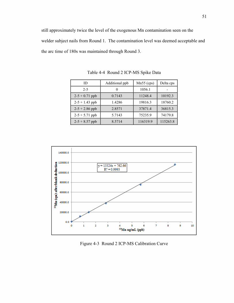
51

still approximately twice the level of the exogenous Mn contamination seen on the

welder subject nails from Round 1. The contamination level was deemed acceptable and

the arc time of 180s was maintained through Round 3.



2-5 0 1056.1 -

2-5 + 0.71 ppb 0.7143 11248.4 10192.3

2-5 + 1.43 ppb 1.4286 19816.3 18760.2

2-5 + 2.86 ppb 2.8571 37871.4 36815.3

2-5 + 5.71 ppb 5.7143 75235.9 74179.8

2-5 + 8.57 ppb 8.5714 116319.9 115263.8


52

4.3 Estimation of Required Sample Size

In order to determine the number of additional samples required in Round 3 to assure

statistical power in testing the study’s hypotheses, an estimation of required sample size

was made by pooling the data from Round 1 and Round 2. All data were pooled except

the EU samples from Round 1 which were exposure contamination samples done at

varied arc time in order to estimate arc time versus contamination level and thus were not

appropriate for comparison to the UU and other EU samples. An assumption was made

at this point, because of the very low sample sizes and the fact that σ was not known for

any of the populations, that the data was approximately normally distributed and the

Student’s t-distribution should be used. Descriptive statistics were calculated as well as

confidence intervals based on the Student’s t-distribution for the various treatment groups.

The confidence intervals between the treatment groups relevant to each hypothesis were

compared. The pooled data are shown in Table 4-5 and the descriptive statistics and

confidence limits are depicted in Table 4-6 below.

The welder EU and EC treatment groups already had confidence intervals that were

significantly separated with the EU group much higher in Mn concentration. This was a

good indication of validity to hypothesis 1 – that welders do indeed have significant

exogenous contamination of Mn on their nails which must be removed in order to

properly interpret nail tissue Mn levels as a biomarker of internalized welding fume Mn

exposure. It was decided to go ahead and run two additional welder EU and two welder

EC samples in Round 3 in order to solidify the statistical power of this assumption.

53

Similarly, the control subject UC versus EC comparison, even at six and four samples

respectively, already shows significantly separated confidence intervals, indicating failure

to find validity of hypothesis 3 – that the current cleaning method is capable of removing

all the exogenous welding fume Mn contamination from the nail tissue. However, the

tightness of the confidence intervals and the closeness of the two means is an indication

that the vast majority of the external contamination is being removed. Nonetheless, as

this is the heart of the study, it was decided that four additional samples each of the UC

and EC treatment groups would be included in Round 3 to improve the statistical power

of this conclusion.

Table 4-5 Round 1 & 2 pooled data

Sample ID

Group Subject Nail Tissue conc.

(ng/mg) or (µg/g)

1-9 W-EU WW13 FL 8.79

1-12 W-EU WW15 FR 8.27

1-10 W-EC WW13 FR 3.30

1-11 W-EC WW15 FL 3.31

1-1 UU JCB FL 0.19

1-4 UU JCB FR 0.65

2-1 UU JCB FL 0.44

2-4 UU JCB FR 0.37

2-2 EU JCB FR 8.43

2-3 EU JCB FL 12.03

1-5 UC JCB FL 0.22

1-8 UC JCB FR 0.16

2-5 UC JCB FL 0.11

2-8 UC JCB FR 0.14

2-9 UC JCB FL 0.14

2-12 UC JCB FR 0.11

2-6 EC JCB FR 0.80

2-7 EC JCB FL 0.46

2-10 EC JCB FR 0.52

2-11 EC JCB FL 0.51

54

Table 4-6 Descriptive statistics & CI for Round 1 & 2 pooled data

Group n Mean Mn

(µg/g) S SE T95 LCL95 UCL95 E

W-EU 2 8.531 0.372 0.263 12.706 5.188 11.875 3.344

W-EC 2 3.303 0.009 0.006 12.706 3.221 3.384 0.081

UU 4 0.414 0.192 0.096 3.182 0.107 0.720 0.306

EU 2 10.230 2.548 1.801 12.706 -12.660 33.120 22.890

UC 6 0.147 0.042 0.017 2.571 0.102 0.191 0.044

EC 4 0.572 0.156 0.078 3.182 0.324 0.821 0.248

Lastly, the UU and EU treatment groups did have confidence intervals which overlapped,

however this was chiefly due to the significantly high variance and very low sample size

of the EU group. A calculation was made to determine an appropriate number of EU

samples to run in Round 3 which would be able to clarify the comparison between the

UU and EU treatment groups. With the vastly higher mean Mn concentration of the EU

group, it was clear that the margin of error for the EU group did not need to be contracted

by much, a margin of error of approximately 3 would already put the UU and EU

confidence intervals well apart. The equation for the t-distribution confidence limit is:

The confidence limit is the mean surrounded by the margin of error which is essentially

the t value, given by the percent confidence desired and the degrees of freedom

multiplied by the standard error of the mean ( equal to the standard deviation divided by

the square root of the sample size ). Thus the margin of error is simply:

55

An estimated guess of n=6 leads to a 95% t-value of 2.571 and with the EU standard

deviation of 2.548 we arrive at:

A margin of error of approximately 2.67 was determined to be more than adequate and

should leave room for error if the variance of the EU group was to increase somewhat

even with the larger sample size. The decision was made to run four additional EU

samples in Round 3 to bring the total to six. As the UU group versus EU group

comparison is required during each run in order to ascertain the actual level of

contamination for the particular run, an additional two UU samples were also set to be

run in Round 3. The set of additional samples run in Round 3 is shown in Table 3-8

4.4 Round 3 Results




eliminate the signal noise of the instrument. The Chemists ran similar serial dilution

samples ahead of the actual Round 3 ICP-MS run to determine the appropriate serial

dilution level to use. All samples chosen for the main Round 2 run were prepared from

the initial stock solution with the exception of sample 3-17B which was prepared from a

one tenth dilution of the sample 3-17 stock solution.

56


five standard addition spikes made with that sample’s stock solution. Data from the



deducted. Figure 4-4 also shows the line equation for the Round 3 calibration curve. The

Round 3 calibration slope is 47228 which indicates that every 47228 cps 55Mn equals 1

ng/mL or ppb Mn in the sample preparation. From the deduced Mn concentration of each

sample preparation, a stepwise calculation backward to the actual nail tissue sample Mn

concentration was performed to arrive at the tissue concentration levels seen in Table 4-7.

The one tenth dilution factor for sample 17B was taken into account in the calculation of

tissue concentration, not other samples required correction.

The nail tissue Mn concentration of the exposed samples in Round 3 was estimated by

the average nail tissue concentration of the four Exposed/Uncleaned samples (avg. 11.9

µg/g Mn). The Round 3 contamination level was quite close to the Round 2 average

Exposed/Uncleaned samples (avg. 10.2 µg/g Mn). This is an indication that the

contamination protocol is fairly reproducible for a maintained set of parameters (wire

alloy, wire speed, arc time, etc.). The reproducibility of this experimental design may

prove useful toward further research in this area.

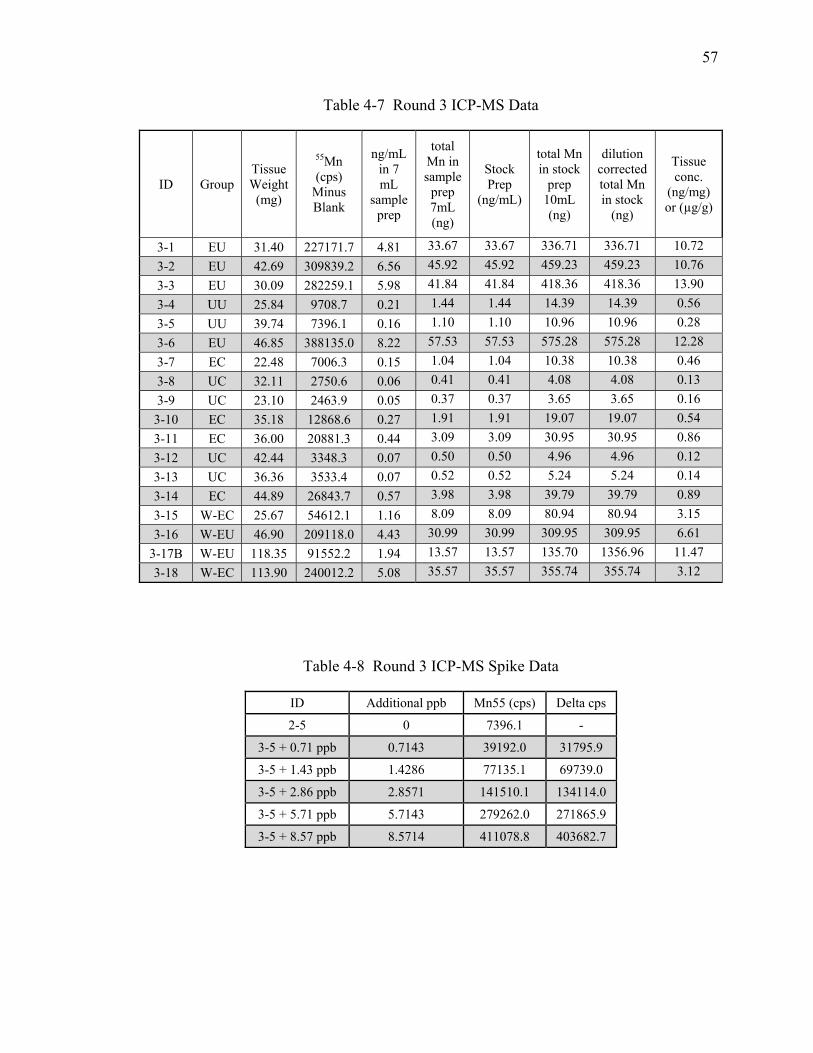
57


ID Group Tissue Weight

(mg)

55Mn (cps)

Minus Blank

ng/mL in 7 mL

sample prep

total Mn in sample

prep 7mL (ng)

Stock Prep

(ng/mL)

total Mn in stock

prep 10mL (ng)

dilution corrected total Mn in stock

(ng)

Tissue conc.

(ng/mg) or (µg/g)

3-1 EU 31.40 227171.7 4.81 33.67 33.67 336.71 336.71 10.72

3-2 EU 42.69 309839.2 6.56 45.92 45.92 459.23 459.23 10.76

3-3 EU 30.09 282259.1 5.98 41.84 41.84 418.36 418.36 13.90

3-4 UU 25.84 9708.7 0.21 1.44 1.44 14.39 14.39 0.56

3-5 UU 39.74 7396.1 0.16 1.10 1.10 10.96 10.96 0.28

3-6 EU 46.85 388135.0 8.22 57.53 57.53 575.28 575.28 12.28

3-7 EC 22.48 7006.3 0.15 1.04 1.04 10.38 10.38 0.46

3-8 UC 32.11 2750.6 0.06 0.41 0.41 4.08 4.08 0.13

3-9 UC 23.10 2463.9 0.05 0.37 0.37 3.65 3.65 0.16

3-10 EC 35.18 12868.6 0.27 1.91 1.91 19.07 19.07 0.54

3-11 EC 36.00 20881.3 0.44 3.09 3.09 30.95 30.95 0.86

3-12 UC 42.44 3348.3 0.07 0.50 0.50 4.96 4.96 0.12

3-13 UC 36.36 3533.4 0.07 0.52 0.52 5.24 5.24 0.14

3-14 EC 44.89 26843.7 0.57 3.98 3.98 39.79 39.79 0.89

3-15 W-EC 25.67 54612.1 1.16 8.09 8.09 80.94 80.94 3.15

3-16 W-EU 46.90 209118.0 4.43 30.99 30.99 309.95 309.95 6.61

3-17B W-EU 118.35 91552.2 1.94 13.57 13.57 135.70 1356.96 11.47

3-18 W-EC 113.90 240012.2 5.08 35.57 35.57 355.74 355.74 3.12



2-5 0 7396.1 -

3-5 + 0.71 ppb 0.7143 39192.0 31795.9

3-5 + 1.43 ppb 1.4286 77135.1 69739.0

3-5 + 2.86 ppb 2.8571 141510.1 134114.0

3-5 + 5.71 ppb 5.7143 279262.0 271865.9

3-5 + 8.57 ppb 8.5714 411078.8 403682.7

58


59

CHAPTER 5. ANALYSIS

Table 5-1 below shows the data for the W-EU and W-EC treatment groups pooled from

all three rounds of testing. Table 5-2 shows the data for the UU and EU treatment groups

and Table 5-3 displays the data for the UC and EC treatment groups, likewise pooled

from all three rounds of testing. The descriptive statistics and confidence limits for all

data pooled from all three rounds are depicted in Table 5-4. The following sections

describe in detail the statistical analyses utilized to make judgment on the specific

hypotheses associated with Objectives 1 through 3.

Table 5-1 Groups W-EU and W-EC Pooled Data – All Rounds

Sample Group Subject Nail Tissue

1-9 W-EU WW13 FL 8.79

1-12 W-EU WW15 FR 8.27

3-16 W-EU WW10 FR 6.61

3-17 W-EU WW17 FL 11.47

1-10 W-EC WW13 FR 3.30

1-11 W-EC WW15 FL 3.31

3-15 W-EC WW10 FL 3.15

3-18 W-EC WW17 FR 3.12

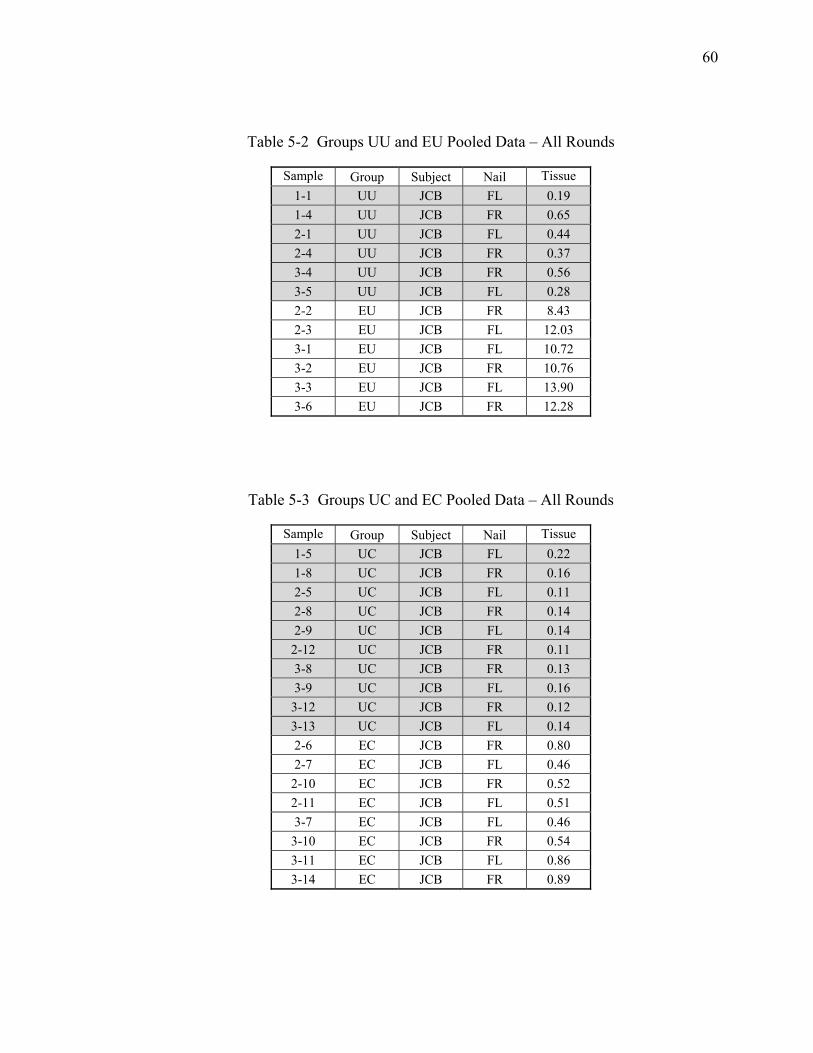
60

Table 5-2 Groups UU and EU Pooled Data – All Rounds


1-1 UU JCB FL 0.19

1-4 UU JCB FR 0.65

2-1 UU JCB FL 0.44

2-4 UU JCB FR 0.37

3-4 UU JCB FR 0.56

3-5 UU JCB FL 0.28

2-2 EU JCB FR 8.43

2-3 EU JCB FL 12.03

3-1 EU JCB FL 10.72

3-2 EU JCB FR 10.76

3-3 EU JCB FL 13.90

3-6 EU JCB FR 12.28

Table 5-3 Groups UC and EC Pooled Data – All Rounds


1-5 UC JCB FL 0.22

1-8 UC JCB FR 0.16

2-5 UC JCB FL 0.11

2-8 UC JCB FR 0.14

2-9 UC JCB FL 0.14

2-12 UC JCB FR 0.11

3-8 UC JCB FR 0.13

3-9 UC JCB FL 0.16

3-12 UC JCB FR 0.12

3-13 UC JCB FL 0.14

2-6 EC JCB FR 0.80

2-7 EC JCB FL 0.46

2-10 EC JCB FR 0.52

2-11 EC JCB FL 0.51

3-7 EC JCB FL 0.46

3-10 EC JCB FR 0.54

3-11 EC JCB FL 0.86

3-14 EC JCB FR 0.89

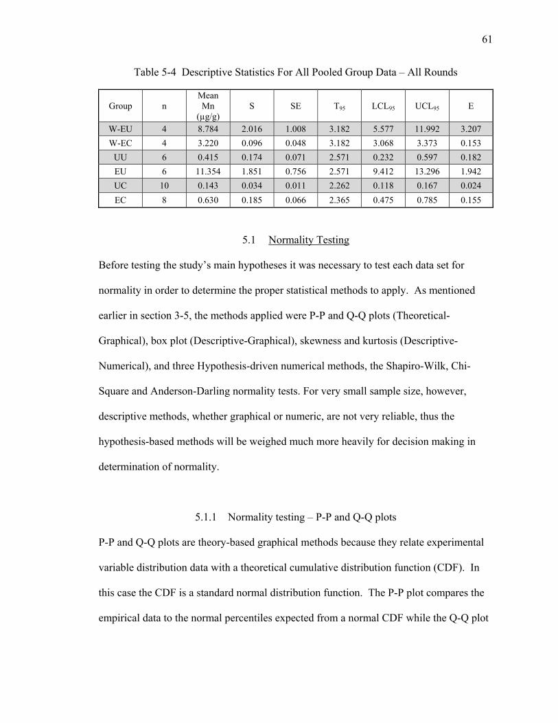
61

Table 5-4 Descriptive Statistics For All Pooled Group Data – All Rounds

Group n Mean Mn

(µg/g) S SE T95 LCL95 UCL95 E

W-EU 4 8.784 2.016 1.008 3.182 5.577 11.992 3.207

W-EC 4 3.220 0.096 0.048 3.182 3.068 3.373 0.153

UU 6 0.415 0.174 0.071 2.571 0.232 0.597 0.182

EU 6 11.354 1.851 0.756 2.571 9.412 13.296 1.942

UC 10 0.143 0.034 0.011 2.262 0.118 0.167 0.024

EC 8 0.630 0.185 0.066 2.365 0.475 0.785 0.155

5.1 Normality Testing

Before testing the study’s main hypotheses it was necessary to test each data set for

normality in order to determine the proper statistical methods to apply. As mentioned

earlier in section 3-5, the methods applied were P-P and Q-Q plots (Theoretical-

Graphical), box plot (Descriptive-Graphical), skewness and kurtosis (Descriptive-

Numerical), and three Hypothesis-driven numerical methods, the Shapiro-Wilk, Chi-

Square and Anderson-Darling normality tests. For very small sample size, however,

descriptive methods, whether graphical or numeric, are not very reliable, thus the

hypothesis-based methods will be weighed much more heavily for decision making in

determination of normality.

5.1.1 Normality testing – P-P and Q-Q plots

P-P and Q-Q plots are theory-based graphical methods because they relate experimental

variable distribution data with a theoretical cumulative distribution function (CDF). In

this case the CDF is a standard normal distribution function. The P-P plot compares the

empirical data to the normal percentiles expected from a normal CDF while the Q-Q plot

62

compares the data to the normal quartiles expected. The deviation of the experimental

data from the normal CDF line indicates nonconformity with the normal CDF. Figures 5-

1 through 5-12 depict the various P-P and Q-Q plots computed for this normality analysis.

As will be evident in later normality tests as well, for the most part the data do not

deviate excessively from the normal CDF, however the cleaned treatment group

counterparts each of the uncleaned groups does seems to deviate more than the uncleaned

group data. This may indicate that the cleaning factor is in some way de-normalizing the

data.

5.1.2 Normality testing – Box plots

Box plots are fairly self-representative illustrations of the 1st, 2nd (median) and 3rd quartile

and maximum / minimum range in relation to the mean of the data set. A normally

distributed data series should display rather symmetric 1st and 3rd quartiles and the mean

and median should be centered toward the middle of the box.

Box plots were prepared for the three treatment group comparisons respective to the three

major hypotheses. Box plots displaying the 1st and 3rd quartile about the mean with a

horizontal bar representing the median and vertical capped bars displaying the range were

prepared as a graphical representation of the treatment group distributions. Groups W-EU

and WEC, related to Hypothesis 1, are displayed in Figure 5-13, groups UU and EU,

related to Hypothesis 2, are displayed in Figure 5-14, and groups UC and EC, related to

Hypothesis 3, are displayed in Figure 5-15.

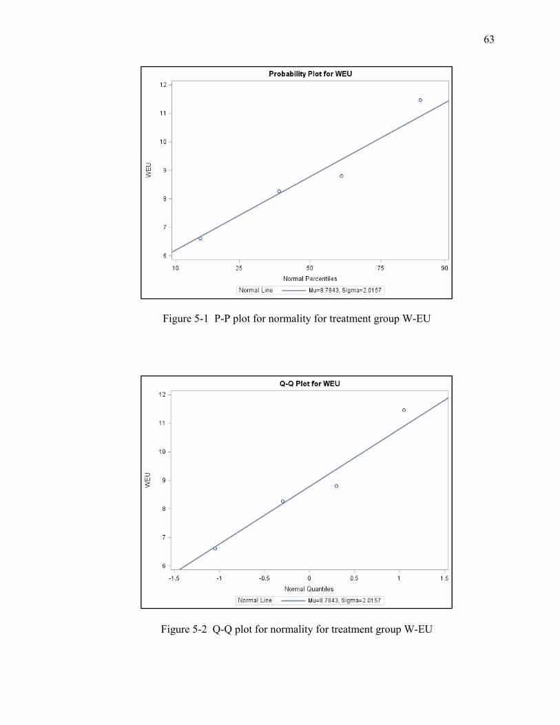
63

Figure 5-1 P-P plot for normality for treatment group W-EU

Figure 5-2 Q-Q plot for normality for treatment group W-EU

64

Figure 5-3 P-P plot for normality for treatment group W-EC

Figure 5-4 Q-Q plot for normality for treatment group W-EC

65

Figure 5-5 P-P plot for normality for treatment group UU

Figure 5-6 Q-Q plot for normality for treatment group UU

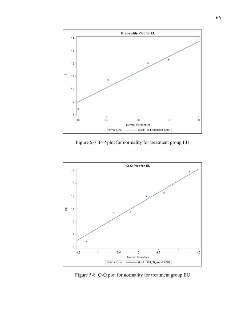
66

Figure 5-7 P-P plot for normality for treatment group EU

Figure 5-8 Q-Q plot for normality for treatment group EU

67

Figure 5-9 P-P plot for normality for treatment group UC

Figure 5-10 Q-Q plot for normality for treatment group UC

68

Figure 5-11 P-P plot for normality for treatment group EC

Figure 5-12 Q-Q plot for normality for treatment group EC

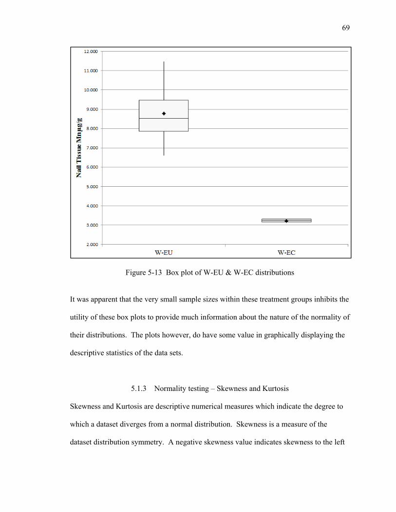
69

Figure 5-13 Box plot of W-EU & W-EC distributions

It was apparent that the very small sample sizes within these treatment groups inhibits the

utility of these box plots to provide much information about the nature of the normality of

their distributions. The plots however, do have some value in graphically displaying the

descriptive statistics of the data sets.

5.1.3 Normality testing – Skewness and Kurtosis

Skewness and Kurtosis are descriptive numerical measures which indicate the degree to

which a dataset diverges from a normal distribution. Skewness is a measure of the

dataset distribution symmetry. A negative skewness value indicates skewness to the left

70

Figure 5-14 Box plot of UU & EU distributions

(more observations to the right) and positive skewness indicates the opposite. Skewness

is given by the equation:

Kurtosis is a measure of the dataset distribution peakedness. A kurtosis value below 3

indicates that the dataset distribution has a lower peak and thicker tails than a normal

distribution, while a value above 3 shows it has higher peak and thinner tails than normal.

Kurtosis is given by the equation:

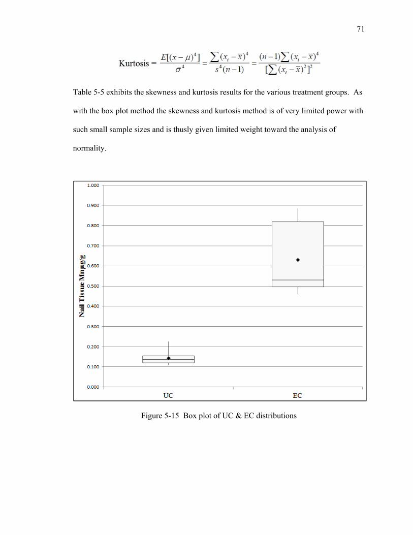
71

Table 5-5 exhibits the skewness and kurtosis results for the various treatment groups. As

with the box plot method the skewness and kurtosis method is of very limited power with

such small sample sizes and is thusly given limited weight toward the analysis of

normality.

Figure 5-15 Box plot of UC & EC distributions

72

Table 5-5 Skewness and kurtosis by treatment group

Group n Mean Mn

(µg/g) S Skewness Kurtosis

W-EU 4 8.784 2.016 0.720 1.475

W-EC 4 3.220 0.096 -0.069 -5.430

UU 6 0.415 0.174 0.125 -1.085

EU 6 11.354 1.851 -0.370 0.713

UC 10 0.143 0.034 1.686 3.618

EC 8 0.630 0.185 0.617 -1.980

5.1.4 Normality testing – Chi-Square Test

The Chi-Square Test for distributional adequacy uses standardized values which are

calculated for each data point and placed in to k number of bins. The test statistic Χ2 is

given by:

Where Oi is the observed frequency by bin and Ei is the expected frequency for the

particular bin i. Ei is given as:

Ei = N (F(Yu) – F(Yl))

Where Yu is the upper limit, Yl is the lower limit, F is the particular distribution function

being tested, and N is the sample size.

The results of the Chi-Square test for normality are seen in Table 5-6 below. For all

groups except UC and EC, p-values for the Chi-Square Test were clearly high enough to

accept the null hypothesis that the sample data could have come from a normal

73

distribution. The EC group, however, came much closer to the rejection level at p =

0.1092. Group UC clearly had a Chi Square Test p-value low enough to reject the

normality assumption (p = 0.0011). As we will see in the other hypothesis-based

numerical methods, it is the cleaned groups which seem to be trending away from the

normality assumption.

Table 5-6 Results of Chi-Square Test for normality

Group n Mean Mn

(µg/g) S

Chi Square

df P value

W-EU 4 8.784 2.016 0.616 3 0.8927

W-EC 4 3.220 0.096 1.238 3 0.7440

UU 6 0.415 0.174 0.007 3 0.9998

EU 6 11.354 1.851 0.007 3 0.9998

UC 10 0.143 0.034 16.080 3 0.0011

EC 8 0.630 0.185 6.050 3 0.1092

5.1.5 Normality testing – Shapiro-Wilk Test

The Shapiro-Wilk Test derives a positive value (W) which is less than or equal to one.

Closeness to one indicates normality. The W measure is a ratio of the best estimator of

variance to the corrected sum of squares estimator of variance. The W statistic is derived

by regression of ordered data upon the matching expected values based on normal order.

If the dataset is normally distributed, this regression will approach linearity. Validity

exists for the W statistic from a sample size range of 3 to 50.25 There are approaches to

increase the range but they are not relevant to this study as none of the treatment groups

approached n=50. The W statistic is derived by:

74

Where x(i) are the ordered sample values and the ai are constants generated from means,

variances, and covariances of the order statistics drawn from a normal distribution for a

sample size of n. Tables are available to draw the ai values from. Once the W statistic is

calculated it is compared against a critical value of W for a particular confidence level,

typically an alpha level of 5%. If the W statistic is greater than the critical value, the null

hypothesis, that samples are drawn from a normal distribution, is not rejected.

The results of the Shapiro-Wilk Tests are depicted in Table 5-7. The p-value are all

greater than the critical value of 0.5 except for treatment group EC (p-value 0.0249). For

all groups we cannot reject the null hypothesis that the data are normally distributed,

although again one additional group approached rejection (UC). Group W-EC, though

not necessarily approaching rejection, was significantly closer to Wcrit than the three non-

cleaned groups. There does seem to be some indication that the cleaning process itself is

tending to deviate the data distributions away from normality.

Table 5-7 Results of Shapiro-Wilk Test for normality

Group n Mean Mn

(µg/g) S VAR W Wcrit p-value

W-EU 4 8.784 2.016 4.063 0.9627 0.748 0.7958 W-EC 4 3.220 0.096 0.009 0.8327 0.748 0.1749

UU 6 0.415 0.174 0.030 0.9817 0.788 0.9598 EU 6 11.354 1.851 3.425 0.9669 0.788 0.8712 UC 10 0.143 0.034 0.001 0.8495 0.842 0.0573 EC 8 0.630 0.185 0.034 0.7927 0.818 0.0249

75

5.1.6 Normality testing – Anderson-Darling Test

The Anderson-Darling Test is actually a modified Kolmogorov-Smirnov Test which

weights the tail ends of the distributions heavier. The test statistic, A2,is given by:

Where Φ is the normal cumulative distribution function and Yi are the ordered data. The

test statistic is compared to a critical value dependent on the specific cumulative

distribution function. The results of the Anderson-Darling Test are shown in Table 5-8.

Similarly to the Shapiro-Wilk Test results, the Anderson-Darling Test results show

acceptance of the null hypothesis that the data come from a normal distribution for all

groups except EC, although the UC group again approached rejection. Again it is seen

that all of the cleaned nail groups trend toward rejection significantly more than the

uncleaned groups.

Table 5-8 Results of the Anderson-Darling Test for normality

Group n Mean Mn

(µg/g) S VAR A2 p-value

W-EU 4 8.784 2.016 4.063 0.231 > 0.250

W-EC 4 3.220 0.096 0.009 0.402 0.179

UU 6 0.415 0.174 0.030 0.138 > 0.250

EU 6 11.354 1.851 3.425 0.227 > 0.250

UC 10 0.143 0.034 0.001 0.568 0.105

EC 8 0.630 0.185 0.034 0.775 0.025

76

5.1.7 Normality testing – Synopsis

As is the case with any study involving such small sample sized treatment groups, it is

difficult to draw absolute conclusion about the normality of the dataset cumulative

distribution function. Based on the previous three hypothesis-based normality tests as

well as the graphical methods, the only group which can reliably be rejected normality is

group EC (at p-value 0.025) It appears from the data that some factor related to the

cleaning method is responsible for the trend away from normality for the cleaned groups.

This is likely to be the case due to the within-subject nature of the samples.

Based on the assumption of normality for all but one treatment group, Two-Group t-Tests

of the difference of means for independent groups for sample sizes less than 30 were used

to test the main study hypotheses. In addition, modified box plots which display the 1st

and 3rd quartile about the mean were prepared as above except with the vertical capped

whisker bars displaying the 95% confidence intervals of the datasets instead of the data

ranges. This was done as the author believes it is a better graphical representation of the

differences between datasets for such small sample size groups. In addition, due to the

fact that the EC group was not normally distributed and the other cleaned groups tended

away from normality, the non-parametric hypothesis test, the Wilcoxon signed-rank test

will also be run in parallel for each hypothesis analysis.

5.2 Statistical Testing of Hypothesis 1

Figure 5-16 shows a modified box plot (with confidence limits shown as capped whiskers

instead of the typical range values) for the comparison of treatment groups W-EC and W-

77

EU. The difference between the means is of such magnitude that even with only four

data points each, the confidence limits do not overlap. This is a strong indication that

there is statistical confidence that the W-EU group has a higher population mean than the

W-EC group. In other words, the uncleaned welder fingernails do indeed have a

significant amount of exogenous Mn contamination on them, as was postulated in

Hypothesis 1.

Figure 5-16 Box plot mean with confidence intervals W-EU vs. W-EC

The difference of means between UU and UC was only 0.272 µg/g Mn compared to a

difference of means between W-EU and W-EC of 5.564 µg/g Mn. As the W-EU and W-

EC samples came from welders and the fact that the control groups UU vs. UC showed

78

only about 5% of the difference between cleaned and uncleaned nail in the welder groups,

it is proposed that the exogenous Mn found on the welder nails is most likely a result of

welding fume to which they are occupationally exposed. This indicates that external

exposure to welding fume of the nail tissue conveys potentially long-term carry over

contamination effect which must be dealt cleaned off in order to have valid use of nail

tissue as an acceptable biomarker of Mn exposure

To support this conclusion of Hypothesis 1, a Two Group t-Test was performed to

challenge the independence of the means of the two treatment groups. The results of the

t-Test are displayed in Table 5-9 along with the equality of variances results from a

folded F test show in Table 5-10. . The test for equality of variance between the two

groups resulted in an F statistic of 442.26 and a p-value of 0.0004, thus the variances are

determined to be significantly different and either the Satterthwaite or Cochran methods

for unequal variances can be used to provide a more conservative p-value for the t-test.

These non-pooled approaches take a weighted average of the two group variances and

determine a standard error for the t-test while the general pooled method takes an

arithmetic average of the standard deviations of each group and converts that into a

standard error. Both non-equal variance methods still have very low p-values for the t-

test (0.0116 and 0,0117) resulting in rejection of the null hypothesis that the population

means are equal. The population mean in ppm Mn for the welder group uncleaned nails

(W-EU) is significantly larger than the population mean for the welder group cleaned

nails (W-EC). This provides confirmation that the study’s Hypothesis 1, that welders do

have significant exogenous contamination of Mn on their sampled fingernail tissue.

79

Even though both groups passed the hypothesis –numerical analyses for normality, the

W-EC group had p-values less than 0.25 ( p = 0.175 Shapiro-Wilk Test and p=0.179 ).

Therefore, non-parametric tests were also run to determine whether the population means

Table 5-9 Two-Sample t-test results W-EC vs. W-EU

Method Variances DF t p-value

Pooled Equal 6 -5.51 0.0015

Satterthwaite Unequal 3.0136 -5.51 0.0116

Cochran Unequal 3 -5.51 0.0117

Table 5-10 Folded F results for W-EC vs. W-EU t-test

Method DF Den DF F Value Pr > F

Folded F 3 3 442.26 0.0004

were significantly different under the assumption that one or both treatment group

distributions were not a normal cumulative distribution function. The tests chosen were

the Wilcoxon Ranked Sum Test and the Kruskal-Wallis Test. As will become apparent

below, the shape and scale of the welder treatment groups sample distributions, and

likewise those of the further comparisons made for the other hypotheses, were not equal.

A major assumption of the Kruskal-Wallis Test is that the two groups have

indistinguishable scaled and shaped distributions, with the exception for any difference in

medians, an assumption the Wilcoxon Test does not presume. Therefore, for the

purposes of hypothesis testing the Wilcoxon Test was relied upon as the non-parametric

parallel to the parametric Two-Sided t-tests performed.

80

The results of the Wilcoxon and Kruskal-Wallis Tests are presented in Table 5-11 and

graphical representations of the treatment groups sample distributions (for nail tissue Mn

concentration) are shown in Figure 5-17. The graphical depictions of the distributions

shows clear dissimilarity between the group sample distributions, thus the rejection of the

Kruskal-Wallis Test. A box plot depicting the distribution of Wilcoxon Test Scores for

both treatment groups is presented in Figure 5-18. The Wilcoxon test p-value for the 2-

sided normal approximation was significant at 0.0304 while under the t-distribution

approximation the p-value was 0.0671, just approaching significance. In light of the

normality tests and the parametric methods above, the conclusion was made that the

population means of these two welder treatment groups were significantly different.

Table 5-11 Results of Wilcoxon and Kruskal-Wallis Tests for W-EC and W-EU

Wilcoxon Test Kruskal-Wallis Test

Normal

Approximation t-dist Approximation

Z p - 1 sided

p - 2 sided

p - 1 sided

p - 2 sided

Chi-Square df p - Chi Sq.

2.1651 0.0152 0.0304 0.0336 0.0671 5.3333 1 0.0209

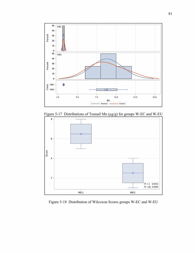
81

Figure 5-17 Distributions of Toenail Mn (µg/g) for groups W-EC and W-EU

Figure 5-18 Distribution of Wilcoxon Scores groups W-EC and W-EU

82


Figure 5-19 shows another modified box plot (with confidence limit whiskers) for the

comparison of treatment groups UU and EU. There is statistically significant difference

between the means of the UU and EU groups, as would be expected due to the

experimental design of intentionally contaminating the nails in the EU group and not

cleaning them. Additionally the dramatic gap between the confidence limits shows

impressive support of Hypothesis 2, that the welding fume exposure protocol of the

experimental method does work and exposed nails did experience significant exogenous

contamination of Mn by the welding fume.

To support this conclusion of Hypothesis 2, a Two Group t-Test was performed to

challenge the independence of the means of the two treatment groups. The results of the

t-Test are displayed in Table 5-12 along with the equality of variances results from a

folded F test show in Table 5-13. . The test for equality of variance between the two

groups resulted in an F statistic of 113.75 and a p-value of 0.0004, thus the variances are

determined to be significantly different and either the Satterthwaite or Cochran methods

for unequal variances can be used to provide a more conservative p-value for the t-test.

Again, both non-equal variance methods still have very low p-values for the t-test (both

had p-value < 0.0001) resulting in rejection of the null hypothesis that the population

means are equal. The study’s Hypothesis 2 is confirmed that nail tissue exposed to

welding fume in the welding fume containment vessel after a 180s GMAW arc time and

contained for 2 hours during deposition, does have significant exogenous contamination

of Mn compared to paired within-subject unexposed nail tissue.

83

Figure 5-19 Box plot mean with confidence intervals UU vs. EU

Table 5-12 Two-Sample t-test results EU vs. UU


Pooled Equal 10 14.42 < 0.0001

Satterthwaite Unequal 5.0879 14.42 < 0.0001

Cochran Unequal 5 14.42 < 0.0001

Table 5-13 Folded F results for EU vs. UU t-test


Folded F 5 5 113.75 < 0.0001

Again, though both groups passed the hypothesis –numerical analyses for normality (both

had p > 0.87 Shapiro-Wilk and p > 0.25 Anderson-Darling), non-parametric tests were

also run to fortify the statistical conclusions of the study in the event that one or both

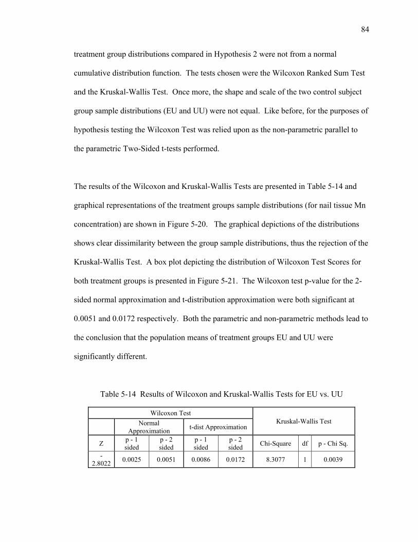
84

treatment group distributions compared in Hypothesis 2 were not from a normal

cumulative distribution function. The tests chosen were the Wilcoxon Ranked Sum Test

and the Kruskal-Wallis Test. Once more, the shape and scale of the two control subject

group sample distributions (EU and UU) were not equal. Like before, for the purposes of

hypothesis testing the Wilcoxon Test was relied upon as the non-parametric parallel to

the parametric Two-Sided t-tests performed.





Kruskal-Wallis Test. A box plot depicting the distribution of Wilcoxon Test Scores for

both treatment groups is presented in Figure 5-21. The Wilcoxon test p-value for the 2-

sided normal approximation and t-distribution approximation were both significant at

0.0051 and 0.0172 respectively. Both the parametric and non-parametric methods lead to

the conclusion that the population means of treatment groups EU and UU were

significantly different.

Table 5-14 Results of Wilcoxon and Kruskal-Wallis Tests for EU vs. UU


Normal


Z p - 1 sided

p - 2 sided

p - 1 sided

p - 2 sided


-2.8022

0.0025 0.0051 0.0086 0.0172 8.3077 1 0.0039

85

Figure 5-20 Distributions of Toenail Mn (µg/g) for groups EU and UU

Figure 5-21 Distribution of Wilcoxon Scores groups EU and UU

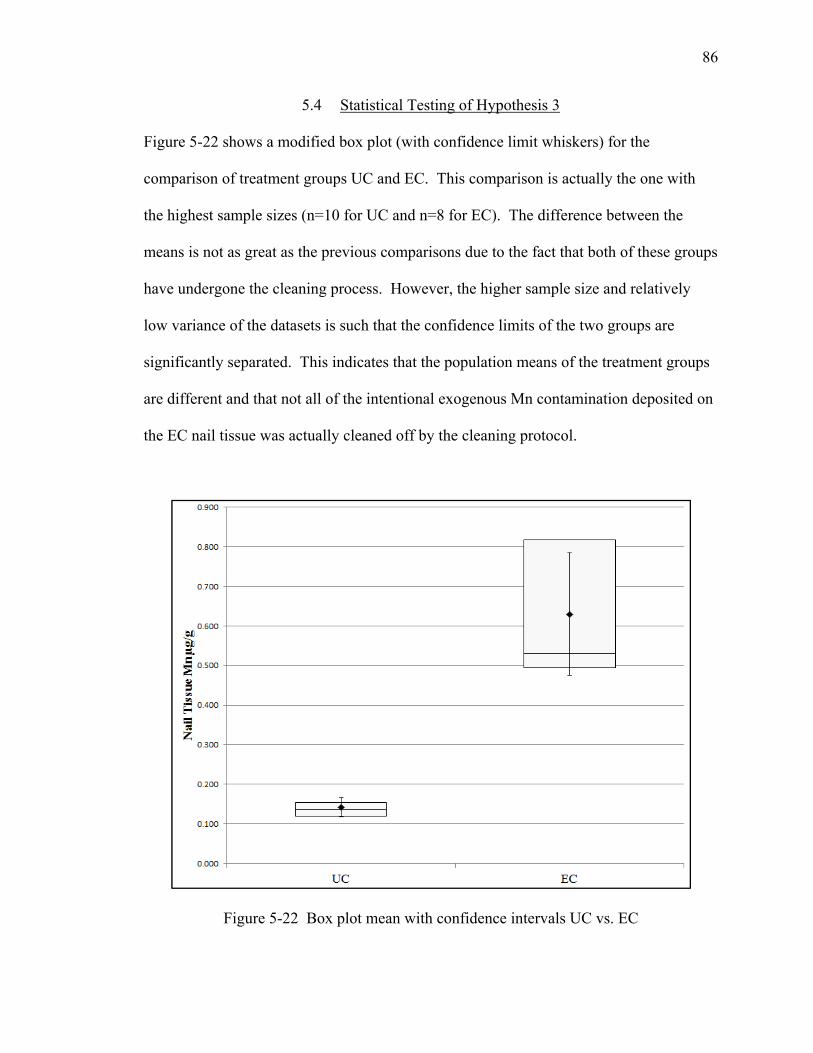
86


Figure 5-22 shows a modified box plot (with confidence limit whiskers) for the

comparison of treatment groups UC and EC. This comparison is actually the one with

the highest sample sizes (n=10 for UC and n=8 for EC). The difference between the

means is not as great as the previous comparisons due to the fact that both of these groups

have undergone the cleaning process. However, the higher sample size and relatively

low variance of the datasets is such that the confidence limits of the two groups are

significantly separated. This indicates that the population means of the treatment groups

are different and that not all of the intentional exogenous Mn contamination deposited on

the EC nail tissue was actually cleaned off by the cleaning protocol.

Figure 5-22 Box plot mean with confidence intervals UC vs. EC

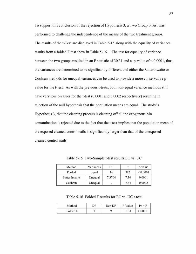
87

To support this conclusion of the rejection of Hypothesis 3, a Two Group t-Test was

performed to challenge the independence of the means of the two treatment groups.

The results of the t-Test are displayed in Table 5-15 along with the equality of variances

results from a folded F test show in Table 5-16. . The test for equality of variance

between the two groups resulted in an F statistic of 30.31 and a p-value of < 0.0001, thus

the variances are determined to be significantly different and either the Satterthwaite or

Cochran methods for unequal variances can be used to provide a more conservative p-

value for the t-test. As with the previous t-tests, both non-equal variance methods still

have very low p-values for the t-test (0.0001 and 0.0002 respectively) resulting in

rejection of the null hypothesis that the population means are equal. The study’s

Hypothesis 3, that the cleaning process is cleaning off all the exogenous Mn

contamination is rejected due to the fact that the t-test implies that the population mean of

the exposed cleaned control nails is significantly larger than that of the unexposed

cleaned control nails.

Table 5-15 Two-Sample t-test results EC vs. UC


Pooled Equal 16 8.2 < 0.0001

Satterthwaite Unequal 7.3704 7.34 0.0001

Cochran Unequal . 7.34 0.0002

Table 5-16 Folded F results for EC vs. UC t-test


Folded F 7 9 30.31 < 0.0001

88

Both groups trended away from normality in the hypothesis–numerical analyses for

normality. Group UC (p = 0.0573 Shapiro-Wilk and p = 0.105 Anderson-Darling) was

approaching rejection of normality, while group EC (p = 0.0268 Shapiro-Wilk and p =

0.025 Anderson-Darling) was significant for rejection of normality. For this reason the

non-parametric tests are most important for the Hypothesis 3 analysis. The tests chosen

were the Wilcoxon Ranked Sum Test and the Kruskal-Wallis Test. Once more, the shape

and scale of the two control subject group sample distributions (EC and UC) were not

equal. Like before, for the purposes of hypothesis testing the Wilcoxon Test was relied

upon as the non-parametric parallel to the parametric Two-Sided t-tests performed.





Kruskal-Wallis Test.

Table 5-17 Results of Wilcoxon and Kruskal-Wallis Tests for EC vs. UC


Normal


Z p - 1 sided

p - 2 sided

p - 1 sided

p - 2 sided


3.5097 0.0002 0.0004 0.0013 0.0027 12.6316 1 0.0004

89

A box plot depicting the distribution of Wilcoxon Test Scores for both treatment groups

is presented in Figure 5-24. The Wilcoxon test p-value for the 2-sided normal

approximation and t-distribution approximation were both significant at 0.0004 and

0.0027 respectively. Both the parametric and non-parametric methods lead to the

conclusion that the population means of treatment groups EC and UC were significantly

different.

Figure 5-23 Distributions of Toenail Mn (µg/g) for groups EC and UC

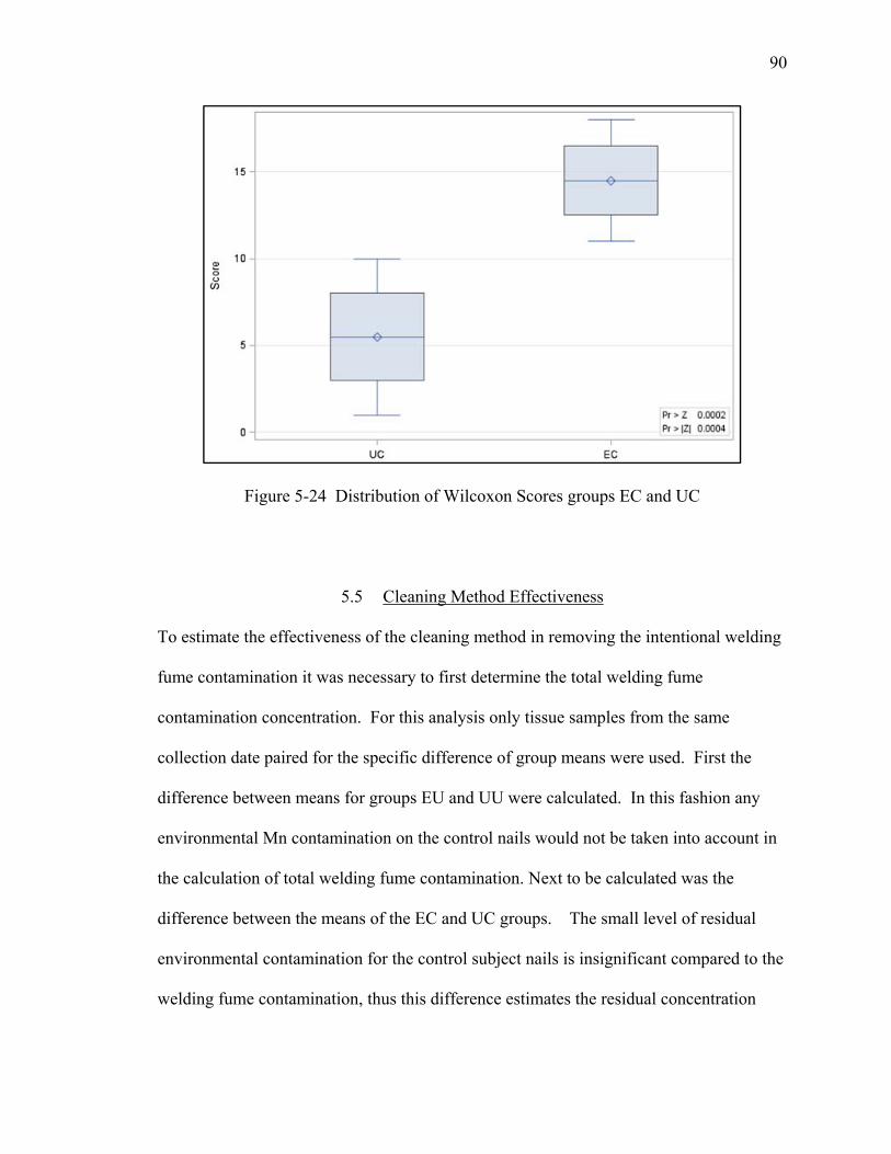
90

Figure 5-24 Distribution of Wilcoxon Scores groups EC and UC

5.5 Cleaning Method Effectiveness

To estimate the effectiveness of the cleaning method in removing the intentional welding

fume contamination it was necessary to first determine the total welding fume

contamination concentration. For this analysis only tissue samples from the same

collection date paired for the specific difference of group means were used. First the

difference between means for groups EU and UU were calculated. In this fashion any

environmental Mn contamination on the control nails would not be taken into account in

the calculation of total welding fume contamination. Next to be calculated was the

difference between the means of the EC and UC groups. The small level of residual

environmental contamination for the control subject nails is insignificant compared to the

welding fume contamination, thus this difference estimates the residual concentration

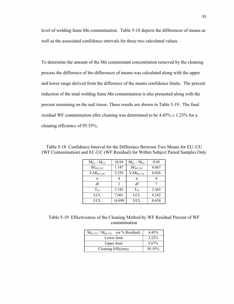
91

level of welding fume Mn contamination. Table 5-18 depicts the differences of means as

well as the associated confidence intervals for these two calculated values.

To determine the amount of the Mn contaminant concentration removed by the cleaning

process the difference of the differences of means was calculated along with the upper

and lower range derived from the difference of the means confidence limits. The percent

reduction of the total welding fume Mn contamination is also presented along with the

percent remaining on the nail tissue. These results are shown in Table 5-19. The final

residual WF contamination after cleaning was determined to be 4.45% ± 1.23% for a

cleaning efficiency of 95.55%.

Table 5-18 Confidence Interval for the Difference Between Two Means for EU–UU (WF Contamination) and EC-UC (WF Residual) for Within Subject Paired Samples Only

MEU - MUU 10.94 MEC - MUC 0.49

SEEU-UU 1.147 SEEC-UC 0.067

VAREU-UU 5.258 VAREC-UC 0.036

n 4 n 8

df 3 df 7

T95 3.182 T95 2.365

LCL 7.601 LCL 0.342

UCL 14.898 UCL 0.658

Table 5-19 Effectiveness of the Cleaning Method by WF Residual Percent of WF contamination

MEC-UC / MEU-UU (or % Residual) 4.45% Lower limit 3.22%

Upper limit 5.67%

Cleaning Efficiency 95.55%

92

CHAPTER 6. DISCUSSION

6.1 Primary Findings

Significant Mn contamination was observed on fingernails sampled from occupationally

exposed welders indicating the necessity of proper cleaning methods to remove such

contamination. Development of a methodology to contaminate control subject fingernail

tissue with GMAW welding fume was establish and using said method a primary nail

tissue cleaning protocol was investigated for its efficacy. Though statistically significant

levels of residual welding fume Mn contamination were present on the nail tissue post-

cleaning, the protocol was able to eliminate 95.55% of the contamination Mn.

6.1.1 Occupational Exogenous WF Contamination to Fingernail Tissue

The results of this study indicate that welders have significant exogenous Mn from

occupational exposure which needs to be cleaned off in order to have a valid nail

biomarker of internalized exposure from WF Mn This was shown through the evaluation

of Hypothesis 1.

Though the study design did not facilitate a true determination of the amount of residual

occupational welding fume Mn external contamination after the cleaning process, it was

93

clear from the sheer amount of Mn removed from the welder fingernails that significant

exogenous contamination has occurred. Even if some of the welders occupational

contamination did remain, the level of Mn reduction from cleaning the welder nails,

[WEU – WEC] (difference of means 5.56 µg/g Mn, margin of error 2.47 µg/g Mn) was

nearly twenty times the apparent level of Mn reduction from the cleaning of unexposed

control nails, a likely level of environmental external Mn contamination, [UU – UC]

(difference of means 0.27 µg/g Mn, margin of error 0.15 µg/g Mn). It will be of interest

to see how they welder fingernails compare to welder toenails for this level of

occupational external nail contamination.

Whether toenails are more protected from the welding fume environment than fingernails,

due to boots, shoes, socks, etc. needs to be determined. There could even be differing

mechanisms involved in levels of residual Mn after cleaning for finger and toe nail tissue.

Perhaps the abrasive environment of toenail inside shoes and socks, grinds WF Mn into

the outer nail keratin matrix, resulting in less external contamination than fingernails but

which may be harder to remove. Toenails have been selected by most researchers in this

field because of the perceived protective nature of foot coverings, but the true differences

and similarities between toe and finger nail tissue with regard to cleaning of exogenous

WF Mn has not been determined to date. It is possible that fingernail tissue may have

been overlooked too hastily. Some possibilities toward future research which may shed

light on this issue are discussed below.

94

6.1.2 Effectiveness of Design for GMAW Contamination of Nail Tissue

The GMAW generation, containment, and deposition methods developed in the study

were effective at contaminating nail tissue with WF Mn, as observed by the analysis of

Hypothesis 2. Exposed uncleaned samples (means 11.35 µg/g Mn, margin of error 1.94

µg/g Mn) were significantly higher than the unexposed uncleaned samples (means 0.42

µg/g Mn, margin of error 0.18 µg/g Mn)

Repeatability of the design was also indicated. The nail tissue Mn concentration of the

exposed samples in Round 3 was estimated by the average nail tissue concentration of the

four Exposed/Uncleaned samples (avg. 11.9 µg/g Mn). The Round 3 contamination level

was quite close to the Round 2 average Exposed/Uncleaned samples (avg. 10.2 µg/g Mn).

This is an indication that the contamination protocol is fairly reproducible for a

maintained set of parameters (wire alloy, wire speed, arc time, etc.).

The conclusion is that the methodology and experimental design presented through this

study, will allow researchers to predictably and repeatedly expose nail tissue to WF Mn

during further research into the use of nail tissue as biomarker for WF metals exposure.

6.1.3 Efficacy of Nail Tissue Cleaning Method for GMAW WF Mn

The current cleaning protocol was shown unable to remove all the exogenous WF Mn

contamination. The EC and UC treatment groups indicate significantly different

population means by both parametric and non-parametric test of conservative nature

95

(Two Sample t-test p = 0.0002 Cochran method; Wilcoxon Test p = 0.0027 2-sided t-

distribution approximation).

Despite the fact that there is statistical significance that the cleaning method did not

remove all of the welding fume contamination it is worth noting the magnitude of effect

the cleaning method did have on the nail tissue Mn concentration of the exposed nails.

Based on the large contamination deposition seen in the EU samples, however, it does

appear that the cleaning protocol is removing a relatively large proportion of the external

Mn contamination. The difference seen between the means of the UU and EU treatment

groups (10.94 µg/g Mn; Margin of Error 1.69 µg/g Mn) represents the amount of

contamination deposited during the exposure and the difference between the means of the

UC and EC treatment groups (0.49 µg/g Mn; Margin of Error 0.14 µg/g Mn) represents

the residual contamination after the cleaning method. This indicates that roughly only

4.45% (Margin of error 1.23%) of the welding fume Mn contamination remains as

residual contamination after the cleaning protocol. In other words 95.55% (Margin of

error 1.23%) of the welding fume Mn contamination presented on exposed nail tissue in

this study was cleaned by the current cleaning protocol, supporting the notion that the

current cleaning protocol is likely to prove to be an acceptable cleaning method. Further

research will be needed to identify the cleaning efficiency of the protocol for removal of

long-term occupational exogenous contamination of nail tissue both on toenail and

fingernail.

96

6.1.4 Residual WF Mn and

The author’s speculation on the potential reasons for the residual uncleaned Mn

contamination include possible covalent bonding of Mn to sulfhydryl bridges in the

keratin proteins on the surface of the nail tissue as well as potential for Mn to become

chelated to the Triton X-100 surfactant and a certain amount of that surfactant may stay

bound to the nail tissue even after the DDI rinse step via hydrogen bonding or van der

Waals forces. Further investigation into the degree of and binding nature of residual WF

Mn contamination is essential to understanding the use of nail tissue as a biomarker for

WF exposure. Potential future work is discussed below.

It is also apparent from the UU vs. UC comparison (confidence limits do not overlap),

that there is either a certain degree of environmental Mn contamination on the control

subjects nails (0.49 µg/g Mn; Margin of Error 0.14 µg/g Mn), perhaps from exposure to

Mn in tap water via bathing, hand washing, etc., or there is some degree of leaching

effect by the cleaning process which may be removing some of the bio-metabolized

internal nail Mn.

The utility of nail as biomarker for WF Mn exposure will likely rely heavily on the

relative efficiency of the cleaning process to leave low levels of contamination which are

significantly less that Mn tissue concentrations expected to have neurodegenerative effect.

The ability of the cleaning protocol to remove the significant majority of GMAW WF Mn

contamination in this study (levels twice that found on occupationally exposed welder

nails) suggests valid use of nail tissue as biomarker for WF Mn exposure.

97

Another issue at hand is the potential for Mn to bypass the regular lung metabolic route

and travel directly to the brain via the olfactory nerve. Elder found that after 12 days of

exposure to Mn ultrafine particles (UFP) via inhalation route, exhibited a 3.5 fold

increase in in Mn concentrations in the olfactory bulb while lung Mn levels merely

doubled.27 Elder concluded that the olfactory neuronal pathway was effective for

transport of inhaled Mn oxide (UFP) to central nervous system tissue which can result in

inflammatory changes. Elder suggests that similar pathways exist in human olfactory

systems as well.27 Henriksson and Tjalve also found olfactory transport of Mn directly to

the brain, bypassing the blood brain barrier. They concluded that the neuronal cell

pathways along the olfactory nerve deliver Mn straight to the olfactory bulb.28

It is the author’s belief that the fraction of occupational airborne welding fume exposure

which travels the olfactory route is likely to have fairly low variance among welders and

likewise the fraction of exposure through the lung pathway should also stay relatively

consistent. It is therefore likely, that even if some degree of WF Mn exposure is not seen

in the nail tissue because of the olfactory route, the nail tissue should still highly correlate

with both the olfactory route fraction and the lung route fraction. Thus the nail tissue use

as a biomarker for WF Mn exposure should still be valid regardless of the potential for

separate routes of inhalation exposure to the brain and body. Nail Mn concentration

likely will still correlate to neurodegeneration tests and disease outcomes. Future work

will hopefully reveal the ratio of olfactory route versus lung route from welding fume

exposure so that it can be incorporated into the methodology and analysis of nail tissue as

biomarker.

98

6.2 Limitations of this study

6.2.1 Single control subject

One issue with this study was the use of the single control subject. While it was helpful

in some respects, for testing the overall methodology of the contamination method, the

fact that only one control subject was used means that the variability of human

endogenous and environmental Mn contamination was not discernable in relation to the

contamination method and the cleaning protocol. Larger studies in the future may

address these issues.

6.2.2 Limited sample sizes

The sample sizes of the individual treatment groups were also quite small and it is

difficult to establish a normal range for control or welder groups Mn levels. Again,

future studies will likely address this issue by incorporating larger sample sizes.

6.2.3 Artificial Method of Exposure

While actual fresh GMAW WF was specifically chosen as the contaminant for the study,

as opposed to MnCl WF dust etc., it was a rapid contamination rather than an extended

external exposure over the full term of the nail growth. Also the nails did not experience

any trauma or physical abrasion between exposure and testing as would be expected

during the course of nail tissue growth. Future study designs will not to address this issue

to get a clearer picture of the relative efficiency of the cleaning process on actual

occupational WF Mn exposure over the full growth term of the nail tissue.

99

6.2.4 Fingernails vs. Toenails.

This study utilized fingernail tissue for logistical reasons. In the majority of nail

biomarker for WF exposure studies, toenail is the chosen nail tissue, due evidently to the

presumed protective environment of shoes and socks6,11,15 and, as is the case with The

Wabash Study, welders often cannot provide adequate tissue sample mass from

fingernails but can with toenails.

Welder finger nails were shown to have significant exogenous contamination in this

study, but this work needs to be repeated with toenails to ensure the uncertainty and

efficiency of the cleaning method is similar with toenail tissue. The findings of this study

that welder fingernails carry excessive exogenous contamination seems clear evidence for

need of reliable cleaning method, though an understanding of the exogenous

contamination effect on welder toenails and whether footwear has a sheltering effect

crucial to understanding the utility of this method. For the Wabash Study cohort welders

which were investigated in this study an average post cleaning fingernail Mn

concentration was found to be 3.22 µg/g while the corresponding toenail concentrations

previous determined for the same welders had an average of 11.74 µg/g Mn. As

previously mentioned, fingernail tissue has an approximate growth rate twice that of

toenail, leading to the speculation that fingernail tissue concentration would be roughly

half that of toenail concentration. In this study welder fingernail Mn concentration

actually had only 27% of the toenail concentration. The nature of this apparent

discrepancy is not obvious at this time.

100

6.2.5 Unable to determine leaching effect

Another limitation of this study was that its design lacked an ability to test for the

potential leaching of endogenous Mn from the nail tissue by the cleaning method. As the

cleaning method did not include any harsh chemicals such as nitric acid, it was presumed

that little leaching was occurring and that the difference between the unexposed

uncleaned control nail and the unexposed cleaned control nail (UU – UC) was do to

environmental external exposure, possibly from tap water. Future studies should attempt

to discern whether leaching is occurring and to what extent.

6.3 Lack of literature

It is unclear why there is no apparent literature on the subject of nail cleaning for use with

nail being used for biomarker of welding fume exposure. Multiple research groups are

already using similar cleaning protocols as the method in the present study. Presumably

because they believe there is at least potential for exogenous welding fume contamination

of the nail tissue samples and thus their use of the cleaning methods. Future work will

need to address the issue of optimal cleaning methods so that a consensus can be made on

a standard cleaning method which will allow better comparison of nail study data.

Eastman did do a study similar to this one in some ways, with treated hair and

environmentally exposed hair. The method of analysis for the hair was laser ablation

followed by ICP-MS. Eastman used five cleaning method procedures:

(1) No cleaning; - hair was processed for analyses without cleaning.

(2) MQ water - rinse; hair was rinsed five-times with ultrapure MQ water.

101

(3)Triton sonication (T); hair was sonicated in 0.5% Triton X-100 for 10 min,

rinsed five-times with MQ water, rinsed once with 1 N trace metal grade (TMG)

nitric acid, and rinsed five-times with MQ water.

(4) Triton and nitric sonication (TN); hair was sonicated for 20 min in 0.5%

Triton, rinsed five-times with MQ water, sonicated for 10 min in 1 N TMG nitric

acid, rinsed once with 1 N TMG nitric acid, and then rinsed five-times with MQ

water.

(5) 3×TN; the Triton and nitric acid sonication (TN) cleaning described above

was performed three-times in succession.

Hair samples from the subset of five subjects were intentionally contaminated with Mn

containing environmental dust or two concentrations of Mn contaminated water (70 µg/L

Mn and 700 µg/L Mn). Samples were cleaned with the various procedures and analyzed

for comparison.

The baseline Eastman used as a reflection of endogenous Mn of the hair was the

untreated Triton + nitric sonication . She found the data to indicate that the TN cleaning

method was able to remove even excessive contamination with Mn and other metals

without overcleaning. As in our study with the control nail tissue, Eastman found

significant environmental exogenous Mn contamination (Untreated no cleaning mean

0.833 µg/g Mn compared to the baseline untreated Triton + nitric mean 0.170 µg/g Mn)

which amounts to 0.663 µg/g, not far off from the environmental contamination on this

study’s single control subject. The 3 times TN cleaning did, however, reduce the hair Mn

102

concentration further in each group (down to 0.066 µg/g Mn in the case of the untreated

hair), which leads to speculation that continued repetitions of the TN method may be

actually leaching out bio metabolized endogenous Mn from the hair tissue.

Although none of her cleaning methods was exactly the same as this study’s method, the

Triton sonication with DDI rinse plus single nitric rinse was probably the closest. For the

dust contaminate hair the with the Triton sonication with DDI rinse plus single nitric

rinse showed 0.593 µg/g compared to the same hair with Milli-Q water rinse at 0.573

µg/g for a nearly 90% cleaning, though it must be added that Eastman did not show

results for the contaminated uncleaned group. For the highest dose water contaminated

samples the Triton sonication with DDI rinse plus single nitric rinse had a mean of 2.31

µg/g Mn compared to the simple Milli-Q water rinse samples at 10.5 µg/g Mn for a mere

78% cleaning efficiency. To be certain the simple Milli-Q water rinse may have had

some effect thus the cleaning efficiency could be artificially low by these numbers. That

said, the results appear in the same rough efficiency window as the current study’s.

6.4 Potential future work

Further attempts will be required to more fully understand the nature of the welding fume

nail contamination and whether other cleaning protocol alternatives will be able to

remove all of the exogenous contamination without leaching of endogenous, bio-

metabolized Mn incorporated in the nail tissues keratin matrix. Below are listed some

potential avenues of future investigation into this area.

103

6.4.1 Effects of sonication

Additional comparison of the cleaning method protocol using two types of sonicators will

likely be performed. The Branson Sonifier from the original cleaning protocol (400W

power output converted to 20 kHz ultrasonic mechanical vibration) will be compared to a

Mettler Cavitator Ultrasonic Cleaner bath (85W power output converted to 67 kHz) in

order to determine whether the Mettler Cavitator provides comparable cleaning to the

Branson Sonifier. While the Branson Sonifier only has the capability of running a single

sample at one time, the Mettler Cavitator can run 24 samples or more at one time, thus

allowing researchers a chance to eliminate a bottleneck in the nail sample preparation

procedure and increase the efficiency of the overall process.

6.4.2 Alternative Cleaning Procedures

As was seen in the Eastman study with hair, additional cleaning procedure options should

be examined with nail as the biomarker. Some options include multiple repetitions of

cleaning procedures in succession, addition of metal chelation agents such as EDTA, or

variations of the ultrasonic bath power, frequency, and duration. In addition adding

nitric acid to the cleaning solution to etch the outer surface of the nail tissue thus assisting

removal of external contamination could be analyzed as well but this could lead to

leaching endogenous Mn and methodology to determine potential leaching effect must be

incorporated.

104

6.4.3 Nature of binding of residual exogenous Mn

Transmission electron microscope (TEM) studies could be used to determine the nature

of the adherence of exogenous Mn from welding fume and the effects the cleaning

process have on endogenous nail Mn. Proper experimental design could determine to

what degree the exogenous Mn is covalently bonded to sulfhydryl bridges in the keratin,

hydrogen or van der Waals bonded, adhered by loose physical deposition, or perhaps be

physical entrapment through processes of friction or grinding of welding fume particles

into the surface of the nail tissue.

Laser ablation techniques such as those used with hair could also be useful in analyzing

various depth layers of the nail to determine actual levels of exogenous Mn before and

after cleaning.

6.4.4 Cleaning for other metals (Pb, As, Cr, Cu, Zn, etc.)

As the nature of the metal elements of occupational and environmental concern, behave

quite differently, other research will be needed to investigate the usefulness of cleaning

protocols for metals such as Pb, As, Cr, Cu, Zn, etc. It will need to be determined if

researchers could also successfully utilize nail tissue as a biomarker for those metals

without distortion from external nail contamination or leaching effects of cleaning

processes. This study and its experimental design may prove useful in further endeavors

into the nature and validity of nail tissue as biomarker for welding fume exposures.

105

6.4.5 Relation between personal nail growth variability, clipping depth, and

chronological window of exposure depicted by nail sample

Nail growth rate variability in human populations have been reported. 10 An

understanding of the true relation between the section of toenail sampled and the time

frame of that samples growth (an hence exposure window) needs to be understood before

practical application of this biomarker can come to fruition. One approach would be to

have nail tissue donors carefully mark their nails periodically during a longitudinal study

in order to arrive at individual growth rates. It might then be possible to measure the

depth of clipping and relate that to the growth rate and the persons total nail bed length,

in order to obtain a better vision of the exposure time window represented by the clipping.

6.4.6 Within-Subject Welder Design to Ascertain Exogenous WF Contamination Level

Another approach to attempting to discern the actual level of exogenous contamination

on occupationally exposed toenail could be to run a within-subject design utilizing a

protection method for one foot’s nails and not for the other. Special enamel coatings with

no Mn or perhaps a Teflon sock could be useful. Of course this method would incur

potential compliance bias from the welders which would have to be addressed.

106

CHAPTER 7. CONCLUSION

It is crucial that exposure biomarkers be able to reveal levels of internalized body burden

due to external sources. Nail tissue may be such a biomarker if cleaning methods are

employed which adequately remove potential external contamination which the nail may

be presented with during the subject’s exposure period. In the case of Mn exposure from

welding fumes, this study has shown that such exogenous contamination does exist. A

method of applying GMAW WF contamination was designed, implemented and

confirmed. The contamination method was utilized to contaminate control welder nails

successfully at approximately twice the contamination level seen on welder fingernails

and the presented cleaning method protocol was shown to remove this contamination at

an efficiency of 95.55%. The results of this study support the validity and utility of nail

tissue as a biomarker for welding fume Mn internal exposure. As the cleaning protocol

applied in this study is likely to result in similar removal of additional metals of interest,

it is likely that nail tissue may also prove useful for measuring body burden of other

occupational and environmental metal exposures as well.

107

LIST OF REFERENCES

107

LIST OF REFERENCES

1. Schoonover, T. (2009). Personal exposure and biomarkers among production welders and non-welders. Proquest Disertations and Theses.

2. Eastman, R. R., Jursa, T. P., Benedetti, C., Lucchini, R. G., & Smith, D. R. (2013). Hair as a biomarker of environmental manganese exposure. Environmental Science & Technology, 47, 1629−1637.

3. Gil, F. & Pla, A. (2001). Biomarkers as biological indicators of xenobiotic exposure. Journal of Applied Toxicology, 21, 245-255.

4. Santamaria, A. B. & Sulsky, S. I. (2010). Risk assessment of essential element: manganese. Journal of Toxicology and Environmental Health, Part A, 73, 128-155.

5. Lees-Haley, P.R., Rohling, M.L., & Langhinrichsen-Rohling, J. (2006). A meta-analysis of the neurological effects of occupational exposure to manganese. Clinical Neuropsychology, 20, 90-107.

6. Laohaudomchok, W., Lin, X., Herrick, R. F., Fang, S. C., Cavallari, J. M., Christiani, D. C., & Weisskopf, M. G. (2011). Toenail, blood and urine as biomarkers of manganese exposure. Journal of Occupational and Environmental Medicine/American College of Occupational and Environmental Medicine, 53(5), 506-510.

7. Longnecker, M. P., Stampfer, M. J., Morris, J. S., Spate, V., Baskett, C., Mason, M., & Willett, W. C. (1993). A 1-y trial of the effect of high-selenium bread on selenium concentrations in blood and toenails. The American journal of clinical nutrition, 57(3), 408-413.

8. Garland, M., Morris, J. S., Rosner, B. A., Stampfer, M. J., Spate, V. L., Baskett, C. J., & Hunter, D. J. (1993). Toenail trace element levels as biomarkers: reproducibility over a 6-year period. Cancer Epidemiology Biomarkers & Prevention, 2(5), 493-497.

9. Palmeri, A., P ichini, S., Pacifici, R., Zuccaro, P., & Lopez, A. (2000). Drugs in nails. Clinical pharmacokinetics, 38(2), 95-110.

10. Yaemsiri, S., Hou, N., Slining, M. M., & He, K. (2010). Growth rate of human fingernails and toenails in healthy American young adults. Journal of the European Academy of Dermatology and Venereology, 24(4), 420-423.

11. Grashow, R., Zhang, J., Fang, S. C., Weisskopf, M. G., Christiani, D. C., & Cavallari, J. M. (2014). Toenail metal concentration as a biomarker of occupational welding fume exposure. Journal of Occupational and Environmental Hygiene, 11(6), 397-405.

108

12. Slotnick, M.J., & Nriagu, J.O. (2006). Validity of human nails as a biomarker of arsenic and selenium exposure: A review. Environmental. Research, 102(1), 125–139.

13. McCarthy, D.J. (2004). Anatomic considerations of the human nail. Clinical Podiatric Medicine & Surgery, 21(4), 477–491.

14. Harkey, M. R. (1993). Anatomy and physiology of hair. Forensic Science International, 63, 9−18.

15. Sriram, K., Lin, G. X., Jefferson, A. M., Roberts, J. R., Andrews, R. N., Kashon, M. L., & Antonini, J. M. (2012). Manganese accumulation in nail clippings as a biomarker of welding fume exposure and neurotoxicity. Toxicology, 291(1), 73-82.

16. Coelho, P., Costa, S., Silva, S., et al.(2012). Metal(loid) levels in biological matrices from human populations exposed to mining contamination - Panasqueira Mine (Portugal). Journal of Toxicology and Environmental Health, Part A, 75(13–15), 893–908.

17. Carpenter, K. R. & Monaghan, B. J. (2008). Influence of shielding gas on fume size morphology and particle composition for gas metal arc welding. ISIJ International, 48(11), 1570-1576.

18. Greenwood, Norman N.; Earnshaw, Alan (1997). Chemistry of the Elements (2nd ed.). Oxford: Butterworth-Heinemann.

19. Hu, J. & Tsai, H.L. (2007). Heat and mass transfer in gas metal arc welding. Part I: The arc. International Journal of Heat and Mass Transfer, 50(5–6), 833–846.

20. Chung, K. Y. K., Aiken, R. J., & Bradley, D. R. (1997). Development and testing of a new sampler for welding fume. Annals of Occupational Hygiene, 41(3), 355-372.

21. Jenkins, N. T., Pierce, W. M.-G., & Eagar, T.W. (2005). Particle size distribution gas metal and flux cored arc welding fumes. Welding Journal, 84(10), 156-s-163-s.

22. Quimby, B. J. & Ulrich, G. D. (1999). Fume formation rates in gas metal arc welding. American Welding Society Welding Journal, April, 142-s-149-s.

23. Ghasemi, A. & Zahediasl, S. (2012). Normality tests for statistical analysis - A guide for non-statisticians. International Journal of Endocrinol Metabolism, 10(2), 486-489.

24. Razali, N. & Wah, Y. B., (2011). Power comparisons of Shapiro–Wilk, Kolmogorov–Smirnov, Lilliefors and Anderson–Darling tests. Journal of Statistical Modeling and Analytics 2 (1), 21–33.

25. Shapiro, S. S., & M. B. Wilk. (1965). An analysis of variance test for normality (complete samples). Biometrika, 52(3/4) (December),591-611.

26. Mayeux, R., (2004). Biomarkers: potential uses and limitations. NeuroRx, 1(2), 182-188.

27. Elder, A., Gelein, R., Silva, V., Feikert, T., Opanashuk, L., Carter, J., (2006). Translocation of inhaled ultrafine manganese oxide particles to the central nervous system. Environmental Health Perspectives, 114(8), 1172(7).

109

28. Henriksson, J. & Tjälve, H., (1998), Uptake of Inorganic Mercury in the Olfactory Bulbs via Olfactory Pathways in Rats. Environmental Research, 77(2), 130-140.

29. Ward, E. J., Ma, R., Yeh, C., et al. (2014) Neurological Health Effects Correlate with Low Level ChronicExposure in Welders. Poster presentation at the SOT 53rd Annual Meeting and ToxExpo, Phoenix, Arizona.

110

APPENDICES

110

Appendix A Nail Digestion and ICP-MS Sample Protocol

1. Sample Preparation Prior to Microwave Digestion (No blanks)

a. Place toenail sample in to 15 mL Falcon tube and clearly label the sample ID number.

b. Fill Falcon tube with 10 mL of 1% Triton X-100 solution and seal with cap.

c. Place Falcon Tubes in Branson Sonifier ultrasonic cleaning bath (only run one falcon tube at a time).

d. Make sure caps are sealed, do not allow water to dilute Triton solution in Falcon tubes.

e. Run water into the Branson Sonifier bath at proper rate to maintain level slightly above the nail sample and below the meniscus of the Triton X-100 solution in the Falcon Tube.

f. Set the Branson Sonifier for 15 minute dwell and 50% power level. g. Continue to monitor water level to ensure it neither overflows nor run

below the nail sample level. Proper sonication will be visually observed by the nail samples suspended and vibrating in the cleaning solution by ultrasonic cavitation occurring.

h. Continue this process repeating steps a. through g. for each nail sample to be cleaned.

i. After ultrasonic cleaning, rinse each sample 5 times with DDI water or until surfactant suds are no longer seen in the tube. Use a clean small beaker as an intermediary when pouring out of tube to make sure no nail sample is lost in the sink. Rinse the beaker out with DDI after completing the rinse of each sample.

j. Place sample in drying oven (Zheng Lab) for 24 hrs at 60˚ C. The polypropylene Falcon Tubes and tube racks are safe at this temperature.

k. Carefully weigh each dried sample and record sample’s mass. Do this immediately after the oven drying to ensure no moisture condensates on or absorbs back into the nail tissue.

l. If microwave digestion will be performed immediately, place each cleaned and weighed sample into a microwave digestion vessel, place in the carousel and note the position carefully (carousel position will be the only indicator of the sample ID until after digestion). After all samples are prepared in vessels in the carousel, proceed with Step 2.

m. If digestion will be performed at a later time, samples can be placed back into their individually labelled Falcon tubes temporarily.

n. Note we will not do a blank at this step because the blank would simply evaporate entirely during the drying step.

111

2. Microwave Digestion of Samples

a. Take the carousel to a lab hood for this step. Turn on fume hood fan. b. Wear proper PPE (nitrile gloves double layer, lab coat, and safety glasses).

Concentrated nitric acid fumes and is highly corrosive and will cause damages to skin, eyes, mucosal membranes and lungs. Work carefully and patiently. Locate the nearest eyewash station prior to working with the concentrated nitric acid.

c. Take care in noting the specific position ID number of the carousel in which each sample’s vessel is placed. There no other identification will exist during the digestion phase. Strict order of placement must be controlled.

d. Place cleaned, dried and weighed samples individually into microwave digestion vessels and place each vessel into its proper identified position in the carousel. Create a vessel placement pattern in the carousel which is as evenly dispersed as possible to ensure even microwave dispersal during digestion.

e. Using a 1mL micropipette, into each microwave digestion vessel add precisely 2.00 mL of ultrapure HNO3 (the current reagent is JT Baker Ultrex II 6901-05 67-70% Nitric Acid for trace metals analysis), place the plug in vessel, lightly screw cap on until resistance is felt, and seal the vial tightly with the MARSXpress tensioning tool. You will hear a click when it is tensioned properly. Do NOT over tighten.

f. Place carousel with all sealed digestion vessels in microwave digester unit. g. Place exhaust ducting end into the fume hood and ensure the hood fan is

on. h. Update the microwave digester oven log book to indicate the date, time,

power, and your initials for the runs you make. i. Turn on the oven. Select “Load Method” “User Method” “Test WJ

– Xpress”. Setting for this method should be: organic; 600W, 100% power; Ramp time 15 minutes; control temp 200 degrees Celsius; hold time 10 minutes.

j. Make sure carousel is properly seated in the oven, close door and run the “Test WJ” program. Ramp up lasts 15 min, cool down is 15 min. Let exhaust an additional 1.5 hour to ensure all the nitric fumes have exhausted into the hood.

k. Continue to observe the digestion for the entire cooking ramp up time of 15 minutes. If vessels are not sealed properly, nitric acid may burst or leak potentially contaminating other samples. If this happens, the oven must be manually stopped by pressing “P/T” and then pressing “0”. Let the oven chamber vent to the hood at least a few minutes, then open and remove the carousel to the hood for cleanup and resealing vessels. Also clean out the oven chamber. Once cleanup is complete re-run the digestion from the beginning.

112

l. After samples have cooled (approx. 2 hrs.), open the digester and put carousel in hood to prepare stock solutions.

m. Once the entire digestion is complete, clean the entire inside surface of the oven chamber with DDI water and lab wipes to avoid contaminating later sample digestions.

3. Stock Solution Preparation

a. Ensure hood fan is on and carefully open the first vessel. Take care as vessel may be pressurized and nitric may fume out as the seal is cracked. Shield yourself with you gloved hand as the vial is opened. Be extremely careful to not spill any of the digested material.

b. Each digested sample should be clear and completely digested in the vessel before proceeding. If sample is cloudy or visible material remains in the nitric solution, re-seal and run an additional digestion (for nail samples this will rarely happen).

c. Carefully pipette the digested sample/nitric mixture into a clean 10 mL Pyrex volumetric flask. Drops of the mixture may be in the cap and vessel grooves, on the plug and along the walls of the vessel. Use the micropipette to obtain as much of the sample mixture as possible. Note: Use of a 2-20 ultra-micropipette with a capillary type tip can be very useful in capturing the tiny droplets from the difficult areas of the vessel and plug, however, when using be very certain to not suck too much solution into the micropipette as going beyond the capacity of the pipette tip could damage the micropipette.

d. Pipette DDI Water until flask is filled to the 10 mL line. Be sure to read the meniscus properly. Go slow at the end, DO NOT overfill. Dilution to exactly 10 mL is crucial for proper analysis of nail tissue metal concentration.

e. Cover top of flask with a piece of parafilm. Press thumb to top of flask to seal Parafilm carefully then shake and mix thoroughly.

f. Pour this diluted digestion mixture into a Falcon Tube and label with sample ID, “Stock Solution”, and any other identifiers needed. This will be the stock solution from which we will prepare further dilutions for ICP-MS analysis.

g. Prepare a “Blank Stock Solution” by adding 2 mL of the same ultrapure trace metals analysis grade concentrated nitric acid used for the digestion and 8 mL of DDI water into a Falcon Tube. Seal, mix, and label as “Blank Stock Solution”.

4. ICP-MS Blank Preparation

a. Pipette 1 mL of “Blank Stock Solution” and 6 mL of DDI water into a Falcon tube. Label as “Blank”.

b. Seal tube with lid and mix again.

113

c. Depending on the total number of sample to be run, multiple blanks may need to be prepared in this manner and provided to the MS lab. If you are unsure how many to prepare, ask Karl.

5. ICP-MS Sample Preparation

a. Pipette 1 mL of stock solution and 6 mL of DDI water into a Falcon tube. Label with Sample ID.

b. Seal tube with lid and mix again. c. Continue for each sample stock solution until all sample preparations are

prepared. d. Note that procedure will have to be completed twice for each sample if

performing samples from air filters because of a mass concentration range difference between Mn and Fe.

6. Standard Dilution Preparation (for spiked ICP-MS samples)

a. Place a cleaned and dried 250 mL narrow mouth HDPE bottle on the scale and tare.

b. Pour precisely 199.8 grams of DDI water into the bottle. c. Use a calibrated micropipette to pipette 200 uL (microliters) of 10 ppm

trace metals standard into the bottle. Our current reagent is Exaxol - 68 Element Standard - Part A - MS68A-100 which has 10 ppm of 49 elements, including Mn, Cu, Fe, Pd, and Zi.

d. Cap tightly and mix thoroughly. This is now the 10 ppb standard to be used as a spike.

e. Label as “Wabash Study 10 ppb Standard Solution”. Date the standard solution preparation. New 10 ppb standard solutions should be prepared at a minimum of every couple of months as 10 ppb level is less stable than the 10 ppm standard.

7. Spike Addition Preparation (Must be done for each sample batch sent to the lab)

a. Pick a moderate Mn level sample for use as spike samples. This will either be a heavier sample weight control group nail sample or a lighter weight welder group nail sample. Use this sample’s stock solution for preparation of the spikes additions. Spiking an actual nail sample stock solution maintains common matrix effects from the constituents of the nail material.

b. For “10 ppb addition” add 1 mL of the stock sample chosen above to a Falcon tube. Add 1 mL “Wabash Study 10 ppb Standard Solution” and 5 mL of DDI. This is technically a 1.429 ppb addition to the sample preparation after the further dilution is taken into account.

114

c. For “20 ppb addition” add 1 mL stock sample, 2 mL “10 ppb Standard Solution” and 4 mL of DDI. This is technically a 2.857 ppb addition to the sample preparation after the further dilution is taken into account.

d. For “30 ppb addition” add 1 mL stock sample, 3 mL “10 ppb Standard Solution” and 3 mL of DDI. This is technically a 4.286 ppb addition to the sample preparation after the further dilution is taken into account.

e. If higher levels are expected in the samples a “400 ppb addition” may be valuable as well. It is good to have standard spikes which fall on either side of the majority of samples if possible.

f. For “40 ppb addition” add 1 mL stock sample, 4 mL “10 ppb Standard Solution” and 2 mL of DDI. This is technically a 5.715 ppb addition to the sample preparation after the further dilution is taken into account.

8. Preparing Serial Dilutions of Stock Solutions (if necessary)

a. If the expected range of sample preparation concentration for Mn is expected to be more than about 10-15 ppm or if the range is completely unknown, it is wise to provide the analytical chemists with serial dilutions of the sample preparations which may have high concentrations. The chemists will be able to do a pre-run from most dilute to least dilute to determine which sample is best for the actual run to ensure optimal results. This also helps them to protect their equipment as high metal concentrations in samples can negatively affect their system.

b. If serial dilutions are required, begin by preparing a 1/10th dilution (0.1X) of a sample’s stock solution by pipetting exactly 1 mL of the stock solution into a clean 10 mL Pyrex volumetric flask and pipette DDI water until flask is filled to the 10 mL line. Be sure to read the meniscus properly. Go slow at the end, DO NOT overfill.

c. Cover top of flask with a piece of Parafilm. Press thumb to top of flask to seal Parafilm carefully then shake and mix thoroughly.

d. Pour this diluted stock solution into a Falcon Tube and label with sample ID, “0.1X Stock Solution”, and any other identifiers needed. This will be the 1/10th serial dilution stock solution from which you will prepare a 0.1X serial dilution sample preparation.

e. If further serial dilutions are necessary, continue in a stepwise manner using the 0.1X Stock Solution to create a 0.01X Stock Solution and so on.

9. Preparing serial diluted ICP-MS sample preparations

a. This is similar to the regular sample preparations with one addition. The regular stock solutions have approximately 20% volume as 70% nitric acid resulting in 7mL sample preparations which have 2% nitric acid which is required for the ICP-MS analysis and to maintain proper matrix effect consistency of the sample preparation relative to the standard spikes and blanks. Once a stock solution has been serial diluted its nitric acid

115

concentration becomes negligible and additional ultrapure nitric acid must be added to each serial dilution sample preparation in order to maintain the 2% nitric acid required.

b. Pipette 1 mL of serial diluted stock solution and 5.8 mL of DDI water into a Falcon tube labeled with Sample ID and the level of the serial dilution.

c. Pipette 200 µL of ultrapure trace metals analysis 67-70% nitric acid into solution. Total volume should be 7 mL.

d. Seal tube with lid and mix again. e. If serial diluted sample preparations are given to the MS lab, be sure to

indicate precisely which they are and the nature of the serial dilutions to aid the lab.

10. Preparing Entire Sample Run for ICP-MS Analysis

a. Ensure that you have necessary blanks, spikes, and all sample preps for each type of metal analysis you need run.

b. Place all Falcon tubes in Styrofoam holders. Label holders “Rosenthal/Dydak”, the date, your initials, and the metals you want run.

c. Label each sample only with ID number, on lid and tube. Label spikes with chosen sample ID use to make the spikes and “+10ppb”, “+20ppb” and “+30ppb” respectively. Label blanks “Blank” and clearly label any serial diluted samples.

d. Send to Karl Wood in WTHR 157. Analysis data return will take approximately a week or two.

116

Appendix B Images of Welding Fume Contamination Process

Figure B 1: Century 100 MIG Welder Used in Study

Figure B 2: Safety Equipment For MIG Welding

117

Figure B 3: Placement of Nail Tissue for WF Exposure

Figure B 4: Placement of the Spatter Shield

118

Figure B 5: MIG Arc Creating Welding Fume

Figure B 6: Continuing Fume Generation

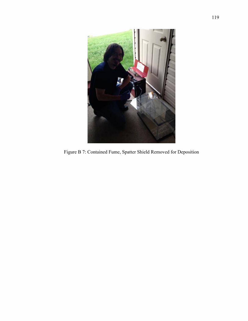
119

Figure B 7: Contained Fume, Spatter Shield Removed for Deposition

120

VITA

120

VITA

Jeffrey Corral Bainter Graduate School, Purdue University

Education B.A., Chemistry, 1994, Indiana University, Bloomington, Indiana B.S., Psychology, 1994, Indiana University, Bloomington, Indiana M.S., Environmental Science, 2011, Indiana University, Bloomington, Indiana M.S., Occupational and Environmental Health and Safety, 2014, Purdue University, West Lafayette, Indiana

Research Interests Welding Fume Exposure Assessment Biomarkers of Metal Exposures Hazardous Materials Safety Certifications Chemical and Hazardous Materials Manager (C.H.M.M.) Certified by the Institute of Hazardous Materials on December 8, 2011 Credential Number 15804

PUBLICATIONS

121

PUBLICATIONS

Bainter, J. C., Beckley, J. A., Morton, B. (2005). Conversion Coatings: Adding Performance to CAB Aluminum Heat Exchangers. Novi, MI: AFC-Holcroft Annual Aluminum Brazing Conference. Sievers, B. A., Bainter, J. C., Restifo, C. M. & Jazenski, P. J. (Fall, 2001). An Alternative to Phosphate Pre-treatments for Use in Rubber Bonding (Paper no. 120). Cleveland, OH: American Chemical Society Rubber Division Meeting. Restifo, C. M., Bainter, J. C. “A New Alternative to Traditional Iron Phosphating for Ferrous Substrates,” Metal Finishing, New York, NY, September, 2000, Vol. 98, No. 9.

Efficacy of cleaning method for removal of exogenous welding ...

Documents

Transcript of Efficacy of cleaning method for removal of exogenous welding ...