Effects of two acoustic continua on the within-category perceptual structure of tones.

of 16

Effects of two acoustic continua on the within-category perceptual structure of tones

Abstract The present study investigated effects of two acoustic continua on the within-category perceptual

structure of Putonghua Tone 2 and Tone 3. These two tones were simulated with tokens varying

along two acoustic continua about F0 contour: the timing of F0 turning point and falling of F0. Three different syllable durations were tested. Multidimensional scaling analyses were applied to

investigate relative influence of phonetic identification and category goodness on the perceptual dissimilarity of synthesized tonal tokens. The result revealed that Tone 3 has later F0 turning

point and greater F0 falling than Tone 2, which confirms former findings. The new finding is that

perceptual representation of these two tones categories is different in their internal structures. Best tokens disperse within categories and are usually not unique. Perceptual space involving

Tone 2 tokens shrink but that involving Tone 3 doesn’t. Goodness rating contributes significantly to the dissimilarity scaling across Tone 2 tokens but not Tone 3 tokens.

Keywords Tone, categorical perception, magnet effect, dissimilarity

1.0 Introduction One concern about phonetic categories is their internal structure. The Native Language

Magnet model (NLM) predicts that the perceptual distance of identically labelled stimuli should

be influenced by category goodness. Even for tokens that are consistently identified as members of a single category, “magnet effects” shrink the perceptual space near native prototypes; then it is more difficult to discriminate phonetic variation around prototypes than around non-prototypes,

or poor exemplars, of the same category ( Iverson & Kuhl, 1995, 2000; Iverson, et al., 2003; Kuhl, 1991; Kuhl & Iverson, 1995). However, listeners frequently identify “non-prototypes” as

exemplars of a different category (Sussman & Lauckner-Morano, 1995). Kuhl et al. also found

“prototypes” with different acoustic parameters from their earlier studies (Kuhl & Iverson,

1995). Lotto et al. argued that the “Perceptual Magnet Model” may be nothing more than a further demonstration that general discriminability is greater for cross-category stimulus pairs

than for within-category pairs (Lotto, Kluender, & Holt, 1998).Despite all these controversies, researchers have reached a general agreement that not only the boundaries but also the internal structures are worth the effort to investigate. However, former studies mainly focus on internal

structures of segmental categories, whereas tonal categories were rarely taken into consideration. Most perceptual studies on tonal perception are generalizations within the “categorical

perception” (CP) paradigm (Liberman, Harris, Hoffman, & Griffith, 1957) and discussions about the tonal categoricality have been based on a single specific acoustic continuum of fundamental

frequency (Abramson, 1979; Chan, Chuang, & Wang, 1975; Peng, et al., 2010; Wong & Diehl,

2003; Xu, & Gandour, 2006). Nevertheless, several acoustic continua have been proved to affect tonal perception, such as precursor registers (Moore & Jongman, 1997), voice quality (Whalen &

Xu, 1992; Yang, 2009), syllable duration (T_d) (Blicher, Diehl, & Cohen, 1990; Fu & Zeng, 2000), and amplitude (Whalen & Xu, 1992). Even when only pitch contour is taken into

consideration, by measuring dissimilarity ratings of different pitch patterns, Gandour found that the differences can be attributed to several measurements, such as average pitch, endpoint,

extreme endpoint, and length (Gandour 1978). As an exploratory study on internal structures of

tonal categories, the present work found it reasonable to build up experiments on the combination of a few dominant continua while put relevant covariants under control. And the controversy on

of 16

the perceptual related acoustic cues of Putonghua Tone 2 and Tone 3 make them appropriate examples for this investigation.

Putonghua has four phonological tones, commonly numbered as tones 1-4. There is a general agreement that fundamental frequency is the primary acoustic correlate of Putonghua tones

(Garding, Kratochvil, Svantesson, & Zhang, 1986; Lin, 1988; Shen & Lin, 1991). According to traditional description, the first one is high-level, the second mid-rising, the third low-dipping (or low-falling-rising), the fourth high-falling” (Chao, 1955). As for Tone 2, a short low or dipping

part can precede the rising part (Moore & Jongman, 1997; Shen & Lin, 1991). As for Tone 3 it is generally accepted that a rising second half mostly appears in citation form while a low-falling

(“half third tone”) appears in running speech or nonprepausal position (Garding, Kratochvil, Svantesson, & Zhang, 1986; Hallé 1994). As a result, pitch contours of Putonghua Tone 2 and Tone 3 in citation both involve a falling phase followed by a rising phase, which may be the

reason of their frequent confusion (Gandour, 1983; Li & Thompson, 1977; So & Best, 2010). On the other hand, creaky voice appears much more frequently in the lowest part of Tone 3 than in

Tone 2 (Keating and Esposito 2007; Kong 2007) and with pitch contour under control, stimuli

resynthesized with PSOLA method from Tone 2 recordings are perceived differently from those

resynthesized from Tone 3 recordings (Yang 2009). Thus it is reasonable to suspect that the existence of creaky voice might be important for distinguishing these two tones and put it under control. Low-falling Tone 3 is also similar to Tone 4 because they both involve falling phases.

This confounder should be taken into consideration although the present study focuses on the

perceptual representation of Tone 2 and Tone 3. Earlier studies showed that the timing of a

turning point (T_t, or duration of falling phase in other words), and the falling of F0 (F0_△) are

important for the identification of Tone 2 and Tone3. T_t is negatively related to the identification

score of Tone 2 (Moore & Jongman, 1997; Shen & Lin, 1991; Zue, 1976). The larger F0_△ is,

the less likely is a stimulus identified as Tone 2 (Moore & Jongman, 1997; Shen & Lin, 1991). By elongating the syllable while keeping the proportion between the falling phase and the syllable

duration constant, the identification of Tone 2 decreased; this was interpreted as evidence for the essentiality of the absolute duration of the falling phase (Blicher et al., 1990). On the other hand, our earlier studies showed that by elongating the syllable while keeping the absolute duration of

the falling phase constant, the identification of Tone 2 increased with the decreased proportion of the falling phase (Wu, 2011). Hence both T_t and the proportion T_t/T_d, with negative effects,

should be taken as independent predictors of the identification functions of these two tones. The present study explored categories of Putonghua Tone 2 and Tone 3 and the internal

structures of these categories by investigating the following aspects. How do tonal identification

and discrimination correlate along more than one acoustic continuum? Does tonal goodness rating shed light on phenomena unrevealed by identification? How much do goodness and identification

contribute respectively to the distortion of perceptual space? Acoustic stimulus matrices varying along two acoustic continua were built for identifying and rating. The timing of the turning point

(T_t) and the size of an fall in fundamental frequency (F0_△) were selected as the two acoustic

continua defining the stimulus space. Syllable duration (T_d) was selected as another variance

varying from matrix to matrix. Stimulus pairs were sampled from the matrix for discrimination and dissimilarity scaling tasks.

2.0 Method 2.1 Subjects

15 subjects (5 male, 10 female) participated in this experiment. All are native Putonghua

speaking Beijingers. Subjects received payment for their services.

2.2 Stimuli

of 16

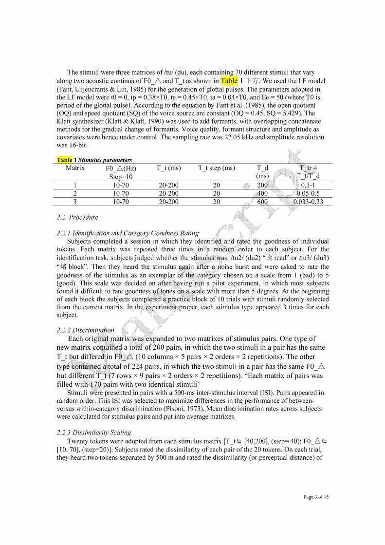
The stimuli were three matrices of /tu/ (du), each containing 70 different stimuli that vary

along two acoustic continua of F0_△ and T_t as shown in Table 1 下方. We used the LF model

(Fant, Liljencrants & Lin, 1985) for the generation of glottal pulses. The parameters adopted in

the LF model were t0 = 0, tp = 0.38×T0, te = 0.45×T0, ta = 0.04×T0, and Ee = 50 (where T0 is period of the glottal pulse). According to the equation by Fant et al. (1985), the open quotient (OQ) and speed quotient (SQ) of the voice source are constant (OQ = 0.45, SQ = 5.429). The

Klatt synthesizer (Klatt & Klatt, 1990) was used to add formants, with overlapping concatenate methods for the gradual change of formants. Voice quality, formant structure and amplitude as

covariates were hence under control. The sampling rate was 22.05 kHz and amplitude resolution was 16-bit.

Table 1 Stimulus parameters

Matrix F0_△(Hz)

Step=10

T_t (ms) T_t step (ms) T_d

(ms)

T_tr =

T_t/T_d

1 10-70 20-200 20 200 0.1-1 2 10-70 20-200 20 400 0.05-0.5 3 10-70 20-200 20 600 0.033-0.33

2.2. Procedure

2.2.1 Identification and Category Goodness Rating

Subjects completed a session in which they identified and rated the goodness of individual tokens. Each matrix was repeated three times in a random order to each subject. For the

identification task, subjects judged whether the stimulus was. /tu2/ (du2) “读 read” or /tu3/ (du3)

“堵 block”. Then they heard the stimulus again after a noise burst and were asked to rate the

goodness of the stimulus as an exemplar of the category chosen on a scale from 1 (bad) to 5

(good). This scale was decided on after having run a pilot experiment, in which most subjects

found it difficult to rate goodness of tones on a scale with more than 5 degrees. At the beginning of each block the subjects completed a practice block of 10 trials with stimuli randomly selected

from the current matrix. In the experiment proper, each stimulus type appeared 3 times for each subject.

2.2.2 Discrimination

Each original matrix was expanded to two matrixes of stimulus pairs. One type of

new matrix contained a total of 200 pairs, in which the two stimuli in a pair has the same

T_t but differed in F0_△ (10 columns × 5 pairs × 2 orders × 2 repetitions). The other

type contained a total of 224 pairs, in which the two stimuli in a pair has the same F0_△

but different T_t (7 rows × 9 pairs × 2 orders × 2 repetitions). “Each matrix of pairs was

filled with 170 pairs with two identical stimuli” Stimuli were presented in pairs with a 500-ms inter-stimulus interval (ISI). Pairs appeared in

random order. This ISI was selected to maximize differences in the performance of between- versus within-category discrimination (Pisoni, 1973). Mean discrimination rates across subjects were calculated for stimulus pairs and put into average matrixes.

2.2.3 Dissimilarity Scaling

Twenty tokens were adopted from each stimulus matrix [T_t∈ [40,200], (step= 40); F0_△∈

[10, 70], (step=20)]. Subjects rated the dissimilarity of each pair of the 20 tokens. On each trial,

they heard two tokens separated by 500 m and rated the dissimilarity (or perceptual distance) of

of 16

each pair on an integer scale from 1 (similar) to 5 (dissimilar). In each block each subject completed a practice block of 10 trials with pairs randomly selected from the current matrix.

3.0 Analyses and Results 3.1. Identification

A repeated ANOVA by subjects on mean P_I of each matrix (Table 2) yielded a significant main effect of syllable duration [F (14, 588) = 45.4, p<0.005]. The longer the duration, the more

tokens in the matrix are identified as Tone 2. Based on the binomial distribution of the identification scores (P_I) and the sigmoid shape of

the response function, a logistic regression as in Eq. (1) between P_I and the two repeated

measure predictors (T_t & F0_△) was adopted to obtain the mean identification function for each

matrix. This method was adapted from Xu, Gandour & Francis (2006).

(1)

By generalizing the category boundary from a single value to a function, we derived the mean

position of the category boundary in each matrix from the function involving T_t and F0_△

corresponding to the 50% identification score. See Eq. (2).

(2)

The estimated regression coefficients are presented in Table 2. As shown by the coefficients in

the response functions, as syllable duration gets longer, category boundary moves rightwards, indicating that a longer duration of the falling phase is allowed for Tone 2 when syllable duration increases.

Table 2 Correlations of z-transformed goodness and identification score

T_d (ms) mean P_I b0 b1 b2 b1/b2 200 0.504 4.864 −0.039 −0.015 2.600 400 0.592 7.315 −0.042 −0.047 0.894 600 0.663 7.628 −0.038 −0.053 0.717

3.2. Discrimination

For discrimination curve along one acoustic continuum, its peak was taken as the categorical boundary (Liberman, et al., 1957). Generalizing this idea to a discrimination surface, its ridge was

taken as the counterpart of “peak” on the classical discrimination curve. The average discrimination rate (P_d) of each stimulus-pair was assigned to the point between them in the

matrix. For example, if the two stimuli were specified as [F0_△=10 Hz, T_t =160 ms] and

[F0_△ = 30 Hz, T_t = 160 ms], the correlated P_d was assigned to [F0_△ = 20 Hz, T_t = 160

ms]. Functions of the original data are shown in Fig. 4. A smooth P_d function was obtained by interpolating T_t and F0_△ at 20 times with a cubic

method. Assuming that one discrimination space contains only one category boundary and this

category boundary intercepts the limits of F0_△, a quadratic regression between the interpolated

discrimination rate and T_t was applied to each array of data sharing F0_△. Then the set of {T_t,

F0_△} corresponding to the vertexes of the estimated functions was taken as the category

boundary in the discrimination data (Fig. 4).

When stimuli in pairs are different in F0_△, the discrimination rate decreases as F0_△

increases. For T_t coordinate arrays of category boundary, RM-ANOVAs were performed with

duration (200, 400, 600 ms) and pair difference (in F0_△, in T_t) as within-subject factors. The

RM-ANOVA showed a main effect of duration [F (2, 160) = 173.720, p<0.005] and pair

of 16

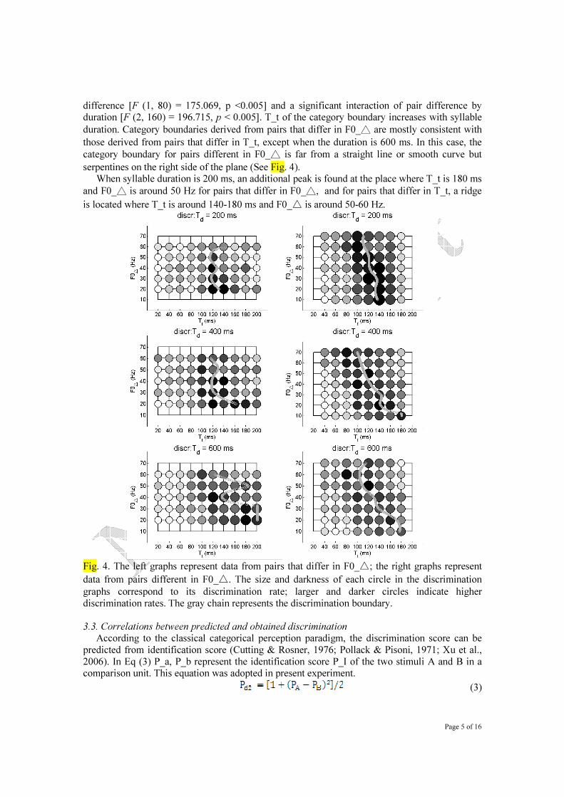
difference [F (1, 80) = 175.069, p <0.005] and a significant interaction of pair difference by duration [F (2, 160) = 196.715, p < 0.005]. T_t of the category boundary increases with syllable

duration. Category boundaries derived from pairs that differ in F0_△ are mostly consistent with

those derived from pairs that differ in T_t, except when the duration is 600 ms. In this case, the

category boundary for pairs different in F0_△ is far from a straight line or smooth curve but

serpentines on the right side of the plane (See Fig. 4). When syllable duration is 200 ms, an additional peak is found at the place where T_t is 180 ms

and F0_△ is around 50 Hz for pairs that differ in F0_△, and for pairs that differ in T_t, a ridge

is located where T_t is around 140-180 ms and F0_△ is around 50-60 Hz.

Fig. 4. The left graphs represent data from pairs that differ in F0_△; the right graphs represent

data from pairs different in F0_△. The size and darkness of each circle in the discrimination

graphs correspond to its discrimination rate; larger and darker circles indicate higher

discrimination rates. The gray chain represents the discrimination boundary.

3.3. Correlations between predicted and obtained discrimination According to the classical categorical perception paradigm, the discrimination score can be

predicted from identification score (Cutting & Rosner, 1976; Pollack & Pisoni, 1971; Xu et al.,

2006). In Eq (3) P_a, P_b represent the identification score P_I of the two stimuli A and B in a comparison unit. This equation was adopted in present experiment.

(3)

of 16

The similarity in the shape of the two discrimination functions was measured by Fisher’s z-transformed correlation coefficient (z) of the Pearson product correlation coefficient (r) to obtain

normally distributed data. Correlation coefficients (r) and (z) between discrimination rates obtained from average

discrimination matrices and the discrimination rates predicted from average identification matrices are shown in Table 3. All the correlations are significant [p < 0.05, df = 48 for matrixes

different in F0_△, df = 54 for matrixes different in T_t]. Effects of pair difference and syllable

duration are both insignificant [p > 0.05, df = 2]. But correlation increases with syllable duration.

For z-transformed correlations calculated for each subject. RM-ANOVA were performed with

duration [200, 400, 600 ms] and pair difference (in F0_△, in T_t) as within-subject factors. It

shows neither a main effect of pair difference [F (1, 14) = 2.539, p >0.05], nor a main effect of duration [F (2, 28) = 0.025, p >0.05], but the interaction of pair difference and duration is

significant [F (2, 28) = 3.522, p<0.005]. Further one-way RM-ANOVAs show that only for the

subgroup with durations of 600 ms, is the effect of pair difference significant [F (1, 14) =4.812,

p<0.005]. When the duration is 600 ms, obtained matrices with pairs different in F0_△ are more

similar to the predicted matrixes than those with pairs different in T_t. Correlations of obtained and predicted discrimination data are much greater for average

matrices than for corresponding matrixes by individual subjects.

Table 3. Correlations of obtained and predicted discrimination data for average matrixes.

T_d (ms) different in r z 200 F0_△ 0.380 * 0.401

200 T_t 0.490 * 0.536

400 F0_△ 0.559 * 0.631

400 T_t 0.528 * 0.587

600 F0_△ 0.618 * 0.722

600 T_t 0.583 * 0.667

3.4 Category Goodness Rating

The comparison of identification and goodness ratings revealed differences across matrixes

and complexity hidden under identification result. Goodness rating data of each matrix by each subject were normalized into z-scores to reduce individual biases. The identification and goodness rating were averaged across subjects for each token of each matrix respectively.

For 200 ms tokens identified as Tone 3, only a few near the category boundary are good ones.

When the turning phase is longer than 160 ms, which is proportionally 0.8 of the syllable duration,

and the goodness is low, especially when the falling phase falls more. Some subjects reported they heard /tu4/ (du4) in these trials, indicating that these tokens fall into another category Tone 4 (a falling tone). Tokens with goodness lower than 2.5 are represented by squares in Fig. 7.

The best Tone 2 and Tone 3 stimulus positions were calculated for each subject by

determining the t_t and F0_∆ frequencies of the Tone 2 and Tone 3 tokens with the highest

goodness ratings. The shading in Fig. 5 represents how frequently each token is taken as the best token. As shown in Fig. 5, the best tokens spread through their corresponding category. When syllable duration is 200 ms, best Tone 3 tokens are near the category boundary. This is consistent

with average goodness and can be explained by the finding that most 200-ms stimuli with T_t longer than 160 ms fall into an other category. Most subjects always take some tokens as equally

best. The number of the 15 subjects who assign the highest rating to more than one tokens was

9 for Tone 2 of 200 ms, 6 for Tone 3 of 200 ms, 10 for Tone 2 of 400 ms, 7 for Tone 3 of 400 ms, 9 for Tone 2 of 600 ms and 6 for Tone 3 of 600 ms.

of 16

For each subject who takes no more than three tokens as the best of a category, a z-test was carried out to determine whether the goodness of the best token(s) is significantly different from the others in the same category. Best tokens with goodness significantly (p < 0.05) different from

the others are represented by circles in Fig. 5 with subject ID noted. Positions of these best tokens

differ across subjects. Only the following stimuli were rated significantly better than others by more than one subject: [140 ms, 20 Hz] and [140 ms, 10 Hz] for Tone 3 of 200 ms, [180 ms, 50 Hz], [180 ms, 70 Hz], and [200 ms, 40 Hz] for Tone 3 of 400 ms, [20 ms, 10Hz] and [20 ms, 20

Hz] for Tone 2 of 600 ms, and [180 ms, 70 Hz] for Tone 3of 600 ms. This kind of best tokens seem to occur more often in Tone 3 categories.

In sum, best tokens scatter through corresponding categories, one subject usually having more than one best token for a category, and even if one subject has only one best token for a category and the goodness of this token is significantly higher than others, the position of this token not

necessarily coincides with that of other subjects.

Fig. 5. Distribution of best tokens. The darker a pixel is, the more frequently the corresponding stimulus is taken as a best token. Those Best tokens whose goodness significantly different from

the other tokens of the same category and of which no more than 2 tokens share the same goodness are represented with circles. Subject ID is labeled by the upper right side of the token.

Pearson product correlations and Canny edge detection (Canny, 1987) were adopted to

examine the relationship between goodness and identification. Inter-subject averaged z-

transformed goodness (G_z) and identification scores (P_I) were adopted for the correlation.

Tone 2 tokens and Tone 3 tokens were calculated separately. The correlations are shown inTable .

For Tone 2 tokens, goodness positively correlates with identification score, indicating that when a

Tone 2 token is rated with higher goodness, it is more likely to be identified as Tone 2. For Tone 3 tokens, when syllable duration is 600 ms, goodness negatively correlates with identification scores, indicating that when a Tone 3 token is rated with higher goodness, it is less likely to be

identified as Tone 2 and correspondingly more likely to be identified as Tone 3; when syllable

duration is 400 ms, the correlation is negative but insignificant; when syllable duration is 200 ms,

like what have been shown in Fig. 5 and Fig. 7, best tokens and highly-rated tokens are near category boundary, which leads to the significant positive correlation between goodness and identification score.

Correlations were also calculated for each subject. Correlations for Tone 2 tokens are significant for most subjects [df = 68, p < 0.05, except for subject 10 and 13 for tokens of 200 ms,

subject 14 for tokens of 400ms, and subject 12, 15 for tokens of 600 ms]. Correlations for Tone 3 tokens are insignificant for most subjects [df = 68, p > 0. 05], significant [df = 68, p < 0. 05] only

for the following subjects: subject 12 and 13 for tokens of 200 ms, subject 1, 2, 9, 13 for tokens

of 400 ms, and subject 1, 2, 11, 13 for tokens of 600 ms. Hence, the positive correlations of

goodness and identification score of Tone 2 are significant for most subjects, but the negative

of 16

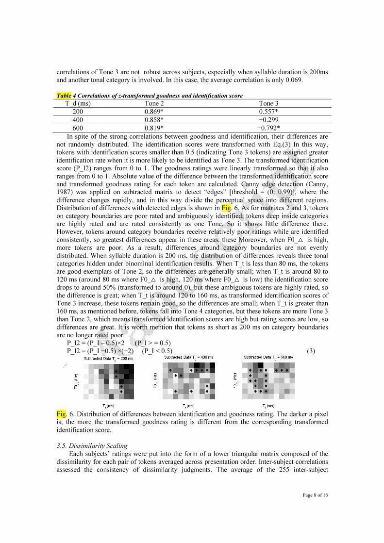
correlations of Tone 3 are not robust across subjects, especially when syllable duration is 200ms and another tonal category is involved. In this case, the average correlation is only 0.069.

Table 4 Correlations of z-transformed goodness and identification score

T_d (ms) Tone 2 Tone 3 200 0.869* 0.557* 400 0.858* −0.299 600 0.819* −0.792*

In spite of the strong correlations between goodness and identification, their differences are not randomly distributed. The identification scores were transformed with Eq.(3) In this way, tokens with identification scores smaller than 0.5 (indicating Tone 3 tokens) are assigned greater

identification rate when it is more likely to be identified as Tone 3. The transformed identification score (P_I2) ranges from 0 to 1. The goodness ratings were linearly transformed so that it also

ranges from 0 to 1. Absolute value of the difference between the transformed identification score and transformed goodness rating for each token are calculated. Canny edge detection (Canny, 1987) was applied on subtracted matrix to detect “edges” [threshold = (0, 0.99)], where the

difference changes rapidly, and in this way divide the perceptual space into different regions. Distribution of differences with detected edges is shown in Fig. 6. As for matrixes 2 and 3, tokens

on category boundaries are poor rated and ambiguously identified; tokens deep inside categories are highly rated and are rated consistently as one Tone. So it shows little difference there. However, tokens around category boundaries receive relatively poor ratings while are identified

consistently, so greatest differences appear in these areas. these Moreover, when △F0_ is high,

more tokens are poor. As a result, differences around category boundaries are not evenly

distributed. When syllable duration is 200 ms, the distribution of differences reveals three tonal categories hidden under binominal identification results. When T_t is less than 80 ms, the tokens are good exemplars of Tone 2, so the differences are generally small; when T_t is around 80 to

120 ms (around 80 ms where △ △F0_ is high, 120 ms where F0_ is low) the identification score

drops to around 50% (transformed to around 0), but these ambiguous tokens are highly rated, so

the difference is great; when T_t is around 120 to 160 ms, as transformed identification scores of Tone 3 increase, these tokens remain good, so the differences are small; when T_t is greater than 160 ms, as mentioned before, tokens fall into Tone 4 categories, but these tokens are more Tone 3

than Tone 2, which means transformed identification scores are high but rating scores are low, so

differences are great. It is worth mention that tokens as short as 200 ms on category boundaries

are no longer rated poor. P_I2 = (P_I – 0.5)×2 (P_I > = 0.5)

P_I2 = (P_I −0.5) ×(−2) (P_I < 0.5) (3)

Fig. 6. Distribution of differences between identification and goodness rating. The darker a pixel is, the more the transformed goodness rating is different from the corresponding transformed

identification score.

3.5. Dissimilarity Scaling

Each subjects’ ratings were put into the form of a lower triangular matrix composed of the

dissimilarity for each pair of tokens averaged across presentation order. Inter-subject correlations assessed the consistency of dissimilarity judgments. The average of the 255 inter-subject

of 16

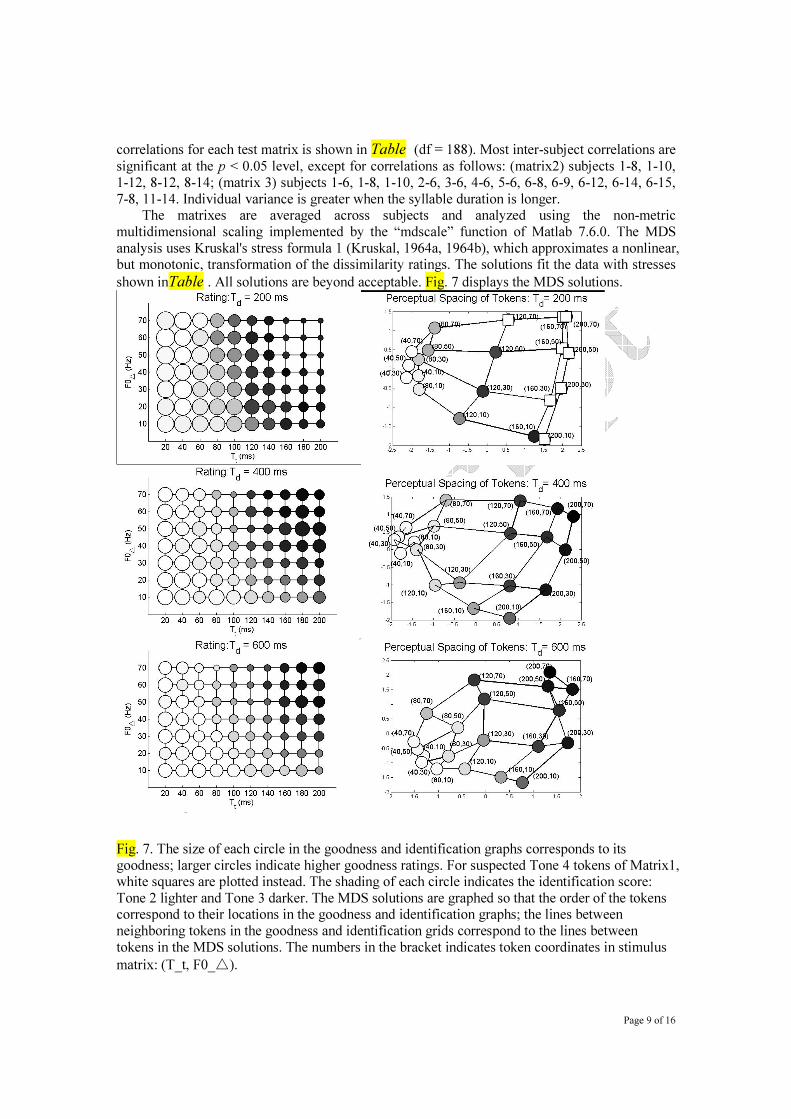
correlations for each test matrix is shown in Table (df = 188). Most inter-subject correlations are

significant at the p < 0.05 level, except for correlations as follows: (matrix2) subjects 1-8, 1-10,

1-12, 8-12, 8-14; (matrix 3) subjects 1-6, 1-8, 1-10, 2-6, 3-6, 4-6, 5-6, 6-8, 6-9, 6-12, 6-14, 6-15,

7-8, 11-14. Individual variance is greater when the syllable duration is longer. The matrixes are averaged across subjects and analyzed using the non-metric

multidimensional scaling implemented by the “mdscale” function of Matlab 7.6.0. The MDS

analysis uses Kruskal's stress formula 1 (Kruskal, 1964a, 1964b), which approximates a nonlinear, but monotonic, transformation of the dissimilarity ratings. The solutions fit the data with stresses

shown inTable . All solutions are beyond acceptable. Fig. 7 displays the MDS solutions.

Fig. 7. The size of each circle in the goodness and identification graphs corresponds to its

goodness; larger circles indicate higher goodness ratings. For suspected Tone 4 tokens of Matrix1, white squares are plotted instead. The shading of each circle indicates the identification score:

Tone 2 lighter and Tone 3 darker. The MDS solutions are graphed so that the order of the tokens correspond to their locations in the goodness and identification graphs; the lines between

neighboring tokens in the goodness and identification grids correspond to the lines between

tokens in the MDS solutions. The numbers in the bracket indicates token coordinates in stimulus

matrix: (T_t, F0_△).

of 16

Table 5 Averages inter-subject correlations of dissimilarity scaling and stress of MDS solutions shown in

Fig. 7

T_d (ms) Averages inter-subject correlations MDS stress1

200 0.561 0.076 (good - fair )

400 0.339 0.100 (fair)

600 0.247 0.130 (fair- acceptable)

The MDS solutions revealed influences of both acoustic distance and category goodness on perceptual dissimilarity. The ordering of tokens on the horizontal axes corresponds to T_t and the

vertical ordering of tokens corresponds to F0_△, demonstrating a strong relationship between

dissimilarity and acoustic distance. In addition, the perceptual space clusters in regions with high

goodness ratings. The distortion of the perceptual space may be attributed to Magnet effect (P. Iverson & Kuhl, 1996; Partricia K. Kuhl & Iverson, 1995). Nevertheless, the influences of

category goodness on perceptual dissimilarity are different between Tone 2 tokens and Tone 3 tokens. As shown by the MDS solutions, Tone 2 tokens cluster closely together, but the clustering of Tone 3 tokens is much looser. Moreover, for Tone 3 tokens, the contributions of T_t variance

and F0_△ variance are different. The perceptual spaces of Tone 3 cluster more along T_t

dimensions than along F0_△ dimensions.

As discussed in the former section, the category goodness data of Matrix1 (T_d = 200 ms) reveal complexity hidden under identification result. For tokens identified as Tone 3, only a few near the category boundary are good ones. When the falling phase is longer than 160 ms, which is

proportionally 0.8 of the syllable duration, and especially when the falling phase falls a lot, the

tokens falls into another category Tone 4 (a falling tone). Correspondingly, the MDS solution

cluster into 3 groups. The left group is Tone 2, consistent with other stimulus matrix. Tokens of the middle group share a same T_t of 120 ms, which are Tone 3. The right group is Tone 4. The

perceptual space of Tone 4 also clusters more in T_t dimension than in F0_△ dimension.

As shown in the former section, when syllable duration is 400 or 600 ms, there are more

poor exemplars distributed on areas with high △F0_ and middle T_t. This is consistent with the △ △farther departure around category boundaries in high F0_ areas than low F0_ areas.

3.3. Tests of the relationship between dissimilarity, acoustic differences, identification, and goodness

Additional analyses further assessed how well acoustic differences, identification, and goodness predict dissimilarity. Datum transformations of acoustic differences, identification and

goodness were adapted from (P. Iverson & Kuhl, 1996). The identification score were used to estimate identification distances by calculating the absolute value of the difference for each pair of tokens. Acoustic distances were estimated by measuring the distances between tokens in the

two-dimensional stimulus space displayed in Fig. 7(calculated by taking the root means of the squared differences of coordinates). Goodness was quantified by averaging the z-transformed

goodness ratings for each pair of tokens, but 1 is assigned to the pair with tokens from different

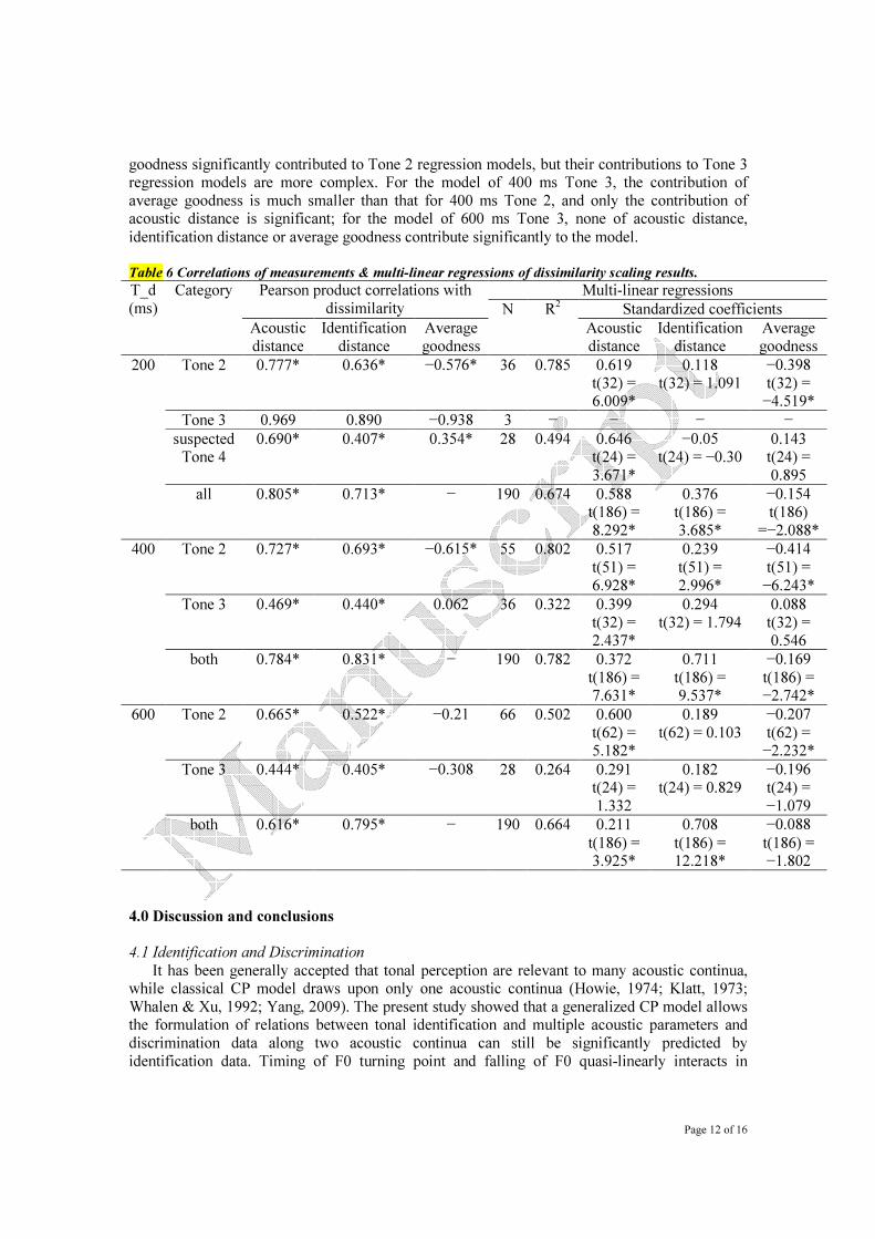
categories. Table displays the results of the multi-linear regression analyses. Separate analyses were

conducted for each category of each stimulus matrix and another analysis was conducted for all tokens of each matrix together. For stimulus matrix of 200 ms, a separate analysis was carried out

for tokens rated lower than 2.5, which was suspected to be Tone 4 as mentioned in former

sections. For Tone 2 tokens of 200 ms, the model accounts for 78.5% of the variance, and

acoustic distance [t (32) = 6.009, p < 0.05] and average goodness [t (32) = −4.519, p < 0.05] significantly contribute to the regression model, while the contribution of identification distance [t (32) = 1.091, p > 0.05] is insignificant. For Tone 3 tokens of 200 ms, the number of tokens is

of 16

too small for a meaningful regression. For suspected Tone 4 tokens of 200 ms, which were identified as poor exemplars of Tone 3,the model accounts for 49.4% of the variance, and

acoustic distance [t(24) = 3.671, p < 0.05] significantly contributes to the regression model, while the contributions of identification distance [t(24) = −0.30, p > 0.05] and average goodness [t(24)

= 0.895, p > 0.05] are insignificant. For all tokens of 200 ms, the model accounts for 67.4% of the variance, and acoustic distance [t (186) = 8.292, p < 0.05], identification distance [t (186) = 3.685, p < 0.05], and average goodness [t (186) = −2.088, p < 0.05] all significantly contribute to

the regression model. For Tone 2 tokens of 400 ms, the model accounts for 80.2% of the variance, and acoustic distance [t (51) = 6.928, p < 0.05], identification distance [t (51) = 2.996, p > 0.05],

and average goodness [t (51) = −6.243, p < 0.05] all significantly contribute to the regression model. For Tone 3 tokens of 400 ms, the model accounts for 32.2% of the variance, and acoustic distance [t (32) = 2.437, p < 0.05] significantly contributes to the regression model, while the

contributions of identification distance [t (32) = 1.794, p > 0.05] and average goodness [t (32) = 0.546, p > 0.05] are insignificant. For all tokens of 400 ms, the model accounts for 78.2% of the

variance, and acoustic distance [t (186) = 7.631, p < 0.05], identification distance [t (186) = 9.537,

p < 0.05], and average goodness [t (186) = −2.742, p < 0.05] all significantly contribute to the

regression model. For Tone 2 tokens of 600 ms, the model accounts for 50.2% of the variance, and acoustic distance [t (62) = 5.182, p < 0.05] and average goodness [t (62) = −2.232, p < 0.05] significantly contribute to the regression model, while the contribution of identification distance

[t (62) = 0.103, p > 0.05] is insignificant. For Tone 3 tokens of 600 ms, the model accounts for

26.4% of the variance, but none of acoustic distance [t (24) = 1.332, p >0.05], identification

distance [t (24) = 0.829, p > 0.05], and average goodness [t (24) = −1.079, p > 0.05] significantly contributes to the regression model. For all tokens of 600 ms, the model accounts for 66.4% of the variance, and acoustic distance [t (186) = 3.925, p < 0.05] and identification distance [t (186)

= 12.218, p < 0.05] significantly contribute to the regression model, while the contribution of

average goodness [t (186) = −1.802, p > 0.05] is insignificant. For all models, all of the condition

indexes are less than 15, indicating that there is no significant problem of collinearity. Table also displays Pearson product correlations of dissimilarity with acoustic differences,

identification distances and average goodness. Correlations with average goodness of all tokens are excluded because the constant “1” assigned to inter-category pairs would make the correlation

biased. Except for the only three Tone 3 tokens of 200 ms, all correlations with acoustic distances and identification distances are significant. Average goodness only reveals significant

correlations with dissimilarity when the model accounts for Tone 2 categories of 200ms or 400ms or suspected Tone 4 categories of 200 ms.

In most cases (except for the model for all tokens of 600 ms), acoustic distance most strongly

corresponds to dissimilarity; subjects judged that tokens were more different to the extent that

they had T_t and F0_△ differences. Dissimilarity is also related to identification distance and

average goodness; subjects judged that tokens were more different when they were identified

differently, and they thought tokens were more similar when they were good exemplars of the

same category. In addition, while only identification distance would predict that tokens in a same category should have uniform dissimilarity, the patterns of clustering for Tone 2 tokens are better predicted by average goodness. Goodness significantly contributes to Tone 2 models and the two

models involving all tokens of 200 ms and 400 ms. These findings offer supports for Magnet

Effect.

However, as revealed by the models, obvious differences reveal themselves between Tone 2 and Tone 3 categories. Firstly, the perceptual space of Tone 3 tokens does not cluster like corresponding Tone 2 tokens; instead, the space almost represents the acoustic distances of these

tokens. The perceptual space of 600 ms Tone 3 tokens partly twists toward the category boundary,

but it can hardly be predicted by either acoustic distance or average goodness. Secondly, the

regression models for Tone 2 always accounts for more than 50% of the variance, while the models for Tone 3 leave out much more variance. And last, both acoustic distances and average

of 16

goodness significantly contributed to Tone 2 regression models, but their contributions to Tone 3 regression models are more complex. For the model of 400 ms Tone 3, the contribution of

average goodness is much smaller than that for 400 ms Tone 2, and only the contribution of acoustic distance is significant; for the model of 600 ms Tone 3, none of acoustic distance,

identification distance or average goodness contribute significantly to the model. Table 6 Correlations of measurements & multi-linear regressions of dissimilarity scaling results.

T_d

(ms)

Category Pearson product correlations with

dissimilarity

Multi-linear regressions N R

2 Standardized coefficients

Acoustic

distance

Identification

distance

Average

goodness

Acoustic

distance

Identification

distance

Average

goodness 200 Tone 2 0.777* 0.636* −0.576* 36 0.785 0.619

t(32) = 6.009*

0.118 t(32) = 1.091

−0.398

t(32) = −4.519*

Tone 3 0.969 0.890 −0.938 3 − − − − suspected

Tone 4 0.690* 0.407* 0.354* 28 0.494 0.646

t(24) =

3.671*

−0.05

t(24) = −0.30 0.143

t(24) =

0.895 all 0.805* 0.713* − 190 0.674 0.588

t(186) =

8.292*

0.376 t(186) =

3.685*

−0.154

t(186)

=−2.088* 400 Tone 2 0.727* 0.693* −0.615* 55 0.802 0.517

t(51) =

6.928*

0.239

t(51) =

2.996*

−0.414

t(51) =

−6.243* Tone 3 0.469* 0.440* 0.062 36 0.322 0.399

t(32) =

2.437*

0.294 t(32) = 1.794

0.088 t(32) =

0.546 both 0.784* 0.831* − 190 0.782 0.372

t(186) = 7.631*

0.711

t(186) = 9.537*

−0.169

t(186) = −2.742*

600 Tone 2 0.665* 0.522* −0.21 66 0.502 0.600

t(62) = 5.182*

0.189

t(62) = 0.103

−0.207

t(62) = −2.232*

Tone 3 0.444* 0.405* −0.308 28 0.264 0.291 t(24) =

1.332

0.182 t(24) = 0.829

−0.196

t(24) =

−1.079 both 0.616* 0.795* − 190 0.664 0.211

t(186) = 3.925*

0.708

t(186) = 12.218*

−0.088

t(186) = −1.802

4.0 Discussion and conclusions

4.1 Identification and Discrimination

It has been generally accepted that tonal perception are relevant to many acoustic continua, while classical CP model draws upon only one acoustic continua (Howie, 1974; Klatt, 1973;

Whalen & Xu, 1992; Yang, 2009). The present study showed that a generalized CP model allows the formulation of relations between tonal identification and multiple acoustic parameters and

discrimination data along two acoustic continua can still be significantly predicted by

identification data. Timing of F0 turning point and falling of F0 quasi-linearly interacts in

of 16

predicting category boundary. This result suggested that categorical perception CP paradigm is applicable when more than one acoustic continuum is taken into consideration. This

generalization of CP offered a new approach to investigate interactions of different acoustic continua relevant to phonological categories.

4.2. Different internal structures of Tone 2 and Tone 3 categories

There has always been a lot conflicting around Putonghua Tone 2 and Tone 3. On one way, Tone 2 and Tone 3 are often confused with each other, both for foreigners and native acquisition

(Gandour, 1983; Li & Thompson, 1977; So & Best, 2010). On the other way, they are very similar, even occasionally identical, in their pitch contour. This causes difficulties of linguistic description. Traditionally Tone 2 was describes as “high rising”, Tone 3 as “low falling rising” or

“low dipping ”(Chao, 1955) in their pitch contour. Phonologists used to attribute the conflicting descriptions of Tone 3 to different assumptions about its underlying phonological representation

(Gandour, 1983; Yip, 1980). But the concrete fact underlying is that the two tones (especially Tone 3) show such great variation in their acoustic forms that researchers are always arguing

about which acoustic parameters are responsible for their respective individual integrity, though this integrity is phonologically self-evident.

By using fully synthesized stimuli, present study put formerly mentioned covariants under

control and focuses on the F0 contour. The result supported earlier research that perceptual

distance shrunk around good exemplars and goodness rating significantly contributes to

similarity/dissimilarity scaling. And except for stimulus of 200 ms, identification and goodness rating space on both sides of category boundaries are generally symmetric. However, obvious differences revealed themselves between Tone 2 and Tone 3 categories. All Tone 2 tokens

resemble each other; each Tone 3 token is unique in its own way. Dissimilarity scaling of Tone 2

tokens can be well predicted by acoustic distance, goodness and identification; but dissimilarity

scaling of Tone 3 tokens seems to account mostly on acoustic distance. This indicates that the perception of these two tones may rely differently on a same set of

acoustic cues. Tone 3 sometimes contain creaky voice (but not necessarily) (Keating & Esposito,

2007; Kong, 2007), which has been taken as part of the realization of the tone (Yang, 2009). And

perceived category boundaries are different for two sets of stimuli with same adjusted pitch

contours but different original tone (Yang, 2009). Some phonologists asserts that Tone 3 belongs to another register (Duanmu, 1990; Yip, 1980). Thus, it is reasonable to propose that, in respect of pitch contour, Tone 2 holds its integrity as acoustic stimuli which is to a side of a 2-D category

boundary, and as long as a stimulus fits this criteria, it is taken as Tone 2; but Tone 3 is just

perceived as the rest stimuli which are not Tone1, Tone 2 and Tone 4 (its relation with the other

two tones needs further proof), so each token can still be perceived differently. On the other way, specific voice quality features may be responsible for the integrity of Tone 3. Though specific

voice quality is not necessary for Tone 3 identification, it could be sufficient or contribute greatly to the integrity of Tone 3. A further hypothesis can be raise that if right voice quality is add to stimuli, the perceptual space of Tone 3 will shrink like that of Tone 2.

4.3. Goodness rating does not support a single distinctive prototype but is not “nothing”

Former studies assumed that a token with the highest goodness is the “prototype” of a specific category (P. Iverson & Kuhl, 1996). However, this assumption suffers two obvious challenges. Firstly, how can the possibility of multiple prototypes are eliminated when more than one best

token are found? As mentioned in (P. Iverson & Kuhl, 1996), best frequencies were averaged when more than one token received the same highest rating. This could result a false place of

“prototype” if those best tokens were far away. Secondly, even with only one best token, unless the second best and others are significantly worse than it, it is difficult to eliminate the possibility that the position of the best token is just a result of random chance.

of 16

Regarding these two aspects, we examined the distribution of best tokens across subjects and tested the difference of the best tokens with other tokens. As a result, best tokens dispersed

instead of clustering within a respective category, most subjects always assign highest ratings to more than one tokens of a category, and even when the goodness of the only few (no more than

three) best tokens is significantly higher than others, the positions of these tokens not necessarily coincides with those by other subjects. Advocators for “prototypes” may attribute the dispersion of best tokens to the theory that different subjects develop different prototypes from their own

language experiences. They can also attribute multiple best tokens to complex experiences. Except that some stimuli seem to be taken as best tokens more frequently than others, there is

little support for a single distinctive “prototype” in the two tonal categories of Putonghua speaking Beijingers.

(Lotto, et al., 1998) argued against the importance of goodness rating, claiming that its

contribution on predicting perceptual distance reveals nothing more than the differences of within and across category discriminability. However, the present study proved that rating data not only

reveal undercover internal structure within tonal categories, but also contribute significantly in

predicting dissimilarity across Tone 2 tokens. If the syllable duration is short enough, tokens on

category boundaries are no longer rated poor, no matter what tone they are identified as. As syllable duration grows longer, poor exemplars appear around category boundaries. These poor exemplars are not evenly distributed along category boundaries. More importantly, this

dissymmetry of goodness rating better predicts the distortion of dissimilarity data than distributed

identification scores which are mostly symmetrically distributed along category boundaries. In a

word, goodness has its own contribution in revealing mental representation of tone categories. 4.4. The influence of brief duration on the internal structure of tones

When syllable duration is as short as 200 ms, the internal structures of tonal categories

revealed some peculiar features. Most of these features can be attributing to the involvement of Tone 4. Firstly, tokens with long and great falling phase were poorly rated as Tone 3. This is because they mostly sound like Tone 4. Secondly, tokens with long but small falling phase

however were better rated than those with long and great falling phase, even when there is no ring phase. Discrimination data also showed additional peak between tokens with long great and long

small falling phase. This confirmed the classical “low level” description variant of Tone 3. Correspondingly, only a small set of tokens with middle length of falling phase are good Tone 3 tokens, very close to the category boundary of identification. However, an additional feature

cannot be attributed to the involvement of Tone 4. For stimulus matrix with longer durations, tokens on and around category boundaries were poor rated, just like what had been reported in

former studies. But none of real Tone 2 and Tone 3 tokens was rated poor when syllable duration is 200 ms (poor rates are given instead to tokens like Tone 4). Two possible explanations are available here: either the category boundary actually lies between Tone 2 and Tone 3 tokens so

that no stimulus on the category boundary is rated, or there is no longer poor tokens between Tone 2 and Tone 3 categories when syllables are short enough, which means a different model of

internal structure of tonal category.

Acknowledgements

of 16

Reference List Abramson, A. S. (1979). The noncategorical perception of tone categories in Thai. Frontiers of

speech communication research, 127-134.

Blicher, D. L., Diehl, R. L., & Cohen, L. B. (1990). Effects of syllable duration on the perception of the Mandarin Tone 2/Tone 3 distinction: Evidence of auditory enhancement. Journal of Phonetics.

Canny, J. (1987). A computational approach to edge detection. Readings in computer vision: issues, problems, principles, and paradigms, 184, 87-116.

Chan, S. W., Chuang, C. K., & Wang, W. S. Y. (1975). Crosslanguage study of categorical perception for lexical tone. Journal of the Acoustical Society of America, 58, 119.

Chao, Y. R. (1955). Mandarin primer.

Cutting, J. E., & Rosner, B. S. (1976). Discrimination functions predicted from categories in speech and music. Perception and Psychophysics, 20, 87-88.

Duanmu, S. (1990). A formal study of syllable, tone, stress and domain in Chinese languages.

MIT. Fant, G., Liljencrants, J., & Lin, Q. (1985). A four-parameter model of glottal flow. STL-QPSR, 4,

1-13. Fu, Q. J., & Zeng, F. G. (2000). Identification of temporal envelope cues in Chinese tone

recognition. ASIA PACIFIC JOURNAL OF SPEECH LANGUAGE AND HEARING, 5,

45-58. Gandour, J. T. (1978). "Perceived dimensions of 13 tones: a multidimensional scaling

investigation." Phonetica 35(3): 169. Gandour, J. (1983). Tone perception in Far Eastern languages. Journal of Phonetics, 11, 149-175.

Garding, E., Kratochvil, P., Svantesson, J. O., & Zhang, J. (1986). Tone 4 and Tone 3 discrimination in modern Standard Chinese. Language and Speech, 29, 281.

Hallé, P. A. (1994). "Evidence for tone-specific activity of the sternohyoid muscle in Modern Standard Chinese." Language and speech 37(2): 103.

Howie, J. M. (1974). On the domain of tone in Mandarin. Phonetica, 30, 129-148.

Iverson, P., & Kuhl, P. K. (1995). Mapping the perceptual magnet effect for speech using signal detection theory and multidimensional scaling. Journal of the Acoustical Society of

America, 97, 553-562.

Iverson, P., & Kuhl, P. K. (1996). Influences of phonetic identification and category goodness on

American listeners’ perception of /r/ and /l/. The Journal of the Acoustical Society of America, 99, 1130.

Iverson, P., & Kuhl, P. K. (2000). Perceptual magnet and phoneme boundary effects in speech perception: Do they arise from a common mechanism? Perception and Psychophysics, 62,

874-886.

Iverson, P., Kuhl, P. K., Akahane-Yamada, R., Diesch, E., Tohkura, Y., Kettermann, A., &

Siebert, C. (2003). A perceptual interference account of acquisition difficulties for non-native phonemes. Cognition, 87, B47-B57.

Keating, P., & Esposito, C. (2007). Linguistic voice quality. Working Papers in Phonetics, Department of Linguistics, UCLA, UC Los Angeles, 105, 85-91.

Klatt, D. H. (1973). Discrimination of fundamental frequency contours in synthetic speech: implications for models of pitch perception. The Journal of the Acoustical Society of

America, 53, 8.

Klatt, D. H., & Klatt, L. C. (1990). Analysis, synthesis, and perception of voice quality variations among female and male talkers. The Journal of the Acoustical Society of America, 87,

820. Kong, J. (2007). Laryngeal dynamics and physiological models: high speed imaging and

acoustical techniques (1 ed.). Beijing: Peking University Press.

of 16

Kruskal, J. B. (1964a). Multidimensional scaling by optimizing goodness of fit to a nonmetric hypothesis. Psychometrika, 29, 1-27.

Kruskal, J. B. (1964b). Nonmetric multidimensional scaling: a numerical method. Psychometrika, 29, 115-129.

Kuhl, P. K. (1991). Human adults and human infants show a" perceptual magnet effect" for the prototypes of speech categories, monkeys do not. Perception and Psychophysics, 50, 93-

107.

Kuhl, P. K., & Iverson, P. (1995). Linguistic Experience and the "Perceptual Magnet Effect". In. Li, C. N., & Thompson, S. A. (1977). The acquisition of tone in Mandarin-speaking children.

Journal of Child Language, 4, 185-199.

Liberman, A. M., Harris, K. S., Hoffman, H. S., & Griffith, B. C. (1957). The discrimination of speech sounds within and across phoneme boundaries. Journal of Experimental

Psychology, 54, 358-368.

Lin, M. C. (1988). The acoustic characteristics and perceptual cues of tones in Standard Chinese. Zhongguo Yuwen, 204, 182-193.

Lotto, A. J., Kluender, K. R., & Holt, L. L. (1998). Depolarizing the perceptual magnet effect. The Journal of the Acoustical Society of America, 103, 3648.

Moore, C. B., & Jongman, A. (1997). Speaker normalization in the perception of Mandarin Chinese tones. The Journal of the Acoustical Society of America, 102, 1864.

Peng, G., Zheng, H. Y., Gong, T., Yang, R. X., Kong, J. P., & Wang, W. S. Y. (2010). The influence of language experience on categorical perception of pitch contours. Journal of

Phonetics.

Pisoni, D. B. (1973). Auditory and phonetic memory codes in the discrimination of consonants and vowels. Perception and Psychophysics, 13, 253-260.

Pollack, I., & Pisoni, D. (1971). On the comparison between identification and discrimination tests in speech perception. Psychonomic Science.

Shen, X. S., & Lin, M. (1991). A perceptual study of Mandarin tones 2 and 3. Language and Speech, 34, 145.

So, C. K., & Best, C. T. (2010). Cross-language Perception of Non-native Tonal Contrasts: Effects of Native Phonological and Phonetic Influences. Language and Speech, 53, 273.

Stevens, S. S., & Volkmann, J. (1940). The relation of pitch to frequency: A revised scale. The

American Journal of Psychology, 53, 329-353.

Sussman, J. E., & Lauckner-Morano, V. J. (1995). Further tests of the "perceptual magnet effect"

in the perception of [i]: Identification and change/no‐change discrimination. The

Journal of the Acoustical Society of America, 97, 539.

Whalen, D. H., & Xu, Y. (1992). Information for Mandarin tones in the amplitude contour and in brief segments. Phonetica, 49, 25-47.

Wong, P., & Diehl, R. L. (2003). Perceptual normalization for inter-and intratalker variation in Cantonese level tones. Journal of Speech, Language, and Hearing Research, 46, 413.

Wu, J. (2011). Formulating the identification of mandarin Tone2 and Tone3 in multi-dimensional

spaces. In. Xu, Y., Gandour, J. T., & Francis, A. L. (2006). Effects of language experience and stimulus

complexity on the categorical perception of pitch direction. The Journal of the Acoustical

Society of America, 120, 1063. Yang, R. (2009). A study on categorical perception of tones in Mandarin through a phonation

perspective. Peking University, Beijing.

Yip, M. J. (1980). The tonal phonology of Chinese. Zue, V. W. (1976). Some perceptual experiments on the Mandarin tones. The Journal of the

Acoustical Society of America, 60, S45.

Effects of two acoustic continua on the within-category perceptual structure of tones.

Documents

Transcript of Effects of two acoustic continua on the within-category perceptual structure of tones.