Effects of economic shocks on children's employment and schooling in Brazil

r.com/locate/econbase
Journal of Development Economics 84 (2007) 188–214
www.elsevie

Effects of economic shocks on children's employmentand schooling in Brazil☆

Suzanne Duryea a, David Lam b,⁎, Deborah Levison c

a Research Department, Inter-American Development Bank, Washington, D.C. 20577, United Statesb Department of Economics and Population Studies Center, University of Michigan, Ann Arbor, MI 48106, United States

c Humphrey Institute of Public Affairs, University of Minnesota, Minneapolis MN 55455, United States

Received 9 August 2005; received in revised form 2 October 2006; accepted 22 November 2006

Abstract

This paper uses longitudinal employment survey data to analyze the impact of household economicshocks on the schooling and employment transitions of young people in metropolitan Brazil. The paperuses data on over 100,000 children ages 10–16 from Brazil's Monthly Employment Survey (PME) from1982 to 1999. Taking advantage of the rotating panels in the PME, we compare households in which themale household head becomes unemployed during a four-month period with households in which the headis continuously employed. Probit regressions indicate that an unemployment shock significantly increasesthe probability that a child enters the labor force, drops out of school, and fails to advance in school. Theeffects can be large, implying increases of as much as 50% in the probability of entering employment for16-year-old girls. In contrast, shocks occurring after the school year do not have significant effects,suggesting that these results are not due to unobserved characteristics of households that experienceunemployment shocks. The results suggest that some households are not able to absorb short-run economicshocks, with negative consequences for children.© 2006 Elsevier B.V. All rights reserved.

JEL classification: J13; O12; J22Keywords: Brazil; Child labor; Schooling; Shocks

☆ This research was supported by a grant from the National Institute of Child Health and Human Development of the U.S.National Institutes of Health, Grant Number R01-HD31214. Excellent research assistance was provided by Jasper Hoek. Thispaper does not necessarily express the views of the Inter-American Development Bank or its Board of Directors.⁎ Corresponding author.E-mail addresses: [email protected] (S. Duryea), [email protected] (D. Lam), [email protected] (D. Levison).

0304-3878/$ - see front matter © 2006 Elsevier B.V. All rights reserved.doi:10.1016/j.jdeveco.2006.11.004

mailto:[email protected]



http://dx.doi.org/10.1016/j.jdeveco.2006.11.004

189S. Duryea et al. / Journal of Development Economics 84 (2007) 188–214

1. Introduction

Does economic volatility have negative long-term consequences for children in developingcountries? It is often argued that households feeling the pinch of financial crises or structuraladjustment programs will reallocate their resources to best weather the negative economic shock.In the case of poor urban households, the time allocation of family members may be one of themajor resources available for adjustment. This paper focuses on the question of whetherhouseholds reallocate the time of children in ways that have important consequences forchildren's current and future welfare. In particular, do households under economic stress transferchildren's time out of school and studying and into labor force work? If households are not able tobuffer short-term economic downturns then children who were previously not employed may besent to work, potentially causing interruptions to their education or reduced progress in school. Inaddition to direct policy concern about the effects of economic shocks on children, researchers areinterested in whether such effects exist because of what they reveal about households' ability tosmooth transitory economic shocks. If an adult becoming unemployed leads to increased workactivity of children, this suggests that households are not able to fully insure against short-termincome volatility. The extent to which households can buffer short-run shocks is an importantissue in thinking about the policy implications of economic crises such as those experienced inLatin America during the 1980s or in East Asia in the late 1990s.

In this paper we analyze the relationship between household economic shocks and childemployment in Brazil's six largest cities. Brazil has had relatively high levels of childemployment, especially considering the country's relatively high per capita income. As we willsee below, employment rates for 14-year-old boys were around 20% in the 1980s. Concern thathigh rates of youth employment may be competing with schooling are reinforced by Brazil's poorschooling performance in recent decades (Birdsall and Sabot, 1996). Brazil's case is alsointeresting because of the economic volatility experienced during the 1980s and 1990s. After twodecades of rapid economic growth in the 1960s and 1970s, the country experienced an economiccrisis in the early 1980s, followed by large fluctuations that left per capita income in 1990 atroughly the 1980 level. Brazil's economic performance was better in the 1990s, although itcontinued to be characterized by considerable volatility. Our analysis uses Brazil's MonthlyEmployment Survey (PME), a survey with a longitudinal design that allows us to observe month-to-month transitions in and out of employment by all household members ages ten and over. Wetake advantage of this component to investigate our question of primary interest: do negativeeconomic shocks at the household level cause children to move into employment or impede theireducational attainment?

We begin with a review of related literature analyzing the impact of income volatility onchildren's work and schooling in developing countries. We follow this with a discussion of thePME data, including consideration of attrition bias. In order to place our results in the context ofchanging patterns of children's work in Brazil, we use the PME to document large declines inchild labor from 1982 to 1999. Using the panel data to estimate transitions in and out of work, weshow that the probability of a non-working child entering employment falls over time, and theprobability of a working child leaving employment rises over time, with both factors helpingexplain the decline in youth employment. We then present our probit regression results, whichindicate that unemployment shocks have a significant impact on the probability that children enteremployment, drop out of school, and fail to advance in school. As a key robustness check, weshow that shocks occurring after the end of the school year do not affect outcomes during theschool year, suggesting that we are not simply picking up unobserved heterogeneity across

190 S. Duryea et al. / Journal of Development Economics 84 (2007) 188–214

households. The magnitude of our estimated effects is quite large. Unemployment shocks to themale household head increase the probability that children enter the labor force by 30–50%, andincrease the probability of failing to advance in school by 14–34% in our examples. We concludethe paper with a discussion of how these short-run effects may cumulate to substantial dis-advantages over a child's school-age years.

2. Related literature on household shocks

Asia, Latin America, and Africa have all gone through periods of substantial economicvolatility in recent decades. Policy makers and international agencies have focused attention onhow households are affected by and respond to the economic shocks associated with this volatility,including fluctuations in prices, wages, unemployment, and exchange rates. Researchers havestudied the impact of these shocks on a wide variety of outcomes at the household level, includingpoverty, employment, health, fertility, and schooling (e.g., Fallon and Lucas (2002), Frankenberget al. (2003) and Tapinos et al. (1997). Concern about the impact of economic shocks on childrenhas been an important focus in this literature, stimulated in part by the concerns voiced byorganizations such as UNICEF about the impact of structural adjustment programs on children(Jolly, 1991). Fallon and Lucas (2002) summarize the evidence of the impact of economic crises onhouseholds, with particular attention to the 1990s financial crises in southeast Asia and Mexico.They find evidence of declines in school enrollment, especially among poor children, duringperiods of economic crisis. Funkhouser (1999) finds that school attendance declined in Costa Ricaduring a recessionary period in the early 1980s. Thomas et al. (2004), using panel data from theIndonesia Family Life Survey, find that the Indonesian financial crisis of 1998 caused a decline inschooling expenditures, with the largest declines among households that were poorest in 1997.Enrollment also declined, especially for younger children. They interpret this as evidence thatfamilies focused on keeping older children in school, at the expense of the schooling of youngerchildren.

This research has built on the broader literature on the extent to which short-run incomevariability affects child labor and schooling in developing countries. Jacoby and Skoufias (1997)show that child labor and school attendance adjust in response to seasonal income fluctuations inrural India, adjustments which they interpret as evidence of incomplete financial markets. Usingexchange rate fluctuations as an instrument for household income, Rucci (2004) finds effects ofthe Argentine crisis of 1998–2002 on school attendance and labor supply for 14–17-year-olds.Beegle et al. (2006), using panel data from Tanzania, find that accidental crop loss leads toincreased child labor. Like Jacoby and Skoufias and Rucci, they interpret this as evidence of creditconstraints, and find that the effect is mitigated when households have collateralizable assets.Edmonds (2006), taking advantage of the sharp discontinuity in age eligibility for South Africa'sold age pension, concludes that pension income, which should be entirely anticipated,significantly decreases child labor and increases school attendance of 10–17-year-olds. Lookingat a very different level of data, Dehejia and Gatti (2005) interpret aggregate cross-national data assupporting a link between credit constraints and child labor, finding a negative relationshipbetween the extent of financial development in a country and the employment level of children.

In this paper we look at the impact of short-run economic shocks to households in largemetropolitan areas. The shock we focus on is job loss by the household head during a four-monthperiod. Since there are few longitudinal data sets from developing countries with data on short-term work and school transitions, previous research in this area is limited. Brazil and Mexico havewhat may be the most interesting data for these purposes. Skoufias and Parker (2006) and


Cunningham and Maloney (2000) use the Mexico National Urban Employment Survey (ENEU),which follows households over five consecutive quarters, to analyze issues related to those weconsider here. Looking at youth aged 12–17 in the ENEU from 1987–1997, Cunningham andMaloney find weak evidence that parental job loss causes children to leave school and enteremployment, with some evidence that girls are more affected than boys. Skoufias and Parker usethe ENEU panels during the economic crisis period 1995–97 to look at the effects of adult job losson the time allocation of both adults and children. They find some evidence that job loss by thehead leads to increased work activity for girls, though there is no effect on time allocated toschool. They find no significant effects of job loss on the time allocation of boys, and concludethat children appear to be largely unaffected by household economic shocks. In research usingBrazil's PME, Duryea (1997) finds that children are less likely to advance to the next grade if theirfather becomes unemployed during the school year. This study expands on that research, lookingat the impact of unemployment shocks on both schooling and employment outcomes.

This paper expands our understanding of the impact of short-run economic shocks in severalways. The unusual Brazilian panel data allow us to look at the impact of shocks over almost twodecades, a much longer period than covered in most previous research. Large sample sizes allowus to measure the impact of shocks that occur to a small fraction of households in any givenperiod, permitting us to see effects that would be statistically insignificant in smaller samples. Weare able to study household responses to idiosyncratic shocks in the very short run, an importantindicator of a household's ability to do intertemporal smoothing. The responses we consider takeplace during a four-month period, a short-run response that would be impossible to observe inpanel surveys with one or more years between waves. The data also permit us to test for thecontaminating influence of unobserved household heterogeneity in a way that has not beenpossible in most previous research. By showing that ex post shocks do not affect the probabilitythat children enter the labor force, we provide some of the strongest evidence to date that jobloss by fathers has an unexpected component that causes large and immediate negative effectson children.

3. Overview of data and trends

3.1. Brazil's monthly employment survey

Our empirical analysis uses Brazil's Monthly Employment Survey, the Pesquisa Mensal deEmprego (PME). The PME is organized with a panel structure similar to the United States CurrentPopulation Survey (CPS). Respondent households are surveyed once per month for four con-secutive months, rotate out of the sample for eight months, and then rotate back in for four finalmonths. The appendix provides a detailed discussion of the data, including an analysis of sampleattrition. As discussed in the appendix, it is possible to match individuals across waves in thePME, even though the survey is not designed primarily for the purpose of longitudinal analysis.During the period we analyze, the PME covered Brazil's six largest metropolitan areas – SãoPaulo, Rio de Janeiro, Belo Horizonte, Porto Alegre, Recife, and Salvador – surveying 4500 to7500 households in each metropolitan region per month. Our analysis is based on PME surveys inthe period bracketed by February 1982 and August 1999.

Our sample includes 10–16-year-olds and male heads of their households. Because the PME isbased on dwellings rather than households, and because it is not designed explicitly for lon-gitudinal analysis, attrition across waves is relatively high. As shown in Table A1 in theAppendix, we lose about 30% of our sample of 10–16-year-olds between their first month in the

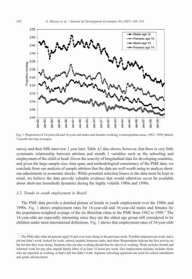
Fig. 1. Proportion of 14-year-old and 16-year-old males and females working, 6 metropolitan areas, 1982–1999, Brazil,3-month moving averages.


survey and their fifth interview 1 year later. Table A1 also shows, however, that there is very littlesystematic relationship between attrition and month 1 variables such as the schooling andemployment of the child or head. Given the scarcity of longitudinal data for developing countries,and given the large sample size, time span, and methodological consistency of the PME data, weconclude from our analysis of sample attrition that the data are well worth using to analyze short-run adjustments to economic shocks. While potential selection biases in the data must be kept inmind, we believe the data provide valuable evidence that would otherwise never be availableabout short-run household dynamics during the highly volatile 1980s and 1990s.

3.2. Trends in youth employment in Brazil

The PME data provide a detailed picture of trends in youth employment over the 1980s and1990s. Fig. 1 shows employment rates for 14-year-old and 16-year-old males and females forthe population-weighted average of the six Brazilian cities in the PME from 1982 to 1999.1 The14-year-olds are especially interesting since they are the oldest age group still considered to bechildren under most international definitions. Fig. 1 shows that employment rates of 14-year-olds

1 The PME asks what all persons aged 10 and over were doing in the previous week. Possible responses are work, had ajob but didn't work, looked for work, retired, student, domestic tasks, and other. Respondents indicate the first activity onthe list that they were doing. Students who are also working should thus be shown as working. Work includes formal andinformal work for pay plus unpaid family labor of at least 15 hours per week. Our employment measure includes thosewho are reported as working or had a job but didn’t work. Separate schooling questions are used for school enrollmentand grade advancement.

Fig. 2. Rates of entry into and exit from employment, 14-year-old boys and girls, 6 metropolitan areas, 1982–99, 3-monthmoving averages, Brazil PME.


in Brazil have been relatively high, with over 20% of boys and over 10% of girls working in theearly 1980s. Employment rates for 16-year-olds reach levels as high as 50% for boys and 30% forgirls in the 1980s. During the 1980s there is relatively little decline in youth employment rates,and even evidence of rising employment rates in the mid-1980s. There are, however, substantialdeclines in employment rates for males and females in both age groups from the early 1980s to thelate 1990s. In most cases employment rates in 1998 are about half what they were in 1982.

The longitudinal dimension of the PME makes it possible to estimate month-to-month laborforce transitions. Fig. 2 shows monthly employment transitions for 14-year-old males andfemales in the combined six PME cities. The exit rate for month t is the number of children whomove from the category “working in month t” to “not working in month t+1” divided by thenumber who were working in month t. The entry rate is defined analogously using the numberwho move from “not working in month t” to “working in month t+1.” In the early 1980s theprobability that a 14-year-old boy who is not working in a given month is observed working inthe next month is about 10%, while the entry rate for girls is about 5%. The probability that aworking boy leaves employment by the next month is around 25%, with similar estimates forgirls.2 The transition rates in Fig. 2 suggest that the lower employment rates for girls in Fig. 1 areexplained almost entirely by the fact that girls have lower entry rates than boys. Exit rates for

2 The large monthly variations in Fig. 2 reflect both seasonal movements and monthly volatility due to small samplesizes. The volatility is especially large in exit rates because of the small number of 14-year-olds observed working in anysingle month in the sample.


boys and girls are fairly similar, suggesting that girls who do enter employment have similar jobattachment as boys.

The large declines in employment rates over time, shown in Fig. 1, appear to result from bothdecreasing entry rates and increasing exit rates. Exit rates rise to levels around 30% by the end ofthe 1990s for both males and females. In other words, about one-third of the children who areworking in a given month are not working in the following month, a high degree of labor forcemobility.3 While all of these estimates may be subject to measurement error, it seems unlikely thatmeasurement error can explain either the large increases in exit rates over time or the differencesin entry rates by gender and socioeconomic status. Duryea et al. (2005) provide additional detailon these transition rates, including breakdowns by mother's education. These breakdownsindicate that the fact that boys with less educated mothers have roughly twice the employmentrates of those with more educated mothers is almost entirely due to the fact that the disadvantagedboys are twice as likely to enter employment each month. Once they take a job, the estimatessuggest that boys in the two groups are about equally likely to stay employed.4

The high degree of mobility in and out of employment suggests that the percentage of childrenwho work at some point during the year may be much higher than the rates estimated for anyparticular month. The PME data allow us to confirm this empirically. Levison et al. (2006) use thePME panels to construct a measure of whether a child works at any point during a consecutivefour-month period. These results indicate that the proportion of 14-year-old girls who work atleast once in a four-month period is roughly twice as high as the one-month employment ratesshown in Fig. 1. For 14-year-old boys, calculating employment on this four-month basis raises theemployment rate about 15 percentage points in the 1980s, and about 10 percentage points in the1990s, bringing the employment rate in 1998 to around 20%.

3.3. Trends in schooling and other variables

Table 1 shows means of child schooling and other outcomes by year from 1982 to 1998.5 Thetable focuses on 14-year-olds in order to provide a clearer picture of trends over time for a singleage group. Table 1 shows large improvements in schooling in Brazil between 1982 and 1998.Mean completed years of schooling of 14-year-olds rises from 4.7 to 5.7 years, and enrollmentrates rise from 85% to 94%. These improvements in schooling are consistent with the decline inyouth employment shown in Fig. 1. As shown in Table 1, the proportion of 14-year-olds workingin the labor force falls from 17% to 5.5% over this period. Columns 4 and 5 of Table 1 show thepercentage working and mean schooling of male household heads. The percentage of male headsworking averages 87% for the entire period, with annual volatility of 3 to 4 percentage points inboth decades. The 13% of male heads who were not working in Table 1 are made up of 2.6%unemployed (searching for work), 8.5% retired, and 2% in other categories. Mean schooling ofmale heads rose by over two years, from 4.5 to 6.7. As shown by Levison (1991), Barros and Lam(1996), and Lam and Duryea (1999), there is a strong relationship between parental schooling andchildren's schooling and work in Brazil, so these improvements in adult schooling may have hadan important direct role in explaining the rising schooling and falling rates of youth employment.

3 This phenomenon is explored further in Levison et al. (2006).4 We do not know the duration of employment in particular jobs. Employed children who change jobs but report being

employed in two consecutive monthly interviews are counted as continuously employed.5 Only even-numbered years are shown because most households enter the PME sample in even years. These are

therefore the base years for calculating school advancement probabilities.

Table1

Sam

plemeans

forselected

variablesby

year

forchild

renage14

,BrazilPME19

82–98

Year

Valuesforchild

andhead

inMonth

1Outcomes

conditional

onstatein

Month

1

Child

inscho

olChild's

yearsof

schooling

Child

working

Malehead

working

Malehead's

schooling

Child

startsworking

bymon

th4

Child

leaves

scho

olby

mon

th4

Child

fails

toadvance

inschool

Headlosesjobby

mon

th4

(1)

(2)

(3)

(4)

(5)

(6)

(7)

(8)

(9)

1982

0.84

74.72

0.170

0.87

54.47

0.130

0.030

0.370

0.03

819

840.84

24.71

0.148

0.84

14.36

0.121

0.024

0.350

0.06

219

860.86

84.81

0.166

0.87

34.73

0.129

0.026

0.368

0.02

519

880.85

14.79

0.163

0.87

85.11

0.101

0.020

0.345

0.03

619

900.86

64.97

0.150

0.89

05.46

0.111

0.015

0.396

0.03

719

920.89

05.11

0.109

0.86

75.77

0.076

0.014

0.344

0.04

819

940.91

75.28

0.096

0.86

95.93

0.065

0.009

0.314

0.04

219

960.93

85.55

0.090

0.86

66.48

0.061

0.008

0.279

0.03

919

980.94

25.74

0.055

0.83

36.70

0.053

0.009

0.242

0.06

6

Total

0.88

45.06

0.129

0.86

65.40

0.094

0.017

0.334

0.04

3

N39

,393

39,385

39,393

31,930

31,919

34,283

29,383

26,366

17,571

Note:Means

areestim

ated

forthelargestp

ossiblesampleforeach

outcom

ein

each

year.C

olum

n6iscond

itionalon

notw

orking

inmon

th1.

Colum

ns7and8arecond

itionalon

school

enrollm

entin

mon

th1.

Colum

n9iscond

itional

onhead

employ

edin

mon

th1.



The last four columns of Table 1 show means for the key transitions that are the focus of ouranalysis. Column 6 shows the probability that a child who is not working in month 1 beginsworking by month 4. This probability is 13% for 14-year-olds in 1982, changes relatively little inthe 1980s, then falls to around 5% by 1998. Column 7 shows dropout rates between month 1 andmonth 4. Only 3% of 14-year-olds enrolled in school in month 1 were out of school in month 4 inthe early 1980s, a rate that fell to less than 1% in the late 1990s. While few children are reported asdropping out of school during a school year, a much higher percentage fails to advance to the nextgrade. Column 8 shows the proportion who fail to advance a grade between the first month ofobservation and 1 year later, conditional on enrollment in month 1. Among 14-year-olds in schoolin 1982, 37% did not advance to the next grade. This rate stayed between 34% and 40% until1992, then fell to 24% in 1998. The failure to advance grades is primarily a reflection of graderepetition rather than dropping out. Taking all 14-year-olds ever enrolled in school in month 1over the 1982–1999 period, 33% failed to advance a grade from month 1 to month 13. Of this33% who failed to advance, 88% were enrolled in school in month 13.

3.4. Unemployment shocks to male household heads

Column 9 of Table 1 shows the prevalence of the economic shock variable that will be thefocus of our analysis — the transition from employed to unemployed by the male householdhead between month 1 and month 4. As the table shows, 3.8% of male heads lost their jobbetween month 1 and month 4 in 1982. This rate stays around 3% to 5% in most years,rising to almost 7% in 1998. The shock we will be focusing on can thus be seen to be arelatively unusual event for households. Nonetheless, given our very large sample sizes, asubstantial number of heads are observed to lose their jobs during the period of our study.Unemployment shocks are more common among heads with less human capital. For menwith less than 1 year of schooling (13% of male heads), the probability of an unemploymentshock is 6.7% over the entire period, compared to 2.2% for men with 11 or more years ofschooling (not shown).

Table 2 provides additional detail about these unemployment shocks, and helps illustratethe logic of our econometric analysis. We define male household heads as experiencing anunemployment shock if they move from employed to unemployed (searching for work)between month 1 and month 4.6 The first seven rows of Table 2 show all combinations ofemployment sequences that generate this shock, using the sample of male heads in householdswith 10–16-year-olds that will be used in our regression in Table 4 below. The first line showsthat we observe 282 cases in which the male head is employed in month 1 but is unemployedin months 2, 3, and 4, 0.3% of the 106,648 cases. Summing up all sequences that include atleast one month of unemployment in months 2, 3, or 4, we see that 3.16% of headsexperienced an unemployment shock between month 1 and month 4. In just under half thesecases, the head is employed again in month 4. The rows at the bottom of the table show that90% of the heads were employed in months 1–4 and month 13, 2% were employed in all ofthe first four months but were unemployed in month 13, and 4.7% left the labor force betweenmonth 1 and month 13.

6 Although the PME asks whether workers quit or were fired from their previous jobs, in practice the question is notvery useful. Among those who became unemployed between month 1 and month 2, 65% say they were fired, 11% saythey quit, and 24% are missing. Since the Brazil employment insurance system (FGT) creates incentives for workers to befired rather than quit, and since employers do not bear the full cost of the resulting compensation, even workers who wantto quit may arrange to be fired.

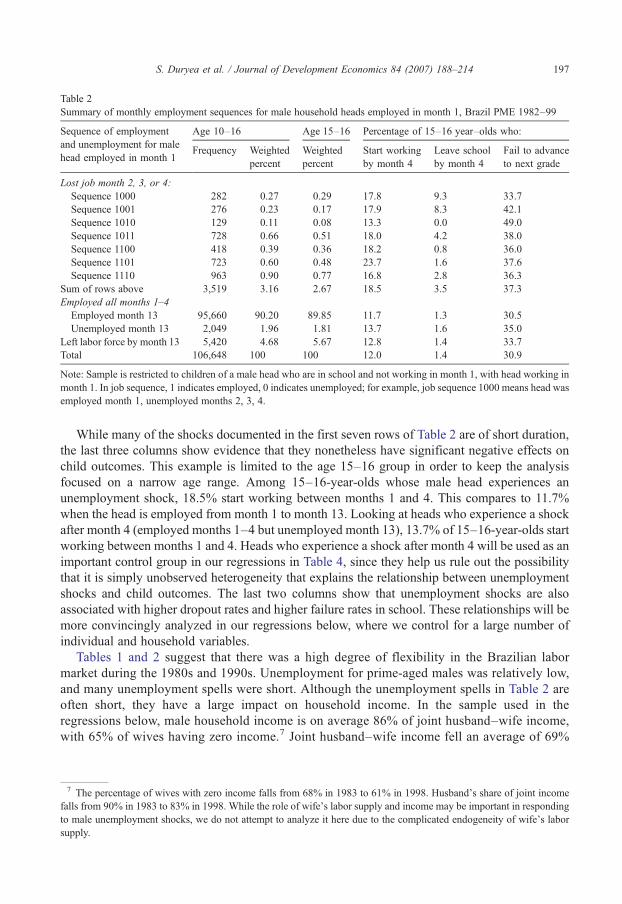
Table 2Summary of monthly employment sequences for male household heads employed in month 1, Brazil PME 1982–99

Sequence of employmentand unemployment for malehead employed in month 1

Age 10–16 Age 15–16 Percentage of 15–16 year–olds who:

Frequency Weightedpercent

Weightedpercent

Start workingby month 4

Leave schoolby month 4

Fail to advanceto next grade

Lost job month 2, 3, or 4:Sequence 1000 282 0.27 0.29 17.8 9.3 33.7Sequence 1001 276 0.23 0.17 17.9 8.3 42.1Sequence 1010 129 0.11 0.08 13.3 0.0 49.0Sequence 1011 728 0.66 0.51 18.0 4.2 38.0Sequence 1100 418 0.39 0.36 18.2 0.8 36.0Sequence 1101 723 0.60 0.48 23.7 1.6 37.6Sequence 1110 963 0.90 0.77 16.8 2.8 36.3

Sum of rows above 3,519 3.16 2.67 18.5 3.5 37.3Employed all months 1–4

Employed month 13 95,660 90.20 89.85 11.7 1.3 30.5Unemployed month 13 2,049 1.96 1.81 13.7 1.6 35.0

Left labor force by month 13 5,420 4.68 5.67 12.8 1.4 33.7Total 106,648 100 100 12.0 1.4 30.9

Note: Sample is restricted to children of a male head who are in school and not working in month 1, with head working inmonth 1. In job sequence, 1 indicates employed, 0 indicates unemployed; for example, job sequence 1000 means head wasemployed month 1, unemployed months 2, 3, 4.


While many of the shocks documented in the first seven rows of Table 2 are of short duration,the last three columns show evidence that they nonetheless have significant negative effects onchild outcomes. This example is limited to the age 15–16 group in order to keep the analysisfocused on a narrow age range. Among 15–16-year-olds whose male head experiences anunemployment shock, 18.5% start working between months 1 and 4. This compares to 11.7%when the head is employed from month 1 to month 13. Looking at heads who experience a shockafter month 4 (employed months 1–4 but unemployed month 13), 13.7% of 15–16-year-olds startworking between months 1 and 4. Heads who experience a shock after month 4 will be used as animportant control group in our regressions in Table 4, since they help us rule out the possibilitythat it is simply unobserved heterogeneity that explains the relationship between unemploymentshocks and child outcomes. The last two columns show that unemployment shocks are alsoassociated with higher dropout rates and higher failure rates in school. These relationships will bemore convincingly analyzed in our regressions below, where we control for a large number ofindividual and household variables.

Tables 1 and 2 suggest that there was a high degree of flexibility in the Brazilian labormarket during the 1980s and 1990s. Unemployment for prime-aged males was relatively low,and many unemployment spells were short. Although the unemployment spells in Table 2 areoften short, they have a large impact on household income. In the sample used in theregressions below, male household income is on average 86% of joint husband–wife income,with 65% of wives having zero income.7 Joint husband–wife income fell an average of 69%

7 The percentage of wives with zero income falls from 68% in 1983 to 61% in 1998. Husband's share of joint incomefalls from 90% in 1983 to 83% in 1998. While the role of wife’s labor supply and income may be important in respondingto male unemployment shocks, we do not attempt to analyze it here due to the complicated endogeneity of wife's laborsupply.


between months 1 and 4 for those who experienced an unemployment shock, compared to theaverage income change for all couples, controlling for variables such as month 1 income, age,schooling, city, and month/year. Among men who experienced an unemployment shock butreturned to work by month 4, earnings fell by 27% compared to the average change betweenmonths 1 and 4 for all workers, controlling for month 1 earnings, age, schooling, city, andmonth/year.

4. The impact of unemployment shocks on work and school transitions

4.1. Consumption smoothing and children's time allocation

The above results demonstrate that youth employment is not a rare event in Brazil's cities,and that this employment is characterized by a high degree of volatility. We have also seen thatsignificant fractions of children fail to advance in school, and that unemployment shocks tomale household heads, while relatively rare, appear to be associated with increased labor forceentry and poorer school outcomes for youth. The possibility that even very short unem-ployment spells could affect children's work and schooling has important implications forhuman capital accumulation and may indicate that some households are unable to smoothconsumption.

As shown by Jacoby and Skoufias (1997), if households have access to perfect capitalmarkets we would not expect transitory income fluctuations to affect the time children allocateto work or school. Investments in children's human capital should be based on long-runoptimization, with borrowing or insurance used to smooth consumption in response to negativeincome shocks. If a household is credit constrained, however, short-run income shocks mayforce adjustments in the labor supply of other household members, including children. Ifchildren are pushed into employment as a result of the shock, it may come at the expense oftime spent attending school or doing homework. This may affect their probability of gradeadvancement, even if they do not drop out of school, by affecting the likelihood of passing end-of-year exams. School effort may be disrupted even if there is not an increase in employment.Children may be pulled out of school, even temporarily, because of problems paying schoolfees or transport costs. Some children, especially girls, may be pulled into increased domesticduties if the mother increases employment in response to the father's job loss.8 Increased stressin the household may disrupt the child's school performance even in the absence of directeffects on enrollment. Although we cannot isolate all of the mechanisms through which jobloss affects work and school transitions, we will be able to look directly at whether the childstarts working, drops out of school, or fails to advance to the next grade in school in response tothe male head becoming unemployed.

4.2. Estimation strategy

Taking advantage of the PME's panel structure, we follow male household heads and thechildren living with them over the first four months in which they are interviewed in the PME.

8 While results of studies of children’s work and school interactions are sensitive to whether household chores arecounted as “work” (e.g., Levison et al., 2001; Assaad et al., 2006), the PME does not include measures of householdwork that would allow us to address this possibility.


The sample used for the regressions consists of children aged 10–16 who are enrolled in schooland not working at the time of the first interview. The sample is restricted to children who live inhouseholds with a male head present (we sometimes refer to this male head as the “father,”although he may have some other relationship to the child). We restrict the analysis to childrenwho are a son, daughter or other relative of the household head.9 We drop all children for whomthe first four PME interview months include the long summer break between the end of a schoolyear and the beginning of the next school year. This means that the unemployment shocks andchildren's entry into work all occur during a school year. A major focus of our analysis is on thetiming of shocks and responses. As in Duryea (1997), an important issue in looking at the effectsof household economic shocks is that the observation of a shock such as unemployment maysimply be a proxy for household characteristics that are correlated with outcomes such as graderepetition or child employment. In other words, the observed child outcome may not be causallylinked to the shock itself, but will be correlated with the shock in the data. Our panel data make itpossible to separate the effect of shocks that occur during the school year from shocks that occurafter the school year, allowing us to control, at least to some extent, for household heterogeneitythat may cause spurious correlations between shocks and negative child outcomes.

The dependent variable capturing entry into labor force employment, L, is equal to 1 if a childwho was not employed in month 1 is employed in month 2, 3, or 4. If the child is not employed inall four months then L=0. Children's optimal work hours are based on the difference between themarket wage and the reservation wage. Formally, the reservation wage is

wri;t ¼ f ðYT

i;t; YPi ;Xi;mt; atÞ; ð1Þ

where Xi is a vector of demographic characteristics for the household and the child, YiP is a vector

of permanent income variables for the family, and the vector Yit is an indicator of transitory shocks

to household income. Month dummies mt are included to control for seasonal variation in thereservation wage. To control for intertemporal changes we include period-specific constant termsat representing the different year-to-year panels from 1982–83 to 1998–99. The market wageincludes productivity-related components of X such as the child's age and progress throughschool, as well as seasonal and annual components. The child's optimal hours L⁎ are a function ofthe difference between the market wage and the reservation wage,

Lit⁎ ¼ XiVhþ YiVprþ TitVdþ mt þ at þ mit; ð2Þwhere the coefficients pick up effects from both the reservation wage and the market wage, andwhere νit is a zero-mean normally distributed stochastic term that combines stochastic componentsin both the reservation wage and market wage. The child is observed working if Lit⁎N0,

Lit ¼ 1 if mitz−XiVh−YtVpr−TitVd−mt−at: ð3ÞWe will estimate a probit version of Eq. (3), where the transitory shock is indicated by the

husband moving from unemployment into unemployment. If households could perfectly smoothconsumption, we would not expect them to use child labor as a buffer against volatility, and wouldtherefore expect θ in Eq. (3) to be zero.

9 In the full sample of children aged 10–16, less than 1% of children are classified as the household head or spouse ofhead, 91% are a child of the head, 8% are some “other relative,” and less than 1% are another status such as a domesticworker or child of domestic worker. In the sample used in our regressions below, 98% are a child of the head, with theother 2% classified as “other relative” of the head.


If the child starts working in response to a shock (and perhaps even if the child does not) thechild may withdraw from school. We estimate a probit identical to Eq. (3) in which the dependentvariable is dropping out of school rather than entering work. Since dropping out may be directlyrelated to the work decision, we use the same set of regressors. As shown above, dropping outduring the school year is rare for the age group we are studying, but failing to advance a grade inschool is much more common. We therefore consider the possibility that adjustments in thechild's time allocation in response to the shock may have a negative effect on school progress.This could be because of a shift into child labor, but could also occur even if the child does notstart working. We define a variable indicating advancement in school, S, where S=1 if the childpassed the grade he or she was attending in month 1 and advanced to the next grade as of themonth 13 interview, one year later. If the child does not advance to the next grade then S=0. Thiscould occur either because the child drops out of school or because the child repeats the grade, arelatively common outcome in Brazilian schools. Note that while the four months we observeoccur in one year, evidence of the successful completion of the grade is not observed until the nextyear, given the eight-month gap between the fourth and fifth interviews. If the child is attendinggrade 5 in March through June 1994, evidence that the child passed grade 5 is not observed untilthe child is re-interviewed in March 1995 (in the household's fifth interview).

More formally, achievement in school is assumed to be a function of the child's effort spent onschoolwork with a stochastic component:

Sit⁎ ¼ XiVhþ YiVprþ TitVdþ mt þ at þ lit; ð4Þwhere we include the same variables defined for Eq. (1), with the stochastic component μitreflecting the fact that parents and children cannot perfectly predict the amount of effort necessaryto pass a grade. We will normalize such that the child advances in school if SitN0,

Sit ¼ 1 if uitz−XiVh−YiVpr−TitVd−mt−at ð5ÞSince our other outcome measures are the “bad” outcomes of entry into employment and

dropping out of school, for ease of interpretation we will use the failure to advance in school,F=1−S, as our dependent variable for the probit corresponding to Eq. (5).

We use job loss by the male household head to indicate a negative transitory household incomeshock. We focus on male heads because they tend to be primary income earners with high laborforce attachment. Ideally we would want to measure deviations from the head's lifetime earningsprofile to capture the existence and magnitude of transitory income shocks. Since the PME is ashort panel of 8 interviews over a 16-month period, however, it is impossible to know whether adrop in earnings signals a return to the head's long-run income path or a short-run deviation fromthat path. We also prefer to use transitions into unemployment rather than earnings changesbecause of several complications with the PME earnings variable. In addition to dealing withmissing values, measuring changes in monthly earnings is complicated by periods of hy-perinflation that reached over 50% per month in the 1980s. A further complication is that earningsare reported as zero if the job held at the time of the interview is different that the job held duringthe previous month (the reference period for earnings). This mismatch of earnings and jobshappens when the respondent changes jobs between monthly interviews, a relatively commonoccurrence given Brazil's large informal labor sector.10

10 Neri et al. (2000) analyze the effect of transitions from positive to zero income by the household head. They findevidence that the complete loss of income by the head between the fourth and eighth interview (1 year later) is associatedwith an increased probability of child labor and decreased probability of school advancement. The evidence on earningsloss is problematic for the reasons indicated, however, so we focus on more clearly measured exits from employment.


Given the problems with using changes in earnings, we use transitions to unemployment as theindicator of a negative income shock. Capturing the transitory nature of the shock is only asufficient step in our estimation strategy. If we find that the father's move into unemploymentaffects a child's entry into the labor force or advancement in school, there are at least two possibleexplanations for the result. The first is that the income shock is unanticipated and affectschildren's work and schooling. The second is that there is some permanent characteristic of thefamily related to the unemployment that affects work and school transitions. In other words, it ispossible that unemployment is negatively associated with children's work and school outcomesbecause of some persistent unobserved heterogeneity that drives all of the outcomes. Forexample, fathers with low ability and many labor force changes may have children with unsteadyperformance in school and frequent employment transitions, even if there is not a direct causalrelationship between one particular shock and the child's work and school transitions.

We leave it as an empirical question whether unemployment shocks are anticipated. If they areanticipated, then shocks occurring after the school year could affect outcomes during the schoolyear. Since we observe shocks both during and after the school year, we can test directly whethershocks are anticipated. While we will see that shocks appear to be unanticipated, we do allowsome flexibility in the sequence of shocks and outcomes. Since we do not expect job loss to beentirely without warning in the very short run (at least one or two weeks), and since the precisetiming of transitions may not show up perfectly in our data, we do not require strictly that the headbecomes unemployed before the child begins work. If the head becomes unemployed any time inmonth 2, 3, or 4, and the child enters employment in month 2, 3, or 4, we interpret the head'semployment as causing the child's transition. On the other hand, we let the data tell us whetherunemployment that occurs during the gap between months 5 and 13 has an impact on childtransitions in months 2–4.

In our first set of regressions the unemployment variables are constructed with the aim ofcomparing the impact of an unemployment shock occurring during a given school year with theimpact of a shock occurring after the end of the school year. This provides evidence about whetherchildren's work and school transitions are a response to a transitory, unanticipated shock ratherthan the result of persistent unobserved heterogeneity. Our control group is male heads who areemployed in months 1, 2, 3, 4 and 13 (we sometimes refer to this as “continuously employedin months 1–13,” but it should be kept in mind that we have no data on employment in months5–12). Our treatment group is male heads who are employed in month 1 but are unemployed atleast once in months 2, 3, or 4. If the child was in grade 5 in March 1994 and the father becameunemployed in April through June 1994, we examine whether the child started work or leftschool in April, May, or June, and whether the child was in grade 6 in March 1995. As arobustness test we also consider the case of an ex-post unemployment shock occurring after theschool year. Since the shock occurs after month 4, it should have no impact on whether the childbecame employed between months 1 and 4 as long as the shock was unanticipated and unrelatedto persistent heterogeneity with respect to characteristics that drive child employment andschooling. Heads that leave the labor force after month 1 are treated as a separate category sincethey may not represent the same kind of negative shock as unemployment. Leaving the labor forcemay be associated with advantageous changes, such as pension eligibility, or with negative changessuch as disability. These transitions are dummied out to keep the main contrasts regardingunemployment shocks clean. If unemployment precedes leaving the labor force, the head iscategorized as unemployed.

After analyzing the issue of ex-ante versus ex-post shocks in Regression 1, in Regression 2 weuse a simpler shock measure that allows us to include interactions with a number of other


variables. In these regressions the control group continues to be heads who are employed in everymonth of observation from month 1 through month 13. The “shock” variable will be defined equalto 1 for all heads who become unemployed between month 1 and month 4, independent of whathappens after month 4. The case of ex-post unemployment and leaving the labor force aredropped from the sample to simply the shock versus no-shock comparison.

In summary, the sample is restricted to 10–16-year-olds who are attending school but are notemployed in the first interview. This is about 85% of all 10–16-year-olds who can be followedfrom month 1 to month 13. The male household head (who is either the father or a relative of thechild) must be present in the household and must be employed in the first interview. All otherchildren are excluded from the sample. We also control for the sex and age of the child andwhether the child is more than 2 years behind schedule in school. To control for household'spermanent income we include quadratic functions of the age and schooling of the father and themother. To control for local conditions, we include dummies for the metropolitan area, with SãoPaulo as the omitted area. We include dummies for month to control for seasonal patterns, and weinclude dummies for year pairs to capture time trends.11 We omit all cases in which the first fourmonths of interviews do not fall fully within a single school year. Households observed for thefirst time in September through January are thus excluded from the regressions.

Table 3 gives mean characteristics for the samples used in our regressions. Regression 1 willinclude the more detailed breakdown of employment transitions, allowing us to analyze whetherex-post unemployment affects child transitions between months 1 and 4. Regression 2 will use thesimpler shock variable with interactions for decade, gender, age, and father's schooling. Thesample size for Regression 1 is 106,648 10–16-year-olds for whom the impact of shocks onschool and work transitions can be studied over the 1982–99 period. The sample for Regression 2is about 7000 observations smaller, the result of dropping cases where shocks occur after theschool year or heads leave the labor force. Looking at the means of our dependent variables,shown in the first three rows, about 5% enter employment by month 4, about 1% drop out ofschool by month 4, and about 29% fail to advance to the next grade in school by month 13. Thenext rows of Table 4 show that 90% of the male heads are employed in interview rounds 1 through5 (month 2, 3, 4, and 13), 3.2% become unemployed in month 2, 3, or 4, 2.1% becomeunemployed after month 4, and 4.7% leave the labor force after month 1.

4.3. Probit regression results

Table 4 presents our first set of regressions. Robust standard errors are estimated to correct forpotentially correlated error terms across multiple children from a household. Looking at thecoefficients on the main unemployment shock variable, we see that an unemployment shock to themale head during the three months after the first interview has a statistically significant positiveeffect on the probability of entering work by month 4, the probability of dropping out of school bymonth 4, and the probability of failing to advance to the next grade. The magnitude of these effectsis relatively large, as will be discussed below. These are the effects we might predict if householdsare credit constrained and use children's time allocation as a way to buffer a transitory incomeshock. The coefficient on the variable indicating an ex-post unemployment shock (that is, a shock

11 The PME rotation scheme operates on two-year cycles, with most new households entering in even-numbered years.We include dummy variables for the two-year cycle in which households first enter the sample in order to flexibly capturetime trends and general period effects that affect all households.

Table 3Sample means for samples used in probit regressions in Tables 4 and 5, children age 10–16 in metropolitan Brazil, 1982–99

Variable Sample for regression 1(N=106,648)

Sample for regression 2(N=99,184)

Mean Standard deviation Mean Standard deviation

Dependent variablesChild enters employment by month 4 0.052 0.221 0.051 0.220Child drops out of school by month 4 0.008 0.089 0.008 0.089Child fails to advance in school 0.287 0.452 0.285 0.452

Male head's unemployment transitions, regression 1Continuously employed months 1–4 and 13 0.902 0.297Loses job by month 4 0.032 0.175Employed months 1–4, unemployed month 13 0.021 0.144Leaves labor force after month 1 0.047 0.211

Male head's unemployment transitions, regression 2Unemployment shock: Head loses job by month 4 0.034 0.181Shock⁎1990s 0.020 0.142Shock⁎ (age 10–14) 0.028 0.165Shock⁎ father's education 0.160 1.076Shock⁎male child 0.017 0.130Male child 0.495 0.500 0.495 0.500Child more than 2 years behind in school 0.184 0.388 0.181 0.385Age of child 12.60 1.91 12.59 1.91Age of father 42.83 7.23 42.63 7.06Age of mother 39.14 6.54 39.00 6.43Years of schooling of child 4.52 2.15 4.53 2.15Years of schooling of father 6.04 4.45 6.12 4.48Years of schooling of mother 5.47 4.05 5.53 4.06

Metropolitan areaSalvador 0.072 0.258 0.070 0.256Belo Horizonte 0.097 0.296 0.095 0.293Recife 0.070 0.255 0.069 0.253Rio de Janeiro 0.261 0.439 0.265 0.441Porto Alegre 0.074 0.262 0.074 0.262São Paulo 0.426 0.495 0.426 0.494

Note: Both samples are conditional on child enrolled in school and not working in month 1, male head working in month 1.


after month 4) is not statistically significant for any of the three outcomes, with point estimates thatare much smaller than the coefficients for the ex-ante shock. This is strong evidence that theapparent effect of an ex-ante unemployment shock is not simply due to a correlation betweenunemployment shocks and unmeasured household characteristics that cause both unemploymentfor the head and bad outcomes for the child. It also suggests that unemployment shocks occurringseveral months in the future are not fully anticipated. Looking at the impact of the permanenthousehold characteristics included as regressors in Table 4, we find that males are considerablymore likely to enter the labor force and fail to advance in school. We estimate large and statisticallysignificant effects of the mother's and the father's education on all three outcomes. Significantdifferences across cities and across years are also observed for both sets of outcomes. These effectswill be discussed in more detail below when we calculate predicted probabilities.

Table 4Probit regressions: impact of unemployment shock on work and school transitions, age 10–16, Brazil PME 1982–1999

Variable Enter labor force bymonth 4

Leave school bymonth 4

Fail to advance to next gradein school

Head's transitions (continuously employed omitted)Unemployment shock in month 2–4 0.091 (0.050)⁎ 0.179 (0.075)⁎⁎ 0.086 (0.033)⁎⁎⁎

Unemployment shock in month 5–13 0.016 (0.064) 0.074 (0.108) 0.017 (0.039)Left labor force 0.016 (0.040) −0.103 (0.066) 0.047 (0.026)⁎

Child's age (age 16 omitted)Child age 10 −1.294 (0.041)⁎⁎⁎ −0.438 (0.066)⁎⁎⁎ −0.165 (0.022)⁎⁎⁎

Child age 11 −1.169 (0.037)⁎⁎⁎ −0.434 (0.066)⁎⁎⁎ −0.115 (0.022)⁎⁎⁎

Child age 12 −0.938 (0.034)⁎⁎⁎ −0.296 (0.061)⁎⁎⁎ −0.075 (0.021)⁎⁎⁎

Child age 13 −0.739 (0.033)⁎⁎⁎ −0.296 (0.062)⁎⁎⁎ −0.023 (0.021)Child age 14 −0.447 (0.030)⁎⁎⁎ −0.165 (0.058)⁎⁎⁎ −0.003 (0.022)Child age 15 −0.210 (0.030)⁎⁎⁎ −0.124 (0.057)⁎⁎ 0.014 (0.023)

Male child 0.395 (0.019)⁎⁎⁎ −0.019 (0.034) 0.167 (0.010)⁎⁎⁎

Child 2+ years behind in school 0.100 (0.021)⁎⁎⁎ 0.520 (0.040)⁎⁎⁎ 0.194 (0.014)⁎⁎⁎

Father's age −0.010 (0.010) −0.046 (0.018)⁎⁎⁎ −0.014 (0.007)⁎⁎

Mother's age 0.029 (0.012)⁎⁎ 0.017 (0.022) −0.017 (0.007)⁎⁎

Father's age squared /100 0.011 (0.011) 0.050 (0.018)⁎⁎⁎ 0.015 (0.007)⁎⁎

Mother's age squared/100 −0.042 (0.014)⁎⁎⁎ −0.027 (0.026) 0.017 (0.009)⁎⁎

Father's schooling −0.027 (0.008)⁎⁎⁎ −0.022 (0.015) −0.015 (0.005)⁎⁎⁎

Mother's schooling −0.036 (0.008)⁎⁎⁎ −0.036 (0.017)⁎⁎ −0.029 (0.005)⁎⁎⁎

Father's schooling squared /100 −0.064 (0.054) −0.002 (0.112) −0.026 (0.032)Mother's schooling squared /100 0.002 (0.063) 0.142 (0.133)⁎⁎⁎ 0.096 (0.035)Metro area (São Paulo omitted)

Salvador −0.037 (0.029) −0.120 (0.057)⁎⁎ 0.426 (0.017)⁎⁎⁎

Belo Horizonte 0.082 (0.024)⁎⁎⁎ 0.161 (0.048)⁎⁎⁎ 0.148 (0.015)⁎⁎⁎

Recife −0.030 (0.028) 0.007 (0.052) 0.299 (0.017)⁎⁎⁎

Rio de Janeiro −0.338 (0.028)⁎⁎⁎ −0.023 (0.053) 0.276 (0.016)⁎⁎⁎

Porto Alegre −0.150 (0.027)⁎⁎⁎ 0.154 (0.051)⁎⁎⁎ 0.277 (0.017)⁎⁎⁎

Year (1982 omitted)Year 1984 −0.058 (0.034)⁎ −0.055 (0.061) −0.124 (0.023)⁎⁎⁎

Year 1986 0.044 (0.034) −0.028 (0.061) −0.005 (0.022)Year 1988 −0.086 (0.039)⁎⁎ −0.028 (0.068) −0.062 (0.025)⁎⁎

Year 1990 −0.062 (0.037)⁎ −0.086 (0.065) 0.039 (0.023)⁎

Year 1992 −0.274 (0.040)⁎⁎⁎ −0.055 (0.071) −0.068 (0.024)⁎⁎⁎

Year 1994 −0.251 (0.038)⁎⁎⁎ −0.290 (0.070)⁎⁎⁎ −0.117 (0.024)⁎⁎⁎

Year 1996 −0.230 (0.038)⁎⁎⁎ −0.379 (0.076)⁎⁎⁎ −0.235 (0.024)⁎⁎⁎

Year 1998 −0.304 (0.041)⁎⁎⁎ −0.187 (0.076)⁎⁎ −0.268 (0.026)⁎⁎⁎

Month of first observation (February omitted)March −0.055 (0.036) 0.011 (0.067) 0.008 (0.022)April −0.060 (0.036)⁎ −0.122 (0.070)⁎ 0.013 (0.022)May −0.024 (0.035) −0.127 (0.069)⁎ −0.052 (0.022)⁎⁎

June −0.005 (0.035) −0.073 (0.067) −0.048 (0.022)⁎⁎

July 0.005 (0.034) −0.011 (0.065) −0.057 (0.022)⁎⁎⁎

August 0.011 (0.035) −0.035 (0.065) −0.05 (0.021)⁎⁎

Constant −0.967 (0.266)⁎⁎⁎ −1.203 (0.506)⁎⁎ 0.255 (0.164)Number of Observations 106,648 106,648 106,648

Note: Robust standard errors in parentheses; Significance levels: ⁎ = .10, ⁎⁎ = .05, ⁎⁎⁎ = .01 Sample is conditional on childin school and not working in month 1 and male head working in month 1.


Table 5Probit regressions with interactions: Impact of unemployment shock on work and school transitions, age 10–16, BrazilPME 1982–1999

Variable Enter labor forceby month 4

Leave schoolby month 4

Fail to advance tonext grade in school

Head's transitions (continuously employed omitted)Unemployment shock in month 2–4 0.354 (0.137)⁎⁎ 0.358 (0.179)⁎⁎ 0.225 (0.097)⁎⁎

Unemployment shock ⁎ 1990s −0.168 (0.105) 0.291 (0.151)⁎ −0.084 (0.067)Unemployment shock ⁎ age 10–14 −0.203 (0.106)⁎ −0.230 (0.159) −0.072 (0.081)Unemployment shock ⁎ father's schooling −0.011 (0.017) −0.051 (0.028)⁎ 0.003 (0.010)Unemployment shock ⁎ male child −0.003 (0.098) −0.014 (0.155) −0.089 (0.055)

Child's age (age 16 omitted)Child age 10 −1.283 (0.042)⁎⁎⁎ −0.420 (0.067)⁎⁎⁎ −0.155 (0.023)⁎⁎⁎

Child age 11 −1.154 (0.039)⁎⁎⁎ −0.400 (0.068)⁎⁎⁎ −0.102 (0.023)⁎⁎⁎

Child age 12 −0.921 (0.036)⁎⁎⁎ −0.279 (0.064)⁎⁎⁎ −0.065 (0.022)⁎⁎⁎

Child age 13 −0.722 (0.034)⁎⁎⁎ −0.281 (0.065)⁎⁎⁎ −0.018 (0.022)Child age 14 −0.436 (0.031)⁎⁎⁎ −0.149 (0.060)⁎⁎ 0.003 (0.023)Child age 15 −0.201 (0.031)⁎⁎⁎ −0.115 (0.059)⁎ 0.020 (0.023)

Male child 0.391 (0.020)⁎⁎⁎ −0.012 (0.036) 0.175 (0.011)⁎⁎⁎

Child 2+ years behind in school 0.107 (0.022)⁎⁎⁎ 0.517 (0.041)⁎⁎⁎ 0.194 (0.015)⁎⁎⁎

Father's age −0.018 (0.011) −0.050 (0.019)⁎⁎⁎ −0.015 (0.007)⁎⁎

Mother's age 0.035 (0.013)⁎⁎⁎ 0.034 (0.022) −0.014 (0.007)⁎

Father's age squared /100 0.022 (0.013)⁎ 0.056 (0.020)⁎⁎⁎ 0.016 (0.008)⁎⁎

Mother's age squared /100 −0.049 (0.016)⁎⁎⁎ −0.048 (0.027)⁎ 0.014 (0.009)Father's schooling −0.024 (0.008)⁎⁎⁎ −0.014 (0.016) −0.015 (0.005)⁎⁎⁎

Mother's schooling −0.033 (0.009)⁎⁎⁎ −0.043 (0.017)⁎⁎ −0.032 (0.005)⁎⁎⁎

Father's schooling squared /100 −0.077 (0.057) −0.048 (0.116) −0.022 (0.033)Mother's schooling squared /100 −0.031 (0.066) 0.188 (0.135) 0.111 (0.036)⁎⁎⁎

Metro area (São Paulo omitted)Salvador −0.016 (0.030) −0.113 (0.059)⁎ 0.424 (0.018)⁎⁎⁎

Belo Horizonte 0.090 (0.025)⁎⁎⁎ 0.158 (0.051)⁎⁎⁎ 0.153 (0.016)⁎⁎⁎

Recife −0.018 (0.029) −0.010 (0.055) 0.303 (0.018)⁎⁎⁎

Rio de Janeiro −0.326 (0.029)⁎⁎⁎ −0.012 (0.054) 0.278 (0.016)⁎⁎⁎

Porto Alegre −0.149 (0.029)⁎⁎⁎ 0.141 (0.053)⁎⁎⁎ 0.275 (0.017)⁎⁎⁎

Year (1982 omitted)Year 1984 −0.081 (0.036)⁎⁎ −0.070 (0.063) −0.125 (0.023)⁎⁎⁎

Year 1986 0.015 (0.035) −0.033 (0.063) −0.003 (0.023)Year 1988 −0.096 (0.040)⁎⁎ −0.047 (0.071) −0.063 (0.025)⁎⁎

Year 1990 −0.078 (0.039)⁎⁎ −0.134 (0.068)⁎⁎ 0.047 (0.024)⁎

Year 1992 −0.279 (0.042)⁎⁎⁎ −0.068 (0.073) −0.063 (0.025)⁎⁎

Year 1994 −0.266 (0.039)⁎⁎⁎ −0.311 (0.073)⁎⁎⁎ −0.115 (0.025)⁎⁎⁎

Year 1996 −0.231 (0.040)⁎⁎⁎ −0.401 (0.082)⁎⁎⁎ −0.228 (0.025)⁎⁎⁎

Year 1998 −0.307 (0.043)⁎⁎⁎ −0.234 (0.083)⁎⁎⁎ −0.263 (0.027)⁎⁎⁎

Month of first observation (February omitted)March −0.058 (0.038) 0.009 (0.070) 0.005 (0.023)April −0.066 (0.037)⁎ −0.11 (0.072) 0.007 (0.023)May −0.020 (0.037) −0.133 (0.072)⁎ −0.055 (0.022)⁎⁎

June −0.013 (0.037) −0.065 (0.070) −0.052 (0.022)⁎⁎

July 0.006 (0.036) −0.024 (0.068) −0.064 (0.023)⁎⁎⁎

August 0.018 (0.036) −0.028 (0.067) −0.058 (0.022)⁎⁎⁎

Constant −0.911 (0.290)⁎⁎⁎ −1.482 (0.505)⁎⁎⁎ 0.217 (0.176)Number of observations 99,184 99,184 99,184

Note: Robust standard errors in parentheses; Significance levels: ⁎ = .10, ⁎⁎ = .05, ⁎⁎⁎ = .01 Sample is conditional on childin school and not working in month 1 and male head working in month 1.



Table 5 presents a similar set of regressions using a simpler measure of the unemploymentshock and including interactions of this shock with several key variables. The shock variable inTable 5 simply compares the control group of male heads who are continuously employed inmonths 1–4 and 13 with the group that becomes unemployed in months 2, 3, or 4 (whether or notthey are employed in month 13). Cases in which heads become unemployed after month 4 andcases in which heads go from employed to out of the labor force are dropped from the regression.The unemployment shock variable is interacted with the male dummy, the 1990s decade dummy,a dummy indicating that the child is age 10–14, and father's schooling. As in Table 4, we estimatestatistically significant positive effects of the unemployment shock on the probability of laborforce entry, the probability of leaving school, and the probability of failing to advance to the nextgrade in school. The interaction with the 1990s dummy is only significant in the dropoutregression, where it indicates increased sensitivity of dropout to shocks in the 1990s. For the othertwo outcomes the point estimates of the interaction indicates less sensitivity to shocks in the1990s. The interaction on the 10–14 dummy indicates a significantly smaller magnitude of theunemployment shock on the probability that younger children enter employment. The pointestimates for the interactions with the male dummy suggest that boys are less affected byunemployment shocks on all three outcomes, although these coefficients are not statisticallysignificant at the 10% level.

The interactions with father's education are included as a test of whether poor households aremore affected by unemployment shocks, treating father's education as an indicator of permanentincome. If credit constraints play a role in causing a link between unemployment shocks andchanges in children's time allocation, then households with higher permanent income may be lessaffected by the shock. Although there is good reason to think that poor households would be lessable to buffer a shock, these interaction terms are only statistically significant for the dropoutregression. Although the negative point estimates in the other two regressions are in the expecteddirection, we cannot reject the hypothesis that there is no interaction between shocks and theschooling of the head. We have experimented with other measures of household socioeconomicstatus, including measures of month 1 income, and continue to find insignificant interactions withthe shock variable in the regressions for entering work and failing to advance in school. It ispossible that the low frequency of shocks makes it difficult to precisely identify this interactioneffect. It is also possible that even these better off households are seriously affected by anunemployment shock, with young people becoming more likely to enter employment and withdisruptions to school performance.

4.4. Robustness checks

Our results are robust to a variety of changes in specification. The results in Tables 4 and 5 donot use the PME earnings measures because of our concern about missing values, measurementerror related to hyperinflation, and the problem of incorrect earnings reports in the case of jobchanges. Using earnings does not significantly change the results, however. We have added thelogarithm of the male head's earnings in month 1 as an additional control in the regressionsshown in Table 5. This lowers our sample size about 10% due to missing incomes, but has verylittle impact on the coefficients or standard errors on our shock variable in any of the threeregressions. We have also created an alternative shock measure in which heads who experience a50% decline in earnings between months 1 and 4 are also considered to have experienced ashock, increasing the percentage experiencing a shock from 4% to 7%. We estimate somewhatsmaller, but still statistically significant, impacts of the shock on our three outcomes, suggesting


that income changes alone are not as disruptive as job loss. Interacting this broader shock withmonth 1 income, we still find no evidence that shocks have smaller impacts in higher incomehouseholds.

4.5. Predicted impact of shocks

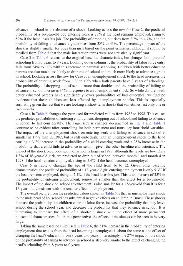
Table 6 illustrates the magnitude of the effects of unemployment shocks implied by ourregressions in Table 5. The baseline used for simulating the impact is a 16-year-old female in SãoPaulo in February 1982 who is not behind in school and whose parents have zero schooling. Thefirst line shows that her predicted probability of entering work, conditional on being enrolled inschool and not working in month 1, is 24.2% if the male head remains continuously employed. Ifthe head loses his job in month 2, 3, or 4, the probability she enters employment rises to 36.5%, anincrease of over 50%. Her probability of leaving school between months 1 and 4 more thandoubles from 2.3% to 5% if the head becomes unemployed. The impact on school advancement isalso substantial. In the absence of an unemployment shock she has a 31.1% chance of failing toadvance to the next grade. This rises to 39.4% if he loses his job, an increase of 27%.

The remaining rows of Table 6 consider other simulated examples to show how the impact ofthe shock varies with alternative baseline assumptions. Row 2 shows the case in which otherbaseline characteristics are kept the same but the child is male instead of female. Looking downcolumn 1, boys are 57% more likely than girls to start working and 21% more likely to fail to

Table 6Impact of unemployment shock to male head on child's work and school transitions

Case Predicted probability withno employment shock

Predicted probability withemployment shock

Percentage increase dueto employment shock

Enterlaborforce

Dropout ofschool

Fail toadvancegrade

Enterlaborforce

Dropout ofschool

Fail toadvancegrade

Enterlaborforce

Dropout ofschool

Fail toadvancegrade

(1) (2) (3) (4) (5) (6) (7) (8) (9)

Case 1: baseline (see notefor definition)

0.242 0.023 0.311 0.365 0.050 0.394 51 121 27

Baseline, but with:Case 2: child male instead of

female0.379 0.022 0.375 0.517 0.047 0.427 37 116 14

Case 3: parental schooling8 years instead of 0

0.110 0.009 0.208 0.192 0.022 0.278 74 149 34

Case 4: year 1998 instead of 1982 0.157 0.013 0.224 0.206 0.056 0.269 31 344 20Case 5: child age 12 instead of 16 0.053 0.011 0.288 0.071 0.016 0.342 35 39 19

Percentage difference from Case 1:Case 2: child male instead of

female57 −3 21 42 −5 8 −28 −5 −48

Case 3: parental schooling 8 yearsinstead of 0

−54 −60 −33 −47 −56 −30 46 22 26

Case 4: year 1998 instead of 1982 −35 −44 −28 −44 12 −32 −39 184 −26Case 5: child age 12 instead of 16 −78 −50 −7 −81 −69 −13 −31 −68 −30

Note: Baseline is 16-year-old female in São Paulo, father age 45, mother age 40, father and mother with zero schooling,father continuously employed between months 1–4 and 13. Based on probit regressions with interactions in Table 5.


advance in school in the absence of a shock. Looking across the row for Case 2, the predictedprobability of a 16-year-old boy entering work is 38% if the head remains employed, rising to52% if the head loses his job. The probability of dropping out rises from 2.2% to 4.7%, and theprobability of failing to advance a grade rises from 38% to 43%. The percentage impact of theshock is slightly smaller for boys than girls based on the point estimates, although it should berecalled from Table 5 that the male interaction terms were not statistically significant.

Case 3 in Table 6 returns to the original baseline characteristics, but changes both parents'schooling from 0 years to 8 years. Looking down column 1, the probability of labor force entryfalls from 24% to 11% with this increase in parental schooling. Children with better educatedparents are also much less likely to drop out of school and much more likely to advance a gradein school. Looking across the row for Case 3, an unemployment shock to the head increases theprobability of entering work from 11% to 19% when both parents have 8 years of schooling.The probability of dropping out of school more than doubles and the probability of failing toadvance in school increases 34% in response to an unemployment shock. So while children withbetter educated parents have significantly lower probabilities of bad outcomes, we find noevidence that these children are less affected by unemployment shocks. This is especiallysurprising given the fact that we are looking at short-term shocks that sometimes last only one ortwo months.

Case 4 in Table 6 changes the year used for predicted values from 1982 to 1998. This causesthe predicted probabilities of entering employment, dropping out of school, and failing to advancein school to fall considerably. The large secular changes documented in Fig. 1 and Table 1continue to be evident after controlling for both permanent and transitory household variables.The impact of the unemployment shock on entering work and failing to advance in school issmaller in 1998 than in 1982, but is still quite high, with an unemployment shock to the headcausing a 31% increase in the probability of a child entering work and a 25% increase in theprobability that a child fails to advance in school, given the other baseline characteristics. Theimpact of the shock on dropping out of school is larger in 1998, although the levels are low. Only1.3% of 16-year-old girls are predicted to drop out of school between month 1 and month 4 in1998 if the head remains employed, rising to 5.6% if the head becomes unemployed.

Case 5 in Table 6 changes the age of the child from 16 to 12. Given other baselinecharacteristics, the predicted probability of a 12-year-old girl entering employment is only 5.3% ifthe head remains employed, rising to 7.1% if the head loses his job. This is an increase of 35% inthe probability of entering employment, somewhat smaller than the effect for a 16-year-old.The impact of the shock on school advancement is also smaller for a 12-year-old than it is for a16-year-old, consistent with the smaller effect on employment.

The overall picture from the predicted values shown in Table 6 is that an unemployment shockto the male head of household has substantial negative effects on children in Brazil. These shocksincrease the probability that children enter the labor force, increase the probability that they leaveschool during the school year, and decrease the probability that they advance in school. It isinteresting to compare the effect of a short-run shock with the effect of more permanenthousehold characteristics. Put in this perspective, the effects of the shocks can be seen to be verylarge.

Taking the same baseline child used in Table 6, the 51% increase in the probability of enteringemployment that results from the head becoming unemployed is about the same as the effect ofchanging the head's education from 8 years to 0 years. Interestingly, the 27% impact of the shockon the probability of failing to advance in school is also very similar to the effect of changing thehead's schooling from 8 years to 0 years.


4.6. Long-term impacts of shocks

The shocks we analyze are short-term shocks. The unemployment spell may last as little as onemonth, although some impact persists in the form of lower earnings. We have seen that theseshort-term shocks lead to substantial impacts on child work and schooling in the monthsimmediately during and after the shock. An important policy question is whether these short-runadjustments in children's time allocation have long term consequences. A key point in this regardis that failing to advance a grade in school, the most common negative outcome in our results, haslong-term consequences almost by definition. Grade repetition is an important predictor ofultimate schooling attainment in Brazil. Students who drop an additional year behind in grade forage will face additional problems at older ages, as indicated by the negative impact of beingbehind in school in our regression results. It is interesting to contrast our results with those ofJacoby and Skoufias (1997). They find that unanticipated income shocks reduce schoolattendance immediately after the shock, but conclude that eliminating this effect would have onlymodest effects on children's ultimate human capital attainment. We find, on the other hand, thatvery few children actually drop out of school during the school year in which the shock occurs,but significant percentages fail to advance to the next grade. This is partly a reflection of thehistorically high levels of grade repetition in the Brazilian school system, with a relatively modestadjustment in short-run time allocation potentially having a substantial impact on progressthrough school.

While we would like to get a better direct estimate of the longer-term impact of unemploymentshocks, the combination of the short PME panels and the rarity of the unemployment shocks makeit difficult to learn much in our data. The data do indicate that children who experienced a shock inmonths 1–4 are more likely to be working and less likely to be in school in month 13. In manycases these children still have an unemployed head, however, so it is difficult to distinguish thepersistent effect of a shock in the prior year from the ongoing impact of the household's pooreconomic condition. If we limit the analysis to cases in which the head is back at work in month13, the effect of the shock is not statistically significant, but the small sample size makes this aweak test of the persistent impact of the shock.

While the estimated effects of unemployment shocks are quite large when compared to effectsof large changes in permanent household characteristics, it is important to note that the effects ofunemployment shocks per se appear to play a relatively small role in explaining the levels ofwork and school transitions and their changes over time. As shown in Table 1, about 4% of maleheads experience an unemployment shock, rising to around 7% in 1998. Given the predictedvalues in Table 6, having 7% of heads becoming unemployed in a given 4-month period versus0% of heads becoming unemployed implies a difference in the proportion of children who enterthe labor force of 25.1% versus 24.2%. So while there is a large impact on children in householdsthat experience these shocks, the low prevalence of the shocks means that their elimination in andof itself would have only a modest effect on overall child labor. On the other hand, it is importantto recognize that the unemployment shock we are analyzing can be thought of as a proxy for moregeneral negative income shocks. While it is relatively uncommon for male heads to becomeunemployed in a given four month period, large unexpected income shocks may occur for manyother reasons. Our results suggest that these shocks could have significant impacts on child laborand schooling.

It is also worth noting that these probabilities can translate into much larger probabilities ofshocks occurring over the full range of schooling years. For simplicity, suppose that theprobability of the head becoming unemployed is independent across four-month periods and


across years. If 95% of children experience no shock in one four-month school period, thenabout 90% experience no shock over two such periods, roughly representing one school year.Over 10 years of schooling the probability of experiencing no shock would be 0.910 =0.35,implying that about 65% of children would experience a shock at some point in their schooling.Given the large impact of these shocks on the probability of entering work and falling behind inschool, and given the potential for further long-term impact from falling behind in school, theeffects we estimate imply substantial costs of short-term unemployment shocks on schoolingattainment.

Finally, we note that child labor declined significantly in the 1990s, in spite of an increase inthe prevalence of unemployment shocks. Based on Table 1, the mean probability of a male headbecoming unemployed in a given four month period in the 1980s was 4%, with the probabilityincreasing to 4.6% in the 1990s. While this increase in and of itself should have increased childlabor and decreased progress in school, other factors clearly offset these effects and led to largedeclines in child labor and improvements in school outcomes. Factors working in this directioninclude increased parents' education, reduced numbers of siblings, and reductions in the size ofthe school-age population beginning around 1990 (Lam and Marteleto, 2005). The 1990s alsosaw increased investments in education and the introduction of conditional grant programs suchas Bolsa Escola and the Program to Eradicate Child Labor (PETI). Although there is evidencethat these programs may have increased schooling and reduced child labor, they wereintroduced too late to explain the large improvements of the early 1990s (Cardoso and Souza,2004).

5. Conclusion

The rotating panel structure of Brazil's Monthly Employment Survey provides a uniqueopportunity to analyze the impact of economic shocks on children's schooling and employmenttransitions over almost two decades. The PME data indicate relatively high levels of employmentfor 10–16-year-olds in the early 1980s in metropolitan Brazil, with considerable short-runvolatility. About 20% of 14-year-old boys were working in a given month in 1982, with about 10%of non-working boys enteringwork eachmonth and about 20% ofworking boys leavingwork eachmonth. Employment levels for 10–16-year-olds dropped substantially in the 1990s, driven both bydecreasing probabilities of entering employment and increasing probabilities of leavingemployment. Taking advantage of the PME's longitudinal structure, we estimate significantimpacts of household economic shocks on the probability that children enter employment, leaveschool, and fail to advance in school. The shock we analyze – the male household head becomingunemployed between months 1 and 4 of the survey – is a relatively rare event, occurring to about4% of male heads in any given month. With our sample size of over 100,000 10–16-year-olds weare nonetheless able to estimate statistically significant impacts of the shocks. The magnitudes ofthe estimated effects are large. For a 16-year-old girl who was in school and not working in SãoPaulo in 1982, we estimate that the male head becoming unemployed increased her probability ofentering the labor force in a 4-month period from 24% to 37%.Her probability of failing to advancea grade in school increased from 31% to 40%. Shocks occurring after the school year do not havesignificant effects on the outcomes observed during the school year, suggesting that these resultsare not being driven by unobservable characteristics of households that would have resulted inpoorer child outcomes even in the absence of shocks.

Our results suggest that Brazilian youth adjust their school and labor force behavior inresponse to an unexpected, transitory economic shock to the household, with their increased labor


force activity linked to a decline in school performance. This implies that programs that improvethe ability of households to buffer short-run economic shocks may have beneficial impacts oninvestments in human capital. While the large impact of unemployment shocks on youthoutcomes should be of concern to policy makers, it is also important to note that child and youthemployment declined substantially in Brazil over the two decades analyzed in this paper. Most ofthese declines took place in the 1990s, a decade in which adult unemployment actually increased.Factors such as steady increases in parental schooling more than offset the effect of risingunemployment rates, suggesting that improvements in long-run economic conditions are alsoimportant in driving employment and schooling outcomes of young people.

Although the shock we study in this paper – the male head becoming unemployed in a givenfour-month period – occurs to a relatively small fraction of households, our shock measure can bethought of as a proxy for more general negative income shocks. Since unexpected incomevariation is not unusual in Brazil, our results suggest that short-run income volatility hassubstantial negative effects on young people. If households experience frequent short-run incomefluctuations, the results can cumulate to have a large impact on schooling attainment.

Appendix A

This appendix provides an overview of our data, including an analysis of sample attrition. ThePesquisa Mensal de Emprego (PME), collected by Brazil's national statistical agency, the In-stituto Brasileiro de Geografia e Estatística, is Brazil's primary source of information onemployment. It is organized with a panel structure similar to the United States Current PopulationSurvey (CPS). Households are surveyed once per month for four consecutive months, rotate outof the sample for eight months, then rotate back in for four months. Unlike the CPS, the PMEoperates with 2-year rotation windows in which most households enter the sample in even-numbered years, completing their second year in the survey in odd-numbered years. Beginning inFebruary 1982 the PME includes questions on earnings, schooling, and employment for everyonein the household aged 10 and over. Our analysis is based on PME surveys in the period bracketedby February 1982 and August 1999. We only use households that first enter the sample betweenFebruary and August in order to focus only on months during the regular school year (February–November). During the period we consider the PME covered Brazil's six largest metropolitanareas – São Paulo, Rio de Janeiro, and Belo Horizonte in the Southeast; Porto Alegre in the South;and Recife and Salvador in the Northeast – surveying 4500 to 7500 households in eachmetropolitan region.

Like many national employment surveys with rotating panel designs, the PME's panelstructure is designed primarily to reduce volatility in estimates of month-to-month and year-to-year changes in unemployment. It is not designed explicitly for analyzing longitudinal transitionsof individuals. Dwellings are the focus of the sample design. Households only remain in thesample if they continue to live in the sampled dwelling. Public release versions of the data are notdesigned for longitudinal analysis, although they do contain household identification numbersthat make it possible to link households across months. Individuals in households must be linkedusing month and year of birth, a process that provides relatively straightforward matching formost individuals. We impose a set of filters on matches of individuals across months, usingvariables such as sex, month/year of birth, and schooling. As shown below, sample attrition isrelatively high in the PME over the 16-month period that households theoretically are included inthe sample. Since linking individuals across months is critical to our analysis, we analyze themagnitude and selectivity of sample attrition in Table A1.


Table A1 presents summary statistics for children aged 10–16 using alternative datarestrictions. Sample A is the set of all 10–16-year-olds who are related to the household head whoare ever observed in a month corresponding to the first month a household enters the PMEsample. As shown in Table A1, we observe 280,535 such individuals between March 1982 andAugust 1999.12 Sample B adds the restriction that the head of household in month 1 is male, arestriction required for our analysis of the impact of a male head becoming unemployed. As seenin Table A1, 82% of the children in Sample A resided with a male household head in month 1.Sample C adds the restriction that the child is observed in the sample for the first five rounds ofthe PME for their rotation group—months 1, 2, 3, 4, and 13. About 69% of children in Sample Ameet this test. Sample D adds the restriction that both the child and the head are observed frommonth 1 through month 13, restrictions required for our analysis of children's labor force entryand advancement in school. This is about 56% of the sample of all children in Sample A.

As shown in Table A1, over 30% of our initial sample of children disappears before the month 13interview. This is similar to attrition rates estimated for the U.S. CPS by Peracchi andWelch (1995),who found that 35% of individuals could not be matched over the 1 year period 1990 to 1991. Givenattrition of this magnitude, it is important to consider the extent to which the sample that remains isdifferent than the sample of all children. Given the PME's design, households are lost from thesample if they move residences, a potential source of selection bias that may be related to theoutcomes we are studying. No information is provided on why households disappear from thesample. While overall attrition is high, it is less disturbing in a survey like the PME than it would bein a surveymore explicitly designed to followhouseholds longitudinally. This is becausemuch of theattrition occurs for reasons unrelated to household characteristics. For example, we lose a largenumber ofmatches due to occasional changes in sample design, such as a 25% sample size reductionin 1986. Problems such as coding inconsistencies across years sometimes make it difficult to matchhouseholds for reasons that have nothing to do with household characteristics.

While we can never know whether households that disappear from the sample were morelikely to experience an unemployment shock, we can analyze attrition with respect tocharacteristics observed in month 1. Table A1 analyzes the extent to which sample attrition is non-random using three month 1 variables directly relevant to our analysis — child's schooling,child's employment, and male head's employment. Table A1 shows that there are relatively smalldifferences in means for these variables across the sub-samples. Children observed continuouslyfrom month 1 to month 13 (Sample C) have mean month 1 schooling of 4.51 years, compared to4.36 years for the sample of all children observed in month 1. Restricting to the sample in whichboth the child and head are observed from month 1 to month 13 (Sample D), 9.8% of 10–16-year-olds were working in month 1, compared to 11% in the sample of all month 1 children. Asexpected, children who remain in the sample are less likely to have been working in month 1 andhave higher schooling for both the child and the head. The differences between samples are quitesmall, however, suggesting that most of the attrition is not selective with respect to thesecharacteristics. Comparing the father's characteristics in Sample B and Sample D, meanschooling and the percent employed are very similar in the sample observed in all five monthscompared to the sample observed in month 1.

12 All summary statistics and regressions in this paper use sample weights corresponding to inverse samplingprobabilities. These are based on IBGE's weights, which are calculated ex post using estimated city sizes and theobserved sample size in each city for each year. Our weights normalize the size of the combined six cities to the levelobserved in 1990, giving roughly equal weight to the data for each year.


The last two rows of Table A1 provide additional evidence regarding sample attrition bias.Sample E imposes the restrictions on initial conditions we use for our regressions, requiring thatchildren are enrolled in school and not working in month 1, and that the father is working inmonth 1. Sample E includes all such children observed in our data, a total of 165,572 children.Sample F includes only the children that satisfy the initial conditions, are observed over the entireperiod from month 1 to month 13, and have non-missing data for both the mother and the father, atotal of 99,184 children. About 60% of the children who meet the first-period restrictions are alsoobserved in month 13, allowing us to determine whether they have advanced to the next grade inschool. Comparing sample means between Sample E and Sample F, we see once again that thereis surprisingly little selectivity on two key observable characteristics — child's schooling andhead's schooling. The sample observed over the full period from month 1 to month 13 has slightlyhigher mean schooling for both the child and the head. The differences are only around 2%,however, suggesting that the sample we use for our analysis looks quite similar to the full sampleof children, at least in terms of variables we can observe.

Table A1. Measures of sample attrition and selection bias, children aged 10–16 in metropolitan Brazil, PME 1982–99

Sample
Number ofobservations
Percent ofSample A

Mean childschoolingmonth 1

Percent childrenworking month1

Mean father'sschoolingmonth 1

Percent fathersworking month 1

A. Child presentin month 1

277,021
100 4.36 11.0 – –
B. Child and fatherpresent in month 1

227,139
82 4.41 10.4 5.48 87.5
C. Child in samplein months 1–13

162,142
59 4.51 9.9 – –
D. Child and father insample in months 1–13

156,733
57 4.52 9.8 5.52 87.8
Sample conditional on month 1 activity
E. Child in school, child
not working, headworking

165,572
60 4.43 0 6.03 100
F. Same as E plus allsample restrictions forregression in

99,184
36 4.53 0 6.12 100
References

Assaad, Ragui, Levison, Deborah, Zibani, Nadia, 2006. The Effect of Child Work on Schooling: Evidence from Egypt.manuscript.

Barros, Ricardo, Lam, David, 1996. Income inequality, inequality in education, and children's schooling attainment inBrazil. In: Birdsall, Nancy, Sabot, Richard H. (Eds.), Opportunity Foregone: Education in Brazil. The Inter-AmericanDevelopment Bank, pp. 337–366.

Beegle, Kathleen, Rajeev, Dehejia, Roberta, Gatti, 2006. Child labor and agricultural shocks. Journal of DevelopmentEconomics 81 (1), 80–96.

Birdsall, Nancy, Sabot, Richard (Eds.), 1996. Opportunity Foregone: Education in Brazil. Washington, Inter-AmericanDevelopment Bank.

Cardoso, Eliana, Souza, Andre Portela, 2004. The impact of cash transfers on child labor and school attendance in Brazil.Vanderbilt University Working Paper No. 04-W07.

Cunningham, Wendy V., Maloney, William F., 2000. Child Labor and Schooling Decisions. World Bank. manuscript.


Dehejia, Rajeev H., Gatti, Roberta, 2005. Child labor: the role of income variability and access to credit in a cross sectionof countries. Economic Development and Cultural Change 53 (4), 913–932.

Duryea, Suzanne, 1997. Children's advancement through school in Brazil: the role of transitory shocks to householdincome. Working Paper Series #376, Research Department, Inter-American Development Bank.

Duryea, S., Hoek, J., Lam, D, Levison, D., 2005. Dynamics of Child Labor: Labor Force Entry and Exit in Urban Brazil.Social Protection Discussion Paper Series No. 0513, World Bank.

Edmonds, Eric, 2006. Child labor and schooling responses to anticipated income in South Africa. Journal of DevelopmentEconomics 81 (2), 386–414.

Fallon, Peter R., Lucas, Robert E.B., 2002. The impact of financial crises on labor markets, household incomes, andpoverty: a review of evidence. The World Bank Research Observer 17 (1), 21–45.

Frankenberg, Elizabeth, Smith, James P., Thomas, Duncan, 2003. Economic shocks, wealth, and welfare. Journal ofHuman Resources 38 (22), 280–321.

Funkhouser, Edward, 1999. Cyclical economic conditions and school attendance in Costa Rica. Economics of EducationReview 18 (1), 31–50.

Jacoby, Hanan, Skoufias, Emmanuel, 1997. Risk, financial markets, and human capital in a developing country. Review ofEconomic Studies 64 (3), 311–335.

Jolly, Richard, 1991. Adjustment with a human face: a UNICEF record and perspective on the 1980s. World Development19 (12), 1807–1821.

Lam, David, Duryea, Suzanne, 1999. Effects of schooling on fertility, labor supply, and investments in children, withevidence from Brazil. Journal of Human Resources 34 (1), 160–192.

Lam, David, Marteleto, Letícia, 2005. Small families and large cohorts: the impact of the demographic transition onschooling in Brazil. In: Lloyd, Cynthia, Behrman, Jere, Stromquist, Nelly, Cohen, Barney (Eds.), The ChangingTransitions to Adulthood in Developing Countries. National Academies Press.

Levison, Deborah, 1991. Children's labor force activity and schooling in Brazil. Ph.D. dissertation, University ofMichigan, 1991.

Levison, Deborah, Moe, Karine, Knaul, Felicia, 2001. Youth education and work in Mexico. World Development 29 (1),167–188 (January).

Levison, Deborah, Duryea, Suzanne, Hoek, Jasper, Lam, David, 2006. Implications of Intermittent Employment for ChildLabor Estimates. manuscript.

Neri, Marcelo, Gustafsson-Wright, Emily, Sedlacek, Guilherme, Ribeiro da Costa, Daniela, Pinto, Alexandre, 2000.Microeconomic Instability and Children's Human Capital Accumulation: The Effects of Idiosyncratic Shocks toFather's Income on Child Labor, School Drop-outs and Repetition Rates in Brazil. World Bank. manuscript.

Peracchi, Franco, Welch, Finis, 1995. How representative are matched cross-sections? Evidence from the currentpopulation survey. Journal of Econometrics 68 (1), 153–179.

Rucci, Graciana, 2004. Macro Shocks and Schooling Decisions: the Case of Argentina. University of California at LosAngeles. manuscript.

Skoufias, Emanuel, Parker, Susan W., 2006. Job loss and family adjustments in work and schooling during the Mexicanpeso crisis. Journal of Population Economics 19, 163–181.

Tapinos, Georges, Andrew, Mason, Bravo, Jorge (1997) Demographic Responses to Economic Adjustment in LatinAmerica. Oxford, New York: Clarendon Press. Oxford University Press.

Thomas, Duncan, Beegle, Kathleen, Frankenberg, Elizabeth, Sikoki, Bondan, Strauss, John, Teruel, Graciela, 2004.Education in a crisis. Journal of Development Economics 74 (1), 53–85.

Effects of economic shocks on children's employment and schooling in Brazil

Documents

Transcript of Effects of economic shocks on children's employment and schooling in Brazil