Effects of cold metal transfer welding on properties of ferritic ... - CORE
279
Effects of cold metal transfer welding on properties of ferritic stainless steel MAGOWAN, Stephen Available from Sheffield Hallam University Research Archive (SHURA) at: http://shura.shu.ac.uk/17304/ This document is the author deposited version. You are advised to consult the publisher's version if you wish to cite from it. Published version MAGOWAN, Stephen (2017). Effects of cold metal transfer welding on properties of ferritic stainless steel. Doctoral, Sheffield Hallam University. Repository use policy Copyright © and Moral Rights for the papers on this site are retained by the individual authors and/or other copyright owners. Users may download and/or print one copy of any article(s) in SHURA to facilitate their private study or for non- commercial research. You may not engage in further distribution of the material or use it for any profit-making activities or any commercial gain. Sheffield Hallam University Research Archive http://shura.shu.ac.uk
-
Upload
khangminh22 -
Category
Documents
-
view
2 -
download
0
Transcript of Effects of cold metal transfer welding on properties of ferritic ... - CORE
Effects of cold metal transfer welding on properties of ferritic stainless steel
MAGOWAN, Stephen
Available from Sheffield Hallam University Research Archive (SHURA) at:
http://shura.shu.ac.uk/17304/
This document is the author deposited version. You are advised to consult the publisher's version if you wish to cite from it.
Published version
MAGOWAN, Stephen (2017). Effects of cold metal transfer welding on properties of ferritic stainless steel. Doctoral, Sheffield Hallam University.
Repository use policy
Copyright © and Moral Rights for the papers on this site are retained by the individual authors and/or other copyright owners. Users may download and/or print one copy of any article(s) in SHURA to facilitate their private study or for non-commercial research. You may not engage in further distribution of the material or use it for any profit-making activities or any commercial gain.
Sheffield Hallam University Research Archivehttp://shura.shu.ac.uk
Effects of Cold Metal Transfer Welding on Properties of Ferritic Stainless Steel
Stephen Magowan
A thesis submitted in partial fulfilment of the requirements of Sheffield Hallam University
for the degree of Doctor of Philosophy
January 2017
Collaborating Organisations Outokumpu Research Foundation
Abstract
Stainless steels are a classification of materials that have been available for over 100
years and over that time manufacturers have created variations on chemical
composition and manufacturing route, to create materials that meet specific criteria
set by the consumer. One type of stainless steel, ferritic, is restricted in applications as
a result of a reduction in properties, namely toughness, when it is welded as a result of
grain coarsening in the heat affected zone. Welding equipment manufacturers are
constantly incorporating new technologies and capabilities into welding equipment, to
make welding easier and create better welds, which then gives that manufacturer a
competitive advantage. Cold Metal Transfer (CMT) welding is one such innovation and
is claimed by the manufacturer to be a lower heat input process. This research project
examines the effects of this lower heat welding process, on the joining of ferritic
stainless steels to determine if CMT can reduce the detrimental effects, seen in this
material, through welding.
The research examines the mechanical and metallurgical effects of using the Cold
Metal Transfer (CMT) welding process to weld various grades of ferritic stainless steel
including, EN1.4016, EN1.4509, EN1.4521 and EN1.4003 and compares them to welds
created using a standard Gas Metal Arc Welding (GMAW) technique, with comparisons
made using tensile testing, hardness testing, impact testing, fatigue testing and
microstructural characterisation.
Experimental results show that grades such as EN1.4016 and EN1.4003 are more
sensitive to the welding process due to a phase change to martensite present within
the heat affected zone. Work has been conducted to determine the temperature at
which ferrite transforms to austenite, prior to transformation to martensite under non
equilibrium cooling. Some of the findings from this work included;
Fatigue testing and microstructural characterisation has shown a benefit in properties
for using CMT over the conventional GMAW process for the EN1.4003 material.
A relationship has also been proposed which examines the effect of the percentage of
fusion zone defects on the fatigue life of the welded joints.
Overall it was found that there was variation in the voltage and current by 1.9 Volts
and 15 Amps respectively through a 400mm weld.
The ALC settings from -30% to +30% affected the net heat input by 6J/mm
NDT techniques utilised in the study were ineffective at detecting the lack of side wall
fusion evident in some of the welds.

Acknowledgements
The author would like to express sincere gratitude to the people, that without their
help, the work would have never been completed. To my supervisor, Professor Alan
Smith, for the never ending support and guidance throughout, thanks also to David
Dulieu and Professor Staffan Hertzman for their support through this project and the
Outokumpu Research Foundation, for sponsoring the project.
Thanks also must be given to Seppo Lantto and Hannu-Pekka Heikkinen of Outokumpu
Tornio, for the manufacture of MAG welds, advice and the supply of material. At
Sheffield Hallam University, thanks to Jamie Boulding for support provided within the
Materials Characterisation Laboratory, to Tim O'Hara and Phil Stevenson for all the
support with the Fatigue testing, Michael Wilson and Samuel Naylor for conducting
some of the heat treatments, Russ Mather and James Harcus for the support with the
Radiography, Jeremy Bladen for support with the drawings, Vinay Patel, Simone
Robinson, Steve McCluskey, Josh Chetham, Danny Deugo and Liam Cuthbert for
undertaking some of the testing.
Thanks to Darren Helley, who set me on the path that led to this and for the
entertainment along the way, to family and other friends who kept me sane
throughout, in particular Dad, Mum, Michelle, Brandon, Mike, Dave, Bob, Andy, Dan,
Phil, Dave S, Andy R, Colin and finally, but certainly not least, the first welder in the
family, my Nan, Mabel Milton.
Table of Contents
1 Introduction ............................................................................................................... 1
2 Literature Review ....................................................................................................... 4
2.1 Stainless Steel ..................................................................................................... 4
2.1.1 Definition of Stainless Steel ........................................................................ 4
2.1.2 History of Stainless Steel ............................................................................. 4
2.1.3 Manufacturing Methods of Stainless Steel ................................................. 7
2.1.4 Types of Stainless Steel ............................................................................... 9
2.1.5 Alloying Additions Used in Stainless Steels ............................................... 16
2.2 Definition of Welding & Brief History ............................................................... 18
2.2.1 Fusion Welding Processes ......................................................................... 19
2.3 Welding Stainless Steel..................................................................................... 49
2.3.1 Grain Growth ............................................................................................. 50
2.3.2 Sensitization .............................................................................................. 51
2.3.3 Formation of Secondary Phases ................................................................ 52
2.3.4 Solidification Cracking ............................................................................... 57
2.3.5 475°C Embrittlement ................................................................................ 59
2.3.6 Sigma Phase Embrittlement ...................................................................... 60
2.3.7 High Temperature Embrittlement ............................................................ 62
2.3.8 Liquation.................................................................................................... 63
2.3.9 Impurity Elements ..................................................................................... 63
2.3.10 Liquid Metal Embrittlement ...................................................................... 64
2.3.11 Stainless steel summary ............................................................................ 66
2.4 Fatigue .............................................................................................................. 66
2.4.1 Fatigue Testing .......................................................................................... 67
2.4.2 Different types of fatigue testing .............................................................. 69
2.4.3 Fatigue Failure Mechanisms ..................................................................... 72
2.4.4 Key factors affecting fatigue performance of welds ................................. 78
2.4.5 Models for fatigue life prediction ............................................................. 82
2.5 Summary of the Literature ............................................................................... 83
3 Experimental Procedure .......................................................................................... 84
3.1 Materials Used in the Research ........................................................................ 84
3.1.1 Parent Materials ........................................................................................ 84
Page No.
3.1.2 Welding Filler Materials ............................................................................ 85
3.1.3 Shielding Gas Used in the Project ............................................................. 86
3.2 Comparison Trial between CMT & MAG Welds in Different Grades and
Thicknesses .................................................................................................................. 86
3.3 CMT Welding Trials to Examine the Effect of Variation of Welding Gap &
Speed to Reduce Heat Input ....................................................................................... 87
3.4 Trial to Determine the Consistency of Welds Produce Using CMT Process .... 88
3.5 EN1.4003 CMT/MAG Welding Comparison Trial Comparing Microstructure
and Mechanical Properties. ......................................................................................... 91
3.6 HAZ Thermal Cycle Simulation Trials ................................................................ 92
3.7 Process for the Creation of all CMT Welds & MAG Welds created at Sheffield
Hallam University using EN1.4003 Grade Stainless Steel Parent Material in 3.8 &
5.8mm Thicknesses ..................................................................................................... 94
3.7.1 Description of the Welding Test Coupon .................................................. 94
3.7.2 Equipment Used to Create the Welds and Monitor the Welding
Parameters ............................................................................................................... 95
3.7.3 Heat Input ............................................................................................... 100
3.8 Non Destructive Examination ......................................................................... 101
3.9 Microstructural Evaluation of all Welded Samples ........................................ 102
3.9.1 Sectioning of As-Welded Samples .......................................................... 102
3.9.2 Hot Mounting of Welded Cross Sections ................................................ 102
3.9.3 Grinding/Polishing of Welded Cross Sections ......................................... 103
3.9.4 Etching of the As-Polished Welded Cross Sections ................................. 104
3.9.5 Optical Examination of Welded Cross Sections ...................................... 106
3.9.6 Infinite Focus Microscope Examination of Weld Profiles on Untested
Fatigue Samples ..................................................................................................... 108
3.10 Mechanical Evaluation of Welds .................................................................... 108
3.10.1 Hardness Testing ..................................................................................... 108
3.10.2 Tensile Testing of Welded Samples ........................................................ 109
3.10.3 Impact Testing of Welded and Heat Treated Samples ........................... 110
3.10.4 Fatigue Testing of As-Welded Samples ................................................... 112
3.10.5 Staircase Fatigue Testing Procedure and Equations ............................... 114
3.11 Compositional Analysis of Parent Materials Used in the Study ..................... 116
3.11.1 Optical Emission Spectrometry ............................................................... 116
4 Experimental Results ............................................................................................. 117
4.1 Materials Characterisation of the Parent Materials Used in the Study ......... 117
4.1.1 EN 1.4003 Grade Stainless Steel ............................................................. 117
EN 1.4016 Grade Stainless Steel ............................................................................ 118
4.1.2 EN 1.4509 Grade Stainless Steel ............................................................. 119
4.1.3 EN 1.4521 Grade Stainless Steel ............................................................. 119
4.2 Initial Comparison of Requisite Heat Input for MAG and CMT Welds on
EN1.4016, EN1.4509 & EN1.4521 Ferritic Stainless Steel Parent Materials. ............ 120
4.3 The Effect of Heat Input on Weld/HAZ Shape & Size, Penetration Levels and
HAZ Grain Size, using CMT ........................................................................................ 124
4.4 Trial to Examine the Effects of Variation in the Welding Gap, Torch Traverse
Speed and Torch Angle using 2mm Thickness EN1.4016 and EN1.4509 Parent
Materials. ................................................................................................................... 129
4.5 Trial to Determine the Consistency of the Welding Parameters and
Subsequent Welds with the CMT Welding Process .................................................. 132
4.5.1 Power Setting ......................................................................................... 136
4.5.2 Traverse Speed ........................................................................................ 140
4.5.3 Torch Angle ............................................................................................. 141
4.5.4 Arc Length Correction ............................................................................. 143
4.5.5 Pulse Correction ...................................................................................... 146
4.6 Comparison of CMT Welded and MAG Welded EN 1.4003 Parent Material in
3.8mm & 5.8mm Thicknesses ................................................................................... 149
4.7 CMT/MAG 1.4003 Comparison Trial .............................................................. 149
4.7.1 Non Destructive Examination and Destructive Validification ................. 150
4.7.2 Comparison of Microstructural Analysis of CMT & MAG Welds in 3.8mm
Thick EN1.4003 Parent Material ............................................................................ 154
4.7.3 Tensile Data of CMT and MAG Welded Joints ........................................ 157
4.7.4 Impact Results of CMT and MAG Welded Joints .................................... 161
4.7.5 Fatigue Results ........................................................................................ 163
4.7.6 Bulk Effect of Fusion Defects on Fatigue Properties ............................... 167
4.7.7 Comparison of Weld Angle with Fatigue Results .................................... 171
4.8 Heat Treatment Trial To Identify Key Temperatures At Which Microstructural
Changes Occur And The Effect of Time On These Changes. ..................................... 186
4.8.1 Effect of Thermal Cycles on the Mechanical Properties and Grain Size of
the EN1.4003 Grade Stainless Steel....................................................................... 205
5 Discussion .............................................................................................................. 209
5.1 Microstructural Materials Characterisation ................................................... 209
5.2 Initial Comparison of Required Heat Input for MAG and CMT On EN1.4016,
EN1.4509 & EN1.4521 Ferritic Stainless Steel Parent Materials. .............................. 209
5.3 Effect on Microstructure and Weld Dimensions of Heat Input Using Pulsed Arc
with CMT on EN1.4016 2mm Thick Parent ............................................................... 211
5.4 Trial to Examine the Effects of Variation in the Welding Gap, Torch Traverse
Speed and Torch Angle on the Heat Input Required to Give a Fully Penetrating Weld
using 2mm Thickness EN1.4016 and EN1.4509 Parent Materials. ........................... 213
5.5 Trial to Determine the Consistency of the Welding Parameters and
Subsequent Welds with the CMT Welding Process .................................................. 215
5.5.1 CMT Power Setting .................................................................................. 216
5.5.2 Arc Length Correction ............................................................................. 218
5.5.3 Pulse Correction ...................................................................................... 219
5.5.4 Traverse Speed ........................................................................................ 221
5.5.5 Torch Angle ............................................................................................. 221
5.5.6 ALX Data .................................................................................................. 222
5.6 Comparison of Microstructure and Mechanical Properties for CMT Welded
and MAG Welded EN 1.4003 Parent Material in 3.8mm & 5.8mm Thicknesses ...... 224
5.6.1 Non Destructive Examination - Radiography .......................................... 226
5.6.2 Microstructural Comparison for Welds Created Using the CMT Welding
Process and MAG Welding Process Using 3.8mm Thick EN1.4003 ....................... 227
5.6.3 Comparison of Tensile Data for Welds Created Using the CMT Welding
Process and MAG Welding Process Using 3.8mm & 5.8mm Thick EN1.4003 ....... 229
5.6.4 Impact Results From 3.8mm & 5.8mm Thick EN1.4003 MAG/CMT
Comparison ............................................................................................................ 233
5.6.5 Fatigue Results From 3.8mm Thick EN1.4003 MAG/CMT Comparison .. 234
5.6.6 Effect of Weld Defects on the Fatigue Properties of 3.8mm Thick
EN1.4003 Parent Material ..................................................................................... 235
5.6.7 Effect on Fatigue Properties of the Parent Metal to Reinforcement Weld
Angle 237
5.7 Heat Treatment Trial To Identify Key Temperatures At Which Microstructural
Changes Occur And The Effect of Time On These Changes. ..................................... 237
6 Conclusions ............................................................................................................ 241
6.1 Research on thin grades (<2mm) of ferritic stainless steel welded using CMT &
MAG techniques ........................................................................................................ 241
6.2 Grade EN1.4003 3.8mm and 5.8mm thick material welded using CMT and
MAG techniques ........................................................................................................ 242
7 Further Work ......................................................................................................... 244
8 Works Cited ............................................................................................................ 245
9 List of Equipment ................................................................................................... 257
List of Figures
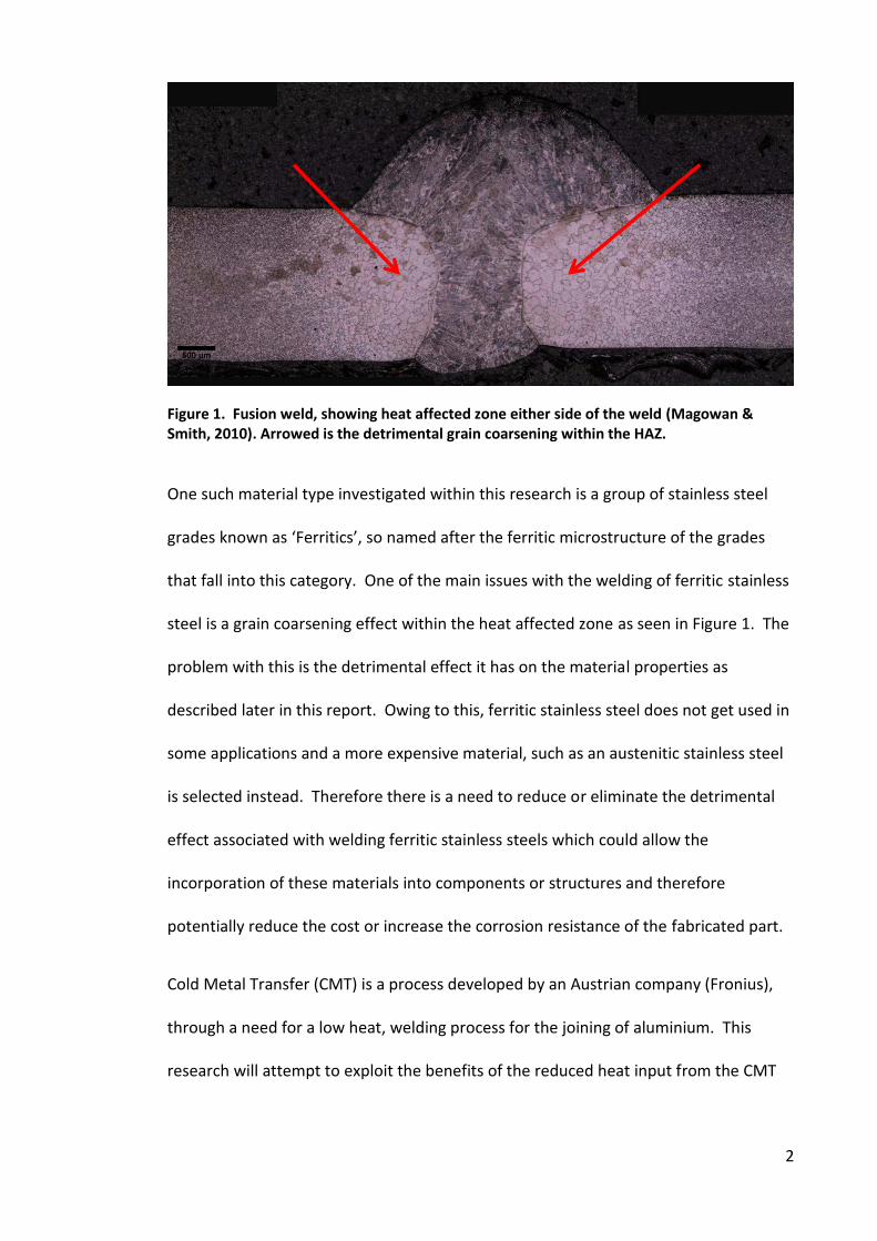
Figure 1. Fusion weld, showing heat affected zone either side of the weld (Magowan &
Smith, 2010). Arrowed is the detrimental grain coarsening within the HAZ. .................. 2
Figure 2. Manufacturing route of stainless steel as utilised at Kawasaki Steel (Ono &
Kaito, 1986). ...................................................................................................................... 8
Figure 3. Schaeffler diagram with stainless steel grades indicated (Outokumpu, 2010).
......................................................................................................................................... 11
Figure 4. Showing the difference in power densities for various fusion welding
processes (Lancaster, 1984). ........................................................................................... 20
Figure 5. Schematic of resistance spot welding (Westgate, 2009). ............................... 21
Figure 6. Image showing a resistance spot weld (RSW) (Westgate, 2009). ................... 22
Figure 7. Schematic of resistance seam welding (Pires, Louriero, & Bolmsjo, 2006). ... 23
Figure 8. Showing resistance seam welding (Westgate, 2009). .................................... 23
Figure 9. Diagram of the manual metal arc welding process (Wermac, 2016) ............. 26
Figure 10. Diagram showing the submerged arc welding process (The Welding Institute
Limited, 1995) ................................................................................................................. 27
Figure 11. Diagram of the gas tungsten arc welding process (Mechanical Engineering,
2016) ............................................................................................................................... 28
Figure 12. Diagram showing transfer modes according to arc current (I) and voltage (V)
(Iordachescu & Quintino, 2008). ..................................................................................... 31
Figure 13. Showing globular transfer (Lucas, Iordachescu, & Ponomarev, 2005). ......... 32
Figure 14. Showing short circuit cycle with effect on current and voltage (ESAB)......... 33
Figure 15. Showing short circuit transfer (Lucas, Iordachescu, & Ponomarev, 2005). ... 33
Figure 16. Showing spray transfer (Lucas, Iordachescu, & Ponomarev, 2005). ............ 34
Figure 17. Pulsed spray transfer graph of current (I) against time (t) for two pulsing
cycles and images depicting the events for one pulsing cycle (Hackl). .......................... 35
Figure 18. Showing pulsed transfer (Lucas, Iordachescu, & Ponomarev, 2005). .......... 36
Figure 19. MIG/MAG process diagram (The Welding Institute, 2010). ......................... 36
Figure 20. Images showing dip arc transfer (Izutani, Shimizu, Suzuki, & Koshiishi, 2007)
where the first image (far left) shows the arc and the consumable electrode with a
spherical molten mass as the end moving toward the work piece as the wire is fed.
The second image (centre) shows the consumable electrode in contact with the weld
pool, provided the short circuit phase. The third image (far right) shows the transfer of
the molten portion of the consumable electrode, which eliminates the contact with it
and so the arc is re-established. ..................................................................................... 37
Figure 21. Schematic diagram of the CMT process showing wire motion, arrowed
(Fronius International GmBH, 2007). .............................................................................. 38
Figure 22. High speed images showing CMT cycle (Fronius International GmbH, 2004).
Corresponding to the schematic in Figure 22 above. ..................................................... 38
Figure 23. Graphs showing voltage (V)(top) and current (I) (bottom) against time for
the CMT process (Rosado, Almeida, Pires, Miranda, & Quintino, 2008). ....................... 39
Figure 24. Showing effect on transfer mode of carbon dioxide addition to argon
shielding gas (Zielinska, et al., 2009). .............................................................................. 46
Figure 25. Image showing grain growth in GMA welded ferritic stainless steel
(Magowan & Smith, 2010). ............................................................................................. 50
Figure 26. Iron-Chromium equilibrium diagram (Computational Thermodynamics Inc.,
2011). .............................................................................................................................. 53
Figure 27. Part of Iron - Chromium equilibrium diagram showing effects of carbon and
nitrogen on the shape and size of the gamma loop (Deddoes, Parr, & Hanson, 1999). 53
Figure 28. Time Temperature Transformation diagram for delta ferrite to austenite in
the high temperature HAZ (Warmelo, Nolan, & Norrish, 2007). .................................... 56
Figure 29. Diagram showing mechanics of shrinkage cracking (University of Ljubljana,
2000) ............................................................................................................................... 57
Figure 30. Suutala diagram for predicting susceptibility to shrinkage cracking from
weld metal composition (Kujanpaa, Suutala, Takalo, & Moisio, 1979). ......................... 58
Figure 31. Use of modified versions of Murakami's reagent to colour delta ferrite and
sigma phase in stainless steel welds. (a) Delta ferrite coloured blue and brown in an
austenitic matrix in type 312 stainless steel weld metal (as-welded) using modified
Murakami's reagent (30 g sodium hydroxide, 30 g potassium ferricyanide, 100 mL
water, at 100 °C, or 212 °F, for 10 s). The arrow points to a slag inclusion in the weld
nugget. (b) Sigma phase formed in a type 312 stainless steel weld (from the delta
ferrite phase) by aging at 816 °C (1500 °F) for 160 h. Sigma was coloured green and
orange by etching with Murakami's reagent (10 g sodium hydroxide, 10 g potassium
ferri a ide, L ater for s at °C °F . The ag ifi atio ars are μ in length (Vandervoort, Colour Metallography - Film Formation and Interference
Techniques, 2004). .......................................................................................................... 61
Figure 32. Image showing Sigma phase (Vandervoort, Examination of Microstructures,
2003). .............................................................................................................................. 62
Figure 33. Image showing liquid copper which has penetrated down the grain
boundaries of an AISI 304 austenitic stainless steel (Magowan S. , 2006). .................... 65
Figure 34. Showing different fatigue cycles. (NDT Resource Centre, 2016) .................. 68
Figure 35. Presentation of data from low cycle fatigue testing (KTH, 2003) ................. 70
Figure 36. Showing S-N curve typical reporting of high cycle fatigue data (eFUNDA,
2016). .............................................................................................................................. 70
Figure 37. Showing three stages of crack growth rate (Engineers Edge, 2016). ............ 72
Figure 38. Figure showing persistant slip bands. (NDT Resource Centre, 2016) ............ 74
Figure 39. Showing fatigue crack propagation (Key to Metals AG, 2005) ..................... 75
Figure 40. SEM image showing fatigue striations (ASM International, 2008). .............. 75
Figure 41. Showing relationship between parent/weld interface angle and fatigue
strength (Harris & Syers, 1979). ...................................................................................... 79
Figure 42. Graph showing relationship between penetration root angle and fatigue life
for similar thickness CMT welds (Ashcroft, 2008). ......................................................... 80
Figure 43. 9—S–N curves of the investigated specimens with different maximum pore
volumes (PV) for A1Si7Mg0.3 (Tijani, Heinreitz, Stets, & Voigt, 2013) ........................... 81
Figure 44. Fatigue test results for defect-free and defective 6mm high strength steel
parent specimen (Ottersbock, Leitner, Stoschka, & Maurer, 2016) ............................... 81
Figure 45. Sectioning of weld plan, sections taken at 10mm, 40mm, 70mm, 110mm,
140mm and 170mm. Green arrow shows welding direction (Boulding, The Effects of
Parameters and Consistency of Cold Metal Transfer Welded Ferritic Stainless Steel
Joints, 2012). ................................................................................................................... 90
Figure 46. Schematic of parent plate size and setup for all CMT & MAG welded samples
the plate length was either 400mm as indicated above, or 200mm. ............................. 95
Figure 47. Showing the CMT welding equipment at Sheffield Hallam University. ........ 96
Figure 48. Image showing tractor and track used to traverse the welding torch. ........ 97
Figure 49. Image showing ABB robotic arm used in some of the CMT and MAG welding
trials. ................................................................................................................................ 98
Figure 50. Welding set up showing ALX weld monitoring equipment (Boulding, The
Effects of Parameters and Consistency of Cold Metal Transfer Welded Ferritic Stainless
Steel Joints, 2012). .......................................................................................................... 99
Figure 51. Showing clamping arrangement for holding the parent material in place
whilst welding. .............................................................................................................. 100
Figure 52. Images showing fresh glyceregia (left) and glyceregia following
approximately 1 hours use (right) where it requires disposal. ..................................... 105
Figure 53. Schematic of weld cross section showing measurements made on optical
examination .................................................................................................................. 106
Figure 54. Image showing calibration of measurement capability of DM2500 optical
measuring system. ........................................................................................................ 107
Figure 55. Leica DM2500 optical microscope, connected to Buehler Omnimet 9.0 image
analysis software. .......................................................................................................... 107
Figure 56. Schematic of hardness testing survey positions. ........................................ 109
Figure 57. Instron Dynatup 9250 impact test machine. ............................................... 110
Figure 58. Showing the sampling of impact (left), microstructural (middle) and tensile
specimens (right) from the welded sheet. .................................................................... 111
Figure 59. ESH Fatigue testing machine. ...................................................................... 112
Figure 60. Showing the sampling of fatigue specimens from the as-welded sheet. ... 113
Figure 61. Etched microstructure of 3.8mm thick EN1.4003 used in the study showing
an equiaxed fully ferritic structure (Etched in Glyceregia). .......................................... 117
Figure 62. Etched microstructure of 5.8mm thick EN1.4003 used in the study showing
an equiaxed fully ferritic structure (Etched in Glyceregia). .......................................... 118
Figure 63. Etched microstructure of the EN1.4016 material used in the study showing
an equiaxed fully ferritic structure (Etched in Glyceregia). .......................................... 118
Figure 64. Etched microstructure of the EN 1.4509 material used in the study showing
an equiaxed fully ferritic structure (Etched in Glyceregia). .......................................... 119
Figure 65. Etched microstructure of the EN 1.4521 material used in the study showing
an equiaxed fully ferritic structure with carbides arrowed (Etched in Glyceregia). ..... 119
Figure 66. Graph comparing calculated heat input, weld bead and heat affected zone
width of MAG and CMT welded joints. ......................................................................... 121
Figure 67. Image taken within the HAZ of the CMT welded EN1.4016 material, showing
martensite (red arrow) at the grain boundaries. .......................................................... 121
Figure 68. Comparison of the 1.4016 MAG weld/HAZ middle hardness profiles......... 122
Figure 69. Comparison of the 1.4016 CMT weld/HAZ middle micro hardness profiles.
....................................................................................................................................... 123
Figure 70. Showing effect of heat input on HAZ width for pure CMT and CMT with
Pulsed arc welded samples, EN1.4016 parent material. .............................................. 126
Figure 71. Showing effect of heat input on grain size for pure CMT and CMT with
pulsed arc welded samples, EN1.4016 parent material. .............................................. 126
Figure 72. Line scan of interface between AISI 430 parent metal and AISI 308L weld
metal. ............................................................................................................................ 127
Figure 73. Elemental Map of parent metal and weld metal interface for AISI 430 parent
material and 308LSi filler. ............................................................................................. 128
Figure 74. Graph showing forehand (15°) welds produced using 1.4016 material at
1mm, 1.15mm and 1.25mm joint gaps and 762, 1016 & 1270 mm/min welding speeds,
categorised according to whether weld penetration was achieved. ........................... 129
Figure 75. Graph showing forehand (15°) welds produced using 1.4509 material at
1mm, 1.15mm and 1.25mm joint gaps and 762, 1016 & 1270 mm/min welding speeds,
categorised according to whether weld penetration was achieved. ........................... 130
Figure 76. Graph showing the effect of torch angle on achieving penetration of welds
produced using grade 1.4016 parent material, using a 1mm joint gap, at different
welding speeds. ............................................................................................................. 130
Figure 77. Graph showing the effect of torch angle on achieving penetration of welds
produced using grade 1.4509 parent material, using a 1mm joint gap, at different
welding speeds. ............................................................................................................. 131
Figure 78. Image showing the effect of heat input on weld and HAZ dimensions. The
left hand weld cross section of 2mm thick, CMT+P welded, 1.4016 material with heat
input of 0.113 kJ/mm and the right is the same material and welded using the same
process but with a net heat input of 0.060 kJ/mm. ...................................................... 131
Figure 79. Example 1, showing a fully penetrated weld (Boulding, The Effects of
Parameters and Consistency of Cold Metal Transfer Welded Ferritic Stainless Steel
Joints, 2012). ................................................................................................................. 135
Figure 80. Example 2, showing an incomplete penetrated weld (Boulding, The Effects
of Parameters and Consistency of Cold Metal Transfer Welded Ferritic Stainless Steel
Joints, 2012). ................................................................................................................. 135
Figure 81. Example 3, showing misaligned parent/penetration to one side (Boulding,
The Effects of Parameters and Consistency of Cold Metal Transfer Welded Ferritic
Stainless Steel Joints, 2012). ......................................................................................... 135
Figure 82. Graph showing the width of the HAZ for each of the CMT welds conducted
at 3.5m/min (average net heat input 72.2 J/mm) on EN1.4016 grade parent material.
....................................................................................................................................... 137
Figure 83. Graph showing the width of the HAZ for each of the CMT welds conducted
at 4.5m/min (average net heat input 88.5 J/mm) on EN1.4016 grade parent material.
....................................................................................................................................... 137
Figure 84. Graph showing the width of the HAZ for each of the CMT welds conducted
at 5.5m/min (average net heat input 109.3 J/mm) on EN1.4016 grade parent material.
....................................................................................................................................... 138
Figure 85. Graph showing the current and voltage trace for the CMT weld conducted
at 3.5m/min on EN1.4016 grade parent material. ....................................................... 138
Figure 86. Graph showing the current and voltage trace for the CMT weld conducted
at 4.5m/min on EN1.4016 grade parent material. ....................................................... 139
Figure 87. Graph showing the current and voltage trace for the CMT weld conducted
at 5.5m/min on EN1.4016 grade parent material. ....................................................... 139
Figure 88. Graph showing the width of the HAZ for each of the CMT welds conducted
at a traverse speed of 0.762m/min (average net heat input 118.3 J/mm) on EN1.4016
grade parent material. .................................................................................................. 140
Figure 89. Graph showing the width of the HAZ for each of the CMT welds conducted
at a traverse speed of 1.27m/min (average net heat input 69.6 J/mm) on EN1.4016
grade parent material. .................................................................................................. 141
Figure 90. Graph showing the width of the HAZ for each of the CMT welds created
using a torch orientation +15° to the direction of traverse on EN1.4016 grade parent
material. ........................................................................................................................ 142
Figure 91. Graph showing the width of the HAZ for each of the CMT welds created
using a torch orientation -15° to the direction of traverse on EN1.4016 grade parent
material. ........................................................................................................................ 142
Figure 92. Graph showing the width of the HAZ for each of the CMT welds conducted
with an ALC value of -30 on EN1.4016 grade parent material. .................................... 143
Figure 93. Graph showing the width of the HAZ for each of the CMT welds conducted
with an ALC value of +30 on EN1.4016 grade parent material. .................................... 144
Figure 94. Graph showing voltage and current trace for a CMT weld conducted with an
ALC of -30 on EN1.4016 grade parent material. ........................................................... 145
Figure 95. Graph showing voltage and current trace for a CMT weld conducted with an
ALC of +30 on EN1.4016 grade parent material. .......................................................... 145
Figure 96. Graph showing the width of the HAZ for each of the CMT welds conducted
with a PC of -5 on EN1.4016 grade parent material. .................................................... 146
Figure 97. Graph showing the width of the HAZ for each of the CMT welds conducted
with a PC of +5 on EN1.4016 grade parent material. ................................................... 147
Figure 98. Graph showing the current and voltage trace for a CMT weld conducted
with a pulse correction of -5 on EN1.4016 grade parent material. .............................. 147
Figure 99. Graph showing the current and voltage trace for a CMT weld conducted
using a pulse correction of +5 on EN1.4016 grade parent material. ............................ 148
Figure 100. CMT weld cross section of the 5.8mm thick EN1.4003 grade parent
material ......................................................................................................................... 149
Figure 101. Lack of side wall fusion in CMT weld produced using the 5.8mm thick
EN1.4003 grade material. ............................................................................................. 149
Figure 102. Showing radiograph for test weld that was sectioned to destructively
examine, with identification of indications observed through examination of the
radiograph and suggested possibility of defect type. Red arrows showing spatter, blue
arrows showing gas porosity and yellow arrows showing indications of a lack of side
wall fusion. .................................................................................................................... 150
Figure 103. showing section 7 of the weld, the three pieces of spatter circled
(Robinson, 2014) ........................................................................................................... 151
Figure 104. Lack of side wall fusion in root of section 1a of CMT welded 5.8mm thick
EN1.4003 (Robinson, 2014)........................................................................................... 152
Figure 105. Showing gas porosity in section 5a of CMT welded 5.8mm thick EN1.4003
(Robinson, 2014). .......................................................................................................... 152
Figure 106. Gas porosity (left) lack of side wall fusion (right) in section 9a of CMT
welded 5.8mm thick EN1.4003 (Robinson, 2014)......................................................... 153
Figure 107. Image showing weld (top right) and HAZ , which has two distinct regions,
the first next to the weld (red arrow) has a martensitic structure and grain coarsening,
the second region of the HAZ (orange arrow) has a martensitic structure but without
any grain coarsening and then the blue arrow indicates unaffected parent material of
3.8mm thick EN1.4003 parent, CMT welded sample 25.10 (etched in glyceregia). .... 155
Figure 108. Image showing weld (top right) and grain coarsened with martensite HAZ
(mid image) and martensite HAZ (bottom left) of 3.8mm thick EN1.4003 parent, CMT
welded sample 25.10 (etched in glyceregia) ................................................................ 155
Figure 109. Image showing weld (top left) and HAZ , which has two distinct regions,
the first next to the weld has a martensitic structure and grain coarsening (red arrow),
the second region of the HAZ (orange arrow) has a martensitic structure but without
any grain coarsening and then the blue arrow indicates unaffected parent material of
3.8mm thick EN1.4003 parent, MAG welded sample 30.7 (etched in glyceregia). ...... 156
Figure 110. Image showing weld (top left) and twin region HAZ (mid image & bottom
right) of 3.8mm thick EN1.4003 parent, MAG welded sample 30.7 (etched in
glyceregia). .................................................................................................................... 156
Figure 111. Staircase Fatigue results for the CMT welded samples. ............................ 163
Figure 112. Graph to show fatigue load range for CMT welded 3.8mm thick EN1.4003
(red line indicates the pass criteria of 2 million cycles). ............................................... 164
Figure 113. Staircase Fatigue results for the MAG welded samples. ........................... 165
Figure 114. Graph to show fatigue load range for MAG welded 3.8mm thick EN1.4003
(red line indicates the pass criteria of 2 million cycles). ............................................... 166
Figure 115. Image showing a lack of side wall fusion (arrowed). ................................ 167
Figure 116. Image showing a lack of root penetration (arrowed) ............................... 167
Figure 117. Image showing weld porosity (arrowed). ................................................. 167
Figure 118. SEM image showing a region with a lack of fusion and the areas where
analysis .......................................................................................................................... 168
Figure 119. Graph of element analysis spectrum 3 ...................................................... 168
Figure 120. Graph of element analysis spectrum 4. ..................................................... 168
Figure 121. Graph showing the effect of defect area of the fracture face against
number of cycles to failure for CMT welded samples. ................................................. 169
Figure 122. Graph showing the effect of defect area of the fracture face against the
number of cycles to failure for each of the tested loads on CMT welded samples. .... 169
Figure 123. Graph showing the effect on gradient of the % defects within the fracture
surface against the number of cycles survived for each load, therefore as the load is
increased the gradient also increases on the EN1.4003 parent CMT welded samples.
....................................................................................................................................... 170
Figure 124. Graph showing the effect on gradient of the % defects within the fracture
surface against the number of cycles survived for each load, with the result for 46kN
removed, therefore as the load is increased the gradient also increases on the
EN1.4003 parent CMT welded samples ........................................................................ 170
Figure 125. Showing plan of the weld cap of a MAG welded sample, red line showing
location for one of profiles taken. ................................................................................ 172
Figure 126. Profile trace for weld cap of MAG welded sample as seen in Figure 122. 173
Figure 127. Showing IFM 3D scan of the weld cap of a MAG welded sample. ............ 174
Figure 128. Showing plan of the weld root of a MAG welded sample, red line showing
location for one of profiles taken. ................................................................................ 175
Figure 129. Profile trace for weld root of MAG welded sample as seen in Figure 125.
....................................................................................................................................... 176
Figure 130. Showing IFM 3D scan of the weld root of a MAG welded sample. ........... 177
Figure 131. Graph showing weld root angle against the number of cycles before failure
for the CMT welded samples fatigue tested at 46 kN .................................................. 178
Figure 132. Graph showing weld root angle against the number of cycles before failure
for the CMT welded samples fatigue tested at 45.5 kN ............................................... 179
Figure 133. Graph showing weld root angle against the number of cycles before failure
for the CMT welded samples fatigue tested at 45 kN .................................................. 179
Figure 134. Graph showing weld root angle against the number of cycles before failure
for the CMT welded samples fatigue tested at 44.5 kN ............................................... 180
Figure 135. Graph showing weld root angle against the number of cycles before failure
for the CMT welded samples fatigue tested at 44 kN .................................................. 180
Figure 136. Graph showing weld root angle against the number of cycles before failure
for the CMT welded samples fatigue tested at 43.5 kN ............................................... 181
Figure 137. Graph showing weld root angle against the number of cycles before failure
for the CMT welded samples fatigue tested at 43 kN .................................................. 181
Figure 138. Graph showing weld root angle against the number of cycles before failure
for the CMT welded samples fatigue tested at 42.5 kN ............................................... 182
Figure 139. Graph showing weld root angle against the number of cycles before failure
for the CMT welded samples fatigue tested at 42 kN .................................................. 182
Figure 140. Graph showing weld root angle against the number of cycles before failure
for the CMT welded samples fatigue tested at 41.5 kN ............................................... 183
Figure 141. Showing the root angle against number of cycles for the CMT welded
samples. ........................................................................................................................ 183
Figure 142. Graph showing weld root angle against the number of cycles before failure
for the MAG welded samples fatigue tested at 38.5kN ............................................... 184
Figure 143. Graph showing weld root angle against the number of cycles before failure
for the MAG welded samples fatigue tested at 35.5kN ............................................... 184
Figure 144. Graph showing weld root angle against the number of cycles before failure
for the MAG welded samples fatigue tested at 32.5kN ............................................... 185
Figure 145. Graph showing weld root angle against the number of cycles before failure
for the MAG welded samples fatigue tested at 29.5kN ............................................... 185
Figure 146. Showing the root angle against number of cycles for the MAG welded
samples. ........................................................................................................................ 186
Figure 147. Image showing fully ferritic microstructure of sample subjected to 700°C 20
min soak water quench as seen in the as received EN1.4003 material ....................... 187
Figure 148. Image Showing fully ferritic microstructure of sample subjected to 700°C
20 min soak water quench as seen in the as received EN1.4003 material. ................. 187
Figure 149. Image showing ferritic (light areas) and martensitic (dark areas)
microstructure of sample subjected to 800°C 20 min soak water quench similar to the
microstructure in the region of the HAZ furthest from the fusion zone of welds on a
EN1.4003 grade material. ............................................................................................. 188
Figure 150. Image showing ferritic and martensitic microstructure (250 HV10) of sample
subjected to 800°C 20 min soak water quench similar to the microstructure in the
region of the HAZ furthest from the fusion zone of welds on an EN1.4003 grade
material. ........................................................................................................................ 188
Figure 151. Image showing martensitic microstructure of EN1.4003 sample subjected
to 900°C 20 min soak water quench. ............................................................................ 189
Figure 152. Image showing martensitic microstructure (277 HV10) of EN1.4003 sample
subjected to 900°C 20 min soak water quench. ........................................................... 189
Figure 153. Image showing martensitic microstructure with some grain growth of
EN1.4003 sample subjected to 1000°C 20 min soak water quench, this is similar to
what would be seen in the region of the HAZ closest to the fusion zone. ................... 190
Figure 154. Image showing martensitic microstructure with some grain growth of
EN1.4003 sample subjected to 1000°C 20 min soak water quench, this is similar to
what would be seen in the region of the HAZ closest to the fusion zone. ................... 190
Figure 155. Image showing martensitic microstructure and grain growth of EN1.4003
sample subjected to 1100°C 20 min soak water quench, this is similar to what would be
seen in the region of the HAZ closest to the fusion zone. ............................................ 191
Figure 156. Image showing ferritic and martensitic microstructure and grain growth of
EN1.4003 sample subjected to 1100°C 20 min soak water quench, this is similar to
what would be seen in the region of the HAZ closest to the fusion zone. ................... 191
Figure 157. Image showing ferritic microstructure of EN1.4003 sample subjected to
747°C 20 min soak water quench, as would be seen in the unaffected parent material.
....................................................................................................................................... 192
Figure 158. Image showing ferritic microstructure of sample subjected to 747°C 20 min
soak water quench, as would be seen in the unaffected parent material. .................. 192
Figure 159. Image showing ferritic microstructure of an EN1.4003 sample subjected to
758°C 20 min soak water quench as would be seen in the unaffected parent material.
....................................................................................................................................... 193
Figure 160. Image showing ferritic microstructure of an EN1.4003 sample subjected to
758°C 20 min soak water quench as would be seen in the unaffected parent material.
....................................................................................................................................... 193
Figure 161. Image showing ferritic microstructure (light areas) with martensite (dark
areas) at the grain boundaries of an EN1.4003 sample subjected to 769°C 20 min soak
water quench, this would be typical of a microstructure seen in the HAZ at its furthest
distance from the fusion zone. ..................................................................................... 194
Figure 162. Image showing ferritic microstructure with martensite at the grain
boundaries of an EN1.4003 sample subjected to 769°C 20 min soak water quench, this
would be typical of a microstructure seen in the HAZ at its furthest distance from the
fusion zone. ................................................................................................................... 194
Figure 163. Image showing ferritic (light areas) and martensitic (dark areas)
microstructure of an EN1.4003 sample subjected to 779°C 20 min soak water quench.
....................................................................................................................................... 195
Figure 164. Image showing ferritic (light areas) and martensitic (dark areas)
microstructure of an EN1.4003 sample subjected to 779°C 20 min soak water quench.
....................................................................................................................................... 195
Figure 165. Image showing ferritic (light areas) and martensitic (dark areas)
microstructure of an EN1.4003 sample subjected to 790°C 20 min soak water quench.
....................................................................................................................................... 196
Figure 166. Image showing ferritic (light areas) and martensitic (dark areas)
microstructure of an EN1.4003 sample subjected to 790°C 20 min soak water quench.
....................................................................................................................................... 196
Figure 167. Image showing martensitic microstructure of an EN1.4003 sample
subjected to 800°C 2 hour soak water quench. ............................................................ 197
Figure 168. Image showing martensitic microstructure of an EN1.4003 sample
subjected to 800°C 2 hour soak water quench. ............................................................ 197
Figure 169. Image showing ferritic (light areas) and martensitic (dark areas)
microstructure of an EN1.4003 sample subjected to 770°C 2 hour soak water quench.
....................................................................................................................................... 198
Figure 170. Image showing ferritic (light areas) and martensitic (dark areas)
microstructure of an EN1.4003 sample subjected to 760°C 2 hour soak water quench.
....................................................................................................................................... 198
Figure 171. Image showing ferritic (light areas) and martensitic (dark areas)
microstructure of EN 1.4003 sample subjected to 750°C 2 hour soak water quench. 199
Figure 172. Image showing ferritic microstructure of an EN 1.4003 sample subjected to
740°C 2 hour soak water quench. ................................................................................. 199
Figure 173. Image showing martensitic microstructure of an EN1.4003 sample
subjected to 800°C 2 hour soak Furnace cool to determine the effect of time at
temperature. ................................................................................................................. 200
Figure 174. Image showing martensitic microstructure of an EN1.4003 sample
subjected to 800°C 2 hour soak Furnace cool to determine the effect of time at
temperature. ................................................................................................................. 200
Figure 175. Image showing ferritic (light areas) and martensitic (dark areas)
microstructure of an EN1.4003 sample subjected to 800°C 6 hour soak 30°C/hour cool
rate. ............................................................................................................................... 201
Figure 176. Image showing ferritic (light areas) and martensitic (dark areas)
microstructure of an EN1.4003 sample subjected to 800°C 6 hour soak 30°C/hour cool
rate. ............................................................................................................................... 201
Figure 177. Image showing martensitic microstructure of an EN1.4003 sample
subjected to 1000°C 6 hour soak 30°C/hour cool rate grain coarsening also evident. 202
Figure 178. Image showing martensitic microstructure of an EN1.4003 sample
subjected to 1000°C 6 hour soak 30°C/hour cool rate, grain coarsening also evident.
....................................................................................................................................... 202
Figure 179. Image showing martensitic microstructure of an EN1.4003 sample
subjected to 900°C 6 hour soak 30°C/hour cool rate, grain coarsening also evident. . 203
Figure 180. Image showing martensitic microstructure of an EN1.4003 sample
subjected to 900°C 6 hour soak 30°C/hour cool rate, grain coarsening also evident. . 203
Figure 181. Figure showing microstructures of samples subjected to a hold for a time
at a temperature. .......................................................................................................... 204
Figure 182. Graph showing effect of peak temperature on hardness (HV10). ............. 205
Figure 183. Graph showing effect of peak temperature on grain size. ....................... 206
Figure 184. Graph showing effect of grain size on material toughness. ..................... 206
Figure 185. Graph showing effect of different thermal cycles on impact properties. 207
Figure 186. Graph showing effect of various thermal cycles on hardness. ................. 207
Figure 187. Graph showing effect of various thermal cycles on grain size. ................ 208
Figure 188. CMT weld cross section of the 5.8mm thick EN1.4003 grade parent
material ......................................................................................................................... 224
Figure 189. . Image showing weld (top right) and HAZ , which has two distinct regions,
the first next to the weld (red arrow) has a martensitic structure and grain coarsening,
the second region of the HAZ (orange arrow) has a martensitic structure but without
any grain coarsening and then the blue arrow indicates unaffected parent material of
3.8mm thick EN1.4003 parent, CMT welded sample 25.10 (etched in glyceregia). .... 227
Figure 190. . Image showing weld (top left) and HAZ , which has two distinct regions,
the first next to the weld has a martensitic structure and grain coarsening (red arrow),
the second region of the HAZ (orange arrow) has a martensitic structure but without
any grain coarsening and then the blue arrow indicates unaffected parent material of
3.8mm thick EN1.4003 parent, MAG welded sample 30.7 (etched in glyceregia). ...... 228
List of Tables
Table 1. Table showing stainless steel grades and chemical compositions (Outokumpu,
2010). .............................................................................................................................. 10
Table 2. Classification of droplet transfer modes and typical process mode utilised
(Izutani, Shimizu, Suzuki, & Koshiishi, 2007). .................................................................. 30
Table 3. Showing the properties of various shielding gases (Praxair, 2005). ................ 43
Table 4. Materials and thicknesses used in the research. .............................................. 84
Table 5. Mechanical properties of ferritic stainless steels at room temperature
(Outokumpu, 2011). ........................................................................................................ 85
Table 6. Chemical analysis data of the parent materials used within the project. ....... 85
Table 7. Composition of AISI 308L-Si filler material (Avesta Welding, 2006). ................ 85
Table 8. Table showing variation of each of the ten settings used in the CMT
consistency trial (Boulding, The Effects of Parameters and Consistency of Cold Metal
Transfer Welded Ferritic Stainless Steel Joints, 2012). ................................................... 89
Table 9. Welding parameters used in the EN1.4003 CMT/MAG comparison trial. ....... 92
Table 10. Showing heat treatment temperature, durations and method of cooling for
samples of 5.8mm thick EN1.4003 (where WQ = Water Quenched). ............................ 93
Table 11. Showing chemical composition to make 120ml of glyceregia. .................... 104
Table 12. Table showing parameters for scans performed on the IFM ....................... 108
Table 13. Table used to collect the staircase fatigue testing data also provides
information necessary for calculations to determine mean fatigue load. ................... 114
Table 14. Showing some of the welding parameters and calculated heat inputs. ...... 120
Table 15 Summary of weld/HAZ dimensions for pure CMT welded samples with
increasing net heat input. ............................................................................................. 124
Table 16. Summary of weld/HAZ dimensions for CMT with pulsed arc welded samples
with increasing net heat input. ..................................................................................... 125
Table 17. Table showing actual readings and calculated heat inputs for each weld
produced on the trial. ................................................................................................... 133
Table 18. Showing assessments of the extent of penetration of the filler metal for each
sample examined (Boulding, The Effects of Parameters and Consistency of Cold Metal
Transfer Welded Ferritic Stainless Steel Joints, 2012). For colour coding PTO. ........... 134
Table 19. Showing key to assessments made on penetration (Boulding, The Effects of
Parameters and Consistency of Cold Metal Transfer Welded Ferritic Stainless Steel
Joints, 2012). ................................................................................................................. 135
Table 20. Table showing defects observed through microstructural examination of
EN1.4003 5.8mm thick CMT welded plate. The sample identification numbers in the
left hand column are based on those presented in Figure 99. ..................................... 151
Table 21. Showing average measured values for the HAZ in the coarse region and the
entire HAZ width and the grain size taken in the course region of the HAZ of 3.8mm
thick EN1.4003 grade parent material. ......................................................................... 154
Table 22. CMT 3.8mm EN1.4003 Tensile results.......................................................... 157
Table 23. MAG 3.8mm EN1.4003 Tensile results. (* sample M28.9 not included in
calculations as failed next to spatter). .......................................................................... 158
Table 24. Statistical T.Test P values comparing the data for the 3.8mm thick CMT and
MAG welded tensile data. ............................................................................................. 158
Table 25. CMT 5.8mm EN1.4003 Tensile results.......................................................... 159
Table 26. MAG 5.8mm EN1.4003 Tensile results. ........................................................ 160
Table 27. Statistical T.Test P values comparing the data for the 5.8mm thick CMT and
MAG welded tensile data. ............................................................................................. 160
Table 28. Impact test results for CMT welded 3.8mm thick EN1.4003. ....................... 161
Table 29. Impact test results for MAG welded 3.8mm thick EN1.4003....................... 161
Table 30. Statistical T.Test P values comparing the data for the 3.8mm thick CMT and
MAG welded impact data. ............................................................................................ 161
Table 31. Impact test results for CMT welded 5.8mm thick EN1.4003. ...................... 162
Table 32. Impact test results for MAG welded 5.8mm thick EN1.4003....................... 162
Table 33. Statistical T.Test P values comparing the data for the 5.8mm thick CMT and
MAG welded impact data. ............................................................................................ 162
List of Equations
Equation 1. Equation showing amount of niobium required to stabilise a stainless steel.
......................................................................................................................................... 18
Equation 2. Equation to calculate arc energy. ............................................................... 47
Equation 3. Equation to calculate weld heat input. ........................................................ 47
Equation 4. Equation to determine the ferrite factor (Zheng, Ye, Jiang, Wang, Liu, &
Wang, 2010) .................................................................................................................... 56
Equation 5. Equation to determine the chromium equivalent. ..................................... 58
Equation 6. Equation to determine the nickel equivalent. ............................................. 58
Equation 7. Equation to determine the maximum fatigue stress. ................................. 68
Equation 8. Equation to determine the minimum fatigue stress. ................................. 68
Equation 9. Equation to determine the mean fatigue stress. ........................................ 68
Equation 10. Equation to determine the fatigue stress range. ..................................... 68
Equation 11. Equation to determine the fatigue stress ratio ........................................ 68
Equation 12. Paris equation to model crack growth. ..................................................... 73
Equation 13. Ashcrofts model for fatigue life prediction against root angle. ............... 82
Equation 14. Equation to calculate mean fatigue load ................................................. 115
Equation 15. Equation to calculate convergence factor ............................................... 115
Equation 16. Equation to calculate standard deviation ................................................ 115
Equation 17. Equation to calculate standard error for mean fatigue load................... 115
List of Acronyms
ALC Arc Length Correction
BCC Body Centred Cubic
BCT Body Centred Tetragonal
CCT Continuous Cooling Transformation
CMT Cold Metal Transfer
CMT+P Cold Metal Transfer with Pulsed Arc
FCC Face Centred Cubic
GMAW Gas Metal Arc Welding
GTAW Gas Tungsten Arc Welding
HAZ Heat Affected Zone
HTHAZ High Temperature Heat Affected Zone
MIG Metal Inert Gas
MAG Metal Active Gas
PC Pulse Correction
TTT Time Temperature Transformation
XRF X-Ray Fluorescence
1
1 Introduction
Welding is a widely used and effective method of joining different components
together. There is however no single welding process that will obtain the optimum
weld in every situation. Factors such as process applicability, cost, time, access to the
area to be joined, deposition rate and the service environment of the joint will be
paramount in selecting the most appropriate joining method, such as welds produced
on an aftermarket sports exhaust tailpipe, where Gas Tungsten Arc Welding (GTAW) is
used for the aesthetical appearance or where Resistance Spot Welding (RSW) is not
used due to the requirement of overlap of the parent materials, which creates the
crevices for corrosion to initiate and accelerate.
As fusion welds tend to require a heat source (the exception being friction stir
welding), there is also an effect on the parent materials as a result of this heat, which
produces what is commonly known as the Heat Affected Zone (HAZ). The heat
affected zone can contain a whole host of differences to that of the base material.
They can, for example, contain a totally different phase in the microstructure, they
could contain portions of a different microstructure, the formation of carbides or other
phases are common within the heat affected zone, there can also be grain coarsening
within this region. All of these aspects have the potential to effect the material
properties in this area, this effect may be an increase or decrease in strength,
toughness, ductility, hardness or corrosion resistance, sometimes this may be
beneficial, other times detrimental to the component or structure.
2
Figure 1. Fusion weld, showing heat affected zone either side of the weld (Magowan &
Smith, 2010). Arrowed is the detrimental grain coarsening within the HAZ.
One such material type investigated within this research is a group of stainless steel
grades k o as Ferriti s , so a ed after the ferriti i rostru ture of the grades
that fall into this category. One of the main issues with the welding of ferritic stainless
steel is a grain coarsening effect within the heat affected zone as seen in Figure 1. The
problem with this is the detrimental effect it has on the material properties as
described later in this report. Owing to this, ferritic stainless steel does not get used in
some applications and a more expensive material, such as an austenitic stainless steel
is selected instead. Therefore there is a need to reduce or eliminate the detrimental
effect associated with welding ferritic stainless steels which could allow the
incorporation of these materials into components or structures and therefore
potentially reduce the cost or increase the corrosion resistance of the fabricated part.
Cold Metal Transfer (CMT) is a process developed by an Austrian company (Fronius),
through a need for a low heat, welding process for the joining of aluminium. This
research will attempt to exploit the benefits of the reduced heat input from the CMT

3
welding process to joining ferritic stainless steels, where this has the detrimental
effects associated with the thermal cycle of the fusion.
Therefore this research aims to assess the capability of the CMT process when welding
ferritic stainless steel parent materials and comparing with conventional Gas Metal Arc
Welding (GMAW), this is to be qualified through assessment of mechanical properties
and microstructural evaluations. The use of this process for the joining of ferritic
stainless steel is limited and therefore this research will expand the body of knowledge
in this area of welding and if CMT offers significant advantages over the conventional
welding process, could mean that ferritic stainless steels could replace the use of
austenitic stainless steels in some applications.
4
2 Literature Review
2.1 Stainless Steel
2.1.1 Definition of Stainless Steel
Stainless steels are a group of materials which, using iron as the primary element, may
also include other significant additions such as chromium, nickel, and carbon
depending on the particular type of stainless steel intended. To be considered
stainless, the material must contain at least 10.5% chromium (Lippold & Kotecki, 2005)
as this permits the formation of a chromium rich oxide layer on the surface of the
material, thereby providing protection from atmospheric conditions. It must be noted
that some alloys containing equal or greater amounts of the prescribed chromium
content will still in fact corrode. The reason for this is that chromium has a strong
affinity for carbon and so has a tendency to form carbides, thus, reducing free
chromium from the matrix and thereby limiting the chromium content available to
form the passive oxide layer.
2.1.2 History of Stainless Steel
Making additions of chromium to steel and noting the benefits with regards to
corrosion performance has been documented from as early as 1821 during
experiments conducted by Pierre Berthier (Cobb, 2010). This first instance recorded
gave the development of a 1.5% Cr alloy that was suggested could be suitable for use
in the cutlery industry. However the high carbon content reduced the alloys
formability, so it was not adopted. This work was conducted as a result of reading
about trials using additions of chromium to steel to create metallic mirrors that didn't
5
tarnish (Stodart & Faraday, 1822). In June 1872, J.E.T. Woods and J. Clark obtained
British Provisional Patent 1932, for a weather resistant iron alloy that contained 30-
35% chromium and 2% tungsten, the first patent for what would now be considered a
stainless steel.
In 1892 high chromium steels were under investigation by Robert A. Hadfield in
Sheffield, England. Using relatively high carbon contents (up to 2%) and chromium
contents up to 16.74%, the materials were rejected as it displayed a reduction in
corrosion performance under the conditions of the test. This was due to the
accelerated corrosion test using a solution of 50% sulphuric acid, utilised by scientists
of the day, under the common belief, that the media used was representative of
corrosion in general.
In 1912 Harry Brearley visited a small arms factory to look at issues with gun barrels,
his recommendations were to develop a low carbon, high chromium steel. On the 20th
August 1913 (Cobb, 2010) Brearley produced a cast which contained 0.24% carbon and
12.8% chromium and when trying to etch the alloy, to permit microstructural analysis
he found that this alloy did not etch or etched very slowly (Brearley, 1991) and is
therefore credited with the invention of ferritic stainless steel (British Stainless Steel
Association).
Around the same time that Brearley was experimenting with chromium contents in
steel above that required to give the self healing layer, it is reported that others were
also investigating these materials. The Americans claim that Elwood Haynes, was the
first person to discover stainless steel and that it was only as a result of Brearley not
being able to get the patent for the process in England and that he was successful in
getting it in the U.S. that meant he was credited with the discovery (Marble, 1921).
6
The French scientist Leon Guillet was examining materials with compositions that
would now be considered as martensitic grades, whilst another Frenchman, Albert
Portevin was looking at steels with compositions similar to those now classed as EN
1.4016 ferritic stainless steel, whilst in 1908 the Krupp Iron Works in Germany had
produced a chromium nickel steel for the hull of a yacht, the actual composition of the
steel is not known, however two employees of the Krupp Iron Works, Eduard Maurer
and Benno Strauss where at the same time as Brearley working on austenitic stainless
steels (British Stainless Steel Association). So although there was a significant amount
of research into these materials, globally, it was Brearley who has been recorded as
the inventor.
7
2.1.3 Manufacturing Methods of Stainless Steel
The manufacturing procedure for stainless steel varies according to the product being
produced and the intended application. The manufacturing route seen in Figure 2,
used by Kawasaki, gives a general indication of the processes involved, with the use of
the Electric Arc Furnace (EAF) being the start of the journey, melting the raw material
(and potentially recycled materials) and then the molten material is transferred to the
Argon Oxygen Decarburisation (AOD) plant, where two gases (argon and oxygen) are
blown through the molten material to reduce the amount of carbon in the steel. The
inert gas is used to lower the partial pressure of carbon monoxide allowing higher
chromium contents to be in equilibrium with lower carbon contents, the oxygen is
there to combine with the carbon to form carbon monoxide which can then be
expelled (Choulet, 1997). At this point alloying additions may be made or they may be
made just prior to continuous casting if that is the following route. If it is, then the
molten material is poured into the casting machine where it is cast into the desired
size, cooled and then cut to length. Some grinding may be conducted to remove
surface defects prior to hot rolling. On hot rolling the material is heated to
te peratures arou d ⁰C a d the rolled, i itiall o a roughi g ill here large
reductions in the thickness can be made. The steel is then passed through another
furnace to keep the temperature above the recrystallisation temperature of the steel
and then rolled again to reduce the thickness further. It is then cooled and coiled
(ArcelorMittal).
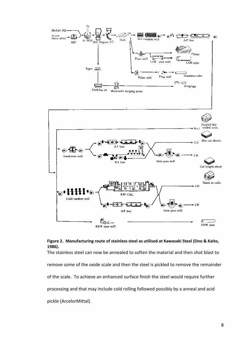
8
Figure 2. Manufacturing route of stainless steel as utilised at Kawasaki Steel (Ono & Kaito,
1986).
The stainless steel can now be annealed to soften the material and then shot blast to
remove some of the oxide scale and then the steel is pickled to remove the remainder
of the scale. To achieve an enhanced surface finish the steel would require further
processing and that may include cold rolling followed possibly by a anneal and acid
pickle (ArcelorMittal).

9
2.1.4 Types of Stainless Steel
Stainless steels are grouped according to the microstructure of the material, which
gives the following three different classifications:
• Ferritic
• Austentic
• Martensitic
However there are two other categories of stainless:
• Duplex
• Precipitation Hardenable
There are a multitude of grades in various conditions associated with each type,
detailed information about which can be found in the following sections, and in
Table 1.
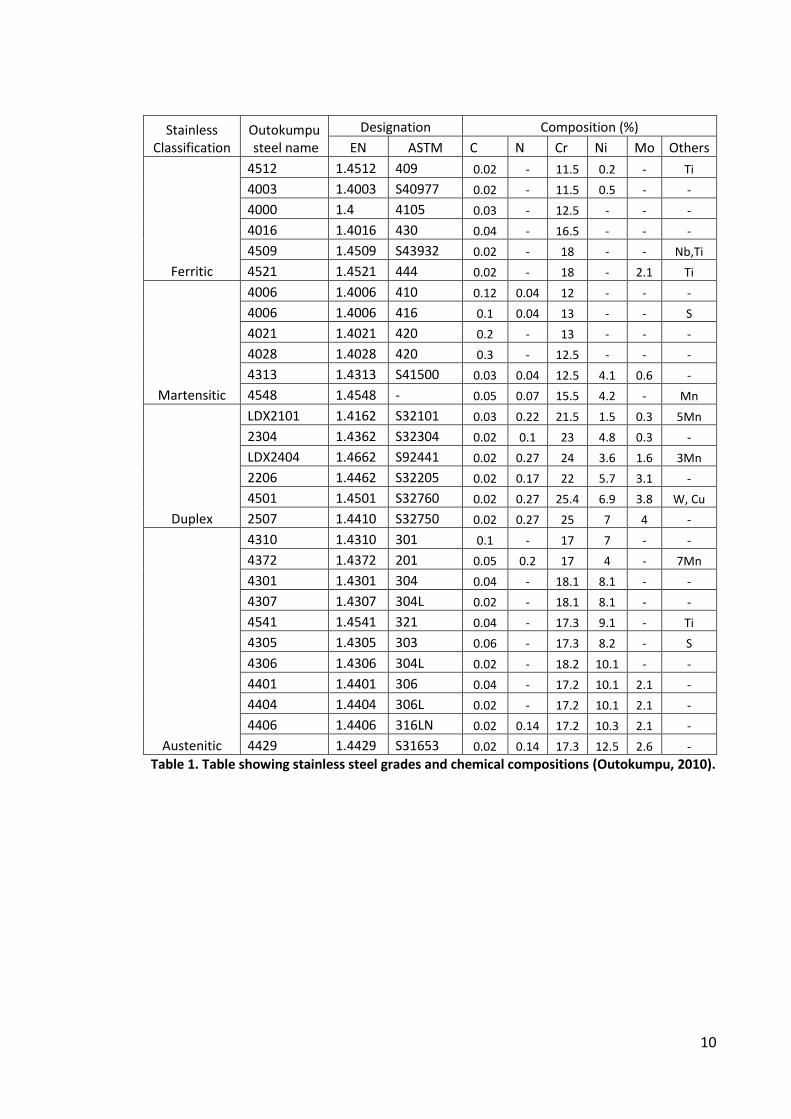
10
Table 1. Table showing stainless steel grades and chemical compositions (Outokumpu, 2010).
Stainless
Classification
Outokumpu
steel name
Designation Composition (%)
EN ASTM C N Cr Ni Mo Others
Ferritic
4512 1.4512 409 0.02 - 11.5 0.2 - Ti
4003 1.4003 S40977 0.02 - 11.5 0.5 - -
4000 1.4 4105 0.03 - 12.5 - - -
4016 1.4016 430 0.04 - 16.5 - - -
4509 1.4509 S43932 0.02 - 18 - - Nb,Ti
4521 1.4521 444 0.02 - 18 - 2.1 Ti
Martensitic
4006 1.4006 410 0.12 0.04 12 - - -
4006 1.4006 416 0.1 0.04 13 - - S
4021 1.4021 420 0.2 - 13 - - -
4028 1.4028 420 0.3 - 12.5 - - -
4313 1.4313 S41500 0.03 0.04 12.5 4.1 0.6 -
4548 1.4548 - 0.05 0.07 15.5 4.2 - Mn
Duplex
LDX2101 1.4162 S32101 0.03 0.22 21.5 1.5 0.3 5Mn
2304 1.4362 S32304 0.02 0.1 23 4.8 0.3 -
LDX2404 1.4662 S92441 0.02 0.27 24 3.6 1.6 3Mn
2206 1.4462 S32205 0.02 0.17 22 5.7 3.1 -
4501 1.4501 S32760 0.02 0.27 25.4 6.9 3.8 W, Cu
2507 1.4410 S32750 0.02 0.27 25 7 4 -
Austenitic
4310 1.4310 301 0.1 - 17 7 - -
4372 1.4372 201 0.05 0.2 17 4 - 7Mn
4301 1.4301 304 0.04 - 18.1 8.1 - -
4307 1.4307 304L 0.02 - 18.1 8.1 - -
4541 1.4541 321 0.04 - 17.3 9.1 - Ti
4305 1.4305 303 0.06 - 17.3 8.2 - S
4306 1.4306 304L 0.02 - 18.2 10.1 - -
4401 1.4401 306 0.04 - 17.2 10.1 2.1 -
4404 1.4404 306L 0.02 - 17.2 10.1 2.1 -
4406 1.4406 316LN 0.02 0.14 17.2 10.3 2.1 -
4429 1.4429 S31653 0.02 0.14 17.3 12.5 2.6 -
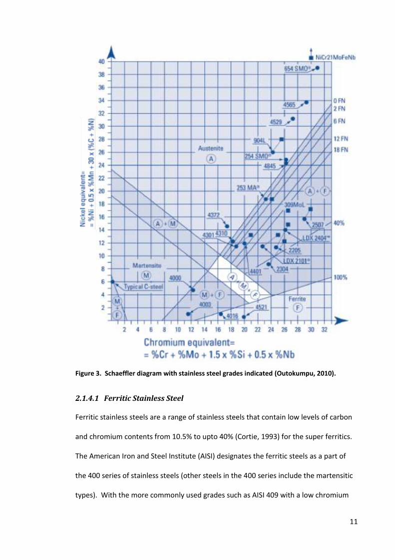
11
Figure 3. Schaeffler diagram with stainless steel grades indicated (Outokumpu, 2010).
2.1.4.1 Ferritic Stainless Steel
Ferritic stainless steels are a range of stainless steels that contain low levels of carbon
and chromium contents from 10.5% to upto 40% (Cortie, 1993) for the super ferritics.
The American Iron and Steel Institute (AISI) designates the ferritic steels as a part of
the 400 series of stainless steels (other steels in the 400 series include the martensitic
types). With the more commonly used grades such as AISI 409 with a low chromium
12
content, AISI 430 with a medium chromium content and AISI 446 with a high
chromium content as seen in Table 1.
The ferritic stainless steels generally have a Body Centred Cubic (BCC) crystal structure
with a ferritic microstructure from room temperature to the melting point of the
material. As this structure only holds small amounts of carbon in solution, carbon is
generally present in the form of chromium carbide precipitates (Demo, 1982).
The exception to this is when the gamma loop, as seen on the iron – chromium
equilibrium diagram in Figure 26 (page 53), extends into the region of the particular
ferritic alloy in question. Upon cooling from melting point, this will cause a
transformation from ferrite to austenite and if the cooling rate is slow enough, back to
ferrite. If it is t slo e ough the tra sfor atio will create martensite. This is
because austenite is able to hold considerably more carbon in solution than ferrite
and so upon a fast cool the carbon has insufficient time to come out of solution and
martensite forms. Therefore, in general, unless the gamma loop impinges on the alloy,
it is not possible to harden a ferritic stainless steel through heating and rapidly cooling.
The strengthening mechanisms which can occur in ferritic stainless steels, through
heat treatment are generally not desirable due to the significant reduction in the
ductility and toughness (Demo, 1982).
Ferritic stainless steels are generally used in environments that are subjected to fresh
water and in temperatures upto 650°C. There are however some grades that are used
within catalytic convertors operating at higher temperatures than 650°C and some of
the higher chromium content ferritics are used within the marine industry (Lula, 1989).

13
2.1.4.2 Austenitic Stainless Steel
Generally the austentic class of stainless steels are within the 300 series of the AISI
designations. The grades contain significant proportions of austenite phase, stabilising
elements, predominantly nickel and carbon, but also manganese and nitrogen,
amongst others, which allow austenite to be present at room temperature. Like the
ferritic grades, this type of stainless steel cannot be hardened via heat treatment,
regardless of the cooling rate (Lula, 1989).
The austentic stainless steels have a Face Centre Cubic (FCC) crystal structure (Ashby &
Jones, 2001) and are therefore less susceptible to a reduction in toughness at low
temperatures than the ferritic stainless steels. They are also nonmagnetic when fully
austenitic, which makes them better suited to environments where magnetic materials
could be detrimental to the component or structure, such as a mine sweeper or a
scanning electron microscope (Ashby & Jones, 2001).
The environments where the materials are commonly employed include service
conditions subjected to atmospheric corrosion, marine environment, low
temperatures and high temperatures above 650°C (Lula, 1989).
2.1.4.3 Martensitic Stainless Steel
The martensitic grades of stainless steel, as can be seen in
Table 1, are categorised within the AISI 400 series, with the common grades being the
AISI 410, 420 and 440. The chromium content is generally in the range of 12-17%, with
an associated high carbon content of approximately 0.1 to 0.5%, they contain relatively
few other additions, occasionally silicon for an increased resistance to scale and nickel
14
to maintain the hardenability in some of the higher chromium grades (Colombier &
Hochmann, 1967) The crystal structure of the martensitic stainless steel is Body
Centred Tetragonal (BCT) and is the product of a diffusionless shear transformation.
During the transformation to BCT there is insufficient time for carbon to move to
preferred sites within the crystal lattice and so becomes trapped and subsequently
distorts the crystal lattice. This distortion of the lattice prevents the occurrence of slip
which is manifested by increases in the hardness and yield strength, but with
associated low ductility (Higgins, 2001).
Unlike both the austenitic and ferritic grades of stainless steel, the martensitic grades
rely on heat treatment to attain the desired properties of the material, but careful
control of the furnace atmosphere must be made during these heat treatments as
martensitic stainless steels can be very susceptible to surface decarburisation (ASM
Handbook Committee, 1988).
The martensitic grades are used where the materials require high strength at room
temperature or maintain strength at high temperature (Lula, 1989).
2.1.4.4 Duplex Stainless Steel
Duplex stainless steels contain a combination of microstructures, they have ferrite and
austenite in varying quantities (Colombier & Hochmann, 1967) and therefore a mixture
of the body centred cubic and face centred cubic crystal structures within the separate
phases. This class of materials can offer a compromise between the properties of the
austenitic and ferritic stainless steels, therefore utilising the benefits of both whilst still
15
subject to the problems of either. They are also able to exhibit super plasticity, where
tensile stress is spread out as opposed to localised (Beddoes & Parr, 1999).
Duplex stainless steels exhibit corrosion resistance to both, localised and uniform
corrosion, with a good resistance to stress corrosion cracking (Outokumpu, 2012).
2.1.4.5 Precipitation Hardenable Stainless Steel
Precipitation hardenable stainless steels can have a matrix of any of the three phases
identified above (ferrite, austenite or martensite). However, generally they have a
matrix of either austenite or martensite, where they are utilised in applications such as
jet engine frames, turbine blades and surgical blades for the austenitic variants and
gears, shafts and valves for those grades whose microstructure is that of martensite
(Lippold & Kotecki, 2005).
This category of stainless steel can achieve very high tensile strengths above 1520
N/mm² and is able to do this through the addition of elements which are taken into
solution and then encouraged to form very small precipitates within the structure that
act as barriers to dislocation movement (Chakrabarty, 1987). These materials are used
in situations where strength is required at temperature (Lula, 1989). Elements
commonly used to produce the precipitates include aluminium, molybdenum or
copper (Beddoes & Parr, 1999).
16
2.1.5 Alloying Additions Used in Stainless Steels
The various grades of stainless steel include the use of a number of purposefully added
elements which benefit the steel in different ways. Details of the main elements used
in stainless steels are as follows.
2.1.5.1 Carbon (C)
A crucial component in stainless steel, but generally maintained at levels below 0.1%
and when welding stainless steel carbon levels significantly below this are preferred. It
provides the steel with strength and is an important addition in the martensitic grades.
Carbon is a very strong austenite stabiliser but uncontrolled it can combine with other
elements and reduce the corrosion resistance of the steel (Cunat, 2004).
2.1.5.2 Chromium (Cr)
As previously stated the addition of chromium to the steel at levels above 10.5% is
what provides the self healing protective oxide layer that imparts the improved
corrosion performance of the material. It is a ferrite stabiliser and readily combines
with carbon and nitrogen to form various forms of carbides, nitrides and carbo-nitrides
(Streicher, 1977). It is also a key element in the embrittling phases which hinder
stainless steel, such as sigma phase which is a combination of chromium and iron, but
it is also present within the Chi and Laves phases (Sigma phase considered later in
section 2.3.6).
2.1.5.3 Nickel (Ni)
The primary function for the addition of nickel is generally to stabilise the austenitic
phase. Unlike chromium it does not readily combine with other elements such as
carbon or nitrogen. At levels in the range of 8-10% nickel there is a marked reduction
in the ability of the stainless steel to resist stress corrosion cracking however
17
increasing or decreasing from this range yields a greater resistance to this detrimental
corrosion mechanism (The Specialty Steel Industry of North America, 2016). Nickel
also surpresses the gamma loop seen on the left hand side of the Fe-Cr equilibrium
diagram (Figure 26).
2.1.5.4 Manganese (Mn)
Manganese is added to stainless steels in various quantities, and in general is regarded
as an austenite stabiliser, with its potency dependant on the nickel content. The main
purpose for the addition of manganese is to combine with sulphur and thus prevent
the formation of a low melting point iron sulphide that, in extreme cases, can cause a
material to fall apart when the melting point of this iron sulphide is passed, this
phenomena is commonly referred to as hot shortness (AMG Vanadium Inc., 2009).
2.1.5.5 Silicon (Si)
Silicon can provide the steel with a number of benefits including an increase in the
fluidity of the melt, which can increase the complexity of casting which may be
produced. It is primarily added as a deoxidiser within the melting process but can also
add advantages in terms of oxidation resistance of the resultant alloy, at high
temperature. Low levels of silicon have little effect on stabilising either ferrite or
austenite, however higher levels are reported to stabilise ferrite. It can combine with
iron to form iron silicides which can be detrimental to the mechanical properties of the
steel (Lippold & Kotecki, 2005).
2.1.5.6 Molybdenum (Mo)
Molybdenum is a ferrite stabilising element and is added, normally in quantities of 2-
4%, sometimes upto 8% (Cunat, 2004) to increase corrosion resistance of the stainless
steel. It can also increase the hot strength of the steel, however this can provide
18
problems when hot working the material. Molybdenum is also added to some of the
precipation hardenable series of stainless steels to promote the precipitation reaction
(Mathers, Precipitation hardening stainless steel : Job knowledge 102, 2016)
2.1.5.7 Titanium (Ti)
In a role similar to niobium, titanium is added to combine with the nitrogen and carbon
within the stainless steel. The stochiometric quantity of titanium required to combine
with the available nitrogen and carbon can be calculated however as titanium also has
an affinity for sulphur additional titanium must be added (Galenko & Zhuravlev, 1995).
2.1.5.8 Niobium (Nb)
The addition of niobium is used to stabilise the carbon and prevent it from combining
with the chromium and therefore reducing the amount of chromium to produce the
passive layer. The amount of niobium necessary to stabilise the stainless steel can be
calculated from the following equation;
Equation 1. Equation showing amount of niobium required to stabilise a stainless steel.
%N ≤ 0.2 + 5 %C + %N (Cunat, 2004)
It is also reported that in ferritic stainless steels the addition of niobium is an effective
method to increase the high temperature fatigue properties of the material (Stainless
Steel for Design Engineers, 2014).
2.2 Definition of Welding & Brief History
Welding can be described as the fusion of two or more pieces of either the same or
different materials. When designing a component the designer must account for the
processing method to ensure the component will endure the entirety of its design life,
19
in the expected service environment. Welding has increasingly become a prominent
fabrication method since its inception and allows the manufacture of parts of a
component at separate sites and facilitates the combination of these parts at its
intended location, an example of this could be oil pipelines (Easterling, 1992) or
automotive exhaust systems.
Although forge welding, as practiced by blacksmiths had been in existence for
thousands of years, welding, as it is commonly recognised, has its roots when Sir
Humphy Davy demonstrated the creation of an electrical arc between two carbon
electrodes, using a battery in 1800 (Cary, The History of Welding, 1998). This paved
the way for the development of electrical welding processes, with the first patent for
an electrical welding technique being applied for in 1864 (Kjellberg, 2004). Gas welding
was developed and in use before the turn of the 20th century, with the discovery of
a et le e Ed u d Da i it as t u til a out he a et le e as
used for the purposes of cutting and welding (Hobart Institute of Welding Technology,
1998)
2.2.1 Fusion Welding Processes
There are a number of fusion joining processes with variations within each of these
processes, such as with Gas Metal Arc Welding (GMAW), there are a high number of
variants including Cold Metal Transfer (CMT) welding. The differences are broad using
completely different technologies to achieve the joint. Resistance welding, for
example, uses the resistance of the material to be joined, to the flow of electricity to
create sufficient heat to permit local melting of the materials. Then there are the
processes that use an arc to create very high local temperatures, allowing melting and
subsequent fusion. More specialised high energy processes such as laser beam and
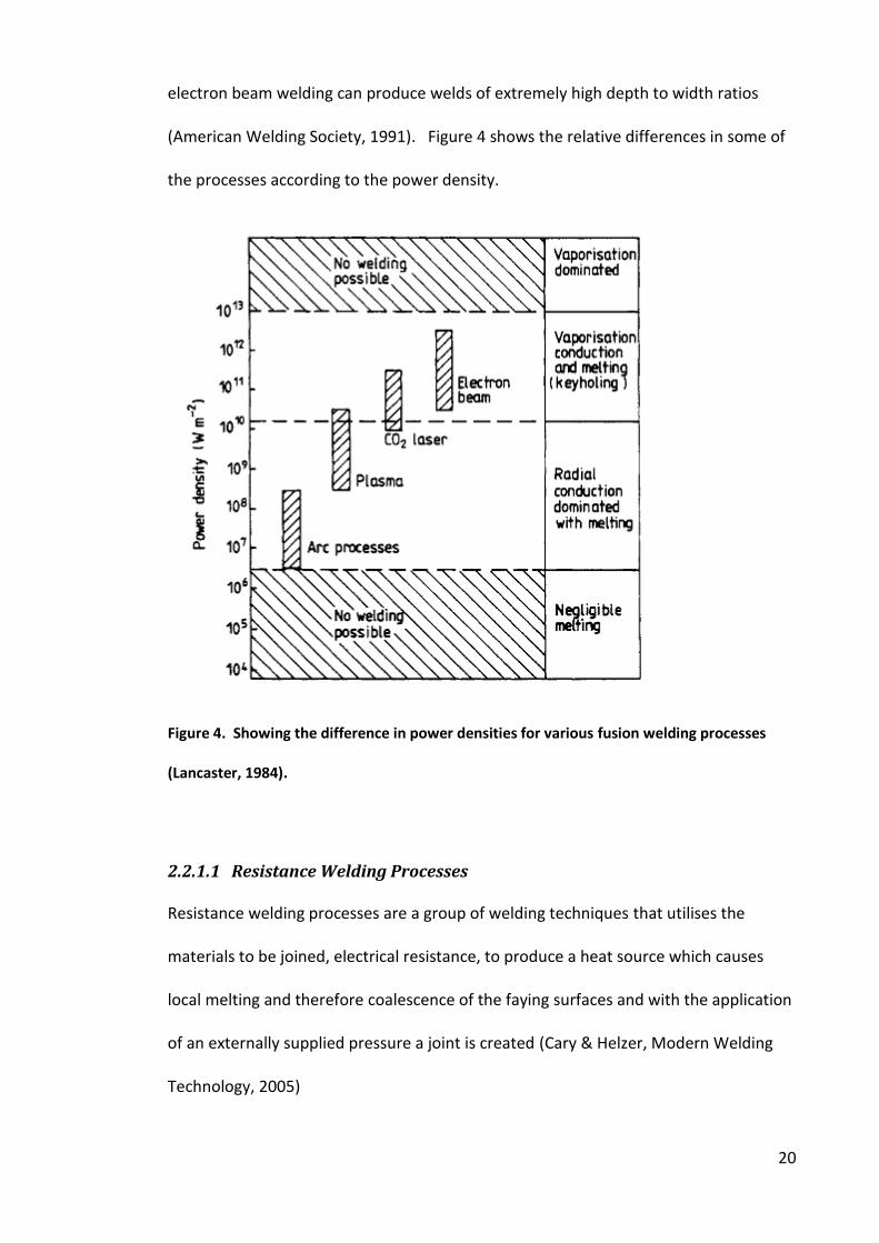
20
electron beam welding can produce welds of extremely high depth to width ratios
(American Welding Society, 1991). Figure 4 shows the relative differences in some of
the processes according to the power density.
Figure 4. Showing the difference in power densities for various fusion welding processes
(Lancaster, 1984).
2.2.1.1 Resistance Welding Processes
Resistance welding processes are a group of welding techniques that utilises the
materials to be joined, electrical resistance, to produce a heat source which causes
local melting and therefore coalescence of the faying surfaces and with the application
of an externally supplied pressure a joint is created (Cary & Helzer, Modern Welding
Technology, 2005)
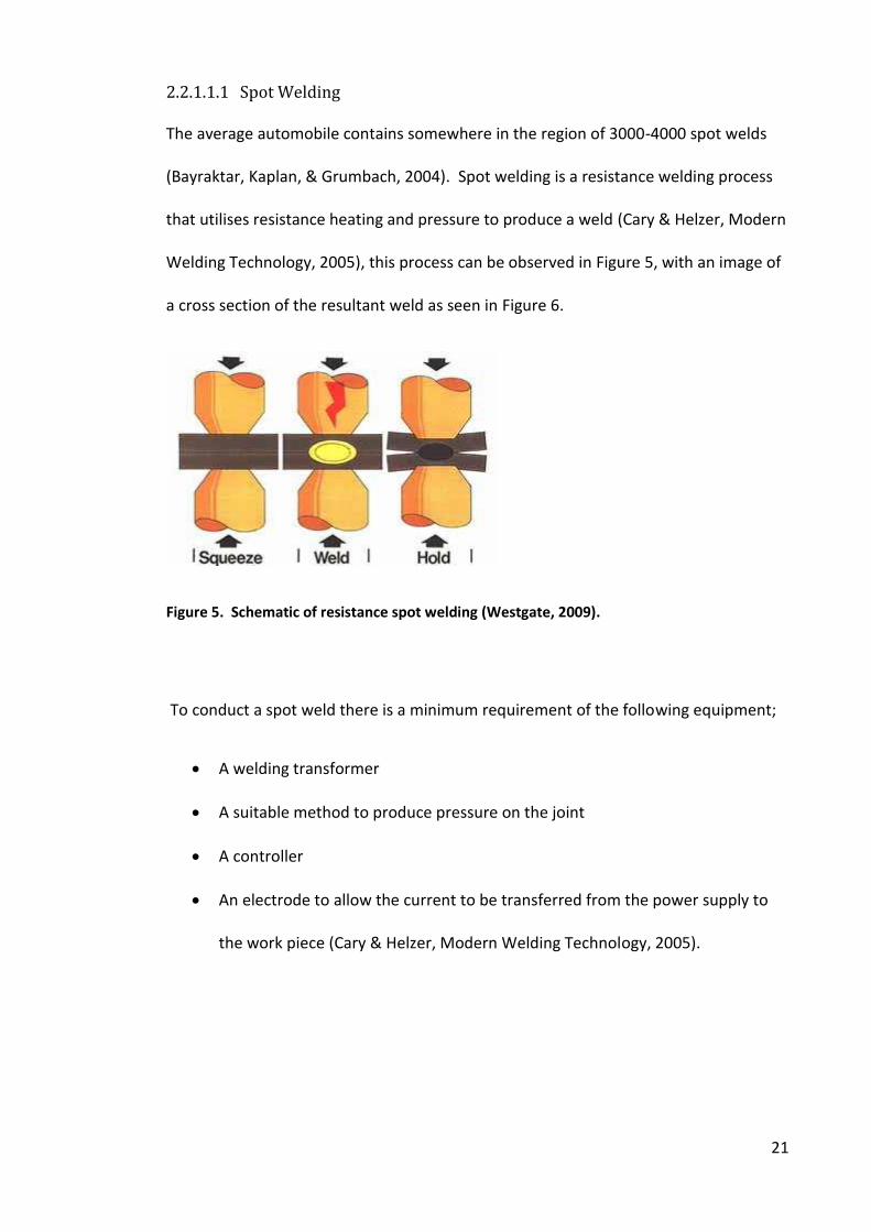
21
2.2.1.1.1 Spot Welding
The average automobile contains somewhere in the region of 3000-4000 spot welds
(Bayraktar, Kaplan, & Grumbach, 2004). Spot welding is a resistance welding process
that utilises resistance heating and pressure to produce a weld (Cary & Helzer, Modern
Welding Technology, 2005), this process can be observed in Figure 5, with an image of
a cross section of the resultant weld as seen in Figure 6.
Figure 5. Schematic of resistance spot welding (Westgate, 2009).
To conduct a spot weld there is a minimum requirement of the following equipment;
• A welding transformer
• A suitable method to produce pressure on the joint
• A controller
• An electrode to allow the current to be transferred from the power supply to
the work piece (Cary & Helzer, Modern Welding Technology, 2005).
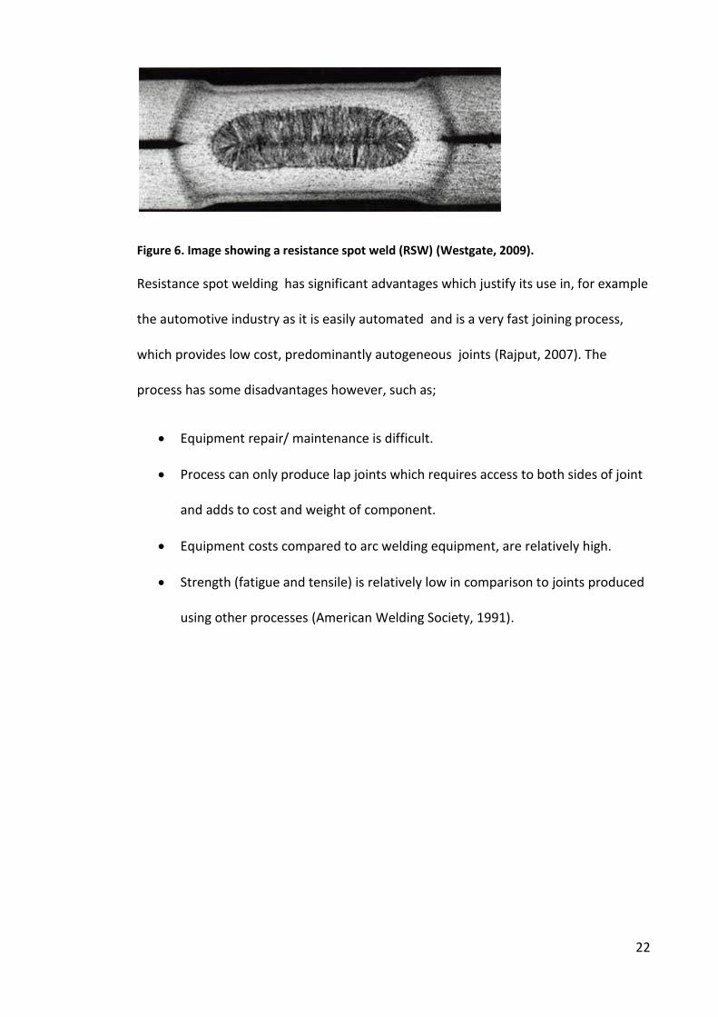
22
Figure 6. Image showing a resistance spot weld (RSW) (Westgate, 2009).
Resistance spot welding has significant advantages which justify its use in, for example
the automotive industry as it is easily automated and is a very fast joining process,
which provides low cost, predominantly autogeneous joints (Rajput, 2007). The
process has some disadvantages however, such as;
• Equipment repair/ maintenance is difficult.
• Process can only produce lap joints which requires access to both sides of joint
and adds to cost and weight of component.
• Equipment costs compared to arc welding equipment, are relatively high.
• Strength (fatigue and tensile) is relatively low in comparison to joints produced
using other processes (American Welding Society, 1991).
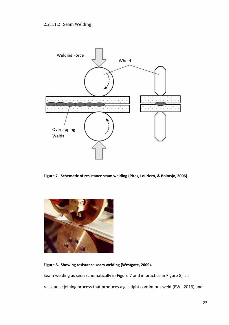
23
2.2.1.1.2 Seam Welding
Figure 7. Schematic of resistance seam welding (Pires, Louriero, & Bolmsjo, 2006).
Figure 8. Showing resistance seam welding (Westgate, 2009).
Seam welding as seen schematically in Figure 7 and in practice in Figure 8, is a
resistance joining process that produces a gas tight continuous weld (EWI, 2016) and
Welding Force
Wheel
Electrode rce
Overlapping
Welds
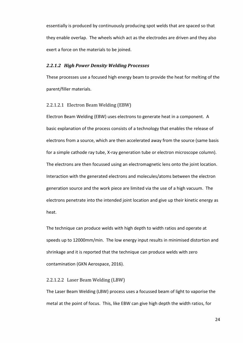
24
essentially is produced by continuously producing spot welds that are spaced so that
they enable overlap. The wheels which act as the electrodes are driven and they also
exert a force on the materials to be joined.
2.2.1.2 High Power Density Welding Processes
These processes use a focused high energy beam to provide the heat for melting of the
parent/filler materials.
2.2.1.2.1 Electron Beam Welding (EBW)
Electron Beam Welding (EBW) uses electrons to generate heat in a component. A
basic explanation of the process consists of a technology that enables the release of
electrons from a source, which are then accelerated away from the source (same basis
for a simple cathode ray tube, X-ray generation tube or electron microscope column).
The electrons are then focussed using an electromagnetic lens onto the joint location.
Interaction with the generated electrons and molecules/atoms between the electron
generation source and the work piece are limited via the use of a high vacuum. The
electrons penetrate into the intended joint location and give up their kinetic energy as
heat.
The technique can produce welds with high depth to width ratios and operate at
speeds up to 12000mm/min. The low energy input results in minimised distortion and
shrinkage and it is reported that the technique can produce welds with zero
contamination (GKN Aerospace, 2016).
2.2.1.2.2 Laser Beam Welding (LBW)
The Laser Beam Welding (LBW) process uses a focussed beam of light to vaporise the
metal at the point of focus. This, like EBW can give high depth the width ratios, for

25
LBW ratios of 8:1 are possible (for EBW ratios of 30:1 are achievable) with power
densities in the range of 1010 – 1012 Wm-2 (Kaul, Ganesh, Tripathi, Nandedkar, & Nath,
2003).
Laser beam welding can be used to produce autogeneous welds and unlike EBW does
not need to be conducted under a vacuum and does not create X-rays as a by-product
as EBW does. It is a process that is easily automated and has the ability to join a wide
range of materials (American Welding Society, 1991).
2.2.1.3 Arc Welding Processes
Arc welding processes are so characterised due to the fact that they utilise an electric
arc as a means of introducing thermal energy into the process. This encompasses a
wide range of welding techniques currently employed in fabrication applications.
2.2.1.3.1 Manual Metal Arc Welding (MMA)
Sometimes known as shielded metal arc welding, this is one of the early arc welding
processes. A simple set up for the technique can be seen in Figure 9, which consists of
a power source, which transfers power to the electrode holder via a lead. The
electrode holder allows attachment of the consumable electrode. It must also be able
to transfer the power from the welding lead to the electrode and be designed in a way
that allows the operator to manipulate it effectively to carry out the weld. The
electrodes consist of a wire coated in a mixture of different materials (predominantly
non metal) which disassociate under the arc, stabilising it and provide a gas shield
around it, finally it forms a protective slag on the weld pool, which prevents interaction
with gases in the surrounding environment.
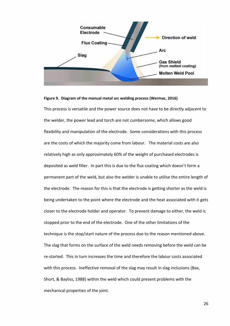
26
Figure 9. Diagram of the manual metal arc welding process (Wermac, 2016)
This process is versatile and the power source does not have to be directly adjacent to
the welder, the power lead and torch are not cumbersome, which allows good
flexibility and manipulation of the electrode. Some considerations with this process
are the costs of which the majority come from labour. The material costs are also
relatively high as only approximately 60% of the weight of purchased electrodes is
deposited as eld filler. I part this is due to the flu oati g hi h does t for a
permanent part of the weld, but also the welder is unable to utilise the entire length of
the electrode. The reason for this is that the electrode is getting shorter as the weld is
being undertaken to the point where the electrode and the heat associated with it gets
closer to the electrode holder and operator. To prevent damage to either, the weld is
stopped prior to the end of the electrode. One of the other limitations of the
technique is the stop/start nature of the process due to the reason mentioned above.
The slag that forms on the surface of the weld needs removing before the weld can be
re-started. This in turn increases the time and therefore the labour costs associated
with this process. Ineffective removal of the slag may result in slag inclusions (Bax,
Short, & Bayliss, 1988) within the weld which could present problems with the
mechanical properties of the joint.
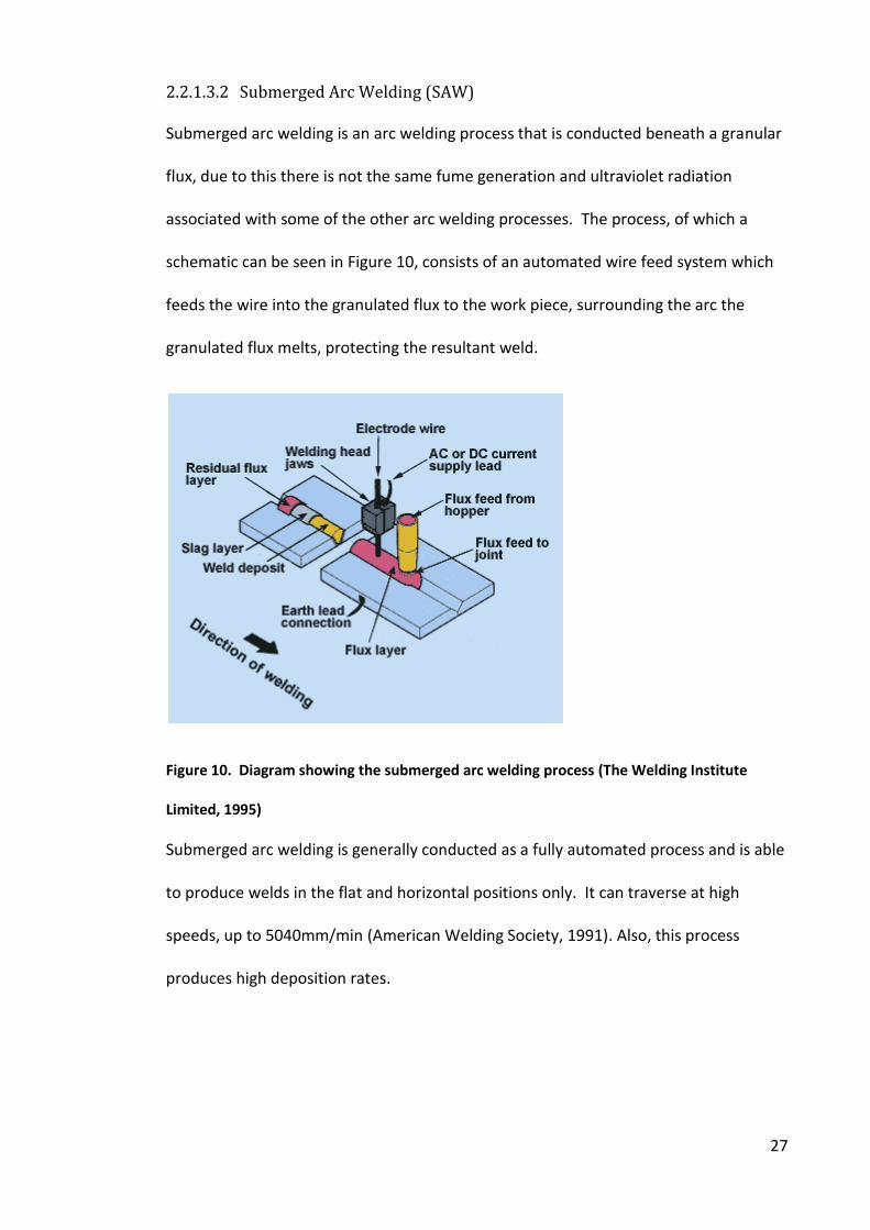
27
2.2.1.3.2 Submerged Arc Welding (SAW)
Submerged arc welding is an arc welding process that is conducted beneath a granular
flux, due to this there is not the same fume generation and ultraviolet radiation
associated with some of the other arc welding processes. The process, of which a
schematic can be seen in Figure 10, consists of an automated wire feed system which
feeds the wire into the granulated flux to the work piece, surrounding the arc the
granulated flux melts, protecting the resultant weld.
Figure 10. Diagram showing the submerged arc welding process (The Welding Institute
Limited, 1995)
Submerged arc welding is generally conducted as a fully automated process and is able
to produce welds in the flat and horizontal positions only. It can traverse at high
speeds, up to 5040mm/min (American Welding Society, 1991). Also, this process
produces high deposition rates.
28
2.2.1.3.3 Gas Tunsten Arc Welding (GTAW)
Gas tungsten arc welding, more commonly referred to as TIG (Tungsten Inert Gas), as it
is generally conducted using an inert shielding gas. In the UK the gas primarily used for
the technique is argon, however helium can also be used, which provides an enhanced
surface cleaning action. Combinations of the two gases are sometimes utilised.
Figure 11. Diagram of the gas tungsten arc welding process (Mechanical Engineering, 2016)
The process seen in Figure 11, consists of a power source, this can be D.C. or A.C.
depending on material to be welded and a hose which contains the power lead and gas
piping to the torch. The torch itself contains the termination of the gas pipe which
then goes through a diffuser to evenly distribute the protective shielding gas around
the electrode and resultant arc. The torch also contains the electrode which is
electrically coupled to the power lead. The non-consumable electrodes are
predominantly tungsten with the addition of other materials such as thorium or
zirconium. These additions improve electron emission and arc stability.
When using A.C. with an argon shielding gas, one half of the cycle provides a cleaning
action, removing tenacious oxide layers as found on aluminium and magnesium. The
other half of the cycle gives the heating action which melts the material and therefore
allows the potential for fusion to occur. Therefore A.C. TIG is generally used for the
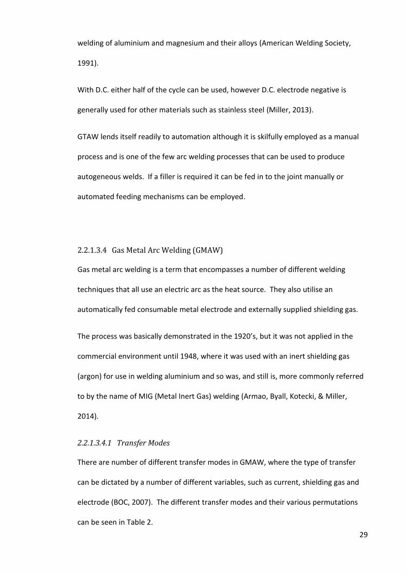
29
welding of aluminium and magnesium and their alloys (American Welding Society,
1991).
With D.C. either half of the cycle can be used, however D.C. electrode negative is
generally used for other materials such as stainless steel (Miller, 2013).
GTAW lends itself readily to automation although it is skilfully employed as a manual
process and is one of the few arc welding processes that can be used to produce
autogeneous welds. If a filler is required it can be fed in to the joint manually or
automated feeding mechanisms can be employed.
2.2.1.3.4 Gas Metal Arc Welding (GMAW)
Gas metal arc welding is a term that encompasses a number of different welding
techniques that all use an electric arc as the heat source. They also utilise an
automatically fed consumable metal electrode and externally supplied shielding gas.
The pro ess as asi all de o strated i the s, ut it as ot applied i the
commercial environment until 1948, where it was used with an inert shielding gas
(argon) for use in welding aluminium and so was, and still is, more commonly referred
to by the name of MIG (Metal Inert Gas) welding (Armao, Byall, Kotecki, & Miller,
2014).
2.2.1.3.4.1 Transfer Modes
There are number of different transfer modes in GMAW, where the type of transfer
can be dictated by a number of different variables, such as current, shielding gas and
electrode (BOC, 2007). The different transfer modes and their various permutations
can be seen in Table 2.
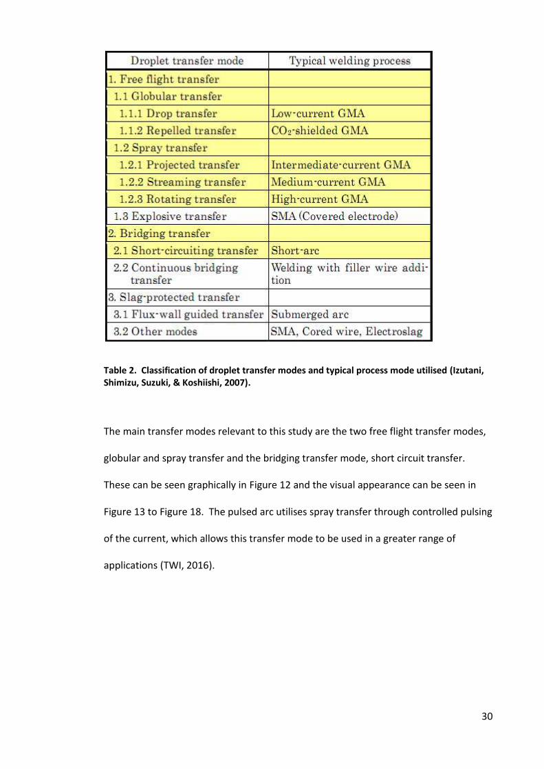
30
Table 2. Classification of droplet transfer modes and typical process mode utilised (Izutani,
Shimizu, Suzuki, & Koshiishi, 2007).
The main transfer modes relevant to this study are the two free flight transfer modes,
globular and spray transfer and the bridging transfer mode, short circuit transfer.
These can be seen graphically in Figure 12 and the visual appearance can be seen in
Figure 13 to Figure 18. The pulsed arc utilises spray transfer through controlled pulsing
of the current, which allows this transfer mode to be used in a greater range of
applications (TWI, 2016).
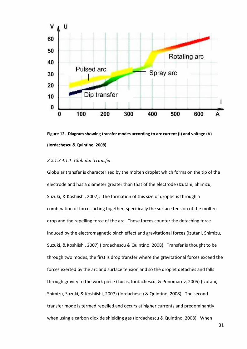
31
Figure 12. Diagram showing transfer modes according to arc current (I) and voltage (V)
(Iordachescu & Quintino, 2008).
2.2.1.3.4.1.1 Globular Transfer
Globular transfer is characterised by the molten droplet which forms on the tip of the
electrode and has a diameter greater than that of the electrode (Izutani, Shimizu,
Suzuki, & Koshiishi, 2007). The formation of this size of droplet is through a
combination of forces acting together, specifically the surface tension of the molten
drop and the repelling force of the arc. These forces counter the detaching force
induced by the electromagnetic pinch effect and gravitational forces (Izutani, Shimizu,
Suzuki, & Koshiishi, 2007) (Iordachescu & Quintino, 2008). Transfer is thought to be
through two modes, the first is drop transfer where the gravitational forces exceed the
forces exerted by the arc and surface tension and so the droplet detaches and falls
through gravity to the work piece (Lucas, Iordachescu, & Ponomarev, 2005) (Izutani,
Shimizu, Suzuki, & Koshiishi, 2007) (Iordachescu & Quintino, 2008). The second
transfer mode is termed repelled and occurs at higher currents and predominantly
when using a carbon dioxide shielding gas (Iordachescu & Quintino, 2008). When
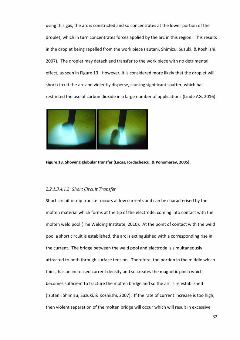
32
using this gas, the arc is constricted and so concentrates at the lower portion of the
droplet, which in turn concentrates forces applied by the arc in this region. This results
in the droplet being repelled from the work piece (Izutani, Shimizu, Suzuki, & Koshiishi,
2007). The droplet may detach and transfer to the work piece with no detrimental
effect, as seen in Figure 13. However, it is considered more likely that the droplet will
short circuit the arc and violently disperse, causing significant spatter, which has
restricted the use of carbon dioxide in a large number of applications (Linde AG, 2016).
Figure 13. Showing globular transfer (Lucas, Iordachescu, & Ponomarev, 2005).
2.2.1.3.4.1.2 Short Circuit Transfer
Short circuit or dip transfer occurs at low currents and can be characterised by the
molten material which forms at the tip of the electrode, coming into contact with the
molten weld pool (The Welding Institute, 2010). At the point of contact with the weld
pool a short circuit is established, the arc is extinguished with a corresponding rise in
the current. The bridge between the weld pool and electrode is simultaneously
attracted to both through surface tension. Therefore, the portion in the middle which
thins, has an increased current density and so creates the magnetic pinch which
becomes sufficient to fracture the molten bridge and so the arc is re established
(Izutani, Shimizu, Suzuki, & Koshiishi, 2007). If the rate of current increase is too high,
then violent separation of the molten bridge will occur which will result in excessive
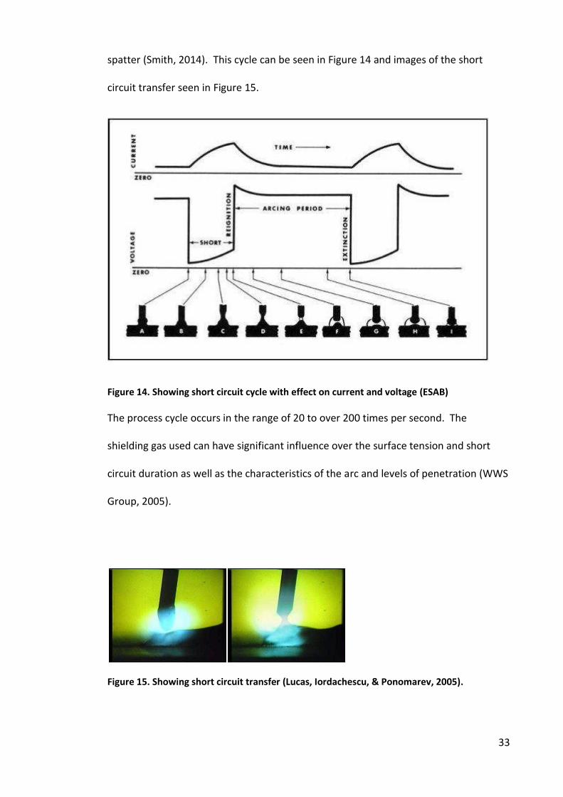
33
spatter (Smith, 2014). This cycle can be seen in Figure 14 and images of the short
circuit transfer seen in Figure 15.
Figure 14. Showing short circuit cycle with effect on current and voltage (ESAB)
The process cycle occurs in the range of 20 to over 200 times per second. The
shielding gas used can have significant influence over the surface tension and short
circuit duration as well as the characteristics of the arc and levels of penetration (WWS
Group, 2005).
Figure 15. Showing short circuit transfer (Lucas, Iordachescu, & Ponomarev, 2005).
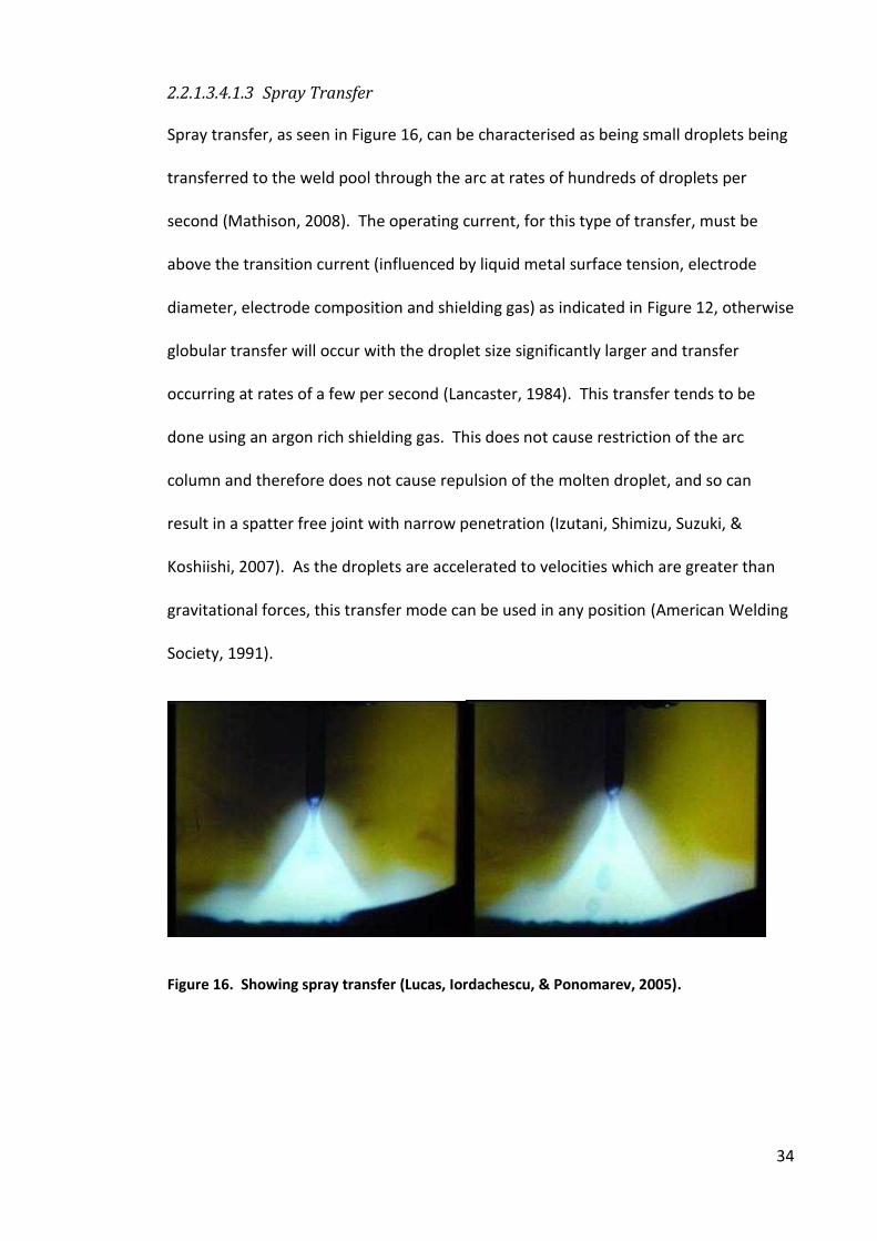
34
2.2.1.3.4.1.3 Spray Transfer
Spray transfer, as seen in Figure 16, can be characterised as being small droplets being
transferred to the weld pool through the arc at rates of hundreds of droplets per
second (Mathison, 2008). The operating current, for this type of transfer, must be
above the transition current (influenced by liquid metal surface tension, electrode
diameter, electrode composition and shielding gas) as indicated in Figure 12, otherwise
globular transfer will occur with the droplet size significantly larger and transfer
occurring at rates of a few per second (Lancaster, 1984). This transfer tends to be
done using an argon rich shielding gas. This does not cause restriction of the arc
column and therefore does not cause repulsion of the molten droplet, and so can
result in a spatter free joint with narrow penetration (Izutani, Shimizu, Suzuki, &
Koshiishi, 2007). As the droplets are accelerated to velocities which are greater than
gravitational forces, this transfer mode can be used in any position (American Welding
Society, 1991).
Figure 16. Showing spray transfer (Lucas, Iordachescu, & Ponomarev, 2005).
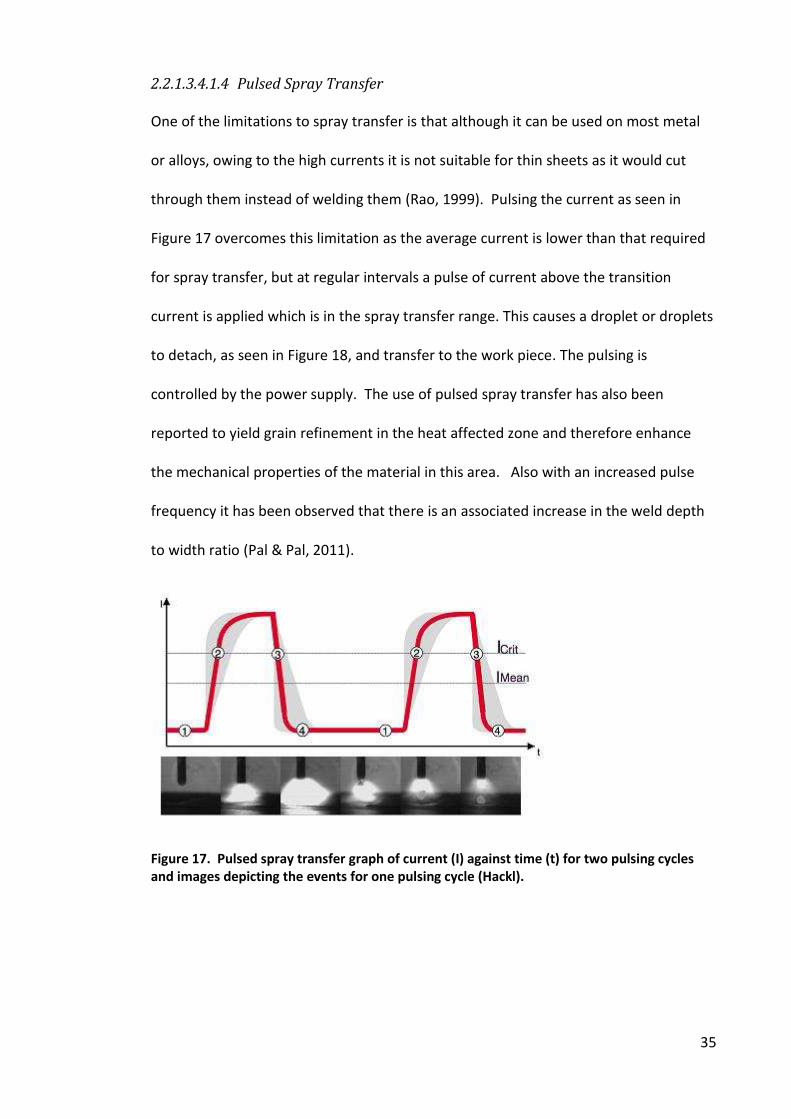
35
2.2.1.3.4.1.4 Pulsed Spray Transfer
One of the limitations to spray transfer is that although it can be used on most metal
or alloys, owing to the high currents it is not suitable for thin sheets as it would cut
through them instead of welding them (Rao, 1999). Pulsing the current as seen in
Figure 17 overcomes this limitation as the average current is lower than that required
for spray transfer, but at regular intervals a pulse of current above the transition
current is applied which is in the spray transfer range. This causes a droplet or droplets
to detach, as seen in Figure 18, and transfer to the work piece. The pulsing is
controlled by the power supply. The use of pulsed spray transfer has also been
reported to yield grain refinement in the heat affected zone and therefore enhance
the mechanical properties of the material in this area. Also with an increased pulse
frequency it has been observed that there is an associated increase in the weld depth
to width ratio (Pal & Pal, 2011).
Figure 17. Pulsed spray transfer graph of current (I) against time (t) for two pulsing cycles
and images depicting the events for one pulsing cycle (Hackl).
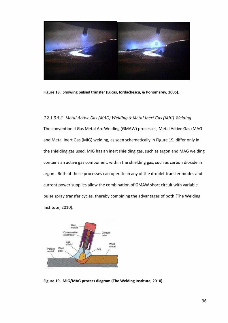
36
Figure 18. Showing pulsed transfer (Lucas, Iordachescu, & Ponomarev, 2005).
2.2.1.3.4.2 Metal Active Gas (MAG) Welding & Metal Inert Gas (MIG) Welding
The conventional Gas Metal Arc Welding (GMAW) processes, Metal Active Gas (MAG
and Metal Inert Gas (MIG) welding, as seen schematically in Figure 19, differ only in
the shielding gas used, MIG has an inert shielding gas, such as argon and MAG welding
contains an active gas component, within the shielding gas, such as carbon dioxide in
argon. Both of these processes can operate in any of the droplet transfer modes and
current power supplies allow the combination of GMAW short circuit with variable
pulse spray transfer cycles, thereby combining the advantages of both (The Welding
Institute, 2010).
Figure 19. MIG/MAG process diagram (The Welding Institute, 2010).
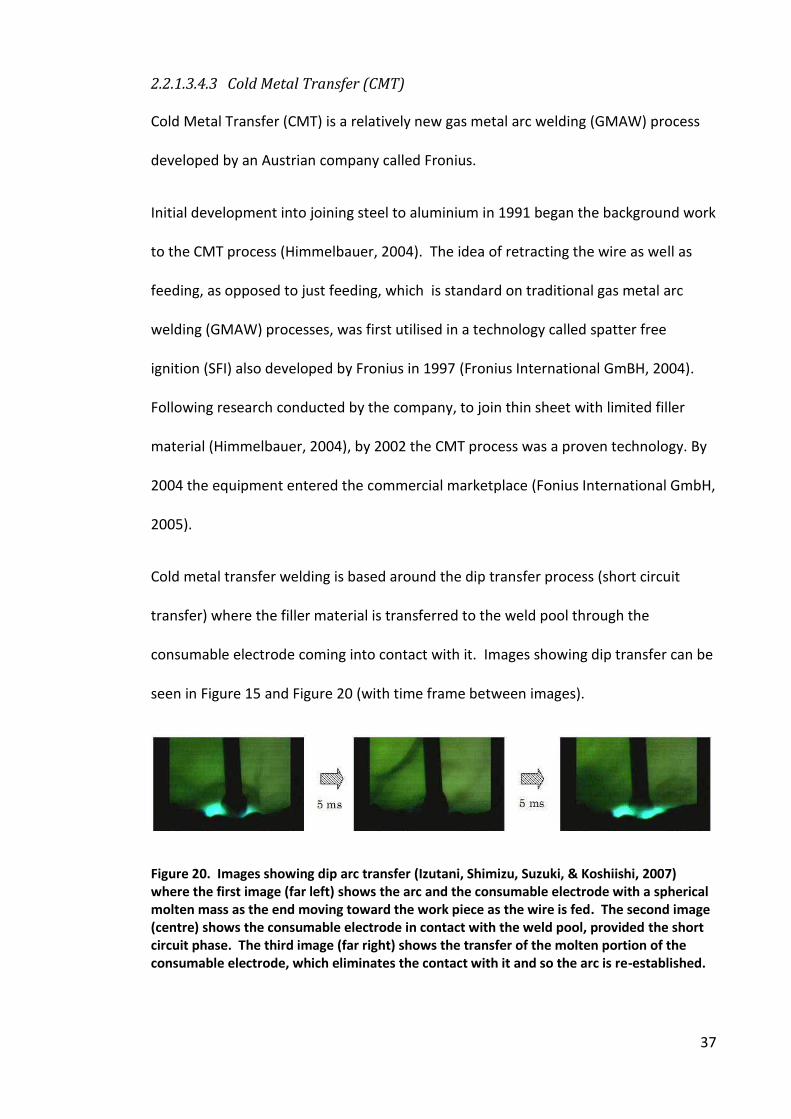
37
2.2.1.3.4.3 Cold Metal Transfer (CMT)
Cold Metal Transfer (CMT) is a relatively new gas metal arc welding (GMAW) process
developed by an Austrian company called Fronius.
Initial development into joining steel to aluminium in 1991 began the background work
to the CMT process (Himmelbauer, 2004). The idea of retracting the wire as well as
feeding, as opposed to just feeding, which is standard on traditional gas metal arc
welding (GMAW) processes, was first utilised in a technology called spatter free
ignition (SFI) also developed by Fronius in 1997 (Fronius International GmBH, 2004).
Following research conducted by the company, to join thin sheet with limited filler
material (Himmelbauer, 2004), by 2002 the CMT process was a proven technology. By
2004 the equipment entered the commercial marketplace (Fonius International GmbH,
2005).
Cold metal transfer welding is based around the dip transfer process (short circuit
transfer) where the filler material is transferred to the weld pool through the
consumable electrode coming into contact with it. Images showing dip transfer can be
seen in Figure 15 and Figure 20 (with time frame between images).
Figure 20. Images showing dip arc transfer (Izutani, Shimizu, Suzuki, & Koshiishi, 2007)
where the first image (far left) shows the arc and the consumable electrode with a spherical
molten mass as the end moving toward the work piece as the wire is fed. The second image
(centre) shows the consumable electrode in contact with the weld pool, provided the short
circuit phase. The third image (far right) shows the transfer of the molten portion of the
consumable electrode, which eliminates the contact with it and so the arc is re-established.
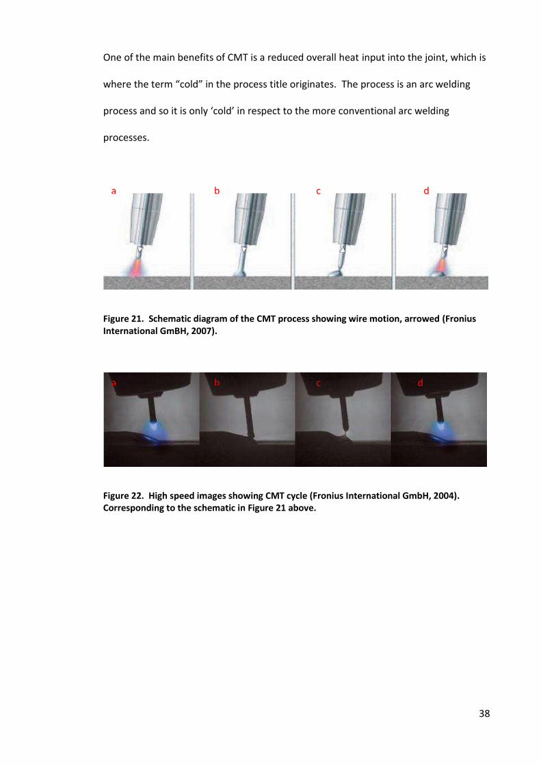
38
One of the main benefits of CMT is a reduced overall heat input into the joint, which is
here the ter old i the pro ess title origi ates. The pro ess is a ar eldi g
pro ess a d so it is o l old i respe t to the ore o e tio al ar eldi g
processes.
Figure 21. Schematic diagram of the CMT process showing wire motion, arrowed (Fronius
International GmBH, 2007).
Figure 22. High speed images showing CMT cycle (Fronius International GmbH, 2004).
Corresponding to the schematic in Figure 21 above.
a b c d
a b c d
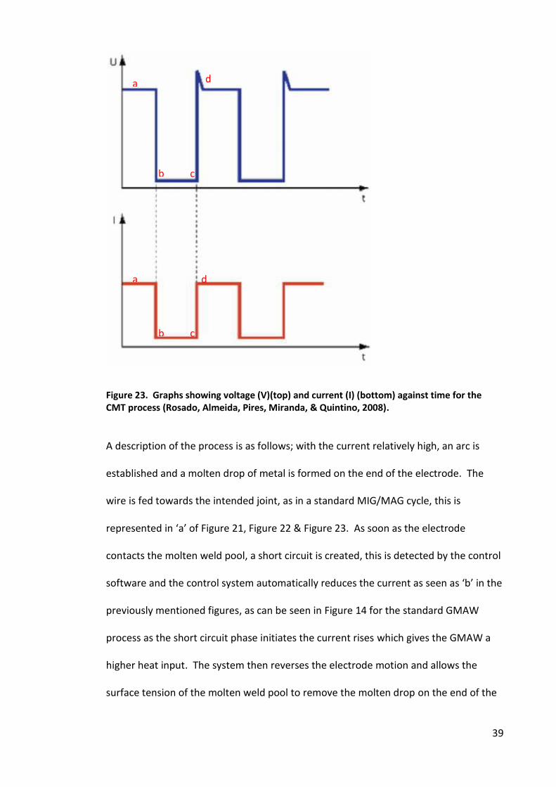
39
Figure 23. Graphs showing voltage (V)(top) and current (I) (bottom) against time for the
CMT process (Rosado, Almeida, Pires, Miranda, & Quintino, 2008).
A description of the process is as follows; with the current relatively high, an arc is
established and a molten drop of metal is formed on the end of the electrode. The
wire is fed towards the intended joint, as in a standard MIG/MAG cycle, this is
represe ted i a of Figure 21, Figure 22 & Figure 23. As soon as the electrode
contacts the molten weld pool, a short circuit is created, this is detected by the control
software and the control syste auto ati all redu es the urre t as see as i the
previously mentioned figures, as can be seen in Figure 14 for the standard GMAW
process as the short circuit phase initiates the current rises which gives the GMAW a
higher heat input. The system then reverses the electrode motion and allows the
surface tension of the molten weld pool to remove the molten drop on the end of the
a
b c
d
a
b c
d
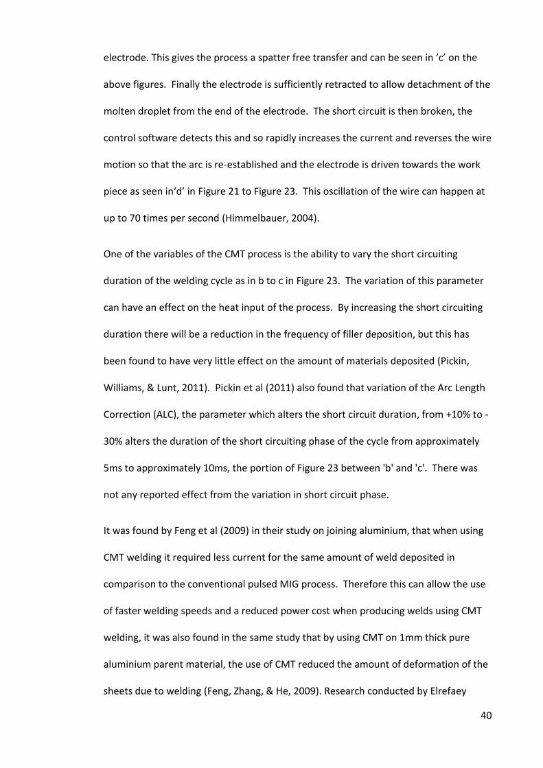
40
ele trode. This gi es the pro ess a spatter free tra sfer a d a e see i o the
above figures. Finally the electrode is sufficiently retracted to allow detachment of the
molten droplet from the end of the electrode. The short circuit is then broken, the
control software detects this and so rapidly increases the current and reverses the wire
motion so that the arc is re-established and the electrode is driven towards the work
pie e as see i d i Figure 21 to Figure 23. This oscillation of the wire can happen at
up to 70 times per second (Himmelbauer, 2004).
One of the variables of the CMT process is the ability to vary the short circuiting
duration of the welding cycle as in b to c in Figure 23. The variation of this parameter
can have an effect on the heat input of the process. By increasing the short circuiting
duration there will be a reduction in the frequency of filler deposition, but this has
been found to have very little effect on the amount of materials deposited (Pickin,
Williams, & Lunt, 2011). Pickin et al (2011) also found that variation of the Arc Length
Correction (ALC), the parameter which alters the short circuit duration, from +10% to -
30% alters the duration of the short circuiting phase of the cycle from approximately
5ms to approximately 10ms, the portion of Figure 23 between 'b' and 'c'. There was
not any reported effect from the variation in short circuit phase.
It was found by Feng et al (2009) in their study on joining aluminium, that when using
CMT welding it required less current for the same amount of weld deposited in
comparison to the conventional pulsed MIG process. Therefore this can allow the use
of faster welding speeds and a reduced power cost when producing welds using CMT
welding, it was also found in the same study that by using CMT on 1mm thick pure
aluminium parent material, the use of CMT reduced the amount of deformation of the
sheets due to welding (Feng, Zhang, & He, 2009). Research conducted by Elrefaey
41
(2015) also found advantages with welding aluminium materials using CMT over using
conventional MIG or TIG techniques and identified them as comparable to welds
created using the friction stir welding process and laser beam welding technique. On
research conducted examining the use of CMT for welding aluminium to steel, CMT
welds were created with and without a pulsed arc, with tensile samples created and
tested for each (Madhavan, Kamaraj, & Vijayaraghavan, 2016). Although the welding
of these materials creates an intermetallic compound that normally weakens the joint,
it was reported in this study that although this intermetallic compound was present in
small amounts, the tensile tests all failed in the heat affected zone region on the
aluminium, with the addition of a pulsed current to the CMT cycle increasing the joint
strength and hardness (Madhavan, Kamaraj, & Vijayaraghavan, 2016). This was not
the same found for a study examining the joining of an aluminium alloy (1060) and a
magnesium alloy (AZ31), where under tensile testing failures were seen in the fusion
zone along a brittle intermetallic layer that had formed during the welding (Wang,
Feng, & Wang, 2008).
Work conducted look at joining Inconel 718 found the welds to be aesthetically similar
to those conducted using the conventional MIG technique, but with the lower heat
input of the CMT process provided a reduced HAZ size and reduced residual stress
levels, in comparison to the traditional MIG welding technique employed (Benoit,
Jobez, Paillard, Klosek, & Baudin, 2011), therefore for a material more comparable to
those under examination in this study, there appear to be advantages of CMT over the
conventional GMA welding techniques.
42
2.2.1.3.4.4 Cold Metal Transfer Advanced
Welding processes are constantly being developed and the CMT process is no
different. The CMT advanced process providing the ability to reverse the poles from
positive to negative or vice versa during welding. This is reported to allow higher
deposition rates (up to 60%) and an enhanced gap bridgability as well as providing an
ability to reduce the heat input into the weld (Fronius International GmbH, 2009). This
then permits the welding of thin materials (0.3mm) and bridging welding gaps as wide
as 2mm across 2mm thick aluminium based parent materials using an aluminium
silicon alloy filler material (Fronius UK, 2015).
2.2.1.3.5 Gas Shielding
The use of a shielding gas is primarily to exclude the atmosphere or more precisely,
particular elements in the atmosphere (predominantly oxygen and nitrogen) from the
molten material produced during the process. Without this shield the formation of
porosity, oxides and nitrides may take place, causing detrimental effects to joint
integrity. Shielding gases may be inert or active. The active gases contain proportions
(eg 2%) of an active component (such as carbon dioxide or oxygen) in an inert gas,
although the use of 100% carbon dioxide as a shielding gas is commonly used in the
welding of steel. Different gases impart different properties (for details of the
properties of some of the common shielding gases refer to Table 3) on the processes
involved in the welding cycle. The development of new shielding gas mixtures has
been with the aim of creating a more stable arc, to reduce fume emissions and/or to
provide an enhanced molten metal transfer. All of which may have a positive effect on
production, consistency and quality (Pires, Quintino, & Miranda, 2007). Subsequent
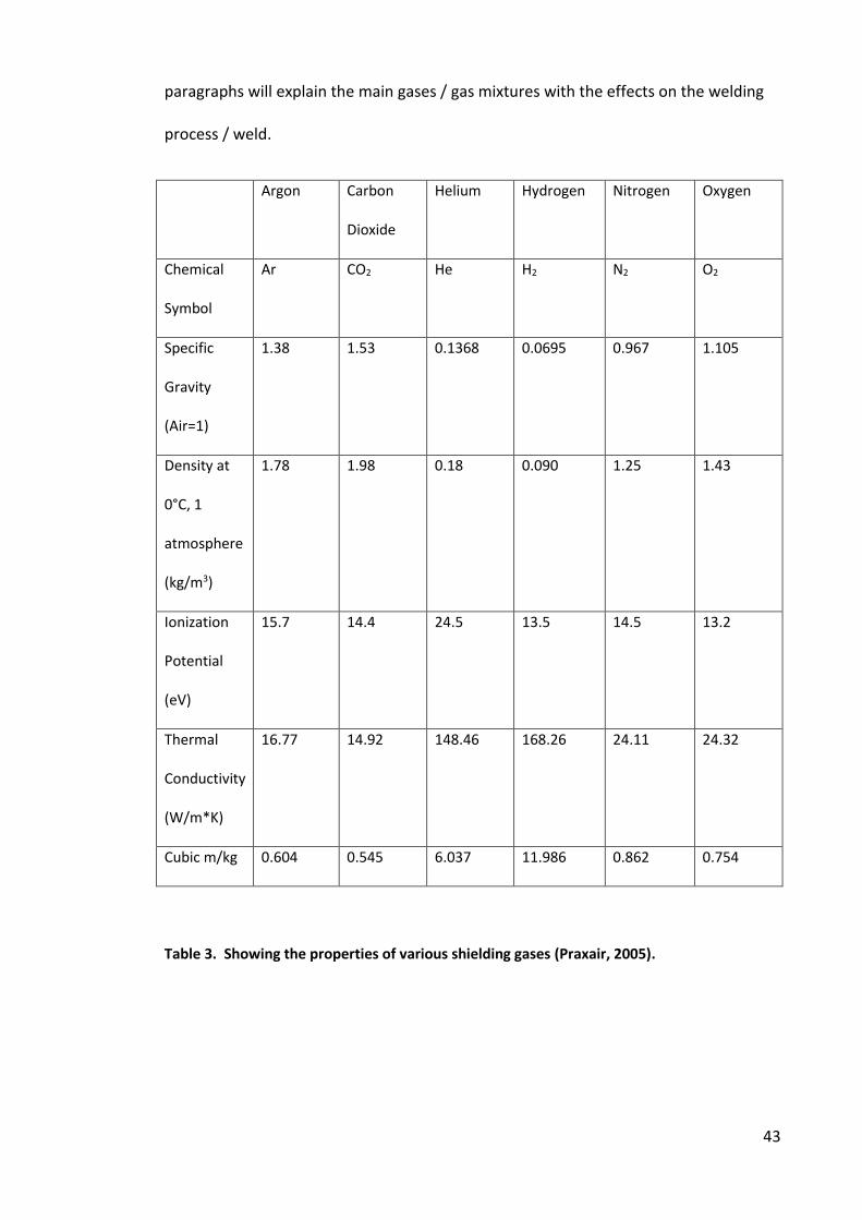
43
paragraphs will explain the main gases / gas mixtures with the effects on the welding
process / weld.
Argon Carbon
Dioxide
Helium Hydrogen Nitrogen Oxygen
Chemical
Symbol
Ar CO2 He H2 N2 O2
Specific
Gravity
(Air=1)
1.38 1.53 0.1368 0.0695 0.967 1.105
Density at
0°C, 1
atmosphere
(kg/m3)
1.78 1.98 0.18 0.090 1.25 1.43
Ionization
Potential
(eV)
15.7 14.4 24.5 13.5 14.5 13.2
Thermal
Conductivity
(W/m*K)
16.77 14.92 148.46 168.26 24.11 24.32
Cubic m/kg 0.604 0.545 6.037 11.986 0.862 0.754
Table 3. Showing the properties of various shielding gases (Praxair, 2005).
44
2.2.1.3.5.1 Argon
Argon is an inert gas which is approximately 1.4 times denser than air, as can be seen
in Table 3, which makes it extremely good at shielding welds in the down hand position
and is extensively used in pure form to join non ferrous materials such as aluminium,
titanium and copper. In the UK it is the predominant shielding gas for GTA welding of
these materials (BOC UK, 2010). The low ionization potential of argon, creates a
stable, constricted, high density arc which results in a narrow penetration profile
(Praxair, 1995).
2.2.1.3.5.2 Helium
Helium, another inert gas has a density of 0.169kg/m3 (AIR LIQUIDE, 2009) against air
which has a density of 1.202kg/m3 (AIR LIQUIDE, 2009) at 15°C making it lot lighter
than argon and therefore higher flow rates are required to afford the same levels of
shielding. Welding with helium creates a hotter weld and due to the high thermal
conductivity results in a broad weld profile with reduced penetration when used on
stainless steel joints (Armao, Byall, Kotecki, & Miller, 2014).
2.2.1.3.5.3 Argon / Helium
It is common practice for shielding gases to be mixtures of two or more gases such as
with a combination of 70% Ar and 30% He as recommended by Air Products (Air
Products, 2017) for the joining of aluminium. The combination of argon and helium is
used to combine the advantages of each for example when joining aluminium,
magnesium or their alloys, argon improves arc stability and the cleaning action
provided by the arc and helium is said to improve wetting and weld metal coalescence
(ESAB, 2002). For welding stainless steel the addition of helium to argon, enhances the
45
fluidity of the weld pool, which increases the penetration. It also permits the use of
faster welding speeds (Linde AG, 2012).
2.2.1.3.5.4 Argon / Oxygen
The addition of small quantities, such as 2% of oxygen to the argon based shielding gas
creates a more stable arc. It also increases the speed at which molten droplets are
transferred to the weld pool, reducing the amount of current required for spray
transition and lengthens the duration for which the weld pool is molten and therefore
effects weld penetration as a result (Praxair, 1995). However for stainless steel welds
due to the oxidising effect, the weld bead will appear grey.
2.2.1.3.5.5 Argon / Carbon Dioxide
The use of pure argon tends to create an erratic arc and also a greater likelihood for
undercut. The addition of small amounts of other elements reduces this effect.
Carbon dioxide can be added in quantities of 3 to 25% to argon and produces a
noticeable difference in the arc characteristics, and eliminates the problem of
undercut afforded by pure argon. The addition of carbon dioxide also increases the
etta ilit of the eld ead (Filho, Ferraresi, & Scotti, 2010), giving a greater
amount of penetration than just argon alone. The use of argon/carbon dioxide mixes
tends to be used for applications where the desired transfer mode is short circuit
transfer. However, it is also suited for operating in spray and pulsed transfer modes
(American Welding Society, 1991). It was reported by Zielinska et al (2009) that the
addition of carbon dioxide to the argon shielding gas promotes a globular transfer
mode, which can be seen in Figure 24, where the addition of 15% CO2 to the argon
shielding gas changes the transfer mode from spray to globular. This was found not to
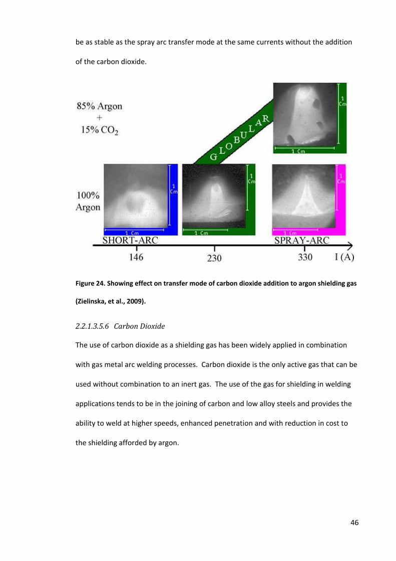
46
be as stable as the spray arc transfer mode at the same currents without the addition
of the carbon dioxide.
Figure 24. Showing effect on transfer mode of carbon dioxide addition to argon shielding gas
(Zielinska, et al., 2009).
2.2.1.3.5.6 Carbon Dioxide
The use of carbon dioxide as a shielding gas has been widely applied in combination
with gas metal arc welding processes. Carbon dioxide is the only active gas that can be
used without combination to an inert gas. The use of the gas for shielding in welding
applications tends to be in the joining of carbon and low alloy steels and provides the
ability to weld at higher speeds, enhanced penetration and with reduction in cost to
the shielding afforded by argon.
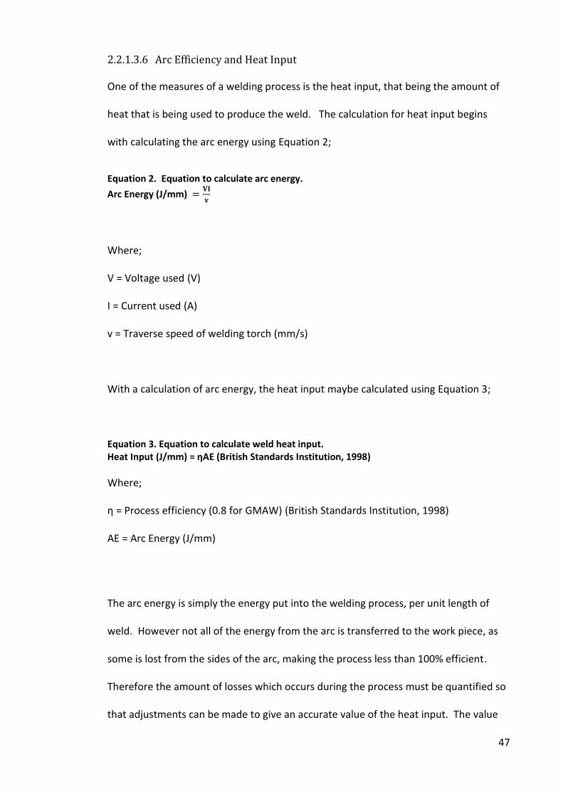
47
2.2.1.3.6 Arc Efficiency and Heat Input
One of the measures of a welding process is the heat input, that being the amount of
heat that is being used to produce the weld. The calculation for heat input begins
with calculating the arc energy using Equation 2;
Equation 2. Equation to calculate arc energy.
Arc Energy (J/mm) = ���
Where;
V = Voltage used (V)
I = Current used (A)
v = Traverse speed of welding torch (mm/s)
With a calculation of arc energy, the heat input maybe calculated using Equation 3;
Equation 3. Equation to calculate weld heat input.
Heat Input (J/mm) = ηAE (British Standards Institution, 1998)
Where;
η = Pro ess effi ie . for GMAW (British Standards Institution, 1998)
AE = Arc Energy (J/mm)
The arc energy is simply the energy put into the welding process, per unit length of
weld. However not all of the energy from the arc is transferred to the work piece, as
some is lost from the sides of the arc, making the process less than 100% efficient.
Therefore the amount of losses which occurs during the process must be quantified so
that adjustments can be made to give an accurate value of the heat input. The value
48
as specified by British Standards for the GMAW processes is 0.8 (British Standards
Institution, 1998).
Work conducted by DuPont and Marder (1995) found that the arc efficiency for the gas
metal arc welding process varied and with measured values of 0.84 they had a
tolerance of ±0.04. Therefore potentially the process efficiency could be higher by
10%, with a process efficiency of 0.88 rather than the 0.8 stated within the British
Standard.
Work has also been undertaken to assess the process efficiency of a number of the
variant gas metal arc welding processes including the cold metal transfer process. The
conclusions were that the process efficiency of CMT was 0.85 and that it was not too
dissimilar to the standard GMAW process tested. (Pepe, Egerland, Colegrove, Yapp,
Leonhartsberger, & Scotti, 2011) This then means that calculated heat inputs based on
the process efficiency values given in the British Standard will appear lower than they
actually are. It was also found that welding in a groove, such as with vee butt joint
preparation for example, increased the process efficiency to around 0.9, this is thought
to be due to less radiant heat being lost from the arc as it would have been absorbed
by the walls of the material. This then may mean that when welding thicker sections
with a wider gap, there is an increase in the process efficiency and therefore when
calculating the heat input with either the value stated in the British Standard or one
from recent research, may still yield inaccuracies in the values obtained.
49
2.3 Welding Stainless Steel
The integration of different materials into one component allows the part to take on
the advantages of certain materials, whilst reducing or eliminating the effects of the
disadvantages. Stainless steels can offer a vast array of properties to a component or
structure, such as enhanced corrosion resistance, enhanced mechanical properties,
wear resistance and aesthetical appearance. The cost of stainless steel may make it
economically unviable to produce the entire component or structure from the material
and this creates the need to find suitable technologies to allow the integration of this
classification of materials into components and structures.
Various welding techniques have filled this requirement well and have allowed the
combination of stainless steel with a whole host of different materials. Greater control
of the welding process has allowed a greater consistency of weld. In particular
advances in the electronic systems within welding equipment has allowed automated
manipulation of certain parameters through the welding cycle and the instigation of
welding robots have permitted greater consistency in the torch traverse speeds and
distance to work piece. Investigations into the as welded metallurgical properties of
the materials have permitted identification of problems associated with welding
different materials. The following information highlights the main problems that may
be encountered whilst welding stainless steels, the effects of which may be a reduction
in corrosion resistance, alteration of mechanical properties or simply affecting the
aesthetics of the part.
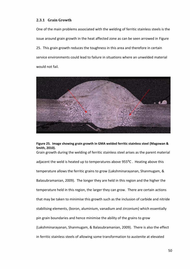
50
2.3.1 Grain Growth
One of the main problems associated with the welding of ferritic stainless steels is the
issue around grain growth in the heat affected zone as can be seen arrowed in Figure
25. This grain growth reduces the toughness in this area and therefore in certain
service environments could lead to failure in situations where an unwelded material
would not fail.
Figure 25. Image showing grain growth in GMA welded ferritic stainless steel (Magowan &
Smith, 2010).
Grain growth during the welding of ferritic stainless steel arises as the parent material
adjacent the weld is heated up to temperatures above ⁰C . Heati g a o e this
temperature allows the ferritic grains to grow (Lakshminarayanan, Shanmugam, &
Balasubramanian, 2009). The longer they are held in this region and the higher the
temperature held in this region, the larger they can grow. There are certain actions
that may be taken to minimise this growth such as the inclusion of carbide and nitride
stabilising elements, (boron, aluminium, vanadium and zirconium) which essentially
pin grain boundaries and hence minimise the ability of the grains to grow
(Lakshminarayanan, Shanmugam, & Balasubramanian, 2009). There is also the effect
in ferritic stainless steels of allowing some transformation to austenite at elevated
51
temperatures as this also reduces grain growth. However, without controlled cooling
this can lead to other problems as discussed in 2.3.3.
2.3.2 Sensitization
Sensitization occurs in both austenitic and ferritic stainless steels and dramatically
reduces the corrosion resistance of the material in aggressive environments. The
pro le arises duri g the eldi g le as te peratures i e ess of ⁰C pro ides
sufficient energy to allow carbon to migrate through the grain to the grain boundary
and form carbides. These carbides are predominantly with the chromium in the form
of M23C6 or M7C3 (Amunda & Mridha, 2011). This leaves the area adjacent to the grain
boundary denuded of free chromium, the element which gives stainless its protective,
self healing, chromium oxide layer. Therefore this prevents the protective layer
forming at this grain boundary and so leaves an area that is unable to resist attack
from a corrosive media.
The techniques employed to reduce or eliminate the detrimental effects of
sensitization include controlling the interstitial elements in the material,
predominantly carbon and nitrogen. It is these elements which combine with the
chromium and therefore reduce the levels of this element necessary for passivation.
The addition of stabilising elements has been successfully used, with additions of
elements such as titanium, vanadium, niobium, tantalum, yttrium and zirconium, being
added to the material during manufacture of the steel. These elements then form
stable carbides or nitrides and essentially reduce the amount of carbon within the
material that is free to form carbides with the chromium (Amunda & Mridha, 2011).
52
Another method is via controlling the heat input and cooling rate of the welding
process. It has been found that low heat inputs yield fast cooling rates during the early
part of the thermal cycle which produces fully ferritic structures. This however gives a
structure super saturated with carbon and therefore results in the formation of
carbides and nitrides at the grain boundaries. As the cooling rates are high, it also
prevents any reverse diffusion of the chromium back to any depleted regions. It has
been claimed that higher heat inputs are critical in managing sensitization in ferritic
stainless steels as it provides a slower cooling rate which allows the chromium to
redistribute to areas of lower concentrations and essentially desensitize itself (Amunda
& Mridha, 2011).
2.3.3 Formation of Secondary Phases
The thermal cycle induced within the parent material during welding raises the
temperature to its melting point immediately adjacent to the weld and the
temperature gradually diminishes with distance, the further away from the edge of the
fusion zone. The speed of cooling is relatively fast, which, in some instances, prevents
certain microstructural phases forming. One such instance of this is with certain
grades of ferritic stainless steel. The microstructure that is not completely ferritic from
room temperature to melting temperature, and there is the appearance of what is
commonly referred to as the gamma loop. An example of an iron-chromium
equilibrium diagram can be seen in Figure 26 with the loop apparent on the left hand
side extending from the y-axis between 912 & 1394°C.
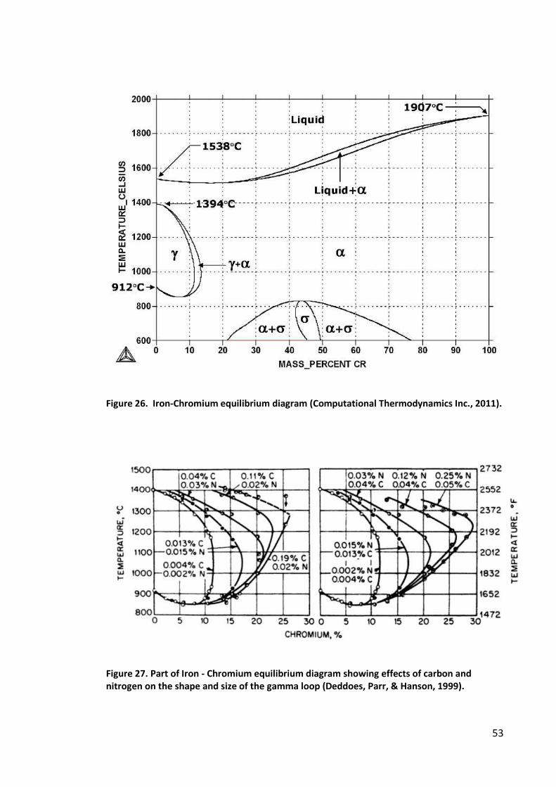
53
Figure 26. Iron-Chromium equilibrium diagram (Computational Thermodynamics Inc., 2011).
Figure 27. Part of Iron - Chromium equilibrium diagram showing effects of carbon and
nitrogen on the shape and size of the gamma loop (Deddoes, Parr, & Hanson, 1999).
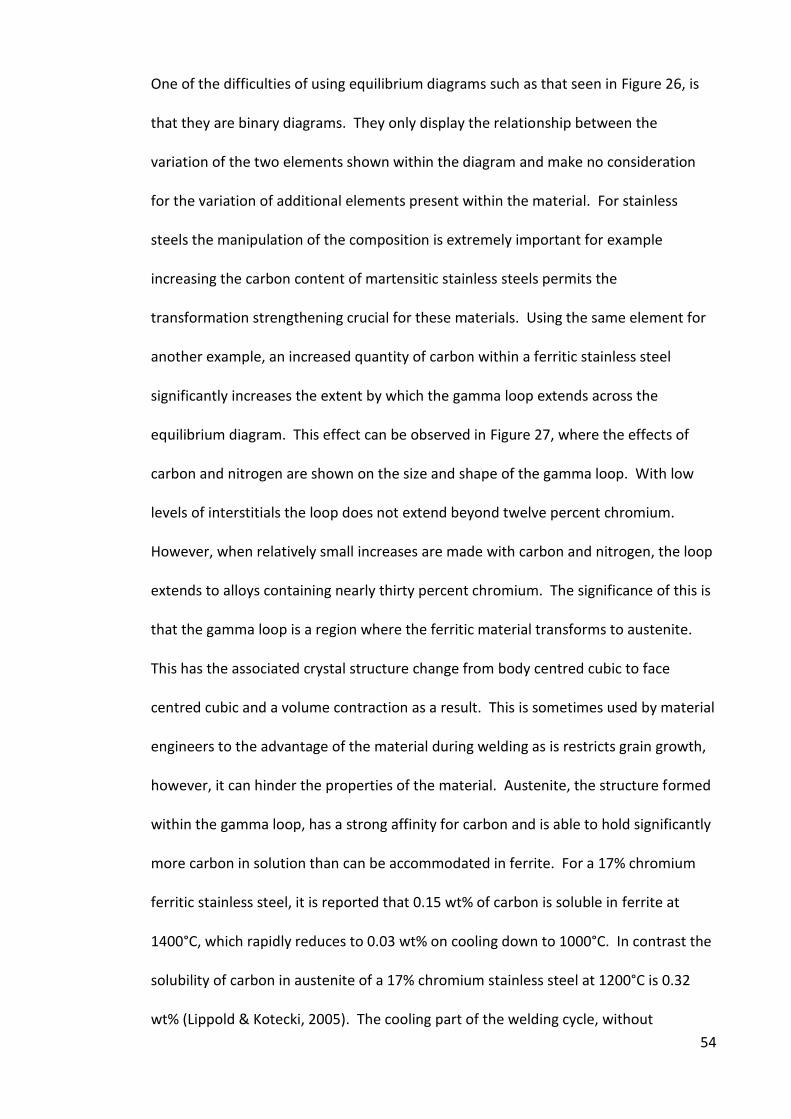
54
One of the difficulties of using equilibrium diagrams such as that seen in Figure 26, is
that they are binary diagrams. They only display the relationship between the
variation of the two elements shown within the diagram and make no consideration
for the variation of additional elements present within the material. For stainless
steels the manipulation of the composition is extremely important for example
increasing the carbon content of martensitic stainless steels permits the
transformation strengthening crucial for these materials. Using the same element for
another example, an increased quantity of carbon within a ferritic stainless steel
significantly increases the extent by which the gamma loop extends across the
equilibrium diagram. This effect can be observed in Figure 27, where the effects of
carbon and nitrogen are shown on the size and shape of the gamma loop. With low
levels of interstitials the loop does not extend beyond twelve percent chromium.
However, when relatively small increases are made with carbon and nitrogen, the loop
extends to alloys containing nearly thirty percent chromium. The significance of this is
that the gamma loop is a region where the ferritic material transforms to austenite.
This has the associated crystal structure change from body centred cubic to face
centred cubic and a volume contraction as a result. This is sometimes used by material
engineers to the advantage of the material during welding as is restricts grain growth,
however, it can hinder the properties of the material. Austenite, the structure formed
within the gamma loop, has a strong affinity for carbon and is able to hold significantly
more carbon in solution than can be accommodated in ferrite. For a 17% chromium
ferritic stainless steel, it is reported that 0.15 wt% of carbon is soluble in ferrite at
1400°C, which rapidly reduces to 0.03 wt% on cooling down to 1000°C. In contrast the
solubility of carbon in austenite of a 17% chromium stainless steel at 1200°C is 0.32
wt% (Lippold & Kotecki, 2005). The cooling part of the welding cycle, without
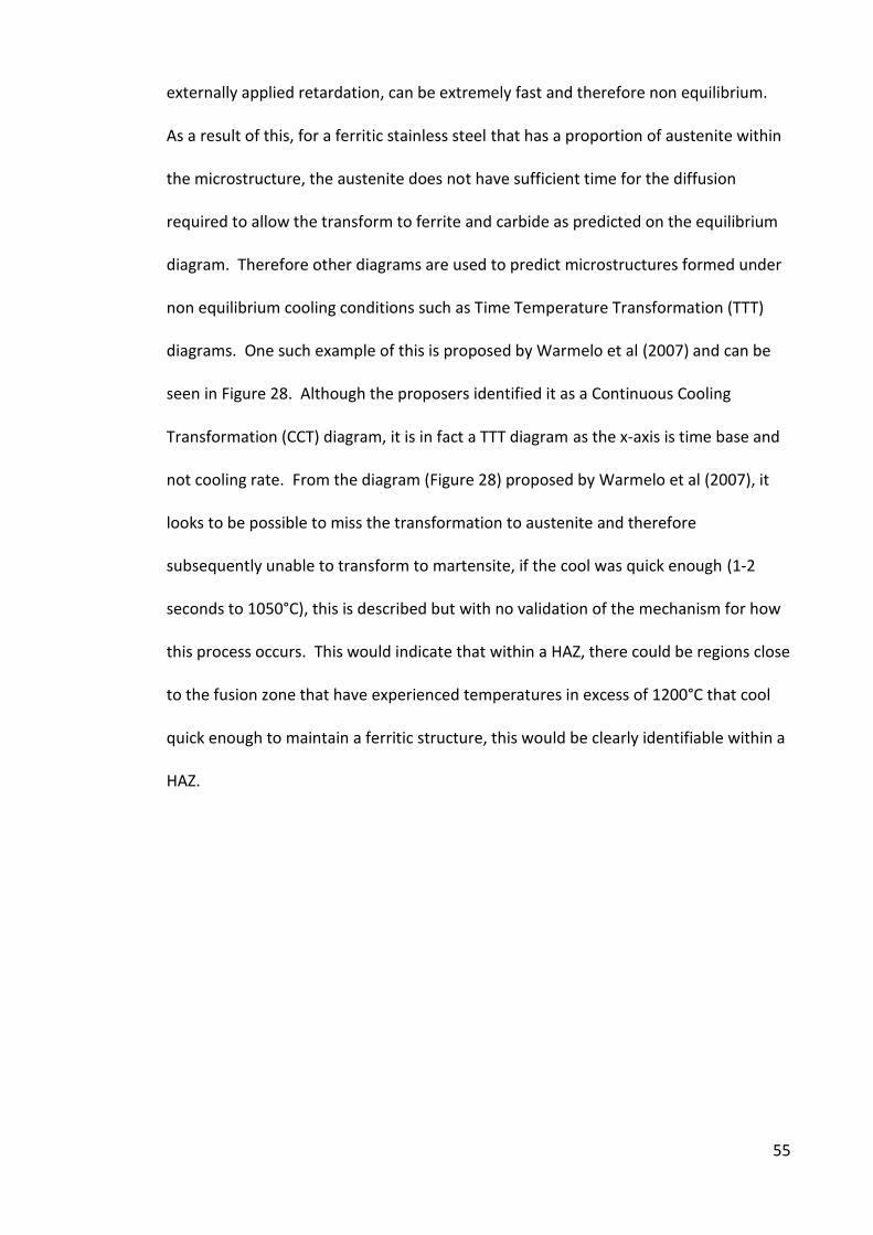
55
externally applied retardation, can be extremely fast and therefore non equilibrium.
As a result of this, for a ferritic stainless steel that has a proportion of austenite within
the microstructure, the austenite does not have sufficient time for the diffusion
required to allow the transform to ferrite and carbide as predicted on the equilibrium
diagram. Therefore other diagrams are used to predict microstructures formed under
non equilibrium cooling conditions such as Time Temperature Transformation (TTT)
diagrams. One such example of this is proposed by Warmelo et al (2007) and can be
seen in Figure 28. Although the proposers identified it as a Continuous Cooling
Transformation (CCT) diagram, it is in fact a TTT diagram as the x-axis is time base and
not cooling rate. From the diagram (Figure 28) proposed by Warmelo et al (2007), it
looks to be possible to miss the transformation to austenite and therefore
subsequently unable to transform to martensite, if the cool was quick enough (1-2
seconds to 1050°C), this is described but with no validation of the mechanism for how
this process occurs. This would indicate that within a HAZ, there could be regions close
to the fusion zone that have experienced temperatures in excess of 1200°C that cool
quick enough to maintain a ferritic structure, this would be clearly identifiable within a
HAZ.
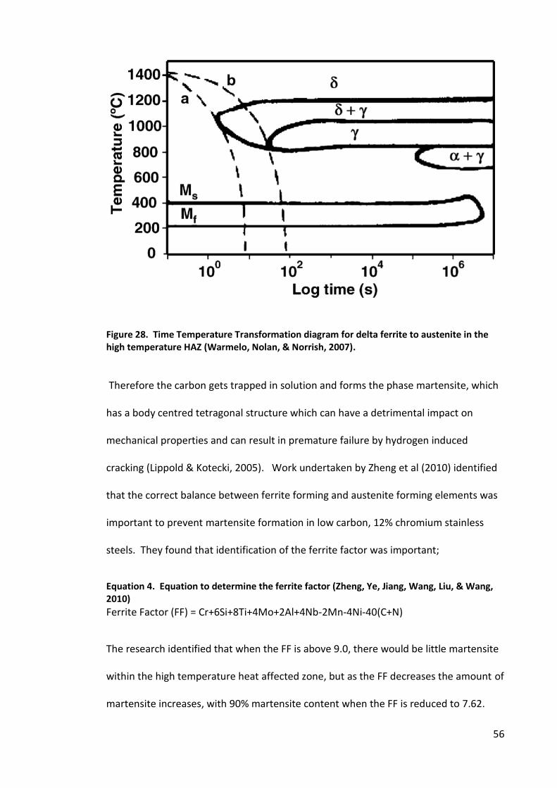
56
Figure 28. Time Temperature Transformation diagram for delta ferrite to austenite in the
high temperature HAZ (Warmelo, Nolan, & Norrish, 2007).
Therefore the carbon gets trapped in solution and forms the phase martensite, which
has a body centred tetragonal structure which can have a detrimental impact on
mechanical properties and can result in premature failure by hydrogen induced
cracking (Lippold & Kotecki, 2005). Work undertaken by Zheng et al (2010) identified
that the correct balance between ferrite forming and austenite forming elements was
important to prevent martensite formation in low carbon, 12% chromium stainless
steels. They found that identification of the ferrite factor was important;
Equation 4. Equation to determine the ferrite factor (Zheng, Ye, Jiang, Wang, Liu, & Wang,
2010)
Ferrite Factor (FF) = Cr+6Si+8Ti+4Mo+2Al+4Nb-2Mn-4Ni-40(C+N)
The research identified that when the FF is above 9.0, there would be little martensite
within the high temperature heat affected zone, but as the FF decreases the amount of
martensite increases, with 90% martensite content when the FF is reduced to 7.62.
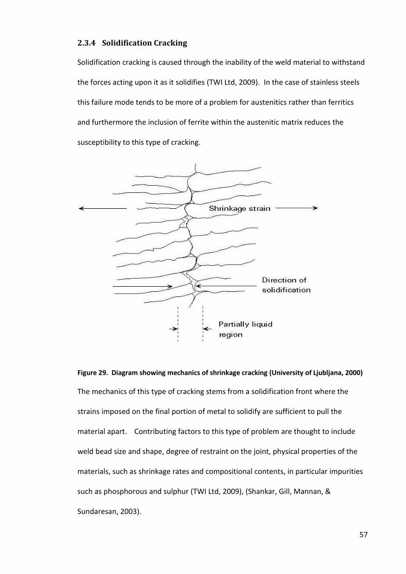
57
2.3.4 Solidification Cracking
Solidification cracking is caused through the inability of the weld material to withstand
the forces acting upon it as it solidifies (TWI Ltd, 2009). In the case of stainless steels
this failure mode tends to be more of a problem for austenitics rather than ferritics
and furthermore the inclusion of ferrite within the austenitic matrix reduces the
susceptibility to this type of cracking.
Figure 29. Diagram showing mechanics of shrinkage cracking (University of Ljubljana, 2000)
The mechanics of this type of cracking stems from a solidification front where the
strains imposed on the final portion of metal to solidify are sufficient to pull the
material apart. Contributing factors to this type of problem are thought to include
weld bead size and shape, degree of restraint on the joint, physical properties of the
materials, such as shrinkage rates and compositional contents, in particular impurities
such as phosphorous and sulphur (TWI Ltd, 2009), (Shankar, Gill, Mannan, &
Sundaresan, 2003).

58
Research conducted by Kujanpaa et al (1979) investigated the potential of shrinkage
cracking based on the composition of the weld material and produced a predictive
diagram often referred to as the Suutala diagram. The Suutala diagram as seen in
Figure 30 shows that the risk of cracking is reduced with low levels of sulphur and
phosphorus and also as the Creq / Nieq ratio is increased above a particular level
(approximately 1.5). This is representative of the shift in the solidification behaviour
from primary austenite, to primary ferrite and so the susceptibility to the cracking type
shows a dramatic decrease even at high impurity levels.
Equation 5. Equation to determine the chromium equivalent.
Creq = Cr + 1.37Mo + 1.5Si +2Nb + 3Ti
Equation 6. Equation to determine the nickel equivalent.
Nieq = Ni + 0.31Mn + 22C + 14.2N + Cu
Figure 30. Suutala diagram for predicting susceptibility to shrinkage cracking from weld
metal composition (Kujanpaa, Suutala, Takalo, & Moisio, 1979).
59
2.3.5 475°C Embrittlement
Iron Chromium alloys containing 15 – 70wt% Cr can be affected by this type of
embrittlement phenomena. To become embrittled through this mechanism the
material must be held at a temperature in the range of 400°C to 550°C. Theories as to
how this embrittlement occurs are not agreed by all, however the predominant theory
is that it is due to the formation of a coherent precipitate. Materials within the
prescribed compositional range that were held at temperatures below 550°C were
found to form a chromium rich ferrite (alpha prime) and an iron rich ferrite (alpha)
(Williams & Paxton, 1982). The time held at the aging temperature before the material
becomes embrittled was found to vary according the composition of the material, in
particular the chromium content. Higher chromium stainless steels become embrittled
within a shorter period, although at a higher temperature, than the lower chromium
containing stainless steels. For low to medium chromium stainless steels, the material
needs to have been held at temperature in excess of 100 hours before the mechanism
was detectable, although higher chromium steels exhibited a loss of ductility and
toughness after shorter durations. The addition of carbide forming elements, such as
molybdenum, niobium and titanium have been found to speed up the embrittlement.
This may be as a result of the fact that they free up the amount of chromium available
and so effectively raise the chromium content of the stainless steel that can combine
with other elements (Lippold & Kotecki, 2005).
There are reports that the embrittlement effect, termed 475°C, brought about due to
the formation of alpha prime results in an effect of the materials resistance to attack
by corrosive media. This is thought to be as a result of the selective attack being
directed at the iron rich ferritic phase, although this may be as a result of a reduction
60
in the free chromium content that is available to form the self healing passive oxide
layer.
A remedy to the embrittlement is through heat treatment in the range of 550-600°C
for a short period. Holding at these temperatures for excessive durations will
encourage the onset of the detrimental sigma phase embrittlement, as discussed in
section 2.3.6.
2.3.6 Sigma Phase Embrittlement
Sigma phase embrittlement affects iron – chromium alloys containing chromium
contents in the range of 20 to 70wt% in environments held at temperatures within the
range of 500 -800°C. As with the 475°C embrittlement, materials with higher
chromium content's have an increased risk of this type of formation at lower times
(typically a few hours). Steels with less than 20% chromium requires exposure in the
critical temperature range for hundreds of hours before effects are observable.
Examples of sigma phase can be seen in Figure 31 and Figure 32, etched using a
odified Murika i s reage t (Vandervoort, Colour Metallography - Film Formation
and Interference Techniques, 2004).
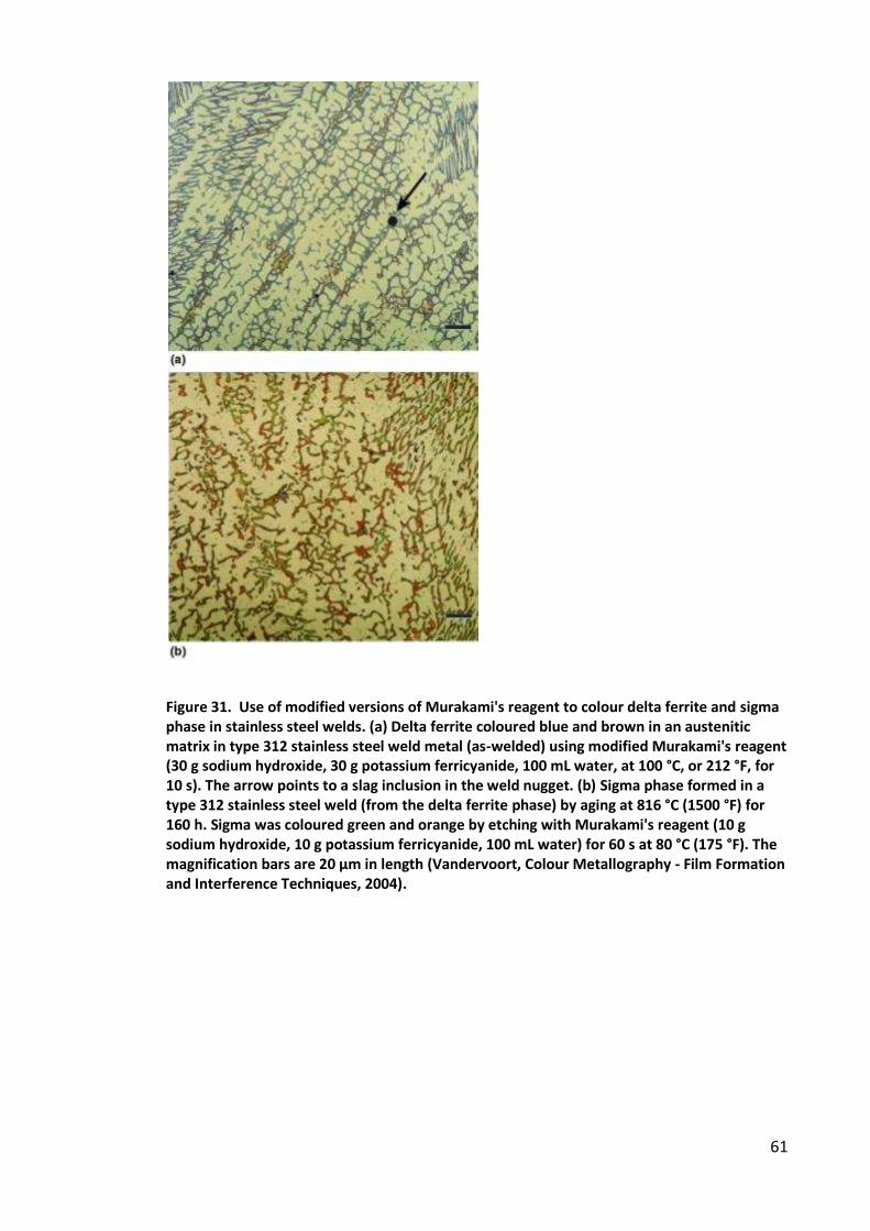
61
Figure 31. Use of modified versions of Murakami's reagent to colour delta ferrite and sigma
phase in stainless steel welds. (a) Delta ferrite coloured blue and brown in an austenitic
matrix in type 312 stainless steel weld metal (as-welded) using modified Murakami's reagent
(30 g sodium hydroxide, 30 g potassium ferricyanide, 100 mL water, at 100 °C, or 212 °F, for
10 s). The arrow points to a slag inclusion in the weld nugget. (b) Sigma phase formed in a
type 312 stainless steel weld (from the delta ferrite phase) by aging at 816 °C (1500 °F) for
160 h. Sigma was coloured green and orange by etching with Murakami's reagent (10 g
sodium hydroxide, 10 g potassium ferricyanide, 100 mL water) for 60 s at 80 °C (175 °F). The
ag ifi atio ars are 20 μ i le gth (Vandervoort, Colour Metallography - Film Formation
and Interference Techniques, 2004).
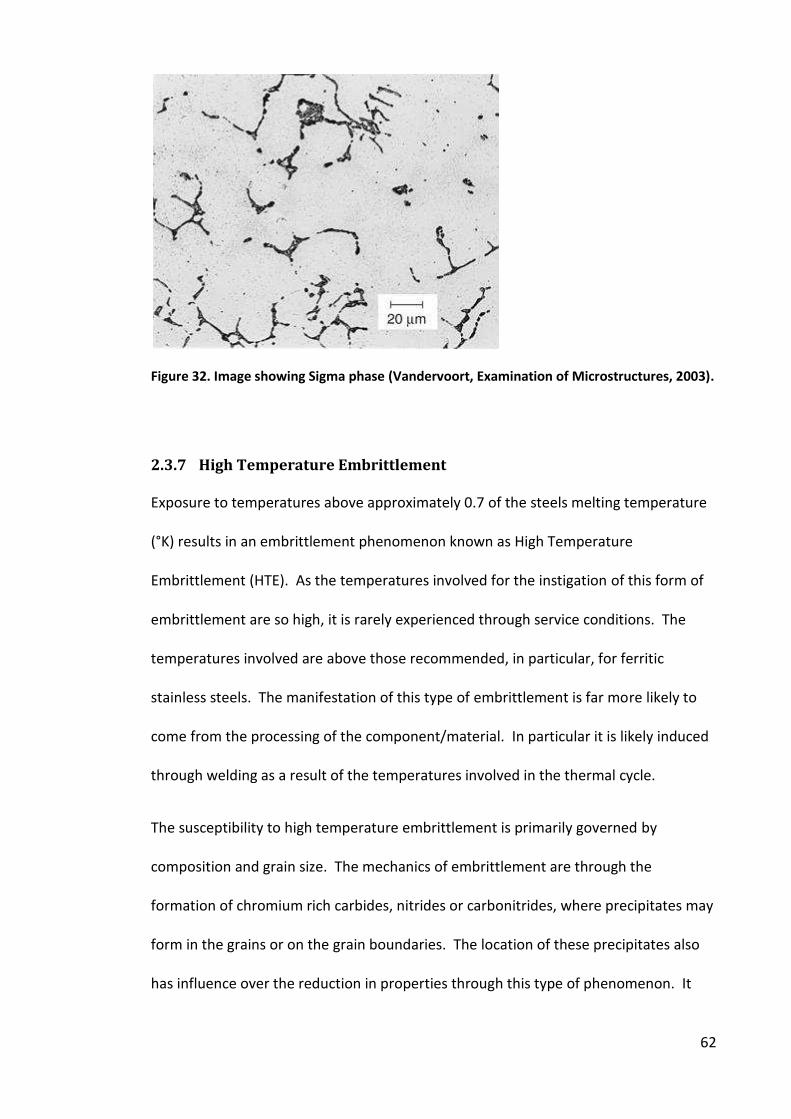
62
Figure 32. Image showing Sigma phase (Vandervoort, Examination of Microstructures, 2003).
2.3.7 High Temperature Embrittlement
Exposure to temperatures above approximately 0.7 of the steels melting temperature
(°K) results in an embrittlement phenomenon known as High Temperature
Embrittlement (HTE). As the temperatures involved for the instigation of this form of
embrittlement are so high, it is rarely experienced through service conditions. The
temperatures involved are above those recommended, in particular, for ferritic
stainless steels. The manifestation of this type of embrittlement is far more likely to
come from the processing of the component/material. In particular it is likely induced
through welding as a result of the temperatures involved in the thermal cycle.
The susceptibility to high temperature embrittlement is primarily governed by
composition and grain size. The mechanics of embrittlement are through the
formation of chromium rich carbides, nitrides or carbonitrides, where precipitates may
form in the grains or on the grain boundaries. The location of these precipitates also
has influence over the reduction in properties through this type of phenomenon. It
63
must be noted that stabilised grades do not form this type of embrittlement as easily
as the non-stabilised grades.
2.3.8 Liquation
Liquation is an issue that presents more of a problem within the austenitic grades of
stainless steel than ferritic. During welding liquation cracking can occur within the
heat affected zone or in the weld itself. Within the heat affected zone this type of
cracking is produced as a result of liquid films being produced at grain boundaries in
partially melted regions. Mitigation from this form of cracking can be made by
increasing the amount of ferrite that is formed in this region, reduction of the impurity
levels in the stainless steel, reducing the grain size and reducing the heat input during
the welding procedure. In welds, the resulting cracks are formed as a result of
segregation and are more common in multipass welds due to the repeated thermal
cycling. This allows the lower melting point materials that form on the grain
boundaries, to melt and then form cracks upon solidification.
2.3.9 Impurity Elements
Certain elements have detrimental effects on stainless steel materials, the most
prominent of these are phosphorous and sulphur.
2.3.9.1 Phosphorus
Phosphorus is an element that has been linked with a reduction in the corrosion
resistance of a stainless steel and reported to have effect on increasing the likelihood
of cracking during the welding process (DuPont, Microstructural Development and
Solidification Cracking Susceptibility of a Stabilised Stainless Steel, 1999). In stainless
steel it is recommended to have phosphorus levels less than 0.003% (Mathers,
Welding of Austenitic Stainless Steel: Job Knowledge 103, 2016).

64
2.3.9.2 Sulphur
Sulphur is sometimes intentionally added to improve the machinability of the material,
although it can result in a detrimental effect on the corrosion resistance of the
material and may create problems when welding some of the grades (Lippold &
Kotecki, 2005). As with phosphorus there is a recommendation to keep sulphur levels
to less than 0.003%, however it has been reported that when sulphur levels get really
low (<0.005%) the weld profile changes to a broader profile with less penetration,
whereas when levels are above 0.010%, the weld is narrower with deeper penetration
(Mathers, Welding of Austenitic Stainless Steel: Job Knowledge 103, 2016).
2.3.10 Liquid Metal Embrittlement
Liquid metal embrittlement or penetration is a phenomenon that occurs when
stainless steel is in contact with a liquid metal such as zinc or copper (Bailey, 1994).
The penetration occurs through the wetting of the molten material on the grain
boundaries as can be observed in Figure 33. This results in the flowing of the media
down the grain boundaries and essentially creating a crack, which weakens the
material. Even if penetration does not completely pass through the
material/component it could still dramatically affect the integrity of it under various
loading conditions. The importance of this potentially damaging mechanism, whilst
joining is that the integration of stainless steels into various components and
structures may result in the contact of stainless with copper. For example if the joint is
to brazed using a copper braze material.
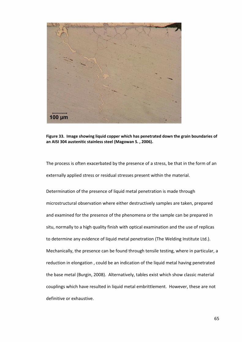
65
Figure 33. Image showing liquid copper which has penetrated down the grain boundaries of
an AISI 304 austenitic stainless steel (Magowan S. , 2006).
The process is often exacerbated by the presence of a stress, be that in the form of an
externally applied stress or residual stresses present within the material.
Determination of the presence of liquid metal penetration is made through
microstructural observation where either destructively samples are taken, prepared
and examined for the presence of the phenomena or the sample can be prepared in
situ, normally to a high quality finish with optical examination and the use of replicas
to determine any evidence of liquid metal penetration (The Welding Institute Ltd.).
Mechanically, the presence can be found through tensile testing, where in particular, a
reduction in elongation , could be an indication of the liquid metal having penetrated
the base metal (Burgin, 2008). Alternatively, tables exist which show classic material
couplings which have resulted in liquid metal embrittlement. However, these are not
definitive or exhaustive.
66
2.3.11 Stainless steel summary
The ferritic stainless steel grades are restricted in use due to the reduction in
mechanical properties as a result of welding. Those particularly sensitive to welding
are the non-stabilised grades such as the EN1.4016 and EN1.4003, which are
susceptible to the formation of martensite as well as grain coarsening. Therefore due
to the environments these materials may operate in it is imperative that the
mechanical properties are well understood, including the tensile, hardness, impact and
fatigue properties.
2.4 Fatigue
Fatigue is a failure mechanism resulting from some form of cyclic loading regime. This
loading may not necessarily be in the traditional sense, of a load applied and then
removed, but in the case of thermal fatigue could be as a result of cyclic stresses from
the expansion and contraction as a structure undergoes multiple heating/cooling
cycles. This could be as seen in the service environment for a typical engine block
whilst in this same structure there will be con rods and cam/crankshafts, valves and
pistons, all subject to more standard cyclic loading mechanisms; however these are all
operating in contrasting environments, where temperature, corrosion products,
abrasive particles will all influence the ability to succumb to a fatigue failure. An
automotive suspension spring, although not subject to elevated temperatures will
have a varied life being exposed to different corrosion products, the loading
mechanism will be different for every spring depending on how the vehicle is loaded
and the road surface and speed.
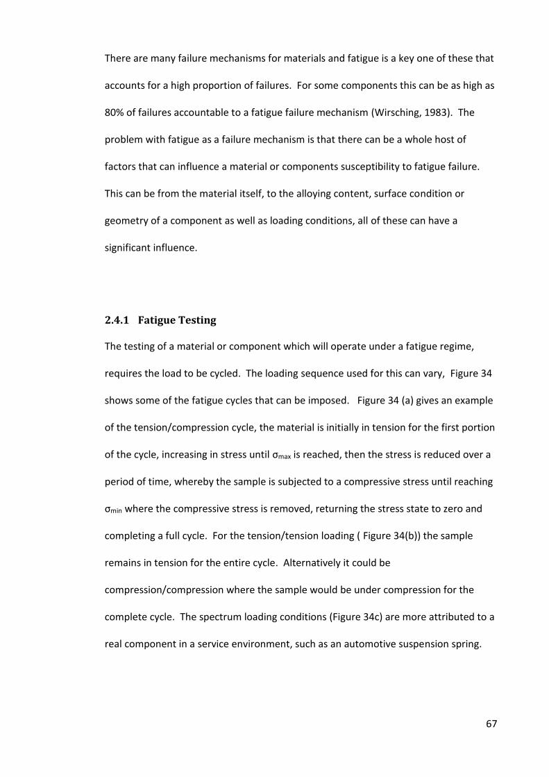
67
There are many failure mechanisms for materials and fatigue is a key one of these that
accounts for a high proportion of failures. For some components this can be as high as
80% of failures accountable to a fatigue failure mechanism (Wirsching, 1983). The
problem with fatigue as a failure mechanism is that there can be a whole host of
factors that can influence a material or components susceptibility to fatigue failure.
This can be from the material itself, to the alloying content, surface condition or
geometry of a component as well as loading conditions, all of these can have a
significant influence.
2.4.1 Fatigue Testing
The testing of a material or component which will operate under a fatigue regime,
requires the load to be cycled. The loading sequence used for this can vary, Figure 34
shows some of the fatigue cycles that can be imposed. Figure 34 (a) gives an example
of the tension/compression cycle, the material is initially in tension for the first portion
of the cycle, increasing in stress until σmax is reached, then the stress is reduced over a
period of time, whereby the sample is subjected to a compressive stress until reaching
σmin where the compressive stress is removed, returning the stress state to zero and
completing a full cycle. For the tension/tension loading ( Figure 34(b)) the sample
remains in tension for the entire cycle. Alternatively it could be
compression/compression where the sample would be under compression for the
complete cycle. The spectrum loading conditions (Figure 34c) are more attributed to a
real component in a service environment, such as an automotive suspension spring.
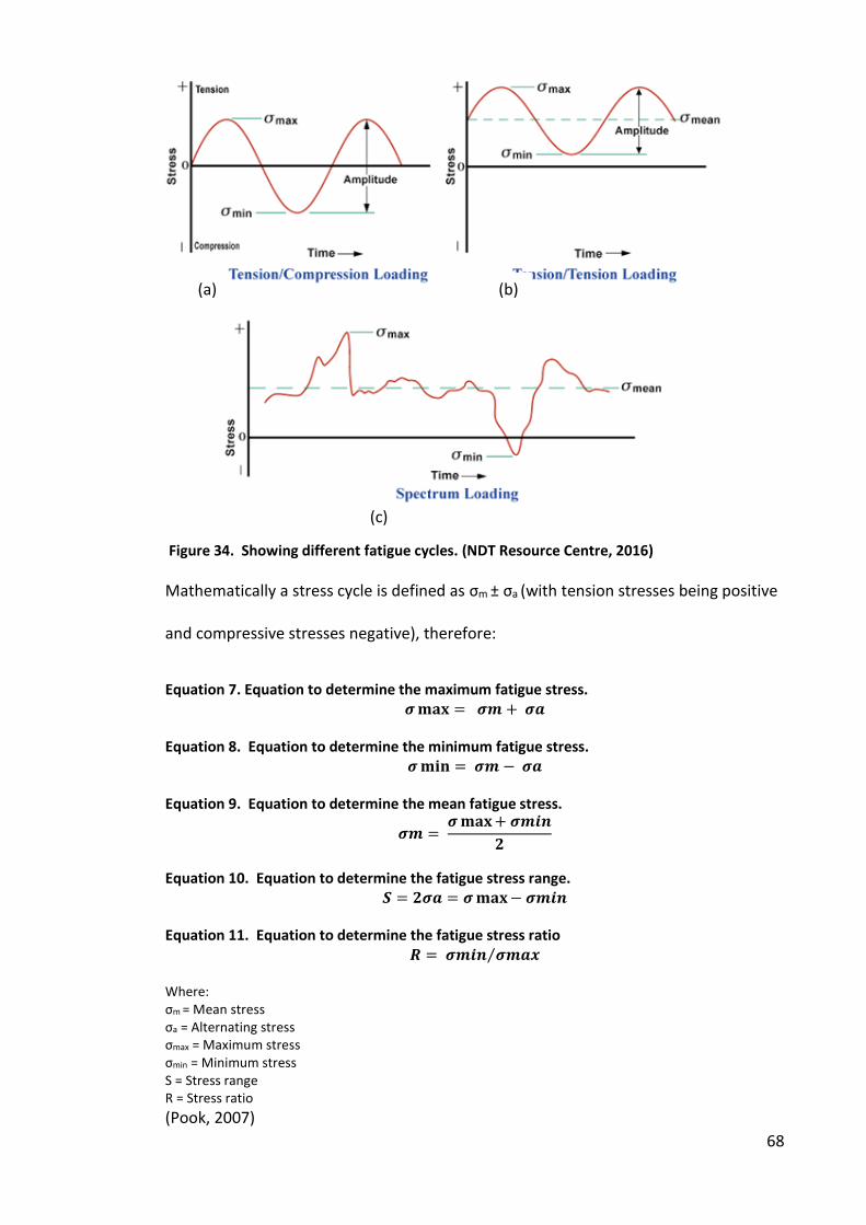
68
Figure 34. Showing different fatigue cycles. (NDT Resource Centre, 2016)
Mathematically a stress cycle is defined as σm ± σa (with tension stresses being positive
and compressive stresses negative), therefore:
Equation 7. Equation to determine the maximum fatigue stress. � �� = � + ��
Equation 8. Equation to determine the minimum fatigue stress. � � = � − ��
Equation 9. Equation to determine the mean fatigue stress. � = � �� + � �
Equation 10. Equation to determine the fatigue stress range. = �� = � �� − � �
Equation 11. Equation to determine the fatigue stress ratio = � � � ��⁄
Where:
σm = Mean stress
σa = Alternating stress
σmax = Maximum stress
σmin = Minimum stress
S = Stress range
R = Stress ratio
(Pook, 2007)
(a) (b)
(c)
69
2.4.2 Different types of fatigue testing
There are a number of different methods for fatigue testing a material or component
but most fall under three categories; reversed direct stress, reversed plane bending
and rotating bending (Frost, Marsh, & Pook, 1974). Although there are other types
such as alternating torsion and combined stress (Fatigue Testing, 1986).
It has been found that the fatigue properties can vary across the aforementioned
testing types with the fatigue limit varying by as much as 30% (Frost, Marsh, & Pook,
1974), therefore it is vitally important that the fatigue testing that is undertaken is in
the form that closely resembles that which would be experienced under service
conditions as this allows a better understanding of how the material or component
would react in this environment and therefore permit a more accurate prediction of
fatigue life and therefore a more effective design.
Further to this the type of fatigue test can be broken down into high cycle or low cycle
fatigue testing. The generally accepted differentiation between the two, in terms of
cycles would be anything below 104 cycles would be classed as low cycle and anything
above 105 cycles classed as high cycle fatigue testing. As can be seen this is not a clear
definition if the number of cycles should fall between 104 and 105 cycles then by this
definition it could be either. In practice the differentiation is made as to whether the
material is elastic or plastic under the dominant component of strain (Fatigue Testing,
1986) with low cycle fatigue testing inducing loads that are within the plastic region
and high cycle, loads that are within the elastic region of the material.
Reporting of high and low cycle fatigue tests are generally conducted in different ways,
with an example of the presentation of low cycle fatigue seen in Figure 35 whereby the
data presented is the plastic strain range, as determined by the hysteresis loop

70
produced under testing against the number of cycles and high cycle fatigue seen in
Figure 36, where it is a plot of stress against number of cycles.
Figure 35. Presentation of data from low cycle fatigue testing (KTH, 2003)
Figure 36. Showing S-N curve typical reporting of high cycle fatigue data (eFUNDA, 2016).
The determination of fatigue properties for a material can be extremely costly and
time consuming and therefore methods have been developed to ascertain this
information through the use of statistical theory. One such technique is the method
71
called Staircase Fatigue Testing, sometimes referred to as the up and down method
(Grove & Campean, 2007).
The basis for staircase fatigue testing, is that statistically speaking the independent
variable associated with a fatigue test is the stress at which it was tested, the
discussions being that at the start of the test, the stress is known and the number of
cycles to failure is unknown, but once the test is complete the life is known, leaving the
stress as the variable. Realistically, the stress is not the independent variable, but
rather the formation and growth of a crack. As it isn't possible to test samples under a
fixed cycle to failure regime, which would allow determination of a mean strength and
standard deviation, the staircase fatigue method and other probit methods have been
created to allow such information to be determined (Frost, Marsh, & Pook, 1974).
Within the staircase fatigue testing process a sample is subjected to a particular stress
level for a predetermined number of cycles. If the sample fails prior to the required
life, then the next sample is tested at a stress level increment below. The particular
increment relates to an expected level of the standard deviation (International Council
on Combustion Engines, 2009). If the sample survives the pre-set life then the test is
stopped, the sample removed and the next sample tested at an increment level above.
This is continued for a number of samples, Grove and Campean (2007) suggest 12 to
20 samples, however the creators of this analysis suggested the sample size needed to
be 40 to 50 (Dixon & Mood, 1948). Research conducted later determined that even
with a sample size of 5 to 10 samples, the analysis is reliable (Brownlee, Hodges, &
Rosenblatt, 1953). It is considered that the more samples tested the greater the
reliability of the data, therefore a sample size of 25 is normally suggested (Frost,
Marsh, & Pook, 1974).
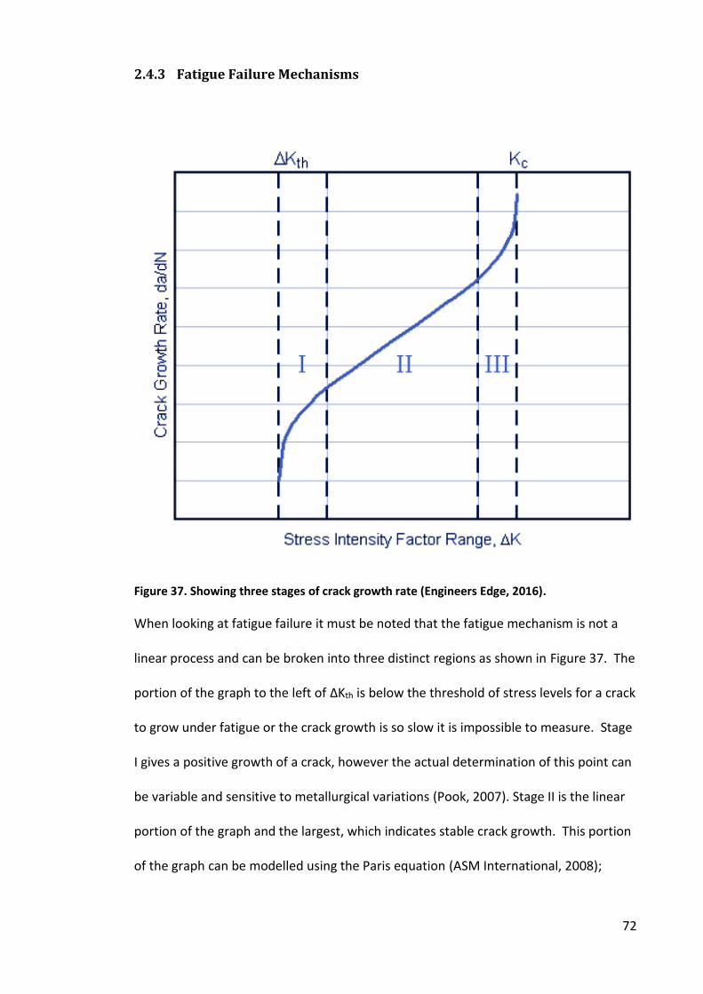
72
2.4.3 Fatigue Failure Mechanisms
Figure 37. Showing three stages of crack growth rate (Engineers Edge, 2016).
When looking at fatigue failure it must be noted that the fatigue mechanism is not a
linear process and can be broken into three distinct regions as shown in Figure 37. The
portion of the graph to the left of ∆Kth is below the threshold of stress levels for a crack
to grow under fatigue or the crack growth is so slow it is impossible to measure. Stage
I gives a positive growth of a crack, however the actual determination of this point can
be variable and sensitive to metallurgical variations (Pook, 2007). Stage II is the linear
portion of the graph and the largest, which indicates stable crack growth. This portion
of the graph can be modelled using the Paris equation (ASM International, 2008);
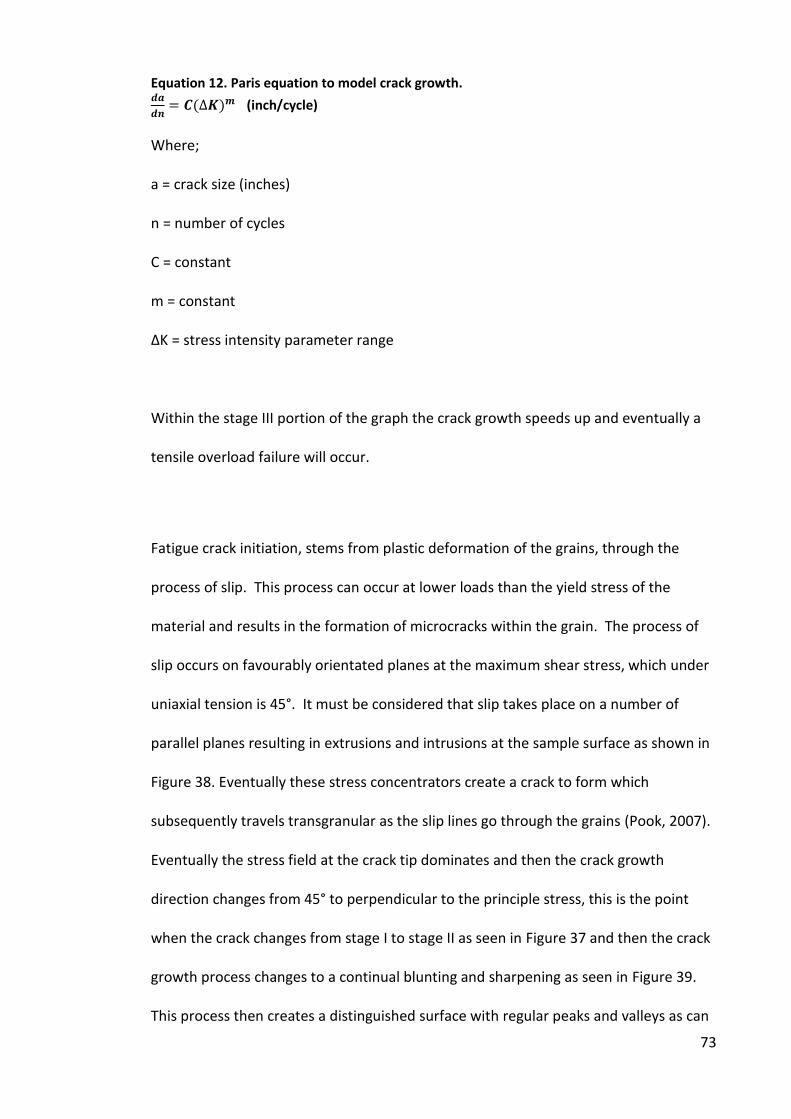
73
Equation 12. Paris equation to model crack growth. ��� = ∆� (inch/cycle)
Where;
a = crack size (inches)
n = number of cycles
C = constant
m = constant
∆K = stress intensity parameter range
Within the stage III portion of the graph the crack growth speeds up and eventually a
tensile overload failure will occur.
Fatigue crack initiation, stems from plastic deformation of the grains, through the
process of slip. This process can occur at lower loads than the yield stress of the
material and results in the formation of microcracks within the grain. The process of
slip occurs on favourably orientated planes at the maximum shear stress, which under
uniaxial tension is 45°. It must be considered that slip takes place on a number of
parallel planes resulting in extrusions and intrusions at the sample surface as shown in
Figure 38. Eventually these stress concentrators create a crack to form which
subsequently travels transgranular as the slip lines go through the grains (Pook, 2007).
Eventually the stress field at the crack tip dominates and then the crack growth
direction changes from 45° to perpendicular to the principle stress, this is the point
when the crack changes from stage I to stage II as seen in Figure 37 and then the crack
growth process changes to a continual blunting and sharpening as seen in Figure 39.
This process then creates a distinguished surface with regular peaks and valleys as can

74
be seen in Figure 40, these are known as striations and can only be observed at high
magnifications. It is considered that each striation is related to each fatigue cycle
(ASM International, 2008), however it has been reported that this is not always the
case and one striation may be as a result of a number of cycles, in the order of tens of
thousands (Gross & Lampman, 1996).
Figure 38. Figure showing
persistant slip bands. (NDT
Resource Centre, 2016)
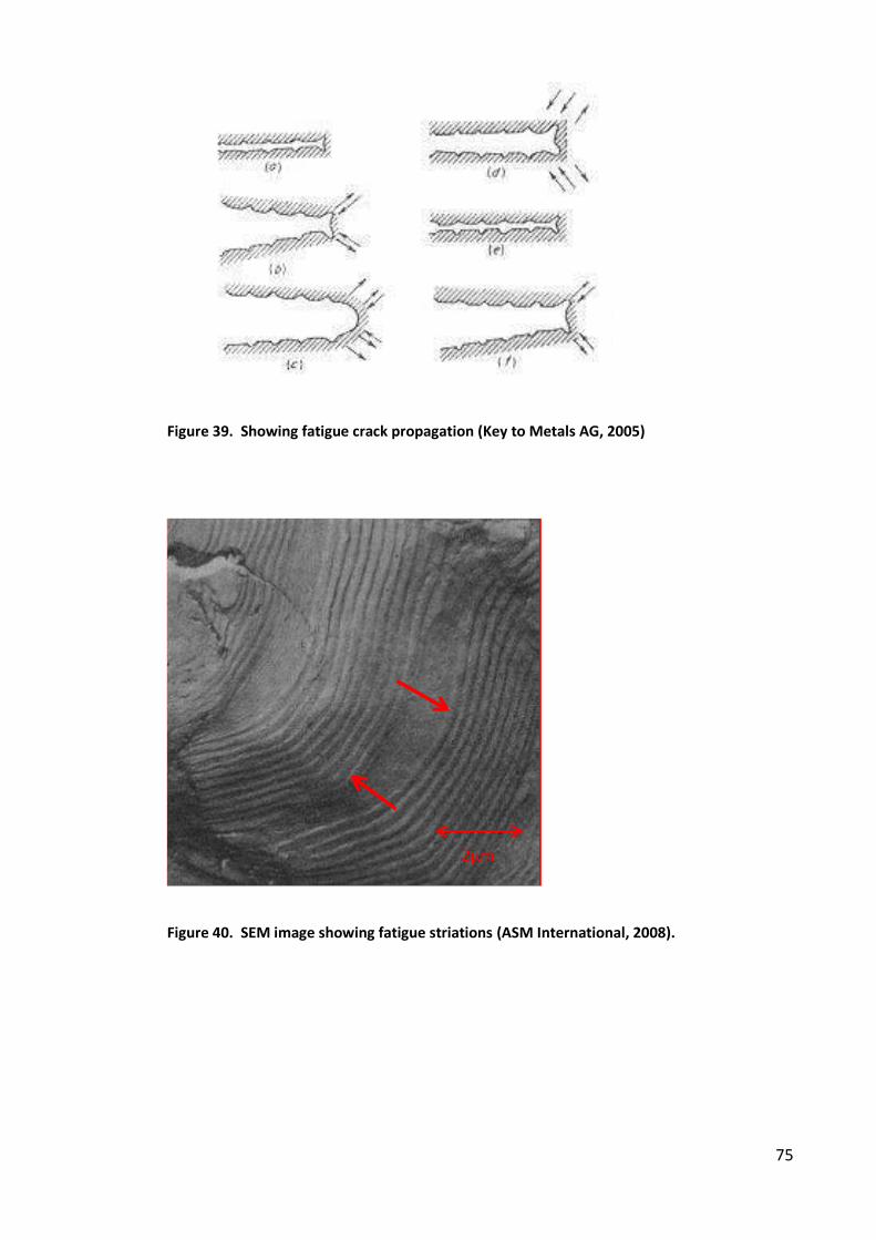
75
Figure 39. Showing fatigue crack propagation (Key to Metals AG, 2005)
Figure 40. SEM image showing fatigue striations (ASM International, 2008).
2µm
76
2.4.3.1 The Effect of the Environment on Fatigue Life
The environment in which the fatigue is experienced can have significant impact on the
properties of the material. The fatigue properties of a material under vacuum can be
different to those in normal atmospheric conditions. The reason for this is reported to
be that the growth rates of cracks is smaller under a vacuum, with reported levels for
crack initiation being 1 to 2 orders of magnitude slower under vacuum than in air
(Lukas, 1996). Therefore as reported by Frost et al (1974) preventing the atmosphere
from reaching the specimen surface can increase fatigue properties. As well as gas
interactions there is also the potential for chemical interaction thereby transforming
the fatigue from a mechanical induced failure to one that also has some chemical
assistance, this may be as simple as humidity levels in the atmosphere, where it has
been shown on some aluminium alloys that the fatigue strength is lower when the
humidity levels are higher (Frost, Marsh, & Pook, 1974). With the introduction of
other environments such as an aqueous substance that may not corrode the material
under a static condition, due to a protective layer that forms, for example in the case
of stainless steel in an oxygen containing atmosphere, under fatigue conditions this
layer may be broken allowing the corrosive media to react with the underlying
material and therefore cause cracks to develop and propagate at lower stress levels
than those operating within normal air environment without the additional chemical
element (Frost, Marsh, & Pook, 1974).
Temperature has been found to have a significant effect on the fatigue properties,
with testing conducted on a number of different materials at cryogenic temperatures
and the results found a general improvement in retarding the crack growth in the near
threshold region (McEvily, 1996). Research conducted on some titanium allows found
77
that the fatigue properties were improved at elevated temperature (175°C) rather
than at room temperature (25°C), and this was identified as being in part due to crack
closure (Albertson, Stephens, & Bayha, 1997). Other research (Lim, Jeong, & Keum,
2003) identified that with a P92 Steel, up to a particular temperature there was no
change in the fatigue properties however once a critical threshold temperature was
exceeded then the fatigue performance of the material rapidly decreased.
2.4.3.2 Surface Condition
The surface condition of the material is paramount to fatigue initiation as it is
considered that fatigue crack initiation in a metal is at the surface (Pook, 2007).
Therefore the surface condition plays an important role in the fatigue life of a material.
Firstly the surface profile is an important factor, as described in 2.4.3 the initial crack
on a smooth surface initiates from the extrusions and intrusions as a result of
dislocation motion, therefore by creating essentially coarser extrusions and intrusions
through having a rougher surface can have a significant effect on the fatigue life of a
material. In work conducted by Bayoumi and Abdellatif (1995) it was found that there
was a significant decrease in the fatigue life when the surface finish was modified from
0.45µm Ra to a value of 1.8µm.
Stress at the surface also has an effect on the fatigue life of the material. Compressive
stresses at the surface, induced by shot peening or a softened/hardened layer through
a decarburisation process or carburisation process effects the ability for cracks to form
at the surface layer (Pook, 2007). Research conducted by Mirzazadeh and Plumtree
(2012) found that the effects associated with shot peening were varied, in certain
instances tested, it had positive, neutral and negative effects on fatigue properties,
78
whereas the general consensus with processes such as shot peening is that it is
beneficial in the enhancement of fatigue properties of a material (Battelle-Columbus,
1996) through the introduction of residual compressive stresses into the surface of the
material.
2.4.4 Key factors affecting fatigue performance of welds
There is general agreement about the factors that affect the performance of a weld
under fatigue conditions and the effect of each is something which comes under
discussion, however these factors are:
• Applied stress amplitude
• Mean and residual stresses
• Material properties
• Geometrical stress concentrators
• Size and location of welding defects
(Lawrence, Dimitrakis, & Munse , 1996)
One of the factors that can affect the fatigue life of welds is the angle between the
parent material and the weld reinforcement, Harris and Syers (1979) present data that
demonstrates the effect of the angle between the two and how that affects the fatigue
strength (see Figure 41). As can be seen a decrease in angle and therefore a greater
stress concentrator, has a detrimental effect on the fatigue properties of the material.
The two conditions shown, one for a machined surface and one which has a mill scale

79
on the surface have a parallel effect for this change in angle which demonstrates that
although the surface finish has an effect of its own, the change in angle effects both in
the same way and at similar rates. The study examined the effects on fatigue strength
exceeding 2x10⁶ cycles for the change in reinforcement angle and it was shown that
for a machined plate, reducing the angle from 180° to 120° reduces the fatigue
strength by approximately 67%, therefore a flatter weld bead enhances the fatigue
properties of the material.
Figure 41. Showing relationship between parent/weld interface angle and fatigue strength
(Harris & Syers, 1979).
Another component that has been identified as having a significant role in the fatigue
life of a weld is the defects present within the weld. This is not just constrained to
defects themselves but the size, shape and concentration of these defects as these
traits can all play a significant part in the life of a component under cyclic loading
conditions. Results from investigations looking at the effect of defect length and the
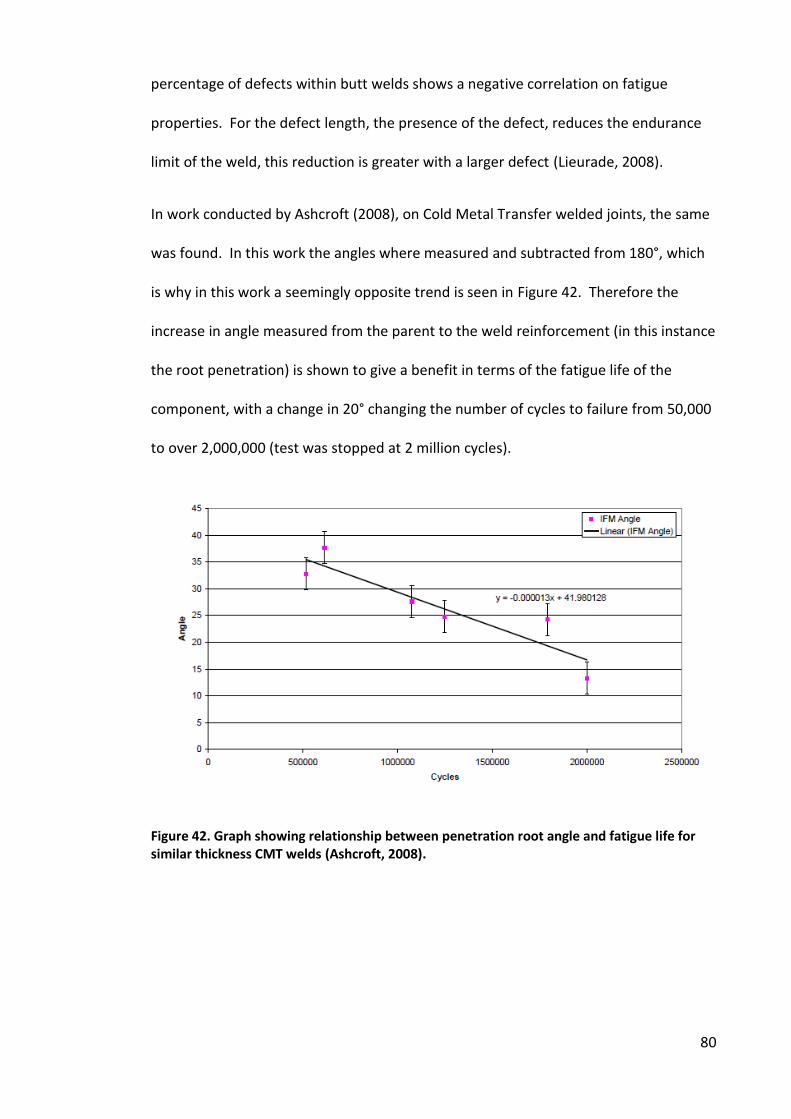
80
percentage of defects within butt welds shows a negative correlation on fatigue
properties. For the defect length, the presence of the defect, reduces the endurance
limit of the weld, this reduction is greater with a larger defect (Lieurade, 2008).
In work conducted by Ashcroft (2008), on Cold Metal Transfer welded joints, the same
was found. In this work the angles where measured and subtracted from 180°, which
is why in this work a seemingly opposite trend is seen in Figure 42. Therefore the
increase in angle measured from the parent to the weld reinforcement (in this instance
the root penetration) is shown to give a benefit in terms of the fatigue life of the
component, with a change in 20° changing the number of cycles to failure from 50,000
to over 2,000,000 (test was stopped at 2 million cycles).
Figure 42. Graph showing relationship between penetration root angle and fatigue life for
similar thickness CMT welds (Ashcroft, 2008).
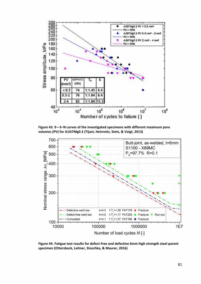
81
Figure 43. 9—S–N curves of the investigated specimens with different maximum pore
volumes (PV) for A1Si7Mg0.3 (Tijani, Heinreitz, Stets, & Voigt, 2013)
Figure 44. Fatigue test results for defect-free and defective 6mm high strength steel parent
specimen (Ottersbock, Leitner, Stoschka, & Maurer, 2016)
82
In the study reported by Tijani et al (2013) there was an examination of the volume of
defects within an aluminium alloy and the effect it had on the endurance limit. This
work can be seen in Figure 43 where 3 different defect percentages were tested, pore
volumes of <0.5, 0.5-2 and 2-4mm3. The results from this were that increasing the
percentage of defects within the material had a negative impact on the subsequent
fatigue properties. Other work (Ottersbock, Leitner, Stoschka, & Maurer, 2016)
conducted on 6mm thick, high stength steel welds with and without defects also
identified a reduction in the fatigue properties when defects were present, as seen in
Figure 44.
2.4.5 Models for fatigue life prediction
In work conducted by Ashcroft (2008) looking at Cold Metal Transfer welded joints, the
following model was proposed to predict the fatigue life of these joints based on a
relationship between the weld root angle and the number of cycles to failure.
Equation 13. Ashcrofts model for fatigue life prediction against root angle. � = − . ∗ − � + .
Where,
θ = angle at root penetration (°)
x = fatigue life in cycles
83
2.5 Summary of the Literature
As have been discussed there are a number of different welding techniques that have
advantages and disadvantages and a wide range of parameters within each of those
processes that can have effect on the integrity of the final joint. One quantifiable
measure of a weld is with the heat input, as this can have a considerable effect on the
final joint in particular the HAZ. The arc efficiency factor has been questioned
previously which ultimately may skew results if CMT is more efficient that MAG
welding however the determination of this is outside the scope of this research.
The effects of porosity in the weld has been shown to reduce the fatigue life of a
component and relationships have been drawn between weld root angles and fatigue
endurance and these issue will be of interest in this research.
The use of ferritic stainless steels is limited due to the detrimental effects associated
with welding, such as a reduced toughness owing to grain growth in the HAZ, phase
transformations in the lower alloy content grades, reduction in corrosion resistance,
therefore with a welding techniques such as CMT that in principle induces less heat
into the joint, should therefore minimise the detrimental effects associated with the
heat. The following work investigates the welding of ferritic stainless steel using the
CMT process and compares with the MAG welding process.
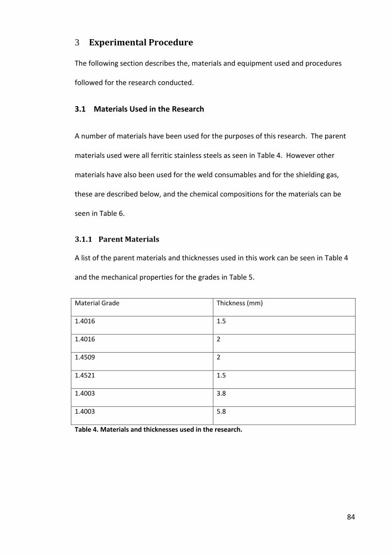
84
3 Experimental Procedure
The following section describes the, materials and equipment used and procedures
followed for the research conducted.
3.1 Materials Used in the Research
A number of materials have been used for the purposes of this research. The parent
materials used were all ferritic stainless steels as seen in Table 4. However other
materials have also been used for the weld consumables and for the shielding gas,
these are described below, and the chemical compositions for the materials can be
seen in Table 6.
3.1.1 Parent Materials
A list of the parent materials and thicknesses used in this work can be seen in Table 4
and the mechanical properties for the grades in Table 5.
Material Grade Thickness (mm)
1.4016 1.5
1.4016 2
1.4509 2
1.4521 1.5
1.4003 3.8
1.4003 5.8
Table 4. Materials and thicknesses used in the research.

85
Table 5. Mechanical properties of ferritic stainless steels at room temperature (Outokumpu,
2011).
Material C (%) Mn (%) Si(%) Cr(%) Ni(%) Nb(%) Mo(%)
1.4016 0.018 0.315 0.248 17.216 0.232 0.046 0.098
1.4509 0.002 0.483 0.558 19.893 0.334 0.3 0.062
1.4521 0.013 0.512 0.457 19.526 0.29 0.28 1.087
1.4003 0.010 1.42 0.27 11.0 0.4 - -
Table 6. Chemical analysis data of the parent materials used within the project.
3.1.2 Welding Filler Materials
The filler material recommended for the joining of ferritic stainless steel and therefore
used in the research included:
1.0mm diameter AISI 308L-Si
1.2mm diameter AISI 308L-Si
Both of these wires are of the same chemical composition and this analysis can be
seen in Table 7, the material is an austenitic stainless steel.
Element C Cr Si Ni Mn
Composition
(%)
0.02 20 0.85 10.5 1.8
Table 7. Composition of AISI 308L-Si filler material (Avesta Welding, 2006).
86
3.1.3 Shielding Gas Used in the Project
High purity shielding gas mixtures used in the work included:
1% Oxygen, 99% Argon
2% Oxygen, 98% Argon
2% Carbon Dioxide, 98% Argon
3.2 Comparison Trial between CMT & MAG Welds in Different Grades and
Thicknesses
Pulsed Metal Active Gas (MAG) welds were produced at the Outokumpu research
facility in Tornio, Finland. Parent material from the same batch as shown in Table 6,
was sent to the ACES welding laboratory at Sheffield Hallam University to allow
comparable welds to be produced using the Cold Metal Transfer (CMT) process, with
and without pulsed arc.
Stainless steel grades used in the trials were 1.4016 (1.5mm thick), 1.4509 (2mm thick)
and 1.4521 (1.5mm thick). The filler wire used in all cases was 1mm diameter, 308L.
The shielding gas used in the manufacture of the CMT welds for this part of the work,
was argon with 2% oxygen and the joint gap was held constant at 0.5mm. All MAG
welds were produced using a shielding gas of argon with 2% CO2 and the joint gap set
between 0.5 and 1mm.
87
3.3 CMT Welding Trials to Examine the Effect of Variation of Welding Gap &
Speed to Reduce Heat Input
In Gas Metal Arc Welding (GMAW) the filler wire and parent materials, under the
power of the arc, melt and fuse together. The welding gap therefore will have an
effect on the amount of energy required to achieve sufficient melting of the parent
material to ensure full penetration. The smaller the welding gap the more parent
material will need to be melted. Additionally published data states that variation of
the torch angle affects the level of penetration within a weld and that welding
backhand (with the electrode directed away from the direction of travel) will increase
the penetration of the weld (American Welding Society, 1991) possibly allowing a
reduction in the heat input of the joint to be made. Accordingly a trial was conducted
at Sheffield Hallam University, using 2mm thick, 1.4016 material and followed up using
2mm thick 1.4509, to determine the minimum heat input achievable with different
joint gaps and torch angles, whilst still maintaining complete penetration of the joint.
The amount of parent material available allowed trials at three different welding gaps,
values of 1mm, 1.15mm and 1.25mm were chosen. Torch angles of 15° lead
(forehand) and 15° drag (backhand - described within the report as -15°) were used.
Based on earlier experience, welds were produced at differing torch traverse speeds of
762, 1016 and 1270 millimetres per minute and the welding power adjusted in an
attempt to maintain penetration, whilst minimising the power used to produce the
joint.
88
3.4 Trial to Determine the Consistency of Welds Produce Using CMT Process
As the effect of the CMT variables is not well known a trial was conducted to allow
assessment of these and determine the effect on changing variables would have on
the consistency of the weld. The shielding gas used for all welds produced in this trial
was Argon with 1% O2 and the filler wire was 1mm diameter 308L Si.
A 2.5m x 1.25m sheet of 2mm thick, 1.4016 was marked out into sections 200mm long
X 120mm wide for sectioning and each coupon was identified in terms of orientation
and position relative to the uncut sheet. This allowed the sheets to be welded back to
the same piece they were originally joined to, prior to sectioning. The reason for this
was to eliminate any variations which may occur across the plate in terms of
dimensions, microstructure and or composition.
Assessment was made of the effect and consistency of a number of parameters which
can be seen in Table 8. These settings were determined for the wire feed speed by the
power used to produce similar fully penetrated welds in previous work (Magowan S. ,
2010), with the 3.5m/min, wire feed speed, having provided sufficient power to
produce a fully penetrating weld. The 4.5m/min, was set as a base as it was found in
previous work that this level of power consistently provides fully penetrating welds
and the 5.5m/min to allow comparison when providing too much power. At these
settings the torch angle was set to drag (-15°), the pulse correction and arc length
correction set to zero and the traverse speed set to 1.016m/min, as can be seen in
Table 8. For the rest of the trials the variation in parameters had the wire feed speed
set to 4.5m/min as this then allowed the effect of changes in each variable to be
identified.
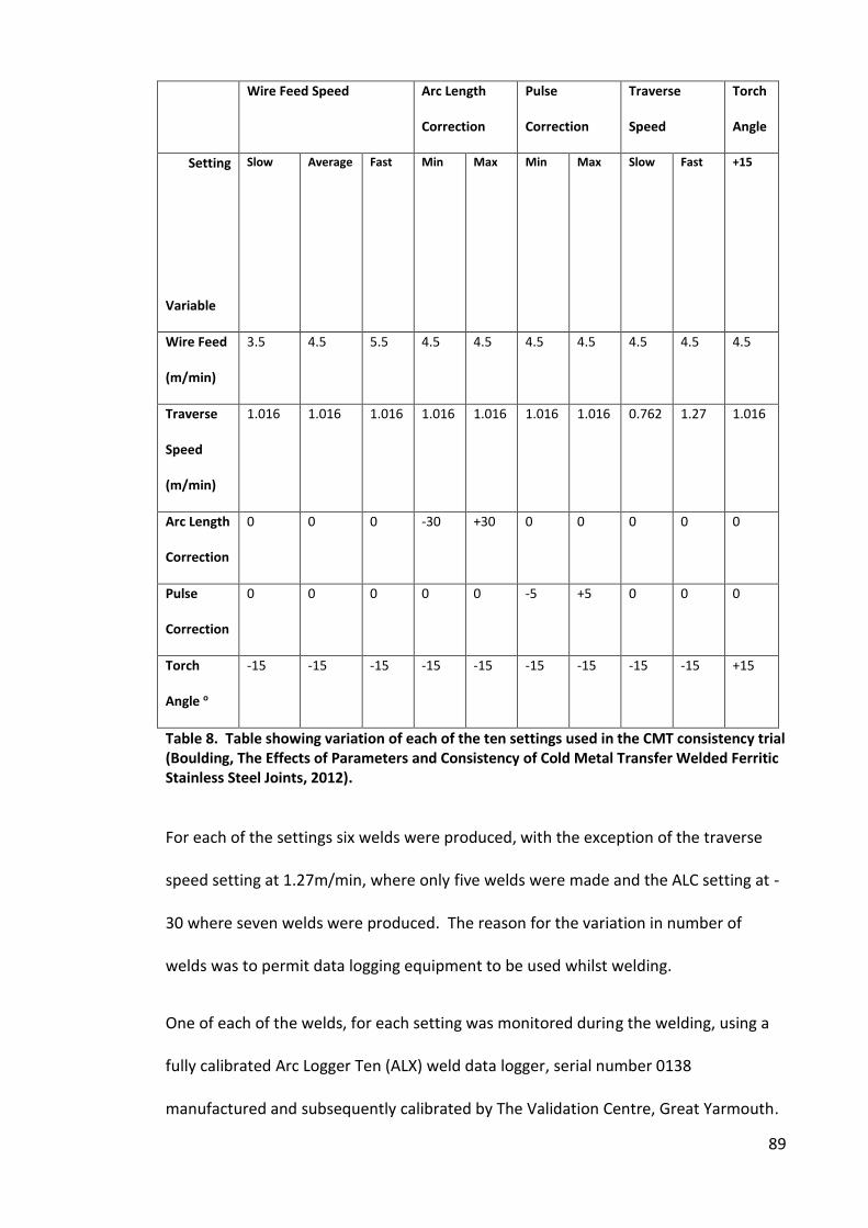
89
Wire Feed Speed Arc Length
Correction
Pulse
Correction
Traverse
Speed
Torch
Angle
Setting
Variable
Slow Average Fast Min Max Min Max Slow Fast +15
Wire Feed
(m/min)
3.5 4.5 5.5 4.5 4.5 4.5 4.5 4.5 4.5 4.5
Traverse
Speed
(m/min)
1.016 1.016 1.016 1.016 1.016 1.016 1.016 0.762 1.27 1.016
Arc Length
Correction
0 0 0 -30 +30 0 0 0 0 0
Pulse
Correction
0 0 0 0 0 -5 +5 0 0 0
Torch
Angle o
-15 -15 -15 -15 -15 -15 -15 -15 -15 +15
Table 8. Table showing variation of each of the ten settings used in the CMT consistency trial
(Boulding, The Effects of Parameters and Consistency of Cold Metal Transfer Welded Ferritic
Stainless Steel Joints, 2012).
For each of the settings six welds were produced, with the exception of the traverse
speed setting at 1.27m/min, where only five welds were made and the ALC setting at -
30 where seven welds were produced. The reason for the variation in number of
welds was to permit data logging equipment to be used whilst welding.
One of each of the welds, for each setting was monitored during the welding, using a
fully calibrated Arc Logger Ten (ALX) weld data logger, serial number 0138
manufactured and subsequently calibrated by The Validation Centre, Great Yarmouth.
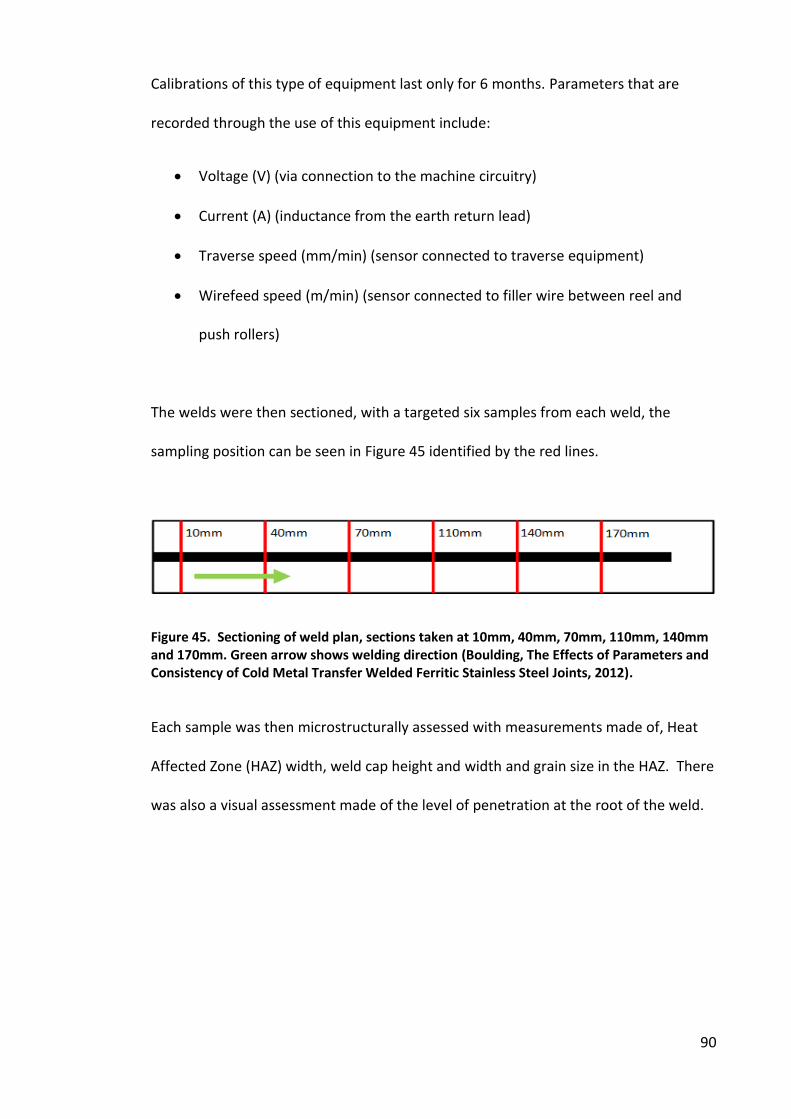
90
Calibrations of this type of equipment last only for 6 months. Parameters that are
recorded through the use of this equipment include:
• Voltage (V) (via connection to the machine circuitry)
• Current (A) (inductance from the earth return lead)
• Traverse speed (mm/min) (sensor connected to traverse equipment)
• Wirefeed speed (m/min) (sensor connected to filler wire between reel and
push rollers)
The welds were then sectioned, with a targeted six samples from each weld, the
sampling position can be seen in Figure 45 identified by the red lines.
Figure 45. Sectioning of weld plan, sections taken at 10mm, 40mm, 70mm, 110mm, 140mm
and 170mm. Green arrow shows welding direction (Boulding, The Effects of Parameters and
Consistency of Cold Metal Transfer Welded Ferritic Stainless Steel Joints, 2012).
Each sample was then microstructurally assessed with measurements made of, Heat
Affected Zone (HAZ) width, weld cap height and width and grain size in the HAZ. There
was also a visual assessment made of the level of penetration at the root of the weld.
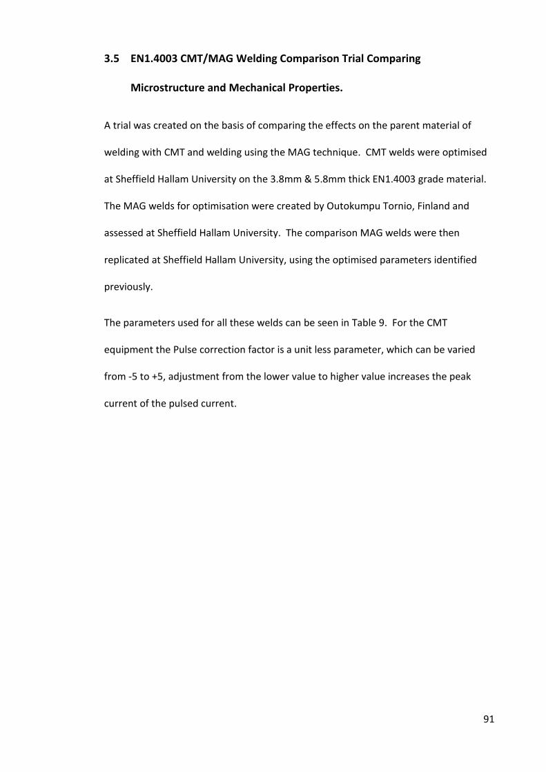
91
3.5 EN1.4003 CMT/MAG Welding Comparison Trial Comparing
Microstructure and Mechanical Properties.
A trial was created on the basis of comparing the effects on the parent material of
welding with CMT and welding using the MAG technique. CMT welds were optimised
at Sheffield Hallam University on the 3.8mm & 5.8mm thick EN1.4003 grade material.
The MAG welds for optimisation were created by Outokumpu Tornio, Finland and
assessed at Sheffield Hallam University. The comparison MAG welds were then
replicated at Sheffield Hallam University, using the optimised parameters identified
previously.
The parameters used for all these welds can be seen in Table 9. For the CMT
equipment the Pulse correction factor is a unit less parameter, which can be varied
from -5 to +5, adjustment from the lower value to higher value increases the peak
current of the pulsed current.
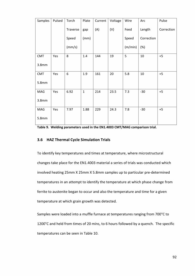
92
Samples Pulsed Torch
Traverse
Speed
(mm/s)
Plate
gap
(mm)
Current
(A)
Voltage
(V)
Wire
Feed
Speed
(m/min)
Arc
Length
Correction
(%)
Pulse
Correction
CMT
3.8mm
Yes 8 1.4 144 19 5 10 +5
CMT
5.8mm
Yes 6 1.9 161 20 5.8 10 +5
MAG
3.8mm
Yes 6.92 1 214 23.5 7.3 -30 +5
MAG
5.8mm
Yes 7.97 1.88 229 24.3 7.8 -30 +5
Table 9. Welding parameters used in the EN1.4003 CMT/MAG comparison trial.
3.6 HAZ Thermal Cycle Simulation Trials
To identify key temperatures and times at temperature, where microstructural
changes take place for the EN1.4003 material a series of trials was conducted which
involved heating 25mm X 25mm X 5.8mm samples up to particular pre-determined
temperatures in an attempt to identify the temperature at which phase change from
ferrite to austenite began to occur and also the temperature and time for a given
temperature at which grain growth was detected.
Samples were loaded into a muffle furnace at temperatures ranging from 700°C to
1200°C and held from times of 20 mins, to 6 hours followed by a quench. The specific
temperatures can be seen in Table 10.
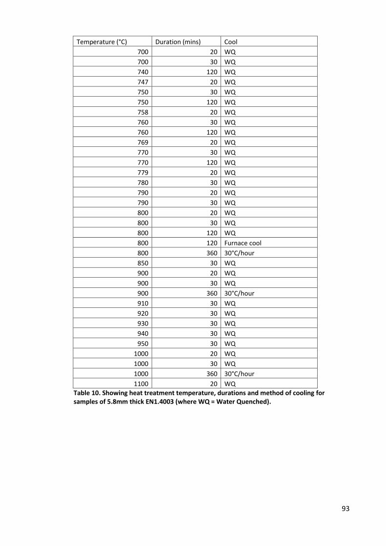
93
Temperature (°C) Duration (mins) Cool
700 20 WQ
700 30 WQ
740 120 WQ
747 20 WQ
750 30 WQ
750 120 WQ
758 20 WQ
760 30 WQ
760 120 WQ
769 20 WQ
770 30 WQ
770 120 WQ
779 20 WQ
780 30 WQ
790 20 WQ
790 30 WQ
800 20 WQ
800 30 WQ
800 120 WQ
800 120 Furnace cool
800 360 30°C/hour
850 30 WQ
900 20 WQ
900 30 WQ
900 360 30°C/hour
910 30 WQ
920 30 WQ
930 30 WQ
940 30 WQ
950 30 WQ
1000 20 WQ
1000 30 WQ
1000 360 30°C/hour
1100 20 WQ
Table 10. Showing heat treatment temperature, durations and method of cooling for
samples of 5.8mm thick EN1.4003 (where WQ = Water Quenched).
94
Once key temperatures were identified, following hardness testing and microstructural
evaluation (microstructure and grain size) showed a change to that of the parent, then
a number of non-standard Charpy impact specimens (5.8 x 10 x 55mm) were subjected
to the same heat treatment cycle and then subsequently tested to identify the effect
on impact properties. The samples had to be non-standard as the thickness of the
parent material limited one of the dimensions, therefore the standard size of 10 x 10 x
55mm could not be created.
3.7 Process for the Creation of all CMT Welds & MAG Welds created at
Sheffield Hallam University using EN1.4003 Grade Stainless Steel Parent
Material in 3.8 & 5.8mm Thicknesses
Following the welding consistency trials and the trials to optimise process parameters,
the welds created for the research were consistently produced in terms of the
procedures and equipment used, this information is described below.
3.7.1 Description of the Welding Test Coupon
The weld coupons used for the welding trials were 120mm wide and either 200mm or
400mm long, with the weld being made in the longer dimension as per Figure 46. The
rolling direction was maintained parallel to the 120mm dimension on all welds
produced at Sheffield Hallam University.
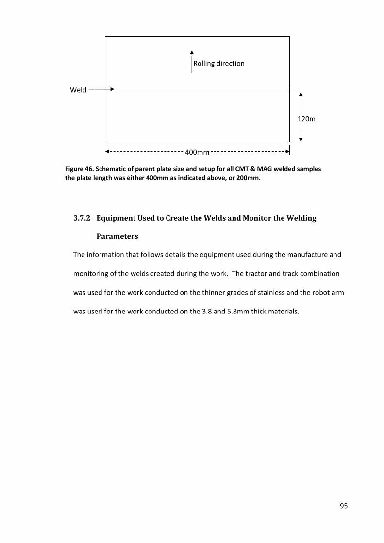
95
3.7.2 Equipment Used to Create the Welds and Monitor the Welding
Parameters
The information that follows details the equipment used during the manufacture and
monitoring of the welds created during the work. The tractor and track combination
was used for the work conducted on the thinner grades of stainless and the robot arm
was used for the work conducted on the 3.8 and 5.8mm thick materials.
Rolling direction
Weld
400mm
120m
Figure 46. Schematic of parent plate size and setup for all CMT & MAG welded samples
the plate length was either 400mm as indicated above, or 200mm.
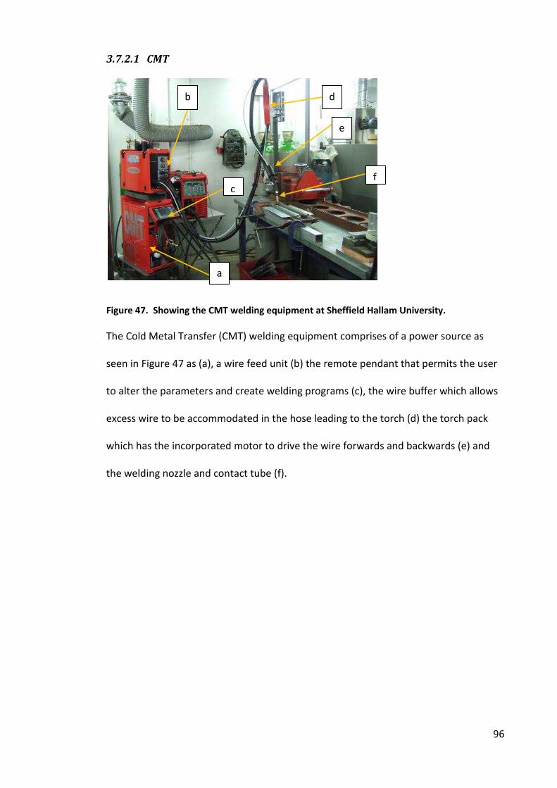
96
3.7.2.1 CMT
Figure 47. Showing the CMT welding equipment at Sheffield Hallam University.
The Cold Metal Transfer (CMT) welding equipment comprises of a power source as
seen in Figure 47 as (a), a wire feed unit (b) the remote pendant that permits the user
to alter the parameters and create welding programs (c), the wire buffer which allows
excess wire to be accommodated in the hose leading to the torch (d) the torch pack
which has the incorporated motor to drive the wire forwards and backwards (e) and
the welding nozzle and contact tube (f).
b
c
a
d
e
f
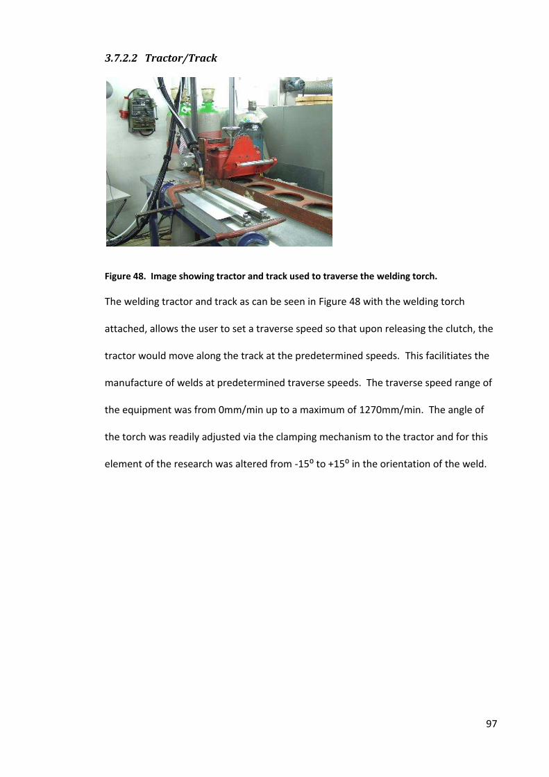
97
3.7.2.2 Tractor/Track
Figure 48. Image showing tractor and track used to traverse the welding torch.
The welding tractor and track as can be seen in Figure 48 with the welding torch
attached, allows the user to set a traverse speed so that upon releasing the clutch, the
tractor would move along the track at the predetermined speeds. This facilitiates the
manufacture of welds at predetermined traverse speeds. The traverse speed range of
the equipment was from 0mm/min up to a maximum of 1270mm/min. The angle of
the torch was readily adjusted via the clamping mechanism to the tractor and for this
element of the research was altered from - ⁰ to + ⁰ i the orie tatio of the eld.
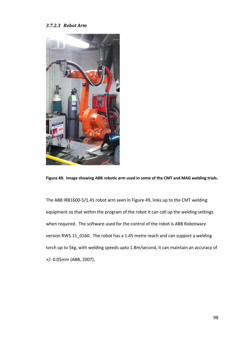
98
3.7.2.3 Robot Arm
Figure 49. Image showing ABB robotic arm used in some of the CMT and MAG welding trials.
The ABB IRB1600-5/1.45 robot arm seen in Figure 49, links up to the CMT welding
equipment so that within the program of the robot it can call up the welding settings
when required. The software used for the control of the robot is ABB Robotware
version RW5.11_0160. The robot has a 1.45 metre reach and can support a welding
torch up to 5kg, with welding speeds upto 1.8m/second, it can maintain an accuracy of
+/- 0.05mm (ABB, 2007).
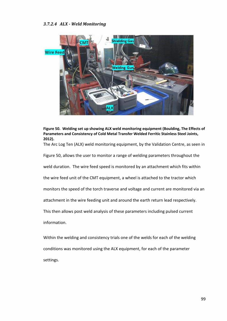
99
3.7.2.4 ALX - Weld Monitoring
Figure 50. Welding set up showing ALX weld monitoring equipment (Boulding, The Effects of
Parameters and Consistency of Cold Metal Transfer Welded Ferritic Stainless Steel Joints,
2012).
The Arc Log Ten (ALX) weld monitoring equipment, by the Validation Centre, as seen in
Figure 50, allows the user to monitor a range of welding parameters throughout the
weld duration. The wire feed speed is monitored by an attachment which fits within
the wire feed unit of the CMT equipment, a wheel is attached to the tractor which
monitors the speed of the torch traverse and voltage and current are monitored via an
attachment in the wire feeding unit and around the earth return lead respectively.
This then allows post weld analysis of these parameters including pulsed current
information.
Within the welding and consistency trials one of the welds for each of the welding
conditions was monitored using the ALX equipment, for each of the parameter
settings.

100
3.7.2.5 Sample Positioning and Securing
Figure 51. Showing clamping arrangement for holding the parent material in place whilst
welding.
3.7.3 Heat Input
Calculated values of heat input were made using the following equation:
Equation 2. Equation to calculate arc energy.
Arc Energy (J/mm) = ���
Where;
V = Voltage used (Volts)
I = Current used (Amperes)
v = Travel of welding torch (mm per second)
From the calculation of arc energy, the heat input is calculated by using the equation
below (British Standards Institution, 1998);
Equation 3. Equation to calculate weld heat input.
Heat Input (J/mm) = ηAE
Where;
η = Pro ess effi ie . for GMAW (British Standards Institution, 1998)
AE = Arc Energy (J/mm)

101
3.8 Non Destructive Examination
Radiographic equipment, Xograph Bucky Star with a Canon LANMIX CDXI-50G detector
was used to assess CMT welds, in a bid to identify defects within them. This was used
on initial CMT welds created using 3.8mm & 5.8mm EN1.4003. The parameters used
for these inspections were:
Distance from source: 115cm
for 3.8mm welds: 80kV & 50mAs
for 5.8mm welds: 80kV & 40mAs
From one of the test radiographs a complete assessment was made destructively to
assess the suitability of the technique for the identification of defects within these
welds.
102
3.9 Microstructural Evaluation of all Welded Samples
Microstructural evaluations were made on samples throughout the work, the following
section describes the procedure for the preparation of the welds to produce these
samples.
3.9.1 Sectioning of As-Welded Samples
Sectioning of samples throughout the work varied according to the thickness of the
material. Samples required for mechanical tested were water jet cut to eliminate any
heat being put into the material during this stage of the preparation. Materials for
metallurgical examination at 2mm thick and under were first sectioned using a
mechanical shear and then samples for examination were extracted using a Beuhler
AbrasiMet precision cutting machine.
Materials thicker than 2mm, had sections milled or water jet cut from the weld and
then sections were cut from these more manageable pieces using the Beuhler
AbrasiMet precision cutting machine.
The samples taken were cross sections of the weld and were less than 30mm long to
enable them to fit into the hot mounting press for mounting in conductive bakelite.
3.9.2 Hot Mounting of Welded Cross Sections
Hot mounting was achieved using a Beuhler SimpliMet 2000 and a conductive Bakelite.
The mould size for the hot mounting was 30mm diameter and the cycle time was 4
minutes heating and 4 minutes cooling. Immediately after removing from the hot
mounting press, the sample identification was engraved on the reverse of the
mounted sample. The temperatures involved in hot mounting are up to 190°C and as
103
it is below tempering temperatures of the material would not be considered to have
any significant detrimental effect on the materials involved in this work.
3.9.3 Grinding/Polishing of Welded Cross Sections
The grinding and polishing was conducted in the laboratories at Sheffield Hallam
University on Beuhler Alpha Beta grinder polishing stations. The route adopted
included grinding using a P120 silicon carbide paper to ensure the sample was flat,
then subsequent operations to gradually reduce the level of deformation in the sample
through P400, P600 and finally P1200 silicon carbide papers. All these stations had
water projected onto the platen to keep the sample cool and remove the grinding
debris.
Polishing was conducted on identical equipment to the grinding, however a pad
i preg ated ith a dia o d paste as used ith first μ a i u parti le size,
then after cleaning with a detergent and water, another pad containing a diamond
paste ith a a i u parti le size of μ . I oth ases the sa ple as o tra-
rotated on the pad to eliminate any directionality. Following the final stage the sample
was cleaned using water and detergent and then dried with the aid of a solvent
(industrial methylated spirits).
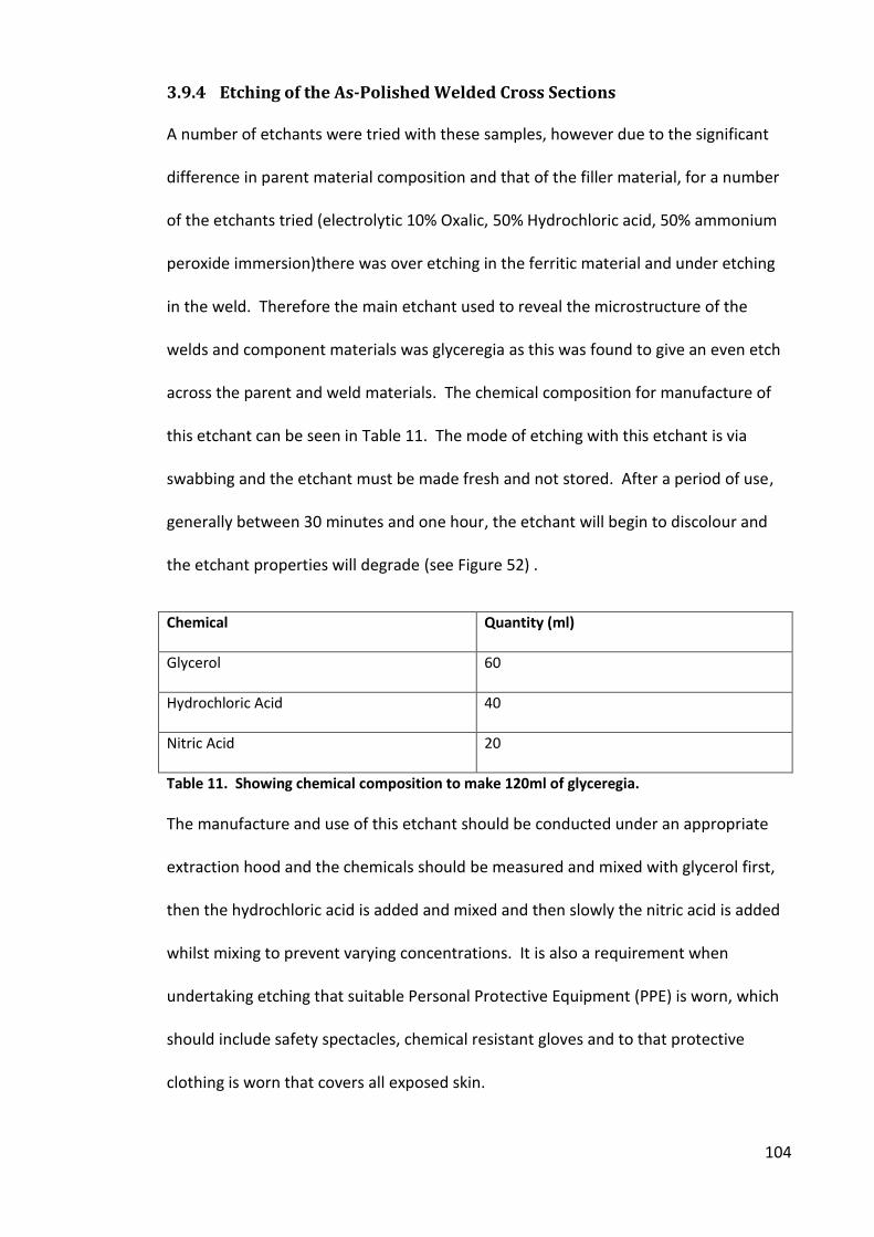
104
3.9.4 Etching of the As-Polished Welded Cross Sections
A number of etchants were tried with these samples, however due to the significant
difference in parent material composition and that of the filler material, for a number
of the etchants tried (electrolytic 10% Oxalic, 50% Hydrochloric acid, 50% ammonium
peroxide immersion)there was over etching in the ferritic material and under etching
in the weld. Therefore the main etchant used to reveal the microstructure of the
welds and component materials was glyceregia as this was found to give an even etch
across the parent and weld materials. The chemical composition for manufacture of
this etchant can be seen in Table 11. The mode of etching with this etchant is via
swabbing and the etchant must be made fresh and not stored. After a period of use,
generally between 30 minutes and one hour, the etchant will begin to discolour and
the etchant properties will degrade (see Figure 52) .
Chemical Quantity (ml)
Glycerol 60
Hydrochloric Acid 40
Nitric Acid 20
Table 11. Showing chemical composition to make 120ml of glyceregia.
The manufacture and use of this etchant should be conducted under an appropriate
extraction hood and the chemicals should be measured and mixed with glycerol first,
then the hydrochloric acid is added and mixed and then slowly the nitric acid is added
whilst mixing to prevent varying concentrations. It is also a requirement when
undertaking etching that suitable Personal Protective Equipment (PPE) is worn, which
should include safety spectacles, chemical resistant gloves and to that protective
clothing is worn that covers all exposed skin.
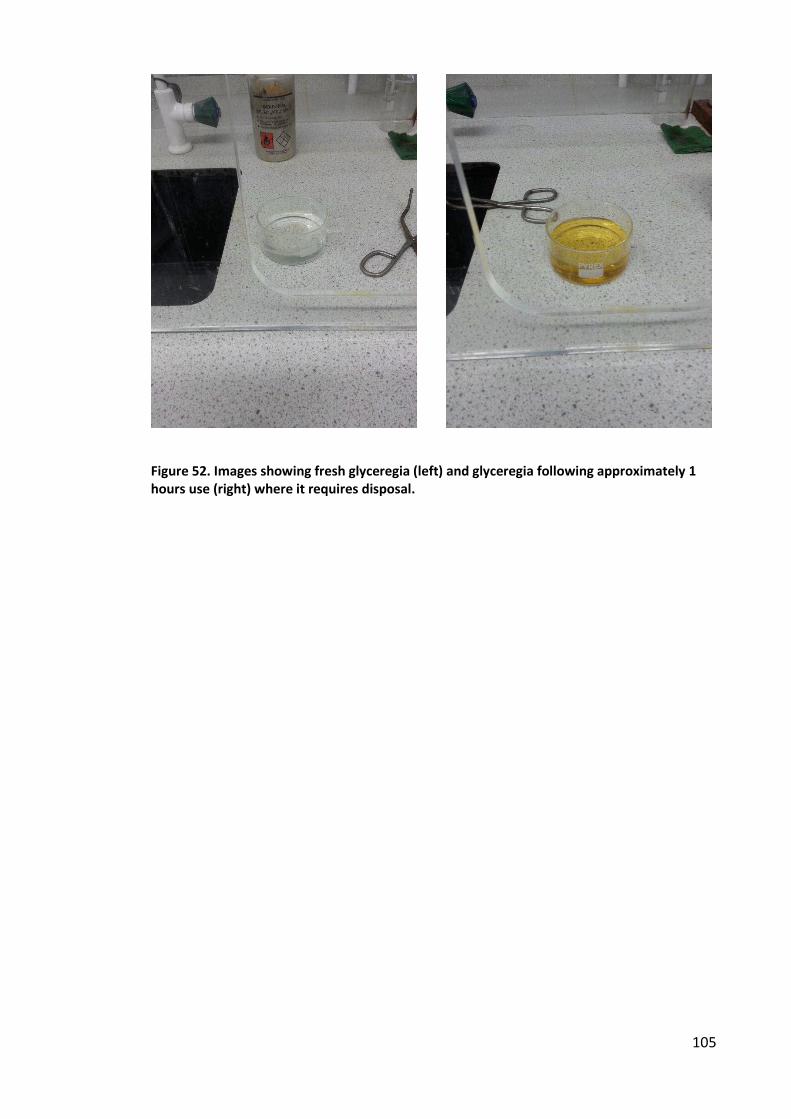
105
Figure 52. Images showing fresh glyceregia (left) and glyceregia following approximately 1
hours use (right) where it requires disposal.
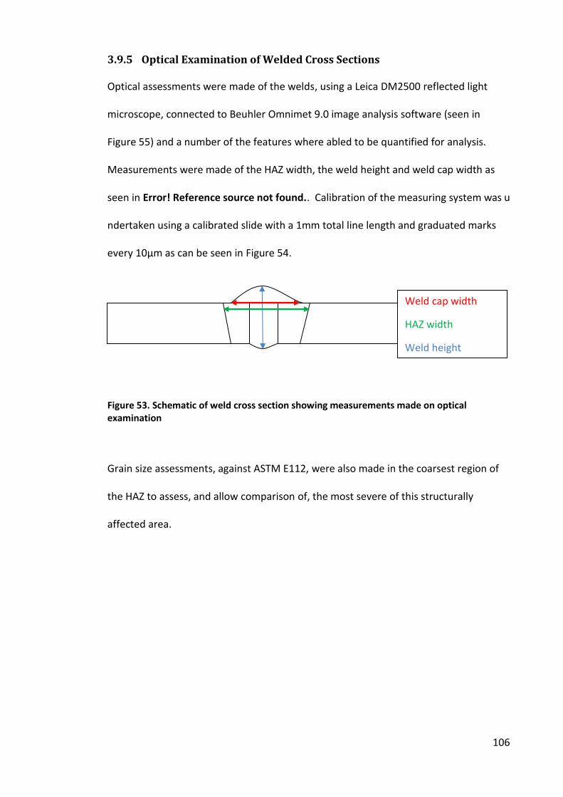
106
3.9.5 Optical Examination of Welded Cross Sections
Optical assessments were made of the welds, using a Leica DM2500 reflected light
microscope, connected to Beuhler Omnimet 9.0 image analysis software (seen in
Figure 55) and a number of the features where abled to be quantified for analysis.
Measurements were made of the HAZ width, the weld height and weld cap width as
seen in Error! Reference source not found.. Calibration of the measuring system was u
ndertaken using a calibrated slide with a 1mm total line length and graduated marks
every 10µm as can be seen in Figure 54.
Figure 53. Schematic of weld cross section showing measurements made on optical
examination
Grain size assessments, against ASTM E112, were also made in the coarsest region of
the HAZ to assess, and allow comparison of, the most severe of this structurally
affected area.
Weld cap width
HAZ width
Weld height
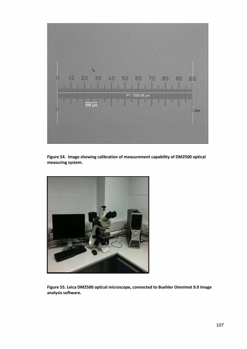
107
Figure 54. Image showing calibration of measurement capability of DM2500 optical
measuring system.
Figure 55. Leica DM2500 optical microscope, connected to Buehler Omnimet 9.0 image
analysis software.

108
3.9.6 Infinite Focus Microscope Examination of Weld Profiles on Untested
Fatigue Samples
The Infinite Focus Microscope (IFM), which is a confocal microscope manufactured by
the Austrian company, Alicona, was used to give 3D surface profilometry of the weld
cap and root prior to fatigue testing, so that information relating to the weld profile
could be assessed against fatigue performance. The parameters used for the scans can
be seen in Table 12.
Objective Lens G4 5X
Exposure 24.3ms
Contrast 0.38
Vertical resolution 5.77µm
Lateral resolution 14.02µm
Table 12. Table showing parameters for scans performed on the IFM
From each scan, of each side of the weld, a number of measurements were made
relating to the angle of the change in section from the parent material to the weld cap
or weld root.
3.10 Mechanical Evaluation of Welds
A means of quantitively assessing the welds produced was through assessment of
various mechanical properties, these included micro and macro hardness testing, uni
axial tensile testing, impact testing and fatigue testing.
3.10.1 Hardness Testing
Hardness testing was conducted using a Wilson Vickers hardness testing machine, with
loads that can be varied from 1kg to 30kg and a Buehler microhardness testing
machine, which is capable of using loads as low as ten grams up to one thousand
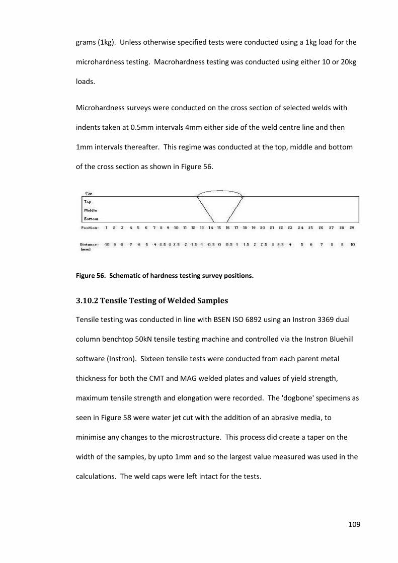
109
grams (1kg). Unless otherwise specified tests were conducted using a 1kg load for the
microhardness testing. Macrohardness testing was conducted using either 10 or 20kg
loads.
Microhardness surveys were conducted on the cross section of selected welds with
indents taken at 0.5mm intervals 4mm either side of the weld centre line and then
1mm intervals thereafter. This regime was conducted at the top, middle and bottom
of the cross section as shown in Figure 56.
Figure 56. Schematic of hardness testing survey positions.
3.10.2 Tensile Testing of Welded Samples
Tensile testing was conducted in line with BSEN ISO 6892 using an Instron 3369 dual
column benchtop 50kN tensile testing machine and controlled via the Instron Bluehill
software (Instron). Sixteen tensile tests were conducted from each parent metal
thickness for both the CMT and MAG welded plates and values of yield strength,
maximum tensile strength and elongation were recorded. The 'dogbone' specimens as
seen in Figure 58 were water jet cut with the addition of an abrasive media, to
minimise any changes to the microstructure. This process did create a taper on the
width of the samples, by upto 1mm and so the largest value measured was used in the
calculations. The weld caps were left intact for the tests.
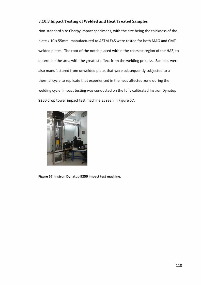
110
3.10.3 Impact Testing of Welded and Heat Treated Samples
Non-standard size Charpy impact specimens, with the size being the thickness of the
plate x 10 x 55mm, manufactured to ASTM E45 were tested for both MAG and CMT
welded plates. The root of the notch placed within the coarsest region of the HAZ, to
determine the area with the greatest effect from the welding process. Samples were
also manufactured from unwelded plate, that were subsequently subjected to a
thermal cycle to replicate that experienced in the heat affected zone during the
welding cycle. Impact testing was conducted on the fully calibrated Instron Dynatup
9250 drop tower impact test machine as seen in Figure 57.
Figure 57. Instron Dynatup 9250 impact test machine.
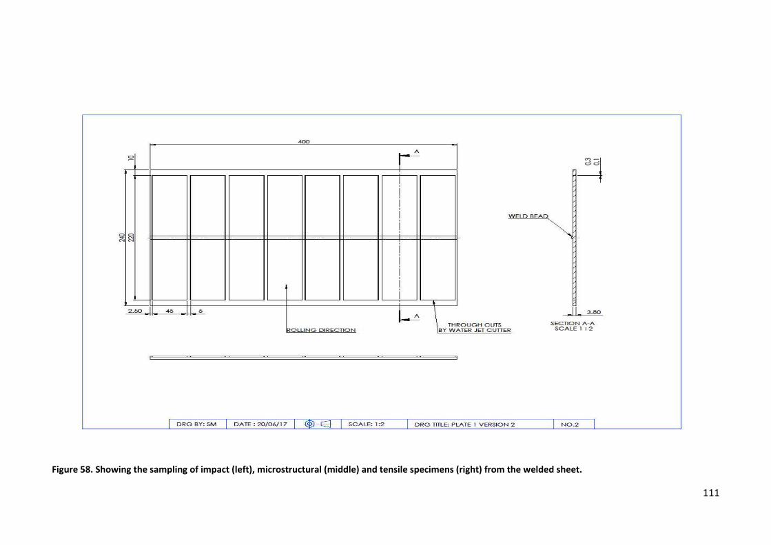
111
Figure 58. Showing the sampling of impact (left), microstructural (middle) and tensile specimens (right) from the welded sheet.
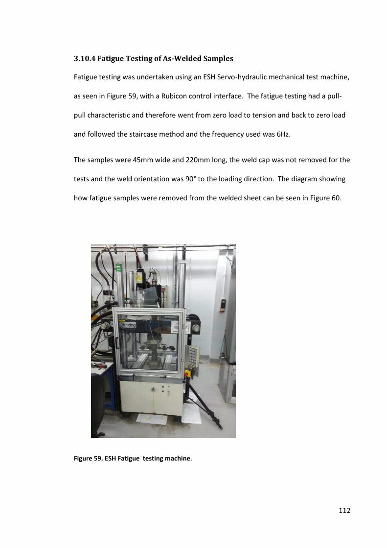
112
3.10.4 Fatigue Testing of As-Welded Samples
Fatigue testing was undertaken using an ESH Servo-hydraulic mechanical test machine,
as seen in Figure 59, with a Rubicon control interface. The fatigue testing had a pull-
pull characteristic and therefore went from zero load to tension and back to zero load
and followed the staircase method and the frequency used was 6Hz.
The samples were 45mm wide and 220mm long, the weld cap was not removed for the
tests and the weld orientation was 90° to the loading direction. The diagram showing
how fatigue samples were removed from the welded sheet can be seen in Figure 60.
Figure 59. ESH Fatigue testing machine.
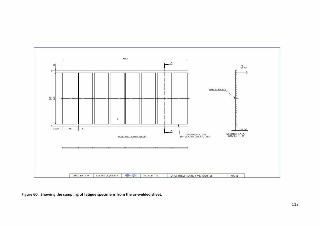
113
Figure 60. Showing the sampling of fatigue specimens from the as-welded sheet.
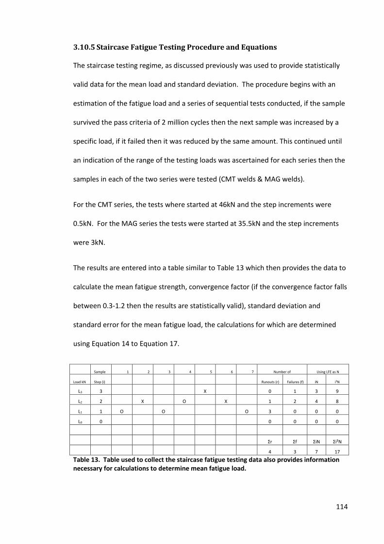
114
3.10.5 Staircase Fatigue Testing Procedure and Equations
The staircase testing regime, as discussed previously was used to provide statistically
valid data for the mean load and standard deviation. The procedure begins with an
estimation of the fatigue load and a series of sequential tests conducted, if the sample
survived the pass criteria of 2 million cycles then the next sample was increased by a
specific load, if it failed then it was reduced by the same amount. This continued until
an indication of the range of the testing loads was ascertained for each series then the
samples in each of the two series were tested (CMT welds & MAG welds).
For the CMT series, the tests where started at 46kN and the step increments were
0.5kN. For the MAG series the tests were started at 35.5kN and the step increments
were 3kN.
The results are entered into a table similar to Table 13 which then provides the data to
calculate the mean fatigue strength, convergence factor (if the convergence factor falls
between 0.3-1.2 then the results are statistically valid), standard deviation and
standard error for the mean fatigue load, the calculations for which are determined
using Equation 14 to Equation 17.
Sample 1 2 3 4 5 6 7 Number of Using LFE as N
Load kN Step (i) Runouts (r) Failures (f) iN i²N
L3 3 X 0 1 3 9
L2 2 X O X 1 2 4 8
L1 1 O O O 3 0 0 0
L0 0 0 0 0 0
Σr Σf ΣiN Σi²N
4 3 7 17
Table 13. Table used to collect the staircase fatigue testing data also provides information
necessary for calculations to determine mean fatigue load.

115
Calculated Mean Fatigue Load (kN): χ = Pd +d (� ± )
When N= failure + , when N= runout -
Equation 14. Equation to calculate mean fatigue load
Convergence Factor: = � × −�
>0.3 or <1.2 for statistical validity
Equation 15. Equation to calculate convergence factor
Standard Deviation (kN): � = . ×� � × −� + .
Equation 16. Equation to calculate standard deviation
Standard Error for Mean Fatigue Load (kN): sx = �√� . �
Equation 17. Equation to calculate standard error for mean fatigue load
Where;
χ = Mean fatigue load (kN)
s = Standard deviation (kN)
Po = Total load for step 0 (kN)
N = Total number of Least frequent Events (LFE) - failure or runout
d = Step divide/load interval (kN)
A = Σi * Ni
B = Σi2 * Ni
i = Step number
g = 1.15 (Nordeberg, 1973)

116
3.11 Compositional Analysis of Parent Materials Used in the Study
It was important to have the capability to determine the composition of the materials
in use throughout the research, this enabled the comparison with analysis supplied or
stated on supply of the materials used.
3.11.1 Optical Emission Spectrometry
Compositional data was analysed using a Spectromax optical emission spectrometer,
this allowed the complete composition to be determined, including the lighter
elements such as carbon and nitrogen.
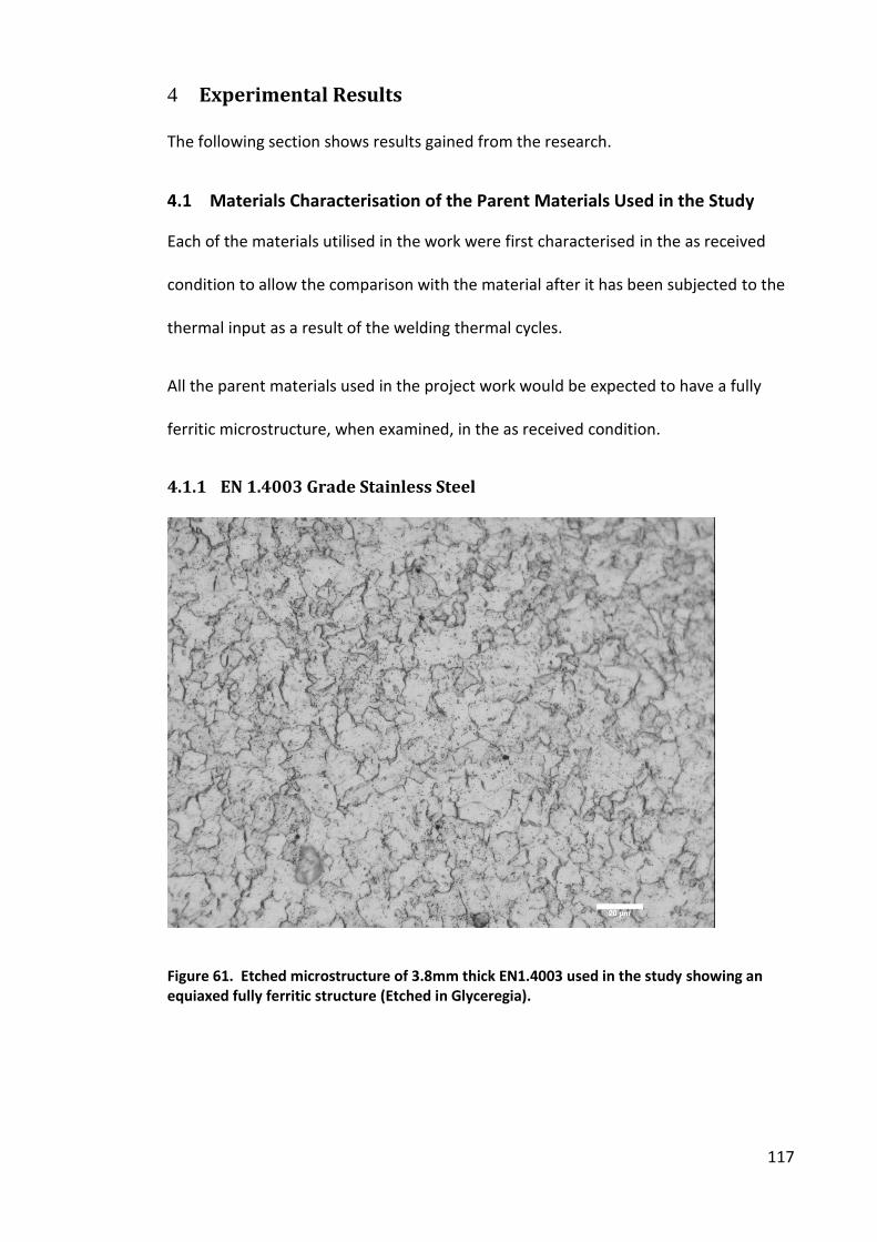
117
4 Experimental Results
The following section shows results gained from the research.
4.1 Materials Characterisation of the Parent Materials Used in the Study
Each of the materials utilised in the work were first characterised in the as received
condition to allow the comparison with the material after it has been subjected to the
thermal input as a result of the welding thermal cycles.
All the parent materials used in the project work would be expected to have a fully
ferritic microstructure, when examined, in the as received condition.
4.1.1 EN 1.4003 Grade Stainless Steel
Figure 61. Etched microstructure of 3.8mm thick EN1.4003 used in the study showing an
equiaxed fully ferritic structure (Etched in Glyceregia).
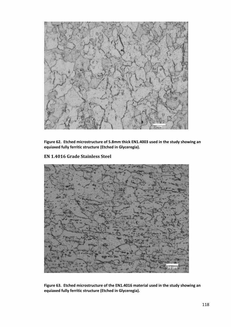
118
Figure 62. Etched microstructure of 5.8mm thick EN1.4003 used in the study showing an
equiaxed fully ferritic structure (Etched in Glyceregia).
EN 1.4016 Grade Stainless Steel
Figure 63. Etched microstructure of the EN1.4016 material used in the study showing an
equiaxed fully ferritic structure (Etched in Glyceregia).
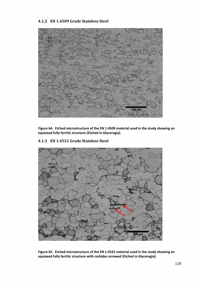
119
4.1.2 EN 1.4509 Grade Stainless Steel
Figure 64. Etched microstructure of the EN 1.4509 material used in the study showing an
equiaxed fully ferritic structure (Etched in Glyceregia).
4.1.3 EN 1.4521 Grade Stainless Steel
Figure 65. Etched microstructure of the EN 1.4521 material used in the study showing an
equiaxed fully ferritic structure with carbides arrowed (Etched in Glyceregia).
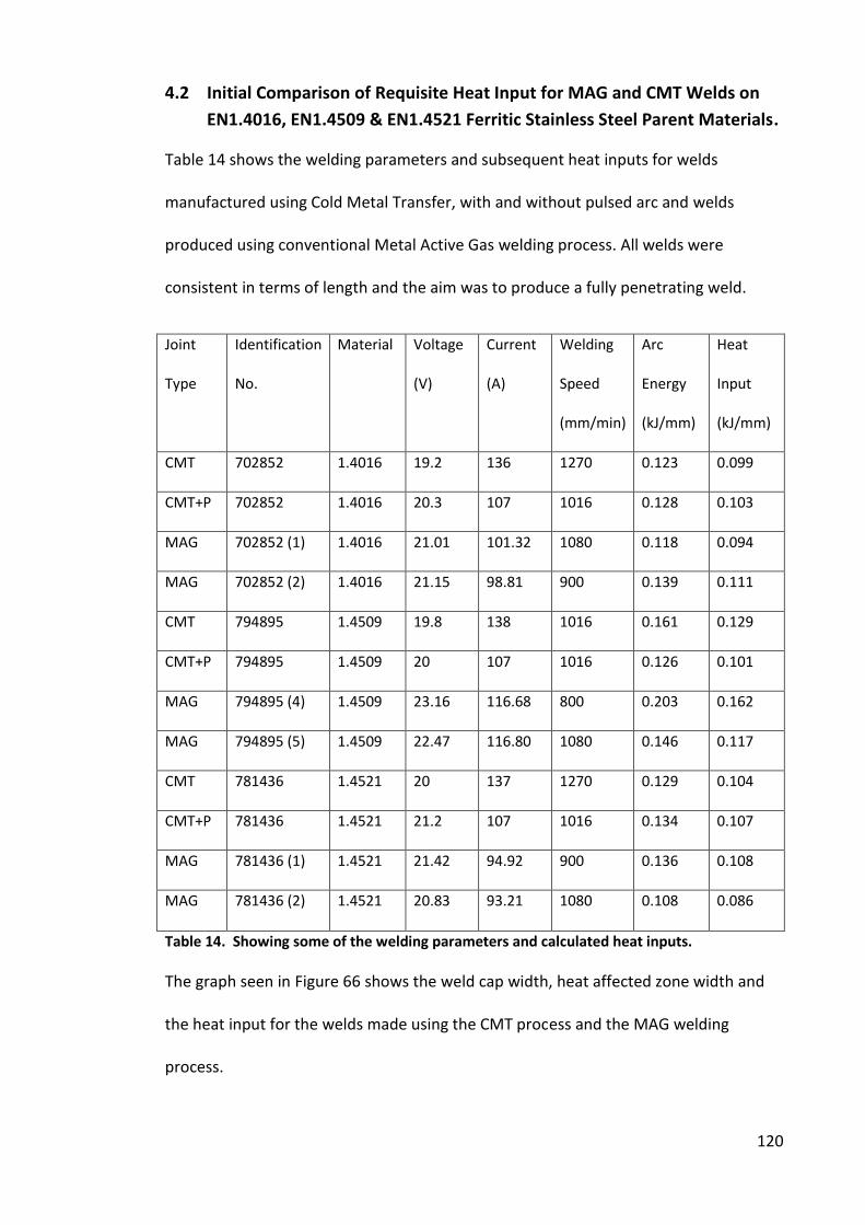
120
4.2 Initial Comparison of Requisite Heat Input for MAG and CMT Welds on
EN1.4016, EN1.4509 & EN1.4521 Ferritic Stainless Steel Parent Materials.
Table 14 shows the welding parameters and subsequent heat inputs for welds
manufactured using Cold Metal Transfer, with and without pulsed arc and welds
produced using conventional Metal Active Gas welding process. All welds were
consistent in terms of length and the aim was to produce a fully penetrating weld.
Joint
Type
Identification
No.
Material Voltage
(V)
Current
(A)
Welding
Speed
(mm/min)
Arc
Energy
(kJ/mm)
Heat
Input
(kJ/mm)
CMT 702852 1.4016 19.2 136 1270 0.123 0.099
CMT+P 702852 1.4016 20.3 107 1016 0.128 0.103
MAG 702852 (1) 1.4016 21.01 101.32 1080 0.118 0.094
MAG 702852 (2) 1.4016 21.15 98.81 900 0.139 0.111
CMT 794895 1.4509 19.8 138 1016 0.161 0.129
CMT+P 794895 1.4509 20 107 1016 0.126 0.101
MAG 794895 (4) 1.4509 23.16 116.68 800 0.203 0.162
MAG 794895 (5) 1.4509 22.47 116.80 1080 0.146 0.117
CMT 781436 1.4521 20 137 1270 0.129 0.104
CMT+P 781436 1.4521 21.2 107 1016 0.134 0.107
MAG 781436 (1) 1.4521 21.42 94.92 900 0.136 0.108
MAG 781436 (2) 1.4521 20.83 93.21 1080 0.108 0.086
Table 14. Showing some of the welding parameters and calculated heat inputs.
The graph seen in Figure 66 shows the weld cap width, heat affected zone width and
the heat input for the welds made using the CMT process and the MAG welding
process.
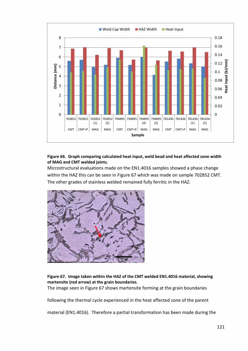
121
Figure 66. Graph comparing calculated heat input, weld bead and heat affected zone width
of MAG and CMT welded joints.
Microstructural evaluations made on the EN1.4016 samples showed a phase change
within the HAZ this can be seen in Figure 67 which was made on sample 702852 CMT.
The other grades of stainless welded remained fully ferritic in the HAZ.
Figure 67. Image taken within the HAZ of the CMT welded EN1.4016 material, showing
martensite (red arrow) at the grain boundaries.
The image seen in Figure 67 shows martensite forming at the grain boundaries
following the thermal cycle experienced in the heat affected zone of the parent
material (EN1.4016). Therefore a partial transformation has been made during the
0
0.02
0.04
0.06
0.08
0.1
0.12
0.14
0.16
0.18
0
1
2
3
4
5
6
7
8
702852 702852 702852
(1)
702852
(2)
794895 794895 794895
(4)
794895
(5)
781436 781436 781436
(1)
781436
(2)
CMT CMT+P MAG MAG CMT CMT+P MAG MAG CMT CMT+P MAG MAG
He
at
Inp
ut
(kJ/
mm
)
Dis
tan
ce (
mm
)
Sample
Weld Cap Width HAZ Width Heat Input
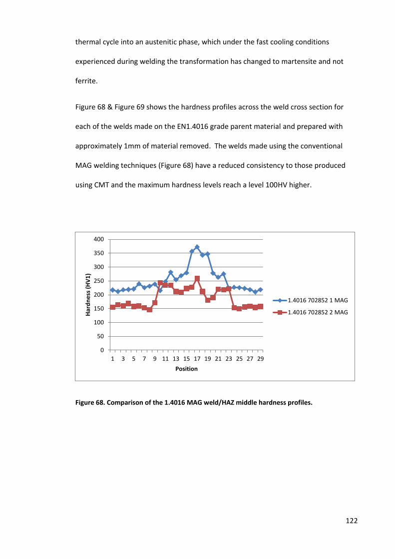
122
thermal cycle into an austenitic phase, which under the fast cooling conditions
experienced during welding the transformation has changed to martensite and not
ferrite.
Figure 68 & Figure 69 shows the hardness profiles across the weld cross section for
each of the welds made on the EN1.4016 grade parent material and prepared with
approximately 1mm of material removed. The welds made using the conventional
MAG welding techniques (Figure 68) have a reduced consistency to those produced
using CMT and the maximum hardness levels reach a level 100HV higher.
Figure 68. Comparison of the 1.4016 MAG weld/HAZ middle hardness profiles.
0
50
100
150
200
250
300
350
400
1 3 5 7 9 11 13 15 17 19 21 23 25 27 29
Ha
rdn
ess
(H
V1
)
Position
1.4016 702852 1 MAG
1.4016 702852 2 MAG
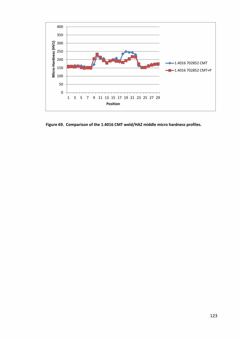
123
Figure 69. Comparison of the 1.4016 CMT weld/HAZ middle micro hardness profiles.
0
50
100
150
200
250
300
350
400
1 3 5 7 9 11 13 15 17 19 21 23 25 27 29
Mic
ro-H
ard
ne
ss (
HV
1)
Position
1.4016 702852 CMT
1.4016 702852 CMT+P
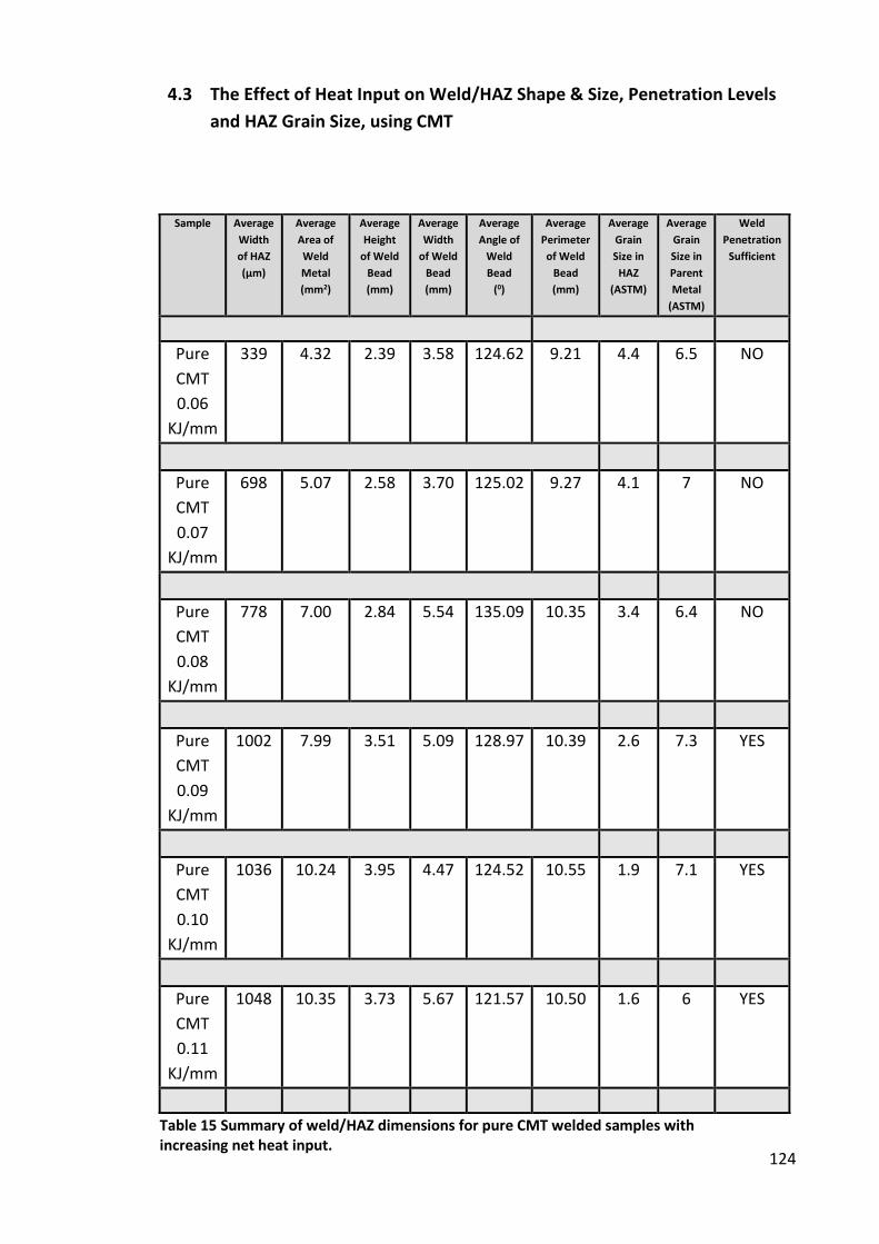
124
4.3 The Effect of Heat Input on Weld/HAZ Shape & Size, Penetration Levels
and HAZ Grain Size, using CMT
Sample Average
Width
of HAZ
(µm)
Average
Area of
Weld
Metal
(mm2)
Average
Height
of Weld
Bead
(mm)
Average
Width
of Weld
Bead
(mm)
Average
Angle of
Weld
Bead
(0)
Average
Perimeter
of Weld
Bead
(mm)
Average
Grain
Size in
HAZ
(ASTM)
Average
Grain
Size in
Parent
Metal
(ASTM)
Weld
Penetration
Sufficient
Pure
CMT
0.06
KJ/mm
339 4.32 2.39 3.58 124.62 9.21 4.4 6.5 NO
Pure
CMT
0.07
KJ/mm
698 5.07 2.58 3.70 125.02 9.27 4.1 7 NO
Pure
CMT
0.08
KJ/mm
778 7.00 2.84 5.54 135.09 10.35 3.4 6.4 NO
Pure
CMT
0.09
KJ/mm
1002 7.99 3.51 5.09 128.97 10.39 2.6 7.3 YES
Pure
CMT
0.10
KJ/mm
1036 10.24 3.95 4.47 124.52 10.55 1.9 7.1 YES
Pure
CMT
0.11
KJ/mm
1048 10.35 3.73 5.67 121.57 10.50 1.6 6 YES
Table 15 Summary of weld/HAZ dimensions for pure CMT welded samples with
increasing net heat input.
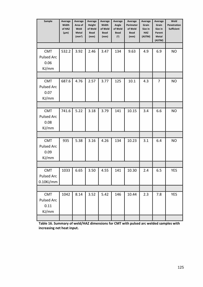
125
Sample Average
Width
of HAZ
(µm)
Average
Area of
Weld
Metal
(mm2)
Average
Height
of Weld
Bead
(mm)
Average
Width
of Weld
Bead
(mm)
Average
Angle
of Weld
Bead
(o)
Average
Perimeter
of Weld
Bead
(mm)
Average
Grain
Size in
HAZ
(ASTM)
Average
Grain
Size in
Parent
Metal
(ASTM)
Weld
Penetration
Sufficient
CMT
Pulsed Arc
0.06
KJ/mm
532.2 3.92 2.46 3.47 134 9.63 4.9 6.9 NO
CMT
Pulsed Arc
0.07
KJ/mm
687.6 4.76 2.57 3.77 125 10.1 4.3 7 NO
CMT
Pulsed Arc
0.08
KJ/mm
741.6 5.22 3.18 3.79 141 10.15 3.4 6.6 NO
CMT
Pulsed Arc
0.09
KJ/mm
935 5.38 3.16 4.26 134 10.23 3.1 6.4 NO
CMT
Pulsed Arc
0.10KJ/mm
1033 6.65 3.50 4.55 141 10.30 2.4 6.5 YES
CMT
Pulsed Arc
0.11
KJ/mm
1042 8.14 3.52 5.42 146 10.44 2.3 7.8 YES
Table 16. Summary of weld/HAZ dimensions for CMT with pulsed arc welded samples with
increasing net heat input.
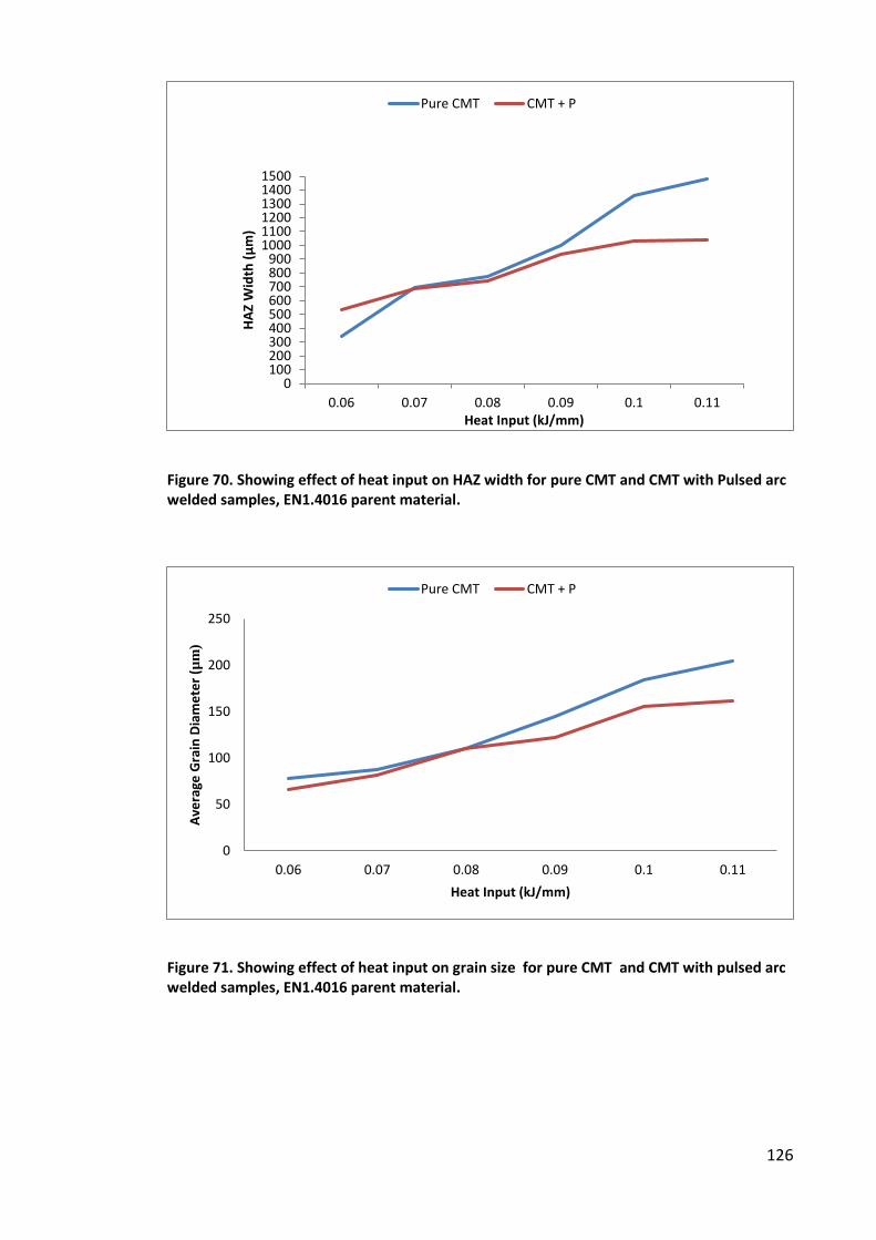
126
Figure 70. Showing effect of heat input on HAZ width for pure CMT and CMT with Pulsed arc
welded samples, EN1.4016 parent material.
Figure 71. Showing effect of heat input on grain size for pure CMT and CMT with pulsed arc
welded samples, EN1.4016 parent material.
0100200300400500600700800900
100011001200130014001500
0.06 0.07 0.08 0.09 0.1 0.11
HA
Z W
idth
(µ
m)
Heat Input (kJ/mm)
Pure CMT CMT + P
0
50
100
150
200
250
0.06 0.07 0.08 0.09 0.1 0.11
Av
era
ge
Gra
in D
iam
ete
r (µ
m)
Heat Input (kJ/mm)
Pure CMT CMT + P
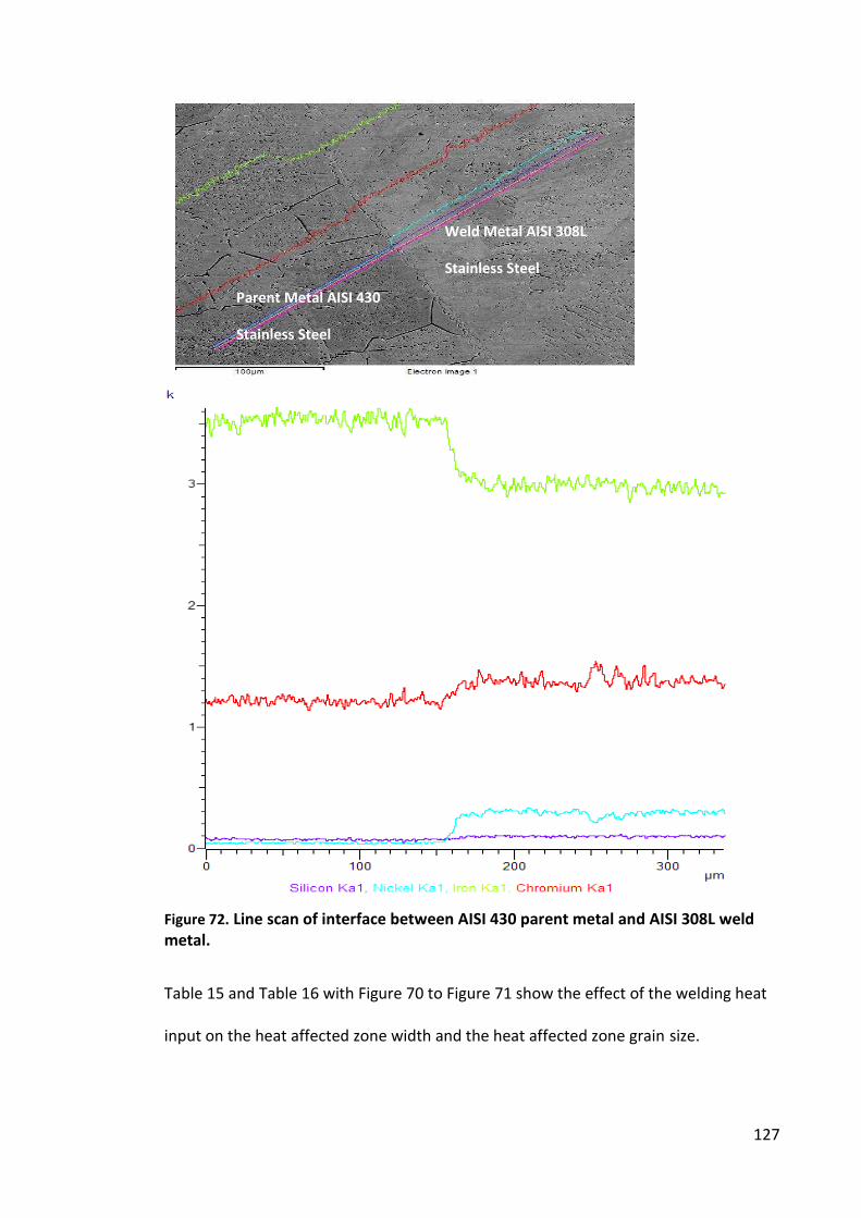
127
Figure 72. Line scan of interface between AISI 430 parent metal and AISI 308L weld
metal.
Table 15 and Table 16 with Figure 70 to Figure 71 show the effect of the welding heat
input on the heat affected zone width and the heat affected zone grain size.
Parent Metal AISI 430
Stainless Steel
Weld Metal AISI 308L
Stainless Steel
Parent Metal AISI 430
Stainless Steel
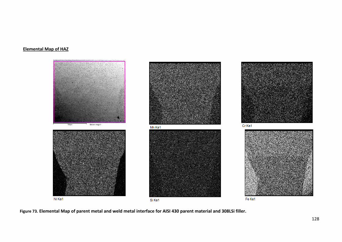
128
Elemental Map of HAZ
Figure 73. Elemental Map of parent metal and weld metal interface for AISI 430 parent material and 308LSi filler.
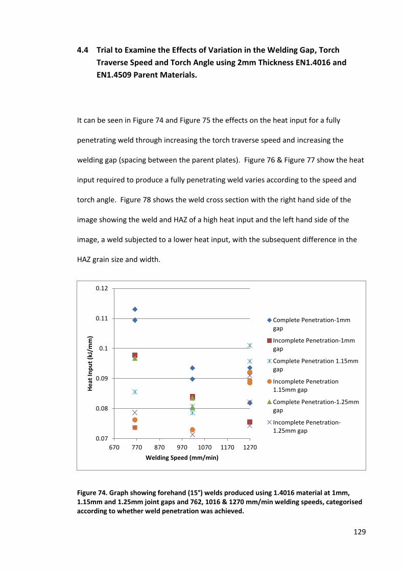
129
4.4 Trial to Examine the Effects of Variation in the Welding Gap, Torch
Traverse Speed and Torch Angle using 2mm Thickness EN1.4016 and
EN1.4509 Parent Materials.
It can be seen in Figure 74 and Figure 75 the effects on the heat input for a fully
penetrating weld through increasing the torch traverse speed and increasing the
welding gap (spacing between the parent plates). Figure 76 & Figure 77 show the heat
input required to produce a fully penetrating weld varies according to the speed and
torch angle. Figure 78 shows the weld cross section with the right hand side of the
image showing the weld and HAZ of a high heat input and the left hand side of the
image, a weld subjected to a lower heat input, with the subsequent difference in the
HAZ grain size and width.
Figure 74. Graph showing forehand (15°) welds produced using 1.4016 material at 1mm,
1.15mm and 1.25mm joint gaps and 762, 1016 & 1270 mm/min welding speeds, categorised
according to whether weld penetration was achieved.
0.07
0.08
0.09
0.1
0.11
0.12
670 770 870 970 1070 1170 1270
He
at
Inp
ut
(kJ/
mm
)
Welding Speed (mm/min)
Complete Penetration-1mm
gap
Incomplete Penetration-1mm
gap
Complete Penetration 1.15mm
gap
Incomplete Penetration
1.15mm gap
Complete Penetration-1.25mm
gap
Incomplete Penetration-
1.25mm gap
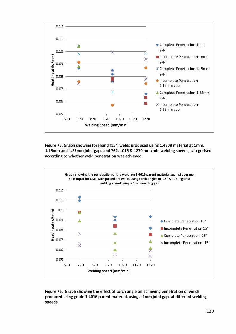
130
Figure 75. Graph showing forehand (15°) welds produced using 1.4509 material at 1mm,
1.15mm and 1.25mm joint gaps and 762, 1016 & 1270 mm/min welding speeds, categorised
according to whether weld penetration was achieved.
Figure 76. Graph showing the effect of torch angle on achieving penetration of welds
produced using grade 1.4016 parent material, using a 1mm joint gap, at different welding
speeds.
0.05
0.06
0.07
0.08
0.09
0.10
0.11
0.12
670 770 870 970 1070 1170 1270
He
at
Inp
ut
(kJ/
mm
)
Welding Speed (mm/min)
Complete Penetration-1mm
gap
Incomplete Penetration-1mm
gap
Complete Penetration 1.15mm
gap
Incomplete Penetration
1.15mm gap
Complete Penetration-1.25mm
gap
Incomplete Penetration-
1.25mm gap
0.05
0.06
0.07
0.08
0.09
0.1
0.11
0.12
670 770 870 970 1070 1170 1270
He
at
inp
ut
(kJ/
mm
)
Welding speed (mm/min)
Graph showing the penetration of the weld on 1.4016 parent material against average
heat input for CMT with pulsed arc welds using torch angles of -15° & +15° against
welding speed using a 1mm welding gap
Complete Penetration 15°
Incomplete Penetration 15°
Complete Penetration -15°
Incomplete Penetration -15°
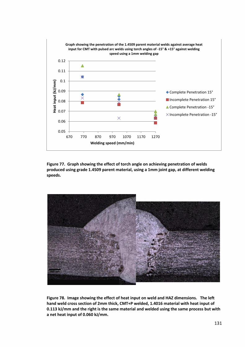
131
Figure 77. Graph showing the effect of torch angle on achieving penetration of welds
produced using grade 1.4509 parent material, using a 1mm joint gap, at different welding
speeds.
Figure 78. Image showing the effect of heat input on weld and HAZ dimensions. The left
hand weld cross section of 2mm thick, CMT+P welded, 1.4016 material with heat input of
0.113 kJ/mm and the right is the same material and welded using the same process but with
a net heat input of 0.060 kJ/mm.
0.05
0.06
0.07
0.08
0.09
0.1
0.11
0.12
670 770 870 970 1070 1170 1270
He
at
inp
ut
(kJ/
mm
)
Welding speed (mm/min)
Graph showing the penetration of the 1.4509 parent material welds against average heat
input for CMT with pulsed arc welds using torch angles of -15° & +15° against welding
speed using a 1mm welding gap
Complete Penetration 15°
Incomplete Penetration 15°
Complete Penetration -15°
Incomplete Penetration -15°

132
4.5 Trial to Determine the Consistency of the Welding Parameters and
Subsequent Welds with the CMT Welding Process
Table 18 shows the results from an inspection of the cross section of the welds to
identify if the welds had sufficient penetration, for welds produced with a variation in
one parameter, therefore in most cases for each variation in parameter, 6 welds were
created and from each of these welds six areas along that weld were examined.
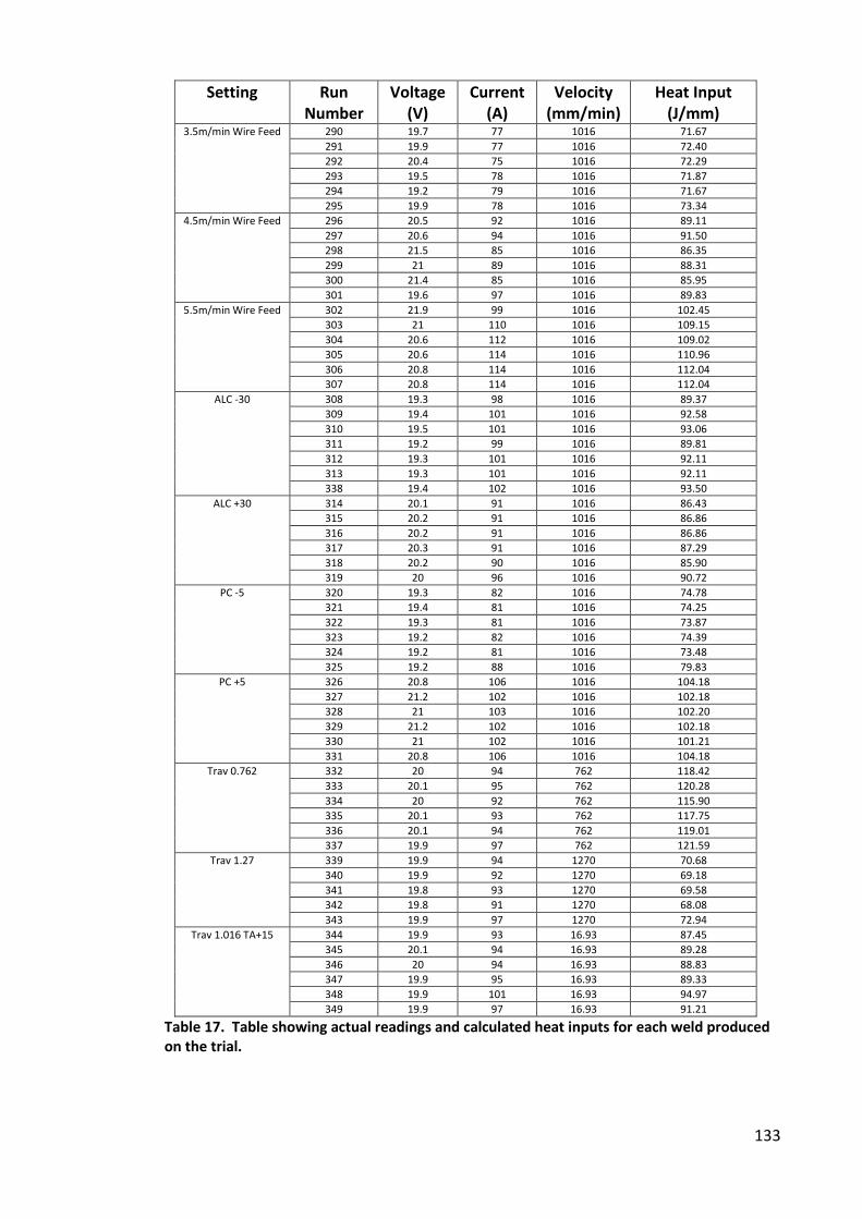
133
Setting Run
Number
Voltage
(V)
Current
(A)
Velocity
(mm/min)
Heat Input
(J/mm) 3.5m/min Wire Feed 290 19.7 77 1016 71.67
291 19.9 77 1016 72.40
292 20.4 75 1016 72.29
293 19.5 78 1016 71.87
294 19.2 79 1016 71.67
295 19.9 78 1016 73.34
4.5m/min Wire Feed 296 20.5 92 1016 89.11
297 20.6 94 1016 91.50
298 21.5 85 1016 86.35
299 21 89 1016 88.31
300 21.4 85 1016 85.95
301 19.6 97 1016 89.83
5.5m/min Wire Feed 302 21.9 99 1016 102.45
303 21 110 1016 109.15
304 20.6 112 1016 109.02
305 20.6 114 1016 110.96
306 20.8 114 1016 112.04
307 20.8 114 1016 112.04
ALC -30 308 19.3 98 1016 89.37
309 19.4 101 1016 92.58
310 19.5 101 1016 93.06
311 19.2 99 1016 89.81
312 19.3 101 1016 92.11
313 19.3 101 1016 92.11
338 19.4 102 1016 93.50
ALC +30 314 20.1 91 1016 86.43
315 20.2 91 1016 86.86
316 20.2 91 1016 86.86
317 20.3 91 1016 87.29
318 20.2 90 1016 85.90
319 20 96 1016 90.72
PC -5 320 19.3 82 1016 74.78
321 19.4 81 1016 74.25
322 19.3 81 1016 73.87
323 19.2 82 1016 74.39
324 19.2 81 1016 73.48
325 19.2 88 1016 79.83
PC +5 326 20.8 106 1016 104.18
327 21.2 102 1016 102.18
328 21 103 1016 102.20
329 21.2 102 1016 102.18
330 21 102 1016 101.21
331 20.8 106 1016 104.18
Trav 0.762 332 20 94 762 118.42
333 20.1 95 762 120.28
334 20 92 762 115.90
335 20.1 93 762 117.75
336 20.1 94 762 119.01
337 19.9 97 762 121.59
Trav 1.27 339 19.9 94 1270 70.68
340 19.9 92 1270 69.18
341 19.8 93 1270 69.58
342 19.8 91 1270 68.08
343 19.9 97 1270 72.94
Trav 1.016 TA+15 344 19.9 93 16.93 87.45
345 20.1 94 16.93 89.28
346 20 94 16.93 88.83
347 19.9 95 16.93 89.33
348 19.9 101 16.93 94.97
349 19.9 97 16.93 91.21
Table 17. Table showing actual readings and calculated heat inputs for each weld produced
on the trial.
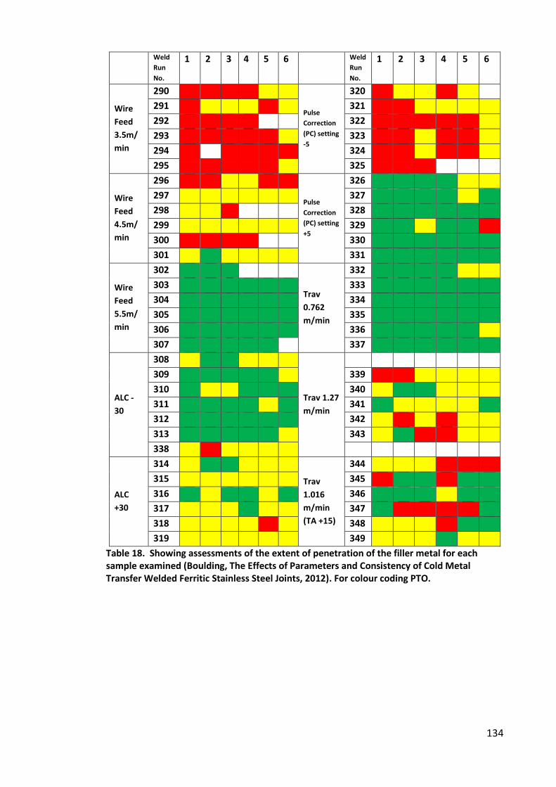
134
Weld
Run
No.
1 2 3 4 5 6
Weld
Run
No.
1 2 3 4 5 6
Wire
Feed
3.5m/
min
290
Pulse
Correction
(PC) setting
-5
320
291 321
292 322
293 323
294 324
295 325
Wire
Feed
4.5m/
min
296
Pulse
Correction
(PC) setting
+5
326
297 327
298 328
299 329
300 330
301 331
Wire
Feed
5.5m/
min
302
Trav
0.762
m/min
332
303 333
304 334
305 335
306 336
307 337
ALC -
30
308
Trav 1.27
m/min
309 339
310 340
311 341
312 342
313 343
338
ALC
+30
314
Trav
1.016
m/min
(TA +15)
344
315 345
316 346
317 347
318 348
319 349
Table 18. Showing assessments of the extent of penetration of the filler metal for each
sample examined (Boulding, The Effects of Parameters and Consistency of Cold Metal
Transfer Welded Ferritic Stainless Steel Joints, 2012). For colour coding PTO.
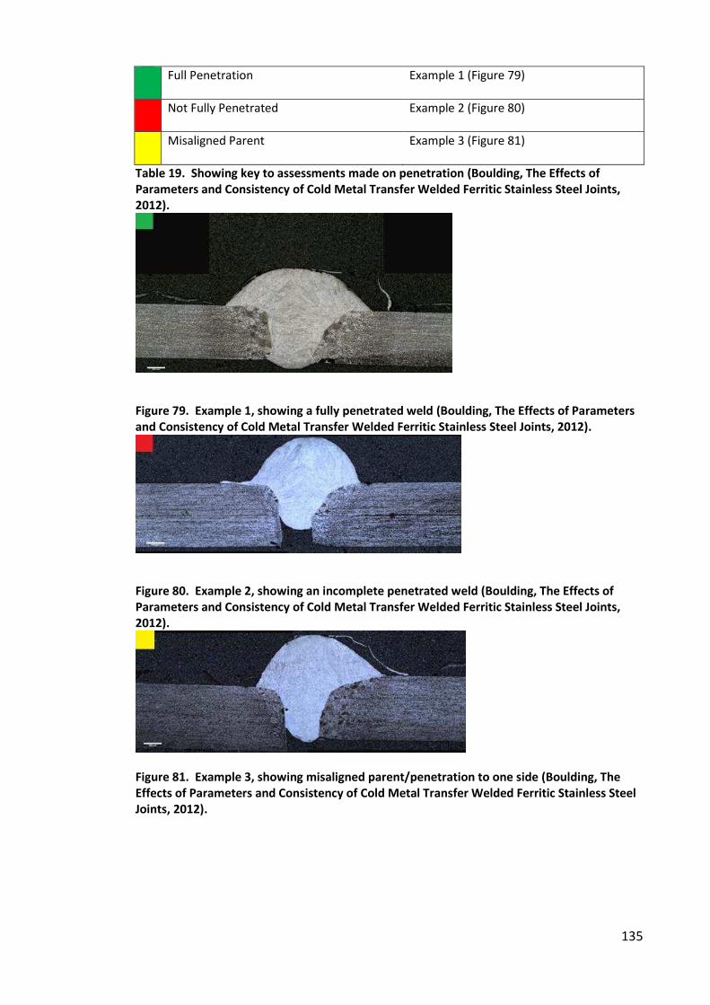
135
Full Penetration Example 1 (Figure 79)
Not Fully Penetrated Example 2 (Figure 80)
Misaligned Parent Example 3 (Figure 81)
Table 19. Showing key to assessments made on penetration (Boulding, The Effects of
Parameters and Consistency of Cold Metal Transfer Welded Ferritic Stainless Steel Joints,
2012).
Figure 79. Example 1, showing a fully penetrated weld (Boulding, The Effects of Parameters
and Consistency of Cold Metal Transfer Welded Ferritic Stainless Steel Joints, 2012).
Figure 80. Example 2, showing an incomplete penetrated weld (Boulding, The Effects of
Parameters and Consistency of Cold Metal Transfer Welded Ferritic Stainless Steel Joints,
2012).
Figure 81. Example 3, showing misaligned parent/penetration to one side (Boulding, The
Effects of Parameters and Consistency of Cold Metal Transfer Welded Ferritic Stainless Steel
Joints, 2012).

136
Table 19 and Figure 79 to Figure 81 show the key to the colour coding seen in Table
18. The weld cross sections shown in Figure 79 to Figure 81 are representatives of the
different categories highlighted, with the first being a fully penetrating weld, the
second showing a weld with a lack of root penetration and the third, where the parent
plate is misaligned. In all cases the parent material was a 2 mm thick EN1.4016 grade
ferritic stainless steel.
4.5.1 Power Setting
The welds were created in a synergic mode and therefore the wire speed, voltage and
current are all linked. Adjustment of power is made through variation of the wire feed
speed, an increase in wire feed speed increases the power levels, a decrease in the
wire feed speed decreases the power. The following three graphs (Figure 82 to Figure
84) shows the effects of varying the power levels in the welding process on the heat
affected zone width, they also show the consistency of the measurements made from
weld to weld and at various distances along each of the welds. There appears to be a
variation in the measurements from weld to weld and also along the length of the
plate. It is also worth noting the increase in HAZ width as a result of increasing the
power.
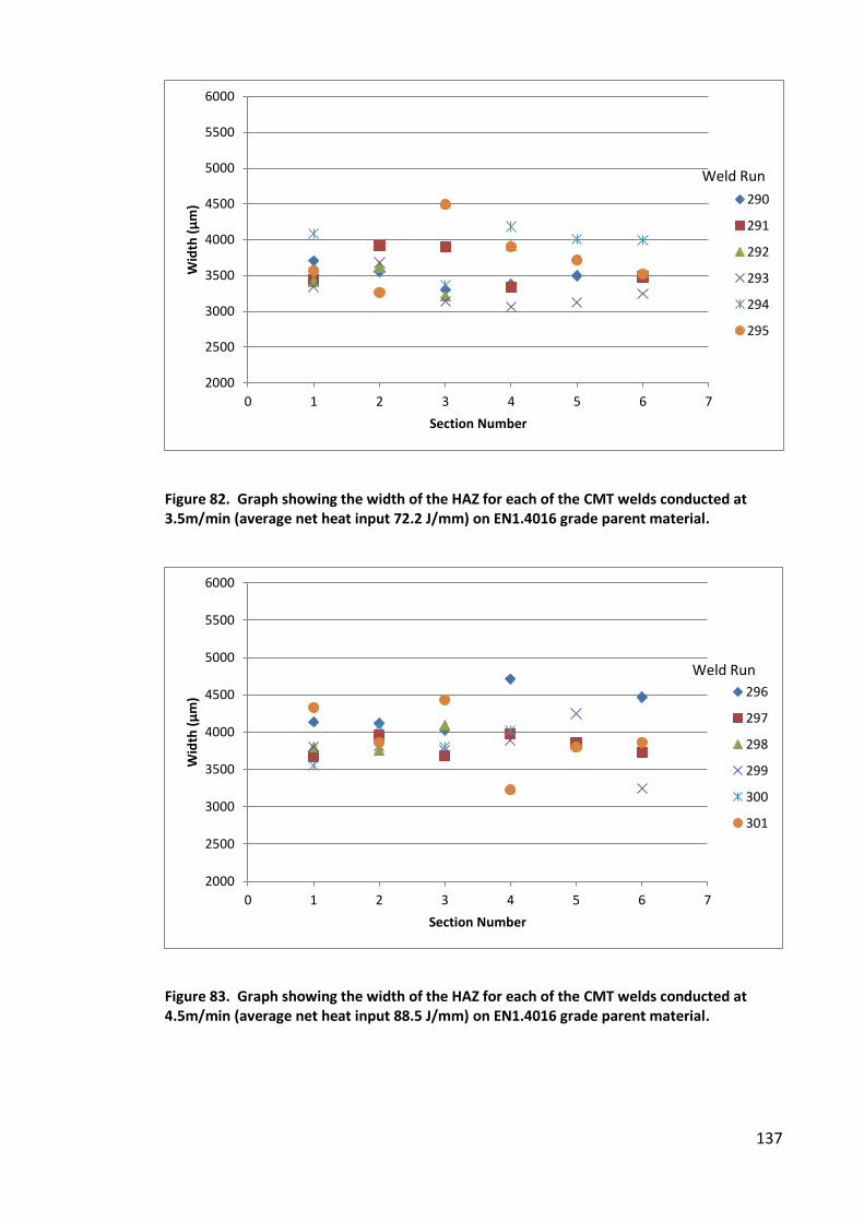
137
Figure 82. Graph showing the width of the HAZ for each of the CMT welds conducted at
3.5m/min (average net heat input 72.2 J/mm) on EN1.4016 grade parent material.
Figure 83. Graph showing the width of the HAZ for each of the CMT welds conducted at
4.5m/min (average net heat input 88.5 J/mm) on EN1.4016 grade parent material.
2000
2500
3000
3500
4000
4500
5000
5500
6000
0 1 2 3 4 5 6 7
Wid
th (
µm
)
Section Number
290
291
292
293
294
295
Weld Run
2000
2500
3000
3500
4000
4500
5000
5500
6000
0 1 2 3 4 5 6 7
Wid
th (
µm
)
Section Number
296
297
298
299
300
301
Weld Run

138
Figure 84. Graph showing the width of the HAZ for each of the CMT welds conducted at
5.5m/min (average net heat input 109.3 J/mm) on EN1.4016 grade parent material.
Figure 85. Graph showing the current and voltage trace for the CMT weld conducted at
3.5m/min on EN1.4016 grade parent material.
2000
2500
3000
3500
4000
4500
5000
5500
6000
0 1 2 3 4 5 6 7
Wid
th (
µm
)
Section Number
302
303
304
305
306
307
Weld Run
0
50
100
150
200
250
300
350
400
40
00
40
21
40
42
40
63
40
84
41
05
41
26
41
47
41
68
41
89
42
10
42
31
42
52
42
73
42
94
43
15
43
36
43
57
43
78
43
99
44
20
44
41
44
62
44
83
Data Point
Current (A)
Voltage (V)
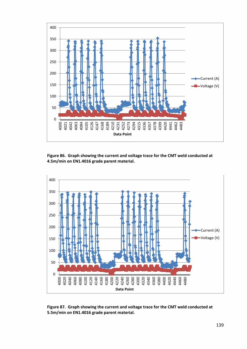
139
Figure 86. Graph showing the current and voltage trace for the CMT weld conducted at
4.5m/min on EN1.4016 grade parent material.
Figure 87. Graph showing the current and voltage trace for the CMT weld conducted at
5.5m/min on EN1.4016 grade parent material.
0
50
100
150
200
250
300
350
400
40
00
40
21
40
42
40
63
40
84
41
05
41
26
41
47
41
68
41
89
42
10
42
31
42
52
42
73
42
94
43
15
43
36
43
57
43
78
43
99
44
20
44
41
44
62
44
83
Data Point
Current (A)
Voltage (V)
0
50
100
150
200
250
300
350
400
40
00
40
20
40
40
40
60
40
80
41
00
41
20
41
40
41
60
41
80
42
00
42
20
42
40
42
60
42
80
43
00
43
20
43
40
43
60
43
80
44
00
44
20
44
40
44
60
44
80
Data Point
Current (A)
Voltage (V)
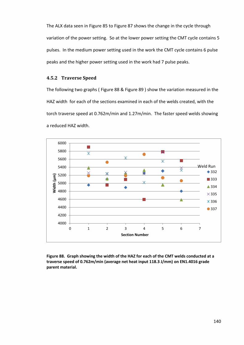
140
The ALX data seen in Figure 85 to Figure 87 shows the change in the cycle through
variation of the power setting. So at the lower power setting the CMT cycle contains 5
pulses. In the medium power setting used in the work the CMT cycle contains 6 pulse
peaks and the higher power setting used in the work had 7 pulse peaks.
4.5.2 Traverse Speed
The following two graphs ( Figure 88 & Figure 89 ) show the variation measured in the
HAZ width for each of the sections examined in each of the welds created, with the
torch traverse speed at 0.762m/min and 1.27m/min. The faster speed welds showing
a reduced HAZ width.
Figure 88. Graph showing the width of the HAZ for each of the CMT welds conducted at a
traverse speed of 0.762m/min (average net heat input 118.3 J/mm) on EN1.4016 grade
parent material.
4000
4200
4400
4600
4800
5000
5200
5400
5600
5800
6000
0 1 2 3 4 5 6 7
Wid
th (
µm
)
Section Number
332
333
334
335
336
337
Weld Run
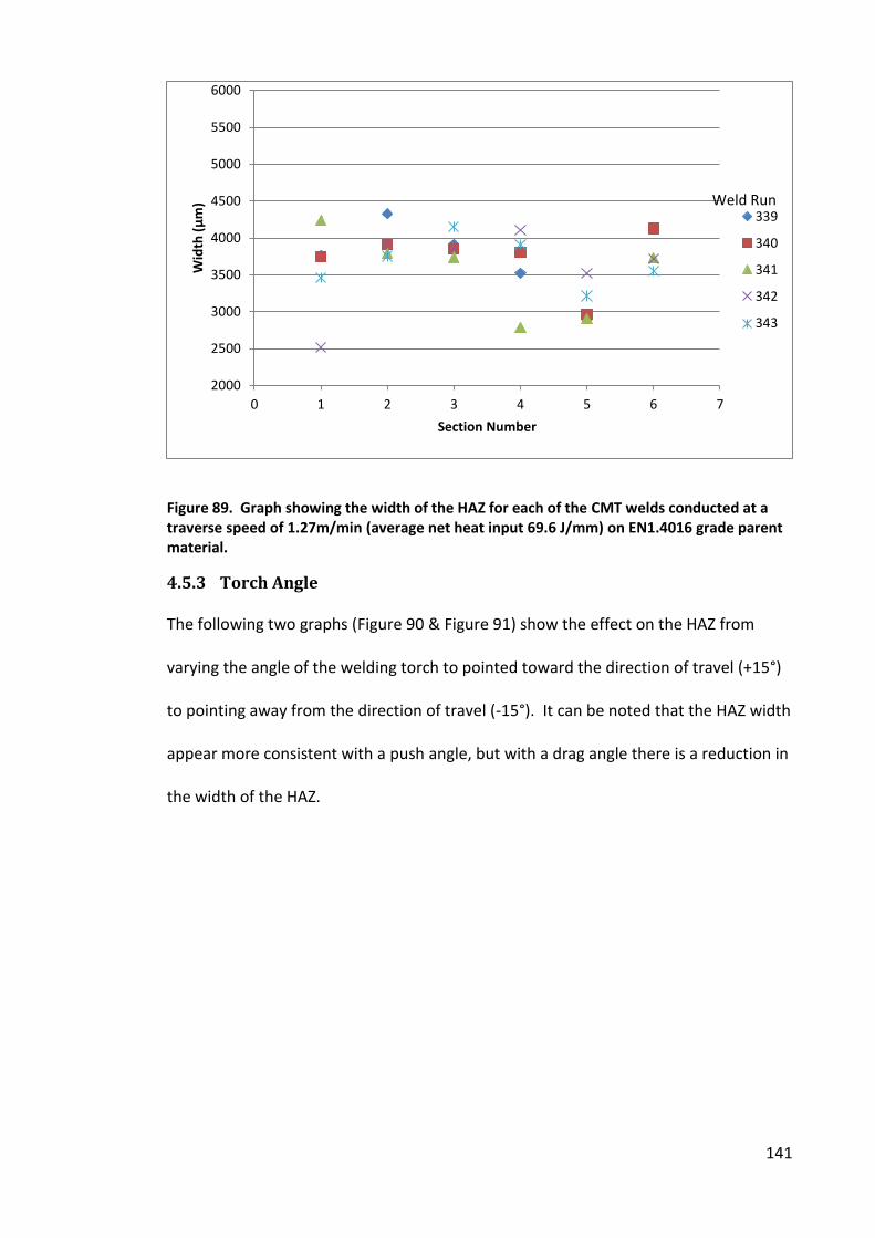
141
Figure 89. Graph showing the width of the HAZ for each of the CMT welds conducted at a
traverse speed of 1.27m/min (average net heat input 69.6 J/mm) on EN1.4016 grade parent
material.
4.5.3 Torch Angle
The following two graphs (Figure 90 & Figure 91) show the effect on the HAZ from
varying the angle of the welding torch to pointed toward the direction of travel (+15°)
to pointing away from the direction of travel (-15°). It can be noted that the HAZ width
appear more consistent with a push angle, but with a drag angle there is a reduction in
the width of the HAZ.
2000
2500
3000
3500
4000
4500
5000
5500
6000
0 1 2 3 4 5 6 7
Wid
th (
µm
)
Section Number
339
340
341
342
343
Weld Run
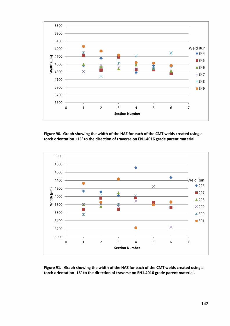
142
Figure 90. Graph showing the width of the HAZ for each of the CMT welds created using a
torch orientation +15° to the direction of traverse on EN1.4016 grade parent material.
Figure 91. Graph showing the width of the HAZ for each of the CMT welds created using a
torch orientation -15° to the direction of traverse on EN1.4016 grade parent material.
3500
3700
3900
4100
4300
4500
4700
4900
5100
5300
5500
0 1 2 3 4 5 6 7
Wid
th (
µm
)
Section Number
344
345
346
347
348
349
Weld Run
3000
3200
3400
3600
3800
4000
4200
4400
4600
4800
5000
0 1 2 3 4 5 6 7
Wid
th (
µm
)
Section Number
296
297
298
299
300
301
Weld Run
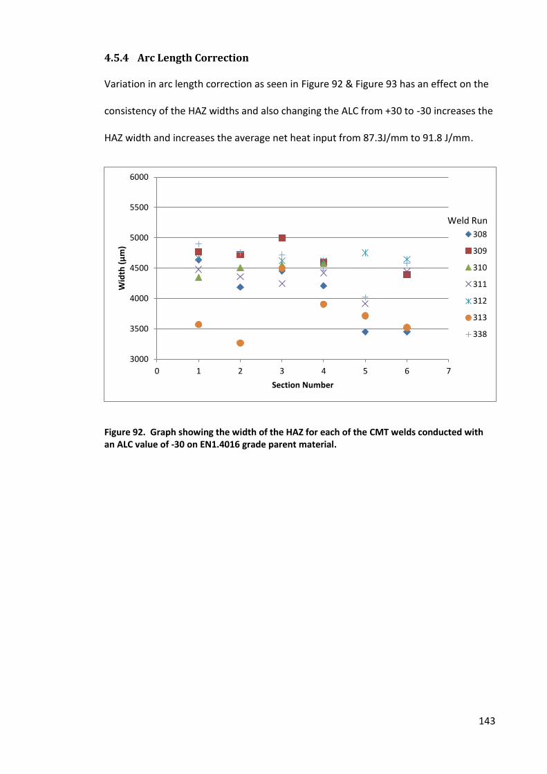
143
4.5.4 Arc Length Correction
Variation in arc length correction as seen in Figure 92 & Figure 93 has an effect on the
consistency of the HAZ widths and also changing the ALC from +30 to -30 increases the
HAZ width and increases the average net heat input from 87.3J/mm to 91.8 J/mm.
Figure 92. Graph showing the width of the HAZ for each of the CMT welds conducted with
an ALC value of -30 on EN1.4016 grade parent material.
3000
3500
4000
4500
5000
5500
6000
0 1 2 3 4 5 6 7
Wid
th (
µm
)
Section Number
308
309
310
311
312
313
338
Weld Run
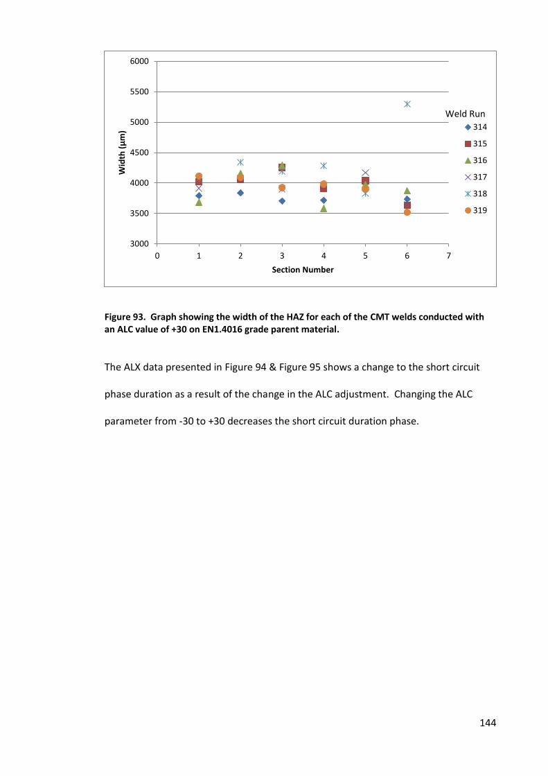
144
Figure 93. Graph showing the width of the HAZ for each of the CMT welds conducted with
an ALC value of +30 on EN1.4016 grade parent material.
The ALX data presented in Figure 94 & Figure 95 shows a change to the short circuit
phase duration as a result of the change in the ALC adjustment. Changing the ALC
parameter from -30 to +30 decreases the short circuit duration phase.
3000
3500
4000
4500
5000
5500
6000
0 1 2 3 4 5 6 7
Wid
th (
µm
)
Section Number
314
315
316
317
318
319
Weld Run
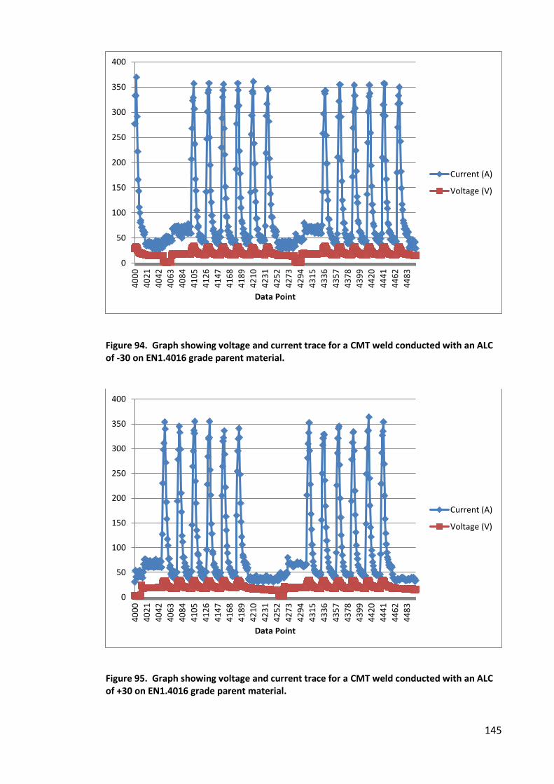
145
Figure 94. Graph showing voltage and current trace for a CMT weld conducted with an ALC
of -30 on EN1.4016 grade parent material.
Figure 95. Graph showing voltage and current trace for a CMT weld conducted with an ALC
of +30 on EN1.4016 grade parent material.
0
50
100
150
200
250
300
350
400
40
00
40
21
40
42
40
63
40
84
41
05
41
26
41
47
41
68
41
89
42
10
42
31
42
52
42
73
42
94
43
15
43
36
43
57
43
78
43
99
44
20
44
41
44
62
44
83
Data Point
Current (A)
Voltage (V)
0
50
100
150
200
250
300
350
400
40
00
40
21
40
42
40
63
40
84
41
05
41
26
41
47
41
68
41
89
42
10
42
31
42
52
42
73
42
94
43
15
43
36
43
57
43
78
43
99
44
20
44
41
44
62
44
83
Data Point
Current (A)
Voltage (V)
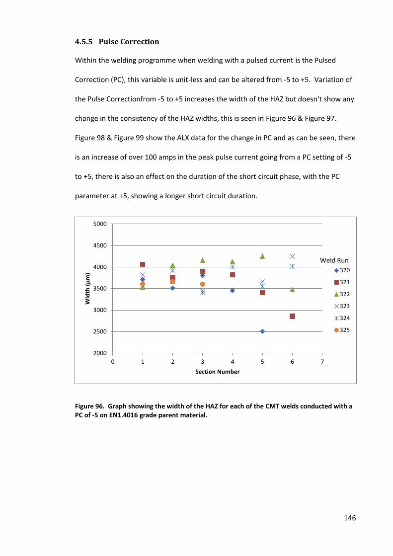
146
4.5.5 Pulse Correction
Within the welding programme when welding with a pulsed current is the Pulsed
Correction (PC), this variable is unit-less and can be altered from -5 to +5. Variation of
the Pulse Correctionfrom -5 to +5 increases the width of the HAZ but doesn't show any
change in the consistency of the HAZ widths, this is seen in Figure 96 & Figure 97.
Figure 98 & Figure 99 show the ALX data for the change in PC and as can be seen, there
is an increase of over 100 amps in the peak pulse current going from a PC setting of -5
to +5, there is also an effect on the duration of the short circuit phase, with the PC
parameter at +5, showing a longer short circuit duration.
Figure 96. Graph showing the width of the HAZ for each of the CMT welds conducted with a
PC of -5 on EN1.4016 grade parent material.
2000
2500
3000
3500
4000
4500
5000
0 1 2 3 4 5 6 7
Wid
th (
µm
)
Section Number
320
321
322
323
324
325
Weld Run
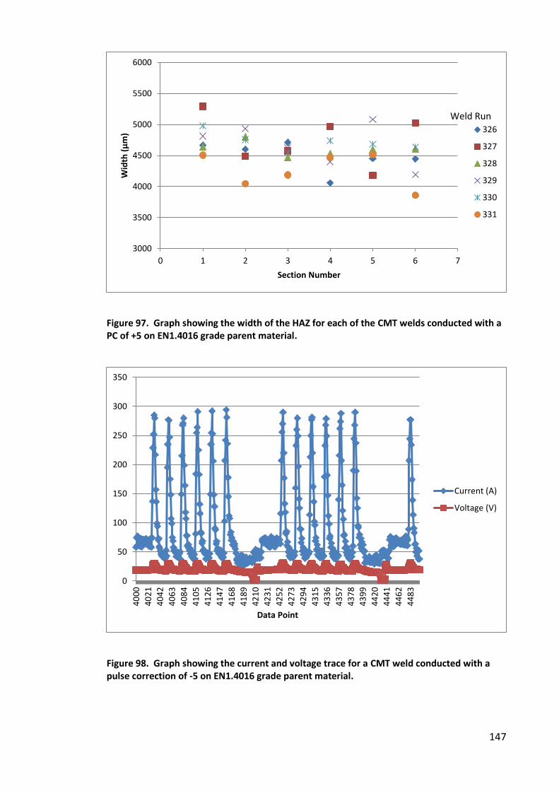
147
Figure 97. Graph showing the width of the HAZ for each of the CMT welds conducted with a
PC of +5 on EN1.4016 grade parent material.
Figure 98. Graph showing the current and voltage trace for a CMT weld conducted with a
pulse correction of -5 on EN1.4016 grade parent material.
3000
3500
4000
4500
5000
5500
6000
0 1 2 3 4 5 6 7
Wid
th (
µm
)
Section Number
326
327
328
329
330
331
Weld Run
0
50
100
150
200
250
300
350
40
00
40
21
40
42
40
63
40
84
41
05
41
26
41
47
41
68
41
89
42
10
42
31
42
52
42
73
42
94
43
15
43
36
43
57
43
78
43
99
44
20
44
41
44
62
44
83
Data Point
Current (A)
Voltage (V)
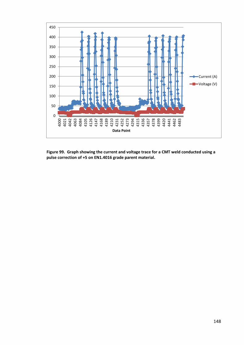
148
Figure 99. Graph showing the current and voltage trace for a CMT weld conducted using a
pulse correction of +5 on EN1.4016 grade parent material.
0
50
100
150
200
250
300
350
400
450
40
00
40
21
40
42
40
63
40
84
41
05
41
26
41
47
41
68
41
89
42
10
42
31
42
52
42
73
42
94
43
15
43
36
43
57
43
78
43
99
44
20
44
41
44
62
44
83
Data Point
Current (A)
Voltage (V)
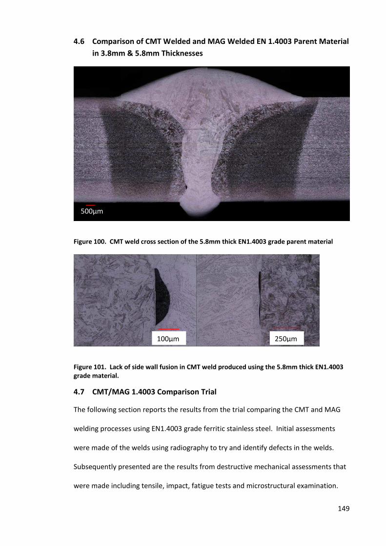
149
4.6 Comparison of CMT Welded and MAG Welded EN 1.4003 Parent Material
in 3.8mm & 5.8mm Thicknesses
Figure 100. CMT weld cross section of the 5.8mm thick EN1.4003 grade parent material
Figure 101. Lack of side wall fusion in CMT weld produced using the 5.8mm thick EN1.4003
grade material.
4.7 CMT/MAG 1.4003 Comparison Trial
The following section reports the results from the trial comparing the CMT and MAG
welding processes using EN1.4003 grade ferritic stainless steel. Initial assessments
were made of the welds using radiography to try and identify defects in the welds.
Subsequently presented are the results from destructive mechanical assessments that
were made including tensile, impact, fatigue tests and microstructural examination.
500µm
100µm 250µm
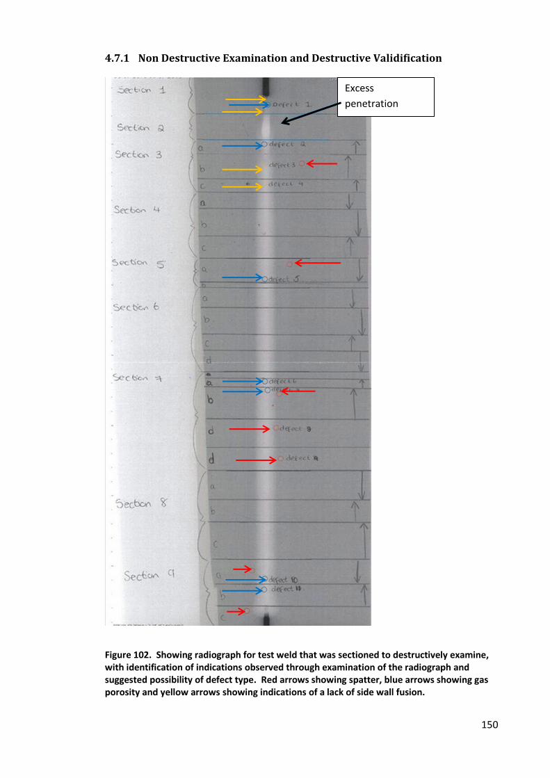
150
4.7.1 Non Destructive Examination and Destructive Validification
Figure 102. Showing radiograph for test weld that was sectioned to destructively examine,
with identification of indications observed through examination of the radiograph and
suggested possibility of defect type. Red arrows showing spatter, blue arrows showing gas
porosity and yellow arrows showing indications of a lack of side wall fusion.
Excess
penetration
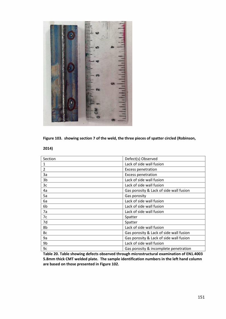
151
Figure 103. showing section 7 of the weld, the three pieces of spatter circled (Robinson,
2014)
Section Defect(s) Observed
1 Lack of side wall fusion
2 Excess penetration
3a Excess penetration
3b Lack of side wall fusion
3c Lack of side wall fusion
4a Gas porosity & Lack of side wall fusion
5a Gas porosity
6a Lack of side wall fusion
6b Lack of side wall fusion
7a Lack of side wall fusion
7c Spatter
7d Spatter
8b Lack of side wall fusion
8c Gas porosity & Lack of side wall fusion
9a Gas porosity & Lack of side wall fusion
9b Lack of side wall fusion
9c Gas porosity & incomplete penetration
Table 20. Table showing defects observed through microstructural examination of EN1.4003
5.8mm thick CMT welded plate. The sample identification numbers in the left hand column
are based on those presented in Figure 102.
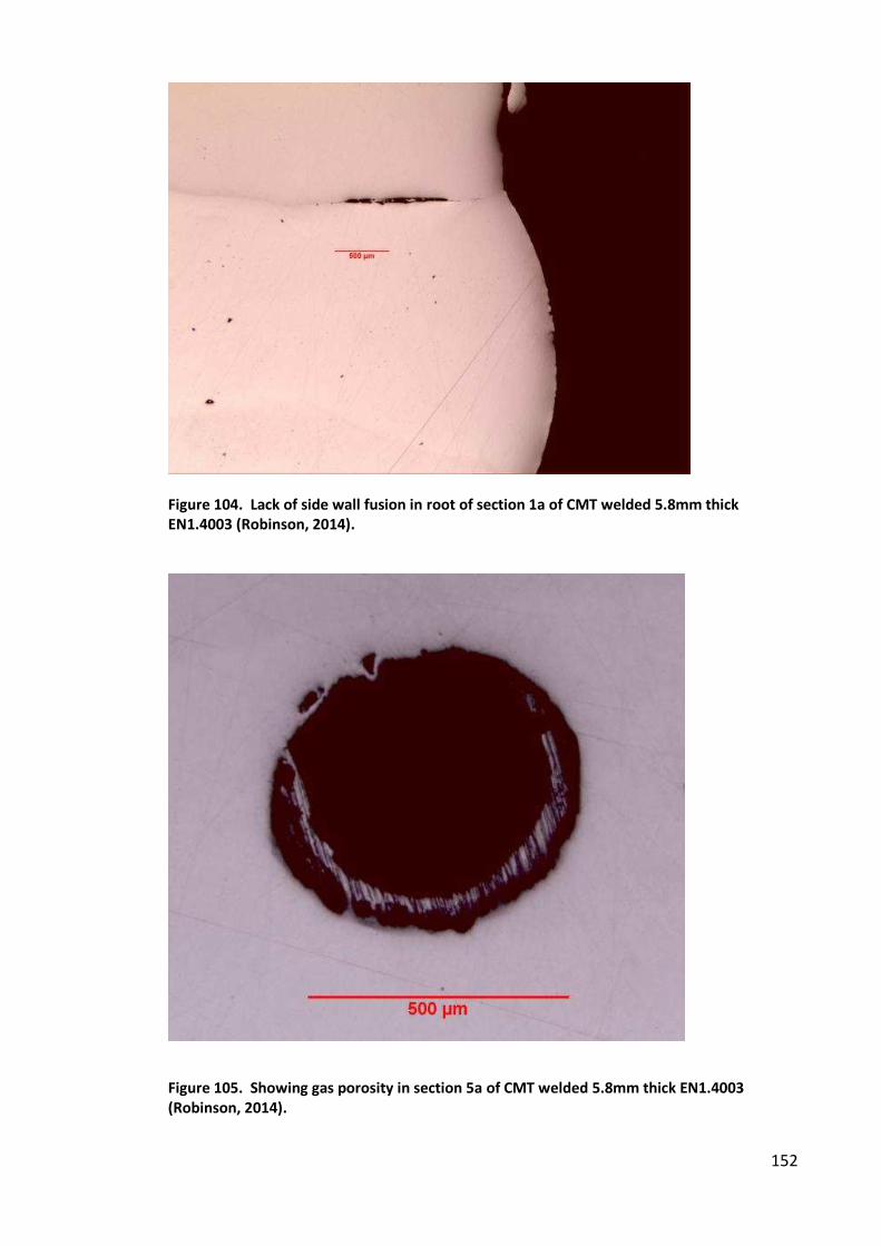
152
Figure 104. Lack of side wall fusion in root of section 1a of CMT welded 5.8mm thick
EN1.4003 (Robinson, 2014).
Figure 105. Showing gas porosity in section 5a of CMT welded 5.8mm thick EN1.4003
(Robinson, 2014).
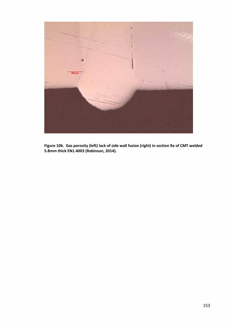
153
Figure 106. Gas porosity (left) lack of side wall fusion (right) in section 9a of CMT welded
5.8mm thick EN1.4003 (Robinson, 2014).
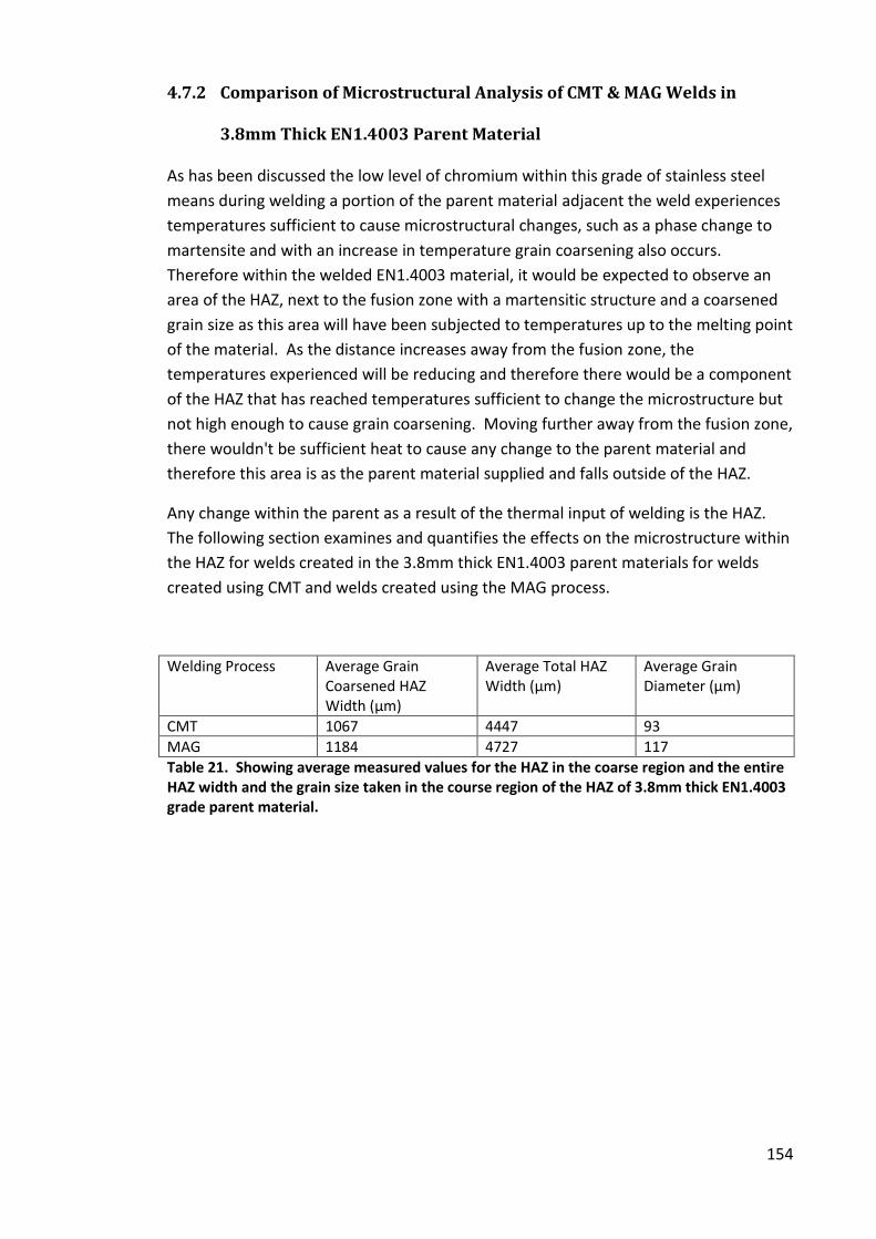
154
4.7.2 Comparison of Microstructural Analysis of CMT & MAG Welds in
3.8mm Thick EN1.4003 Parent Material
As has been discussed the low level of chromium within this grade of stainless steel
means during welding a portion of the parent material adjacent the weld experiences
temperatures sufficient to cause microstructural changes, such as a phase change to
martensite and with an increase in temperature grain coarsening also occurs.
Therefore within the welded EN1.4003 material, it would be expected to observe an
area of the HAZ, next to the fusion zone with a martensitic structure and a coarsened
grain size as this area will have been subjected to temperatures up to the melting point
of the material. As the distance increases away from the fusion zone, the
temperatures experienced will be reducing and therefore there would be a component
of the HAZ that has reached temperatures sufficient to change the microstructure but
not high enough to cause grain coarsening. Moving further away from the fusion zone,
there wouldn't be sufficient heat to cause any change to the parent material and
therefore this area is as the parent material supplied and falls outside of the HAZ.
Any change within the parent as a result of the thermal input of welding is the HAZ.
The following section examines and quantifies the effects on the microstructure within
the HAZ for welds created in the 3.8mm thick EN1.4003 parent materials for welds
created using CMT and welds created using the MAG process.
Welding Process Average Grain
Coarsened HAZ
Width (µm)
Average Total HAZ
Width (µm)
Average Grain
Diameter (µm)
CMT 1067 4447 93
MAG 1184 4727 117
Table 21. Showing average measured values for the HAZ in the coarse region and the entire
HAZ width and the grain size taken in the course region of the HAZ of 3.8mm thick EN1.4003
grade parent material.
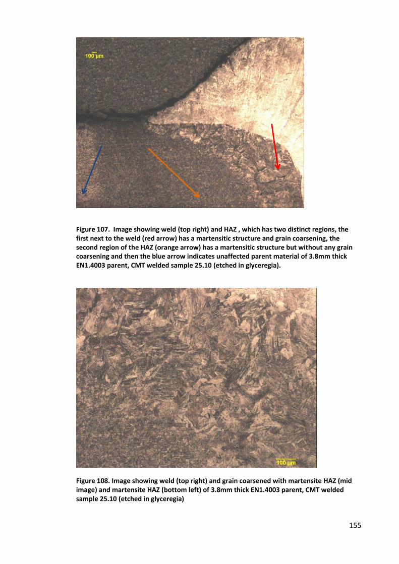
155
Figure 107. Image showing weld (top right) and HAZ , which has two distinct regions, the
first next to the weld (red arrow) has a martensitic structure and grain coarsening, the
second region of the HAZ (orange arrow) has a martensitic structure but without any grain
coarsening and then the blue arrow indicates unaffected parent material of 3.8mm thick
EN1.4003 parent, CMT welded sample 25.10 (etched in glyceregia).
Figure 108. Image showing weld (top right) and grain coarsened with martensite HAZ (mid
image) and martensite HAZ (bottom left) of 3.8mm thick EN1.4003 parent, CMT welded
sample 25.10 (etched in glyceregia)
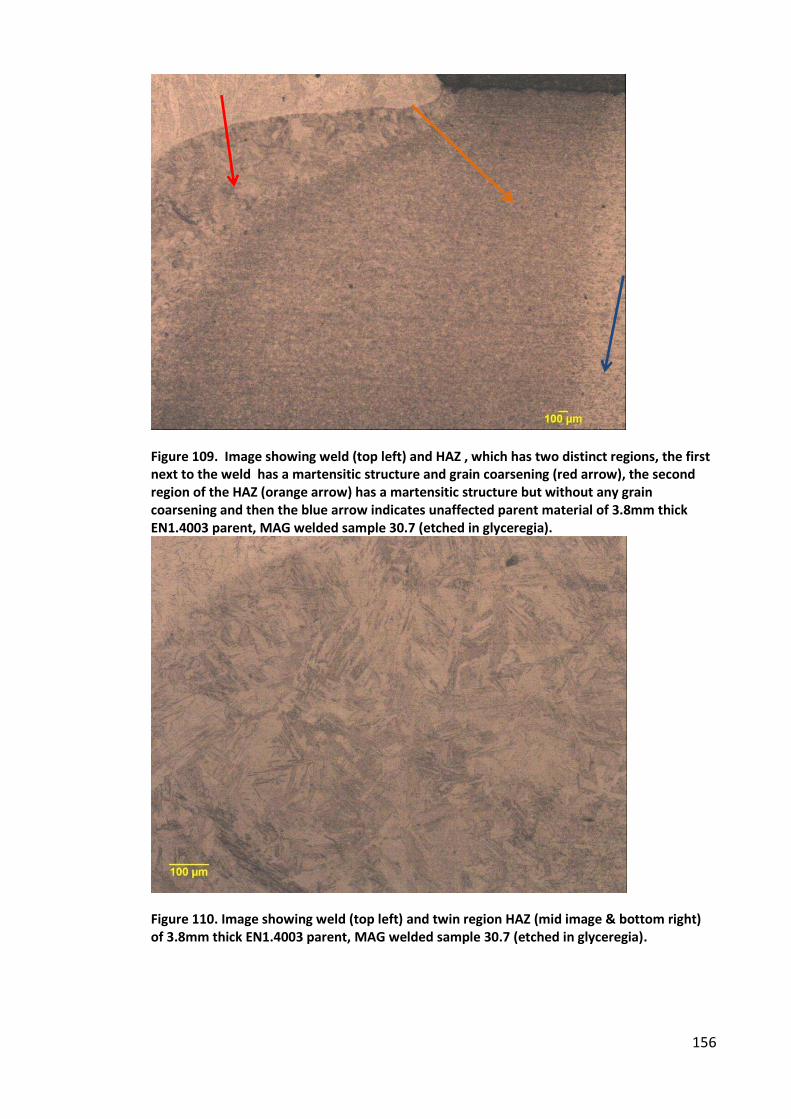
156
Figure 109. Image showing weld (top left) and HAZ , which has two distinct regions, the first
next to the weld has a martensitic structure and grain coarsening (red arrow), the second
region of the HAZ (orange arrow) has a martensitic structure but without any grain
coarsening and then the blue arrow indicates unaffected parent material of 3.8mm thick
EN1.4003 parent, MAG welded sample 30.7 (etched in glyceregia).
Figure 110. Image showing weld (top left) and twin region HAZ (mid image & bottom right)
of 3.8mm thick EN1.4003 parent, MAG welded sample 30.7 (etched in glyceregia).
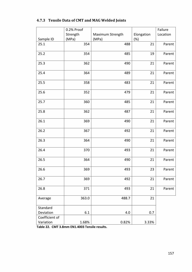
157
4.7.3 Tensile Data of CMT and MAG Welded Joints
Sample ID
0.2% Proof
Strength
(MPa)
Maximum Strength
(MPa)
Elongation
(%)
Failure
Location
25.1 354 488 21 Parent
25.2 354 485 19 Parent
25.3 362 490 21 Parent
25.4 364 489 21 Parent
25.5 358 483 21 Parent
25.6 352 479 21 Parent
25.7 360 485 21 Parent
25.8 362 487 21 Parent
26.1 369 490 21 Parent
26.2 367 492 21 Parent
26.3 364 490 21 Parent
26.4 370 493 21 Parent
26.5 364 490 21 Parent
26.6 369 493 23 Parent
26.7 369 492 21 Parent
26.8 371 493 21 Parent
Average 363.0 488.7 21
Standard
Deviation 6.1 4.0 0.7
Coefficient of
Variation 1.68% 0.82% 3.33%
Table 22. CMT 3.8mm EN1.4003 Tensile results.
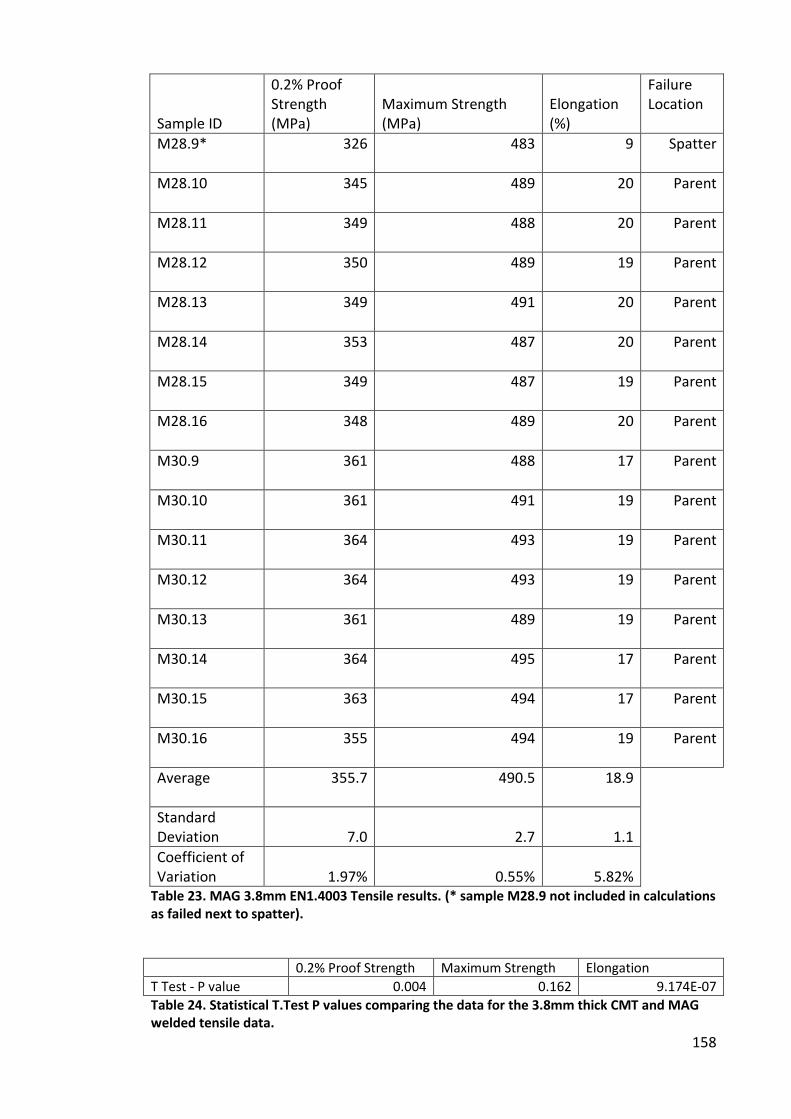
158
Sample ID
0.2% Proof
Strength
(MPa)
Maximum Strength
(MPa)
Elongation
(%)
Failure
Location
M28.9* 326 483 9 Spatter
M28.10 345 489 20 Parent
M28.11 349 488 20 Parent
M28.12 350 489 19 Parent
M28.13 349 491 20 Parent
M28.14 353 487 20 Parent
M28.15 349 487 19 Parent
M28.16 348 489 20 Parent
M30.9 361 488 17 Parent
M30.10 361 491 19 Parent
M30.11 364 493 19 Parent
M30.12 364 493 19 Parent
M30.13 361 489 19 Parent
M30.14 364 495 17 Parent
M30.15 363 494 17 Parent
M30.16 355 494 19 Parent
Average 355.7 490.5 18.9
Standard
Deviation 7.0 2.7 1.1
Coefficient of
Variation 1.97% 0.55% 5.82%
Table 23. MAG 3.8mm EN1.4003 Tensile results. (* sample M28.9 not included in calculations
as failed next to spatter).
0.2% Proof Strength Maximum Strength Elongation
T Test - P value 0.004 0.162 9.174E-07
Table 24. Statistical T.Test P values comparing the data for the 3.8mm thick CMT and MAG
welded tensile data.
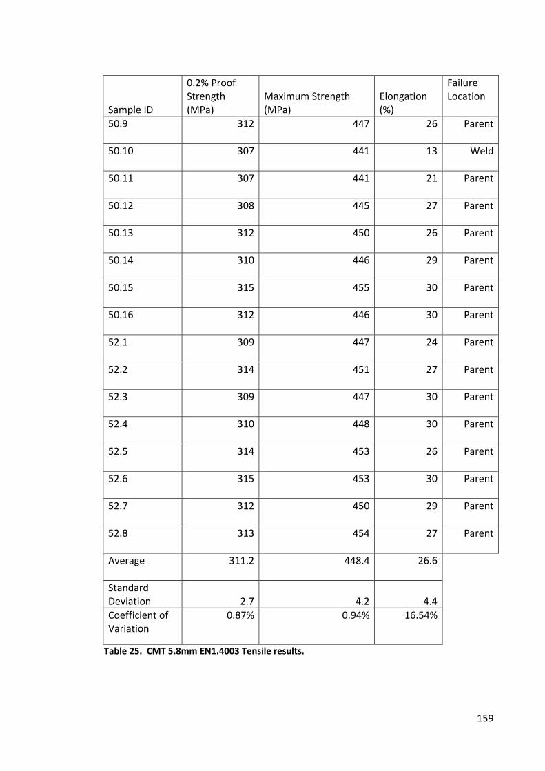
159
Sample ID
0.2% Proof
Strength
(MPa)
Maximum Strength
(MPa)
Elongation
(%)
Failure
Location
50.9 312 447 26 Parent
50.10 307 441 13 Weld
50.11 307 441 21 Parent
50.12 308 445 27 Parent
50.13 312 450 26 Parent
50.14 310 446 29 Parent
50.15 315 455 30 Parent
50.16 312 446 30 Parent
52.1 309 447 24 Parent
52.2 314 451 27 Parent
52.3 309 447 30 Parent
52.4 310 448 30 Parent
52.5 314 453 26 Parent
52.6 315 453 30 Parent
52.7 312 450 29 Parent
52.8 313 454 27 Parent
Average 311.2 448.4 26.6
Standard
Deviation 2.7 4.2 4.4
Coefficient of
Variation
0.87% 0.94% 16.54%
Table 25. CMT 5.8mm EN1.4003 Tensile results.
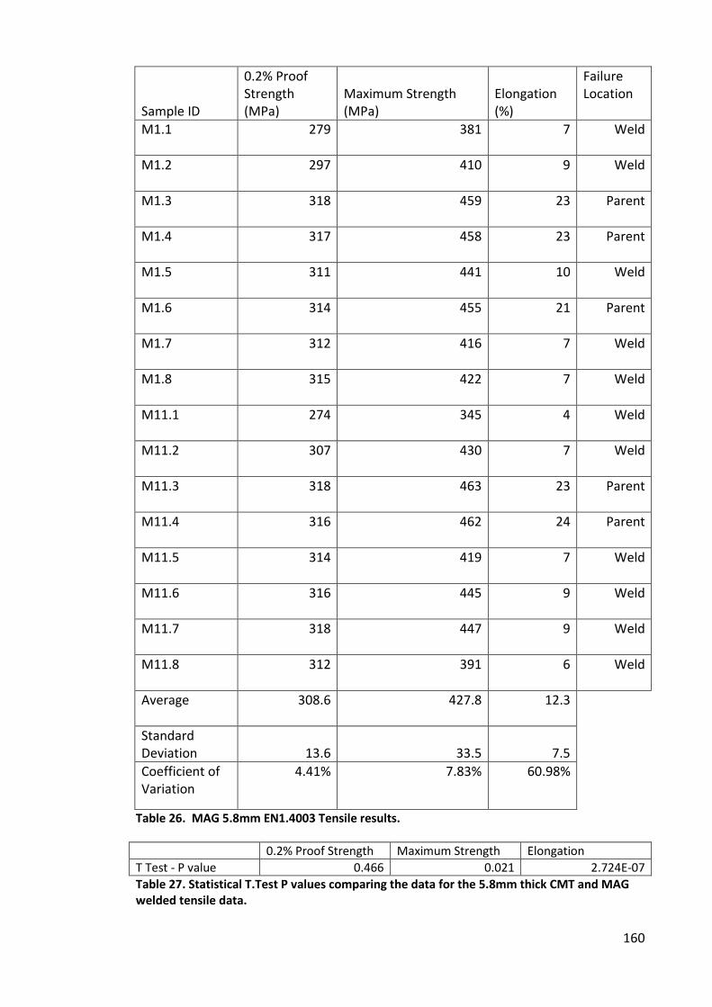
160
Sample ID
0.2% Proof
Strength
(MPa)
Maximum Strength
(MPa)
Elongation
(%)
Failure
Location
M1.1 279 381 7 Weld
M1.2 297 410 9 Weld
M1.3 318 459 23 Parent
M1.4 317 458 23 Parent
M1.5 311 441 10 Weld
M1.6 314 455 21 Parent
M1.7 312 416 7 Weld
M1.8 315 422 7 Weld
M11.1 274 345 4 Weld
M11.2 307 430 7 Weld
M11.3 318 463 23 Parent
M11.4 316 462 24 Parent
M11.5 314 419 7 Weld
M11.6 316 445 9 Weld
M11.7 318 447 9 Weld
M11.8 312 391 6 Weld
Average 308.6 427.8 12.3
Standard
Deviation 13.6 33.5 7.5
Coefficient of
Variation
4.41% 7.83% 60.98%
Table 26. MAG 5.8mm EN1.4003 Tensile results.
0.2% Proof Strength Maximum Strength Elongation
T Test - P value 0.466 0.021 2.724E-07
Table 27. Statistical T.Test P values comparing the data for the 5.8mm thick CMT and MAG
welded tensile data.
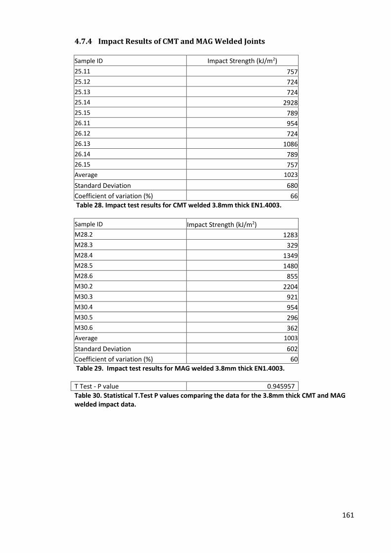
161
4.7.4 Impact Results of CMT and MAG Welded Joints
Sample ID Impact Strength (kJ/m2)
25.11 757
25.12 724
25.13 724
25.14 2928
25.15 789
26.11 954
26.12 724
26.13 1086
26.14 789
26.15 757
Average 1023
Standard Deviation 680
Coefficient of variation (%) 66
Table 28. Impact test results for CMT welded 3.8mm thick EN1.4003.
Sample ID Impact Strength (kJ/m2)
M28.2 1283
M28.3 329
M28.4 1349
M28.5 1480
M28.6 855
M30.2 2204
M30.3 921
M30.4 954
M30.5 296
M30.6 362
Average 1003
Standard Deviation 602
Coefficient of variation (%) 60
Table 29. Impact test results for MAG welded 3.8mm thick EN1.4003.
T Test - P value 0.945957
Table 30. Statistical T.Test P values comparing the data for the 3.8mm thick CMT and MAG
welded impact data.
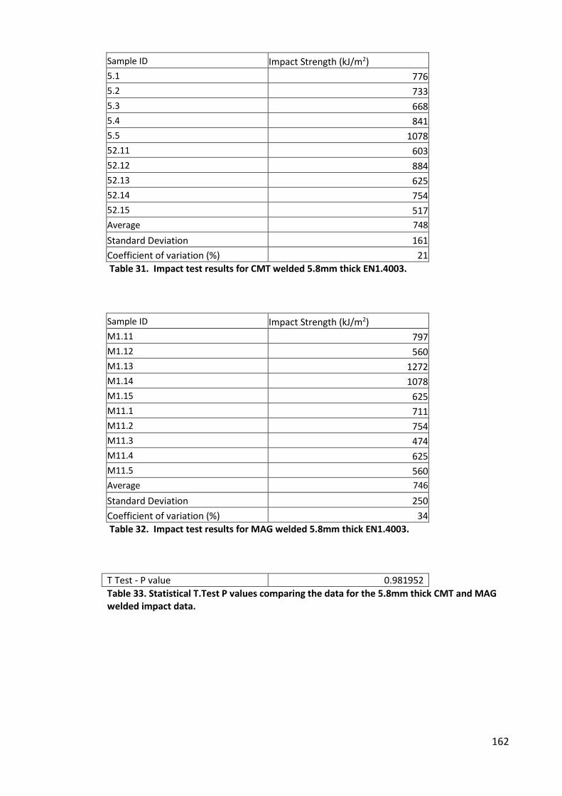
162
Sample ID Impact Strength (kJ/m2)
5.1 776
5.2 733
5.3 668
5.4 841
5.5 1078
52.11 603
52.12 884
52.13 625
52.14 754
52.15 517
Average 748
Standard Deviation 161
Coefficient of variation (%) 21
Table 31. Impact test results for CMT welded 5.8mm thick EN1.4003.
Sample ID Impact Strength (kJ/m2)
M1.11 797
M1.12 560
M1.13 1272
M1.14 1078
M1.15 625
M11.1 711
M11.2 754
M11.3 474
M11.4 625
M11.5 560
Average 746
Standard Deviation 250
Coefficient of variation (%) 34
Table 32. Impact test results for MAG welded 5.8mm thick EN1.4003.
T Test - P value 0.981952
Table 33. Statistical T.Test P values comparing the data for the 5.8mm thick CMT and MAG
welded impact data.
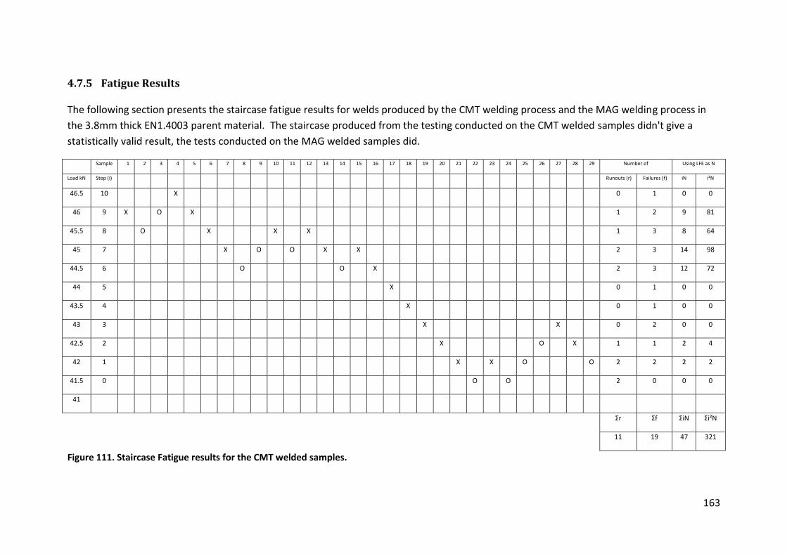
163
4.7.5 Fatigue Results
The following section presents the staircase fatigue results for welds produced by the CMT welding process and the MAG welding process in
the 3.8mm thick EN1.4003 parent material. The staircase produced from the testing conducted on the CMT welded samples didn't give a
statistically valid result, the tests conducted on the MAG welded samples did.
Sample 1 2 3 4 5 6 7 8 9 10 11 12 13 14 15 16 17 18 19 20 21 22 23 24 25 26 27 28 29 Number of Using LFE as N
Load kN Step (i) Runouts (r) Failures (f) iN i²N
46.5 10 X 0 1 0 0
46 9 X O X 1 2 9 81
45.5 8 O X X X 1 3 8 64
45 7 X O O X X 2 3 14 98
44.5 6 O O X 2 3 12 72
44 5 X 0 1 0 0
43.5 4 X 0 1 0 0
43 3 X X 0 2 0 0
42.5 2 X O X 1 1 2 4
42 1 X X O O 2 2 2 2
41.5 0 O O 2 0 0 0
41
Σr Σf ΣiN Σi²N
11 19 47 321
Figure 111. Staircase Fatigue results for the CMT welded samples.
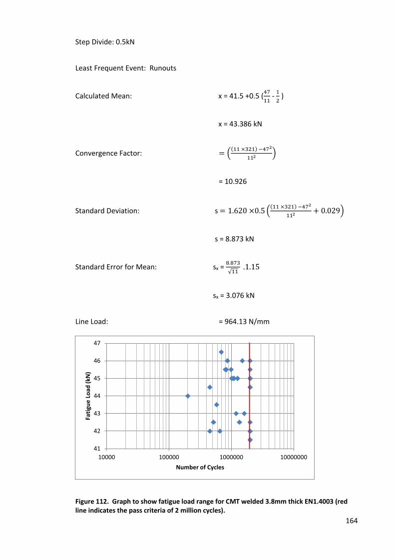
164
Step Divide: 0.5kN
Least Frequent Event: Runouts
Calculated Mean: x = 41.5 +0.5 ( - )
x = 43.386 kN
Convergence Factor: = × − 22
= 10.926
Standard Deviation: s = . × . × − 22 + . 9
s = 8.873 kN
Standard Error for Mean: sx = .√ . .
sx = 3.076 kN
Line Load: = 964.13 N/mm
Figure 112. Graph to show fatigue load range for CMT welded 3.8mm thick EN1.4003 (red
line indicates the pass criteria of 2 million cycles).
41
42
43
44
45
46
47
10000 100000 1000000 10000000
Fa
tig
ue
Lo
ad
(k
N)
Number of Cycles
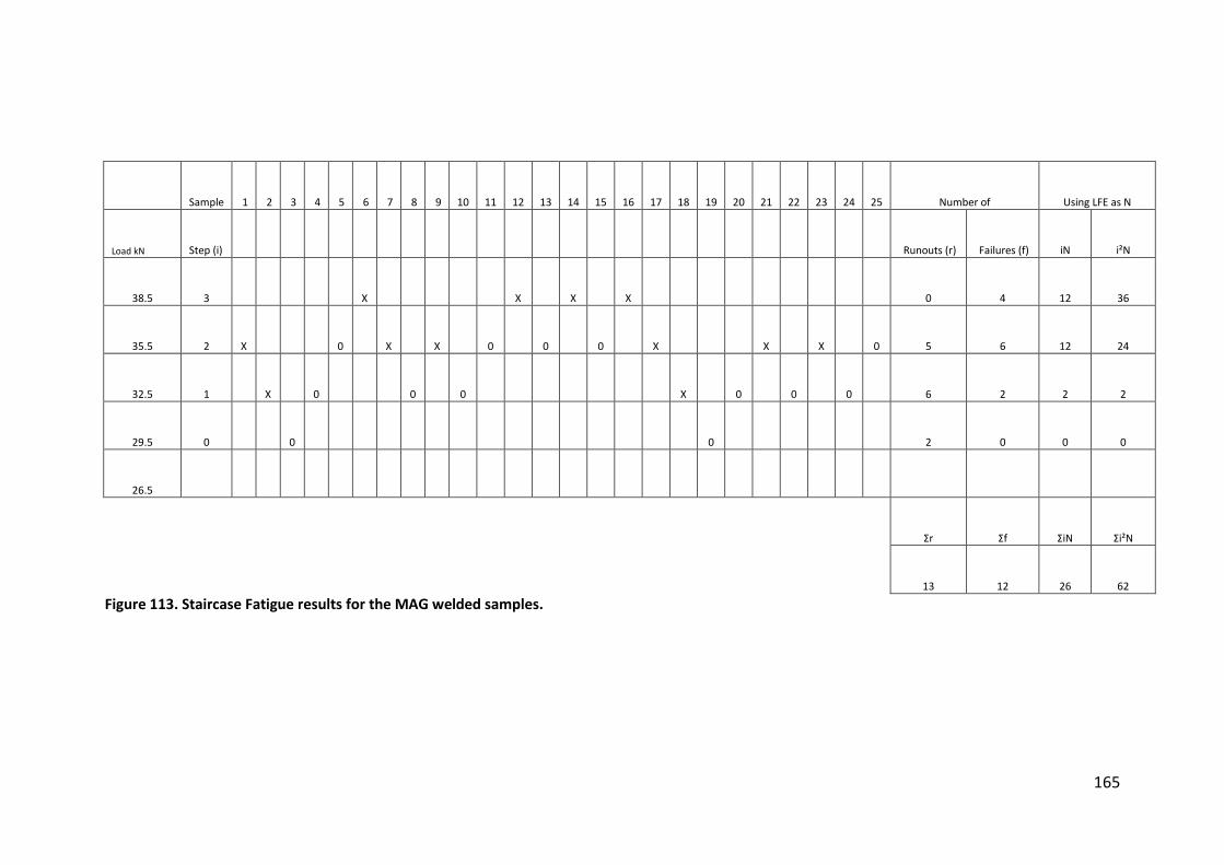
165
Sample 1 2 3 4 5 6 7 8 9 10 11 12 13 14 15 16 17 18 19 20 21 22 23 24 25 Number of Using LFE as N
Load kN Step (i) Runouts (r) Failures (f) iN i²N
38.5 3 X X X X 0 4 12 36
35.5 2 X 0 X X 0 0 0 X X X 0 5 6 12 24
32.5 1 X 0 0 0 X 0 0 0 6 2 2 2
29.5 0 0 0 2 0 0 0
26.5
Σr Σf ΣiN Σi²N
13 12 26 62
Figure 113. Staircase Fatigue results for the MAG welded samples.
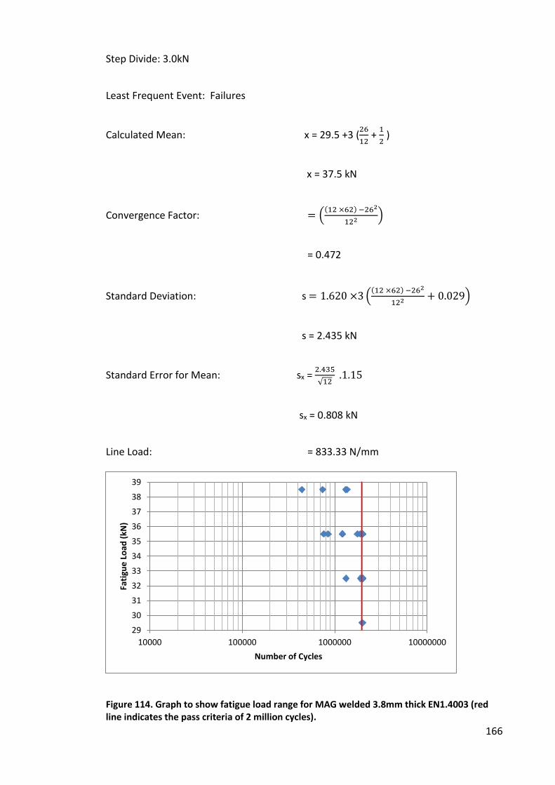
166
Step Divide: 3.0kN
Least Frequent Event: Failures
Calculated Mean: x = 29.5 +3 ( + )
x = 37.5 kN
Convergence Factor: = × − 22
= 0.472
Standard Deviation: s = . × × − 22 + . 9
s = 2.435 kN
Standard Error for Mean: sx = .√ . .
sx = 0.808 kN
Line Load: = 833.33 N/mm
Figure 114. Graph to show fatigue load range for MAG welded 3.8mm thick EN1.4003 (red
line indicates the pass criteria of 2 million cycles).
29
30
31
32
33
34
35
36
37
38
39
10000 100000 1000000 10000000
Fa
tig
ue
Lo
ad
(k
N)
Number of Cycles
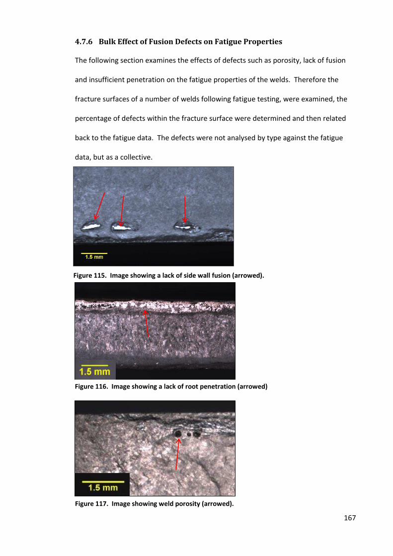
167
4.7.6 Bulk Effect of Fusion Defects on Fatigue Properties
The following section examines the effects of defects such as porosity, lack of fusion
and insufficient penetration on the fatigue properties of the welds. Therefore the
fracture surfaces of a number of welds following fatigue testing, were examined, the
percentage of defects within the fracture surface were determined and then related
back to the fatigue data. The defects were not analysed by type against the fatigue
data, but as a collective.
Figure 115. Image showing a lack of side wall fusion (arrowed).
Figure 116. Image showing a lack of root penetration (arrowed)
Figure 117. Image showing weld porosity (arrowed).
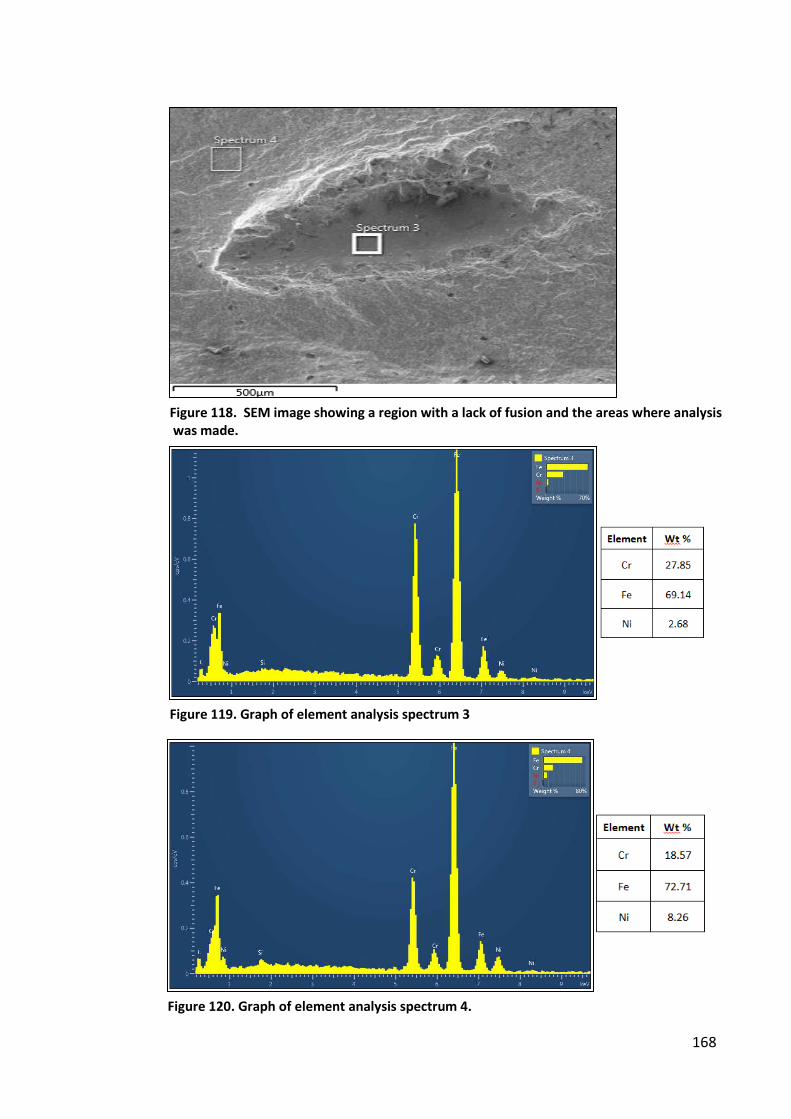
168
Figure 118. SEM image showing a region with a lack of fusion and the areas where analysis
was made.
Figure 119. Graph of element analysis spectrum 3
Figure 120. Graph of element analysis spectrum 4.
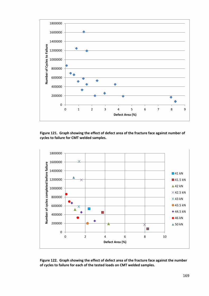
169
Figure 121. Graph showing the effect of defect area of the fracture face against number of
cycles to failure for CMT welded samples.
Figure 122. Graph showing the effect of defect area of the fracture face against the number
of cycles to failure for each of the tested loads on CMT welded samples.
0
200000
400000
600000
800000
1000000
1200000
1400000
1600000
1800000
0 1 2 3 4 5 6 7 8 9
Nu
mb
er
of
Cy
cle
s to
Fa
ilu
re
Defect Area (%)
0
200000
400000
600000
800000
1000000
1200000
1400000
1600000
1800000
0 2 4 6 8 10
Nu
mb
er
of
cycl
es
com
ple
ted
be
fore
fa
ilu
re
Defect Area (%)
41 kN
41.5 kN
42 kN
42.5 kN
43 kN
43.5 kN
44.5 kN
46 kN
50 kN
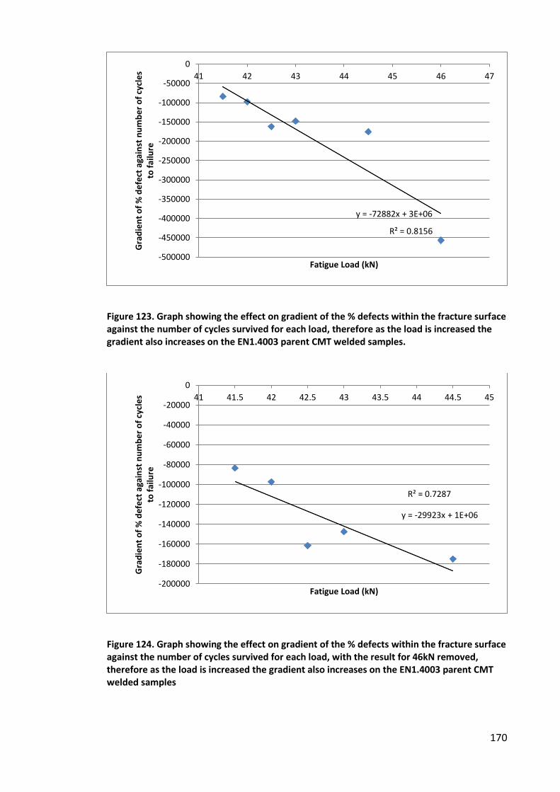
170
Figure 123. Graph showing the effect on gradient of the % defects within the fracture surface
against the number of cycles survived for each load, therefore as the load is increased the
gradient also increases on the EN1.4003 parent CMT welded samples.
Figure 124. Graph showing the effect on gradient of the % defects within the fracture surface
against the number of cycles survived for each load, with the result for 46kN removed,
therefore as the load is increased the gradient also increases on the EN1.4003 parent CMT
welded samples
y = -72882x + 3E+06
R² = 0.8156
-500000
-450000
-400000
-350000
-300000
-250000
-200000
-150000
-100000
-50000
0
41 42 43 44 45 46 47
Gra
die
nt
of
% d
efe
ct a
ga
inst
nu
mb
er
of
cycl
es
to f
ail
ure
Fatigue Load (kN)
y = -29923x + 1E+06
R² = 0.7287
-200000
-180000
-160000
-140000
-120000
-100000
-80000
-60000
-40000
-20000
0
41 41.5 42 42.5 43 43.5 44 44.5 45
Gra
die
nt
of
% d
efe
ct a
ga
inst
nu
mb
er
of
cycl
es
to f
ail
ure
Fatigue Load (kN)
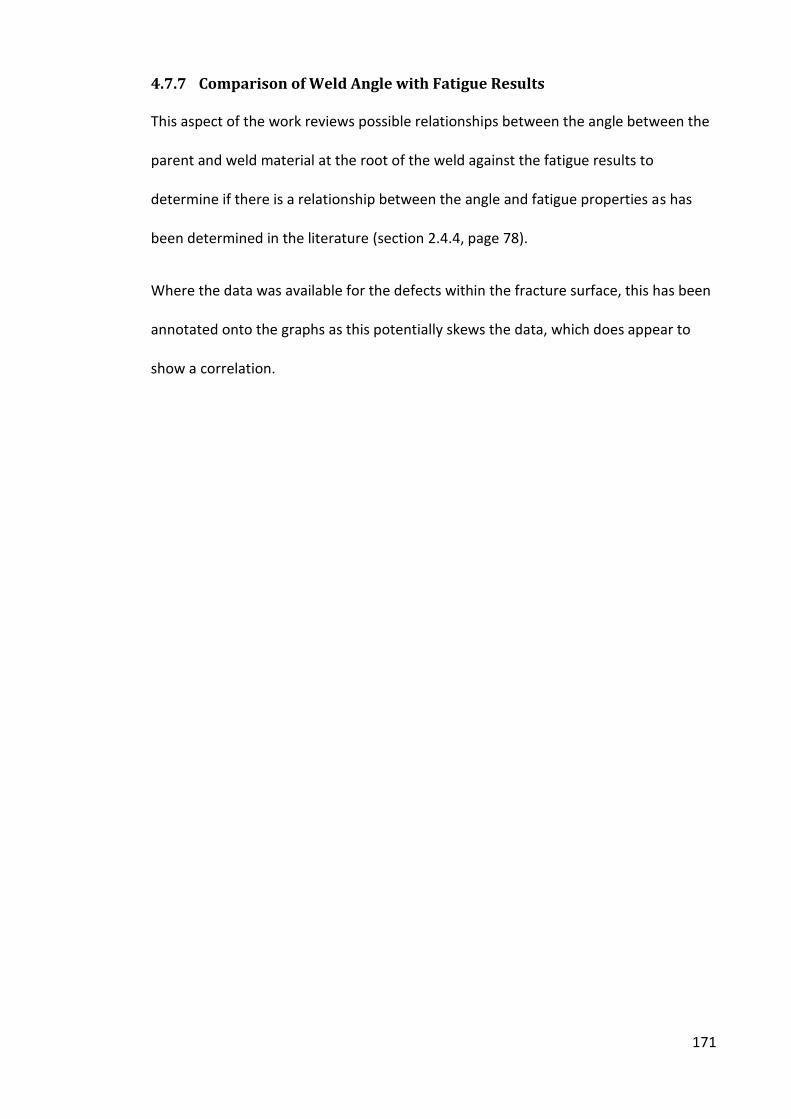
171
4.7.7 Comparison of Weld Angle with Fatigue Results
This aspect of the work reviews possible relationships between the angle between the
parent and weld material at the root of the weld against the fatigue results to
determine if there is a relationship between the angle and fatigue properties as has
been determined in the literature (section 2.4.4, page 78).
Where the data was available for the defects within the fracture surface, this has been
annotated onto the graphs as this potentially skews the data, which does appear to
show a correlation.
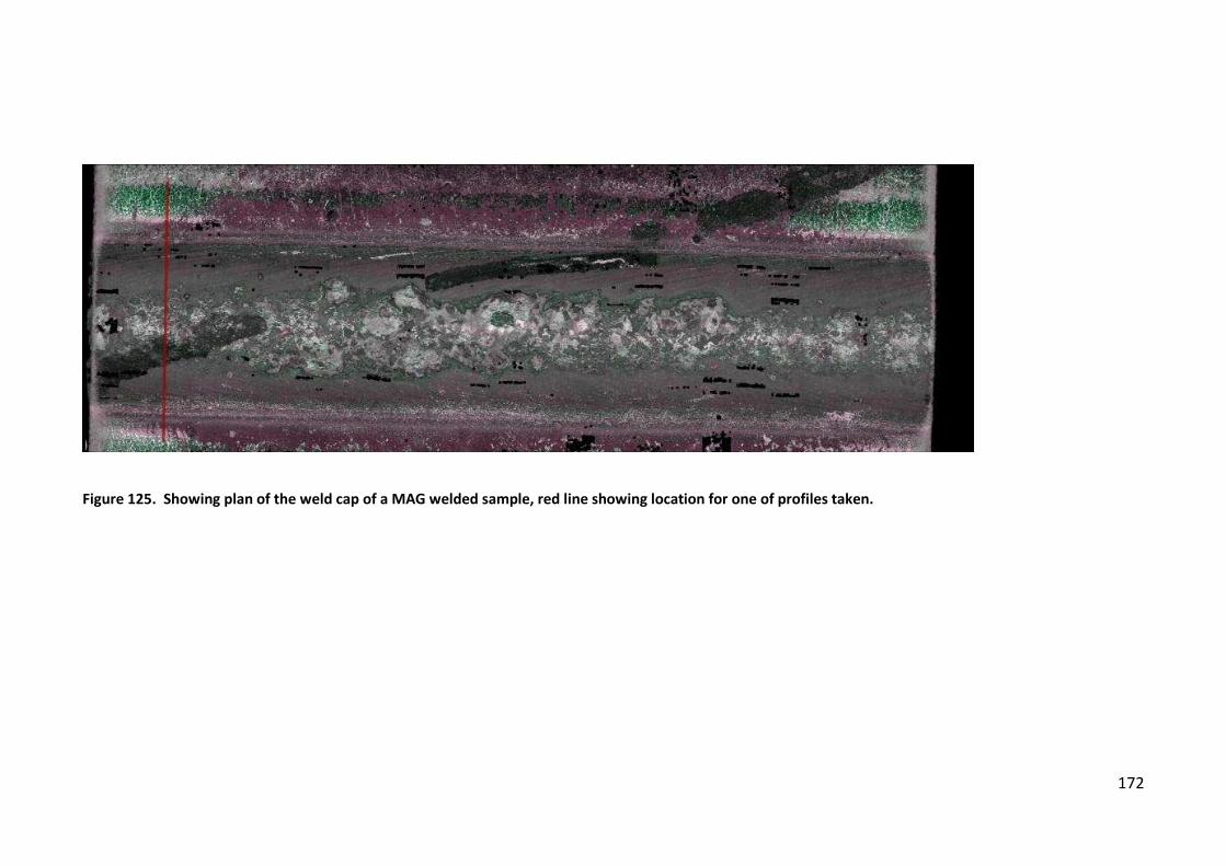
172
Figure 125. Showing plan of the weld cap of a MAG welded sample, red line showing location for one of profiles taken.
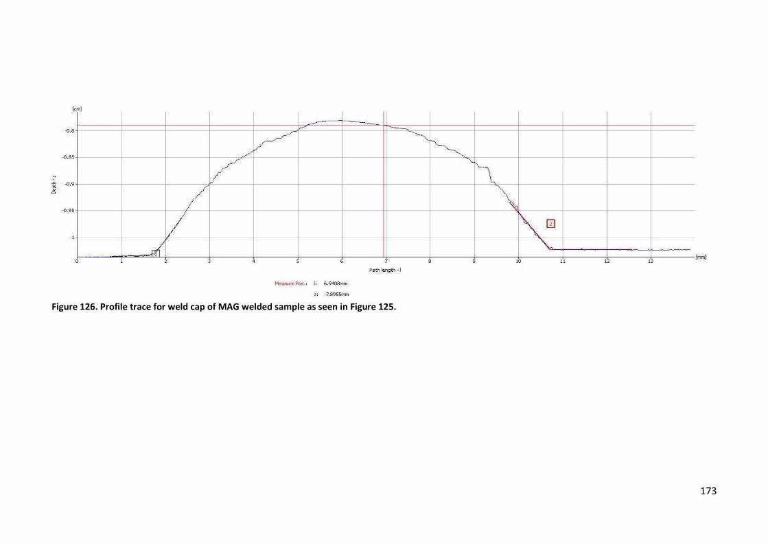
173
Figure 126. Profile trace for weld cap of MAG welded sample as seen in Figure 125.
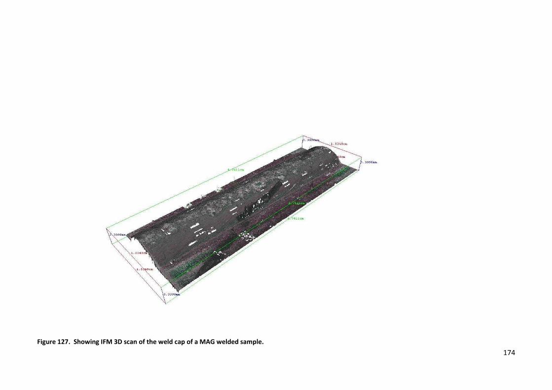
174
Figure 127. Showing IFM 3D scan of the weld cap of a MAG welded sample.
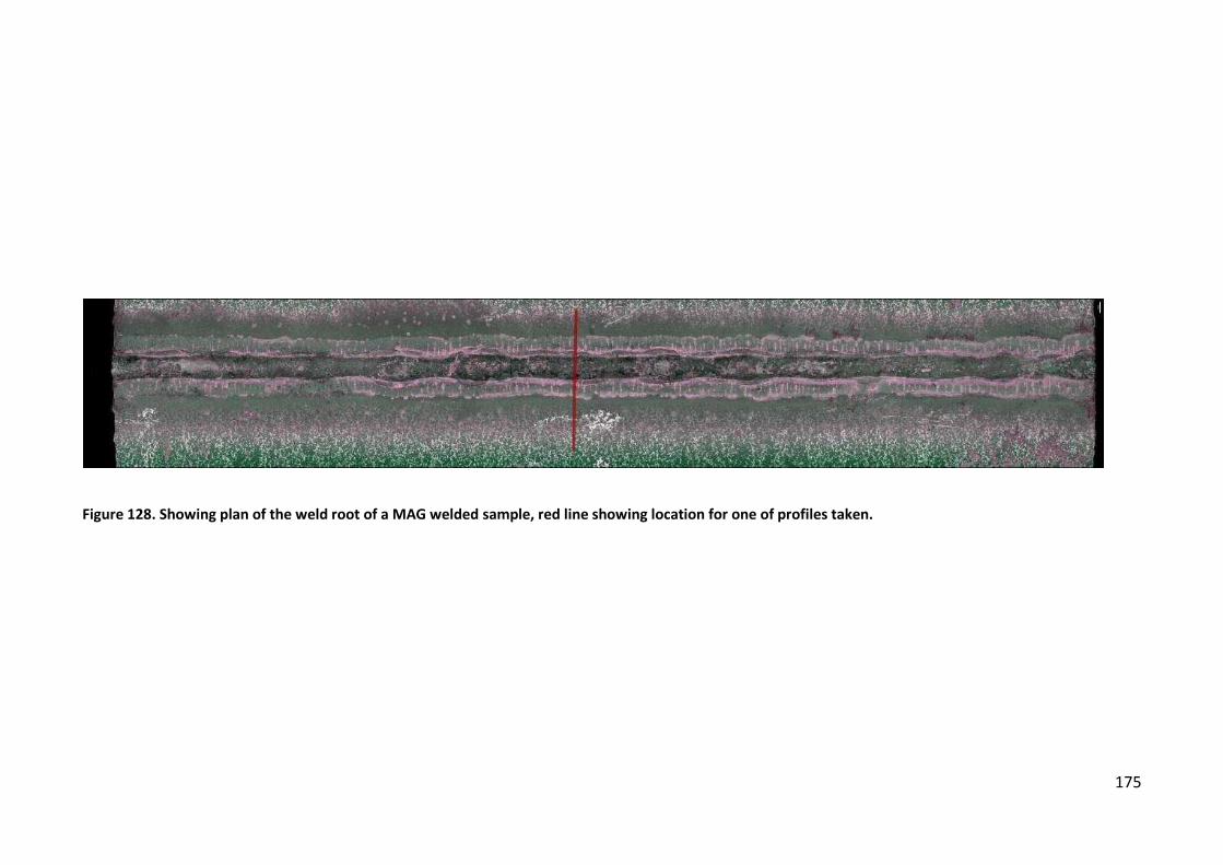
175
Figure 128. Showing plan of the weld root of a MAG welded sample, red line showing location for one of profiles taken.
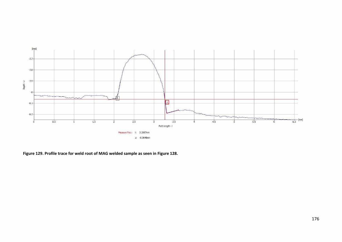
176
Figure 129. Profile trace for weld root of MAG welded sample as seen in Figure 128.
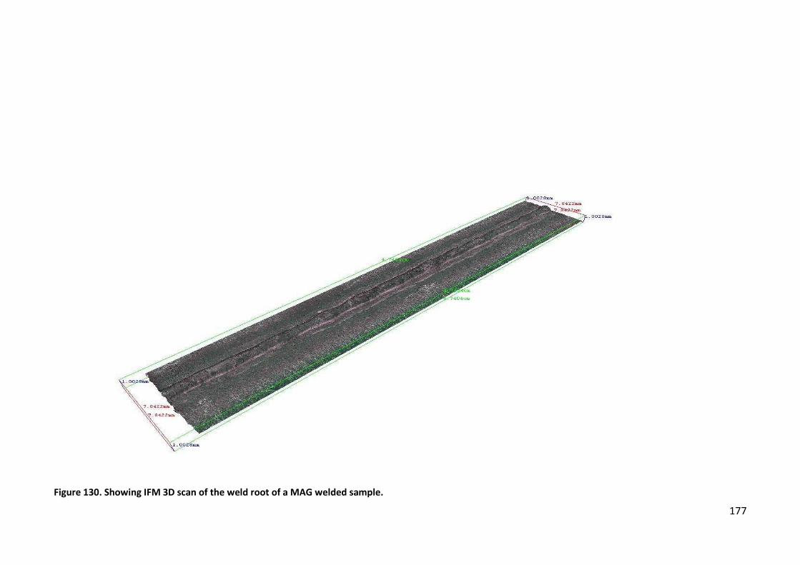
177
Figure 130. Showing IFM 3D scan of the weld root of a MAG welded sample.
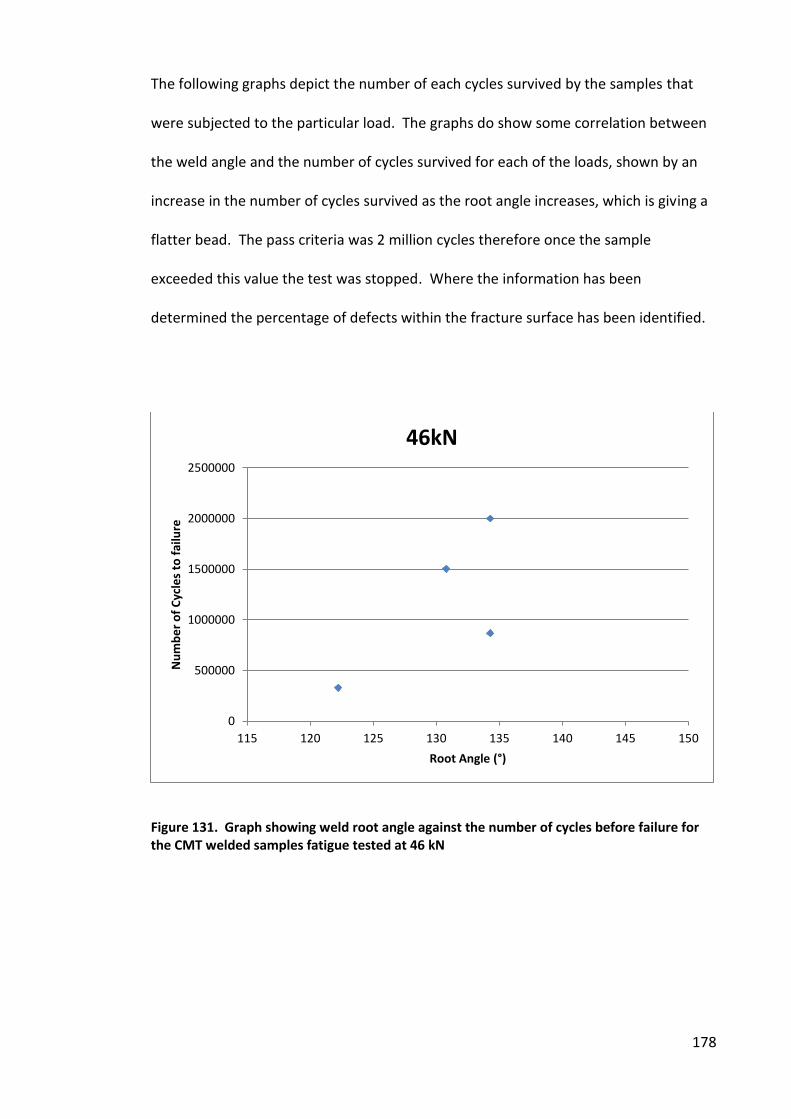
178
The following graphs depict the number of each cycles survived by the samples that
were subjected to the particular load. The graphs do show some correlation between
the weld angle and the number of cycles survived for each of the loads, shown by an
increase in the number of cycles survived as the root angle increases, which is giving a
flatter bead. The pass criteria was 2 million cycles therefore once the sample
exceeded this value the test was stopped. Where the information has been
determined the percentage of defects within the fracture surface has been identified.
Figure 131. Graph showing weld root angle against the number of cycles before failure for
the CMT welded samples fatigue tested at 46 kN
0
500000
1000000
1500000
2000000
2500000
115 120 125 130 135 140 145 150
Nu
mb
er
of
Cy
cle
s to
fa
ilu
re
Root Angle (°)
46kN
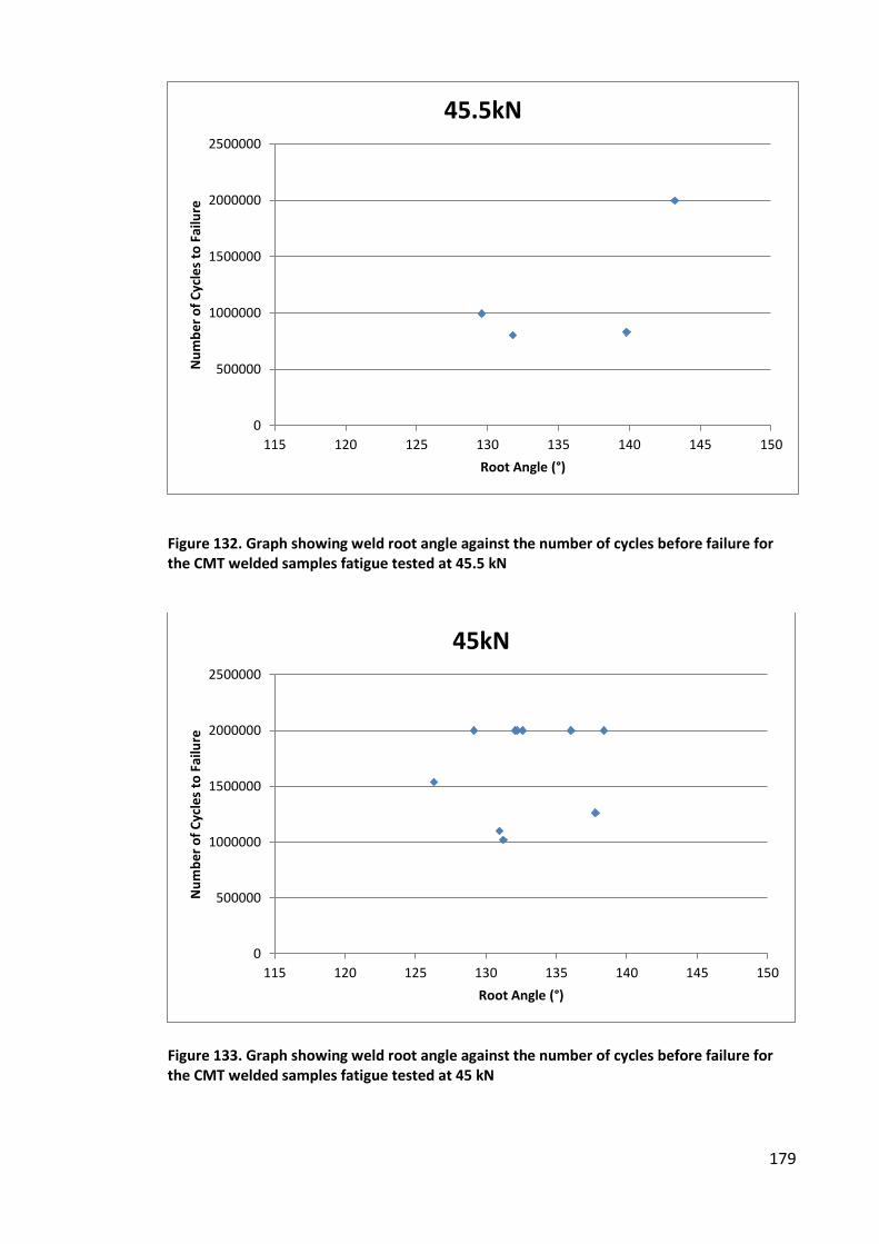
179
Figure 132. Graph showing weld root angle against the number of cycles before failure for
the CMT welded samples fatigue tested at 45.5 kN
Figure 133. Graph showing weld root angle against the number of cycles before failure for
the CMT welded samples fatigue tested at 45 kN
0
500000
1000000
1500000
2000000
2500000
115 120 125 130 135 140 145 150
Nu
mb
er
of
Cy
cle
s to
Fa
ilu
re
Root Angle (°)
45.5kN
0
500000
1000000
1500000
2000000
2500000
115 120 125 130 135 140 145 150
Nu
mb
er
of
Cy
cle
s to
Fa
ilu
re
Root Angle (°)
45kN
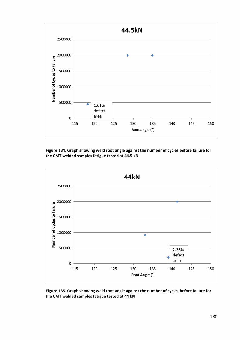
180
Figure 134. Graph showing weld root angle against the number of cycles before failure for
the CMT welded samples fatigue tested at 44.5 kN
Figure 135. Graph showing weld root angle against the number of cycles before failure for
the CMT welded samples fatigue tested at 44 kN
0
500000
1000000
1500000
2000000
2500000
115 120 125 130 135 140 145 150
Nu
mb
er
of
Cy
cle
s to
Fa
ilu
re
Root angle (°)
44.5kN
1.61%
defect
area
0
500000
1000000
1500000
2000000
2500000
115 120 125 130 135 140 145 150
Nu
mb
er
of
Cy
cle
s to
fa
ilu
re
Root Angle (°)
44kN
2.23%
defect
area
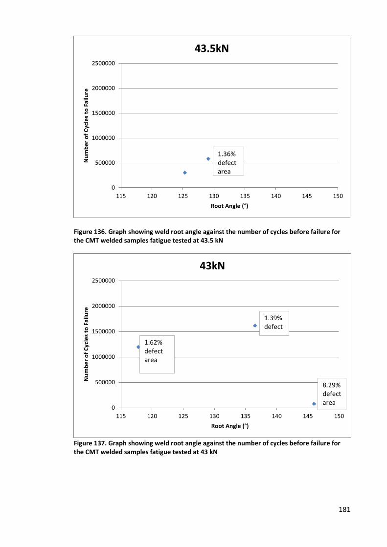
181
Figure 136. Graph showing weld root angle against the number of cycles before failure for
the CMT welded samples fatigue tested at 43.5 kN
Figure 137. Graph showing weld root angle against the number of cycles before failure for
the CMT welded samples fatigue tested at 43 kN
0
500000
1000000
1500000
2000000
2500000
115 120 125 130 135 140 145 150
Nu
mb
er
of
Cy
cle
s to
Fa
ilu
re
Root Angle (°)
43.5kN
1.36%
defect
area
0
500000
1000000
1500000
2000000
2500000
115 120 125 130 135 140 145 150
Nu
mb
er
of
Cy
cle
s to
Fa
ilu
re
Root Angle (°)
43kN
1.62%
defect
area
8.29%
defect
area
1.39%
defect
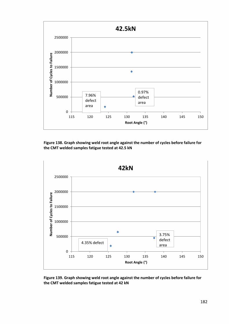
182
Figure 138. Graph showing weld root angle against the number of cycles before failure for
the CMT welded samples fatigue tested at 42.5 kN
Figure 139. Graph showing weld root angle against the number of cycles before failure for
the CMT welded samples fatigue tested at 42 kN
0
500000
1000000
1500000
2000000
2500000
115 120 125 130 135 140 145 150
Nu
mb
er
of
Cy
cle
s to
Fa
ilu
re
Root Angle (°)
42.5kN
7.96%
defect
area
0.97%
defect
area
0
500000
1000000
1500000
2000000
2500000
115 120 125 130 135 140 145 150
Nu
mb
er
of
Cy
cle
s to
Fa
ilu
re
Root Angle (°)
42kN
4.35% defect
3.75%
defect
area
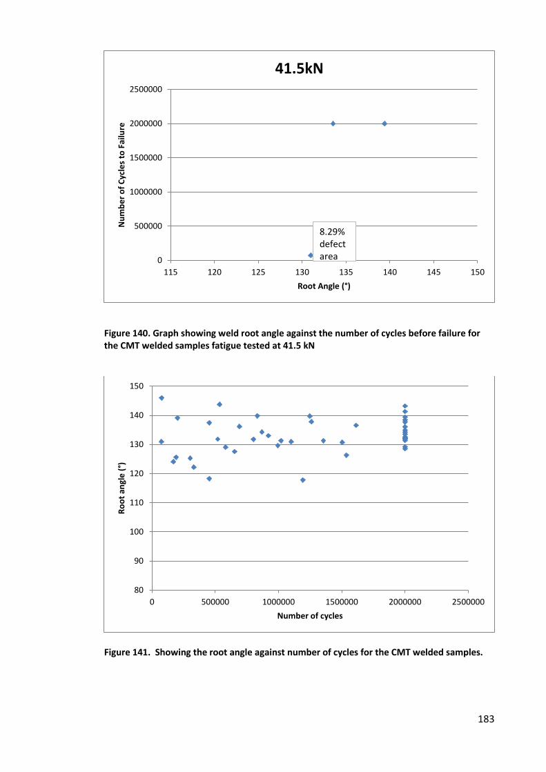
183
Figure 140. Graph showing weld root angle against the number of cycles before failure for
the CMT welded samples fatigue tested at 41.5 kN
Figure 141. Showing the root angle against number of cycles for the CMT welded samples.
0
500000
1000000
1500000
2000000
2500000
115 120 125 130 135 140 145 150
Nu
mb
er
of
Cy
cle
s to
Fa
ilu
re
Root Angle (°)
41.5kN
8.29%
defect
area
80
90
100
110
120
130
140
150
0 500000 1000000 1500000 2000000 2500000
Ro
ot
an
gle
(°)
Number of cycles
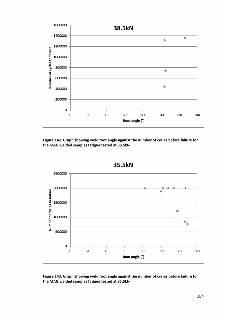
184
Figure 142. Graph showing weld root angle against the number of cycles before failure for
the MAG welded samples fatigue tested at 38.5kN
Figure 143. Graph showing weld root angle against the number of cycles before failure for
the MAG welded samples fatigue tested at 35.5kN
0
200000
400000
600000
800000
1000000
1200000
1400000
1600000
0 20 40 60 80 100 120 140
Nu
mb
er
of
cycl
es
to f
ail
ure
Root angle (°)
38.5kN
0
500000
1000000
1500000
2000000
2500000
0 20 40 60 80 100 120 140
Nu
mb
er
of
cycl
es
to f
ail
ure
Root angle (°)
35.5kN
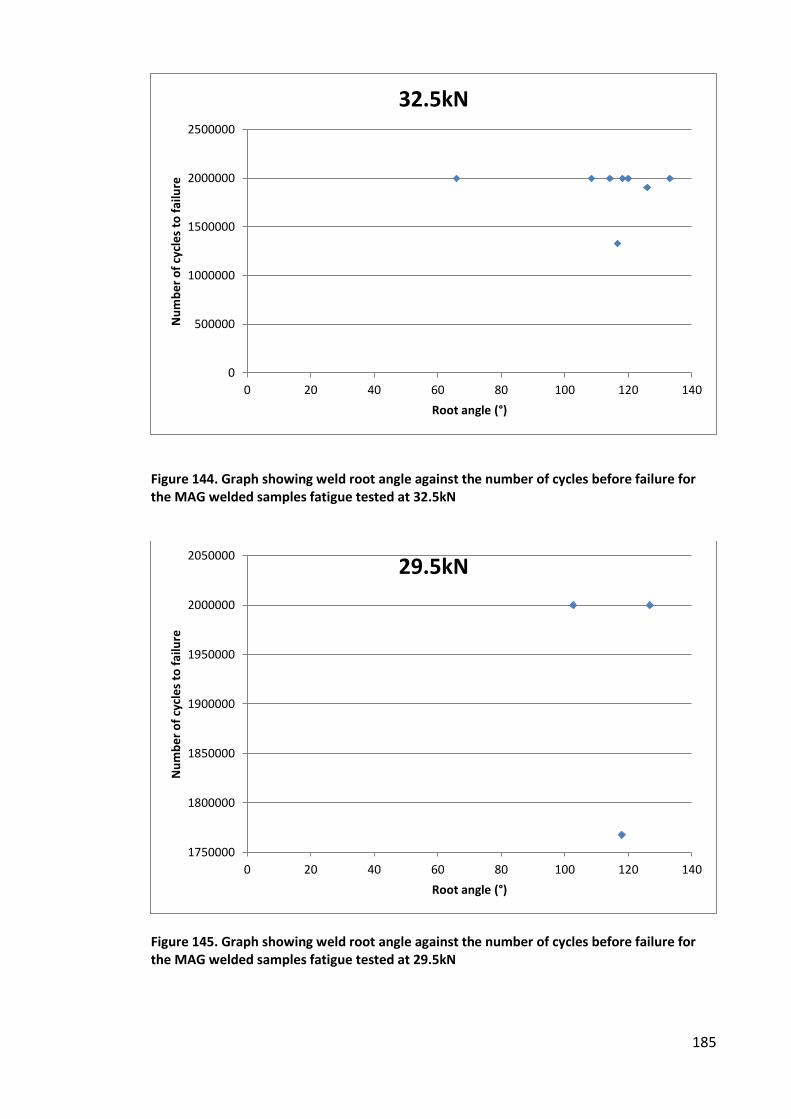
185
Figure 144. Graph showing weld root angle against the number of cycles before failure for
the MAG welded samples fatigue tested at 32.5kN
Figure 145. Graph showing weld root angle against the number of cycles before failure for
the MAG welded samples fatigue tested at 29.5kN
0
500000
1000000
1500000
2000000
2500000
0 20 40 60 80 100 120 140
Nu
mb
er
of
cycl
es
to f
ail
ure
Root angle (°)
32.5kN
1750000
1800000
1850000
1900000
1950000
2000000
2050000
0 20 40 60 80 100 120 140
Nu
mb
er
of
cycl
es
to f
ail
ure
Root angle (°)
29.5kN
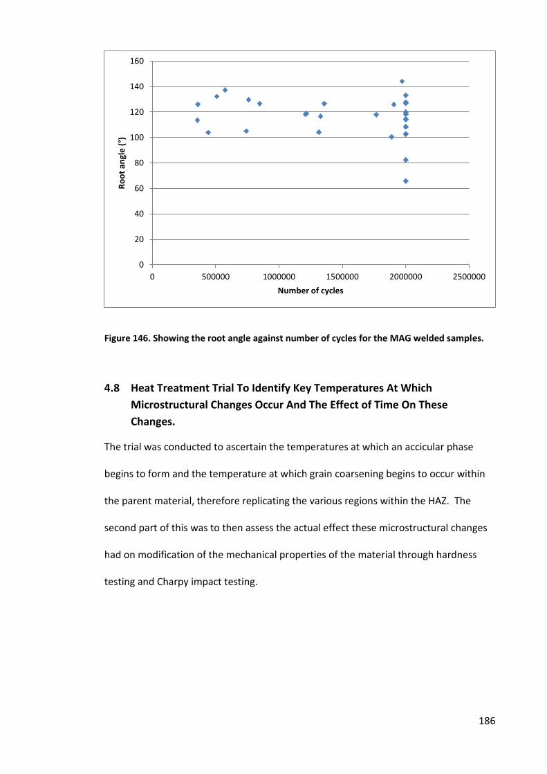
186
Figure 146. Showing the root angle against number of cycles for the MAG welded samples.
4.8 Heat Treatment Trial To Identify Key Temperatures At Which
Microstructural Changes Occur And The Effect of Time On These
Changes.
The trial was conducted to ascertain the temperatures at which an accicular phase
begins to form and the temperature at which grain coarsening begins to occur within
the parent material, therefore replicating the various regions within the HAZ. The
second part of this was to then assess the actual effect these microstructural changes
had on modification of the mechanical properties of the material through hardness
testing and Charpy impact testing.
0
20
40
60
80
100
120
140
160
0 500000 1000000 1500000 2000000 2500000
Ro
ot
an
gle
(°)
Number of cycles
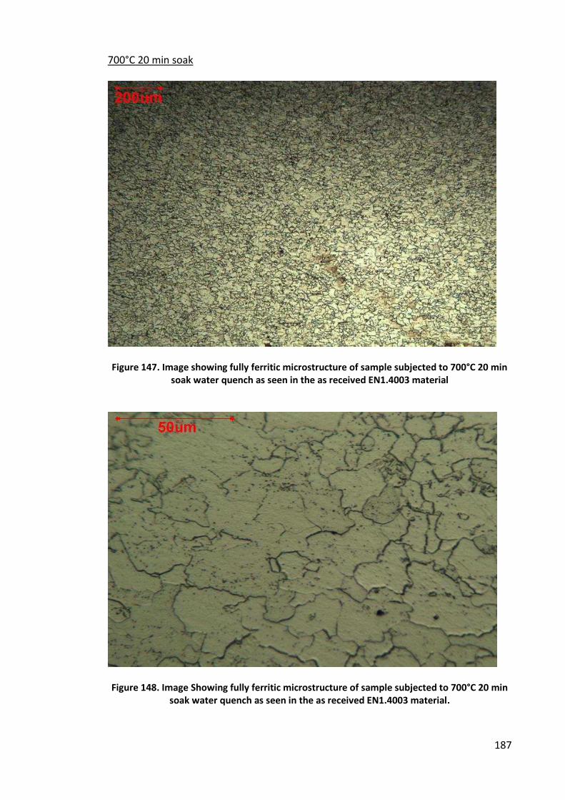
187
700°C 20 min soak
Figure 147. Image showing fully ferritic microstructure of sample subjected to 700°C 20 min
soak water quench as seen in the as received EN1.4003 material
Figure 148. Image Showing fully ferritic microstructure of sample subjected to 700°C 20 min
soak water quench as seen in the as received EN1.4003 material.
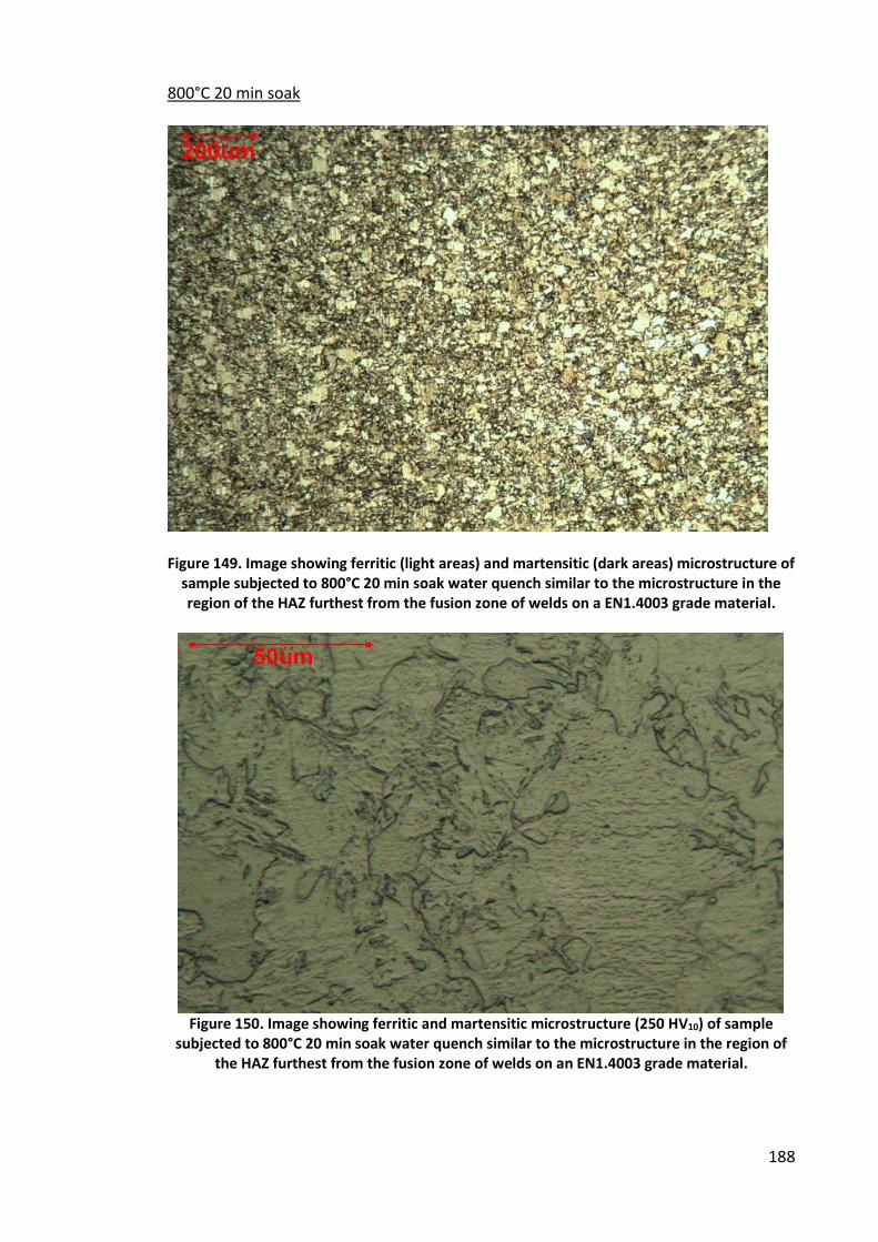
188
800°C 20 min soak
Figure 149. Image showing ferritic (light areas) and martensitic (dark areas) microstructure of
sample subjected to 800°C 20 min soak water quench similar to the microstructure in the
region of the HAZ furthest from the fusion zone of welds on a EN1.4003 grade material.
Figure 150. Image showing ferritic and martensitic microstructure (250 HV10) of sample
subjected to 800°C 20 min soak water quench similar to the microstructure in the region of
the HAZ furthest from the fusion zone of welds on an EN1.4003 grade material.

189
900°C 20 min soak
Figure 151. Image showing martensitic microstructure of EN1.4003 sample subjected to
900°C 20 min soak water quench.
Figure 152. Image showing martensitic microstructure (277 HV10) of EN1.4003 sample
subjected to 900°C 20 min soak water quench.
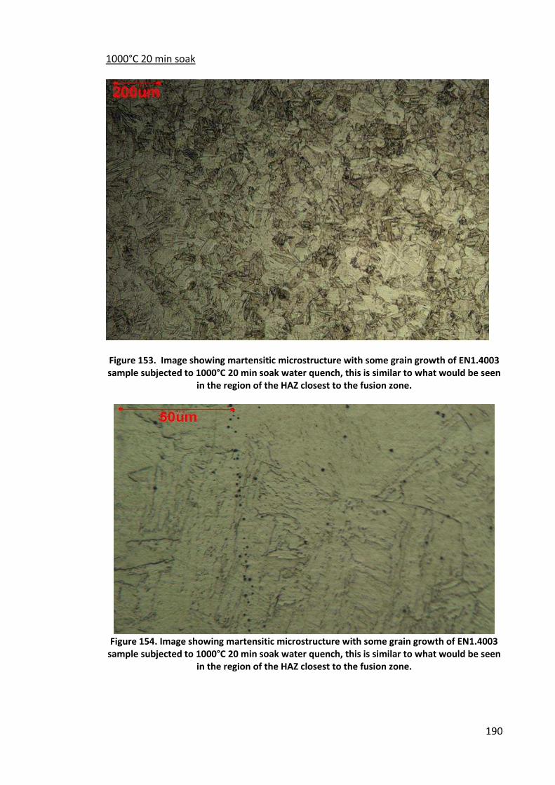
190
1000°C 20 min soak
Figure 153. Image showing martensitic microstructure with some grain growth of EN1.4003
sample subjected to 1000°C 20 min soak water quench, this is similar to what would be seen
in the region of the HAZ closest to the fusion zone.
Figure 154. Image showing martensitic microstructure with some grain growth of EN1.4003
sample subjected to 1000°C 20 min soak water quench, this is similar to what would be seen
in the region of the HAZ closest to the fusion zone.
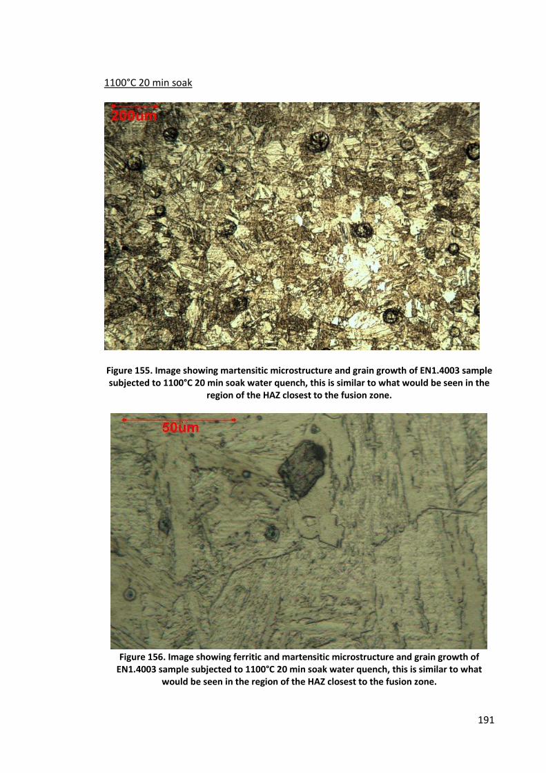
191
1100°C 20 min soak
Figure 155. Image showing martensitic microstructure and grain growth of EN1.4003 sample
subjected to 1100°C 20 min soak water quench, this is similar to what would be seen in the
region of the HAZ closest to the fusion zone.
Figure 156. Image showing ferritic and martensitic microstructure and grain growth of
EN1.4003 sample subjected to 1100°C 20 min soak water quench, this is similar to what
would be seen in the region of the HAZ closest to the fusion zone.
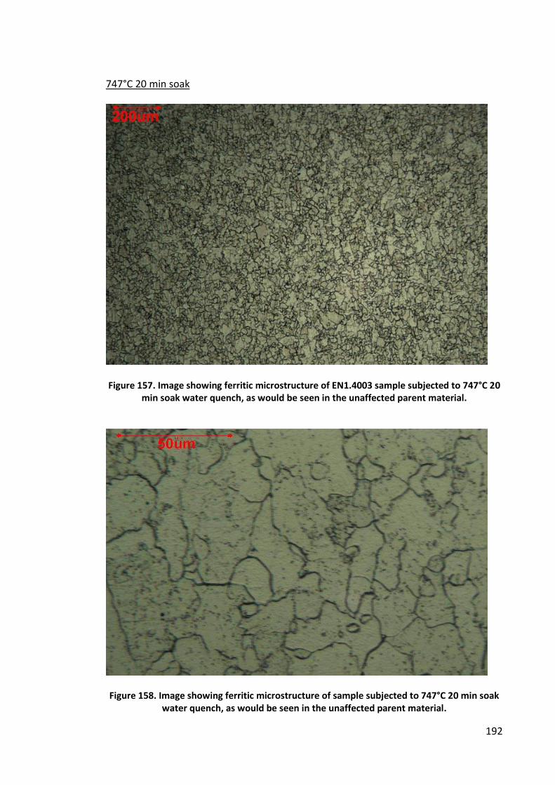
192
747°C 20 min soak
Figure 157. Image showing ferritic microstructure of EN1.4003 sample subjected to 747°C 20
min soak water quench, as would be seen in the unaffected parent material.
Figure 158. Image showing ferritic microstructure of sample subjected to 747°C 20 min soak
water quench, as would be seen in the unaffected parent material.
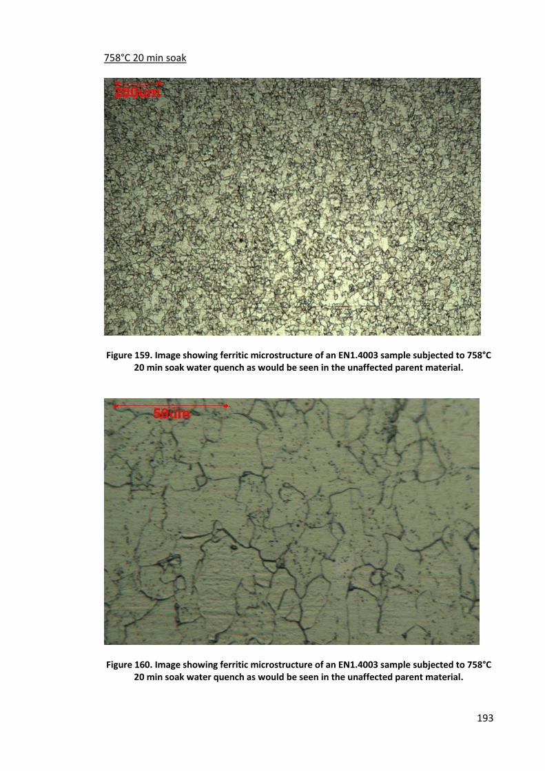
193
758°C 20 min soak
Figure 159. Image showing ferritic microstructure of an EN1.4003 sample subjected to 758°C
20 min soak water quench as would be seen in the unaffected parent material.
Figure 160. Image showing ferritic microstructure of an EN1.4003 sample subjected to 758°C
20 min soak water quench as would be seen in the unaffected parent material.
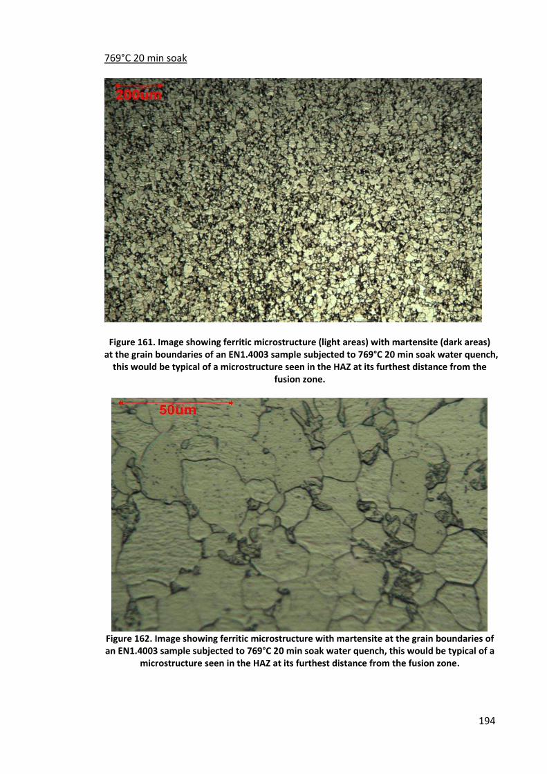
194
769°C 20 min soak
Figure 161. Image showing ferritic microstructure (light areas) with martensite (dark areas)
at the grain boundaries of an EN1.4003 sample subjected to 769°C 20 min soak water quench,
this would be typical of a microstructure seen in the HAZ at its furthest distance from the
fusion zone.
Figure 162. Image showing ferritic microstructure with martensite at the grain boundaries of
an EN1.4003 sample subjected to 769°C 20 min soak water quench, this would be typical of a
microstructure seen in the HAZ at its furthest distance from the fusion zone.
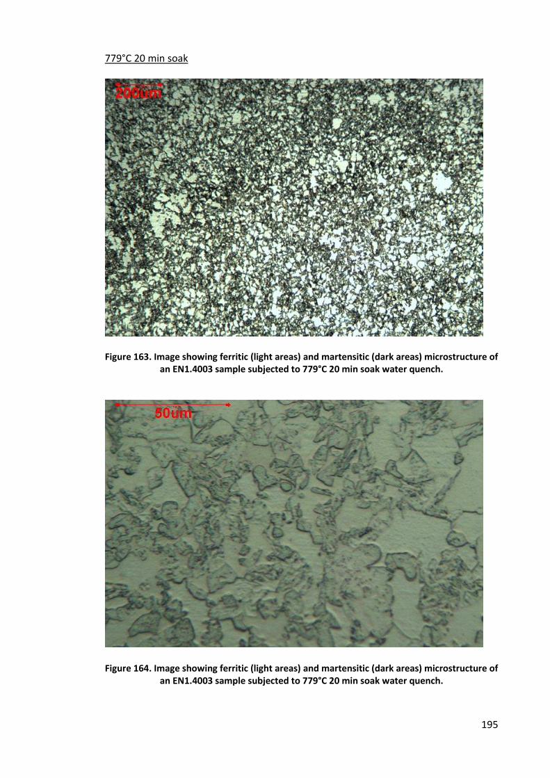
195
779°C 20 min soak
Figure 163. Image showing ferritic (light areas) and martensitic (dark areas) microstructure of
an EN1.4003 sample subjected to 779°C 20 min soak water quench.
Figure 164. Image showing ferritic (light areas) and martensitic (dark areas) microstructure of
an EN1.4003 sample subjected to 779°C 20 min soak water quench.
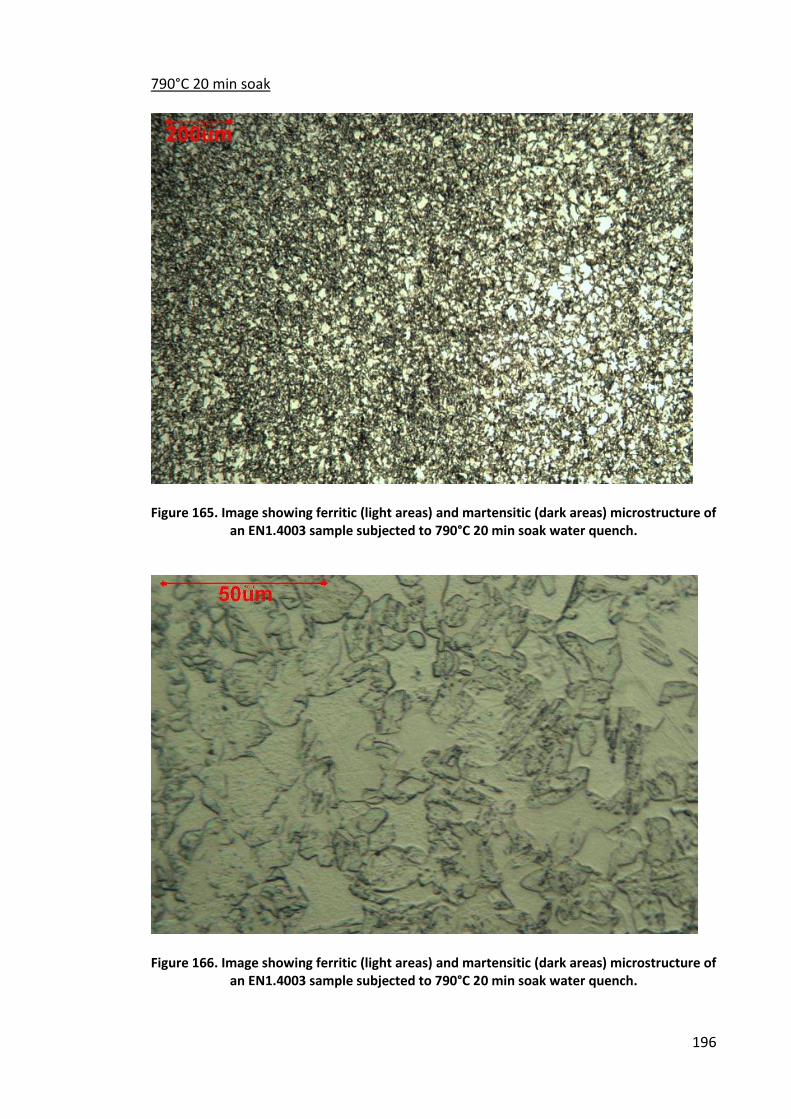
196
790°C 20 min soak
Figure 165. Image showing ferritic (light areas) and martensitic (dark areas) microstructure of
an EN1.4003 sample subjected to 790°C 20 min soak water quench.
Figure 166. Image showing ferritic (light areas) and martensitic (dark areas) microstructure of
an EN1.4003 sample subjected to 790°C 20 min soak water quench.
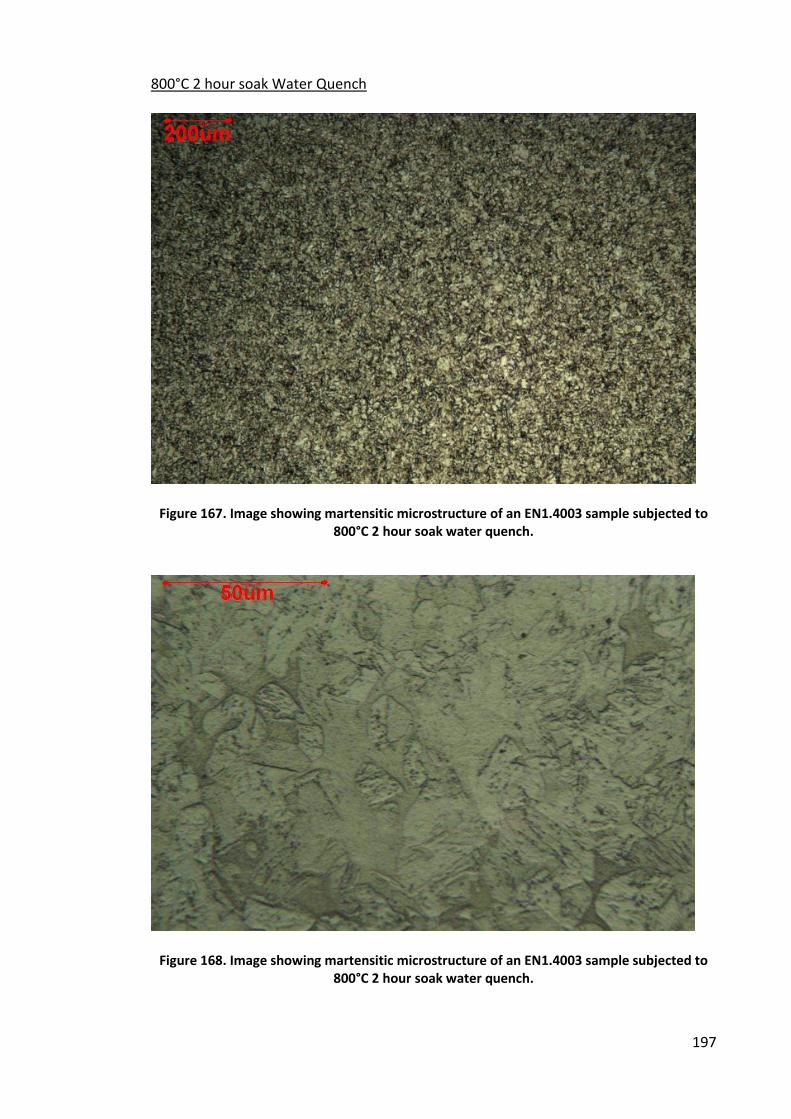
197
800°C 2 hour soak Water Quench
Figure 167. Image showing martensitic microstructure of an EN1.4003 sample subjected to
800°C 2 hour soak water quench.
Figure 168. Image showing martensitic microstructure of an EN1.4003 sample subjected to
800°C 2 hour soak water quench.
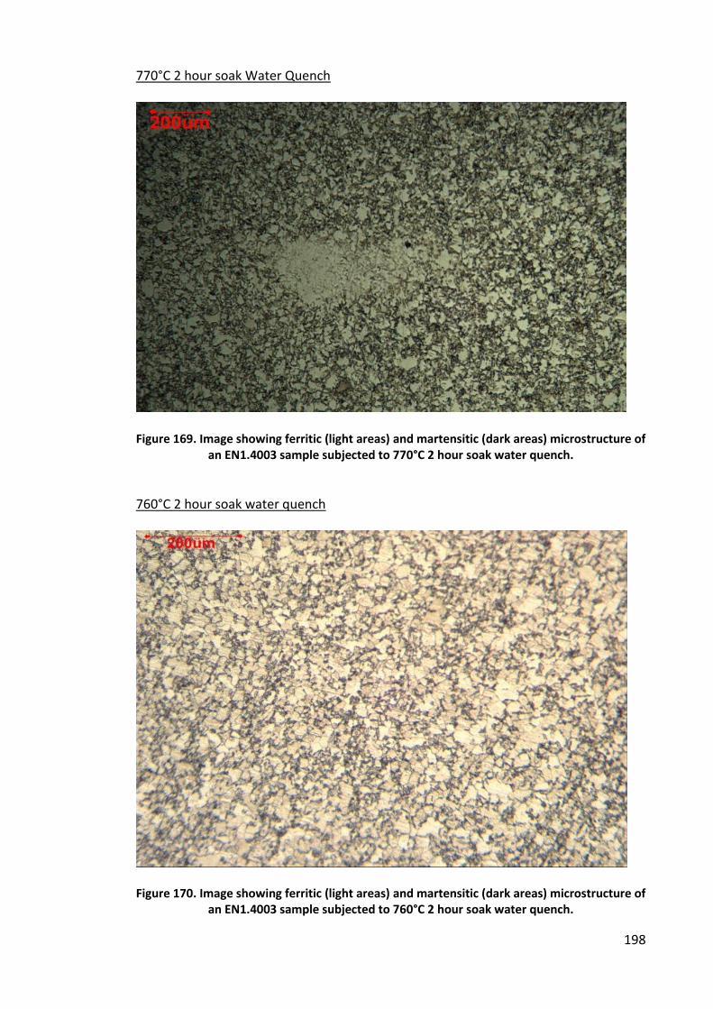
198
770°C 2 hour soak Water Quench
Figure 169. Image showing ferritic (light areas) and martensitic (dark areas) microstructure of
an EN1.4003 sample subjected to 770°C 2 hour soak water quench.
760°C 2 hour soak water quench
Figure 170. Image showing ferritic (light areas) and martensitic (dark areas) microstructure of
an EN1.4003 sample subjected to 760°C 2 hour soak water quench.
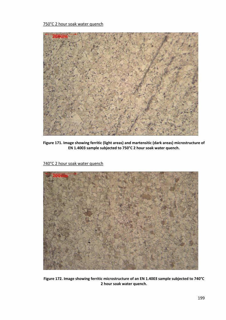
199
750°C 2 hour soak water quench
Figure 171. Image showing ferritic (light areas) and martensitic (dark areas) microstructure of
EN 1.4003 sample subjected to 750°C 2 hour soak water quench.
740°C 2 hour soak water quench
Figure 172. Image showing ferritic microstructure of an EN 1.4003 sample subjected to 740°C
2 hour soak water quench.
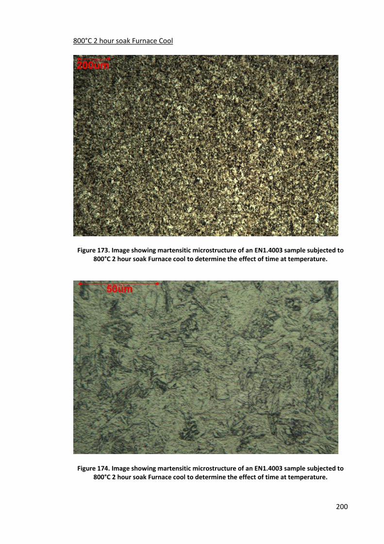
200
800°C 2 hour soak Furnace Cool
Figure 173. Image showing martensitic microstructure of an EN1.4003 sample subjected to
800°C 2 hour soak Furnace cool to determine the effect of time at temperature.
Figure 174. Image showing martensitic microstructure of an EN1.4003 sample subjected to
800°C 2 hour soak Furnace cool to determine the effect of time at temperature.
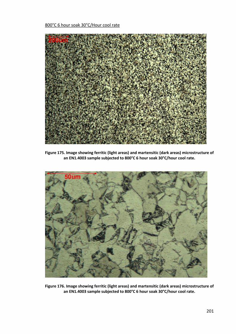
201
800°C 6 hour soak 30°C/Hour cool rate
Figure 175. Image showing ferritic (light areas) and martensitic (dark areas) microstructure of
an EN1.4003 sample subjected to 800°C 6 hour soak 30°C/hour cool rate.
Figure 176. Image showing ferritic (light areas) and martensitic (dark areas) microstructure of
an EN1.4003 sample subjected to 800°C 6 hour soak 30°C/hour cool rate.
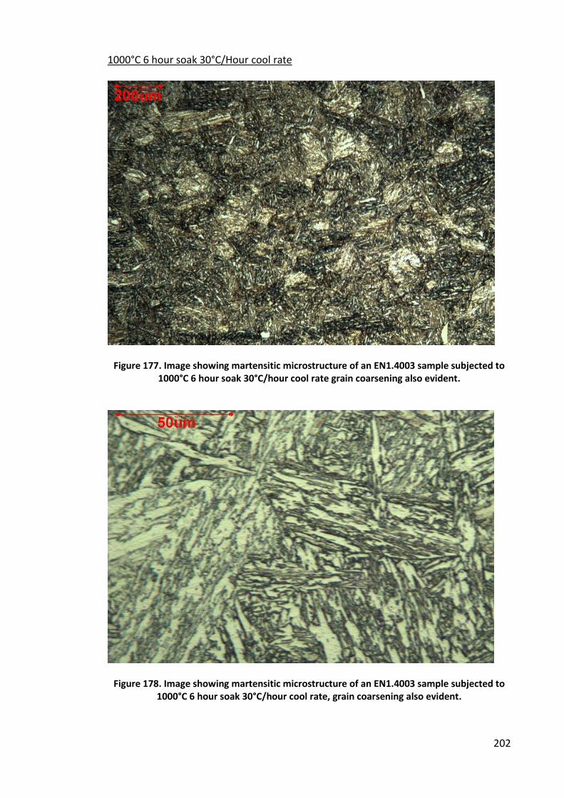
202
1000°C 6 hour soak 30°C/Hour cool rate
Figure 177. Image showing martensitic microstructure of an EN1.4003 sample subjected to
1000°C 6 hour soak 30°C/hour cool rate grain coarsening also evident.
Figure 178. Image showing martensitic microstructure of an EN1.4003 sample subjected to
1000°C 6 hour soak 30°C/hour cool rate, grain coarsening also evident.
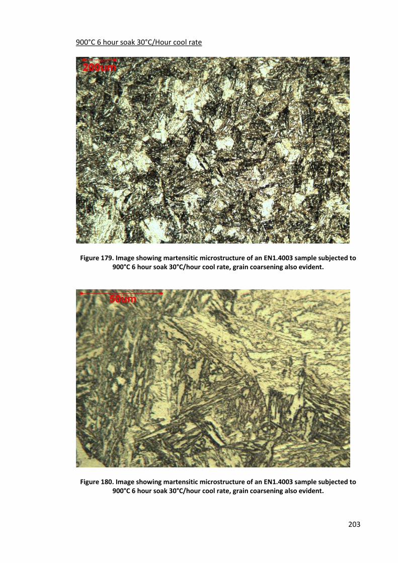
203
900°C 6 hour soak 30°C/Hour cool rate
Figure 179. Image showing martensitic microstructure of an EN1.4003 sample subjected to
900°C 6 hour soak 30°C/hour cool rate, grain coarsening also evident.
Figure 180. Image showing martensitic microstructure of an EN1.4003 sample subjected to
900°C 6 hour soak 30°C/hour cool rate, grain coarsening also evident.
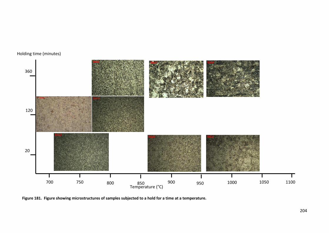
204
Figure 181. Figure showing microstructures of samples subjected to a hold for a time at a temperature.
Temperature (°C) 700 750 800 850 900 950 1000 1050 1100
20
120
360
Holding time (minutes)
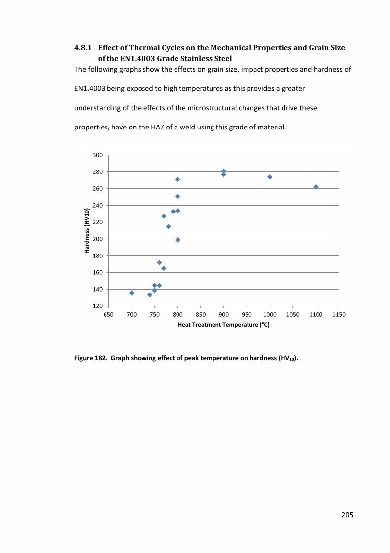
205
4.8.1 Effect of Thermal Cycles on the Mechanical Properties and Grain Size
of the EN1.4003 Grade Stainless Steel
The following graphs show the effects on grain size, impact properties and hardness of
EN1.4003 being exposed to high temperatures as this provides a greater
understanding of the effects of the microstructural changes that drive these
properties, have on the HAZ of a weld using this grade of material.
Figure 182. Graph showing effect of peak temperature on hardness (HV10).
120
140
160
180
200
220
240
260
280
300
650 700 750 800 850 900 950 1000 1050 1100 1150
Ha
rdn
ess
(H
V1
0)
Heat Treatment Temperature (°C)
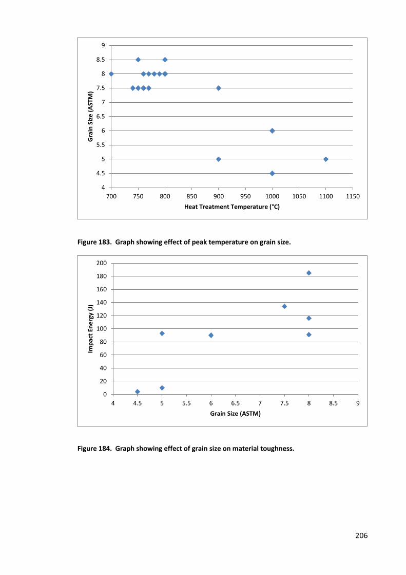
206
Figure 183. Graph showing effect of peak temperature on grain size.
Figure 184. Graph showing effect of grain size on material toughness.
4
4.5
5
5.5
6
6.5
7
7.5
8
8.5
9
700 750 800 850 900 950 1000 1050 1100 1150
Gra
in S
ize
(A
ST
M)
Heat Treatment Temperature (°C)
0
20
40
60
80
100
120
140
160
180
200
4 4.5 5 5.5 6 6.5 7 7.5 8 8.5 9
Imp
act
En
erg
y (
J)
Grain Size (ASTM)
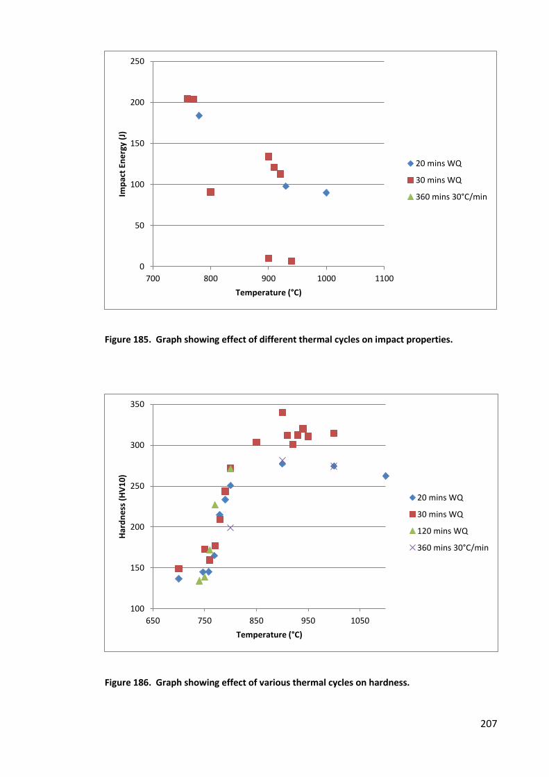
207
Figure 185. Graph showing effect of different thermal cycles on impact properties.
Figure 186. Graph showing effect of various thermal cycles on hardness.
0
50
100
150
200
250
700 800 900 1000 1100
Imp
act
En
erg
y (
J)
Temperature (°C)
20 mins WQ
30 mins WQ
360 mins 30°C/min
100
150
200
250
300
350
650 750 850 950 1050
Ha
rdn
ess
(H
V1
0)
Temperature (°C)
20 mins WQ
30 mins WQ
120 mins WQ
360 mins 30°C/min
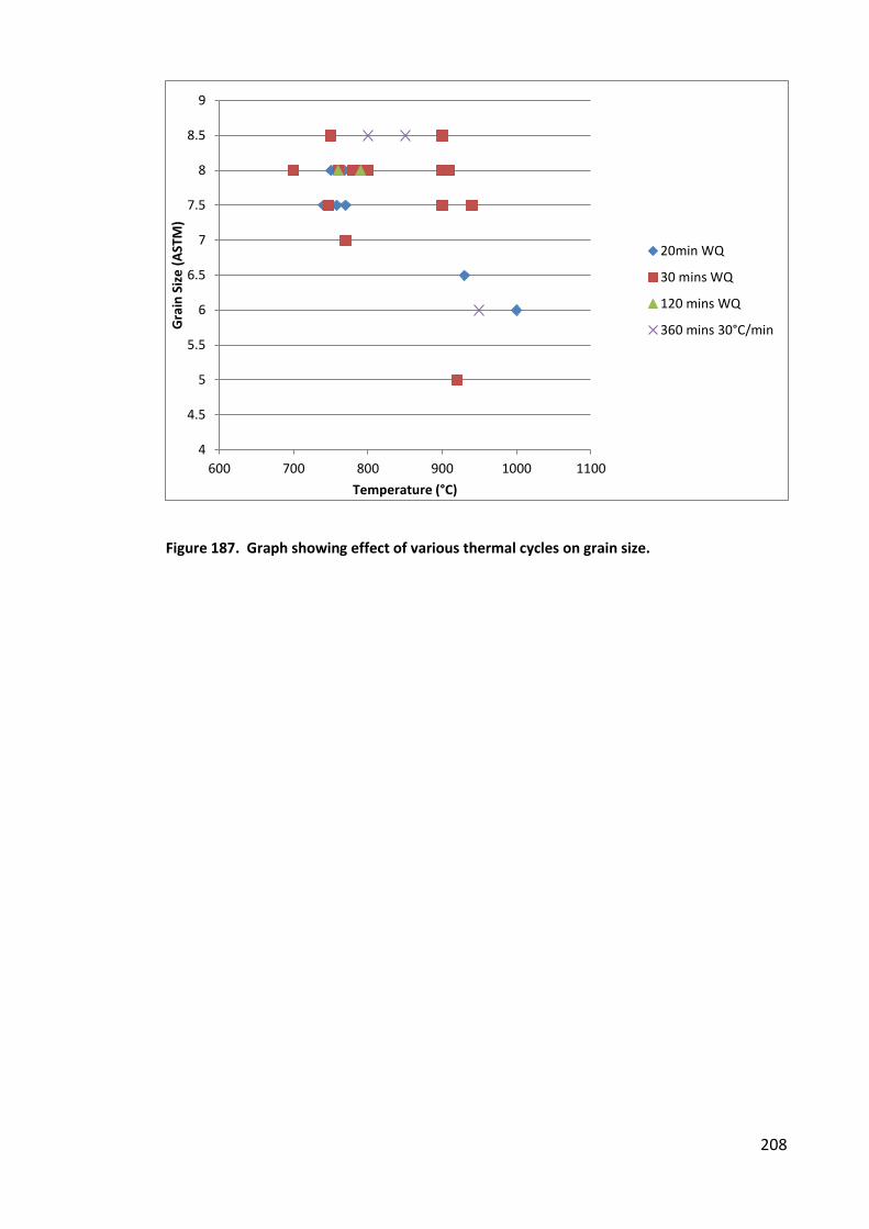
208
Figure 187. Graph showing effect of various thermal cycles on grain size.
4
4.5
5
5.5
6
6.5
7
7.5
8
8.5
9
600 700 800 900 1000 1100
Gra
in S
ize
(A
ST
M)
Temperature (°C)
20min WQ
30 mins WQ
120 mins WQ
360 mins 30°C/min
209
5 Discussion
5.1 Microstructural Materials Characterisation
The microstructural characterisation of the parent materials used in the study showed
the structures that would be expected for each of the grades used. Therefore as can
be seen in Figure 61 to Figure 65 the parent materials show a fully ferritic
microstructure with equi-axed grains. The only evidence of directionality comes from
the consistent orientation of the carbides as seen in Figure 65.
5.2 Initial Comparison of Required Heat Input for MAG and CMT On
EN1.4016, EN1.4509 & EN1.4521 Ferritic Stainless Steel Parent Materials.
The results obtained were based on a relatively small set of samples under laboratory
conditions and it is possible that both the MAG and CMT welding parameters were
capable of further optimisation. The trials did identify the importance of the joint fit
up.
There was a presumption at the commencement of the work that the CMT+P process
would offer the advantage of a reduction in spatter and, more importantly, potential
for a reduction in net heat input, which would be relevant to microstructural control in
ferritic stainless steel joints.
The results from this element of the work indicated that the cold metal transfer
process, with and without pulsed arc, offered no apparent benefit with regards to the
net heat input when compared with MAG welding when joining the 1.5mm thick
materials and under the conditions of test. This is also indicated by the analysis of the
HAZ grain size, where the CMT welded 1.5mm thick 1.4016 & 1.4521 materials had
210
larger average grain sizes, within the coarsest zones, when compared with the results
from the MAG welded joints. However it needs to be taken into account that only
limited material was supplied with the MAG welds to allow the production of the
comparator CMT welds and so full optimisation was not possible on the welds
produced.
The measurements made of the heat affected zone width through optical assessment,
on samples in the etched condition, appear to be confirmed, in most cases, by the
hardness profiles. The exception to this is the MAG welded 1.4016 (702852 1) as seen
in Figure 68 where the hardness in the 20mm span does not return to the base
hardness that is apparent on the other joints produced using the same parent
material. These measurements were checked to confirm the findings. It is likely that
there was some other difference in that area of the plate, possibly compositional
difference, which could be difficult to check as techniques such as XRF are unable to
determine carbon levels and carbon is one of the key elements that can affect the
hardness of a stainless steel, it may also have been as a result of additional cold work.
This would have been evident prior to welding if tests had have been conducted
before the weld was made. It may have been possible that there was cold work
induced in the material due to restraint from the clamping mechanism and the thermal
expansion/contraction associated with the welding process, but this is highly unlikely
as the clamping was consistent across all the samples welded and therefore this would
have been observed in multiple samples and not just the one.
Indications from this work suggest that the CMT process may be of benefit for thicker
materials. When the cold metal transfer welds produced using the 1.4509 (2mm thick)
material are compared, in coarse grain size, with the MAG controls, the grain size for
211
the CMT/CMT+P are ASTM 3.5 and 3.6 respectively. The same material/thickness
combination joined using the MAG process had measured grain sizes, made in the
same locations, of ASTM 3.0 & 3.1, with net heat inputs of 0.129 & 0.101 kJ/mm for
the CMT/CMT+P, the MAG welds had heat inputs of 0.162 & 0.117 kJ/mm.
5.3 Effect on Microstructure and Weld Dimensions of Heat Input Using
Pulsed Arc with CMT on EN1.4016 2mm Thick Parent
The purpose of this aspect of the work was to assess the effect on weld dimensions
and microstructure through variation of the heat input, using CMT welding, with and
without a pulsed arc. Therefore welds were produced at predefined parameter
settings to give specific heat inputs. As can be seen in Table 15 & Table 16 as the heat
input increases, so does the average width of the heat affected zone, this is to be
expected as with an increase in energy into the joint would increase the area that is
affected by this energy. It has also been observed with these results that in the case of
the CMT with the additional pulsed arc, as the heat input increases, the parent to weld
cap angle increases, which therefore means that the weld cap is getting flatter. This
trend was not observed in the results for the pure CMT welds. The power levels and
therefore the heat input was at the same level, as the welds created using the
additional pulsed arc, but the pure CMT welds had a consistent angle across all the
power settings. This indicates that the weld pool had a reduced wettability, which
would indicate the temperature was lower than that with the addition of the pulsed
arc.
The grain size measurements made in the parent material give an ASTM grain size of
approximately 7. The results show that in the HAZ there is a significant change in this
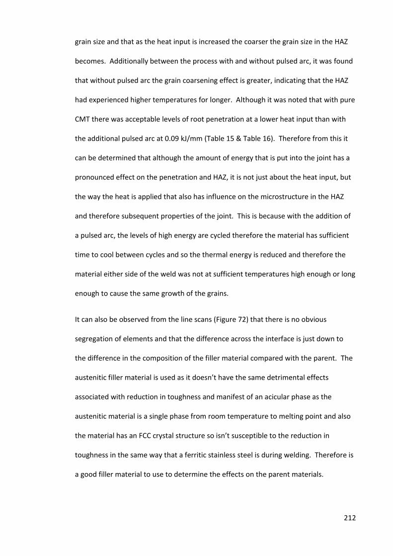
212
grain size and that as the heat input is increased the coarser the grain size in the HAZ
becomes. Additionally between the process with and without pulsed arc, it was found
that without pulsed arc the grain coarsening effect is greater, indicating that the HAZ
had experienced higher temperatures for longer. Although it was noted that with pure
CMT there was acceptable levels of root penetration at a lower heat input than with
the additional pulsed arc at 0.09 kJ/mm (Table 15 & Table 16). Therefore from this it
can be determined that although the amount of energy that is put into the joint has a
pronounced effect on the penetration and HAZ, it is not just about the heat input, but
the way the heat is applied that also has influence on the microstructure in the HAZ
and therefore subsequent properties of the joint. This is because with the addition of
a pulsed arc, the levels of high energy are cycled therefore the material has sufficient
time to cool between cycles and so the thermal energy is reduced and therefore the
material either side of the weld was not at sufficient temperatures high enough or long
enough to cause the same growth of the grains.
It can also be observed from the line scans (Figure 72) that there is no obvious
segregation of elements and that the difference across the interface is just down to
the difference in the composition of the filler material compared with the parent. The
auste iti filler aterial is used as it does t ha e the sa e detri e tal effe ts
associated with reduction in toughness and manifest of an acicular phase as the
austenitic material is a single phase from room temperature to melting point and also
the aterial has a FCC r stal stru ture so is t sus epti le to the redu tio i
toughness in the same way that a ferritic stainless steel is during welding. Therefore is
a good filler material to use to determine the effects on the parent materials.

213
5.4 Trial to Examine the Effects of Variation in the Welding Gap, Torch
Traverse Speed and Torch Angle on the Heat Input Required to Give a
Fully Penetrating Weld using 2mm Thickness EN1.4016 and EN1.4509
Parent Materials.
The first part of the trial made attempt to examine the relationship between weld gap
and weld speed and the ability to produce fully penetrating welds, with identification
of the heat input associated with the welds for both a EN1.4016 and EN1.4509 grade
material. Weld penetration was assessed through a visual inspection of the completed
weld. It can be seen through examination of Figure 74 & Figure 75 that three welding
gaps were tested, 1mm, 1.15mm and 1.25mm and these were welded at three
different welding speeds, 762, 1016 & 1270mm/min. It can be seen that for both
materials there is advantage to increasing the welding gap size, this relates back to
Pepe et al (2011) who identified that it may be more efficient when welding in a gap.
Also increasing the torch traverse speed to reducing the required heat input to
complete a fully penetrating weld. Also subsequently variation of the torch angle from
15° to -15° has a significant effect on the ability to produce a fully penetrating weld at
lower heat inputs in the EN1.4016 material as can be seen in Figure 76, but this was
not as clear when looking at the results for the welding tests conducted on the
EN1.4509 grade material (Figure 77) although the effect of increasing the traverse
speed can be observed.
The use of gap and welding speed variations produced welds in 2mm 1.4016 & 1.4509
with calculated heat inputs significantly lower than those achieved by comparable
MAG welds in 1.4509 in the main comparison programme (Table 14). From this work
images have been taken which show the effect on heat affected zone microstructure
of a reduced heat input (Figure 78). For the welds calculated to have a lower heat
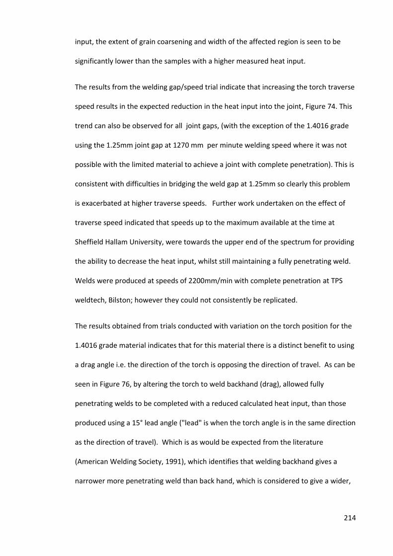
214
input, the extent of grain coarsening and width of the affected region is seen to be
significantly lower than the samples with a higher measured heat input.
The results from the welding gap/speed trial indicate that increasing the torch traverse
speed results in the expected reduction in the heat input into the joint, Figure 74. This
trend can also be observed for all joint gaps, (with the exception of the 1.4016 grade
using the 1.25mm joint gap at 1270 mm per minute welding speed where it was not
possible with the limited material to achieve a joint with complete penetration). This is
consistent with difficulties in bridging the weld gap at 1.25mm so clearly this problem
is exacerbated at higher traverse speeds. Further work undertaken on the effect of
traverse speed indicated that speeds up to the maximum available at the time at
Sheffield Hallam University, were towards the upper end of the spectrum for providing
the ability to decrease the heat input, whilst still maintaining a fully penetrating weld.
Welds were produced at speeds of 2200mm/min with complete penetration at TPS
weldtech, Bilston; however they could not consistently be replicated.
The results obtained from trials conducted with variation on the torch position for the
1.4016 grade material indicates that for this material there is a distinct benefit to using
a drag angle i.e. the direction of the torch is opposing the direction of travel. As can be
seen in Figure 76, by altering the torch to weld backhand (drag), allowed fully
penetrating welds to be completed with a reduced calculated heat input, than those
produced using a 15° lead angle ("lead" is when the torch angle is in the same direction
as the direction of travel). Which is as would be expected from the literature
(American Welding Society, 1991), which identifies that welding backhand gives a
narrower more penetrating weld than back hand, which is considered to give a wider,
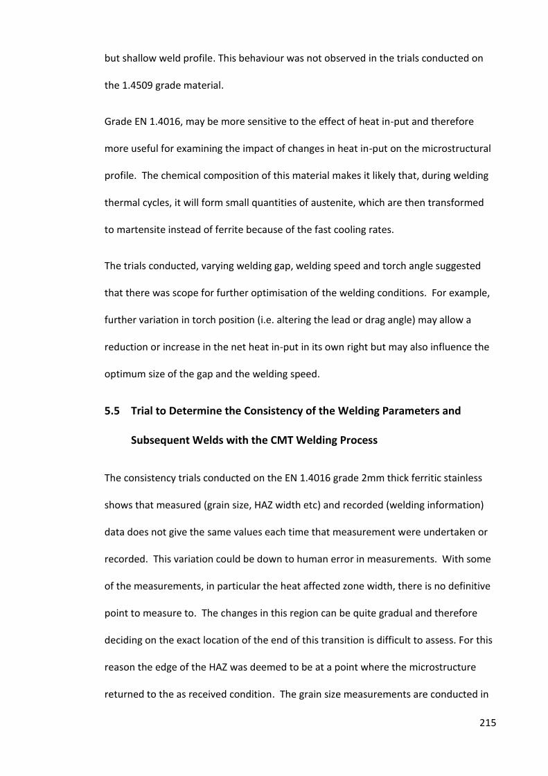
215
but shallow weld profile. This behaviour was not observed in the trials conducted on
the 1.4509 grade material.
Grade EN 1.4016, may be more sensitive to the effect of heat in-put and therefore
more useful for examining the impact of changes in heat in-put on the microstructural
profile. The chemical composition of this material makes it likely that, during welding
thermal cycles, it will form small quantities of austenite, which are then transformed
to martensite instead of ferrite because of the fast cooling rates.
The trials conducted, varying welding gap, welding speed and torch angle suggested
that there was scope for further optimisation of the welding conditions. For example,
further variation in torch position (i.e. altering the lead or drag angle) may allow a
reduction or increase in the net heat in-put in its own right but may also influence the
optimum size of the gap and the welding speed.
5.5 Trial to Determine the Consistency of the Welding Parameters and
Subsequent Welds with the CMT Welding Process
The consistency trials conducted on the EN 1.4016 grade 2mm thick ferritic stainless
shows that measured (grain size, HAZ width etc) and recorded (welding information)
data does not give the same values each time that measurement were undertaken or
recorded. This variation could be down to human error in measurements. With some
of the measurements, in particular the heat affected zone width, there is no definitive
point to measure to. The changes in this region can be quite gradual and therefore
deciding on the exact location of the end of this transition is difficult to assess. For this
reason the edge of the HAZ was deemed to be at a point where the microstructure
returned to the as received condition. The grain size measurements are conducted in
216
such a way as to capture the coarsest grains within the heat affected zone. This is
determined by the operator making the assessments and so subject to errors, but this
was considered the best way of capturing this information as it allowed quantitative
assessment of the grains most likely to reduce the properties of the joint overall. That
said the coarsest grains contained within the heat affected zone, as a rule, tend to be
located close to the weld fusion zone, which is due to this area reaching higher
temperatures than those experienced further away from the fusion zone
(Lakshminarayanan, Shanmugam, & Balasubramanian, 2009) and are generally under
the weld cap. The fact that they are under the weld cap potentially provides two
benefits, the first is that the cross section in this area is increased to greater than that
of the parent material owing to the reinforcement on the weld cap. The second, is
that the filler material used was austenitic, therefore the enhanced grain size in the
HAZ can reduce the toughness of the steel, through reducing the number of barriers
(grain boundaries) to the movement of dislocations, but the filler could compensate
for this reduction in properties, due to the austenitic filler having a Face Centred Cubic
(FCC) crystal structure (Ashby & Jones, 2001) that allows the mechanism of ductility,
dislocation motion, across a greater number of slip systems, than the Body Centred
Cubic (BCC) ferritic stainless steel parent material. Consistency with these
measurements was maintained through the same operator making them.
5.5.1 CMT Power Setting
The variation in power setting was done via the wire feed adjustment as all welds were
conducted using a synergic programme. This automatically adjusts the power settings
when the filler material and thickness and shielding gas are inputted into the
equipment. Therefore, it was found that increasing the power has a profound effect
217
on the heat input of the weld, and increasing the power level, increased the heat
input, with an associated decrease with a reduction in power level. The consistency of
the average values from run to run at the same settings varied. Variations in both the
measured average value for current and voltage changing by up to 15 amps and 1.9
volts respectively which is as a result of the CMT control software means that if there
is a variation in the energy going in to the material there is bound to be a related
variation to the structure and mechanical properties caused through the input of this
heat.
The increase in power had the associated increase on the measurements made of the
weld cap width, HAZ width and weld cap height. It was found that the weld cap width
increased approximately 700µm for every 1m/min increase in the wire feed speed.
There was a similar increase also seen for the HAZ width and weld cap height. The
weld cap height is unsurprising since there was an increase in the amount of wire that
was being fed towards the joint it is expected that the weld cap would be either taller,
wider or both.
The consistency of the measured data from the microstructural measurements made
varied from run to run, as a rule the pattern was similar for each of the HAZ width
measurements made on each run. Furthermore there would be the expectation that
toward the end of the run the HAZ width would increase, due to the heat build-up, but
there was no clear evidence of this occurring.
The investigation also revealed that an increase or decrease of the wire feed setting,
affected the number of pulses per CMT cycle. With the 3.5m/min having 5 pulses per
CMT cycle, the 4.5m/min setting having 6 pulses per CMT cycle and the 5.5m/min
having 7 pulses per CMT cycle. So not only is there an increase in the base power, but
218
also there is an increase in the number of short bursts of high power inputted into the
joint, which will have the associated effects on the microstructure of potentially an
extended HAZ and enlarged grain size.
5.5.2 Arc Length Correction
The variation permitted in the arc length correction function ranges from a value of -30
to +30 and was found to have an effect on the HAZ width. The consistency of the HAZ
width, reduced by changing the ALC to -30 as when the ALC is set to +30 the results are
relatively consistent as can be seen in Figure 92 & Figure 93. The heat input was found
to alter slightly through the extremes of this parameter, with a value of -30 showing a
higher value than that with an arc length correction of zero. This again was slightly
higher than that with an arc length correction of +30, however the total difference was
calculated to be approximately 6 J/mm between the two extremities of variation for
this parameter.
When examining Table 18, it can be seen a greater number of welds are produced with
complete penetration when the arc length correction is set at -30, which may be due
to the extended period in the short circuit phase of the cycle as discussed by Pickin et
al (2011). There may also be a benefit from the slight additional heat that this setting
affords the joint. However it may be as a result of the difference in arc length that this
parameter potentially affords. The welds created at the increased levels of arc length
correction have a high concentration of welds with penetration bias to one side. This
may again be as a direct result of the change in arc length and the ability of deviation
of the arc that is facilitating this bias in the weld. This may be due to slight changes in
magnetic field as the parent material is magnetic, the filler isn't and therefore slight
variations in dilution could affect the orientation of the arc relative to the torch and
219
work piece. The longer the arc, the greater effect the deviation will have which
potentially explains why this is not seen at ALC of -30, where the length of the arc is
shorter.
The measurements made under the optical microscope also provide similar results.
When the arc length correction factor is set at -30 there is a slight increase in the
measured heat affected zone width and weld cap width and height. At both the other
settings for this parameter (0 and +30) there was not a distinct difference between the
measured heat affected zone or weld cap dimensions, between the two. This suggests
that for this material grade, thickness combination the parameter needs to be adjusted
to below 0 to produce a fully penetrating weld.
One of the interesting things to note from this parameter setting is that measurements
made along each of the weld runs are fairly consistent giving a relatively flat line when
the +30 arc length correction is used. With the -30 setting the welds were found to be
less consistent then the +30 not just weld to weld but also across the weld.
5.5.3 Pulse Correction
The pulse correction parameter on the CMT equipment has adjustability from -5 to +5,
this is a unit less parameter. When the correction was set at -5, the heat input was
calculated to be approximately 74 J/mm. When set to zero the calculated heat input
was determined to be approximately 88 J/mm and when at +5 the heat input was
found to be approximately 102 J/mm. Therefore there appears to be a linear increase
in the heat input when altering this setting. It was found through this study that the
reason for this is because the variation of this parameter varies the power of each of
the pulses. Increasing the pulse correction increases the voltage and current of each
220
of the pulses within the CMT cycle and therefore gives the increase/decrease in the
heat input.
Examination of Table 18 shows that a pulse correction factor of -5 does not produce
one part of the weld examined, on any of the welds produced with this setting, with
complete penetration and is therefore a product of insufficient heat into the weld.
When the setting is at 0, there are a number of places in the weld where the
penetration is insufficient but the majority of the welds show penetration to one side.
However this is consistent across most of the weld sections examined therefore from
the 31 sections, only one had suitable penetration (9 were identified as not having
suitable penetration) and so it is unlikely that achieving a consistently fully penetrating
weld is possible with these settings even if the penetration was not bias to one side.
There is a significant increase in the measured values of the width of the heat affected
zone for the welds with a pulse correction of +5, with values increasing as much as
1.5mm from those measured from welds created with a -5 pulse correction setting. It
is likely however that these results are as a result of the low heat input and therefore
lack of penetration of the welds created at -5 pulse correction.
As there is such a dramatic effect from variation of this parameter it would be
interesting to repeat this trial but with variation at increased wire feed settings as they
would have an increased number of pulses per CMT cycle and therefore the variation
of the pulse correction should have notable variation across the whole range from -5
to +5.
221
5.5.4 Traverse Speed
The heat input formula as seen in Equation 3, as seen on page 47, which is essentially
the power divided by the traverse speed means that there is expected to be a
significant difference in the heat input by variation of the traverse speed. Variations
conducted in a separate trial within this study have shown that there is the possibility
of reducing the heat input into a weld through increasing the speed of traverse. The
variation in heat input through the change in traverse speed from 0.762 to 1.27m/min,
results in a change of up to 50 J/mm from approximately 120 J/mm for the slower
traverse speed to 70 J/mm for the faster traverse speed.
The welds created utilising a slower traverse speed produced a significant proportion
of fully penetrated welds as compared to the faster speeds which only yielded portions
of a weld run with complete penetration, as seen in Table 18.
The heat affected zone as would be expected is significantly larger for the slower
traverse speed that with the faster traverse speed (Figure 88 & Figure 89), with a
difference between the two of approximately 0.5 to 1mm. It was observed that the
reduction in speed also provides a more consistent weld along the length of the run
and also reasonable consistency from weld to weld.
The limitation of traverse speed was in the case of these trials of no apparent benefit
as at the upper range assessed the welds were incomplete in terms of penetration.
5.5.5 Torch Angle
The variation in torch angle was made from a push angle of approximately +15° to a
drag angle of approximately -15°. The calculated heat input showed that changing
between the two resulted in a difference, with a marginal increase through using a
222
push angle. The reason for this is, at this time, unknown and may simply be as a result
of the limited number of readings as the range between the two overlap. It could be
that as with a push angle there is a flatter bead and therefore an increased time
duration to contact with the weld pool and therefore an increase in the open circuit
part of the CMT cycle.
There are also a higher number of incompletely penetrated welds with push angle and
at the same time a higher number of completely penetrated welds than those welds
conducted utilising a -15° torch angle. This goes against the concept of a certain
requirement of heat input to provide a fully penetrating weld for certain
materials/thickness combination, or alludes that other factors need to be taken into
account when calculating the net heat input of a weld as variation of the torch angle
does not in itself add any energy, but directs it either at the newly made weld (pull) or
away from the weld (push), but has a significant effect on the penetration and
geometry of the weld and therefore may influence the efficiency of the process.
The measurements made on the optical microscope show that with a torch angle of
+15° (push angle), the heat affected zone is approximately 0.5mm larger, than the
results from the examinations taken from the welds produced using a -15° torch angle.
This then confirms work done previously in this study where drag angles produce a
thin and deep weld profile, whereas a push angle yields a wide and shallow weld
profile. This shallow profile produces a wider weld reinforcement and a wider HAZ.
5.5.6 ALX Data
The arc logging equipment provided the ability to monitor the weld as it was being
produced, with readings taken of current, voltage, traverse speed and wire feed speed
at a rate of 3000 data capture points per second, throughout the duration of the
223
monitored weld. This enabled the identification of the number of pulses per CMT
cycle as identified earlier in this discussion and was easy to determine through
examination of the trace of voltage and current against data point as seen in Figure 85
to Figure 87, where the peaks of each pulse can easily be determined. It is also been
observed from these graphs that the effect of the pulse correction is to increase the
current of the pulse. Therefore when the pulse correction is set to -5, the current for
each of the pulses is approximately 280 amps, with the pulse correction set at 0 and +5
the currents are 340 amperes and 400 amperes, respectively. There also appears to be
an increased duration between the last pulse within a CMT cycle and the first pulse of
the next, as the pulse correction value in increased. The reason for this could be that
with an increased pulse correction, there is the determined increase in pulsing current,
which in turn would be increasing the amount of material that is melted and projected
to the joint and therefore increases the arc length and so the time required for the
electrode tip to make contact with the weld pool.
This theory is substantiated when the traces for the arc length correction parameters
were altered, as similar differences can be observed with these results. When
variation of the arc length correction parameter is made a similar effect can be seen on
the graph where the time duration between the last pulse of the CMT cycle and the
voltage drop through detection of short circuit. This effect is probably that which
provides the slightly higher calculated heat input when the arc length correction is set
to -30, than at +30.
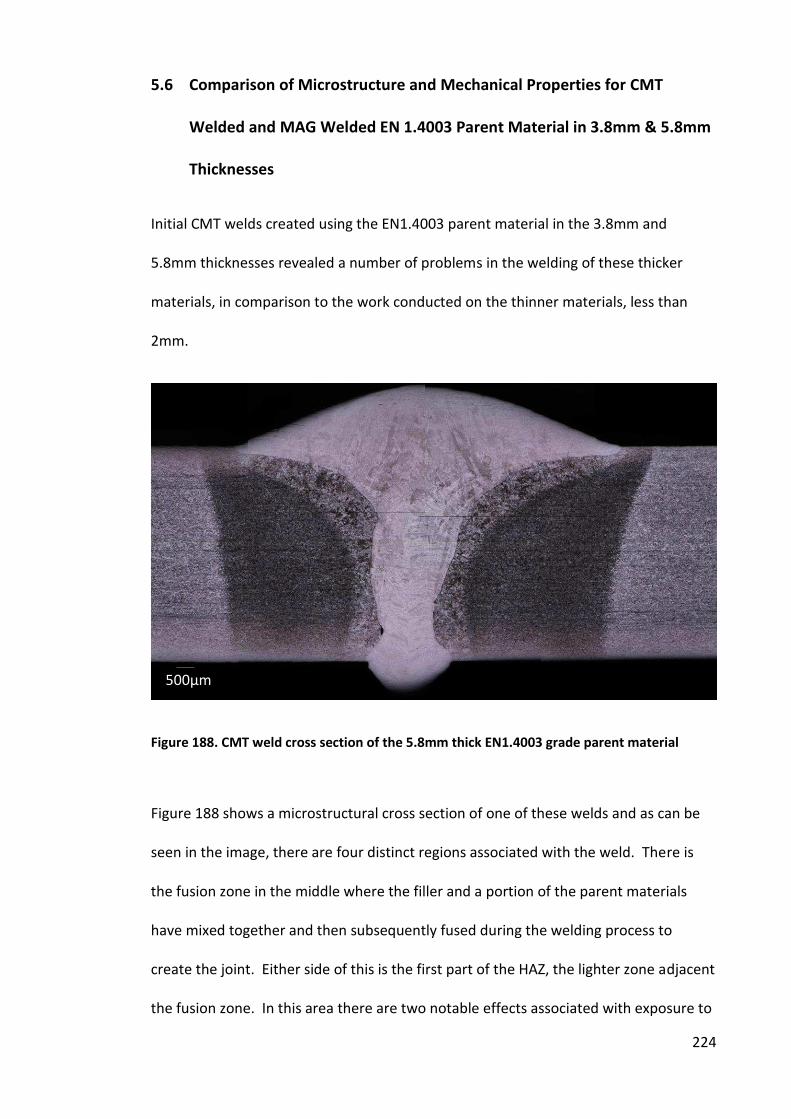
224
5.6 Comparison of Microstructure and Mechanical Properties for CMT
Welded and MAG Welded EN 1.4003 Parent Material in 3.8mm & 5.8mm
Thicknesses
Initial CMT welds created using the EN1.4003 parent material in the 3.8mm and
5.8mm thicknesses revealed a number of problems in the welding of these thicker
materials, in comparison to the work conducted on the thinner materials, less than
2mm.
Figure 188. CMT weld cross section of the 5.8mm thick EN1.4003 grade parent material
Figure 188 shows a microstructural cross section of one of these welds and as can be
seen in the image, there are four distinct regions associated with the weld. There is
the fusion zone in the middle where the filler and a portion of the parent materials
have mixed together and then subsequently fused during the welding process to
create the joint. Either side of this is the first part of the HAZ, the lighter zone adjacent
the fusion zone. In this area there are two notable effects associated with exposure to
500µm
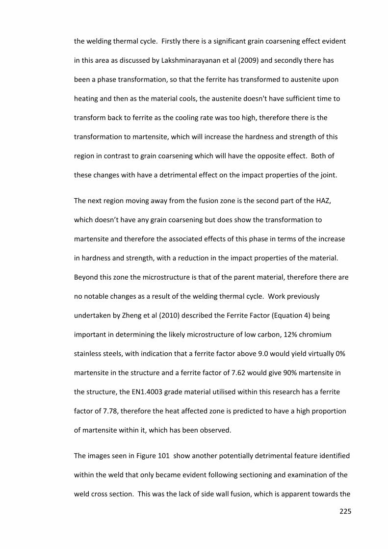
225
the welding thermal cycle. Firstly there is a significant grain coarsening effect evident
in this area as discussed by Lakshminarayanan et al (2009) and secondly there has
been a phase transformation, so that the ferrite has transformed to austenite upon
heating and then as the material cools, the austenite doesn't have sufficient time to
transform back to ferrite as the cooling rate was too high, therefore there is the
transformation to martensite, which will increase the hardness and strength of this
region in contrast to grain coarsening which will have the opposite effect. Both of
these changes with have a detrimental effect on the impact properties of the joint.
The next region moving away from the fusion zone is the second part of the HAZ,
hi h does t ha e a grai oarse i g ut does sho the tra sfor atio to
martensite and therefore the associated effects of this phase in terms of the increase
in hardness and strength, with a reduction in the impact properties of the material.
Beyond this zone the microstructure is that of the parent material, therefore there are
no notable changes as a result of the welding thermal cycle. Work previously
undertaken by Zheng et al (2010) described the Ferrite Factor (Equation 4) being
important in determining the likely microstructure of low carbon, 12% chromium
stainless steels, with indication that a ferrite factor above 9.0 would yield virtually 0%
martensite in the structure and a ferrite factor of 7.62 would give 90% martensite in
the structure, the EN1.4003 grade material utilised within this research has a ferrite
factor of 7.78, therefore the heat affected zone is predicted to have a high proportion
of martensite within it, which has been observed.
The images seen in Figure 101 show another potentially detrimental feature identified
within the weld that only became evident following sectioning and examination of the
weld cross section. This was the lack of side wall fusion, which is apparent towards the
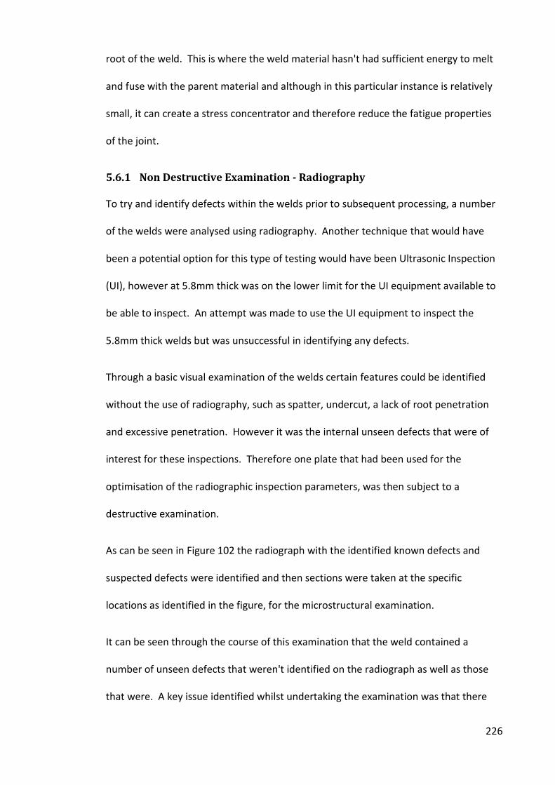
226
root of the weld. This is where the weld material hasn't had sufficient energy to melt
and fuse with the parent material and although in this particular instance is relatively
small, it can create a stress concentrator and therefore reduce the fatigue properties
of the joint.
5.6.1 Non Destructive Examination - Radiography
To try and identify defects within the welds prior to subsequent processing, a number
of the welds were analysed using radiography. Another technique that would have
been a potential option for this type of testing would have been Ultrasonic Inspection
(UI), however at 5.8mm thick was on the lower limit for the UI equipment available to
be able to inspect. An attempt was made to use the UI equipment to inspect the
5.8mm thick welds but was unsuccessful in identifying any defects.
Through a basic visual examination of the welds certain features could be identified
without the use of radiography, such as spatter, undercut, a lack of root penetration
and excessive penetration. However it was the internal unseen defects that were of
interest for these inspections. Therefore one plate that had been used for the
optimisation of the radiographic inspection parameters, was then subject to a
destructive examination.
As can be seen in Figure 102 the radiograph with the identified known defects and
suspected defects were identified and then sections were taken at the specific
locations as identified in the figure, for the microstructural examination.
It can be seen through the course of this examination that the weld contained a
number of unseen defects that weren't identified on the radiograph as well as those
that were. A key issue identified whilst undertaking the examination was that there
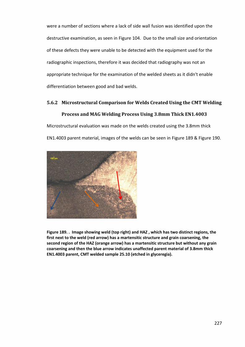
227
were a number of sections where a lack of side wall fusion was identified upon the
destructive examination, as seen in Figure 104. Due to the small size and orientation
of these defects they were unable to be detected with the equipment used for the
radiographic inspections, therefore it was decided that radiography was not an
appropriate technique for the examination of the welded sheets as it didn't enable
differentiation between good and bad welds.
5.6.2 Microstructural Comparison for Welds Created Using the CMT Welding
Process and MAG Welding Process Using 3.8mm Thick EN1.4003
Microstructural evaluation was made on the welds created using the 3.8mm thick
EN1.4003 parent material, images of the welds can be seen in Figure 189 & Figure 190.
Figure 189. . Image showing weld (top right) and HAZ , which has two distinct regions, the
first next to the weld (red arrow) has a martensitic structure and grain coarsening, the
second region of the HAZ (orange arrow) has a martensitic structure but without any grain
coarsening and then the blue arrow indicates unaffected parent material of 3.8mm thick
EN1.4003 parent, CMT welded sample 25.10 (etched in glyceregia).
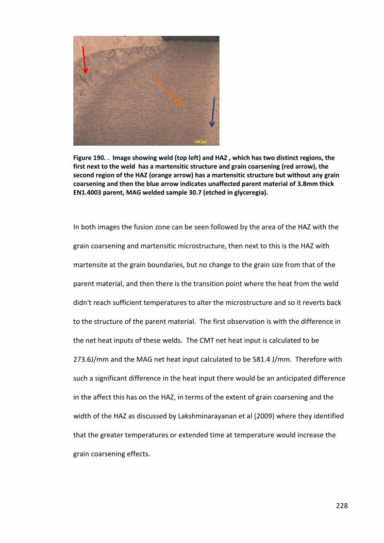
228
Figure 190. . Image showing weld (top left) and HAZ , which has two distinct regions, the
first next to the weld has a martensitic structure and grain coarsening (red arrow), the
second region of the HAZ (orange arrow) has a martensitic structure but without any grain
coarsening and then the blue arrow indicates unaffected parent material of 3.8mm thick
EN1.4003 parent, MAG welded sample 30.7 (etched in glyceregia).
In both images the fusion zone can be seen followed by the area of the HAZ with the
grain coarsening and martensitic microstructure, then next to this is the HAZ with
martensite at the grain boundaries, but no change to the grain size from that of the
parent material, and then there is the transition point where the heat from the weld
didn't reach sufficient temperatures to alter the microstructure and so it reverts back
to the structure of the parent material. The first observation is with the difference in
the net heat inputs of these welds. The CMT net heat input is calculated to be
273.6J/mm and the MAG net heat input calculated to be 581.4 J/mm. Therefore with
such a significant difference in the heat input there would be an anticipated difference
in the affect this has on the HAZ, in terms of the extent of grain coarsening and the
width of the HAZ as discussed by Lakshminarayanan et al (2009) where they identified
that the greater temperatures or extended time at temperature would increase the
grain coarsening effects.
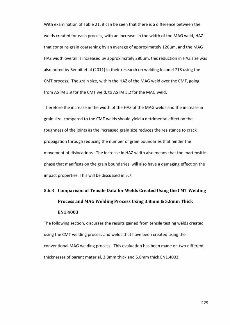
229
With examination of Table 21, it can be seen that there is a difference between the
welds created for each process, with an increase in the width of the MAG weld, HAZ
that contains grain coarsening by an average of approximately 120µm, and the MAG
HAZ width overall is increased by approximately 280µm, this reduction in HAZ size was
also noted by Benoit et al (2011) in their research on welding Inconel 718 using the
CMT process. The grain size, within the HAZ of the MAG weld over the CMT, going
from ASTM 3.9 for the CMT weld, to ASTM 3.2 for the MAG weld.
Therefore the increase in the width of the HAZ of the MAG welds and the increase in
grain size, compared to the CMT welds should yield a detrimental effect on the
toughness of the joints as the increased grain size reduces the resistance to crack
propagation through reducing the number of grain boundaries that hinder the
movement of dislocations. The increase in HAZ width also means that the martensitic
phase that manifests on the grain boundaries, will also have a damaging effect on the
impact properties. This will be discussed in 5.7.
5.6.3 Comparison of Tensile Data for Welds Created Using the CMT Welding
Process and MAG Welding Process Using 3.8mm & 5.8mm Thick
EN1.4003
The following section, discusses the results gained from tensile testing welds created
using the CMT welding process and welds that have been created using the
conventional MAG welding process. This evaluation has been made on two different
thicknesses of parent material, 3.8mm thick and 5.8mm thick EN1.4003.
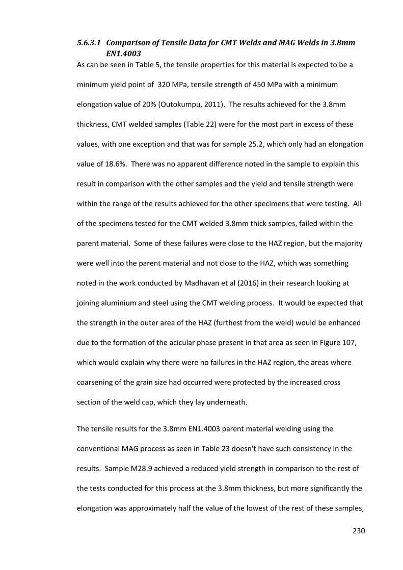
230
5.6.3.1 Comparison of Tensile Data for CMT Welds and MAG Welds in 3.8mm
EN1.4003
As can be seen in Table 5, the tensile properties for this material is expected to be a
minimum yield point of 320 MPa, tensile strength of 450 MPa with a minimum
elongation value of 20% (Outokumpu, 2011). The results achieved for the 3.8mm
thickness, CMT welded samples (Table 22) were for the most part in excess of these
values, with one exception and that was for sample 25.2, which only had an elongation
value of 18.6%. There was no apparent difference noted in the sample to explain this
result in comparison with the other samples and the yield and tensile strength were
within the range of the results achieved for the other specimens that were testing. All
of the specimens tested for the CMT welded 3.8mm thick samples, failed within the
parent material. Some of these failures were close to the HAZ region, but the majority
were well into the parent material and not close to the HAZ, which was something
noted in the work conducted by Madhavan et al (2016) in their research looking at
joining aluminium and steel using the CMT welding process. It would be expected that
the strength in the outer area of the HAZ (furthest from the weld) would be enhanced
due to the formation of the acicular phase present in that area as seen in Figure 107,
which would explain why there were no failures in the HAZ region, the areas where
coarsening of the grain size had occurred were protected by the increased cross
section of the weld cap, which they lay underneath.
The tensile results for the 3.8mm EN1.4003 parent material welding using the
conventional MAG process as seen in Table 23 doesn't have such consistency in the
results. Sample M28.9 achieved a reduced yield strength in comparison to the rest of
the tests conducted for this process at the 3.8mm thickness, but more significantly the
elongation was approximately half the value of the lowest of the rest of these samples,

231
at 8.6%. It was noted for this sample that the failure initiated in the parent material
next to a piece of spatter. The remainder of the samples all failed in the parent
material, although were noted to have all failed close to the HAZ. These tensile tests
also demonstrated a similar yield point to those created using the CMT process, but
there was a greater variation and an overall reduction in the average elongation values
from 21% for the CMT welds to 18% for the MAG welds and a slight associated
increase in the tensile strength to that of the CMT welds.
5.6.3.2 Comparison of Tensile Data for CMT Welds and MAG Welds in 5.8mm
EN1.4003
For the tensile tests conducted on the 5.8mm thick material welded using the CMT
process, the elongation values (Table 25) are above the specification identified in Table
5 with the exception of sample 50.10, where the value was 12.9%. On this sample the
tensile test failed within the weld region and the fracture surface revealed regions that
lacked fusion through the welding process, the interesting point to note was that it
didn't affect the yield strength or tensile strength values for this sample. Two other
samples were also noted to have cracking in the weld region following testing, even
though failure was in the parent material away from the weld in both instances
(samples 50.11 & 52.1) and both of these demonstrated a slightly reduced elongation
value. A high proportion of these tests didn't meet the specification for the material in
terms of tensile strength and all of them failed to meet the requirements for yield
strength.
The tensile samples testing the properties of the MAG welded 5.8mm thick material
(Table 26) had a greater amount of variability to the data, with again none of these
samples meeting the minimum criteria for yield strength. A number of the samples

232
met the minimum tensile strength requirements however only five of the samples
failed in the parent material (M1.3, M1.4, M1.6, M11.3, M11.4), with the remainder
failing in the weld and a number of instances of evidence showing a lack of fusion
observed in these which indicated that the welds were not optimised and therefore to
the likelihood is that they would need an increase in the power to ensure the fusion in
the root of the weld is achieved. This increase in the heat input into the weld would
have a more pronounced effect on the detrimental effects associated with welding this
material
There was also no removal of the weld cap or any excess penetration in the root,
therefore the weld itself and any of the HAZ between the cap and root will have had an
increase in cross sectional area, which isn't accounted for in the strength
measurements as just the parent cross sectional areas were used for these
calculations. Therefore with the additional cross section in the weld area, reduced the
likelihood of failure in this region, with a sound weld. Although this test was useful in
comparing the two welding processes, failures within the weld themselves have only
manifested due to welding defects, rather than providing the ability to differentiate
between microstructural differences that are created as a result of the different
welding processes. For the welds created using both processes in both thicknesses
there appears to be some advantage to the results seen for the CMT welds as at the
3.8mm thickness the difference is marginal, with slightly better results for the CMT
welds. With the thicker parent material joints it is evident that the joints in all cases
aren't complete and this is having a significant effect on the properties, in particular,
the elongation values.
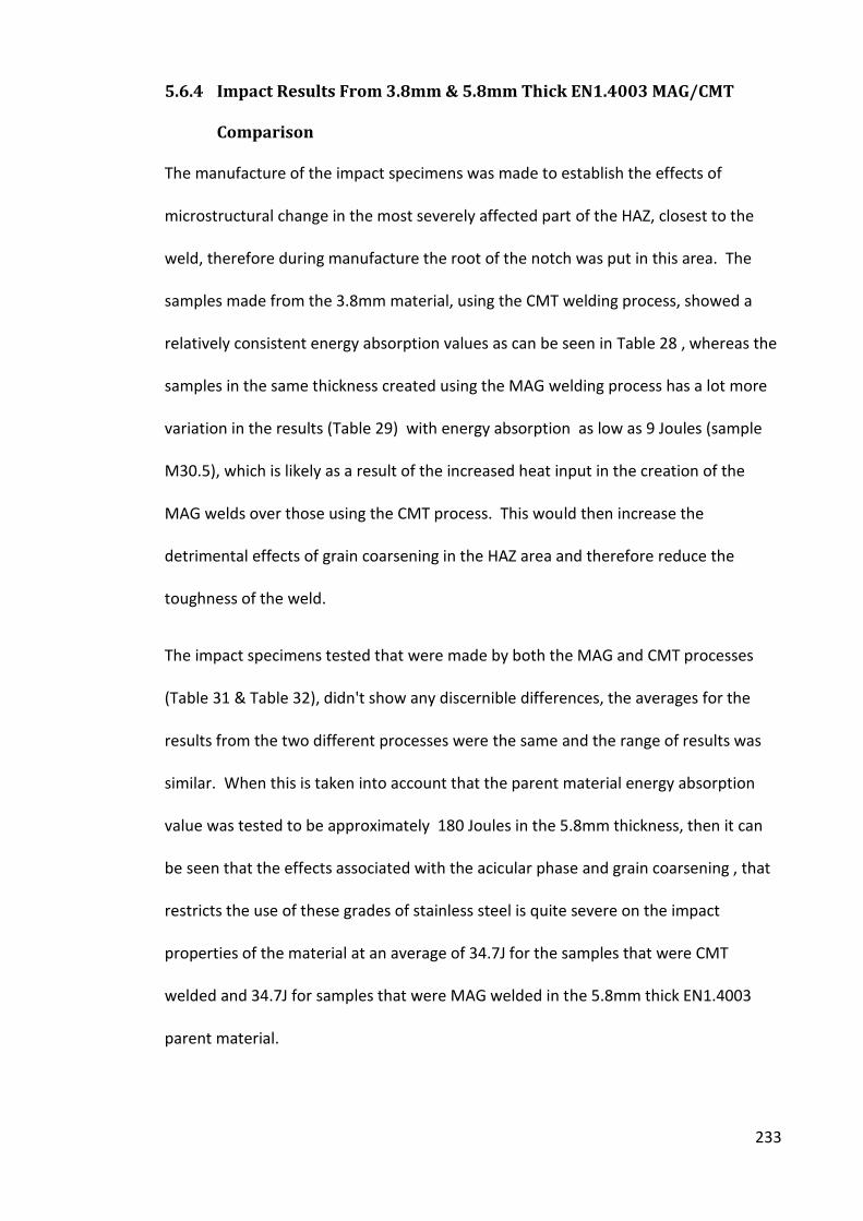
233
5.6.4 Impact Results From 3.8mm & 5.8mm Thick EN1.4003 MAG/CMT
Comparison
The manufacture of the impact specimens was made to establish the effects of
microstructural change in the most severely affected part of the HAZ, closest to the
weld, therefore during manufacture the root of the notch was put in this area. The
samples made from the 3.8mm material, using the CMT welding process, showed a
relatively consistent energy absorption values as can be seen in Table 28 , whereas the
samples in the same thickness created using the MAG welding process has a lot more
variation in the results (Table 29) with energy absorption as low as 9 Joules (sample
M30.5), which is likely as a result of the increased heat input in the creation of the
MAG welds over those using the CMT process. This would then increase the
detrimental effects of grain coarsening in the HAZ area and therefore reduce the
toughness of the weld.
The impact specimens tested that were made by both the MAG and CMT processes
(Table 31 & Table 32), didn't show any discernible differences, the averages for the
results from the two different processes were the same and the range of results was
similar. When this is taken into account that the parent material energy absorption
value was tested to be approximately 180 Joules in the 5.8mm thickness, then it can
be seen that the effects associated with the acicular phase and grain coarsening , that
restricts the use of these grades of stainless steel is quite severe on the impact
properties of the material at an average of 34.7J for the samples that were CMT
welded and 34.7J for samples that were MAG welded in the 5.8mm thick EN1.4003
parent material.
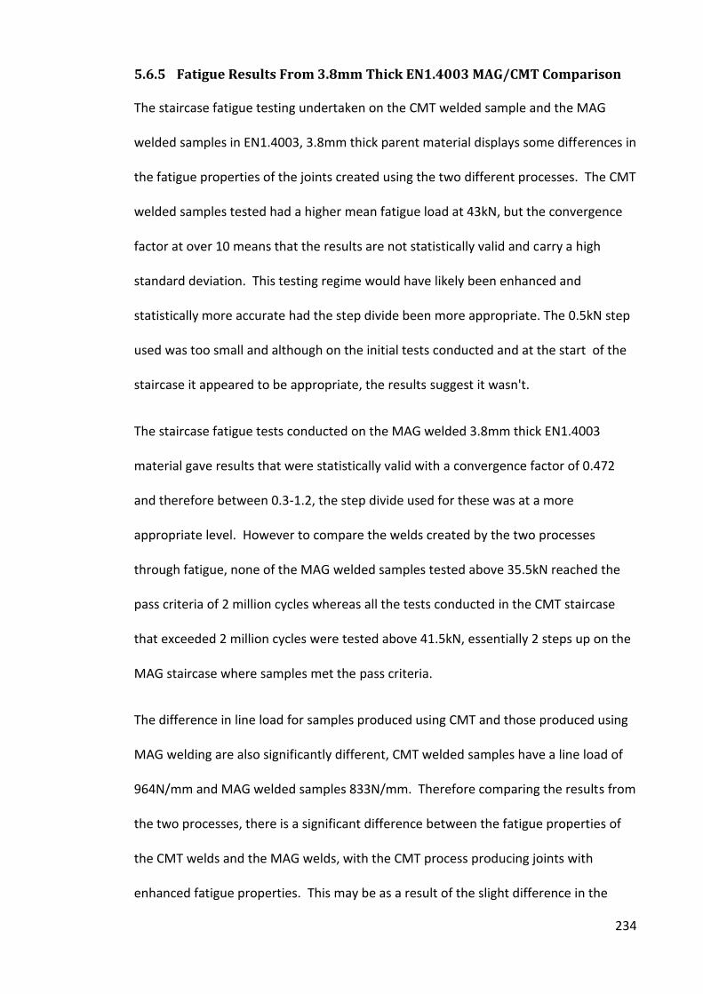
234
5.6.5 Fatigue Results From 3.8mm Thick EN1.4003 MAG/CMT Comparison
The staircase fatigue testing undertaken on the CMT welded sample and the MAG
welded samples in EN1.4003, 3.8mm thick parent material displays some differences in
the fatigue properties of the joints created using the two different processes. The CMT
welded samples tested had a higher mean fatigue load at 43kN, but the convergence
factor at over 10 means that the results are not statistically valid and carry a high
standard deviation. This testing regime would have likely been enhanced and
statistically more accurate had the step divide been more appropriate. The 0.5kN step
used was too small and although on the initial tests conducted and at the start of the
staircase it appeared to be appropriate, the results suggest it wasn't.
The staircase fatigue tests conducted on the MAG welded 3.8mm thick EN1.4003
material gave results that were statistically valid with a convergence factor of 0.472
and therefore between 0.3-1.2, the step divide used for these was at a more
appropriate level. However to compare the welds created by the two processes
through fatigue, none of the MAG welded samples tested above 35.5kN reached the
pass criteria of 2 million cycles whereas all the tests conducted in the CMT staircase
that exceeded 2 million cycles were tested above 41.5kN, essentially 2 steps up on the
MAG staircase where samples met the pass criteria.
The difference in line load for samples produced using CMT and those produced using
MAG welding are also significantly different, CMT welded samples have a line load of
964N/mm and MAG welded samples 833N/mm. Therefore comparing the results from
the two processes, there is a significant difference between the fatigue properties of
the CMT welds and the MAG welds, with the CMT process producing joints with
enhanced fatigue properties. This may be as a result of the slight difference in the
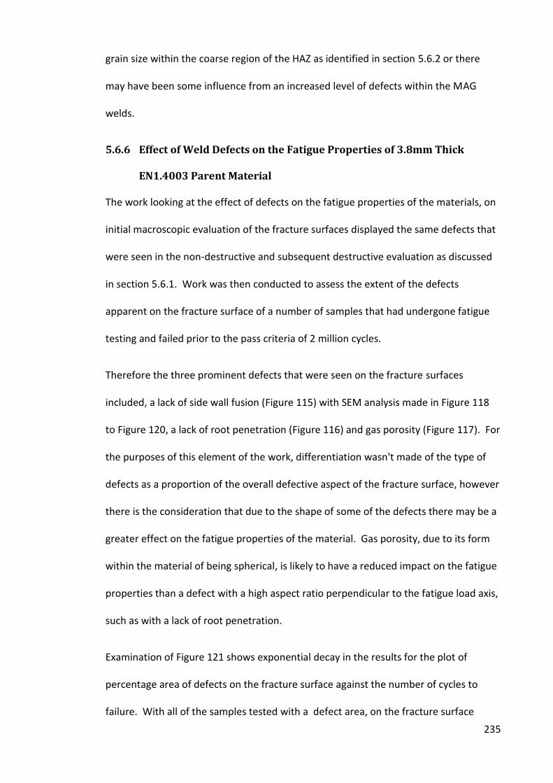
235
grain size within the coarse region of the HAZ as identified in section 5.6.2 or there
may have been some influence from an increased level of defects within the MAG
welds.
5.6.6 Effect of Weld Defects on the Fatigue Properties of 3.8mm Thick
EN1.4003 Parent Material
The work looking at the effect of defects on the fatigue properties of the materials, on
initial macroscopic evaluation of the fracture surfaces displayed the same defects that
were seen in the non-destructive and subsequent destructive evaluation as discussed
in section 5.6.1. Work was then conducted to assess the extent of the defects
apparent on the fracture surface of a number of samples that had undergone fatigue
testing and failed prior to the pass criteria of 2 million cycles.
Therefore the three prominent defects that were seen on the fracture surfaces
included, a lack of side wall fusion (Figure 115) with SEM analysis made in Figure 118
to Figure 120, a lack of root penetration (Figure 116) and gas porosity (Figure 117). For
the purposes of this element of the work, differentiation wasn't made of the type of
defects as a proportion of the overall defective aspect of the fracture surface, however
there is the consideration that due to the shape of some of the defects there may be a
greater effect on the fatigue properties of the material. Gas porosity, due to its form
within the material of being spherical, is likely to have a reduced impact on the fatigue
properties than a defect with a high aspect ratio perpendicular to the fatigue load axis,
such as with a lack of root penetration.
Examination of Figure 121 shows exponential decay in the results for the plot of
percentage area of defects on the fracture surface against the number of cycles to
failure. With all of the samples tested with a defect area, on the fracture surface

236
above 2%, none of the samples survived above 600,000 cycles, just over a quarter of
that required against the 2 million cycle pass criteria. These findings relate to the work
of Tijani et al (2013) who also found relationships between the percentage of defects
in a material and the number of cycles to failure under fatigue loading conditions.
In Figure 121 there is no account taken for the actual load which the samples were
subjected to therefore in Figure 122, there is the information relating to the load
which the sample was tested under. From this data it can be seen that some of the
samples that have relatively low defects observable on the fracture surface and yet
have still failed at a low number of cycles, have in fact been tested at a higher load
level and therefore would be expected to have a reduced life under fatigue testing
conditions. An interesting observation from this figure, is that, where there are
multiple results at the same loading criteria, there appears to be a correlation between
the number of cycles to failure and the percentage of defects measured on the
fracture surface, for each of the testing loads. When the gradient for the number of
cycles to failure against percentage area of defects on the fatigue for each is plotted
against the load, there is a correlation which can be seen in Figure 123. This,
confirming the work that Ottersbock et al (2016) undertook, shows that as the fatigue
load is increased and or the area of defects containing within the weld are increased
there is a reduction in the number of cycles the weld can be subjected to before
failure. But as the load is increased the presence of defects has a more significant
impact on the fatigue life of the component.
237
5.6.7 Effect on Fatigue Properties of the Parent Metal to Reinforcement
Weld Angle
There appears to be a correlation, as seen by Ashcroft (2008) between the root angle
and the number of cycles to failure from looking at the results altogether (see Figure
141), for all the samples that passed two million cycles, the angle of the root was as a
minimum 128 degrees. There was a great deal of variation within this data and some
of this was likely as a result of defects within the joints as discussed in section 5.6.6.
One of the key parameters in the prediction of fatigue life is the load and when
examining the graphs for the angles/cycles at each load (Figure 131 to Figure 140) ,
there would be the expectation from work conducted by Harris and Syers (1979) that
as the load is increased the sensitivity to the angle would increase, however the results
do not indicate this to be the case and it would be recommended for future work to
assess the content of defects evident on the facture surfaces for all the samples.
5.7 Heat Treatment Trial To Identify Key Temperatures At Which
Microstructural Changes Occur And The Effect of Time On These
Changes.
The thermal cycle experienced during the welding process has extremely rapid heating
and cooling rates associated with it as a result of very high arc temperatures and a high
thermal conductivity common to metals. In an attempt to try and simulate the
thermal cycle the trial was devised to identify the point at which temperatures are
sufficient to create microstructural change, such as that seen in the heat affected zone
238
and then identify the effects of the change on the impact properties and hardness of
the material.
It is well established in the literature (Lippold & Kotecki, 2005) that the microstructural
response to a thermal cycle is not just dependant on temperature, but also time and
therefore whilst the trial conducted wasn't an exact replication of the thermal cycle
that was experienced during the manufacture of a weld, it allows some comparisons to
be drawn between observable microstructural features within a heat affected zone,
the likelihood of the temperature reached in this area and then the effect of this on
the mechanical properties.
It can be seen when comparing the image for the sample that had been subjected to
700°C for 20 minutes (Figure 147) to the image of the material in the un-heat treated
state (Figure 62) that there is no observable difference between them in terms of
microstructure. This is the same for all the heat treated samples, held for 20 mins at
temperature, right up until the temperature gets to approximately 770°C (Figure 161)
where the microstructure changes from a fully ferritic structure to one that contains
ferrite and martensite. Associated with this, as can be seen in Figure 182 there is an
increase in the hardness from below 150HV10 to 165HV10 as a result of the presence of
the harder martensite.
When the samples are held for longer (2 hours), the martensitic phase can be seen
appearing in the structure on samples exposed to temperatures of 750°C followed by a
water quench, as seen in Figure 171, with the same cycle applied at 740°C (Figure 172)
the structure remains ferritic which means at this time/temperature combination the
transformation to austenite does not take place.
239
As the temperature is increased, then as is the quantity of martensite within the
microstructure and subsequently the hardness which increases from the parent
material value of 150 HV10, increasing up to approximately 281 HV10 at 900°C and then
as can be seen in Figure 186, the hardness reaches its maximum level of 340 HV10
which varies according to how long the sample has been left at temperature, for the
samples left for 20 minutes, the hardness is not as high as for those samples that were
left for 30 minutes, this could be that 20 minutes at temperature, may not give
sufficient time for elements, particularly carbon, to go into a solid solution, therefore
reducing the hardening effect associated with a fast cool. When looking at the results
for the samples that have been left for 360 minutes there is a slightly softer material
and this will be because holding at the elevated temperatures longer, will permit a
greater amount of grain coarsening and also the slower cool afforded to these
samples, will reduce the amount of carbon that is trapped in solution and therefore
the strain on the structure that gives the increase in hardness associated with
martensite. This reduction on the hardness properties may be as a result of the high
temperature embrittlement that affects these materials when subjected to
temperatures in excess of 900°C, with the additional time allowing the diffusion of
carbon to form the detrimental carbides and carbo-nitrides as discussed in section 2.3.
The other observable trend with the results is that the grain size of ASTM 8, remains
constant up to 900°C where the sample that was held for an extended period of 360
minutes, showed a significant increase in the grain size, going from the ASTM 8, to
ASTM 5 (Figure 187), this is not in agreement with work conducted by
Lakshminarayanan et al (2009) who reported that temperatures above 955°C needed
to be achieved for grain coarsening. For the samples held at shorter durations (20

240
and 30 mins) the samples needed to be at higher temperatures, 940°C - 1000°C to
have a noticeable effect on the grain size, which then when comparing to the welding
process, which experiences temperatures up to the melting point of the material,
would suggest that for the grain coarsening observed in the heat affected zone, may
occur as a result of the higher temperatures experienced during welding (up to the
melting point of the material) rather than the specific temperatures identified in this
study. It also must be noted that with the simulations made in this element of the
work, it was not possible to replicate the heating rates and superheating which will
have effect on the weld and HAZ.
A number of nonstandard impact specimens (5.8 x 10 x 55mm) were created and heat
treated to the same parameters identified through the microstructural work and then
tested to determine the effect on the impact properties of the various microstructural
changes identified. As can be seen in Figure 185 the impact properties of the material
that have undergone no microstructural change is at around 200J. When there is the
introduction of martensite within the structure this reduced the toughness of the
samples down by approximately 30%. When there was not only the martensite within
the structure but also grain growth associated with the higher temperatures, then the
energy absorbed by the specimens dropped to less than 10 J in some instances. The
effect associated with the martensitic structure, is likely as martensite is a brittle phase
and therefore doesn't absorb much energy when a crack is propagating through it.
The grain coarsening reduces the number of grain boundaries that hinder the motion
of dislocations and therefore reduce the toughness of the material.
241
6 Conclusions
The research has examined and compared the CMT welding process against the
conventional GMAW process using ferritic stainless steel and after a review of the
literature and analysis of the results from the work conducted within this research the
following conclusions can be made;
6.1 Research on thin grades (<2mm) of ferritic stainless steel welded using
CMT & MAG techniques
• Increasing the heat input increases the width of the HAZ
• When CMT welding the addition of a pulsed arc, which gives an increase in the
heat input, resulting in a flatter weld reinforcement
• With the use of just CMT, without a pulsed arc, it was found to yield a larger
grain size within the HAZ
• Pure CMT was found to produce fully penetrating welds at a lower heat input
than welds produced with the additional pulsed arc
• The overall heat input has a significant effect on the penetration and HAZ
characteristics and it was found that it wasn't just the energy that is put into
the weld that controls the weld characteristics, but how that energy is applied
e.g. torch angle, pulsed current, torch traverse speed, weld gap as there may
be a variation in the efficiency of the arc energy.
• Greater welding gaps create bridgeability issues at higher torch traverse speeds
• Drag torch angle produces fully penetrating welds at lower heat inputs than
leading angles possibly due to the filler being directly toward previously heated
materials.
242
• Grade EN1.4016 is more sensitive to the thermal cycle associated with welding
than EN1.4009
• The measured power levels of the welds monitored varied by up to 15 amps
and 1.9 volts for the same set level using the CMT process
• The variation in ALC between -30% and +30% was calculated to give a
difference of approximately 6J/mm to the net heat input
• An ALC setting of -30 gave a greater amount of penetration than when the
setting was at +30
• The pulse correction function increases the energy levels of the pulses within
the welding cycle to allow incorporation of short bursts of higher energy.
6.2 Grade EN1.4003 3.8mm and 5.8mm thick material welded using CMT and
MAG techniques
• The HAZ of a weld using EN1.4003 grade parent material has 2 distinct regions,
the first closest the fusion zone has a martensite content and grain coarsening
and further away from the fusion zone, martensite alone
• NDT techniques utilised within the research were insufficient to detect the lack
of side wall fusion evident in the samples following destructive examination
• Tensile tests conducted on the 3.8mm thickness, welding using CMT,
demonstrated 100% joint efficiency
• Tensile tests conducted on the 5.8mm thickness materials produced using each
of the welding techniques did not produce welds that consistently
demonstrated 100% joint efficiency
243
• Average values for the impact tests conducted on samples welded using each
of the techniques were comparable and therefore no discernible difference
could be noted between the effect on toughness
• Fatigue results for CMT shows enhanced properties over the MAG welded
samples for 3.8mm thick EN1.4003 grade material likely due to a reduced effect
on the heat affected zone and a reduced number of defects within the weld.
• Under fatigue testing, no sample that had the fracture surface examined
survived 2 million cycles with a defect area greater than 2% of the fracture
surface
• There was found to be a relationship between the number of cycles to failure at
a particular load and the percentage of the defect area measured on the
fracture surface, which sho s the greater the fatigue load the ore se siti e
the aterial e o es to the defe t o te t
• The weld root angle was >128° for all fatigue tested samples that exceeded 2
million cycles
• At temperatures in excess of 750°C microstructural change is observed from
ferrite to ferrite and martensite for simulated heat treated samples
• The hardness levels associated with martensite in the microstructure of the
simulated heat treated samples increase up to 900°C
• Grain coarsening was observed in the heat treated samples at 900°C after being
held at this temperature for 360 minutes. An increase in temperature above
900°C was required to observe any grain growth for reduced holding times.
• The reduction in impact properties as a result of martensite in the structure
was measured to be approximately 30% for simulated heat treated samples

244
• Impact tests made on simulated heat treatment samples with grain coarsening
and a martensite content were found to reduce the toughness by
approximately 95%
7 Further Work
Following a review of the work undertaken, suggestions for further work are
highlighted below:
• Explore the modification of other welding parameters, such as shielding gas,
the use of a backing gas, welding wire or edge preparation on the production of
welds to eliminate the lack of side wall fusion, seen in a number of welds
produced in this study.
• As part of this work, two thicknesses (3.8mm & 5.8mm) of EN1.4003 grade
stainless steel were subject to assessment, testing of the 5.8mm thick material
requires completing as time limitations prevented this occurring within this
project.
• The results from the CMT 3.8mm thick EN1.4003 parent material, under fatigue
testing didn't produce statistically valid results, therefore for an enhanced
comparison, it is suggested that these tests be repeated using a different step
divide.
• Increase the analysis on defects within the failed fatigue samples to provide a
greater data set and allow comparison between CMT and MAG welded joints.
• Explore options of NDT techniques for the identification of small defects within
welds or optimise radiographic parameters to this end.
• Compare CMT with other 'low heat input' GMAW processes that have been
brought to market.
• Continue work on heat treatment to explore the temperatures at which the
acicular phase first manifests, perhaps using EBSD for phase identification.
245
• Explore the effect of CMT, compared to conventional GMAW on grades of
ferritic stainless more sensitive to embrittlement phenomena.
8 Works Cited
ABB. (2007, November). Arc Welding. Retrieved July 3, 2017, from Complete robot
automation packages for industrial applications:
https://library.e.abb.com/public/91c69c27716683e9c125739b002f8787/Arc%2
0welding%20folder%20WEB.pdf
AIR LIQUIDE. (2009). Gas Encyclopaedia - Helium. Retrieved April 26, 2011, from Air
Liquide: http://encyclopedia.airliquide.com/Encyclopedia.asp?GasID=32
AIR LIQUIDE. (2009). Gas Encyclopedia - Air. Retrieved April 26, 2011, from Air Liquide:
http://encyclopedia.airliquide.com/Encyclopedia.asp?LanguageID=11&CountryI
D=19&Formula=&GasID=73&UNNumber=&EquivGasID=32&VolLiquideBox=&M
asseLiquideBox=&VolGasBox=&MasseGasBox=&RD20=29&RD9=8&RD6=64&R
D4=2&RD3=22&RD8=27&RD2=20&RD18=41&RD7=18&RD13=71&RD16=35
Air Products. (2017). Welding Gas Selector. Retrieved June 27, 2017, from Air Products:
http://www.airproducts.co.uk/microsite/uk/welding_selector/aluminium.htm#
res2
Albertson, T. P., Stephens, R. R., & Bayha, T. D. (1997). Fatigue Crack Growth of Two
Advanced Titanium Alloys at Room and Elevated Temperature. In R. S. Piascik,
R. P. Gangloff, & A. Saxena (Eds.), Elevated Temperature Effects on Fatigue and
Fracture (pp. 140-161). ASTM.
American Welding Society. (1991). Welding Handbook - Welding Processes (8th Edition
ed., Vol. 2). (R. L. O'Brien, Ed.) Miami: American Welding Society.
AMG Vanadium Inc. (2009). Manganese. Retrieved May 26th, 2012, from
Metallurgvanaduim:
http://www.metallurgvanadium.com/manganesepage.html
Amunda, M. O., & Mridha, S. (2011, April 27th). An Overview of Sensitization Dynamics
in Ferritic Stainless Steel Welds. (F. J. Perez, Ed.) International Journal of
Corrosion, 2011, 1-9.
ArcelorMittal. (n.d.). What is Stainless Steel? Manufacturing Process. Retrieved May
19th, 2012, from ArcelorMittal Stainless Europe:
http://www.arcelormittal.com/stainlesseurope/manufacturing-process.html
Armao, F., Byall, L., Kotecki, D., & Miller, D. (2014). Gas Metal Arc Welding Guidelines.
Retrieved September 10, 2016, from

246
http://www.lincolnelectric.com/assets/global/products/consumable_miggmaw
wires-superarc-superarcl-56/c4200.pdf
Ashby, M. F., & Jones, D. R. (2001). Engineering Materials 2 (2nd ed.). Oxford, UK:
Butterworth-Heinemann.
Ashcroft, E. (2008). Mechanical and Metallurgical Properties of Dissimilar Metal Joints
Using Novel Joining Techniques. Sheffield: Sheffield Hallam University.
ASM Handbook Committee. (1988). Metals Handbook- Metallography and
Microstructures (9th ed., Vol. 9). (K. Mills, J. R. Davies, J. D. Destefani, D. A.
Dieterich, G. M. Crankovic, H. J. Frissell, et al., Eds.) Ohio, USA: American
Society For Metals.
ASM International. (2008). Fatigue. Retrieved August 5, 2016, from ASM International:
http://www.asminternational.org/documents/10192/1849770/05224G_Chapte
r14.pdf
Avesta Welding. (2006). Avesta 308LSi Welding Wire. Retrieved August 28, 2012, from
Avesta.com: http://www.avestawelding.com/3273.epibrw
Bailey, N. (1994). Weldability of Ferritic Steels. Cambridge, UK: Abington Publishing.
Battelle-Columbus, B. L. (1996). Effect of Surface Conditions and Processing on Fatigue
Performance. In Fatigue and Fracture (Vol. 19, pp. 785-794). ASM International.
Bax, M., Short, D., & Bayliss, M. (1988). Underwater Inspections (3rd ed.). Taylor and
Francis Ltd.
Bayoumi, M. R., & Abdellatif, A. K. (1995). Effect of Surface Finish on Fatigue Strength.
Engineering Fracture Mechanics, 51(5), 861-870.
Bayraktar, E., Kaplan, D., & Grumbach, M. (2004). Application of Impact Tensile Testing
to Spot Welded Sheets. Journal of Materials Processing Technology(153-154),
80-86.
Beddoes, J., & Parr, G. J. (1999). Introduction to Stainless Steel (3rd ed.). ASM
International.
Benoit, A., Jobez, S., Paillard, P., Klosek, V., & Baudin, T. (2011). Study of Inconel 718
weldability using MIG CMT process. Science and Technology of Welding and
Joining, 16(6), 477-482.
BOC. (2007). Welding Processes. Retrieved September 10, 2016, from
http://www.bocworldofwelding.com.au/media/pdf/file/library/WOWLibrary-
GMAW-FCAW-MCAW%20Welding.pdf
247
BOC UK. (2010). Pureshield Argon - BOC UK. Retrieved March 12th, 2011, from BOC
online:
http://www.boconline.co.uk/products/products_by_type/industrial_gases/iner
t_gases/pureshield_argon.asp
Boulding, J. (2012). The Effects of Parameters and Consistency of Cold Metal Transfer
Welded Ferritic Stainless Steel Joints. Undergraduate Final Year Project,
Sheffield Hallam University, Department of Engineering, Sheffield.
Boulding, J. (2012). The Effects of Parameters and Consistency of Cold Metal Transfer
Welded Ferritic Stainless Steel Joints. Final Year Project, Sheffield Hallam
University, Department of Engineering, Sheffield.
Brearley, H. (1991). Harry Brearley Stainless Pioneer - autobiographical notes.
Sheffield: British Steel Stainless in conjunction with The Kelham Island Industrial
Museum.
British Stainless Steel Association. (n.d.). The Discovery of Stainless Steel. Retrieved
May 26th, 2012, from British Stainless Steel Association:
http://www.bssa.org.uk/about_stainless_steel.php?id=31
British Standards Institution. (1998). Welding - Recommendations for Welding of
Metallic Materials - Part 1 General guidance for arc welding. BSI.
Brownlee, K. A., Hodges, J. L., & Rosenblatt, M. (1953). The up and down method with
small samples. Journal of the American Statistical Association, 48(262), 262-
277.
Burgin, F. K. (2008). Liquid Metal Embrittlement in the Arc Brazing of Stainless Steels.
Retrieved July 23, 2011, from Sheffield Hallam University:
http://www.shu.ac.uk/_assets/pdf/outo-LME%20Poster%20Pres%2004.pdf
Cary, H. B. (1998). The History of Welding. Retrieved June 6, 2010, from Miller:
http://www.millerwelds.com/resources/articles/index?page=articles14.html
Cary, H. B., & Helzer, C. S. (2005). Modern Welding Technology. (E. Francis, Ed.) New
Jersey, Ohio, USA: Pearson Prentice Hall.
Chakrabarty, J. (1987). Theory of Plasticity. McGraw-Hill.
Choulet, R. J. (1997). Stainless Steel Refining. AISE Seminar. Detroit: Praxair Technology
Inc.
Cobb, H. M. (2010). The History of Stainless Steel. USA: ASM International.
Colombier, L., & Hochmann, J. (1967). Stainless and Heat Resisting Steels (1st (English)
ed.). St. Etienne, France: Edward Arnold Ltd.
248
Computational Thermodynamics Inc. (2011). Phase Diagrams - Iron Chromium.
Retrieved June 11, 2011, from Computational Thermodynamics:
http://www.calphad.com/iron-chromium.html
Cortie, M. B. (1993, July). History and Development of Ferritic Stainless Steels. Journal
of The South African Institute of Mining and Metallurgy, 93(7), 165-176.
Cunat, P.-J. (2004). Alloying Elements. Retrieved May 26th, 2012, from Euro-Inox:
www.euro-inox.org/pdf/map/AlloyingElements_EN.pdf
Deddoes, J., Parr, G. J., & Hanson, A. (1999). Introduction to Stainless Steels (3rd ed.).
(J. Beddoes, Ed.) ASM International.
Demo, J. J. (1982). Structure, Costitution and General Characteristics of Wrought
Ferritic Stainless Steels. In R. A. Lula, & R. A. Lula (Ed.), Source Book On The
Ferritic Stainless Steels (pp. 1-65). American Society For Metals.
Dixon, W. J., & Mood, A. M. (1948). A Method for Obtaining and Analyzing Sensitivity
Data. Journal of the American Statistical Association, 43(241), 109-126.
DuPont, J. N. (1999, July). Microstructural Development and Solidification Cracking
Susceptibility of a Stabilised Stainless Steel. Welding Research Supplement, 253-
263.
DuPont, J. N., & Marder, A. R. (1995, December). Thermal Efficiency of Arc Welding
Processes. Welding Research Supplement, pp. 406-416.
Easterling, K. (1992). Introduction to the Physical Metallurgy of Welding (2nd Edition
ed.). Butterworth Heineman.
eFUNDA. (2016). High Cycle Fatigue. Retrieved September 17, 2016, from
http://www.efunda.com/formulae/solid_mechanics/fatigue/fatigue_highcycle.
cfm
Elrefaey, A. (2015). Effectiveness of cold metal transfer process for welding 7075
aluminium alloys. Science and Technology of Welding and Joining, 20(4), 280-
285.
Engineers Edge. (2016). Fatigue Crack Growth Analysis Review - Strength of Materials.
Retrieved August 5, 2016, from
http://www.engineersedge.com/material_science/fatigue_crack_growth_analy
sis_review_10071.htm
ESAB. (2002). Gas Properties. Retrieved May 21, 2011, from ESAB:
http://www.esabna.com/euweb/mig_handbook/592mig4_6.htm
ESAB. (n.d.). Short Circuit (Short Arc) Welding. Retrieved January 27, 2017, from
http://www.esabna.com/euweb/mig_handbook/592mig1_4.htm
249
EWI. (2016). Resistance Seam Welding. Retrieved January 3, 2017, from
https://ewi.org/resistance-seam-welding/
Feng, J., Zhang, H., & He, P. (2009). The CMT short-circuiting metal transfer process
and its use in thin aluminium sheets welding. Materials and Design, 1850-1852.
Filho, D. F., Ferraresi, V. A., & Scotti, A. (2010). Shielding Gas Influence on the Ferritic
Stainless Steel Weldability. Journal of Engineering Manufacture, 224(Part B),
951-961.
Fonius International GmbH. (2005, September). Weld + Vision Archives. Retrieved June
5, 2010, from Fronius International:
http://www.fronius.com/cps/rde/xchg/SID-35E91591-
8A995FC0/fronius_international/hs.xsl/79_11392_ENG_HTML.htm
Fronius International GmBH. (2004, January). CMT Process - A Revolution in Materials-
Joining Technology. Retrieved June 5th, 2010, from Guangxi Technological
college of Machinery and Electricity:
http://www.gxcme.edu.cn/jpkc1/hj060522/weld12.6/lesson/lesson5/5_1_6.pd
f
Fronius International GmbH. (2004, December 17). The New Revolution in GMA
Welding. Retrieved June 5th, 2010, from Fronius International:
http://www.fronius.com/cps/rde/xchg/SID-B6C98EF1-
D9C2FB8C/fronius_international/hs.xsl/79_1997_ENG_HTML.htm
Fronius International GmBH. (2007, July 10). CMT:Cold Metal Transfer - MIG/MAG Dip
Arc Transfer Process. Retrieved June 5, 2010, from Welding Solutions:
http://www.digitalweldingsolutions.com/CMT.pdf
Fronius International GmbH. (2009, September). Weld + Vision - Even more
possibilities, with CMT Advanced. Retrieved April 26, 2011, from Fronius:
http://www.fronius.com/cps/rde/xchg/SID-2A4EB063-
79E5B103/fronius_international/hs.xsl/79_17482_ENG_HTML.htm
Fronius UK. (2015, December 15). CMT Advanced technology from Fronius is suitable
for welding thin sheets of metal. Retrieved June 27, 2017, from The Engineer:
https://www.theengineer.co.uk/supplier-network/product/cmt-advanced-
technology-from-fronius-is-suitable-for-welding-thin-sheets-of-metal/
Frost, N. E., Marsh, K. J., & Pook, L. P. (1974). Metal Fatigue. Oxford: Oxford University
Press.
Galenko, P., & Zhuravlev, V. (1995). Physics of Dendrites : Computational Experiments.
World Scientific.
250
GKN Aerospace. (2016). Electron Beam Welding. Retrieved September 10, 2016, from
http://www.gkn.com/aerospace/products-and-
capabilities/capabilities/metallics/electron-beam-welding/Pages/default.aspx
Gross, T. S., & Lampman, S. (1996). Micromechanisms of Monotonic and Cyclic Crack
Growth. In A. International, Fatigue and Fracture (Vol. 19, pp. 124-133). ASM.
Grove, D., & Campean, F. (2007, December 14). A Comparison of Two Methods of
Analysing Staircase Fatigue Test Data. Quality and Reliability Engineering
International, 24, 485-497.
Hackl, H. (n.d.). Digitally Controlled GMA Power Sources. Austria: Fronius International
GmbH.
Harris, W. J., & Syers, G. (1979). Fatigue Alleviation. Oxford University Press.
Higgins, R. A. (2001). Properties of Engineering Materials (2nd ed.). Wednesbury, UK:
Butterworth-Heinemann.
Himmelbauer, K. (2004, 12 17). The CMT Process - A revolution in welding technology.
Retrieved 6 5, 2010, from Fronius International GmBH Web Site:
http://www.fronius.com/internet/eng/doc/ST/22_cmt_the_new_revolution_in
_digital_gma_welding_gb.pdf
Hobart Institute of Welding Technology. (1998). The History of Welding. Retrieved
September 4, 2016, from https://www.millerwelds.com/resources/article-
library/the-history-of-welding
Instron. (n.d.). Bluehill 3. Retrieved June 27, 2017, from Instron Testing Software:
http://www.instron.co.uk/en-gb/products/materials-testing-software/bluehill-
software
International Council on Combustion Engines. (2009). Guidance for evaluation of
Fatigue Tests.
Iordachescu, D., & Quintino, L. (2008). Steps Towards a New Classification of Metal
Transfer in Gas Metal Arc Welding. Journal of Materials Processing
Technology(202), 391-397.
Izutani, S., Shimizu, H., Suzuki, K., & Koshiishi, F. (2007). Observation and Classification
of Droplet Transfer in Gas Metal Arc Welding.
Kaul, R., Ganesh, P., Tripathi, P., Nandedkar, R. V., & Nath, A. K. (2003). Comparision of
Laser and Gas Tungsten Arc Weldments of Stabilized 17 wt% Cr Ferritic
Stainless Steel. Materials and Manufacturing Processes, 18(4), 563-580.
251
Key to Metals AG. (2005, October). Structural features of fatigue. Retrieved August 5,
2016, from totalmateria:
http://www.totalmateria.com/page.aspx?ID=CheckArticle&site=kts&NM=162
Kjellberg, O. (2004). Autobiography - March 1918. (B. Altemuhl, Ed.) Svetsaren - The
ESAB Welding and Cutting Journal, 59(1), pp. 5-7.
Koninklijke Philips Electronics N.V. . (2004). Automotive Headlamp. Retrieved May
19th, 2012, from Philips.co.uk: http://www.philips.co.uk/c/car-lamps/longlife-
h4-12-v-55-w-12342llecob1/prd/
KTH. (2003). Coffin-Mason Relation. Retrieved August 3, 2016, from
http://www.energy.kth.se/compedu/webcompedu/S5_Aeroelasticity/B1_Intro
duction_to_Aeroelasticity/C7_Introduction_to_High_Cycle_Fatigue/ID122_files
/Coffin-Manson_relation.htm
Kujanpaa, V., Suutala, N., Takalo, T., & Moisio, T. (1979). Correlation Between
Solidification Cracking and Microstructure in Austenitic and Austenitic-Ferritic
Stainless Steel Welds.
Lakshminarayanan, A. K., Shanmugam, K., & Balasubramanian, V. (2009). Effect of
Welding Processes on Tensile, Impact, Hardness and Microstructure of Joints
Made Of AISI 409M FSS Base Metal and AISI 308L ASS Filler Metals. Ironmaking
and Steelmaking, 36(1), 75-80.
Lancaster, J. F. (1984). The Physics of Welding. Physics in Technology, 15.
Lawrence, F. V., Dimitrakis, S. D., & Munse , W. H. (1996). Factors Influencing
Weldment Fatigue. In A. International, ASM Handbook - Fatigue & Fracture
(Vol. 19).
Lieurade, H.-P. (2008). Fatigue Strength of Welded Joints. In R. Blondeau (Ed.),
Metallurgy and Mechanics of Welding (pp. 207-237). John Wiley & Sons, Inc.
Lim, B. S., Jeong, C. S., & Keum, Y. T. (2003, December). Effect of Temperature on
Fatigue Crack Growth in P92 Steel. Metals And Materials International, 9(6),
543-547.
Linde AG. (2012). Gases For All Types of Stainless Steel. Retrieved September 11, 2016,
from http://www.linde-
gas.com/internet.global.lindegas.global/en/images/Shielding_gases_for_stainle
ss_steel_60785_1217_82204.pdf?v=2.0
Linde AG. (2016). Shielding Gases the right gas working for you. Retrieved September
10, 2016, from http://www.linde-
gas.com/internet.global.lindegas.global/en/images/Overview_of_shielding_gas
es_60734_1217_82202.pdf?v=3.0
252
Lippold, J. C., & Kotecki, D. J. (2005). Welding Metallurgy and Weldability of Stainless
Steels. Hoboken, New Jersey, USA: John Wiley & Sons, Inc.
Lucas, W., Iordachescu, D., & Ponomarev, V. (2005). Classification of Metal Transfer
Modes in GMAW. IIW.
Lukas, P. (1996). Factors That Influence Crack Nucleation. In Fatigue and Fracture (Vol.
19, pp. 261-263). ASM International.
Lula, R. A. (1989). Stainless Steel. Natrona Heights, USA: American Society For Metals.
Madhavan, S., Kamaraj, M., & Vijayaraghavan, L. (2016). Microstructure and
mechanical properties of cold metal transfer welding aluminium/dual phase
steel. Science and Technology of Welding and Joining, 21(3), 194-200.
Magowan, S. (2006). Impact Properties of Arc Brazed Joints. Undergraduate Final Year
Project, Sheffield.
Magowan, S. (2010). Initial Investigation of Ferritic Stainless Steel to Ferritic Stainless
Steel Joints produced using MAG, CMT & CMT + P Processes. Research Progress
Report, Sheffield.
Magowan, S. J., & Smith, A. J. (2010). The Effects of Cold Metal Transfer (CMT) Welding
on the Properties of Ferritic Stainless Steel. Junior EuroMat.
Marble, W. H. (1921, May 11th). Stainless Steel: To the Editor of The New York Times.
The New York Times.
Mathers, G. (2016). Precipitation hardening stainless steel : Job knowledge 102.
Retrieved September 3, 2016, from The Welding Institute: http://www.twi-
global.com/technical-knowledge/job-knowledge/precipitation-hardening-
stainless-steels-102/
Mathers, G. (2016). Welding of Austenitic Stainless Steel: Job Knowledge 103. Retrieved
September 17, 2016, from http://www.twi-global.com/technical-
knowledge/job-knowledge/welding-of-austenitic-stainless-steel-103/
Mathison, J. (2008). Understanding Transfer Modes for GMAW. Retrieved September
11, 2016, from
http://www.thefabricator.com/article/consumables/understanding-transfer-
modes-for-gmaw
McEvily, A. J. (1996). Fatigue Crack Thresholds. In Fatigue and Fracture (Vol. 19, pp.
351-353). ASM International.
Mechanical Engineering. (2016). Gas Tungsten Arc Welding. Retrieved September 10,
2016, from http://mechanicalinventions.blogspot.co.uk/2012/12/gas-tungsten-
arc-welding-gtaw-or.html
253
Miller. (2013). Guidelines for Gas Tungsten Arc Welding (GTAW). Retrieved September
10, 2016, from
https://www.google.co.uk/url?url=https://www.millerwelds.com/~/media/mill
er%2520electric/files/pdf/resources/bookspamphlets/gtawbook.pdf&rct=j&fr
m=1&q=&esrc=s&sa=U&ved=0ahUKEwjrs66MoYXPAhXTSxoKHS7aCGAQFgggM
AI&usg=AFQjCNGKKY19wVhO5llmt2jN1D4YJnO-HQ
Mirzazadeh , M. M., & Plumtree, A. (2012, August). High Cycle Fatigue Behavior of Shot
Peened Steels. Metallurgical and Materials Transactions, 43(8), 2777-2784.
NDT Resource Centre. (2016). Fatigue Properties. Retrieved August 3, 2016, from
https://www.nde-
ed.org/EducationResources/CommunityCollege/Materials/Mechanical/Fatigue.
htm
Nordeberg, H. (1973). On Evaluation Methods for Fatigue. Stockholm: Institute of
Metals Research.
Ono, Y., & Kaito, H. (1986). Manuafacturing Process and Properties of Stainless Steels.
Kawasaki Steel. Kawasaki Steel Corporation.
Ottersbock, M., Leitner, M., Stoschka, M., & Maurer, W. (2016). Effect of weld defects
on the fatigue strength. Procedia Engineering, 160, 214-222.
Outokumpu. (2010, September 23rd). Stainless Steel Grades. Retrieved May 26th,
2012, from Outokumpu:
http://www.outokumpu.com/en/Products/Grades/Pages/default.aspx
Outokumpu. (2011, September). Ferritic Stainless Grades Brouchure. Retrieved August
28, 2012, from Outokumpu:
http://www.outokumpu.com/SiteCollectionDocuments/Ferritic_Stainless_Grad
es_Brochure.pdf
Outokumpu. (2012). Duplex Stainless Steels. Retrieved August 28, 2012, from
http://www.outokumpu.com/en/Products/Grades/duplex-stainless-steel-
grades/Pages/default.aspx
Pal, K., & Pal, S. K. (2011, August). Effect of Pulse Parameters on Weld Quality in Pulsed
Gas Metal Arc Welding: A Review. Journal of Materials Engineering and
Performance, 20(6), 918-931.
Pepe, N., Egerland, S., Colegrove, P. A., Yapp, D., Leonhartsberger, A., & Scotti, A.
(2011). Measuring the Process Efficiency of Controlled Gas Metal Arc Welding
Processes. Science and Technology of Welding and Joining, 16(5), 412-417.
254
Pickin, C. G., Williams, S. W., & Lunt, M. (2011). Characterisation of the Cold Metal
Transfer (CMT) Process and its Application for Low Dilution Cladding. Journal of
Materials Processing Technology, 211, 496-502.
Pires, I., Quintino, L., & Miranda, R. M. (2007). Analysis of the Influence of Shielding
Gas Mixtures on the Gas Metal Arc Welding Metal Transfer Modes and Fume
Formation Rate. Materials and Design, 28, 1623-1631.
Pires, J. N., Louriero, A., & Bolmsjo, G. (2006). Welding Robots-Technology, System
Issues and Applications. Springer.
Pook, L. (2007). Metal Fatigue What It Is, Why It Matters (Vol. 145). (G. M. Gladwell,
Ed.) Springer.
Praveen, P., Kang, M. J., & Yarlagadda, K. D. (2006, January - February).
Characterization of Dynamic Behaviour of Short Circuit in Pulsed Gas Metal Arc
Welding of Aluminium. Journal of Achievements in Materials and
Manufacturing Engineering, 14(1-2), 75-82.
Praxair. (1995, November). The Basics of Gas Metal Arc Welding - Examining metal
transfer modes, electrodes and shielding gases. Retrieved May 21st, 2011, from
Praxair:
http://www.praxair.com/praxair.nsf/0/c56dbfa8e80d0dbd85256ab300140b28/
$FILE/P-8126.pdf
Praxair. (2005, October 31). Shielding Gas Selection Manual. Retrieved August 28,
2012, from
http://www.awssection.org/uploads/longisland/files/Praxair_Shielding_Gas_M
anual.pdf
Rajput, R. K. (2007). A Text Book of Manufacturing Technology: Manufacturing
Processes. Laxmi Publications.
Rao, P. (1999). Manufacturing Technology: Foundry, Forming and Welding (2nd ed.).
McGraw Hill Education.
Robinson, S. (2014). Qualification of Radiography Through Destructive Examination.
BEng Final Year Disseration, Sheffield Hallam University, Department of
Engineering and Maths.
Rosado, T., Almeida, P., Pires, I., Miranda, R., & Quintino, L. (2008). Innovations In Arc
Welding.
Shankar, V., Gill, T. P., Mannan, S. L., & Sundaresan, S. (2003, June/August).
Solidification Cracking in Austenitic Stainless Steel Welds. Sadhana, 28(3 & 4),
359-382.
255
Smith, B. (2014). Welding Practice. Routledge.
Stodart, J., & Faraday, M. (1822, March 21). On the Alloys of Steel. Philosphical
Transactions of The Royal Society of London, 112, 253-270.
Streicher, M. A. (1977). Stainless Steels: Past, Present and Future. In R. Q. Barr (Ed.),
Stainless Steel '77, (pp. 1-34).
The Specialty Steel Industry of North America. (2016). Corrosion: Chloride Stress
Corrosion Cracking. Retrieved September 3, 2016, from
http://www.ssina.com/corrosion/stress-corrosion-cracking.html
The Welding Institute. (2010). Job Knowledge for Welders 4:MIG Welding. Retrieved
June 6, 2010, from TWI: http://www.twi.co.uk/content/jk4.html
The Welding Institute Limited. (1995, February). Job Knowledge 5:Submerged Arc
Welding Process. Retrieved May 19th , 2012, from The Welding Institute:
http://www.twi.co.uk/services/technical-information/job-knowledge/job-
knowledge-5-submerged-arc-welding-process/
The Welding Institute Ltd. (n.d.). Peace of Mind Assured Using On-site Metallography.
Retrieved July 23, 2011, from TWI:
http://www.twi.co.uk/content/case_495.html
Tijani, Y., Heinreitz, A., Stets, W., & Voigt, P. (2013). Detection and Influence of
Shrinkage Pores and Non Metallic Inclusions on Fatigue Life of Cast Aluminium
Alloys. Metallurgical and Materials Transactions A, 44A, 5408-5415.
TWI. (2016). FAQ: What is Pulsed MIG/MAG welding and what are its advantages over
conventional MIG/MAG processes? . Retrieved September 10, 2016, from
http://www.twi-global.com/technical-knowledge/faqs/process-faqs/faq-what-
is-pulsed-mig-mag-welding-and-what-are-its-advantages-over-conventional-
mig-mag-processes/
TWI Ltd. (2009). Job Knowledge for Welders 44: Defects - Solidification Cracking.
Retrieved June 11, 2011, from TWI web site:
http://www.twi.co.uk/content/jk44.html
University of Ljubljana. (2000). Lecture 2.6: Weldability of Structural. Retrieved June
11, 2011, from http://www.fgg.uni-lj.si/kmk/esdep/master/wg02/l0600.htm
Vandervoort, G. F. (2003). Examination of Microstructures. Retrieved June 12, 2011,
from ASM Hanbooks Online:
http://products.asminternational.org.lcproxy.shu.ac.uk/hbk/index.jsp
256
Vandervoort, G. F. (2004). Colour Metallography - Film Formation and Interference
Techniques. Retrieved June 12, 2011, from ASM Handbooks Online:
http://products.asminternational.org.lcproxy.shu.ac.uk/hbk/index.jsp
Wang, J., Feng, J. C., & Wang, Y. X. (2008). Microstructure of Al-Mg dissimilar weld
made by cold metal transfer MIG welding. Materials Science and Technology,
24(7), 827-831.
Warmelo, M., Nolan, D., & Norrish, J. (2007). Mitigation of Senitisation effects in
unstabilised 12%Cr ferritic stainless steel welds. Materials Science and
Engineering, 157-169.
Wermac. (2016). Shielded Metal Arc Welding. Retrieved September 10, 2016, from
http://www.wermac.org/others/welding_electrode_manual-metal-arc-
welding-process_smaw.html
Westgate, S. (2009). Resistance Welding of Sheet Metals - A Guide to Best Practice.
(TWI Limited) Retrieved June 6, 2010, from The Welding Institute Limited:
http://www.twi.co.uk/content/bprwsms01.html
Williams, R. O., & Paxton, H. W. (1982). Source Book on The Ferritic Stainless Steels. (R.
A. Lula, Ed.) Natrona Heights, USA: American Society for Metals.
Wilson, M. (2014). Simulation of heat affected zones when CMT welding Ferritic
Stainless Steel. Undergraduate Final Year Project, Sheffield Hallam University,
Engineering & Maths, Sheffield.
Wirsching, P. H. (1983). Statistical Summaries of fatigue Data for Design Purposes.
Iniversity of Arizona. NASA.
WWS Group. (2005). An Introduction to MIG Welding. Retrieved September 11, 2016,
from http://www.weldability-sif.com/media/docs/Intro_MIG_Welding.pdf
Zheng, H., Ye, X., Jiang, L., Wang, B., Liu, Z., & Wang, G. (2010). Study on
microstructure of low carbon 12% chromium stainless steel in high
temperature heat affected zone. Materials & Design, 4836-4841.
Zielinska, S., Valensi, F., Pellerin, N., Pellerin, S., Musiol, K., de Izarra, C., et al. (2009).
Microstructural Analysis of the Anode in Gas Metal Arc Welding (GMAW).
Journal of Materials Processing Technology, 209, 3581-3591.

257
9 List of Equipment
ABB IRB 1600-5/1.45 Robot Arm
ABB
Daresbury Park
Warrington
Chesire
WA4 4BT
http://new.abb.com/uk
Arc Logger Ten (ALX)
The Validation Centre Limited
Unit 9 Sinclair Court,
Faraday Road
Great Yarmouth
Norfolk
NR31 0NH
www.tvcalx.co.uk
Cold Metal Transfer (CMT) welding equipment
(Fronius TransPulsSynergic 4000 CMT unit, controlled using a Fronius RCU 500i control
unit)
Fronius U.K. Limited
Maidstone Road
Kingston
Milton Keynes
MK10 0BD
United Kingdom
http://www.fronius.co.uk
Infinite Focus Microscope (IFM)
Alicona Imaging GmbH
Dr.-Auner-Strasse 21a
8074 Raaba/Graz, Austria
http://www.alicona.com
Radiography Equipment
(Xograph Bucky Star with a Canon LANMIX CDXI-50G detector)
Xograph Healthcare
Xograph House
Ebley Road
Stonehouse
Gloucestershire
GL10 2LU
UK
http://www.xograph.com
258
Sample Preparation Equipment for metallographic inspection & Hardness Test
equipment
(Abrasimet precision cutting machine, SimpliMet 2000 hot mounting press, Alpha Beta
grinder/polishing stations, Wilson Vickers Hardness Testing machine and Beuhler
microhardness test machine)
Beuhler
Warwick Manufacturing Group
IMC Building
University of Warwick
Coventry
CV4 7AL
United Kingdom
www.buehler.co.uk
Tensile Testing and Impact Testing Equipment
(Instron 3369 dual column 50kN tensile machine & Dynatup 9250 drop tower impact
machine)
Instron
Coronation Road,
High Wycombe,
Buckinghamshire,
HP12 3SY
United Kingdom
http://www.instron.co.uk
Fatigue Equipment/controller
Denison Mayes Group
Unit 14 Enterprise Park Ind Estate,
Beeston,
Leeds
LS11 8HA
http://www.denisonmayesgroup.com