Effectiveness Of Retrieval In Similarity Searches Of Chemical Databases: A Review

Of Performance Measures

Sarah J. Edgar, John D. Holliday and Peter Willett1

Krebs Institute of Biomolecular Research and Department of Information

Studies, University of Sheffield, Western Bank, Sheffield S10 2TN, UK

Abstract This paper reviews measures for evaluating the effectiveness of similarity searches

in chemical databases, drawing principally upon the many measures that have been described

previously for evaluating the performance of text search-engines. The use of the various

measures is exemplified by fragment-based 2D similarity searches on several databases for

which both structural and bioactivity data are available. It is concluded that the cumulative

recall and G-H score measures are the most useful of those tested.

INTRODUCTION

The performance of a database retrieval system can be evaluated from two principal

viewpoints: the efficiency of retrieval is based on the resources, such as computer time and

memory, that are required for a search; while the effectiveness of retrieval is based on the

extent to which a search has successfully met a user’s information need, as described by the

query that has been submitted to the retrieval system. This paper discusses criteria for

measuring the effectiveness of a chemical similarity search [1], which involves calculating the

similarity of a user-defined target structure with each of the molecules in a database using

some quantitative measure of inter-molecular structural similarity [2, 3]. The resulting

similarities are then sorted so that the database molecules are ranked in decreasing order of

similarity with the target structure (or increasing order of distance from the target structure if

a coefficient such as the Euclidean distance is used). A cut-off may be applied to retrieve

some fixed number of the top-ranked database structures, the nearest neighbours, or to

retrieve all molecules with a similarity greater than (or a distance less than) a threshold value.

1 to whom all correspondence should be addressed. Email: p.willett@sheffield.ac.uk

It is known that structurally similar molecules tend to have the same properties [2, 4], which

implies that the nearest neighbours of a target structure with some particular biological

activity will also be expected to exhibit that activity. Accordingly, the effectiveness of a

similarity search for a bioactive target structure can be determined by the extent to which

further molecules with that activity occur towards the top of the ranking.

In this paper we discuss several ways in which bioactivity data can be used to measure search

effectiveness. The paper seeks to provide a tutorial overview of the performance measures

that are currently available; and thus to alert researchers in the fields of molecular similarity

and molecular diversity to the need to use standard methods of experimental reporting to

facilitate the comparison of different computational procedures. Many of the measures that

we consider are based on those that have been developed for quantifying the performance of

text-based information retrieval systems [5-7], and the next section hence provides a brief

introduction to performance evaluation in information retrieval. We then exemplify the use

of these measures for evaluating the performance of chemical similarity searches, and the

paper concludes with a summary of our major findings.

EFFECTIVENESS OF SEARCHING IN INFORMATION RETRIEVAL SYSTEMS

There is an extensive literature associated with the measurement of retrieval effectiveness in

information retrieval systems [8-11]. However, nearly all of these measures can be described

in terms of the 2×2 contingency table shown in Table 1, where it is assumed that a search has

been carried out resulting in the retrieval of n documents (or molecules in the case of a

chemical database system): this could either be the n nearest neighbours from a ranking or the

n documents that satisfy the logical constraints associated with a Boolean query. Assume that

these n documents include a of the A relevant documents in the complete database, which

contains a total of N documents. Then the recall, R, is defined to be the fraction of the

relevant documents that are retrieved, i.e.,

AaR = ,

and the precision, P, is defined to be the fraction of the retrieved documents that are relevant,

i.e.,

naP = .

Any retrieval mechanism seeks to maximise both the recall and the precision of a search so

that, in the ideal case, a user would be presented with all of the documents relevant to a query

without any additional, irrelevant documents. In practice, it has been found that recall and

precision are inversely related to each other so that an increase in the recall of a search (as

may be accomplished, e.g., by going further down a ranking or by including additional OR

terms in a Boolean query) is generally accompanied by a decrease in precision, and vice versa

[12].

It is possible to define several other measures from the contingency table. For example, the

fallout, F, is defined to be the fraction of the non-relevant documents that are retrieved, i.e.,

ANanF

−−

= ,

while the generality, G, characterises the particular query that is being searched for (rather

than the performance of that query) and is defined to be the fraction of the database that is

relevant, i.e.,

NAG = .

Further measures based on the table are discussed by Boyce et al. [9] and by Robertson and

Sparck Jones [13]; the latter have been used as evaluation criteria for substructural analysis of

high-throughput screening data [14]. Their origins in the same basic contingency table mean

that the various measures mentioned above are closely related, e.g., Salton and McGill [5]

note that

)1( GFRGRGP

−+= .

The need to specify two parameters, typically R and P but occasionally R and F, to quantify

the effectiveness of a search has led several workers to suggest single-valued measures that

combine R and P by some form of averaging procedure. Examples are the measures

described by Vickery [15]

3)/2()/2(1

−+ RP,

and by Heine [16]

1)/1()/1(1

−+ RP.

van Rijsbergen [17] subsequently described a measure, which he called the effectiveness or E

measure, that is a generalisation of the Vickery and Heine measures and is given by

)/1)(1()/1(1

RP αα −+,

where α (0 ≤ α ≤ 1) is the relative importance assigned by the user to the precision of the

search. Setting α to 0.5 in the formula above yields the measure suggested by Shaw [18]

)2/1()2/1(1

RP +.

Voiskunskii [19] has noted that similarity coefficients provide a simple and direct basis for

the measurement of retrieval performance and demonstrates the use of the cosine coefficient

to obtain the combined measure

PR .

Given two objects X and Y, containing x and y attributes respectively, of which c are in

common, then the binary form of the cosine coefficient is defined to be [1]

xyc

.

Let X and Y here denote the set of records that are retrieved and the set of relevant records,

respectively (so that the attributes here are individual record identifiers); then, using the

information in the contingency table (Table 1), the cosine coefficient is given by

nAa

.

Now

naP = and

AaR = ,

from which the cosine coefficient is PR , as noted above. It is thus possible to define a

whole range of different performance measures depending upon the similarity coefficient that

is used: for example, the Tanimoto and Dice coefficients [1] yield the Heine and Shaw

measures, respectively. Voiskunskii argues that the cosine-based measure is superior to all

other possible combinations of P and R [19].

Finally, a rather different approach to the measurement of performance is provided by the

normalised recall [5]. Consider a cumulative recall graph, which plots the recall against the

number of documents retrieved. The best-possible such graph would be one in which the A

relevant documents are at the top of the ranking, i.e., at rank-positions 1, 2, 3…A (or at rank-

positions, N-A+1, N-A+2, N-A+3…N in the case of the worst-possible ranking). In practice,

of course, the clustering of the relevant documents is much less pronounced, and the area

between the actual and ideal cumulative recall plots can be used as a measure of the

effectiveness of the ranking. Let RANK(I) denote the rank of the I-th relevant document; then

the normalised recall is defined to be

1 - )(

)(1 1

ANA

IIRANKA

I

A

I

−

−∑ ∑= = ,

which Salton and McGill note is equivalent to the area under a recall-fallout curve [5].

It will be clear from the above that the measurement of retrieval effectiveness is of central

importance in textual information retrieval; however, rather less interest in the evaluation of

performance is evident when we consider chemical information systems. At least in part, this

reflects the fact that most early information systems provided facilities only for 2D

substructure searching, where the use of the first-stage screening search and the second-stage

atom-by-atom search ensured that all queries resulted in perfect recall and perfect precision,

respectively. The only performance measure that is widely quoted for substructure searching

systems is the screenout (the fraction of a database that is eliminated by the initial screen

search), and it can be argued that this is really a measure of efficiency, rather than

effectiveness; other such measures are much rarer, e.g., that described by Bawden and Fisher

[20].

There is less consensus as to how the results of chemical similarity searches should be

reported. For example, the Sheffield group has generally quoted the mean numbers of active

compounds identified in some number (e.g., the top-20) of the nearest neighbours, when

averaged over a set of searches for bioactive target structures; an example is a study of

distance-based measures for 3D similarity searching [21]. Alternatively, the Merck group

have used cumulative recall diagrams, from which it is simple to obtain the enrichment, i.e.,

the number of actives retrieved relative to the number that would be retrieved if compounds

were picked from the database at random. The use of such diagrams is exemplified by a study

of similarity searching using geometric pair descriptors [22]. More recently, Güner and

Henry have proposed a new combined measure, the G-H score, for evaluating the

effectiveness of 3D database searches [23] and suggest that it is superior to existing single-

variable performance measures. Using the previous notation, the G-H score is defined to be

2RP βα +

,

where α and β are weights describing the relative importance of recall and precision. The

lowerbound for the G-H score is zero; if both weights are set to unity, then the score is simply

the mean of recall and precision,

2RP +

,

(i.e., the square of the Voiskunskii measure divided by the Shaw measure).

Having introduced the various measures, we conclude this section by noting their upperbound

behaviours. As noted previously when discussing normalised recall, the best possible

similarity search is one in which all of the A actives are in the first A positions in the ranking.

From such a perfect ranking it is possible to calculate an upperbound to the value of the

various measures that can be achieved given some number, n, of retrieved structures. We will

illustrate this by considering precision and recall. Given a perfect ranking, there are three

cases to be considered: n < A; n = A; and n > A. When n < A, all of the retrieved molecules

are active so that P = 1; however, there are still other actives that have not yet been retrieved

and R = n/A. When n = A, we have the perfect outcome, in which all of the actives have been

retrieved, so that R = 1, and none of the inactives have been retrieved, so that P =1 also.

When n > A, R = 1 (as all of the actives have been retrieved) but P = A/n, so that the precision

steadily decreases in line with the size of the output. Examples of upperbound values are

detailed in Table 2.

EXPERIMENTAL DETAILS

Much of the literature on similarity searching relates to the different measures that can be

used to compute the degree of resemblance between a target structure and a database structure

[1-3]. The most common type of similarity search procedure determines the extent of this

resemblance by a comparison of the molecules’ fragment bit-strings or fingerprints, with the

degree of similarity being a function of the number of bits (and hence 2D substructural

fragments) that they have in common. The experiments reported below have used 2D

similarity searching routines based on the Tanimoto coefficient. However, the measures of

effectiveness discussed here are applicable to any type of similarity measure, subject only to it

producing a ranking of a database in order of decreasing similarity with the target structure.

The experiments used a subset of the World Drugs Index (WDI) database [24]. Those

structures which did not include activity data were removed, leaving a set of 19102 unique

compounds that were characterised by UNITY 2D fragment bit-strings [25]. This set of

structures will be referred to as the actives database. Fifty target structures, each associated

with a distinct activity class (such as ‘phytoncide’ or ‘hypotensive’), were chosen from the

actives database using a MaxMin diversity selection algorithm [26] to ensure that the targets

were structurally heterogeneous. Each member of this target set had between 5 and 2932

associated active structures.

The bit-string of each of the molecules in the target set was used to carry out a similarity

search of the actives database, with the structures being ranked in order of decreasing

Tanimoto coefficient. Each compound in a ranking was labelled with a ‘one’ where it shared

the same activity as the target molecule, and a ‘zero’ otherwise, and plots were generated of

the values of the various measures at intervals of 100 positions in the ranked list. Note that

we have generated plots for the entire ranked dataset to illustrate the behaviour of the various

measures over the full range of similarity values. In a typical virtual screening application

[27], a searcher is likely to be interested in just the uppermost parts of the ranking; for

example, Brown and Martin [28] suggest the retrieval of structures with a Tanimoto similarity

of 0.85 or greater, these corresponding to, typically, just the first few structures from the

entire ranked list (and thus to points at the extreme left-hand edge of the various plots that are

discussed below).

EXPERIMENTAL RESULTS AND DISCUSSION

Cumulative recall. A typical cumulative recall graph is shown in Figure 1a, together with

the ideal case, where all of the actives occur at the very top of the ranking. The target

illustrated shares its activity with 83 other compounds, and shows the best retrieval out of the

50 searches carried out, with most of these actives being retrieved within the first 2000

positions. Figure 1b illustrates an example of poor retrieval in which the shared actives are

approximately evenly distributed throughout the rankings, with little obvious grouping of

them. Figures 1c and 1d illustrate the stepped cumulative-recall plots that characterise target

structures for which there are few other active compounds. The first of these plots illustrates

effective searching, with six of the eight actives for this target being near to the top of the

ranking, and the other two in the middle of the ranking; the effectiveness of the search in

Figure 1d is much lower.

For ease of comparison, these four target structures will be used for most of the illustrations

of the other measures: the structures, which are shown in Figure 2, are referred to

subsequently as targets A (anabolics), B (blood-substitutes), C (antioxidants) and D

(sweeteners).

Precision-recall Plots of precision against recall are widely used in the information retrieval

literature [5, 12] and typically involve an inverse relationship, with high values of recall being

associated with low values of precision and vice versa. Such inverse relationships were

encountered only rarely in the individual chemical searches considered here: the plot for

target A (Figure 3a) shows some degree of inverse behaviour but this is certainly not the case

for target B (Figure 3b). The most common type of plot was one characterised by peaks

where the performance is high, indicating that groups of actives are being retrieved together,

and troughs where few actives are retrieved, whereas a steady curve would indicate much less

grouping of the actives in the ranked list. An extreme example of this behaviour is provided

by structure-8067, Cl2FC-CFCl2, which has a total of 517 other actives. The precision-recall

plot for this search is shown in Figure 3c and contains several well-marked peaks. The

actives associated with the top two peaks (at around rank positions 100-400) were inspected

and were all found to contain a PhCF3 moiety, with many of them also possessing a proximate

nitrogen atom (as illustrated in Figure 4). Thus the peaked behaviour observed here appears

to arise from the occurrence of large numbers of similar active structures; this is likely to be a

frequent occurrence with corporate databases which often contain very large analogue series.

The behaviour is different from that observed in most text retrieval applications where there is

less likelihood of high similarities between the documents that are relevant to a particular

query, with the result that precision-recall plots are generally much smoother than those

observed here.

Normalised recall It will be realised that cumulative recall and normalised recall are closely

related, but they do not result in identical curves since the values for the latter measure take

account of the maximum recall that could be achieved (i.e., the upperbound portions of the

cumulative recall plots shown in Figure 1). Normalised recall values fall into the range of 1

to 0, with the former representing the case that all the active molecules have been retrieved

before any non-actives and the lower the value, the greater the deviation from this ideal

behaviour. The normalised recall plots for targets A and B are shown in Figure 5. The first

portion of Figure 5a illustrates a high level of performance, but there is then a noticeable dip

corresponding to a section of the ranking where few actives are being identified, despite the

fact that there are still many to be retrieved; thereafter, the curve tends to unity. By way of

contrast, the normalised recall plot for target B (Figure 5b) is almost featureless.

Vickery, Heine and Shaw measures The single-valued measures of Vickery, Heine and

Shaw are very similar in nature and consistently result in highly comparable plots: we have

hence included only the Vickery plots for targets A and B (in Figures 6a and 6b,

respectively). The first of these, where most of the actives were retrieved near to the top of

the ranking, gives a well-marked peak that then drops steadily away as fewer and fewer

further actives are identified. Figure 6b again has an initial peak, but the remainder is much

more complex, with a large number of small peaks on the main curve as the remaining actives

are identified. In general form, this plot is not dissimilar to this target’s precision-recall plot

(Figure 3b).

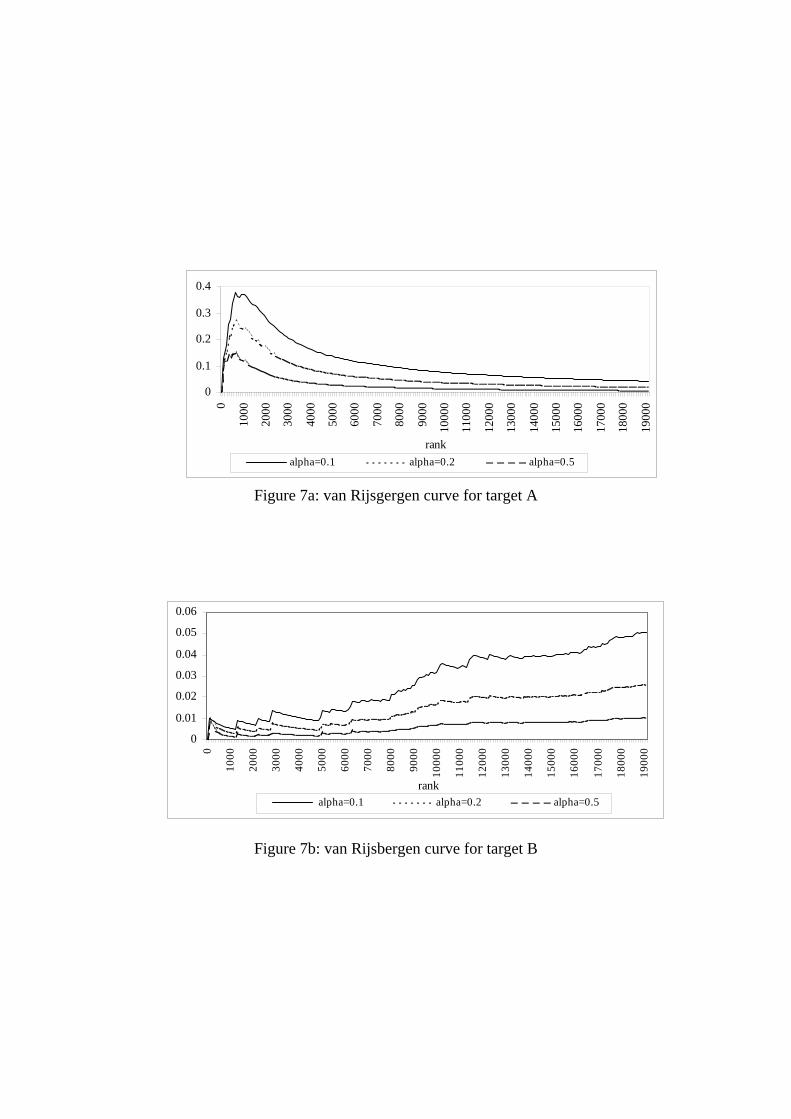
Van Rijsbergen measure The graphs for the van Rijsbergen measure for targets A-D are

shown in Figure 7. The formula for the van Rijsbergen measure differs only slightly from the

Vickery, Heine and Shaw, the extent of the difference depending upon the value chosen for α,

a user-defined parameter which defines the relative contribution of precision and recall to the

overall score (with a high α value reflecting an emphasis on precision rather than recall). The

low values of precision in targets C and D result in near-featureless curves when α is 0.5;

with lower values for α, the plots obtained are similar to those obtained for the Vickery

measure in Figure 6a.

Voiskunskii The form of the measure proposed by Voiskunskii is significantly different from

the measures discussed above, but the plots that are obtained (in Figure 8) are similar in

outline to many of those shown previously, although there are some differences: for example,

the plot for target D reflects the progressive identification of each of the six actives for this

target more obviously than in the corresponding Vickery plot.

G-H score The final measure used to analyse the data is the G-H score of Güner and Henry

[23]. The precise form of the plots resulting from use of this measure again depend upon the

values of user-defined parameters (α and β here) but comparably-shaped curves are obtained

for a wide range of combinations of values, some of which are illustrated in Figure 9. It will

be seen that the effect of the parameter values on the plot shapes seems to diminish for small

numbers of active structures (as exemplified in Figures 9c and 9d).

It will be seen that all of the G-H score plots tend to a limiting value of 0.5. For simplicity,

assume, without loss of generality, that α=β=1, so that the measure is given by

P R+2

.

As n → N, i.e., when very many molecules have been retrieved, a → A, and hence the

precision and recall are given by P = A/N and R = 1, respectively. Thus the score at the n-th

rank position, GHn, is given by

nGHAN→+1

2, i.e.,

A NN+

2.

Now N >> A, i.e., the total file size is much greater than the number of actives for the chosen

target structure, and hence

nGH → 1 2/ ,

which is what is observed in practice in Figure 9. By similar arguments, the Vickery, van

Rijsbergen (with α = 0.5) and Voiskunskii measures tend to A/2N, 2A/N and √(A/N),

respectively (all of which are close to zero as N >> A).

In general, the G-H score plots are very similar to the cumulative recall plots: we have noted

previously that there are close relationships between several of the measures considered here,

and it is simple to demonstrate such a relationship for this pair of measures. Consider the case

when n molecules have been retrieved, a of which are active: then the cumulative recall at this

point, CRn, is given by

AaCRn

=

and the corresponding G-H score (again assuming α=β=1) by

2Aa

na

GH n

+= .

Taking the ratio of these two measures and simplifying we obtain

n

n

CRGH

nA n

=+

2.

A will be small for most target structures and the ratio will hence tend to the constant value of

2 as n increases, i.e., as more and more structures are retrieved. The G-H score can hence best

be considered as a more flexible form of the cumulative recall measure, with the flexibility

being provided by the user’s ability to specify values for the parameters α and β. This is, of

course, also the aim of the van Rijsbergen measure, and the other related measures (Heine,

Vickery and Shaw) all involve the adoption of an implicit weighting of precision as against

recall; however, the cumulative recall and G-H score plots we have obtained seem, to us at

least, to be intuitively more comprehensible than those resulting from the other measures.

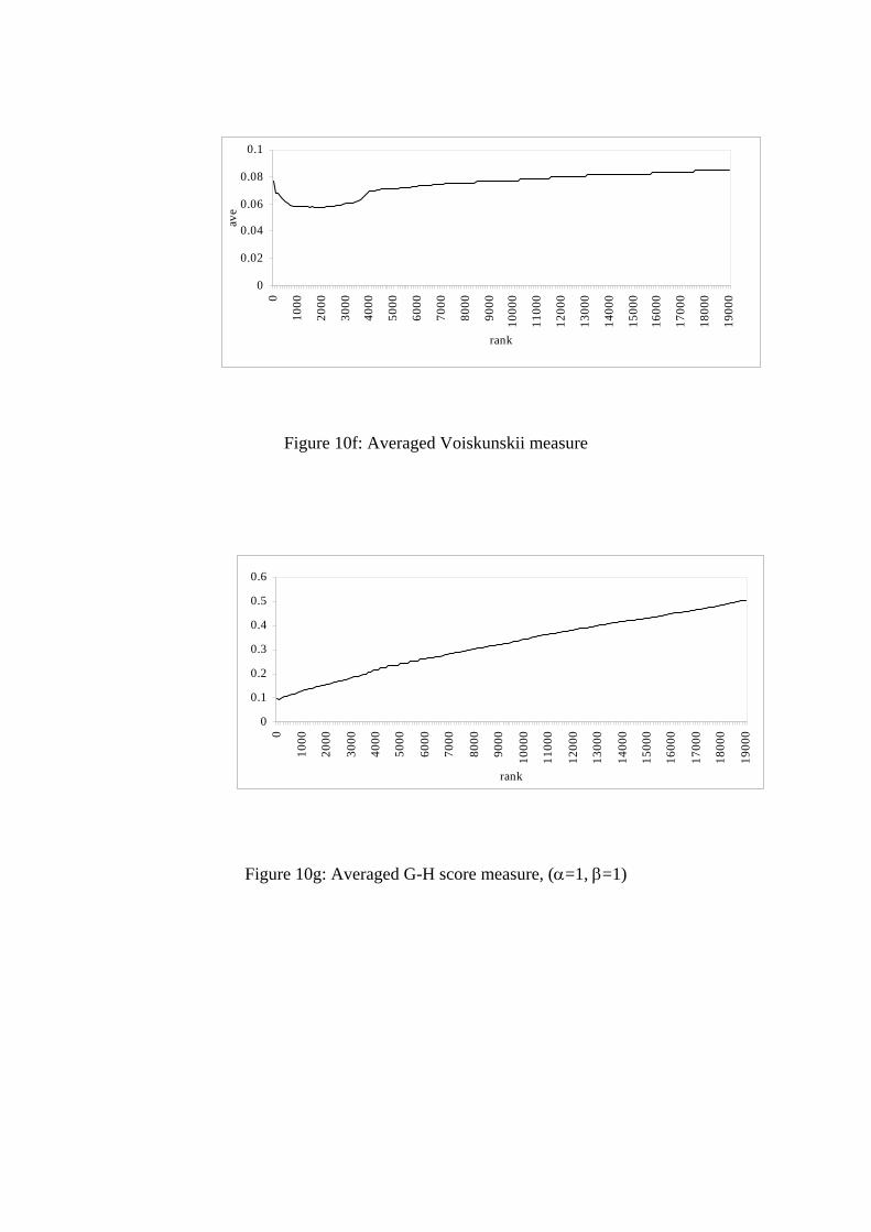
Average plots The final set of plots here (in Figure 10) represent mean values calculated

across the entire set of 50 targets. For the van Rijsbergen measure, α was set to 0.2, while α

and β were both set to 1 for the G-H score. The plots demonstrate the high degree of

commonality between the Vickery, van Rijsbergen and Voiskunskii measures. There are no

obvious peaks due to the averaging, but all three show the same characteristics with a

pronounced trough, followed by a noticeable improvement in performance at about rank-4000

that is rather less evident in the G-H score plot, although even here a slight bump is observed

in the plot. There does not seem to be any obvious reason for this behaviour and we hence

assume that it is specific to this set of structures and targets. The G-H score plot is very

similar to the cumulative recall and normalised recall plots; however, as noted previously, the

last of these can give very different types of curve for individual searches. The averaged

precision-recall plot shows the inverse relationship that characterises such plots in the textual

information retrieval (with the exception of the initial peak at low recall); however, this

measure also can give very different types of curve (as demonstrated by Figure 3).

CONCLUSIONS

In this paper we have illustrated the use of a range of measures for evaluating the

effectiveness of retrieval in bit-string similarity searches of 2D chemical databases. Our

investigations show that there is little to distinguish between the single-valued measures of

van Rijsbergen, Vickery, Heine, Shaw and Voiskunskii, and that there are also close

similarities between the cumulative recall and G-H score measures. We believe that the plots

resulting from the latter measures are rather easier to interpret, and hence recommend their

adoption for reporting the results of chemical similarity searching experiments.

Acknowledgements. We thank Derwent Information for provision of the World Drug Index

database, Tripos Inc. for software support, the Humanities Research Board of the British

Academy for the award of a studentship to SJE, and Val Gillet for helpful comments.

REFERENCES

1. Willett, P., Barnard, J.M. and Downs, G.M. Chemical similarity searching. J. of Chem.

Inf. Comput. Sci. 1998, 38, 983-996.

2. Johnson, M.A. and Maggiora, G.M., Eds., Concepts and Applications of Molecular

Similarity, Wiley, New York, 1990

3. Dean, P.M., Ed., Molecular Similarity in Drug Discovery, Chapman and Hall, Glasgow,

1994

4. Patterson, D.E., Cramer, R.D., Ferguson, A.M., Clark, R.D. and Weinberger, L.E.,

Neighbourhood behaviour: a useful concept for validation of “molecular diversity”

descriptors. J. Med. Chem. 1996, 39, 3049-3059.

5. Salton, G. and McGill, M.J., Introduction to Modern Information Retrieval, McGraw-

Hill, New York, 1983.

6. Frakes, W.B. and Baeza-Yates, R., Eds., Information Retrieval: Data Structures and

Algorithms, Prentice Hall, Englewood Cliffs NJ, 1992

7. Sparck Jones, K. and Willett, P., Eds., Readings in Information Retrieval, Morgan

Kaufmann, San Francisco, 1997.

8. Sparck Jones, K., Ed., Information Retrieval Experiment, Butterworth, London, 1981.

9. Boyce, B.R., Meadow, C.T. and Kraft, D.H. Measurement in Information Science,

Academic Press, San Diego, 1994.

10. Special issue on Evaluation Issues in Information Retrieval, Inf. Proc. Manag. 1992, 28,

439-528.

11. Special issue on Evaluation, J. Am. Soc. Inf. Sci. 1996, 47, 1-105.

12. Cleverdon, C.W. On the inverse relationship of recall and precision. J. Docum. 1972, 23,

195-201.

13. Robertson, S.E. and Sparck Jones, K. Relevance weighting of search terms. J. Am. Soc.

Inf. Sci. 1976, 27, 129-146.

14. Cosgrove, D.A. and Willett, P. SLASH: a program for analysing the functional groups in

molecules. J. Mol. Graph. Modell. 1998, 16, 19-32.

15. Vickery, B.C., In Cleverdon, C.W., Mills, J. and Keen, E.M., Eds., Factors Determining

the Performance of Indexing Systems (Aslib-Cranfield Research Project), Cranfield,

1966.

16. Heine, M.H. Distance between sets as an objective measure of retrieval effectiveness.

Inf. Stor. Ret. 1973, 9, 181-198.

17. van Rijsbergen, C.J. Information Retrieval, Butterworth, London, 1979.

18. Shaw, W.M. On the foundation of evaluation. J. Am. Soc. Inf. Sci. 1986, 37, 346-348.

19. Voiskunskii, V.G. Evaluation of search results: a new approach. J. Am. Soc. Inf. Sci.

1997, 48, 133-142.

20. Bawden, D. and Fisher, J.D. A note on measures of screening effectiveness in chemical

substructure searching. J. Chem. Inf. Comput. Sci. 1985, 25, 36-38.

21. Pepperrell, C.A. and Willett, P. Techniques for the calculation of three-dimensional

structural similarity using inter-atomic distances. J. Comput.-Aided Mol. Design 1991, 5,

455-474.

22. Sheridan, R.P., Miller, M.D., Underwood, D.J. and Kearsley, S.K. Chemical similarity

using geometric pair descriptors. J. Chem. Inf. Comput. Sci. 1996, 36, 128-136.

23. Güner, O.F. and Henry, D.R. Formula for determining the “goodness of hit lists” in 3D

database searches. At http://www.netsci.org/Science/Cheminform/feature09.html.

24. The World Drug Index database is available from Derwent Information at

http://www.derwent.co.uk/

25. The UNITY chemical information management system is available from Tripos Inc. at

http://www.tripos.com/

26. Snarey, M., Terret, N.K., Willett, P. and Wilton, D.J. Comparison of algorithms for

dissimilarity-based compound selection. J. Mol. Graph. Modell. 1997, 15, 372-385.

27. Bohm, H.-J. & Schneider, G., Eds., Virtual Screening for Bioactive Molecules, Wiley-

VCH, Weinheim, in the press.

28. Brown, R.D. and Martin, Y.C. Use of structure-activity data to compare structure-based

clustering methods and descriptors for use in compound selection. J. Chem. Inf. Comput.

Sci. 1996, 36, 572-584.

Relevant Yes No

Retrieved Yes a n-a n No A-a N-n-A+a N-n A N-A N

Table 1. Contingency table describing the output of a search in terms of records retrieved and records that are relevant Measure n < A n = A n > A

Precision-recall P = 1, R = n

A P = R = 1 P = A

n, R = 1

Vickery

nAn−2

1 An A2 −

van Rijsbergen (α=0.5)

2nA n+

1 2 AA n+

Voiskunskii n

A

1 An

G-H score (α=β=1) n A

A+2

1 n An+2

Table 2: Upperbound values of the various performance measures

0

0.2

0.4

0.6

0.8

1

0

1000

2000

3000

4000

5000

6000

7000

8000

9000

1000

0

1100

0

1200

0

1300

0

1400

0

1500

0

1600

0

1700

0

1800

0

1900

0

rank

reca

ll

cumulative recall best case

Figure 1a: Cumulative recall for target A

0

0.2

0.4

0.6

0.8

1

0

1000

2000

3000

4000

5000

6000

7000

8000

9000

1000

0

1100

0

1200

0

1300

0

1400

0

1500

0

1600

0

1700

0

1800

0

1900

0

rank

reca

ll

Figure 1b: Cumulative recall for target B

0

0.2

0.4

0.6

0.8

10

1000

2000

3000

4000

5000

6000

7000

8000

9000

1000

0

1100

0

1200

0

1300

0

1400

0

1500

0

1600

0

1700

0

1800

0

1900

0

rank

reca

ll

Figure 1c: Cumulative recall for target C

00.20.40.60.8

1

0

1000

2000

3000

4000

5000

6000

7000

8000

9000

1000

0

1100

0

1200

0

1300

0

1400

0

1500

0

1600

0

1700

0

1800

0

1900

0

rank

reca

ll

Figure 1d: Cumulative recall for target D

A

B

C

D

N ON

O

SN

N

N

N

F

N

F

F

FF

FF

FFF

FF

F

FF

FF

FFF

F

NSO

OO

Figure 2: Target structures A-D used to illustrate the behaviour of the various

performance measures.

0

0.02

0.04

0.06

0.08

0.1

0.12

0 0.2 0.4 0.6 0.8 1

recall

prec

ision

Figure 3a: Precision-recall curve for target A

0

0.002

0.004

0.006

0.008

0.01

0.012

0 0.2 0.4 0.6 0.8 1

recall

prec

isio

n

Figure 3b: Precision-recall curve for target B

0

0.005

0.01

0.015

0.02

0.025

0.03

0 0.2 0.4 0.6 0.8 1

recall

prec

ision

Figure 3c: Precision-recall curve for target structure 8067

F

F

F

N

O

H

(119)

N

N

F

F

F

O O

H

H

(151)

N

N

F

F

F

O O

H

H

(211)

N

H F

F

F

O OO

OH

(219)

N

FF

O

F

(245)

F

F

F

NN

O

O

(271)

N

F

F

F

Cl Cl

O

O

N

S

N

H

H

(291)

N

N

F F

F

O O

N

H F

F

F

(308)

O

O

N

NF

F

F

O

O

H

(389)

OOO

H OH

N

H

N

F

FF

(399)

Figure 4: Retrieval position (in parentheses) of the active structures associated with the two peaks between n=100 and n=400 in the recall-precision plot for target structure 8067, Cl2FC-CFCl2.

0

0.2

0.4

0.6

0.8

1

0

1000

2000

3000

4000

5000

6000

7000

8000

9000

1000

0

1100

0

1200

0

1300

0

1400

0

1500

0

1600

0

1700

0

1800

0

1900

0

rank

Figure 5a: Normalised recall curve for target A

0

0.2

0.4

0.6

0.8

1

0

1000

2000

3000

4000

5000

6000

7000

8000

9000

1000

0

1100

0

1200

0

1300

0

1400

0

1500

0

1600

0

1700

0

1800

0

1900

0rank

Figure 5b: Normalised recall curve for target B

0

0.01

0.02

0.03

0.04

0.05

0

1000

2000

3000

4000

5000

6000

7000

8000

9000

1000

0

1100

0

1200

0

1300

0

1400

0

1500

0

1600

0

1700

0

1800

0

1900

0

rank

Figure 6a: Vickery curve for target A

0

0.0005

0.001

0.0015

0.002

0.0025

0.003

0

1000

2000

3000

4000

5000

6000

7000

8000

9000

1000

0

1100

0

1200

0

1300

0

1400

0

1500

0

1600

0

1700

0

1800

0

1900

0rank

Figure 6b: Vickery curve for target B

0

0.1

0.2

0.3

0.4

0

1000

2000

3000

4000

5000

6000

7000

8000

9000

1000

0

1100

0

1200

0

1300

0

1400

0

1500

0

1600

0

1700

0

1800

0

1900

0

rankalpha=0.1 alpha=0.2 alpha=0.5

Figure 7a: van Rijsgergen curve for target A

0

0.01

0.02

0.03

0.04

0.05

0.06

0

1000

2000

3000

4000

5000

6000

7000

8000

9000

1000

0

1100

0

1200

0

1300

0

1400

0

1500

0

1600

0

1700

0

1800

0

1900

0

rank alpha=0.1 alpha=0.2 alpha=0.5

Figure 7b: van Rijsbergen curve for target B

00.05

0.10.15

0.20.25

0.30.35

0.4

0

1000

2000

3000

4000

5000

6000

7000

8000

9000

1000

0

1100

0

1200

0

1300

0

1400

0

1500

0

1600

0

1700

0

1800

0

1900

0

rank

alpha=0.1 alpha=0.2 alpha=0.5

Figure 7c: van Rijsbergen curve for target C

00.010.020.030.040.050.060.07

0

1000

2000

3000

4000

5000

6000

7000

8000

9000

1000

0

1100

0

1200

0

1300

0

1400

0

1500

0

1600

0

1700

0

1800

0

1900

0

rankalpha=0.1 alpha=0.2 alpha=0.5

Figure 7d: van Rijsbergen curve for target D

0

0.05

0.1

0.15

0.2

0.25

0

1000

2000

3000

4000

5000

6000

7000

8000

9000

1000

0

1100

0

1200

0

1300

0

1400

0

1500

0

1600

0

1700

0

1800

0

1900

0

rank

Figure 8a: Voiskunskii curve for target A

0

0.02

0.04

0.06

0.08

0

1000

2000

3000

4000

5000

6000

7000

8000

9000

1000

0

1100

0

1200

0

1300

0

1400

0

1500

0

1600

0

1700

0

1800

0

1900

0

rank

Figure 8b: Voiskunskii curve for target B

0

0.05

0.1

0.15

0.2

0.25

0

1000

2000

3000

4000

5000

6000

7000

8000

9000

1000

0

1100

0

1200

0

1300

0

1400

0

1500

0

1600

0

1700

0

1800

0

1900

0

rank

Figure 8c: Voiskunskii curve for target C

0

0.01

0.02

0.03

0.04

0.05

0

1000

2000

3000

4000

5000

6000

7000

8000

9000

1000

0

1100

0

1200

0

1300

0

1400

0

1500

0

1600

0

1700

0

1800

0

1900

0

rank

Figure 8d: Voiskunskii curve for target D

0

0.10.2

0.30.4

0.50.6

0

1000

2000

3000

4000

5000

6000

7000

8000

9000

1000

0

1100

0

1200

0

1300

0

1400

0

1500

0

1600

0

1700

0

1800

0

1900

0

rank

alpha=1 beta=1 alpha=0.25 beta=1

Figure 9a: G-H score curve for target A

00.10.20.30.40.50.6

0

1000

2000

3000

4000

5000

6000

7000

8000

9000

1000

0

1100

0

1200

0

1300

0

1400

0

1500

0

1600

0

1700

0

1800

0

1900

0

rank

alpha=1 beta=1 alpha=0.25 beta=1

Figure 9b: G-H score curve for target B

0

0.10.2

0.3

0.40.5

0.60

1000

2000

3000

4000

5000

6000

7000

8000

9000

1000

0

1100

0

1200

0

1300

0

1400

0

1500

0

1600

0

1700

0

1800

0

1900

0

rankalpha=1 beta=1 alpha=0.25 beta=1

Figure 9c: G-H score curve for target C

0

0.1

0.2

0.3

0.4

0.5

0.6

0

1000

2000

3000

4000

5000

6000

7000

8000

9000

1000

0

1100

0

1200

0

1300

0

1400

0

1500

0

1600

0

1700

0

1800

0

1900

0

rank

alpha=1 beta=1 alpha=0.25 beta=1

Figure 9d: G-H score curve for target D

00.20.40.60.8

1

0

1000

2000

3000

4000

5000

6000

7000

8000

9000

1000

0

1100

0

1200

0

1300

0

1400

0

1500

0

1600

0

1700

0

1800

0

1900

0

rank

Figure 10a: Averaged cumulative recall

0

0.02

0.04

0.06

0.08

0.1

0.11

0.25

0.32

0.41

0.47

0.53

0.58

0.63

0.69

0.74

0.79

0.83

0.87

0.91

0.97

Recall

Prec

ision

Figure 10b: Averaged precision-recall

0

0.2

0.4

0.6

0.8

0

1000

2000

3000

4000

5000

6000

7000

8000

9000

1000

0

1100

0

1200

0

1300

0

1400

0

1500

0

1600

0

1700

0

1800

0

1900

0

Rank

Figure 10c: Averaged normalised recall

00.005

0.010.015

0.020.025

0.030.035

0.04

0

1000

2000

3000

4000

5000

6000

7000

8000

9000

1000

0

1100

0

1200

0

1300

0

1400

0

1500

0

1600

0

1700

0

1800

0

1900

0

rank

ave

Figure 10d: Averaged Vickery measure

00.010.020.030.040.050.060.070.08

0

1000

2000

3000

4000

5000

6000

7000

8000

9000

1000

0

1100

0

1200

0

1300

0

1400

0

1500

0

1600

0

1700

0

1800

0

1900

0rank

ave

Figure 10e: Averaged van Rijsbergen measure (α=0.2)

0

0.02

0.04

0.06

0.08

0.1

0

1000

2000

3000

4000

5000

6000

7000

8000

9000

1000

0

1100

0

1200

0

1300

0

1400

0

1500

0

1600

0

1700

0

1800

0

1900

0

rank

ave

Figure 10f: Averaged Voiskunskii measure

0

0.1

0.2

0.3

0.4

0.5

0.6

0

1000

2000

3000

4000

5000

6000

7000

8000

9000

1000

0

1100

0

1200

0

1300

0

1400

0

1500

0

1600

0

1700

0

1800

0

1900

0

rank

Figure 10g: Averaged G-H score measure, (α=1, β=1)