EFFECT OF ROOFTOP GREENERY ON OUTDOOR MEAN ...

EFFECT OF ROOFTOP GREENERY ON OUTDOOR MEAN

RADIANT TEMPERATURE IN THE TROPICAL URBAN

ENVIRONMENT

TAN CHUN LIANG

(B.Arch. (Hons.), NUS; M.Arch., NUS)

A000355Y

A THESIS SUBMITTED

FOR THE DEGREE OF DOCTOR OF PHILOSOPHY

DEPARTMENT OF BUILDING

SCHOOL OF DESIGN AND ENVIRONMENT

NATIONAL UNIVERSITY OF SINGAPORE

2015

i

DECLARATION

I hereby declare that this thesis is my original work and it has been

written by me in its entirety. I have duly acknowledged all the sources

of information which have been used in the thesis.

This thesis has also not been submitted for

any degree in any university previously.

……………………………………………………………

Tan Chun Liang

22/06/2015

ii

ACKNOWLEDGEMENTS

I would like to express my immense and sincere gratitude

to Professor Wong Nyuk Hien, who has been a guiding light to my journey in

exploring urban greenery. Associate Professor Tan Puay Yok and Associate

Professor Nalanie Mithraratne for their expert guidance and willingness to

enrich me with their knowledge and experience.

Dr. Steve Kardinal Jusuf, whose brilliance I can only try to emulate. This

thesis would not have been possible without him, as well as expert advice

and guidance from Mr Marcel Ignatius, Ms Lee Seu Quin, Ms Religiana

Hendarti, Mr Daniel Hii, Mr Alex Tan, Ms Norishahaini Binti Mohamed Ishak

and Ms Erna Tan.

Mr Komari, Mr Zaini and Mr Guna for their technical assistance and always

accommodating to my numerous requests.

Mr Chiam Zhiquan, Mr Sim Yong Xiong, Mr Zheng Kai, Ms Alvina Au-Yong

and Ms Chia Pei Yu for enduring my physically and mentally demanding

requests for field measurement and data analysis.

Mr Zac Toh of Chop Ching Hin Pte Ltd, whose introduction was nothing short

of divine intervention. I hope our aspirations for urban greenery can be

realized in good time.

Ms Natalie He, who has been an unwavering pillar of support in my most

trying moments.

iii

This study would not have been possible without any one of them.

In the five years, I have learned many things and experienced countless

epiphanies, the most important being a staunch respect for nature. Nature

speaks to us through science, and this thesis is but a modest testimony to her

splendor.

Tan Chun Liang

iv

EXECUTIVE SUMMARY

Urbanization has been widely acknowledged to be a major contributory

factor to many environmental issues. Some issues include global warming

and pollution. Rising temperature due to climate change and the Urban Heat

Island (UHI) effect has led to intensive research into adaptive and mitigative

strategies to improve thermal comfort.

The implementation of urban greenery has become a widely accepted way

of mitigating effects of climate change and the Urban Heat Island effect. In

view of this, there is a need for the formulation of an objective framework for

selection and allocation of urban vegetation. This will ensure sensible design

and planning practices that do not adhere chiefly to aesthetics, and that

ecosystem resources can be optimised.

With the main focus of quantifying air (ta) and mean radiant temperature

(tmrt) attenuation profiles of rooftop greenery, the proposed research seeks to

achieve the following objectives:

1. To quantify characteristics of rooftop greenery and measure their

effects on ta and tmrt; and

2. To develop a model framework for selection and allocation of greenery

in the urban environment.

This is done by correlating changes in temperature with vegetative attributes

such as plant evapotranspiration rate and shrub albedo.

A regression model is established using data of this study. The model

substantiates the need to evaluate plants based of quantifiable traits and sets

the framework for plant selection and allocation based on their heat reduction

potential.

v

LIST OF FIGURES

Figure 1. Mitigation and adaptation (Smit, 1993) ............................................ 2

Figure 2. Urban heat island characteristics (Voogt, 2004)............................. 10

Figure 3. UHI profile in Singapore (Wong and Chen, 2005) .......................... 11

Figure 4. Average air temperatures measured from park to the built

environment (Wong and Chen, 2006b) ......................................................... 15

Figure 5. Estimated solar radiation exposure under selected shade trees

(Brown and Gillespie, 1990) ......................................................................... 17

Figure 6. Net radiation in the shaded area (thin line) and in the unshaded area

(thick line) (Papadakis et al., 2001) ............................................................... 18

Figure 7. Analysis of tree position for optimal shade (Heisler, 1986a) ........... 20

Figure 8. Comparison of shade generated by trees of different shapes

(Kotzen, 2003) .............................................................................................. 23

Figure 9. Simulation of tree shade using Ecotect (Shahidan et al., 2010) ..... 24

Figure 10. Tree input parameters in RayMan (Gulyás et al., 2006) ............... 27

Figure 11. Effects of plant canopy on outdoor thermal environment (Yoshida,

2006) ............................................................................................................ 28

Figure 12. Spatial variations of tmrt simulated using SOLWEIG v2 (Lindberg

and Grimmond, 2011) ................................................................................... 30

Figure 13. Sectional perspective of a leaf (BBC, 2013) ................................. 30

Figure 14. Evapotranspiration rate and plant development (Allen et al. 1998)

..................................................................................................................... 31

Figure 15. The mechanism of Energy balance at the vegetated surface ....... 46

Figure 16. Range of albedo of natural surfaces (Dobos, 2006) ..................... 52

Figure 17. Diurnal variations of albedo (Ahmad & Lockwood, 1979) ............. 54

Figure 18. Hypothesised effects of ET and SA on tmrt ................................... 66

Figure 19. Hypothetical model on landscape design assessment in the

mitigation and adaptation model ................................................................... 67

Figure 20. Research methodology ................................................................ 68

Figure 21. Effect of rooftop greenery on temperature at a given point .......... 70

Figure 22. 40 mm globe thermometer mounted on net radiometer ............... 74

Figure 23. Diurnal short wave (K) and long wave (L) profile for 18th March

2011 ............................................................................................................. 79

Figure 24. Calculation of tmrt using Method A and B (ISO 7726:1998) – 18th

March 2011 .................................................................................................. 80

file:///C:/Users/4ZKH82S/Desktop/rewrite%202015-12-11/terrence%20thesis%20draft%2024%20-%20rewrite%20after%205%20round%20of%20ithenticate.docx%23_Toc438855534

vi

Figure 25. Calculation of tmrt using Method A and B(Recalibrated) – 18th

March 2011 .................................................................................................. 82

Figure 26. Calculation of tmrt using Method A and B(Recalibrated) – Study

Area 2, 16th August 2011 .............................................................................. 83

Figure 27. Whisker plot for Study Area 2 (Method A – Method B) ................. 84

Figure 28. Rooftop greenery measurement setup ......................................... 90

Figure 29. Rooftop measurement points ....................................................... 91

Figure 30. Measurement of plant evapotranspiration rate with load cell ........ 94

Figure 31. Measurement of Leaf Area Index ................................................. 94

Figure 32. Measurement of Shrub Albedo .................................................... 95

Figure 33. Typical clear (13th June 2014) and overcast (5th July 2014) sky

solar irradiance profiles ................................................................................ 99

Figure 34. Mean radiant temperature profile for clear sky conditions (13th June

2014) .......................................................................................................... 100

Figure 35. Mean radiant temperature profile for overcast sky conditions (5th

July 2014) ................................................................................................... 101

Figure 36. Air temperature profile for clear sky conditions (13th June 2014) 102

Figure 37. Air temperature profile for overcast sky conditions (12th July 2014)

................................................................................................................... 103

Figure 38. Location of air temperature probes ............................................ 104

Figure 39. Stratified air temperature profile for Plot 1 (26th July 2014) ........ 104

Figure 40. Stratified air temperature profile for Plot 2 (26th July 2014) ........ 105

Figure 41. Stratified air temperature profile for Plot 3 (26th July 2014) ....... 105

Figure 42. Solar radiation against mean radiant temperature profile (13th June

2014) .......................................................................................................... 107

Figure 43. Solar radiation against air temperature profile (13th June 2104) . 108

Figure 44. Photosynthetically Active Radiation against mean radiant

temperature profile (13th June 2014) ........................................................... 109

Figure 45. Photosynthetically Active Radiation against air temperature profile

(13th June 2014) ......................................................................................... 110

Figure 46. Relative Humidity against mean radiant temperature profile (13th

June 2014) ................................................................................................. 111

Figure 47. Relative Humidity against air temperature profile (13th June 2014)

................................................................................................................... 112

Figure 48. Evapotranspiration rate against mean radiant temperature profile

(13th June 2014) ......................................................................................... 113


vii

Figure 49. Evapotranspiration rate against air temperature profile (13th June

2014) .......................................................................................................... 114

Figure 50. Albedo against mean radiant temperature profile (13th June 2014)

................................................................................................................... 115

Figure 51. Albedo against air temperature profile (13th June 2014) ............. 116

Figure 52. LAI-2000 canopy analyzer. (Source: http://www.licor.com) ........ 117

Figure 53. Leaf samples used for reflectance measurement (5 cm X 5 cm) 119

Figure 54. Reflectivity results ...................................................................... 119

Figure 55. Decagon leaf porometer (Source: http://www.decagon.com) ..... 120

Figure 56: Stomata Conductance (3rd June 2014) ...................................... 121

Figure 57. Average leaf surface temperature profiles for Plots 1, 2 and 3 (24th

June 2014) ................................................................................................. 122

Figure 58: Infrared thermography of green roof plots and concrete ............ 123

Figure 59. Average soil temperature profiles for Plot 1, 2 and 3 (24th June

2014) .......................................................................................................... 124

Figure 60. Concrete temperature profiles for Plot 1 to Plot 3 (24th June 2014)

................................................................................................................... 125

Figure 61: Incoming and outgoing radiation for Plots 1 to 3 (7th July 2014) . 127

Figure 62. Net all-wave radiation (Q*) for Plots 1 to 3 (7th July 2014) .......... 128

Figure 63. Boundary concrete surface temperature profiles (24th June 2014)

................................................................................................................... 128

Figure 64. Boundary air temperature profile (24th June 2014) ..................... 129

Figure 65. Air temperature profiles of rooftop greenery plots on 26th July 2014

................................................................................................................... 131

Figure 66. Scatter plots of Plant ET and Albedo on Plant air temperature .. 133

Figure 67. Air and mean radiant temperature profile plotted against plant ET

from 07:00 hrs to 19:00 hrs (13th June 2014) .............................................. 135

Figure 68. Solar irradiance, plant evapotranspiration rate and tmrt above

concrete from 07:00 hrs to 19:00 hrs for days with clear sky conditions ...... 140

Figure 69. Histograms, Q-Q and box plots for measured variables ............. 141

Figure 70. Scatter plots of tmrt(plant) and independent variables ..................... 142

Figure 71. Scatterplot for measured and modelled tmrt values ..................... 145

Figure 72. Box plot of modelled and measured tmrt values .......................... 146

Figure 73. Prediction model workflow ......................................................... 147

Figure 74. Box plot of Reference tmrt values from 07:00 hrs to 19:00 hrs .... 149

Figure 75. Box plot of Reference tmrt values from 13:00 hrs to 17:00 hrs .... 149

viii

Figure 76. Box plot of plant evapotranspiration rates from 13:00 hrs to 17:00

hrs .............................................................................................................. 150

Figure 77. Box plot of shrub albedo values from 13:00 hrs to 17:00 hrs...... 153

Figure 78. Plot of Plant tmrt and Reference tmrt ............................................. 155

Figure 79. Plot of Plant tmrt and Plant Evapotranspiration Rate ................... 156

Figure 80. Plot of Plant tmrt and Shrub Albedo ............................................. 157

Figure 81. Rooftop greenery panel on load cell .......................................... 160

Figure 82. ET rates of plants commonly used for rooftop greenery (13th

January 2015) ............................................................................................ 160

Figure 83. Botanical illustration of plants used for measurement ................ 165

Figure 84. Plant selection via chart (Percentage decrease in tmrt) ............... 173

Figure 85. Proposed landscape planning framework .................................. 175

Figure 86. Elaboration of proposed landscape planning framework ............ 176

Figure 87. Hypothetical urban model (Baseline) ......................................... 179

Figure 88. Pedestrain level tmrt modelling hierarchy .................................... 179

Figure 89. Simulation of tmrt via SOLWEIG and ArcGIS ............................... 182

Figure 90. Areas where shrubs can be added to reduce tmrt ....................... 183

Figure 91. Areas allocated for shrubbery (Highlighted in green) ................. 184

Figure 92. Simulation result with input from regression model .................... 185

Figure 93. Comparison of Tmrt simulation results......................................... 186

Figure 94. Solar insolation modelling .......................................................... 188

Figure 95. Close-up of solar insolation map ................................................ 189

Figure 96. Landscape planning for building surfaces .................................. 190

Figure 97. Assessment of building surfaces using solar insolation map ...... 193

Figure 98. Sites A and B ............................................................................. 215

Figure 99. Diurnal profiles of tmrt for Site A and Site B ................................. 218

Figure 100. Scatterplots of tmrt and SVF for Site A and Site B at 14:00 hrs . 219

Figure 101. Profiles of tmrt for Site A and Site B from 0:00 hrs to 07:00 hrs . 222

Figure 102. Thermal imaging of tree surface temperature for Site B ........... 223

Figure 103. SVF of Point 4 and Point 9....................................................... 224

Figure 104.Measurement points above rooftop greenery plot ..................... 226

Figure 105. Averaged diurnal tmrt profiles under clear sky conditions .......... 228

Figure 106. Surface temperature measurement spots ................................ 231

Figure 107. Measurement setup. Globe thermometers were attached to poles

with white PVC pipes housing surface and air temperature loggers. ........... 233

Figure 108. Position of tmrt and ta measurement points ............................... 235





ix

Figure 109. CCTV footage of site showing self-shading and overshadowing

................................................................................................................... 236

Figure 110. Surface Temperature profiles for Period A and Period B ......... 238

Figure 111. Air temperature profiles for Period A and Period B................... 239

Figure 112. Comparison of tmrt profile for Points 1-7 for Period A and Period B

................................................................................................................... 241

Figure 113. Points 2, 4 and 6 ...................................................................... 242

Figure 114. Plot of Points 2,4 and 6 against solar irradiance for Period A and

Period B ..................................................................................................... 243

Figure 115. Comparison of tmrt profiles at 0.5 m intervals from the wall for

Time Range 3, Period B ............................................................................. 245

Figure 116. Comparison of points at peak solar irradiance ......................... 246

Figure 117. GIS visualisation of tmrt ............................................................. 247

Figure 118. Plan and measurement setup .................................................. 251

Figure 119. Setup details ............................................................................ 252

Figure 120. Solar irradiance profile for 10th June 2014................................ 254

Figure 121. Air temperature profiles for green roof, green walls and concrete

walls ........................................................................................................... 256

Figure 122. Mean radiant temperature profiles for green roof, green walls and

concrete walls ............................................................................................. 256

Figure 123. Albedo profiles for green roof and green walls ......................... 257

Figure 124. Albedo profiles of Green Roof and Green Walls combined ...... 258

Figure 125. Effect of sun position on albedo ............................................... 259

Figure 126. Plant ET profiles for green roof and green walls ...................... 259

Figure 127. Infrared thermography of green roof plots and concrete (10th June

2014) .......................................................................................................... 262

Figure 128. Green Mark award criteria (NRB/4.1) ....................................... 264

Figure 129. Energy related requirements .................................................... 266

Figure 130. NRB 1-1 Thermal performance of building envelope - Envelope

thermal transfer value (ETTV) .................................................................... 268

Figure 131. Comparison of U-values for normal wall and green wall .......... 270

Figure 132. Carrier and Support systems ................................................... 271

Figure 133. An example of greenery in front of glass façade ...................... 272

Figure 134. Sketch section of greenery in front of window .......................... 273

Figure 135. Energy efficiency checklist ....................................................... 275

Figure 136. NRB 1-10 Energy efficient practices and features .................... 277

Figure 137. Water efficiency checklist ........................................................ 277


x

Figure 138. NRB 2-3 Irrigation system and landscaping ............................. 279

Figure 139. Hypothetical rooftop garden design plan .................................. 279

Figure 140. Environmental protection checklist ........................................... 280

Figure 141. Greenery provision checklist .................................................... 280

Figure 142. Illustration of Green Plot Ratio (GnPR) calculation .................. 281

Figure 143. Point allocation based on solar insolation map ........................ 283

Figure 144. LUSH 2.0 landscape replacement policy ................................. 284

Figure 145. Indoor environmental quality checklist ..................................... 285

Figure 146. NRB 4-2 Noise level ................................................................ 285

Figure 147. NRB 4-3 Indoor air pollutants ................................................... 286

Figure 148. Green roof panel specifications ............................................... 314

Figure 149. Irrigation plan ........................................................................... 315

LIST OF TABLES

Table 1. Classification of plant functional traits (Pérez-Harguindeguy et al.,

2013) ............................................................................................................ 57

Table 2. Influence of hypothesized variables on tmrt ...................................... 65

Table 3. Hypothesized variables ................................................................... 69

Table 4. Measurement period ....................................................................... 72

Table 5. Summary of main plant groups (Tan and Sia, 2009) ....................... 88

Table 6. Plant selection and attributes .......................................................... 89

Table 7. Measurement variables and period ................................................. 92

Table 8. Equipment list ................................................................................. 96

Table 9. Averaged Leaf Area Indices for Plot 1 to Plot 3 ............................. 118

Table 10. Peak air temperature values of rooftop greenery plots on 26th July

2014 ........................................................................................................... 130

Table 11. Studies on air temperature reduction due to greenery................. 132

Table 12. Variables and days used for regression modelling ...................... 138

Table 13. Pearson r Correlation Chart ........................................................ 141

Table 14. Regression summary .................................................................. 143

Table 15. Variables and days used for model validation ............................. 144

Table 16. Plant evapotranspiration rates from reviewed literature ............... 151

Table 17. Common albedo values of vegetated surfaces ........................... 152

Table 18. Range of values used for sensitivity analysis .............................. 153

Table 19. Averaged values used for sensitivity ........................................... 153

Table 20. Values used for Tmrt(Ref) sensitivity analysis ............................. 154


xi

Table 21. Values used for Plant ET sensitivity analysis .............................. 155

Table 22.Values used for Shrub Albedo sensitivity analysis ....................... 156

Table 23. Percentage reduction of Tmrt(plant) derived using Tmrt(ref) of 50

°C and 70 °C .............................................................................................. 157

Table 24. Albedo spot measurements at 13:00 hrs in National University of

Singapore UTown roof gardens .................................................................. 163

Table 25. Recommendations for landscape planning ................................. 168

Table 26. Factors to consider in rating plant species and cultivars (CTLA,

1992) .......................................................................................................... 173

Table 27. Additional factors in rating plant species (Miller, 2007)................ 174

Table 28. Model properties ......................................................................... 177

Table 29. Software recommended for simulation ........................................ 181

Table 30. Software recommended for simulation ........................................ 188

Table 31. Plant categorisation for landscape design (Boo et al., 2014) ....... 196

Table 32. Site Characteristics ..................................................................... 215

Table 33. Measurement period ................................................................... 216

Table 34. SVF values for measurement points in Site A and Site B ............ 220

Table 35. Days used for analysis ................................................................ 227

Table 36. Properties of Green walls ............................................................ 230


Table 38. Instruments used for measurement ............................................. 235

Table 39. Time range used for analysis ...................................................... 235

Table 40. Properties of green roof and green walls .................................... 253


Table 42. Instruments used for measurement ............................................. 253

Table 43. U-values of normal roof and green roof (Wong et al., 2003b) ...... 276

xii

ABBREVIATIONS

AE Actual Evapotranspiration Rate

ALB Average Surface Albedo

ASHRAE American Society of Heating, Refrigeration, and Air-

Conditioning Engineers

ASL Atmospheric Surface Layer

BCA Building and Construction Authority

BPR Building Plot Ratio

BR Bowen Ratio

BREB Bowen Ratio and Energy Balance

CBD Central Business District

DEMs Digital Elevation Model

ET EvapoTranspiration rate

ETTV Envelope Thermal Transfer Value

GIS Geographical Information Systems

GPR Green Plot Ratio

IBM SPSS IBM Statistical Package for the Social Sciences

ISO International Organisation Standardization

LAD Leaf Angle Distribution

LAI Leaf Area Index

LRA Landscape Replacement Area

NParks Singapore National Parks Board

PAR Photosynthetically Active Radiation

PE Potential Evapotranspiration

PET Physiological equivalent temperature

PT model Priestley-Taylor model

PVC Polyvinyl Chloride

SET Standard Effective Temperature

SVF Sky View Factor

TAS Thermal Analysis Simulation

UGS Urban Green Spaces

UHI Urban Heat Island

UNGI Urban Neighbourhood Green Index

UTCI Universal Thermal Climate Index

WBGT Wet Bulb Globe Temperature

xiii

TABLE OF CONTENTS

ACKNOWLEDGEMENTS ........................................................................................................... II

EXECUTIVE SUMMARY .......................................................................................................... IV

LIST OF FIGURES .................................................................................................................... V

LIST OF TABLES ...................................................................................................................... X

ABBREVIATIONS .................................................................................................................... XII

TABLE OF CONTENTS .......................................................................................................... XIII

1 INTRODUCTION ........................................................................................................... 1

1.1 Urban greenery ................................................................................................................ 2

1.2 Optimizing ecosystem services ....................................................................................... 5

1.3 Research question ........................................................................................................... 6

1.4 Objectives and scope of research ................................................................................... 6

1.4.1 Objective 1 ........................................................................................................... 7

1.4.2 Objective 2 ........................................................................................................... 7

1.4.3 Objective 3 ........................................................................................................... 7

1.5 Thesis structure ............................................................................................................... 8

2 LITERATURE REVIEW ............................................................................................... 10

2.1 Urban microclimate of Singapore .................................................................................. 10

2.2 Role of greenery in the urban microclimate ................................................................... 12

2.3 Impact of greenery on the built environment.................................................................. 14

2.3.1 Outdoor air and surface temperature ................................................................. 14

2.3.2 Outdoor radiation ................................................................................................ 17

2.3.3 Energy usage ..................................................................................................... 18

2.3.4 Strategic placement of greenery ......................................................................... 19

2.3.5 Alternate forms of urban greenery ...................................................................... 21

2.4 Measuring the effects of greenery on the built environment .......................................... 23

2.4.1 Shade ................................................................................................................. 23

2.4.2 Temperature ....................................................................................................... 25

2.4.3 Simulation........................................................................................................... 26

2.5 Plant physiology and biotic processes ........................................................................... 30

2.5.1 Evapotranspiration ............................................................................................. 30

2.5.2 Plant canopy....................................................................................................... 48

2.5.3 Plant functional traits .......................................................................................... 56

2.6 Mean radiant temperature (tmrt) and thermal comfort ..................................................... 60

2.7 Knowledge Gap ............................................................................................................. 63

3 HYPOTHESES AND RESEARCH METHODOLOGY .................................................. 64

3.1 Hypotheses .................................................................................................................... 64

3.2 Methodology .................................................................................................................. 68

3.2.1 Calibration of globe thermometers for use in the tropical urban environment .... 71

xiv

3.2.2 Sampling ............................................................................................................ 88

3.2.3 Measurement setup ............................................................................................ 90

3.2.4 Equipment .......................................................................................................... 96

3.3 Final deliverables ........................................................................................................... 98

3.4 Importance and potential contribution of research ......................................................... 98

3.5 Limitations ..................................................................................................................... 98

4 MEASUREMENT OF MEAN RADIANT TEMPERATURE IN A ROOF GARDEN SETTING .................................................................................................................................. 99

4.1.1 Results ............................................................................................................... 99

4.1.2 Analysis ............................................................................................................ 130

5 ROOFTOP GREENERY MEAN RADIANT TEMPERATURE PREDICTION MODEL137

5.1 Methodology and selection of variables for model development ................................. 137

5.1.1 Model development .......................................................................................... 139

5.2 Sensitivity analysis ...................................................................................................... 148

5.2.1 Establishing range limit for variables ................................................................ 149

5.2.2 Sensitivity analysis of prediction model ............................................................ 153

6 DISCUSSION ............................................................................................................ 158

6.1 Impact of plant selection on ambient and mean radiant temperature .......................... 159

6.1.1 Plant evapotranspiration rate............................................................................ 159

6.1.2 Shrub albedo .................................................................................................... 162

6.1.3 Consideration of plant functional traits for plant selection ................................ 163

6.1.4 Leaf Area Index ................................................................................................ 166

6.2 Landscape planning guidelines ................................................................................... 167

6.2.1 Recommendations based on quantitative results of study ............................... 168

6.2.2 Plant selection chart ......................................................................................... 171

6.2.3 Landscape planning framework........................................................................ 173

6.2.4 Hypothetical case study illustrating usage of prediction model......................... 175

7 CONCLUSION ........................................................................................................... 194

7.1 Objective 1 ................................................................................................................... 194

7.2 Objective 2 ................................................................................................................... 194

7.3 Objective 3 ................................................................................................................... 194

7.4 Contributions of research............................................................................................. 195

7.4.1 Objective plant selection and placement criteria .............................................. 195

7.4.2 A novel landscape planning and design ethos ................................................. 196

7.4.3 Optimizing the effects of urban greenery .......................................................... 197

7.5 Limitations of study ...................................................................................................... 198

7.6 Suggestions for further study ....................................................................................... 198

8 PUBLICATION AND CONFERENCE LIST ................................................................ 200

8.1 Conferences ................................................................................................................ 200

8.2 Journal publications ..................................................................................................... 201

9 REFERENCES .......................................................................................................... 202

xv

10 APPENDIX................................................................................................................. 214

10.1 Large scale urban mapping of mean radiant temperature ........................................... 214

10.1.1 Objective ........................................................................................................ 214

10.1.2 Methodology ................................................................................................... 214

10.1.3 Results and discussion ................................................................................... 216

10.1.4 Conclusion ...................................................................................................... 224

10.2 Impact of plant height stratification on mean radiant temperature ............................... 226

10.2.1 Objective ........................................................................................................ 226

10.2.2 Methodology ................................................................................................... 226

10.2.3 Results and discussion ................................................................................... 227

10.3 Comparative studies on vertical greenery.................................................................... 229

10.3.1 Impact on vertical greenery on mean radiant temperature ............................. 229

10.3.2 Analysis of similar plant types in horizontal and vertical setup ....................... 250

10.4 Recommendations for Green Building Rating Tools .................................................... 263

10.4.1 Green buildings and Green Building Rating Tools (GBRTs) ........................... 263

10.4.2 BCA Green Mark Scheme .............................................................................. 264

10.4.3 Greenery in Green Mark ................................................................................. 265

10.4.4 Recommendations for improvement ............................................................... 288

10.5 Data for regression model ........................................................................................... 289

10.6 Data for validation of model ......................................................................................... 301

10.7 Data for sensitivity analysis ......................................................................................... 305

10.8 Plant selection chart .................................................................................................... 307

10.9 Specifications for green roof ........................................................................................ 313

10.9.1 Green roof panel ............................................................................................. 313

10.9.2 Substrate ........................................................................................................ 314

10.9.3 Irrigation ......................................................................................................... 315

10.10 BCA Green Mark for New Non-Residential Buildings Version NRB/4.1 ...................... 316

10.11 LUSH 2.0 landscape replacement circular................................................................... 336

10.12 Response to comments from examiners ..................................................................... 338

10.12.1 Comments from Examiner 1 ................................................................ 338



1

1 INTRODUCTION

Modern civilisation has improved our lives in many ways. It has also produced

a new environment, creating issues of adaptation. These issues include

global warming, industrial waste, and pollution. As urban population increases

at the global scale, more people will be affected by these issues (UN, 2004).

Towards the end of the 21st century, average surface temperature increase is

projected to be between 0.3 °C to 6.5 °C (IPCC, 2007). The rise in

temperature will have a severe impact on thermal comfort of urbanised

outdoor areas.

Outdoor spaces are important as it encompasses pedestrian traffic as well as

various outdoor activities. Increased outdoor activity in urbanised areas can

generate many positive attributes (Hakim et al., 1998; Jacobs, 1961).

Therefore, it is important for outdoor spaces to be properly designed. The

outdoor microclimate is an important factor that determines quality of outdoor

urban spaces as it affects thermal comfort and subsequent usage

(Nikolopoulou and Lykoudis, 2007).

Methods used to curb the rise in temperature are often categorised into

mitigation or adaptation strategies (Smit, 1993). Mitigation is an effort to deal

with the causes of changes in climate. Adaptation strategies are concerned

with finding appropriate responses to effects of climate change. It may be

autonomous (for example, intuitive action by individuals) or fostered (for

example, by policy). Both adaptation and mitigation are needed and are

mutually complementary (Figure 1). Provision of greenery into the urban

landscape can be considered, to a certain extent, as both an adaption and

mitigation strategy.

2

Figure 1. Mitigation and adaptation (Smit, 1993)

1.1 Urban greenery

The outdoor urban environment is different from the rural landscape, with

vastly different proportions of built-up area and vegetation (Johansson, 2006;

Shashua-Bar and Hoffman, 2003). These factors can affect urban

microclimate via the UHI effect, which is an increase in night time air

temperature in the city. The UHI effect is aggravated by loss of outdoor

greenery, as it can help to improve the built environment microclimate, adapt

to changes in the climate and lower energy consumption (Ali-Toudert and

Mayer, 2007; Eliasson, 2000; Kurn et al., 1994; Oke, 2006; Oke et al., 1989).

Benefits of vegetation in cities continue to be validated around the world.

Many studies have confirmed the reduction of air temperature and

improvement of outdoor thermal comfort due to introduction of greenery in the

urban environment (Berkovic et al., 2012; Correa et al., 2012; Hwang et al.,

2010; Hwang et al., 2011; Lin et al., 2010; Lin et al., 2012b; Mahmoud, 2011;

Makaremi et al., 2012; Nasir et al., 2012; Ng and Cheng, 2012; Picot, 2004;

Shashua-Bar and Hoffman, 2000; Shashua-Bar and Hoffman, 2003; Yan et

al., 2012). Savings in building cooling load have also been documented in

many studies (Akbari et al., 1997b; Donovan and Butry, 2009; Rosenfeld et

al., 1998; Sander et al., 2010). Shade provided by trees can help to reduce a

Climate change and variability

Impacts

Responses

Adaptation Mitigation

3

significant amount of incident solar radiation, thereby lowering surface

temperature of the building envelope (Papadakis et al., 2001; Tooke et al.,

2011). Ground level vegetation can serve as windbreaks and decrease wind-

induced loading for low-rise buildings (Stathopoulos et al., 1994). Studies

have also shown an inverse relationship between crime rate and greenery

coverage (Troy et al., 2012), as well as the potential of trees for carbon

sequestration and emissions trading (McHale et al., 2007).

The temperature reducing effect of vegetation in urban microclimates is

simulated in many studies. Simulation enables architects and urban planners

to predict potential savings in cooling load due to addition of greenery as well

as to aid in design decisions such as street orientation and placement of

ground level vegetation (Ali-Toudert and Mayer, 2007; Gulyás et al., 2006;

Jesionek and Bruse, 2003; Matzarakis et al., 2010; Raeissi and Taheri, 1999;

Shashua-Bar and Hoffman, 2002; Shashua-Bar and Hoffman, 2004;

Simpson, 2002; Wang, 2006).

Recognising the benefits of urban vegetation, several major cities have

incorporated the provision of greenery in their urban planning policy (Greater

London Authority, 2004; HKSAR Government, 2010; NYC, 2011; Sydney,

2011; Tan et al., 2013b; Zhao, 2011). There are several ways of incorporating

greenery into the urban landscape. At the larger scale, green zones can be

identified within city limits and strategically sited to provide thermal comfort for

its inhabitants (Gómez et al., 2001). At the micro scale, suitable tree species

will be identified and planting site conditions assessed to ensure a conducive

environment for growth and species diversity (Jim, 1999; Jim and Zhang,

2013). Urban spatial quality can be evaluated by means of thermal comfort or

heat stress indices (Nikolopoulou and Steemers, 2003), or by a critique of

landscape elements such as visual quality of tree forms (Müderrisoğlu et al.,

2006).

4

Evaluation of urban greenery can be done in many ways. Vegetation can be

analysed in tandem with thermal comfort indices to determine the impact of

greenery on outdoor thermal comfort (Lin et al., 2008). The Leaf Area Index is

one of the factors used to quantify tree canopy and solar insolation (Fahmy et

al., 2010). LAI is defined as a ‘dimensionless value of the total upper leaves

area of a tree divided by the tree planting ground area’ (Jonckheere et al.,

2004). Higher values of LAI will result in higher levels of shade, as shown in

studies that have quantified the LAI of different tree canopies and effective

shade coverage (Kotzen, 2003; Shahidan et al., 2010). Computer modelling

of trees can be done to observe the quality of the radiant environment due to

their placement (Kotzen, 2003; Lindberg and Grimmond, 2011; Shahidan et

al., 2012; Shahidan et al., 2010). The amount of greenery can be varied and

its effect on air temperature quantified by empirical models (e.g. Green CTTC

model (Shashua-Bar et al., 2010)). Height and physical dimensions of trees,

as well as configuration of tree clusters can be varied using computer

modelling to determine optimal daylight provision (Hongbing et al., 2010).

5

1.2 Optimizing ecosystem services

An ecosystem service is defined as the processes through which a natural

ecosystem aids in sustaining and improving anthropogenic needs. Ecosystem

services maintain biodiversity and production of ecosystem goods such as

seafood, biomass fuels and pharmaceuticals (Daily, 1997).

Ecosystem services can be categorized in numerous ways and can be

grouped according to numerous functional attributes (De Groot et al., 2002).

Ecosystems influence climate locally as well as globally. At the mesoclimatic

scale, vegetative ecosystems aid in carbon sequestration. At the

microclimatic precinct scale, changes in greenery coverage can influence

humidity and temperature. Urban greenery can be considered to be an

ecosystem service that aids in climate regulation.

The concept of urban greenery as an ecosystem service is essential for a

healthy urban environment. Application of urban greenery to improve the

urban environment is analogous to the concept of streamlining processes of

building design and construction for optimal performance. In the design and

construction of a building, decisions on placement and orientation can be

made in view of prevailing wind conditions. Building materials can be selected

for their heat transmission attributes. Similarly, deployment of plants in the

urban environment can also be done with an emphasis on how different types

of plants and their placement can improve outdoor conditions. It is in this light

that the full potential of urban greenery design as an ecosystem service can

be realised.

6

1.3 Research question

Urban environments comprise mainly built-up areas, leaving little space for

proper landscaping. Therefore, there is a need to realise the cooling potential

of every bit of urban greenery. The decision to site the next tree or shrub

should take into consideration factors such as plant species, planting location,

physical dimensions, etc. What is the impact of the increased usage of

rooftop greenery in the city landscape? There is a need to quantify traits

inherent in urban vegetation that contribute to the reduction of temperature

and to develop a framework for the objective selection and placement of

plants in the urban environment. This leads to the research question:

What are the factors that contribute to the reduction of mean radiant

temperature by rooftop greenery in the tropical urban landscape, and how do

we test for these factors?

1.4 Objectives and scope of research

The implementation of urban greenery has become a common way of

mitigating effects of temperature rise in the urban environment. There is

therefore a need for the formulation of an objective framework for selection

and allocation of urban vegetation. This will ensure sensible design and

planning objectives that do not adhere solely to aesthetics, and that

ecosystem resources can be optimised.

In this study, the criteria to which temperature reduction potential of plants is

assessed is through evaluation of mean radiant temperature (tmrt).The tmrt is

one of the main factors affecting outdoor thermal comfort, as shown in studies

that have confirmed the high dependence on both long and short wave fluxes

from the surroundings (Mayer, 1993; Mayer and Höppe, 1987).

7

With the main focus of quantifying tmrt attenuation profiles of urban vegetation,

the proposed research has the following objectives:

1.4.1 Objective 1

To quantify the effect of rooftop greenery on temperature in the tropical

outdoor environment.

1.4.2 Objective 2

To identify plant traits that influence the reduction of temperature in the

tropical outdoor environment.

1.4.3 Objective 3

To develop a model framework for selection and allocation of greenery in the

tropical urban environment.

This is done by correlating changes in temperature with vegetative attributes

such as:

1. Plant evapotranspiration rate; and

2. Shrub Albedo.

The scope of this study is restricted to plants that are commonly found in the

tropical urban environment and recommended by the National Parks Board of

Singapore for use in rooftop greenery.

8

1.5 Thesis structure

Chapter 1 highlights how greenery can be utilised to mitigate the issue of

rising temperature in the urban environment, and the need for this process to

be optimised. Objectives and scope of this thesis are elaborated.

Chapter 2 reviews literature on the role of vegetation in the urban

environment. The first part looks into the microclimate of Singapore. The

second part explores the impact of greenery on the built environment. The

third part presents methods of measuring effects of greenery on the

environment. The fourth part highlights aspects of plant physiology and

processes that can influence the thermal environment. The fifth part illustrates

the role of mean radiant temperature in establishing thermal comfort. The

knowledge gap is subsequently identified.

Chapter 3 elaborates on the hypotheses and research methodology used for

this study. The process of recalibrating the existing ASHRAE tmrt formula for

use in the tropical urban environment is described in this chapter. Final

deliverables and potential contribution to science are outlined. Limitations of

this study are discussed.

Chapter 4 presents results and analyses from the main study on the effect of

rooftop greenery on tmrt.

Chapter 5 introduces the mean radiant temperature reduction regression

model based on plant attributes, using data collected from the preceding

chapter. A series of sensitivity analyses are performed with the model. A

plant selection chart is derived using the regression model.

9

Chapter 6 explores applicability of the regression model. The importance of

plant selection for rooftop greenery is elaborated in this chapter. A

hypothetical design scenario is presented to illustrate application of the

landscape planning framework derived from findings of this study.

Chapter 7 serves to conclude the thesis. Limitations to the study as well as

future directions for research are identified.

In addition to field measurement data, the appendix contains information on

additional studies conducted with intent to better understand the impact of

greenery on mean radiant temperature in the tropical urban environment. The

studies are as follows:

- Large scale urban mapping of mean radiant temperature;

- Impact of plant height stratification on mean radiant temperature;

- Impact of vertical greenery on mean radiant temperature;

- Analysis of similar plant types in horizontal and vertical setup; and

- Review of the role of greenery in green building rating tools.

10

2 LITERATURE REVIEW

2.1 Urban microclimate of Singapore

Urban Heat Island (UHI) is a phenomenon where temperature in an urbanised

region is drastically higher than rural areas around it. This may be due to the

reduction of green spaces, low wind speed arising from high built-up density

and albedo of urban surfaces (Takahashi et al., 2004). More heat is trapped

by buildings and asphalt surfaces, which results in an increased demand for

air conditioning, leading to higher temperatures (Crutzen, 2004). Figure 2

shows air temperature profiles across different parts of an urban area for both

night and day of a city suffering from the UHI effect (Voogt, 2004).

Figure 2. Urban heat island characteristics (Voogt, 2004).

11

The UHI phenomenon is also prevalent in Singapore. A study conducted

using satellite imagery shows that surface temperature is significantly higher

in industrial and commercial areas. Areas with lower temperature can be

found in parks and forested areas (Wong et al., 2002).

A separate study shows that a 3.5 °C difference in temperature between the

central business district and areas with large amounts of greenery can be

found (Nieuwolt, 1966). The drastic difference in temperature between the

urbanised and rural area is believed to be caused by increased solar

insolation and reduced evapotranspiration in the city. Remote sensing

technology shows that a temperature difference of 4.0 °C was recorded for

city and rural areas (Nichol, 1994). Diurnal UHI measurement in 2001 show

that night time heat island temperature differences of up to 4.0 °C can be

observed in densely populated areas (Roth et al., 1989).

Figure 3. UHI profile in Singapore (Wong and Chen, 2005)

12

Wong and Chen (2005) analysed surface temperature via thermal satellite

imagery and mobile survey. The satellite image shows that the UHI effect

during daytime and hot areas can be observed for built-up areas such as

industrial and commercial zones while cool areas can be observed in parks.

Figure 3 shows the temperature profile between different land uses.

2.2 Role of greenery in the urban microclimate

Vegetation can play a crucial role in the climate of cities and the microclimate

of buildings. Besides providing a conducive environment for social activity

(Gobster, 1998; Maas et al., 2009; Troy and Grove, 2008), promotion of

mental health (Grahn and Stigsdotter, 2010; Korpela and Hartig, 1996;

Takano et al., 2002), the introduction of greenery is a useful mitigation

strategy for rising temperature due to climate change and the UHI effect. For

densely built-up urban environments, greenery can help to cool the air and

provide shade. It can also lower energy usage by reducing heat gain into

buildings.

Urban greenery can bring about benefits to the microclimate through several

physical processes (Dimoudi and Nikolopoulou, 2003; Wilmers, 1991):

Shading from plants and trees lower solar heat gain on the building

envelope;

Terrestrial (long wave) radiation is reduced due to lower surface

temperature through shading;

Evapotranspiration of plants help to lower dry-bulb temperature; and

Latent heat of cooling is increased due to added moisture to the air via

evapotranspiration.

13

The cooling effect of greenery has been validated worldwide (Ca et al., 1998;

Chen et al., 2009; Chudnovsky et al., 2004; Dimoudi and Nikolopoulou, 2003;

Emmanuel et al., 2007; Gill et al., 2007; Giridharan et al., 2008; Honjo and

Takakura, 1991; Jauregui, 1991; Jonsson, 2004; Lin et al., 2008; Nichol and

Wong, 2005; Sad de Assis and Barros Frota, 1999; Saito et al., 1991;

Shashua-Bar and Hoffman, 2004; Weng and Yang, 2004; Wong and Chen,

2005). Urban greenery can be categorised in a variety of ways. Some

examples include the Green Plot Ratio (GPR), a concept developed by

combining the concepts of Leaf Area Index and Building Plot Ratio (Ong,

2003). The Urban Neighbourhood Green Index (UNGI) can be used by

planners to quantify the proximity to greenery for each neighbourhood (Gupta

et al., 2012). Park provision ratio and per capita green cover are urban

planning benchmarks that have been used in countries such as Singapore

(Tan et al., 2013b). Provision of Urban Green Spaces (UGS) also acts as

urban lungs, helping to absorb pollutants and releasing oxygen, providing

clean air (Hough, 2004; Levent and Nijkamp, 2004).

The primary metric for greenery is land cover. This metric is sometimes

further delineated into lawns and shrubs-and-trees. The cooling effect

exhibited by plants is a result of its metabolic processes, such as

photosynthesis and evapotranspiration. The intensity of such processes is

generally related to the amount of bio-mass (e.g. leaves) available (Jones,

1992).

14

2.3 Impact of greenery on the built environment

2.3.1 Outdoor air and surface temperature

Many studies have shown significant reductions in outdoor air and building

surface temperature due to the presence of greenery. Ca (1998) measured

temperature around a park in Tokyo and observed that temperature above

greenery could be up to 2.8 °C lower compared to temperature above built-up

surfaces.

Streiling and Matzarakis (2003) observed that temperature reduction is

evident even in the presence of one single tree. Air temperature differences of

up to 2.2 °C can be observed between areas with and without trees.

Measurements of air temperature were 0.1 °C higher under the single tree

when compared to a tree cluster. Measurements of Physiological Equivalent

Temperature (PET) showed that comfort levels in the presence of trees are

much better.

15

Wong and Chen (2006b) observed that urban parks are able to provide

cooling for their surroundings. A difference of 1.3 °C could be observed at

different spots around the parks. Deviations of temperature measured in the

park are smaller compared to built-up areas, suggesting the ability of

vegetation to stabilize temperature fluctuations (Figure 4). Temperature

measured within parks also exhibited a high correlation with plant Leaf Area

Index. Results derived from Thermal Analysis Simulation (TAS) show energy

savings of up to 10% for buildings sited close to parks. Envi-MET simulation

shows that the park provides cooling to its surroundings throughout the day.

Figure 4. Average air temperatures measured from park to the built environment (Wong and Chen, 2006b)

Kawashima (1991) observed via satellite imagery that lower surface

temperatures can be observed in forested areas while higher temperatures

are prevalent on built-up surfaces in daytime Tokyo. It is noted that the

cooling potential of greenery is less effective in urbanised areas than in

suburban areas.

16

Wong and Chen (2006a) measured the impact of rooftop greenery on

buildings and their surrounding environment. Results show that rooftop

greenery can provide benefits to the building as well as outdoor ambient

temperature. Reductions of up to 31.0 °C in surface temperature and 1.5 °C

in air temperature were observed. In the absence of plants, the metal roof

surface (experiment control) recorded temperature of up to 70.0 °C during

daytime and lower than 20.0 °C at night. With vegetation, the range is limited

to between 24.0 °C to 32.0 °C. The study showed that plant density was

significant in influencing temperature fluctuation. The mean surface

temperature reduction values of surfaces below weeds, sparse and dense

vegetation are 1.4 °C, 1.9 °C and 4.7 °C respectively.

Radiation absorption by a single tree was measured using a Whirligig (Green,

1993). Transpiration rate of the tree was estimated by the Penman-Monteith

(PM) model. Net photosynthetic rate was estimated by combining a

photosynthetic light response curve with total PAR absorbed by the foliage. It

was concluded that the evapotranspiration process accounted for up to two-

thirds of total solar radiation captured was eventually converted into latent

heat.

17

2.3.2 Outdoor radiation

Trees can have both a direct and indirect impact on outdoor radiation

conditions. Brown and Gillespie (1990) noted that air temperature underneath

a single tree may be the same as in the open, but radiant conditions may vary

significantly. The study interprets solar transmissivity values of trees, into

values of radiation received by a person under the trees and into resultant

thermal comfort levels. Quantification of radiation received by person under

specific trees enables the objective selection of trees that have inherently

better shading characteristics (Figure 5).

Figure 5. Estimated solar radiation exposure under selected shade trees (Brown and Gillespie, 1990)

18

Papadakis (2001) compared physical parameters of a wall that

simultaneously contained shaded and unshaded parts. Parts shaded by trees

exhibited a significant reduction in net solar irradiance as well as wall surface

temperature (Figure 6). It is also observed that night-time radiation is lower for

unshaded areas, which may be justified by the trees blocking longwave

radiation emitted by hard surfaces.

Figure 6. Net radiation in the shaded area (thin line) and in the unshaded area (thick line)

(Papadakis et al., 2001)

2.3.3 Energy usage

Tsiros (2010) noted that tree covers may reduce summer time cooling load

during the day by up to 8.6 %. The impact of shading from trees is considered

to be the biggest factor for energy reduction.

Parker (1981) showed that savings in 50 % for cooling load can be achieved

by adding shrubs and trees near a building. Akbari et al. (1997a) analysed

peak-power and cooling loads of two houses in California. The two houses

are well-shaded by trees. It was observed that average savings of 3.6 kWh

and 4.8 kWh per day could be achieved. Peak-demand savings were about

27 % savings in one house and 42 % in the other.

19

Rudie Jr and Dewers (1984) studied the impact of on cooling load in College

Station, Texas. Tree shade on roofs were observed from 1977 to 1979 (June

to September). Tree height was measured as a means to approximate shade

cast, at hourly intervals. It was observed that roof and wall colour, as well as

shade provide by trees significantly affect total energy consumption.

Remote sensing techniques were used by Jensen et al. (2003) to

approximate LAI at randomly allocated locations in Indiana. Values of LAI

obtained were compared with energy consumption for the relevant areas.

Regression analysis shows that daily electricity usage decreases by 4.17

kWh for every unit increase in LAI.

2.3.4 Strategic placement of greenery

Heisler (1986a) highlighted the important fact that trees around buildings do

not always save energy. Instead, it is the strategic placement and proper

management of trees that saves energy. The positioning of trees, in addition

to aesthetics, should be considered for optimal energy efficiency (Figure 7).

The study argues that optimum arrangement of trees for the purpose of

energy conservation could yield up to 25 % in annual savings of energy

consumption.

20

Figure 7. Analysis of tree position for optimal shade (Heisler, 1986a)

Simpson and McPherson (1996) observed that trees blocking the western sun

provide the highest cooling potential. The study recommends trees to be

placed westwards to provide maximum shading. Additional trees may be

located to shade windows on the west and southwest sides first, followed by

the east. The study also noted that the shade provided tends to diminish as

building-to-tree distance is increased. Therefore, tree planting in landscape

design should be done such that the edge of the canopy is as close to the

building wall as possible as the tree matures. Tree planting in the south,

resulting in additional shading during winter, should be avoided.

Donovan and Butry (2009) analysed electricity bills from houses in California

and observed that electricity consumption in summer is reduced when trees

are placed on western and southern sides of the house but may increase

when trees are placed on the northern side of the house. Similar reductions in

electricity consumption can be observed for a tree that is placed about 12 m

on the south and for the same tree to be placed about 18 m on the western

side. The study acknowledges that due to high land prices, many

homeowners are unable to allocate plants in optimal locations and advocates

21

the provision of strategic tree planting during development and planning

stage, not simply as an afterthought.

Gómez-Muñoz et al. (2010) studied the effect of tree shadowing on buildings.

Simplified models of three types of trees were analysed. Shadow projections

were compared against blocked solar radiation on walls, and subsequently

linked to energy savings indoors. The study concluded that it is more

expensive to plant young trees than to plant more mature trees to begin with.

2.3.5 Alternate forms of urban greenery

Roof gardens and vertical greenery are often employed as alternative forms

of green cover for densely built-up cities that do not have adequate land to

provide for Urban Green Space (UGS). Countries with high population density

such as Hong Kong and Singapore, are characterized by their compact city

form and land scarcity (Ganesan and Lau, 2000; Neville, 1993). Rooftop and

vertical greenery can provide numerous benefits to the urban landscape

without the need for ground level space. Singapore, for instance, has paid

particular attention to maximising available real estate to create a ‘Vertical

Garden City’, via the introduction of rooftop gardens, vertical greenery and

sky terraces (Tan, 2012).

There are many studies done on the benefits of vertical greenery. Most

studies focus on temperature reduction through the use of vertical greenery

(Chen et al., 2013; Cheng et al., 2010; Perini et al., 2011; Wong et al.,

2010a). Vegetation can reduce impact of the UHI effect through shade

provision and the plant evapotranspiration process (McPherson et al., 1994).

Vegetation can also reduce diurnal temperature fluctuation from direct

sunlight (Dunnett and Kingsbury, 2008). Surface temperatures of green walls

22

are lower than common building materials such as concrete and metal

surfaces (Bass and Baskaran, 2003). This reduction in surface temperature

can lead to lower cooling load for the building interior (Alexandri and Jones,

2008; Mazzali et al., 2013; Papadakis et al., 2001; Peck et al., 1999; Pérez et

al., 2011; Wong et al., 2009). Numerous studies have also shown vertical

greenery to be able to improve acoustics insulation (Van Renterghem et al.,

2012; Wong et al., 2010b).

Many studies on green roofs have focused on surface temperature of roofs as

well as quantification of cooling energy savings for the building (Akbari and

Konopacki, 2005; Rosenfeld et al., 1998). Research into green roofs often

focuses on the quantification of roof surface temperature. There are also

studies into various aspects of rooftop greenery such as types of plants used,

growth substrates, acoustic performance, air quality and maintainability (Baik

et al., 2012; Parizotto and Lamberts, 2011; Saadatian et al., 2013). Various

feasibility studies have been undertaken to determine structural and logistical

considerations in green roof implementation (Castleton et al., 2010).

23

2.4 Measuring the effects of greenery on the built environment

2.4.1 Shade

Studies on tree shade have focused on comparing different types of trees

within an objective framework. Kotzen (2003) demonstrates how short, large

canopy trees tend to provide more shading than a taller tree (Figure 8).

Figure 8. Comparison of shade generated by trees of different shapes (Kotzen, 2003)

The shade of six native trees from the Negev desert are quantified and results

indicate a general trend of increased shade provided by broad shaped

canopies over the entire duration of the day, especially during summer

midday. The study concludes that canopy size is more significant than tree

height in terms of shade provision and that a systematic evaluation of the

shading properties of trees is possible to go beyond the fundamental

knowledge that trees provide shade.

24

Shahidan et al. (2010) studied the effects of shade casted by trees during the

day. The methodological framework consists of the use of simulation via

Autodesk Ecotect and the measurements of actual shade cast by two trees,

namely Mesua ferrea L. and Hura crepitans L. (Figure 9). The study

systematically compared the shading potential of two types of tree species by

analysing their radiation modification characteristics.

Figure 9. Simulation of tree shade using Ecotect (Shahidan et al., 2010)

Results show that Mesua ferrea L. provides more shading than Hura

crepitans L., with 93 % average filtration. Therefore, Mesua ferrea L. is

objectively proven to be more effective in blocking direct soar radiation than

Hura crepitans. This is attributed to its substantial branch structure, high LAI

of 6.1 and low canopy transmission. A strong correlation is also exhibited

between thermal radiation filtration and LAI values of Mesua ferrea L. and

Hura crepitans L. (R2 = 0.96 and 0.95).

The conclusion that reduction in canopy transmission will result in lower

surface temperature beneath the tree and subsequently lesser emittance of

long wave radiation is consistent with the studies with Brown and Gillespie

25

(1995) and Kotzen (2003). Results of this study may be made applicable to

architects and urban planners as a tool for improving outdoor thermal comfort.

Heisler (1986b) measured the crown size and visual density of a sample of

four trees and analysed the effects of shading on a house for a year using a

Heliodon model. Pyranometers are used to measure solar insolation and

attenuation. Measurements are made for trees with and without leaves, and

insolation is categorised as desirable during winter and undesirable during

summer. Results indicate that for mid-sized deciduous trees located in the

west provided more desirable insolation reductions than the south of the

house throughout the year.

2.4.2 Temperature

Wong and Chen (2006b) measured the air temperature of city parks by

installing air temperature sensors in two urban parks. Results show that there

is a maximum difference of 1.3 °C from the parks to residential areas. It was

also observed that compared to built-up areas, vegetation can reduce

temperature fluctuations more effectively on a diurnal basis.

Bogren et al. (2000) measured the effects of heat attenuation on surface

temperature due to tree shade on road surfaces. Results show that a drop in

temperature can be observed almost immediately when a site is screened. A

maximum temperature difference of 10.0 °C is evident at 14:00 hrs. The act of

transition from non-shade to shade results in a decrease in surface

temperature of 7.5 °C in under an hour. The study also shows that a surface

temperature during the day is required to produce a significant temperature

differential after sunset. Measurements indicate that during January, surface

temperature difference of about 2.0 °C results in no difference in surface

temperature after sunset. In mid-February, the surface temperature difference

26

during the day is 6.5 °C, which results in a temperature difference of 2.0 °C at

sunset and 1.5 °C four hours later.

2.4.3 Simulation

Van Elsacker et al. (1983) used photography exclusively to simulate the

profile of trees and to quantify the subsequent interception of short wave

radiation. This technique eliminated requirements for solar insolation data.

McPherson and Rowntree (1988) studied different types of shapes that best

represent trees to be used for simulation. Photographic samples were taken

and simplified to generic shapes (e.g. cone, paraboloid, sphere, etc). A

statistical comparison showed significant correlation between the estimated

tree canopy profiles and photographic samples. The mean percentage

difference between the areas for the sample was only 1.3 %.

McPherson et al. (1988) performed simulation on typical single-storey ranch

homes using the MICROPAS building energy simulation program and SPS

shading simulator. Results show that space cooling costs were most

significant to roof and west wall shading from vegetation. This indicates that

there are specific areas that benefit more from intervention, and that

placement of vegetation may be most effective when considered using

simulation.

27

Gulyás et al. (2006) used the RayMan simulation tool to generate the

Physiological Equivalent Temperature (PET) indices as well as the tmrt of a

section of the town of Szeged, located in the southern part of Hungary. In the

RayMan software, information on vegetation can be inserted as input

parameters. This includes the type of tree (Deciduous, Coniferous), the tree

location, dimensions of the tree (height, crown radius, trunk length and

diameter), albedo and emission coefficient (Figure 10). Different scenarios

were simulated (Only buildings, buildings and trees, and trees only). Results

show that the PET exhibits stronger correlation with tmrt than with air

temperature in summer. The PET index differential amongst these places due

to varying solar exposure can be as high as 15.0 °C to 20.0 °C. In particular,

the planting of deciduous trees provides more shading and reduces heat

stress in the summer afternoon, while the leafless trees reduce cold stress

while maximising low-angle solar irradiance in winter.

Figure 10. Tree input parameters in RayMan (Gulyás et al., 2006)

28

Matzarakis and Rutz (2005) used the RayMan software to simulate PET and

tmrt of potential tourist spots to identify areas that are not adequate in

providing thermal comfort. The study showcases the possibility of planning for

dwellings that provide passive cooling and thermal comfort-inducing facilities

for hotels and resorts. It can be utilised shade analysis for the purpose of

creating comfortable thermal conditions in tourism areas and resorts. The

RayMan software has been validated by field measurements (Matzarakis et

al., 2000).

Yoshida (2006) introduced the concept of the three dimensional plant canopy

model to study the drag force of trees, shading effects on long and shortwave

radiation and the transpiration properties of the plant canopy (Figure 11). The

tmrt and Standard Effective Temperature (SET) are also simulated to deduce

outdoor human thermal comfort.

Figure 11. Effects of plant canopy on outdoor thermal environment (Yoshida, 2006)

29

Results show that increasing the turf area improves outdoor thermal

conditions during summer. However, excessive planting tends to worsen

outdoor thermal conditions due to reduction of air velocity. This is mainly due

to the effect of drag force of the plant canopies. This study emphasises the

need for an objective framework for landscape planning, and challenges the

popular notion that the planting of trees is always beneficial.

Akbari et al. (1997a) simulated cooling energy savings in two houses (T1 and

T2) by shading them with sixteen trees. DOE-2.1E building energy analysis

was used for simulation. Trees were modelled as rectangular forms, with a

transmissivity value of 0.10. Results show that cooling load savings at both

sites are 47 % for T1 and 26 % for T2. Peak cooling power usage was

reduced by 0.8±0.1 kW at T1, and by 0.6±0.1 kW at T2. Simulation results

show the ability of trees to reduce energy loads.

Lindberg et al. (2008a) developed a mean radiant temperature simulation

program, SOLWEIG, which considers the effects of long and shortwave

radiation fluxes in complex urban settings. The program was further refined

(Lindberg and Grimmond, 2011) to include vegetation, namely trees and

shrubs. The main function of this introduction is to project shadows casted by

vegetation. Digital Elevation Models (DEMs) are used to represent vegetation.

Three types of vegetation can be inserted: coniferous trees, deciduous trees,

and bushes. Simulations effectively highlight the tmrt reduction potential of

vegetation both on ground level as well as on the buildings (Figure 12).

30

Figure 12. Spatial variations of tmrt simulated using SOLWEIG v2 (Lindberg and Grimmond,

2011)

2.5 Plant physiology and biotic processes

2.5.1 Evapotranspiration

Evapotranspiration is a process in which water vapour moves into the

atmosphere through plants and soil. It describes water loss through a

vegetated surface via the process of plant transpiration as well as water

evaporation from the soil.

Figure 13. Sectional perspective of a leaf (BBC, 2013)

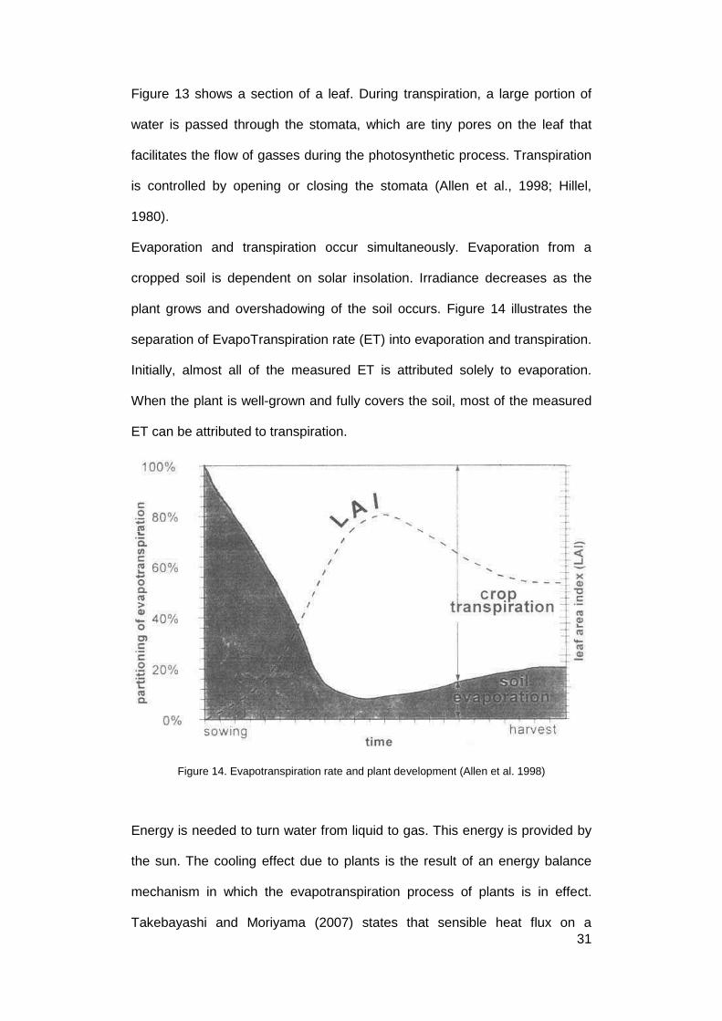
31

Figure 13 shows a section of a leaf. During transpiration, a large portion of

water is passed through the stomata, which are tiny pores on the leaf that

facilitates the flow of gasses during the photosynthetic process. Transpiration

is controlled by opening or closing the stomata (Allen et al., 1998; Hillel,

1980).

Evaporation and transpiration occur simultaneously. Evaporation from a

cropped soil is dependent on solar insolation. Irradiance decreases as the

plant grows and overshadowing of the soil occurs. Figure 14 illustrates the

separation of EvapoTranspiration rate (ET) into evaporation and transpiration.

Initially, almost all of the measured ET is attributed solely to evaporation.

When the plant is well-grown and fully covers the soil, most of the measured

ET can be attributed to transpiration.

Figure 14. Evapotranspiration rate and plant development (Allen et al. 1998)

Energy is needed to turn water from liquid to gas. This energy is provided by

the sun. The cooling effect due to plants is the result of an energy balance

mechanism in which the evapotranspiration process of plants is in effect.

Takebayashi and Moriyama (2007) states that sensible heat flux on a

32

vegetated surface decreases due to an increase in latent heat flux from the

evapotranspiration process. The ambient temperature, therefore, can be

reduced through this process. Niachou et al. (2001) showed that ambient

temperature can decrease by 10.0 °C on the insulated roof constructed from

green roof. Wong et al. (2003a) observed that the surrounding ambient

temperature of rooftop gardens could be reduced by around 4.0 °C.

Factors that influence the rate of evapotranspiration in plants are as follows

(Allen et al., 1998):

1. Solar radiation

Solar radiation is a major factor in plant evapotranspiration. Maximum ET

occurs under clear sky conditions, and is at its minimal under cold and cloudy

conditions. Location, latitude, sun altitude and azimuth as well as atmospheric

pollution are determinants for net radiant energy exposure.

2. Wind

Wind maintains vapour pressure gradients above the vegetation surface by

removing water molecules from the canopy. It serves as a heat transport

medium and accelerates evaporation by removing water from the plant to the

atmosphere. Wind has a higher influence on ET when ta is low.

3. Vapour pressure gradient

Vapour pressure gradient is determined by immediate surface conditions.

Lack of moisture above a surface will limit continuity of the evapotranspiration

process. This will result in a decline for actual evapotranspiration, below the

potential evapotranspiration rate. This is a common occurrence when the soil

is dry and will result in a moisture deficit. Subsequently, plants will be

vulnerable to moisture stress and nutrients deficiencies.

33

4. Humidity and air temperature

Humidity and air temperature are determinants for dryness of the

atmosphere. Air temperature affects the potential of solar and wind factors in

vaporizing water.

5. Crop characteristic

Evapotranspiration rates can be different due to the influence of crop

characteristics such as type, variety, resistance to transpiration, height,

roughness and root, even when other conditions are kept identical.

6. Management and environmental aspects

The evapotranspiration process may be adversely affected by land fertility as

well as soil management practices. Some factors that may affect ET include

plant density, soil type and water availability.

2.5.1.1 Measurement and estimation of plant evapotranspiration rate

There are 4 approaches for evapotranspiration rate (ET) measurements:

1. Hydrology

Soil water balance

ET can be derived based on the principle of mass conservation (one

dimensional). The average rate of ET in mm per day is ascertained by

recording changes in soil water volume over time (Rana and Katerji, 2000):

𝑃 + 𝐼 + 𝑊 − 𝐸𝑇 − 𝑅 − 𝐷 = ±[∆𝑆]0𝑟 [1]

Where,

𝑃 = Precipitation (mm·day-1)

𝐼 = Irrigation (mm·day-1)

𝑊 = Contribution from water table upward (mm·day-1)

𝑅 = Surface runoff (mm·day-1)

34

𝐷 = Drainage (mm·day-1)

∆𝑆 = Soil water storage in the soil layer (mm·day-1)

Precipitation, irrigation and surface runoff can be measured easily. However,

measurement of drainage and soil moisture content is complex. Therefore,

this method can be used only on a large scale, long-term basis where it can

be assumed that drainage to bedrock is balanced by water release from

spring seepage and where the change in soil moisture content is negligible

(Smithson et al., 2002).

Weighing lysimeters

In this direct measurement method, a container is used to measure the

movement of water over a specified area. The ET is determined by changes

in water mass. Lysimeters can be grouped into (Allen et al., 2011):

1. Non-weighing, constant water-table lysimeters. These are used when

the water table is sufficiently high and at similar levels outside the

lysimeter.

2. Non-weighing, percolation lysimeters. Small samples are taken for the

precise measurement of water mass.

3. Weighing lysimeters. Changes in water content are measured by

weighing with a scale or load cell. This method can provide the most

accurate data for short measurement frequencies of 30 min. However,

data obtained from a lysimeter may only represent the ET of just one

specific location of the field (Grebet and Cuenca, 1991) due to variance

in vegetation density, soil and plant height. Especially in arid

environments, neighbouring crops in close proximity may also affect

measurement (Allen et al., 1991).

35

2. Energy balance

This approach considers evapotranspiration in terms of energy usage for

turning water inside the vegetation into vapour. This change in energy is

termed latent heat. Approaches to estimate latent heat flux (Rana and Katerji,

2000) are as follows:

The Bowen Ratio and Energy Balance (BREB) method

Latent heat flux is calculated by means of balancing the energy budget of the

plant. As latent heat flux cannot be measured directly, the BREB method is

used to provide an indirect estimate.

The Bowen Ratio (BR) can be determined by measurements of air

temperature and vapour pressure gradients near the plant (Bowen, 1926).

The temperature and vapour pressure gradient are generally measured

around 0.3 m above dense foliage. Net radiant measurement should consider

the ratio between the fetch and the height of the equipment to gain a

representative surface condition. Fetch is defined as the distance of the field

edge to the location of the BR equipment. Measurement of soil heat flux is

typically conducted between 0.05 m to 0.15 m below the surface (Allen et al.,

2011).

The BREB method does not require aerodynamic data and provide reliable

measurements of ET over a wide variety of vegetation surfaces. However,

homogeneous condition of the surface has to be established to avoid a large

error in calculation. In order to achieve equilibrium condition, Panofsky and

Townsend (1964) stated that the ratio of fetch to the highest position of BR

measurement for temperature and humidity gradient could be from 10:1 to

200:1. Subsequently, Heilman et al. (1989) confirmed that a fetch-to-height

ratio of 20:1 still provides reliable estimations of the Bowen ratio. This study

36

also supports the calculation of Yeh and Brutsaert (1971) which reported that

BR estimation is insensitive to fluctuating fetch conditions as long as the

Bowen ratio is small.

Aerodynamic method

Calculation of latent heat flux (λE) using this method is described by the

following equation (Rana and Katerji, 2000):

λ𝐸 = −λ𝜌𝑢𝑞 [2]

Where,

λ𝐸 = Latent heat flux (Wm-2)

ρ = Density of air (kgm3)

u = Friction velocity (ms-1)

q = Specific air humidity (kgkg-1)

Another approach conducted by Pieri and Fuchs (1990) to avoid difficulties in

measuring water vapour gradients is by determining sensible heat flux by

means of measuring flux-gradients (Equation 3). Latent heat flux is estimated

using the equation:

37

𝐻 = −𝜌𝑐𝑃𝑢 ∙ 𝑇 [3]

Where,

𝐻 = Latent heat flux (Wm-3)

𝜌 = Density of air (kgm-3)

𝑢 = Friction velocity (ms-1)

cp = Specific heat of air (kJ(kgK)-1)

T = Temperature (°C)

The friction of velocity is obtained by wind speed and profile measurements.

The stability function is calculated through an iterative process and requires

measurements of at least three levels (Webb, 1965).

Eddy covariance

This method takes into account turbulent fluxes that occur with the confines of

the atmospheric boundary layer. Measurement is used to estimate heat,

water, CO2 exchange and other gasses. The measurement takes

instantaneous vertical air speed, air temperature, vapour density and

statistical covariance (correlation) data to derive flux values, especially for

sensible heat and evapotranspiration measurement (Uddin et al., 2013). A

high speed measurement system, usually at frequencies of 5- 20 Hz, is

recommended (Allen et al., 2011).

38

The statistical relationship for evaporation rate is as follows (Swinbank, 1951):

𝐸 = 𝜌𝑎𝑊′𝑞′ =

0.622

𝑃𝜌𝑎𝑊′𝑒′ [4]

Where,

ρa = Density of moist air (kgm-3)

P = Atmospheric pressure (Pa)

q′ = Instantaneous deviation of specific humidity from mean specific humidity

(kgm-1)

e′ = Instantaneous deviation of vapour pressure from mean vapour pressure

(Pa)

W′ = Instantaneous deviation of vertical wind velocity from mean vertical wind

velocity (ms-1)

E = Evaporation rate (kgm-2s-1).

39

3. Plant physiology

Sap flow method

This method measures water flow in the plant xylem in two ways (Allen et al.,

2011):

1. Speed of heat pulse being moved away from specified heat source;

and

2. Rate of heat dissipation in plant from convection heat transfer.

This method only measures the plant transpiration component of the

evapotranspiration process as it does not measure the evaporation over a

heterogeneous surface. Cohen et al. (1988) noted that the sap flow method

seemed to be inaccurate when used on plants with low transpiration rates and

that calibration is required for each species being measured.

This method takes into account conductive losses upstream (qu), downstream

(qd) and radially (qr) away from the heat source (Allen et al., 2011):

𝑞𝑓 = 𝑃𝑤 − 𝑞𝑢 − 𝑞𝑑 − 𝑞𝑟 [5]

Where,

𝑞𝑓 = Convective heat loss (W)

Pw = Total power provided by heater (W)

qu = Upstream heat flux (W)

qd = Downstream heat flux (W)

qr = Radial heat flux (W)

40

This method can only be implemented for branches less than 50 mm in

diameter, since the portion of branch being measured must first be uniformly

heated to yield valid results.

Chambers system.

The chamber system was firstly described by Reicosky and Peters (1977)

where latent heat flux can be estimated via the gradient of vapour density

against time, latent heat of vaporisation, area of soil surface and volume of

chamber (Dugas et al., 1991). The chamber was made from a clear plastic

and was covered by a square metal frame, but was later modified into clear

glass to reduce solar irradiance (Reicosky et al., 1983).

Stannard (1988) constructed a chamber for a small area with different types

of vegetation which also has been studied and implemented by Mcleod et al.

(2004). This method is sensitive to surrounding conditions. The major

environmental conditions affecting measurement are air temperature and

wind velocity, which could affect the plant transpiration process (Rana and

Katerji, 2000).

41

4. Statistical Analogy

The estimation models for the evapotranspiration rate based on analytical

approach are as follows:

Penman-Monteith model

This model is originally suggested by Penman (1948) to eliminate the

measurement of surface temperature difference, so that it is possible to write

an expression for the sensible heat flux between the air and surface. The

volumetric heat capacity of dry air used to approximate the heat capacity of

air. In summary, the Penman-Monteith model for evaporation becomes:

𝐸 =

{𝑠(∅𝑛 − 𝐺) + 𝜌𝑎𝑐𝑝gH𝛿𝑒}

λ[𝑠 + (𝛾gHgW

)] [6]

Where,

s = Slope of the curve relating saturation vapour pressure to temperature

(kPa°C-1)

∅𝑛 = Net radiant (Wm−2)

G = Soil heat flux (Wm−2)

𝜌𝑎 = Air density (kgm-3)

𝑐𝑝 = Specific heat capacity (J(kgK)-1)

gH = Heat conductance (molm-2s-1)

𝛿𝑒 = Water vapor deficit (kPa)

𝛾 = Psychrometer constant (kPaK–1)

gW = Water conductance (Sm-1)

λ = Latent heat of vaporization (Jg-1)

42

This equation can also be expressed with different forms, such as by using

the value of the resistance and is described as follows (Zhang et al., 2008):

λ𝐸 =𝑠(∅𝑛 − 𝐺) + (

𝜌𝑎𝑐𝑝𝐷𝑟𝑎

)

s + 𝛾[1 + (𝑟𝑐𝑟𝑎

)] [7]

Where,

𝑟𝑎 = Aerodynamic resistance (sm-1)

𝑟𝑐 = Surface canopy resistance (sm-1), depends on climate factors and

availability of soil water

This model indicates that evaporation (E) increases with increasing radiant

energy and with increasing vapour pressure deficit of the ambient

temperature as well as with the increasing of total water vapour conductance.

Priestley-Taylor (PT) model

The PT model can be considered to be a simplified version of the PM model

and is derived from the equilibrium evaporation concept (Amarakoon et al.,

2000; Penman, 1948; Slatyer and McIlroy, 1961). Equilibrium evaporation

defined as a condition in which the vapour pressure (e) tends to be equal to

the saturation vapour pressure at air temperature (e’).

43

The model can be expressed as follows (Priestley and Taylor, 1972):

𝐸𝑇 = 𝛼𝑃𝑇

𝑆(∅𝑛 − 𝐺)

𝑆 + 𝛾 [8]

Where,

𝛼𝑃𝑇 = Priestly-Taylor coefficient with the value of 1.26

𝑆 = Slope of the curve relating saturation vapour pressure to temperature

(kPa °C-1)

∅𝑛 = Net radiation (Wm-2)

𝐺 = Soil heat flux (Wm-2)

𝛾 = Psychrometer constant (kPa ºC-1)

In practice, PT coefficient varies according to vegetation type, soil moisture

condition and strength of advection (Flint and Childs, 1991). Gunston and

Batchelor (1983) reported that both PM and PT model provides a satisfactory

equation for estimating the evapotranspiration rate in humid tropical climates.

The PT coefficient, 1.26, was confirmed to be suitable for the tropical climate

if conditions remain homogeneous or free from advection, relatively high

humidity and low wind speed. While Li et al. (2012) reported that this model

with the coefficient of 1.26 is not suitable for a desert region since the results

was an overestimation of 5.1 times of the observed eddy covariance. For arid

environments, the modified PT model by Ding et al. (2013) showed a good

agreement with their observation using eddy covariance measurement

methods.

44

2.5.1.2 Energy budget of the evapotranspiration process

The principle of energy conservation can be applied to predict plant

evapotranspiration rate. At any instant, the total energy reaching any surface

has to be equal to the total energy that is leaving it.

The energy balance of green roofs is describe in Equation (9) (Hillel, 1998;

Nobel, 1983):

𝑅𝑛 = 𝐸𝑇 + 𝑄𝑠 + 𝑄𝑐 + 𝑆𝑡 + 𝑀 [9]

Where,

𝑅𝑛 = Sum of all incoming radiation fluxes minus all outgoing radiation. (Wm-2)

This includes all long and shortwave radiation

𝐸𝑇 = Latent heat flux or heat converted in the evapotranspiration process

(Wm-2)

𝑄𝑠 = Convective heat flux (Wm-2)

𝑄𝑐 = Conduction heat flux from green roof into the building (Wm-2)

𝑆𝑡 = Thermal storage for substrate and plants (Wm-2)

𝑀 = Metabolic storage of photosynthesis and respiration (Wm-2)

45

In Equation (9), 𝑀 is assumed to be negligible, as it consists of only a very

small portion of overall radiation (Jones, 1992). Therefore, the equation can

be further elaborated as:

𝑄 = 𝐿𝐸 + 𝐻 + 𝐺 or 𝑅𝑛 = 𝜆𝐸𝑇 + 𝐻 + 𝐺 [10]

𝜆𝐸𝑇 = 𝑅𝑛 − 𝐻 − 𝐺 [11]

Where,

Q = 𝑅𝑛 = Net radiation (Wm-2)

𝐻 = Sensible heat flux (Wm-2)


𝜆𝐸𝑇 = Latent heat flux (Wm-2)

46

Figure 15 illustrates the relationship between all heat fluxes.

Figure 15. The mechanism of Energy balance at the vegetated surface

Equation (11) also explains that net radiation flux entering the crop

environment is use for evaporation, soil and air heating. Latent heat flux

(𝜆𝐸𝑇), which is a description of the evapotranspiration process, can be

determined if data for all other variables are available. Meteorological

variables such as soil heat flux and net radiation can be measured directly.

Latent heat flux is often measured indirectly through calculation of the Bowen

ratio (β), which is defined as the ratio of sensible to latent heat flux (𝐻/ 𝜆𝐸𝑇).

The Bowen ratio is proportional to the ratio of the air temperature gradient

(ΔT) to the vapour pressure gradient (Δе) over a specified vertical distance

above the crop canopy (Fritschen and Simpson, 1989):

47

𝛽 =

𝐻

𝜆𝐸𝑇= 𝛾

∆𝑇

∆𝑒 [12]

Where,

β = Bowen ratio

H = Sensible heat flux (Wm-2)

λET = Latent heat flux (Wm-2)

ΔT = Air temperature gradient (°C)

Δе = Vapour pressure gradient (Pa)

The value of λET can be estimated as follows:

𝜆𝐸𝑇 =

𝑅𝑛 − 𝐺

1 + 𝛽 [13]

Where,

𝜆𝐸𝑇 = Latent heat flux (Wm-2)

𝑅𝑛 = Net radiation (Wm-2)


β = Bowen ratio

The advantages of employing the BREB method are that it can provide

continuous diurnal measurement and wind speed data is not required. Tanner

(1960) observed that the Bowen ratio provides advantages for calculating

latent heat flux because:

1. It does not require data on wind speed; and

2. Limitations of fetch do not affect measurements significantly.

48

Measurements of evapotranspiration from lysimeters and those derived from

energy balance methods showed good agreement in humid regions with

plants that are well-irrigated. Estimates of Bowen ratio in arid regions are less

accurate due to severe advection. Xing et al. (2008) observed similar

concerns regarding the accuracy of the BR method on the semi-arid,

advective environments.

The BREB method makes several assumptions without significantly

compromising its accuracy. Measurement sensors are assumed to be located

in a region where energy fluxes are constant with respect to height. The entire

vegetative surface is assumed to be homogeneous in terms of energy fluxes

and aerodynamic characteristics. Flux movement is assumed to be one-

dimensional.

2.5.2 Plant canopy

2.5.2.1 Leaf Area Index

Leaf Area Index is defined as the ‘total one-sided area of leaf tissue per unit

ground surface area or the ratio of the total area of all leaves on a plant to the

area of ground covered by the plant’ (Watson, 1947). For instance, the LAI of

a plant would be 1 it has only one layer of leaves and they are placed next to

each other without gaps, covering one square meter. LAI is the key parameter

that influences both canopy microclimate both above and below the canopy,

light attenuation and gas exchange (Chason et al., 1991).

Direct measurement of LAI can be done by obtaining a statistically

significant sample of leaves from a vegetative canopy, measuring all available

leaf area and dividing the area by the total surface area (Wilson, 1959). LAI

can also be determined indirectly by measuring canopy shape (cone, sphere,

etc) or correlation with light attenuation (Marshall and Waring, 1986; Rhoads

et al., 2004).

49

2.5.2.2 Leaf Angle Distribution

Foliage is distributed differently between different plant types. For instance,

Heliconia plants have leaves are hung vertically while Wedelia plants have

leaves that spread horizontally. The Leaf Angle Distribution (LAD) is a

statistical description of the approximated angles of leaves distributed within a

canopy. For the same plant, LAD may change throughout the day as leaves

may re-orientate themselves to face the Sun.

The LAD of a plant canopy is important because it determines total solar

insolation for leaf surfaces and the entire plant canopy (Falster and Westoby,

2003). This directly affects the amount of transpiration and water loss

experienced by plants (Ehleringer and Werk, 1986). Plants with leaves that

are vertically hung tend to receive less direct solar radiation during midday.

This results in lesser heat gain and water usage by plants.

Leaf Angle Distribution can be measured in two ways:

1. Direct measurement – Measuring individual leaves (Lang, 1973;

Ranson et al., 1981; Wilson, 1965).

2. Indirect measurement – Using a light interception model. The mean

inclination angle of foliage is estimated by measurements of light

interception by the canopy (Norman et al., 1989). For computer

modelling, mathematical models are often used to approximate LAD

(Campbell, 1986, 1990; Goel and Strebel, 1984).

50

Measurement of LAD can be conducted in the following ways (Kucharik et al.,

1998):

Direct measurement

Direct measurements of LAD can be done with a protractor, compass and

metre rule (Norman and Campbell, 1989). The protractor is used to measure

leaf inclination angle. The compass is used to measure leaf azimuth angle.

The ruler is used to determine distance of the leaf from a pre-determined

reference point such as the substrate level. For this method to be effective,

sample size needs to be in the hundreds and selection should cover the

entire plant canopy. This method does not consider plant effects such as

plant heliotropism, movement due to moisture or wind. Lang (1973)

developed an instrument to measure LAD directly, by using potentiometers

linked to mechanical arms. The angle of each arm is measured as it rotates to

match the orientation of the leaf being measured (Lang et al., 1990). Using

the instrument, leaf position, azimuth and inclination angle can be measured

(Daughtry et al., 1990). This method is seen to be the most accurate and

convenient way to obtain direct measurements of LAD (Pearcy et al., 1989).

Indirect measurement

Indirect measurements of LAD can be done with measurements of light

attenuation as light travels through the plant canopy. This method is also

known as the gap-fraction inversion technique (Norman and Campbell, 1989).

Canopy gap-fraction can be measured by:

1. The LAI-2000 plant canopy analyser;

2. Quantum sensors (Chen and Black, 1992); and

3. Hemispherical (fish-eye) photography (Rich, 1990),

51

Chen et al. (1997) highlights some issues with gap-fraction measurements,

such as overlapping penumbra from leaves and non-randomness in the plant

canopy, which may lead to measurement errors.

2.5.2.3 Leaf and canopy reflectance

Leaf reflectance affects the total amount of sunlight absorbed and

temperature of the leaf. It is often measured in relation to crop growth and

yield (Carlson and Yarger, 1971; Kraft et al., 1996; Woolley, 1971).

Measurement of leaf reflectivity can be done using a spectroradiometer.

There is a significant difference between canopy reflectance and leaf

reflectance. Reflectance of a leaf tends to be higher than the entire canopy

because a portion of solar radiation incident on a canopy will be transmitted

into the porous canopy structure (Campbell and Norman, 1998). Canopy

reflectance can be measured by remote sensing methods (Kobayashi et al.,

2007).

52

2.5.2.4 Albedo of vegetative surfaces

Solar radiation incident to a vegetative surface can be absorbed, reflected or

transmitted by plants. The albedo of a surface is a description of the portion of

incident radiation that is reflected from the surface. It can be considered to be

a ‘measure of the overall reflecting potential of a surface’ (Ahmad and

Lockwood, 1979). Albedo can be differentiated into spectral (specific

wavelength) and total (all wavelengths) albedo (Dobos, 2006).

Albedo values can range from 0 to 1. A theoretical blackbody has an albedo

of 0 as all the radiation are absorbed while the inverse is true for an ideal

reflector of absolute white surface, where all the radiation are reflected

(Figure 16). In actuality, surface albedo is not defined by a single number but

by a range of values.

Figure 16. Range of albedo of natural surfaces (Dobos, 2006)

53

Surface albedo is influenced by surface condition, sun position, sky condition

and angle of surface to the horizontal (Ahmad and Lockwood, 1979).

Surfaces that are dry, light-colored and smooth are often associated with high

albedo while surfaces that are wet, dark-colored and rough are associated

with low albedo. In Figure 16, dry clay soil has an albedo of 0.15 to 0.35 while

dry sandy soil has an albedo of 0.25 to 0.45. This is because clayey soil can

maintain a higher moisture content than sandy soil and smaller particle size of

the sandy soil creates a relatively smooth surface which reflects more

radiation. Sun zenith angle will influence diurnal variations, while sky

condition refers to cloud cover characteristics. An overcast day with uniform

and heavy clouds would lessen total solar insolation. In terms of albedo of

vegetative surfaces, they are further affected by crop parameters such as LAI,

height of plant canopy, temperature and moisture conditions (Doughty et al.,

2011).

Measurement of albedo

Albedo can be measured using an albedometer or similar high-quality

instruments such as a pyranometer. The pyranometer has to be oriented in

both upward and downward directions such that readings are collected

simultaneously for both directions. The upward-facing pyranometer measures

the incident radiation while the downward-facing measures the reflected

radiation. The setup is simple but has several problems as identified by

Dobos (2006). The measurement of the surface albedo is complex under

natural condition as the incident radiation includes diffused light from other

directions. It is difficult to ensure that the incident radiation is solely from the

radiation source. Additionally, the measured surfaces do not reflect radiation

in all directions equally and evenly. Readings might vary at different parts of a

54

same surface. Also, the sensors are only able to gather light from a specific

range of angles.

Diurnal variation of albedo

The reflection of radiation from vegetative surfaces is complex as it composes

of reflected radiation from plants as well as surrounding surfaces (Ahmad and

Lockwood, 1979). As shown in Figure 17, the albedo of vegetative surfaces

on a sunny day exhibits a typical bowl-shaped curve due to the diurnal

variations of the sun zenith angle (Ahmad and Lockwood, 1979). This is also

observed by Monteith and Szeicz (1961), Graham and King (1961) and

Stewart (1971) who had studied different vegetation such as grass, maize

and pine forests. Albedo values are at the minimum in the midday with most

of the incident radiation directly from overhead. Little amount of radiation is

reflected as most of them are trapped within the canopy. In this case solar

radiation penetrates into the shrubbery and is reflected multiple times

between the leaves. However, albedo increases the sun gets closer to the

horizon. This is because more solar irradiance is reflected from the plant

surface and there is less radiation is trapped inside the shrubbery.

Figure 17. Diurnal variations of albedo (Ahmad & Lockwood, 1979)

55

Nkemdirim (1972) concluded that albedo values showed a clear correlation to

sun zenith angle under clear sky conditions. Under overcast sky conditions,

little variation in albedo values was observed. Similar results were observed

by Ahmad (1978), where diurnal variation in albedo is more noticeable as

cloudiness decreases. It was also observed that the values of albedo before

noon are generally lower than after noon for similar zenith angles. According

to Song (1998), this asymmetry is because of solar ray asymmetric variation

and canopy reclination which is caused by strong prevailing winds.

56

2.5.3 Plant functional traits

Plant functional traits can be defined as plant features (physiological,

morphological, etc) that are representative of their response to environmental

influences. The variations in traits are useful in ecological pattern and

processes, which includes opportunities and constraints similar plants face in

different habitats (Grime, 1979; Southwood, 1977). Results can be used to

develop dynamic global vegetation models, carbon models, water budget and

land management models, forecast impacts of environmental change, plant

effects on ecosystem function and resilience and examine evolutionary and

phylogenetic relationships among species, fundamental trade-offs in plant

design and eco-physiology (McGill et al., 2006; Reich et al., 2003; Westoby et

al., 2002; Westoby and Wright, 2006).

Plant functional traits can be broadly classified into five main categories, as

summarized in Table 1 (Pérez-Harguindeguy et al., 2013). Within these

categories are specific traits which can be further explored. Most traits can be

measured quantitatively but some has to be measured qualitatively due to

methodological or logistical limitations. Some traits are more difficult to

measure than others, as they require long period of measurements or

experimental manipulations (Weiher et al., 1999).

57

Table 1. Classification of plant functional traits (Pérez-Harguindeguy et al., 2013)

Whole-plant

traits

Leaf

traits

Stem

traits

Below-

ground

traits

Regenerative

traits

Life history Specific leaf area Stem-specific

density

Specific root

length

Dispersal mode

Life form Area of a leaf Twig dry-matter

content

Root-system

morphology

Dispersule size

and shape

Growth form Leaf dry-matter

content

Bark thickness Nutrient

uptake

strategy

Dispersal

potential

Plant height Leaf thickness Xylem

conductivity

Seed mass

Clonality pH of green

leaves or leaf

litter

Vulnerability to

embolism

Seedling

morphology

Spinescence Leaf nitrogen and

phosphorus

concentrations

Resprouting

capacity

Branching

architecture

Physical strength

of leaves

Leaf to sapwood

area

Leaf lifespan and

duration of green

foliage

Root-mass

fraction

Photosynthetic

pathway

Salt-tolerance

traits

Vein density

Relative growth

rate

Light-saturated

photosynthetic

rate

Water-flux traits Leaf dark

respiration

Electrolyte

leakage

Leaf water

potential

Leaf palatability

Litter

decomposability

58

2.5.3.1 Plant height

The height of a plant is defined as the ‘shortest distance between soil or

substrate level and the upper boundary of the main photosynthetic tissues on

a plant’ (Pérez-Harguindeguy et al., 2013). Maximum plant height (Hmax) is

defined as ‘maximum height achieved by a typical mature individual plant

species in a particular environment’ (Pérez-Harguindeguy et al., 2013).

Studies have shown Hmax to be associated with plant growth, potential

lifespan, position of the species with respect to light availability and

competitive vitality (Gaudet and Keddy, 1988; Thomas, 1996).

2.5.3.2 Measurement of plant height

Measurement of plant height can be categorised as follows (Pérez-

Harguindeguy et al., 2013):

1. Short plant species – Measurements of plant height should be taken

for at least 25 plants for each species;

2. Tall plant species (trees) – Measurements of at least 5 of the tallest

mature individual plants per species ; and

3. Tall plant species (trees) where time and resources are available -

Measurements of at least 25 of the tallest mature individual plants per

species.

The recorded height should be representative of general plant canopy, and

should excluded inflorescences (flowers), outlying braches or leaves.

Measurement for short plant species can be conducted with the use of sticks

or rulers with decimetre marks. Measurements for tall plant species can be

used either with either a telescopic measuring stick with decimetre marks, or

using the following trigonometric function:

59

𝐻 = 𝑑 × [tan(𝛼) + tan(𝛽)] [14]

Where,

𝐻 = Plant Height (m)

𝑑 = Horizontal distance from plant to measurement point (m)

𝜶 = Angle between horizontal plane and plant canopy (°)

𝜷 = Angel between horizontal plane and plant base (°)

2.5.3.3 Leaf area

The leaf area (LA) is defined as the area (or projected area) of an individual

leaf (one-sided only). Measurement of LA has been correlated with climatic

variation, water-loss efficiency, growth form and radiation exposure (Givnish,

1987; Parkhurst and Loucks, 1972; Royer et al., 2008).

2.5.3.4 Measurement of leaf area

Prior to measurement, each leaf has to be cut from the stem. The inclusion of

petioles should be based on research agenda. All leaves should be patted dry

before measurement. Samples of at least 4 specimens from 10 individuals

are recommended.

Measurement of leaf area can be categorised to the following (Pérez-

Harguindeguy et al., 2013):

1. Using specialised leaf-area meters – Calibration is necessary. This is

done using pieces of known length and area. The entire leaf is to be

positioned within the scanning area and has to be flat;

2. Using a digital camera – Leaf samples are recommended to be

secured under a glass plate. Images are to be taken with a ruler for

the purpose of calibration. The camera is to be mounted on a tripod

60

with adequate lighting. The use of flash photography is not

recommended ; and

3. Using a flatbed scanner – This method has the added advantage of

capturing other features of interest such as leaf veins at high

resolution. Leaves may be cut to facilitate scanning. Post-processing

software such as Leafarea (Price et al., 2011) can be used to

calculate leaf area.

2.6 Mean radiant temperature (tmrt) and thermal comfort

There are several methods of determining the quality of both the indoor

(Fanger, 1972; Gagge, 1971) and outdoor (Höppe and Mayer, 1987)

microclimate. The use of biometeorological indices has enabled quantification

of thermal comfort and assessment in tandem with behavioural aspects.

Useful heat stress indices have also been developed to describe thermal

stress (d’Ambrosio Alfano et al., 2011b; Epstein and Moran, 2006; Parsons,

2003). According to Parsons (2003), evaluations of thermal environments by

means of a suitable comfort or stress index require the measurement of wind

speed, relative humidity, air and mean radiant temperature. Among them, one

of the main factors contributing to the thermal response of man to his

surrounding environment is the mean radiant temperature (tmrt). This quantity

plays a crucial role not only in indoor situations but also outdoors as indicated

in several studies which have stressed that outdoor thermal comfort is highly

dependent on radiative heat transfer from its surroundings (Mayer, 1993;

Mayer and Höppe, 1987). Estimation of tmrt can be done by two-sphere

radiometers, globe thermometers, constant-air-temperature sensors (ISO

7726, 1998). Calculation of tmrt is also possible using radiant fluxes and the

angle factors of surrounding surfaces (ISO 7726, 1998; Palmer and

61

Chapman, 2000). The calculation of tmrt can be done with the ASHRAE

formula:

𝑡mrt = [(𝑡g + 273.15)4 +1.1 × 108𝑉a0.6

휀𝐷0.4× (𝑡g − 𝑡a)]

0.25

− 273.15 [15]

Where,

tg = Globe temperature (°C) , measured by a temperature sensor placed inside the globe

Va = Air velocity (ms-1) , measured at the level of the globe

ta = Air temperature (°C) , measured near the globe

D = Globe diameter (m)

ε = Globe emissivity

In some cases, the mean convective coefficient of the globe thermometer has

to be recalibrated to suit the contextual outdoor conditions (Thorsson et al.,

2007).

The effects of tmrt can be studied through numerical modelling (Ali-Toudert

and Mayer, 2006; La Gennusa et al., 2005). This method is useful when used

for iterative studies such as the comparison of width-to-height ratios and

orientations of street canyons. However, model geometry and ambient

conditions are often simplified. Recent developments in solar and long wave

environmental irradiance modelling takes into account large-scale urban

geometry as well as important urban components such as tree and shrubs

(Lindberg and Grimmond, 2011).

The estimation of radiant temperature is often an integral component to the

assessment of thermal environments. Common thermal assessment indices

such as the Physiological Equivalent Temperature (PET) and the recently

developed Universal Thermal Climate Index (UTCI) are evaluated with tmrt as

62

a variable component (Höppe, 1999; Jendritzky et al., 2012; Lin et al., 2012a).

Other heat stress indices such as the Wet Bulb Globe Temperature (WBGT)

consider radiant temperature in the form of the globe surface temperature

(Gaspar and Quintela, 2009; Lemke and Kjellstrom, 2012). Fluctuating

radiation fluxes due to complex environments have contributed to the

uncertainty in tmrt estimation, and studies have shown that it can affect the

overall thermal assessment in some temperature ranges (Weihs et al., 2012).

Therefore, it is important that the estimated tmrt can accurately reflect the

prevalent conditions of radiation fluxes of the measured space.

63

2.7 Knowledge Gap

A review of the literature has uncovered several crucial knowledge gaps in

the study of measuring the cooling effect of urban greenery. They are as

follows:

- Globe thermometer used for outdoor tmrt measurement needs to be

calibrated for the tropical outdoor conditions;

- Studies on the measurement of outdoor tmrt in the tropics at the diurnal

scale are lacking;

- Studies on the cooling effect of outdoor greenery are largely on parks

and large trees. There is little knowledge on the effects of outdoors tmrt

due to specific types of urban greenery systems such as shrubs and

rooftop greenery;

- On the subject of cooling effect of plants, there is no distinction

between the cooling due to reduction of radiant heat flux from plant

shade and cooling due to evapotranspiration of plant;

- Reflectivity of a plant (shrub) is not considered in its entirety, but is

ascertained by measuring the reflectivity of individual leaves and

defining the Leaf Area Distribution; and

- There are no scientific criteria for the selection and placement of

plants for rooftop greenery design.

64

3 HYPOTHESES AND RESEARCH METHODOLOGY

3.1 Hypotheses

Based on reviewed literature, it is found that:

- Addition of greenery in the urban environment can significantly

lower the ambient temperature; and

- The cooling effect of outdoor greenery has been largely attributed

to shade provision of trees and the plant evapotranspiration

process.

For rooftop greenery, which has more exposure to direct sunlight, the

opportunity for the shade provision by tree canopy is significantly reduced.

The plant evapotranspiration rate, reflectance of short wave and long wave

radiation as well as emission of terrestrial (long wave) radiation is

hypothesized to be significant factors in the contribution of radiant heat flux.

Hence, the hypothesis can be rationalized as follows:

The overall cooling effect of plants comprises the plant evapotranspiration

rate and albedo of the said plants.

𝑪𝒐𝒐𝒍𝒊𝒏𝒈 𝒆𝒇𝒇𝒆𝒄𝒕 𝒐𝒇 𝒓𝒐𝒐𝒇𝒕𝒐𝒑 𝒈𝒂𝒓𝒅𝒆𝒏 𝒑𝒍𝒂𝒏𝒕𝒔 [16]

= 𝑓 (𝑃𝑙𝑎𝑛𝑡 𝑎𝑡𝑡𝑟𝑖𝑏𝑢𝑡𝑒𝑠 𝑐𝑎𝑢𝑠𝑖𝑛𝑔 𝑎 𝑟𝑒𝑑𝑢𝑐𝑡𝑖𝑜𝑛 𝑖𝑛 𝑎𝑖𝑟 𝑡𝑒𝑚𝑝𝑒𝑟𝑎𝑡𝑢𝑟𝑒,

𝑃𝑙𝑎𝑛𝑡 𝑎𝑡𝑡𝑟𝑖𝑏𝑢𝑡𝑒𝑠 𝑐𝑎𝑢𝑠𝑖𝑛𝑔 𝑎 𝑟𝑒𝑑𝑢𝑐𝑡𝑖𝑜𝑛 𝑖𝑛 𝑟𝑎𝑑𝑖𝑎𝑛𝑡 𝑡𝑒𝑚𝑝𝑒𝑟𝑎𝑡𝑢𝑟𝑒)

= 𝑓 (𝑃𝑙𝑎𝑛𝑡 𝐸𝑣𝑎𝑝𝑜𝑡𝑟𝑎𝑛𝑠𝑝𝑖𝑟𝑎𝑡𝑖𝑜𝑛 𝑅𝑎𝑡𝑒, 𝑆ℎ𝑟𝑢𝑏 𝐴𝑙𝑏𝑒𝑑𝑜)

65

Since tmrt is a function of the air and surface temperature of its surroundings, it

can be used to measure the overall reduction in temperature due to greenery.

This gives us the equation:

𝑹𝒆𝒅𝒖𝒄𝒕𝒊𝒐𝒏 𝒊𝒏 𝒕𝒎𝒓𝒕 𝒅𝒖𝒆 𝒕𝒐 𝒑𝒓𝒆𝒔𝒆𝒏𝒄𝒆 𝒐𝒇 𝒑𝒍𝒂𝒏𝒕𝒔 [17]

= 𝑓(𝑃𝑙𝑎𝑛𝑡 𝐸𝑣𝑎𝑝𝑜𝑡𝑟𝑎𝑛𝑠𝑝𝑖𝑟𝑎𝑡𝑖𝑜𝑛 𝑅𝑎𝑡𝑒, 𝑆ℎ𝑟𝑢𝑏 𝐴𝑙𝑏𝑒𝑑𝑜)

The rationale for proposing the following variables are shown in Table 2 and

Figure 18.

Table 2. Influence of hypothesized variables on tmrt

Variable Influence on tmrt

Plant EvapoTranspiration Rate

(ET)

Increased ET will reduce surrounding air

temperature through increased latent heat of

vaporization. This will also result in cooler leave

surfaces than will reduce longwave emission

Shrub Albedo Albedo of shrub is a representation of leaf angle

and shrub reflectivity. A lower albedo will result

in higher thermal absorption for the shrub and

subsequent increase in thermal emission to its

surroundings

66

Equation (17) forms the basis of the proposed hypothetical model on

optimized landscape design (Figure 19).

Evapotranspiration Rate Shrub Albedo

How it affects

Radiant Temperature

Air Temperature

Higher ET

Lower canopy surface

temperature

Lower direct Longwave emission

Higher ET

More water released into

the air

Increased evaporative

cooling

Lower air temperature

Radiant Temperature

Air Temperature

Higher Albedo

More heat reflected from

canopy

Less heat absorbed by

shrub

Lower surface temperature

Lower direct Longwave emission

Higher Albedo

More heat reflected from

canopy

Less heat absorbed by

shrub

Lower surface temperature

Lower direct Longwave emission to

surrounding air

Lower air temperature

Figure 18. Hypothesised effects of ET and SA on tmrt

How it affects

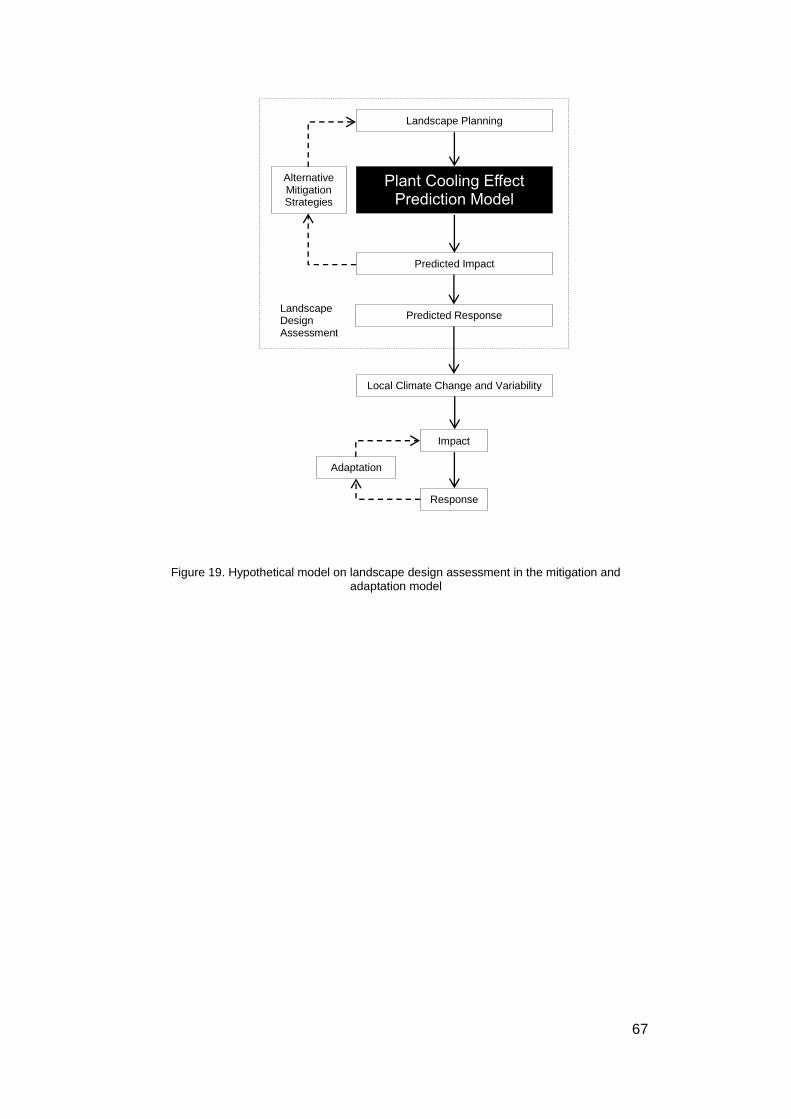
67

Figure 19. Hypothetical model on landscape design assessment in the mitigation and adaptation model

Landscape Planning

Plant Cooling Effect Prediction Model

Predicted Impact

Predicted Response

Local Climate Change and Variability

Impact

Response

Adaptation

Alternative Mitigation Strategies

Landscape Design Assessment

68

3.2 Methodology

The overall research methodology is illustrated in Figure 20. Studies on

rooftop greenery will be conducted with different plants. Three quarters of all

relevant data collected will be used for analysis and construction of a

regression model for estimating tmrt based on plant characteristics. The

remaining quarter of data collected will be used for the purpose of validation.

Figure 20. Research methodology

Background Study

Objectives

Literature Review

Hypotheses on Cooling Effect Prediction

Calibration of Globe Thermometers

Study on Rooftop Greenery

Regression Modelling

Validation of Model

Discussion

Conclusion

69

Quantification of the cooling effect of plants will be done through field

measurement. Therefore, a series of measurements is proposed with the aim

of quantifying plant evapotranspiration rates, radiant and functional attributes

of plants used for rooftop greenery. The variables to be measured are shown

in Table 3.

Table 3. Hypothesized variables

Variable Corresponding measurement

Mean radiant temperature Globe temperature, air temperature,

wind velocity Plant evapotranspiration rate Water loss rate Shrub albedo Albedo

1. Calibration of the globe thermometer

The 38 mm globe thermometer will first be calibrated for use in the tropical

outdoor urban environment. This is to enable accurate diurnal measurement

of tmrt near the plant canopy. The calibration process is documented in

Chapter 3.2.1.

2. Measurement of plants in a roof garden setting

Measurements are proposed for a typical roof garden setting. Attributes of

different plants that are hypothesized to be significant variables for cooling will

be measured. The variables include plant evapotranspiration rate and shrub

albedo (Figure 21). The complete list of measured variables is shown in Table

7.

Measurements from the hypothesized variables will be analysed to deduce

their correlation with tmrt.

70

Figure 21. Effect of rooftop greenery on temperature at a given point

71

3.2.1 Calibration of globe thermometers for use in the tropical urban

environment

Content from Chapter 3.2.1 (Pages 71 to 87) has been published in the

Journal of Building and Environment, for which I am the main author:

Tan, C.L., Wong, N.H., Jusuf, S.K., 2013, Outdoor mean radiant temperature estimation in the tropical urban environment, Building and Environment 64:118-129.

3.2.1.1 Objectives

The objective of this study is to assess the feasibility of deploying customised

40 mm globe thermometers for outdoor tmrt measurement in the tropics.

Calibration of the mean convection coefficient in the ASHRAE tmrt formula is

performed to ensure accuracy of estimation.

3.2.1.2 Methodology

Customized globe thermometers are used to estimate the tmrt outdoors to

ensure the accuracy of tmrt estimation, readings from the customized globe

thermometers are first estimated against readings from a net radiometer. The

mean convection coefficient of the formula used for tmrt estimation is

recalibrated for use in the local context. The mean radiant temperature is

defined as the ‘uniform temperature of an imaginary enclosure in which the

radiant heat transfer from the human body equals the radiant heat transfer in

the actual non-uniform enclosure’ (ASHRAE, 2001a). It is often used as a

parameter to estimate thermal comfort. Mean radiant temperature can be

measured with a globe thermometer (De Dear, 1987; Keuhn et al., 1970;

Nikolopoulou et al., 1999; Vernon, 1932). It can be used for indoor and

outdoor conditions (Nikolopoulou and Lykoudis, 2006). The Vernon globe is a

black copper sphere of 75 mm radius with a thermometer positioned in the

middle of the sphere. For convenience, smaller globes were developed. The

38 mm globe thermometer is a common option as the globe used is a table

72

tennis ball, which can be readily purchased and conveniently replaced

(Humphreys, 1977). Accuracy of the 38 mm globe thermometer can be

adjusted to cater to outdoor conditions by recalibrating the mean convection

coefficient. This method has been tested in Sweden (Thorsson et al., 2007)

and shown to be effective in outdoor conditions. To ensure validity of the tmrt

estimation for this study, the mean convection coefficient of the formula for tmrt

estimation via the globe thermometer is recalibrated. This is done by

comparing the estimates from the customised globe thermometer to the long

wave and short wave readings from a net radiometer. Two sets of

measurements are made, one at each of the study areas (Table 4).

Two different methods for measuring the tmrt outdoors are put to comparison:

1. Method A - Radiant flux measurements, where tmrt calculation is based

on short wave and long wave angular factors for a sphere;

2. Method B – 40 mm globe thermometer with tmrt equation from ISO

7726:1998 (ISO 7726, 1998).

Table 4. Measurement period

Study Area 1 Green Technology Laboratory rooftop

Study Area 2 School of Design and Environment Block 1 rooftop

Measurement date 28/02/2011 to 18/03/2011

30/03/2011 to 12/04/2011 13/08/2011 to 13/09/2011

No. of days measured 33 32 Purpose of measurement

Recalibration of mean convection coefficient

Validation of recalibrated mean convection coefficient

No. of days used for recalibration of mean convection coefficient

33 -

No. of days used for validation of mean convection coefficient

- 32

73

Results are used to recalibrate the tmrt formula for Method B, so that the mean

convection coefficient in the tmrt equation will be representative of local

outdoor conditions. Recalibration is done via statistical analysis using the IBM

SPSS software.

Measurements are then made in another area with Methods A and B. The tmrt

formula used for the second measurement will be with the recalibrated mean

convection coefficient. This is done to ensure validity of the recalibration.

Measurements are taken at the frequency of one minute, and averaged to five

minute intervals (Thorsson et al., 2007). Data gathered from Methods A and B

will be used to recalibrate the globe thermometer to improve the accuracy of

the globe thermometer with respect to radiant flux measurements. Table 8

shows the measured variables and equipment used.

Figure 22 shows the measurement setup. A net radiometer with three

integrated pyranometer and pyrgeometer arms (Kipp and Zonen, CNR 4) is

used to measure long and shortwave radiation for the following directions:

North

East

South

West

Upper hemisphere

Lower hemisphere

The newly purchased net radiometer was factory calibrated. The

pyranometers were calibrated side by side to a reference CMP 3 pyranometer

according to ISO 9847:1992 annex A.3.1. The pyrgeometers were calibrated

side by side to a reference CG(R) 3 pyrgeometer (Kipp, 2008).

74

Figure 22. 40 mm globe thermometer mounted on net radiometer

In a previous study conducted in Sweden (Thorsson et al., 2007), the globe

thermometer used consisted of a grey acrylic sphere that is 38 mm in

diameter with a Pt100 sensor (De Dear, 1987; Humphreys, 1977;

Nikolopoulou et al., 1999).

In this study, the globe thermometer is made of a 40 mm ping pong ball with a

HOBO thermocouple wire at its centre. The ping pong is coated in flat grey

paint (Phylox Nippon 144 dove grey). The 40 mm ping pong ball is preferred

over the original 38 mm due to the decrease in availability of 38 mm ping

pong balls (ITTF, 2009). The globe thermometer is secured on the arm of one

of the net radiometer sensors to ensure accuracy of readings for both

methods of tmrt calculation. A total of nine other customised globe

thermometers are set up near the globe thermometer to ensure measurement

consistency. All thermocouple loggers and Type-T Copper-Constantan

thermocouple sensors used for this study are new and factory calibrated. The

75

globe thermometers are positioned such that they will not experience any

effects of overshadowing from the mounting structure.

3.2.1.3 Results and discussion

Validation of customised globe thermometers

Calculation of tmrt can be done for Method A using the following method

(Thorsson et al., 2007):

1. Estimate mean radiant flux density (Sstr)

2. Estimate tmrt using value of Sstr

Estimation of Sstr is done using Equation (18) (VDI, 1994):

𝑆𝑠𝑡𝑟 = 𝛼k ∑ 𝐾i𝐹i

6

𝑖=1

+ 휀p ∑ 𝐿i𝐹i

6

𝑖=1

[18]

Where,

Ki = Short wave radiation (Wm-2)

Li = Long wave radiation (Wm-2)

Fi = Angular factors between observer and external surrounding

Value of 0.167 used (Fanger, 1972; Thorsson et al. 2007)

αk = Absorption coefficient for short wave radiation. Value of 0.7 is used

(Thorsson et al. 2007)

εp = Emissivity of the human body. Value of 0.97 is used (Thorsson et al.

2007)

76

The tmrt (°C) can be calculated from the Stefan–Boltzmann equation:

𝑇𝑚𝑟𝑡 = √(𝑆𝑠𝑡𝑟

휀𝑝𝜎)

4

− 273.15 [19]

Where,

Sstr = Mean radiant flux density (Wm-2)

σ = Stefan–Boltzmann constant (5.67·10−8 Wm

−2K−4)

εp = Emissivity of the human body. Value of 0.97 is used (Thorsson et al.

2007)

Estimation of tmrt can be done for Method B using Equation (15) from ISO

7726 (1998):

𝑇𝑚𝑟𝑡 = [(𝑇g + 273.15)4 +

1.1 × 108𝑉a0.6

휀𝐷0.4× (𝑇g − 𝑇a)]

0.25

− 273.15 [15]

Where,

tg = Globe temperature (°C)

Va = Air velocity (ms-1)

ta = Air temperature (°C)



Mean convection coefficient of the globe (1.1 X 108 Va 0.6) comprises of the

wind exponent as well as an empirically derived constant.

77

Values of tmrt for Method B are calculated using Equation (19).

A total of 65 days of field data from the two study areas are measured (Table

5). A typical clear sunny day is used for analysis of the diurnal tmrt profile at

Study Area 1. The 18th of March 2011 was a sunny day with clear skies. The

mean near-surface air temperature was 27.3 °C, the minimum near-surface

air temperature recorded was 24.2 °C and the maximum near-surface air

temperature recorded was 31.0 °C. The mean wind speed was 3 ms-1. The

sun rose at 07:10 hrs and set at 19:16 hrs. The sun reached its maximum

altitude of 87.5° at 13:13 hrs. Mean wind speed was measured with a weather

station that was placed within 10 m of the mean radiant temperature

measurement site.

Figure 23 shows the short wave and long wave radiation fluxes for six

directions. KNORTH, KSOUTH, KEAST and KWEST represents the short wave

radiation fluxes from the North, South, East and West respectively. KUP

represents short wave radiation from the sky (upper hemisphere), and KDOWN

represents short wave radiation from the ground (lower hemisphere).

Direct solar radiation KUP peaked at 1142 Wm-2 at 14:10 hrs. Its value is most

significantly affected by the position of the sun. The reflected short wave

radiation KDOWN follows a similar pattern to that of KUP but with significantly

lower values. It peaked at 133 Wm-2 at 14:10 hrs. KEAST peaked at 351 Wm-2

in the morning (10:00 hrs). Thereafter, readings remained low. In contrast,

KWEST remained low in the morning and increased slowly until it reached its

peak of 684 Wm-2 (almost twice the peak value of KEAST) at 16:25 hrs. This is

due to exposure to more intense direct solar radiation from the West. KNORTH

and KSOUTH remained low throughout the day. KNORTH peaked at 291 Wm-2 at

16:25 hrs. KSOUTH peaked at 246 Wm-2 at 12:50 hrs. There is negligible short

wave radiation activity in the absence of sunlight.

78

LNORTH, LSOUTH, LEAST and LWEST represents the long wave radiation fluxes from

North, South, East and West respectively. LUP represents long wave radiation

from the sky (upper hemisphere), and LDOWN represents long wave radiation

from the ground (lower hemisphere).

The long wave fluctuations for all six directions follow a similar pattern. The

LUP profile is notably lower than the other profiles. This is due to the fact that

LUP is facing the sky and not directly at any objects. LUP peaked at 465 Wm-2

at 14:15 hrs. LDOWN exhibited the highest profile, due to the fact that it is facing

downwards and has maximum exposure to objects and surfaces. The

difference between the other points is most evident during periods of intense

exposure to sunlight. LDOWN peaked at 546 Wm-2 at 13:50 hrs. LEAST increased

steadily until 14:00 hrs. LWEST does not exhibit a similar trend. This may be

because there is a wall on the West side of the net radiometer, and it is

exposed to direct sunlight after 14:00 hrs. LEAST peaked at 519 Wm-2 at 16:30

hrs and LWEST peaked at 498 Wm-2 at 14:10 hrs. LWEST, LNORTH and LSOUTH

showed similar trends in fluctuation throughout the day. LNORTH peaked at 499

Wm-2 at 14:10 hrs and LSOUTH peaked at 497 Wm-2 at 13:50 hrs. The minimum

value for all long wave radiation ranges from 433 Wm-2 to 440 Wm-2 at 06:40

hrs. There are slight fluctuations in the absence of sunlight.

79

Figure 23. Diurnal short wave (K) and long wave (L) profile for 18th March 2011

Measurements using Method A (Net radiometer) are used to plot the diurnal

tmrt profile for 18th March 2011. The plot is overlaid with a plot of diurnal tmrt

using Method B. The tmrt profile generated is similar to that of KUP, indicating

the high relevance of direct solar radiation to tmrt. Figure 24 shows that the

calculation of tmrt using the globe thermometer (Method B) differs from the

values obtained via the net radiometer (Method A) drastically.

0

200

400

600

800

1,000

1,200K

(W

m-2

)

0

200

400

600

800

1,000

1,200

0:0

0

1:0

0

2:0

0

3:0

0

4:0

0

5:0

0

6:0

0

7:0

0

8:0

0

9:0

0

10

:00

11

:00

12

:00

13

:00

14

:00

15

:00

16

:00

17

:00

18

:00

19

:00

20

:00

21

:00

22

:00

23

:00

0:0

0

L(W

m-2

)

Time (Hrs)

EAST WEST UP DOWN NORTH SOUTH

KDOWN

KUP

KEAST

KWEST

KNORTH

KSOUT

H

LUP

LDOWN

80

Results show that measurement of tmrt using the customised globe

thermometers and Equation (15) is highly unsuited for use in the given

context. There is a slight overestimate of tmrt in the absence of sunlight and a

drastic underestimate during sunlit hours. Any measurement of outdoor tmrt

using the customised globe thermometers using Equation (15) would be

highly inaccurate.

Figure 24 shows that the calculation of tmrt using the globe thermometer

(Method B) differs from the values obtained via the net radiometer (Method A)

drastically. This is due to the mean convection coefficient used for the tmrt

formula (Equation 15) that does not adequately represent the convective

conditions found in the tropical outdoor climate.

Figure 24. Calculation of tmrt using Method A and B (ISO 7726:1998) – 18th March 2011

10.0

20.0

30.0

40.0

50.0

60.0

70.0

80.0

0:0

0

1:0

0

2:0

0

3:0

0

4:0

0

5:0

0

6:0

0

7:0

0

8:0

0

9:0

0

10

:00

11

:00

12

:00

13

:00

14

:00

15

:00

16

:00

17

:00

18

:00

19

:00

20

:00

21

:00

22

:00

23

:00

0:0

0

Mea

n R

adia

nt

Tem

per

atu

re (

°C)

Time (Hrs)

Method A (Net radiometer) Method B (ISO 7726:1998)

81

In order to utilise the formula in this context, the mean convection coefficient

of 1.1 X 108Va0.6 is recalibrated. This is done by considering the field

measurements of the following variables:

- Mean radiant temperature (°C)

- Globe temperature (°C)

- Air temperature (°C)

- Air velocity (ms-1)

Only measurements taken from Study Area 1 are used for the calibration. A

total of 33 days, which consists of diverse weather conditions, are used. The

best fit curve generated gives the new mean convection coefficient of 2.20 X

108Va0.119, giving us the recalibrated equation:

𝑇𝑚𝑟𝑡 = [(𝑇g + 273.15)4 +

2.20 × 108𝑉a0.119

휀𝐷0.4× (𝑇g − 𝑇a)]

0.25

− 273.15 [20]

Where,

tg = Globe temperature (°C)

Va = Air velocity (ms-1)

ta = Air temperature (°C)



The derived values are significant at 95% confidence interval.

A re-plot of the tmrt profile for 18th March 2011 with Equation (20) shows the

new tmrt profiles. The new profile is much closer to that of the tmrt profile

generated by Method A (Figure 25). There is still a slight underestimation for

certain periods during the day. The slight overestimation of tmrt during night

time is reduced to match the tmrt of Method A. The profiles of the two methods

82

show that the 40 mm globe thermometer has a response time of less than 5

minutes, which is similar to the 38 mm globe thermometers used in previous

indoor tests (Höppe, 1999). There is a general trend of underestimation of tmrt

with increasing short wave radiation. This suggests that the albedo of the

globe may be slightly higher than desired, and may be reduced further by

using a darker shade of grey.

Figure 25. Calculation of tmrt using Method A and B(Recalibrated) – 18th March 2011

To validate the new mean convection coefficient, Equation (20) is used to

calculate the tmrt of the same 40 mm globe thermometer at Study Area 2. A

typical clear sunny day is chosen for analysis. A plot of the tmrt profile for 16th

August 2011 with Equation (20) shows the new tmrt profile. Similar to the

previous re-plot, the new profile is much closer to that of the tmrt profile

generated by Method A (Figure 26).

10.0

20.0

30.0

40.0

50.0

60.0

70.0

80.0

0:0

0

1:0

0

2:0

0

3:0

0

4:0

0

5:0

0

6:0

0

7:0

0

8:0

0

9:0

0

10

:00

11

:00

12

:00

13

:00

14

:00

15

:00

16

:00

17

:00

18

:00

19

:00

20

:00

21

:00

22

:00

23

:00

0:0

0

Mea

n R

adia

nt

Tem

per

atu

re (

°C)

Time (Hrs)

Method A (Net radiometer) Method B (Recalibrated)

83

Figure 26. Calculation of tmrt using Method A and B(Recalibrated) – Study Area 2, 16th August 2011

Figure 27 shows the whisker plot for the difference between tmrt values

derived from Method A and Method B. The median is approximately -0.4 °C,

the inter-quartile range is approximately between 0.5 °C and -1.4 °C and the

extreme values lie between 3.4 °C and -4.3 °C. This shows that most of the

tmrt values derived from Method B do not differ from that of Method A by 4.0

°C.

10.0

20.0

30.0

40.0

50.0

60.0

70.0

80.0

0:0

0

1:0

0

2:0

0

3:0

0

4:0

0

5:0

0

6:0

0

7:0

0

8:0

0

9:0

0

10

:00

11

:00

12

:00

13

:00

14

:00

15

:00

16

:00

17

:00

18

:00

19

:00

20

:00

21

:00

22

:00

23

:00

0:0

0

Mea

n R

adia

nt

Tem

per

atu

re (

°C)

Time (Hrs)

Method A (Net radiometer) Method B (Recalibrated)

84

Figure 27. Whisker plot for Study Area 2 (Method A – Method B)

The 40 mm globe, together with the HOBO thermocouple data logger, can

provide a good diurnal tmrt profile that can be comparable to that of one

derived through radiant flux measurements via a net radiometer (Figure 25

and Figure 26). The size of the globe does not demonstrate any significant

impediment to its response time.

85

3.2.1.4 Conclusion

Recalibration of globe thermometer for use in the tropical urban

environment

The objective of this study is to assess the feasibility of deploying 40 mm

globe thermometers outdoors for tmrt measurement in the tropics. The 40 mm

ping pong ball is preferred over the original 38 mm due to the decrease in

availability of 38 mm ping pong balls. Two methods are used to collect tmrt

measurements. Method A involves radiant flux measurements via a net

radiometer, Method B involves using the 40 mm grey globe thermometer with

a mean convection coefficient as stated in ISO 7726:1998. 5 minute mean

values are used to compare readings from the two methods. The advantage

of using Method A is that long wave and short wave radiation can be

measured and analysed in different directions. Method B, while unable to

measure long wave and short wave radiation, can provide estimates of tmrt if

air temperature and wind velocity data are provided.

Initial comparisons indicate that the tmrt values obtained via the customised

globe thermometers and ISO 7726:1998 deviated acutely from

measurements obtained via the net radiometer. By redefining the mean

convection coefficient of the 40 mm globe thermometer, a recalibrated

Equation (20) for the 40 mm grey globe thermometer is obtained. The

difference between Method A and Method B with the recalibrated formula is

generally small. By conducting the measurement at two different sites, results

show that Equation (20) is valid for typical outdoor conditions in Singapore.

The air velocity ranges between 0 ms-1 and 4 ms-1, and the incoming solar

radiation of up to 1300 Wm-2. Remaining errors may be attributed to

instrumentation errors from the net radiometer and the 40 mm grey globe

thermometers (e.g. location of sensors, etc.). The albedo of the 40 mm grey

86

globe may have caused the slight underestimation of short wave radiation,

and it is recommended that a darker shade of grey (lower albedo) be tested

for improved results.

In this study, a net radiometer is used for the calibration of the customised

globe thermometer. One area of concern is the level of uncertainty in

measuring tmrt with this method due to the fluctuating nature of radiation fluxes

as well as the sensitivity of the net radiometer. A previous study has shown

that measurement results from different net radiometers may vary significantly

due to equipment specifications alone (d’Ambrosio Alfano et al., 2013). This

variation, while in compliance to ISO standards, will affect the subsequent

results of thermal comfort indices when used as input variables (d’Ambrosio

Alfano et al., 2011a; Gaspar and Quintela, 2009). Dell’Isola et al. (2012)

concluded from a study of measurement uncertainties on thermal

environment assessment that the globe thermometer and net radiometer only

produced similar results for the Predicted Mean Vote (PMV) only in conditions

of low radiation asymmetry (Dell’Isola et al., 2012). Since the customised

globe thermometer for this study is meant for outdoor deployment and will be

subjected to high levels of short wave radiation, further validation using

different tmrt measurement methods is recommended.

This study has validated the application of the 40 mm grey globe thermometer

in the tropical urban environment. Net radiometers can be used for accurate

measurements of tmrt but the equipment is bulky and requires a constant AC

power source. The availability and portability of the customised globe

thermometer makes it a convenient tool for outdoor tmrt measurements. Since

the values of air velocity, globe and air temperature are needed for Equation

(20), usage of the 40 mm grey globe thermometers on a large scale for

extended periods would entail the concurrent deployment of anemometers

and air temperature sensors.

87

The revised mean convection coefficient provides the possibility of outdoor

deployment of the 40 mm globe thermometer together with a data-logger for

an extended period of time at an urban scale. Moreover, the availability and

portability, coupled with relative ease of deployment makes it an ideal tool for

outdoor field measurements.

To assess the deployability of recalibrated globe thermometers, an urban

scale mapping of tmrt is conducted after recalibration of the tmrt formula with

the intention of understanding the diurnal tmrt profile of highly urbanized areas.

Measurement areas are categorized into the following:

- Area with high density commercial buildings;

- Area in close proximity to a large water body;

- Area with high density residential buildings;

- Park.

Results of the urban scale mapping of tmrt are shown in Appendix 10.1.

88

3.2.2 Sampling

The chief variable for this study is plant type. The objective is to sample

plants commonly used for outdoor landscaping.

Tan and Sia (2009) categorised a list of 300 of the most commonly used

landscape plants in Singapore into five major groups (Table 5).

Table 5. Summary of main plant groups (Tan and Sia, 2009)

Component Sub-Category LAI

Tree Includes angiosperms and gymnosperms

Dense Canopy 4.0

Intermediate Canopy 3.0 Open Canopy 2.5

Shrubs Includes monocots and dicots Monocot 3.5

Dicot

4.5

Palms Include single-stemmed and multi-stemmed plants

Solitary 2.5 Cluster

4.0

Turf

Refers to grass species Planted Area 2.0

Plants that are categorised have the highest populations in landscaped areas

managed by the National Parks Board of Singapore. Two methods are used

to measure the LAI of plants in the various groups. This includes direct

measurement of leaf area through partial sampling of the leaves, and indirect

measurement using the plant canopy analyser LAI-2000 (under diffuse light

conditions). At least three measurements are made for every specimen.

Since plants used for rooftop greenery are from the shrubs category, various

shrubs of differing characteristics will be selected for measurement. The

criteria for selection are based on:

1. Sub-category (Monocot/Dicot)

2. Physical characteristics of plant

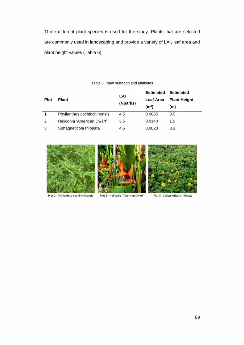
89

Three different plant species is used for the study. Plants that are selected

are commonly used in landscaping and provide a variety of LAI, leaf area and

plant height values (Table 6).

Table 6. Plant selection and attributes

Plot Plant LAI

(Nparks)

Estimated

Leaf Area

(m2)

Estimated

Plant Height

(m)

1 Phyllanthus cochinchinensis 4.5 0.0005 0.5

2 Heliconia ‘American Dwarf’ 3.5 0.0140 1.5

3 Sphagneticola trilobata 4.5 0.0020 0.3

90

3.2.3 Measurement setup

The proposed measurement setups are discussed in this section.

Measurement will be conducted on the rooftop of SDE1, National University

of Singapore. Measurements for rooftop greenery will be done with 3.0 m by

3.0 m roof garden plots (Figure 28). The proposed setup is derived from

reviewed literature (DiGiovanni et. al, 2013; Jim, 2012) and customized to suit

the objectives of this study. Mean radiant temperature and shrub albedo is

measured 0.3 m above the center of the plot canopy to ensure homogenous

conditions above the canopy surface as well as reliable measurements of

albedo (Akbari et al., 1998; ASHRAE, 2001b; Townsend, 1964).

Figure 28. Rooftop greenery measurement setup

Location of all measurement points are shown in Figure 29. Measurement

period and days used for analysis are shown in Table 7.

Not all data obtained was used for analysis. For Chapter 4, results shown are

representative of typical clear or overcast sky conditions. Rainy days are not

used for analysis unless no suitable alternatives are available.

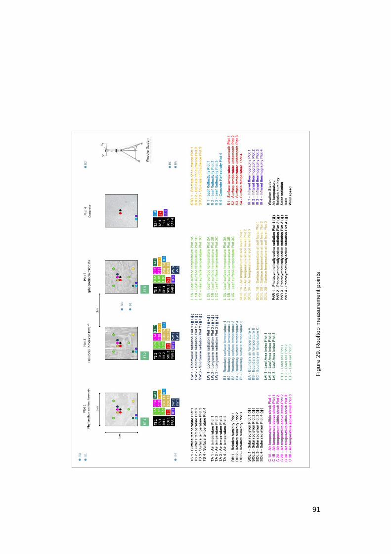
91

Fig

ure

29

. R

oo

ftop

me

asu

rem

en

t p

oin

ts

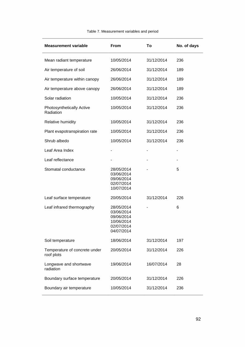
92

Table 7. Measurement variables and period

Measurement variable From To No. of days

Mean radiant temperature

10/05/2014 31/12/2014 236

Air temperature of soil 26/06/2014 31/12/2014 189

Air temperature within canopy 26/06/2014 31/12/2014 189

Air temperature above canopy 26/06/2014 31/12/2014 189

Solar radiation 10/05/2014 31/12/2014 236

Photosynthetically Active Radiation

10/05/2014 31/12/2014 236

Relative humidity 10/05/2014 31/12/2014 236

Plant evapotranspiration rate 10/05/2014 31/12/2014 236

Shrub albedo 10/05/2014 31/12/2014 236

Leaf Area Index

- - -

Leaf reflectance - - -

Stomatal conductance

28/05/2014 03/06/2014 09/06/2014 02/07/2014 10/07/2014

- 5

Leaf surface temperature

20/05/2014 31/12/2014 226

Leaf infrared thermography

28/05/2014 03/06/2014 09/06/2014 10/06/2014 02/07/2014 04/07/2014

- 6

Soil temperature 18/06/2014 31/12/2014 197

Temperature of concrete under roof plots

20/05/2014 31/12/2014 226

Longwave and shortwave radiation

19/06/2014 16/07/2014 28

Boundary surface temperature 20/05/2014 31/12/2014 226

Boundary air temperature 10/05/2014 31/12/2014 236

93

Measurement details for the hypothesized variables are as follows:

1. Plant EvapoTranspiration rate (ET)

Measurement are conducted for tmrt, air temperature and ET. ET is obtained

by measuring the water loss with a load cell. An extensive roof garden tray of

0.5 m by 0.5 m filled with the relevant plant is used. Surface temperature, air

temperature and air velocity will be measured at 1 minute intervals at the

homogenous level. Load cells will be placed next to each roof garden plot and

on each rack measured (Figure 30). The weight of substrate is standardized

at 10.0 Kg to ensure that the capacity for water absorption is the same

throughout all plots. The bottom and sides of the tray are insulated with

extruded foam to minimize effects due to advection.

Logging of load cell weight is done every 20 seconds. Data is processed to 1

minute intervals and averaged to hourly intervals.

Calculating of ET is performed in the following manner:

𝐸𝑇 (𝑇𝑖𝑚𝑒) = (

𝑊𝑎 − 𝑊𝑏

10 𝑚𝑖𝑛𝑢𝑡𝑒𝑠) 𝑥

1

𝐴𝑃𝑙𝑜𝑡

[21]

Where,

ET = Plant evapotranspiration rate (mm·min-1)

T = Time (min)

Wa = Weight of load cell 5 minutes before (Kg)

Wb = Weight of load cell after 5 minutes after (Kg)

APlot = Area of plot (m2)

For instance,

𝐸𝑇 (12: 00 ℎ𝑟𝑠) = (

𝑊𝑒𝑖𝑔ℎ𝑡 @ 11: 55 ℎ𝑟𝑠 − 𝑊𝑒𝑖𝑔ℎ𝑡 @ 12: 05 ℎ𝑟𝑠

10 𝑚𝑖𝑛𝑢𝑡𝑒𝑠) 𝑥

1

0.25 [22]

94

Figure 30. Measurement of plant evapotranspiration rate with load cell

2. Leaf Area Index

Measurement of LAI is done by removing all the leaves in a 0.5 m by 0.5 m

area for each plot and green wall (Figure 31). Leaves are scanned and

digitally processed. Leaf pixel will be totaled and LAI is estimated by dividing

total leaf pixel area by total scanned area in the 0.5 m by 0.5 m plot.

Figure 31. Measurement of Leaf Area Index

95

3. Shrub Albedo

Shrub albedo is defined as the ratio of reflected radiation from the shrub over

global solar radiation. The measured albedo will provide data on the average

leaf angle as well as shrub reflectivity. Pyranometers will be used to measure

radiation exposure. One pyranometer will be directed towards the sky to

measure global solar radiation. Subsequent pyranometers will be directed

towards the shrub to measure reflected radiation (Figure 32). The

pyranometers will be placed within 0.5 m of the canopy of the shrubs (Akbari

et al., 1998; ASHRAE, 2001b).

Figure 32. Measurement of Shrub Albedo

Concurrent measurements of tmrt as well as albedo at a nearby location

without the influence of rooftop greenery will also be made to serve as a

control for the experiment.

96

3.2.4 Equipment

Equipment used for all measurements are shown in Table 8:

Table 8. Equipment list

Variable Equipment Measurement Range

Accuracy

Air temperature, ta HOBO U12-012

Temp/RH data logger -20 °C – 70 °C

±0.35 °C from 0 °C – 50 °C, to a maximum of +/- 3.5%

HOBO U23 Pro v2 External Temperature data logger – U23-004

-40 °C – 100 °C

±0.21 °C from 0 °C – 50 °C

Evapotranspiration Rate (ET)

HBM Z6FC3 load cell and Quantum X logger

0 to 200 kg 0.0018 % of full span

Globe temperature, tg

HOBO Thermocouple Data Logger, U12-014 with Type-T Copper-Constantan thermocouple sensors and 40 mm diameter ping pong ball

-200 °C – 100 °C

±1.5 °C

Leaf Area Index, LAI

Canon All-In-One Printer, MP276

Optical Resolution: 1200 x 2400dpi

-

LAI 2200 Plant Canopy Analyzer

Wavelength Range: 320-490 nm.

-

Reflectivity SHIMADZU Spectrophotometer, UV-3150 UV-VIS-NIR

190 nm to 3200 nm

UV/VIS region: ±0.2 nm NIR region: ±0. 8 nm

Relative Humidity, RH

HOBO U12-012 Temp/RH data logger

5 % to 95 % RH

±2.5 % typical, 3.5 % maximum, from 10 to 90 % RH

Solar Irradiance Onset S-LIB-M003 Silicon Pyranometer

Onset S-LIA-M003 PAR sensor

0 to 1280 W/m2

0 to 2500

umol/m2/sec

±10 W/m2 or ±5%, whichever is greater in sunlight. Additional temperature induced error ±0.38 W/m2 /°C from 25°C

http://www.microdaq.com/occ/u12/u12-014.php


97

Variable Equipment Measurement Range

Accuracy

Shading characteristics

Close-circuit television

- -

Shrub Height Measuring pole 0 to 2 m 0.001 m

Short and long wave radiation, K, L

Kipp & Zonen, CNR 4 With Integrated pyranometer, pyrgeometer, Pt-100 and thermistor

Pyranometer: 0 Wm-2 – 2000 Wm-2 Pyrgeometer: -250 Wm-2 – 250 Wm-2 Pt-100: -200 °C to 600 °C Thermistor: -40 °C to 300 °C

Pyranometer: < 5% uncertainty (95 % confidence level) Pyrgeometer: < 10% uncertainty (95 % confidence level) Pt-100 / Thermistor: ±0.7 °C

Sky View Factor, SVF

Nikon D80 Digital SLR camera

Effective pixels:10.2 million

Sensitivity:100 to 1600 (ISO equivalent) in steps of 1/3 EV, plus HI-0.3, HI-0.7 and HI-1

Sky View Factor, SVF

Nikon D80 Digital SLR camera

Effective pixels:10.2 million

Sensitivity:100 to 1600 (ISO equivalent) in steps of 1/3 EV, plus HI-0.3, HI-0.7 and HI-1

Stomata conductance

Decagon SC-1 Porometer

0 to 1000 mmolm-

2s-1 10 %

Surface Temperature, ts

Fluke Thermal Imager

-20 °C to 150 °C (-4 °F to 302 °F)

±2 °C or 2 % (whichever is greater)

Surface temperature, ts

HOBO Thermocouple Data Logger, U12-014 with Type-T Copper-Constantan thermocouple sensors

-200 °C – 100 °C ±1.5 °C

Surface temperature, ts

Yokogawa DX230 DAQ Station, T type

-200 °C – 400 °C ±1.5 % of reading + 0.5 °C

Wind speed, Va Onset Wind Speed Smart Sensor, S-WSA-M003

0 ms-1 – 45 ms-1 ±1.1 ms-1 or ±4% of reading, whichever is greater



98

3.3 Final deliverables

The proposed deliverables for this research are as follows:

1. A prediction model for the overall cooling effect of rooftop greenery

based on plant characteristics such as plant evapotranspiration rate

and shrub albedo.

2. Guidelines for plant selection for rooftop greenery based on the

objective of maximum reduction in tmrt.

3.4 Importance and potential contribution of research

The prediction model will enable architects, urban and landscape designers to

practice landscape design and allocate plants within an objective framework.

Crucial areas that require more and appropriate plantings can be identified

and redundancies can be avoided. This will help achieve the overall concept

of optimizing vegetation ecosystem services and mitigating the effects of

climate change as well as the UHI effect.

3.5 Limitations

Limitations of this research are as follows:

1. Structure of the substrate for shrubs on green roofs differs significant

from shrubs at ground level. The depth of the substrate at green roofs

is typically much shallower than conventional plantings at ground level

(Extensive roof garden plots). This will have an impact on the overall

evapotranspiration rate for plants.

2. Studies are conducted in the tropical urban environment. Due to

differences in aridity and solar exposure, results may not be valid for

temperate regions.

3. The study assumes all plants of the same genus to have statistically

similar physiological attributes.

99

4 MEASUREMENT OF MEAN RADIANT TEMPERATURE

IN A ROOF GARDEN SETTING

4.1.1 Results

4.1.1.1 Diurnal mean radiant temperature profiles

Figure 33. Typical clear (13th June 2014) and overcast (5th July 2014) sky solar irradiance profiles

Figure 33 shows the typical solar irradiance profile on days with clear sky and

overcast sky conditions. The overall peak solar irradiance for a clear sky day

was observed at 13:00 hrs with an approximate value of 900 Wm-2. In

comparison, the overall peak solar irradiance for an overcast day occurs at

14:00 hrs with a value of 500 Wm-2. Both profiles show that the first solar

irradiance is recorded at around 7:00 hrs when the Sun rises and decreases

to 0.6 Wm-2 when the Sun sets between 19:00 hrs to 20:00 hrs. Results in the

0

100

200

300

400

500

600

700

800

900

1000

0:0

0

1:0

0

2:0

0

3:0

0

4:0

0

5:0

0

6:0

0

7:0

0

8:0

0

9:0

0

10

:00

11

:00

12

:00

13

:00

14

:00

15

:00

16

:00

17

:00

18

:00

19

:00

20

:00

21

:00

22

:00

23

:00

0:0

0

Sola

r R

adia

tio

n (

W/m

2)

Time (Hrs)

Solar radiation - Clear Sky ConditionsSolar radiation - Overcast sky conditions

100

following section are generally classified as observations made under the two

different sky conditions.

Clear sky conditions

Figure 34. Mean radiant temperature profile for clear sky conditions (13th June 2014)

Figure 34 shows the mean radiant temperature profile for a typical day with

clear sky conditions. Peak temperature can be observed at 14:00 hrs where

concrete has the highest temperature recorded of 64.6 °C, followed by Plot 2,

Plot 3 and Plot 1. The maximum temperature difference observed is between

the concrete and Plot 1 with a difference of 10.0 °C at the peak. The

temperature of concrete is generally higher than the plots.

25

30

35

40

45

50

55

60

65

70

0:0

0

1:0

0

2:0

0

3:0

0

4:0

0

5:0

0

6:0

0

7:0

0

8:0

0

9:0

0

10

:00

11

:00

12

:00

13

:00

14

:00

15

:00

16

:00

17

:00

18

:00

19

:00

20

:00

21

:00

22

:00

23

:00

0:0

0

Mea

n R

adia

nt

Tem

per

atu

re (

oC

)

Time (Hrs)

Plot 1 - Phyllanthus cochinchinensisPlot 2 - Heliconia 'American Dwarf'Plot 3 - Sphagneticola trilobataConcrete

101

Overcast sky conditions

Figure 35. Mean radiant temperature profile for overcast sky conditions (5th July 2014)

Figure 35 shows the mean radiant temperature profile for a typical day with

overcast sky conditions. Overall peak temperatures for all the plots and

concrete are lower than those observed under clear sky conditions. Peak

temperature can be observed at 14:00 hrs with Plot 2 being the highest at

59.6 °C, followed by concrete, Plot 1, and Plot 3. The maximum temperature

difference is between Plot 2 and Plot 3 with a temperature of 5.0 °C.

18

23

28

33

38

43

48

53

58

63

0:0

0

1:0

0

2:0

0

3:0

0

4:0

0

5:0

0

6:0

0

7:0

0

8:0

0

9:0

0

10

:00

11

:00

12

:00

13

:00

14

:00

15

:00

16

:00

17

:00

18

:00

19

:00

20

:00

21

:00

22

:00

23

:00

0:0

0

Mea

n R

adia

nt

Tem

per

atu

re (

oC

)

Time (Hrs)


102

4.1.1.2 Diurnal ambient temperature profiles

Clear sky conditions

Figure 36. Air temperature profile for clear sky conditions (13th June 2014)

Figure 36 shows the air temperature profile for a typical day with clear sky

conditions. Peak air temperature can be observed at 14:00 hrs where

concrete has the highest temperature of 34.2 °C. This is followed by Plot 1,

Plot 3 and Plot 2 which has the lowest peak temperature of 32.6 °C. There is

a maximum difference of 1.6 °C between Plot 1 and Plot 2 at peak

temperature. It can also be observed that Plot 1 has the lowest air

temperature before 9:00 hrs and after 18:00 hrs while the air temperatures for

Plot 2, Plot 3 and concrete are similar before 9:00 hrs and after 21:00 hrs.

26

27

28

29

30

31

32

33

34

350

:00

1:0

0

2:0

0

3:0

0

4:0

0

5:0

0

6:0

0

7:0

0

8:0

0

9:0

0

10

:00

11

:00

12

:00

13

:00

14

:00

15

:00

16

:00

17

:00

18

:00

19

:00

20

:00

21

:00

22

:00

23

:00

0:0

0

Am

bie

nt

Tem

per

atu

re (

oC

)

Time (Hrs)


103

Overcast sky conditions

Figure 37. Air temperature profile for overcast sky conditions (12th July 2014)

Figure 37 shows the air temperature profile for a typical day with overcast sky

conditions. A dip in air temperature was observed at 8:00 hrs and is likely due

to a short period of rain. The peak temperature can be observed at 17:00 hrs

where Plot 1 and concrete recorded a temperature of 31.0 °C. In comparison,

Plot 2 has the lowest air temperature at 17:00 hrs and its difference with Plot

1 and concrete is 1.3 °C.

24

25

26

27

28

29

30

31

32

0:0

0

1:0

0

2:0

0

3:0

0

4:0

0

5:0

0

6:0

0

7:0

0

8:0

0

9:0

0

10

:00

11

:00

12

:00

13

:00

14

:00

15

:00

16

:00

17

:00

18

:00

19

:00

20

:00

21

:00

22

:00

23

:00

0:0

0

Am

bie

nt

Tem

per

atu

re (

oC

)

Time (Hrs)Plot 1 - Phyllanthus cochinchinensisPlot 2 - Heliconia 'American Dwarf'Plot 3 - Sphagneticola trilobataConcrete

104

4.1.1.3 Stratification – soil layer, within shrub, above shrub

Measurement of air temperature was conducted at the soil, within and above

the plant canopies of Plots 1 to 3. Schematic location of the points is shown in

Figure 38.

Figure 38. Location of air temperature probes

Figure 39. Stratified air temperature profile for Plot 1 (26th July 2014)

25

26

27

28

29

30

31

32

33

0:0

0

1:0

0

2:0

0

3:0

0

4:0

0

5:0

0

6:0

0

7:0

0

8:0

0

9:0

0

10

:00

11

:00

12

:00

13

:00

14

:00

15

:00

16

:00

17

:00

18

:00

19

:00

20

:00

21

:00

22

:00

23

:00

0:0

0

Am

bie

nt

Tem

per

atu

re (

oC

)

Time (Hrs)

Soil Canopy Above Canopy

Plot 1Phyllanthus cochinchinensis

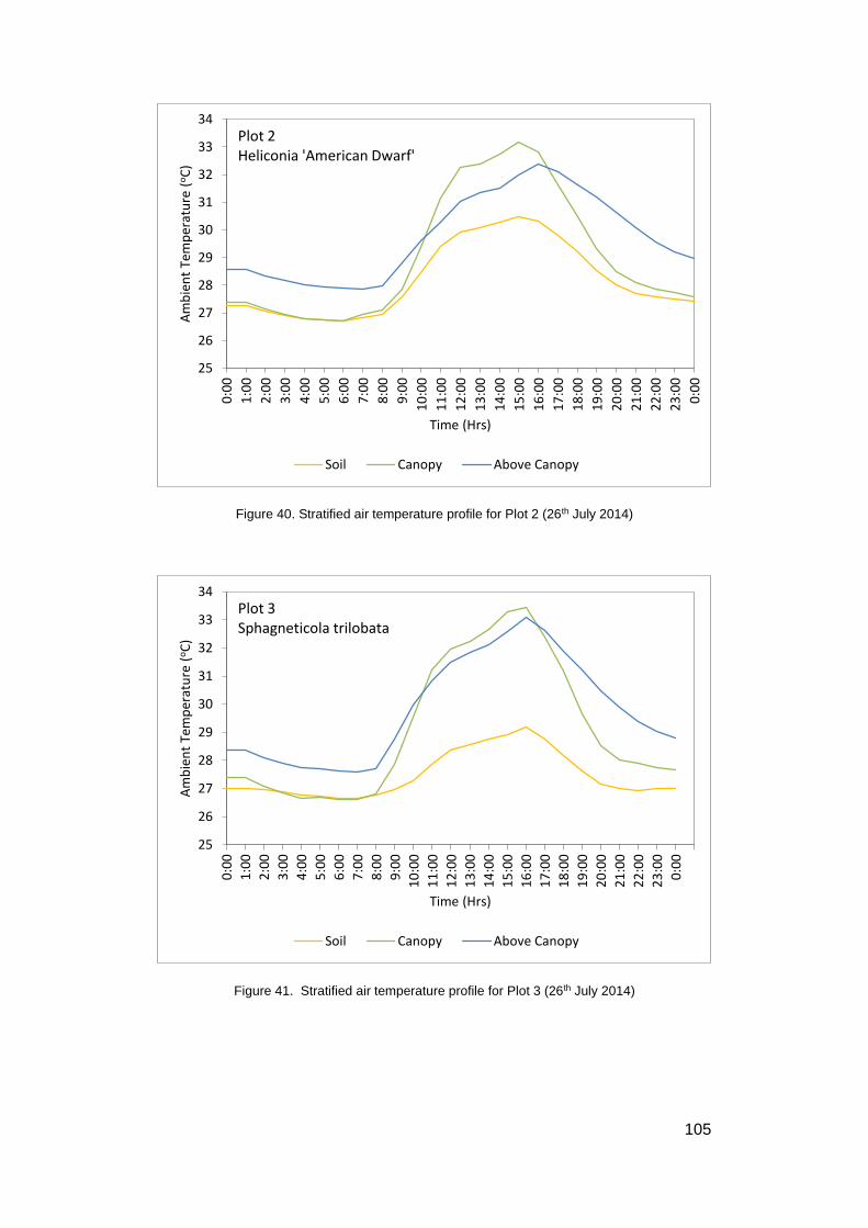
105



25

26

27

28

29

30

31

32

33

34

0:0

0

1:0

0

2:0

0

3:0

0

4:0

0

5:0

0

6:0

0

7:0

0

8:0

0

9:0

0

10

:00

11

:00

12

:00

13

:00

14

:00

15

:00

16

:00

17

:00

18

:00

19

:00

20

:00

21

:00

22

:00

23

:00

0:0

0

Am

bie

nt

Tem

per

atu

re (

oC

)

Time (Hrs)


Plot 2Heliconia 'American Dwarf'

25

26

27

28

29

30

31

32

33

34

0:0

0

1:0

0

2:0

0

3:0

0

4:0

0

5:0

0

6:0

0

7:0

0

8:0

0

9:0

0

10

:00

11

:00

12

:00

13

:00

14

:00

15

:00

16

:00

17

:00

18

:00

19

:00

20

:00

21

:00

22

:00

23

:00

0:0

0

Am

bie

nt

Tem

per

atu

re (

oC

)

Time (Hrs)


Plot 3Sphagneticola trilobata

106

Figure 39, Figure 40 and Figure 41 show stratified air temperature profiles for

Plot 1, Plot 2 and Plot 3 on a typical clear day condition respectively. Soil

temperature for all three plots is generally lower compared to canopy and

above-canopy air temperature.

Stratified air temperature profile for Plot 1 in Figure 39 shows a peak

temperature of 32.5 °C at 16:00 hrs above the plant canopy while peak

temperature for soil and canopy temperature graph occurs at 15:00 hrs.

There is a difference of 2.0 °C between air temperature at soil level and air

temperature above the plant canopy.

In comparison, the above canopy temperatures for both Plot 2 and Plot 3

(Figure 40 and Figure 41) have the highest temperature of approximately 33.0

°C and peaked at 16:00 hrs. The soil temperatures for these two plots were

30.5 °C and 29.1 °C at peak temperature. This would also represent a

difference in 2.5 °C and 4.0 °C between the canopy and soil temperature.

Comparison of the stratified air temperature profiles for all 3 Plots show that

air temperature above the canopy is slightly lower than within the canopy for

Plot 2 and Plot 3. Air temperature within the canopy for Plot 1 is slightly lower

than above it. This may be explained by the fact that Phyllanthus

cochinchinensis has many small leaves that occupy the entire volume of the

shrub, while Plot 3, in comparison, has its leaves only at the outermost

portions of the canopy and only has stems within the inner regions of the

canopy.

107

4.1.1.4 Meteorological variables

Solar radiation

Figure 42. Solar radiation against mean radiant temperature profile (13th June 2014)

25

30

35

40

45

50

55

60

65

70

0

100

200

300

400

500

600

700

8000

:00

2:0

0

4:0

0

6:0

0

8:0

0

10

:00

12

:00

14

:00

16

:00

18

:00

20

:00

22

:00

0:0

0

Mea

n R

adia

nt

Tem

per

atu

re (

oC

)

Sola

r R

adia

tio

n (

W/m

²)

Time (Hrs)

Solar RadiationPlot 1 - Phyllanthus cochinchinensisPlot 2 - Heliconia 'American Dwarf'Plot 3 - Sphagneticola trilobataConcrete

108

Figure 43. Solar radiation against air temperature profile (13th June 2104)

Figure 42 and Figure 43 show the diurnal tmrt and solar irradiance profile for

13th June 2014 (clear sky conditions). The profiles follow a similar curve,

peaking at 14:00 hrs. The highest solar radiation observed is 773.8 Wm-2. It

can be observed that both air and tmrt profiles are directly proportional to solar

irradiance.

26

27

28

29

30

31

32

33

34

35

0

100

200

300

400

500

600

700

800

0:0

0

2:0

0

4:0

0

6:0

0

8:0

0

10

:00

12

:00

14

:00

16

:00

18

:00

20

:00

22

:00

0:0

0

Am

bie

nt

Tem

per

atu

re (

oC

)

Sola

r R

adia

tio

n (

W/m

²)

Time (Hrs)

Solar Radiation Plot 1 - Phyllanthus cochinchinensis

Plot 2 - Heliconia 'American Dwarf' Plot 3 - Sphagneticola trilobata

Concrete

109

Photosynthetically Active Radiation (PAR)

Figure 44. Photosynthetically Active Radiation against mean radiant temperature profile (13th June 2014)

0

200

400

600

800

1000

1200

1400

1600

1800

25

30

35

40

45

50

55

60

65

70

0:0

0

2:0

0

4:0

0

6:0

0

8:0

0

10

:00

12

:00

14

:00

16

:00

18

:00

20

:00

22

:00

0:0

0

Ph

oto

syn

thet

ical

ly A

ctiv

e R

adit

aio

n (

uE)

Mea

n R

adia

nt

Tem

per

atu

re (

oC

)

Time (Hrs)

Plot 1 - Phyllanthus cochinchinensis Plot 2 - Heliconia 'American Dwarf'

Plot 3 - Sphagneticola trilobata Concrete

PAR

110

Figure 45. Photosynthetically Active Radiation against air temperature profile (13th June 2014)

Figure 44 and Figure 45 show the diurnal tmrt and air temperature with solar

irradiance profile for 13th June 2014. The profiles follow a similar curve,

peaking at 13:00 hrs. The highest PAR observed is 1765.8 µE. Similar to the

profiles of solar irradiance, both PAR profiles are directly proportional to tmrt

and air temperature.

0

200

400

600

800

1000

1200

1400

1600

1800

2000

25

26

27

28

29

30

31

32

33

34

35

0:0

0

2:0

0

4:0

0

6:0

0

8:0

0

10

:00

12

:00

14

:00

16

:00

18

:00

20

:00

22

:00

0:0

0

Ph

oto

syn

thet

ical

ly A

ctiv

e R

adit

aio

n (

uE)

Air

Tem

per

atu

re (

oC

)

Time (Hrs)



PAR

111

Relative humidity (RH)

Figure 46. Relative Humidity against mean radiant temperature profile (13th June 2014)

60

65

70

75

80

85

90

95

25

30

35

40

45

50

55

60

65

70

0:0

0

2:0

0

4:0

0

6:0

0

8:0

0

10

:00

12

:00

14

:00

16

:00

18

:00

20

:00

22

:00

0:0

0

Rel

ativ

e H

um

idit

y (%

)

Mea

n R

adia

nt

Tem

per

atu

re (

oC

)

Time (Hrs)

Plot 1 - Phyllanthus cochinchinensis Plot 2 - Heliconia 'American Dwarf'Plot 3 - Sphagneticola trilobata ConcretePlot 1 RH Plot 2 RHPlot 3 RH Concrete RH

112

Figure 47. Relative Humidity against air temperature profile (13th June 2014)

Figure 46 and Figure 47 show the diurnal tmrt and air temperature with relative

humidity (RH) for 13th June 2014. The RH profiles are inversely proportional

to tmrt and air temperature profiles. The lowest RH recorded was at 14:00 hrs

for concrete (63.1 %) followed by Plot 1 (65.9 %), Plot 3 (69.6 %) and Plot 2

(69.6 %) under clear sky conditions. There is a difference of approximately

6.5% between the concrete and Plots 2 and 3.

60

65

70

75

80

85

90

95

25

26

27

28

29

30

31

32

33

34

35

0:0

0

2:0

0

4:0

0

6:0

0

8:0

0

10

:00

12

:00

14

:00

16

:00

18

:00

20

:00

22

:00

0:0

0

Rel

ativ

e H

um

idit

y (%

)

Air

Tem

per

atu

re (

oC

)

Time (Hrs)



Plot 1 RH Plot 2 RH

Plot 3 RH Concrete RH

113

4.1.1.5 Shrub characteristics

Evapotranspiration rate

Figure 48. Evapotranspiration rate against mean radiant temperature profile (13th June 2014)

-0.05

-0.04

-0.03

-0.02

-0.01

0

0.01

0.02

0.03

25

30

35

40

45

50

55

60

65

0:0

0

2:0

0

4:0

0

6:0

0

8:0

0

10

:00

12

:00

14

:00

16

:00

18

:00

20

:00

22

:00

0:0

0

Evap

otr

ansp

irat

ion

Rat

e (m

m/m

in)

Mea

n R

adia

nt

Tem

per

atu

re (

oC

)

Time (Hrs)

Plot 1 - Phyllanthus cochinchinensis Plot 2 - Heliconia 'American Dwarf'Plot 3 - Sphagneticola trilobata ConcretePlot 1 ET Plot 2 ETPlot 3 ET

114

Figure 49. Evapotranspiration rate against air temperature profile (13th June 2014)

Figure 48 and Figure 49 show the diurnal evapotranspiration (ET) profile for

13th June 2014. There is a sharp dip in ET from 06:00 hrs to 07:00 hrs due to

the plot irrigations. The ET rate for Plot 1 is low in the morning but picks up in

the afternoon and has a highest value of 2.4 mmmin-1. In comparison, Plot 3

has the highest ET rate in the morning period but gets lower than plot 2 in the

late afternoon (17:00 hrs). The ET rates for Plot 2 and 3 peaked at 17:00 hrs

with a value of 1.9 mmmin-1 and 1.7 kgmin-1 respectively. Generally, the ET

rate is above zero from 11:00 hrs for Plot 3 and 12:00 hrs for Plot 1 and 2.

-0.05

-0.04

-0.03

-0.02

-0.01

0

0.01

0.02

0.03

26

27

28

29

30

31

32

33

34

35

0:0

0

2:0

0

4:0

0

6:0

0

8:0

0

10

:00

12

:00

14

:00

16

:00

18

:00

20

:00

22

:00

0:0

0

Evap

otr

ansp

irat

ion

Rat

e (m

m/m

in)

Air

Tem

per

atu

re (

oC

)

Time (Hrs)



Plot 1 ET Plot 2 ET

Plot 3 ET

115

Shrub albedo

Figure 50. Albedo against mean radiant temperature profile (13th June 2014)

0

0.2

0.4

0.6

0.8

1

1.2

25

30

35

40

45

50

55

60

65

70

0:0

0

2:0

0

4:0

0

6:0

0

8:0

0

10

:00

12

:00

14

:00

16

:00

18

:00

20

:00

22

:00

0:0

0

Alb

edo

Mea

n R

adia

nt

Tem

per

atu

re (

oC

)

Time (Hrs)



Plot 1 Albedo Plot 2 Albedo

Plot 3 Albedo Concrete Albedo (22nd June 2014)

116

Figure 51. Albedo against air temperature profile (13th June 2014)

Figure 50 and Figure 51 show the diurnal albedo profile for 13th June 2014

and 22nd June 2014. Albedo of concrete in the day is constant at 0.17. It is

lower than the albedo for the shrubs throughout the day.

Albedo values of Plots 1 to 3 are relatively consistent. The lowest albedo

value is at peak temperature around 14:00 hrs. Plot 2 has a lower albedo than

Plot 1 and Plot 3. Their average values are 0.16, 0.28 and 0.28 respectively.

0

0.2

0.4

0.6

0.8

1

1.2

25

26

27

28

29

30

31

32

33

34

35

0:0

0

2:0

0

4:0

0

6:0

0

8:0

0

10

:00

12

:00

14

:00

16

:00

18

:00

20

:00

22

:00

0:0

0

Alb

edo

Air

Tem

per

atu

re (

oC

)

Time (Hrs)



Plot 1 Albedo Plot 2 Albedo

Plot 3 Albedo Concrete Albedo (22nd June 2014)

117

Leaf Area Index (LAI)

Leaf area index was measured and estimated using the following methods:

1. Indirect measurement: Measurement of light attenuation due to plant

canopy with the LAI-2000 (Figure 52).

2. Direct measurement: Plucking out leaves within a 0.5 m by 0.5 m

area, and tabulating the total green area (Outlined in Section 3.2.3).

3. Literature reference: From the National Parks Board (Nparks)

published handbook on LAI (Tan and Sia, 2009).

Figure 52. LAI-2000 canopy analyzer. (Source: http://www.licor.com)

118

Table 9. Averaged Leaf Area Indices for Plot 1 to Plot 3

Plot

LAI measurement method

Indirect measurement (Using LAI-2000)

Direct measurement (Plucking out leaves in 50 x 50 cm plot, pixel calculation)

Nparks handbook (Tan and Sia, 2009)

1 2 3

Avera

ge

1 Phyllanthus cochinchinensis Shrub (Dicot)

4.65 4.22 4.16 4.34 2.78 4.5

2 Heliconia American Dwarf Shrub (Monocot)

3.14 3.69 3.58 3.47 7.21 3.5

3 Sphagneticola trilobata Ground cover

4.70 4.28 4.83 4.60 3.59 4.5

Table 9 shows measured LAI of the plots and the corresponding LAI for each

plant provided by the NParks (Tan and Sia, 2009). Using the indirect

measurement method, Plot 3 has the highest LAI of 4.60, followed by Plot 1

at 4.34 and Plot 2 at 3.47. However, when direct measurements are

conducted, the results are reversed. Plot 2 shows the highest LAI at 3.47

whereas Plot 3 and Plot 1 have a lower LAI at 3.59 and 2.78 respectively. The

difference in both methods may be due to the excess direct shading captured

by the LAI-2000 plant canopy analyzer to obtain measurement using the

indirect measurement method.

119

Leaf Reflectance

Leaf reflectance was measured by first plucking out fresh leaves from Plots 1

to 3, and measuring the reflectance using a photospectrometer. Leave

samples used for measurement are shown in Figure 53.

Figure 53. Leaf samples used for reflectance measurement (5 cm X 5 cm)

Figure 54. Reflectivity results

0

10

20

30

40

50

60

70

80

90

20

0

30

0

40

0

50

0

60

0

70

0

80

0

90

0

10

00

11

00

12

00

13

00

14

00

15

00

16

00

17

00

18

00

19

00

20

00

21

00

22

00

23

00

24

00

25

00

Ref

lect

ivit

y (%

)

Wavelength (nm)



VisibleUV Near-Infrared Shortwave Infrared

120

Figure 54 shows the reflectivity of the leaves taken from Plots 1 to 3. Under

visible light which spans approximately 400nm to 700nm, reflectivity of

concrete can be up to 40.4 %. Vegetation under visible light displayed a

relatively lower reflectivity at the peak of 21.6 % (Plot 3), 14.5 % (Plot 1) and

13.8 % (Plot 2). At approximately 800 nm, reflectivity of leaves is higher than

that of concrete. Plot 1 has the highest value of 85.9 %, followed by Plot 3

(85.0 %), Plot 2 (83.3 %) and concrete (42.2 %).

Stomatal conductance

Stomatal conductance was measured for Plots 1 to 3 with a porometer

(Figure 55). Measurements were conducted on an hourly basis and a total of

four leaves were measured for each plot. Averaged values from all four

leaves are used for analysis.

Figure 55. Decagon leaf porometer (Source: http://www.decagon.com)

121

Figure 56: Stomata Conductance (3rd June 2014)

Figure 56 shows stomatal conductance levels from 11:00 hrs to 18:00 hrs on

3rd June 2014. Plot 3 has the highest stomatal conductance level, peaking at

13:00 hrs at a value of 803.7 mmolm⁻ ²s⁻ ¹, while Plot 1 and Plot 2 are greatly

lower. Stomatal conductance levels for all plots are drastically reduced in the

later part of the day. This corresponds to the reduction of evapotranspiration

rate after 17:00 hrs shown in Figure 48.

0

100

200

300

400

500

600

700

800

900

11:00 13:00 14:00 15:00 16:00 17:00 18:00

Sto

mat

al C

on

du

ctan

ce(m

mo

l m⁻²

s⁻¹

)

Time (Hrs)

Plot 1 - Phyllanthus cochinchinensis

Plot 2 - Heliconia 'American Dwarf'

Plot 3 - Sphagneticola trilobata

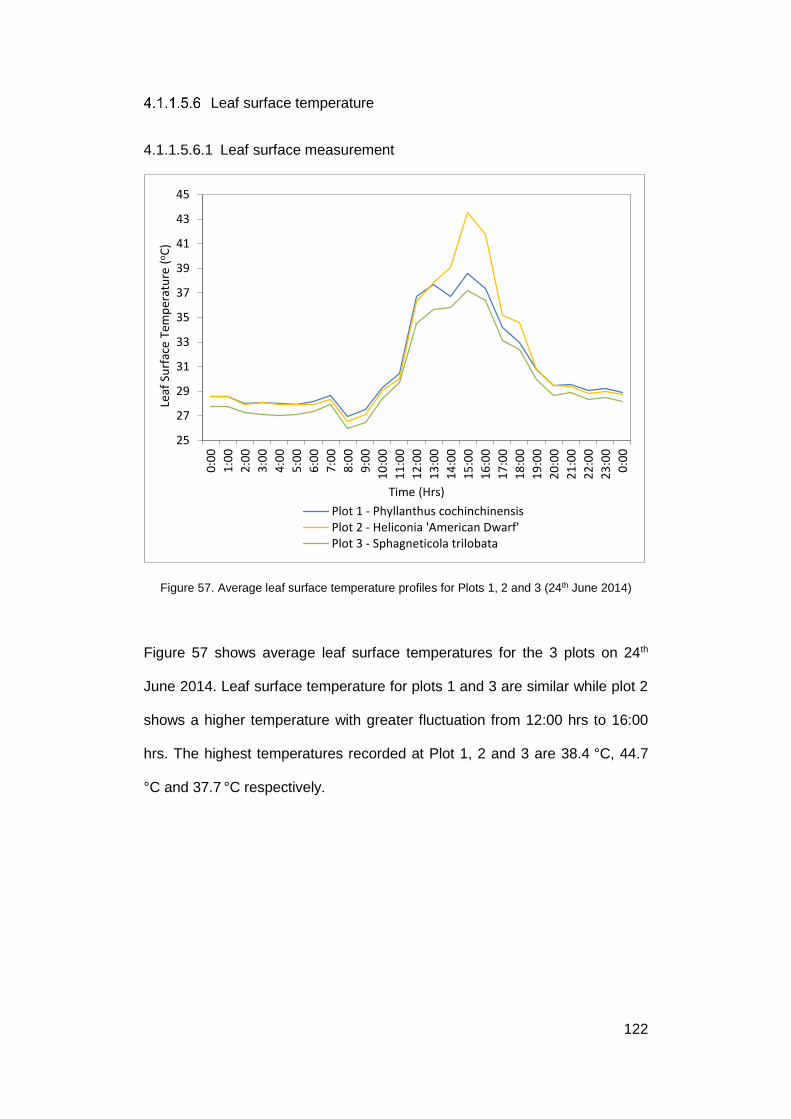
122

Leaf surface temperature

4.1.1.5.6.1 Leaf surface measurement

Figure 57. Average leaf surface temperature profiles for Plots 1, 2 and 3 (24th June 2014)

Figure 57 shows average leaf surface temperatures for the 3 plots on 24th

June 2014. Leaf surface temperature for plots 1 and 3 are similar while plot 2

shows a higher temperature with greater fluctuation from 12:00 hrs to 16:00

hrs. The highest temperatures recorded at Plot 1, 2 and 3 are 38.4 °C, 44.7

°C and 37.7 °C respectively.

25

27

29

31

33

35

37

39

41

43

450

:00

1:0

0

2:0

0

3:0

0

4:0

0

5:0

0

6:0

0

7:0

0

8:0

0

9:0

0

10

:00

11

:00

12

:00

13

:00

14

:00

15

:00

16

:00

17

:00

18

:00

19

:00

20

:00

21

:00

22

:00

23

:00

0:0

0

Leaf

Su

rfac

e Te

mp

erat

ure

(oC

)

Time (Hrs)

Plot 1 - Phyllanthus cochinchinensisPlot 2 - Heliconia 'American Dwarf'Plot 3 - Sphagneticola trilobata

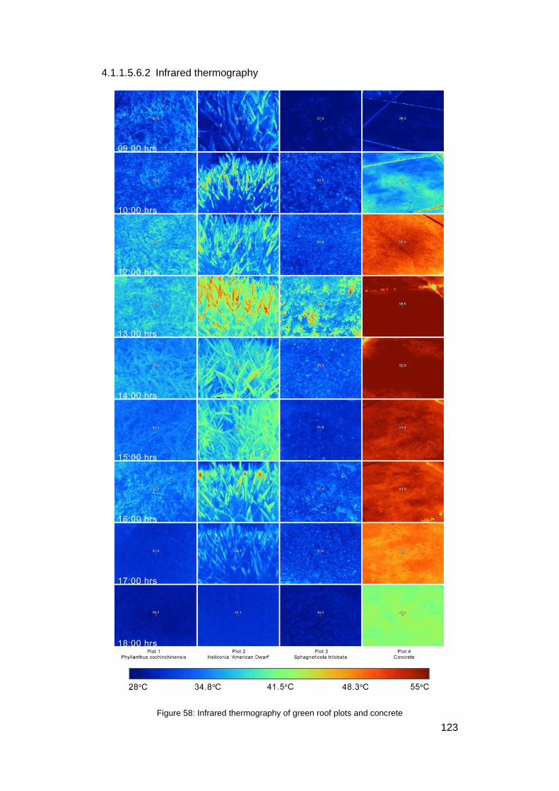
123

4.1.1.5.6.2 Infrared thermography

Figure 58: Infrared thermography of green roof plots and concrete

124

Figure 58 shows infrared thermography of the plots and concrete on a typical

clear sky condition day. Results concur with leave surface temperature

measurements in Chapter 4.1.1.5.6.1. Surface temperature of concrete is

consistently higher than all other plots throughout the day. This is followed by

Plot 2 which is higher than Plot 1 and 3 as seen from the brighter colours on

the leaf surfaces. Significantly higher temperatures can be seen on the leaf

edges for Heliconia ‘American Dwarf’ (Plot 2).

4.1.1.6 Soil temperature

Figure 59. Average soil temperature profiles for Plot 1, 2 and 3 (24th June 2014)

Figure 59 shows average substrate temperatures of the 3 plots on 24th June

2014. Peak temperatures were observed at 16:00 hrs for all three plots with

Plot 2 having the highest temperature at 35.7 °C. Plot 1 and Plot 3 shows

similar profile and has a peak temperature of 33.9 °C and 34.0 °C. The higher

temperature peak for Plot 2 may be explained by the porosity of the Heliconia

26

27

28

29

30

31

32

33

0:0

0

1:0

0

2:0

0

3:0

0

4:0

0

5:0

0

6:0

0

7:0

0

8:0

0

9:0

0

10

:00

11

:00

12

:00

13

:00

14

:00

15

:00

16

:00

17

:00

18

:00

19

:00

20

:00

21

:00

22

:00

23

:00

0:0

0

Sub

stra

te T

emp

erat

ure

(oC

)

Time (Hrs)Plot 1 - Phyllanthus cochinchinensisPlot 2 - Heliconia 'American Dwarf'Plot 3 - Sphagneticola trilobata

125

shrub, compared to Plot 3, where the Sphagneticola trilobata shrub is much

more compact. This provides significantly more shade at the soil level.

4.1.1.7 Temperature of concrete under roof garden plots

Figure 60. Concrete temperature profiles for Plot 1 to Plot 3 (24th June 2014)

Figure 60 shows concrete temperature profiles beneath all 3 plots on 24th

June 2014. The 3 plots show similar profile and temperature ranging from

27.5 °C to 28.1 °C. The concrete temperature is generally lower than the leaf

surface temperature and substrate temperature as shown from Figure 57 to

Figure 59.

25

30

35

40

45

50

55

600

:00

1:0

0

2:0

0

3:0

0

4:0

0

5:0

0

6:0

0

7:0

0

8:0

0

9:0

0

10

:00

11

:00

12

:00

13

:00

14

:00

15

:00

16

:00

17

:00

18

:00

19

:00

20

:00

21

:00

22

:00

23

:00

0:0

0

Co

ncr

ete

Tem

per

atu

re (

oC

)

Time (Hrs)

Concrete surface under Plot 1 - Phyllanthus cochinchinensis

Concrete surface under Plot 2 - Heliconia 'American Dwarf'

Concrete surface under Plot 3 - Sphagneticola trilobata

Concrete surface exposed to direct solar radiation

126

4.1.1.8 Net all-wave radiation

Net all-wave radiation describes the rooftop greenery energy surface budget

(in the day) in the form of long and shortwave radiation (Oke, 1988):

Q* = K↓ - K↑ + L↓ - L↑ [23]

= K* + L*

Where,

Q* = Net all-wave radiation (Wm-2)

K↓ = Incident shortwave radiation (Wm-2)

K↑ = Reflected shortwave radiation (Wm-2)

K* = Net shortwave radiation (Wm-2)

L↓ = Incident longwave radiation (Wm-2)

L↑ = Reflected longwave radiation (Wm-2)

L* = Net longwave radiation (Wm-2)

127

Figure 61: Incoming and outgoing radiation for Plots 1 to 3 (7th July 2014)

Figure 61 shows incoming and outgoing radiation of all 3 plots. Incoming

radiation peaked at 14:00 hrs with Plot 2 having the greatest radiation of

1288.9 Wm-2 and the lowest for Plot 1 at 1251.5 Wm-2. Outgoing radiation is

drastically lower than incoming radiation and peaks were observed much

later. Plot 2 shows the lowest outgoing radiation of 603.2 Wm-2 while Plot 1

and Plot 3 show similar values of approximately 661.0 Wm-2. Diurnal net all-

wave radiation (Q*) profile for Plots 1 to 3 are shown in Figure 62. It can be

observed that net all-wave radiation for Plot 2 is higher than that of Plot 1 and

Plot 3. This is likely due to the hotter leaf surface temperature (Chapter

4.1.1.5.6) which resulted in higher longwave emission for Plot 2.

350

450

550

650

750

850

950

1050

1150

1250

1350

0:0

0

1:0

0

2:0

0

3:0

0

4:0

0

5:0

0

6:0

0

7:0

0

8:0

0

9:0

0

10

:00

11

:00

12

:00

13

:00

14

:00

15

:00

16

:00

17

:00

18

:00

19

:00

20

:00

21

:00

22

:00

23

:00

0:0

0

Inco

min

g an

d o

utg

oin

g ra

dia

tio

n (

W/m

2 )

Time (Hrs)


Plot 3 - Sphagneticola trilobata Plot 1 - Phyllanthus cochinchinensis

Plot 2 - Heliconia 'American Dwarf' Plot 3 - Sphagneticola trilobata

IncomingRadiation

K↓ + L↓

OutgoingradiationK↑ + L↑

128

Figure 62. Net all-wave radiation (Q*) for Plots 1 to 3 (7th July 2014)

4.1.1.9 Boundary conditions

Figure 63. Boundary concrete surface temperature profiles (24th June 2014)

-100

0

100

200

300

400

500

600

700

800

0:0

0

1:0

0

2:0

0

3:0

0

4:0

0

5:0

0

6:0

0

7:0

0

8:0

0

9:0

0

10

:00

11

:00

12

:00

13

:00

14

:00

15

:00

16

:00

17

:00

18

:00

19

:00

20

:00

21

:00

22

:00

23

:00

0:0

0

Net

all-

wav

e ra

dia

tio

n (

W/m

2 )

Time (Hrs)

Plot 1 - Phyllanthus cochinchinensisPlot 2 - Heliconia 'American Dwarf'Plot 3 - Sphagneticola trilobata

25

30

35

40

45

50

55

0:0

0

1:0

0

2:0

0

3:0

0

4:0

0

5:0

0

6:0

0

7:0

0

8:0

0

9:0

0

10

:00

11

:00

12

:00

13

:00

14

:00

15

:00

16

:00

17

:00

18

:00

19

:00

20

:00

21

:00

22

:00

23

:00

0:0

0

Bo

un

dar

y C

on

cret

e Te

mp

erat

ure

(oC

)

Time (Hrs)

B1 B2 B3 B4 B5

129

Figure 64. Boundary air temperature profile (24th June 2014)

Figure 63 and Figure 64 represent boundary conditions for the setup. The two

figures show that there is no significant difference in the boundary concrete

surface temperature and boundary air temperature. Thus, it is reasonable to

state that there is little external influence to the experimental setup.

26

28

30

32

34

36

38

40

0:0

0

1:0

0

2:0

0

3:0

0

4:0

0

5:0

0

6:0

0

7:0

0

8:0

0

9:0

0

10

:00

11

:00

12

:00

13

:00

14

:00

15

:00

16

:00

17

:00

18

:00

19

:00

20

:00

21

:00

22

:00

23

:00

0:0

0

Bo

un

dar

y A

ir T

emp

erat

ure

(oC

)

Time (Hrs)

BA BB BC

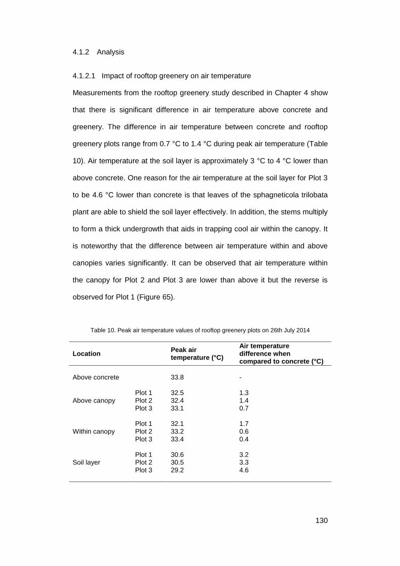
130

4.1.2 Analysis

4.1.2.1 Impact of rooftop greenery on air temperature

Measurements from the rooftop greenery study described in Chapter 4 show

that there is significant difference in air temperature above concrete and

greenery. The difference in air temperature between concrete and rooftop

greenery plots range from 0.7 °C to 1.4 °C during peak air temperature (Table

10). Air temperature at the soil layer is approximately 3 °C to 4 °C lower than

above concrete. One reason for the air temperature at the soil layer for Plot 3

to be 4.6 °C lower than concrete is that leaves of the sphagneticola trilobata

plant are able to shield the soil layer effectively. In addition, the stems multiply

to form a thick undergrowth that aids in trapping cool air within the canopy. It

is noteworthy that the difference between air temperature within and above

canopies varies significantly. It can be observed that air temperature within

the canopy for Plot 2 and Plot 3 are lower than above it but the reverse is

observed for Plot 1 (Figure 65).

Table 10. Peak air temperature values of rooftop greenery plots on 26th July 2014

Location Peak air temperature (°C)

Air temperature difference when compared to concrete (°C)

Above concrete

33.8

-

Above canopy Plot 1 32.5 1.3 Plot 2 32.4 1.4 Plot 3 33.1 0.7

Within canopy Plot 1 32.1 1.7 Plot 2 33.2 0.6 Plot 3 33.4 0.4

Soil layer

Plot 1 30.6 3.2 Plot 2 30.5 3.3 Plot 3

29.2

4.6

131

Figure 65. Air temperature profiles of rooftop greenery plots on 26th July 2014

Previous studies on greenery (Table 11) show that reduction of air

temperature due to rooftop greenery (shrubs only, without tree canopy shade)

can be as high as 4 °C. Results from this field measurement (0.7 °C to 1.4 °C

above shrubbery) are within the range found in reviewed literature. Even in

the absence of tree canopy shade, introduction of shrubbery can lead to

significant reduction in air temperature.

26

27

28

29

30

31

32

33

34

0:0

0

1:0

0

2:0

0

3:0

0

4:0

0

5:0

0

6:0

0

7:0

0

8:0

0

9:0

0

10

:00

11

:00

12

:00

13

:00

14

:00

15

:00

16

:00

17

:00

18

:00

19

:00

20

:00

21

:00

22

:00

23

:00

0:0

0

Air

tem

per

atu

re (

°C)

Time (Hrs)

Plot 1 - Soil layer Plot 1 - Within canopy Plot 1 - Above canopy



Concrete

132

Table 11. Studies on air temperature reduction due to greenery

Focus of study Finding Author

Measurement of air temperature reduction due to trees

2 °C to 3.8 °C reduction

Sitawati et al., 2011

Measurement of air temperature along reduced-scale street canyon with green wall and green roof

1.5 °C reduction for street with green wall

Djedjig et al., 2013

Measurement of air temperature under tree canopies

2 °C cooler on average under tree canopy

Taha et al., 1991

Measurement of air temperature above rooftop greenery

4.2 °C cooler than concrete roof at 300mm above greenery

Wong et al., 2003a

Measurement of air temperature above rooftop greenery at multi-storey carpark

6.1 °C to 5.5 °C at 300 mm 3.8 °C to 4.3 °C at 1200 mm

Wong et al., 2007

Measurement of air temperature in parks

Up to 3.5 °C reduction Bernatzky, 1982

Measurement of air temperature in a garden

Up to 6.9 °C reduction Oliveira et al., 2011

It can be observed from Figure 66 that plant air temperature is not closely

correlated to plant evapotranspiration rate and shrub albedo.

133

Figure 66. Scatter plots of Plant ET and Albedo on Plant air temperature

y = 0.001x - 0.021R² = 0.045

-0.010

-0.005

0.000

0.005

0.010

0.015

0.020

0.025

0.030

28 30 32 34 36

Pla

nt

Evap

otr

ansp

irat

ion

Rat

e (m

mm

in-1

)

Air temperature (°C)

Plant Evapotranspiration Rate Linear (Plant Evapotranspiration Rate)

y = 0.0018x + 0.2047R² = 0.0024

0.00

0.05

0.10

0.15

0.20

0.25

0.30

0.35

0.40

0.45

28 30 32 34 36

Shru

b A

lbed

o

Air temperature (°C)

Albedo Linear (Albedo)

134

4.1.2.2 Impact of rooftop greenery on mean radiant temperature

Results from Chapter 4.1.1.1 show that there is significant reduction in tmrt

above the roof surface due to the introduction of plants. This study further

explores the magnitude in reduction of different plant types by means of

statistical approach to evaluating tmrt reduction against specific plant

characteristics. Chapter 5 outlines the statistically derived regression model

and concludes the significance of plant characteristics such as plant

evapotranspiration rate and shrub albedo in the reduction of tmrt. The

coefficient of determination (R2) of both the regression model (0.850) as well

as data used for validation (0.8179) indicates a good fit and reliability of the

plant tmrt prediction model.

Figure 67 provides insight into the role of plant evapotranspiration rate (ET) in

air and mean radiant temperature reduction. At 12:00 hrs, when average plant

ET is approximately 0 mmmin-1, it can be observed that there is an average

reduction of approximately 3.4 °C for tmrt and 0.7 °C for ta. At this point, the

reduction in temperature can be contributed almost exclusively to plant

shade. Thereafter, reductions in tmrt and ta can be attributed to both plant ET

and plant shade.

It is important to note that this is data for one typical day with clear sky

conditions and a limitation is that it may not represent a general characteristic

of the plants.

135

Figure 67. Air and mean radiant temperature profile plotted against plant ET from 07:00 hrs to 19:00 hrs (13th June 2014)

-0.05

-0.04

-0.03

-0.02

-0.01

0.00

0.01

0.02

0.03

25

30

35

40

45

50

55

60

65

70

7:0

0

8:0

0

9:0

0

10

:00

11

:00

12

:00

13

:00

14

:00

15

:00

16

:00

17

:00

18

:00

19

:00

Pla

nt

Evap

otr

ansp

irat

ion

Rat

e (m

mm

in-1

)

Mea

n R

adia

nt

Tem

per

atu

re (

°C)

Time (Hrs)

Rooftop Greenery (Average of 3 Plots)

Concrete

Plant Evapotranspiration Rate (Average of 3 Plots)

-0.05

-0.04

-0.03

-0.02

-0.01

0.00

0.01

0.02

0.03

27

28

29

30

31

32

33

34

35

7:0

0

8:0

0

9:0

0

10

:00

11

:00

12

:00

13

:00

14

:00

15

:00

16

:00

17

:00

18

:00

19

:00

Pla

nt

Evap

otr

ansp

irat

ion

Rat

e (m

mm

in-1

)

Air

Tem

per

atu

re (

°C)

Time (Hrs)

Rooftop Greenery (Average of 3 Plots)ConcretePlant Evapotranspiration Rate (Average of 3 Plots)

Negative ET

Positive ET

Negative ET

Positive ET

136

Results from Chapter 4.1.1 show that air and mean radiant temperature can

be reduced significantly in the presence of rooftop greenery. Meteorological

factors play an important role in temperature reduction, as evident in Chapter

4.1.1.4. A similar trend can be observed in a separate measurement

conducted for vertical greenery outlined in Appendix 10.3.1. The potential for

cooling by plants in the absence of substantial solar exposure is minimal. This

is largely due to the process of plant evapotranspiration, which is light-

dependent. A separate study on the impact of height stratification on mean

radiant temperature above plant canopies is further explored in Appendix

10.2.

Measurements of shrub characteristics show that plant evapotranspiration

rate can vary significantly between plant types. This is verified by

measurements of leaf stomata conductance. Similarly, diurnal shrub albedo

profiles are observed to vary between plant types. The two factors contribute

to lower shrub temperature, which can be observed in Chapter 4.1.1.5.6. This

leads to lower longwave emission from the plants to the environment. This is

verified by measurements of shortwave and longwave radiation.

Comparisons of LAI values with temperature do not show a correlation of LAI

with rooftop greenery cooling potential. Although Heliconia ‘American Dwarf’

has a high LAI value of 7.21, it exhibits the least cooling potential. This may

be due to the large leaf area and shrub size of the Heliconia plant, which

impedes the delivery of water from soil to leaf. This results in higher leaf

surface temperatures, as evident in infrared thermal images shown in Chapter

4.1.1.5.6.2. A more detailed discussion is presented in Chapter 6.1.4.

137

5 ROOFTOP GREENERY MEAN RADIANT

TEMPERATURE PREDICTION MODEL

5.1 Methodology and selection of variables for model

development

Parts of Chapter 4.1.1, 5.1 and 5.2 have been published in the Journal of

Building and Environment, for which I am the main author:

Tan, C.L., Wong, N.H., Tan, P.Y., Jusuf, S.K., Chiam, Z.Q., 2015, Impact of plant evapotranspiration rate and shrub albedo on temperature reduction in the tropical outdoor environment, Building and Environment 94:206-217. This chapter discusses the development of an empirically derived prediction

model that can be utilised to evaluate the impact of rooftop greenery on mean

radiant temperature (tmrt). Data that has been collected in Chapter 4 is used in

the development of the empirical model. Measurement data and period used

for modelling is shown in Table 12.

Variables used for regression modelling are based on observations from the

preceding chapter as well as reviewed literature.

From Chapter 4.1.1, it can be observed that evapotranspiration rate and

shrub albedo are closely correlated to temperature reduction. These variables

influence the overall energy balance of the rooftop greenery system and its

resultant temperature. Plant attributes such as LAI, which is observed to have

little correlation with overall cooling potential, is omitted from the model.

Mean radiant temperature of the point of measurement (tmrt(plant)) is calculated

as the dependent variable of the prediction model. Independent variables of

the models can be categorized into:

1. Reference mean radiant temperature (tmrt(ref));

2. Plant EvapoTranspiration (ET) rate; and

3. Shrub albedo (SA).

138

Reference mean radiant temperature (tmrt(ref)) is defined as the mean radiant

temperature 0.3 m above the concrete surface.

Methodology for measurement of all variables is outlined in Chapter 3.2.3.

A total of 675 data points were used. 525 data points were used for

regression modelling. 150 points were used for validation and to test for

variability in plant measurement.

A total of 236 days were collected in all. Of the 236 days, 35 days were used

for regression modelling and 12 days were used for validation. Data from 188

days were omitted due to one or more of the following reasons:

1. Periods of rain that occurs at any time during 04:00 hrs to 19:00 hrs;

and

2. Periods where any equipment used for data collection of the proposed

variables is faulty.

Table 12. Variables and days used for regression modelling

Variable Total no. of days measured

Dates selected for regression modelling (2014)

No. of days used for modelling

Mean radiant temperature above rooftop greenery tmrt(plant)

Reference mean radiant temperature tmrt(ref)

Plant EvapoTranspiration Rate (ET) Shrub Albedo (SA)

10/05/2014 to 31/12/2014 236 days

May 13, 15, 22, 24, 25, 28, 29

35 days

June

8, 10, 11, 13, 16, 17, 18, 19, 20, 21, 22, 23, 24, 25

July

1, 7, 8, 10, 13, 16, 18, 20, 21, 25, 26

August 17

September 1, 2

139

5.1.1 Model development

Time range of measurements used for modelling is determined based on

observations of solar irradiance, mean radiant temperature above concrete

and plant evapotranspiration rate. Data from measurements in the absence of

sunlight is excluded from consideration. Box plots the three variables are

plotted for the period of 07:00 hrs to 19:00 hrs at hourly intervals. Only data

from days with clear sky conditions are selected for observation.

From Figure 68, it can be observed that:

1. Significant solar exposure occurs from 10:00 hrs to 17:00 hrs. In this

instance, significant solar exposure is defined as solar irradiance that

is above 300 Wm-2.

2. Mean radiant temperature of 50 °C occurs from 11:00 hrs to 17:00 hrs.

3. Plant evapotranspiration rate of above 0 mmmin-1 occurs from 13:00

hrs to 19:00 hrs.

Figure 34 shows that during the period of 13:00 hrs to 17:00 hrs, significant

reductions of tmrt due to rooftop greenery can be observed.

In consideration of the above points, data from the period of 13:00 hrs to

17:00 hrs is used for regression modelling. Data used for modelling is shown

in Appendix 10.5.

140

Figure 68. Solar irradiance, plant evapotranspiration rate and tmrt above concrete from 07:00 hrs to 19:00 hrs for days with clear sky conditions

141

5.1.1.1 Sample characteristics

Visual inspection of normal Q-Q plots, box plots as well as histograms show

that all variables are approximately normally distributed (Figure 69).

Figure 69. Histograms, Q-Q and box plots for measured variables

5.1.1.2 Correlation analysis

Pearson r correlation analysis is conducted to measure linear correlation

between the variables in terms of direction, strength, and significance. Table

13 and Figure 70 shows the relationship between the dependent variable

(tmrt(plant)) and the independent variables (tmrt(ref), ET and SA). There is

significant correlation between independent variables with tmrt(plant) (p<0.01, 2-

tailed). Therefore, it can be reasoned that tmrt(plant) can be modelled by using

several explanatory variables.

Table 13. Pearson r Correlation Chart

Tmrt (Reference)

Plant Evapotranspiration Rate

Shrub Albedo

tmrt(plant)

Pearson Correlation (r)

0.824 -0.350 -0.536

Significance

0.000

0.000

0.000

*All correlations are significant at 0.01 level (2-tailed)

142

Figure 70. Scatter plots of tmrt(plant) and independent variables

y = 0.7796x + 16.748p<0.01

R² = 0.6797n = 525

35

40

45

50

55

60

65

70

75

80

0 20 40 60 80

Tmrt

(°C

)

Tmrt (°C)

Tmrt (Reference) Linear (Tmrt (Reference))

y = -0.0003x + 0.0243p<0.01

R² = 0.1228n = 525

-0.015

-0.010

-0.005

0.000

0.005

0.010

0.015

0.020

0.025

0.030

0 20 40 60 80

Pla

nt

Evap

otr

ansp

irat

ion

Rat

e (m

mm

in-1

)

Tmrt (°C)

Plant Evapotranspiration Rate Linear (Plant Evapotranspiration Rate)

y = -0.0031x + 0.4377p<0.01

R² = 0.287n = 525

0.00

0.05

0.10

0.15

0.20

0.25

0.30

0.35

0.40

0.45

0 20 40 60 80

Shru

b A

lbed

o

Tmrt (°C)

Shrub Albedo Linear (Shrub Albedo)

143

5.1.1.3 Regression model development

Multi-linear regression was conducted using 525 data points. Behavior of

variables was analyzed by means of comparing their regression coefficient

values (or Beta coefficients) and their correlations (Pearson Correlation or r)

with the dependent variable. Observation was made with regards to the

significance of the independent variables. Only significant variables (p<.05)

with beta coefficient signs similar to the Pearson Coefficient (r) were included

in the final model. Subsequently, issues with regards to multi-collinearity were

addressed by assessing the Variance Inflation Factor (VIF). From published

literature, it is recommended for VIF to be lower than the maximum value of

10 (Hair et al., 1995; Kennedy, 1992; Marquardt, 1970; Neter et al., 1989).

Another indicator of multi-collinearity is tolerance, where higher levels of

tolerance are desired. A value of 0.10 is recommended as the minimum level

(Tabachnick and Fidell, 2001). Results of regression modelling is shown in

Table 14.

Table 14. Regression summary

Model Summary

R R Square Adjusted R Square

Std. Error of the Estimate

Change Statistics R Square Change

F Change df1

0.923a 0.851 0.850 2.85933 0.851 991.983 3

Coefficientsa

Model Unstandardized Coefficients

Standardized Coefficients

t Sig. Correlations

B Std. Error Beta Zero-order (Constant) 26.937 001.479 18.218 0.000 Tmrt(ref) 0.782 000.018 0.740 42.855 0.000 0.824 SA -61.011 003.108 -0.353 -19.628 0.000 -0.536 ET -200.111 023.883 -0.149 -08.379 0.000 -0.350

Coefficientsa

Model Correlations Collinearity Statistics Partial Part Tolerance VIF

(Constant)

Tmrt(Ref) 0.883 0.725 0.960 1.042 SA -0.652 -0.332 0.886 1.129 ET -0.345 -0.142 0.903 1.108

a. Dependent Variable: Tmrt(plant)

144

Based on results of regression modelling, the mean radiant temperature

prediction model can be written as:

𝑇𝑚𝑟𝑡 𝑃𝑙𝑎𝑛𝑡 = 0.782𝑇𝑚𝑟𝑡𝑟𝑒𝑓 − 200.111(°Cmin • mm−1)𝐸𝑇 − 61.011(°C)𝑆𝐴 + 26.937(°C)

[24]

Where,

TmrtPlant = Mean radiant temperature above rooftop greenery (°C)

TmrtRef = Mean radiant temperature above concrete (°C)

ET = Plant evapotranspiration rate (mm•min-1)

SA = Shrub Albedo

5.1.1.4 Model Validation

Strength and accuracy of the regression model is assessed with several

approaches. A total of 150 data points from 12 days were used for validation

(Table 15). Figure 71 shows the scatter plot of simulated tmrt values against

measured tmrt values. The predicted trend line shows significantly high

correlation between measured and simulated values with a high R-squared

value.

Table 15. Variables and days used for model validation

Variable Total no. of days measured

Days selected for validation (2014)

No. of days used for validation

Mean radiant temperature above rooftop greenery tmrt(Plant)

Reference mean radiant temperature tmrt(Ref)

Plant EvapoTranspiration Rate (ET) Shrub Albedo (SA)

10 May 2014 to 31 Dec 2014 236 days

September 7, 8, 10

12

October 2, 3, 9, 10, 19, 20, 23, 25

November 1

December

145

Figure 71. Scatterplot for measured and modelled tmrt values

It can be observed from Figure 71 that the empirical model is able to explain

the behavior of tmrt above rooftop greenery plant by considering the proposed

independent variables. A box plot of the difference between modelled and

measured tmrt values is show in Figure 72. The box plot illustrates the 25th,

50th and 75th percentile of both modelled and measured tmrt values. It can be

observed that the difference between modelled and measured data has a

mean of close to 0. In addition, the 25th and 75th percentile lie within a range

of -4 °C to 2 °C. Therefore, it can be concluded that the empirical model is

able to predict plant tmrt with sufficient accuracy.

y = 0.9828x + 1.9556R² = 0.8179

n=150RMSE = 3.4

30

40

50

60

70

80

90

30 40 50 60 70 80 90

Mea

sure

d T

mrt

(°C

)

Modelled Tmrt (°C)

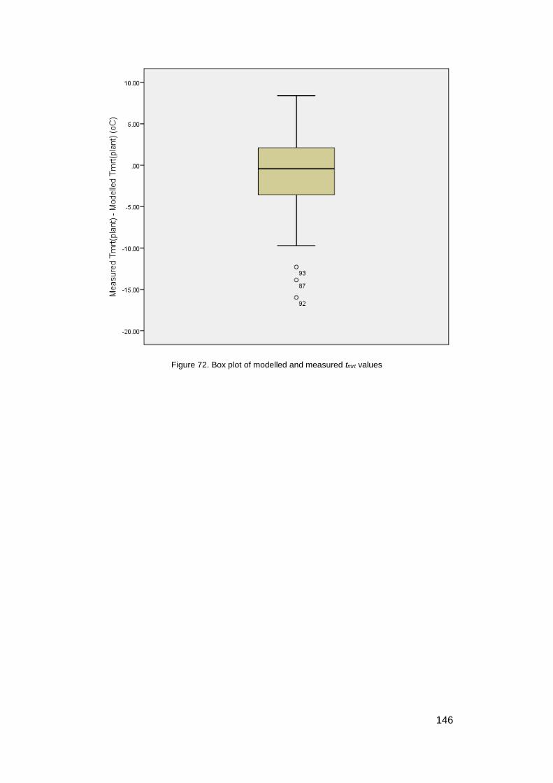
146

Figure 72. Box plot of modelled and measured tmrt values

147

By comparing values of modelled and measured tmrt values, it can be

concluded that the model is able to explain the behaviour of plant

evapotranspiration rate and shrub albedo well in terms of how they can affect

rooftop greenery tmrt values.

This chapter has demonstrated how the empirical model can predict rooftop

greenery tmrt values. A total of 675 data points from 48 days with clear sky

conditions were used to generate a robust and reliable model. The final

prediction model work flow can be seen in Figure 73. Co-efficient of

determination (R2) of the empirical model is fairly high (0.85). In addition,

analysis has shown that the comparison between modelled and measured tmrt

values is similar in terms of magnitude and trend. The following chapter

highlights the sensitivity analysis of these models.

Figure 73. Prediction model workflow

148

5.2 Sensitivity analysis

The objective of this chapter is to analyze the dependence of rooftop

greenery tmrt with regards to variations in each independent variable.

Sensitivity analyses were carried out to analyze changes in plant tmrt with

certain systematic variations in plant evapotranspiration rate and shrub

albedo by using the model developed in Chapter 5.1.

The limit ranges of independent variables are established prior to sensitivity

analysis. This is done by creating a matrix comprising of variables and their

respective workable range. The variables that are subjected to sensitivity

analysis are as follows:

- Reference mean radiant temperature (tmrt(ref));

- Plant evapotranspiration rate (ET);and

- Shrub Albedo (SA).

149

5.2.1 Establishing range limit for variables

5.2.1.1 Range limit for reference mean radiant temperature

Range limit for reference mean radiant temperature is established by

observing the box plot of tmrt(ref) values from 13:00 hrs to 17:00 hrs. It can be

observed that the range of 50 °C to 70 °C covers a large portion of upper and

lower interquartile ranges of the box plots (Figure 74). This range adequately

covers the 25th to 75th percentile of all tmrt(ref) values (Figure 75).

Figure 74. Box plot of Reference tmrt values from 07:00 hrs to 19:00 hrs

Figure 75. Box plot of Reference tmrt values from 13:00 hrs to 17:00 hrs

150

5.2.1.2 Range limit for plant evapotranspiration rate

Range limit for plant evapotranspiration rate (ET) is established by first

reviewing available literature on plant ET studies. Table 16 shows that plant

ET can range from approximately 0.0010 mmmin-1 to 0.1110 mmmin-1. It is

important to note that most studies measure plant ET in terms of mmday-1 or

mmhr-1, and values shown in Table 16 have been processed to mmmin-1 for

ease of comparison. These averaged values assume plant ET rate to be

constant throughout the day (1440 minutes), which is highly unlikely due to

the fact that transpiration activity takes place mainly in the daytime

(approximately 720 minutes) for most plants. It can be expected that actual

plant ET values should be noticeably higher during the day. Nonetheless,

Table 16 provides a reasonable estimation for the lower limit of plant ET

(0.0010 mmmin-1). The higher limit is established by observing the box plot of

measured ET rates from Chapter 4. It can be observed from Figure 76 that

the 25th to 75th percentile of measured plant ET values ranges from 0.0064

mmmin-1 to 0.0126 mmmin-1. Figure 48 shows that measured plant ET can be

as high as 0.0200 mmmin-1. Plant ET rates for trees are observed to be

significantly higher (0.1110 mmmin-1).

Figure 76. Box plot of plant evapotranspiration rates from 13:00 hrs to 17:00 hrs

151

Table 16. Plant evapotranspiration rates from reviewed literature

Vegetation

Plant evapotranspiration rate (mmmin-1)

Source

Bahiagrass

0.0016

Jia et al., 2009

Bermuda grass overseeded with perennial ryegrass

0.0026 – 0.0032 Devitt et al., 1992

Common Bermuda grass

0.0030 – 0.0033

Carrow, 1995

Buffalo grass

0.0030 to 0.0037

Kim and Beard, 1988

Begonia Cyclamen Gardenia Gloxinia Hibiscus Impatiens Pelargonium Poinsettia Schefflera

0.0033 0.0047 0.0055 0.0030 0.0055 0.0063 0.0068 0.0018 0.0052

Baille et al., 1994

Carax acutiformis Phragmites australis Carax disticha Schoeneplectus lacustris Thypha latifolia

0.0023 0.0030 0.0025 0.0024 0.0016

Behrendt et al., 2003

Willow (Tree) Poplar (Tree)

0.0580 – 0.1110 0.0560 – 0.0670

Guidi et al., 2008

Riparian Sandstone Fynbos Dryland Sandstone Fynbos Sand Plain Fynbos

0.0028 0.0010 0.0020

Dzikiti et al., 2014

152

5.2.1.3 Range limit for shrub albedo

Range limit for shrub albedo is established by referencing measured albedo

values of vegetated surfaces. Reviewed literature suggests that albedo

values of vegetated surfaces range from 0.05 to 0.30 (Table 17). Albedo

measured in Chapter 4 shows that the 25th to 75th quartile of measured

albedo values ranges from 0.24 to 0.29 (Figure 77).

Table 17. Common albedo values of vegetated surfaces

Natural surface type Approximated albedo

Source

Forest

0.05 - 0.20

Dobos, 2006

Grassland and cropland 0.10 - 0.25

Deciduous forest 0.17 Kondratiev et al., 1964; Kung et al., 1964

Tops of oak 0.18 Pine forest 0.14

Corn 0.20 - 0.25 Breuer et al., 2003

soybean 0.21 sunflower 0.24 - 0.30

Evergreen forest (mostly tropical)

0.125 ± 0.03 Dickinson and Hanson, 2013

Deciduous forest 0.147 ± 0.03 Shrub and low tree 0.175 ± 0.03 Tall grass and vegetation 0.175 ± 0.03 Short vegetation, grass, pasture 0.175 ± 0.03 Crop, agriculture 0.145 ± 0.04 Green roof 0.196 Gaffin et al., 2009

Short turf grass 0.25 – 0.30 Oke, 1988

153

Figure 77. Box plot of shrub albedo values from 13:00 hrs to 17:00 hrs

5.2.2 Sensitivity analysis of prediction model

From the preceding section, the range of values that are used for sensitivity

analysis is as follows:

Table 18. Range of values used for sensitivity analysis

Variable Range Unit


50

-

70

°C

Plant evapotranspiration rate (ET) 0.001 - 0.030 mmmin-1 Shrub albedo (SA) 0.01 - 0.30 -

The proposed ranges reflect values found in review literature as well as those

derived from field measurement.

Sensitivity analysis is conducted using the prediction model generated from

Chapter 5.1.1.3 using the equation below:

𝑇𝑚𝑟𝑡 𝑃𝑙𝑎𝑛𝑡 = 0.782𝑇𝑚𝑟𝑡𝑟𝑒𝑓 − 200.111𝐸𝑇 − 61.011𝑆𝐴 + 26.937 [25]

The averaged values of all variables (based on field measurement data) are

shown in Table 19. These values are used for sensitivity analysis.

Table 19. Averaged values used for sensitivity

Plant mean radiant temperature tmrt(Plant)


Plant evapotranspiration rate (ET) (mmmin-1)

Shrub albedo (SA)

154

(°C) (°C)

56.8 61.0 0.0095

0.26

5.2.2.1 Reference mean radiant temperature (tmrt(ref))

Sensitivity analysis is conducted for tmrt(ref) using values shown in Table 20.

Figure 78 shows the positive linear relationship between tmrt(ref) and tmrt(plant).

For every increase of 1 °C for tmrt(ref), there is a corresponding increase of 0.8

°C for tmrt(plant).

Table 20. Values used for Tmrt(Ref) sensitivity analysis


(°C)


(°C)


Shrub albedo (SA)

56.8 50.0 - 70.0 0.0095

0.26

155

Figure 78. Plot of Plant tmrt and Reference tmrt

5.2.2.2 Plant evapotranspiration rate (ET)

Sensitivity analysis is conducted for plant evapotranspiration rate (ET) using

values shown in Table 21. Figure 79 shows the negative linear relationship

between plant (ET) and tmrt(plant). For every increase of 0.001 mmmin-1 for plant

ET, there is a corresponding decrease of 0.2 °C for tmrt(plant).

Table 21. Values used for Plant ET sensitivity analysis


(°C)


(°C)


Shrub albedo (SA)

56.8 61.0 0.001 – 0.030

0.26

45

50

55

60

65

70

75

45 50 55 60 65

Tmrt

(R

efer

ence

) (°

C)

Tmrt (Plant) (°C)

Tmrt(Reference) Linear (Tmrt(Reference))

156

Figure 79. Plot of Plant tmrt and Plant Evapotranspiration Rate

5.2.2.3 Shrub albedo (SA)

Sensitivity analysis is conducted for shrub albedo (SA) using values shown in

Table 22. Figure 80 shows the negative linear relationship between (SA) and

tmrt(plant). For every increase of 0.01 for SA, there is a corresponding decrease

of 0.6 °C for tmrt(plant).

Table 22.Values used for Shrub Albedo sensitivity analysis


(°C)


(°C)


Shrub albedo (SA)

56.8 61.0 0.0095

0.01 – 0.30

0.000

0.005

0.010

0.015

0.020

0.025

0.030

0.035

52 53 54 55 56 57 58 59

Pla

nt

ET

(mm

min

-1)

Tmrt (Plant) (°C)

ET Linear (ET )

157

Figure 80. Plot of Plant tmrt and Shrub Albedo

5.2.2.4 Values of tmrt(plant) for tmrt(ref) values of 50 °C to 70 °C

Values of tmrt(plant) are estimated using the empirically derived prediction model

for tmrt(ref) values ranging from 50 °C to 70 °C. Results are appended in

Chapter 10.8. It can be observed from Table 23 that for the range of 50 °C to

70 °C, reductions in mean radiant temperature can be observed with a

minimum albedo of 0.17 and plant ET of 0.029. At peak tmrt(ref) (70 °C), it can

be observed that a SA value of 0.19 will result in reduced tmrt(plant) with plant

ET as low as 0.001 mmmin-1.

Table 23. Percentage reduction of Tmrt(plant) derived using Tmrt(ref) of 50 °C and 70 °C

0.00

0.05

0.10

0.15

0.20

0.25

0.30

0.35

50 55 60 65 70 75

Shru

b A

lbed

o

Tmrt (Plant) (°C)

Alb Linear (Alb)

158

6 DISCUSSION

This chapter discusses the significance of findings from Chapter 4, as well as

a proposed methodology for landscape planning based on results of Chapter

5.

159

6.1 Impact of plant selection on ambient and mean radiant

temperature

6.1.1 Plant evapotranspiration rate

Results from Chapter 4 have shown that plant EvapoTranspiration rate (ET)

has a significant effect on mean radiant temperature (tmrt) in the tropical urban

outdoor environment. Therefore, in the process of plant selection, it is

important to choose plants with high ET rates for the purpose of attaining

maximum cooling potential. There is a wide variety of flora available for

selection, and a systematic categorization of ET rates for commonly used

rooftop greenery plants is necessary. The list of plants to be tested can be

referenced from relevant literature such as ‘A selection of plants for green

roofs in Singapore’ (Tan and Sia, 2008).

A review of existing literature shows that ET rates of plants range from

approximately 0.0010 mmmin-1 to 0.1110 mmmin-1 (Table 16). However, it is

noted that most studies measure plant ET on a daily or monthly basis

(Behrendt et al., 2003; Devitt et al., 1992; Dzikiti et al., 2014). This makes it

impossible to discern the true impact of ET on cooling effect at specific

periods (e.g. 13:00 hrs to 17:00 hrs, the hottest period of the day). Moreover,

there is very little ET activity as night for most plants owing to the fact that ET

is a photosynthetic process.

This study has also looked into ET rates of plants commonly used for rooftop

greenery specifically at minute and hourly intervals so as to observe the

behavior of plants in terms of their ET during different parts of the day (Figure

81). Additional measurements of plant ET for different plants show that ET

rates can vary significantly for different plant types (Figure 82).

Measurements were taken on 13th January 2015, under clear sky conditions

with peak solar irradiance of 791.2 Wm-2 at 15:00 hrs.

160

Figure 81. Rooftop greenery panel on load cell

161

ET Plant Average Evapotranspiration Rate (mmmin-1) (13:00 hrs to 17:00 hrs)

1 Pedilanthus tithymaloides 0.0074 2 Schefflera arboricola 0.0074 3 Euphorbia milii 0.0051 4 Asparagus officinalis 0.0080

For the purpose of optimizing cooling effect, it is recommended that following

plants be avoided:

- Crassulacean Acid Metabolism (CAM) plants

Generally, plants undergoing CAM photosynthesis have leaf stomata

fully or partially closed during daytime in order to decrease the rate of

ET, but are open during nighttime to receive carbon dioxide (CO2)

(Zeiger et al., 1987). This is a common characteristic in plants found in

arid environments (e.g. cacti), where water is limited. While this is an

effective water conservation strategy for the plants, it will drastically

reduce ET rate during daytime and is therefore unsuitable for rooftop

greenery.

0.00

0.00

0.00

0.00

0.00

0.01

0.01

0.01

0.01

0.01

0.02

0.02

13:00 14:00 15:00 16:00 17:00

Pla

nt

Evap

otr

ansp

irat

ion

Rat

e (m

mm

in-1

)

Time (Hrs)

ET 1 ET 2 ET 3 ET 4

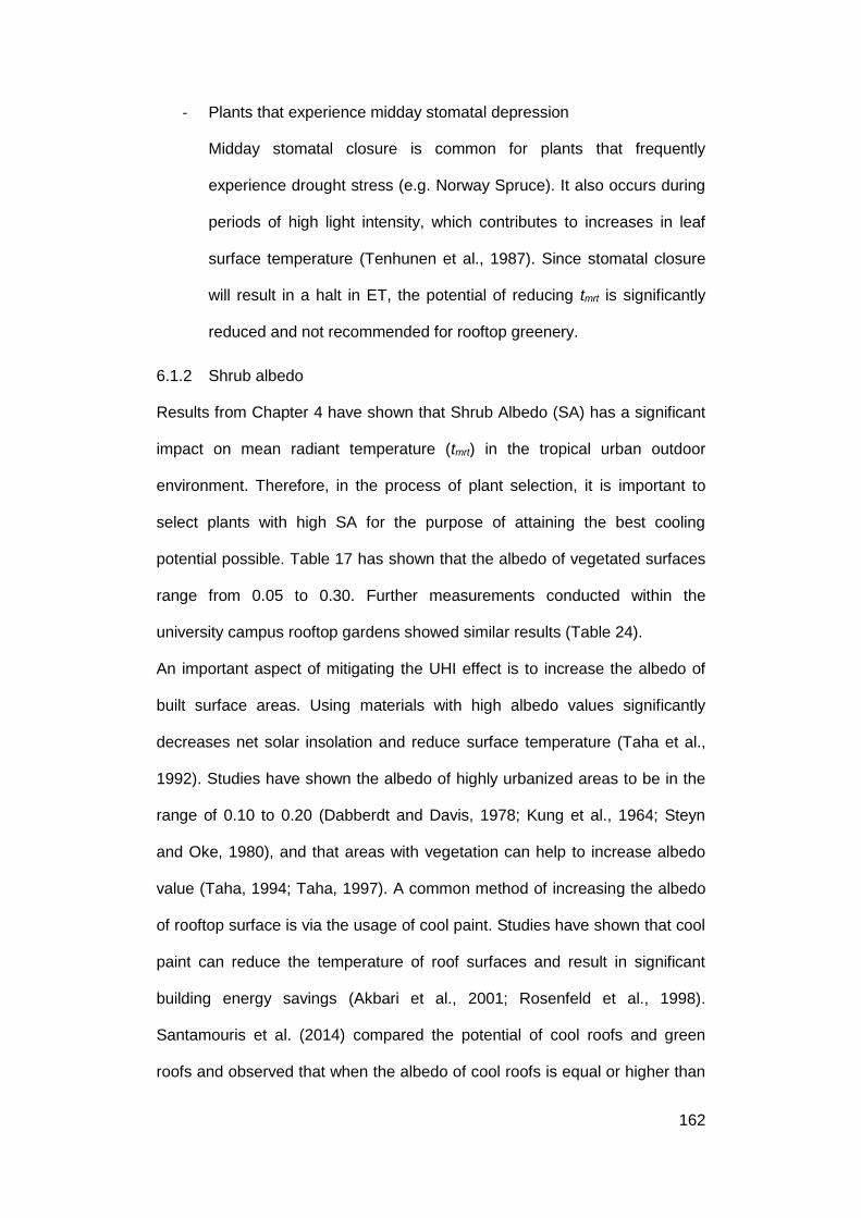
162

- Plants that experience midday stomatal depression

Midday stomatal closure is common for plants that frequently

experience drought stress (e.g. Norway Spruce). It also occurs during

periods of high light intensity, which contributes to increases in leaf

surface temperature (Tenhunen et al., 1987). Since stomatal closure

will result in a halt in ET, the potential of reducing tmrt is significantly

reduced and not recommended for rooftop greenery.

6.1.2 Shrub albedo

Results from Chapter 4 have shown that Shrub Albedo (SA) has a significant

impact on mean radiant temperature (tmrt) in the tropical urban outdoor

environment. Therefore, in the process of plant selection, it is important to

select plants with high SA for the purpose of attaining the best cooling

potential possible. Table 17 has shown that the albedo of vegetated surfaces

range from 0.05 to 0.30. Further measurements conducted within the

university campus rooftop gardens showed similar results (Table 24).

An important aspect of mitigating the UHI effect is to increase the albedo of

built surface areas. Using materials with high albedo values significantly

decreases net solar insolation and reduce surface temperature (Taha et al.,

1992). Studies have shown the albedo of highly urbanized areas to be in the

range of 0.10 to 0.20 (Dabberdt and Davis, 1978; Kung et al., 1964; Steyn

and Oke, 1980), and that areas with vegetation can help to increase albedo

value (Taha, 1994; Taha, 1997). A common method of increasing the albedo

of rooftop surface is via the usage of cool paint. Studies have shown that cool

paint can reduce the temperature of roof surfaces and result in significant

building energy savings (Akbari et al., 2001; Rosenfeld et al., 1998).

Santamouris et al. (2014) compared the potential of cool roofs and green

roofs and observed that when the albedo of cool roofs is equal or higher than

163

0.7, it has a higher cooling potential than green roofs during the peak period.

In general, cool roofs perform better than green roofs in sunny climates.

However, deterioration of cool roofs due to weathering (dust, moisture

penetration, mircobial growth, etc) can significantly decrease its cooling

potential (Cheng et al., 2012; Cheng et al., 2011). Green roofs can also

significantly reduce surface temperature, as shown in Chapter 4.1.1.7.

Compared to cool roofs, green roofs require more maintenance such as

regular pruning and replacement of plants, as well as a reliable irrigation

schedule. While the upkeep for rooftop greenery is higher, it offers

opportunities for roof spaces to be an appropriate venue for social activities

and can improve the aesthetics of the outdoor environment.

Table 24. Albedo spot measurements at 13:00 hrs in National University of Singapore UTown roof gardens

Plant Upward facing pyranometer (Wm-2)

Downward facing pyranometer (Wm-2)

Albedo

Crinum asiaticum

436 111 0.25

Zoysia japonica

360 107 0.30

Rhododendron macgregoriae F.Muell.

833 292 0.35

Cyanotis cristata D.Don

890 200 0.22

Nephrolepis auriculata

972 267 0.27

6.1.3 Consideration of plant functional traits for plant selection

Chapters 6.1.1 and 6.1.2 have looked into quantifiable aspects of plants (ET

and SA) and their impact on mean radiant temperature (tmrt). In the course of

164

field measurement, it was also noted that physical plant traits have a

significant impact on resultant plant surface temperature and by extrapolation,

mean radiant temperature. It has been observed that Heliconia ‘American

Dwarf’ plants (Plot 2) have leaves that are much larger than both Phyllanthus

cochinchinensis (Plot 1) and Sphagneticola trilobata (Plot 3) plants (Figure

83). The surface area of its leaves is observed to be much higher than the

other plots (Figure 58). The average height of Plot 2 plants is also much

higher than Plots 1 and 3. In terms of the plant canopy, Plot 2 is much more

porous, compared to Plot 3, which forms a thick, inter-twined undergrowth

with its stems. This undergrowth provides excellent shade, which translates to

higher reduction in air temperature (Figure 65). Cool air is effectively trapped

within the canopy. While there is insufficient data to determine the statistical

impact of plant functional traits, there is evidence to suggest that that leaves

with smaller surface areas tend to be more effective at reducing tmrt.

Therefore, selection of plants with small leaves for the purpose of reducing

outdoor tmrt is recommended.

165

Fig

ure

83

. B

ota

nic

al ill

ustr

ation

of

pla

nts

use

d f

or

me

asu

rem

en

t

166

6.1.4 Leaf Area Index

Numerous studies have shown plant Leaf Area Index to be strongly correlated

with temperature reduction. In such cases, temperature reduction is mostly

due to shade provided by tree canopy, resulting in reduced heat absorbed by

building surfaces, pavements and pedestrians (Fahmy et al., 2010; Gómez-

Muñoz et al., 2010; Hardin and Jensen, 2007). Shahidan et al. (2010) found

significant correlation between LAI and radiation filtration for M. Ferrea L and

H. crepittan (R2 = 0.96 and 0.95). A higher LAI value will mean more leaves,

providing increased reduction of thermal radiation under a tree (Brown and

Gillespie, 1995; Kotzen, 2003).

As for the impact of LAI on tmrt, this study has shown that LAI is not strongly

correlated with tmrt reduction. Table 9 shows that although the LAI of Plot 2 –

Heliconia ‘American Dwarf’ is 7.21, it is least effective at reducing tmrt. This

would suggest that overall radiative qualities of the plant canopy (albedo,

absorptance, reflectance, canopy structure) are more substantial at

determining its impact on tmrt. It was observed from this study that leaves for

Plot 1 and Plot 2 are able to form a compact canopy while leaves for Plot 2

form a porous canopy due to its large vertically-hung leaves.

167

6.2 Landscape planning guidelines

The underlying objective of this thesis is to discern the impact of plants in the

outdoor environment and to explore novel methods of practicing landscape

planning to improve outdoor thermal comfort. For the purpose of optimizing

the landscape planning process, numerous field measurements were

conducted. Data was analyzed with the intention of obtaining insight on how

best to improve outdoor thermal conditions based on plants selection and

placement. This study defines the optimization of selection and placement

processes in the following manner:

- Plant selection

Plants should be selected based on their potential to cool the surrounding

environment.

- Plant placement

Plants should be placed in areas where their potential to cool the surrounding

environment can be maximized.

The remainder of this chapter summarizes all findings from this study and

their implication on plant selection and placement criteria. A framework for

landscape planning is proposed, based on these findings. A discussion on

relevant tools and technical processes ensues, forming the basis of

recommendations on how it can be translated into industry practice.

168

6.2.1 Recommendations based on quantitative results of study

Chapters 3.2.1 to 10.3 describe the process of recalibrating globe

thermometers for use in the tropical outdoor environment, measurement of tmrt

in parks and urban areas as well as measurement of tmrt above rooftop

greenery. Findings and recommendations are summarized in Table 25.

Table 25. Recommendations for landscape planning

Chapter number

Title Findings from measurement

Recommendation for landscape planning

Page

3.2.1 Calibration of

globe thermometers for use in the tropical urban environment

Recalibration of tmrt formula for use in the tropical urban environment

Formula to be used for measurement of tmrt using 40 mm globes

81

4 Measurement

of mean radiant temperature on roof garden setting

Rooftop greenery can significantly reduce air and mean radiant temperature. Rooftop greenery can reduce air temperature at night, reducing the impact of the Urban Heat Island effect Plant ET and SA characteristics vary significantly from species to species Leaf Area Index is not strongly correlated with tmrt reduction Plant traits such as leaf size and shrub height can affect overall thermal performance

Rooftop greenery can be used to improve outdoor thermal comfort and reduce UHI effect Selection of plants should take into consideration plant characteristics such as ET and SA. Special attention should be given to plant behavior from 13:00 hrs to 17:00 hrs In terms of tmrt, LAI should not be used to assess the thermal performance of rooftop greenery Plants with small leaves and short shrub height should be preferred

100 113 115 118 122

169

Chapter number



Page

Surface temperature of

concrete is reduced tremendously with rooftop greenery

Rooftop greenery can be used to improve indoor thermal comfort

125

4.1.2 Potential of rooftop greenery for reducing air and mean radiant temperature

Potential of plants to reduce air temperature may be affected by plant functional traits such as shrub structure Air temperature reduction is poorly related to ET and SA

Selection of plants should include consideration of shrub structure to optimize cooling potential Selection of plants for temperature reduction should be for tmrt and not for air temperature

131 133

5 Rooftop greenery mean radiant temperature prediction model

Plant ET and SA are statistically significant functions of tmrt reduction due to rooftop greenery Development of regression model of tmrt reduction due to rooftop greenery Development of ET and SA table for plant selection

Selection of plants should include consideration of ET and SA Impact of rooftop greenery can be assessed using regression model Plants selected can assessed using selection table

141 144 157

6.1 Impact of plant selection on ambient and mean radiant temperature

Rooftop greenery plants have a wide range of ET rates. Some plants with very low ET rates are highlighted Rooftop greenery plants have a wide range of albedo values Evidence of plant cooling potential due to plant functional traits Leaf Area Index is poorly correlated with tmrt reduction

Plants with high ET rates are preferred. Plants such as CAM plants should be avoided Plants with high SA are preferred Plants with small leaves and short shrub height should be preferred In terms of tmrt, LAI should not be used to assess the thermal performance of rooftop greenery

161 163 164 166

170

Chapter number



Page

10.1 Large scale

urban mapping of mean radiant temperature

There is little difference between tmrt of urban areas and park areas in the absence of sunlight Trees can reduce tmrt significantly by means of shade provision. Sky View Factor (SVF) can be correlated with tmrt reduction

Selection and placement of plants need not consider impact at night More trees should be planted on ground level. Trees with large canopies are preferred, as they provide more shade Assessment of shade quality can be done with SVF

218 216 222

10.2 Impact of plant height stratification on mean radiant temperature

Temperature stratification above plants vary from species to species

Selection of plants should include consideration of tmrt reduction due to height stratification

227

10.3.1 Impact on vertical greenery on mean radiant temperature

Vertical greenery can reduce air temperature and tmrt Cooling effect of vertical greenery is insignificant when shaded GIS can be used to generate tmrt map

Vertical greenery can be used to improve outdoor thermal comfort Vertical greenery should be placed at areas with high exposure to solar irradiance GIS can be used as a planning/simulation platform for landscape planning

239 241 243 247

10.3.2 Analysis of similar plant types in horizontal and vertical setup

Rooftop greenery is more effective at reducing tmrt than vertical greenery Westward facing green walls exhibit higher cooling potential compared to eastward facing green walls Vertical greenery tends to reduce surface albedo Vertical greenery tends to increase ET rate

Rooftop greenery should be preferred to vertical greenery if budget is limited Priority should be given to westward-facing facades Plants with high SA are preferred Plants with high ET are preferred

255 256 257 260

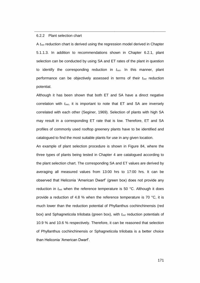
171

6.2.2 Plant selection chart

A tmrt reduction chart is derived using the regression model derived in Chapter

5.1.1.3. In addition to recommendations shown in Chapter 6.2.1, plant

selection can be conducted by using SA and ET rates of the plant in question

to identify the corresponding reduction in tmrt. In this manner, plant

performance can be objectively assessed in terms of their tmrt reduction

potential.

Although it has been shown that both ET and SA have a direct negative

correlation with tmrt, it is important to note that ET and SA are inversely

correlated with each other (Seginer, 1969). Selection of plants with high SA

may result in a corresponding ET rate that is low. Therefore, ET and SA

profiles of commonly used rooftop greenery plants have to be identified and

catalogued to find the most suitable plants for use in any given location.

An example of plant selection procedure is shown in Figure 84, where the

three types of plants being tested in Chapter 4 are catalogued according to

the plant selection chart. The corresponding SA and ET values are derived by

averaging all measured values from 13:00 hrs to 17:00 hrs. It can be

observed that Heliconia ‘American Dwarf’ (green box) does not provide any

reduction in tmrt when the reference temperature is 50 °C. Although it does

provide a reduction of 4.8 % when the reference temperature is 70 °C, it is

much lower than the reduction potential of Phyllanthus cochinchinensis (red

box) and Sphagneticola trilobata (green box), with tmrt reduction potentials of

10.9 % and 10.6 % respectively. Therefore, it can be reasoned that selection

of Phyllanthus cochinchinensis or Sphagneticola trilobata is a better choice

than Heliconia ‘American Dwarf’.

172

Since there is lesser chance of reducing tmrt through shade provision by large

canopy trees on roof gardens and sky terraces, it is important that the shrubs

used can help reduce tmrt as much as possible. The plant selection chart can

provide easy reference for landscape architects and help them visualise the

impact of their choices.

Reference Tmrt 50°C

Shrub Albedo

0.21 0.22 0.23 0.24 0.25 0.26 0.27 0.28 0.29 0.30

Pla

nt

Ev

ap

otr

an

sp

ira

tio

n R

ate

0.001 - - - - - - 1.3 2.5 3.7 4.9 0.002 - - - - - 0.5 1.7 2.9 4.1 5.3 0.003 - - - - - 0.9 2.1 3.3 4.5 5.7 0.004 - - - - - 1.3 2.5 3.7 4.9 6.1 0.005 - - - - 0.4 1.7 2.9 4.1 5.3 6.5 0.006 - - - - 0.8 2.1 3.3 4.5 5.7 6.9 0.007 - - - - 1.2 2.5 3.7 4.9 6.1 7.3 0.008 - - - 0.4 1.6 2.9 4.1 5.3 6.5 7.7 0.009 - - - 0.8 2.0 3.3 4.5 5.7 6.9 8.1 0.010 - - - 1.2 2.4 3.7 4.9 6.1 7.3 8.5 0.011 - - - 1.6 2.8 4.1 5.3 6.5 7.7 8.9 0.012 - - 0.4 2.0 3.2 4.5 5.7 6.9 8.1 9.3 0.013 - - 0.8 2.4 3.6 4.9 6.1 7.3 8.5 9.7 0.014 - 0.4 1.2 2.8 4.0 5.3 6.5 7.7 8.9 10.1 0.015 - 0.8 1.6 3.2 4.4 5.7 6.9 8.1 9.3 10.5 0.016 - 1.2 2.0 3.6 4.8 6.1 7.3 8.5 9.7 10.9 0.017 0.4 1.6 2.4 4.0 5.2 6.5 7.7 8.9 10.1 11.3

Reference Tmrt 70°C

Shrub Albedo

0.21 0.22 0.23 0.24 0.25 0.26 0.27 0.28 0.29 0.30

Pla

nt

Ev

ap

otr

an

sp

ira

tio

n R

ate

0.001 1.9 2.8 3.4 4.5 5.4 6.3 7.1 8.0 8.9 9.8 0.002 2.2 3.1 3.7 4.8 5.7 6.6 7.4 8.3 9.2 10.0 0.003 2.5 3.4 3.9 5.1 6.0 6.8 7.7 8.6 9.5 10.3 0.004 2.8 3.6 4.2 5.4 6.3 7.1 8.0 8.9 9.7 10.6 0.005 3.1 3.9 4.5 5.7 6.5 7.4 8.3 9.2 10.0 10.9 0.006 3.3 4.2 4.8 6.0 6.8 7.7 8.6 9.4 10.3 11.2 0.007 3.6 4.5 5.1 6.2 7.1 8.0 8.9 9.7 10.6 11.5 0.008 3.9 4.8 5.4 6.5 7.4 8.3 9.1 10.0 10.9 11.8 0.009 4.2 5.1 5.7 6.8 7.7 8.6 9.4 10.3 11.2 12.0 0.010 4.5 5.4 5.9 7.1 8.0 8.8 9.7 10.6 11.5 12.3 0.011 4.8 5.6 6.2 7.4 8.3 9.1 10.0 10.9 11.7 12.6 0.012 5.1 5.9 6.5 7.7 8.5 9.4 10.3 11.2 12.0 12.9 0.013 5.3 6.2 6.8 8.0 8.8 9.7 10.6 11.4 12.3 13.2 0.014 5.6 6.5 7.1 8.2 9.1 10.0 10.9 11.7 12.6 13.5 0.015 5.9 6.8 7.4 8.5 9.4 10.3 11.1 12.0 12.9 13.8 0.016 6.2 7.1 7.7 8.8 9.7 10.6 11.4 12.3 13.2 14.0 0.017 6.5 7.4 7.9 9.1 10.0 10.8 11.7 12.6 13.5 14.3


Plot 2 - Heliconia 'American Dwarf'


173

Figure 84. Plant selection via chart (Percentage decrease in tmrt)

6.2.3 Landscape planning framework

Generally, landscape planning frameworks are concerned with issues such as

plant health, maintainability and aesthetic requirements. The purpose of

having such frameworks is to ensure comprehensive appraisal and inventory

of urban greenery (CTLA, 1992). The criteria for urban greenery assessment

may be classified as shown in Table 26.

Table 26. Factors to consider in rating plant species and cultivars (CTLA, 1992)

Factor

Climate adaptability Cold hardiness Frost tolerance Drought tolerance Storms: resistance to ice, snow, wind Growth characteristics Tolerance to difficult sites Vigour Structural strength Life expectancy Soil adaptability Structure and texture Drainage Moisture excess or deficiency Acidity and alkalinity Nutritional deficiencies or excesses Resistance or tolerance Diseases Insects Air pollution Maintenance requirements Training and pruning Cleanliness: flowers, fruit, leaves, twigs, duration of

leaf fall Roof problems Pests Structural problems (cabling and bracing) Allergenic properties Pollen Dermal toxins Aesthetic values Branches and tree form - growth habit, bark colour

and texture Foliage -density, colour texture and duration Flowers – Prominence , fragrance/odor, duration,

colour and size Fruit – Prominence, duration, use, colour, size,

174

fragrance /odour

For the proposed landscape planning workflow, benefits of greenery in terms

of how it can improve climatological conditions are factored into the

framework. Miller (2007) outlines the positive impacts of urban greenery in

terms of their climatological and engineering uses (Table 27).

Table 27. Additional factors in rating plant species (Miller, 2007)

Factor

Climatological uses

Human comfort Radiant temperature Air temperature Air movement Humidity and precipitation Building energy budgets Heating Cooling Solar energy and trees

Engineering uses

Sound pollution reduction Air quality control Urban hydrology Erosion control Wastewater treatment Glare and reflection reduction

This study proposes a landscape planning framework that aims to improve

radiant and air temperature conditions of the outdoor landscape (Figure 85).

In this case, impact of urban greenery on outdoor climate is considered to be

a factor in rating its overall value (specifically, air and mean radiant

temperature). The proposed workflow is based on findings shown in Chapters

6.2.1 and 6.2.2.

175

Figure 85. Proposed landscape planning framework

6.2.4 Hypothetical case study illustrating usage of prediction model

A workflow sequence is elaborated, based on the proposed framework

(Figure 86). This section outlines the procedure of landscape planning

optimization and demonstrates its technical viability with a hypothetical case

study.

176

Fig

ure

86

. E

labo

ratio

n o

f p

ropo

se

d la

nd

sca

pe

pla

nnin

g f

ram

ew

ork

177

6.2.4.1 Hypothetical urban model

A hypothetical scenario is developed to illustrate efficacy of the proposed

landscape planning framework (Figure 87). The site measures 400 m by 400

m and is modelled with urban constituents that are representative of a

commercial district in a dense urban setting. Common urban morphological

parameters such as high-rise commercial buildings, podium blocks, roof

gardens and sky terraces are included. A portion of the model is allocated as

park space with several low-lying amenity blocks. Areas subjected to the

proposed landscape planning methodology are as follows:

1. Pedestrian level; and

2. Building surfaces.

Pedestrian level is defined as 2 m above ground level. Building surfaces

include all wall and roof surfaces, as well as building insets. Several iterations

of the model are developed to illustrate the capabilities of the landscape

planning framework (Table 28).

Table 28. Model properties

Model Characteristics

Iteration 1 Trees with 5 m diameter canopy Generically allocated Iteration 2 Trees with 15 m diameter canopy

Generically allocated

Iteration 3 Trees with 20 m diameter canopy Generically allocated

With additional trees in areas exposed to high solar irradiance

Iteration 4 Trees with 20 m diameter canopy Generically allocated

With additional trees in areas exposed to high solar irradiance With addition of shurbs and predicted cooling effect

179

Figure 87. Hypothetical urban model (Baseline)

6.2.4.2 Pedestrian level

In this exercise, the area of interest is a park slated for development with food

and beverage outlets. Since a sizable crowd is expected to occupy the open

space during events and there is a large pathway that transverses the park

diagonally, the proposed landscape planning framework will be utilized to

facilitate the landscape design process. The proposed technical workflow is

illustrated in Figure 88. Simulation of tmrt is first conducted with tree

information (partial plant input) and subsequently completed with shrub

information (complete plant input). Cooling effect due to shrubbery is based

on the prediction model derived in Chapter 5.

Figure 88. Pedestrain level tmrt modelling hierarchy

180

Geographical Information Systems (GIS) as climatic mapping tool

Relevant data is represented through climatic mapping via a GIS platform.

Climatic mapping is selected as the mode of presentation as it is already a

widely-used tool for urban planning. Climatic maps are able to serve as

visualisation aid from micro to macro level. Through the GIS platform, multiple

layers of spatial information can be analysed simultaneously. The use of

climatic mapping has become a prominent feature in studies of the outdoor

climate (Katzschner et al., 2004; Katzschner and Mülder, 2008; Koster, 1998;

Stocks and Wise, 2000).

In particular, there has been extensive usage of GIS for the mapping of green

spaces. Kamishima et al. (2002) used ADS40 (Airborne Digital Sensor)

images to analyse the urban landscape of Tokyo. GIS was used to proximate

greenery distribution using the ADS40 images. Subsequently, this information

was layered with building data through the GIS platform.

Laing et.al. (2006) measured environmental values of green spaces via GIS

spatial analysis for aiding decision in relation to urban green planning. The

use of computer visualization provided advances in the presentation and

delivery of spatial information.

Table 29 shows software that can be used to facilitate the landscape planning

process. Impact of tmrt due to shrub can be attained by using the regression

model derived in Chapter 5, with the assumption that temperature reduction

of extensive green roof systems are similar to ground level planting

conditions. In this exercise, Rhinoceros 3D is used to generate the 3D model,

SOLWEIG (Lindberg et al., 2008b) is used to simulate outdoor tmrt conditions

and ArcGIS is the GIS platform of choice.

181

Table 29. Software recommended for simulation

Item Software

3D Model Autodesk AUTOCAD, Rhinoceros

3D,or equivalent CAD software

Digital Elevation Model ArcGIS, or equivalent GIS software Simulated Mean Radiant Temperature Map SOLWEIG, Townscope, Thermo

Render, or equivalent tmrt simulation software

Final Mean Radiant Temperature Map ArcGIS, or equivalent GIS software

Figure 89 demonstrates how landscape planning can be conducted

systematically via tmrt mapping.

In Iteration 1, trees with small canopies (5 m diameter) are placed at locations

designated by the landscape planner.

In Iteration 2, trees with larger canopies are assumed (15 m diameter) at the

same spots. The tmrt reduces drastically near the trees.

In Iteration 3, more trees (20 m diameter) are added at areas that are

anticipating larger pedestrian flow. As a result, thermal conditions of these

areas can be improved.

182

Figure 89. Simulation of tmrt via SOLWEIG and ArcGIS

183

Use of prediction model for landscape planning

This section describes how the prediction model derived in Chapter 5 can be

used for landscape planning.

Figure 89 has shown how the tree selection and placement process can be

optimized through tmrt simulation. In Iteration 3, trees with large canopies are

proposed and additional trees are allocated to areas that are exposed to high

levels of solar radiation. Although outdoor thermal condition has improved

significantly when compared to Iteration 1, the map is incomplete as cooling

effect of shrubbery has yet to be considered.

Suppose the landscape planner has reviewed simulation results from Iteration

3 and wishes to improve thermal conditions of Areas A and B, as well as the

main pedestrian walkway by planting shrubs (Figure 90). To simulate the

cooling effect of shrubs, a fourth iteration is conducted, using the regression

model derived in Chapter 5.

Figure 90. Areas where shrubs can be added to reduce tmrt

184

In the 4th Iteration, cooling effect of shrubbery is considered based on the

prediction model derived from Chapter 5:

𝑇𝑚𝑟𝑡 𝑃𝑙𝑎𝑛𝑡 = 0.782𝑇𝑚𝑟𝑡𝑟𝑒𝑓 − 200.111𝐸𝑇 − 61.011𝑆𝐴 + 26.937 [25]

Where,

TmrtPlant = Mean radiant temperature above rooftop greenery (°C)

TmrtRef = Mean radiant temperature above concrete (°C)

ET = Plant evapotranspiration rate (mm·min-1)

SA = Shrub Albedo

The shrub to be used is assumed to have traits similar to Phyllanthus

cochinchinensis and allocated as shown in Figure 91:

- Evapotranspiration Rate (ET) of 0.011 mmmin-1; and

- Shrub Albedo (SA) of 0.28.

Figure 91. Areas allocated for shrubbery (Highlighted in green)

185

This information (ET and SA) serves as input variables to Equation (25).

Together with values of tmrt(ref) obtained from Iteration 3, resultant tmrt is

calculated for every pixel of the simulation map using ArcGIS. Simulation

result of Iteration 4 is shown in Figure 92.

Figure 92. Simulation result with input from regression model

In Iteration 4, thermal effects of shrubbery are factored into the tmrt map via

the regression model and plant selection chart derived from this study.

Comparison of all four iterations reveals the immense positive impact of tree

and shrub allocation using the proposed landscape planning framework

(Figure 93). The proposed methodology is an iterative process and can be

performed ad infinitum until the desired result is attained.

It is important to note that simulation is currently performed with the

assumption that the temperature reduction potential of extensive roof systems

is the same as intensive roof systems or shrubbery at ground level. Further

study is required to ascertain the actual reduction potential of intensive roof

systems and shrubbery at ground level.

186

Figure 93. Comparison of Tmrt simulation results

187

6.2.4.3 Building surfaces

In this exercise, the areas of interest are building surfaces. Numerous studies

on vertical and rooftop greenery have focused on the issue of heat

transmission through building façade and cooling energy (Chen et al., 2013;

Cheng et al., 2010; Perini et al., 2011; Wong et al., 2010a). For this study, the

emphasis is on identifying suitable areas for plants to be allocated and for

them to fully realize their cooling potential on the outdoor environment.

Therefore, solar insolation conditions are critically assessed before plants are

selected (Figure 94). The list of software recommended for this exercise is

shown in Table 30. In this case, Rhinoceros 3D is used for 3D modelling and

DIVA (Jakubiec and Reinhart, 2011) is used for solar insolation simulation.

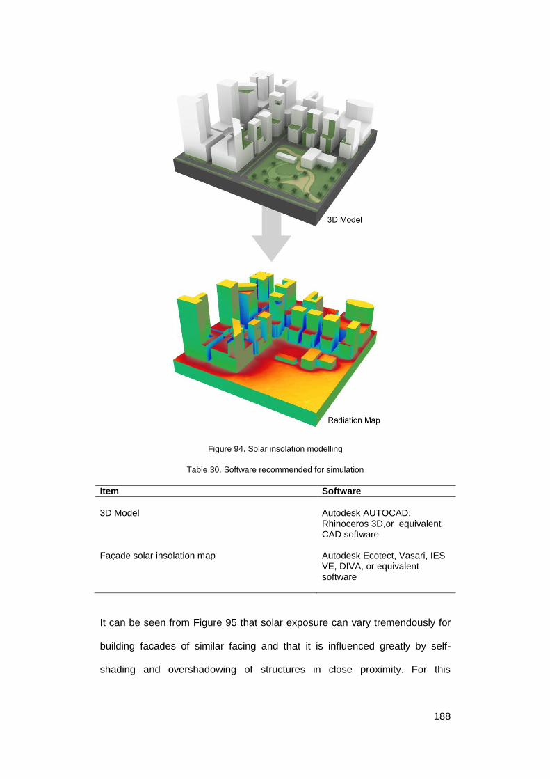
188

Figure 94. Solar insolation modelling

Table 30. Software recommended for simulation

Item Software

3D Model Autodesk AUTOCAD,

Rhinoceros 3D,or equivalent CAD software

Façade solar insolation map Autodesk Ecotect, Vasari, IES VE, DIVA, or equivalent software

It can be seen from Figure 95 that solar exposure can vary tremendously for

building facades of similar facing and that it is influenced greatly by self-

shading and overshadowing of structures in close proximity. For this

189

hypothetical planning exercise, a few building surfaces are selected for

assessment (dotted region).

Figure 95. Close-up of solar insolation map

Use of prediction model for landscape planning

This section describes how the prediction model derived in Chapter 5 can be

used for landscape planning. In this instance, landscape planning can be

conducted using the plant selection chart derived from the regression model.

The proposed methodology for landscape planning of building surfaces is as

follows (Figure 96):

1. Simulation of solar insolation of building surfaces.

2. Segregation of building surfaces according to degree of solar

exposure.

190

3. Reference to plant selection chart for allocation of plants to rooftop or

vertical greenery.

Figure 96. Landscape planning for building surfaces

In this hypothetical scenario, conclusions are drawn based on perspectives

of:

- The urban planner

Urban planning is a process that looks into issues such as land use and

overall impact to the outdoor environment. Urban planners shape the city

though planning guidelines, which are interpreted by the architect and

translated into form. From Figure 97, it can be observed that solar insolation

levels of higher roofs (R1) are about 20 % more than lower roofs (R2). A

green roof on R1 will reduce more heat transmission into the building than the

191

same green roof on R2. Therefore, priority should be given to R1 in terms of

green roof allocation. For R2, it can be observed that areas that are further

away from S3 receive higher solar exposure. It can therefore be inferred that

plants with higher ET and SA can be used to improve radiant conditions at

these areas.

Also, building facades along S2 have a higher solar exposure than facades

along S1, although they are of the same orientation. The solar insolation

diagram can be used as a planning tool to justify the allocation of vertical

greenery along S2 rather than S1. Semi-shade or shade tolerant plants can

be used for vertical greenery located along S1, and full sun plants can be

used for vertical greenery allocated along S2. Plant selection can be done via

the selection chart derived from Chapter 5.

While it has been established that westward-facing facades should be

retrofitted with vertical greenery to reduce heat gain, Figure 97 shows that it is

more effective to allocate vertical greenery on W1 than on W2. This is

because W1 has a higher solar exposure level. In this way, policies do not

have to be overly generalised (All westward-facing facades must be retrofitted

with vertical greenery), but can be optimised by first examining local solar

insolation conditions and making an informed judgement based on these

examinations.

- The architect or landscape designer

Contrary to urban designers, architects operate at a much finer scale and

require an accurate portrayal of form and materiality. In this case, placement

of greenery is exact and plant selection is specific to the genus. In this

hypothetical scenario, the architect is tasked with selecting an appropriate

façade for retrofitting a green wall (W2, S2 or S3). By using the solar

insolation diagram, the architect can make an objective decision based on

solar exposure. It can be seen that S3 has the highest solar exposure and for

192

the purpose of reducing heat transmission into the building as well as to

improve outdoor thermal conditions, S3 is the best candidate for green wall

retrofit. Figure 97 also shows that solar insolation need not be homogeneous

across a single surface. W2, for instance, will benefit more if a green wall is

allocated at the upper portion of the wall (due to higher solar exposure) than if

it were to be allocated at the lower portion.

After vertical and rooftop greenery spaces have been allocated, the solar

insolation map can be used to identify the type of plants to be used at these

areas. Different plants require different light conditions for optimal growth.

This is more commonly categorised as full sun, semi-shaded, and fully

shaded conditions. The plant selection chart derived from Chapter 5 can be

used to select plants based on their evapotranspiration rate and albedo. With

the solar insolation map, it is possible to recommend the appropriate type of

plants to be allocated based on local insolation levels.

The proposed methodology differs slightly from the preceding section, in that

a slightly more qualitative approach to planning and allocation is adopted.

193

Figure 97. Assessment of building surfaces using solar insolation map

194

7 CONCLUSION

7.1 Objective 1

The first objective is to quantify the effect of rooftop greenery in the tropical

outdoor urban environment. Measurements of air and mean radiant

temperature were conducted on a rooftop garden setting and results have

shown that they are influenced by both meteorological factors and plant

attributes. Plants can reduce air temperature as well as mean radiant

temperature, and that certain plant characteristics can affect overall rate of

reduction. Solar exposure has been shown to be different at ground level,

building envelope and rooftop surfaces. The heterogeneous thermal climate

indicated a consequential need for cooling requirements to be uniquely suited

to its locality.

7.2 Objective 2

The second objective is to identify relevant plant traits that contribute to

temperature reduction and conditions to which the cooling effect can be

maximized. Regression modelling was conducted based on measured data.

Plant evapotranspiration rate and shrub albedo were identified to be

statistically significant variables to mean radiant temperature reduction in the

outdoor environment. Other traits such as LAI were found to be poorly

correlated to mean radiant temperature reduction. A chart was derived using

the regression model with the purpose of aiding the plant selection process.

7.3 Objective 3

The final objective is to propose guidelines for landscape planning based on

identified plant traits via this study. A hypothetical case study was used to

demonstrate new landscape planning principles derived from findings of this

195

study. The BCA Green Mark Scheme, a local green building rating tool, was

reviewed and the role of greenery was concluded to be wanting. Details of the

review are presented in Appendix 10.4. It was evident that the numerous

benefits of greenery that has been widely acknowledged in the academic

realm have yet to be translated into industry practice. Recommendations

were made to improve the current assessment criteria, based on results

derived from this study as well as reviewed literature.

7.4 Contributions of research

7.4.1 Objective plant selection and placement criteria

This study has shown that it is both possible and beneficial to select and

allocate plants based on objective, scientific principles. The proposed series

of landscape planning guidelines outline the first steps to optimizing urban

greenery as an ecosystem service.

Objective plant selection has become an important criterion in landscape

planning. The concept itself is not entirely new: Cameron et al. (2014) showed

that different plant species varied distinctively in their cooling capacity and the

mechanisms for cooling varied between species. The roles of

evapotranspirative cooling and shade cooling were differentiated and it was

recommended that plant physiology be considered when selecting plants to

maximise the cooling potential of vertical greenery. Fahmy et al. (2010)

measured the LAI of Ficus elastica and Peltophorum pterocarpum trees and

concluded a significant correlation between LAI and solar radiation

interception. The LAI was used as a criterion for tree selection. Taha et al.

(1991) measured meteorological variables in and around an isolated

vegetative canopy and showed that extensive planting is not necessary; one

or two rows of trees is sufficient to achieve significant cooling. The effects of

wind attenuation can also be factored into the landscape proposal.

196

In practice, plants are already categorised according to various traits and

functions. Boo et al. (2014) categorises the functional traits of plants for the

purpose of landscape design (Table 31). The emphasis is on maintainability

and aesthetics. This study has shown that temperature reduction potential

can also be a functional category in plant selection and landscape planning

design.

Table 31. Plant categorisation for landscape design (Boo et al., 2014)

Plant habit

Plant care requirements Plant use characteristics

Trees Preference to full-shade condition Tropical native Shrub Preference to semi-shade condition Suitability for roadside planting Climbers Preference to full-sun condition Suitability for seaside planting Ferns Requires occasional spraying Aquatic plants Palms Requires little water for maintenance Drought tolerant plants Cycads Requires moderate watering for Indoor plants

maintenance Ornamental flowers Requires lots of water for Herbs and spices maintenance and to be given on a Attracts birds regular basis Ornamental foliage Attracts butterflies

7.4.2 A novel landscape planning and design ethos

One of the aims of this study is to find ways to refine the landscape planning

and design process. Scientific objectives are proposed to lend sophistication

to the landscape design process and to not let it be limited to aesthetics. This

is ever more pertinent in light of the lack of large canopy shade provision by

vertical and rooftop greenery. Introduction of solar insolation mapping in this

study has highlighted the importance of context and locality. Adjacent

buildings can affect solar exposure significantly, thereby influencing the plant

selection and placement process, dispelling the common myth that plants can

improve the environment by cooling temperature indiscriminately.

197

In addition to shade provision, this study has highlighted the role of plants as

water delivery agents. The efficiency to which water is channelled from soil to

leaves can result in significant difference in plant cooling potential.

The proposed landscape planning framework offers a look at how plants can

affect the urban environment in an extremely fine spatial and temporal scale.

This provides more flexibility in landscape planning, as specific areas can be

targeted at specific timings for intervention.

7.4.3 Optimizing the effects of urban greenery

The concept of landscape optimization stems from the simple fact that

resources are limited. It is hoped that through the proposed landscape

planning framework, urban greenery can be utilized to its full potential. Mean

radiant temperature maps can be superimposed with air temperature, wind

and relative humidity maps to deduce overall outdoor thermal comfort.

This is can be promoted via building policies as well as a greater part of the

Green Mark assessment. An important consideration is whether the proposed

landscape planning framework would burden the existing framework in any

manner. Chapter 10.4 shows that the proposed framework only requires

available information on greenery to be further processed via simulation and

does not involve any additional costs for implementation. On the contrary, it

can reduce the need for maintenance and significantly lower building energy

consumption.

The urban greenery optimization agenda will comprise of many facets of

greenery. Cooling potential is but one criterion that will bring about better

landscape planning practices. Collaboration between scientists, architects,

facility managers and building users is essential for the agenda to be realised

to its potential. It is in this light that we can truly partake in climate-responsive

landscape design.

198

7.5 Limitations of study

Limitations of this study are as follows:

- Measurements in Chapter 4 are done for extensive rooftop greenery

systems. Cooling effect of intensive rooftop greenery systems and

ground level shrubbery may differ in magnitude;

- Plant selection chart is derived using regression model via three types

of plants. The study acknowledges limitations in the experiment

design in terms of the number of plant species tested as well as space

and equipment constraints for replication purposes. Cooling effect

reflected on the chart can be more comprehensive if more plants of

varying species are used for regression modelling and if replications

are permissible; and

- Superimposition of GIS layers outlined in Chapter 6.2.4.2 is made with

the assumption that tmrt reduction potential is the same for ground

level plantings and that all layers are simulated at the same height

above ground.

7.6 Suggestions for further study

Suggestions for further study are as follows:

- The methodology adopted to measure the effects of rooftop greenery

and to derive the regression model can be used to determine the

effect of vertical greenery on outdoor mean radiant temperature.

Several comparative studies of vertical greenery have been conducted

in tandem with the main rooftop greenery study and results indicate

significant temperature reduction. Details of these studies can be

199

found in Appendix 10.3. A similar plant selection chart can be

generated thereafter;

- Plant functional traits such as leaf area and shrub height may be

measured to systematically to determine their impact on temperature

in the outdoor environment; and

- A more comprehensive urban greenery assessment matrix comprising

of existing landscape planning frameworks such as biodiversity

quotient, irrigation and maintainability may be developed for use by

landscape planners.

200

8 PUBLICATION AND CONFERENCE LIST

8.1 Conferences

Wong, N.H., Jusuf, S.K., Tan, C.L., Tan, E., Nindyani, A.D.S., 2011, Influence of Water bodies on Outdoor Air Temperature in Hot and Humid Climate. International Conference on Sustainable Design and Construction, Kansas, USA. Oral Presentation, Published in proceedings. Wong, N.H., Jusuf, S.K., Tan, C.L., 2011, Urban Climatic Map and STEVE Tool for Sustainable Urban Planning in Singapore, PLEA 2011 - 27th International conference on Passive and Low Energy Architecture, Louvaine La Nouve, Belgium. Oral Presentation, Published in proceedings. Wong, N.H., Jusuf, S.K., Tan, C.L., 2011, Influence of Urban Morphology on Air Temperature Condition: A Case Study of Eco-Township in Singapore, 18th International Seminar on Urban Form, Montréal, Canada. Oral Presentation, Published in proceedings. Jusuf, S.K., Wong, N.H., Tan, C.L., Tan, A., 2012, STEVE Tool: Bridging the Gap between Urban Climatology Research and Urban Planning Process, ICSDC 2011, Kansas, USA. Oral Presentation, Published in proceedings. Tan, C.L., 2011, A convenient method for estimating the mean radiant temperature in tropical outdoor urban settings, Croucher Advanced Study

Institute. Urban Climatology on Tropical and Sub‐Tropical Regions. The Chinese University of Hong Kong, Hong Kong. Poster presentation.

Wong, N.H., Jusuf, S.K., Tan, C.L., Chia, P.Y., 2012, Outdoor mean radiant temperature measurement in the tropical urban environment, iNTA 2012, National University of Singapore, Singapore. Oral Presentation, Published in proceedings.

Wong, N.H., Jusuf, S.K., Tan, C.L., Chia, P.Y., 2012, Effects of vertical greenery on mean radiant temperature in the tropical urban environment, iNTA 2012, National University of Singapore, Singapore. Oral Presentation, Published in proceedings. Wong, N.H., Jusuf, S.K., Tan, C.L., 2013, Selective placement of vertical and rooftop greenery, SB 13, Marina Bay Sands Expo and Convention Centre, Singapore. Oral Presentation, Published in proceedings. Wong, N.H., Jusuf, S.K., Tan, C.L., 2013, Scientific approaches to landscape design, International Skyrise Greenery Conference, Singapore Expo, Singapore. Poster Presentation. Wong, N.H., Jusuf, S.K., Tan, C.L., Chia, P.Y., 2013, Effect of cool roofs and green roofs on temperature in the tropical urban environment, AIVC 2013, Athens. Oral Presentation by Jusuf, S.K., Published in proceedings.

201

Tan, C.L., Wong, N.H., Jusuf, S.K., 2015, Plant selection and placement criteria for vertical and rooftop greenery, TAU Conference: Mitigating and Adapting Built Environments for Climate Change in the Tropics. School of Architecture, Tanri Abeng University, Jakarta, Indonesia, Oral Presentation, Published in proceedings.

8.2 Journal publications

Wong, N.H., Jusuf, S.K., Tan, C.L., 2011, Integrated urban microclimate assessment method as a sustainable urban development and urban design tool, Landscape and Urban Planning 100(4):386-389. Tan, C.L., Wong, N.H., Jusuf, S.K., 2013, Outdoor mean radiant temperature estimation in the tropical urban environment, Building and Environment 64:118-129. Tan, C.L., Wong, N.H., Jusuf, S.K., 2014, Effects of vertical greenery on mean radiant temperature in the tropical urban environment, Landscape and urban planning 127: 52-64. Tan, C.L., Wong, N.H., Tan, P.Y., Jusuf, S.K., Chiam, Z.Q., 2015, Impact of plant evapotranspiration rate and shrub albedo on temperature reduction in the tropical outdoor environment, Building and Environment 94:206-217. All journal publications are managed by Elsevier. By choosing to be published under Elsevier, authors agree to transfer copyright to the publisher. However, authors retain rights to use the material under a variety of circumstances. One such scenario is for personal use, which is defined as the inclusion of relevant content in a thesis, on the conditions that the thesis will not be published commercially. For more information, please visit https://elsevier.com/about/company-information/policies/copyright.

202

9 REFERENCES

Ahmad, S. B., 1978, Albedo studies of urban and agricultural surfaces near Leeds, University of Leeds. Ahmad, S. B., Lockwood, J., 1979, Albedo, Progress in Physical Geography 3(4):510-543. Akbari, H., Bretz, S., Kurn, D. M., Hanford, J., 1997a, Peak power and cooling energy savings of high-

albedo roofs, Energy and Buildings 25(2):117-126. Akbari, H., Konopacki, S. J., 2005, Calculating energy-saving potentials of heat-island reduction

strategies, Energy Policy 33:721-756. Akbari, H., Konopacki, S. J., Eley, C. N., Wilcox, B. A., Van Geem, M. G., Parker, D. S., 1998, Calculations

for reflective roofs in support of standard 90.1, ASHRAE Transactions 104:976-987. Akbari, H., Kurn, D. M., Bretz, S. E., Hanford, J. W., 1997b, Peak power and cooling energy savings of

shade trees, Energy and Buildings 25(2):139-148. Akbari, H., Pomerantz, M., Taha, H., 2001, Cool surfaces and shade trees to reduce energy use and

improve air quality in urban areas, Solar Energy 70(3):295-310. Alexandri, E., Jones, P., 2008, Temperature decreases in an urban canyon due to green walls and green

roofs in diverse climates, Building and Environment 43(4):480-493. Ali-Toudert, F., Mayer, H., 2006, Numerical study on the effects of aspect ratio and orientation of an

urban street canyon on outdoor thermal comfort in hot and dry climate, Building and Environment 41(2):94-108.

Ali-Toudert, F., Mayer, H., 2007, Effects of asymmetry, galleries, overhanging facades and vegetation on thermal comfort in urban street canyons, Solar Energy 81(6):742-754.

Allen, R. G., Pereira, L. S., Howell, T. A., Jensen, M. E., 2011, Evapotranspiration information reporting: I. Factors governing measurement accuracy, Agricultural Water Management 98(6):899-920.

Allen, R. G., Pereira, L. S., Raes, D., Smith, M., 1998, Crop evapotranspiration-Guidelines for computing crop water requirements-FAO Irrigation and drainage paper 56, FAO, Rome 300:6541.

Allen, R. G., Pruitt, W. O., Jensen, M. E., 1991, Environmental requirements of lysimeters, Lysimeters for evapotranspiration and environmental measurements:23-25.

Amarakoon, D., Chen, A., McLean, P., 2000, Estimating daytime latent heat flux and evapotranspiration in Jamaica, Agricultural and Forest Meteorology 102(2):113-124.

ASHRAE, 2001a, ASHRAE fundamentals handbook, in: American Society of Heating, Refrigerating, and Air-Conditioning Engineers,.

ASHRAE, 2001b, Standard 90.1-2001 (S-I edition)—Energy Standard for Buildings Except Low-Rise Residential Buildings (IESNA cosponsored; ANSI approved; Continuous Maintenance Standard), SI edition:175.

Baik, J.-J., Kwak, K.-H., Park, S.-B., Ryu, Y.-H., 2012, Effects of building roof greening on air quality in street canyons, Atmospheric Environment 61:48-55.

Baille, M., Baille, A., Laury, J. C., 1994, A simplified model for predicting evapotranspiration rate of nine ornamental species vs. climate factors and leaf area, Scientia Horticulturae 59(3–4):217-232.

Bass, B., Baskaran, B., 2003, Evaluating rooftop and vertical gardens as an adaptation strategy for urban areas, Institute for Research and Construction, NRCC-46737, Project no. A020, CCAF

Report B1046. Ottawa, Canada: National Research Council. BBC, 2013, BBC Bitesize: Making Food. Behrendt, A., Schalitz, G., Mueller, L., Schindler, U., 2003, Evapotranspiration and Nutrient Leaching of

Rewetting, in: International Soil Tillage Research Organization conference, University of Queensland, Brisbane, pp. 87-93.

Berkovic, S., Yezioro, A., Bitan, A., 2012, Study of thermal comfort in courtyards in a hot arid climate, Solar Energy 86(5):1173-1186.

Bernatzky, A., 1982, The contribution of trees and green spaces to a town climate, Energy and Buildings 5:1-10.

Bogren, J., Gustavsson, T., Karlsson, M., Postgård, U., 2000, The impact of screening on road surface temperature, Meteorological Applications 7(2):97-104.

Boo, C. M., Chew, S. Y. J., Yong, J. W. H., 2014, Plants in Tropical Cities. Bowen, I. S., 1926, The ratio of heat losses by conduction and by evaporation from any water surface,

Physical review 27(6):779. Breuer, L., Eckhardt, K., Frede, H.-G., 2003, Plant parameter values for models in temperate climates,

Ecological Modelling 169(2–3):237-293. Brown, R., Gillespie, T., 1990, Estimating radiation received by a person under different species of

shade trees, Journal of Arboriculture 16(6):158-161. Brown, R. D., Gillespie, T. J., 1995, Microclimatic landscape design: creating thermal comfort and

energy efficiency, John Wiley & Sons. Ca, V. T., Asaeda, T., Abu, E. M., 1998, Reductions in air conditioning energy caused by a nearby park,

Energy and Buildings 29(1):83-92.

203

Cameron, R. W. F., Taylor, J. E., Emmett, M. R., 2014, What's ‘cool’ in the world of green façades? How plant choice influences the cooling properties of green walls, Building and environment 73(0):198-207.

Campbell, G., 1986, Extinction coefficients for radiation in plant canopies calculated using an ellipsoidal inclination angle distribution, Agricultural and forest meteorology 36(4):317-321.

Campbell, G., 1990, Derivation of an angle density function for canopies with ellipsoidal leaf angle distributions, Agricultural and Forest Meteorology 49(3):173-176.

Campbell, G. S., Norman, J. M., 1998, An introduciton to environmental biophysics, Springer-Verlag New York, Inc.

Carlson, R. E., Yarger, D. N., 1971, An Evaluation of Two Methods for Obtaining Leaf Transmissivity from Leaf Reflectivity Measurements1, Agron. J. 63(1):78-81.

Carrow, R. N., 1995, Drought Resistance Aspects of Turfgrasses in the Southeast: Evapotranspiration and Crop Coefficients, Crop Sci. 35(6):1685-1690.

Castleton, H. F., Stovin, V., Beck, S. B. M., Davison, J. B., 2010, Green roofs; building energy savings and the potential for retrofit, Energy and Buildings 42(10):1582-1591.

Chason, J. W., Baldocchi, D. D., Huston, M. A., 1991, A comparison of direct and indirect methods for estimating forest canopy leaf area, Agricultural and Forest Meteorology 57(1–3):107-128.

Chen, H., Ooka, R., Huang, H., Tsuchiya, T., 2009, Study on mitigation measures for outdoor thermal environment on present urban blocks in Tokyo using coupled simulation, Building and Environment 44(11):2290-2299.

Chen, J., Black, T., 1992, Foliage area and architecture of plant canopies from sunfleck size distributions, Agricultural and Forest Meteorology 60(3):249-266.

Chen, J. M., Cihlar, J., 1995, Quantifying the effect of canopy architecture on optical measurements of leaf area index using two gap size analysis methods, Geoscience and Remote Sensing, IEEE Transactions on 33(3):777-787.

Chen, J. M., Rich, P. M., Gower, S. T., Norman, J. M., Plummer, S., 1997, Leaf area index of boreal forests: Theory, techniques, and measurements, Journal of Geophysical Research: Atmospheres (1984–2012) 102(D24):29429-29443.

Chen, Q., Li, B., Liu, X., 2013, An Experimental Evaluation of the Living Wall System in Hot and Humid Climate, Energy and Buildings 61:298-307.

Cheng, C. Y., Cheung, K. K., Chu, L., 2010, Thermal performance of a vegetated cladding system on facade walls, Building and environment 45(8):1779-1787.

Cheng, M.-D., Miller, W., New, J., Berdahl, P., 2012, Understanding the long-term effects of environmental exposure on roof reflectance in California, Construction and Building Materials 26(1):516-526.

Cheng, M.-D., Pfiffner, S. M., Miller, W. A., Berdahl, P., 2011, Chemical and microbial effects of atmospheric particles on the performance of steep-slope roofing materials, Building and environment 46(5):999-1010.

Chua, K.J., Chou, S.K., 2010, An ETTV-based approach to improving the energy performance of commercial buildings, Energy and Buildings 42(4):491-499. Chudnovsky, A., Ben-Dor, E., Saaroni, H., 2004, Diurnal thermal behavior of selected urban objects

using remote sensing measurements, Energy and Buildings 36(11):1063-1074. Cohen, Y., Fuchs, M., Falkenflug, V., Moreshet, S., 1988, Calibrated heat pulse method for determining

water uptake in cotton, Agronomy Journal 80(3):398-402. Connelly, M., Hodgson, M., 2008, Sound transmission loss of green roofs, in: Sixth Annual Greening

Rooftops for Sustainable Communities, Baltimore, MD. Correa, E., Ruiz, M. A., Canton, A., Lesino, G., 2012, Thermal comfort in forested urban canyons of low

building density. An assessment for the city of Mendoza, Argentina, Building and environment 58:219-230.

Council of Tree and Landscape Appraisers, 1992, Guide for Plant Appraisal, International Society of Arboriculture, Savoy, III.

Cowan, I., 1982, Regulation of water use in relation to carbon gain in higher plants, in: Physiological Plant Ecology II, Springer, pp. 589-613.

Crutzen, P. J., 2004, The growing urban heat and pollution ‘‘island’’ effect—impact on chemistry and climate, Atmospheric Environment 38:3539–3540.

d’Ambrosio Alfano, F. R., Dell’Isola, M., Palella, B. I., Riccio, G., Russi, A., 2013, On the Measurement of the Mean Radiant Temperature and its Influence on the Indoor Thermal Environment Assessment, Building and environment 63:79-88.

d’Ambrosio Alfano, F. R., Palella, B. I., Riccio, G., 2011a, The role of measurement accuracy on the thermal environment assessment by means of PMV index, Building and Environment 46(7):1361-1369.

d’Ambrosio Alfano, F. R., Palella, B. I., Riccio, G., 2011b, Thermal Environment Assessment Reliability Using Temperature-Humidity Indices, Industrial health 49(1):95-106.

204

Dabberdt, W., Davis, P., 1978, Determination of energetic characteristics of urban-rural surfaces in the greater St. Louis area, Boundary-Layer Meteorology 14(1):105-121.

Daily, G. C., 1997, Introduction: What are ecosystem services? In: Nature’s Services: Societal Dependence on Natural Ecosystems:1 - 10.

Daughtry, C. S. T., Goel N.S., Norman, J. M., 1990, Canopy structure: Direct Methods. Instrumentation for studying Vegetation Canopies for Remote Sensing in Optical and Thermal Infrared Regions.:66 - 71.

De Dear, R., 1987, Ping-pong globe thermometers for mean radiant temperatures, Heating and Ventilating Engineer 60(681):10-12.

De Groot, R. S., Wilson, M. A., Boumans, R. M., 2002, A typology for the classification, description and valuation of ecosystem functions, goods and services, Ecological economics 41(3):393-408.

Dell’Isola, M., Frattolillo, A., Palella, B., Riccio, G., 2012, Influence of Measurement Uncertainties on the Thermal Environment Assessment, International Journal of Thermophysics 33(8-9):1616-1632.

Devitt, D. A., Morris, R. L., Bowman, D. C., 1992, Evapotransportation, Crop Coefficients, and Leaching Fractions of Irrigated Desert Turfgrass Systems, Agron. J. 84(4):717-723.

Dickinson, R. E., Hanson, B., 2013, Vegetation-Albedo Feedbacks, in: Climate Processes and Climate Sensitivity, American Geophysical Union, pp. 180-186.

DiGiovanni, K., Montalto, F., Gaffin, S., Rosenzweig, C., 2013, Applicability of Classical Predictive Equations for the Estimation of Evapotranspiration from Urban Green Spaces: Green Roof Results, Journal of Hydrologic Engineering 18(1):99-107.

Dimoudi, A., Nikolopoulou, M., 2003, Vegetation in the urban environment: microclimatic analysis and benefits, Energy and buildings 35(1):69-76.

Ding, R., Kang, S., Li, F., Zhang, Y., Tong, L., 2013, Evapotranspiration measurement and estimation using modified Priestley–Taylor model in an irrigated maize field with mulching, Agricultural and forest meteorology 168:140-148.

Djedjig, R., Bozonnet, E., Belarbi, R., 2013, Experimental study of the urban microclimate mitigation potential of green roofs and green walls in street canyons, International Journal of Low-Carbon Technologies.

Dobos, E., 2006, Albedo, in: Encyclopedia of Soil Science. Donovan, G. H., Butry, D. T., 2009, The value of shade: estimating the effect of urban trees on

summertime electricity use, Energy and Buildings 41(6):662-668. Doughty, C., Field, C., McMillan, A. S., 2011, Can crop albedo be increased through the modification of

leaf trichomes, and could this cool regional climate?, Climatic Change 104(2):379-387. Dugas, W., Fritschen, L., Gay, L., Held, A., Matthias, A., Reicosky, D., Steduto, P., Steiner, J., 1991,

Bowen ratio, eddy correlation, and portable chamber measurements of sensible and latent heat flux over irrigated spring wheat, Agricultural and forest meteorology 56(1):1-20.

Dunnett, N., Kingsbury, N., 2008, Planting green roofs and living walls, Portland, USA: Timber Press. Dzikiti, S., Jovanovic, N., Bugan, R., Israel, S., Le Maitre, D., 2014, Measurement and modelling of

evapotranspiration in three fynbos vegetation types, Water SA 40:189-198. Ehleringer, J., Werk, K., 1986, Modifications of solar-radiation absorption patterns and implications for

carbon gain at the leaf level, in: Givnish TJ (ed) On the economy of plant form and function., Cambridge University Press, London.

Eliasson, I., 2000, The use of climate knowledge in urban planning, Landscape and urban planning 48(1):31-44.

Emmanuel, R., Rosenlund, H., Johansson, E., 2007, Urban shading—a design option for the tropics? A study in Colombo, Sri Lanka, International Journal of Climatology 27(14):1995-2004.

Epstein, Y., Moran, D. S., 2006, Thermal comfort and the heat stress indices, Industrial Health 44(3):388-398.

Fahmy, M., Sharples, S., Yahiya, M., 2010, LAI based trees selection for mid latitude urban developments: A microclimatic study in Cairo, Egypt, Building and environment 45(2):345-357.

Falster, D.S., Westoby, M., 2003, Leaf size and angle vary widely across species: what consequences for light interception? New Phytologist 158(3):509-525.

Fanger, P. O., 1972, Thermal comfort. Analysis and applications in environmental engineering, New York: McGraw-Hill.

Flint, A. L., Childs, S. W., 1991, Use of the Priestley-Taylor evaporation equation for soil water limited conditions in a small forest clearcut, Agricultural and Forest Meteorology 56(3):247-260.

Fritschen, L. J., Simpson, J. R., 1989, Surface energy and radiation balance systems-General description and improvements, Journal of Applied Meteorology 28:680-689.

Gaffin, S., Khanbilvardi, R., Rosenzweig, C., 2009, Development of a Green Roof Environmental Monitoring and Meteorological Network in New York City, Sensors 9(4):2647-2660.

205

Gagge, A., 1971, An effective temperature scale based on a simple model of human physiological regulatory response, ASHRAE Trans. 77:247-262.

Ganesan, S., Lau, S., 2000, Urban challenges in Hong Kong: future directions for design, Urban Design International 5(1):3-12.

Gaspar, A. R., Quintela, D. A., 2009, Physical modelling of globe and natural wet bulb temperatures to predict WBGT heat stress index in outdoor environments, International journal of biometeorology 53(3):221-230.

Gaudet, C. L., Keddy, P. A., 1988, A comparative approach to predicting competitive ability from plant traits, Nature 334(6179):242-243.

Gill, S., Handley, J., Ennos, A., Pauleit, S., 2007, Adapting cities for climate change: the role of the green infrastructure, Built environment 33(1):115-133.

Giridharan, R., Lau, S., Ganesan, S., Givoni, B., 2008, Lowering the outdoor temperature in high-rise high-density residential developments of coastal Hong Kong: The vegetation influence, Building and Environment 43(10):1583-1595.

Givnish, T. J., 1987, Comparative Studies of Leaf Form: Assessing the Relative Roles of Selective Pressures and Phylogenetic Constraints, New Phytologist 106(1):131-160.

Gobster, P. H., 1998, Urban parks as green walls or green magnets? Interracial relations in neighborhood boundary parks, Landscape and urban planning 41(1):43-55.

Goel, N. S., Strebel, D. E., 1984, Simple beta distribution representation of leaf orientation in vegetation canopies, Agronomy Journal 76(5):800-802.

Gómez-Muñoz, V. M., Porta-Gándara, M., Fernández, J., 2010, Effect of tree shades in urban planning in hot-arid climatic regions, Landscape and urban planning 94(3):149-157.

Gómez, F., Tamarit, N., Jabaloyes, J., 2001, Green zones, bioclimatics studies and human comfort in the future development of urban planning, Landscape and Urban planning 55(3):151-161.

Graham, W. G., King, K. M., 1961, Short-wave reflection coefficient for a field of maize, Quarterly Journal of the Royal Meteorological Society 87(373):425-428.

Grahn, P., Stigsdotter, U. K., 2010, The relation between perceived sensory dimensions of urban green space and stress restoration, Landscape and Urban Planning 94(3):264-275.

Greater London Authority, 2004, The London Plan, London, GLA. Grebet, P., Cuenca, R. H., 1991, History of lysimeter design and effects of environmental disturbances,

ASCE, NEW YORK, NY,(USA).10-18. Green, S., 1993, Radiation balance, transpiration and photosynthesis of an isolated tree, Agricultural

and forest meteorology 64(3):201-221. Grime, J., 1979, Competition and the struggle for existence, in: Population Dynamics (R. M. Anderson,

T. B.D., T. L.R., eds.), Blackwell Scientific Oxford. Guidi, W., Piccioni, E., Bonari, E., 2008, Evapotranspiration and crop coefficient of poplar and willow

short-rotation coppice used as vegetation filter, Bioresource Technology 99(11):4832-4840. Gulyás, Á., Unger, J., Matzarakis, A., 2006, Assessment of the microclimatic and human comfort

conditions in a complex urban environment: Modelling and measurements, Building and Environment 41(12):1713-1722.

Gunston, H., Batchelor, C., 1983, A comparison of the Priestley-Taylor and Penman methods for estimating reference crop evapotranspiration in tropical countries, Agricultural Water Management 6(1):65-77.

Gupta, K., Kumar, P., Pathan, S., Sharma, K., 2012, Urban Neighborhood Green Index–A measure of green spaces in urban areas, Landscape and Urban Planning 105(3):325-335.

Hair, J. F. J., Anderson, R. E., Tatham, R. L., Black, W. C., 1995, Multivariate Data Analysis, Macmillan, New York.

Hakim, A. A., Petrovitch, H., Burchfiel, C. M., Ross, G. W., Rodriguez, B. L., White, L. R., Yano, K., Curb, J. D., Abbott, R. D., 1998, Effects of walking on mortality among nonsmoking retired men, New England Journal of Medicine 338(2):94-99.

Hardin, P. J., Jensen, R. R., 2007, The effect of urban leaf area on summertime urban surface kinetic temperatures: A Terre Haute case study, Urban Forestry & Urban Greening 6(2):63-72.

Heilman, J., Brittin, C., Neale, C., 1989, Fetch requirements for Bowen ratio measurements of latent and sensible heat fluxes, Agricultural and forest meteorology 44(3):261-273.

Heisler, G. M., 1986a, Effects of individual trees on the solar radiation climate of small buildings, Urban Ecology 9(3):337-359.

Heisler, G. M., 1986b, Energy savings with trees, Journal of Arboriculture 12(5). Hillel, D., 1980, Applications of soil physics, Academic Press Inc.(London) Ltd. Hillel, D., 1998, Environmental soil physics: Fundamentals, applications, and environmental

considerations, Academic press. HKSAR Government, 2010, Greening masterplan. Hongbing, W., Jun, Q., Yonghong, H., Li, D., 2010, Optimal tree design for daylighting in residential

buildings, Building and Environment 45(12):2594-2606.

206

Honjo, T., Takakura, T., 1991, Simulation of thermal effects of urban green areas on their surrounding areas, Energy and Buildings 15(3):443-446.

Höppe, P., 1999, The physiological equivalent temperature–a universal index for the biometeorological assessment of the thermal environment, International Journal of Biometeorology 43(2):71-75.

Höppe, P., Mayer, H., 1987, Planungsrelevante Bewertung der thermischen Komponente des Stadtklimas, Landschaft+ Stadt 19:22-30.

Hough, M., 2004, Cities and natural process: a basis for sustainability, Psychology Press. Humphreys, M. A., 1977, The optimum diameter for a globe thermometer for use indoors, Annals of

Occupational Hygiene 20(2):135-140. Hwang, R.-L., Lin, T.-P., Cheng, M.-J., Lo, J.-H., 2010, Adaptive comfort model for tree-shaded outdoors

in Taiwan, Building and Environment 45(8):1873-1879. Hwang, R.-L., Lin, T.-P., Matzarakis, A., 2011, Seasonal effects of urban street shading on long-term

outdoor thermal comfort, Building and environment 46(4):863-870. IPCC, 2007, Report of the nineteenth session of the Intergovernmental Panel on Climate Change

Geneva. ISO 7726, I., 1998, 7726: Ergonomics of the thermal environment–Instruments for measuring physical

quantities, Geneva: International Standard Organization. ITTF, 2009, ITTF Technical Leaflet T3: The Ball. Jacobs, J., 1961, The Death and Life of Great American Cities, West Sussex, UK: John Wiley & Sons, Ltd. Jakubiec, J. A., Reinhart, C. F., 2011, DIVA-FOR-RHINO 2.0: Environmental parametric modeling in

Rhinoceros/Grasshopper using Radiance, Daysim and EnergyPlus, in: Building Simulation 2011: 12th Conference of International Building Performance Simulation Association, Sydney, Australia, pp. 2202-2209.

Jauregui, E., 1991, Influence of a large urban park on temperature and convective precipitation in a tropical city, Energy and buildings 15(3):457-463.

Jendritzky, G., de Dear, R., Havenith, G., 2012, UTCI—Why another thermal index?, International journal of biometeorology 56(3):421-428.

Jensen, R. R., Boulton, J. R., Harper, B. T., 2003, The Relationship between Urban Leaf Area and Household Energy Usage in Terre Haute, Indiana, US, Journal of Arboriculture 29(4):226-230.

Jesionek, K., Bruse, M., 2003, Impacts of vegetation on the microclimate: modeling standardized building structures with different greening levels, ICUC5, Lodz.

Jia, X., Dukes, M., Jacobs, J., 2009, Bahiagrass crop coefficients from eddy correlation measurements in central Florida, Irrigation Science 28(1):5-15.

Jim, C.Y., 1999, A planning strategy to augment the diversity and biomass of roadside trees in urban Hong Kong, Landscape and Urban Planning 44(1):13-32.

Jim, C. Y., 2012, Effect of vegetation biomass structure on thermal performance of tropical green roof, Landscape and Ecological Engineering 8(2):173-187.

Jim, C.Y., Zhang, H., 2013, Species diversity and spatial differentiation of old-valuable trees in urban Hong Kong, Urban Forestry & Urban Greening 12:171-182.

Johansson, E., 2006, Influence of urban geometry on outdoor thermal comfort in a hot dry climate: A study in Fez, Morocco, Building and environment 41(10):1326-1338.

Jonckheere, I., Fleck, S., Nackaerts, K., Muys, B., Coppin, P., Weiss, M., Baret, F., 2004, Review of methods for in situ leaf area index determination: Part I. Theories, sensors and hemispherical photography, Agricultural and forest meteorology 121(1):19-35.

Jones, H. G., 1992, Plants and microclimate: a quantitative approach to environmental plant physiology, Cambridge University Press.

Jonsson, P., 2004, Vegetation as an urban climate control in the subtropical city of Gaborone, Botswana, International journal of climatology 24(10):1307-1322.

Kamishima, K., Kohmura, K., Mochizuki, K., 2002, The Analysis of Greening Effects on Urban Environment Using GIS, in: Esri International User Conference, ESRI, San Diego, CA.

Katzschner, L., Bosch, U., Röttgen, M., 2004, A methodology for bioclimatic microscale mapping of urban spaces, University of Kassel, Kassel, Germany.

Katzschner, L., Mülder, J., 2008, Regional climatic mapping as a tool for sustainable development, Journal of Environmental Management 87(2):262-267.

Kawashima, S., 1991, Effect of vegetation on surface temperature in urban and suburban areas in winter, Energy and Buildings 15(3):465-469.

Kennedy, P., 1992, A Guide to Econometrics, Blackwell, Oxford. Keuhn, L., Stubbs, R., Weaver, R., 1970, Theory of the Globe Thermometer, DTIC Document. Kim, K. J., Kil, M. J., Song, J. S., Yoo, E. H., Son, K.-C., Kays, S. J., 2008, Efficiency of volatile formaldehyde

removal by indoor plants: contribution of aerial plant parts versus the root zone, Journal of the American Society for Horticultural Science 133(4):521-526.

Kim, K. S., Beard, J. B., 1988, Comparative Turfgrass Evapotranspiration Rates and Associated Plant Morphological Characteristics, Crop Sci. 28(2):328-331.

207

King, D. A., 1997, The functional significance of leaf angle in Eucalyptus, Australian Journal of Botany 45(4):619-639.

Kipp, Z., 2008, CNR 4 instruction manual 2013. Kobayashi, H., Suzuki, R., Kobayashi, S., 2007, Reflectance seasonality and its relation to the canopy leaf

area index in an eastern Siberian larch forest: Multi-satellite data and radiative transfer analyses, Remote Sensing of Environment 106(2):238-252.

Kondratiev, K. Y., Mironova, Z. F., Otto, A. N., 1964, Spectral albedo of natural surfaces, pure and applied geophysics 59(1):207-216.

Korpela, K., Hartig, T., 1996, Restorative qualities of favorite places, Journal of Environmental Psychology 16(3):221-234.

Koster, E., 1998, Urban morphology and computers, Urban Morphology 2(1):3-7. Kotzen, B., 2003, An investigation of shade under six different tree species of the Negev desert towards

their potential use for enhancing micro-climatic conditions in landscape architectural development, Journal of Arid environments 55(2):231-274.

Kraft, M., Weigel, H.-J., Mejer, G.-J., Brandes, F., 1996, Reflectance measurements of leaves for detecting visible and non-visible ozone damage to crops, J. Plant Physiol 145:148-154.

Kucharik, C.J., Norman, J.M., Gower, S.T., 1998, Measurements of leaf orientation, light distribution and sunlit leaf area in a boreal aspen forest, Agricultural and Forest Meteorology, 91:127-148.

Kuehn, L. A., Stubbs, R. A., Weaver, R. S., 1970, Theory of the globe thermometer, Journal of Applied Physiology 29(5):750-757.

Kung, E. C., Bryson, R. A., Lenschow, D. H., 1964, Study of a continental surface albedo on the basis of flight measurements and structure of the Earth’s surface cover over North America, Monthly Weather Review 92(12):543-564.

Kurn, D., Bretz, S., Huang, B., Akbari, H., 1994, The potential for reducing urban air temperatures and energy consumption through vegetative cooling, ACEEE Summer Study on Energy Efficiency in Buildings, American Council for an Energy Efficient Economy. Pacific Grove, CA.

La Gennusa, M., Nucara, A., Rizzo, G., Scaccianoce, G., 2005, The calculation of the mean radiant temperature of a subject exposed to the solar radiation—a generalised algorithm, Building and environment 40(3):367-375.

Lagstrom, J., 2004, Do extensive green roofs reduce noise?, International Green Roof Institute. Laing, R. A., Miller, D., Davies, A.-M., Scott, S., 2006, Urban greenspace: the incorporation of

environmental values in a decision support system, Journal of Information Technology in Construction 11:177-196.

Lang, A., 1973, Leaf orientation of a cotton plant, Agricultural Meteorology 11:37-51. Lang, A. R. G., Goel N.S., Norman, J. M., 1990, An instrument for measuring canopy structure.

Instrumentation for studying Vegetation Canopies for Remote Sensing in Optical and Thermal Infrared Regions. :66 - 71.

Lemke, B., Kjellstrom, T., 2012, Calculating workplace WBGT from meteorological data: a tool for climate change assessment, Industrial Health 50(4):267-278.

Levent, T. B., Nijkamp, P., 2004, Urban Green Space Policies: A Comparative Study on Performance and Success Conditions in European Cities.

Li, X., Lu, L., Yang, W., Cheng, G., 2012, Estimation of evapotranspiration in an arid region by remote sensing—a case study in the middle reaches of the Heihe River Basin, International Journal of Applied Earth Observation and Geoinformation 17:85-93.

Lin, B., Li, X., Zhu, Y., Qin, Y., 2008, Numerical simulation studies of the different vegetation patterns’ effects on outdoor pedestrian thermal comfort, Journal of Wind Engineering and Industrial Aerodynamics 96(10):1707-1718.

Lin, T.-P., Matzarakis, A., Hwang, R.-L., 2010, Shading effect on long-term outdoor thermal comfort, Building and Environment 45(1):213-221.

Lin, T.-P., Tsai, K.-T., Hwang, R.-L., Matzarakis, A., 2012a, Quantification of the effect of thermal indices and sky view factor on park attendance, Landscape and Urban Planning 107(2):137-146.

Lin, T.-P., Tsai, K.-T., Liao, C.-C., Huang, Y.-C., 2012b, Effects of thermal comfort and adaptation on park attendance regarding different shading levels and activity types, Building and environment 59:599-611.

Lindberg, F., Grimmond, C., 2011, The influence of vegetation and building morphology on shadow patterns and mean radiant temperatures in urban areas: model development and evaluation, Theoretical and applied climatology 105(3-4):311-323.

Lindberg, F., Holmer, B., Thorsson, S., 2008a, SOLWEIG 1.0–Modelling spatial variations of 3D radiant fluxes and mean radiant temperature in complex urban settings, International Journal of Biometeorology 52(7):697-713.

Lindberg, F., Holmer, B., Thorsson, S., 2008b, SOLWEIG 1.0 – Modelling spatial variations of 3D radiant fluxes and mean radiant temperature in complex urban settings, International Journal of Biometeorology 52(7):697-713.

208

Maas, J., Spreeuwenberg, P., Van Winsum-Westra, M., Verheij, R. A., de Vries, S., Groenewegen, P. P., 2009, Is green space in the living environment associated with people's feelings of social safety?, Environment and planning. A 41(7):1763.

Mahmoud, A. H. A., 2011, Analysis of the microclimatic and human comfort conditions in an urban park in hot and arid regions, Building and Environment 46(12):2641-2656.

Makaremi, N., Salleh, E., Jaafar, M. Z., GhaffarianHoseini, A., 2012, Thermal comfort conditions of shaded outdoor spaces in hot and humid climate of Malaysia, Building and environment 48:7-14.

Marquardt, D. W., 1970, Generalized inverses, ridge regression, biased linear estimation and nonlinear estimation, Technometrics 12(3):591-612.

Marshall, J. D., Waring, R. H., 1986, Comparison of methods of estimating leaf-area index in old-growth Douglas-Fir, Ecology 67(4):975-979.

Matzarakis, A., Rutz, F., 2005, Application of RayMan for tourism and climate investigations, Annalen der Meteorologie 41(2):631-636.

Matzarakis, A., Rutz, F., Mayer, H., 2000, Estimation and calculation of the mean radiant temperature within urban structures, in: Biometeorology and Urban Climatology at the Turn of the Millenium (ed. by RJ de Dear, JD Kalma, TR Oke and A. Auliciems): Selected Papers from the Conference ICB-ICUC, pp. 273-278.

Matzarakis, A., Rutz, F., Mayer, H., 2010, Modelling radiation fluxes in simple and complex environments: basics of the RayMan model, International Journal of Biometeorology 54(2):131-139.

Mayer, H., 1993, Urban bioclimatology, Experientia 49(11):957-963. Mayer, H., Höppe, P., 1987, Thermal comfort of man in different urban environments, Theoretical and

Applied Climatology 38(1):43-49. Mazzali, U., Peron, F., Romagnoni, P., Pulselli, R. M., Bastianoni, S., 2013, Experimental investigation on

the energy performance of Living Walls in a temperate climate. , Building and Environment 64:57 - 66.

McGill, B. J., Enquist, B. J., Weiher, E., Westoby, M., 2006, Rebuilding community ecology from functional traits, Trends in Ecology & Evolution 21(4):178-185.

McHale, M. R., Gregory McPherson, E., Burke, I. C., 2007, The potential of urban tree plantings to be cost effective in carbon credit markets, Urban Forestry & Urban Greening 6(1):49-60.

McLeod, M. K., Daniel, H., Faulkner, R., Murison, R., 2004, Evaluation of an enclosed portable chamber to measure crop and pasture actual evapotranspiration at small scale, Agricultural Water Management 67(1):15-34.

McPherson, E. G., Herrington, L. P., Heisler, G. M., 1988, Impacts of vegetation on residential heating and cooling, Energy and Buildings 12(1):41-51.

McPherson, E. G., Platt, R. H., Rowntree, R. A., Muick, P. C., 1994, Cooling urban heat islands with sustainable landscapes, The ecological city: preserving and restoring urban biodiversity, Amherst, MA: University of Massachusetts Press: 151-172.

McPherson, E. G., Rowntree, R. A., 1988, Geometric solids for simulation of tree crowns, Landscape and urban planning 15(1):79-83.

Miller, R. W., 2007, Urban Forestry: Planning and Managing Urban Greenspaces, Waveland Press, Inc, Illinois

Monteith, J. L., Szeicz, G., 1961, The radiation balance of bare soil and vegetation, Quarterly Journal of the Royal Meteorological Society 87(372):159-170.

Müderrisoğlu, H., Eroğlu, E., Özkan, Ş., Ak, K., 2006, Visual perception of tree forms, Building and Environment 41(6):796-806.

Nasir, R. A., Ahmad, S. S., Ahmed, A. Z., 2012, Psychological Adaptation of Outdoor Thermal Comfort in Shaded Green Spaces in Malaysia, Procedia-Social and Behavioral Sciences 68:865-878.

NEA, 2011, WEATHERWise Singapore, National Environment Agency. Neter, J., Wasserman, W., Kutner, M. H., 1989, Applied Linear Regression Models, Irwin, Homewood, IL. Neville, W., 1993, The impact of economic development on land functions in Singapore, Geoforum

24(2):143-163. Ng, E., Cheng, V., 2012, Urban human thermal comfort in hot and humid Hong Kong, Energy and

Buildings 55:51-65. Niachou, A., Papakonstantinou, K., Santamouris, M., Tsangrassoulis, A., Mihalakakou, G., 2001, Analysis

of the green roof thermal properties and investigation of its energy performance, Energy and Buildings 33(7):719-729.

Nichol, J., Wong, M. S., 2005, Modeling urban environmental quality in a tropical city, Landscape and urban planning 73(1):49-58.

Nichol, J. E., 1994, Modelling the relationship between LANDSAT TM thermal data and urban morphology, in: ACMS/ASPRS Annual Convention and Exposition, Baltimore, United States.

Nieuwolt, S., 1966, The urban microclimate of Singapore, The Journal of Tropical Geography 22:30-31.

209

Nikolopoulou, M., Baker, N., Steemers, K., 1999, Improvements to the globe thermometer for outdoor use, Architectural Science Review 42(1):27-34.

Nikolopoulou, M., Lykoudis, S., 2006, Thermal comfort in outdoor urban spaces: analysis across different European countries, Building and Environment 41(11):1455-1470.

Nikolopoulou, M., Lykoudis, S., 2007, Use of outdoor spaces and microclimate in a Mediterranean urban area, Building and environment 42(10):3691-3707.

Nikolopoulou, M., Steemers, K., 2003, Thermal comfort and psychological adaptation as a guide for designing urban spaces, Energy and Buildings 35(1):95-101.

Nkemdirim, L. C., 1972, A Note on the Albedo of Surfaces, Journal of Applied Meteorology 11(5):867-874.

Nobel, P. S., 1983, Biophysical plant physiology and ecology, WH Freeman San Francisco. Norman, J. M., Campbell, G. S., Pearcy, R., Ehleringer, J., Mooney, H., Rundel, P., 1989, Canopy

structure. Plant Physiological Ecology: Field Methods and Instrumentation: 301 - 325. NYC, 2011, plaNYC – A greenery, greater New York. Oke, T. R., 1988, Boundary layer climates, 2nd edn, Routledge, London. Oke, T. R., 2006, Towards better scientific communication in urban climate, Theoretical and Applied

Climatology 84(1-3):179-190. Oke, T. R., Crowther, J., McNaughton, K., Monteith, J., Gardiner, B., 1989, The micrometeorology of the

urban forest [and discussion], Philosophical Transactions of the Royal Society of London. B, Biological Sciences 324(1223):335-349.

Oliveira, S., Andrade, H., Vaz, T., 2011, The cooling effect of green spaces as a contribution to the mitigation of urban heat: A case study in Lisbon, Building and environment 46(11):2186-2194.

Ong, B. L., 2003, Green plot ratio: an ecological measure for architecture and urban planning, Landscape and urban planning 63(4):197-211.

Palmer, J., Chapman, K., 2000, Direct calculation of mean radiant temperature using radiant intensities, National Inst. of Standards and Technology, Gaithersburg, MD (US).

Panofsky, H. A., Townsend, A., 1964, Change of terrain roughness and the wind profile, Quarterly Journal of the Royal Meteorological Society 90(384):147-155.

Papadakis, G., Tsamis, P., Kyritsis, S., 2001, An experimental investigation of the effect of shading with plants for solar control of buildings, Energy and Buildings 33(8):831-836.

Parizotto, S., Lamberts, R., 2011, Investigation of green roof thermal performance in temperate climate: A case study of an experimental building in Florianópolis city, Southern Brazil, Energy and Buildings 43(7):1712-1722.

Parker, J., 1981, Use of landscaping for energy conservation, Department of Physical Sciences, Florida International University, Miami, FL.

Parkhurst, D. F., Loucks, O. L., 1972, Optimal Leaf Size in Relation to Environment, Journal of Ecology 60(2):505-537.

Parsons, K. C., 2003, Human thermal environments: the effect of hot, moderate and cold environments on human health, comfort and performance, Taylor & Francis, New York.

Pearcy, R. W., Ehleringer, J. R., Mooney, H. A., Rundel, P. W., 1989, Plant physiological ecology: field methods and instrumentation, Chapman and Hall Ltd.

Peck, S. W., Callaghan, C., Kuhn, M. E., Bass, B., 1999, Greenbacks from green roofs: forging a new industry in Canada, CMHC/SCHL.

Penman, H. L., 1948, Natural evaporation from open water, bare soil and grass, Proceedings of the Royal Society of London. Series A. Mathematical and Physical Sciences 193(1032):120-145.

Pérez-Harguindeguy, N., Díaz, S., Garnier, E., Lavorel, S., Poorter, H., Jaureguiberry, P., Bret-Harte, M. S., Cornwell, W. K., Craine, J. M., Gurvich, D. E., Urcelay, C., Veneklaas, E. J., Reich, P. B., Poorter, L., Wright, I. J., Ray, P., Enrico, L., Pausas, J. G., de Vos, A. C., Buchmann, N., Funes, G., Quétier, F., Hodgson, J. G., Thompson, K., Morgan, H. D., ter Steege, H., van der Heijden, M. G. A., Sack, L., Blonder, B., Poschlod, P., Vaieretti, M. V., Conti, G., Staver, A. C., Aquino, S., Cornelissen, J. H. C., 2013, New handbook for standardised measurement of plant functional traits worldwide, Australian Journal of Botany 61(3):167-234.

Pérez, G., Rincón, L., Vila, A., González, J. M., Cabeza, L. F., 2011, Green vertical systems for buildings as passive systems for energy savings, Applied energy 88(12):4854-4859.

Perini, K., Ottelé, M., Fraaij, A., Haas, E., Raiteri, R., 2011, Vertical greening systems and the effect on air flow and temperature on the building envelope, Building and Environment 46(11):2287-2294.

Picot, X., 2004, Thermal comfort in urban spaces: impact of vegetation growth: Case study: Piazza della Scienza, Milan, Italy, Energy and Buildings 36(4):329-334.

Pieri, P., Fuchs, M., 1990, Comparison of Bowen ratio and aerodynamic estimates of evapotranspiration, Agricultural and forest meteorology 49(3):243-256.

210

Price, C. A., Symonova, O., Mileyko, Y., Hilley, T., Weitz, J. S., 2011, Leaf Extraction and Analysis Framework Graphical User Interface: Segmenting and Analyzing the Structure of Leaf Veins and Areoles, Plant Physiology 155:236-245.

Priestley, C. H. B., Taylor, R. J., 1972, On the Assessment of Surface Heat Flux and Evaporation Using Large-Scale Parameters, Monthy Weather Review 100:81–92.

Raeissi, S., Taheri, M., 1999, Energy saving by proper tree plantation, Building and Environment 34(5):565-570.

Rana, G., Katerji, N., 2000, Measurement and estimation of actual evapotranspiration in the field under Mediterranean climate: a review, European Journal of Agronomy 13(2):125-53.

Ranson, K. J., Vanderbilt, V., Biehl, L., Robinson, B., Bauer, M., 1981, Soybean canopy reflectance as a function of view and illumination geometry, in: International Symposium on Remote Sensing of Environment, 15 th, Ann Arbor, MI, pp. 853-865.

Reich, P. B., Wright, I. J., Cavender-Bares, J., Craine, J. M., Oleksyn, J., Westoby, M., Walters, M. B., 2003, The evolution of plant functional variation : traits, spectra, and strategies, International Journal of Plant Sciences 164(S3):143-164.

Reicosky, D., Peters, D., 1977, A portable chamber for rapid evapotranspiration measurements on field plots, Agronomy Journal 69(4):729-732.

Reicosky, D., Sharratt, B., Ljungkull, J., Baker, D., 1983, Comparison of alfalfa evapotranspiration measured by a weighing lysimeter and a portable chamber, Agricultural meteorology 28(3):205-211.

Rhoads, A. G., Hamburg, S. P., Fahey, T. J., Siccama, T. G., Kobe, R., 2004, Comparing direct and indirect methods of assessing canopy structure in a northern hardwood forest, Canadian Journal of Forest Research 34(3):584-591.

Rich, P. M., 1990, Characterizing plant canopies with hemispherical photographs, Remote Sensing Reviews 5:13-29.

Rosenfeld, A. H., Akbari, H., Romm, J. J., Pomerantz, M., 1998, Cool communities: strategies for heat island mitigation and smog reduction, Energy and Buildings 28(1):51-62.

Roth, M., Oke, T. R., Emery, W. J., 1989, Satellite-derived urban heat islands from three coastal cities and the utilization of such data in urban climatology. , International Journal of Remote Sensing 10:1699-1720.

Royer, D. L., McElwain, J. C., Adams, J. M., Wilf, P., 2008, Sensitivity of leaf size and shape to climate within Acer rubrum and Quercus kelloggii, New Phytologist 179(3):808-817.

Rudie Jr, R. J., Dewers, R. S., 1984, Effects of tree shade on home cooling requirements, Journal of arboriculture 10:320-322.

Ryel, R. J., Beyschlag, W., Caldwell, M., 1993, Foliage Orientation and Carbon Gain in Two Tussock Grasses as Assessed With a New Whole-Plant Gas-Exchanage Model, Functional Ecology 7(1):115-124.

Saadatian, O., Sopian, K., Salleh, E., Lim, C. H., Riffat, S., Saadatian, E., Toudeshki, A., Sulaiman, M. Y., 2013, A review of energy aspects of green roofs, Renewable and Sustainable Energy Reviews 23:155-168.

Sad de Assis, E., Barros Frota, A., 1999, Urban bioclimatic design strategies for a tropical city, Atmospheric Environment 33(24):4135-4142.

Saito, I., Ishihara, O., Katayama, T., 1991, Study of the effect of green areas on the thermal environment in an urban area, Energy and Buildings 15(3):493-498.

Sander, H., Polasky, S., Haight, R. G., 2010, The value of urban tree cover: a hedonic property price model in Ramsey and Dakota Counties, Minnesota, USA, Ecological Economics 69(8):1646-1656.

Santamouris, M., 2014, Cooling the cities–a review of reflective and green roof mitigation technologies to fight heat island and improve comfort in urban environments, Solar Energy 103:682-703.

Seginer, I., 1969, The effect of albedo on the evapotranspiration rate, Agricultural Meteorology 6(1):5-31.

Shahidan, M. F., Jones, P. J., Gwilliam, J., Salleh, E., 2012, An evaluation of outdoor and building environment cooling achieved through combination modification of trees with ground materials, Building and environment 58:245-257.

Shahidan, M. F., Shariff, M. K., Jones, P., Salleh, E., Abdullah, A. M., 2010, A comparison of Mesua ferrea L. and Hura crepitans L. for shade creation and radiation modification in improving thermal comfort, Landscape and Urban Planning 97(3):168-181.

Shashua-Bar, L., Hoffman, M., 2000, Vegetation as a climatic component in the design of an urban street: An empirical model for predicting the cooling effect of urban green areas with trees, Energy and Buildings 31(3):221-235.

Shashua-Bar, L., Hoffman, M., 2002, Quantitative Evaluation of the Effects of Built-Up Geometry and Trees on Diurnal Air Temperature in Canyon-Type Courtyards, Advances in Building Technology 2(3):1493-1500.

211

Shashua-Bar, L., Hoffman, M. E., 2003, Geometry and orientation aspects in passive cooling of canyon streets with trees, Energy and Buildings 35(1):61-68.

Shashua-Bar, L., Hoffman, M. E., 2004, Quantitative evaluation of passive cooling of the UCL microclimate in hot regions in summer, case study: urban streets and courtyards with trees, Building and Environment 39(9):1087-1099.

Shashua-Bar, L., Tsiros, I. X., Hoffman, M. E., 2010, A modeling study for evaluating passive cooling scenarios in urban streets with trees. Case study: Athens, Greece, Building and Environment 45(12):2798-2807.

Simpson, J. R., 2002, Improved estimates of tree-shade effects on residential energy use, Energy and Buildings 34(10):1067-1076.

Simpson, J. R., McPherson, E. G., 1996, Potential of tree shade for reducing residential energy use in California, Journal of Arboriculture 22:10-18.

Sitawati, S. M. S., Guritno, B., Suryanto, A., 2011, Ability of trees in reducing air temperature, Journal of Applied Environmental and Biological Sciences 1(11):533-537.

Slatyer, R., McIlroy, I., 1961, Practical Microclimatology, Practical Microclimatology. Smit, B., 1993, Adaptation to climatic variability and change, in: Report of the taskforce on climate

adaptation, the Canadian Climate Program, Department of Geography, University of Guelph. Smithson, P., Addison, K., Atkinson, K., 2002, Fundamentals of the physical environment, Routledge. Song, J., 1998, Diurnal asymmetry in surface albedo, Agricultural and Forest Meteorology 92(3):181-

189. Southwood, T. R. E., 1977, Habitat, the template for ecological strategies?, Journal of Animal Ecology

46:337-365. Stannard, D. I., 1988, Use of a hemispherical chamber for measurement of evapotranspiration,

Department of the Interior, US Geological Survey. Stathopoulos, T., Chiovitti, D., Dodaro, L., 1994, Wind shielding effects of trees on low buildings,

Building and Environment 29(2):141-150. Steele, J., 1997, Sustainable architecture : principles, paradigms, and case studies, McGraw-Hill, New

York. Stewart, J. B., 1971, The albedo of a pine forest, Quarterly Journal of the Royal Meteorological Society

97(414):561-564. Steyn, D. G., Oke, T. R., 1980, Effects of a small scrub fire on the surface radiation budget, Weather

35(7):212-215. Stocks, C. E., Wise, S., 2000, The Role of GIS in Environmental Modelling, Geographical and

Environmental Modelling 4(2):219-235. Streiling, S., Matzarakis, A., 2003, Influence of single and small clusters of trees on the bioclimate of a

city: a case study, Journal of Arboriculture 29(6):309-316. Swinbank, W., 1951, The Measurement of Vertical Transfer of Heat and Water Vapor by Eddies in the

Lower Atmosphere, Journal of Atmospheric Sciences 8:135-145. Sydney, C. o., 2011, Greening Sydney plan. 2011. Tabachnick, B. G., Fidell, L. S., 2001, Using Multivariate Statistics, Allyn and Bacon, Boston, MA. Taha, H., 1994, Aircraft-based albedo measurements over the south coast air basin in: Analysis of

Energy Efficiency of Air Quality in the South Coast Air Basin (H. Taha, ed.), Lawrence Berkeley National Laboratory Berkeley, CA, pp. 43-59.

Taha, H., 1997, Urban climates and heat islands: albedo, evapotranspiration, and anthropogenic heat, Energy and Buildings 25(2):99-103.

Taha, H., Akbari, H., Rosenfeld, A., 1991, Heat island and oasis effects of vegetative canopies: Micro-meteorological field-measurements, Theoretical and Applied Climatology 44(2):123-138.

Taha, H., Sailor, D. J., Akbari, H., 1992, High-albedo materials for reducing building cooling energy use, in: Lawrence Berkeley Laboratory Report 31721 UC-350, Berkeley, California

Takahashi, K., Yoshida, H., Tanaka, Y., Aotake, N., Wang, F., 2004, Measurement of thermal environment in Kyoto City and its prediction by CFD simulation, Energy and Buildings 16:771–779.

Takano, T., Nakamura, K., Watanabe, M., 2002, Urban residential environments and senior citizens’ longevity in megacity areas: the importance of walkable green spaces, Journal of epidemiology and community health 56(12):913-918.

Takebayashi, H., Moriyama, M., 2007, Surface heat budget on green roof and high reflection roof for mitigation of urban heat island, Building and Environment 42(8):2971-2979.

Tan, A., Chiang, K., 2009, Vertical Greenery for the Tropics Centre for Urban Greenery and Ecology, Nparks, Singapore.

Tan, C. L., Wong, N. H., Jusuf, S. K., 2013a, Outdoor mean radiant temperature estimation in the tropical urban environment, Building and Environment 64:118-129.

Tan, P. Y., 2012, Singapore, a vertical Garden City in the making, (Architecture and Urbanism Special Edition):138 - 141.

212

Tan, P. Y., Sia, A., 2008, A selection of plants for green roofs in Singapore, Centre for Urban Greenery and Ecology.

Tan, P. Y., Sia, A., 2009, Leaf Area Index of tropical plants: A guidebook on its use in the calculation of green plot ratio. , National Parks Board.

Tan, P. Y., Wang, J., Sia, A., 2013b, Perspectives on five decades of the urban greening of Singapore, Cities 32:24-32.

Tanner, C., 1960, Energy balance approach to evapotranspiration from crops, Soil Science Society of America Journal 24(1):1-9.

Tenhunen, J. D., Pearcy, R. W., Lange, O. L., 1987, Diurnal variations in leaf conductance and gas exchange in natural environments, in: Stomatal Function (E. Zeiger, G. D. Farquhar, I. R. Cowan, eds.), Stanford University Press, Stanford, California, pp. 312-351.

Thomas, S. C., 1996, Asymptotic Height as a Predictor of Growth and Allometric Characteristics in Malaysian Rain Forest Trees, American Journal of Botany 83(5):556-566.

Thorsson, S., Lindberg, F., Eliasson, I., Holmer, B., 2007, Different methods for estimating the mean radiant temperature in an outdoor urban setting, International Journal of Climatology 27(14):1983-1993.

Tooke, T. R., Coops, N. C., Voogt, J. A., Meitner, M. J., 2011, Tree structure influences on rooftop-received solar radiation, Landscape and Urban Planning 102(2):73-81.

Troy, A., Grove, J. M., 2008, Property values, parks, and crime: A hedonic analysis in Baltimore, MD, Landscape and Urban Planning 87(3):233-245.

Troy, A., Morgan Grove, J., O’Neil-Dunne, J., 2012, The relationship between tree canopy and crime rates across an urban–rural gradient in the greater Baltimore region, Landscape and Urban Planning 106(3):262-270.

Tsiros, I. X., 2010, Assessment and energy implications of street air temperature cooling by shade tress in Athens (Greece) under extremely hot weather conditions, Renewable Energy 35(8):1866-1869.

Uddin, J., Hancock, N., Smith, R., Foley, J., 2013, Measurement of evapotranspiration during sprinkler irrigation using a precision energy budget (Bowen ratio, eddy covariance) methodology, Agricultural Water Management 116:89-100.

UN, 2004, World Urbanization Prospectus 2004. URA, 2009, Guidelines For Landscape Replacement Areas Within New Developments in (Part)

Downtown Core, (Part) Straits View, (Part) Kallang and (Part) Jurong East Planning Areas. URA, 2014a, Guidelines for landscape replacement areas within new developments and

redevelopments. URA, 2014b, LUSH 2.0: Extending the greenery journey skywards. Valladares, F., Pugnaire, F. I., 1999, Tradeoffs between irradiance capture and avoidance in semi-arid

environments assessed with a crown architecture model, Annals of Botany 83(4):459-469. Van Elsacker, P., Keppens, H., Impens, I., 1983, A simple photographical method for analyzing the

radiation interception by an individual tree, Agricultural Meteorology 29(4):285-298. Van Renterghem, T., Hornikx, M., Forssen, J., Botteldooren, D., 2012, The potential of building envelope

greening to achieve quietness, Building and environment 61:34-44. VDI, 1994, Environmental meteorology, interactions between atmosphere and surface; calculation of

short-and long wave radiation (Part I: Climate, VDI 3789, Part 2: VDI/DIN- Handbuch Reinhaltung der Luft, Band 1b, Düsseldorf.).

Vernon, H. M., 1932, The measurement of radiant temperature in relation to human comfort, Journal of Industrial Hygiene 14:95-111.

Voogt, J. A., 2004, Urban Heat Islands: Hotter Cities, Action BioScience. Wang, F., 2006, Modelling sheltering effects of trees on reducing space heating in office buildings in a

windy city, Energy and buildings 38(12):1443-1454. Watson, D. J., 1947, Comparative physiological studies on the growth of field crops: I. Variation in net

assimilation rate and leaf area between species and varieties, and within and between years, Annals of Botany 11(1):41-76.

Webb, E., 1965, Aerial microclimate, Meteorological monographs 6(28):27-58. Weiher, E., van der Werf, A., Thompson, K., Roderick, M., Garnier, E., Eriksson, O., 1999, Challenging

Theophrastus: A common core list of plant traits for functional ecology, Journal of Vegetation Science 10(5):609-620.

Weihs, P., Staiger, H., Tinz, B., Batchvarova, E., Rieder, H., Vuilleumier, L., Maturilli, M., Jendritzky, G., 2012, The uncertainty of UTCI due to uncertainties in the determination of radiation fluxes derived from measured and observed meteorological data, International journal of biometeorology 56(3):537-555.

Weng, Q., Yang, S., 2004, Managing the adverse thermal effects of urban development in a densely populated Chinese city, Journal of Environmental Management 70(2):145-156.

213

Werner, C., Ryel, R. J., Correia, O., Beyschlag, W., 2001, Structural and functional variability within the canopyand its relevance for carbon gain and stress avoidance, Acta Oecologica 22(2):129-138.

Westoby, M., Falster, D. S., Moles, A. T., Vesk, P. A., Wright, I. J., 2002, Plant ecological strategies: Some leading dimensions of variation between species, Annual Review of Ecology and Systematics 33(1):125-159.

Westoby, M., Wright, I. J., 2006, Land-plant ecology on the basis of functional traits, Trends in Ecology & Evolution 21(5):261-268.

Wilmers, F., 1991, Effects of vegetation on urban climate and buildings, Energy and buildings 15(3):507-514.

Wilson, J. W., 1959, Analysis of the spatial distribution of foliage by two‐dimensional point quadrats, New phytologist 58(1):92-99.

Wilson, J. W., 1965, Point quadrat analysis of foliage distribution for plants growing singly or in rows, Australian Journal of Botany 13(3):405-409.

Wolverton, B., Wolverton, J. D., 1993, Plants and soil microorganisms: removal of formaldehyde, xylene, and ammonia from the indoor environment, Journal of the Mississippi Academy of Sciences 38(2):11-15.

Wolverton, B. C., Douglas, W. L., Bounds, K., 1989, A study of interior landscape plants for indoor air pollution abatement, Stennis Space Center, MS:Science and Technology Laboratory, John C. Stennis Space Center, National Aeronautics and Space Administration.

Wong, N. H., Chen, Y., 2005, Study of green areas and urban heat island in a tropical city, Habitat International 29(3):547-558.

Wong, N. H., Chen, Y., 2006a, A comparison of two rooftop systems in tropical climates, in: 2nd iNTA Conference Proceedings, Jogjakarta, Indonesia.

Wong, N. H., Chen, Y., 2006b, Thermal benefits of city parks, Energy and Buildings 38(2):105-120. Wong, N. H., Chen, Y., Ong, C. L., Sia, A., 2003a, Investigation of thermal benefits of rooftop garden in

the tropical environment, Building and environment 38(2):261-270. Wong, N. H., Chen, Y., Wong, V. L., Lee, S. E., Cheong, K. W., Lim, G. T., Ong, C. L., Sia, A., 2002, The

thermal effects of plants on buildings, Architectural Science Review 45:1-12. Wong, N. H., Cheong, D. K. W., Yan, H., Soh, J., Ong, C. L., Sia, A., 2003b, The effects of rooftop garden

on energy consumption of a commercial building in Singapore, Energy and Buildings 35(4):353-364.

Wong, N. H., Kwang Tan, A. Y., Chen, Y., Sekar, K., Tan, P. Y., Chan, D., Chiang, K., Wong, N. C., 2010a, Thermal evaluation of vertical greenery systems for building walls, Building and environment 45(3):663-672.

Wong, N. H., Kwang Tan, A. Y., Tan, P. Y., Chiang, K., Wong, N. C., 2010b, Acoustics evaluation of vertical greenery systems for building walls, Building and environment 45(2):411-420.

Wong, N. H., Tan, A. Y. K., Tan, P. Y., Wong, N. C., 2009, Energy simulation of vertical greenery systems, Energy and buildings 41(12):1401-1408.

Wong, N. H., Tan, P. Y., Chen, Y., 2007, Study of thermal performance of extensive rooftop greenery systems in the tropical climate, Building and environment 42(1):25-54.

Woolley, J. T., 1971, Reflectance and transmittance of light by leaves, Plant Physiol. 47:656-662. Xing, Z., Chow, L., Meng, F.-R., Rees, H. W., Steve, L., Monteith, J., 2008, Validating evapotranspiraiton

equations using bowen ratio in New Brunswick, Maritime, Canada, Sensors 8(1):412-428. Yan, H., Wang, X., Hao, P., Dong, L., 2012, Study on the microclimatic characteristics and human

comfort of park plant communities in summer, Procedia Environmental Sciences 13:755-765.

Yeh, G. T., Brutsaert, W., 1971, Sensitivity of the Solution for Heat Flux or Evaporation to Off‐Diagonal Turbulent Diffusivities, Water Resources Research 7(3):734-735.

Yoshida, S., 2006, Development of three dimensional plant canopy model for numerical simulation of outdoor thermal environment, in: the 6th International Conference on Urban Climate (ICUC 6), Goteborg, Sweden, June 12-16, 2006.

Zeiger, E., Farquhar, G. D., Cowan, I. R., 1987, Stomatal Function, Stanford University Press, Stanford, California.

Zhang, B., Kang, S., Li, F., Zhang, L., 2008, Comparison of three evapotranspiration models to Bowen ratio-energy balance method for a vineyard in an arid desert region of northwest China, Agricultural and Forest Meteorology 148(10):1629-1640.

Zhao, J., 2011, Towards Sustainable Cities in China, Springer.

214

10 APPENDIX

10.1 Large scale urban mapping of mean radiant temperature

Content from Chapter 10.1 (Pages 212 to 223) has been published in the

Journal of Building and Environment, for which I am the main author:

Tan, C.L., Wong, N.H., Jusuf, S.K., 2013, Outdoor mean radiant temperature estimation in the tropical urban environment, Building and Environment 64:118-129. It was also presented in: Wong, N.H., Jusuf, S.K., Tan, C.L., Chia, P.Y., 2012, Outdoor mean radiant temperature measurement in the tropical urban environment, iNTA 2012, National University of Singapore, Singapore. Oral Presentation, Published in proceedings.

10.1.1 Objective

The purpose of this study is to observe the diurnal tmrt profile of the outdoor

environment and to identify any relation between tmrt and the corresponding

urban typology.

10.1.2 Methodology

An urban scale mapping of tmrt is conducted after the recalibration of the tmrt

formula with the intention of understanding the diurnal tmrt profile of highly

urbanized areas. The measurement areas are categorized into the following:

- Area with high density commercial buildings;

- Area in close proximity to a large water body;

- Area with high density residential buildings;

- Park.

Singapore has a tropical climate. Near-surface air temperature usually ranges

from 23 °C to 32 °C. April and May are the warmer months and the

monsoon period is from November to March (NEA, 2011) . The first site, Site

A, is located in the Central Business District (CBD) of Singapore. The second

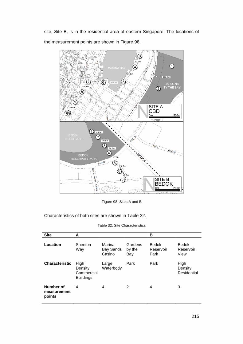
215

site, Site B, is in the residential area of eastern Singapore. The locations of

the measurement points are shown in Figure 98.

Figure 98. Sites A and B

Characteristics of both sites are shown in Table 32.

Table 32. Site Characteristics

Site A B

Location Shenton

Way Marina Bay Sands Casino

Gardens by the Bay

Bedok Reservoir Park

Bedok Reservoir View

Characteristic High

Density Commercial Buildings

Large Waterbody

Park Park High Density Residential

Number of measurement points

4 4 2 4 3

216

Measurements are conducted for a total of four months in 2012. Only days of

clear, sunny weather are used for analysis (Table 33). The term clear, sunny

weather is defined by scrutinizing the hourly solar irradiance profile and

ensuring a smooth curve of at peak of at least 700 Wm-2 at the hottest time of

the day. Equipment used for measurement is show in Table 8.


Site A Site B

Measurement period March to April 2012 April to June 2012

Dates used for analysis

15/03/2012

13/04/2012

16/03/2012 16/04/2012 17/03/2012 23/04/2012 01/04/2012 26/04/2012 04/04/2012 27/04/2012 13/04/2012 28/04/2012 15/04/2012 09/05/2012 18/04/2012 10/05/2012 23/04/2012 16/05/2012

- 06/06/2012

10.1.3 Results and discussion

10.1.3.1 Diurnal tmrt profiles of Site A and Site B

Days selected for analysis for both sites are shown in Table 33. Solar

irradiance is plotted for all relevant days and the diurnal profile is used to

determine the clear, sunny days to be used for analysis.

The diurnal tmrt profiles of all ten measurement points in Site A are shown in

Figure 99. Measurements are taken every minute and averaged to one hour

intervals. Two distinctive trends can be observed. Points 1 to 6 exhibit

significantly higher values of tmrt in the day, especially during the periods of

08:00 hrs to 12:00 hrs and 14:00 hrs to 18:00 hrs. In comparison, Points 7 to

10 recorded lower values of tmrt. The higher values recorded for Points 7 to 10

occur during the period of 11:30 hrs to 14:00 hrs. Points 1 to 6 are situated in

217

the park and near a large water body, whereas Points 7 to 10 are located

along a street surrounded by high rise commercial buildings.

The diurnal tmrt profiles of all seven measurement points in Site B are also

shown in Figure 99. Measurements are taken every minute and averaged to

one hour intervals. Three distinctive trends can be observed. In general,

Points 3 and 4 exhibit the lowest tmrt profiles during the day. Points 1 and 2

exhibit slightly higher readings, especially after 12:00 hrs. Points 5 to 7 exhibit

the highest readings. Points 1 to 4 are situated in the park, whereas Points 5

to 7 are located along high rise residential buildings.

The measurements are plotted against solar irradiance. The difference in tmrt

of the maximum and minimum points for Sites A and B are 23.2 °C and 14.3

°C respectively.

218

Figure 99. Diurnal profiles of tmrt for Site A and Site B

0.0

100.0

200.0

300.0

400.0

500.0

600.0

700.0

800.0

900.0

20.0

30.0

40.0

50.0

60.0

70.0

80.0

0:00

1:00

2:00

3:00

4:00

5:00

6:00

7:00

8:00

9:00

10:0

0

11:0

0

12:0

0

13:0

0

14:0

0

15:0

0

16:0

0

17:0

0

18:0

0

19:0

0

20:0

0

21:0

0

22:0

0

23:0

0

0:00

Sola

r Ir

rad

ian

ce (

W·m

-2)

Mea

n R

adia

nt

Tem

per

atu

re (

°C)

Time (Hrs)

Point 1 Point 2 Point 3Point 4 Point 5 Point 6Point 7 Point 8 Point 9Point 10 Solar Irradiance

0.0

100.0

200.0

300.0

400.0

500.0

600.0

700.0

800.0

900.0

20.0

30.0

40.0

50.0

60.0

70.0

80.0

0:00

1:00

2:00

3:00

4:00

5:00

6:00

7:00

8:00

9:00

10:0

0

11:0

0

12:0

0

13:0

0

14:0

0

15:0

0

16:0

0

17:0

0

18:0

0

19:0

0

20:0

0

21:0

0

22:0

0

23:0

0

0:00

Sola

r Ir

rad

ian

ce (

W·m

-2)

Mea

n R

adia

nt

Tem

per

atu

re (

°C)

Time (Hrs)

Point 1 Point 2 Point 3

Point 4 Point 5 Point 6

Point 7 Solar Irradiance

SITE A

SITE B

219

10.1.3.2 Comparison with Sky View Factor (SVF)

The tmrt profile for both sites are analysed with respect to urban morphology.

There is a significant difference in tmrt profile between measurement points

along the streets of high rise buildings and the other areas. The Sky View

Factor (SVF), which is an indirect representation of built morphology, is used

to identify any significant correlation. The SVF value for each measurement

point is calculated by first taking a photograph of each point using a fisheye

lens. Each photograph is subsequently processed using the RayMan software

(Matzarakis et al., 2010).

Values of SVF for all measurement points in Site A and Site B are shown in

Table 34. A scatterplot is made for the hottest time of the day for both sites.

Scatterplots of the SVF and tmrt values show that there is a correlation

between SVF and tmrt (Figure 100).

Figure 100. Scatterplots of tmrt and SVF for Site A and Site B at 14:00 hrs

Site Ay = 31.557x + 38.427

R² = 0.6093

30.0

35.0

40.0

45.0

50.0

55.0

60.0

65.0

70.0

0.000 0.100 0.200 0.300 0.400 0.500 0.600 0.700 0.800 0.900

Mea

n R

adia

nt

Tem

per

atu

re (°C

)

Sky View Factor

Site By = 18.626x + 36.751

R² = 0.317930.0

35.0

40.0

45.0

50.0

55.0

60.0

65.0

70.0

0.000 0.100 0.200 0.300 0.400 0.500 0.600 0.700 0.800 0.900 1.000

Mea

n R

adia

nt

Tem

per

atu

re (

°C)

Sky View Factor

220

10.1.3.3 Influence of urban constituents on tmrt

Figure 99 shows that buildings affect the tmrt differently for both sites. While

the tmrt is the lowest along the high-rise buildings for Site A, the reverse is true

for Site B. Although the measurement points are surrounded by high-rise

buildings, there is a significant difference between the SVF values for the

points in the two sites (Table 34).

Table 34. SVF values for measurement points in Site A and Site B

Measurement Point Site A Site B

1 0.646 0.270 2 0.711 0.341 3 0.668 0.614 4 0.671 0.178 5 0.602 0.486 6 0.803 0.664 7 0.340 0.668 8 0.512 - 9 0.240 - 10 0.275 -

The tmrt profile for Site A shows that measurement points near large water

bodies actually exhibited the highest tmrt values. Corresponding SVF values

are also relatively higher, when compared to the other points. Points 1 and 2

for Site B, while located in the park, show higher tmrt profiles when compared

to other measurement points within the park.

Measurement points in Site A show significantly higher readings than those in

Site B. This may be due to the fact that there are much more trees in Site B

than in Site A, and that the primary function of the trees is to block direct short

wave radiation from the sun, rather than reduce the temperature by means of

evapotranspiration. The corresponding SVF also supports the correlation

between SVF value and tmrt.

221

10.1.3.4 Estimation of tmrt in the absence of sunlight

In the absence of sunlight, the tmrt values do not fluctuate greatly. This is

evident in the diurnal profiles of the two Sites (Figure 99). The difference

between the maximum and minimum tmrt values for Site A in the absence of

sunlight is 1.3 °C. The difference between the maximum and minimum tmrt

values for Site B in the absence of sunlight is 1.0 °C.

The tmrt profile is plotted at 5 minute intervals from 00:00 hrs to 07:00 hrs for

both sites (Figure 101). The tmrt profile is fairly constant for Site A, with a slight

dip from 05:15 hrs onwards. This dip is observed until 05:35 hrs, and the

average decrease in tmrt is 1.6 °C. The dip is more frequent and significant for

Site B. The first dip occurred from 01:25 hrs to 01:55 hrs. Point 5 exhibited

the largest drop of 4.8 °C. The second dip occurred from 03:50 hrs to 04:15

hrs. Point 5 exhibited the largest drop of 2.2 °C. The final dip occurred from

04:55 hrs to 05:10 hrs. Point 5 exhibited the largest drop of 2.4 °C. Site B was

surveyed to understand the drop in tmrt from 01:25 hrs to 01:55 hrs. Wind and

air temperature data was observed to have remained constant during the said

period. Cloud cover was minimal. Infrared red imaging was used to survey the

measurement site for changes in surface temperature. Measurements of the

leave surface of trees indicate a slight decrease in temperature of less than

2.0 °C (Figure 102).

222

Figure 101. Profiles of tmrt for Site A and Site B from 0:00 hrs to 07:00 hrs

21.0

22.0

23.0

24.0

25.0

26.0

27.0

28.0

29.0

0:00

0:10

0:20

0:30

0:40

0:50

1:00

1:10

1:20

1:30

1:40

1:50

2:00

2:10

2:20

2:30

2:40

2:50

3:00

3:10

3:20

3:30

3:40

3:50

4:00

4:10

4:20

4:30

4:40

4:50

5:00

5:10

5:20

5:30

5:40

5:50

6:00

6:10

6:20

6:30

6:40

6:50

7:00

Mea

n R

adia

nt

Tem

per

atu

re (°C

)

Time (Hrs)

Point 1 Point 2 Point 3 Point 4Point 5 Point 6 Point 7 Point 8Point 9 Point 10

21.0

22.0

23.0

24.0

25.0

26.0

27.0

28.0

29.0

0:00

0:10

0:20

0:30

0:40

0:50

1:00

1:10

1:20

1:30

1:40

1:50

2:00

2:10

2:20

2:30

2:40

2:50

3:00

3:10

3:20

3:30

3:40

3:50

4:00

4:10

4:20

4:30

4:40

4:50

5:00

5:10

5:20

5:30

5:40

5:50

6:00

6:10

6:20

6:30

6:40

6:50

7:00

Mea

n R

adia

nt

Tem

per

atu

re (°C

)

Time (Hrs)

Point 1 Point 2 Point 3 Point 4Point 5 Point 6 Point 7

SITE A

SITE B

223

Figure 102. Thermal imaging of tree surface temperature for Site B

224

10.1.4 Conclusion

10.1.4.1 Characteristics of tmrt profile in the urban environment

The objective of this study is to observe diurnal tmrt behaviour in the urban

environment in relation to urban constituents and to determine reasonable

expectations for any attempts at reduction. Figure 99 shows that the tmrt

profile does not differ significantly in the absence of sunlight. Therefore, any

attempt at lowering the tmrt should logically be done only in daytime.

Since reduction of tmrt is subjected to environmental limitations, it is important

to identify a reasonable extent of influence to any proposed intervention via

passive methods. Figure 99 shows that the peak tmrt at Site A for Point 4 has

the potential to be lowered, and by drawing reference to Point 9, a reasonable

value would be by around 25 °C to approximately 43 °C. A possible way to

quantify the reduction is by comparison of the SVF values of both points

(Figure 103), and to propose additions to the landscape to lower the SVF

(e.g. planting more trees).

Figure 103. SVF of Point 4 and Point 9

225

Strategic placement of vegetation is essential for achieving the desired

amount of tmrt attenuation. Figure 99 shows that although the type and

quantity of trees in Site B are similar throughout the park, the diurnal tmrt

profiles can be different. Measurement Point 1 exhibits a higher maximum tmrt

value, as well as at a much later time than Measurement Point 3. This may

be due to the fact that Measurement Point 1 is next to a large clearing (water

body) and is exposed to direct sunlight in the late afternoon. As each

measurement point is isolated and analysed, it is possible to critique the tmrt

attenuation potential of the surrounding vegetation.

The dip in tmrt profile in the absence of sunlight for Site B may be due to the

large amount of vegetation found in Site B. There is a significant amount of

vegetation in the park, and the trees may be the cause of the dip. While a

slight decrease in surface temperature of the leaves are observed, it may not

fully account for the dip. A more detailed study is required to ascertain the

cause of the dips.

Most estimations of tmrt are made in the form of spot readings and do not

cover large areas. This presents a challenge to the comparison of tmrt in

different urban typologies. Diurnal measurements of tmrt can help urban

planners to appreciate the quality of outdoor urban spaces in view of thermal

comfort. With the customised globe thermometer, air temperature sensor and

anemometer, large scale measurements of the urban outdoor environment

can be conducted. Measurement points with high values of tmrt can be

identified and lowered if necessary, so as to improve the quality of outdoor

urban space.

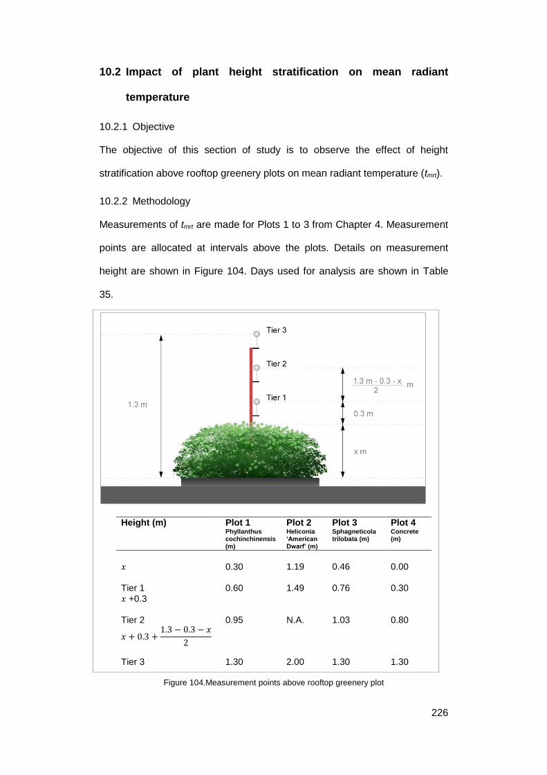
226

10.2 Impact of plant height stratification on mean radiant

temperature

10.2.1 Objective

The objective of this section of study is to observe the effect of height

stratification above rooftop greenery plots on mean radiant temperature (tmrt).

10.2.2 Methodology

Measurements of tmrt are made for Plots 1 to 3 from Chapter 4. Measurement

points are allocated at intervals above the plots. Details on measurement

height are shown in Figure 104. Days used for analysis are shown in Table

35.

Height (m) Plot 1 Phyllanthus cochinchinensis (m)

Plot 2 Heliconia ‘American Dwarf’ (m)

Plot 3 Sphagneticola trilobata (m)

Plot 4 Concrete (m)

𝑥

0.30

1.19 0.46 0.00

Tier 1 𝑥 +0.3

0.60 1.49 0.76 0.30

Tier 2

𝑥 + 0.3 +1.3 − 0.3 − 𝑥

2

0.95 N.A. 1.03 0.80

Tier 3

1.30 2.00 1.30 1.30

Figure 104.Measurement points above rooftop greenery plot

227

Table 35. Days used for analysis

Measurement Period Dates used for analysis during clear sky conditions

01/10/2013 to 24/01/2014

07/11/2013 08/11/2013 21/11/2013 27/11/2013 28/11/2013 02/01/2014

116 days

6 days

10.2.3 Results and discussion

Figure 105 shows the (6 days) averaged diurnal tmrt profile of the rooftop

greenery plots. It can be observed that in general, tmrt for Plot 1 and Plot 2

increases with height. This result is logical as the cooling effect of greenery

should naturally diminish with decreasing proximity. It is interesting to note

that the tmrt profile for Tiers 2 and 3 of Plot 3 are quite similar. This would

suggest that the cooling effect of sphagneticola trilobata is evident for up to

1.3 m. Although the phyllanthus cochinchinensis shrub (Plot 1) is about the

same height as sphagneticola trilobata (Plot 3), its cooling potential is

significantly diminished beyond the 300 mm level. This makes sphagneticola

trilobata a better plant in terms of being able to provide cooling. Therefore, in

view of objectifying plant selection for the purpose of improving overall

thermal comfort, sphagneticola trilobata may be rationalised as the preferred

option.

228

Figure 105. Averaged diurnal tmrt profiles under clear sky conditions

20

30

40

50

60

70

80

Mea

n r

adia

nt

tem

per

atu

re (

°C) Plot 1 - Phyllanthus cochinchinensis

20

30

40

50

60

70

80

Mea

n r

adia

nt

tem

per

atu

re (

°C) Plot 2 - Heliconia 'American Dwarf'

20

30

40

50

60

70

80

0:0

0

1:0

0

2:0

0

3:0

0

4:0

0

5:0

0

6:0

0

7:0

0

8:0

0

9:0

0

10

:00

11

:00

12

:00

13

:00

14

:00

15

:00

16

:00

17

:00

18

:00

19

:00

20

:00

21

:00

22

:00

23

:00

0:0

0

Mea

n r

adia

nt

tem

per

atu

re (

°C)

Time (Hrs)


Tier 1 Tier 2 Tier 3

229

10.3 Comparative studies on vertical greenery

While the focus of this thesis is on rooftop greenery, the study recognizes the

impact of vertical greenery as another common alternative to urban greenery

design. Many studies have shown vertical greenery to be effective at reducing

building envelope temperature and energy consumption (Chen et al., 2013;

Cheng et al., 2010; Perini et al., 2011; Wong et al., 2010a). This section

seeks to investigate the impact of vertical greenery on outdoor tmrt as well as

the effect of using the same type of plants for both vertical and rooftop

greenery.

10.3.1 Impact on vertical greenery on mean radiant temperature

Content from Chapter 10.3.1 (Pages 227 to 247) has been published in the

Journal of Landscape and Urban Planning, for which I am the main author:

Tan, C.L., Wong, N.H., Jusuf, S.K., 2014, Effects of vertical greenery on mean radiant temperature in the tropical urban environment, Landscape and urban planning 127: 52-64. It was also presented in: Wong, N.H., Jusuf, S.K., Tan, C.L., Chia, P.Y., 2012, Effects of vertical greenery on mean radiant temperature in the tropical urban environment, iNTA 2012, National University of Singapore, Singapore. Oral Presentation, Published in proceedings.

10.3.1.1 Objective

The objective of this study is to quantify the effects on tmrt due to exposure to

vertical greenery.

10.3.1.2 Methodology

The first of two sets of data consisted of temperature data collected from two

vertical greenery systems (Green Wall A and Green Wall B). Subsequently,

Green Wall B was removed. The latter set of data consisted of temperature

data from Green Wall A and the concrete wall previously covered by Green

Wall B. Measurements are made for the following:

230

- Air temperature (ta) in front of the green walls;

- Surface temperature (ts) of concrete wall behind green walls; and

- Estimation of mean radiant temperature (tmrt) in front of the green

walls.

Properties of the two green walls are shown in Table 36. Both green walls are

categorised as plant carrier systems. The Suntory Midorie system consists of

a lightweight sponge material which is supplemented with nutrients. This

system uses a dripping system, where an irrigation pipe is installed on the top

most and water slowly drips to the lower part of the wall, such that excess

water flows back to the water tank. The light-weight Shimizu Parabienta

System is a panel-type wall greening system which uses a dripping system

where pipes are connected directly onto each panel of the planting media,

and any excess water flows to the drain.

Table 36. Properties of Green walls

Green Wall A Green Wall B

System

Suntory Midorie System

Shimizu Parabienta System

Dimensions (H X W)

2.27 m X 1.90 m

3.18 m X 2.40 m

Types of plants used

Piper sarmentosum Philodendron Cordyline terminalis Schefflera

Hemigraphis alternata Portulaca grandiflora Nephrolepis acutifolia

LAI 3.8 3.5

The surface temperature of the concrete wall behind the green walls was

measured using thermocouples Figure 106. There was a thermocouple wire

attached to the concrete wall behind each green wall (Points X1 and Z1), as

well as one between the green walls that is directly exposed to the sun (Point

Y1). For every point in the exterior, there was a corresponding point on the

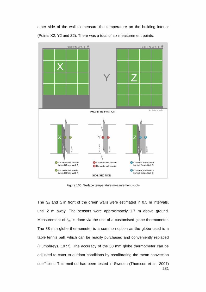
231

other side of the wall to measure the temperature on the building interior

(Points X2, Y2 and Z2). There was a total of six measurement points.

Figure 106. Surface temperature measurement spots

The tmrt and ta in front of the green walls were estimated in 0.5 m intervals,

until 2 m away. The sensors were approximately 1.7 m above ground.

Measurement of tmrt is done via the use of a customised globe thermometer.

The 38 mm globe thermometer is a common option as the globe used is a

table tennis ball, which can be readily purchased and conveniently replaced

(Humphreys, 1977). The accuracy of the 38 mm globe thermometer can be

adjusted to cater to outdoor conditions by recalibrating the mean convection

coefficient. This method has been tested in Sweden (Thorsson et al., 2007)

232

and shown to be effective in outdoor conditions. For this study, tmrt is

estimated using customised globe thermometers calibrated for localised

usage (Tan et al., 2013a). The LAI of both green walls were calculated by

removing a 10 cm by 10 cm segment of the green wall, measuring the total

leaf area size with a flatbed scanner and extrapolating it to the size of the

green walls. Close-circuit television was used to monitor the effects of

shading on estimated tmrt.

Measurements were conducted on the roof top of Block SDE2 in the National

University of Singapore, Singapore (1°17′44″N 103°46′36″E). Also known as

the Greenery Technology Laboratory (GTL), the site measures approximately

9 m by 9 m (Figure 107). Two green systems were installed on an existing

wall. The environment around the green walls is open space, and the room

behind the green walls is a smoke-stop lobby that is not mechanically

ventilated. There was no machinery or heat generation equipment near the

green walls.

http://toolserver.org/~geohack/geohack.php?pagename=National_University_of_Singapore&params=1_17_44_N_103_46_36_E_region:SG_type:edu

233

Figure 107. Measurement setup. Globe thermometers were attached to poles with white PVC pipes housing surface and air temperature loggers.

For this study, measurements were conducted from 27th September 2011 to

13th March 2012. The measurement period was divided into Period A and B,

where Period A denoted the measurement of both green walls, and Period B

denoted measurement with Green Wall B removed (Table 37). Only data for

clear, sunny days were used for analysis. Selection of the days was based on

solar irradiance data measured on-site with a pyranometer. Measurements

were made at one minute intervals and averaged to hourly intervals for

analysis. A total of 28 points were set up for tmrt and ta measurement. Each

measurement point, which consists of a customised globe thermometer fixed

at 1.7 m above ground and an air temperature sensor housed in a PVC pipe,

was secured with a concrete footing.

234

For the purpose of discussion, the measurement points are aligned and

named as shown in Figure 108. Air temperature was measured at

measurement spots 1 to 28 as well as the weather station.

As the green walls were exposed to self-shading and overshadowing at

different periods of the day (Figure 109), daily data were grouped into five

periods corresponding to changes in exposure to solar radiation (Table 39).


Period Measurement duration

No. of days measured

No. of days used for analysis

Dates used for analysis

Purpose

A

27/09/2011 to 03/11/2012

99 5

06/10/2011 13/10/2011 16/10/2011 17/10/2011 25/11/2011

Measurement for Green Wall A and Green Wall B

B

04/01/2012 to 13/03/2012

70 9

15/01/2012 16/01/2012 17/01/2012 21/01/2012 01/02/2012 08/02/2012 10/02/2012 11/02/2012 07/03/2012

Measurement for Green Wall A. Green Wall B is removed

235

Figure 108. Position of tmrt and ta measurement points

Table 38. Instruments used for measurement

Variable Instrument

Air temperature, ta

HOBO Weatherstation, H21-001

Globe temperature, tg HOBO Thermocouple Data Logger, U12-014 Wind speed, Va HOBO Weatherstation, H21-001 Surface temperature, ts HOBO Thermocouple Data Logger, U12-014 Shading characteristics Close-circuit television Leaf Area Index, LAI

Canon All-In-One Printer, MP276

Table 39. Time range used for analysis

Time Range Period Condition of wall

1

0000 hrs – 0700 hrs

Night to Sunrise

2 0700 hrs – 1400 hrs Self-shaded 3 1400 hrs – 1700 hrs Exposed to direct sunlight 4 1700 hrs – 1900 hrs Overshadowing from trees 5 1900 hrs – 0000 hrs

Sunset to night



236

Figure 109. CCTV footage of site showing self-shading and overshadowing

237


Surface temperature (ts)

Surface temperatures of the two green walls was compared to a portion of the

wall directly exposed to the sun. The aim of this comparison is to determine

the surface temperature reduction due to the green walls. Data for five days

were used for the analysis of Period A and for nine days were used for the

analysis of Period B. The daily data were averaged to produce a single profile

for every measurement point.

An increase in surface temperature is observed for Point Z after the removal

of Green Wall B. Point Z1 has a flat profile for Period A, but increased steadily

to reach a peak of 34.3 °C at 17:00 hrs for Period B. The removal of Green

Wall B has resulted in an increase in surface temperature of 6.7 °C. The

maximum difference in diurnal surface temperature for the building interior

(Point Z2) for Period A was 0.3 °C, but significantly larger for Period B (Up to

3.8 °C). With the exception of Green Wall A, diurnal temperature fluctuations

have generally increased.

The exposed concrete surface (Point Y1) exhibited the highest surface

temperature for both periods (Figure 110). The highest value for Period A was

35.7 °C at 15:00 hrs. The maximum value was much higher for Period B (44.6

°C at 17:00 hrs) and occurred 2 hours later. The increase in temperature was

8.9 °C. The interior surface temperature (Point Y2) also increased after the

removal of Green Wall B. The profile of Point Y2 was relatively flat for Period

A, but increased significantly and peaking at 34.6 °C at 19:00 hrs for Period

B. The removal of Green Wall B has significantly increased the surface

temperature of the exposed concrete wall. The temperature of Y1 is generally

much higher than Point Z1. This may be due to the fact that Point Y1 was

238

located closer to a structural concrete column, and thus exposed to a higher

thermal mass.

Figure 110. Surface Temperature profiles for Period A and Period B

The surface temperature of Point X2 was similar to Point X1 for Period A but

was consistently higher in Period B. No significant fluctuations were

observed. The removal of Green Wall B had no significant effect on Green

Wall A.

239

Air temperature (ta)

Air temperatures at all 28 measurement points in front of the green walls were

analysed. Figure 111 shows that the range of air temperature did not fluctuate

greatly. The maximum range recorded was about 1.1 °C for Period A, and

increased slightly to 1.5 °C for Period B. This is similar to a study conducted

by Wong et al. (2010a), where the ambient temperature range recorded 0.6 m

from green walls and a concrete wall was 1.3 °C.

Figure 111. Air temperature profiles for Period A and Period B

240

Profile of tmrt across Measurement Points 1 to 7

The tmrt profiles for Period A for Measurement Points 1 to 7 are shown in

Figure 112. It can be observed that a portion of the readings near the bottom

does not deviate significantly across the 7 points (19:00 hrs to 07:00 hrs). As

the sun rised to its zenith, the average tmrt increased steadily, and the

difference between the 7 points begin to exhibit increasing amounts of

deviation.

A distinct pattern is observed from 15:00 hrs to 17:00 hrs, where most

readings peak at Point 4. This pattern exhibits itself most evidently at the

highest recorded tmrt at 15:00 hrs. A comparison with Figure 108 shows that

Point 4 was the spot that was closest to the part of the wall that was exposed

to direct sunlight, whereas the other points are covered with Green Walls A

and B. This pattern diminished significantly until the fluctuations cease from

approximately 21:10 hrs onwards.

The same patterns were observed for Period B. However, higher peak

readings were recorded. This is expected, as there was more concrete

surface that was exposed to direct sunlight for Period B. Measurements of

Points 5 to 7 are also higher than in Period A during Time Range 3. The

difference in tmrt value is clearly only significant during Time Range 3 (14:00

hrs – 17:00 hrs). Outside of this time range, the difference in tmrt between

Points 1 to 7 is minimal.

241

Figure 112. Comparison of tmrt profile for Points 1-7 for Period A and Period B

242

Profile of tmrt for Points 2, 4 and 6

The diurnal tmrt profile is compared with the corresponding solar irradiance

profile. To simplify the analysis, only 3 points were plotted. The points are

show in Figure 113.

Figure 113. Points 2, 4 and 6

Figure 114 shows the diurnal tmrt plots across Points 2, 4 and 6 for Period A

and Period B. Time Ranges 1 and 5 show no relation between the tmrt profile

and solar irradiance (due to the absence of sunlight). Time Range 2 shows an

increase in tmrt with solar irradiance. Similarly, Time Range 4 shows a similar

trend, with tmrt decreasing with solar irradiance correspondingly. It can be

seen that the tmrt values correspond to fluctuations of direct and intense solar

irradiance (Time Range 3). More importantly, the largest differences in tmrt for

the different points occur during periods of peak solar irradiance. In other

words, tmrt in front of the Green Walls are reduced during periods of peak

solar irradiance.

243

Figure 114. Plot of Points 2,4 and 6 against solar irradiance for Period A and Period B

244

Similar to Period A, Time Range 1 and the later part of Time Range 5 show

no relation between the tmrt profile and solar irradiance (due to the absence of

sunlight). Time Range 2 shows an increase in tmrt with solar irradiance.

Similarly, Time Range 4 shows a similar trend, with tmrt decreasing with solar

irradiance correspondingly. It can be seen from Time Range 3 that the tmrt

values reached their peak at approximately 17:00 hrs, and it does not

correspond to the solar irradiance peak to the likes of Period A. It would seem

that the exposure to increased concrete surface area has resulted in a delay

of the diurnal tmrt peak. Increased longwave radiation may have been stored

and subsequently emitted by the exposed wall surface, resulting in the time

lag.

This time lag is further scrutinised by comparing tmrt profiles at 0.5m intervals

away from the wall (Figure 115). It can be seen from Graph A that the tmrt

rises rapidly from 14:00 hrs to 15:00 hrs and reaches its peak at 17:00 hrs,

when the solar irradiance has passed its peak. As the distance from the wall

increases, this phenomenon gradually decreases until the effect cannot be

observed on Graph D (2 m away). A comparison shows that the time lag is

approximately 2 hours.

245

Figure 115. Comparison of tmrt profiles at 0.5 m intervals from the wall for Time Range 3, Period B

Profile of tmrt plotted against distance from wall

To understand the effect of tmrt with increasing distance from wall,

measurements are taken at 0.5 m increments, up to a maximum of 2 m.

Figure 116 shows three sets of measurement for Periods A and B. The

measurements are positioned at 0.5 m intervals starting from the centre of the

green walls and concrete column. The highest tmrt value recorded for Period

A is at 13:20 hrs and the highest tmrt value recorded for Period B is at 16:20

hrs. The removal of Green Wall B has caused a general increase to the tmrt

profile, especially to the points closest to the wall. There is an increase of

12.7 °C for Point 2, 12.9 °C for Point 4, and 10.9 °C for Point 6. The increase

in tmrt for points away from the wall (Points 9 - 16 - 23, Points 11 - 18 - 25 and

Points 13 - 20 – 27) ranges from 1.9 °C to 6.4 °C.

The effect on tmrt due to the removal of the wall is most significant within a

region of 0.5 m. The highest recorded difference is 12.8 °C for Point 4.

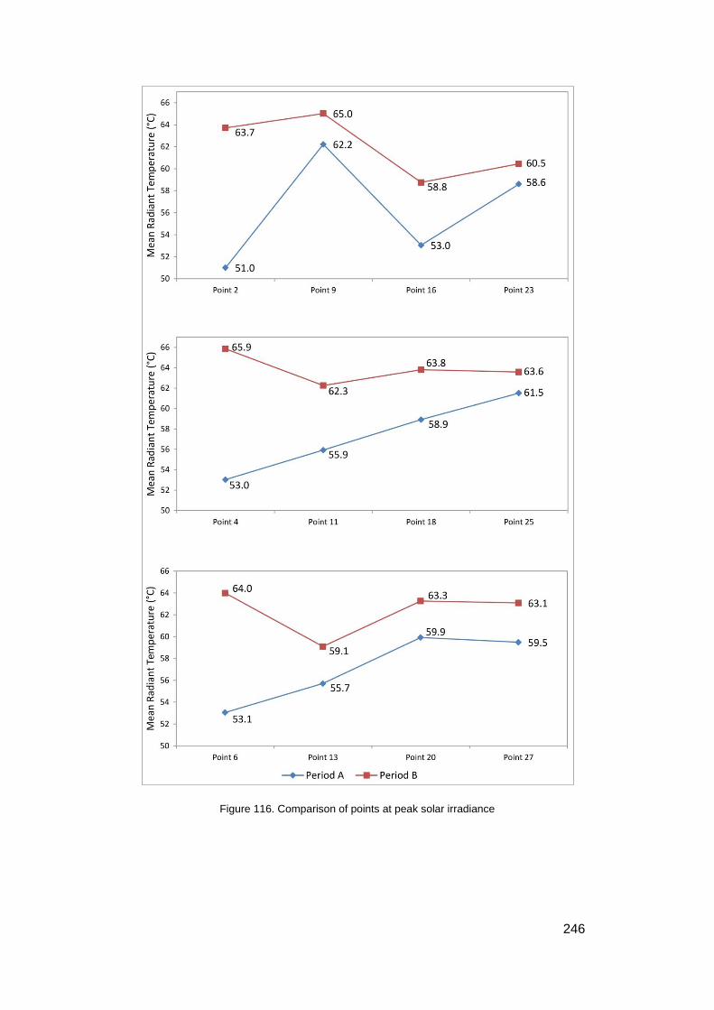
246

Figure 116. Comparison of points at peak solar irradiance

247

Visualisation of tmrt using Geographical Information Systems (GIS)

All 28 points are used for data interpolation using GIS. This facilitates rapid

analysis of the conditions of the surveyed area. Hot spots can be identified

easily with this method. Measurements for a typical clear sunny day are used

for visualisation via GIS. Figure 117 shows the tmrt map of selected timings

from 15:55 hrs to 00:35 hrs. It can be seen that the hot spot (dotted circle),

which corresponds to Point 4, has a significantly high value compared to the

rest of the points. This trend can be observed until approximately 00:00 hrs,

although the magnitude of the difference differs drastically across different

timings.

Figure 117. GIS visualisation of tmrt

248

Conclusion

The purpose of this study is to observe the effect of green walls on the

temperature of a surrounding environment.

Surface temperature measured behind the green walls show that the green

wall can reduce the surface temperature of the building envelope. This effect

is not restricted to areas covered by the installation of a green wall; areas that

are in close proximity to the green wall can also experience a reduction in

surface temperature. The implementation of green wall helps to reduce

fluctuations of surface temperature. Removal of Green Wall B only resulted in

a slight increase in air temperature. However, there is significant difference in

the tmrt, especially within 1 m of the green walls. The maximum increase in tmrt

after the removal of Green Wall B is 12.8 °C. When one green wall is

removed, the effect of time lag can be observed. The peak readings in tmrt are

delayed for approximately 2 hours. Since the LAI of both green walls are

similar, no significant correlation between LAI and temperature reduction can

be ascertained.

Results show that the implementation of vertical greenery can lower the tmrt of

its surroundings. The effect of this attenuation is evident for up to 1 m away

from the wall. However, this lowering is effective only during periods of

intense direct solar exposure. The effect is minimal during times when the

green walls experience self-shading or overshadowing. Consideration should

be made to the placement of vertical greenery to ensure maximum exposure

to direct sunlight so as to take advantage of its tmrt reducing attributes.

This study has shown that the effects of shading provide the optimal form of

tmrt reduction. Peak tmrt was recorded at 15:00 hrs in the presence of both

green walls. When Green Wall B was removed, peak tmrt occurred

significantly later (17:00 hrs) and was 10.9 °C to 12.9 °C higher (0.5 m from

the wall). Measurement points further away from the wall also recorded an

249

increase in tmrt ranging from 1.9 °C to 6.4 °C. Areas that do not have access

to shade may consider the utilization of green walls, strategically placed to

provide further reduction to tmrt. This can help architects and urban planners

make informed decisions during design conceptualisation and to achieve

better overall outdoor thermal comfort.

The physical dimensions of the green walls are not considered in the

analysis, and may become a variable in subsequent attempts at

measurement. Similarly, the type of plants used will also be varied to explore

the effects of different types of plants on the effects on tmrt.

The use of GIS for data visualisation provides an easy way to comparing

temperature profiles across different locations and timings. The interpolated

values serve to provide a method to assess the tmrt of any given space that is

easily comprehensible to architects and planners. From the figures, it is

evident that vertical greenery facilitated the reduction of mean radiant

temperature at different magnitudes throughout the day.

This study has shown the feasibility of quantifying thermal effects of greenery

on mean radiant temperature in a systematic manner, and can be used for

the measurement of other forms of vegetation in the tropical urban context.

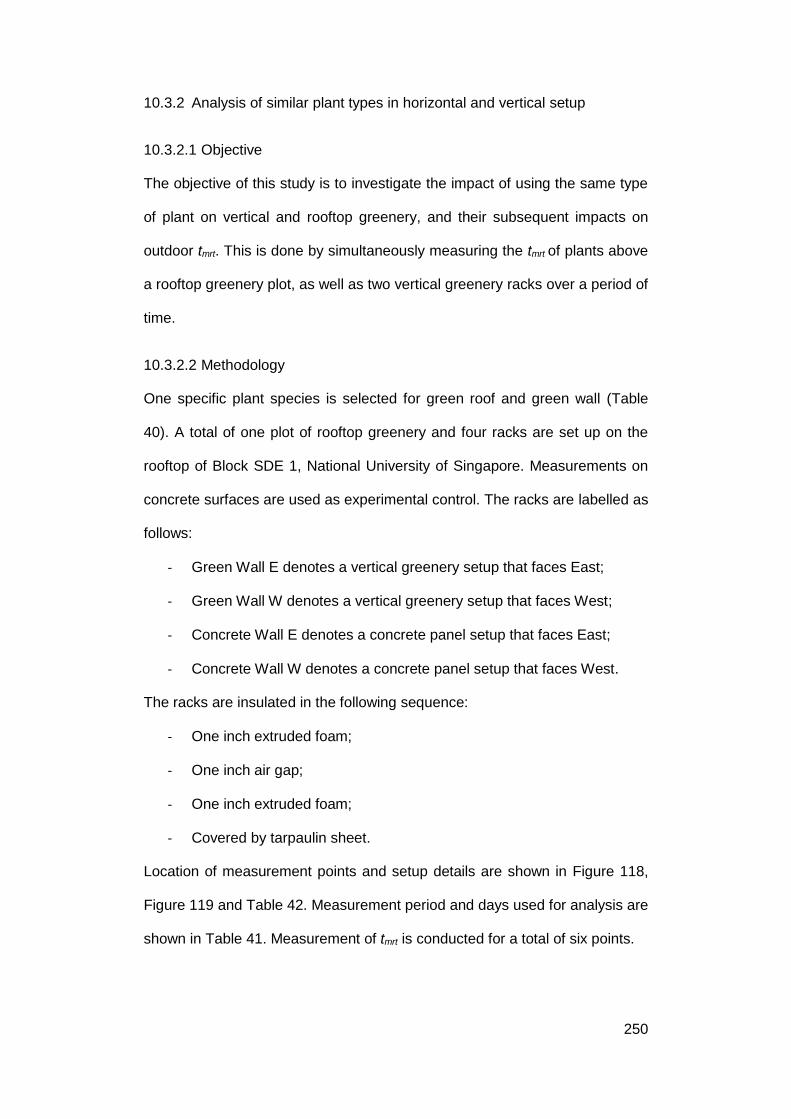
250

10.3.2 Analysis of similar plant types in horizontal and vertical setup

10.3.2.1 Objective

The objective of this study is to investigate the impact of using the same type

of plant on vertical and rooftop greenery, and their subsequent impacts on

outdoor tmrt. This is done by simultaneously measuring the tmrt of plants above

a rooftop greenery plot, as well as two vertical greenery racks over a period of

time.

10.3.2.2 Methodology

One specific plant species is selected for green roof and green wall (Table

40). A total of one plot of rooftop greenery and four racks are set up on the

rooftop of Block SDE 1, National University of Singapore. Measurements on

concrete surfaces are used as experimental control. The racks are labelled as

follows:

- Green Wall E denotes a vertical greenery setup that faces East;

- Green Wall W denotes a vertical greenery setup that faces West;

- Concrete Wall E denotes a concrete panel setup that faces East;

- Concrete Wall W denotes a concrete panel setup that faces West.

The racks are insulated in the following sequence:

- One inch extruded foam;

- One inch air gap;

- One inch extruded foam;

- Covered by tarpaulin sheet.

Location of measurement points and setup details are shown in Figure 118,

Figure 119 and Table 42. Measurement period and days used for analysis are

shown in Table 41. Measurement of tmrt is conducted for a total of six points.

251

Figure 118. Plan and measurement setup

252

Fig

ure

11

9.

Se

tup

deta

ils

253

Table 40. Properties of green roof and green walls

Green Roof Green Wall E and W Concrete Wall E and W

Dimensions

3 m X 3 m 2 m X 2.4 m 2 m X 2.4 m

Plant used

Sphagneticola trilobata


Measurement duration No. of days measured Date used for analysis

08/05/2014 to 12/06/2014

36 10/06/2014

Table 42. Instruments used for measurement

Variable Instrument

Air temperature, ta HOBO U12-012 Temp/RH data logger Globe temperature, tg HOBO Thermocouple Data Logger, U12-014 Wind speed, Va Onset Wind Speed Smart Sensor, S-WSA-M003 Solar irradiance and rainfall HOBO Weatherstation, H21-001 Evapotranspiration Rate (ET) HBM Z6FC3 load cell and Quantum X logger


254


A typical day with clear sky condition is selected for analysis (Figure 120).

Peak irradiance was observed at 14:00 hrs (811.8 Wm-2). The diurnal profile

can be observed to closely resemble a symmetrical profile. This is a

significant aspect for this study as the walls have direct exposure to solar

irradiance for only one half of the day, and irradiance levels need to be similar

for both East-facing and West-facing walls on either half.

Figure 120. Solar irradiance profile for 10th June 2014

0

100

200

300

400

500

600

700

800

900

0:0

0

1:0

0

2:0

0

3:0

0

4:0

0

5:0

0

6:0

0

7:0

0

8:0

0

9:0

0

10

:00

11

:00

12

:00

13

:00

14

:00

15

:00

16

:00

17

:00

18

:00

19

:00

20

:00

21

:00

22

:00

23

:00

0:0

0

Sola

r Ir

rad

ian

ce (

Wm

-2)

Time (Hrs)

Solar Irradiance

255

Air temperature (ta)

Figure 121 shows diurnal air temperature profiles for green roof, green walls

and concrete walls. It can be observed that air temperature near the

eastward-facing concrete wall is highest at peak temperature (35.2 °C),

followed by air temperature above the concrete roof at 35.1 °C. Air

temperature in front of eastward facing walls tends to be higher compared to

westward-facing walls. Air temperature above the green roof is similar to air

temperature in front of westward-facing walls.

Mean radiant temperature (tmrt)

Figure 122 shows mean radiant temperature (tmrt) profiles for green roof,

green walls and concrete walls. It can be observed that tmrt above the

concrete roof is highest at peak temperature (15:00 hrs, 66.7 °C). For

eastward-facing walls, tmrt is highest around noon, and decreases steadily

after noon. This can be attributed to self-shading when the sun is in the West.

There is little difference in tmrt between Green Wall E and Concrete Wall E.

In contrast, tmrt profiles for Green Wall W and Concrete Wall W differ

significantly. It can be observed that tmrt in front of Green Wall W is lower than

Concrete Wall W from 09:00 hrs to 13:00 hrs (about 3 °C cooler), and 15:00

hrs to 16:00 hrs (about 5 °C cooler). Peak tmrt for westward-facing walls (54.6

°C to 59.3 °C) is significantly higher than eastward-facing walls (42.1 °C to

42.3 °C). This would suggest that there is little impact in terms of tmrt due to

eastward-facing green walls. From Figure 122, it is clear that the western sun

has a much higher impact on tmrt than the eastern sun and the impact of

adding green walls is more significant on westward-facing facades. This

observation is drastically different from Figure 121, where all six

measurement points exhibit similar air temperature profiles.

256

Figure 121. Air temperature profiles for green roof, green walls and concrete walls

Figure 122. Mean radiant temperature profiles for green roof, green walls and concrete walls

27

28

29

30

31

32

33

34

35

36

0:0

0

1:0

0

2:0

0

3:0

0

4:0

0

5:0

0

6:0

0

7:0

0

8:0

0

9:0

0

10

:00

11

:00

12

:00

13

:00

14

:00

15

:00

16

:00

17

:00

18

:00

19

:00

20

:00

21

:00

22

:00

23

:00

0:0

0

Air

Tem

per

atu

re (

°C)

Time (Hrs)

Green Roof Concrete Roof Green Wall W

Concrete Wall W Green Wall E Concrete Wall E

23

28

33

38

43

48

53

58

63

68

0:0

0

1:0

0

2:0

0

3:0

0

4:0

0

5:0

0

6:0

0

7:0

0

8:0

0

9:0

0

10

:00

11

:00

12

:00

13

:00

14

:00

15

:00

16

:00

17

:00

18

:00

19

:00

20

:00

21

:00

22

:00

23

:00

0:0

0

Mea

n R

adia

nt

Tem

per

atu

re (

°C)

Time (Hrs)

Green Roof Concrete Roof Green Wall W

Concrete Wall W Green Wall E Concrete Wall E

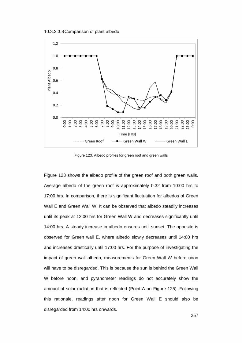
257

Comparison of plant albedo

Figure 123. Albedo profiles for green roof and green walls

Figure 123 shows the albedo profile of the green roof and both green walls.

Average albedo of the green roof is approximately 0.32 from 10:00 hrs to

17:00 hrs. In comparison, there is significant fluctuation for albedos of Green

Wall E and Green Wall W. It can be observed that albedo steadily increases

until its peak at 12:00 hrs for Green Wall W and decreases significantly until

14:00 hrs. A steady increase in albedo ensures until sunset. The opposite is

observed for Green wall E, where albedo slowly decreases until 14:00 hrs

and increases drastically until 17:00 hrs. For the purpose of investigating the

impact of green wall albedo, measurements for Green Wall W before noon

will have to be disregarded. This is because the sun is behind the Green Wall

W before noon, and pyranometer readings do not accurately show the

amount of solar radiation that is reflected (Point A on Figure 125). Following

this rationale, readings after noon for Green Wall E should also be

disregarded from 14:00 hrs onwards.

0.0

0.2

0.4

0.6

0.8

1.0

1.2

0:0

0

1:0

0

2:0

0

3:0

0

4:0

0

5:0

0

6:0

0

7:0

0

8:0

0

9:0

0

10

:00

11

:00

12

:00

13

:00

14

:00

15

:00

16

:00

17

:00

18

:00

19

:00

20

:00

21

:00

22

:00

23

:00

0:0

0

Pla

nt

Alb

edo

Time (Hrs)

Green Roof Green Wall W Green Wall E

258

Albedo values of Green Wall E and Green Wall W are combined and

compared with albedo of the green roof (Figure 124). It can be seen that

albedo of the green walls are significantly lower that the green roof. This may

be explained by the fact that when the sun is at its zenith (14:00 hrs), the

direction of solar radiation is almost parallel to the wall surface and reflection

is minimal at this point (Point B on Figure 125). Since Chapter 6.1.2 has

already highlighted the significance of albedo on tmrt reduction, it follows that

vertical greenery may be less effective at reducing tmrt than green roof. This is

consistent with measurements shown in Figure 122, where tmrt reduction is

significantly higher for green roof compared to both green walls.

Figure 124. Albedo profiles of Green Roof and Green Walls combined

0.00

0.20

0.40

0.60

0.80

1.00

1.20

0:0

0

1:0

0

2:0

0

3:0

0

4:0

0

5:0

0

6:0

0

7:0

0

8:0

0

9:0

0

10

:00

11

:00

12

:00

13

:00

14

:00

15

:00

16

:00

17

:00

18

:00

19

:00

20

:00

21

:00

22

:00

23

:00

0:0

0

Pla

nt

Alb

edo

Time (Hrs)

Green Roof Green Wall

Green Wall E

Green Wall W

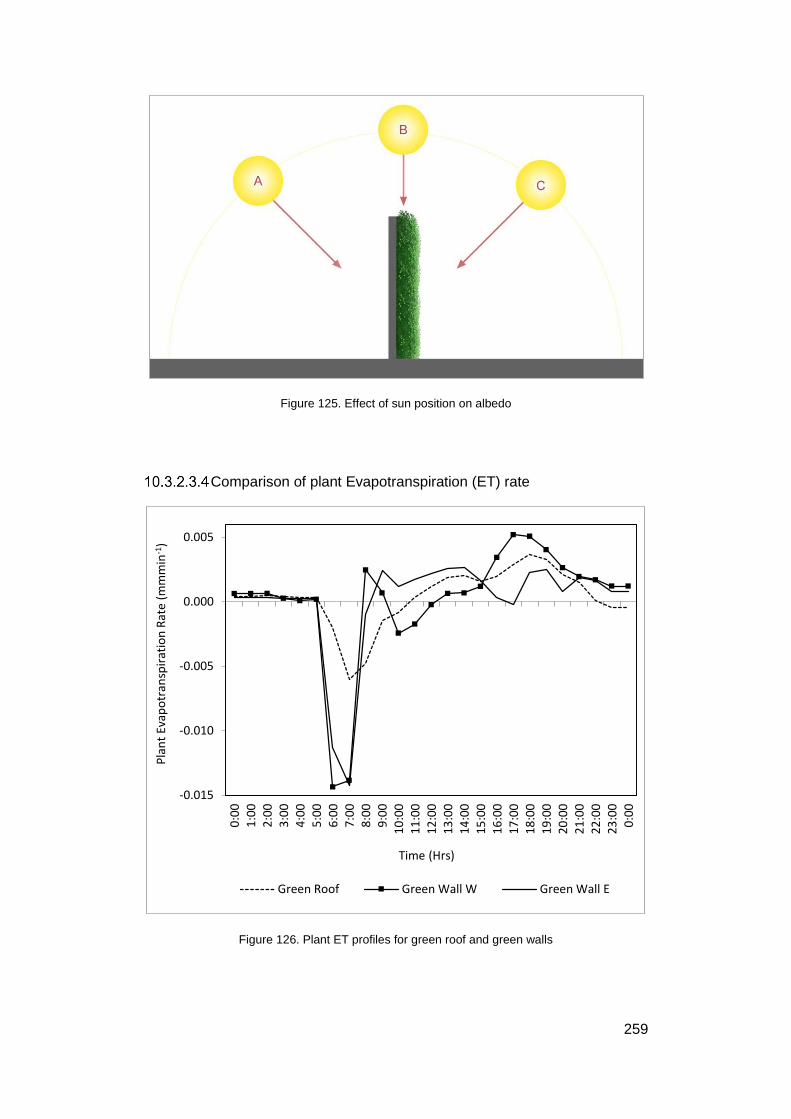
259

Figure 125. Effect of sun position on albedo

Comparison of plant Evapotranspiration (ET) rate

Figure 126. Plant ET profiles for green roof and green walls

-0.015

-0.010

-0.005

0.000

0.005

0:0

01

:00

2:0

03

:00

4:0

05

:00

6:0

07

:00

8:0

09

:00

10

:00

11

:00

12

:00

13

:00

14

:00

15

:00

16

:00

17

:00

18

:00

19

:00

20

:00

21

:00

22

:00

23

:00

0:0

0

Pla

nt

Evap

otr

ansp

irat

ion

Rat

e (m

mm

in-1

)

Time (Hrs)

Green Roof Green Wall W Green Wall E

260

Figure 126 shows ET profiles for the green roof and both green walls. For the

green roof, ET increases steadily from 10:00 hrs to 17:00 hrs. It can be

observed that for Green Wall E, ET is higher than the green roof from sunrise

until 15:00 hrs, and decreases significantly thereafter. It is possibly due to

higher exposure to direct solar radiation in the morning. Conversely, ET is low

for Green Wall W, since it is self-shaded during this period. After 15:00 hrs,

ET of Green Wall W increases drastically due to higher exposure to direct

solar radiation, and ET of Green Wall E decreases due to self-shade. It can

be concluded that ET rate of a plant can be higher in a green wall setting than

in a green roof setting.

261

Conclusion

The objective of this section of study is to subject the same type of plant

simultaneously in both vertical and horizontal arrays and to investigate their

corresponding impact on tmrt in the tropical outdoor environment. This chapter

has shown that green roofs have a higher potential than green walls in terms

of reducing outdoor tmrt. It is observed that for the same plant species, albedo

is lower and ET is higher when installed vertically. A comparison of surface

temperature via infrared thermography (Figure 127) shows that there can be

a difference of about 20 °C for a roof surface with plants and about 7 °C for a

wall surface with plants.

Results from this study have also shown that the potential for building

surfaces to be retrofitted with vertical greenery can be assessed based on

objective criteria such as exposure level to solar radiation and plant functional

attributes. Data from tmrt measurements (Chapter 10.3.2.3.2) suggests that

retrofitting of vertical greenery should be prioritised for westward-facing walls,

as there is evidence of higher potential for tmrt reduction.

262

Figure 127. Infrared thermography of green roof plots and concrete (10th June 2014)

263

10.4 Recommendations for Green Building Rating Tools

10.4.1 Green buildings and Green Building Rating Tools (GBRTs)

Green Building is the practice of building construction with emphasis on

efficient use of resources such as energy, construction materials and water. It

also strives to exert minimal impact on its surrounding environment as well as

to the users of the building throughout the lifespan of the building. This is

often achieved through both passive and active intervention by architects,

contractors, and users alike. Some methods include a better choice of site,

design and construction methods with consideration to the surrounding

environment, energy saving operation procedures, and environment friendly

removal methods when the building has reached the end of its life-cycle.

The beginnings of green building dates back to the 1970s when activities of

the building industry started to be perceived as a significant component in

environmental degradation. Rising oil prices in the 1970s resulted in a

significant effort to improve energy efficiency and to revise traditional building

practices (Steele, 1997). A call for more sustainable measures of building

construction spurred the formation of several schools of thought that

eventually led to the birth of the Green Building movement.

The earliest attempts with contemporary green building brought to light

several important issues, one of which being the need to be able to, in the

most objective and unbiased manner, bestow upon a building the status of

being Green. One solution that has been put forward is the Green Building

Rating system. It is a checklist to which building appraisal is performed, with

emphasis on Green Building features. With the checklist, a design approach

that is more sensitive to its impact on the environment can be realised. With

the formation of the rating tool, the building and construction industry can

make an objective assessment of a construction project, from the stage of

264

preliminary design all the way to the stage of operations and maintenance.

This system provides an avenue for architects and designers to remain

creative and building contractors to maintain the freedom to choose their

preferred construction method, without imposing totalitarian regulations in

their pursuit of the Green Building agenda.

10.4.2 BCA Green Mark Scheme

In January 2005, the Building and Construction Authority of Singapore (BCA)

launched the BCA Green Mark Scheme. It was the Republics’ first step in an

attempt to promote the practice of Green Building in the construction industry.

Figure 128. Green Mark award criteria (NRB/4.1)

265

Under the BCA Green Mark Assessment framework, points are awarded for

implementing environment-friendly features in the building proposal (Figure

128). Specific targets are set out and the rationale is that if more targets are

met, the building under assessment is likely to be environment-friendlier than

buildings which have not considered similar issues. Points are given for

targets that are met in the checklist and are collated in the end. The net score

is supposed to provide a gauge for the overall environment-friendliness of a

building. This minimum environmental sustainability standard reflects the

commitment of BCA to push for Green Building in Singapore.

10.4.3 Greenery in Green Mark

The following section outlines the involvement of urban greenery in the Green

Mark evaluation process. For the purpose of discussion, BCA Green Mark for

New Non-Residential Buildings Version NRB/4.1 will be used as the scheme

of interest. Recommendations made in this section are based on reviewed

literature as well as findings listed from Chapters 6.2.1 to 6.2.4.

266

10.4.3.1 Energy Efficiency

It can be observed from Figure 129 that energy efficiency is prominently

featured in the Green Mark assessment process. Out of a maximum of 190

points, 116 have been allocated for energy related requirements (61%).

Figure 129. Energy related requirements

Potential contribution of greenery is outlined in the following requirements:

1. NRB 1-1 Thermal performance of building envelope – Envelope

thermal transfer value (ETTV)

2. NRB 1-3 Building envelope – Design / thermal parameters

3. NRB 1-10 Energy efficient practices and features

267

NRB 1-1 Thermal performance of building envelope – Envelope

thermal transfer value (ETTV)

Figure 130 shows energy requirements for thermal performance of building

envelopes. Thermal performance is determined by measuring the Envelope

Thermal Transfer Value (ETTV). Developed by Chua and Chou (2010), ETTV

describes the amount of heat a building gains via its envelope. Components

that are considered for ETTV calculation are as follows:

1. Heat gain through walls and windows;

2. Solar radiation gain through windows.

They are averaged over the building envelope area to derive the ETTV value.

The ETTV formula is presented as (Chua and Chou, 2010):

𝐸𝑇𝑇𝑉 = 𝑇𝐷𝑒𝑞(1 − 𝑊𝑊𝑅)𝑈𝑤 + ∆𝑇(𝑊𝑊𝑅)𝑈𝑓 + 𝑆𝐹(𝑊𝑊𝑅)(𝐶𝐹)(𝑆𝐶) [25]

Where,

ETTV = Envelope Thermal Transfer Value (Wm-2)

TDeq = Equivalent temperature difference (°C)

WWR = Window-to-wall ratio

Uw = Thermal transmittance of opaque wall (Wm-2K)

ΔT = Temperature difference (°C)

Uf = Thermal transmittance of fenestration (Wm-2K)

SF = Solar factor (Wm-2)

CF = Solar correction factor for fenestration

SC = Shading coefficient of fenestration

268

Figure 130 shows that 1.2 points can be earned for every reduction of 1 Wm-2

in ETTV from the baseline model. A maximum of 12 points can be attained in

this manner. From Equation (26), it can be seen that ETTV can be reduced by

decreasing thermal transmittance values of the wall (Uw) and fenestration (Uf),

as well as the fenestration shading coefficient (SC).

Figure 130. NRB 1-1 Thermal performance of building envelope - Envelope thermal transfer value (ETTV)

Many studies have attempted to quantify the reduction of thermal

transmittance using vertical greenery. Using field measurement data, Wong et

al. (2003b) estimated R-values of various forms of vegetation (tree, shrub and

turf) and used those values to simulate the effects of building energy

consumption. Wong et al. (2009) used the derived R-values to show that the

U-value of walls can be reduced significantly, resulting in lower ETTV values.

269

An example of a typical wall and green wall construction is shown in Figure

131. It can be seen that U-value of the wall can be reduced by more than 70

% with vertical greenery. Surface temperature reduction is further

substantiated by measurements of wall surface temperature shown in

Chapter 10.3.1.3.1. The U-value of fenestration (i.e. glass windows) can also

be reduced, but to a lesser extent (Wong et al., 2009).

In addition to reducing the U-value of walls, greenery can also reduce the

shading coefficient of fenestration, hence lowering heat transmission. Wong

et al. (2009) showed that the correlation between plant shading coefficient

and LAI can be expressed via the equation below:

𝑃𝑙𝑎𝑛𝑡 𝑆ℎ𝑎𝑑𝑖𝑛𝑔 𝐶𝑜𝑒𝑓𝑓𝑖𝑐𝑖𝑒𝑛𝑡 = −0.3043 𝐿𝐴𝐼 + 0.8112 [26]

Where,

LAI = Leaf Area Index

Assuming an LAI value of 2 is assigned for vertical greenery (Tan and Sia,

2009), Plant Shading Coefficient

= -0.3043 LAI + 0.8112

= -0.3043 X 2 + 0.8112

= 0.2

If we consider a glass fenestration of SC value 0.50,

Overall shading coefficient with windows with greenery in front

= Shading coefficient of windows X Shading coefficient of plants

= 0.50 x 0.2

= 0.10

It can be seen that fenestration SC can be reduced significantly by 80 %. This

gives greenery a tremendous ability to in reduce solar penetration into the

building.

270

Typical normal wall composition

Typical green wall composition

Component R-Value R-Value Outside air film 0.0440 0.0440 Plant - 0.3600 Substrate - 1.9230 Air gap - 0.1600 Plaster – Sand / Cement 0.0094 0.0094 Precast panel 0.3151 0.3151 Air space 0.1525 0.1525 Gypsum plaster board 0.0735 0.0735 Plaster – Sand / Cement 0.0094 0.0094 Inside surface 0.1200 0.1200 Total R-Value (m2KW-1) 0.7239 3.1669 U-Value (Wm-2K-1) 1.3814 0.3158

Figure 131. Comparison of U-values for normal wall and green wall

271

Green wall systems are commonly categorised into carrier

(casement/cassette/modular pots) and support systems (creepers) (Tan and

Chiang, 2009). Figure 132 illustrates the difference between the two systems.

Figure 132. Carrier and Support systems

To reduce the SC of building fenestrations, vertical greenery support systems

can be used so as not to obstruct views to the exterior completely. An

example of vertical greenery in from of a glass façade is shown in Figure 133.

Some suggestions for detailing are shown in Figure 134.

272

Figure 133. An example of greenery in front of glass façade

273

Figure 134. Sketch section of greenery in front of window

Although greenery is not explicitly mentioned in this section, ample evidence

has been put forth to suggest that it can reduce solar heat gain into buildings.

In addition, as these measurements were conducted in Singapore, R-values

derived from these studies are suitable for use in the Green Mark assessment

criteria.

Therefore, it is highly recommended that the impact of greenery be

considered when calculating U-value and SC.

NRB 1-3 Building envelope – Design / thermal parameters

Figure 135 shows design and thermal parameters for the building envelope.

274

Section (c) emphasises on better thermal transmittance (U-value) of external

west facing walls, and that U-value of walls should be less than 2 Wm-2K-1.

The methodology for utilising vertical greenery to improve U-value has been

outlined in the previous section.

Section (d) emphasises on better thermal transmittance (U-value) of roof. The

U value of roofs can be significantly reduced by adding greenery. (Wong et

al., 2003b) showed installation of rooftop greenery can result in 1 % - 15 %

savings in annual energy consumption.

Table 43 shows that a reasonable expectation in reduction of U-value is 1.212

Wm-2. Since 1 point is allocated for every 0.1 Wm-2 of reduction of green roof

U-value, adding rooftop greenery, in addition to lowering energy consumption,

can help to improve overall Green Mark score by up to 5 points.

275

Figure 135. Energy efficiency checklist

276

Table 43. U-values of normal roof and green roof (Wong et al., 2003b)

Typical normal roof composition

Typical green roof composition

Component R-Value R-Value Outside air film 0.055 0.055 Turf - 0.360 Substrate - 0.063 WOLFIN IB single layer polymerised 0.001 0.001 Cement and sand base screed to fall 0.094 0.094 RC concrete 0.104 0.104 Inside air film 0.162 0.162 Total R-Value (m2KW-1) 0.416 0.839 U-Value (Wm-2K-1) 2.404 1.192

NRB 1-10 Energy efficient practices and features

Figure 136 elaborates on energy efficient practices and features. Section (b)

awards the use of vertical greenery systems on east and west façade to

reduce heat gain through building envelope. Chapter 10.3.2.3.2 has shown

that the westward facing wall can be significantly hotter than the eastward

facing wall. Therefore, more points should be awarded for adding greenery on

westward facing walls. As only a maximum of 1 point is award in this section,

there may be little incentive for architects to pay attention to this section. More

points may be awarded if more effort is put in by architects to evaluate the

impact of greenery placement, such as using the method outlined in Chapter

6.2.4.3 to determine optimal plant selection and allocation.

277

Figure 136. NRB 1-10 Energy efficient practices and features

10.4.3.2 Water efficiency

Figure 137 shows water efficiency requirements for Green Mark assessment.

Water efficiency is allocated 17 out of a total of 190 points (8.9 %).

Figure 137. Water efficiency checklist


1. NRB 2-3 – Irrigation system and landscaping

278

NRB 2-3 Irrigation system and landscaping

Figure 138 shows irrigation system and landscaping requirements. Section (c)

awards the use of drought tolerant plants that require minimal irrigation.

Chapter 6.1.1 has discussed the merits of choosing plants with high ET rates

for the purpose of reducing ambient temperature and outdoor tmrt. The use of

drought tolerant plants is discouraged as the ET rate of drought tolerant

plants are low and will reduce their cooling potential.

Since the purpose of Section (c) is to minimise water usage, landscape

design can be optimised in the following manner:

1. Drought tolerant plants can be used at areas far away from pedestrian

pathways; and

2. Plants with high ET rates can be used along pedestrian pathways.

In this manner, water usage can be kept to its minimal without comprising

outdoor thermal comfort for pedestrians. Figure 139 illustrates the possible

segregation of areas in a hypothesized rooftop garden plan. Areas that are

near to designated pedestrian paths (blue) are highlighted in dark green.

Drought tolerant plants can be allocated in areas highlighted in light green. An

irrigation plan can be set up based on this diagram. Usage of this method

may be awarded more points for the intention of optimising urban greenery.

279

Figure 138. NRB 2-3 Irrigation system and landscaping

Figure 139. Hypothetical rooftop garden design plan

280

10.4.3.3 Environmental protection

Figure 140 shows requirements for environmental protection. A total of 42 out

of 190 points are allocated (22 %).

Figure 140. Environmental protection checklist


1. NRB 3-3 – Greenery provision

NRB 3-3 Greenery provision

Figure 141 shows greenery provision requirements for Green Mark

assessment. Section (a) awards up to 6 points for increasing the Green Plot

Ratio to 4 and above.

Figure 141. Greenery provision checklist

Green Plot Ratio (GnPR) is defined as the ‘ratio of the total single-side leaf

area of the planted landscape to the plot or site area’ (Ong, 2003) and can be

expressed as follows:

281

𝐺𝑟𝑒𝑒𝑛 𝑃𝑙𝑜𝑡 𝑅𝑎𝑡𝑖𝑜

=(𝑇𝑜𝑡𝑎𝑙 𝐿𝑒𝑎𝑓 𝐴𝑟𝑒𝑎)

𝑆𝑖𝑡𝑒 𝐴𝑟𝑒𝑎

= ∑(𝐿𝐴𝐼 1 × 𝐶𝑎𝑛𝑜𝑝𝑦 𝐴𝑟𝑒𝑎 1 … + 𝐿𝐴𝐼 𝑁 × 𝐶𝑎𝑛𝑜𝑝𝑦 𝐴𝑟𝑒𝑎 𝑁)

𝑆𝑖𝑡𝑒 𝐴𝑟𝑒𝑎

[27]

Where,

LAI = Leaf Area Index

Figure 142 demonstrates how GnPR is calculated. GnPR is now adopted by

Singapore’s National Parks Board (NParks) as a method in quantifying

greenery density (Tan and Sia, 2009).

Figure 142. Illustration of Green Plot Ratio (GnPR) calculation

282

From Section (a) of Figure 141, it can be deduced that:

1. With a maximum of 6 points to be awarded, the impact of greenery is

perceived to be most relevant here compared to other sections;

2. Environmental protection is achieved by reducing the UHI effect;

3. The UHI effect can be mitigated by adding greenery; and

4. More greenery equates to better environmental protection.

Item 4 raises a point of contention, in that it carries the assumption that more

greenery will bring about more benefits. It also advocates the belief that

plants should only be distinguished by their LAI value, and that other

functional traits need not be considered. The limitation of using GnPR as an

indicator of plant density and hence level of protection to the environment was

recognised by Ong (2003), who acknowledged that GnPR alone cannot

indicate relevant environmental factors such as species richness on site.

Results from Chapter 4 have also shown that plant traits such as ET and SA

contribute significantly to plant cooling potential, and that LAI is poorly

correlated with tmrt reduction. Most importantly, this study has shown that

plant selection and allocation is not a one-dimensional process and there is a

need to consider the effects of context and locality.

Therefore, the study proposes the steps taken in Chapter 6.2, namely the

simulation of building and site conditions to locate optimal plant placement

spots. More points may be awarded for landscape proposals that take solar

insolation into consideration for selection and allocation of plants.

An example is given in Figure 143. More points can be awarded for greenery

allocated on building surfaces with higher solar exposure.

283

Figure 143. Point allocation based on solar insolation map

This recommendation is not limited to the Green Mark rating tool, as the

intention of increasing greenery density is prevalent in other government

agencies. For instance, the Urban Redevelopment Authority of Singapore

(URA) encourages addition of greenery within the urban environment via its

Landscaping for Urban Spaces and High-Rises (LUSH) 2.0 programme

(URA, 2014b). One requirement is to ensure that the displaced site area is

fully replaced with landscape, with at least 40 % of the development site area

comprising of permanent planting (i.e. softscape) (Figure 144)(URA, 2014a).

The Landscape Replacement Areas (LRAs) guidelines are set out to achieve

the following objectives (URA, 2009):

1. Using greenery to enhance quality of life;

2. Enhancing image of a city in the tropics by having greenery at ground

and above-ground levels; and

3. Improving thermal comfort and air quality through greenery.

284

Figure 144. LUSH 2.0 landscape replacement policy

Since the objective of LUSH 2.0 LRA guidelines (Point 3) is similar to BCA

Green Mark (NRB 3-3), selection and allocation of plants can follow the

methodology proposed in this chapter.

285

10.4.3.4 Indoor Environmental Quality

Figure 145 shows requirements of indoor environmental quality for Green

Mark assessment. A total of 8 out of 190 points is allocated for indoor

environmental quality (4 %).

Figure 145. Indoor environmental quality checklist


1. NRB 4-2 – Noise level

2. NRB 4-3 – Indoor air pollutants

NRB 4-2 Noise level

Figure 146 shows requirements for noise level control.

Figure 146. NRB 4-2 Noise level

286

For occupied spaces that are not able to achieve the desired sound level,

greenery can be used to improve sound conditions. There have been

numerous studies showcasing the acoustic absorbing properties of plants.

Lagstorm (2004) observed that supplementary noise reduction of up to 20 dB

could be achieved with the installation of rooftop greenery. This finding was

similar to findings by Connelly and Hodgson (2008), who recorded up to 13

dB with an extensive green roof. Wong et al. (2010b) showed that vertical

greenery systems can also provide noise reduction capabilities and that the

potential is higher with increasing greenery coverage.

NRB 4-3 Indoor air pollutants

Figure 147 shows requirements for indoor air pollutants.

Figure 147. NRB 4-3 Indoor air pollutants

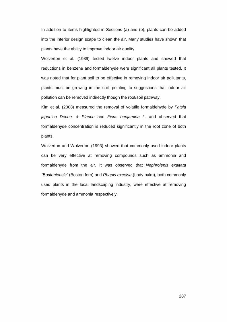
287

In addition to items highlighted in Sections (a) and (b), plants can be added

into the interior design scape to clean the air. Many studies have shown that

plants have the ability to improve indoor air quality.

Wolverton et al. (1989) tested twelve indoor plants and showed that

reductions in benzene and formaldehyde were significant all plants tested. It

was noted that for plant soil to be effective in removing indoor air pollutants,

plants must be growing in the soil, pointing to suggestions that indoor air

pollution can be removed indirectly though the root/soil pathway.

Kim et al. (2008) measured the removal of volatile formaldehyde by Fatsia

japonica Decne. & Planch and Ficus benjamina L. and observed that

formaldehyde concentration is reduced significantly in the root zone of both

plants.

Wolverton and Wolverton (1993) showed that commonly used indoor plants

can be very effective at removing compounds such as ammonia and

formaldehyde from the air. It was observed that Nephrolepis exaltata

“Bostoniensis” (Boston fern) and Rhapis excelsa (Lady palm), both commonly

used plants in the local landscaping industry, were effective at removing

formaldehyde and ammonia respectively.

288

10.4.4 Recommendations for improvement

A detailed analysis of the current BCA Green Mark scheme (Chapter 10.4.2)

has highlighted the involvement of greenery in the entire assessment

process. It is clear that the role of greenery is mainly to reduce the UHI effect.

Findings from this study as well as reviewed literature have shown that

greenery can be more prominently featured in the areas of energy and water

efficiency, as well as indoor environmental quality.

As the building footprint in a city is often limited, building and roof spaces will

become increasingly important to improve overall liveability and well-being of

its inhabitants. The expectation of urban greenery to enhance the

environment will increase in tandem. This may include higher cooling,

biodiversity and aesthetic requirements. The proposed recommendations

serve to realise the full potential of greenery.

Suggestions for the next version of Green Mark assessment criteria are as

follows:

1. Inclusion of thermal transmission of greenery in cooling load

simulation (Chapter 10.4.3.1);

2. More points awarded to greenery in the areas of energy and water

efficiency, as well as indoor environmental quality; and

3. Use of solar insolation simulation and plant selection chart for

landscape plan, in addition to GnPR requirements (Chapter 10.4.3.3).

289

10.5 Data for regression model


Date Time Tmrt Plant Tmrt Reference Plant ET Albedo

13-May 13:00 57.09 63.07 0.0076 0.29

14:00 58.75 67.75 0.0182 0.27

15:00 57.09 72.22 0.0221 0.29

16:00 55.07 70.89 0.0248 0.29

17:00 53.84 65.33 0.0270 0.29

15-May 13:00 53.92 59.68 0.0044 0.28

14:00 46.55 55.45 0.0127 0.27

15:00 49.12 61.55 0.0194 0.29

16:00 46.98 57.89 0.0226 0.33

17:00 38.39 43.37 0.0248 0.30

22-May 13:00 59.61 57.94 0.0080 0.29

14:00 54.07 59.34 0.0089 0.27

15:00 54.08 63.73 0.0087 0.29

16:00 51.11 61.42 0.0085 0.33

17:00 38.40 44.80 0.0090 0.40

24-May 13:00 53.33 56.24 0.0084 0.31

14:00 55.46 63.29 0.0109 0.29

15:00 47.22 55.44 0.0115 0.30

16:00 53.46 62.62 0.0098 0.34

17:00 48.88 58.36 0.0110 0.41

25-May 13:00 55.90 62.17 0.0106 0.29

14:00 57.92 69.06 0.0106 0.27

15:00 57.62 69.97 0.0105 0.29

16:00 45.44 55.02 0.0113 0.30

17:00 36.98 44.07 0.0119 0.41

28-May 13:00 58.29 64.23 0.0066 0.30

14:00 54.30 63.11 0.0111 0.28

15:00 53.73 61.83 0.0141 0.28

16:00 51.67 62.92 0.0134 0.30

17:00 55.14 69.69 0.0158 0.36

29-May 13:00 47.44 48.53 0.0050 0.30

14:00 46.99 51.45 0.0091 0.28

15:00 54.77 62.66 0.0146 0.30

16:00 54.85 62.75 0.0184 0.31

17:00 45.92 49.03 0.0208 0.31

8-Jun 13:00 53.44 58.05 0.0107 0.29

14:00 51.38 58.14 0.0116 0.28

15:00 54.04 66.67 0.0118 0.30

16:00 51.48 67.03 0.0115 0.31

17:00 53.43 67.16 0.0102 0.32

290

10-Jun 13:00 56.98 63.15 0.0068 0.30

14:00 55.24 60.47 0.0096 0.28

15:00 51.75 61.39 0.0133 0.28

16:00 53.35 66.68 0.0195 0.33

17:00 40.37 47.50 0.0227 0.31

11-Jun 13:00 55.48 58.07 -0.0019 0.30

14:00 57.48 64.20 0.0077 0.28

15:00 52.90 64.64 0.0151 0.34

16:00 47.06 57.30 0.0203 0.31

17:00 51.77 65.43 0.0243 0.32

13-Jun 13:00 55.46 63.62 0.0058 0.29

14:00 54.29 64.56 0.0110 0.27

15:00 52.65 60.69 0.0152 0.28

16:00 50.51 59.49 0.0203 0.30

17:00 41.01 48.08 0.0203 0.30

16-Jun 13:00 59.57 68.16 0.0072 0.27

14:00 55.76 62.58 0.0102 0.26

15:00 57.73 67.17 0.0126 0.27

16:00 53.96 60.06 0.0158 0.29

17:00 42.89 46.90 0.0168 0.30

17-Jun 13:00 58.12 67.33 0.0058 0.27

14:00 57.98 66.26 0.0125 0.26

15:00 57.93 67.16 0.0157 0.25

16:00 59.70 68.84 0.0165 0.26

17:00 59.02 67.86 0.0176 0.25

18-Jun 13:00 57.23 60.49 -0.0022 0.29

14:00 52.58 58.56 -0.0014 0.25

15:00 50.86 58.78 0.0042 0.25

16:00 45.17 50.90 0.0121 0.27

17:00 40.12 43.26 0.0143 0.27

19-Jun 13:00 49.12 52.24 0.0000 0.29

14:00 56.04 59.89 0.0004 0.26

15:00 58.13 62.45 0.0072 0.25

16:00 52.97 58.52 0.0124 0.25

17:00 43.39 46.81 0.0142 0.26

20-Jun 13:00 62.10 68.71 0.0079 0.27

14:00 61.96 68.70 0.0104 0.26

15:00 61.43 69.48 0.0128 0.25

16:00 59.43 66.14 0.0163 0.25

17:00 55.50 61.17 0.0189 0.26

21-Jun 13:00 60.87 67.30 0.0059 0.27

14:00 58.05 65.61 0.0120 0.26

15:00 57.31 65.19 0.0150 0.25

16:00 55.78 62.31 0.0191 0.25

291

17:00 58.35 64.54 0.0227 0.26

22-Jun 13:00 59.41 64.85 -0.0053 0.29

14:00 63.88 70.82 0.0073 0.27

15:00 54.92 63.40 0.0207 0.28

16:00 43.37 51.01 0.0200 0.30

17:00 39.43 43.62 0.0163 0.30

23-Jun 13:00 62.39 67.42 -0.0017 0.28

14:00 63.04 69.67 0.0130 0.25

15:00 54.17 60.62 0.0174 0.27

16:00 49.41 54.09 0.0169 0.26

13:00 39.69 42.81 0.0168 0.26

24-Jun 13:00 59.37 62.90 -0.0114 0.27

14:00 56.80 58.02 0.0008 0.28

15:00 55.76 58.63 0.0064 0.25

16:00 57.50 60.52 0.0147 0.27

17:00 42.89 45.03 0.0220 0.29

25-Jun 13:00 52.86 55.86 -0.0052 0.27

14:00 57.08 60.40 0.0001 0.30

15:00 57.21 62.27 0.0046 0.24

16:00 60.58 63.67 0.0096 0.29

17:00 51.12 53.28 0.0178 0.27

1-Jul 13:00 61.52 63.51 0.0075 0.27

14:00 61.19 64.88 0.0079 0.27

15:00 64.57 72.00 0.0076 0.26

16:00 56.49 63.86 0.0093 0.26

17:00 35.06 42.66 0.0121 0.26

7-Jul 13:00 58.67 57.82 0.0071 0.28

14:00 65.11 66.02 0.0081 0.26

15:00 60.72 66.56 0.0089 0.25

16:00 60.93 68.33 0.0095 0.25

17:00 54.72 60.30 0.0085 0.25

8-Jul 13:00 53.01 53.67 0.0023 0.28

14:00 51.33 54.16 0.0050 0.27

15:00 48.02 52.88 0.0068 0.27

16:00 47.34 52.58 0.0079 0.27

17:00 47.00 53.72 0.0084 0.28

10-Jul 13:00 53.66 55.35 0.0077 0.28

14:00 64.47 66.47 0.0089 0.30

15:00 60.47 66.77 0.0073 0.28

16:00 61.13 65.96 0.0069 0.27

17:00 47.07 58.28 0.0057 0.25

13-Jul 13:00 62.16 61.19 0.0054 0.27

14:00 66.13 65.27 0.0067 0.26

15:00 61.10 66.57 0.0086 0.26

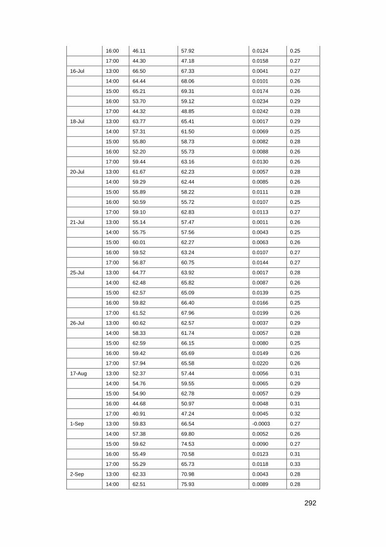
292

16:00 46.11 57.92 0.0124 0.25

17:00 44.30 47.18 0.0158 0.27

16-Jul 13:00 66.50 67.33 0.0041 0.27

14:00 64.44 68.06 0.0101 0.26

15:00 65.21 69.31 0.0174 0.26

16:00 53.70 59.12 0.0234 0.29

17:00 44.32 48.85 0.0242 0.28

18-Jul 13:00 63.77 65.41 0.0017 0.29

14:00 57.31 61.50 0.0069 0.25

15:00 55.80 58.73 0.0082 0.28

16:00 52.20 55.73 0.0088 0.26

17:00 59.44 63.16 0.0130 0.26

20-Jul 13:00 61.67 62.23 0.0057 0.28

14:00 59.29 62.44 0.0085 0.26

15:00 55.89 58.22 0.0111 0.28

16:00 50.59 55.72 0.0107 0.25

17:00 59.10 62.83 0.0113 0.27

21-Jul 13:00 55.14 57.47 0.0011 0.26

14:00 55.75 57.56 0.0043 0.25

15:00 60.01 62.27 0.0063 0.26

16:00 59.52 63.24 0.0107 0.27

17:00 56.87 60.75 0.0144 0.27

25-Jul 13:00 64.77 63.92 0.0017 0.28

14:00 62.48 65.82 0.0087 0.26

15:00 62.57 65.09 0.0139 0.25

16:00 59.82 66.40 0.0166 0.25

17:00 61.52 67.96 0.0199 0.26

26-Jul 13:00 60.62 62.57 0.0037 0.29

14:00 58.33 61.74 0.0057 0.28

15:00 62.59 66.15 0.0080 0.25

16:00 59.42 65.69 0.0149 0.26

17:00 57.94 65.58 0.0220 0.26

17-Aug 13:00 52.37 57.44 0.0056 0.31

14:00 54.76 59.55 0.0065 0.29

15:00 54.90 62.78 0.0057 0.29

16:00 44.68 50.97 0.0048 0.31

17:00 40.91 47.24 0.0045 0.32

1-Sep 13:00 59.83 66.54 -0.0003 0.27

14:00 57.38 69.80 0.0052 0.26

15:00 59.62 74.53 0.0090 0.27

16:00 55.49 70.58 0.0123 0.31

17:00 55.29 65.73 0.0118 0.33

2-Sep 13:00 62.33 70.98 0.0043 0.28

14:00 62.51 75.93 0.0089 0.28

293

15:00 56.43 70.54 0.0167 0.29

16:00 50.68 64.43 0.0169 0.31

17:00 50.01 59.50 0.0107 0.34

Plot 2-Heliconia 'American Dwarf'


13-May 13:00 66.86 63.07 0.0011 0.20

14:00 67.03 67.75 0.0072 0.20

15:00 64.73 72.22 0.0103 0.22

16:00 61.85 70.89 0.0127 0.26

17:00 57.66 65.33 0.0167 0.30

15-May 13:00 62.29 59.68 0.0022 0.20

14:00 50.50 55.45 0.0068 0.19

15:00 53.45 61.55 0.0126 0.22

16:00 50.46 57.89 0.0162 0.29

17:00 39.39 43.37 0.0188 0.32

22-May 13:00 65.63 57.94 0.0069 0.18

14:00 58.99 59.34 0.0044 0.18

15:00 59.33 63.73 0.0044 0.20

16:00 55.58 61.42 0.0034 0.26

17:00 41.21 44.80 0.0058 0.33

24-May 13:00 56.68 56.24 0.0098 0.19

14:00 59.00 63.29 0.0100 0.19

15:00 50.47 55.44 0.0084 0.21

16:00 56.30 62.62 0.0094 0.27

17:00 51.46 58.36 0.0116 0.38

25-May 13:00 61.80 62.17 0.0082 0.18

14:00 64.11 69.06 0.0082 0.18

15:00 62.21 69.97 0.0051 0.20

16:00 49.05 55.02 0.0038 0.24

17:00 38.84 44.07 0.0091 0.35

28-May 13:00 64.67 64.23 0.0050 0.19

14:00 59.31 63.11 0.0067 0.20

15:00 57.47 61.83 0.0088 0.22

16:00 56.28 62.92 0.0108 0.24

17:00 59.19 69.69 0.0122 0.34

29-May 13:00 50.66 48.53 0.0030 0.20

14:00 50.01 51.45 0.0034 0.19

15:00 58.80 62.66 0.0051 0.21

16:00 59.24 62.75 0.0084 0.25

17:00 47.39 49.03 0.0132 0.28

8-Jun 13:00 58.99 58.05 0.0164 0.18

14:00 56.04 58.14 0.0128 0.18

15:00 61.07 66.67 0.0092 0.21

294

16:00 58.15 67.03 0.0083 0.24

17:00 58.33 67.16 0.0049 0.30

10-Jun 13:00 63.30 63.15 0.0027 0.18

14:00 60.36 60.47 0.0046 0.18

15:00 57.48 61.39 0.0030 0.20

16:00 60.79 66.68 0.0073 0.25

17:00 43.44 47.50 0.0150 0.29

11-Jun 13:00 60.01 58.07 -0.0026 0.18

14:00 64.47 64.20 0.0018 0.18

15:00 61.23 64.64 0.0052 0.23

16:00 51.99 57.30 0.0079 0.24

17:00 56.86 65.43 0.0146 0.30

13-Jun 13:00 62.99 63.62 0.0040 0.19

14:00 62.10 64.56 0.0076 0.19

15:00 57.88 60.69 0.0106 0.22

16:00 56.00 59.49 0.0154 0.24

17:00 45.23 48.08 0.0192 0.25

16-Jun 13:00 70.63 68.16 0.0059 0.18

14:00 62.22 62.58 0.0069 0.19

15:00 64.08 67.17 0.0067 0.21

16:00 57.59 60.06 0.0090 0.24

17:00 44.71 46.90 0.0126 0.26

17-Jun 13:00 68.19 67.33 0.0021 0.19

14:00 66.11 66.26 0.0057 0.20

15:00 65.56 67.16 0.0094 0.20

16:00 65.88 68.84 0.0107 0.22

17:00 64.11 67.86 0.0119 0.25

18-Jun 13:00 67.77 60.49 -0.0012 0.19

14:00 59.31 58.56 0.0009 0.18

15:00 55.88 58.78 0.0052 0.20

16:00 47.67 50.90 0.0124 0.22

17:00 42.76 43.26 0.0142 0.26

19-Jun 13:00 53.54 52.24 0.0021 0.21

14:00 62.76 59.89 0.0021 0.19

15:00 64.56 62.45 0.0079 0.20

16:00 57.92 58.52 0.0126 0.22

17:00 45.91 46.81 0.0151 0.24

20-Jun 13:00 72.49 68.71 0.0059 0.18

14:00 70.96 68.70 0.0099 0.18

15:00 69.43 69.48 0.0103 0.20

16:00 66.68 66.14 0.0091 0.22

17:00 60.18 61.17 0.0124 0.26

21-Jun 13:00 70.19 67.30 0.0006 0.18

14:00 67.49 65.61 0.0059 0.18

295

15:00 64.65 65.19 0.0083 0.20

16:00 62.14 62.31 0.0110 0.22

17:00 63.74 64.54 0.0153 0.26

22-Jun 13:00 67.45 64.85 -0.0073 0.19

14:00 72.14 70.82 0.0018 0.19

15:00 59.56 63.40 0.0147 0.22

16:00 45.64 51.01 0.0172 0.23

17:00 40.80 43.62 0.0156 0.23

23-Jun 13:00 71.32 67.42 -0.0047 0.18

14:00 71.16 69.67 0.0061 0.19

15:00 59.43 60.62 0.0105 0.21

16:00 52.27 54.09 0.0123 0.24

13:00 41.74 42.81 0.0142 0.26

24-Jun 13:00 65.06 62.90 -0.0124 0.19

14:00 62.53 58.02 -0.0025 0.21

15:00 60.09 58.63 0.0022 0.20

16:00 63.04 60.52 0.0086 0.23

17:00 44.38 45.03 0.0153 0.27

25-Jun 13:00 56.96 55.86 -0.0044 0.21

14:00 62.37 60.40 -0.0004 0.22

15:00 63.30 62.27 0.0023 0.20

16:00 65.90 63.67 0.0070 0.24

17:00 54.69 53.28 0.0151 0.25

1-Jul 13:00 70.79 63.51 0.0092 0.21

14:00 66.97 64.88 0.0108 0.22

15:00 69.94 72.00 0.0089 0.22

16:00 59.86 63.86 0.0074 0.22

17:00 35.73 42.66 0.0121 0.23

7-Jul 13:00 64.33 57.82 0.0113 0.22

14:00 70.84 66.02 0.0110 0.21

15:00 66.87 66.56 0.0118 0.21

16:00 65.91 68.33 0.0110 0.22

17:00 58.31 60.30 0.0076 0.25

8-Jul 13:00 59.31 53.67 0.0067 0.22

14:00 58.29 54.16 0.0080 0.21

15:00 54.32 52.88 0.0073 0.23

16:00 51.99 52.58 0.0082 0.24

17:00 52.35 53.72 0.0099 0.26

10-Jul 13:00 58.50 55.35 0.0120 0.20

14:00 70.23 66.47 0.0121 0.22

15:00 68.91 66.77 0.0048 0.22

16:00 67.54 65.96 0.0059 0.23

17:00 57.81 58.28 0.0090 0.23

13-Jul 13:00 69.27 61.19 0.0071 0.18

296

14:00 71.02 65.27 0.0058 0.19

15:00 69.09 66.57 0.0041 0.21

16:00 57.45 57.92 0.0051 0.22

17:00 44.35 47.18 0.0099 0.22

16-Jul 13:00 73.70 67.33 0.0000 0.18

14:00 71.62 68.06 0.0033 0.18

15:00 71.57 69.31 0.0076 0.20

16:00 59.78 59.12 0.0157 0.25

17:00 47.89 48.85 0.0211 0.26

18-Jul 13:00 71.03 65.41 0.0019 0.19

14:00 63.67 61.50 0.0072 0.18

15:00 61.55 58.73 0.0097 0.22

16:00 57.26 55.73 0.0064 0.22

17:00 64.49 63.16 0.0083 0.26

20-Jul 13:00 67.92 62.23 0.0062 0.18

14:00 65.22 62.44 0.0074 0.20

15:00 61.01 58.22 0.0093 0.22

16:00 55.12 55.72 0.0112 0.21

17:00 64.41 62.83 0.0109 0.26

21-Jul 13:00 60.26 57.47 0.0006 0.18

14:00 60.87 57.56 0.0020 0.18

15:00 65.71 62.27 0.0043 0.20

16:00 65.35 63.24 0.0066 0.23

17:00 62.05 60.75 0.0085 0.27

25-Jul 13:00 70.46 63.92 -0.0014 0.19

14:00 69.57 65.82 0.0024 0.18

15:00 68.77 65.09 0.0055 0.19

16:00 67.61 66.40 0.0072 0.22

17:00 68.32 67.96 0.0112 0.25

26-Jul 13:00 66.22 62.57 -0.0003 0.20

14:00 64.18 61.74 0.0015 0.19

15:00 68.97 66.15 0.0029 0.20

16:00 66.73 65.69 0.0068 0.22

17:00 64.78 65.58 0.0146 0.25

17-Aug 13:00 57.86 57.44 0.0059 0.22

14:00 59.82 59.55 0.0066 0.21

15:00 62.69 62.78 0.0036 0.22

16:00 52.63 50.97 0.0014 0.23

17:00 48.79 47.24 0.0027 0.24

1-Sep 13:00 68.74 66.54 0.0034 0.17

14:00 71.12 69.80 0.0036 0.17

15:00 72.91 74.53 0.0072 0.19

16:00 66.25 70.58 0.0141 0.22

17:00 60.09 65.73 0.0126 0.26

297

2-Sep 13:00 70.76 70.98 0.0066 0.18

14:00 72.25 75.93 0.0061 0.18

15:00 65.90 70.54 0.0101 0.20

16:00 58.21 64.43 0.0131 0.23

17:00 54.92 59.50 0.0101 0.26



13-May 13:00 60.45 63.07 0.0095 0.27

14:00 59.79 67.75 0.0133 0.26

15:00 58.54 72.22 0.0140 0.27

16:00 57.79 70.89 0.0136 0.29

17:00 55.04 65.33 0.0149 0.31

15-May 13:00 56.11 59.68 0.0097 0.27

14:00 47.17 55.45 0.0124 0.26

15:00 49.47 61.55 0.0154 0.27

16:00 47.83 57.89 0.0171 0.33

17:00 38.78 43.37 0.0178 0.32

22-May 13:00 57.49 57.94 0.0069 0.27

14:00 54.49 59.34 0.0057 0.26

15:00 56.64 63.73 0.0047 0.28

16:00 54.73 61.42 0.0028 0.32

17:00 40.89 44.80 0.0047 0.40

24-May 13:00 52.40 56.24 0.0112 0.29

14:00 55.38 63.29 0.0104 0.27

15:00 48.58 55.44 0.0066 0.28

16:00 54.49 62.62 0.0065 0.34

17:00 50.80 58.36 0.0074 0.41

25-May 13:00 56.42 62.17 0.0083 0.27

14:00 59.29 69.06 0.0082 0.26

15:00 59.08 69.97 0.0049 0.27

16:00 46.97 55.02 0.0042 0.29

17:00 38.98 44.07 0.0084 0.41

28-May 13:00 58.84 64.23 0.0077 0.29

14:00 55.74 63.11 0.0074 0.28

15:00 54.81 61.83 0.0073 0.28

16:00 54.62 62.92 0.0086 0.30

17:00 59.01 69.69 0.0086 0.38

29-May 13:00 47.29 48.53 0.0054 0.29

14:00 47.30 51.45 0.0065 0.27

15:00 54.96 62.66 0.0067 0.29

16:00 56.97 62.75 0.0083 0.31

298

17:00 46.65 49.03 0.0109 0.32

8-Jun 13:00 55.77 58.05 0.0147 0.30

14:00 53.22 58.14 0.0124 0.29

15:00 58.50 66.67 0.0094 0.30

16:00 57.28 67.03 0.0077 0.32

17:00 58.76 67.16 0.0048 0.36

10-Jun 13:00 58.45 63.15 0.0075 0.31

14:00 55.14 60.47 0.0081 0.28

15:00 53.79 61.39 0.0061 0.28

16:00 56.39 66.68 0.0078 0.33

17:00 42.01 47.50 0.0116 0.34

11-Jun 13:00 55.55 58.07 0.0026 0.29

14:00 58.25 64.20 0.0047 0.28

15:00 55.87 64.64 0.0064 0.34

16:00 50.17 57.30 0.0074 0.32

17:00 56.00 65.43 0.0102 0.35

13-Jun 13:00 57.53 63.62 0.0076 0.29

14:00 57.81 64.56 0.0085 0.28

15:00 55.01 60.69 0.0101 0.29

16:00 53.71 59.49 0.0138 0.31

17:00 43.58 48.08 0.0161 0.31

16-Jun 13:00 60.90 68.16 0.0099 0.28

14:00 56.45 62.58 0.0106 0.27

15:00 59.82 67.17 0.0103 0.27

16:00 56.30 60.06 0.0104 0.29

17:00 44.35 46.90 0.0116 0.30

17-Jun 13:00 59.18 67.33 0.0082 0.29

14:00 59.85 66.26 0.0119 0.28

15:00 61.31 67.16 0.0136 0.26

16:00 63.11 68.84 0.0131 0.26

17:00 62.65 67.86 0.0134 0.25

18-Jun 13:00 57.05 60.49 0.0084 0.31

14:00 52.80 58.56 0.0083 0.27

15:00 52.72 58.78 0.0098 0.26

16:00 46.46 50.90 0.0122 0.28

17:00 41.13 43.26 0.0140 0.27

19-Jun 13:00 49.99 52.24 0.0070 0.29

14:00 57.05 59.89 0.0088 0.28

15:00 58.84 62.45 0.0119 0.27

16:00 54.05 58.52 0.0139 0.26

17:00 45.48 46.81 0.0145 0.26

20-Jun 13:00 62.76 68.71 0.0116 0.28

14:00 63.60 68.70 0.0136 0.26

15:00 63.17 69.48 0.0130 0.27

299

16:00 62.33 66.14 0.0132 0.26

17:00 59.38 61.17 0.0147 0.26

21-Jun 13:00 60.13 67.30 0.0095 0.29

14:00 59.95 65.61 0.0131 0.27

15:00 58.92 65.19 0.0141 0.27

16:00 58.14 62.31 0.0155 0.27

17:00 62.23 64.54 0.0176 0.26

22-Jun 13:00 59.00 64.85 0.0024 0.30

14:00 63.80 70.82 0.0099 0.28

15:00 55.13 63.40 0.0172 0.28

16:00 44.51 51.01 0.0170 0.29

17:00 39.77 43.62 0.0146 0.29

23-Jun 13:00 60.79 67.42 0.0043 0.30

14:00 62.19 69.67 0.0128 0.26

15:00 53.25 60.62 0.0152 0.27

16:00 48.80 54.09 0.0146 0.27

13:00 39.49 42.81 0.0143 0.25

24-Jun 13:00 57.82 62.90 -0.0042 0.28

14:00 53.52 58.02 0.0041 0.26

15:00 54.89 58.63 0.0082 0.26

16:00 56.12 60.52 0.0122 0.26

17:00 40.51 45.03 0.0156 0.25

25-Jun 13:00 49.94 55.86 0.0016 0.28

14:00 54.91 60.40 0.0050 0.31

15:00 57.72 62.27 0.0081 0.26

16:00 57.83 63.67 0.0102 0.26

17:00 48.93 53.28 0.0141 0.26

1-Jul 13:00 57.16 63.51 0.0117 0.29

14:00 58.03 64.88 0.0120 0.28

15:00 63.45 72.00 0.0099 0.27

16:00 55.09 63.86 0.0095 0.26

17:00 34.89 42.66 0.0119 0.25

7-Jul 13:00 57.59 57.82 0.0208 0.28

14:00 63.13 66.02 0.0223 0.27

15:00 61.66 66.56 0.0206 0.27

16:00 61.97 68.33 0.0173 0.26

17:00 55.48 60.30 0.0108 0.26

8-Jul 13:00 52.43 53.67 0.0136 0.29

14:00 52.14 54.16 0.0134 0.28

15:00 48.72 52.88 0.0101 0.28

16:00 48.57 52.58 0.0100 0.28

17:00 49.52 53.72 0.0112 0.28

10-Jul 13:00 52.11 55.35 0.0146 0.30

14:00 61.48 66.47 0.0154 0.32

300

15:00 62.03 66.77 0.0077 0.29

16:00 61.26 65.96 0.0068 0.28

17:00 53.59 58.28 0.0068 0.27

13-Jul 13:00 55.82 61.19 0.0095 0.28

14:00 61.10 65.27 0.0091 0.27

15:00 62.09 66.57 0.0078 0.27

16:00 53.41 57.92 0.0080 0.27

17:00 41.53 47.18 0.0114 0.28

16-Jul 13:00 60.85 67.33 0.0051 0.29

14:00 61.40 68.06 0.0077 0.28

15:00 63.80 69.31 0.0113 0.28

16:00 52.96 59.12 0.0154 0.29

17:00 44.59 48.85 0.0171 0.28

18-Jul 13:00 59.10 65.41 0.0057 0.30

14:00 56.09 61.50 0.0092 0.27

15:00 54.79 58.73 0.0104 0.28

16:00 52.75 55.73 0.0100 0.28

17:00 60.16 63.16 0.0104 0.28

20-Jul 13:00 56.58 62.23 0.0070 0.29

14:00 56.59 62.44 0.0091 0.29

15:00 53.38 58.22 0.0110 0.28

16:00 52.33 55.72 0.0118 0.28

17:00 60.11 62.83 0.0119 0.28

21-Jul 13:00 52.19 57.47 0.0039 0.27

14:00 53.62 57.56 0.0068 0.26

15:00 59.18 62.27 0.0095 0.28

16:00 60.63 63.24 0.0108 0.29

17:00 57.70 60.75 0.0111 0.29

25-Jul 13:00 60.33 63.92 0.0040 0.29

14:00 60.30 65.82 0.0078 0.28

15:00 61.14 65.09 0.0099 0.28

16:00 61.16 66.40 0.0104 0.28

17:00 61.88 67.96 0.0121 0.28

26-Jul 13:00 57.74 62.57 0.0039 0.30

14:00 56.74 61.74 0.0057 0.28

15:00 62.31 66.15 0.0068 0.28

16:00 60.83 65.69 0.0097 0.28

17:00 60.20 65.58 0.0140 0.28

17-Aug 13:00 53.80 57.44 0.0065 0.29

14:00 56.42 59.55 0.0086 0.28

15:00 58.36 62.78 0.0049 0.27

16:00 47.07 50.97 0.0024 0.28

17:00 43.60 47.24 0.0037 0.28

1-Sep 13:00 56.17 66.54 0.0103 0.26

301

14:00 58.10 69.80 0.0102 0.25

15:00 62.43 74.53 0.0115 0.25

16:00 60.21 70.58 0.0132 0.27

17:00 58.74 65.73 0.0118 0.27

2-Sep 13:00 59.88 70.98 0.0068 0.27

14:00 64.32 75.93 0.0088 0.26

15:00 60.77 70.54 0.0130 0.27

16:00 54.27 64.43 0.0151 0.26

17:00 53.54 59.50 0.0117 0.28

10.6 Data for validation of model



7-Sep 13:00 54.58 59.03 -0.0006 0.29

14:00 60.27 66.66 0.0060 0.27

15:00 58.38 69.56 0.0155 0.28

16:00 53.52 63.05 0.0210 0.31

17:00 42.80 49.92 0.0227 0.33

8-Sep 13:00 64.23 77.71 0.0036 0.27

14:00 61.25 76.88 0.0134 0.26

15:00 62.48 77.43 0.0181 0.28

16:00 54.70 70.10 0.0196 0.31

17:00 53.81 64.21 0.0242 0.34

10-Sep 13:00 64.10 75.88 -0.0002 0.29

14:00 56.65 68.75 0.0078 0.30

15:00 58.74 70.23 0.0112 0.31

16:00 53.51 65.62 0.0206 0.34

17:00 47.50 56.36 0.0245 0.35

2-Oct 13:00 54.06 68.39 0.0036 0.31

14:00 53.71 63.31 0.0108 0.32

15:00 50.28 59.83 0.0159 0.33

16:00 42.84 50.25 0.0178 0.34

17:00 40.08 45.82 0.0207 0.35

3-Oct 13:00 60.15 75.81 0.0070 0.31

14:00 59.37 76.01 0.0122 0.31

15:00 58.53 75.95 0.0237 0.34

16:00 55.21 70.47 0.0224 0.36

17:00 50.59 61.50 0.0150 0.37

9-Oct 13:00 62.04 75.41 -0.0022 0.31

14:00 61.75 77.27 0.0073 0.31

15:00 64.38 78.79 0.0182 0.33

16:00 44.82 59.80 0.0289 0.35

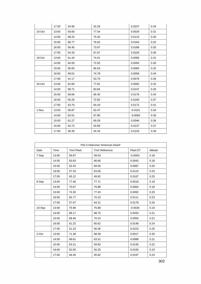
302

17:00 34.90 42.26 0.0237 0.34

10-Oct 13:00 59.83 77.54 0.0029 0.31

14:00 58.25 75.35 0.0110 0.30

15:00 58.77 76.62 0.0164 0.32

16:00 56.45 73.97 0.0189 0.35

17:00 54.33 67.67 0.0226 0.36

19-Oct 13:00 61.44 74.01 0.0095 0.31

14:00 64.55 72.52 0.0093 0.30

15:00 56.93 66.54 0.0065 0.32

16:00 59.01 74.78 0.0059 0.34

17:00 41.17 53.70 0.0076 0.35

20-Oct 13:00 62.83 77.81 0.0092 0.32

14:00 58.71 60.84 0.0147 0.33

15:00 58.06 66.40 0.0176 0.34

16:00 55.25 72.82 0.0160 0.37

17:00 53.70 64.19 0.0172 0.41

1-Nov 13:00 58.87 62.47 -0.0151 0.34

14:00 62.51 67.80 -0.0083 0.35

15:00 61.27 69.29 0.0046 0.36

16:00 44.72 54.69 0.0137 0.37

17:00 39.30 44.16 0.0153 0.39

Plot 2-Heliconia 'American Dwarf'


7-Sep 13:00 59.67 59.03 -0.0003 0.18

14:00 63.63 66.66 0.0043 0.18

15:00 62.42 69.56 0.0087 0.20

16:00 57.33 63.05 0.0123 0.23

17:00 45.12 49.92 0.0167 0.25

8-Sep 13:00 77.46 77.71 0.0018 0.18

14:00 75.67 76.88 0.0064 0.18

15:00 74.30 77.43 0.0092 0.20

16:00 65.77 70.10 0.0111 0.23

17:00 57.67 64.21 0.0178 0.26

10-Sep 13:00 75.96 75.88 -0.0026 0.19

14:00 68.17 68.75 0.0033 0.21

15:00 68.46 70.23 0.0056 0.21

16:00 61.22 65.62 0.0148 0.24

17:00 51.23 56.36 0.0223 0.25

2-Oct 13:00 71.38 68.39 0.0017 0.20

14:00 68.61 63.31 0.0088 0.21

15:00 63.21 59.83 0.0135 0.22

16:00 52.05 50.25 0.0155 0.23

17:00 46.49 45.82 0.0197 0.24

303

3-Oct 13:00 78.83 75.81 0.0046 0.19

14:00 79.34 76.01 0.0097 0.20

15:00 78.00 75.95 0.0183 0.22

16:00 71.97 70.47 0.0176 0.24

17:00 62.80 61.50 0.0137 0.27

9-Oct 13:00 78.83 75.41 -0.0052 0.20

14:00 80.94 77.27 0.0023 0.20

15:00 81.47 78.79 0.0115 0.22

16:00 57.92 59.80 0.0241 0.24

17:00 38.97 42.26 0.0233 0.24

10-Oct 13:00 76.69 77.54 -0.0005 0.19

14:00 77.09 75.35 0.0054 0.19

15:00 77.50 76.62 0.0093 0.21

16:00 73.81 73.97 0.0131 0.24

17:00 68.18 67.67 0.0193 0.27

19-Oct 13:00 75.21 74.01 0.0092 0.20

14:00 83.50 72.52 0.0096 0.20

15:00 73.47 66.54 0.0087 0.22

16:00 73.58 74.78 0.0099 0.24

17:00 51.00 53.70 0.0136 0.25

20-Oct 13:00 79.15 77.81 0.0079 0.19

14:00 76.97 60.84 0.0095 0.19

15:00 76.27 66.40 0.0114 0.21

16:00 74.42 72.82 0.0144 0.23

17:00 67.44 64.19 0.0169 0.26

1-Nov 13:00 63.65 62.47 -0.0108 0.24

14:00 67.28 67.80 -0.0062 0.24

15:00 66.00 69.29 0.0030 0.24

16:00 51.94 54.69 0.0113 0.26

17:00 42.36 44.16 0.0138 0.27



7-Sep 13:00 53.04 59.03 0.0038 0.26

14:00 59.35 66.66 0.0082 0.25

15:00 59.36 69.56 0.0120 0.25

16:00 55.41 63.05 0.0153 0.27

17:00 44.30 49.92 0.0169 0.28

8-Sep 13:00 67.07 77.71 0.0064 0.26

14:00 68.67 76.88 0.0116 0.24

15:00 72.88 77.43 0.0141 0.25

16:00 64.18 70.10 0.0151 0.27

17:00 60.25 64.21 0.0179 0.27

10-Sep 13:00 68.69 75.88 0.0032 0.27

304

14:00 62.06 68.75 0.0081 0.27

15:00 66.97 70.23 0.0104 0.26

16:00 63.09 65.62 0.0155 0.28

17:00 53.57 56.36 0.0177 0.29

2-Oct 13:00 59.94 68.39 0.0066 0.28

14:00 60.23 63.31 0.0103 0.28

15:00 57.04 59.83 0.0134 0.29

16:00 47.94 50.25 0.0153 0.30

17:00 44.41 45.82 0.0160 0.30

3-Oct 13:00 66.05 75.81 0.0078 0.27

14:00 68.05 76.01 0.0110 0.26

15:00 69.80 75.95 0.0176 0.26

16:00 67.13 70.47 0.0180 0.27

17:00 60.31 61.50 0.0132 0.28

9-Oct 13:00 65.24 75.41 -0.0003 0.28

14:00 68.37 77.27 0.0057 0.27

15:00 71.82 78.79 0.0123 0.27

16:00 51.11 59.80 0.0208 0.30

17:00 37.65 42.26 0.0199 0.31

10-Oct 13:00 61.75 77.54 0.0043 0.28

14:00 65.92 75.35 0.0076 0.27

15:00 69.70 76.62 0.0109 0.26

16:00 69.02 73.97 0.0154 0.27

17:00 65.25 67.67 0.0179 0.28

19-Oct 13:00 63.22 74.01 0.0106 0.24

14:00 68.27 72.52 0.0102 0.23

15:00 65.55 66.54 0.0077 0.25

16:00 67.99 74.78 0.0063 0.26

17:00 47.81 53.70 0.0073 0.27

20-Oct 13:00 64.28 77.81 0.0084 0.25

14:00 65.30 60.84 0.0099 0.25

15:00 68.86 66.40 0.0117 0.25

16:00 69.30 72.82 0.0131 0.26

17:00 62.73 64.19 0.0131 0.27

1-Nov 13:00 61.32 62.47 -0.0071 0.26

14:00 67.37 67.80 -0.0036 0.24

15:00 67.22 69.29 0.0034 0.25

16:00 50.27 54.69 0.0093 0.27

17:00 43.09 44.16 0.0111 0.27

305

10.7 Data for sensitivity analysis

Tmrt Plant Tmrt Reference Plant ET Albedo

48.17 50.00 0.0095 0.26

48.95 51.00 0.0095 0.26

49.73 52.00 0.0095 0.26

50.51 53.00 0.0095 0.26

51.29 54.00 0.0095 0.26

52.08 55.00 0.0095 0.26

52.86 56.00 0.0095 0.26

53.64 57.00 0.0095 0.26

54.42 58.00 0.0095 0.26

55.20 59.00 0.0095 0.26

55.99 60.00 0.0095 0.26

56.77 61.00 0.0095 0.26

57.55 62.00 0.0095 0.26

58.33 63.00 0.0095 0.26

59.11 64.00 0.0095 0.26

59.90 65.00 0.0095 0.26

60.68 66.00 0.0095 0.26

61.46 67.00 0.0095 0.26

62.24 68.00 0.0095 0.26

63.02 69.00 0.0095 0.26

63.81 70.00 0.0095 0.26

58.50 61.04 0.0010 0.26

58.30 61.04 0.0020 0.26

58.10 61.04 0.0030 0.26

57.90 61.04 0.0040 0.26

57.70 61.04 0.0050 0.26

57.50 61.04 0.0060 0.26

57.30 61.04 0.0070 0.26

57.10 61.04 0.0080 0.26

56.90 61.04 0.0090 0.26

56.70 61.04 0.0100 0.26

56.50 61.04 0.0110 0.26

306

56.30 61.04 0.0120 0.26

56.10 61.04 0.0130 0.26

55.90 61.04 0.0140 0.26

55.70 61.04 0.0150 0.26

55.50 61.04 0.0160 0.26

55.30 61.04 0.0170 0.26

55.10 61.04 0.0180 0.26

54.90 61.04 0.0190 0.26

54.70 61.04 0.0200 0.26

54.50 61.04 0.0210 0.26

54.30 61.04 0.0220 0.26

54.10 61.04 0.0230 0.26

53.90 61.04 0.0240 0.26

53.70 61.04 0.0250 0.26

53.50 61.04 0.0260 0.26

53.30 61.04 0.0270 0.26

53.10 61.04 0.0280 0.26

52.90 61.04 0.0290 0.26

52.70 61.04 0.0300 0.26

72.16 61.04 0.0095 0.01

71.55 61.04 0.0095 0.02

70.94 61.04 0.0095 0.03

70.33 61.04 0.0095 0.04

69.72 61.04 0.0095 0.05

69.11 61.04 0.0095 0.06

68.50 61.04 0.0095 0.07

67.89 61.04 0.0095 0.08

67.28 61.04 0.0095 0.09

66.67 61.04 0.0095 0.10

66.06 61.04 0.0095 0.11

65.45 61.04 0.0095 0.12

64.84 61.04 0.0095 0.13

64.23 61.04 0.0095 0.14

63.62 61.04 0.0095 0.15

63.01 61.04 0.0095 0.16

62.40 61.04 0.0095 0.17

61.79 61.04 0.0095 0.18

61.18 61.04 0.0095 0.19

60.57 61.04 0.0095 0.20

59.96 61.04 0.0095 0.21

59.35 61.04 0.0095 0.22

58.74 61.04 0.0095 0.23

58.13 61.04 0.0095 0.24

57.52 61.04 0.0095 0.25

307

56.91 61.04 0.0095 0.26

56.30 61.04 0.0095 0.27

55.69 61.04 0.0095 0.28

55.08 61.04 0.0095 0.29

54.47 61.04 0.0095 0.30

10.8 Plant selection chart

Reference Tmrt

50 °C

Shrub Albedo

0.16 0.17 0.18 0.19 0.20 0.21 0.22 0.23 0.24 0.25 0.26 0.27

Pla

nt E

vapotr

anspiratio

n R

ate

0.001 56.1 55.5 54.9 54.2 53.6 53.0 52.4 52.0 51.2 50.6 50.0 49.4

0.002 55.9 55.3 54.7 54.0 53.4 52.8 52.2 51.8 51.0 50.4 49.8 49.2

0.003 55.7 55.1 54.5 53.8 53.2 52.6 52.0 51.6 50.8 50.2 49.6 49.0

0.004 55.5 54.9 54.3 53.6 53.0 52.4 51.8 51.4 50.6 50.0 49.4 48.8

0.005 55.3 54.7 54.1 53.4 52.8 52.2 51.6 51.2 50.4 49.8 49.2 48.6

0.006 55.1 54.5 53.9 53.2 52.6 52.0 51.4 51.0 50.2 49.6 49.0 48.4

0.007 54.9 54.3 53.7 53.0 52.4 51.8 51.2 50.8 50.0 49.4 48.8 48.2

0.008 54.7 54.1 53.5 52.8 52.2 51.6 51.0 50.6 49.8 49.2 48.6 48.0

0.009 54.5 53.9 53.3 52.6 52.0 51.4 50.8 50.4 49.6 49.0 48.4 47.8

0.010 54.3 53.7 53.1 52.4 51.8 51.2 50.6 50.2 49.4 48.8 48.2 47.6

0.011 54.1 53.5 52.9 52.2 51.6 51.0 50.4 50.0 49.2 48.6 48.0 47.4

0.012 53.9 53.3 52.7 52.0 51.4 50.8 50.2 49.8 49.0 48.4 47.8 47.2

0.013 53.7 53.1 52.5 51.8 51.2 50.6 50.0 49.6 48.8 48.2 47.6 47.0

0.014 53.5 52.9 52.3 51.6 51.0 50.4 49.8 49.4 48.6 48.0 47.4 46.8

0.015 53.3 52.7 52.1 51.4 50.8 50.2 49.6 49.2 48.4 47.8 47.2 46.6

0.016 53.1 52.5 51.9 51.2 50.6 50.0 49.4 49.0 48.2 47.6 47.0 46.4

0.017 52.9 52.3 51.7 51.0 50.4 49.8 49.2 48.8 48.0 47.4 46.8 46.2

0.018 52.7 52.1 51.5 50.8 50.2 49.6 49.0 48.6 47.8 47.2 46.6 46.0

0.019 52.5 51.9 51.3 50.6 50.0 49.4 48.8 48.4 47.6 47.0 46.4 45.8

0.020 52.3 51.7 51.1 50.4 49.8 49.2 48.6 48.2 47.4 46.8 46.2 45.6

0.021 52.1 51.5 50.9 50.2 49.6 49.0 48.4 48.0 47.2 46.6 46.0 45.4

0.022 51.9 51.3 50.7 50.0 49.4 48.8 48.2 47.8 47.0 46.4 45.8 45.2

0.023 51.7 51.1 50.5 49.8 49.2 48.6 48.0 47.6 46.8 46.2 45.6 45.0

0.024 51.5 50.9 50.3 49.6 49.0 48.4 47.8 47.4 46.6 46.0 45.4 44.8

0.025 51.3 50.7 50.1 49.4 48.8 48.2 47.6 47.2 46.4 45.8 45.2 44.6

0.026 51.1 50.5 49.9 49.2 48.6 48.0 47.4 47.0 46.2 45.6 45.0 44.4

308

0.027 50.9 50.3 49.7 49.0 48.4 47.8 47.2 46.8 46.0 45.4 44.8 44.2

0.028 50.7 50.1 49.5 48.8 48.2 47.6 47.0 46.6 45.8 45.2 44.6 44.0

0.029 50.5 49.9 49.3 48.6 48.0 47.4 46.8 46.4 45.6 45.0 44.4 43.8

0.030 50.3 49.7 49.1 48.4 47.8 47.2 46.6 46.2 45.4 44.8 44.2 43.6

Percentage reduction in mean radiant temperature

Reference Tmrt

50 °C

Shrub Albedo

0.16 0.17 0.18 0.19 0.20 0.21 0.22 0.23 0.24 0.25 0.26 0.27

Pla

nt E

vapotr

anspiratio

n R

ate

0.001 - - - - - - - - - - - 1.3

0.002 - - - - - - - - - - 0.5 1.7

0.003 - - - - - - - - - - 0.9 2.1

0.004 - - - - - - - - - - 1.3 2.5

0.005 - - - - - - - - - 0.4 1.7 2.9

0.006 - - - - - - - - - 0.8 2.1 3.3

0.007 - - - - - - - - - 1.2 2.5 3.7

0.008 - - - - - - - - 0.4 1.6 2.9 4.1

0.009 - - - - - - - - 0.8 2.0 3.3 4.5

0.010 - - - - - - - - 1.2 2.4 3.7 4.9

0.011 - - - - - - - - 1.6 2.8 4.1 5.3

0.012 - - - - - - - 0.4 2.0 3.2 4.5 5.7

0.013 - - - - - - - 0.8 2.4 3.6 4.9 6.1

0.014 - - - - - - 0.4 1.2 2.8 4.0 5.3 6.5

0.015 - - - - - - 0.8 1.6 3.2 4.4 5.7 6.9

0.016 - - - - - - 1.2 2.0 3.6 4.8 6.1 7.3

0.017 - - - - - 0.4 1.6 2.4 4.0 5.2 6.5 7.7

0.018 - - - - - 0.8 2.0 2.8 4.4 5.6 6.9 8.1

0.019 - - - - - 1.2 2.4 3.2 4.8 6.0 7.3 8.5

0.020 - - - - 0.3 1.6 2.8 3.6 5.2 6.4 7.7 8.9

0.021 - - - - 0.7 2.0 3.2 4.0 5.6 6.8 8.1 9.3

0.022 - - - - 1.1 2.4 3.6 4.4 6.0 7.2 8.5 9.7

0.023 - - - 0.3 1.5 2.8 4.0 4.8 6.4 7.6 8.9 10.1

0.024 - - - 0.7 1.9 3.2 4.4 5.2 6.8 8.0 9.3 10.5

0.025 - - - 1.1 2.3 3.6 4.8 5.6 7.2 8.4 9.7 10.9

0.026 - - 0.3 1.5 2.7 4.0 5.2 6.0 7.6 8.8 10.1 11.3

0.027 - - 0.7 1.9 3.1 4.4 5.6 6.4 8.0 9.2 10.5 11.7

0.028 - - 1.1 2.3 3.5 4.8 6.0 6.8 8.4 9.6 10.9 12.1

0.029 - 0.3 1.5 2.7 3.9 5.2 6.4 7.2 8.8 10.0 11.3 12.5

0.030 - 0.7 1.9 3.1 4.3 5.6 6.8 7.6 9.2 10.4 11.7 12.9

309

Reference Tmrt

60 °C

Shrub Albedo

0.12 0.13 0.14 0.15 0.16 0.17 0.18 0.19 0.20 0.21 0.22 0.23

Pla

nt E

vapotr

anspiratio

n R

ate

0.001 66.3 65.7 65.1 64.5 63.9 63.3 62.7 62.1 61.5 60.8 60.2 59.8

0.002 66.1 65.5 64.9 64.3 63.7 63.1 62.5 61.9 61.3 60.6 60.0 59.6

0.003 65.9 65.3 64.7 64.1 63.5 62.9 62.3 61.7 61.1 60.4 59.8 59.4

0.004 65.7 65.1 64.5 63.9 63.3 62.7 62.1 61.5 60.9 60.2 59.6 59.2

0.005 65.5 64.9 64.3 63.7 63.1 62.5 61.9 61.3 60.7 60.0 59.4 59.0

0.006 65.3 64.7 64.1 63.5 62.9 62.3 61.7 61.1 60.5 59.8 59.2 58.8

0.007 65.1 64.5 63.9 63.3 62.7 62.1 61.5 60.9 60.3 59.6 59.0 58.6

0.008 64.9 64.3 63.7 63.1 62.5 61.9 61.3 60.7 60.1 59.4 58.8 58.4

0.009 64.7 64.1 63.5 62.9 62.3 61.7 61.1 60.5 59.9 59.2 58.6 58.2

0.010 64.5 63.9 63.3 62.7 62.1 61.5 60.9 60.3 59.7 59.0 58.4 58.0

0.011 64.3 63.7 63.1 62.5 61.9 61.3 60.7 60.1 59.5 58.8 58.2 57.8

0.012 64.1 63.5 62.9 62.3 61.7 61.1 60.5 59.9 59.3 58.6 58.0 57.6

0.013 63.9 63.3 62.7 62.1 61.5 60.9 60.3 59.7 59.1 58.4 57.8 57.4

0.014 63.7 63.1 62.5 61.9 61.3 60.7 60.1 59.5 58.9 58.2 57.6 57.2

0.015 63.5 62.9 62.3 61.7 61.1 60.5 59.9 59.3 58.7 58.0 57.4 57.0

0.016 63.3 62.7 62.1 61.5 60.9 60.3 59.7 59.1 58.5 57.8 57.2 56.8

0.017 63.1 62.5 61.9 61.3 60.7 60.1 59.5 58.9 58.3 57.6 57.0 56.6

0.018 62.9 62.3 61.7 61.1 60.5 59.9 59.3 58.7 58.1 57.4 56.8 56.4

0.019 62.7 62.1 61.5 60.9 60.3 59.7 59.1 58.5 57.9 57.2 56.6 56.2

0.020 62.5 61.9 61.3 60.7 60.1 59.5 58.9 58.3 57.7 57.0 56.4 56.0

0.021 62.3 61.7 61.1 60.5 59.9 59.3 58.7 58.1 57.5 56.8 56.2 55.8

0.022 62.1 61.5 60.9 60.3 59.7 59.1 58.5 57.9 57.3 56.6 56.0 55.6

0.023 61.9 61.3 60.7 60.1 59.5 58.9 58.3 57.7 57.1 56.4 55.8 55.4

0.024 61.7 61.1 60.5 59.9 59.3 58.7 58.1 57.5 56.9 56.2 55.6 55.2

0.025 61.5 60.9 60.3 59.7 59.1 58.5 57.9 57.3 56.7 56.0 55.4 55.0

0.026 61.3 60.7 60.1 59.5 58.9 58.3 57.7 57.1 56.5 55.8 55.2 54.8

0.027 61.1 60.5 59.9 59.3 58.7 58.1 57.5 56.9 56.3 55.6 55.0 54.6

0.028 60.9 60.3 59.7 59.1 58.5 57.9 57.3 56.7 56.1 55.4 54.8 54.4

0.029 60.7 60.1 59.5 58.9 58.3 57.7 57.1 56.5 55.9 55.2 54.6 54.2

310

0.030 60.5 59.9 59.3 58.7 58.1 57.5 56.9 56.3 55.7 55.0 54.4 54.0


Reference Tmrt

60 °C

Shrub Albedo

0.12 0.13 0.14 0.15 0.16 0.17 0.18 0.19 0.20 0.21 0.22 0.23

Pla

nt E

vapotr

anspiratio

n R

ate

0.001 - - - - - - - - - - - 0.3

0.002 - - - - - - - - - - - 0.6

0.003 - - - - - - - - - - 0.3 1.0

0.004 - - - - - - - - - - 0.6 1.3

0.005 - - - - - - - - - - 0.9 1.6

0.006 - - - - - - - - - 0.3 1.3 2.0

0.007 - - - - - - - - - 0.6 1.6 2.3

0.008 - - - - - - - - - 0.9 1.9 2.6

0.009 - - - - - - - - 0.2 1.3 2.3 3.0

0.010 - - - - - - - - 0.6 1.6 2.6 3.3

0.011 - - - - - - - - 0.9 1.9 2.9 3.6

0.012 - - - - - - - 0.2 1.2 2.3 3.3 4.0

0.013 - - - - - - - 0.6 1.6 2.6 3.6 4.3

0.014 - - - - - - - 0.9 1.9 2.9 3.9 4.6

0.015 - - - - - - 0.2 1.2 2.2 3.3 4.3 5.0

0.016 - - - - - - 0.5 1.6 2.6 3.6 4.6 5.3

0.017 - - - - - - 0.9 1.9 2.9 3.9 4.9 5.6

0.018 - - - - - 0.2 1.2 2.2 3.2 4.3 5.3 6.0

0.019 - - - - - 0.5 1.5 2.6 3.6 4.6 5.6 6.3

0.020 - - - - - 0.9 1.9 2.9 3.9 4.9 5.9 6.6

0.021 - - - - 0.2 1.2 2.2 3.2 4.2 5.3 6.3 7.0

0.022 - - - - 0.5 1.5 2.5 3.6 4.6 5.6 6.6 7.3

0.023 - - - - 0.8 1.9 2.9 3.9 4.9 5.9 6.9 7.6

0.024 - - - 0.2 1.2 2.2 3.2 4.2 5.2 6.3 7.3 8.0

0.025 - - - 0.5 1.5 2.5 3.5 4.6 5.6 6.6 7.6 8.3

311

0.026 - - - 0.8 1.8 2.9 3.9 4.9 5.9 6.9 7.9 8.6

0.027 - - 0.1 1.2 2.2 3.2 4.2 5.2 6.2 7.3 8.3 9.0

0.028 - - 0.5 1.5 2.5 3.5 4.5 5.6 6.6 7.6 8.6 9.3

0.029 - - 0.8 1.8 2.8 3.9 4.9 5.9 6.9 7.9 8.9 9.6

0.030 - 0.1 1.1 2.2 3.2 4.2 5.2 6.2 7.2 8.3 9.3 10.0

Reference Tmrt

70 °C

Shrub Albedo

0.09 0.10 0.11 0.12 0.13 0.14 0.15 0.16 0.17 0.18 0.19

Pla

nt E

vapotr

anspiratio

n R

ate

0.001 76.0 75.4 74.8 74.2 73.5 72.9 72.3 71.7 71.1 70.5 69.9

0.002 75.8 75.2 74.6 74.0 73.3 72.7 72.1 71.5 70.9 70.3 69.7

0.003 75.6 75.0 74.4 73.8 73.1 72.5 71.9 71.3 70.7 70.1 69.5

0.004 75.4 74.8 74.2 73.6 72.9 72.3 71.7 71.1 70.5 69.9 69.3

0.005 75.2 74.6 74.0 73.4 72.7 72.1 71.5 70.9 70.3 69.7 69.1

0.006 75.0 74.4 73.8 73.2 72.5 71.9 71.3 70.7 70.1 69.5 68.9

0.007 74.8 74.2 73.6 73.0 72.3 71.7 71.1 70.5 69.9 69.3 68.7

0.008 74.6 74.0 73.4 72.8 72.1 71.5 70.9 70.3 69.7 69.1 68.5

0.009 74.4 73.8 73.2 72.6 71.9 71.3 70.7 70.1 69.5 68.9 68.3

0.010 74.2 73.6 73.0 72.4 71.7 71.1 70.5 69.9 69.3 68.7 68.1

0.011 74.0 73.4 72.8 72.2 71.5 70.9 70.3 69.7 69.1 68.5 67.9

0.012 73.8 73.2 72.6 72.0 71.3 70.7 70.1 69.5 68.9 68.3 67.7

0.013 73.6 73.0 72.4 71.8 71.1 70.5 69.9 69.3 68.7 68.1 67.5

0.014 73.4 72.8 72.2 71.6 70.9 70.3 69.7 69.1 68.5 67.9 67.3

0.015 73.2 72.6 72.0 71.4 70.7 70.1 69.5 68.9 68.3 67.7 67.1

0.016 73.0 72.4 71.8 71.2 70.5 69.9 69.3 68.7 68.1 67.5 66.9

0.017 72.8 72.2 71.6 71.0 70.3 69.7 69.1 68.5 67.9 67.3 66.7

0.018 72.6 72.0 71.4 70.8 70.1 69.5 68.9 68.3 67.7 67.1 66.5

0.019 72.4 71.8 71.2 70.6 69.9 69.3 68.7 68.1 67.5 66.9 66.3

0.020 72.2 71.6 71.0 70.4 69.7 69.1 68.5 67.9 67.3 66.7 66.1

0.021 72.0 71.4 70.8 70.2 69.5 68.9 68.3 67.7 67.1 66.5 65.9

0.022 71.8 71.2 70.6 70.0 69.3 68.7 68.1 67.5 66.9 66.3 65.7

0.023 71.6 71.0 70.4 69.8 69.1 68.5 67.9 67.3 66.7 66.1 65.5

0.024 71.4 70.8 70.2 69.6 68.9 68.3 67.7 67.1 66.5 65.9 65.3

0.025 71.2 70.6 70.0 69.4 68.7 68.1 67.5 66.9 66.3 65.7 65.1

0.026 71.0 70.4 69.8 69.2 68.5 67.9 67.3 66.7 66.1 65.5 64.9

312

0.027 70.8 70.2 69.6 69.0 68.3 67.7 67.1 66.5 65.9 65.3 64.7

0.028 70.6 70.0 69.4 68.8 68.1 67.5 66.9 66.3 65.7 65.1 64.5

0.029 70.4 69.8 69.2 68.6 67.9 67.3 66.7 66.1 65.5 64.9 64.3

0.030 70.2 69.6 69.0 68.4 67.7 67.1 66.5 65.9 65.3 64.7 64.1


Reference Tmrt

70 °C

Shrub Albedo

0.09 0.10 0.11 0.12 0.13 0.14 0.15 0.16 0.17 0.18 0.19

Pla

nt E

vapotr

anspiratio

n R

ate

0.001 - - - - - - - - - - 0.2

0.002 - - - - - - - - - - 0.5

0.003 - - - - - - - - - - 0.7

0.004 - - - - - - - - - - 1.0

0.005 - - - - - - - - - 0.4 1.3

0.006 - - - - - - - - - 0.7 1.6

0.007 - - - - - - - - 0.1 1.0 1.9

0.008 - - - - - - - - 0.4 1.3 2.2

0.009 - - - - - - - - 0.7 1.6 2.5

0.010 - - - - - - - 0.1 1.0 1.9 2.7

0.011 - - - - - - - 0.4 1.3 2.2 3.0

0.012 - - - - - - - 0.7 1.6 2.4 3.3

0.013 - - - - - - 0.1 1.0 1.9 2.7 3.6

0.014 - - - - - - 0.4 1.3 2.1 3.0 3.9

0.015 - - - - - - 0.7 1.6 2.4 3.3 4.2

0.016 - - - - - 0.1 1.0 1.8 2.7 3.6 4.5

0.017 - - - - - 0.4 1.3 2.1 3.0 3.9 4.7

0.018 - - - - - 0.7 1.5 2.4 3.3 4.2 5.0

0.019 - - - - 0.1 1.0 1.8 2.7 3.6 4.4 5.3

0.020 - - - - 0.4 1.2 2.1 3.0 3.9 4.7 5.6

0.021 - - - - 0.7 1.5 2.4 3.3 4.1 5.0 5.9

0.022 - - - - 0.9 1.8 2.7 3.6 4.4 5.3 6.2

0.023 - - - 0.4 1.2 2.1 3.0 3.8 4.7 5.6 6.5

0.024 - - - 0.6 1.5 2.4 3.3 4.1 5.0 5.9 6.7

0.025 - - - 0.9 1.8 2.7 3.5 4.4 5.3 6.2 7.0

0.026 - - 0.3 1.2 2.1 3.0 3.8 4.7 5.6 6.4 7.3

0.027 - - 0.6 1.5 2.4 3.2 4.1 5.0 5.9 6.7 7.6

313

0.028 - - 0.9 1.8 2.7 3.5 4.4 5.3 6.1 7.0 7.9

0.029 - 0.3 1.2 2.1 2.9 3.8 4.7 5.6 6.4 7.3 8.2

0.030 - 0.6 1.5 2.4 3.2 4.1 5.0 5.8 6.7 7.6 8.5

10.9 Specifications for green roof

10.9.1 Green roof panel

Material – Polypropylene

Depth – 70 mm

314

10.9.2 Substrate

Composition – pumice

Weight of substrate per unit panel – 10 Kg

Fig

ure

14

8.

Gre

en

ro

of p

an

el sp

ecific

ation

s

315

10.9.3 Irrigation

Automatic drip irrigation system

Emitter flow rate – 1.0 Litre per hour

Battery powered controller used to control irrigation

Irrigation timing – 06:00 hrs to 07:00 hrs daily

Amount of water supplied to single 500 mm X 500 mm green roof panel –

1.16 Kg

Figure 149. Irrigation plan

316

10.10 BCA Green Mark for New Non-Residential Buildings Version

NRB/4.1

336

10.11 LUSH 2.0 landscape replacement circular

338

10.12 Response to comments from examiners

10.12.1 Comments from Examiner 1

Comment:

The link between Knowledge Gap, Research Questions and Objectives are

not clear. The candidate needs to rework on this to make the flow of the

thesis smoother.

Response:

Knowledge Gap is on page 79

Research Question is on page 22

Objectives is on page 22

Knowledge Gap is elaborated as follows:

“…

1.3 Knowledge Gap

A thorough review of relevant literature reveals that although the benefits of

urban greenery have been widely established, there is a lack of objective and

systematic methodology for landscape planning based on the temperature

reduction potential of plants. While landscape planners and architects may be

aware of how greenery can reduce temperature, they are unable to evaluate

the temperature reduction potential of their landscape design proposals

based on their choice and placement of plants.

The thesis seeks to address this issue by first identifying the appropriate

environment component that can be used to evaluate the cooling potential of

plants. Thereafter, plant traits that affect temperature reduction are identified

and empirically modelled as variables for temperature reduction. The model

will be used as a basis for an objective landscape planning framework for

landscape design optimisation.

…“

339

Comment:

Figure 20 on the Research Methodology needs improvement.

Response:

Research methodology (Figure 20) elaborated.

340

Comment:

The candidate should elaborate on the limitations of the experimental parts to

justify the issues with sample size, repeatability and reproducibility. An

example is section 3.5.

Response:

Currently, the limitations are as follows:

Structure of the substrate for shrubs on green roofs differs significant from

shrubs at ground level. The depth of the substrate at green roofs is typically

much shallower than conventional plantings at ground level (Extensive roof

garden plots). This will have an impact on the overall evapotranspiration rate

for plants.

Studies are conducted in the tropical urban environment. Due to differences

in aridity and solar exposure, results may not be valid for temperate regions.

The study assumes all plants of the same genus to have statistically similar

physiological attributes.

Limitations to sample size is added as follows:

The sample size is limited to three samples. If more plants of different species

are used, the regression model will be representative of a larger spectrum of

plants.

The regression model may not be representative of all shrub types. Some

shrubs such as CAM plants or plants that experience mid-day stomatal

depression plants (Discussed in Chapter 6.1.1) should not be used to

construct the regression model.

341


Comment:

In the abbreviation section, only the abbreviations of some commonly used

terms are provided. Mathematical abbreviations should also be included to

facilitate reading of the thesis.

Response:

Mathematical abbreviations are elaborated below all equations to facilitate

reading

Comment:

P.1 5th line: state whether the 48% means the percentage of the world’s

population.

Response:

Rephrased

Comment:

P.15 last line: indicate where is the green area.

Response:

Amended to “… in forested areas…”

Comment:

P.61 Eqt 15: state the location where the air velocity and temperature are

measured when using the equation.

Response:

To be added below Equation 15 “…

tg = Globe temperature (°C), measured by a temperature sensor placed inside

the globe

Va = Air velocity (ms-1), measured at the level of the globe

342

ta = Air temperature (°C), measured near the globe

Comment:

P.76:

1st line: explain how Fi=0.167 is obtained for a sphere or quoted relevant

reference.

9th line after Eqt 19: Equation (22) should be Equation (15).

Eqt 20 is the same as Eqt 15 and should be corrected to avoid confusion.

Response:

Value of Fi=0.167 was quoted from Fanger (1972). Citation added.

Equation number amended

Equation number amended

Fanger, P. O., 1972, Thermal comfort. Analysis and applications in

environmental engineering, New York: McGraw-Hill.

Comment:

P.77 9th line: explain how the mean wind speed was obtained, for example,

state the location where the measurement was conducted.

Response:

Added:

“… Mean wind speed was measured with a weather station that was placed

within 10 m of the mean radiant temperature measurement site…”

Comment:

P.92 Table 7: State whether there are any special treatment of data (e.g.

discarded) under raining or thunderstorm condition.

Response:

343

Added:

“… Not all data obtained was used for analysis. For Chapter 4, results shown

are representative of typical clear or overcast sky conditions. Rainy days are

not used for analysis unless no suitable alternatives are available...”

Comment:

P.103 2nd and 3rd line: it mentioned that the dip in air temperature was

observed and is likely due to a short period of rain. If this is the case, it should

not be used for analyzing the ambient temperature variation due to the plant

species under overcast conditions.

Response:

The 12th of July was used as there were no suitable alternatives to observe

the effect of plants on overcast days. It is important to note that rain only

occurred for a very short period (06:47 hrs to 06:53 hrs) and should not affect

analysis of peak temperature conditions around 16:30 hrs.

Air temperature for 5th July 2014 was highly erratic due to rain (05:00 hrs to

17:00 hrs) and therefore deemed unsuitable for analysis of air temperature.

0

0.1

0.2

0.3

0.4

0.5

0.6

0.7

24

25

26

27

28

29

30

31

12

:00

AM

12

:56

AM

1:5

2 A

M

2:4

8 A

M

3:4

4 A

M

4:4

0 A

M

5:3

6 A

M

6:3

2 A

M

7:2

8 A

M

8:2

4 A

M

9:2

0 A

M

10

:16

AM

11

:12

AM

12

:08

PM

1:0

4 P

M

2:0

0 P

M

2:5

6 P

M

3:5

2 P

M

4:4

8 P

M

5:4

4 P

M

6:4

0 P

M

7:3

6 P

M

8:3

2 P

M

9:2

8 P

M

10

:24

PM

11

:20

PM

Rai

nfa

ll (m

m)

Air

tem

per

atu

re (

°C)

Time (Hrs)

Rainfall and air temperature on 12th July 2014

Temp, °C Rain, mm

344

Comment:

P.104 Figure 39: specify the weather condition on 26 July 14 whereas the

maximum temperature occurred at 5 pm.

Response:

Weather condition specified below:

23

24

25

26

27

28

29

30

31

1:0

0

2:0

0

3:0

0

4:0

0

5:0

0

6:0

0

7:0

0

8:0

0

9:0

0

10

:00

11

:00

12

:00

13

:00

14

:00

15

:00

16

:00

17

:00

18

:00

19

:00

20

:00

21

:00

22

:00

23

:00

0:0

0

Air

tem

pre

atu

re (

°C)

Time (Hrs)

Air temperature profile 5th July 2014

T-Plot 1-3-hour T-Plot 2-1-hour T-Plot 2-2-hour T-Plot 3-2-hour

T-Plot 3-3-hour T-Plot 5-2-hour T-Plot 5-3-hour

252627282930313233

0

200

400

600

800

1000

12

:00

1:0

02

:00

3:0

04

:00

5:0

06

:00

7:0

08

:00

9:0

01

0:0

01

1:0

01

2:0

01

:00

2:0

03

:00

4:0

05

:00

6:0

07

:00

8:0

09

:00

10

:00

11

:00

12

:00

Air

tem

per

atu

re (

°C)

Sola

r R

adia

tio

n (

W/m

2 )

Time (Hrs)

Weather data for 26th July 2014

Solar Radiation (W/m²) Air temperature (°C)

345

Comment:

P106 last 3rd line: the explanation on the lowered temperature within the

canopy for Plot 3 is not reasonable.

Response:

Plot 3 (Sphagneticola trilobatta) provides a lush canopy cover and a thick

undergrowth of stems below the canopy. As a result, the undergrowth is very

well-shaded from the sun and pockets of air with lower temperature is

observed.

346

Comment:

P.118: there is no deep analysis on the cause of the discrepancy of LAI

results obtained from different methods and no determination on whether the

indirect or direct measurement result should be adopted or not for analysis.

Noted that the results of the indirect method and the literature matched with

each other. Furthermore, the result of the soil temperature also matched with

the result of LAI determined by the indirect method as shown in Fig. 59 on

P.124. However, on P.136 it is concluded that there is no correlation between

LAI and the mean radiant temperature. Such a conclusion is not persuasive.

Response:

The purpose of measuring LAI using these different methods is to:

Identify the most accurate value of LAI for the 3 types of plants being studied

To ascertain the influence of LAI in mean radiant temperature reduction using

statistical methods

Method 1: Indirect measurement using LAI-2000

Method 2: Direct measurement by plucking leaves and calculating total

amount of green pixels

Method 3: Reference to NParks handbook

The most accurate method of LAI measurement is via Method 2. This is

because every leaf will be measured at a high degree of precision. However,

it is often impractical to employ Method 2 as this is a destructive method and

leaves have to be physically removed. Also, it requires extensive manpower

to pluck, scan and count the number of green pixels.

Method 1 is a non-destructive and more convenient method of measuring LAI.

However, LAI is measured in the form of light attenuation and not actual leaf

347

count. This method is not able to differentiate between light blocked by a

single leaf and light blocked by multiple leaves in the canopy. This method is

often used to measure LAI of large forested areas and trees with large

canopies

Method 3 is a generalised method of assigning LAI values to plants for the

purpose of landscape planning.

Values of LAI obtained via Method 2 were deemed to be most accurate.

Values of LAI obtained via Methods 1 and 3 were displayed in Table 9 were

used as a comparison. It could be observed that there were significant over

and under-estimates of LAI using Methods 1 and 3. LAI for Heliconica (Plot 2)

is lower using Method 1 most likely due to the fact that leaves of the Heliconia

plant, while large, do not spread horizontally across the shrub and are

hanging vertically from the stem. This results in larger open spaces within the

canopy, leading to more light captured by the LAI-2000 sensor.

Table: Averaged Leaf Area Indices for Plot 1 to Plot 3

Plot

LAI measurement method

Indirect measurement (Using LAI-2000)

Direct measurement (Plucking out

leaves in 50 x 50 cm plot, pixel calculation)

Nparks handbook

(Tan and Sia, 2009)

1 2 3 Ave

1 Phyllanthus cochinchinensis Shrub (Dicot)

4.65 4.22 4.16 4.34 2.78 4.5

2 Heliconia American Dwarf Shrub (Monocot)

3.14 3.69 3.58 3.47 7.21 3.5

3 Sphagneticola trilobata Ground cover

4.70 4.28 4.83 4.60 3.59 4.5

348

Subsequently, values of LAI obtained via Method 2 were used for analysis.

It can be observed that Plot 2 has the highest LAI of 7.21 from the direct

measurement method, which is the most accurate method of measuring LAI.

However, the corresponding reduction in Tmrt is the lowest. This can be

explained by the lack of water transferred to its leaves during periods of high

solar irradiance. This results in a higher leaf surface temperature, which can

be observed using infrared thermography (figure below).

349

Numerous studies have shown plant Leaf Area Index to be strongly correlated

with temperature reduction. In such cases, temperature reduction is mostly

due to shade provided by tree canopy, resulting in reduced heat absorbed by

building surfaces, pavements and pedestrians (Fahmy et al., 2010; Gómez-

Muñoz et al., 2010; Hardin and Jensen, 2007). Shahidan et al. (2010) found a

strong correlation between thermal radiation filtration and LAI for M. Ferrea L

and H. crepittan (R2 = 0.96 and 0.95). A higher LAI will result in more layers

of leaves that will result in reduction thermal radiation under a tree (Brown

and Gillespie, 1995; Kotzen, 2003).

However, with regards to the impact of LAI on Tmrt, this study has shown that

LAI is not strongly correlated with Tmrt reduction. On the contrary, temperature

is increased with higher LAI. One hypothesis put forth by the author is that as

leaf area increases, ease of delivery of water from soil to leaf is reduced. This

will result in increased leaf surface temperature. For the same LAI, however,

it may be possible to find plants with smaller leaf areas and more leaves. This

in turn may result in lower surface temperature for the leaves. Further study is

required to validate this assumption. This would suggest that overall radiative

qualities of the plant canopy (albedo, absorptance, reflectance, canopy

structure) are more substantial at determining its impact on Tmrt.

It is the opinion of the author that besides looking solely at LAI, plant

functional traits may affect overall temperature reduction potential. This was

highlighted in Chapter 6.1.3. A variable that combines values of LAI as well as

plant functional traits such as shrub height, leaf dimension, stem structure etc.

may provide more insight into how they can provide effective temperature

reduction.

350

References:

Fahmy, M., Sharples, S., Yahiya, M., 2010, LAI based trees selection for mid

latitude urban developments: A microclimatic study in Cairo, Egypt, Building

and environment 45(2):345-357.

Gómez-Muñoz, V. M., Porta-Gándara, M., Fernández, J., 2010, Effect of tree

shades in urban planning in hot-arid climatic regions, Landscape and urban

planning 94(3):149-157.

Hardin, P. J., Jensen, R. R., 2007, The effect of urban leaf area on

summertime urban surface kinetic temperatures: A Terre Haute case study,

Urban Forestry & Urban Greening 6(2):63-72.

Shahidan, M. F., Shariff, M. K., Jones, P., Salleh, E., Abdullah, A. M., 2010, A

comparison of Mesua ferrea L. and Hura crepitans L. for shade creation and

radiation modification in improving thermal comfort, Landscape and Urban

Planning 97(3):168-181.

Brown, R. D., Gillespie, T. J., 1995, Microclimatic landscape design: creating

thermal comfort and energy efficiency, John Wiley & Sons.

Kotzen, B., 2003, An investigation of shade under six different tree species of

the Negev desert towards their potential use for enhancing micro-climatic

conditions in landscape architectural development, Journal of Arid

environments 55(2):231-274.

351

Comment:

P.127 Fig. 61:

I. Give more details on how the incident/reflected shortwave/longwave

radiations were measured.

II. It is not understandable why the incoming radiation depends on the

plant species.

Response:

I. Figure provided below:

II. Incoming radiation does not depend on plant species. They are

slightly different as they are located 5 to 11 m apart from each other.

Comment:

P.134-135: Comparison of data was done on a specific day only, it is not

enough to make a conclusion based on one day’s result.

Response:

Added “…It is important to note that this is data for one typical day with clear

sky conditions and a limitation is that it may not represent a general

characteristic of the plants…”

352

Comment:

P.137 last 11th line: there is little discussion on LAI in this study. Many studies

indicate LAI has strong cooling effect on the environment and it is used as a

criterion for tree selection. Inclusion of this parameter may improve the

accuracy of the regression equation.

Response:

Please refer to item 11 for explanation of why LAI was not used for regression

equation

Comment:

P.138 table 12: the presentation in this table is confusing, as the data in

columns 2-5 are referred to all the variables in column one.

Response:

Reformatted to:

Variable Total no. of days

measured

Dates selected for

regression modelling (2014)

No. of days

used for

modelling

Mean radiant temperature

above rooftop greenery

tmrt(plant)

Reference mean radiant

temperature

tmrt(ref)

Plant EvapoTranspiration

Rate

(ET)

Shrub Albedo

(SA)

10/05/2014

to

31/12/2014

236 days

May 13, 15, 22, 24, 25,

28, 29

35 days

June

8, 10, 11, 13, 16, 17,

18, 19, 20, 21, 22,

23, 24, 25

July 1, 7, 8, 10, 13, 16,

18, 20, 21, 25, 26

August 17

September 1, 2

353

Comment:

P.142 Fig. 70: from the observation, the correlation between ET and Tmrt and

between shrub Albedo and Tmrt are not too high as mentioned, particularly

the former one.

Response:

Albedo and Plant ET are hypothesized to be significant variables that can

reduce Tmrt from reviewed literature.

Although correlation with ET and Albedo are not too high, the two variables

exhibit high substantive significance from reviewed literature as well as

results from measured data (infrared surface temperature measurements,

stomatal conductance measurements, etc.). Results from regression

modelling also show that they are significant variables and to omit them would

be to commit a Type 2 statistical error.

Comment:

P.160 Figure 82: ET depends on plant species and solar intensity, explain

how to determine a representative ET rate and why ET was averaged from

13:00 to 17:00 hrs.

Response:

Reviewed literature shows that ET can be represented in different timescales

(mm∙day-1, mm∙hour-1, etc). For this case, ET was averaged from 13:00 hrs to

17:00 hrs for the purpose of comparing with ET values used for regression

modelling (also average of 13:00 hrs to 17:00 hrs).

354

Comment:

P.163 last 4th line: the statement “there is evidence to suggest that leaves

with smaller …” needs justification or quote relevant reference.

Response:

This is in reference to data obtained from this study. Comparison of leaf size

and leaf surface temperature shows that bigger leaves tend to have higher

temperatures. Please refer to Figure 58: Infrared thermography of green roof

plots and concrete and Figure 83. Botanical illustration of plants used for

measurement.

Comment:

P.180: explain how the Tmrt reduction due to the introduction of trees with

small canopies, large canopies and more trees can be obtained during the

first 3 iterations.

Response:

In Iterations 1 to 3, Tmrt is reduced as shortwave radiation is blocked by tree

canopies. Trees with bigger canopies provide larger blockage of shortwave

radiation and hence provide more reduction to Tmrt

355

Comment:

P.200: this chapter would better be separated into two parts, one is the

reference that have been quoted in the manuscript. The other part is the

bibliography.

Response:

Chapter renamed as “References”

Typographical and grammatical errors

Check all the equations with proper typing of subscript to avoid confusion.

P.iv 12th line: “quantify air temperature (ta)”.

P.69 4th line: “The variables to be measured ….”.

P.86 5th line: “….the level of uncertainty …”.

P.102 last 4th line: Plot 4 should be Plot 1. Also on last 3rd line: “It can also

be ….”.

The title of many figures (e.g. Figs. 42 to 51) should be amended to truly

reflect their contents. For example, to reflect the content in Fig. 42, the title

should better be hourly variation of solar radiation and mean radiant

temperature over the day.

P.124 4th line: “higher than that”.

P.127 last 3rd line: “Plot 2 is higher than that of Plot 2 made Plot 3.”\

P.130 7th line: “…. Lower than that.

P.138 6th line: “due to one or more ….”

P.153 Section 5.2.2 Sensitivity analysis of prediction model: the analysis can

be simplified without the need of the graphical determination. The conclusions

in this section (e.g. for every increase of 1 oC for tmrt (plant), there is a

356

corresponding increase of 0.8 oC for tmrt (plant)) can be derived directly from

Eqt. 25.

Response:

All typographical and grammatical errors have been amended

357


Comment:

Comparative efficacy of rooftop greenery as the background

In the introduction of research question on the page 6, you have question to

the efficacy of rooftop greenery to the urban microclimate as the background

of this research. However, it is difficult to discuss absolute value of the effect

of individual UHI countermeasure because UHI is quite complex phenomenon

and each element might influence each other. So, this kind of effect should be

discussed under the comparison to other existing countermeasures; for

example high-reflection paint, water retention material and so on.

My suggestion is making a simple study on the effect of other

countermeasure in the same condition or citing other achievements to clarify

the comparative efficacy of rooftop greenery as the background.

Response:

Urban greenery has been proven to be an effective UHI mitigation

component. Although this thesis has focused solely on the temperature

reduction potential of rooftop greenery, the author fully acknowledges the

mitigative impact of other various UHI countermeasures such as cool paint

and water retention material. Comparison with other UHI countermeasures

have been conducted in the author’s capacity as a research assistant. These

studies include:

I. Study of temperature reduction potential for rooftop greenery and cool

roof

II. Study of temperature reduction potential of rooftop greenery system

with water retention layer

III. Study of temperature reduction potential of trees in the urban

environment

358

IV. Study of temperature reduction potential of vertical greenery in the

urban environment

These studies have been represented in the following manner:

I. Wong, N.H., Jusuf, S.K., Tan, C.L., Chia, P.Y., 2013, Effect of cool

roofs and green roofs on temperature in the tropical urban

environment, AIVC 2013, Athens. Oral Presentation by Jusuf, S.K.,

Published in proceedings.

II. Wong, N.H., Tan, P.Y., Tan, C.L., Lim, C.V.J., Chua, H.X.V.,

Takasuna, H., Kudo, T., Takemasa, Y., 2016, Impact of Soil and

Water Retention Characteristics on Green Roof Thermal Performance,

4th International Conference on Countermeasures to Urban Heat

Island, 30-31 May and 1 June 2016, National University of Singapore,

Singapore.

III. Chapter 10.1 of thesis

IV. Chapter 10.3 of thesis

These studies can help provide a more holistic understanding of common UHI

countermeasures.

359

Comment:

Basis of hypothetical urban model

In the discussion of landscape planning guidelines on the page 177, you

suggest hypothetical urban model as a case study. However, it is possible to

show different result if the model is different as many past achievement

mentioned. This study may have been delivered based on specified idea.

My suggestion is remarking the basis of the model; for example based on the

existing urban district, arrangement of preliminary study result, to emphasize

specified phenomenon, and so on to clarify significance of the case study.

Response:

The author acknowledges the importance of substantiating simulated results

with actual measurements and that subsequent studies on actual sites may

be considered should the opportunity arise.

However, the purpose of introducing the hypothetical study is to demonstrate

the steps landscape planners can take to understand the thermal impact of

their design decisions (Figure 88). These steps are used as a basis for

recommendations to improve the existing green building rating tool in

Singapore (BCA Green Mark Scheme). To provide simulated results for the

purpose of validation against actual results is beyond the scope of this thesis

and requires a wholly different methodology.

The objective of this exercise is to show that numerous design iterations can

be made with tools that are readily available (Table 29).

Although the model is hypothetical, it is based on actual planning parameters

used by the Urban Redevelopment Authority of Singapore (URA). Moreover,

the first round of simulation is based on physical (not empirical) modelling.

Therefore, simulation results derived from this hypothetical model should

resemble actual conditions in a significant manner.

EFFECT OF ROOFTOP GREENERY ON OUTDOOR MEAN ...

Documents

Transcript of EFFECT OF ROOFTOP GREENERY ON OUTDOOR MEAN ...