
EE C222/ ME C237 - Spring'18 - Lecture 1 Notes
104
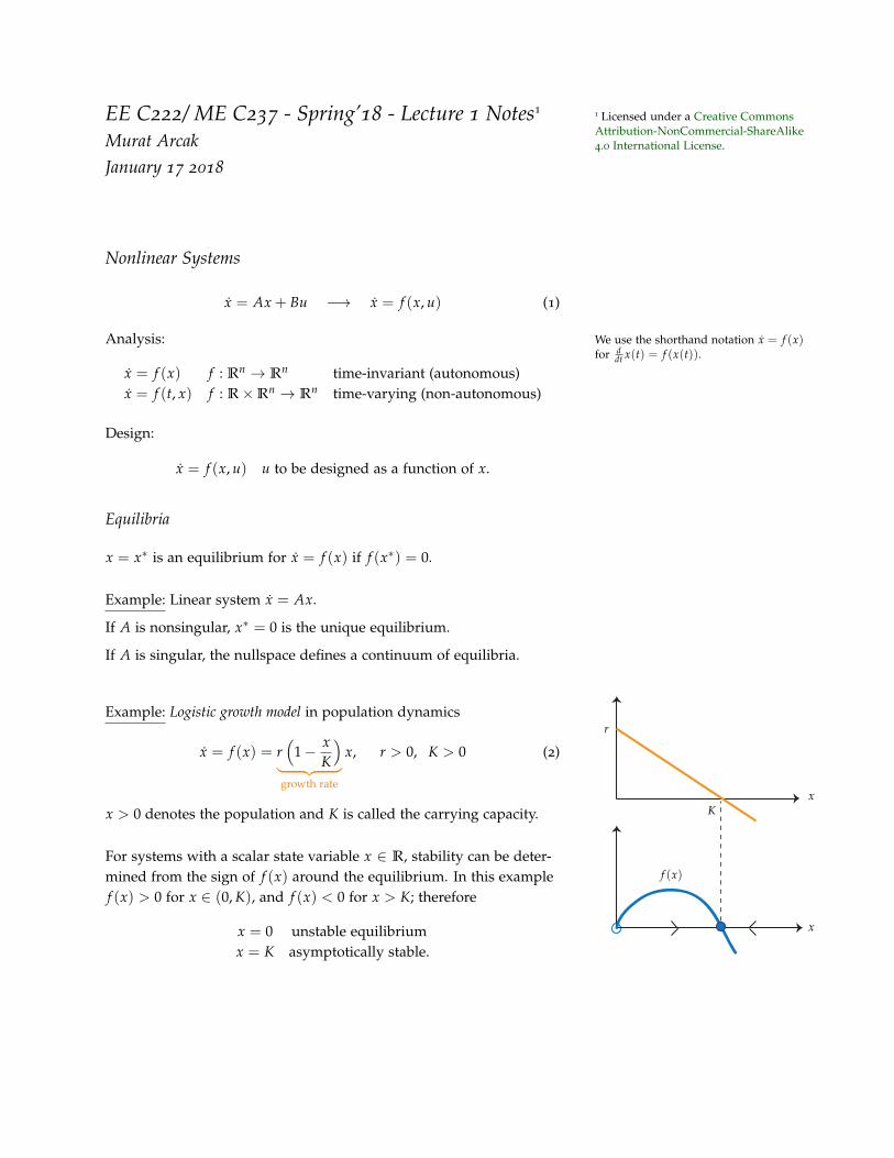
EE C222/ ME C237 - Spring’18 - Lecture 1 Notes 1 1 Licensed under a Creative Commons Attribution-NonCommercial-ShareAlike 4.0 International License. Murat Arcak January 17 2018 Nonlinear Systems ˙ x = Ax + Bu -→ ˙ x = f ( x, u) (1) Analysis: We use the shorthand notation ˙ x = f (x) for d dt x(t)= f (x(t)). ˙ x = f ( x) f : R n → R n time-invariant (autonomous) ˙ x = f (t, x) f : R × R n → R n time-varying (non-autonomous) Design: ˙ x = f ( x, u) u to be designed as a function of x. Equilibria x = x * is an equilibrium for ˙ x = f ( x) if f ( x * )= 0. Example: Linear system ˙ x = Ax. If A is nonsingular, x * = 0 is the unique equilibrium. If A is singular, the nullspace defines a continuum of equilibria. Example: Logistic growth model in population dynamics ˙ x = f ( x)= r 1 - x K | {z } growth rate x, r > 0, K > 0 (2) x > 0 denotes the population and K is called the carrying capacity. x x r K f (x) For systems with a scalar state variable x ∈ R, stability can be deter- mined from the sign of f ( x) around the equilibrium. In this example f ( x) > 0 for x ∈ (0, K), and f ( x) < 0 for x > K; therefore x = 0 unstable equilibrium x = K asymptotically stable.
-
Upload
khangminh22 -
Category
Documents
-
view
4 -
download
0
Transcript of EE C222/ ME C237 - Spring'18 - Lecture 1 Notes
EE C222/ ME C237 - Spring’18 - Lecture 1 Notes11 Licensed under a Creative CommonsAttribution-NonCommercial-ShareAlike4.0 International License.Murat Arcak
January 17 2018
Nonlinear Systems
x = Ax + Bu −→ x = f (x, u) (1)
Analysis: We use the shorthand notation x = f (x)for d
dt x(t) = f (x(t)).
x = f (x) f : Rn → Rn time-invariant (autonomous)x = f (t, x) f : R×Rn → Rn time-varying (non-autonomous)
Design:
x = f (x, u) u to be designed as a function of x.
Equilibria
x = x∗ is an equilibrium for x = f (x) if f (x∗) = 0.
Example: Linear system x = Ax.
If A is nonsingular, x∗ = 0 is the unique equilibrium.
If A is singular, the nullspace defines a continuum of equilibria.
Example: Logistic growth model in population dynamics
x = f (x) = r(
1− xK
)︸ ︷︷ ︸growth rate
x, r > 0, K > 0 (2)
x > 0 denotes the population and K is called the carrying capacity.x
x
r
K
f (x)For systems with a scalar state variable x ∈ R, stability can be deter-mined from the sign of f (x) around the equilibrium. In this examplef (x) > 0 for x ∈ (0, K), and f (x) < 0 for x > K; therefore
x = 0 unstable equilibriumx = K asymptotically stable.

ee c222/ me c237 - spring’18 - lecture 1 notes 2
Linearization
Local stability properties of x∗ can be determined by linearizing thevector field f (x) at x∗:
f (x∗ + x) = f (x∗)︸ ︷︷ ︸= 0
+∂ f∂x
∣∣∣∣x=x∗︸ ︷︷ ︸
, A
x + higher order terms (3)
Thus, the linearized model is:
˙x = Ax. (4)
If <λi(A) < 0 for each eigenvalue λi of A, then x∗ is asymp. stable.
If <λi(A) > 0 for some eigenvalue λi of A, then x∗ is unstable.
Example: Logistic growth model above:
f ′(0) > 0unstable
f ′(K) < 0stable
f (x)
x
Caveats:
1. Only local properties can be determined from the linearization.
Example: The logistic growth model linearized at x = 0 (x = rx)would incorrectly predict unbounded growth of x(t). In reality,x(t)→ K.
2. If <λi(A) ≤ 0 with equality for some i, then linearization isinconclusive as a stability test. Higher order terms determinestability.
Example: f (x) = x3 vs. f (x) = −x3
xx
f ′(0) = 0 in each case, but one is stable and the other is unstable.
ee c222/ me c237 - spring’18 - lecture 1 notes 3
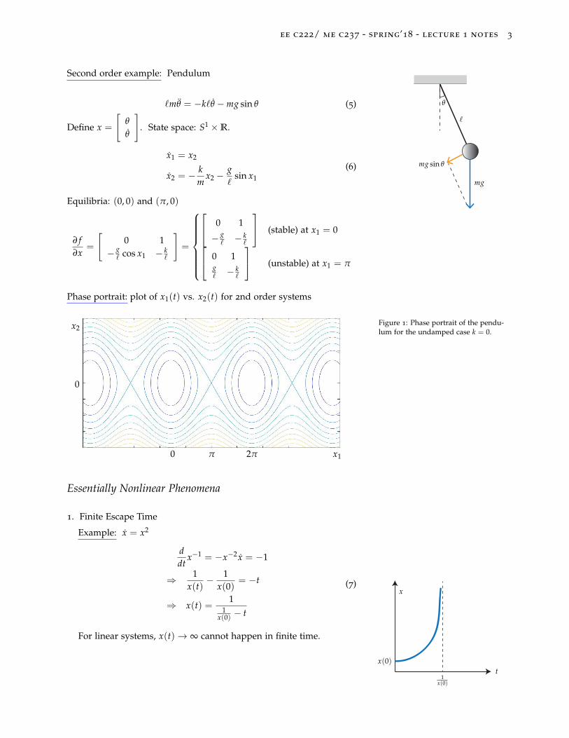
Second order example: Pendulum
θ
`
mg
mg sin θ
`mθ = −k`θ −mg sin θ (5)
Define x =
[θ
θ
]. State space: S1 ×R.
x1 = x2
x2 = − km
x2 −g`
sin x1
(6)
Equilibria: (0, 0) and (π, 0)
∂ f∂x
=
[0 1
− g` cos x1 − k
`
]=
0 1
− g` − k
`
(stable) at x1 = 0 0 1g` − k
`
(unstable) at x1 = π
Phase portrait: plot of x1(t) vs. x2(t) for 2nd order systems
0 π 2π x1
x2
0
Figure 1: Phase portrait of the pendu-lum for the undamped case k = 0.
Essentially Nonlinear Phenomena
1. Finite Escape Time
Example: x = x2
ddt
x−1 = −x−2 x = −1
⇒ 1x(t)− 1
x(0)= −t
⇒ x(t) =1
1x(0) − t
(7)
t
x
x(0)
1x(0)
For linear systems, x(t)→ ∞ cannot happen in finite time.
ee c222/ me c237 - spring’18 - lecture 1 notes 4
2. Multiple Isolated Equilibria
Linear systems: either unique equilibrium or a continuum
Pendulum: two isolated equilibria (one stable, one unstable)
“Multi-stable” systems: two or more stable equilibria
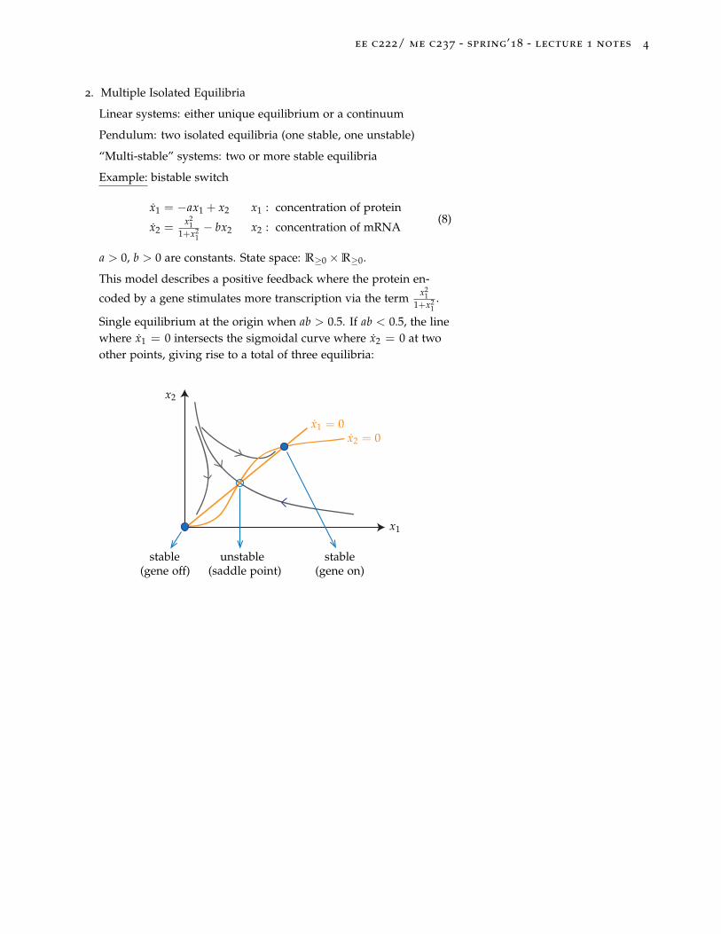
Example: bistable switch
x1 = −ax1 + x2 x1 : concentration of protein
x2 =x2
11+x2
1− bx2 x2 : concentration of mRNA
(8)
a > 0, b > 0 are constants. State space: R≥0 ×R≥0.
This model describes a positive feedback where the protein en-
coded by a gene stimulates more transcription via the term x21
1+x21.
Single equilibrium at the origin when ab > 0.5. If ab < 0.5, the linewhere x1 = 0 intersects the sigmoidal curve where x2 = 0 at twoother points, giving rise to a total of three equilibria:
x1
x2
x1 = 0x2 = 0
stable(gene on)
stable(gene off)
unstable(saddle point)

EE C222/ME C237 - Spring’18 - Lecture 2 Notes11 Licensed under a Creative CommonsAttribution-NonCommercial-ShareAlike4.0 International License.Murat Arcak
January 22 2018
Essentially Nonlinear Phenomena Continued
1. Finite escape time
2. Multiple isolated equilibria
3. Limit cycles: Linear oscillators exhibit a continuum of periodicorbits; e.g., every circle is a periodic orbit for x = Ax where
A =
[0 −β
β 0
](λ1,2 = ∓jβ).
In contrast, a limit cycle is an isolated periodic orbit and can occuronly in nonlinear systems.
limit cycleharmonicoscillator
Example: van der Pol oscillator
CvC = −iL + vC − v3C
LiL = vC
iL
LC+
−vC
iR
vC
iR = −vC + v3C
"negative resistance"∧∧
iL
vC

ee c222/me c237 - spring’18 - lecture 2 notes 2
4. Chaos: Irregular oscillations, never exactly repeating.
Example: Lorenz system (derived by Ed Lorenz in 1963 as a sim-plified model of convection rolls in the atmosphere):
x = σ(y− x)
y = rx− y− xz
z = xy− bz.
Chaotic behavior with σ = 10, b = 8/3, r = 28:
0 10 20 30 40 50 60-30
-20
-10
0
10
20
30
-20 -15 -10 -5 0 5 10 15 200
5
10
15
20
25
30
35
40
45
50
x
z
t
y(t)
• For continuous-time, time-invariant systems, n ≥ 3 state vari-ables required for chaos.n = 1: x(t) monotone in t, no oscillations:
x
f (x)
n = 2: Poincaré-Bendixson Theorem (to be studied in Lecture 3)guarantees regular behavior.
• Poincaré-Bendixson does not apply to time-varying systems andn ≥ 2 is enough for chaos (Homework problem).
• For discrete-time systems, n = 1 is enough (we will see anexample in Lecture 5).
Planar (Second Order) Dynamical SystemsChapter 2 in both Sastry and Khalil
Phase Portraits of Linear Systems: x = Ax
• Distinct real eigenvalues
T−1 AT =
[λ1 00 λ2
]

ee c222/me c237 - spring’18 - lecture 2 notes 3
In z = T−1x coordinates:
z1 = λ1z1, z2 = λ2z2.
The equilibrium is called a node when λ1 and λ2 have the samesign (stable node when negative and unstable when positive). It iscalled a saddle point when λ1 and λ2 have opposite signs.
z1z1z1
z2z2z2
λ1 < λ2 < 0 λ1 > λ2 > 0 λ2 < 0 < λ1
stablenode
unstablenode saddle
• Complex eigenvalues: λ1,2 = α∓ jβ
T−1 AT =
[α −β
β α
]z1 = αz1 − βz2
z2 = αz2 + βz1→ polar coordinates →
r = αr
θ = β
z1z1z1
z2z2z2
stablefocus
unstablefocus center
α < 0 α > 0 α = 0
The phase portraits above assume β > 0 so that the direction ofrotation is counter-clockwise: θ = β > 0.
Phase Portraits of Nonlinear Systems Near Hyperbolic Equilibria
hyperbolic equilibrium: linearization has no eigenvalues on the imagi-nary axis
Phase portraits of nonlinear systems near hyperbolic equilibria arequalitatively similar to the phase portraits of their linearization. Ac-cording to the Hartman-Grobman Theorem (below) a “continuousdeformation” maps one phase portrait to the other.

ee c222/me c237 - spring’18 - lecture 2 notes 4
x∗h
Hartman-Grobman Theorem: If x∗ is a hyperbolic equilibrium ofx = f (x), x ∈ Rn, then there exists a homeomorphism2 z = h(x) defined 2 a continuous map with a continuous
inversein a neighborhood of x∗ that maps trajectories of x = f (x) to those of
z = Az where A , ∂ f∂x
∣∣∣x=x∗
.
The hyperbolicity condition can’t be removed:
Example:
x1 = −x2 + ax1(x21 + x2
2)
x2 = x1 + ax2(x11 + x2
2)=⇒
r = ar3
θ = 1
x∗ = (0, 0) A =∂ f∂x
∣∣∣∣x=x∗
=
[0 −11 0
]
There is no continuous deformation that maps the phase portrait ofthe linearization to that of the original nonlinear model:
(a > 0)x = Ax x = f (x)
Periodic Orbits in the Plane
Bendixson’s Theorem: For a time-invariant planar system
x1 = f1(x1, x2) x2 = f2(x1, x2),
if ∇ · f (x) = ∂ f1∂x1
+ ∂ f2∂x2
is not identically zero and does not changesign in a simply connected region D, then there are no periodic orbitslying entirely in D.

ee c222/me c237 - spring’18 - lecture 2 notes 5
Proof: By contradiction. Suppose a periodic orbit J lies in D. Let Sdenote the region enclosed by J and n(x) the normal vector to J at x.Then f (x) · n(x) = 0 for all x ∈ J. By the Divergence Theorem:
JS
• x
f (x) n(x)
∫J
f (x) · n(x)d`︸ ︷︷ ︸= 0
=∫∫
S∇ · f (x)dx︸ ︷︷ ︸6= 0
.
Example: x = Ax, x ∈ R2 can have periodic orbits only if
Trace(A) = 0, e.g.,
A =
[0 −β
β 0
].
Example:
x1 = x2
x2 = −δx2 + x1 − x31 + x2
1x2 δ > 0
∇ · f (x) =∂ f1
∂x1+
∂ f2
∂x2= x2
1 − δ
Therefore, no periodic orbit can lie entirely in the region x1 ≤ −√
δ
where ∇ · f (x) ≥ 0, or −√
δ ≤ x1 ≤√
δ where ∇ · f (x) ≤ 0, orx1 ≥
√δ where ∇ · f (x) ≥ 0.
x1 = −√
δ
x1 = −√
δ
x1 =√
δ
x1 =√
δ
x1
x1
x2
x2
not possible:
possible:

EE C222/ME C237 - Spring’18 - Lecture 3 Notes11 Licensed under a Creative CommonsAttribution-NonCommercial-ShareAlike4.0 International License.Murat Arcak
January 24 2018
Invariant Sets
Notation: φ(t, x0) denotes a trajectory of x = f (x) with initial condi-tion x(0) = x0.
Definition: A set M ⊂ Rn is positively (negatively) invariant if, foreach x0 ∈ M, φ(t, x0) ∈ M for all t ≥ 0 (t ≤ 0).
n(x)
f (x)M
If f (x) · n(x) ≤ 0 on the boundary then M is positively invariant.
Example 1: A predator-prey model
x = (a− by)x Prey (exponential growth when y = 0)
y = (cx− d)y Predator (exponential decay when x = 0)
a, b, c, d,> 0
The nonnegative quadrant is invariant:
x
y
( dc , a
b )
saddle
Example 2:x1 = x1 + x2 − x1(x2
1 + x22)
x2 = −2x1 + x2 − x2(x21 + x2
2)
Show that Br , x|x21 + x2
2 ≤ r2 is positively invariant for sufficientlylarge r.

ee c222/me c237 - spring’18 - lecture 3 notes 2
f (x) · n(x) = x21 + x1x2 − x2
1(x21 + x2
2)− 2x1x2 + x22 − x2
2(x21 + x2
2)
= −x1x2 + (x21 + x2
2)− (x21 + x2
2)2
x1
x2n(x)=
[x1x2
]
f (x)
−x1x2 ≤12
x21 +
12
x22 (completion of squares)
Therefore, f (x) · n(x) ≤ 32 r2 − r4 ≤ 0 if r2 ≥ 3
2 .
Periodic Orbits in the Plane Continued
Two criteria:
1. Bendixson (absence of periodic orbits)
2. Poincaré-Bendixson (existence of periodic orbits)
Poincaré-Bendixson Theorem: Suppose M is compact2 and positively 2 i.e., closed and bounded
invariant for the planar, time invariant system x = f (x), x ∈ R2. If Mcontains no equilibrium points, then it contains a periodic orbit.
Example 3: Harmonic Oscillator
A =
[0 −11 0
]x1 = −x2
x2 = x1.
x1
x2
For any R > r > 0, the ring x : r2 ≤ x21 + x2
2 ≤ R2 is compact,invariant and contains no equilibria ⇒ at least one periodic orbit.(We know there are infinitely many in this case.)
The “no equilibrium” condition in the PB theorem can be relaxed as:
“If M contains one equilibrium which is an unstable focus orunstable node”
Proof sketch: Since the equilibrium is an unstable focus or node, wecan encircle it with a small closed curve on which f (x) points out-ward. Then the set obtained from M by carving out the interior of theclosed curve is positively invariant and contains no equilibrium.
M

ee c222/me c237 - spring’18 - lecture 3 notes 3
Example 2 above: Br is positively invariant for r ≥√
32 but contains
the equilibrium x = 0.
∂ f∂x
∣∣∣∣x=0
=
[1 1−2 1
]λ1,2 = 1∓ j
√2 unstable focus.
Therefore, Br must contain a periodic orbit.
A more general form of the PB Theorem states that, for time invari-ant, planar systems, bounded trajectories converge to equilibria,periodic orbits, or unions of equilibria connected by trajectories.
Corollary: No chaos for time invariant planar systems.
Index Theory
Again, applicable only to planar systems.
Definition (index): The index of a closed curve is k if, when traversingthe curve in one direction, f (x) rotates by 2πk in the same direction.The index of an equilibrium is defined to be the index of a smallcurve around it that doesn’t enclose another equilibrium.
type of equilibrium or curve index
node, focus, center +1
saddle -1
any closed orbit +1
a closed curve not encircling any equilibria 0
The last claim (index = 0) follows from the following observations:• Continuously deforming a closed curve without crossing equilibrialeaves its index unchanged.• A curve not encircling equilibria can be shrunk to an arbitrarilysmall one, so f (x) can be considered constant.

ee c222/me c237 - spring’18 - lecture 3 notes 4
Theorem: The index of a closed curve is equal to the sum of indicesof the equilibria inside.
Graphical proof: Shrinking curve c to c′ below without crossing equi-libria does not change the index. The index of c′ is the sum of theindices of the curves encircling the equilibria because the thin "pipes"connecting these curves do not affect the index of c′.
c′
c
contributions from the two sides cancel out
The following corollary is useful for ruling out periodic orbits (likeBendixson’s Theorem studied in the previous lecture):
Corollary: Inside any periodic orbit there must be at least one equi-librium and the indices of the equilibria enclosed must add up to+1.
Example (from last lecture):
x1 = x2
x2 = −δx2 + x1 − x31 + x2
1x2 δ > 0
Bendixson’s Criterion: No periodic orbit can lie entirely in one of theregions x1 ≤ −
√δ, −√
δ ≤ x1 ≤√
δ, or x1 ≥√
δ.
Now apply the corollary above.
Equilibria: (0, 0), (∓1, 0). To find their indices evaluate the Jacobian:
∂ f∂x
∣∣∣x=(0,0)
=
[0 11 −δ
]λ2 + δλ −1︸︷︷︸
<0
= 0.
The eigenvalues are real and have opposite signs, therefore (0, 0) is asaddle: index = −1.
∂ f∂x
∣∣∣x=(∓1,0)
=
[0 1−2 1− δ
]λ2 + (δ− 1)λ +2︸︷︷︸
>0
= 0.
The eigenvalues are either real with the same sign (node) or complexconjugates (focus or center), therefore (∓1, 0) each has index= +1.
Thus, the corollary above rules out the periodic orbit in the middleplot below. It does not rule out the others, but does not prove theirexistence either. Bendixson’s Criterion rules out neither of the three.

ee c222/me c237 - spring’18 - lecture 3 notes 5
x1 = −√
δ
x1 = −√
δ
x1 = −√
δ
x1 =√
δ
x1 =√
δ
x1 =√
δ
x1
x1
x1
x2
x2
x2
not possible

EE C222/ ME C237 - Spring’18 - Lecture 4 Notes11 Licensed under a Creative CommonsAttribution-NonCommercial-ShareAlike4.0 International License.Murat Arcak
January 29 2018
Bifurcations
A bifurcation is an abrupt change in qualitative behavior as a parame-ter is varied. Examples: equilibria or limit cycles appearing/disappearing,becoming stable/unstable.
Fold Bifurcation
Also known as “saddle node” or “blue sky” bifurcation.
Example: x = µ− x2
If µ > 0, two equilibria: x = ∓√µ. If µ < 0, no equilibria.
“bifurcation diagram”
µ
x
Transcritical Bifurcation
Example: x = µx− x2
Equilibria: x = 0 and x = µ.∂ f∂x
= µ− 2x =
µ if x = 0−µ if x = µ
µ < 0 : x = 0 is stable, x = µ is unstable
µ > 0 : x = 0 is unstable, x = µ is stable
µ
x
ee c222/ me c237 - spring’18 - lecture 4 notes 2
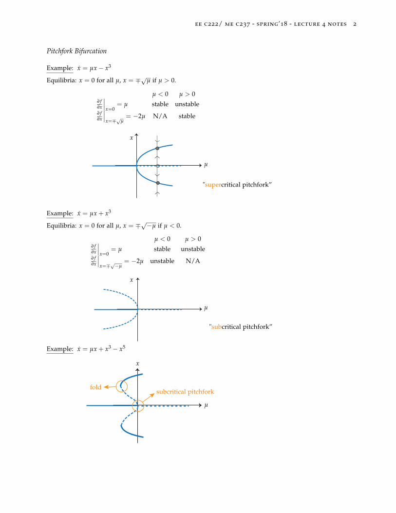
Pitchfork Bifurcation
Example: x = µx− x3
Equilibria: x = 0 for all µ, x = ∓√µ if µ > 0.
µ < 0 µ > 0∂ f∂x
∣∣∣x=0
= µ stable unstable∂ f∂x
∣∣∣x=∓√µ
= −2µ N/A stable
µ
x
"supercritical pitchfork”
Example: x = µx + x3
Equilibria: x = 0 for all µ, x = ∓√−µ if µ < 0.
µ < 0 µ > 0∂ f∂x
∣∣∣x=0
= µ stable unstable∂ f∂x
∣∣∣x=∓√−µ
= −2µ unstable N/A
µ
x
"subcritical pitchfork”
Example: x = µx + x3 − x5
µ
x
subcritical pitchforkfold
ee c222/ me c237 - spring’18 - lecture 4 notes 3
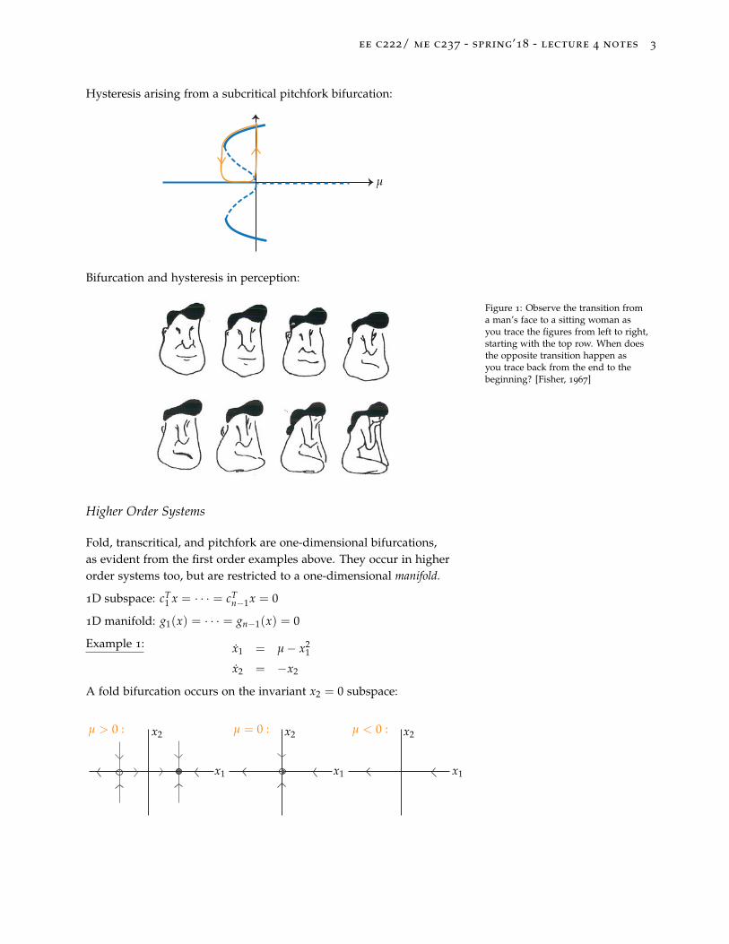
Hysteresis arising from a subcritical pitchfork bifurcation:
µ
Bifurcation and hysteresis in perception:
Figure 1: Observe the transition froma man’s face to a sitting woman asyou trace the figures from left to right,starting with the top row. When doesthe opposite transition happen asyou trace back from the end to thebeginning? [Fisher, 1967]
Higher Order Systems
Fold, transcritical, and pitchfork are one-dimensional bifurcations,as evident from the first order examples above. They occur in higherorder systems too, but are restricted to a one-dimensional manifold.
1D subspace: cT1 x = · · · = cT
n−1x = 0
1D manifold: g1(x) = · · · = gn−1(x) = 0
Example 1: x1 = µ− x21
x2 = −x2
A fold bifurcation occurs on the invariant x2 = 0 subspace:
x1x1x1
x2x2x2µ > 0 : µ = 0 : µ < 0 :

ee c222/ me c237 - spring’18 - lecture 4 notes 4
Example 2: bistable switch (Lecture 1)
x1 = −ax1 + x2
x2 =x2
11 + x2
1− bx2
A fold bifurcation occurs at µ , ab = 0.5:
x1
x2
x2 = 1b
x21
1+x21
x2 = ax1
a > 0.5/ba = 0.5/b
a < 0.5/b
Characteristic of one-dimensional bifurcations:
∂ f∂x
∣∣∣∣µ=µc , x=x∗(µc)
has an eigenvalue at zero
where x∗(µ) is the equilibrium point undergoing bifurcation and µc
is the critical value at which the bifurcation occurs.
Example 1 above:
∂ f∂x
∣∣∣∣µ=0,x=0
=
[0 00 −1
]→ λ1,2 = 0 ,−1
Example 2 above:
∂ f∂x
∣∣∣∣µ= 1
2 ,x1=1,x2=a=
[−a 1
12 −b
]→ λ1,2 = 0 ,−(a + b)
Hopf Bifurcation
Two-dimensional bifurcation unlike the one-dimensional types above.
Example: Supercritical Hopf bifurcation
x1 = x1(µ− x21 − x2
2)− x2
x2 = x2(µ− x21 − x2
2) + x1
In polar coordinates:
r = µr− r3
θ = 1
ee c222/ me c237 - spring’18 - lecture 4 notes 5
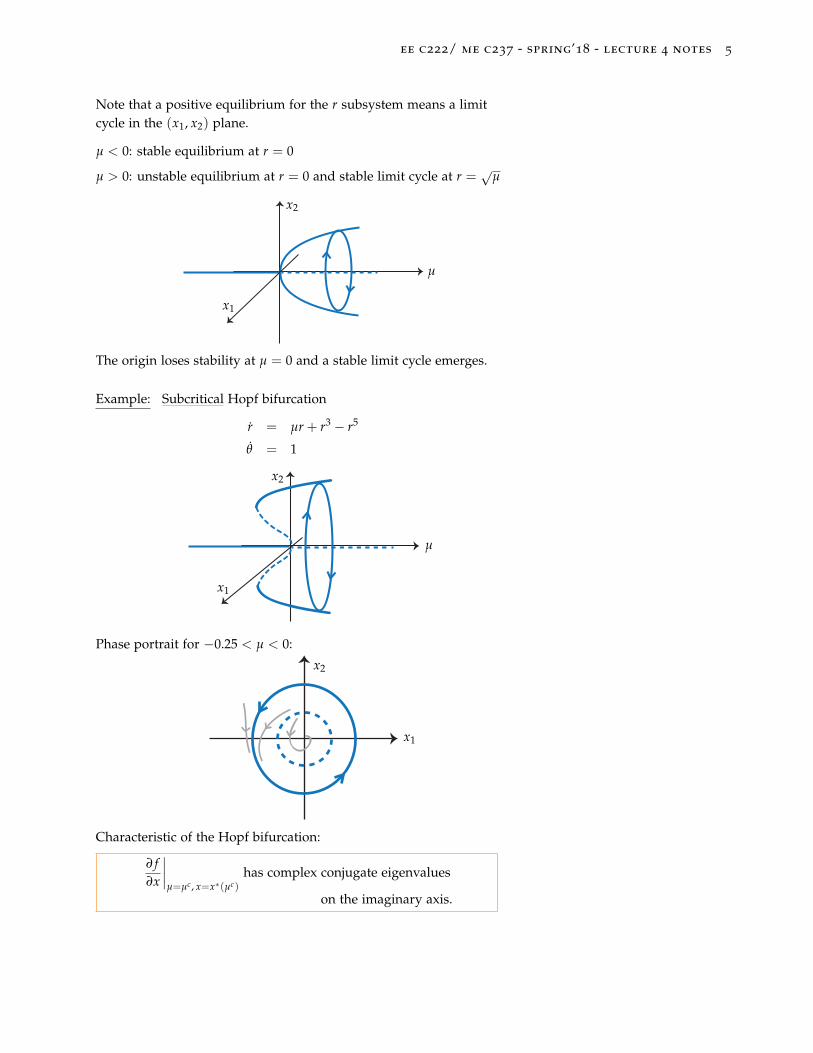
Note that a positive equilibrium for the r subsystem means a limitcycle in the (x1, x2) plane.
µ < 0: stable equilibrium at r = 0
µ > 0: unstable equilibrium at r = 0 and stable limit cycle at r =√
µ
µ
x2
x1
The origin loses stability at µ = 0 and a stable limit cycle emerges.
Example: Subcritical Hopf bifurcation
r = µr + r3 − r5
θ = 1
µ
x2
x1
Phase portrait for −0.25 < µ < 0:
x1
x2
Characteristic of the Hopf bifurcation:
∂ f∂x
∣∣∣∣µ=µc , x=x∗(µc)
has complex conjugate eigenvalues
on the imaginary axis.

EE C222/ME C237 - Spring’18 - Lecture 5 Notes11 Licensed under a Creative CommonsAttribution-NonCommercial-ShareAlike4.0 International License.Murat Arcak
January 31 2018
Center Manifold TheoryKhalil (Section 8.1), Sastry (Section7.6.1)x = f (x) f (0) = 0 (1)
Suppose A ,∂ f∂x
∣∣∣∣x=0
has k eigenvalues will zero real parts, and
m = n− k eigenvalues with negative real parts.
Define
[yz
]= Tx such that
TAT−1 =
[A1 00 A2
]
where the eigenvalues of A1 have zero real parts and the eigenvaluesof A2 have negative real parts.
Rewrite x = f (x) in the new coordinates:
y = A1y + g1(y, z)
z = A2z + g2(y, z)(2)
gi(0, 0) = 0, ∂gi∂y (0, 0) = 0, ∂gi
∂z (0, 0) = 0, i = 1, 2.
Theorem 1: There exists an invariant manifold z = h(y) defined in aneighborhood of the origin such that
h(0) = 0∂h∂y
(0) = 0.
y
z = h(y)
z
Reduced System: y = A1y + g1(y, h(y)) y ∈ Rk
Theorem 2: If y = 0 is asymptotically stable (resp., unstable) for thereduced system, then x = 0 is asymptotically stable (resp., unstable)for the full system x = f (x).

ee c222/me c237 - spring’18 - lecture 5 notes 2
Characterizing the Center Manifold
Define w , z− h(y) and note that it satisfies
w = A2z + g2(y, z)− ∂h∂y
(A1y + g1(y, z)
).
The invariance of z = h(y) means that w = 0 implies w = 0. Thus, theexpression above must vanish when we substitute z = h(y):
A2h(y) + g2(y, h(y))− ∂h∂y
(A1y + g1(y, h(y))
)= 0.
To find h(y) solve this differential equation for h as a function on y.
If the exact solution is unavailable, an approximation is possible. Forscalar y, expand h(y) as
h(y) = h2y2 + · · ·+ hpyp + O(yp+1)
where h1 = h0 = 0 because h(0) = ∂h∂y (0) = 0. The notation O(yp+1)
refers to the higher order terms of power p + 1 and above.
Example:y = yz
z = −z + ay2 a 6= 0
This is of the form (2) with g1(y, z) = yz, g2(y, z) = ay2, A2 = −1.Thus h(y) must satisfy
−h(y) + ay2 − ∂h∂y
yh(y) = 0.
Try h(y) = h2y2 + O(y3):
0 = −h2y2 + O(y3) + ay2 − (2h2y + O(y2))y(h22 + O(y3))
= (a− h2)y2 + O(y3)
=⇒ h2 = a
Reduced System: y = y(ay2 + O(y3)) = ay3 + O(y4).
If a < 0, the full systems is asymptotically stable. If a > 0 unstable.
ee c222/me c237 - spring’18 - lecture 5 notes 3
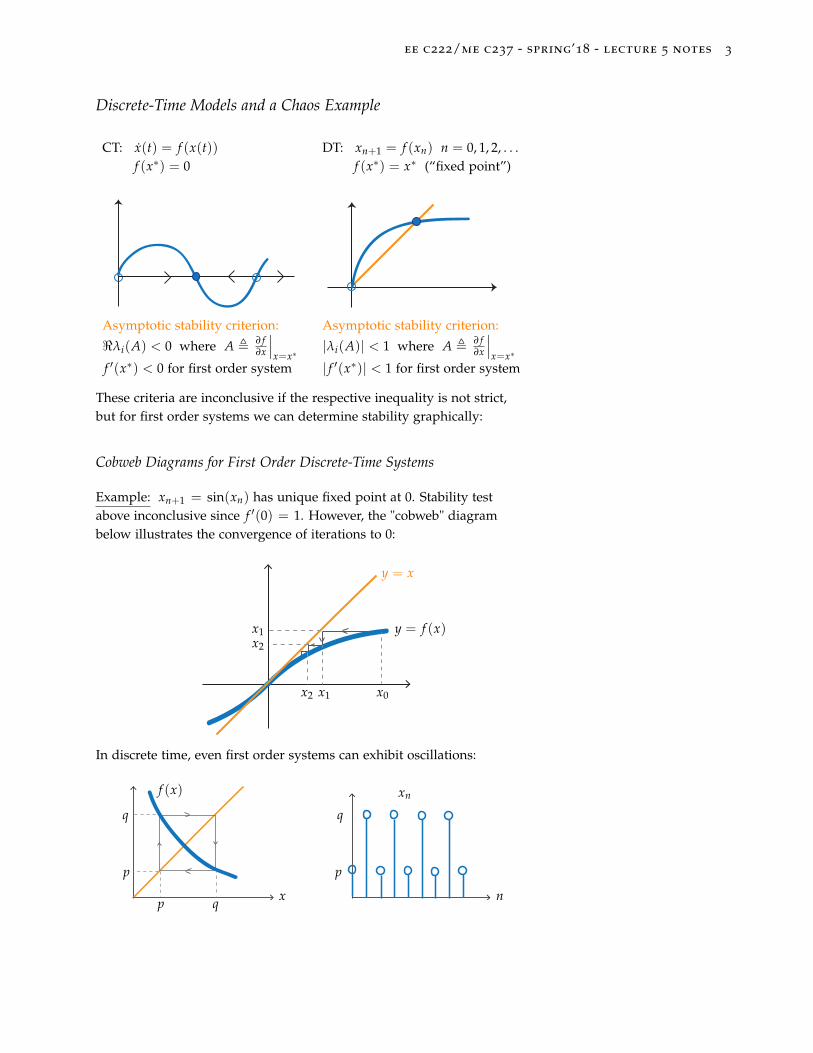
Discrete-Time Models and a Chaos Example
CT: x(t) = f (x(t)) DT: xn+1 = f (xn) n = 0, 1, 2, . . .f (x∗) = 0 f (x∗) = x∗ (“fixed point”)
Asymptotic stability criterion: Asymptotic stability criterion:
<λi(A) < 0 where A , ∂ f∂x
∣∣∣x=x∗
|λi(A)| < 1 where A , ∂ f∂x
∣∣∣x=x∗
f ′(x∗) < 0 for first order system | f ′(x∗)| < 1 for first order system
These criteria are inconclusive if the respective inequality is not strict,but for first order systems we can determine stability graphically:
Cobweb Diagrams for First Order Discrete-Time Systems
Example: xn+1 = sin(xn) has unique fixed point at 0. Stability testabove inconclusive since f ′(0) = 1. However, the "cobweb" diagrambelow illustrates the convergence of iterations to 0:
x0x1x2
x1x2
y = x
y = f (x)
In discrete time, even first order systems can exhibit oscillations:
nx
f (x) xn
p q
p
q
p
q

ee c222/me c237 - spring’18 - lecture 5 notes 4
Detecting Cycles Analytically
f (p) = q f (q) = p =⇒ f ( f (p)) = p f ( f (q)) = q
For the existence of a period-2 cycle, the map f ( f (·)) must have twofixed points in addition to the fixed points of f (·).
Period-3 cycles: fixed points of f ( f ( f (·))).
Chaos in a Discrete Time Logistic Growth Model
xn+1 = r(1− xn)xn (3)
Range of interest: 0 ≤ x ≤ 1 (xn > 1 ⇒ xn+1 < 0)
x
r/4
0 1
We will study the range 0 ≤ r ≤ 4 so that f (x) = r(1− x)x maps [0, 1]onto itself.
Fixed points: x = r(1− x)x ⇒
x∗ = 0 andx∗ = 1− 1
r if r > 1.
r ≤ 1: x∗ = 0 unique and stable fixed point
x0 1
r > 1: x = 0 unstable because f ′(0) = r > 1
x1− 1
r0 1

ee c222/me c237 - spring’18 - lecture 5 notes 5
Note that a transcritical bifurcation occurred at r = 1, creating thenew equilibrium
x∗ = 1− 1r
.
Evaluate its stability using f ′(x∗) = r(1− 2x∗) = 2− r.
r < 3 ⇒ | f ′(x∗)| < 1 (stable)
r > 3 ⇒ | f ′(x∗)| > 1 (unstable).
At r = 3, a period-2 cycle is born:
x = f ( f (x))
= r(1− f (x)) f (x)
= r(1− r(1− x)x)r(1− x)x
= r2x(1− x)(1− r + rx− rx2)
0 = r2x(1− x)(1− r + rx− rx2)− x
Factor out x and (x− 1 + 1r ), find the roots of the quotient:
p, q =r + 1∓
√(r− 3)(r + 1)2r
x1− 1
r0 1p q
f ( f (x))
y = x
This period-2 cycle is stable when r < 1 +√
6 = 3.4494:
ddx
f ( f (x))∣∣∣∣x=p
= f ′( f (p)) f ′(p) = f ′(p) f ′(q) = 4 + 2r− r2
|4 + 2r− r2| < 1 ⇒ 3 < r < 1 +√
6 = 3.4494
At r = 3.4494, a period-4 cycle is born!
“period doubling bifurcations”
r0 1 3 3.44
ee c222/me c237 - spring’18 - lecture 5 notes 6
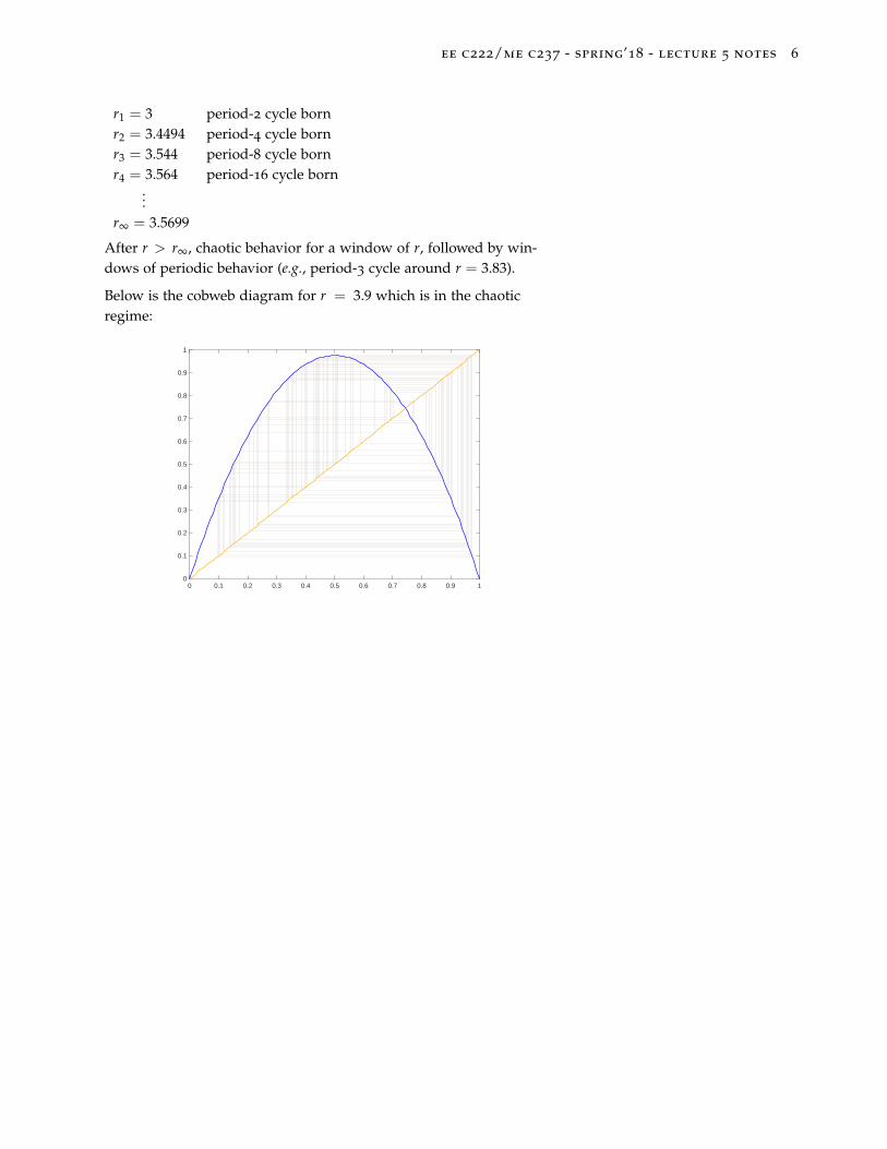
r1 = 3 period-2 cycle bornr2 = 3.4494 period-4 cycle bornr3 = 3.544 period-8 cycle bornr4 = 3.564 period-16 cycle born
...r∞ = 3.5699
After r > r∞, chaotic behavior for a window of r, followed by win-dows of periodic behavior (e.g., period-3 cycle around r = 3.83).
Below is the cobweb diagram for r = 3.9 which is in the chaoticregime:
0 0.1 0.2 0.3 0.4 0.5 0.6 0.7 0.8 0.9 10
0.1
0.2
0.3
0.4
0.5
0.6
0.7
0.8
0.9
1

EE C222/ME C237 - Spring’18 - Lecture 6 Notes11 Licensed under a Creative CommonsAttribution-NonCommercial-ShareAlike4.0 International License.Murat Arcak
February 5 2018
Mathematical BackgroundSastry, Chapter 3
x = f (x) x(0) = x0 (1)
Do solutions exist? Are they unique?
• If f (·) is continuous (C0) then a solution exists, but C0 is not suffi-cient for uniqueness.
Example: x = x13 with x(0) = 0
x(t) ≡ 0, x(t) =(
23
t) 3
2are both solutions
x
x1/3
∞ slopeat x=0
• Sufficient condition for uniqueness: “Lipschitz continuity” (morerestrictive than C0)
| f (x)− f (y)| ≤ L|x− y| (2)
Definition: f (·) is locally Lipschitz if every point x0 has a neighbor-hood where (2) holds for all x, y in this neighborhood and for all t forsome L.
Example: (·) 13 is NOT locally Lipschitz (due to ∞ slope)
(·)3 is locally Lipschitz:
x3 − y3 = (x2 + xy + y2)︸ ︷︷ ︸in any nbhdof x0, we canfind L to upperbound this
(x− y)
=⇒ |x3 − y3| ≤ L|x− y|

ee c222/me c237 - spring’18 - lecture 6 notes 2
• If f (·) is continuously differentiable (C1), then it is locally Lips-chitz.
Examples: x3, x2, ex, etc.
The converse is not true: local Lipschitz 6⇒ C1
Example:
x
sat(x)
−1
1−1
1
Not differentiable at x = ∓1, but locally Lipschitz:
| sat(x)− sat(y)| ≤ |x− y| (L = 1).
LC0
C1
x1/3
sat(x)
x2, x3, ...
Definition continued: f (·) is globally Lipschitz if (2) holds ∀x, y ∈ Rn
(i.e., the same L works everywhere).
Examples: sat(·) is globally Lipschitz. (·)3 is not globally Lipschitz:
x
→ slope getting steeper
• Suppose f (·) is C1. Then it is globally Lipschitz iff ∂ f∂x is bounded.
L = supx| f ′(x)|

ee c222/me c237 - spring’18 - lecture 6 notes 3
Preview of existence theorems:
1. f (·) is C0 =⇒ existence of solution x(t) on finite interval [0, t f ).
2. f (·) locally Lipschitz =⇒ existence and uniqueness on [0, t f ).
3. f (·) globally Lipschitz =⇒ existence and uniqueness on [0, ∞).
Examples:
• x = x2 (locally Lipschitz) admits unique solution on [0, t f ), butt f < ∞ from Lecture 1 (finite escape).
• x = Ax globally Lipschitz, therefore no finite escape
|Ax− Ay| ≤ L|x− y| with L = ‖A‖
The rest of the lecture introduces concepts that are used in proving theexistence theorems mentioned above.
Normed Linear Spaces
Definition: X is a normed linear space if there exists a real-valuednorm | · | satisfying:
1. |x| ≥ 0 ∀x ∈ X, |x| = 0 iff x = 0.
2. |x + y| ≤ |x|+ |y| ∀x, y ∈ X (triangle inequality)
3. |αx| = |α| · |x| ∀α ∈ R and x ∈ X.
Definition: A sequence xk in X is said to be a Cauchy sequence if
|xk − xm| → 0 as k, m→ ∞. (3)
Every convergent sequence is Cauchy. The converse is not true.
Definition: X is a Banach space if every Cauchy sequence convergesto an element in X.
All Euclidean spaces are Banach spaces.
Example:
Cn[a, b]: the set of all continuous functions [a, b]→ Rn with norm:
|x|C = maxt∈[a,b]
|x(t)|
tba
x
1. |x|C ≥ 0 and |x|C = 0 iff x(t) ≡ 0.

ee c222/me c237 - spring’18 - lecture 6 notes 4
2. |x + y|C = maxt∈[a,b]
|x(t) + y(t)| ≤ maxt∈[a,b]
|x(t)|+ |y(t)| ≤ |x|C + |y|C
3. |α · x|C = maxt∈[a,b]
|α| · |x(t)| = |α| · |x|C
It can be shown that Cn[a, b] is a Banach space.
Fixed Point Theorems
T(x) = x (4)
Brouwer’s Theorem (Euclidean spaces):
If U is a closed bounded subset of a Euclidean space and T : U → Uis continuous, then T has a fixed point in U.
Schauder’s Theorem (Brouwer’s Thm→ Banach spaces):
If U is a closed bounded convex subset of a Banach space X andT : U → U is completely continuous2, then T has a fixed point in U. 2 continuous and for any bounded set
B ⊆ U the closure of T(B) is compactContraction Mapping Theorem:
If U is a closed subset of a Banach space and T : U → U is such that
|T(x)− T(y)| ≤ ρ|x− y| ρ < 1 ∀x, y ∈ U
then T has a unique fixed point in U and the solutions of xn+1 =
T(xn) converge to this fixed point from any x0 ∈ U.
Example: The logistic map (Lecture 5)
T(x) = rx(1− x) (5)
with 0 ≤ r ≤ 4 maps U = [0, 1] to U. |T′(x)| ≤ r ∀x ∈ [0, 1], so thecontraction property holds with ρ = r.
x
r/4
0 1
If r < 1, the contraction mapping theorem predicts a unique fixedpoint that attracts all solutions starting in [0, 1].

ee c222/me c237 - spring’18 - lecture 6 notes 5
x
Proof steps for the Contraction Mapping Thm:
1. Show that xn formed by xn+1 = T(xn) is a Cauchy sequence.Since we are in a Banach space, this implies a limit x∗ exists.
2. Show that x∗ = T(x∗).
3. Show that x∗ is unique.
Details of each step:
1. |xn+1 − xn| = |T(xn)− T(xn−1)| ≤ ρ|xn − xn−1|≤ ρ2|xn−1 − xn−2|
...
≤ ρn|x1 − x0|.
|xn+r − xn| ≤ |xn+r − xn+r−1|+ · · ·+ |xn+1 − xn|≤ (ρn+r + · · ·+ ρn)|x1 − x0|= ρn(1 + · · ·+ ρr)|x1 − x0|
≤ ρn 11− ρ
|x1 − x0|
Since ρn
1−ρ → 0 as n→ ∞, we have |xn+r − xn| → 0 as n→ ∞.
2. |x∗ − T(x∗)| = |x∗ − xn + T(xn−1)− T(x∗)|≤ |x∗ − xn|+ |T(xn−1)− T(x∗)|≤ |x∗ − xn|+ ρ|x∗ − xn−1|.
Since xn converges to x∗, we can make this upper bound ar-bitrarily small by choosing n sufficiently large. This means that|x∗ − T(x∗)| = 0, hence x∗ = T(x∗).
3. Suppose y∗ = T(y∗) y∗ 6= x∗.
|x∗ − y∗| = |T(x∗)− T(y∗)| ≤ ρ|x∗ − y∗| =⇒ x∗ = y∗.
Thus we have a contradiction.
EE C222/ME C237 - Spring’18 - Lecture 7 Notes11 Licensed under a Creative CommonsAttribution-NonCommercial-ShareAlike4.0 International License.Murat Arcak
February 7 2018
Existence and Uniqueness Theorems for ODEsKhalil (Section 3.1), Sastry (Section 3.4)
x = f (t, x) x(0) = x0 (1)
Theorem 1: f (t, x) locally Lipschitz in x and continuous in t
⇒ existence and uniqueness on some finite interval [0, δ].
Sketch of the proof: From the local Lipschitz assumption, we canfind r > 0 and L > 0 such that
| f (t, x)− f (t, y)| ≤ L|x− y| ∀x, y ∈ x ∈ Rn : |x− x0| ≤ r.
If x(t) is a solution, then:
x(t) = x0 +∫ t
0f (τ, x(τ))dτ︸ ︷︷ ︸
=: T(x)(t)
.
To apply the Contraction Mapping Theorem:
1. Choose δ small enough that T maps the following subset ofCn[0, δ] to itself :
U = x ∈ Cn[0, δ] : |x(t)− x0| ≤ r ∀t ∈ [0, δ],
i.e.
|x(t)− x0| ≤ r ∀t ∈ [0, δ] ⇒ |T(x)(t)− x0| ≤ r ∀t ∈ [0, δ]. (2)
To find such a δ note that
T(x)(t)− x0 =∫ t
0f (τ, x(τ))dτ =
∫ t
0
(f (τ, x(τ))− f (τ, x0) + f (τ, x0)
)dτ
|T(x)(t)− x0| ≤∫ δ
0| f (τ, x(τ))− f (τ, x0)|dτ +
∫ δ
0| f (τ, x0)|dτ
≤∫ δ
0L|x(τ)− x0|dτ +
∫ δ
0hdτ where h is a bound on | f (τ, x0)|
≤ (Lr + h)δ.
Thus, by choosing δ ≤ rLr+h we ensure that the implication (2)
holds.
2. Show that T is a contraction in U, i.e., there exists ρ < 1 s.t.
x, y ∈ U =⇒ |T(x)− T(y)|C ≤ ρ|x− y|C.
ee c222/me c237 - spring’18 - lecture 7 notes 2
Note that, for all t ∈ [0, δ],
|T(x)(t)− T(y)(t)| =∫ t
0| f (τ, x(τ))− f (τ, y(τ))|dτ
≤ L∫ t
0|x(τ)− y(τ)|dτ
≤ Lδ︸︷︷︸=:ρ
maxτ∈[0,δ]
|x(τ)− y(τ)| = ρ|x− y|C.
Therefore,
|T(x)− T(y)|C = maxt∈[0,δ]
|T(x)(t)− T(y)(t)| ≤ ρ|x− y|C
and ρ < 1 if δ ≤ rLr+h as prescribed above.
Theorem 2: f (t, x) globally Lipschitz in x uniformly2 in t, and contin- 2 same L works for all t
uous in t =⇒ existence and uniqueness on [0, ∞).
Proof: Choose a δ that doesn’t depend on x0 and apply Theorem 1 re-peatedly to cover [0, ∞). This is possible because L works everywhereand we can pick r as large as we wish. Indeed, for any δ < 1
L , we canchoose r large enough that δ ≤ r
Lr+h .
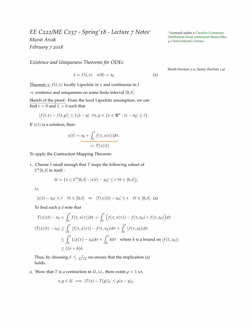
Q: Why can’t we do this in Theorem 1?
A: δ depends on x0 (no universal L) and x0 changes at the next itera-tion. We can’t use the same δ in every iteration:
t f0 δ1 δ2 δ3
• The theorems above are sufficient only, and can be conservative:
Example: x = −x3 is not globally Lipschitz but
x(t) = sgn(x0)
√x2
01 + 2tx2
0
is defined on [0, ∞).
Continuous Dependence on Initial Conditions and Parameters
Theorem 3: (Continuous dependence on initial conditions) Letx(t), y(t) be two solutions of x = f (t, x) starting from x0 and y0,and remaining in a set with Lipschitz constant L on [0, τ]. Then, forany ε > 0, there exists δ(ε, τ) > 0 such that
|x0 − y0| ≤ δ =⇒ |x(t)− y(t)| ≤ ε ∀t ∈ [0, τ].
ee c222/me c237 - spring’18 - lecture 7 notes 3
• This conclusion does not hold on infinite time intervals (even if fis globally Lipschitz).
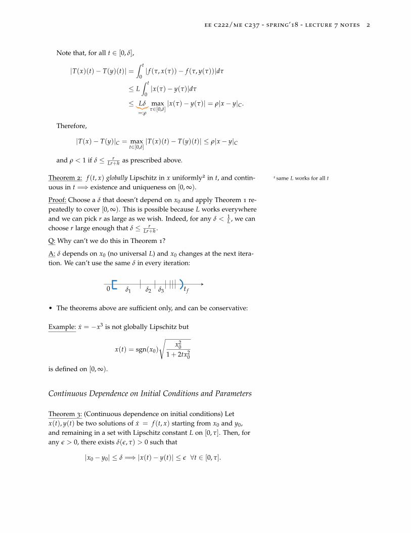
Example: bistable system
x(t)
y(t)
x0 y0• •
If ε is smaller than the distance between the two stable equilibria, nochoice of δ guarantees |x(t)− y(t)| ≤ ε ∀t ≥ 0.
• Theorem 3 also shows continuous dependence on parameter µ inf (t, x, µ) if we rewrite the system equations as:
x = f (t, x, µ)
µ = 0X =
[xµ
]X = F(t, X) ,
[f (t, x, µ)
0
],
where µ appears as a state variable with initial condition µ(0) = µ.
Q: How do you reconcile bifurcations with continuous dependenceon parameters? We could pick two values of the bifurcation param-eter arbitrarily close, but one below and one above the critical value,thereby expecting a drastic difference in the solutions.
A: The two solutions are close in the short term (Theorem 3 holds onfinite time intervals); the drastic difference builds up over time.
Sensitivity to Parameters
Consider the system
x = f (t, x, µ) x ∈ Rn, µ ∈ Rp (3)
where µ is a vector of p parameters, and let φ(t, x0, µ) denote thetrajectories starting at the initial condition x0.
To determine to what extent this trajectory depends on the parame-ters we define the n× p sensitivity matrix:
S(t, x0, µ) :=∂φ(t, x0, µ)
∂µ=
[∂φ(t, x0, µ)
∂µ1· · · ∂φ(t, x0, µ)
∂µp
], (4)

ee c222/me c237 - spring’18 - lecture 7 notes 4
where each column is the sensitivity with respect to a particularparameter.
To see how S(t, x0, µ) can be computed numerically, first note thatφ(t, x0, µ) satisfies the equation (3), that is,
∂φ(t, x0, µ)
∂t= f (t, φ(t, x0, µ), µ).
Next, differentiate both sides with respect to µ:
∂2φ(t, x0, µ)
∂t∂µ=
∂ f∂x
(t, φ(t, x0, µ), µ)∂φ(t, x0, µ)
∂µ+
∂ f∂µ
(t, φ(t, x0, µ), µ)
and use the definition of the sensitivity matrix to rewrite this as
∂S(t, x0, µ)
∂t=
∂ f∂x
(t, φ(t, x0, µ), µ)S(t, x0, µ) +∂ f∂µ
(t, φ(t, x0, µ), µ).
Thus, S can be computed by numerical integration of (3) simultane-ously with
S =∂ f∂x
(t, x, µ)S +∂ f∂µ
(t, x, µ).
The initial condition for S is ∂x0∂µ = 0, assuming that x0 is independent
of the parameters.
Example: For the harmonic oscillator
x1 = −µx2
x2 = µx1
we have∂ f∂x
=
[0 −µ
µ 0
]∂ f∂µ
=
[−x2
x1
].
Thus the sensitivity equation is
S =
[0 −µ
µ 0
]S +
[−x2
x1
].
Logarithmic Sensitivity
To compare the sensitivity with respect to multiple parametersµ1, . . . , µp it is preferable to use the logarithmic sensitivity
∂φ(t, x0, µ)
∂µi/µi=
∂φ(t, x0, µ)
∂ ln µi
so that the denominator is dimensionless and represents the changein the parameter µi relative to its nominal value. This means thatthe ith column of the sensitivity matrix S in (4) must be multipliedwith the nominal parameter µi, i = 1, . . . , p, before these columns arecompared for the relative significance of the parameters.

ee c222/me c237 - spring’18 - lecture 7 notes 5
Application to Parameter Tuning and Identification
Sensitivity equations are useful for solving a class of optimizationproblems of the form
minµ J(µ) =∫ t1
t0q(t, x(t), µ)dt
subject to x = f (t, x, µ), x(t0) = x0.
For example, one may take q(t, x) = |h(x(t))− r(t)|2 to penalize theerror between the output y(t) = h(x(t)) of a control system and areference trajectory r(t) to be followed. In this example x = f (t, x, µ)
represents the closed loop model with tunable control parameters µ.
In other applications x = f (t, x, µ) may represent the model of aphysical process with unknown parameters, and q(t, x) = |h(x(t))−r(t)|2 penalizes the error between the model prediction for a variable,y(t) = h(x(t)), and the experimental observation r(t). Then theoptimization problem above aims to find parameters that best fit theexperimental data.
A typical optimization algorithm requires the gradient ∂J(µ)∂µ , which
can be obtained with the help of the chain rule and the sensitivityequations:
∂J(µ)∂µ
=∫ t1
t0
(∂q∂x
(t, x(t), µ)S(t, x0, µ) +∂q∂µ
(t, x(t), µ)
)dt.

EE C222/ME C237 - Spring’18 - Lecture 8 Notes11 Licensed under a Creative CommonsAttribution-NonCommercial-ShareAlike4.0 International License.Murat Arcak
February 12 2018
Lyapunov Stability TheoryKhalil Chapter 4, Sastry Chapter 5
Consider a time invariant system
x = f (x)
and assume equilibrium at x = 0, i.e. f (0) = 0. If the equilibrium ofinterest is x∗ 6= 0, let x = x− x∗:
˙x = f (x) = f (x + x∗) , f (x) =⇒ f (0) = 0.
Definition: The equilibrium x = 0 is stable if for each ε > 0, thereexists δ > 0 such that
|x(0)| ≤ δ =⇒ |x(t)| ≤ ε ∀t ≥ 0. (1)
Bε
Bδ
It is unstable if not stable.
Asymptotically stable if stable and x(t) → 0 for all x(0) in a neigh-borhood of x = 0.
Globally asymptotically stable if stable and x(t)→ 0 for every x(0).
Note that x(t) → 0 does not necessarily imply stability: one canconstruct an example where trajectories converge to the origin, butonly after a large detour that violates the stability definition.
Bε
a homoclinic orbit

ee c222/me c237 - spring’18 - lecture 8 notes 2
Lyapunov’s Stability Theorem
Aleksandr Lyapunov (1857-1918)
1. Let D be an open, connected subset of Rn that includes x = 0. Ifthere exists a C1 function V : D → R such that
V(0) = 0 and V(x) > 0 ∀x ∈ D− 0 (positive definite)
and
V(x) := ∇V(x)T f (x) ≤ 0 ∀x ∈ D (negative semidefinite)
then x = 0 is stable.
2. If V(x) < 0 ∀x ∈ D− 0 (negative definite)
then x = 0 is asymptotically stable.
3. If, in addition, D = Rn and
|x| → ∞ =⇒ V(x)→ ∞ (radially unbounded)
then x = 0 is globally asymptotically stable.
Sketch of the proof:
The sets Ωc , x : V(x) ≤ c for constants c are called level sets of Vand are positively invariant because ∇V(x)T f (x) ≤ 0.
Stability follows from this property: choose a level set inside the ballof radius ε, and a ball of radius δ inside this level set. Trajectoriesstarting in Bδ can’t leave Bε since they remain inside the level set.
Bε
level set inside Bε
Bδ inside level set
ee c222/me c237 - spring’18 - lecture 8 notes 3
Asymptotic stability:
Since V(x(t)) is decreasing and bounded below by 0, we conclude
V(x(t))→ c ≥ 0.
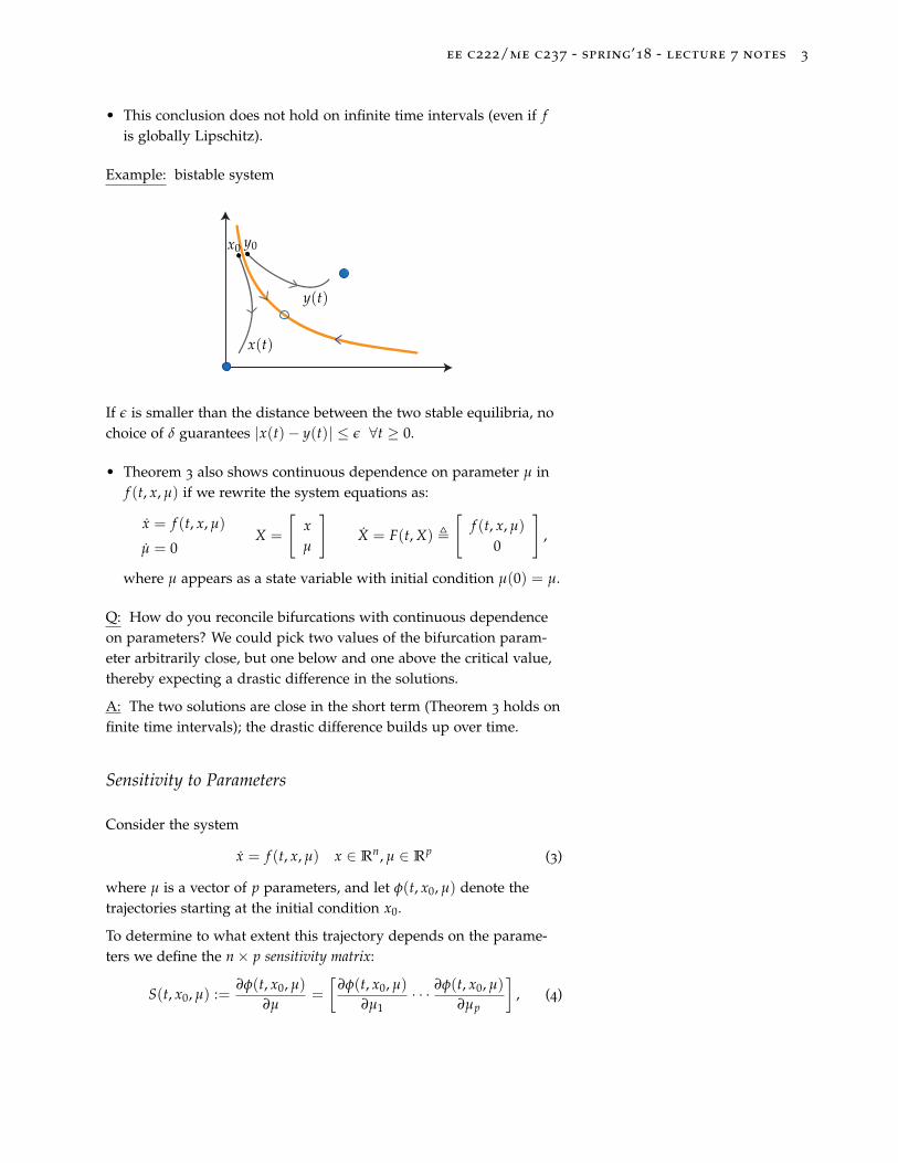
We will show c = 0 (i.e., x(t)→ 0) by contradiction. Suppose c 6= 0:
V(x) = V(x0)
V(x) = c 6= 0x0•
Letγ , max
x: c≤V(x)≤V(x0)−V(x) > 0
where the maximum exists because it is evaluated over a bounded2 2 By positive definiteness of V, the levelsets x : V(x) ≤ constant are boundedwhen the constant is sufficiently small.Since we are proving local asymptoticstability we can assume x0 is closeenough to the origin that the constantV(x0) is sufficiently small.
set, and is positive because V(x) < 0 away from x = 0. Then,
V(x) ≤ −γ =⇒ V(x(t)) ≤ V(x0)− γt,
which implies V(x(t)) < 0 for t > V(x0)γ – a contradiction because
V ≥ 0. Therefore, c = 0 which implies x(t)→ 0.
Global asymptotic stability:
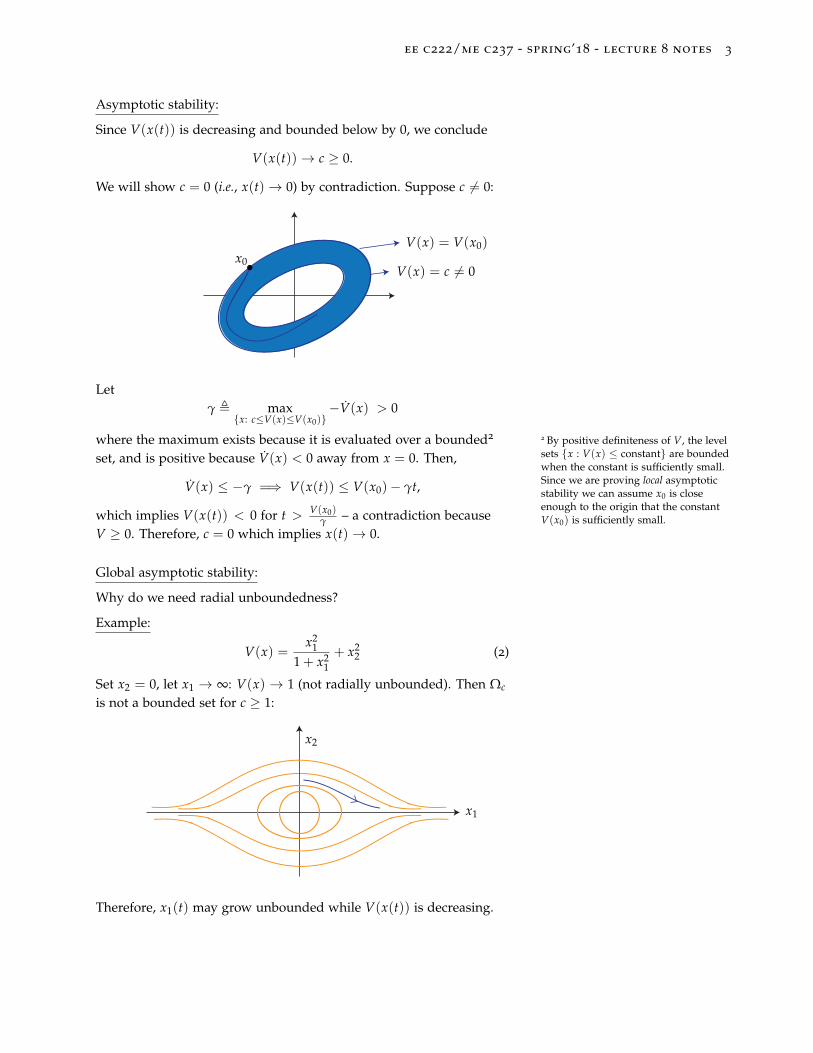
Why do we need radial unboundedness?
Example:
V(x) =x2
11 + x2
1+ x2
2 (2)
Set x2 = 0, let x1 → ∞: V(x) → 1 (not radially unbounded). Then Ωc
is not a bounded set for c ≥ 1:
x1
x2
Therefore, x1(t) may grow unbounded while V(x(t)) is decreasing.

ee c222/me c237 - spring’18 - lecture 8 notes 4
Finding Lyapunov Functions
Example:x = −g(x) x ∈ R, xg(x) > 0 ∀x 6= 0 (3)
x
g(x)
V(x) = 12 x2 is positive definite and radially unbounded.
V(x) = −xg(x) is negative definite. Therefore x = 0 is globallyasymptotically stable.
If xg(x) > 0 only in (−b, c)− 0, then take D = (−b, c)
x
g(x)
−b c=⇒ x = 0 is locally asymptotically stable.
There are other equilibria where g(x) = 0, so we know global asymp-totic stability is not possible.
Example:
x1 = x2
x2 = −ax2 − g(x1) a ≥ 0, xg(x) > 0 ∀x ∈ (−b, c)− 0(4)
The pendulum is a special case withg(x) = sin(x).
The choice V(x) = 12 x2
1 +12 x2
2 doesn’t work because V(x) is signindefinite (show this).
The functionV(x) =
∫ x1
0g(y)dy +
12
x22
is positive definite on D = (−b, c)− 0 and
V(x) = g(x1)x2 − ax22 − x2g(x1) = −ax2
2
is negative semidefinite =⇒ stable.
If a = 0, no asymptotic stability because V(x) = 0 =⇒ V(x(t)) =
V(x(0)).
"conservative system"
If a > 0, (4) is asymptotically stable but the Lyapunov function abovedoesn’t allow us to reach that conclusion. We need either another Vwith negative definite V, or the Lasalle-Krasovskii Invariance Princi-ple to be discussed in the next lecture.

EE C222/ME C237 - Spring’18 - Lecture 9 Notes11 Licensed under a Creative CommonsAttribution-NonCommercial-ShareAlike4.0 International License.Murat Arcak
February 14 2018
LaSalle-Krasovskii Invariance Principle
• Applicable to time-invariant systems.
• Allows us to conclude asymptotic stability from V(x) ≤ 0 ifadditional conditions hold:
Suppose Ωc = x : V(x) ≤ c is bounded and V(x) ≤ 0 in Ωc. DefineS = x ∈ Ωc : V(x) = 0 and let M be the largest invariant set in S.Then, for every x(0) ∈ Ωc, x(t)→ M.
Corollary: If no solution other than x(t) ≡ 0 can stay identically in Sthen M = 0 and we conclude asymptotic stability.
Example (from last lecture):
x1 = x2
x2 = −ax2 − g(x1) a > 0, xg(x) > 0 ∀x 6= 0(1)
V(x) =∫ x1
0g(y)dy +
12
x22 =⇒ V(x) = −ax2
2
S = x ∈ Ωc|x2 = 0
If x(t) stays identically in S, then x2(t) ≡ 0 =⇒ x2(t) ≡ 0 =⇒g(x1(t)) ≡ 0 =⇒ x1(t) ≡ 0 =⇒ asymptotic stability from Corollary.
Example (linear system): Same system above with g(x1) = bx1:
x1 = x2
x2 = −ax2 − bx1 a > 0, b > 0(2)
V(x) = b2 x2
1 +12 x2
2 =⇒ V(x) = −ax22 =⇒ Invariance Principle works
as in the example above.
Alternatively, construct another Lyapunov function with negativedefinite V(x). Try V(x) = xT Px where P = PT > 0 is to be selected.
V(x) = xT Px + Px = xT(AT P + PA)x where A =
[0 1−b −a
]
Let P = 12
[b ε
ε 1
], that is V(x) = b
2 x21 + εx1x2 +
12 x2
2.
Note that P > 0 if ε2 < b.

ee c222/me c237 - spring’18 - lecture 9 notes 2
AT P+ PA =
[−εb −εa/2−εa/2 ε− a
] ≤ 0 if ε = 0
< 0 if 0 < ε < a and εb(a− ε) >ε2a2
4︸ ︷︷ ︸0<ε< ba
b+ a24
Linear SystemsSastry (Sec. 5.7-5.8), Khalil (Sec. 4.3)
x = Ax x ∈ Rn (3)
x = 0 is stable if <λi(A) ≤ 0 for all i = 1, · · · , n and eigenvalues onthe imaginary axis have Jordan blocks of order one.2 It is asymptoti- 2 i.e., if λ is an eigenvalue of multiplicity
q then λI − A must have rank n− q.cally stable if <λi(A) < 0 for all i, i.e., A is "Hurwitz."
Example:
A =
[0 10 0
]is unstable:
x1 = x2
x2 = 0
x1(t) = x1(0) + x2(0)t
A =
[0 00 0
]is stable.
Lyapunov Functions for Linear Systems
V(x) = xT Px P = PT > 0
V(x) = xT(AT P + PA)x(4)
If ∃P = PT > 0 such that AT P + PA = −Q < 0, then A is Hurwitz.The converse is also true:
Theorem: A is Hurwitz if and only if for any Q = QT > 0, thereexists P = PT > 0 such that
AT P + PA = −Q. (5)
Moreover, the solution P is unique. (5) is known as the Lyapunov Equation.The Matlab command lyap(A’,Q)
returns the solution P.Proof:
(if) From (4) above, the Lyapunov function V(x) = xT Px provesasymptotic stability which means A is Hurwitz.
(only if) Assume <λi(A) < 0 ∀i. Show ∃P = PT > 0 such thatAT P + PA = −Q.
Candidate:P =
∫ ∞
0eAT tQeAtdt. (6)
ee c222/me c237 - spring’18 - lecture 9 notes 3
• The integral exists because ‖eAt‖ ≤ κe−αt.
• P = PT
• P > 0 because xT Px =∫ ∞
0(eAtx)TQ(eAtx)︸ ︷︷ ︸
,φ(t,x)
dt ≥ 0 and
xT Px = 0 =⇒ φ(t, x) ≡ 0 =⇒ x = 0 because eAt is nonsingular.
• AT P + PA =∫ ∞
0
(ATeAT tQeAt + eAT tQeAt A
)︸ ︷︷ ︸
=ddt
(eAtQeAt
)dt
= eAT tQeAt∣∣∣∞0= 0−Q = −Q
Uniqueness:
Suppose there is another P = PT > 0 satisfying P 6= P, and AT P +
PA = −Q.
=⇒ (P− P)A + AT(P− P) = 0
Define W(x) = xT(P− P)x.
ddt
W(x(t)) = 0 =⇒W(x(t)) = W(x(0)) ∀t.
Since A is Hurwitz, x(t)→ 0 and W(x(t))→ 0.
Combining the two statements above, we conclude W(x(0)) = 0 forany x(0). This is possible only if P− P = 0 which contradicts P 6= P.
Invariance Principle Applied to Linear Systems
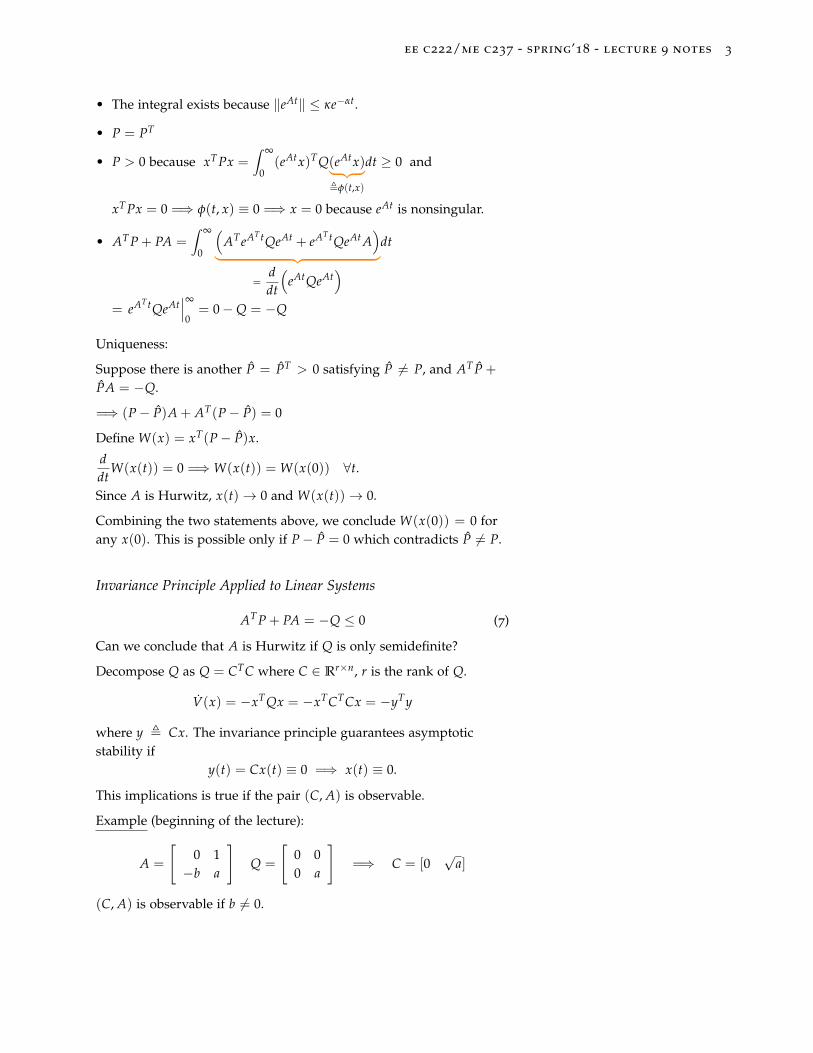
AT P + PA = −Q ≤ 0 (7)
Can we conclude that A is Hurwitz if Q is only semidefinite?
Decompose Q as Q = CTC where C ∈ Rr×n, r is the rank of Q.
V(x) = −xTQx = −xTCTCx = −yTy
where y , Cx. The invariance principle guarantees asymptoticstability if
y(t) = Cx(t) ≡ 0 =⇒ x(t) ≡ 0.
This implications is true if the pair (C, A) is observable.
Example (beginning of the lecture):
A =
[0 1−b a
]Q =
[0 00 a
]=⇒ C = [0
√a]
(C, A) is observable if b 6= 0.
EE C222/ME C237 - Spring’18 - Lecture 10 Notes11 Licensed under a Creative CommonsAttribution-NonCommercial-ShareAlike4.0 International License.Murat Arcak
February 21 2018
Lyapunov’s Linearization Method
x = f (x) f (0) = 0
Define A = ∂ f (x)∂x
∣∣∣x=0
and decompose f (x) as
f (x) = Ax + g(x) where|g(x)||x| → 0 as |x| → 0.
Theorem: The origin is asymptotically stable if <λi(A) < 0 foreach eigenvalue, and unstable if <λi(A) > 0 for some eigenvalue.
Note: We can conclude only local asymptotic stability from this lin-earization. Inconclusive if A has eigenvalues on the imaginary axis.
Proof: Find P = PT > 0 such that AT P + PA = −Q < 0. Use V(x) =xT Px as a Lyapunov function for the nonlinear system x = Ax + g(x).
V(x) = xT P(Ax + g(x)) + (Ax + g(x))T Px
= xT(PA + AT P)x + 2xT Pg(x)
≤ −xTQx + 2|x|‖P‖|g(x)|
λmin(Q)|x|2 ≤ xTQx ≤ λmax(Q)|x|2
V(x) ≤ −λmin(Q)|x|2 + 2‖P‖|x||g(x)|
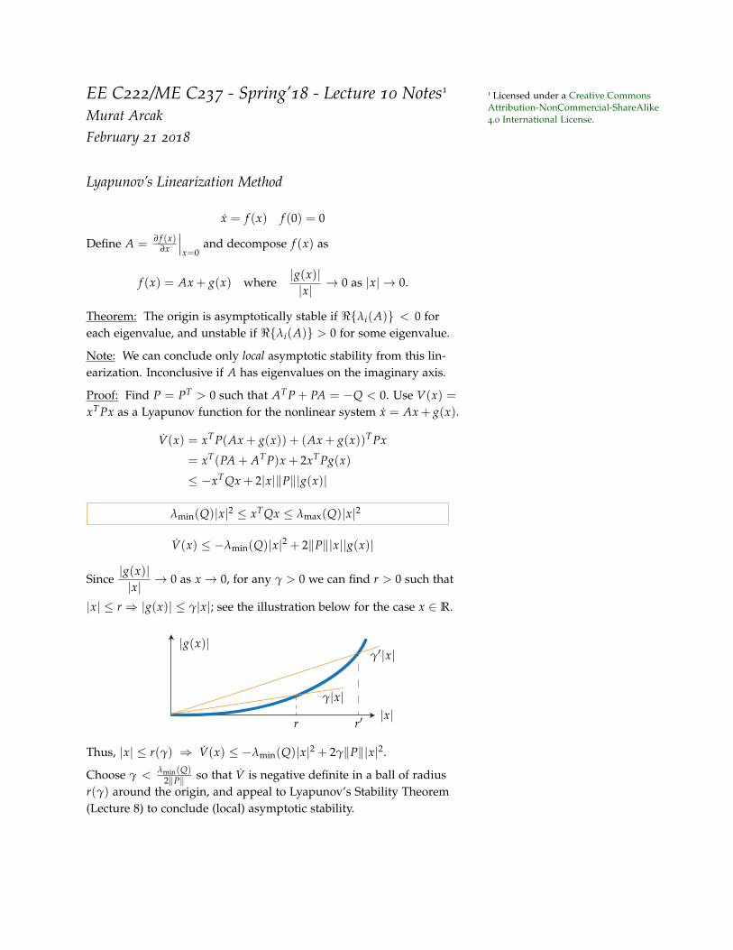
Since|g(x)||x| → 0 as x → 0, for any γ > 0 we can find r > 0 such that
|x| ≤ r ⇒ |g(x)| ≤ γ|x|; see the illustration below for the case x ∈ R.
|x|γ|x|
r
|g(x)|γ′|x|
r′
Thus, |x| ≤ r(γ) ⇒ V(x) ≤ −λmin(Q)|x|2 + 2γ‖P‖|x|2.
Choose γ < λmin(Q)2‖P‖ so that V is negative definite in a ball of radius
r(γ) around the origin, and appeal to Lyapunov’s Stability Theorem(Lecture 8) to conclude (local) asymptotic stability.

ee c222/me c237 - spring’18 - lecture 10 notes 2
Region of Attraction
RA = x : φ(t, x)→ 0 (1)
“Quantifies” local asymptotic stability. Global asymptotic stability:RA = Rn.
Proposition: If x = 0 is asymptotically stable, then its region of at-traction is an open, connected, invariant set. Moreover, the boundaryis formed by trajectories.
Example: van der Pol system in reverse time:
x1 = −x2
x2 = x1 − x2 + x32
(2)
The boundary is the (unstable) limit cycle. Trajectories starting withinthe limit cycle converge to the origin.
∨∨
Example: bistable switch:
x1 = −ax1 + x2
x2 =x2
11 + x2
1− bx2
(3)
x1
x2
Estimating the Region of Attraction with a Lyapunov Function
Suppose V(x) < 0 in D − 0. The level sets of V inside D areinvariant and trajectories starting in them converge to the origin.

ee c222/me c237 - spring’18 - lecture 10 notes 3
Therefore we can use the largest levet set of V that fits into D as an(under)approximation of the region of attraction.
D x : V(x) ≤ c ⊂ RA
This estimate depends on the choice of Lyapunov function. A simple(but often conservative) choice is: V(x) = xT Px where P is selectedfor the linearization (see p.1).
Time-Varying SystemsKhalil (Sec. 4.5), Sastry (Sec. 5.2)
x = f (t, x) f (t, 0) ≡ 0 (4)
To simplify the definitions of stability and asymptotic stability forthe equilibrium x = 0, we first define a class of functions known as"comparison functions."
Comparison Functions
Definition: A continuous function α : [0, ∞) → [0, ∞) is class-K ifit is zero at zero and strictly increasing. It is class-K∞ if, in addition,α(r)→ ∞ as r → ∞.
A continuous function β : [0, ∞)× [0, ∞)→ [0, ∞) is class-KL if:
1. β(·, s) is class-K for every fixed s,
2. β(r, ·) is decreasing and β(r, s)→ 0 as s→ ∞, for every fixed r.
Example: α(r) = tan−1(r) is class-K, α(r) = rc, c > 0 is class-K∞,β(r, s) = rce−s is class-KL.
Proposition: If V(·) is positive definite, then we can find class-Kfunctions α1(·) and α2(·) such that
α1(|x|) ≤ V(x) ≤ α2(|x|). (5)
If V(·) is radially unbounded, we can choose α1(·) to be class-K∞.
Example: V(x) = xT Px P = PT > 0
α1(|x|) = λmin(P)|x|2 α2(|x|) = λmax(P)|x|2.

ee c222/me c237 - spring’18 - lecture 10 notes 4
Stability Definitions
Definition: x = 0 is stable if for every ε > 0 and t0, there exists δ > 0such that
|x(t0)| ≤ δ(t0, ε) =⇒ |x(t)| ≤ ε ∀t ≥ t0.
If the same δ works for all t0, i.e. δ = δ(ε), then x = 0 is uniformly stable.
It is easier to define uniform stability and uniform asymptotic stabil-ity using comparison functions:
• x = 0 is uniformly stable if there exists a class-K function α(·) anda constant c > 0 such that
|x(t)| ≤ α(|x(t0)|)
for all t ≥ t0 and for every initial condition such that |x(t0)| ≤ c.
• uniformly asymptotically stable if there exists a class-KL β(·, ·) s.t.
|x(t)| ≤ β(|x(t0)|, t− t0)
for all t ≥ t0 and for every initial condition such that |x(t0)| ≤ c.
• globally uniformly asymptotically stable if c = ∞.
• uniformly exponentially stable if β(r, s) = kre−λs for some k, λ > 0:
|x(t)| ≤ k|x(t0)|e−λ(t−t0)
for all t ≥ t0 and for every initial condition such that |x(t0)| ≤ c.
Example: Consider the following system, defined for t > −1:
x =−x
1 + t(6)
x(t) = x(t0)e∫ t
t0−11+s ds
= x(t0)elog(1+s)|t0t
= x(t0)elog 1+t01+t = x(t0)
1 + t0
1 + t
|x(t)| ≤ |x(t0)| =⇒ the origin is uniformly stable with α(r) = r.
The origin is also asymptotically stable, but not uniformly, becausethe convergence rate depends on t0:
x(t) = x(t0)1 + t0
1 + t0 + (t− t0)=
x(t0)
1 + t−t01+t0
.
t− t0
increasing t0
x(t)

EE C222/ME C237 - Spring’18 - Lecture 11 Notes11 Licensed under a Creative CommonsAttribution-NonCommercial-ShareAlike4.0 International License.Murat Arcak
February 26 2018
Time-Varying Systems Continued
Uniform stability: There exists a class K function α(·) and a constantc > 0, both independent of t0, such that
|x(t)| ≤ α(|x(t0)|) ∀t ≥ t0 when |x(t0)| ≤ c.
Uniform asymptotic stability: There exists a class KL function β(·, ·)and a constant c > 0 such that
|x(t)| ≤ β(|x(t0)|, t− t0) ∀t ≥ t0 when |x(t0)| ≤ c.
Uniform exponential stability: There exist constants k, λ, c > 0 s.t.
|x(t)| ≤ k|x(t0)|e−λ(t−t0) ∀t ≥ t0 when |x(t0)| ≤ c,
that is β(r, s) = kre−λs.
k > 1 allows for overshoot:
tt0
k|x(t0)|e−λ(t−t0)|x(t)|
|x(t0)|
k|x(t0)|
Example:
x = −x3 ⇒ x(t) = sgn(x(t0))
√x2
01 + 2(t− t0)x2
0
x = 0 is asymptotically stable but not exponentially stable.
Proposition: x = 0 is exponentially stable for x = f (x), f (0) = 0, if
and only if A , ∂ f∂x
∣∣∣x=0
is Hurwitz, that is <λi(A) < 0 ∀i.
Although strict inequality in <λi(A) < 0 is not necessary for asymp-totic stability (see example above where A = 0), it is necessary forexponential stability.

ee c222/me c237 - spring’18 - lecture 11 notes 2
Lyapunov’s Stability Theorem for Time-Varying SystemsKhalil, Section 4.5
1. If W1(x) ≤ V(t, x) ≤ W2(x) and V(t, x) , ∂V∂t + ∂V
∂x f (t, x) ≤ 0 forsome positive definite functions W1(·), W2(·) on a domain D thatincludes the origin, then x = 0 is uniformly stable.
xW1(x)
W2(x)V(t1, x)
V(t2, x)
2. If, further, V(t, x) ≤ −W3(x) ∀x ∈ D for some positive definiteW3(·), then x = 0 is uniformly asymptotically stable.
3. If D = Rn and W1(·) is radially unbounded, then x = 0 is globallyuniformly asymptotically stable.
4. If Wi(x) = ki|x|a, i = 1, 2, 3, for some constants k1, k2, k3, a > 0,then x = 0 is uniformly exponentially stable.
Proof:
1. α1(|x|) ≤W1(x) ≤ V(t, x) ≤W2(x) ≤ α2(|x|)
V ≤ 0⇒ V(x(t), t) ≤ V(x(t0), t0)
⇒ α1(|x(t)|) ≤ α2(|x(t0)|)⇒ |x(t)| ≤ α(|x(t0)|) , (α−1
1 α2)(|x(t0)|).
Note: The inverse of a class-K function is well defined locally(globally if K∞) and is class-K. The composition of two class-Kfunctions is also class-K.
2. V ≤ −W3(x) ≤ −α3(|x|) ≤ −α3(α−12 (V)) , −γ(V)
ddt
V(t, x(t)) ≤ −γ(V(t, x(t)))
Let y(t) be the solution of y = −γ(y), y(t0) = V(t0, x(t0)). Then,
V(t, x(t)) ≤ y(t).y
−γ(y)Since y = −γ(y) is a first order differential equation and −γ(y) <0 when y > 0, we conclude monotone convergence of y(t) to 0:
y(t) = β(y(t0), t− t0) =⇒ V(t, x(t)) ≤ β(V(t0, x(t0))︸ ︷︷ ︸≤α2(|x(t0)|)
, t− t0)
⇒ α1(|x(t)|) ≤ β(α2(|x(t0)|), t− t0)
⇒ |x(t)| ≤ β(|x(t0)|, t− t0) , α−11 (β(α2(|x(t0)|), t− t0))

ee c222/me c237 - spring’18 - lecture 11 notes 3
3. If α1(·) is class K∞ then α−11 (·) exists globally above.
4. α3(|x|) = k3|x|a, α2(|x|) = k2|x|a
⇒ γ(V) = α3(α−12 (V)) = k3
((Vk2
) 1a)a
=k3
k2V
y = − k3
k2y ⇒ y(t) = y(t0)e−(k2/k2)(t−t0)
β(r, s) = re−(k3/k2)s ⇒ β(r, s) =(
k2
k1rae−(k3/k2)s
) 1a=
(k2
k1
) 1a
r−k3ak2
s.
Example:x = −g(t)x3 where g(t) ≥ 1 for all t
V(x) =12
x2 ⇒ V(t, x) = −g(t)x4 ≤ −x4 , W3(x)
Globally uniformly asymptotically stable but not exponentially sta-ble. Take g(t) ≡ 1 as a special case:
x = −x3 ⇒ x(t) = sgn(x(t0))
√x2
01 + 2(t− t0)x2
0
which converges slower than exponentially.
Example: x = A(t)x. Take V(x) = xT P(t)x:
V(x) = xT P(t)x + xT P(t)x + xT P(t)x
= xT(P + AT P + PA)︸ ︷︷ ︸,−Q(t)
x
If k1 I ≤ P(t) ≤ k2 I and k3 I ≤ Q(t), k1, k2, k3 > 0, then
k1|x|2 ≤ V(t, x) ≤ k2|x|2 and V(t, x) ≤ −k3|x|2
⇒ global uniform exponential stability.
What if W3(·) is only semidefinite? Khalil, Section 8.3
Lasalle-Krasovskii Invariance Principle is not applicable to time-varying systems. Instead, use the following (weaker) result:
Theorem: Suppose W1(x) ≤ V(t, x) ≤W2(x)
∂V∂t
+∂V∂x
f (t, x) ≤ −W3(x),
where W1(·), W2(·) are positive definite and W3(·) is positive semidef-inite. Suppose, further, W1(·) is radially unbounded, f (t, x) is locallyLipschitz in x and bounded in t, and W3(·) is C1. Then
W3(x(t))→ 0 as t→ ∞.
ee c222/me c237 - spring’18 - lecture 11 notes 4
Note: This proves convergence to S = x : W3(x) = 0 whereas theInvariance Principle, when applicable, guarantees convergence to thelargest invariant set within S.
Example:
x1 = −x1 + w(t)x2
x2 = −w(t)x1
V(t, x) = 12 x2
1 +12 x2
2 ⇒ V(t, x) = −x21. If w(t) is bounded in t then
the theorem above implies x1(t) → 0 as t → ∞, but no guaranteeabout the convergence of x2(t) to zero.
By contrast, if w(t) ≡ w 6= 0, then we can use the Invariance Principleand conclude x2(t)→ 0 (show this).
Barbalat’s Lemma (used in proving the theorem above):
If limt→∞
∫ t
0φ(τ)dτ exists and is finite, and φ(·) is uniformly continu-
ous2 then φ(t)→ 0 as t→ ∞. 2 For every ε > 0 there exists δ > 0such that ∀t1, t2 |t1 − t2| ≤ δ ⇒|φ(t1) − φ(t2)| ≤ ε. Boundedness ofthe derivative φ(t) implies uniformcontinuity.
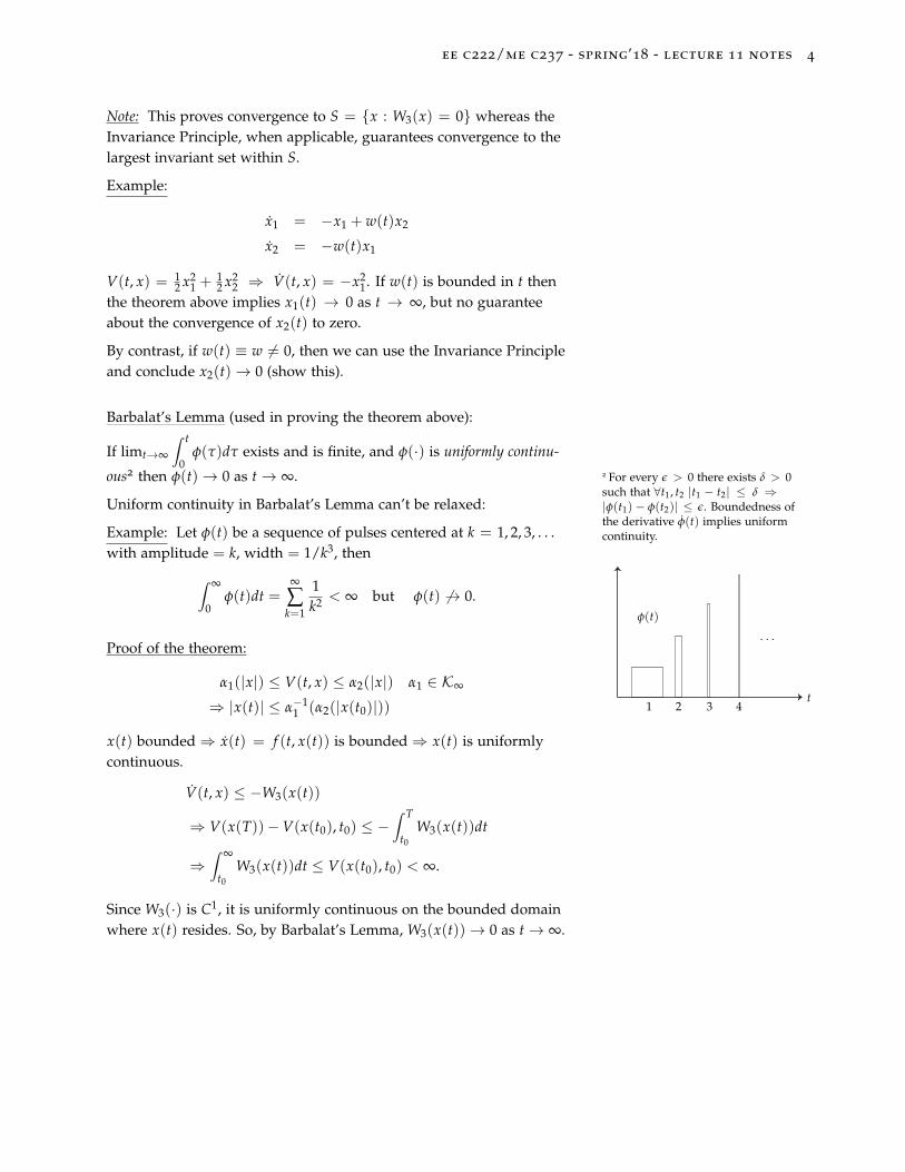
Uniform continuity in Barbalat’s Lemma can’t be relaxed:
Example: Let φ(t) be a sequence of pulses centered at k = 1, 2, 3, . . .with amplitude = k, width = 1/k3, then∫ ∞
0φ(t)dt =
∞
∑k=1
1k2 < ∞ but φ(t) 6→ 0.
· · ·
φ(t)
t1 2 3 4
Proof of the theorem:
α1(|x|) ≤ V(t, x) ≤ α2(|x|) α1 ∈ K∞
⇒ |x(t)| ≤ α−11 (α2(|x(t0)|))
x(t) bounded⇒ x(t) = f (t, x(t)) is bounded⇒ x(t) is uniformlycontinuous.
V(t, x) ≤ −W3(x(t))
⇒ V(x(T))−V(x(t0), t0) ≤ −∫ T
t0
W3(x(t))dt
⇒∫ ∞
t0
W3(x(t))dt ≤ V(x(t0), t0) < ∞.
Since W3(·) is C1, it is uniformly continuous on the bounded domainwhere x(t) resides. So, by Barbalat’s Lemma, W3(x(t))→ 0 as t→ ∞.
EE C222/ME C237 - Spring’18 - Lecture 12 Notes11 Licensed under a Creative CommonsAttribution-NonCommercial-ShareAlike4.0 International License.Murat Arcak
February 28 2018
Linear Time-Varying SystemsKhalil Section 4.6, Sastry Section 5.7
x = A(t)x x(t) = Φ(t, t0)x(t0) (1)
• The state transition matrix Φ(t, t0) satisfies the equations:
∂
∂tΦ(t, t0) = A(t)Φ(t, t0) (2)
∂
∂t0Φ(t, t0) = −Φ(t, t0)A(t0) (3)
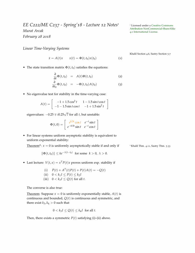
• No eigenvalue test for stability in the time-varying case:
A(t) =
[−1 + 1.5 cos2 t 1− 1.5 sin t cos t−1− 1.5 sin t cos t −1 + 1.5 sin2 t
]
eigenvalues: −0.25∓ i0.25√
7 for all t, but unstable:
Φ(t, 0) =
[e0.5t cos t e−t sin t
e−0.5t sin t e−t cos t
]
• For linear systems uniform asymptotic stability is equivalent touniform exponential stability:
Theorem2: x = 0 is uniformly asymptotically stable if and only if 2 Khalil Thm. 4.11, Sastry Thm. 5.33
‖Φ(t, t0)‖ ≤ ke−λ(t−t0) for some k > 0, λ > 0.
• Last lecture: V(t, x) = xT P(t)x proves uniform exp. stability if
(i) P(t) + AT(t)P(t) + P(t)A(t) = −Q(t)(ii) 0 < k1 I ≤ P(t) ≤ k2 I(iii) 0 < k3 I ≤ Q(t) for all t.
The converse is also true:
Theorem: Suppose x = 0 is uniformly exponentially stable, A(t) iscontinuous and bounded, Q(t) is continuous and symmetric, andthere exist k3, k4 > 0 such that
0 < k3 I ≤ Q(t) ≤ k4 I for all t.
Then, there exists a symmetric P(t) satisfying (i)–(ii) above.

ee c222/me c237 - spring’18 - lecture 12 notes 2
Proof:
Time-invariant: P =∫ ∞
0eATτQeAτdτ
Time-varying: P(t) =∫ ∞
tΦT(τ, t)Q(τ)Φ(τ, t)dτ
Using the Leibniz rule, property (3), and Φ(t, t) = I we obtain:
P(t) =∫ ∞
t
(∂
∂tΦT(τ, t)Q(τ)Φ(τ, t) + ΦT(τ, t)Q(τ)
∂
∂tΦ(τ, t)
)dτ
−ΦT(t, t)Q(t)Φ(t, t)
=∫ ∞
t
(−AT(t)ΦT(τ, t)Q(τ)Φ(τ, t)−ΦT(τ, t)Q(τ)Φ(τ, t)A(t)
)dτ
−ΦT(t, t)Q(t)Φ(t, t)
= −AT(t)P(t)− P(t)A(t)−Q(t).
Lyapunov-based Feedback Design Examples
Model Reference Adaptive Control
Illustrated on a first order system:
y = a∗y + u (4)
where a∗ is unknown.
Reference model:
ym = −aym + r(t) a > 0, r(t) : reference signal. (5)
Goal: Design a controller that guarantees y(t)− ym(t) → 0 withoutthe knowledge of a∗.
If we knew a∗, we would choose:
u = −(a∗ + a)︸ ︷︷ ︸=: k∗
y + r(t) ⇒ y = −ay + r(t).
The tracking error e(t) := y(t)− ym(t) then satisfies:
e = −ae ⇒ e(t)→ 0 exponentially.
Adaptive design when a∗ (therefore, k∗) is unknown:
u = −k(t)y + r(t)
where k(t) is to be designed. Then: e = −ae− (k(t)− k∗)︸ ︷︷ ︸=: k(t)
y.

ee c222/me c237 - spring’18 - lecture 12 notes 3
Use the Lyapunov function: V = 12 e2 + 1
2 k2:
V = −ae2 − key + k ˙k
= −ae2 + k( ˙k− ey).
Note ˙k = k and choose k = ey so that V = −ae2.
This guarantees stability of (e, k) = (0, 0) and boundedness of(e(t), k(t)) since the level sets of V = 1
2 e2 + 12 k2 are positively in-
variant. In addition, if r(t) is bounded, then ym(t) in (5) is bounded,and so is y(t) = ym(t) + e(t). Then we can apply the Theorem fromLecture 11, page 3, to the time-varying model
e = −ae− y(t)k, ˙k = y(t)e,
and conclude from V = −ae2 that e(t)→ 0.
Whether k(t) → 0 (k(t) → k∗) depends on further properties of thereference signal r(·) that are beyond the scope of this lecture.
BacksteppingKhalil (Sec. 14.3), Sastry (Sec. 6.8)
Feedback stabilization: Given the system
x = f (x) + g(x)u (6)
with input u, design a control law u = α(x) such that x = 0 isasymptotically stable for the closed-loop system:
x = f (x) + g(x)α(x).
Backstepping is a technique that simplifies this task for a class ofsystems.
Suppose a stabilizing feedback u = α(X) is available for:
X = F(X) + G(X)u X ∈ Rn, u ∈ R
and suppose the closed-loop system admits a Lyapunov functionV(X) such that
∂V∂X
(F(X) + G(X)α(X)
)≤ −W(X) < 0 ∀X 6= 0.
Can we modify α(X) to stabilize the augmented system below?
X = F(X) + G(X)x
x = u.
Define the error variable z = x− α(X) and change variables:

ee c222/me c237 - spring’18 - lecture 12 notes 4
(X, x)→ (X, z):
X = F(X) + G(X)α(X) + G(X)z
z = u− α(X, z)
where α(X, z) = ∂α∂X
(F(X) + G(X)α(X) + G(X)z
). Take the new
Lyapunov function:
V+(X, z) = V(X) +12
z2.
V+ =∂V∂X
(F(X) + G(X)α(X)
)︸ ︷︷ ︸
≤ −W(X)
+∂V∂X
G(X)z + z(u− α)︸ ︷︷ ︸= z(
u− α +∂V∂X
G(X))
Let: u = α− ∂V∂X
G(X)− kz, k > 0.
Then, V+ ≤ −W(X)− kz2 ⇒ (X, z) = 0 is asymptotically stable.
Example: x1 = x21 + x2
x2 = u.(7)
Treat x2 as “virtual” control input for the x1-subsystem:
α(x1) = −k1x1 − x21 k1 > 0
V1(x1) =12
x21.
Apply backstepping:
z2 = x2 − α(x1) = x2 + k1x1 + x21
z2 = u− α
u = α− ∂V1
∂x1− k2z2, k2 > 0
= −(k1 + 2x1)(x21 + x2)︸ ︷︷ ︸
= α
− x1︸︷︷︸=
∂V1
∂x1
− k2(x2 + k1x1 + x21)︸ ︷︷ ︸
= z2
.

EE C222/ME C237 - Spring’18 - Lecture 13 Notes11 Licensed under a Creative CommonsAttribution-NonCommercial-ShareAlike4.0 International License.Murat Arcak
March 5 2018
BacksteppingKhalil (Sec. 14.3), Sastry (Sec. 6.8)
Suppose a stabilizing feedback u = α(X), α(0) = 0, is available for:
X = F(X) + G(X)u X ∈ Rn, u ∈ R, F(0) = 0,
along with a Lyapunov function V such that
∂V∂X
(F(X) + G(X)α(X)
)≤ −W(X) < 0 ∀X 6= 0.
Can we modify α(X) to stabilize the augmented system below?
X = F(X) + G(X)x
x = u.
Define the error variable z = x− α(X) and change variables:
(X, x)→ (X, z):
X = F(X) + G(X)α(X) + G(X)z
z = u− α(X, z)
where α(X, z) = ∂α∂X
(F(X) + G(X)α(X) + G(X)z
). Take the new
Lyapunov function:
V+(X, z) = V(X) +12
z2.
V+ =∂V∂X
(F(X) + G(X)α(X)
)︸ ︷︷ ︸
≤ −W(X)
+∂V∂X
G(X)z + z(u− α)︸ ︷︷ ︸= z(
u− α +∂V∂X
G(X))
Let: u = α− ∂V∂X
G(X)− kz, k > 0.
Then, V+ ≤ −W(X)− kz2 ⇒ (X, z) = 0 is asymptotically stable.
Example 1: x1 = x21 + x2
x2 = u.(1)
Treat x2 as “virtual” control input for the x1-subsystem:
α(x1) = −k1x1 − x21 k1 > 0
V1(x1) =12
x21.

ee c222/me c237 - spring’18 - lecture 13 notes 2
Apply backstepping:
z2 = x2 − α(x1) = x2 + k1x1 + x21
z2 = u− α
u = α− ∂V1
∂x1− k2z2, k2 > 0
= −(k1 + 2x1)(x21 + x2)︸ ︷︷ ︸
= α
− x1︸︷︷︸=
∂V1
∂x1
− k2(x2 + k1x1 + x21)︸ ︷︷ ︸
= z2
.
• Above we discussed backstepping over a pure integrator. The mainidea generalizes trivially to:
X = F(X) + G(X)x
x = f (X, x) + g(X, x)u
where X ∈ Rn, x ∈ R, and g(X, x) 6= 0 for all (X, x) ∈ Rn+1.
With the preliminary feedback
u =1
g(X, x)(− f (X, x) + v) (2)
the x-subsystem becomes a pure integrator: x = v. Substituting thebackstepping control law from above:
v = α− ∂V∂X
G(X)− kz, z , x− α(X), k > 0
into (2), we get:
u =1
g(X, x)
(− f (X, x) + α− ∂V
∂XG(X)− kz
).
• Backstepping can be applied recursively to systems of the form:2 2 Systems of this form are called “strictfeedback systems.”
x1 = f1(x1) + g1(x1)x2
x2 = f2(x1, x2) + g2(x1, x2)x3
x3 = f3(x1, x2, x3) + g3(x1, x2, x3)x4
...
xn = fn(x) + gn(x)u
(3)
where gi(x1, . . . , xi) 6= 0 for all x ∈ Rn, i = 1, 2, · · · , n.
Example 2: x1 = (x1x2 − 1)x31 + (x1x2 + x2
3 − 1)x1
x2 = x3
x3 = u.
(4)

ee c222/me c237 - spring’18 - lecture 13 notes 3
Not in strict feedback form because x3 appears too soon. In fact,this system is not globally stabilizable because the set x1x2 ≥ 2 ispositively invariant regardless of u:
n(x) =
x2
x1
0
x1
x2
To see this, note that
n(x) · f (x, u) = [(x1x2 − 1)x31 + (x1x2 + x2
3 − 1)x1]x2 + x3x1
and substitute x1x2 = 2 :
=(
x31 + (1 + x2
3)x1
)x2 + x3x1
=(
x21 + (1 + x2
3))
x1x2 + x3x1
= 2x21 + 2(1 + x2
3) + x3x1
= 2x21 + x3x1 + 2x2
3︸ ︷︷ ︸≥0
+ 2 > 0.
• The condition gi(x1, . . . , xi) 6= 0 in (3) can be relaxed in some cases:
Example 3: x1 = x21x2
x2 = u(5)
Treat x2 as virtual control and let α1(x1) = −x1 which stabilizes the
x1-subsystem, as verified with Lyapunov function V1(x1) =12 x2
1.Then z2 := x2 − α1(x1) satisfies z2 = u− α1, and
u = α1 −∂V1
∂x1x2
1 − k2z2 = −x21x2 − x3
1 − k2(x2 + x1)
achieves global asymptotic stability:
V =12
x21 +
12
z22 ⇒ V = −x1
4 − k2z22.
Note that we can’t conclude exponential stability due to the quarticterm x4
1 above (recall the Lyapunov sufficient condition for expo-nential stability in Lecture 11, p.2). In fact, the linearization of the

ee c222/me c237 - spring’18 - lecture 13 notes 4
closed-loop system proves the lack of exponential stability:[0 00 −k2
]→ λ1,2 = 0,−k2.
Design example: Active suspension Krstic et al., Nonlinear and AdaptiveControl Design, Section 2.2.2.
Q xaxs
ca ka
Mb
car body
Mb xs = −ka(xs − xa)− ca(xs − xa)
xa =1A
Q A: effective piston surface
Flow: Q = −c f Q + k f u u: current applied to the
solenoid valve (control input)
Define state variables: x1 = xs, x2 = xs, x3 = xa, x4 = Q:
x1 = x2
x2 = − ka
Mb(x1 − x3)−
ca
Mb(x2 −
1A
x4)
x3 =1A
x4
x4 = −c f x4 + k f u.
(6)
This system is not in strict feedback form due to the x4 term in x2. Toovercome this problem define:
x3 ,ka
Mbx3 +
ca
Mb Ax4
ξ , x3
and change variables to (x1, x2, x3, ξ):
x1 = x2
x2 = − ka
Mbx1 −
ca
Mbx2 + x3
˙x3 =ka − cac f
Mb Ax4 +
cak f
Mb Au.

ee c222/me c237 - spring’18 - lecture 13 notes 5
Two steps of backstepping starting with the virtual control law: The stiff nonlinearity k1x31 prevents
large excursions of x1.
α1(x1) = −c1x1 − k1x31
will stabilize the (x1, x2, x3) subsystem. Full (x1, x2, x3, ξ) system:
(x1, x2, x3)subsystem
x3ξ=− ka
Mb A ξ + 1A x3
The ξ-subsystem is an asymptotically stable linear system driven byx3; therefore the full system is stabilized.
EE C222/ME C237 - Spring’18 - Lecture 14 Notes11 Licensed under a Creative CommonsAttribution-NonCommercial-ShareAlike4.0 International License.Murat Arcak
March 7 2018
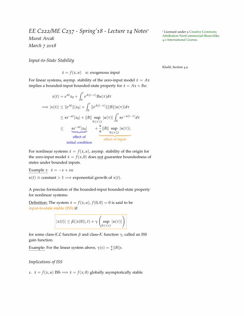
Input-to-State StabilityKhalil, Section 4.9
x = f (x, u) u: exogenous input
For linear systems, asymp. stability of the zero-input model x = Aximplies a bounded-input bounded-state property for x = Ax + Bu:
x(t) = eAtx0 +∫ t
0eA(t−τ)Bu(τ)dτ
=⇒ |x(t)| ≤ ‖eAt‖|x0|+∫ t
0‖eA(t−τ)‖‖B‖|u(τ)|dτ
≤ κe−αt|x0|+ ‖B‖ sup0≤τ≤t
|u(τ)|∫ t
0κe−α(t−τ)dτ
≤ κe−αt|x0|︸ ︷︷ ︸effect of
initial condition
+κ
α‖B‖ sup
0≤τ≤t|u(τ)|.︸ ︷︷ ︸
effect of input
For nonlinear systems x = f (x, u), asymp. stability of the origin forthe zero-input model x = f (x, 0) does not guarantee boundedness ofstates under bounded inputs.
Example 1: x = −x + xu
u(t) ≡ constant > 1 =⇒ exponential growth of x(t).
A precise formulation of the bounded-input bounded-state propertyfor nonlinear systems:
Definition: The system x = f (x, u), f (0, 0) = 0 is said to beinput-to-state stable (ISS) if:
|x(t)| ≤ β(|x(0)|, t) + γ
(sup
0≤τ≤t|u(τ)|
)
for some class-KL function β and class-K function γ, called an ISSgain function.
Example: For the linear system above, γ(s) = κα‖B‖s.
Implications of ISS
1. x = f (x, u) ISS =⇒ x = f (x, 0) globally asymptotically stable

ee c222/me c237 - spring’18 - lecture 14 notes 2
Proof:
Substitute u(t) ≡ 0 in the definition above: |x(t)| ≤ β(|x(0)|, t).
2. u(t)→ 0 as t→ ∞ ⇒ x(t)→ 0 as t→ ∞.
Proof:
Need to show that for any ε > 0, there exists T such that
|x(t)| ≤ ε ∀t ≥ T.
Since u(t) → 0, we can find T1 such that γ(|u(t)|) ≤ ε/2 for allt ≥ T1. Choose t0 = T1 and apply ISS definition:
|x(t)| ≤ β(|x(T1)|, t− T1) + ε/2 ∀t ≥ T1.
Choose T2 such that
β(|x(T1)|, T2) ≤ ε/2.
Then, |x(t)| ≤ ε for all t ≥ T1 + T2 , T.
A Lyapunov Characterization of ISS
The system x = f (x, u) is ISS if there exist class-K∞ functions αi, i =1, 2, 3, 4, and a C1 function V such that
α1(|x|) ≤ V(x) ≤ α2(|x|)∂V∂x
f (x, u) ≤ −α3(|x|) + α4(|u|).
V is called an “ISS Lyapunov function.”
Sketch of the proof:
Let u , supτ≥0 |u(τ)|. Then:
|x| ≥ r , α−13 (α4(u)) ⇒ ∂V
∂xf (x, u(t)) ≤ 0 ∀t ≥ 0.
This implies that the level set x : V(x) ≤ α2(r) is invariant andattractive. Thus, all trajectories converge to this level set which isenclosed in the outer ball |x| ≤ R , α−1
1 (α2(r)).
V(x) = α2(r)
r
R = α−11 (α2(r)) = α−1
1 (α2(α−13 (α4(u))))

ee c222/me c237 - spring’18 - lecture 14 notes 3
Example 2: x = −xr + xsu, r: odd integer, is ISS if r > s. Take:
V(x) =12
x2
V(x) = −xr+1 + xs+1u.
Young’s inequality (recall from homework):
yz ≤ λp
p|y|p + 1
qλq |z|q
for any λ > 0, and p > 1, q > 1 satisfying (p− 1)(q− 1) = 1. Applyto:
xs+1u ≤ λp
p|x|(s+1)p +
1qλq |u|
q
and choose
p =r + 1s + 1
q = 1 +1
p− 1and λ such that
λp
p=
12
⇒ xs+1u ≤ 12|x|r+1 +
1qλq |u|
q
⇒ V(x) ≤ −|x|r+1 +12|x|r+1 +
1qλq |u|
q
≤ −12|x|r+1︸ ︷︷ ︸
−α3(|x|)
+1
qλq |u|q.︸ ︷︷ ︸
−α4(|u|)
Note:
• x = −x + xu (r = s = 1) is not ISS as shown in Example 1.
• x = −x + x2u (r = 1, s = 2) is not ISS: it exhibits finite time escapefor u(t) ≡ constant 6= 0, even with an exponentially decaying u(t).
• x = −x3 + u (r = 3, s = 0) is ISS.
Example 3:
x1 = −x1 + x22
x2 = −x2 + u.
Let V(x) = 12 x2
1 +a4 x4
2, a > 0 to be determined.2 2 Why not quadratic V?
V(x) = −x21 + x1x2
2 + a(−x42 + x3
2u)
Apply the Young Inequalities:
x1x22 ≤
12
x21 +
12
x42
x32u ≤ λ4/3
4/3x4
2 +1
4λ4 u4

ee c222/me c237 - spring’18 - lecture 14 notes 4
Choose λ such that λ4/3
4/3 = 12 .
V(x) ≤ −12
x21 +
12
x42 + a
(−1
2x4
2 +1
4λ4 u4)
Let a = 2:V(x) ≤ −1
2x2
1 −12
x42︸ ︷︷ ︸
≤−α3(|x|)
+1
2λ4 u4︸ ︷︷ ︸=α4(|u|)
for an appropriate choice of α3. Thus, the system is ISS.
Stability of Series Interconnections
x1 = f1(x1, x2) x1 ∈ Rn1
x2 = f2(x2) x2 ∈ Rn2(1)
x2 = f2(x2) x1 = f1(x1, x2)x2
Suppose x2 = 0 is globally asymptotically stable for x2 = f2(x2)
and x1 = 0 is globally asymptotically stable for x1 = f1(x1, 0). Is(x1, x2) = 0 globally asymptotically stable for the interconnection?
Answer: No.
Example 4: x1 = −x1 + x21x2
x2 = −x2
exhibits finite time escape.
Proposition: Consider the series interconnection:
x1 = f1(x1, x2)
x2 = f2(x2, u).
If the x1 subsystem is ISS with x2 viewed as an input, and the x2
subsystem is ISS with input u, then the interconnection is ISS.
Example 3 revisited:
x1 = −x1 + x22 is ISS with respect to x2
x2 = −x2 + u is ISS with input u
⇒ the interconnection is ISS — an alternative to the proof in Ex. 3.
Corollary: (x1, x2) = 0 is globally asymptotically stable when u ≡ 0. GAS ISS ≡ GAS
Note that Example 4 fails the ISS condition for the x1 subsystem.

ee c222/me c237 - spring’18 - lecture 14 notes 5
Example: Active suspension design example in Lecture 13:
(x1, x2, x3)subsystem
x3ξ=− ka
Mb A ξ + 1A x3
The (x1, x2, x3)-subsystem globally asymptotically stabilized by back-stepping. The ξ-subsystem is an asymptotically stable linear system,therefore ISS with respect to the input x3.
EE C222/ME C237 - Spring’18 - Lecture 15 Notes11 Licensed under a Creative CommonsAttribution-NonCommercial-ShareAlike4.0 International License.Murat Arcak
March 12 2018
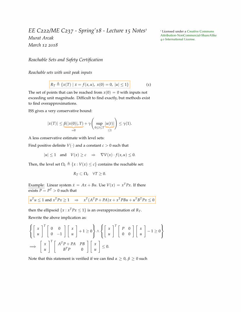
Reachable Sets and Safety Certification
Reachable sets with unit peak inputs
RT , x(T) | x = f (x, u), x(0) = 0, |u| ≤ 1 (1)
The set of points that can be reached from x(0) = 0 with inputs notexceeding unit magnitude. Difficult to find exactly, but methods existto find overapproximations.
ISS gives a very conservative bound:
|x(T)| ≤ β(|x(0)|, T)︸ ︷︷ ︸=0
+ γ
(sup
0≤t≤T|u(t)|︸ ︷︷ ︸≤1
)≤ γ(1).
A less conservative estimate with level sets:
Find positive definite V(·) and a constant c > 0 such that
|u| ≤ 1 and V(x) ≥ c ⇒ ∇V(x) · f (x, u) ≤ 0.
Then, the level set Ωc , x : V(x) ≤ c contains the reachable set:
RT ⊂ Ωc ∀T ≥ 0.
Example: Linear system x = Ax + Bu. Use V(x) = xT Px. If thereexists P = PT > 0 such that
uTu ≤ 1 and xT Px ≥ 1 ⇒ xT(AT P + PA)x + xT PBu + uT BT Px ≤ 0
then the ellipsoid x : xT Px ≤ 1 is an overapproximation of RT .
Rewrite the above implication as:[
xu
]T [0 00 −1
] [xu
]+ 1 ≥ 0
∧[
xu
]T [P 00 0
] [xu
]− 1 ≥ 0
=⇒
[xu
]T [AT P + PA PB
BT P 0
] [xu
]≤ 0.
Note that this statement is verified if we can find α ≥ 0, β ≥ 0 such

ee c222/me c237 - spring’18 - lecture 15 notes 2
that, for all x and u,[xu
]T [AT P + PA PB
BT P 0
] [xu
]+ α
[ xu
]T [P 00 0
] [xu
]− 1
+β
[ xu
]T [0 00 −I
] [xu
]+ 1
≤ 0 (2)
or, equivalently:[xu
]T [AT P + PA + αP PB
BT P −βI
] [xu
]≤ α− β.
This inequality holds for all x and u if and only if[AT P + PA + αP PB
BT P −βI
]≤ 0 (3)
β− α ≤ 0. (4)
Let β = α which is the best choice to satisfy (3) without violating (4):[AT P + PA + αP PB
BT P −αI
]≤ 0. (5)
Summary: procedure to overapproximate the reachable set
Look for P = PT > 0 and α > 0 satisfying the matrix inequality(5). This in not a linear matrix inequality (LMI) in α and P, but it isan LMI in P if α is fixed. The resulting ellipsoid x : xT Px ≤ 1 is asuperset of RT .
Additional objectives can be incorporated, such as minimizing thevolume of the ellipsoid, which is proportional to
√det P−1:
minimize log(det P−1) which is convex in P.
S-procedure
The principle used to obtain (2) is known as the S-procedure in con-trol theory. To show that:
q0(ξ) ≥ 0 whenever qi(ξ) ≥ 0 i = 1, 2, . . . , p
look for τ1, τ2, . . . , τp ≥ 0 such that
q0(ξ)−p
∑i=1
τiqi(ξ) ≥ 0.
In (2), qi(·), i = 0, 1, 2, are quadratic functions of ξ =
[xu
].

ee c222/me c237 - spring’18 - lecture 15 notes 3
Reachable sets with unit energy inputs
RT , x(T) | x = f (x, u), x(0) = 0,∫ T
0uT(t)u(t)dt ≤ 1 (6)
For an overapproximation, find positive definite V(·) such that
∇V(x) · f (x, u) ≤ uTu.
ddt
V(x(t)) ≤ uTu ⇒ V(x(T))−V(x(0)) ≤∫ T
0uT(t)u(t)dt ≤ 1
⇒ V(x(T)) ≤ 1.
Therefore, x ∈ RT implies V(x) ≤ 1, i.e., the level set contains thereachable set:
RT ⊂ x : V(x) ≤ 1.
Example:x = Ax + Bu V(x) = xT Px.
Find P = PT > 0 such that
xT(AT P + PA)x + xT PBu + uT BT Px ≤ uTu
or, written more compactly:[xu
]T [AT P + PA PB
BT P 0
] [xu
]≤[
xu
]T [0 00 I
] [xu
].
This means [AT P + PA PB
BT P −I
]≤ 0
which is a LMI in P.
Safety Certification
Given an “unsafe” set U, show that
RT ∩U = ∅.
The level set overapproximations above can be used to prove safety:
RT
U
x|V(x) ≤ 1

ee c222/me c237 - spring’18 - lecture 15 notes 4
Look for a V with the additional property that x ∈ U ⇒ V(x) > 1.Such functions V are sometimes called “barrier functions.”
Example: Suppose the unsafe set is the half-space:
U = x : aTx > 1.
Let V(x) = xT Px. From the S-procedure, if there exists τ > 0 suchthat
(xT Px− 1)− τ(aTx− 1) ≥ 0, (7)
then x ∈ U ⇒ V(x) > 1.
Exercise: Show that (7) is equivalent to: P ≥ aaT .
Thus, the LMIs in the previous examples can be augmented with thisadditional constraint to certify safety.

EE C222/ME C237 - Spring’18 - Lecture 16 Notes11 Licensed under a Creative CommonsAttribution-NonCommercial-ShareAlike4.0 International License.Murat Arcak
March 19 2018
Sum of Squares Programming
Establishing nonnegativity of functions is critical in nonlinear systemanalysis, e.g., a Lyapunov function V for x = f (x) must satisfy
V(x) > 0 ∀x 6= 0 (1)
−∇V(x)T f (x) ≥ 0 ∀x. (2)
For f (x) = Ax and V(x) = xT Px, the conditions above are simplematrix inequalities:
P > 0, −AT P− PA ≥ 0.
How can we check nonnegativity when f and V are more generalpolynomials?
Sum of Squares (SOS) Polynomials
A monomial is a product of powers of variables (e.g., m(x) = x21x2)
and its degree is the sum of its exponents (e.g., 3 for m(x) = x21x2).
A polynomial is a finite linear combination of monomials and its de-gree is the maximum degree of these monomials.
Example 1: The polynomial
q(x1, x2) = x21 − 2x1x2
2 + 2x41 + 2x3
1x2 − x21x2
2 + 6x42 (3)
has degree 4.
Definition: A polynomial p is a sum of squares (SOS) if there existpolynomials g1, · · · , gr such that
p =r
∑i=1
g2i . (4)
A SOS polynomial p(x) is nonnegative for all x. The converse is nottrue: there exist nonnegative polynomials that are not SOS.
The polynomial q(x1, x2) in (3) is SOS because it can be rewritten as:
(x1 − x22)
2 +12
(2x2
1 + x1x2 − 3x22
)2+
12
(3x1x2 + x2
2
)2. (5)
You can verify the equivalence of (3) and (5) by multiplying out termsin (5) and matching them to those in (3).
How a SOS decomposition like (5) can be obtained is discussed next.

ee c222/me c237 - spring’18 - lecture 16 notes 2
SOS Decomposition
Let z(x) be the vector of all monomials of degree ≤ d in n variables2: 2 The length of this vector is l[n,d] :=(n + d
d
).z(x) , [1, x1, x2, . . . , xn, x2
1, x1x2, . . . , xdn]
T .
Then any polynomial with degree ≤ 2d can be rewritten as
p(x) = z(x)TQ z(x) (6)
where Q is a symmetric matrix.
Example 2: Let p(x1, x2) = 2x21x2
2 which has degree 4. With n = 2and d = 2,
z(x) = [1, x1, x2, x21, x1x2, x2
2]T , (7)
and (6) holds with either
Q1 =
0 0 0 0 0 00 0 0 0 0 00 0 0 0 0 00 0 0 0 0 00 0 0 0 2 00 0 0 0 0 0
or Q2 =
0 0 0 0 0 00 0 0 0 0 00 0 0 0 0 00 0 0 0 0 10 0 0 0 0 00 0 0 1 0 0
.
Thus, the choice of Q is not unique.
Theorem: A polynomial p with degree ≤ 2d is SOS if and only ifthere exists Q = QT ≥ 0 satisfying (6).
Proof: (only if) If p is SOS then, by definition, p = ∑ri=1 g2
i for somepolynomials gi, i = 1, · · · , r. Write gi as:
gi(x) = Ciz(x) (8)
where Ci is a row vector of coefficients. Then g2i = zTCT
i Ciz and
p =r
∑i=1
g2i = zT
(r
∑i=1
CTi Ci
)︸ ︷︷ ︸
Q ≥ 0
z.
(if) Given Q = QT≥ 0 satisfying (6), decompose Q as Q = CTCwhere C has as many rows as the rank of Q, say r. Then,
Q = CTC =r
∑i=1
CTi Ci
where Ci is the ith row. If we define gi as in (8), then zTQz = ∑ri=1 g2
i .
Since Q is not unique, not all Q satisfying (6) will certify SOS. In Ex-ample 2 above, Q1 ≥ 0 but Q2 is indefinite. We need to characterizethe set of all Q satisfying (6) and search for a Q ≥ 0 in this set.

ee c222/me c237 - spring’18 - lecture 16 notes 3
Parameterization of all matrices Q satisfying (6):
Find a particular solution Q0 such that
p(x) = z(x)TQ0z(x),
and find a basis of symmetric matrices Nj, j = 1, 2, · · · , K, such that33 There are K =
l[n,d](l[n,d]+1)2 − l[n,2d] such
matrices.
z(x)T Njz(x) = 0 for all x. (9)
Then we can parameterize the set of all Q satisfying (6) as
Q = Q0 +K
∑j=1
λjNj λj ∈ R,
and p is SOS if and only if there exist λ1, · · · , λK such that Q ≥ 0.
For n = d = 2, z(x) is as defined in (7) and a basis as in (9) is:
N1 =
0 0 0 0 0 −10 0 0 0 0 00 0 2 0 0 00 0 0 0 0 00 0 0 0 0 0−1 0 0 0 0 0
N2 =
0 0 0 0 −1 00 0 1 0 0 00 1 0 0 0 00 0 0 0 0 0−1 0 0 0 0 0
0 0 0 0 0 0
N3 =
0 0 0 0 0 00 0 0 0 0 −10 0 0 0 1 00 0 0 0 0 00 0 1 0 0 00 −1 0 0 0 0
N4 =
0 0 0 −1 0 00 2 0 0 0 00 0 0 0 0 0−1 0 0 0 0 0
0 0 0 0 0 00 0 0 0 0 0
N5 =
0 0 0 0 0 00 0 0 0 −1 00 0 0 1 0 00 0 1 0 0 00 −1 0 0 0 00 0 0 0 0 0
N6 =
0 0 0 0 0 00 0 0 0 0 00 0 0 0 0 00 0 0 0 0 −10 0 0 0 2 00 0 0 −1 0 0
.
Example 1 revisited: For q(x1, x2) in (3), a suitable choice for Q0 is
Q0 =
0 0 0 0 0 00 1 0 0 0 −10 0 0 0 0 00 0 0 2 1 00 0 0 1 −1 00 −1 0 0 0 6
.

ee c222/me c237 - spring’18 - lecture 16 notes 4
Note that Q0 6≥ 0, but Q0 + 6N6 ≥ 0. Moreover, Q0 + 6N6 can bedecomposed as 0 1 0 0 0 −1
0 0 0 2 1 −30 0 0 0 3 1
T 1 0 0
0 12 0
0 0 12
0 1 0 0 0 −1
0 0 0 2 1 −30 0 0 0 3 1
which explains how the SOS form (5) was obtained.
Synthesizing SOS Polynomials
With the method above we can numerically check whether a givenpolynomial function V satisfies (1)-(2). However, in practice, it ismore important to be able to search for a V satisfying (1)-(2). This isaccomplished by synthesizing V as a weighted sum of basis polyno-mials with weights left as decision variables.
This leads to the following SOS synthesis problem:
Given basis polynomials pi, i = 0, 1, · · · , m, each with degree ≤ 2d, findparameters a1, · · · , am such that p0 + a1 p1 + · · ·+ am pm is SOS.
To solve this problem, find a matrix Qi satisfying pi = zTQiz for eachi = 0, 1, · · · , m. Then search for a1, · · · , am and λ1, · · · , λK satisfying
Q0 +m
∑i=1
aiQi +K
∑j=1
λjNj ≥ 0. (10)
This is a linear matrix inequality (LMI) and can be solved numeri-cally with standard semidefinite program (SDP) solvers.
There are also software packages4 that follow the procedures above 4 e.g., SOSOPT
to automatically convert SOS programs to LMIs, such as (10).
EE C222/ME C237 - Spring’18 - Lecture 17 Notes11 Licensed under a Creative CommonsAttribution-NonCommercial-ShareAlike4.0 International License.Murat Arcak
March 21 2018
Review of Sum of Squares (SOS) Polynomials
Checking whether a polynomial is SOS
A polynomial p with degree ≤ 2d is a sum of squares if and only ifthere exists Q = QT ≥ 0 s.t.
p(x) = z(x)TQ z(x) (1)
where z(x) is the vector of all monomials of degree ≤ d:
z(x) , [1, x1, x2, . . . , xn, x21, x1x2, . . . , xd
n]T .
Find a particular solution Q0 such that
p(x) = z(x)TQ0z(x),
and find a basis of symmetric matrices Nj, j = 1, 2, · · · , K, such that
z(x)T Njz(x) = 0 for all x. (2)
Then p is SOS if and only if there exist reals λ1, · · · , λK such that
Q = Q0 +K
∑j=1
λjNj ≥ 0. (3)
This is a linear matrix inequality (LMI) and can be solved numeri-cally with standard semidefinite program (SDP) solvers.
Synthesizing SOS Polynomials
Given pi, i = 0, 1, · · · , m, each with degree ≤ 2d, find reals a1, · · · , am
s.t. p0 + a1 p1 + · · ·+ am pm is SOS.
Find a particular Qi satisfying pi = zTQiz for each i = 0, 1, · · · , m.Then search for a1, · · · , am and λ1, · · · , λK satisfying the LMI
Q0 +m
∑i=1
aiQi +K
∑j=1
λjNj ≥ 0. (4)
ee c222/me c237 - spring’18 - lecture 17 notes 2
Applications
Searching for a Lyapunov Function
Given x = f (x), f (0) = 0, where f is a vector of polynomials, searchfor a Lyapunov function of the form
V(x) = p0(x) + a1 p1(x) + · · ·+ am pm(x) (5)
where pi, i = 0, 1, · · · , m are basis polynomials selected ahead oftime, and ai, i = 1, · · · , m are weights to be determined.
To ensure V is positive definite, pick a positive definite polynomial `(e.g., `(x) = εxTx for some small ε) and impose the constraint:
V(x)− `(x) is SOS. (6)
To ensure ∇V(x)T f (x) is negative semidef., impose the constraint:
−∇V(x)T f (x) is SOS. (7)
Constraints (6) and (7) can be brought to the LMI form (4) and feasi-ble ai, i = 1, · · · , m can be determined numerically (if they exist).
Overapproximating Reachable Sets
Recall from Lecture 15 that
RT ,
x(T) | x = f (x, u), x(0) = 0,∫ T
0uT(t)u(t)dt ≤ 1
(8)
defines the reachable set from x(0) = 0 under unit energy inputs and,if we can find a positive definite V such that
∇V(x)T f (x, u) ≤ uTu, (9)
then we can overapproximate RT by:
RT ⊂ x : V(x) ≤ 1.
This follows because, from (9),
ddt
V(x(t)) ≤ uTu ⇒ V(x(T))−V(x(0)) ≤∫ T
0uT(t)u(t)dt ≤ 1
⇒ V(x(T)) ≤ 1.
If f (x, u) is a vector of polynomials in x and u, we can search for apolynomial V of the form (5), and encode (9) with the constraint:
−∇V(x)T f (x, u) + uTu is SOS in x and u. (10)
This can then be combined with (6) and brought to the LMI form (4).
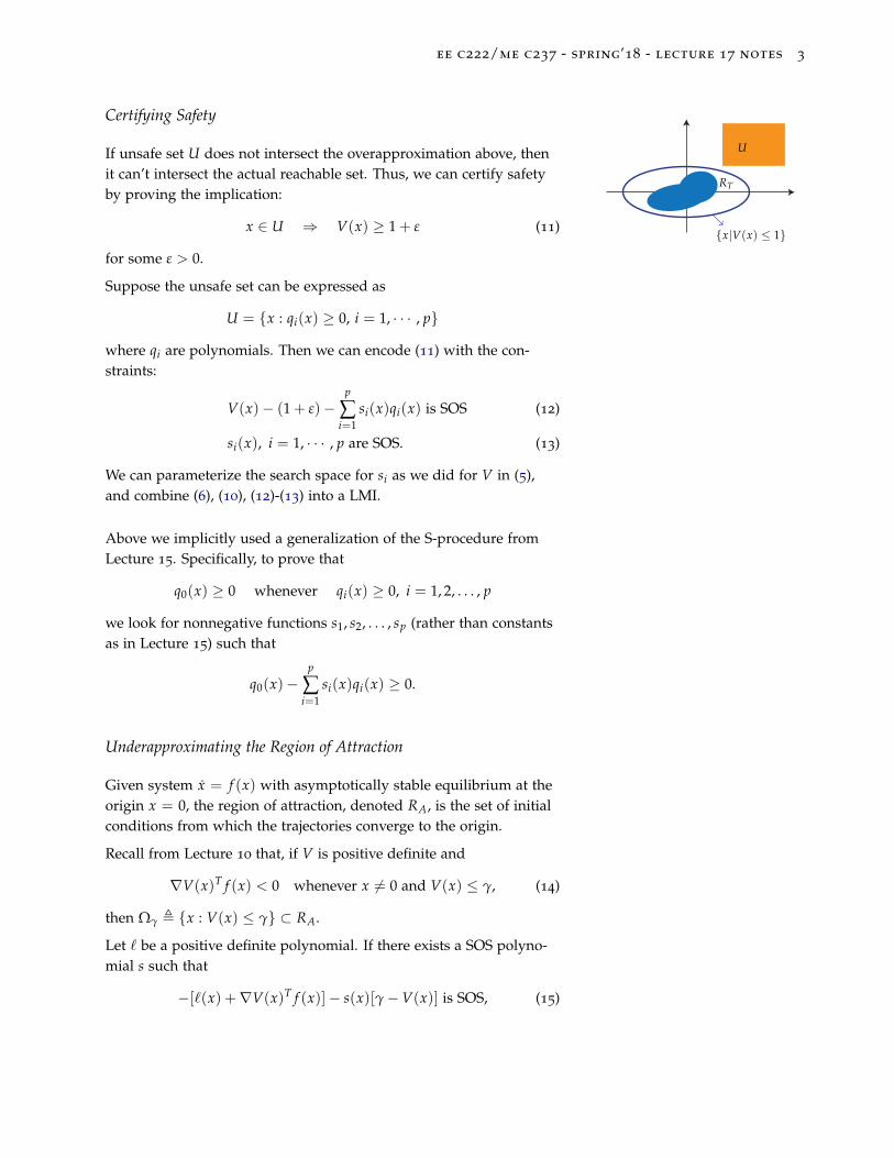
ee c222/me c237 - spring’18 - lecture 17 notes 3
Certifying Safety
RT
U
x|V(x) ≤ 1
If unsafe set U does not intersect the overapproximation above, thenit can’t intersect the actual reachable set. Thus, we can certify safetyby proving the implication:
x ∈ U ⇒ V(x) ≥ 1 + ε (11)
for some ε > 0.
Suppose the unsafe set can be expressed as
U = x : qi(x) ≥ 0, i = 1, · · · , p
where qi are polynomials. Then we can encode (11) with the con-straints:
V(x)− (1 + ε)−p
∑i=1
si(x)qi(x) is SOS (12)
si(x), i = 1, · · · , p are SOS. (13)
We can parameterize the search space for si as we did for V in (5),and combine (6), (10), (12)-(13) into a LMI.
Above we implicitly used a generalization of the S-procedure fromLecture 15. Specifically, to prove that
q0(x) ≥ 0 whenever qi(x) ≥ 0, i = 1, 2, . . . , p
we look for nonnegative functions s1, s2, . . . , sp (rather than constantsas in Lecture 15) such that
q0(x)−p
∑i=1
si(x)qi(x) ≥ 0.
Underapproximating the Region of Attraction
Given system x = f (x) with asymptotically stable equilibrium at theorigin x = 0, the region of attraction, denoted RA, is the set of initialconditions from which the trajectories converge to the origin.
Recall from Lecture 10 that, if V is positive definite and
∇V(x)T f (x) < 0 whenever x 6= 0 and V(x) ≤ γ, (14)
then Ωγ , x : V(x) ≤ γ ⊂ RA.
Let ` be a positive definite polynomial. If there exists a SOS polyno-mial s such that
−[`(x) +∇V(x)T f (x)]− s(x)[γ−V(x)] is SOS, (15)
ee c222/me c237 - spring’18 - lecture 17 notes 4
then V(x) ≤ γ implies ∇V(x)T f (x) ≤ −`(x) as stipulated in (14).
To obtain a LMI from (15), one option is to fix the Lyapunov func-tion2 V and to parameterize the search space for s. We can further 2 choose, e.g., a quadratic Lyapunov
function for the linearized model atx = 0
maximize γ subject to (15) by incrementing γ until the the resultingLMI is infeasible.
Alternatively s can be fixed and V parameterized. If we parameter-ize both s and V, however, (15) is no longer affine in the parametersbecause the term s(x)V(x) contains the products of these parameters.
Below is a procedure that alternates between first fixing V, varyings, and next fixing s, varying V. When a new V is obtained, however,the shape of the level set changes and it may be ambiguous whetherthe new one is bigger. To remove this ambiguity we define a "shapefunction" p and use its level sets to judge the size of the region ofattraction estimate.
Step 1: Let V0(x) be an initial choice for a Lyapunov function, e.g., aquadratic function for the linearized model at the origin. Find
γ∗ := max γ s.t. ∇V0(x)T f (x) < 0 whenever x 6= 0 and V0(x) ≤ γ.
To satisfy the constraint look for a SOS multiplier s1(x) that satisfies
−[`(x) +∇V0(x)T f (x)]− s1(x)[γ−V0(x)] is SOS
where ` is positive definite, e.g., `(x) := ε(x21 + x2
2) for some ε > 0.
Step 2: Let p(x) be some fixed, positive definite convex polynomial(e.g., p(x) = x2
1 + x22), and let V0(x) and γ∗ be as in Step 1. Find
β∗ := max β s.t. V0(x) ≤ γ∗ whenever p(x) ≤ β.
To satisfy the constraint look for a SOS multiplier s2(x) such that
[γ∗ −V0(x)]− s2(x)[β− p(x)] is SOS.
This means that x : p(x) ≤ β is contained in x : V0(x) ≤ γ∗.
Step 3: Given γ∗, s1(x) from Step 1 and p(x), s2(x) from Step 2,search for V(x) to solve:
maxβ>0
4th-order V(x)
β
subject to V(x)− `(x) is SOS
− [`(x) +∇V(x)T f (x)]− s1(x)[γ∗ −V(x)] is SOS
[γ∗ −V(x)]− s2(x)[β− p(x)] is SOS.

ee c222/me c237 - spring’18 - lecture 17 notes 5
The first constraint ensures V is positive definite. The second im-plies that the level set x : V(x) ≤ γ∗ is invariant, hence a validapproximation for the region of attraction. The third constraint andthe maximization of β ensure that V is selected such that the level setx : V(x) ≤ γ∗ is as large as possible, as measured by function p.
To proceed, replace V0(x) in Step 1 with the function V(x) fromStep 3, and repeat the steps above for several iterations, until thechange in β∗ in Step 2 is sufficiently small. The final approximationof the ROA is the set where V(x) ≤ γ∗.

EE C222/ME C237 - Spring’18 - Lecture 18 Notes11 Licensed under a Creative CommonsAttribution-NonCommercial-ShareAlike4.0 International License.Murat Arcak
April 2 2018
Feedback LinearizationSastry, Chapter 9; Khalil, Chapter 13
Today: Relative degree, input-output linearization, zero dynamics
Consider the single-input single-output (SISO) nonlinear system:
x = f (x) + g(x)u
y = h(x).(1)
Relative degree (informal definition): Number of times we need totake the time derivative of the output to see the input:
y =∂h∂x
f (x)︸ ︷︷ ︸=: L f h(x)
+∂h∂x
g(x)︸ ︷︷ ︸=: Lgh(x)
u
L f h is called the Lie derivative of h alongthe vector field f
If Lgh(x) 6= 0 in an open set containing the equilibrium, then the rela-tive degree is equal to 1. If Lgh(x) ≡ 0, continue taking derivatives:
y = L f L f h(x)︸ ︷︷ ︸=: L2
f h(x)
+ LgL f h(x)u.
If LgL f h(x) 6= 0, then relative degree is 2. If LgL f h(x) ≡ 0, continue.
Definition: The system (1) has relative degree r if, in a neighbourhoodof the equilibrium,
LgLi−1f h(x) = 0 i = 1, 2, . . . , r− 1
LgLr−1f h(x) 6= 0.
(2)
Examples:
1. x1 = x2
x2 = −x31 + u
y = x1
(3)
has relative degree = 2.
2. SISO linear system:
x = Ax + Bu y = Cx

ee c222/me c237 - spring’18 - lecture 18 notes 2
Lgh(x) = CB, LgL f h(x) = CAB, . . . , LgLr−1f = CAr−1B.
CB 6= 0 ⇒ relative degree = 1
CB = 0, CAB 6= 0 ⇒ relative degree = 2
CB = · · · = CAr−2B = 0, CAr−1B 6= 0 ⇒ relative degree = r
The parameters CAi−1B i = 1, 2, 3, . . . are called Markov parametersand are invariant under similarity transformations.
3. x1 = x2 + x33 y = x1
x2 = x3 y = x1 = x2 + x33
x3 = u y = x2 + 3x23 x3 = x3 + 3x2
3u
LgL f h(x) = 3x23 = 0 when x3 = 0, and 6= 0 elsewhere. Thus, this
system does not have a well-defined relative degree around x = 0.
Input-Output Linearization
If a system has a well-defined relative degree then it is input-outputlinearizable:
y(r) = Lrf h(x) + LgLr−1
f h(x)︸ ︷︷ ︸6=0
u
Apply preliminary feedback:
u =1
LgLr−1f h(x)
(− Lr
f h(x) + v
)(4)
where v is a new input to be designed. Then, y(r) = v is a linearsystem in the form of an integrator chain:
ζ1 = ζ2
ζ2 = ζ3
...
ζr = v
where ζ1 =: y = h(x), ζ2 =: y = L f h(x), . . . , ζr =: y(r−1) = Lr−1f h(x).
To ensure y(t)→ 0 as t→ ∞, apply the feedback:
v = −k1ζ1 − k2ζ2 − · · · − krζr
= −k1h(x)− k2L f h(x)− · · · − krLr−1f h(x)
(5)
where k1, . . . , kr are such that sr + krsr−1 + · · ·+ k2s + k1 has all rootsin the open left half-plane.

ee c222/me c237 - spring’18 - lecture 18 notes 3
Does the controller (4)-(5) achieve asymptotic stability of x = 0?
Not necessarily! It renders the (n− r)-dimensional manifold:
h(x) = L f h(x) = · · · = Lr−1f h(x) = 0
invariant and attractive. The dynamics restricted to this manifold arecalled zero dynamics and determine whether or not x = 0 is stable.
If the origin of the zero dynamics is asymptotically stable, the systemis called minimum phase. If unstable, it is called nonminimum phase.
Example: n = 3, r = 1
h(x) = 0
minimum phase nonminimum phase
Finding the Zero Dynamics
Set y = y = · · · = y(r−1) = 0 and substitute (4) with v = 0, that is:
u∗ =−Lr
f h(x)
LgLr−1f h(x)
.
The remaining dynamical equations describe the zero dynamics.
Example: x1 = x2
x2 = αx3 + u
x3 = βx3 − u
y = x1
(6)
This system has relative degree 2. With x1 = x2 = 0 and u∗ = −αx3,the remaining dynamical equation is
x3 = (α + β)x3.
Thus this system is minimum phase if α + β < 0.
For a linear SISO system, relative degree is the difference betweenthe degrees of the denominator and the numerator of the transferfunction, and zeros are the roots of the numerator. The definitions ofrelative degree and zero dynamics above generalize these concepts tononlinear systems. As an example, the transfer function for (6) is
s− (α + β)
s2(s− β),
which has relative degree two and a zero at s = α + β as expected.

ee c222/me c237 - spring’18 - lecture 18 notes 4
Example: Cart/Pole
θ `
y : output
u
m
M
y =1
Mm + sin2 θ
(um
+ θ2` sin θ − g sin θ cos θ
)
θ =1
`(Mm + sin2 θ)
(− u
mcos θ − θ2` cos θ sin θ +
M + mm
g sin θ
) (7)
Relative degree = 2.
To find the zero dynamics, substitute y = y = 0, and
u∗ = −m(θ2` sin θ − g sin θ cos θ)
in the θ equation:
θ =g`
sin θ.
Same as the dynamics of the pole when the cart is held still:
m
θ `
Nonminimum phase because θ = 0 is unstable for the zero dynamics.
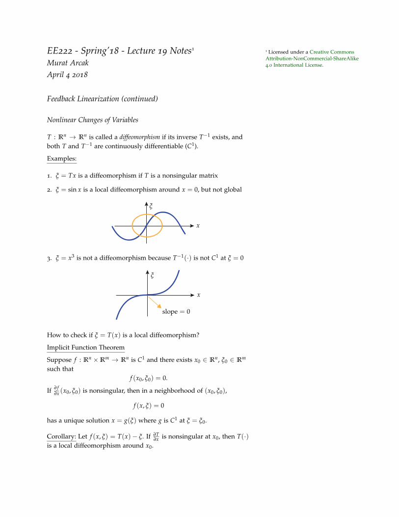
EE222 - Spring’18 - Lecture 19 Notes11 Licensed under a Creative CommonsAttribution-NonCommercial-ShareAlike4.0 International License.Murat Arcak
April 4 2018
Feedback Linearization (continued)
Nonlinear Changes of Variables
T : Rn → Rn is called a diffeomorphism if its inverse T−1 exists, andboth T and T−1 are continuously differentiable (C1).
Examples:
1. ξ = Tx is a diffeomorphism if T is a nonsingular matrix
2. ξ = sin x is a local diffeomorphism around x = 0, but not global
x
ξ
3. ξ = x3 is not a diffeomorphism because T−1(·) is not C1 at ξ = 0
x
ξ
slope = 0
How to check if ξ = T(x) is a local diffeomorphism?
Implicit Function Theorem
Suppose f : Rn ×Rm → Rn is C1 and there exists x0 ∈ Rn, ξ0 ∈ Rm
such thatf (x0, ξ0) = 0.
If ∂ f∂x (x0, ξ0) is nonsingular, then in a neighborhood of (x0, ξ0),
f (x, ξ) = 0
has a unique solution x = g(ξ) where g is C1 at ξ = ξ0.
Corollary: Let f (x, ξ) = T(x)− ξ. If ∂T∂x is nonsingular at x0, then T(·)
is a local diffeomorphism around x0.

ee222 - spring’18 - lecture 19 notes 2
A "Normal Form" that Explicitly Displays the Zero Dynamics
Theorem: If x = f (x) + g(x)u, y = h(x) has a well-defined relative
degree r ≤ n, then there exist a diffeomorphism T : x →[
zζ
],
z ∈ Rn−r, ζ ∈ Rr, that transforms the system to the form:
z = f0(z, ζ)
ζ1 = ζ2
...
ζr = b(z, ζ) + a(z, ζ)u, y = ζ1.
(1)
In particular, z = f0(z, 0) represents the zero dynamics.
To obtain this form, let ζ = [h(x) L f h(x) . . . Lr−1f h(x)]T , and
find n− r independent variables z such that z does not contain u.
Note that the terms b(z, ζ) and a(z, ζ) correspond to Lrf (x) and
LgLr−1f h(x) in the original coordinates.
Example: x1 = x2
x2 = αx3 + u
x3 = βx3 − u
y = x1.
Let ζ1 = x1, ζ2 = x2, and note that z = x2 + x3 is independent ofζ1, ζ2, and z does not contain u. Thus, the normal form is:
z = (α + β)x3 = (α + β)z− (α + β)ζ2
ζ1 = ζ2
ζ2 = αx3 + u = αz− αζ2 + u.
I/O Linearizing Controller in the new coordinates (1):
u =1
a(z, ζ)
(− b(z, ζ) + v
)(2)
v = −k1ζ1 · · · − krζr (3)
where k1, · · · , kr are such that all roots of sr + krsr−1 + · · ·+ k2s + k1
have negative real parts.
Theorem: If z = 0 is locally exponentially stable for the zero dynam-ics z = f0(z, 0), then (2)–(3) locally exponentially stabilizes x = 0.
Proof: Closed-loop system:
z = f0(z, ζ)
ζ = Aζ

ee222 - spring’18 - lecture 19 notes 3
where
A =
0 1 0 . . .0 0 1 . . .
. . .1
−k1 −k2 −k3 . . . −kr
is Hurwitz. The Jacobian linearization at (z, ζ) = 0 is:
J =
[∂ f0∂z (0, 0) ∂ f0
∂ζ (0, 0)0 A
]
where ∂ f0∂z (0, 0) is Hurwitz since z = f0(z, 0) is exponentially stable
by the proposition in Lecture 11, page 1. Since A is also Hurwitz, alleigenvalues of J have negative real parts ⇒ exponential stability.
Global asymptotic stability can be guaranteed with additional as-sumptions on the zero dynamics, such as ISS of
z = f0(z, ζ)
with respect to the input ξ:
z = f0(z, ζ)ζ = Aζζ
Example: z = −z + z2ζ, ζ = −kζ Note: the z subsystem is not ISS
(z, ζ) = 0 is locally exponentially stable, but not globally: solutionsescape in finite time for large z(0).
I/O Linearizing Controller for Tracking
For the output y(t) to track a reference signal2 yd(t), replace (3) with: 2 assumed to be r times differentiable
v = −k1(ζ1 − yd(t))− k2(ζ2 − yd(t)) · · · − kr(ζr − y(r−1)d (t)) + y(r)d (t)
Let e1 , ζ1 − yd(t), e2 , ζ2 − yd(t), . . . , er , ζr − y(r−1)d (t). Then:
e1 = e2
e2 = e3
...
er = v− y(r)d (t) = −k1e1 − · · · − krer
e = Ae.
Thus e(t)→ 0, that is y(t)− yd(t)→ 0.

ee222 - spring’18 - lecture 19 notes 4
If yd(t) and its derivatives are bounded, then ζ(t) is bounded. If thezero dynamics z = f0(z, ζ) is ISS with respect to ζ, then z(t) is alsobounded. Thus, all internal signals are bounded.

EE C222/ME C237 - Spring’18 - Lecture 20 Notes11 Licensed under a Creative CommonsAttribution-NonCommercial-ShareAlike4.0 International License.Murat Arcak
April 16 2018
Full-State Feedback Linearization
The system x = f (x) + g(x)u, x ∈ Rn, u ∈ R, is (full state) feedbacklinearizable if a function h : Rn 7→ R exists such that the relativedegree from u to y = h(x) is n.
Since r = n, the normal form in Lecture 19 has no zero dynamics and
x →
ζ1
ζ2...
ζn
=
h(x)
L f h(x)...
Ln−1f h(x)
is a diffeomorphism that transforms the system to the form:
ζ1 = ζ2
ζ2 = ζ3
...
ζn = Lnf h(x) + LgLn−1
f h(x)u.
Then, the feedback linearizing controller
u =1
LgLn−1f h(x)
(− Ln
f h(x) + v
), v = −k1ζ1 · · · − knζn,
yields the closed-loop system:
ζ = Aζ where A =
0 1 0 . . .0 0 1 . . .
. . .1
−k1 −k2 −k3 . . . −kn
.
Example: x1 = x2 + 2x21
x2 = x3 + u
x3 = x1 − x3
The choice y = x3 gives relative degree r = n = 3.

ee c222/me c237 - spring’18 - lecture 20 notes 2
Let ζ1 = x3, ζ2 = x3 = x1− x3, ζ3 = x3 = x1− x3 = x2 + 2x21− x1 + x3.
ζ1 = ζ2
ζ2 = ζ3
ζ3 = (4x1 − 1)(x2 + 2x21) + x1 + u.
Feedback linearizing controller:
u = −(4x1 − 1)(x2 + 2x21)− x1 − k1ζ1 − k2ζ2 − k3ζ3.
Summary so far:
I/O Linearization: • suitable for tracking• output y is an intrinsic physical variable
Full state linearization: • set point stabilization• output is not intrinsic, selected to enable
a linearizing change of variables.
Remaining question:
• When is a system feedback linearizable, i.e., how do we knowwhether a relative degree r = n output exists?
Basic Definitions from Differential Geometry
Definition: The Lie bracket of two vector fields f and g is a new vec-tor field defined as:
[ f , g](x) =∂g∂x
f (x)− ∂ f∂x
g(x).
Note:
1. [ f , g] = −[g, f ],
2. [ f , f ] = 0,
3. If f , g are constant then [ f , g] = 0.
Notation for repeated applications:
[ f , [ f , g]] = ad2f g, [ f , [ f , [ f , g]]] = ad3
f g, · · ·
ad0f g(x) , g(x), adk
f g , [ f , adk−1f g] k = 1, 2, 3, . . .
Definition: Given vector fields f1, . . . , fk, a distribution ∆ is defined as∆(x) = span f1(x), . . . , fk(x).
f ∈ ∆ means that there exist scalar functions αi(x) such that
f (x) = α1(x) f1(x) + · · ·+ αk(x) fk(x).
ee c222/me c237 - spring’18 - lecture 20 notes 3
Definition: ∆ is said to be nonsingular if f1(x), . . . , fk(x) are linearlyindependent for all x.
Definition: ∆ is said to be involutive if
g1 ∈ ∆, g2 ∈ ∆ =⇒ [g1, g2] ∈ ∆
that is, ∆ is closed under the Lie bracket operation.
Proposition: ∆ = span f1, . . . , fk is involutive if and only if
[ fi, f j] ∈ ∆ 1 ≤ i, j ≤ k.
Example 1: ∆ = span f1, . . . , fk where f1, . . . , fk are constant vec-tors
Example 2: a single vector field f (x) is involutive since [ f , f ] = 0 ∈∆
Definition: A nonsingular k-dimensional distribution
∆(x) = span f1(x), . . . , fk(x) x ∈ Rn
is said to be completely integrable if there exist n− k functions
φ1(x), . . . , φn−k(x)
such that
∂φi∂x
f j(x) = 0 i = 1, . . . , n− k, j = 1, . . . , k
and dΦi(x) :=∂φi∂x
, i = 1, . . . , n− k, are linearly independent.
Example 3: If f1, . . . , fk are linearly independent constant vectors,then we can find n− k independent row vectors T1, . . . , Tn−k s.t.
Ti[ f1 . . . fk] = 0.
Therefore, ∆ = span f1, . . . , fk is completely integrable and
φi(x) = Tix, i = 1, . . . , n− k.
Frobenius Theorem: A nonsingular distribution is completely inte-grable if and only if it is involutive.
Example 3 above is a special case since ∆ is involutive by Example 1.
Back to (Full State) Feedback Linearization
Recall: x = f (x) + g(x)u, x ∈ Rn, u ∈ R is feedback linearizable if wecan find an output y = h(x) such that relative degree r = n.

ee c222/me c237 - spring’18 - lecture 20 notes 4
How do we determine if a relative degree r = n output exists?
Lgh(x) = LgL f h(x) = · · · = LgLn−2f h(x) = 0 in a nbhd of x0 (1)
LgLn−1f h(x0) 6= 0. (2)
Proposition:2 (1)-(2) are equivalent to: 2 follows from (5) below with j = 0
Lgh(x) = Lad f gh(x) = · · · = Ladn−2f gh(x) = 0 in a nbhd of x0 (3)
Ladn−1f gh(x0) 6= 0. (4)
The advantage of (3) over (1) is that it has the form:
∂h∂x
[g(x) ad f g(x) . . . adn−2f g(x)] = 0
which is amenable to the Frobenius Theorem.
Theorem: x = f (x) + g(x)u is feedback linearizable around x0 if andonly if the following two conditions hold:
C1) [g(x0) ad f g(x0) . . . adn−1f g(x0)] has rank n
C2) ∆(x) = spang(x), ad f g(x), . . . , adn−2f g(x) is involutive in a
neighborhood of x0.
Proof: (if) Given C1 and C2 show that there exists h(x) satisfying(3)-(4).
∆(x) is nonsingular by C1 and involutive by C2. Thus, by the Frobe-nius Theorem, there exists h(x) satisfying (3) and dh(x) 6= 0.
To prove (4) suppose, to the contrary, Ladn−1f
h(x0) = 0. This implies
dh(x0)[g(x0) ad f g(x0) . . . adn−1f g(x0)]︸ ︷︷ ︸
nonsingular by C1
= 0.
Thus dh(x0) = 0, a contradiction.
(only if) Given that y = h(x) with r = n exists, that is (3)-(4) hold,show that C1 and C2 are true.
We will use the following fact3 which holds when r = n: 3 see, e.g., Khalil, Lemma C.8
Ladif gLj
f h(x) =
0 if i + j ≤ n− 2
(−1)n−1−jLgLn−1f h(x) 6= 0 if i + j = n− 1.
(5)
Define the matrix
M =
dh
dL f h...
dLn−1f h
[
g − ad f g ad2f g . . . (−1)n−1 adn−1
f g]
(6)

ee c222/me c237 - spring’18 - lecture 20 notes 5
and note that the (k, `) entry is:
Mk` = dLk−1f h(x)(−1)`−1 ad`−1
f g(x)
= (−1)`−1Lad`−1f gLk−1
f h(x).
Then, from (5):
0 0 · · · ?
0 ...
... ?...
? · · · · · · ?
Mk` =
0 `+ k ≤ n
6= 0 `+ k = n + 1.
Since the diagonal entries are nonzero, M has rank n and thus thefactor [
g − ad f g ad2f g . . . (−1)n−1 adn−1
f g]
in (6) must have rank n as well. Thus C1 follows.
This also implies ∆(x) is nonsingular; thus, by the Frobenius Thm,
complete integrability ≡ involutivity.
∆(x) is completely integrable since h(x) satisfying (3) exists by as-sumption; thus, we conclude involutivity (C2).
Example: x1 = x2 + 2x21
x2 = x3 + u
x3 = x1 − x3
Feedback linearizability was shown on page 1 by inspection: y = x3
gives relative degree = 3. Verify with the theorem above:
f (x) =
x2 + 2x21
x3
x1 − x3
g(x) =
010
[ f , g](x) =
−100
[ f , [ f , g]](x) =
4x1
01
Conditions of the theorem:
1.
0 −1 4x1
1 0 00 0 1
full rank
2. ∆ = span
0
10
,
−100
involutive
∂h∂x
0 −11 00 0
satisfied by h(x) = x3.

EE C222/ME C237 - Spring’18 - Lecture 21 Notes11 Licensed under a Creative CommonsAttribution-NonCommercial-ShareAlike4.0 International License.Murat Arcak
April 18 2018
Feedback Linearization Continued
Recall “strict feedback systems" discussed in Lecture 13:
x1 = f1(x1) + g1(x1)x2
x2 = f2(x1, x2) + g2(x1, x2)x3
x3 = f3(x1, x2, x3) + g3(x1, x2, x3)x4
...
xn = fn(x) + gn(x)u.
(1)
Such systems are feedback linearizable when gi(x1, . . . , xi) 6= 0 nearthe origin, i = 1, 2, · · · , n, because the relative degree is n with thechoice of output y = h(x) = x1:
y(n) = Lnf h(x) + g1(x1)g2(x1, x2) · · · gn(x)︸ ︷︷ ︸
LgLn−1f h(x) 6= 0
u.
Feedback linearizability is lost when gi(0) = 0 for some i; however,backstepping may be applicable as the following example illustrates:
Example 1:
x1 = x21x2
x2 = u.
Treat x2 as virtual control and let α1(x1) = −x1 which stabilizes thex1-subsystem, as verified with Lyapunov function V1(x1) =
12 x2
1.Then z2 := x2 − α1(x1) satisfies z2 = u− α1, and
u = α1 −∂V1
∂x1x2
1 − k2z2 = −x21x2 − x3
1 − k2(x2 + x1)
achieves global asymptotic stability:
V =12
x21 +
12
z22 ⇒ V = −x1
4 − k2z22.
In contrast the system is not feedback linearizable, because condition(C1) in the theorem for feedback linearizability (Lecture 20, p.4) fails.To see this note that
f (x) =
[x2
1x2
0
], g(x) =
[01
], ad f g(x) = [ f , g](x) =
[−x2
10
],
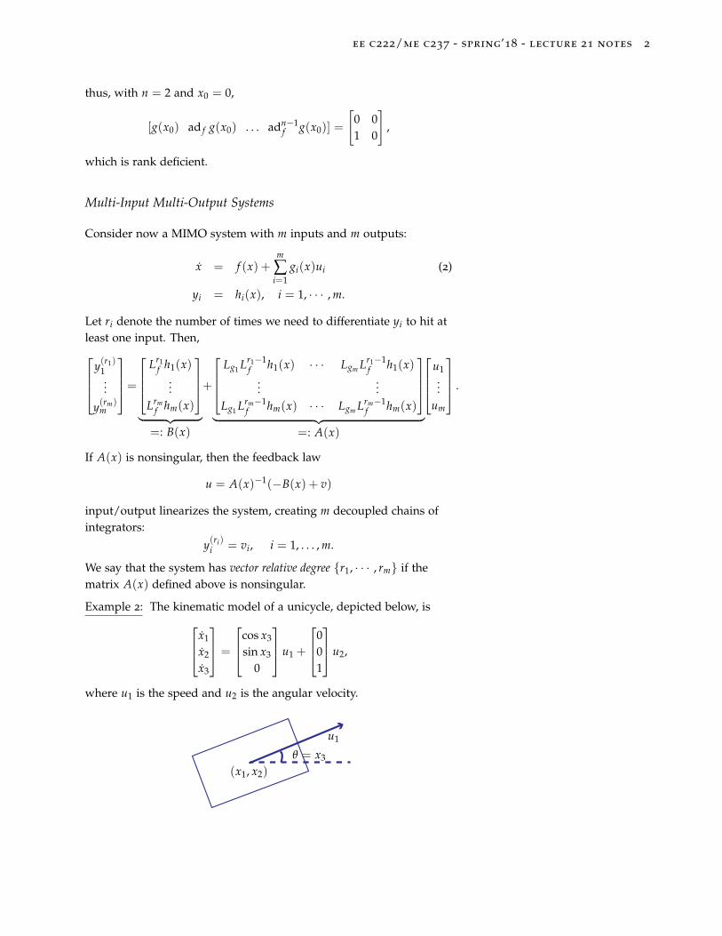
ee c222/me c237 - spring’18 - lecture 21 notes 2
thus, with n = 2 and x0 = 0,
[g(x0) ad f g(x0) . . . adn−1f g(x0)] =
[0 01 0
],
which is rank deficient.
Multi-Input Multi-Output Systems
Consider now a MIMO system with m inputs and m outputs:
x = f (x) +m
∑i=1
gi(x)ui (2)
yi = hi(x), i = 1, · · · , m.
Let ri denote the number of times we need to differentiate yi to hit atleast one input. Then,
y(r1)1...
y(rm)m
=
Lr1f h1(x)
...Lrm
f hm(x)
︸ ︷︷ ︸=: B(x)
+
Lg1 Lr1−1
f h1(x) · · · Lgm Lr1−1f h1(x)
......
Lg1 Lrm−1f hm(x) · · · Lgm Lrm−1
f hm(x)
︸ ︷︷ ︸
=: A(x)
u1...
um
.
If A(x) is nonsingular, then the feedback law
u = A(x)−1(−B(x) + v)
input/output linearizes the system, creating m decoupled chains ofintegrators:
y(ri)i = vi, i = 1, . . . , m.
We say that the system has vector relative degree r1, · · · , rm if thematrix A(x) defined above is nonsingular.
Example 2: The kinematic model of a unicycle, depicted below, isx1
x2
x3
=
cos x3
sin x3
0
u1 +
001
u2,
where u1 is the speed and u2 is the angular velocity.
(x1, x2)
θ = x3
u1

ee c222/me c237 - spring’18 - lecture 21 notes 3
Let y1 = x1 and y2 = x2, and note that[y1
y2
]=
[cos x3 0sin x3 0
]︸ ︷︷ ︸=: A(x)
[u1
u2
].
Since A(x) is singular, the system does not have a well-defined vectorrelative degree.
The notion of zero dynamics and the normal form can be extended toMIMO systems2. If the system has vector relative degree r1, · · · , rm, 2 see, e.g., Sastry, Section 9.3
then r := r1 + · · ·+ rm ≤ n and
ζ := [h1(x) L f h1(x) · · · Lr1−1f h1(x) · · · hm(x) L f hm(x) · · · Lrm−1
f hm(x)]T
defines a partial set of coordinates. As in normal form discussed inLecture 19, one can find n− r additional functions z1(x), · · · , zn−r(x)so that x 7→ (z, ζ) is a complete coordinate transformation.
Full-state feedback linearization amounts to finding m output func-tions h1, · · · , hm such that the system has vector relative degreer1, · · · , rm with r1 + · · · + rm = n. Necessary and sufficient con-ditions for the existence of such functions, analogous to those inLecture 20 for SISO systems, are available3. 3 see, e.g., Sastry, Proposition 9.16
Example 3: Consider the following model of a planar vertical take-offand landing (PVTOL) aircraft4 4 Sastry, Section 10.4.2
x = − sin(θ)u1 + µ cos(θ)u2
z = cos(θ)u1 + µ sin(θ)u2 − 1
θ = u2,
where µ is a constant that accounts for the coupling between therolling moment and translational acceleration, and −1 in the secondequation is the gravitational acceleration, normalized to unity byappropriately scaling the variables.
x
θ
u1
z
ee c222/me c237 - spring’18 - lecture 21 notes 4
If we take x and z as the two outputs we get[xz
]=
[0−1
]+
[− sin θ µ cos θ
cos θ µ sin θ
]︸ ︷︷ ︸
A(θ)
[u1
u2
]
where A(θ) is invertible when µ 6= 0:
A−1(θ) =
[− sin θ cos θ1µ cos θ 1
µ sin θ
].
Thus the systems has vector relative degree 2, 2 when µ 6= 0, andthe input/output linearizing controller is[
u1
u2
]=
[− sin θ cos θ1µ cos θ 1
µ sin θ
]([01
]+
[v1
v2
]).
The zero dynamics is obtained by substituting u∗2 = 1µ sin θ, needed
to maintain z at a constant value and z at zero, in the dynamicalequation for θ:
θ =1µ
sin θ.
The system is nonminimum phase for µ > 0, since θ = 0 is unstable.
Drift-Free Systems
Suppose f (x) = 0 for all x in (2). Such system are called drift-free andencompass linear systems of the form
x = Bu, x ∈ Rn, u ∈ Rm.
Assuming the columns of the n × m matrix B are linearly indepen-dent, we can find n−m row vectors Ti, i = 1, · · · , n−m, such that
TiB = 0.
This means that φi(x) := Tix satisfies
ddt
φi(x(t)) = 0 ⇒ φi(x(t)) = φi(x(0)) (3)
regardless of the control inputs. Since there are n − m such con-straints, controllability is not possible in drift-free linear systems withfewer control inputs than the state dimension (m < n).
The Frobenius Theorem (Lecture 20) implies that constraints of theform (3), called holonomic constraints, also exist for nonlinear drift-freesystems
x =m
∑i=1
gi(x)ui (4)
ee c222/me c237 - spring’18 - lecture 21 notes 5
when the distribution ∆ = spang1, · · · , gm is nonsingular andinvolutive.
When ∆ is non-involutive, however, controllability may be possiblewith m < n – another essentially nonlinear phenomenon.
Indeed, Chow’s Theorem states that (4) is controllable if the involutiveclosure5 of ∆ = spang1, · · · , gm has dimension n. This condition 5 the smallest involutive distribution
that containts ∆means that the Lie brackets of g1, · · · , gm span new dimensions thatare not already spanned by these basis vector fields. Drift-free sys-tems satisfying Chow’s Theorem are called nonholonomic.
Example 4: Recall the unicycle model discussed in Example 2, where
g1(x) =
cos x3
sin x3
0
, g2 =
001
, and [g1, g2](x) =
− sin x3
cos x3
0
.
∆ = spang1, g2 is non-involutive, as [g1, g2] generates a new di-rection. Taken together, g1, g2, and [g1, g2] span the entire three-dimensional space at each point x; therefore, the system is control-lable by Chow’s Theorem. This conclusion sheds light on how paral-lel parking is possible despite lack of sideways actuation.
To present an interpretation of the Lie bracket [g1, g2], we let Φgit (x0)
denote the solution of the system x = gi(x) at time t from initialcondition x0. Then it can be shown that
Φ−g2t (Φ−g1
t (Φg2t (Φg1
t (x0)))) = t2[g1, g2](x0) +O(t3),
which suggests that motion in the direction of the Lie bracket [g1, g2]
can be generated by alternating actuation of the two inputs u1 and u2
with positive and negative signs, as one does in parallel parking.

EE C222/ME C237 - Spring’18 - Lecture 22 Notes11 Licensed under a Creative CommonsAttribution-NonCommercial-ShareAlike4.0 International License.Murat Arcak
April 23 2018
Finite Time Convergence
Systems with Lipschitz continuous dynamics converge to equilib-rium points no faster than exponentially (Homework 10, Problem 1).Finite-time convergence is thus possible only with non-Lipschitz ordiscontinuous dynamics, as illustrated in the following examples.
Example 1: Consider the system x = −x1/3, where the right-hand side is not Lipschitz. We rearrange the differential equationas x−1/3 x = 3
2ddt x2/3 = −1 for x 6= 0, and obtain the solution
x(t)2/3 = x(0)2/3 − 2t3
which holds until x(t) reaches 0 at t = 32 x(0)2/3.
Example 2: Consider the system x = −sgn(x) where
sgn(x) :=
1 if x > 00 if x = 0−1 if x < 0.
The solution is x(t) = x(0)− t when x(0) > 0 and x(t) = x(0) + twhen x(0) < 0, until x(t) reaches zero at t = |x(0)| in each case.
The following proposition allows us to conclude finite time conver-gence from a Lyapunov function.
Proposition: Consider the system x = f (t, x), f (t, 0) = 0 ∀t. If thereexists a positive definite, continuously differentiable and radiallyunbounded function V : Rn 7→ R, and constants c > 0 and α ∈ (0, 1)such that, for all t and x,
V(x) := ∇V(x)T f (t, x) ≤ −cV(x)α
then all trajectories converge to the origin in finite time.
The proof follows by defining w(t) := V(x(t)), which satisfies thedifferential inequality w(t) ≤ −cw(t)α. Finite time convergence ofw(t) and, thus of x(t), can then be argued by rearranging and solvingthe differential equation ˙w = −cwα, w(0) = w(0), as in Example 1
above, and noting that w(t) ≤ w(t).
As an illustration, in Example 2 above V = 12 x2 yields
V = −x sgn(x) = −|x| = −√
2V,
which satisfies the proposition above with c =√
2 and α = 1/2.

ee c222/me c237 - spring’18 - lecture 22 notes 2
Example 3: Consider the control system
x = u + δ(x), x ∈ R, u ∈ R,
where δ(x) is unknown, but an upper bound ρ(x) is available:
|δ(x)| ≤ ρ(x).
To stabilize the origin despite the unknown δ(x) we can apply
u = −(ρ(x) + ρ0)sgn(x),
where ρ0 > 0 is a constant. Then V = 12 x2 gives
V = −(ρ(x) + ρ0)|x|+ xδ(x)
≤ −(ρ(x) + ρ0)|x|+ |x||δ(x)|= −ρ0|x| − (ρ(x)− |δ(x)|)|x|≤ −ρ0|x| = −ρ0
√2V.
This implies that, in addition to dominating the uncertain term δ(x),we achieve finite time stability of x = 0.
Sliding Mode Control
Example 3 demonstrated the ability of a discontinuous controller todominate uncertain terms. Sliding mode control extends this idea tohigher order systems, as illustrated in the following example.
Example 4: Consider the second order system
x1 = x2
x2 = h(x) + g(x)u(1)
where g(x) ≥ g0 > 0 ∀x. If we can drive the trajectories to the surface
s := x2 + a1x1 = 0,
where a1 > 0 is a design parameter, then x1 is governed by x1 =
−a1x1 on this surface and converges to zero along with x2 = −a1x1.To ensure s(t)→ 0 note that
s = a1x2 + h(x) + g(x)u, (2)
and let ρ be a function such that
|a1x2 + h(x)|g(x)
≤ ρ(x). (3)

ee c222/me c237 - spring’18 - lecture 22 notes 3
Then apply the controller
u = −(ρ(x) + ρ0)sgn(s), ρ0 > 0, (4)
and note that V = 12 s2 satisfies
V = s[a1x2 + h(x)− g(x)(ρ(x) + ρ0)sgn(s)]
≤ |a1x2 + h(x)||s| − g(x)(ρ(x) + ρ0)|s|≤ (|a1x2 + h(x)| − g(x)ρ(x))︸ ︷︷ ︸
≤ 0 by (3)
|s| − g0ρ0|s|.
Thus, V ≤ −g0ρ0|s| = −√
2g0ρ0V1/2, and the proposition on page 1
implies s(t)→ 0 in finite time.
An advantage of the controller (4) is that it does not require exactknowledge of h and g; it relies only on the upper bound (3).
The closed-loop system evolves in two phases. In the reaching phasethe controller forces the trajectories to the surface s = 0 in finite time.In the sliding phase the trajectories slide on this surface to the origin.
s = 0
reaching phase
slidingphase
s < 0s > 0
x1
x2
chattering
In practice delays in switching lead to "chattering" around the slidingsurface, as illustrated in the figure above (right).
To mitigate chattering one idea is to divide the control into a continu-ous part for the nominal dynamical model and a discontinuous partfor the remaining uncertain terms. With this approach the magnitudeof the discontinuity is reduced and, thus, chattering is less severe.
Example 4 revisited: Let h and g > 0 denote nominal models for hand g. Define
δ(x) := h(x)− h(x).
and rewrite (2) as
s = a1x2 + h(x) + δ(x) + g(x)u.
Then we can attempt to cancel the first two, known terms with
u = − a1x2 + h(x)g(x)
+ v, (5)

ee c222/me c237 - spring’18 - lecture 22 notes 4
where v is left to be designed. Because the cancelation is inexactwhen g 6= g, this results in
s =(
1− g(x)g(x)
)(a1x2 + h(x)) + δ(x)︸ ︷︷ ︸=: ∆(x)
+g(x)v,
and the task for v is to dominate the combined uncertain term ∆(x).This is accomplished with the choice
v = −(r(x) + r0)sgn(s), r0 > 0, (6)
where r is a function satisfying
|∆(x)|g(x)
≤ r(x). (7)
The finite time convergence of s(t) to zero follows from a Lyapunovanalysis similar to that in Example 4 above.
The advantage of the control (5)-(6) is that the continuous part (5) ac-counts for the nominal term h, save for the inexact cancelation wheng 6= g. Thus, the magnitude of r in the discontinuous term (6) can besignificantly smaller than ρ in (4), leading to reduced chattering.
Example 5: For a specific illustration of the control design (5)-(6),consider the model
x1 = x2
x2 = θx21 + u,
where θ is an uncertain parameter in the interval [0.9, 1.1]. Thismodel is of the form (1) with h(x) = θx2
1 and g(x) = 1. We leth(x) = x2
1, and g = g = 1, since the latter is perfectly known. Thus
δ(x) := h(x)− h(x) = (θ − 1)x21
where |θ − 1| ≤ 0.1, and we can take r(x) = 0.1x21 to satisfy (7). The
controller (5)-(6) is then
u = −a1x2 − x21 − (0.1x2
1 + r0)sgn(a1x1 + x2), a1 > 0, r0 > 0.
Note that the magnitude of the sgn function is diminished relative tothe purely discontinuous controller (4) where ρ must satisfy (3), e.g.,
ρ(x) = a1|x2|+ 1.1x21.

EE C222/ME C237 - Spring’18 - Lecture 23 Notes11 Licensed under a Creative CommonsAttribution-NonCommercial-ShareAlike4.0 International License.Murat Arcak
April 25 2018
Sliding Mode Control Continued
We generalize the sliding mode control examples of the last lecture tothe class of systems
η = fa(η, ω)
ω = fb(η, ω) + δ(η, ω) + G(η, ω)u,(1)
where ω ∈ Rp, u ∈ Rp, η ∈ Rn−p. The uncertain terms are δ(η, ω)
and the p× p matrix G(η, ω), assumed to be diagonal with entries
gi(η, ω) ≥ g0 > 0, i = 1, · · · , p.
Let φ(η) be a virtual control law for ω that stabilizes the origin of theη-subsystem, η = fa(η, φ(η)). To drive the trajectories to the slidingsurface ω = φ(η), we note that s := ω− φ(η) ∈ Rp satisfies
s = fb(η, ω)− ∂φ(η)
∂ηfa(η, ω) + δ(η, ω) + G(η, ω)u,
and let
u = −G−1(η, ω)
[fb(η, ω)− ∂φ(η)
∂ηfa(η, ω)
]+ v
where G(η, ω) is a nominal model for G(η, ω), and v is to be de-signed. Then,
s = (I − GG)
[fb(η, ω)− ∂φ(η)
∂ηfa(η, ω)
]+ δ(η, ω)︸ ︷︷ ︸
=: ∆(η, ω)
+G(η, ω)v,
which means that the ith entry of s satisfies
si = ∆i(η, ω) + gi(η, ω)vi, i = 1, · · · , p.
We letvi = −(ρi(η, ω) + ρ0)sgn(si), ρ0 > 0, (2)
where ρi(η, ω) is a function such that
|∆i(η, ω)|gi(η, ω)
≤ ρi(η, ω).

ee c222/me c237 - spring’18 - lecture 23 notes 2
Then the Lyapunov function Vi =12 s2
i satisfies Vi ≤ −√
2ρ0g0V1/2,which guarantees finite time convergence of si to 0, as discussed inLecture 22.
Thus the trajectories reach the sliding surface ω = φ(η) in finite timeand, if the subsystem η = fa(η, φ(η) + s) is ISS with respect to s, thenη remains bounded during the reaching phase and converges to zeroasymptotically during the sliding phase.
Continuous Approximation of Sliding Mode Control
To avoid the chattering phenomenon discussed in the previous lec-ture, we can employ the continuous function
σε(x) :=
x/ε when x ∈ [−ε, ε]
sgn(x) otherwise,
which approximates sgn(·) when ε > 0 is a small constant.x
σε(x)
ε−ε
1
−1
If we implement (2) above with σε(si) instead of sgn(si), the Lya-punov analysis is unchanged when |si| ≥ ε, where the two functionsare identical. Thus, |si| ≥ ε implies Vi ≤ −
√2ρ0g0V1/2 < 0, from
which we conclude that si reaches the interval [−ε, ε] in finite timeand remains in it thereafter. Likewise, if η = fa(η, φ(η) + s) is ISSwith respect to s, then η converges to a residual set around η = 0whose size shrinks as ε→ 0.
Therefore, the continuous approximation eliminates chattering, butguarantees convergence to a small set around the origin rather thanto the origin.
Example: For the system
x1 = x1x2
x2 = θx21 + u, |θ| ≤ 2,
the virtual control φ(x1) = −x21 and the variable s := x2 − φ(x1) =
x2 + x21 result in
x1 = −x31 + x1s,
which is ISS with respect to s. To drive s to zero we note that
s = 2x21x2 + θx2
1 + u
and apply the controlu = −2x2
1x2 + v,
which guarantees global asymptotic stability of the origin (x1, x2) =
(0, 0) with the discontinuous feedback v = −(2x21 + ρ0)sgn(s).
If we apply the continuous approximation v = −(2x21 + ρ0)σε(s) we
achieve convergence to a set which shrinks to the origin as ε→ 0.

ee c222/me c237 - spring’18 - lecture 23 notes 3
Tracking Control
Consider a model represented in the normal form for input-outputlinearization:
z = f0(z, ζ)
ζ1 = ζ2
...
ζr−1 = ζr
ζr = b(z, ζ) + a(z, ζ)u
y = ζ1,
where a(z, ζ) and b(z, ζ) are imperfectly known, but
a(z, ζ) ≥ g0 > 0
with some positive constant g0. In addition we assume the zero dy-namics subsystem z = f0(z, ζ) is ISS with respect to ζ.
This system is of the general form (1) with η = [zT , ζ1, · · · , ζr−1]T and
ω = ζr, and we can design a virtual control
ζr = −kr−1ζr−1 − · · · − k1ζ1 (3)
with coefficients kr1 , · · · k1 such thatζ1......
ζr−1
=
0 1 · · · 0... 0
. . ....
. . . 1−k1 · · · · · · −kr−1
︸ ︷︷ ︸
=: A0
ζ1......
ζr−1
(4)
is asymptotically stable.
The dynamics restricted to the sliding surface (3) consist of the sub-system (4) driving the ISS zero dynamics; therefore the trajectoriesconverge to the origin. Finite time convergence to the surface isachieved with the standard design approach discussed on page 1.
When the goal is to ensure that the output ζ1 tracks the desired tra-jectory yd(t), we define the tracking error variables
e1 := ζ1 − yd(t), e2 := ζ2 − yd(t), · · · , er := ζr − y(r−1)d (t)

ee c222/me c237 - spring’18 - lecture 23 notes 4
and rewrite the system equations as
z = f0(z, e1 + yd(t), . . . , er + y(r−1)d (t))
e1 = e2...
er−1 = er
er = b(z, ζ)− y(r)d (t) + a(z, ζ)u.
As the sliding surface we select
s := er + kr−1er−1 + · · ·+ k1e1 = 0, (5)
where kr−1, · · · k1 are such that the matrix A0 defined in (4) has alleigenvalues with negative real parts. Thus, e(t) → 0 on the slidingsurface and z(t) remains bounded by the ISS assumption, and by theboundedness of yd(t) and its derivatives.
For the reaching phase we note that
s = er + kr−1 er−1 + · · ·+ k1 e1
= b(z, ζ)− y(r)d (t) + kr−1er + · · ·+ k1e2 + a(z, ζ)u,
and select
u = − 1a(z, ζ)
[b(z, ζ)− y(r)d (t) + kr−1er + · · ·+ k1e2
]+ v. (6)
This yields
s =(
1− a(z, ζ)
a(z, ζ)
)[ · · · ] + (b(z, ζ)− b(z, ζ))︸ ︷︷ ︸=: ∆(z, ζ, t)
+a(z, ζ)v
where [ · · · ] is the square bracketed term in (6), and ∆(z, ζ, t) de-pends on t due to the derivatives of yd(t) occuring in this expression.
We then choose ρ(z, ζ, t) such that
|∆(z, ζ, t)|a(z, ζ)
≤ ρ(z, ζ, t)
and complete the design (6) with
v = −(ρ(z, ζ, t) + ρ0)sgn(s), ρ0 > 0. (7)
Note that, if we set yd(t) ≡ 0, the tracking controller (6)-(7) reduces toa stabilizing controller for the origin (z, ζ) = 0.
Example: Consider the system
x1 = x2 + sin x1
x2 = θ1x21 + (1 + θ2)u |θ1| ≤ 2, |θ2| ≤ 0.5,
y = x1.
(8)

ee c222/me c237 - spring’18 - lecture 23 notes 5
To design a tracking controller we first bring the system to the nor-mal form with the new variables ζ1 = x1 and ζ2 = x2 + sin x1:
ζ1 = ζ2
ζ2 = (x2 + sin x1) cos x1 + θ1x21 + (1 + θ2)u.
(9)
Then we define the error variables e1 = ζ1− yd(t) and e2 = ζ2− yd(t),which are governed by
e1 = e2
e2 = (x2 + sin x1) cos x1 − yd(t) + θ1x21 + (1 + θ2)u,
and select the sliding surface
s := e2 + k1e1 = 0, k1 > 0.
Thus,
s = (x2 + sin x1) cos x1 − yd(t) + k1e2 + θ1x21 + (1 + θ2)u
and the feedback
u = −(x2 + sin x1) cos x1 + yd(t)− k1e2 + v
v = −(ρ(x, t) + ρ0) ρ0 > 0
results in
s = θ2(−(x2 + sin x1) cos x1 + yd(t)− k1e2) + θ1x21︸ ︷︷ ︸
=: ∆(x1, x2, t)
+(1 + θ2)v.
Using the bounds |θ1| ≤ 2, |θ2| ≤ 0.5 we get
|∆(x1, x2, t)|1 + θ2
≤0.5|(x2 + sin x1) cos x1 − yd(t) + k1e2|+ 2x2
10.5
= |(x2 + sin x1) cos x1 − yd(t) + k1e2|+ 4x21
and, substituting e2 = ζ2 − yd(t) = x2 + sin x1 − yd(t), we select
ρ(x, t) = |(x2 + sin x1) cos x1 − yd(t) + k1(x2 + sin x1 − yd(t)|+ 4x21.
It is important to note that sliding mode control can address onlylimited forms of uncertainty. In the example (8) the uncertain termsappear in the same equation as the control input; that is, they are“matched" to the input. The first equation in (8) contains no uncer-tainty, which allowed us to bring the system to the normal form (9).