Economic Impact of Hospital Closure on Rural Communities in Three Southern States: A...

Economic Impact of Hospital Closure on Rural Communities in Three Southern States: A Quasi-Experimental Approach Lucia Y Ona, Agus Hudoyo, and David Freshwater University of Kentucky - USA

Abstract. Contradicting the main goals of the Hill-Burton program initiated in the 1940s, many hospitals have since closed in rural communities, mainly during the last two decades. This paper analyzes the economic impact of such hospital closures on rural communities in Geor-gia, Tennessee, and Texas in the period 1998-2000 by using a quasi-experimental control group method. The essence of this method is the careful identification of a control group -- a set of places whose economic development enables measurement of what would have happened in the place under study without the phenomenon or policy being studied. The results indicate that the rural counties that suffered hospital closures did not appear to be affected in economic terms relative to those that did not suffer such a closure.

1. Introduction

The Hill-Burton program, which started in 1946, provided financing for constructing hospitals in small communities. The primary goal of the program was to increase residents‟ access to medical care. The second-ary goal was to improve income levels, which pro-motes development in general. The program was ef-fectively applied for 20 years. As a result, an addi-tional 6,594 hospital beds were provided nationally, and the supply of hospitals in rural areas increased. Twenty five years later, in 1971, approximately 40% of the 10,748 projects that received funds were located in communities with a population lower than 10,000, while 60% were located in communities with a popu-lation lower than 25,000 (Christianson and Faulkner 1981).

In contradiction to the goals of the Hill-Burton program, during the last two decades a large number of hospitals closed in rural communities across the United States. Between 1988 and 1997, for example, 243 rural hospitals closed their doors (Pearson and Tajalli 2003). Among the main factors explaining such behavior are rural out-migration, changes in Medicare payment methodologies, and chronic operating losses.

Have the economies of rural communities been adversely affected as a result of these hospital clo-

sures? Several researchers have studied this problem. However, the results have been contradictory. Hart, Piriani, and Rosenblatt (1991) examined the opinions of mayors of towns experiencing hospital closure be-tween 1980 and 1988. They used a survey that in-cluded both closed and open-ended questions con-cerning the effects of the hospital closure. The mayors were asked to cite the negative aspects of the closure. Adverse economic effects were cited more often (63.4 percent) than the costs of increased travel distance (60.4 percent) or reduced access to health services and a corresponding decline in health status (56.4 percent). Using I/O analysis, Christianson and Faulkner in their 1981 article “The Contribution of Rural Local Hospit-als to Local Economies” found that the hospital as a single institution contributed more in salaries to rural communities, on average, than did many other major sectors of rural economies. Their study and others (e.g., Doeksen, Johnson and Willioughby 1997) found that rural hospitals are often the only entities that at-tract new residents and businesses into these com-munities. Hospitals are considered the locus of rural health systems, and most of the health care personnel of the community are either employed or supported by the local hospital.

A comparative approach has been used in some previous research. Probst et al. (1999) analyzed the

MCRSA Presidential Symposium, JRAP 37(2): 155-164. © 2007 MCRSA. All rights reserved.

156 Ona et al.

economic impact of hospital closure on small rural communities in the 1980s using a comparative analy-sis. They did not find a statistically significant differ-ence in income trends in the closure counties relative to comparison counties. Closure counties exhibit a flattening of income growth in the closure year and the following two years, versus consistent growth reg-istered by comparison counties. Differences, however, are not statistically significant. Pearson and Tajalli (2003) used a pre-test/post-test model to analyze the economic health of the local communities in Texas and found that the results did not show that hospital clo-sure caused significant short- or long-term harm to the economies of the 24 rural counties studied.

1.1 Objective

The overall objective of this research is to analyze

the economic impact of rural hospital closures on rural communities in Georgia, Tennessee, and Texas by us-ing a quasi-experimental control group method. In particular, the results will indicate whether rural communities that experienced hospital closures were affected in economic terms relative to similar places that did not experience a closure.

1.2 Rural Hospitals Closed in the Period 1998-2000

According to the Department of Health and Hu-

man Services, 167 hospitals closed across the United States between 1998 and 2000. Fifty eight, or thirty five percent, of those hospitals were in rural areas. This number represented around 1.2 percent of all hospitals in the United States. The rural hospitals closed in these three years had an average of 51 beds, smaller than the national average of 68 beds.

The states of Georgia, Tennessee, and Texas each experienced at least two rural hospital closures in the 1998-2000 period. According to the Department of Health and Human Services ten hospitals, or seven-teen percent of the hospitals closed in rural areas, were closed in those states in the period of analysis. How-ever, two of them were eliminated from this research study because they were located in counties not consi-dered rural according to the urban influence codes defined by the Economic Research Service of the US-DA.

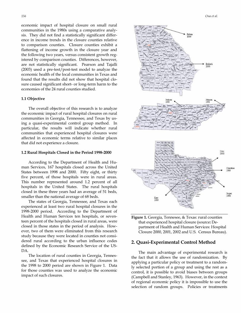
The location of rural counties in Georgia, Tennes-see, and Texas that experienced hospital closures in the 1998 to 2000 period are shown in Figure 1. Data for those counties was used to analyze the economic impact of such closures.

Figure 1. Georgia, Tennesee, & Texas: rural counties that experienced hospital closure (source: De-partment of Health and Human Services: Hospital Closure 2000, 2001, 2002 and U.S. Census Bureau).

2. Quasi-Experimental Control Method The main advantage of experimental research is

the fact that it allows the use of randomization. By applying a particular policy or treatment to a random-ly selected portion of a group and using the rest as a control, it is possible to avoid biases between groups (Campbell and Stanley, 1963). However, in the context of regional economic policy it is impossible to use the selection of random groups. Policies or treatments

Hospital Closures 157

applied – hospital closure in this case – are not as-signed randomly but because of a particular reason. The control group is selected after the treatment has happened such that it permits isolating the treatment effect. That is the reason why in the case of regional economic policy evaluation the use of quasi-experimental methods is more appropriate. The qua-si-experimental method or technique has most of the aspects of an experiment: a treatment, an outcome measure, and a control group whose experiences serve as a baseline against which the effects of treatment can be measured.

Quasi-experimental control group methods have been used as a measurement technique to analyze economic and spatial structural change. As Isserman and Merrifield (1982) explain, the essence of such me-thods is the careful identification of a control group – a set of places whose economic development trajectory enables measurement of what would have happened in the place under study, absent the effect of the phe-nomenon or policy being studied. To allow this, the control areas are selected on the basis of their similari-ty to the treated region in the period before the policy or treatment was implemented.

Some of the advantages of the quasi-experimental approach (Isserman and Merrifield, 1982) are the fol-lowing:

1. The method controls for a variety of events

that occur simultaneously with the regional policy, such as recent changes in national economic cycles and inflation.

2. Unlike economic base or input-output anal-ysis, the quasi-experimental approach may be applied to cases where the structure of the economy is radically transformed. This method identifies structural changes. The quasi-experimental method requires neither assumptions about fixed structural relation-ships nor any complex and time-consuming adjustment mechanisms to approximate structural change.

Instead, the quasi-experimental approach requires

the conviction that the control group is wisely chosen. The quasi-experimental design proposed might be

thought of as a combination of the non-equivalent un-treated control group design and the interrupted time-series design (Campbell and Stanley, 1963). The main idea of this method is to match policy-treated counties with untreated counties that have similar economic and spatial characteristics. The resulting design is di-agrammed in Figure 2. In the figure the first row represents the time series of the treatment group, the

second row represents the time series of the control group, the Os represent the economic and spatial cha-racteristics, the subscripts represent the time intervals, and the X represents the treatment.

Figure 2. Quasi-experimental Design. In the „non equivalent group design‟ proposed by

Campbell and Stanley (1963), the treatment or policy group (or region) is compared, or matched, to an un-treated group in the period before the treatment hap-pens. If the two groups show statistical similarity be-fore the treatment is applied, then the criterion for a control group is met. These groups will be tested again after the treatment or policy is applied to check for differences between the treated and the untreated (control) regions. The measured differences will be considered to be a measure of the impact of applying the policy/treatment. Thus, the economic perfor-mance of the untreated or control group will be the expectation of what would have happened to the treated group if no policy or treatment was applied.

2.1 Hospital and Closure Definitions

For the purpose of this study, the following defini-

tions (Department of Health and Human Services 1993) will be used:

Rural Hospital: a facility located in a rural

area that provides general, short-term, acute medical and surgical inpatient services.

Closed Hospital: one that stopped providing general, short-term, and acute inpatient ser-vices during the period of analysis. If a hospital merged with or was sold to another hospital and the physical plant closed for inpatient acute care, it was considered a clo-sure. If a hospital both closed and reopened in the same year, it was not considered a closure. If a hospital closed, reopened, and then closed again during the years in the study, it will be counted as a closure only once.

2.2 Time Periods

It will be necessary to distinguish different time

periods: the selection period and the treatment period. The selection period is the interval before the policy is administered. It is composed of the calibration period

158 Ona et al.

and the selection-test period. The calibration period is used to identify an appropriate control group. Va-riables that describe conditions and growth rates with-in this period (selection variables) are the basis for se-lecting the control counties.

For the rural counties that experienced hospital closure in 1998 the calibration period is from 1987 to 1992. For the rural counties that experienced hospital closure in 1999 and 2000 the calibration periods are from 1988 to 1993 and 1989 to 1994, respectively. Five years provides a long enough interval that short term fluctuations do not drive the selection process, but is not so long that underlying economic structures change markedly.

The selection-test period is used to perform a sta-tistical pre-test to explicitly evaluate the validity of the control group. By doing this it is possible to evaluate the ability of the control group to accurately trace out the growth path of the treated county. This period starts at the end of the selection period and it ends just before the treatment begins. Because no treatment occurred during the selection test period, the counter-factual traced out by the control group during that period should be identical to the actual.

For the rural counties that experienced hospital closure in 1998 the selection-test period went from 1992 to 1997. For the rural counties that experienced hospital closure in 1999 and 2000 the selection-test pe-riods went from 1993 to 1998 and 1994 to 1999, respec-tively. The reasons for a five year interval are the same as for the calibration interval.

The treatment period is the period after the policy is administered. A treatment effect is identified if the actual and the control, or counter-factual, conditions diverge during this period, and their difference is sta-tistically significant.

In this research the treatment period stretches from the year of closure to three years after closure. Therefore, the treatment period went from 1998 to 2001 for the 1998 closures, from 1999 to 2002 for the 1999 closures, and from 2000 to 2003 for the 2000 clo-sures. The treatment period of three years was chosen mainly because of the availability of the data we used for the analysis. It is also expected that if closure is to have a detectable impact it should be evident within three years.

2.3 Selecting Control Groups

The more similar the treated and untreated groups

or regions are, the more effective the control group becomes. Therefore, it is extremely important to care-fully select the control regions in this type of analysis.

In order to select a control group it is important to fol-low two steps (Rephann 1993 and Ray 1999).

The first step is deciding what variables are im-portant in defining and identifying similar places. The decision on the variables will depend on the type of research and the availability of data.

The purpose of this research is to analyze the im-pact of rural hospital closures on the economic devel-opment of the affected counties. However, it is impor-tant to consider that factors other than the closure may have affected the economic development of the closure counties. In order to know what would have hap-pened in the absence of the hospital closure in these counties, a group of control counties will be selected. A county will be chosen to match each of the counties on the basis of similar economic structure, spatial structure, and growth patterns.

The variables used to match counties, which will be called selection variables, in this research study in-cluded previous growth variables (income growth rate and population growth rate), spatial structure va-riables (population, population density, distance to the nearest metropolitan statistical area or MSA, and net migration rate1), economic structure (per capita in-come, farming earnings, manufacturing earnings, combined earnings from the wholesale, retail and ser-vice sectors, and health service earnings), and, finally, the number of beds per 1000 inhabitants and the num-ber of doctors.

The second step is to choose a selection method for sorting and selecting a control region(s) for each treatment region. We employed an iterative optimiza-tion algorithm to obtain the “best” set of matches. It searches for the set of control matches which minimiz-es the aggregate distance of the matches (taken as a group) from the treatment observations.

In order to measure similarity in cases of multiva-riate data, the Mahalanobis distance (Rephann, 1993) which is defined as follows, is used frequently in sta-tistical analysis:

d(xT,xi) = (xT-xi)‟∑-1(xT-xi),

where d(xT,xi) is the distance between the vector of selection variables for treated county and county i, and ∑ is the variance-covariance matrix of the variables for the potential twins. The Mahalanobis metric implicitly scales and weighs the variables by a factor determined from the variability of data. For example, if a variable has high variance, ceteris paribus, the variable will contribute less to the dissimilarity between the treat-

1 Net migration rate was considered as a spatial structure variable

because it reflects the attractiveness of the location


ment region and a control candidate than if the varia-ble has a low variance. The Mahalanobis metric is for-giving on those high-variance dimensions for which it is difficult to find close observations

The Mahalanobis metric has several advantages, including a reduction in researcher subjectivity and the preservation of the distributional characteristics of the data. In the absence of knowledge about the im-portance of different covariates in affecting outcomes, as in the case of regional development research, it may be preferred to discretion. If the purpose is to find the best control group possible, preferring the set of matches that produces the minimum summed Maha-lanobis distance from each treated county to its matched untreated county would be the best.

2.4 Statistical Testing of Control Group Matches

The matching procedure should produce matched

counties that are a reasonable control group for the treated counties. However, a more rigorous statistical evaluation will test the extent to which this is true. Statistical tests are used both to evaluate the suitability of the control groups and to assess the economic ef-fects of hospital closures in rural communities.

Tests of univariate significance refer to statistically significant differences between the policy treated counties and their control group in terms of growth rates of individual variables. These variables will be called behavioral variables. The pairwise matching method will assume that the mean of the pairwise growth rate differences is distributed approximately normally and use a conventional t-test for univariate statistical significance.

The specific approach is a t-test of the mean growth rate difference of the matched pairs, with the null hypothesis of:

,0:0

C

jt

T

jt

TC

jt rrDH

where D is the growth rate difference, T is the treated (closure) group, C is the no-closure control group, rj is growth rate of behavioral variable j, and t is the test year.

According to Rephann (1993, 148), “the appropri-ate test in this case would be a standard difference of means test. This test is less efficient than testing on paired growth differences because it throws away in-formation about pairwise association.” The test statis-tic which is based on the mean differences is the fol-lowing:

)//( fst djtmjtjt

where δm is the mean of growth rate differences, sd is the standard deviation of the growth rate differences, and f is number of treatment regions.

A test of global significance is calculated to study the overall degree of fit of the twins. It refers to statis-tically significant differences for the vector of growth rates taken as a whole. If no statistically significant differences are revealed, it implies that the matches are good. The simplifying assumptions in this case are the independence of growth rates over time and among variables. The statistic used in testing here is the Ho-telling T2 test statistic, which is a multivariate exten-sion of the univariate t-test.

Following Johnson and Wichern (1982), the hypo-theses and test statistic are:

00 :H

01 :H

)()'( 0

1

0

2xSxnT

where n

j jxnx1

)/1( is a px1 vector, where p is the

number of variables, n = number of treated (and paired untreated) counties, )')(())1/(1(

1xxxxnS j

n

j j

is a pxp matrix, and µo is the px1 vector of the variable mean values of the control counties. The test statistic T2 is distributed (n-1)p/(n-p) Fp,n-p, where Fp,n-p de-notes a random variable with an F distribution with p and n-p degrees of freedom.

Because the control group will indicate what would have happened to the treated counties in the absence of treatment, both univariate and global signi-ficance tests are performed to evaluate whether the control group is a good proxy for the hypothetical treated county growth after the treatment. If the con-trol group shows that it is a good proxy for the hypo-thetical treated county growth before the closure year then that should be the case. Ideally there should be no statistically significant differences between the growth rates of the closure counties and the selected control group before closure happened.

2.5 Statistical Testing of Economic Impact

The mean growth differences of the selected beha-

vioral variables in the post treatment period are the primary measure of the program effects. For each year after the closure year, the growth rate from the closure year to the last year of the study will be calculated for each treated county and its twin, for each variable. A univariate t-test of the mean growth rate differences, similar to the one performed in the pre-test period, will be performed. It will be estimated for each con-

160 Ona et al.

secutive year from the closure year to the last date analyzed.

3. Results

3.1 Optimal Matching The first step was to determine the counties that

could be possible matches. Those counties had to meet the criteria of both being rural2 and of having a number of beds greater than zero, an indication of hospital presence in the county. The number of coun-ties considered in this research was 69 for the state of Georgia, 48 for the state of Tennessee, and 132 for the state of Texas. Therefore, the total of number of coun-ties which could be possible matches for the closure counties was 248.3 The next step was to use SAS to estimate the Mahalanobis distance between each clo-sure county and all the possible matches. The result-ing numbers were ranked, and finally the county with the lowest distance or twin was chosen. The results from applying the Mahalanobis distance are summa-rized in Table 1. Table 1. Hospital Closure Counties and Their

Matches within Region.

Year of Closure State County Match within Region

1998 Tennessee Johnson Dimmit (Texas) 1998 Texas Jasper Monroe (Tennessee) 1999 Georgia Rabun Candler (Georgia) 1999 Tennessee Jackson Franklin (Texas) 1999 Texas Cherokee Navarro (Texas) 1999 Texas Kerr Howard (Texas) 2000 Georgia Bulloch Coffee (Georgia) 2000 Texas Cass Cooke (Texas)

3.2 Statistical Testing of Control Group Validity

Prior to assessing the success of matching, a test of

the stability of the control groups for the selected be-havioral variables was conducted. This test indicated

2 The division between rural and urban was done using the urban influence codes as defined by the Economic Research Service of the USDA. 3 Twins were found both within the same state and within the whole region (Georgia, Tennessee, and Texas). However, because the Ma-

halanobis distances were lower in almost all cases (except for one), the twins within the region were preferred to the ones within the

same state.

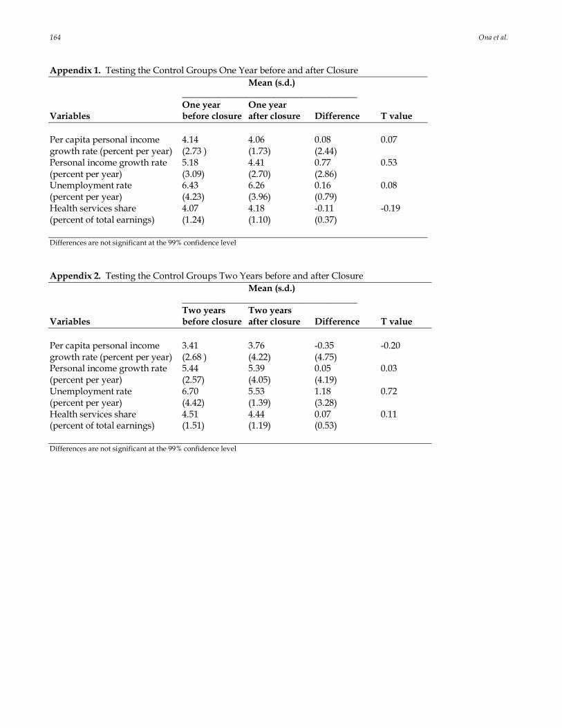
that the control groups grew at a constant rate for the variables considered when comparing one year before closure with one year after closure and when compar-ing two years before closure with two years after clo-sure. These results4 provide a first indication that this is a reasonable control group.

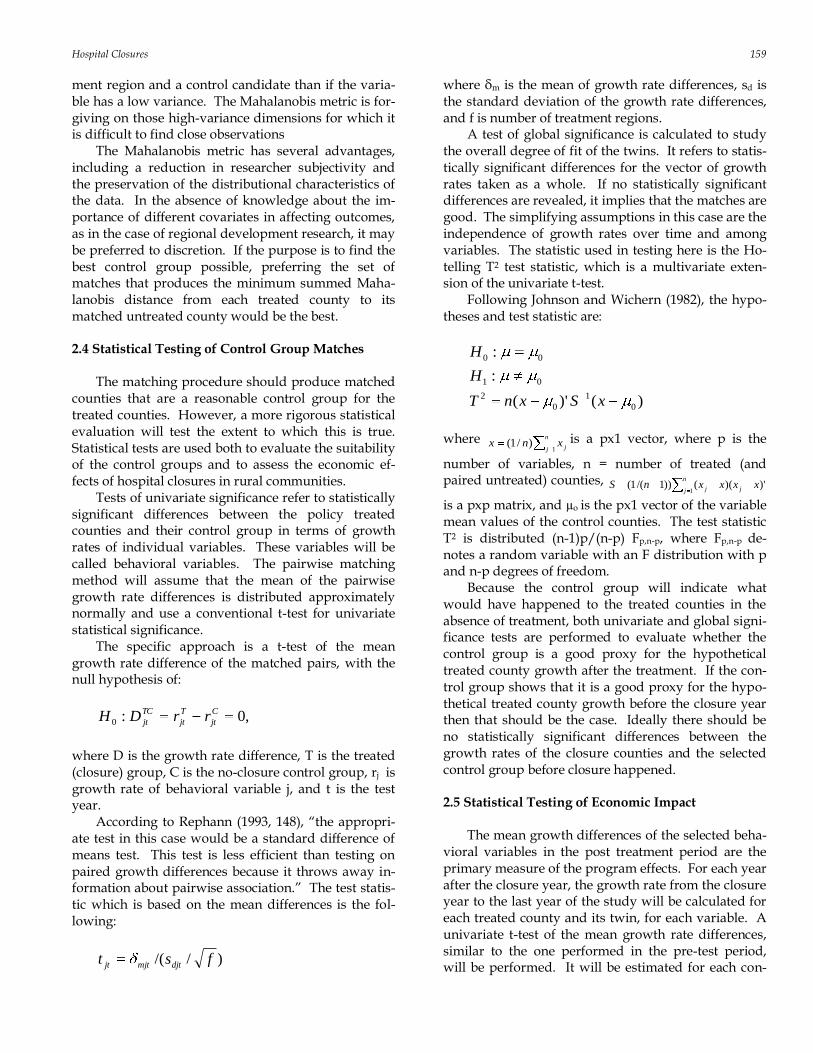
The tests to evaluate the appropriateness of the control group were the univariate and global tests for closure and control counties. The results of these tests are summarized in Table 2. During the testing period, the average growth rates of the closure counties were higher for three of the four selection variables consi-dered: per capita personal income, total population, and personal income. In the case of health services share, the shares of the matched counties was higher than the shares of the closed counties. None of the four differences, however, was significant at the 99% confidence level.

For the global test, the Hotelling T square test was applied to test if the matches obtained applying op-timal matching (Mahalanobis distance) were good at the 99% confidence level. Using the same set of four variables, the results indicated that the matches are good.

3.3 Statistical Test of Economic Impact

The results of the economic impact of rural hospit-

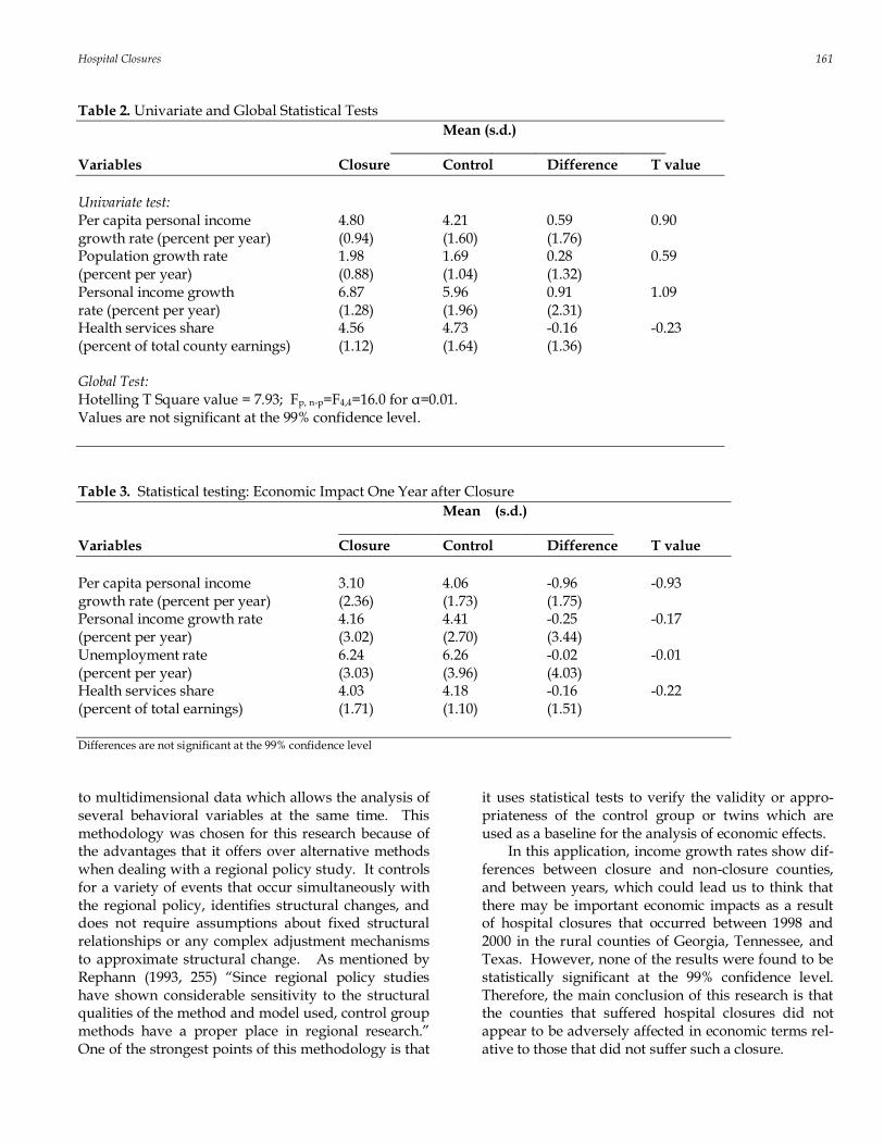
al closure are provided in Tables 3, 4, and 5. The un-ivariate tests to analyze if there was an economic im-pact in the counties that suffered hospital closure ex-amined per capita personal income, personal income, unemployment rate, and health services share. Analy-sis was over the first three years after hospital closure.

In the first year after closure all the variables were higher in the matched counties than in the closure counties. In the second year after closure the average growth rates of per capita income and unemployment rate were higher in the closure counties than in the matched counties, while the average growth rates of personal income and the health services share were lower in the closure counties than in the matched counties. Finally, in the third year after closure, all the variables considered were lower in the closure coun-ties than in their twin. None of these results, however, was significant at the 99% confidence level.

4. Conclusions

This paper used the quasi-experimental control group method to analyze regional economic effects of hospital closure. This control group method is applied

4 The results of this test are included in Appendices 1 and 2.


Table 2. Univariate and Global Statistical Tests

Mean (s.d.) ______________________________________ Variables Closure Control Difference T value

Univariate test: Per capita personal income 4.80 4.21 0.59 0.90 growth rate (percent per year) (0.94) (1.60) (1.76) Population growth rate 1.98 1.69 0.28 0.59 (percent per year) (0.88) (1.04) (1.32) Personal income growth 6.87 5.96 0.91 1.09 rate (percent per year) (1.28) (1.96) (2.31) Health services share 4.56 4.73 -0.16 -0.23 (percent of total county earnings) (1.12) (1.64) (1.36) Global Test: Hotelling T Square value = 7.93; Fp, n-p=F4,4=16.0 for α=0.01. Values are not significant at the 99% confidence level.

Table 3. Statistical testing: Economic Impact One Year after Closure


Per capita personal income 3.10 4.06 -0.96 -0.93 growth rate (percent per year) (2.36) (1.73) (1.75) Personal income growth rate 4.16 4.41 -0.25 -0.17 (percent per year) (3.02) (2.70) (3.44) Unemployment rate 6.24 6.26 -0.02 -0.01 (percent per year) (3.03) (3.96) (4.03) Health services share 4.03 4.18 -0.16 -0.22 (percent of total earnings) (1.71) (1.10) (1.51)

Differences are not significant at the 99% confidence level

to multidimensional data which allows the analysis of several behavioral variables at the same time. This methodology was chosen for this research because of the advantages that it offers over alternative methods when dealing with a regional policy study. It controls for a variety of events that occur simultaneously with the regional policy, identifies structural changes, and does not require assumptions about fixed structural relationships or any complex adjustment mechanisms to approximate structural change. As mentioned by Rephann (1993, 255) “Since regional policy studies have shown considerable sensitivity to the structural qualities of the method and model used, control group methods have a proper place in regional research.” One of the strongest points of this methodology is that

it uses statistical tests to verify the validity or appro-priateness of the control group or twins which are used as a baseline for the analysis of economic effects.

In this application, income growth rates show dif-ferences between closure and non-closure counties, and between years, which could lead us to think that there may be important economic impacts as a result of hospital closures that occurred between 1998 and 2000 in the rural counties of Georgia, Tennessee, and Texas. However, none of the results were found to be statistically significant at the 99% confidence level. Therefore, the main conclusion of this research is that the counties that suffered hospital closures did not appear to be adversely affected in economic terms rel-ative to those that did not suffer such a closure.

162 Ona et al.

Table 4. Statistical testing: Economic Impact Two Years after Closure


Per capita personal income 4.28 3.76 0.52 0.29 growth rate (percent per year) (2.71) (4.22) (3.61) Personal income growth rate 4.89 5.39 -0.50 -0.26 (percent per year) (3.57) (4.05) (4.3) Unemployment rate 5.79 5.53 0.26 0.34 (percent per year) (1.71) (1.39) (2.04) Health services share 4.40 4.44 -0.04 -0.05 (percent of total earnings) (2.25) (1.19) (2.22)


Table 5. Statistical testing: Economic Impact Three Years after Closure


Per capita personal income 1.05 3.07 -2.02 -1.00 growth rate (percent per year) (2.93) (4.92) (5.11) Personal income growth rate 1.80 4.60 -2.80 -1.53 (percent per year) (2.99) (4.21) (4.66) Unemployment rate 6.10 6.18 -0.08 -0.09 (percent per year) (1.93) (1.22) (2.38) Health services share 4.62 4.96 -0.34 -0.30 (percent per year) (2.51) (1.92) (3.33)


Among the possible explanations are the existence of alternative health service providers in the areas of study (e.g., hospital in adjacent county, alternative health care and emergency treatment centers) and the fact that some other rural hospitals opened or re-opened (in a different facility). Of course, there is also the possibility that the twins do not provide precise enough measures of economic change without closure, i.e., they are a less than ideal control group. The small number of observations may also have hampered the identification of significant effects. Future research with an expanded area of study and/or a different time period could provide an increase in the number of observations.

References Area Connect, Latitude and Longitude data, Retrieved

from: http://longviewtx.areaconnect.com/ zip2.htm.

Bartels, C., W. Nicol, and J. van Duijin. 1982. “Esti-mating the impact of regional policy: A review of applied research methods.” Regional Science and Urban Economics 12:3-41.

Bureau of Economic Analysis. Per Capita Personal In-come, Personal Income, Health Services Earnings, Total Earnings data, Retrieved from http://www.bea.gov/bea/regional/data.htm.

Bureau of Labor Statistics, Unemployment Rate data, Retrieved from http://www.bls.gov/lau.

Campbell, D. and J. Stanley. 1963. Experimental and Quasi-experimental Designs for Research. Chicago: R. McNally.


Christianson, J. and L. Faulkner. 1981. The contribu-tion of rural hospitals to local economies. Inquiry

18(Spring):46-60. Department of Health and Human Services. 2000,

2001, and 2002. Hospital Closure. Washington, DC.

Doeksen, G., T. Johnson, and C. Willioughby. 1997. Measuring the Economic Importance of the Health Sector on a Local Economy: A Brief Literature Re-view and Procedures to Measure Local Impacts. SRCD Number 202, Mississippi State University.

Economic Research Service. 2003 Urban Influence Codes for Georgia, Tennessee, and Texas, Re-trieved from http://www.ers.usda.gov/ data/urbaninfluencecodes/2003.

Hart, L.G., M.J. Piriani, and R.A. Rosenblatt. 1991. Causes and consequences of rural small hospital closures from the perspectives of mayors. The Journal of Rural Health 7(1): 222-245.

Isserman, A.M. 1994. A Family of Geographical Con-trol Group Methods for Regional Research. Re-gional Research Institute Research Paper No. 9436, West Virginia University.

Isserman, A. M. and J. Merrifield. 1982. The use of control groups in evaluating regional economic policy. Regional Science and Urban Economics 12: 45-48.

Johnson R. and D. Wichern. 1982. Applied Multivariate Statistical Analysis. Englewood Cliffs,

N.J.:Prentice-Hall. King, L.J. 1969. Statistical Analysis in Geography. En-

glewood Cliffs, NJ: Prentice Hall. National Center for Health Workforce Analysis. 2003.

Area Resource File, Health Resources and Services Administration. US Department of Health and

Human Services, Health Resources and Services Administration, Bureau of Health Professions. Rockville, MD.

Pearson, D.R. and H. Tajalli. 2003. The impact of rural hospital closure on the economic health of the lo-cal communities. Texas Journal of Rural Health 21(3):46-51.

Proximity, MSAs, Retrieved from http://proximityone.com/metros.htm.

Probst, J., M. Samuels, J. Hussey, D. Berry, and T. Ricketts. 1999. Economic impact of hospital clo-sure on small rural counties, 1984 to 1988: Demon-stration of a comparative analysis approach. The Journal of Rural Health 15(4):375-390.

Ray, M. 1999. Effectiveness of Credit Pooling Techniques for Infrastructure Development in Rural Communities: A Quasi-Experimental Analysis. Unpublished Ph.D.

Dissertation, Clemson University. Rephann, T.J. 1993. A Study of the Relationship Between

Highways and Regional Economic Growth and Devel-

opment using Quasi-Experimental Control Group Me-thods. Unpublished Ph.D. Dissertation, West Vir-

ginia University. Shadish, W., D. Cook, and D. Campbell. 2002. Experi-

mental and Quasi-Experimental Designs for Genera-lized Causal Inference. Boston : Houghton Mifflin.

U.S. Census Bureau, County Population Centroids for Georgia, Tennessee, and Texas, Retrieved from http://www.census.gov/geo/www/cenpop/county/coucntr48.html.

U.S. Census Bureau, Georgia, Tennessee, and Texas maps, Retrieved from http://quickfacts.census.gov/qfd/maps.

U.S. Census Bureau, Net migration data, Retrieved from http:// www.census.gov/popest/ archives/1990s/co-99-08/99c8_13.txt.

U.S. Census Bureau, Population Per Square Mile, Re-trieved from http://www.census.gov/ population/censusdata/90den_stco.txt.

ZIP‟s Data User Guide, Distance Calculation Formula, Retrieved from http://www.melissadata.com/ manuals/zdman.pdf.

164 Ona et al.

Appendix 1. Testing the Control Groups One Year before and after Closure

Mean (s.d.) ______________________________________ One year One year Variables before closure after closure Difference T value

Per capita personal income 4.14 4.06 0.08 0.07 growth rate (percent per year) (2.73 ) (1.73) (2.44) Personal income growth rate 5.18 4.41 0.77 0.53 (percent per year) (3.09) (2.70) (2.86) Unemployment rate 6.43 6.26 0.16 0.08 (percent per year) (4.23) (3.96) (0.79) Health services share 4.07 4.18 -0.11 -0.19 (percent of total earnings) (1.24) (1.10) (0.37) Differences are not significant at the 99% confidence level

Appendix 2. Testing the Control Groups Two Years before and after Closure

Mean (s.d.) ______________________________________ Two years Two years Variables before closure after closure Difference T value

Per capita personal income 3.41 3.76 -0.35 -0.20 growth rate (percent per year) (2.68 ) (4.22) (4.75) Personal income growth rate 5.44 5.39 0.05 0.03 (percent per year) (2.57) (4.05) (4.19) Unemployment rate 6.70 5.53 1.18 0.72 (percent per year) (4.42) (1.39) (3.28) Health services share 4.51 4.44 0.07 0.11 (percent of total earnings) (1.51) (1.19) (0.53)


Economic Impact of Hospital Closure on Rural Communities in Three Southern States: A...

Documents

Transcript of Economic Impact of Hospital Closure on Rural Communities in Three Southern States: A...