Economic Analysis of Water Conservation Technologies or ...

Farm Level Economic Analysis of Water Conservation and Water Use Efficiency

Technologies In Ontario Commercial Agricultural Production

by

David Jacques

A Thesis

presented to

The University of Guelph

In partial fulfilment of requirements

for the degree of

Master of Science

in

Food, Agricultural and Resource Economics

Guelph, Ontario, Canada

©David Jacques, August, 2014

Abstract

Farm Level Economic Analysis ofWater Conservation andWater Use Efficiency Technologies In Ontario

Commercial Agricultural Production

David Jacques

University of Guelph, 2014

Advisor(s):

Glenn Fox

The goal of this thesis is to assess the farm level economics of three technologies that conserve water or that

increase technical water use efficiency in Ontario commercial agricultural production. Case studies were conducted

on three technologies: subsurface drip irrigation, a chipping potato variety with higher technical water use efficiency

and wood chips in orchard tree rows. The technologies in the case studies were assessed using a stochastic net present

value framework. Of the three technologies assessed only growing a chipping potato variety with higher technical

water use efficiency has a positive net present value under baseline assumptions. The results indicate that the effect a

technology has on yields plays an important role in determining whether or not it will be a worthwhile investment for

an individual producer.

Acknowledgements

I would like to thank my advisor, Professor Glenn Fox, for helping to keep my work on track while still allowing

me to make and learn from my mistakes. His time, patients and encouragement made working on this thesis an

invaluable learning experience. I am thankful to the members of my thesis committee, Professors Alan Ker and

Alfons Weersink, and my external examiner, Professor Rakhal Sarker, for providing constructive criticism and

feedback on the thesis. This thesis could not have been written without the help of professionals in Ontario’s

agricultural sector. Researchers at the University of Guelph, representatives from growers associations and

employees at the Ontario Ministry of Agriculture, Food and Rural Affairs. All of whom shared their knowledge

and advice in the early stages of my research. In particular I would like to thank Bruce Kelly from Farm Food

Care Ontario, Peter White from the University of Guelph, Peter VanderZaag of Sunrise Potato Storage Ltd and

John Zandstra from the University of Guelph for taking the time to meet with me and for sharing information that

formed the basis of my case studies. I owe a debt of gratitude to the staff and faculty of the Food, Agricultural

and Resource Economics department at the University of Guelph. Finally I would like to thank my family,

friends and my lady friend Patrice for their support and patients over the last two years.

iii

Table of Contents

1 Introduction 1

1.1 Background . . . . . . . . . . . . . . . . . . . . . . . . . . . . . . . . . . . . . . . . . . . . . . . . 1

1.2 The Economic Problem . . . . . . . . . . . . . . . . . . . . . . . . . . . . . . . . . . . . . . . . . . 2

1.3 The Economic Research Problem . . . . . . . . . . . . . . . . . . . . . . . . . . . . . . . . . . . . . 2

1.4 The Purpose Of This Thesis . . . . . . . . . . . . . . . . . . . . . . . . . . . . . . . . . . . . . . . 3

1.5 The Objectives Of This Thesis . . . . . . . . . . . . . . . . . . . . . . . . . . . . . . . . . . . . . . 3

1.6 Outline Of The Thesis . . . . . . . . . . . . . . . . . . . . . . . . . . . . . . . . . . . . . . . . . . 4

2 Water conservation and water use efficiency in agricultural production 7

2.1 Water use by the agricultural sector in Ontario . . . . . . . . . . . . . . . . . . . . . . . . . . . . . . 7

2.2 The Hydrology of a Farm . . . . . . . . . . . . . . . . . . . . . . . . . . . . . . . . . . . . . . . . . 8

2.3 Agricultural water use, withdrawal and consumption . . . . . . . . . . . . . . . . . . . . . . . . . . 9

2.4 Water conservation in agricultural production . . . . . . . . . . . . . . . . . . . . . . . . . . . . . . 10

2.5 Technical water use efficiency in agricultural production . . . . . . . . . . . . . . . . . . . . . . . . 10

2.6 Economic efficiency and agricultural water use . . . . . . . . . . . . . . . . . . . . . . . . . . . . . 11

2.7 The economics of water conservation and technical water use efficiency . . . . . . . . . . . . . . . . 13

2.8 Conclusion . . . . . . . . . . . . . . . . . . . . . . . . . . . . . . . . . . . . . . . . . . . . . . . . 14

3 The production economics of water conservation in agriculture 17

3.1 A model of profit maximization, water use and water conservation at the producer level . . . . . . . . 17

3.1.1 The objective function . . . . . . . . . . . . . . . . . . . . . . . . . . . . . . . . . . . . . . 17

3.1.2 The production function . . . . . . . . . . . . . . . . . . . . . . . . . . . . . . . . . . . . . 19

3.1.3 The effective irrigation function . . . . . . . . . . . . . . . . . . . . . . . . . . . . . . . . . 19

3.1.4 The drainage function . . . . . . . . . . . . . . . . . . . . . . . . . . . . . . . . . . . . . . 20

3.1.5 Using the model to say something about the adoption of water conserving technologies in

agriculture . . . . . . . . . . . . . . . . . . . . . . . . . . . . . . . . . . . . . . . . . . . . 21

3.2 Production functions, total product curves, technological change and water conservation . . . . . . . 22

3.2.1 Polynomial total product function of water and water conservation . . . . . . . . . . . . . . . 22

iv

3.2.2 Cobb-Douglas production function, technological change and water conservation . . . . . . . 24

3.2.3 Choosing the functional form of the crop-water production function . . . . . . . . . . . . . . 26

3.3 Substitution between water and other inputs . . . . . . . . . . . . . . . . . . . . . . . . . . . . . . . 27

3.4 Taking into account uncertainty and the option to wait . . . . . . . . . . . . . . . . . . . . . . . . . . 28

3.5 Models that account for intraseasonal water use and profitable technology adoption . . . . . . . . . . 29

3.6 Irrigation systems as a form of insurance . . . . . . . . . . . . . . . . . . . . . . . . . . . . . . . . . 30

3.7 Modelling water as a damage control input . . . . . . . . . . . . . . . . . . . . . . . . . . . . . . . . 30

3.8 Conclusion . . . . . . . . . . . . . . . . . . . . . . . . . . . . . . . . . . . . . . . . . . . . . . . . 32

4 Methods 38

4.1 Sources of data for case studies . . . . . . . . . . . . . . . . . . . . . . . . . . . . . . . . . . . . . . 38

4.2 Finding and selecting case studies . . . . . . . . . . . . . . . . . . . . . . . . . . . . . . . . . . . . 38

4.3 Economic analysis . . . . . . . . . . . . . . . . . . . . . . . . . . . . . . . . . . . . . . . . . . . . 38

5 Subsurface drip irrigation in corn production 44

5.1 What is a subsurface drip irrigation system? . . . . . . . . . . . . . . . . . . . . . . . . . . . . . . . 44

5.2 Corn production in Ontario . . . . . . . . . . . . . . . . . . . . . . . . . . . . . . . . . . . . . . . . 47

5.3 The case study subsurface drip irrigation system . . . . . . . . . . . . . . . . . . . . . . . . . . . . . 48

5.4 Methods for assessing the farm level economics of a subsurface drip irrigation used to grow corn . . . 49

5.5 Capital cost of the subsurface drip irrigation system . . . . . . . . . . . . . . . . . . . . . . . . . . . 51

5.6 How using the subsurface drip irrigation system affects cash income . . . . . . . . . . . . . . . . . . 52

5.7 How using the subsurface drip irrigation system affects expenses . . . . . . . . . . . . . . . . . . . . 58

5.8 System longevity . . . . . . . . . . . . . . . . . . . . . . . . . . . . . . . . . . . . . . . . . . . . . 59

5.9 Results and Discussion . . . . . . . . . . . . . . . . . . . . . . . . . . . . . . . . . . . . . . . . . . 60

6 The use of varieties with higher technical water use efficiency in Ontario chipping potato production 82

6.1 The potato sector in Ontario . . . . . . . . . . . . . . . . . . . . . . . . . . . . . . . . . . . . . . . 82

6.2 Technical water use efficiency and potato varieties . . . . . . . . . . . . . . . . . . . . . . . . . . . . 84

6.3 2012 and 2013 potato on farm variety trials in Alliston, Ontario: a hint of increased technical water

use efficiency . . . . . . . . . . . . . . . . . . . . . . . . . . . . . . . . . . . . . . . . . . . . . . . 86

6.3.1 Experimental design of the 2012 and 2013 field trials in Alliston, Ontario . . . . . . . . . . . 86

6.3.2 The technical water use efficiency of the T10-3 and Dakota Pearl varieties in the 2012 and

2013 trials in Alliston, Ontario . . . . . . . . . . . . . . . . . . . . . . . . . . . . . . . . . . 87

6.4 The farm level economics of growing a potato variety with higher technical water use efficiency . . . 89

6.5 Methods for assessing the farm level economics of a chipping potato variety with higher technical

water use efficiency . . . . . . . . . . . . . . . . . . . . . . . . . . . . . . . . . . . . . . . . . . . . 89

v

6.6 Change in cash income from growing a chipping potato with higher technical water use efficiency . . 91

6.7 Change in cash expenses from growing a high water use efficiency potato variety . . . . . . . . . . . 96

6.8 Results . . . . . . . . . . . . . . . . . . . . . . . . . . . . . . . . . . . . . . . . . . . . . . . . . . . 98

6.8.1 Net present value of growing T10-3 rather than Atlantic and of growing T10-3 rather than

Dakota Pearl . . . . . . . . . . . . . . . . . . . . . . . . . . . . . . . . . . . . . . . . . . . 98

6.8.2 Sensitivity Analysis On Net present value calculation of growing T10-3 rather than Atlantic

and of growing T10-3 rather than Dakota Pearl . . . . . . . . . . . . . . . . . . . . . . . . . 99

6.8.3 Break-even analysis on the yield of T10-3 . . . . . . . . . . . . . . . . . . . . . . . . . . . . 101

6.9 Discussion . . . . . . . . . . . . . . . . . . . . . . . . . . . . . . . . . . . . . . . . . . . . . . . . . 102

7 The use of in row ground covers in peach orchards 122

7.1 The peach sector in Ontario . . . . . . . . . . . . . . . . . . . . . . . . . . . . . . . . . . . . . . . . 122

7.2 Ground covers in peach tree rows as a water conservation technology . . . . . . . . . . . . . . . . . . 124

7.3 The case study orchard and within row ground cover . . . . . . . . . . . . . . . . . . . . . . . . . . 125

7.4 Methods for assessing the farm level economics of using wood chips as a in row ground cover . . . . 125

7.5 Capital cost of the tree row ground cover . . . . . . . . . . . . . . . . . . . . . . . . . . . . . . . . . 127

7.6 Change in cash income from using ground covers in peach production . . . . . . . . . . . . . . . . . 129

7.7 Change in expenses from using ground covers in peach production . . . . . . . . . . . . . . . . . . . 133

7.8 Results and discussion . . . . . . . . . . . . . . . . . . . . . . . . . . . . . . . . . . . . . . . . . . 134

8 Conclusion 150

8.1 Summary . . . . . . . . . . . . . . . . . . . . . . . . . . . . . . . . . . . . . . . . . . . . . . . . . 150

8.2 The case studies technologies, water conservation, technical water use efficiency and economic efficiency151

8.3 Major findings and lessons learned . . . . . . . . . . . . . . . . . . . . . . . . . . . . . . . . . . . . 152

8.4 Limitation and recommendations for future research . . . . . . . . . . . . . . . . . . . . . . . . . . . 152

References 161

vi

List of Tables

1.1 Estimated Agricultural Water Withdrawal in Ontario 1991 to 2011, Excluding Aquaculture and Golf

Course Water Use . . . . . . . . . . . . . . . . . . . . . . . . . . . . . . . . . . . . . . . . . . . . . 6

5.1 Baseline Parameters Of Case Study Subsurface Drip Irrigation System Used To Grow Corn In Norfolk

County, Ontario . . . . . . . . . . . . . . . . . . . . . . . . . . . . . . . . . . . . . . . . . . . . . . 74

5.2 Baseline Capital Cost Of Case Study Subsurface Drip Irrigation System With 40.5 Hectares (100 acres)

Of Irrigated Area Used To Grow Corn In Norfolk County, Ontario . . . . . . . . . . . . . . . . . . . 75

5.3 Results Of Sensitivity Analyses On The Stochastic Simulation Used To Calculate The Net Present

Value Of A Subsurface Drip Irrigation System Used To Grow Corn On 40.5 Hectares (100 acres) In

Norfolk County, Ontario . . . . . . . . . . . . . . . . . . . . . . . . . . . . . . . . . . . . . . . . . 77

5.4 Mean and Median Net Present Value Elasticities Of Subsurface Drip Irrigation System Parameters . . 78

6.1 Precipitation Climate Normals In Alliston, ON And At The Chipping Potato Farm Trial Site In 2012

And 2013 . . . . . . . . . . . . . . . . . . . . . . . . . . . . . . . . . . . . . . . . . . . . . . . . . 108

6.2 Parameters Of Normal Distributions Used To Characterize The Monthly Price Of Chipping Potatoes

In Ontario . . . . . . . . . . . . . . . . . . . . . . . . . . . . . . . . . . . . . . . . . . . . . . . . . 113

6.3 Baseline Parameters Used To Calculate Net Present Value Of Growing A Higher Water Use Efficiency

Chipping Potato Variety, T10-3, Rather Than Conventionally Grown Chipping Potatoes In Ontario . . 114

6.4 Parameters Of Normal Distribution Of Fertilizer Prices Used To Calculate Net Present Value Of Grow-

ing A Higher Water Use Efficiency Chipping Potato Variety, T10-3, Rather Than Conventionally

Grown Chipping Potatoes In Ontario . . . . . . . . . . . . . . . . . . . . . . . . . . . . . . . . . . . 114

6.5 Results Of Sensitivity Analyses On The Stochastic Partial Capital Budgeting Simulation Used To

Calculate The Net Present Value Of A Growing A Higher Water Use Efficiency Chipping Potato

Variety, T10-3, Rather Than The Atlantic Variety . . . . . . . . . . . . . . . . . . . . . . . . . . . . 117

6.6 Results Of Sensitivity Analyses On The Stochastic Partial Capital Budgeting Simulation Used To

Calculate The Net Present Value Of A Growing A Higher Water Use Efficiency Chipping Potato

Variety, T10-3, Rather Than The Dakota Pearl Variety . . . . . . . . . . . . . . . . . . . . . . . . . . 118

6.7 Mean net present value elasticity of growing the T10-3 chipping potato variety rather than the Atlantic 119

vii

6.8 Mean net present value elasticity of growing the T10-3 chipping potato variety rather than the Dakota

Pearl . . . . . . . . . . . . . . . . . . . . . . . . . . . . . . . . . . . . . . . . . . . . . . . . . . . . 119

7.1 Baseline Parameters for the use of wood chips as a ground cover in Ontario peach production . . . . . 145

7.2 Results Of Sensitivity Analyses On The Stochastic Partial Capital Budgeting Simulation Used To Cal-

culate The Net Present Value Of Using Wood Chips As A Ground Cover In Ontario Peach Production

For 10 Years . . . . . . . . . . . . . . . . . . . . . . . . . . . . . . . . . . . . . . . . . . . . . . . . 147

7.3 Mean Net Present Value Elasticities Of Using Wood Chips As A Ground Cover In Peach Tree Rows . 148

viii

List of Figures

1.1 Estimated Percent of Total Average Water Consumption (m3/day)inOntariobyEconomicSector . . 5

2.1 The Hydrology Of A Farm . . . . . . . . . . . . . . . . . . . . . . . . . . . . . . . . . . . . . . . . 15

2.2 The Economics Of Water Use . . . . . . . . . . . . . . . . . . . . . . . . . . . . . . . . . . . . . . 16

3.1 Marginal Revenue Product Of A Quadratic Crop Water Total Product Function . . . . . . . . . . . . 34

3.2 Marginal Revenue Product Of A Quadratic Crop Water Total Product Function . . . . . . . . . . . . 35

3.3 (a) Water Conserving Technological Change In Quadratic Total Physical Product Of Water Function . 36

3.4 A Cobb-Douglas Production Function With Water Conserving Technological Change . . . . . . . . . 37

5.1 Layout And Components Of A Subsurface Drip Irrigation System . . . . . . . . . . . . . . . . . . . 68

5.2 Quantity Of Fodder And Grain Corn Produced In Ontario From 1990 to 2013 (metric tons) . . . . . . 69

5.3 Area Of Fodder And Grain Corn Harvested In Ontario From 1990 to 2013 (hectares) . . . . . . . . . 70

5.4 Real Price Of Corn In Ontario From 1990 to 2013 (real 2013$/metric ton) . . . . . . . . . . . . . . . 71

5.5 Case Study Two Component Normal Distribution Used To Characterize Corn Yields In Norfolk County 72

5.6 Case Study Two Component Normal Distribution Used To Characterize Corn Yields In Norfolk County

When A Subsurface Drip Irrigation System Is Used . . . . . . . . . . . . . . . . . . . . . . . . . . . 73

5.7 Results of Stochastic Simulation Calculating The Net Present Value For Baseline Parameters Of A

Subsurface Drip Irrigation System Used To Grow Corn On 40.5 Hectares (100 acres) In Norfolk

County, Ontario . . . . . . . . . . . . . . . . . . . . . . . . . . . . . . . . . . . . . . . . . . . . . . 76

5.8 Effect On Mean Yield In Normal Years Break Even Analysis For A Subsurface Drip Irrigation System

Used To Grow Corn On 40.5 Hectares (100 Acres) In Norfolk County, Ontario . . . . . . . . . . . . 79

5.9 Capital Cost Break Even Analysis: Median Net Present Values For A Subsurface Drip Irrigation Sys-

tem Used To Grow Corn On 40.5 Hectares (100 acres) In Norfolk County, Ontario . . . . . . . . . . 80

5.10 Results of Stochastic Simulation Where Three Parameters Have Changed Calculating The Net Present

Value Of A Subsurface Drip Irrigation System Used To Grow Corn On 40.5 Hectares (100 acres) In

Norfolk County, Ontario . . . . . . . . . . . . . . . . . . . . . . . . . . . . . . . . . . . . . . . . . 81

6.1 Land Used In Ontario Potato Production From 1990 to 2013 (hectares) . . . . . . . . . . . . . . . . . 103

ix

6.2 Production Of Potatoes In Ontario From 1990 to 2013 (metric ton) . . . . . . . . . . . . . . . . . . . 104

6.3 Average Yield Of Potatoes In Ontario From 1990 to 2013 (metric ton/hectare) . . . . . . . . . . . . . 105

6.4 Price Of Commercial, Processing And Table Potatoes In Ontario From 1990 To 2013 (real 2013 $) . . 106

6.5 Average Monthly Price Of Processing Potatoes In Ontario (real 2013 $/metric ton) . . . . . . . . . . 107

6.6 Canopy Cover Of T10-3 And Dakota Pearl During The 2012 Growing Season In Farm Trials Con-

ducted Alliston, Ontario . . . . . . . . . . . . . . . . . . . . . . . . . . . . . . . . . . . . . . . . . . 109

6.7 Canopy Cover Of T10-3 And Dakota Pearl During The 2013 Growing Season In Farm Trials Con-

ducted Alliston, Ontario . . . . . . . . . . . . . . . . . . . . . . . . . . . . . . . . . . . . . . . . . . 110

6.8 Yield Of T10-3 And Dakota Pearl Potato Varieties From Farm Trials Conducted In Alliston, Ontario

During The 2012 Growing Season . . . . . . . . . . . . . . . . . . . . . . . . . . . . . . . . . . . . 111

6.9 Yield Of T10-3 And Dakota Pearl Potato Varieties From Farm Trials Conducted In Alliston, Ontario

During The 2013 Growing Season . . . . . . . . . . . . . . . . . . . . . . . . . . . . . . . . . . . . 112

6.10 Results of Stochastic Partial Capital Budgeting Simulation Calculating The Net Present Value (real

2013$/hectare) Of Growing The T10-3 Variety Of Chipping Potato Rather Than The Atlantic Variety

Of Chipping Potato In Ontario For 10 Growing Seasons . . . . . . . . . . . . . . . . . . . . . . . . . 115

6.11 Results of Stochastic Partial Capital Budgeting Simulation Calculating The Net Present Value (real

2013$/hectare) Of Growing The T10-3 Variety Of Chipping Potato Rather Than The Dakota Pearl

Variety Of Chipping Potato In Ontario For 10 Growing Seasons . . . . . . . . . . . . . . . . . . . . 116

6.12 Yield Break-even Analysis: Net Present Value (real 2013$/hectare) Of Growing A Higher Water Use

Efficiency Chipping Potato Variety, T10-3, Rather Than The Atlantic Variety For 10 Seasons . . . . . 120

6.13 Yield Break-even Analysis: Net Present Value (real 2013$/hectare) Of Growing A Higher Water Use

Efficiency Chipping Potato Variety, T10-3, Rather Than The Dakota Pearl Variety For 10 Seasons . . 121

7.1 Areas Of Peach Production In Ontario . . . . . . . . . . . . . . . . . . . . . . . . . . . . . . . . . . 138

7.2 Land Used In Ontario Peach Production From 1980 to 2013 (hectares) . . . . . . . . . . . . . . . . . 139

7.3 Production of peaches in Ontario from 1980 to 2013 (metric ton) . . . . . . . . . . . . . . . . . . . . 140

7.4 Total farm value of peach production in Ontario from 1980 to 2013 (real 2013 $) . . . . . . . . . . . 141

7.5 Price of peaches Ontario from 1980 to 2013 (real 2013 $/metric ton) . . . . . . . . . . . . . . . . . . 142

7.6 Peach Tree Row With And Without Wood Chips . . . . . . . . . . . . . . . . . . . . . . . . . . . . . 143

7.7 Soil Moisture In Peach Rows With And Without Wood Chips During A Trial In 2013 At The Cedar

Springs Research Station In Raleigh, Ontario . . . . . . . . . . . . . . . . . . . . . . . . . . . . . . 144

7.8 Results Of Stochastic Partial Capital Budgeting Simulation Calculating The Net Present Value (real

2013$/hectare) Of Using Wood Chips As A Ground Cover To Grow Peaches In Ontario For 10 Years . 146

7.9 Break Even Analysis On The Effect On Yield Of Wood Chips In Peach Orchard Rows . . . . . . . . 149

x

Chapter 1: Introduction

1.1 Background

In Ontario the agricultural sector is a major consumer of water. Figure 1.1 illustrates the proportion of water consump-

tion by economic sector in Ontario as estimated by DeLoë et al. (2001). The municipal and manufacturing sectors

consume 38% and 28% respectively. With a 20% share in water consumption, the agricultural sector is the third largest

consumer of water in Ontario. Golf courses are estimated to consume 4% of water. Mining, thermal power generation

and rural residential sectors are estimated to consume 3% each. Kalantzis (2013) demonstrates that the quantity of

water withdrawn by the agricultural sector in Ontario has been relatively constant over the last 20 years. Table 1.1

presents the estimated quantity of water that was withdrawn by Ontario’s agricultural sector from 1991 to 2011 in five

year intervals. The total amount of water withdrawn has been relatively stable over the last 20 years. The livestock,

and vegetable crop sectors have also been relatively stable over the same period. In contrast to the vegetable crop and

livestock sectors, in 2011 the field crop sector is estimated to withdraw less than half the water it did in 1991. The fruit

crop and specialty crop sectors have seen slight increases in the amount of water withdrawn per year.

At the provincial and federal levels of government there are agreements and statutes that aim to increase water

conservation in Ontario. First, as part of the Canada-Ontario Agreement Respecting The Great Lakes Basin Ecosystem,

both the federal and provincial government have committed to fostering water conservation in the great lakes region.

Second, one purpose of the Ontario Water Opportunities Act 2010 is to conserve water resources in Ontario. In

order to achieve this goal the Act grants the government of Ontario the statutory authority to require public agencies

and municipalities to set and achieve water conservation targets. Taken together, the Canada-Ontario Agreement

Respecting The Great Lakes Basin Ecosystem and the Ontario Water Opportunities Act 2010 show that the provincial

government is committed to increasing water conservation in Ontario. Another aspect of water use in Ontario, technical

water use efficiency, is also being emphasized by the provincial government as an aspect of agricultural practices

that need to be improved. For example the Canada-Ontario Environmental Farm Program includes worksheets for

producers to assess their use of water. The aim of the worksheets is to help growers get a sense of whether or not they

are following practices that reduce the use of water in their production system.

Although Ontario has relatively abundant freshwater resources there are times and places in the province where

water is scarce. Kreutzwiser (1996), as reported by Dolan et al. (2000), found that in a selection of southern townships

in Ontario 35% of rural residents experienced a shortage of water at least once in the previous 10 years. Population

1

growth around the Greater Toronto Area is expected to put a strain on water supplies in some municipalities. For

example, in its 2005 Watershed Report the Grand River Conservation Authority discusses the expected difficulties

in providing water to a population that is projected to increase by 57% by 2031. Additionally, Tan and Reynolds

(2003) anticipate an increase in the use of irrigation systems in southwestern Ontario. The future of water supplies

for agricultural production are not clear. However, projected population growth in southern Ontario and an anticipated

increase in the use of irrigation have the potential to create conflict over water supplies in Ontario.

1.2 The Economic Problem

There are two factors that have increased the likelihood that commercial farms in Ontario will have to become more

efficient in their use of fresh water resources or have to cut back on their use of water. First, provincial legislation

has established the statutory authority to implement water conservation plans in Ontario. Second, although infrequent,

there have been episodes of fresh water scarcity in parts of Ontario. These two factors point to a future where com-

mercial farms in Ontario will have to be more intensive in their use of freshwater or may even have to reduce the

total amount of water that they use. If commercial farms are to reduce their consumption of water while maintain-

ing production levels they will have to adopt water conservation technologies or change their water use practices. If

commercial farms are to increase their water use efficiency then they will have to adopt technologies that reduce water

losses in their agricultural practices. Choosing to adopt a water conservation technology or practice will have costs and

benefits to individual farming operations. Therefore, these choices pose an economic problem to the farm operators

making them.

1.3 The Economic Research Problem

At present there is a lack of information on the farm level costs and benefits of adopting technologies that help conserve

water or make more efficient use of water in Ontario commercial agricultural operations. Understanding the impact to

growers of having to conserve water or of having to make more efficient use of water is the responsibility of the policy

advisors in the Environmental and Land Use Policy unit of the Ontario Ministry of Agriculture and Food (Queen’s

Printer for Ontario, 2012). Determining the farm level costs and benefits of adopting water conservation or water use

efficiency technologies will allow the Environmental and Land Use Policy unit to make more informed decision and

offer better advice on the implementation of water conservation plans in Ontario. Additionally, agricultural commodity

group representatives and members have an interest in understanding the costs and benefits to a farming operation of

adopting water conserving practices or technologies. Example of commodity groups with a stake in the aforementioned

economic research problem include: The Ontario Cattlemen’s Association, The Ontario Greenhouse Alliance and The

Ontario Forage Council.

The problem of determining the farm level impact of adopting water conservation technologies, involves evaluating

the costs and benefits of adopting a new technology or management practice. It falls under the area of research in

2

agricultural conservation practices. Economic theory including producer theory and investment analysis can be used

to identify the the economic implication for agricultural producers if they were to adopt technologies that conserve

water or increase their water use efficiency.

The research in this thesis focuses on a set of three types of commercial farming operations in Ontario. Technolo-

gies that can be used to reduce water use or to increase the technical efficiency of water use are considered. Tech-

nologies and practices available for implementation in Ontario commercial farming operations are considered. The

case studies presented in the thesis were selected based on the quantity of water consumed by the production system

and the potential for a technology to reduce water consumption or to increase technical efficiency in that production

system.

1.4 The Purpose Of This Thesis

The purpose of this research is to assess the economic implications to an individual agricultural producer who chooses

to adopt the use of a technology that reduces his or her use of water or improves the technical water use efficiency of

their production processes.

1.5 The Objectives Of This Thesis

The purpose of this research is to measure the costs and benefits to commercial agricultural operators in Ontario

of adopting water conservation technologies or technical water use efficiency technologies. This goal was met by

achieving the following objectives:

1. To select commercial agricultural production systems in Ontario for use in case studies by identifying the three

agricultural production systems in Ontario that consume the most water. Work by Kalantzis (2013) and findings

from de Loë (2005) will be used to determine the three agricultural production systems with the highest water

use in Ontario.

2. To identify water conservation technologies or technical water use efficiency technologies to use in case studies

by speaking with production system specific irrigation experts, researchers at the University of Guelph and water

specialist from producer groups.

3. To construct mathematical models for each case study by consulting literature where capital budgeting has been

used to model the effects of farm level decisions on farm profitability.

4. To calibrate the models by changing model parameters and identifying whether or not the model produces

sensible outputs.

5. To determine the effect of adopting a water conservation technology or technical water use efficiency technology

by simulating adaption using the models for each case study.

3

1.6 Outline Of The Thesis

Chapter 2 reviews the terminology of water conservation, technical water use efficiency and economic water use

efficiency. The purpose of this chapter is to lay the groundwork for understanding the role that the technologies

assessed in the case studies can play in the use of water by Ontario’s agricultural sector. Chapter 3 reviews past

methods that have been used to characterize and model farm level technological change that leads to reductions in

on farm water use. Chapter 4 presents the methods used in the three case studies. The purpose of the chapter is to

explain the stochastic partial capital budgeting approach and net present value calculation. These two parts form the

common framework for economic analysis applied to the three case studies. Chapter 5 presents a case study on the

economic implications to a corn grower in Norfolk County, Ontario of purchasing and operating a subsurface drip

irrigation system. Chapter 6 considers whether or not it is worthwhile for a chipping potato farm to grow a variety of

chipping potatoes that has been found to have higher technical water use efficiency than chipping potato varieties that

are conventionally grown in Ontario. Chapter 7 presents a case study on the costs and benefits of using wood chips

as an in tree row ground cover in an Ontario peach orchard. Chapter 8 presents conclusions that can be drawn from

looking at all three case studies as a whole. The chapter also discusses the contributions of this thesis.

4

Figure 1.1: Estimated Percent of Total Average Water Consumption (m3/day) in Ontario by Economic Sector

3%

3%

3%

4%

20%

28%

38%

MunicipalIndustrial - manufacturingAgricultureGolf CoursesIndustrial - miningIndustrial - thermal power generationRural residential

Source: DeLoë et al. (2001)

5

Table 1.1: Estimated Agricultural Water Withdrawal in Ontario 1991 to 2011, Excluding Aquaculture and Golf CourseWater Use

Million m3/yearAgricultural Sector 1991 1996 2001 2006 2011Livestock 61.5 53.7 53.0 52.3 68.1

(36.6%) (31%) (30.5%) (31%) (39.6%)Field Crops 20.3 23.6 20.2 11.4 7.9

(12.1%) (13.6%) (11.6%) (6.8%) (4.6%)Fruit Crops 11.6 21.8 14.9 13.8 17.4

(6.9%) (12.6%) (8.6%) (8.2%) (10.1%)Vegetable Crops 22.7 22.2 24.2 22.0 21.0

(13.5%) (12.8%) (13.9%) (13%) (12.2%)Specialty Crops 52.2 51.8 61.4 69.8 64.7

(31.1%) (29.9%) (35.3%) (41.3%) (37.6%)Total 168 173 174 169 172Source: Kalantzis (2013)

6

Chapter 2: Water conservation and water use efficiency in agricultural

production

The goal of this thesis is to characterize the economic implications to a commercial agricultural producer in Ontario

of purchasing and using a water conservation technology or a technology that increases technical water use efficiency

in their production system. This is done by conducting case studies on three technologies. Before getting into the

details of each case study it is worth taking the time to understand what exactly conservation and efficiency mean in

the context of water use by an agricultural producer. In discussions of water use by the agricultural sector the terms

conservation and efficiency are often used without clearly stating the difference between the two terms. Sometimes

the two are even used interchangeably. Water conservation and efficiency do not mean the same thing. Why this is

true should be clear by the end of this chapter. Discussions of efficiency are even more complicated than the relatively

simple distinction between efficiency and conservation. There are multiple definitions of efficiency that are used in

discussions of water use. The purpose of this chapter is to explain exactly what is meant by water conservation and

by water use efficiency. Clarifying the difference between water conservation and the multiple definitions of water

use efficiency will allow for a clear understanding of how the case study technologies can affect Ontario’s fresh water

resources.

The chapter is organized as follows: the first section is an overview of water use by the agricultural sector in

Ontario; second is an explanation of the hydrology of a farm; third the hydrology of a farm is used to define agricultural

water use, withdrawal and consumption; forth is a discussion of water conservation in agricultural production; last is

a discussion of technical water use efficiency in agricultural production and economic efficiency in water use.

2.1 Water use by the agricultural sector in Ontario

DeLoë et al. (2001) estimated the amount of water used by Ontario’s agricultural sector in 1991 and 1996. They

estimate the volume of water taken from groundwater and surface water by farms in Ontario for use in irrigation,

planting, growing, packaging and processing. Using DeLoë et al. (2001)’s method Kalantzis (2013) estimated water

use by the agricultural sector in 1991, 1996, 2001, 2006 and 2011. The estimates of water use by DeLoë et al. (2001)

and Kalantzis (2013) occur at five year intervals because the estimates are based on data from Statistic Canada’s

Censuses of Agriculture which are only conducted every five years. In her work Kalantzis (2013) did use data from

7

the Ontario Ministry of Agriculture, Food and Rural Affaires to make yearly estimates of water use by the agricultural

sector in Ontario. However, the yearly data do not provide as full an account of water use by the agricultural sector

in Ontario relative to the data from a Census of Agriculture. This is because the yearly data do not track as many

species of livestock animals and types of crops produced in Ontario. Whereas the Censuses of Agriculture are more

comprehensive. Therefore the results of Kalantzis’s estimation using Census of Agriculture will be presented here to

help understand how much water is used in Ontario’s agricultural sector.

Total water use by the agricultural sector in Ontario has not changed much over the last twenty years. The total

estimated volume of water used in 1991 was 168 million m3 and in 2011 it was 172 million m3. Of the five years

of water use estimated by Kalantzis (2013), 2001 saw the highest volume of water use with 174 million m3 and the

year with the lowest estimated water use was 1991. Kalantzis (2013) also reports estimated water use for individual

crops and types of livestock. These estimates are the most relevant to the subject of this thesis because they help

identify the relative use of water in the production of individual crops and types of livestock. Given that water use

by the agricultural sector has not changed much only water use levels from 2011 will be discussed here. Dairy cows

are estimated to use the largest volume of water in the livestock sub-sector at 10,782,454 m3. In the field crop sub-

sector soy bean production used the most water at 338,675 m3. For the fruit crop sub-sector apple production used

the most water at 11,317,735 m3. Dry onions were estimated to have the highest water use among vegetable crops

with 1,934,031 m3. Lastly, with an estimated 31,164,709 m3 of water used in 2011, sod production used the most

water among specialty crops. With an 18 % share of total water use in 2011 sod production was also the commodity

with the largest proportion of water use among all crop and livestock types. Another interesting result of Kalantzis

(2013) work is that eighty-nine commodities, only five commodities—sod, nursery products, dry onions and dairy

cows—accounted for approximately 50% of the water used by the agricultural sector in Ontario. As for how water is

used on farms in Ontario, Kalantzis (2013) found that over 50% of water was used for irrigation.

2.2 The Hydrology of a Farm

While inside the producers production system water is used for several purposes. Statistics Canada (2008) identifies

the following uses: irrigation, livestock watering, cleaning facilities, washing equipment and sanitizing equipment. To

better understand the role of water as an input we can take a systems based perspective of a farm. In the systems based

perspective an agricultural production system can be thought of as an open system. The land, equipment and other

physical capital needed for farming can be thought of as being inside a box in which energy and materials move in and

out. Figure 2.1 illustrates the flow of water into and out of an agricultural production system. The flow of water can

be accounted for like an accountant would use a balance sheet to keep track of a company’s finances. Unless there is

a change in storage, the quantity of water that goes into the agricultural production system is equal to the quantity that

comes out.

Water enters an agricultural production system by precipitation, pumping groundwater or surface water diversion.

8

Water is stored in soil, impoundments or cisterns. Changes in storage can also occur as a result of chemical reactions

inside the system. The process of photosynthesis that occurs in plants on the farm consumes water. On the other

hand, cellular respiration that takes place in the cells of plants and animals synthesizes water. Water exits an agricul-

tural production system through: (1) transpiration and evaporation to the atmosphere (2) run-off to surface water (3)

percolation to groundwater (4) incorporation into commodities that are sold or moved off the farm.

All agricultural production in Ontario occurs in a watershed. Decisions made by farmers in the upper portions of

a watershed will have an effect on people using water downstream or on those drawing water from the same aquifer.

If an agricultural producer chooses to plant a crop that has a higher rate of evapotranspiration compared to what is

currently growing or covering the land, then more water will be evaporated to the atmosphere and less will make it into

aquifers, lakes and rivers in the watershed. An individual producer’s decisions about which crops to grow and animals

to house will have an effect on people in the same watershed. The way water is used in a producer’s production system

will also have an effect on the flow of water into and out of his or her production system. For example if someone

managing a dairy farm purchases a pressure washer so that less water is needed to clean the parlour, then less water

will enter the producer’s production system. The reduction in water entering the producer’s production system means

that there is more water available for other uses in the watershed.

2.3 Agricultural water use, withdrawal and consumption

Before jumping into the distinction between water conservation and efficiency it is important to understand what is

considered water use. Definitions of water use tend to be broad. Perry (2011, p.1841) defines water use as "Any

deliberate application of water to a specified purpose". Water withdrawal has a slightly different definition. Dewar and

Soulard (2010, p.57) define water withdrawal as "total amount of water added to the water system of an establishment

or household to replace water discharged or consumed."

The term water consumption is usually defined in such a way as to distinguish between water that remains in the

watershed it was drawn from and water that is used but not returned to where it was taken from. Environment Canada

(2013) defines water consumption as the amount of water that has been diverted from a water course or water body

that is not returned to the source from which it was removed. A typical example of water consumption is that of

irrigation in agriculture. Water is taken from a groundwater source or diverted from a river. A portion of the water

applied to the field evaporates and is transpired by plants. Evaporated water does not return to where the water was

taken and so is considered to be consumed. A broader definition of water consumption is proposed by Perry (2011).

Rather then defining consumption as water not returned to its source, Perry (2011) defines consumption as water that

leaves the watershed from which it was taken. By Perry’s (2011) definition agricultural water consumption would

include evaporation, transpiration and assimilation of water into products sold outside the watershed it was produced

in. The Food and Agriculture Organization of the United Nations AQUASTAT’s programme has adopted a similar

definition (Kohli et al., 2010). In terms of the hydrology of a farm represented in Figure 2.1 water consumption—

9

both Environment Canada’s (2013) and Perry’s (2011)—occurs when water that enters the production system from

surface water, groundwater or precipitation leaves the production system through evaporation or transpiration. Water

that leaves the production system as runoff or deep percolation is not considered to be consumed.

2.4 Water conservation in agricultural production

Water conservation is a reduction in the total volume of water that enters an agricultural production system. In terms

of Figure 2.1 depicting the hydrology of a farm, water conservation occurs when there is less water coming into the

system in a given period of time. Either through precipitation, surface water diversions and ground water pumping.

Reducing precipitation into the system is usually not an option. Water conservation efforts focus on reducing the

amount of water that enters a production system from surface water diversions and groundwater pumping. Another

way water can be conserved is by reducing the amount of water that evaporates or transpires out of the production

system.Vickers (2001) identifies two broad categories of water conservation measures. The first types are equipment

measures such as irrigation systems that divert less water while still delivering the same amount of water to the crop’s

roots. The second type of conservation measures are behavioural changes. Behavioural changes include behaviours

like reducing the number of times farming equipment is washed.

2.5 Technical water use efficiency in agricultural production

The word efficiency is often used in discussions of water conservation. There are so many definitions of efficiency

that just saying "efficient water use" is almost meaningless. Worse still is that the word efficiency can easily lead to

confusion. Engineers, agronomists and animal scientists all use different measures of efficiency. Problems with the

use of the word efficiency have gotten bad enough that according to Perry (2007) the American Society of Agricultural

Engineers and the American Society of Civil Engineers are phasing out the use of the word efficiency in their manuals.

Engineers and agronomist usually a measure efficiency in terms of how much you get out for what you put in. For

example if a factory worker spends 4 hours making 100 pencils and his coworker makes 150 pencils in 4 hours. It

could be said that with regards to time, the second worker is more efficient. The varying definitions water use efficiency

all measure efficiency in terms of how much water is used to achieve or produce a certain output. The purpose of this

section is to illustrate the breadth of definitions for the terms water use efficiency.

Seckler et al. (2003) discuss several definitions used in the design and evaluation of irrigation systems. The

engineering definition of efficiency is a measure of how much water was withdrawn from a water course or aquifer

relative to the amount of water that the irrigated plant actually needed to grow. For example, if 1 L is withdrawn from a

water source and a plant requires .4 L to achieve maximum growth, then the irrigation system would have an efficiency

of 40%. Inefficiencies occur when water escapes the irrigation system during conveyance, when the water applied to

the field percolates past the plant roots or when the water evaporates from the soil surface to the atmosphere. In the

previous example these loses would account for 60% of the water that was withdrawn from its source. The earlier

10

discussion in this chapter on the hydrological cycle makes clear, and this is a point also noted by Seckler et al. (2003),

that this measure of efficiency is misleading. Implicit in this definition of efficiency is that water diverted but not used

by the plants is lost. However, this definition does not take into account the fact that water that is lost between the

point of diversion and the root of the plants does not disappear. Other then water that is evaporated, all the water that

is lost between the point diversion and the plant remains in the watershed. This water can still be put to use by others

in the watershed or elsewhere.

In the world of agronomy the term efficiency also has several definitions and is typically referred to as water use

efficiency. All of the agronomic definitions of water use efficiency relate in some way to the physiological aspects of

plant water use. Bacon (2004) offers a few definitions of water use efficiency. These include the quantity of carbon

dioxide that enters the plant versus the amount of water vapour that leaves the plant; the ratio of biomass accumulation

to water the amount of water that is taken up by the plant’s roots; and the ratio of harvestable yield to the amount of

water taken up by the plant’s roots.

The technical definitions of water use efficiency offered by irrigation system engineers and agronomists differ from

water conservation because they measure how much water is used to achieve a goal. This means that technical water

use efficiency can be increased without any reduction in the total amount of water that enters the agricultural production

system. For example if a producer uses more nitrogen which then increases yields. The amount of irrigation water

used and precipitation remain the same. This means that water has not been conserved. However, more yield has

been produced per unit of water, which means that water use efficiency has increased. Increasing technical water use

efficiency does not necessarily lead to water conservation.

2.6 Economic efficiency and agricultural water use

Economist take a very different perspective on the term efficiency when compared to the agronomic and engineering

definitions of water use efficiency. At its core the economic definition of efficiency is based on the value that people

place on water and its uses. In addition to taking into account how much people value water, the economic definition

of efficiency also accounts for the fact that people do not have an equal value for the same water use. For example

someone who own a cottage on the shore of a river may think that having water flow down the river is extremely

valuable. Whereas, someone who lives in a city not connect to the river in any way will have a much lower value for

having the water flow through the river. Another aspect of efficiency that is taken into account by economist is the fact

that water can not be in two places at once. When the cottage owner and someone downstream both would like to use

more water than is available to meet their needs than there is scarcity in water.

The following example, inspired by Tietenberg and Lewis (2000), will help illustrate water use efficiency through

the lens of economics. Picture a short section of river. There are 10,000 litres of water that move through the river

per day. A farm up stream draws water from the river to use in its production process. The farm’s production process

results in water being evaporated to the atmosphere and some of the water is incorporated into the crops that are grown

11

on the farm. None of the water that the farm takes from the river is returned to the river. Downstream is family living

in a cottage that draws its water from the river.

Suppose the family living in the cottage could meet all of its needs for water if it had 6,000 L/day available. The

family in the cottage use the water for drinking, showering and the rest of the water is put to recreational use. Any less

than 6,000 L/day of water would be a burden on the family. Similarly, the farm could put a maximum of 10,000 L/day

to use. The producer who owns the farm uses the water to irrigate their crop and for washing equipment. Together

the cottage and farm could put 16,000 L of water to use every day. The fact that there is only 10,000 L/day flowing

through this section of the river means that there is scarcity in water. If there was 16,000 L/day of water flowing down

the river, both the farm and the cottage could use as much water as they like. They would both get their fill of water.

However, in this example there are only 10,000 L/day flowing in the river.

Suppose that the farm uses 6,000 L/day. This leaves 4,000 L/day for the cottage to use. With water being used in

this way the marginal benefit of an additional litre of water to the cottage is greater then the marginal cost to the farm

of loosing one litre of water. This situation is illustrated in Figure 2.2 where the level of marginal benefit derived from

using water by the farm and cottage are presented. The benefits derived from using water by each user is represent by

the area below their marginal benefits curve and between their allocation of water on their y-axis. The marginal benefit

to the farm of an additional litre of water is noted by MBf and the marginal benefit to the cottage of an additional litre

of water is noted by MBc.

Changing the allocation of water between the farm and the cottage could increase the total benefit derived by both

parties. The total benefit, the sum of the farm’s benefits and the cottage’s benefits, would increase as long as the farm’s

marginal benefit from water use was greater than the marginal benefit of the cottage. At about 4,200 L/day for the

farm and 5,800 L/day, the marginal benefit of both the farm and the cottage are equal to each other. Any change in

allocation would result in a loss in total benefits. In Figure 2.2 this point is marked by MB∗ and Q∗. It is at this point

where the total benefits, the benefits of the farm and the benefits of the cottage, are at a maximum. This is also the

point where water is being used efficiently.

So far the discussion of economic efficiency in the use of water has focused on the benefits derived from the use

of water. The example of the cottage and the farm show that there are situations where one user could be using too

much water. If such a situation is present how can the allocation of water change to reach the point were the marginal

benefits of the two users are equal to each other? For the two users to negotiate an allocation of water that would be

efficient their would have to be private property rights in the water flowing down the river. If the farmer owned the right

to use 6,000 L/day of water and he or she also had the right to sell some of their allocation of water, then the farmer

could work with the cottage to transfer some of his or her allocation of water to the cottage. Doing so would allow the

use of water to move towards the efficient allocation of water. In a situation where individuals can not have property

rights in water there is no incentive for the user with the higher marginal benefit at a given allocation to reduce their

use of water.

In most cases there are multiple people who have access to water and they each have different uses for water and

12

different values for those uses. The example of the river could include people who value being able to boat on the river.

Nevertheless the principal illustrated in the in two person example would stay the same. The total benefit derived from

using water is at its maximum when the marginal value of water to all users is equal.

The issue of water scarcity is more nuanced then the previous example lets on. The properties of water will affect

its usefulness. Substances in suspension, dissolved chemicals, the state (gas, liquid, solid), and the temperature of

water must be within certain ranges in order for water to be useful. So when thinking about water scarcity one must

take into account the properties of water. Doing so means that there are more ways that water can become scarce. Not

only can there be situations where there is an insufficient quantity of water for everyone to meet their needs. There can

also be situations where there is an insufficient quantity of water with certain properties to meet everyones needs.

2.7 The economics of water conservation and technical water use efficiency

At its core water conservation is about reducing water use. The economics of water conservation were addressed

indirectly in the example of the farm and the cottage. If the farm is withdrawing 6,000 L/day of water and they

implement water conservation plans. After their conservation efforts the farm now only uses 4,200 L/day. The farm’s

water conservation leads to an increase in the total value that could be derived in our two person economy. This is an

example of water conservation and Figure 2.2 shows how this water conservation affects the benefits that the farmer

and the cottage derive from their use of water.

The farm and cottage example can also serve to show how water conservation could end up reducing the total

benefit derived from the use of water. Which also means that water conservation could lead to a less than efficient

use of water. If the farm conserved even more water then the 1,800 L/day they cut back from the beginning. If they

conserved another 1,000 L/day. The farm would be using 3,200 L/day and the cottage would use 7,200 L/day. The

situation would be similar to the first scenario where the farm was using 6,000 L/day. The cost to the cottage of using

less water would be less then the benefits the farm would get from using more water. Therefore, too much water

conservation on the part of the farm could reduce the total benefits derived by the farm and the cottage and the water

would not be put to its most efficient use.

Another way that water conservation could reduce the total benefits derived from the use of water would be if

both the cottage and the farm conserve too much. If both the farm and the cottage decided to conserve water and

were each using 2,000 L/day then there would be 8000 L/day of water that would flow past the farm and the cottage.

Because in our example neither the farm or the cottage place any value on water that remains in the river, the 5,000

L/day flowing past them would be wasted. It is possible for there to be too much water conservation. Again this is

a simplified example. In most situations there are more then two people who place a value on water. Also, there is

usually someone who does place a value on water that remains in the river, so the 8,000 L/day of water that flows past

the farm and the cottage would not be wasted. Nevertheless, the example does illustrate the idea that it is possible for

there to be too much water conservation.

13

The economics of technical water use efficiency can also be assessed using the cottage and farm example illustrated

in Figure 2.2. A farm could adopt a technology that has a higher technical efficiency but does not change the total

amount of water that enters their production system. If that were the case and the farm was using 6,000 L/day of water

than nothing in Figure 2.2 would change. The marginal benefits that the farm derives from its use of water would be

higher than the cottage’s marginal benefit from their use of the water that is left over. There would still be the potential

for total benefits from the use of water to be increased.

2.8 Conclusion

The purpose of this chapter was clearly define water conservation and water use efficiency. This was done by charac-

terizing an agricultural production system as an open system in which water can move in and out. Water conservation

was defined as the reduction in the amount of water that enters the agricultural production system over a given period

of time. Technical water use efficiency was defined as measure of how much yield is produced for a given amount

of water. Technical water use efficiency can increase without water being conserved. The technologies assessed in

the three case studies of this thesis either increase technical water use efficiency, have a relatively high technical effi-

ciency or conserve water. They are a grab bag of the ways technologies can affect the use of water in an agricultural

production system.

The economic definition of water use efficiency was also discussed in this chapter. Although economic efficiency

between multiple water users is not the focus of this thesis it is important to keep in mind how water use by one user

affects others in the same watershed. From the perspective of multiple users it is possible for users to conserve too

much water. If the marginal benefits of all water users are not equal to each other, then there is room for improvement

in the allocation of water. This is in terms of the total benefits derived from the use of water.

14

Figure 2.1: The Hydrology Of A Farm

Source: Author and iStockphoto

15

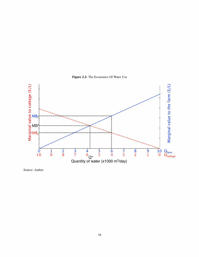
Figure 2.2: The Economics Of Water Use

Source: Author

16

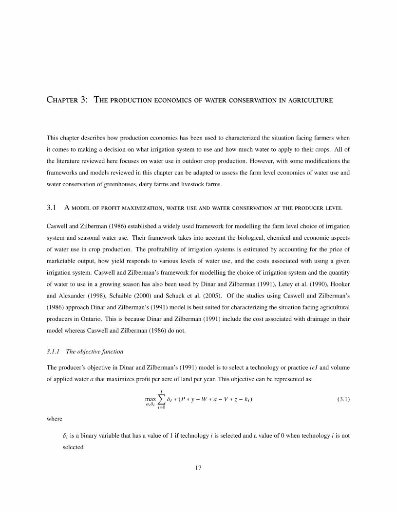
Chapter 3: The production economics of water conservation in agriculture

This chapter describes how production economics has been used to characterized the situation facing farmers when

it comes to making a decision on what irrigation system to use and how much water to apply to their crops. All of

the literature reviewed here focuses on water use in outdoor crop production. However, with some modifications the

frameworks and models reviewed in this chapter can be adapted to assess the farm level economics of water use and

water conservation of greenhouses, dairy farms and livestock farms.

3.1 A model of profit maximization, water use and water conservation at the producer level

Caswell and Zilberman (1986) established a widely used framework for modelling the farm level choice of irrigation

system and seasonal water use. Their framework takes into account the biological, chemical and economic aspects

of water use in crop production. The profitability of irrigation systems is estimated by accounting for the price of

marketable output, how yield responds to various levels of water use, and the costs associated with using a given

irrigation system. Caswell and Zilberman’s framework for modelling the choice of irrigation system and the quantity

of water to use in a growing season has also been used by Dinar and Zilberman (1991), Letey et al. (1990), Hooker

and Alexander (1998), Schaible (2000) and Schuck et al. (2005). Of the studies using Caswell and Zilberman’s

(1986) approach Dinar and Zilberman’s (1991) model is best suited for characterizing the situation facing agricultural

producers in Ontario. This is because Dinar and Zilberman (1991) include the cost associated with drainage in their

model whereas Caswell and Zilberman (1986) do not.

3.1.1 The objective function

The producer’s objective in Dinar and Zilberman’s (1991) model is to select a technology or practice iε I and volume

of applied water a that maximizes profit per acre of land per year. This objective can be represented as:

maxa,δi

I∑i=0

δi ∗ (P ∗ y −W ∗ a − V ∗ z − ki ) (3.1)

where

δi is a binary variable that has a value of 1 if technology i is selected and a value of 0 when technology i is not

selected

17

i identifies the particular irrigation technology being used

P is the price received for output from the production process

y is the quantity of marketable output produced per unit area

W is the costs of using water in the irrigation system

V represents the costs of deep percolation or run-off of water form a producers land

z represents the volume of water the leaves the producers field as deep percolation and run-off

ki represents the discounted capital cost of technology i

Irrigation technologies differ in two ways. First, in their physical characteristics such as uniformity of irrigation and

flow rate. Second, in the management of the technology. A plot of land is assumed to be irrigated by only one

technology. Therefore, δi must sum to 1, so∑I

i=0 δi = 1. The quantity of marketable output is a function of several

other variables that will be explained in the next subsections when the production function of the model is discussed.

The costs of using water in the irrigation system are captured by the variable W . In Ontario agricultural producers

can get their water from several sources and each will have different cost associated with its use. For example water

drawn from a well will require energy to pump water up and out of the well and to deliver it to the field. Theses costs

would be included in the variable W . Another example is a producer who sources his or her water from a municipality

and pays the city for each litre of water used. In this case W would represent the producer’s payment to the city. The

volume of water that percolates or runs-off of a producer’s land, z, is a function of applied water, the technology in

use, soil quality and climatic condition. The details of the drainage function will be explained in more detail below.

Technologies are assumed to be arranged in order of capital cost from lowest to highest so that ki < ki+1.

There are two points worth noting about Dinar and Zilberman’s (1991) formulation of the profit equation. First,

because the model characterizes the combination of a technology and a crop per unit area of land it allows for more

then one technology to be used by one producer. The model also allows for more then one type of crop to be evaluated.

If it so happens that a combination of three crops and two technologies maximizes the farmers profits, then the model

will allow that situation to be identified. Second, by including the cost of drainage V and a function for the volume of

drainage water z, the model accounts not only for the cost of using water in a production process but also the cost of

the run-off and deep percolation. In Ontario the cost associated with run-off and deep percolation vary depending on

the type of crop being grown or livestock being raised. Typically fruit and vegetable growers are not subject to a tax

or charge for the water that runs-off their land. However, greenhouse vegetable producers in Ontario have been under

increasing pressure from the provincial government to reduce the amount of fertilizer in the water discharged from

their greenhouses (Taylor, 2013). Including V and z, the cost and volume of run-off and deep percolation, means that

the situation facing greenhouse vegetable producers in Ontario can be modelled.

18

3.1.2 The production function

In Dinar and Zilberman’s (1991) model the quantity of marketable output produced per unit area in one year is captured

by the production function

y = f {e, i,c} (3.2)

where

y is the quantity of marketable output produced per unit area

e is effective irrigation


c captures the average weather conditions during the growing season

The effective irrigation, e, is the ratio of water taken up by the crop’s roots to the amount applied to the crop. Or put

another way it is the ratio of water that is taken up by the crop to what is lost through evaporation, run-off and deep

percolation. Effective irrigation is assumed to increase yield at a decreasing rate, fe > 0 and fee ≤ 0. The volume

of water that leaves the boundaries of the producers property as deep percolation, evaporation from soil or as surface

run-off can be calculated by subtracting the volume of water applied to the field and the effective irrigation. Irrigation

systems with higher capital cost are assumed to have a higher technical efficiency. Meaning that more of the water that

is put into the irrigation system actually makes it to the crop’s roots rather than leaking out of the system, evaporating

from the soil or draining past the root zone of the drop. The variable c, which identifies average weather conditions

during the growing season, accounts for the temperature, wind, solar radiation and humidity the crop is exposed to. It

can be measured in degree days or pan evaporation. Higher values of c are assumed to increase yield and transpiration

up to a certain point, after which an increase leads to a reduction in yield. This relationship is specific to each species

and variety of plants being grown. The marginal effect of weather on yields is assumed to decrease as c increases up

to a point. Therefore, fc > 0 and fcc ≤ 0.

3.1.3 The effective irrigation function

Effective irrigation depends on the amount of applied water, the technology being used for irrigation, the quality of the

land on which a crop is grown and the weather the crop is exposed to. This can be represented as

e = h(a, i,q,c) (3.3)

where

e is effective irrigation

a is quantity of water applied

19


q is the quality of the land on which the irrigation system is being used


The quality of land, q, can measure either: soil salinity, the salinity of irrigation water or the capacity of soil to retain

water. Farms in Ontario usually receive enough precipitation for soil salinity not to be a problem. Therefore, in the case

of Ontario agriculture it makes sense to think of q as measuring the soil’s capacity to retain water. Soil water retention

or field capacity is defined by Ehlers and Goss (2003) as a function of soil grain size. Sandy soils, which have relatively

low field capacity, are of lower quality when compared to clay soils that can retain more water. Dinar and Zilberman

(1991) assume that soils of higher quality increase water effectiveness at a decreasing rate, so hq > 0 and hqq ≤ 0.

Irrigation technologies are assumed to act on the quality of the soil in which a crop is grown. Technologies with

higher capital cost are assumed to have a higher water effectiveness relative to low cost technologies. For example

a relatively expensive subsurface drip irrigation system also has the highest water effectiveness. Effective water is

assumed to increase as more water is applied to the field but at a decreasing rate. This means that applied water, a, has

a diminishing marginal effect on effectiveness e, so that ha > 0 and haa ≤ 0. Finally, weather conditions are assumed

to have diminish marginal effects on effectiveness as well. That is ha < 0 and haa ≤ 0.

3.1.4 The drainage function

The volume of runoff or deep percolation per unit area is denoted by z and is a function of applied water, the technology

in use, land quality and weather conditions. The drainage function is expressed as

z = g(a, i,q,c) (3.4)

where

z is the quantity of water that drains from the producer’s field

a is quantity of water applied



Dinar and Zilberman (1991) assume that the function has the following properties: drainage declines as land quality

increases, gq < 0 and gqq ≤ 0; drainage increase as more water is applied, gq > 0 and gqq ≥ 0; and technologies that

have a higher capital cost generate less drainage, g(a, i + 1,q,c) < g(a, i,q,c).

20

3.1.5 Using the model to say something about the adoption of water conserving technologies in agriculture

Before looking at what Dinar and Zilberman’s model has to say about water conservation another of the assumptions

made in the model merits careful explanation. Dinar and Zilberman (1991) assume that more technically efficient

irrigation systems increase soil quality. Soil quality is determined by the soil’s capacity to retain water that can be

taken up by a plant roots. Sandy soils, at one extreme of the soil quality spectrum, have coarse grains and large pore

spaces which can not retain much water for plants to use. Therefore, sandy soil is of relatively poor quality. At the

other end of the soil quality spectrum are clay soils. Clay soils are of high quality because they can retain a relatively

large volume of water for plants to use. Because irrigation systems increase the amount of water available for plants to

use, Dinar and Zilberman (1991) assume that installing an irrigation system in effect increases the quality of the soil.

This means that if an irrigation system is used on sandy soil, the quality of the sandy soil would move closer to that of

a clay soil.

Because they assume that more capital intensive technologies augment soil quality, looking at how the quantity of

applied water changes as soil quality changes will tell us how water use changes as technology changes. Dinar and

Zilberman (1991) take the partial derivative of the profit equation with respect to q and get:

dadq

= −[1/P · fee · (ha )2 + P · fe · haa − V · gaa] · [P · fe · haq + P · fee · ha · hq − V · gaq] (3.5)

or written in terms of elasticities

dadq

= −[a/q] · ηa,U {ηh,aq + ηh,qη f ,ee − ηg,aq [V · ga/U]} (3.6)

where

U = W + V · ga

Dinar and Zilberman (1991) identify three ways that increasing soil quality affects water use. The first is through

the marginal effectiveness effect, ηh,aq , which is the elasticity of effective irrigation, e = h(a, i,q,c), with respect to

the derivative of applied water with respect to quality, aq . The marginal effectiveness effect indicates that as water

effectiveness increases water use also increases. The second way increasing soil quality affects water use is through the

marginal productivity effect, ηh,qη f ,ee . As soil quality increases less water will be used when marginal productivity

of applied water declines. The last way that increased soil quality affects water use is through the marginal drainage

effect V · ηg,aq . If the cost of drainage declines more water is expected to be used. Again, the cost of drainage only

affects the per unit area profitability of a technology if there is a cost associated with drainage. That is if V > 0.

Caswell and Zilberman (1986) contend that in a situation where there is no cost associated with drainage water there

will be an unambiguous decrease in water use as soil quality increases.

21

3.2 Production functions, total product curves, technological change and water conservation

3.2.1 Polynomial total product function of water and water conservation

The relationship between the use of an input and the level of output is captured by the total product function. In the

case of water used in agricultural production, the total product function answers the question: how much yield will

be produced when water is used in the production process. For reasons that will be explained in the next section the

total product of water measured at the field level in Ontario is best characterized as a second or third order polynomial

function. A second order polynomial function has the following form

y = βW + γW 2 (3.7)

where

y is the quantity of marketable yield per hectare per year

W is the volume of water per hectare per year.

β is a parameter

γ is a parameter

Figure 3.1 illustrates a total product function with a second order polynomial form. On the x-axis is the volume

of water used during the year and on the y-axis is the yield. The function passes through the origin because if no

water is used there is no yield. For the first part of the function every additional litre of water leads to an increase in

yield. However, an additional litre of water does not lead to as large an increase in yield as the previous litre. This

diminishing return to water continues until adding one more litre of water does not increase yield at all. Beyond this

point additional water has a negative effect on yield. In this portion of the total product function, water has negative

returns.

Taking the derivative of the total product function of water gives the marginal physical product of water. The

marginal physical product answers the question: how will yield change if one more or one less litre of water is used.

The marginal physical product is expressed in units of kg per hectare per year. This can be changed into units of dollar

per year per hectare by multiplying the marginal physical product of water by the price of yield. Doing so will turn

the marginal physical product into the marginal revenue product. The marginal revenue product answers the question:

how does revenue change if an additional litre is used. The marginal revenue product of a second order polynomial

crop-water production function is illustrated in Figure 3.2. The first litre of water makes the largest contribution to

revenue. Each additional litre of water makes a smaller and smaller contribution towards total revenue. Eventually

when adding more water has a detrimental effect on yield the marginal value of water becomes negative. In figure 3.1

the point where the function starts to slope downwards is also the point where the marginal physical product function

crosses the x-axis in Figure 3.2.

22

The marginal cost of water is the price the producer pays to use water. It will change depending on where the

farmer gets his or her water from and on the irrigation system or systems being used. If water is sourced from a

municipality, then the producer will pay the municipality for each litre of water used. If water comes from a well or

surface water then the producer pays for the energy used to power a pump that transports the water from its source to

the farm. We can also include the cost of energy to pressurize irrigation systems in the price of water. For example

overhead sprinkler and drip irrigation systems must be pressurized in order to operate. The cost of pressurization is

incurred for each litre of water used. Therefore the cost of pressurization can be incorporated into the per litre price of

water. Taking into account the various per litre cost of water, the cost of water can be written as:

W = Pw + Pl + Pp (3.8)

where

W is the total cost per litre of water

Pw is the price paid for water to an external supplier such as a municipality.

Pl is the price paid for energy to lift water from a well or to transported it from a river or lake to the farm

Pp is the cost of energy to pressurize an irrigation system.

Figure 3.1 shows the marginal cost of water which is a horizontal line. The height of the line on the y axis is determined

by the sum of the costs associated with using one litre of water.

The profit maximizing quantity of water to use occurs when the marginal revenue of water is equal to the marginal

cost of water. In Figure 3.2 the profit maximizing quantity of water is indicated by Q∗w . Mathematically profit

maximization occurs when,

P · fe · ha = W + V · ga (3.9)

A change in technology will change the height of the marginal cost of water and the slope of the marginal revenue of

water. For example, if after adopting a new irrigation system, a farmer continues sourcing his water from the same

location but his irrigation system requires pressurization, then the marginal cost of water will be higher. If only the

price of water were to increase, then the profit maximizing level of water use would be lower after adoption then it

was before adoption.

A change in technology could also affect the slope of the marginal revenue curve for water. If a change in tech-

nology leads to a change in the marginal revenue product curve such that all or a part of the curve is lower then the

marginal revenue product curve before the change in technology, then that change will reduce water use. A change in

technology will be water conserving if the derivative of the total physical product in water and yield is smaller after the

change then before the change. For a crop-water production function that is quadratic in water and yield, a technology

is water conserving when,dyida

>dyi+1

da(3.10)

23

Figure 3.3 illustrates two situations where a change in technology leads to water conservation. In both situations the

profit maximizing quantity to use is smaller after the change in technology. In the first case, panel 3.3, the slope of

the new marginal revenue curve is always below the old marginal revenue curve. This means that for any price of

water the technology will reduce water use. The second case illustrated in Figure 3.2 shows a situation where new

technology will conserve water for relatively low water prices. When water prices are high enough more water is used

with the new technology then would have been used with the old technology. In the second case only part of the new

marginal revenue curve is below the old marginal revenue curve.

3.2.2 Cobb-Douglas production function, technological change and water conservation

If the production function is specified using the Cobb-Douglas functional form it is possible to specify the function

such that changes in technology lead to water conservation. Fox (2014) identified the following function as

y = α(t)X β (t )W (1−β (t )) (3.11)

where


α is a parameter

t is a parameter that characterizes technological change

X is the set of production inputs other than water

β is a parameter

W is the input of water into the production process

The following conditions must hold: 0 < β(t) < 1, α′

(t) > 0, β′

> 0 and β′′

(t) < 0. The profit function can be

defined as:

Π = Pyy − PxX − PwW (3.12)

where

Π is the profit derived from the production system

Py is the price of the marketable yield


Px is the price of all other inputs used in the production process


24

Pw is the cost of water


Replacing equation 3.11, the production function, in equation 3.12, the profit function, and taking the first deriva-

tive with respect to W gives:∂Π

∂W= −Pw + PytW−tβX tβα(1 − t β) (3.13)

where





β is a parameter


α is a parameter

Setting equation 3.13 equal to zero and solving for W gives the profit maximizing quantity of water to use in the

production process. The result of this algebraic manipulation gives:

W ∗ =

(−

PytX tβα(−1 + t β)Pw

) 1tβ

(3.14)

where

W ∗ is the optimal quantity of water to use is a growing season




β is a parameter

α is a parameter


25

Parameterizing equations 3.11 and 3.12 can help to give a sense of how the profit maximizing volume of water to

use in the production process, W ∗, changes as the parameter that characterizes technological change, t, changes. Figure

3.4 presents the marginal product of water for two values of t. The function of the solid curve has a value for t of 0.6.

The function of the dashed curve has a value for t of 0.8. All the other parameters in the two functions are the same

and they were set to the following values: β = 0.8,X = 2,and α = 3. The coordinates of the vertical and horizontal

lines that move away from the two marginal product function and join the x and y axies were calculated using equation

3.14. Figure 3.4 shows that when the value of t increases the profit maximizing volume of water decreases. This can

be interpreted as meaning that a change in technology can lead to a lower profit maximizing level of water use. At a

technical level the figure demonstrates that it is possible to specify a Cobb-Douglas production function in such away

that technological progress can lead to water conservation.

3.2.3 Choosing the functional form of the crop-water production function

Dinar and Zilberman (1991) selected a functional form for the crop-water production function. They chose a linear

plateau specification. The distinguishing feature of this type of function is that the dependent variable, in this case

yield, is either increasing or is constant as the independent variable, say water, increases. This type of function is also

referred to in the literature as a von Liebig function because it models the late agronomist Justus von Liebig’s Law of

the Minimum. According to von Liebig, crop yield is constrained by the most limiting nutrient. Crops respond to the

addition of an input linearly until yield reaches a plateau when another nutrient becomes limiting. In an econometric

estimation of crop-water production functions of corn, wheat and cotton, Grimm et al. (1987) found that the linear

plateau function was a better fit then Cobb-Douglas, Mitscherlich and polynomial functions.

Dinar and Zilberman (1991) justify using the linear plateau functional form by assuming that adequate drainage

is in place in the field so that any water that can not be held in the soil is transported away from the field. This

assumption seems justified given that they were modelling an agricultural production system in the San Joaquin Valley

which receives little or no precipitation during the growing season and all water that makes its way to the field is

applied through an irrigation system.

Schoengold and Zilberman (2007) note that at aggregate levels, econometric estimations of crop-water production

functions using the Cobb-Douglas function form have been reasonably accurate. However this is not the case at

the farm level. In economically relevant regions, where R+ 7→ R+, the Cobb-Douglas production function has one

important draw back when it comes to accurately modelling how yield responds to the total seasonal volume of applied

water: it is asymptotic in yield as the total volume of applied water increases. In other words it does not exhibit negative

marginal physical product in water. This behaviour does not conform with how crops respond to high levels of water

use in a growing season. Ehlers and Goss (2003) identify several factors associated with excessive water that can

reduce yields. These include: an increase in weeds and harmful organisms; slower soil warming; and reduced oxygen

availability for root growth and nitrogen mineralization. The Cobb-Douglas can not account for these harmful affects

on yield of over saturated soil.

26

Hexem and Heady (1978) suggest using a second or third order polynomial functions to model seasonal yield

responses to inputs. The field level studies conducted by Hexem and Heady (1978) on crop response to seasonal water

and nitrogen use support their proposition. Recent agronomic studies by DeTar (2008) and Wanjura et al. (2002) on

cotton and by Kipkorir et al. (2002) on maize and onion corroborate Hexem and Heady (1978) position. These studies

found that either second or third order polynomial functions best fit data of water use and yield in a growing season. In

their work Caswell and Zilberman (1986) find that simulated results from their model is a better match to data on water

use in California and Arizona when a second order polynomial function rather than a Cobb-Douglas function is used

in the specification of the crop-water production function. In a review of potential functional forms for a crop-water

production function Dinar and Letey (1996) cite the asymptotic properties of the Cobb-Douglas production function

as the most important reason not to use it in models of farm level water use.

The Cobb-Douglas functional form for a farm level crop-water production function is considered to be poor rep-

resentation of how crops respond to the use of inputs. The linear plateau function and the polynomial functions are

consistent with agronomic principles. Berck and Helfand (1990) note that the linear plateau function is a good repre-

sentation of yield response to inputs at the level of an individual plant. At the field level a smooth polynomial function

is a better representation. They argue that the two can be reconciled by accounting for heterogeneity in inputs at the

field level. When selecting a crop-water production function to model agricultural production in Ontario the polyno-

mial function is likely the better choice for field grown crops and orchards. Unlike crops in the San Joaquin Valley

modelled by Dinar and Zilberman (1991) crops in Ontario typically receive considerable amount of precipitation in

a growing season and there is the potential for water logging to decrease yields. In the case of greenhouses a linear

response function is probably the better choice given how tightly producers can control the use of inputs.

3.3 Substitution between water and other inputs

Understanding the potential for agricultural producers to substitute water for other inputs is another aspect of water

conservation at the level of individual producers. If the cost of using water as an input changes or if the price of other

inputs changes a producer can respond by changing his or her relative use of inputs.

Several studies have explored the extent of substitution between water and other inputs. First, Nieswiadomy (1988)

used a translog cost function to estimate the elasticity of substitution between water, labor and capital in the High Plains

of Texas. The forms of capital assessed by Nieswiadomy (1988) were furrow, linear move and centre pivot irrigation

systems. Nieswiadomy found that in the 1970s Texan farmers producing cotton responded to increasing cost of water

by substituting water for furrow irrigation systems and labor. He also found that centre pivot irrigation systems are

a substitute for furrow systems and attributes this result to the fact that centre pivot systems require 75 % less labor

than furrow irrigation systems. Edwards et al. (1996) focused on the effects of increasing cost of water on cropping

decisions and water use. They found that an increase in the cost of pumping groundwater lead to decreased water use

in Arizona and Colorado. They also found that producers substituted water with labor and fertilizer. Cai et al. (2008)

27

used linear programming and data from Maipo River basin in Chile to look at the substitution of water for other inputs

used in agricultural production. Irrigation systems, machinery, labor and pesticides were found to be substitutes for

water. Meaning that as water prices increase the use of these inputs increased. The use of fertilizer was found to

decreases as water prices increased.

Based on the studies reviewed here one could expect that agricultural producers in Ontario facing higher cost of

using water would conserve water and change their use of other inputs. Specifically, water would be substituted with

pesticides, labor, irrigation systems and machinery. Edwards et al. (1996) and Cai et al. (2008) have conflicting results

on whether or not fertilizer is a substitute for water. Therefore, it is unclear whether or not fertilizer use would decrease

or increases if agricultural producers faced a higher costs of using water.

3.4 Taking into account uncertainty and the option to wait

The models developed by Caswell and Zilberman (1986) and Dinar and Zilberman (1991) assume that farmers will

invest in an irrigation system if the expected net present value of investing is greater then the expected net present

value of not investing. However, Carey and Zilberman (2002) note that in California, irrigation systems that are

more technically efficient and have higher expected profitability were available for several years before they became

widely adopted. Furthermore, the pattern of adoption was not one of smooth diffusion, but rather one of large spikes

in adoption that occurred after severe droughts. Carey and Zilberman (2002) develop a model similar to Dinar and

Zilberman (1991) except that it takes into account the value of having the option to wait till some time in the future

to purchase a more technically efficient irrigation system. Their model also accounts for future uncertainty in the

price and quantity of water and the fact that there are sunk cost associated with investing in an irrigation technology.

Another feature of Carey and Zilberman’s model is that it takes into account the fact that farmers in California can buy

and sell allocations of water for use in their production processes. After parameterizing their model using data from

California, Carey and Zilberman (2002) find that expected profit from the more technically efficient technology must

be considerably higher then the net present value calculated using a model that does not account for uncertainty, the

option to wait and irreversibility.

Baerenklau and Knapp (2007) take into account the same factors as Carey and Zilberman (2002) when they put

together their model of irrigation technology investment. However, rather than assuming that the decision to invest in a

more technically efficient irrigation technology is irreversible, they assume that it is possible for the producer to revert

back to the old technology. Baerenklau and Knapp (2007) also assume that irrigation systems are vintage technologies.

A vintage technology is one whose rate of depreciation is not exponential. Benhabib and Rustichini (1991) points out

that a technology may become more productive in the early years of its adoption as operators become more adept

at using the technology. In this type of situation an exponential rate of capital depreciation would not be warranted

and Baerenklau and Knapp (2007) argue that irrigation systems exhibit this type of depreciation. With reversibility

and non-exponential capital depreciation accounted for Baerenklau and Knapp (2007) find that the hurtle rate to the

28

adoption of a more technically efficient system is not as high as what Carey and Zilberman (2002) found.

Whether or not the models developed by Carey and Zilberman (2002) and Baerenklau and Knapp (2007) would

provide a better approximation of the situation faced by producers in Ontario is unclear. There is no market for the sale

and purchase of water for use in Ontario agriculture. Therefore, the effect of uncertainty in the price of water and the

associated value in waiting to invest in more technically efficient irrigation technologies is debatable. That is not to say

that there is no uncertainty in the price of water in Ontario. Droughts, government regulation and competing demands

for water from other sectors could increase the cost of water for farmers in Ontario. The degree to which these factors

increase the uncertainty in the price of water faced by producers in Ontario is not clear. Without this information we

can not tell by how much the net present value model of Dinar and Zilberman (1991) and others deviate from those

proposed by Carey and Zilberman (2002) and Baerenklau and Knapp (2007).

3.5 Models that account for intraseasonal water use and profitable technology adoption

So far in this chapter all of the models that have been discussed characterize water use based on the total volume

of water used in a growing season. However, water use on a farm is spread throughout the growing season across

a number of irrigation events. The timing of water availability within a growing season could have an effect on the

yields from a farmers production process. These effects can not be simulated in a model that accounts for water use

on a seasonal basis.

In the literature on the farm level economics of water use, models that account for the use of water throughout the

growing season are known as transient state models. A transient state model that compares the profitability of irrigation

systems was developed by Shani et al. (2009). Shani et al. (2009) argue that their model is better at accounting

for the fact that irrigation systems are not equally capable of maintaining optimal temporal allocation of irrigation

water. For example irrigation events with flood irrigation systems occur in pulses. With a flood irrigation system soil

moisture levels have a relatively large variance. On the other hand subsurface drip irrigation systems can deliver water

continuously and the rate of irrigation can be controlled to match the plant’s water requirements. Irrigation systems

that can better match the supply of water to the plant’s demand for water increase yields relative to other irrigation

systems.

In a comparison of transient versus seasonal models of profitable water use Dinar and Letey (1996), note that

transient models require more data than seasonal models. Transient models require information on the daily or hourly

use of water for irrigation, whereas seasonal models require the total volume of water used to grow a crop. Letey and

Knapp (1995) compared how well seasonal and transient state models forecast yields. They found that both models

matched actual yields closely. However, the data on yields they were comparing too was limited. Whether or not a

transient state model or a seasonal model should be used to compare the profitability of irrigation systems has not been

settled.

29

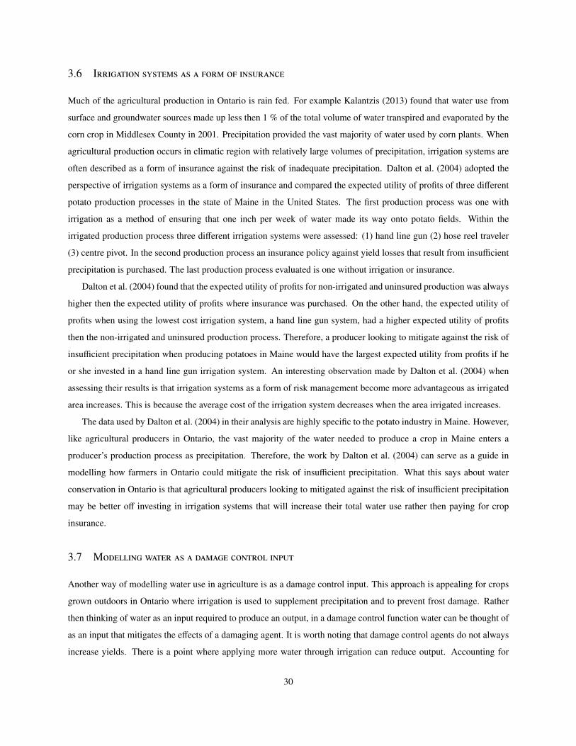
3.6 Irrigation systems as a form of insurance

Much of the agricultural production in Ontario is rain fed. For example Kalantzis (2013) found that water use from

surface and groundwater sources made up less then 1 % of the total volume of water transpired and evaporated by the

corn crop in Middlesex County in 2001. Precipitation provided the vast majority of water used by corn plants. When

agricultural production occurs in climatic region with relatively large volumes of precipitation, irrigation systems are

often described as a form of insurance against the risk of inadequate precipitation. Dalton et al. (2004) adopted the

perspective of irrigation systems as a form of insurance and compared the expected utility of profits of three different

potato production processes in the state of Maine in the United States. The first production process was one with

irrigation as a method of ensuring that one inch per week of water made its way onto potato fields. Within the

irrigated production process three different irrigation systems were assessed: (1) hand line gun (2) hose reel traveler

(3) centre pivot. In the second production process an insurance policy against yield losses that result from insufficient

precipitation is purchased. The last production process evaluated is one without irrigation or insurance.

Dalton et al. (2004) found that the expected utility of profits for non-irrigated and uninsured production was always

higher then the expected utility of profits where insurance was purchased. On the other hand, the expected utility of

profits when using the lowest cost irrigation system, a hand line gun system, had a higher expected utility of profits

then the non-irrigated and uninsured production process. Therefore, a producer looking to mitigate against the risk of

insufficient precipitation when producing potatoes in Maine would have the largest expected utility from profits if he

or she invested in a hand line gun irrigation system. An interesting observation made by Dalton et al. (2004) when

assessing their results is that irrigation systems as a form of risk management become more advantageous as irrigated

area increases. This is because the average cost of the irrigation system decreases when the area irrigated increases.

The data used by Dalton et al. (2004) in their analysis are highly specific to the potato industry in Maine. However,

like agricultural producers in Ontario, the vast majority of the water needed to produce a crop in Maine enters a

producer’s production process as precipitation. Therefore, the work by Dalton et al. (2004) can serve as a guide in

modelling how farmers in Ontario could mitigate the risk of insufficient precipitation. What this says about water

conservation in Ontario is that agricultural producers looking to mitigated against the risk of insufficient precipitation

may be better off investing in irrigation systems that will increase their total water use rather then paying for crop

insurance.

3.7 Modelling water as a damage control input

Another way of modelling water use in agriculture is as a damage control input. This approach is appealing for crops

grown outdoors in Ontario where irrigation is used to supplement precipitation and to prevent frost damage. Rather

then thinking of water as an input required to produce an output, in a damage control function water can be thought of

as an input that mitigates the effects of a damaging agent. It is worth noting that damage control agents do not always

increase yields. There is a point where applying more water through irrigation can reduce output. Accounting for

30

water use in a production process as a damage control agent will change the production function. The purpose of this

section is to explain how to formulate a production function that accounts for water as a damage control agent.

Although water can be used to mitigate the effects of both frost and soil moisture deficit, for the sake of simplicity

we will focus only on the use of water as an input that reduces the damage to yield caused by insufficient soil moisture.

The purpose of this explanation is not to provide the most accurate account of how water can be used to mitigate the

the effects of all damaging agents. Rather it is to illustrate an alternative view of water use on a farm. Namely, as

an input that reduces the effect of a damaging agent on yield. The formulation of water as a damage control agent

presented here is based on the work of Lichtenberg and Zilberman (1986); Fox and Weersink (1995)

In the case of irrigation, the damage agent is insufficient soil moisture. If there were no damage agent, if soil

moisture were always at the level required to meet the water requirement of the plant, then the farmer would get

quantity Y0 of output at the end of the growing season. In an ideal world where Y0 there is just enough precipitation

and at just the right time to keep soil moisture at the level needed to meet the plant’s water requirement throughout

the growing season. When precipitation does not provide enough water to meet the plant’s needs there is damage the

potential yield Y0 and the farmer only gets a portion Y of the yield he or she would have received had the damage not

occurred. The effect of insufficient moisture on yield can be represented by the damage function

Y = Y0[1 − D(Z )] (3.15)

where

Y quantity of output received by the agricultural producer when there is a shortfall in precipitation

Y0 quantity of output received by the agricultural producer when there is enough precipitation in a growing

season

Z represents the level of soil moisture deficiency

D(Z ) is a function that characterizes how insufficient soil moisture effects yield

If precipitation arrives in the quantity and times needed to maintain soil moisture at their ideal levels then D(Z ) = 0

and Y = Y0. The effects of insufficient soil moisture can be mitigated through the use of irrigation. If the irrigation is

timed correctly and enough water is applied, then soil moisture can be maintained at the level required to fully meet

the plant’s water requirements. The use of irrigation to avoid the yield losses from insufficient soil moisture can be

characterized by a damage control function

Z = Z0[1 − C(I)] (3.16)

where

Z represents the level of soil moisture deficiency

Z0 is the level of damage to yield that occurs if irrigation is not used

31

C(I) is the control function that characterizes how the damage control agent, in this case water, affects the

damaging agent, soil moisture deficiency

I is the volume of water added to the field through irrigation

The damage control function is assumed to have the properties of a cumulative distribution function that can have a

value ranging from 0 to 1. When the the volume and timing of irrigation is such that there is no damage to yield from

insufficient soil moisture C(I) = 1 and Z = 0. On the other hand if there is no water used to make up for shortfalls

in precipitation, then C(I) = 0 and Z = 1. If C(I) has a value between 0 and 1, then the parameter Z will have

a positive value. Substituting the damage control function D(Z ) in the damage function Y = F[Z,C(I)], the total

product function for water as a damage control input is

Y = Y0

(1 − D

(Z0

(1 − C(I)

)))(3.17)

where

Y quantity of output received by the agricultural producer when there is a shortfall in precipitation

Y0 quantity of output received by the agricultural producer when there is enough precipitation in a growing

season

D is the damage function

Z0 is the level of damage to yield that occurs if irrigation is not used

C(I) is the control function that characterizes how the damage control agent, in this case water, affects the

damaging agent, soil moisture deficiency

I is the volume of water added to the field through irrigation

The total product function of water as a damage control agent can be used to formulate a production function and

implemented in a profit equation. Identifying technologies that conserve water and maximize profits can be done

following the two-step framework of Caswell and Zilberman (1986). Changes in irrigation technology or practice will

affect the control function C(I) and technologies with the highest profit will be selected.

3.8 Conclusion

There are three broad categories of models that have been used to assess the production economics of water conserva-

tion at the level of individual producers. First are the profit maximization models based on the framework proposed by

Caswell and Zilberman (1986). Dinar and Zilberman’s interpretation of a profit maximization model was explained

in detail to illustrate the nuts and bolts of how these models work and how they are used to understand the conditions

that will lead a profit maximizing agricultural producer to conserve water. The second type of model presented in

32

the chapter are those that take into account uncertainty and the option to wait before investing in more technically

efficiency irrigation systems. With additional factors taken into consideration these models indicate that the expected

profits under a more technically efficient irrigation systems have to be considerably higher than they are under the

current system before a producer will invest. The third category of models are those that treat water as an input that

either reduces risk from variability in precipitation or as a damage control input.

33

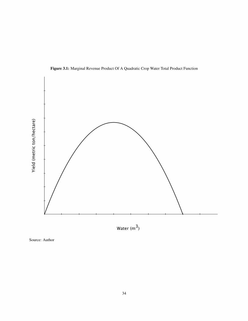
Figure 3.1: Marginal Revenue Product Of A Quadratic Crop Water Total Product Function

Water (m3)

Yiel

d (m

etric

ton/

hect

are)

Source: Author

34

Figure 3.2: Marginal Revenue Product Of A Quadratic Crop Water Total Product Function

Volume of water (L)

Mar

gina

l rev

enue

of w

ater

($/L

)

Pw

Qw*

Source: Author

35

Figure 3.3: (a) Water Conserving Technological Change In Quadratic Total Physical Product Of Water Function

Technological Change That Always Leads To Water Conservation

Volume of water (L)

Mar

gina

l rev

enue

of w

ater

($/L

)

Pw

Qw*0Qw

*1

(b) Technological Change That Leads To Water Conservation Only WhenWater Prices Are Relatively Low

Volume of water (L)

Mar

gina

l rev

enue

of w

ater

($/L

)

Pw

Qw*0Qw

*1

Source: Author

36

Figure 3.4: A Cobb-Douglas Production Function With Water Conserving Technological Change

Source: Author based on Fox (2014)

37

Chapter 4: Methods

4.1 Sources of data for case studies

The case studies in this thesis were developed based on information provided by commercial agricultural producers in

Ontario and researchers at the University of Guelph. Information about the farming operations or studies on which the

cases are built was collected through interviews and site visits. Although the foundation of each case study is based on

information gathered through interviews and site visits, information from the literature on the particular technology in

each case study was used to fill in information not obtained from participants.

4.2 Finding and selecting case studies

The case studies undertaken in this thesis were selected from a list of thirteen potential case studies. The list of

potential case studies was created at the outset of the project. Potential case studies were identified by speaking with

researchers at the University of Guelph, managers and engineers at the Ontario Ministry of Agriculture and Food and

representatives from producers associations in Ontario. Interviewees were asked if they knew of a farm in Ontario that

had adopted a water conservation technology that had not been widely adopted in Ontario. There are dozens of crops

and agricultural commodities produced in Ontario where a water conservation technology could be used. To limit

the number of commodities that could be considered as potential case study only the three largest water users in each

agricultural sub-sector were considered. The three crops that use the most water per sub-sector were selected from the

results of Kalantzis (2013). The commodities considered in the livestock sector where dairy cows, cattle and pigs; in

the field crop sector: tobacco, soybeans and grain corn; in the fruit sector: apples, strawberries and peaches; in the

vegetables sector: potatoes, dry onions and carrots; in the specialty crop sector: sod, nursery products and greenhouse

flowers.

4.3 Economic analysis

The economic analysis for each case study consist of a partial capital budget that captures the farm level economic

impact of purchasing and operating a water conservation technology on a commercial farm. The use of a partial

budget, rather than a full budget, is justified by the assumption that the use of a water conservation technology will

38

not have an effect on how other parts of the farm are operated or managed. The partial capital budget for each case

study accounts for the costs and benefits to a farm business of adopting the use of a technology that leads to water

conservation or that increases technical water use efficiency.

One of the costs associated with using a water conservation technology or a technology that increases technical

water use efficiency is the capital cost of the technology. The capital cost includes the purchase price of the technology

itself and the cost of installation. Not all technologies will have a capital cost. For example a change in practice would

not require the purchase of new equipment. If a dairy farmer were to reduce the amount of water he or she uses when

cleaning their parlour. This would not require any new equipment. Which means that their would be no capital cost

associated with this water conservation technology. On the other hand adding variable rate nozzles to a centre pivot

irrigation system would have capital costs. In the case studies presented in this thesis if there is a capital cost for the

technology any government subsidies that could be used to offset the price of the technology were taken into account.

Two types of annual costs are taken into account in the case studies: new expenses associated with using the

technology and reductions in revenue. The first type of annual costs are changes in expenses. For example if a sod

grower decides to use soil moisture sensors to better inform his or her irrigation decisions. Fixing or replacing broken

sensors would be a new ongoing expense associated with using the technology. The second type of costs are changes

in revenue. If using a water conserving technology reduces yields, then there would be an associated reduction in

revenue to the farm business. The size of the reduction in revenue will dependent on how much yields are reduced

and on the price of the commodity. For example a 1% decrease in corn yield that can be sold for 250 $/metric ton

will have a smaller impact than a 1% decrease in peach yield which can be sold for 1,000 $/metric ton. Again in the

case studies, when accounting for the costs associated with adopting the use of a technology two potential costs were

taken into account. The increase in expenses associated with using the technology and the change in cash income. A

particular water conservation technology or technology that increases technical water use efficiency may have some or

all types of costs.

There are two types of benefits that were accounted for in the partial capital budget. The first are reductions in

expenses. For example if a tomato grower decides to purchase automation software that would automatically apply

irrigation water. The automation would reduce the amount of time the grower spends on turning the irrigation system

on and off. This reduction in time spend operating the irrigation system can be included in the partial capital budget by

accounting for the time saved and the value of the grower’s labour. The second type of benefits increases in revenue.

If the use of a water conservation technology or a technology with higher technical water use efficiency leads to higher

yield, then their would be an associated increase in revenue. Whether or not a water conservation technology will have

both types of benefits, reduced expenses and increased revenue, depends on the particular technology. It is possible

that a technology will have only one of the two benefits. The same is true of technologies that increase technical water

use efficiency. Technologies that have neither type of benefit were not considered for assessment because one can

easily deduce that such a technology would not be beneficial for an individual producer.

In the three case studies the economic outcome of using a technology that conserves water or one that increases

39

technical water use efficiency was assessed based on the net present value of the partial capital budget. The net present

value takes into account the time value of future costs and benefits and compares them to the capital cost of the

technology. The net present value calculation was based on the method described by Boehlje and Eidman (1984). The

equation used to calculate the net present value in each case study is:

N PV =

T∑t=1

∆It(1 + d)t

−O (4.1)

where

N PV is the net present value

T is the last period that a cost or benefit from the investment will be incurred

t is the one year time period

∆It is the change in net cash flow in period t

d is the real discount rate

O is the capital cost of the water conservation technology

The net cash flow, ∆It , in period t takes into account expected costs and benefits that results from using a technol-

ogy. It also takes into account the taxes paid on additional cash income if there is any. The discounted change in net

cash flow is subtracted by the capital cost of the technology, O, to arrive at the net present value of the technology.

The net cash flow per period was calculated as follows:

∆It = ∆CIt − ∆CEt − ∆Γt + T SICt=1 + ST (4.2)

where

∆It is the change in net cash flow in period t


∆CIt is the change in cash income in period t from using the technology

∆CEt is the change in cash expenses in period t from using the technology

∆Γt is the change in income taxes in period t

T SICt=1 is the reduction in taxes in the first year if the investment is eligible for government investment credit

ST is the salvage value of the technology in the last year,T , that the technology will be used

T is the last year that a cost or benefit from using the water conservation technology will be incurred

40

The change in cash income, ∆CIt , in each period can be either a gain in revenue or a loss in revenue from using the

technology. Whether or not the change in cash income will be a cost or a benefit depends on the particular technology

being considered. The change in cash expenses, ∆CEt , is made up of the new expenses associated with using the

technology. The change in cash expenses also includes time saving and the reduced use of inputs. Taxes in period t

are calculated using the following equation:

∆Γt = [∆CIt − (∆CEt + Dt )]T Rt (4.3)

where



∆CIt is the change in cash income in period t

∆CEt is the change in cash expenses in period t

Dt is the capital cost allowance for the water conservation technology in period t

T Rt is the tax rate in period t

Capital cost allowances Dt were calculated using the Canada Revenue Agency’s (2013) "Form T2042 - Statement of

Farming Activities". If the calculated tax in a period returned a negative value, then T Rt was set to zero. This could

occur when annual operating cost and the depreciation for that year are larger then the cash income associated with

using the technology. The tax rate, T Rt , was set to 30% in each case study.

To this point the net present value calculation has been described as a static calculation. Meaning that each value

listed in the change in income and tax equations of the net present value calculation have fixed values. However,

there is uncertainty in exactly what value some of the equations parameters will take in the future. For example part

of calculating the change in cash income, ∆CIt , involves multiplying yields by the price of the crop. Yields in each

year that a water conservation technology will be used will not all be the same. Their are factors beyound the growers

control the lead to variation from year to year. Because the water conservation and water use efficiency technologies

considered in the case studies are used for multiple years, a more accurate representation of the world would take into

account this variation in yield. Similarly, past experience shows that the price of the crops assessed in the case studies

is not the same in each year or even in each month. Assuming that real corn prices are the same for the useful life of

an irrigation system would not capture the variation in prices that sector has seen the past. To take into account the

fact that there is uncertainty in some of the parameters of the net present value calculation a Monte Carlo simulation

was used in each case study.

In the Monte Carlo simulations some of the parameters in the partial capital budget were characterized using

statistical distributions rather than fixed value. For example a normal distribution with a mean of 1,221 $/metric ton

41

and a standard deviation of 277 $/metric ton can be used to characterize peach prices. Yields, input cost and any other

part of the partial capital budget can be characterized using a distribution. In the case studies only some of the net

present value’s parameters were characterized using distribution. If there was a relatively high degree of certainty in

the future value of a parameter then a fixed value was used. For example the tax rate, T Rt , was set to 30% in each case

study. On the other hand parameters that vary from year to year were characterized using a statistical distribution.

For each case study the Monte Carlo simulation was implemented using the @RISK add-on developed by Palisade

Corporation for Microsoft Excel. In calculating the net present value @RISK makes random draws from the statistical

distributions defined in the partial capital budget. The randomly drawn values are used to calculated the net present

value. To capture the variation in the statistical distributions the net present value was repeated one hundred thousand

times. Each time the net present value is calculated using newly selected values from the statistical distributions.

All prices and discount rates discussed in the case studies or used in the economic analysis in the case studies are

adjusted to real 2013 values in Canadian dollars (CAD). For example in the subsurface drip irrigation on corn case

study historical corn prices used to project future corn prices were set to 2013 values. In each case the prices were set

to real 2013 values using a yearly average consumer price index. The yearly consumer price index was calculated by

taking the average of monthly consumer price indices in a calendar year. The monthly consumer price indices used

were the All-items CPI for Ontario calculated by Statistics Canada (2013c) where 2002 is the base period. Prices were

adjusted according to the following formula:

nominal price in year t ∗2002 avg CPI

avg CPI in year t(4.4)

Real interest rates and the real discount rate were calculated using the procedure described by Boardman et al.

(2010, p. 148)

r =i − m1 + m

(4.5)

where

r is the real interest rate

i is the nominal interest rate

m is the inflation rate

The inflation rate, m, was set to 2%. This value was selected because it is the Bank of Canada’s (2013) target inflation

rate for the Canadian economy. In the baseline scenario for all three case studies the nominal interest rate, i, was

set to 5%. Which means that in the baseline scenarios for all three case studies the real discount rate, r , works out

to 5%. This figure will not necessarily apply to every agricultural producer assessing the technologies in the case

studies. Someone who places a higher value on future costs and benefits would have a lower discount rate than is

implied from the 5% figure selected for the baseline scenario. On the other hand a producer assessing the merits of

a particular technology may place a lower value on future cost and benefits than is assumed in the baseline scenario.

42

This means that their discount rate would be higher than the 5%. To account for the uncertainty in the discount rate in

the sensitivity analysis for each case study the discount rate was evaluated at 4% and 6% to see how a change in the

real discount rate affects the distribution of net present values.

43

Chapter 5: Subsurface drip irrigation in corn production

The case study presented in this chapter is about the economic implication to a corn farmer in Ontario of purchasing

and operating a subsurface drip irrigation system. Subsurface drip irrigation systems are the most technically efficient

irrigation systems. Almost all of the water pumped into a subsurface drip irrigation system will make its way to the

root zone of the crop. Assessing the farm level economics of purchasing and operating a subsurface drip irrigation is

important in light of the findings of Lobell et al. (2014). In their work Lobell et al. (2014) looked at how sensitive corn

yields are to drought conditions. They found that in Iowa, Indiana and Illinois in the United States over the period

from 1995 to 2012 corn yields have become more sensitive to drought stress. They suspect that this has occurred

because most aspects of corn production other than moisture levels have come under the control of corn producers. A

subsurface drip irrigation system would afford a producer the kind of control that could eliminated his or her crop’s

sensitivity to drought conditions. As part of this case study the capital cost, the annual operating cost and the potential

gains in corn yields were taken into account in order to determine the expected net present value of purchasing and

operating a subsurface drip irrigation system to grow corn in Norfolk County, Ontario.

The outline of the case study is as follows: first is a explanation of what a subsurface drip irrigation system is, how

one is installed and some of advantages and disadvantages of the system; second is an overview of the corn sector in

Ontario; third is an explanation of how the net present value of the subsurface drip irrigation system was calculated;

fourth is a brief description of the results; and last is a brief discussion of the results.

5.1 What is a subsurface drip irrigation system?

A subsurface drip irrigation system consist of a network of pipes and tubing placed underground to deliver water to

the root zone of a crop. Figure 5.1 presents the layout and components that make up a properly functioning subsurface

drip irrigation system. The key components of the system are the water pump, water filters, chemical injector and

pipes. The pump, filters and chemical injector are usually housed in a shed or under a roof to protect them from the

elements. Another component that can be added to the system that is not illustrated in Figure 5.1 is a tank to store

liquid fertilizer and a pump to inject the fertilizer into the system. Flow meters, air vents and pressure release valves

are also included at key points in the system.

The diameter of plastic pipes used in a subsurface drip irrigation system vary based on their location in the field.

The large main line delivers water from the filters to the sub main line which runs along the length of the highest side

44

of the field. Connected to the sub main line at regular intervals are the lateral lines that deliver water to the root zone

of the crop. The lateral lines, or drip lines as they are often referred to, are made of relatively thin plastic and are

shaped like a giant flattened drinking straw. They run parallel to each other forming a striped pattern across the field.

At the side of the field opposite the sub main line, the drip lines are connected to a flush valves. However, rather than

having the terminal end of the drip lines connected to individual flush valves, like they are in Figure 5.1. It is possible

to have all of the drip lines connected to a flush line. A flush line is made of PVC pipe like the sub main line and has

one or two flush valves connected to it. Large fields are typically split into several irrigation zones, each with its own

sub main line, lateral lines and flush lines.

The lateral lines have emitters that allow water to move out of the lateral lines and into the soil. The distance

between drip lines and the spacing between emitters depends on the type of soil they are located in and the crop that

will be grown on the field. Sandy soils through which water can move relatively easily tend to have lateral lines and

emitters spaced closer together. Whereas clay soils which do not conduct water as easily can have more distance

between lateral lines and emitters.

One important decision in designing the system is the selection of a water pump. There are two types of pumps

that can be used: electric or diesel. Relative to diesel pumps, electric pumps are more efficient on the basis of energy

consumed per litre of water pumped. However, using an electric pump requires a connection to three phase electric

power. Depending on the location of the pump shed, the cost of running a three phase connection from the closest

utility line can cost twenty to one hundred thousand dollars. In cases where the pump shed can not be located near a

source of three phase power a diesel motor would be employed.

To ensure proper installation an expert in subsurface drip irrigation system is usually contracted to supervise the

installation. To bury the main line, sub-mains and manifolds, trenches are dug and the PVC pipes are placed at the

bottom of the trench and glued together. The manifold pipes are buried at a lower depth then the drip lines, around 1

metre below the soil surface, and holes are drilled into the top of the manifold pipe. The lateral lines are connected

to the manifold using a curved riser tube. One end of the riser tube is glued vertically to the top of the manifold and

the other end is attached horizontally to the drip line using steel wire. The drip lines are buried into the ground using

specially designed applicator towed by a tractor. The drip line applicator has three to four applicator shanks that slice

through the ground and leave behind a continuous run of drip line. The applicator shanks are shaped like a blade with

the sharp edge facing up field. At the top of each applicator shank, the drip line is carried on a spool. From the spool

the drip line runs along the back of the applicator shank down into the soil to the bottom of the shank. The drip line is

fed into the applicator so that the emitters on the drip line are facing upward once they are in the soil. The depth of the

applicator shanks determines how far into the soil the drip lines will be placed. The distance between the drip lines in

the soil is determined by the spacing of the shanks on the applicator.

Like other irrigation systems a subsurface drip irrigation system requires some management to ensure that it is

operating correctly and to maintain its performance for as long as possible. Lamm et al. (2003) offer an overview of

the management involved in the use of a subsurface drip irrigation system. As far as maintenance is concerned Lamm

45

et al. (2003) recommend that the system components that are located in the pump shed be inspected at least once a year

just before the system is put to use. They also recommend keeping a close eye on the soil surface early in the growing

season when the system is in operation and the crop has yet to fully develop. Doing so helps to identify leaks from

the system. When a properly functioning system is in use there should not be any wetting of the soil surface. Patches

of wet soil at the surface are an indication that there is a leak in the system. Leaks can be caused either from animals

chewing on the drip lines or, if the system has just been installed, by a tear in the drip line. To help reduce the chance

of burrowing animals making holes in the drip lines Lamm et al. (2003) recommend reducing rodent habitat by setting

traps around the irrigated field and tilling the soil. In addition to inspecting the subsurface drip irrigation system’s

components, another maintenance procedure is flushing the system. Flushing the system involves running the system

at higher then usual pressures and at higher water velocities. The higher water velocities allow material that may have

made its way into the drip lines to be carried out the terminal end of the drip line and into the flush line. Lamm et al.

(2003) recommend that flushing occur before the system is put to use during a growing season. Depending on the

quality of the water used in the system, acids and chlorine can be added to the irrigation water to remove precipitates

and algae in the system.

Compared to sprinkler or flood irrigation, a subsurface drip irrigation system is unique in its operation for three

reasons. First, because of its relatively uniform application of water across a field, a subsurface drip irrigation system

can be used to deliver fertilizer to the root zone of the crop. Second, because the soil surface is not wetted during

irrigation, determining how much irrigation water needs to be applied and when can not be determined just by looking

and feeling the soil surface. Soil moisture sensors can be used or evapotranspiration can be used to calculate how

much water needs to be replaced. Third, because so many of the system’s components are buried underground, careful

monitoring and record keeping are required to determine whether or not the system is operating correctly. These three

unique aspects of using a subsurface drip irrigation require time and practice for the operator to familiarize his or her

self with.

Payero et al. (2005) and Lamm and Camp (2006) list some of the advantages and disadvantages of subsurface drip

irrigation system in agricultural production. The first drawback of the system is its cost. Subsurface irrigation systems

are the most expensive irrigation systems to purchase and instal. Second, because of its relatively low irrigating

capacity, a steady supply of water must be available for use throughout the season. If water is not available to use

in the system during a prolonged period of low or no precipitation it can be difficult or impossible to return the soil

to adequate moisture levels. A third disadvantage is the relatively steep learning curve required to correctly operate

the system. In the first few years of use, a novice operator will have to commit more time to operate and maintain

the system then he or she would for another type of irrigation system. Proper maintenance of the system is key to

avoid having emitters clogged by sand, minerals or plant roots. Fourth, there is the potential for rodents to chew on

lateral lines. Last, the initial design of the system is more important relative to other irrigation systems. The spacing

and depth of drip lines and the system’s capacity are all set from the beginning and are expensive to change once the

system has been installed.

46

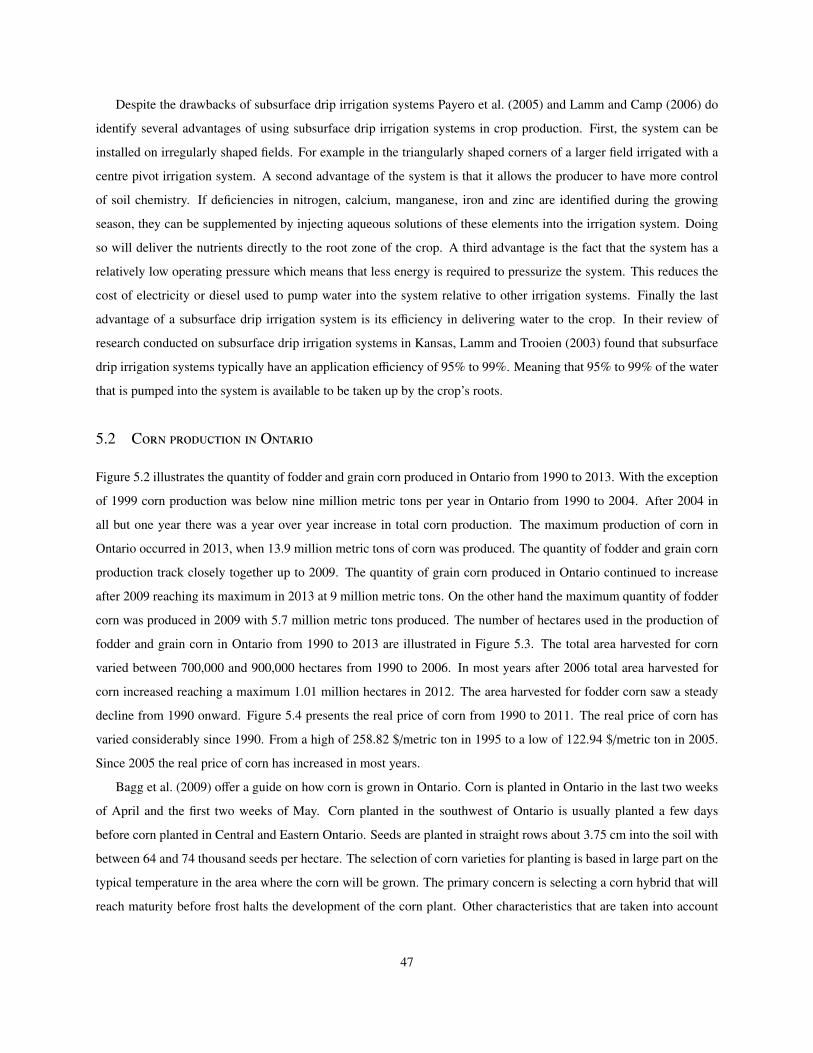
Despite the drawbacks of subsurface drip irrigation systems Payero et al. (2005) and Lamm and Camp (2006) do

identify several advantages of using subsurface drip irrigation systems in crop production. First, the system can be

installed on irregularly shaped fields. For example in the triangularly shaped corners of a larger field irrigated with a

centre pivot irrigation system. A second advantage of the system is that it allows the producer to have more control

of soil chemistry. If deficiencies in nitrogen, calcium, manganese, iron and zinc are identified during the growing

season, they can be supplemented by injecting aqueous solutions of these elements into the irrigation system. Doing

so will deliver the nutrients directly to the root zone of the crop. A third advantage is the fact that the system has a

relatively low operating pressure which means that less energy is required to pressurize the system. This reduces the

cost of electricity or diesel used to pump water into the system relative to other irrigation systems. Finally the last

advantage of a subsurface drip irrigation system is its efficiency in delivering water to the crop. In their review of

research conducted on subsurface drip irrigation systems in Kansas, Lamm and Trooien (2003) found that subsurface

drip irrigation systems typically have an application efficiency of 95% to 99%. Meaning that 95% to 99% of the water

that is pumped into the system is available to be taken up by the crop’s roots.

5.2 Corn production in Ontario

Figure 5.2 illustrates the quantity of fodder and grain corn produced in Ontario from 1990 to 2013. With the exception

of 1999 corn production was below nine million metric tons per year in Ontario from 1990 to 2004. After 2004 in

all but one year there was a year over year increase in total corn production. The maximum production of corn in

Ontario occurred in 2013, when 13.9 million metric tons of corn was produced. The quantity of fodder and grain corn

production track closely together up to 2009. The quantity of grain corn produced in Ontario continued to increase

after 2009 reaching its maximum in 2013 at 9 million metric tons. On the other hand the maximum quantity of fodder

corn was produced in 2009 with 5.7 million metric tons produced. The number of hectares used in the production of

fodder and grain corn in Ontario from 1990 to 2013 are illustrated in Figure 5.3. The total area harvested for corn

varied between 700,000 and 900,000 hectares from 1990 to 2006. In most years after 2006 total area harvested for

corn increased reaching a maximum 1.01 million hectares in 2012. The area harvested for fodder corn saw a steady

decline from 1990 onward. Figure 5.4 presents the real price of corn from 1990 to 2011. The real price of corn has

varied considerably since 1990. From a high of 258.82 $/metric ton in 1995 to a low of 122.94 $/metric ton in 2005.

Since 2005 the real price of corn has increased in most years.

Bagg et al. (2009) offer a guide on how corn is grown in Ontario. Corn is planted in Ontario in the last two weeks

of April and the first two weeks of May. Corn planted in the southwest of Ontario is usually planted a few days

before corn planted in Central and Eastern Ontario. Seeds are planted in straight rows about 3.75 cm into the soil with

between 64 and 74 thousand seeds per hectare. The selection of corn varieties for planting is based in large part on the

typical temperature in the area where the corn will be grown. The primary concern is selecting a corn hybrid that will

reach maturity before frost halts the development of the corn plant. Other characteristics that are taken into account

47

when selecting a corn hybrid are: its ability to cope with less then idea growing conditions; the plant’s ability to stay

standing through the fall; and the moisture content of the kernels at the time of harvest.

Once the corn seeds are planted it takes between 6 and 21 days for the first leaf to emerge from the soil. Throughout

May, June and early July the corn plant is in its vegetative stage of growth. During this period the plant stalk grows

vertically adding leaves as it grows upward. In the last week of July tassels emerge from the top of the corn plant and

two days later silks emerge from the husk at the tip of the ear of corn. The emergence of silks on the ear of corn, there

is only one ear per plant, marks the end of the vegetative growth state and the beginning of the reproductive growth

stage. Throughout the vegetative growth stage nutrients in the soil and the output of photosynthesis were utilized in

the growth of the plant’s stem and leaves. In the reproductive growth stage the output of photosynthesis in the plant’s

leaves is shuttled into the kernels of the cob. The reproductive stage occurs over the months of August and September.

By the end of September the corn plant has reached physiological maturity and the kernels are no longer accumulating

dry matter. At this stage the corn kernels have between 31% and 33% moisture content.

The time of harvest depends on the intended use of the crop. Corn that will be used for silage can be harvested at

the beginning of september when 90% of the grain yield has been achieved. Corn that will be used for grain is left to

stand after the plant reaches maturity in order to allow some of the water in the kernels to evaporate. The decision to

harvest corn that has been left standing through the fall is based on how much moisture is left in the kernels, how well

the corn stalks are standing, the chance of a strong wind blowing the stalks down and the condition of the field itself.

Over the course of the growing season the corn crop is susceptible to insects, animals, bacteria, fungus and weather

conditions that can reduce the corn yield from the field. There are half a dozen diseases and 18 insects and pests that

can damage corn plants. The incidence of insects, pests and diseases varies over the course of the corn plant’s growth

stages. Some insects and diseases attack the corn plant during the early vegetative stage while others only affect the

corn plant during the reproductive stage. Therefore, managing the impact of diseases, insects and pests requires careful

observation of the crop throughout the growing season. The damage to yields from adverse weather events varies over

the growing season as well. Adverse weather events that can affect yields include: early and late season cold, heat,

hail, flooding, and, the most relevant to this research, drought.

5.3 The case study subsurface drip irrigation system

In section 5.1 a fairly detailed description of the layout, components, maintenance and operation of a subsurface drip

irrigation system was given. All of the components mentioned in that description, the pumps, filters, pipes and a

pump shed, would be required to build a properly functioning subsurface drip irrigation system that would be used to

grow corn in Ontario. Furthermore, the management of a subsurface drip irrigation system described in section 5.1

including maintenance and monitoring would be required to properly operate a system used to grow corn in Ontario.

The subsurface drip irrigation system profiled in this case study is covers an area of 40.5 hectares (100 acres) of coarse

textured sandy loam soil and is assumed to be located in Norfolk County, Ontario. The system is laid out in 6 zones.

48

This means that there are 6 pairs of manifolds and flush lines with drip lines running between them. The system’s

dimensions and capacity are based on a subsurface drip irrigation system what was installed on a commercial farm

in LaSallet, Ontario in Norfolk County. The drip lines are buried 36 cm (14 inches) underground and spaced 112 cm

(44 inches) apart. The emitters in the drip lines are spaced 61 cm (24 inches) apart. The drip lines have an inside

diameter of 22 mm (7/8 inch) and wall thickness of 0.4 mm. The system is capable of delivering water to two zones

at a time and can apply 6.4 mm (1/4 inch) of water in a 6 hour period. The system draws water from an open pond on

the field using an electric pump. Aqueous fertilizer and macronutrients can be added to the irrigation water before it

is delivered to the crop’s roots.

5.4 Methods for assessing the farm level economics of a subsurface drip irrigation used to

grow corn

The merits of the subsurface drip irrigation system were assessed based on its net present value. The net present value

was calculated based on a partial capital budget of the subsurface drip irrigation system. The partial capital budget

captures the costs and benefits to the grower who would purchase and operate the subsurface drip irrigation system.

The costs and benefits of the system can either change the cash income or the cash expenses of the farm business.

For example a benefit of using the subsurface drip irrigation system is that it increases corn yields. This leads to an

increase in cash income to the farm business. On the other hand a cost of the system is ongoing maintenance that

must be undertaken for the system to operate correctly. This cost increases the cash expenses of the farm business.

In addition to accounting for how cash income and cash expenses would be affected if the subsurface drip irrigation

system were purchases and put to use, the partial capital budget also takes into account how taxes would change.

Government subsidies and the salvage value of the system are also taken into account in the partial capital budget.

Mathematically the net present value of the partial capital budget can be represented as follows:

N PV =

T∑t=1

∆CIt − ∆CEt − ∆Γt + T SICt=1 + ST(1 + d)t

−O (5.1)

where




∆CIt is the change in cash income in period t from using the subsurface drip irrigation system

∆CEt is the change in cash expenses in period t from using the subsurface drip irrigation system


49

T SICt=1 is the reduction in taxes in the first year if the investment is eligible for government investment credit

ST is the salvage value of the technology in the last year,T , that the subsurface drip irrigation system will be

used


O is the capital cost of the subsurface drip irrigation system

Taxes in period t were calculated using the following equation:

∆Γt = [∆CIt − (∆CEt + Dt )]T Rt (5.2)

where





Dt is the capital cost allowance for the subsurface drip irrigation system in period t


The capital cost allowances, Dt , in each period, t, were calculated using the Canada Revenue Agency’s (2013) "Form

T2042 - Statement of Farming Activities". If the calculated tax in a period returned a negative value, then T Rt was set

to zero. This could occur when annual operating cost and the depreciation for that year are larger then the cash income

associated with using the subsurface drip irrigation system. The tax rate, T Rt , was set to 30% in each period t.

To this point the explanation of the net present value calculation has been described as a static calculation. Meaning

that each value listed in the change in cash income and tax equations of the net present value calculation has a fixed

value. However, their is uncertainty in exactly what value some of the equations parameters will take in the future.

For example part of calculating the change in cash income, ∆CIt , involves multiplying corn yields by the price of

corn. Corn yields in each year that the subsurface drip irrigation system will be used will not all be the same. Their

are factors beyond the grower’s control the lead to variation from year to year. Because the subsurface drip irrigation

system is used for multiple years, a more accurate representation of the world would take into account this variation in

yield. Similarly, past experience shows that the real price of corn is not the same in each year. Assuming that real corn

prices are the same for the useful life of an irrigation system would not capture the variation in prices that the sector

has seen the past. To take into account the fact that there is uncertainty in some of the parameters of the net present

value calculation a stochastic simulation was used.

50

In the stochastic simulation for this case study some of the parameters in the partial capital budget were char-

acterized using statistical distributions rather than fixed values. For example a normal distribution with a mean of

191.2$/metric ton and a standard deviation of 39.65$/metric ton was used to characterize corn prices. In this case

study corn prices and corn yields were characterized using statistical distributions. A detailed explanation of the

distributions used to characterized corn yields and corn prices is presented in the next section.

The stochastic simulation was implemented using the @RISK add-on developed by Palisade Corporation for Mi-

crosoft Excel. In calculating the net present value, @RISK makes random draws from the statistical distributions

defined in the partial capital budget. The randomly drawn values are used to calculate one net present value. To

capture the variation in the statistical distributions the net present value calculation is repeated one hundred thousand

times. Each time the net present value is calculated using new randomly selected values from the statistical distri-

butions. The result of repeatedly calculating the net present value is a distribution of net present values. It is this

distribution that is reported in the results of this case study.

All prices and discount rates discussed in the case study are real values. Meaning that prices and discount rates

are adjusted for inflation to real 2013 $. The real discount rate for this case study was set to 5% and varied in the

sensitivity analysis.

5.5 Capital cost of the subsurface drip irrigation system

Table 5.2 lists the estimated capital cost of the case study subsurface drip irrigation system. With regards to the net

present value calculation, the capital cost of the system are represented by the parameter O in Equation 5.1. The

capital cost the subsurface drip irrigation system includes the cost of components and the cost of installation. The cost

of pumps, pipes and other components were estimated by using three price quotations provided by Vanden Bussche

Irrigation. The quoted systems have the same parts as those used in the case study subsurface irrigation system. What

differs between the quoted systems and the case study system is the size of the fields they would be installed in. This

means that the length of pipes, the number of drip lines and the number of other components differs between the four

systems. The capacity and the price for the system controller, water pump and filters is the same for all three quoted

systems. Therefore, the estimated price of the these components for the case study system was set equal to those of

the quoted systems. The price of pipes, laterals and fittings were estimated by taking the average per hectare cost from

the three quoted systems and multiplying by 40.5 hectares (100 acres). The result is an estimate of the total cost of

purchasing the components required for a subsurface drip irrigation system that can irrigate 40.5 hectare (100 acres).

The cost of installing the system was estimated using information provided by Bakker (2013). The cost of installation

was estimated by taking the per hectare cost of installing a subsurface drip irrigation system on 32.37 hectares (80

acres) field and multiplying by 40.47 hectares (100 acres). A labour cost of 10.50$/hr was assumed in the estimation

of installation costs. The pumping equipment needs to be kept out of the elements. A used 6 metre (20 foot) shipping

container which cost about $2,000 could be used. With the cost of a cement for a slab accounted for, the total cost of

51

the pump shed was assumed to be $2,134. The cost of the shed housing the pumping and filtration equipment would

be equal for a large range field sizes.

Government subsidies to offset the capital cost of the subsurface drip irrigation system were not included in the

partial capital budget because no applicable programs could be identified. The Growing Forward 2 program does

provide funding for the installation of irrigations systems with relatively high technical water use efficiency such

as the subsurface drip irrigation system in this case study. However as the Ontario Soil and Crop Improvement

Association’s (2013) guide for producers explains, producers installing an irrigation system on previously unirrigated

land are ineligible for funding. Because the case study being analyzed here involves the installation of a subsurface

drip irrigation system on previously unirrigated fields, the cost of the system can not be offset by the Growing Forward

2 program.

5.6 How using the subsurface drip irrigation system affects cash income

In this case study cash income in the production of corn is generated by selling the corn produced on the irrigated

field. The difference between expected yield without the subsurface drip irrigation system and yield with the system

captures how the use of the subsurface drip irrigation system will affect cash income. In this case study expected yields

over the useful life of the irrigation system were projected using a modified version of the statistical distribution of

yields for the Haldimand-Norfolk census devision calculated by Tolhurst and Ker (2013). In their work Tolhurst and

Ker (2013) propose using a mixture of two normal distributions to characterize yields at the county level. Their two

component distribution also includes an embedded time trend. This means that their model of corn yields not only

accounts for the distribution of yields but also how the parameters of the distribution change over time. Tolhurst and

Ker (2013) use census devision data from 1949 to 2010 to determine the parameters of the two component normal

distribution for the Haldimand-Norfolk census devision.

In their nomenclature Tolhurst and Ker (2013) refer to the normal distribution with the lowest mean yield as

the "lower" distribution and the normal distribution with the highest mean yield as the "upper" distribution. For the

purposes of this case study Tolhurst and Ker’s (2013) "lower" distribution was renamed the "normal years" distribu-

tion and the "upper" distribution was called the "exceptional years" distribution. Mathematically the two component

distribution used in this case study can be defined as follows:

Yt ∼ (1 − λ)N (αn + βnt,σ2n ) + λN (αe + βet,σ2

e ) (5.3)

where

Y is the per acre yield in period t


λ is the probability of having a yield in the exceptional years distribution rather than in the normal years distri-

bution

52

αn is the mean yield in the normal years distribution

βn is the change in the mean of the normal years distribution in period t + 1

σ2n is the variance of yields in the normal years distribution

αe is the mean yield in the exceptional years distribution

βe is the change in mean of the exceptional years distribution in period t + 1

σ2e is the variance of yields in the exceptional years distribution

There are a few assumptions implicit in this distribution that are worth noting. First, the average yields in the two

components of the distribution will continue to increase at the rates that they did between 1949 and 2010. The term

βnt in the normal years sub-distribution and βet in the exceptional years sub-distribution means that as t increases, as

time moves forward, the mean yield of both distributions increases. This property of the bimodal distribution means

that it does not account for the possibility of average yields levelling off. The second implication of using the bimodal

distribution estimated by Tolhurst and Ker (2013) is that the standard deviation of the normal years sub-distribution

and the exceptional years sub-distribution remain the same. The last implication of using this particular bimodal

distribution is that the average yield of the two sub-distributions diverge as t gets larger. This is because the rate of

change in the means, βn and βe , are not the same.

Figure 5.5 illustrates five years of projected corn yield distributions using the two component distribution defined

by Tolhurst and Ker (2013). The tallest of the two sub-distributions is the normal years sub-distribution. The shortest is

the exceptional years sub-distribution. The height of the distribution corresponds to the probability of a yield quantity

being drawn from that portion of the distribution in the stochastic partial capital budget simulation. The highest points

in each sub-distribution are the averages plus the accumulated change in yield for that period, αn + βnt and αe + βet,

for each sub-distribution. The figure shows that the position of the normal years sub-distribution moves toward the

right as time moves forward. Again this is occuring because the βnt term in equation Equation 5.3 causes the average

yield in the normal years sub-distribution to increase in each year. The same is true of the exceptional years sub-

distribution. Comparing the jumps from year to year of the two sub-distribution one can notice that the exceptional

years sub-distribution moves further to the right from year to year. By 2025 the exceptional years sub-distribution

has made more progress towards the right than the normal years sub-distribution has. This happens because the βnt

term, the change in average yields in the normal years sub-distribution, is smaller than the equivalent term, βet, in

the exceptional years sub-distribution. This means that the means of the two sub-distributions diverge as time moves

forward. Figure 5.5 also shows that the width of the normal years and exceptional years sub-distributions do not

change between 2013 and 2025. This happens because it was assumed that the standard deviation does not change

with time. The assumptions implicit in the use of the bimodal distribution estimated by Tolhurst and Ker (2013) can

lead to nonsensical forecast of yields in the far future. However, for the 15 to 20 years of useful life of a subsurface

drip irrigation system being assessed in this case study it seems that the projected yields are not too farfetched.

53

The assumptions implicit in the two component distribution mean that the first calendar year that the subsurface

drip irrigation system will be used affect the estimated yield in each year. Again the terms βnt and βet in Equation 5.3

mean that the average yield in each sub-distribution is changing as time moves forward. In the baseline scenario for

this case study it was assumed that the first year that the system would be used is 2013. Because Tolhurst and Ker

(2013) report the variables of the Haldimand-Norfolk two component corn yield distribution assuming that the first

period, t = 0, is 1949. The values of αn , the mean yield in the normal years distribution, and αe , the mean yield in the

exceptional years distribution had to be calculated so that the first period, t = 0, can be 2013 rather than 1949. This

was done by replacing the period variable t in Tolhurst and Ker (2013) equation by 64. This is the number of periods

between 1949 and 2013. When t = 64, αn works out to 8.2582 metric tons/hectare (131.50 bushel/acre)1 and αe to

10.748 metric tons/hectare (171.15 bushels/acre).

All the other parameters in Equation 5.3, which characterizes expected corn yields without the subsurface drip

irrigation system in this case study, were set to the values reported by Tolhurst and Ker (2013). The probability of

having a yield in the exceptional years distribution rather than in the normal years distribution, λ, was set to 0.107;

the change in the mean of the normal years distribution in period t + 1, βn , was set to 0.0842 metric ton/hectare (1.34

bushel/acre); the variance of yields in normal years, σ2n , was set to 6.79 metric tons2/hectare2 (108 bushel2/acre2); the

change in mean yields in exceptional years in period t +1, βe , was set to 0.1225 metric ton/hectare (1.950 bushel/acre);

lastly, the variance of yields in the exceptional years distribution, σ2e , 0.43 metric ton2/hectare2 (6.8 bushel2/acre2).

Again these are the parameters for the two component distribution used to characterized corn yields in this case study

when a subsurface drip irrigation system is not being used.

The yields forecasted using Tolhurst and Ker’s (2013) bimodal distribution represent what the case study farm

could expect had the subsurface drip irrigation system not been installed. To get at how using the subsurface drip

irrigation system will affect yields, one has to determine how much the system increases or decreases yields. In this

case study the change in corn yields caused by the subsurface drip irrigation system was estimated by multiplying

the forecasted yield without subsurface drip irrigation by fixed proportions. Specifically the mean yields in the two

sub-distributions were multiplied by fixed proportions. The expected yield with the system in each year was then

subtracted by the expected yield in each year without the subsurface drip irrigation system. In mathematical terms the

change in yield was calculated as follows:

∆Yt ∼ [(1− λ)N ((αn + βnt)Φn ,σ2n ) + λN ((αe + βet)Φe ,σ

2e )]− [(1− λ)N (αn + βnt,σ2

n ) + λN (αe + βet,σ2e )] (5.4)

where

∆Yt is the change in yield in period t from using the subsurface drip irrigation system


1 Tolhurst and Ker (2013) report there results in bushels per acre. These values were converted to metric tons/hectare using the following

conversion factor 1 bushel/acre = .0628 metric tons/hectare as per Johanns (2013).

54

λ is the probability of having a yield in the exceptional years distribution rather than in the normal years distri-

bution

αn is the mean yield in the normal years distribution

βn is the change in the mean of the normal years distribution in period t + 1

Φn is the proportional increase in yield in the normal years component of the two component distribution from

using a subsurface drip irrigation system to grow corn on the case study farm

σ2n is the variance of yields in the normal years distribution

αe is the mean yield in the exceptional years distribution

βe is the change in mean of the exceptional years distribution in period t + 1

Φe is the proportional increase in yield in the exceptional years component of the two component distribution

from using a subsurface drip irrigation system to grow corn on the case study farm

σ2e is the variance of yields in the exceptional years distribution

If Φn or Φe are set to zero this implies that using the subsurface drip irrigation system has no affect on yield. For

this case study the proportional increases in yields, Φn and Φe , were set to be constants over the useful life of the

system. This means that the proportional increase is not characterizing the year to year effect of using the subsurface

drip irrigation system. It is characterizing the effect on the yield distribution over the useful life of the subsurface drip

irrigation system. Figure 5.6 illustrates how the subsurface drip irrigation system affects the distribution of yields. In

the figure the outline of the distributions in Figure 5.5 are reproduced. These are the same five years, 2013, 2016,

2019, 2022, 2025, illustrated in Figure 5.5. Also shown in Figure 5.6 are distributions for the same five years except

they have been transformed to characterize how the subsurface drip irrigation system affects corn yields. It was also

assumed that the subsurface drip irrigation system would not have an effect on the variance of yields. This is reflected

in figure 5.6 by all of the projected yields having the same widths.

Again the subsurface drip irrigation system is assumed to increase the means of the normal years and exceptional

years sub-distributions. The effects on the two means are captured by the Φn and Φe terms in equation 5.6. These

increases in the two means cause the whole two component distribution to shift to the right in each year. In Figure

5.6 and in the baseline scenario of this case study it was assumed that the subsurface drip irrigation system would

increase the mean of the normal years sub-distribution by 30%. This means that Φn was set to 1.30. The subsurface

drip irrigation system was assumed to affect the mean of the exceptional years sub-distribution by increasing it by

10%. This means that Φe was set to 1.10 in the baseline scenario of this case study and this is the value that was used

to generate the filled in distributions in Figure 5.6.

In this case study the change in yield from using the subsurface drip irrigation system, ∆Yt , is the only benefit

of using the system. This means that the proportional increases in yield, Φn and Φe , play a key role in determining

55

wether or not the system will have a positive net present value. The larger the increase in yield the more beneficial the

subsurface drip irrigation system will be. Two approaches were considered but ultimately turned down as methods for

estimating the effect that a subsurface drip irrigation system would have on corn yields. The first was the use of crop

simulation software. CROPWAT, AquaCrop and DRAINMOD are all capable of predicting corn yields with a sub-

surface drip irrigation system and without a subsurface drip irrigation system. However, this method for anticipating

future corn yields on the case study farm was not used for two reasons. First, the crop simulators require maximum and

minimum temperatures on a daily or weekly basis. Forecasting daily or weekly maximum and minimum temperatures

is beyond the scope of this thesis. There are climate models available that forecast daily maximum and minimum

temperatures. Specifically, from the University of Victoria’s Pacific Climate Impacts Consortium. However, the level

of uncertainty for a forecasted daily maximum and minimum temperature 15 years into the future is probably very

large. The second reason why crop simulation software was not use as a method to forecast corn yields on the case

study farm is the fact that simulation software requires a significant amount of time to set up and validate. Because of

the time required to use crop simulation software and the amount of information required, this method was not used

to forecast the yield of corn grown with subsurface drip irrigation in this case study. The second approach that was

considered for determining how a subsurface drip irrigation system would affect corn yields was to use corn yields

from other farms in Ontario that have used a subsurface drip irrigation system in corn production. No farm or exper-

imental plot with more than one year’s worth of data could be identified. Therefore, data from other farms or from

experimental trials in Ontario could not be used as a guide to help estimate how a subsurface drip irrigation system

would affect yields in this case study.

In the end the effect that the subsurface drip irrigation system has on corn yields was set to 30% for the normal

years sub-distribution and to 10% for the exceptional years sub-distribution based on the findings of Powell and

Wright (1993) and after consulting with researchers at the Simcoe Research Station in Ontario. Powell and Wright

(1993) studied the use of a subsurface drip irrigation system to grow corn during 4 years at the Tidewater Agricultural

Experiment Station in Suffolk, Virginia in the United States. They grew corn on loamy sand soil from 1986 to 1990

both with and without a subsurface drip irrigation system being used. A non irrigated plot in each year was used as

a control. Within their irrigated treatments they studied whether or not the distance between drip lines had an effect

on corn yield. Among the three line spacing treatments they also assessed whether or not irrigation quantity had an

effect on corn yields. In the yields reported in Table 4 of Powell and Wright (1993) paper one can see that over 4

years there is about a 30% difference in yield between the different irrigated and non-irrigated plots. In some years

there are is a large difference between the irrigated treatment and the non irrigated control. While in other years the

irrigated treatments have lower yields. For example in 1987 corn grown with a subsurface drip irrigation system that

had 0.91 metre between drip lines and a high irrigation amount had a 74% higher yield than the non irrigated control.

On the other hand in 1989 most of the irrigation treatments led to lower yields than the non irrigated control. Over the

4 years of their study the average difference in corn yield between treatments and the non irrigated control reported

by Powell and Wright (1993) is 28.8%. Given this finding and the fact that in this case study 89% of the corn yields

56

in the stochastic simulation are coming from the normal years distribution, it seems reasonable to assume that the

average yield in the normal years sub-distribution would be increased by 30%. As a sanity check on this conclusion,

researchers at the Simcoe Research Station who have been studying the use of a subsurface drip irrigation system

to grow corn in the Sand Plains region of Ontario were asked for their opinion on what effect the subsurface drip

irrigation system would have on corn yields. White (2013) agreed that an average increase in corn yields of 30% was

not unreasonable.

As for the effect the system has on the exceptional years sub-distribution, again it was assumed that the mean of

the sub-distribution would be increased by 10%. This value was chosen based on the assumption that the exceptional

years sub-distribution represents corn yields in years with ideal agronomic conditions. Yields in the exceptional years

sub-distribution are those that occur when temperature, precipitation and crop management practices in a growing

season are such that corn yields are maximized or nearly maximized. In the stochastic simulation in this case study

a yield is only drawn from this distribution 11% of the time. Again this is based on the findings of Tolhurst and Ker

(2013). The argument for increasing the mean of the exceptional years sub-distribution by 10% is that even with

nearly ideal weather and crop management, on average corn grown with a sub subsurface drip irrigation will have a

higher yield than corn grown without a subsurface drip irrigation system. This is because a subsurface drip irrigation

system affords an additional level of control over soil nutrient content and soil moisture levels that is not possible on

an unirrigated field.

When it comes to determining the effect that the subsurface drip irrigation system will have on cash income, corn

yields are only half the story. The other half is the price received for the corn harvested from the field. There is no

indication that corn grown on a field irrigated with a subsurface drip irrigation commands a price premium or suffers a

penalty in pricing. Therefore, the problem of estimating future cash income on the case study farm when it is using the

subsurface drip irrigation system comes down to forecasting future corn prices. The economic outcomes calculated as

part of this case study used past corn prices to inform what corn prices will be in the future. Specifically, a normal

distribution was used to characterize corn prices in the partial capital budget. The parameters of the normal distribution

matched the normal distribution of real grain corn prices in Ontario from 1985 to 2013 as reported by Statistics Canada

(2014b). The distribution used to characterize the price of corn in this case study was:

Pc,t ∼ N (µc, t ,σ2c, t ) (5.5)

where

Pc,t is the price of grain corn in period t

t indicates the one year period

N means that the price of corn is normally distributed

µc, t is the mean price of corn in period t

57

σ2c, t is the variance of corn prices in period t

For this case study µc = 191.23 real 2013 $/metric ton and σ2c = 1572.1 real 2013 $2/metric ton2. This means that

for each of the one hundred thousand runs that constitute the stochastic simulation, in each one of the calculations the

price of corn was randomly drawn from the aforementioned distribution.

Mathematically the calculation of the change in cash income associated with using the subsurface drip irrigation

system on the case study farm can be expressed as:

∆CIt = Pc,t ∗ ∆Yt (5.6)

where



Pc,t is the price of grain corn in period t

∆Yt is the change in yield in period t from using the subsurface drip irrigation system

In this case study the change in cash income is driven solely by the affect that the subsurface drip irrigation

system has on corn yields. In the stochastic net present value calculation the two component distribution identified by

Tolhurst and Ker (2013) was assumed to be the expected corn yield without a subsurface drip irrigation system. Using

a subsurface drip irrigation was assumed to increase the mean of the normal years sub-distribution by 30% and the

mean of the exceptional years sub-distribution by 10%. The difference between expected yield with the subsurface drip

irrigation system and expected yield without the subsurface drip irrigation captures the benefit of using the system.

5.7 How using the subsurface drip irrigation system affects expenses

As was explained earlier the operation of a subsurface drip irrigation system requires time to activate the system and

to carry out maintenance. There is also the cost of electricity to operate the water pump and the fertilizer injection

pump. These are recurring expenses that constitute the annual expenses associated with using the subsurface drip

irrigation system. These expenses are captured by the ∆CEt variable in Equation 5.1 in the calculations of economic

outcomes. Lamm et al. (2012) offer suggestions on the estimated cost of operating a subsurface drip irrigation system.

In their work Lamm et al. (2012) compare the economics of using a centre pivot or a subsurface drip irrigation system

to grow corn in the state of Kansas in the United States. In their comparison they assume that the following cost

are associated with operating a subsurface drip irrigation system: 16.1 $/hectare/year (6.50 $/acre/year) for irrigation

labour; 112.4 $/hectare/year (45.50 $/acre/year) for fuel and oil for pumping; and 19.3 $/hectare/year (7.80 $/acre/year)

for maintenance and repairs. The energy cost estimated by Lamm et al. (2012) are for a diesel engine. However, in

this case study a three phase electric motor is assessed. The New South Wales Farmers Association (2013) offers

58

a guide for comparing the cost of operating an electric motor for irrigation versus using a diesel motor. Given the

prices of diesel and electricity in Ontario, using an electric motor would cost about 1/3 less than using a diesel motor.

Therefore, Lamm et al.’s (2012) estimate of 112.4 $/hectare/year (45.50 $/acre/year) for fuel and oil for pumping was

cut down to 37.47 $/hectare (15.17$/acre/year) in this case study. Taken together the cost of irrigation labour, energy

and maintenance add up to 72.87 $/hectare/year (29.47 $/acre/year) or 2,951 $/year for a system covering 40.5 hectares

(100 acres).

Another estimate of the annual expenses associated with operating a subsurface drip irrigation system is put for-

ward by Solomon et al. (2007). They estimate that as a percentage of initial capital cost the annual cost of labor will be

1.5%, 3-7% for power, and 3% for maintenance. Because the subsurface drip irrigation system being examined in this

case study will stay in place permanently the 1.5% cost for labor estimated by Solomon et al. (2007) is probably too

high. In their work they are assessing micro irrigation systems that are removed after each growing season. Therefore,

in this case study a value of 0.75% of capital cost would be more appropriate. If one assumes that the cost of power

will be 5% of capital cost, that labour costs are 0.75% of capital cost and maintenance is 3% of capital cost, then the

annual operating cost of the system being profiled in this case study would be 16,395 $/year. That is almost 13,500

$/year more than the estimated annual operating cost calculated using values provided by Lamm et al. (2012).

Because Lamm et al. (2012) are estimating the cost of using a subsurface drip irrigation system specifically for corn

production. Whereas, Solomon et al. (2007) are providing estimates for micro irrigation systems in general and for

unspecified crops. The estimated annual operating cost offered by Lamm et al. (2012) will be used for this case study.

In fact the 2,951 $/year estimate of using a subsurface drip irrigation system to grow corn on 40.5 hectare (100 acres)

in Ontario is likely too high. This is because Lamm et al. (2012) are providing estimates for corn grown in Kansas,

an area with higher temperatures than Ontario. Despite this potential over estimate and given the fact that an estimate

derived from the figures provided by Solomon et al. (2007) gives a much larger estimated annual operating cost, using

the values of annual operating cost presented by Lamm et al. (2012) is approximately what a corn producer in Ontario

would be facing. Therefore in this case study the change in expenses from using the subsurface drip irrigation system

is assumed to be 2,951 real 2013 $/year. In terms of the net present value calculation the variable that accounts for the

change in expenses, ∆CEt , in Equation 5.1 was set to 2,951 real 2013 $/year for all values of t.

5.8 System longevity

The number of years that the subsurface drip irrigation system can be operated does play a role in determining the

economic outcome of investing in the system. If the system can only be operated for 5 years, then it has to increase

corn yields substantially in order to recover the cost of the initial investment and the discounting of future benefits.

The useful life of a subsurface drip irrigation system used to grow row crops on a commercial farm has not been

assed in Ontario. One indication of the useful life of a subsurface drip irrigation system comes from work by Medina

et al. (2011). In their assessment of management practices of subsurface drip irrigation systems in West Texas, they

59

identified systems that had been in operation between 6 and 20 years. In order to capture the range of potential useful

life of a subsurface drip irrigation system to produce corn in Ontario the results of this case study will assess 10, 15

and 20 years of use.

In this case study it has been assumed that when the subsurface drip irrigation system has reached the end of its

useful life it has no economic value other then the salvage value of its components. The water pump motor, variable

speed drive and sand filters are assumed to have a salvage value of 30% of their initial capital cost. The drip lines,

pipes and other system components in the field are assumed to have no value.

5.9 Results and Discussion

Figure 5.10 presents the results of the stochastic net present value calculation of using a 40.5 ha (100 acres) subsurface

drip irrigation system to grow corn in Norfolk County, Ontario for 15 years. The histogram is made of 100,000

net present values calculated in the stochastic partial capital budgeting simulation. The histogram has the following

properties: the average net present value is -35,719 real 2013 $, the median net present value is -35,522 real 2013 $

and the standard deviation is 12,845 real 2013 $. 90% of the calculated net present values fall between -57,381 and

-14,882 real 2013 $. There are two potential interpretations of these results. If one accepts the assumptions about

the system’s impact on corn yields, the expenses associated with operating and maintaining the system and the capital

cost of the system, then this result would indicate that some aspect of the subsurface drip irrigation system would

have to change in order for it to be a worthwhile investment. On the other hand if one disagrees with the assumptions

made in sections 5.5, 5.6 and 5.7 about the capital cost of the system, the effect on yields and the yearly expenses,

then the histogram can serve as an illustration to help visualize the distribution of net present values considered in the

sensitivity analysis. The sensitivity analysis will be discussed shortly but first it is worth taking the time to look at

what is leading to the the negative mean net present value in the baseline scenario.

In this case study there are costs and benefits associated with using the subsurface drip irrigation system in each

year. On one side of the ledger, the gain in yields lead to an increase in annual gross revenue of about 20,000 real 2013

$ per year. The average increase in gross revenue in 2013 is 18,011 real 2013 $ and in 2027 it is 20,598.10 real 2013

$. In each year there is an increase in the year over year gross revenue because in the underlying yield distributions

that were used to characterize corn yields it was assumed that average yields increased each year. On the other side of

the ledger in each year is the cost of operating and maintaining the subsurface drip irrigation system. Again this was

assumed to be 2,951 real 2013 $/year. The net value of the yearly costs and benefits is positive in all 15 years that the

system would be used. The net value is about 13,000 real 2013 $ each year. It is not the same in each year because

of changes in capital cost allowances and the change in year over year gross revenue noted earlier. Now because the

net value in each year is being discounted at 5% the yearly net value of the system is not the same in each year. For

example the average discounted net value in 2014 is 10,968 real 2013 $. Whereas the average discounted net value of

the system in 2026 is 7,353 real 2013 $. When the discounted net values of the system in each year are added together

60

the result is the present value of the system. In this case study the average present value of the system works out to

163,456 real 2013 $. In this case study it was assumed that the system cost 187,360 real 2013 $. Comparing the the

present value of the subsurface drip irrigation system, 163,456 real 2013 $, and its capital cost, 187,360 real 2013 $,

we can see that the system earns back approximately 87% of its cost.

Given that this thesis is about the farm level economics of water conservation and technical water use efficiency

technologies it is worth assessing what role water plays in the partial capital budget of this case study. Because this

case study is assessing the potential for installing a subsurface drip irrigation system on a previously unirrigated field,

purchasing and operating the system will not lead to a reduction in water use. In fact it would lead to an increase

in the the amount of water that enters the agricultural production system. If this case study was assessing the farm

level economics of replacing a centre pivot irrigation system with a subsurface drip irrigation system, then their would

be savings in water use. Nevertheless, water does play a role in the partial capital budget of this case study. In this

case study the cost of pumping water is accounted for in the yearly expenses associated with operating the subsurface

drip irrigation system. The cost of pumping was estimated based on the work of Lamm et al. (2012) and Solomon

et al. (2007). A value of 2,951 real 2013 $/year for a 40.5 hectare system was assumed. This includes the cost of

operating the system’s motors, maintenance and operating labour. Corn producers in Ontario do not pay per unit

of water that they use the way homes in Ontario pay for their water. This means only the cost of maintenance and

pumping increase the more water is pumped. If agricultural producers did pay a fee per litre of water they used this

would be an additional annual expenses that would have to be taken into account in the partial capital budget of this

case study.

In the sensitivity analysis key variables of the stochastic net present value calculation were changed to see how the

distribution of net present values would be affected. Table 5.3 presents the results of the sensitivity analysis. In each

scenario only one parameter in the stochastic net present value calculation is being changed. All other parameters are

kept at the baseline values presented in Table 5.1. For example in scenario 1 the capital cost of the system are lowered

to $168,624. In this case the effect on the normal years and exceptional years distribution, the yearly expenses, the

discount rate and the useful life of the system are all kept at their baseline values. Only the capital cost of the system

in the stochastic net present value calculation is changed. In each scenario the distribution of net present values has

the same shape as the one in Figure 5.10. The only thing that changes is the position from left to right of the highest

point of the histogram.

In the baseline scenario the subsurface drip irrigation system was assumed to have a capital cost of 187,360 real

2013 $ for a system that can irrigate 40.5 (100 acres). The capital cost was derived from system component quotes

provided by an irrigation equipment supplier in Ontario and the installation costs were based on figures provided by

a grower who has recently installed a subsurface drip irrigation system. This baseline value for the capital cost is for

a subsurface drip irrigation system with all new components and a brand new pump shed. It is possible for a grower

who is considering purchasing a subsurface drip irrigation system to place the pumping equipment in a building that

is already constructed. This would eliminate the cost of building a pump shed and also lower the capital cost of the

61

system. Another reduction in the capital cost of the system could be found by purchasing some used components for

the system. For example second hand sand filters could be purchased rather than buying them brand new. Scenario 1

in the sensitivity analysis considers the effects on the distribution of net present values if the capital cost of the system

is lower than what is assumed in the baseline scenario. Lowering the capital cost of the system has a positive effect on

the mean and median net present values. A 10% decrease in the capital cost of the subsurface drip irrigation system

leads to an increase of 17,207 real 2013 $ in the average net present value relative to the baseline scenario. On the

other hand an increase in the capital cost of the system leads to a similar effect on the average net present value except

in the other direction.

The baseline assumption on the annual expenses associated with operating and maintaining the subsurface drip

irrigation system was that they would cost 2,951 real 2013 $/year. Again this figure is based on Lamm et al. (2012)’s

(2012) estimates with some modification to account for the fact that the subsurface drip irrigation system profiled in

this case study uses an electric motor. The annual operating costs include the cost of irrigation labour, the cost of

energy to run the pump and the cost of maintenance and repairs. This is a fairly crude estimate of the annual operating

cost for a subsurface drip irrigation system used to grow corn in this case study for two reasons. Lamm et al. (2012)

estimates are for a system used to grow corn in Kansas, United States rather than in Ontario. To account for the

potentially inaccurate annual operating cost assumed in the baseline scenario. Scenarios 3 and 4 illustrate how the

distribution of net present values is affected by changes in the annual operating and maintenance cost of the system.

A change in the annual operating cost leads to small changes in the average net present value relative to the baseline

scenario. This can be seen in scenario 4 where the annual operating cost is increased by 10% relative to the baseline

scenario. This results in a 5.6 % decrease in the average net present value relative to the baseline scenario.

Scenarios 5 through 8 in the sensitivity analysis illustrate how the effect that the system has on yields affects the

distribution of net present values. In the stochastic partial capital budgeting simulation the change in yield from using

the subsurface drip irrigation system was calculated by subtracting the forecasted corn yield without the system from

the forecasted yield with the system. Future corn yields without the system were characterized by the two component

distribution of corn yields for the Haldimand-Norfolk census devision that was estimated by Tolhurst and Ker (2013).

Future corn yields with the subsurface drip irrigation system were characterized by transforming Tolhurst and Ker’s

(2013) two component distribution to account for the effect the subsurface drip irrigation system would have on mean

yields.

The mean of the exceptional years distribution was increased by 10%. The argument for a 10% increase was

that even with almost ideal agronomic conditions a subsurface drip irrigation system offers a level of control over

soil moisture and soil nutrient content that would allow for an increase in yields. Scenarios 5 considers the effects

on the distribution of net present values if this assumption is changed. Specifically it considers a scenario where the

subsurface drip irrigation system has no effect on corn yields in exceptional years, when agronomic conditions are

close to ideal. In scenario 5 the effect the system has on the mean of the exceptional years distribution is set to 0%. In

the case study stochastic partial capital budgeting simulation if the system has no effect on the exceptional years sub-

62

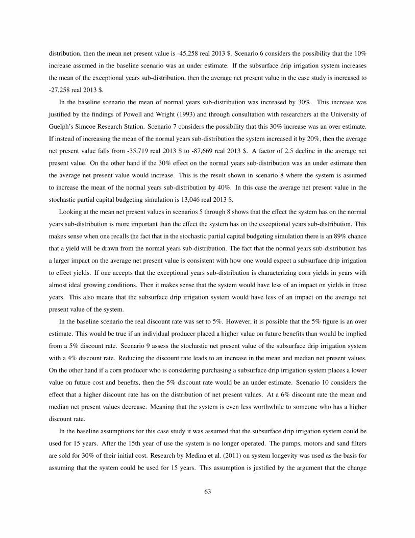
distribution, then the mean net present value is -45,258 real 2013 $. Scenario 6 considers the possibility that the 10%

increase assumed in the baseline scenario was an under estimate. If the subsurface drip irrigation system increases

the mean of the exceptional years sub-distribution, then the average net present value in the case study is increased to

-27,258 real 2013 $.

In the baseline scenario the mean of normal years sub-distribution was increased by 30%. This increase was

justified by the findings of Powell and Wright (1993) and through consultation with researchers at the University of

Guelph’s Simcoe Research Station. Scenario 7 considers the possibility that this 30% increase was an over estimate.

If instead of increasing the mean of the normal years sub-distribution the system increased it by 20%, then the average

net present value falls from -35,719 real 2013 $ to -87,669 real 2013 $. A factor of 2.5 decline in the average net

present value. On the other hand if the 30% effect on the normal years sub-distribution was an under estimate then

the average net present value would increase. This is the result shown in scenario 8 where the system is assumed

to increase the mean of the normal years sub-distribution by 40%. In this case the average net present value in the

stochastic partial capital budgeting simulation is 13,046 real 2013 $.

Looking at the mean net present values in scenarios 5 through 8 shows that the effect the system has on the normal

years sub-distribution is more important than the effect the system has on the exceptional years sub-distribution. This

makes sense when one recalls the fact that in the stochastic partial capital budgeting simulation there is an 89% chance

that a yield will be drawn from the normal years sub-distribution. The fact that the normal years sub-distribution has

a larger impact on the average net present value is consistent with how one would expect a subsurface drip irrigation

to effect yields. If one accepts that the exceptional years sub-distribution is characterizing corn yields in years with

almost ideal growing conditions. Then it makes sense that the system would have less of an impact on yields in those

years. This also means that the subsurface drip irrigation system would have less of an impact on the average net

present value of the system.

In the baseline scenario the real discount rate was set to 5%. However, it is possible that the 5% figure is an over

estimate. This would be true if an individual producer placed a higher value on future benefits than would be implied

from a 5% discount rate. Scenario 9 assess the stochastic net present value of the subsurface drip irrigation system

with a 4% discount rate. Reducing the discount rate leads to an increase in the mean and median net present values.

On the other hand if a corn producer who is considering purchasing a subsurface drip irrigation system places a lower

value on future cost and benefits, then the 5% discount rate would be an under estimate. Scenario 10 considers the

effect that a higher discount rate has on the distribution of net present values. At a 6% discount rate the mean and

median net present values decrease. Meaning that the system is even less worthwhile to someone who has a higher

discount rate.

In the baseline assumptions for this case study it was assumed that the subsurface drip irrigation system could be

used for 15 years. After the 15th year of use the system is no longer operated. The pumps, motors and sand filters

are sold for 30% of their initial cost. Research by Medina et al. (2011) on system longevity was used as the basis for

assuming that the system could be used for 15 years. This assumption is justified by the argument that the change

63

expenses assumed in the case study account for proper maintenance of the system. Proper maintenance includes daily

backflushing of the sand filters, annual system flushing and the annual injection of chlorine and acid into the system.

As Medina et al. (2011) note in their work, a subsurface drip irrigation system that is properly maintained will have

a much longer useful life than one that is not. However, Medina et al. (2011) only studied subsuface drip irrigation

systems used to grow row crops in West Texas, an area whose climate is considerably different than Norfolk Counties.

To account for the uncertainty in the useful life of the system in scenario 11 the useful life of the system is reduced by

5 years from the baseline value of 15 years. In the stochastic partial capital budgeting simulation if the system is used

for 10 years the average net present value is -69,217 real 2013 $. On the other hand if the system can be used for 20

years the average net present value works out to -9,085 real 2013 $.

The last scenario considered in the sensitivity analysis is a change in the probability of a yield being drawn from the

normal years sub-distribution in the stochastic partial capital budgeting simulation. In baseline scenario the probability

of drawing a yield from the normal years sub-distribution was 89%. In scenario 13 the probability is reduced to 79%.

This change only affects the distribution of yield that is used to characterize corn yields when the subsurface drip

irrigation system is in use. The probability of a yield coming from the normal years sub-distribution in the distribution

that characterizes unirrigated corn yield is unchanged. The effect of this change is a reduction in the average net

present value from -89,504 real 2013 $ to -100,037 real 2013 $. The fact the average net present value is lower makes

sense given the fact that the system is assumed to increase the mean of the exceptional years distribution by only 10%.

If more yields are being drawn from the exceptional years sub-distribution, then fewer of the yields being draw in

the stochastic partial capital budgeting simulation are enjoying the kind of boost they were receiving when they were

being drawn from the normal years sub-distribution.

To get a sense of how each parameter in the stochastic net present value calculation affects the mean and median

net present values, the mean and median net present value elasticities for each parameter were calculated. The mean

net present value elasticity is the percent change in mean net present value when the parameter in question is increased

by 1%. For example the mean net present value elasticity for capital cost was calculated by increasing the capital cost

in the stochastic calculation by 1% from the baseline assumption and calculating the percent change in the average

net present value relative to the baseline scenario. The mean net present value elasticity of the discount rate was

calculated by changing the discount rate from 5% to 6%. The mean net present value elasticities for the effects the

subsurface drip irrigation system has on the two component distribution’s mean yields were calculated by increasing

the proportional effects on mean yield by 1%. Specifically the mean net present value elasticity for the effect the

system has on average yields in the normal years sub-distribution was calculated by increasing Φn from 1.30 to 1.31.

Similarly, the mean net present value elasticity for the effect the system has on average yields in the exceptional years

sub-distribution was calculated by increasing Φe from 1.10 to 1.11. The median net present value elasticities for the

parameters of stochastic partial capital budge in this case study were calculated in the same way as the mean net

present value elasticities with one exception. Rather than calculating the percent change in the mean net present value,

the percent change in the median net present value was calculated. Calculating the mean and median net present value

64

elasticities is useful because they can identify which one of the stochastic net present value calculation’s parameters

has the most influence on the outcome of the simulation. This information can be used by researchers working on the

implementation of subsurface drip irrigation systems to grow corn in Norfolk County to identify which aspects of the

system has the largest effect on the net present value of a subsurface drip irrigation system.

The mean and median net present value elasticities are presented in table 5.4. The table shows that a change in the

discount rate has the largest effect on the mean net present value of purchasing and using a subsurface drip irrigation

system to grow corn in Norfolk, County for 15 years. Although the discount rate does play an important role in

determining the average net present value it is not a variable that is a function of the subsurface drip irrigation system

itself. Of the variables that are a property of the subsurface drip irrigation system, the effect that the system has on

average yields in a normal year has the largest effect on the mean and median net present value of the system. In the

stochastic net present value calculation a 1% increase in the average yield in a normal year leads to a 7.645% increase

in the mean net present value. The other variable in the stochastic net present value calculation that has a considerable

effect on the mean and the median net present value is the capital cost of the system. A 1% increase in the capital cost

of the system leads to a 2.289% decrease in the mean net present value. The two properties of the system that have the

largest effect on the mean net present value are its effect on yields in a normal year and the capital cost of the system.

In this case study a subsurface drip irrigation system with the baseline parameters presented in table 5.1 end up

having a negative average net present value in the stochastic simulation. A break even analysis allows one to determine

how much one of the irrigation system’s parameters would have to change in order for the system to break even on

average. A parameter is at its break even value when 50% of the time the net presents values calculated in the stochastic

simulation are positive and the other 50% of the time they are negative. Put another way, when the median net present

value calculated in the stochastic simulation is zero, then the system has equal probability of having a negative net

present value as it does a positive net present value. The value of the system parameter that returns a distribution of

results with a median of zero is the break even value for that system parameter. Given that the capital cost of the

system and the effect the system has on yields in a normal year have the largest effects on the average and median net

present values they are the variables that were analyzed to determine their break even points.

Figure 5.8 presents the break even analysis for the effect that the subsurface drip irrigation system has on average

yields in a normal year. The figure shows that when the subsurface drip irrigation system can increase the average

corn yield in normal years by 38% then 50% of the time the system will have a positive net present value. This is an

8% difference from the baseline assumption that the system would increase the mean of the normal years distribution

by 30%. Figure 5.9 presents the break even analysis for the capital cost of the case study subsurface drip irrigation

system. The figure shows that the subsurface drip irrigation system would have to cost 148,000 real 2013 $ in order

for it to have a positive net present value 50% of the time.

The effect the subsurface drip irrigation system has on yields has relatively large impact on the net present value of

the system. Future research on the use of subsurface drip irrigation system used to grow corn in Ontario should focus

on getting a better sense of what kind of yield gains producers in Ontario could expect if they decide to purchase and

65

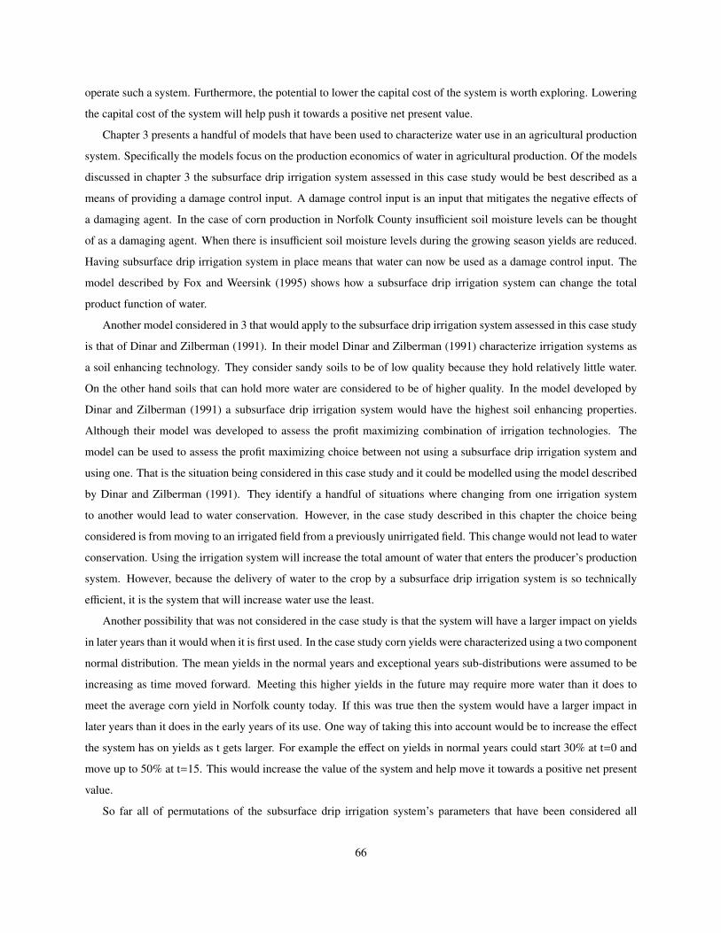
operate such a system. Furthermore, the potential to lower the capital cost of the system is worth exploring. Lowering

the capital cost of the system will help push it towards a positive net present value.

Chapter 3 presents a handful of models that have been used to characterize water use in an agricultural production

system. Specifically the models focus on the production economics of water in agricultural production. Of the models

discussed in chapter 3 the subsurface drip irrigation system assessed in this case study would be best described as a

means of providing a damage control input. A damage control input is an input that mitigates the negative effects of

a damaging agent. In the case of corn production in Norfolk County insufficient soil moisture levels can be thought

of as a damaging agent. When there is insufficient soil moisture levels during the growing season yields are reduced.

Having subsurface drip irrigation system in place means that water can now be used as a damage control input. The

model described by Fox and Weersink (1995) shows how a subsurface drip irrigation system can change the total

product function of water.

Another model considered in 3 that would apply to the subsurface drip irrigation system assessed in this case study

is that of Dinar and Zilberman (1991). In their model Dinar and Zilberman (1991) characterize irrigation systems as

a soil enhancing technology. They consider sandy soils to be of low quality because they hold relatively little water.

On the other hand soils that can hold more water are considered to be of higher quality. In the model developed by

Dinar and Zilberman (1991) a subsurface drip irrigation system would have the highest soil enhancing properties.

Although their model was developed to assess the profit maximizing combination of irrigation technologies. The

model can be used to assess the profit maximizing choice between not using a subsurface drip irrigation system and

using one. That is the situation being considered in this case study and it could be modelled using the model described

by Dinar and Zilberman (1991). They identify a handful of situations where changing from one irrigation system

to another would lead to water conservation. However, in the case study described in this chapter the choice being

considered is from moving to an irrigated field from a previously unirrigated field. This change would not lead to water

conservation. Using the irrigation system will increase the total amount of water that enters the producer’s production

system. However, because the delivery of water to the crop by a subsurface drip irrigation system is so technically

efficient, it is the system that will increase water use the least.

Another possibility that was not considered in the case study is that the system will have a larger impact on yields

in later years than it would when it is first used. In the case study corn yields were characterized using a two component

normal distribution. The mean yields in the normal years and exceptional years sub-distributions were assumed to be

increasing as time moved forward. Meeting this higher yields in the future may require more water than it does to

meet the average corn yield in Norfolk county today. If this was true then the system would have a larger impact in

later years than it does in the early years of its use. One way of taking this into account would be to increase the effect

the system has on yields as t gets larger. For example the effect on yields in normal years could start 30% at t=0 and

move up to 50% at t=15. This would increase the value of the system and help move it towards a positive net present

value.

So far all of permutations of the subsurface drip irrigation system’s parameters that have been considered all

66

consist of changing one variable and keeping all the other variables at their baseline values. This is what was done in

the sensitivity analysis and it is how the mean and median net present value elasticities were calculated. What would

happen if more than one variable changed? Figure 5.10 shows the distribution of net present values when the yearly

expenses, the effect on yields and the cost of the system are all changed from their baseline values. In this scenario

the yearly expenses from operating and maintaining the system are 1,500 real 2013 $/year rather than 2,951 real 2013

$/year. The mean yield in the normal years distribution is increased by 35% rather than 30%. The capital cost of the

system is 180,000 real 2013 $ rather than 187,360 real 2013 $. All the other parameters of the stochastic net present

value calculation were kept at the baseline values presented in Table 5.1. Under this new set of assumptions using the

subsurface drip irrigation system to grow corn for 15 years has an average net present value of 7,488 real 2013 $ and

a median of 7,899 real 2013 $.

67

Figure 5.1: Layout And Components Of A Subsurface Drip Irrigation System

systems. Screen filters and disk filters are common as alternatives or for use in combination ZLWK�VDQG�PHGLD�ÀOWHUV�

Sand media filters provide filtration to ��PHVK��ZKLFK�LV�QHFHVVDU\�WR�FOHDQ�VXUIDFH�water and water from open canals for drip irrigation. These water sources pick up a lot of fine grit and organic material, which must be removed before the water passes through the drip tape emitters.

Sand media filters are designed to be self-FOHDQLQJ�WKURXJK�D�´EDFN�ÁXVKµ�PHFKDQLVP��7KLV�mechanism detects the drop in pressure due to the DFFXPXODWLRQ�RI�ÀOWHUHG�SDUWLFOHV��,W�WKHQ�ÁXVKHV�water back through the sand to dispose of clay, silt, and organic particles.

6DQG�XVHG�IRU�ÀOWHUV�VKRXOG�EH�EHWZHHQ�VL]HV�� DQG�� WR� SUHYHQW� H[FHVV� EDFN� IOXVKLQJ��%HFDXVH�FOHDQ�ZDWHU�IURP�RQH�ÀOWHU�LV�QHHGHG�WR�EDFN�ÁXVK�DQRWKHU�ÀOWHU��DW�OHDVW�WZR�VDQG�PHGLD�ÀOWHUV�DUH�JHQHUDOO\�XVHG��,Q�DGGLWLRQ�WR�D�VDQG�media filter, a screen filter can be used as a SUHÀOWHU�WR�UHPRYH�ODUJHU�RUJDQLF�GHEULV�EHIRUH�LW�UHDFKHV�WKH�VDQG�PHGLD�ÀOWHU��RU�DV�D�VHFRQGDU\�ÀOWHU�EHIRUH�WKH�LUULJDWLRQ�ZDWHU�HQWHUV�WKH�GULS�WXEH��)LJXUH��)RU�EHVW�UHVXOWV��ÀOWHUV�VKRXOG�UHPRYH�SDUWLFOHV�

four times smaller than the emitter opening, as particles may clump together and clog emitters. 6FUHHQ�ÀOWHUV�FDQ�DFW�DV�D�VDIHJXDUG�LI�WKH�PDLQ�filters fail, or may act as the main filter if a VXIÀFLHQWO\�FOHDU�XQGHUJURXQG�ZDWHU�VRXUFH�LV�used.

)LJXUH��'ULS�LUULJDWLRQ�V\VWHP�ZLWK�D�SUHÀOWHU��SXPS�VWDWLRQ�ZLWK�EDFNÁRZ�SUHYHQWLRQ��DQG�FKHPLFDO�LQMHFWLRQ�VLWH��$�SUHVVXUH�FRQWURO�YDOYH�LV�UHFRPPHQGHG�WR�DGMXVW�WKH�ZDWHU�SUHVVXUH�DV�GHVLUHG�EHIRUH�it enters the drip lines. A water meter can be placed after the pressure control or between a solenoid

YDOYH�DQG�HDFK�]RQH��$Q�DLU�YHQW�SURYLGHV�YDFXXP�UHOLHI��9DFXXP�UHOLHI�LV�QHFHVVDU\�EHWZHHQ�WKH�VROHQRLG�YDOYH�DQG�WKH�GULS�WDSHV�WR�DYRLG�VXFWLRQ�RI�VRLO�LQWR�WKH�HPLWWHUV�ZKHQ�WKH�V\VWHP�LV�VKXW�RII�

4

Sub main lineDrip line

Prefilter

(optional)

Pressure

relief

valve

Backflow

preventionBack wash

Filters

Air vent

Pressure

control

Main line

Water meter

Drip line

Pressure-

reducing

solenoid

valve

ZONE 1

Pump

Chemical

injection

Sub main line

Flush

valves

Source: Reproduced from Shock (2013) with permission. Illustrated by Jessica Flock edited by Byron Shock.

68

Figure 5.2: Quantity Of Fodder And Grain Corn Produced In Ontario From 1990 to 2013 (metric tons)

0

1

2

3

4

5

6

7

8

9

10

1990

1991

1992

1993

1994

1995

1996

1997

1998

1999

2000

2001

2002

2003

2004

2005

2006

2007

2008

2009

2010

2011

2012

2013

Corn prod

uc*o

n (m

illions, m

etric

tons)

Year Corn for grain Corn for fodder

Source: Statistics Canada (2013b)

69

Figure 5.3: Area Of Fodder And Grain Corn Harvested In Ontario From 1990 to 2013 (hectares)

0

100

200

300

400

500

600

700

800

900

1000

1990

1991

1992

1993

1994

1995

1996

1997

1998

1999

2000

2001

2002

2003

2004

2005

2006

2007

2008

2009

2010

2011

2012

2013

Harvested area (tho

usan

ds, h

ectares)

Year Corn for grain Corn for fodder


70

Figure 5.4: Real Price Of Corn In Ontario From 1990 to 2013 (real 2013$/metric ton)

0

50

100

150

200

250

300

1990

1991

1992

1993

1994

1995

1996

1997

1998

1999

2000

2001

2002

2003

2004

2005

2006

2007

2008

2009

2010

2011

2012

2013

Price (201

3 real $/m

etric

ton)

Year


71

Figure 5.5: Case Study Two Component Normal Distribution Used To Characterize Corn Yields In Norfolk County

2013 2016 2019 20252022

0 2 4 6 8 10 12 140.0

0.1

0.2

0.3

0.4

0.5

0.6

Corn yield Hmetric tons�hectareL

Pro

ba

bility

de

nsity

Notes: The two component distribution is composed of two sub-distributions. The tallest of the two sub-distributionsis the normal years distribution and the shortest of the two is the exceptional years distribution. The probably of acorn yield being in the normal years rather than in the exceptional years sub-distribution is 89%.Source: Author, based on distribution parameters from Tolhurst and Ker (2013).

72

Figure 5.6: Case Study Two Component Normal Distribution Used To Characterize Corn Yields In Norfolk CountyWhen A Subsurface Drip Irrigation System Is Used

2013 20162016 201

92019 20222022 2025

0 2 4 6 8 10 12 140.0

0.1

0.2

0.3

0.4

0.5

0.6

Corn yield Hmetric tons�hectareL

Pro

ba

bility

de

nsity

Notes: The distributions that are not filled in are 5 years worth of forecasted corn yields for a field that is not irrigatedwith a subsurface drip irrigation system. The distributions that are filled in with shades of grey are the forecasted cornyield for a field that has a subsurface drip irrigation system in place. The two component distributions are composedof two sub-distributions. The tallest of the two sub-distributions is the normal years distribution and the shortest ofthe two is the exceptional years distribution. The probably of a corn yield being in the normal years rather than in theexceptional years sub-distribution is 89%. The distributions that are filled have the same parameters as those that arenot filled in except that the mean yield in the normal years sub-distribution is 30% higher in each year and the meanyield in the exceptional years sub-distribution is 10% higher in each year. Source: Author, based on distributionparameters from Tolhurst and Ker (2013).

73

Table 5.1: Baseline Parameters Of Case Study Subsurface Drip Irrigation System Used To Grow Corn In NorfolkCounty, Ontario

Capital costi $187,360Government funding $0Terminal salvage valuei $6,755Annual operating costii 2,951 $/yearFirst year of use 2013Useful life 15 yearsTax rate 30%Real discount rate 5%Change in mean yield of exceptional years distributionfrom using system 10%

Change in mean yield of normal years distribution fromusing system 30%

Probability of a normal yeariii 89%Price of corniv Pc ∼ N (191.23$/Mg,1572.1$2/Mg2)Area irrigated 40.5 hectares (100 acres)Soil type coarse textured sandy loamNotes: Costs are in real 2013 dollars. See Table 5.2 for a break down of capital cost of the subsurfacedrip irrigation system. Terminal salvage value is assumed to be 30% of the capital cost of themotor, pump and sand filter. See Table 5.2 for cost of motor, pump and sand filter. Corn yieldsare characterized by a two component normal distribution. See subsection 5.6 for a full explanationof the distribution used to characterize corn yields. The price of corn is assumed to have a normaldistribution with a mean of 191.23 real 2013 $ per metric metric ton and a variance of 1572.12 real2013 $2/metric ton2

Source: iAuthor’s calculation based on information provided by MacKenzie (2013) and Bakker(2013). iiAuthor’s calculation based on Lamm et al. (2012), iii Tolhurst and Ker (2013), ivStatisticsCanada (2014b)

74

Table 5.2: Baseline Capital Cost Of Case Study Subsurface Drip Irrigation System With 40.5 Hectares (100 acres) OfIrrigated Area Used To Grow Corn In Norfolk County, Ontario

Cost ($) for 40.5 ha (100acre) of irrigated area Cost ($/ha) Cost ($/acre)

In pump shed Electric motor and pump $4000 $99 $40Variable speed drive $6000 $148 $60Injector acid backflow meter $5549 $137 $55Sand filter and filter backflush $12518 $309 $125Controller $2579 $64 $26Shed and cement for slab $2134 $53 $21

In field Drip line $50843 $1256 $508Ties, tools and riser barbs $5888 $145 $59Above ground Schedule 40 pipe $2170 $54 $22PVC Main Line $1602 $40 $16PVC Header $15792 $390 $158PVC Flush header $5699 $141 $57Flush assembly $6016 $149 $60Valve stations $7713 $191 $77Wire $1069 $26 $11Glue and primer tape $1719 $42 $17Misc. parts $6063 $150 $61Misc. budget $4544 $112 $45

Installation Infield Consultant $15048 $372 $150Trenching $9021 $223 $90Applicator rental $4333 $107 $43Labour $17063 $422 $171

Totals $187360 $4630 $1874Notes: Total capital cost are in real 2013 dollars for 40.5 hectare (100 acre) of irrigated area. See section 5.1for an explanation of the components and the installation process of the subsurface drip irrigation system.Source: Items marked with asterisks (*) are calculated based on information provided by Bakker (2013) allother items were calculated based on information from MacKenzie (2013)

75

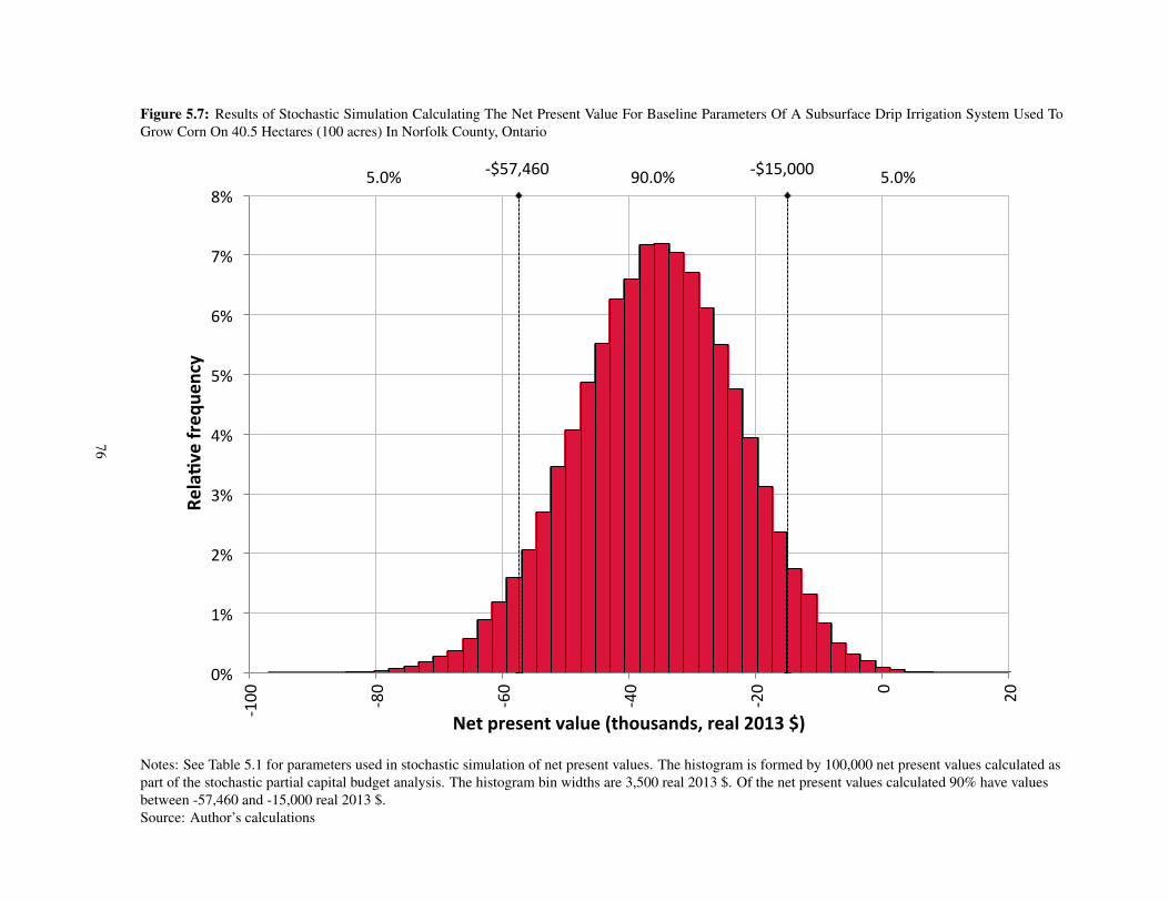
Figure 5.7: Results of Stochastic Simulation Calculating The Net Present Value For Baseline Parameters Of A Subsurface Drip Irrigation System Used ToGrow Corn On 40.5 Hectares (100 acres) In Norfolk County, Ontario

!$57,460) !$15,000)5.0%) 90.0%) 5.0%)

0%)

1%)

2%)

3%)

4%)

5%)

6%)

7%)

8%)

!100

)

!80)

!60)

!40)

!20) 0) 20)

Rela%v

e'freq

uency'

Net'present'value'(thousands,'real'2013'$)'

@RISK Student Version For Academic Use Only










Notes: See Table 5.1 for parameters used in stochastic simulation of net present values. The histogram is formed by 100,000 net present values calculated aspart of the stochastic partial capital budget analysis. The histogram bin widths are 3,500 real 2013 $. Of the net present values calculated 90% have valuesbetween -57,460 and -15,000 real 2013 $.Source: Author’s calculations

76

Table 5.3: Results Of Sensitivity Analyses On The Stochastic Simulation Used To Calculate The Net Present Value Of A Subsurface Drip Irrigation SystemUsed To Grow Corn On 40.5 Hectares (100 acres) In Norfolk County, Ontario

Distribution of net present values (real 2013 $ )Scenario Change in parameter from baseline Baseline value Modified value Mean Median Variance 5%a 95%b

Baseline n.a. n.a. n.a. -$35,719 -$35,522 $165,014,320 -$57,381 -$14,8821 Lower capital cost ($) $187,360 $168,624 -$18,512 -$18,283 $159,105,901 -$39,855 $1,9492 Higher capital cost ($) $187,360 $206,096 -$53,153 -$52,952 $170,018,309 -$75,068 -$31,9363 Lower annual operating cost ($\year) $2,951 $2,656 -$33,207 -$33,016 $163,960,551 -$54,825 -$12,4714 Higher annual operating cost ($\year) $2,951 $3,246 -$38,239 -$38,025 $166,067,940 -$59,966 -$17,322

5Smaller effect on mean yield in an ex-ceptional year (%) 10% 0% -$45,258 -$43,944 $335,570,832 -$76,988 -$17,251

6Larger effect on mean yield in an ex-ceptional year (%) 10% 20% -$27,258 -$27,280 $103,202,489 -$44,083 -$10,670

7Smaller effect on mean yield in a nor-mal year (%) 30% 20% -$87,669 -$87,747 $61,782,882 -$100,669 -$74,554

8Larger effect on mean yield in a normalyear (%) 30% 40% $13,046 $13,606 $311,246,849 -$16,747 $41,163

9 Decrease in real discount rate (%) 5% 4% -$25,083 -$24,852 $183,611,356 -$47,915 -$2,99010 Increase in real discount rate (%) 5% 6% -$45,328 -$45,116 $149,263,405 -$65,916 -$25,55311 Shorter useful life of system 15 years 10 years -$69,217 -$69,040 $140270,873 -$88,983 -$50,13312 Longer useful life of system 15 years 20 years -$9,085 -$8,747 $183,454,026 -$31,882 $12,765

13Lower probability of a yield comingfrom the normal years sub-distribution 89% 79% -$35,669 -$35,237 $167,214,899 -$57,495 -$15,266

Notes: With the exception of the baseline scenario, one parameter of the net present value calculation was modified in each scenario. See Table 5.1 for acomplete list of baseline parameters used in the net present value calculation. a5% of calculated net present values are less then this value. b5% of calculatednet present values are greater then this value. cRepresents a change in the effect that the system has on the mean of the exceptional years component of thetwo component normal distribution used to characterize corn yields. dRepresents a change in the effect that the system has on the mean of the normal yearscomponent of the two component normal distribution used to characterize corn yields.Source: Author’s calculations

77

Table 5.4: Mean and Median Net Present Value Elasticities Of Subsurface Drip Irrigation System Parameters

ParameterMean Net PresentValue Elasticitya

Median Net PresentValue Elasticityb

Effect of system on mean yield in normal yearc 7.645 % 7.866 %Effect of system on mean yield in exceptional yearc 1.169 % 1.205 %Useful life of system 0.4010 % 0.4830 %Annual operating cost -0.5770 % -0.4600 %Capital cost -2.289 % -2.182 %Real discount rated -9.115 % -9.507 %Notes: aMean Net Present Value Elasticity is the percent change in mean net present value when the parameterin question is increased by 1%. bMedian Net Present Value Elasticity is the percent change in median net presentvalue when the parameter in question is increased by 1%. c A 1% increase in the effect of the subsurface dripirrigation system on mean yield in the two sub-distributions means that the system was assumed to increase meanyields an extra 1% beyond the mean yield with the system in place. dA 1% change in the real discount rate meansthat the real discount rate was increased from 5% to 6%.Source: Author’s calculation

78

Figure 5.8: Effect On Mean Yield In Normal Years Break Even Analysis For A Subsurface Drip Irrigation SystemUsed To Grow Corn On 40.5 Hectares (100 Acres) In Norfolk County, Ontario

!150%

!100%

!50%

0%

50%

100%

150%

20%% 30%% 40%% 50%% 60%%

Med

ian'Net'Present'Value

'(tho

usan

ds,'real'2013'$)'

Change'In'Average'Yield'In'Normal'Year'(%)ᵃ

Notes: A bimodal distribution was used to characterize corn yields without a subsurface drip irrigation system. Thetwo normal distributions that make up the bimodal distribution were called "normal years" and "exceptional years". Itwas assumed that there was an 89% chance that a yield would come from the normal years distribution rather thanfrom the exceptional years distribution. aRepresents the effect that the subsurface drip irrigation system has on themean of the the normal years yield distribution. The graph was constructed by varying the effect that the subsurfacedrip irrigation system has on the average yield in the normal years distribution. All other parameters in the stochasticnet present value simulation were kept at the baseline values presented in table 5.1. The purple point identifies theresults of the stochastic net present value calculation with the baseline value for the effect of the system on theSource: Author’s calculations

79

Figure 5.9: Capital Cost Break Even Analysis: Median Net Present Values For A Subsurface Drip Irrigation SystemUsed To Grow Corn On 40.5 Hectares (100 acres) In Norfolk County, Ontario

!60$

!50$

!40$

!30$

!20$

!10$

0$

10$

20$

30$

$120,000$ $140,000$ $160,000$ $180,000$ $200,000$

Med


'(tho

usan

ds,'real'2013'$)'

Capital'Cost'(real'2013'$)$

Notes: For each value of capital cost all other parameters of the stochastic net present value simulation have thebaseline values from table 5.1. The orange point identifies the results of the stochastic net present value calculationwith the baseline value of capital cost.Source: Author’s calculations

80

Figure 5.10: Results of Stochastic Simulation Where Three Parameters Have Changed Calculating The Net Present Value Of A Subsurface Drip IrrigationSystem Used To Grow Corn On 40.5 Hectares (100 acres) In Norfolk County, Ontario

!17,647' 31,546'5.0%' 90.0%' 5.0%'

0%'

1%'

2%'

3%'

4%'

5%'

6%'

7%'

8%'

!60'

!40'

!20' 0' 20'

40'

60'

80'

Rela%v

e'freq

uency'

Net'present'value'(thousands,'real'2013'$)'











Source: Author’s calculations

81

Chapter 6: The use of varieties with higher technical water use efficiency in

Ontario chipping potato production

This case study is about the economic implications for a potato producer in Ellora, Ontario of growing a variety of

chipping potatoes, the T10-3, that has a relatively higher technical water use efficiency than varieties conventionally

grown in the province. Technical water use efficiency measures the amount of yield relative to the quantity of water

that a crop receives over the course of a growing season. Farm trials conducted in Alliston, Ontario in 2012 and 2013

by Peter VanderZaag are an indication that there is potential to increase the technical water use efficiency of Ontario

chipping potato production. As part of this case study the difference in fertilizer requirements and yields for the T10-3,

Atlantic and Dakota Pearl varieties are taken into account to estimate the change in net present value of growing the

T10-3 variety rather than the Atlantic variety and of growing the T10-3 variety rather than the Dakota Pearl variety.

The outline of the case study is as follows: first is an overview of the potato production sector in Ontario and details

on chipping potato production relevant to this case study; second is an explanation of technical water use efficiency and

how differences between chipping potato varieties affect technical water use efficiency; third is an analysis of data on

farm trials of chipping potato varieties and an assessment of the potential difference in technical water use efficiency

of potato varieties in the trial; lastly is a comparison of the change in cash income and costs of production to estimate

the difference in the net present value of growing a chipping potato variety with higher technical water use efficiency.

6.1 The potato sector in Ontario

Figure 6.1 illustrates the amount of land used to grow all potatoes in Ontario from 1985 to 2013. The lowest area used

in potato production occurred in 1990 when 14 thousand hectares were under production. Between 1990 and 2003

the area under potato production increased up to a maximum of 17.8 thousand hectares and declined sharply over

the next two years. In the last 10 years the amount of land used to produce all potatoes has been fairly level varying

between 14 and 16 thousand hectares. The quantity of potatoes produced in Ontario from 1990 to 2013 is illustrated

in Figure 6.2. With the exception of the period from 1996 to 2001, since 1990 there has been a wide variation in total

production of potatoes in Ontario. This is not surprising given the crops sensitivity to weather conditions, especially

temperature and precipitation. The largest harvest of potatoes occurred in 2003 when just over 400,000 metric tons

of potatoes were produced in Ontario. The smallest harvest since 1990 occurred in 2007 when 233,000 metric tons

82

were produced. Figure 6.3 illustrates that average yield of potatoes in Ontario from 1990 to 2013. Over this period

the quantity of potatoes produced per hectare has seen sharp changes from year to year. The highest yield of potatoes

occurred in 1992 when potato yields in Ontario reached 27 metric tons/hectare. The lowest yield was in 2007 when

average yields were 16 metric tons/hectare.

In its overview of the potato sector in North America the Extension Section of The Potato Association of America

(2010) divides the potato sector into three markets based on the utilization of potatoes. First is the fresh market which

accounts for the potatoes sold in grocery stores and restaurants. Second is the processing market where potatoes are

frozen in various form, dehydrated or turned into potato chips. Finally is the seed market where potatoes are sold to

other potato growers to plant the next year’s crop. The feed sector is not usually recognized as market for potatoes.

However, in years where agronomic conditions result in a crop that does not meet the quality standards of the fresh or

processing markets, the next best option for a potato farmer is to sell the unusable potatoes as cattle feed.

The varieties of potatoes used in the processing, fresh market and seed markets are not all the same. Producers

grow potato varieties that have desirable properties for their respective uses. For example a Yukon Gold potato will

not be used to make potato chips. Because of its thick skin and relatively high sugar content a Yukon Gold potato

is better suited for cooking. As a result Yukon Gold potatoes are sold to the fresh market. On the other hand an

Atlantic potato has a thin skin that can be easy removed and has a relatively low sugar content that make it a good fit

for transformation into potato chips. Potato varieties that are used for potato chip production are know as chipping

varieties. Potatoes that will be turned into potato chips tend to have a higher quantity of dry matter content. As the

Extension Section of The Potato Association of America (2010) note, processors place an emphasis on the dry matter

content of the potatoes they purchase. As a result contracts between processors and growers will include bonuses for

potatoes with higher dry matter content and penalties for potatoes with lower dry matter content. Potato tuber size and

defects are also taken into account when determining premiums in processing potato contracts.

In addition to growing potato varieties that have properties for a particular market, potato growers also grow more

then one variety even if all the potatoes they are growing are destined for a particular use. Potatoes grown for potato

chip production are one example of multiple varieties being grown for a particular market. There are a number of

chipping potato varieties. One important difference between them is their sugar content at the time of harvest. Chipping

potato varieties that have ideal sugar content when they are harvested in late August and September are known as field

fry varieties. They can be pulled out of the ground and sent straight to the potato chip manufacture. On the other hand,

storage varieties are better suited for medium to long term storage in temperature controlled environments. This case

study will be focusing on field fry varieties of chipping potatoes.

Figure 6.4 presents the real price of table, processing and seed potatoes in Ontario from 1990 to 2013. Table

and seed potatoes have had large variations in their prices. This is especially true for the period from 1998 to 2013.

On the other hand, the real price of processing potatoes has been relative flat over the last 20 years. The price of

processing potatoes was above 300 real 2013 $/metric ton in 2002 and from 2009 to 2011 and saw its highest price

in 2009. Because chipping potatoes are not all sold as soon as they are harvested it is worth looking at how the price

83

of processing potatoes vary over the course of a year. Figure 6.5 presents the average monthly price of processing

potatoes in Ontario. Each month’s price represents the average real price of potatoes in that month from 1993 to 2013.

For example the average price of processing potatoes in July is 425.05 real 2013 $/metric ton (19.28 real 2013 $/cwt)

which is the average of all processing potato prices in July from 1993 to 2013. Figure 6.5 shows that in the time after

harvest the price of processing potatoes is not always the same. The price of processing potatoes is highest just after

harvest in August and declines in each month until January when prices start increasing again.

6.2 Technical water use efficiency and potato varieties

As was explained in chapter 2 technical water use efficiency is defined as the proportion of marketable yield to the

quantity of water used. In this case study the definition of technical water use efficiency explained by Gregory (2004)

will be used. They define technical water use efficiency as a measure of how much marketable yield is produced for a

given amount of water used in a growing season. In the case of unirrigated potato production this relationship can be

defined mathematically using Gregory’s (2004) equation:

WUE =M

(Es + T + R + D)(6.1)

where

WUE is the technical water use efficiency

M is the weight of marketable potato tubers produced

Es is the amount of water that evaporates from the soil surface

T is the amount of water that transpires from the potato crop

R is water runoff

D is water that drains below the root zone

The variables accounting for amounts of water used are measured in m3 and the weight of yields is measured in kg.

Therefore, technical water use efficiency is measured in kg/m3. Taken together the terms for evaporation from the soil,

Es , the amount of water that transpires from the crop, T , runoff from the field, R, and drainage below the root zone,

D, add up to the amount of precipitation that fell and the field in a growing season and any changes in water stored

in the soil. If a potato crop is irrigated the four terms in the denominator of equation 6.1 would sum to the amount of

water the fell on the field as precipitation, the amount that was added through irrigation and changes in water stored

in the soil. Including terms for evaporation, transpiration, runoff and drainage in the technical water use efficiency

equation helps to illustrate which portions of a farms hydrological cycle can be changed to increase technical water

use efficiency. Because evaporation, transpiration, runoff and drainage are in the denominator of the technical water

use efficiency equation if these variables get smaller technical water use efficiency will increase.

84

R. A. Richards and van Herwaarden (2002) identify four factors that are partly controlled by a plant’s genotype

that will affect technical water use efficiency of a crop. Although their work is focused on cereal crops, the factors

identified by R. A. Richards and van Herwaarden (2002) offer a framework for thinking about the aspects of technical

water use efficiency of chipping potatoes that are partly influenced by the plant’s genotype. The four factors identified

by R. A. Richards and van Herwaarden (2002) are: transpiration efficiency, seedling establishment, seedling vigour

and harvest index. Each one of these properties of a plant will be discussed in tern to explain their influence on

technical water use efficiency of chipping potatoes.

First, transpiration efficiency is the quantity of water transpired from the plant relative to the dry matter accumula-

tion over the course of a growing season. A plant with a higher transpiration efficiency will also have a higher technical

water use efficiency because a relatively high transpiration efficiency means that for each unit of water transpired from

the plant there is more biomass added to the plant. Transpiration efficiency measures the weight of dry matter that

is produced in a growing season for a given volume of water that transpires from the plant over the course of the

growing season. There has been some research on genetic differences in transpiration efficiency of potatoes. Vos and

Groenwold (1989) assessed the transpiration efficiency of 6 potato varieties. In their experiment Vos and Groenwold

(1989) grew 6 potato varieties in containers under a rain shelter and supplied water through a subsurface drip irrigation

system. Evaporative losses from the soil surface were minimized by covering the containers with a plastic sheet. After

a 100 day growing season the weight of the plant’s roots, stolons and tubers—every part of the potato plant that is

below the surface—were measured for their dry matter content. Transpiration efficiency ranged from 7.94 g/L to 9.49

g/L with the Up-to-Date variety having the highest transpiration efficiency and the Surprise variety having the lowest.

These results show that not all potato varieties have the same transpiration efficiency. Although Vos and Groenwold

(1989) do not report on the other factors that affect technical water use efficiency such as seeding establishment,

seeding vigour or harvest index, their experiment is suggestive that technical water use efficiency, through changes in

transpiration efficiency, does vary between potato varieties.

The second factor identified by R. A. Richards and van Herwaarden (2002) that can affect technical water use

efficiency is seedling establishment. Seedling establishment measures how quickly the vegetative portions of a plant

emerge from the soil after seeds have been planted. Seedling establishment affects technical water use efficiency by

decreasing the amount of water that evaporates from the soil surface. Seedling establishment affects the Es term in

the technical water use efficiency equations 6.1 and ??. This effect can occur for two reasons. First, by reducing the

amount of water that is lost to evaporation. Second, by reducing the number of weeds present around the crop. All

else being equal, a variety of potatoes that has a higher seedling establishment will have a higher technical water use

efficiency.

The third factor that can affect technical water use efficiency is seeding vigour. Like seeding establishment, seeding

vigour reduces the amount of water that evaporates from the soil. A plant with a higher seeding vigour will have a

lower Es over a growing season than one that with a lower seeding vigour. This is because plants with a relatively

high vigour will shade the ground and reduce the amount of water that evaporates from the soil. A variety of potatoes

85

that more rapidly reaches 100% canopy cover will have a higher technical water use efficiency than a variety that takes

longer for its leaves to grow to the point where they are completely covering the soil.

The last factor identified by R. A. Richards and van Herwaarden (2002) that can affect technical water use efficiency

is the harvest index. This is the proportion of a plant’s total mass that can actually be harvested and sold. In the case of

a chipping potatoes varieties, a variety with a higher harvest index produces larger or more tubers of marketable sizes.

The harvest index is not accounted for in the technical water use efficiency equations 6.1 and ??. However the two

equations could be modified to account for harvest index by specifying the term M , the weight of marketable potato

tubers, as the product of the total plant mass and the harvest index.

Technical water use efficiency measures how much marketable yield is produced for a given amount of water

applied to a crop. A variety of chipping potatoes that has a relatively larger yield for the same amount of precipitation

will have a higher technical water use efficiency. There are four aspects of plant physiology that can affect technical

water use efficiency: transpiration efficiency, seedling establishment, seeding vigour and harvest index. All else being

equal a chipping potato variety who’s genotype leads to less evaporation from the soil by having a better seedling

establishment or more seedling vigour will have a higher technical water use efficiency. Additionally a chipping

potato variety that has a greater transpiration efficiency or harvest index will also have a higher technical water use

efficiency.

6.3 2012 and 2013 potato on farm variety trials in Alliston, Ontario: a hint of increased

technical water use efficiency

Two on farm trials one conducted in 2012 and the other in 2013 by Peter VanderZaag, owner and operator of Sunrise

Potato Storage Ltd, are an indication that technical water use efficiency in Ontario chipping potato production can be

improved by growing varieties with higher technical water use efficiency. The farm trials are noteworthy because they

took place in years with significantly different amounts of precipitation during the growing season. Table 6.1 presents

the climate normals in Alliston, Ontario for the potato growing season from 1981 to 2010. The climate normals for

Alliston, Ontario are taken from the Environment Canada weather station closest to the trial site. Table 6.1 also lists

the amount of precipitation in 2012 and 2013 as measured by a weather station installed at the farm trial site. The table

shows that in 2012 the farm trial site saw relatively little precipitation over the growing season. Whereas in 2013 the

farm trial site received significantly more precipitation than in 2012. Given the difference in precipitation in 2012 and

2013 the farm trials help to show how chipping potato varieties can affect technical water use efficiency both in dry

years and in years that are closer to normal.

6.3.1 Experimental design of the 2012 and 2013 field trials in Alliston, Ontario

In 2012 and 2013 trials with randomized complete block designs were undertaken to evaluate the growth and yield of

9 chipping potato varieties in Alliston, Ontario. Among the varieties were two field fry varieties the T10-3 and Dakota

86

Pearl. In 2012 the potatoes were grown without irrigation. Replicated plots were two rows wide with an area of 8m2

(90 ft2) and 15 seed tubers were planted per row. Four replicates were grown. Potato seeds were planted May 17th,

2012, desiccated on August 23rd, 2012 and harvested in October. Because the potatoes in this trial were not irrigated

both T10-3 and Dakota Pearl received water from precipitation over the growing season. The total precipitation at the

trial site, as measured by an onsite weather station, was 183.6mm.

In 2013 a similar trial as the one conducted in 2012 also took place in Alliston, Ontario. The same varieties were

planted, including T10-3 and Dakota Pearl. However the plot sizes were 11.2m2 (120ft2). Potato seeds were planted

on May 23rd, 2013, desiccated on August 30th, 2013 and harvested on October 18th, 2013. Rather then depending

on precipitation to supply water to the crop, irrigation was applied when needed and both T10-3 and Dakota Pearl

varieties received the same amount of irrigation. The total water that reached the trial site, as measured by an onsite

weather station, was 313.5mm.

6.3.2 The technical water use efficiency of the T10-3 and Dakota Pearl varieties in the 2012 and 2013 trials in

Alliston, Ontario

Data from the field trials conducted in Alliston, Ontario in 2012 and 2013 provided by VanderZaag (2013) show

how well the T10-3 and Dakota Pearl varieties compare in terms of their technical water use efficiency. Of the four

genotypically influenced factors identified by R. A. Richards and van Herwaarden (2002)—transpiration efficiency,

seedling establishment, seedling vigour and harvest index—the trials from 2012 and 2013 offer some insight into how

well the T10-3 variety fares relative to the Dakota Pearl variety.

Seedling vigour affects technical water use efficiency by lowering the amount of evaporation from the soil. A potato

variety that can can grow leaves to cover the soil faster than another variety under the same growing conditions will

have a higher technical water use efficiency. Figure 6.6 illustrates the percent of canopy cover for T10-3 and Dakota

Pearl over the course of the 2012 growing season. A canopy cover of 100% means that the potato plants leave’s are

completely obscuring the soil there by reducing the amount of water that evaporates from the soil. Neither of the two

varieties reached 100% canopy cover in the 2012 trial. The Dakota Pearl variety had a larger canopy than T10-3 for

most of the growing season. The Dakota Pearl variety had a larger canopy than the T10-3 variety for approximately

84 days out of 98 days. During the time that Dakota Pearl had a larger canopy than T10-3, the Dakota Pearl canopy

covered an average of 7% more of the soil. On the other hand, over the 14 days that the T10-3 variety had a larger

canopy it covered an average of 9.25% more soil. As for the canopy cover in 2013, Figure 6.7 presents the percent

canopy cover for Dakota Pearl and T10-3. The Dakota Pearl variety had a larger canopy for the first 49 days after

planting. Both varieties had a full canopy for 14 days and in the later portion of the 2013 growing season T10-3 had a

larger canopy. During the time that the Dakota Pearl variety had a larger canopy it covered and average of 13% more

of the soil. Whereas when the T10-3 variety had a larger canopy it covered an average of 12% more soil.

What do the results of the trials in Alliston, Ontario on T10-3 and Dakota Pearl mean for the technical water use

efficiency of each variety? If the only thing that differed between the Dakota Pearl and T10-3 varieties in 2012 was

87

their canopy cover, the Dakota Pearl variety would have a higher technical water use efficiency. It can be inferred from

the canopy cover of the Dakota Pearl variety that in the 2012 less water evaporated from the soil where the Dakota

Pearl was being grown. The same goes for 2013, between the two varieties the Dakota Pearl would have a higher

water use efficiency.

Although evaporative losses from the soil are one aspect of technical water use efficiency, a direct measure of

technical water use efficiency can be made if one knows the marketable yield of a crop and the amount of water that

the crop received over the course of a growing season. In terms of equation 6.1 which was used to define technical

water use efficiency for this case study: if one knows the weight of marketable potato tubers, M , and the other terms

in the equation a measure of technical water use efficiency can be made. For the trials on T10-3 and Dakota Pearl in

2012 and 2013 in Alliston, Ontario there was no measurement made of the amount of water that evaporated from the

soil surface, that transpired from the crop, that ran off the surface or that drained past the root zone. However, the sum

of these aspects of technical water use efficiency was measured by determining how much water fell on the crop in

each year. In 2012 183.6 mm of rain fell on both the T10-3 variety and the Dakota Pearl variety over the course of the

growing season. In 2013 313.5 mm of water fell on the two varieties from precipitation or from over head irrigation. In

each year T10-3 and Dakota Pearl had the same denominators in question 6.1. This means that if there is a difference

in yield between the two varieties there will be a difference in technical water use efficiency. The variety with the

highest yield will also have a higher technical water use efficiency.

In 2012 the Dakota Pearl variety had an average total yield across the four replications of 16.14 metric ton/ha

(143.97 cwt/acre)1.The T10-3 variety had a total yield of 15.19 metric ton/ha (135.50 cwt/acre). Although the Dakota

Pearl variety had a larger average total yield it had a larger proportion of unmarketable potatoes than the T10-3 variety.

Figure 6.8 shows the weight of small, unmarketable potatoes, and marketable potatoes for the two varieties. The T10-3

variety had a slightly higher average yield of marketable potatoes, at 13.56 metric ton/hectare (120.98 cwt/acre), than

the Dakota Pearl variety with an average of 12.88 metric ton/hectare (114.93 cwt/acre). As for the results in 2013,

Figure 6.9 illustrates the yield of the T10-3 and Dakota Pearl varieties. T10-3 had a slightly higher average yield than

the Dakota Pearl across four replications. The yield for both varieties was of adequate size to meet standards for sale

to potato chip processors. Therefore, neither variety had any unmarketable yield. The mean marketable yield for the

T10-3 variety was 62.24 metric ton/hectare (555.31 cwt/acre) and the Dakota Pearl variety had a mean marketable

yield of 58.31 metric ton/hectare (520.23 cwt/acre).

The technical water use efficiency of the T10-3 and Dakota Pearl variety in the two farm trials can be calculated

based on their yields and the amount of water that reached the crop in each year. In 2012 1836 m3 of water reached

both the T10-3 and the Dakota Pearl variety. The T10-3 variety had a marketable yield of 13,560 kg/ha and the Dakota

Pearl had a marketable yield of 12,880 kg/ha. This implies that in 2012 the T10-3 variety had a technical water use

efficiency of 7.386 kg/m3/ha and the Dakota Pearl had a technical water use efficiency of 7.015 kg/m3/ha. In 2013 the

1The data collected from the potato trials were reported in pounds. These values were converted to metric ton/ha and cwt/acre using the following

equations: yield(

metric tonhectare

)=

yield from experiment(lb)experimental plot area(ft2 )

∗107639(ft2 )1(hectare) ∗

1(metric ton)2205(lb) and yield

(cwtacre

)=

yield from experiment(lb)plot area

(ft2

) ∗1(cwt)100(lb) ∗

43 560(ft2

)1(acre)

88

T10-3 had a marketable yield of 62,240 kg/ha and the Dakota Pearl had a marketable yield of 58,310 kg/ha. In the

same year the two varieties received 3135 m3 of water either through precipitation or over head irrigation. This implies

that in 2013 the T10-3 had a technical water use efficiency of 19.85 kg/m3/ha and the Dakota Pearl had a technical

water use efficiency of 18.6 kg/m3/ha. In both years the T10-3 variety had a higher technical water use efficiency than

the Dakota Pearl variety. For every millimetre of water that fell on the two varieties in 2012 and 2013 the T10-3 variety

produced more marketable chipping potatoes.

6.4 The farm level economics of growing a potato variety with higher technical water use

efficiency

The results of the 2012 and 2013 field trials on Dakota Pearl and T10-3 in Alliston, Ontario show that technical water

use efficiency in chipping potato production can be improved by growing varieties with higher yields. This section of

the chapter considers the economic implications to an agricultural producer in Ontario of growing the T10-3 variety

rather then two conventionally grown varieties. The varieties to which T10-3 will be compared are the Atlantic and

Dakota Pearl. The Atlantic is not widely grown in Ontario. In fact in 2010 only 2 hectare of land were used to grow the

Atlantic variety in Ontario (Agriculture and Agri-Food Canada, 2010). However, the Atlantic has had a long history

in the province as a chipping potato variety and is recognized by the Canadian Food Inspection Agency (2013) as the

standard used to evaluate chipping potatoes. Furthermore, Vanessa Currie, who has been working at the University

of Guelph in the Potato Breeding Program since 1990, identifies the Atlantic as a benchmark chipping potato variety.

Given the Atlantic’s history in the chipping potato sector in Ontario and its status as a basis for comparing other

chipping potato varieties, it will be one of the two varieties to which the T10-3 will be compared. The other variety

of chipping potato that will be compared to the T10-3 is the Dakota Pearl. The Dakota Pearl is more widely grown

in Ontario than the Atlantic. In 2010 13 hectares were used in the production of Dakota Pearl (Agriculture and Agri-

Food Canada, 2010). VanOostrum (2014) identifies the Dakota Pearl as being the second most popular chipping potato

variety after Frito Lay private varieties. Because the Dakota Pearl is a relatively popular chipping potato it will be the

second variety to which the economics of growing the T10-3 will be compared.

6.5 Methods for assessing the farm level economics of a chipping potato variety with higher

technical water use efficiency

The merits of growing the T10-3 variety were assessed based on its net present value. Two net present values were

assessed in this case study. The first is the net present value of growing the T10-3 variety rather than the Atlantic. The

other net present value was that of growing the T10-3 rather than the Dakota Pearl. Both net present values were based

on partial capital budgets that capture the costs and benefits to the grower who would choose to grow the T10-3 rather

than the Atlantic or who would choose to grow the T10-3 rather than the Dakota Pearl. The costs and benefits of the

89

growing the T10-3 can either change the cash income or the cash expenses of the farm business. For example a benefit

of using the growing the T10-3 rather than the Dakota Pearl is that the T10-3 has higher yields on average. In addition

to accounting for how cash income and cash expenses would be affected if the T10-3 were grown, the partial capital

budgets also take into account how taxes would change. Mathematically the net present value of the partial capital

budget can be represented as follows:

N PV =

T∑t=1

∆CIt − ∆CEt − ∆Γt

(1 + d)t(6.2)

where








Taxes in period t are calculated using the following equation:

∆Γt = [∆CIt − ∆CEt ]T Rt (6.3)

where






The tax rate, T Rt , was set to 30% in each period t.


that each value listed in equations 6.5 and 6.5 of the net present value calculation have fixed values. However, their

is uncertainty in exactly what value some of the equations parameters will take in the future. For example part of

calculating the change in cash income, ∆CIt , involves multiplying chipping potato prices by potato yields. Chipping

90

potato yields in each year that the T0-3 variety is grown will not all be the same. Their are factors beyond the grower’s

control the lead to variation from year to year. Because the T10-3 variety is grown for multiple years, a more accurate

representation of the world would take into account this variation in yield. Similarly, past experience shows that the

real price of chipping potatoes is not the same in each month. Assuming that real potato prices are the same in each

period t would not capture the variation in prices that the sector has seen the past. To take into account the fact that

there is uncertainty in some of the parameters of the net present value calculation a Monte Carlo simulation was used.

In the Monte Carlo simulation for this case study some of the parameters in the partial capital budget were char-


1541.74$/metric ton and a standard deviation of 170.069 $/metric ton was used to characterize urea prices in the case

study. Yields, input cost and any other part of the partial capital budget can be characterized using a distribution.

In this case study monthly chipping potato prices prices, potato yields and fertilizer prices were characterized using

statistical distributions. Detailed explanations of the statistical distributions used in the case study are presented in the

next two sections.

The Monte Carlo simulation was implemented using the @RISK add-on developed by Palisade Corporation for

Microsoft Excel. In calculating the net present value, @RISK makes random draws from the statistical distributions



times. Each time the net present value is calculated using newly selected values from the statistical distributions. The

result of repeatedly calculating the net present value is a distribution of net present values. It is this distribution that is

reported in the results of this case study.




6.6 Change in cash income from growing a chipping potato with higher technical water use

efficiency

To determine how cash income would be affected if a producer chose to grow the T10-3 variety rather than the Atlantic

or the Dakota Pearl, one has to determine two things: the difference in yield and how the price received for the potatoes

would be affected. In this case study the price received for marketable chipping potatoes was assumed to be the same

for all three varieties. How the price received for the three varieties was characterized in this case study is explained

in more detail later in this section.

The difference in yield from growing the T10-3 was estimated by creating a yield distribution for the T10-3

variety and subtracting it from the distribution of potato yields to which the T10-3 is being compared. To assess

the difference in yield from growing the T10-3 rather than the Atlantic, in the stochastic partial capital budgeting

91

simulation the distribution of T10-3 yields was subtracted from the distribution of Atlantic yields. To assess the

difference in yield from growing the T10-3 rather than the Dakota Pearl, in the stochastic partial capital budgeting

simulation the distribution of T10-3 yields was subtracted from the distribution of Dakota Pearl yields.

In this case study the distribution of yields for all three varieties were created based on yield data from potato trials

conducted as part of the Potato Research Project at the University of Guelph’s Elora Research Station. From 2003

to 2012 researchers with the Potato Research Project grew Atlantic chipping potatoes in yearly trials. In these trials

Atlantic potatoes were grown without irrigation on silt loam soil. Industry standard agronomic practices were followed

before planting, over the course of the growing season, during harvest and after harvest. Currie (2014) provided yield

data from the 9 trials conducted on the Atlantic variety. It is these data that were used to derive the parameters of the

yield distribution of Atlantic potatoes in this case study. The distributions of yields for the Dakota Pearl and the T10-3

varieties were derived from the Atlantic’s distribution. Studies that have compared the yield of the Dakota Pearl to the

Atlantic’s and the T10-3 to the Dakota Pearl’s were used to derive their distributions in this case study.

In this case study it was assumed that the distribution of Atlantic potato yields is normally distributed with the

same mean and variance as the yields of Atlantic East potatoes from the Potato Research Project between 2003 and

2012. The distribution of yields of the Atlantic variety used in this case study can be expressed as:

YAtlantic,t ∼ N (µA,t ,σ2A,t ) (6.4)

where

YAtlantic,t is the yield of Atlantic potatoes in period t


N means that yields are normally distributed

µA,t is the mean yield of Atlantic potatoes in period t

σ2A,t is the variance of yields of Atlantic potatoes in period t

The mean yield of Atlantic potatoes, µA, was set to 27.63 metric ton/hectare (246.53 cwt/acre) and the variance, σ2A,

was set to 146.41 metric ton2/hectare2 (11659 cwt2/acre2)2. Again these parameters are the mean and variance of

Atlantic potatoes in 9 years of field trials at the University of Guelph’s Elora Research Station.

There is no multi-year data on the yields of the Dakota Pearl and the T10-3 varieties that could be used as the basis

for creating yield distributions for this case study. Although the Dakota Pearl has been grown in Ontario for well over

a decade a reliable source of yield data in Ontario for this specific variety could not be found. As for the T10-3 it is

very much an experimental variety. It has not been grown in Ontario other than the two farm trials in 2012 and 2013

2Mean marketable yield which is reported in kg in Currie’s (2014) data were converted to cwt/acre by multiplying experimental yield by 15 as

per Currie (2014). The conversion factor for cwt/acre to metric ton/hectare was 0.1121−1 as per Johanns (2013)

92

conducted by VanderZaag (2013). Therefore, for the purposes of this case study the yield distributions for the Dakota

Pearl and the T10-3 were derived from the Atlantic’s distribution.

The Dakota Pearl’s distribution in this case study was created by adjusting the Atlantic’s normal distribution

according to the findings of Thompson et al. (2005). They conducted trials on both the Atlantic variety and the Dakota

Pearl variety in 1994, 1997 and 1998. Thompson et al. (2005) conducted their trials under non-irrigated conditions in

North Dakota and found that the Dakota Pearl had an average total yield of 23.8 metric tons/hectare (212.31 cwt/acre),

whereas the Atlantic had an average total yield of 26.0 metric tons/hectare (231.94 cwt/acre). A difference of 8.5%.

Based on this information, the distribution of Atlantic yields previously specified was modified to form the distribution

of Dakota Pearl yields. The distribution of Dakota Pearl yields was assumed to be the same as the Atlantic’s except

that the mean yield was set 8.5% lower than the mean yield of the Atlantic. The yield distribution for the Dakota Pearl

variety assumed in this case study can be represented as:

YDakota Pearl,t ∼ N (µD,t ,σ2D,t ) (6.5)

where

YDakota Pearl,t is the yield of Dakota Pearl potatoes in period t



µD,t is the mean yield of Dakota Pearl potatoes in period t

σ2D,t is the variance Dakota Pearl yields in period t

The mean yield of Dakota Pearl potatoes, µD, was set to 10.84 metric tons/hectare (207.7 cwt/acre) which is the mean

yield of Atlantic potatoes from the Elora Research Station trials minus the 8.5% difference found by Thompson et al.

(2005). The variance for the distribution of Dakota Pearl yields, σ2D, was assumed to be the same as the variance of

Atlantic yields from the Elora Research Station trials, 146.41 metric tons2/hectare2 (11659 cwt2/acre2).

For this case study the distribution of T10-3 yields was defined in a similar manner as the distribution of Dakota

Pearl yields. The distribution of T10-3 yields was assumed to be the same as the Dakota Pearl’s distribution except

that the mean yield was changed to reflect the difference in yields between the Dakota Pearl and T10-3 variety found

during the 2012 and 2013 farm trials in Alliston, Ontario. In those farm trials the T10-3 variety had a 5% higher yield

of marketable potatoes than the Dakota Pearl variety. Using this information the distribution of yields for T10-3 was

defined as:

YT10-3,t ∼ N (µT,t ,σ2T,t ) (6.6)

where

YT10-3,t is the yield of T10-3 potatoes in period t

93



µT,t is the mean yield of T10-3 potatoes in period t

σT,t is the variance T10-3 yields in period t

The mean yield of T10-3, µT, was set to 11.38 metric tons/hectare (218.09 cwt/acre) which is 5% higher then the

mean yield of Dakota Pearl, µD. The variance of T10-3, σ2T, was set equal to 253.76 metric tons2/hectare2 (11,660

cwt2/acre2), which is the same as the variance of the Dakota Pearl and Atlantic yield distributions assumed in this case

study.

Table 6.3 presents the baseline values of the yield distributions for the T10-3, Dakota Pearl and Atlantic. When

looking at the table an assumption made about the yield distributions for the three chipping potato varieties should

stand out. The variance of yield for all three distributions was assumed to be the same. The argument for making

this assumption is that the case study is characterizing the situation faced by an individual potato grower. The yield

distributions for all three chipping potato varieties considered in this case study are founded on the data of Atlantic

yields collected at the Elora Research Station. Which means that the variance that characterizes the potato yields

of the varieties in this case study is the same as the variance in Atlantic potato yields at the Elora Research Station

from 2003 to 2012. Characterizing the variance in yield in this way means that the variance of the distributions used to

characterize potato yields for the three captures the vagaries of growing chipping potatoes without irrigation. Using the

variance from Atlantic yields at the Elora Research Station means that very dry years like 2007 which saw extremely

low yields at the Elora are accounted for. It also means that years with more favourable growing conditions at that

particular location are represented in the yield distributions of the case study varieties.

There is a problem with assuming that the variance of the three varieties would be the same. The assumption does

not acknowledge the possibility that the Dakota Pearl or the T10-3 might see smaller differences in their yields under

varying environmental conditions. For example it is possible that in relatively dry years the Dakota Pearl would have

higher yields than the Atlantic and that in closer to ideal growing conditions the Atlantic has higher yields than the

Dakota Pearl. If this were true then the Dakota Pearl would have a tighter variance than the Atlantic’s. However, there

is no long term data on Dakota Pearl yields in Ontario that could be used to assess this possibility. The same is true

of the T10-3. Therefore it seems safer to assume that they have the same variance in yields rather than assuming that

they have an arbitrary difference in their variances.

Cash income in chipping potato production is derived from sales to potato chip manufactures. The T10-3, Dakota

Pearl and Atlantic varieties are field fry varieties. This means that their sugar content is optimal for processing into

potato chips as soon as they are harvested. VanderZaag (2013) estimates that under proper storage conditions the T10-

3 and Dakota Pearl varieties will have optimal sugar content for frying for about 5 months from the time of harvest.

As for the Atlantic variety, it will also be ready for processing into potato chips right after harvest and can be kept

94

in storage for a short period afterwards according to The Potato Association of America (2009). It is not clear how

long the Atlantic variety will have optimal sugar content for processing in to potato chips after harvest. However, it

is unlikely to be significantly different than the T10-3 and Dakota Pearl varieties. Therefore, in this case study the

selling period for the three potato varieties evaluated will be from August to December. In addition to assuming that

each variety is sold over the five month period from August to December another assumption made about the sale of

each variety is that an equal proportion of the harvest is sold in each month. This means that one fifth of the harvest is

sold in each month.

In the case of field fry varieties like T10-3, Dakota Pearl and Atlantic, processors pay for the weight of potatoes

delivered to the processing facility. Because the price of potatoes is not the same in each month, in this case study the

price of potatoes will depend on the month in which they are sold. The price received by the producer in each month

is assumed to be normally distributed with parameters based on Statistics Canada’s (2014a) reporting of monthly farm

product prices in Ontario from 1993 to 2013. The price of processing potatoes reported by Statistics Canada (2014a)

include applicable bonuses for product quality such as the percentage of defects. The distribution used to characterize

processing potato prices can be expressed as:

Pp,m ∼ N (µp,m ,σ2p,m ) (6.7)

where

Pp,m is the price of potatoes sold in month m

m is an index representing the month in which potatoes are sold

N means that the price is normally distributed

µp,m is the mean real 2013 price of potatoes sold in month m

σ2p,m is the variance of real 2013 prices of potatoes sold in month m

The variable that defines the month in which potatoes are sold, m, can take on values from 1 to 12. For example if the

potatoes are sold in October then m would be 10. In this case study it was assumed that an equal proportion of a year’s

harvest is sold in each month from August to December. This covers the period of time that field fry potatoes like

the T10-3, the Atlantic and the Dakota Pearl the sugar content required for processing into potato chips. This means

that in this case study for each one year period, t, the index of monthly potato prices, m, ranges from 8 to 12. Table

6.2 presents the parameters of the normal distributions of potato prices in each month that T10-3, Dakota Pearl and

Atlantic can be sold.

In the baseline scenario for this case study the difference in cash income from growing T10-3 relative to Atlantic

was calculated by taking the difference in cash income from selling the T10-3 versus growing Atlantic for 10 years.

Mathematically the difference in cash income was calculated as follows:

∆CIAvT,t =

12∑m=8

Pp,m ρ(YAtlantic,t − YT10-3,t ) (6.8)

95

where

∆CIAvT,t is the change in cash income in period t from growing the T10-3 variety rather than the Atlantic variety


m is the month in which potatoes are sold

Pp,m is the price of processing potatoes in month m

ρ is the proportion of a year’s harvest sold in month m

YAtlantic,t is the yield of Atlantic potatoes in period t


The difference in cash income from growing T10-3 relative to Dakota Pearl was calculated by taking the differ-

ence in yield from growing T10-3 versus growing Dakota Pearl and multiplying by the price of processing potatoes.

Mathematically the difference in cash income was calculated as follows:

∆CIDvT,t =

12∑m=8

Pp,m ρ(YDakota Pearl,t − YT10-3,t ) (6.9)

where

∆CIDvT,t is the change in cash income in period t from growing the T10-3 variety rather than the Dakota Pearl

variety


m is the month in which potatoes are sold

Pp,m is the price of processing potatoes in month m

ρ is the proportion of a year’s harvest sold in month m

YDakota Pearl,t is the yield of Dakota Pearl potatoes in period t


6.7 Change in cash expenses from growing a high water use efficiency potato variety

Using the T10-3 variety does not require purchasing new equipment. Therefore, there are no capital cost associated

with using this variety of potatoes. However there are differences in input cost for the T10-3 variety relative the va-

rieties of chipping potatoes conventionally grown in Ontario, the Atlantic and Dakota Pearl. The largest difference

96

in input costs between the T10-3, Dakota Pearl and Atlantic are nitrogen fertilizer requirements. According to Van-

derZaag (2013) the T10-3 variety requires 202 kg/ha/yr (180 lb/acre/yr) of pure nitrogen in a growing season. Whereas

the Dakota Pearl variety needs 280 kg/ha (250 lb/acre). As for the Atlantic variety, Davis et al. (1996) recommends

using 202 kg/ha/yr (180 lb/acre/yr). There are two types of fertilizer used to meet the nitrogen requirements of a potato

crop: urea and ammonium sulphate (VanderZaag, 2013). Fertilizer accounts for a relatively large portion of variable

potato production costs. For example, Patterson (2008) estimates that fertilizer accounts for 14% of total potato pro-

duction cost in Idaho. Any changes in fertilizer requirements between varieties will have a noticeable effect on the

relative costs of production.

To estimate the difference in fertilizer costs associated with using the T10-3 variety relative to the Atlantic and

Dakota Pearl varieties normal distributions of past urea and ammonium sulphate prices were used as part of the

stochastic partial capital budgeting simulation. The parameters of the normal distribution of urea prices were estimated

by using prices reported in the Ontario Farm Input Monitoring Project. As part of the project periodic surveys of farm

supply retail stores in Ontario have been conducted since 1993. From 1993 to 2004 the yearly average price of urea

provided by McEwan (2014) were used. From 2004 to 2013 the prices from the four yearly surveys reported by

McEwan (2013) were used. Based on this information the distribution of urea prices used in this case study was the

following:

Purea,t ∼ N (µurea,t ,σ2urea,t ) (6.10)

where

Purea,t is the price of urea in period t

t indicates the period

N means that the prices are normally distributed

µurea,t is the mean real 2013 price of urea

σ2urea,t is the variance of urea real 2013 prices

The mean real 2013 price of urea, µurea, is 541.74$/metric ton (0.2457 $/lb) and the the variance of real 2013 urea

prices, σ2urea, is 28,923.80 $2/metric ton2 (.00594441 $2/lb2).

As for the second type of fertilizer used in Ontario potato production, ammonium sulphate, its price in this case

study was estimated using data from the United States Department Of Agriculture. The average U.S. farm price for

ammonium sulphate from 1960 to 2013 reported by United States Department of Agriculture (2013) were used. These

prices were converted to real 2013 values using the U.S. Consumer Price Index reported by Crawford and Church

(2014) and set to Canadian dollar amounts using the exchange rate from 1960 to 2013 reported by Statistics Canada

(2014b). The distribution used to characterize the price of ammonium sulphate in this case study is:

Pas,t ∼ N (µast ,σ2as,t ) (6.11)

97

where

Pas,t is the price of ammonium sulphate in period t


N means that the prices are normally distributed

µas,t is the mean real 2013 price of ammonium sulphate

σ2as,t is the variance of ammonium sulphate real 2013 prices

The mean real 2013 price of ammonium sulphate, µas, is 410.44$/metric ton (0.2052 $/lb) and the variance of real

2013 ammonium sulphate prices, σ2as, is 4,679.93 $2/metric ton2 (0.0011696$2/lb2). Table 6.4 presents the parameters

of the normal distributions used to define the price of urea and ammonium sulphate.

Other than nitrogen requirements, there does not seem to be any other difference in variable cost of growing the

T10-3 variety relative to the Atlantic or the Dakota Pearl. For example, all three varieties require fungicide application

to combat early and late season blight and they are all planted and harvested the same way.

6.8 Results

6.8.1 Net present value of growing T10-3 rather than Atlantic and of growing T10-3 rather than Dakota Pearl

Figure 6.10 illustrates the histogram of net present values calculated in the stochastic partial capital budgeting simu-

lation. The results are a comparison of the per hectare difference in net present value from growing the T10-3 variety

rather than the Atlantic variety for 10 years. Put another way, the results capture the net present value of the difference

in growing the T10-3 rather than growing the Atlantic. The mean net present value of the 100,000 calculated net

present values is -13,789.95 real 2013 $/hectare and the median net present value is -9,055.69 real 2013 $/hectare.

The standard deviation of the calculated net present values is 43,521.37 real 2013 $/hectare and 90% of the values fall

between -91,079.39 real 2013 $/hectare and 50,485.06 real 2013 $/hectare.

Figure 6.11 illustrates the distribution of net present values of growing the T10-3 variety rather than the Dakota

Pearl variety for 10 seasons. Again, the results capture the net present value in the difference of growing the 10-3

variety rather than the Dakota Pearl. The mean net present value of the 100,000 net present values calculated in

the stochastic partial capital budgeting simulation is -2,418.88 real 2013$/hectare. The net present values have a

median of 3,006.51 real 2013 $/hectare, a standard deviation of 41,984.61 real 2013 $/hectare. 90% of the net present

values calculated in the stochastic partial capital budgeting simulation are between -78,179.44 real 2013 $/hectare and

59,684.12 real 2013 $/hectare.

What exactly is happening in the net present value calculation to produce these distributions of net present values?

In a net present value calculation there are cost and benefits. In the case of growing the T10-3 variety rather than the

98

Atlantic under the baseline assumptions there are no benefits to growing the T10-3 variety. The T10-3 has a lower

average yield than the Atlantic. This means that on average the T10-3 will have a lower yield than the Atlantic which

leads to a reduction in cash revenue. In the net present value calculation in each period the average reduction in

revenue of growing the T10-3 is -1,154.69 real 2013 $/hectare (-467.30 real 2013 $/acre). Both the Atlantic and the

T10-3 require the same amount of nitrogen fertilizer. Therefore, growing one or the other does not make a difference

in fertilizer cost. After taxes have been taken into account the net value of the difference in growing the T10-3 rather

than the Atlantic is an average of -1,154.69 real 2013 $/hectare (-467.30 real 2013 $/acre). If the T0-3 is grown for

10 years when the Atlantic could have been grown on the same field for those same 10 years means that the producer

would see, on average, a reduction in cash revenue in of those 10 years. Discounting 10 years worth of future values

at 5% gives an average present value of -13,399 real 2013 $/hectare. Because there are no capital cost or cash outlays

that have to be made to start growing the T10-3 variety the present value of each year’s lost revenue is the net present

value.

In the case of growing the T10-3 rather than the Dakota Pearl there are cost and benefits that are accounted for in

calculating the net present value of making such a decision. In the case study there are two benefits in each year from

growing the T10-3 rather than the Dakota Pearl. In the baseline assumption for this case study it was assumed that the

T10-3 had a 5% higher average yield than the Dakota Pearl. Again this difference is based on the farm trials conducted

in 2012 and 2013 by VanderZaag (2013). This difference in yield means that on average cash income from growing the

T10-3 is higher than the Dakota Pearl. In the case study the difference in cash revenue is 421.82 real 2013 $/hectare

(170.71 real 2013 $/acre) per year, on average. The other benefit of growing the T10-3 rather than the Dakota Pearl is

that the T10-3 needs less fertilizer. In the case study each year that the T10-3 is growing instead of growing the Dakota

Pearl leads to a savings of 100 real 2013 $/hectare (-40 real 2013 $/acre). When taxes are accounted for the net value

of the difference in yield and the savings in fertilizer cost leads to an average net value of 365.27 real 2013 $/hectare

per year. Discounting the future benefits at 5% and summing 10 years worth gives an average present value of -2,304

real 2013 $/hectare. Again, there is not upfront cost to growing the T10-3 variety rather than the Dakota Pearl. Which

means that the present value of the yield difference and of the fertilizer savings is also the net present value of growing

the T10-3 variety rather than the Dakota Pearl.

6.8.2 Sensitivity Analysis On Net present value calculation of growing T10-3 rather than Atlantic and of growing

T10-3 rather than Dakota Pearl

Table 6.5 presents the results of the sensitivity analysis on the parameters in the net present value calculation comparing

the economics of growing the T10-3 variety rather than the Atlantic variety. When the mean yield of the T10-3 relative

to the Atlantic increases by 10% so that the T10-3 has a 2% lower yield than the Atlantic, the mean of the calculated

net present values increases to -7,238 real 2013 $/hectare. When the T10-3 has an 8% higher average yield than the

Atlantic the mean net present value increases relative to the baseline scenario and the median increases dramatically.


99


from a 5% discount rate. On the other hand if a chipping potato producer who is considering growing the T10-3 variety

places a lower value on future cost and benefits, then the 5% discount rate would be an under estimate. Decreasing the

discount rate from 5% to 4% decreases the mean net present value to -14,415.86 real 2013 $/hectare and increasing the

discount rate from 5% to 6% increases the mean net present value to -13052.58 real 2013 $/hectare. This effect of the

discount rate may seem counter intuitive. In this case study the effect of a change in the discount rate is the opposite

of what it was in the last case study. The reason for this is that in this case study there are no capital cost associated

with adopting the use of a chipping potato variety with a higher technical water use efficiency. Changing the discount

rate from 5% to 4% means that each years average loss in cash income is more significant than it is in the baseline

scenario. This leads to a larger negative net present value.

Decreasing the number of seasons of growing T10-3 rather then Atlantic from 10 years to 5 years decreases the

losses from making the switch and also decreases the standard deviation of net present values. Similarly extending the

number of years that T10-3 is grown increases losses and increases the standard deviation of net present values.

A decrease in the sales period from 5 months (August to December) to 3 months (August to September) increased

the net present value to -7552.94 real 2013 $/hectare. This is to be expected given that the price of chipping pota-

toes decreases in each month as illustrated in Figure 6.5. Selling more potatoes in August, September, October and

November means that the difference in cash income is larger than it is in the baseline scenario.

Table 6.6 presents the result of the sensitivity analysis on the parameters of the net present value calculation used

to assess the economics of growing the T10-3 variety rather than the Dakota Pearl variety. In each scenario only the

parameter under consideration is changed and all other parameters are left at their baseline values as defined in Table

6.3. In scenario 1 the mean yield of T10-3 is 5% lower than the Dakota Pearl’s. When the T10-3 mean yield is lower

than the Dakota Pearl the mean and median net present values are lower than they are when the T10-3’s mean yield is

higher than the Dakota Pearl’s. Lowering the mean yield of T10-3 does not have an appreciable impact on the standard

deviation of yields. In scenario 2 the mean yield of the T10-3 variety is increased. In this scenario the mean yield

of T10-3 is 15% higher than the Dakota Pearl’s. In this case the mean net present value increases to 3,152 real 2013

$/hectare and the median increases to 7,210 real 2013 $/hectare. Like scenario 1 an increase in the yield of T10-3

relative to the baseline scenario does not have an appreciable impact on the standard deviation of net present values.

Scenarios 3 and 4 consider changes in the discount rate. In the baseline scenario the real discount rate was set to

5%. However, it is possible that the 5% figure is an over estimate. This would be true if an individual producer placed

a higher value on future benefits than would be implied from a 5% discount rate. On the other hand if a chipping

potato producer who is considering growing the T10-3 variety places a lower value on future cost and benefits, then

the 5% discount rate would be an under estimate. With a 4% real discount rate the mean and median net present

values decrease relative to the baseline scenario. With a 6% real discount rate the mean and median net present values

increase. Again the effect the discount rate has on the mean and median net present values is to be expected because

there is no capital cost associated with growing the T10-3 variety. That means that in each year the increase in cash

100

income from growing the T10-3 rather than the Dakota Pearl and the savings in fertilizer cost are the only things being

taken into account in the net present value calculation.

In scenario 5 the length of time that the T10-3 is grown is shortened from 10 years to 5 years. This change causes

the median net present value to decrease to 1,959 real 2013 $/hectare. On the other hand if the T10-3 is grown for 15

years instead of 10 the median net present value increases to 3,615 real 2013 $/hectare. Although scenario 5 and 6

both consider changing the period of T10-3 production by 5 years, the effect on the median net present value is much

more important in scenario 5 than it is in scenario 6. This occurs because the benefits in the 5 additional years of

scenario 6 are not worth as much as they are in scenario 5. If the discount rate were decreased one would expect this

difference in years of production to be less substantial.

Scenario 7 considers the possibility of the chipping potatoes being sold in a shorter period of time than in the

baseline scenario. Although chipping potato prices are higher in August, September and October selling in only these

months does not have a large effect on the mean or median net present values.

The net present value elasticity can be used to measure how a change in one parameter of the net present value

calculation affects the mean and median net present values of growing the T10-3 variety rather than the conventional

varieties. Because the distribution of net present values is not normally distributes the median net present value

elasticity is a more meaning full assessment of how each parameter affects the distribution of net present values. Table

6.7 presents the mean and median net present value elasticities of the difference from growing the T10-3 rather than

the Atlantic. The yield of the T10-3 relative to the Atlantic’s has the largest effect on the median net present value.

Closing the gap in mean yield between the T10-3 and the Atlantic by 1% leads to an 8% increase in the median net

present value. Increasing the discount rate by 1%, from 5% to 6%, leads to an increase in the median net present value

of 5%. Finally an extra 1/10th of a year of growing the T10-3 instead of the Atlantic leads to a 1.2% decrease in the

median net present value.

When it comes to growing the T10-3 rather than the Dakota Pearl changing the discount rate only has a small

effect on the median net present value. A 1% increase in the real discount rate increases the median net present value

by 0.66%. Growing the T10-3 for 1% less time reduces the median net present value by 4.3%. Finally increasing the

yield of the T10-3 relative to the Dakota Pearl’s lead to a 9% increase in the median net present value.

6.8.3 Break-even analysis on the yield of T10-3

The mean net present value elasticities show that the difference in average yield from growing the T10-3 rather than

the Atlantic or the Dakota Pearl has the largest effect on the mean net present value of growing the T10-3 variety.

A break even analysis can reveal what difference in marketable potato yields would have to be in order for the the

use of the T10-3 to break even. A technology that increases technical water use efficiency will break even when the

distribution of net present values calculated in the stochastic simulation has a median of zero. Put another way, the

break even point is when 50% of the net present values calculated in the stochastic simulation have a negative value

and the other 50% a positive value. Figure 6.12 shows that the T10-3 variety would have to increase marketable yield

101

by about 1% relative to the Atlantic if growing the T10-3 is to return a positive net present value 50% of the time. 6.13

shows that the T10-3 variety could afford to have a 1.2% lower yield of marketable chipping potatoes relative to the

Dakota Pearl and still return a positive net present value 50% of the time.

6.9 Discussion

The standard deviation of net present values of growing the T10-3 rather than the Atlantic and the standard deviation

of net present values of growing the T10-3 rather than the Dakota Pearl are relatively large compared to the two other

case studies. These relatively large standard deviations are to be expected given the yield distributions assumed for the

T10-3, Atlantic and Dakota Pearl varieties. Again all three of the distribution of yields assumed in this case study are

based on the yield of Atlantic potatoes from 2002 and 2012 at the Elora Research Station. In these trials the potatoes

being grown were not irrigated which means that the potatoes were susceptible to the vagaries of precipitation in a

growing season. Under these growing conditions there is the potential for relatively large yields such as those seen

in 2006 when two replicates of Atlantic potatoes at the Elora Research Station had an average yield of 45.316 metric

tons/hectare (404.25 cwt/acre). There is also the potential for relatively low yields under the growing conditions at the

Elora Research Station. An example this is the year 2006 when unusually low precipitation during the potato growing

season lead to the lowest yields in the 9 years for which data are available. The average yield of two replicates of

Atlantic potatoes in 2006 at the Elora Research Station was 5.55 metric tons/hectare (49.5 cwt/acre). This range in

yields between 2006 and 2007 at the Elora Research Station and the fact that the yields distributions for the T10-3,

Atlantic and Dakota Pearl varieties assumed in this case study were derived from yield data from the Elora Research

Station helps to explain the relatively large variance of net present values calculated in this case study.

It is worth noting that most of the points made in this case study with regards to technical water use efficiency of

chipping potatoes and the farm level economics of growing chipping potatoes also apply to other processing potato

varieties and to table potatoes. The only difference in technical water use efficiency between the varieties of potatoes

is the definition of marketable yield. For example the minimum size of potatoes that can be sold for processing into

potato flakes will be different than the minimum size of potatoes that can be sold for processing into potato chips. If

the economics of growing table varieties of potatoes with higher technical water use efficiency were to be considered

all that would have to change in the framework utilized in this case study would be to identify the fertilizer requirement

for each variety and their yield distributions.

This case study on the farm level economics of growing chipping potato varieties with higher technical water use

efficiency only applies to production systems where irrigation is not used. Future research could extend the framework

developed in this case study to consider the cost of irrigation in the net present value calculation.

102

Figure 6.1: Land Used In Ontario Potato Production From 1990 to 2013 (hectares)

0

2

4

6

8

10

12

14

16

18

20

1990

1991

1992

1993

1994

1995

1996

1997

1998

1999

2000

2001

2002

2003

2004

2005

2006

2007

2008

2009

2010

2011

2012

2013

Area (tho

usan

ds, h

ectares)

Year

Notes: Area of potato production reported by Statistics Canada (2013a) was converted from acres to hectare bymultiplying acres by 2.471−1 as per Johanns (2013)Source: Author’s calculation based on data from Statistics Canada (2013a)

103

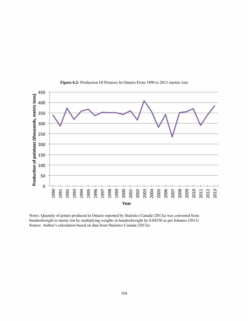
Figure 6.2: Production Of Potatoes In Ontario From 1990 to 2013 (metric ton)

0

50

100

150

200

250

300

350

400

450

1990

1991

1992

1993

1994

1995

1996

1997

1998

1999

2000

2001

2002

2003

2004

2005

2006

2007

2008

2009

2010

2011

2012

2013

Prod

uc'o

n of potatoe

s (thou

sand

s, m

etric

tons)

Year

Notes: Quantity of potato produced in Ontario reported by Statistics Canada (2013a) was converted fromhundredweight to metric ton by multiplying weights in hundredweight by 0.04536 as per Johanns (2013)Source: Author’s calculation based on data from Statistics Canada (2013a)

104

Figure 6.3: Average Yield Of Potatoes In Ontario From 1990 to 2013 (metric ton/hectare)

0

5

10

15

20

25

30

1990

1991

1992

1993

1994

1995

1996

1997

1998

1999

2000

2001

2002

2003

2004

2005

2006

2007

2008

2009

2010

2011

2012

2013

Average yield (m

etric

tons/hectare)

Year

Notes: Quantity of potato produced in Ontario reported by Statistics Canada (2013a) was converted fromhundredweight/acre to metric ton by multiplying weights in hundredweight by 0.1121 as per Johanns (2013)Source: Author’s calculation based on data from Statistics Canada (2013a)

105

Figure 6.4: Price Of Commercial, Processing And Table Potatoes In Ontario From 1990 To 2013 (real 2013 $)

0

100

200

300

400

500

600

700

1990

1991

1992

1993

1994

1995

1996

1997

1998

1999

2000

2001

2002

2003

2004

2005

2006

2007

2008

2009

2010

2011

2012

2013

Price (real 201

3 $/metric

ton)

Year Table Processing Seed

Notes: Nominal yearly prices reported by Statistics Canada (2014a) were converted to real 2013 $ using the All-itemsCPI for Ontario reported by Statistics Canada (2013c).Source: Author’s calculation based on data from Statistics Canada (2014a)

106

Figure 6.5: Average Monthly Price Of Processing Potatoes In Ontario (real 2013 $/metric ton)

0

50

100

150

200

250

300

350

400

450

500

August

Septem

ber

Octob

er

Novem

ber

Decembe

r

Janu

ary

February

March

April

May

June

July

Price (real 201

3 $/metric

ton)

Month

Notes: Average monthly prices are the average price per month of processing potatoes in Ontario from 1993 to 2012.The first month in the graph is August because this is the earliest time that a season’s crop can begin to be harvestedand sold. Starting with average monthly prices in August illustrates how the price of a processing potatoes changesonce they have been harvested.Source: Author’s calculations based on prices from Statistics Canada (2014a)

107

Table 6.1: Precipitation Climate Normals In Alliston, ON And At The Chipping Potato Farm Trial Site In 2012 And2013

Precipitation (mm)Month Alliston, ON climate normali Farm trial site 2012ii Farm trial site 2013ii

May 78.3 0.8 91.2June 81 13.8 86.3July 77.6 101.2 81.5August 82.3 73.1 104.6Notes: Climate normal for Alliston, ON are based on climate normals from 1981-2010 at Envi-ronment Canada weather station number 6110218. Farm trial precipitation in 2012 and 2013 werecalculated by summing hourly measurements of precipitation in each month.Source: iEnvironment Canada (2014), iiVanderZaag (2013).

108

Figure 6.6: Canopy Cover Of T10-3 And Dakota Pearl During The 2012 Growing Season In Farm Trials ConductedAlliston, Ontario

0

10

20

30

40

50

60

70

80

90

100

33 48 55 63 71 77 84 91 98

% Can

opy Co

ver

Days a.er plan0ng

T10-‐3 Dakota Pearl

Notes: Canopy cover was measured on the days listed on the x axis of the graph. The planting date for this trial wasMay 17th, 2012. The % canopy cover for each variety is the mean % canopy cover of the four replicates grown on thetrial plot in Alliston, Ontario in 2012.Source: VanderZaag (2013)

109

Figure 6.7: Canopy Cover Of T10-3 And Dakota Pearl During The 2013 Growing Season In Farm Trials ConductedAlliston, Ontario

0

10

20

30

40

50

60

70

80

90

100

28 35 42 49 63 70 77 84 91 98

% Can

opy Co

ver

Days a.er plan0ng


Notes: Canopy cover was measured on the days listed on the x axis of the graph. The planting date for the 2013 trialswas May 23rd, 2013. The % canopy cover for each variety is the mean % canopy cover of the four replicates grownon the trial plot in Alliston, Ontario in 2012.Source: VanderZaag (2013)

110

Figure 6.8: Yield Of T10-3 And Dakota Pearl Potato Varieties From Farm Trials Conducted In Alliston, OntarioDuring The 2012 Growing Season

0

2

4

6

8

10

12

14

16

Weight of unmarketable tubers Weight of marketable tubers

Potato yield (m

etric

tons/hectare)


Notes: Yields for each variety represent the average yield of four replicates in the trial. Yields were reported byVanderZaag (2013) in kg/plot and converted to metric ton/hectare using the following equation:yield

(metric ton

hectare

)=

yield from experiment(lb)90(ft2)

∗107639(ft2)1(hectare) ∗

1(metric ton)2205(lb)

Source: Author’s calculation based on data provided by VanderZaag (2013)

111

Figure 6.9: Yield Of T10-3 And Dakota Pearl Potato Varieties From Farm Trials Conducted In Alliston, OntarioDuring The 2013 Growing Season

0

5

10

15

20

25

30

35

40

45

50

Weight of unmarketable tubers Weight of marketable tubers

Potato yield (m

etric

tons/hectare)


Notes: Yields for each variety represent the average yield of four replicates in the trial. Yields were reported byVanderZaag (2013) in kg/plot and converted to metric ton/hectare using the following equation:yield

(metric ton

hectare

)=

yield from experiment(lb)120(ft2)

∗107639(ft2)1(hectare) ∗

1(metric ton)2205(lb)

Source: Author’s calculation based on data provided by VanderZaag (2013)

112

Table 6.2: Parameters Of Normal Distributions Used To Characterize The Monthly Price Of Chipping Potatoes InOntario

ma µA,t (real 2013$/metric ton) σ2A,t (real 2013$2/metric ton2) µA,t (real 2013$/cwt) σ2

A,t (real 2013$2/cwt2)8 444.5 6516 20.16 13.409 356.3 5297 16.16 10.8910 337.4 2224 15.30 4.58011 337.1 1758 15.29 3.61012 336.3 1887 15.25 3.881Notes: m is the index values of the month in which the potatoes are sold. See section 6.6 for an explanation of thefunction used to characterize chipping potato prices. Normal distribution parameters for each month’s price werecalculated based on the monthly price of processing potatoes reported by Statistics Canada (2014a) from 1993 to2013. Real 2013 $/cwt prices were converted to real 2013 $/metric ton by multiplying the real 2013 $/cwt pricesby 22.05 as per Johanns (2013).Source: Author’s calculation based on data from Statistics Canada (2014a)

113

Table 6.3: Baseline Parameters Used To Calculate Net Present Value Of Growing A Higher Water Use EfficiencyChipping Potato Variety, T10-3, Rather Than Conventionally Grown Chipping Potatoes In Ontario

Atlantic Dakota Pearl T10-3

Mean yield (metric ton/hectare)a 27.6 23.3 24.4Variance of yield (metric tons2/hectare2)b 146 146 146Difference in mean yield relative to T10-3c +11.5% -4.76% -Nitrogen requirement (kg/ha/yr) 202 280 202Proportion of nitrogen requirement met with urea 0.5 0.5 0.5Proportion of nitrogen requirement met with ammonium sulphate 0.5 0.5 0.5Years under production 10 10 10Real discount rate 5% 5% 5%Proportion of sales per month:

August 1/5 1/5 1/5September 1/5 1/5 1/5

October 1/5 1/5 1/5November 1/5 1/5 1/5December 1/5 1/5 1/5

Notes: Atlantic and Dakota Pearl are chipping potato varieties conventionally grown in Ontario. T10-3is an experimental chipping potato variety that has had higher technical water use efficiency in field trialsconducted in 2012 and 2013 in Alliston, Ontario. aRepresents the mean of the normal distribution used tocharacterize yields of chipping potato varieties in this case study. bRepresents the variance of the normaldistribution used to characterize yields of chipping potato varieties in this case study. cRepresents therelative difference in the mean yield of the variety in question with respect to the mean yield of T10-3

Table 6.4: Parameters Of Normal Distribution Of Fertilizer Prices Used To Calculate Net Present Value Of Growing AHigher Water Use Efficiency Chipping Potato Variety, T10-3, Rather Than Conventionally Grown Chipping PotatoesIn Ontario

Urea Ammonium Sulphate

Mean (real 2013 $/metric ton) 541.74 410.44Variance (real 2013 $2/metric ton2) 28,924 4,679.9Notes: Parameters of urea price distribution are based on the mean and variance of urea retail prices inOntario from 1993 to 2013 as reported by McEwan (2013, 2014). Parameters of ammonium sulphatedistribution are based on the annual average U.S. price of ammonium sulphate from 1960 to 2013 reportedby United States Department of Agriculture (2013). Nominal United States dollar prices were converted toreal 2013 values using the U.S. Consumer Price Index reported by Crawford and Church (2014) and set toCanadian dollar amounts using the exchange rate from 1960 to 2013 reported by Statistics Canada (2014b).Source: Author’s calculation based on data from McEwan (2013, 2014) and United States Department ofAgriculture (2013).

114

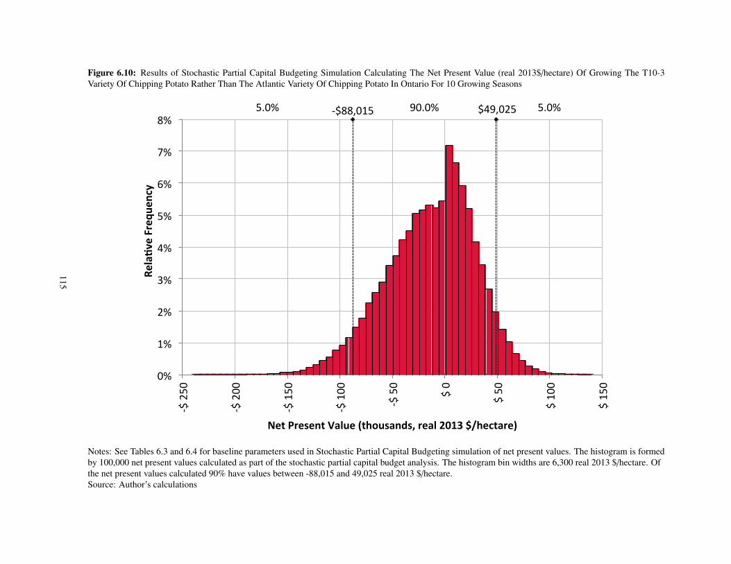
Figure 6.10: Results of Stochastic Partial Capital Budgeting Simulation Calculating The Net Present Value (real 2013$/hectare) Of Growing The T10-3Variety Of Chipping Potato Rather Than The Atlantic Variety Of Chipping Potato In Ontario For 10 Growing Seasons

!$88,015( $49,025(5.0%( 90.0%( 5.0%(

0%(

1%(

2%(

3%(

4%(

5%(

6%(

7%(

8%(

!$(250

(

!$(200

(

!$(150

(

!$(100

(

!$(50(

$(0(

$(50(

$(100(

$(150(

Rela%v

e'Freq

uency'

Net'Present'Value'(thousands,'real'2013'$/hectare)'











Notes: See Tables 6.3 and 6.4 for baseline parameters used in Stochastic Partial Capital Budgeting simulation of net present values. The histogram is formedby 100,000 net present values calculated as part of the stochastic partial capital budget analysis. The histogram bin widths are 6,300 real 2013 $/hectare. Ofthe net present values calculated 90% have values between -88,015 and 49,025 real 2013 $/hectare.Source: Author’s calculations

115

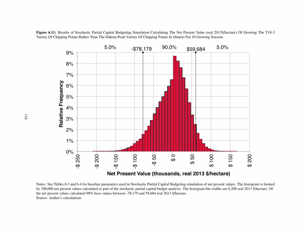
Figure 6.11: Results of Stochastic Partial Capital Budgeting Simulation Calculating The Net Present Value (real 2013$/hectare) Of Growing The T10-3Variety Of Chipping Potato Rather Than The Dakota Pearl Variety Of Chipping Potato In Ontario For 10 Growing Seasons

-$78,179! $59,684!5.0%! 90.0%! 5.0%!

0%!

1%!

2%!

3%!

4%!

5%!

6%!

7%!

8%!

9%!

-$ 2

50!

-$ 2

00!

-$ 1

50!

-$ 1

00!

-$ 5

0!

$ 0!

$ 50!

$ 10

0!

$ 15

0!

$ 20

0!

Rel

ativ

e Fr

eque

ncy!

Net Present Value (thousands, real 2013 $/hectare)!

Net present value ($/hectare)!











Notes: See Tables 6.3 and 6.4 for baseline parameters used in Stochastic Partial Capital Budgeting simulation of net present values. The histogram is formedby 100,000 net present values calculated as part of the stochastic partial capital budget analysis. The histogram bin widths are 6,200 real 2013 $/hectare. Ofthe net present values calculated 90% have values between -78,179 and 59,684 real 2013 $/hectare.Source: Author’s calculations

116

Table 6.5: Results Of Sensitivity Analyses On The Stochastic Partial Capital Budgeting Simulation Used To Calculate The Net Present Value Of A GrowingA Higher Water Use Efficiency Chipping Potato Variety, T10-3, Rather Than The Atlantic Variety

Distribution of net present values (real 2013$ /hectare)Scenario Change in parameter from baseline Baseline value Modified value Mean Median Variance 5%a 95%b

Baseline n.a. n.a. n.a. -$13,399 -$8,770 $1,756,592,980 -$87,094 $48,584

1Increase in mean yield of T10-3 rela-tive to Atlantic (% difference)c -12% -2% -$7,238 -$2,092 $1,705,460,413 -$80,959 $54,828

2Increase in mean yield of T10-3 rela-tive to Atlantic (% difference)c -12% +8% -$718 $3,943 $1,629,540,078 -$73,208 $60,187

3 Decrease in real discount rate 5% 4% -$14,074 -$9,212 $1,938,112,607 -$91,483 $51,0334 Increase in real discount rate 5% 6% -$12,771 -$8,360 $1,595,905,849 -$83,015 $46,3095 Decrease in years under production 10 5 -$7,514 -$5,032 $553,324,210 -$48,957 $27,0966 Increase in years under production 10 15 -$18,051 -$12,654 $3,188,621,898 -$117,785 $66,9017 Decrease in sales period after harvest 5 months 3 months -$14,039 -$9,481 $1,929,682,610 -$91,278 $51,571Notes: With the exception of the baseline scenario, one parameter of the net present value calculation was modified in each scenario. See Tables 6.3 and 6.4for a list of baseline parameters used in the net present value calculation. a5% of calculated net present values are less then this value. b5% of calculatednet present values are greater then this value. cRepresents a change in the mean of the normal distribution of yield used to characterize T10-3 yields. The %difference is the difference in the mean yield of T10-3 relative to the mean yield of the AtlanticSource: Author’s calculations

117

Table 6.6: Results Of Sensitivity Analyses On The Stochastic Partial Capital Budgeting Simulation Used To Calculate The Net Present Value Of A GrowingA Higher Water Use Efficiency Chipping Potato Variety, T10-3, Rather Than The Dakota Pearl Variety

Distribution of net present values (real 2013$ /hectare)Scenario Change in parameter from baseline Baseline value Modified value Mean Median Variance 5%a 95%b

Baseline n.a. n.a. n.a. -$2,304 $3,024 $1,635,265,639 -$74,643 $57,784

1Decreased in mean yield of T10-3 rela-tive to Dakota Pearl (% difference)c +5% -5% -$7,788 -$2,562 $1,686,195,860 -$80,298 $53,188

2Increase in mean yield of T10-3 rela-tive to Dakota Pearl (% difference)c +5% +15% $3,152 $7,210 $1,561,506,827 -$66,997 $62,366

3 Decrease in real discount rate 5% 4% -$2,453 $2,667 $1,822,820,780 -$79,152 $61,1084 Increase in real discount rate 5% 6% -$2,226 $2,420 $1,500,970,756 -$71,825 $55,4525 Decrease in years under production 10 5 -$1,326 $1,959 $523,649,032 -$42,910 $32,6706 Increase in years under production 10 15 -$3,086 $3,615 $2,942,482,298 -$99,129 $77,3117 Decrease in sales period after harvest 5 months 3 months -$2,513 $3,075 $1,802,149,340 -$78,617 $60,269Notes: With the exception of the baseline scenario, one parameter of the net present value calculation was modified in each scenario. See Tables 6.3 and 6.4for a list of baseline parameters used in the net present value calculation. a5% of calculated net present values are less then this value. b5% of calculatednet present values are greater then this value. cRepresents a change in the mean of the normal distribution of yield used to characterize T10-3 yields. The %difference is the difference in the mean yield of T10-3 relative to the mean yield of the Dakota PearlSource: Author’s calculations

118

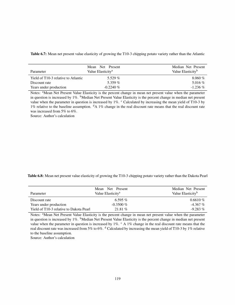
Table 6.7: Mean net present value elasticity of growing the T10-3 chipping potato variety rather than the Atlantic



Yield of T10-3 relative to Atlantic 5.529 % 8.060 %Discount rate 5.359 % 5.016 %Years under production -0.2240 % -1.236 %Notes: aMean Net Present Value Elasticity is the percent change in mean net present value when the parameterin question is increased by 1%. bMedian Net Present Value Elasticity is the percent change in median net presentvalue when the parameter in question is increased by 1%. c Calculated by increasing the mean yield of T10-3 by1% relative to the baseline assumption. dA 1% change in the real discount rate means that the real discount ratewas increased from 5% to 6%.Source: Author’s calculation

Table 6.8: Mean net present value elasticity of growing the T10-3 chipping potato variety rather than the Dakota Pearl



Discount rate 6.595 % 0.6610 %Years under production -0.3500 % -4.367 %Yield of T10-3 relative to Dakota Pearl 21.81 % -9.283 %Notes: aMean Net Present Value Elasticity is the percent change in mean net present value when the parameterin question is increased by 1%. bMedian Net Present Value Elasticity is the percent change in median net presentvalue when the parameter in question is increased by 1%. c A 1% change in the real discount rate means that thereal discount rate was increased from 5% to 6%. d Calculated by increasing the mean yield of T10-3 by 1% relativeto the baseline assumption.Source: Author’s calculation

119

Figure 6.12: Yield Break-even Analysis: Net Present Value (real 2013$/hectare) Of Growing A Higher Water UseEfficiency Chipping Potato Variety, T10-3, Rather Than The Atlantic Variety For 10 Seasons

!30$

!20$

!10$

0$

10$

20$

30$

!28%$ !10%$ 9%$ 27%$ 45%$

Med


'(tho

usan

ds,'real'2013$/hectare)'

%'difference'in'yield'rela?ve'to'Atlan?c'

Notes: The median net present value is the median of 100,000 values calculated in a stochastic simulation. Other thanthe yield of the T10-3 variety all other values in the net present value calculation are the same as the baselineparameters presented in Table 6.3 The purple point identifies the results of the stochastic net present value calculationwith the baseline value of capital cost..Source: Author’s calculations

120

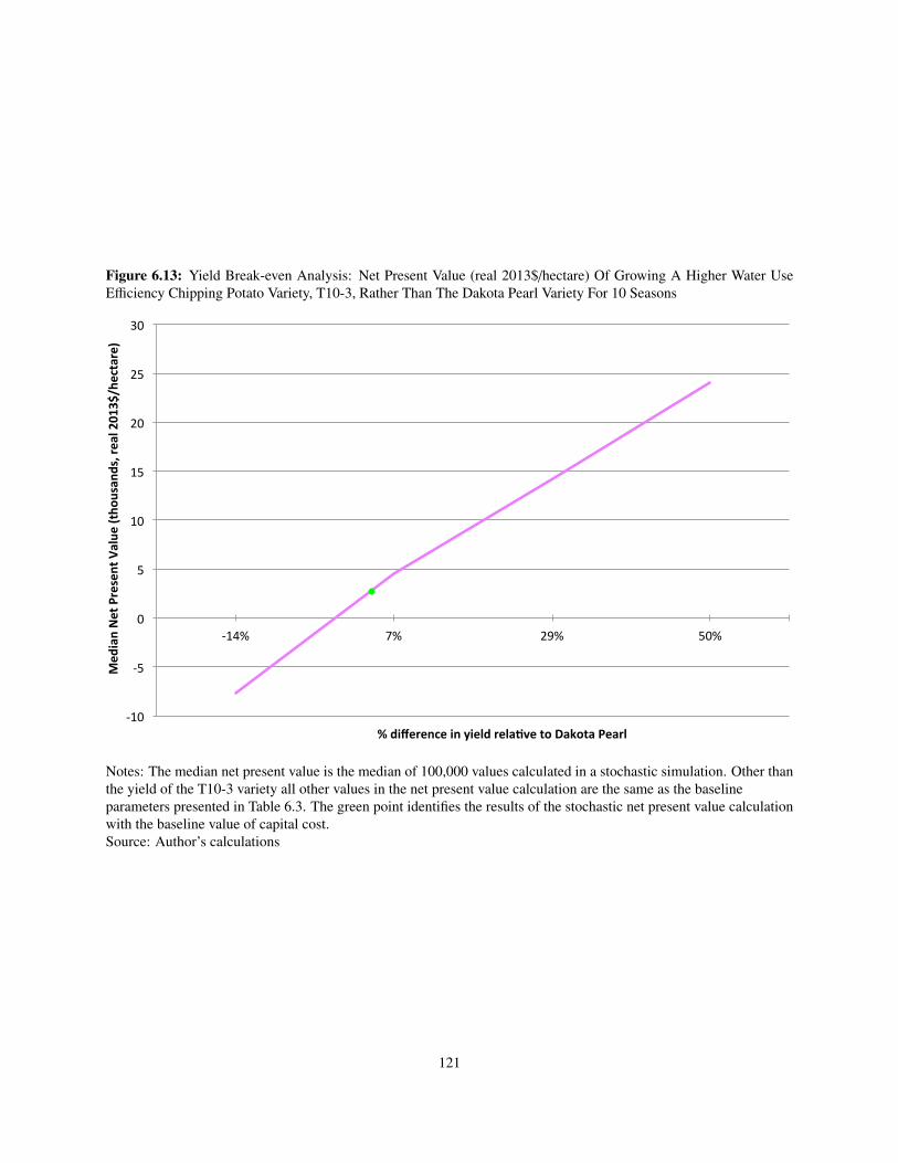
Figure 6.13: Yield Break-even Analysis: Net Present Value (real 2013$/hectare) Of Growing A Higher Water UseEfficiency Chipping Potato Variety, T10-3, Rather Than The Dakota Pearl Variety For 10 Seasons

!10$

!5$

0$

5$

10$

15$

20$

25$

30$

!14%$ 7%$ 29%$ 50%$

Med


'(tho

usan

ds,'real'2013$/hectare)'

%'difference'in'yield'rela?ve'to'Dakota'Pearl'

Notes: The median net present value is the median of 100,000 values calculated in a stochastic simulation. Other thanthe yield of the T10-3 variety all other values in the net present value calculation are the same as the baselineparameters presented in Table 6.3. The green point identifies the results of the stochastic net present value calculationwith the baseline value of capital cost.Source: Author’s calculations

121

Chapter 7: The use of in row ground covers in peach orchards

The case study presented in this chapter considers the economic implication to a peach grower in Ontario of choosing

to use wood chips as an in row ground cover. This orchard floor management system has been shown to increase soil

moisture content over the course of a growing season relative to the industry standard practice of keeping orchard rows

bare. A study on the use of wood chips in apple tree rows has also found that irrigation water use was lower in tree

rows where wood chips were used as a ground cover. In this case study the net present value of using wood chips as

a water conservation technology are assessed by taking into account the cost of purchasing and applying wood chips

in the rows of an orchard. The change in yield from having wood chips in tree rows and the potential energy savings

from having to pump less water are also taken into account. The partial capital budget that results from taking into

account the costs and benefits of using wood chips as an in row ground cover is used to calculate the net present value

of adopting wood chips in peach tree rows as a water conservation technology.

The outline of the case study is as follows: first is an overview of the peach sector in Ontario; second is description

of orchard floor management practices and the potential for water conservation when wood chips are used in peach

tree rows; third is an explanation of the cost and benefits that were taken into account to calculate the net present value

of using wood chips as an in row ground cover rather than following the industry standard practice of keeping tree

rows bare; fourth, the results of the net present value calculation are described; and finally, there is a brief discussion

about the results on the case study.

7.1 The peach sector in Ontario

Slingerland (2003) provides an overview of the of environmental conditions and agronomic practices required for

successful peach production in Ontario. Peach trees are sensitive to low temperatures and can be injured if winter

temperatures are too low. Sites whose temperatures fall below -20◦C are not suitable for peach trees. As a result, peach

production in Ontario is concentrated near one of the great lakes whose large bodies of water moderate temperatures

during the winter. In addition to sensitivity in temperature, peach trees also do not perform well in wet soils. As a

result peach orchards tend to be located on well drained sandy soils. Given these constraints on temperature and soil

moisture it is not surprising that peach production in Ontario is concentrated in relatively small parts of the province.

In fact as Gardner et al. (2006) note, 90% of all peaches produced in Ontario are grown on the Niagara Peninsula. This

area is illustrated in light striped pink in Figure 7.1. The figure also illustrates the other areas in Ontario where peaches

122

are grown. These areas include Essex and Kent counties in light orange; Huron and Erie counties in bleu chequers;

and Norfolk-Brant in light purple with white dots.

In commercial peach orchards in Ontario trees are planted in rows with equal spacing between trees and equal

spacing between rows. The area between trees rows is often referred to as the drive alley and the area directly below

the canopy of the peach trees as the tree row. Slingerland (2003) note that the spacing between rows can range from 4

to 6 metres and row width can range from 1 to 3 metres. Spacing between trees in a row ranges from 1.25 to 4 metres.

Planting density will have an impact on per hectare yield and on the useful life of the orchard. Relatively low density

orchards with approximately 383 trees/hectare (155 trees/acre) will have a useful life of 14 to 20 years. Whereas high

density orchards with 1,920 trees/hectare (777 trees/acre) will have a useful life of 8 to 12 years.

In their review of peach cultivars that can be grown in Ontario Slingerland and Subramanian (2007) note that

peach cultivars can be classified into two broad categories based on their indented use: fresh market and processing.

At maturity fresh market peaches will have a pit that is barely attached to the surrounding flesh of the fruit. The

distinguishing feature that separates processing peach cultivars from fresh market cultivars is the degree to which the

fruit’s flesh sticks to the pit. At maturity processing peach cultivars will have a fruit whose flesh is attached to the pit.

Depending on the cultivar, fresh market peaches can be harvested from the end of July till mid September. Whereas

processing peaches can be harvested from the beginning of August till mid September. Orchardist will usually grow a

variety of cultivars with varying harvesting dates so that an entire orchard does not have to be harvested all at once.

The area in Ontario used to produce peaches has been in decline since 1993. This can be seen in Figure 7.2 which

illustrates the area under peach production in Ontario from 1980 to 2013. The largest area under peach production

in Ontario occurred in 1988 when 3,440 hectares of land were being used to grow peaches. The smallest area under

production, 1,760 hectares, occurred in 2013. The amount of peaches produced in Ontario from 1980 to 2013 is

illustrated in Figure 7.3. From 1980 to 1995 peach production in Ontario saw a steady increase. The largest quantity

of peaches produced in Ontario between 1980 and 2013 occurred in 1995 when 39,358 metric tons of peaches were

produced. Between 1995 and 1997 there was a sharp decline in production. During this period peach production in

Ontario declined by 40%. Production did not recover from this sharp decline in production and continued to decline

in most years afterwards. The real total farm value of peach production in Ontario has varied considerably in the

last 30 years. This can be see in Figure 7.4 which illustrates the real 2013 $ total farm value of peach production in

Ontario from 1980 to 2013. After large spikes and drops in total farm value from 1989 to 1996, the total farm value of

peach production in Ontario saw a steady decline until reaching its lowest point in 2010. Figure 7.5 presents the real

2013 $/metric ton price of peaches in Ontario from 1980 to 2013. From 1980 to 1996 the real price of peaches saw

larger drops than gains from year to year. The lowest price of peaches occurred in 1996 when it reached 859 real 2013

$/metric ton. Prices bounced back sharply in 1997 increasing 42% from the year before. Peach prices were relatively

stable from 1997 to 2011 and spiked again in 2012 where it reached its highest value at 2,070 real 2013 $/metric ton.

123

7.2 Ground covers in peach tree rows as a water conservation technology

Neilsen et al. (2003) identify a particular type of orchard floor management system as the industry standard. In this

system drive alleys sod is used as a ground cover and bare soil is maintained in the tree rows. To keep weeds from

growing in the tree rows orchardists usually apply herbicide at regular intervals to suppress weed growth. An example

of the industry standard orchard floor management system is presented in Figure 7.6a. The figure illustrates parallel

tree rows with bare soil and the drive alleys are covered in sod.

Leaving the soil in tree rows bare is not the only options for managing the area below the peach trees. Adding a

ground cover in the tree rows is also an option. There are many types of ground cover that can be used. Tworkoski

and Glenn (2008) identify several including sod, plastic covers, geotextiles, shredded paper, news paper, poultry litter,

hay and mulches. Figure 7.6b presents an example of a peach tree row with wood chips being used as a ground cover.

Merwin (2003) points out that using organic mulches like wood chips, bark and compost in orchard tree rows can have

several benefits. These include suppressing weeds that can compete for nutrients and soil water; providing soil organic

matter, potassium and nitrogen; increasing soil temperature; and helping to maintain soil moisture content.

An example of the effect that wood chips can have on soil moisture can be seen in Figure 7.7. The figure illustrates

soil moisture levels during a trial on peach trees conducted by Zandstra (2014b) at the University of Guelph’s Cedar

Springs Research Station in 2013. For most of the period where soil moisture content was recorded the peach tree

rows with wood chips had higher soil moisture levels than those without wood chips. Additionally, peach tree rows

with wood chips had less day-to-day variation in soil moisture levels than rows without wood chips. On average rows

with wood chips saw soil moisture levels change by 1.69% from day-to-day. Whereas rows without wood chips had

an average day-to-day change in soil moisture of 4.25%. Given this effect on soil moisture levels one would expect

that having a biomass ground cover like wood chips in tree rows would reduce irrigation requirements. In fact such an

effect has been found by Granatstein and Mullinix (2008). In their three years of assessment Granatstein and Mullinix

(2008) found that apple orchard rows with wood chips required 20 to 30 % irrigation compared to a bare soil control.

Although there are several potential benefits to using mulches like wood chips as a ground cover in orchard tree

rows, there are also potential downsides. Merwin (2003) note that past research on the use of hay, plastic covers and

fabric covers as ground covers in rows have seen increased populations of voles that injure trees and reduce yields.

Using biomass as a ground cover can also provide a favourable environment for weeds after a few growing seasons.

Thus, weed management in rows with biomass ground covers can not be eliminated. Finally, the mulch’s ability to

maintain soil moisture levels can be a problem when soils are poorly drained.

There is no prescription on how and when to apply ground covers in orchard tree rows. Ground covers can

be applied during any portion of an orchard’s useful life. From orchard establishment to the time the orchard is

bearing fruit. The methods for applying the ground cover on the peach tree rows are only limited to the orchardist’s

imagination. In the experimental trials conducted by Zandstra (2014b) a tractor with a front end loader was driven

down the orchard’s drive alleys and the wood chips were shovelled from the bucket and spread onto the tree row.

124

This method may work for a relatively small trial orchard but it would be too labour intensive for a large commercial

orchard. One option shared with the author by VanWaes (2014) is to use a forage wagon with a conveyer belt attached

to the back. The wagon can carry large quantities of mulch and the conveyer belt can deliver the mulch directly on the

the tree row. After the mulch has been deposited on the row a team of labourers spread the mulch to the desired width

and thickness.

7.3 The case study orchard and within row ground cover

The peach orchard profiled in this case study was developed based on the orchard parameters studied by Zandstra

(2014b) and the drip irrigation system described by Tan and Layne (1990). The features of the orchard profiled in

this case study are presented in Table 7.1. The orchard is assumed to have a tree density of 768 trees/hectare with 4.3

metres separating trees between rows and 3.1 metres separating trees within rows. The orchard is assumed to be 7

years old when the in row ground cover is first used. The drip irrigation system used in the orchard is assumed to have

two emitters per tree with an emitter pressure of 104 kilopascal. Each emitter has a discharge rate of 4.5 litres/hour.

The total flow rate of the irrigation system is 1.92 litres/second and the system is powered by a 2.2 kW (3 horsepower)

electric motor. The irrigation system is assumed to be operated in daily intervals rather than every other day or on a

weekly basis.

For this case study wood chips were assumed to be the ground cover used within tree rows. The physical dimen-

sions of the in row ground cover are based on the experimental design of Granatstein and Mullinix (2008). The ground

cover is assumed to have a width of 1.60 metres centred on the tree trunks and a depth of 0.10 metre. Given that trees

in a row are 3.1 metres apart the total volume of wood chips works out to about 0.50 m3/tree or 380.93 m3/hectare.

7.4 Methods for assessing the farm level economics of using wood chips as a in row ground

cover

The merits of the wood chips as a ground cover in peach tree rows were assessed based on the net present value of

adopting the use of the wood chips. The net present value was calculated based on a partial capital budget of using

wood chips as an in row ground cover. The partial capital budget captures the costs and benefits to the grower who

would choose to purchase and apply wood chips. The costs and benefits of using the wood chips can either change

the cash income or the cash expenses of the farm business. For example a benefit of using the wood chips is that they

reduce irrigation water requirements for the orchard. This leads to a decrease in cash expenses of the farm business. In

addition to accounting for how cash income and cash expenses would be affected if wood chips were used as an in tree

row ground cover, the partial capital budget also takes into account how taxes would change. Government subsidies

are also taken into account in the partial capital budget. Mathematically the net present value of the partial capital

125

budget can be represented as follows:

N PV =

T∑t=1

∆CIt − ∆CEt − ∆Γt + T SICt=1

(1 + d)t−O (7.1)

where




∆CIt is the change in cash income in period t from using wood chips as in row ground cover

∆CEt is the change in cash expenses in period t from using wood chips as in row ground cover


T SICt=1 is the reduction in taxes in the first year if the cost of purchasing and applying wood chips is eligible

for government investment credit


O is the capital cost of purchasing and applying the wood chips

Taxes in period t are calculated using the following equation:

∆Γt = [∆CIt − ∆CEt ]T Rt (7.2)

where






The tax rate, T Rt , was set to 30% in each period t.


that each value listed in equations 7.4 and 7.4 of the net present value calculation has a fixed value. However, their

is uncertainty in exactly what value some of the equations parameters will take in the future. For example part of

calculating the change in cash income, ∆CIt , involves multiplying peach yields by the price of peaches. Peach yields

126

in each year that the wood chips would be in place will not all be the same. Their are factors beyond the grower’s

control the lead to variation from year to year. Because the wood chips would be in place for multiple years, a more

accurate representation of the world would take into account this variation in yield. Similarly, past experience shows

that the real price of peaches is not the same in each year. Assuming that real peach prices are the same for the useful

life of wood chips would not capture the variation in prices that the sector has seen the past. To take into account the

fact that there is uncertainty in some of the parameters of the net present value calculation a Monte Carlo simulation

was used.

In the Monte Carlo simulation for this case study some of the parameters in the partial capital budget were char-


1,221$/metric ton and a standard deviation of 277.0$/metric ton was used to characterize peach prices. Yields, input

cost and any other part of the partial capital budget can be characterized using a distribution. In this case study peach

prices, peach yields and coloured diesel prices were characterized using statistical distributions. Detailed explanations

of the statistical distributions used in the case study are presented in the next two sections.

The Monte Carlo simulation was implemented using the @RISK add-on developed by Palisade Corporation for

Microsoft Excel. In calculating the net present value, @RISK makes random draws from the statistical distributions



times. Each time the net present value is calculated using newly selected values from the statistical distributions. The

result of repeatedly calculating the net present value is a distribution of net present values. It is this distribution that is

reported in the results of this case study.




7.5 Capital cost of the tree row ground cover

The expenses associated with using wood chips as a ground cover within rows includes the volumetric cost of the

wood chips and the cost of applying them. The cost of the ground cover itself will depend on the volume being used

and the price of the ground cover. The price of wood chips will vary depending their source. In their report on the

availability of mulch material for orchards in Central Washington, United States, Granatstein et al. (2003) identify

several places were orchardist can acquire wood chips. These include retail stores, land fills, recycling centres, tree

service businesses and lumber mills. With some research a peach grower could easily find someone willing to give

away wood chips. The only cost that would be incurred by the producer would be the cost of delivering or picking

up the wood chips. For this case study the only cost associated with acquiring wood chips is assumed to be the cost

of delivery. The cost of delivery was estimated by contacting retail garden centres in Ontario that offer deliveries of

127

wood chips and inquiring about the cost of delivery. Of eight stores contacted three reported delivery prices of about

$50. Therefore, in this case study the cost of wood chips was set to 50 real 2013 $/hectare.

The other cost associated with using wood chips as within row ground cover is the expense of applying the wood

chips. The cost of applying the ground cover will depend on the cost of operating a tractor to carry the ground cover

through the orchard’s drive alleys, the cost of labour to spread the wood chips and the time required to complete the

work. VanWaes (2014) estimates that it takes four people about 16 hours to apply wood chips on a one hectare orchard.

Therefore, in this case study the application time was assumed to be 16 hours/hectare. Hourly wages per worker was

assumed to be 10.50 real 2013 $/hour. If four people are needed to apply the wood chips that means that the cost of

labour would be 42 real 2013$/hour. As for the cost of operating a tractor, the per hour cost was estimated based on

the method reported by Stiles and Griffin (ated). It was assumed that the peach producer already owns a 2 wheel drive,

37kW1 (50 horse power) tractor. Stiles and Griffin (ated) estimate that this type of tractor uses 9.73 litre/hour of diesel.

The price of diesel in this case study was assumed to have a normal distribution with parameters based on the mean

real 2013 $ price of colour diesel in Ontario from 1993 to 2013 as reported by McEwan (2013, 2014). The following

function defined the distribution of diesel prices in this case study:

Pf,t ∼ N (µf,t ,σ2f,t ) (7.3)

where

Pf,t is the price of coloured diesel fuel in period t


µf,t is the mean price of coloured diesel

σ2f,t is the variance of diesel prices

The mean price of coloured diesel, µf, was set to 0.88 real 2013 $/litre and the variance of coloured diesel prices, σ2f ,

was set to 0.0529 real 2013 $2/litre2. Stiles and Griffin (ated) assume that the cost of lubricants is15% of the price

of coloured diesel and that the cost of maintenance is 0.67 $/hour. These values were used in this case study as well.

The total cost of operating a tractor to apply wood chips works out to 10.52 real 2013$/hour. With the cost of labour

and of operating a tractor added together and the time required accounted for, the total cost of applying wood chips is

estimated to be 830.51 real 2013 $/hectare.

The frequency that the ground cover is applied to the orchard rows will effect the costs and benefits to the peach

grower of using the ground cover. For example if the ground cover is only applied once then the ground cover is a one

time expense and their are no ongoing yearly expenses associated with using the ground cover. On the other hand if the

ground cover is reapplied every three years then there will be on going application costs over the total period of time

that the ground cover is used. For this case study it was assumed that the ground cover is only applied once. Meaning

that the costs to acquire and apply the ground cover are incurred once at the beginning of the period of analysis.

1metric conversion based on Thompson and Taylor (2008)

128

7.6 Change in cash income from using ground covers in peach production

Estimating the change in cash income from using wood chips as a ground cover in peach production involves two parts.

First is determining how peach yields are affected by using wood chips as a ground cover. Second is determining how

the price received for the peaches produced under these conditions will change. The method for characterizing how

a ground cover affects peach yields in this case study will be presented first. Later in this section the method for

characterizing peach prices in this case study will be discussed.

To get at the change in yield from using wood chips as an in row ground cover a normal distribution of peach

yields was defined based on data from Mailvaganam (2014). This is the distribution that characterizes peach yields

when wood chips are not being used as an in row ground cover. Next the distribution was modified based on research

on the effect of ground covers on apple and peach yields. This modified version of the yield distribution was assumed

to characterize peach yields when a ground cover is in place.

The without ground cover peach yield distribution was assumed to be normally distributed with parameters match-

ing the mean and variance of peach yields in Ontario reported by Mailvaganam (2014). The mean yield of peaches in

Ontario from 1979 to 2013 was 9.96 metric tons/hectare and the variance was 2.31 metric ton2/hectare2. In this case

study the distribution used to characterize peach yields when a ground cover is not in place was the following:

Ypeach,t ∼ N (µpeach,t ,σ2peach,t ) (7.4)

where

Ypeach,t is the yield of peaches in period t



µpeach,t is the mean yield of peaches in period t

σ2peach,t is the variance of peaches yields in period t

The mean yield, µpeach,, was set to 9.96 metric tons/hectare and the variance, σ2peach,, was set to 2.31 metric tons2/hectare2.

In this case study it was assumed that using wood chips as an in row ground cover would only effect the mean

yield of peaches. To characterize peach yields when a ground cover is in place the distribution defined in equation

7.6 was modified by adding a variable to account for the change in mean yield. The variable ν is the proportional

change in mean peach yields from having a ground cover in tree rows. To determine the change in peach yields the

distribution that characterizes peach yields with wood chips was subtracted by the distribution without wood chips.

The mathematical the change in yield from having wood chips in place can be expressed as:

∆Ypeach,t = N (νµpeach,t ,σ2peach,t ) − N (µpeach,t ,σ

2peach,t ) (7.5)

where

129

∆Ypeach,t is the change peach yield in period t



ν is the proportional change in mean peach yields from having a ground cover in tree rows

µpeach,t is the mean yield of peaches in period t

σ2peach,t is the variance of peaches yields in period t

The proportional change in mean peach yields, ν, captures the effect that using wood chips as an in row ground cover

has on average peach yields. In this case study it was assumed that the effect on mean yield of using wood chips would

be the same in every year. Meaning that the proportional change in mean peach yields, ν, is assumed to be the same

in every period t. The value of the proportional change in mean peach yields, ν, plays a key role in the stochastic

partial capital budget simulation. If the value is negative, meaning that a ground cover lowers average peach yields,

then the grower would see a reduction in cash income if he or she chose to apply wood chips in their tree rows. On

the other hand if the value of the proportional change in mean peach yields, ν, is positive this means that in each year

the grower would see an increase in cash income when the ground cover is in place. In this case study the value of

the proportional change in mean peach yields, ν, was set based on studies by Merwin and Stiles (1994), Atucha et al.

(2011), Neilsen et al. (2003) and Zandstra (2014b). These studies have assessed the effect that biomass ground covers

like wood chips have on the yields of apples and peaches. They point towards the conclusion that wood chips would

have little to no effect on peach yields. Which means that for this case study the proportional change in mean peach

yields, ν, should be set at or near zero.

The evidence on the effect that wood chips have on peach yields points towards wood chips in tree rows having

little to no effect on yields relative to the industry standard of keeping tree rows bare. The first piece of evidence

supporting this conclusion are conflicting results from experiments in apple orchards where biomass ground covers

similar to wood chips were tested relative to the keeping rows bare. Two studies in the use of biomass ground covers

have found that using a biomass ground cover decreases apple yields relative to keeping tree rows bare. The first study

was conducted by Merwin and Stiles (1994). In this study the effect of 8 in row floor management systems on Empire

apple yields were studied for 6 years in Ithaca, NY in the United States. The row floor management system that

most closely approximates the use of wood chips was the hay-straw mulch treatment. Of the 8 row floor management

systems studied, apple trees grown with hay-straw mulch in tree rows had the highest cumulative yield per tree over

the 6 years studied. However, trees grown with hay-straw mulch in their rows had a significantly higher mortality rate

than the other row floor management systems. After 6 years root disease and meadow voles caused 38% of the apple

trees grown with hay-mulch to die. This means that despite having a higher yield per tree, on a per hectare basis the

hay-straw mulch would have a lower yield than the other row floor management systems. The other study that found

130

a negative effect of using a biomass ground cover in apple tree rows was completed by Atucha et al. (2011). In their

study Atucha et al. (2011) grew Empire apple’s in an experimental orchard in Ithaca, NY in the United States under

four tree row ground floor management systems. After 14 years apple trees grown with hard wood bark mulch on the

floor of their rows had the second highest cumulative yield relative to the other treatments. The apple trees with the

highest cumulative yield were those whose rows were kept bare using herbicide that was applied each year in mid-May

and July. In both of these studies the conventional practice of keeping tree rows bare lead to a higher cumulative yield

than using a biomass ground cover similar to wood chips. An experiment reported by Neilsen et al. (2003) conflicts

with the findings of Merwin and Stiles (1994) and Atucha et al. (2011). Neilsen et al. (2003) also studied the effect that

a biomass ground cover placed in apple tree rows has on yields. Their work was conducted on Spartan apples grown

at the Pacific Agri-Food Research Centre in Summerland, BC. The biomass ground cover studied was shredded paper.

Compared to the standard orchard management practice of keeping tree rows bare, apple trees with shredded office

paper in their rows had an 80% higher yield. Neilsen et al. (2003) do not offer a clear explanation or hypothesis that

would explain the large gain in yields from using shredded office paper as an in row ground cover. They do note that

all of the in row ground covers they assessed increased yields by approximately the same amount. If all three studies

that have looked at the effect that biomass ground covers have apple yield found that there was a significant change

in yield, either positive or negative, then this could have been an indication that using wood chips in peach tree rows

would have an effect on peach yields. However, the results of these studies does not provide a clear cut answer either

way which gives some support to the conclusion that wood chips would have little or no effect on peach yields.

The other piece of evidence that supports the conclusion the using wood chips in peach tree rows will have little to

no effect on yields is the study undertaken by Zandstra (2014b). They studied the difference in processing peach yields

between trees grown with a bare soil in their rows and trees grown with wood chips in their rows. The study took

place at the University of Guelph’s Cedar Springs Research Station in Raleigh, Ontario. The study was undertaken

on a 7 year old peach orchard and it lasted one year. Zandstra (2014b) found that there is no statistically significant

difference in the yield of peach trees grown with wood chips in their rows relative to those grown with bare rows.

Studies on the effect of biomass ground covers in apple orchards have produced conflicting results. The experiment

conducted by Zandstra (2014b) found no statistically significant difference in peach yields when wood chips were used

as an in row ground cover for one year. Given the conflicting results of using ground covers in apple orchard and the

relatively short study of Zandstra (2014b) in this case study wood chips were assumed to affect peach yields by

increasing them by 1%. This was done for two reasons. First, because of the uncertainty in how peach yields would be

affected by wood chips in tree rows. Second, because a 1% increase is relatively minor but will help to better illustrate

the economics of using wood chips as an in row ground cover. With respect to equation 7.6 which was used to define

the change in yield from using wood chips, the proportional change in mean peach yields, ν, was set to 1.01. This

assumption is also presented in table 7.1 which presents the assumptions made in the baseline scenario of this case

study.

The other component of cash income in peach production is the price that a producer receives for the peaches he

131

or she produces in a growing season. In this case study the price of peaches is characterized by a normal distribution

whose parameters are defined by the mean and variance of real 2013 $ peach prices in Ontario from 1942 to 2013.

Peach prices were collected from three sources. First, prices from 1942 to 1971 are based on prices reported by

Ministry of Agriculture and Food (1974). Second, prices from 1972 to 1978 were taken from Ministry of Agriculture

and Food (1980). Third, Mailvaganam’s (Mailvaganam2014) peach prices were used for the years 1979 to 2013.

Nominal cents/lb reported by Ministry of Agriculture and Food (1974, 1980) were converted to nominal $/metric ton

using conversion factors prescribed by Johanns (2013). The All-Price monthly CPI in Ontario reported by Statistics

Canada (2013c) only goes back till 1979. Therefore, the Canada All-Price monthly CPI reported by Statistics Canada

(2013c) was used to set nominal peach prices from 1942 to 1978 to real 2013 $. The distribution used to characterize

peach prices in the net present value calculation of this case study can be expressed as follows:

Ppeach,t ∼ N (µp,t ,σ2p,t ) (7.6)

where

Ppeach,t is the price of peaches in period t


N means that the price is normally distributed

µp,t is the real 2013 $ mean of peach prices

σ2p,t is the real 2013 $ variance of peach prices

The mean price, µp, was set to 1221.13 real 2013 $/metric ton. The variance,σ2p , was set to 76,734 real 2013 $2/metric

ton2. There is no evidence that using a ground cover in peach orchard rows has an effect on the price received for

peaches grown under these conditions. Therefore in this case study it was assumed that the price of peaches grown

under the conventional practice of keeping rows bare and those grown in rows with a ground cover command the same

price when sold.

Taken together the change in yield from using wood chips as a ground cover and the price of peaches capture the

effect that using wood chips as a ground cover will have on the cash income of a producer using this water conservation

technology. In mathematical terms the change in cash income in this case study was calculated as follows:

∆CIpeach,t = Ppeach,t ∗ ∆Ypeach,t (7.7)

where

∆CIpeach,t is the change in cash income from using the ground cover in period t

t indicates the one year time period

Ppeach,t is the price of peaches in period t

∆Ypeach,t is the change peach yield in period t from using the ground cover

132

7.7 Change in expenses from using ground covers in peach production

Using wood chips can have an effect on expenses in two ways. The first is by reducing the cost of herbicides. In

conventional orchard floor management systems tree rows are kept bare using herbicides that suppresses the growth of

vegetation in the orchard’s rows. Having a biomass ground cover like wood chips in place has been shown to suppress

weed growth as well, but only for a few years. After the first three or four years researchers such as Atucha et al.

(2011) have had to use herbicides to suppress weed growth in the tree rows. Furthermore, based on his experience

conducting ground cover trials in apple orchards Granatstein (2014) has found wood chips to be ineffective as a method

of controlling weed growth in tree rows. Given the results presented by Atucha et al. (2011) and the experience of

Granatstein (2014) in this case study using wood chips as a ground cover in peach tree rows is assumed to have no

effect on the cost of managing in row weeds.

The second way wood chips can effect expenses is by reducing irrigation water requirements. As was noted in

section 7.2, tree rows with wood chips on their surface tend to have higher soil moisture levels than those without. This

effect on soil moisture levels has been found to reduce irrigation water requirements. To get at the effect that a ground

cover will have on irrigation cost, in this case study an average daily irrigation amount using surface drip irrigation

system was calculated. The estimated daily irrigation amount was calculated based on the method described by Tan

and Layne (1990). Using average weekly evapotranspiration, irrigation system parameters and orchard parameters,

Tan and Layne’s (1990) method allows one to estimate the daily volume of water to apply per peach tree and the

amount of time to run the irrigation system to apply that volume of water. For this case study these daily amounts were

summed together to estimate the seasonal volume of water and time required to irrigate a peach orchard that has bare

rows.

For this case study the average daily evapotranspiration reported by Tan and Layne (1990) was used to calculated

the daily water requirements per peach tree. The orchard and irrigation system parameters described in section 7.3

and presented in table 7.1 were used to calculated the daily volume of water to apply with the irrigation system.

With these orchard and irrigation system parameters the estimated seasonal water use per tree is 4657.55 litre/tree and

3,576,998.4 litre for 768 peach trees. To apply this quantity of water over a growing season would require 517.51

hours. If a 2.2 kilowatt (3 horsepower) electric motor is used to drive the irrigation system and the cost of electricity is

7.5 cents/kilowatt hour, then the total cost of applying water in one season would be 85.08 real 2013 $/hectare. Again

this is assuming that there is no ground cover in place.

The change in irrigation water requirement that results from using wood chips as a ground cover was assumed to be

the same as that reported by Granatstein and Mullinix (2008). In their work Granatstein and Mullinix (2008) found that

using wood chips as a ground cover in Gala apple production reduced irrigation requirement by 20 to 30%. Therefore,

in this case study the effect of having wood chips in place in a peach orchard was assumed to reduce seasonal irrigation

requirement by 20%. A 20% reduction in irrigation requirement means that the cost of operating the irrigation system

would be 68.06 real 2013$/hectare. A difference of 17.02 real 2013 $/hectare relative to the orchard without the wood

133

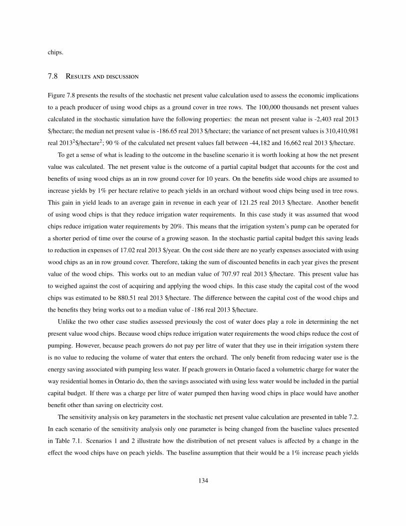
chips.

7.8 Results and discussion

Figure 7.8 presents the results of the stochastic net present value calculation used to assess the economic implications

to a peach producer of using wood chips as a ground cover in tree rows. The 100,000 thousands net present values

calculated in the stochastic simulation have the following properties: the mean net present value is -2,403 real 2013

$/hectare; the median net present value is -186.65 real 2013 $/hectare; the variance of net present values is 310,410,981

real 20132$/hectare2; 90 % of the calculated net present values fall between -44,182 and 16,662 real 2013 $/hectare.

To get a sense of what is leading to the outcome in the baseline scenario it is worth looking at how the net present

value was calculated. The net present value is the outcome of a partial capital budget that accounts for the cost and

benefits of using wood chips as an in row ground cover for 10 years. On the benefits side wood chips are assumed to

increase yields by 1% per hectare relative to peach yields in an orchard without wood chips being used in tree rows.

This gain in yield leads to an average gain in revenue in each year of 121.25 real 2013 $/hectare. Another benefit

of using wood chips is that they reduce irrigation water requirements. In this case study it was assumed that wood

chips reduce irrigation water requirements by 20%. This means that the irrigation system’s pump can be operated for

a shorter period of time over the course of a growing season. In the stochastic partial capital budget this saving leads

to reduction in expenses of 17.02 real 2013 $/year. On the cost side there are no yearly expenses associated with using

wood chips as an in row ground cover. Therefore, taking the sum of discounted benefits in each year gives the present

value of the wood chips. This works out to an median value of 707.97 real 2013 $/hectare. This present value has

to weighed against the cost of acquiring and applying the wood chips. In this case study the capital cost of the wood

chips was estimated to be 880.51 real 2013 $/hectare. The difference between the capital cost of the wood chips and

the benefits they bring works out to a median value of -186 real 2013 $/hectare.

Unlike the two other case studies assessed previously the cost of water does play a role in determining the net

present value wood chips. Because wood chips reduce irrigation water requirements the wood chips reduce the cost of

pumping. However, because peach growers do not pay per litre of water that they use in their irrigation system there

is no value to reducing the volume of water that enters the orchard. The only benefit from reducing water use is the

energy saving associated with pumping less water. If peach growers in Ontario faced a volumetric charge for water the

way residential homes in Ontario do, then the savings associated with using less water would be included in the partial

capital budget. If there was a charge per litre of water pumped then having wood chips in place would have another

benefit other than saving on electricity cost.

The sensitivity analysis on key parameters in the stochastic net present value calculation are presented in table 7.2.

In each scenario of the sensitivity analysis only one parameter is being changed from the baseline values presented

in Table 7.1. Scenarios 1 and 2 illustrate how the distribution of net present values is affected by a change in the

effect the wood chips have on peach yields. The baseline assumption that their would be a 1% increase peach yields

134

when wood chips are used as a ground cover in peach tree rows was based on research of biomass ground cover use

in apple orchards. These studies are equivocal with regards to the effect of biomass ground covers like wood chips.

The other reason for assuming a 1% increase is the one year study of wood chips in a peach orchard conducted by

Zandstra (2014a). In scenario 1 the potential for the wood chips to cause a decrease in yield of 11% is considered. In

this scenario the mean of the distribution used to characterize peach yields when wood chips are in place is reduced

by 10% from the baseline assumption. Specifically, in scenario 1 the distribution used to characterize yields without

wood chips has a mean of 10.06 metric tons/hectare/year and the mean yield of peaches with wood chips is 9.064

metric tons/hectare/year. When wood chips have a negative effect on peach yield the mean and median net present

values to drop considerably. The mean net present reduces by 77% from the outcome in the baseline scenario. The

median net present value decreases by 98%. On the other hand when the effect that wood chips have in mean peach

yields is to increase them by 11%, the mean and median net present values make a dramatic swing toward the positive

side. In this case study if the wood chips placed in the peach tree rows increased peach yields by 11% compared to

peaches grown with wood chips, the mean net present value is 5,267 real 2013 $/hectare and the median is 6,026 real

2013 $/hectare.

Scenarios 3 and 4 show how the distribution of net present values is affected by a change in the water conserving

ability of the wood chips. In the baseline assumption for this case study wood chips reduced water use by 20%.

The 20% figure was the lower end of the conservation effect found by Granatstein and Mullinix (2008). Scenario 3

considers the possibility that the wood chips reduce irrigation water use by 10% rather than 20%. In this scenario

the mean net present value is reduced by 56 real 2013 $/hectare and the median decreases by 46 real 2013 $/hectare.

Granatstein and Mullinix (2008) also found that wood chips used in apple tree rows could reduce water use by up to

30%. This is the possibility considered in scenario 4 where the effect of wood chips on is to reduce water requirements

per tree by 30%. In this scenario the mean net present value increases by about 3% and the median net present value

increases by 25% relative to the results in the baseline scenario.

In the baseline assumption for this case study the cost of getting wood chips and applying them was estimated to

be 881 real 2013 $/hectare. It is possible that this was an over estimate. For example if it takes less time to apply

the wood chips then was originally estimated, then the cost of the wood chips would be lower. This possibility is

considered in scenario 5. When the cost of wood chips is lowered by 10% from 881 real 2013 $/hectare to 792 real

2013 $/hectare the mean net present value increases to -2,315 real 2013 $/hectare and the median increases to -98

real 2013 $/hectare. On the other hand if the cost of applying the wood chips was under estimated in the baseline

scenario than the mean and median net present values would be lower than the baseline result. The cost of acquiring

and applying the wood chips could be higher for several reasons. For example the cost of applying the wood chips

was based in part of the assumption that labour cost 10.50 $/hour. Scenario 6 considers this possibility. When the cost

of acquiring and applying the ground cover increases to 969 real 2013 $/hectare, the mean net present value decreases

to -2,441 real 2013 $/hectare.

In all of the scenarios considered so far the useful life of the wood chips is assumed to be 10 years. This means that

135

the effect the wood chips have on yields and the pumping cost they save last 10 years. Scenarios 7 and 8 consider the

possibility that the effect of the wood chips last one year less and one year more. If the wood chips last 9 years instead

of 10 the mean and median net present values are lower than the baseline outcome. This is to be expected given that

the benefits of using the wood chips do not last as long. This means that there is less time for the wood chips to offset

the cost of obtaining and applying the wood chips. Conversely, if the effects of the wood chips last an extra year the

mean and media net present values increase.



from a 5% discount rate. Scenario 9 assess the stochastic net present value of the subsurface drip irrigation system

with a 4% discount rate. Reducing the discount rate leads to a small change in the mean and median net present value.

On the other hand if a peach grower who is considering using wood chips and an in row ground cover has a lower

value on future cost and benefits, then the 5% discount rate would be an under estimate. Scenario 10 considers the

effect that a higher discount rate has on the distribution of net present values. At a 6% discount rate the median net

present values decrease. Meaning that using wood chips as a water conservation technology is even less worthwhile

to someone who has a higher discount rate.

The mean and median net present value elasticity were calculated to get a sense of how the distribution of net

present values is affected by changes in key parameters. The mean and median net present value elasticities are

the percent change in mean and median net present value when the parameter in question is increased by 1%. For

example the effect the wood chips have on peach yields is to increase their mean yield from 9.96 metric tons/hectare

to 10.06 metric tons/hectare. The mean and median net present values were calculated by increasing the mean yield

of peaches grow with wood chips by 1% from 10.06 metric tons/hectare to 10.16 metric tons/hectare. The mean and

median elasticities of the real discount rate were calculated by increasing the base line value of 5% to 6%. Table 7.3

shows that the effect that wood chips have on the mean peach yield has by far the largest effect on the distribution of

net present values. Given that the distribution of net present values presented in Figure 7.8 is not exactly normally

distributed Table 7.3 has been sorted by median net present values elasticities. A 1% increase in mean peach yields

leads to a 381% increase in the median net present value of using wood chips as an in row ground cover. The effect the

wood chips have on irrigation water use has a non-negligible effect on the median net present value. A 1% decrease in

pumping cost leads to a 6.6 % increase in the median net present value of the wood chips. This value would be even

higher if the peach grower’s irrigation cost included a volumetric charge for water in addition to the cost of electricity

to pump water through their irrigation system.

In chapter 3 the production economics of water in agriculture were discussed. The chapter reviewed economic

models that have been used to characterize water conservation at the farm level. An aspect of water use in an agri-

cultural production function is the total product curve. The total product curve characterizes how yields respond to

the use of water. As was discussed in section 7.1 of this chapter peach yields are sensitive to shortages in water as

well excesses in water. Therefore, it is reasonable to characterize the total product curve of water in peach production

136

as a second order polynomial function. In section 3.2.1 of chapter 3 the characteristics of a second order polynomial

total product function were discussed. The most important feature of a second order polynomial total product curve is

that it captures the increase in yields that occur when irrigation water is used. It also captures the fact that excessive

irrigation water will lead to decreases in peach yields. It was also shown that for relatively low water prices, like the

ones faced by peach growers in Ontario, adopting a technology that changes the shape of the quadratic total product

curve could lead to water conservation. Using wood chips as an in tree ground cover can be modelled as a change in

the shape of a quadratic total product curve for water. Having the wood chips in place means that the quadratic total

product curve for water has a tighter shape. Put another way, the use of wood chips can be modelled by a quadratic

function with steeper positive and negative slopes. This change in the shape of the quadratic total product curve leads

to a lower profit maximizing quantity of water to use in a growing season as illustrated in figure 3.3.

The effect wood chips have on the mean yield of peaches is by far the most important factor in determining whether

or not using wood chips as an in row ground cover will be worthwhile for a producer. A break even analysis can reveal

what effect wood chips would have to have an mean peach yields in order for the investment to break even. In this

case study a water conservation technology will break even when the distribution of net present values calculated in

the stochastic simulation has a median of zero. Put another way, the break even point is when 50% of the net present

values calculated in the stochastic simulation have a negative value and the other 50% a positive value. Figure 7.9

shows that having wood chips in peach rows would have to increase mean peach yields by 1.12% in order for the

investment to break even. This is only slightly higher than the baseline assumption of a 1% increase in peach yields.

Based on the fact that studies of ground covers in apple tree rows have found diametrically opposing results with

regards to the effect of ground covers on yields. It is difficult to say whether or not a 1.12% increase in peach yields

can be expected if wood chips were placed in tree rows. However, given the extreme sensitivity of the net present

value on changes in peach yields, future researcher would do well to focus on getting a better sense of how ground

covers used in tree rows affect peach yields in Ontario orchards.

137

Figure 7.1: Areas Of Peach Production In Ontario

Source: Author based on Gardner et al. (2006) and OpenStreetMap contributors (2014)

138

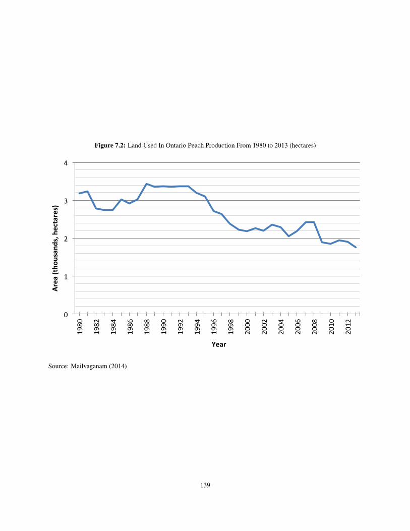
Figure 7.2: Land Used In Ontario Peach Production From 1980 to 2013 (hectares)

0

1

2

3

4

1980

1982

1984

1986

1988

1990

1992

1994

1996

1998

2000

2002

2004

2006

2008

2010

2012

Area (tho

usan

ds, h

ectares)

Year

Source: Mailvaganam (2014)

139

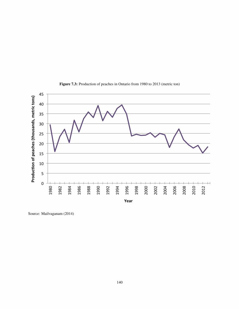
Figure 7.3: Production of peaches in Ontario from 1980 to 2013 (metric ton)

0

5

10

15

20

25

30

35

40

45

1980

1982

1984

1986

1988

1990

1992

1994

1996

1998

2000

2002

2004

2006

2008

2010

2012

Prod

uc'o

n of peaches (tho

usan

ds, m

etric

tons)

Year


140

Figure 7.4: Total farm value of peach production in Ontario from 1980 to 2013 (real 2013 $)

0

10

20

30

40

50

60

1980

1982

1984

1986

1988

1990

1992

1994

1996

1998

2000

2002

2004

2006

2008

2010

2012

Total farm value

(tho

usan

ds, real 201

3 $)

Year


141

Figure 7.5: Price of peaches Ontario from 1980 to 2013 (real 2013 $/metric ton)

0

500

1000

1500

2000

2500

1980

1982

1984

1986

1988

1990

1992

1994

1996

1998

2000

2002

2004

2006

2008

2010

2012

Price of peaches (real 201

3 $/metric

ton)

Year


142

Figure 7.6: Peach Tree Row With And Without Wood Chips

(a) Peach tree in row without ground cover (b) Peach tree row with wood chips being used as a ground cover

Source: Author

143

Figure 7.7: Soil Moisture In Peach Rows With And Without Wood Chips During A Trial In 2013 At The CedarSprings Research Station In Raleigh, Ontario

0

5

10

15

20

25

30

13-‐05-‐22

13-‐06-‐05

13-‐06-‐19

13-‐07-‐03

13-‐07-‐17

13-‐07-‐31

13-‐08-‐14

13-‐08-‐28

13-‐09-‐11

13-‐09-‐25

13-‐10-‐09

13-‐10-‐23

13-‐11-‐06

Soil moisture (%

)

Date With wood chips Without wood chips

Notes: Daily soil moisture level were measured at a depth of 30 centimetre from 2013/05/22 to 2013/11/18. The soilat the trial site is a Fox Gravelly Loam soil with 47.8 % sand, 38.1 % silt and 14.1 % clay.Source: Zandstra (2014a)

144

Table 7.1: Baseline Parameters for the use of wood chips as a ground cover in Ontario peach production

Orchard parametersAge of orchard when ground covers are first used (years)ii 7Space between rows (m)ii 4.3Space between trees (m)ii 3.1Tree density (trees/ha)ii 768Diameter of shade cast by tree at noon (m)iii 2

Drip irrigation system parametersNumber of emitters (per tree)iii 2Discharge rate per emitter at 104 kPa [20 psi] (L/h)iii 4.5Irrigation frequencyi dailySystem flow rate (L/s)i 1.92Seasonal water use without ground cover (L/tree)i 4657.55Seasonal system operation time without ground cover (hours)i 517.51Pump power (kW)iv 2.2Cost of electricity (cents/kWh)v 7.5¢

Ground cover parametersWidth of ground cover (m)vi 1.60Depth of ground cover (m)vi 0.10Volume of ground cover (m3/ha)i 380.93Volume of ground cover (m3/tree)i 0.50Useful life (years) 10Reapplication frequency neverCost of wood chips ($/ha)i $50Cost of applying wood chipsi a $830.51Effect of ground cover on average peach yield +1%Change in irrigation water usevi -20 %Real discount ratei 5 %Notes: athe cost of applying the ground cover includes the costs of labour and of operating a tractorSource: iAuthor’s calculation, iiZandstra (2014b), iiiTan and Layne (1990), ivCuykendall and White(1998), vOntario Energy Board (2014), viGranatstein and Mullinix (2008).

145

Figure 7.8: Results Of Stochastic Partial Capital Budgeting Simulation Calculating The Net Present Value (real 2013$/hectare) Of Using Wood Chips As AGround Cover To Grow Peaches In Ontario For 10 Years

!$33,830' $23,856'5.0%' 90.0%' 5.0%'

0%'

2%'

4%'

6%'

8%'

10%'

12%'

!$'120

'

!$'100

'

!$'80'

!$'60'

!$'40'

!$'20'

$'0'

$'20'

$'40'

$'60'

$'80'

Rela%v

e'freq

uency'

Net'present'value'(thousands,'real'2013'$/hectare)'











Notes: The histogram has bin widths of 3842.38 real 2013 $/hectare. 90 % of the calculated net present values fall between -33,830 real 2013 $/hectare and23,856 real 2013 $/hectare. 5% are less than -33,830 real 2013 $/hectare and 5% are greater than 23,856 real 2013 $/hectare.Source: Author’s calculations

146

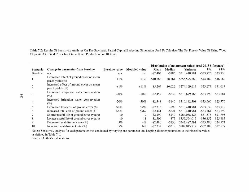
Table 7.2: Results Of Sensitivity Analyses On The Stochastic Partial Capital Budgeting Simulation Used To Calculate The Net Present Value Of Using WoodChips As A Ground Cover In Ontario Peach Production For 10 Years

Distribution of net present values (real 2013 $ /hectare)Scenario Change in parameter from baseline Baseline value Modified value Mean Median Variance 5% 95%Baseline n.a. n.a. n.a. -$2,403 -$186 $310,410,981 -$33,726 $23,730

1Decreased effect of ground cover on meanpeach yield (%) +1% -11% -$10,588 -$8,764 $355,595,580 -$44,182 $16,662

2Increased effect of ground cover on meanpeach yields (%) +1% +11% $5,267 $6,026 $274,169,613 -$23,677 $31,017

3Decreased irrigation water conservation(%) -20% -10% -$2,459 -$232 $310,679,763 -$33,792 $23,684

4Increased irrigation water conservation(%) -20% -30% -$2,348 -$140 $310,142,308 -$33,660 $23,776

5 Decreased total cost of ground cover ($) $881 $792 -$2,315 -$98 $310,410,981 -$33,638 $23,8186 increased total cost of ground cover ($) $881 $969 -$2,441 -$224 $310,410,981 -$33,764 $23,6927 Shorter useful life of ground cover (years) 10 9 -$2,290 -$240 $264,038,426 -$31,378 $21,7958 Longer useful life of ground cover (years) 10 11 -$2,509 -$77 $359,594,017 -$36,452 $25,6859 Decreased real discount rate (%) 5% 4% -$2,480 -$150 $342,487,591 -$35,380 $24,97410 Increased real discount rate (%) 5% 6% -$2,332 -$218 $282,015,717 -$32,188 $22,577Notes: Sensitivity analysis for each parameter was conducted by varying one parameter and keeping all other parameters at their baseline valuesas defined in Table 7.1.Source: Author’s calculations

147

Table 7.3: Mean Net Present Value Elasticities Of Using Wood Chips As A Ground Cover In Peach Tree Rows



Effect of wood chips ona mean peach yields 32.96 % 381.5 %Effect of wood chips on irrigation water use 0.6090 % 6.582 %Useful life of wood chips -0.8480 % 2.278 %Total cost of wood chips 0.06400 % -0.9630 %Real discount rate 3.391 % -16.19 %Notes: aMean Net Present Value Elasticity is the percent change in mean net present value whenthe parameter in question is increased by 1%. bMedian Net Present Value Elasticity is the percentchange in median net present value when the parameter in question is increased by 1%. cA 1%change in the real discount rate means that the real discount rate was increased from 5% to 6%.Source: Author’s calculation

148

Figure 7.9: Break Even Analysis On The Effect On Yield Of Wood Chips In Peach Orchard Rows

!4000$

!3000$

!2000$

!1000$

0$

1000$

2000$

3000$

!3%$ !2%$ !1%$ 0$ +1%$ +2%$ +3%$ +4%$ +5%$

Med


'(real'2013'$/he

ctare)'

Effect'On'Mean'Peach'Yield'(%)ᵃ

Notes: aEffect on mean peach yields represents the % difference in average peach yield when wood chips are used asan in row ground cover rather than keeping peach tree rows bare. The blue point identifies the results of the stochasticnet present value calculation with the baseline value of capital cost.Source: Author’s calculations

149

Chapter 8: Conclusion

8.1 Summary

The Ontario Water Opportunities Act of 2010 accorded the provincial government the authority to mandate ministries

to set and achieve water conservation targets. The implementation of water conservation targets will likely affect the

agricultural sector in Ontario given that the sector is estimated to have a twenty percent share of total water use in the

province. In addition to possible government regulation, the potential for reduced and more sporadic precipitation as

a result of climate change have added more uncertainty in the supply of water to the agricultural sector. In this thesis I

reviewed the hydrology of a farm to better understand the role that technologies can play in reducing the total amount of

water that moves onto a farm and the role that technologies can play in increasing the amount of agricultural products

produced on a farm for a given amount of water. Past research on the farm level economics of water conserving

technological change was reviewed. This review of the literature found that there are three types of models used to

assess the production economics of water conservation at the level of individual producers. Three case studies were

developed on three technologies. The technologies considered either reduced the amount of water needed to grow a

crop and thus was a water conserving technology or increased the quantity of yield for a given amount of water and

therefore increased the technical water use efficiency of a farm. The first case study considered the use of a subsurface

drip irrigation to grow corn in Norfolk County, Ontario. The second case study was on the use of a chipping potato

variety that has a higher technical water use efficiency than chipping potatoes conventionally grown in Ontario. The

third case study was on the use of wood chips in peach tree rows as an orchard floor management system. In the three

case studies partial capital budgets were developed to determine the costs and benefits of adopting one a technology.

Stochastic net present values of the costs and benefits were calculated to assess the economic implications of using

the technology under consideration in a given case study. In each case study a sensitivity analysis was conducted

to illustrate how the distribution of net present values calculated in the stochastic simulation are affected by changes

in key parameters. Parameters in the net present value calculation that were found to have the largest impact on the

distribution of net present values were further analyzed to determine what values they would have to take on in order

for the technology to be a worthwhile investment from the point of view of an individual producer.

150

8.2 The case studies technologies, water conservation, technical water use efficiency and eco-

nomic efficiency

In chapter 2 definitions of water conservation and of water use efficiency were given. Water conservation occurs when

there is a decrease in the total volume of water that enters a producer’s production system in a given period. Technical

water use efficiency measures the amount of output produced per unit of water. An agronomic definition of technical

water use efficiency is the amount of marketable yield to the quantity of water that a crop receives through irrigation

and precipitation. Another definition of water use efficiency discussed in chapter 2 is the economic definition. Water

use is economically efficient when the marginal benefits of water use are equal to each other.

The three technologies profiled in the case studies of this thesis highlight the diversity of technologies related to

water use in agricultural production systems. Technologies used in agriculture that effect water use do not necessarily

increase conservation, technical efficiency and economic efficiency. For example in the case of the subsurface drip

irrigation system it was assumed that the system was being installed on a previously unirrigated field. This means that

when the system is put to use the total amount of water that enters the production system will increase and not decrease

as would be required for their to be conservation in water. However, the gains in corn yield from using the subsurface

drip irrigation system could be such that the technical water use efficiency of the production system increases. Given

the sensitivity of corn yields to soil moisture deficits at certain points in the season, the sandy soils in Norfolk County,

and the control over soil nutrients afforded by a subsurface drip irrigation system; it is not inconceivable that technical

water use efficiency would be increased by using a subsurface drip irrigation system. What a subsurface drip irrigation

system means for economic efficiency is a whole other story. In chapter 2 it was shown that it is possible for their

to be too little water use. If this was the situation in the watershed where the subsurface drip irrigation system was

installed, then there would be an increase in economic efficiency. On the other hand if the marginal benefits that the

farmer gains from using the extra water is lower than the marginal benefit that someone else in the watershed could

have derived from using that same water, then installing the system would lead to a reduction in economic efficiency.

The case study on the T10-3 chipping potato variety showed that it is possible to increase technical water use

efficiency in chipping potato production. However, growing the T10-3 variety does not mean that water will be

conserved. In fact in the case study, precipitation was assumed to be the only input of water into the production

system. Even if irrigation was used to grow the T10-3 variety it probably would not lead to water conservation despite

the fact that more yield could be produced for the same amount of water. This is because the only cost associated with

pumping is the electricity or fuel required to run the irrigation pump. Given the relatively low cost of pumping water

compared to the value of the crop, when in doubt it is a safer bet to irrigate than to consider the cost of pumping the

water.

The case study on the wood chips in peach tree rows presents a technology that can lead to increased technical

water use efficiency and to conservation of water. Having the wood chips in place increases soil moisture levels and

lowers irrigation water requirements. This means that the total volume of water that enters the production system is

151

lower when wood chips are place in the tree rows. If using the wood chips has no effect on yields or increases yield,

then the technical water use efficiency of the production system would increase. As far as economic efficiency goes the

observations made about the subsurface drip irrigation system also apply here. If the marginal benefit that the peach

orchard would loose from conserving water is lower than the marginal benefit that someone else in the watershed

would get from using the extra water, then the wood chips in peach tree rows would help improve economic efficiency

in water use.

8.3 Major findings and lessons learned

Results from the case studies suggest that the effect a technology has on yields has a large influence on whether or not

a it will have a positive mean and median net present value. In all three case studies the effect a technology has on

yields was found to be the most influential on the average net present value. The results of the case study looking at

the use of a subsurface drip irrigation system used to grow corn show that the system would have to increase average

yields by about 8% and cost less then 1,480 real 2013 $/hectare (598 real 2013 $/hectare). The results of the case study

on the use of of a chipping potato variety with higher technical water use efficiency, the T10-3, indicate that it would

have to yield about 1% more marketable chipping potatoes than the Atlantic to have a positive net present value 50%

of the time. If a grower is considering switching from growing the Dakota Pearl to the T10-3. The T10-3 could have

an average yield that is 1.2% lower and still have a positive net present value 50% of the time. Lastly the results of the

case study looking at the use a wood chips as an in row ground cover in peach orchards indicate that a ground cover

would have to increase yields by just over 1% to offset the cost of applying the ground cover.

In the context of water conservation by the agricultural industry as a whole, the results of the three case studies

considered in this research show that a water conservation technology that has a negative effect on yields will have

to offer fairly large benefits to offset the losses in yield. In the case of high value crops like peaches the effect that a

technology has on yields plays a very large role in determining whether or not the net present value of a technology

will be positive or negative. The policy implication when it comes to promoting water conservation by the agricultural

sector is that a water conservation technology that reduces yields will probably require subsidies for them to be a

worthwhile investment for individual producers.

8.4 Limitation and recommendations for future research

Although the limitations of each case study were discussed in their respective chapters there is a limitation that applies

to all three case studies. It is the fact that normal distributions were assumed for all of the stochastic variables.

The parameters of the normal distributions were defined based on past data for the respective variable being defined.

For example in the ground cover in peach production case study the price of peaches was assumed to be normally

distributed and the mean and variance of the assumed distribution were assumed to be the same as the real 2013 $

price of peaches in Ontario from 1942 to 2013. However, the assumption that past prices or past yields are normally

152

distributed may not be true. Future research could improve on the method used in the three case studies considered

in this thesis by reading through the literature on yield and price forecasting and determining the what is currently

considered to be the best approach.

Another recommendation for future research would be to evaluate water conservation technologies other than the

three considered in this thesis. There are many technologies that have not been widely adopted in Ontario that have the

potential to increase water conservation or increase technical water use efficiency in Ontario agriculture. For example

in 2013 the Water Resource Adaptation and Management Initiative funded seventeen projects that showcased water

conservation and technical water use efficiency technologies. Two of the case studies presented in this thesis were

based on projects funded under the Water Resource Adaptation and Management Initiative. That leaves fifteen more

technologies to evaluate.

153

References

Agriculture and Agri-Food Canada (2010). 2009-2010 potato market information review. Technical report, Market

Analysis and Information Section Horticulture and Special Crops Division Agriculture and Agri-Food Canada.

Atucha, A., I. A. Merwin, and M. G. Brown (2011). Long-term effects of four groundcover management systems in

an apple orchard. HortScience 46(8), 1176–1183.

Bacon, M. A. (2004). Water Use Efficiency In Plant Biology, Chapter "Water Use Efficiency In Plant Biology". Boca

Raton, FL: CRC Press LLC.

Baerenklau, K. A. and K. C. Knapp (2007). Dynamics of agricultural technology adoption: Age structure, reversibility,

and uncertainty. American Journal of Agricultural Economics 89(1), 190–201.

Bagg, J., S. Banks, T. Baute, H. Bohner, C. Brown, M. Cowbrough, B. Hall, A. Hayes, P. Johnson, H. Martin,

I. McDonald, G. Quesnel, K. Reid, H. Spieser, G. Stewart, AlbertTenuta, and A. Verhallen. (2009). Agronomy

Guide for Field Crops. Number 811. Toronto, ON: Ministry of Agriculture, Food and Rural Affairs.

Bakker, A. (2013, December). Capital cost of subsurface drip irrigation system. Personal Communication.

Bank of Canada (2013, May). Inflation-control target. Backgrounders, Bank of Canada.

Benhabib, J. and A. Rustichini (1991). Vintage capital, investment, and growth. Journal of Economic Theory 55(2),

323 – 339.

Berck, P. and G. Helfand (1990). Reconciling the von liebig and differentiable crop production functions. American

Journal of Agricultural Economics 72(4), 985–996.

Boardman, A. E., D. H. Greenberg, A. R. Vining, and D. L. Weimer (2010). Cost-Benefit Analysis Concepts and

Practice (4th ed.). Person series in economics. New Jersey: Prentice Hall.

Boehlje, M. D. and V. R. Eidman (1984). Farm management. New York: Wiley.

Cai, X., C. Ringler, and J.-Y. You (2008). Substitution between water and other agricultural inputs: Implications for

water conservation in a river basin context. Ecological Economics 66(1), 38 – 50.

Canada Revenue Agency (2013, October). Capital cost allowance - Form T2042 statement of farming activities.

154

Canadian Food Inspection Agency (2013). Atlantic.

Carey, J. M. and D. Zilberman (2002). A model of investment under uncertainty: Modern irrigation technology and

emerging markets in water. American Journal of Agricultural Economics 84(1), 171–183.

Caswell, M. F. and D. Zilberman (1986). The effects of well depth and land quality on the choice of irrigation

technology. American Journal of Agricultural Economics 68(4), 798–811.

Crawford, M. and J. Church (2014, February). CPI detailed report data for february 2014. Technical report, United

States Department of Labor.

Currie, V. (2014, March). Potato variety trials at the University Of Guelph, Elora Research Station. Personal commu-

nication.

Cuykendall, C. H. and G. B. White (1998, September). Economics of drip irrigation for apple orchards in New York

state. RB 98-07, Department of Agricultural, Resource, and Managerial Economics College of Agriculture and Life

Sciences Department of Agricultural, Resource, and Managerial Economics, Cornell University, Ithaca, NY.

Dalton, T. J., G. A. Porter, and N. G. Winslow (2004). Risk management strategies in humid production regions: A

comparison of supplemental irrigation and crop insurance. Agricultural and Resource Economics Review 33(2),

220–232.

Davis, J., R. Davidson, and S. Essah (1996). Fertilizing potatoes. Fact sheet 0.541, Colorado State University.

DeLoë, R., R. Kreutzwiser, and J. Ivey (2001). Agricultural water use in Ontario. Canadian Water Resources Jour-

nal 26(1), 17–42.

DeTar, W. (2008). Yield and growth characteristics for cotton under various irrigation regimes on sandy soil. Agricul-

tural Water Management 95(1), 69 – 76.

Dewar, H. and F. Soulard (2010). Human activity and the environment human activity and human activity and the

environment: Freshwater supply and demand in Canada. Catalogue no. 16-201-X, Statistics Canada.

Dinar, A. and J. Letey (1996). Modeling economic management and policy issues of water in irrigated agriculture.

Westport, CT: Greenwood Publishing Group.

Dinar, A. and D. Zilberman (1991). The economics of resource-conservation, pollution-reduction technology selec-

tion: The case of irrigation water. Resources and Energy 13(4), 323 – 348.

Dolan, A. H., R. Kreutzwiser, and R. deLoë (2000). Rural water use and conservation in southwestern Ontario. Journal

of Soil and Water Conservation 55(2), 161–171.

155

Edwards, B. K., R. E. Howitt, and S. J. Flaim (1996). Fuel, crop, and water substitution in irrigated agriculture.

Resource and Energy Economics 18(3), 311 – 331.

Ehlers, W. and M. J. Goss (2003). Water dynamics in plant production. Wallingford, UK: CABI Publishing, CAB

International.

Environment Canada (2013, 05). Environment Canada - water availability Retrived from

http://www.ec.gc.ca/indicateurs-indicators/default.asp?lang=enn=5736c951-1wlsectoren.

Environment Canada (2014, February). Canadian climate normals 1981-2010 station data, Alliston Nelson Re-

trived from http://climate.weather.gc.ca/climatenormals/results19812010e.html?stnid = 4402lang = edcode =

1dispback = 1stationname = allistonsearchtype = containsprovince = allprovbut = gomonth1 =

4month2 = 7submit = viewlegenda.

Extension Section of The Potato Association of America (2010, October). Commercial Potato Production in North

America (Second Revision ed.), Volume 57 of USDA Handbook. The Potato Association of America.

Fox, G. (2014, July). A water conserving cobb-douglas production function. Personal Communication.

Fox, G. and A. Weersink (1995). Damage control and increasing returns. American Journal of Agricultural Eco-

nomics 77(1), 33–39.

Gardner, J., K. Slingerland, and P. Fisher (2006, April). What you should know about fruit production in ontario. Fact

sheet 04-045, Ontario Ministry of Agriculture, Food and Rural Affairs, Toronto, ON.

Granatstein, D. (2014, May). Wood chips as a weed control method in apple orchards. Personal Communication.

Granatstein, D., E. Kirby, and L. VanWechel (2003, October). Availability of mulch material for orchards in central

washington – 2002. Technical report, Center for Sustaining Agriculture and Natural Resources Washington State

University, Wenatchee, WA.

Granatstein, D. and K. Mullinix (2008). Mulching options for northwest organic and conventional orchards.

HortScience 43(1), 45–50.

Gregory, P. J. (2004). Water Use Efficiency In Plant Biology, Chapter Agronomic Approaches To Increasing Water Use

Efficiency, pp. 142–170. Boca Raton, FL: CRC Press LLC.

Grimm, S. S., Q. Paris, and W. A. Williams (1987). A von liebig model for water and nitrogen crop response. Western


Hexem, R. W. and E. O. Heady (1978). Water production functions for irrigated agriculture. Ames, Iowa: Iowa State

University Press.

156

Hooker, M. A. and W. E. Alexander (1998). Estimating the demand for irrigation water in the central valley of california.

Journal of the American Water Resources Association 34(3), 497–505.

Johanns, A. (2013, May). Metric conversions. File C6-80, Iowa State University Extension and Outreach.

Kalantzis, E. (2013). Economic analysis of water conservation in ontario agriculture. Master’s thesis, University of

Guelph.

Kipkorir, E., D. Raes, and B. Massawe (2002). Seasonal water production functions and yield response factors for maize

and onion in perkerra, kenya. Agricultural Water Management 56(3), 229 – 240.

Kohli, A., K. Frenken, and C. Spottorno (2010). Disambiguation of water statistics. Technical report, The Food and

Agriculture Organization of the United Nations.

Lamm, F. R. and C. R. Camp (2006). Microirrigation for Crop Production, Chapter 13. Subsurface Drip Irrigation.

Elsevier Science.

Lamm, F. R., D. M. O’Brien, D. H. Rogers, and T. J. Dumler (2012). Using the K-State center pivot sprinkler and SDI

economic comparison spreadsheet - 2012. In Proceedings of the 24th Annual Central Plains Irrigation Conference,

Colby, Kansas, February 21-22, 2012, pp. 159–169. Kansas State University.

Lamm, F. R., D. H. Rogers, M. Alam, and G. A. Clark (2003, November). Management considerations for operating a

subsurface drip irrigation (SDI) system. MF 2590, Kansas State University.

Lamm, F. R. and T. P. Trooien (2003). Subsurface drip irrigation for corn production: a review of 10 years of research in

Kansas. Irrigation Science 22(3-4), 195–200.

Letey, J., A. Dinar, C. Woodring, and J. Oster (1990). An economic analysis of irrigation systems. Irrigation Sci-

ence 11(1), 37–43.

Letey, J. and K. C. Knapp (1995). Simulating saline water management strategies with application to arid-region agro-

forestry simulating saline water management strategies with application to arid-region agroforestry. Journal of Envi-

ronmental Quality 24(5), 934–940.

Lichtenberg, E. and D. Zilberman (1986). The econometrics of damage control: Why specification matters. American


Lobell, D. B., M. J. Roberts, W. Schlenker, N. Braun, B. B. Little, R. M. Rejesus, and G. L. Hammer (2014). Greater

sensitivity to drought accompanies maize yield increase in the U.S. Midwest. Science 344(6183), 516–519.

MacKenzie, R. (2013, December). Capital cost of subsurface drip irrigation systems. Personal Communication.

Mailvaganam, S. (2014, April). Peaches: Area, production, farm value, price and yield, Ontario, 1979 - 2013.

157

McEwan, K. (2013). Research reports - reports on farm input prices in Ontario.

McEwan, K. (2014, March). Ontario farm input prices from 1993 to 2004. Personal Communication.

Medina, J. E., W. L. Multer, and F. R. Lamm (2011). Management, maintenance, and water quality effects on

the longâARterm performance of subsurface drip irrigation systems. Applied Engineering in Agriculture 27(6),

969âAR978.

Merwin, I. (2003). Orchard-floor management systems, Chapter 13, pp. 303–318. Wallingford, UK: CABI Publishing.

Merwin, I. A. and W. C. Stiles (1994). Orchard groundcover management impacts on apple tree growth and yield, and

nutrient availability and uptake. Journal of the American Society for Horticultural Science 119(2), 209–215.

Ministry of Agriculture and Food (1974). Publication 20: Agricultural statistics for ontario 1973. Technical report,

Ontario Ministry of Agriculture and Food, Toronto, ON.

Ministry of Agriculture and Food (1980). Publication 20: Agricultural statistics for ontario 1979. Technical report,

Ontario Ministry of Agriculture and Food, Toronto, ON.

Neilsen, G., E. Hogue, T. Forge, and D. Neilsen (2003). Mulches and biosolids affect vigor, yield and leaf nutrition of

fertigated high density apple. HortScience 38(1), 41–45.

Neilsen, G. H., E. J. Hogue, and D. N. T. Forge (2003). Surface application of mulches and biosolids affect orchard soil

properties after 7 years. Canadian Journal of Soil Science 83(1), 121–130.

New South Wales Farmers Association (2013). Diesel versus electric pumps. Technical report, New South Wales Farmers

Association.

Nieswiadomy, M. L. (1988). Input substitution in irrigated agriculture in the High Plains of Texas, 1970-80. Western

Journal of Agricultural Economics 13(1), pp. 63–70.

Ontario Energy Board (2014, May). Electricity prices. Retrieved from http://www.ontarioenergyboard.ca/oeb/consumers/

electricity/electricity+prices.

Ontario Soil and Crop Improvement Association (2013). Implementation funding assistance - program guide for pro-

ducers. Booklet, Guelph, ON.

OpenStreetMap contributors (2014). Open street map. Retrieved from http://www.openstreetmap.org/map=8/43.773/-

80.601.

Patterson, P. E. (2008). 2007 cost of potato production comparisons for idaho commercial potato production. Agricultural

Economics Extension Series 08-02, University of Idaho.

158

Payero, J. O., C. D. Yonts, S. Irmak, and D. Tarkalson (2005). Advantages and disadvantages of subsurface drip irrigation.

Extension EC776, Institute of Agriculture and Natural Resources at the University of Nebraska–Lincoln.

Perry, C. (2007). Efficient irrigation; inefficient communication; flawed recommendations. Irrigation and

Drainage 56(4), 367–378.

Perry, C. (2011). Accounting for water use: Terminology and implications for saving water and increasing production.

Agricultural Water Management 98(12), 1840 – 1846.

Powell, N. L. and F. S. Wright (1993). Grain yield of subsurface microirrigated corn as affected by irrigation line spacing.

Agronomy Journal 85(6), 1164–1169.

Queen’s Printer for Ontario (2012, January). Service Ontario INFO-GO -

government of Ontario employee and organization directory. Retrieved from

http://www.infogo.gov.on.ca/infogo/office.do?actiontype=servicedirectoryinfotype=serviceunitid=unt0027794locale.

R. A. Richards, G. J. Rebetzke, A. G. C. and A. F. van Herwaarden (2002). Breeding opportunities for increasing the

efficiency of water use and crop yield in temperate cereals. Crop Science 42(1), 111–121.

Schaible, G. D. (2000). Economic and conservation tradeoffs of regulatory vs. incentive-based water policy in the pacific

northwest. International Journal of Water Resources Development 16(2), 221–238.

Schoengold, K. and D. Zilberman (2007). The economics of water, irrigation, and development. In R. Evenson and

P. Pingali (Eds.), Agricultural Development: Farmers, Farm Production and Farm Markets, Volume 3 of Handbook

of Agricultural Economics, Chapter 58, pp. 2933 – 2977. Elsevier.

Schuck, E. C., W. M. Frasier, R. S. Webb, L. J. Ellingson, and W. J. Umberger (2005). Adoption of more technically

efficient irrigation systems as a drought response. International Journal of Water Resources Development 21(4), 651–

662.

Seckler, D., D. Molden, and R. Sakthivadivel (2003). The Concept of Efficiency in Water-resources Mangement and

Policy, Chapter 3. Comprehensive Assessment of Water Management in Agriculture Series. CABI Publishing.

Shani, U., Y. Tsur, A. Zemel, and D. Zilberman (2009). Irrigation production functions with water-capital substitution.

Agricultural Economics 40(1), 55–66.

Shock, C. (2013, March). Drip irrigation: An introduction. EM 8782, Oregon State University Extension Service.

Slingerland, K. (2003). Peach and nectarine production. Retrieved from

http://www.omafra.gov.on.ca/english/crops/facts/peach.htm.

Slingerland, K. and J. Subramanian (2007, August). Peach and nectarine cultivars. Fact Sheet 07-041, Ministry of

Agriculture, Food and Rural Affairs.

159

Solomon, K. H., A. M. El-Gindy, and S. R. Ibatullin (2007). Planning and System Selection (2nd ed.)., Chapter 3, pp.

57–75. Design and Operation of Farm Irrigation Systems. American Society of Agricultural and Biological Engineers.

Statistics Canada (2008, Spring). Envirostats. Catalogue no. 16-002-X, Statistics Canada.

Statistics Canada (2013a). Table 001-0014 annual area, production and farm value of potatoes.

Statistics Canada (2013b). Table 001-0017 estimated areas, yield, production and average farm price of principal field

crops, in metric units.

Statistics Canada (2013c). Table 326-0020 consumer price index (cpi), 2011 basket.

Statistics Canada (2014a). Table 002-0043 farm product prices, crops and livestock.

Statistics Canada (2014b). Table 176-0049 foreign exchange rates, United States and United Kingdom.

Stiles, S. and T. Griffin (undated). Estimating farm machinery costs. Fact Sheet FSA21, University of Arkansas.

Tan, C. and R. Layne (1990, April). Irrigation scheduling for fruit crops. Fact Sheet 210/560, Ontario Ministry of

Agriculture and Food.

Tan, C. and W. Reynolds (2003). Impacts of recent climate trends on agriculture in southwestern ontario. Canadian

Water Resources Journal 28(1), 87–97.

Taylor, J. (2013, July). Personal Communication.

The Potato Association of America (2009). Varieties - atlantic (solanum tuberosum). Retrieved from

http://potatoassociation.org/industry%20outreach/varieties/white%20rounds/atlantic.html.

Thompson, A., R. Novy, B. Farnsworth, G. Secor, N. Gudmestad, J. Sowokinos, E. Holm, J. Lorenzen, and D. Preston

(2005). Dakota pearl: An attractive, bright white-skinned, cold-chipping cultivar with tablestock potential. American

Journal of Potato Research 82(6), 481–488.

Thompson, A. and B. N. Taylor (2008, March). Guide for the use of the international system of units (si). NIST Special

Publication 811, National Institute of Standards and Technology, Gaithersburg, MD.

Tietenberg, T. H. and L. Lewis (2000). Environmental and Natural Resource Economics. Addison-Wesley Reading, MA.

Tolhurst, T. and A. Ker (2013, July). Technological change, crop yield distributions, and soil quality in ontario. Working

Paper Series - 13-03.

Tworkoski, T. and D. Glenn (2008). The Peach: Botany, Production and Uses, Chapter 14 Orchard Floor Management

systems. Cambridge, MA: CAB International.

United States Department of Agriculture (2013). Average U.S. farm prices of selected fertilizers.

160

VanderZaag, P. (2013, September). Potato variety trials in Alliston, Ontario during the 2012 and 2013 growing seasons.

Personal Communication.

VanOostrum, M. (2014, April). Potato varieties grown in Ontario. Personal Communication.

VanWaes, N. (2014, May). Ground cover application in peach orchards. Personal Communication.

Vickers, A. (2001). Water Use And Conservation. Amherst, MA: WaterPlow Press.

Vos, J. and J. Groenwold (1989). Genetic differences in water-use efficiency, stomatal conductance and carbon isotope

fractionation in potato. Potato Research 32(2), 113–121.

Wanjura, D. F., D. R. Upchurch, J. R. Mahan, and J. J. Burke (2002). Cotton yield and applied water relationships under

drip irrigation. Agricultural Water Management 55(3), 217 – 237.

White, P. (2013, December). Effect of subsurface drip irrigation on corn yields. Personal Communication.

Zandstra, J. (2014a, April). Data from 2013 ground cover trials at the cedar springs research station. Personal Commu-

nication.

Zandstra, J. (2014b, March). The water resource adaptation and management initiative: Use of ground covers and remote

soil moisture monitoring equipment to maximize water use efficiency in peach orchards. Report, Farm and Food Care

Ontario, Guelph, ON.

161

Economic Analysis of Water Conservation Technologies or ...

Documents

Transcript of Economic Analysis of Water Conservation Technologies or ...