ECONOMETRIC MODELLING OF UK AGGREGATE INVESTMENT:

THE ROLE OF PROFITS AND UNCERTAINTY

Alan Carruth*, Andrew Dickerson*, and Andrew Henley†

October 1997

Revised July 1998

AbstractThis paper focuses on the determinants of aggregate investment spending in theUK for the industrial and commercial company (ICC) sector. It complementsrecent work by Cuthbertson and Gasparro (1995), who study an augmentedTobin’s q model of investment in the manufacturing sector. Important focal pointsof our analysis are a role for real profits (internal funds), which allow firms tocombat liquidity constraints when access to capital markets is not perfect,Chirinko (1987), and the impact of irreversibility and uncertainty in determiningaggregate investment spending. Earlier work on manufacturing investment byBean (1981a) developed a dynamic, error correction specification based on theflexible accelerator model. Following Cuthbertson and Gasparro we usemultivariate cointegration techniques to discover a parsimonious dynamic model,which can explain the 1980s and early 1990s investment experience of the ICCsector. Our results show that a model based on investment and output alone doesnot cointegrate, and a short-run dynamic model of these variables suffers fromheteroscedasticity. This may be consistent with the idea that increased(uncontrolled for) uncertainty has led to increased volatility in investment. Thepossibility that movements in the real price of gold reflect uncertainty in financialand other traded commodity markets is explored. Investigation of this moregeneral model indicates that real profits and the real price of gold can enhance theexplanation of investment spending by the ICC sector.

JEL Classification: E2

Keywords: Aggregate investment, real profits, uncertainty

Acknowledgements: We would like to thank Heather Gibson, Euclid Tsakalotos and PeterSanfey for helpful discussions. This research was funded by the ESRC under grant numberR000221709.

Address for correspondence: Professor Alan Carruth, Department of Economics, Universityof Kent, Canterbury, CT2 7NP, UK; Email: A.A.Carruth@ukc.ac.uk

*University of Kent at Canterbury and † University of Wales, Aberystwyth

1

ECONOMETRIC MODELLING OF UK AGGREGATE INVESTMENT:

THE ROLE OF PROFITS AND UNCERTAINTY

1. Introduction

The modelling of investment expenditure, both at the microeconomic and aggregate

level, is a topic that has occupied applied econometricians for a considerable number of years.

Nevertheless in the 1980s and 1990s the modelling of aggregate investment expenditure has

been a much less researched topic than, say, the modelling of aggregate consumer expenditure

or the demand for money. This is somewhat surprising given the importance of physical

capital accumulation to the process of economic growth, and the massive research effort on

new growth theory. However there has been considerable recent theoretical interest in an

approach which treats investment as a financial call option. This has led to a burgeoning

literature on the effects of irreversibility and uncertainty on investment behaviour (Dixit and

Pindyck, 1994). Some empirical work on this issue has been attempted, but is lagging behind,

partly because of the difficulty of taking a theoretical innovation which essentially suggests

that there is a greater range of inactivity before investment decisions may be triggered, and

turning it into an empirical model of investment expenditure. Much of this empirical work has

been concerned with the disaggregated level of the industry or, in particular, the firm. Such

aggregate work as has been attempted has been generally concerned with the USA.1 By and

large this research has focused on the appropriate definition and specification of proxy

1 See, for example, time series aggregate analysis performed by Ferderer (1993), Huizinga(1993), Goldberg (1993) and Episcopos (1995). Pindyck and Solimano (1993) presentinternational aggregate cross-sectional analysis. Papers by Driver and Moreton (1991) andPrice (1995, 1996) using UK aggregate data are an exception.

2

measures for uncertainty in order to assess the impact of increased uncertainty on the level or

rate of investment activity.2

A rather older tradition in the empirical modelling of investment has been concerned

with the potential role for profits in explaining investment activity. Early empirical work on

investment, drawing from a more institutionalist or Keynesian methodological basis, pointed

to the possibility that, in a world of less than perfect capital markets, firms may face liquidity

constraints, and so current and past profitability can provide a cheaper and more readily

accessible source of investment funds (Kuh 1963). Using flow-of-funds data, Bond and

Jenkinson (1996) show that, over the period 1970-94, 93 per cent of all fixed investment was

funded from internal sources in the UK, and 96 per cent in the US. Comparable figures for

Germany and Japan are 80 per cent and 70 per cent respectively. If capital markets are perfect,

and the tax treatment of different sources of finance are the same, then investment spending

should never be limited by a shortage of internal finance. Yet a quarter of large British

manufacturing companies, surveyed by the CBI, reported that their investment was

constrained by the availability of internal finance. So the perfect capital market assumption is

not supported by the economic facts, and real profits may be a useful proxy for potentially

available internal funds.

In a recent study of UK manufacturing industry, Cuthbertson and Gasparro (1995)

embrace the theoretical framework of dynamic optimisation that underlies the popular q

model. By augmenting this model to include the agency costs of debt and periodic demand

constraints, they derive a model whereby I = F(q, Y, G): q is effectively average q, Y is

2 In a more direct approach, Pindyck and Solimano (1993) attempt to proxy the threshold levelat which investment is triggered.

3

output, and G is capital gearing. This model is investigated using cointegration and ECM

techniques, and with the aid of a number of dummy variables, the empirical model performs

satisfactorily. One contentious issue in much macroeconometrics is the extent to which the

theory and the empirical model are linked. Dynamic optimisation theory generates non-linear,

structural relationships in the form of Euler equations. However, empirical macroeconomic

research in the UK rarely estimates such structural relationships, mainly due to the difficulty

of obtaining results consistent with the underlying theory.

Chirinko (1987), in a study of US aggregate investment, emphasises the importance of

linking the financial and real sectors within the framework of dynamic optimisation. However,

he notes the empirical performance of structural q models has been disappointing for three

reasons. First, lagged variables are found to be significant determinants of investment,

contrary to the theory (c.f. the Hall (1978) rational expectations permanent income hypothesis

consumption function debate). Second, q itself is found to have weak explanatory power both

within sample and out-of-sample. Third, the implied structural parameters are not believable,

especially with respect to the adjustment of the capital stock to unexpected shocks. He shows

that basic q theory can be misleading and requires augmentation to include endogenous

financial policy, which is consistent with the augmented q framework of Cuthbertson and

Gasparro. Chirinko amends the basic q analysis to account for firms participating in a number

of financial markets, and estimates a non-linear, first-order structural condition which includes

debt variables. The disappointment is that his more general model does not work very well

empirically, and he proposes the ad hoc addition of internal funds and macroeconomic

demand conditions, proxied by the change in real GDP. As such it is perhaps not too

surprising that Cuthbertson and Gasparro chose not to estimate the structural Euler equations

underlying their theory model.

4

Moreover, it might be argued that the representative firm, dynamic optimisation

approach invites a microeconometric response. In this vein, Bond and Meghir (1994) adopt a

discrete time representation of the firm’s dynamic optimisation problem, and augment the q

approach by taking account of imperfect competition and quadratic adjustment costs. This

yields an Euler equation which includes output and cash flow. A further extension of their

model to incorporate financial decisions augments the Euler equation with a debt variable.

Other, sophisticated and disaggregated empirical analyses, such as those by Fazzari, Hubbard

and Petersen (1988), Hayashi and Inoue (1991), and Blundell, Bond, Devereux and

Schiantarelli (1992), support a role for real profit flows by revealing excess sensitivity of

corporate investment to internal finance. Aggregate analysis of the relationship between

investment and q has not been particularly successful for the UK (Oulton 1981, Poterba and

Summers 1983), though Cuthbertson and Gasparro (1995), for the UK manufacturing sector,

is an exception. There have been, however, no recent attempts to explain the time series of

aggregate investment in terms of aggregate profit flows.3

The recent theoretical emphasis on the role of uncertainty is also sympathetic to a

renewed interest in profits, given the role of current profitability as a signal of potential future

earnings. Q theory relies on stock market sentiment as an indicator of the market value of

capital to provide an accurate, sufficient statistic for investment. While profitability may be

more backward looking, it may provide a more accurate reflection of the expectations of those

responsible for fixed investment decisions. The ability of profits to explain and forecast

3 Anderson (1981) constructs an aggregate “cash-flow” variable and uses this, in a distributedlag formulation, to explain investment. However, as Bean (1981b) points out, his approachraises stock-flow problems in the availability of finance.

5

investment over and above information contained in other variables is, in practice, an

empirical issue.

In this paper we focus on the industrial and commercial corporate (ICC) sector of the

UK economy. During the 1980s and 1990s rates of growth in gross fixed capital formation in

this sector have been highly volatile and much more so than GDP. As Figure 1 shows,

annualised growth in real investment peaked in the first quarter of 1985 at 45 per cent but had

fallen to minus 13 per cent by the second quarter of 1991. Even by the standards of the

volatility in personal sector spending in the last fifteen years, ICC investment is extremely

volatile. We pose the question of how well the traditional flexible-accelerator to investment-

output model can explain this volatility, raising the issue of whether there is a role for profits

in the determination of aggregate investment expenditure. We also make use of the

international gold price as an indirect proxy for uncertainty4. Since gold is generally regarded

as a low-risk hedge, movements in its price ought to reveal important information about

market sentiment vis à vis other asset returns. Given that gold is highly inelastic in supply, we

would expect price movements to reflect changes in demand and so, in contrast to other price

series, we expect movements in the gold price to reflect more closely demand-driven

substitution for other assets. Our results suggest important and significant effects for both real

profits and the real gold price in both the short and the long-run. If we concentrate on a

4 As a measure of uncertainty, this has the advantage that it has a global dimension and mighttherefore be construed as exogenous. There is also an issue over whether the correctterminology should be “risk” rather than “uncertainty”. Here we use them interchangeably. Itis not possible to provide a compelling theory that links uncertainty and the price of gold.Company financial policy, and liquidity constraints create agency problems. Uncertainty addsto the difficulties for the parties interested in company performance, but as Chirinko pointsout makes it very difficult to derive structural econometric models. Often �

2 is appended totheory models, and then a proxy is sought from the CAPM model or the measurement ofconditional variance using ARCH techniques. We tried both of these methods, but with littlesuccess.

6

simpler bivariate model of investment and output, then we find no significant long-run

relationship, and a short-run dynamic model that suffers from heteroscedasticity. Real profits

and the real price of gold together can resolve this heteroscedasticity in our more general

model, emphasising their importance for the specification of the empirical model, and

consistent with the interpretation that heteroscedasticity is illustrative of increased uncertainty.

The remainder of the paper is structured as follows. Section 2 considers the

irreversibility and uncertainty literature and its impact on the debate about modelling

investment. Section 3 sets out a simple model which introduces a role for profits in the

theoretical explanation of investment spending. Section 4 considers the long-run equilibrium

of investment models for the industrial and commercial companies sector, after appraising the

time series properties of the individual series. Section 5 develops a dynamic model of

investment for the industrial and commercial companies sector. Section 6 concludes.

2. Irreversibility and Uncertainty

The recent literature on irreversible investment and uncertainty is concerned not so

much with modelling the determinants of the steady-state level of fixed investment, but with

the proposition that the timing of investment may be altered by uncertainty. There is, of

course, nothing new in the suggestion that investor behaviour will be sensitive to uncertainty

about future conditions. Indeed it is implicit in early adjustment costs models and in q-models.

A key result, established by Hartmann (1972) and extended by Abel (1983), is that uncertainty

over future input and output prices can increase the value of a marginal unit of capital and

increase the level of investment. On the other hand other authors have subsequently

demonstrated that the presence of irreversibility may lead to postponement of investment

decisions (Bernanke 1983, MacDonald and Siegel 1986). With increasing uncertainty (or

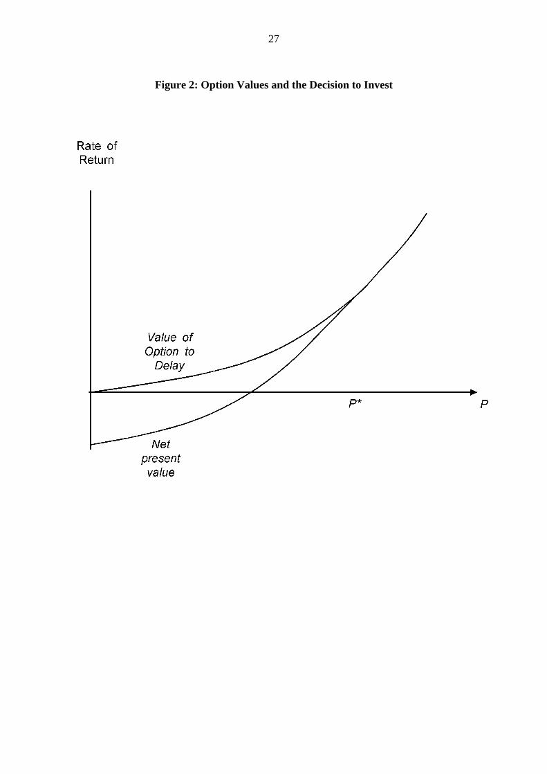
7

strictly speaking increasing variance in the distribution of the future rate of return from the

project) the value of the “call option” to delay an investment project increases and the

decision to invest is delayed. Increased uncertainty, other things equal, will reduce the current

level of investment. This is illustrated in Figure 2 which shows two relationships between the

rate of return and the final product price, P, which the firm takes as parametric but uncertain.

The first shows the conventional net present value of an investment to produce goods for sale

at P. The second includes the value of the option to delay the project. At low levels of P, the

option to delay is more valuable than conventional net present value, and the two only become

equal at or above a critical price level, P*. We will therefore observe lower levels of actual

investment than predicted by conventional theory at prices below P*. It can also be shown (see

Dixit and Pindyck, 1994) that increased uncertainty raises the option value curve and so shifts

outwards the threshold price, P*. Aggregate empirical evidence, to be discussed below,

generally supports the existence of this second, negative relationship between uncertainty and

investment (see Carruth, Dickerson and Henley, 1998).

Since the irreversible investment literature deals with the timing of investment and not

necessarily the level of investment activity, a full model needs to incorporate an independent

explanation of the “certainty-equivalent” determinants of investment. A further point concerns

aggregation: if firm (or sectoral) fluctuations in uncertainty are not coincident then it is

possible that these fluctuations will cancel each other out at the aggregate level, or that the

uncertainty element will be submerged in the dynamic specification of any time series

empirical model. However Bernanke (1983) makes two arguments for why the effects of

uncertainty may not disappear in aggregate. Firstly macroeconomic factors, such as

uncertainty about future interest, exchange and inflation rates or shocks in monetary, fiscal or

regulatory policy regimes, may be important in determining firm-level decisions. Secondly if a

8

firm is uncertain about whether a shock is transitory or permanent then it may delay

investment decisions in order to learn more about its degree of permanence. Here there are the

elements of a mechanism through which (genuinely) transitory shocks become converted into

a more permanent fluctuation. As Bernanke points out, the propagating mechanism through

which uncertainty affects long-run investment decisions is the irreversibility effect. However,

the influence of irreversibility may be submerged in dynamic specification (timing of

investment) in aggregate time series studies, so the quest to find good measures of aggregate

uncertainty may be an elusive one. In other words, uncertainty may well be an important

determinant of investment, but in aggregate empirical models attempts to find a role for

explicit proxies may be fruitless, because the effects of uncertainty are already embedded in

the modelling of investment dynamics, which are usually quite complex, and consistent with

complex, possibly non-linear forms of dynamic adjustment.

There are a number of empirical issues here. One concerns the appropriate way to

measure the effects of uncertainty. A number of approaches and proxy variables have been

adopted in previous work. By and large all studies use a variance measure capturing volatility

in output, inflation or exchange rates as a proxy for uncertainty. There is an apparent

distinction in the literature between work which uses an unconditional variance, usually

constructed using some form of moving moment method (Pindyck and Solimano 1993,

Goldberg 1993, Favero, Pesaran and Sharma 1994) and work which uses an estimated

conditional variance computed from preliminary estimation of some form of ARCH model

(Huizinga 1993, Price 1995, 1996, Episcopos 1995).5 On the other hand Ferderer (1993)

5 ARCH measures of uncertainty are dependent on the (mis)specification of the empiricalmodel, Engle (1983), p. 287. It is quite common to use a univariate VAR on output orinflation, which display an ARCH error test failure, as the basis for estimating the conditionalvariance of these variables. This is not an adequate way of proxying uncertainty, because more

9

adopts a more direct approach by using the implied risk premium in the term structure of

interest rates as a measure of uncertainty. We propose here the use of an indirect (rather than

variance) proxy for uncertainty, namely gold prices.6 As an indirect measure, gold is

commonly regarded as a hedge commodity, the demand for which rises as returns on other

less safe assets become more volatile. Thus, in aggregate, the price of gold will reflect

investor sentiment. We would therefore expect a rising gold price to be coincident with rising

uncertainty about investment returns. A time series plot of the growth in the real sterling-

denominated gold price against real ICC fixed investment growth is illustrated in Figure 3.

Particularly in the period from the late 1970s until 1990 there is some evidence of a negative

association.

A further concern is the question of whether uncertainty has only a short-run or both a

long and short-run effect on investment. Much will depend on how proxies for uncertainty are

established and on the stationarity/non-stationarity of the relevant time series. This is an

empirical issue, but it does suggest that any empirical methodology adopted should be able to

distinguish long-run from short-run dynamic behaviour.

3. Empirical Approach

Broadly speaking, the pre-irreversibility, theoretical literature on investment divides

itself into two main strands: the flexible accelerator approach and the neoclassical approach.

In addition to these main strands is a subsidiary literature concerned with the importance of

appropriate (different) models of output or inflation processes may not exhibit ARCH errorfailures. However the discovery of a better specification, which passes the ARCH test, doesnot mean that the impact of uncertainty in economic behaviour has disappeared.6 In preliminary work we also investigated using the Confederation of British Industry’squarterly business optimism series as a more direct proxy for uncertainty. We could find no

10

corporate liquidity in determining investment. Accelerator models posit a desired capital-

output ratio, and construct some form of dynamic adjustment mechanism to relate actual gross

investment to output. The neoclassical approach argues that such a simple bivariate

specification ignores substitution possibilities among factor inputs within the firm, and hence

suggests that factor prices, notably the user cost of capital, should be taken into account. The

data-based methodology of Cuthbertson and Gasparro (1995) as well as Bean (1981a)

integrates neoclassical theory with a general-to-specific approach to the parameterisation of

the dynamic relationships between the variables, and we adopt a similar approach here.

Suppose we start from a constant elasticity of substitution, constant returns to scale

technology, and suppose that demand for capital is subject to a mean zero disturbance, �7. The

factor demand for capital will be given by:

K = A Y [(1 + 1/�)/C ]� exp(�), (1)

where A is the scale parameter, K is capital, Y is output, C is the user cost of capital, � is the

output price elasticity of demand, and � is the elasticity of substitution. We can think of � as

capturing the size of the wedge between the user cost of an extra unit of capital and its present

value that arises from the option value of refraining from investing, as illustrated in Figure 2.

The familiar identity describing the dynamic evolution of capital stock is:

I = �K + d K, (2)

significant relationship with ICC investment. It is, of course, a moot point as to whether anincrease in optimism necessarily implies a reduction in uncertainty.7 We adopt a static framework to illustrate the basic arguments that lead to a reduced formempirical specification. Dynamic optimisation of the representative firm’s intertemporal valuefunction is a more popular theory model, but is more appropriate to the estimation ofstructural Euler equations.

11

where I is gross investment, d represents the change and � is the depreciation rate. Assume

the existence of a steady state in which capital stock and output are growing at a constant rate

g, then from (2):

I = (g + �)K. (3)

Substituting (1) into (3) eliminates the capital stock term and gives:

I = A (g + �)Y [(1 + 1/�)/C ]� exp(�). (4)

If we assume that the elasticity of demand, �, is constant, and allow a general polynomial lag

structure to model dynamic adjustment costs, then the discrete time analogue of equation (4)

is:

a1(L)�it = a0 + a2(L)�yt + a3(L)�ct + a4(L)��t + b1it-j + b2yt-j + b3ct-j + b4�t-j + ut, (5)

where a1 to a4 are polynomials in the lag operator, L, ut is the error term, and lower case letters

denote logs. The parameterisation of the log levels terms allows the imposition of a long-run

steady-state solution in a conventional equilibrium correction form (ECM).

We can relax the assumption of a constant elasticity of demand in an empirical

specification by using the Lerner condition identity between 1 + 1/� and the price-cost margin.

Movements in profit margins may therefore reflect changes in market power and so in the

firm’s derived demand for capital. Parameterisation of this within the time series investment

function is attractive since profit margins may exhibit considerable cyclical variability

(Rotemberg and Saloner 1986, Bils 1987); and, if aggregate industrial structural conditions

display secular movement, then we may expect to observe long-run movements in �.

However, any aggregate empirical profit margin construct such as a profit-sales ratio presents

a problem for empirical representation here in that it is an I(0) series. Therefore, we use a

12

measure of real profits (�) since this displays the same integration properties as real

investment and output. This leads to an empirical formulation of the following form:

a1(L)�it = a0 + a2(L)�yt + a3(L)�ct + a4(L)��t + a5(L)��t +

b1it-j + b2yt-j + b3ct-j + b4�t-j + b5�t-j + ut. (6)

Implicit in modelling investment in terms of the cost of capital is the assumption that

capital markets are perfect; so, for example, the firm is indifferent between rented capital

goods and capital goods bought with borrowed funds. Furthermore, and perhaps more

importantly, the firm is assumed to be indifferent between internal and external financing of

funds, since external finance is not rationed and is available at the same opportunity cost as

internal finance. By contrast, as mentioned in the introduction, recent microeconometric

evidence has provided a number of alternative justifications for the general hypothesis that

profits may, in part, determine investment. The stock of finance available to the firm will be a

determinant of investment expenditure under less than perfect capital markets. In addition to

the suggestion that current profits might capture information about investment sentiment

about the future, real profits might play an important long-run role in such a model by

proxying retained earnings. While these different justifications suggest different measures of

profitability, given the high collinearity that exists between pre-tax and post-tax profit, net and

gross profit, profit including dividends and retained profits, and stock market valuation

(Tobin’s q), it seems unlikely that time-series modelling of aggregate investment will allow us

to discriminate econometrically between the different explanations for the role of real profits.

One further problem is the possible collinearity between profitability and output.

When comparing long-run equilibrium outcomes for a profit-maximising firm under imperfect

competition, in a stable industrial structure, one should observe a monotonic relationship

13

between output and profits (once output is determined profit must be determined). Hence any

profit-based theory becomes empirically indistinguishable from the simple bivariate

investment-output model. However, it is certainly not clear that at all points in time all firms

will be observed to be in long-run equilibrium. For example Costrell (1983) shows that

changes in profitability affect investment but that the direction of this relationship depends on

whether risk aversion is an increasing or decreasing function of income, and so on whether

agents prefer risk-free holdings of money or bonds to risky investment. Moreover it is not the

case that profits and output are collinear either in a cyclical or secular sense as Figure 4

illustrates8.

As already discussed, in order to capture the impact of uncertainty we use a measure of

uncertainty based on the real gold price. In the results presented below, this is derived as the

dollar price of gold, converted to sterling and deflated by the GDP deflator. The alternative of

simply deflating the dollar gold price by the UK GDP deflator made no difference to our

findings, so we are confident that our results are not being explained as the impact of

exchange rate movements on investment.

4. Data Description and Long-Run Analysis

Definitions and sources of the various data series are explained in the Appendix.

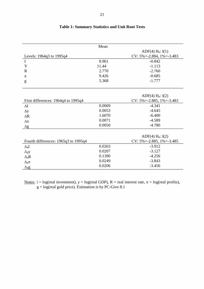
Table 1 reports summary statistics and augmented Dickey-Fuller unit root tests for the real

ICC investment, real GDP, real ICC profits, the real sterling gold price, a real long-term

interest rate as the cost of capital (yield on 20 year gilts). All of the series, with the exception

of the real interest rate, are expressed in natural logs. The descriptive statistics reveal that

8 Strictly speaking, the comparison should be between profits and ICC output, rather thanGDP, but ICC output is difficult to measure (see Anderson, 1981), so GDP may be areasonable instrument.

14

average annual investment growth over the sample period was 2.6%, slightly higher than the

annual growth in profits and output which were 2.1% and 2.5% respectively. Growth in the

real gold price was of a very similar order of magnitude at 2.1% per annum. The table also

shows that for all the levels series we do not reject the null hypothesis of a unit root.

Stationarity is present in all the I(1) levels cases, when the series are expressed as quarterly or

annual differences. As the raw series are not seasonally adjusted, we use annual differences in

the short-run dynamic estimation. This can also be justified on the grounds that annual

percentage changes are more likely to be contained in agents’ information sets; however,

similar results can be obtained with the variables defined as quarterly changes.

Granger (1981, 1986) established an important result between cointegrated regressions

and error or, nowadays, equilibrium correction mechanisms, ECM. This is the idea that for

any group of cointegrated variables an ECM representation holds, and the converse is also

true. This link has ensured the continuing popularity of ECM parameterisations of time series

econometric relationships, and is the empirical methodology adopted by Cuthbertson and

Gasparro despite their setting out of a dynamic optimisation, theory model. With multivariate

long-run relationships there are a number of ways to proceed. One possibility is to adopt the

Engle-Granger (1987) method, and to estimate either a static long-run relationship or solve for

the static solution to an ADL dynamic long-run relationship. This method has been criticised

because it ignores the possibility of multiple cointegrating vectors but, in practice, it is seen to

work quite well, and can give eminently sensible results (albeit of a reduced form nature). An

alternative is to use Johansen’s multivariate technique (Johansen and Juselius, 1990), even

though the underlying structural model is not developed analytically. However, the possibility

of multiple cointegration vectors can lead to severe identification problems, requiring the

researcher to provide an economic interpretation of the relationships that are identified.

15

Moreover, the number of significant cointegrating vectors found is often dependent on the

length of the lags chosen for the VAR, so a judicious choice of lag length can serve to

disguise these kinds of difficulties. Given the relative advantages and disadvantages of the

different methods, we compare the results from all of them in our empirical analysis.

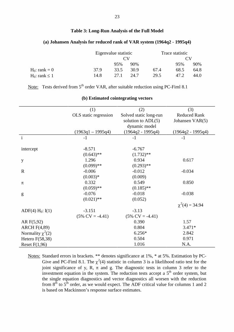
Tables 2 and 3 report the results of the long-run analysis of the data. Table 2 restricts

the empirical model to examine investment and output alone which parallels the earlier work

of Bean (1981a) who estimated an investment-output ECM model9, while Table 3 also

includes profits, the interest rate and the price of gold. Panel (a) uses Johansen’s analysis to

provide evidence of the rank of the long-run matrix of a vector autoregression representation.

On the basis of the model reduction methodology employed by PC-Fiml V8.1 (Doornik and

Hendry, 1995) it was established that lags above order five were not jointly significant and so

the results reported are derived from a VAR which uses lags up to and including order 5. For

Table 2, the eigenvalue statistic does not reject the null of non-cointegration (rank = 0) at the

5 per cent level (using Osterwald-Lenum critical values). For Table 3, it rejects the null of

non-cointegration, but indicates that the rank of the long-run matrix is not above one. The

trace statistics confirm these results, although they only reject non-cointegration at the 10%

level in Table 3.

If we impose a reduced rank of one for both models, then we obtain the vectors

reported in column 3 of panel (b) in Tables 2 and 3. In both cases, these are very close to the

unrestricted rank cointegrating vector. Columns 1 and 2 report alternative OLS estimates of a

9 This model could be expanded to include the real interest rate, but this would not change theessence of the results. In fact when we do this the results look worse because the real interestrate enters with the wrong sign. This is also true of the dynamic model results of Table 4.

16

long-run relationship between the appropriate variables, the first based on a static regression

and the second as the long-run solution to a 5th order ADL specification. For the simple

investment-output model, the results of both the static and the dynamic OLS estimation are

very close to the Johansen result, but the results do not support a valid cointegrating

relationship according to the ADF(4) test and MacKinnon’s response surface critical values in

either case. For Table 3, a similar result holds for columns 1 and 2.

Thus the simple investment-output model does not appear to cointegrate using

Johansen’s methodology, although it looks to be close for the dynamic OLS results. Whereas

the more general model is cointegrated for Johansen estimation, but not for the other two OLS

cases. Furthermore the inclusion of the real price of gold is important to the Johansen results

of Table 3. If it is removed as a potential regressor, then cointegration is rejected at the 5%

level amongst the remaining four variables.10 Casual diagrammatic investigation of the

residuals for all 3 columns of Table 2 and Table 3 shows that they are quite similar with

considerable mean reversion, indicative of stationarity. It is well known that the cointegration

tests have low power, so the foregoing results suggest that it is not unreasonable to investigate

the short-run dynamic properties of the data for the investment-output and more general

models.

For Table 3 there are some differences in the size of the coefficients in the long-run

vector from each method. In the OLS methods, the long-run investment-output elasticity is

close to or above unity and the long-run investment-profits elasticity is rather smaller in size.

In the Johansen analysis this ranking is reversed and the long-run proportional impact of

10 These results are not reported and are available from the authors on request.

17

profits on investment is larger than that of output. Each long-run solution finds a small

negative impact for the real interest rate.11 We also find a small negative long-run impact on

investment from increases in the real gold price. However it should be noted that neither the

interest rate nor the gold price are statistically significant in the dynamic ADL equation.12

Given these differences we explore the use of the residuals from all three methods as a

measure of equilibrium correction in a dynamic model, following the methodology of Engle

and Granger (1987). However, for Table 2, we use only the dynamic OLS residuals since the

three sets of results are so close in their estimation of the long-run investment-output

elasticity.

5. Dynamic Modelling

The Engle-Granger approach is to parameterise a short-run dynamic representation of

the data generating process through specifying a relationship between lag polynomials of the

stationary, differenced variables and lagged values of the ECM term derived from the long-run

representation. A general to specific modelling strategy may then allow the discovery of a

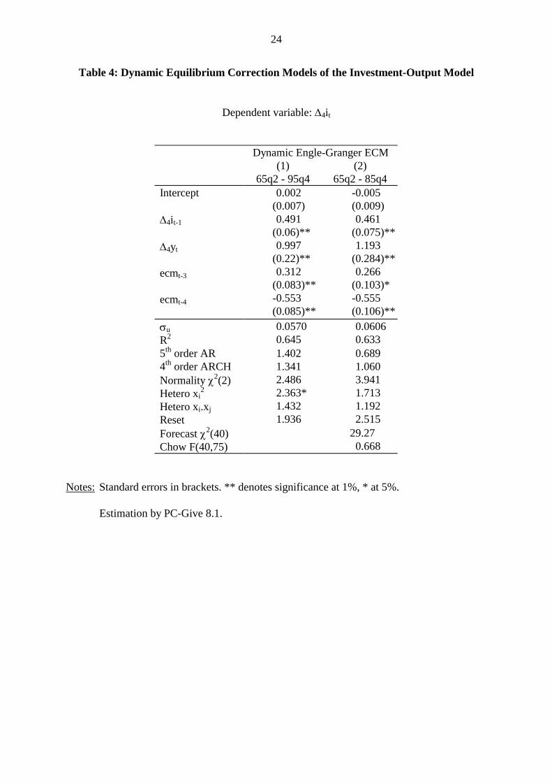
parsimonious model structure. Table 4 reports the results of such an exercise using

equilibrium correction from the dynamic OLS results of Table 2. While this simple model

performs well enough, it is noticeable that it fails the heteroscedasticity diagnostic. This is

consistent with increased unmodelled volatility in investment arising from changes in investor

uncertainty, though this is not the only possible explanation. As such we will concentrate on

11 Initial work attempted to measure a cost of capital series which incorporated estimates ofthe impact of investment subsidies and corporate taxation on the real interest rate, but likeICC output it is hard to combine the appropriate information across different sectors of theeconomy over long periods of time. As such the real interest rate outperformed (encompassed)our cost of capital measure.12 This conclusion is supported by F-tests of the joint significance of the terms in eachvariable: for R, F(6,97) = 1.74; for g, F(6, 97) = 0.98, CV 5% = 2.17.

18

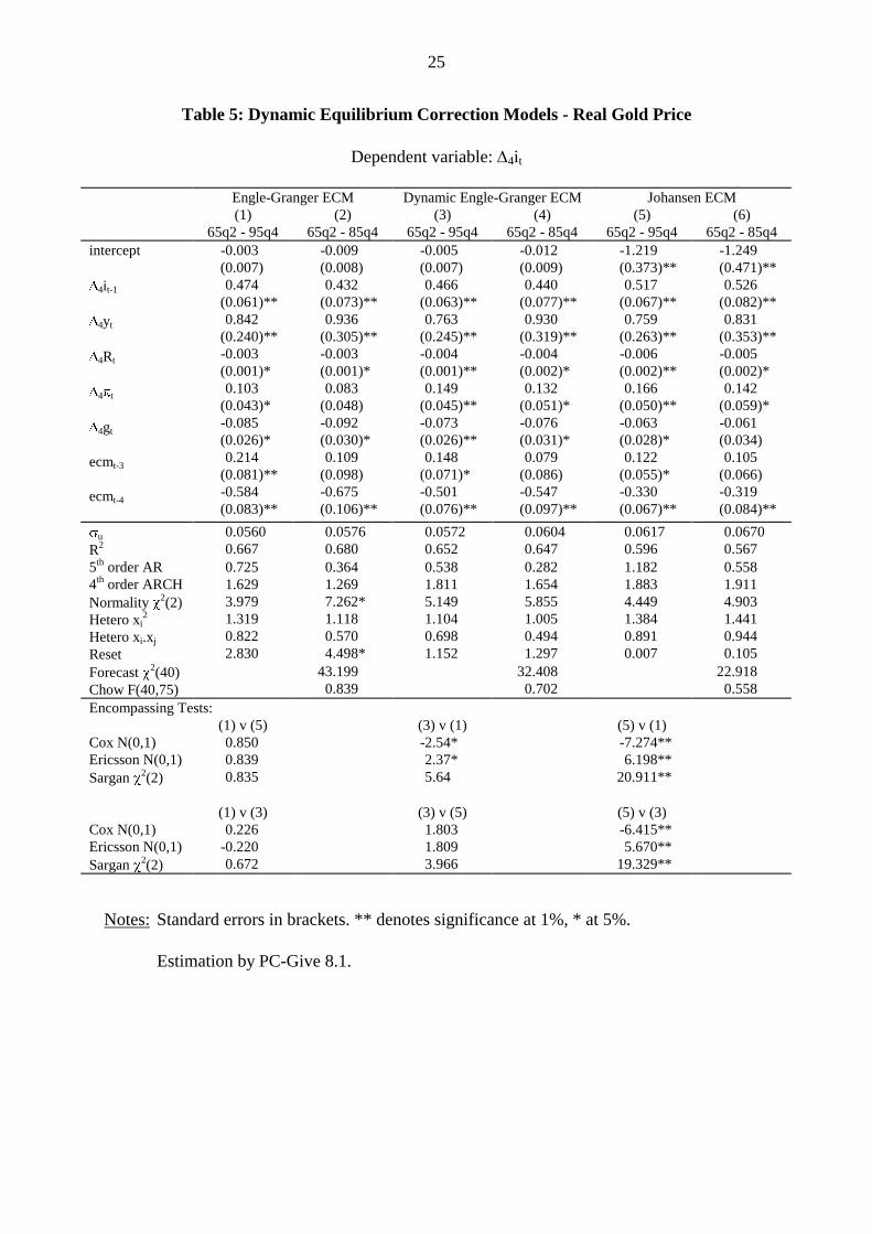
the results of Table 5, which uses the equilibrium corrections from each of the three long-run

vectors in Table 3 (note that real gold price information is used in determining these equilibria

and ECMs). Results in each case are reported for the full period and for a sub-period up to

1985 quarter 4 to investigate forecast performance in the final ten years of the sample.

In general the Table 5 results are very robust to the alternative methods of deriving the

ECM term. The Engle-Granger ECM model (columns 1 and 2 using static OLS residuals from

Table 3, column 1) yields the smallest regression standard error. On the basis of the reported

encompassing test statistics model 1 is preferred to models 3 and 5 and model 3 is in turn

preferred to model 5. In all cases the models satisfy the reported diagnostic tests for

autocorrelation (AR), autoregressive-conditional heteroscedasticity (ARCH), and for

heteroscedasticity due to omitted squared regressors (Hetero xi2) and due to omitted cross-

products (Hetero xi.xj). The normality tests reveal slight evidence of significant non-normality

on the sub-sample estimates for the Engle Granger ECM, column 2.

The significant presence of the lagged dependent variable (�4it-1) points to a degree of

autoregression in the determination of short-run movements in investment, consistent with the

earlier discussion on how the irreversibility idea may manifest itself in the timing of

investment and on to the dynamic structure of an aggregate time series model of investment

spending. The largest short-run impact on investment comes through changes in output (�4yt);

the impact elasticity varies between 0.76 and 0.94 depending on specification and sample

period. Changes in profits have a significant though quantitatively smaller impact; the

elasticity varies between 0.08 and 0.17 and is largest in the Johansen ECM model. The long-

run rate of interest has a quantitatively small but significant short-run impact. The gold price

also has a negative and significant short-run impact on investment; the elasticity varies

19

between -0.06 and -0.09. The two equilibrium correction variables are allowing lagged

information in the disequilibrium levels of the data to control for short-run dynamics, over and

above the lagged dependent variable dynamics of the investment growth process. This follows

a suggestion of Phillips and Loretan (1991). The sum of the two coefficients on the

equilibrium correction terms reveals the speed of adjustment towards equilibrium. This is

generally quicker in the Engle-Granger ECM models than in the Johansen ECM model.

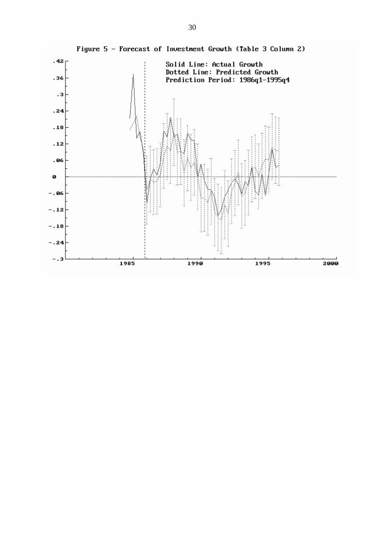
The even numbered columns in Table 5 reveal the forecast performance of the models.

In each case the model coefficients are pleasingly robust to sample period and this is

confirmed by the forecast Chow test statistics. The overall forecast performance, given by the

�2(40) statistic for the significance of the difference between actual and forecast predictions, is

good. Figure 5 provides a visual presentation of the forecast performance of the model in

column 2 of Table 5. It is evident that the predictions track the data very well, and remain

within the error bounds throughout the 10 year forecast period, 1986q1 to 1995q4. Finally, the

encompassing tests of Table 5 favour the disequilibrium errors generated from the OLS

estimated long-run relationships against the system based Johansen errors.

6. Conclusions

Recent work has attempted to address the appropriate way to capture the impact of

uncertainty on investment, usually relying on some initial parameterisation of price or output

variance, however these conditional variance approaches adopt an inappropriate methodology,

relying on misspecification of an empirical model to generate a conditional variance measure

(see footnote 5). Uncertainty may well be an important determinant of investment but, in

aggregate empirical models, finding significant, explicit proxies may be difficult because the

effects of uncertainty are already implicit in the modelling of the dynamics of investment. In

20

this paper we have employed a more indirect, and arguably, more interesting proxy for

uncertainty - namely the gold price. The size of the relationship between investment and gold

price movements is small but significant - a long-run elasticity of around -0.07 (Tables 3

and 5). Disaggregated analysis may find a stronger relationship at the company level for the

UK, but this requires further research.

We have also addressed the question of whether there is an aggregate role for

corporate financial performance, as found in recent micro-econometric studies. Our results

show that corporate profits significantly explain long and short-run movements in aggregate

investment. A 10 per cent increase in corporate profits is associated with up to a 1.6 per cent

short-run increase in fixed investment by the UK industrial and corporate sector. In the long-

run the impact could be as high as 8.5 per cent. Aggregate analysis cannot reveal the source of

this relationship, but it is consistent with a world of less than perfect capital markets in which

industrial and commercial companies may be liquidity constrained, and heavily reliant on

internally generated funds to fund long-term fixed investment activity. It is also consistent

with current profits capturing investor expectational effects. While we find a significant,

negative impact for long-term interest rates, it is a quantitatively small one. One conclusion to

draw from this is that changes in corporate taxation policy may have a much larger impact on

investment through the availability of internal corporate funds than through any impact on the

cost of capital. Similarly we found on investigation of a simple investment-output model

(Tables 2 and 4), that investment and output may not cointegrate but more importantly that

there was some evidence of heteroscedasticity in the dynamic model. This was suggestive of a

misspecification, perhaps due to the omitted effects of uncertainty, or missing variables like

real profits or the real price of gold. The inclusion of real profits and the real gold price appear

to satisfactorily eliminate this misspecification problem.

21

Table 1: Summary Statistics and Unit Root Tests

Levels: 1964q3 to 1995q4

MeanADF(4) H0: I(1)

CV: 5%=-2.884, 1%=-3.483IYR�

g

8.96111.442.7709.4265.368

-0.842-1.113-2.760-0.685-1.777

First differences: 1964q4 to 1995q4ADF(4) H0: I(2)

CV: 5%=-2.885, 1%=-3.483�I�y�R��

�g

0.00690.00531.60700.00710.0050

-4.341-4.645-6.400-4.589-4.780

Fourth differences: 1965q3 to 1995q4ADF(4) H0: I(2)

CV: 5%=-2.885, 1%=-3.485�4I�4y�4R�4�

�4g

0.02630.02070.13900.02490.0206

-3.912-3.127-4.256-3.843-3.456

Notes: i = log(real investment), y = log(real GDP), R = real interest rate, � = log(real profits),g = log(real gold price). Estimation is by PC-Give 8.1

22

Table 2: Long-run Analysis of Investment-Output Model

(a) Johansen Analysis for reduced rank of VAR system (1964q2 - 1995q4)

Eigenvalue statistic Trace statisticCV CV

95% 90% 95% 90%H0: rank = 0 9.79 14.1 12.1 11.22 15.4 13.3H0: rank � 1 1.43 3.8 2.7 1.43 3.8 2.7

Note: Tests derived from 5th order VAR, after suitable reduction using PC-Fiml 8.1

(b) Estimated cointegrating vectors

(1)OLS static regression

(1963q1-1995q4)

(2)Solved static long-run

solution to ADL(5)dynamic model

(1964q2 - 1995q4)

(3)Reduced Rank

Johansen VAR(5)

(1964q2 - 1995q4)i -1 -1 -1

intercept -9.838(0.515)**

-10.95(1.92)**

y 1.643(0.045)**

1.737(0.168)**

1.713

ADF(4) H0: I(1) -3.00 -3.06(5% CV = -3.34) (5% CV = -3.34)

AR F(5,110)ARCH F(4,107)Normality �2 (2)Hetero F(22,92)Reset F(1,96)

0.6622.942*1.3822.001*2.346

1.945.225**5.6482.656**N.A.

Notes: Standard errors in brackets. ** denotes significance at 1%, * at 5%, but not that thestatic OLS standard errors are not reliable. Estimation by PC-Give and PC-Fiml 8.1.The diagnostic tests in column 3 refer to the investment equation in the system. Thereduction tests accept a 5th order system, but the single equation diagnostics and vectordiagnostics all worsen with the reduction from 8th to 5th order, as we would expect.The ADF critical values for columns 1 and 2 are based on Mackinnon’s responsesurface estimates.

23

Table 3: Long-Run Analysis of the Full Model

(a) Johansen Analysis for reduced rank of VAR system (1964q2 - 1995q4)

Eigenvalue statistic Trace statisticCV CV

95% 90% 95% 90%H0: rank = 0 37.9 33.5 30.9 67.4 68.5 64.8H0: rank � 1 14.8 27.1 24.7 29.5 47.2 44.0

Note: Tests derived from 5th order VAR, after suitable reduction using PC-Fiml 8.1

(b) Estimated cointegrating vectors

(1)OLS static regression

(1963q1 – 1995q4)

(2)Solved static long-run

solution to ADL(5)dynamic model

(1964q2 - 1995q4)

(3)Reduced Rank

Johansen VAR(5)

(1964q2 - 1995q4)i -1 -1 -1

intercept -8.571(0.643)**

-6.767(1.732)**

y 1.296(0.099)**

0.934(0.293)**

0.617

R -0.006(0.003)*

-0.012(0.009)

-0.034

� 0.332(0.059)**

0.549(0.185)**

0.850

g -0.076(0.021)**

-0.018(0.052)

-0.038

�2(4) = 34.94

ADF(4) H0: I(1) -3.151 -3.13(5% CV = -4.41) (5% CV = -4.41)

AR F(5,92)ARCH F(4,89)Normality �2(2)Hetero F(58,38)Reset F(1,96)

0.3900.8046.256*0.5041.016

1.573.471*2.8420.971N.A.

Notes: Standard errors in brackets. ** denotes significance at 1%, * at 5%. Estimation by PC-Give and PC-Fiml 8.1. The �2(4) statistic in column 3 is a likelihood ratio test for thejoint significance of y, R, � and g. The diagnostic tests in column 3 refer to theinvestment equation in the system. The reduction tests accept a 5th order system, butthe single equation diagnostics and vector diagnostics all worsen with the reductionfrom 8th to 5th order, as we would expect. The ADF critical value for columns 1 and 2is based on Mackinnon’s response surface estimates.

24

Table 4: Dynamic Equilibrium Correction Models of the Investment-Output Model

Dependent variable: �4it

Dynamic Engle-Granger ECM(1)

65q2 - 95q4(2)

65q2 - 85q4Intercept

�4it-1

�4yt

ecmt-3

ecmt-4

0.002(0.007)0.491

(0.06)**0.997

(0.22)**0.312

(0.083)**-0.553(0.085)**

-0.005(0.009)0.461

(0.075)**1.193

(0.284)**0.266

(0.103)*-0.555(0.106)**

�u

R20.05700.645

0.06060.633

5th order AR4th order ARCHNormality �2(2)Hetero xi

2

Hetero xi.xj

Reset

1.4021.3412.4862.363*1.4321.936

0.6891.0603.9411.7131.1922.515

Forecast �2(40)Chow F(40,75)

29.270.668

Notes: Standard errors in brackets. ** denotes significance at 1%, * at 5%.

Estimation by PC-Give 8.1.

25

Table 5: Dynamic Equilibrium Correction Models - Real Gold Price

Dependent variable: �4it

Engle-Granger ECM Dynamic Engle-Granger ECM Johansen ECM(1)

65q2 - 95q4(2)

65q2 - 85q4(3)

65q2 - 95q4(4)

65q2 - 85q4(5)

65q2 - 95q4(6)

65q2 - 85q4intercept

�4it-1

�4yt

�4Rt

�4�t

�4gt

ecmt-3

ecmt-4

-0.003(0.007)0.474

(0.061)**0.842

(0.240)**-0.003(0.001)*0.103

(0.043)*-0.085(0.026)*0.214

(0.081)**-0.584(0.083)**

-0.009(0.008)0.432

(0.073)**0.936

(0.305)**-0.003(0.001)*0.083

(0.048)-0.092(0.030)*0.109

(0.098)-0.675(0.106)**

-0.005(0.007)0.466

(0.063)**0.763

(0.245)**-0.004(0.001)**0.149

(0.045)**-0.073(0.026)**0.148

(0.071)*-0.501(0.076)**

-0.012(0.009)0.440

(0.077)**0.930

(0.319)**-0.004(0.002)*0.132

(0.051)*-0.076(0.031)*0.079

(0.086)-0.547(0.097)**

-1.219(0.373)**0.517

(0.067)**0.759

(0.263)**-0.006(0.002)**0.166

(0.050)**-0.063(0.028)*0.122

(0.055)*-0.330(0.067)**

-1.249(0.471)**0.526

(0.082)**0.831

(0.353)**-0.005(0.002)*0.142

(0.059)*-0.061(0.034)0.105

(0.066)-0.319(0.084)**

�u

R20.05600.667

0.05760.680

0.05720.652

0.06040.647

0.06170.596

0.06700.567

5th order AR4th order ARCHNormality �2(2)Hetero xi

2

Hetero xi.xj

Reset

0.7251.6293.9791.3190.8222.830

0.3641.2697.262*1.1180.5704.498*

0.5381.8115.1491.1040.6981.152

0.2821.6545.8551.0050.4941.297

1.1821.8834.4491.3840.8910.007

0.5581.9114.9031.4410.9440.105

Forecast �2(40)Chow F(40,75)

43.1990.839

32.4080.702

22.9180.558

Encompassing Tests:(1) v (5) (3) v (1) (5) v (1)

Cox N(0,1)Ericsson N(0,1)Sargan �2(2)

0.8500.8390.835

-2.54*2.37*5.64

-7.274**6.198**

20.911**

(1) v (3) (3) v (5) (5) v (3)Cox N(0,1)Ericsson N(0,1)Sargan �2(2)

0.226-0.2200.672

1.8031.8093.966

-6.415**5.670**

19.329**

Notes: Standard errors in brackets. ** denotes significance at 1%, * at 5%.

Estimation by PC-Give 8.1.

26

Figure 1: Real UK Corporate Fixed Investment Growth

-20

-10

0

10

20

30

40

50

Mar

-65

Mar

-66

Mar

-67

Mar

-68

Mar

-69

Mar

-70

Mar

-71

Mar

-72

Mar

-73

Mar

-74

Mar

-75

Mar

-76

Mar

-77

Mar

-78

Mar

-79

Mar

-80

Mar

-81

Mar

-82

Mar

-83

Mar

-84

Mar

-85

Mar

-86

Mar

-87

Mar

-88

Mar

-89

Mar

-90

Mar

-91

Mar

-92

Mar

-93

Mar

-94

Mar

-95

per

cent

per

ann

um

27

Figure 2: Option Values and the Decision to Invest

28

Figure 3: Investment and Gold Price Growth

-40

-20

0

20

40

60

80

100

120

Mar

-65

Mar

-66

Mar

-67

Mar

-68

Mar

-69

Mar

-70

Mar

-71

Mar

-72

Mar

-73

Mar

-74

Mar

-75

Mar

-76

Mar

-77

Mar

-78

Mar

-79

Mar

-80

Mar

-81

Mar

-82

Mar

-83

Mar

-84

Mar

-85

Mar

-86

Mar

-87

Mar

-88

Mar

-89

Mar

-90

Mar

-91

Mar

-92

Mar

-93

Mar

-94

Mar

-95

per

cent

per

ann

um

real investment growth Real sterling gold price growth

29

Figure 4: Real GDP and Profits Growth

-60

-40

-20

0

20

40

60

Mar

-65

Mar

-66

Mar

-67

Mar

-68

Mar

-69

Mar

-70

Mar

-71

Mar

-72

Mar

-73

Mar

-74

Mar

-75

Mar

-76

Mar

-77

Mar

-78

Mar

-79

Mar

-80

Mar

-81

Mar

-82

Mar

-83

Mar

-84

Mar

-85

Mar

-86

Mar

-87

Mar

-88

Mar

-89

Mar

-90

Mar

-91

Mar

-92

Mar

-93

Mar

-94

Mar

-95

per

cent

per

ann

um

real GDP growth real ICC profit growth

30

31

Appendix - Data Sources and Definitions

All series are for the period 1963:1 to 1995:4 and seasonally unadjusted.

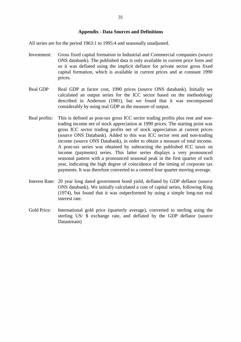
Investment: Gross fixed capital formation in Industrial and Commercial companies (sourceONS databank). The published data is only available in current price form andso it was deflated using the implicit deflator for private sector gross fixedcapital formation, which is available in current prices and at constant 1990prices.

Real GDP Real GDP at factor cost, 1990 prices (source ONS databank). Initially wecalculated an output series for the ICC sector based on the methodologydescribed in Anderson (1981), but we found that it was encompassedconsiderably by using real GDP as the measure of output.

Real profits: This is defined as post-tax gross ICC sector trading profits plus rent and non-trading income net of stock appreciation at 1990 prices. The starting point wasgross ICC sector trading profits net of stock appreciation at current prices(source ONS Databank). Added to this was ICC sector rent and non-tradingincome (source ONS Databank), in order to obtain a measure of total income.A post-tax series was obtained by subtracting the published ICC taxes onincome (payments) series. This latter series displays a very pronouncedseasonal pattern with a pronounced seasonal peak in the first quarter of eachyear, indicating the high degree of coincidence of the timing of corporate taxpayments. It was therefore converted to a centred four quarter moving average.

Interest Rate: 20 year long dated government bond yield, deflated by GDP deflator (sourceONS databank). We initially calculated a cost of capital series, following King(1974), but found that it was outperformed by using a simple long-run realinterest rate.

Gold Price: International gold price (quarterly average), converted to sterling using thesterling US/ $ exchange rate, and deflated by the GDP deflator (sourceDatastream)

32

References

Abel, A. (1983), “Optimal investment under uncertainty”, American Economic Review, Vol73, pp. 228-33

Anderson, G.J. (1981), “A new approach to the empirical investigation of investmentexpenditures”, Economic Journal, Vol 91, pp. 88-103.

Bean, C.J. (1981a), “An econometric model of manufacturing investment in the UK”,Economic Journal, Vol 91, pp. 106-121.

Bean, C.J. (1981b), “A new approach to the empirical investigation of investmentexpenditures: a comment”, Economic Journal, Vol 91, pp. 104-105.

Bernanke, B.S. (1983), “Irreversibility, uncertainty and cyclical investment”, QuarterlyJournal of Economics, Vol 98, pp. 85-106.

Bils, M. (1987), “The cyclical behaviour of marginal cost and price”, American EconomicReview, Vol 77, pp. 838-855.

Bond, S. and Meghir, C. (1994), “Dynamic investment models and the firm’s financial policy”Review of Economic Studies, Vol 61, pp. 197-222.

Bond, S. and Jenkinson, T. (1996), “The Assessment: Investment Performance and Policy”,Oxford Review of Economic Policy, 12, 1-29.

Blundell, R., Bond, S., Devereux, M. and Schiantarelli, F. (1992), “Investment and Tobin’s Q:evidence from company panel data”, Journal of Econometrics, Vol 51, pp. 233-257.

Carruth, A., Dickerson, A. and Henley, A. (1998), “What do we know about Investment underUncertainty?”, University of Kent, Studies in Economics, 98/4.

Chirinko, R. S. (1987), “Tobin’s Q and Financial Policy”, Journal of Monetary Economics,19, 69-87.

Costrell, R.M. (1983), “Profitability and aggregate investment under demand uncertainty”,Economic Journal, Vol 93, pp. 166-181.

Cuthbertson, K. and Gasparro, D. (1995), “Fixed Investment Decisions in UK manufacturing:The importance of Tobin’s Q, Output and Debt”, European Economic Review, 39,919-941.

Dixit, A.K. and Pindyck, R.S. (1994), Investment Under Uncertainty, Princeton: PrincetonUniversity Press.

Doornik, J.A. and Hendry, D.F (1995), PC-Give/PC-Fiml 8.: An Interactive EconometricModelling System, London: International Thompson Publishing.

33

Driver, C. and Moreton, D. (1991), “The influence of uncertainty on aggregate spending: anempirical analysis”, Economic Journal, Vol 101, pp. 1452-59.

Engle, R. F. (1983), “Estimates of the Variance of US Inflation Based upon the ARCHModel”, Journal of Money Credit and Banking, 15, 286-301.

Engle, R.F. and Granger, C.W.J. (1987), “Cointegration and error correction: representation,estimation and testing”, Econometrica, Vol 55, pp. 251-76.

Episcopos, A. (1995), “Evidence on the relationship between uncertainty and irreversibleinvestment”, Quarterly Review of Economics and Finance, Vol 35(1), pp. 41-52.

Favero, C.A., Pesaran, M.H., and Sharma, S., (1994), “A duration model of irreversibleinvestment: theory and empirical evidence”, Journal of Applied Econometrics, Vol 9,pp. S95-S112.

Fazzari, S.M., Hubbard, R.G. and Petersen, B.C. (1988), “Financing constraints and corporateinvestment”, Brookings Papers on Economic Activity, pp. 141-195.

Ferderer, J.P. (1993), “The impact of uncertainty on aggregate investment spending: anempirical analysis”, Journal of Money, Credit and Banking, Vol 25, pp. 30-48.

Goldberg, L.S. (1993), “Exchange rates and investment in United States industry”, Review ofEconomics and Statistics, Vol 75(4), pp. 575-589.

Granger, C.W.J. (1981), “Some properties of time series data and their use in econometricmodel specification”, Journal of Econometrics, Vol 16, pp. 121-30.

Granger, C.W.J. (1986), “Developments in the study of cointegrated economic variables”,Oxford Bulletin of Economics and Statistics, Vol 48, pp. 213-228.

Hall R.E. (1978), “Stochastic Implications of the Life Cycle - Permanent Income Hypothesis:Theory and Evidence”, Journal of Political Economy, Vol 96, pp. 971-987.

Hartmann, R. (1972), “The effects of price and cost uncertainty on investment”, Journal ofEconomic Theory, Vol 5, pp. 258-66.

Hayashi, F. and Inoue, T. (1991), “The relation between firm growth and q with multiplecapital goods: theory and evidence from Japanese panel data”, Econometrica, Vol 59,pp. 731-754.

Huizinga, J. (1993), “Inflation uncertainty, relative price uncertainty, and investment in USmanufacturing”, Journal of Money, Credit and Banking, Vol 25, pp. 521-54.

Johansen, S. and Juselius, K. (1990), “Maximum Likelihood Estimation and Inference onCointegration - with Applications to the Demand for Money, Oxford Bulletin ofEconomics and Statistics, Vol 52, pp. 169-210.

34

King, M. (1974), “Taxation and the cost of capital”, Review of Economic Studies, Vol 41, pp.21-35.

Kuh, E. (1963), Capital Stock Growth: A Microeconometric Approach, Amsterdam: NorthHolland.

MacDonald, R. and Siegel, D.R. (1986), “Investment and the valuation of firms when there isan option to shut down”, International Economic Review, Vol 26(2), pp. 331-49.

Oulton, N. (1981), “Aggregate investment and Tobin's Q: the evidence from Britain”, OxfordEconomic Papers, Vol 33, pp. 177-202.

Phillips, P.C.B. and Loretan, M. (1991), “Estimating Long-Run Economic Equilibria”, Reviewof Economic Studies, Vol 58, pp. 407-436.

Pindyck, R.S. and Solimano, A., (1993), “Economic instability and aggregate investment”,NBER Macroeconomics Annual, pp. 259-303.

Poterba, J.M. and Summers, L.H. (1983), “Dividend taxes, corporate investment and ‘Q’”,Journal of Public Economics, Vol 22, pp. 135-67.

Price, S. (1995), “Aggregate uncertainty, capacity utilisation and manufacturing investment”,Applied Economics, Vol 27, pp. 147-154.

Price, S. (1996), “Aggregate uncertainty, investment and asymmetric adjustment in the UKmanufacturing sector”, Applied Economics, Vol 28, pp. 1369-79.

Rotemberg, J.J. and Saloner, G. (1986), “A supergame theoretic model of price wars duringbooms”, American Economic Review, Vol 76, pp. 390-407.