Business-to-Business data sharing: An economic and legal ...
ECMT1020-Business and Economic Statistics B
Nektarios Aslanidis
Semester 2, 2014Lecture 1: Review of statistics 1
Aslanidis (University of Sydney) Review of statistics 1Semester 2, 2014 Lecture 1: Review of statistics 1 1
/ 33
Some notation
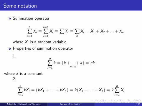
Summation operator
n
∑i=1Xi �
i=n
∑i=1Xi � ∑Xi � ∑
xXi = X1 + X2 + ...+ Xn
where Xi is a random variable.
Properties of summation operator
1.n
∑i=1k = (k + ...+ k
n�k) = nk
where k is a constant2.
n
∑i=1kXi = (kX1 + ....+ kXn) = k(X1 + ....+ Xn) = k
n
∑i=1Xi
Aslanidis (University of Sydney) Review of statistics 1Semester 2, 2014 Lecture 1: Review of statistics 1 2
/ 33
Some notation
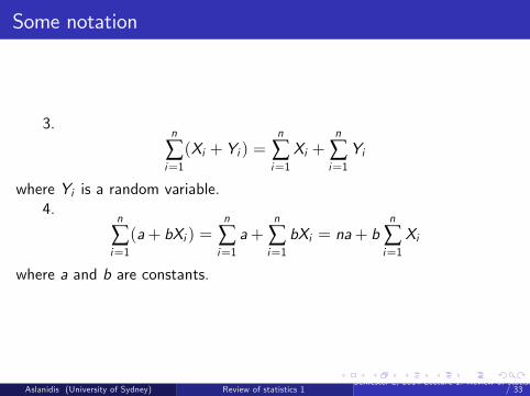
3.n
∑i=1(Xi + Yi ) =
n
∑i=1Xi +
n
∑i=1Yi
where Yi is a random variable.4.
n
∑i=1(a+ bXi ) =
n
∑i=1a+
n
∑i=1bXi = na+ b
n
∑i=1Xi
where a and b are constants.
Aslanidis (University of Sydney) Review of statistics 1Semester 2, 2014 Lecture 1: Review of statistics 1 3
/ 33
Probability: Classical or a priori de�nition
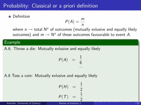
De�nitionP(A) =
mn
where n ! total No of outcomes (mutually exlusive and equally likelyoutcomes) and m ! No of these outcomes favourable to event A.
ExampleA.6. Throw a die: Mutually exlusive and equally likely
P(A) =16...
A.6 Toss a coin: Mutually exlusive and equally likely
P(H) =12
P(T ) =12
Aslanidis (University of Sydney) Review of statistics 1Semester 2, 2014 Lecture 1: Review of statistics 1 4
/ 33
Probability: Classical or a priori de�nition
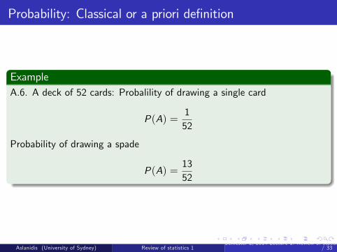
ExampleA.6. A deck of 52 cards: Probalility of drawing a single card
P(A) =152
Probability of drawing a spade
P(A) =1352
Aslanidis (University of Sydney) Review of statistics 1Semester 2, 2014 Lecture 1: Review of statistics 1 5
/ 33
Probability: Classical or a priori de�nition
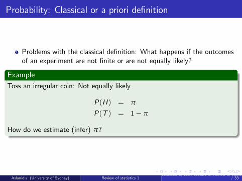
Problems with the classical de�nition: What happens if the outcomesof an experiment are not �nite or are not equally likely?
ExampleToss an irregular coin: Not equally likely
P(H) = π
P(T ) = 1� π
How do we estimate (infer) π?
Aslanidis (University of Sydney) Review of statistics 1Semester 2, 2014 Lecture 1: Review of statistics 1 6
/ 33
Probability: Classical or a priori de�nition
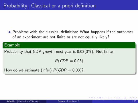
Problems with the classical de�nition: What happens if the outcomesof an experiment are not �nite or are not equally likely?
ExampleProbability that GDP growth next year is 0.03(3%): Not �nite
P(GDP = 0.03)
How do we estimate (infer) P(GDP = 0.03)?
Aslanidis (University of Sydney) Review of statistics 1Semester 2, 2014 Lecture 1: Review of statistics 1 7
/ 33
Probability: Empirical de�nition
ExampleA.7. Distribution of marks (Table A-1).
Provided the number of observation is relatively large, the relativefrequencies are treated as probabilities.
Aslanidis (University of Sydney) Review of statistics 1Semester 2, 2014 Lecture 1: Review of statistics 1 8
/ 33
Properties of probabilities
Properties1.
0 � P(A) � 12. If A,B,C , ... are mutually exclusive events
P(A+ B + C + ...) = P(A) + P(B) + P(C ) + ...
Aslanidis (University of Sydney) Review of statistics 1Semester 2, 2014 Lecture 1: Review of statistics 1 9
/ 33
Properties of probabilities
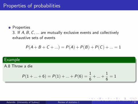
Properties3. If A,B,C , ... are mutually exclusive events and collectivelyexhaustive sets of events
P(A+ B + C + ...) = P(A) + P(B) + P(C ) + ... = 1
ExampleA.8 Throw a die
P(1+ ...+ 6) = P(1) + ...+ P(6) =16+ ...+
16= 1
Aslanidis (University of Sydney) Review of statistics 1Semester 2, 2014 Lecture 1: Review of statistics 1 10
/ 33
Properties of probabilities
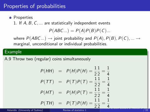
Properties1. If A,B,C , ... are statistically independent events
P(ABC ...) = P(A)P(B)P(C )...
where P(ABC ...)! joint probability and P(A),P(B),P(C ), ...!marginal, unconditional or individual probabilities.
ExampleA.9 Throw two (regular) coins simultaneously
P(HH) = P(H)P(H) =1212=14
P(TT ) = P(T )P(T ) =1212=14
P(HT ) = P(H)P(T ) =1212=14
P(TH) = P(T )P(H) =1212=14
Aslanidis (University of Sydney) Review of statistics 1Semester 2, 2014 Lecture 1: Review of statistics 1 11
/ 33
Properties of probabilities
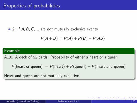
2. If A,B,C , ... are not mutually exclusive events
P(A+ B) = P(A) + P(B)� P(AB)
ExampleA.10. A deck of 52 cards: Probability of either a heart or a queen
P(heart or queen) = P(heart) + P(queen)� P(heart and queen)
Heart and queen are not mutually exclusive
Aslanidis (University of Sydney) Review of statistics 1Semester 2, 2014 Lecture 1: Review of statistics 1 12
/ 33
Conditional probabilities
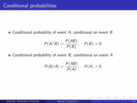
Conditional probability of event A, conditional on event B
P(A/B) =P(AB)P(B)
, P(B) > 0
Conditional probability of event B, conditional on event A
P(B/A) =P(AB)P(A)
, P(A) > 0
Aslanidis (University of Sydney) Review of statistics 1Semester 2, 2014 Lecture 1: Review of statistics 1 13
/ 33
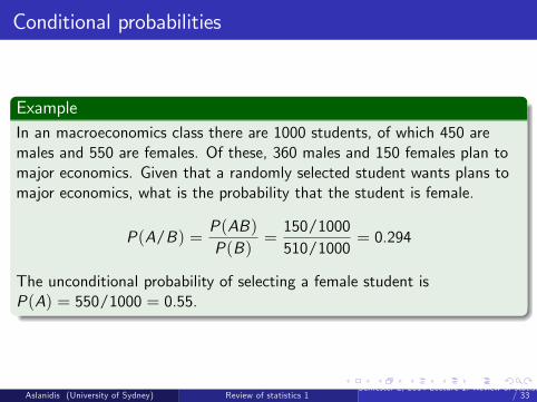
Conditional probabilities
ExampleIn an macroeconomics class there are 1000 students, of which 450 aremales and 550 are females. Of these, 360 males and 150 females plan tomajor economics. Given that a randomly selected student wants plans tomajor economics, what is the probability that the student is female.
P(A/B) =P(AB)P(B)
=150/1000510/1000
= 0.294
The unconditional probability of selecting a female student isP(A) = 550/1000 = 0.55.
Aslanidis (University of Sydney) Review of statistics 1Semester 2, 2014 Lecture 1: Review of statistics 1 14
/ 33
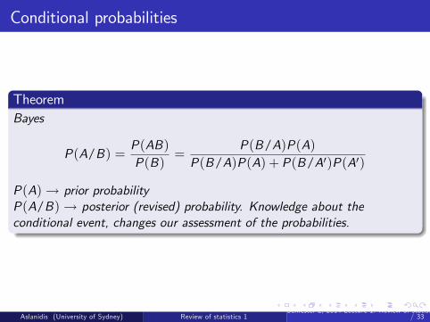
Conditional probabilities
TheoremBayes
P(A/B) =P(AB)P(B)
=P(B/A)P(A)
P(B/A)P(A) + P(B/A0)P(A0)
P(A)! prior probabilityP(A/B)! posterior (revised) probability. Knowledge about theconditional event, changes our assessment of the probabilities.
Aslanidis (University of Sydney) Review of statistics 1Semester 2, 2014 Lecture 1: Review of statistics 1 15
/ 33
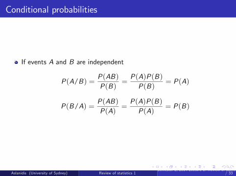
Conditional probabilities
If events A and B are independent
P(A/B) =P(AB)P(B)
=P(A)P(B)P(B)
= P(A)
P(B/A) =P(AB)P(A)
=P(A)P(B)P(A)
= P(B)
Aslanidis (University of Sydney) Review of statistics 1Semester 2, 2014 Lecture 1: Review of statistics 1 16
/ 33
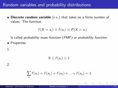
Random variables and probability distributions
Discrete random variable (r.v.) that takes on a �nite number ofvalues. The function
f (X = xi ) � f (xi ) � P(X = xi )
is called probability mass function (PMF ) or probability function.
Properties
1.
0 � f (xi ) � 12.
∑xf (xi ) = f (x1) + f (x2) + ...+ f (xn) = 1
Aslanidis (University of Sydney) Review of statistics 1Semester 2, 2014 Lecture 1: Review of statistics 1 17
/ 33
Random variables and probability distributions
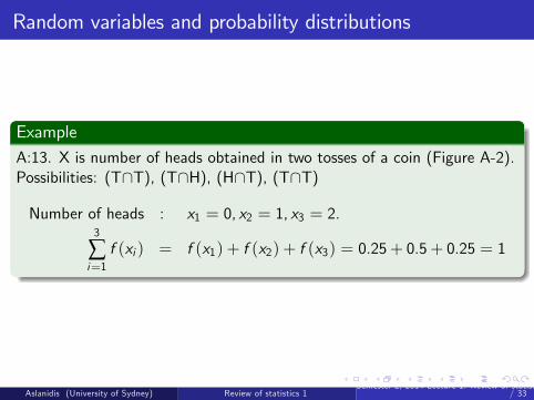
ExampleA:13. X is number of heads obtained in two tosses of a coin (Figure A-2).Possibilities: (T\T), (T\H), (H\T), (T\T)
Number of heads : x1 = 0, x2 = 1, x3 = 2.3
∑i=1f (xi ) = f (x1) + f (x2) + f (x3) = 0.25+ 0.5+ 0.25 = 1
Aslanidis (University of Sydney) Review of statistics 1Semester 2, 2014 Lecture 1: Review of statistics 1 18
/ 33
Random variables and probability distributions
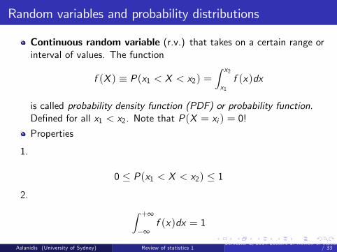
Continuous random variable (r.v.) that takes on a certain range orinterval of values. The function
f (X ) � P(x1 < X < x2) =Z x2
x1f (x)dx
is called probability density function (PDF) or probability function.De�ned for all x1 < x2. Note that P(X = xi ) = 0!
Properties
1.
0 � P(x1 < X < x2) � 12. Z +∞
�∞f (x)dx = 1
Aslanidis (University of Sydney) Review of statistics 1Semester 2, 2014 Lecture 1: Review of statistics 1 19
/ 33
Random variables and probability distributions
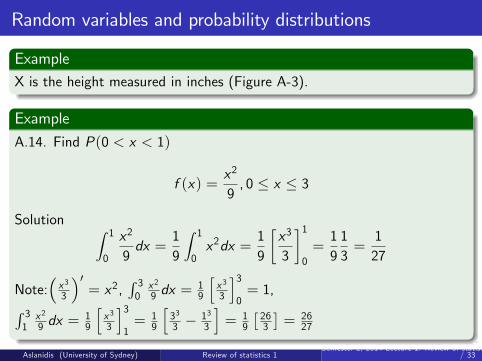
ExampleX is the height measured in inches (Figure A-3).
Example
A.14. Find P(0 < x < 1)
f (x) =x2
9, 0 � x � 3
Solution Z 1
0
x2
9dx =
19
Z 1
0x2dx =
19
�x3
3
�10=1913=127
Note:�x 33
�0= x2,
R 30x 29 dx =
19
hx 33
i30= 1,R 3
1x 29 dx =
19
hx 33
i31= 1
9
h333 �
133
i= 1
9
� 263
�= 26
27
Aslanidis (University of Sydney) Review of statistics 1Semester 2, 2014 Lecture 1: Review of statistics 1 20
/ 33
Random variables and probability distributions
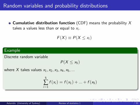
Cumulative distribution function (CDF) means the probability Xtakes a values less than or equal to xi .
F (X ) � P(X � xi )
ExampleDiscrete random variable
P(X � x5)where X takes values x1, x2, x3, x4, x5, ...
5
∑i=1f (xi ) = f (x1) + ...+ f (x5)
Aslanidis (University of Sydney) Review of statistics 1Semester 2, 2014 Lecture 1: Review of statistics 1 21
/ 33
Random variables and probability distributions
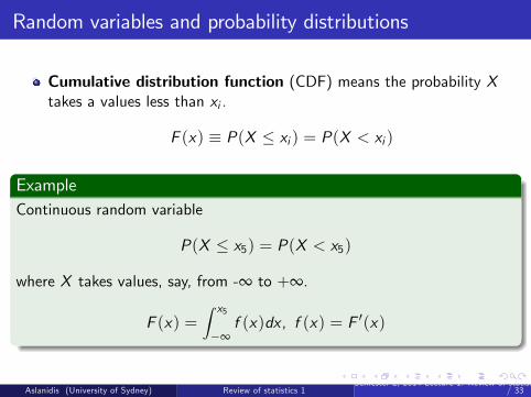
Cumulative distribution function (CDF) means the probability Xtakes a values less than xi .
F (x) � P(X � xi ) = P(X < xi )
ExampleContinuous random variable
P(X � x5) = P(X < x5)
where X takes values, say, from -∞ to +∞.
F (x) =Z x5
�∞f (x)dx , f (x) = F 0(x)
Aslanidis (University of Sydney) Review of statistics 1Semester 2, 2014 Lecture 1: Review of statistics 1 22
/ 33
Random variables and probability distributions
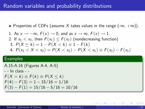
Properties of CDFs (assume X takes values in the range (-∞, +∞)).
1. As x ! �∞, F (x)! 0, and as x ! ∞, F (x)! 1.2. If x1 < x2, then F (x1) � F (x2) (nondecreasing function)3. P(X � k) = 1� P(X < k) � 1� F (k)4. P(x1 < X < x2) = P(X < x2)� P(X < x1) � F (x2)� F (x1)
ExamplesA.15-A.16 (Figures A-4, A-5)- - In class - -F (X = k) � F (k) � P(X � k)F (4)� F (3) = 1� 15/16 = 1/16F (3)� F (1) = 15/16� 5/16 = 10/16
Aslanidis (University of Sydney) Review of statistics 1Semester 2, 2014 Lecture 1: Review of statistics 1 23
/ 33
Multivariate probability distributions
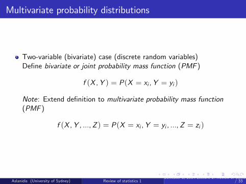
Two-variable (bivariate) case (discrete random variables)De�ne bivariate or joint probability mass function (PMF )
f (X ,Y ) = P(X = xi ,Y = yi )
Note: Extend de�nition to multivariate probability mass function(PMF )
f (X ,Y , ...,Z ) = P(X = xi ,Y = yi , ...,Z = zi )
Aslanidis (University of Sydney) Review of statistics 1Semester 2, 2014 Lecture 1: Review of statistics 1 24
/ 33
Multivariate probability distributions
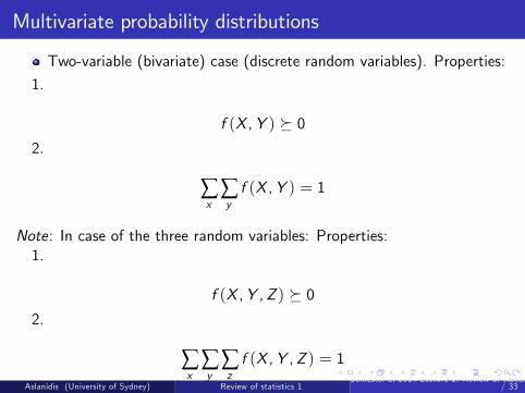
Two-variable (bivariate) case (discrete random variables). Properties:
1.
f (X ,Y ) � 02.
∑x
∑yf (X ,Y ) = 1
Note: In case of the three random variables: Properties:1.
f (X ,Y ,Z ) � 02.
∑x
∑y
∑zf (X ,Y ,Z ) = 1
Aslanidis (University of Sydney) Review of statistics 1Semester 2, 2014 Lecture 1: Review of statistics 1 25
/ 33
Multivariate probability distributions
ExampleA.17 (Tables A-2, A-3)- - In class - -
Aslanidis (University of Sydney) Review of statistics 1Semester 2, 2014 Lecture 1: Review of statistics 1 26
/ 33
Multivariate probability distributions
For continuous random variables the joint PDF can be de�nedanalogously, though the expresions are more involved.
f (X ,Y ) = P(a < X < b, c < Y < d) =Z b
a
Z d
cf (X ,Y )dXdY
Note that continuous random variables cannot take a single value!
Properties1.
f (X ,Y ) � 02. Z
x
Zyf (X ,Y )dXdY = 1
Aslanidis (University of Sydney) Review of statistics 1Semester 2, 2014 Lecture 1: Review of statistics 1 27
/ 33
Multivariate probability distributions
In relation to f (X ,Y ), f (X ) and f (Y ) are the univariate,unconditional or the marginal PMFs
f (X ) = ∑yf (X ,Y )
f (Y ) = ∑xf (X ,Y )
For continuous random variables the the marginal PDFs
f (X ) =Zyf (X ,S)ds
f (Y ) =Zxf (S ,Y )ds
Aslanidis (University of Sydney) Review of statistics 1Semester 2, 2014 Lecture 1: Review of statistics 1 28
/ 33
Multivariate probability distributions
De�ne conditional probability mass function (PMF )
f (X/Y ) = P(X = xi/Y = yi )f (Y /X ) = P(Y = yi/X = xi )
Di¤erently,
f (X/Y ) =f (X ,Y )f (Y )
f (Y /X ) =f (X ,Y )f (X )
Aslanidis (University of Sydney) Review of statistics 1Semester 2, 2014 Lecture 1: Review of statistics 1 29
/ 33
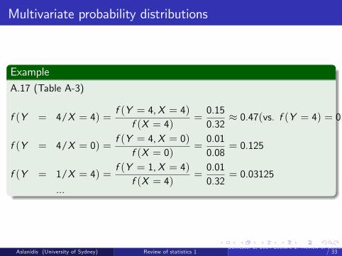
Multivariate probability distributions
ExampleA.17 (Table A-3)
f (Y = 4/X = 4) =f (Y = 4,X = 4)
f (X = 4)=0.150.32
� 0.47(vs. f (Y = 4) = 0.23)
f (Y = 4/X = 0) =f (Y = 4,X = 0)
f (X = 0)=0.010.08
= 0.125
f (Y = 1/X = 4) =f (Y = 1,X = 4)
f (X = 4)=0.010.32
= 0.03125
...
Aslanidis (University of Sydney) Review of statistics 1Semester 2, 2014 Lecture 1: Review of statistics 1 30
/ 33
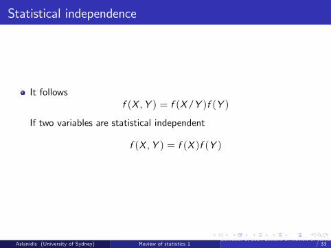
Statistical independence
It followsf (X ,Y ) = f (X/Y )f (Y )
If two variables are statistical independent
f (X ,Y ) = f (X )f (Y )
Aslanidis (University of Sydney) Review of statistics 1Semester 2, 2014 Lecture 1: Review of statistics 1 31
/ 33
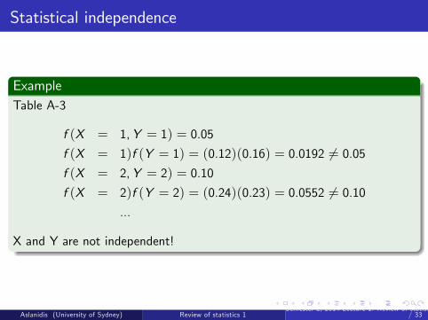
Statistical independence
ExampleTable A-3
f (X = 1,Y = 1) = 0.05
f (X = 1)f (Y = 1) = (0.12)(0.16) = 0.0192 6= 0.05f (X = 2,Y = 2) = 0.10
f (X = 2)f (Y = 2) = (0.24)(0.23) = 0.0552 6= 0.10...
X and Y are not independent!
Aslanidis (University of Sydney) Review of statistics 1Semester 2, 2014 Lecture 1: Review of statistics 1 32
/ 33
Bibliography
Appendix A from Gujarati Damodar N. and Dawn C. Porter (2010),Essentials of Econometrics, 4th ed, McGraw-Hill.
No tutorials this week.
Aslanidis (University of Sydney) Review of statistics 1Semester 2, 2014 Lecture 1: Review of statistics 1 33
/ 33
Copyright © 2022 FDOKUMEN