ECE 332 Feedback control systems - 12000.org
309
University Course ECE 332 Feedback control systems University of Wisconsin, Madison Fall 2015 My Class Notes Nasser M. Abbasi Fall 2015
-
Upload
khangminh22 -
Category
Documents
-
view
13 -
download
0
Transcript of ECE 332 Feedback control systems - 12000.org

University Course
ECE 332Feedback control systems
University of Wisconsin, MadisonFall 2015
My Class Notes
Nasser M. Abbasi
Fall 2015


Contents
1 Introduction 11.1 Syllabus . . . . . . . . . . . . . . . . . . . . . . . . . . . . . . . . . . . . . . . . 2
2 Class notes 52.1 Summary table . . . . . . . . . . . . . . . . . . . . . . . . . . . . . . . . . . . . 52.2 Lecture 1, Thursday Sept. 3, 2015 . . . . . . . . . . . . . . . . . . . . . . . . . 72.3 Lecture 2, Tuesday Sept. 8, 2015, Closed loop and Simulink review . . . . . . 82.4 Lecture 3, Thursday Sept. 10, 2015, Steady state and transient responses . . 92.5 Lecture 4, Tuesday Sept. 15, 2015, Performance specs, steady state error . . 112.6 Lecture 5, Thursday Sept. 17, 2015, MIMO matrix of transfer functions . . . 132.7 Lecture 6, Tuesday Sept. 22, 2015, Armature controlled DC motor with MIMO 182.8 Lecture 7, Wednesday Sept. 23, 2015, Start of signal graph and Mason rule . 222.9 Lecture 8, Thursday Sept. 24, 2015, Mason, benefits of feedback, non-linear
systems . . . . . . . . . . . . . . . . . . . . . . . . . . . . . . . . . . . . . . . . . 292.10 Lecture 9, Tuesday Sept. 29, 2015, First exam . . . . . . . . . . . . . . . . . . 332.11 Lecture 10, Thursday Oct. 1, 2015, No lecture . . . . . . . . . . . . . . . . . . 342.12 Lecture 11, Tuesday Oct. 6, 2015, Sensitivity of transfer function . . . . . . . 352.13 Lecture 12. Thursday Oct 8, 2015, control to reject noise and disturbances . 452.14 Lecture 13. Tuesday Oct 13, 2015, Noise rejection, second order systems . . 482.15 Lecture 14. Thursday Oct 15, 2015, More second order, Overshoot and
resonance . . . . . . . . . . . . . . . . . . . . . . . . . . . . . . . . . . . . . . . 522.16 Lecture 15. Tuesday Oct 20, 2015, Feedback using user specified time specs 552.17 Lecture 16. Thursday Oct 22, 2015, Routh stability . . . . . . . . . . . . . . . 612.18 Lecture 17, Tuesday Oct 27, 2015, Starting on root locus . . . . . . . . . . . . 652.19 Lecture 18, Thursday Oct 29, 2015, More root locus . . . . . . . . . . . . . . 682.20 Lecture 19, Nov. 3, 2015. No lecture . . . . . . . . . . . . . . . . . . . . . . . . 712.21 Lecture 20, Nov. 5, 2015. Roots Locus completed . . . . . . . . . . . . . . . . 712.22 Lecture 21, Nov 10 2015, Extension Root Locus . . . . . . . . . . . . . . . . . 752.23 Lecture 22, Nov 12 2015, second exam . . . . . . . . . . . . . . . . . . . . . . 782.24 Lecture 23, Nov 17 2015, Started Nyquist . . . . . . . . . . . . . . . . . . . . . 792.25 Lecture 24, Nov 19 2015, More Nyquist . . . . . . . . . . . . . . . . . . . . . . 822.26 Lecture 25, Tuesday Nov 24 2015, gain and phase margins . . . . . . . . . . . 942.27 Lecture 26, Thursday Nov. 26 2015, thanks giving, no class . . . . . . . . . . 972.28 Lecture 27, Tuesday December 1 2015, Start Bode frequency analysis . . . . 982.29 Lecture 28, Thursday December 4 2015, More Bode analysis . . . . . . . . . 105
iii

Contents CONTENTS
2.30 Lecture 29, Dec 8 2015, Bode gain and phase, e�ects of delay . . . . . . . . . 1092.31 Lecture 30, Dec 10 2015, Final exam . . . . . . . . . . . . . . . . . . . . . . . 1122.32 Cheat sheet . . . . . . . . . . . . . . . . . . . . . . . . . . . . . . . . . . . . . . 113
3 HWs 1153.1 HW 1 . . . . . . . . . . . . . . . . . . . . . . . . . . . . . . . . . . . . . . . . . . 1163.2 HW 2 . . . . . . . . . . . . . . . . . . . . . . . . . . . . . . . . . . . . . . . . . . 1263.3 HW 3 . . . . . . . . . . . . . . . . . . . . . . . . . . . . . . . . . . . . . . . . . . 1533.4 HW 4 . . . . . . . . . . . . . . . . . . . . . . . . . . . . . . . . . . . . . . . . . . 1803.5 HW 5 . . . . . . . . . . . . . . . . . . . . . . . . . . . . . . . . . . . . . . . . . . 1903.6 HW 6 . . . . . . . . . . . . . . . . . . . . . . . . . . . . . . . . . . . . . . . . . . 2143.7 HW 7 . . . . . . . . . . . . . . . . . . . . . . . . . . . . . . . . . . . . . . . . . . 2353.8 HW 8 . . . . . . . . . . . . . . . . . . . . . . . . . . . . . . . . . . . . . . . . . . 266
4 Exams 2994.1 First exam . . . . . . . . . . . . . . . . . . . . . . . . . . . . . . . . . . . . . . . 3004.2 Second exam . . . . . . . . . . . . . . . . . . . . . . . . . . . . . . . . . . . . . 3024.3 Final exam . . . . . . . . . . . . . . . . . . . . . . . . . . . . . . . . . . . . . . . 304
iv

Chapter 1
Introduction
Took this course in Fall 2015.
Instructor: professor B Ross Barmish O�ce Hours: Wednesday 1:00-2:30 PM
1

1.1. Syllabus CHAPTER 1. INTRODUCTION
1.1 Syllabus
ECE 332 – Handout Organization
• Course OrganizationLectures: B. R. Barmish (3613 Engineering Hall)E-mail: [email protected] Hours: Wednesday 1:00-2:30 PM
• No Official Course TextbookI will draw on material from the following textbooks on Reserve:
B. C. Kuo and F. Golnaraqhi, Automatic Control Systems, John Wileyand Sons, Ninth Edition, New York.
R. C. Dorf and R. H. Bishop, Modern Control Systems, Prentice Hall,Eleventh Edition, New York.
J. J. DiStefano, A. R. Stubberud and I. J. Williams, Feedback and ControlSystems, Schaum’s Outline Series, McGraw-Hill, New York.
Given the classical nature of the material, there are also hundreds ofsources on the web providing coverage of the ECE 332 topics with manyillustrative examples demonstrating the theory covered in class.
• Course Grading ComponentsTest 1: 25%; Tuesday, September 29, 2015Test 2: 30%; Thursday, November 12, 2015Test 3: 35%; Thursday, December 10, 2015Homework: 10% (Total of 7-10 Assignments)Instructor Discretion: Maximum 10% in any category
• Cancellations and Makeup ClassesNo lectures on Thursday October 1, Tuesday November 3 and TuesdayDecember 15; no office hours on Wednesday September 30.Makeup or Review Classes: Scheduled for 6 PM on Wednesday Septem-ber 23, Wednesday November 18 and Wednesday December 9.
• Additional PointsCourse Announcements: via e-mailHomework: E = excellent; S = satisfactory; U = unsatisfactoryMatlab/Simulink: Both used heavily in course
2

1.1. Syllabus CHAPTER 1. INTRODUCTION
ECE 332 – Handout Overview
Catalog Data: Modelling of continuous systems; computer-aided solu-tion to systems problems; feedback control systems; stability, frequencyresponse and transient response using root locus; frequency domain andstate variable methods.
Prerequisites: ECE 330 or consent of instructor.
No Required Textbook: I have a number of books on reserve. Inprevious offerings of this course, I have used:
B. C. Kuo and F. Golnaraqhi Automatic Control Systems, John Wileyand Sons.
Instructor: Professor B. Ross Barmish, ECE Department
Goals: This junior/senior level course develops the fundamentals associ-ated with the analysis, design and simulation of automatic control systems.
Prerequisites by Topic:1. Linear differential equations with constant coefficients2. Laplace transforms and transfer functions for linear systems3. Elementary matrix manipulations (such as determinant and inverse)4. Adequate familiarity with computers and use of various packages; thespecific package used in this course is Matlab/Simulink
Topics:1. Modelling of dynamic systems in a control context2. Block diagrams, signal flow graphs and Mason’s Rule3. Feedback in a sensitivity, linearization, disturbance context4. Steady state behavior of feedback systems5. Time response with emphasis on second order systems6. Stability analysis: criteria of Routh, Nyquist and Kharitonov7. The root locus and its variants8. Frequency response: Bode analysis of feedback systems9. Compensator design methods: PID, lead/lag and root locus methods10. Closed loop considerations: frequency response and Nichol’s plot
Computer Usage:Extensive use of Simulink and Matlab on weekly homework
3

1.1. Syllabus CHAPTER 1. INTRODUCTION
4

Chapter 2
Class notes
2.1 Summary table
These are my notes taken during lectures. Any errors in these notes, then all blames to meand not to the instructor.
date day event Topic
1. Sept 3, 2015 Thursday First class Introduction, Laplace transforms
2. Sept 8, 2015 Tuesday Closed loop and Simulink review
3. Sept 10, 2015 Thursday HW 1 Steady state and transient responses, di�er-ent feedback loops
4. Sept 15, 2015 Tuesday Performance specs, steady state error
5. Sept 17, 2015 Thursday MIMOmatrix of transfer functions, MIMOin a feedback loop.
6. Sept 22, 2015 Tuesday HW 2 Armature controlled DC motor withMIMO Example. signal graph
7. Sept 23, 2015 Wednesday make up Start of signal graph and Mason rule. Ma-son gain
8. Sept 24, 2015 Thursday HW3 Mason example, benefits of feedback, non-linear systems
9. Sept 29, 2015 Tuesday Exam 1 First exam
10. Oct. 1, 2015 Thursday No class
11. Oct. 6, 2015 Tuesday Sensitivity Sensitivity of transfer function with changeof parameters
12. Oct. 8, 2015 Thursday Noise rejection Design controls to reject noise and distur-bances using feedback
13. Oct. 13, 2015 Tuesday HW4. Second order Noise rejection, second order systems, dom-inant pole method
5

2.1. Summary table CHAPTER 2. CLASS NOTES
14. Oct. 15, 2015 Thursday Second order More second order, Overshoot and reso-nance calculations.
15. Oct 20, 2015 Tuesday Design for k Feedback using user specified time specsfor response
16. Oct 22, 2015 Thursday Stability/Ruth Routh stability table examples, stability, ex-amples
17. Oct 27, 2015 Tuesday Root Locus Starting on root locus, how 𝐾 a�ect poleslocations
18. Oct 29, 2015 Thursday Root Locus More root locus, more lemmas, up tolemma 4
19. Nov. 3, 2015 Tuesday No lecture
20. Nov 5, 2915 Thursday Root Locus Finished Root Locus, all 9 lemmas. Exam-ples given
21. Nov 10, 2015 Tuesday Extension Root Locus Review mid term 2, started extension rootlocus (will be on final)
22. Nov 12, 2015 Thursday Exam 2 Hard exam
23. Nov 17, 2015 Tuesday Starting Nyquist Started Nyquist. What it does and how tomake Nyquist path
24. Nov 19, 2015 Thursday More Nyquist More Nyquist. 2 examples. Handout given
25. Nov 24, 2015 Tuesday More Nyquist More Nyquist. Using for stability, gain andphase margins
26. Nov 26, 2015 Thursday thanks giving No class
27. Dec 1, 2015 Tuesday Starting Bode Start Bode frequency analysis
28. Dec 4, 2015 Thursday More Bode More Bode analysis and examples
29. Dec 8,2015 Tuesday Bode gain and phase E�ects of delay on Bode, gain and phasemargins.
30. Dec 10,2015 Thursday Final exam Finals
6

2.2. Lecture 1, Thursday Sept. 3, 2015 CHAPTER 2. CLASS NOTES
2.2 Lecture 1, Thursday Sept. 3, 2015
Introduction to Laplace transform, handouts, syllabus overview
7
2.3. Lecture 2, Tuesday Sept. 8, 2015, . . . CHAPTER 2. CLASS NOTES
2.3 Lecture 2, Tuesday Sept. 8, 2015, Closed loop andSimulink review
Discussion on Laplace transform. We want to be able to switch from 𝑡 to 𝑠 domain andback. For tough ones, use tables. In Matlab use syms. Examples shown how to use syms inMatlab and obtain the Laplace and inverse Laplace transforms. Use of expand and simplifycommands.
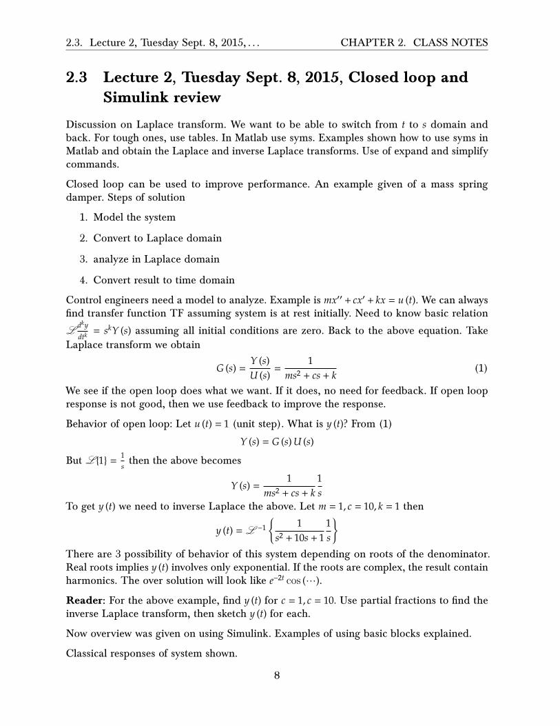
Closed loop can be used to improve performance. An example given of a mass springdamper. Steps of solution
1. Model the system
2. Convert to Laplace domain
3. analyze in Laplace domain
4. Convert result to time domain
Control engineers need a model to analyze. Example is 𝑚𝑥′′ + 𝑐𝑥′ +𝑘𝑥 = 𝑢 (𝑡). We can alwaysfind transfer function TF assuming system is at rest initially. Need to know basic relation
ℒ𝑑𝑘𝑦𝑑𝑡𝑘
= 𝑠𝑘𝑌 (𝑠) assuming all initial conditions are zero. Back to the above equation. TakeLaplace transform we obtain
𝐺 (𝑠) =𝑌 (𝑠)𝑈 (𝑠)
=1
𝑚𝑠2 + 𝑐𝑠 + 𝑘(1)
We see if the open loop does what we want. If it does, no need for feedback. If open loopresponse is not good, then we use feedback to improve the response.
Behavior of open loop: Let 𝑢 (𝑡) = 1 (unit step). What is 𝑦 (𝑡)? From (1)
𝑌 (𝑠) = 𝐺 (𝑠)𝑈 (𝑠)
But ℒ{1} = 1𝑠 then the above becomes
𝑌 (𝑠) =1
𝑚𝑠2 + 𝑐𝑠 + 𝑘1𝑠
To get 𝑦 (𝑡) we need to inverse Laplace the above. Let 𝑚 = 1, 𝑐 = 10, 𝑘 = 1 then
𝑦 (𝑡) = ℒ −1 �1
𝑠2 + 10𝑠 + 11𝑠�
There are 3 possibility of behavior of this system depending on roots of the denominator.Real roots implies 𝑦 (𝑡) involves only exponential. If the roots are complex, the result containharmonics. The over solution will look like 𝑒−2𝑡 cos (⋯).
Reader: For the above example, find 𝑦 (𝑡) for 𝑐 = 1, 𝑐 = 10. Use partial fractions to find theinverse Laplace transform, then sketch 𝑦 (𝑡) for each.
Now overview was given on using Simulink. Examples of using basic blocks explained.
Classical responses of system shown.
8

2.4. Lecture 3, Thursday Sept. 10, 2015, . . . CHAPTER 2. CLASS NOTES
2.4 Lecture 3, Thursday Sept. 10, 2015, Steady state andtransient responses
Open loop vs. closed loop. In closed loop we add a controller to obtain desired response.
H(s) G(s)R(s)
Y (s)U(s)E(s)
feed forward path
plantcontroller
error signal
+−
Another possibility is to put the controller in the feedback path
H(s)
G(s)R(s)
Y (s)E(s)
feed back path
plant
controller
error signal
+
−
Now we will find the closed loop TF for the feed forward path configuration.
𝑌 (𝑠) = 𝐸 (𝑠)𝐻 (𝑠) 𝐺 (𝑠)𝐸 (𝑠) = 𝑅 (𝑠) − 𝑌 (𝑠)
Substituting the second equation in the first gives
𝑌 (𝑠) = (𝑅 (𝑠) − 𝑌 (𝑠))𝐻 (𝑠) 𝐺 (𝑠)= 𝑅 (𝑠)𝐻 (𝑠) 𝐺 (𝑠) − 𝑌 (𝑠)𝐻 (𝑠) 𝐺 (𝑠)
Hence
𝑌 (𝑠) (1 + 𝐻 (𝑠) 𝐺 (𝑠)) = 𝑅 (𝑠)𝐻 (𝑠) 𝐺 (𝑠)𝑌 (𝑠)𝑅 (𝑠)
=𝐻 (𝑠) 𝐺 (𝑠)
1 + 𝐻 (𝑠) 𝐺 (𝑠)
Reader: Do the above for the feedback path configuration. We should get 𝑌(𝑠)𝑅(𝑠) =
𝐺(𝑠)1+𝐻(𝑠)𝐺(𝑠)
Reader: For the feedforward case, find the error transfer function 𝐸(𝑠)𝑅(𝑠)
Working with the feedforward case. 𝐸 = 𝑅 − 𝑌. We want 𝐸 = 0 for tracking. Most commonchoices of 𝐻 (𝑠) are
1. 𝐻 = 𝑘 a constant. Called proportional or pure gain.
9

2.4. Lecture 3, Thursday Sept. 10, 2015, . . . CHAPTER 2. CLASS NOTES
2. 𝐻 = 𝑘1 +𝑘2𝑠 The second term is an integrator. This is called PI controller.
3. 𝐻 = 𝑘1 +𝑘2𝑠 + 𝑠𝑘3. This is called PID. Note that 𝑠 is derivative. So if there is lots of
noise in the 𝐸 signal, this will cause problems since derivative of noise generated largesignal (large actuating signal). So it is safe to use an integrator, but not always saveto use derivative, unless we know that the error signal will always be smooth.
For example, let 𝐺 (𝑠) = 1𝑠+2 with a unit step �1𝑠 � input. Then in the openloop, 𝑌 (𝑠) = 1
𝑠+21𝑠 or
𝑦 (𝑡) = 12 −
12𝑒
−2𝑡. Now we close the loop, using the feedforward configuration and add a puregain controller 𝑘. Hence
𝑌𝑅=
𝐻𝐺1 + 𝐻𝐺
=𝑘 1𝑠+2
1 + 𝑘 1𝑠+2
=𝑘
𝑠 + (2 + 𝑘)
Now 𝑅 (𝑠) = 1𝑠 , hence
𝑌 (𝑠) =1𝑠
𝑘𝑠 + (2 + 𝑘)
And
𝑦 (𝑡) =
steady state response
�𝑘𝑘+ 2
−
transient response
���������������𝑘𝑘 + 2
𝑒−𝑡(𝑘+2)
By design, we want 𝑦 (𝑡) to track 𝑟 (𝑡) which is unit step in this case. Also we want the transientresponse to go away quickly. In this example, only when 𝑘 very large do we approach asteady state close to one. But in practice having very large gain is not good due to sensitivityproblems. (will talk about sensitivity later in the course). Also large 𝑘might lead to actuatingsignal that can not be satisfied. Note also, no matter how large 𝑘 is, we can’t obtain perfecttracking. Some application might require perfect tracking.
Reader: Redo the analysis above using integrator only controller. i.e. 𝐻 (𝑠) = 𝑘𝑠 and see if
𝑦 (𝑡) will now track the input at steady state.
Final value theorem: Suppose 𝐹 (𝑠) = 𝑁(𝑠)𝐷(𝑠) is stable, then
lim𝑡→∞
𝑓 (𝑡) = lim𝑠→0
𝑠𝐹 (𝑠)
10
2.5. Lecture 4, Tuesday Sept. 15, 2015, . . . CHAPTER 2. CLASS NOTES
2.5 Lecture 4, Tuesday Sept. 15, 2015, Performancespecs, steady state error
Watch today for email on HW1 solution and HW2. See this you tube on steady state error??
Today we will spend more time on final value theorem. Then talk about typical specs forcontrol system.
F.V.T. is important for tracking. Given 𝐹 (𝑠), does 𝑓 (𝑡) have a final value? ie. does lim𝑡→∞ 𝑓 (𝑡)exist? Sometimes infinity is allowed as final value. But many times we do not have a finalvalue, such as for period signals such as cos (𝑡).
When can we apply F.V.T. ? In practice, 𝐹 (𝑠) should be stable. This means the poles shouldbe in the left half plane. But we allow one pole to be at the origin. Example 1
𝑠+1 ⟺𝑒−𝑡. How
about 1𝑠+1
1𝑠 ? Final value still exist.
Reader Consider 𝐹 (𝑠) = 1𝑠2
1𝑠+1
When 𝐹 (𝑠) is stable, then lim𝑡→∞ 𝑓 (𝑡) = lim𝑠→0 𝑠𝐹 (𝑠) .
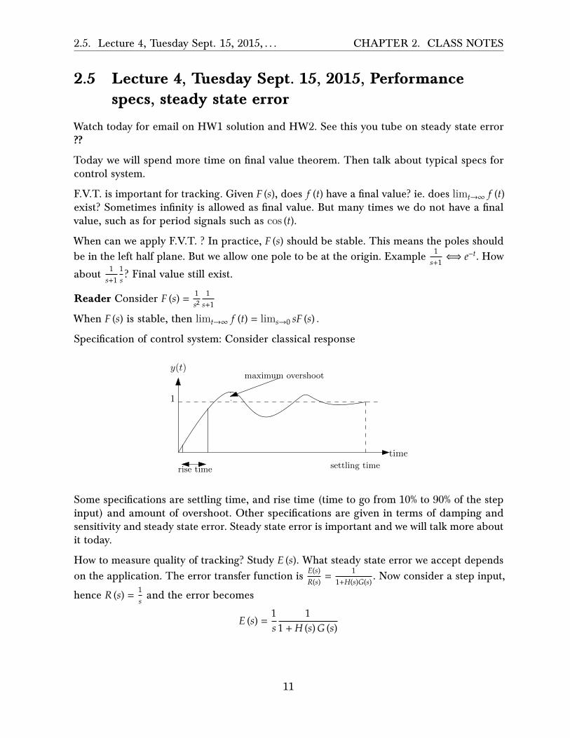
Specification of control system: Consider classical response
time
y(t)
1
maximum overshoot
rise time settling time
Some specifications are settling time, and rise time (time to go from 10% to 90% of the stepinput) and amount of overshoot. Other specifications are given in terms of damping andsensitivity and steady state error. Steady state error is important and we will talk more aboutit today.
How to measure quality of tracking? Study 𝐸 (𝑠). What steady state error we accept dependson the application. The error transfer function is 𝐸(𝑠)
𝑅(𝑠) =1
1+𝐻(𝑠)𝐺(𝑠) . Now consider a step input,
hence 𝑅 (𝑠) = 1𝑠 and the error becomes
𝐸 (𝑠) =1𝑠
11 + 𝐻 (𝑠) 𝐺 (𝑠)
11

2.5. Lecture 4, Tuesday Sept. 15, 2015, . . . CHAPTER 2. CLASS NOTES
Assuming F.V.T. applies (i.e. 𝐸 (𝑠) is stable) then
lim𝑡→∞
𝑒 (𝑡) = lim𝑠→0
𝑠𝐸 (𝑠)
= lim𝑠→0
11 + 𝐻 (𝑠) 𝐺 (𝑠)
=1
1 + 𝐻 (0)𝐺 (0)
Example, if 𝐺 (𝑠) = 1𝑠2+2𝑠+4 then lim𝑡→∞ 𝑒 (𝑡) =
45 which is not good. We want this to be zero.
So for 11+𝐻(0)𝐺(0) to be zero, we want 𝐻 (0)𝐺 (0) to be very large. This means 𝐻 (𝑠) should have
1𝑠 in it as a factor. This means an integrator. Hence an integrator in 𝐻 (𝑠) guarantees thaterror goes to zero when the input is step.
Reader For the mass spring damper, 𝐺 = 1𝑚𝑠2+𝑐𝑠+𝑘 design 𝐻 (𝑠) leading to zero steady state
error for step command. Use 𝑘𝑠 in 𝐻 (𝑠).
What if the input is ramp? which is 1𝑠2 ? Then
𝐸 (𝑠) =1𝑠2
11 + 𝐻 (𝑠) 𝐺 (𝑠)
lim𝑡→∞
𝑒 (𝑡) = lim𝑠→0
𝑠𝐸 (𝑠)
= lim𝑠→0
1𝑠
11 + 𝐻 (𝑠) 𝐺 (𝑠)
= lim𝑠→0
1𝑠𝐻 (𝑠) 𝐺 (𝑠)
So now we need 𝐻 (𝑠) to have 1𝑠2 factor in it, so that it becomes very large at 𝑠 = 0 and cause
the error to go to zero. This means 2 integrator in series. This means to track 𝑟 (𝑡) = 𝑡𝑘 weneed 𝑘 + 1 integrators in 𝐻 (𝑠) to get zero error at steady state.
Finally for any signal 𝑟 (𝑡) = ∑𝑘𝑖=0 𝑎𝑖𝑡
𝑖, we need 𝑘 + 1 integrators, since the largest term is theonly term that needs to be satisfied, due to linearity of the system. So given a complicatedpolynomial, we look at the largest power and this tells us how many integrators we need forzero steady state error.
12

2.6. Lecture 5, Thursday Sept. 17, 2015, . . . CHAPTER 2. CLASS NOTES
2.6 Lecture 5, Thursday Sept. 17, 2015, MIMO matrixof transfer functions
Today lecture on more complicated systems. So far we talked about SISO in the mostcommon configuration
H(s) G(s)R(s)
Y (s)U(s)E(s)
feed forward path
plantcontroller
error signal
+−
But systems come in more complicated forms. We need to reformulate complicated systemsthis the above common configuration form to be able to analyze them. There can be multipleinputs and multiple outputs as well, more blocks, loops, etc.. To illustrate, given this system
R(s)Y (s)H1(s)
H2(s)
G(s)
H3(s)
R(s)−H3(s)Y (s)
H2(s)(R(s)−H3(s)Y (s))
H1(s)G(s)(R(s)−H3(s)Y (s))
+ ++
-
How to find 𝑌(𝑠)𝑅(𝑠)? We can go to first principles. Use signal analysis. The goal is to find 𝑌(𝑠)
𝑅(𝑠)
without all the intermediate variables. i.e we want 𝑌(𝑠)𝑅(𝑠) to be a function of only the shown
blocks transfer functions 𝐻1, 𝐻2, 𝐻3, 𝐺. Hence
𝑌 = 𝐻2 (𝑅 − 𝐻3𝑌) + 𝐻1𝐺 (𝑅 − 𝐻3𝑌)
Solve for 𝑌 in terms of 𝑅 from the above
𝑌 = 𝐻2𝑅 − 𝐻2𝐻3𝑌 + 𝐻1𝐺𝑅 − 𝐻1𝐺𝐻3𝑌𝑌 (1 + 𝐻2𝐻3 + 𝐻1𝐻3𝐺) = 𝑅 (𝐻2 + 𝐻1𝐺)
Hence𝑌𝑅=
𝐻2 + 𝐻1𝐺1 + 𝐻2𝐻3 + 𝐻1𝐻3𝐺
=𝐻2 + 𝐻1𝐺
1 + 𝐻3 (𝐻2 + 𝐻1𝐺)But for more complicated systems, with more loops and inner blocks, this process canbecome more complicated and one can make mistakes. We need a more systematic way.Next lecture we will look at Mason formula to do the above.
For the rest of the lecture we will look at multiple input, multiple output (MIMO). Motivationexample, is an electric circuit with say 2 input ports (voltages 𝑉1, 𝑉2) and 2 output ports,
13

2.6. Lecture 5, Thursday Sept. 17, 2015, . . . CHAPTER 2. CLASS NOTES
way 𝑉3, 𝑉4. In block diagram we draw
G(s)
U1(s)
U2(s)
Y1(s)
Y2(s)
In the above 𝐺 (𝑠) will now be a matrix of 𝐺𝑖𝑗 (𝑠) transfer functions. The above is the openloop block diagram of a 2 input/2 outputs system. Internally, there can be cross coupling.Meaning, one input can a�ect all of some of the other outputs. Like this
G(s)
U1(s)
U2(s)
Y1(s)
Y2(s)
So we need a transfer function 𝐺𝑖𝑗 (𝑠) from each input 𝑈𝑗 to each output 𝑉𝑖. So need a totalof 4 transfer functions in this case.⎛
⎜⎜⎜⎜⎝𝑌1 (𝑠)𝑌2 (𝑠)
⎞⎟⎟⎟⎟⎠ =
⎛⎜⎜⎜⎜⎝𝐺11 (𝑠) 𝐺12 (𝑠)𝐺21 (𝑠) 𝐺22 (𝑠)
⎞⎟⎟⎟⎟⎠
⎛⎜⎜⎜⎜⎝𝑈1 (𝑠)𝑈2 (𝑠)
⎞⎟⎟⎟⎟⎠
Expanding
𝑌1 (𝑠) = 𝐺11 (𝑠)𝑈1 (𝑠) + 𝐺12 (𝑠)𝑈2 (𝑠)𝑌2 (𝑠) = 𝐺21 (𝑠)𝑈1 (𝑠) + 𝐺22 (𝑠)𝑈2 (𝑠)
Suppose we want to find 𝐺11 (𝑠) only. How to do this?
𝐺11 (𝑠) =𝑌1 (𝑠)𝑈1 (𝑠) 𝑈2=0
In practice, this is done by shorting the input 𝑈2 (i.e making the input 𝑈2 zero) and thensupplying the input 𝑈1 only and then measuring the output at port 𝑌2.
Reader Create transfer function model for this circuit
+
+L
R2 Y2
C Y1
U2
U1
R1
14

2.6. Lecture 5, Thursday Sept. 17, 2015, . . . CHAPTER 2. CLASS NOTES
In the above, there are 2 input voltages 𝑈1, 𝑈2 and 2 outputs 𝑌1, 𝑌2. Notice in the above wecan not use the impedance method and use the voltage divider as in the first problem inHW1. We need to setup 2 loop equations and solve. Another possibility is to short 𝑈1 andthen solve the circuit without 𝑈1 and then short 𝑈2 input and then solve the circuit again.
Reader solution
We first set up the 2 loops, and obtain these 2 equations
𝑢1 − 𝑢2 = 𝐼1 �𝑅1 +1𝐶𝑠�
− 𝐼21𝐶𝑠
(1)
0 = 𝐼2 �1𝐶𝑠
+ 𝐿𝑠 + 𝑅2� − 𝐼11𝐶𝑠
(2)
And the output equations are
𝑌1 = (𝐼1 − 𝐼2)1𝐶𝑠
𝑌2 = 𝐼2𝑅2
Solving (1,2) for 𝐼1, 𝐼2 gives
𝐼1 =1 + 𝐶𝑠 (𝑅2 + 𝐿𝑠) (𝑢1 − 𝑢2)
𝑅2 + 𝐿𝑠 + 𝑅1 (1 + 𝐶𝑠 (𝑅2 + 𝐿𝑠))
𝐼2 =𝑢1 − 𝑢2
𝑅2 + 𝐿𝑠 + 𝑅1 (1 + 𝐶𝑠 (𝑅2 + 𝐿𝑠))
Using these in the output equations gives
𝑌1 = �1 + 𝐶𝑠 (𝑅2 + 𝐿𝑠) (𝑢1 − 𝑢2)
𝑅2 + 𝐿𝑠 + 𝑅1 (1 + 𝐶𝑠 (𝑅2 + 𝐿𝑠))−
𝑢1 − 𝑢2𝑅2 + 𝐿𝑠 + 𝑅1 (1 + 𝐶𝑠 (𝑅2 + 𝐿𝑠))
�1𝐶𝑠
𝑌2 =𝑢1 − 𝑢2
𝑅2 + 𝐿𝑠 + 𝑅1 (1 + 𝐶𝑠 (𝑅2 + 𝐿𝑠))𝑅2
These can be written in matrix form as
⎛⎜⎜⎜⎜⎝𝑌1
𝑌2
⎞⎟⎟⎟⎟⎠ =
⎛⎜⎜⎜⎜⎜⎝
𝑅2+𝐿𝑠𝑅2+𝐿𝑠+𝑅1(1+𝐶𝑠(𝑅2+𝐿𝑠))
𝑅2+𝐿𝑠𝑅2+𝐿𝑠+𝑅1(1+𝐶𝑠(𝑅2+𝐿𝑠))
𝑅2𝑅2+𝐿𝑠+𝑅1(1+𝐶𝑠(𝑅2+𝐿𝑠))
𝑅2𝑅2+𝐿𝑠+𝑅1(1+𝐶𝑠(𝑅2+𝐿𝑠))
⎞⎟⎟⎟⎟⎟⎠
⎛⎜⎜⎜⎜⎝𝑢1𝑢2
⎞⎟⎟⎟⎟⎠
More generally, given 𝑚 inputs and 𝑟 outputs then𝑟×1⏞𝑌 =
𝑟×𝑚⏞𝐺
𝑚×1⏞𝑈
15

2.6. Lecture 5, Thursday Sept. 17, 2015, . . . CHAPTER 2. CLASS NOTES
So 𝐺 is an 𝑟 × 𝑚 matrix.
𝐺𝑖𝑗 (𝑠) =𝑌𝑗 (𝑠)𝑈𝑖 (𝑠) 𝑈𝑘=0 for 𝑘≠𝑗
Now we are ready to take a MIMO open loop block and imbed it in a feedback loop as wedid with SISO. The process is the same, but now we have to be careful with order sincethese are now matrices and not scalars. Given the system
G(s)
r ×mU(s)m× 1
Y (s)r × 1
This is multi-line input This is multi-line output
Now we want to add a controller as before. Hence we obtain
G(s)r×m
U(s)m×1
H(s)m×r
controller plant
E(s)r×1R(s)r×1
Input signals
Y (s)r×1
feedback with MIMO system
Say we want 𝑌𝑖 to track input 𝑅𝑖. So now we want the closed loop transfer function as wedid with SISO, but now we have to do it using vectors and matrices. So order is important.As before we write
𝑌 (𝑠) =
closed loop T.F. matrix
�������������������������������������(𝐼 + 𝐺 (𝑠)𝐻 (𝑠))−1𝐺 (𝑠)𝐻 (𝑠) 𝑅 (𝑠)
In the above, the closed loop transfer function is (𝐼 + 𝐺 (𝑠)𝐻 (𝑠))−1 where 𝐼 is the identitymatrix or size 𝑟 × 𝑟
𝑟×1�𝑌(𝑠) = �𝐼 +
𝑟×𝑚�𝐺(𝑠)
𝑚×𝑟�𝐻(𝑠)�
−1 𝑟×𝑚�𝐺(𝑠)
𝑚×𝑟�𝐻(𝑠)
𝑟×1�𝑅(𝑠)
Example, given𝐺 (𝑠) =⎛⎜⎜⎜⎜⎝1 1
𝑠2
𝑠+1 1
⎞⎟⎟⎟⎟⎠ ,𝐻 (𝑠) =
⎛⎜⎜⎜⎜⎝−2 −1−3 1
𝑠
⎞⎟⎟⎟⎟⎠ find closed loop transfer function (𝐼 + 𝐺𝐻)
−1𝐺𝐻
First,
𝐺𝐻 =⎛⎜⎜⎜⎜⎝1 1
𝑠2
𝑠+1 1
⎞⎟⎟⎟⎟⎠
⎛⎜⎜⎜⎜⎝−2 −1−3 1
𝑠
⎞⎟⎟⎟⎟⎠
=⎛⎜⎜⎜⎜⎝−3𝑠 − 2
1𝑠2 − 1
− 4𝑠+1 − 3
1𝑠 −
2𝑠+1
⎞⎟⎟⎟⎟⎠
16

2.6. Lecture 5, Thursday Sept. 17, 2015, . . . CHAPTER 2. CLASS NOTES
Then
(𝐼 + 𝐺𝐻)−1𝐺𝐻 =⎛⎜⎜⎜⎜⎝
⎛⎜⎜⎜⎜⎝1 00 1
⎞⎟⎟⎟⎟⎠ +
⎛⎜⎜⎜⎜⎝−3𝑠 − 2
1𝑠2 − 1
− 4𝑠+1 − 3
1𝑠 −
2𝑠+1
⎞⎟⎟⎟⎟⎠
⎞⎟⎟⎟⎟⎠
−1 ⎛⎜⎜⎜⎜⎝−3𝑠 − 2
1𝑠2 − 1
− 4𝑠+1 − 3
1𝑠 −
2𝑠+1
⎞⎟⎟⎟⎟⎠
=
⎛⎜⎜⎜⎜⎜⎝− 𝑠3+𝑠4𝑠3+10𝑠2−2𝑠−4
14𝑠3+10𝑠2−2𝑠−4
�−𝑠3 − 𝑠2 + 𝑠 + 1�
− 3𝑠3+7𝑠2
4𝑠3+10𝑠2−2𝑠−41
3𝑠2+7𝑠�3𝑠3 + 7𝑠2� 𝑠2+4𝑠+3
4𝑠3+10𝑠2−2𝑠−4
⎞⎟⎟⎟⎟⎟⎠
⎛⎜⎜⎜⎜⎝−3𝑠 − 2
1𝑠2 − 1
− 4𝑠+1 − 3
1𝑠 −
2𝑠+1
⎞⎟⎟⎟⎟⎠
=
⎛⎜⎜⎜⎜⎜⎜⎜⎝
12�−2𝑠3−5𝑠2+𝑠+2�
�−5𝑠3 − 10𝑠2 + 𝑠 + 4� −12(𝑠 − 1) (𝑠+1)2
−2𝑠3−5𝑠2+𝑠+2
−12𝑠
2 3𝑠+7−2𝑠3−5𝑠2+𝑠+2 −1
23𝑠3+6𝑠2−5𝑠−4−2𝑠3−5𝑠2+𝑠+2
⎞⎟⎟⎟⎟⎟⎟⎟⎠
=1
−2𝑠3 − 5𝑠2 + 𝑠 + 2
⎛⎜⎜⎜⎜⎝12�−5𝑠3 − 10𝑠2 + 𝑠 + 4� −1
2(𝑠 − 1) (𝑠 + 1)2
−12𝑠
2 (3𝑠 + 7) −12�3𝑠3 + 6𝑠2 − 5𝑠 − 4�
⎞⎟⎟⎟⎟⎠
Verify using Matlab syms.
17

2.7. Lecture 6, Tuesday Sept. 22, 2015, . . . CHAPTER 2. CLASS NOTES
2.7 Lecture 6, Tuesday Sept. 22, 2015, Armaturecontrolled DC motor with MIMO
Reminder, class tomorrow at 6 pm. No class Oct. 1, 2015. Test on sept 29. Exam everythingup to and including MIMO.
Consolidating exampleWe will cover main points in class so far, from modeling, to findingT.F. to building block diagrams and MIMO. The example is to model Armature controlledDC motor. From physical system to di�erential equations.
iF
Va
+
-
Ra
La
back emf
iaindependently applied field current
θ
motor arm
TL(s)
applied torquecommand
to rotate motor arm
Applying kircho� voltage rule on the circuit gives
𝑉𝑎 (𝑡) = 𝑅𝑎𝑖𝑎 + 𝐿𝑎𝑑𝑖𝑎𝑑𝑡+ 𝑘1𝜔 (1)
Where 𝑘1𝜔 is the backemf voltage induced by the rotating arm and 𝜔 is the angular velocity𝑑𝜃𝑑𝑡 of the motor arm. In addition, we have a mechanical relation between the applied torque𝑡𝐿 and 𝑖𝑎
𝐽𝑑𝜔𝑑𝑡
= 𝑘2𝑖𝑎 − 𝑡𝐿 (2)
Finally
𝑡𝐿 = 𝑘𝐿𝑖𝑎 (3)
The above are the three equations needed. Let 𝑘1 = 𝑘2 = 𝑘𝑚. Taking Laplace transform ofeach gives
18

2.7. Lecture 6, Tuesday Sept. 22, 2015, . . . CHAPTER 2. CLASS NOTES
𝑉𝑎 (𝑠) = 𝑅𝑎𝐼𝑎 (𝑠) + 𝑠𝐿𝑎𝐼𝑎 (𝑠) + 𝑠𝑘𝑚𝜃 (𝑠) (1A)
𝑠𝐽𝑊 (𝑠) = 𝑘2𝐼𝑎 (𝑠) − 𝑇𝐿 (𝑠) (2A)
𝑇𝐿 (𝑠) = 𝑘𝐿𝐼𝑎 (𝑠) (3A)
Notice that 𝑊(𝑠) is the Laplace transform of 𝜔 and that 𝜔 = 𝑑𝜃𝑑𝑡 or 𝑊(𝑠) = 𝑠𝜃 (𝑠), hence
𝑊(𝑠)𝑠 = 𝜃 (𝑠). Now we build the block diagram from the above three equations. The input is
𝑉𝑎 (𝑠) and the output is 𝜃 (𝑠). From the above we find
𝐼𝑎 (𝑠) =𝑉𝑎 (𝑠) − 𝑘𝑚𝑊(𝑠)
𝑅𝑎 + 𝑠𝐿
𝑊 (𝑠) =𝑘𝑚𝐼𝑎 (𝑠) − 𝑇𝐿 (𝑠)
𝐽𝑠And the block diagram is
Va(s)1
Ls+Ra
Ia(s)KL
+
Km
TL(s)
+
-1Js
W (s)
Km
-1s θ(s)
Reader: Find the transfer function 𝜃(𝑠)𝑉𝑎(𝑠)
. Consider step input. Find steady state 𝜃 (∞) forstep input. Does it go to one? Note, every RLC circuit is stable circuit. Called passive circuit.
Reader answer
I get this
𝐸 = 𝑅 (𝑠) − 𝑠𝜃𝑘𝑚
𝜃 = 𝐸 (𝑠) �𝑘𝑚 − 𝑘𝐿
(𝑅𝑎 + 𝑠𝐿) 𝑠2𝐽�
Hence
19
2.7. Lecture 6, Tuesday Sept. 22, 2015, . . . CHAPTER 2. CLASS NOTES
𝜃 = (𝑅 (𝑠) − 𝑠𝜃𝑘𝑚) �𝑘𝑚 − 𝑘𝐿
(𝑅𝑎 + 𝑠𝐿) 𝑠2𝐽�
𝜃 = 𝑅 (𝑠) �𝑘𝑚 − 𝑘𝐿
(𝑅𝑎 + 𝑠𝐿) 𝑠2𝐽� − 𝑠𝜃𝑘𝑚 �
𝑘𝑚 − 𝑘𝐿(𝑅𝑎 + 𝑠𝐿) 𝑠2𝐽
�
𝜃 �1 + 𝑠𝑘𝑚 �𝑘𝑚 − 𝑘𝐿
(𝑅𝑎 + 𝑠𝐿) 𝑠2𝐽�� = 𝑅 (𝑠) �
𝑘𝑚 − 𝑘𝐿(𝑅𝑎 + 𝑠𝐿) 𝑠2𝐽
�
𝜃 (𝑠)𝑅 (𝑠)
=� 𝑘𝑚−𝑘𝐿(𝑅𝑎+𝑠𝐿)𝑠2𝐽
�
1 + 𝑠𝑘𝑚 �𝑘𝑚−𝑘𝐿
(𝑅𝑎+𝑠𝐿)𝑠2𝐽�
=𝑘𝑚 − 𝑘𝐿
𝑠2𝐽 (𝑅𝑎 + 𝑠𝐿) + 𝑠𝑘𝑚 (𝑘𝑚 − 𝑘𝐿)
=𝑘𝑚 − 𝑘𝐿
𝑠3𝐽𝐿 + 𝑠2𝐽𝑅𝑎 + 𝑠𝑘2𝑚 − 𝑠𝑘𝑚𝑘𝐿
=(𝑘𝑚 − 𝑘𝐿)
𝐽𝐿1
𝑠3 + 𝑠2 𝑅𝑎𝐿2 + 𝑠 �𝑘2𝑚−𝑘𝑚𝑘𝐿
𝐽𝐿�
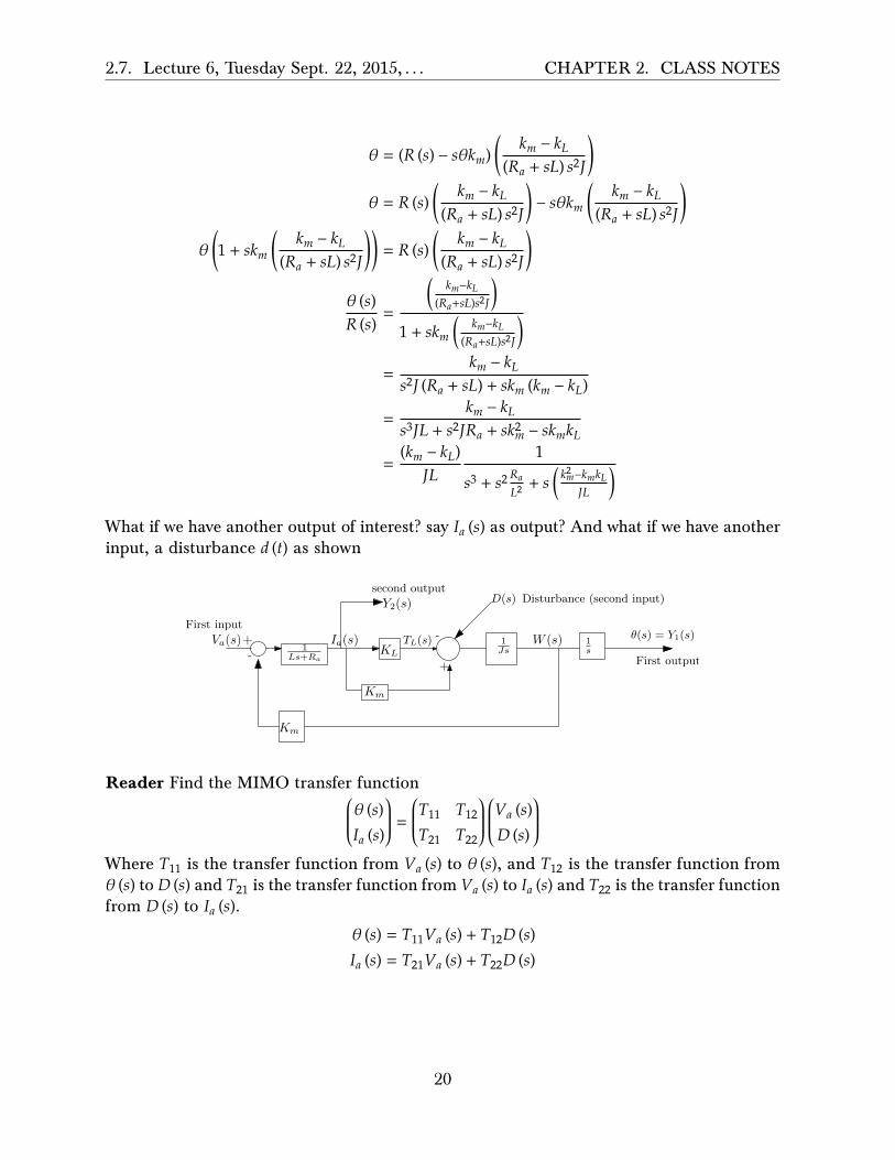
What if we have another output of interest? say 𝐼𝑎 (𝑠) as output? And what if we have anotherinput, a disturbance 𝑑 (𝑡) as shown
Va(s)1
Ls+Ra
Ia(s)KL
+
Km
TL(s)
+
-1Js
W (s)
Km
-1s
Y2(s)second output
θ(s) = Y1(s)
First output
D(s) Disturbance (second input)
First input
Reader Find the MIMO transfer function⎛⎜⎜⎜⎜⎝𝜃 (𝑠)𝐼𝑎 (𝑠)
⎞⎟⎟⎟⎟⎠ =
⎛⎜⎜⎜⎜⎝𝑇11 𝑇12𝑇21 𝑇22
⎞⎟⎟⎟⎟⎠
⎛⎜⎜⎜⎜⎝𝑉𝑎 (𝑠)𝐷 (𝑠)
⎞⎟⎟⎟⎟⎠
Where 𝑇11 is the transfer function from 𝑉𝑎 (𝑠) to 𝜃 (𝑠), and 𝑇12 is the transfer function from𝜃 (𝑠) to 𝐷 (𝑠) and 𝑇21 is the transfer function from 𝑉𝑎 (𝑠) to 𝐼𝑎 (𝑠) and 𝑇22 is the transfer functionfrom 𝐷 (𝑠) to 𝐼𝑎 (𝑠).
𝜃 (𝑠) = 𝑇11𝑉𝑎 (𝑠) + 𝑇12𝐷 (𝑠)𝐼𝑎 (𝑠) = 𝑇21𝑉𝑎 (𝑠) + 𝑇22𝐷 (𝑠)
20

2.7. Lecture 6, Tuesday Sept. 22, 2015, . . . CHAPTER 2. CLASS NOTES
Hence
𝑇11 =𝜃 (𝑠)𝑉𝑎 (𝑠)
𝑇12 =𝜃 (𝑠)𝐷 (𝑠)
𝑇21 =𝐼𝑎 (𝑠)𝑉𝑎 (𝑠)
𝑇22 =𝐼𝑎 (𝑠)𝐷 (𝑠)
We now start on signal graph. First we convert block diagram to signal graph. The blockbecome a branch, and the variable become a node.
Then we will start on Mason rule, which uses the signal graph to obtain the transfer function.
21
2.8. Lecture 7, Wednesday Sept. 23, 2015, . . . CHAPTER 2. CLASS NOTES
2.8 Lecture 7, Wednesday Sept. 23, 2015, Start of signalgraph and Mason rule
6PM lecture. Makeup lecture.
On Monday there will be extra o�ce hrs. Exam on Tuesday.
Example. Lets say we have 𝑋1, 𝑋2 as variables, and 𝑈 as input and 𝑌 as output. Then given
𝑋1 + 𝛼𝑋2 = 𝑈𝛽𝑋1 − 3𝑋2 = 3𝑈
𝑌 = 𝑋1 + 2𝑋2
The goal is to solve for 𝑌 in terms of 𝑈 without all the variables 𝑋1, 𝑋2 involved. This canbe solved of course using algebra:
>> clear all>> syms X1 X2 U Y alpha beta>> eq1=X1+alpha*X2==U;>> eq2=beta*X1-3*X2==3*U;>> eq3=Y==X1+2*X2;>> [X1,X2]=solve(eq1,eq2,X1,X2)
X1 =(3*(U + U*alpha))/(alpha*beta + 3)X2 =-(3*U - U*beta)/(alpha*beta + 3)
>> subs(Y)>> pretty(ans)
3 (U + U alpha) (3 U - U beta) 2--------------- - ----------------
alpha beta + 3 alpha beta + 3
Using Mason method, we first rewrite the equations so that the variables are on the LHS.In the above, this becomes
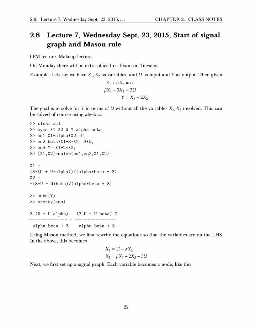
𝑋1 = 𝑈 − 𝛼𝑋2
𝑋2 = 𝛽𝑋1 − 2𝑋2 − 3𝑈
Next, we first set up a signal graph. Each variable becomes a node, like this
22

2.8. Lecture 7, Wednesday Sept. 23, 2015, . . . CHAPTER 2. CLASS NOTES
U
-3
-2
−α1
1
2X1 X2 Y
self loop
β
Note: At each node, all incoming branch gains are added. We now setup the loop gains. Aloop must not visit a node more than once. There are two loops here. The gains on themare �−𝛼𝛽, −2�. Next, we find all the forward paths from 𝑈 to 𝑌. A forward path must notvisit same node more than once. There are 4 forward paths. The gains on each are
𝑀1 = (−3) (2) = −6
𝑀2 = (1) �𝛽� (2) = 2𝛽𝑀3 = (1) (1) = 1𝑀4 = (−3) (−𝛼) (1) = 3𝛼
Now we defined Mason delta Δ
Δ = 1 −� loop gains +� loop gains 2 at times −� loop gains 3 at times⋯
In the above, when looking for loop gains 2 at times, the loops must not be sharing a node.Same for loop gains 3 at times and higher sums. In our example, this gives
Δ = 1 −� loop gains
= 1 − �−𝛼𝛽 − 2�
= 3 + 𝛼𝛽
Finally, we define Δ𝑖, which is Mason Δ but with the forward path 𝑀𝑖 removed from thegraph. There are 4 forward paths in this problem, so there are Δ1, Δ2, Δ3, Δ4. Each time weremove a forward path, we find Δ again using the above Mason rule method. In this problemwe see that
Δ1 = 1Δ2 = 1Δ3 = 1 − (−2) = 3Δ4 = 1
23

2.8. Lecture 7, Wednesday Sept. 23, 2015, . . . CHAPTER 2. CLASS NOTES
Finally, we apply the Mason gain formula
𝑌𝑈=∑4
𝑖=1𝑀𝑖Δ1
Δ
=(−6) (1) + �2𝛽� (1) + (1) (3) + (3𝛼) (1)
3 + 𝛼𝛽
=𝛼 + 2𝛽 − 33 + 𝛼𝛽
Reader Find 𝑌𝑈 for this graph
U
-3
-2
−α1
1
2X1 X2 Y
γ
ε
β
δ
Second example. Here we take a circuit and obtain the equations, then use signal graph inorder to use Mason rule to obtain the transfer function
Vin
+
-
R1
L
I1
R2
C
I2Vout
Solving the circuit loops gives (all in Laplace domain)
(𝑅1 + 𝑠𝐿) 𝐼1 − 𝐼2𝐿𝑠 − 𝑉𝑖𝑛 (𝑠) = 0
�𝑅2 +1𝐶𝑠�
𝐼2 + 𝐿𝑠𝐼2 − 𝐼1𝐿𝑠 = 0
𝑉𝑜𝑢𝑡 (𝑠) = 𝑅2𝐼2Now the variables are 𝐼1, 𝐼2, so we need to have these on the LHS. To do this, do this trick:Add 𝐼1 to each side of the first equation, and add 𝐼2 to each side of the second equation, this
24

2.8. Lecture 7, Wednesday Sept. 23, 2015, . . . CHAPTER 2. CLASS NOTES
gives
𝐼1 = (𝑅1 + 𝑠𝐿) 𝐼1 − 𝐼2𝐿𝑠 − 𝑉𝑖𝑛 (𝑠) + 𝐼1
𝐼2 = 𝐼2 + �𝑅2 +1𝐶𝑠�
𝐼2 + 𝐿𝑠𝐼2 − 𝐼1𝐿𝑠
Now set up the signal graph
Vin I1
I2
Vout
1 +R1 + Ls
1Cs +R2 + Ls+ 1
-1−Ls
−Ls R2
Reader: Find 𝑉𝑜𝑢𝑡𝑉𝑖𝑛
for the above.
𝑉𝑜𝑢𝑡𝑉𝑖𝑛
=∑1
𝑖=1𝑀𝑖Δ𝑖
1 − ∑one at time +∑ 2 at times
=(−1) (−𝐿𝑠) (𝑅2)
1 − ∑ (𝑅1 + 𝐿𝑠 + 1) + �1𝐶𝑠 + 𝑅2 + 𝐿𝑠 + 1� + ∑ (𝑅1 + 𝐿𝑠 + 1) �
1𝐶𝑠 + 𝑅2 + 𝐿𝑠 + 1�
=𝐿𝑠𝑅2
1 − �𝑅1 + 𝑅2 +1𝐶𝑠 + 2𝐿𝑠 + 2� + (𝑅1 + 𝐿𝑠 + 1) �𝑅2 +
1𝐶𝑠 + 𝐿𝑠 + 1�
=𝐿𝑠𝑅2
1𝐶𝑠(𝑅1 + 𝐿𝑠) �𝐶𝐿𝑠2 + 𝐶𝑅2𝑠 + 1�
Now we take a block diagram and convert to signal graph. Given
H(s) G(s)R(s)
Y (s)U(s)E(s)
feed forward path
plantcontroller
error signal
+−
We know that 𝑌(𝑠)𝑅(𝑠) =
𝐻(𝑠)𝐺(𝑠)1+𝐻(𝑠)𝐺(𝑠) and that 𝐸(𝑠)
𝑅(𝑠) =1
1+𝐻(𝑠)𝐺(𝑠) . Use Mason to show the above.
Reader Find 𝑌𝑈 for this
25

2.8. Lecture 7, Wednesday Sept. 23, 2015, . . . CHAPTER 2. CLASS NOTES
Ua
b
e
k
d
f
i
jc
2h
f
2.8.1 MIMO Practice problems
ECE 332 – Handout MIMO Practice Problems
Problem 1: A system with inputs u1,u2 outputs y1,y2 and intermediatestates x1, x2 and x3 is described by the differential equations
x1 = x2 − x3 + u1 + 3u2;
x2 = −3x1 + x3 − 4u2;
x3 = −2x2 + u1;
y1 = 2x1 − x3 + u1;
y2 = x1 + x2 − u2.
For this MIMO system, find the associated open loop transfer functionmatrix G(s). Express each entry of G(s) as a quotient of polynomialswith numerator and denominator factored, if possible.
Problem 2: (a) Consider a MIMO 2 × 2 controller H(s) connected ina classical unity feedback configuration to the system G(s) in Problem 1.With
H(s) =
0 11/s 0
,use syms in Matlab to find the closed loop transfer function matrix T (s).You may wish to check your solution by calculating by hand.
(b) Is the closed loop stable? Explain.
26

2.8. Lecture 7, Wednesday Sept. 23, 2015, . . . CHAPTER 2. CLASS NOTES
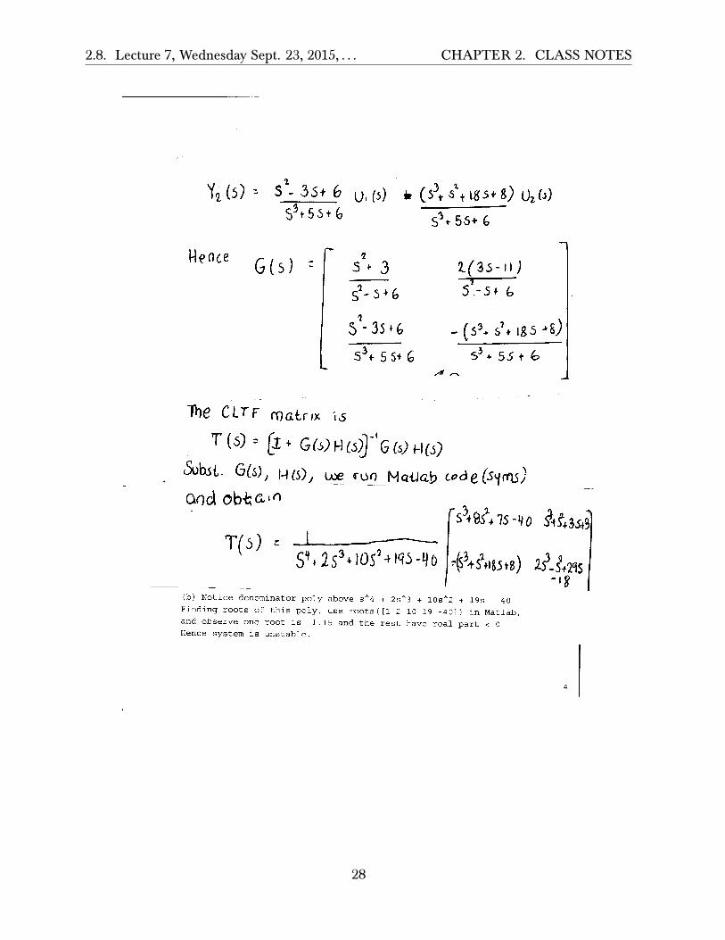
WmSoo): Ml M O Problerq Solutions
TCn^e ^ LOLfcb 2erO l O i l i J COOdctioOJ
SX . ( 3 ) \b)'X2b)^ U.(5).30a(5)
S X, (5) - - 3x, (5) * (6) - H (5)
5X3(5) -iXib)'\},b)
So We (algebra) QOd ob-tG.o ooitt 4>C5)=s\5Sf6
X,6) S-f 3) U. 65) + 05'- 45 - 2) 65)]
Lb) = x r(3-2i)U,(5) -(H5'-*45)U,65)
(5^3)0,65) +(g5+lg)Ui65)j
(b(5)
KoU Y.C5) . +2X,(5) -X3(5)> DiO)
Ya(5) X,(5) + Xi65)- Ui6s)
W< qooo Stbsbibote Xlii) lofco Y.'i'> Ya65) and after 60 me algcbo- obtain
S '5^6
27
2.8. Lecture 7, Wednesday Sept. 23, 2015, . . . CHAPTER 2. CLASS NOTES
SW55+G
Hence G(s)
1 5^ 3 S ' - 5 H
2(35-11) • 5.-5*
Tbe CLTF roatr/x 15
-- [ i r G 6 5 ; H(53" 'G (S ; 1-1(5)
Sobst. G(s)^ l-l(5)y uje f00 Mailab <-«'de(54rfi3)
T(5)
#4S'lS5t8) is'-sYl' S
(b) Notice denominator poly above s^4 + 2s^3 + 10s^2 + 19s - 40 Find i n g roots of t h i s poly, use r o o t s ( [ 1 2 10 19 -40]) i n Matlab, and observe one root i s 1.15 and the r e s t have r e a l p a r t < 0 Hence system i s un s t a b l e .
28

2.9. Lecture 8, Thursday Sept. 24, 2015, . . . CHAPTER 2. CLASS NOTES
2.9 Lecture 8, Thursday Sept. 24, 2015, Mason, bene�tsof feedback, non-linear systems
Exam 1 on Tuesday Sept. 29, 2015. Closed book, closed notes. There will be o�ce hoursMonday 1-3 pm.
Keywords for exam:
1. Modeling, basic circuit or spring mass damper.
2. Block diagrams. Go from model to block diagram. Laplace and transfer function.For example, given a mass/spring, find the ODE and use Laplace to find thetransfer function
3. Block diagram, open loop vs. closed loop. Classic unity feedback
4. Know basic Laplace and inverse Laplace
5. Given TF, and 𝑅 (𝑠) find 𝑌 (𝑠)
6. Steady state error. Know when to use F.V.T. This is related to tracking. The morecomplicated the signal, the more integrated we need. This is called the integratorprinciple.
7. MIMO basics. Matrix transfer function. Watch out for order here.
8. 4 or 5 questions.
Now for one more Mason problem. We use Mason any time we want to find a transferfunction. Find 𝑌(𝑠)
𝑈(𝑠) for this signal graph
U a
f
g
b
kh
c
i
d
l
e Y
j
There are 4 forward paths from 𝑈 to 𝑌, here they are, with the associated Mason Δ
𝑀1 = 𝑎𝑏𝑐𝑑𝑒, Δ1 = 1𝑀2 = 𝑎𝑓ℎ𝑒, Δ2 = 1 − 𝑖𝑀3 = 𝑎𝑓𝑐𝑑𝑒, Δ3 = 1𝑀4 = 𝑎𝑏ℎ𝑒, Δ4 = 1 − 𝑖
29

2.9. Lecture 8, Thursday Sept. 24, 2015, . . . CHAPTER 2. CLASS NOTES
We need 𝑌𝑈 =
∑4𝑖=1𝑀𝑖Δ𝑖
Δ . The loops are �𝑘, 𝑗, 𝑖, 𝑏𝑐𝑔, 𝑑𝑙, 𝑓ℎ𝑙 𝑔, 𝑏ℎ𝑙 𝑔, 𝑓𝑐𝑔�, hence
Δ = 1 − �𝑘 + 𝑖 + 𝑗 + 𝑑𝑘 + 𝑓ℎ𝑙 𝑔 + 𝑏ℎ𝑙 𝑔 + 𝑓𝑐𝑔� + �𝑘𝑖 + 𝑘𝑗 + 𝑖𝑗 + 𝑘𝑑𝑙 + 𝑗𝑏𝑐𝑔 + 𝑗𝑓𝑐𝑔� − �𝑘𝑖𝑗�
Hence
𝑌𝑈=∑4
𝑖=1𝑀𝑖Δ𝑖
Δ
=𝑎𝑏𝑐𝑑𝑒 (1) + 𝑎𝑓ℎ𝑒 (1 − 𝑖) + 𝑎𝑓𝑐𝑑𝑒 (1) + 𝑎𝑏ℎ𝑒 (1 − 𝑖)
1 − �𝑘 + 𝑖 + 𝑗 + 𝑑𝑘 + 𝑓ℎ𝑙 𝑔 + 𝑏ℎ𝑙 𝑔 + 𝑓𝑐𝑔� + �𝑘𝑖 + 𝑘𝑗 + 𝑖𝑗 + 𝑘𝑑𝑙 + 𝑗𝑏𝑐𝑔 + 𝑗𝑓𝑐𝑔� − �𝑘𝑖𝑗�
Next topic we will start on is the benefits of feedback. So far we talked about tracking only.Other benefits are
1. Linearization
2. Sensitivity
3. Disturbances
We can use feedback to pre compensate a nonlinear system to make it approximately linear.Given a non-linear device, say diode, with input 𝑈 = 𝑋 which represent voltage and output𝑌 which is nonlinear function of the input such as 𝑌 = 𝑁𝑋 can we use feedback to make theoutput closed to linear?
U = X Y = NX
”static” nonlinear device
Warning: When the system is non-linear, we can not use transfer functions and can not useLaplace. These are only for linear systems. Transfer functions and Laplace transforms areused only when the system is linear. So how do we analyze non-linear system? We use timedomain. For example, if 𝑌 = 𝑋2
+
-H(s) nonlinear Y (s)x N(x)
These are not transfer functions
R(s)
Closed loop is nonlinear. We need relation between 𝑅 (𝑠) and 𝑌 (𝑠)
There are two type of nonlinearity, saturations and dead-zone. Dead zone is an area wherethe input is not yet su�cient to cause any output to be generated, it might be a thresholdfor the device to start operating. Here is a typical output from a non linear device
30

2.9. Lecture 8, Thursday Sept. 24, 2015, . . . CHAPTER 2. CLASS NOTES
− 12
12
Y = N(x)
x1
-1
Reader For this open loop, if 𝑥 = 2 sin 𝑡, sketch 𝑦 (𝑡). Another example
+
-K nonlinear Y (s)x = 2(R−N(x)) N(x)R(s)
R−N(x)
We know
𝑌 = 𝑁 (𝑥) (1)
and
𝑥 = 2 (𝑅 − 𝑌)
hence 2𝑌 = 2𝑅 − 𝑥 and
𝑌 = 𝑅 −𝑥2
(2)
(1) and (2) must both hold. For each 𝑅 input, we solve (1,2) for 𝑌, 𝑥 and plot them. Forexample, for 𝑅 = {0, 0.1, 0.2,⋯} for each 𝑅 (𝑖) we solve for 𝑌 (𝑖)
𝑅 𝑌 = 𝑅 − 𝑥2
0 0 − 𝑥2
0.1 0.1 − 𝑥2
0.2 0.2 − 𝑥2
⋮ ⋮
For each line in the above, such as −𝑥2 , 0.1−
𝑥2 ,⋯, we now draw this line on top of the original
𝑌 (𝑥) plot, and see where this line intersect with the original 𝑌 (𝑥). The point of intersectionis the new value of 𝑌. This is done for each entry of 𝑅, so we obtain
31
2.9. Lecture 8, Thursday Sept. 24, 2015, . . . CHAPTER 2. CLASS NOTES
− 12
12
Y = N(x)
x1
-1
−x2 0.1− x
2
So we obtain this table
𝑅 𝑌 = 𝑅 − 𝑥2
0 00.1 00.2 0⋮ ⋮
big .3⋮ 1
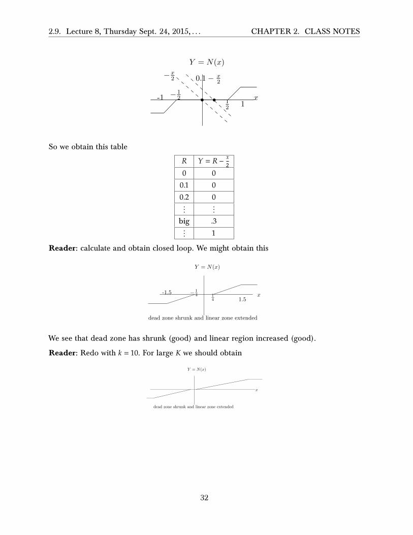
Reader: calculate and obtain closed loop. We might obtain this
− 14 1
4
Y = N(x)
x1.5
-1.5
dead zone shrunk and linear zone extended
We see that dead zone has shrunk (good) and linear region increased (good).
Reader: Redo with 𝑘 = 10. For large 𝐾 we should obtain
Y = N(x)
x
dead zone shrunk and linear zone extended
32

2.10. Lecture 9, Tuesday Sept. 29, 2015, . . . CHAPTER 2. CLASS NOTES
2.10 Lecture 9, Tuesday Sept. 29, 2015, First exam
First exam
33

2.11. Lecture 10, Thursday Oct. 1, 2015, . . . CHAPTER 2. CLASS NOTES
2.11 Lecture 10, Thursday Oct. 1, 2015, No lecture
No lecture today
34
2.12. Lecture 11, Tuesday Oct. 6, 2015, . . . CHAPTER 2. CLASS NOTES
2.12 Lecture 11, Tuesday Oct. 6, 2015, Sensitivity oftransfer function
Today lecture on sensitivity. Definition of sensitivity: percentage change in magnitude oftransfer function 𝑇 (𝑠) per one percent change of parameter 𝛼 in the transfer function. Wenormally make this parameter be 𝛼. This could be 𝑅 (resistance) or 𝐶 (capacitance) and soon. We call this 𝑆𝑇𝛼 which is read as the sensitivity of the 𝑇 (𝑠) with respect to changes in 𝛼.
Therefore
𝑆𝑇𝛼 =Δ𝑇𝑇Δ𝛼𝛼
=Δ𝑇Δ𝛼
𝛼𝑇
=𝑑𝑇𝑑𝛼𝛼𝑇
We then have to evaluate 𝑆𝑇𝛼 at the nominal value of the parameter 𝛼 = 𝛼0. Therefore
𝑆𝑇𝛼 𝛼=𝛼0=𝑑𝑇𝑑𝛼𝛼𝑇 𝛼=𝛼0
𝛼0 is given numerical value. It is meant to be the value that the parameter 𝛼 fluctuate aroundand will be given in the problem to use.
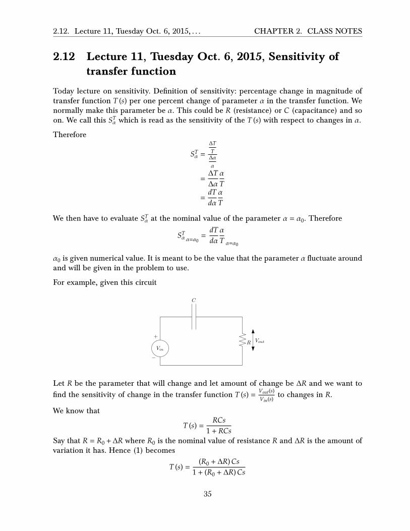
For example, given this circuit
R
C
Vin
+Vout
−
Let 𝑅 be the parameter that will change and let amount of change be Δ𝑅 and we want tofind the sensitivity of change in the transfer function 𝑇 (𝑠) = 𝑉𝑜𝑢𝑡(𝑠)
𝑉𝑖𝑛(𝑠)to changes in 𝑅.
We know that
𝑇 (𝑠) =𝑅𝐶𝑠
1 + 𝑅𝐶𝑠Say that 𝑅 = 𝑅0 +Δ𝑅 where 𝑅0 is the nominal value of resistance 𝑅 and Δ𝑅 is the amount ofvariation it has. Hence (1) becomes
𝑇 (𝑠) =(𝑅0 + Δ𝑅)𝐶𝑠
1 + (𝑅0 + Δ𝑅)𝐶𝑠
35

2.12. Lecture 11, Tuesday Oct. 6, 2015, . . . CHAPTER 2. CLASS NOTES
To find 𝑆𝑇𝑅 we let 𝑅 = 𝛼 and apply the definition 𝑆𝑇𝛼 =𝑑𝑇𝑑𝛼
𝛼𝑇 𝛼=𝛼0
Hence
𝑆𝑇𝛼 =𝑑𝑇𝑑𝛼𝛼𝑇
=𝑑𝑑𝛼 �
𝛼𝐶𝑠1 + 𝛼𝐶𝑠�
𝛼𝛼𝐶𝑠
1+𝛼𝐶𝑠
Assume 𝐶 = 1 and assume nominal value of 𝑅 is 1 also. This means 𝛼0 = 1. The abovebecomes
𝑆𝑇𝛼 =𝑑𝑑𝛼
�𝛼𝑠
1 + 𝛼𝑠�𝛼𝛼𝑠
1+𝛼𝑠
=𝑠
(𝑠𝛼 + 1)21 + 𝛼𝑠𝑠
=1
𝑠𝛼 + 1Evaluate at 𝛼 = 𝛼0 = 1 then
𝑆𝑇𝛼 𝛼=𝛼0=
1𝑠 + 1
Next step is to replace 𝑠 = 𝑗𝜔 and plot the magnitude in frequency domain
𝑆𝑇𝛼 =1
𝑗𝜔 + 1
�𝑆𝑇𝛼� =1
√1 + 𝜔2
A plot is
Out[6]=
0 5 10 15 20
0.0
0.2
0.4
0.6
0.8
1.0
ω
|(SαT)
Example 1
Examples below shows to calculate 𝑆𝑇𝛼 for di�erence parameters.
2.12.0.1 Example 1
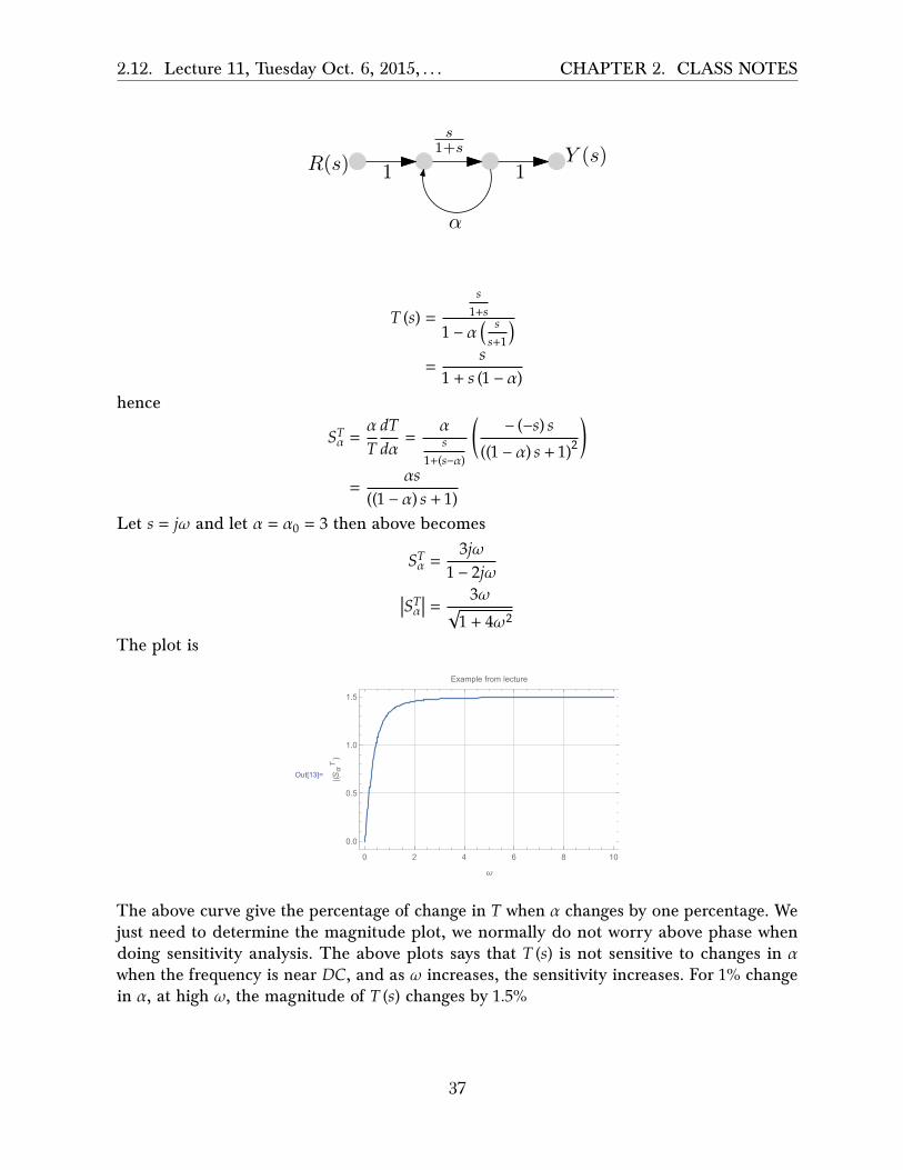
Given the signal graph
36
2.12. Lecture 11, Tuesday Oct. 6, 2015, . . . CHAPTER 2. CLASS NOTES
R(s)
s1+s
α
Y (s)1 1
𝑇 (𝑠) =𝑠
1+𝑠
1 − 𝛼 � 𝑠𝑠+1�
=𝑠
1 + 𝑠 (1 − 𝛼)hence
𝑆𝑇𝛼 =𝛼𝑇𝑑𝑇𝑑𝛼
=𝛼𝑠
1+(𝑠−𝛼)�
− (−𝑠) 𝑠((1 − 𝛼) 𝑠 + 1)2
�
=𝛼𝑠
((1 − 𝛼) 𝑠 + 1)Let 𝑠 = 𝑗𝜔 and let 𝛼 = 𝛼0 = 3 then above becomes
𝑆𝑇𝛼 =3𝑗𝜔
1 − 2𝑗𝜔
�𝑆𝑇𝛼� =3𝜔
√1 + 4𝜔2
The plot is
Out[13]=
0 2 4 6 8 10
0.0
0.5
1.0
1.5
ω
|(SαT)
Example from lecture
The above curve give the percentage of change in 𝑇 when 𝛼 changes by one percentage. Wejust need to determine the magnitude plot, we normally do not worry above phase whendoing sensitivity analysis. The above plots says that 𝑇 (𝑠) is not sensitive to changes in 𝛼when the frequency is near 𝐷𝐶, and as 𝜔 increases, the sensitivity increases. For 1% changein 𝛼, at high 𝜔, the magnitude of 𝑇 (𝑠) changes by 1.5%
37

2.12. Lecture 11, Tuesday Oct. 6, 2015, . . . CHAPTER 2. CLASS NOTES
2.12.1 Example 2
Given the circuit
C
L
Vin
Vout
Let us see how 𝑇 (𝑠) = 𝑉𝑜𝑢𝑡(𝑠)𝑉𝑖𝑛(𝑠)
changes when 𝐿 changes. So we make 𝐿 as our 𝛼 here. Thenominal 𝛼0 = 1 and we also take 𝐶 = 1.
𝑇 (𝑠) =𝐿𝑠
𝐿𝑠 + 1𝐶𝑠
=𝛼𝑠
𝛼𝑠 + 1𝑠
=𝛼𝑠2
𝛼𝑠2 + 1
Hence
𝑆𝑇𝛼 =𝛼𝑇𝑑𝑇𝑑𝛼
=1
𝛼𝑠2 + 1Let 𝑠 = 𝑗𝜔 𝛼 = 𝛼0 = 1 and the above becomes
𝑆𝑇𝛼 =1
1 − 𝜔2
Hence
�𝑆𝑇𝛼� =1
�1 − 𝜔2�Notice that at 𝜔 = 1 there is resonance. Here is the plot
Out[15]=
0 1 2 3 4
0
1
2
3
ω
|(SαT)
Example from lecture
The above says that when 𝜔 near 1, then the transfer function is very sensitive to changesin 𝐿. For 1% change in 𝐿, the magnitude of the transfer function become very large at thatfrequency. This can cause problems, so we need to avoid getting close to 𝜔 = 1 and must
38

2.12. Lecture 11, Tuesday Oct. 6, 2015, . . . CHAPTER 2. CLASS NOTES
stay above it for safe operations.
2.12.2 Example 3
Given this circuit
CL
Vin
VoutR
Now we will find the 𝑆𝑇𝛼 for each parameter in the circuit. These are 𝑅, 𝐿, 𝐶, each time wefix all the parameters, except the one in interest, and call that one 𝛼 and repeat the stepswe did in the earlier examples.
𝑇 (𝑠) =𝑉𝑜𝑢𝑡 (𝑠)𝑉𝑖𝑛 (𝑠)
=𝑅
𝑅 + 1𝐶𝑠 + 𝐿𝑠
=𝑅𝐶𝑠
𝑅𝐶𝑠 + 𝐿𝐶𝑠2 + 1
Let 𝛼 = 𝑅, and let 𝐶 = 1, 𝐿 = 1 and let 𝛼0 = 1 as well. Hence
𝑇 (𝑠) =𝛼𝑠
𝑠2 + 𝛼𝑠 + 1Hence
𝑆𝑇𝛼 =𝛼𝑇𝑑𝑇𝑑𝛼
=1 + 𝑠2
𝑠2 + 𝛼𝑠 + 1We now switch to 𝜔 domain
𝑆𝑇𝛼 =1 − 𝜔2
1 − 𝜔2 + 𝛼𝑗𝜔 𝛼=1
=1 − 𝜔2
1 − 𝜔2 + 𝑗𝜔Hence
�𝑆𝑇𝛼� =�1 − 𝜔2�
��1 − 𝜔2�
2+ 𝜔2
Be careful to use �1 − 𝜔2� above and not just 1 −𝜔2 since these are norms. Plotting the abovegives
39
2.12. Lecture 11, Tuesday Oct. 6, 2015, . . . CHAPTER 2. CLASS NOTES
Out[19]=
0 1 2 3 4 5 6
0.0
0.2
0.4
0.6
0.8
1.0
ω|(S
αT)
Example from lecture, for R sensitivity
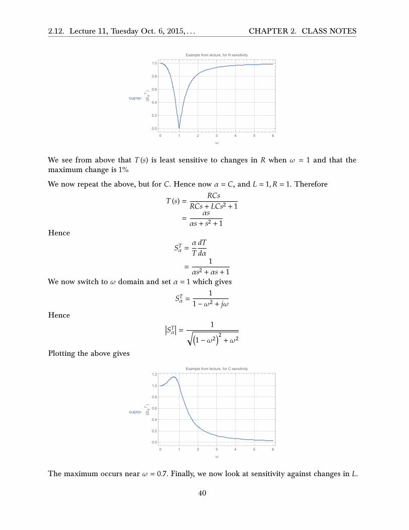
We see from above that 𝑇 (𝑠) is least sensitive to changes in 𝑅 when 𝜔 = 1 and that themaximum change is 1%
We now repeat the above, but for 𝐶. Hence now 𝛼 = 𝐶, and 𝐿 = 1, 𝑅 = 1. Therefore
𝑇 (𝑠) =𝑅𝐶𝑠
𝑅𝐶𝑠 + 𝐿𝐶𝑠2 + 1=
𝛼𝑠𝛼𝑠 + 𝑠2 + 1
Hence
𝑆𝑇𝛼 =𝛼𝑇𝑑𝑇𝑑𝛼
=1
𝛼𝑠2 + 𝛼𝑠 + 1We now switch to 𝜔 domain and set 𝛼 = 1 which gives
𝑆𝑇𝛼 =1
1 − 𝜔2 + 𝑗𝜔Hence
�𝑆𝑇𝛼� =1
��1 − 𝜔2�
2+ 𝜔2
Plotting the above gives
Out[20]=
0 1 2 3 4 5 6
0.0
0.2
0.4
0.6
0.8
1.0
1.2
ω
|(SαT)
Example from lecture, for C sensitivity
The maximum occurs near 𝜔 = 0.7. Finally, we now look at sensitivity against changes in 𝐿.
40

2.12. Lecture 11, Tuesday Oct. 6, 2015, . . . CHAPTER 2. CLASS NOTES
Hence now 𝛼 = 𝐿, and 𝐶 = 1, 𝑅 = 1. Therefore
𝑇 (𝑠) =𝑅𝐶𝑠
𝑅𝐶𝑠 + 𝐿𝐶𝑠2 + 1=
𝑠𝛼𝑠 + 𝑠2 + 1
Hence
𝑆𝑇𝛼 =𝛼𝑇𝑑𝑇𝑑𝛼
=−𝛼𝑠2
𝛼𝑠2 + 𝛼𝑠 + 1We now switch to 𝜔 domain and set 𝛼 = 1 which gives
𝑆𝑇𝛼 =− �−𝜔2�
1 − 𝜔2 + 𝑗𝜔Hence
�𝑆𝑇𝛼� =𝜔2
��1 − 𝜔2�
2+ 𝜔2
Plotting the above gives
Out[22]=
0 1 2 3 4 5 6
0.0
0.2
0.4
0.6
0.8
1.0
1.2
ω
|(SαT)
Example from lecture, for L sensitivity
The maximum occurs near 𝜔 = 1.14.
2.12.3 Example 4
Given this circuit
41

2.12. Lecture 11, Tuesday Oct. 6, 2015, . . . CHAPTER 2. CLASS NOTES
CL1
Vin
VoutL2
Let the nominal values be 𝐶 = 1, 𝐿1 = 1 and 𝐿2 = 1. We will find 𝑆𝑇𝛼 for each of theseparameters now one at a time as in the above example.
𝑇 (𝑠) =𝐿2𝑠
(𝐿1 + 𝐿2) 𝑠 +1𝐶𝑠
=𝐿2𝐶𝑠2
(𝐿1 + 𝐿2) 𝐶𝑠2 + 1
When 𝛼 = 𝐿1 then (after putting 𝐶 = 1, 𝐿2 = 1) the above becomes
𝑇 (𝑠) =𝑠2
(𝛼 + 1) 𝑠2 + 1Hence
𝑆𝑇𝛼 =𝛼𝑇𝑑𝑇𝑑𝛼
=−𝛼𝑠2
(𝛼 + 1) 𝑠2 + 1We now switch to 𝜔 domain and set 𝛼 = 1 which gives
𝑆𝑇𝛼 =𝜔2
1 − 2𝜔2
Hence
�𝑆𝑇𝛼� =𝜔2
�1 − 2𝜔2�The plot is
Out[28]=
0 1 2 3 4
0.0
0.2
0.4
0.6
0.8
1.0
ω
|(SαT)
Example from lecture, for L1 sensitivity
42

2.12. Lecture 11, Tuesday Oct. 6, 2015, . . . CHAPTER 2. CLASS NOTES
We see that �𝑆𝑇𝛼� blows up at 𝜔 = 1
√2and at 𝜔 = 1, �𝑆𝑇𝛼� = 1. We now consider 𝛼 = 𝐿2 then
(after putting 𝐶 = 1, 𝐿1 = 1) the transfer function becomes
𝑇 (𝑠) =𝛼𝑠2
(1 + 𝛼) 𝑠2 + 1Hence
𝑆𝑇𝛼 =𝛼𝑇𝑑𝑇𝑑𝛼
=𝑠2 + 1
(𝛼 + 1) 𝑠2 + 1We now switch to 𝜔 domain and set 𝛼 = 1 which gives
𝑆𝑇𝛼 =1 − 𝜔2
1 − 2𝜔2
Hence
�𝑆𝑇𝛼� =�1 − 𝜔2��1 − 2𝜔2�
The plot is
Out[30]=
0 1 2 3 4
0.0
0.5
1.0
1.5
2.0
ω
|(SαT)
Example from lecture, for L2 sensitivity
We see that now at low frequency 𝑇 (𝑠) is sensitive to 𝐿2 while it is not sensitive to changes in𝐿1. Finally, looking at 𝛼 = 𝐶 then (after putting 𝐿2 = 1, 𝐿1 = 1) the transfer function becomes
𝑇 (𝑠) =𝛼𝑠2
2𝛼𝑠2 + 1Hence
𝑆𝑇𝛼 =𝛼𝑇𝑑𝑇𝑑𝛼
=1
2𝛼𝑠2 + 1We now switch to 𝜔 domain and set 𝛼 = 1 which gives
𝑆𝑇𝛼 =1
1 − 2𝜔2
43

2.12. Lecture 11, Tuesday Oct. 6, 2015, . . . CHAPTER 2. CLASS NOTES
Hence
�𝑆𝑇𝛼� =1
�1 − 2𝜔2�The plot is
Out[31]=
0 1 2 3 4
0.0
0.5
1.0
1.5
2.0
2.5
ω
|(SαT)
Example from lecture, for C sensitivity
We see that �𝑆𝑇𝛼� blows up at 𝜔 = 1
√2.
In conclusion, we can use these plots to determine how each component a�ect the transferfunction. We do not want the transfer function to be sensitive to changes in components.If we know the range of operating frequencies, we can now know which components cancause most problems and may be spend more money to buy better quality component forthat specific one.
44
2.13. Lecture 12. Thursday Oct 8, 2015, . . . CHAPTER 2. CLASS NOTES
2.13 Lecture 12. Thursday Oct 8, 2015, control to rejectnoise and disturbances
First midterm and second HW returned. Review of midterm results given.
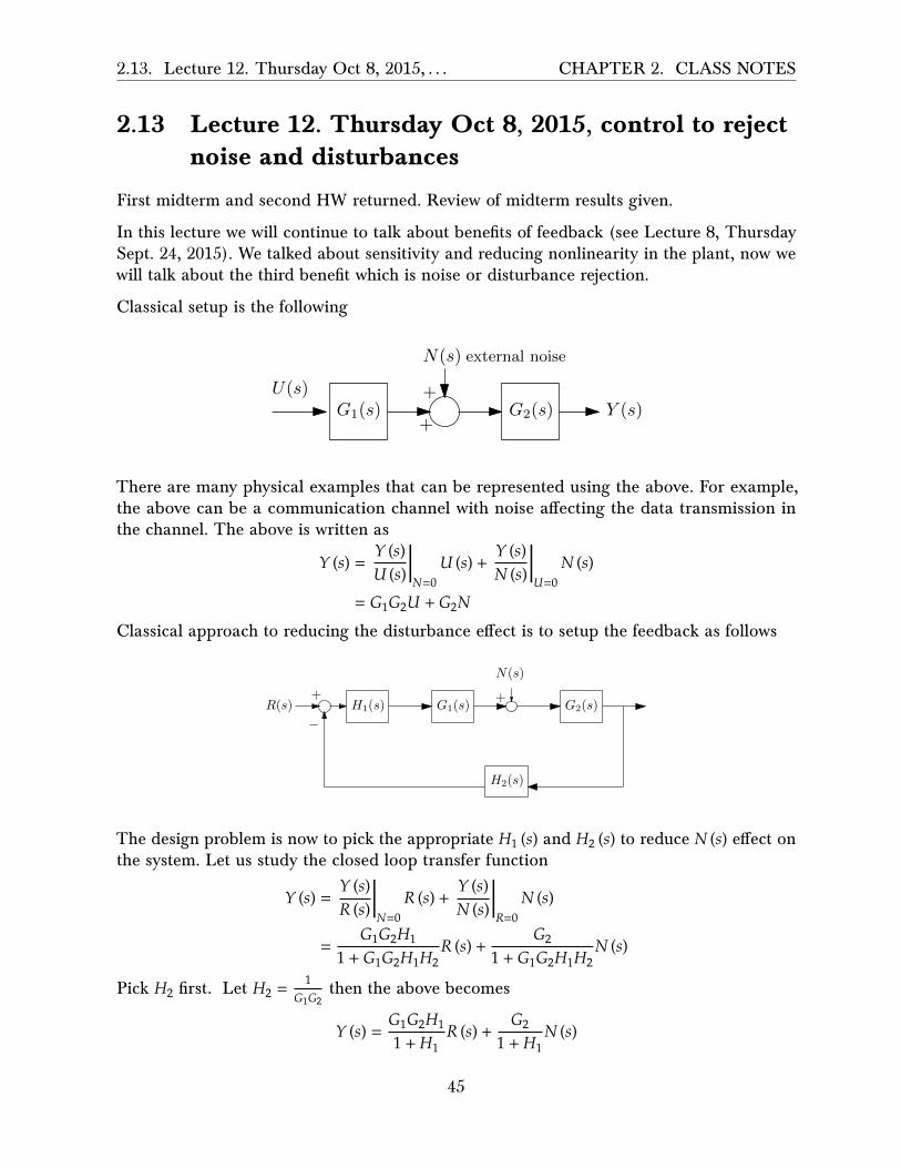
In this lecture we will continue to talk about benefits of feedback (see Lecture 8, ThursdaySept. 24, 2015). We talked about sensitivity and reducing nonlinearity in the plant, now wewill talk about the third benefit which is noise or disturbance rejection.
Classical setup is the following
G1(s)
N(s)
G2(s)+
+
U(s)Y (s)
external noise
There are many physical examples that can be represented using the above. For example,the above can be a communication channel with noise a�ecting the data transmission inthe channel. The above is written as
𝑌 (𝑠) =𝑌 (𝑠)𝑈 (𝑠)
�𝑁=0
𝑈 (𝑠) +𝑌 (𝑠)𝑁 (𝑠)
�𝑈=0
𝑁 (𝑠)
= 𝐺1𝐺2𝑈 + 𝐺2𝑁
Classical approach to reducing the disturbance e�ect is to setup the feedback as follows
G1(s) G2(s)
H2(s)
H1(s)R(s)+
−
N(s)
+
The design problem is now to pick the appropriate 𝐻1 (𝑠) and 𝐻2 (𝑠) to reduce 𝑁 (𝑠) e�ect onthe system. Let us study the closed loop transfer function
𝑌 (𝑠) =𝑌 (𝑠)𝑅 (𝑠)
�𝑁=0
𝑅 (𝑠) +𝑌 (𝑠)𝑁 (𝑠)
�𝑅=0
𝑁 (𝑠)
=𝐺1𝐺2𝐻1
1 + 𝐺1𝐺2𝐻1𝐻2𝑅 (𝑠) +
𝐺21 + 𝐺1𝐺2𝐻1𝐻2
𝑁 (𝑠)
Pick 𝐻2 first. Let 𝐻2 =1
𝐺1𝐺2then the above becomes
𝑌 (𝑠) =𝐺1𝐺2𝐻11 + 𝐻1
𝑅 (𝑠) +𝐺2
1 + 𝐻1𝑁 (𝑠)
45

2.13. Lecture 12. Thursday Oct 8, 2015, . . . CHAPTER 2. CLASS NOTES
And let 𝐻1 = 𝛼 where 𝛼 is a very large gain value. Then above reduces to
𝑌 (𝑠) =𝐺1𝐺2𝛼1 + 𝛼
𝑅 (𝑠) +𝐺21 + 𝛼
𝑁 (𝑠)
lim𝛼→∞
𝑌 (𝑠) = 𝐺1𝐺2𝑅 (𝑠)
Which is good. This is what we wanted. So 𝑁 (𝑠) e�ect has no been eliminated. But thismethod has the following disadvantages
1. If 𝐺1𝐺2 =1
1+𝑠 then 𝐻2 becomes 1𝐺1𝐺2
= 𝑠 + 1. This is not good. We normally do notwant to have di�erentiators in the loop as they cause problems we talked about earlyin the course.
2. Another problem. Lets say 𝐺1𝐺2 =1+𝑠
𝑠2+2𝑠+1 . Then 𝐻2 =𝑠2+2𝑠+11+𝑠 , and we still have the
same problem as above since after long division, we see this is still 1 + 𝑠. There was ahidden di�erentiator in there. In general, if the numerator has degree less than thedenominator in 𝐺1𝐺2 then 𝐻2 that results will have a di�erentiator.
How to fix the above? The fix is to introduce a low pass filter, called 𝐻𝐿𝑃 (𝑠). So that insteadof using 𝐻2 (𝑠) we use 𝐻2 (𝑠)𝐻𝐿𝑃 (𝑠) . Low pass filter attenuate high frequency noise. Thesimplest low pass filter is
𝐻𝐿𝑃 (𝑠) =1
(𝜖𝑠 + 1)𝑘
Where 𝑘 is an integer specified by the designer and 𝜖 > 0. Now we introduce frequency. Thisis done by letting 𝑠 = 𝑗𝜔. Imaging we have this system
HLP (s)
s = jω
Harmonics atfrequency ω
𝐻𝐿𝑃 �𝑗𝜔� is called the frequency response. It is complex valued. Has magnitude and phase.
Example: 𝜀 = 1, 𝑘 = 1 then 𝐻𝐿𝑃 �𝑗𝜔� =1
1+𝑗𝜔 and |𝐻𝐿𝑃| =1
√1+𝜔2and phase ∢𝐻𝐿𝑃 = 0 − tan−1𝜔
Plotting the magnitude |𝐻𝐿𝑃| gives
|H(jω)|
ω
11√2
1
So back to using 𝐻𝐿𝑃 in our original problem, which is noise rejection. As we said, we nowwill use 𝐻2𝐻𝐿𝑃 in place of 𝐻2. Does 𝐻𝐿𝑃 mess up the cancellation of 𝐺1𝐺2 as we had before?
46

2.13. Lecture 12. Thursday Oct 8, 2015, . . . CHAPTER 2. CLASS NOTES
It depends on the noise type. For low frequency noise, then |𝐻𝐿𝑃| will be close to 1 and hence𝐻2𝐻𝐿𝑃 will remain very close to 𝐻2. But if the noise is high frequency, then |𝐻𝐿𝑃| is muchsmaller than one, and hence 𝐻2𝐻𝐿𝑃 will be much smaller than original 𝐻2. For example, if𝜔 = 1, then 𝐻2 is attenuated by about 30%. Next time, we will build more on this topic.
47

2.14. Lecture 13. Tuesday Oct 13, 2015, . . . CHAPTER 2. CLASS NOTES
2.14 Lecture 13. Tuesday Oct 13, 2015, Noise rejection,second order systems
Today we will finish noise attenuation, then start on second order systems. The classicalmethod of noise attenuating is based on this feedback system block diagram
R(s) H1(s) G1(s)
N(s)
G2(s) Y (s)
H2(s)
+
−
noise source
+
+
We often have systems where noise or disturbance comes in between the input and theoutput. Without 𝑁 (𝑠) we would have perfect open loop. The classical approach to noiseattenuation is as shown in the above diagram, which is to add 𝐻1 (𝑠) and 𝐻2 (𝑠) with the ideato reduce the e�ect of 𝑁 (𝑠) while at the same time to preserve 𝑅 (𝑠) input signal and nota�ect it. For 𝐻1 (𝑠) we use large pure gain 𝛼, this is for attenuation. For 𝐻2 (𝑠), we start withwhat is called the inversion method, which is to use 𝐻2 (𝑠) =
1𝐺1𝐺2
. As discussed in last lecture,this method looks good in math, but not good in practice, since 𝐻2 (𝑠) becomes impropertransfer function. Now we will explain a more practical method, which is to introduce alow pass filter 𝐻𝐿𝑃 =
1
(𝜀𝑠+1)𝑘which will reject noise frequency and also make 𝐻2 (𝑠) become
proper. We will use 𝐻2 (𝑠) =1
𝐺1𝐺2𝐻𝐿𝑃 (𝑠) instead of just 𝐻2 (𝑠) =
1𝐺1𝐺2
as before.
We need to pick 𝜀, 𝑘. Both are positive. To design for 𝐻𝐿𝑃 (𝑠) we need to know somethingabout 𝑁 (𝑠). We need to know the frequency content of 𝑁 (𝑠) so we can design 𝐻𝐿𝑃 (𝑠) to blockmost of frequency content of 𝑁 (𝑠) while allowing all the content of 𝑅 (𝑠) to pass through. Weassume 𝑅 (𝑠) frequency is all in the passband of the low pass filter. This is done in frequencydomain.
�𝐻𝐿𝑃 �𝑗𝜔�� =��
1
�𝜀𝑗𝜔 + 1�𝑘��=
1
�𝜀𝑗𝜔 + 1�𝑘=
1
�√𝜀2𝜔2 + 1�𝑘 =
1
�𝜀2𝜔2 + 1�𝑘2
The plot of �𝐻𝐿𝑃 �𝑗𝜔�� might now look like this
|H(jω)|
ω
11
2k2
1ε
We can make the filter closed to desired by boosting 𝑘 and decreasing 𝜀.
48

2.14. Lecture 13. Tuesday Oct 13, 2015, . . . CHAPTER 2. CLASS NOTES
Second order systems
We will now start on second order systems. We want to study transient response. So far, wesaid nothing about transient response. Final value theorem give the steady state response(when it exists, if the system is stable) but not what happens in between. The system couldhave undesired transient response before getting to the steady state. For example, we couldwant to send the response to zero very quickly, but this can cause bad transient response.
Why consider only second order systems?
1. Many physical systems are second order system
2. Many systems can be well approximated by second order system, using the methodof dominant poles.
3. Math is much simplified when using second order system than higher order
When we design, say RLC circuit we get second order system. Same for mass spring damper.When the system is higher order, we use dominant pole method to approximate the systemto second order. But after approximate to second order and doing the analysis on the secondorder, we should go back and simulate the original higher order system numerically (sayusing simulink) and compare the second order approximation with the full order system tomake sure the approximation used produces close enough results.
Dominant pole method
Imagine 6th order system. We can ignore poles much further away from the imaginary axis,since these indicate modes that attenuate very fast
X
X
X
X
XX
Dominant poles
These poles can be ignored
imaginay axis
αβ
In many practical systems, 𝛽 ≫ 𝛼 and the poles further to the left can be ignored sincethese are modes which disappear very quickly. So we are left with the two dominant poles𝑠1,2 = −𝛼 ± 𝑗𝜔. Generic second order system is given by
𝐺 (𝑠) =𝜔2𝑛
𝑠2 + 2𝜉𝜔𝑛𝑠 + 𝜔2𝑛
Where 𝜔𝑛 is the natural frequency and 𝜉 is the damping ratio. Consider a unit step input
49

2.14. Lecture 13. Tuesday Oct 13, 2015, . . . CHAPTER 2. CLASS NOTES
𝑅 (𝑠) = 1𝑠 . For practical system, 0 < 𝜉 < 1.
𝑌 (𝑠) = 𝐺 (𝑠) 𝑅 (𝑠)
=𝜔2𝑛
𝑠2 + 2𝜉𝜔𝑛𝑠 + 𝜔2𝑛
1𝑠
The inverse Laplace transform of the above is
𝑦 (𝑡) = 1 −𝑒−𝜉𝜔𝑛𝑡
√1 − 𝜉2sin �𝜔𝑑𝑡 + 𝜙� (1)
To plot the above in Matlab, here is small code
t=0:.1:45;z=0.707;wn=.2;y=@(t,z,wn) 1- exp(-z*wn*t)/sqrt(1-z^2).*sin(wn*sqrt(1-z^2)*t+acos(z));plot(t,y(t,z,wn));
To use Matlab step() command, here is small code
z=0.707;wn=.2;s=tf('s');sys= wn^2/(s^2+2*z*wn*s+wn^2);step(sys);
In (1), 𝜔𝑑 is the damped natural frequency given by 𝜔𝑑 = 𝜔𝑛√1 − 𝜉2 and 𝜙 = cos−1 𝜉. (In our
textbook, 𝜙 was defined as 𝜙 = tan−1 �1−𝜉2
−𝜉 , but this seems strange to me. I will use the more
common definition of sin𝜙 = √1 − 𝜉2 and cos𝜙 = 𝜉 as used by Nise text and other, hence
𝜙 = tan−1 �1−𝜉2
𝜉 from now on).
What if we are not given a standard second order system transfer function such as 𝐺 (𝑠) =25
𝑠2+5𝑠+10 , we can convert this to standard by doing 𝐺 (𝑠) =� 2510 �10
𝑠2+5𝑠+10 = 2.510
𝑠2+5𝑠+10 and now apply
the result to 10𝑠2+5𝑠+10 and then scale the output by 2.5.
For undamped case, 𝜉 = 0, the response is pure harmonics with no damping. The harmonicshave 𝜔𝑛 frequencies. We will now look at poles and zeros of 𝐺 (𝑠) in complex domain. Poles
of 𝐺 (𝑠) = 𝜔2𝑛
𝑠2+2𝜉𝜔𝑛𝑠+𝜔2𝑛are
𝑠1,2 = −𝜉𝜔𝑛 ±�𝜔2𝑛 �𝜉2 − 1�
= −𝜉𝜔𝑛 ± 𝜔𝑛�𝜉2 − 1
50
2.14. Lecture 13. Tuesday Oct 13, 2015, . . . CHAPTER 2. CLASS NOTES
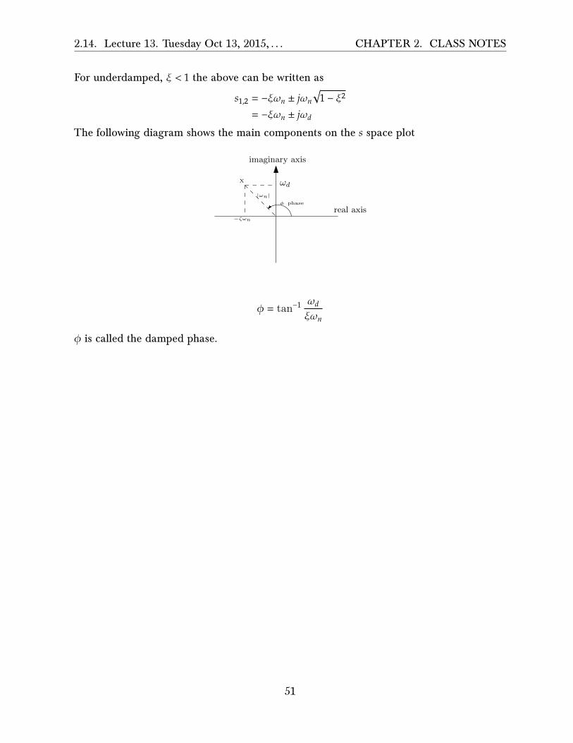
For underdamped, 𝜉 < 1 the above can be written as
𝑠1,2 = −𝜉𝜔𝑛 ± 𝑗𝜔𝑛�1 − 𝜉2
= −𝜉𝜔𝑛 ± 𝑗𝜔𝑑
The following diagram shows the main components on the 𝑠 space plot
X ωd
imaginary axis
−ζωn
|ωn|φ phase
real axis
𝜙 = tan−1 𝜔𝑑𝜉𝜔𝑛
𝜙 is called the damped phase.
51

2.15. Lecture 14. Thursday Oct 15, 2015, . . . CHAPTER 2. CLASS NOTES
2.15 Lecture 14. Thursday Oct 15, 2015, More secondorder, Overshoot and resonance
Will now determine the maximum overshoot called 𝑂𝑆max as shown in this diagram
max overshoot secondary overshoot
1
time t
We will use 𝑑𝑦𝑑𝑡 = 0 to find 𝑦max. Since
𝑑𝑦𝑑𝑡 = 0 will generate many solutions, we will take the
first one.
𝑦 (𝑡) = 1 −𝑒−𝜉𝜔𝑛𝑡
√1 − 𝜉2sin �𝜔𝑑𝑡 + 𝜙�
Then𝑑𝑦𝑑𝑡= 0 = 𝜉𝜔𝑛
𝑒−𝜉𝜔𝑛𝑡
√1 − 𝜉2sin �𝜔𝑑𝑡 + 𝜙� −
𝑒−𝜉𝜔𝑛𝑡
√1 − 𝜉2𝜔𝑑 cos �𝜔𝑑𝑡 + 𝜙�
0 = 𝜉 sin �𝜔𝑑 + 𝜙� − �1 − 𝜉2 cos �𝜔𝑑𝑡 + 𝜙� (1)
To solve this, since cos𝜙 = 𝜉 and sin𝜙 = √1 − 𝜉2
then (1) becomes
0 = cos𝜙 sin �𝜔𝑑𝑡 + 𝜙� − sin𝜙 cos �𝜔𝑑𝑡 + 𝜙�
Using sin (𝐴 − 𝐵) = cos𝐴 sin𝐵 − sin𝐴 cos𝐵 the above can be written as (using 𝐴 = 𝜙)
0 = sin �𝜙 − �𝜔𝑑𝑡 + 𝜙��
Hence
sin (𝜔𝑑𝑡) = 0
The solution is 𝜔𝑑 = 𝜔𝑛√1 − 𝜉2𝑡 = 𝑘𝜋 for 𝑘 = 0, 1, 2,⋯. We pick 𝑘 = 1 since this is the firstone after 𝑡 = 0, hence
𝜔𝑛�1 − 𝜉2𝑡max = 𝜋
𝑡max =𝜋
𝜔𝑛√1 − 𝜉2
=𝜋𝜔𝑑
To find 𝑦max (𝑡) = 𝑦 (𝑡max), we plug the above 𝑡max back in the original solution which is
52

2.15. Lecture 14. Thursday Oct 15, 2015, . . . CHAPTER 2. CLASS NOTES
𝑦 (𝑡) = 1 − 𝑒−𝜉𝜔𝑛𝑡
�1−𝜉2sin �𝜔𝑑𝑡 + 𝜙�. Hence
𝑂𝑆max = 𝑦 (𝑡max) − 1
= �1 −𝑒−𝜉𝜔𝑛𝑡max
√1 − 𝜉2sin �𝜔𝑑𝑡max + 𝜙�� − 1 (2)
Reader: Show that the above reduces to
𝑂𝑆max = 𝑒−𝜋𝜉
�1−𝜉2
Reader solution: substitute 𝑡max =𝜋
𝜔𝑛�1−𝜉2in (2) gives
𝑂𝑆max = −𝑒−𝜉𝜔𝑛�
𝜋
𝜔𝑛�1−𝜉2�
√1 − 𝜉2sin �𝜔𝑑 �
𝜋𝜔𝑑� + 𝜙�
= −𝑒
−𝜋𝜉
�1−𝜉2
√1 − 𝜉2sin �𝜋 + 𝜙�
But sin �𝜋 + 𝜙� = − sin𝜙 which is −√1 − 𝜉2, hence the above becomes
𝑂𝑆max = −𝑒
−𝜋𝜉
�1−𝜉2
√1 − 𝜉2�−�1 − 𝜉2�
= 𝑒−𝜋𝜉
�1−𝜉2
Notice the overshoot do not depend on 𝜔𝑛. It only depends on damping. There are twoways to change damping. Either change the system itself, or add a controller to compensate.
Second main property of second order system is resonance. This arises in the frequencycontext. When the frequency the system is operating at is close to the natural frequency ofthe system. We are now interested in �𝐺 �𝑗𝜔�� vs. 𝜔. We will call the resonance frequency 𝜔𝑟
and �𝐺 �𝑗𝜔𝑟�� = 𝑀𝑟. From
𝐺 (𝑠) =𝜔2𝑛
𝑠2 + 2𝜉𝜔𝑛𝑠 + 𝜔2𝑛
�𝐺 �𝑗𝜔�� =𝜔2𝑛
��𝜔2𝑛 − 𝜔2�
2+ 4𝜉2𝜔2
𝑛𝜔2
To find where this is maximum,𝑑𝑑𝜔
�𝐺 �𝑗𝜔�� = 0
To simplify, we will instead use �𝐺 �𝑗𝜔��2to get rid of the square root of the denominator
53

2.15. Lecture 14. Thursday Oct 15, 2015, . . . CHAPTER 2. CLASS NOTES
giving
�𝐺 �𝑗𝜔�� =𝜔4𝑛
�𝜔2𝑛 − 𝜔2�
2+ 4𝜉2𝜔2
𝑛𝜔2
Then the maximum is where the denominator is minimum. Hence𝑑𝑑𝜔
��𝜔2𝑛 − 𝜔2�
2+ 4𝜉2𝜔2
𝑛𝜔2� = 0
2 �𝜔2𝑛 − 𝜔2� 2𝜔 + 8𝜉2𝜔2
𝑛𝜔 = 0
𝜔𝑟 = 𝜔𝑛�1 − 2𝜉2
So the above 𝜔𝑟 is where 𝐺�𝑗𝜔� is maximum. To find 𝑀𝑟 we plug-in is 𝜔𝑟 in place of 𝜔 in
�𝐺 �𝑗𝜔��.
Reader:
Show that
𝑀𝑟 = �𝐺 �𝑗𝜔𝑟�� =1
2𝜉√1 − 𝜉2
Reader answer:
From
�𝐺 �𝑗𝜔�� =𝜔2𝑛
��𝜔2𝑛 − 𝜔2�
2+ 4𝜉2𝜔2
𝑛𝜔2
Replacing𝜔 in the above by𝜔𝑟 = 𝜔𝑛√1 − 2𝜉2 and working out the algebra gives �𝐺 �𝑗𝜔 = 𝜔𝑟�� =1
2𝜉�1−𝜉2. To verify, here is small Matlab code
syms wn w z positiveassume(z>0&z<1)
wr = wn*sqrt(1-2*z^2);G_mag = wn^2/sqrt( (wn^2-w^2)^2 + 4*z^2*wn^2*w^2)G_mag = simplify(subs(G_mag, w , wr))
1/(2*z*(1 - z^2)^(1/2))
54
2.16. Lecture 15. Tuesday Oct 20, 2015, . . . CHAPTER 2. CLASS NOTES
2.16 Lecture 15. Tuesday Oct 20, 2015, Feedback usinguser speci�ed time specs
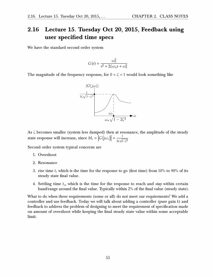
We have the standard second order system
𝐺 (𝑠) =𝜔2𝑛
𝑠2 + 2𝜉𝜔𝑛𝑠 + 𝜔2𝑛
The magnitude of the frequency response, for 0 < 𝜁 < 1 would look something like
1
2ζ√
1−ζ2
ωn√
1− 2ζ2ω
|G(jω)|
ωr
As 𝜁 becomes smaller (system less damped) then at resonance, the amplitude of the steadystate response will increase, since 𝑀𝑟 = �𝐺 �𝑗𝜔𝑟�� =
1
2𝜉�1−𝜉2
Second order system typical concerns are
1. Overshoot
2. Resonance
3. rise time 𝑡𝑟 which is the time for the response to go (first time) from 10% to 90% of itssteady state final value.
4. Settling time 𝑡𝑠, which is the time for the response to reach and stay within certainband/range around the final value. Typically within 2% of the final value (steady state).
What to do when these requirements (some or all) do not meet our requirements? We add acontroller and use feedback. Today we will talk about adding a controller (pure gain 𝑘) andfeedback to address the problem of designing to meet the requirement of specification madeon amount of overshoot while keeping the final steady state value within some acceptablelimit.
55
2.16. Lecture 15. Tuesday Oct 20, 2015, . . . CHAPTER 2. CLASS NOTES
Lets take the open loop 𝐺 (𝑠) and say we have 𝜁 = 0.01, then the overshoot
𝑦max = 1 + 𝑂𝑆max
= 1 + 𝑒−𝜋𝜁
�1−𝜁2
= 1 + 𝑒−𝜋(0.01)
�1−(0.01)2
= 1.969 1
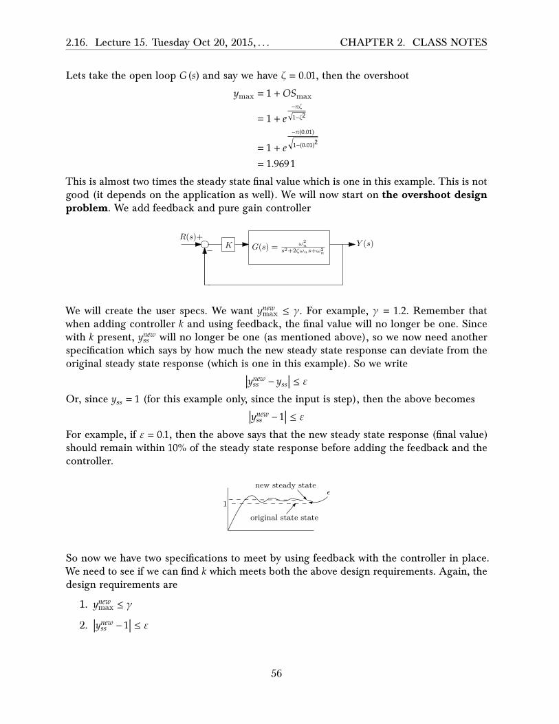
This is almost two times the steady state final value which is one in this example. This is notgood (it depends on the application as well). We will now start on the overshoot designproblem. We add feedback and pure gain controller
K G(s) =ω2
n
s2+2ζωns+ω2n
Y (s)R(s)+
−
We will create the user specs. We want 𝑦𝑛𝑒𝑤max ≤ 𝛾. For example, 𝛾 = 1.2. Remember thatwhen adding controller 𝑘 and using feedback, the final value will no longer be one. Sincewith 𝑘 present, 𝑦𝑛𝑒𝑤𝑠𝑠 will no longer be one (as mentioned above), so we now need anotherspecification which says by how much the new steady state response can deviate from theoriginal steady state response (which is one in this example). So we write
�𝑦𝑛𝑒𝑤𝑠𝑠 − 𝑦𝑠𝑠� ≤ 𝜀
Or, since 𝑦𝑠𝑠 = 1 (for this example only, since the input is step), then the above becomes
�𝑦𝑛𝑒𝑤𝑠𝑠 − 1� ≤ 𝜀
For example, if 𝜀 = 0.1, then the above says that the new steady state response (final value)should remain within 10% of the steady state response before adding the feedback and thecontroller.
1
εnew steady state
original state state
So now we have two specifications to meet by using feedback with the controller in place.We need to see if we can find 𝑘 which meets both the above design requirements. Again, thedesign requirements are
1. 𝑦𝑛𝑒𝑤max ≤ 𝛾
2. �𝑦𝑛𝑒𝑤𝑠𝑠 − 1� ≤ 𝜀
56

2.16. Lecture 15. Tuesday Oct 20, 2015, . . . CHAPTER 2. CLASS NOTES
Once we add the feedback and the controller, we obtain a closed loop transfer function
𝑇 (𝑠) =𝐾𝐺 (𝑠)
1 + 𝐾𝐺 (𝑠)
=𝐾 𝜔2
𝑛𝑠2+2𝜉𝜔𝑛𝑠+𝜔2𝑛
1 + 𝐾𝜔2𝑛
𝑠2+2𝜉𝜔𝑛𝑠+𝜔2𝑛
=𝐾𝜔2
𝑛𝑠2 + 2𝜉𝜔𝑛𝑠 + 𝜔2
𝑛 (1 + 𝐾)(1)
So the new 𝑇 (𝑠) has di�erent natural frequency, given by (will call ��𝑛, �� the new 𝜔𝑛 and thenew 𝜁 ).
��2𝑛 = 𝜔2
𝑛 (1 + 𝐾)
or
��𝑛 = 𝜔𝑛�(1 + 𝐾) (2)
Re-scalling (1) gives
𝑇 (𝑠) =𝐾𝜔2
𝑛��2𝑛��2𝑛
𝑠2 + 2𝜉𝜔𝑛����𝑛
����𝑛𝑠 + ��2𝑛
We want 𝜉𝜔𝑛����𝑛
= 1 to obtain the same form of the standard second order system. Hence, using(2)
𝜉𝜔𝑛����𝑛
= 1
𝜉𝜔𝑛
�� �𝜔𝑛√(1 + 𝐾)�= 1 (2.1)
𝜉��√(1 + 𝐾)
= 1
�� =𝜉
√(1 + 𝐾)(3)
And we call 𝐾𝜔2𝑛
��2𝑛as Δ which is scaling term. Hence
Δ =𝐾𝜔2
𝑛𝜔2𝑛 (1 + 𝐾)
=𝐾
1 + 𝐾(4)
Therefore, 𝑇 (𝑠) can now be written in standard second order system as
𝑇 (𝑠) = �𝐾
1 + 𝐾���2𝑛
𝑠2 + 2����𝑛𝑠 + ��2𝑛
Where �� is given by (3) and ��𝑛 is given by (2). Summary is below before we go to next stageand design for 𝐾
57

2.16. Lecture 15. Tuesday Oct 20, 2015, . . . CHAPTER 2. CLASS NOTES
𝑇 (𝑠) = �𝐾
1 + 𝐾���2𝑛
𝑠2 + 2����𝑛𝑠 + ��2𝑛
�� =𝜉
√(1 + 𝐾)��𝑛 = 𝜔𝑛�(1 + 𝐾)
Now we find to find 𝐾 which meets 𝑦𝑛𝑒𝑤max ≤ 𝛾 and �𝑦𝑛𝑒𝑤𝑠𝑠 − 1� ≤ 𝜀 at the same time. We start𝑦𝑛𝑒𝑤max ≤ 𝛾. Since we know that
𝑦𝑛𝑒𝑤max = 1 + 𝑒−𝜋��
�1−��2
Then, since system is linear, then 𝑦𝑛𝑒𝑤max is just just the constant � 𝐾1+𝐾
� times the above, or
𝑦𝑛𝑒𝑤max = �𝐾
1 + 𝐾�
⎛⎜⎜⎜⎜⎝1 + 𝑒
−𝜋��
�1−��2
⎞⎟⎟⎟⎟⎠
So our requirement becomes
𝐾1 + 𝐾
⎛⎜⎜⎜⎜⎝1 + 𝑒
−𝜋��
�1−��2
⎞⎟⎟⎟⎟⎠ ≤ 𝛾
𝑒−𝜋��
�1−��2 ≤ 𝛾1 + 𝐾𝐾
− 1
≤𝛾 (1 + 𝐾) − 𝐾
𝐾Taking natural logs gives
−𝜋��
√1 − ��2≤ ln �
𝛾 (1 + 𝐾) − 𝐾𝐾 �
By multiplying both sides by −1, this will change the inequality sign from ≤ to ≥ and theabove becomes
𝜋��
√1 − ��2≥ − ln �
𝛾 (1 + 𝐾) − 𝐾𝐾 �
𝜋��
√1 − ��2≥ ln �
𝐾𝛾 (1 + 𝐾) − 𝐾�
Moving all terms to one sides gives
1 ≥ ln �𝐾
𝛾 (1 + 𝐾) − 𝐾�√1 − ��2
𝜋��
Or, same as above
ln �𝐾
𝛾 (1 + 𝐾) − 𝐾�√1 − ��2
𝜋��≤ 1 (5)
The above complete the specification for 𝑦𝑛𝑒𝑤max ≤ 𝛾. We now work on the second specification
58

2.16. Lecture 15. Tuesday Oct 20, 2015, . . . CHAPTER 2. CLASS NOTES
�𝑦𝑛𝑒𝑤𝑠𝑠 − 1� ≤ 𝜀. Since the new system is scaled by 𝐾1+𝐾 , then 𝑦𝑛𝑒𝑤𝑠𝑠 = 𝐾
1+𝐾𝑦𝑠𝑠 but 𝑦𝑠𝑠 = 1, then𝑦𝑛𝑒𝑤𝑠𝑠 = 𝐾
1+𝐾 . Therefore, this requirement says
�𝐾
1 + 𝐾− 1� ≤ 𝜀
Since 𝐾1+𝐾 < 1 then �
𝐾1+𝐾 − 1� = 1 −
𝐾1+𝐾 and the above becomes
1 −𝐾
1 + 𝐾≤ 𝜀
(1 + 𝐾) − 𝐾1 + 𝐾
≤ 𝜀
11 + 𝐾
≤ 𝜀
Therefore we now have two specifications ready for design. They are
1. (A) 𝐹 (𝐾) = ln � 𝐾𝛾(1+𝐾)−𝐾
� �1−��2
𝜋�� ≤ 1 which comes from 𝑦𝑛𝑒𝑤max ≤ 𝛾
2. (B) 11+𝐾 ≤ 𝜀 which comes from �𝑦𝑛𝑒𝑤𝑠𝑠 − 1� ≤ 𝜀
We now start the design for finding 𝐾. Suppose that user specification is that 𝜀 = 0.1 and𝛾 = 1.2. Assume also that 𝜁 = 0.1. We start with (𝐵) above1.
11 + 𝐾
≤ 𝜀
11 + 𝐾
≤ 0.1
1 + 𝐾 ≥ 10𝐾 ≥ 9
We now work on (𝐴). Recall that �� = 𝜉
√(1+𝐾)= 0.1
√(1+𝐾), hence
ln �𝐾
𝛾 (1 + 𝐾) − 𝐾�√1 − ��2
𝜋��≤ 1
ln �𝐾
1.2 (1 + 𝐾) − 𝐾��1 − (0.1)2
(1+𝐾)
𝜋 0.1
√(1+𝐾)
≤ 1
ln �𝐾
0.2𝐾 + 1.2�1
0.1𝜋�(1 + 𝐾) − (0.1)2 ≤ 1
ln �𝐾
0.2𝐾 + 1.2�10𝜋 √
𝐾 + 0.99 ≤ 1
Reader: Plot 𝐹 (𝐾) = 10𝜋 √𝐾 + 0.99 ln � 𝐾
0.2𝐾+1.2�
1Note that 𝐾 < −1 is also a solution, but we are looking for positive gain. Also 𝐾 < −1 do not work withthe second constraint below.
59

2.16. Lecture 15. Tuesday Oct 20, 2015, . . . CHAPTER 2. CLASS NOTES
Here is a plot of 𝐹 (𝐾) above
f[k_] := Log[k/(0.2 k + 1.2)] 10/Pi Sqrt[k + 0.99]Plot[{1, f[k]}, {k, .3, 3}, Frame -> True, GridLines -> Automatic,GridLinesStyle -> LightGray,FrameLabel -> {{"F(k)", None}, {k, "Value of F(k) as k changes"}}]
Out[364]=
0.5 1.0 1.5 2.0 2.5 3.0
-4
-2
0
2
k
F(k)
Value of F(k) as k changes
We see from the above, that for 𝐹 (𝐾) ≤ 1 the largest 𝐾 is around 𝐾 = 1.9.
Reduce[f[k] <= 1 && k > 0, k, Reals]0 < k <= 1.90086
But our requirement for �𝑦𝑛𝑒𝑤𝑠𝑠 − 1� ≤ 𝜀 said we needed 𝐾 ≥ 9. This means we are not able tomeet user specifications to find 𝐾 which satisfies both A and B at the same time.
Reader: How much does the 𝛾 specs has to be relaxed so that we can find 𝐾 with 𝜀 = 0.1kept the same as above?
Reader: How much does the 𝜀 specs has to be relaxed so that we can find 𝐾 with 𝛾 = 1.2kept the same as above?
Reader: With 𝜁 = 0.1, find the region in the �𝜀, 𝛾� space for which a spec meeting 𝐾 exist.
60

2.17. Lecture 16. Thursday Oct 22, 2015, . . . CHAPTER 2. CLASS NOTES
2.17 Lecture 16. Thursday Oct 22, 2015, Routh stability
Today lecture is on stability and how to use Routh table to check for stability. We will useBIBO stability. BIBO stable system is one which has bounded output for all time, when theinput is also bounded for all time. Analytically, a system can be determined if it is stablefrom the convolution definition of system response given by
𝑦 (𝑡) = �𝑡
0𝑟 (𝑡 − 𝜏) 𝑔 (𝜏) 𝑑𝜏 (1)
Where 𝑟 (𝑡) is the input, and 𝑔 (𝑡) is the impulse response of the system. For bounded input,which means |𝑟 (𝑡)| ≤ 𝐵 where 𝐵 is some constant that do not depend on time, the output 𝑦 (𝑡)magnitude can be now found from (1) as follows
�𝑦 (𝑡)� = ��𝑡
0𝑟 (𝑡 − 𝜏) 𝑔 (𝜏) 𝑑𝜏�
≤ �𝑡
0�𝑟 (𝑡 − 𝜏) 𝑔 (𝜏)� 𝑑𝜏
= �𝑡
0|𝑟 (𝑡 − 𝜏)| �𝑔 (𝜏)� 𝑑𝜏
≤ 𝐵�𝑡
0�𝑔 (𝜏)� 𝑑𝜏
Therefore, for �𝑦 (𝑡)� to be bounded, which means �𝑦 (𝑡)� ≤ 𝐶 where 𝐶 is some constant, then
we need ∫𝑡
0�𝑔 (𝜏)� 𝑑𝜏 ≤ ∞. This means that a system is BIBO is ∫
∞
0�𝑔 (𝑡)� 𝑑𝑡 ≤ ∞ where 𝑔 (𝑡) is
the impulse response of the system. The following are examples how to use the above todetermine BIBO stability.
Example: Given 𝐺 (𝑠) = 1𝑠−1 check if it is BIBO stable. The impulse response is 𝑔 (𝑡) = 𝑒𝑡.
Hence ∫∞
0�𝑒𝑡� 𝑑𝑡 = ∫
∞
0𝑒𝑡𝑑𝑡 = 𝑒𝑡�∞
0= ∞ so this is not BIBO stable.
We can also see that this is not stable, since it has one pole in the RHS.
Example: Given 𝐺 (𝑠) = 1𝑠+1 check if it is BIBO stable. The impulse response is 𝑔 (𝑡) = 𝑒−𝑡.
Hence ∫∞
0�𝑒−𝑡� 𝑑𝑡 = ∫
∞
0𝑒=𝑡𝑑𝑡 = −𝑒−𝑡�∞
0= 1 so this is BIBO stable.
We can also see that this is stable since it has no poles in the RHS.
Therefore, as long as a system has no poles in the RHS, then it is BIBO stable. One way tocheck if there are poles in the RHS and how many there are, without actually solving for theroots or without doing the above integration, is to use Routh-Hurwitz table. We will lookat three cases. When the first column in the table has no zeros (classical case), and whenthe first column has a zero, and when a whole row in the table has zeros, and see how tohandle each case. We will do this using three examples of each case.
Example 1: Given 𝐺 (𝑠) = 𝑁(𝑠)𝐷(𝑠) where 𝐷 (𝑠) = 3𝑠
4 + 10𝑠3 + 5𝑠2 + 5𝑠 + 2. We set up Routh tableas follows
61

2.17. Lecture 16. Thursday Oct 22, 2015, . . . CHAPTER 2. CLASS NOTES
𝑠4 3 5 2𝑠3 10 5𝑠2 3.5 2𝑠1 −5
7 0𝑠0 2 0
Looking at the first numerical column (i.e. second column in the table above), we see thereare two sign changes. This means there are 2 poles in the RHS. Which also means thissystem is not BIBO stable.
Reader: Check the roots using Matlab using roots command and verify the above.
Example 2: Given 𝐺 (𝑠) = 𝑁(𝑠)𝐷(𝑠) where 𝐷 (𝑠) = 4𝑠
4+10𝑠3+5𝑠2+12.5𝑠+5. We set up Routh tableas follows
𝑠4 4 5 5𝑠3 10 12.5𝑠2 0 5
Since we have zero at the pivot, then we change it with 𝜀 and continue as follows
𝑠4 4 5 5𝑠3 10 12.5𝑠2 𝜀 5𝑠1 12.5 − 50
𝜀𝑠0 5
We now take the limit as 𝜀 → 0 from above, and see that a sign change between the thirdand fourth row and then another sign change from the fourth to the fifth row. So this is notsable system.
Example 3: Given 𝐺 (𝑠) = 𝑁(𝑠)𝐷(𝑠) where 𝐷 (𝑠) = 𝑠
6 + 2𝑠5 + 8𝑠4 + 12𝑠3 + 20𝑠2 + 20𝑠2 + 16𝑠 + 16. Weset up Routh table as follows
𝑠6 1 8 20 16𝑠5 2 12 16𝑠4 2 12 16𝑠3 0 0
Since we have row of zeros. To handle this, we take the polynomial from the row above,which is 𝐴 (𝑠) = 2𝑠4 + 12𝑠2 + 16 and take its derivative, giving 𝐴′ (𝑠) = 8𝑠3 + 24𝑠, and use thisto replace the row of zeros, so we end up with
62

2.17. Lecture 16. Thursday Oct 22, 2015, . . . CHAPTER 2. CLASS NOTES
𝑠6 1 8 20 16𝑠5 2 12 16𝑠4 2 12 16𝑠3 8 24
And now we continue as before
𝑠6 1 8 20 16𝑠5 2 12 16𝑠4 2 12 16𝑠3 8 24𝑠2 6 16𝑠 8
3𝑠0 16
So there is no sign change, so this is stable.
Another example. Given this system
G
G
R1(s)
R2(s)
+
−
+
+
++
Y1(s)
Y2(s)
The above is called master/slave controller design. Where 𝐺 = 𝐾(𝑠+1)(𝑠+2) and we want to find
if the transfer function from any input to any output is BIBO stable or not. We use Masonrule to obtain the denominator, which is Mason Δ. The signal graph is
1 1
1
1
1
1
1
−1
G
G
R1
R2
Y1
Y2
Mason delta is
Δ = 1 − �−𝐺 + 𝐺 + 𝐺2� + (−𝐺𝐺) = 1 − 2𝐺2
Hence for 𝐺 = 𝐾(𝑠+1)(𝑠+2) then Δ = 𝑠
4 + 6𝑠3 + 13𝑠2 + 12𝑠 + 4 − 2𝑘2 and now we setup Routh table
63

2.17. Lecture 16. Thursday Oct 22, 2015, . . . CHAPTER 2. CLASS NOTES
𝑠4 1 13 4 − 2𝑘2
𝑠3 6 12𝑠2 11 4 − 2𝑘2
𝑠1 108+12𝑘2
11𝑠0 4 − 2𝑘2
Therefore for no sign change we need 108+12𝑘2
11 > 0 which is always true, and we want also
4 − 2𝑘2 > 0 or |𝑘| < √2 as the condition for stability.
Final example. For 𝐺 (𝑠) = 1𝑠4+3𝑠3+𝑘2𝑠2+4𝑠+𝑘1
find conditions for stability.
𝑠4 1 𝑘2 𝑘1𝑠3 3 4𝑠2 3𝑘2−4
3 𝑘1
𝑠14� 3𝑘2−43 �−3𝑘1
3𝑘2−43
𝑠0 𝑘1
The condition is 3𝑘2−33 > 0 or 𝑘2 >
43 and 𝑘1 > 0. We see the region of stability to be the
following
k2
k1
43
Region of allowed k1, k2
Reader For 𝐺 (𝑠) = 1𝑠2(𝑠+1)(𝑠+2) and 𝐻 (𝑠) = 2𝑠 + 𝑘 find 𝑘 for stable system in the following
G(s)
H(s)
U(s) Y (s)+
−
64

2.18. Lecture 17, Tuesday Oct 27, 2015, . . . CHAPTER 2. CLASS NOTES
2.18 Lecture 17, Tuesday Oct 27, 2015, Starting on rootlocus
Suppose we want to know how does the controller a�ect pole locations? Routh table justtells us if the system is stable or not and how many poles are in the RHS, but it does not tellus how the poles behave as the gain 𝐾 changes. Suppose our controller 𝐻 (𝑠) is a functionof (𝐾1, 𝐾2,⋯) where we the designer set the values of these 𝐾𝑖 for example, selecting 𝐾1 forovershoot specification as we did before. Now we will talk about how to select 𝐾 for otherpurpose, which is pole locations of the closed loop system. Closed loop pole location givesus many information about the system, and pole locations are informative about behaviorof closed loop response. For example
××
×
×
−σ
imaginary
real axis
The above diagram tell us about the speed of the response or speed of decay. 𝑒−𝜎𝑡 is indicatorof speed to decay of response. If we have large 𝜎 then the system will go to its final value(steady state much faster). There is also what is called the damping cone. This is the conewhere the poles lie inside.
××
×
×
imaginary
real axisθ
damping cone
The angle 𝜃 above is informative about damping. Large damping implies small angle 𝜃.Suppose we have combination of needs: speed of decay of response and low damping, hencewe have region where we want the poles be located.
65
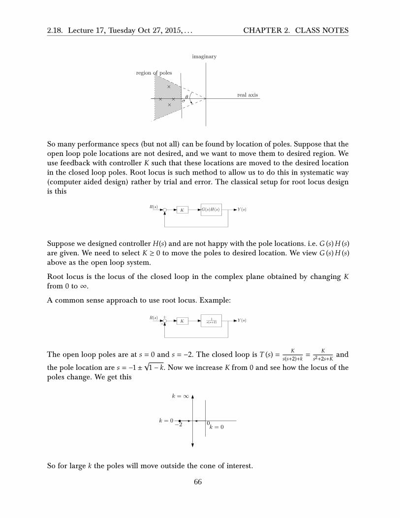
2.18. Lecture 17, Tuesday Oct 27, 2015, . . . CHAPTER 2. CLASS NOTES
××
×
×
imaginary
real axisθσ
×
×× ×
region of poles
So many performance specs (but not all) can be found by location of poles. Suppose that theopen loop pole locations are not desired, and we want to move them to desired region. Weuse feedback with controller 𝐾 such that these locations are moved to the desired locationin the closed loop poles. Root locus is such method to allow us to do this in systematic way(computer aided design) rather by trial and error. The classical setup for root locus designis this
K G(s)H(s)R(s)
Y (s)
Suppose we designed controller 𝐻(𝑠) and are not happy with the pole locations. i.e. 𝐺 (𝑠)𝐻 (𝑠)are given. We need to select 𝐾 ≥ 0 to move the poles to desired location. We view 𝐺 (𝑠)𝐻 (𝑠)above as the open loop system.
Root locus is the locus of the closed loop in the complex plane obtained by changing 𝐾from 0 to ∞.
A common sense approach to use root locus. Example:
K1
s(s+2)
R(s)Y (s)
+
−
The open loop poles are at 𝑠 = 0 and 𝑠 = −2. The closed loop is 𝑇 (𝑠) = 𝐾𝑠(𝑠+2)+𝑘 =
𝐾𝑠2+2𝑠+𝐾 and
the pole location are 𝑠 = −1±√1 − 𝑘. Now we increase 𝐾 from 0 and see how the locus of thepoles change. We get this
−2 0
k =∞
k = 0k = 0
So for large 𝑘 the poles will move outside the cone of interest.
66

2.18. Lecture 17, Tuesday Oct 27, 2015, . . . CHAPTER 2. CLASS NOTES
Reader: How large can 𝐾 be to satisfy damping constraint of 𝛼 = 450?
−2 0
k =∞
k = 0k = 0
α = 450
Formal root locus. Will develop 9 lemmas. Each lemma gives more information about thelocus. We begin with 𝐺 (𝑠)𝐻 (𝑠) which is the open loop. Write it as 𝑁(𝑠)
𝐷(𝑠) where it is proper
(degree of numerator (𝑚) ≤ degree of denominator (𝑛)). Closed loop is 𝑇 (𝑠) = 𝐾𝐺𝐻1+𝐾𝐺𝐻 . To
find closed loop poles, we write
1 + 𝐾𝐺𝐻 = 0
1 + 𝐾𝑁 (𝑠)𝐷 (𝑠)
= 0
𝐷 (𝑠) + 𝐾𝑁 (𝑠) = 0
Observer that, for 𝐾 ≠ 0, the above have 𝑛 poles.
Lemma 1 root locus has 𝑛 branches for 𝐾 > 0.
Root locus (R.L.) geometry: Central idea. A point 𝑠 is on R.L. if 1 + 𝐾𝐺𝐻 = 0 for some 𝐾value. 𝐺𝐻 = − 1
𝐾 . Hence the phase of 𝐺𝐻 is 𝜋. And the corresponding magnitude of 𝐾 is � 1𝐺𝐻 �.
So to decide of point 𝑠 is on the R.L. quickly, look at the angle. For example, for open looppoles 𝑠 = −2 and 𝑠 = 0, and suppose to want to know if some point 𝑠∗ is on the R.L., thenwe draw this
−2 0
s∗
θ1θ2
Then
∢𝐺𝐻 = −𝜃1 − 𝜃2 ≠ 𝜋
Then 𝑠∗ is not on the root locus path.
67

2.19. Lecture 18, Thursday Oct 29, 2015, . . . CHAPTER 2. CLASS NOTES
2.19 Lecture 18, Thursday Oct 29, 2015, More root locus
Reminder: No lecture Tuesday Nov 3. Makeup lecture on Wed. Nov 18 at 6 pm.
Will continue root locus. We are using the classical setup
K G(s)H(s)R(s)
Y (s)
We want to study the behavior of closed loop poles as 𝐾 changes from zero to infinity. Thereis a geometric condition which is the driver behind root locus. It is the angle condition. Thiscondition says that a point 𝑠∗ is on R.L. i� phase of open loop 𝐺 (𝑠)𝐻 (𝑠) evaluated at 𝑠∗ is 𝜋
∢ 𝐺 (𝑠)𝐻 (𝑠)|𝑠=𝑠∗ = 𝜋
When the point 𝑠∗ is on the R.L., then the corresponding gain is (notice, this is valid onlyafter we decided the point 𝑠∗ is on R.L.)
𝑘 =1
|𝐺 (𝑠)𝐻 (𝑠)|𝑠=𝑠∗Let us now look at 𝐺 (𝑠)𝐻 (𝑠) with two zeros and three poles.
𝐺 (𝑠)𝐻 (𝑠) =(𝑠 − 𝑧1) (𝑠 − 𝑧2)
�𝑠 − 𝑝1� �𝑠 − 𝑝2� �𝑠 − 𝑝3�
We want to know if point 𝑠∗ is on R.L.
×
×
×◦◦p3
p2
z1
p1
z2
s∗
How to know if 𝑠∗ on R.L.? We check the angle ∢ 𝐺 (𝑠)𝐻 (𝑠)|𝑠=𝑠∗ and see if it 𝜋. We do thisgraphically, like this
×
×
×◦◦
s∗
θ1θ2
ψ1
ψ2
ψ3
68

2.19. Lecture 18, Thursday Oct 29, 2015, . . . CHAPTER 2. CLASS NOTES
We look at the angle each pole and zero makes with the point 𝑠∗, then
∢ 𝐺 (𝑠)𝐻 (𝑠)|𝑠=𝑠∗ = (𝜃1 + 𝜃2) − �𝜓1 + 𝜓2 + 𝜓3�
i.e. we add the zero angles, and subtract the poles angles. Angle is always measured counterclock wise from the horizontal line as shown. If the above adds to 𝜋 then the point 𝑠∗ is onR.L. The gain 𝐾 in this case is
𝐾 =1
|𝐺 (𝑠)𝐻 (𝑠)|=
1|(𝑠−𝑧1)(𝑠−𝑧2)|
��𝑠−𝑝1��𝑠−𝑝2��𝑠−𝑝3��
=��𝑠 − 𝑝1� �𝑠 − 𝑝2� �𝑠 − 𝑝3��
|(𝑠 − 𝑧1) (𝑠 − 𝑧2)|=𝐷1𝐷2𝐷3𝑑1𝑑2
Where 𝐷𝑖 is the size of the vector from each pole 𝑝𝑖 to 𝑠∗ and 𝑑 is the length of the vectorfrom each zero 𝑧𝑖 to 𝑠∗
×
×
×◦◦
s∗
θ1θ2
ψ1
ψ2
ψ3
|D1|
|D2||D3|
|d1||d2|
Back to the 9 lemmas. When used together, enable us to draw R.L. for any system.
Lemma 1: R.L. has 𝑛 branches, where 𝑛 is number of open loop 𝐺𝐻 poles.
Lemma 2: We talk about very small 𝐾 and very large 𝐾. When 𝐾 is very small, R.L. is at theopen loop poles. This means R.L. always starts from the open loop pole locations. When𝐾 is very large, R.L. is at open loop zeros. For example 𝐺𝐻 = (𝑠+1)(𝑠−2)
(𝑠+4)5, the open loop has
poles at 𝑠 = −4, this is where R.L. starts from. Since it has zero at 𝑠 = −1 and zero at 𝑠 = 2,then this is where 2 of the branches will end up at. This also means for large gain 𝐾 theclosed loop is not stable, since it ends up at 𝑠 = 2.
Since 𝑛 = 5 in the above, so we have 5 branches. Two of these end up at 𝑠 = −1 and 𝑠 = 2.What about the other three? Those will end up infinity. And we need to check if there willbe stable or not.
Lemma 3 (called the number criterion) Which real axis points are on the R.L. ? Sincecomplex poles lead to angle cancellations when point 𝑠∗ being checked for is on the realaxis, then only poles and zeros of the open loop decide if a point 𝑠∗ is on R.L. or not. Areal axis point 𝑠∗ is on R.L. i� the number of real axis poles and zeros (taking multiplicityinto account) found as we travel towards 𝑠∗ from the right side is odd.
Example: 𝐺𝐻 =(𝑠+2)(𝑠−5)2�𝑠2+8𝑠+20�
(𝑠+1)2�𝑠3−1��𝑠2+𝑠+1�. R.L. has 7 branches since 𝑛 = 7 from lemma 1. From
69
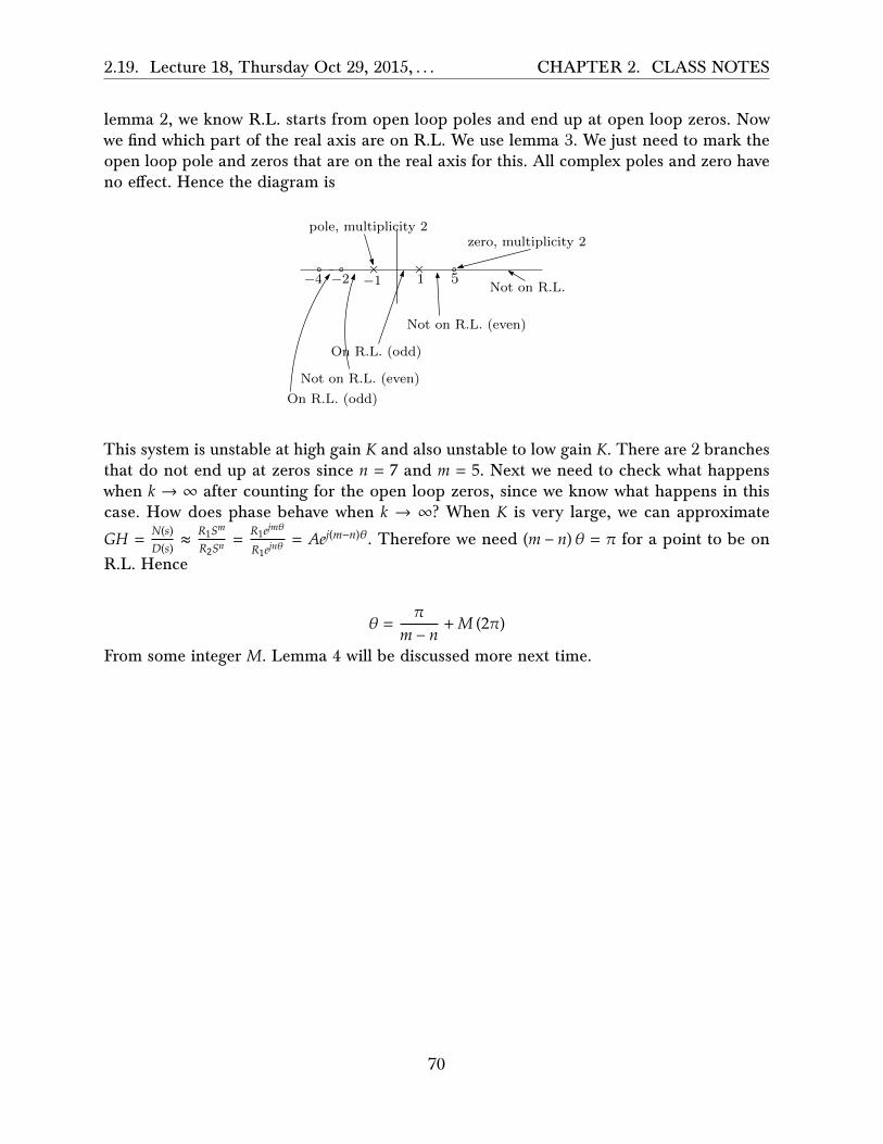
2.19. Lecture 18, Thursday Oct 29, 2015, . . . CHAPTER 2. CLASS NOTES
lemma 2, we know R.L. starts from open loop poles and end up at open loop zeros. Nowwe find which part of the real axis are on R.L. We use lemma 3. We just need to mark theopen loop pole and zeros that are on the real axis for this. All complex poles and zero haveno e�ect. Hence the diagram is
5
zero, multiplicity 2
×1
×−1
pole, multiplicity 2
−2−4Not on R.L.
Not on R.L. (even)
On R.L. (odd)
Not on R.L. (even)
On R.L. (odd)
This system is unstable at high gain 𝐾 and also unstable to low gain 𝐾. There are 2 branchesthat do not end up at zeros since 𝑛 = 7 and 𝑚 = 5. Next we need to check what happenswhen 𝑘 → ∞ after counting for the open loop zeros, since we know what happens in thiscase. How does phase behave when 𝑘 → ∞? When 𝐾 is very large, we can approximate
𝐺𝐻 = 𝑁(𝑠)𝐷(𝑠) ≈
𝑅1𝑆𝑚
𝑅2𝑆𝑛= 𝑅1𝑒𝑗𝑚𝜃
𝑅1𝑒𝑗𝑛𝜃= 𝐴𝑒𝑗(𝑚−𝑛)𝜃. Therefore we need (𝑚 − 𝑛) 𝜃 = 𝜋 for a point to be on
R.L. Hence
𝜃 =𝜋
𝑚 − 𝑛+𝑀(2𝜋)
From some integer 𝑀. Lemma 4 will be discussed more next time.
70

2.20. Lecture 19, Nov. 3, 2015. No lecture CHAPTER 2. CLASS NOTES
2.20 Lecture 19, Nov. 3, 2015. No lecture
2.21 Lecture 20, Nov. 5, 2015. Roots Locus completed
Reminder: Exam 2 on Nov 12 Thursday. Learn relation between damping ratio 𝜁 anddamping cone. Exam will cover up to root locus. Will finish root locus today. Quick reminderof lemmas covered so far
1. Mark open pole loops (where R.L. starts) and open loop zeros.
2. Tells us that R.L. starts at open loop poles and ends up with open loop zeros. Somebranches left will end up at ±∞
3. Tells us what happens on the real axis. The segments that R.L. will travel over on thereal axis. Called the "odd" lemma
4. Tell us how to generate the asymptotes of R.L. using 𝜃 = 1800±𝑘360𝑛−𝑚 . Example, for
𝑛 = 6,𝑚 = 3, (where 𝑛,𝑚 are number of open loop poles and zeros respectively) then𝜃 = 600 ± 𝑘1200 for 𝑘 = 0, 1,⋯
Reader: With 𝑛 − 𝑚 > 2 argue that closed loop is unstable. (answer: with 𝑛 − 𝑚 > 2, anasymptote will be moving to the RHS. Hence one of the branches will eventually move tothe RHS for large gain, which means unstable).
Lemma 5: This lemma for finding from which point on the real axis the asymptotes willstart. The centroid is given by
𝜎𝑐 =�𝑝𝑜𝑙𝑒𝑠 −�𝑧𝑒𝑟𝑜𝑠
𝑛 − 𝑚The above is for poles and zeros of the open loop, not the closed loop!. For example,
for 𝐺𝐻 = (𝑠+2)2
(𝑠+1)(𝑠+6)(𝑠+8)4then 𝜎𝑐 = −8.75 and the angles at 𝜃 = 1800±𝑘360
4 = 450 ± 900. So theasymptotes are
450900
450900
900
Example: 𝐺𝐻 = 1𝑠(𝑠+1)(𝑠+2) . Lemma 1: 𝑛 = 3,𝑚 = 0. Lemma 2: Start from open loop poles.
Lemma 3: Real axis, use the odd criteria. Lemma 4: Find the asymptotes and the centroid.
71

2.21. Lecture 20, Nov. 5, 2015. Roots . . . CHAPTER 2. CLASS NOTES
𝜎𝑐 =0−1−2
3 = −1. 𝜃 = 180±𝑘3603 = 600 ± 𝑘120. The result is this root locus
6001200
×××−2 −1
We still need to find where the break away points are and where root locus intersects theimaginary axis at.
Reader: Without using root locus, find the gain 𝐾 what makes the closed loop unstable.(answer: use Routh table).
Lemma 6: This lemma tells us where the break points are on the real axis. Solve 𝑑𝐾𝑑𝑠 = 0.
Note not all solution points will be valid. Using the above example 𝐺𝐻 = 1𝑠(𝑠+1)(𝑠+2) , then the
characteristic polynomial is
𝐾 + 𝐺𝐻 = 0(𝑠 + 1) (𝑠 + 2) + 𝐾 = 0
𝐾 = −𝑠3 − 3𝑠2 − 2𝑠𝑑𝐾𝑑𝑠
= −3𝑠2 − 6𝑠 − 2
Hence we solve −3𝑠2 − 6𝑠 − 2 = 0, and find 𝑠 = −1. 577 and 𝑠 = −0.423. But 𝑠 = −1. 577 is not onroot locus (from above) so only 𝑠 = −0.423 is on root locus, and that is the breakaway point.
Lemma 7 Departure angle. R.L. depart each pole. We want to find the departure angles.Use
�∢𝑧𝑖 −�∢𝑝𝑖 = 1800 ± 𝑘3600 𝑘 = 0, 1,⋯
Where �∢𝑧𝑖 is sum of all angles from all zeros to the pole in question (the one we want tofind the departure angle from) and �∢𝑝𝑖 is the sum of all the angles from each pole to thepole in question. In the above, the left side will contain only one unknown, which is 𝜃, theangle of departure of that one pole. Do the above for each pole at a time.
Lemma 8 Apply the same method as lemma 7, but now do it for each zero at a time tofind the arrival angles at each zero.
Lemma 9 Find where root locus crosses the imaginary axis. Use Routh table for this.
Example: 𝐺𝐻 = 𝑠2+4𝑠+8𝑠2(𝑠+4) Reader: reproduce the solution below
72

2.21. Lecture 20, Nov. 5, 2015. Roots . . . CHAPTER 2. CLASS NOTES
-8 -7 -6 -5 -4 -3 -2 -1 0 1-2.5
-2
-1.5
-1
-0.5
0
0.5
1
1.5
2
2.5Root Locus
Real Axis (seconds-1)
Imag
inar
y A
xis
(sec
onds
-1)
Reader: Do this problem sent to us by email also. Find root locus for 𝐺 = 𝐾𝑠(𝑠+4)�𝑠2+4𝑠+20�
See my HW6 for more detailed root locus steps.
2.21.1 Summary of root locus
1. Mark on plot all open loop poles and open zero locations.
2. R.L. starts from open loop poles and ends up at open loop zeros. Some will end upat ±∞ when 𝑛 − 𝑚 > 0 (which is almost always the case)
3. Mark on real line where R.L. exist. Use the odd criteria.
4. Find centroid of asymptotes 𝜎 =�𝑝𝑖−�𝑧𝑖
𝑛−𝑚 . i.e. sum of all poles minus sum of all zeros.𝑛 is number of poles, and 𝑚 is number of zeros (these are for the open loop, not theclosed loop!)
5. Find asymptotes angles. 𝜃 = 1800±3600
𝑛−𝑚
73

2.21. Lecture 20, Nov. 5, 2015. Roots . . . CHAPTER 2. CLASS NOTES
6. Find breakaway points. From 1 +𝐾𝐺 = 0 find 𝑘 = 𝑓 (𝑠) and solve 𝑑𝐾𝑑𝑠 = 0 for 𝑠. These are
locations where the breakaway and break-in points on root locus will be.
7. Find departure angles for each pole (the complex ones, the ones on real line will have1800) and arrival angles for the zeros (also complex ones). This can be done using�∢𝑧𝑖 −�∢𝑝𝑖− = 1800 ± 3600𝑘, where in the LHS, we have one unknown angle eachtime. This is the angle of either the departure of arrival. Then solve for it. The aboveis sum of angles that all other poles and zeros make with the point in question. SeeHW 6 for details.
8. Find where root locus crosses the imaginary line. Find 𝐾 which makes the closed loopunstable. Then solve for the polynomial above that row in Routh table for this 𝐾 andsolve for 𝑠. This will be where it crosses the imaginary line. See HW6 for details.
74
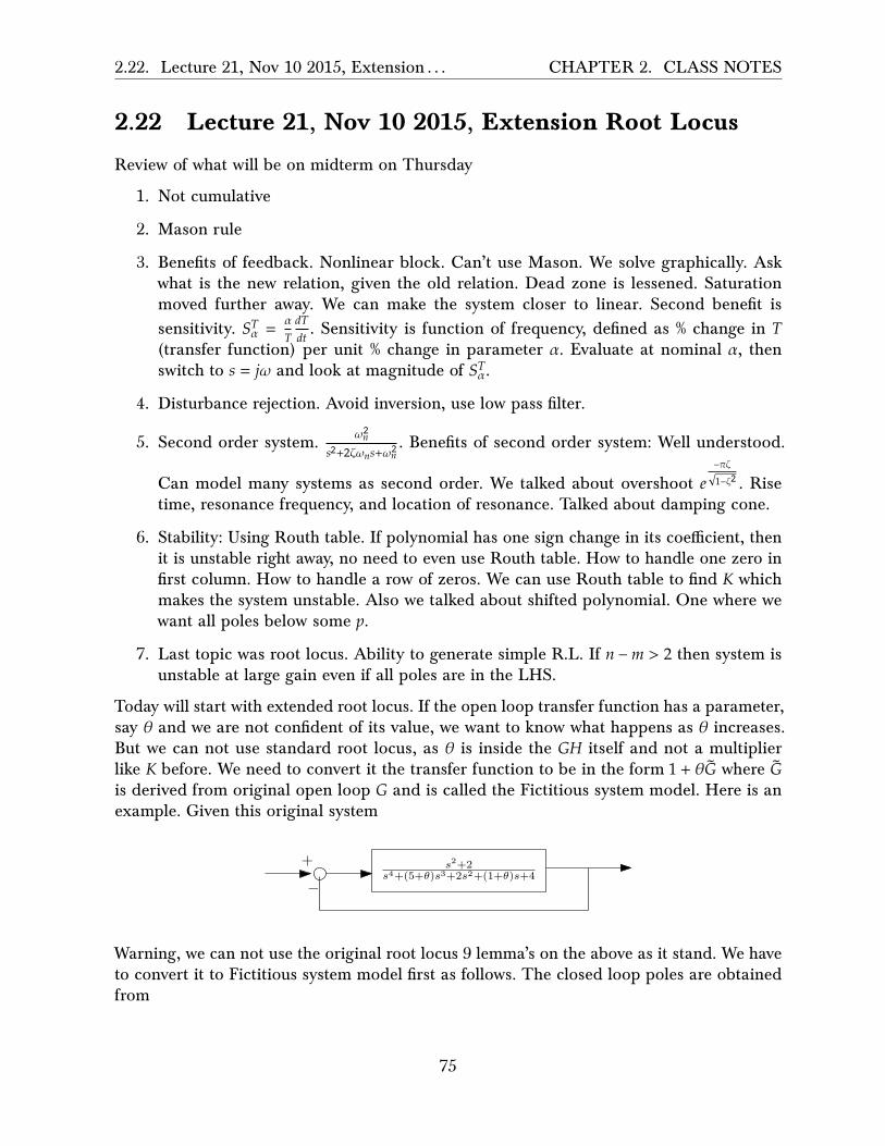
2.22. Lecture 21, Nov 10 2015, Extension . . . CHAPTER 2. CLASS NOTES
2.22 Lecture 21, Nov 10 2015, Extension Root Locus
Review of what will be on midterm on Thursday
1. Not cumulative
2. Mason rule
3. Benefits of feedback. Nonlinear block. Can’t use Mason. We solve graphically. Askwhat is the new relation, given the old relation. Dead zone is lessened. Saturationmoved further away. We can make the system closer to linear. Second benefit issensitivity. 𝑆𝑇𝛼 =
𝛼𝑇𝑑𝑇𝑑𝑡 . Sensitivity is function of frequency, defined as % change in 𝑇
(transfer function) per unit % change in parameter 𝛼. Evaluate at nominal 𝛼, thenswitch to 𝑠 = 𝑗𝜔 and look at magnitude of 𝑆𝑇𝛼.
4. Disturbance rejection. Avoid inversion, use low pass filter.
5. Second order system. 𝜔2𝑛
𝑠2+2𝜁𝜔𝑛𝑠+𝜔2𝑛. Benefits of second order system: Well understood.
Can model many systems as second order. We talked about overshoot 𝑒−𝜋𝜁
�1−𝜁2 . Risetime, resonance frequency, and location of resonance. Talked about damping cone.
6. Stability: Using Routh table. If polynomial has one sign change in its coe�cient, thenit is unstable right away, no need to even use Routh table. How to handle one zero infirst column. How to handle a row of zeros. We can use Routh table to find 𝐾 whichmakes the system unstable. Also we talked about shifted polynomial. One where wewant all poles below some 𝑝.
7. Last topic was root locus. Ability to generate simple R.L. If 𝑛 − 𝑚 > 2 then system isunstable at large gain even if all poles are in the LHS.
Today will start with extended root locus. If the open loop transfer function has a parameter,say 𝜃 and we are not confident of its value, we want to know what happens as 𝜃 increases.But we can not use standard root locus, as 𝜃 is inside the 𝐺𝐻 itself and not a multiplierlike 𝐾 before. We need to convert it the transfer function to be in the form 1 + 𝜃�� where ��is derived from original open loop 𝐺 and is called the Fictitious system model. Here is anexample. Given this original system
s2+2s4+(5+θ)s3+2s2+(1+θ)s+4
+
−
Warning, we can not use the original root locus 9 lemma’s on the above as it stand. We haveto convert it to Fictitious system model first as follows. The closed loop poles are obtainedfrom
75
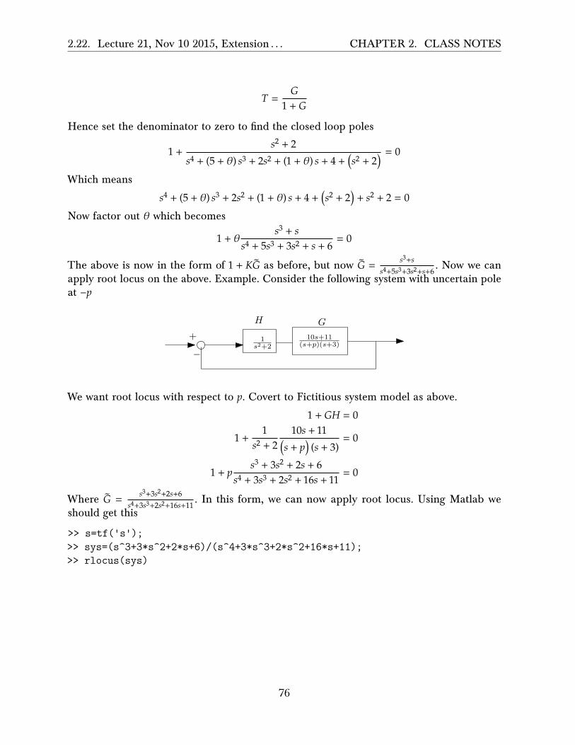
2.22. Lecture 21, Nov 10 2015, Extension . . . CHAPTER 2. CLASS NOTES
𝑇 =𝐺
1 + 𝐺
Hence set the denominator to zero to find the closed loop poles
1 +𝑠2 + 2
𝑠4 + (5 + 𝜃) 𝑠3 + 2𝑠2 + (1 + 𝜃) 𝑠 + 4 + �𝑠2 + 2�= 0
Which means
𝑠4 + (5 + 𝜃) 𝑠3 + 2𝑠2 + (1 + 𝜃) 𝑠 + 4 + �𝑠2 + 2� + 𝑠2 + 2 = 0
Now factor out 𝜃 which becomes
1 + 𝜃𝑠3 + 𝑠
𝑠4 + 5𝑠3 + 3𝑠2 + 𝑠 + 6= 0
The above is now in the form of 1 + 𝐾�� as before, but now �� = 𝑠3+𝑠𝑠4+5𝑠3+3𝑠2+𝑠+6
. Now we canapply root locus on the above. Example. Consider the following system with uncertain poleat −𝑝
10s+11(s+p)(s+3)
+
−1
s2+2
H G
We want root locus with respect to 𝑝. Covert to Fictitious system model as above.
1 + 𝐺𝐻 = 0
1 +1
𝑠2 + 210𝑠 + 11
�𝑠 + 𝑝� (𝑠 + 3)= 0
1 + 𝑝𝑠3 + 3𝑠2 + 2𝑠 + 6
𝑠4 + 3𝑠3 + 2𝑠2 + 16𝑠 + 11= 0
Where �� = 𝑠3+3𝑠2+2𝑠+6𝑠4+3𝑠3+2𝑠2+16𝑠+11
. In this form, we can now apply root locus. Using Matlab weshould get this
>> s=tf('s');>> sys=(s^3+3*s^2+2*s+6)/(s^4+3*s^3+2*s^2+16*s+11);>> rlocus(sys)
76

2.22. Lecture 21, Nov 10 2015, Extension . . . CHAPTER 2. CLASS NOTES
-7 -6 -5 -4 -3 -2 -1 0 1-2.5
-2
-1.5
-1
-0.5
0
0.5
1
1.5
2
2.5Root Locus
Real Axis (seconds-1)
Imag
inar
y A
xis
(sec
onds
-1)
77

2.23. Lecture 22, Nov 12 2015, second exam CHAPTER 2. CLASS NOTES
2.23 Lecture 22, Nov 12 2015, second exam
Exam 2
78

2.24. Lecture 23, Nov 17 2015, Started . . . CHAPTER 2. CLASS NOTES
2.24 Lecture 23, Nov 17 2015, Started Nyquist
There are two more HWs for the course. The final Exam will emphasis Nyquist and Bode.The rest of the course will cover Nyquist and Bode. Nyquist is considered the hardest partof the course. For motivation, we are moving to frequency domain now. So far we have notworked much in frequency domain. Now it will be the main emphasis. We will develop toolsin the frequency domain. Some of the tools we did was Routh table for stability and secondorder system analysis. We did cover some frequency domain when we did noise attenuationand using low pass filter.
Nyquist method is a view of stability in the frequency domain. Why we care about this. Wealready have stability tools? Such as Routh table and Root locus also does tell us somethingabout stability. Because Nyquist tells us more. Nyquist gives new information about stabilityand shows new ways a system can become unstable.
We have Routh table to check for stability. But Routh table assumes the model is perfect.But what if the model is not certain? What is there is amplifier that has frequency drift?This is called model imperfection.
The main measures of stability are gain and phase margins. This tells us how tolerant themodel to imperfections. Nyquist is a graphical description of stability, while Routh table isalgebraic. Engineers use Nyquist since it is considered CAS based method.
2.24.1 What is the Nyquist criteria?
We will generate contour in complex plane, look at the contour and say right away if thesystem is stable or not. We will generate Γ𝐺𝐻 contour. Γ𝐺𝐻 is directed and closed curve. Weuse 𝐺𝐻 which is the open loop transfer function to generate Γ𝐺𝐻 . Then by looking at Γ𝐺𝐻we will say if the closed loop is stable or not.
2.24.2 Preliminary example
Suppose we have generated Γ𝐺𝐻 that looks like the following (we will later learn how togenerate Γ𝐺𝐻).
−1
ΓGH
<
=
79

2.24. Lecture 23, Nov 17 2015, Started . . . CHAPTER 2. CLASS NOTES
Now we apply the Nyquist criteria: The closed loop transfer function (we assume we haveunity feedback), is stable, i� the number of net clockwise encirclements of the critical point−1 on the real axis is equal to the number of unstable RHP poles of the open loop transferfunction (strictly in the RHP). So we need to learn how to count encirclements. For this,we draw straight line from the point −1 on the real line, outwards. It does not matter whichdirection we draw the line. Any one will end up giving the same result. This is due to howwe will do the counting of the encirclements around −1. To show this, the above graph isredrawn below with 3 lines on it. (but we only need one, any one will do).
−1
ΓGH
<
=
ray 1
ray 2
ray 3
In the above we have randomly drawn 3 lines (or rays). Now we count the number of timesthe straight line cross the Γ𝐺𝐻 graph. Each time it crosses Γ𝐺𝐻 we count the direction of Γ𝐺𝐻at that point, if it is clock wise, or anticlock wise. We add one when it is clock wise, andsubtract one when it is counter clock wise. For example, for ray 1 in the above diagram, wesee that there are 2 counter clock wise crossings, and one clock wise crossing. There forthe final result is one counter clock wise crossing. This is the same as saying the result is −1clock wise crossing. So think of counter clock wise as negative numbers, and clock wise aspositive numbers and simply add them. If the final number that results from the above, isthe same as the number open open loop poles in the RHP, then the system is stable.
Reader: The other rays (lines 2 and 3) will give the same final result of one counter clocknet encirclements. Show this.
Example, suppose we have 𝐺𝐻 which has two unstable poles in the RHP such as one withdenominator (𝑠 − 1) �𝑠2 + 𝑠 + 2� (𝑠 − 6), then when we draw Γ𝐺𝐻 and count the encirclements,and find that the net number of clock wise encirclements is also 2, then we know the closedloop is stable.
Now that we know how to interpret Γ𝐺𝐻 and how to use it to find if the closed loop is stableor not, we need to learn how to generate Γ𝐺𝐻. The plan is to become an expert in generatingΓ𝐺𝐻 and also learn how to use it to obtain other stability information from it. To generateΓ𝐺𝐻, we first generate Γ, which is called the Nyquist contour. Then we map Γ to Γ𝐺𝐻. Butfirst we need to generate Γ. The first step is to mark all the open loop poles on the complexplane (we do not need to mark the open loop zeros, but we can do that as well if we want).The we draw a counter clock wise curve around that incloses all these poles in the RHP. If
80

2.24. Lecture 23, Nov 17 2015, Started . . . CHAPTER 2. CLASS NOTES
there are any open loop poles on the imaginary axis, we draw small circle around them tobypass them. Here are two examples
××
×
Γ
open loop poles
Example of Γ for open loop thathas no poles on the imaginary axis.Let R → ∞
R
Now we show an example of Γ for the case when the open loop transfer function 𝐺𝐻 haspoles on the imaginary axis.
×
×
×
Γ
unstable open loop poles
Example of Γ for open loop thathas additional three poles on theimaginary axis. Let R→ ∞ and letε→ 0
Rε
ε
ε
×
×
×
open loop poleson imagineryaxis. By pass.
81
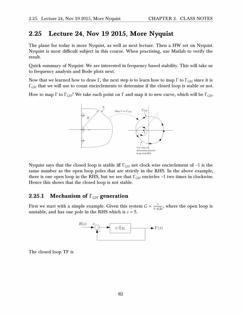
2.25. Lecture 24, Nov 19 2015, More Nyquist CHAPTER 2. CLASS NOTES
2.25 Lecture 24, Nov 19 2015, More Nyquist
The plane for today is more Nyquist, as well as next lecture. Then a HW set on Nyquist.Nyquist is most di�cult subject in this course. When practising, use Matlab to verify theresult.
Quick summary of Nyquist: We are interested in frequency based stability. This will take usto frequency analysis and Bode plots next.
Now that we learned how to draw Γ, the next step is to learn how to map Γ to Γ𝐺𝐻 since it isΓ𝐺𝐻 that we will use to count encirclements to determine if the closed loop is stable or not.
How to map Γ to Γ𝐺𝐻? We take each point on Γ and map it to new curve, which will be Γ𝐺𝐻.
×
Γ
Rε
ε
ε
×
×
×
−1
ΓGHMap Γ to ΓGH
Use this todetermine closedloop stability
Nyquist says that the closed loop is stable i� Γ𝐺𝐻 net clock wise encirclement of −1 is thesame number as the open loop poles that are strictly in the RHS. In the above example,there is one open loop in the RHS, but we see that Γ𝐺𝐻 encircles −1 two times in clockwise.Hence this shows that the closed loop is not stable.
2.25.1 Mechanism of Γ𝐺𝐻 generation
First we start with a simple example. Given this system 𝐺 = 𝑠1−0.2𝑠 , where the open loop is
unstable, and has one pole in the RHS which is 𝑠 = 5.
s1−0.2s
+
−
R(s)Y (s)
The closed loop TF is
82

2.25. Lecture 24, Nov 19 2015, More Nyquist CHAPTER 2. CLASS NOTES
𝑌𝑅=
𝐺1 + 𝐺
=𝑠
(1 − 0.2𝑠) + 𝑠
=𝑠
1 + 0.8𝑠
So the closed loop is stable, since it has no poles in the RHS. So we expect that Γ𝐺𝐻 toencircle −1 one time only, in clockwise, since that is the number of open loop poles in RHS.So we start by drawing Γ. And we start to map Γ to Γ𝐺𝐻.
5
We start always from 𝑠 = 𝑗∞ And go down on 𝑗𝜔 axis of the Γ path. We call this branch 1.When 𝑠 = 𝑗∞ then 𝑌
𝑅 ≈𝑠
−0.2𝑠 ≈ −5, this means that on branch 1 on Γ, the starting point willmap to 𝑠 = −5 on the Γ𝐺𝐻 path. So we have this diagram now
5 −5
ΓΓGH
segment 1
segment 2
segment 3
starting point
Now we move down the +𝑗𝜔 axes and map segment 1 to Γ𝐺𝐻. At segment 1, where 𝑠 = 𝑗𝜔,then 𝐺 = 𝑠
1−0.2𝑠 =𝑗𝜔
1−0.2�𝑗𝜔�. Now we need to see the real part and imaginary part to be able
to see the mapping to Γ𝐺𝐻. Hence we write
83

2.25. Lecture 24, Nov 19 2015, More Nyquist CHAPTER 2. CLASS NOTES
𝐺 =𝑗𝜔
1 − 0.2 �𝑗𝜔�
=𝑗𝜔
1 − 0.2 �𝑗𝜔�
1 + 0.2 �𝑗𝜔�
1 + 0.2 �𝑗𝜔�
=𝑗𝜔 − 0.2𝜔2
1 + 0.04𝜔
Therefore the real part is −0.2𝜔2
1+0.04𝜔 and the imaginary part is 𝜔1+0.04𝜔 .So starting from large
positive 𝜔 going down the segment one, we see that the real part is negative and theimaginary part is negative. This means Γ𝐺𝐻 will be somewhere in the second quadrant. Wedo not care about the shape of Γ𝐺𝐻 that results from mapping segment one. We just knowso far is starts from −5 and remains in the second quadrant. What is important in Nyquist,is where Γ𝐺𝐻 crosses the imaginary and real axis, and now its shape in between. To getthe crossing with the real axis, we set the imaginary part of 𝐺𝐻 to zero. And to get theimaginary axis crossings, we set the real part of 𝐺𝐻 to zero.
To find where Γ𝐺𝐻 crosses the real axis, then from −0.2𝜔2
1+0.04𝜔 = 0 we find 𝜔 = 0. And to find
where Γ𝐺𝐻 crosses the imaginary axis, then from 𝜔1+0.04𝜔 = 0 we also get 𝜔 = 0. So there is
only one point where Γ𝐺𝐻 crosses the axes, which is the origin. At 𝜔 = 0, we see that 𝐺 = 0,therefore the full segment one now maps to Γ𝐺𝐻 as in the following diagram
5 −5
ΓΓGH
segment 1
segment 2
segment 3
starting point
segment onemaps to this
Now we go to segment 2. Along this segment (we are still moving down the imaginary axis),along this, the real part of 𝐺𝐻 is negative, and the imaginary part is also negative. We themapping is now in the third quadrant of Γ𝐺𝐻. We also know this will be the case due tosymmetry about the real axis. So now Γ𝐺𝐻 will look as the following
84

2.25. Lecture 24, Nov 19 2015, More Nyquist CHAPTER 2. CLASS NOTES
5 −5
ΓΓGH
segment 1
segment 2
segment 3
starting point
segment onemaps to this
segment 2maps to this
Now we just need to do segment three. For this segment 𝑠 = Re𝑗𝜃 with 𝑅 becoming verylarge and 𝜃 going from −900 to 00 and then to +900 in the Γ path. But since 𝐺 = 𝑠
1−0.2𝑠 then
𝐺 = Re𝑗𝜃
1−0.2Re𝑗𝜃≈ Re𝑗𝜃
−0.2Re𝑗𝜃for large 𝑅. Hence 𝐺 ≈ −5 as well for segment three. This means all
of segment three in Γ, maps to the one point 𝑠 = −5 in Γ𝐺𝐻. So the Γ𝐺𝐻 will not change. Hereis the final result
5 −5
ΓΓGH
segment 1
segment 2
segment 3
starting point
segment onemaps to this
segment 2maps to this
segment 3maps to −5
Now that we have build Γ𝐺𝐻 , we can find the number of net encirclements around −1. Wesee that there is one clock wise encirclement. But this is the same as the number of unstableopen loop poles. Therefore the closed loop is stable (as we knew before). But this showshow to Nyquist to find out. We now do a second example. Let 𝐺𝐻 = 5(1−0.5𝑠)
𝑠(1+0.1𝑠)(1−0.25𝑠) .
Reader: Is the closed loop stable? Use Routh table to find out. The closed loop denominatoris 𝑃 (𝑠) = 0.025𝑠3+0.15𝑠2+0.15𝑠−5 = 0. This is not stable closed loop. Use Nyquist to confirm.Here is the result using Matlab
s=tf('s');sys=5*(1-0.5*s)/(s*(1+0.1*s)*(1-0.25*s));close all;nyquist1([2.5 -5],[0.025 0.15 -1 0]) %use http://ctms.engin.umich.edu/CTMS/Content/Introduction/Control/Frequency/nyquist1.m
85

2.25. Lecture 24, Nov 19 2015, More Nyquist CHAPTER 2. CLASS NOTES
Real Axis-10 0 10 20 30 40 50
Imag
Axi
s
-60
-40
-20
0
20
40
60
2.25.2 Nyquist Handouts
2.25.2.1 Nyquist Handout 1
The following is Handout 1 Nyquist.
86
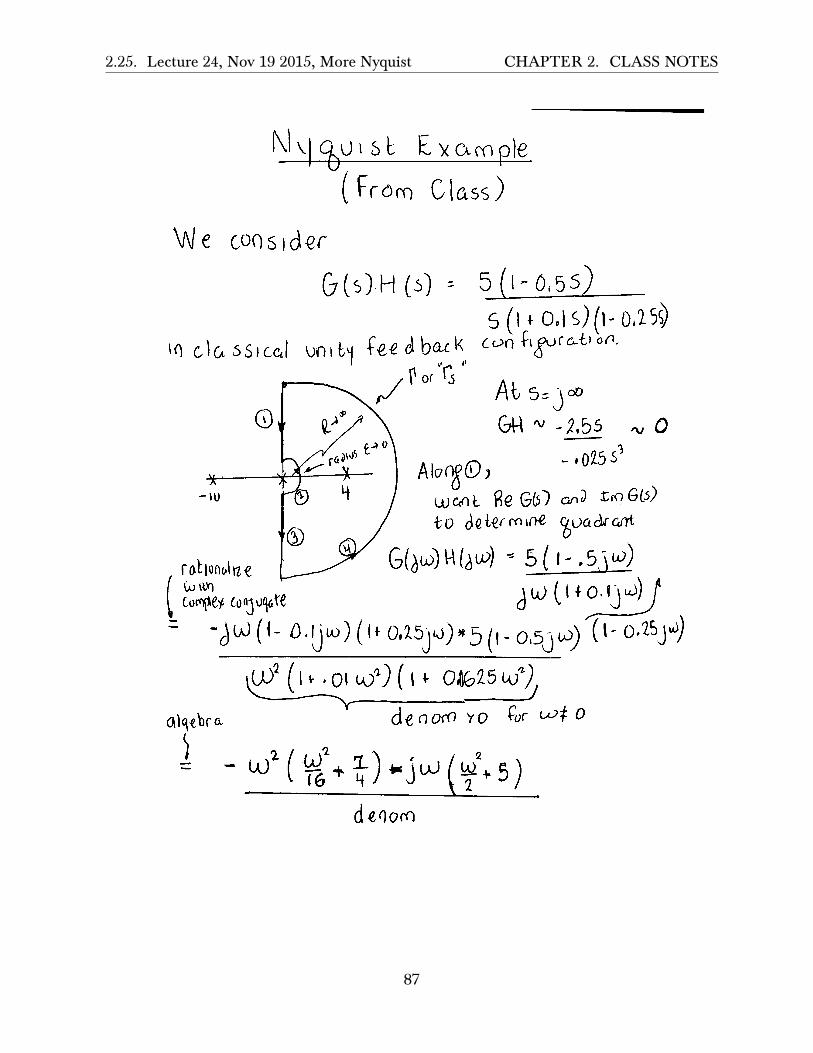
2.25. Lecture 24, Nov 19 2015, More Nyquist CHAPTER 2. CLASS NOTES
y a . 00 Die
(Froro Class)
consider
&(s}.H(5) 5(1-0,55) S(i + 0,1s) (1-0.25)
'0 classical on 1 tM f ec dl ba<: k cwn - f i ^ r t ^ O o n .
At 5=j°° <bV \H - -;.55 ^ 0
- J O
rationalize {jjm
-d OJ (1 - 0. Iju;) ( I f 0.25jo} 5 (, - 0.5j a) t l ^ ^ J " )
.0)^ (I > . 0( CO'') ( I ^ 0^&25 u;"), ^ ^^ , :
a % W a den cm vo fur 0
deoom
87

2.25. Lecture 24, Nov 19 2015, More Nyquist CHAPTER 2. CLASS NOTES
Wence fie G(a'^)H(a^)
deo om
-lence GIDO^©^ Re < O an^ X<Y) < o m-eam
IS lo Q EI ( b h i r d q u a d r a n t )
MoU bh&fc khef<Z a r^ no CtXi6 crossir^^s
Since fie ^ 0 and t 0 .
0 - So''. >Jouj G H
ge^"* So IGH arc a t l o f v o i t ^ ^^^^S ^""'^
7 9 0 ° t o + 9 0 " t I
MB Alorg(i)j Pg »5 -tbe C o n j i ^ a + € of ®. So
U)e re f lec t w . r . t . r e a l axrS and See in Q H to i to fib Q X i a i CfosSiH^S-
n GH
88

2.25. Lecture 24, Nov 19 2015, More Nyquist CHAPTER 2. CLASS NOTES
^ d p06li>^^ const.
Mote: Often, a Coooputer ^enera+ec)
Wvj(^oiSt plot does not sbou; Soch arrc. AI50 arcs Oct lO^tnib^ <pfbeO O^ir 5ln«j/oJA.
Houaevtr cue 5 b o o ; Such ou-ct sioee theij help OS dlrau;^lob. Mcu; combtoin^ resu/b5 -froro ©- u;e obtavO
/
Ooct cloc)^u;ii,e <20c\r6l€roenti oJ^-l^jO-
I cciO eoc. 5ioa ^^^^^ 15 Doe OU ri9ht bctit pictne pde. l eflf 005-tftble
The following is my derivation of the above reader
89
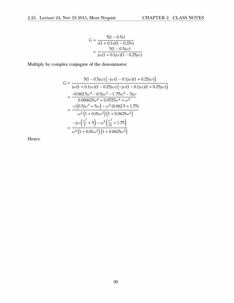
2.25. Lecture 24, Nov 19 2015, More Nyquist CHAPTER 2. CLASS NOTES
𝐺 =5(1 − 0.5𝑠)
𝑠(1 + 0.1𝑠)(1 − 0.25𝑠)
=5(1 − 0.5𝑗𝜔)
𝑗𝜔(1 + 0.1𝑗𝜔)(1 − 0.25𝑗𝜔)
Multiply by complex conjugate of the denominator
𝐺 =5(1 − 0.5𝑗𝜔) �−𝑗𝜔(1 − 0.1𝑗𝜔)(1 + 0.25𝑗𝜔)�
𝑗𝜔(1 + 0.1𝑗𝜔)(1 − 0.25𝑗𝜔) �−𝑗𝜔(1 − 0.1𝑗𝜔)(1 + 0.25𝑗𝜔)�
=−0.062 5𝜔4 − 0.5𝑗𝜔3 − 1. 75𝜔2 − 5𝑗𝜔
0.000625𝜔6 + 0.0725𝜔4 + 𝜔2
=−𝑗 �0.5𝑗𝜔3 + 5𝜔� − 𝜔2 (0.062 5 + 1.75)
𝜔2 �1 + 0.01𝜔2� �1 + 0.0625𝜔2�
=−𝑗𝜔 �𝜔
2
2 + 5� − 𝜔2 �𝜔2
16 + 1.75�
𝜔2 �1 + 0.01𝜔2� �1 + 0.0625𝜔2�
Hence
90
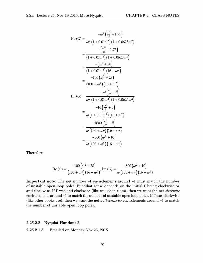
2.25. Lecture 24, Nov 19 2015, More Nyquist CHAPTER 2. CLASS NOTES
Re (𝐺) =−𝜔2 �𝜔
2
16 + 1.75�
𝜔2 �1 + 0.01𝜔2� �1 + 0.0625𝜔2�
=− �𝜔
2
16 + 1.75�
�1 + 0.01𝜔2� �1 + 0.0625𝜔2�
=− �𝜔2 + 28�
�1 + 0.01𝜔2� �16 + 𝜔2�
=−100 �𝜔2 + 28�
�100 + 𝜔2� �16 + 𝜔2�
Im (𝐺) =−𝜔 �𝜔
2
2 + 5�
𝜔2 �1 + 0.01𝜔2� �1 + 0.0625𝜔2�
=−16 �𝜔
2
2 + 5�
𝜔 �1 + 0.01𝜔2� �16 + 𝜔2�
=−1600 �𝜔
2
2 + 5�
𝜔 �100 + 𝜔2� �16 + 𝜔2�
=−800 �𝜔2 + 10�
𝜔 �100 + 𝜔2� �16 + 𝜔2�
Therefore
Re (𝐺) =−100 �𝜔2 + 28�
�100 + 𝜔2� �16 + 𝜔2�, Im (𝐺) =
−800 �𝜔2 + 10�
𝜔 �100 + 𝜔2� �16 + 𝜔2�
Important note: The net number of encirclements around −1 must match the numberof unstable open loop poles. But what sense depends on the initial Γ being clockwise oranti-clockwise. If Γ was anti-clockwise (like we use in class), then we want the net clockwiseencirclements around −1 to match the number of unstable open loop poles. If Γ was clockwise(like other books use), then we want the net anti-clockwise encirclements around −1 to matchthe number of unstable open loop poles.
2.25.2.2 Nyquist Handout 2
2.25.2.1.3 Emailed on Monday Nov 23, 2015
91

2.25. Lecture 24, Nov 19 2015, More Nyquist CHAPTER 2. CLASS NOTES
(}los, de (
Nlturst Exomple
Gtsl ll $): 5 0sG+2) (Sr. q)
Slncc G(s)l l(r) har polce et +J2 rnd -J2. lc k nccerratyto choosc th. Nyqull t Polh noc P.!! tn3 th.tc Pofurc.. theNyqulst peth lr dlvtdcd tntg clSht lccclone as shovn'
On Sec. ( Iv ) : He le t " - g .Jo1e- { ) , 0 var lce f ro i l +90. to-90' ln clockrr ln dtrect lon. Tlrcnr-
c ( s ) H ( s ) - + - - e - J 0Seet
-
Thus, tha GH plot of Sec. ( tV; 1" a acr lc l rc lc atrh lnf ln l3. :radluc, lnd starls froo -90. to +90. ln thc countrrclockrr!.a.|d I rect 1on.
92
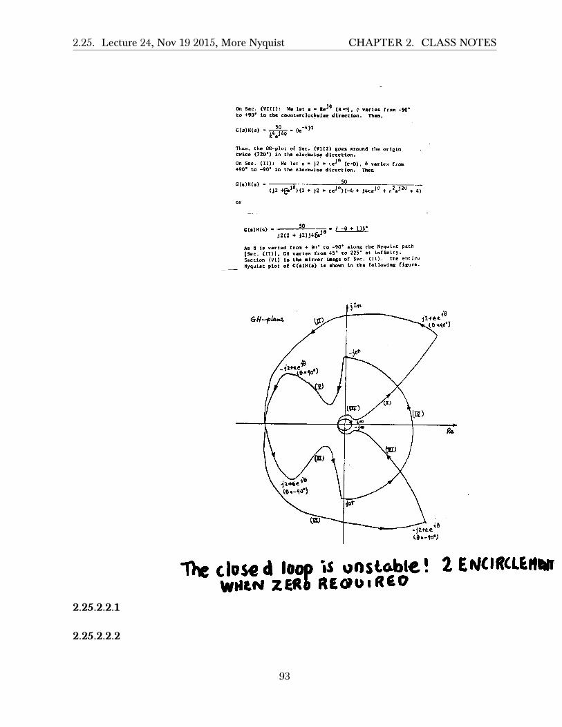
2.25. Lecture 24, Nov 19 2015, More Nyquist CHAPTER 2. CLASS NOTES
2.25.2.2.1
O n S e c . ( V I I I ) : l { c l e t g . X . J 0 ( R * ) , , 1 v . r l e s f r o l - 9 0 .to *90' ln thc countcrcloclrlrc dtreccton. Thcn,
c (e )H(a ) - f f t -oe -4 jo
l l rus, the GH-ploc of Sec. (VIII) gocs rround the orlgl.ntrr lce (72O') ln th. clor:kvlgc rt lrect lon.
O n S e c , ( t I ) : l l e l e t s . J 2 + , r . J ' ) ( a * 0 ) , 0 v a r l e s f r o of90" to -90' ln the clockntge dlrect lon. Then
c ( s ) H ( s ) ' - 5 0 - -t l t € ' o ) ( 2 + ) 2 * . . J ' j ) 1 - o ' + l r e e J o + , 2 . J 2 d * r )
o r
qnG(r)n(s) -;' /--:-9-!-!-15'.
Jz(z + 1zl $tnJo
Ag 0 t s va r l ed f r om + 90 " t o - 90 ' a l ong t hc Nyqu l s t pa th
[ S e c . ( I l ) l ' G H v e r l e s f r o l 4 5 ' c o 2 2 5 o a t l n f l n t t y '
i e c t t on ( v l ) l e t he n l r r o r t r age o f Sec ' ( l l ) . The en t i r e
Nyqulr t p loc of G(s) l l ( r ) 1r rhowr ln the fo l lonln3 f lgurc '
< i 0-tz+ee'
llr clos€ d lom is uosqebJet. - wnlrv zEf,b RE,ou tReo
2 ENCItr(LEilAI
2.25.2.2.2
93
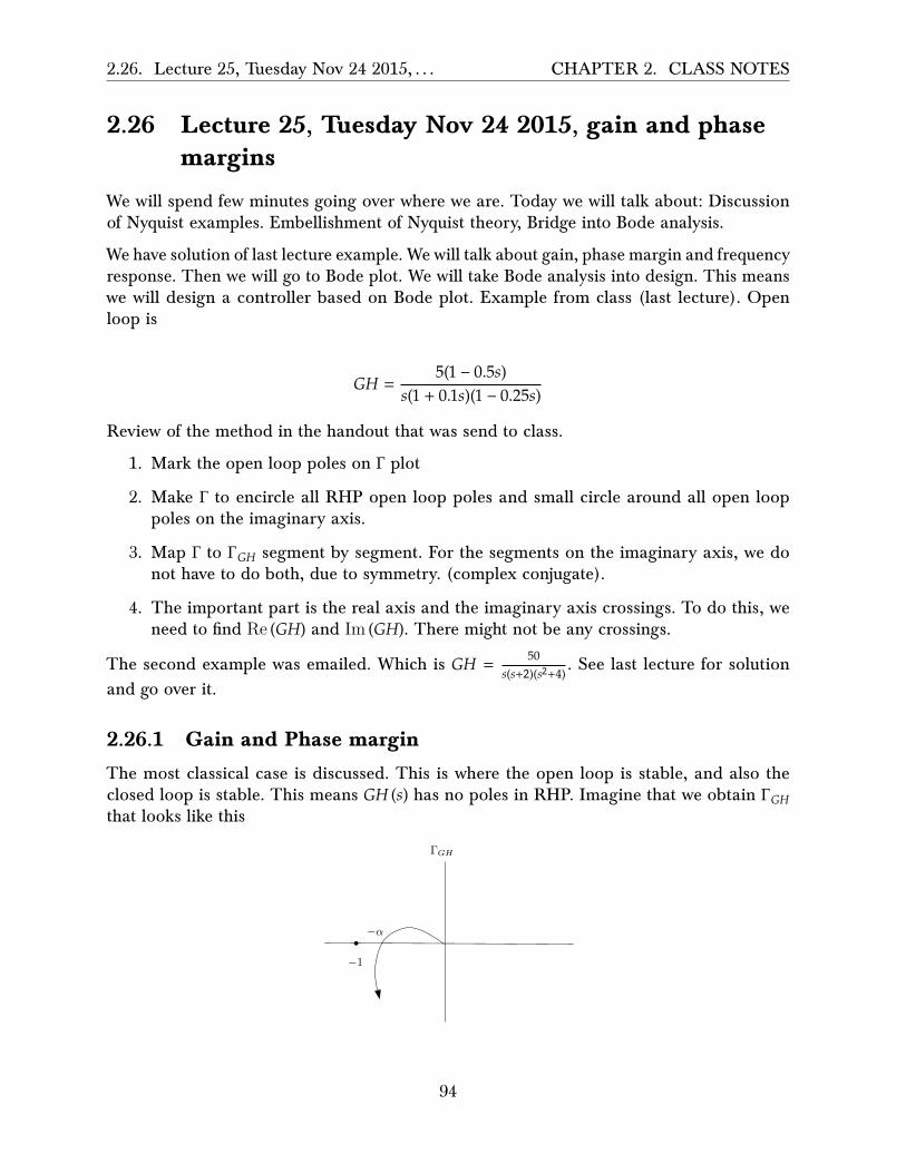
2.26. Lecture 25, Tuesday Nov 24 2015, . . . CHAPTER 2. CLASS NOTES
2.26 Lecture 25, Tuesday Nov 24 2015, gain and phasemargins
We will spend few minutes going over where we are. Today we will talk about: Discussionof Nyquist examples. Embellishment of Nyquist theory, Bridge into Bode analysis.
We have solution of last lecture example. We will talk about gain, phase margin and frequencyresponse. Then we will go to Bode plot. We will take Bode analysis into design. This meanswe will design a controller based on Bode plot. Example from class (last lecture). Openloop is
𝐺𝐻 =5(1 − 0.5𝑠)
𝑠(1 + 0.1𝑠)(1 − 0.25𝑠)
Review of the method in the handout that was send to class.
1. Mark the open loop poles on Γ plot
2. Make Γ to encircle all RHP open loop poles and small circle around all open looppoles on the imaginary axis.
3. Map Γ to Γ𝐺𝐻 segment by segment. For the segments on the imaginary axis, we donot have to do both, due to symmetry. (complex conjugate).
4. The important part is the real axis and the imaginary axis crossings. To do this, weneed to find Re (𝐺𝐻) and Im (𝐺𝐻). There might not be any crossings.
The second example was emailed. Which is 𝐺𝐻 = 50𝑠(𝑠+2)(𝑠2+4) . See last lecture for solution
and go over it.
2.26.1 Gain and Phase margin
The most classical case is discussed. This is where the open loop is stable, and also theclosed loop is stable. This means 𝐺𝐻 (𝑠) has no poles in RHP. Imagine that we obtain Γ𝐺𝐻that looks like this
−1
−α
ΓGH
94

2.26. Lecture 25, Tuesday Nov 24 2015, . . . CHAPTER 2. CLASS NOTES
Closed loop is stable (since it has zero net clockwise encirclement around −1). Note thatif closed loop is unstable, then we can not talk about gain and phase margins. This onlyapplied to closed loop which is already stable. If 𝛼 point in the figure above is very close to−1 then are close to being unstable. This are dangerous if Γ𝐺𝐻 is close to −1. (this is for thisclassical case). For example, say the true system is 𝛾𝐺 (𝑠)𝐻 (𝑠), but our Γ𝐺𝐻 is based on just𝐺 (𝑠)𝐻 (𝑠) and 𝛾 is the small variation of the true system. 𝐺 (𝑠)𝐻 (𝑠) is our math model of thetrue system approximation. So we need to know the margin of safety because the systemcan be unstable if 𝛾 is large enough. Assume 𝛾 is an uncertain gain. Call it now 𝐾. example,an amplifier gain. The math model used to generate Γ𝐺𝐻 is based on 𝐾 = 1.
Reader: What does 𝐾 do to the Nyquist Γ𝐺𝐻 plot?
𝐾 scales the Γ𝐺𝐻. The scaling is centered at the origin. So large 𝐾 magnifies Γ𝐺𝐻 and small𝐾 contracts Γ𝐺𝐻. So we need to find the largest 𝐾max and still be stable. We need 𝐾max𝛼 < 1or
𝐾max =1𝛼
This is called the gain margin. We express this in dB
(𝐾max)𝑑𝐵 = 20 log101𝛼
For example, if 𝛼 = 0.5 then (𝐾max)𝑑𝐵 = 6𝑑𝐵. The gain margin is a measure of safety. We canget 𝐾max also using Routh table. We can also have two sided gain margin
−1 αβ
Assume the 𝐺𝐻 now has one pole in RHP. So we want to have one net clockwise encirclement.So the Γ𝐺𝐻 plot shows that the closed loop is stable. But to maintain stability we need 𝐾𝛼 < 1and 𝐾𝛽 > 1. This means for closed loop stability, we need
1𝛽< 𝐾 <
1𝛼
This is two sided gain margin. Now we talk about phase margin. So far we have not talkedabout phase of 𝐺𝐻 (𝑠). Suppose the true system is 𝐺 (𝑠)𝐻 (𝑠) 𝑒𝑗𝜃 where 𝜃 is the phase error.How does small phase error a�ect stability? Could large phase error destabilize the closedloop? Consider now the classical case (again, this is where open loop is stable, and closedloop remain stable). Here is an example Γ𝐺𝐻 which we will use to analyze the e�ect of phasemargin
95

2.26. Lecture 25, Tuesday Nov 24 2015, . . . CHAPTER 2. CLASS NOTES
−1
unit circleΓGH
−1
unit circleejθΓGHphase margin
rotated clockwise by θ if θ is negative.
How does multiplying 𝐺 (𝑠)𝐻 (𝑠) by 𝑒𝑗𝜃changes the above Γ𝐺𝐻? Each point 𝑧 on Γ𝐺𝐻 now goto 𝑧𝑒𝑗𝜃. So Γ𝐺𝐻 rotates counter clock wise around the origin if 𝜃 > 0 and rotates clock wiseif 𝜃 < 0. How large the angle 𝜃 become before the closed loop become unstable? We draw aunit circle around origin as shown and extend a straight line to where Γ𝐺𝐻 intersects theunit circle. The angle between this line and negative real axis is the phase margin. If 𝜃 < 0,then it will rotate anti clockwise, and will become unstable after rotating −𝑝𝑚, where 𝑝𝑚, isthe phase margin.
96

2.27. Lecture 26, Thursday Nov. 26 2015, . . . CHAPTER 2. CLASS NOTES
2.27 Lecture 26, Thursday Nov. 26 2015, thanks giving,no class
No class. Thanks giving day
97

2.28. Lecture 27, Tuesday December 1 . . . CHAPTER 2. CLASS NOTES
2.28 Lecture 27, Tuesday December 1 2015, Start Bodefrequency analysis
Reminder: Final exam on December 10. Final topic of course is Bode analysis. We touchedon frequency response before but did not go heavily into frequency based design. When welook at the open loop transfer function, we would like to quickly find the frequency response.
The frequency response is defined as the magnitude and phase of the transfer function,when viewed as complex function, which happens when we replace 𝑠 by 𝑗𝜔 where 𝜔 is thefrequency. i.e �𝐺𝐻 �𝑗𝜔�� and ∢𝐺𝐻 �𝑗𝜔� are the frequency response.
Bode method is better for design in frequency domain than Nyquist as it is easier to determinethe magnitude and phase. Nyquist plot already have frequency response information in it,but hard to read.
phase
|GH(jω)|
reading magnitude and phase from Nyquist plot
So if we plot the magnitude and phase, as 𝜔 changes we get something like
ω
|GH(jω)|
ω
angle (or phase) of GH(jω)
Simple motivating example: Say 𝐺 (𝑠) = 11+𝜏𝑠 . We will now use 𝐺 (𝑠) as the open loop. We
could also use 𝐺 (𝑠)𝐻 (𝑠). We know that the �𝐺 �𝑗𝜔�� = 1
√1+𝜏2𝜔2and ∢𝐺 �𝑗𝜔� = − tan−1 (𝜔𝜏). To
easily see what happens to phase as 𝜔 changes, we draw line from the pole, which we know
98
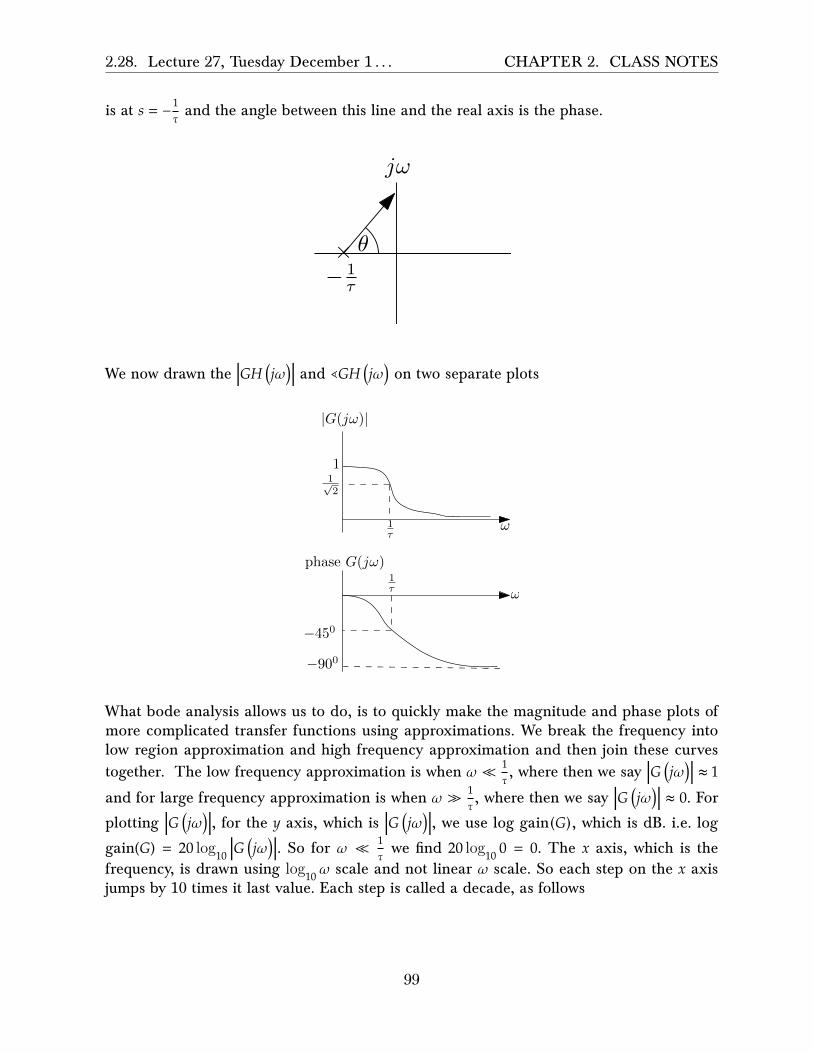
2.28. Lecture 27, Tuesday December 1 . . . CHAPTER 2. CLASS NOTES
is at 𝑠 = − 1𝜏 and the angle between this line and the real axis is the phase.
− 1τ
× θ
jω
We now drawn the �𝐺𝐻 �𝑗𝜔�� and ∢𝐺𝐻 �𝑗𝜔� on two separate plots
ω
11√2
1τ
|G(jω)|
ω1τ
phase G(jω)
−450
−900
What bode analysis allows us to do, is to quickly make the magnitude and phase plots ofmore complicated transfer functions using approximations. We break the frequency intolow region approximation and high frequency approximation and then join these curvestogether. The low frequency approximation is when 𝜔 ≪ 1
𝜏 , where then we say �𝐺 �𝑗𝜔�� ≈ 1
and for large frequency approximation is when 𝜔 ≫ 1𝜏 , where then we say �𝐺 �𝑗𝜔�� ≈ 0. For
plotting �𝐺 �𝑗𝜔��, for the 𝑦 axis, which is �𝐺 �𝑗𝜔��, we use log gain(𝐺), which is dB. i.e. log
gain(𝐺) = 20 log10 �𝐺 �𝑗𝜔��. So for 𝜔 ≪ 1𝜏 we find 20 log10 0 = 0. The 𝑥 axis, which is the
frequency, is drawn using log10𝜔 scale and not linear 𝜔 scale. So each step on the 𝑥 axisjumps by 10 times it last value. Each step is called a decade, as follows
99

2.28. Lecture 27, Tuesday December 1 . . . CHAPTER 2. CLASS NOTES
1τ
log10ω10τ
100τ
1000τ
20log10|G(jω)| (dB)
Now we go back to the first example 𝐺 (𝑠) = 11+𝜏𝑠 , then �𝐺 �𝑗𝜔�� =
1
√1+𝜏2𝜔2hence
20 log10 �𝐺 �𝑗𝜔�� = 20 log10 1 − 20 log10√1 + 𝜏2𝜔2
= 0 − 10 log10 �1 + 𝜏2𝜔2�
Now we apply the Bode approximation. When 𝜔 ≫ 1𝜏 (large frequency approximation), we
get
20 log10 �𝐺 �𝑗𝜔�� = 0 − 10 log10 �𝜏2𝜔2�
= −20 log10 𝜏𝜔
So for large 𝜔 the �𝐺 �𝑗𝜔�� (in db) has a slope of −20 per decade. So we have the followingapproximation of the magnitude
1τ
10τ
100τ0
−20
−40
log10ω
|G(jω)| (dB)
slope −20 dB per decade
1τ
10τ0
−450
−900
log10ωangle
slope −450 per decade
110τ
Notice: the phase plot break point starts the slope from 110𝜏value, and goes down −450 per
decade. The magnitude starts from the 1𝜏 break point and goes down −20 db per decade.
Reader: Do Bode plot for 𝐺 (𝑠) = 1 + 𝜏𝑠. Everything now is flipped from last example of𝐺 (𝑠) = 1
1+𝜏𝑠 .
100

2.28. Lecture 27, Tuesday December 1 . . . CHAPTER 2. CLASS NOTES
1τ
10τ
100τ
0 log10ω
|G(jω)| (dB)slope +20 dB per decade
1τ
10τ
110τ
+450 per decade
angle
log10ω
Now we build on this for more complicate transfer functions. Key remark: Using
log10 (𝐴𝐵𝐶) = log10𝐴 + log10 𝐵 = log10 𝐶Then if 𝐴𝐵𝐶 was complicated transfer function, we break it into simple functions and makebode plot for each, and then just add them to make the over all bode plot. For phase we use
∢ (𝐴𝐵𝐶) = ∢𝐴 + ∢𝐵 + ∢𝐶
Here is an example. Let 𝐺 (𝑠) = 1(1+10𝑠)(1+100𝑠) . For
11+100𝑠 , 𝜏 = 100, so the break point is
1100 = 0.01.
For 11+10𝑠 , if we write it as 1
1+𝜏𝑠 then 𝜏 = 10, and the break points for this term are 110 = 0.1.
These values will go on the 𝑥𝑎𝑥𝑖𝑠 (𝜔). Looking at the magnitudes, we plot each transferfunction on its own, like this
0.01 0.1 1
|G(jω)| (db)
−20
−40
ω rad/sec
−20 db perdecade, startingfrom 0.01. Thisplot represent the
11+100s
transferfunction
−20 db perdecade, startingfrom 0.1. Thisplot represent the
11+10s
transferfunction
Next, we add them. We see that from 0.01 to 0.1, only one TF is active, so the slope is −20db per decade. But from 0.1 to 1 and beyond, both transfer functions are active, and so theslope become −40 db per decade. So the result becomes
101
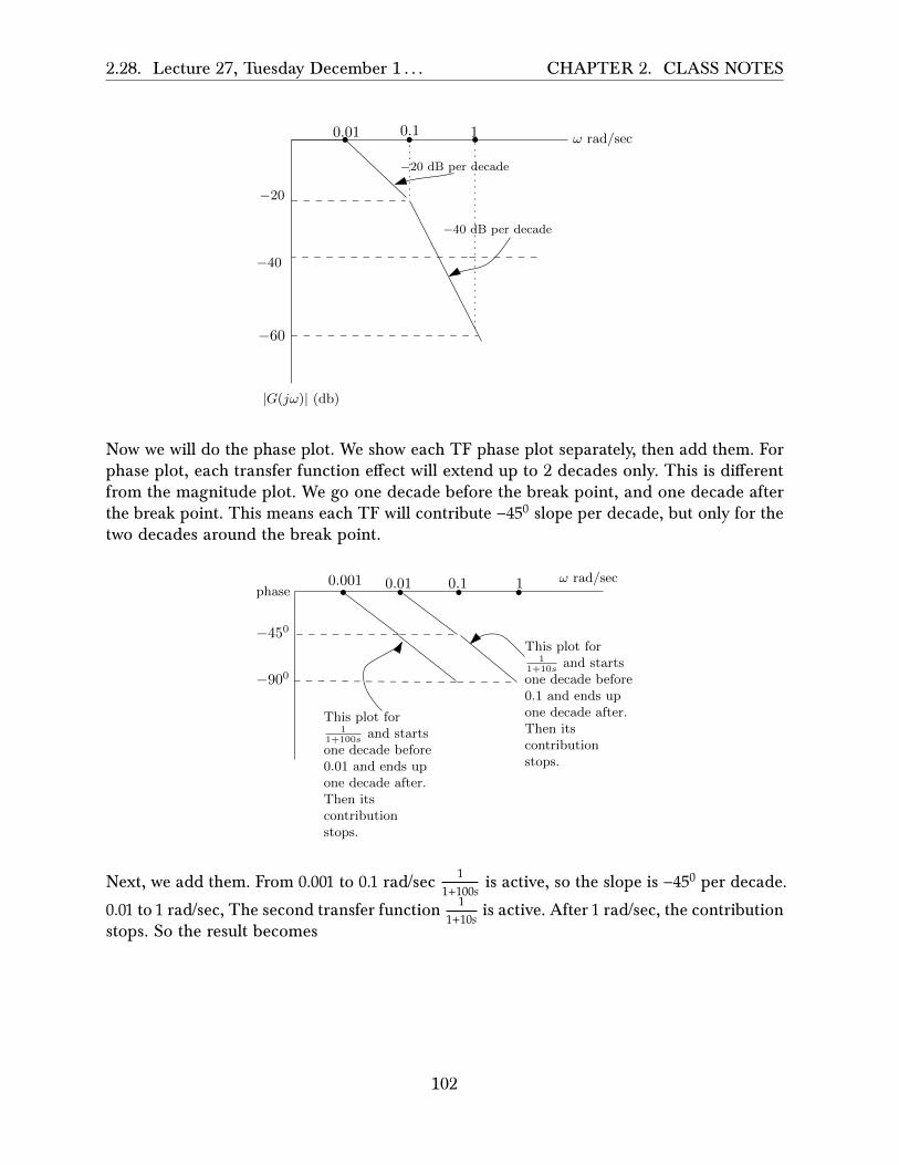
2.28. Lecture 27, Tuesday December 1 . . . CHAPTER 2. CLASS NOTES
0.01 0.1 1
|G(jω)| (db)
−20
−40
ω rad/sec
−60
−20 dB per decade
−40 dB per decade
Now we will do the phase plot. We show each TF phase plot separately, then add them. Forphase plot, each transfer function e�ect will extend up to 2 decades only. This is di�erentfrom the magnitude plot. We go one decade before the break point, and one decade afterthe break point. This means each TF will contribute −450 slope per decade, but only for thetwo decades around the break point.
0.001 0.01 0.1 1
−450
−900
This plot for1
1+100sand starts
one decade before0.01 and ends upone decade after.Then itscontributionstops.
This plot for1
1+10sand starts
one decade before0.1 and ends upone decade after.Then itscontributionstops.
ω rad/secphase
Next, we add them. From 0.001 to 0.1 rad/sec 11+100𝑠 is active, so the slope is −450 per decade.
0.01 to 1 rad/sec, The second transfer function 11+10𝑠 is active. After 1 rad/sec, the contribution
stops. So the result becomes
102
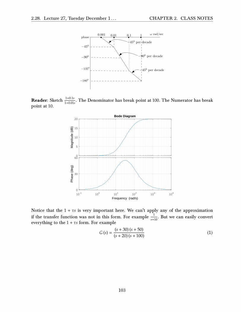
2.28. Lecture 27, Tuesday December 1 . . . CHAPTER 2. CLASS NOTES
0.001 0.01 0.1 1
−450
−900
ω rad/secphase
−1350
−1800
−450 per decade
−900 per decade
−450 per decade
Reader: Sketch 1+0.1𝑠1+0.01𝑠 . The Denominator has break point at 100. The Numerator has break
point at 10.
Mag
nitu
de (
dB)
0
5
10
15
20
10-1 100 101 102 103 104
Pha
se (
deg)
0
30
60
Bode Diagram
Frequency (rad/s)
Notice that the 1 + 𝜏𝑠 is very important here. We can’t apply any of the approximationif the transfer function was not in this form. For example 1
𝑠+10 . But we can easily converteverything to the 1 + 𝜏𝑠 form. For example
𝐺 (𝑠) =(𝑠 + 30) (𝑠 + 50)(𝑠 + 20) (𝑠 + 100)
(1)
103

2.28. Lecture 27, Tuesday December 1 . . . CHAPTER 2. CLASS NOTES
This is not the standard form. We convert each one at a time. Hence
(𝑠 + 30) = 30 �𝑠30+ 1�
(𝑠 + 50) = 50 �𝑠50+ 1�
(𝑠 + 20) = 20 �𝑠20+ 1�
(𝑠 + 100) = 100 �𝑠100
+ 1�
Hence (1) becomes
𝐺 (𝑠) =(30) (50)(20) (100)
� 𝑠30 + 1� �
𝑠50 + 1�
� 𝑠20 + 1� �
𝑠100 + 1�
= 0.75� 𝑠30 + 1� �
𝑠50 + 1�
� 𝑠20 + 1� �
𝑠100 + 1�
The e�ect of the constant 0.75 is to just shift the magnitude plot by 20 log10 0.75. This constantwill not a�ect the phase plot. (if it is positive, as in this example). For negative, it subtracts1800 from the phase.
104
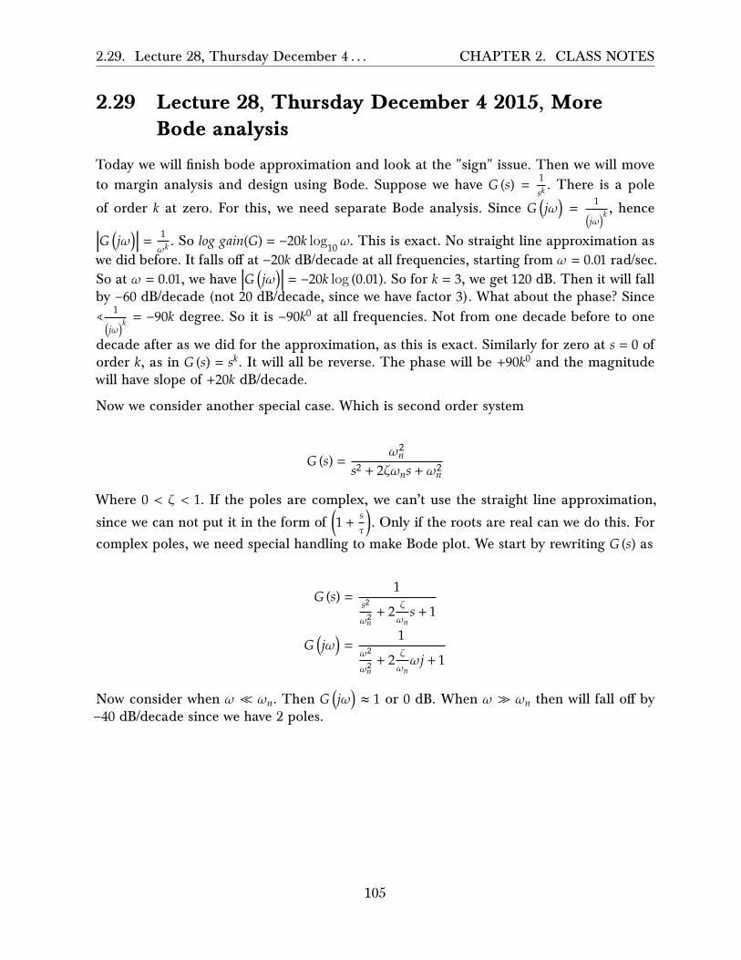
2.29. Lecture 28, Thursday December 4 . . . CHAPTER 2. CLASS NOTES
2.29 Lecture 28, Thursday December 4 2015, MoreBode analysis
Today we will finish bode approximation and look at the "sign" issue. Then we will moveto margin analysis and design using Bode. Suppose we have 𝐺 (𝑠) = 1
𝑠𝑘. There is a pole
of order 𝑘 at zero. For this, we need separate Bode analysis. Since 𝐺�𝑗𝜔� = 1
�𝑗𝜔�𝑘 , hence
�𝐺 �𝑗𝜔�� = 1𝜔𝑘 . So 𝑙𝑜𝑔 𝑔𝑎𝑖𝑛(𝐺) = −20𝑘 log10𝜔. This is exact. No straight line approximation as
we did before. It falls o� at −20𝑘 dB/decade at all frequencies, starting from 𝜔 = 0.01 rad/sec.So at 𝜔 = 0.01, we have �𝐺 �𝑗𝜔�� = −20𝑘 log (0.01). So for 𝑘 = 3, we get 120 dB. Then it will fallby −60 dB/decade (not 20 dB/decade, since we have factor 3). What about the phase? Since∢ 1
�𝑗𝜔�𝑘 = −90𝑘 degree. So it is −90𝑘0 at all frequencies. Not from one decade before to one
decade after as we did for the approximation, as this is exact. Similarly for zero at 𝑠 = 0 oforder 𝑘, as in 𝐺 (𝑠) = 𝑠𝑘. It will all be reverse. The phase will be +90𝑘0 and the magnitudewill have slope of +20𝑘 dB/decade.
Now we consider another special case. Which is second order system
𝐺 (𝑠) =𝜔2𝑛
𝑠2 + 2𝜁𝜔𝑛𝑠 + 𝜔2𝑛
Where 0 < 𝜁 < 1. If the poles are complex, we can’t use the straight line approximation,
since we can not put it in the form of �1 + 𝑠𝜏�. Only if the roots are real can we do this. For
complex poles, we need special handling to make Bode plot. We start by rewriting 𝐺 (𝑠) as
𝐺 (𝑠) =1
𝑠2
𝜔2𝑛+ 2 𝜁
𝜔𝑛𝑠 + 1
𝐺 �𝑗𝜔� =1
𝜔2
𝜔2𝑛+ 2 𝜁
𝜔𝑛𝜔𝑗 + 1
Now consider when 𝜔 ≪ 𝜔𝑛. Then 𝐺�𝑗𝜔� ≈ 1 or 0 dB. When 𝜔 ≫ 𝜔𝑛 then will fall o� by−40 dB/decade since we have 2 poles.
105
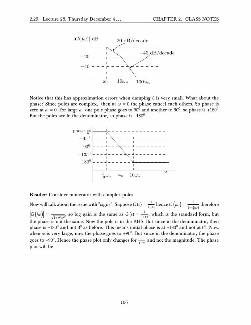
2.29. Lecture 28, Thursday December 4 . . . CHAPTER 2. CLASS NOTES
−20
−40
ωn 10ωn 100ωn
|G(jω)| dB −20 dB/decade
−40 dB/decade
Notice that this has approximation errors when damping 𝜁 is very small. What about thephase? Since poles are complex, then at 𝜔 = 0 the phase cancel each others. So phase iszero at 𝜔 = 0. For large 𝜔, one pole phase goes to 900 and another to 900, so phase is +1800.But the poles are in the denominator, so phase is −1800.
110ωn ωn 10ωn
00
−450
−900
−1350
−1800
phase
ω
Reader: Consider numerator with complex poles
Now will talk about the issue with "signs". Suppose 𝐺 (𝑠) = 11−𝜏𝑠 hence𝐺�𝑗𝜔� =
11−𝜏�𝑗𝜔�
therefore
�𝐺 �𝑗𝜔�� = 1
√1+𝜏2𝜔2, so log gain is the same as 𝐺 (𝑠) = 1
1+𝜏𝑠 , which is the standard form, but
the phase is not the same. Now the pole is in the RHS. But since in the denominator, thenphase is −1800 and not 00 as before. This means initial phase is at −1800 and not at 00. Now,when 𝜔 is very large, now the phase goes to +900. But since in the denominator, the phasegoes to −900. Hence the phase plot only changes for 1
1−𝜏𝑠 and not the magnitude. The phaseplot will be
106
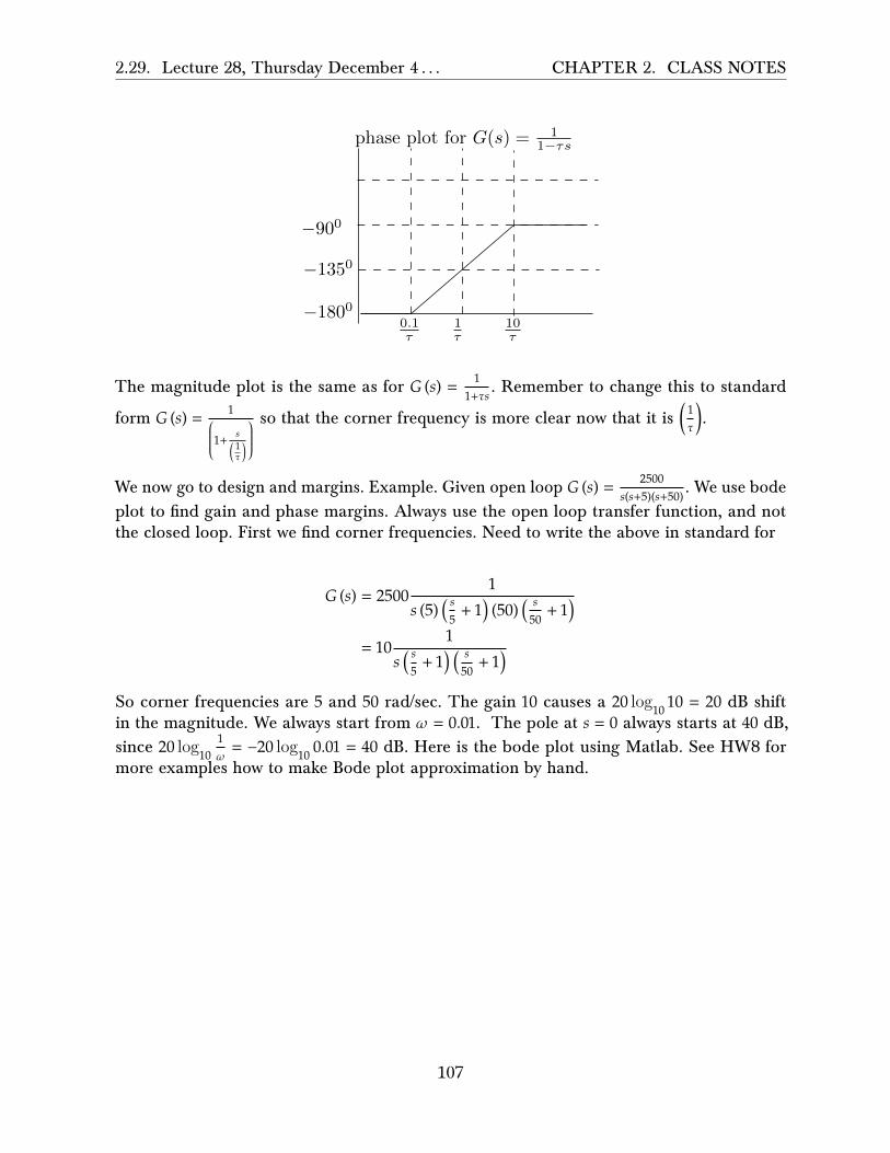
2.29. Lecture 28, Thursday December 4 . . . CHAPTER 2. CLASS NOTES
−1800
−1350
−900
0.1τ
1τ
10τ
phase plot for G(s) = 11−τs
The magnitude plot is the same as for 𝐺 (𝑠) = 11+𝜏𝑠 . Remember to change this to standard
form 𝐺 (𝑠) = 1⎛⎜⎜⎜⎜⎜⎝1+
𝑠
� 1𝜏 �
⎞⎟⎟⎟⎟⎟⎠
so that the corner frequency is more clear now that it is � 1𝜏�.
We now go to design and margins. Example. Given open loop 𝐺 (𝑠) = 2500𝑠(𝑠+5)(𝑠+50) . We use bode
plot to find gain and phase margins. Always use the open loop transfer function, and notthe closed loop. First we find corner frequencies. Need to write the above in standard for
𝐺 (𝑠) = 25001
𝑠 (5) � 𝑠5 + 1� (50) �𝑠50 + 1�
= 101
𝑠 � 𝑠5 + 1� �𝑠50 + 1�
So corner frequencies are 5 and 50 rad/sec. The gain 10 causes a 20 log10 10 = 20 dB shiftin the magnitude. We always start from 𝜔 = 0.01. The pole at 𝑠 = 0 always starts at 40 dB,since 20 log10
1𝜔 = −20 log10 0.01 = 40 dB. Here is the bode plot using Matlab. See HW8 for
more examples how to make Bode plot approximation by hand.
107
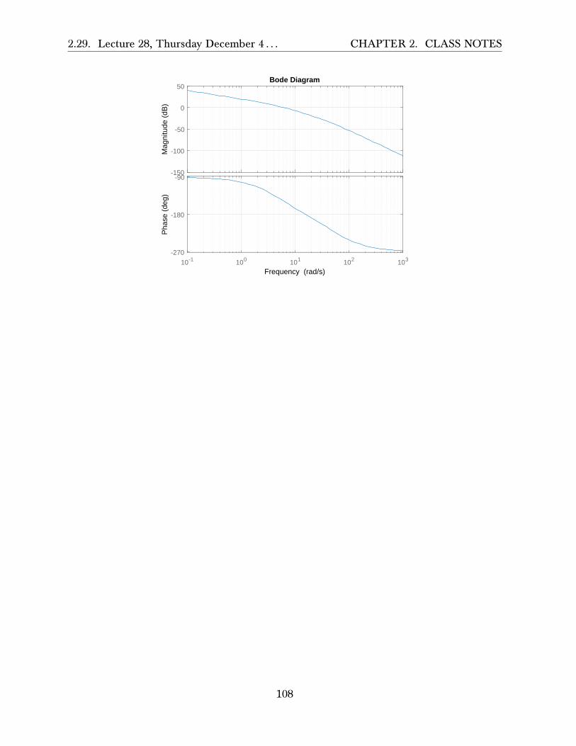
2.29. Lecture 28, Thursday December 4 . . . CHAPTER 2. CLASS NOTES
Mag
nitu
de (
dB)
-150
-100
-50
0
50
10-1 100 101 102 103
Pha
se (
deg)
-270
-180
-90
Bode Diagram
Frequency (rad/s)
108
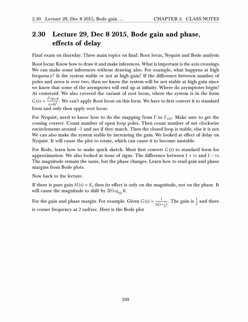
2.30. Lecture 29, Dec 8 2015, Bode gain . . . CHAPTER 2. CLASS NOTES
2.30 Lecture 29, Dec 8 2015, Bode gain and phase,e�ects of delay
Final exam on thursday. Three main topics on final: Root locus, Nyquist and Bode analysis.
Root locus: Know how to draw it and make inferences. What is important is the axis crossings.We can make some inferences without drawing also. For example, what happens at highfrequency? Is the system stable or not at high gain? If the di�erence between number ofpoles and zeros is over two, then we know the system will be not stable at high gain sincewe know that some of the asymptotes will end up at infinity. Where do asymptotes begin?At centeroid. We also covered the variant of root locus, where the system is in the form
𝐺 (𝑠) = 𝑠2+𝑝𝑠+6
(𝑠+8)3. We can’t apply Root locus on this form. We have to first convert it to standard
form and only then apply root locus.
For Nyquist, need to know how to do the mapping from Γ to Γ𝐺𝐻. Make sure to get thecossing correct. Count number of open loop poles. Then count number of net clockwiseencirclements around −1 and see if they match. Then the closed loop is stable, else it is not.We can also make the system stable by increasing the gain. We looked at e�ect of delay onNyquist. It will cause the plot to rotate, which can cause it to become unstable.
For Bode, learn how to make quick sketch. Must first convert 𝐺 (𝑠) to standard form forapproximation. We also looked at issue of signs. The di�erence between 1 + 𝜏𝑠 and 1 − 𝜏𝑠.The magnitude remain the same, but the phase changes. Learn how to read gain and phasemargins from Bode plots.
Now back to the lecture.
If there is pure gain 𝐻 (𝑠) = 𝐾, then its e�ect is only on the magnitude, not on the phase. Itwill cause the magnitude to shift by 20 log10 𝐾.
For the gain and phase margin. For example. Given 𝐺 (𝑠) = 12𝑠�1+ 𝑠
2 �. The gain is 1
2 and there
is corner frequency at 2 rad/sec. Here is the Bode plot
109

2.30. Lecture 29, Dec 8 2015, Bode gain . . . CHAPTER 2. CLASS NOTES
Mag
nitu
de (
dB)
0
5
10
15
20
10-1 100 101 102 103 104
Pha
se (
deg)
0
30
60
Bode Diagram
Frequency (rad/s)
The gain margin is at frequency where phase is −1800. Notice that in this example, the phaseactually is never −1800 but can get as close to it as we want. So in theory, this has infinitegain margin. The phase has to actually dip below −1800 to get an actual crossing. Matlabreports infinite gain margin also. The frequency at which phase is −1800 is called 𝜔𝑝𝑐 andthe frequency at which magnitude is 0 dB is called 𝜔𝑔𝑐. From the plot the phase margin isabout 760.
So a gain only controller 𝐻 (𝑠) = 𝐾 only a�ects the magnitude but not the phase.
Now we will talk about the e�ect of delay on Bode plot. If we have 𝑒−𝑗𝜔𝑇 in forward path,then since �𝑒−𝑗𝜔𝑇� = 1, the delay only a�ects the phase and not the magnitude. Nyquist plotrotates clock wise by amout 𝑇 at 𝜔 = 1. For bode, as 𝜔 increases, the phase will decreasemore and more. So starting with a system that has postive phase margin, as 𝜔 is increasedfor some 𝑇, we will see the phase margin decreasing, and the system can become unstable.
110
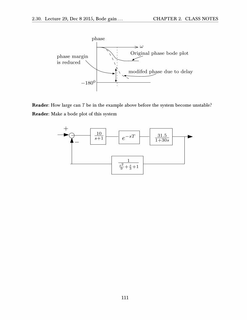
2.30. Lecture 29, Dec 8 2015, Bode gain . . . CHAPTER 2. CLASS NOTES
Original phase bode plot
modifed phase due to delay
phase
ω
−1800
phase marginis reduced
Reader: How large can 𝑇 be in the example above before the system become unstable?
Reader: Make a bode plot of this system
10s+1 e−sT 31.5
1+30s
1s2
9 + s3+1
+
−
111

2.31. Lecture 30, Dec 10 2015, Final exam CHAPTER 2. CLASS NOTES
2.31 Lecture 30, Dec 10 2015, Final exam
Final exam.
112

2.32. Cheat sheet CHAPTER 2. CLASS NOTES
2.32 Cheat sheet
2.32.1 Laplace Transforms for exam
time Laplace
impulse 𝛿 (𝑡) 1delayed impulse 𝛿 (𝑡 − 𝑎) 𝑒−𝑎𝑠
unit step 𝑢 (𝑡) 1𝑠
delayed unit impulse 𝑢 (𝑡 − 𝑎) 1𝑠 𝑒
−𝑎𝑠
ramp 𝑡 1𝑠2
parabolic 𝑡2 2𝑠3
𝑡𝑓 (𝑡) −𝐹′ (𝑠)scaled 𝑓 (𝑎𝑡) 1
𝑎𝐹 �𝑠𝑎�
𝑒𝑎𝑡𝑓 (𝑡) 𝐹 (𝑠 − 𝑎)𝑓 (𝑡) 𝐹 (𝑠)
derivative 𝑓′ (𝑡) 𝑠𝐹 (𝑠) − 𝑓 (0)second derivative 𝑓′′ (𝑡) 𝑠2𝐹 (𝑠) − 𝑠𝑓 (0) − 𝑓′ (0)
integrator ∫𝑡
0𝑓 (𝜏) 𝑑𝜏 1
𝑠𝐹 (𝑠)
delay in time 𝑓 (𝑡 − 𝑎) 𝑢 (𝑡 − 𝑎) 𝑒−𝑎𝑠𝐹 (𝑠)convolution 𝑓 (𝑡) ⊛ 𝑔 (𝑡) 𝐹 (𝑠) 𝐺 (𝑠)
𝑒−𝑎𝑡𝑢 (𝑡) 1𝑠+𝑎
𝑒−𝑎|𝑡| 2𝑎𝑎2−𝑠2
�1 − 𝑒−𝑎𝑡� 𝑢 (𝑡) 𝑎𝑠(𝑠+𝑎)
sin (𝑎𝑡) 𝑢 (𝑡) 𝑎𝑠2+𝑎2
cos (𝑎𝑡) 𝑢 (𝑡) 𝑠𝑠2+𝑎2
𝑒−𝑏𝑡 sin (𝑎𝑡) 𝑢 (𝑡) 𝑎(𝑠+𝑏)2+𝑎2
𝑒−𝑏𝑡 cos (𝑎𝑡) 𝑢 (𝑡) 𝑠+𝑏(𝑠+𝑏)2+𝑎2
2.32.2 Partial fractions
1.1
(𝑠 + 𝑎) (𝑠 + 𝑏)=
𝐴(𝑠 + 𝑎)
+𝐵
(𝑠 + 𝑏)
𝐴 = lim𝑠→−𝑎
1(𝑠 + 𝑏)
𝐵 = lim𝑠→−𝑏
1(𝑠 + 𝑎)
113

2.32. Cheat sheet CHAPTER 2. CLASS NOTES
2.1
(𝑠 + 𝑎) (𝑠 + 𝑏)2=
𝐴(𝑠 + 𝑎)
+𝐵
(𝑠 + 𝑏)+
𝐶(𝑠 + 𝑏)2
𝐴 = lim𝑠→−𝑎
1(𝑠 + 𝑏)2
𝐵 = lim𝑠→−𝑏
𝑑𝑑𝑠 �
1(𝑠 + 𝑎)�
𝐶 = lim𝑠→−𝑏
1(𝑠 + 𝑎)2
3.1
(𝑠 + 𝑎) �𝑠2 + 𝑏�=
𝐴(𝑠 + 𝑎)
+𝐵𝑠 + 𝐶�𝑠2 + 𝑏�
𝐴 = lim𝑠→−𝑎
1�𝑠2 + 𝑏�
For 𝐵,𝐶, expand now and compare coe�cients (but there should be faster way)
2.32.3 Final value
Suppose 𝐹 (𝑠) = 𝑁(𝑠)𝐷(𝑠) is stable, then
lim𝑡→∞
𝑓 (𝑡) = lim𝑠→0
𝑠𝐹 (𝑠)
𝐹 (𝑠) is allowed to have only one pole at origin and still use FVT. But if 𝐹 (𝑠) has more thanone pole at the origin, or unstable, we can’t use FVT to determine lim𝑡→∞ 𝑓 (𝑡).
2.32.4 Tracking𝐸(𝑠)𝑅(𝑠) =
11+𝐺𝐻 . To have lim𝑡→∞ 𝑒 (𝑡) = 0 when the input 𝑅 (𝑠) is step, we need to have integrator
in 𝐺 (𝑠)𝐻 (𝑠). Since we want 𝐺𝐻 to be very large for 𝑠 = 0. And integrator is 1𝑠 . If the input is
ramp 𝑡, then we need 1𝑠2 in 𝐺𝐻. If the input is 𝑡
2 then we need 1𝑠3 in the controller. and so on.
2.32.5 Second order system
𝐺 (𝑠) = 𝜔2𝑛
𝑠2+2𝜁𝜔𝑛𝑠+𝜔2𝑛, 𝑦𝑠𝑡𝑒𝑝 (𝑡) = 1 −
𝑒−𝜁𝜔𝑛𝑡
�1−𝜁2�sin𝜔𝑛√1 − 𝜁2𝑡 + 𝜙� where 𝜙 = cos−1 𝜁. Maximum over-
shoot is 𝑒−𝜋𝜁
�1−𝜁2 . Resonance frequency 𝜔𝑟 = 𝜔𝑛√1 − 2𝜁2, and |𝐺 (𝜔𝑟)| =1
2𝜁�1−𝜁2
114

Chapter 3
HWs
Local contents3.1 HW 1 . . . . . . . . . . . . . . . . . . . . . . . . . . . . . . . . . . . . . . . . . . . . 1163.2 HW 2 . . . . . . . . . . . . . . . . . . . . . . . . . . . . . . . . . . . . . . . . . . . . 1263.3 HW 3 . . . . . . . . . . . . . . . . . . . . . . . . . . . . . . . . . . . . . . . . . . . . 1533.4 HW 4 . . . . . . . . . . . . . . . . . . . . . . . . . . . . . . . . . . . . . . . . . . . . 1803.5 HW 5 . . . . . . . . . . . . . . . . . . . . . . . . . . . . . . . . . . . . . . . . . . . . 1903.6 HW 6 . . . . . . . . . . . . . . . . . . . . . . . . . . . . . . . . . . . . . . . . . . . . 2143.7 HW 7 . . . . . . . . . . . . . . . . . . . . . . . . . . . . . . . . . . . . . . . . . . . . 2353.8 HW 8 . . . . . . . . . . . . . . . . . . . . . . . . . . . . . . . . . . . . . . . . . . . . 266
115

3.1. HW 1 CHAPTER 3. HWS
3.1 HW 1
3.1.1 Problems
2.
ECE 332Honrework 1
1. For the circuit below, find the transfer function ffi.
Find the inverse Laplace transforms of the following:
(a) r(s) : G+br(U) ^F(s) _ F+s,f,3,,1a
(c) r(s): 3filift3?(d) P(s):fffi"-'
A system is described by the difierential equation
y(n) + y(t) + by(z) * Ty(o) + y - uQ) *2u(2) + 3u(r) + 7u
Find the transfer function ffi.4. For the system in Problem 3, find the step response using lhe Matlob toolbox Simulink
(see handout).
(a) Plot your output for 30 seconds and comment. Please include descriptive titlesand axis labels.
(b) In view of the result in (a), a feedback gain K is introduced into the system.This leads to a system with 7y(t) replaced bV (7 + K)y(t). Using Simulink, finda suitable value of K so that the unstable oscillations in (a) are eliminated. Plot30 seconds of the step response for the stabilized system. (Note: Try not to usean excessively large gain if avoidable.)
For this problem submit the two plots as well as a copy of the Simulink schematic fileused to generate the plots ("oly one schematic is needed). Please enlarge the necessaryblocks so that all of the numbers inseide are visible, e.g. the transfer function block.
3.1.2 Problem 1 solution
Let the input impedance be 𝑍𝑖𝑛 and the output impedance be 𝑍𝑜𝑢𝑡, then
𝑍𝑜𝑢𝑡 = 𝑅2||𝑍𝑐1
116

3.1. HW 1 CHAPTER 3. HWS
Where 𝑍𝑐1 is the capacitor impedance given by 𝑍𝑐1 =1𝐶1𝑠
. To find 𝑍𝑜𝑢𝑡, we use the parallelformula
1𝑍𝑜𝑢𝑡
=1𝑅2
+1𝑍𝑐1
=𝑍𝑐1 + 𝑅2
𝑅2𝑍𝑐1
Therefore
𝑍𝑜𝑢𝑡 =𝑅2𝑍𝑐1𝑍𝑐1 + 𝑅2
Now we find the input impedance, which is
𝑍𝑖𝑛 = 𝑅1 + 𝑅2||𝑍𝑐1
= 𝑅1 +𝑅2𝑍𝑐1𝑍𝑐1 + 𝑅2
Simplifying gives
𝑍𝑖𝑛 =𝑅1 (𝑍𝑐1 + 𝑅2) + 𝑅2𝑍𝑐1
𝑍𝑐1 + 𝑅2
Now voltage divider is used, which gives
𝑉2 (𝑠)𝑉1 (𝑠)
=𝑍𝑜𝑢𝑡𝑍𝑖𝑛
=
𝑅2𝑍𝑐1𝑍𝑐1+𝑅2
𝑅1�𝑍𝑐1+𝑅2�+𝑅2𝑍𝑐1𝑍𝑐1+𝑅2
=𝑅2𝑍𝑐1
𝑅1 �𝑍𝑐1 + 𝑅2� + 𝑅2𝑍𝑐1
=𝑅2𝑍𝑐1
𝑅1𝑍𝑐1 + 𝑅1𝑅2 + 𝑅2𝑍𝑐1
=1
𝑅1𝑅2+ 𝑅1
𝑍𝑐1+ 1
=1
𝑅1𝑅2+ 𝑅1𝐶𝑠 + 1
=𝑅2
(𝑅1 + 𝑅2) + 𝑅2𝑅1𝐶𝑠Hence the transfer function is
𝐺 (𝑠) = 𝑉2(𝑠)𝑉1(𝑠)
= 𝑅2(𝑅1+𝑅2)+𝑅2𝑅1𝐶𝑠
The above is a low pass filter since making 𝑠 = 𝑗𝜔 gives
𝐺 (𝜔) =𝑅2
(𝑅1 + 𝑅2) + 𝑅2𝑅1𝐶𝑗𝜔117
3.1. HW 1 CHAPTER 3. HWS
As the frequency 𝜔 → ∞ then |𝐺 (𝜔)| → 0 and as 𝜔 → 0, |𝐺 (𝜔)| → 𝑅2𝑅1+𝑅2
. So the abovetransfer function attenuate large frequencies.
3.1.3 Problem 2 solution
3.1.3.1 Part (a)
𝐹 (𝑠) = 1(𝑠+2)4
. Using the Laplace transform property
𝐹 (𝑠 − 𝑎)⟺ 𝑒𝑎𝑡𝑓 (𝑡) (1)
Where 𝑓 (𝑡) is the inverse Laplace transform of 𝐹 (𝑠). And also using the property
1𝑠𝑛⟺
𝑡𝑛−1
(𝑛 − 1)!(2)
Then, combining (1) and (2) gives
1(𝑠 − 𝑎)𝑛
⟺𝑒𝑎𝑡𝑡𝑛−1
(𝑛 − 1)!For 𝑎 = −2 and 𝑛 = 4 the above becomes
1(𝑠 + 2)4
⟺𝑒−2𝑡𝑡3
3!= 𝑒−2𝑡
𝑡3
6
3.1.3.2 Part (b)
𝐹 (𝑠) = 1𝑠3+5𝑠2+8𝑠+4 . Using the computer, the factors are first found
𝑠3 + 5𝑠2 + 8𝑠 + 4 = (𝑠 + 1) (𝑠 + 2)2
Applying partial fractions decomposition on 1(𝑠+1)(𝑠+2)2
gives
1(𝑠 + 1) (𝑠 + 2)2
=𝐴
(𝑠 + 1)+
𝐵(𝑠 + 2)
+𝐶
(𝑠 + 2)2(1)
Multiplying both sides by (𝑠 + 1) and evaluating at 𝑠 = −1 gives
𝐴 =1
(𝑠 + 2)2𝑠=−1𝐴 = 1
Multiplying both sides by (𝑠 + 2)2 and evaluating at 𝑠 = −2 gives
𝐶 =1
(𝑠 + 1)𝑠=−2𝐶 = −1
118

3.1. HW 1 CHAPTER 3. HWS
Therefore (1) now becomes1
(𝑠 + 1) (𝑠 + 2)2=
1(𝑠 + 1)
+𝐵
(𝑠 + 2)−
1(𝑠 + 2)2
=(𝑠 + 2)2 + 𝐵 (𝑠 + 2) (𝑠 + 1) − (𝑠 + 1)
(𝑠 + 1) (𝑠 + 2)2
=2𝐵 + 3𝑠 + 𝐵𝑠2 + 3𝐵𝑠 + 𝑠2 + 3
(𝑠 + 1) (𝑠 + 2)2
Comparing numerator of RHS and LHS gives
1 = (2𝐵 + 3) + (3 + 3𝐵) 𝑠 + (𝐵 + 1) 𝑠2
Comparing coe�cients (powers of 𝑠) gives 1 = 2𝐵+3 or 𝐵 = −1. Therefore the partial fractiondecomposition of (1) becomes
1(𝑠+1)(𝑠+2)2
= 1(𝑠+1) −
1(𝑠+2) −
1(𝑠+2)2
The inverse Laplace transform is now applied to each term in the RHS and using 𝐹 (𝑠 − 𝑎)⟺𝑒𝑎𝑡𝑓 (𝑡) which results in
1(𝑠 + 1)
−1
(𝑠 + 2)−
1(𝑠 + 2)2
⟺𝑒−𝑡 − 𝑒−2𝑡 − 𝑡𝑒−2𝑡
= 𝑒−𝑡 �1 − 𝑒−𝑡 − 𝑡𝑒−𝑡�
3.1.3.3 Part (c)
𝐹 (𝑠) = 7𝑠2+48𝑠+62𝑠3+7𝑠2+10𝑠 . The denominator can be written as 𝑠 �𝑠2 + 7𝑠 + 10� which is now factored to
𝑠 (𝑠 + 2) (𝑠 + 5). Applying partial fractions on this gives gives
𝐹 (𝑠) =7𝑠2 + 48𝑠 + 62𝑠 (𝑠 + 2) (𝑠 + 5)
=𝐴𝑠+
𝐵𝑠 + 2
+𝐶𝑠 + 5
Hence
𝐴 = lim𝑠→0
7𝑠2 + 48𝑠 + 62(𝑠 + 2) (𝑠 + 5)
=6210
𝐵 = lim𝑠→(−2)
7𝑠2 + 48𝑠 + 62𝑠 (𝑠 + 5)
=7 (4) + 48 (−2) + 62
−2 (−2 + 5)= 1
𝐶 = lim𝑠→(−5)
7𝑠2 + 48𝑠 + 62𝑠 (𝑠 + 2)
=7 (25) + 48 (−5) + 62
−5 (−5 + 2)= −
15
Therefore
𝐹 (𝑠) =62101𝑠+
1𝑠 + 2
−15
1𝑠 + 5
119
3.1. HW 1 CHAPTER 3. HWS
The inverse Laplace transform is
𝑓 (𝑡) =6210+ 𝑒−2𝑡 −
15𝑒−5𝑡
For 𝑡 ≥ 0.
3.1.3.4 Part (d)
𝐹 (𝑠) = 10(𝑠+2)𝑠�𝑠2+4�(𝑠+1)
𝑒−𝑠. This is solved using time shifting property of Laplace transform, which
says that
ℒ�𝑓 (𝑡 − 𝑎)� = 𝑒−𝑎𝑠𝐹 (𝑠)
Where 𝐹 (𝑠) is the Laplace transform of 𝑓 (𝑡). We see that 𝑎 = 1 in the above. So we just need
to find ℒ −1 �10(𝑠+2)
𝑠�𝑠2+4�(𝑠+1)� and then time shift (delay) the result by the amount 𝑎 which is 1 in
this case. Applying partial fractions on 10(𝑠+2)𝑠�𝑠2+4�(𝑠+1)
gives
10 (𝑠 + 2)𝑠 �𝑠2 + 4� (𝑠 + 1)
=𝐴𝑠+
𝐵(𝑠 + 1)
+𝐶𝑠 + 𝐷�𝑠2 + 4�
(1)
Hence
𝐴 = lim𝑠→0
10 (𝑠 + 2)�𝑠2 + 4� (𝑠 + 1)
= 5
𝐵 = lim𝑠→−1
10 (𝑠 + 2)𝑠 �𝑠2 + 4�
=10−5
= −2
Therefore (1) becomes10 (𝑠 + 2)
𝑠 �𝑠2 + 4� (𝑠 + 1)=5𝑠−
2(𝑠 + 1)
+𝐶𝑠 + 𝐷�𝑠2 + 4�
=5 (𝑠 + 1) �𝑠2 + 4� − 2 (𝑠) ��𝑠2 + 4�� + (𝐶𝑠 + 𝐷) (𝑠) (𝑠 + 1)
𝑠 �𝑠2 + 4� (𝑠 + 1)
Or
10 (𝑠 + 2) = 5 (𝑠 + 1) �𝑠2 + 4� − 2 (𝑠) ��𝑠2 + 4�� + (𝐶𝑠 + 𝐷) (𝑠) (𝑠 + 1)
10𝑠 + 20 = 12𝑠 + 𝑠𝐷 + 𝐶𝑠2 + 𝐶𝑠3 + 𝑠2𝐷 + 5𝑠2 + 3𝑠3 + 20= 𝑠 (12 + 𝐷) + 20 + 𝑠2 (𝐶 + 𝐷 + 5) + (𝐶 + 3) 𝑠3
Comparing coe�cients gives
12 + 𝐷 = 10𝐷 = −2
120
3.1. HW 1 CHAPTER 3. HWS
And
0 = 𝐶 + 𝐷 + 5𝐶 = −𝐷 − 5= −3
Therefore10 (𝑠 + 2)
𝑠 �𝑠2 + 4� (𝑠 + 1)=𝐴𝑠+
𝐵(𝑠 + 1)
+𝐶𝑠 + 𝐷�𝑠2 + 4�
=5𝑠−
2(𝑠 + 1)
−3𝑠 + 2�𝑠2 + 4�
=5𝑠−
2(𝑠 + 1)
− 3𝑠
�𝑠2 + 4�−
2�𝑠2 + 4�
(3)
Using tables,ℒ−1 � 𝑠𝑠2+𝑎2
� = cos (𝑎𝑡) , henceℒ−1 �𝑠
�𝑠2+4�� = cos 2𝑡. Also, from tablesℒ−1 � 𝑎𝑠2+𝑎2
� =
sin (𝑎𝑡), hence ℒ−1 � 2𝑠2+4
� = sin 2𝑡. The complete the inverse Laplace transform of 10(𝑠+2)𝑠�𝑠2+4�(𝑠+1)
is now found to be
𝑔 (𝑡) = ℒ −1
⎛⎜⎜⎜⎜⎝
10 (𝑠 + 2)𝑠 �𝑠2 + 4� (𝑠 + 1)
⎞⎟⎟⎟⎟⎠
= 5 − 2𝑒−𝑡 − 3 cos 2𝑡 − sin 2𝑡Therefore the final answer is just a time shifted version of the above, which is
𝑓 (𝑡) = 𝑔 (𝑡 − 1)
= 5 − 2𝑒−(𝑡−1) − 3 cos 2 (𝑡 − 1) − sin 2 (𝑡 − 1)
For 𝑡 ≥ 1 and zero otherwise.
3.1.4 Problem 3 solution
Taking Laplace transform of both sides, and assuming zero for all initial conditions gives
𝑠4𝑌 (𝑠) + 𝑠3𝑌 (𝑠) + 5𝑠2𝑌 (𝑠) + 7𝑠𝑌 (𝑠) + 𝑌 (𝑠) = 𝑠3𝑈 (𝑠) + 2𝑠2𝑈 (𝑠) + 3𝑠𝑈 (𝑠) + 7𝑈 (𝑠)
𝑌 (𝑠) �𝑠4 + 𝑠3 + 5𝑠2 + 7𝑠 + 1� = 𝑈 (𝑠) �𝑠3 + 2𝑠2 + 3𝑠 + 7�𝑌 (𝑠)𝑈 (𝑠)
=𝑠3 + 2𝑠2 + 3𝑠 + 7
𝑠4 + 𝑠3 + 5𝑠2 + 7𝑠 + 1
3.1.5 Problem 4 solution
3.1.5.1 Part (a)
Simulink model was setup and run for 30 seconds. The step response shows that the plantis not stable. This is due to the numerator having roots with positive real parts
121
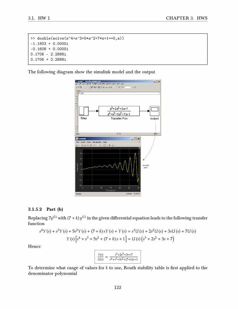
3.1. HW 1 CHAPTER 3. HWS
>> double(solve(s^4+s^3+5*s^2+7*s+1==0,s))-1.1803 + 0.0000i-0.1608 + 0.0000i0.1706 - 2.2888i0.1706 + 2.2888i
The following diagram show the simulink model and the output
Unstable plant
3.1.5.2 Part (b)
Replacing 7𝑦(1) with (7 + 𝑘) 𝑦(1) in the given di�erential equation leads to the following transferfunction
𝑠4𝑌 (𝑠) + 𝑠3𝑌 (𝑠) + 5𝑠2𝑌 (𝑠) + (7 + 𝑘) 𝑠𝑌 (𝑠) + 𝑌 (𝑠) = 𝑠3𝑈 (𝑠) + 2𝑠2𝑈 (𝑠) + 3𝑠𝑈 (𝑠) + 7𝑈 (𝑠)
𝑌 (𝑠) �𝑠4 + 𝑠3 + 5𝑠2 + (7 + 𝑘) 𝑠 + 1� = 𝑈 (𝑠) �𝑠3 + 2𝑠2 + 3𝑠 + 7�
Hence
𝑌(𝑠)𝑈(𝑠) =
𝑠3+2𝑠2+3𝑠+7𝑠4+𝑠3+5𝑠2+(7+𝑘)𝑠+1
To determine what range of values for 𝑘 to use, Routh stability table is first applied to thedenominator polynomial
122

3.1. HW 1 CHAPTER 3. HWS
1 5 11 7 + 𝑘 0
− (2 + 𝑘) 1 0−(2+𝑘)(7+𝑘)−1
−(2+𝑘) 0
Therefore, for no sign change in the first column, we need − (2 + 𝑘) > 0 or 2 + 𝑘 < 0 or 𝑘 < −2and we also need −(2+𝑘)(7+𝑘)−1
−(2+𝑘) > 0 or 𝑘2+9𝑘+152+𝑘 > 0 which means 𝑘2 + 9𝑘 + 15 > 0. The roots of
this quadratic are 𝑘 = −2.208 7, 𝑘 = −6.7913. Putting all these conditions together gives therange of value on 𝑘 for a stable system as
−6.79 < 𝑘 < −2.208
So any 𝑘 in this range can be used. Here is the response using simulink using 4 di�erentvalues of 𝑘, all within the above range to keep the system stable, showing that all the responsesare stable, using the same 30 seconds duration.
K=-6 K=-5
K=-4 K=-3
123

3.1. HW 1 CHAPTER 3. HWS
3.1.6 HW 1 key solution
BCE 332 Homework 1 Solutions
1. By voltage division, we know lhat V2 = Zfu;r,
, -- or#Z z : R z l l * : t R r * o
Therefore,
Rz"Ct
1Rr+A
and in this case, Zr : 8r and
Rz"C,
V z -
R r *
V z :Rz
RrRzCrs* (Rt1^Bz)
RztCt
IRz*- ;
sur
/ 1 r B zf t , (n2 * *,) +;
2- (')
F(s ) :# r + f ( t ) ,'[#']jtse-2'u(t)
Y^,I
f (t)
f(t)
(b)
r(")
f (t)
f (t)
f(") =
F(") _
f ( t ) _
6.2 I- +s s * 2
s 3 + 5 s 2 * 8 s * 4 ( s + 1 ) ( s + 2 ) ,
4-r (P(s))
("-' - e-2' - te-)') u(t)
7s2 + 48s * 62 7s2 * 48s * 62s 3 + 7 s 2 * l o s s ( s * 2 ) ( s + 5 )
I
s * 1 s * 2 ( s * 2 ) 2
( . )
5(s + 5)
|"-")"1r;(o.z + e-2' -
Say V_1 = 1 volt
Since V_1 is not necessarily one volt, the quantity on the right hand side is the required transfer function V_2(s)/V_1(s)
;
124

3.1. HW 1 CHAPTER 3. HWS
(d)
f ( t) : { t- tcos[2(t- 1)] -sin[2(t- 1)] - 2"-t t-r t lu(t- 1)
3. Given the differential equation
y(n) + y(.) + 5y(z) * 7y(t) * v - u(s) *2uQ) 13u(r) 17u
Taking the Laplace Transform of both sides yields:
say(s) * s3y(s) * 5s2y(s) * 7sy(s) + Y(s) : s3u(s) * 2s2U(s)+ 3sU(s) + 7U(s)
Y(") _u(')" 3 + 2 " ' * 3 s * 7
s a { s 3 * 5 s 2 * 7 s * l
4. (a) The transfer function depicting a system which is unstable. The output oscillates
about the point a :7. (approximatally)
(b) K - -3 or K - -4 seem to work well'
Simulink Sdrematic lor Hornwork lt PrcUem 4.
HTinp
I
6
og 4
E.€ 2
0
-2
40
o nEf=o-E
Unstable System ResPonse. Stable System ResPonse. K = -3
-2010 1 0 ? o 3 0
Time, seconds0 1 0 ? o 3 0
Time, seconG
?( l,latlab script file used to generate the plots.
subplot (22L), plot(t ine,yunst), grid, r label( 'Tine, seconds' )
y label ( 'Anpl i tude ' ) , t i t te( 'Unstable Systen Response. ' )
subplot Q2r) , p lo t ( t ine,y) , x label ( 'T iue, seconds ' ) , y label ( 'Anpl i tude ' )
gr id , t i t le( 'Stabl .e Systeu Response- K = -3 ' )
2 lr + 1 1
Scope
You may wish to ignore the code above if you have been succesful making Simulink run
;
125

3.2. HW 2 CHAPTER 3. HWS
3.2 HW 2
3.2.1 Problem 1ECE 332 - Homework #2
problenr 1: Dctermrnc the step, rilmp ancl parabolic steady-state errors oi the tbllowing
unity-f'eec.lback control systems. l'he lbrward-pilth transf'er I'unctions aI€ glven
(a) G(s)H(s)=*#h,
(b) C(s)H(s; = - . t t " 'Us ( s + l 0 X s + 1 0 0 )
K ( l + 2 s X l + 4 s )( c ) C ( s ) l l ( s ) = , , ,'
s - ( s - + s + l )
(ct) What r.clati6nslrips ciln you llnd betwcen the nunrber of poles of G(s) ut the origin and
the rype ol ' input signal l<u which therc is a constant stcady-state error (* 0)? If there
is a relation, state i t ; i l ' thcre is no relation, give the evidence to support your claim.
Problent 2: C'onsider thc l inelr cont l 'o l systct l l shown
and let R(t)=1.5t. Whtt is the steady state crror' /
SOLUTION:
In all of these systems, the feedback block diagram is configured as follows
H(s) G(s)R(s)
Y (s)
feed forward path
plantcontroller
+−
E(s)
E(s)R(s) = 1
1+H(s)G(s)
Since we are looking at steady state, we need to obtain the transfer function between 𝐸 (𝑠)and 𝑅 (𝑠). Given that 𝐸 (𝑠) = 𝑅 (𝑠) − 𝑌 (𝑠) and 𝑌 (𝑠) = 𝐸 (𝑠) 𝐺 (𝑠)𝐻 (𝑠) then we solve these twoequations for 𝐸 (𝑠) by eliminating 𝑌 (𝑠) giving
𝐸 (𝑠) = 𝑅 (𝑠) − 𝐸 (𝑠) 𝐺 (𝑠)𝐻 (𝑠)𝐸 (𝑠) (1 + 𝐺 (𝑠)𝐻 (𝑠)) = 𝑅 (𝑠)
𝐸 (𝑠)𝑅 (𝑠)
=1
1 + 𝐺 (𝑠)𝐻 (𝑠)The above is is the transfer function used for the di�erent 𝑅 (𝑠) signals: unit step 𝑢 (𝑡), ramp𝑡, and parabolic 𝑡2.
126
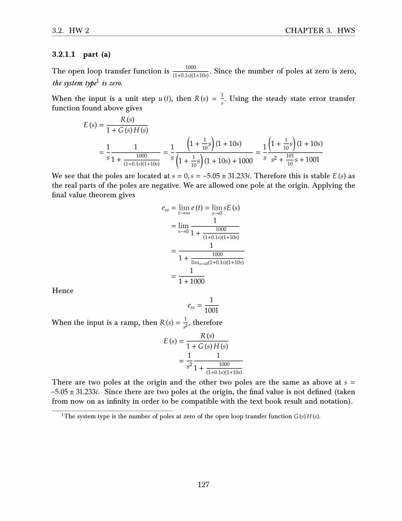
3.2. HW 2 CHAPTER 3. HWS
3.2.1.1 part (a)
The open loop transfer function is 1000(1+0.1𝑠)(1+10𝑠) . Since the number of poles at zero is zero,
the system type1 is zero.
When the input is a unit step 𝑢 (𝑡), then 𝑅 (𝑠) = 1𝑠 . Using the steady state error transfer
function found above gives
𝐸 (𝑠) =𝑅 (𝑠)
1 + 𝐺 (𝑠)𝐻 (𝑠)
=1𝑠
11 + 1000
(1+0.1𝑠)(1+10𝑠)
=1𝑠
�1 + 110𝑠� (1 + 10𝑠)
�1 + 110𝑠� (1 + 10𝑠) + 1000
=1𝑠
�1 + 110𝑠� (1 + 10𝑠)
𝑠2 + 10110 𝑠 + 1001
We see that the poles are located at 𝑠 = 0, 𝑠 = −5.05 ± 31.233𝑖. Therefore this is stable 𝐸 (𝑠) asthe real parts of the poles are negative. We are allowed one pole at the origin. Applying thefinal value theorem gives
𝑒𝑠𝑠 = lim𝑡→∞
𝑒 (𝑡) = lim𝑠→0
𝑠𝐸 (𝑠)
= lim𝑠→0
11 + 1000
(1+0.1𝑠)(1+10𝑠)
=1
1 + 1000lim𝑠→0(1+0.1𝑠)(1+10𝑠)
=1
1 + 1000Hence
𝑒𝑠𝑠 =1
1001When the input is a ramp, then 𝑅 (𝑠) = 1
𝑠2 , therefore
𝐸 (𝑠) =𝑅 (𝑠)
1 + 𝐺 (𝑠)𝐻 (𝑠)
=1𝑠2
11 + 1000
(1+0.1𝑠)(1+10𝑠)
There are two poles at the origin and the other two poles are the same as above at 𝑠 =−5.05 ± 31.233𝑖. Since there are two poles at the origin, the final value is not defined (takenfrom now on as infinity in order to be compatible with the text book result and notation).
1The system type is the number of poles at zero of the open loop transfer function 𝐺 (𝑠)𝐻 (𝑠).
127

3.2. HW 2 CHAPTER 3. HWS
Finally, when the input is 𝑡2, then 𝑅 (𝑠) = 2𝑠3 and
𝐸 (𝑠) =2𝑠3
11 + 𝐺 (𝑠)𝐻 (𝑠)
=2𝑠3
11 + 1000
(1+0.1𝑠)(1+10𝑠)
=2 (1 + 0.1𝑠) (1 + 10𝑠)
𝑠3 (1 + 0.1𝑠) (1 + 10𝑠) + 1000𝑠3
=2 (1 + 0.1𝑠) (1 + 10𝑠)𝑠3 �𝑠2 + 10.1𝑠 + 1001�
There are now three poles at the origin 𝑠 = 0. As above, this means the final value is takenas infinity.
3.2.1.2 part (b)
The open loop transfer function is 1000𝑠(1+10)(𝑠+100) . There is one pole at the origin which means
the system type is one.
When the input is a unit step, then 𝑅 (𝑠) = 1𝑠 and
𝐸 (𝑠) =1𝑠
𝑅 (𝑠)1 + 𝐺 (𝑠)𝐻 (𝑠)
=1𝑠
11 + 1000
𝑠(1+10)(𝑠+100)
=1
𝑠 + 1000(1+10)(𝑠+100)
=(1 + 10) (𝑠 + 100)
𝑠 (1 + 10) (𝑠 + 100) + 1000=
(1 + 10) (𝑠 + 100)11𝑠2 + 1100𝑠 + 1000
The poles are at 𝑠 = −0.9175, 𝑠 = −99.08. This is stable 𝐸 (𝑠) and we can now apply the finalvalue theorem
𝑒𝑠𝑠 = lim𝑡→∞
𝑒 (𝑡) = lim𝑠→0
𝑠𝐸 (𝑠)
= lim𝑠→0
𝑠1𝑠
1 + 1000𝑠(1+10)(𝑠+100)
=1
1 + lim𝑠→01000
𝑠(1+10)(𝑠+100)
Hence
𝑒𝑠𝑠 = 0
128
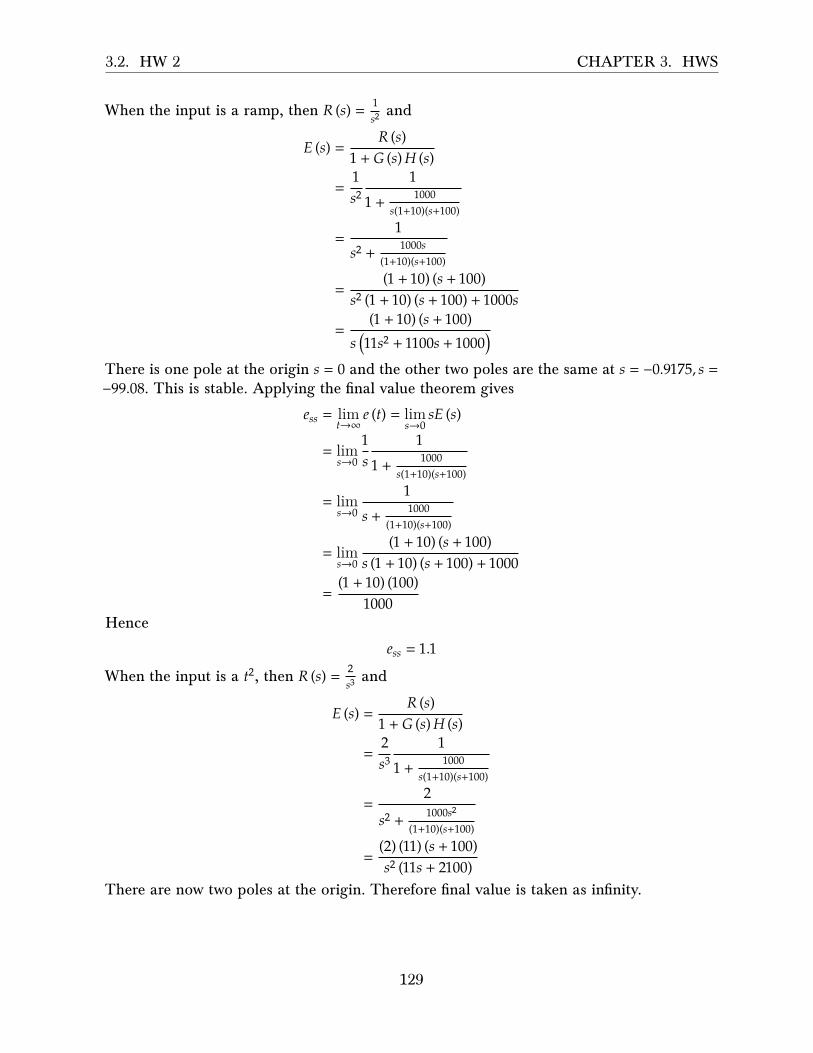
3.2. HW 2 CHAPTER 3. HWS
When the input is a ramp, then 𝑅 (𝑠) = 1𝑠2 and
𝐸 (𝑠) =𝑅 (𝑠)
1 + 𝐺 (𝑠)𝐻 (𝑠)
=1𝑠2
11 + 1000
𝑠(1+10)(𝑠+100)
=1
𝑠2 + 1000𝑠(1+10)(𝑠+100)
=(1 + 10) (𝑠 + 100)
𝑠2 (1 + 10) (𝑠 + 100) + 1000𝑠
=(1 + 10) (𝑠 + 100)
𝑠 �11𝑠2 + 1100𝑠 + 1000�
There is one pole at the origin 𝑠 = 0 and the other two poles are the same at 𝑠 = −0.9175, 𝑠 =−99.08. This is stable. Applying the final value theorem gives
𝑒𝑠𝑠 = lim𝑡→∞
𝑒 (𝑡) = lim𝑠→0
𝑠𝐸 (𝑠)
= lim𝑠→0
1𝑠
11 + 1000
𝑠(1+10)(𝑠+100)
= lim𝑠→0
1𝑠 + 1000
(1+10)(𝑠+100)
= lim𝑠→0
(1 + 10) (𝑠 + 100)𝑠 (1 + 10) (𝑠 + 100) + 1000
=(1 + 10) (100)
1000Hence
𝑒𝑠𝑠 = 1.1
When the input is a 𝑡2, then 𝑅 (𝑠) = 2𝑠3 and
𝐸 (𝑠) =𝑅 (𝑠)
1 + 𝐺 (𝑠)𝐻 (𝑠)
=2𝑠3
11 + 1000
𝑠(1+10)(𝑠+100)
=2
𝑠2 + 1000𝑠2
(1+10)(𝑠+100)
=(2) (11) (𝑠 + 100)𝑠2 (11𝑠 + 2100)
There are now two poles at the origin. Therefore final value is taken as infinity.
129

3.2. HW 2 CHAPTER 3. HWS
3.2.1.3 part (c)
The open loop transfer function is 𝐾(1+2𝑠)(1+4𝑠)𝑠2�𝑠2+𝑠+1�
. There are two poles at the origin which means
the system type is 2.
When the input is a unit step, then 𝑅 (𝑠) = 1𝑠 and
𝐸 (𝑠) =𝑅 (𝑠)
1 + 𝐺 (𝑠)𝐻 (𝑠)
=1𝑠
1
1 + 𝐾(1+2𝑠)(1+4𝑠)𝑠2�𝑠2+𝑠+1�
=1
𝑠 + 𝐾(1+2𝑠)(1+4𝑠)𝑠�𝑠2+𝑠+1�
=𝑠 �𝑠2 + 𝑠 + 1�
𝑠2 �𝑠2 + 𝑠 + 1� + 𝐾 (1 + 2𝑠) (1 + 4𝑠)
We have to now assume that 𝐸 (𝑠) is stable to be able to apply the final value theorem as thisdepends on the value of 𝑘 which is not given in the problem. Therefore
𝑒𝑠𝑠 = lim𝑡→∞
𝑒 (𝑡) = lim𝑠→0
𝑠𝐸 (𝑠)
= lim𝑠→0
𝑠
⎛⎜⎜⎜⎜⎜⎜⎜⎜⎝1𝑠
1
1 + 𝐾(1+2𝑠)(1+4𝑠)𝑠2�𝑠2+𝑠+1�
⎞⎟⎟⎟⎟⎟⎟⎟⎟⎠
= lim𝑠→0
𝑠2 �𝑠2 + 𝑠 + 1�
𝑠2 �𝑠2 + 𝑠 + 1� + 𝐾 (1 + 2𝑠) (1 + 4𝑠)
=0𝐾
Which means
𝑒𝑠𝑠 = 0
130

3.2. HW 2 CHAPTER 3. HWS
When the input is a ramp, then 𝑅 (𝑠) = 1𝑠2 . Applying the final value theorem gives
𝑒𝑠𝑠 = lim𝑡→∞
𝑒 (𝑡) = lim𝑠→0
𝑠𝐸 (𝑠)
= lim𝑠→0
𝑠
⎛⎜⎜⎜⎜⎜⎜⎜⎜⎝1𝑠2
1
1 + 𝐾(1+2𝑠)(1+4𝑠)𝑠2�𝑠2+𝑠+1�
⎞⎟⎟⎟⎟⎟⎟⎟⎟⎠
= lim𝑠→0
𝑠
⎛⎜⎜⎜⎜⎜⎜⎜⎜⎝
1
𝑠2 + 𝐾(1+2𝑠)(1+4𝑠)�𝑠2+𝑠+1�
⎞⎟⎟⎟⎟⎟⎟⎟⎟⎠
= lim𝑠→0
𝑠⎛⎜⎜⎜⎜⎝
�𝑠2 + 𝑠 + 1�
𝑠2 �𝑠2 + 𝑠 + 1� + 𝐾 (1 + 2𝑠) (1 + 4𝑠)
⎞⎟⎟⎟⎟⎠
= lim𝑠→0
𝑠 �1𝐾�
Hence
𝑒𝑠𝑠 = 0
When the input is 𝑡2 then 𝑅 (𝑠) = 2𝑠3 and
𝑒𝑠𝑠 = lim𝑡→∞
𝑒 (𝑡) = lim𝑠→0
𝑠𝐸 (𝑠)
= lim𝑠→0
𝑠
⎛⎜⎜⎜⎜⎜⎜⎜⎜⎝2𝑠3
1
1 + 𝐾(1+2𝑠)(1+4𝑠)𝑠2�𝑠2+𝑠+1�
⎞⎟⎟⎟⎟⎟⎟⎟⎟⎠
= lim𝑠→0
𝑠⎛⎜⎜⎜⎜⎝2𝑠
�𝑠2 + 𝑠 + 1�
𝑠2 �𝑠2 + 𝑠 + 1� + 𝐾 (1 + 2𝑠) (1 + 4𝑠)
⎞⎟⎟⎟⎟⎠
= lim𝑠→0
�21𝑘�
Hence
𝑒𝑠𝑠 =2𝐾
3.2.1.4 Part (d)
Summary of results from the above parts is
𝐺 (𝑠)𝐻 (𝑠) system type (number of poles at origin) 𝑒𝑠𝑠 step 𝑒𝑠𝑠 ramp 𝑒𝑠𝑠 𝑡2
part(a) 1000(1+0.1𝑠)(1+10𝑠) 0 1
1001 ∞ ∞
part(b) 1000𝑠(1+10)(𝑠+100) 1 0 11
10 ∞
part(c) 𝐾(1+2𝑠)(1+4𝑠)𝑠2�𝑠2+𝑠+1�
2 0 0 2𝐾
From the above table, we see that as the system type (number of poles at origin of the open
131

3.2. HW 2 CHAPTER 3. HWS
loop 𝐺 (𝑠)𝐻 (𝑠)) increases, then the system can handle more signal types while still producingzero steady state error (this is good). The input signal that gives constant (non zero) steadystate error per system type is summarized below.
System type (open loop number of poles at origin) Input that gives constant nonzero 𝑒𝑠𝑠0 step �𝑡0�1 ramp �𝑡1�2 parabolic �𝑡2�
So the relation between number of poles at origin of open loop and the type of signal thatgives constant non zero steady state error can be written as
if the system type is 𝑚 then nonzero constant 𝑒𝑠𝑠 is generated by signal 𝑡𝑚.
3.2.2 Problem 2
ECE 332 - Homework #2
problenr 1: Dctermrnc the step, rilmp ancl parabolic steady-state errors oi the tbllowing
unity-f'eec.lback control systems. l'he lbrward-pilth transf'er I'unctions aI€ glven
(a) G(s)H(s)=*#h,
(b) C(s)H(s; = - . t t " 'Us ( s + l 0 X s + 1 0 0 )
K ( l + 2 s X l + 4 s )( c ) C ( s ) l l ( s ) = , , ,'
s - ( s - + s + l )
(ct) What r.clati6nslrips ciln you llnd betwcen the nunrber of poles of G(s) ut the origin and
the rype ol ' input signal l<u which therc is a constant stcady-state error (* 0)? If there
is a relation, state i t ; i l ' thcre is no relation, give the evidence to support your claim.
Problent 2: C'onsider thc l inelr cont l 'o l systct l l shown
and let R(t)=1.5t. Whtt is the steady state crror' /
SOLUTION:
Let the first input 𝑅 (𝑠) be 𝑈1 (𝑠) and the second input (the constant 0.25) be 𝑈2 (𝑠), then
𝑌 (𝑠) = ��2 +1𝑠 �𝐸 (𝑠) + 𝑈2 (𝑠)� 𝐺 (𝑠)
And
𝐸 (𝑠) = 𝑈1 (𝑠) − 𝑌 (𝑠)
132

3.2. HW 2 CHAPTER 3. HWS
Hence
𝐸 (𝑠) = 𝑈1 (𝑠) − ��2 +1𝑠 �𝐸 (𝑠) + 𝑈2 (𝑠)� 𝐺 (𝑠)
= 𝑈1 (𝑠) − �2 +1𝑠 �𝐸 (𝑠) 𝐺 (𝑠) − 𝑈2 (𝑠) 𝐺 (𝑠)
𝐸 (𝑠) �1 + �2 +1𝑠 �𝐺 (𝑠)� = 𝑈1 (𝑠) − 𝑈2 (𝑠) 𝐺 (𝑠)
𝐸 (𝑠) =𝑈1 (𝑠) − 𝑈2 (𝑠) 𝐺 (𝑠)
1 + �2 + 1𝑠�𝐺 (𝑠)
(1)
To obtain the error transfer function from 𝐸 (𝑠) to 𝑈1 (𝑠), the input 𝑈2 (𝑠) is set to zero. Toobtain the error transfer function from 𝐸 (𝑠) to 𝑈2 (𝑠), the input 𝑈1 (𝑠) is set to zero. Applyingthese to (1) gives
𝐸 (𝑠)𝑈1 (𝑠)
�𝑈2=0
=1
1 + �2 + 1𝑠�𝐺 (𝑠)
𝐸 (𝑠)𝑈2 (𝑠)
�𝑈1=0
=−𝐺 (𝑠)
1 + �2 + 1𝑠�𝐺 (𝑠)
In Matrix form,
𝐸 (𝑠) = �1
1+�2+ 1𝑠 �𝐺(𝑠)
−𝐺(𝑠)
1+�2+ 1𝑠 �𝐺(𝑠)
�
⎛⎜⎜⎜⎜⎝𝑈1 (𝑠)𝑈2 (𝑠)
⎞⎟⎟⎟⎟⎠
But 𝑈1 (𝑠) =1.5𝑠2 and 𝑈2 (𝑠) =
0.25𝑠 , and the above becomes
𝐸 (𝑠) =
⎛⎜⎜⎜⎜⎜⎝
1
1+�2+ 1𝑠 �
100
(0.05𝑠+1)2
− 100
(0.05𝑠+1)2
1+�2+ 1𝑠 �
100
(0.05𝑠+1)2
⎞⎟⎟⎟⎟⎟⎠
⎛⎜⎜⎜⎜⎝
1.5𝑠20.25𝑠
⎞⎟⎟⎟⎟⎠
Hence
𝐸(𝑠) =
𝐸1(𝑠)
�����������������������������������������������1.5𝑠
(0.05𝑠 + 1)2
0.0025𝑠3 + 0.1𝑠2 + 201𝑠 + 100.0−
𝐸2(𝑠)
�������������������������������������10000𝑠3 + 40𝑠2 + 80400𝑠 + 40000
The poles of the first term are −19.751 ± 282.83𝑖 ,𝑠 = −0.497, 𝑠 = 0, Hence this is stable andhave at most one pole at origin. Then using F.V.T. gives
𝑒𝑠𝑠1 = lim𝑠→0
𝑠𝐸1 (𝑠)
= lim𝑠→0
1.5(0.05𝑠 + 1)2
0.0025𝑠3 + 0.1𝑠2 + 201𝑠 + 100= 0.015
For 𝐸2 (𝑠), the poles are at , 𝑠 = −19.75 ± 282.83𝑖, 𝑠 = −0.498, Hence this is stable. Therefore
133
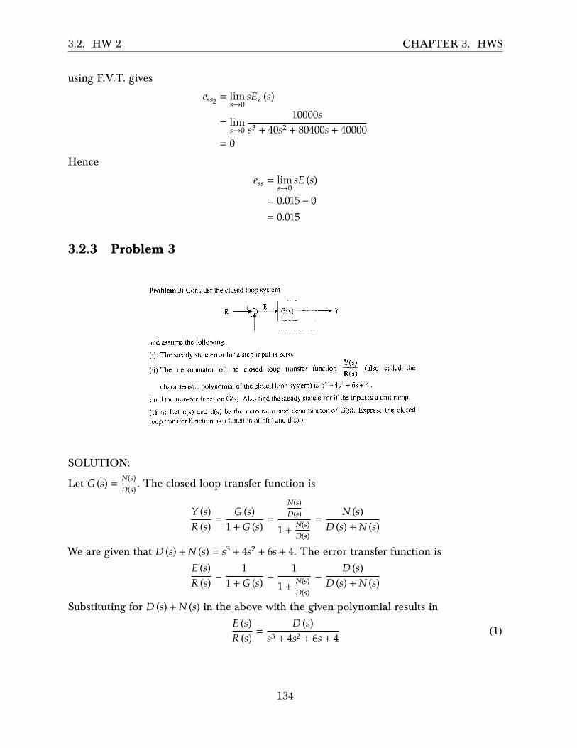
3.2. HW 2 CHAPTER 3. HWS
using F.V.T. gives
𝑒𝑠𝑠2 = lim𝑠→0
𝑠𝐸2 (𝑠)
= lim𝑠→0
10000𝑠𝑠3 + 40𝑠2 + 80400𝑠 + 40000
= 0
Hence
𝑒𝑠𝑠 = lim𝑠→0
𝑠𝐸 (𝑠)
= 0.015 − 0= 0.015
3.2.3 Problem 3
Problem 3: Consider the closed loop system
r FR - -rC) " -+1 G(s) l----1--"-+ Y- t r i i
L _ ____land assume thc tbl lowing:
(i) The steady state effor I'or u step input is zcro.
(ii)'l 'he denominator ol' the closed loop transt'er lunction P (also called theR(s)
characterist ic polynornial ol ' the closccl loop system) is s3 + 4sr + 6s + 4 .
Fintl the t lansl 'c; l ' t i rrct ion G(s). Also l ' inclthc steudy sti l te errol ' i1' the input is a unit ramp'
(l{ i1t: Lct n(s) ancl cl(s) bc the nLuncl 'ator lncl denominator of G(s). Express the closed
loop transf 'er function as I I 'unction ol 'n(s) and d(s) )
l 'roblenr 4: Two l'eeclbuck systcms arc shown in Figure I and Figurc 2.
Figule l: Feedback System I
Figure 2: Fecdback System 2
(a) Let K,, = l . Determine the values of K, fbr system I and K. and K., tbr system 2 so
that both of' the systems cxhibit zero steady error to step inputs and such the steady
statc en'or to a Llnit ramp is I in both citscs.
(b) Suppose K,, changes f}om I to t + 6. Show that the steady state effor with this
perturbed K,, is still zero to a unit step input, for Figure l. Also show that this is not
the case fbr Figure 2.
(c) A tttntntl utl4ineer woultl pral'er tlrc .s\tstam in b'i14ure I to tlrc one itt Figura 2. Do you
agree with this staternent? Justify.
SOLUTION:
Let 𝐺 (𝑠) = 𝑁(𝑠)𝐷(𝑠) . The closed loop transfer function is
𝑌 (𝑠)𝑅 (𝑠)
=𝐺 (𝑠)
1 + 𝐺 (𝑠)=
𝑁(𝑠)𝐷(𝑠)
1 + 𝑁(𝑠)𝐷(𝑠)
=𝑁 (𝑠)
𝐷 (𝑠) + 𝑁 (𝑠)
We are given that 𝐷 (𝑠) + 𝑁 (𝑠) = 𝑠3 + 4𝑠2 + 6𝑠 + 4. The error transfer function is
𝐸 (𝑠)𝑅 (𝑠)
=1
1 + 𝐺 (𝑠)=
1
1 + 𝑁(𝑠)𝐷(𝑠)
=𝐷 (𝑠)
𝐷 (𝑠) + 𝑁 (𝑠)
Substituting for 𝐷 (𝑠) + 𝑁 (𝑠) in the above with the given polynomial results in
𝐸 (𝑠)𝑅 (𝑠)
=𝐷 (𝑠)
𝑠3 + 4𝑠2 + 6𝑠 + 4(1)
134

3.2. HW 2 CHAPTER 3. HWS
We are told that lim𝑠→0 𝑠𝐸 (𝑠) = 0 when 𝑅 (𝑠) =1𝑠 . Applying this to (1) gives
𝐸 (𝑠) =1𝑠
𝐷 (𝑠)𝑠3 + 4𝑠2 + 6𝑠 + 4
𝐸 (𝑠) above is stable since the poles are at −2, −1 ± 𝑖 with another pole at zero. Hence F.V.T.can be applied to 𝐸 (𝑠)
𝑒𝑠𝑠 = lim𝑠→0
𝑠𝐸 (𝑠)
= lim𝑠→0
𝑠 �1𝑠
𝐷 (𝑠)𝑠3 + 4𝑠2 + 6𝑠 + 4�
= lim𝑠→0
𝐷 (𝑠)4
We are also told that the above is zero. Hence
0 = lim𝑠→0
𝐷 (𝑠)4
The above implies that 𝐷 (𝑠) must contain only 𝑠 terms and no constant terms, since wewant 𝐷 (𝑠) = 0 when 𝑠 = 0.
Assuming proper transfer function 𝐺 (𝑠) where degree of 𝑁 (𝑠) ≤ degree of 𝑁 (𝑠), then 𝐷 (𝑠)can be 𝑠3 or 𝑠3 +4𝑠2, or 𝑠3 +4𝑠2 +6𝑠, since any of these will give lim𝑠→0
𝐷(𝑠)4 = 0. But 𝐷 (𝑠) can
not be 𝑠2 for example, else 𝐺 (𝑠) will not proper 𝐺 (𝑠) .
There are actually an infinite number of 𝐷 (𝑠) polynomials which meets this condition (if weuse fractions for the coe�cients). Below is an example of two possible 𝐷 (𝑠) choices and thecorresponding 𝐺 (𝑠)
𝐷1 (𝑠) = 𝑠3 + 4𝑠2 + 6𝑠
Then
𝐺 (𝑠) = 4𝑠3+4𝑠2+6𝑠
For steady state when input is ramp, using the above 𝐺 (𝑠) gives
𝑒𝑠𝑠 = lim𝑠→0
𝑠 �1𝑠2
𝑠3 + 4𝑠2 + 6𝑠𝑠3 + 4𝑠2 + 6𝑠 + 4�
= lim𝑠→0
𝑠2 + 4𝑠 + 6𝑠3 + 4𝑠2 + 6𝑠 + 4
Hence
𝑒𝑠𝑠 = 1.5
Another choice is 𝐷2 (𝑠) = 𝑠3 + 4𝑠2. Using this, 𝐺 (𝑠) = 6𝑠+4𝑠3+4𝑠2 . Using this, and when the input
135

3.2. HW 2 CHAPTER 3. HWS
is ramp then
𝑒𝑠𝑠 = lim𝑠→0
𝑠 �1𝑠2
𝑠3 + 4𝑠2
𝑠3 + 4𝑠2 + 6𝑠 + 4�
= lim𝑠→0
𝑠2 + 4𝑠𝑠3 + 4𝑠2 + 6𝑠 + 4
= 0
So the steady state error for ramp depends on which 𝐺 (𝑠) is used.
3.2.4 Problem 4
Problem 3: Consider the closed loop system
r FR - -rC) " -+1 G(s) l----1--"-+ Y- t r i i
L _ ____land assume thc tbl lowing:
(i) The steady state effor I'or u step input is zcro.
(ii)'l 'he denominator ol' the closed loop transt'er lunction P (also called theR(s)
characterist ic polynornial ol ' the closccl loop system) is s3 + 4sr + 6s + 4 .
Fintl the t lansl 'c; l ' t i rrct ion G(s). Also l ' inclthc steudy sti l te errol ' i1' the input is a unit ramp'
(l{ i1t: Lct n(s) ancl cl(s) bc the nLuncl 'ator lncl denominator of G(s). Express the closed
loop transf 'er function as I I 'unction ol 'n(s) and d(s) )
l 'roblenr 4: Two l'eeclbuck systcms arc shown in Figure I and Figurc 2.
Figule l: Feedback System I
Figure 2: Fecdback System 2
(a) Let K,, = l . Determine the values of K, fbr system I and K. and K., tbr system 2 so
that both of' the systems cxhibit zero steady error to step inputs and such the steady
statc en'or to a Llnit ramp is I in both citscs.
(b) Suppose K,, changes f}om I to t + 6. Show that the steady state effor with this
perturbed K,, is still zero to a unit step input, for Figure l. Also show that this is not
the case fbr Figure 2.
(c) A tttntntl utl4ineer woultl pral'er tlrc .s\tstam in b'i14ure I to tlrc one itt Figura 2. Do you
agree with this staternent? Justify.
SOLUTION:
3.2.4.1 Part(a)
For system 1. Using 𝐾0 = 0 we first obtain expression for 𝐸 (𝑠) and 𝑌 (𝑠)
𝐸 (𝑠) = 𝑅 (𝑠) − 𝑌 (𝑠)
𝑌 (𝑠) = 𝐸 (𝑠) �𝐾1𝑠 � �
14𝑠 + 1�
136

3.2. HW 2 CHAPTER 3. HWS
Solving for 𝐸 (𝑠) from the above two equations gives
𝐸 (𝑠) = 𝑅 (𝑠) − �𝐸 (𝑠)𝐾1
𝑠 (4𝑠 + 1)�
𝐸 (𝑠) �1 +𝐾1
𝑠 (4𝑠 + 1)�= 𝑅 (𝑠)
𝐸 (𝑠) = 𝑅 (𝑠)𝑠 (4𝑠 + 1)
𝑠 (4𝑠 + 1) + 𝐾1
When 𝑅 (𝑠) = 1𝑠 we want 𝑒𝑠𝑠 = 0, therefore
𝑒𝑠𝑠 = 0 = lim𝑠→0
𝑠𝐸 (𝑠)
0 = lim𝑠→0
𝑠 (4𝑠 + 1)𝑠 (4𝑠 + 1) + 𝐾1
= lim𝑠→0
𝑠 (4𝑠 + 1)𝐾1
=0𝐾1
The above is true for any 𝐾1 since the numerator is already zero. Considering now the rampinput. When 𝑅 (𝑠) = 1
𝑠2 we want 𝑒𝑠𝑠 = 1, hence
𝑒𝑠𝑠 = 1 = lim𝑠→0
𝑠𝐸 (𝑠)
1 = lim𝑠→0
𝑠1𝑠2
𝑠 (4𝑠 + 1)𝑠 (4𝑠 + 1) + 𝐾1
= lim𝑠→0
4𝑠 + 1𝑠 (4𝑠 + 1) + 𝐾1
=1𝐾1
Therefore
𝐾1 = 1
For system 2
𝐸 (𝑠) = 𝑅 (𝑠) − 𝑌 (𝑠) (1)
But
𝑌 (𝑠) = 𝑈 (𝑠) 𝐾31
4𝑠 + 1(2)
And
𝑈 (𝑠) = 𝑅 (𝑠) 𝐾2 − 𝑌 (𝑠)
137

3.2. HW 2 CHAPTER 3. HWS
Hence (2) becomes
𝑌 (𝑠) = (𝑅 (𝑠) 𝐾2 − 𝑌 (𝑠))𝐾3
4𝑠 + 1
𝑌 (𝑠) �1 +𝐾3
4𝑠 + 1�= 𝑅 (𝑠)
𝐾2𝐾34𝑠 + 1
𝑌 (𝑠) = 𝑅 (𝑠)𝐾2𝐾34𝑠+1
1 + 𝐾34𝑠+1
= 𝑅 (𝑠)𝐾2𝐾3
4𝑠 + 1 + 𝐾3(3)
Substituting (3) into (1) gives
𝐸 (𝑠) = 𝑅 (𝑠) − 𝑅 (𝑠)𝐾2𝐾3
4𝑠 + 1 + 𝐾3
𝐸 (𝑠) = 𝑅 (𝑠) �1 −𝐾2𝐾3
4𝑠 + 1 + 𝐾3� (4)
When 𝑅 (𝑠) = 1𝑠 we want 𝑒𝑠𝑠 = 0, hence
𝑒𝑠𝑠 = 0 = lim𝑠→0
𝑠𝐸 (𝑠)
0 = lim𝑠→0
𝑠1𝑠 �1 −
𝐾2𝐾34𝑠 + 1 + 𝐾3
�
= 1 −𝐾2𝐾31 + 𝐾3
For the above to be true, then
𝐾2𝐾31+𝐾3
= 1 (5)
We now obtain a second equation from the ramp condition. When 𝑅 (𝑠) = 1𝑠2 we want 𝑒𝑠𝑠 = 1,
hence
𝑒𝑠𝑠 = 1 = lim𝑠→0
𝑠𝐸 (𝑠)
1 = lim𝑠→0
𝑠1𝑠2 �
1 −𝐾2𝐾3
4𝑠 + 1 + 𝐾3�
= lim𝑠→0
1𝑠 �1 −
𝐾2𝐾34𝑠 + 1 + 𝐾3
�
= lim𝑠→0
1𝑠 �4𝑠 + 1 + 𝐾3 − (𝐾2𝐾3)
4𝑠 + 1 + 𝐾3�
138

3.2. HW 2 CHAPTER 3. HWS
Replacing 𝐾2𝐾3 in the above with 1 + 𝐾3 found in (5) gives
1 = lim𝑠→0
1𝑠 �4𝑠 + 1 + 𝐾3 − (1 + 𝑘3)
4𝑠 + 1 + 𝐾3�
= lim𝑠→0
1𝑠 �
4𝑠4𝑠 + 1 + 𝐾3
�
=4
lim𝑠→0 (4𝑠 + 1 + 𝐾3)
1 =4
1 + 𝐾3
Hence 1 + 𝐾3 = 4 or
𝐾3 = 3
Now that we found 𝐾3 we go back to (5) and solve for 𝐾2
𝐾2𝐾31 + 𝐾3
= 1
𝐾2 =1 + 𝐾3𝐾3
=1 + 33
Hence
𝐾2 =43
Summary
𝐾1 𝐾2 𝐾3
system 1 1 N/A N/A
system 2 N/A 43 3
3.2.4.2 Part (b)
For system 1.
𝐸 (𝑠) = 𝑅 (𝑠) − 𝑌 (𝑠)
𝑌 (𝑠) = 𝐸 (𝑠)𝐾1𝑠(1 + 𝛿)4𝑠 + 1
139

3.2. HW 2 CHAPTER 3. HWS
Hence
𝐸 (𝑠) = 𝑅 (𝑠) − �𝐸 (𝑠)𝐾1𝑠1 + 𝛿4𝑠 + 1�
𝐸 (𝑠) �1 +𝐾1𝑠1 + 𝛿4𝑠 + 1�
= 𝑅 (𝑠)
𝐸 (𝑠) = 𝑅 (𝑠)1
1 + 𝐾1𝑠
1+𝛿4𝑠+1
= 𝑅 (𝑠)𝑠 (4𝑠 + 1)
𝑠 (4𝑠 + 1) + 𝐾1 (1 + 𝛿)
When 𝑅 (𝑠) = 1𝑠 then
𝑒𝑠𝑠 = lim𝑠→0
𝑠𝐸 (𝑠)
= lim𝑠→0
𝑠 (4𝑠 + 1)𝑠 (4𝑠 + 1) + 𝐾1 (1 + 𝛿)
=lim𝑠→0 𝑠 (4𝑠 + 1)
𝐾1 (1 + 𝛿)
=0
𝐾1 (1 + 𝛿)The above is zero for any 𝐾1 and any perturbation 𝛿 since the numerator is already zero.This is the same condition we found in part(a). Perturbing 𝐾0 has no e�ect on the result of𝑒𝑠𝑠 for step input.
For system 2
𝐸 (𝑠) = 𝑅 (𝑠) − 𝑌 (𝑠) (1)
But
𝑌 (𝑠) = 𝑈 (𝑠) 𝐾31 + 𝛿4𝑠 + 1
(2)
And
𝑈 (𝑠) = 𝑅 (𝑠) 𝐾2 − 𝑌 (𝑠)
Replacing 𝑈 (𝑠) into (2)
𝑌 (𝑠) = (𝑅 (𝑠) 𝐾2 − 𝑌 (𝑠)) 𝐾31 + 𝛿4𝑠 + 1
𝑌 (𝑠) �1 +𝐾3 (1 + 𝛿)4𝑠 + 1 � = 𝑅 (𝑠)
𝐾2𝐾3 (1 + 𝛿)4𝑠 + 1
𝑌 (𝑠) = 𝑅 (𝑠)𝐾2𝐾3(1+𝛿)
4𝑠+1
1 + 𝐾3(1+𝛿)4𝑠+1
= 𝑅 (𝑠)𝐾2𝐾3 (1 + 𝛿)
4𝑠 + 1 + 𝐾3 (1 + 𝛿)(3)
140

3.2. HW 2 CHAPTER 3. HWS
Substituting 𝑌 (𝑠) from (3) into (1) gives
𝐸 (𝑠) = 𝑅 (𝑠) − 𝑅 (𝑠)𝐾2𝐾3 (1 + 𝛿)
4𝑠 + 1 + 𝐾3 (1 + 𝛿)
= 𝑅 (𝑠) �1 −𝐾2𝐾3 (1 + 𝛿)
4𝑠 + 1 + 𝐾3 (1 + 𝛿)� (4)
When 𝑅 (𝑠) = 1𝑠and using the F.V.T. gives
𝑒𝑠𝑠 = lim𝑠→0
𝑠𝐸 (𝑠)
= lim𝑠→0
𝑠1𝑠 �1 −
𝐾2𝐾3 (1 + 𝛿)4𝑠 + 1 + 𝐾3 (1 + 𝛿)
�
= lim𝑠→0
�1 −𝐾2𝐾3 (1 + 𝛿)
4𝑠 + 1 + 𝐾3 (1 + 𝛿)�
= 1 −𝐾2𝐾3 (1 + 𝛿)1 + 𝐾3 (1 + 𝛿)
For the above 𝑒𝑠𝑠 to be zero, then the condition is that𝐾2𝐾3 (1 + 𝛿)1 + 𝐾3 (1 + 𝛿)
= 1
or
𝐾2𝐾3 (1 + 𝛿) = 1 + 𝐾3 (1 + 𝛿)
𝐾2𝐾3 − 𝐾3 =1
1 + 𝛿Using 𝐾2 =
43 and 𝐾3 = 3 found in part (a) then the above becomes
�43�3 − 3 =
11 + 𝛿
1 =1
1 + 𝛿But this is impossible since the RHS must be either larger than one or smaller than one(depending on the sign of 𝛿). This means if 𝐾0 is perturbed from unity, then it is no longerpossible to obtain zero steady state error for a step input with the same 𝑘2, 𝑘3.
3.2.4.3 Part(c)
I agree. For first system, it gives 𝑒𝑠𝑠 = 0 for a step input regardless of the value of 𝐾1 or 𝐾0as was shown in part (b) above. But for system two, 𝑒𝑠𝑠 = 0 for step input only when usingspecific values of 𝐾𝑖. Any small change in 𝐾0, the steady state error is no longer zero. Inother words, system one is more robust in this regard to changes in 𝐾0 and it is thereforethe preferred system.
141

3.2. HW 2 CHAPTER 3. HWS
3.2.5 Problem 5 - I
Problem 5t An imporrrnt p'oblem tbr tclevision
wobbling of the picture due to movement of the
cumera is mountcd on u moving truck or ui l 'plane'
below) which is intendecl to reducc the ell'ect ol'
scanning motion ol 25a/c, is expccted.
camera systems is the jumPing and
canlera. This effect occurs when the
A system has been designed (shown
rapid scanning motion, A maximum
ump l i f i e r m 0 t 0 f
c a m e r aspeed
v b
b e l l o w ss p e e d
(a) Deterrnine thc stcady statc cn'or ol' thc systcm lbl' a step input
that t , is "negl ig ib le" and Kg = K, = l '
(b) Dctctrninc thc neccssary loop gain K,K,,, when t l" /sec steady state effor ls
rl lowable. (Srnte i tssutnptions as Parl (a))
(c) Show thut tltc stcp responsc of the systeln is of the tblm
v , , ( t ) = l { , - . - ' }q t
'
under the assumptions in Part (a), Express k and q in terms of the system parametefs'
(cl) The sctrling rrrno is cJelinecl as thc timc it takes lbr the step lesponse to be within 27o
ol thc steady state valuc. Givcn the expression of thc step response determined in Part
(c), clelivc the exprcssion tirr the settlilg timc of v,,. Also, find the loop gain K"K'
so that thc settling time of v,, iS less than <-rr equal to 0.04 sec' Take T,', = 0'4sec as
thc motor ttmc constunt.
V.(s) = I. Orrurn"
sTr , , + l
t a c h o m e t e r
SOLUTION:
3.2.5.1 Part (a)
We first need to find 𝐸(𝑠)𝑉𝑐(𝑠)
. From the block diagram2.
𝑉𝑏 (𝑠) = 𝐸 (𝑠) 𝐾𝑎 �𝐾𝑚
1 + 𝑠𝜏𝑚� (1)
And
𝐸 (𝑠) = 𝑉𝑐 (𝑠) �𝐾𝑔
1 + 𝑠𝜏𝑔� − 𝐾𝑡𝑉𝑏 (𝑠) (2)
2Notice that the problem is saying 𝐸 (𝑠) is the variable to the left of the amplifier 𝐾𝑎 and this solution isbased on this and not on using 𝐸 (𝑠) = 𝑉𝑏 (𝑠) − 𝑉𝑐 (𝑠)
142

3.2. HW 2 CHAPTER 3. HWS
Replacing 𝑉𝑏 (𝑠) in (2) with (1) gives
𝐸 (𝑠) = 𝑉𝑐 (𝑠) �𝐾𝑔
1 + 𝑠𝜏𝑔� − 𝐾𝑡𝐸 (𝑠) 𝐾𝑎 �
𝐾𝑚1 + 𝑠𝜏𝑚
�
𝐸 (𝑠) �1 + 𝐾𝑡𝐾𝑎 �𝐾𝑚
1 + 𝑠𝜏𝑚�� = 𝑉𝑐 (𝑠) �
𝐾𝑔
1 + 𝑠𝜏𝑔�
𝐸 (𝑠)𝑉𝑐 (𝑠)
=�
𝐾𝑔1+𝑠𝜏𝑔
�
1 + 𝐾𝑡𝐾𝑎 �𝐾𝑚
1+𝑠𝜏𝑚�
Hence
𝐸(𝑠)𝑉𝑐(𝑠)
= �1+𝑠𝜏𝑚1+𝑠𝜏𝑔�
𝐾𝑔1+𝑠𝜏𝑚+𝐾𝑡𝐾𝑎𝐾𝑚
When 𝑉𝑐 (𝑠) =25𝑠 , 𝐾𝑔 = 𝐾𝑡 = 1 then 𝐸 (𝑠) from above becomes
𝐸 (𝑠) =25𝑠 �
1 + 𝑠𝜏𝑚1 + 𝑠𝜏𝑔
�1
(1 + 𝐾𝑎𝐾𝑚) + 𝑠𝜏𝑚
The above 𝐸 (𝑠) has one pole at the origin, and has a pole at 𝑠 = −1𝜏𝑔
and a pole at 𝑠 = −1+𝐾𝑎𝐾𝑚𝜏𝑚
.
Hence this is stable (assuming 𝐾𝑎𝐾𝑚 > −1). Applying F.V.T. gives
𝑒𝑠𝑠 = lim𝑠→0
𝑠𝐸 (𝑠)
= lim𝑠→0
25 �1 + 𝑠𝜏𝑚1 + 𝑠𝜏𝑔
�1
(1 + 𝐾𝑎𝐾𝑚) + 𝑠𝜏𝑚Hence
𝑒𝑠𝑠 =25
1 + 𝐾𝑎𝐾𝑚
3.2.5.2 Part(b)
When 𝑒𝑠𝑠 is one degree per second, then from the above
1 =25
1 + 𝐾𝑎𝐾𝑚
Or
𝐾𝑎𝐾𝑚 = 24
143

3.2. HW 2 CHAPTER 3. HWS
3.2.5.3 Part(c)
To find the step response, we find the closed loop 𝑉𝑏(𝑠)𝑉𝑐(𝑠)
transfer function first. Substituting(2) into (1) found in part (a) above to obtain an expression for 𝑉𝑏 (𝑠)
𝑉𝑏 (𝑠) = �𝑉𝑐 (𝑠) �𝐾𝑔
1 + 𝑠𝜏𝑔� − 𝐾𝑡𝑉𝑏 (𝑠)� 𝐾𝑎 �
𝐾𝑚1 + 𝑠𝜏𝑚
�
𝑉𝑏 (𝑠) �1 +𝐾𝑚𝐾𝑡𝐾𝑎1 + 𝑠𝜏𝑚
� = 𝑉𝑐 (𝑠)𝐾𝑔𝐾𝑎𝐾𝑚
�1 + 𝑠𝜏𝑔� (1 + 𝑠𝜏𝑚)
Hence the closed loop transfer function is
𝑉𝑏 (𝑠)𝑉𝑐 (𝑠)
=
𝐾𝑔𝐾𝑎𝐾𝑚�1+𝑠𝜏𝑔�(1+𝑠𝜏𝑚)
1 + 𝐾𝑚𝐾𝑡𝐾𝑎1+𝑠𝜏𝑚
=1
�1 + 𝑠𝜏𝑔�𝐾𝑔𝐾𝑎𝐾𝑚
(1 + 𝑠𝜏𝑚) + 𝐾𝑚𝐾𝑡𝐾𝑎
Using same assumptions as part (a), and now using that 𝜏𝑔 is negligible so that 1�1+𝑠𝜏𝑔�
≈ 1
in the above, and using 𝑉𝑐 (𝑠) =1𝑠 since we are told in this part it is a step input (should we
have used 25𝑠 again here? It is not clear, but it says step input so I think 1
𝑠 should be used inthis part), then the above simplifies to
𝑉𝑏 (𝑠) = �1𝑠 �
𝐾𝑎𝐾𝑚(1 + 𝑠𝜏𝑚) + 𝐾𝑚𝐾𝑎
=1𝑠
𝐾𝑎𝐾𝑚(1 + 𝐾𝑚𝐾𝑎) + 𝑠𝜏𝑚
=𝐾𝑎𝐾𝑚𝜏𝑚
1𝑠
1
𝑠 + �1+𝐾𝑚𝐾𝑎𝜏𝑚�
We now need to find the inverse Laplace transform. Using partial fractions
�𝐾𝑎𝐾𝑚𝜏𝑚
�1𝑠
1
𝑠 + �1+𝐾𝑚𝐾𝑎𝜏𝑚�=𝐴𝑠+
𝐵
𝑠 + �1+𝐾𝑚𝐾𝑎𝜏𝑚�
(3)
Hence
𝐴 = lim𝑠→0
�𝐾𝑎𝐾𝑚𝜏𝑚
�1
1+𝐾𝑚𝐾𝑎𝜏𝑚
+ 𝑠=
𝐾𝑎𝐾𝑚1 + 𝐾𝑚𝐾𝑎
And
𝐵 = lim𝑠→−(1+𝐾𝑚𝐾𝑎)
𝜏𝑚
𝐾𝑎𝐾𝑚𝜏𝑚
1𝑠=𝐾𝑎𝐾𝑚𝜏𝑚
1−(1+𝐾𝑚𝐾𝑎)
𝜏𝑚
= −𝐾𝑎𝐾𝑚
1 + 𝐾𝑚𝐾𝑎
144

3.2. HW 2 CHAPTER 3. HWS
Now that we found 𝐴,𝐵 using partial fractions, we replace these values in (3) to obtain 𝑉𝑏 (𝑠)
𝑉𝑏 (𝑠) =𝐾𝑎𝐾𝑚
1 + 𝐾𝑚𝐾𝑎
1𝑠−
𝐾𝑎𝐾𝑚1 + 𝐾𝑚𝐾𝑎
11+𝐾𝑚𝐾𝑎
𝜏𝑚+ 𝑠
(4)
Now we can apply inverse Laplace transform. Hence
𝑣𝑏 (𝑡) = �𝐾𝑎𝐾𝑚
1 + 𝐾𝑚𝐾𝑎−
𝐾𝑎𝐾𝑚1 + 𝐾𝑚𝐾𝑎
𝑒−1+𝐾𝑚𝐾𝑎
𝜏𝑚𝑡� 𝑢 (𝑡)
=𝐾𝑎𝐾𝑚
1 + 𝐾𝑚𝐾𝑎�1 − 𝑒
− 1+𝐾𝑚𝐾𝑎𝜏𝑚
𝑡� 𝑢 (𝑡)
Let
𝑞 = 1+𝐾𝑚𝐾𝑎𝜏𝑚
and
𝑘 = 𝐾𝑎𝐾𝑚𝜏𝑚
Then 𝑣𝑏 (𝑡) can be written as required
𝑣𝑏 (𝑡) =𝑘𝑞�1 − 𝑒−𝑞𝑡� 𝑢 (𝑡)
3.2.5.4 Part(d)
We first need to find the steady state 𝑣𝑏 (𝑡). From (4) found above in part (c)
𝑉𝑏 (𝑠) =𝐾𝑎𝐾𝑚
1 + 𝐾𝑚𝐾𝑎
1𝑠−
𝐾𝑎𝐾𝑚1 + 𝐾𝑚𝐾𝑎
11+𝐾𝑚𝐾𝑎
𝜏𝑚+ 𝑠
Then applying F.V.T. assuming stability
𝑉𝑏 (∞) = lim𝑠→0
𝑠𝑉𝑏 (𝑠)
= lim𝑠→0
𝑠
⎛⎜⎜⎜⎜⎜⎜⎝𝐾𝑎𝐾𝑚
1 + 𝐾𝑚𝐾𝑎
1𝑠−
𝐾𝑎𝐾𝑚1 + 𝐾𝑚𝐾𝑎
11+𝐾𝑚𝐾𝑎
𝜏𝑚+ 𝑠
⎞⎟⎟⎟⎟⎟⎟⎠
=𝐾𝑎𝐾𝑚
1 + 𝐾𝑚𝐾𝑎
=𝑘𝑞
Let the settling time be 𝑡𝑠, then we want to solve for 𝑡𝑠 from
𝑣𝑏 (𝑡𝑠) = 0.98𝑉𝑏 (∞)𝑘𝑞�1 − 𝑒−𝑞𝑡𝑠� = 0.98
𝑘𝑞
1 − 𝑒−𝑞𝑡𝑠 = 0.98𝑒−𝑞𝑡𝑠 = 0.02
145

3.2. HW 2 CHAPTER 3. HWS
Taking natural logs on both sides gives
−𝑞𝑡𝑠 = ln (0.02)𝑞𝑡𝑠 = 3.912
Hence
𝑡𝑠 =3.912
� 1+𝐾𝑚𝐾𝑎𝑡𝑚
�
Using 𝑡𝑚 = 0.4 seconds in the above gives
𝑡𝑠 =1.56481 + 𝐾𝑚𝐾𝑎
For 𝑡𝑠 ≤ 0.04 then1.5648
(1 + 𝐾𝑚𝐾𝑎)≤ 0.04
1 + 𝐾𝑚𝐾𝑎 ≥1.56480.04
1 + 𝐾𝑚𝐾𝑎 ≥ 39.12
Hence
𝐾𝑚𝐾𝑎 ≥ 38.12
146

3.2. HW 2 CHAPTER 3. HWS
3.2.6 HW 2 key solution
, ECD332
-}IW. #2 Solutions
s 2 + l 0 J s + ll-(a)w.(s)=;ffiT
. l - I- rh+-1001 "1,*=- e ' | r . . *=-
"rs+lOXs+100)l-(b)w.(s)=ffi
t,. l*=o t. l,*=1 e.l*.on =-
l-(c) W.(s) =s 2 ( s 2 + s + l )
3\o/ - s'1s' + s + l) + K(l+ 2s)(l+ as)
t.l*=o ..1,*=o ,.1*.-.=*
l-(d) Systems with e.l* = k (bcing k finitc and different from 0) have G(s) with no
poles at the origin (s = 0); Systems with e.l,* = k (being k finirc and diffcrent fr,om 0)
have G(s) with one pole at the origrn; Systems with e.lr_rr. = k (being k finitc arddifferent from 0) have G(s) with trvo poles at thc origin.
;
147

3.2. HW 2 CHAPTER 3. HWS
r00
R(s) +
(0.05s+l)(0.05s+l)
Where D(s) is the constant input D(s) = 925s
So lim dt) = liry sE(s)l--t- r-+0
= n'[,rd l \
s(0.05s+1X0.05s+l)s(0.05s + 1)(0.05s+t)+ (Zs + t)tm
100+ l )
100(O05s + l)(O05s + l)
D(s)
025 -100s 15S _s s(005s + lX0.05s + t) + (Zs + tlm F
IJ= m
= o'ol5
3I-et G(s) = *, where n(s) ard d(s) are polynomials. Thend ( s ) '
E(s)_ I __ I d(s)RGt=t+c(')=F=4ffi
d(s)
n(s)
Ii'l = G(s) =-9(l)-= n(s)RG) l+G(s)
r * n ( t )
-d (s )+n(s )
d(s)
Since the denominaton of the closed loop function is s3 + 4s2 + 6s + 4 then we have
n ( s ) + d ( s ) = s 3 + 4 s 2 + 6 + 4
Now, since the steady statc error for a step input is zero, wc have
* ( z + !
lim sE(s) - li,n r-d(t) d(s) I;b'*\-" ;jt" n(sffi R(s) - }gt;;fu1= 0
;
148

3.2. HW 2 CHAPTER 3. HWS
Ttrc cquubn abora irplics that lir4d(s) = 0, or in othcr worrds d(s) = s p(s), whcre p(s)
is a pdymnial. So jrut trke
d(s )=s3+4s2+&
ard as consoquerEe we have
n(s) = 4
G(s)=#
Notc that this is not the only possiblc answcr.The stcady statc to a unitramp is
"3 +Asl +6r I 6l imsE(s)= l ims#*=i=15rdt d r-a4ff i f ; t=;='
4-(e) Fint find tlrc transfcrfunctiqrs facach sysEm
n:_-_ ,^ Y(s) _ K,KoIlgurc t'
RGi= s(4s+l)+K,Ko
E:_._ ". Y(r) _ KrK2Ko.gur 't
RG =
(4* * l) + KsKo
Ncxt calculatc thc srcady strtr crru dr to a scp.
Figrre l: W.(s) = R(s)- Y(s) = n6{r #r]
E(5)=nr,{r #lqJ
E(s),=-t,t"ffi],.1*=H*ft=o
;
149

3.2. HW 2 CHAPTER 3. HWS
Figure z' 5.trt = R(s)-Y(s) = nrr{r #t]
[.('F*o{'-ffi]L6)=-,,{ffi
,.1.r=gffi..1*=ff=o #
Whcn 1+ KrKo - K3K2K. = 0 thcn thc stcp rcspottsc will haw zc,ro stcady-statcerror. Thc constanrc K, and Kr will bc chccn so tlut this is tnrc.
Now that wc know that both of thc syst€ms havc zcro stcady-starc crror to stcpinputs, wc can say that for cach trtnsftr firctbn, TF(s), thc DC gain (gaur atftcqrncy zrro) is I which npuls TF(0) = I fc botr syrcms.
Ncxt, wc can 6nd thc.stcady stalc c(rcr duc to unit nnp. Itm thc equatbru ebove,we soe thc patern is W.(s) = n(r[l-ffft)]which rncurr thet
r-1,*=rimdr-ff(,t+=Ts+=ry|_Givcn that wc want c.l,* = l, wc harrc thc folbwing cquatbns for systans that
nrc'rc strdying
Fig'rc,' -#1-" =(4s '+s+K,Ks)r l . .n
* K r = l
Figr'e r. - o(Ttslll.- = ffi
= t
= I
= I
= lK,Ko Kr
+ 4KrK, - ( l+ K3)2
;150

3.2. HW 2 CHAPTER 3. HWS
From equation # wc get I + K, = KrKr. Substituting thins ino equcion * we get
4(1+ Kr; = (l + Kr)2+ Kr = -1 or Kr = 3
Solving for K, in equation * we find that
1+ K"Kr=Ti
4So, we get K, = 0 or K, =
i but K, = 0 is not feasible.
The final rcsult is then
K r = 1 K r = : K r = 3
4-(b) I.et Ko = 1+6
Figure l: e.l*4 s 2 + s 4 s 2 + s=lsffi=Sre'=o
which is indcpendcnt of 6.
Figure 2:e-ln=lSffi
..lo* = HSubstituting with the results obaincd in Part (a) wc get
, s(3- 1*)".1* =ft;f *oHence, thc srcady statc crror is not zero in this casc
+(c) I agee because the first system is cbarly robust to variatbns in Ko, whib the
second is not.
;
151

3.2. HW 2 CHAPTER 3. HWS
5. Uncler stated assumption, the error TF is
E(") ) 1
V"(r): TT@*^4
A straightforward calculation with V"(s) :251s Ieads to
25e"t: l , iSssE(s)
: r+ K"K*
5-(b) The condition
Ieads to
1
Ieads to KoK^ :24.
5-(c) With ,R(s) : !f s, a Mason calculation gives bellows output
T-- KV 6 @ ) : - , ,s(s * u#-) s(s * q)
whereKoK^ t + KoK-
h - , -
i q : , -
Now, the inverse Laplace transform gives the desired result.
5-(d) Enforcing the error requirement
e ( t \ : K
, - n ' < 0 ' 0 2 K a t f : 0 ' 0 4- \ - / q
- q
.04q> 4: i .". ' o.o+1!!44t1' a' 0 .4
requirement KoK- > 39.with resulting Ioop gain
;
152

3.3. HW 3 CHAPTER 3. HWS
3.3 HW 3
3.3.1 Problem 1
SOLUTION:
𝐺 (𝑠) =𝐾𝑠 + 1
𝑠3 + 𝑠2 + (𝐾 + 𝑘) 𝑠 + 1
3.3.1.1 Part (a)
For 𝐾 = 1 the above becomes
𝐺 (𝑠) =𝑠 + 1
𝑠3 + 𝑠2 + (1 + 𝑘) 𝑠 + 1Hence
𝑆𝐺𝑘 =𝑑𝐺𝑑𝑘
𝑘𝐺
=𝑑𝑑𝑘
𝑠 + 1𝑠3 + 𝑠2 + (1 + 𝑘) 𝑠 + 1
⎛⎜⎜⎜⎜⎜⎜⎝
𝑘𝑠+1
𝑠3+𝑠2+(1+𝑘)𝑠+1
⎞⎟⎟⎟⎟⎟⎟⎠
=−𝑠 (𝑠 + 1)
�𝑠 + 𝑘𝑠 + 𝑠2 + 𝑠3 + 1�2
𝑘 �𝑠3 + 𝑠2 + (1 + 𝑘) 𝑠 + 1�𝑠 + 1
=−𝑘𝑠
1 + (1 + 𝑘) 𝑠 + 𝑠2 + 𝑠3
At nominal 𝑘 = 2 the above becomes
𝑆𝐺𝑘 �𝑘=2 =−2𝑠
3𝑠 + 𝑠2 + 𝑠3 + 1
153

3.3. HW 3 CHAPTER 3. HWS
Let 𝑠 = 𝑗𝜔 then
𝑆𝐺𝑘 =−2 �𝑗𝜔�
3𝑗𝜔 + �𝑗𝜔�2+ �𝑗𝜔�
3+ 1
=−2𝑗𝜔
𝑗 �3𝜔 − 𝜔3� + �1 − 𝜔2�
Taking the magnitude
�𝑆𝐺𝑘 � =2𝜔
��1 − 𝜔2�
2+ �3𝜔 − 𝜔3�
2
Here is a plot of �𝑆𝐺𝑘 � as function of 𝜔
Out[126]=
0 1 2 3 4 5
0.0
0.5
1.0
1.5
ω (rad/sec)
|(SkG)
Problem 1, part (a)
3.3.1.2 Part (b)
For 𝐾 = 100 the transfer function becomes
𝐺 (𝑠) =𝐾𝑠 + 1
𝑠3 + 𝑠2 + (𝐾 + 𝑘) 𝑠 + 1
=100𝑠 + 1
𝑠3 + 𝑠2 + (100 + 𝑘) 𝑠 + 1
154

3.3. HW 3 CHAPTER 3. HWS
Hence
𝑆𝐺𝑘 =𝑑𝐺𝑑𝑘
𝑘𝐺
=𝑑𝑑𝑘
100𝑠 + 1𝑠3 + 𝑠2 + (100 + 𝑘) 𝑠 + 1
⎛⎜⎜⎜⎜⎜⎜⎝
𝑘100𝑠+1
𝑠3+𝑠2+(100+𝑘)𝑠+1
⎞⎟⎟⎟⎟⎟⎟⎠
=−𝑠 (100𝑠 + 1)
�100𝑠 + 𝑘𝑠 + 𝑠2 + 𝑠3 + 1�2
𝑘 �𝑠3 + 𝑠2 + (100 + 𝑘) 𝑠 + 1�100𝑠 + 1
=−𝑘𝑠
100𝑠 + 𝑘𝑠 + 𝑠2 + 𝑠3 + 1At nominal 𝑘 = 2 the above becomes
𝑆𝐺𝑘 �𝑘=2 =−2𝑠
100𝑠 + 2𝑠 + 𝑠2 + 𝑠3 + 1
=−2𝑠
102𝑠 + 𝑠2 + 𝑠3 + 1Let 𝑠 = 𝑗𝜔 then
𝑆𝐺𝑘 =−2 �𝑗𝜔�
102𝑗𝜔 + �𝑗𝜔�2+ �𝑗𝜔�
3+ 1
=−2𝑗𝜔
102𝑗𝜔 − 𝜔2 − 𝑗𝜔3 + 1
=−2𝑗𝜔
𝑗 �102𝜔 − 𝜔3� + �1 − 𝜔2�
Taking the magnitude
�𝑆𝐺𝑘 � =2𝜔
��1 − 𝜔2�
2+ �102𝜔 − 𝜔3�
2
Here is a plot of �𝑆𝐺𝑘 � as function of 𝜔
155
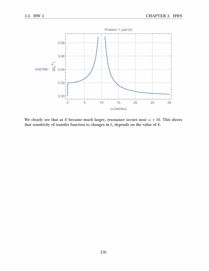
3.3. HW 3 CHAPTER 3. HWS
Out[156]=
0 5 10 15 20 25 30
0.00
0.02
0.04
0.06
0.08
ω (rad/sec)
|(SkG)
Problem 1, part (b)
We clearly see that as 𝐾 became much larger, resonance occurs near 𝜔 = 10. This showsthat sensitivity of transfer function to changes in 𝑘, depends on the value of 𝐾.
156
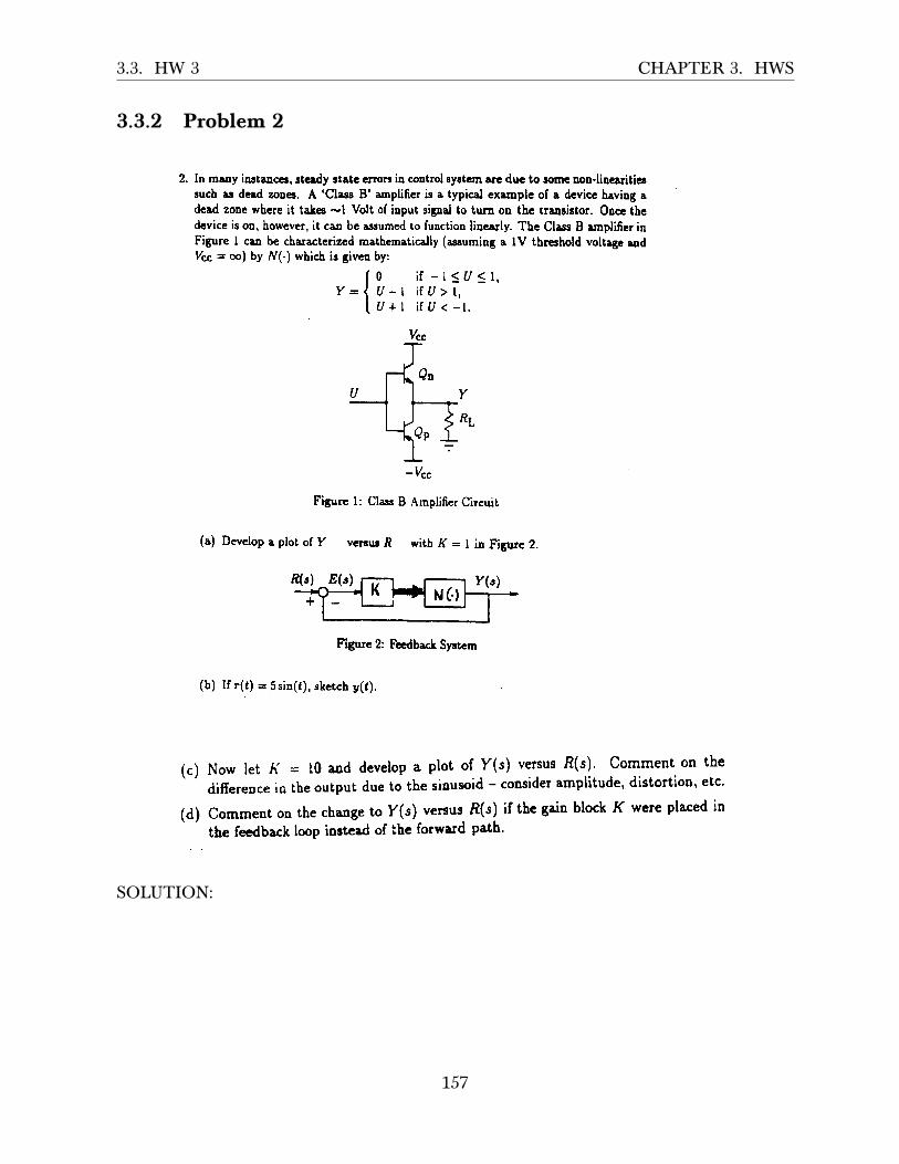
3.3. HW 3 CHAPTER 3. HWS
3.3.2 Problem 2
ECE 332 - Homework ff4Due Tuesday, October 13, 2011
1. Consider the system with transfer function
K s * lG(s ) :
s 3 + s 2 + ( K + k ) + 1
(a) For K : l, find the sensitivity ,Sf; of this transfer function with respect
to k assuming nominal value k :2. Then plot is magnitude ars a function
of frequency.
(b) Repeat (u) with K : 100 and compare the effect of a large loop
gain on the sensitivity.
2. In many instaocel, stcdy statc errors in control eyctcm are due to some non-lineariticrsuch as dcad zooes. A 'Clasg B' amplifier is a typical exa,mple of a dcvice haviag adead zone where it takes -l Volt of ioput sigjal to tur:n oo thc traogistor. Oncc tbcdevice is on, however, it can be assumed to function lincarly. The Class B amplifier inFigure I can be cbaracterizcd mathematically (assuming a lV threshold voltage andVcc = o) by ff(.) which is given by:
[ 0 i f - l s u s l ,Y : l u - L i f u > 1 ,
I u + L i f u < - r .
Vsc
_Vcc
Figure 1: Class B Amplifier Circuit
(a) Develop a plot of Y vcnur f, with K = I in Figurc 2.
Figure 2: Fecdback Syrtem
(b) If r(t) = Ssin(l), sketch y(t).
(c) Now let l( = l0 and develop a plot of Y(s) venus R(s). Commenl on the
difierence in the output due to tbe sinusoid - coosider amplitude, distortion, etc'
(d) Comment on the change to Y(s) ve6us 8(s) if the gain block K were placed in
the feedback loop instead of lhe forward path'
3' The blocl diagram of a fcdbrck control syrtcrn is shown rn Figure 3
n(s)
Figure 3: Block Diagrart
(a) Apply Mason's gain formula to the block diagraru to find the transfer functions
c(') | c(") IR(") l "o N( t ) ln-o
E:cpress C(s) in terms of R(c) and N(s) wheo both inputs are applied simultare
ously.
(b) Find thc decired relation amoDg the traosfer functionr Gt("), Gr("), Gt(r), G.(')'' '
ffr(s) asd &(s) so that thc oritput C(s) is not a,ffccted by the disturbance signal
N(s) at all.
Gr(s)
f fr(s)
SOLUTION:
157

3.3. HW 3 CHAPTER 3. HWS
3.3.2.1 Part (a)
+
-K nonlinear Y (s)x = K(R−N(x)) N(x)R(s)
R−N(x)
From the above we see that
𝑌 = 𝑁 (𝑥) (1)
The plot of 𝑌 (𝑥) is given below based on the definition given in the problem
Out[649]=
-3 -2 -1 0 1 2 3
-2
-1
0
1
2
x
Y(x)
Nonlinear device
At the output of the controller we have
𝑥 = 𝑘 (𝑅 − 𝑁 (𝑥))𝑥 = 𝑘 (𝑅 − 𝑌)𝑥 = 𝑘𝑅 − 𝑘𝑌
𝑌 = 𝑅 −𝑥𝑘
(2)
Equations (1) and (2) must both hold. We now setup a table of 𝑅 and corresponding 𝑌values, and using 𝑘 = 1 for this part, we obtain
𝑅 𝑌 = 𝑅 − 𝑥 solution of 𝑌 = 𝑁 (𝑥) 𝑌 at solution
0 −𝑥 𝑥 = 0 00.1 0.1 − 𝑥 𝑥 = 0 00.2 0.2 − 𝑥 ⋮ ⋮
see program ⋮ ⋮ ⋮
Small code was written to finish the above table, using 𝑅 = −2⋯2 range with increments of0.1. Here is the generated table, followed by the plot
158
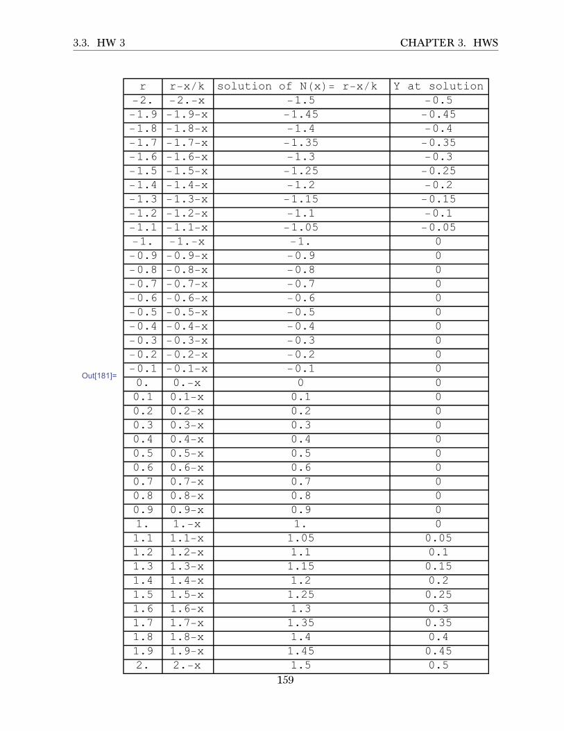
3.3. HW 3 CHAPTER 3. HWS
Out[181]=
r r-x/k solution of N(x)= r-x/k Y at solution-2. -2.-x -1.5 -0.5-1.9 -1.9-x -1.45 -0.45-1.8 -1.8-x -1.4 -0.4-1.7 -1.7-x -1.35 -0.35-1.6 -1.6-x -1.3 -0.3-1.5 -1.5-x -1.25 -0.25-1.4 -1.4-x -1.2 -0.2-1.3 -1.3-x -1.15 -0.15-1.2 -1.2-x -1.1 -0.1-1.1 -1.1-x -1.05 -0.05-1. -1.-x -1. 0-0.9 -0.9-x -0.9 0-0.8 -0.8-x -0.8 0-0.7 -0.7-x -0.7 0-0.6 -0.6-x -0.6 0-0.5 -0.5-x -0.5 0-0.4 -0.4-x -0.4 0-0.3 -0.3-x -0.3 0-0.2 -0.2-x -0.2 0-0.1 -0.1-x -0.1 00. 0.-x 0 00.1 0.1-x 0.1 00.2 0.2-x 0.2 00.3 0.3-x 0.3 00.4 0.4-x 0.4 00.5 0.5-x 0.5 00.6 0.6-x 0.6 00.7 0.7-x 0.7 00.8 0.8-x 0.8 00.9 0.9-x 0.9 01. 1.-x 1. 01.1 1.1-x 1.05 0.051.2 1.2-x 1.1 0.11.3 1.3-x 1.15 0.151.4 1.4-x 1.2 0.21.5 1.5-x 1.25 0.251.6 1.6-x 1.3 0.31.7 1.7-x 1.35 0.351.8 1.8-x 1.4 0.41.9 1.9-x 1.45 0.452. 2.-x 1.5 0.5
159
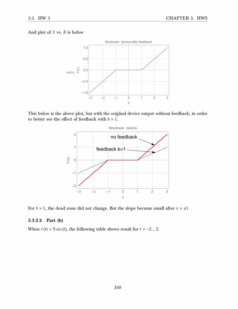
3.3. HW 3 CHAPTER 3. HWS
And plot of 𝑌 vs. 𝑅 is below
Out[57]=
-3 -2 -1 0 1 2 3
-1.0
-0.5
0.0
0.5
1.0
x
Y(x)
Nonlinear device after feedback
This below is the above plot, but with the original device output without feedback, in orderto better see the e�ect of feedback with 𝑘 = 1.
no feedback
feedback k=1
-3 -2 -1 0 1 2 3
-2
-1
0
1
2
x
Y(x)
Nonlinear device
For 𝑘 = 1, the dead zone did not change. But the slope became small after 𝑥 = ±1
3.3.2.2 Part (b)
When 𝑟 (𝑡) = 5 sin (𝑡), the following table shows result for 𝑡 = −2…2.
160

3.3. HW 3 CHAPTER 3. HWS
Out[188]=
t r = 5 sin(t) r-x/k solution of N(x)=r-x/k Y at solution-2. -4.54649 -4.54649-x -2.77324 -1.77324-1.9 -4.7315 -4.7315-x -2.86575 -1.86575-1.8 -4.86924 -4.86924-x -2.93462 -1.93462-1.7 -4.95832 -4.95832-x -2.97916 -1.97916-1.6 -4.99787 -4.99787-x -2.99893 -1.99893-1.5 -4.98747 -4.98747-x -2.99374 -1.99374-1.4 -4.92725 -4.92725-x -2.96362 -1.96362-1.3 -4.81779 -4.81779-x -2.9089 -1.9089-1.2 -4.6602 -4.6602-x -2.8301 -1.8301-1.1 -4.45604 -4.45604-x -2.72802 -1.72802-1. -4.20735 -4.20735-x -2.60368 -1.60368-0.9 -3.91663 -3.91663-x -2.45832 -1.45832-0.8 -3.58678 -3.58678-x -2.29339 -1.29339-0.7 -3.22109 -3.22109-x -2.11054 -1.11054-0.6 -2.82321 -2.82321-x -1.91161 -0.911606-0.5 -2.39713 -2.39713-x -1.69856 -0.698564-0.4 -1.94709 -1.94709-x -1.47355 -0.473546-0.3 -1.4776 -1.4776-x -1.2388 -0.238801-0.2 -0.993347 -0.993347-x -0.993347 0-0.1 -0.499167 -0.499167-x -0.499167 00. 0. 0.-x 0 00.1 0.499167 0.499167-x 0.499167 00.2 0.993347 0.993347-x 0.993347 00.3 1.4776 1.4776-x 1.2388 0.2388010.4 1.94709 1.94709-x 1.47355 0.4735460.5 2.39713 2.39713-x 1.69856 0.6985640.6 2.82321 2.82321-x 1.91161 0.9116060.7 3.22109 3.22109-x 2.11054 1.110540.8 3.58678 3.58678-x 2.29339 1.293390.9 3.91663 3.91663-x 2.45832 1.458321. 4.20735 4.20735-x 2.60368 1.603681.1 4.45604 4.45604-x 2.72802 1.728021.2 4.6602 4.6602-x 2.8301 1.83011.3 4.81779 4.81779-x 2.9089 1.90891.4 4.92725 4.92725-x 2.96362 1.963621.5 4.98747 4.98747-x 2.99374 1.993741.6 4.99787 4.99787-x 2.99893 1.998931.7 4.95832 4.95832-x 2.97916 1.979161.8 4.86924 4.86924-x 2.93462 1.934621.9 4.7315 4.7315-x 2.86575 1.865752. 4.54649 4.54649-x 2.77324 1.77324
the following is the plot of the output with the feedback for 𝑘 = 1
161

3.3. HW 3 CHAPTER 3. HWS
no feedback
feedback with r=5 sin(t), k=1
-3 -2 -1 0 1 2 3
-2
-1
0
1
2
x
Y(x)
Nonlinear device
Matlab code to plot the solution
%matlab code to generate plot for part(b), HW3, problem 2%ECE 332close all; clear all;figuret=0:.1:10;f=@(x) (x+1).*(x<-1)+(x-1).*(x>1)+0; %non-linear devicer = 5 *sin(t); %inputk =1; %change to 10 for second partx = fsolve(@(x) f(x)-(r-x/k),r);
plot(t,f(x));grid;title('output of 5*sin(t), k=1');
3.3.2.3 Part (c)
Now 𝑘 = 10, and part(b) was repeated. the following table shows result for 𝑡 = −2…2.
162

3.3. HW 3 CHAPTER 3. HWS
t r = 5 sin(t) r-x/10 solution of N(x)=r-x/10 Y at solution-2. -4.54649 -4.54649-x -5.04226 -4.04226-1.9 -4.7315 -4.7315-x -5.21045 -4.21045-1.8 -4.86924 -4.86924-x -5.33567 -4.33567-1.7 -4.95832 -4.95832-x -5.41666 -4.41666-1.6 -4.99787 -4.99787-x -5.45261 -4.45261-1.5 -4.98747 -4.98747-x -5.44316 -4.44316-1.4 -4.92725 -4.92725-x -5.38841 -4.38841-1.3 -4.81779 -4.81779-x -5.2889 -4.2889-1.2 -4.6602 -4.6602-x -5.14563 -4.14563-1.1 -4.45604 -4.45604-x -4.96003 -3.96003-1. -4.20735 -4.20735-x -4.73396 -3.73396-0.9 -3.91663 -3.91663-x -4.46967 -3.46967-0.8 -3.58678 -3.58678-x -4.1698 -3.1698-0.7 -3.22109 -3.22109-x -3.83735 -2.83735-0.6 -2.82321 -2.82321-x -3.47565 -2.47565-0.5 -2.39713 -2.39713-x -3.0883 -2.0883-0.4 -1.94709 -1.94709-x -2.67917 -1.67917-0.3 -1.4776 -1.4776-x -2.25236 -1.25236-0.2 -0.993347 -0.993347-x -1.81213 -0.812133-0.1 -0.499167 -0.499167-x -1.36288 -0.3628790. 0. 0.-x 0 00.1 0.499167 0.499167-x 1.36288 0.3628790.2 0.993347 0.993347-x 1.81213 0.8121330.3 1.4776 1.4776-x 2.25236 1.252360.4 1.94709 1.94709-x 2.67917 1.679170.5 2.39713 2.39713-x 3.0883 2.08830.6 2.82321 2.82321-x 3.47565 2.475650.7 3.22109 3.22109-x 3.83735 2.837350.8 3.58678 3.58678-x 4.1698 3.16980.9 3.91663 3.91663-x 4.46967 3.469671. 4.20735 4.20735-x 4.73396 3.733961.1 4.45604 4.45604-x 4.96003 3.960031.2 4.6602 4.6602-x 5.14563 4.145631.3 4.81779 4.81779-x 5.2889 4.28891.4 4.92725 4.92725-x 5.38841 4.388411.5 4.98747 4.98747-x 5.44316 4.443161.6 4.99787 4.99787-x 5.45261 4.452611.7 4.95832 4.95832-x 5.41666 4.416661.8 4.86924 4.86924-x 5.33567 4.335671.9 4.7315 4.7315-x 5.21045 4.210452. 4.54649 4.54649-x 5.04226 4.04226
And the following is the plot of the result
163
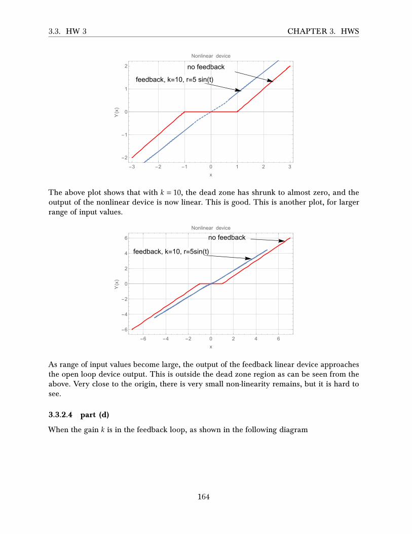
3.3. HW 3 CHAPTER 3. HWS
no feedback
feedback, k=10, r=5 sin(t)
-3 -2 -1 0 1 2 3
-2
-1
0
1
2
x
Y(x)
Nonlinear device
The above plot shows that with 𝑘 = 10, the dead zone has shrunk to almost zero, and theoutput of the nonlinear device is now linear. This is good. This is another plot, for largerrange of input values.
no feedback
feedback, k=10, r=5sin(t)
-6 -4 -2 0 2 4 6
-6
-4
-2
0
2
4
6
x
Y(x)
Nonlinear device
As range of input values become large, the output of the feedback linear device approachesthe open loop device output. This is outside the dead zone region as can be seen from theabove. Very close to the origin, there is very small non-linearity remains, but it is hard tosee.
3.3.2.4 part (d)
When the gain 𝑘 is in the feedback loop, as shown in the following diagram
164

3.3. HW 3 CHAPTER 3. HWS
+
-
K
nonlinear Y (s)x = R− kY N(x)R(s)
Therefore
𝑥 = 𝑅 − 𝑘𝑌
𝑌 =(𝑅 − 𝑥)𝑘
Before, when the gain was in the feedforward, 𝑌 = 𝑅 − 𝑥𝑘 , so now 𝑘 a�ects 𝑅 as well. Using
this new 𝑥, the above plot was reproduced for the case of 𝑟 (𝑡) = 5 sin (𝑡).
the following table shows result for 𝑡 = −2…2.
165

3.3. HW 3 CHAPTER 3. HWS
t r = 5 sin(t) (r-x)/10 solution of N(x)=(r-x)/10 Y at solution-2. -4.54649 (-4.54649-x)/10 -1.32241 -0.322408-1.9 -4.7315 (-4.7315-x)/10 -1.33923 -0.339227-1.8 -4.86924 (-4.86924-x)/10 -1.35175 -0.351749-1.7 -4.95832 (-4.95832-x)/10 -1.35985 -0.359848-1.6 -4.99787 (-4.99787-x)/10 -1.36344 -0.363443-1.5 -4.98747 (-4.98747-x)/10 -1.3625 -0.362498-1.4 -4.92725 (-4.92725-x)/10 -1.35702 -0.357023-1.3 -4.81779 (-4.81779-x)/10 -1.34707 -0.347072-1.2 -4.6602 (-4.6602-x)/10 -1.33275 -0.332745-1.1 -4.45604 (-4.45604-x)/10 -1.31419 -0.314185-1. -4.20735 (-4.20735-x)/10 -1.29158 -0.291578-0.9 -3.91663 (-3.91663-x)/10 -1.26515 -0.265149-0.8 -3.58678 (-3.58678-x)/10 -1.23516 -0.235162-0.7 -3.22109 (-3.22109-x)/10 -1.20192 -0.201917-0.6 -2.82321 (-2.82321-x)/10 -1.16575 -0.165747-0.5 -2.39713 (-2.39713-x)/10 -1.12701 -0.127012-0.4 -1.94709 (-1.94709-x)/10 -1.0861 -0.0860992-0.3 -1.4776 (-1.4776-x)/10 -1.04342 -0.0434183-0.2 -0.993347 (-0.993347-x)/10 -0.993347 0-0.1 -0.499167 (-0.499167-x)/10 -0.499167 00. 0. (0.-x)/10 0 00.1 0.499167 (0.499167-x)/10 0.499167 00.2 0.993347 (0.993347-x)/10 0.993347 00.3 1.4776 (1.4776-x)/10 1.04342 0.04341830.4 1.94709 (1.94709-x)/10 1.0861 0.08609920.5 2.39713 (2.39713-x)/10 1.12701 0.1270120.6 2.82321 (2.82321-x)/10 1.16575 0.1657470.7 3.22109 (3.22109-x)/10 1.20192 0.2019170.8 3.58678 (3.58678-x)/10 1.23516 0.2351620.9 3.91663 (3.91663-x)/10 1.26515 0.2651491. 4.20735 (4.20735-x)/10 1.29158 0.2915781.1 4.45604 (4.45604-x)/10 1.31419 0.3141851.2 4.6602 (4.6602-x)/10 1.33275 0.3327451.3 4.81779 (4.81779-x)/10 1.34707 0.3470721.4 4.92725 (4.92725-x)/10 1.35702 0.3570231.5 4.98747 (4.98747-x)/10 1.3625 0.3624981.6 4.99787 (4.99787-x)/10 1.36344 0.3634431.7 4.95832 (4.95832-x)/10 1.35985 0.3598481.8 4.86924 (4.86924-x)/10 1.35175 0.3517491.9 4.7315 (4.7315-x)/10 1.33923 0.3392272. 4.54649 (4.54649-x)/10 1.32241 0.322408
And the following is the plot
166
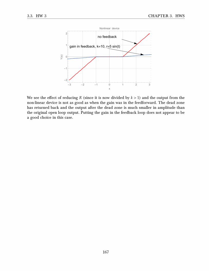
3.3. HW 3 CHAPTER 3. HWS
no feedback
gain in feedback, k=10, r=5 sin(t)
-3 -2 -1 0 1 2 3
-2
-1
0
1
2
x
Y(x)
Nonlinear device
We see the e�ect of reducing 𝑅 (since it is now divided by 𝑘 > 1) and the output from thenon-linear device is not as good as when the gain was in the feedforward. The dead zonehas returned back and the output after the dead zone is much smaller in amplitude thanthe original open loop output. Putting the gain in the feedback loop does not appear to bea good choice in this case.
167
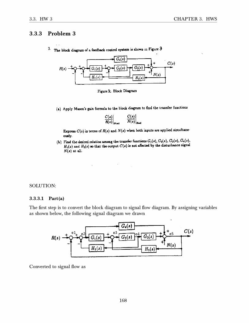
3.3. HW 3 CHAPTER 3. HWS
3.3.3 Problem 3(c) Now let l( = l0 and develop a plot of Y(s) venus R(s). Commenl on the
difierence in the output due to tbe sinusoid - coosider amplitude, distortion, etc'
(d) Comment on the change to Y(s) ve6us 8(s) if the gain block K were placed in
the feedback loop instead of lhe forward path'
3' The blocl diagram of a fcdbrck control syrtcrn is shown rn Figure 3
n(s)
Figure 3: Block Diagrart
(a) Apply Mason's gain formula to the block diagraru to find the transfer functions
c(') | c(") IR(") l "o N( t ) ln-o
E:cpress C(s) in terms of R(c) and N(s) wheo both inputs are applied simultare
ously.
(b) Find thc decired relation amoDg the traosfer functionr Gt("), Gr("), Gt(r), G.(')'' '
ffr(s) asd &(s) so that thc oritput C(s) is not a,ffccted by the disturbance signal
N(s) at all.
Gr(s)
f fr(s)
SOLUTION:
3.3.3.1 Part(a)
The first step is to convert the block diagram to signal flow diagram. By assigning variablesas shown below, the following signal diagram we drawn
Converted to signal flow as
168

3.3. HW 3 CHAPTER 3. HWS
R(s)
N(s)
G1 G2 G3
−H1
−H2
G4
−1
−1
C(s)e1 e2
e3 e4 e5
For finding 𝐶(𝑠)𝑅(𝑠) then 𝑁 (𝑠) is set to zero. There are two forward paths from 𝑅 (𝑠) to 𝐶 (𝑠) they
are
𝑀1 = {1, 1, 𝐺1, 𝐺2, 𝐺3, 1} = 𝐺1𝐺2𝐺3
𝑀2 = {1, 1, 𝐺4, 1} = 𝐺4
The corresponding Mason deltas are
Δ1 = 1Δ2 = 1 − (𝐺2) (−1) = 1 + 𝐺2
The loops, one at a time are
𝐿1 = (𝐺2) (−1) , (𝐺1) (𝐺2) (−𝐻1) , (𝐺2) (𝐺3) (−𝐻2) , (1) (𝐺1) (𝐺2) (𝐺3) (1) (−1) , (𝐺4) (1) (−1)= −𝐺2, −𝐺1𝐺2𝐻1, −𝐻2𝐺2𝐺3, −𝐺1𝐺2𝐺3, −𝐺4
Two at a time are
𝐿2 = {(𝐺2) (−1) × (𝐺4) (1) (−1) (1)}= 𝐺2𝐺4
Hence
Δ = 1 −�(−𝐺2 − 𝐺1𝐺2𝐻1 − 𝐻2𝐺2𝐺3 − 𝐺1𝐺2𝐺3 − 𝐺4) +�𝐺2𝐺4
= 1 + 𝐺2 + 𝐺1𝐺2𝐻1 + 𝐻2𝐺2𝐺3 + 𝐺1𝐺2𝐺3 + 𝐺4 + 𝐺2𝐺4
Hence𝐶 (𝑠)𝑅 (𝑠)
=∑𝑀𝑖Δ𝑖Δ
=𝐺1𝐺2𝐺3 (1) + 𝐺4 (1 + 𝐺2)
1 + 𝐺2 + 𝐺1𝐺2𝐻1 + 𝐻2𝐺2𝐺3 + 𝐺1𝐺2𝐺3 + 𝐺4 + 𝐺2𝐺4
Hence
𝐶(𝑠)𝑅(𝑠) =
𝐺1𝐺2𝐺3+𝐺4+𝐺4𝐺21+𝐺2+𝐺1𝐺2𝐻1+𝐻2𝐺2𝐺3+𝐺1𝐺2𝐺3+𝐺4+𝐺2𝐺4
169

3.3. HW 3 CHAPTER 3. HWS
For finding 𝐶(𝑠)𝑁(𝑠) then 𝑅 (𝑠) is set to zero. There is now one forward path from 𝑁 (𝑠) to 𝐶 (𝑠)
𝑀1 = {1, 1} = 1
The corresponding Mason deltas are
Δ1 = 1 − {(𝐺2) (−1) + (𝐺1) (𝐺2) (−𝐻1)} = 1 + 𝐺2 + 𝐺1𝐺2𝐻1
The loops remain the same as above. Hence the mason delta do not change. Therefore
𝐶 (𝑠)𝑁 (𝑠)
=∑𝑀𝑖Δ𝑖Δ
=(1) (1 + 𝐺2 + 𝐺1𝐺2𝐻1)
1 + 𝐺2 + 𝐺1𝐺2𝐻1 + 𝐻2𝐺2𝐺3 + 𝐺1𝐺2𝐺3 + 𝐺4 + 𝐺2𝐺4
Hence
𝐶(𝑠)𝑁(𝑠) =
1+𝐺2+𝐺1𝐺2𝐻11+𝐺2+𝐺1𝐺2𝐻1+𝐻2𝐺2𝐺3+𝐺1𝐺2𝐺3+𝐺4+𝐺2𝐺4
3.3.3.2 Part (b)
Since
𝐶 (𝑠) =1 + 𝐺2 + 𝐺1𝐺2𝐻1
1 + 𝐺2 + 𝐺1𝐺2𝐻1 + 𝐻2𝐺2𝐺3 + 𝐺1𝐺2𝐺3 + 𝐺4 + 𝐺2𝐺4𝑁 (𝑠)
Then we want 1 + 𝐺2 + 𝐺1𝐺2𝐻1 = 0 or for the denominator
1 + 𝐺2 + 𝐺1𝐺2𝐻1 + 𝐻2𝐺2𝐺3 + 𝐺1𝐺2𝐺3 + 𝐺4 + 𝐺2𝐺4
to be very large. Both of these will cause 𝐶 (𝑠) to remain zero for any value of 𝑁 (𝑠). But sincethe denominator is the same as for 𝐶(𝑠)
𝑅(𝑠) then making this very large will also a�ect 𝐶(𝑠)𝑅(𝑠) which
we do not want to. Hence the choice left is
1 + 𝐺2 + 𝐺1𝐺2𝐻1 = 0
170
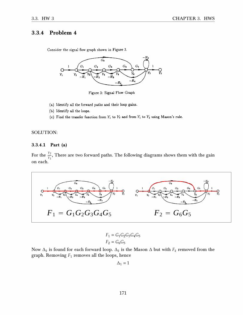
3.3. HW 3 CHAPTER 3. HWS
3.3.4 Problem 4
SOLUTION:
3.3.4.1 Part (a)
For the 𝑌7𝑌1, There are two forward paths. The following diagrams shows them with the gain
on each.
F1 G1G2G3G4G5 F2 G6G5
𝐹1 = 𝐺1𝐺2𝐺3𝐺4𝐺5
𝐹2 = 𝐺6𝐺5
Now Δ𝑘 is found for each forward loop. Δ𝑘 is the Mason Δ but with 𝐹𝑘 removed from thegraph. Removing 𝐹1 removes all the loops, hence
Δ1 = 1
171

3.3. HW 3 CHAPTER 3. HWS
When removing 𝐹2 what remains is 𝐿2 and 𝐿3, hence
Δ2 = 1 − (𝐿2 + 𝐿3)= 1 − (−𝐻2𝐺2 − 𝐻3𝐺3)= 1 + (𝐻2𝐺2 + 𝐻3𝐺3)
For the 𝑌2𝑌1, there is one forward path 𝐹1 = 1, the associated Δ1 is
Δ1 = 1 −�−𝐺2𝐻2 − 𝐺3𝐻3 − 𝐺4𝐺5𝐻4 − 𝐻6 − 𝐺2𝐺3𝐺4𝐺5𝐻5
+�(−𝐺2𝐻2) (−𝐺4𝐺5𝐻4) + (−𝐺2𝐻2) (−𝐻6) + (−𝐺3𝐻3) (−𝐻6)
= 1 +one at a time
�����������������������������������������������������������������𝐺2𝐻2 + 𝐺3𝐻3 + 𝐺4𝐺5𝐻4 + 𝐻6 + 𝐺2𝐺3𝐺4𝐺5𝐻5 +two at a time
�������������������������������������������������𝐺2𝐻2𝐺4𝐺5𝐻4 + 𝐺2𝐻2𝐻6 + 𝐺3𝐻3𝐻6
3.3.4.2 Part(b)
There are 8 loops. The following diagrams shows the loops with the gains
172
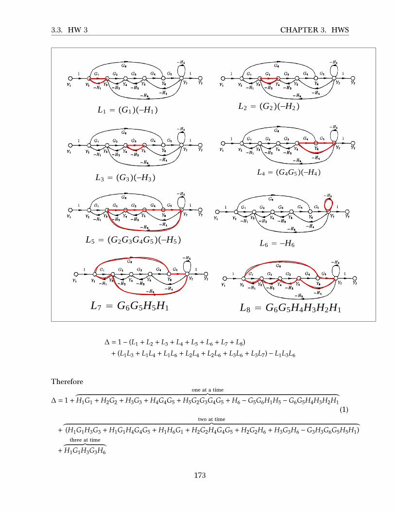
3.3. HW 3 CHAPTER 3. HWS
L1 G1H1 L2 G2H2
L3 G3H3L4 G4G5H4
L5 G2G3G4G5H5 L6 H6
L7 G6G5H5H1 L8 G6G5H4H3H2H1
Δ = 1 − (𝐿1 + 𝐿2 + 𝐿3 + 𝐿4 + 𝐿5 + 𝐿6 + 𝐿7 + 𝐿8)+ (𝐿1𝐿3 + 𝐿1𝐿4 + 𝐿1𝐿6 + 𝐿2𝐿4 + 𝐿2𝐿6 + 𝐿3𝐿6 + 𝐿3𝐿7) − 𝐿1𝐿3𝐿6
Therefore
Δ = 1 +one at a time
�����������������������������������������������������������������������������������������������������������������������������𝐻1𝐺1 + 𝐻2𝐺2 + 𝐻3𝐺3 + 𝐻4𝐺4𝐺5 + 𝐻5𝐺2𝐺3𝐺4𝐺5 + 𝐻6 − 𝐺5𝐺6𝐻1𝐻5 − 𝐺6𝐺5𝐻4𝐻3𝐻2𝐻1(1)
+two at time
���������������������������������������������������������������������������������������������������������������������������������������������(𝐻1𝐺1𝐻3𝐺3 + 𝐻1𝐺1𝐻4𝐺4𝐺5 + 𝐻1𝐻6𝐺1 + 𝐻2𝐺2𝐻4𝐺4𝐺5 + 𝐻2𝐺2𝐻6 + 𝐻3𝐺3𝐻6 − 𝐺3𝐻3𝐺6𝐺5𝐻5𝐻1)
+three at time
�����������������𝐻1𝐺1𝐻3𝐺3𝐻6
173
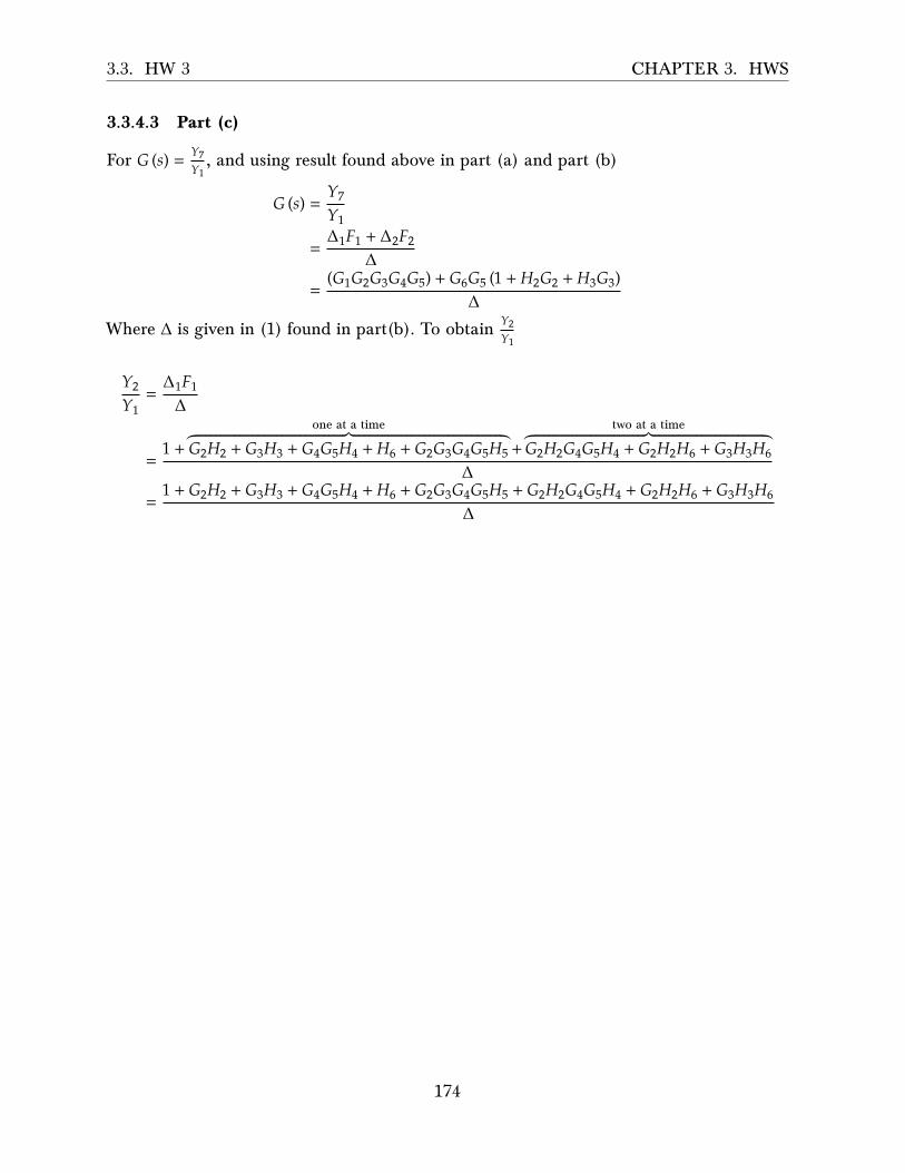
3.3. HW 3 CHAPTER 3. HWS
3.3.4.3 Part (c)
For 𝐺 (𝑠) = 𝑌7𝑌1, and using result found above in part (a) and part (b)
𝐺 (𝑠) =𝑌7𝑌1
=Δ1𝐹1 + Δ2𝐹2
Δ
=(𝐺1𝐺2𝐺3𝐺4𝐺5) + 𝐺6𝐺5 (1 + 𝐻2𝐺2 + 𝐻3𝐺3)
ΔWhere Δ is given in (1) found in part(b). To obtain 𝑌2
𝑌1
𝑌2𝑌1
=Δ1𝐹1Δ
=1 +
one at a time
�����������������������������������������������������������������𝐺2𝐻2 + 𝐺3𝐻3 + 𝐺4𝐺5𝐻4 + 𝐻6 + 𝐺2𝐺3𝐺4𝐺5𝐻5 +two at a time
�������������������������������������������������𝐺2𝐻2𝐺4𝐺5𝐻4 + 𝐺2𝐻2𝐻6 + 𝐺3𝐻3𝐻6Δ
=1 + 𝐺2𝐻2 + 𝐺3𝐻3 + 𝐺4𝐺5𝐻4 + 𝐻6 + 𝐺2𝐺3𝐺4𝐺5𝐻5 + 𝐺2𝐻2𝐺4𝐺5𝐻4 + 𝐺2𝐻2𝐻6 + 𝐺3𝐻3𝐻6
Δ
174
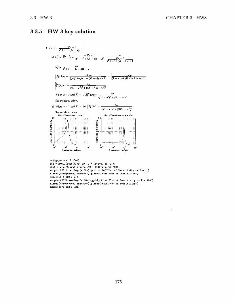
3.3. HW 3 CHAPTER 3. HWS
3.3.5 HW 3 key solutionECE 332 Homervork 3 Solutions
kc =
(b) lsfti,ll = 2u/tt - r t) '+ ( loz.r - r t) '
Plot of Sensitivity -- K . 1000
6go
vt
E 0.1of.=cCDao
>=u,Ce
v,
E 1I
.:otC'
0 :10 - ' 1oo 1ot
Frequency, radsec1o'ro'
0 :10 - ' ' roo 10'
Frequency, radlsec
r . logspace(-1 ,2 , looo) ;S G k = 2 + u . / ( s q r t ( ( f - c . ' 2 ) . ^ 2 + ( 3 + c - c . - S ) . ' Z ) ) ;
S G k l = 2 t y . / ( s q r t ( ( f - c . - Z ) . ' 2 + ( t 0 2 + c - c . - 3 ) . - 2 ) ) ;subplot (22L) , seui logr( r ,SGk),gr id , t i t le ( ' P lot o f Sensi t iv i ty - -r label ( 'Frequency, rad/sec' ) , ylabel ( ' l {agnitude of Sens it ivi ty' )a r i s ( [1e -1 1e2 0 2 ] )subplot (222) ,seui logr(n,SGk1) , gr id , t i t le( ' PIot o f Sensi t iv i ty - -: label ( ' Frequency, rad/sec' ),ylabel( ' l , lagnitude of Ssusit ivity' )a r i s ( [ t e - l 1 e 2 0 . 2 ] )
l . G ( s ) = - ' K s + l- ' - \ " , f s r + s , + ( K * a ) s + I
(a) 5*c : AGTF
Ils.'ri,rl =1 1=lsfti."ll =
(1 - r ') ' + ((K + &)or - rt) '
When k =2 and K = l, l.Src(jr)l =
See printout below.
When k:2 aud K = l (X),
See printout below.Plot ot Sensitivity - K. 1
- (Ks + l ) &@ E ' s J * s ' + ( K + A ) s + t
- -k iu
K = 1 ' )
K =n 100 ' )
: : : : : l . : : : :
: : : : : 1 . : : i i i i" n
: : : : : : : : : : : : : : l : l .: : : : : : : . , , . : : I :
;
175

3.3. HW 3 CHAPTER 3. HWS
) ( a ) I f K - l , t h e n U = R - f a Y - R - UF o r f t : { . . . , - 2 , - 1 , 0 , 1 , 2 , 3 , . . . } d r a w t h e l i n e Y : R - U . T h e i n t e r s e c t i o npoints give the correspondeing values of Y.
Transfer Function Between Y and U
1 i \ \ ' \\ : \ \ : \
\ : \ \ : \
0Input, U
Resulting Y versus r?:Transfer Function Between Y and R
4
3
tgfo
62-24
-1
-2
-3
-4
_51-6
fCLJo
22
4
0
-1
8
2. 1
^ :5 0ttfO - 1
5
-5
-5
I(,ro=
l 23P 4oog 6oa
0Input, r(t)
0
0 5 1 0Tim€, s€conds
(b) r ( t ) = 5s in( t ) . Us ing thetransfer function between Yand R, we cen generate y(t)graphically by "bouncing" r(t)(left) off of the transfer func-tion graph (upper left) ontoy(t) (top). The t ime at whichthe output becomes greaterthan I occrus at | = sin-t(|).
Resultant Output, y(0
\ , lV
1 0
;
176
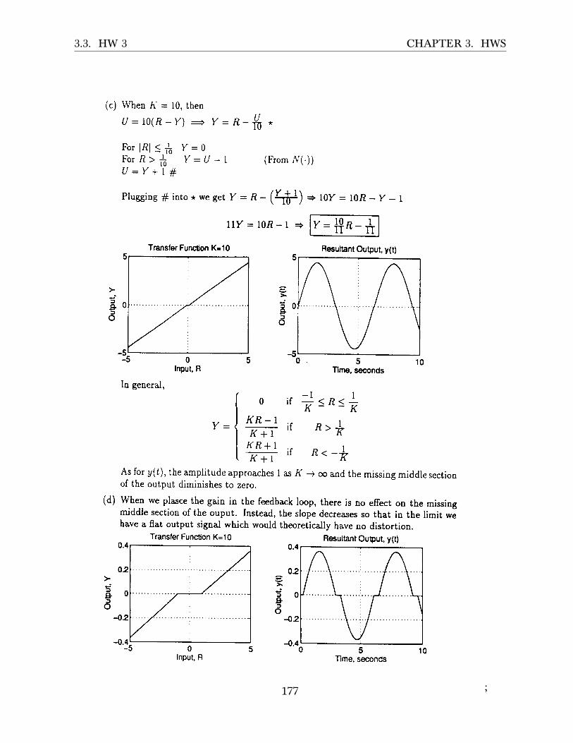
3.3. HW 3 CHAPTER 3. HWS
(c) When r\ = I0, thenU - r 0 ( r ? - Y ) - Y - R - # "
F o r l l ? l ! f i Y : 0F o r R > f i Y = U - l ( F r o m N ( ' ) )U : Y + l #
Plugging $ into* we get Y = R- (ftf) + lOY = tQ.R -Y - |
r z - l 0 p I" - T rl l Y = 1 0 R - 1 = +
5 oEfo
I t 'fo
Transfer Function K-10
Y _
Transler Function K=10
Reultant Output, y(t)
-5_ -5- 5 0 5 - 0 5 1 0Input, R Time, seconds
In general,- l ro i f 7 s n s K
K R - T . .f f i i r n '*K R + l . , n , IK + r
t l I t < - k
As for y(t), the amplitude approaches I as K + m and the missing middle sectionof the output diminishes to zero.
(d) When we plasce the gain in the feedback loop, there is no effect on the missingmiddle section of the ouput. Instead, the slope decreases so that in the limit wehave a flat output signai which would theoretically have no distortion.
0.40.4Resultant Ouput, y(t)
-0.4- -4.4r -: I- 5 0 5
- " 0 5 1 0
02xE OIt:o
42
A ofo
-02
Input, R rime. seconds
;177
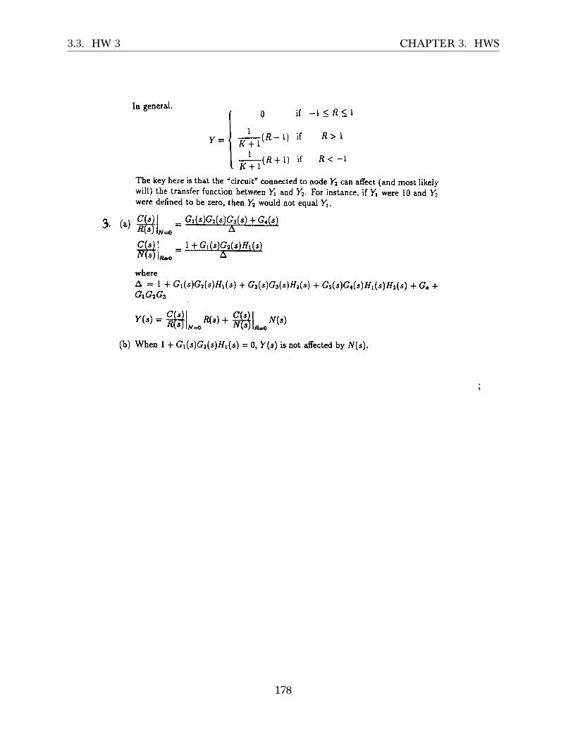
3.3. HW 3 CHAPTER 3. HWS
In general, '=l i f - l < R s i
u f t n - r l i r R> r
frtt* t1 ir ft < -iTbe key here is that the "circuit" connected to node Y2 can affect (and most likelywill) the transfer function between Fr and Y2. For instance, if Y, were I0 and Y2were defined to be zero, then Y2 would not equal y1.
a /^ \ C(r ) l _ Gr(s)Gz(s)Gs(s) + Gr(s)J. (ai ff i ;"_o---f
whereA = I * Gr(s)Gz(s)I{1(s) + Gr(s)Gs(s)II2( * G2(s)Ga(r)H,(")Hr(s) + Gr +GrGzGs
Y(s) = g8il"* n(s) + #fJl*" ",',(b) When I + Gr(s)G2(s)Il1(s) = 0, Y(s) is not affected by N(s).
;
178

3.3. HW 3 CHAPTER 3. HWS
;
179

3.4. HW 4 CHAPTER 3. HWS
3.4 HW 4
3.4.1 Problem 1
ECE 332 – Homework #4Due Thursday, October 15, 2015.
Problem 1: Consider the system with transfer function
G(s) =Ks + 1
s3 + s2 + (K + k) + 1.
(a) For K = 1, find the sensitivity SGk of this transfer function with respect
to k assuming nominal value k = 2. Then plot is magnitude as a functionof frequency.
(b) Repeat (a) with K = 100 and compare the effect of a large loopgain on the sensitivity.
Problem 2: Consider the block diagram set-up for the disturbance at-tenuation problem formulated in lecture with
G1(s) =s + 1
s2 + 10s + 100
and
G2(s) =1
s + 2.
(a) Design control blocks H1(s) and H2(s) such that the following twospecifications are satisfied: First,
|Y (jω)
N(jω)| ≤ 0.01
for all frequencies ω ≥ 0. Second, the output y(t) should respond tocommand to r(t) in approximately the same manner in the closed loop asin the open loop; i.e. for the closed loop, we desire
Y (s) ≈ G1(s)G2(s)R(s).
Note: In class, we did not fully solve for H1; i.e., we never found the con-stant α. In this homework, a specific solution is sought.
(b) To make your solution “proper,” introduce a second order lowpassfilter as appropriate and solve for the filter parameter ε.
(c) For the compensated system resulting from (b), generate a frequencyresponse plot for the closed loop transfer function |Y (jω)/R(jω)| and com-pare it to the target transfer function |G(jω)G2(jω)|. Plot the error be-tween these two frequency responses as a function of the frequency ω ≥ 0.
SOLUTION:
3.4.1.1 Part (a)
The second condition which says that the closed loops should approximate the open loopresponse, implies that we should use 𝐻2 (𝑠) =
1𝐺1𝐺2
, i.e. to apply the inversion. This is because𝑌(𝑠)𝑅(𝑠) =
𝐻1𝐺1𝐺21+𝐻1𝐺1𝐺2𝐻2
�𝑁=0
and this becomes 𝑌(𝑠)𝑅(𝑠) ≈ 𝐺1𝐺2 when we set 𝐻2 =
1𝐺1𝐺2
and also by
making 𝐻1 = 𝛼 where 𝛼 is a large gain. So now we just need to worry about finding 𝛼 s.t.
180

3.4. HW 4 CHAPTER 3. HWS
�𝑌�𝑗𝜔�
𝑁�𝑗𝜔�� ≤ 0.01 for all 𝜔 > 0.
We know that 𝑌(𝑠)𝑁(𝑠) =
𝐺21+𝐺1𝐺2𝐻2𝐻1
, but since we are using the inversion, this reduces to
𝑌 (𝑠)𝑁 (𝑠)
=𝐺2
1 + 𝐻1
By setting 𝐻1 (𝑠) = 𝛼 and using 𝐺2 =1
𝑠+2 and moving to the frequency domain, the abovebecomes
𝑌 �𝑗𝜔�
𝑁 �𝑗𝜔�=
1𝑗𝜔+2
1 + 𝛼=
1�𝑗𝜔 + 2� (1 + 𝛼)
=1
(1 + 𝛼) 𝑗𝜔 + 2 (1 + 𝛼)
Taking the magnitude
�𝑌 �𝑗𝜔�
𝑁 �𝑗𝜔�� =
1
�(1 + 𝛼)2𝜔2 + 4 (1 + 𝛼)2
We want the above to be smaller than 0.01 for all 𝜔, which implies1
�(1 + 𝛼)2𝜔2 + 4 (1 + 𝛼)2
≤ 0.01
1(1 + 𝛼)2𝜔2 + 4 (1 + 𝛼)2
≤ 0.012
(1 + 𝛼)2𝜔2 + 4 (1 + 𝛼)2 ≥ 10000
𝜔2 ≥10000 − 4 (1 + 𝛼)2
(1 + 𝛼)2
𝜔2 ≥10000(1 + 𝛼)2
− 4
𝜔 ≥�
10000(1 + 𝛼)2
− 4
The smallest 𝛼 to allow the above is when 𝜔 = 0, hence we need to solve for 𝛼 from
�
10000(1 + 𝛼)2
− 4 = 0
10000(1 + 𝛼)2
− 4 = 0
1(1 + 𝛼)2
=4
10000
(1 + 𝛼)2 =100004
= 2500
1 + 𝛼 = 50
181

3.4. HW 4 CHAPTER 3. HWS
Hence
𝛼 ≥ 49
Therefore 𝐻1 (𝑠) = 𝛼 where 𝛼 ≥ 49 and 𝐻1 (𝑠) =1
𝐺1(𝑠)𝐺2(𝑠). This complete this part.
3.4.1.2 Part(b)
One problem with the above inversion method for finding 𝐻2 (𝑠) =1
𝐺1𝐺2is that 𝐻2 (𝑠) becomes
improper:
𝐻2 (𝑠) =1
𝐺1𝐺2=
1𝑠+1
𝑠2+10𝑠+1001
𝑠+2
=�𝑠2 + 10𝑠 + 100� (𝑠 + 2)
𝑠 + 1
=𝑠3 + 12𝑠2 + 120𝑠 + 200
𝑠 + 1𝐻2 (𝑠) is improper, since the numerator has a degree larger than the denominator. Thisintroduces di�erentiator in the feedback loop which is something we do not like to have.
We will now replace 𝐻2 =1
𝐺1𝐺2by � 1
𝐺1𝐺2�𝐻𝐿𝑃 (𝑠) where 𝐻𝐿𝑃 (𝑠) =
1
(𝜀𝑠+1)𝑘is a low pass filter
where 𝑘 is an integer and 𝜀 is some parameter, both are positive. The goal is to block high
frequency noise content and also make � 1𝐺1𝐺2
�𝐻𝐿𝑃 (𝑠) become a proper transfer function. We
also want to make sure �𝑌�𝑗𝜔�
𝑁�𝑗𝜔�� remain less than 0.01.
Let
𝐻2 (𝑠) =1
𝐺1𝐺2
1(𝜀𝑠 + 1)𝑘
=𝑠3 + 12𝑠2 + 120𝑠 + 200
(𝑠 + 1)1
(𝜀𝑠 + 1)𝑘
The degree of the numerator is 3. So we want 𝑘 to be at least 2 (it can be more), so thatthe denominator has at least degree 3 as well. If we want strict proper, then we make 𝑘 = 3.Using 𝑘 = 2 we now have
𝐻2 (𝑠) =1
𝐺1𝐺2
1(𝜀𝑠 + 1)2
Therefore,𝑌�𝑗𝜔�
𝑁�𝑗𝜔�now becomes
𝑌 (𝑠)𝑁 (𝑠)
=𝐺2
1 + 𝐺1𝐺2𝐻1 �1
𝐺1𝐺2
1(𝜀𝑠+1)2
�
=1
𝑠+21 + 𝛼
(𝜀𝑠+1)2(1)
182
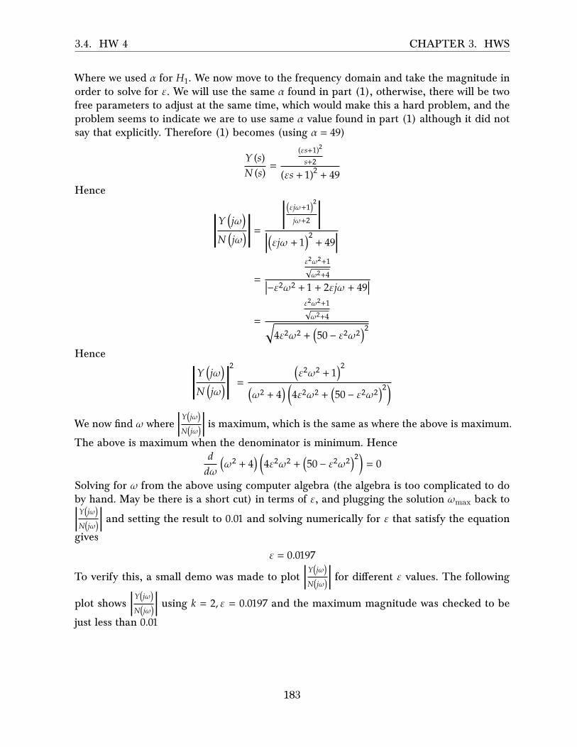
3.4. HW 4 CHAPTER 3. HWS
Where we used 𝛼 for 𝐻1. We now move to the frequency domain and take the magnitude inorder to solve for 𝜀. We will use the same 𝛼 found in part (1), otherwise, there will be twofree parameters to adjust at the same time, which would make this a hard problem, and theproblem seems to indicate we are to use same 𝛼 value found in part (1) although it did notsay that explicitly. Therefore (1) becomes (using 𝛼 = 49)
𝑌 (𝑠)𝑁 (𝑠)
=(𝜀𝑠+1)2
𝑠+2
(𝜀𝑠 + 1)2 + 49Hence
�𝑌 �𝑗𝜔�
𝑁 �𝑗𝜔�� =
��𝜀𝑗𝜔+1�
2
𝑗𝜔+2 �
��𝜀𝑗𝜔 + 1�2+ 49�
=
𝜀2𝜔2+1
√𝜔2+4
�−𝜀2𝜔2 + 1 + 2𝜀𝑗𝜔 + 49�
=
𝜀2𝜔2+1
√𝜔2+4
�4𝜀2𝜔2 + �50 − 𝜀2𝜔2�
2
Hence
�𝑌 �𝑗𝜔�
𝑁 �𝑗𝜔��
2
=�𝜀2𝜔2 + 1�
2
�𝜔2 + 4� �4𝜀2𝜔2 + �50 − 𝜀2𝜔2�2�
We now find 𝜔 where �𝑌�𝑗𝜔�
𝑁�𝑗𝜔�� is maximum, which is the same as where the above is maximum.
The above is maximum when the denominator is minimum. Hence𝑑𝑑𝜔
�𝜔2 + 4� �4𝜀2𝜔2 + �50 − 𝜀2𝜔2�2� = 0
Solving for 𝜔 from the above using computer algebra (the algebra is too complicated to doby hand. May be there is a short cut) in terms of 𝜀, and plugging the solution 𝜔max back to
�𝑌�𝑗𝜔�
𝑁�𝑗𝜔�� and setting the result to 0.01 and solving numerically for 𝜀 that satisfy the equation
gives
𝜀 = 0.0197
To verify this, a small demo was made to plot �𝑌�𝑗𝜔�
𝑁�𝑗𝜔�� for di�erent 𝜀 values. The following
plot shows �𝑌�𝑗𝜔�
𝑁�𝑗𝜔�� using 𝑘 = 2, 𝜀 = 0.0197 and the maximum magnitude was checked to be
just less than 0.01
183

3.4. HW 4 CHAPTER 3. HWS
epsilon 0.0197
w
0 200 400 600 800 1000
0.002
0.004
0.006
0.008
0.010
ω (rad/sec)
magnitude
H(s) Magnitude plot
3.4.1.3 Part (c)
We will now use
𝐻1 = 49
𝐻2 =1
𝐺1𝐺2
1(0.0197𝑠 + 1)2
And plot �𝑌(𝑠)𝑅(𝑠) � = �𝐻1𝐺1𝐺2
1+𝐻1𝐺1𝐺2𝐻2� against the |𝐺1𝐺2| to see how good the choice of 𝐻1 and 𝐻2 are.
𝑌 (𝑠)𝑅 (𝑠)
=𝐻1𝐺1𝐺2
1 + 𝐻1𝐺1𝐺2𝐻2
=49𝐺1𝐺2
1 + 49𝐺1𝐺21
𝐺1𝐺2
1(0.0197𝑠+1)2
=49 𝑠+1
𝑠2+10𝑠+1001
𝑠+2
1 + 49 1(0.0197𝑠+1)2
=49 𝑠+1
𝑠2+10𝑠+1001
𝑠+2(0.0197𝑠 + 1)2
(0.0197𝑠 + 1)2 + 49While
𝐺1𝐺2 =𝑠 + 1
𝑠2 + 10𝑠 + 1001
𝑠 + 2
The following plot shows �𝑌(𝑠)𝑅(𝑠) � vs. |𝐺1𝐺2| side by side
184

3.4. HW 4 CHAPTER 3. HWS
Out[348]=
open loop G1 G2 Compensated closed loop
0 100 200 300 400 500 6000
0.002
0.004
0.006
0.008
0.010
ω (rad/sec)
magnitude
H(s) Magnitude plot
0 100 200 300 400 500 6000
0.002
0.004
0.006
0.008
0.010
ω (rad/sec)
magnitude
H(s) Magnitude plot
The following plot shows both on the same plot
compensated open loop
0 100 200 300 400 500 6000
0.002
0.004
0.006
0.008
0.010
ω (rad/sec)
mag
nitu
de
H(s) Magnitude plot
The following plot show di�erence between the magnitudes
Out[386]=
0 100 200 300 400 500 600
0.0000
0.0002
0.0004
0.0006
0.0008
0.0010
0.0012
0.0014
ω (rad/sec)
|difference
|
|G1 G2|-|compensated|
Observations:
From the above di�erence plot, we see that the maximum di�erence between |𝐺1𝐺2| and the
compensated � 𝐻1𝐺1𝐺21+𝐻1𝐺1𝐺2𝐻2
� occurred at around 𝜔 = 350 and had value of about 0.0014. Thisvalue seems relatively small, and seems to indicate that 𝐻1 and 𝐻2 used for compensationwere a good choice.
185
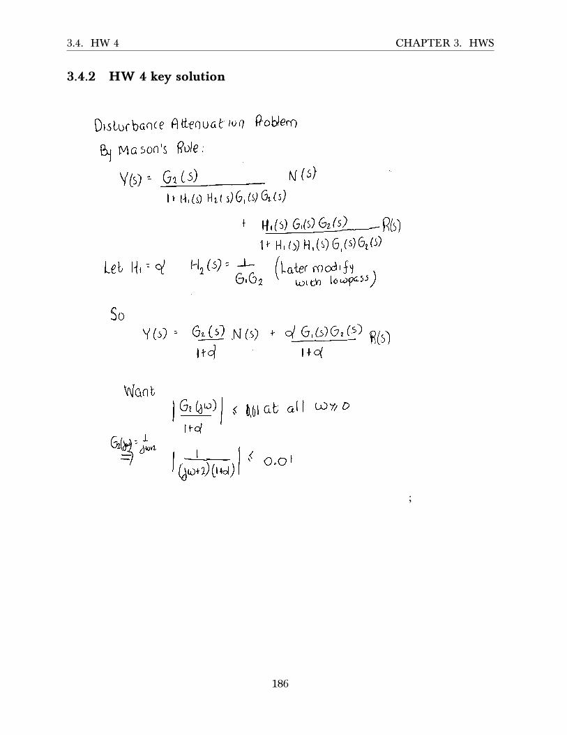
3.4. HW 4 CHAPTER 3. HWS
3.4.2 HW 4 key solutionE C E 3 3 ? - S o l u t , t o o s f i 5
fi [d,eo nGA rcrl ftoble.r)DrsLuc baoc e
q Mc son's Rrsle:
Y(s) ? Grts) NI (5)
I r t-1, (s) l l t t s) 6 ,0 Gr6)
l-l ,(s) G,$) Crk) R(s)1 r H, ( t H, (s) 6,(s) 6r(s)
Lel, ll'
So
- J - ( t-, ., t raLer ro od' f Y \b,l) 2 \ u:t ch lo agcst )
Vlr(s) =
C,Q N(s ) t d G ,b )OrG)fi(tftd r + q
Wonu0,bl a,b al | {:JYr oGrt4u1
l f d/ (
l s6u' o!,,,-t
0"* t)0+d)o,o I
;
186
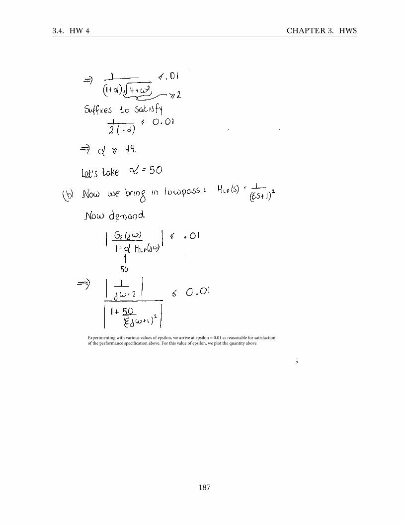
3.4. HW 4 CHAPTER 3. HWS
=t < , 0 l
[* a)Y L
5v{1t", * t1'il or
2 (r+ "t)
9 d Y / q q
Lots LaVe q' = 50
tS \(oo tr>e bcro5 \o lot'ogo'ss:
Jrfot^-, d eo oo cL
l G z T d l . , o l' l +d H rpb ' ) 't
-
50
I
6 ts+2 , _
H.p(s) :6r,
l + 5 0 - ^ lVA*r,) ' I
Experimenting with various values of epsilon, we arrive at epsilon = 0.01 as reasonable for satisfactionof the performance specification above. For this value of epsilon, we plot the quantity above
;
187

3.4. HW 4 CHAPTER 3. HWS
-KJ M) 1 1+^ Hipfai^}
x l O -3 Plot Of |Yaw)/NOw)| with Lowpass Filter 1 r
;
188

3.4. HW 4 CHAPTER 3. HWS
[ 0 iGf^et; . GAMGiU^) Aci^al'- /\M)-. c[GJMGii^)
ITCH Bl^w) --JM. flj^u) Plot
w
;
189

3.5. HW 5 CHAPTER 3. HWS
3.5 HW 5
3.5.1 Problem 1ECE 332 – Homework #5
Due Thursday, October 29, 2015
Problem 1: Performances specifications for a second order system
G(s) =ω2
n
s2 + 2ζωns+ ω2n
with 0 < ζ < 1 require that the maximum overshoot to a step input notexceed 30% and that the settling time be less than 0.25 seconds. Using
the settling time approximation
ts ≈3.2
ζωn
,
find and sketch the region in the complex plane where the two poles needto be located.
Problem 2: For the system shown in the figure below, find gains K
and Kt so that the maximum overshoot of the output c(t) to a unit stepinput r(t) is about 20% and that the rise time is approximately 0.05 sec-onds. Find the resulting closed loop transfer function C(s)/R(s) and
simulate the step response in Matlab. In your solution, use the rise timeapproximation
tr ≈1− 0.4167ζ + 2.917ζ2
ωn
.
SOLUTION:
There are two inequalities to satisfy. The first is given by the settling time requirement
𝑡𝑠 =3.2𝜁𝜔𝑛
< 0.25 (1)
The second is given by the overshoot requirement
𝑒− 𝜋𝜁
�1−𝜁2 < 0.3 (2)
From (2), taking the log of both sides gives
−𝜋𝜁
√1 − 𝜁2< ln (0.3)
Multiplying both sides by −1 changes the inequality from < to >𝜋𝜁
√1 − 𝜁2> − ln (0.3)
Simplifying gives
𝜋𝜁
√1 − 𝜁2> ln �
10.3�
> 1.204
190

3.5. HW 5 CHAPTER 3. HWS
Squaring both sides and solving for 𝜁
𝜁2
1 − 𝜁2> �
1.204𝜋 �
2
𝜁2 > 0.14688 �1 − 𝜁2�
1.146 88𝜁2 > 0.14688𝜁2 > 0.12807
Since 𝜁 has to be positive then the positive root is used giving
𝜁 > 0.35787
Back to the (1) specifications, which says3.2𝜁𝜔𝑛
< 0.25
𝜁𝜔𝑛 > 12.8
For each 𝜁𝑖 > 0.3578, we solve for 𝜔𝑛 from 𝜁𝜔𝑛 > 12.8. This will give full description of wherethe poles are located.
ωn
√1− ζ2
imaginary axis
−ζωn
|ωn|
real axis
X
X
Here is a plot of the (𝜁, 𝜔𝑛) space showing allowed values of 𝜁, 𝜔𝑛.
191
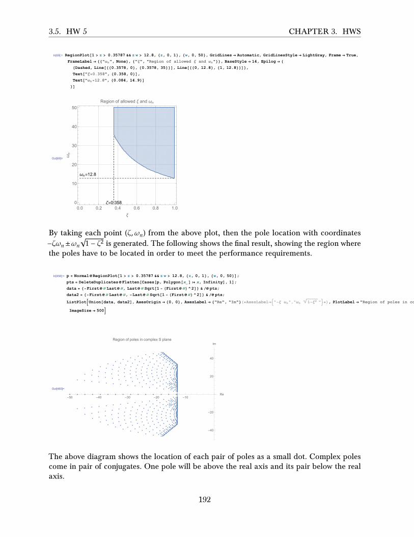
3.5. HW 5 CHAPTER 3. HWS
In[69]:= RegionPlot[1 > z > 0.35787 && z w > 12.8, {z, 0, 1}, {w, 0, 50}, GridLines → Automatic, GridLinesStyle → LightGray, Frame → True,
FrameLabel → {{"ωn", None}, {"ξ", "Region of allowed ξ and ωn"}}, BaseStyle → 14, Epilog → {
{Dashed, Line[{{0.3578, 0}, {0.3578, 35}}], Line[{{0, 12.8}, {1, 12.8}}]},
Text["ζ=0.358", {0.358, 0}],
Text["ωn=12.8", {0.084, 14.9}]
}]
Out[69]=
0.0 0.2 0.4 0.6 0.8 1.00
10
20
30
40
50
ξ
ωn
Region of allowed ξ and ωn
ζ=0.358
ωn=12.8
By taking each point (𝜁, 𝜔𝑛) from the above plot, then the pole location with coordinates−𝜁𝜔𝑛±𝜔𝑛√1 − 𝜁2 is generated. The following shows the final result, showing the region wherethe poles have to be located in order to meet the performance requirements.
In[456]:= p = Normal@RegionPlot[1 > z > 0.35787 && z w > 12.8, {z, 0, 1}, {w, 0, 50}];
pts = DeleteDuplicates@Flatten[Cases[p, Polygon[x_] ⧴ x, Infinity], 1];
data = {-First@# Last@#, Last@# Sqrt[1 - (First@#)^2]} & /@ pts;
data2 = {-First@# Last@#, -Last@# Sqrt[1 - (First@#)^2]} & /@ pts;
ListPlotUnion[data, data2], AxesOrigin → {0, 0}, AxesLabel → {"Re", "Im"}(*AxesLabel→"-ξ ωn","ωn 1-ξ2 "*), PlotLabel → "Region of poles in complex S plane",
ImageSize → 500
Out[460]=
-50 -40 -30 -20 -10Re
-40
-20
20
40
ImRegion of poles in complex S plane
The above diagram shows the location of each pair of poles as a small dot. Complex polescome in pair of conjugates. One pole will be above the real axis and its pair below the realaxis.
192
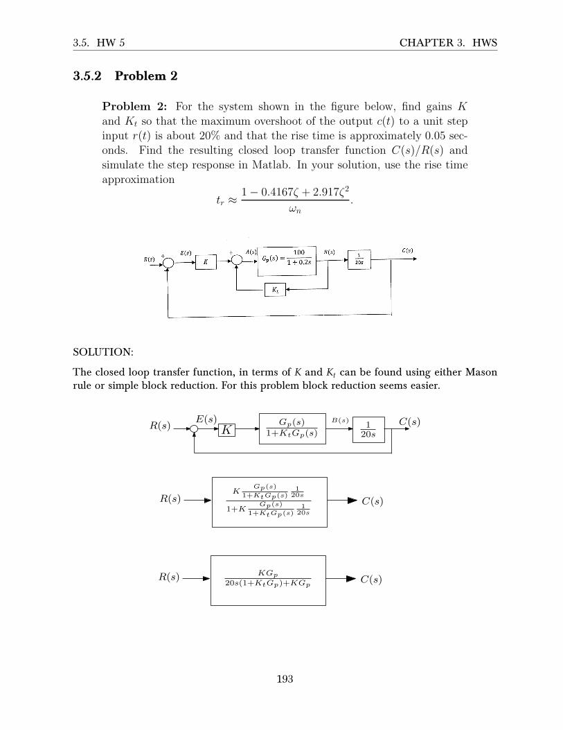
3.5. HW 5 CHAPTER 3. HWS
3.5.2 Problem 2
ECE 332 – Homework #5
Due Thursday, October 29, 2015
Problem 1: Performances specifications for a second order system
G(s) =ω2
n
s2 + 2ζωns+ ω2n
with 0 < ζ < 1 require that the maximum overshoot to a step input notexceed 30% and that the settling time be less than 0.25 seconds. Using
the settling time approximation
ts ≈3.2
ζωn
,
find and sketch the region in the complex plane where the two poles needto be located.
Problem 2: For the system shown in the figure below, find gains K
and Kt so that the maximum overshoot of the output c(t) to a unit stepinput r(t) is about 20% and that the rise time is approximately 0.05 sec-onds. Find the resulting closed loop transfer function C(s)/R(s) and
simulate the step response in Matlab. In your solution, use the rise timeapproximation
tr ≈1− 0.4167ζ + 2.917ζ2
ωn
.
SOLUTION:
The closed loop transfer function, in terms of 𝐾 and 𝐾𝑡 can be found using either Masonrule or simple block reduction. For this problem block reduction seems easier.
KGp(s)
1+KtGp(s)1
20s
E(s) B(s) C(s)
KGp(s)
1+KtGp(s)1
20s
1+KGp(s)
1+KtGp(s)1
20s
R(s)
R(s) C(s)
KGp
20s(1+KtGp)+KGpR(s) C(s)
193

3.5. HW 5 CHAPTER 3. HWS
Using 𝐺𝑝 =100
1+0.2𝑠 the above becomes
𝐶 (𝑠)𝑅 (𝑠)
=𝐾 � 100
1+0.2𝑠�
20𝑠 �1 + 𝐾𝑡100
1+0.2𝑠� + 𝐾 100
1+0.2𝑠
=100𝐾
20𝑠 (1 + 0.2𝑠 + 100𝐾𝑡) + 100𝐾
=100𝐾
4𝑠2 + (20 + 2000𝐾𝑡) 𝑠 + 100𝐾
=25𝐾
𝑠2 + (5 + 500𝐾𝑡) 𝑠 + 25𝐾
The standard form is 𝜔2𝑛
𝑠2+2𝜁𝜔𝑛𝑠+𝜔2𝑛therefore by comparing to the above we find
𝜔2𝑛 = 25𝐾
𝜔𝑛 = 5√𝐾 (1)
And
5 + 500𝐾𝑡 = 2𝜁𝜔𝑛
= 2𝜁 �5√𝐾�
𝜁 =5 + 500𝐾𝑡
10√𝐾(2)
Hence the transfer function is𝐶 (𝑠)𝑅 (𝑠)
=𝜔2𝑛
𝑠2 + 2𝜁𝜔𝑛𝑠 + 𝜔2𝑛
Where 𝜔𝑛 = 5√𝐾 and 𝜁 = 5+500𝐾𝑡10√𝐾
. We now apply the user specifications in order to determine
𝐾 and 𝐾𝑡. From the overshoot requirement, we write
𝑒− 𝜋𝜁
�1−𝜁2 ≤ 0.2 (3)
And from the rise time requirements we have
1 − 0.4167𝜁 + 2.917𝜁2
𝜔𝑛= 0.05 (4)
From (3) and (4) we can now solve for 𝜔𝑛 and 𝜁 and this allow us to find 𝐾 and 𝐾𝑡 by using
194

3.5. HW 5 CHAPTER 3. HWS
(1,2). From (3), taking logs and solving for 𝜁 gives
−𝜋𝜁
√1 − 𝜁2≤ ln (0.2)
𝜋𝜁
√1 − 𝜁2≥ ln (5)
𝜋𝜁
√1 − 𝜁2≥ 1. 6094
𝜋2𝜁2 ≥ (1. 6094)2 �1 − 𝜁2�
𝜋2𝜁2 ≥ 2.5902 − 2.5902𝜁2
�𝜋2 + 2.5902� 𝜁2 ≥ 2.5902
𝜁 ≥�
2.5902�𝜋2 + 2.5902�
Hence
𝜁 ≥ 0.456
Any 0.456 ≤ 𝜁 < 1 can be used. In order to find 𝜔𝑛, let us choose
𝜁 = 0.46
For the rest of the calculations . From (4) we find
1 − 0.4167 (0.46) + 2.917 (0.46)2
𝜔𝑛= 0.05
𝜔𝑛 =1.425 60.05
Therefore
𝜔𝑛 = 28.512 rad/sec
Now that we found 𝜁 and 𝜔𝑛 , we use (1,2) to find the gains. From (1)
𝜔𝑛 = 5√𝐾
𝐾 =𝜔2𝑛25
=28.5122
25Therefore
𝐾 = 32.517
And from (2)
𝜁 =5 + 500𝐾𝑡
10√𝐾
0.46 =5 + 500𝐾𝑡
10√32.517
195

3.5. HW 5 CHAPTER 3. HWS
Hence
𝐾𝑡 = 0.04246
The final transfer function is𝐶 (𝑠)𝑅 (𝑠)
=25𝐾
𝑠2 + (5 + 500𝐾𝑡) 𝑠 + 25𝐾
=25 (32.517)
𝑠2 + (5 + 500 (0.04246)) 𝑠 + 25 (32.517)Or
𝐶(𝑠)𝑅(𝑠) =
812.93𝑠2+26.23𝑠+812.93
Matlab is used to simulate the step response, and to also verify the user requirements aremet.
close all;clear all;s = tf('s');sys = 812.93/(s^2+26.23*s+812.93);step(sys)grid
0 0.05 0.1 0.15 0.2 0.25 0.3 0.35 0.40
0.2
0.4
0.6
0.8
1
1.2Step Response
Time (seconds)
Am
plitu
de
The step information was also verified using the command stepinfo() which showed thespecifications was indeed met.
stepinfo(sys)
RiseTime: 0.0549SettlingTime: 0.2916
196
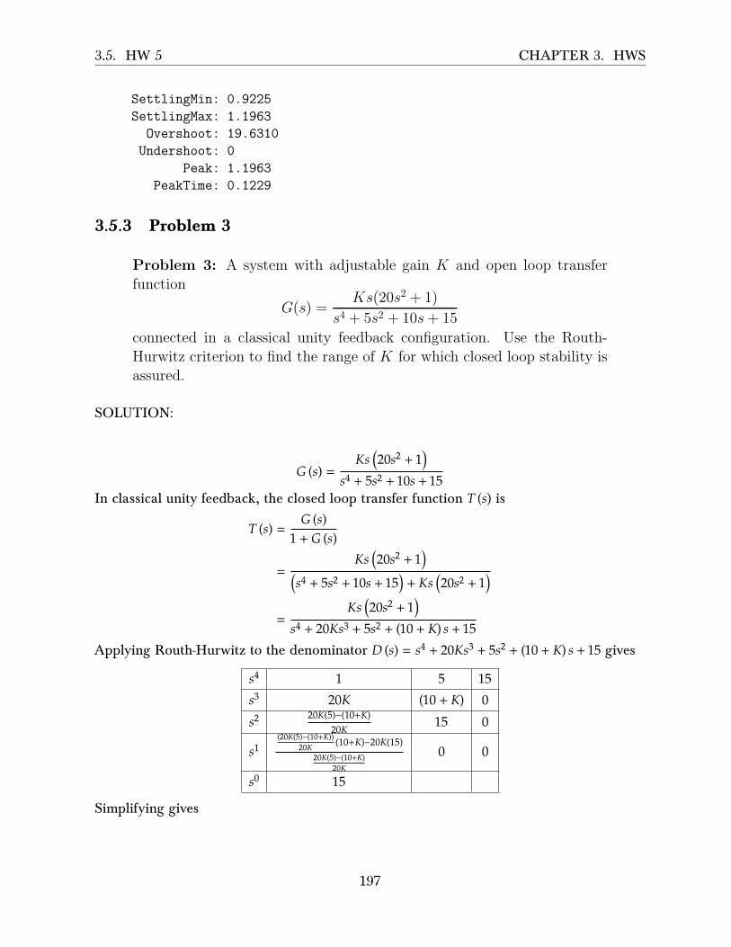
3.5. HW 5 CHAPTER 3. HWS
SettlingMin: 0.9225SettlingMax: 1.1963
Overshoot: 19.6310Undershoot: 0
Peak: 1.1963PeakTime: 0.1229
3.5.3 Problem 3
Problem 3: A system with adjustable gain K and open loop transfer
function
G(s) =Ks(20s2 + 1)
s4 + 5s2 + 10s+ 15
connected in a classical unity feedback configuration. Use the Routh-
Hurwitz criterion to find the range of K for which closed loop stability isassured.
Problem 4: Consider the system with open loop transfer function
G(s) =K
s(1 + Ts)
is connected in a unity feedback configuration. Given a > 0, the speci-fication is that all closed loop poles have real part less than −a. Show
how the Routh-Hurwitz criterion can modified to address this problem.Subsequently, for T = 1, find and sketch the region in the (a,K) planeassociated with closed loop stability.
Problem 5: An automatic depth control system for a submarine is de-
picted in the figure below. The depth is measured by a pressure trans-ducer. For what values of K will the systern be stable? Take H(s) = 1
and submarine transfer function
G(s) =(s+ 2)2
s2 + 0.01
SOLUTION:
𝐺 (𝑠) =𝐾𝑠 �20𝑠2 + 1�
𝑠4 + 5𝑠2 + 10𝑠 + 15In classical unity feedback, the closed loop transfer function 𝑇 (𝑠) is
𝑇 (𝑠) =𝐺 (𝑠)
1 + 𝐺 (𝑠)
=𝐾𝑠 �20𝑠2 + 1�
�𝑠4 + 5𝑠2 + 10𝑠 + 15� + 𝐾𝑠 �20𝑠2 + 1�
=𝐾𝑠 �20𝑠2 + 1�
𝑠4 + 20𝐾𝑠3 + 5𝑠2 + (10 + 𝐾) 𝑠 + 15Applying Routh-Hurwitz to the denominator 𝐷 (𝑠) = 𝑠4 + 20𝐾𝑠3 + 5𝑠2 + (10 + 𝐾) 𝑠 + 15 gives
𝑠4 1 5 15𝑠3 20𝐾 (10 + 𝐾) 0𝑠2 20𝐾(5)−(10+𝐾)
20𝐾 15 0
𝑠1(20𝐾(5)−(10+𝐾))
20𝐾 (10+𝐾)−20𝐾(15)20𝐾(5)−(10+𝐾)
20𝐾
0 0
𝑠0 15
Simplifying gives
197

3.5. HW 5 CHAPTER 3. HWS
𝑠4 1 5 15𝑠3 20𝐾 (10 + 𝐾) 0𝑠2 1
20𝐾(99𝐾 − 10) 15 0
𝑠1 110−99𝐾
�5901𝐾2 − 980𝐾 + 100� 0 0𝑠0 15
For stability, we need the first column to be positive. Hence the conditions are
20𝐾 > 0120𝐾
(99𝐾 − 10) > 0
110 − 99𝐾
�5901𝐾2 − 980𝐾 + 100� > 0
The first just says that 𝐾 > 0. The second says 99𝐾 − 10 > 0 or 𝐾 > 1099 . Now for the third
condition1
10 − 99𝐾�5901𝐾2 − 980𝐾 + 100� > 0
Since 𝐾 > 1099 is required, then
110−99𝐾 is negative quantity since 10−99𝐾 is negative for 𝐾 > 10
99 .This means the above becomes
5901𝐾2 − 980𝐾 + 100 < 0
Notice the change of inequality from > to < since we multiplied both sides by a negativequantity (10 − 99𝐾) to cancel it out. But 5901𝐾2 − 980𝐾 + 100 < 0 can not be satisfied with apositive 𝐾 > 10
99 . For example, using the minimum allowed 𝐾 which is 1099 , then the value of
5901𝐾2 − 980𝐾 + 100 becomes
5901 �1099�
2
− 980 �1099�
+ 100 = 61.218
But it needs to be negative. So there does not exist 𝐾 which makes the closed loop stable.
3.5.4 Problem 4
Problem 3: A system with adjustable gain K and open loop transfer
function
G(s) =Ks(20s2 + 1)
s4 + 5s2 + 10s+ 15
connected in a classical unity feedback configuration. Use the Routh-
Hurwitz criterion to find the range of K for which closed loop stability isassured.
Problem 4: Consider the system with open loop transfer function
G(s) =K
s(1 + Ts)
is connected in a unity feedback configuration. Given a > 0, the speci-fication is that all closed loop poles have real part less than −a. Show
how the Routh-Hurwitz criterion can modified to address this problem.Subsequently, for T = 1, find and sketch the region in the (a,K) planeassociated with closed loop stability.
Problem 5: An automatic depth control system for a submarine is de-
picted in the figure below. The depth is measured by a pressure trans-ducer. For what values of K will the systern be stable? Take H(s) = 1
and submarine transfer function
G(s) =(s+ 2)2
s2 + 0.01
SOLUTION:
198

3.5. HW 5 CHAPTER 3. HWS
Given 𝐺 (𝑠) = 𝐾𝑠(1+𝑇𝑠) then the closed loop transfer function is
𝐺𝑐𝑙𝑜𝑠𝑒𝑑 (𝑠) =𝐺
1 + 𝐺
=𝐾
𝑠 (1 + 𝑇𝑠) + 𝐾
=𝐾
𝑇𝑠2 + 𝑠 + 𝐾Therefore 𝐷 (𝑠) = 𝑇𝑠2 + 𝑠 + 𝐾. For the closed loop poles with real part to be less than −𝑎, let𝑠1 = 𝑠 + 𝑎. Then 𝑠 = 𝑠1 − 𝑎. We apply Routh-Hurwitz to 𝐷 (𝑠) but with 𝑠 = 𝑠1 − 𝑎. The newdenominator polynomial becomes
𝐷 (𝑠1) = 𝑇 (𝑠1 − 𝑎)2 + (𝑠1 − 𝑎) + 𝐾
Expanding gives
𝐷 (𝑠1) = 𝑇 �𝑠21 + 𝑎2 − 2𝑠1𝑎� + 𝑠1 − 𝑎 + 𝐾
= 𝑇𝑠21 + 𝑠1 (1 − 2𝑇𝑎) + �𝑇𝑎2 − 𝑎 + 𝐾�
Routh table applied to the above polynomial is
𝑠21 𝑇 𝑇𝑎2 − 𝑎 + 𝐾𝑠11 1 − 2𝑇𝑎 0𝑠01 𝑇𝑎2 − 𝑎 + 𝐾
We need all entries in the first column to be same sign (positive in this case, since 𝑇 = 1)for stability to hold (This is in addition to having the poles be with real part less than −𝑎).For 𝑇 = 1 the above becomes
𝑠2 1 𝑎2 + 𝑎 + 𝐾𝑠1 1 − 2𝑎 0𝑠0 𝑎2 − 𝑎 + 𝐾
The conditions for stability are
1 − 2𝑎 > 0𝑎 (1 − 𝑎) + 𝐾 > 0
The first condition gives 𝑎 > 12 . The second condition gives
𝐾 > 𝑎2 − 𝑎
Here is plot of the region in the (𝑎, 𝐾) plane associated with closed loop stability.
199

3.5. HW 5 CHAPTER 3. HWS
Out[1]=
0 5 10 15 20
0
100
200
300
400
a
K
Region of allowed a and K
3.5.5 Problem 5
Problem 3: A system with adjustable gain K and open loop transfer
function
G(s) =Ks(20s2 + 1)
s4 + 5s2 + 10s+ 15
connected in a classical unity feedback configuration. Use the Routh-
Hurwitz criterion to find the range of K for which closed loop stability isassured.
Problem 4: Consider the system with open loop transfer function
G(s) =K
s(1 + Ts)
is connected in a unity feedback configuration. Given a > 0, the speci-fication is that all closed loop poles have real part less than −a. Show
how the Routh-Hurwitz criterion can modified to address this problem.Subsequently, for T = 1, find and sketch the region in the (a,K) planeassociated with closed loop stability.
Problem 5: An automatic depth control system for a submarine is de-
picted in the figure below. The depth is measured by a pressure trans-ducer. For what values of K will the systern be stable? Take H(s) = 1
and submarine transfer function
G(s) =(s+ 2)2
s2 + 0.01
SOLUTION:
The closed loop transfer function is
𝑇 (𝑠) =𝐾𝐺 (𝑠) 1𝑠
1 + 𝐻𝐾𝐺 (𝑠) 1𝑠
200

3.5. HW 5 CHAPTER 3. HWS
Replacing 𝐻 (𝑠) = 1 and 𝐺 = (𝑠+2)2
𝑠2+0.01 the above becomes
𝑇 (𝑠) =𝐾(𝑠+2)2
𝑠2+0.011𝑠
1 + 𝐾(𝑠+2)2
𝑠2+0.011𝑠
=𝐾 (𝑠 + 2)2
𝑠 �𝑠2 + 0.01� + 𝐾 (𝑠 + 2)2
=𝐾 (𝑠 + 2)2
𝑠3 + 𝐾𝑠2 + (0.01 + 4𝐾) 𝑠 + 4𝐾The Routh table for 𝐷 (𝑠) = 𝑠3 + 𝐾𝑠2 + (0.01 + 4𝐾) 𝑠 + 4𝐾 is
𝑠3 1 0.01 + 4𝐾𝑠2 𝐾 4𝐾𝑠1 4𝐾 − 3.99 0𝑠0 4𝐾
Therefore for stability we need
𝐾 > 04𝐾 > 3.994𝐾 > 0
The first and the third conditions give 𝐾 > 0. From the second condition, 𝐾 > 3.994 = 0.9975.
Therefore
𝐾 > 0.9975
To verify, here is the step response for 𝑘 = 0.9974 and 𝑘 = 0.9976, showing one is unstableand the second is stable.
close all; clear all;s = tf('s');G = (s+2)^2/(s^2+0.01);
k = .9974;sys = feedback(k*G*1/s,1);subplot(2,1,1);step(sys);title(sprintf('k=%f',k)); grid
subplot(2,1,2);k = .9976;sys = feedback(k*G*1/s,1);step(sys);title(sprintf('k=%f',k)); grid
201

3.5. HW 5 CHAPTER 3. HWS
#105
0 1 2 3 4 5 6 7 8
#1013
-5
0
5k=0.997400
Time (seconds)
Am
plitu
de
#104
0 2 4 6 8 10 12 140
0.5
1
1.5
2k=0.997600
Time (seconds)
Am
plitu
de
202

3.5. HW 5 CHAPTER 3. HWS
3.5.6 HW 5 key solution
1) HOMEWORKOVERSHOOTSETTLING:
Theaboveshadedregionrepresentscosθ≥0.358.Theθ intheabovefigureiscos‐1(0.358)=69o
;
203

3.5. HW 5 CHAPTER 3. HWS
Forthesettlingtimeconstraint,wehave,
Sincewewantbothconditionstobesatisfied,theallowedregionforthepolesisthecommonshadedregionfromtheabovetwofigures:
;
204
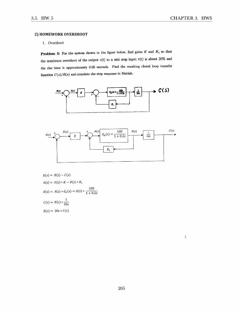
3.5. HW 5 CHAPTER 3. HWS
2)HOMEWORKOVERSHOOT
;
205

3.5. HW 5 CHAPTER 3. HWS
;
206

3.5. HW 5 CHAPTER 3. HWS
;
207
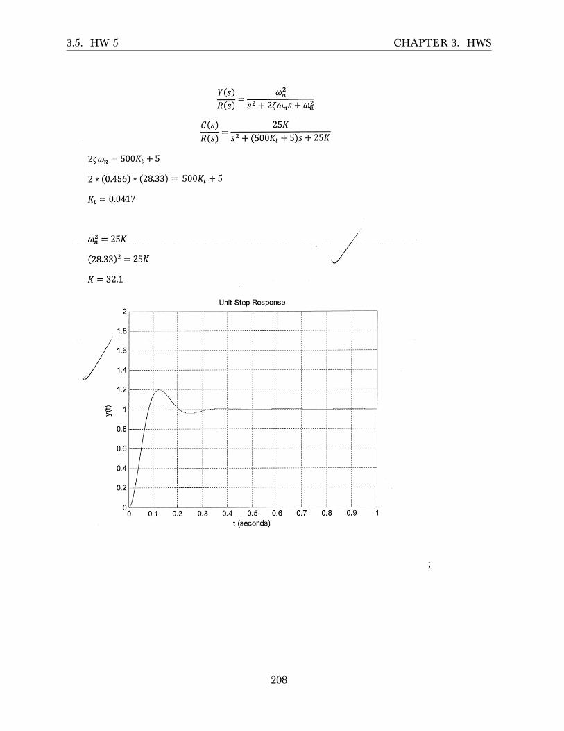
3.5. HW 5 CHAPTER 3. HWS
;
208

3.5. HW 5 CHAPTER 3. HWS3)PROBLEM1:
ECE 332 - HW #5
Due Thursday, March 13, 2003
Problem 1: A s.ystem with with adjustable gain K and open loop transfer functiorr
G ( " ) :K s(20s2 + 1)
s 4 + 5 s 2 * 1 0 s f 1 5
is connected in a classical unity feedback configuration. Find the range of giiins h for
which closed loop stability is assured.
Problem 2: consider the svstem with open loop transfer function
G ( s ) : , *
s (1 + Zs)
t'otrttected in clmsical unity feedback configuration. Given a ) 0, the specifica,ti.n for
this svst'enr is that all close{ loop poles have real part less tha,n -o. T}rnt is, a,ll cl'stxl
loop poles should lie to the left of the line z : -a in the cr-rnrplex pla,ne. Show how
the Rorrth-Hurwitz criterion carr be modified to acldress this problern. Subseqrre'tly,
with ? 3 I ' find the region in the (o, K) plane a^ssr-rciated with closecl loop stabilit 1,.
Problem 3; An automabic depth control system for a submarine is depicted in the figurebe low.
kstreldrpa+r e&n Y6)
FeSdure cneoJore roeob
The depth is measured by a Pressure transducer. For what values of the actuator 1( willthe system be stable? The submarine has an approximate transfer function
G ( s ) = ( s + 0 . 2 ) 2\ / s 2 + 0 . 0 1
and the transducer may be taken to be
A c t , S a t o c
fl(s) - 1
;
209

3.5. HW 5 CHAPTER 3. HWS
O s ls'
S,
S,
so
O u b l r n e o lloneu:orK $ct # 5
o
7 o 7 l 4 z o
7oV O
20K
%fKrO2 0 . K
5
(orx)
t 5
r 5
oo
oTo q,votd stgn chqn9e.-r 20K-
@ WK- ro r o -+ n r f f iO (on x lpsK-ro) 6@K"
a - 5 9 0 | K 2 + 9 B o K t o o
* No reel volua o{ K -L-soJnfrco { qlxve ln
t dWJ&u b ooobob,b Joc
I
I0p;i>t@'J o' ' ( g g K - r o )
f 5 - t *
o
d reo l l ( ,
{
rol Susl-emsSolU b rons -
;
210

3.5. HW 5 CHAPTER 3. HWS4) PROBLEM2:
ECE 332 - HW #5
Due Thursday, March 13, 2003
Problem 1: A s.ystem with with adjustable gain K and open loop transfer functiorr
G ( " ) :K s(20s2 + 1)
s 4 + 5 s 2 * 1 0 s f 1 5
is connected in a classical unity feedback configuration. Find the range of giiins h for
which closed loop stability is assured.
Problem 2: consider the svstem with open loop transfer function
G ( s ) : , *
s (1 + Zs)
t'otrttected in clmsical unity feedback configuration. Given a ) 0, the specifica,ti.n for
this svst'enr is that all close{ loop poles have real part less tha,n -o. T}rnt is, a,ll cl'stxl
loop poles should lie to the left of the line z : -a in the cr-rnrplex pla,ne. Show how
the Rorrth-Hurwitz criterion carr be modified to acldress this problern. Subseqrre'tly,
with ? 3 I ' find the region in the (o, K) plane a^ssr-rciated with closecl loop stabilit 1,.
Problem 3; An automabic depth control system for a submarine is depicted in the figurebe low.
kstreldrpa+r e&n Y6)
FeSdure cneoJore roeob
The depth is measured by a Pressure transducer. For what values of the actuator 1( willthe system be stable? The submarine has an approximate transfer function
G ( s ) = ( s + 0 . 2 ) 2\ / s 2 + 0 . 0 1
and the transducer may be taken to be
A c t , S a t o c
fl(s) - 1
t .
I t t\;/
oIJ
_\
, (s,) =
ltl S,79-Y O
G(s) =
= $ + A o
0 lin!,
K
Jr/ot-ul
s ben3S, benX&.J L"oJ
e"JLe Q - .
) bbcrin
sl
3 ,
S O
[:or
sfe,cq
6 , - q ( r t S , T
Ch o r aclur tLic eBaa
Ts,' + (r - 2o-f)5, -
T - - g + Q ' T
l-20.T C
e + d r n I
,5,
+ l L
l r G i l t u = t )
R,ie u)
= S ' * . O I J + , 4 t ( S r K ' 6 ' + , o 4 l <
I Q
drb ctb
- c,tT
L ton
C L I
( loo
t l d
eX,om pEl u,g, coo obtotru o s Luble
o
t ' i02 f-ozT = t 9K r a2 -
,f
f?Y O . l - 2 a T Y o K' ) t
0 r r ev e( se (0 e loo l i l re
T(
$
3 r A
A ) l t
t0 Mo,Oon r:
1(. ( s+ 't)'s ( s '+ ,o t ) 5 ( s " r . o r )
;
211

3.5. HW 5 CHAPTER 3. HWS
5) PROBLEM3:
ECE 332 - HW #5
Due Thursday, March 13, 2003
Problem 1: A s.ystem with with adjustable gain K and open loop transfer functiorr
G ( " ) :K s(20s2 + 1)
s 4 + 5 s 2 * 1 0 s f 1 5
is connected in a classical unity feedback configuration. Find the range of giiins h for
which closed loop stability is assured.
Problem 2: consider the svstem with open loop transfer function
G ( s ) : , *
s (1 + Zs)
t'otrttected in clmsical unity feedback configuration. Given a ) 0, the specifica,ti.n for
this svst'enr is that all close{ loop poles have real part less tha,n -o. T}rnt is, a,ll cl'stxl
loop poles should lie to the left of the line z : -a in the cr-rnrplex pla,ne. Show how
the Rorrth-Hurwitz criterion carr be modified to acldress this problern. Subseqrre'tly,
with ? 3 I ' find the region in the (o, K) plane a^ssr-rciated with closecl loop stabilit 1,.
Problem 3; An automabic depth control system for a submarine is depicted in the figurebe low.
kstreldrpa+r e&n Y6)
FeSdure cneoJore roeob
The depth is measured by a Pressure transducer. For what values of the actuator 1( willthe system be stable? The submarine has an approximate transfer function
G ( s ) = ( s + 0 . 2 ) 2\ / s 2 + 0 . 0 1
and the transducer may be taken to be
A c t , S a t o c
fl(s) - 1
;
212
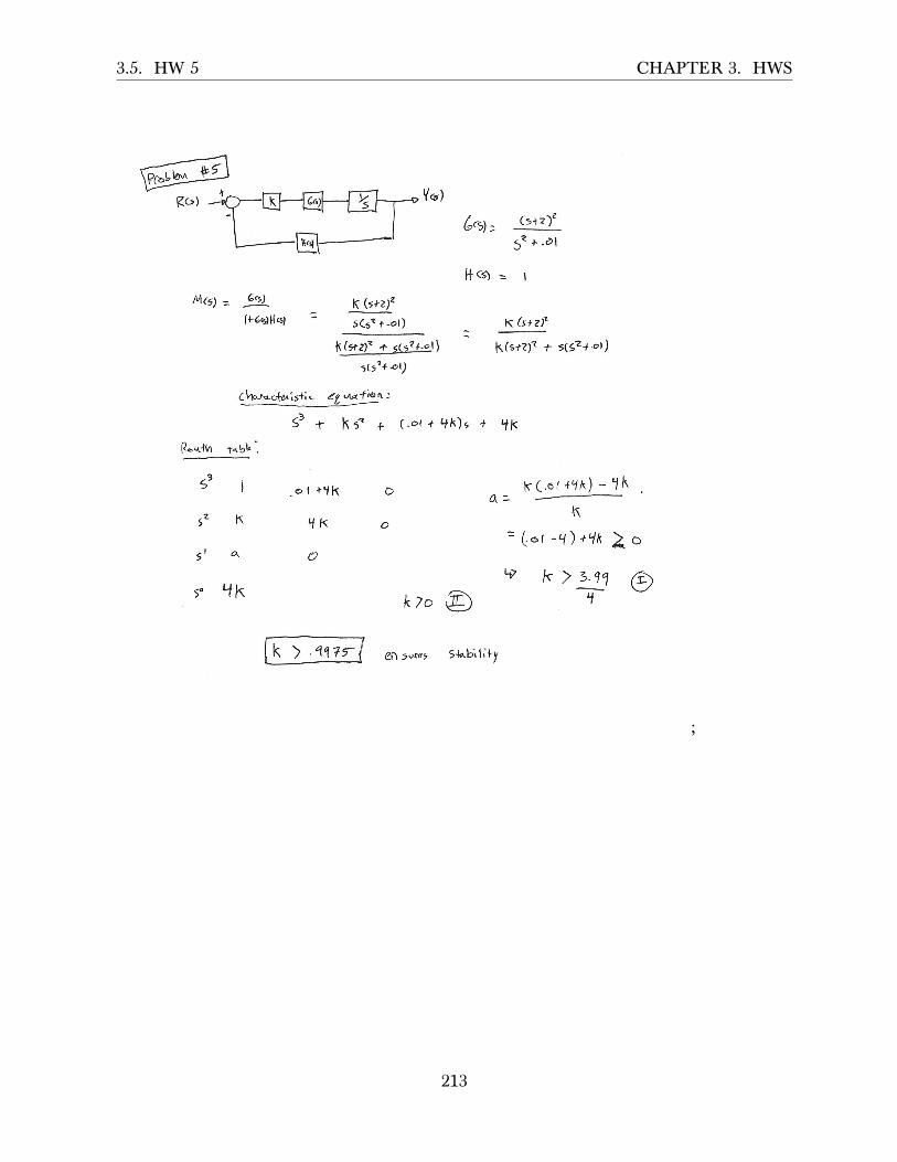
3.5. HW 5 CHAPTER 3. HWS
;
213

3.6. HW 6 CHAPTER 3. HWS
3.6 HW 6
3.6.1 Problem 1ECE 332 - Homework Set 6
Due Wednesday, November 11, 2011 at 9 AMPlease slide submissions under my door
Problem 1
Problem 2SOLUTION:
3.6.1.1 Part(a)
K 1s(s+2)(s+5)(s+10) Y (s)R(s)
+
−
1. 𝑛 = 4 (The number of open loop poles), 𝑚 = 0 (The number of open loop zeros).
2. Root Locus (R.L.) starts at the open loop poles 𝑠 = 0, 𝑠 = −2, 𝑥 = −5, 𝑠 − 10 when 𝑘 = 0.Since there are no open loop zeros, the branches will end up at ±∞
3. On the real axis, R.L. exists on segments based on number of poles and zeros to theright of the segment. If this sum (including multiplicity) is odd, then the segment ison the R.L., else it is not. The plot below shows the segments found.
××××−2−5−10
4. Center of asymptotes is now found using 𝜎 =∑𝑝𝑜𝑙𝑒𝑠−∑𝑧𝑒𝑟𝑜𝑠
𝑛−𝑚 = (0−2−5−10)4 = −4.25
214
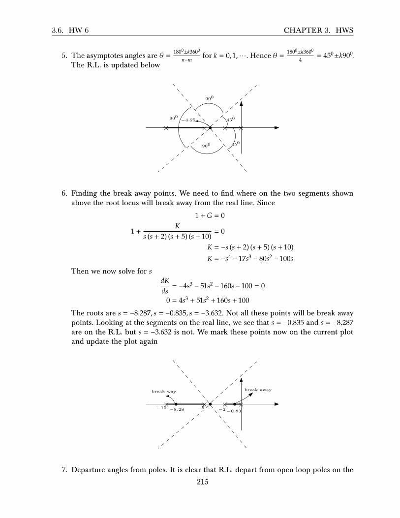
3.6. HW 6 CHAPTER 3. HWS
5. The asymptotes angles are 𝜃 = 1800±𝑘3600
𝑛−𝑚 for 𝑘 = 0, 1,⋯. Hence 𝜃 = 1800±𝑘3600
4 = 450±𝑘900.The R.L. is updated below
××××−4.25 450
900
900
900 450
6. Finding the break away points. We need to find where on the two segments shownabove the root locus will break away from the real line. Since
1 + 𝐺 = 0
1 +𝐾
𝑠 (𝑠 + 2) (𝑠 + 5) (𝑠 + 10)= 0
𝐾 = −𝑠 (𝑠 + 2) (𝑠 + 5) (𝑠 + 10)𝐾 = −𝑠4 − 17𝑠3 − 80𝑠2 − 100𝑠
Then we now solve for 𝑠𝑑𝐾𝑑𝑠
= −4𝑠3 − 51𝑠2 − 160𝑠 − 100 = 0
0 = 4𝑠3 + 51𝑠2 + 160𝑠 + 100
The roots are 𝑠 = −8.287, 𝑠 = −0.835, 𝑠 = −3.632. Not all these points will be break awaypoints. Looking at the segments on the real line, we see that 𝑠 = −0.835 and 𝑠 = −8.287are on the R.L. but 𝑠 = −3.632 is not. We mark these points now on the current plotand update the plot again
××××−2−5−10
−0.83−8.28
break awaybreak way
7. Departure angles from poles. It is clear that R.L. depart from open loop poles on the
215

3.6. HW 6 CHAPTER 3. HWS
real axis as shown, moving towards the break away points. Hence the plot now lookslike the following
××××−2
−5−10 −0.83−8.28
8. We now extend the branch from the break away points towards the asymptotes, sincethere are no zeros, no need to calculate arrival angles. The branch will move to theasymptotes. So we end up with the following
××××−2
−5−10 −0.83−8.28
It is important to remember that root locus will always be symmetric with respect tothe real axis.
9. Now the only lemma left is to find where R.L. crosses the imaginary axis. For thiswe use Routh stability stable as follows. Since the characteristic polynomial is 𝐾 +𝑠 (𝑠 + 2) (𝑠 + 5) (𝑠 + 10) = 0 then
𝑃(𝑠) = 𝑠4 + 17𝑠3 + 80𝑠2 + 100𝑠 + 𝐾
𝑠4 1 80 𝐾𝑠3 17 100𝑠2 74.118 𝐾𝑠1 100 − 0.229𝐾𝑠0 𝐾
216

3.6. HW 6 CHAPTER 3. HWS
We just need to find where it cross the imaginary axis. Setting the 𝑠1 row to zerogives 𝐾 = 436.68. This means the closed loop will become unstable for 𝑘 > 436.68.To find where R.L. crosses the imaginary axes, we go back to the even polynomial𝑠2 (the row above the line 𝑠1) in above Routh table, which yields 74.118𝑠2 + 𝐾 = 0 or74.118𝑠2 + 436.68 = 0, therefore 𝑠 = ±2.43𝑖. This complete R.L. Here is the final plot
×××× −2−5−10 −0.83−8.28
2.43
−2.43
K = 436
K = 0
K =∞K =∞
K =∞K =∞
−4.25s = 0
3.6.1.2 Part(b)
K 1(s2+s+2)(s+1) Y (s)R(s)
+
−
𝐺 (𝑠) =𝐾
�𝑠2 + 𝑠 + 2� (𝑠 + 1)
1. 𝑛 = 3 (The number of open loop poles), 𝑚 = 0 (The number of open loop zeros).
2. Root Locus (R.L.) starts at the open loop poles 𝑠 = −1, 𝑠 = −0.5 ± 1.323𝑖 when 𝑘 = 0.Since there are no open loop zeros, the branches end up at ±∞
3. On the real axis, R.L., since one pole on the real axis, then the R.L. segment is to theleft of the only pole, which is 𝑠 = −1
217

3.6. HW 6 CHAPTER 3. HWS
×−1
4. Center of asymptotes is now found. 𝜎 =∑𝑝𝑜𝑙𝑒𝑠−∑𝑧𝑒𝑟𝑜𝑠
𝑛−𝑚 = (−1−0.5−0.5)3 = −0.667
5. The asymptotes angles are 𝜃 = 1800±𝑘3600
𝑛−𝑚 for 𝑘 = 0, 1,⋯. Hence 𝜃 = 1800±𝑘3600
3 = 600 ±𝑘1200. Therefore the R.L. now looks like the following
×−0.667−1
600
1200
1200
600
×−0.5 + 1.323i
×−0.5− 1.323i
origin
6. Break away points. There is no break away points, since there are no segments betweentwo poles on the real line. We can see this also if we try to solve 𝑑𝐾
𝑑𝑠 = 0 as follows
1 + 𝐺 = 0
1 +𝐾
�𝑠2 + 𝑠 + 2� (𝑠 + 1)= 0
𝐾 = �𝑠2 + 𝑠 + 2� (𝑠 + 1)
𝐾 = 𝑠3 + 2𝑠2 + 3𝑠 + 2
Then we now solve for𝑑𝐾𝑑𝑠
= 3𝑠2 + 4𝑠 + 3 = 0
The solution gives only complex roots. So we go to the next lemma.
7. Departure angles from poles. It is clear that R.L. depart from open loop pole on the
218
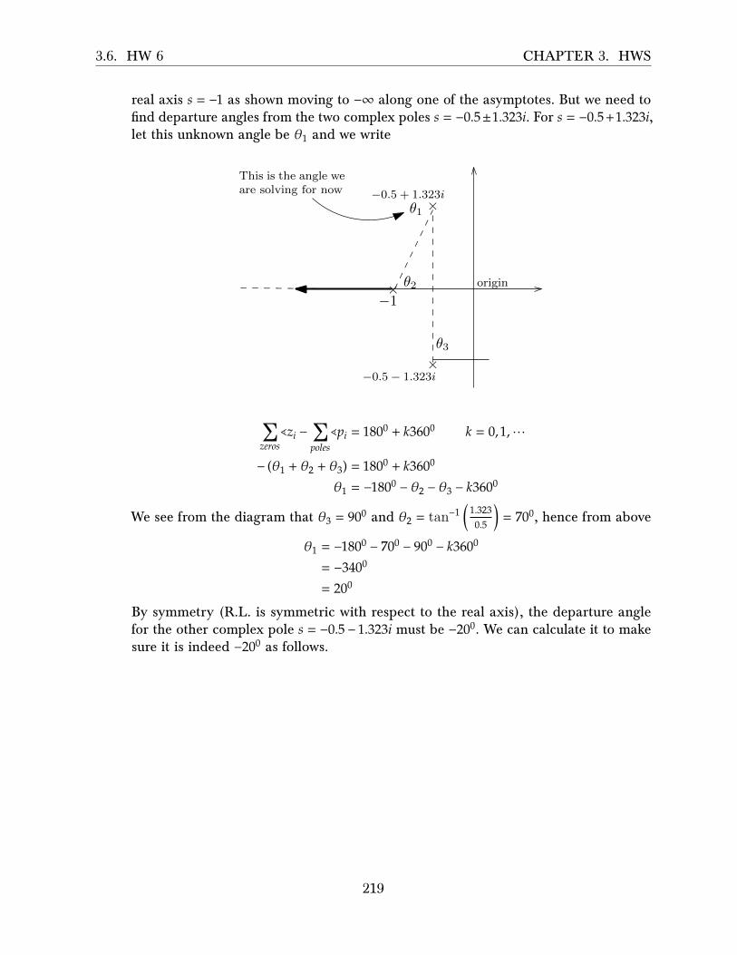
3.6. HW 6 CHAPTER 3. HWS
real axis 𝑠 = −1 as shown moving to −∞ along one of the asymptotes. But we need tofind departure angles from the two complex poles 𝑠 = −0.5±1.323𝑖. For 𝑠 = −0.5+1.323𝑖,let this unknown angle be 𝜃1 and we write
×−1
×−0.5 + 1.323i
×−0.5− 1.323i
originθ2
θ3
θ1
This is the angle weare solving for now
�𝑧𝑒𝑟𝑜𝑠
∢𝑧𝑖 − �𝑝𝑜𝑙𝑒𝑠
∢𝑝𝑖 = 1800 + 𝑘3600 𝑘 = 0, 1,⋯
− (𝜃1 + 𝜃2 + 𝜃3) = 1800 + 𝑘3600
𝜃1 = −1800 − 𝜃2 − 𝜃3 − 𝑘3600
We see from the diagram that 𝜃3 = 900 and 𝜃2 = tan−1 �1.3230.5
� = 700, hence from above
𝜃1 = −1800 − 700 − 900 − 𝑘3600
= −3400
= 200
By symmetry (R.L. is symmetric with respect to the real axis), the departure anglefor the other complex pole 𝑠 = −0.5 − 1.323𝑖 must be −200. We can calculate it to makesure it is indeed −200 as follows.
219
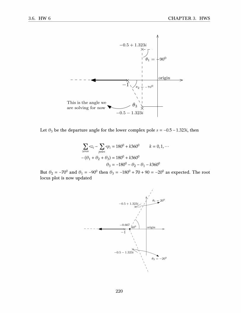
3.6. HW 6 CHAPTER 3. HWS
×−1
×−0.5 + 1.323i
×−0.5− 1.323i
origin
θ2 = −700
θ3
θ1 = −900
This is the angle weare solving for now
Let 𝜃3 be the departure angle for the lower complex pole 𝑠 = −0.5 − 1.323𝑖, then
�𝑧𝑒𝑟𝑜𝑠
∢𝑧𝑖 − �𝑝𝑜𝑙𝑒𝑠
∢𝑝𝑖 = 1800 + 𝑘3600 𝑘 = 0, 1,⋯
− (𝜃1 + 𝜃2 + 𝜃3) = 1800 + 𝑘3600
𝜃3 = −1800 − 𝜃2 − 𝜃1 − 𝑘3600
But 𝜃2 = −700 and 𝜃1 = −900 then 𝜃3 = −1800 + 70 + 90 = −200 as expected. The rootlocus plot is now updated
×−1
×−0.5 + 1.323i
×−0.5− 1.323i
origin−0.667
θ1 = 200
θ3 = −200
600
220

3.6. HW 6 CHAPTER 3. HWS
8. We now extend R.L. to the asymptotes, since there are no zeros, there is no need tocalculate arrival angles and we end up with the following
×−1
×−0.5 + 1.323i
×−0.5− 1.323i
origin−0.667
θ1 = 200
θ3 = −200
600
9. Now the only lemma left is to find where R.L. crosses the imaginary axis. For thiswe use Routh stability stable as follows. Since the characteristic polynomial is 𝐾 +�𝑠2 + 𝑠 + 2� (𝑠 + 1) = 0 then
𝑃(𝑠) = 𝑠3 + 2𝑠2 + 3𝑠 + 𝐾 + 2
𝑠3 1 3𝑠2 2 𝐾 + 2𝑠1 4−𝑘
2𝑠0 𝐾 + 2
We need 𝐾 = 4 (by setting the 𝑠1 row to zero). This means system will be unstable for𝑘 > 4. To find where R.L. crosses the imaginary axes, we go back to the 𝑠2 polynomialabove the line 𝑠1 in Routh table, which yields 2𝑠2 + 𝐾 + 2 = 0 or 2𝑠2 + 6 = 0, therefore𝑠 = ±1.73𝑖. This complete R.L. Here is the final plot
221

3.6. HW 6 CHAPTER 3. HWS
×−1
×−0.5 + 1.323i
×−0.5− 1.323i
origin−0.667
θ1 = 200
θ3 = −200
600
1.73i
−1.73i
3.6.1.3 Part(c)
K s2+2s+10s(s+5)(s+10) Y (s)R(s)
+
−
𝐺 (𝑠) =𝐾 �𝑠2 + 2𝑠 + 10�𝑠 (𝑠 + 5) (𝑠 + 10)
1. 𝑛 = 3 (The number of open loop poles), 𝑚 = 2 (The number of open loop zeros).
2. Root Locus (R.L.) starts at the open loop poles 𝑠 = 0, 𝑠 = −5, 𝑠 = −10 when 𝑘 = 0 andtwo of the branches end up at zeros 𝑠 = −1 ± 3𝑖. One branch will end up at ±∞.
3. On the real axis, there is R.L. segment between 𝑠 = 0, 𝑠 = −5 and another segmentto the left of 𝑠 = −10. No R.L. segment exist between 𝑠 = −5 and 𝑠 = −10. Currentdiagram now looks like the following
222

3.6. HW 6 CHAPTER 3. HWS
×−5
××s = 0−10
−1 + 3i
−1− 3i
4. Center of asymptotes is now found. 𝜎 =∑𝑝𝑜𝑙𝑒𝑠−∑𝑧𝑒𝑟𝑜𝑠
𝑛−𝑚 = −15−(−1−1)1 = −13
5. The asymptotes angles are 𝜃 = 1800±𝑘3600
𝑛−𝑚 for 𝑘 = 0, 1,⋯. Hence 𝜃 = 1800±𝑘3600
1 = 1800 ±𝑘3600. Therefore the R.L. now looks like the following
×−5
××s = 0−10
−1 + 3i
−1− 3i
1800asymptotes
σs = −13
6. Finding the break away points
1 + 𝐺 = 0
1 +𝐾 �𝑠2 + 2𝑠 + 10�𝑠 (𝑠 + 5) (𝑠 + 10)
= 0
𝑠 (𝑠 + 5) (𝑠 + 10) + 𝐾 �𝑠2 + 2𝑠 + 10�𝑠 (𝑠 + 5) (𝑠 + 10)
= 0
𝑠 (𝑠 + 5) (𝑠 + 10) + 𝐾 �𝑠2 + 2𝑠 + 10� = 0
𝐾 =−𝑠 (𝑠 + 5) (𝑠 + 10)�𝑠2 + 2𝑠 + 10�
=−𝑠3 − 15𝑠2 − 50𝑠𝑠2 + 2𝑠 + 10
223

3.6. HW 6 CHAPTER 3. HWS
We now solve for𝑑𝐾𝑑𝑠 = 0
𝑑𝐾𝑑𝑠
= 0
𝑑𝑑𝑠 �
−𝑠3 − 15𝑠2 − 50𝑠𝑠2 + 2𝑠 + 10 � = 0
𝑠4 + 4𝑠3 + 10𝑠2 + 300𝑠 + 500
�𝑠2 + 2𝑠 + 10�2 = 0
𝑠4 + 4𝑠3 + 10𝑠2 + 300𝑠 + 500 = 0
The roots are {𝑠 = 2.43 ± 5.895𝑖, 𝑠 = −1.727, 𝑠 = −7.12}We want breakaway between 𝑠 = 0and 𝑠 = −5, hence only valid value is −1.727. We now go to the next lemma.
7. Departure angles from poles. Since poles are all on the real axis, the angles of departureare as shown below. The root locus plot now appears as follows
×−5
××s = 0−10
−1 + 3i
−1− 3i
−1.727break away
8. Since there are zeros, we now need to calculate arrival angles. There are two anglesto calculate since there are two zeros. But we really need to calculate one, since theother will be symmetrical. Let us pick the top zero. 𝑠 = −1+3𝑖. Let its unknown arrivalangle be 𝜃1. This is the angle we want to solve for. So we set up the following diagramto use for the calculation
×−5
×× s = 0−10
−1 + 3i
−1− 3i
θ1angle to find
θ2 θ3
θ4
θ5
224

3.6. HW 6 CHAPTER 3. HWS
�𝑧𝑒𝑟𝑜𝑠
∢𝑧𝑖 − �𝑝𝑜𝑙𝑒𝑠
∢𝑝𝑖 = 1800 + 𝑘3600 𝑘 = 0, 1,⋯
(𝜃4 + 𝜃1) − (𝜃2 + 𝜃3 + 𝜃5) = 1800 + 𝑘3600
Now we do a little geometry to calculate the angles. 𝜃4 = 900, 𝜃2 = tan−1 � 310−1
� =
18.4350, 𝜃3 = tan−1 �34� = 36.80 and 𝜃5 = 180 − tan−1 �3
1� = 108.430. The above now
becomes
�900 + 𝜃1� − �18.4350 + 36.80 + 108.430� = 1800 + 𝑘3600
𝜃1 = 1800 − 900 + 18.4350 + 36.80 + 108.430 + 𝑘3600
= 253.670
= −106.330
Therefore, the arrival angle at the lower zero will be −253.670 or 106.330. The rootlocus now is as follows
×−5
×× s = 0−10
−1 + 3i
−1− 3i
−1060
106.330
−1.727
9. The only lemma left is to find where R.L. crosses the imaginary axis. But we do nothave to do this, since the zeros are to the left of the imaginary axis and the thirdbranch goes to −∞. So we are done. The above is the final root locus.
225

3.6. HW 6 CHAPTER 3. HWS
3.6.2 Problem 2
ECE 332 - Homework Set 6
Due Wednesday, November 11, 2011 at 9 AMPlease slide submissions under my door
Problem 1
Problem 2
SOLUTION:
3.6.2.1 part a
K s2+2s+10s(s+5)(s+10) Y (s)R(s)
+
−
𝐺 (𝑠) =𝐾 (𝑠 + 1) (𝑠 + 5)𝑠 (𝑠 + 1.5) (𝑠 + 2)
1. 𝑛 = 3 (The number of open loop poles), 𝑚 = 2 (The number of open loop zeros).
2. Root Locus (R.L.) starts at the open loop poles 𝑠 = 0, 𝑠 = −1.5, 𝑠 = −2 when 𝑘 = 0 andtwo of the branches end up at zeros 𝑠 = −1 and 𝑠 = −5. One branch will end up at ±∞.
×××0
−1.5
−2
−1.5
−5
3. On the real axis, the following diagram shows the segments.
226

3.6. HW 6 CHAPTER 3. HWS
×××0
−1.5
−2
−1.5
−5
4. Center of asymptotes is now found. 𝜎 =∑𝑝𝑜𝑙𝑒𝑠−∑𝑧𝑒𝑟𝑜𝑠
𝑛−𝑚 = −3.5−(−6)1 = 2.5
5. The asymptotes angles are 𝜃 = 1800±𝑘3600
𝑛−𝑚 for 𝑘 = 0, 1,⋯. Hence 𝜃 = 1800±𝑘3600
1 = 1800 ±𝑘3600. So the asymptote is the real axis itself. This is clear since all zeros and polesare on the real axis.
6. Break away points.
1 + 𝐺 = 0
1 +𝐾 (𝑠 + 1) (𝑠 + 5)𝑠 (𝑠 + 1.5) (𝑠 + 2)
= 0
𝑠 (𝑠 + 1.5) (𝑠 + 2) + 𝐾 (𝑠 + 1) (𝑠 + 5)𝑠 (𝑠 + 1.5) (𝑠 + 2)
= 0
𝑠 (𝑠 + 1.5) (𝑠 + 2) + 𝐾 (𝑠 + 1) (𝑠 + 5) = 0
𝐾 =−𝑠 (𝑠 + 1.5) (𝑠 + 2)(𝑠 + 1) (𝑠 + 5)
=−𝑠3 − 3.5𝑠2 − 3𝑠𝑠2 + 6𝑠 + 5
Then we now solve for 𝑑𝐾𝑑𝑠 = 0
𝑑𝐾𝑑𝑠
= 0
𝑑𝑑𝑠 �
−𝑠3 − 3.5𝑠2 − 3𝑠𝑠2 + 6𝑠 + 5 � = 0
−𝑠4 + 12𝑠3 + 33𝑠2 + 35𝑠 + 15𝑠4 + 12𝑠3 + 46𝑠2 + 60𝑠 + 25
= 0
𝑠4 + 12𝑠3 + 33𝑠2 + 35𝑠 + 15.0 = 0
The roots are 𝑠 = −0.823 ± 0.57𝑖, 𝑠 = −8.619, 𝑠 = −1.735 We want breakaway between𝑠 = −1.5 and 𝑠 = −2, since these are two poles facing each others, one of the breakawaypoints is 𝑠 = −1.735 on that segment. The complex root is discarded since it is not onthe real line. The point 𝑠 = −8.619 is valid since it is on a segment on the real line. Itwill be a break-in point since it is on a segment with only a zero on it. So the currentplot is now as follows
227
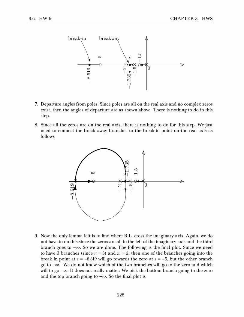
3.6. HW 6 CHAPTER 3. HWS
×××0
−1.5
−2
−1.5
−5
−1.735
breakwaybreak-in
−8.619
7. Departure angles from poles. Since poles are all on the real axis and no complex zerosexist, then the angles of departure are as shown above. There is nothing to do in thisstep.
8. Since all the zeros are on the real axis, there is nothing to do for this step. We justneed to connect the break away branches to the break-in point on the real axis asfollows
×××0
−1.5
−2
−1.5
−5 −1.735
−8.619
9. Now the only lemma left is to find where R.L. cross the imaginary axis. Again, we donot have to do this since the zeros are all to the left of the imaginary axis and the thirdbranch goes to −∞. So we are done. The following is the final plot. Since we needto have 3 branches (since 𝑛 = 3) and 𝑚 = 2, then one of the branches going into thebreak in point at 𝑠 = −8.619 will go towards the zero at 𝑠 = −5, but the other branchgo to −∞. We do not know which of the two branches will go to the zero and whichwill to go −∞. It does not really matter. We pick the bottom branch going to the zeroand the top branch going to −∞. So the final plot is
228

3.6. HW 6 CHAPTER 3. HWS
×××0
−1.5
−2
−1.5
−5 −1.735
−8.619
same branch
same branch
third branch
−∞
3.6.2.2 Part(b)
>> s=tf('s');>> sys=((s+1)*(s+5)/(s*(s+1.5)*(s+2)))sys =s^2 + 6 s + 5-------------------s^3 + 3.5 s^2 + 3 sContinuous-time transfer function.>> rlocus(sys)
-16 -14 -12 -10 -8 -6 -4 -2 0 2-4
-3
-2
-1
0
1
2
3
4Root Locus
Real Axis (seconds-1)
Imag
inar
y A
xis
(sec
onds
-1)
229

3.6. HW 6 CHAPTER 3. HWS
3.6.2.3 Part(c)
The gain 𝐾 any point on the roots locus is given by multiplying the distances from eachpole to the that point, divided by the product of the distances from all the zeros to the samepoint. This comes from
1 + 𝐾𝐺𝑜𝑝𝑒𝑛𝑙𝑜𝑜𝑝 = 0
𝐾 =1
�𝐺𝑜𝑝𝑒𝑛𝑙𝑜𝑜𝑝�In other words, if we want to find gain at some point 𝑟, then
𝐾 =��𝑝𝑖𝑟�� |𝑧𝑖𝑟|
Since the first breakaway point in this case is 𝑟 = −1.735 (the break away point), then theabove becomes
𝐾 =(1.735) (1.735 − 1.5) (2 − 1.735)
(1.735 − 1) (5 − 1.735)The above was done by just looking the diagram of the root locus and measuring the distancefrom each pole to the breakaway point, and similarly for the zeros. The above reduces to
𝐾 = 0.045
For the second break-in point in this case is 𝑟 = −8.617, therefore
𝐾 =(8.617) (8.617 − 1.5) (8.617 − 2)
(8.617 − 1) (8.617 − 5)The above was done by just looking the diagram of the root locus and measuring the distancefrom each pole to the break-in point, and similarly for the zeros. The above reduces to
𝐾 = 14.73
230
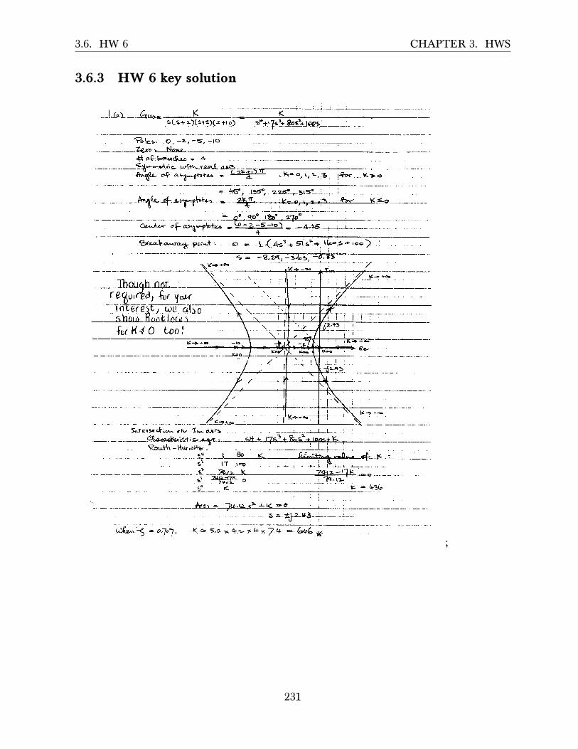
3.6. HW 6 CHAPTER 3. HWS
3.6.3 HW 6 key solutionECE--?-32--)4etwt"nL 6
-5^1,,+i;;-.
t ?
__|.-Co) --&cs>= KKsls+ ?Xst-sXs tle) _:a1.lsl+!9t'd@s_
€o\c-s ' .o , -2 , . -s , : lo--Z'exo '---Np-sa-
S "tr br ,ra&ra = 4
Ql**rr o-{= alr.rytotca }
gt*ar€a* paia.,t'- a .: t'C+{-+5l s?-+JQre-s *-!oo ) ,
, /
\__
[or H-(
-.t
\
t-i r/ K+ +oo
I
d1 $or Y,rt,. \ . I , )
f , / . t i l c a l :of or,t lotur I _O Loo !
\ 4, . ' . - - , J
l . l
, 7
r l v t ,
*r d\ 1 , r I
K.+ - r - lo-----.+-t(-j
ll=a
_ -}J, -i7 t. i I r F - ) - -
* ee-f-clfX -
r-"
. _ /\ , t \
t \----1----:---r
l , - - I
l , t \2 _ 4[*-'-o,--
D(,lJfu,^3 = ot7"1 , K* s.z x *-> r t+ x7.+ - &6 X;
231

3.6. HW 6 CHAPTER 3. HWS
l r r . r t l) 4r . r _ N-
- -'-'vt\
( * + s + . ) C s r r ) +ltEt:7-e:3- -
rt cr?tr.i.s.--e'Jner":r--s<a.Q---aecB-
.6 **a,-4btr-s -- ( ?-E*r\ r8o" --\4: ozb L , &.Vz o- \ ' 5
: (eo'. \8o' ,r- .3eo'-,
*4?llc"r (+ o
&eJe.<
*__?t tr
Act; = t + G =-o
-_;7--_
K{ 0 sho\..lo too I
K-> *-o-
-o 6\l
( ? < _
I
I
;
232
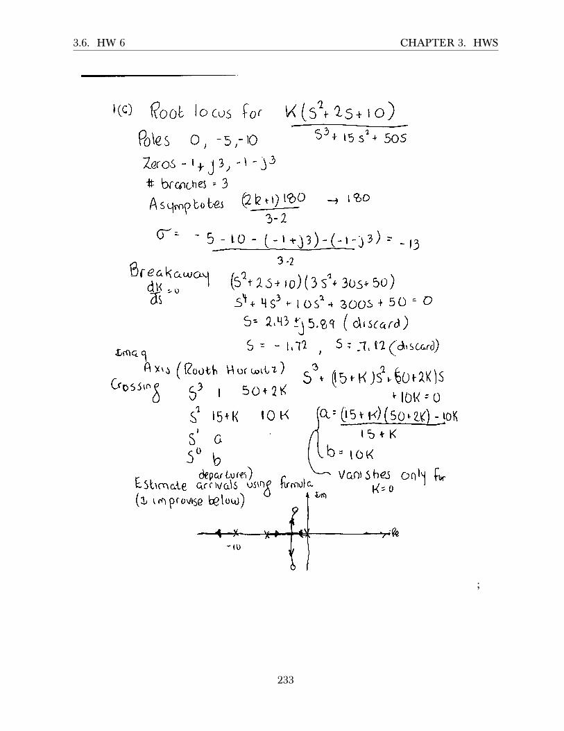
3.6. HW 6 CHAPTER 3. HWS
i(C) 仔00とlocus f。(畑3年S+lO)
釦es 0,-5ノー一〇
九〇3-1自ら一l‾53
♯br的Lhejこう
Asq叩いね
331 15Sa+505
し60 →lQ)○
ナ2
㌻ニ ー5-90-仁一で同一(一口3)ニーlう
賞辞畿議瀧岩盤も二川3年gq(d-5‘ard)
血中∴,∴∴∴主‾口1,3;…(d-SCの
でか、くく霊、辛翌日∵?当るCtq掴)緑0両+10kニ0
缶当「高一 5…k
ぐ15+K iOK 匝tK〉(50し氷
15+K
こ10K
VGn)Shej
q(白vdlsu小笠小0) 日置 圏 �巳も小 一イブ0 五一一一碕
‾’言甲 �′‾
〇両乱
0-0
} OS′\J
油田
p) 0
囲易聞
m 小
-い∴し
国昭
;
233

3.6. HW 6 CHAPTER 3. HWS
7. Grs> __
L U )ki -.
(*tt ur.L'*o-Ut;2* ye.or . AT EI{D OF 50 lu-t=Suat-l* . :' , _-6tca+a;yy_eatnLl __-;-
( A= '*
bs+ s)C3s-+ ils+3)-=*-Cs1,+3.-ss-'-* SsX zs + 6- - - - S*a-rt2 3l+ -r3 s2t " <s -+- t.5 - o
o.& . yce,!- a,l B.---*--ta9 ---_-_=*- E--:-?-.0-J- -+ t""p-ij
( : / t , / b--€ - ----:3-t i3-___
K = z'Vv
L9 3 -- c-es glsclf=<-ft ., - -*\9.-sx-Le)ry*"tr e
-@9- -.* - -----Z--=-.r-j- zJoSK = Z - q q
CL TE -_ S ( s + , ;--__- L---.- K
- S ( s 1 , ;K
h&l-^l-o
-LqI r :
1--=---- (-!D -!Jjl+-Ll- -=--o-:5
- : . . - - * . 1 . - , - - i I l - * *
;
Question 1(b)
g)
x
ct)(UE
20
1 0
0
- 1 0
Question 1(a)
2
.32 1x
5 o(EE - t
-2
-3-1916
.r2x
o,(6
.E
.t2x
o)(UE
20
1 0
0
- 1 0
-rgi
- 1 0 0 1 0RealAxis
Question 1(c)
- 1 0 0Real Axis
- 2 0RealAxis
Question 2(b)
- 5 0RealAxis
;
234

3.7. HW 7 CHAPTER 3. HWS
3.7 HW 7
3.7.1 Problem 1 ECE 332 Homework # T
1. For each of the open loop transfer functions beltrw, a$sume a classical unity feedback
connection and sketch the Nyquist plot. Find the values of the gain K > 0 for which
closed loop stability is guaranteed.
(a) G(.s)H(s): @*rit
(b) c(s)a(s) : #ti*ii
2. The Nyquist plot for a transfer function lfc(s) is shown below for K :7 and s.r ) 0'
Assuming a unity feedback configuration with G(s) having no pole.s in t,he closed right
half plane, find the ranges for K > 0 under which closed loop stability is assured.
Re
3. (a) For the attitude control system shown below, assume that the velocitv feedlnck
gain K, is zero and sketch the Nvquist for open loop system G(s)//(s).
iII
SOLUTION:
3.7.1.1 Part(a)
𝐺𝐻 =𝐾
𝑠 �𝑠2 + 𝑠 + 4�(1)
The poles of the open loop are at 𝑠 = 0 and 𝑠 = −0.5 ± 𝑗1.94. So we draw Γ which encloses allthe poles in the RHS making sure we avoid the pole at 𝑠 = 0 by making small circle. Here isthe result. (we do not care about open loop poles in the LHS).
×
Γ
<(GH)
=(GH)
−1
(1)
(2)
(3) (4)
We now start by mapping each segment from Γ to Γ𝐺𝐻. Starting with segment 2. We see that
lim𝑠→0
𝐾𝑠 �𝑠2 + 𝑠 + 4�
= lim𝑠→0
𝐾𝑠= ∞𝑒−𝑗𝜃
Where 𝜃 goes from +900 to −900 in Γ. This means on Γ𝐺𝐻 segment (2) will map to a verylarge circle which goes from −900 to +900 (anti-clockwise). We update the plot after makingeach segment so we see the progress.
235

3.7. HW 7 CHAPTER 3. HWS
×
Γ
<
=
−1
(1)
(2)
(3) (4)
×
ΓGH
−1
(2)′
=
<
We now go to segment 4 in Γ.
lim𝑠→∞
𝐾𝑠 �𝑠2 + 𝑠 + 4�
= lim𝑠→∞
𝐾𝑠3= 0𝑒−𝑗3𝜃
Where 𝜃 goes from −900 to +900 on Γ. This means on Γ𝐺𝐻 segment (4) will map to a verysmall circle which goes from +2700 to −2700 on Γ𝐺𝐻. This is 1.5 circle rotation in clockwisethat goes from around 5400. updating the plot gives
×
Γ
<
=
−1
(1)
(2)
(3) (4)
×
ΓGH
−1
(2)′
=
<
We now do segment 1. For this we need to find the real and imaginary part of 𝐺𝐻 since weneed the axis crossings. From (1)
𝐺𝐻 =𝐾
𝑠3 + 𝑠2 + 4𝑠=
𝐾
�𝑗𝜔�3+ �𝑗𝜔�
2+ 4 �𝑗𝜔�
=𝐾
−𝑗𝜔3 − 𝜔2 + 4𝑗𝜔=
𝐾𝑗 �4𝜔 − 𝜔3� − 𝜔2
Multiply numerator and denominator by complex conjugate denominator gives
𝐺𝐻 =𝐾
𝑗 �4𝜔 − 𝜔3� − 𝜔2
�−𝑗 �4𝜔 − 𝜔3� − 𝜔2�
�−𝑗 �4𝜔 − 𝜔3� − 𝜔2�
=𝐾 �−𝑗 �4𝜔 − 𝜔3� − 𝜔2�
�𝑗 �4𝜔 − 𝜔3� − 𝜔2� �−𝑗 �4𝜔 − 𝜔3� − 𝜔2�
=−𝑗𝐾 �4𝜔 − 𝜔3� − 𝐾𝜔2
𝜔6 − 7𝜔4 + 16𝜔2
236

3.7. HW 7 CHAPTER 3. HWS
Hence
Re (𝐺𝐻) = −𝐾𝜔4 − 7𝜔2 + 16
Im (𝐺𝐻) =−𝐾 �4𝜔 − 𝜔3�
𝜔6 − 7𝜔4 + 16𝜔2 =𝐾 �𝜔2 − 4�
𝜔 �𝜔4 − 7𝜔2 + 16�
To find the crossing. Γ𝐺𝐻 will cross the real axis when Im (𝐺𝐻) = 0, hence
𝐾 �𝜔2 − 4�
𝜔 �𝜔4 − 7𝜔2 + 16�= 0
𝐾 �𝜔2 − 4� = 0𝜔2 − 4 = 0
𝜔2 = 4𝜔 = ±2 rad/sec
Then
𝐺𝐻�𝑗2� =𝐾
�𝑗2�3+ �𝑗2�
2+ 4 �𝑗2�
=𝐾
�−𝑗8� + (−4) + �𝑗8�
=−14𝐾
So Γ𝐺𝐻 will cross the real axis at −0.25𝐾.
Since 𝐾 > 0, this will be somewhere on the negative real axis. To find where Γ𝐺𝐻 crosses theimaginary axis we set Re (𝐺𝐻) = 0, hence
−𝐾𝜔4 − 7𝜔2 + 16
= 0
Which gives 𝜔 = ±∞. When 𝜔 = ±∞ then 𝐺𝐻 (±∞) = 0±. This means the crossing at origin.This makes sense, as the small circle around the origin shrinks to zero size.
To find where segment (1) maps to, we see that for 𝜔 = +∞, Re (𝐺𝐻) < 0 and Im (𝐺𝐻) > 0,so it starts in first quadrant. 𝜔 = 0+,Re (𝐺𝐻) < 0 and Im (𝐺𝐻) < 0, which means segment (1)starts in the first quadrant but ends in the third quadrant.
Now for segment (3). we see that 𝜔 = 0−,Re (𝐺𝐻) < 0 and Im (𝐺𝐻) > 0, which means segment(3) starts in the first quadrant. 𝜔 = −∞ then Re (𝐺𝐻) < 0 and Im (𝐺𝐻) < 0 which meanssegment (3) in Γ𝐺𝐻 starts in quadrant 1 and ends up in quadrant 3. There will be crossingat the real axis at −0.25𝐾. Therefore the plot now looks like this
237
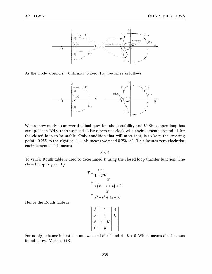
3.7. HW 7 CHAPTER 3. HWS
×
Γ
<
=
−1
(1)
(2)
(3) (4)
×
ΓGH
−1
(2)′
=
<
−0.25K
crossing depends on K
1′
3′
This circleshrinks tozero
As the circle around 𝑠 = 0 shrinks to zero, Γ𝐺𝐻 becomes as follows
×
Γ
<
=
−1
(1)
(2)
(3) (4)
×
ΓGH
−1
(2)′
=
<
1′
3′
−0.25K
We are now ready to answer the final question about stability and 𝐾. Since open loop haszero poles in RHS, then we need to have zero net clock wise encirclements around −1 forthe closed loop to be stable. Only condition that will meet that, is to keep the crossingpoint −0.25𝐾 to the right of −1. This means we need 0.25𝐾 < 1. This insures zero clockwiseencirclements. This means
𝐾 < 4
To verify, Routh table is used to determined 𝐾 using the closed loop transfer function. Theclosed loop is given by
𝑇 =𝐺𝐻
1 + 𝐺𝐻
=𝐾
𝑠 �𝑠2 + 𝑠 + 4� + 𝐾
=𝐾
𝑠3 + 𝑠2 + 4𝑠 + 𝐾Hence the Routh table is
𝑠3 1 4𝑠2 1 𝐾𝑠1 4 − 𝐾𝑠0 𝐾
For no sign change in first column, we need 𝐾 > 0 and 4 −𝐾 > 0. Which means 𝐾 < 4 as wasfound above. Verified OK.
238

3.7. HW 7 CHAPTER 3. HWS
3.7.1.2 Part(b)
𝐺𝐻 =𝐾 (𝑠 + 1)𝑠2 (𝑠 + 2)
=𝐾 (𝑠 + 1)𝑠3 + 2𝑠2
(1)
The poles of the open loop are at 𝑠 = 0 (two poles) and 𝑠 = −2. So we draw Γ which enclosesall the poles in the RHS making sure we avoid the poles at 𝑠 = 0 by making small circle.Here is the result. (we do not care about open loop pole in the LHS and about the zeros ofthe open loop).
×
Γ
<(GH)
=(GH)
−1
(1)
(2)
(3) (4)
We now start by mapping each segment from Γ to Γ𝐺𝐻. Starting with segment 2. We see that
lim𝑠→0
𝐾 (𝑠 + 1)𝑠3 + 2𝑠2
= lim𝑠→0
𝐾𝑠2= ∞𝑒−2𝑗𝜃
Where 𝜃 goes from +900 to −900 in Γ. This means on Γ𝐺𝐻 segment (2) will map to a verylarge circle which goes from −1800 to +1800. This is a full circle in the anti-clockwise. Weupdate the plot after making each segment so we see the progress.
×
Γ
<
=
−1
(1)
(2)
(3) (4)
×
ΓGH
−1
(2)′
=
<
We now go to segment 4 in Γ.
lim𝑠→∞
𝐾 (𝑠 + 1)𝑠3 + 2𝑠2
= lim𝑠→∞
𝐾𝑠𝑠3= lim
𝑠→∞
𝐾𝑠2= 0𝑒−𝑗2𝜃
Where 𝜃 goes from −900 to +900 on Γ. This means on Γ𝐺𝐻 segment (4) will map to a verysmall circle which goes from +1800 to −1800 on Γ𝐺𝐻. This is basically a full circle in clockwisearound zero. updating the plot gives
239

3.7. HW 7 CHAPTER 3. HWS
×
Γ
<
=
−1
(1)
(2)
(3) 4
×
ΓGH
−1
(2)′
=
<4′
We now do segment 1. For this we need to find the real and imaginary part of 𝐺𝐻 since weneed the axis crossings. From (1)
𝐺𝐻 =𝐾 (𝑠 + 1)𝑠3 + 2𝑠2
=𝐾 �𝑗𝜔 + 1�
�𝑗𝜔�3+ 2 �𝑗𝜔�
2 =𝐾 �𝑗𝜔 + 1�−𝑗𝜔3 − 2𝜔2
Multiply numerator and denominator by complex conjugate denominator gives
𝐺𝐻 =𝐾 �𝑗𝜔 + 1�−𝑗𝜔3 − 2𝜔2
�𝑗𝜔3 − 2𝜔2�
�𝑗𝜔3 − 2𝜔2�
=𝑗 �−𝐾𝜔3� − �𝐾𝜔4 + 2𝐾𝜔2�
𝜔4 �𝜔2 + 4�
Hence
Re (𝐺𝐻) =− �𝐾𝜔4 + 2𝐾𝜔2�
𝜔4 �𝜔2 + 4�
Im (𝐺𝐻) =−𝐾𝜔3
𝜔4 �𝜔2 + 4�=
−𝐾𝜔 �𝜔2 + 4�
To find the crossing. Γ𝐺𝐻 will cross the real axis when Im (𝐺𝐻) = 0, hence−𝐾
𝜔 �𝜔2 + 4�= 0
𝜔 = ±∞ rad/sec
Therefore
𝐺𝐻�𝑗∞� = lim𝜔→∞
𝐾 �𝑗𝜔 + 1�−𝑗𝜔3 − 2𝜔2
= lim𝜔→∞
𝑗𝜔−𝑗𝜔3
= lim𝜔→∞
𝑗−𝑗𝜔2
= 0−
So Γ𝐺𝐻 will cross the real axis at 0. Which is where the small circle shrinks to zero. To find
240

3.7. HW 7 CHAPTER 3. HWS
where Γ𝐺𝐻 crosses the imaginary axis we set Re (𝐺𝐻) = 0, hence− �𝐾𝜔4 + 2𝐾𝜔2�
𝜔4 �𝜔2 + 4�= 0
𝐾𝜔4 + 2𝐾𝜔2 = 0
𝜔2 �𝜔2 + 2� = 0
Hence
𝜔 = 0
And
𝜔 = ±𝑖√2
Since 𝜔 has to be real. Then 𝜔 = 0 is only used. When 𝜔 = 0 then 𝐺𝐻�𝑗0� = lim𝜔→0𝐾�𝑗𝜔+1�
−𝑗𝜔3−2𝜔2 =
lim𝜔→0𝐾
−2𝜔2 = ∞ . Hence Γ𝐺𝐻 will cross the imaginary axis at ∞.
To find which quadrants segment (1) maps to, we see that for positive 𝜔 then Re (𝐺𝐻)is negative and Im (𝐺𝐻) is negative (since 𝐾 > 0). Therefore segment (1) maps to thirdquadrant. And for segment (3), we see that negative 𝜔 then Re (𝐺𝐻) is negative and Im (𝐺𝐻)is positive (since 𝐾 > 0). Therefore segment (3) maps to first quadrant
Therefore the plot now looks like this
×
Γ
<
=
−1
(1)
(2)
(3) 4
×
ΓGH
−1
(2)′
=
<4′1′
3′
This willshrink tozero
After the small circle shrinks to zero, and since the crossing on the real axis was found at 0then the final plot looks like
×
Γ
<
=
−1
(1)
(2)
(3) 4
×
ΓGH
−1
(2)′
=
<4′1′
3′
We are now ready to answer the final question about stability and 𝐾. Since open loop haszero poles in RHS, then we need to have zero net clockwise encirclements around −1 forthe closed loop to be stable. We see that there is no encirclements around −1. No matterwhat 𝐾 > 0 value is. So the closed loop is stable for all positive 𝐾. To verify, Routh table is
241

3.7. HW 7 CHAPTER 3. HWS
used to determined 𝐾 using the closed loop transfer function. The closed loop is given by
𝑇 =𝐺𝐻
1 + 𝐺𝐻
=𝐾 (𝑠 + 1)
𝑠3 + 2𝑠2 + 𝐾 (𝑠 + 1)Hence the Routh table is
𝑠3 1 𝐾𝑠2 2 𝐾𝑠1 2𝐾−𝐾
2 = 𝐾2
𝑠0 𝐾
For no sign change in first column, we need 𝐾 > 0 and 𝐾2 > 0. Which is always true since 𝐾
is positive. Verified OK.
3.7.2 Problem 2
ECE 332 Homework # T
1. For each of the open loop transfer functions beltrw, a$sume a classical unity feedback
connection and sketch the Nyquist plot. Find the values of the gain K > 0 for which
closed loop stability is guaranteed.
(a) G(.s)H(s): @*rit
(b) c(s)a(s) : #ti*ii
2. The Nyquist plot for a transfer function lfc(s) is shown below for K :7 and s.r ) 0'
Assuming a unity feedback configuration with G(s) having no pole.s in t,he closed right
half plane, find the ranges for K > 0 under which closed loop stability is assured.
Re
3. (a) For the attitude control system shown below, assume that the velocitv feedlnck
gain K, is zero and sketch the Nvquist for open loop system G(s)//(s).
iII
SOLUTION:
Since there is zero open loop poles in RHP, we need zero net clockwise encirclements around−1. This means we need to keep point −0.5 to the right of −1 and keep the point −2 to theleft of −1. In other words, we need to satisfy
0.5𝐾 < 12𝐾 > 1
Or
𝐾 < 2
242

3.7. HW 7 CHAPTER 3. HWS
And
𝐾 >12
Hence the range of stable closed loop is for 𝐾 to meet the following requirement
0.5 < 𝐾 < 2
3.7.3 Problem 3
ECE 332 Homework # T
1. For each of the open loop transfer functions beltrw, a$sume a classical unity feedback
connection and sketch the Nyquist plot. Find the values of the gain K > 0 for which
closed loop stability is guaranteed.
(a) G(.s)H(s): @*rit
(b) c(s)a(s) : #ti*ii
2. The Nyquist plot for a transfer function lfc(s) is shown below for K :7 and s.r ) 0'
Assuming a unity feedback configuration with G(s) having no pole.s in t,he closed right
half plane, find the ranges for K > 0 under which closed loop stability is assured.
Re
3. (a) For the attitude control system shown below, assume that the velocitv feedlnck
gain K, is zero and sketch the Nvquist for open loop system G(s)//(s).
iII
(b) For the closed loop svstem above, for what range of gains K > 0 is stabilitv a^ssttre<l'l
(c) Now consider the case with both gains K and K,, non-zero. using an aPpropriate
Nvq.ist plot, find the range for these gains under which closed loop stabilitv is asstrrecl.
4. A level control system and its transfer function model is depicted below. Assuming
zero delay (7 : 0), use Matlab to generate the appropriate Nvquist plot w'hich <ran be
used to analyze closed loop stabilitv. Take
1 0 3 . 1 5 IGn ls ) : : 1 : G ls t : : - : - . i G r (s ) :
s + r / - 3 0 s + 1 ' - r \ " / G ' l g ) + ( s / 3 ) + t
6^ t s )
G s ( r /
leue I
SOLUTION:
3.7.3.1 Part(a)
When 𝐾𝑣 = 0 the open loop is 𝐺𝐻 = 𝐾 1𝑠2 . This has no poles in RHP and two poles at zero.
Hence Γ is
243

3.7. HW 7 CHAPTER 3. HWS
×
Γ
<(GH)
=(GH)
−1
(1)
(2)
(3) (4)
We start at segment 2.
lim𝑠→0
𝐾𝑠2= lim
𝜀→0
𝐾
�𝜀𝑒𝑗𝜃�2 = ∞𝑒
−2𝑗𝜃
As 𝜃 goes from +900 to −900 on Γ segment 2 goes from −1800 to +180 on Γ𝐺𝐻 with ∞ radiusin anti-clockwise. Hence the plot now looks as follows
×
Γ
<
=
−1
(1)
(2)
(3) (4)
×
ΓGH
−1
(2)′
=
<
For segment 4 in Γ. We have
lim𝑠→∞
𝐾𝑠2= lim
𝑅→∞
𝐾
�𝑅𝑒𝑗𝜃�2 = 0𝑒
−2𝑗𝜃
𝜃 goes from −900 to +900 on Γ, segment 4 goes from +1800 to −180 on Γ𝐺𝐻 with 0 radius inclockwise. Hence the plot now looks as follows
×
Γ
<
=
−1
(1)
(2)
(3) 4
×
ΓGH
−1
(2)′
=
<4′
Now𝐾𝑠2=
𝐾
�𝑗𝜔�2 =
𝐾−𝜔2
244

3.7. HW 7 CHAPTER 3. HWS
Hence Re (𝐺𝐻) = 𝐾−𝜔2 and there is no imaginary part. Therefore, there is no crossing on
the real axis. There is crossing on the imaginary axis at 𝜔 = ±∞ which occurs at 𝐺𝐻 = 0.This is when the small circle shrinks to zero size. It is clear that segment 1 will map to thirdquadrant and segment 3 will map to second quadrant since there is no crossing. The finalplot is
×
Γ
<
=
−1
(1)
(2)
(3) 4
×
ΓGH
−1
(2)′
=
<4′1′
3′
This willshrink tozero
After the small circle shrinks to zero, and since the crossing on the real axis was found at 0then the final plot looks like
×
Γ
<
=
−1
(1)
(2)
(3) 4
×
ΓGH
−1
(2)′
=
<4′1′
3′
3.7.3.2 Part(b)
Since open loop has zero poles in RHP, we need Γ𝐺𝐻 to have zero net clockwise encirclements.Since Γ𝐺𝐻 has no crossing on the real axis that depends on 𝐾 then Γ𝐺𝐻 will remain as shownfor any 𝐾. So closed loop is stable for all 𝐾 > 0. To verify, we set the Routh table for theclosed loop polynomial
The closed loop is given by
𝑇 =𝐺𝐻
1 + 𝐺𝐻
=𝐾
𝑠2 + 𝐾Hence the Routh table is
𝑠2 1 𝐾𝑠1 0 0𝑠0 0
We see that there is no sign change in first column, no matter what 𝐾 is.
245

3.7. HW 7 CHAPTER 3. HWS
3.7.3.3 Part (c)
We first find the closed loop transfer function. Let 𝐸 (𝑠) be the error (just after the summingjunction) then
𝐸 = 𝜃𝑟 − 𝜃 − 𝐾𝑣𝑠𝜃
𝜃 = 𝐸𝐾1𝑠2
From the second equation 𝐸 = 𝜃𝑠2
𝐾 , hence the first equation becomes
𝜃𝑠2
𝐾= 𝜃𝑟 − 𝜃 − 𝐾𝑣𝑠𝜃
𝜃𝑠2
𝐾+ 𝜃 + 𝐾𝑣𝑠𝜃 = 𝜃𝑟
𝜃 �𝑠2
𝐾+ 1 + 𝐾𝑣𝑠� = 𝜃𝑟
Therefore the closed loop transfer function 𝑇 (𝑠) = 𝜃𝜃𝑟
is
𝜃𝜃𝑟=
1𝑠2
𝐾 + 1 + 𝐾𝑣𝑠
=𝐾
𝑠2 + 𝐾𝐾𝑣𝑠 + 𝐾We now find the open loop transfer function with unity feedback using the closed looptransfer function. Since 𝑇 (𝑠) = 𝐺
1+𝐺 where 𝐺 (𝑠) is the closed loop transfer function, then
letting 𝐺 (𝑠) = 𝑁𝐷 we have
𝐾𝑠2 + 𝐾𝐾𝑣𝑠 + 𝐾
=𝐺
1 + 𝐺
=𝑁𝐷
1 + 𝑁𝐷
=𝑁
𝑁 +𝐷Therefore 𝑁 = 𝐾 and 𝑁 + 𝐷 = 𝑠2 + 𝐾𝐾𝑣𝑠 + 𝐾 which means 𝐷 (𝑠) = 𝑠2 + 𝐾𝐾𝑣𝑠. Therefore theopen loop transfer function is
𝐺 (𝑠) =𝑁𝐷=
𝐾𝑠2 + 𝐾𝐾𝑣𝑠
Hence
𝐺𝐻 = 𝐾𝑠(𝑠+𝐾𝐾𝑣)
Therefore, the open loop has a pole at 𝑠 = 0 and at 𝑠 = −𝐾𝐾𝑣 .
Assuming positive gains, −𝐾𝐾𝑣 is in the LHP. Hence the open loop is stable. Which means
246

3.7. HW 7 CHAPTER 3. HWS
the Nyquist plot should have zero net clockwise encirclement around −1 for the closed loopto be stable.
We now start by mapping each segment from Γ to Γ𝐺𝐻. Starting with segment 2. We see that
lim𝑠→0
𝐾𝑠2 + 𝑠𝐾𝐾𝑣
= lim𝑠→0
1𝑠𝐾𝑣
= lim𝜀→0
1𝜀𝑒𝑗𝜃𝐾𝑣
= ∞𝑒−𝑗𝜃
Where 𝜃 goes from +900 to −900 in Γ. This means on Γ𝐺𝐻 segment (2) will map to a halfcircle which goes from −900 to +900 in anti-clockwise.
×
Γ
<
=
−1
(1)
(2)
(3) (4)
×
ΓGH
−1
(2)′
=
<
We now go to segment 4 in Γ.
lim𝑠→∞
𝐾𝑠2 + 𝑠𝐾𝐾𝑣
= lim𝑠→∞
𝐾𝑠2= lim
𝑅→∞
1𝑅𝑒2𝑗𝜃
= 0𝑒−𝑗2𝜃
Where 𝜃 goes from −900 to +900 on Γ. This means on Γ𝐺𝐻 segment (4) will map to a verysmall circle which goes from +1800 to −1800 on Γ𝐺𝐻. This is basically a full circle in clockwisearound zero. updating the plot gives
×
Γ
<
=
−1
(1)
(2)
(3) (4)
×
ΓGH
−1
(2)′
=
<
To find the intersections,
𝐺𝐻 =𝐾
𝑠2 + 𝑠𝐾𝐾𝑣=
𝐾−𝜔2 + 𝑗𝜔𝐾𝐾𝑣
=𝐾
�−𝜔2 + 𝑗𝜔𝐾𝐾𝑣�
�−𝜔2 − 𝑗𝜔𝐾𝐾𝑣�
�−𝜔2 − 𝑗𝜔𝐾𝐾𝑣�
=−𝐾𝜔2 − 𝑗𝜔𝐾2𝐾𝑣𝐾2𝜔2𝐾2
𝑣 + 𝜔4 =−𝐾
𝐾2𝐾2𝑣 + 𝜔2 − 𝑗
𝐾2𝐾𝑣𝐾2𝜔𝐾2
𝑣 + 𝜔3
Hence Re (𝐺𝐻) = −𝐾𝐾2𝐾2𝑣+𝜔2 and Im (𝐺𝐻) = − 𝐾2𝐾𝑣
𝐾2𝜔𝐾2𝑣+𝜔3 . When Re (𝐺𝐻) = 0, we get 𝜔 = ±∞.When means 𝐺𝐻 = 0 at this frequency. So Γ𝐺𝐻 crosses the imaginary axis at the origin.
247

3.7. HW 7 CHAPTER 3. HWS
When Im (𝐺𝐻) = 0, we also get 𝜔 = ±∞ which also means Γ𝐺𝐻 crosses the real axis at zero.By continuation, and since segment 1 must follow segment 4, then segment 1 maps to thirdquadrant in Γ𝐺𝐻 and segment 3 must map to quadrant 2 in Γ𝐺𝐻. As 𝜀 → 0 the small circlebecome a point at origin and we get the final plot
×
Γ
<
=
−1
(1)
(2)
(3) (4)
×
ΓGH
−1
2′
=
<4′
3′
1′
intersection at origin
Since the intersection is always at the origin, Γ𝐺𝐻 will never move to the left passed −1 tomake any encirclement around −1. We need at least one net encirclement for the closed
loop to be unstable. Hence the closed loop is stable for all positive 𝐾,𝐾𝑣 .
To verify, we show Routh table for the closed loop found above, which is 𝐾𝑠2+𝐾𝐾𝑣𝑠+𝐾
. TheRouth table is
𝑠2 1 𝐾𝑠1 𝐾𝐾𝑣 0𝑠0 𝐾
For positive 𝐾,𝐾𝑣, we see that there can not be a sign change. Hence closed loop is stablefor all 𝐾,𝐾𝑣. (Note, I assume 𝐾,𝐾𝑣 > 0. Verified this with instructor via email).
248
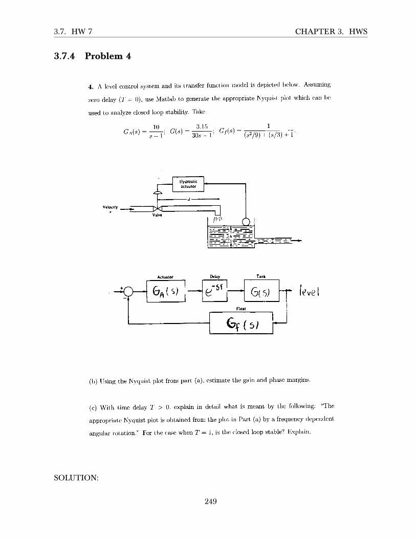
3.7. HW 7 CHAPTER 3. HWS
3.7.4 Problem 4
(b) For the closed loop svstem above, for what range of gains K > 0 is stabilitv a^ssttre<l'l
(c) Now consider the case with both gains K and K,, non-zero. using an aPpropriate
Nvq.ist plot, find the range for these gains under which closed loop stabilitv is asstrrecl.
4. A level control system and its transfer function model is depicted below. Assuming
zero delay (7 : 0), use Matlab to generate the appropriate Nvquist plot w'hich <ran be
used to analyze closed loop stabilitv. Take
1 0 3 . 1 5 IGn ls ) : : 1 : G ls t : : - : - . i G r (s ) :
s + r / - 3 0 s + 1 ' - r \ " / G ' l g ) + ( s / 3 ) + t
6^ t s )
G s ( r /
leue I
(b) Using the Nyquist plot from part (a), estimate the gain and phase margirts.
(c) With time delay T > 0, explain in detail what is meant by the following: "The
appropriate Nvquist plot is obtained from the plot in Part (a) by a frequencv rlepen<lent,
angular rotation." For the case when T:7, is the closed loop stable? Explain.
SOLUTION:
249

3.7. HW 7 CHAPTER 3. HWS
3.7.4.1 Part(a)
The open loop transfer function 𝑇(𝑠) is 𝐺𝐴 (𝑠) 𝑒−𝑠𝑇𝐺 (𝑠)𝐺𝑓 (𝑠). For 𝑇 = 0, we have
𝑇 (𝑠) = 𝐺𝐴 (𝑠) 𝐺 (𝑠) 𝐺𝑓 (𝑠)
=10𝑠 + 1
3.1530𝑠 + 1
1𝑠2
9 +𝑠3 + 1
The Nyquist plot is (using the program I wrote which shows Γ and Γ𝐺𝐻 side by side)
Out[142]=
R0 2.2
2.2ϵ 0.897 x 0.91 y 0.65 show arrow
0.5 1.0 1.5 2.0
-2
-1
1
2
-0.5 0.5
-0.6
-0.4
-0.2
0.2
0.4
0.6
In the limit, as 𝑅 becomes very large we obtain
Out[142]=
R0 10.
10.ϵ 0.897 x 0.91 y 0.65 show arrow
2 4 6 8 10
-10
-5
5
10
-0.5 0.5
-0.6
-0.4
-0.2
0.2
0.4
0.6
Here is also Matlab nyquist output (zoomed in version)
250

3.7. HW 7 CHAPTER 3. HWS
s=tf('s');sys=10/(s+1)*(3.15)/(30*s+1)*1/(s^2/9+s/3+1);sys =850.5----------------------------------------90 s^4 + 363 s^3 + 1092 s^2 + 846 s + 27nyquist([850.5],[90 363 1092 846 27])
-1.5 -1 -0.5 0 0.5 1 1.5
-5
-4
-3
-2
-1
0
1
2
3
4
Nyquist Diagram
Real Axis
Imag
inar
y A
xis
3.7.4.2 Part(b)
For the gain margin, the Γ𝐺𝐻 curve crosses the real axis at about −0.41. Therefore we need
0.41𝐾max < 1
For stability. Hence
𝐾max =10.41
= 2.439
In dB, the above becomes
𝑔𝑚 = 20 log10 2.439= 7.74 db
For the phase margin, we draw a unit circle and find the intersection with Γ𝐺𝐻 and estimatethe angle between the line from origin to the intersection and the −1800 line. As follows
251

3.7. HW 7 CHAPTER 3. HWS
The angle seems to be approximately between 300 and 350. This is the phase margin. To getexact values, Matlab margin command can be used as follows
s=tf('s');sys=10/(s+1)*(3.15)/(30*s+1)*1/(s^2/9+s/3+1);sys =850.5----------------------------------------90 s^4 + 363 s^3 + 1092 s^2 + 846 s + 27>> [Gm,Pm,~,~] = margin(sys)Gm =2.3854Pm =35.6025
Converting the Gm value given in Matlab to dB, gives the result shown above. Matlab gives35.60 as the exact phase margin.
3.7.4.3 Part(c)
Let the open loop 𝐺𝐻 when 𝑇 = 0 (which is what we analyzed in part (b)) be called 𝐺𝐻 (𝑠)which can be written, in frequency domain as
𝐺𝐻 (𝑠)|𝑠=𝑗𝜔 = |𝐺𝐻| 𝑒𝑗𝜃
Where both the magnitude |𝐺𝐻| and the phase 𝜃 in the above, are functions of the frequency𝜔. The above is polar representation of the complex quantity 𝐺𝐻�𝑗𝜔�. When 𝑇 > 0, thenthe open loop is now 𝑒−𝑠𝑇𝐺𝐻 (𝑠), which can be written in frequency domain as
𝑒−𝑗𝜔𝑇𝐺𝐻�𝑗𝜔� = �𝑒−𝑗𝜔𝑇� |𝐺𝐻| 𝑒𝑗(𝜃−𝜔𝑇)
252

3.7. HW 7 CHAPTER 3. HWS
In other words, magnitudes multiply and phases are added. But �𝑒−𝑗𝜔𝑇� = 1, so the above is
𝑒−𝑗𝜔𝑇𝐺𝐻�𝑗𝜔� = |𝐺𝐻| 𝑒𝑗(𝜃−𝜔𝑇)
We see that the resulting open loop has the same magnitude as before, but its phase haschange. We subtract angle 𝜔𝑇 from the original phase 𝜃. subtract angle 𝜔𝑇 is the same asrotating the complex vector representation clockwise 𝜔𝑇. So this causes the whole Nyquistplot, which is a frequency plot 𝐺𝐻�𝑗𝜔� , to just rotate by 𝜔𝑇 clockwise (since negative angle)to what it was before. This makes Γ𝐺𝐻 become closer to −1. This is illustrated in the followingdiagram
−1
unit circleΓGH
phase margin
rotated clockwise by ωT
−1
unit circle
e−ωT ΓGH
reduced phasemargin as ΓGH
rotates clockwisedue to time delay.At frequency 0dB
When 𝑇 = 1, the angle is 𝜔 radians. Since we found the phase margin to be 350 or about 0.61radians, then the closed loop, which corresponds to the open 𝑒−𝑗𝜔𝑇𝐺𝐻�𝑗𝜔� , will have newphase reduced by 𝜔 radians. Since phase margin is measured at 0𝑑𝐵 angle (or 𝜔 = 1 radian,or 57.30). This is larger than the phase margin 350. Therefore the new system is unstable .Γ𝐺𝐻 will rotate and will cross over −1.
−1
unit circleΓGH
350
after clockwise rotation by ωT where T = 1. Unstable.
−1
unit circle
e−ωT ΓGH
What the above shows, is that adding delays 𝑒−𝑠𝑇 makes the system less stable (closer tobecoming unstable). Delays causes the phase margin to reduce. We can find the amount of
delay 𝑇 before the system becomes unstable. We need 𝜔𝑇 < 350 or 𝑇 < 350
57.30 < 0.611 seconds.This is the maximum delay 𝑇 we can have before the closed loop phase margin is all usedup and the system become unstable.
253

3.7. HW 7 CHAPTER 3. HWS
3.7.5 HW 7 key solution
ECE 332 Homework # T
1. For each of the open loop transfer functions beltrw, a$sume a classical unity feedback
connection and sketch the Nyquist plot. Find the values of the gain K > 0 for which
closed loop stability is guaranteed.
(a) G(.s)H(s): @*rit
(b) c(s)a(s) : #ti*ii
2. The Nyquist plot for a transfer function lfc(s) is shown below for K :7 and s.r ) 0'
Assuming a unity feedback configuration with G(s) having no pole.s in t,he closed right
half plane, find the ranges for K > 0 under which closed loop stability is assured.
Re
3. (a) For the attitude control system shown below, assume that the velocitv feedlnck
gain K, is zero and sketch the Nvquist for open loop system G(s)//(s).
iI
I
" Riti 8
/ te '
# 75o tu tr o,oSECE 3 3 L
L
o )6(ll tlts) =
11N,'rrl
-\
s ( s i s + + )
) ^: s - - f QJo
K
= a#e
' 5,pqll ct<le
Qtsl t{s) lr-
Y= -
l f d o
; dR e J '
k= <
B:" :3?
j rJ(-"rijd+4 )
k [- al'- j r^X4 -,,r'l]
K
. ViX circle : S =
q(e) t-l(t)l r = Rd f
. , ; h s t S - - i t l- 6
Qrs) H(r) Il5.jai
_
f 69,^rl Fl(aurl] : " ,
C t a s S P e o l a x i s
i,nl'+ * )Ii+- ro'
k h J ( 4 - ^ ' ) = o
a f c t ) : J
;
254

3.7. HW 7 CHAPTER 3. HWS
7,
F. | 6r.1'^t r-lcjoir) J
= o )
doos rrot cror 5
D < u O ( o o
r - - j d ,
, ) .- K h J
a \ r'Y\aA r naYI
N 4
o.x i5 f " r
uohe n off lU sivnilcr av1 u-n*tl
e^7on.ls" the diaX ran
axi 5 ctossi"t6
Rn I a,i;; H(Fi];=,
Ior s1^bl0{7 , *}t.t
[ 9i '.,.e frr V>4 ,
\ |f s a T N = 2
Inc{eaSizQ k0
5itrc n lhe vnol
: - zt - v / + ) > - r
th*.e are ,
, o { k < 4
qnarcle'r"r*Jt
;
255

3.7. HW 7 CHAPTER 3. HWS
P .t >
b ) k ( s + t ;Grs:b\(5) =
s ' ( 5 t ) )
o S = Z e i o
Qtsluts) | .n' J=12 ) "
9 5 = R u j f
Grg) H(e) \'5 = RJt
oh.c\ "f,^ols
K : - n- l z v- & o -
t!" j to
; 4V P e ' '
93 " l r f
*- j '?
K
6(:)H(s)lr-_,* =
R'n jtt'
o
s - j u 0- J
( j r l
axi 5:) -no ,t sgi nfS
c - [ , o )Nprt e t
,1^b le
cnc^vc lPs the g ' i -1
f * a l l N > o
/ h/ - - ' " - //i
vt
e\-/-
\{
;
256
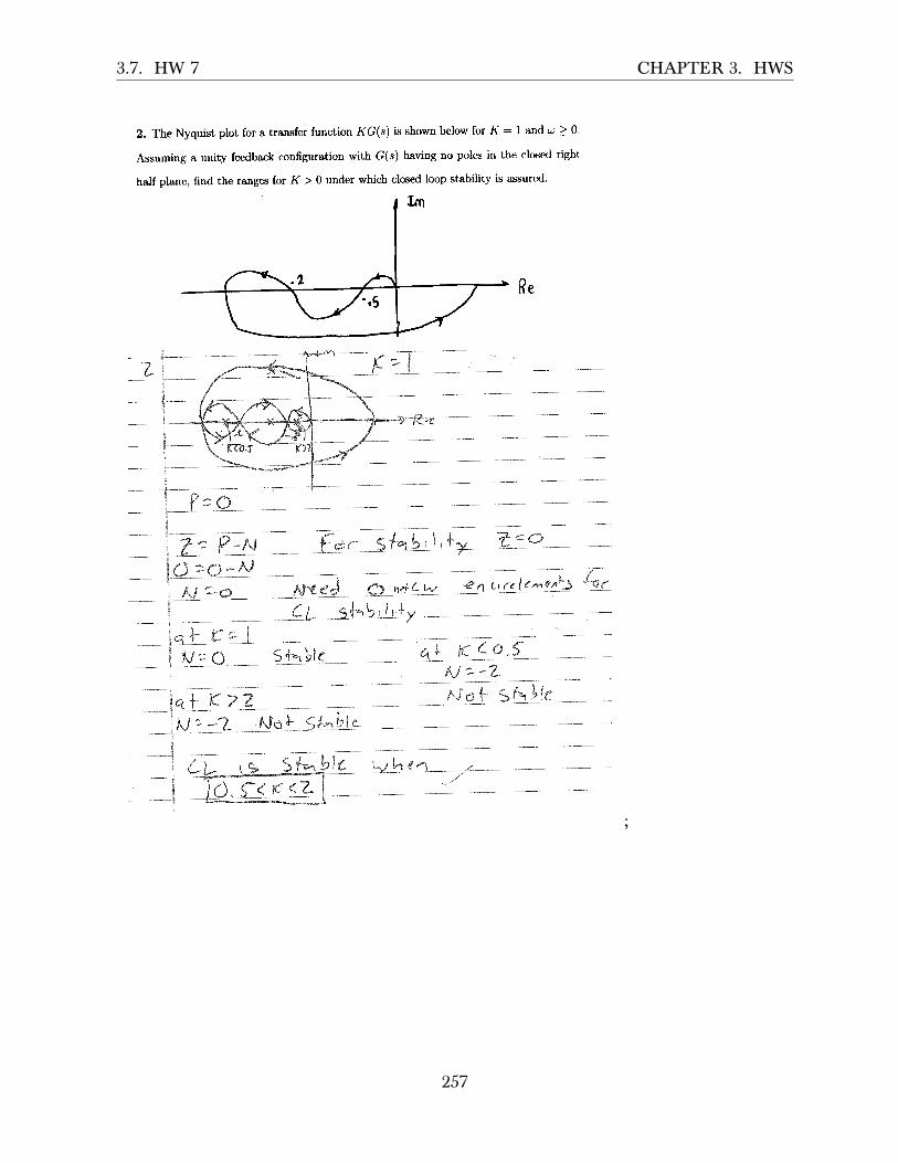
3.7. HW 7 CHAPTER 3. HWS
ECE 332 Homework # T
1. For each of the open loop transfer functions beltrw, a$sume a classical unity feedback
connection and sketch the Nyquist plot. Find the values of the gain K > 0 for which
closed loop stability is guaranteed.
(a) G(.s)H(s): @*rit
(b) c(s)a(s) : #ti*ii
2. The Nyquist plot for a transfer function lfc(s) is shown below for K :7 and s.r ) 0'
Assuming a unity feedback configuration with G(s) having no pole.s in t,he closed right
half plane, find the ranges for K > 0 under which closed loop stability is assured.
Re
3. (a) For the attitude control system shown below, assume that the velocitv feedlnck
gain K, is zero and sketch the Nvquist for open loop system G(s)//(s).
iI
I
;
257

3.7. HW 7 CHAPTER 3. HWS
ECE 332 Homework # T
1. For each of the open loop transfer functions beltrw, a$sume a classical unity feedback
connection and sketch the Nyquist plot. Find the values of the gain K > 0 for which
closed loop stability is guaranteed.
(a) G(.s)H(s): @*rit
(b) c(s)a(s) : #ti*ii
2. The Nyquist plot for a transfer function lfc(s) is shown below for K :7 and s.r ) 0'
Assuming a unity feedback configuration with G(s) having no pole.s in t,he closed right
half plane, find the ranges for K > 0 under which closed loop stability is assured.
Re
3. (a) For the attitude control system shown below, assume that the velocitv feedlnck
gain K, is zero and sketch the Nvquist for open loop system G(s)//(s).
iI
I
(b) For the closed loop svstem above, for what range of gains K > 0 is stabilitv a^ssttre<l'l
(c) Now consider the case with both gains K and K,, non-zero. using an aPpropriate
Nvq.ist plot, find the range for these gains under which closed loop stabilitv is asstrrecl.
4. A level control system and its transfer function model is depicted below. Assuming
zero delay (7 : 0), use Matlab to generate the appropriate Nvquist plot w'hich <ran be
used to analyze closed loop stabilitv. Take
1 0 3 . 1 5 IGn ls ) : : 1 : G ls t : : - : - . i G r (s ) :
s + r / - 3 0 s + 1 ' - r \ " /
G ' l g ) + ( s / 3 ) + t
6 ^ t s )
G s ( r /
leue I
7+
2 ,
3
ar,d'flo
t he
'f
A - j r
U E
o < K < +
Z r k
I(
I
\
l .
5Ys lpvn isI
o ( K < o .
; A
2 et" =)
a r ' ' ' , Iq t5 ) lg= 2 r1s
'/\J
K
< / ^
R e J T : )
Gts ) I '\'
vr \ / , / ls = pqrt '
!nc^{. le *nJ5
p 1 . ( - t , o )
t t / sl"btn f,3 0 3
a.."'d o , g < K
t ' ) K q ( 5 ) =5 t
@ : 5 :
-- ^ "-)>o
V
K-7AT
B=" j: f
a'dd =)
G t ' ) |l5:j ur)
K
O r S =
_ CI:.
;
258

3.7. HW 7 CHAPTER 3. HWS
Y9Rca\ ar iS cYogeir ! fot a l ( O < 6 J 4 o c
--r--{
I h o 5 8
r r la c l u a t t Y
I tv
0 \ A T n e-
O t i e
AY?\.'.-.---.--
voa l
i b )The
a \ l
( C ) . , r,J i l h
sXsIo"" i:
k > o
rnargir"ltX<1^b I e Ji.
S ( S t K K v )
v
i4
z zjo =>
G(t) l, -rJ
ctol, _ *.
O : s
- i e: & Q '
kYu zuju
k^) I >c0K ! / I
: o "-jt/
5 = J d = )
q o ) l =ls=jvJ
k v ) o , k 7 0 , 6 r s ) t
- r o ' t j t i K K v
;
259

3.7. HW 7 CHAPTER 3. HWS
- k r o ' - j t k ' k u
ro4t aJt K ku
f i - ' ( 1\^e "ool axi5 cvossi : r$
l e t - u J i t u : o
ro cvo<5 iv r3 f i " o< (^ )< 6
a l
J i r,4 rnraf rvrar6 ax i s C,r o$in1s ,
ln t F t ^ l ,=o
) ro ctossinl f,, o < rd ( oo
Y6
lo
)
-[o
No
5 o
f"'
5""
-pncircle*,nJs ,f
, the system
K,/ >o
( - 1 . , o ) o - l Y , kv
q t l k > o
) 6
i g slob{e
;
260

3.7. HW 7 CHAPTER 3. HWS
(b) For the closed loop svstem above, for what range of gains K > 0 is stabilitv a^ssttre<l'l
(c) Now consider the case with both gains K and K,, non-zero. using an aPpropriate
Nvq.ist plot, find the range for these gains under which closed loop stabilitv is asstrrecl.
4. A level control system and its transfer function model is depicted below. Assuming
zero delay (7 : 0), use Matlab to generate the appropriate Nvquist plot w'hich <ran be
used to analyze closed loop stabilitv. Take
1 0 3 . 1 5 IGn ls ) : : 1 : G ls t : : - : - . i G r (s ) :
s + r / - 3 0 s + 1 ' - r \ " /
G ' l g ) + ( s / 3 ) + t
6 ^ t s )
G s ( r /
leue I
(b) Using the Nyquist plot from part (a), estimate the gain and phase margirts.
(c) With time delay T > 0, explain in detail what is meant by the following: "The
appropriate Nvquist plot is obtained from the plot in Part (a) by a frequencv rlepen<lent,
angular rotation." For the case when T:7, is the closed loop stable? Explain.
;
261
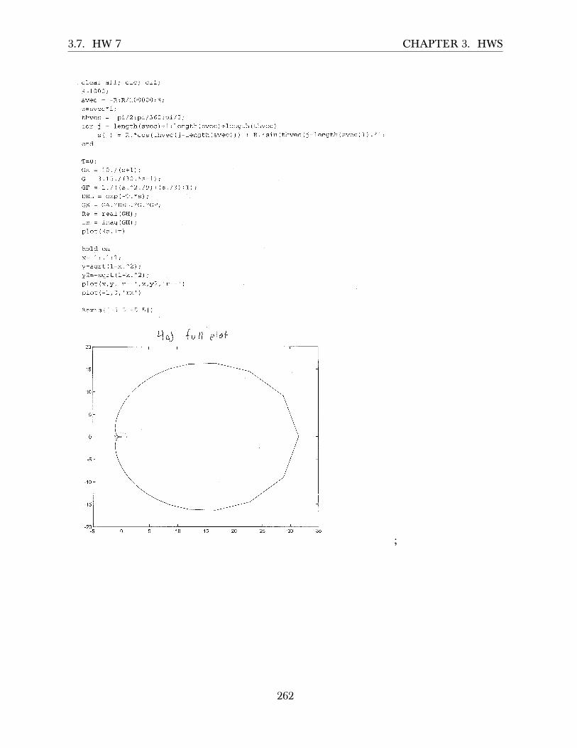
3.7. HW 7 CHAPTER 3. HWS
;
262

3.7. HW 7 CHAPTER 3. HWS
;
263

3.7. HW 7 CHAPTER 3. HWS
c) You need to rotate the plot by the phase corresponding to theappropriatedelayandreexaminethe‐1pointtocheckforstability.Dueto
€
e−sT = e− jωT factor, some points will be rotated more than others,dependinguponthefrequency.
;
264
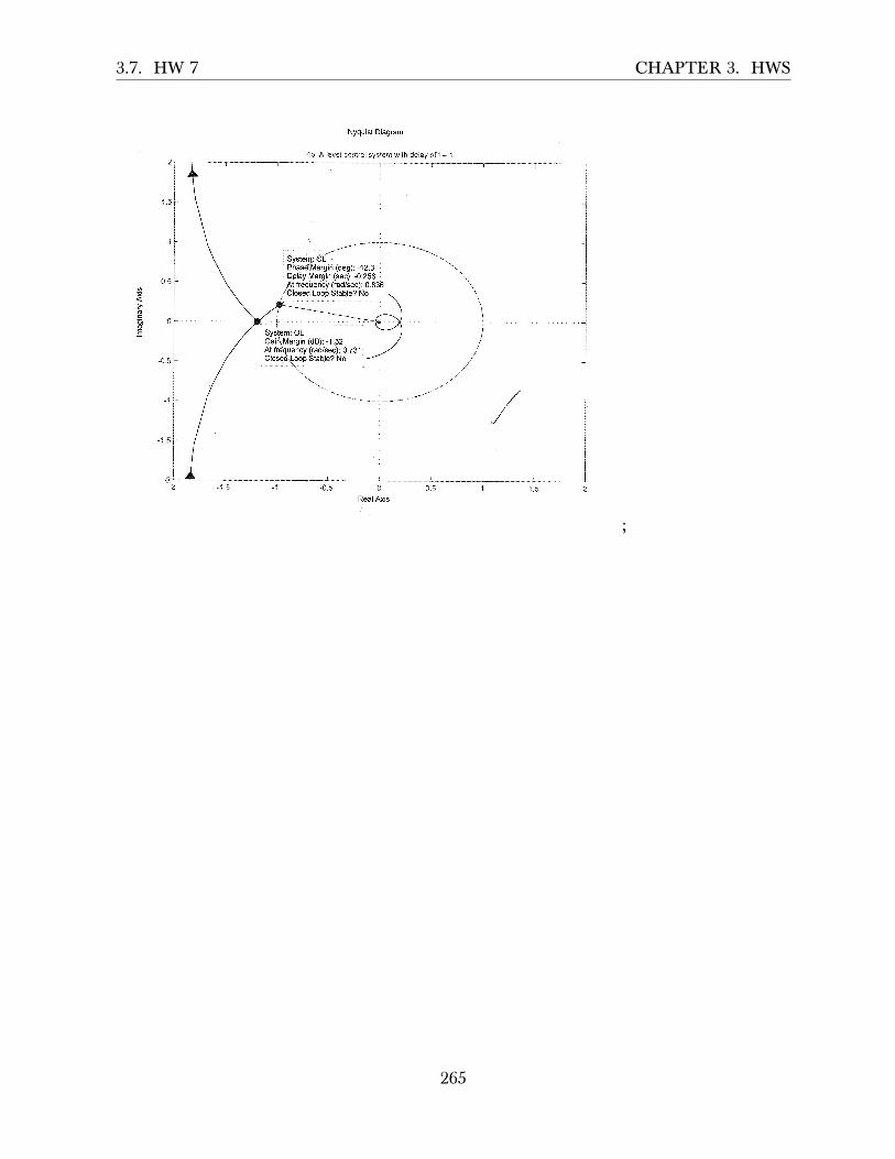
3.7. HW 7 CHAPTER 3. HWS
Acknowledgements:
ThesolutionsofDanMorganandMarkOmernickwerehelpfultotheTAinpreparingthesolutionset.
;
265

3.8. HW 8 CHAPTER 3. HWS
3.8 HW 8
3.8.1 Problem 1
I .
- ECE 332 Homework f $
Derivc a modcl for thc opcn-loop transfer function for thc system whocc frcqucncyrelponT plots a^re given on the last pagc. T\rrn in the plot with the ctraight-linc Bodcapproximationr of qho Td l% gain drawn on top of tUe true Bode plot. Will theclocedJoop aystem be rteble with ncgative unity-feedback? What "r"'tUu gain andphase marginr?
Giveo thc forwa,rd loop traosfer function for a negativc unity-feedbaclc aystem
r,t -\ - (r + 5)(r + 3)t i f a l F- \ - '
s ( r+ l ) ( r z * r+4 ) '
(a) invertigate thc atability of the cyrtem uring both Nyquist atrd Bode in Matlab,(b) fiod the gain aod phrse ma,rginc from eich method and their corresponding
clusover frequenciea. Dieplay thc gain and phase margins on the plots whcretbey occur
The block diagram shown in Figure I represents a model of a hydroelectric alternator,turbine, and penstock with transfer function Gr(r) being givenby
G ' ( s ) - ' 2 5 ( l + 5 s )(sr * 49.277s2 *25.172s + 2.526)
The parameter values are r = L, K - 0.05, M = 10, and D = I with tr(s) = g.
Figure l: Hydroelectric Syotem Block Diagram(a) Using the Bode plots, genereated using Mottab if you wish, find the maximum
nalue of K to retain stability.(b) Find the gain marEin, qh.". matgin and the corresponding crossover frequencier
aod label them on the Bode plots.
Gr(c)
Bode plot for Problem I'
40
llagnilutb ReePonse
@Ecg -20
-40
-60
- - 1
1 0 't02lot100
Itl
B - 1Eo-
Frequency (tad/se)
Phase Re$ome
Frcquency (teUsc)
SOLUTION:
The first step is to find number of poles and number of zeros. Looking at the phase plot, wesee that at high frequency the phase is −2700. Therefore, there are 3 more poles than zeros.
266

3.8. HW 8 CHAPTER 3. HWS
(A pole adds −900 at high frequency and zero adds +900). Now we look at the magnitudeplot and look for any slope change in the positive direction. There is none. The slope startsat −20 dB/decade and remains negative going to −40 dB/decade, then −60 dB/decade.
This implies there are no zeros since a zero makes the slope positive. We now know thatthere are 3 poles and no zeros.
Next we look at where the phase starts. We see it starting at −900. This means this is type1 system (i.e. one pole at the origin.). So now we can say that our system has this generalform
𝐺 (𝑠) =𝐾
𝑠 �1 + 𝑠𝜏1� �1 + 𝑠
𝜏2�
A pole at zero always starts at 40 dB at low frequency since 20 log 1𝜔 = −20 log𝜔, and using
𝜔 = 0.01 as the small frequency value (by convention), we obtain −20 log 0.01 = 40 dB. Itdrops by −20 dB/decade. Now we need to find the locations of the break points 𝜏1 and 𝜏2(also called corner frequencies).
To find 𝜏1 we draw an asymptotic lines between the first segment which has slop of −20dB/decade and the next segment which has slope of −40 dB per decade and look for theintersection point. We find it is 𝜏1 ≈ 1 rad/sec as illustrated below. Similarly between thesecond segment which has slope of −40 dB/decade and the third segment which has slopeof −60 dB/decade we find the intersection to be around 𝜏1 ≈ 10 rad/sec
267
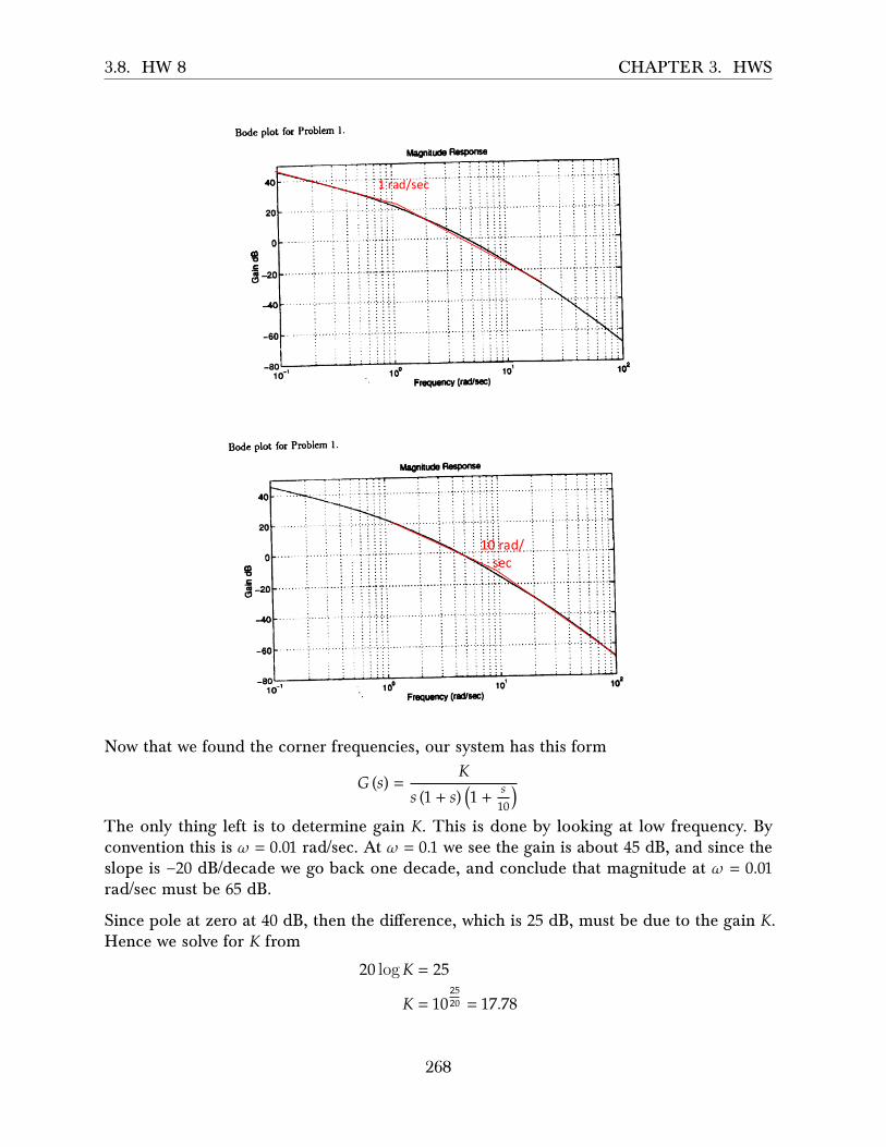
3.8. HW 8 CHAPTER 3. HWS
1 rad/sec
10 rad/sec
Now that we found the corner frequencies, our system has this form
𝐺 (𝑠) =𝐾
𝑠 (1 + 𝑠) �1 + 𝑠10�
The only thing left is to determine gain 𝐾. This is done by looking at low frequency. Byconvention this is 𝜔 = 0.01 rad/sec. At 𝜔 = 0.1 we see the gain is about 45 dB, and since theslope is −20 dB/decade we go back one decade, and conclude that magnitude at 𝜔 = 0.01rad/sec must be 65 dB.
Since pole at zero at 40 dB, then the di�erence, which is 25 dB, must be due to the gain 𝐾.Hence we solve for 𝐾 from
20 log𝐾 = 25
𝐾 = 102520 = 17.78
268

3.8. HW 8 CHAPTER 3. HWS
Therefore our system is now complete. The open loop transfer function is
𝐺 (𝑠) = 17.78𝑠(1+𝑠)�1+ 𝑠
10 �
Now we Draw the magnitude straight line approximation (this below was drawn by handusing drawing program. This is not computer generated)
0.01 0.1 1 10 100
−80
−60−40
−20
0
20
40
60
−20db per decade
−40db per decade
−60db per decade
|G(jω)| db
log(ω) rad/sec
Now we draw the phase straight line approximation. Phase goes down by −450 for each pole,starting one decade before the corner frequency, and ending one decade after the cornerfrequency. This is only for the approximation factors in the form 1
1+ 𝑠𝜏. For the exact pole 1
𝑠 , it
starts at −900 and remains over the whole frequency range. For 𝜏1 = 1 rad/sec, we start from0.1 up to 10 rad/sec. For 𝜏1 = 10 rad/sec, we start from 1 rad/sec up to 100 rad/sec. Using thisinformation, below is sketch of the phase straight line approximation.
269

3.8. HW 8 CHAPTER 3. HWS
0.01 0.1 1 10 100
−2250
−1800
−1350
−900
phase (degree)
log(ω) rad/sec−2700
−450
00
−450 per decade for τ1 term
−450 per decade for τ2 term
−900 for pole at zero
0.01 0.1 1 10 100
−2250
−1800
−1350
−900
phase (degree)
log(ω) rad/sec
−2700
Sum each segment, we obtain the plot below
Below is the straight line approximation on top of the true bode plot as required to show.
s=tf('s'); sys=17.78/(s*(1+s)*(1+s/10))bode(sys)
270

3.8. HW 8 CHAPTER 3. HWS
Since the open loop is stable as it has poles at {0, −1, −0.1}, then the closed loop will be stableif there is zero net clock wise encirclement around −1. This translates to having positivephase margin when magnitude of �𝐺 �𝑗𝜔𝑔𝑐�� is unity and positive gain margin with phase is−1800.
To find the gain margin and the phase margins, we first plot our approximation of the systemfound above: 𝐺 (𝑠) = 17.78
𝑠(1+𝑠)�1+ 𝑠10 �
using the bode command. Here it is, showing on it the 𝜔𝑝𝑐
frequency (where phase is −1800) and the corresponding �𝐺 �𝑗𝜔𝑝𝑐�� in dB found, which wewill use to find the gain margin from
271

3.8. HW 8 CHAPTER 3. HWS
Mag
nitu
de (
dB)
-100
-50
0
50
10-1 100 101 102
Pha
se (
deg)
-270
-180
-90
HW8, problem 1, approximation of the system
Frequency (rad/s)
System: sysFrequency (rad/s): 3.2Phase (deg): -180
System: sysFrequency (rad/s): 3.19Magnitude (dB): 4
We see that at −1800, the frequency is 3.2 rad/sec. This is called 𝜔𝑝𝑐. Going back to themagnitude plot, we see that at 𝜔𝑝𝑐 then �𝐺 �𝑗𝜔𝑝𝑐��
𝑑𝐵= 4 dB. This means the gain margin
𝐺𝑀𝑑𝐵 is
𝐺𝑀𝑑𝐵 = −4 dB
Notice that 𝐺𝑀𝑑𝐵 is negative of �𝐺 �𝑗𝜔𝑝𝑐��𝑑𝐵. The reason is due to the definition of 𝐺𝑀𝑑𝐵,
which is
𝐺𝑀𝑑𝐵 = 20 log101
�𝐺 �𝑗𝜔𝑝𝑐��
But �𝐺 �𝑗𝜔𝑝𝑐�� = 10�𝐺�𝑗𝜔𝑝𝑐��𝑑𝐵
20 . Substituting this in the above gives
272

3.8. HW 8 CHAPTER 3. HWS
𝐺𝑀𝑑𝐵 = 20 log101
10�𝐺�𝑗𝜔𝑝𝑐��𝑑𝐵
20
= −20 log10 10�𝐺�𝑗𝜔𝑝𝑐��𝑑𝐵
20
= − �𝐺 �𝑗𝜔𝑝𝑐��𝑑𝐵
log10 10
= − �𝐺 �𝑗𝜔𝑝𝑐��𝑑𝐵
Therefore, 𝐺𝑀𝑑𝑏 is the negative of �𝐺 �𝑗𝜔𝑝𝑐��𝑑𝑏as read from bode plot. Since 𝐺𝑀𝑑𝐵 < 0 then
closed loop is not stable . To find the phase margin. we find the frequency 𝜔𝑔𝑚 which is
where magnitude plot is at 0 dB. We see that the frequency is 𝜔𝑔𝑚 = 4 rad/sec as shown inthe plot below.
Mag
nitu
de (
dB)
-100
-50
0
50
10-1 100 101 102
Pha
se (
deg)
-270
-180
-90
HW8, problem 1, approximation of the system
Frequency (rad/s)
System: sysFrequency (rad/s): 3.98Phase (deg): -188
System: sysFrequency (rad/s): 4.01Magnitude (dB): -0.0374
At 𝜔𝑔𝑚, the phase is −1880. Subtracting 1800 from this phase gives −70. Hence
273
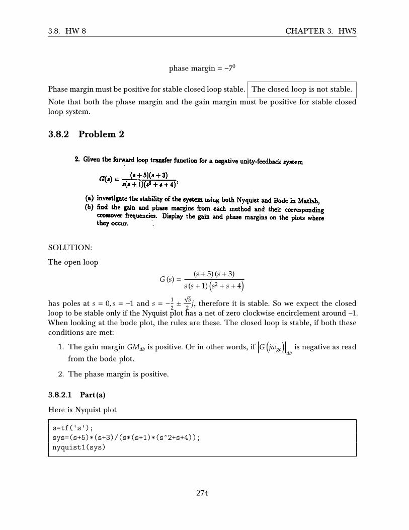
3.8. HW 8 CHAPTER 3. HWS
phase margin = −70
Phase margin must be positive for stable closed loop stable. The closed loop is not stable.
Note that both the phase margin and the gain margin must be positive for stable closedloop system.
3.8.2 Problem 2
I .
- ECE 332 Homework f $
Derivc a modcl for thc opcn-loop transfer function for thc system whocc frcqucncyrelponT plots a^re given on the last pagc. T\rrn in the plot with the ctraight-linc Bodcapproximationr of qho Td l% gain drawn on top of tUe true Bode plot. Will theclocedJoop aystem be rteble with ncgative unity-feedback? What "r"'tUu gain andphase marginr?
Giveo thc forwa,rd loop traosfer function for a negativc unity-feedbaclc aystem
r,t -\ - (r + 5)(r + 3)t i f a l F- \ - '
s ( r+ l ) ( r z * r+4 ) '
(a) invertigate thc atability of the cyrtem uring both Nyquist atrd Bode in Matlab,(b) fiod the gain aod phrse ma,rginc from eich method and their corresponding
clusover frequenciea. Dieplay thc gain and phase margins on the plots whcretbey occur
The block diagram shown in Figure I represents a model of a hydroelectric alternator,turbine, and penstock with transfer function Gr(r) being givenby
G ' ( s ) - ' 2 5 ( l + 5 s )(sr * 49.277s2 *25.172s + 2.526)
The parameter values are r = L, K - 0.05, M = 10, and D = I with tr(s) = g.
Figure l: Hydroelectric Syotem Block Diagram(a) Using the Bode plots, genereated using Mottab if you wish, find the maximum
nalue of K to retain stability.(b) Find the gain marEin, qh.". matgin and the corresponding crossover frequencier
aod label them on the Bode plots.
Gr(c)
SOLUTION:
The open loop
𝐺 (𝑠) =(𝑠 + 5) (𝑠 + 3)
𝑠 (𝑠 + 1) �𝑠2 + 𝑠 + 4�
has poles at 𝑠 = 0, 𝑠 = −1 and 𝑠 = −12 ±
√32 𝑗, therefore it is stable. So we expect the closed
loop to be stable only if the Nyquist plot has a net of zero clockwise encirclement around −1.When looking at the bode plot, the rules are these. The closed loop is stable, if both theseconditions are met:
1. The gain margin 𝐺𝑀𝑑𝑏 is positive. Or in other words, if �𝐺 �𝑗𝜔𝑔𝑐��𝑑𝑏is negative as read
from the bode plot.
2. The phase margin is positive.
3.8.2.1 Part(a)
Here is Nyquist plot
s=tf('s');sys=(s+5)*(s+3)/(s*(s+1)*(s^2+s+4));nyquist1(sys)
274

3.8. HW 8 CHAPTER 3. HWS
Real Axis-5 0 5 10 15 20 25 30 35
Imag
Axi
s
-40
-30
-20
-10
0
10
20
30
40Nyquist plot, problem 2, HW8
It shows there is one encirclement around −1. We can zoom in to make sure:
Real Axis-3 -2 -1 0 1 2 3
Imag
Axi
s
-8
-6
-4
-2
0
2
4
6
8
10
Nyquist plot, problem 2, HW8
The above shows that the closed loop is not stable. We will now look at Bode plot. Here isthe result, where I showed the gain and phase margins on the generated Matlab plot. Thisshows that the gain margin is negative, hence not stable, and it also shows that the phasemargin is negative, also indicating it is not stable.
275

3.8. HW 8 CHAPTER 3. HWS
We can also ask Matlab to give us the margins and the corresponding break frequencies.Matlab was correct and found that the closed system is also not stable:
>> [gm,pm,gwc,pwc]=margin(sys)Warning: The closed-loop system is unstable.> In ctrlMsgUtils.warning (line 25)In DynamicSystem/margin (line 65)gm =0.4254pm =-42.9450gwc =1.9239pwc =2.4785
Notice that Matlab gives the gain margin 𝐺𝑀 in linear value. We see it says 𝐺𝑀 = 0.4254above, which is −7.42 dB. Since it is negative, then closed loop is not stable.
276

3.8. HW 8 CHAPTER 3. HWS
3.8.2.2 Part(b)
We can display the cross over frequencies using Matlab either by using the margin commandor using the GUI by using the mouse as shown below. First we find the frequency where thephase is −1800, this is called 𝜔𝑝𝑐. We see it is 1.93 rad/sec. Then using the mouse, we locatethis frequency on the magnitude plot and read |𝐺(𝑗𝜔)| in dB. We see that |𝐺(𝑗𝜔)| in dB ispositive, hence 𝐺𝑀 is negative, and closed loop is not stable.
Find frequency at -180 phase
Use it to locate magnitude here.
To determine the stability using phase margin, we do the reverse. We locate the frequencywhere the magnitude is zero dB using the mouse. This is called 𝜔𝑔𝑚. We see it is at 2.48rad/sec. Then on the phase plot, we locate the phase at this frequency using the mouse. Wesee it is −2280 . Adding −1800 gives −480. Since this is negative, then the close loop is notstable.
277
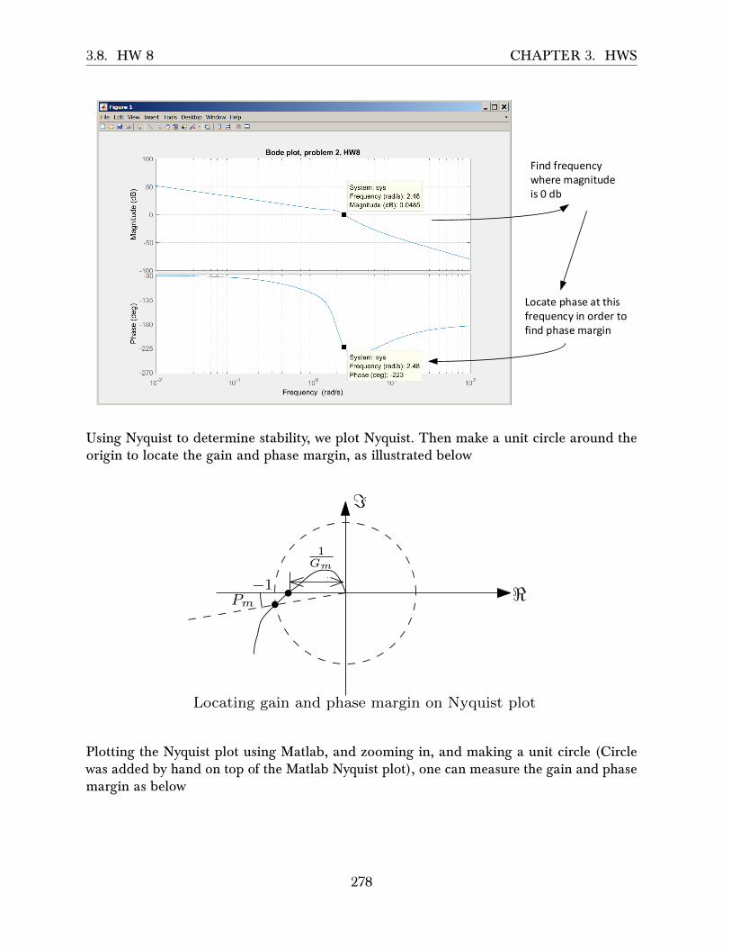
3.8. HW 8 CHAPTER 3. HWS
Find frequency where magnitude is 0 db
Locate phase at this frequency in order to find phase margin
Using Nyquist to determine stability, we plot Nyquist. Then make a unit circle around theorigin to locate the gain and phase margin, as illustrated below
<
=
1Gm
Pm
−1
Locating gain and phase margin on Nyquist plot
Plotting the Nyquist plot using Matlab, and zooming in, and making a unit circle (Circlewas added by hand on top of the Matlab Nyquist plot), one can measure the gain and phasemargin as below
278
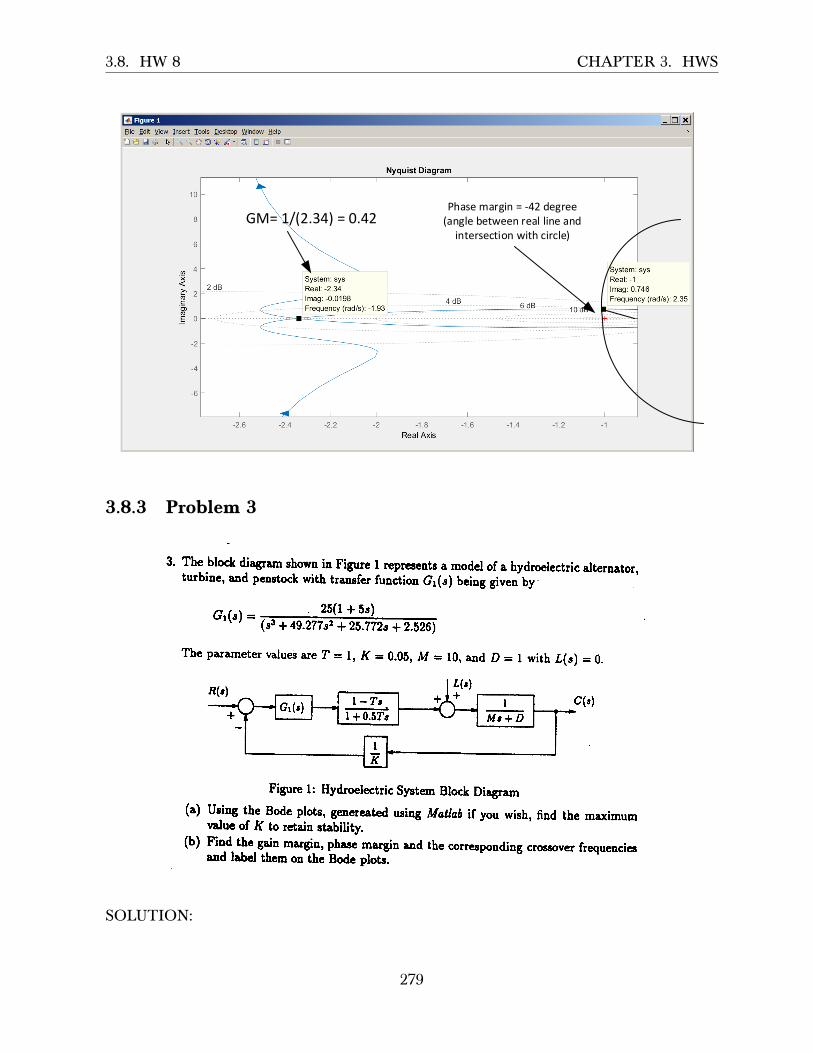
3.8. HW 8 CHAPTER 3. HWS
GM= 1/(2.34) = 0.42Phase margin = -42 degree
(angle between real line and intersection with circle)
3.8.3 Problem 3
I .
- ECE 332 Homework f $
Derivc a modcl for thc opcn-loop transfer function for thc system whocc frcqucncyrelponT plots a^re given on the last pagc. T\rrn in the plot with the ctraight-linc Bodcapproximationr of qho Td l% gain drawn on top of tUe true Bode plot. Will theclocedJoop aystem be rteble with ncgative unity-feedback? What "r"'tUu gain andphase marginr?
Giveo thc forwa,rd loop traosfer function for a negativc unity-feedbaclc aystem
r,t -\ - (r + 5)(r + 3)t i f a l F- \ - '
s ( r+ l ) ( r z * r+4 ) '
(a) invertigate thc atability of the cyrtem uring both Nyquist atrd Bode in Matlab,(b) fiod the gain aod phrse ma,rginc from eich method and their corresponding
clusover frequenciea. Dieplay thc gain and phase margins on the plots whcretbey occur
The block diagram shown in Figure I represents a model of a hydroelectric alternator,turbine, and penstock with transfer function Gr(r) being givenby
G ' ( s ) - ' 2 5 ( l + 5 s )(sr * 49.277s2 *25.172s + 2.526)
The parameter values are r = L, K - 0.05, M = 10, and D = I with tr(s) = g.
Figure l: Hydroelectric Syotem Block Diagram(a) Using the Bode plots, genereated using Mottab if you wish, find the maximum
nalue of K to retain stability.(b) Find the gain marEin, qh.". matgin and the corresponding crossover frequencier
aod label them on the Bode plots.
Gr(c)
SOLUTION:
279

3.8. HW 8 CHAPTER 3. HWS
3.8.3.1 Part (a)
The open loop transfer function is
𝐺 (𝑠) =25 (1 + 5𝑠)
𝑠3 + 42.277𝑠2 + 25.772𝑠 + 2.526 �1 − 𝑇𝑠1 + 0.5𝑇𝑠� �
1𝑀𝑠 + 𝐷� �
1𝐾�
We start with 𝑇 = 1,𝑀 = 10,𝐷 = 1, 𝐾 = 1.
𝐺 (𝑠) =25 (1 + 5𝑠)
𝑠3 + 42.277𝑠2 + 25.772𝑠 + 2.526 �1 − 𝑠1 + 0.5𝑠� �
110𝑠 + 1�
And make a bode plot, then find the �𝐺 �𝑗𝜔𝑝𝑐�� at corresponding −1800.
Mag
nitu
de (
dB)
-150
-100
-50
0
50
10-2 10-1 100 101 102 103
Pha
se (
deg)
-180
0
180
360
HW8, problem 3
Frequency (rad/s)
System: sysFrequency (rad/s): 0.637Phase (deg): 180
System: sysFrequency (rad/s): 0.636Magnitude (dB): -3.79
But the phase do not cross −1800. This indicates an infinite gain margin. Similarly we findthat the phase margin is infinite. Hence we conclude that we can make 𝐾 as close to zero(since it is in denominator) as we want, while keeping the system stable and can make it aslarge as we want. Note that we are assuming that gain itself can only be positive here.
280

3.8. HW 8 CHAPTER 3. HWS
3.8.3.2 Part (b)
Both the gain and the phase margin are infinite. There is no corresponding crossoverfrequencies.
3.8.4 Problem 4
t :
Problem 4: Thc opcn bop tnndcr ftnctim of r podtirur omuol sysrm is
G(s)-ffiAssrure a rcguive unity ftcdbackconfiguntion.
(a) Skcrch thc Bodc diagram for K = I (Do Not Usc MATLAB). Fird rhc gsin nargiagain-crossover frcquerrcn plusc margin ard thc phasc-crossorrcr @ucncy for thcsystcm.
(b) Usc MATLAB ocbcctyourplot
(c) Detcrmine the valuc of K which will satisfy thc following design criaria
l. Aphascmarginof55".
2. A gain margn of 2,6 dB.
SOLUTION:
3.8.4.1 part(a)
𝐺 (𝑠) =�1 + 𝑠
10�
𝑠 �1 + 𝑠5� �1 + 𝑠
2.5�
For the magnitude, the corner frequencies are at 𝑠 = 0, 𝑠 = 5, 𝑠 = 2.5 for the poles and 𝑠 = 10for the zeros. The pole at zero starts at 40 dB (we use 𝜔 = 0.01 as starting point by convention)with slope of −20 dB/decade. Each pole in the denominator adds a −20 dB/decade slope,while each zero adds +20 dB/decade. Here is the magnitude plot approximation
281

3.8. HW 8 CHAPTER 3. HWS
40
20
0−20
−40
−60
0.01 0.1 1 10 100
2.5 5
−20 db/decade
+20 db/decade−20 db/decade
40
20
0−20
−40
−60
0.01 0.1 1 10 100
2.5 5
−20 db/decade
Add each segment
−40 db/decade
−60 db/decade
−40 db/decade
For the phase, since this is type 1 system, it starts at −900 at the 𝜔 = 0.01. This stays for allthe range of frequencies. At 𝜔 = 5 and 𝜔 = 2.5, A −450 slope is added. This slope extendsone decade before the corner frequency up to one decade above it. At 𝜔 = 10 rad/sec, weadd +450 for the zero. Here is the result
282
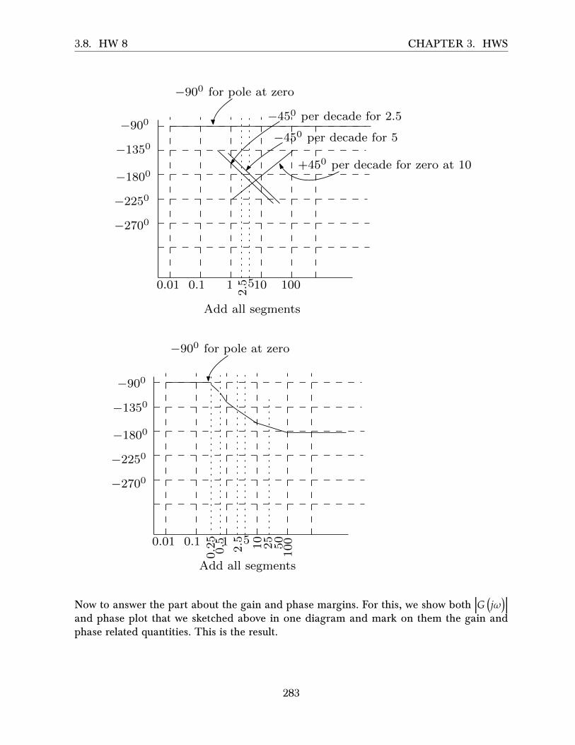
3.8. HW 8 CHAPTER 3. HWS
−900
−1350
−1800
−2250
−2700
0.01 0.1 1 10 100
2.5 5
−450 per decade for 2.5
−450 per decade for 5
+450 per decade for zero at 10
−900 for pole at zero
Add all segments
0.01 0.1 1
2.5 5
−900 for pole at zero
Add all segments
−900
−1350
−1800
−2250
−2700
0.25
25
10010
50
0.5
Now to answer the part about the gain and phase margins. For this, we show both �𝐺 �𝑗𝜔��and phase plot that we sketched above in one diagram and mark on them the gain andphase related quantities. This is the result.
283

3.8. HW 8 CHAPTER 3. HWS
In next part, we use Matlab to get accurate margin values, which shows that gain marginis 30 dB and phase margin is 640. The gain cross over frequency is 7 rad/sec and the phasecross over frequency is 0.92 rad/sec. The closed loop is stable.
3.8.4.2 Part(b)
Using Matlab
284

3.8. HW 8 CHAPTER 3. HWS
clears=tf('s');sys=tf( (1+s/10)/(s*(1+s/5)*(1+s/2.5)));bode(sys);grid[gm,pm,gcw,pcw]=margin(sys)gm =30.0007pm =64.4735gcw =7.0711pcw =0.9260
Mag
nitu
de (
dB)
-100
-50
0
50
10-1 100 101 102
Pha
se (
deg)
-225
-180
-135
-90
HW 8, problem 4, part(b)
Frequency (rad/s)
3.8.4.3 Part(c)
3.8.4.3.1 Part(1) For phase margin of 550 we want the phase at −1250 to correspond to0 dB in the magnitude plot. At phase −1250 the frequency is 1.3 rad/sec from the plot. Atthis frequency the magnitude is −3.55 dB and not zero dB. Hence positive gain margin of3.55 dB. We want to shift this up to 0 dB. So we need to solve for additional gain from
285

3.8. HW 8 CHAPTER 3. HWS
20 log10 𝐾 = 3.55
𝐾 = 10� 3.5520 �
= 1.5
Hence
𝐾 = 1.5
To verify, here is the Matlab margin command, which shows the phase margin is indeednow 550 when using 𝐾 = 1.5
clears=tf('s');K=1.5;sys=tf( K* (1+s/10)/(s*(1+s/5)*(1+s/2.5)));bode(sys);grid[gm,pm,gcw,pcw]=margin(sys)gm =20.0005pm =55.3798gcw =7.0711pcw =1.2991
3.8.4.3.2 Part(2) At −1800 in the phase plot, we want the corresponding gain marginto be 26 dB which means we want �𝐺 �𝑗𝜔𝑔𝑐�� = −26 dB. Currently, we see that at −1800, thefrequency is 7.1. The magnitude is −30 dB at this frequency. We want magnitude to be −26
dB instead. Hence we want to shift up by 4 dB the magnitude plot, or 𝐾 = 10� 420 � = 1.585
𝐾 = 1.585
To verify, here is the Matlab margin command, which shows the gain margin is close to 26dB now using 𝐾 = 1.585. (Matlab gives 𝑔𝑚 = 18.92 which is 25.54 dB)
286

3.8. HW 8 CHAPTER 3. HWS
clears=tf('s');K=1.585;sys=tf( K* (1+s/10)/(s*(1+s/5)*(1+s/2.5)));[gm,pm,gcw,pcw]=margin(sys)gm =18.9279pm =54.0559gcw =7.0711pcw =1.3568>> 20*log10(gm)25.5420
287

3.8. HW 8 CHAPTER 3. HWS
3.8.5 HW 8 key solution
Problem1:
;
288

3.8. HW 8 CHAPTER 3. HWS
Remark:
This problem has no single correct solution. Any solution, backed upwithavalidreasoningisacceptable.
;
289

3.8. HW 8 CHAPTER 3. HWS
Problem2:
I .
- ECE 332 Homework f $
Derivc a modcl for thc opcn-loop transfer function for thc system whocc frcqucncyrelponT plots a^re given on the last pagc. T\rrn in the plot with the ctraight-linc Bodcapproximationr of qho Td l% gain drawn on top of tUe true Bode plot. Will theclocedJoop aystem be rteble with ncgative unity-feedback? What "r"'tUu gain andphase marginr?
Giveo thc forwa,rd loop traosfer function for a negativc unity-feedbaclc aystem
r,t -\ - (r + 5)(r + 3)t i f a l F- \ - '
s ( r+ l ) ( r z * r+4 ) '
(a) invertigate thc atability of the cyrtem uring both Nyquist atrd Bode in Matlab,(b) fiod the gain aod phrse ma,rginc from eich method and their corresponding
clusover frequenciea. Dieplay thc gain and phase margins on the plots whcretbey occur
The block diagram shown in Figure I represents a model of a hydroelectric alternator,turbine, and penstock with transfer function Gr(r) being givenby
G ' ( s ) - ' 2 5 ( l + 5 s )
(sr * 49.277s2 *25.172s + 2.526)
The parameter values are r = L, K - 0.05, M = 10, and D = I with tr(s) = g.
Figure l: Hydroelectric Syotem Block Diagram
(a) Using the Bode plots, genereated using Mottab if you wish, find the maximumnalue of K to retain stability.
(b) Find the gain marEin, qh.". matgin and the corresponding crossover frequencieraod label them on the Bode plots.
Gr(c)
First a SUMMARY. Then supporting plots to follow It is easy to verify (for example use Routh) that closed loop isunstable. Hence there are no gain and phase margins.
This is not really a gain margin. But it reflects the decibeldeficiency in the closed loop
Same comment here. THis is not really a phase margin.It reflects the phase deficiency.
Note that Bode and Nyquist lead to the same "phony" gain and phase margins.
;
290
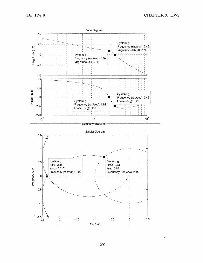
3.8. HW 8 CHAPTER 3. HWS
;
291
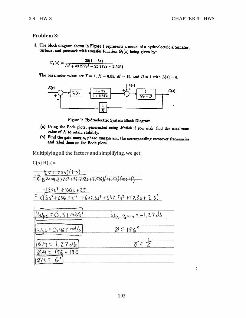
3.8. HW 8 CHAPTER 3. HWS
Problem3:
Multiplyingallthefactorsandsimplifying,weget,
G(s)H(s)=
I .
- ECE 332 Homework f $
Derivc a modcl for thc opcn-loop transfer function for thc system whocc frcqucncyrelponT plots a^re given on the last pagc. T\rrn in the plot with the ctraight-linc Bodcapproximationr of qho Td l% gain drawn on top of tUe true Bode plot. Will theclocedJoop aystem be rteble with ncgative unity-feedback? What "r"'tUu gain andphase marginr?
Giveo thc forwa,rd loop traosfer function for a negativc unity-feedbaclc aystem
r,t -\ - (r + 5)(r + 3)t i f a l F- \ - '
s ( r+ l ) ( r z * r+4 ) '
(a) invertigate thc atability of the cyrtem uring both Nyquist atrd Bode in Matlab,(b) fiod the gain aod phrse ma,rginc from eich method and their corresponding
clusover frequenciea. Dieplay thc gain and phase margins on the plots whcretbey occur
The block diagram shown in Figure I represents a model of a hydroelectric alternator,turbine, and penstock with transfer function Gr(r) being givenby
G ' ( s ) - ' 2 5 ( l + 5 s )
(sr * 49.277s2 *25.172s + 2.526)
The parameter values are r = L, K - 0.05, M = 10, and D = I with tr(s) = g.
Figure l: Hydroelectric Syotem Block Diagram
(a) Using the Bode plots, genereated using Mottab if you wish, find the maximumnalue of K to retain stability.
(b) Find the gain marEin, qh.". matgin and the corresponding crossover frequencieraod label them on the Bode plots.
Gr(c)
;
292
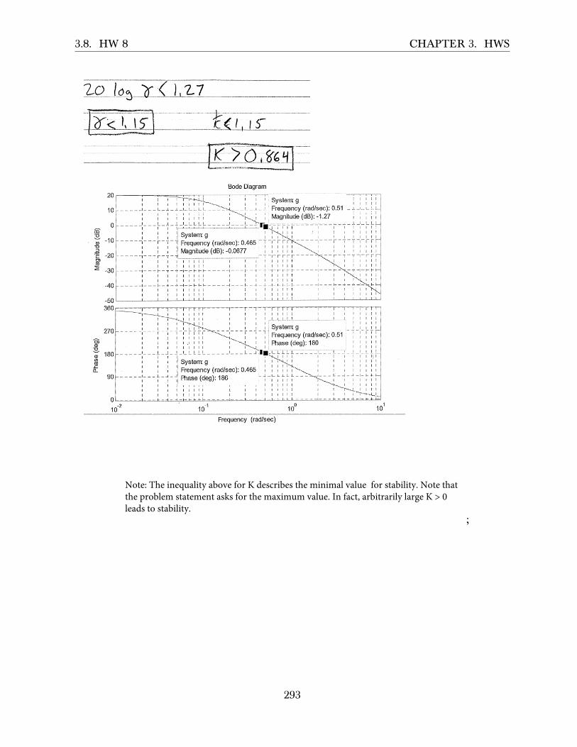
3.8. HW 8 CHAPTER 3. HWS
Note: The inequality above for K describes the minimal value for stability. Note that the problem statement asks for the maximum value. In fact, arbitrarily large K > 0 leads to stability.
;
293

3.8. HW 8 CHAPTER 3. HWS
Problem3:Part(b):
;
294

3.8. HW 8 CHAPTER 3. HWS
;
295

3.8. HW 8 CHAPTER 3. HWS
Problem4:
t :
Problem 4: Thc opcn bop tnndcr ftnctim of r podtirur omuol sysrm is
G(s)-ffiAssrure a rcguive unity ftcdbackconfiguntion.
(a) Skcrch thc Bodc diagram for K = I (Do Not Usc MATLAB). Fird rhc gsin nargiagain-crossover frcquerrcn plusc margin ard thc phasc-crossorrcr @ucncy for thcsystcm.
(b) Usc MATLAB ocbcctyourplot
(c) Detcrmine the valuc of K which will satisfy thc following design criaria
l. Aphascmarginof55".
2. A gain margn of 2,6 dB.
At gain crossover, estimate phaseto be about -130 degrees. So phase margin about 50 degrees.
At phase crossover, log gain is approximately -40 db. So gainmargine is about 40db
;
296

3.8. HW 8 CHAPTER 3. HWS
;
297

3.8. HW 8 CHAPTER 3. HWS
Problem4:Part(c):
Fromtheaboveplot,weseethatK=1satisfiestherequiredcriterion.
TofindvalueofKthatsatisfiesthecriterionexactly,wecanproceedasfollows–
More precisely, we obtain a K which approximately meets both specs.
;
298

Chapter 4
Exams
Local contents4.1 First exam . . . . . . . . . . . . . . . . . . . . . . . . . . . . . . . . . . . . . . . . . 3004.2 Second exam . . . . . . . . . . . . . . . . . . . . . . . . . . . . . . . . . . . . . . . 3024.3 Final exam . . . . . . . . . . . . . . . . . . . . . . . . . . . . . . . . . . . . . . . . . 304
299
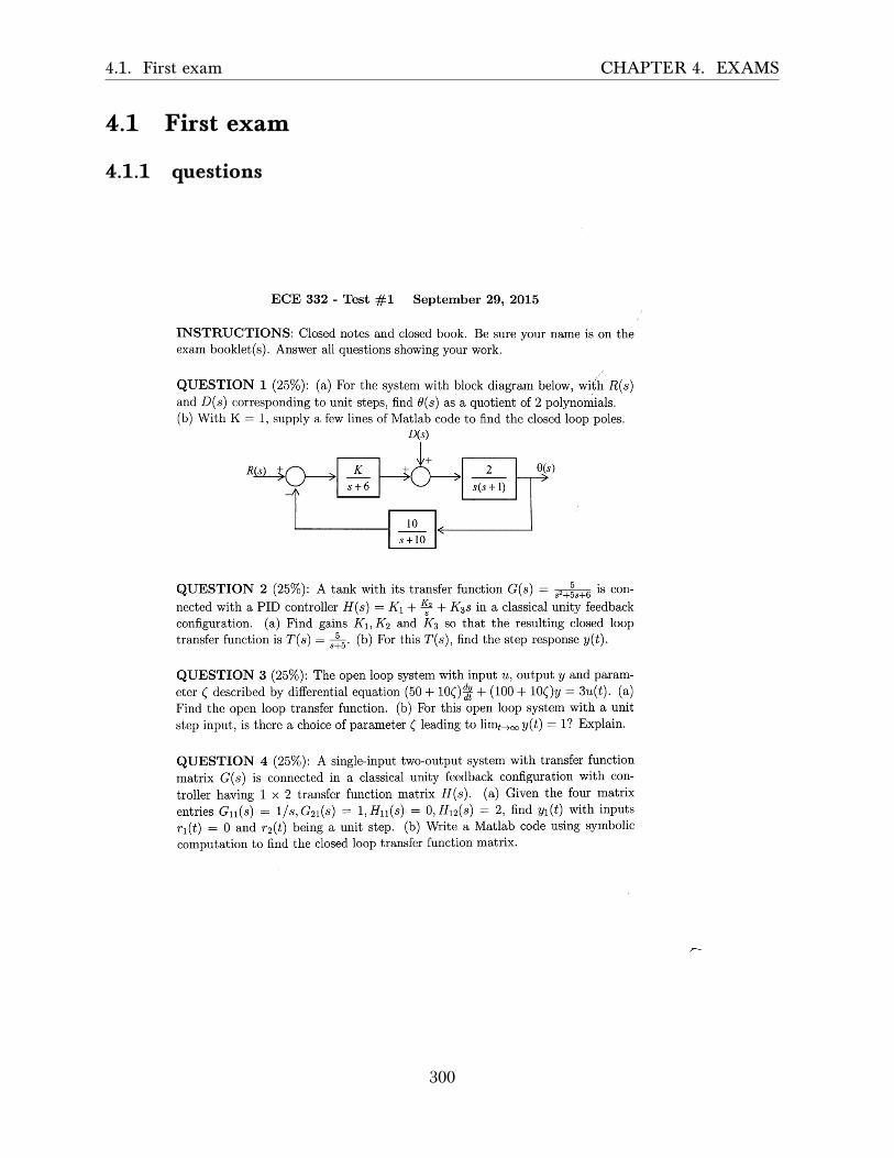
4.1. First exam CHAPTER 4. EXAMS
4.1 First exam
4.1.1 questions
ECE 332 - Test #1 September 29, 2015
INSTRUCTIONS: Closed notes and closed book. Be sure your name is on the exam booklet(s). Answer all questions showing your work.
/ /
QUESTION 1 (25%): (a) For the system with block diagram below, wi¥h R(s) and D( s) corresponding to unit steps, find fJ( s) as a quotient of 2 polynomials. (b) With K = 1, supply a few lines of Matlab code to find the closed loop poles.
D(s)
~ R(s) j;~ I s~61 )~ 2 8( ...:
s(s + 1) " II'
s)
10 " -- .....
s+1O
QUESTION 2 (25%): A tank with its transfer function G(s) = s2+~s+6 is connected with a PID controller H(s) = Kl + ~ + K3S in a classical unity feedback configuration. (a) Find gains K1, K2 and K3 so that the resulting closed loop transfer function is T(s) = s!5' (b) For this T(s), find the step response y(t).
QUESTION 3 (25%): The open loop system with input u, output y and parameter ( described by differential equation (50 + 10()-1t + (100 + 10()y = 3u(t). (a) Find the open loop transfer function. (b) For this open loop system with a unit step input, is there a choice of parameter ( leading to limt-+oo y(t) = I? Explain.
QUESTION 4 (25%): A single-input two-output system with transfer function matrix G( s) is connected in a classical unity feedback configuration with controller having 1 x 2 transfer function matrix H(s). (a) Given the four matrix entries G11 (s) = 1/ S, G21 (S) = 1, Hll(S) = 0, H12(S) = 2, find Yl(t) with inputs rl(t) = 0 and r2(t) being a unit step. (b) Write a Matlab code using symbolic computation to find the closed loop transfer function matrix.
300
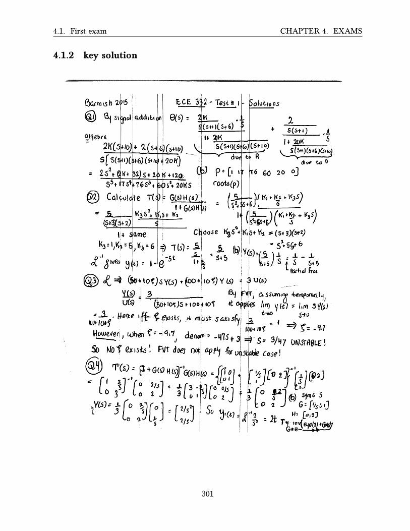
4.1. First exam CHAPTER 4. EXAMS
4.1.2 key solution
=
Bcunu,S h 2. ~,
~ G.t 51 ..I f.ddltt
i: t
I
J;;CE. l~2' TeSH I - ~O_'Q_tl_OO.s
9(5):: ~M • . (St8)( Sf ,)
... 5(S ... ) #1 f~ ~K 5
\....!f5tl) (5 +'J(.sl 'cj T" d UtI' to 0
20 oj
301

4.2. Second exam CHAPTER 4. EXAMS
4.2 Second exam
4.2.1 questions
302

4.2. Second exam CHAPTER 4. EXAMS
4.2.2 key solution
303

4.3. Final exam CHAPTER 4. EXAMS
4.3 Final exam
4.3.1 questions
304

4.3. Final exam CHAPTER 4. EXAMS
4.3.2 key solution
305