Eavesdropping on the Social Lives of Ca21 Sparks

Leighton T. Izu,* Tamas Banyasz,*z C. William Balke,*y and Ye Chen-Izu**Departments of Internal Medicine and yPhysiology, University of Kentucky College of Medicine, Lexington, Kentucky;and zDepartment of Physiology, Medical and Health Science Center, University of Debrecen, Debrecen, Hungary

ABSTRACT Ca21 sparks arise from the stochastic opening of spatially discrete clusters of ryanodine receptors called a Ca21

release unit (CRU). If the RyR clusters were not spatially separated, then Ca21 released from one RyR would immediately diffuseto its neighbor and lead to uncontrolled, runaway Ca21 release throughout the cell. While physical separation provides someisolation from neighbors, CRUs are not incommunicado. When inter-neighbor interactions become large enough, Ca21 wavesspontaneously emerge. A more circumscribed interaction shows up in high-speed two-dimensional confocal images as jumpingCa21 sparks that seem to be sequentially activated along the Z-line and across Z-lines. However, since Ca21 sparks arestochastic events how can we tell whether two sparks occurring close together in space and time are causally related or appearedsimply by coincidence? Here we develop a mathematical method to disentangle cause and coincidence in a statistical sense.From our analysis we derive three fundamental properties of Ca21 spark generation: 1), the ‘‘intrinsic’’ spark frequency, the sparkfrequency one would observe if the CRUs were incommunicado; 2), the coupling strength, which measures how strongly one CRUaffects another; and 3), the range over which the communication occurs. These parameters allow us to measure the effect RyRregulators have on the intrinsic activity of CRUs and on the coupling between them.

INTRODUCTION

The physical separation of Ca21 release units (CRUs) as

discrete clusters of ryanodine receptors is essential for local

control of excitation-contraction coupling in striated muscle

(1). If the CRUs were not separated then Ca21 released from

an RyR would be immediately communicated to its neighbor

and trigger regenerative Ca21 release throughout the cell.

The discreteness of CRUs is manifest in Ca21 sparks (2–5),

the highly localized release of Ca21 from the sarcoplasmic

reticulum (SR). The distance between the CRUs in the plane

of the Z-line in mammalian cardiomyocytes has been esti-

mated to be ;0.3–0.4 mm based on electron microscopy (6);

between ;0.65 and ;1 mm (7,8) based on confocal measure-

ments of fluorescently labeled RyR antibody; and ;0.8 mm

(in rat, (9)) or ;2 mm (in cat, (10)) based on distances be-

tween spark or activation sites on Ca21 waves. The longi-

tudinal spacing of CRUs coincides with the Z-line separation

and is ;2 mm (7,11).

These separation distances are evidently sufficient to pro-

vide a degree of isolation between CRUs that prevents run-

away Ca21 release but not to the degree that the CRUs are

incommunicado. Under certain conditions, communication

between CRUs via Ca21 diffusion can result in Ca21 waves

(12–14). More subtly, Parker et al. (9) found more circum-

scribed communication in which one spark triggers one or

two other sparks within ;15 ms of each other. These trig-

gered sparks were only observed with the transverse confocal

line scans (i.e., directed perpendicular to the cardiomyocytes

long axis) and not with longitudinal line scans. This

observation is explained by the closer transverse spacing of

CRUs (;0.5 �1 mm) in the plane of the Z-line than between

Z-lines (;2 mm). Similarly, Brum et al. (15), using rapid

two-dimensional scanning, found sequential activation of

sparks parallel to the Z-line in frog skeletal muscles.

Images collected on rapid scanning two-dimensional con-

focal microscopes that survey a large area (;2000 mm2) of

the cell often show large number of sparks that appear like

raindrops on a pond. One’s attention is often drawn to sparks

that seem to be coupled because they occur closely in space

and time, giving the impression that sparks are jumping (Fig.

2). It is important to assess the magnitude of coupling

between sparks because if a sufficient number in a small re-

gion occur in a short time period they can coalesce into Ca21

waves (12,14), which could trigger an abnormal action

potential and possibly arrhythmias (16–19). However, just as

it is impossible to say whether two sets of ripples on a pond

were caused by two raindrops (Fig. 3 A) or whether one set

was caused by the splash from one raindrop (Fig. 3 B), when

only the ripples are observable, we cannot determine for any

particular pair of sparks whether they are causally or coinci-

dentally related.

In this article, we develop a method to disentangle cause

and coincidence in the origin of sparks in a statistical sense.

We will show how to derive from the probability distribution

of distances between sparks, three fundamental properties of

spark generation: 1), the intrinsic spark frequency, the spark

frequency one would observe if the CRUs were incommu-

nicado; 2), the coupling strength; and 3), the coupling space

constant. These parameters quantify the intrinsic properties

of CRUs and communication between themselves. These

doi: 10.1529/biophysj.107.112466

Submitted May 9, 2007, and accepted for publication July 17, 2007.

Address reprint requests to L. T. Izu, Tel.: 859-323-6882; E-mail: leightonizu@

uky.edu.

Dr. Banyasz’s permanent address is Dep. of Physiology, Medical and Health

Science Center, University of Debrecen, Debrecen, Hungary.

Editor: Ian Parker.

� 2007 by the Biophysical Society

0006-3495/07/11/3408/13 $2.00

3408 Biophysical Journal Volume 93 November 2007 3408–3420

parameters allow us to measure the effect that RyR reg-

ulators have on the intrinsic activity of CRUs and on the

coupling between them.

METHODS

Cell isolation

Male Sprague-Dawley rats (Harlan, Indianapolis, IN) were anesthetized with

isoflurane supplemented with O2. After suppression of reflexes, the hearts

were removed via midline thoracotomy and a standard enzymatic technique

was used to isolate the ventricular cells as described previously (20). All

animals and procedures were handled strictly in accordance to the National

Institutes of Health guidelines and our Institutional Animal Care and Use

Committee approved protocols. Chemicals and reagents were purchased

from Sigma-Aldrich (St. Louis, MO) if not specified otherwise.

Indicator loading

The cells were loaded with Fluo-4 (Molecular Probes-Invitrogen, Carlsbad,

CA) in Tyrode (Ty) solution containing (in mM): 145 NaCl, 4 KCl, 1 CaCl2,

0.33 NaH2PO4, 1 MgCl2, 10 HEPES, 10 glucose (pH 7.3, adjusted with

NaOH), and 2.5 mM fluo-4 acetylmethyl ester (Molecular Probes-Invitrogen)

at room temperature for 45 min. Di-8-ANEPPS (Molecular Probes-Invitrogen),

15 mM, was added to the above solution in the last 15 min of the loading

period to label the sarcolemma and t-tubules. The cells were studied within

2 h after loading.

Preconditioning train

To achieve a uniform SR Ca21 load, cells in Ty were field-stimulated (1 Hz)

for 2 min, allowing ample time for the cell contraction to reach a steady state.

Confocal image acquisition started 10 s after stopping field stimulation.

Confocal microscopy

Experiments were carried out on the Zeiss 5 Live confocal microscope (Carl

Zeiss, Jena, Germany) equipped with a 100 3 1.4 numerical aperture Plan-

Apo oil objective (Zeiss). The indicators were excited with a 488 nm laser

and the emitted light was passed through a 520 nm longpass filter. Images

were scanned bidirectionally at 80 Hz. The zoom factor was set to 1, which

produces an x-y pixel size of 0.12 mm 3 0.12 mm.

Spark detection and determination ofspark frequency

Sparks were detected using the approach described in Banyasz et al. (21).

Because we need the spark coordinates in relationship to the Z-lines, the

image of the cell is manually rotated so that the longitudinal axis of the cell is

aligned horizontally. Alignment accuracy was improved by lining up the di-

8 ANEPPS labeled t-tubules with vertical gridlines superimposed on the cell

image.

The Ca21 spark frequency, gtotal, for a cell was determined from the slope

of the cumulative spark number (CSN) plotted against the product of time

and cell area (21). The reason for the subscript total in gtotal is explained

later. A linear CSN plot means that the spark frequency is constant. Only

those cells in which the spark frequency was constant were used in the

analysis. (See the discussion after Eq. 17 to see why we only use cells with

constant spark frequency.) The CSN plot sometimes has a quadratic or other

nonlinear shape, which means that the spark frequency is not constant. We

need a way to objectively and automatically determine whether the CSN plot

is linear. We used two tests to determine whether the CSN plot is linear or

quadratic. First, we used an ANOVA to test whether the sum of squared

deviations between the linear and quadratic fitted curves and the data were

significantly different at a probability level of a ¼ 0.01. If the probability

(from the F distribution) was .a, then the CSN was considered to be linear.

However, even when the probability was ,a (meaning the linear and

quadratic plots were statistically distinguishable), the difference might not

be meaningful. Fig. 1 shows such an example. The open circles are the mea-

sured CSN, the solid line is the linear fit, and the dashed curve is the

quadratic fit. The two fits are statistically distinguishable but the difference

does not appear meaningful. To understand why this occurs we first note that

the number of degrees of freedom (df) used in the ANOVA is Nsparks-2 and

Nsparks-3 for the linear and quadratic curves, respectively, and Nsparks is the

number of sparks. Since Nsparks is typically 50 or more, df is almost the same

for both functions. Therefore, if the CSN plot deviates even slightly from

linearity, the null hypothesis (the CSN is linear) is almost always rejected

because the quadratic fit produces a smaller sum of squared deviations.

The intuitive notion of a meaningful difference is captured in the mag-

nitude of the curvature (the coefficient of the quadratic term, c2). Let the

linear fit be given by y ¼ a1 1 b1x and the quadratic fit be y ¼ a2 1 b2x 1

c2x2. To measure the relative contributions of the linear and quadratic terms

we compare c2x2max to b1xmax; where xmax is the maximum space-time value.

If the ratio c2x2max=b1xmax,0:40; then we say that the difference is not

meaningful and we say that the CSN plot is linear. For the data in Fig. 1, this

ratio is 0.395, just below the cut-off so the CSN is considered to be linear.

This particular set of data was chosen to show the worst-case data that would

be used in our subsequent analysis. The spark frequency equals the slope of

the CSN plot, b1.

Definition of neighbors

Let the coordinates of a spark occurring at position (x, y) at time t be given by

(x, y, t). We say that spark S is in the neighborhood of the central spark S0, if

dXmin # jx�x0j# dXmax, dYminjy�y0j# dYmax, and 0 , jt�t0j# dT, where

(x0,y0,t0) are the coordinates of S0. The reason for using nonzero lower

bounds, dXmin ¼ 0.7 mm and dYmin ¼ 0.3 mm, is to preclude counting S0 as

being its own neighbor. This could occur if the rise of the spark continues

over successive frames although this is unlikely since the time per frame is

12.5 ms and the spark rise-time is ;5 ms. A false neighbor could also be

generated if there was a small shift in the center of mass of S0 in successive

frames; the nonzero lower bounds reduce the number of these kinds of false-

positive neighbors. We chose dXmax ¼ dYmax ¼ 15 mm. This distance might

seem far outside the realm of what a neighborhood should be but, as we will

explain later, the determination of g depends on measuring very distant

neighbors. The reason for not choosing dXmax� 15 mm is to keep the size of

FIGURE 1 How gtotal is determined. The number of sparks (cumulative

spark number, CSN) is plotted against the product of the time the spark oc-

curred (time/frame 3 frame number) and the area of the cell. The CSN is fit to

both a line and a quadratic. Although the quadratic fit is statistically better, the

curvature is negligible in the data range so this CSN is considered to be linear.

The solid line is the best linear fit.

Ca21 Spark Coupling 3409

Biophysical Journal 93(10) 3408–3420

the entire neighborhood around the width of the cell. By setting dT¼ 15 ms,

we limit neighboring sparks only to those occurring one frame after S0.

Probability density estimation usingkernel methods

We will need to estimate the probability density function (pdf), f(r), of the

distribution of distances from the central spark. The histogram is the most

familiar method of obtaining the pdf. The histogram is, however, sensitive

to the bin width and the location of the bin boundaries. Kernel methods for

estimating the probability density (22) do not have bin boundaries and are

less sensitive than the histogram to changes in bandwidth (w, the analog of

bin width).

The quantity f(r) is constructed as follows. For each unique distance ri we

define the function

hiðrÞ ¼nðriÞNtotal

exp �ðr � riÞ2

2w2

� �3

1

Knormw; (1)

where n(ri) is the number of sparks that are at a distance ri from the central

spark and Ntotal is the total number of sparks. The factor 1/(Knormw),

Knormw ¼Z N

�N

exp � r2

2w2

� �dr ¼

ffiffiffiffiffiffi2pp

w � 2:5w; (2)

normalizes hi(x) so that its integral equals n(ri)/Ntotal. The pdf is

f ðrÞ ¼ +hiðrÞ; (3)

where the index runs over all unique distances. Note, by construction, the

integral of f(r) over all r equals unity.

Simulating Ca21 sparks

We simulated sparks using a two-dimensional lattice with a CRU on each

lattice point. CRUs were separated along the x and y axes by lx and ly,

respectively, and the lattice dimension was 40 mm on each side. We used

a very high CRU packing density, 100/mm2 (lx ¼ ly ¼ 0.1 mm) or 50/mm2

(lx ¼ 0.2 mm, ly ¼ 0.1 mm), which are 200- or 100-times higher than in real

cells, simply to get a lot of sparks in a short time. Each CRU has an intrinsic

firing rate of g. If a CRU at lattice point i, j fires at time k, then it changes the

firing probability rate of the neighboring CRUs at time k1T to f given in

Eq. 6. The value r is the Euclidean distance between CRU i, j and the CRU

of interest. The influence of CRU i, j does not extend beyond time k1T. The

intrinsic frequency g, coupling strength A, and the coupling space constant

r are input parameters to the program. To determine whether a CRU will fire

at k1T, fT is computed (with T ¼ 1) and a random number from a uniform

distribution is generated. The CRU fires only if this number is ,fT.

RESULTS

Jumping Ca21 sparks

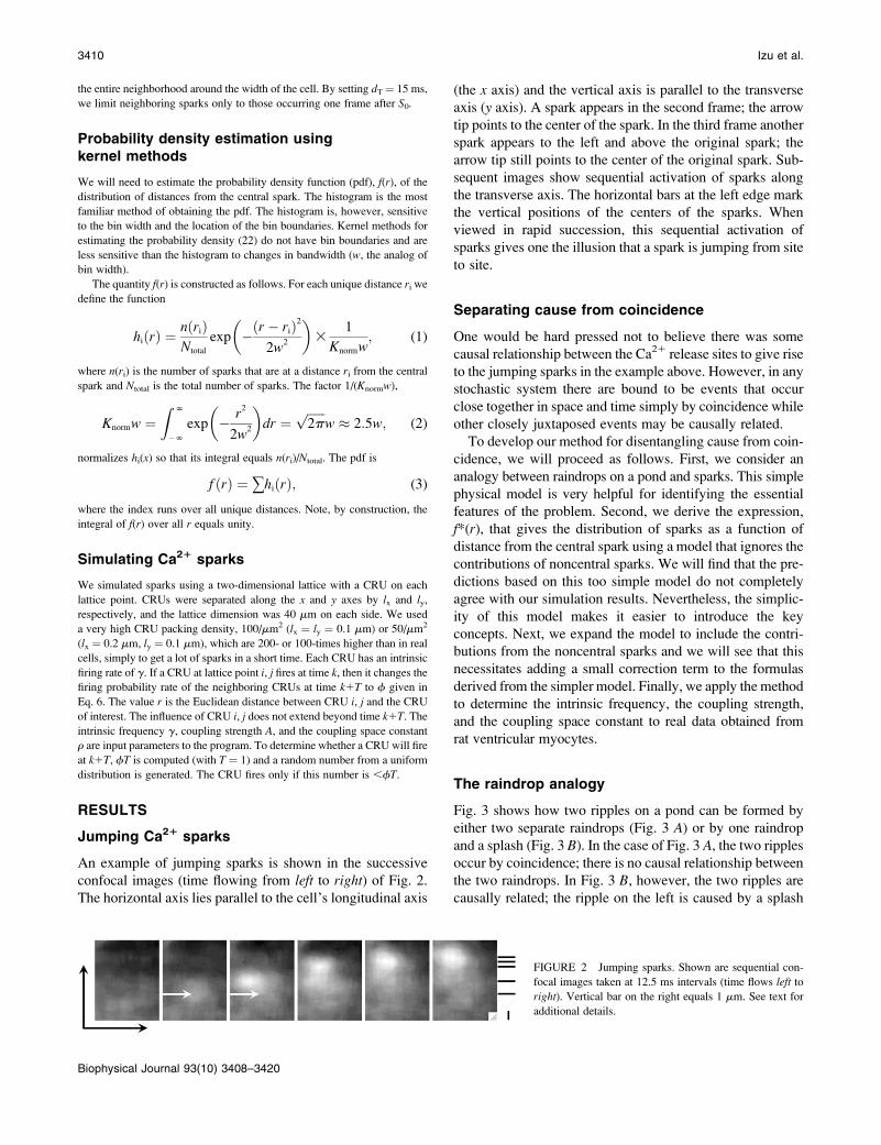
An example of jumping sparks is shown in the successive

confocal images (time flowing from left to right) of Fig. 2.

The horizontal axis lies parallel to the cell’s longitudinal axis

(the x axis) and the vertical axis is parallel to the transverse

axis (y axis). A spark appears in the second frame; the arrow

tip points to the center of the spark. In the third frame another

spark appears to the left and above the original spark; the

arrow tip still points to the center of the original spark. Sub-

sequent images show sequential activation of sparks along

the transverse axis. The horizontal bars at the left edge mark

the vertical positions of the centers of the sparks. When

viewed in rapid succession, this sequential activation of

sparks gives one the illusion that a spark is jumping from site

to site.

Separating cause from coincidence

One would be hard pressed not to believe there was some

causal relationship between the Ca21 release sites to give rise

to the jumping sparks in the example above. However, in any

stochastic system there are bound to be events that occur

close together in space and time simply by coincidence while

other closely juxtaposed events may be causally related.

To develop our method for disentangling cause from coin-

cidence, we will proceed as follows. First, we consider an

analogy between raindrops on a pond and sparks. This simple

physical model is very helpful for identifying the essential

features of the problem. Second, we derive the expression,

f*(r), that gives the distribution of sparks as a function of

distance from the central spark using a model that ignores the

contributions of noncentral sparks. We will find that the pre-

dictions based on this too simple model do not completely

agree with our simulation results. Nevertheless, the simplic-

ity of this model makes it easier to introduce the key

concepts. Next, we expand the model to include the contri-

butions from the noncentral sparks and we will see that this

necessitates adding a small correction term to the formulas

derived from the simpler model. Finally, we apply the method

to determine the intrinsic frequency, the coupling strength,

and the coupling space constant to real data obtained from

rat ventricular myocytes.

The raindrop analogy

Fig. 3 shows how two ripples on a pond can be formed by

either two separate raindrops (Fig. 3 A) or by one raindrop

and a splash (Fig. 3 B). In the case of Fig. 3 A, the two ripples

occur by coincidence; there is no causal relationship between

the two raindrops. In Fig. 3 B, however, the two ripples are

causally related; the ripple on the left is caused by a splash

FIGURE 2 Jumping sparks. Shown are sequential con-

focal images taken at 12.5 ms intervals (time flows left to

right). Vertical bar on the right equals 1 mm. See text for

additional details.

3410 Izu et al.

Biophysical Journal 93(10) 3408–3420

from the raindrop that caused the ripple on the right. If only

ripples are visible (not the raindrops or splashes), how can

we assess the frequency that a splash from a raindrop causes

another ripple? Imagine a snapshot of the ripples on the pond

and focus your attention on the center of one ripple, the

central ripple—the circle with the shaded center in Fig. 3 C.

Let n(r) be the number of centers of ripples (solid circles)

within an annulus of radius r and thickness Dr. Since a splash

from the central ripple is unlikely to travel far, the number of

ripple centers in a very large radius annulus should be propor-

tional to the product of the area of the annulus, 2p r Dr, and

the frequency of the raindrops (raindrops/time/area), g,

nðrÞ} 2prDr 3 g; for large r: (4)

Close to the central ripple, raindrops and splashes would

create ripples so n(r) is

nðrÞ} 2prDr 3 gð1 1 KðrÞÞ: (5)

K(r), the coupling kernel, describes the number of splashes

at a distance r per raindrop. We would expect that K(r) de-

creases monotonically to zero so Eq. 5 merges smoothly to

Eq. 4.

The value g is the intrinsic frequency; it is the frequency

of the raindrops and it is also the frequency of ripples that

would be observed if no splashing occurred. According to

Eq. 4, n(r) is a linear function for large r and its slope is

proportional to g. This is a remarkable result, as it tells us

that we can determine the frequency of raindrops simply by

measuring the spatial distribution of ripples. Later we will

show that this is almost but not completely correct.

A simple, incomplete, but conceptually usefulmodel of Ca21 spark coupling

Our method for determining the magnitude of Ca21 spark

coupling and the intrinsic spark frequency follows by simply

substituting sparks for ripples. Fig. 3 D shows schematically

how the n(r) is determined from two-dimensional confocal

images. The solid circle on the lower rectangle is the position

of the central spark that occurs on the confocal image at time

t. The upper rectangle is the confocal image at time t 1 T. (At

a typical 80 Hz scan rate, T¼ 12.5 ms.) The shaded circle on

this rectangle is the position of the central spark, which may

or may not be present in the image. The solid circles are

sparks that first make their appearance at t 1 T. The

Euclidean distances, r, between the central spark and the other

sparks at t 1 T are computed. The quantity n(r) is the number

of sparks that are at a distance between r and r 1 Dr from the

central spark. This procedure is repeated for each spark. In

other words, each spark is treated as a central spark.

The coupling kernel

Let g be the intrinsic spark frequency; its units are number

of sparks/time per CRU. This is the spark frequency you

would measure if one spark did not influence the probability

of another spark occurring. Experimentally, this influence

could be reduced by loading the cell with a Ca21 buffer such

as EGTA to reduce the diffusion of Ca21 from a release site

to a neighboring CRU. This influence is also nil far from the

central spark. When a spark occurs, Ca21 diffuses to neigh-

boring CRUs and increases their probability of firing so we

expect the spark frequency near the central spark would in-

crease above the intrinsic frequency to g(1 1 K(r)). A Ca21

spark has a roughly Gaussian profile (9,23,24) and we found

that the spark is spatially symmetric (21). We, therefore, pro-

visionally choose the coupling kernel to be a spatially sym-

metric Gaussian and define the spatially dependent spark

frequency, f(r), to be

fðr; g;A; rÞ ¼ g 1 1 Aexp �r2

r2

� �� �; (6)

where A is coupling magnitude and r is the coupling space

constant. The challenge is to determine g, A, and r from the

spatial distribution of sparks, n(r).

The quantity f(r) is the probability of a spark occurring

per unit time. Therefore, the probability that a CRU at a

distance r from the central spark will fire within T is given by

qðr; g;A; rÞ ¼ 1� e�Tfðr;g;A;rÞ

: (7)

(This is simply the complement of the waiting time distri-

bution; see Izu et al. (25).) The number of sparks expected in

an annulus around the central spark within time T equals the

product of the number of CRUs in the annulus and the prob-

ability of firing,

nðr; g;A; r;s; TÞ ¼ ½2prDrs�3 qðr; g;A; r; TÞ: (8)

FIGURE 3 The raindrop analogy. Ripples on a pond can arise in two

ways, either by separate raindrops (A) or from splashes (B). In the former

case, the two ripples are coincidental, in the latter, the ripples are causally

related. (C) Geometry for computing the number of ripples (solid circles)

around the central ripple (shaded circle) as a function of distance from the

center. The dotted lines define the annulus whose inner radius is r and outer

radius is r 1Dr. (D) Schematically shows how distances between central

spark and neighbors are computed. Each plane is a confocal image. Solid

circles mark the position of the central spark first occurring at time t and the

neighboring sparks first occurring at t1T. Position of the central spark on the

t1T image is marked by the shaded circle. The value r is the Euclidean

distance between the central spark and its neighbors.

Ca21 Spark Coupling 3411

Biophysical Journal 93(10) 3408–3420

The first set of factors is the annulus area times the CRU

density (CRU/area), s. In all cases we have encountered the

following inequality holds:

gTð1 1 Ae�r

2=r

2

Þ# gTð1 1 AÞ � 1: (9)

Under this condition Eq. 7 simplifies to q � gTð11Ae�r2=r2Þand Eq. 8 has the same form as Eq. 5. For brevity we will

often write n(r) in place of n(r,g, A,r,s,T).

The quantity n(r) is the number of sparks at a distance rfrom a single central spark. Let N(r) be the aggregate number

of sparks at distance r from all central sparks. (Recall that

each spark is used as a central spark.) Then N(r) is

NðrÞ ¼ Nsparks 3 2prDrsqðrÞ: (10)

Instead of working with N(r), it is more convenient to work

with its density f(r) defined by

NðrÞ ¼ Ndistances

Z r1Dr=2

r�Dr=2

f ðsÞds � Ndistances f ðrÞDr: (11)

Rearrangement of Eqs. 10 and 11 gives

rqðr; g;A; r; TÞ ¼ f ðrÞ 1

2ps

Ndistances

Nsparks

: (12)

The first term on the right is the probability density of the

distance distribution between central and noncentral sparks,

the second term is a cell structure factor as it involves the

CRU density, and the last term is a ratio of extensive

quantities that depend on the size of the data set. For

gTð11Ae�r2=r2Þ � 1; q � fT and Eq. 12 simplifies to

rfðr; g;A; rÞ ¼ f ðrÞ 1

2ps

Ndistances

NsparksT[ f �ðrÞ: (13)

The r q(r,g,A,r,T) curves, shown in Fig. 4 A for different

combinations of g, A, and r, have two distinctive features.

First, they become linear for large r. This happens because,

far from the influence of the central spark, the number of

sparks in each annulus depends primarily on the product of

the intrinsic spark frequency and the area of the annulus,

which scales linearly with r. This linear behavior is anal-

ogous to Eq. 4 of the raindrop problem, where ripples caused

by splashing are unlikely far from the central ripple, and so

the number of ripples depends only on the intrinsic raindrop

frequency. Differentiating Eq. 12 shows that the slope of

r q(r,g, A, r, T) converges to 1� e�gT for large r. Since T is

known, it follows that g can be determined from the slope of

the scaled density of distances given in Eq. 12. Under con-

ditions where Eq. 9 holds, the slope of f*(r) is simply g . In

Fig. 4 A, g was set to 3 3 10�4 for three curves drawn with

solid, dashed, and dotted lines. Note that they all converge to

the same slope at large r. The curve drawn with dashed-

dotted lines was generated using g ¼ 1 3 10�4 and has a

correspondingly shallower slope than the others.

The second distinctive feature of f*(r) is the hump at r� 0.

This hump represents the increased number of sparks that are

triggered close to the central spark. The height and breadth

of this hump depends on the coupling magnitude and the

coupling space constant. Setting A ¼ 0 means coupling is

absent and f*(r) is a straight line (dashed line). The dif-

ference between the curves is shown in Fig. 4 B for A ¼ 10,

r ¼ 0.5 (solid curve) and A ¼ 0. The integral of this dif-

ference over r is the excess number of sparks expected due

to spark coupling in the region 0 , r , R in the time between

t and t 1T, e(R,A),

eðR;AÞ ¼Z 2p

0

sdu

Z R

0

rðqðr;AÞ � qðr; 0ÞÞdr; (14)

where the dependence on the other parameters have been

dropped for brevity. When the integration is carried over all

R, the excess is

FIGURE 4 Distribution of neighbor distances from the

central spark. (A) Plot of rq(r,g, A, r). (Dashed line, g ¼ 5 3

10�4, A ¼ 0, r ¼ 0.5; solid curve, same as before except

A ¼ 10; dotted curve, same except r ¼ 1.0. Dot-dashcurve, g ¼ 1 3 10�4, A ¼ 10, r ¼ 0.5.) (B) Difference

curve, rq(r,g, A, r)� rq(r,g, 0, r). Line style corresponds

to panel A. (C) Normalized distance distribution f*(r) for

simulated data. (D) Schematic of a more complete model

showing how a noncentral spark at s~contributes to sparks

(labeled b) in the annulus. Colors of circles (solid and

shaded) have the same meaning as in Fig. 3 D. Spark coccurred spontaneously and spark a was triggered by the

central spark at the origin O.

3412 Izu et al.

Biophysical Journal 93(10) 3408–3420

eðAÞ ¼ psr2½gE 1 logðgATÞ1 Eið1;gATÞ�; (15)

where gE � 0.5772 is Euler’s number and Ei is the expo-

nential integral (26). (The appearance of the expression in the

brackets is astonishing. It is closely related to the famous

relationship between the logarithm and the harmonic series,

limn/NðgE1logðnÞ �+n

k¼11=kÞ ¼ 0; which has played an

important role in the development of the Riemann hypothesis

(27).) As the coupling magnitude goes to zero, the term in the

brackets goes to zero so the excess e also goes to zero, as we

would expect.

The slope of f*(r) at r ¼ 0 is g (1 1 A) so the value of A is

obtained from the slope of f*(r) at the origin. We obtain r

from the position of the peak of the hump of the f*(r) curve,

rpeak, by

r ¼ rpeakffiffiffiffiffiffiffiffiffiffiffiffiffiffiffiffiffiffiffiffiffiffiffiffiffiffiffiffiffi1

2�W

e�1=2

2A

!vuut; (16)

where W is the Lambert W(x) function that solves WeW ¼ x(28). The important point of this part of the analysis is that g,

A, and r are obtained from the density distribution of

distances from the central spark.

Testing the predicted values of g, A, and r againstsimulated data

Sparks were simulated as described in the Methods with

known input values of g, A, and r. Fig. 4 C shows f*(r) for

the simulated sparks when the input values were g ¼ 5 3

10�4, A¼ 10, and r¼ 0.5 mm. As with the theoretical curves

in Fig. 4 A, this measured f*(r) curve has a hump near r ¼ 0

and becomes linear at large r. Unlike the theoretical curve,

this f*(r) curve declines to zero beyond ;8 mm. This decline

is an artifact of the finite neighborhood size. The linear

portion (from ;2 to 8 mm) is sufficient to determine g.

According to our analysis above, the slope of the linear

portion of f*(r) should be equal to the intrinsic spark

frequency g ¼ 5 3 10�4. The measured slope is 8.14 3 10�4

(see first row of Table 1, entry gfstar). Clearly, something

must be missing from this simple model.

A more complete model of spark coupling

We erred in the derivation for the expression of n(r) by not

accounting for sparks at time t 1T that were triggered by

noncentral sparks at time t. Fig. 4 D is a more accurate

depiction of the origins of sparks. Let the central spark occur

at the origin O on the image frame at time t and let a non-

central be at position vector s~: The shaded circles at t1Tmark the positions occupied by these sparks at t. The solid

circles are new sparks that just appeared at t 1 T. The three

sparks in the annulus could have been triggered by the central

spark (a), by the noncentral spark (b), or might have arisen

spontaneously without influence of either earlier sparks (c).

The error in our simple model was to treat all sparks at t 1 Tto be either of types a or c. To handle the more complex case

that includes sparks of type b, let us first suppose that there

are sparks at time t at position vector s~i 6¼ O; i ¼ 1 . . . M:Each of these sparks will trigger e(g,A,r,T,s) excess sparks

at t 1 T. The total number of excess sparks equals

e(g,A,r,T,s) 3 M. We are not interested, however, in the

total number of excess sparks but rather the number of sparks

in the annulus between r and r 1 Dr. The number of sparks

triggered at t 1 T is

nðr; t1TÞ¼ ½2prDrs�3qðr;g;A;r;TÞ1eðg;A;r;T;sÞ3m;

(17)

where the first term is identical to Eq. 8 and m is the number

of the s~i sparks that have contributed to sparks in the annulus.

In general, this m is unknown because the distribution of the

s~i vectors is unknown. Recall, however, that q(r,g,A,r,T) �q(r,g,A¼ 0,r,T) is sharply peaked at r� 0. Therefore, for the

m sparks to trigger sparks in the annulus, those m sparks

must be close to the annulus itself, which allows us to make

the approximation m ¼ n (r,t). Substituting n(r,t) for m in

Eq. 17 gives the time evolution equation for n(r,t) (see Fig.

5 D, inset and text below). Under steady-state conditions,

n(r,t 1 T) ¼ n(r,t) [ n(r), so the distribution of sparks about

the central spark at the origin is

nðrÞ ¼ ½2prDrs�3 qðr; g;A; r; TÞ1� eðg;A; r; T;sÞ : (18)

Comparing Eqs. 8 and 18 we see that by not counting the

contributions of the noncentral sparks, we underestimate the

number of sparks in the annulus by a factor of 1�e. We note

that e / 0 as A / 0, so Eq. 18 converges to Eq. 8.

TABLE 1 Comparison of input, measured, and estimated

coupling parameter values

# ginput gtotal gfstar gcalculated Ainput Acalculated rinput rcalculated

1 5.0 8.14 8.14 4.82 10 10.00 0.5 0.51

2 4.0 5.76 5.70 3.93 10 9.32 0.5 0.53

3 3.0 3.86 3.90 3.18 10 8.38 0.5 0.46

4 2.0 2.35 2.35 2.04 10 8.56 0.5 0.48

5 1.0 1.09 1.16 1.00 10 9.75 0.5 0.53

6 1.0 1.05 1.13 1.00 5 5.00 0.5 0.53

7 1.0 1.14 1.21 0.95 5 6.13 1.0 0.94

8 5.0 6.18 6.18 5.18 10 7.93 0.5 0.47

9 3.0 3.38 3.39 3.17 10 7.93 0.5 0.47

10 5.0 8.03 8.06 4.72 10 10.25 0.5, 1.0 0.73

11 3.0 3.87 3.87 3.06 10 8.70 0.5, 1.0 0.68

The values ginput, Ainput, and rinput are the values input into the simulation

program. The subscript calculated indicates the parameter values calculated

from analysis. The value gtotal is the spark frequency is obtained from the

slope of the best fit line to the cumulative spark number. The quantity gfstar

is the spark frequency obtained from the linear part of f*(r), i.e., large r. All

values of g are multiplied by 104. In simulations 1–7 the CRUs were

symmetrically spaced with lx ¼ ly ¼ 0.1 mm; in simulations 8–11, the

CRUs were asymmetrically distributed with lx ¼ 0.2 mm and ly ¼ 0.1 mm.

In simulations 8 and 9, the coupling kernel was symmetric (rx¼ ry ¼ r); in

10 and 11, rx ¼ 1.0 mm and ry ¼ 0.5 mm.

Ca21 Spark Coupling 3413

Biophysical Journal 93(10) 3408–3420

It is important to understand the range of r over which Eq.

18 is valid. In Eq. 17 each of the addends are on the order of

r, denoted O(r). For r � 0, however, the addends are of dif-

ferent orders. The first addend, [2prDrr] 3 q(r, g, A, r, T), is

O(r). The second addend is O(r2) since m must be

proportional to the number of CRUs in the circle around

the origin, m ¼ O(r2). Therefore, near the origin, Eq. 17 is

not valid n, and n(r) given by Eq. 8 must be used instead.

Reanalysis of the simulation data

Substituting Eq. 18 in place of 2prDrsq(r) in Eq. 10 leads to

the modified version of Eq. 12:

rqðr; g;A; r; TÞ1� eðg;A; r; TÞ ¼ f ðrÞ 1

2ps

Ndistances

Nsparks

: (19)

We used Eq. 19 to reanalyze the data in Fig. 4 C for large r.

Unlike in the simple model, where the slope of f*(r) at large rdepended only on g, in this more complex model the linear

part of f*(r) depends on g, A, and r. The following pro-

cedure is used to solve for these parameters.

1. The slope of the linear part of f*(r) is measured; call this

gfstar and in this case, gfstar ¼ 8.139 3 10�4 (Fig. 5 A).

2. Measure the location of the peak of the hump of f*(r),

rpeak (Fig. 5 A).

3. Plot the integral of f*(r), F(r2) against r2 (Fig. 5 B). We

use the integral for data analysis because it is smoother

than f*(r). Measure the slope of F(r2) at r ¼ 0; call it s0

(Fig. 5 B, inset). These three measured values—gfstar,

rpeak, and s0—will allow us to uniquely determine g, A,

and r.

4. Let Aguess be the guessed value of A.

5. Compute gguess according to gguess ¼ 2s0/(1 1 Aguess).

6. Compute rguess using Aguess in Eq. 16.

7. Compute e by substituting Aguess, gguess, and rguess in

Eq. 15.

8. Compute gT,guess ¼ gguess/(1�e).9. Increment Aguess and return to Step 4.

The function gfstar,guess (Aguess) is shown as the solid curve

in Fig. 5 C. The correct value of coupling magnitude, A, is

the solution to gfstar,guess (A) ¼ gfstar. This equation can be

solved graphically as shown in Fig. 5 C. The dashed

horizontal line is at the level of gfstar. This line intersects the

gfstar,guess curve at A. For the simulated data, this value of Aturns out to be 10.0, identical to the input value used in the

simulation. Based on this value of A, r is found to be 0.507

(using Eq. 16), very close to the input value of 0.50. The

measured slope of F(r2) at r ¼ 0 is s0 ¼ 2.70 3 10�3, so the

calculated value of g is g ¼ 2s0/(1 1 A) ¼ 4.92 3 10�4,

which is also close to the input value of 5.00 3 10�4. We see

that the intrinsic frequency is accurately recovered when the

contributions from the noncentral sparks are accounted for.

We can gain more insight into the meaning of gfstar by

obtaining the spark frequency in a more traditional way. Fig.

5 D shows the number of sparks on each image frame;

the mean number is 130.8 sparks/frame. As described in

Banyasz et al. (21), we determine the total spark frequency,

gtotal, by first plotting the cumulative spark number (CSN) as

a function of time then fitting a line to the data as was done in

Fig. 1. To obtain gtotal, we divide the slope of the fitted line

(130.7 sparks/frame) by the frame area (40 3 40 mm2), by

the time per frame (T ¼ 1 ms), and by the CRU density (s ¼100 CRU/mm2), which gives gtotal ¼ 8.14 3 10�4. This

value agrees exactly with gfstar measured from the slope of

the linear part of f*(r). We call this the total frequency

FIGURE 5 Recovering the spark coupling parameters.

(A) Data in Fig. 4 C truncated beyond r¼ 6 mm. The value

gT is found from the slope of the linear part of f*(r) and the

arrow points to rpeak where the f*(r) curve has zero slope.

The integral of f*(r), F, shown in B, is plotted against r2.

Because F is less subject to noise it is used for finding the

slope at r ¼ 0, shown in the inset. The Pade approximant

ar2/(11br2) is fit to F for r � 0 and the slope s0 is

calculated from the approximant. Panel C shows how A is

found from the intersection of the computed gT (solid

curve) and the value of gT measured in panel A (dashedline). The intersection occurs at 10.00, exactly equal to the

value of A used in the simulations. The number of sparks

occurring on the simulation lattice at each time step is

shown in D. The mean number of sparks/frame is 130.7.

The inset shows the early time evolution of the number of

sparks. The solid line is the theoretical evolution curve

given by Eq. 20.

3414 Izu et al.

Biophysical Journal 93(10) 3408–3420

because it includes all sparks without regard to whether the

sparks arose independently or due to coupling.

The equality of gfstar and gtotal shows that gfstar measures

the total spark frequency. Results for this and other simu-

lations using different values of g, A, and r are shown in

entries 1–7 in Table 1. In all cases we see that gtotal � gfstar.

Note that the total frequency can be considerably higher than

the intrinsic frequency (63% higher for the first case), al-

though the difference gets smaller as the intrinsic frequency

decreases (see Eq. 22). This table shows that using the pro-

cedure described above, we are able to recover the intrinsic

frequency, the coupling magnitude, and the coupling dis-

tance with reasonable accuracy.

The dynamical relationship between the intrinsicand total spark frequencies

We can get a better understanding of the relationship be-

tween the intrinsic and total frequency by seeing how the

spark frequency evolves as shown in the inset of Fig. 5 D.

The evolution equation for the total number of sparks is (see

Eq. 17)

Nði 1 1Þ ¼ gTNsites 1 eNðiÞ: (20)

For g ¼ 5 3 10�4, A¼ 10, and r¼ 0.5, the excess sparks e¼0.39. The solid line is the graph of the evolution equation

(Eq. 20). To see how the numbers of sparks evolve, we start

with zero sparks on frame 0. There are 4002 CRUs each with

an intrinsic firing frequency of 5 3 10�4/ms. Within T¼ 1 ms

we then expect to see 4002 3 (5 3 10�4/ms) 3 1 ms ¼ 80

sparks. There just so happens to be 80 sparks on frame i ¼ 1.

Starting the random number generator with a different seed

value would produce slightly different numbers of sparks.

Each of the 80 sparks on frame i ¼ 1 will trigger, on aver-

age, 0.39 additional sparks on frame i ¼ 2 for a total of 80 3

0.39¼ 31 sparks. These will be added to the ;80 sparks that

would intrinsically occur. We expect, therefore, 80 1 31 ¼111 sparks on frame 2; we observe 99. On frame 3, we ex-

pect to see 0.39 3 111 1 80 ¼ 123 sparks; we observe 120.

We see that N(i) rapidly evolves to the steady-state value of

Nsteady state ¼ gTNsites=ð1� eÞ ¼ 80=ð1� 0:39Þ � 131: As

noted above, the measured mean number of sparks/frame

is 130.8. From this value we calculate the total spark fre-

quency of 8.14 3 10�4 /ms as was done above.

Therefore, we can say that the total spark frequency gfstar

is the steady-state spark frequency that evolves due to spark

coupling when the intrinsic frequency is g, the coupling

magnitude is A, and the coupling distance is r.

Effect of asymmetric CRU distribution andanisotropic Ca21 diffusion

The simulations up to now used a distribution of CRUs that

was symmetric along the x and y axes. However, as we noted

in the Introduction, the distance between CRUs within the

plane of the Z-line is ;0.5–1 mm, whereas the Z-lines are

spaced ;2 mm apart. Based on our immunolabeling studies

we estimate the mean nearest-neighbor distance between

CRUs in the plane of the Z-line is 1 mm (7). We therefore

carried out simulations in which the CRU separation dis-

tances along the x and y axes had a 2:1 ratio. As before, we

used a high packing density (s ¼ 50/mm2, lx ¼ 0.2 mm, ly ¼0.1 mm) to generate many sparks in a reasonable time.

The results of these simulations are given in entries 8–11 in

Table 1.

Simulations 1 and 8 differ only in the lattice structure. The

values g, A, and r are the same, yet gtotal is larger for

simulation 1. This is reasonable because the CRUs are closer

together along the x axis in simulation 1 than in simulation 8,

thereby increasing the probability that one CRU will trigger

another. The intrinsic frequency is accurately recovered. The

calculated coupling magnitude is 20% lower than the input

value (7.93 vs. 10), reflecting the smaller interaction between

CRUs along the x axis than along the y axis.

We found that Ca21 sparks in ventricular myocytes have a

circular shape, suggesting that Ca21 diffusion is isotropic

(21). Parker et al. (9), however, determined that Ca21 dif-

fuses anisotropically based on the different spark profiles

obtained when the confocal line scan is directed longitudi-

nally (x axis) or transversely (y axis). We studied how such a

diffusional anisotropy would affect the calculated values of

g, A, and r by using an asymmetric coupling kernel in our

spark simulations. We used rx ¼ 1 mm and ry ¼ 0.5 mm as

our inputs to reflect the 2:1 diffusional anisotropy measured

by Parker et al. The results are given in entries 10 and 11. We

again see that gtotal is considerably larger than g and that the

analysis can recover the intrinsic frequency and coupling

magnitude reasonably accurately. Because the analysis of the

distribution of distances is based on a symmetric kernel (see

Eq. 6), the calculated r (0.73 and 0.68 mm) is, as expected,

between rx and ry.

Spark coupling in rat ventricular myocytes

Ca21 sparks were detected in ventricular myocytes using the

spark detection algorithm and statistical sieve described in

Banyasz et al. (21). We used only cells that had a constant

spark frequency for two reasons. The first and obvious rea-

son is that unless the spark frequency is constant there is no

sensible spark frequency. The second and subtler reason is

because the analysis presented above used the assumption

that the spark numbers had reached a steady state (see the

discussion pertaining to Eq. 17). For each cell we measured

the distances between the central spark and its neighbors as

described in the Methods.

Fig. 6 A shows the distribution of distances from central

sparks. The sparks were measured in 63 cells in standard Ty

obtained from four rats. The f*(r) curve has the characteristic

M-shape similar to that from the simulated spark data in

Ca21 Spark Coupling 3415

Biophysical Journal 93(10) 3408–3420

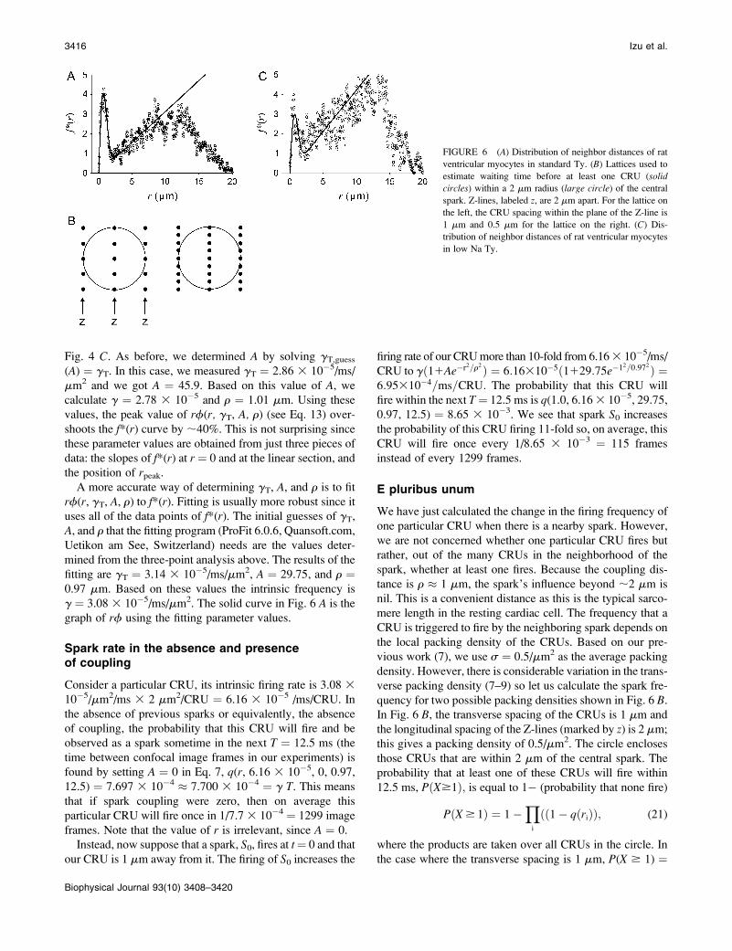
Fig. 4 C. As before, we determined A by solving gT,guess

(A) ¼ gT. In this case, we measured gT ¼ 2.86 3 10�5/ms/

mm2 and we got A ¼ 45.9. Based on this value of A, we

calculate g ¼ 2.78 3 10�5 and r ¼ 1.01 mm. Using these

values, the peak value of rf(r, gT, A, r) (see Eq. 13) over-

shoots the f*(r) curve by ;40%. This is not surprising since

these parameter values are obtained from just three pieces of

data: the slopes of f*(r) at r ¼ 0 and at the linear section, and

the position of rpeak.

A more accurate way of determining gT, A, and r is to fit

rf(r, gT, A, r) to f*(r). Fitting is usually more robust since it

uses all of the data points of f*(r). The initial guesses of gT,

A, and r that the fitting program (ProFit 6.0.6, Quansoft.com,

Uetikon am See, Switzerland) needs are the values deter-

mined from the three-point analysis above. The results of the

fitting are gT ¼ 3.14 3 10�5/ms/mm2, A ¼ 29.75, and r ¼0.97 mm. Based on these values the intrinsic frequency is

g ¼ 3.08 3 10�5/ms/mm2. The solid curve in Fig. 6 A is the

graph of rf using the fitting parameter values.

Spark rate in the absence and presenceof coupling

Consider a particular CRU, its intrinsic firing rate is 3.08 3

10�5/mm2/ms 3 2 mm2/CRU ¼ 6.16 3 10�5 /ms/CRU. In

the absence of previous sparks or equivalently, the absence

of coupling, the probability that this CRU will fire and be

observed as a spark sometime in the next T ¼ 12.5 ms (the

time between confocal image frames in our experiments) is

found by setting A ¼ 0 in Eq. 7, q(r, 6.16 3 10�5, 0, 0.97,

12.5) ¼ 7.697 3 10�4 � 7.700 3 10�4 ¼ g T. This means

that if spark coupling were zero, then on average this

particular CRU will fire once in 1/7.7 3 10�4 ¼ 1299 image

frames. Note that the value of r is irrelevant, since A ¼ 0.

Instead, now suppose that a spark, S0, fires at t¼ 0 and that

our CRU is 1 mm away from it. The firing of S0 increases the

firing rate of our CRU more than 10-fold from 6.16 3 10�5/ms/

CRU to gð11Ae�r2=r2Þ ¼ 6:16310�5ð1129:75e�12=0:972Þ ¼6:95310�4=ms=CRU: The probability that this CRU will

fire within the next T¼ 12.5 ms is q(1.0, 6.16 3 10�5, 29.75,

0.97, 12.5) ¼ 8.65 3 10�3. We see that spark S0 increases

the probability of this CRU firing 11-fold so, on average, this

CRU will fire once every 1/8.65 3 10�3 ¼ 115 frames

instead of every 1299 frames.

E pluribus unum

We have just calculated the change in the firing frequency of

one particular CRU when there is a nearby spark. However,

we are not concerned whether one particular CRU fires but

rather, out of the many CRUs in the neighborhood of the

spark, whether at least one fires. Because the coupling dis-

tance is r � 1 mm, the spark’s influence beyond ;2 mm is

nil. This is a convenient distance as this is the typical sarco-

mere length in the resting cardiac cell. The frequency that a

CRU is triggered to fire by the neighboring spark depends on

the local packing density of the CRUs. Based on our pre-

vious work (7), we use s ¼ 0.5/mm2 as the average packing

density. However, there is considerable variation in the trans-

verse packing density (7–9) so let us calculate the spark fre-

quency for two possible packing densities shown in Fig. 6 B.

In Fig. 6 B, the transverse spacing of the CRUs is 1 mm and

the longitudinal spacing of the Z-lines (marked by z) is 2 mm;

this gives a packing density of 0.5/mm2. The circle encloses

those CRUs that are within 2 mm of the central spark. The

probability that at least one of these CRUs will fire within

12.5 ms, PðX$1Þ; is equal to 1� (probability that none fire)

PðX $ 1Þ ¼ 1�Y

i

ðð1� qðriÞÞ; (21)

where the products are taken over all CRUs in the circle. In

the case where the transverse spacing is 1 mm, P(X $ 1) ¼

FIGURE 6 (A) Distribution of neighbor distances of rat

ventricular myocytes in standard Ty. (B) Lattices used to

estimate waiting time before at least one CRU (solidcircles) within a 2 mm radius (large circle) of the central

spark. Z-lines, labeled z, are 2 mm apart. For the lattice on

the left, the CRU spacing within the plane of the Z-line is

1 mm and 0.5 mm for the lattice on the right. (C) Dis-

tribution of neighbor distances of rat ventricular myocytes

in low Na Ty.

3416 Izu et al.

Biophysical Journal 93(10) 3408–3420

0.0214 so on average, the central spark needs to fire 1/0.0214

� 47 times before seeing at least one CRU in its 2 mm

neighborhood fire. When the CRU transverse spacing is 0.5

mm, PðX$1Þ increases to 0.0621 because there are more

CRUs in the neighborhood and because those CRUs that are

0.5 mm away have a higher firing frequency. In this case, the

central spark needs to fire only �16 times before at least one

neighboring CRU fires.

By contrast, if coupling were absent then the central spark

will fire 217 times (transverse CRU spacing ¼1 mm) or 130

times (transverse CRU ¼ 0.5 mm) on average before at least

one CRU in the 2 mm neighborhood would fire.

What is the intrinsic frequency?

In our simulations, we calculated the intrinsic frequency g

from the total frequency gtotal, which matched very well to

the unique g value that was input into the simulation. Inter-

preting the calculated intrinsic frequency is more complex

for real cells because each myocyte has a different total fre-

quency. The mean spark frequency based on gtotal is

�gtotal ¼ 2:61 3 10�562:90 3 10�5=mm2=ms ðmean6SDÞ; the

median is 1.54 3 10�5/mm2/ms, and the maximum frequency

is 1.34 3 10�4/mm2/ms. The distribution of spark frequen-

cies is very skewed to the left with most cells having low

spark frequencies but a few cells having high frequencies (see

Fig. 4 of (21)). The calculated intrinsic frequency of 3.08 3

10�5/mm2/ms is larger than the mean of gtotal. The difference

between g (or gtotal) and �gtotal depends on how the con-

tribution of each cell’s spark frequency is weighted. In cal-

culating �gtotal; each cell’s contribution was equally weighted

regardless of how many sparks were present. By contrast,

because gtotal derives from the number of distances between

sparks, those cells that have a large number of sparks

(generally those with high spark frequencies) contribute more

heavily to gtotal. Neither �gtotal nor gtotal is inherently ‘‘better’’;

they are simply different ways of representing the data.

Spark coupling in myocytes bathed in low Na1 Ty

To test whether our method could detect changes in spark

coupling under different experimental conditions, we mea-

sured sparks in myocytes bathed in the Ty in which the Na1

concentration had been reduced from 145 to 115 mM and

n-methyl d-glucamine added (30 mM) to maintain the same

osmolarity. Lowering bath Na1 causes an increase in the

cytosolic Ca21 concentration by increasing the reverse-mode

Na1-Ca21 exchange rate, which should increase the spark

frequency. As before, we limited our analyses to cells that

had constant spark frequency.

As expected, the spark frequency was higher in the low

Na1 Ty. The �gtotal was 3.73 3 10�5 6 3.40 3 10�5/mm2/ms;

the median frequency was 2.74 3 10�5/mm2/ms (compared

to 1.54 3 10�5), and the maximum frequency was 1.68 3

10�4/mm2/ms (compared to 1.34 3 10�4). The spark

frequency distribution was highly skewed as in standard Ty.

Fig. 6 C shows the distribution of distances and the solid

curve is rf(r,gT,A,r), with the best-fit parameters gtotal ¼4.24 3 10�5/mm2/ms, A ¼ 15.31, and r ¼ 0.97 mm. Based

on these parameters, the intrinsic frequency is g ¼ 4.19 3

10�5/mm2/ms. We see that the higher spark frequency in

low Na1 Ty is reflected in the larger value of gtotal and g

compared to that in the standard Ty. The coupling space

constant is the same in both solutions. The coupling strength

in low Na1 Ty, however, is only half that in standard Ty.

One possibility that might account for this difference is a

difference in the spark amplitudes, which is a measure of the

amount of Ca21 released. The mean spark amplitude

(defined in (21)) is larger in standard Ty than in low Na1

Ty (0.136 vs. 0.117, p , 10�4, t-test), possibly due to the

reduced SR Ca21 load that we detected using caffeine release

experiments (Y. Chen-Izu and T. Banyasz, unpublished

results). A complication in interpreting these results is that

the lower spark amplitude, combined with a higher resting

fluorescence level, could reduce the number of sparks that

are detected, causing underestimation of both g and A from

their true values.

The magnitude of spark coupling depends on the sensi-

tivity of CRUs to changes in the ambient cytosolic Ca21 con-

centration ((Ca21)i). Treatment with low Na1 Ty increases

baseline (Ca21)i so any increase in (Ca21)i due to CRU firing

would likely lead to a greater number of neighbors firing than

if the baseline (Ca21)i were lower. However, the probability

of firing is also strongly dependent on the SR Ca21 load

(29,30) so changes in coupling reflect the competing influ-

ences of higher (Ca21)i and lower SR Ca21 load. In the case

of low Na1 Ty, our analysis suggests that the lower SR Ca21

load dominates.

DISCUSSION

The Ca21 spark frequency is exquisitely sensitive to the SR

Ca21 content (29,30), the cytosolic Ca21 concentration (31),

phosphorylation of ryanodine receptors (32,33), among a host

of other factors (34). Accordingly, the spark frequency can be

used to gauge the nanoscopic environment of the RyR clusters

and their regulation in a manner analogous to the open prob-

ability of single ion channels. The analogy between analysis

of Ca21 sparks and single ion channels would be complete if

Ca21 sparks occurred independently. However, Parker et al.

(9) and Brum et al. (15) have clearly demonstrated that not

all sparks occur independently as the firing of one spark can

increase the probability of nearby spark occurring.

In this article, we solve the problem of decomposing the

spark frequency into 1), the part that reflects the intrinsic firing

frequency of the CRUs; and 2), the part that reflects the cou-

pling between CRUs. The intrinsic firing frequency is denoted

g and the degree of coupling between CRUs is characterized

by the coupling strength A and the coupling space constant

r. We have shown how these parameters are determined from

the distribution of distances between sparks.

Ca21 Spark Coupling 3417

Biophysical Journal 93(10) 3408–3420

Sparks greatly increase firing frequency ofneighboring CRUs

The spark coupling parameters for cells in standard Ty are

A� 30, g ¼ 6.16 3 10�5/ms, and r� 1 mm. This means that

the occurrence of a spark S0 will increase the firing frequency

of a CRU that is 1 mm away (1 1 30e�1) ¼ 12-fold (see Eq.

6) to 7.4 3 10�4/ms. If the CRU was only 0.5 mm away, the

firing frequency would increase (1 1 30e�0.25) ¼ 24-fold.

On the other hand, a spark occurring on one Z-line has little

influence on a CRU on the adjacent Z-line that is 2 mm

away. In this case, the firing frequency increases only (1 1

30e�4) ¼ 1.6-fold. This result is consistent with Parker

et al.’s observed absence of coordinated firing of sparks

separated by 2 mm (9).

The 12- or 24-fold increase in firing frequency is sur-

prisingly large. This indicates that CRUs on the same Z-line

strongly influence each other’s firing. Despite the large

increase in firing frequency, it is still quite rare to see coupled

sparks because the intrinsic firing rate is small. This is anal-

ogous to increasing the number of white marbles 10-fold

from 10 to a 100 in an urn of 10,000 black marbles. Although

the frequency of randomly choosing a white marble is 10-

fold higher, the probability of getting a white marble is still

very low. This explains why the total frequency gtotal is only

slightly higher than the intrinsic frequency (3.14 3 10�5 vs.

3.08 3 10�5/mm2/ms) despite a coupling strength of 30. Our

results are similar to those of Brum et al. (15), who found that

treatment of skeletal muscle with 1 mM caffeine greatly in-

creased the number of neighboring sparks but these still

constituted only 1–2% of all sparks.

Synergistic effect of high spark frequency on Ca21

wave initiation

We previously showed that when CRUs in a small neigh-

borhood fire synchronously, the firing probability of adjacent

CRUs increases greatly due to superadditivity of sparks (25).

Since the probability of multiple sparks occurring close to-

gether in space and time increases with spark frequency, it is

clear why Ca21 waves are more likely to occur when the

spark frequency is high. It is worth dissecting the relation-

ship between spark frequency and Ca21 wave frequency, in

light of the difference between the total and intrinsic spark

frequencies.

The ratio of the total to the intrinsic spark frequency is 1/

(1�e) (this follows from the steady-state form of Eq. 20). In

the physiological range of g, we can represent e using the

first-order term of the Taylor series expansion of Eq. 15,

e ¼ ðpr2sATÞg [ ag; giving

gfstar=g ¼ 1=ð1� agÞ or gfstar � g 1 ag21 � � � : (22)

For the parameters obtained from cells bathed in Ty, a ¼538.4 ms mm2. When the coupling strength is zero, a ¼ 0.

(Fitting entries 2–5 of Table 1 to the first two terms of Eq. 22

confirms the accuracy of the predicted relationship between

gfstar and g . In this case the coefficient of g is 0.91 6 0.03

and the coefficient of g2 is 1301 6 93.)

Equation 22 has the important meaning that higher intrinsic

frequencies begat even higher total frequencies; this is the

content of the quadratic and higher order terms in the Taylor

expansion. The quadratic (and higher order) term represents

the spark-induced sparks. The higher the intrinsic frequency,

the more prominent are the spark-induced sparks’ contribu-

tion to the total spark frequency. For example, at low to

moderate spark frequencies, ;3 3 10�5/mm2/ms, only ;1–

2% of sparks would be triggered by neighboring sparks.

At high spark frequencies of ;1.5 3 10�4/mm2/ms, ;9% of

the sparks would arise due to coupling.

The rate of wave initiation depends on the number of sparks

that occur in a small neighborhood in a short time span (25).

This number reflects the total spark frequency. It follows then

that the rate of wave initiation increases linearly with g for

small g. But as Eq. 22 shows, the spark-induced spark rate

increases with g2. Therefore, a high spark frequency acts

synergistically on the rate of wave initiation.

Examination of the underlying assumptions ofthe method

We chose the coupling kernel to be a Gaussian function be-

cause the Ca21 distribution underlying a spark (35,36) and

the spark itself (9,24) are approximately Gaussian. When the

CRU currents are large then the Ca21 distribution will have a

flat-topped (platykurtic) shape and the coupling kernel

would be better represented by a Gaussian-like function

exp(�rn/rn). A nice property that these Gaussian-like

functions share is that the coupling strength A can be eval-

uated from the slope of f*(r) at r¼ 0 without knowledge of r.

This decoupling of A and r simplifies their determination

from f*(r). Because of the good fit between f(r)r and f*(r)

using the standard Gaussian function (n ¼ 2), we did not

attempt to try to use different values of n.

The simulation lattices were two-dimensional and modeled

infinitely thin confocal optical slices. Real confocal images

record sparks at the focal plane and the projections of sparks

off the focal plane. The distance between a central spark and

one occurring off the focal plane would be underestimated

(see Fig. 3 of (7)). This leads to an overestimation of the

number of sparks occurring at small distances and, hence, to

an overestimation of the coupling strength A. We do not know

the magnitude of this overestimation. The magnitude will

scale with the axial resolution of the confocal microscope.

However, the large variation in the CRU distances in the plane

of the Z-line (7–9) might overwhelm errors incurred by the

underestimation of distances to out-of-focus sparks.

Our analysis is based on the assumption that the spark fre-

quency is constant (see the discussion before Eq. 18).

Therefore, we cannot apply the analysis to quantify spark

coupling at the verge of Ca21 wave initiation when the spark

3418 Izu et al.

Biophysical Journal 93(10) 3408–3420

frequency is rapidly increasing. However, the method de-

scribed here can still be used to determine how multiple

sparks affect the probability of firing of a neighboring CRU.

Our previous work showed that the probability grows faster

than a linear function of the number of sparks (Fig. 3 of (25)).

The way we can apply the method is to sort through the spark

data and find those sparks pairs that are close together and

occur simultaneously (on the same image frame). Then,

spark distance distribution from these central pairs can be

constructed and g, A, and r can be determined as described

above. The number of such pairs is expected to be low so

large numbers of sparks will be needed to obtain these

parameters.

SUMMARY

The control of cardiac excitation-contraction coupling cru-

cially depends on the spatial separation of the CRUs. Their

physical separation insulates but do not isolate the CRUs

from each other. The method we have developed in this

article allows us to quantify the communication between

CRUs and thereby eavesdrop on the social lives of Ca21

sparks.

This work could not have gone forward without the technical expertise of

Ms. Stephanie Edelmann and Mr. Charles Payne.

This work was supported in part by National Institutes of Health grants No.

K25HL068704 (L.T.I.) and RO1HL071865 (C.W.B. and L.T.I.), and

American Heart Association Scientist Development grant No. 0335250N

(Y.C.-I.).

REFERENCES

1. Stern, M. D. 1992. Theory of excitation-contraction coupling in cardiacmuscle. Biophys. J. 63:497–517.

2. Cheng, H., W. J. Lederer, and M. B. Cannell. 1993. Calcium sparks:elementary events underlying excitation-contraction coupling in heartmuscle. Science. 262:740–744.

3. Lopez-Lopez, J. R., P. S. Shacklock, C. W. Balke, and W. G. Wier.1994. Local, stochastic release of Ca21 in voltage-clamped rat heartcells: visualization with confocal microscopy. J. Physiol. 480:21–29.

4. Lopez-Lopez, J. R., P. S. Shacklock, C. W. Balke, and W. G. Wier.1995. Local calcium transients triggered by single L-type calciumchannel currents in cardiac cells. Science. 268:1042–1045.

5. Tsugorka, A., E. Rıos, and L. A. Blatter. 1995. Imaging elementaryevents of calcium release in skeletal muscle cells. Science. 269:1723–1726.

6. Franzini-Armstrong, C., F. Protasi, and V. Ramesh. 1999. Shape, size,and distribution of Ca21 release units and couplons in skeletal andcardiac muscles. Biophys. J. 77:1528–1539.

7. Chen-Izu, Y., S. L. McCulle, C. W. Ward, C. Soeller, M. B. Cannell,B. M. Allen, C. Rabang, C. W. Balke, and L. T. Izu. 2006. Three-dimensional distribution of ryanodine receptors in cardiac myocytes.Biophys. J. 91:1–13.

8. Soeller, C., R. Gilbert, and M. B. Cannell. 2007. The distribution ofryanodine receptor clusters and its relationship to the contractile appa-ratus in rat ventricular myocytes. 2007 Biophysical Society MeetingAbstracts. Biophys. J. (Supplement):258a.

9. Parker, I., W.-J. Zang, and W. G. Wier. 1996. Ca21 sparks involvingmultiple Ca21 release sites along Z-lines in rat heart cells. J. Physiol.497:31–38.

10. Kockskamper, J., K. A. Sheehan, D. J. Bare, S. L. Lipsius, G. A.Mignery, and L. A. Blatter. 2001. Activation and propagation of Ca21

release during excitation-contraction coupling in atrial myocytes.Biophys. J. 81:2590–2605.

11. Carl, S. L., K. Felix, A. H. Caswell, N. R. Brandt, W. J. Jr. Ball, P. L.Vaghy, G. Meissner, and D. G. Ferguson. 1995. Immunolocalization ofsarcolemmal dihydropyridine receptor and sarcoplasmic reticulartriadin and ryanodine receptor in rabbit ventricle and atrium. J. CellBiol. 129:673–682.

12. Cheng, H., M. R. Lederer, W. J. Lederer, and M. B. Cannell. 1996.Calcium sparks and (Ca21)i waves in cardiac myocytes. Am. J. Physiol.270:C148–C159.

13. Keizer, J., G. D. Smith, S. Ponce-Dawson, and J. E. Pearson. 1998.Saltatory propagation of Ca21 waves by Ca21 sparks. Biophys. J. 75:595–600.

14. Izu, L. T., W. G. Wier, and C. W. Balke. 2001. Evolution of cardiaccalcium waves from stochastic calcium sparks. Biophys. J. 80:103–120.

15. Brum, G., A. Gonzalez, J. Rengifo, N. Shirokova, and E. Rıos. 2000.Fast imaging in two dimensions resolves extensive sources of Ca21

sparks in frog skeletal muscle. J. Physiol. 528:419–433.

16. Lakatta, E. G., and T. Guarnieri. 1993. Spontaneous myocardial calciumoscillations: are they linked to ventricular fibrillation? J. Cardiovasc.Electrophysiol. 4:473–489.

17. Boyden, P. A., J. Pu, J. Pinto, and H. E. D. J. ter Keurs. 2000. Ca21

transients and Ca21 waves in Purkinje cells: role in action potentialinitiation. Circ. Res. 86:448–455.

18. Boyden, P. A., C. Barbhaiya, T. Lee, and H. E. D. J. ter Keurs. 2003.Nonuniform Ca21 transients in arrhythmogenic Purkinje cells thatsurvive in the infarcted canine heart. Cardiovasc. Res. 57:681–693.

19. Katra, R. P., and K. R. Laurita. 2005. Cellular mechanism of calcium-mediated triggered activity in the heart. Circ. Res. 96:535–542.

20. Kirk, M. M., L. T. Izu, Y. Chen-Izu, S. L. McCulle, W. G. Wier, C. W.Balke, and S. R. Shorofsky. 2003. Role of the transverse-axial tubulesystem in generating calcium sparks and calcium transients in rat atrialmyocytes. J. Physiol. 547:441–451.

21. Banyasz, T., Y. Chen-Izu, C. W. Balke, and L. T. Izu. 2007. A newapproach to the detection and statistical classification of Ca21 sparks.Biophys. J. 92:4458–4465.

22. Silverman, B. W. 1986. Density Estimation for Statistics and DataAnalysis. Chapman and Hall, London.

23. Izu, L. T., J. R. H. Mauban, C. W. Balke, and W. G. Wier. 2001. Largecurrents generate cardiac Ca21 sparks. Biophys. J. 80:88–102.

24. Gomez, A. M., H. Cheng, W. J. Lederer, and D. M. Bers. 1996. Ca21

diffusion and sarcoplasmic reticulum transport both contribute to (Ca21)i

decline during Ca21 sparks in rat ventricular myocytes. J. Physiol. 496:575–581.

25. Izu, L. T., S. A. Means, J. N. Shadid, Y. Chen-Izu, and C. W. Balke. 2006.Interplay of ryanodine receptor distribution and calcium dynamics.Biophys. J. 91:95–112.

26. Abramowitz, M., and I. Stegun. 1965. Handbook of Mathematical Func-tions. Dover Publications, New York.

27. Havil, J. 2003. Gamma: Exploring Euler’s Constant. Princeton Univer-sity Press, Princeton, NJ.

28. Corless, R. M., G. H. Gonnet, D. E. G. Hare, and D. J. Jeffery.1993. Lambert’s W function in Maple. Maple Tech. Newslett. 9:12–22.

29. Satoh, H., L. A. Blatter, and D. M. Bers. 1997. Effects of (Ca21)i, SRCa21 load, and rest on Ca21 spark frequency in ventricular myocytes.Am. J. Physiol. 272:H657–H668.

30. Gyorke, S., V. Lukyanenko, and I. Gyorke. 1997. Dual effects oftetracaine on spontaneous calcium release in rat ventricular myocytes.J. Physiol. 500:297–309.

Ca21 Spark Coupling 3419

Biophysical Journal 93(10) 3408–3420

31. Lukyanenko, V., and S. Gyorke. 1999. Ca21 sparks and Ca21 waves

in saponin-permeabilized rat ventricular myocytes. J. Physiol. 521:

575–585.

32. Terentyev, D., S. Viatchenko-Karpinski, I. Gyorke, R. Teretyeva, and

S. Gyorke. 2003. Protein phosphatases decrease sarcoplasmic reticu-

lum calcium content by stimulating calcium release in cardiac

myocytes. J. Physiol. 552:109–118.

33. Kohlhaas, M., T. Zhang, T. Seidler, D. Zibrova, N. Dybkova, A. Steen, S.

Wagner, L. Chen, J. H. Brown, D. M. Bers, and L. S. Maier. 2006.

Increased sarcoplasmic reticulum calcium leak but unaltered contractility

by acute CaMKII overexpression in isolated rabbit cardiac myocytes.

Circ. Res. 98:235–244.

34. Bers, D. M. 2004. Macromolecular complexes regulating cardiac

ryanodine receptor function. J. Mol. Cell. Cardiol. 37:417–429.

35. Smith, G. D., J. E. Keizer, M. D. Stern, W. J. Lederer, and H. Cheng.

1998. A simple numerical model of calcium spark formation and

detection in cardiac myocytes. Biophys. J. 75:15–32.

36. Izu, L. T., W. G. Wier, and C. W. Balke. 1998. Theoretical analysis

of the Ca21 spark amplitude distribution. Biophys. J. 75:1144–

1162.

3420 Izu et al.

Biophysical Journal 93(10) 3408–3420